beyond the string genus

Nuclear Physics B 850 [PM] (2011) 349–386

www.elsevier.com/locate/nuclphysb

Beyond the string genus ✩

Orlando Alvarez a,∗, I.M. Singer b

a Department of Physics, University of Miami, P.O. Box 248046, Coral Gables, FL 33124, USAb Department of Mathematics, Massachusetts Institute of Technology, 77 Massachusetts Avenue, Room 2-387,

Cambridge, MA 02139, USA

Received 14 April 2011; accepted 27 April 2011

Available online 4 May 2011

Abstract

In an earlier work we used a path integral analysis to propose a higher genus generalization of the ellipticgenus. We found a cobordism invariant parametrized by Teichmuller space. Here we simplify the formulaand study the behavior of our invariant under the action of the mapping class group of the Riemann surface.We find that our invariant is a modular function with multiplier just as in genus one.© 2011 Elsevier B.V. All rights reserved.

Keywords: Elliptic genus; String theory

1. Introduction

In Ref. [1] (BEG) we constructed a cobordism invariant using a supersymmetric sigma modelwith target space M , a string manifold, i.e., 1

2 p1(M) = 0. The case of genus one [2–5] gives thestring genus1 à la [2,3]. The cobordism invariant, the semiclassical approximation Zsc(M) of thepartition function, was a function on odd spin Teichmuller space Teich1/2

odd(Σ). Teichmuller space

✩ The work of O.A. was supported by the National Science Foundation under grants PHY-0554821 and PHY-0854366.The work of I.M.S. was supported by two DARPA grants through the Air Force Office of Scientific Research (AFOSR):grant numbers FA9550-07-1-0555 and HR0011-10-1-0054.

* Corresponding author.E-mail addresses: [email protected] (O. Alvarez), [email protected] (I.M. Singer).

1 We use the string genus, a.k.a. the Witten genus, instead of the elliptic genus used by topologists that corresponds toa more complicated field theory.

0550-3213/$ – see front matter © 2011 Elsevier B.V. All rights reserved.doi:10.1016/j.nuclphysb.2011.04.017

http://dx.doi.org/10.1016/j.nuclphysb.2011.04.017

http://www.elsevier.com/locate/nuclphysb

mailto:[email protected]

mailto:[email protected]

http://dx.doi.org/10.1016/j.nuclphysb.2011.04.017

350 O. Alvarez, I.M. Singer / Nuclear Physics B 850 [PM] (2011) 349–386

Teich(Σ) = Met(Σ)/Diff0(Σ) is the space of metrics of constant curvature2 −1 on a Riemannsurface Σ (genus g > 1) divided by the connected diffeomorphisms. Odd spin Teichmuller spaceTeich1/2

odd(Σ) is the covering space of odd spin structures over the space of metrics, all divided byDiff0(Σ), a normal subgroup of Diff(Σ).

The original purpose of the present paper was to refine our previous results so that our cobor-dism invariant would be a function over spin moduli space as opposed to spin Teichmuller space.We attempted do so by dividing our previous result by the action of the mapping class groupMCG(Σ) = Diff(Σ)/Diff0(Σ).

We remind the reader of the exact sequence,

1 → Torelli(Σ) → MCG(Σ) → Sp(2g,Z) → 1, (1.1)

where Torelli(Σ) is the normal subgroup of the mapping class group that is constant on H1(Σ,Z)

and Sp(2g,Z) is the symplectic group. This suggested that we first examine the action ofTorelli(Σ) on our invariant and afterwards the action of the symplectic group on what remains.

One of our main results is that Zsc is a modular function on Teich1/2odd(Σ) with multiplier (Sec-

tion 8.4).

We outline the contents of the paper.In Section 2 we analyze the effect of the Torelli group on Zsc; we are left with the effect of

Sp(2g,Z) = MCG(Σ)/Torelli(Σ) on Zsc.In Section 3 we generalize Ray–Singer torsion to the spinor case. We do so not only for its

intrinsic interest but also because it has (7.24) as a corollary.In Section 4 we focus on Eq. (4.2) shown below

Zsc =(

volΣ

det1⊥ �0

)n(det′ ∂δN2

δ

)n ∫M

n∏k=1

zκ (xkz(h2δ ))

ϑ[κ](xkz(h2δ ))

.

In the above det1⊥ �0 is the determinant of the laplacian on the space of functions of thesurface Σ orthogonal to the constants. An odd spin structure δ is a square root K

1/2δ of the

anti-canonical line bundle K of Σ . The operator ∂δ maps Λ0,1/2(Σ) into Λ1,1/2(Σ) and is ofindex zero. Note that ∂δ gives a family of elliptic operators parametrized by Met(Σ) and ulti-mately parametrized by Teich1/2

odd(Σ). It has generically a one-dimensional kernel3 generated byhδ . Following Quillen [6] det′ ∂δ is a section of the hermitian determinant line bundle of the ∂δfamily and |Nδ| = ‖hδ‖. Riemann surface theory gives us an explicit expression for the squareof the spinor:

h2δ =

∑k

∂ϑ[δ](0)∂zk

ωk.

(ω1, . . . ,ωg) is a symplectic standard basis for the abelian differentials and ϑ[δ](·) is the Rie-mann theta function with characteristic δ.

2 The sectional curvature k is related to the Riemann tensor by RΣabcd

= k(gacgbd −gadgbc). The Ricci scalar is given

by RΣ = 2k. By curvature −1 we mean k = −1.3 When dim ker∂δ > 1, det′ ∂δ = 0 and therefore Zsc = 0. The places where this occurs is a subvariety of spin Teich-

muller space with complex codimension 1.

O. Alvarez, I.M. Singer / Nuclear Physics B 850 [PM] (2011) 349–386 351

We now describe the integral in Zsc. κ is the vector of Riemann constants and ϑ[κ](0;Ω) = 0.The theta divisor Θκ near the origin of the Jacobian J0(Σ) is the zero set of zκ , see Appendix Bfor the details. The xk are the formal eigenvalues of the curvature 2-form on M whose symmetricpolynomials express the Pontryagin classes of M . Thus the integral is a cobordism invariantdepending on the metric of the Riemann surface.

In Section 5, we review the properties of Sp(2g,Z) and compute the transformation propertiesof various quantities that appear in Zsc. Using results in [7,8] we find the transformation laws forthe integral term in Zsc and for h2

δ .In Section 6 we give an exposition of quadratic refinements of cup product and its one-to-one

correspondence with spin structures [9]. The action of the symplectic group on spin structures isderived by knowing its action on quarfs. We also introduce the subgroup Γ1,2 ⊂ Sp(2g,Z).

In Section 7 we show that the symplectic action lifts to an action on Teich1/2odd(Σ), the covering

space of odd spin structures. There is a preferred even spin structure S and we find Eq. (7.34)

det′ ∂δN2

δ

= 1

π

det ∂(S)

ϑ(0),

where δ = Ωa + b and Ω is the Riemann period matrix. The methods of this section give ageneralization of the bosonization theorem to odd spin structures.

In Section 8 we study the determinant for the Dirac laplacian and we note that f ∈ Diff(Σ)

(representing an element Λ ∈ Sp(2g,Z)) induces an isometry between two f -related determinantline bundles. As a consequence, a phase factor eiξ(0,Λ) appears in our computations. When Λ ∈Γ1,2 we can compute eiξ(0,Λ). This section contains our main results, the simplest of which isthat Zsc is a modular function with multiplier when Λ ∈ Γ1,2.

In Appendix A we discuss the conjugate linear isomorphism between Λ1/2,0(Σ) andΛ1/2,1(Σ).

In Appendix B we review some properties of the determinant line bundle for ∂-operators anddiscuss zκ .

In Appendix C we relate our abstract modular transformation result to explicit formulas ingenus one.

Finally we have a small nomenclature of recurring symbols.Section 4 and Appendix B has some overlap with material in BEG. We rely heavily on the

content of these sections in this paper and therefore include it here along with an expandeddiscussion of some topics in BEG.

1.1. Some questions and speculations

We note that when the Riemann surface degenerates our invariant factorizes. How does Zscfit with the modular geometry of Friedan and Shenker [10] that describes the behavior of stringamplitudes when the Riemann surface degenerates?

Our main results give a genus, a map from a subring of the string cobordism ring to a subringof the functions on Teich1/2

odd(Σ). For g = 1 this leads to the string genus. Does our new genusgive any new information about the string cobordism ring?

M.J. Hopkins suggests that we consider the Cayley plane, a string manifold of dimension 16,whose string genus vanishes. We would like to know if our genus Zsc is non-zero for the Cayleyplane; it might give us some information about string cobordism theory. This requires computingthe function zκ , an open problem which may be solvable for a hyperelliptic surface of genus 2.


2. The action of Diff0(Σ) and Torelli

2.1. The Diff0(Σ) action

The action of Diff0(Σ) on the partition function of a quantum field theory is well understood.The seminal work of Alvarez-Gaumé and Witten on gravitational anomalies [11] initiated thesubject. Gravitational anomalies are related to 1-cocycles in the group cohomology of Diff0(Σ).For simplicity we assume the partition function Z only depends on Met(Σ), i.e., Z : Met(Σ) →C. If f ∈ Diff0(Σ) and g ∈ Met(Σ) then the action on a metric is f : g → (f−1)∗g. The parti-tion function behaves as Z((f −1)∗g) = λ(f,g)Z(g) where λ : Diff0(Σ) × Met(Σ) → C× is a1-cocycle in the group cohomology of Diff0(Σ):

λ(f1 ◦ f0,g) = λ(f1,

(f−1

0

)∗g

)λ(f0,g) where f0, f1 ∈ Diff0(Σ). (2.1)

Because of the cocycle condition, the partition function may be interpreted as a section of a linebundle over Teich(Σ) = Met(Σ)/Diff0(Σ). Note that the discussion above is valid whether ornot the metrics have constant curvature.

We make a brief but very important remark before we proceed with details in the ensuingsubsections. Assume h0, h1 ∈ Diff(Σ) represent the same element in the mapping class groupthen there exists f ∈ Diff0(Σ) such that h1 = f ◦ h0. Next we observe that Z((h−1

1 )∗g) =Z((f −1)∗ ◦ (h−1

0 )∗g) = λ(f, (h−10 )∗g)Z((h−1

0 )∗g). Thus when we work in Teich(Σ) and wantto understand the action of the mapping class group on the partition section it does not matterwhich diffeomorphism we choose as a representative for an element in the mapping class group.

2.2. The Torelli action

From the definition in the introduction of Teich1/2odd(Σ), the action of Torelli(Σ) on Teich(Σ)

lifts to an action of Torelli(Σ) on Teich1/2odd(Σ) that we will denote by Torelli1/2

odd(Σ). We now

discuss the action of Torelli1/2odd(Σ) on the determinant line bundle L of [BEG, Theorem 9.1],

where L = ((DET(∂δ))∗)n, dimM = 2n, ∂δ : Λ1/2,0(Σ) → Λ1/2,1(Σ), and Λ1/2,0(Σ) = √

Kδ

is the square root of the canonical bundle corresponding the odd spin structure δ.

Lemma 2.1. Torelli1/2odd(Σ) acting on Teich1/2

odd(Σ) leaves L invariant.

We study ∂δ in the generic case where it has a one-dimensional kernel. The determinant linebundle DET(∂δ) is isomorphic to the dual lie bundle of a line subbundle in H 1,0(Σ) ⊂ Λ1,0(Σ).Observe that Λ1/2,1(Σ) is the linear algebraic dual space of Λ1/2,0(Σ) by using wedge productand integration over Σ ; we also use the standard inner product on Σ to get an inner product onΛ1/2,0(Σ). An elementary computation shows that if hδ is in ker ∂δ then its linear algebraic dualusing the inner product is in ker ∂∗

δ . Thus the determinant line bundle is the dual line bundle of

the line in H 1,0(Σ) determined by h2δ . Moreover, Torelli1/2

odd(Σ) acting on Teich1/2odd(Σ) leaves

the determinant line bundle DET(∂δ) fixed because it sends the one-dimensional kernel of ∂δ tothe one-dimensional kernel of the transformed ∂δ .

If f ∈ Diff(Σ) then f induces a transformation in homology f∗ : H1(Σ,Z) → H1(Σ,Z).

Define a normal subgroup Torelli(Σ) � Diff(Σ) by

Torelli(Σ) = {f ∈ Diff(Σ)

∣∣ f∗ = Id}.


It is a normal subgroup because if g ∈ Diff(Σ) then (gfg−1)∗ = g∗f∗g−1∗ = g∗ Idg−1∗ = Id. Note

that Torelli(Σ) = Torelli(Σ)/Diff0(Σ) and that Sp(2g,Z) = Diff(Σ)/Torelli(Σ).Observe that once a standard symplectic basis (ai ,bj ) of cycles for H1(Σ,Z) is chosen then

the abelian differentials ωi are uniquely determined and depend only on the homology classes([ai], [bj ]).

If f ∈ Diff(Σ), let f : (Σ,g) → (Σ, g) where g and g are the respective metrics. Let cα =(ai ,bj ) be a choice for the standard cycles on (Σ,g). A mapping f is of Torelli type if itpreserves the homology. For such an f there is an induced transformation on cycles z that givesf∗z = z + ∂qα . Hence the Riemann period matrix is invariant:

Ωij =∫bi

ωj =∫

f∗bi

ωj =∫bi

f ∗ωj = Ωij ,

and moreover δij = ∫aiωj = ∫

aiωj .

3. Ray–Singer torsion revisited

Fix a fiducial metric g ∈ Metall(Σ), the space of all metrics on Σ . The metric g determinesa complex structure within the 3(g − 1) complex-dimensional space of complex structures. Werestrict our discussion to surfaces with genus g > 1.

For Riemann surfaces, the complex Ray–Singer torsion theorem [12, Theorem 2.1] is a con-sequence of the conformal anomaly. Let Fχ be the flat holomorphic line bundle associated withthe character χ : π1(Σ) → S1. Fχ comes equipped with a hermitian metric that depends onlyon the complex structure. The sections of Kn ⊗ Km are the “(n,m)-forms” and are denoted byTn,m. The hermitian metric on Σ allows us to identify (n,m)-forms with (n − m,0)-forms. Let∂n : Tn,0 ⊗ Fχ → Tn,1 ⊗ Fχ be the basic operator, ∂∗

n : Tn,1 ⊗ Fχ → Tn,0 ⊗ Fχ be its hermitian

adjoint and let �(−)n = 2∂∗

n ∂n be the corresponding laplacian. Let {φa} be a basis for ker ∂n, theholomorphic sections of Tn,0 ⊗ Fχ . The basis can be chosen to be independent of conformallyscaling the fiducial metric by e2σ , i.e., it only depends on the complex structure. Because of thehermitian metrics on K and Fχ , ker ∂∗

n ⊂ Tn,1 ⊗ Fχ ≈ Tn−1,0 ⊗ Fχ and may be identified withthe holomorphic sections of ∂1−n : T1−n,0 ⊗ F−1

χ → T1−n,1 ⊗ F−1χ . We also have the dual space

identification

T1−n,0 ⊗ F−1χ ≈ (Tn−1,0 ⊗ Fχ)

∗. (3.1)

Let {ψα} be the holomorphic sections of T1−n,0 ⊗F−1χ (chosen to be independent of the confor-

mal factor σ ). The conformal anomaly implies that under an infinitesimal conformal change ofthe metric g → e2(δσ )g we have [13]

δσ log

(det′ �(−)

n

det〈ψα,ψβ〉det〈φa,φb〉)

χ

= −1 + 6n(n − 1)

6π

∫Σ

d2z√

gR(δσ ). (3.2)

The term inside the parentheses on the left-hand side of the equation is the Quillen metric of thedeterminant line bundle DET(∂n). The determinant term associated with ker ∂∗

n appears in thedenominator because of the dual space identification given in Eq. (3.1). This formula is valid for2n ∈ Z. Note that the right-hand side is independent of Fχ .


The Ray–Singer torsion results correspond4 to the case n = 0. Let χ and χ ′ be two non-trivial characters. For both characters, ker ∂0 = {0} and dim ker ∂∗

0 = g − 1. Also the metric onT1,0 ⊗ F−1

χ is independent of the conformal factor and therefore the term det〈ψα,ψβ〉 in theleft-hand side of (3.2) does not change under a conformal variation. Putting all this informationtogether gives

δσ(log det�(−)

0 (χ) − log�(−)0

(χ ′)) = 0. (3.3)

This is the Ray–Singer result for complex analytic torsion on Riemann surfaces. It says that theratio (det�(−)

0 (χ))/(det�(−)0 (χ ′)) only depends on the complex structure.

An immediate consequence of (3.2) is

Theorem 3.1 (Generalized Ray–Singer torsion on Riemann surfaces). Consider a collection{(nr ,χr , kr )}Nr=1 where 2nr ∈ Z, χr : π1(Σ) → S1 is a character, and kr ∈ Z. If this collectionsatisfies

N∑r=1

kr[1 + 6nr(nr − 1)

] = 0

thenN∑

r=1

kr log

(det′ �(−)

det〈ψα,ψβ〉det〈φa,φb〉)

nr ,χr

only depends on the complex structure and is independent of the choice of hermitian metric on Σ .

The two best known examples of this theorem in string theory are the 26-dimensional bosonicstring [14] with {(0,1,26/2), (−1,1,−1)}, and the 10-dimensional superstring [15] with collec-tion {

(0,1,10/2), (1/2, χ,−10/2), (−1,1,−1),(−1/2, χ−1,1

)}associated with 10 bosons, 10 Majorana fermions, diffeomorphisms (vector fields), super-diffeomorphisms (square root of vector fields). In the above χ can be any character correspondingto a spin structure.

3.1. Ray–Singer torsion for spinors

We can be very explicit in general genus in the case of spinors. Pick a reference point P0 ∈Σ and in the standard fashion identify J0(Σ) with Jg−1(Σ) as discussed in Appendix B. Thecharacter χ corresponds to a point u ∈ J0(Σ). There is a special spin structure S such thatthe determinant of the laplacian acting on S ⊗ Fχ is given by (7.20) where u ∈ J0(Σ) is thepoint corresponding to Fχ . This example shows that (det�(u))/(det�(u′)) only depends on thecomplex structure in agreement with the generalized Ray–Singer theorem.

We introduce the notation

Q(u) = det′ D(u)∗D(u)

det〈ψα,ψβ〉det〈φa,φb〉 (3.4)

4 The T0 = T1 result of Ray and Singer is related to the two laplacians we can define.


for convenience and define subvarieties V0, V1, V2, . . . of J0(Σ) where Vk is the set of points u ∈J0(Σ) where dim kerD(u) = k. Note that the theta divisor is given by Θ = ⋃∞

k=1 Vk . Becausethe Dirac operator has index zero, the matrices 〈ψα,ψβ〉 and 〈φa,φb〉 are the same size. We haveseen that if u,u′ ∈ V0 then Q(u)/Q(u′) is independent of the choice of hermitian metric on Σ .Similarly, if u ∈ Vk and v ∈ Vl then Q(u)/Q(v) will be independent of the choice of hermitianmetric on Σ .

In general, φa is a holomorphic section of S ⊗Fχ and ψα is a holomorphic section of S ⊗F−1χ .

When Fχ corresponds to a semi-characteristic so that S ⊗Fχ is a spin structure, F 2χ is the trivial

bundle. Thus Fχ ≈ F−1χ and we can identify the determinants in the denominator of (3.4). In the

generic case where all the odd spin structure are in V1 we have the explicit computations (7.23)(an example involving V0 and V1), and (7.24) (an example only involving V1).

4. The bosonic determinant

We rewrite our key formula [BEG, (4.12)] by changing the orientation of the surface z → z.Now the semiclassical partition “function” (section) becomes

Zsc = (volΣ)n(

det′ ∂δN2

δ

)n ∫M

det[D(∂0 ⊗ I2n)

]−1/2, (4.1)

here dimM = 2n, D = ∗i(∂⊗I2n+A0,1) acting on Λ1,0(Σ)⊗X∗(TM) with X : Σ → M a con-stant map. We integrate over the space of constant maps M . We assume the odd spin structure δ

is generic, so ker ∂δ is 1-dimensional and chose a non-zero element in the kernel hδ ∈ Λ0,1/2(Σ)

and also Nδ ∈ C such that hδ/Nδ has norm 1. Hence hδ/Nδ is an element of norm 1 in Λ0,1/2(Σ).The term A0,1 in the definition of D is h2

δ ⊗ R/2π with R the curvature 2-form of M pulled backvia the constant map X.

Zsc depends on a metric g on Σ and an odd spin structure δ. In Section 6 we review how a

choice of symplectic basis b for H1(Σ,Z) fixes an even spin structure√K

b. Adding an appro-

priate element w ∈ H 1(Σ,Z2) gives an odd spin structure so Zsc = Zsc(g, b,w). If f ∈ Diff(Σ)

then f induces a map (g;b,w) → ((f −1)∗g;f∗b, (f−1)∗w).In BEG we showed that

Zsc =(

volΣ

det1⊥ �0

)n(det′ ∂δN2

δ

)n ∫M

n∏k=1

zκ(xkz(h2δ ))

ϑ[κ](xkz(h2δ ))

. (4.2)

See the Introduction for the definitions of the terms except for zκ that can be found in AppendixB. Riemann surface theory [8] gives us an explicit expression for the square of the spinor:

h2δ =

∑k

∂ϑ[δ](0)∂zk

ωk. (4.3)

Formula (4.1) contains a specific 1-form with curvature zero. The flatness arises because the1-form is the product of the pullback of the curvature on the target space M by the constant map,and the square of the anti-holomorphic spinor.

It is useful to consider the family of operators D = i ∗ (∂ + A0,1) with A0,1 a flat connec-tion. Here D : Λ1,0(Σ) → Λ0,0(Σ) is parametrized by J0(Σ). The determinant line bundleL = DET(D) → J0(Σ) has a Quillen hermitian metric with connection ν and curvature dν


given by the standard translationally invariant polarization form on J0(Σ). It also has a uniqueholomorphic cross section (up to scale), see [BEG, Appendix C].

The computation of the bosonic determinant in (4.1) involves three steps.

1. In Section 4.1 we will lift L and its holomorphic cross section to the covering space H 0,1(Σ)

of J0(Σ), then trivialize the lift hence making the cross section a function which we willidentify as a ϑ -function.

2. In Appendix B, we use elliptic analysis to study L and its unique holomorphic section.3. Combining the two previous items leads to a formula for the aforementioned determinant

after studying a PDE as discussed in [BEG, Section 6].

4.1. Trivializing the determinant line bundle

Remember5 that the jacobian is defined by J0(Σ) = H 0,1(Σ)/LΩ . We identify H 0,1(Σ) withCg by choosing a basis of H 0,1(Σ) given by formula (4.4) with zj the coordinates of Cg . Withthis convention the lattice LΩ ⊂ H 0,1(Σ) is given by (4.5).

A0,1 = 2πi∑

zj (Ω − Ω)−1jk ωk, (4.4)

B0,1nm = 2πi

∑(m + Ωn)j (Ω − Ω)−1

jk ωk, where m,n ∈ Zg. (4.5)

With these conventions, the quasiperiodicity of the theta function are associated with z → z +m + Ωn.

The jacobian torus defined above is the dual torus to the one normally used by algebraicgeometers. If (αj ,βk) is a symplectic basis for H 1(Σ,R) in terms of harmonic 1-forms thenthe abelian differentials are given by ωj = αj + ∑

k Ωjkβk . The algebro-geometric jacobian isH 1,0(Σ) modulo the integer lattice H 1(Σ,Z), see Appendix B. We know that the linear alge-braic dual of H 0,1(Σ) is H 1,0(Σ). There is a hermitian inner product on H 1,0(Σ) and thereforethere is a conjugate linear isomorphism with H 0,1(Σ) that identifies the basis vectors ωi with∑

k(Ω − Ω)jkωk up to an overall normalization.Let π : H 0,1(Σ) → J0(Σ) be the standard projection and define the pull back line bundle

L = π∗L → H 0,1(Σ) with connection ν = π∗ν. On H 0,1(Σ) the 1-form

ρ = i

2π

∫Σ

A0,1 ∧ dH 0,1(Σ)A0,1 (4.6)

has the property that 0 = d(ν − ρ) = ∂(ν − ρ). In [BEG, Section 6] we used the flat connectionν − ρ to trivialize L. We briefly review a slight modification of that discussion here. Let L0 bethe fiber over 0 ∈ H 0,1(Σ). To identify the fiber L0 with C we choose an arbitrary non-zeropoint σ0 ∈ L0. Given two points A0,A1 ∈ H 0,1(Σ), an integral

∫ A1A0

· · · is always taken along the

straight segment6 joining the two points. We defined the flat trivialization ϕ : L → H 0,1(Σ)× C

by using the flat connection ν − ρ to give us a holomorphic trivialization. More explicitly, let σbe a point in the fiber of L over A then parallel transport σ along the straight segment from A

5 The content in this section is required for the flow of this paper; there is overlap with work in BEG.6 Many of our integrals involve a flat connection so the choice of integration path is irrelevant. It will matter to us when

we project the curve down to the J0(Σ) and try to interpret results geometrically.


to 0 to obtain a point σ0 ∈ L0. The trivialization map is ϕ : σ → (A,σ0/σ0). Abusing notationslightly, we write

σ(A) = (ϕσ )(A) exp

(−

A∫0

(ν − ρ)

)σ0. (4.7)

To make things more standard we defined a slightly different trivialization that we called thestandard trivialization Φ by multiplying the above by a non-vanishing holomorphic function onCg . The standard trivialization is defined by

(Φσ)(A) = exp

(−πi

∑j,k

zj (Ω − Ω)−1jk zk

)(ϕσ )(A). (4.8)

If s is any section of L and if s = π∗s is the pull back section to L then s(A + B) = s(A) forany lattice vector B . Consequently the pull back of any section of L in the trivialized bundle(trivialized by the standard trivialization) is represented by a function Φs with quasi-periodicityproperties

(Φs)(A + B) = χ(Bnm) × e−πi

∑j,k njΩjknk e−2πi

∑nj zj (Φs)(A). (4.9)

The above is the standard transformation law for a theta function with lattice character

χ(Bnm) = e−πi∑

mjnj e∫ B

0 ν (4.10)

= e−πi∑

mjnj hol(γ 0nm

)−1, (4.11)

where hol(γ 0nm) is the holonomy of the Quillen connection. The closed curve γ 0

nm is the projectioninto the jacobian of the straight segment from 0 to Bnm in H 0,1(Σ). The bundle L → J0(Σ) hasa unique holomorphic cross section (up to scale). If we write

χ(Bnm) = e−2πin·be2πim·a (4.12)

then (4.9) is the transformation law for the function ϑ[ ab

](z). In Appendix B we show that

the characteristic[ ab

]associated with the holomorphic section of L = DET(D) → J0(Σ) is

κ = Ωa + b where κ is the vector of Riemann constants.The line bundle L = DET(D) → J0(Σ) has a unique holomorphic section θκ up to scale. The

results above state that the pullback section π∗θκ on L = π∗L is related to the ϑ -function on thetrivialized bundle H 0,1(Σ) × C by

(π∗θκ

)(A) = exp

(+πi

∑j,k

zj (Ω − Ω)−1jk zk

)ϑ[κ](z) exp

(−

A∫0

(ν − ρ)

)σ0. (4.13)

It is explicit from the above that the lift of the divisor Θκ of θκ to H 0,1(Σ) is the same as thezero set of ϑ[κ](·).

5. Symplectic action

5.1. Facts about the symplectic group

Let Λ =(

A B)

∈ Sp(2g,F) for some field F. Then
C D


Λt

(0 I

−I 0

)Λ =

(0 I

−I 0

), (5.1)

so that

DtA − BtC = I, AtC − CtA = 0, BtD − DtB = 0.

Thus AtC and BtD are symmetric matrices and(A B

C D

)−1

=(

Dt −Bt

−Ct At

)(5.2)

is a left inverse hence(I 00 I

)=

(A B

C D

) (Dt −Bt

−Ct At

)=

(ADt − BCt −ABt + BAt

CDt − DCt −CBt + DAt

),

implying

DtA − BtC = I, AtC − CtA = 0, BtD − DtB = 0, (5.3a)

ADt − BCt = I, ABt − BAt = 0, CDt − DCt = 0. (5.3b)

Eqs. (5.3) completely characterize a symplectic matrix.Eq. (5.3a) implies (5.3b): multiply the first of (5.3) on the left by A

0 = −A + ADtA − ABtC = (−I + ADt − BCt)A + B CtA︸︷︷︸

AtC

−ABtC

= (−I + ADt − BCt)A + (

BAt − ABt)C.

Multiply the first of (5.3) on the right by Dt

0 = −Dt + DtADt − BtCDt = Dt(−I + ADt − BCt

) + DtB︸︷︷︸BtD

Ct − BtCDt

= Dt(−I + ADt − BCt

) + Bt(DCt − CDt

).

These equations may be written in matrix form (after transposing the second group) as(−I + ADt − BCt BAt − ABt

CDt − DCt −I + DAt − CBt

) (A B

C D

)= 0.

Since the matrix on the right is invertible the one on left must be the zero matrix giving (5.3b).

5.2. Transformation laws

Pick a symplectic basis (aj ,bk) for H1(Σ,Z) and represent the dual basis via harmonicdifferentials (αj ,βk). The standard normalized holomorphic abelian differentials are given by

ωj = αj + ∑k Ωjkβk where Ω is the period matrix. The action of Λ =

(A BC D

)∈ Sp(2g,Z)

gives new bases7 (a′,b′) and (α′, β ′):(a′b′

)=

(D C

B A

) (ab

)and (α β ) = (α′ β ′ )

(D C

B A

). (5.4)

7 We use the notation that a primed quantity is the symplectic transform of the unprimed quantity.


Notice that(D C

B A

)−1

=(

At −Ct

−Bt Dt

). (5.5)

Under the symplectic action

ω = ω′(CΩ + D) and Ω ′ = (AΩ + B)(CΩ + D)−1, (5.6)

where ω is the row vector (ω1, . . . ,ωg). The covering space of the jacobian torus J0(Σ) isCg . In terms of standard coordinates on Cg , the jacobian torus is given by the identificationsz ∼ z + m + nΩ where we write the coordinates as a row vector. Under the action of Λ, thetransformed torus is described by z′ ∼ z′ + m′ + n′Ω ′ so that

z = z′(CΩ + D). (5.7)

Note the Sp(2g,Z) invariance:∑j

ωj

∂

∂zj=

∑j

ω′j

∂

∂z′j

. (5.8)

According to Fay [7,16] a theta function with generic characteristics transforms under sym-plectic transformations by

ϑ

[a′b′

] (z′;Ω ′) = ε(Λ)e−iπφ(a,b,Λ)e

∑Qij zizj det(CΩ + D)1/2ϑ

[a

b

](z;Ω), (5.9)

where ε : Sp(2g,Z) → Z8 is a phase independent of z and Ω ,

φ(a, b,Λ) = aDtBa + bCtAb − [2aBtCb + (

aDt − bCt)(ABt

)d

], (5.10)

and (a′b′

)=

(D −C

−B A

) (a

b

)+ 1

2

((CDt)d(ABt )d

). (5.11)

In the above (ABt )d means the diagonal entries of the matrix product as a column vector. Wedo not need an explicit form for the symmetric matrix Qij because the condition 1

2 p1(M) =0 eliminates that term in our computations. Later we show that transformation law (5.11) isequivalent to the transformation law for quarfs (6.5).

Let δ be the odd theta characteristic for a spin structure with holomorphic spinor hδ . As notedin the introduction

h2δ =

∑k

∂ϑ[δ]∂zk

(0;Ω)ωk. (5.12)

ϑ[δ](0;Ω) = 0, (5.9) and (5.8) implies(h′δ′

)2 = ε(Λ)e−iπφ(δ,Λ) det(CΩ + D)1/2h2δ . (5.13)

Using∫Σ

ωk ∧ ωj = (Ω − Ω)kj

and (4.4) implies that if A0,1 is a 1-form in H 0,1(Σ) then


2πizk(A0,1) =

∫Σ

A0,1 ∧ ωk. (5.14)

If H(Ω) is the Hodge matrix associated with period matrix Ω , then∣∣det(CΩ + D)∣∣2 detH

(Ω ′) = detH(Ω). (5.15)

In our applications the object that enters is not the holomorphic section of√K

δbut the anti-

holomorphic section of√K

δwhich we denote by hδ . The standard coordinate for h2

δ ∈ H 0,1(Σ)

is

2πizk(h2δ

) =∫Σ

h2δ ∧ ωk =

∑j

∂ϑ[κ]∂zj

(0;Ω)(Ω − Ω)jk. (5.16)

Using the complex conjugate of (5.13) gives

2πiz′((h′δ′

)2)(CΩ + D) =

(∫Σ

(h′δ′

)2 ∧ ω′)(CΩ + D)

= ε(Λ)e+iπφ(δ) det(CΩ + D)1/2∫Σ

(hδ)2 ∧ ω

= ε(Λ)e+iπφ(δ) det(CΩ + D)1/22πiz(h2δ

).

Thus the standard coordinates for (h′δ′)2 and the standard coordinates for h2

δ are related by

z′((h′δ′

)2)(CΩ + D) = ε(Λ)e+iπφ(δ) det(CΩ + D)1/2z

(h2δ

). (5.17)

This differs by a scale from the standard relationship (5.7) for the coordinates between corre-sponding points in H 0,1(Σ) under the action of Sp(2g,Z).

To work out the transformation properties of zκ/ϑ[κ](·) we use: (1) the relation (B.4), (2)Remark B.3, (3) M is a string manifold, (4) Eq. (4.2) has a factor that involves

∫M

. Putting allthese observations together gives

Theorem 5.1. Let M be a string manifold with dimM = 2n, if Λ ∈ Sp(2g,Z) is represented byf ∈ Diff(Σ), then under the action of f we have∫

M

n∏r=1

zκ ′(xrz′((h′δ′)2);Ω ′)

ϑ[κ ′](xrz′((h′δ′)2);Ω ′)

= ε(Λ)−ne+iπnφ(δ) det(CΩ + D)n/2

×∫M

n∏r=1

zκ (xrz(h2δ );Ω)

ϑ[κ](xrz(h2δ );Ω)

. (5.18)

For a generic odd spin structure δ, the determinant line bundle DET(∂δ) is the line bundledual to the complex line bundle generated by h2

δ in H 0,1(Σ). Eq. (5.13) tells us how the linetransforms under symplectic transformations thus we see that (5.18) is the transformation lawfor a section of the determinant line bundle DET(∂δ)

n in the trivialization given by (1/h2δ )

n

hence


Theorem 5.2. The function∫M

n∏r=1

zκ(xrz(h2δ );Ω)


: Teich1/2odd(Σ) → C (5.19)

represents a section of the line bundle DET(∂δ)n → M1/2

odd(Σ).

A drawback of the two theorems above is that the integrals are not holomorphic. They will bereformulated shortly to behave in a more holomorphic form analogous to the genus 1 case. Todo this we have to understand the transformation of fermion determinants under the geometricsymplectic action. Much of our intuition draws from the genus 1 case and Appendix C is devotedto it and the insights it gives for higher genus. We hope this review of the genus one case will beilluminating.

6. Quadratic refinements and spin structures

6.1. Introduction

A choice of symplectic basis for H1(Σ,Z) gives a period matrix Ω , normalized holomorphicabelian differentials, and a spin structure

√K ; see Appendix B. The group Sp(2g,Z) oper-

ates on H1(Σ,Z) and H 1(Σ,Z2) and so induces an operation on spin structures. To see thisaction explicitly on Teich1/2(Σ) we introduce the space of quadratic refinements of cup prod-uct on H 1(Σ,Z2) → H 2(Σ,Z2) ≈ Z2 which are called quarfs. Though these objects are wellknown, we give an expository account of them. Following Atiyah [9], we exhibit a map fromspin structures to quarfs. Both spaces are principal homogeneous spaces of H 1(Σ,Z2) and themap commutes with the action of H 1(Σ,Z2). Quarfs will help us compute how Sp(2g,Z) actson Teich1/2(Σ).

6.2. Quarf primer

Let V be a Z2 vector space and let b be a nondegenerate bilinear form on V . A quadraticrefinement (quarf) of b is a function q : V → Z2 with the property that

q(v + w) − q(v) − q(w) + q(0) = b(v,w). (6.1)

The definition implies that b is a symmetric bilinear form and b(v, v) = 0.Let Tz be translation by z ∈ V and let qz = q ◦ Tz. qz is a quarf:

qz(v + w) + qz(v) + qz(w) + qz(0) = q(v + w + z) + q(v + z) + q(w + z) + q(z)

= q(v + w + z) + q(v) + q(w + z) + q(0)︸︷︷︸b(v,w+z)

+ q(v) + q(w + z)︸︷︷︸sum cancel

+q(0)

+ q(v + z) + q(w + z)︸︷︷︸sum cancel

+q(z)

= b(v,w + z) + b(v, z)

= b(v,w).


Also if qr (v) = q(v) + r with r ∈ Z2 then qr is a quarf because 4r = 0.Let Q0 be the quarfs with q(0) = 0 and let Q1 be the quarfs with q(0) = 1. Let q1, q2 ∈ Q0

or let q1, q2 ∈ Q1 then λ = q2 − q1 satisfies (1) λ(0) = 0 and (2) λ(v +w) = λ(v)+ λ(w). Overthe field Z2, the two conditions above imply that λ is a linear functional, i.e., λ is in V ∗, the dualspace of V . Thus the number of distinct quadratic forms is 2dimV for both Q0 and Q1. Also sinceb is non-degenerate there exists a t ∈ V such that λ(v) = b(v, t).

Theorem 6.1. Let q be a quarf. If q = q ◦ Tw for some w ∈ V , then w = 0.

Proof. q(v) = (q ◦ Tw)(v) = q(v + w) = q(v) + q(w) + q(0) + b(v,w) implying b(v,w) =q(w) + q(0) for all v ∈ V . The right-hand side is independent of v and the bilinear form isnon-degenerate therefore w = 0. �Theorem 6.2. Let q and q ′ be quarfs; then there exists a w ∈ V such that q ′

w = q ′ ◦ Tw = q + ε

where ε = q ′(w) + q(0).

Proof. q ′(v)− q ′(0) and q(v)− q(0) are in Q0 so their difference is in V ∗ and given by b(v, t)

for some t ∈ V . Hence

q ′w(v) = q ′(v + w)

= q ′(v) + q ′(w) + q ′(0) + b(v,w)

= (q ′(0) + q(v) − q(0) + b(v, t)

) + q ′(w) + q ′(0) + b(v,w)

= q(v) + b(v, t + w) + q ′(w) + q(0).

Choose w = t so that q ′w = q + ε where ε = q ′(w) + q(0). �

In general Tz does not act on Q0 or Q1 because q(0) is not necessarily the same as(q ◦ Tz)(0) = q(z). This can be easily fixed by defining μz : Q0 → Q0 and νz : Q1 → Q1 by(μzq)(v) = (q ◦ Tz)(v) − q(z) and (νzq)(v) = (q ◦ Tz)(v) − q(z) + 1. The map κ : q → q − 1gives an isomorphism of Q0 with Q1.

Theorem 6.3. There exists a symplectic basis (αj ,βk) for the non-degenerate bilinear form b

such that b(αj ,βk) = δjk .

Proof. (By induction) Assume the theorem for a vector space of dimension 2(g − 1). Choseα1 and find a β1 such that b(α1, β1) = 1. Complete α1, β1 to a basis for the vector space V ,dimV = 2g. With respect to this basis the matrix for b is of the form

b =( 0 1

1 0S

St b′

).

Elementary row and column operations (done symmetrically and using the upper left block) canbe used to define a new basis where S = 0. The problem is now reduced to finding a symplecticbasis for b′, the 2(g − 1)-dimensional case. �

Choose a fixed symplectic basis (αj ,βk) and define the basic quarf q by

q(x · α + y · β) = b(x · α,y · β) = x · y. (6.2)

It is easy to verify that q is a quarf.


Theorem 6.4. q has 2g−1(2g + 1) zeroes and takes the value 1 at 2g−1(2g − 1) points.

Proof. Easily proved by induction on g. Note that (x ·y)2g = (x ·y)2(g−1) +xg ·yg . If (x ·y)2g =0 then either (x · y)2(g−1) = 0 and xg · yg = 0; or (x · y)2(g−1) = 1 and xg · yg = 1. Therefore thetotal number of zeroes is 2g−2(2g−1 + 1) · 3 + 2g−2(2g−1 − 1) · 1 as required. �

In our case the 2g-dimensional vector space V = H 1(Σ,Z2). If ξ, η ∈ H 1(Σ,Z2) let ξ ∧ η

denote the cup product. If 12 is the generator of H 2(Σ,Z2) ≈ Z2 then we write ξ ∧η = (ξ ∪η)12.Our symplectic basis (α,β) for H 1(Σ,Z2) is the mod 2 reduction of the dual symplectic basisin (5.4), still denoted by (αj ,βk). The basic quarf q is given by

q(xjαj + yjβj ) = x · y = (xjαj ) ∪ (ykβk). (6.3)

The following two corollaries will connect quarfs to spin structures.

Corollary 6.5. Let q be the basic quarf ; then every quarf q can be put into the form q = q ◦Tw + q(w) for some w ∈ V . The quarf q has 2g−1(2g + 1) zeroes if and only if q(w) = 0, and2g−1(2g − 1) zeroes if and only if q(w) = 1.

Proof. The first part is an immediate consequence of Theorem 6.2. The second part follows fromTheorem 6.4 and the observation that q ◦ Tw has the same number of zeroes as q . �Corollary 6.6. The map w → q ◦ Tw is a bijection onto the set of quarfs with 2g−1(2g + 1)zeroes.

Proof. Injectiveness is a consequence of Theorem 6.1 and surjectiveness is a consequence of theprevious corollary. �

This corollary can be restated: The set of quarfs with 2g−1(2g + 1) zeroes is a principalhomogenous space for V .

6.3. Quarfs and spin structures

In [9], M.F. Atiyah, gives a map from spin structures (square roots of the canonical bundle K

of Σ ) to quadratic refinements (quarfs). Note that such square roots are a principal homogeneousspace of H 1(Σ,Z2) which is isomorphic to flat line bundles whose square is the trivial bundle.Choose a square root S of K then the associated quarf qS at w is the mod 2 index of ∂ ⊗ IS⊗Fw

where Fw is the square root of the trivial bundle determined by w ∈ H 1(Σ,Z2). Atiyah showsthat qS is a quarf:

qS (w1 + w2) − qS(w1) − qS (w2) + qS (0) = w1 ∪ w2.

For even spin structures qS (0) takes the value 0 and for odd spin structures the value 1. Atiyahalso shows that qS has 2g−1(2g + 1) zeroes.

Theorem 6.7. There is a unique even spin structure S such that qS = q .

Proof. Let S ′ be any spin structure. Corollary 6.6 implies that there exists a unique w withqS ′ = q ◦ Tw , and that q = q ˆ where S = S ′ ⊗ Fw is an even spin structure. �
S


The element w ∈ H 1(Σ,Z/2Z) determines a spin structure S ⊗ Fw . The theta characteristicδ ∈ 1

2Z/Z associated with this spin structure is δ = 12w. The holomorphic section of the determi-

nant line bundle of the ∂S⊗Fwoperator is proportional to ϑ[δ](0;Ω).

6.4. Quarfs and modular transformations

In this section we describe how the symplectic group acts on spin structures. Fix a symplecticbasis for H 1(Σ,Z) and which gives the basic quarf on Σ . Consider the set of all spin struc-tures over Met(Σ) and choose a metric g ∈ Met(Σ). We have shown that there is a unique spinstructure S over g with the property that the associated quarf qS is the basic quarf q . The mapf ∈ Diff(Σ) acts on H1(Σ,Z) as a symplectic transformation in Sp(2g,Z) and therefore inducesan action on H 1(Σ,Z2) via Sp(2g,Z2). Let g′ be the transformed metric f ∗g. There is a uniquespin structure S ′ over the g′ such that the associated quarf qS ′ is the basic quarf q . In general8

S ′ �= f ∗S . To compare spin structures at different metrics we use the basic quarf to single outthe reference spin structures. This argument tells us that f ∗S and S ′ differ by a square root ofthe trivial bundle Ft characterized by t ∈ H 1(Σ,Z2):

f ∗S = S ′ ⊗ Ft . (6.4)

The action on square roots of the trivial bundle is f ∗Fw = Ff ∗w for w ∈ H 1(Σ,Z2). Thusf ∗(S ⊗ Fw) = S ′ ⊗ (Ft ⊗ Ff ∗w). Below we express this equation explicitly when f ∗ is repre-sented by a matrix Λ.

Theorem 6.8. If Λ =(

A BC D

)∈ Sp(2g,Z2), then Λ acts on spin structures and on quarfs such

that qS ′⊗Fw′ (z) = qS⊗Fw(Λ−1z) where w and w′ are related by(

u′v′

)=

(D C

B A

) (u

v

)+

((CDt)d(ABt )d

), (6.5)

and w = ( uv

)in terms of the symplectic basis. Also u′ ·w′ = u ·w and therefore Sp(2g,Z) maps

even (odd) spin structure to even (odd) spin structures respectively.

Proof. Under f ∈ Diff(Σ), the spin structure S ′ ⊗ Fw′ goes to a spin structure S ⊗ Fw andthe action on H 1(Σ,Z2) is given by the symplectic transformation Λ ∈ Sp(2g,Z2). Under theaction of f we have

qS ′⊗Fw′ (z) = qS⊗Fw

(Λ−1z

)(6.6)

as a consequence of Corollary 6.6. Letting z = 0 we see that the even (odd) spin structure S ⊗Fw′maps to an even (odd) spin structure S ⊗ Fw . The displayed equation above is equivalent toq(z + w′) = q(Λ−1z + w) which gives relations between w, w′ and Λ. The definition of quarfsgives

q(z) + q(w′) + b

(z,w′) = q

(Λ−1z

) + q(w) + b(Λ−1z,w

);hence

8 f ∗S = S ′ if f ∈ Torelli(Σ); see also Section 6.5.


q(z) = q(Λ−1z

) + b(Λ−1z,w

) − b(z,w′). (6.7)

Replacing the argument z above by z1 + z2 and using the defining properties of quarfs givesb(z1, z2) = b(Λ−1z1,Λ

−1z2). If Λ∗ is the adjoint with respect to the bilinear form b then Λ∗Λ =I . The equation above may be rewritten as

q(z) = q(Λ−1z

) + b(z,Λw − w′). (6.8)

If we write z =(

xy

)then

q(z) = x · y = (Atx + Cty

) · (Btx + Dty

) + b(z,Λw − w′)

= x · y + x · (ABt

)d

+ y · (CDt

)d

+ b(z,Λw − w′).

Since w = ( uv

),(

u′v′

)=

(D C

B A

) (u

v

)+

((CDt)d(ABt )d

).

Showing that u′ · w′ = u · w (equivalent to the statement that odd (even) is mapped to odd(even) spin structures) is a simple algebraic computation requiring identities (6.9) and (6.10)whose proof we leave as an exercise.

0 = (ABt

)d

· (CDt

)d

= (AtC

)d

· (BtD

)d, (6.9)(

(AtC)d(BtD)d

)=

(At Ct

Bt Dt

) ((DCt)d(BAt )d

). � (6.10)

6.5. The groups Γ2 ⊂ Γ1,2 ⊂ Sp(2g,Z)

Let Sp(2g,Z/2Z) be the mod 2 reduction of Γ1 = Sp(2g,Z). We have the exact sequence

1 → Γ2 → Sp(2g,Z)mod 2−−−→ Sp(2g,Z/2Z) → 1

where Γ2 is the normal subgroup of Γ1 given by

Γ2 = {Λ ∈ Γ1 | Λ = I2g mod 2}. (6.11)

Let Γ1,2 = {Λ ∈ Γ1 | q(Λz) = q(z) mod 2} where q is the basic quarf. Then Γ2 ⊂ Γ1,2 ⊂ Γ1, and

Γ1,2 = {Λ ∈ Γ1 | (

ABt)d

= (CDt

)d

= 0 mod 2}. (6.12)

By (6.10), the conditions defining Γ1,2 imply that (AtC)d = (BtD)d = 0 mod 2. Note that iff ∈ Diff(Σ) represents Λ ∈ Γ1,2, then f ∗S = S ′, i.e., Ft is the trivial bundle. See Eqs. (6.4) and(6.5). It follows that the action of f on a quarf is a linear transformation because the translationpart of (6.5) vanishes.

7. The spinor determinant

In our invariant the term (det′ ∂δ/N2δ )

n appears where δ is an odd spin structure and dimM =2n. We show that this term is related to the determinant section of the preferred spin structureand ϑ(0;Ω); see (7.34). A discussion that applies to even spin structures may be found in [16,Section 5].


The idea is basically the following. Let Jg−1(Σ) be the jacobian torus associated with linebundles with first Chern class c1 = g − 1. The ∂ operator coupled to those line bundles has indexzero and therefore there is a determinant line bundle with a canonical section, a Quillen metric,etc.. The curvature of the Quillen metric is the standard translationally invariant polarization formon the torus. This means that the determinant line bundle has a unique holomorphic section. Thedivisor for the determinant line bundle will be a translate of the Θ divisor on the jacobian. Toanalyze this problem we choose a fiducial spin structure S , and think of Jg−1(Σ) as {S ⊗ F |F ∈ J0(Σ)}. Equivalently a flat line bundle is equivalent to a flat connection and we can studythe holomorphic family of operators D(A) = ∂S + A0,1 where A0,1 ∈ H 0,1(Σ) is a connectionrepresenting the flat line bundle F . The divisor of the section detD(A) will be the standard Θ

divisor [16].How do we define detD(A)? This is discussed in detail in [16] and we provide a brief

overview motivated by the path integral formulation of quantum field theory. Assume we havea chiral right moving Weyl spinor and a chiral left moving Weyl spinor coupled to our flat con-nection A. We know that this path integral can be regulated in a gauge invariant way yieldingthe answer detD(A)∗D(A). If we only had a chiral fermion coupled to the vector potentialthen the answer should be detD(A) (ill defined for the moment). We expect that since we canput the right and left moving systems together into the path integral that det(D(A)∗D(A)) =(detD(A)∗)(detD(A)). The work of Quillen [6] shows that there is no holomorphic factoriza-tion and thus detD(A) cannot be a holomorphic function of A ∈ H 0,1(Σ) if the determinantmultiplication property is to be valid. In fact in [16, Eq. (5.13)] it is shown that on the coverH 0,1(Σ) of the jacobian J0(Σ), the section detD(z) is given by the theta function with generalcharacteristic

[ uv

]where z = Ωu + v:

detD(z) = (det ∂(S)

)ϑ[z](0)ϑ(0)

= (det ∂(S)

)eiπu·Ω·u+2πiu·vϑ(Ωu + v)

ϑ(0). (7.1)

In the above detD(0) = det ∂(S). Because of the exponential factor the last expression above,detD(z) is not a holomorphic function of z = Ωu + v.

7.1. Bosonization theorem for odd spin structures

If an odd spin structure has semi-characteristic δ = Ωa + b, then we know that detD(δ) = 0.Consider detD(δ + z). Note that

ϑ(δ + z) = e−iπa·Ω·a−2πia·(z+b)ϑ[δ](z), (7.2)

and therefore

∂ detD(δ + z)

∂zj

∣∣∣∣z=0

= det ∂(S)

ϑ(0)

∂ϑ[δ](0)∂zj

. (7.3)

In the above we note that since δ is an odd spin structure 4a · b = 1 mod 2.To connect with det′ ∂δ/N2

δ consider (detD∗D)(δ + z) in perturbation theory near z = 0. Letλ(z) be the smallest eigenvalue. Since λ(0) = 0,

limz→0

(detD∗D)(δ + z)

λ(z)= det′∂∗

δ ∂δ by definition. (7.4)

The best way to compute the left-hand side above is to change viewpoint temporarily and thinkof D(z + δ) as a translate of ∂δ by a flat connection. Thus we define D(z) = ∂δ + A0,1 acting


on sections of the line bundle Sδ associated with the odd semi-characteristic δ. Let φ(z) be theeigensection of D∗D(z) with eigenvalue λ(z). Note that φ(0) = hδ which a the holomorphicsection of ∂δ . We now do perturbation theory. Begin with the equation

D∗(z)D(z)φ(z) = λ(z)φ(z) (7.5)

and differentiate:

D∗ ∂D∂zi

φ + D∗D ∂φ

∂zi= ∂λ

∂ziφ + λ

∂φ

∂zi, (7.6)

∂D∗

∂zjDφ + D∗D ∂φ

∂zj= ∂λ

∂zjφ + λ

∂φ

∂zj. (7.7)

Evaluating the above at z = 0 gives

∂∗δ

∂D(0)

∂zihδ + ∂∗

δ ∂δ∂φ(0)

∂zi= ∂λ(0)

∂zihδ, (7.8)

∂∗δ ∂δ

∂φ(0)

∂zj= ∂λ(0)

∂zjhδ. (7.9)

Taking the inner product with hδ gives

0 = ∂λ(0)

∂zi= ∂λ(0)

∂zj. (7.10)

Insert this into the previous equations to obtain

∂

∂zi(Dφ)

∣∣∣∣z=0

= ∂D(0)

∂zihδ + ∂δ

∂φ(0)

∂zi∈ ker ∂∗

δ , (7.11)

∂φ(0)

∂zj∈ ker ∂δ. (7.12)

To show that ∂2λ(0)/∂zi∂zj = 0, differentiate (7.6) one more time and obtain

D∗ ∂D∂zi

∂φ

∂zj+ D∗ ∂D

∂zj

∂φ

∂zi+ D∗D ∂2φ

∂zj ∂zi

= ∂2λ

∂zj ∂ziφ + ∂λ

∂zi

∂φ

∂zj+ ∂λ

∂zj

∂φ

∂zi+ λ

∂2φ

∂zj ∂zi.

Evaluate this expression at z = 0 and take the inner product with hδ to get the desired result. Notethat since the eigenvalue λ(z) is real, ∂2λ(0)/∂zi∂zj = 0, easily corroborated by differentiating(7.7).

Finally we consider the term ∂2λ(0)/∂zi∂zj . Differentiate (7.6) with respect to zj and obtain

∂D∗

∂zj

∂D∂zi

φ + D∗ ∂D∂zi

∂φ

∂zj+ ∂D∗

∂zjD ∂φ

∂zi+ D∗D ∂2φ

∂zj ∂zi

= ∂2λ

∂zj ∂ziφ + ∂λ

∂zi

∂φ

∂zj+ ∂λ

∂zj

∂φ

∂zi+ λ

∂2φ

∂zj ∂zi. (7.13)

Evaluating at z = 0 and regrouping terms gives

∂D∗(0)∂zj

(∂D(0)

∂zihδ + ∂δ

∂φ(0)

∂zi

)+ ∂∗

δ

∂D(0)i

∂φ(0)j

+ ∂∗δ ∂δ

∂2φ(0)j i

= ∂2λ(0)j i

hδ. (7.14)
∂z ∂z ∂z ∂z ∂z ∂z


Taking the inner product with hδ gives⟨hδ,

∂D∗(0)∂zj

(∂D(0)

∂zihδ + ∂δ

∂φ(0)

∂zi

)⟩= ∂2λ(0)

∂zj ∂zi〈hδ,hδ〉. (7.15)

Let ψδ ∈ ker ∂∗δ then (7.11) tells us that there exist constants ri ∈ C such that

∂D(0)

∂zihδ + ∂δ

∂φ(0)

∂zi= riψδ. (7.16)

Taking the inner product with ψδ and using ∂∗δ ψδ = 0,⟨

ψδ,∂D(0)

∂zihδ

⟩= ri〈ψδ,ψδ〉. (7.17)

Next we manipulate (7.15):

∂2λ(0)

∂zj ∂zi〈hδ,hδ〉 =

⟨hδ,

∂D∗(0)∂zj

(∂D(0)

∂zihδ + ∂δ

∂φ(0)

∂zi

)⟩=

⟨∂D(0)

∂zjhδ,

(∂D(0)

∂zihδ + ∂δ

∂φ(0)

∂zi

)⟩=

⟨rjψδ − ∂δ

∂φ(0)

∂zj, riψδ

⟩,

= rj ri〈ψδ,ψδ〉

where we used ∂∗δ ψδ = 0. We rewrite this as

∂2λ(0)

∂zj ∂zi= 1

〈hδ,hδ〉〈ψδ,ψδ〉⟨ψδ,

∂D(0)

∂zjhδ

⟩⟨ψδ,

∂D(0)

∂zihδ

⟩. (7.18)

Note that as required, the answer is independent of how we scale hδ and ψδ and that the secondderivative factorizes. We now derive a simple formula for (7.18).

Observe that ∂δ : Λ1/2,0(Σ) → Λ1/2,1(Σ) ≈ (Λ1/2,0(Σ))∗ and that the hermitian innerproduct on our line bundles gives us a conjugate linear isomorphism between Λ1/2,0(Σ) andΛ1/2,1(Σ). Hence we can identify hδ with ψδ and⟨

ψδ,∂D(0)

∂zihδ

⟩= 1

2i

∫Σ

∂D(0)

∂zi∧ h2

δ

= 1

2i

∫Σ

2πi(Ω − Ω)−1ij ωj ∧

∑k

∂ϑ[δ](0)∂zk

ωk

= π∂ϑ[δ](0)

∂zi.

Thus (7.18) becomes

∂2λ(0)

∂zj ∂zi= π2 1

〈hδ,hδ〉2

∂ϑ[δ](0)∂zj

∂ϑ[δ](0)∂zi

. (7.19)

[16, Eq. (5.11)] states


detD(u)∗D(u) =det ∂∗

S ∂S|ϑ(0)|2

∣∣ϑ(u)∣∣2eiπ(u−u)(Ω−Ω)−1(u−u). (7.20)

Letting u = δ + z we find

detD(u)∗D(u)

=det ∂∗

S ∂S|ϑ(0)|2

∣∣e−iπa·Ω·a−2πia·(z+b)ϑ[δ](z)∣∣2eiπ(u−u)·(Ω−Ω)−1·(u−u). (7.21)

The Taylor series of the above is

detD(u)∗D(u) =det ∂∗

S ∂S|ϑ(0)|2

∣∣∣∣e−iπa·Ω·a ∑j

zj∂ϑ[δ](0)

∂zj

∣∣∣∣2

eiπa·(Ω−Ω)·a + O(z3)

=det ∂∗

S ∂S|ϑ(0)|2

∣∣∣∣∑j

zj∂ϑ[δ](0)

∂zj

∣∣∣∣2

+ O(z3)

. (7.22)

Since for a normalized spinor hδ we defined hδ = Nδhδ and therefore |Nδ|2 = 〈hδ,hδ〉 we have

π2 det′ ∂∗δ ∂δ

|〈hδ,hδ〉|2 = π2 det′ ∂∗δ ∂δ

|Nδ|4 =det ∂∗

S ∂S|ϑ(0)|2 . (7.23)

This formula says that if δ and ε are odd spin structures then

det′ ∂∗δ ∂δ

|〈hδ,hδ〉|2 = det′ ∂∗ε ∂ε

|〈hε,hε〉|2 . (7.24)

In other words the function det′(∂∗δ ∂δ)/|〈hδ,hδ〉|2 on Teich1/2

odd(Σ) descends to a function onTeich(Σ).

This leads to a new result about bosonization for odd spin structures. The standard bosoniza-tion result [17] is that for every even spin structure β(

volΣ detH

det1⊥ �0

)1/2

= 1

2

det ∂∗β ∂β

|ϑ[β](0)|2 . (7.25)

If we compare this with (7.23) we see that for every odd spin structure δ(volΣ detH

det1⊥ �0

)1/2

= π2

2

det′ ∂∗δ ∂δ

|〈hδ,hδ〉|2 . (7.26)

7.2. Trivializing

We discuss the trivialization of the determinant line bundle for the Dirac operator over spinTeichmuller space Teich1/2(Σ) and in the process we clarify what we mean by det ∂ throughoutmuch of this article. Teich(Σ) is a convex space with the topology of (R × R+)3g−3 and there-fore line bundles are trivializable. Spin Teichmuller space Teich1/2(Σ) and spin moduli spaceM1/2(Σ) are respectively finite covers of Teichmuller space Teich(Σ) and moduli space M(Σ)

with projection maps π and π1/2. They are related by the following commutative diagram:


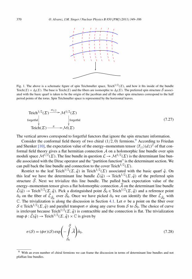
Fig. 1. The above is a schematic figure of spin Teichmuller space, Teich1/2(Σ), and how it fits inside of the bundleTeich(Σ)× J0(Σ). The base is Teich(Σ) and the fibers are isomorphic to J0(Σ). The preferred spin structure S associ-ated with the basic quarf is taken to be the origin of the jacobian and all the other spin structures correspond to the halfperiod points of the torus. Spin Teichmuller space is represented by the horizontal leaves.

Teich1/2(Σ)π1/2

forgetful

M1/2(Σ)

forgetful

Teich(Σ)π M(Σ)

(7.27)

The vertical arrows correspond to forgetful functors that ignore the spin structure information.Consider the conformal field theory of two chiral (1/2,0) fermions.9 According to Friedan

and Shenker [10], the expectation value of the energy–momentum tensor 〈Tzz〉(dz)2 of that con-formal field theory gives a flat hermitian connection A on a holomorphic line bundle over spinmoduli space M1/2(Σ). The line bundle in question L → M1/2(Σ) is the determinant line bun-dle associated with the Dirac operator and the “partition function” is the determinant section. Wecan pull back the line bundle and connection to the cover Teich1/2(Σ).

Restrict to the leaf Teich1/2(Σ, q) in Teich1/2(Σ) associated with the basic quarf q . Onthis leaf we have the determinant line bundle L(q) → Teich1/2(Σ, q) of the preferred spinstructure S . Next we trivialize this line bundle. The pulled back expectation value of theenergy–momentum tensor gives a flat holomorphic connection A on the determinant line bundleL(q) → Teich1/2(Σ, q). Pick a distinguished point S0 ∈ Teich1/2(Σ, q) and a reference pointσ0 on the fiber of L S0

over S0. Once we have picked σ0 we can identify the fiber L S0with

C. The trivialization is along the discussion in Section 4.1. Let σ be a point on the fiber overS ∈ Teich1/2(Σ, q) and parallel transport σ along any curve from S to S0. The choice of curveis irrelevant because Teich1/2(Σ, q) is contractible and the connection is flat. The trivializationmap φ : L(q) → Teich1/2(Σ, q) × C is given by

σ(S) = (φσ)(S) exp

(−

S∫S0

A)σ0. (7.28)

9 With an even number of chiral fermions we can frame the discussion in terms of determinant line bundles and notpfaffian line bundles.


It follows from the definition of spin Teichmuller space that Teich1/2(Σ, q) is isomorphic toTeich(Σ) and we implicitly think of the trivialized line bundle as being Teich(Σ) × C.

We trivialize L → Teich1/2(Σ) by embedding Teich1/2(Σ) in Teich(Σ)× J0(Σ) as depictedin Fig. 1. Fix a point τ ∈ Teich(Σ) and consider the family of operators ∂(S ⊗ F) were F ∈J0(Σ) is a flat line bundle and S is the spin structure associated with the basic quarf q . Bygoing to the cover H 0,1(Σ) of J0(Σ) we can trivialize the family using a parallel transportmethod analogous to the one discussed in Section 4.1. We can restrict to the half lattice points inH 0,1(Σ) and we obtain that if δ = 1

2w where w ∈ H(Σ,Z/2Z) then

det ∂(S ⊗ Fw) = ϑ[δ](0;Ω)

ϑ(0;Ω)det ∂(S), (7.29)

according to (7.1). For the moment det ∂(S) is a point on the fiber of the determinant line atS ∈ Teich1/2(Σ, q) over the point τ ∈ Teich(Σ). Next we use the trivialization of L(q) →Teich1/2(Σ, q) previously described and this is how we interpret the determinant section. Sincewe have the Quillen metric, det ∂(S) is known up to a phase.

Our conformal field theory of chiral spinors is associated with the determinant line bun-dle L → M1/2(Σ) with holomorphic partition section Z. This holomorphic section satis-fies the parallel transport equation ∂M1/2(Σ)Z + AZ = 0, and can be pulled back to a sec-

tion Z of L → Teich1/2(Σ) where it satisfies ∂Teich1/2(Σ)Z + AZ = 0. In the trivialization

just described, Z becomes a function that we denote by det ∂ . Note that after restriction toTeich1/2(Σ, q), the holomorphic determinant section det ∂(S) satisfies the parallel transportequation ∂Teich(Σ) det ∂ + A det ∂ = 0.

Let D → Teich1/2(Σ) be the trivialized determinant line bundle as described in the pre-vious paragraphs. If f ∈ Diff(Σ) represent Λ ∈ Sp(2g,Z) then f ∗D = D ⊗ C where C →Teich1/2(Σ) is a circle bundle because f acts isometrically. Consider the section det ∂ of D .Since f acts by isometries, f ∗(det ∂)f ∗D = u · (det ∂)D where u is a section of C and |u| = 1.Since the determinant sections vary holomorphically over Teich1/2(Σ), u is a constant section.The dependence of u on f is only through Λ since we have already taken into account the actionof the normal subgroup Diff0(Σ).

7.3. Defining det′ ∂

Having trivialized the bundle, we can define det′ ∂ by exploiting the embedding of Teich1/2(Σ)

in Teich(Σ) × J0(Σ). We rewrite (7.1) as

detD(δ + z) = det ∂(S)

ϑ(0)eiπ(a+u)·Ω·(a+u)+2πi(a+u)·(b+v)ϑ(δ + z)

= det ∂(S)

ϑ(0)eiπ(a+u)·Ω·(a+u)+2πi(a+u)·(b+v)

× e−iπa·Ωa−2πiu·(z+b)ϑ[δ](z)= det ∂(S)

ϑ(0)eiπu·Ωu+2πiu·(v+b)ϑ[δ](z). (7.30)

From (7.19) we have

λ(z) =∣∣∣∣ π

N2δ

g∑zj

∂ϑ[δ](0)∂zj

∣∣∣∣2

+ O(z3)

, (7.31)
j=i


and we can take an approximate “holomorphic square root”

√λ(z) = eiψ

π

N2δ

g∑j=i

zj∂ϑ[δ](0)

∂zj+ O

(z2)

. (7.32)

In the above we introduced an arbitrary phase ψ . The subleading terms will not have holomor-phicity properties. Thus we can define det′ ∂δ by mimicking10 (7.4) and defining

det′∂δ = limz→0

D(δ + z)√λ(z)

. (7.33)

We compute the above with the result

det′ ∂δN2

δ

= e−iψ 1

π

det ∂(S)

ϑ(0).

The arbitrary phase in the normalization factor Nδ can be chosen so that eiψ = 1 and

det′ ∂δN2

δ

= 1

π

det ∂(S)

ϑ(0). (7.34)

This agrees with explicit results in genus one.

8. Geometric symplectic action on determinants

8.1. Quillen isometry

The determinant for the Dirac laplacian is given by

(det ∂∗∂

)(S ⊗ Fw) = (

det ∂∗∂)(S)

∣∣∣∣ϑ[δ](0;Ω)

ϑ(0;Ω)

∣∣∣∣2

, (8.1)

where S is the spin structure described by the basic quarf q and δ = 12w mod Z, see (7.21).

Let Λ ∈ Sp(2g,Z) and let f ∈ Diff(Σ) be a representative for Λ. Because of the functorialproperties of ∂ , the eigenvalues are preserved under the action of f and we conclude that(

det ∂∗∂)(

S ′ ⊗ Ft ⊗ Ff ∗w) = (

det ∂∗∂)(S ⊗ Fw). (8.2)

Remark 8.1. Eq. (8.2) states that the diffeomorphism f acts as an isometry with respect to theQuillen metric on the f -related determinant line bundles.

Remark 8.2. The Quillen isometry is more general: if Fw is replaced by an arbitrary flat linebundle Fχ corresponding to character χ , then (8.2) is still valid.

Using the notation that Fw′ = Ff ∗w ⊗Ft , δ′ = 12w

′, etc., a straightforward computation gives

10 This is what the path integral suggests as a possible definition.


(det ∂∗∂

)(S ′ ⊗ Fw′

) = (det ∂∗∂

)(S ′)∣∣∣∣ϑ[δ′](0;Ω ′)

ϑ(0;Ω ′)

∣∣∣∣2

= (det ∂∗∂

)(S ′)∣∣∣∣ε(Λ)e−iπφ(δ) det(CΩ + D)1/2ϑ[δ](0;Ω)

ε(Λ)det(CΩ + D)1/2ϑ(0;Ω)

∣∣∣∣2

= ∣∣det(CΩ + D)∣∣∣∣ϑ[δ](0;Ω)

∣∣2 (det ∂∗∂)(S ′)|ϑ(0;Ω ′)|2 .

Hence

(det ∂∗∂)(S)

|ϑ(0;Ω ′)|2 = ∣∣det(CΩ + D)∣∣ (det ∂∗∂)(S)

|ϑ(0;Ω)|2 . (8.3)

8.2. Determinant section for spin bundles

In this section we study in more detail the Quillen isometry. Remark 8.2 tells us that in generalwe expect a relationship

(det ∂)(

S ′ ⊗ Ft ⊗ f ∗Fχ

) = eiξ(χ)(det ∂)(S ⊗ Fχ).

A difficulty with the above is S ⊗Fχ is an odd spin structure then the determinant sections vanishand it is not clear that the phase can be defined. In this section we develop a limit process thatuniquely determines the phase for an odd spin structure.

Fix a symplectic basis for H1(Σ,Z). Let Fχ be the flat line bundle specified by character χ .We use Fχ as a perturbation and assume it is close to the trivial bundle. Identify the character χwith a point ζ near the origin of Cg . The assignment of ζ is given by the standard coordinates onH 0,1(Σ), the cover of J0(Σ). We abuse notation and denote Fχ by Fζ . Let S ⊗ Fw be an oddspin structure, w ∈ H 1(Σ,Z/2Z). Trivializing the determinant line bundle over H 0,1(Σ) for thefamily of ∂ operators acting on S ⊗ Fζ gives

(det ∂)(S ⊗ Fw ⊗ Fζ ) = (det ∂)(S)ϑ[δ + ζ ](0;Ω)

ϑ(0;Ω). (8.4)

using11 (7.3) and (7.2).Let f ∈ Diff(Σ) that represents Λ ∈ Sp(2g,Z). Since f acts as an isometry on the determi-

nant line bundles, see Section 8.1, we obtain

(det ∂)(

S ′ ⊗ Ft ⊗ Ff ∗w ⊗ Ff ∗z) = eiξ(w+z;Λ)(det ∂)(S ⊗ Fw ⊗ Fz), (8.5)

where ξ is a phase and Ft is the “translational shift” flat line bundle discussed previously.Observe that

eiξ(0,Λ) (det ∂)(S)

ϑ(0;Ω)= (det ∂)(S ′ ⊗ Ft)

ϑ(0;Ω)

= ϑ[t](0;Ω ′)ϑ(0;Ω)

(det ∂)(S ′)ϑ(0;Ω ′)

11 The algebraic geometry ϑ -function conventions use semi-characteristics δ = 12w ∈ 1

2 Z/Z. At times we abuse nota-tion using w and δ interchangeably. Shifting δ, ζ by a lattice vector may lead to phases in the formula above.


= ε(Λ)e−iπφ(0,Λ) det(CΩ + D)1/2 (det ∂)(S ′)ϑ(0;Ω ′)

= ε(Λ)det(CΩ + D)1/2 (det ∂)(S ′)ϑ(0;Ω ′)

, (8.6)

where φ(0,Λ) = 0 by (5.10).

Remark 8.3. In genus one, fermionic determinants are of the form ϑ[δ](τ )/η(τ ), thereforedet/ϑ = 1/η is universal for all even spin structures. This is a special case of (det ∂)(S ⊗Fw)/ϑ[δ](0) = (det ∂)(S)/ϑ(0). Under the modular transformation T (τ) = τ ′ = τ + 1 wehave that (det ∂)(S ′ ⊗ Ft ) = ϑ01(0; τ ′)/η(τ ′) and (det ∂)(S) = ϑ00(0; τ)/η(τ). Note thatϑ01(0; τ ′)/η(τ ′) = e−2πi/24ϑ00(0; τ)/η(τ) and so we conclude that eiξ(0,T ) = e−2πi/24 in thisexample.

Remark 8.4. According to (8.6), ϑ(0;Ω)/det ∂(S) is a modular form of weight 1/2. It is con-stant along the fibers in the covering Teich1/2(Σ) → Teich(Σ) in the sense that for even spinstructures we use result (7.29) and for odd spin structures we use (7.34). For this reason wecan think of ϑ(0;Ω)/det ∂(S) as defined on Teich(Σ) as a higher genus generalization of theDedekind η-function.

Remark 8.5. Even in genus one, the computation of the modular transformations propertiesof the Dedekind η-function using the geometry of determinant line bundles is a very technicalexercise [18].

If in (8.5), S ⊗ Fw is an odd spin structure and z = 0 then we expect that eiξ(w;Λ) is not welldefined because the determinant sections vanish. Below, the flat bundle Fz in (8.5) is used todetermine eiξ(w;Λ) via a limit process for S ⊗ Fw an odd spin structure. First we note that

(det′ ∂)(S ⊗ Fδ)

N2δ

= limz→0

(det ∂)(S ⊗ Fδ ⊗ Fz)

N2δ

√λ(z)

= 1

π

(det ∂)(S)

ϑ(0;Ω), (8.7)

where we used (7.34). Next, using the notation Fw′ = Ft ⊗ Ff ∗w and Fz′ = Ff ∗z we compute

(det′ ∂)(S ′ ⊗ Fw′)

N2δ′

= limz′→0

(det ∂)(S ′ ⊗ Fw′ ⊗ Fz′)

N2δ′√λ′(z′)

= limz′→0

eiξ(δ,Λ)(det ∂)(S ⊗ Fw ⊗ Fz)

π∑

z′j ∂ϑ[δ′](0;Ω ′)/∂z′

j

= limz→0

eiξ(δ,Λ)(det ∂)(S ⊗ Fw ⊗ Fz)

πε(Λ)e−iπφ(δ,Λ) det(CΩ + D)1/2∑

zj ∂ϑ[δ](0;Ω)/∂zj

= eiξ(δ,Λ)

ε(Λ)e−iπφ(δ,Λ) det(CΩ + D)1/2limz→0

(det ∂)(S ⊗ Fw ⊗ Fz)

N2δ

√λ(z)

= eiξ(δ,Λ)

ε(Λ)e−iπφ(δ,Λ) det(CΩ + D)1/2

(det′ ∂)(S ⊗ Fw)

2.

Nδ


Hence

(det′ ∂)(S ′ ⊗ Fw′)

N2δ′

= eiξ(δ,Λ)ε(Λ)−1eiπφ(δ,Λ) det(CΩ + D)−1/2 (det′ ∂)(S ⊗ Fw)

N2δ

. (8.8)

Combining the above with (5.13) gives the interesting “isometry” relation that

(det′∂)(

S ′ ⊗ Fw′)(

h′δ′

Nδ′

)2

= eiξ(δ,Λ)(det′∂)(S ⊗ Fw)

(hδ

Nδ

)2

. (8.9)

This result can be used to determine eiξ(δ,Λ) for an odd semi-characteristic δ:

eiξ(0,Λ) = eiξ(δ,Λ)eiπφ(δ,Λ). (8.10)

Proof. Use (7.34) and (8.6) to observe

(det′ ∂)(S ′ ⊗ Fw′)

N2δ′

= 1

π

(det ∂)(S ′)ϑ(0;Ω ′)

= eiξ(0,Λ)ε(Λ)−1 det(CΩ + D)−1/2 1

π

(det ∂)(S)

ϑ(0;Ω)

= eiξ(0,Λ)ε(Λ)−1 det(CΩ + D)−1/2 (det′ ∂)(S ⊗ Fw)

N2δ

. (8.11)

Comparing (8.11) and (8.8) yields the desired result (8.10). �8.3. Computing ξ(0,Λ)

In this discussion we consider the conformal field theory with two (1/2,0) chiral fermions.The “partition function” Z of this CFT is the determinant section of the determinant line bundleover spin moduli space. The pullback section Z has the property that

Z(S) = Z(f · S) (8.12)

where S ∈ Teich1/2(Σ) and f ∈ Diff(Σ).We consider the case where we have a diffeomorphism f that represents12 Λ ∈ Γ1,2.

This diffeomorphism maps Teich1/2(Σ, q) to itself because of the definition of Γ1,2. Let S ∈Teich1/2(Σ, q) then using (8.12) and trivialization (7.28) we conclude that

det ∂(f · S) exp

(−

f ·S∫S0

A)σ0 = det ∂(S) exp

(−

S∫S0

A)σ0.

We obtain the result

12 We have learned from Igusa [19] and Mumford [8] that using Γ1,2 simplifies life.


det ∂(f · S) = det ∂(S) exp

( f ·S∫S

A). (8.13)

Because of flatness we have that

exp

( f ·S∫S

A)

= exp

( f ·S0∫S0

A),

i.e., the parallel transport factor is independent of basepoint. Any path from S0 to f · S0 projectsto a loop in M1,2(Σ), where M1,2(Σ) = Teich(Σ)/Diff1,2(Σ) and Diff1,2(Σ) are the diffeo-morphisms representing Γ1,2. We see that the exponential above is just the holonomy with respectto the flat connection A pulled back to the pull back line bundle over M1,2(Σ) ⊃ M(Σ). Weknow that the flat hermitian connection gives a homomorphism hol : π1(M1,2(Σ)) → S1 and byrelating (8.13) with (8.5) we obtain

Theorem 8.6. If Λ ∈ Γ1,2 then

eiξ(0,Λ) = hol(Λ)−1. (8.14)

The holonomy is independent of the choice of representative f ∈ Diff(Σ) chosen for Λ.

Remark 8.7. Because S1 is abelian, the set of maps of π1(M1,2(Σ)) → S1 is the same as theset of maps H1(M1,2(Σ),Z) → S1, i.e., the character group of H1(M1,2(Σ),Z) which equalsH 1(M1,2(Σ),R)/H 1(M1,2(Σ),Z), a torus T . Therefore our map hol is a homomorphism fromΓ1,2 to the torus T . Our theorem states that eiξ(0,Λ) = hol(Λ)−1 ∈ T . We will denote eiξ(0,Λ) bytΛ ∈ T . We can also interpret einξ(0,Λ) by defining holn : Γ1,2 → T by holn(Λ) = (hol(Λ))n sothat tnΛ = einξ(0,Λ) = (holn(Λ))−1 ∈ T .

Remark 8.8. The original proposal relating global anomalies to holonomy is due to Witten [20].

8.4. Main results

As we noted in the Introduction, the purpose of this paper is to extend the results of BEG,where we had a theory over Teichmuller space, to a theory over moduli space.

We will denote the dependence of Zsc on a string manifold M and a spin structure S byZsc(M, S).

Remark 8.9. Zsc(M, S) is a function on Teich1/2(Σ) and the map M → Zsc(M, S) is a homo-morphism from string cobordism MString∗ to functions on Teich1/2(Σ), i.e., a genus.

It turns out it is useful to define a function Φ by

Zsc(M, S) =((det ∂)(S)

ϑ(0;Ω)

)2n

Φ(M, S). (8.15)

The map M → Φ(M, S) is also a genus from MString∗ to Teich1/2(Σ).


Formula (4.2) for Zsc contained det′ ∂ and not det′ ∂ , therefore we have to take the complexconjugate. Using the notation of (4.2) we find the transformation law(

det′ ∂δ′

N2δ′

)g′

= ε(Λ)e−iξ(0,Λ) det(CΩ + D)−1/2(

det′ ∂δN2

δ

)g

. (8.16)

A drawback of Theorem 5.1 is that the integral is a combination of objects that vary holo-morphically and objects that vary anti-holomorphically with respect to Teichmuller space. Forexample Ω varies holomorphically while h2

δ varies anti-holomorphically. Next we try to groupterms together in such a way as to try to be as holomorphic as possible. In particular we remindthe reader that our path integral viewpoint acts as a guide to our final result. We use the Belavin–Knizhnik theorem to formally factorize the determinants and also we invoke (7.34). With this inmind we make two substitutions in (4.2):(

volΣ detH

det1⊥ �0

)1/2

−→ 1

2

(det ∂)(S)

ϑ(0;Ω)

(det ∂)(S)

ϑ(0;Ω), (8.17)

det′ ∂δN2

δ

−→ 1

π

(det∂)(S)

ϑ(0;Ω). (8.18)

The expression for Φ now becomes

Φ(M, S) = 1

(4π)n

1

(detH)n

((det∂)(S)

ϑ(0;Ω)

)3n ∫M

n∏r=1

zκ (xrz(h2δ );Ω)


. (8.19)

Using (5.15), (8.6) and (5.18) we obtain

Theorem 8.10. Let M be a string manifold with dimM = 2n; if Λ ∈ Sp(2g,Z) is represented byf ∈ Diff(Σ), then under the action of f we have

Φ ′ = ε(Λ)2ne−3niξ(0,Λ)einπφ(δ,Λ) det(CΩ + D)nΦ (8.20a)

= ε(Λ)2ne−3niξ(δ,Λ)e−2inπφ(δ,Λ) det(CΩ + D)nΦ. (8.20b)

Corollary 8.11. Let M be a string manifold with dimM = 2n; if Λ ∈ Sp(2g,Z) is representedby f ∈ Diff(Σ), then under the action of f we have

Z′sc = e−inξ(δ,Λ)Zsc (8.21a)

= e−inξ(0,Λ)einπφ(δ,Λ)Zsc. (8.21b)

If Λ ∈ Γ1,2 then for a semi-characteristic [ ab ] we have that φ(a, b,Λ) = 12 mod Z. If dimM =

2n = 4k then e−2inπφ(δ,Λ) = 1, and the spin structure S maps onto the preferred spin structure S ′.According to Igusa [19, p. 181], ε(Λ)2 is a character of Γ1,2. Note that ε(Λ)2n = ε(Λ)4k = ±1.

Theorem 8.12. Let M be a string manifold with dimM = 2n = 4k; if Λ ∈ Γ1,2 ⊂ Sp(2g,Z) isrepresented by f ∈ Diff(Σ), then under the action of f we have

Φ ′ = ε(Λ)2ne−3niξ(0,Λ)einπφ(δ,Λ) det(CΩ + D)nΦ (8.22a)

= ε(Λ)2ne−3niξ(δ,Λ) det(CΩ + D)nΦ. (8.22b)

Note that ε(Λ)2n = ±1 and einπφ(δ,Λ) = ±1.


If dimM = 2n = 8l then einπφ(δ,Λ) = 1, einπξ(δ,Λ) = einπξ(0,Λ), and ε(Λ)2n = 1; and we find

Theorem 8.13. Let M be a string manifold with dimM = 2n = 8l; if Λ ∈ Γ1,2 ⊂ Sp(2g,Z) isrepresented by f ∈ Diff(Σ), then under the action of f we have

Φ ′ = e−3niξ(0,Λ) det(CΩ + D)nΦ (8.23)

Z′sc = e−inξ(0,Λ)Zsc. (8.24)

The transformation laws above do not depend on the choice of spin structure δ.

Remark 8.14. We interpret (8.24) as saying that Zsc is a modular function with multiplier t−nΛ ;

see Remark 8.7 for notation.

Remark 8.15. We interpret (8.23) as saying that Φ is a modular form with weight n and withmultiplier t−3n

Λ .

Acknowledgements

We wish to thank M.J. Hopkins for introducing us to quarfs and their relation to spin struc-tures, for explaining the various cobordism theories, and for encouragement in completing thisproject. The work of O.A. was supported in part by the National Science Foundation undergrants PHY-0554821 and PHY-0854366. The work of I.M.S. was supported by two DARPAgrants through the Air Force Office of Scientific Research (AFOSR): grant numbers FA9550-07-1-0555 and HR0011-10-1-0054.

Appendix A. Isomorphism between Λ1/2,0(Σ) and Λ1/2,1(Σ)

On Σ we have local complex coordinates z = x + iy. In isothermal coordinates the metric isds2 = gzz(dz ⊗ dz + dz ⊗ dz). The volume element is

√detg dx ∧ dy. We note that dz ∧ dz =

2i dx ∧ dy. If ωi are the standard abelian differentials then∫Σ

ωi ∧ ωj = (Ω − Ω)ij .If K is the canonical bundle of Σ and if ξ(dz)n and η(dz)n are section of Kn then the inner

product is defined by⟨ξ(dz)n, η(dz)n

⟩ = ∫Σ

(gzz

)nξη

√detg dx ∧ dy. (A.1)

The explicit conjugate linear isomorphism between Λ1/2,1(Σ) and Λ1/2,0(Σ) is constructedas follows. Let h be a section of Λ1/2,0(Σ) then the corresponding section ψ of Λ1/2,1(Σ) isgiven by

ψ = (gzz dz ⊗ dz)1/2h. (A.2)

Appendix B. Identifying a holomorphic cross section of L with a ϑ function

Our purpose is to identify a holomorphic cross section (unique up to scale) of a determinantline bundle with a theta function. We also set the notation for the algebraic geometry we needand provide an introduction for non-experts.


In this appendix we make the identification using facts about Riemann surfaces well knownto algebraic geometers.

Let Jr(Σ) denote the set of holomorphic line bundles over Σ with c1 equal to r . Of par-ticular interest to us is J0(Σ) (our J (Σ)), the set of flat line bundles, which we can identify

with π1(Σ) = {χ :π1(Σ) → S1} � ˜H1(Σ,Z) � H 1(Σ,R)/H 1(Σ,Z). The last isomorphismcan be described in terms of (real) closed 1-forms ω: let χω(γ ) = exp(2πi

∫γω) for γ a

closed path starting at P0 ∈ Σ . Clearly χω is a homomorphism π1(Σ) → S1 and dependsonly on the cohomology class of ω. It is easy to see that ω → χω induces an isomorphism

H 1(Σ,R)/H 1(Σ,Z) → π1(Σ). Here we take π1(Σ) as the closed (piecewise smooth) pathsstarting at P0 with equivalence relationship given by homotopy.

When the real surface Σ has a complex structure, then H 1(Σ,C) = H 1(Σ,R) ⊗ C �H 1,0(Σ) ⊕ H 0,1(Σ). Taking the real part induces an isomorphism of H 0,1(Σ) (or H 1,0(Σ))

with H 1(Σ,R). Let re : H 0,1(Σ) → H 1(Σ,R) be this isomorphism, and let H 0,1(Σ) =(re)−1H 1(Σ,Z) so that H 1(Σ,R)/H 1(Σ,Z) � H 0,1(Σ)/H 0,1(Σ). Since H 0,1(Σ) is a com-

plex vector space, H 0,1(Σ)/H 0,1(Σ) is a complex torus J (Σ), the jacobian of Σ . Our chain ofarguments demonstrates that the jacobian J0(Σ) is isomorphic to H1(Σ,Z), the character groupof H1(Σ,Z). Specifically, if μ ∈ H 0,1(Σ), let

χμ(γ ) = e2πi

∫γ (μ+μ)/2

, (B.1)

with γ a loop with basepoint P0, then μ → χμ induces the isomorphism of H 0,1(Σ)/LΩ =J (Σ) with H1(Σ,Z). LΩ = H 0,1(Σ) will be described differently in the paragraph below. Thecovering space of J (Σ) = J0(Σ) is H 0,1(Σ).

We chose a standard basis (ω1, . . . , ωg) of H 0,1(Σ) obtained from a choice of symplecticbasis (aj ,bk) of H1(Σ,R) so that

∫aiωj = δij . We remind the reader that the Riemann period

matrix Ωij = ∫bi

ωj with imaginary part (Ωij − Ωij )/2i that is positive-definite and in fact equalto 〈ωi,ωj 〉. Then ωi = ∑

αi + Ωijβj where α and β are the harmonic representatives dual tothe a and b cycles. We write a point in H 0,1(Σ) as (uj + ivj )ωj where u and v are real. One

can easily verify that H 0,1(Σ) is represented by 2∑

(m + Ωn)j (Ω − Ω)−1jk ωk where m ∈ Zg

and n ∈ Zg .13

Multiplication mL by a line bundle L ∈ Jr(Σ) gives an isomorphism mL : J0(Σ) → Jr(Σ).In particular a spin structure

√K , where K is the canonical bundle of Σ , gives m√

K: J0(Σ) →

Jg−1(Σ) with g the genus of Σ . Similarly for P0 ∈ Σ let LP0 be the line bundle with divisor P0so that LP0 ∈ J1(Σ). Then mLr

P0: J0(Σ) → Jr(Σ) is an isomorphism. The complex structure

on Jr is chosen such that mL is holomorphic.One can construct a Poincaré line bundle Qr over Jr(Σ) × Σ whose restriction to each fiber

{L} × Σ is the line L ∈ Jr(Σ). The holomorphic line bundle Qr over Jr(Σ) × Σ is determinedonly up to a line bundle on Jr(Σ) pulled up to Jr(Σ)×Σ . A choice of point P0 ∈ Σ determinesQr by stipulating that Qr |Jr (Σ)×{P0} � 1 on Jr(Σ). In [BEG, Appendix B] we construct such aQ0 explicitly. We can use (m

Lg−1P0

)∗Qg−1 instead.

13 The standard basis {ωj } of H 1,0(Σ) identifies H 1,0(Σ) with Cg . Algebraic geometers [8, p. 143] identify H1(Σ,C)

with Cg using the Abel map. As a consequence the lattice LΩ ⊂ Cg is the dual torus to the algebraic geometers’ Jacobiantorus.


Let ∂ ⊗ IQr be the family of ∂ operators parametrized by Qr . Suppose M is a holomorphicline bundle on Jr(Σ) which pulled up to Jr(Σ)×Σ is M. Suppose we have modified our choiceof Poincaré line bundle Qr by Qr ⊗ M. One can show the determinant line bundle of the family∂ ⊗ IQr⊗M, DET(∂ ⊗ IQr⊗M) is isomorphic to DET(∂ ⊗ IQr ) ⊗ Mr+1−g . In particular, when

r = g − 1, DET(∂ ⊗ IQg−1) is independent of choice of Qg−1.The choice of r = g−1 is special because the index of the operator ∂ ⊗ IL, L ∈ Qg−1, is zero.

Generically the operator ∂ ⊗ IL is invertible. Let V = {L ∈ Jg−1(Σ)|∂ ⊗ IL is not invertible}.V is a variety in Jg−1(Σ), in fact the divisor of the line bundle DET(∂ ⊗ IQg−1). Of course,V is also {L ∈ Jg−1(Σ)|L has a nonzero holomorphic section}. Another description of ∂ ⊗ IQg−1

is obtained by choosing a spin structure, a√K , which we denote by Λ1/2,0(Σ). m√

Kmaps

J0(Σ) to Jg−1(Σ) and the family becomes a family over J0(Σ), namely ∂ : Λ1/2,0(Σ)⊗Fχ →Λ1/2,1(Σ) ⊗ Fχ with Fχ ∈ J0(Σ).

We use mL

g−1P0

to compare DET(∂ ⊗ IQg−1) with DET(∂ ⊗ IQ0), the latter our line bundle Lover J0(Σ). The Grothendieck–Riemann–Roch theorem implies that

(mL

g−1P0

)∗(DET(∂ ⊗ IQg−1)

)is isomorphic to L. Although it is well known that H 0(L,C) has complex dimension one, i.e.,the holomorphic sections of L form a one-dimensional subspace [BEG, Appendix C]. We nowwant to identify a properly normalized holomorphic section of L with a ϑ -function.

First identify J0(Σ), the universal cover of J0(Σ), with Cg using the basis {ωj }, where wehave defined the Riemann theta function ϑ and its divisor. Let Lϑ be the holomorphic line bundleover J0(Σ) whose divisor pulls up to the divisor of ϑ . We learn from Riemann surface theorythat there exists a spin structure

√K ∈ Jg−1(Σ) such that Lϑ = m∗√

KDET(∂ ⊗ IQg−1). Put

another way, m√K(divisor of Lϑ) = V . The spin structure is the one determined by the choice of

symplectic basis of cycles in H1(Σ,R). In fact, the spin structure√K has quarf the basic quarf

q described in Section 6.3. See also [8, pp. 162].Putting these two facts together gives

L � (m−1√

Km

Lg−1P0

)∗Lϑ � (mK−1/2L

g−1P0

)Lϑ .

The flat line bundle K−1/2Lg−1P0

lies in J0(Σ) and is in fact κ where κ is the Riemann constant,

see [8, p. 166] or [21, p. 338]. Hence L is the translate of Lϑ by κ . As a result, our ϑ[ ab

]is the

translate of ϑ by κ ; the characteristic[ ab

]equals κ .

Lemma B.1. ϑ[κ](0) = 0.

Proof. This is a consequence of Riemann’s Theorem [8, Corollary 3.6 on p. 160] or [21, p. 338].In Mumford’s conventions14 we have that Θ = Wg−1 − κ . The divisor Wg−1 is the image ofSymg−1(Σ) under the Abel map, i.e., the image in J0(Σ) of line bundles L of Chern class g − 1that have a holomorphic section.15 Note that the origin O ∈ J0(Σ) is in Wg−1 (it is the image

14 Mumford’s vector of Riemann constants is the negative of Griffiths and Harris’ vector of Riemann constants.15 The image under the map L → L ⊗ (L

g−1)−1.

P0


of (P0, . . . ,P0)). Riemann’s Theorem then tells us that −κ ∈ Θ but Θ is symmetric thereforeκ ∈ Θ . We have that ϑ[±κ](0) ∝ ϑ(±κ) = ϑ(κ) = 0. �

Note that ϑ[κ](0) = 0 if κ is an odd characteristic. Mumford [22, p. 3.82], and Farkas andKra [23] discuss that in hyperelliptic surfaces, κ will be even or odd depending on the genus. Ifκ is even then ϑ[κ](·) has a double zero at the origin and this has implications on the numberof zero modes of the Dirac operator. All genus 2 surfaces are hyperelliptic and κ is an oddcharacteristic.

B.1. Definition of zκ

The technicalities in constructing the determinant line bundle are related to the jump in thedimensionality of kerD at the origin O ∈ J0(Σ):

Theorem B.2 ([BEG, Theorem B.1]). Let χ ∈ J (Σ) be a character and let A0,1 be the associatedflat connection. If χ = 1 then dim kerD0 = g. If χ �= 1 then dim kerDA = g − 1.

We can exploit this theorem to give a global construction of the determinant line bundle overJ0(Σ). Note that indexDA = g − 1 thus: (1) if χ �= 1 then DA is surjective, (2) if χ = 1 thenthe image of D0 is 1⊥. This motivates us to define a modified family of operators (parametrizedby flat connections) by DA : Λ1,0(Σ) → 1⊥ where we have “killed the constants” in the range.Hence, these operators have numerical index g and dim coker DA = 0. Consequently ker DA = g

and the kernel of D is an honest holomorphic vector bundle over J0(Σ). The top wedge powerof this vector bundle is the determinant line bundle DET(D) → J0(Σ) and it is isomorphic toDET(D) → J0(Σ). If we fix the metric then this construction is holomorphic because the 1⊥does not vary as we move over J0(Σ).

Our formula for Zsc requires a specific trivialization of the determinant line bundle DETD →J0(Σ). Here we briefly review the detailed construction given in [BEG, Section 7].

In a small neighborhood U of the origin we introduce the operator D : Λ1,0(Σ) → Λ0,0(Σ)

defined16 by

Dφ = Dφ − i

∫Σ

A0,1 ∧ φ (B.2)

that has the property that dim ker D = g on U and we construct DET(D) → U . Note that bothD and D are operators with index equal to g − 1. Let V = J0(Σ)− {O} then dim kerD = g − 1on V , and we construct DET(D) → V . On U ∩ V we have that kerD ⊂ ker D and an exactsequence of vector bundles

0 → kerD → ker D → K → 0.

The holomorphic line bundle K is used to patch DET(D) with DET(D) on U ∩ V , and gives aconstruction of the holomorphic determinant line bundle DET(D) → J0(Σ).

In [BEG, Sections 7 and 8] we discussed a convenient trivialization of DET(D) over U bytrivializing DET(D) over U . Note that ker D|O = H 1,0(Σ) and as a consequence of the Hodgetheorem we can choose a basis (!1, . . . ,!g) for ker D on U such that !j = ωj + Υj where

16 Note that the image of D is contained in 1⊥ by construction.


Υj ∈ H 1,0(Σ)⊥ ⊂ Λ1,0(Σ). In fact [BEG, Eq. (8.1)] shows that if we subject a standard ba-sis (ω1, . . . ,ωg) of H 1,0(Σ) to a symplectic change of basis, see Eq. (5.6), then (!1, . . . ,!g)

transforms the same way.We know [BEG, Appendix C] that DET(D) → J0(Σ) has a unique holomorphic section θκ

up to scale. Lemma B.1 tells us that this section vanishes at the origin. In the (!1, . . . ,!g)

trivialization we write this section as

θκ = zκ

!1 ∧ · · · ∧ !g

(B.3)

as explained in [BEG, Eq. (8.10)]. In the trivialization given by lifting the line bundle to H 0,1(Σ),the universal cover of J0(Σ), the section is given by the theta functions ϑ[κ](·). Therefore theratio zκ(z)/θ [κ](z) is just the holomorphic transition function that takes you from one trivial-ization of the line bundle to the other. In [BEG, Eq. (9.5)] we give a formula for this transitionfunction:

e−πi∑

z(Ω−Ω)−1z zκ (z)

ϑ[κ](z) = (!1 ∧ · · · ∧ !g) ⊗ e− ∫ A0 (ν−ρ)(ω1 ∧ · · · ∧ ωg)

−1. (B.4)

Note that the right-hand side is holomorphic and non-vanishing as required for a transition func-tion. Therefore the ratio on the left-hand side is holomorphic in U .

Remark B.3. An important consequence of the equation above is that the right-hand side of theratio is invariant under the symplectic action.

Appendix C. Genus 1 modular transformation examples

We derive the string genus using (4.2) and specialize to genus 1 using the discussion in [BEG,Remark 3]. The presentation here is more complete than [BEG, Remark 3] because we are check-ing our modularity transformation results for general genus by applying them to genus one. Thereis a single odd spin structure, the theta function is the odd theta function, and consequently

limz→0

ϑ(z; τ)z

= ϑ ′(0; τ) = −2πη(τ)3.

We also have ω = dz, z = −ϑ ′(0; τ)z, and we omit the δ label on the antiholomorphic spinorsince there is only a single odd spin structure h2 = ϑ ′(0; τ) dz. The modular transformationτ ′ = −1/τ gives z′ = z/τ . Some examples:(

h′)2 = ϑ ′(0; τ ′)dz′ ∝ τ 3/2ϑ ′(0; τ) dz/τ = τ 1/2ϑ ′(0; τ) dz = τ 1/2h2, (C.1)

in agreement with the complex conjugate of (5.13). Next we observe that

z′(h′)τ = (τ ′

2ϑ′(0; τ ′))

τ ∝ τ(τ2/τ τ )τ 3/2ϑ(0; τ) = τ 1/2(τ2ϑ(0; τ)) = τ 1/2z(h)

that concurs with (5.17). The main object of interest is∫M

n∏r=1

z(xrz(h))

ϑ(xrz(h); τ)∝

∫M

n∏r=1

ϑ ′(0; τ)ϑ(xrz(h); τ)/(xrz(h))

. (C.2)

The last expression is reminiscent of the integral in (4.2) in the sense that as x → 0 the denomi-nator approaches the numerator. The modular transformation properties are:


∫M

n∏r=1

ϑ ′(0; τ ′)ϑ(xrz′(h′); τ ′)/(xrz′(h′))

∝∫M

n∏r=1

τ 3/2ϑ ′(0; τ)[τ 1/2ϑ(xr τ 1/2z(h); τ)]/(xr τ 1/2z(h)/τ )

∝∫M

n∏r=1

ϑ ′(0; τ)ϑ(xr τ 1/2z(h); τ)/(xr τ 1/2z(h))

∝ τ n/2∫M

n∏r=1

ϑ ′(0; τ)ϑ(xrz(h); τ)/(xrz(h))

in agreement with (5.18). The other terms are

volΣ detH

det1⊥ �0∝ τ 2

2

det1⊥ �0∝ [

η(τ)η(τ)]−2

, (C.3)

det′ ∂1/2

N2∝ τ2η(τ)

2

τ2ϑ ′(0; τ) ∝ 1

η(τ). (C.4)

Abusing notation, detH ′ ∝ τ ′2 ∝ (detH)/(τ τ ),(

volΣ detH

det1⊥ �0

)τ ′

= (τ τ )−1(

volΣ detH

det1⊥ �0

)τ

,

and (volΣ

det1⊥ �0

)τ ′

=(

volΣ

det1⊥ �0

)τ

= 1

τ2

[η(τ)η(τ)

]−2. (C.5)

Note that there is a tradeoff between “holomorphic factorization” in (C.3) and “modular invari-ance” in (C.5). Finally we observe that(

det′ ∂1/2

N2

)τ ′

= τ−1/2(

det′ ∂1/2

N2

)τ

, (C.6)

and ∫M

n∏r=1

z(xrz(h))

ϑ(xrz(h); τ)∝

∫M

n∏r=1

ϑ ′(0; τ)(xrτ2ϑ ′(0; τ))ϑ(xr(τ2ϑ ′(0; τ)); τ)

∝ τn2 ϑ

′(0; τ)nϑ ′(0; τ)n∫M

n∏r=1

xr

ϑ(xr ; τ)

∝ τn2 η(τ)

3nη(τ)3n

∫M

n∏r=1

xr

ϑ(xr ; τ) .

The modular transformation properties become

(τ ′

2

)nη

(τ ′)3n

η(τ ′)3n

∫M

n∏r=1

xr

ϑ(xr ; τ ′)

∝(

τ2

τ τ

)n

(τ τ )3n/2η(τ)3nη(τ)3n

∫ n∏r=1

xr

ϑ(xr ; τ ′)
M


∝ (τ τ )n/2τn2 η(τ)

3nη(τ)3n

∫M

n∏r=1

xr

ϑ((xrτ )/τ ;−1/τ)

∝ (τ τ )n/2τn2 η(τ)

3nη(τ)3n

∫M

n∏r=1

xr

τ 1/2ϑ(xrτ ; τ)

∝ (τ τ )n/2τn2 η(τ)

3nη(τ)3n

∫M

n∏r=1

xrτ

τ 3/2ϑ(xrτ ; τ)

∝ (τ τ )n/2τn2 η(τ)

3nη(τ)3n τn

τ 3n/2

∫M

n∏r=1

xr

ϑ(xr ; τ)

∝ τ n/2

(τn

2 η(τ)3nη(τ)3n

∫M

n∏r=1

xr

ϑ(xr ; τ)

),

in agreement with the abstract result. In fact∫M

n∏r=1

z(xrz(h))

ϑ(xrz(h); τ)∝ τn

2 ϑ′(0; τ)n

∫M

n∏r=1

ϑ ′(0; τ)ϑ(xr ; τ)/xr (C.7)

which is exactly (C.2) if we group a factor of τ2ϑ ′(0; τ) with each xr .The string genus is the product of three terms(

volΣ

det1⊥ �0

)n

×(

det′ ∂1/2

N2

)n

×∫M

n∏r=1

z(xrz(h))

ϑ(xrz(h); τ).

Each term has different modularity and holomorphicity properties; together they conspire to givesomething holomorphic which changes by a phase under modular transformations. There is noclear way of subgrouping the terms pairwise; there is a tradeoff between holomorphicity vs.modularity depending on the grouping.

Note that the string genus is

1

η(τ)2n

∫M

n∏r=1

ϑ ′(0; τ)ϑ(xr ; τ)/xr . (C.8)

This should be compared with (4.2). The fact that in g = 1 the theta function is a function of onevariable allowed us to scale out a variety of terms, namely all the non-holomorphic ones.

We can rewrite (C.8) as∫M

s(M,τ) where s(M, τ) = a(M, τ)/η(τ)dimM/2 and

a(M, τ) =dimM/2∏

j=1

ixj /2π

σ(ixj /2π, τ)(C.9)

and σ is the Weierstrass sigma function. s(M, τ) is the string genus because∫M

a(M,τ) is amodular form of weight dimM/2, giving a homomorphism from string cobordism to the ring ofmodular forms.

The string genus is a generalization of Hirzebruch’s genuses [24, Chapters 1, 2 and 3] whichare homomorphisms from a cobordism theory (MSO∗, MU∗, MSpin∗) to the ring of integers


using the appropriate power series Q(z) respectively given by (L, Todd, A). The homomorphismbeing

∫M

∏j Q(xj ).

In the genus 1 case, the analog of Q(z) is the function of one variable (iz/2π)/σ(iz/2π, τ).When the genus g > 1, see Section 8, we get a genus from a subring of the string cobordism ring,MString∗, to a subring of the functions on Teich1/2(Σ).

C.1. Nomenclature

Met(Σ) The space of metrics on Σ with curvature −1Teich(Σ) The Teichmuller space of ΣTeich1/2

odd(Σ) The odd spin Teichmuller space of Σq The basic quarfS A spin structure

S The spin structure associated to the basic quarf q

References

[1] O. Alvarez, I.M. Singer, Beyond the elliptic genus, Nucl. Phys. B 633 (2002) 309–344, arXiv:hep-th/0104199.

[2] O. Alvarez, T.P. Killingback, M. Mangano, P. Windey, The Dirac–Ramond operator in string theory and loop spaceindex theorems, in: Nonperturbative Methods in Field Theory: Proceedings, Nuclear Physics B (Proc. Suppl.) 1A(1988) 189–216, invited talk presented at the Irvine Conf. on Non-Perturbative Methods in Physics, Irvine, Califor-nia, January 5–9, 1987.

[3] O. Alvarez, T.P. Killingback, M. Mangano, P. Windey, String theory and loop space index theorems, Commun.Math. Phys. 111 (1987) 1–10.

[4] K. Pilch, A.N. Schellekens, N.P. Warner, Path integral calculation of string anomalies, Nucl. Phys. B 287 (1987)362.

[5] E. Witten, Elliptic genera and quantum field theory, Commun. Math. Phys. 109 (1987) 525–536.[6] D. Quillen, Determinants of Cauchy–Riemann operators on Riemann surfaces, Funktsional. Anal. i Prilozhen. 19 (1)

(1985) 37–41;D. Quillen, Determinants of Cauchy–Riemann operators on Riemann surfaces, Funktsional. Anal. i Prilozhen. 19 (1)(1985) 96.

[7] J.D. Fay, Theta Functions on Riemann Surfaces, Lecture Notes on Mathematics, vol. 352, Springer-Verlag, 1973.[8] D. Mumford, Tata Lectures on Theta I, Birkhäuser, 1983.[9] M.F. Atiyah, Riemann surfaces and spin structures, Ann. Sci. École Norm. Sup. (4) 4 (1971) 47–62.

[10] D. Friedan, S.H. Shenker, The analytic geometry of two-dimensional conformal field theory, Nucl. Phys. B 281(1987) 509, doi:10.1016/0550-3213(87)90418-4.

[11] L. Alvarez-Gaumé, E. Witten, Gravitational anomalies, Nucl. Phys. B 234 (1984) 269–330.[12] D.B. Ray, I.M. Singer, Analytic torsion for complex manifolds, Ann. of Math. (2) 98 (1973) 154–177.[13] O. Alvarez, Theory of strings with boundaries: Fluctuations, topology, and quantum geometry, Nucl. Phys. B 216

(1983) 125.[14] A.M. Polyakov, Quantum geometry of bosonic strings, Phys. Lett. B 103 (1981) 207–210, doi:10.1016/0370-

2693(81)90743-7.[15] A.M. Polyakov, Quantum geometry of fermionic strings, Phys. Lett. B 103 (1981) 211–213, doi:10.1016/0370-

2693(81)90744-9.[16] L. Alvarez-Gaume, G. Moore, C. Vafa, Theta functions, modular invariance, and strings, Commun. Math. Phys. 106

(1986) 1–40.[17] L. Alvarez-Gaume, J.B. Bost, G.W. Moore, P.C. Nelson, C. Vafa, Bosonization on higher genus Riemann surfaces,

Commun. Math. Phys. 112 (1987) 503, doi:10.1007/BF01218489.[18] M. Atiyah, The logarithm of the Dedekind η-function, Math. Ann. 278 (1–4) (1987) 335–380,

doi:10.1007/BF01458075.[19] J.-i. Igusa, Theta Functions, Die Grundlehren der Mathematischen Wissenschaften, Band, vol. 194, Springer-Verlag,

New York, 1972.

http://dx.doi.org/10.1016/0550-3213(87)90418-4

http://dx.doi.org/10.1016/0370-2693(81)90743-7

http://dx.doi.org/10.1016/0370-2693(81)90744-9

http://dx.doi.org/10.1007/BF01218489

http://dx.doi.org/10.1007/BF01458075

http://dx.doi.org/10.1016/0370-2693(81)90743-7

http://dx.doi.org/10.1016/0370-2693(81)90744-9


[20] E. Witten, Global gravitational anomalies, Commun. Math. Phys. 100 (1985) 197.[21] P. Griffiths, J. Harris, Principles of Algebraic Geometry, Wiley, 1978.[22] D. Mumford, Tata Lectures on Theta II, Birkhäuser, 1984.[23] H.M. Farkas, I. Kra, Riemann Surfaces, 2nd edition, Graduate Texts in Mathematics, vol. 71, Springer-Verlag, New

York, 1992.[24] F. Hirzebruch, Topological Methods in Algebraic Geometry, Classics in Mathematics, Springer-Verlag, Berlin,

1995, translated from German, and Appendix One by R.L.E. Schwarzenberger, with a preface to the third Englishedition by the author and Schwarzenberger, Appendix Two by A. Borel, reprint of the 1978 edition.

beyond the string genus

Documents