an octahedral macro-element
TRANSCRIPT

Computer Aided Geometric Design 23 (2006) 640–654
www.elsevier.com/locate/cagd
An octahedral C2 macro-element ✩
Ming-Jun Lai a, Alan Le Méhauté b, Tatyana Sorokina a,∗
a Department of Mathematics, The University of Georgia, Athens, GA 30602, USAb Department of Mathematics, The University of Nantes, F.44322 Nantes, France
Received 12 May 2005; received in revised form 12 June 2006; accepted 14 June 2006
Available online 14 July 2006
Abstract
A macro-element of smoothness C2 is constructed on the split of an octahedron into eight tetrahedra. This new element comple-ments those recently constructed on the Clough–Tocher and Worsey–Farin splits of a tetrahedron (cf. Alfeld, P., Schumaker, L.L.,2005a, 2005b). The octahedral element uses supersplines of degree thirteen, and provides optimal order of approximation of smoothfunctions.© 2006 Elsevier B.V. All rights reserved.
MSC: 41A15; 65M60; 65N30
Keywords: Macro-elements; Spline spaces; Octahedron
1. Introduction
This paper is designed to compliment two recent results on trivariate C2 macro-elements obtained by P. Alfeldand L.L. Schumaker. The first one, constructed in (Alfeld and Schumaker, 2005a), is based on the three-dimensionalClough–Tocher split of a tetrahedron into four subtetrahedra, and uses polynomial splines of degree thirteen. Thesecond macro-element is described in (Alfeld and Schumaker, 2005b), and based on the Worsey–Farin split of a tetra-hedron into twelve subtetrahedra. The Worsey–Farin split is more complicated, and allows the use of polynomialsplines of degree nine. In our paper, we use the split of an octahedron into eight tetrahedra (for details, see De-finition 3.1). Our macro-element uses polynomial splines of the same degree as the Clough–Tocher one, thirteen.Whenever applicable, it has an obvious advantage over the Clough–Tocher macro-element. It does not require the split-ting of each tetrahedron into subtetrahedra. Although octahedral partitions of a domain in R
3 are less common thantetrahedral ones, they naturally arise from a number of applications. In particular, uniform type grids are well-suitedfor using octahedral macro-elements (see Remark 6.3). In contrast to tensor-product splines, macro-elements providefull approximation power. Another important application of octahedral macro-elements comes from the uniform re-finement of tetrahedral partitions (see Remark 6.5). Moreover, for some partitions it is possible to use a combinationof the 3D Clough–Tocher macro-element and our octahedral element (see Remarks 6.4 and 6.6).
✩ Results in this paper are based on the research supported by the National Science Foundation under the grant No. 0327577.* Corresponding author.
E-mail addresses: [email protected] (M.-J. Lai), [email protected] (A. Le Méhauté), [email protected] (T. Sorokina).
0167-8396/$ – see front matter © 2006 Elsevier B.V. All rights reserved.doi:10.1016/j.cagd.2006.06.001

M.-J. Lai et al. / Computer Aided Geometric Design 23 (2006) 640–654 641
Following (Alfeld and Schumaker, 2005a), we define a trivariate macro-element on an octahedron P as a pair(S,Λ), where S is a space of polynomial splines defined on a partition of P into tetrahedra, and Λ is a set of linearfunctionals consisting of values and derivatives of s ∈ S at some points in P , that uniquely define s. Let � be anoctahedral partition of a polygonal domain Ω ⊂ R
3, such that if two octahedra intersect at a vertex, edge, or face,then they share this vertex, edge, or face, respectively. We say that a macro-element has smoothness C2 if the macro-element used on each octahedron results in a globally C2 continuous function.
This paper is organized as follows. In Section 2 we review some basic Bernstein–Bézier techniques for splinefunctions over tetrahedral partitions and introduce new notation for later use. Section 3 contains the description of oursplit of an octahedron and several facts about the location of domain points. In Section 4 we describe our C2 macro-element and obtain error bounds for Hermite interpolation using the octahedral macro-element. We prove severaluseful bivariate lemmas in Section 5 which are needed for the proof of the main result in Section 4. The paper isconcluded with several remarks in Section 6.
2. Preliminaries
Let � be a tetrahedral partition of a polyhedral domain Ω in R3. We define the set of polynomial splines of degree d
and smoothness r on � as
Srd(�) := {
s ∈ Cr(Ω): s|T ∈ P3d , for all tetrahedra T ∈ �}
,
where P3d is the space of trivariate polynomials of degree d . We use Bernstein–Bézier techniques as in (Alfeld and
Schumaker, 2002a, 2002b; Lai and Schumaker, 2001, 2003). In particular, given a tetrahedron T := 〈v,u,w, t〉, werepresent a polynomial p of degree d in its B-form with respect to T :
p =∑
i+j+k+l=d
cTijklB
dijkl,
where Bdijkl are the Bernstein polynomials of degree d associated with T . As usual, we associate the coefficients cT
ijkl
with the domain points
DT ,d :={ξTijk := iv + ju + kw + lt
d, i + j + k + l = d
}. (2.1)
Fig. 1 (left) shows all domain points in DT ,5. Let S0d (�) be the space of continuous splines of degree d on �,
and let D�,d be the union of the sets of domain points associated with each tetrahedron of �. Then it is well knownthat each spline in S0
d (�) is uniquely determined by its set of B-coefficients {cξ }ξ∈D�,d, where the coefficients of the
polynomial s|T are precisely {cξ }ξ∈DT ,d.
If v is a vertex of a tetrahedron T = 〈v,u,w, t〉, then we define the shell of radius m around v in T as
HTm(v) := {
ξTd−m,j,k,l ∈DT ,d , for all j + k + l = m
}. (2.2)
Fig. 1. Domain points in DT ,5 (left) and HT3 (v) ∩DT ,5 (right).

642 M.-J. Lai et al. / Computer Aided Geometric Design 23 (2006) 640–654
Fig. 1 (right) shows HT3 (v) ∩DT ,5. The ball of radius m around v in T is defined as
BTm(v) :=
m⋃i=0
HTi (v). (2.3)
We define the frame of the shell HTm(v) as
Fr(HT
m(v)) := {
ξTijkl ∈ HT
m(v), for all j × k × l = 0}. (2.4)
The tube of radius m around the edge 〈v,u〉 in T is
ETm
(〈v,u〉) := {ξTijkl ∈ DT ,d , for all k + l � m, and i + j = d − k − l
}. (2.5)
We also need to define the p-ball of radius m around v in T :
BT⊗,m(v) := {ξTijkl ∈DT ,d , for all i + j + k + l = d, with max{j, k, l} � m
}. (2.6)
Fig. 2 illustrates the visible surface of BT⊗,3(t) ∩DT ,13. The domain points on the surface of the p-ball are located atthe intersections of the line segments on the three visible faces of the box.
In general, if v is a vertex of a tetrahedral partition �, we define the shell Hm(v) of radius m around v as
Hm(v) := {HT
m(v), for all T := 〈v,u,w, t〉 sharing v in �}, (2.7)
where each domain point is counted once if it belongs to more than one tetrahedra in �.The ball Bm(v), frame Fr(Hm(v)), tube Em(〈v,u〉), and p-ball B⊗,m(v) of radius m around v are defined similarly.Additionally, we recall that in the bivariate setting, if v is a vertex of a triangulation �, and D�,d is the set of
domain points for s ∈ S0d (�), then the ring Rm(v) of radius m around v is defined as
Rm(v) := {ξTd−m,i,j ∈D�,d , for all triangles T := 〈v,u,w〉 ∈ �, for all i + j = m
}. (2.8)
The disk Dm(v) of radius m around v is
Dm(v) :=m⋃
i=0
Ri(v). (2.9)
We shall use these notions in Section 5.Given a multi-index α = (α1, α2, α3) with nonnegative integer entries, we define
|α| := α1 + α2 + α3, ‖α‖ := max{α1, α2, α3}. (2.10)
Fig. 2. The visible surface of the p-ball of radius 3 around t in T = 〈v,u,w, t〉.
M.-J. Lai et al. / Computer Aided Geometric Design 23 (2006) 640–654 643
We write Dα for the partial derivative Dα1x D
α2y D
α3z . Given an edge e := 〈u,v〉 of a tetrahedron T ∈ �, and a multi-
index β = (β1, β2), we define Dβe to be the partial derivative associated with two non-collinear vectors orthogonal
to e. That is,
Dβe = Dβ1
e1Dβ2
e2(2.11)
where e1, e2 denote two non-collinear vectors that are perpendicular to e. We also need notation for the followingpoints on e:
ηie,j := (i − j + 1)u + jv
i + 1, j = 1, . . . , i. (2.12)
Given a face F := 〈u,v,w〉 of a tetrahedron T ∈ �, and a nonnegative integer k, we define DkF to be the kth order
derivative associated with a unit vector orthogonal to F . Finally, if η is a point in R3, we use εη to denote the point-
evaluation functional associated with η, i.e., εη := f (η).As is well known, a spline s ∈ S0
d (�) will belong to C2(Ω) if and only if certain smoothness conditions acrossfaces between adjoining tetrahedra are satisfied. To describe these in B-form instead of usual derivatives, suppose thatT := 〈v1, v2, v3, v4〉 and T := 〈v5, v2, v3, v4〉 are two adjoining tetrahedra sharing a face F := 〈v2, v3, v4〉. Suppose
s|T =∑
i+j+k+l=d
cTijklB
dijkl, and s|T =
∑i+j+k+l=d
cTijklB
dijkl,
where {Bdijkl}i+j+k+l=d are the Bernstein polynomials of degree d associated with T . Given 1 � i � d , let
τ ijkl := cT
ijkl −∑
ν+μ+κ+�=i
cTν,j+μ,k+κ,l+�B
iνμκ�(v1) (2.13)
for all j + k + l = d − i. Following (Alfeld and Schumaker, 2002a), we call τ ijkl a smoothness functional of or-
der i. Note that for a given pair of adjoining tetrahedra, this functional is uniquely associated with the domain pointξTijkl ∈ DT ,d . In order to identify such a functional we need to specify T , T , and F . We use the following notation{
τ ijkl, (va, 〈vb, vc, vd〉, ve)
}(2.14)
to describe the smoothness functional of order i, associated with the point ξijkl in T := 〈va, vb, vc, vd〉 across the faceF := 〈vb, vc, vd〉 shared by the neighboring tetrahedron T := 〈ve, vb, vc, vd〉. It is well known that a spline s ∈ S0
d (�)
is Cr continuous across the face F , for 1 � r � d , if and only if
τ ijkls = 0, for all j + k + l = d − i, i = 1, . . . , r.
We will also use bivariate smoothness functionals. They are defined similarly to (2.13). In order to identify a bivariatesmoothness functional we need to specify a triangle F , the neighboring triangle F , and the edge e that they share. Weuse the following notation{
τ ijk, (va, 〈vb, vc〉, vd)
}(2.15)
to describe the smoothness functional of order i, associated with the point ξijk in F := 〈va, vb, vc〉 across the edgee := 〈vb, vc〉 shared by the neighboring triangle F := 〈vd, vb, vc〉.
Given a vertex v of �, and 1 � r � d , we say that s ∈ Cr⊗(v), if for all T ∈ � attached to v, the values of Dα|T (v)
coincide, ‖α‖ � r .Suppose S is a linear subspace of S0
d , and M ⊂ D�,d . Then M is a determining set for S provided that if s ∈ Sand its B-coefficients satisfy cξ = 0 for all ξ ∈ M, then s ≡ 0. The set M is called a minimal determining set (MDS)for S provided that there is no smaller determining set.
Suppose N is a set of linear functionals λ (usually defined as point-evaluations of values or derivatives of s). ThenN is a nodal determining set for S provided that if s ∈ S and λs = 0 for all λ ∈ N , then s ≡ 0. The set N is calleda nodal minimal determining set (NMDS) for S provided that there is no smaller nodal determining set.

644 M.-J. Lai et al. / Computer Aided Geometric Design 23 (2006) 640–654
Fig. 3. The split of the octahedron (left) and the cross-section associated with shells around v2 (right).
3. The split of the octahedron and subsets of domain points
By drawing three not coplanar lines through any point O in R3 we obtain a cross in R
3. Two points vi and vj oneach line are chosen so that O is inside of the segment (vi, vj ). The convex hull of these six vertices forms a crosspolytope P . We call such a cross polytope an octahedron. That is, we require that all three diagonals of an octahedronintersect at one point.
Definition 3.1. Given an octahedron P = {v1, v2, v3, v4, v5, v6}, let OP be the intersection of its three diagonals:〈v1, v4〉, 〈v2, v5〉, 〈v3, v6〉, as shown in Fig. 3 (left). Draw in the line segments 〈vi,OP 〉, i = 1, . . . ,6. The resultingpartition of P into eight tetrahedra is called �P , see Fig. 3 (left).
We write VP , EP , and FP for the sets of six vertices, twelve edges, and eight faces of P , respectively. By D�P ,13we denote the set of domain points for s ∈ S0
13(�P ). In the remainder of this section we prove several lemmas whichare needed for the proof of the main result of Section 4.
Lemma 3.2. Let u and v be two vertices of P connected by the edge e := 〈u,v〉. The intersection of the shells ofradius r around u and radius t around v is contained in the tube of radius four around e for all r, t ∈ {4, . . . ,9},except (r, t) = (9,9).
Proof. First we observe that Hr(u) ∩ Ht(v) lies in two tetrahedra T := 〈OP ,w,u, v〉 and T := 〈OP , w,u, v〉. Due tosymmetry, it suffices to consider Hr(u) ∩ Ht(v) in T . By definition (2.2)
HTr (u) = {
ξTi,j,13−r,k, i + j + k = r
}, HT
t (v) = {ξTm,n,l,13−t , m + n + l = t
}.
Then
HTr (u) ∩ HT
t (v) = {ξTi,j,13−r,13−t , i + j = r + t − 13
}. (3.1)
For r, t ∈ {4, . . . ,9}, (r, t) �= (9,9), the maximal value of the sum r + t − 13 is equal to 4. Therefore, by (2.5), thepoints in (3.1) belong to T4(e). �
We also need a very detailed description of the intersection of the shells of radius nine of two neighboring verticesof P .
Lemma 3.3. Let u and v be two vertices of P connected by the edge e := 〈u,v〉, and Te := 〈w,OP ,u, v〉, Te :=〈w,OP ,u, v〉 be the two tetrahedra in �P sharing e. Let Me be the intersection of shells of radius nine around u
and v. Then
Me := {ξ
Te
5044, ξTe
4144, ξTe
3244, ξTe
2344, ξTe
1444, ξTe
0544, ξTe
1444, ξTe
2344, ξTe
3244, ξTe
4144, ξTe
5044
}. (3.2)
Moreover, Me can be decomposed into the following two subsets:
M1e := {
ξTe
5044, ξTe
4144, ξTe
3244, ξTe
3244, ξTe
4144, ξTe
5044
} ⊂ {H13(OP ) ∪ H12(OP ) ∪ H11(OP )
},
M2e := {
ξTe , ξ
Te , ξTe , ξ
Te , ξTe
} ⊂ {H10(OP ) ∪ H9(OP ) ∪ Fr
(H8(OP )
)},
2344 1444 0544 1444 2344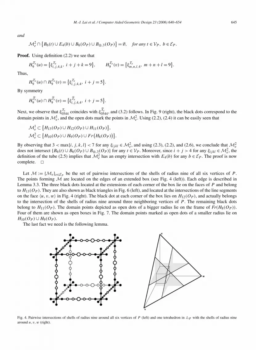
M.-J. Lai et al. / Computer Aided Geometric Design 23 (2006) 640–654 645
and
M2e ∩ {
B6(t) ∪ E4(b) ∪ B6(OP ) ∪ B⊗,3(OP )} = ∅, for any t ∈ VP , b ∈ EP .
Proof. Using definition (2.2) we see that
HTe
9 (u) = {ξ
Te
i,j,4,k, i + j + k = 9}, H
Te
9 (v) = {ξ
Te
m,n,l,4, m + n + l = 9}.
Thus,
HTe
9 (u) ∩ HTe
9 (v) = {ξ
Te
i,j,4,4, i + j = 5}.
By symmetry
HTe
9 (u) ∩ HTe
9 (v) = {ξ
Te
i,j,4,4, i + j = 5}.
Next, we observe that ξTe
0544 coincides with ξTe
0544, and (3.2) follows. In Fig. 9 (right), the black dots correspond to thedomain points in M1
e , and the open dots mark the points in M2e . Using (2.2), (2.4) it can be easily seen that
M1e ⊂ {
H13(OP ) ∪ H12(OP ) ∪ H11(OP )},
M2e ⊂ {
H10(OP ) ∪ H9(OP ) ∪ Fr(H8(OP )
)}.
By observing that 3 < max{i, j, k, l} < 7 for any ξijkl ∈ M2e , and using (2.3), (2.2), and (2.6), we conclude that M2
e
does not intersect {B6(t) ∪ B6(OP ) ∪ B⊗,3(OP )} for any t ∈ VP . Moreover, since i + j > 4 for any ξijkl ∈ M2e , the
definition of the tube (2.5) implies that M2e has an empty intersection with E4(b) for any b ∈ EP . The proof is now
complete. �Let M := {Me}e∈EP
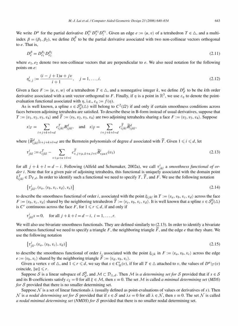
be the set of pairwise intersections of the shells of radius nine of all six vertices of P .The points forming M are located on the edges of an extended box (see Fig. 4 (left)). Each edge is described inLemma 3.3. The three black dots located at the extensions of each corner of the box lie on the faces of P and belongto H13(OP ). They are also shown as black triangles in Fig. 6 (left), and located at the intersections of the line segmentson the face 〈u,v,w〉 in Fig. 4 (right). The black dot at each corner of the box lies on H12(OP ), and actually belongsto the intersection of the shells of radius nine around three neighboring vertices of P . The remaining black dotsbelong to H11(OP ). The domain points depicted as open dots of a bigger radius lie on the frame of Fr(H8(OP )).Four of them are shown as open boxes in Fig. 7. The domain points marked as open dots of a smaller radius lie onH10(OP ) ∪ H9(OP ).
The last fact we need is the following lemma.
Fig. 4. Pairwise intersections of shells of radius nine around all six vertices of P (left) and one tetrahedron in �P with the shells of radius ninearound u,v,w (right).
646 M.-J. Lai et al. / Computer Aided Geometric Design 23 (2006) 640–654
Fig. 5. One tetrahedron in �P with the p-ball of radius three around OP and the shell of radius nine around w (left), the shell of radius nine aroundu (middle) the shell of radius nine around v (right).
Lemma 3.4.
D�P ,13 \ {B9(v)}v∈VP= B⊗,3(OP ). (3.3)
Proof. Let u,v,w ∈ VP , and T := 〈OP ,u, v,w〉 ∈ �P . Due to symmetry, it suffices to prove (3.3) for domain pointsin T . By (2.2), ξT
ijkl /∈ {B9(v)}v∈VPiff max{j, k, l} � 3. Hence, by (2.6), ξT
ijkl ∈ B⊗,3(OP ). �Fig. 2 shows the tetrahedron T with B⊗,3(OP ). Fig. 5 and Fig. 4 (right) illustrate that cutting B9(u),B9(v), and
B9(w) off of T does not touch the box B⊗,3(OP ).
4. An octahedral C2 macro-element
We would like to precede the definition of the spline space of our interest with a brief discussion to motivateour choice of smoothness conditions and a nodal minimal determining set. First of all, we require the coefficientscorresponding to the domain points in B6(v) for each v ∈ VP have to be set using the value and derivatives at v, cf.the construction in (Alfeld and Schumaker, 2005a). To eliminate some degrees of freedom we also set the coefficientscorresponding to the domain points in B⊗,3(OP ) ∪ B6(OP ) using the value and derivatives at OP . Next we set thecoefficients corresponding to the remaining domain points in E3(e) for each edge e ∈ EP using derivatives at somepoints on e. To ensure external C2 smoothness we also set the coefficients corresponding to the remaining domainpoints in H13(OP ) ∪ H12(OP ) ∪ H11(OP ) using the values and derivatives at some points on each F ∈ FP .
By Lemma 3.4 the domain points whose coefficients have not been defined from the above are located on Hi(v),i = 7,8,9, for each v ∈ VP . Each shell Hi(v) forms the set of domain points for a bivariate spline of degree i definedon the split of a parallelogram as shown in Fig. 3 (right). To determine unknown coefficients on Hi(v), i = 7,8,9,we impose additional smoothness conditions on such bivariate splines, see Section 5 for details. However, we have tobe careful since the shells around different vertices of P intersect. Lemmas 3.2 and 3.3 describe such intersections.
Now we describe the exact construction of our macro-element. First we introduce special sets of domain points onthe triangular faces of P . They are used to construct a nodal determining set. We note that these are the same pointsas those used in (Alfeld and Schumaker, 2005a). By associating the first index with the vertex OP of a tetrahedraT ∈ �P , we place the domain point on a face F of P .
A0F := {
ξT0544, ξ
T0454, ξ
T0455
} = {ξT
0ijk: i, j, k � 4},
A1F := {
ξT0ijk: i, j, k � 3
},
A2F := {
ξT0ijk: i, j, k � 2
} \ {ξT
0272, ξT0227, ξ
T0722
}. (4.1)
We note that for i = 2, . . . ,13, v ∈ VP , the shell Hi(v) forms the set of domain points for a bivariate spline ofdegree i defined on the split of a two-dimensional cross polytope or parallelogram P i
v (see the shaded region in
M.-J. Lai et al. / Computer Aided Geometric Design 23 (2006) 640–654 647
Fig. 3 (right)). We denote such a bivariate spline by siv . Each si
v is defined on the split of P iv into four subtriangles
obtained by drawing in two diagonals of P iv .
We now introduce the space of super-splines defined on �P :
SP := {s ∈ C3(P ): s|T ∈ P3
13 all tetrahedra T ∈ �P ,
s ∈ C6(v) for all v ∈ VP , s ∈ C6(OP ) ∩ C3⊗(OP ),
τP s = 0 for all τP ∈ {Te,P , e ∈ EP },siv ∈ SP i
v ,i , i = 7,8,9 for all v ∈ VP
}, (4.2)
where for each edge e := 〈u,v〉 ∈ EP , and the two tetrahedra T := 〈w,OP ,u, v〉, T := 〈w,OP ,u, v〉 in �P attachedto e,
Te,P := {{τ 5−ii44
},(w, 〈OP ,u, v〉, w)
, i = 0,1},
and for each i = 7,8,9, the space of bivariate splines SF,i on the split of a parallelogram F is defined in (5.1)–(5.3).The smoothness functionals in Te,P describe individual smoothness conditions of orders five and four across twelve
interior faces of �P . Note that they are univariate. The domain points associated with {Te,P }e∈EPare depicted in
Fig. 4 (left).
Theorem 4.1. The dimension of the space SP is 1086. Moreover,
N :=⋃
v∈VP
Nv ∪⋃
e∈EP
Ne
⋃F∈FP
(N 0
T ∪N 1T ∪N 2
T
) ∪NP ∪ NP (4.3)
is a nodal minimal determining set for SP , where
(1) Nv := ⋃|α|�6{εvD
α},(2) Ne := ⋃3
i=1⋃i
j=1{εηie,j
Dαe }|α|=i ,
(3) N 0F := {εξDF }ξ∈A0
F,
(4) N 1F := {εξDF }ξ∈A1
F,
(5) N 2F := {εξDF }ξ∈A2
F,
(6) NP := ⋃|α|�6{εOP
Dα},(7) NP := ⋃
|α|>6,‖α‖�3{εOPDα}.
Proof. We first compute the cardinality of N . It is easy to see that the cardinalities of the sets Nv,Ne,N 0F ,N 1
F ,N 2F ,
NP , NP are 84, 20, 3, 10, 18, 84, and 10. Since P has six vertices, twelve edges, and eight faces, it follows thatdimSP = 84 × 6 + 20 × 12 + 31 × 8 + 94 if N is a nodal minimal determining set.
To show that N is a nodal minimal determining set, we show that setting the values {λs}λ∈N of a spline s inSP uniquely determines all B-coefficients of s. First, the C6 smoothness at each v ∈ VP and at OP implies thatsetting {λs}λ∈{Nv∪NP } uniquely determines the B-coefficients corresponding to domain points in the balls B6(v) andB6(OP ). Similarly, the C3⊗ smoothness at OP implies that setting {λs}λ∈NP
uniquely determines the B-coefficients
corresponding to the remaining domain points in the p-ball B⊗,3(OP ). Next, the C3 smoothness around each e ∈ EP
shows that setting {λs}λ∈Neuniquely determines the B-coefficients corresponding to the remaining domain points in
the tube of radius three around e. From the proof of Theorem 3.1 in (Alfeld and Schumaker, 2005a), it follows thatsetting {λs}λ∈{N 0
F ∪N 1F ∪N 2
F } uniquely determines the B-coefficients corresponding to the remaining domain points onH13(OP ), H12(OP ), and H11(OP ), shown as black triangles in Fig. 6. In Fig. 7 all the domain points in H13(v1)
whose coefficients have been defined so far are shown as black dots.Next, we show that applying the C3 smoothness across the interior faces of �P uniquely determines the coefficients
corresponding to the remaining domain points in the tubes of radius four around each e ∈ EP . These points are locatedon H10(OP ) and Fr(H9(OP )), and are depicted as black triangles in Fig. 8. Each of those coefficients is determinedby solving a system of three linear equations with three unknowns. This system is associated with a univariate spline

648 M.-J. Lai et al. / Computer Aided Geometric Design 23 (2006) 640–654
Fig. 6. Black triangles depict domain points whose B-coefficients are determined by the functionals associated with A0F
, A1F
, and A2F
, respectively.
Fig. 7. Domain points on H13(v1).
Fig. 8. Black triangles depict domain points on faces of H10(OP ) (left) and Fr(H9(OP )) (right) whose B-coefficients are determined by the C3
smoothness across interior faces of P .
in S34 (�[a,b]), where �[a,b] is a split of [a, b] into two segments by an arbitrary interior point c. In Fig. 9 (left), we
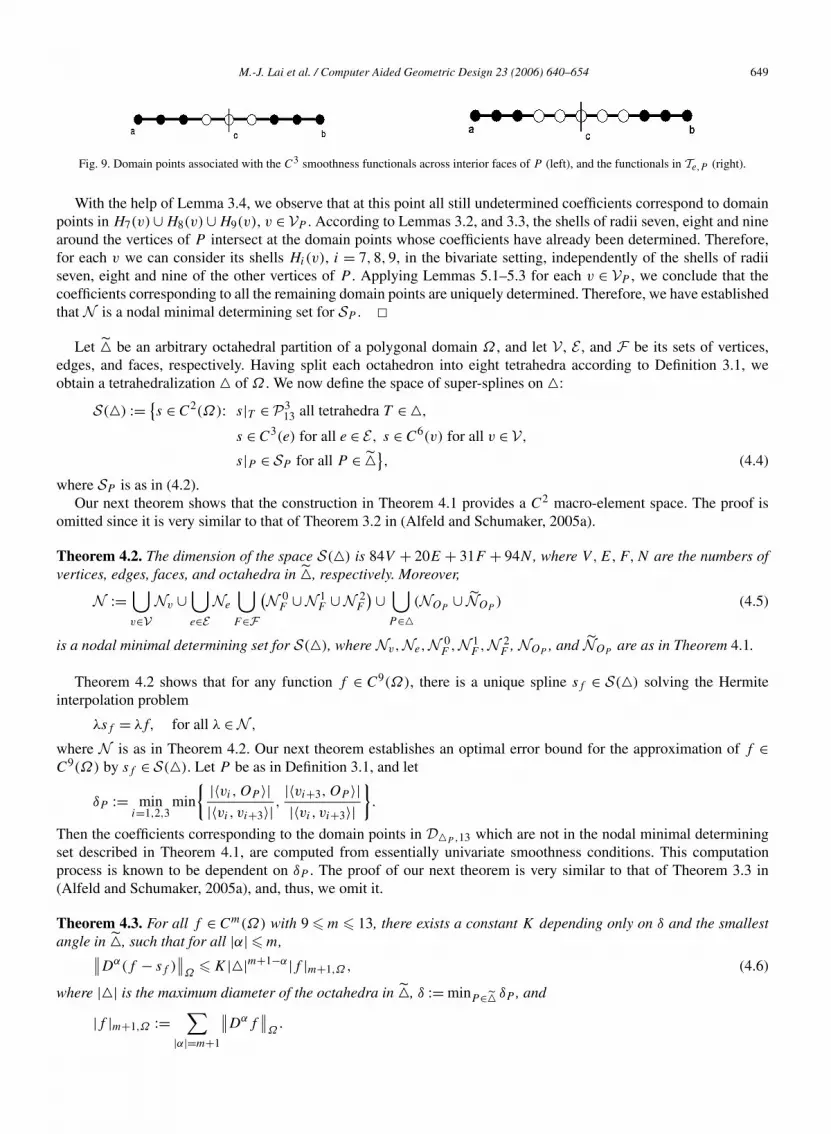
marked the domain points corresponding to the unknown coefficients with open dots, and the domain points whosecoefficients have already been determined are depicted as black dots. The open dot at the split point c is actually locatedon Fr(H9(OP )), and the black dots at the points a and b are located on H13(OP ). The C3 smoothness condition leadsto a 3 × 3 matrix that is known to be nonsingular. At this point, the B-coefficients corresponding to all domain pointsin the tubes of radius four of every e ∈ EP are uniquely determined.
As the next step, we apply the individual C5 and C4 smoothness conditions associated with the functionals inTe,P . The points whose coefficients enter those conditions, are located on the intersections of shells of radius ninearound two neighboring vertices of P , and are depicted in Fig. 4 (left), where the domain points corresponding to theunknown coefficients are marked as open dots. The complete set of these points is described in Lemma 3.3, whereM1
e are the domain points whose coefficients have already been determined, and M2e is the set of domain points with
unknown coefficients. Each of the unknown coefficients is determined by solving a system of five linear equationswith five unknowns. This system is associated with a univariate spline in S5
5 (�[a,b]), where �[a,b] is a split of [a, b]into two segments by an arbitrary interior point c. In Fig. 9 (right), the domain points corresponding to the unknowncoefficients are shown as open dots, and the domain points whose coefficients have already been determined aremarked as black dots. The open dot at the split point c is actually located on Fr(H8(OP )), and the black dots at thepoints a and b are located on H13(OP ). Increasing the smoothness from C3 to C4 and C5, leads to a 5×5 nonsingularmatrix, and allows us to determine uniquely the B-coefficients corresponding to the domain points in M2
e for everye ∈ EP .
M.-J. Lai et al. / Computer Aided Geometric Design 23 (2006) 640–654 649
Fig. 9. Domain points associated with the C3 smoothness functionals across interior faces of P (left), and the functionals in Te,P (right).
With the help of Lemma 3.4, we observe that at this point all still undetermined coefficients correspond to domainpoints in H7(v) ∪ H8(v) ∪ H9(v), v ∈ VP . According to Lemmas 3.2, and 3.3, the shells of radii seven, eight and ninearound the vertices of P intersect at the domain points whose coefficients have already been determined. Therefore,for each v we can consider its shells Hi(v), i = 7,8,9, in the bivariate setting, independently of the shells of radiiseven, eight and nine of the other vertices of P . Applying Lemmas 5.1–5.3 for each v ∈ VP , we conclude that thecoefficients corresponding to all the remaining domain points are uniquely determined. Therefore, we have establishedthat N is a nodal minimal determining set for SP . �
Let � be an arbitrary octahedral partition of a polygonal domain Ω , and let V , E , and F be its sets of vertices,edges, and faces, respectively. Having split each octahedron into eight tetrahedra according to Definition 3.1, weobtain a tetrahedralization � of Ω . We now define the space of super-splines on �:
S(�) := {s ∈ C2(Ω): s|T ∈P3
13 all tetrahedra T ∈ �,
s ∈ C3(e) for all e ∈ E, s ∈ C6(v) for all v ∈ V,
s|P ∈ SP for all P ∈ �}, (4.4)
where SP is as in (4.2).Our next theorem shows that the construction in Theorem 4.1 provides a C2 macro-element space. The proof is
omitted since it is very similar to that of Theorem 3.2 in (Alfeld and Schumaker, 2005a).
Theorem 4.2. The dimension of the space S(�) is 84V + 20E + 31F + 94N , where V,E,F,N are the numbers ofvertices, edges, faces, and octahedra in �, respectively. Moreover,
N :=⋃v∈V
Nv ∪⋃e∈E
Ne
⋃F∈F
(N 0
F ∪N 1F ∪N 2
F
) ∪⋃P∈�
(NOP∪ NOP
) (4.5)
is a nodal minimal determining set for S(�), where Nv,Ne,N 0F ,N 1
F ,N 2F , NOP
, and NOPare as in Theorem 4.1.
Theorem 4.2 shows that for any function f ∈ C9(Ω), there is a unique spline sf ∈ S(�) solving the Hermiteinterpolation problem
λsf = λf, for all λ ∈N ,
where N is as in Theorem 4.2. Our next theorem establishes an optimal error bound for the approximation of f ∈C9(Ω) by sf ∈ S(�). Let P be as in Definition 3.1, and let
δP := mini=1,2,3
min
{ |〈vi,OP 〉||〈vi, vi+3〉| ,
|〈vi+3,OP 〉||〈vi, vi+3〉|
}.
Then the coefficients corresponding to the domain points in D�P ,13 which are not in the nodal minimal determiningset described in Theorem 4.1, are computed from essentially univariate smoothness conditions. This computationprocess is known to be dependent on δP . The proof of our next theorem is very similar to that of Theorem 3.3 in(Alfeld and Schumaker, 2005a), and, thus, we omit it.
Theorem 4.3. For all f ∈ Cm(Ω) with 9 � m � 13, there exists a constant K depending only on δ and the smallestangle in �, such that for all |α| � m,∥∥Dα(f − sf )
∥∥Ω
� K|�|m+1−α|f |m+1,Ω, (4.6)
where |�| is the maximum diameter of the octahedra in �, δ := minP∈� δP , and
|f |m+1,Ω :=∑
|α|=m+1
∥∥Dαf∥∥
Ω.
650 M.-J. Lai et al. / Computer Aided Geometric Design 23 (2006) 640–654
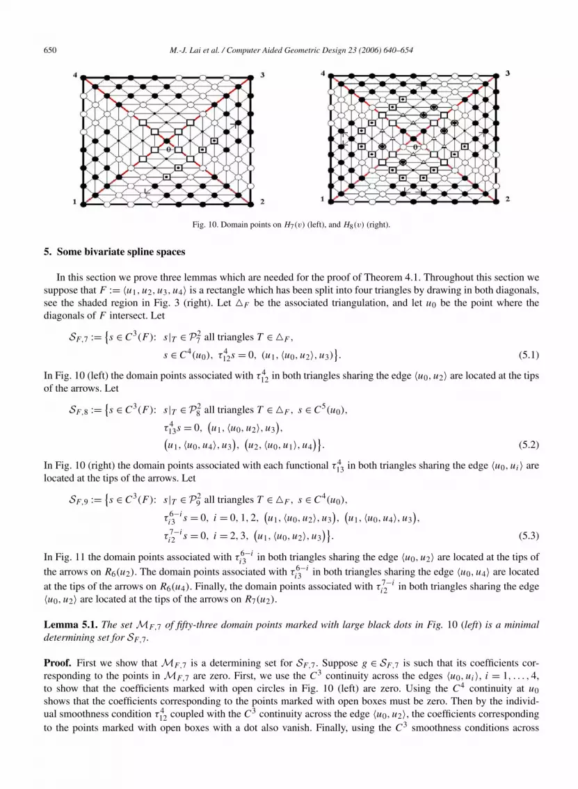
Fig. 10. Domain points on H7(v) (left), and H8(v) (right).
5. Some bivariate spline spaces
In this section we prove three lemmas which are needed for the proof of Theorem 4.1. Throughout this section wesuppose that F := 〈u1, u2, u3, u4〉 is a rectangle which has been split into four triangles by drawing in both diagonals,see the shaded region in Fig. 3 (right). Let �F be the associated triangulation, and let u0 be the point where thediagonals of F intersect. Let
SF,7 := {s ∈ C3(F ): s|T ∈P2
7 all triangles T ∈ �F ,
s ∈ C4(u0), τ 412s = 0, (u1, 〈u0, u2〉, u3)
}. (5.1)
In Fig. 10 (left) the domain points associated with τ 412 in both triangles sharing the edge 〈u0, u2〉 are located at the tips
of the arrows. Let
SF,8 := {s ∈ C3(F ): s|T ∈P2
8 all triangles T ∈ �F , s ∈ C5(u0),
τ 413s = 0,
(u1, 〈u0, u2〉, u3
),(
u1, 〈u0, u4〉, u3),
(u2, 〈u0, u1〉, u4
)}. (5.2)
In Fig. 10 (right) the domain points associated with each functional τ 413 in both triangles sharing the edge 〈u0, ui〉 are
located at the tips of the arrows. Let
SF,9 := {s ∈ C3(F ): s|T ∈P2
9 all triangles T ∈ �F , s ∈ C4(u0),
τ 6−ii3 s = 0, i = 0,1,2,
(u1, 〈u0, u2〉, u3
),
(u1, 〈u0, u4〉, u3
),
τ 7−ii2 s = 0, i = 2,3,
(u1, 〈u0, u2〉, u3
)}. (5.3)
In Fig. 11 the domain points associated with τ 6−ii3 in both triangles sharing the edge 〈u0, u2〉 are located at the tips of
the arrows on R6(u2). The domain points associated with τ 6−ii3 in both triangles sharing the edge 〈u0, u4〉 are located
at the tips of the arrows on R6(u4). Finally, the domain points associated with τ 7−ii2 in both triangles sharing the edge
〈u0, u2〉 are located at the tips of the arrows on R7(u2).
Lemma 5.1. The set MF,7 of fifty-three domain points marked with large black dots in Fig. 10 (left) is a minimaldetermining set for SF,7.
Proof. First we show that MF,7 is a determining set for SF,7. Suppose g ∈ SF,7 is such that its coefficients cor-responding to the points in MF,7 are zero. First, we use the C3 continuity across the edges 〈u0, ui〉, i = 1, . . . ,4,to show that the coefficients marked with open circles in Fig. 10 (left) are zero. Using the C4 continuity at u0shows that the coefficients corresponding to the points marked with open boxes must be zero. Then by the individ-ual smoothness condition τ 4
12 coupled with the C3 continuity across the edge 〈u0, u2〉, the coefficients correspondingto the points marked with open boxes with a dot also vanish. Finally, using the C3 smoothness conditions across

M.-J. Lai et al. / Computer Aided Geometric Design 23 (2006) 640–654 651
Fig. 11. Domain points on H9(v).
the edges 〈u0, u1〉, and 〈u0, u3〉, we see that the remaining coefficients corresponding to the twelve domain pointsmarked with small dots must also be zero. This completes the proof that MF,7 is a determining set for SF,7. Sincedim[S3
7 (�F )∩C4(u0)] = 54 by Theorem 2.2 of (Schumaker, 1988), and we imposed one additional smoothness con-dition, it follows that dimSF,7 � 53. The set MF,7 contains exactly fifty-three points. Hence, MF,7 is a MDS forSF,7. �Lemma 5.2. The set MF,8 of sixty-seven domain points marked with large black dots in Fig. 10 (right) is a minimaldetermining set for SF,8.
Proof. First we show that MF,8 is a determining set for SF,8. Suppose g ∈ SF,8 is such that its coefficients corre-sponding to the points in MF,8 are zero. First, we use the C3 continuity across the edges 〈u0, ui〉, i = 1, . . . ,4, toshow that the coefficients marked with open circles in Fig. 10 (right) are zero. Using the C5 continuity at u0 shows thatthe coefficients corresponding to the points marked with open boxes must be zero. Then, for each i = 1,2,4, by theindividual smoothness condition τ 4
13 associated with that edge 〈u0, ui〉 coupled with the C3 continuity across edge, thecoefficients corresponding to the points marked with open boxes with a dot and located on R5(ui), i = 1,2,4, vanish.Then applying the C5 continuity at u0 across 〈u0, u1〉 and 〈u0, u3〉, shows that the eight coefficients correspondingto the points marked with open triangles are all zero. By the C5 continuity at u0 across 〈u0, u2〉 and 〈u0, u4〉, the sixcoefficients corresponding to the points marked as open circles with a star vanish. Finally, using the C3 smoothnessconditions across the edges 〈u0, u1〉 and 〈u0, u3〉, we see that the remaining coefficients corresponding to the sixdomain points marked with small dots must also be zero. This completes the proof that MF,8 is a determining setfor SF,7. Since dim[S3
8 (�F ) ∩ C5(u0)] = 70 by Theorem 2.2 of (Schumaker, 1988), and we imposed three additionalsmoothness conditions, it follows that dimSF,8 � 67. The set MF,8 contains exactly sixty-seven points. Hence, MF,8is a MDS for SF,8. �Lemma 5.3. The set MF,9 of ninety domain points marked with large black dots and black boxes in Fig. 11 isa minimal determining set for SF,9.
Proof. To show that MF,9 is a determining set for SF,9, suppose g ∈ SF,9 is such that its coefficients correspondingto the points in MF,9 are zero. First, using the C3 continuity across the edges 〈u0, ui〉, i = 1, . . . ,4, shows that thecoefficients marked with open circles in Fig. 11 are zero. Using the C4 continuity at u0 shows that the coefficientscorresponding to the points marked with open boxes must also be zero. Then, for each i = 0,1,2, using the individ-ual smoothness conditions τ 6−i
i3 , associated with the edge 〈u0, ui〉, i = 2,4, coupled with the C3 continuity acrossthat edge, the coefficients corresponding to the points marked with open boxes with a dot and located on R5(ui),i = 2,4, vanish. Then applying C3 continuity across the edges 〈u0, u1〉, and 〈u0, u3〉 shows that the four coefficientscorresponding to the points marked with open triangles are all zero. Next, using the individual smoothness conditions
652 M.-J. Lai et al. / Computer Aided Geometric Design 23 (2006) 640–654
τ 7−ii2 , i = 2,3, associated with the edge 〈u0, u2〉 together with the C3 continuity across the same edge, the coefficients
corresponding to the points marked with circles containing a star and located on R7(u2) vanish. Finally, using the C3
smoothness conditions across the edges 〈u0, u1〉, and 〈u0, u3〉 we see that the remaining coefficients correspondingto the twelve domain points marked with small dots must also be zero. This completes the proof that MF,9 is a de-termining set for SF,9. Since dim[S3
9 (�F ) ∩ C4(u0)] = 98 by Theorem 2.2 of (Schumaker, 1988), and we imposedeight additional smoothness conditions, it follows that dimSF,9 � 90. The set MF,9 contains exactly ninety points,and therefore, it forms a MDS for SF,9. �6. Remarks
Remark 6.1. Bivariate Cr macro-elements have been extensively studied by a number of authors, see e.g. (Alfeld andSchumaker, 2002a, 2002b; Lai and Schumaker, 2001, 2003; Ženišek, 1974).
Remark 6.2. C1 and C2 trivariate macro-elements defined on nonsplit tetrahedra were studied in (Le Méhauté, 1984).They use polynomial splines of degree nine and seventeen, respectively.
Remark 6.3. Let x1 < · · · < xn, y1 < · · · < ym, z1 < · · · < zl be sets of n,m, and l points in R, respectively, and
V := {vijk = (xi, yj , zk), i = 1, . . . , n, j = 1, . . . ,m, k = 1, . . . , l
},
be the set of n × m × l points in the domain Ω := [x1, xn] × [y1, ym] × [z1, zl]. The collection of boxes Qijk =[xi, xi+1] × [yj , yj+1] × [zk, zk+1], where i = 1, . . . , n − 1, j = 1, . . . ,m − 1, forms a partition �1 of Ω . Thenwe split each Qijk into twenty-four tetrahedra. First, we draw in the diagonals of each rectangular face, and thusobtain the centers of the six faces, see Fig. 12 (left). Then we connect the center of Qijk (the intersection of themain diagonals of the box) with each vertex of Qijk , and with the six centers of the faces. The new partition � of Ω
(C1 splines on such partitions were extensively studied in (Hangelbroek et al., 2004) and (Schumaker and Sorokina,2005)) allows us to use the octahedral C2 macro-element constructed in Section 4. Indeed, let Qijk be as in Fig. 12(left), and Qi+1,j,k be its neighbor on the right, sharing the face 〈2,3,6,5〉. Then the octahedron whose vertices arethe centers of Qijk and Qi+1,j,k , and the four vertices forming 〈2,3,6,5〉, is split into eight tetrahedra, as requiredfor our scheme. The boundary of Ω needs a special treatment, because instead of an octahedron we have to deal witha half of it – a pyramid. Suppose u is the interior vertex of such a pyramid, and v1, v2, v3, v4 are boundary vertices.Then we apply the scheme described in Section 4 to shells of radius seven, eight and nine of u. Additionally, we haveto consider Hi(u) for i = 10, . . . ,13. Each of these shells forms a set of domain points for a bivariate spline of degreei and smoothness three. Therefore, it can be treated separately and similarly to the super-spline spaces described inSection 5.
Remark 6.4. Let �1 be as in Remark 6.3, and n,m, l be even. Let
Vb := {vijk ∈ V : i + j + k is even},Vw := {vijk ∈ V : i + j + k is odd}.
Then each box Qijk has four vertices in Vb , and the other four in Vw . We split each Qijk into five tetrahedra as inFig. 12 (middle), where the vertices from Vb are shown as black dots, and the vertices from Vw are marked as opendots. The new partition � of Ω (first described in (Schumaker and Sorokina, 2004), where it was called a type-4
Fig. 12. Two splits of a box and a refinement of a tetrahedron allowing the use of the octahedral macro-element.

M.-J. Lai et al. / Computer Aided Geometric Design 23 (2006) 640–654 653
tetrahedral partition) allows us to use a combination of the octahedral C2 macro-element constructed in Section 4,and the 3D Clough–Toucher macro-element constructed in (Alfeld and Schumaker, 2005a). Indeed, let Qijk be as inFig. 12 (middle), with vijk ∈ Vw being its front-left-lower corner. Then the shaded tetrahedron in Qijk whose verticesare in Vb , and are marked as black dots, can be treated according to the 3D Clough–Toucher scheme. On the otherhand, vijk is shared by eight boxes. The set of six vertices
{vi−1,j,k, vi,j−1,k, vi,j,k−1, vi+1,j,k, vi,j+1,k, vi,j,k+1} ⊂ Vb,
forms an octahedron, which is split into eight tetrahedra using its center—vijk . The boundary of Ω needs a specialtreatment. The easiest way to deal with is to apply the 3D Clough–Toucher scheme to each boundary tetrahedron.
Remark 6.5. Let T := 〈v1, v2, v3, v4〉 be a tetrahedron, and let
UT := {uij := (vi + vj )/2, (ij) ∈ {
(12), (13), (14), (23), (24), (34)}}
be the set of midpoints of six edges of T . It is easy to see that UT forms a set of vertices of an octahedron PT . Drawingin the line segments connecting the midpoints of the edges lying on the same face of T , we obtain the partition of T
into four subtetrahedra, and one octahedron PT whose vertices are the points in UT , see Fig. 12 (right). Now we canuse the 3D Clough–Toucher scheme on each of the four subtetrahedra, and the octahedral macro-element on PT . Thispartition was thoroughly studied in (Ong, 1994), where it was shown that this type of refinement of T does not yieldsmaller angles, and thus, see Theorem 4.3, does not influence stability.
Remark 6.6. We constructed our octahedral macro-element with as much similarity to the 3D Clough–Tocher onein (Alfeld and Schumaker, 2005a) as possible to facilitate their joint usage, see Remark 6.4. We use the same nodalfunctionals on the triangular faces of an octahedron as in (Alfeld and Schumaker, 2005a). However, there are differ-ences in smoothness conditions across interior faces. In particular, in the 3D Clough–Toucher scheme there are fourtetrahedra meeting at the center. In our scheme we have eight tetrahedra sharing the interior vertex. Due to this fact,for the octahedral macro-element it is impossible to set stronger smoothness conditions at the center, as it is was donein (Alfeld and Schumaker, 2005a).
Remark 6.7. The construction of the macro-element described in this paper is not unique in the sense that there areother choices of the extra smoothness conditions which also lead to macro-elements based on the degrees of freedomused here. It is also possible to use different nodal functionals inside of an octahedron.
Remark 6.8. The use of Cr⊗ smoothness seems natural for the family of Cr octahedral macro-elements. In particular,for the C1 octahedral macro-element constructed in (Lai and Le Méhauté, 2004), it is possible to apply C1⊗ at thecenter OP of the octahedron, and set {εOP
Dα}‖α‖�1. This leads to the simplest and most elegant construction.
Remark 6.9. In analyzing the bivariate super-spline spaces of Section 4, we have used the java code developed byAlfeld (www.math.utah.edu/~alfeld), and described in (Alfeld, 2000).
References
Alfeld, P., 2000. Bivariate splines and minimal determining sets. J. Comput. Appl. Math. 119, 13–27.Alfeld, P., Schumaker, L.L., 2002a. Smooth macro-elements based on Clough–Tocher triangle splits. Numer. Math. 90, 597–616.Alfeld, P., Schumaker, L.L., 2002b. Smooth macro-elements based on Powell–Sabin triangle splits. Adv. Comp. Math. 16, 29–46.Alfeld, P., Schumaker, L.L., 2005a. A C2 trivariate macro-element based on the Clough–Toucher split of a tetrahedron. Computer Aided Geometric
Design 22, 710–721.Alfeld, P., Schumaker, L.L., 2005b. A C2 trivariate macro-element based on the Worsey–Farin split of a tetrahedron. SIAM J. Numer. Anal. 43,
1750–1765.Hangelbroek, T., Nürnberger, G., Rössl, C., Zeilfelder, F., 2004. Dimension of C1 splines on type-6 tetrahedral partitions. J. Approx. Theory 131,
157–184.Lai, M.-J., Le Méhauté, A., 2004. A new kind of trivariate C1 spline. Adv. Comp. Math. 21, 273–292.Lai, M.-J., Schumaker, L.L., 2001. Macro-elements and stable local bases for splines on Clough–Tocher triangulations. Numer. Math. 88, 105–119.Lai, M.-J., Schumaker, L.L., 2003. Macro-elements and stable local bases for splines on Powell–Sabin triangulations. Math. Comp. 72, 335–354.

654 M.-J. Lai et al. / Computer Aided Geometric Design 23 (2006) 640–654
Le Méhauté, A., 1984. Interpolation et approximation par des fonctions polynomiales par morceaux dans Rn. Dissertation, L’Universite de Rennes,
France.Ong, M.E.G., 1994. Uniform refinement of a tetrahedron. SIAM J. Sci. Comput. 15, 1134–1145.Schumaker, L.L., 1988. Dual bases for spline spaces on cells. Computer Aided Geometric Design 5, 277–284.Schumaker, L.L., Sorokina, T., 2004. C1 quintic splines on type-4 tetrahedral partitions. Adv. Comp. Math. 21, 421–444.Schumaker, L.L., Sorokina, T., 2005. A trivariate box macro-element. Constr. Approx. 21, 413–431.Ženišek, A., 1974. A general theorem on triangular Cm elements. Rev. Francaise Automat. Informat. Rech. Opér., Anal. Numer. 22, 119–127.