an empirical study on price rigidity - -orca

Cardiff Economics

Working Papers

Peng Zhou

An Empirical Study on Price Rigidity

E2010/11

CARDIFF BUSINESS SCHOOL

WORKING PAPER SERIES

This working paper is produced for discussion purpose only. These working papers are expected to be published in

due course, in revised form, and should not be quoted or cited without the author’s written permission.

Cardiff Economics Working Papers are available online from: http://www.cardiff.ac.uk/carbs/econ/workingpapers

Enquiries: [email protected]

ISSN 1749-6101

October 2010, updated November 2010

Cardiff Business School

Cardiff University

Colum Drive

Cardiff CF10 3EU

United Kingdom

t: +44 (0)29 2087 4000

f: +44 (0)29 2087 4419

www.cardiff.ac.uk/carbs

An Empirical Study on Price Rigidity*

Huw Dixon† Peng Zhou

‡

(Cardiff University and CEPR) (Cardiff University)

Abstract:

This paper§ uses unpublished retailer-level microdata underlying UK consumer price

indices to investigate price rigidity. Based on the conventional method, little rigidity

is found in frequency of price change, since the implied price duration is only 5.5

months. However, it significantly underestimates the true duration (9.3 months) as

suggested by cross-sectional method. Results also exhibit conspicuous heterogeneities

in rigidity across sectors and shop types but weak difference across regions and time.

The overall distribution of duration can be decomposed by sector into a decreasing

component and a cyclical component with 4-month cycles. Both time and state de-

pendent features exist in pricing. These findings support New Keynesian theories and

enable a better calibration to improve the performances of macroeconomic models.

Key Words: Price Rigidity, Price Duration, Microdata, Cross-Sectional

JEL Classification: C41, D22, E31, L11

* This work contains statistical data from ONS which is Crown copyright and reproduced with the

permission of the controller of HMSO and Queen's Printer for Scotland. The use of the ONS statistical

data in this work does not imply the endorsement of the ONS in relation to the interpretation or analy-

sis of the statistical data. This work uses research datasets which may not exactly reproduce National

Statistics aggregates. † Contact: Aberconway building, Cardiff Business School, Colum Drive, Cardiff, CF10 3EU, UK.

Email: [email protected]. ‡ Corresponding Author. Contact: X3, Guest Extension, Cardiff Business School, Column Drive, Car-

diff, CF10 3EU, UK. Email: [email protected]. § We are deeply grateful to Professor James Foreman-Peck, Professor Max Gillman, Professor Patrick

Minford, Professor Gerald Makepeace, Peter Morgan, Xiaodong Chen and Kun Tian in Cardiff Busi-

ness School for their insightful comments and suggestions. I am also thankful to Eric Scheffel in ONS

for his support in excessing microdata.

Table of Contents

1 Introduction .......................................................................................................... 4 2 Methodology .......................................................................................................... 5 3 Data ........................................................................................................................ 7

3.1 Data Description .............................................................................................. 7 3.2 Weight System ................................................................................................. 8 3.3 Descriptive Summary..................................................................................... 10

3.3.1 Overall Distribution of Price Trajectory ................................................. 10 3.3.2 Heterogeneity in Distribution of Price Trajectory .................................. 11

4 Conventional Method ......................................................................................... 13 4.1 Rigidity in Frequency of Price Change .......................................................... 13

4.1.1 Overall Frequency ................................................................................... 13 4.1.2 Time-Series Heterogeneity in Frequency of Price Change ..................... 14 4.1.3 Cross-Sectional Heterogeneity in Frequency of Price Change ............... 15

4.2 Rigidity in Direction of Price Change ........................................................... 17 4.3 Rigidity in Magnitude of Price Change ......................................................... 18

5 Cross-Sectional Method ..................................................................................... 21 5.1 Cross-Sectional Distribution of DAF............................................................. 21

5.1.1 Overall DAF............................................................................................ 21 5.1.2 Time-Series Heterogeneity in DAF ........................................................ 22 5.1.3 Cross-Sectional Heterogeneity in DAF .................................................. 25

5.2 Cross-Sectional Distribution of Age .............................................................. 26 5.3 Relationship between DAF and Age.............................................................. 27

6 Conclusion ........................................................................................................... 29 Reference .................................................................................................................... 30

List of Figures

Figure 1 Time-Series Heterogeneity in Frequency ...................................................... 14

Figure 2 Cross-Sectional Heterogeneity in Frequency by Sector ................................ 15

Figure 3 Cross-Sectional Heterogeneity in Frequency by Shop Type ......................... 16

Figure 4 Cross-Sectional Heterogeneity in Frequency by Region ............................... 17

Figure 5 Distribution of Magnitude of Price Change .................................................. 19

Figure 6 Time-Series Heterogeneity in Mean DAF ..................................................... 23

Figure 7 Time-Series Heterogeneity in Distribution of DAF ...................................... 23

Figure 8 Crude Oil Price in Pounds ............................................................................. 24

Figure 9 Decomposition of Distribution of DAF ......................................................... 25

Figure 10 Time-Series Heterogeneity in Distribution of Age ..................................... 27

Figure 11 True and Derived Distribution of DAF and Age ......................................... 28

List of Tables

Table 1 Overall Frequency of Price Change ................................................................ 13

Table 2 Direction of Price Change............................................................................... 17

Table 3 Distribution of Last Decimal of Price ............................................................. 20

Table 4 Cross-sectional Method versus Conventional Method ................................... 21

Table 5 Distribution of DAF versus Age ..................................................................... 26

4

1 Introduction

The price rigidity has been the fundamental issue of the dispute between Keynesian

and Classical schools of thought since macroeconomics was established in the 1930’s.

In recent theoretical literature, many influential works① incorporate price rigidity into

the Dynamic Stochastic General Equilibrium (DSGE) models. This trend of combing

the New Classical microfoundation and New Keynesian rigidity is often termed as

“New Neoclassical Synthesis”②

. However, this integration in methodology by no

means resolves the discrepancy in assumption on price rigidity between the two par-

ties. Usually, to make judgement, macroeconomic models are compared in terms of

goodness of fit to macro evidence, such as second moments of output and employ-

ment. Little effort was made in terms of micro evidence mainly due to lack of data.

Recently, there is a growing literature on price rigidity using unpublished microdata③,

such as Bils & Klenow (2004) and Nakamura & Steinsson (2008) in the US, Inflation

Persistence Network (IPN) series in the Euro area, and Bunn & Ellis (2009) in the UK.

There are two profound effects of the micro evidence on macroeconomic theory. On

the one hand, these works make it possible to justify or falsify the assumption of price

rigidity, at least in particular place and period. On the other, many papers④ start to uti-

lize the results in calibration to improve the performance of macroeconomic models.

There are basically three aspects of price rigidity, namely, the rigidity in frequency of

price change, the rigidity in direction of price change and the rigidity in magnitude of

price change. The frequency of price change is defined as the proportion of firms that

change prices at a particular point in time. The direction of price change investigates

whether price increases and price decreases share the same rigidity. The magnitude of

price change analyses the frictions in the size of change. A price spell is defined as a

period of time during which a price does not change, and price duration is the length

of the price spell. Price duration is an important measure of rigidity in frequency of

price change, and it is vital for macroeconomic modelling as well as monetary policy.

According to the previous empirical findings, price rigidity is not strong since the im-

plied average price durations are only around 2 quarters for most countries. Unfortu-

nately, the approach used in these studies is criticized by Baharad & Eden (2004) as

①

For example, Goodfriend & King (1997), Rotemberg & Woodford (1997), Chari, Kehoe & McGrat-

tan (2000), Clarida, Gali & Gertler (1999) and Smets & Wouters (2003). ②

The “old” neoclassical synthesis is to name the trend of attempting to summarize the Keynesian theo-

ry in the form of neoclassical economics in the 1950’s and 1960’s. ③

Microdata are usually collected by national authorities to construct macroeconomic statistics, such as

price indices, GDP and unemployment. ④

For example, Dixon & Kara (2010) use US micro evidence, while Dixon & LeBihan (2010) use

French and UK micro evidence.

5

being downward biased due to oversampling of short durations. The results obtained

by conventional method are effectively the duration across contracts, rather than the

duration across firms. Dixon (2010) pushes this argument further and develops a uni-

fied framework to indirectly derive the cross-sectional distribution of duration across

firms (DAF) from other estimated distributions.

This paper is the first attempt in literature to estimate this new measure of price rigidi-

ty from real microdata. It turns out that the conventional method gives a much lower

estimate of duration (5.5 months) than the true duration (9.3 months) according to the

cross-sectional method. Moreover, two other important issues of price rigidity are dis-

cussed. One is to investigate the cross-sectional and time-series heterogeneity in dis-

tribution of DAF. The other is to figure out important factors affecting the price set-

ting behaviour, which generates the distribution of DAF.

Section 2 summarizes the methodologies in a consistent and strict terminology system.

Section 3 introduces the data source used in this study and describes the features of

our sample. Section 4 applies the conventional method to study the three aspects of

price rigidity, to be comparable with other literature. Section 5 employs the cross-

sectional methods to re-evaluate the price rigidity, and Section 6 concludes.

2 Methodology

Price rigidity is often measured by price duration, which is a random variable due to

the uncertainty of when the price change occurs. T denotes the price duration, i.e. the

time to the event of price change. It could be either continuous or discrete, depending

on whether or not the time line is infinitely divisible. An important note on discrete

time is due here. The time line is discrete because either (i) the time line is intrinsical-

ly discrete, or (ii) failure event occurs in continuous time but duration is only ob-

served in discrete intervals. The price duration data in our case is actually the second

possibility, since the price change could occur any time within a month, but the event

is only observed in monthly interval.

The conventional method, as adopted by most authors such as Bils & Klenow (2004)

and Bunn & Ellis (2009), is to calculate the frequency of price change for each period,

then use its inverse as the average duration. Dixon (2010) points out the oversampling

problem for this method, which leads to underestimation of rigidity. The argument is

that “price spells across time are linked by the fact that they are set by the same firm”,

and “focussing on the distribution of durations is in effect ignoring the panel structure

and the fact that it is firms which are generating the price spells”. In other words, it is

6

unfair to firms with longer spells, because firms with short spells are considered too

many times in calculating average duration.

For example, if there are two firms, one changes its price every month, while the other

changes price every 12 months. The frequency of price change is 50% each month,

and the implied duration is 2 months. However, the true mean duration across the two

firms is 1 12 / 2 6.5 months, much higher than the implied duration using con-

ventional method.

To address the oversampling problem, Dixon (2010) proposes a cross-sectional meth-

od in terms of duration across firms (DAF). This new method chooses a cross-section

of firms at a particular point in time. Each firm’s price belongs to a certain duration,

whether it is completed or not at that moment. The essence of this new method is ac-

tually to collapse the panel structure into a cross-sectional structure to remove the

oversampling problem. In the previous example, the mean DAF for each period is

equal to 6.5 months, exactly the same as the true mean duration.

Apart from the cross-sectional distribution of DAF, we can also define cross-sectional

distribution of age. Age is defined as how long the current price has survived since the

last change. Therefore, age is less or equal to a duration. Dixon (2010) also develops a

unified framework to transform between distribution of DAF, distribution of age, dis-

tribution of duration and hazard function. Note that distributions of DAF and age are

defined in the cross-sectional sense, while distributions of duration and hazard func-

tion are defined in the panel sense.

To summarize, there are two methodologies to price rigidity, the conventional method

and the cross-sectional method. This paper will apply both to the same dataset to

compare the different results. There is another agenda of interest in this study, namely,

to check the validity of formulae in Dixon (2010) using the real data.

7

3 Data

The data used in this study are retailer-level price quotes collected by the Office for

National Statistics (ONS) in the UK. The price microdata are monthly collected from

1996m1 to 2008m1, underlying the construction of various price indices such as Con-

sumer Price Index (CPI) and Retail Price Index (RPI). Both price indices measure the

changes in the general price level of products① purchased for the purpose of consump-

tion in the UK. However, they have subtle differences in coverage, methodology and

purpose. For example, a key difference between CPI and RPI is that housing costs,

such as buildings insurance and council tax, are given higher weight in RPI. Also, CPI

uses geometric mean to calculate the primary indices, while RPI uses arithmetic mean.

The price microdata collected by ONS are not publicly available due to the confiden-

tiality issues. To assist the researchers to make full and secure use of these microdata,

the Virtual Microdata Laboratory (VML) was launched in 2004 to allow for access to

these potentially valuable resources including price microdata. This dataset is not up-

dated frequently, and the latest release only includes price microdata from 1996m1 to

2008m1 for CPI/RPI. The only previous users of this price microdata are Bunn & El-

lis (2009) from Bank of England.

Each price quote represents the price of a particular product in a particular retailer in a

given month. The observations not used by ONS in constructing indices are excluded.

The double entries and the zero weighted observations are also omitted. After filtering

out the improper observations, there are around 12.8 million price quotes finally been

used in the clean data, spanning 144 months from 1996m1 to 2007m12.

3.1 Data Description

Individual price quote is collected either locally or centrally. Local collection is used

for most items, where prices are obtained by visiting the retailers in about 150 loca-

tions. Central collection is used for central shops or central items, where prices do not

vary throughout the country. However, the centrally collected data is not available in

VML. The problem of lacking access to the underlying centrally collected microdata

also exists for most studies, such as Bils & Klenow (2004) for the US, Álvarez &

Hernando (2004) for Spain, Veronsese et al (2005) for Italy, and Bunn & Ellis (2009)

for the UK. Fortunately, the coverage of the clean data on the aggregate CPI/RPI is

60.69%, which adequately represents the general price setting behaviour in the whole

economy.

①

In this paper, goods and services are both termed as products.

8

There are over 650 representative items each year to represent price movements in the

fixed CPI/RPI basket each year. For each item collected locally, the sampling process

could be stratified by region, by shop type①, or by both. There are in total 12 govern-

ment office regions and 2 shop types, so there can be 12 strata, 2 strata, or 24 strata,

depending on the stratification method. Within each stratum, locations and retailers

are then randomly sampled. Finally, price quote of an item in a randomly sampled re-

tailer is collected on a particular Tuesday of each month (Index Day). Once the price

quotes are collected, one can calculate indices in 4 steps.

Step 1: Elementary Index ( E

tskjI ,,, ) is obtained for each item within a stratum by ei-

ther geometric mean (CPI) or arithmetic mean (RPI), taking into account the shop

weight P

tskjiw ,,,, for each price quote tskjip ,,,, . Here, the subscripts tskji ,,,, uniquely

identify the retailer, stratum, item, division/group②, and time of any price quote. Ac-

cordingly, jN is the total number of price quotes (i.e. retailers) in stratum j for item

k , kN is the total number of strata for item k , sN is the total number of items for

division/group s , and tN is the total number of divisions/groups for period t .

Step 2: Item Index ( I

tskI ,, ) is obtained across the strata within an item based on ele-

mentary indices E

tskjI ,,, and strata weights E

tskw ,, .

Step 3: Division/Group Index ( S

tsI , ) is obtained across items within a division/group

based on item indices I

tskI ,, and item weights I

tskw ,, .

Step 4: Aggregate Index ( A

tI ) for a month is obtained across divisions/groups based

on division/group indices S

tsI , and division/group weights S

tsw , .

, , , , , ,, , , , , , , , , , , , ,11 1

, , , , , ,

, , , , ,, , , ,1 11

step 3step 1 step 2

kj s

j k s

NN NE EP I I Sj k s t j k s ti j k s t i j k s t k s t k s t s t

jE I S Ai kj k s t k s t s t tN N N

E IPj k s t k s ti j k s t

j ki

w Iw p w I w I

I I I I

w ww

,

1

,

1

step 4

t

t

NS

s t

s

NS

s t

s

w

3.2 Weight System

The weights in calculating price indices reflect the expenditure or market share. The 4

steps above need 4 weights corresponding to each step, i.e. the shop weight P

tskjiw ,,,, ,

stratum weight E

tskw ,, , item weight I

tskw ,, , and division/group weight S

tsw , . If one ig-

①

There are 2 shop types: independent shop, defined as retailer with fewer than 10 outlets; and multiple

shop, defined as retailer with 10 or more outlets. ②

Between item level and the aggregate level of CPI/RPI, there is an intermediate level. For CPI, it is

called “division” based on COICOP (classification of individual consumption by purpose); while for

RPI, it is called “group”. For details, please refer to Consumer Price Indices Technical Manual (2010).

9

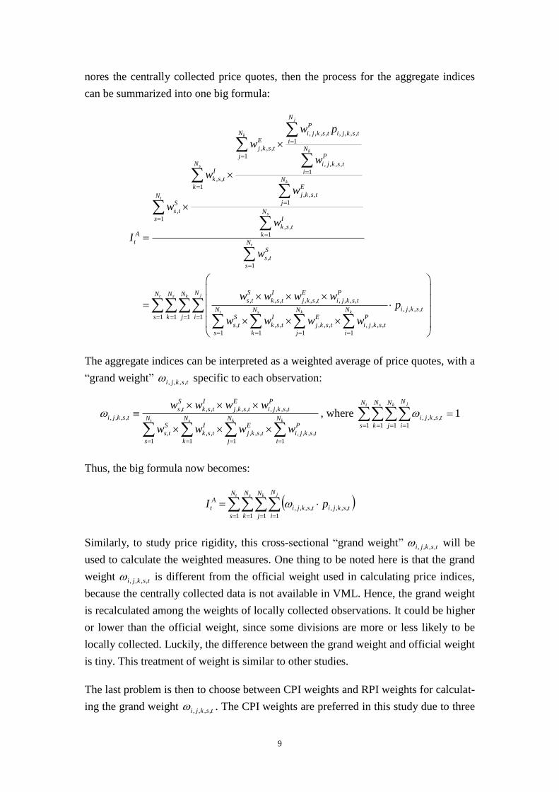
nores the centrally collected price quotes, then the process for the aggregate indices

can be summarized into one big formula:

, , , , , , , ,

1, , ,

1

, , , ,

1, ,

1

, , ,

1

,

1

, ,

1

,

1

, , , , , , , , , ,

, , , , , ,

1 1

j

k

k

s

k

t

s

t

t s

N

P

N i j k s t i j k s tE ij k s t N

Pj

N i j k s tI ik s t N

Ek

j k s tNjS

s t NIs

k s tA k

t NS

s t

s

S I E P

s t k s t j k s t i j k s t

N NS I E

s t k s t j k s t

s k

w p

w

w

w

w

w

w

I

w

w w w w

w w w

, , , ,

1 1 1 1

, , , ,

1 1

jt s k

k k

NN N N

i j k s tN Ns k j i P

i j k s t

j i

p

w

The aggregate indices can be interpreted as a weighted average of price quotes, with a

“grand weight” tskji ,,,, specific to each observation:

kkst N

i

P

tskji

N

j

E

tskj

N

k

I

tsk

N

s

S

ts

P

tskji

E

tskj

I

tsk

S

ts

tskji

wwww

wwww

1

,,,,

1

,,,

1

,,

1

,

,,,,,,,,,,

,,,, , where 11 1 1 1

,,,,

t s k jN

s

N

k

N

j

N

i

tskji

Thus, the big formula now becomes:

t s k jN

s

N

k

N

j

N

i

tskjitskji

A

t pI1 1 1 1

,,,,,,,,

Similarly, to study price rigidity, this cross-sectional “grand weight” tskji ,,,, will be

used to calculate the weighted measures. One thing to be noted here is that the grand

weight tskji ,,,, is different from the official weight used in calculating price indices,

because the centrally collected data is not available in VML. Hence, the grand weight

is recalculated among the weights of locally collected observations. It could be higher

or lower than the official weight, since some divisions are more or less likely to be

locally collected. Luckily, the difference between the grand weight and official weight

is tiny. This treatment of weight is similar to other studies.

The last problem is then to choose between CPI weights and RPI weights for calculat-

ing the grand weight tskji ,,,, . The CPI weights are preferred in this study due to three

10

reasons. Firstly, the published CPI weights are largely calculated from Household Fi-

nal Consumption Expenditure (HHFCE) data, since they cover the relevant population

and range of goods and services and, in addition, are classified by CPI divisions. This

is supplemented by data from the EFS and the International Passenger Survey, which

are used to calculate the weights of package holidays and airfares respectively. By

contrast, the RPI weights are mainly based on data from the EFS and relate to ex-

penditure by private households only, excluding the highest income households and

pensioner households mainly dependent on state benefits. Secondly, when the Bank of

England was announced independent in May 1997, the inflation target was originally

set at 2.5% in terms of the RPI excluding mortgage interest payments (RPIX). How-

ever, since December 2003, the inflation target has changed to 2% in terms of CPI,

previously known as Harmonised Index of Consumer Prices (HCIP). The importance

of CPI in monetary policy justifies the use of CPI weight in this study. The compara-

bility is the third advantage of using CPI weights, because HICP is also used by the

European Central Bank (ECB) as the measure of price stability across the Euro area.

3.3 Descriptive Summary

As mentioned earlier, there are over 650 representative items each year, and a number

of products across strata are sampled for each representative item. Each product has a

price trajectory① made up of several “price spells” or “durations”, while each duration

is made up of several price quotes. Thus, the dataset has a panel structure, because

there are 612,173 products (cross-sectional variation) over 12 years (time-series varia-

tion). The panel of price trajectories are described by the distributions.

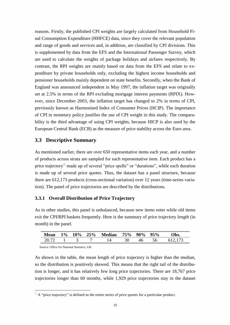
3.3.1 Overall Distribution of Price Trajectory

As in other studies, this panel is unbalanced, because new items enter while old items

exit the CPI/RPI baskets frequently. Here is the summary of price trajectory length (in

month) in the panel.

Mean 1% 10% 25% Median 75% 90% 95% Obs.

20.72 1 3 7 14 30 46 56 612,173

Source: Office for National Statistics, UK.

As shown in the table, the mean length of price trajectory is higher than the median,

so the distribution is positively skewed. This means that the right tail of the distribu-

tion is longer, and it has relatively few long price trajectories. There are 18,767 price

trajectories longer than 60 months, while 1,929 price trajectories stay in the dataset

①

A “price trajectory” is defined as the entire series of price quotes for a particular product.

11

for longer than 120 months, and only 49 price trajectories are present in the dataset

throughout the entire 144 months (12 years).

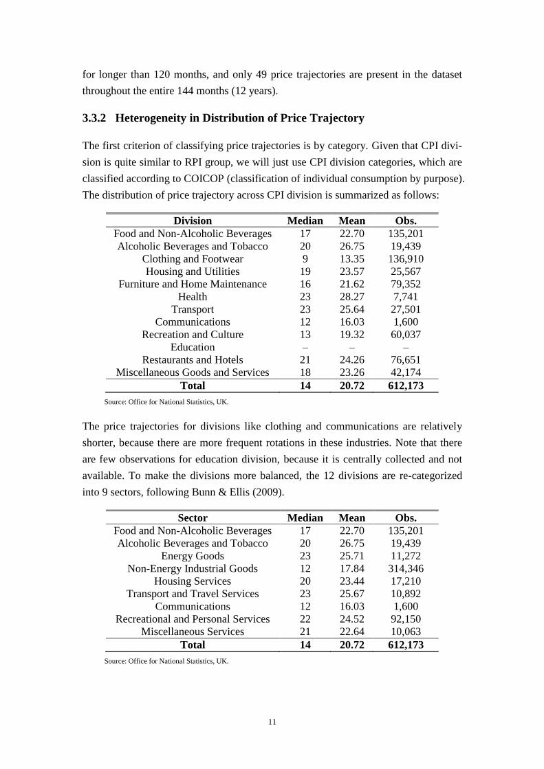
3.3.2 Heterogeneity in Distribution of Price Trajectory

The first criterion of classifying price trajectories is by category. Given that CPI divi-

sion is quite similar to RPI group, we will just use CPI division categories, which are

classified according to COICOP (classification of individual consumption by purpose).

The distribution of price trajectory across CPI division is summarized as follows:

Division Median Mean Obs.

Food and Non-Alcoholic Beverages 17 22.70 135,201

Alcoholic Beverages and Tobacco 20 26.75 19,439

Clothing and Footwear 9 13.35 136,910

Housing and Utilities 19 23.57 25,567

Furniture and Home Maintenance 16 21.62 79,352

Health 23 28.27 7,741

Transport 23 25.64 27,501

Communications 12 16.03 1,600

Recreation and Culture 13 19.32 60,037

Education – – –

Restaurants and Hotels 21 24.26 76,651

Miscellaneous Goods and Services 18 23.26 42,174

Total 14 20.72 612,173


The price trajectories for divisions like clothing and communications are relatively

shorter, because there are more frequent rotations in these industries. Note that there

are few observations for education division, because it is centrally collected and not

available. To make the divisions more balanced, the 12 divisions are re-categorized

into 9 sectors, following Bunn & Ellis (2009).

Sector Median Mean Obs.

Food and Non-Alcoholic Beverages 17 22.70 135,201

Alcoholic Beverages and Tobacco 20 26.75 19,439

Energy Goods 23 25.71 11,272

Non-Energy Industrial Goods 12 17.84 314,346

Housing Services 20 23.44 17,210

Transport and Travel Services 23 25.67 10,892

Communications 12 16.03 1,600

Recreational and Personal Services 22 24.52 92,150

Miscellaneous Services 21 22.64 10,063

Total 14 20.72 612,173


12

Similarly, sectors such as non-energy industrial goods (e.g. clothing) and communica-

tions have shorter price trajectories, due to the frequent rotations of product lines. The

first 4 categories are put together as “goods sectors” and the rest 5 categories are put

together as “services sectors”. For the same reason of rotation frequency, goods sec-

tors tend to have shorter price trajectories.

Sector Median Mean Obs.

Goods 13 19.76 480,258

Services 21 24.23 131,915

Total 14 20.72 612,173


The second criterion of classifying price trajectories is by shop type. This distinction

is important because the price setting behaviour differs significantly between big and

small firms. According to the convention in CPI/RPI, the “independent shop” is basi-

cally defined as small retailer, while the “multiple shop” is defined as big retailer. The

price trajectories for multiple shops tend to be longer, since new products are mostly

sold there and the rotation frequency is higher.

Shop Type Median Mean Obs.

Multiple 13 20.70 372,940

Independent 17 20.76 239,180

Unknown - - 53

Total 14 20.72 612,173


The third criterion of classifying price trajectories is by region. It turns out that the

heterogeneity in price setting behaviour across region in the UK is not significant,

though London has shorter price trajectories because high frequency of rotations.

Region Median Mean Obs.

London 13 19.69 71,978

South East 15 20.51 99,512

South West 16 20.78 52,272

East Anglia 15 20.84 44,335

East Midlands 16 22.15 42,295

West Midlands 15 21.09 53,260

Yorkshire & Humber 14 20.50 51,582

North West 13 19.73 63,928

North 12 20.12 32,078

Wales 16 23.45 28,183

Scotland 15 20.89 46,905

Northern Ireland 15 20.45 22,536

Unknown - - 3,309

Total 14 20.72 612,173


13

4 Conventional Method

The primary results reported in this section follow the conventional method and pro-

vide a comprehensive descriptive statistics of the three aspects of rigidity, including

the frequency, direction and magnitude of price change. These results are in line with

Bunn & Ellis (2009) and other IPN literature. If these naïve empirical results are used

to describe price setting behaviour in the UK, not much rigidity is found. However,

next section will show that this conclusion is biased.

4.1 Rigidity in Frequency of Price Change

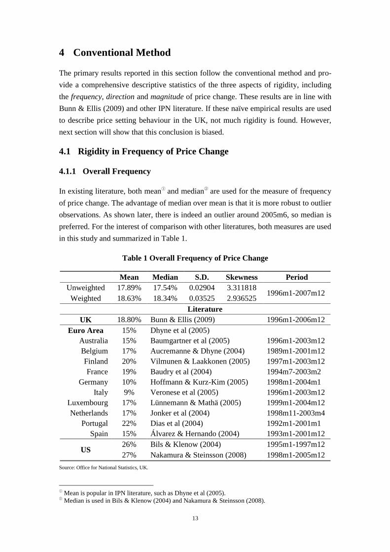
4.1.1 Overall Frequency

In existing literature, both mean① and median

② are used for the measure of frequency

of price change. The advantage of median over mean is that it is more robust to outlier

observations. As shown later, there is indeed an outlier around 2005m6, so median is

preferred. For the interest of comparison with other literatures, both measures are used

in this study and summarized in Table 1.

Table 1 Overall Frequency of Price Change

Mean Median S.D. Skewness Period

Unweighted 17.89% 17.54% 0.02904 3.311818 1996m1-2007m12

Weighted 18.63% 18.34% 0.03525 2.936525

Literature

UK 18.80% Bunn & Ellis (2009) 1996m1-2006m12

Euro Area 15% Dhyne et al (2005)

Australia 15% Baumgartner et al (2005) 1996m1-2003m12

Belgium 17% Aucremanne & Dhyne (2004) 1989m1-2001m12

Finland 20% Vilmunen & Laakkonen (2005) 1997m1-2003m12

France 19% Baudry et al (2004) 1994m7-2003m2

Germany 10% Hoffmann & Kurz-Kim (2005) 1998m1-2004m1

Italy 9% Veronese et al (2005) 1996m1-2003m12

Luxembourg 17% Lünnemann & Mathä (2005) 1999m1-2004m12

Netherlands 17% Jonker et al (2004) 1998m11-2003m4

Portugal 22% Dias et al (2004) 1992m1-2001m1

Spain 15% Álvarez & Hernando (2004) 1993m1-2001m12

US 26% Bils & Klenow (2004) 1995m1-1997m12

27% Nakamura & Steinsson (2008) 1998m1-2005m12


①

Mean is popular in IPN literature, such as Dhyne et al (2005). ②

Median is used in Bils & Klenow (2004) and Nakamura & Steinsson (2008).

14

The result presented here is almost the same as that found in Bunn & Ellis (2009) ex-

cept that the mean frequency is slightly lower. That is because the mean frequency in

2007 is relatively lower (16.46%), which is not included in their study, dragging the

overall mean a bit downward. This tiny difference does not affect the conclusion they

find, i.e. the mean frequency of price change in the UK is higher than that in the Euro

area, but lower than that in the US. Furthermore, according to the conventional meth-

od, the “duration” can be calculated by the inverse of frequency, which describes how

long for all the prices to turnover once. Therefore, the implied mean duration based on

this conventional method, 5.5 months, also lies between the Euro area and the US, and

so does the degree of price rigidity in the UK.

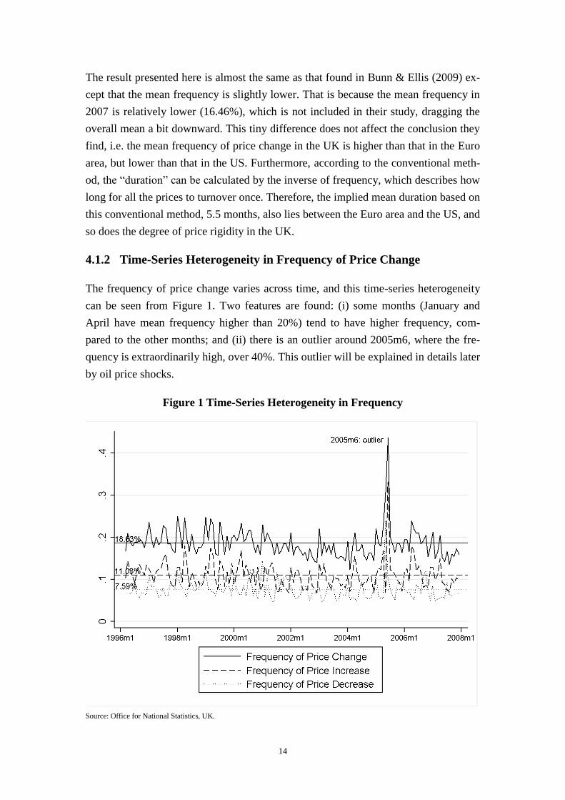
4.1.2 Time-Series Heterogeneity in Frequency of Price Change

The frequency of price change varies across time, and this time-series heterogeneity

can be seen from Figure 1. Two features are found: (i) some months (January and

April have mean frequency higher than 20%) tend to have higher frequency, com-

pared to the other months; and (ii) there is an outlier around 2005m6, where the fre-

quency is extraordinarily high, over 40%. This outlier will be explained in details later

by oil price shocks.

Figure 1 Time-Series Heterogeneity in Frequency


15

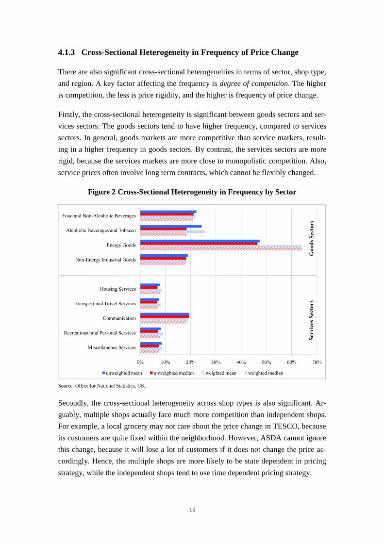
4.1.3 Cross-Sectional Heterogeneity in Frequency of Price Change

There are also significant cross-sectional heterogeneities in terms of sector, shop type,

and region. A key factor affecting the frequency is degree of competition. The higher

is competition, the less is price rigidity, and the higher is frequency of price change.

Firstly, the cross-sectional heterogeneity is significant between goods sectors and ser-

vices sectors. The goods sectors tend to have higher frequency, compared to services

sectors. In general, goods markets are more competitive than service markets, result-

ing in a higher frequency in goods sectors. By contrast, the services sectors are more

rigid, because the services markets are more close to monopolistic competition. Also,

service prices often involve long term contracts, which cannot be flexibly changed.

Figure 2 Cross-Sectional Heterogeneity in Frequency by Sector


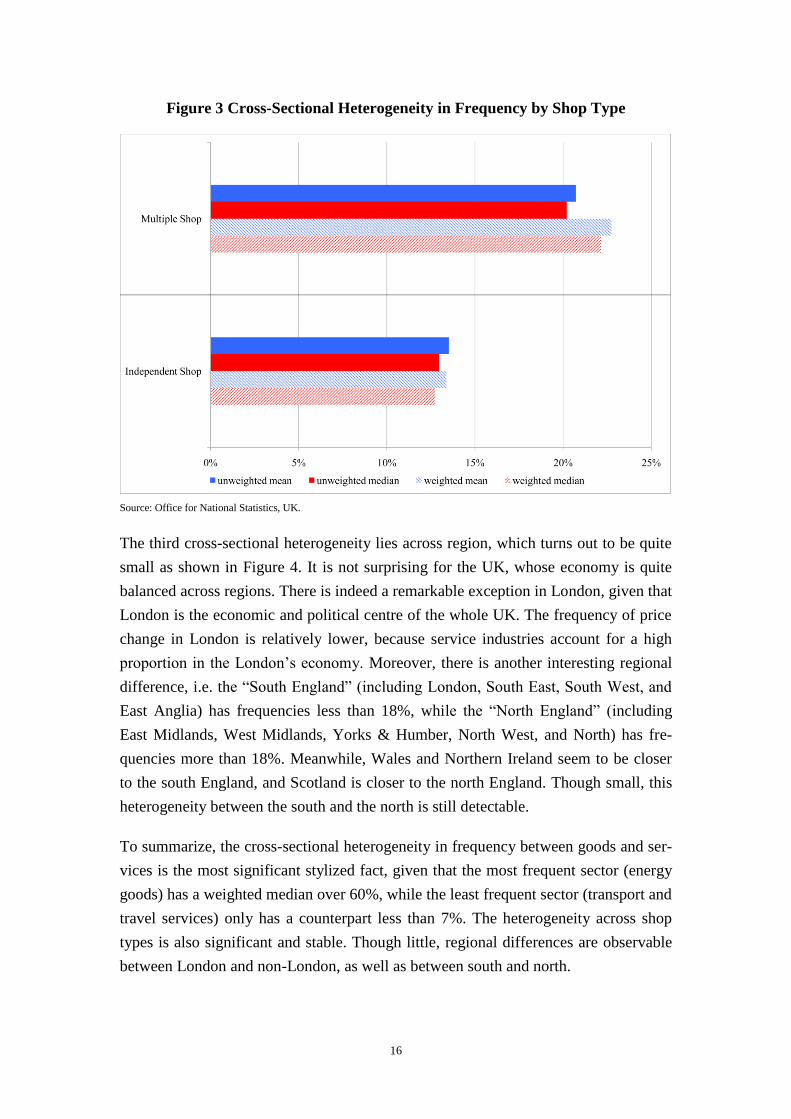
Secondly, the cross-sectional heterogeneity across shop types is also significant. Ar-

guably, multiple shops actually face much more competition than independent shops.

For example, a local grocery may not care about the price change in TESCO, because

its customers are quite fixed within the neighborhood. However, ASDA cannot ignore

this change, because it will lose a lot of customers if it does not change the price ac-

cordingly. Hence, the multiple shops are more likely to be state dependent in pricing

strategy, while the independent shops tend to use time dependent pricing strategy.

16

Figure 3 Cross-Sectional Heterogeneity in Frequency by Shop Type


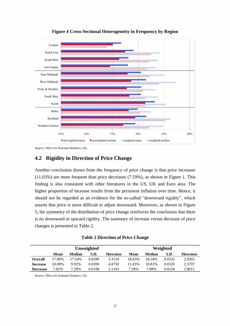
The third cross-sectional heterogeneity lies across region, which turns out to be quite

small as shown in Figure 4. It is not surprising for the UK, whose economy is quite

balanced across regions. There is indeed a remarkable exception in London, given that

London is the economic and political centre of the whole UK. The frequency of price

change in London is relatively lower, because service industries account for a high

proportion in the London’s economy. Moreover, there is another interesting regional

difference, i.e. the “South England” (including London, South East, South West, and

East Anglia) has frequencies less than 18%, while the “North England” (including

East Midlands, West Midlands, Yorks & Humber, North West, and North) has fre-

quencies more than 18%. Meanwhile, Wales and Northern Ireland seem to be closer

to the south England, and Scotland is closer to the north England. Though small, this

heterogeneity between the south and the north is still detectable.

To summarize, the cross-sectional heterogeneity in frequency between goods and ser-

vices is the most significant stylized fact, given that the most frequent sector (energy

goods) has a weighted median over 60%, while the least frequent sector (transport and

travel services) only has a counterpart less than 7%. The heterogeneity across shop

types is also significant and stable. Though little, regional differences are observable

between London and non-London, as well as between south and north.

17

Figure 4 Cross-Sectional Heterogeneity in Frequency by Region


4.2 Rigidity in Direction of Price Change

Another conclusion drawn from the frequency of price change is that price increases

(11.03%) are more frequent than price decreases (7.59%), as shown in Figure 1. This

finding is also consistent with other literatures in the US, UK and Euro area. The

higher proportion of increase results from the persistent inflation over time. Hence, it

should not be regarded as an evidence for the so-called “downward rigidity”, which

asserts that price is more difficult to adjust downward. Moreover, as shown in Figure

5, the symmetry of the distribution of price change reinforces the conclusion that there

is no downward or upward rigidity. The summary of increase versus decrease of price

changes is presented in Table 2.

Table 2 Direction of Price Change

Unweighted Weighted

Mean Median S.D. Skewness Mean Median S.D. Skewness

Overall 17.89% 17.54% 0.0290 3.3118 18.63% 18.34% 0.0352 2.9365

Increase 10.08% 9.92% 0.0200 4.8750 11.05% 10.81% 0.0320 2.5707

Decrease 7.82% 7.29% 0.0198 2.1103 7.58% 7.08% 0.0234 2.8011


18

4.3 Rigidity in Magnitude of Price Change

There are two seemingly contradictory opinions on the rigidity in magnitude. On the

one hand, Mankiw (1985) menu cost model provides an influential explanation on the

“fixed adjustment costs” of price resetting. Similarly, Akerlof & Yellen (1985) sug-

gest that the firm has an interval of optimal prices, rather than a point estimate of a

single optimal price. It results in a so-called “band of inertia”, within which a firm

will not reset its price. Only when there are big changes in the fundamentals, the firm

will review its price and conduct the costly marketing research. Hence, the magnitude

of price change cannot be too precise due to this “fixed adjustment costs”. If this is

true, then one expects to see two interesting phenomena: (i) price levels tend to end

with some particular numbers, like £X.X0, £X.X5, or £X.X9, which is referred to as

“attractive pricing”; (ii) price changes tend to be integers, like 20% or 50%, rather

than fractional percentage changes, like 3.1415926%. On the other hand, Rotemberg

(1982) argues that the magnitude of price change cannot be too large, because it will

upset the customers, and firms are reluctant to invoke this “customer anger”. If this is

true, then one expects to see more small changes than large changes.

Many authors, including Bunn & Ellis (2009), misunderstand that these two strands of

models are competing against each other. However, imprecise change does not neces-

sarily lead to more large changes, and more small changes do not either imply that all

changes are precisely set. The two models focus on different aspects of price change,

i.e. the precision of magnitude and the range of the magnitude. Two empirical results

are used to check the two models: the distribution of magnitude of price changes and

the distribution of the last decimal of price level.

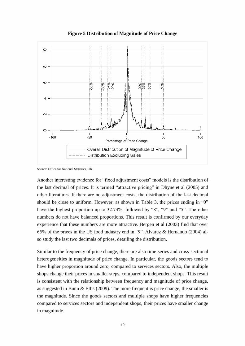
The first feature from Figure 5 is that most price changes are around zero. In other

words, the “customer anger” models are supported. This finding is similar to Bunn &

Ellis (2009) in the UK, but different from the IPN literatures. For example, Álvarez

and Hernando (2004) find that most price changes in Spain are quite large, not around

zero. The second feature is that the distribution of magnitude is almost symmetric,

with several stylized spikes around ±20%, ±25%, ±30%, and ±50%. When sales are

excluded, this stylized pattern is weaker but still significant. This suggests that firms

tend to change their prices by a fixed proportion, rather than tiny fractions. Thus, it

supports the “fixed adjustment costs” models, in the sense that firms prefer to follow

“rule of thumb”, because carrying out marketing research is too costly. For firms with

bounded rationality, it is better for them to change imprecisely than doing nothing.

Hence, the two opinions are not actually contradictory. Rather, they can perfectly co-

exist under our empirical result.

19

Figure 5 Distribution of Magnitude of Price Change


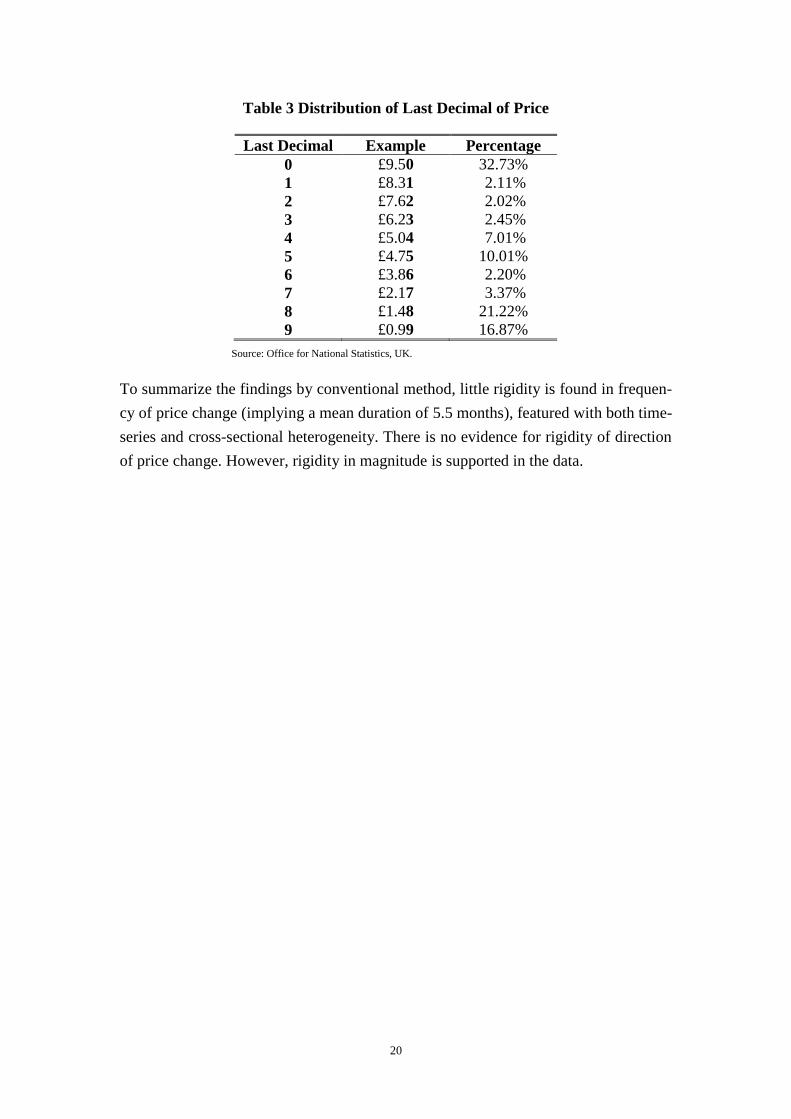
Another interesting evidence for “fixed adjustment costs” models is the distribution of

the last decimal of prices. It is termed “attractive pricing” in Dhyne et al (2005) and

other literatures. If there are no adjustment costs, the distribution of the last decimal

should be close to uniform. However, as shown in Table 3, the prices ending in “0”

have the highest proportion up to 32.73%, followed by “8”, “9” and “5”. The other

numbers do not have balanced proportions. This result is confirmed by our everyday

experience that these numbers are more attractive. Bergen et al (2003) find that over

65% of the prices in the US food industry end in “9”. Álvarez & Hernando (2004) al-

so study the last two decimals of prices, detailing the distribution.

Similar to the frequency of price change, there are also time-series and cross-sectional

heterogeneities in magnitude of price change. In particular, the goods sectors tend to

have higher proportion around zero, compared to services sectors. Also, the multiple

shops change their prices in smaller steps, compared to independent shops. This result

is consistent with the relationship between frequency and magnitude of price change,

as suggested in Bunn & Ellis (2009). The more frequent is price change, the smaller is

the magnitude. Since the goods sectors and multiple shops have higher frequencies

compared to services sectors and independent shops, their prices have smaller change

in magnitude.

20

Table 3 Distribution of Last Decimal of Price

Last Decimal Example Percentage

0 £9.50 32.73%

1 £8.31 2.11%

2 £7.62 2.02%

3 £6.23 2.45%

4 £5.04 7.01%

5 £4.75 10.01%

6 £3.86 2.20%

7 £2.17 3.37%

8 £1.48 21.22%

9 £0.99 16.87%


To summarize the findings by conventional method, little rigidity is found in frequen-

cy of price change (implying a mean duration of 5.5 months), featured with both time-

series and cross-sectional heterogeneity. There is no evidence for rigidity of direction

of price change. However, rigidity in magnitude is supported in the data.

21

5 Cross-Sectional Method

Based on the conventional method, one cannot say there is much rigidity in price set-

ting behavior, since the frequency is quite high (around 18.63%) and the implied du-

ration is less than half a year. However, there are several drawbacks of this method of

measuring duration and rigidity. On the one hand, this naïve method, which computes

the duration by the inverse of frequency, has the problem of oversampling. On the

other hand, the data available is designed for price indices rather than duration, so the

basket is changing each year, resulting in many censoring and truncation cases.

Dixon (2010) argues that the duration implied by the inverse of frequency is down-

ward biased due to oversampling of short durations. He also suggests that the cross-

sectional distribution of duration across firm (DAF) is an unbiased measure of dura-

tion and robust to censorings. The DAF here is defined as the length of the lifespan of

the current price. In reality, it is difficult to know the duration of a current price, be-

cause one does not know ex ante when this price will change in the future. However,

the duration for each price can be easily worked out ex post in the historical data.

5.1 Cross-Sectional Distribution of DAF

5.1.1 Overall DAF

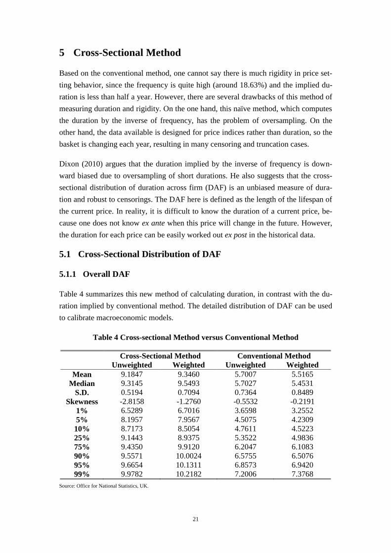
Table 4 summarizes this new method of calculating duration, in contrast with the du-

ration implied by conventional method. The detailed distribution of DAF can be used

to calibrate macroeconomic models.

Table 4 Cross-sectional Method versus Conventional Method

Cross-Sectional Method Conventional Method

Unweighted Weighted Unweighted Weighted

Mean 9.1847 9.3460 5.7007 5.5165

Median 9.3145 9.5493 5.7027 5.4531

S.D. 0.5194 0.7094 0.7364 0.8489

Skewness -2.8158 -1.2760 -0.5532 -0.2191

1% 6.5289 6.7016 3.6598 3.2552

5% 8.1957 7.9567 4.5075 4.2309

10% 8.7173 8.5054 4.7611 4.5223

25% 9.1443 8.9375 5.3522 4.9836

75% 9.4350 9.9120 6.2047 6.1083

90% 9.5571 10.0024 6.5755 6.5076

95% 9.6654 10.1311 6.8573 6.9420

99% 9.9782 10.2182 7.2006 7.3768


22

Not surprisingly, DAF is much higher than duration implied by frequency. This is be-

cause the frequency is based on the oversampled short durations, as argued in Section

2. As a result, the inverse of frequency is a downward biased estimate of duration. By

contrast, DAF does not have this problem. At any point in time, each product’s price

quote corresponds to a duration, i.e. the length of lifespan of the current price. The

cross-sectional distribution of durations, or DAF, can then be obtained. The estimated

mean and median of DAF are both over 9 months, much longer than the implied dura-

tion. This measure of duration strongly supports the price rigidity in frequency.

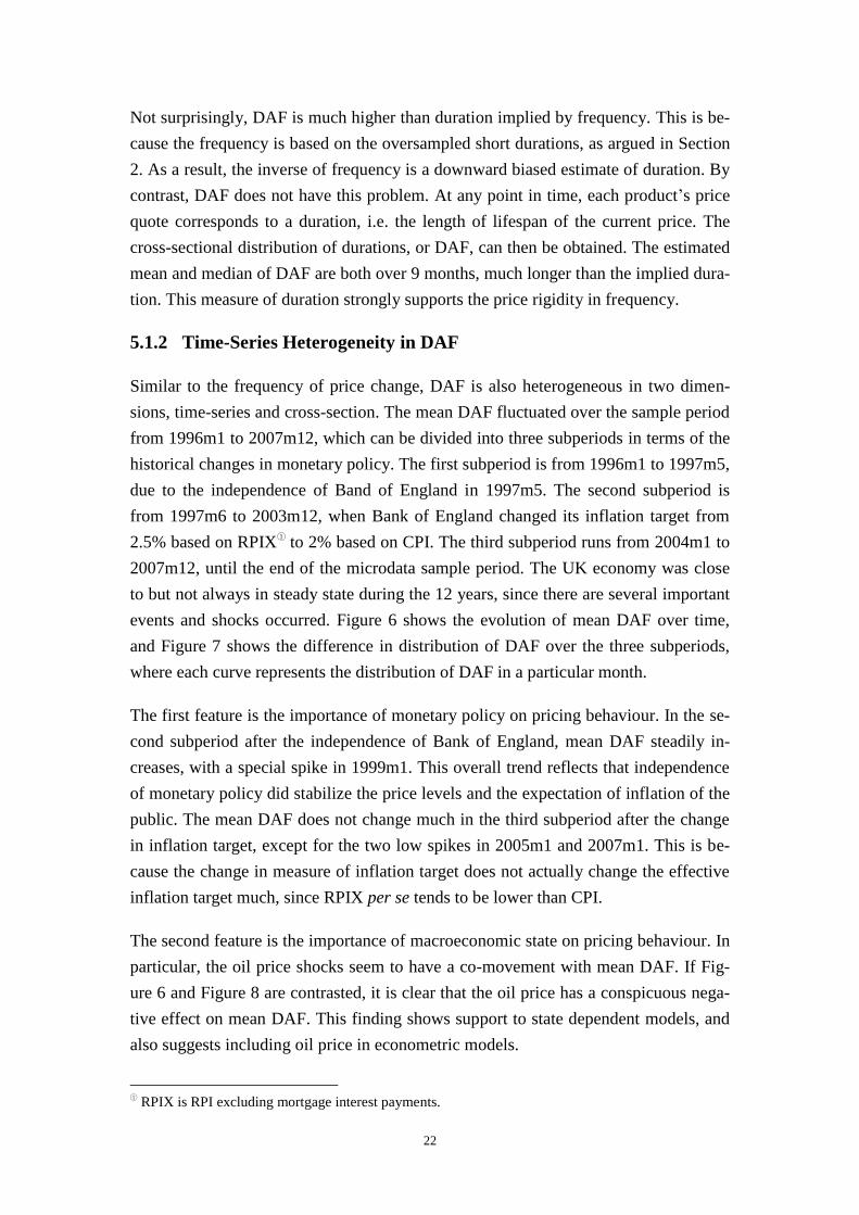
5.1.2 Time-Series Heterogeneity in DAF

Similar to the frequency of price change, DAF is also heterogeneous in two dimen-

sions, time-series and cross-section. The mean DAF fluctuated over the sample period

from 1996m1 to 2007m12, which can be divided into three subperiods in terms of the

historical changes in monetary policy. The first subperiod is from 1996m1 to 1997m5,

due to the independence of Band of England in 1997m5. The second subperiod is

from 1997m6 to 2003m12, when Bank of England changed its inflation target from

2.5% based on RPIX① to 2% based on CPI. The third subperiod runs from 2004m1 to

2007m12, until the end of the microdata sample period. The UK economy was close

to but not always in steady state during the 12 years, since there are several important

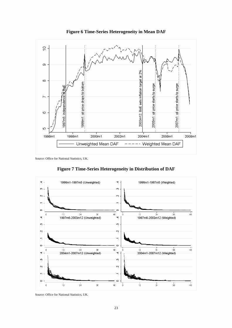
events and shocks occurred. Figure 6 shows the evolution of mean DAF over time,

and Figure 7 shows the difference in distribution of DAF over the three subperiods,

where each curve represents the distribution of DAF in a particular month.

The first feature is the importance of monetary policy on pricing behaviour. In the se-

cond subperiod after the independence of Bank of England, mean DAF steadily in-

creases, with a special spike in 1999m1. This overall trend reflects that independence

of monetary policy did stabilize the price levels and the expectation of inflation of the

public. The mean DAF does not change much in the third subperiod after the change

in inflation target, except for the two low spikes in 2005m1 and 2007m1. This is be-

cause the change in measure of inflation target does not actually change the effective

inflation target much, since RPIX per se tends to be lower than CPI.

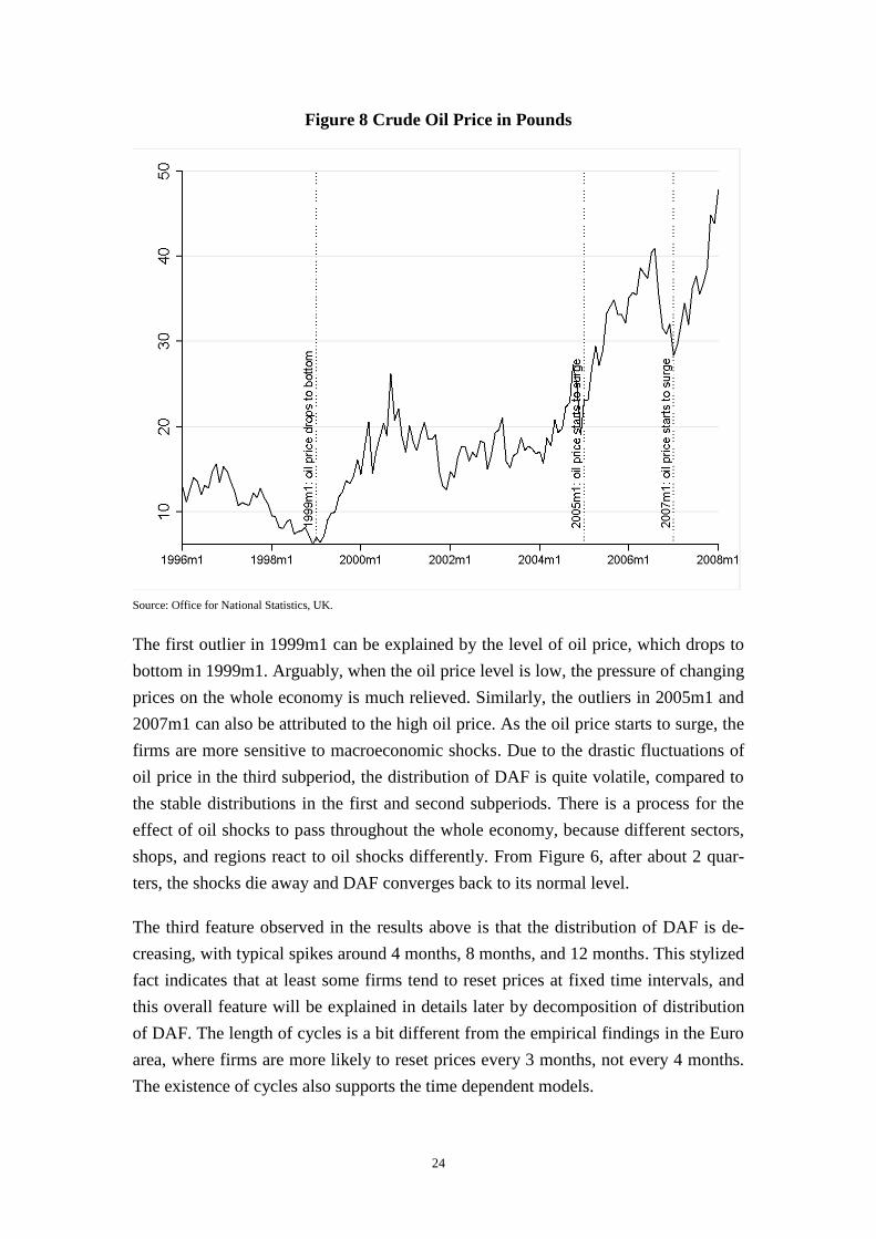
The second feature is the importance of macroeconomic state on pricing behaviour. In

particular, the oil price shocks seem to have a co-movement with mean DAF. If Fig-

ure 6 and Figure 8 are contrasted, it is clear that the oil price has a conspicuous nega-

tive effect on mean DAF. This finding shows support to state dependent models, and

also suggests including oil price in econometric models.

①

RPIX is RPI excluding mortgage interest payments.

23

Figure 6 Time-Series Heterogeneity in Mean DAF


Figure 7 Time-Series Heterogeneity in Distribution of DAF


24

Figure 8 Crude Oil Price in Pounds


The first outlier in 1999m1 can be explained by the level of oil price, which drops to

bottom in 1999m1. Arguably, when the oil price level is low, the pressure of changing

prices on the whole economy is much relieved. Similarly, the outliers in 2005m1 and

2007m1 can also be attributed to the high oil price. As the oil price starts to surge, the

firms are more sensitive to macroeconomic shocks. Due to the drastic fluctuations of

oil price in the third subperiod, the distribution of DAF is quite volatile, compared to

the stable distributions in the first and second subperiods. There is a process for the

effect of oil shocks to pass throughout the whole economy, because different sectors,

shops, and regions react to oil shocks differently. From Figure 6, after about 2 quar-

ters, the shocks die away and DAF converges back to its normal level.

The third feature observed in the results above is that the distribution of DAF is de-

creasing, with typical spikes around 4 months, 8 months, and 12 months. This stylized

fact indicates that at least some firms tend to reset prices at fixed time intervals, and

this overall feature will be explained in details later by decomposition of distribution

of DAF. The length of cycles is a bit different from the empirical findings in the Euro

area, where firms are more likely to reset prices every 3 months, not every 4 months.

The existence of cycles also supports the time dependent models.

25

5.1.3 Cross-Sectional Heterogeneity in DAF

In addition to time dimension, DAF is also heterogeneous across sectors, shop types,

and regions. Similar to the conclusion obtained in conventional method, services sec-

tors (11.38 months) have longer DAF than goods sectors (7.43 months), while inde-

pendent shops (10.06 months) have longer DAF than multiple shops (7.60 months).

The heterogeneity across regions is still small. Thus, the new measure of rigidity does

not change the cross-sectional rankings in rigidity, but the degree of rigidity. The de-

tailed distributions of DAF by sector and by shop type can also be used for future use

in calibrating macroeconomic models.

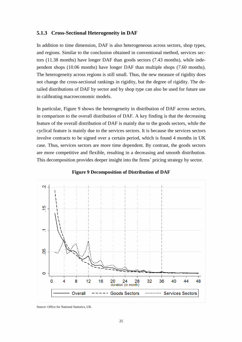
In particular, Figure 9 shows the heterogeneity in distribution of DAF across sectors,

in comparison to the overall distribution of DAF. A key finding is that the decreasing

feature of the overall distribution of DAF is mainly due to the goods sectors, while the

cyclical feature is mainly due to the services sectors. It is because the services sectors

involve contracts to be signed over a certain period, which is found 4 months in UK

case. Thus, services sectors are more time dependent. By contrast, the goods sectors

are more competitive and flexible, resulting in a decreasing and smooth distribution.

This decomposition provides deeper insight into the firms’ pricing strategy by sector.

Figure 9 Decomposition of Distribution of DAF


26

5.2 Cross-Sectional Distribution of Age

The age of price is another cross-sectional measure of rigidity, which is closely corre-

lated with DAF. Age is defined as how long the current price has survived since the

last change. Instead of using complete duration, the current age of each firm’s price,

i.e. how many months have passed since the last change, is used. In fact, age is an in-

complete duration, so the mean/median age must be less than mean/median DAF.

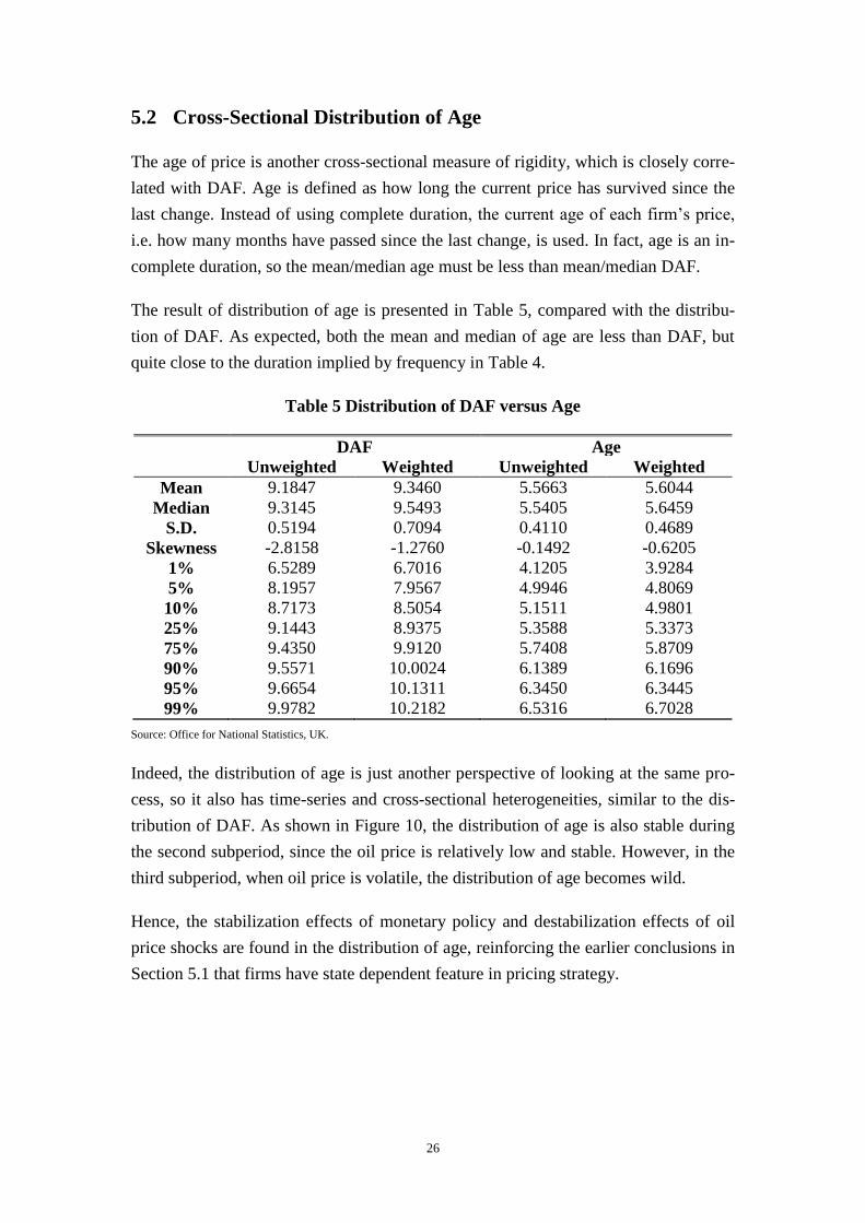
The result of distribution of age is presented in Table 5, compared with the distribu-

tion of DAF. As expected, both the mean and median of age are less than DAF, but

quite close to the duration implied by frequency in Table 4.

Table 5 Distribution of DAF versus Age

DAF Age

Unweighted Weighted Unweighted Weighted

Mean 9.1847 9.3460 5.5663 5.6044

Median 9.3145 9.5493 5.5405 5.6459

S.D. 0.5194 0.7094 0.4110 0.4689

Skewness -2.8158 -1.2760 -0.1492 -0.6205

1% 6.5289 6.7016 4.1205 3.9284

5% 8.1957 7.9567 4.9946 4.8069

10% 8.7173 8.5054 5.1511 4.9801

25% 9.1443 8.9375 5.3588 5.3373

75% 9.4350 9.9120 5.7408 5.8709

90% 9.5571 10.0024 6.1389 6.1696

95% 9.6654 10.1311 6.3450 6.3445

99% 9.9782 10.2182 6.5316 6.7028


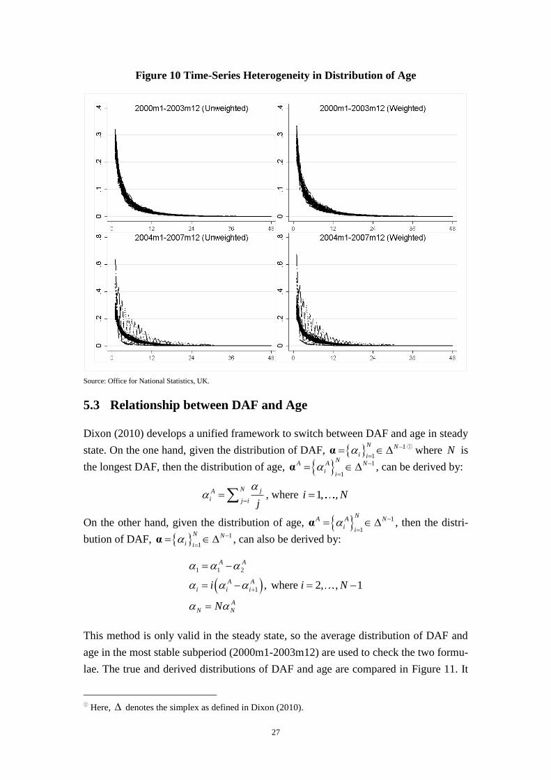
Indeed, the distribution of age is just another perspective of looking at the same pro-

cess, so it also has time-series and cross-sectional heterogeneities, similar to the dis-

tribution of DAF. As shown in Figure 10, the distribution of age is also stable during

the second subperiod, since the oil price is relatively low and stable. However, in the

third subperiod, when oil price is volatile, the distribution of age becomes wild.

Hence, the stabilization effects of monetary policy and destabilization effects of oil

price shocks are found in the distribution of age, reinforcing the earlier conclusions in

Section 5.1 that firms have state dependent feature in pricing strategy.

27

Figure 10 Time-Series Heterogeneity in Distribution of Age


5.3 Relationship between DAF and Age

Dixon (2010) develops a unified framework to switch between DAF and age in steady

state. On the one hand, given the distribution of DAF, 1

1

N N

i i

α

① where N is

the longest DAF, then the distribution of age, 1

1

NA A N

ii

α , can be derived by:

N jA

i j i j

, where 1, ,i N

On the other hand, given the distribution of age, 1

1

NA A N

ii

α , then the distri-

bution of DAF, 1

1

N N

i i

α , can also be derived by:

1 1 2

1 , where 2, , 1

A A

A A

i i i

A

N N

i i N

N

This method is only valid in the steady state, so the average distribution of DAF and

age in the most stable subperiod (2000m1-2003m12) are used to check the two formu-

lae. The true and derived distributions of DAF and age are compared in Figure 11. It

①

Here, denotes the simplex as defined in Dixon (2010).

28

is obvious that the true and derived distributions are quite close, especially for the de-

rived distribution of age. This simple practice successfully justifies this important the-

oretical contribution of Dixon (2010).

Figure 11 True and Derived Distribution of DAF and Age


That is to say, once the distribution of age or other distributions are already obtained,

the distribution of DAF can also be easily derived using the formula in Dixon (2010).

Further work is to be done based on the empirical findings. This unbiased distribution

of duration is essential for macroeconomic modelling, because the micro evidence can

be applied to calibrating and simulating New Keynesian heterogeneous agent models,

or testing theoretical models.

29

6 Conclusion

This paper studies the price setting behaviour for the retailers in the UK during the

latest 12 years. Both conventional and cross-sectional methods are applied to the un-

published microdata, resulting in different conclusions on price rigidity. There are

five important stylized facts:

(i) The overall mean duration is 9.3 months in terms of DAF, much longer

than 5.5 months as implied from the frequency by the conventional method.

This is a strong evidence for rigidity in retailers’ price setting behaviour,

different from other studies based on the conventional method.

(ii) There is little support for rigidity in direction of price change, but we do

find evidence for rigidity in magnitude of price change regarding precision

and range. In other words, price faces the same rigidity to rise or fall, but it

tends to end with attractive numbers and change by fixed proportion.

(iii) Significant cross-sectional heterogeneity is observed by sector and by shop

type, while little regional difference or time-series heterogeneity is found.

Goods sectors tend to be more flexible than services sectors, while multi-

ple shops change prices more frequently than independent shops.

(iv) The distribution of DAF has two stable features over the sample period, i.e.

the decreasing feature due to goods sectors and the cyclical feature due to

services sectors. The length of cycles is around 4 months. This cyclical

feature supports the time dependent models.

(v) Macroeconomic factors have considerable effects on the rigidity of price

change. The independent monetary policy has a stabilization effect, while

oil price shocks have a destabilization effect on the mean DAF. This find-

ing supports state dependent models.

Apart from the stylized facts on rigidity, another important conclusion is drawn in this

paper. The distribution of DAF directly estimated from data is very close to that indi-

rectly derived from the distribution of age according to the formula in Dixon (2010).

On the one hand, the descriptive results in this paper give insight into econometric

modelling of pricing mechanism or strategy. On the other hand, the micro findings of

the distributions can be used to calibrate macroeconomic models in order to better

mimic the macro evidence, such as the second moments of output and inflation.

30

Reference

Álvarez, L. & Hernando, I. (2004) “Price Setting Behaviour in Spain: Stylized Facts

using Consumer Micro Data.” ECB Working Paper, No. 416.

Aucremanne, L. & Dhyne, E. (2005) “Time-Dependent versus State-Dependent

Pricing: a Panel Data Approach to the Determinants of Belgian Consumer Price

Changes.” ECB Working Paper, No. 462.

Baharad, E. & Eden, B. (2004) “Price Rigidity and Price Dispersion: Evidence from

Micro Data.” Review of Economic Dynamics, Vol. 7, 613-641.

Baudry, L., LeBihan, H., Sevestre, P. & Tarrieu, S. (2007) “What do Thirteen Mil-

lion Price Records have to Say about Consumer Price Rigidity?” Oxford Bulletin of

Economics and Statistics, Vol. 67:2, 0305-9049.

Bils, M. & Klenow, P. (2004) “Some Evidence on the Importance of Sticky Prices.”

Journal of Monetary Economics, Vol. 112, 947-85.

Bunn, P. & Ellis, C. (2009) “Price-Setting Behaviour in the United Kingdom: a Mi-

crodata Approach.” Bank of England Quarterly Bulletin, 2009 Q1.

Calvo, G. A. (1983) “Staggered Prices in a Utility Maximising Framework.” Journal

of Monetary Economics, Vol. 12, 383-98.

Cleves, M., Gould, W. W., Gutierrez, R. G. & Marchenko, Y. (2008) “An Intro-

duction to Survival Analysis Using Stata (2nd

Edition).” Stata Press.

Office for National Statistics (2010) “Consumer Price Indices Technical Manual.”

Dhyne, E., Álvarez, L., Le Bihan, H., Veronese, G., Dias, D., Hoffmann, J., Jonk-

er, N., Lünnemann, P., Rumler, F. & Vilmunen, J. (2005) “Price Setting in the Eu-

ro Area: Some Stylized Facts from Individual Consumer Price Data.” ECB Working

Paper, No. 524.

Dixon, H. D. (2010) “A Unified Framework for Using Micro-Data to Compare Dy-

namic Wage and Price Setting Models.” CESIFO Working Paper, No. 3093.

Hoffmann, J. & Kurz-Kim, J. R. (2005) “Consumer Price Adjustment under the

Microscope: Germany in a period of Low Inflation.” Deutsche Bundesbank, mimeo.

Jenkins, S. P. (2004) “Survival Analysis”. Unpublished manuscript, Institute for So-

cial and Economic Research, University of Essex, Colchester, UK.

31

Jonker, N., Folkertsma, C. & Blijenberg, H. (2004) “An Empirical Analysis of Be-

haviour in the Netherlands in the Period 1998-2003 Using Micro Data.” ECB Working

Paper, No. 413.

Lach, S. & Tsiddon, D. (1992) “The Behaviour of Prices and Inflation: an Empirical

Analysis of Disaggregated Price Data.” Journal of Political Economy, Vol. 100, 349-

389.

Lach, S. & Tsiddon, D. (1996) “Staggering and Synchronization in Price Setting:

Evidence from Multiproduct Firms.” American Economic Review, Vol. 86, 1175-1196.

Lünnemann, P. & Mathä, T. (2005) “Consumer Price Behaviour in Luxembourg:

Evidence from Micro CPI Data.” Banque Centrale du Luxembourg, mimeo.

Mankiw, N. G. (1985) “Small Menu Costs and Large Business Cycles: a Macroeco-

nomic Model of Monopoly.” Quarterly Journal of Economics, Vol. 100:2, 529-37.

Nakamura, E. & Steinsson, J. (2008) “Five Facts about Prices: a Re-Evaluation of

Menu Cost Models.” Quarterly Journal of Economics, Vol. 123:4, 1415-1464.

Gabriel, P. & Reiff, Á. (2007) “Estimating the Extent of Price Stickiness in Hungary:

a Hazard-Based Approach.” The Central Bank of Hungary, mimeo.

Rotemberg, J. (1980) “Sticky Prices in the United States.” Journal of Political Econ-

omy, Vol. 90, 187-211.

Taylor, J. (1980) “Aggregate Dynamics and Staggered Contracts.” Journal of Politi-

cal Economy, Vol. 88, 1-23.

Veronese, G., Fabiani, S., Gattulli, A. & Sabbatini, R. (2005) “Consumer Price

Behaviour in Italy: Evidence from Micro CPI Data.” ECB Working Paper, No. 449.

Vilmunen, J. & Laakkonen, H. (2005) “How Often do Prices Change in Finland?

Evidence from Micro CPI Data.” Suomen Pankki, mimeo.

an empirical study on price rigidity - -orca

Documents