the kinked demand curve and price rigidity: evidence from scanner data*

Scand. J. of Economics 112(4), 723–752, 2010DOI: 10.1111/j.1467-9442.2010.01621.x

The Kinked Demand Curve and PriceRigidity: Evidence from Scanner Data∗

Maarten DosscheNational Bank of Belgium, B-1000 Brussels, [email protected]

Freddy HeylenGhent University, B-9000 Ghent, [email protected]

Dirk Van den PoelGhent University, B-9000 Ghent, [email protected]

Abstract

We estimate the curvature of the demand curve for a wide range of products. We use anextension of Deaton and Muellbauer’s Almost Ideal Demand System and scanner data froma large euro area retailer. We find evidence that the overall price elasticity of demand ishigher for price increases than for price decreases. However, the overall degree of curvatureis one to two orders of magnitude smaller than the value economists usually impose. Thissuggests that the shape of the demand curve is unlikely to be the only source of real pricerigidity.

Keywords: Price setting; real price rigidity; Almost Ideal Demand System

JEL classification: C33; D12; E3

I. Introduction

A large body of literature using vector autoregressions has documentedthe persistent effects of a monetary policy shock on real output and in-flation (see, e.g., Christiano et al., 1999; Peersman, 2004). To match this

∗This paper was written with the financial support of the National Bank of Belgium. Theauthors also acknowledge support from the Belgian Program on Interuniversity Poles ofAttraction, initiated by the Belgian State, Federal Office for Scientific, Technical and CulturalAffairs, contract UAP No. P 6/07. We thank two anonymous referees, Filip Abraham, KennAriga, Luc Aucremanne, Mark Bils, Gerdie Everaert, Etienne Gagnon, Nils Gottfries, AlanKackmeister, Jurek Konieczny, Joep Konings, Oleksiy Kryvtsov, Daniel Levy, Morten Ravn,Adam Reiff, Dirk Van de Gaer, Frank Verboven, Jon Willis, and Raf Wouters for helpfulcomments and suggestions. The views expressed in this paper are those of the authors anddo not necessarily reflect the views of the National Bank of Belgium. All errors are ourown.

C© The editors of the Scandinavian Journal of Economics 2010. Published by Blackwell Publishing, 9600 Garsington Road,Oxford, OX4 2DQ, UK and 350 Main Street, Malden, MA 02148, USA.

724 M. Dossche, F. Heylen, and D. Van den Poel

persistence, micro-founded models with sticky prices have been developed.A first attempt was to introduce frictions to nominal price adjustment (e.g.,Taylor, 1980; Calvo, 1983; Mankiw, 1985). However, as shown by severalauthors, the real effects of nominal frictions alone do not last much longerthan the average duration of a price (Ball and Romer, 1990; Bergin andFeenstra, 2000; Chari et al., 2000). Taking into account recent microeco-nomic evidence that the mean price duration lies between 1.8 and 4 quartersfor the US (Bils and Klenow, 2004; Nakamura and Steinsson, 2008), andbetween 4 and 5 quarters for the euro area (Dhyne et al., 2006), nominalfrictions alone fail to generate the persistence observed in the data.

The failure of nominal frictions to generate enough persistence has ledto the development of models that combine nominal and so-called realprice rigidities (Ball and Romer, 1990). Real rigidities refer to strategiccomplementarity in the price-setting decision of firms. A firm is morereluctant to adjust its price in response to changes in the state of theeconomy the less other firms adjust their prices. Different frictions cangenerate this strategic complementarity. One way of introducing real rigidityis the roundabout production structure of Basu (1995). Real price rigidityfollows from the assumption that firms use the output of all other firms asmaterials in their own production (Bergin and Feenstra, 2000). Another wayis to introduce firm-specific production factors.1 In this case the marginalcost is a negative function of the relative price, which dampens the incentiveto change prices.

A recently popular way of introducing real rigidity is through a kinked(or quasi-concave) demand curve.2 The price elasticity of demand thenbecomes a function of the relative price. A key concept is the so-calledcurvature of the demand curve, which measures the price elasticity of theprice elasticity. With positive curvature, a higher relative price raises theelasticity of demand for a firm’s product, so that the firm increasinglyloses profits from relative price increases. Conversely, a lower relativeprice reduces the elasticity of a firm’s demand, so that the firm againincreasingly loses profits from relative price decreases. In this way, thecombination of small costs to nominal price adjustment and a concavedemand curve generates slow adjustment to nominal shocks.

1 For example, Galı and Gertler (1999), Sbordone (2002), Woodford (2003), Altig et al.(2005), and Burstein and Hellwig (2007).2 See, e.g., Bergin and Feenstra (2000), Eichenbaum and Fisher (2004), Dotsey and King(2005), Klenow and Willis (2006), Coenen et al. (2007), and Smets and Wouters (2007).These papers have mainly introduced a quasi-concave demand curve by using the preferencespecification of Kimball (1995). Other ways of introducing a concave demand curve arecustomer search (Benabou, 1988) or loss aversion of consumers (Heidhues and Koszegi,2008).

C© The editors of the Scandinavian Journal of Economics 2010.

The kinked demand curve and price rigidity 725

Table 1. Price elasticity and curvature of demand in the literature

Price elasticity Curvature

Kimball (1995) 11 471(a)

Chari et al. (2000) 10 385(a)

Eichenbaum and Fisher (2004) 11 10, 33Coenen et al. (2007) 5–20 10, 33Smets and Wouters (2007) 3 10Klenow and Willis (2006) 5 10Woodford (2005) 7.67 6.67(a)

Bergin and Feenstra (2000) 3 1.33(a)

Notes: Curvature is defined as the elasticity of the price elasticity of demand with respect to the relativeprice at steady state. Several authors characterize curvature differently. In Dossche et al. (2006), we derive therelationships between alternative definitions of curvature. The numbers indicated with (a) have been computedusing these relationships.

Despite its attractiveness, the literature suffers from a lack of empiricalevidence on the curvature of a typical demand curve. In Table 1, we reportthe parameter values for the price elasticity of demand and for the curvatureas calibrated in recent models using macroeconomic data. Values for thecurvature range from less than 2 to more than 400.

Here, we estimate the curvature of the demand curve. To do this, we usescanner data on both prices and quantities from a large euro area super-market chain. The dataset contains information about prices and quantitiessold of about 15,000 items from 2002 through 2005. For each product, asupermarket supplies many substitutes (items) from competing producersat the same place, which makes it an ideal environment to estimate theprice elasticity of demand and the degree of curvature. Our results shouldtherefore be useful for calibration of macroeconomic models wherein con-sumers hold preferences over a continuum of differentiated goods. How-ever, a supermarket context may be much less suited to test the theorythat a concave demand curve induces price rigidity. Multi-product storesmay adjust prices of goods in narrow product categories simultaneously(Midrigan, 2009). This kind of coordination inevitably breaks the potentiallink between the curvature of demand and the frequency and size of priceadjustment.

The use of supermarket scanner data to study price setting, price rigidity,and the response of consumer demand to price changes has grown stronglyin recent years, both in the economics literature (e.g., Dutta et al., 2002;Chevalier et al., 2003) and in the management science literature (e.g.,Srinivasan et al., 2004; Nijs et al., 2007). The hypothesis of asymmetricprice elasticities has also been investigated in the management scienceliterature (see, e.g., Pauwels et al., 2007). However, to the best of ourknowledge, this paper is the first to offer a large-scale econometric study



of the degree of curvature of demand curves as defined in most macro-economic models. To estimate the price elasticity and curvature of demand,we extend Deaton and Muellbauer’s (1980) Almost Ideal Demand System(AIDS) to be able to freely estimate the curvature of demand. Our extensionresembles work by Banks et al. (1997). Their “quadratic” QUAIDS modelintroduces more flexibility along the income effect on demand; that is, theEngel curve. It cannot, however, account for price elasticities changing inthe relative price.

As is typical for studies with micro data, we find wide variation in theestimated curvature of demand among items/product categories. We observeitems with both a convex and a concave demand curve. Our results wouldideally be matched with a model that can match the entire distributionof the curvatures. In the same way that previous studies on price rigidityusing micro data summarize their results on the frequency and size ofprice adjustment, we attempt to summarize our evidence in a measure thatshould be useful for a model with a representative firm and consumer.We conclude that our overall result supports the introduction of a kinked(concave) demand curve in a representative firm economy. However, theoverall degree of curvature is one to two orders of magnitude smaller thanthe value economists usually calibrate; a sensible value for the curvatureparameter lies around 4. This suggests that the shape of the demand curveis unlikely to be the only source of real price rigidity. That the curvatureis quantitatively less important than assumed in a number of papers isconsistent with the finding of Klenow and Willis (2006). They find thatthe joint assumption of realistic idiosyncratic shocks and a curvature of 10is not compatible with observed nominal and relative price changes in USmicro data.

Section II describes the dataset in detail. Section III presents the econo-metric analysis of curvature parameters for individual items. Section IVconcludes.

II. Basic Facts about the Data

Description of the Dataset

We use scanner data for a sample of six outlets of an anonymous largeeuro area supermarket chain. This retailer carries a very broad assortmentof about 15,000 different items (stock-keeping units).3 The products inthe total dataset correspond to approximately 40% of the euro area CPI.

3 Note that the items that are sold by our retailer can be differently packaged goods of thesame brand. In line with this, product updates also imply the creation of new items. Allitems and/or brands in turn belong to a particular product category (e.g., potatoes, detergent).



The data that we use in this paper are prices and total quantities sold peroutlet of 2,274 individual items belonging to 58 randomly selected productcategories. In addition to the price and quantities sold, we also observe anindicator for whether or not the item is published in the retailer’s circular.This circular is by far the retailer’s main marketing device. We do nothave data on other variables that might affect demand—such as point-of-purchase actions, advertising, and brand-building activities—but theseactivities are much less important. Neither do we have data on pricesat competing supermarket chains. Appendix A describes our product cat-egories and the number of items in each product category. The time spanof our data runs from January 2002 through April 2005. Observations arebi-weekly. The management of the retailer determines prices every twoweeks, and sets the same price for each of the six outlets in our dataset.Within this two-week period, prices are never changed. Therefore, changesin current supply-and-demand conditions cannot affect current price setting.The price and quantity data are recorded when customers pass the checkoutcounter, so the quality of the data is very high. The quantities we observein our dataset are simply the number of items that are sold during aperiod of two weeks. There are mainly two differences with the Dominick’sFiner Foods (DFF) dataset of the University of Chicago Booth School ofBusiness, which is often used in studies on micro price adjustment (e.g.,Dutta et al., 2002; Chevalier et al., 2003). The first difference is that pricesare set for a period of two weeks instead of one week in the DFF dataset.The second difference is that the prices in our dataset do not differ acrossoutlets, whereas in the DFF dataset local managers can set a different priceaccording to their judgment on local demand conditions.

Nominal Price Adjustment

The nominal price friction in our dataset is that prices are predeterminedfor periods of at least two weeks. If they are changed at the beginning ofa two-week period, they are not changed again before the beginning of thenext two-week period, irrespective of demand. A second characteristic ofour data is the high frequency of temporary price markdowns. We definethe latter as any sequence of three, two, or one price(s) that is below boththe most left-adjacent price and the most right-adjacent price.4 The medianitem is marked down 8% of the time, whereas 27% of the median item’soutput is sold at times of price markdowns. In line with the previous, pricemarkdowns are valid for an entire period, and not just for a few days.

4 This definition puts us somewhere in between Klenow and Kryvtsov (2008) and Midrigan(2009).



Table 2. Nominal price adjustment statistics

Including markdowns Excluding markdowns

Percentile 25% 50% 75% 25% 50% 75%

Average absolute size 5% 9% 17% 3% 5% 8%Implied median price duration (quarters) 0.4 0.9 2.8 2.4 6.6 ∞Notes: The statistics reported in this table are based on bi-weekly price data for 2,274 items belonging to 58product categories from January 2002 through April 2005. The data show the average absolute percentage pricechange (conditional on a price change taking place) and the median price duration of the items at the 25th,50th, and 75th percentiles, ordered from low to high.

Using the prices in the dataset, we can estimate the size of price adjust-ment, the frequency of price adjustment, and median price duration, as hasbeen done in Bils and Klenow (2004), Dhyne et al. (2006), and Nakamuraand Steinsson (2008). Table 2 contains these statistics. The total numberof items involved is 2,274. Note that due to entry and exit of items, wedo not observe data for all items in all periods. We calculate price ad-justment statistics, including and excluding temporary price markdowns.When an observed price is a markdown price, we replace it by the lastobserved regular price (see also Klenow and Kryvtsov, 2008). We illustrateour procedure in Appendix A.

Conditional on price changes taking place and including markdowns,Table 2 shows that 25% of the items have an average absolute pricechange of less than 5%. At the other end, 25% have an average abso-lute price change of more than 17%. The median item has an averageabsolute price change of 9%. Filtering out markdowns, the latter falls to5%. As to price duration, the median item’s price lasts 0.9 quarters whenwe include markdown periods. It lasts 6.6 quarters when we exclude mark-down periods. Price duration excluding markdowns in our data is slightlylonger than is typically observed in the US and the euro area (Bils andKlenow, 2004; Dhyne et al., 2006; Nakamura and Steinsson, 2008).

Real Price and Quantity Adjustment

Table 3 presents summary statistics on real (relative) price and quantitychanges over the six outlets in our dataset. All changes are again in com-parison with the previous two-week period. The nominal price pi of indi-vidual item i is common across the outlets. All the other data are differentper outlet. Real (relative) item prices pi/P∗ have been calculated by de-flating the nominal price of item i by the outlet-specific Stone price indexP∗ for the product category to which the item belongs.5 The Stone price

5 As an alternative to the Stone index, we have also worked with the Fisher index. Theresults based on this price index confirm our main findings here.



Table 3. Real price and quantity adjustment

Including markdowns Excluding markdowns

Percentile 25% 50% 75% 25% 50% 75%

Average absolute �ln(pi/P∗) 6% 9% 15% 5% 8% 15%Average absolute �ln(qi/Q) 39% 59% 80% 38% 59% 79%Standard deviation �ln(pi/P∗) 7% 12% 21% 7% 12% 21%Standard deviation �ln(qi/Q) 52% 77% 102% 51% 77% 101%

Notes: The statistics reported in this table are based on changes in bi-weekly data for 2,274 items belonging to58 product categories in six outlets. Individual nominal item prices (pi) are common across the outlets, whileall the other data (P∗, qi, Q) can be different across outlets. For a proper interpretation, note that the medianitem can be different in each row of this table.

index is computed as

ln P∗ =N∑

i=1

si ln pi , (1)

where N is the number of items in the product category to which i belongs,si = (piqi)/X is the outlet-specific share of item i in total nominal expen-ditures X on the product category, qi is the total quantity of item i soldat the outlet, and X = ∑N

i=1 pi qi . Total outlet-specific real expenditures Qon the product category have been obtained as Q = X/P∗. Relative quan-tities qi/Q show much higher and much more variable percentage changesthan relative prices. Including markdowns, the average absolute percentagechange in relative quantity equals 59% for the median item, with a standarddeviation of 77%. The average absolute percentage relative price changefor the median item equals only 9%, with a standard deviation of 12%.

III. How Large is the Curvature?

There are a number of mechanisms that can give rise to a concave demandcurve. First, consumers may be loss-averse relative to a price referencepoint (Tversky and Kahneman, 1991; Heidhues and Koszegi, 2008). Whena firm’s price is higher than this reference point, consumers perceive a lossand will cut their consumption additionally due to loss aversion. Second,there can be customer search, as in Okun (1981) and Benabou (1988).In this model, firms and customers develop long-term relationships. If afirm increases its price, existing customers will feel they are being treatedunfairly and leave; whereas when the firm decreases its price, existingcustomers stay but do not buy more. This creates an asymmetric reaction toprice increases versus price decreases. Third, the asymmetry in the responseto price changes can also simply come from preferences, as assumed byKimball (1995) and Dotsey and King (2005). All these models share the



fact that they can generate a concave demand curve that, in combinationwith small frictions in nominal adjustment, will result in significant non-neutrality of nominal shocks.6 We focus on the empirical question of howlarge the curvature is that one should match when calibrating these models.To find out which model could generate this concavity is beyond the scopeof this paper.

We estimate the price elasticity and the curvature of demand for a broadrange of goods in our dataset. We extend the Almost Ideal Demand System(AIDS) developed by Deaton and Muellbauer (1980) to make room for thebehavioral mechanisms described above. Our “behavioral” AIDS modelallows a more general curvature, which is necessary to answer our researchquestion. The model still has the original AIDS nested as a special case.For several reasons, we believe the AIDS is the most appropriate modelfor our purposes: (i) it is flexible with respect to estimating own- andcross-price elasticities; (ii) it is simple, transparent, and easy to estimate,allowing us to deal with a large number of product categories; (iii) it ismost appropriate in a set-up like ours where consumers may buy differentitems of given product categories; and (iv) it is not necessary to specifythe characteristics of all goods and to use these in the regressions. Thelatter three characteristics particularly distinguish the AIDS from alternativeapproaches, such as the mixed logit model used by Berry et al. (1995).Their demand model is based on a discrete-choice assumption under whichconsumers purchase at most one unit of one item of the differentiatedproduct. This assumption is appropriate for large purchases, such as cars.In a context where consumers might purchase several items, it may beless suitable. Moreover, to estimate the mixed logit model of Berry et al.(1995), the characteristics of all goods/items must be specified. This is amuch easier task with cars than with, for instance, cement or spaghetti.Computational requirements of their methodology are also demanding.

We first describe our extension of the AIDS model. Then we discuss oureconometric set-up and identification and estimation. Finally, we presentour results and discuss their robustness.

6 In all these models, concavity of the demand curve is due to the response of consumers.Other models, going back to Sweezy (1939), put asymmetric competitor reaction at theorigin of a kinked demand curve; that is, competing firms follow price decreases to a largerextent than they follow price increases. Price rigidity would then be an equilibrium outcome.Recent empirical and theoretical research, however, raises doubts about this explanation. Ina setting comparable to ours, Steenkamp et al. (2005) and Nijs et al. (2007) find that theresponse of competitors to price changes is predominantly passive. More generally, in anoverview of recent research, Bhaskar (2008) shows that once the oligopolistic interaction isexplicitly modeled as a dynamic game, the model does not imply price rigidity and shouldrather be thought of as a model of oligopolistic collusion. The kinked demand curve in thismodel, therefore, cannot be used to explain the non-neutrality of nominal shocks.



The Model

Our extension of Deaton and Muellbauer’s AIDS model is specified inexpenditure share form as

si = αi +N∑

j=1

γi j ln p j + βi ln

(X

P

)+

N∑j=1

δi j

(ln

( p j

P

))2, (2)

for i = 1, . . . , N . In this equation, X is the total nominal expenditure onthe product category of N items being analyzed (e.g., detergents), P is theprice index for this product category, pj is the price of the j th item withinthe product category, and si is the share of total expenditures allocated toitem i (i.e., si = piqi/X ). Deaton and Muellbauer define the price index Pas

ln P =α0 +N∑

j=1

α j ln p j + 1

2

N∑j=1

N∑i=1

γi j ln pi ln p j . (3)

Our behavioral extension of the model concerns the last term on theright-hand side of equation (2). The original AIDS model has δij = 0. Al-though this model is generally recognized to be flexible, it is not flexibleenough for our purpose. As we demonstrate below, the curvature parameteris not free in the original AIDS model. It is a restrictive function of theprice elasticity, implying that the original AIDS model would not allow usto freely estimate the curvature. Adding the term

∑Nj=1 δi j (ln(p j/P))2 in

equation (2) allows us to capture both concave and convex asymmetryin consumer reaction to price changes. Provided that standard adding-up (

∑Ni=1 αi = 1,

∑Ni=1 γi j = 0,

∑Ni=1 βi = 0,

∑Ni=1 δi j = 0), homogeneity

(∑N

j=1 γi j = 0), and symmetry (γ ij = γ ji) restrictions hold, our extendedequation is a valid representation of preferences. The (positive) uncompen-sated own-price elasticity of demand for good i is

εi = − ∂ ln qi

∂ ln pi(4)

= 1 − ∂ ln si

∂ ln pi, (5)

where qi = si X/pi. Applied to our behavioral AIDS model, εi can then bederived from equation (2) as

εi(B−AIDS) = 1 − 1

si

⎛⎝γi i −βi

∂ ln P

∂ ln pi+ 2δi i ln

(pi

P

)− 2

N∑j=1

δi j ln(p j

P

) ∂ ln P

∂ ln pi

⎞⎠,

(6)



where we hold total nominal expenditure on the product category X aswell as all other prices pj ( j �= i) constant. In the AIDS model, the correctexpression for the elasticity of the group price P with respect to pi is

∂ ln P

∂ ln pi= αi +

N∑j=1

γi j ln p j . (7)

However, since using the price index from equation (3) often raises empir-ical difficulties (see, e.g., Buse, 1994), researchers commonly use Stone’sgeometric price index P∗, given by (1). The model is then called the “lin-ear approximate AIDS” (LA/AIDS). To obtain the own-price elasticity forthe LA/AIDS model, one has to start from Stone’s P∗ and derive

∂ ln P∗

∂ ln pi= si +

N∑j=1

s j ln p j∂ ln s j

∂ ln pi. (8)

Green and Alston (1990) and Buse (1994) discuss several approaches tocomputing the LA/AIDS price elasticities, depending on the assumptionsmade with regard to ∂ ln sj/∂ ln pi and therefore ∂ ln P∗/∂ ln pi. A commonapproach is to assume ∂ ln sj/∂ ln pi = 0, such that ∂ ln P∗/∂ ln pi = si.Monte Carlo simulations by Alston et al. (1994) and Buse (1994) revealthat this approximation is superior to many others (e.g., smaller estimationbias). In our empirical work, we will also use Stone’s price index and thisapproximation. The (positive) uncompensated own-price elasticity impliedby this approach, then, is

εi(LA/B−AIDS) = 1 − γi i

si+βi − 2δi i ln(pi/P∗)

si+ 2

N∑j=1

δi j ln( p j

P∗)

. (9)

Equation (9) incorporates several channels for the relative price of anitem to affect the price elasticity of demand. The contribution of our ex-tension of the AIDS model is obvious from the presence of δii in thisequation. Since si is typically far below 1, observing δii < 0 will mostlikely imply a concave demand curve, with εi rising in the relative pricepi/P∗. When δii > 0, it is more likely to find convexity in the demandcurve.

At steady state, for all relative prices equal to 1, the price elasticitybecomes


si+βi . (10)



Finally, starting from equation (9), we show in Appendix B that theimplied curvature of the demand function at steady state is

εi(LA/B−AIDS) = ∂ ln εi

∂ ln pi(11)

= 1

εi

⎛⎝(εi − 1)(εi − 1 − βi ) − 2δi i (1 − si )

si+ 2

⎛⎝δi i − si

N∑j=1

δi j

⎞⎠⎞⎠.

(12)

Also in this equation, the role of δii is clear. For given price elasticity, thelower δii, the higher the estimated curvature.

A simple comparison of the above results with the price elasticity andthe curvature in the basic LA/AIDS model underscores the importance ofour extension. Putting δii = δij = 0, one can derive for the basic LA/AIDSmodel that

εi(LA/AIDS) = 1 − γi i

si+ βi , (13)

εi(LA/AIDS) = (εi − 1)(εi − 1 −βi )

εi. (14)

With β i mostly close to zero (and zero on average), the curvature thenbecomes a restrictive and rising function of the price elasticity, at leastfor εi > 1. Moreover, positive price elasticities εi almost unavoidably implypositive curvatures, which excludes convex demand curves.

Identification and Estimation

The sample that we use for estimation contains data for 28 product cat-egories sold in each of the six outlets (supermarkets). The time frequencyis a period of two weeks, with the time series running from the firstbi-weekly period of 2002 until the eighth bi-weekly period of 2005. Theselection of the 28 categories, coming from 58 in Section II, is driven bydata requirements and motivated in Appendix A.

To keep estimation manageable, we include five items per product cat-egory. Four of these items have been selected on the basis of clear criteriato improve data quality and to make estimation possible. The fifth item iscalled “other”. It is constructed as a weighted average of all other items.We include “other” to fully capture substitution opportunities for the fourmain items. Specifying “other” also enables us to deal with entry and exit



of individual items during the sample period.7 We discuss the selectionof the four items and the construction of “other” in Appendix A as well.For each item i within a product category, the basic empirical demandspecification is

simt = αim +5∑

j=1

γi j ln p jt +βi ln

(Xmt

P∗mt

)+

5∑j=1

δi j

(ln

(p jt

P∗mt

))2

+5∑

j=1

ϕi j C jt + λi t + εimt,

i = 1, . . . , 5 m = 1, . . . , 6 t = 1, . . . , 86,

(15)

where simt is the share of item i in total product category expenditure atoutlet m and time t , Xmt is overall product category expenditure at outletm and time t , P∗

mt is Stone’s price index for the category at outlet m, andpjt is the price of the j th item in the category. As we have mentionedbefore, individual item prices are equal across outlets, set in advance,and not changed during the period. This is an important characteristic ofour data, which strongly facilitates identification of the demand curve (cf.infra). Furthermore, αim captures item-specific and outlet-specific fixedeffects. Introducing αim allows us to control for fixed (observable andunobservable) product item characteristics. It also allows us to controlfor structural heterogeneity in consumer preferences across outlets; forexample, due to different demographics.8 To capture demand shocks withrespect to item i at time t , which are common across outlets, we includetwo types of dummies. Circular dummies Cjt are equal to 1 when thesupermarket’s circular mentions an item j in the product category to whichi belongs. The circular is common to all outlets. For each item, we alsoinclude three holiday dummies λit for New Year, Easter, and Christmas.These dummies should capture shifts in market share from one item toanother during the respective periods. Because we do not have data onprices at competing supermarket chains, it is impossible to take the effectof changes in these prices into account. Our results correctly measure theresponse of consumers to price changes if it can be assumed that competingchains do not respond to the price changes in our chain. This assumptionis supported by Steenkamp et al. (2005) and Nijs et al. (2007). They findthat the response of competitors to price changes is predominantly passive.

7 The specification of “other” may also come at a cost. Including “other” imposes a numberof restrictions on the regression. In the Robustness section below, we briefly reconsider thisissue.8 To control for item-specific fixed effects, note that we have also demeaned ln(p jt/P∗

mt )when introducing the additional term

∑δi j (ln(p jt/P∗

mt ))2 in the regression.



Our estimation method is SUR. The assumption underlying this choiceis that prices pit are uncorrelated with the error term εimt. We believethis assumption is justified, for two reasons. Problems in identifying thedemand curve, as discussed by Hausman et al. (1994), Hausman (1997),and Menezes-Filho (2005), for example, should therefore not exist. The firstreason is that our retailer sets prices in advance and does not change themto equilibrate supply and demand in a given period. Prices can therefore beconsidered predetermined with respect to equation (15). Second, prices andprice changes are equal in all outlets. Price changes are driven by variationin costs (i.e., producer prices, wages) and price mark-ups at the level ofthe whole supermarket chain. These variations are independent from outlet-specific demand shocks. Outlet-specific demand shocks for an item do notaffect the price of that item at the chain level.

Against these explanations, one could argue that the supplier may knowin advance that demand will be high or low, so the supplier can fix anappropriate price at the moment of price setting. Prices pit may then becorrelated with the error term εimt, which would undermine the quality ofour estimates.9 We see no convincing evidence for this argument, however.First, this argument can be valid only for anticipated shocks that occur atthe level of the whole supermarket chain, and not just at an individualoutlet. Important demand shocks at the chain level should be captured bythe circular dummies (Cjt) and the item-specific holiday dummies (λit) inour regressions. They will not appear in the error term. As a robustnesscheck, we have included additional seasonal dummies (see the Robustnesssection). Our results are not affected in any serious way. In the same vein,the included fixed effect αim captures the influence on expenditure sharesof time-invariant item-specific characteristics that will also affect the pricecharged by the retailer. Therefore, item-specific characteristics will notappear in the error term of the regressions either.

Furthermore, it could be argued that the supermarket management mayreact to past demand shocks when it sets its price for the current period. Forexample, if the supermarket ran low on inventories in the previous period,it might now raise its price to avoid stockouts. An econometric problemmay then occur if demand shocks are correlated over time. The evidencefor this hypothesis is weak, however. We have tested for autocorrelationin the error term in Appendix C. Although we do find some (positive)autocorrelation, it is very small. If there were endogeneity of the price pit,it would be very limited after all, as would be the possible bias in ourestimates. Nevertheless, we have also used IV methods in the Robustness

9 Positive correlation between the price and the error term would bias our estimates for the(absolute) price elasticity downwards, and vice versa (see also Bijmolt et al., 2005).



section as an additional robustness test. As we explain in that section, thesemethods yield very similar results to the ones we report now.

Following Hausman et al. (1994), we estimate equation (15) imposinghomogeneity and symmetry from the outset (i.e.,

∑5j=1 γi j = 0 and γ ij =

γ ji). We also impose symmetry on the effects of the circular dummies (i.e.,ϕij = ϕji). Finally, the adding-up conditions (

∑5i=1 αim = 1,

∑5i=1 γi j = 0,∑5

i=1 βi = 0,∑5

i=1 δi j = 0,∑5

i=1 ϕi j = 0) allow us to drop one equationfrom the system. We drop the equation for “other”.

Results

Estimation of equation (15) for 28 product categories over six outlets,with each product category containing four items, generates 672 estimatedelasticities and curvatures. Since six of these elasticities were implausible,we decided to drop them, leaving 666 plausible estimates.10

As we cannot discuss the 666 estimated elasticities and curvatures indetail, we present our results in the form of a histogram in Figures 1 and2. Appendix C provides additional data on the distribution of relatedadjusted R2 and Durbin–Watson test statistics, supporting the quality ofour estimates. We find that the unweighted median absolute price elas-ticity is 1.4. The unweighted median curvature is 0.8. If we weight ourresults with the turnover each item generates, we do not find very differentresults. We find a median weighted elasticity of 1.2 and a median weightedcurvature of 0.8. Considering the values that general equilibrium modelersimpose when calibrating their models, these are low numbers (see Table1). The elasticities that we find are also somewhat low in comparisonwith the existing empirical literature (see Bijmolt et al., 2005). Bijmoltet al. (2005) test various hypotheses explaining why estimated elasticitiesmay be low. Among others, these relate to product category effects, effectsfrom including advertising or promotion dummies, and estimation methodeffects. The main reason for our relatively low price elasticity concernsthe product categories in our sample. Food, which is typically less priceelastic, is overrepresented (16 out of 28 categories). Table 4 reports medianestimated elasticities and curvatures per product category. The median esti-mated elasticity among all items belonging to food categories is 1.06. The

10 These six price elasticities were lower than −10 (where our definition is such that theelasticity for a negatively sloped demand curve should be a positive number). Note that wedo not include the estimated elasticities and curvatures for the composite “other” item in ourfurther discussion. Due to the continuously changing composition of this “other” item overtime, any interpretation of the estimates would be difficult.



Fig. 1. Estimates elasticity

Fig. 2. Estimates curvature

median elasticity among all items belonging to 12 non-food categories is1.95.11

11 Distinguishing durable and non-durable goods categories reveals parallel differences, withelasticities being much higher for durable goods. In line with the high fraction of foodcategories, the share of durables in our dataset is relatively small.



Table 4. Elasticity and curvature by product category

Food Non-food

Elasticity Curvature Elasticity Curvature

Baking flour 0.46 −0.84 Airing cupboard 5.07 5.97Biscuits 2.64 0.93 Aluminum foil 1.87 −0.81Cornflakes 0.45 −2.31 Bath mat 2.73 0.26Emmental cheese 2.36 0.86 Cement 1.56 0.90Fruit juice 0.51 −0.47 Detergent 0.49 −4.52Lemonade 1.01 0.63 Floorcloth 2.93 6.67Margarine 0.47 −6.65 Nail polish 1.19 −3.08Mayonnaise 1.80 15.90 Nappies 2.13 3.21Mineral water 0.63 3.20 Plasters 0.81 −5.24Potatoes 0.99 −0.32 Tap 3.43 2.02Smoked salmon 3.65 1.04 Toilet paper 1.47 1.57Spaghetti 1.72 0.68 Toilet soap 6.92 5.56Spinach 1.76 0.20Tea 0.83 0.52Whiskey 1.54 6.08Wine 4.31 5.34

Median, all items 1.06 0.53 Median, all items 1.95 1.14

Note: The elasticity and curvature within a product category are computed as the median across all items in thecategory.

The fact that we include circular dummies in our regressions, and thatan advertisement in the circular most often goes along with price pro-motions, is much less of an explanation for low price elasticities in ourdataset. Although the circular dummy might pick up part of the priceeffect, we hardly see this in our regressions. Excluding circular dummiesimplies higher elasticities, but the increase is small (about +0.3). Esti-mation method effects do not seem to affect our results either. Bijmoltet al. (2005) point to the possibility of positive correlation between de-mand shocks and prices. If the estimation method does not take this intoaccount, estimated elasticities will be biased downward. For reasons men-tioned above, and given our additional IV robustness check described below,we see no evidence for a serious estimation method bias in our regressions.As a final test, we have calculated the median elasticity and curvature forthose regressions in which the test statistics for autocorrelation are the best,and the explanatory power of the model (R2) is the highest. Appendix Csummarizes these results. Again, elasticity and curvature are hardlyaffected.

Figure 3 and Table 5 bring more structure into our estimation results.They provide one way to summarize our findings, which can help to drawrelevant conclusions. Excluding some extreme values for the curvature,Figure 3 reveals that the estimated price elasticity and curvature are strongly



Fig. 3. Correlation of estimates for elasticity and curvature

Table 5. Estimated price elasticity and curvature

Conditional

Unconditional ε > 1 2 <ε ≤ 4 3 <ε ≤ 6 4 <ε ≤ 8 8 < ε ≤ 12

Median elasticity 1.4 2.4 2.8 3.7 4.9 9.8Median curvature 0.8 1.7 2.0 3.5 5.4 11.1Fraction curvature < 0 42% 26% 15% 8% 0% 0%No. observations 666 410 163 101 50 15

positively correlated. The correlation coefficient is 0.53.12 Table 5 reportsthe unweighted median elasticity and curvature, conditional on the elasticitytaking certain values. The condition that the elasticity is strictly higher than1 corresponds to the approach in standard macro models. When we imposethis condition, the median estimated price elasticity is 2.4 and the medianestimated curvature is 1.7. Estimated price elasticities between 3 and 6 gotogether with a median curvature of 3.5, etc.

12 Figure 3 excludes 38 observations with an estimated curvature higher than 40 or lowerthan −40. If we exclude only observations with a curvature above +60 or below −60, thecorrelation is 0.51. Most of the extreme estimates for the curvature occur when the estimatedprice elasticity is very close to zero. Relatively small changes in the absolute value of theelasticity then result in huge percentage changes in the elasticity and, according to ourdefinition, high curvature.



Our results in Table 5 reduce the uncertainty around the curvature para-meter in calibrated macro models. First, as summarized in Table 1, re-searchers typically impose price elasticities in the range between 3 and10. Table 5 reveals corresponding values for the curvature of the sameorder of magnitude, ranging respectively from about 2 to about 11. Theredoes not seem to be any empirical ground for curvature parameters of33 or more. Second, considering all the empirical evidence on price elas-ticities, even a curvature parameter of 10 would be hard to justify. Thelarge survey of studies by Bijmolt et al. (2005) reveals a median priceelasticity of about 2.2. Only 9% of estimated elasticities in this sur-vey exceed 5. More or less in line with these results, the recent indus-trial organization literature reports price–cost mark-ups that are consistentwith price elasticities between 3 and 6 (see, e.g., Domowitz et al., 1988;Konings et al., 2001; Dobbelaere, 2004). Combining these results withour findings in Table 5, a very sensible value to choose for the curvaturewould be around 4. This value is fairly robust to changes in our selec-tion of product categories. The patterns that we observe in Figure 3 andTable 5 allow us to overcome the bias in our overall median estimatesthat may result from an overrepresentation of low-elasticity product cat-egories. Clearly, a value for the curvature of 4 is far below current practice(Table 1). Only Bergin and Feenstra (2000) impose a lower value. Thisfinding is consistent with Klenow and Willis (2006), who observe that thejoint assumption of realistic idiosyncratic shocks and a curvature of 10is not compatible with actual nominal and relative price changes in USdata.

Another implication of our analysis is that the constant elasticityDixit–Stiglitz (1977) benchmark is too simplistic. Over the broad rangeof product categories that we have studied, convex and concave demandcurves coexist. We observe a negative curvature for 42% of the items. Therange of estimated curvatures is very wide. The bottom 20% are below−3, the upper 20% above 6. The high frequency of non-zero estimatedcurvatures, including many negative curvatures, supports our argument thatthe original AIDS model is too restrictive to answer our research ques-tion. A key parameter in our behavioral extension is δii (see our discussionof equation (9)). Additional tests show that this extension makes sense.We find the estimated δii to be statistically different from zero at the10% significance level for 43% of the items. Furthermore, a Wald testrejects the null hypothesis that δ11 = δ22 = δ33 = δ44 = 0 at the 5% signific-ance level for two-thirds of the included product categories. Appendix Cprovides details. A macro model that fits the microeconomic evidence wellshould thus ideally allow for sectors with differing elasticities and curva-tures.



Robustness

We have tested the robustness of our results in various ways. A first seriesof tests concerns our estimation methodology and the use of SUR. Theassumption underlying the use of SUR is that prices pit in equation (15)are uncorrelated to the error term εimt. Shocks in demand for an item at thelevel of the individual outlet at time t do not affect that item’s price at timet . We have given two motivations for this assumption in the Identificationand Estimation section. First, prices and price changes are common acrossall outlets. Price changes are driven by cost and mark-up changes at thelevel of the whole supermarket. Second, prices are predetermined. They areset in advance and not changed to equilibrate supply and demand duringthe period.

Against these arguments, however, one may raise the possibility of com-mon and predictable demand shocks at the level of the whole supermarketchain. Imagine, for example, that demand for certain items is affected bythe weather or the season. It is then possible for the management to fore-see strong or weak demand and to adjust prices accordingly. If we donot account for such demand shifts in the regression equation, correlationbetween the price and the error term will be unavoidable and will under-mine the quality of our estimates. Our basic regressions already includecircular dummies (Cjt) and holiday dummies (λit) to capture the influenceof common demand shocks. As a robustness check, we have introducedadditional seasonal dummies; that is, dummies related to the time of year.Re-estimating our model with additional time dummies did not affect ourresults in any serious way.

Although we have good reasons to assume that prices pit in equation (15)are uncorrelated with the error term εimt, we have dropped this assumptionin a second robustness test. We have re-estimated our model using an IVmethod. Ideally, one can use information on costs (e.g., material prices)as instruments. However, we cannot adopt this approach since data on asufficient number of input prices with a high enough frequency are notavailable in our dataset. Neither can we adopt the approach by Hausmanet al. (1994) and Hausman (1997), who use prices in other outlets of thesupermarket chain as instruments. In their dataset, prices are set at the levelof individual outlets. Prices in other outlets are valid instruments if two keyassumptions hold. The first is that prices in different outlets of the samechain are driven by common cost changes, which are themselves indepen-dent of outlet-specific variables. The second is that demand shocks thatmay affect the price are not correlated across outlets. This procedure can-not work in our set-up since prices are identical across outlets. Moreover,as we argue above, demand shocks may be correlated across outlets. As analternative, we have used twice- to thrice-lagged prices pi and twice-lagged



relative prices pi/P∗ as instruments. Considering that autocorrelation in εimt

is very low (see Appendix C), twice- or thrice-lagged prices would be validinstruments. They have explanatory power for the current price, but theyare not correlated with the current error term. Re-estimating our modelwith the 3SLS methodology, we obtain very similar results for the elas-ticities and curvatures. For example, the median estimated elasticity fallsslightly: by less than 0.2.

As a third robustness check, we have extended equation (15) by includ-ing last period’s prices pjt − 1.13 Including once-lagged prices allows us toconsider intertemporal demand effects. Customers may buy a larger amountof an item than needed in this period when its price is low and stock partof their purchase for consumption in the next period (see, e.g., Hendeland Nevo, 2006). Stockpiling behavior introduces a distinction between theshort-term and long-term elasticity of demand. The short-term elasticitywill then be higher than the long-term elasticity. Long-term reactions toprice changes are important for merger analysis or for the welfare gainsfrom the introduction of new goods. However, the issue of price rigidity isclearly a short-term issue; macroeconomic models only assume that, in theshort term, prices do not adjust to changes in the economic environment.The only issue that is therefore important to check here is whether ourestimates for the short-term price elasticity are stable once we account forintertemporal demand effects. Econometrically, stockpiling corresponds inequation (15) to a positive effect of changes in the lagged price. It is notexcluded a priori that accounting for stockpiling also affects the size ofthe effect of changes in the current price. We find a significant positiveeffect on the lagged price in almost 55% of the estimated coefficients.In about 20%, there is an insignificant positive effect. Including laggedprices, however, hardly affects the estimated contemporaneous price effect(γ ii). The median change remains below 0.02 in absolute value. There isalso no important effect on the estimates of the parameters determiningthe curvature (δij). As a result, our estimated (short-run) elasticities andcurvatures are not affected in any serious way.

A final check on the reliability of our results considers potential impli-cations of the way we specify and introduce the category “other”. Althoughnecessary to make estimation manageable, introducing “other” imposes alarge number of restrictions on the regression. Appendix C reports ad-ditional statistics showing that there is no correlation at all between themarket share of “other” in a product category and the average estimatedelasticity and curvature for the four items in that product category. The

13 In another extension, we also included the next period’s expected prices, with future pricesinstrumented with current and once-lagged prices. These future prices are mostly statisticallyinsignificant.



estimated elasticity and curvature are also not correlated with the totalnumber of items in the category.

IV. Conclusion

The failure of nominal frictions to generate persistent effects of mon-etary policy shocks has led to the development of models that combinenominal and real price rigidities. Many researchers recently began to in-troduce a kinked (concave) demand curve as an attractive way to obtainreal price rigidities. However, the literature suffers from a lack of empir-ical evidence on the extent of curvature in the demand curve. This paperuses scanner data from a large euro area supermarket chain to estimatethe curvature of a large number of items. Despite the fact that our est-imates represent only a subset of total consumption, our results shouldreduce the uncertainty around the curvature parameter in calibrated macromodels.

As is typical for studies with micro data, we find wide variation in theestimated curvature of demand among items/product categories. We observeboth items with a convex and items with a concave demand curve. Thisresult would ideally be matched with a model with heterogeneous firmsthat can match the entire distribution of curvatures. Our results also supportthe introduction of a kinked (concave) demand curve in a representativefirm economy, but the median degree of curvature is much lower thancurrently calibrated. This finding is consistent with Klenow and Willis(2006), who find that the joint assumption of realistic idiosyncratic shocksand a curvature of 10 is not compatible with observed nominal and relativeprice changes in US data.

Appendix A. Description of the Dataset

Table A1 gives an overview of the 58 product categories that are in the dataset used inthis paper. Between parentheses we indicate the number of items within each category.The available data for all these categories have been used to compute the basic statisticsin Section II. Product categories in italics are also included in the econometric analysisin Section III.

Our econometric analysis in Section III includes four items per product category,and a composite of all other items in the category which is called “other”. Includingmore than four items could make sense from the perspective of covering a largershare of the market. However, it would also imply an inflation of coefficients to beestimated. Moreover, since the price of each item occurs as an explanatory variablein the expenditure share equation of all included items within the product category,raising the number of items could limit the estimation capacity when additional itemshave shorter or non-overlapping data availability. Our criteria to select the four itemsper product category reflect these concerns. These criteria are (long) data availability



Table A1. Product categories and number of items

Drinks: tea (67), cola (39), chocolate milk (9), lemonade (33), mineral water (66), wine (17),port wine (54), gin (21), fruit juice (54), beer (6), whiskey (82)

Food: cornflakes (49), tuna (46), smoked salmon (18), biscuits (9), mayonnaise (45), tomato soup(5), Emmental cheese (56), Gruyere cheese (19), spinach (29), margarine (62), potatoes (26),liver torta (98), baking flour (18), spaghetti (30), coffee biscuits (5), minarine (2)

Equipment: airing cupboard (61), knife (19), hedge shears (32), dishwasher (43), washingmachine (36), tape measure (15), tap (24), DVD recorder (20), casserole (74), toaster (40)

Clothes and related: jeans (79), jacket (88)Cleaning products: dishwasher detergent (43), detergent (43), soap powder (98), floorcloth (11),

toilet soap (34)Leisure and education: hometrainer (52), football (32), cartoon (86), dictionary (32), school

book (34)Personal care: plasters (33), nail polish (15), handkerchief (63), nappies (64), toilet paper (13)Other: potting soil (33), cement (43), bath mat (48), aluminum foil (5)

Notes: The number of items in a particular product category is stated in parentheses. Only the product categoriesin italics are included in the econometric analysis in Section III.

and (relatively high) market share within the category.14 More precisely, we ranked allitems within the category on the basis of the total number of observations available (themaximum being 86), and chose those items with the highest number of observations.Among items with an equal number of observations, we selected those with the highestmarket share. If this procedure implied different selections among the six availableoutlets, we chose those products with the best ranking in the most outlets.

The market share of “other” has been constructed as

sother = Xother

X=

N∑j /∈S4

p j q j

X, (A1)

with S4 the selected four items, and all other variables as defined in the main text. Theprice index of “other” is the Stone index for all items included in “other”:

ln pother =N∑

j /∈S4

s j ln p j , (A2)

with sj = pjqj/Xother. Due to different weights, pother will differ across the six outlets.The reduction from 58 to 28 product categories in the econometric analysis in

Section III has been driven by the following criteria. For a category to be included inthe econometric analysis, we required (i) data availability in all six outlets, (ii) the fourselected items to have a total market share of at least 20% in their product category,and (iii) the four selected items to show sufficient price variation. Over the whole timespan, the four items together should show at least 20 price changes of at least 5%,where we counted the typical V-pattern of a price markdown as one price change.At least three of these price changes should be regular price changes. The minimummarket share requirement should make sure that the chosen four items are important

14 Both of these of criteria are strongly (positively) correlated.



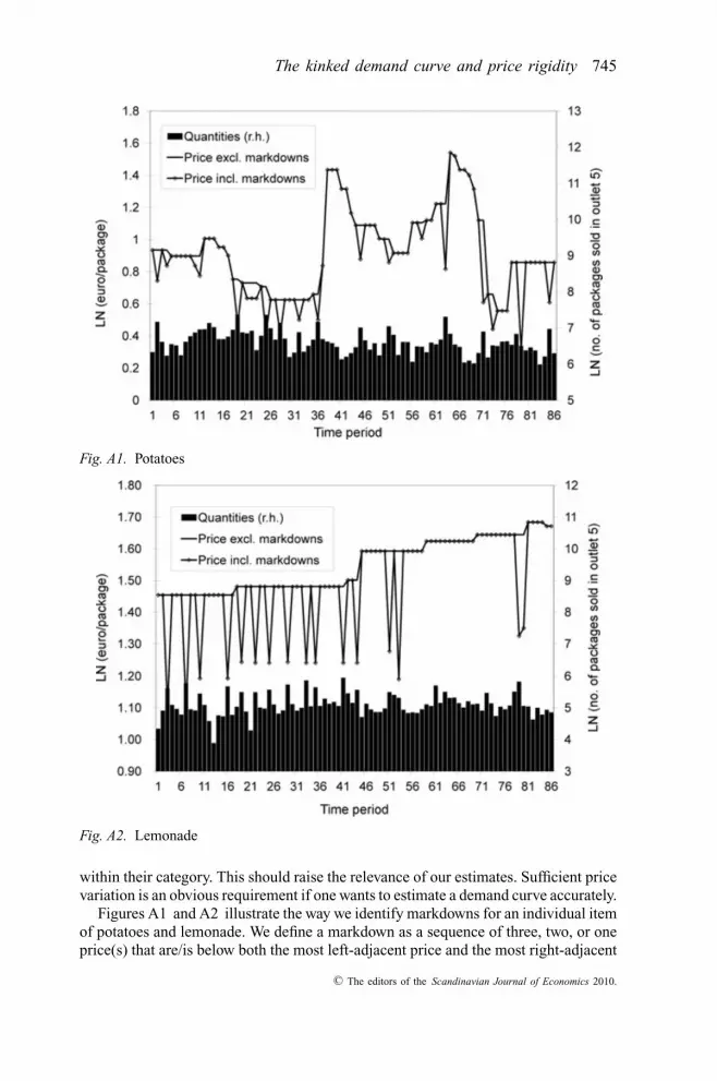
Fig. A1. Potatoes

Fig. A2. Lemonade

within their category. This should raise the relevance of our estimates. Sufficient pricevariation is an obvious requirement if one wants to estimate a demand curve accurately.

Figures A1 and A2 illustrate the way we identify markdowns for an individual itemof potatoes and lemonade. We define a markdown as a sequence of three, two, or oneprice(s) that are/is below both the most left-adjacent price and the most right-adjacent



price. To calculate our “excluding markdowns” statistics in Section II, we have filteredout markdown prices. We have replaced them by the last observed regular price.

Appendix B. Derivation of the Curvature in the Behavioral AIDSModel

Starting from equation (9) in the main text,


si+ βi − 2δi i ln(pi/P∗)

si+ 2

N∑j=1

δi j ln( p j

P∗)

,

the derivation of the curvature goes as follows:

εi(LA/B−AIDS) = ∂ ln εi

∂ ln pi(A3)

= − 1

εi

∂

⎛⎜⎝

γi i + 2δi i ln( pi

P∗)

si− 2

N∑j=1

δi j ln( p j

P∗)⎞⎟⎠

∂ ln pi(A4)

= − 1

εi

⎛⎜⎝

2δi i (1 − si )si − (∂si/∂ ln pi )(γi i + 2δi i ln

( pi

P∗))

si2

− 2

⎛⎝δi i − si

N∑j=1

δi j

⎞⎠

⎞⎟⎠

(A5)

=− 1

εi

⎛⎝2δi i (1 − si )

si+ (εi − 1)

⎛⎝1 − εi +βi + 2

N∑j=1

δi j ln( p j

P∗)⎞⎠−2

⎛⎝δi i −si

N∑j=1

δi j

⎞⎠⎞⎠.

(A6)

In the third line we again use the (empirically supported) assumption that∂ ln P∗/∂ ln pi = si. The fourth line relies on the definition that −(∂si/si)/∂ ln pi

= (εi − 1) and the result derived from equation (9) that

γi i

si+ 2δi i ln(pi/P∗)

si= 1 − εi + βi + 2

N∑j=1

δi j ln( p j

P∗)

.

Rearranging and imposing the steady-state assumption that all relative prices are 1, wefind the following for the curvature:

εi(LA/B−AIDS) = 1

εi

⎛⎝(εi − 1)(εi − 1 −βi ) − 2δi i (1 − si )

si+ 2

⎛⎝δi i − si

N∑j=1

δi j

⎞⎠

⎞⎠ .

(A7)



Appendix C. Supplementary Results and Robustness

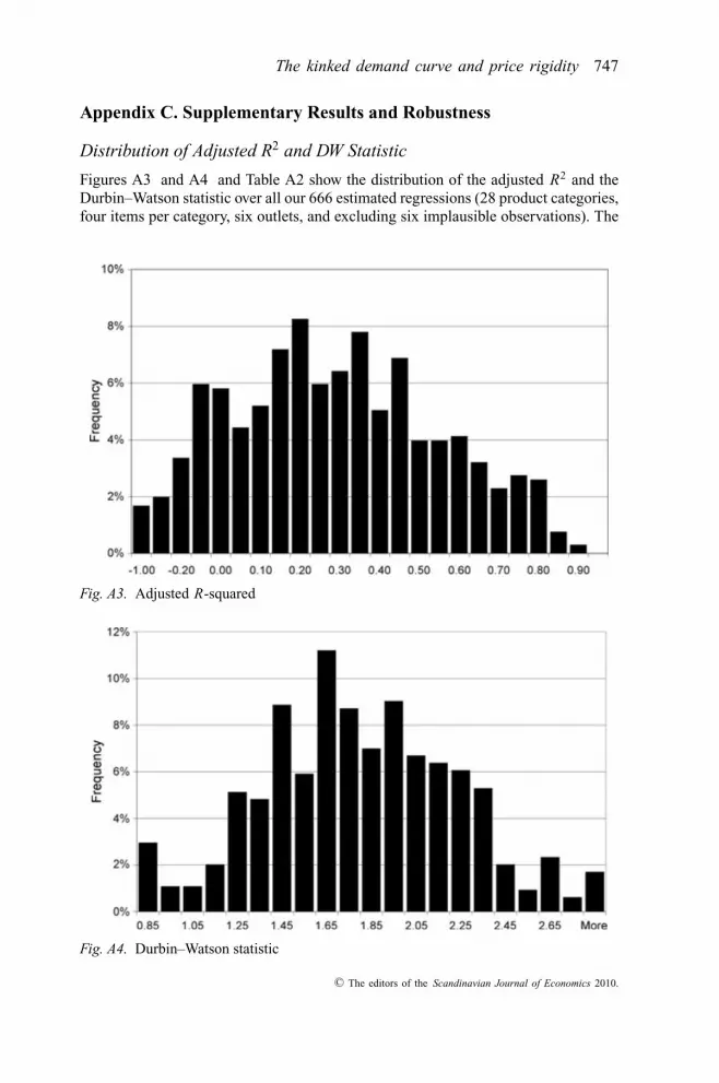
Distribution of Adjusted R2 and DW Statistic

Figures A3 and A4 and Table A2 show the distribution of the adjusted R2 and theDurbin–Watson statistic over all our 666 estimated regressions (28 product categories,four items per category, six outlets, and excluding six implausible observations). The

Fig. A3. Adjusted R-squared

Fig. A4. Durbin–Watson statistic



Table A2. Distribution of adjusted R-squared and Durbin–Watson statistic

25% 50% 75% 90%

Adjusted R2 0.07 0.26 0.45 0.63DW 1.43 1.72 2.06 2.30

Notes: The data show the adjusted R2 and the Durbin–Watson statistic of the regressions (among 666) at the25th, 50th, 75th, and 90th percentiles, ordered from low to high.

Table A3. Estimated price elasticity and curvature

Conditional on

Unconditional Adj. R2 > 0 Adj. R2 > 0.2 Adj. R2 > 0.4 1.5 < DW < 2.5

Median elasticity 1.4 1.4 1.6 1.8 1.4Median curvature 0.8 0.5 0.7 0.5 0.6

median adjusted R2 is 0.26, and the median DW statistic is 1.72. Considering thedistribution of the estimated DW statistics, the null hypothesis of no autocorrelationin the error term cannot be rejected for most of our regressions. Alternatively, onemight see the median of all estimated DW statistics as indicative of the populationmean. A median value of 1.72 would then point to the existence of weak positiveautocorrelation. Predictability of demand from past observations would, after all,be small, as would be the possibility for the supermarket to exploit this in its pricesetting. Additional regressions in which we add a lagged dependent variable to theRHS of equation (15) yield further results that are fully in line with these findings.In 33% of these regressions, the coefficient on the lagged dependent is statisticallyinsignificant at 10%. Among all regressions, the median of this coefficient is only0.02. Its value at the 15th percentile is −0.09, and its value at the 85th percentile is0.12. Weak autocorrelation and very rapid adjustment support the validity of twice-and thrice-lagged prices as instruments in our IV robustness check in the Robustnesssection.

Table A3 summarizes our estimates for the price elasticity and the curvature con-ditional on good test statistics for the adjusted R2 and the Durbin–Watson statistics.Conditioning on good test statistics hardly affects our results for the median-estimatedelasticity and curvature. At best, we see a rise in the estimated elasticity with increasingR2, but this rise is small.

Estimation Results for δi i

Figures A5 and A6 show the distribution of the 112 (28 × 4) estimates of δii and thedistribution of the related absolute t-values. Table A4 contains the results of a Waldtest for each of the 28 product categories of the joint hypothesis that δ11 = δ22 =δ33 = δ44 = 0. The results are briefly discussed in the main text.



Fig. A5. Point estimates δi i

Fig. A6. t-Values δi i

Table A4. Wald test for δ11 = δ22 = δ33 = δ44 = 0

p-Value p ≤ 0.05 0.05 < p ≤ 0.1 0.1 < p ≤ 0.2 0.2 < p

Number of product categories 19 2 4 3



Table A5. Pairwise correlation coefficients over 28 product categories

Market share Number of Median Median“other” items elasticity curvature

Market share “other” 1 — — —Number of items 0.61 1 — —Median elasticity −0.06 −0.19 1 —Median curvature −0.03 0.06 0.56 1Median δii 0.12 −0.19 −0.29 −0.78

The Size of “Other” and the Estimation Results

This appendix reveals that there is no specific relationship between our estimationresults for the elasticity and the curvature in a product category and the numberof items not included in the regressions. Table A5 contains all relevant correlationcoefficients.

ReferencesAlston, J., Foster, A., and Green, R. (1994), Estimating Elasticities with the Linear Approximate

Almost Ideal Demand System: Some Monte Carlo Results, Review of Economics and Statistics76, 351–356.

Altig, D., Christiano, L., Eichenbaum, M., and Linde, J. (2005), Firm-specific Capital, NominalRigidities and the Business Cycle, CEPR Discussion Paper no. 4858.

Ball, L., and Romer, D. (1990), Real Rigidities and the Non-neutrality of Money, Review ofEconomic Studies 57, 183–203.

Banks, J., Blundell, R., and Lewbel, A. (1997), Quadratic Engel Curves and Consumer Demand,Review of Economics and Statistics 79, 527–539.

Basu, S. (1995), Intermediate Goods and Business Cycles: Implications for Productivity andWelfare, American Economic Review 85, 512–531.

Benabou, R. (1988), Search, Price Setting and Inflation, Review of Economic Studies 55, 353–376.Bergin, P., and Feenstra, R. (2000), Staggered Price Setting, Translog Preferences and Endo-

genous Persistence, Journal of Monetary Economics 45, 657–680.Berry, S., Levinsohn, J., and Pakes, A. (1995), Automobile Prices in Market Equilibrium,

Econometrica 63, 841–890.Bhaskar, V. (2008), Kinked Demand Curve, in S. Durlauf and L. Blume (eds.), The New Palgrave

Dictionary of Economics, Palgrave Macmillan, Basingstoke.Bijmolt, T., Van Heerde, H., and Pieters, R. (2005), New Empirical Generalisations on the

Determinants of Price Elasticity, Journal of Marketing Research 42, 141–156.Bils, M., and Klenow, P. (2004), Some Evidence on the Importance of Sticky Prices, Journal of

Political Economy 112, 947–985.Burstein, A., and Hellwig, C. (2007), Prices and Market Shares in a Menu Cost Model,

manuscript, UCLA.Buse, A. (1994), Evaluating the Linearized Almost Ideal Demand System, American Journal of

Agricultural Economics 76, 781–793.Calvo, G. (1983), Staggered Prices in a Utility-maximizing Framework, Journal of Monetary

Economics 12, 383–398.Chari, V., Kehoe, P., and McGrattan, E. (2000), Sticky Price Models of the Business Cycle: Can

the Contract Multiplier Solve the Persistence Problem?, Econometrica 68, 1151–1179.



Chevalier, J., Kashyap, A., and Rossi, P. (2003), Why Don’t Prices Rise during Periods of PeakDemand? Evidence from Scanner Data, American Economic Review 93, 15–37.

Christiano, L., Eichenbaum, M., and Evans, C. (1999), Monetary Policy Shocks: What HaveWe Learned and to What End?, in M. Woodford and J. Taylor (eds.), Handbook of Macroeco-nomics, Vol. 1A, Elsevier Science, Amsterdam, 65–148.

Coenen, G., Levin, A., and Christoffel, K. (2007), Identifying the Influences of Nominal andReal Rigidities in Aggregate Price Setting Behavior, Journal of Monetary Economics 54,2439–2466.

Deaton, A., and Muellbauer, J. (1980), An Almost Ideal Demand System, American EconomicReview 70, 312–326.

Dhyne, E., Alvarez, L., Le Bihan, H., Veronese, G., Dias, D., Hoffman, J., Jonker, N., Lunnemann,P., Rumler, F., and Vilmunen, J. (2006), Price Setting in the Euro Area: Some Stylized Factsfrom Individual Consumer Price Data, Journal of Economic Perspectives 20, 171–192.

Dixit, A., and Stiglitz, J. (1977), Monopolistic Competition and Optimum Product Diversity,American Economic Review 67, 297–308.

Dobbelaere, S. (2004), Estimation of Price–Cost Margins and Union Bargaining Power forBelgian Manufacturing, International Journal of Industrial Organization 22, 1381–1398.

Domowitz, I., Hubbard, G., and Petersen, B. (1988), Market Structure and Cyclical Fluctuationsin US Manufacturing, Review of Economics and Statistics 70, 55–66.

Dossche, M., Heylen, F., and Van den Poel, D. (2006), The Kinked Demand Curve and PriceRigidity: Evidence from Scanner Data, National Bank of Belgium Working Paper no. 99.

Dotsey, M., and King, R. (2005), Implications of State-dependent Pricing for Dynamic Macro-economic Models, Journal of Monetary Economics 52, 213–242.

Dutta, S., Bergen, M., and Levy, D. (2002), Price Flexibility in Channels of Distribution: Evidencefrom Scanner Data, Journal of Economic Dynamics and Control 26, 1845–1900.

Eichenbaum, M., and Fisher, J. (2004), Evaluating the Calvo Model of Sticky Prices, NBERWorking Paper no. 10617.

Galı, J., and Gertler, M. (1999), Inflation Dynamics: A Structural Econometric Analysis, Journalof Monetary Economics 44, 195–222.

Green, R., and Alston, J. (1990), Elasticities in AIDS Models, American Journal of AgriculturalEconomics 72, 442–445.

Hausman, J. (1997), Valuation of New Goods under Perfect and Imperfect Competition, in T.Bresnahan and R. Gordon (eds.), The Economics of New Goods, University of Chicago Press,Chicago, 209–237.

Hausman, J., Leonard, G., and Zona, J. (1994), Competitive Analysis with Differentiated Prod-ucts, Annales d’Economie et de Statistique 34, 159–180.

Heidhues, P., and Koszegi, B. (2008), Competition and Price Variation when Consumers AreLoss Averse, American Economic Review 98, 1245–1268.

Hendel, I., and Nevo, A. (2006), Sales and Consumer Inventory, RAND Journal of Economics37, 543–561.

Kimball, M. (1995), The Quantitative Analytics of the Basic Neomonetarist Model, Journal ofMoney, Credit and Banking 27, 1241–1277.

Klenow, P., and Kryvtsov, O. (2008), State-dependent or Time-dependent Pricing: Does It Matterfor Recent U.S. Inflation?, Quarterly Journal of Economics 123, 863–904.

Klenow, P., and Willis, J. (2006), Real Rigidities and Nominal Price Changes, Federal ReserveBank of Kansas City Working Paper no. 06-03.

Konings, J., Van Cayseele, P., and Warzynski, F. (2001), The Dynamics of Industrial Mark-upsin Two Small Open Economies: Does National Competition Policy Matter?, InternationalJournal of Industrial Organization 19, 841–859.

Mankiw, N. (1985), Small Menu Costs and Large Business Cycles, Quarterly Journal of Eco-nomics 100, 529–537.



Menezes-Filho, N. (2005), Is the Consumer Sector Competitive in the U.K.? A Test usingHousehold-level Demand Elasticities and Firm-level Price Equations, Journal of Businessand Economic Statistics 23, 295–304.

Midrigan, V. (2009), Menu Costs, Multi-product Firms, and Aggregate Fluctuations, manuscript,New York University.

Nakamura, E., and Steinsson, J. (2008), Five Facts about Prices: A Reevaluation of Menu CostModels, Quarterly Journal of Economics 123, 1415–1464.

Nijs, V., Srinivasan, S., and Pauwels, K. (2007), Retail-price Drivers and Retailer Profits, Mar-keting Science 26, 473–487.

Okun, A. (1981), Prices and Quantities, Brookings Institution Press, Washington, DC.Pauwels, K., Srinivasan, S., and Franses, P. (2007), When Do Price Thresholds Matter in Retail

Categories?, Marketing Science 26, 83–100.Peersman, G. (2004), The Transmission of Monetary Policy in the Euro Area: Are the

Effects Different across Countries?, Oxford Bulletin of Economics and Statistics 66, 285–308.

Sbordone, A. (2002), Prices and Unit Labor Costs: A New Test of Price Stickiness, Journal ofMonetary Economics 49, 265–292.

Smets, F., and Wouters, R. (2007), Shocks and Frictions in US Business Cycles: A BayesianApproach, American Economic Review 97, 586–606.

Srinivasan, S., Pauwels, K., Hanssens, D., and Dekimpe, M. (2004), Do Promotions BenefitManufacturers, Retailers or Both?, Management Science 50, 617–629.

Steenkamp, J., Nijs, V., Hanssens, D., and Dekimpe, M. (2005), Competitive Reactions to Ad-vertising and Promotion Attacks, Marketing Science 24, 35–54.

Sweezy, P. (1939), Demand under Conditions of Oligopoly, Journal of Political Economy 47,432–447.

Taylor, J. (1980), Aggregate Dynamics and Staggered Contracts, Journal of Political Economy88, 1–23.

Tversky, A., and Kahneman, D. (1991), Loss Aversion in Riskless Choice: A Reference-dependent Model, Quarterly Journal of Economics 106, 1039–1061.

Woodford, M. (2003), Interest and Prices: Foundations of a Theory of Monetary Policy, PrincetonUniversity Press, Princeton, NJ.

Woodford, M. (2005), Firm-specific Capital and the New Keynesian Phillips Curve, InternationalJournal of Central Banking 1, 1–46.


the kinked demand curve and price rigidity: evidence from scanner data*

Documents