http://www.bio-protocol.org/e1424 Vol 5, Iss 6, Mar 20, 2015

1

Scanner-based Time-lapse Root Phenotyping

Michael O. Adu1, 2, 5*

, Lea Wiesel1, Malcolm J. Bennett

2, 3, Martin R. Broadley

2, 3, Philip J. White

1, 4 and

Lionel X. Dupuy1

1Department of Ecological Sciences, James Hutton Institute, Invergowrie, Dundee, UK;

2Plant and

Crop Sciences Division, School of Biosciences, University of Nottingham, Sutton Bonington Campus,

Leicestershire, UK; 3Centre for Plant Integrative Biology, University of Nottingham, Sutton Bonington

Campus, Leicestershire, UK; 4College of Science, King Saud University, Riyadh, Kingdom of Saudi

Arabia; 5Current address: Department of Crop Science, School of Agriculture, College of Agriculture

and Natural Sciences, University of Cape Coast, Central Region, Ghana

*For

correspondence: michael.adu@ucc.edu.gh

[Abstract] Non-destructive phenotyping of root system architecture can facilitate breeding for root

traits that optimize resource acquisition. This protocol describes the construction of a low-cost, high-

resolution root phenotyping platform, requiring no sophisticated equipment and adaptable to most

laboratory and glasshouse environments. The phenotyping platform consists of germination paper

abutting scanners and open-source image acquisition software which allows live imaging of root

systems. The phenotyping platform is scalable, modular and inexpensive.

Materials and Reagents

1. Seeds of the plants to be investigated

Note: We used seeds of Brassica rapa L.

2. Nutrient solution (see Recipes)

Note: Composition will depend on experimental requirements.

Equipment

1. Large (30 x 42 cm) and small (12 x 12 cm) steel blue Anchor seed germination paper Anchor

Paper Company, catalog number: SGB1924B) for phenotyping platform and seed germination,

respectively

2. Duct tape (office DEPOT)

3. Ferrite magnetic strip with adhesive back (0.75 mm thick) (RS Components, catalog number:

297-9116)

4. Square bioassay or petri dishes (120 mm x 120 mm x 17 mm) (Sigma-Aldrich, catalog

number: Z617679)

Note: This could be improvised with empty compact disc (CD) cases or any kind of

transparent box that meets the specified dimensions.

http://www.bio-protocol.org/e1424 Vol 5, Iss 6, Mar 20, 2015

2

5. Black Perspex plates (21.5 x 30.0 cm) custom-made from opaque cast acrylic boards

(Perspex Cast 9T30 Black Sheet) (plastock)

6. Computer

Note: This should be Windows-based and should have a directory with sufficient space to

save images. In our platform, a Canon flatbed scanner imaging a root system at 300 dpi

produces a single image of 40.2 MB. With 24 scanners in operation and images taken every

12 h, a minimum free space of approximately 30.0 GB is required for an experiment lasting 14

days. We used a Dell computer Intel® Core™ i3-4150 Processor- Dual Core, 4 GB 1,600 MHz

Memory and 500 GB Hard Drive for our experiments but images were saved on 2 TB WD

external hard drive.

7. Canon flatbed scanners (CanoScan, model: 5600F)

Note: Any scanner with a TWAIN driver can be used. A TWAIN driver is software that comes

as part of the software package of digital imaging devices such as scanners and cameras.

The TWAIN driver provides an interface for communication between the software and the

hardware of digital imaging devices (http://www.twain.org/). In our platform, the TWAIN driver

translated commands from our ArchiScan image acquisition software

(http://www.archiroot.org.uk/) into instructions to control the hardware of the scanners.

a. Setting up scanners

i. Remove the cover of the scanner as shown in Figure 1.

ii. Attach magnetic strips to the short-edges of the scanner window (Figure 1B).

Note: This is optional as duct tape could be used to hold plates to scanners.

Figure 1. A. Original flatbed scanner. B. Modified flatbed scanner with cover detached.

8. Support for germination paper

a. Glue to the edges of the Perspex plates strips of Perspex (0.3 x 0.3 x 30 cm and 0.3 x 0.3

x 21.5 cm for the long-edges and short-edges of the Perspex plate, respectively).

Note: This is to provide some separation between the plate and the scanners.

http://www.bio-protocol.org/e1424 Vol 5, Iss 6, Mar 20, 2015

3

b. Allow two gaps in the Perspex strips, each approximately 3 cm wide, along the long edge

of the Perspex plates to allow gas exchange with the surrounding atmosphere and

unimpeded shoot growth (Figure 2).

c. Fix magnetic strips along the two short-edges of the Perspex plate to aid abutting of the

Perspex plate to the scanner window (optional).

Figure 2. (A) Schematic representation of the Perspex plate used as a scanner cover

and also to attach germination paper onto scanners. (B) Black Perspex plates used as

scanner covers and also to hold germination paper vertically on scanner surfaces

Software

1. ImageJ (http://imagej.nih.gov/ij/)

2. ArchiScan and ImageJ custom macros for convex hull and particle analyses (Adu et al., 2014;

http://www.archiroot.org.uk/ )

3. SmartRoot (Lobet et al., 2011; http://www.uclouvain.be/en-smartroot)

Procedure

A. Seed germination

Note: This procedure was performed in a sterile hood, but the whole process was not necessarily

sterile since scanners and tanks were not autoclaved and the experiments were not performed in

a sterile room.

1. Line the bottom of a square petri dish (12 x 12 cm) with paper towel.

Note: Empty CD cases can be used instead of petri dishes.

2. Cover the paper towel with a small germination sheet (12 x 12 cm).

3. Spray the germination papers with deionized water.

4. Put seeds on top of the wet seed germination paper. Allow each seed as much space as

possible.

http://www.bio-protocol.org/e1424 Vol 5, Iss 6, Mar 20, 2015

4

Note: Seeds should be surface sterilised prior to germination. Brassica rapa seeds were

surface sterilised for 10 min in 10% hydrogen peroxide, followed by 1 min in 70% ethanol, and

then rinsed 3 times with deionised water.

5. Place one layer of paper towels on top of the seeds.

6. Spray the top layer of paper towels with deionized water.

7. Place the lid on the petri dish and allow excess water to drain off by holding in a tilted position

for about 30 sec.

8. Cover the petri dish with aluminium foil.

9. Place the petri dish in a vertical orientation in an incubator at 20 °C.

Figure 3. Example of Brassica rapa seeds after 3 days of germination

B. Transferring seedlings onto scanners

1. Fix the top half of a large germination paper (30 x 42 cm; www.anchorpaper.com/) onto a

Perspex plate.

Note: Scanner surfaces were cleaned with Virkon® disinfectant (http://www2.dupont.com/).

Similarly, tanks and Perspex plates were thoroughly washed with Virkon® disinfectant and

dried after each experiment. Slightly moistening the paper enables it to be fixed to the plate

easily.

2. Transfer seedlings of similar size with radicles 2-3 cm in length (Figure 3) to the large (30 x 42

cm) sheets of germination paper fixed to Perspex plates.

a. Transfer two seedlings per plate.

b. Ensure that about 0.5 cm of the small germination paper surrounding each radicle is cut

and transferred with the seedling to the large germination papers to minimize disturbance

during the transfer process. (Figure 21 shows a video of this).

c. Use a moistened tissue or parafilm tape, just below the cotyledons, to stick the seedlings

to the large germination papers.

Note: Put the small germination paper that has been cut with the seedling on it at the top

of the large germination paper and tape both to the large germination paper by putting the

parafilm tape just below the cotyledons of the seedling. Alternatively, in the absence of

parafilm tape, a damp, narrow strip of tissue paper (about 4 cm long) can be used to affix

the seeds plus small germination paper to the large germination paper.

http://www.bio-protocol.org/e1424 Vol 5, Iss 6, Mar 20, 2015

5

3. Attach the assemblage of Perspex plate, large germination paper and seedlings to the

scanners using magnetic strips fixed to the plates and scanner windows.

Note: Duct tape can also be used hold the Perspex plate to the scanner (Figure 4).

4. Position scanners in near-vertical positions 5 cm above 20 L of nutrient solution contained in

opaque polyvinyl plastic tanks, each supplying six scanners (Figure 4).

a. The first scanners put on the tank could lean against a wall to provide support and

subsequent scanners can be stacked with each leaning against the previous one (Figure

4).

b. Allow approximately 10 cm of the large germination paper to be submerged in the nutrient

solution (Figure 4).

c. Connect all scanners to the computer on which the ArchiScan software is installed using

a USB hub with multiple ports. Connect scanners, computers and USB ports to a power

supply.

Note: You can use either one computer or multiple computers to control the scanners.

The number of scanners per computer depends on the number of plants to be screened,

duration of experiment, frequency of scanning and the computers’ storage capacity. In our

experiments, there are occasions when up to 24 scanners are managed by one computer

but we normally use 2 computers to control 24 scanners. On the latter occasions, each

computer managed 12 scanners and scanners were connected to the computer using a

D-Link USB Hub; http://www.misco.co.uk/; Misco number: 94282).

Figure 4. A. Schematic representation of the pouch-and-wick system of a single scanner.

Roots grow on the surface of germination paper held between a clear-Perspex plate and the

glass window of a scanner. The scanner is fixed in near-vertical position 5 cm above 20 L of

nutrient solution contained in opaque polyvinyl plastic tank. Approximately 10 cm of the

germination paper is submerged in the nutrient solution (Adu et al., 2014). B. Phenotyping

platform composed of a bank of six scanners.

C. Time-lapse imaging of roots

Run the image acquisition software, ArchiScan. ArchiScan is Windows-based software that

provides an interface for managing multiple scanners and for simultaneous scanning of images.

ArchiScan must be installed on a computer directory on which there is sufficient space to save

http://www.bio-protocol.org/e1424 Vol 5, Iss 6, Mar 20, 2015

6

images (Extended information on ArchiScan is found in the ‘READ ME’ pdf file at

http://www.archiroot.org.uk/index.php/tools/ArchiScan).

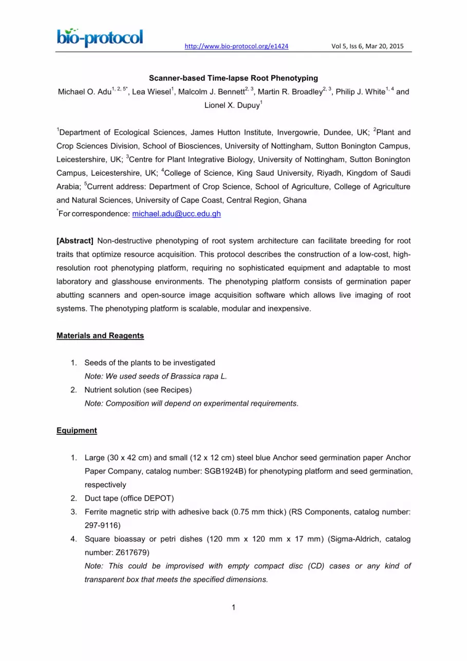
1. Input parameters of the new project including:

Initial scanning time

Note: This depends on experimental requirements. In this example, we began scanning at

Time=0; Figure 5.

Project duration

Note: This is indicated by Number of Scans (Figure 5) and depends on the frequency of

taking images and duration of experiment. e.g.: If images are taken every 24 hours and the

experiment was to last 15 d, the number of scans would be 16.

Time period between consecutive scans (Time between Scan; Figure 5)

Note: In most of our experiments images are scanned every 12 h.

Figure 5. ArchiScan interface for setting experiment parameters

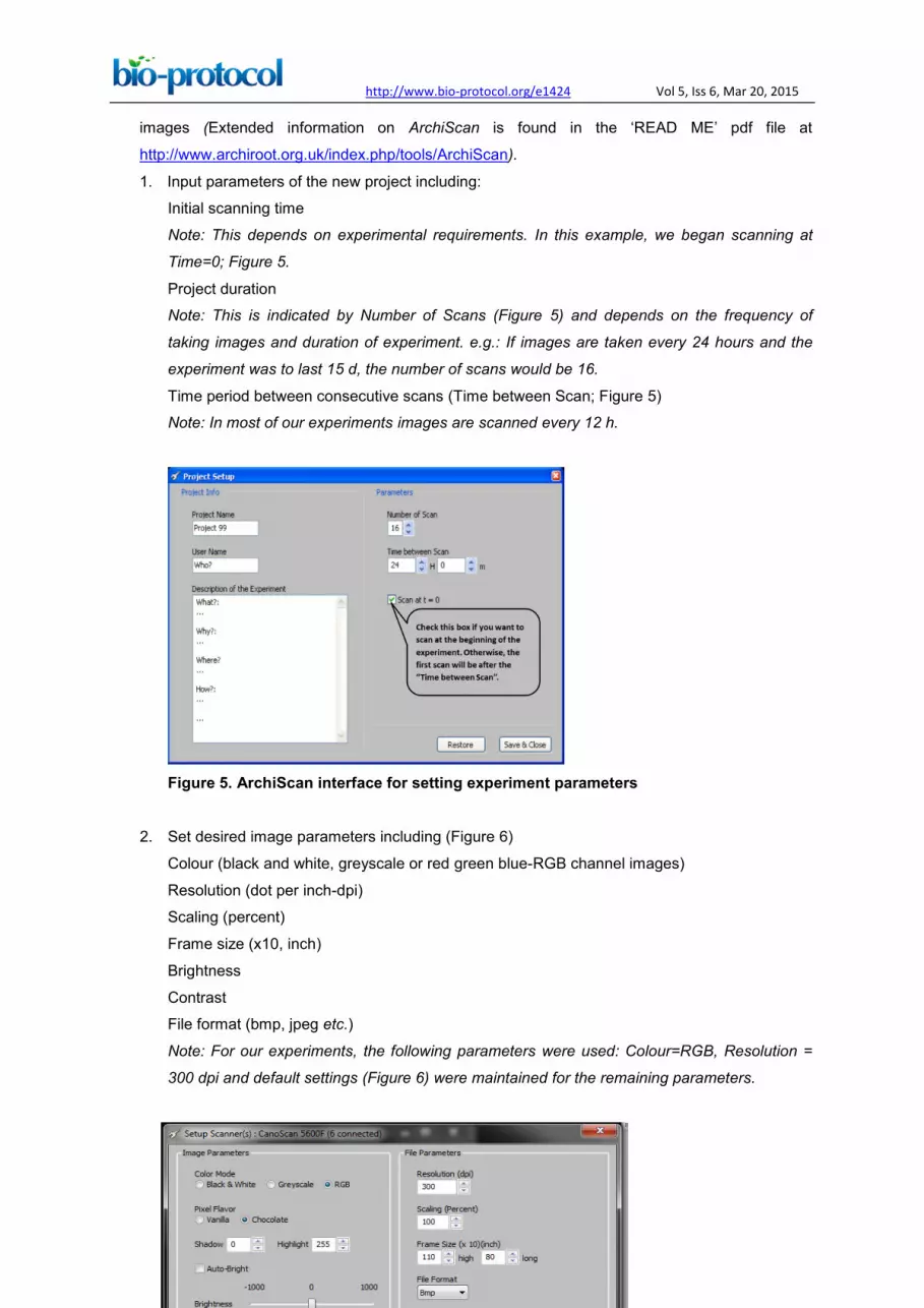
2. Set desired image parameters including (Figure 6)

Colour (black and white, greyscale or red green blue-RGB channel images)

Resolution (dot per inch-dpi)

Scaling (percent)

Frame size (x10, inch)

Brightness

Contrast

File format (bmp, jpeg etc.)

Note: For our experiments, the following parameters were used: Colour=RGB, Resolution =

300 dpi and default settings (Figure 6) were maintained for the remaining parameters.

http://www.bio-protocol.org/e1424 Vol 5, Iss 6, Mar 20, 2015

7

Figure 6. ArchiScan interface for setting image parameters

D. Image segmentation and extraction of root features

Image segmentation and extraction of root features from single root images or from a stack of

time-lapse image sequences can be performed with ImageJ (http://imagej.nih.gov/ij/) using

custom macros that can be downloaded from http://archiroot.org.uk/index.php/tools/ArchiScan.

Extraction of root features can also be done with a variety of software including SmartRoot (Lobet

et al., 2011; http://www.uclouvain.be/en-smartroot).

E. Segmentation and extraction of root features using ImageJ

Total root length:

1. Total root length of a single image

a. To process and analyse a single root image, open the image with ImageJ (File>Open;

Figure 7) and proceed from point 3 below.

Figure 7. To open a single image, open ImageJ and select File > Open. Navigate to your

folder and select the image, then select OK.

http://www.bio-protocol.org/e1424 Vol 5, Iss 6, Mar 20, 2015

8

2. Total root length of a time-lapse stacked images to measure the rate of root length increase

per unit time

b. For each plant, import the image stack consisting of image sequences from the beginning

to the end of an experiment into ImageJ (File>Import>Image Sequences; Figure 8).

Figure 8. To import a sequence of images, open ImageJ and select File > Import >

Image Sequence. Navigate to your folder and select the first image, then select OK. ImageJ

will launch a sequence options dialog. The default values are usually appropriate but images

could be resized here. We typically maintain the default 100% but checking the ‘Use Virtual

Stack’ box opens images as a read-only virtual stack and allows image sequences too big to

fit in RAM to be opened.

c. Set the scale or images by indicating the correct relationship between distance in pixels

and the desired unit of measurement before analyses (Analyse > Set Scale; Figure 9).

http://www.bio-protocol.org/e1424 Vol 5, Iss 6, Mar 20, 2015

9

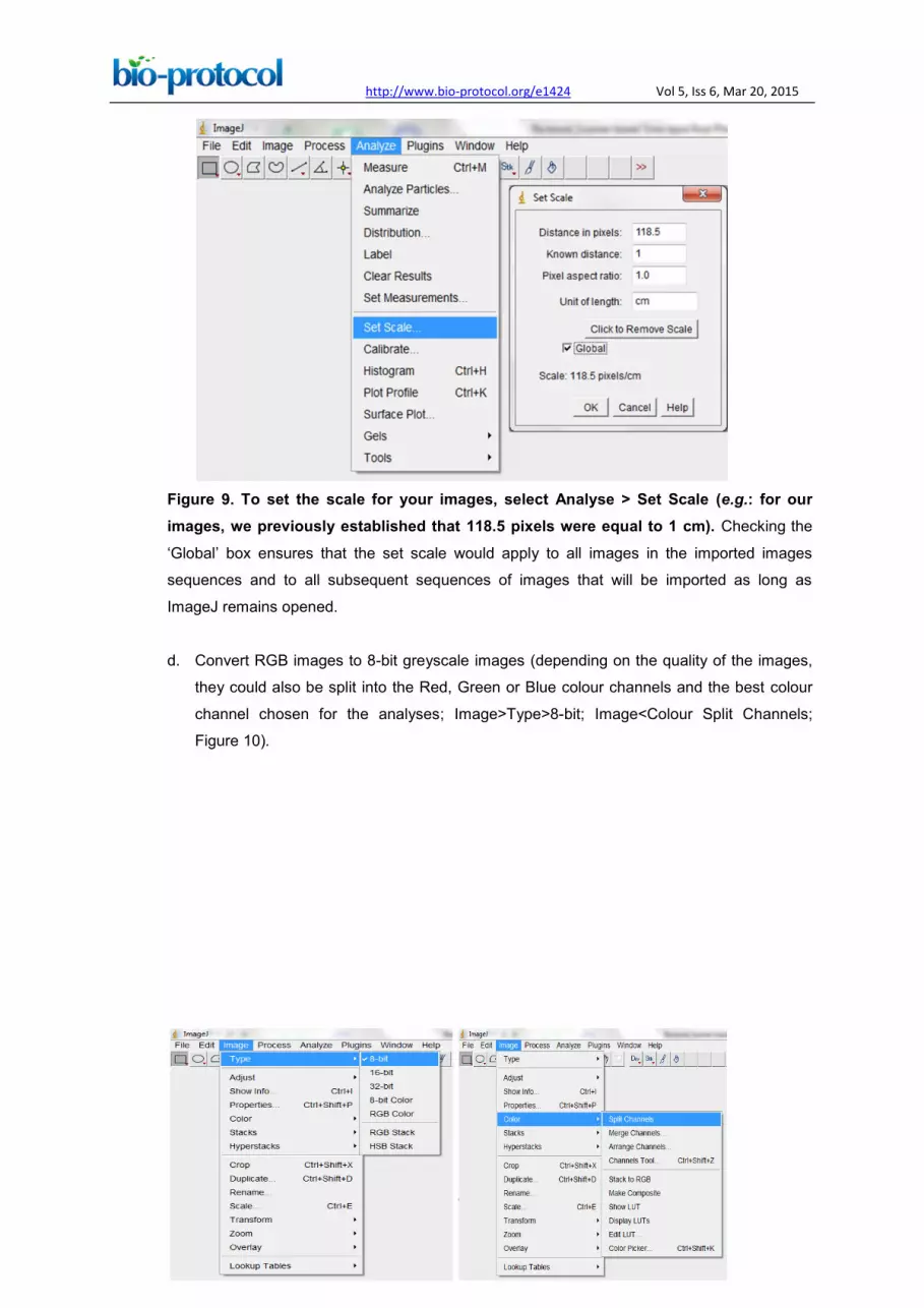
Figure 9. To set the scale for your images, select Analyse > Set Scale (e.g.: for our

images, we previously established that 118.5 pixels were equal to 1 cm). Checking the

‘Global’ box ensures that the set scale would apply to all images in the imported images

sequences and to all subsequent sequences of images that will be imported as long as

ImageJ remains opened.

d. Convert RGB images to 8-bit greyscale images (depending on the quality of the images,

they could also be split into the Red, Green or Blue colour channels and the best colour

channel chosen for the analyses; Image>Type>8-bit; Image<Colour Split Channels;

Figure 10).

http://www.bio-protocol.org/e1424 Vol 5, Iss 6, Mar 20, 2015

10

Figure 10. To Convert RGB images to 8-bit greyscale images, select Image>Type>8-bit

or select Image<Colour Split Channels to split images into the Red, Green or Blue

colour channels

e. Filter with the median, followed by the Gaussian, filter to remove short range variations on

the image (i.e. remove variations introduced by water droplets condensing at the surface

of scanners or due to inhomogeneity of the surface of the germination paper;

Process>Filter>Median; Process>Filter>Gaussian Blur; Figure 11).

Note: The range of radii for filtering depends on the quality of the image but we typically

use a range of 2-4.

Figure 11. Select Process>Filter>Median, followed by Process>Filter>Gaussian Blur to

remove short range artefacts on your image/images. A Median and Gaussian Blur options

dialog box would be lunched for the radius and Sigma radius (Gaussian Blur) to be modified

subject to the quality of your images.

f. Use background subtraction to remove variations in pixel intensity over longer distances

than the root diameter (long range variations are artefacts or inhomogeneities in the

background that remain after short range variations have been removed and may be

caused by non-uniform moisture content of the germination paper; Process>Subtract

Background; Figure 12).

http://www.bio-protocol.org/e1424 Vol 5, Iss 6, Mar 20, 2015

11

Note: The range of radii for background subtraction depends on the quality of the image

but we typically use a range of 40-50.

Figure 12. Select Process>Subtract Background to remove long range artefacts on

your images. A Subtract Background dialog box would be lunched. We normally modified the

‘Rolling ball’ radius to optimise the background subtraction.

g. Auto-threshold with the Moment-preserving threshold algorithm.

Note: depending on the quality of the image this algorithm may be suboptimal compared

to other auto-threshold algorithms in ImageJ. Other algorithms could be tried or a second

algorithm could be added; Image>Adjust>Auto threshold; Figure 13).

http://www.bio-protocol.org/e1424 Vol 5, Iss 6, Mar 20, 2015

12

Figure 13. Select Image>Adjust>Auto threshold to threshold images. An Auto Threshold

dialog box will be lunched. We typically use the ‘Moments’ threshold method but other

algorithms could be tried to select the most optimal for your images.

h. Convert processed image to mask (Process>Binary>Convert to Mask; Figure 14, Figure

19).

Figure 14. Select Process>Binary>Convert to convert processed image/images to mask

i. Run particle analyses to measure root features of interest including the root perimeter

from which the total root length can be calculated. Note: different size and circularity

options might be tried to get the best results. Selecting Show>Outlines in the Particle

Analyses pop up box will show the root perimeter and ticking the Display results box will

show the measurement of all of the particles; Analyse>Analyse particles; Figure 15).

http://www.bio-protocol.org/e1424 Vol 5, Iss 6, Mar 20, 2015

13

Figure 15. Select Analyse>Analyse particles to measure root traits of interest. An Analyse

Particles dialog box will be lunched for the Size and Circularity to be modified Note: circularity is a

dimensionless shape descriptor which is a function of the object perimeter and the area and gives

a measure of similarity between a given shape and a perfect circle. It ranges between 0-1. We

typically used Size = 0.2 and Circularity = 0.00 -0.2. The results will be for a single image (if only

one image was opened) or for sequence of images (if time-lapse stacked images were imported

into ImageJ) from which rate of change in total root length per unit time can be calculated. 50% of

the root perimeter = total root length.

Area of roots:

j. From #6, run Gaussian Blur filter again (Figure 11).

k. Find the local maxima to select root pixels on the image (Process>Find Maxima; Figure

16).

Note: This could be modified to optimise it for your images but we typically used noise=0

output=Point Selection and exclude edges.

http://www.bio-protocol.org/e1424 Vol 5, Iss 6, Mar 20, 2015

14

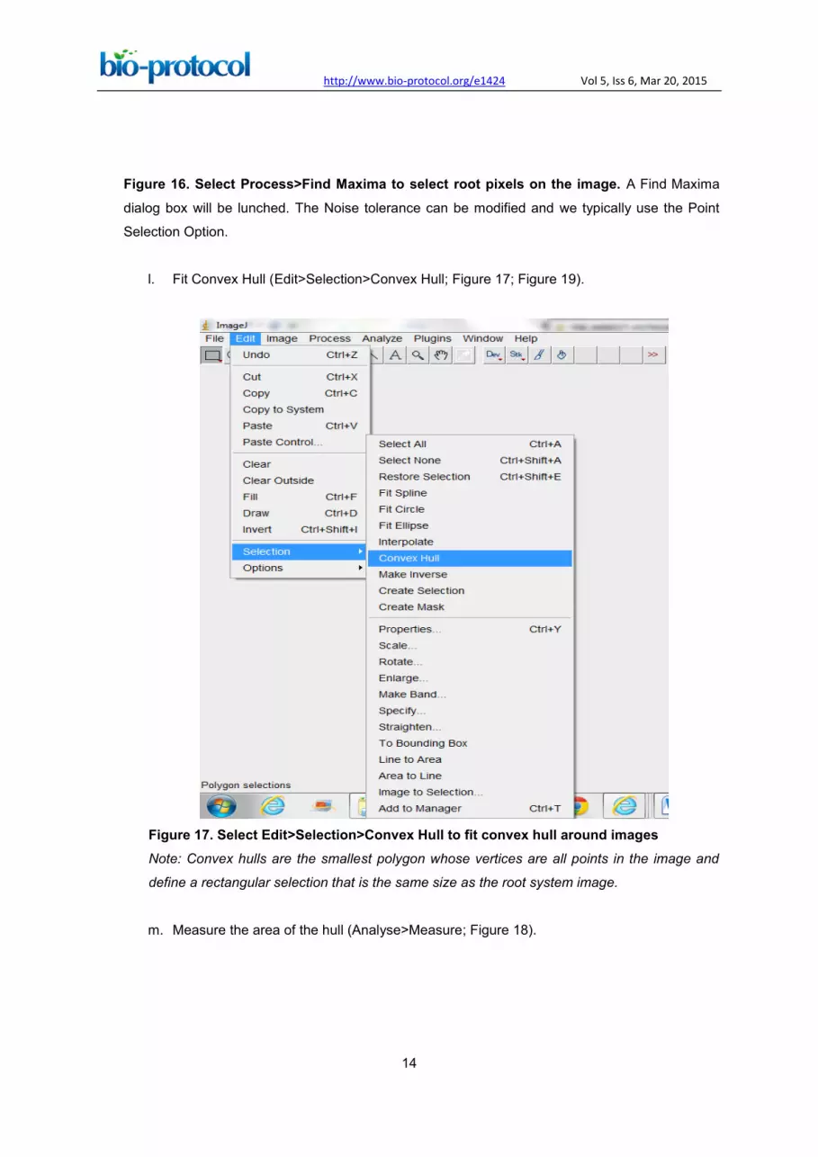
Figure 16. Select Process>Find Maxima to select root pixels on the image. A Find Maxima

dialog box will be lunched. The Noise tolerance can be modified and we typically use the Point

Selection Option.

l. Fit Convex Hull (Edit>Selection>Convex Hull; Figure 17; Figure 19).

Figure 17. Select Edit>Selection>Convex Hull to fit convex hull around images

Note: Convex hulls are the smallest polygon whose vertices are all points in the image and

define a rectangular selection that is the same size as the root system image.

m. Measure the area of the hull (Analyse>Measure; Figure 18).

http://www.bio-protocol.org/e1424 Vol 5, Iss 6, Mar 20, 2015

15

Figure 18. Select Analyse>Measure to measure the area of the hull (Surface area of the

root system)

Figure 19. Sample image showing original root RGB image, segmented root image,

perimeter or root for measuring root length and convex hull for measuring root area

http://www.bio-protocol.org/e1424 Vol 5, Iss 6, Mar 20, 2015

16

Figure 20. Representative data showing animated video of time-lapse segmented root

system

Recipes

1. Nutrient solution

Reagent Company (Catalogue No.) 1 L Stock Solution

20 L Nutrient Solution

Reagent to add (g/L)

Conc. (M)

Volume of Stock to add (ml)

Final Conc. (mM)

Ca(NO3)2, VWR International (22388.292) 236.15 1 40 2

NH4NO3 VWR International (21278.295) 80 1 40 2

MgSO4 VWR International (25165.292) 92.43 0.5 30 0.75

KOH VWR International (26668.296) 29.92 0.5333 19 0.5

KH2PO4 VWR International (26936.293) 36.3 0.2667 19 0.25

FeNaEDTA

VWR International (280233V) 18.35 0.05 40 0.1

CaCl2 VWR International (22317.260) 367.55 2.5 200 25

H3BO3 VWR International (20185.260) 185.49 3 200 30

Na2MoO4 VWR International (27937.236) 120.975 0.5 20 0.5

ZnSO4 VWR International (29253.236) 143.775 0.5 40 1

MnSO4 VWR International (ALFAB22081.22)

223.06 1 200 10

CuSO4 VWR International (23174.233) 124.84 0.5 120 3

Make up nutrient solution in 20 L deionised water and adjust to pH 6 using H2SO4.

Note: Nutrient solution could be replaced or changed depending on experimental

requirements. In our experiments we did not replace our solution for experiments that lasted

up to 14 day. Nutrient solutions should ideally be changed for experiments of longer duration

as there could be depletion of nutrients and/or growth of microorganisms in the solution. We

also experienced fungal growth on the germination papers occasionally.

2. Growth room requirements

Day/night cycle: 16/8 h

Temperature: 15 °C

Light intensity during the day at plant height: 100 μmol/m2/s

Relative humidity: 60%

Acknowledgements

This protocol was adapted from previous work Adu, 2014 and Adu et al., 2014. This work was

supported by the Rural and Environment Science and Analytical Services Division (RESAS) of the

Scottish Government through Work Package 3.3, ‘The soil, water and air interface and its

http://www.bio-protocol.org/e1424 Vol 5, Iss 6, Mar 20, 2015

17

response to climate and land use change’ (2011-2016). Funding for this study was provided by a

BBSRC Professorial Fellowship (to M. J. B.). M.O.A. was supported by the University of

Nottingham Vice-Chancellor’s Scholarship for Research Excellence.

References

1. Adu, M. O. (2014). Variations in root system architecture and root growth dynamics of

Brassica rapa genotypes using a new scanner-based phenotyping system. Ph.D. Thesis.

University of Nottingham: U.K.

2. Adu, M. O., Chatot, A., Wiesel, L., Bennett, M. J., Broadley, M. R., White, P. J. and Dupuy, L.

X. (2014). A scanner system for high-resolution quantification of variation in root growth

dynamics of Brassica rapa genotypes. J Exp Bot 65(8): 2039-2048.

3. Lobet, G., Pages, L. and Draye, X. (2011). A novel image-analysis toolbox enabling

quantitative analysis of root system architecture. Plant Physiol 157(1): 29-39.