Annals of Operations Research 15(1988)207 - 225 207

AN E F F I C I E N T METHOD TO D E T E R M I N E T H E OPTIMAL

C O N F I G U R A T I O N OF A F L E X I B L E M A N U F A C T U R I N G

SYSTEM

Yves DALLERY and Yannick FREIN

Laboratoire d'Automatique de Grenoble (L.A.G.), Associ~ au C.N.R.S. (U.A. 228), E.N.S.LE. G. - LN.P.G., B.P. 46, F-38402 Sain t-Martin-d'H~res, France

Abst rac t

A frequently encountered design issue for a flexible manufacturing system (FMS) is to find the lowest cost configuration, i.e. the number of resources of each type (machines, p a l l e t s , . . . ), which achieves a given production rate. In this paper, an efficient method to determine this optimal configuration is presented. The FMS is modelled as a closed queueing network. The proposed procedure first derives a heuristic solution and then the optimal solution. The computational complexity for finding the optimal solution is very reasonable even for large systems, except in some extreme cases. Moreover, the heuristic solution can always be determined and is very close (and often equal) to the optimal solution. A comparison with the previous method of Vinod and Solberg shows that our method performs very well.

K e y w o r d s

Flexible manufacturing systems, optimal configuration, queueing network models, product-form queueing networks, lower configuration, heuristic solution, optimal solution.

1. Introduction

Queueing network models are efficient tools for performance prediction of flexible manufacturing systems (FMSs) during the early stages of the design. Several models have been proposed to handle different features of an FMS [1,2]. The basic one is due to Solberg [3]. The FMS is modelled as a closed single-class queueing network. Under stochastic assumptions such as "the service time is exponentially distributed at any first-come first-served (FCFS) station", it can be shown that the queueing network has the so-called product form solution [4]. Efficient algorithms can then be used to derive the performance parameters such as throughputs, utiliza- tions, and mean queue lengths [5,6]. Several studies have shown that although the assumptions are rather restrictive, the queueing model is robust for a large class of

© J.C. Baltzer AG, Scientific Publishing Company

208 Y. Dallery and Y. Frein, Optimal configuration o f an FMS

FMSs. A theoretical explanation of this robustness is provided by the operational approach of queueing networks [ 7 - 9 ] .

The advantage of using analytical models as opposed to simulation is that they are easy to both develop and run. This is attractive for performance evaluation and even more so for optimization purposes. In particular, the problem of allocation of servers in a queueing network can be analyticalIy approached. For instance, Shanthikumar and Yao solved the problem of optimal server allocation in a system consisting of a set of independent multiserver stations [10]. Another problem of server allocation is related to a frequently encountered design issue for an FMS, which is to find the best configuration of the FMS which ensures a given productivity. A configuration is defined by the number of resources of each type. A cost is associated with each resource type and the best configuration is the one which has the lowest overall cost. This can be formulated as an optimization problem. This problem has been studied in a recent paper by Vinod and Solberg [11]. The FMS is modelled as a closed queueing network and a procedure for finding the optimal configuration is proposed. However, this procedure has two major drawbacks: (1) the required initial solution is highly dependent on the choice of an arbitrary starting point; (2) the computational time rapidly increases with the number of stations and the procedure is often infeasible.

In this paper, we propose an alternative procedure to obtain the optimal con- figuration. This requires three steps: (1) determine a lower configuration, (2) derive a heuristic solution, and (3) find the optimal solution. With this procedure, the previously mentioned drawbacks are avoided. The paper is organized as follows. In sect. 2, we review the queueing network model and formulate the optimization problem. The three steps of our procedure are presented in sect. 3. In sect. 4, a comparison of our procedure and the one proposed by Vinod and Solberg is provided, as well as numerical examples. Finally, in sect. 5, we extend this method to queueing network models with several classes of customers.

2. T h e m a t h e m a t i c a l f o r m u l a t i o n

2.1. THE QUEUEING NETWORK MODEL

The FMS is modelled by a closed single-class queueing network consisting of M stations and N customers. At each type of work station of the FMS is associated a station of the closed queueing network (CQN). The number of servers Ci, C i ~> 1, at station i, i = 1 , . . . , M - 1, is equal to the number of identical work stations of type i. Station M models the material handling system (MHS). I f the MHS consists of a set of carts, then station M is a multiple-server station with C M servers (C M is the number of available carts). Alternatively, if the MHS is a loop-conveyor, station M is a delay (or infinite servers) station. The number of customers N is equal to the number of pallets available in the FMS. This model assumes that any pallet is able to carry any part type.

Y. Dallery and Y. Frein, Optimal configuration o f an FMS 209

The following characteristic parameters of the CQN can easily be derived from both the manufacturing plans of the different part types and the prescribed production ratios: Si, the mean service time at station i; Vi, the visit ratio at station i (this is the average number of times a customer visits station i between two successive visits at the loading/unloading (L/U) station). Let Yi = ~ ' Si, Yi is called the loading of station i. A detailed discussion of this model is provided in [2,3].

Under certain assumptions, it can be proved that this CQN has a product-form solution, i.e. the proportion of time the system is in state n = (n 1 . . . . , n i . . . . . riM) , where n i is the number of customers present at station i, is given by:

where

M ni

1 I-I F-I f i ( j ) , (1) p(n) = G ( M , N ) i--1 i - -o

=

1 for j = 0

Y, for/~> 1.

ri(J)

ri( j) = min(C i, j ) for a multiple-server station; ri(j) = j for a delay station, and G(M, N) is a normalizing constant such that:

p(n) = 1. n

This result holds under stochastic assumptions such as the service time is exponentially distributed at any first-come first-served (FCFS) station [4] and under the homogeneity assumptions of the operational approach [8,9]. The performance parameters of the CQN, especially the throughput of the L/U station X, can then be derived using computational algorithms such as the convolution algorithm [5] or the mean value analysis (MVA) algorithm [6]. In the following, the parameter X wilt be of special interest, since it measures the production rate of the FMS.

2.2. OPTIMIZATION PROBLEM FORMULATION

The goal is to find the optimal system configuration. That is, among all the configurations which achieve a prescribed system throughput for the CQN (or equivalently a desired production rate for the FMS), find the one which has the minimal cost. It may be mathematically stated as follows:

minimize Z ( x )

subject to X ( x ) >1 XP, (2)

210 Y. Dallery and Y. Frein, Optimal configuration o f an FMS

where

X P

X

X(x) Z(x)

is the prescribed system throughput of the CQN (which is equal to the desired production rate of the FMS);

is the integer decision variable vector;

is the system throughput of the CQN associated with configuration x;

is the cost associated with configuration x.

The decision variables may include both the number of servers at a given set of stations and the number of customers. For easier presentation, we restrict our attention to the case where the number of servers at any station, including the MHS station, is a decision variable (we assume that the MHS consists of a set of carts). However, exten- sions to cases where there is no decision variables associated with some of the stations (because these stations are either delay stations or the number of servers is already specified) are straightforward. Therefore, the decision variable vector will be either x = (C l . . . . . C M) if the number of customers Nis fixed, or x = (C 1 . . . . . C M, N ) if the number of customers N is a decision variable.

No assumption on the cost function Z ( x ) is required, except that it is an increasing function, i.e.:

x >>- x ' -* Z ( x ) >>- Z ( x ' ) (3)

(we use the classical order relation: x ~> x ' iff x i >t x[ , for any i). Note that this assumption is not physically restrictive. Indeed, it means nothing but that adding a server or a customer increases the configuration cost.

3. So lu t ion t e c h n i q u e

Tile complexity of any procedure for finding the optimal solution is mainly a function of (1) the number of configurations which are actually considered, and (2) the number of throughput evaluations which are required. In this section, we propose an efficient procedure which is composed of three steps: first determine a lower con- figuration for the CQN; then determine a "good" heuristic solution and, finally, find the optimal solution.

3.1. LOWER CONFIGURATION

A configuration x will be called a lower configuration if for any configuration x ' such that there exists an index i such that x[ < xi, the system throughput verifies X ( x ' ) < XP. Such a lower configuration consists of a set of lower bounds on the decision variables. Our goal is to find a lower configuration which is as close as possible to the optimal configuration. For this purpose, we use some well-known properties of CQNs, provided by the so-called asymptotic bound analysis (ABA) [8,12,13].

Y. Dallery and Y. Frein, Optimal configuration o f an FMS 211

ABA provides upper bounds on the throughput of general CQNs. These bounds are given by:

and

q. X ~< rain - - (4)

i Y/

N X -<< - - , (5)

Ro

where R o is the total loading defined by

M

Ro-- Z r,. i = I

These bounds are obtained by considering the extremes of system behaviour: either no queueing delay occurs or at least one station is saturated. Moreover, it can easily be shown that for product-form CQNs, eq. (4) is a strict inequality for any finite population N. From these bounds and the prescribed throughput, the following lower bounds on the decision variables can be obtained:

C i > X P . Yi for any i (6)

N >1 X P . R o . (7)

Let C/b (respectively N b) denote the integer strictly greater (respectively greater) than the quantity X P . Yi (respectively X P .Ro). Then x = (C~ . . . . . C~, N b) is a lower configuration. Any configuration x ' such that either there is a station i such that C; < C~, or N ' < N b, can not achieve the prescribed throughput, whatever the values of the other decision variables are. Therefore, such configurations need not be considered during the optimal solution search procedure.

3.2. HEURISTIC SOLUTION

In order to reduce the number of throughput evaluations required during the optimal solution search procedure, and therefore speed up the optimization, we need a "good" starting solution. A way of obtaining such a heuristic solution is now described.

3.2.1. Fixed number o f customers

Assume first that the number of customers N is fixed. Let u i = (0, . . . . 0, 1 ,0 , . . . , 0) denote the M dimensional vector defined by u~ = 1 and u} = 0 for any j 4: i. The

212 Y. Dallely and Y. Frein, Optimal configuration o fan FMS

following procedure can be used to obtain a heuristic solution. The initial configura- tion is provided by the lower server configuration derived in sect. 3.1. Then, at each step of this procedure the number of servers at one station is increased by one. This station is the one which maximizes the ratio of the extra throughput to the extra cost, due to the additional server. The procedure is stopped as soon as the prescribed system throughput is achieved. This procedure is detailed in the following algorithm:

Step 1: Start with the following initial configuration:

x = (C b,N) = ( C ~ , . . . j C~, N).

Step 2: If the throughput of the current configuration x is such that X(x) >1 XP, stop the procedure; the current configuration provides the heuristic solution x tl = (C, N) and its associated cost Z h = Z(C, N).

Step 3: For the current configuration x, and for any i, i = 1 . . . . . M, calculate:

A.= X(C + u', N) - X(C, N) ' Z ( C + u i , N ) - Z ( C , N ) "

Step 4: Let i o be an index such that:

Aio -~ max A i . i

Add a server at station i o to the current configuration (C = C + uio). Go to step 2.

3.2.2. Variable number o f customers

Suppose now that the number of customers is a decision variable. The above procedure could still be applied: at each step, either a server or a customer would be added. However, in most physical cases, the difference between the number of customers in the final and the initial configuration is large compared to the one relative to the number of servers. As a result, the computation of A i for i = 1 . . . . . M is often useless.

We therefore propose the following alternative procedure. The initial con- figuration is again provided by the lower configuration derived in sect. 3.1. An initial solution is then found by increasing the number of customers until the prescribed throughput is achieved (property 1 given in the appendix shows that there always exists a finite population N such that X(C b, N)>1 XP). Then, using a procedure similar to the one in 3.2.1, we increase, step by step, the number of servers in the CQN. At each step, we calculate the number of customers required to achieve the prescribed throughput and check whether or not the associated solution is better than the current best one. The procedure is stopped when adding a server at any station

Y. Dallery and Y. Frein, Optimal configuration o]'an FMS 213

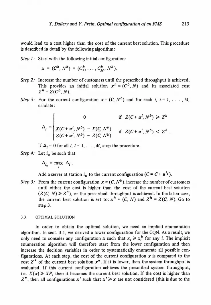
would lead to a cost higher than the cost of the current best solution. This procedure is described in detail by the following algorithm:

Step 1: Start with the following initial configuration:

x = (C b, N b) = (Cba . . . . . C~I, Nb) .

Step 2: Increase the number of customers until the prescribed throughput is achieved. This provides an initial solution x h = (C ~, N) and its associated cost Z h = Z(C b. N).

Step 3: For the current configuration x = (C, N b) and for each i, i = 1, . . . , M, calulate:

!

0

X ( C + II i, N b) - X(C, N b)

Z ( C + u i, N b) - Z(C, N b)

if Z(C + u i, N b) >1 Z h

if Z(C + u i, N b) < Z h .

If A i = 0 for all i, i = 1 , . . . , M, stop the procedure.

Step 4: Let i o be such that

Aio = max A i . i

Add a server at station i o to the current configuration (C = C+ uio).

Step 5: From the current configuration x = (C, Nb), increase the number of customers until either the cost is higher than the cost of the current best solution (Z(C, N) ~> ZI2), or the prescribed throughput is achieved. In the latter case, the current best solution is set to: x h = (C, N) and Z h = Z(C, N). Go to step 3.

3 3 . OPTIMAL SOLUTION

In order to obtain the optimal solution, we need an implicit enumeration algorithm. In sect. 3.1, we derived a lower configuration for the CQN. As a result, we only need to consider any configuration x such that x i /> x b for any i. The implicit enumeration algorithm will therefore start from the lower configuration and then increase the decision variables in order to systematically enumerate all possible con- figurations. At each step, the cost o f the current configuration x is compared to the cost Z* of the current best solution x*. If it is lower, then the system throughput is evaluated. I f this current configuration achieves the prescribed system throughput, i.e. X ( x ) >1 XP, then it becomes the current best solution. If the cost is higher than Z*, then all configurations x ' such that x ' / > x are not considered (this is due to the

214 Y. Dallery and Y. Frein, Optimal configuration o f an FMS

fact that the cost is an increasing function (3)). The initialization of the current best solution is provided by the heuristic solution derived in sect. 3.2. The detailed algo- rithm corresponding to this procedure is described below (n denotes the dimension of x, either n = M if the number of customers is fixed, or n = M + 1 if it is a decision variable).

Step 1: Initialization:

x = x b (i.e. the current configuration is initialized to the lower configuration). x* = x h and Z* = Z h (i.e. the current best configuration is initialized to the configuration of the heuristic solution). j = n

Step 2: For the current configuration x, calculate the cost function Z(x) . If Z(x) /> Z*, go to step 4.

Step 3: For the current configuration x, calculate the throughput X(x) . If X ( x ) >1 XP:

then Z* = Z(x ) and x* = x (i.e. x becomes the current best configuration) go to step 4.

else x n = x n + 1 and/" = n (i.e. the current configuration is modified by increasing the last decision variable by one) go to step 2.

If f = 1 (i.e. the implicit enumeration is finished) then Z ° = Z*, x ° = x* (x ° is the optimal configuration)

STOP.

else xj = x~, xj_ 1 = xj_ 1 + 1, j = j - 1 (i.e. the current configuration is modified in the following way:

- the j th decision variable is set to its value in the lower con- figuration

- the ( j - 1)th decision variable is increased by one). go to step 2.

Step 4:

4. Analys is o f t h e p r o p o s e d m e t h o d

In this section, we briefly explain the method developed by Vinod and Solberg (referred to as the V-S method). We then compare the method derived in sect. 3 (referred to as the proposed method) with the V-S method, first qualitatively and then quantitatively, using several experimental results.

4.1. COMPARISON WITH VINOD AND SOLBERG'S METHOD

The V-S method is composed of three steps. The first step consists of the choice of an upper bound U on the decision variables. This choice is arbitrary, but it

Y. Dallery and Y. Frein, Optimal configuration o f an FMS 215

is assumed that the optimal solution x ° is such that x ° ~< U. The second step provides an initial solution by using a so-called "bisection search procedure". The idea is to find the lowest possible configuration proportional to the upper bound which achieves the prescribed throughput. The third step is the search of the optimal solution. Almost all configurations lower than the upper bound have to be considered. For each con- figuration, the throughput is evaluated only if (1) the cost of this configuration is lower than the cost of the current best solution, and (2) the upper bound of this configuration, provided by eq. (4) of ABA, is greater than the prescribed throughput.

The first difference between the proposed method and the V- S method is that the former (respectively the latter) starts with a lower (respectively upper) bound on the decision variables and then considers configurations upper (respectively lower) than this lower (respectively upper) configuration. However, the upper bound of the V-S method must be arbitrarily chosen and therefore the quality of the initial solution, which is higtfiy dependent on this choice, is doubtful. For the proposed method, the lower bound can be determined by ABA, and therefore this has a physical meaning. Similarly, the initial solution can be derived by a heuristic procedure based on a "gradient analysis". Now the computation complexity of either method is a function of (1) the number of configurations actually considered, which depends on the quality of the bound configuration, and (2) the number of throughput evaluations, which depends on the quality of the initial solution. As we will see with the examples, our lower bound and initial solution are usually very good, and therefore the proposed method will appear to be more efficient than the V-S method.

4.2. EXPERIMENTAL RESULTS

We now present several examples to illustrate our method. To compare the efficiency of the proposed method and the V-S method, the following measures of complexity will be used: (1) the overall number of throughput evaluations required during the procedure; the throughput is calculated in 0 ( M N 2) arithmetic operations, using either the convolution or the MVA algorithm; (2) the number of configurations actually considered in the optimal search procedure; for each configuration, the cost Z must be computed, and this requires O(M) operations. The total computation time (CPU) of the procedure will also be used as an overall complexity measure (the examples were mn on a Norsk Data 560 Computer).

The data for the examples will be: the loading vector Y; the number of customers N, if not a decision variable; the cost function Z; the upper bound for the V- S method U. For all examples, the prescribed throughput will be XP = 3.0.

216 Y. Dallery and Y. Frein, Op t imal conf igurat ion o f an F M S

F o u r s tat ion examples

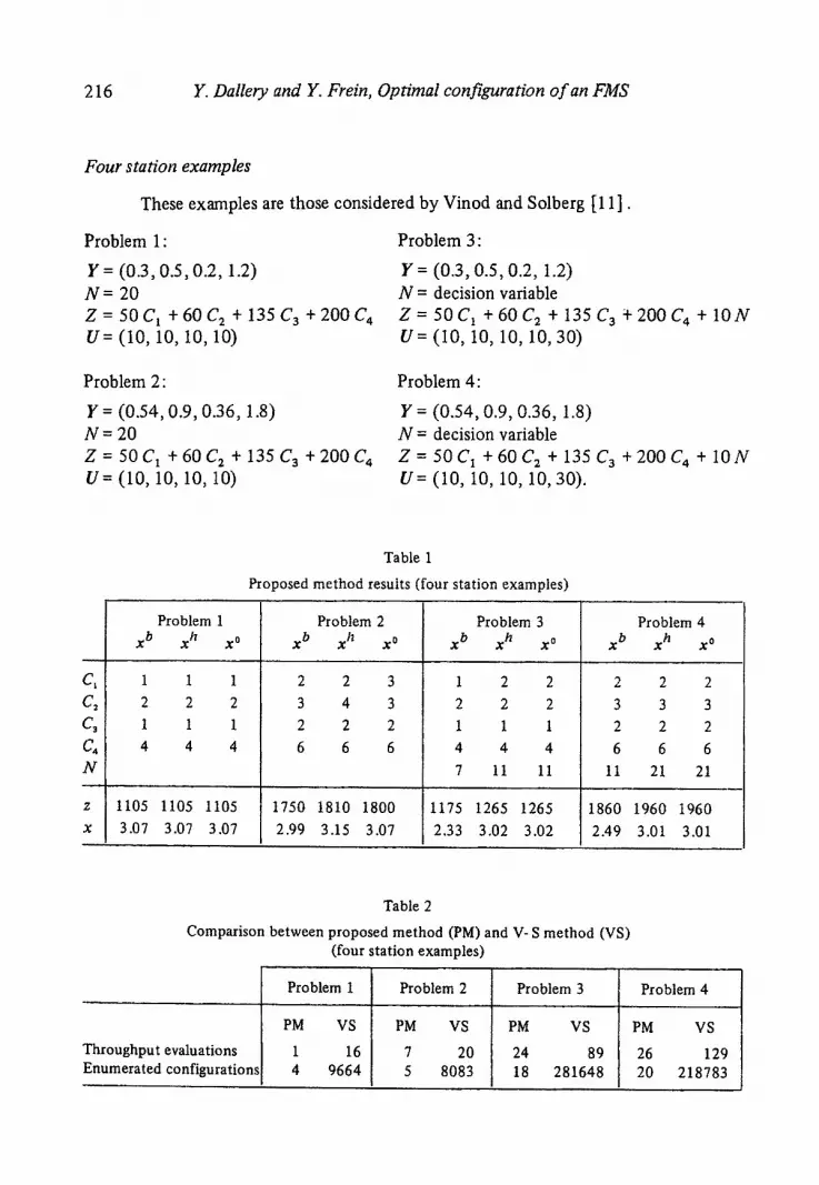
These examples are those considered by Vinod and Solberg [11] .

Problem 1"

Y = (0.3, 0.5, 0.2, 1.2)

N = 20

Z = 50C1 + 6 0 C 2 + 135 C 3 + 2 0 0 C 4 U = (10, 10, 10, 10)

Problem 3:

Y = (0.3, 0.5, 0.2, 1.2)

N = decision variable

Z = 5 0 C 1 + 6 0 C 2 + 135 C 3 ÷ 2 0 0 C 4 + 1 0 N U = (10, 10, 10, 10, 30)

Problem 2:

Y = (0.54, 0.9, 0.36, 1.8)

N = 20

Z = 5 0 C 1 + 6 0 C 2 + 1 3 5 C a + 2 0 0 C 4 U = (10, 10, 10, 10)

Problem 4:

Y = (0.54, 0.9, 0.36, 1.8)

N = decision variable

Z = 5 0 C I + 6 0 C z + 135 C 3 + 2 0 0 C 4 + 1 0 N U = (10, 10, 10, 10, 30).

C~

C~

c~ c, N

Z

X

Problem 1 x b x h x o

1 1 1

2 2 2 1 1 1

4 4 4

1105 1105 1105

3.07 3.07 3.07

Table 1

Proposed method results four station examples)

Problem 2 Problem 3 x b X h xo

2 2 3

3 4 3

2 2 2

6 6 6

x b X h xO

1 2 2 2 2 2 1 1 1 4 4 4

7 11 11

Problem 4 x b x h x o

1750 1810 1800

2.99 3.15 3.07 1175 1265 1265

2.33 3.02 3.02

2 2 2

3 3 3 2 2 2

6 6 6

11 21 21

1860 1960 1960

2.49 3.01 3.01

Table 2

Comparison between proposed method (PM) and V- S method (VS) (four station examples)

Problem 1 Problem 2 Problem 3

Throughput evaluations Enumerated configuration~

Problem 4

PM VS

1 16 4 9664

PM VS

7 20 5 8083

PM VS

24 89 18 281648

PM VS

26 129 20 218783

Y. Dallery and Y. Frein, Optimal configuration of an FMS 217

The results provided by the proposed method are detailed in table 1. For each problem, the lower configuration, the initial solution and the optimal solution, as well as their associated cost and throughput, are given. The comparison between the com- plexity of the proposed method and that of the V-S method is provided in table 2.

The following points should be noted: first, the lower configuration is close to the optimal solution; actually, it is the optimal solution for problem 1. The heuristic solution appears to be a very good solution; for problems 1,2 and 4, it is equal to the optimal solution. As a result, our procedure is very efficient and performs well com- pared to the V-S method (see table 2). The total number of throughput evaluations (including those for finding the heuristic solution) is always smaller than those for the V-S method. Moreover, the number of configurations actually enumerated in the optimal search procedure and therefore the number of evaluations of the cost function is very low compared to the V-S method one. Note that the number of configurations enumerated by the V-S method is almost equal to the number of all possible con- figurations lower than the upper bound (10000 for problems 1 and 2, 300000 for problems 3 and 4).

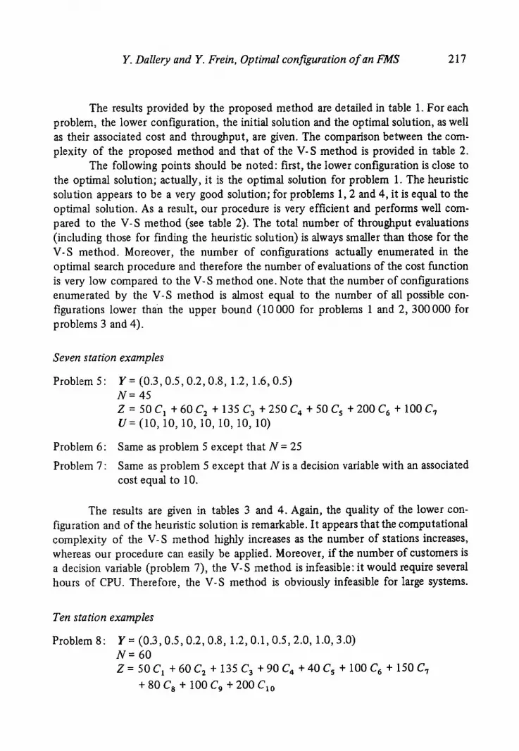
Seven station examples

Problem 5: Y = (0.3, 0.5, 0.2, 0.8, 1.2, 1.6, 0.5) N = 45 Z = 5 0 C ~ + 6 0 C 2 + 1 3 5 C 3 + 2 5 0 C 4 + 5 0 C s+200C 6 + 1 0 0 C 7 U= (10, 10, 10, 10, i0, 10, 10)

Problem 6: Same as problem 5 except that N = 25

Problem 7: Same as problem 5 except that N is a decision variable with an associated cost equal to 10.

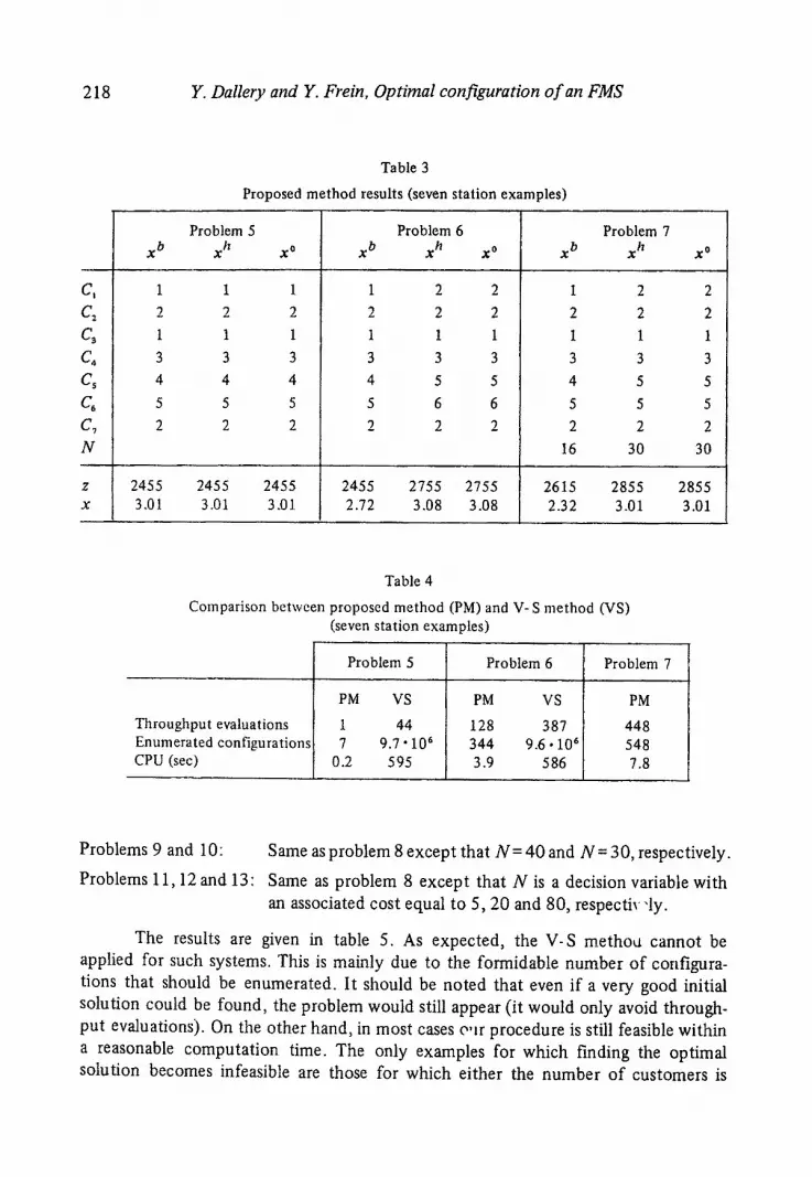
The results are given in tables 3 and 4. Again, the quality of the lower con- figuration and of the heuristic solution is remarkable. It appears that the computational complexity of the V-S method higtfly increases as the number of stations increases, whereas our procedure can easily be applied. Moreover, if the number of customers is a decision variable (problem 7), the V-S method is infeasible: it would require several hours of CPU. Therefore, the V-S method is obviously infeasible for large systems.

Ten station examples

Problem 8: Y = (0.3, 0.5, 0.2, 0.8, 1.2, 0.1,0.5, 2.0, 1.0, 3.0) N = 60 Z = 5 0 C 1 + 6 0 C 2 + 1 3 5 C 3 + 9 0 C 4 + 4 0 C s +100C 6 + 1 5 0 C 7

+ 80 C 8 + 100 C 9 + 200 C,0

218 Y. Dallery and Y. Frein, Opt imal configuration o f a n FMS

Table 3

Proposed method results (seven station examples)

CI

~3

C5

C7

N

x b Problem 5

x h x 0

1 1 1

2 2 2

1 1 1

3 3 3

4 4 4

5 5 5

2 2 2

Problem 6 X b X h .g0

1 2 2

2 2 2

1 1 1

3 3 3

4 5 5

5 6 6

2 2 2

x b

I

2

I

3

4

5

2

16

Problem 7 x h

2 2 1 3 5 5 2

30

x 0

2 2 1 3 5 5 2

30

z 2455 2455 2455 2455 2755 2755 2615 2855 2855 x 3.01 3.01 3.01 2.72 3.08 3.08 2.32 3.01 3.01

Table 4

Comparison between proposed method (PM) and V- S method (VS) (seven station examples)

Throughput evaluations Enumerated configurations CPU (sec)

Problem 5

PM VS

1 44 7 9.7" 106

0.2 595

Problem 6

PM VS

128 387 344 9.6 • 106 3.9 586

Problem 7

PM

448 548 7.8

Problems 9 and 10: Same as problem 8 except that N = 40 and N = 30, respectively.

Problems 11, 12 and 13: Same as problem 8 except that N is a decision variable with an associated cost equal to 5, 20 and 80, respectiv "ly.

The results are given in table 5. As expected, the V-S metho~t cannot be applied for such systems. This is mainly due to the formidable number of configura- tions that should be enumerated. It should be noted that even if a very good initial solution could be found, the problem would still appear (it would only avoid through- put evaluations). On the other hand, in most cases e, lr procedure is still feasible within a reasonable computation time. The only examples for which finding the optimal solution becomes infeasible are those for which either the number of customers is

C I

C2

c,

Cs

C~

Cs

N

z x TE

C

PU

(sec

l

Pro

blem

8

x b

x h

x o

1 1

1 2

2 2

1 1

1

3 3

3 4

4 4

1 1

1 2

2 2

7 7

7 4

4 4

10

10

10

4095

40

95

4095

3.

04

3.04

3.

04

1 (1

+ 0

)

0.5

Tab

le 5

Pro

pose

d m

etho

d re

sult

s,

Pro

blem

9

x b

x h

x o

1 2

2 2

3 3

1 1

1

3 3

3 4

5 5

1 1

1

2 2

2 7

8 8

4 4

4

10

10

10

4095

43

25

4325

2.

77

3.01

3.

01

155

(41

+ 11

6)

15.5

Pro

blem

10

x b

x h

1 3

2 4

1 2

3 5

4 7

1 i

2 3

7 9

4 6

I0

12

4095

55

60

2.46

3.

01

171

10.5

ten

stat

ion

exam

ples

)

Pro

blem

11

x b

x h

xo

1 1

1 2

2 2

1 1

1

3 3

3 4

4 4

1 1

1 2

2 2

7 7

7 4

4 4

10

10

10

29

56

56

4240

43

75

4375

2.

41

3.00

3.

00

200

(64

+ 13

6)

16.0

Pro

blem

12

x b

x h

x o

1 2

2 2

2 2

1 1

1

3 3

3 4

5 5

1 1

1 2

2 2

7 7

7 4

4 4

10

10

10

29

44

44

4675

50

65

5065

2.

41

3.01

3.

01

5130

(14

2 +

4988

)

338.

0

Pro

blem

13

x b

x h

1 2

2 3

1 1

3 4

4 6

1 1

2 2

7 8

4 4

10

10

29

37

6415

74

15

2.41

3.

00

220

15.0

For

the

thr

ough

put

eval

uati

ons

(TE

), t

he

tota

l nu

mbe

r of

eva

luat

ions

, as

wel

t as

the

rep

arti

tion

bet

wee

n th

e he

uris

tic

proc

edur

e an

d th

e op

tim

al s

olut

ion

sear

ch p

roce

dure

, ar

e pr

ovid

ed.

to

~o

220 Y. Dallery and Y. Frein, Optimal configuration o f an FMS

close to the ABA lower bound ofeq. (5) (N b = 29 for this example), or the number of customers is a decision variable whose associated cost is high (with respect to the cost of the servers). In both cases, the number of customers would be a critical resource for the queueing network. It appears that this will hardly ever be the case for FMS appli- cations. Anyway, for such cases, the heuristic solution can still be obtained at a low computation cost. Now, as observed on all the many examples we tested, the heuristic solution is very often equal to the optimal solution, or at least very close to it. As a result, the heuristic solution can be used with high confidence in the place of the optimal solution.

The conclusion of the previous analysis of the proposed method can be stated as follows: (1) the heuristic solution can always be obtained at a low computation cost, whatever the number of stations is; this heuristic solution is very often equal to, or at least very close to, the optimal solution; (2) the procedure for obtaining the optimal solution is feasible, whatever the number of stations, except if the customers are a critical resource.

For all the previous examples, the cost function was linear. This seems to be realistic for FMS applications. Note, however, that examples with a nonlinear cost function can be analyzed and that the proposed method performs as well as in the case of linear cost function. The only restriction is that the cost function must be an increasing one (see sect. 2).

4.3. COMPUTATIONAL SAVING USING SSD BOUNDS

In sect. 3.1, we used the ABA bounds to find the lower configuration of the network. We now show that further computational saving can be obtained by using the single-server disaggregation (SSD) bounds [14]. This technique provides quick bounds on the throughput of queueing networks with multiple-server stations. It consists of replacing any multiple-server station by a set of single-server stations. Throughput bounds can then be obtained by using the balanced job bound (BJB) analysis [15,16]. For the queueing network defined in sect. 2.1, the upper bound on the throughput using the SSD technique [14] together with the improved BJB analysis [ 16] is given by:

N X U (s) R u+ ( N - 1) Yu'

where

M

i =1 Ci

and

Y. Dallery and Y. Frein, Optimal configuration o f an FMS 221

Yu - Ru i=1 \ C i / "

The computational complexity of this bound is O(M).

For our purpose, this bound may be useful any time the throughput of the queueing network needs to be evaluated in the optimal solution procedure. Instead of computing the exact throughput (which requires O(MN 2 )), the upper bound given by (8) is first calculated. If this upper bound is lower than the prescribed throughput ( X U < XP), then we can be sure that the exact throughput is lower than the prescribed throughput (X<~ X U < XP) and therefore there is no need to compute the exact throughput. As a result, the number of throughput evaluations required by the procedure can easily and significantly be reduced. For instance, in problem 7 more than one third of the throughput evaluations can be avoided using this bound.

5. E x t e n s i o n to mul t ic lass q u e u e i n g n e t w o r k s

5.1. PROBLEM FORMULATION

In this section, we briefly describe the extension of our method for finding the optimal configuration of closed queueing networks with several classes of customers. Let us consider a closed queueing network consisting of M stations and R classes of customers. The number of customers of class r is N r. The characteristic parameters are Sir, the mean service time of class r customers at station i; V/r is the visit ratio of class r customers at station l". Let Y/r = V/r" Sir; Y/r is the loading of class r customers at station L This queueing network can model an FMS in which each part type requires a specific pallet type [17,2]. Under some stochastic assumptions such as the service time is exponentially distributed at any FCFS station and does not depend on the class of customers, it can be shown that the queueing network has a product form solution [18]. This result also holds under the homogeneity assumptions of opera- tional analysis [19]. Then, the performance parameters (especially the throughput of class r customers, Xr, which provides the production rate of each part type in an FMS) can be derived using either the convolution algorithm or the mean value analysis algorithm.

The optimal problem formulation is then to find the lowest cost configuration which achieves a prescribed throughput for each class of customers, i.e. X r >t XP r for all r = 1 . . . . . R. We restrict our attention to the case for which the number of each class, Nr, is fixed, and therefore the number of servers of each station, Ci, are the only decision variables.

222 Y. Dallery and Y. Frein, Optimal configuration o f an FMS

5.2. SOLUTION TECHNIQUE

The solution procedure is a generalization of the one described in sect. 3. The lower configuration can be determined using the following asymptotic analysis: any configuration which is a solution of the optimization pr9blem is such that X r >~ XPr, for any r = 1 , . . . , R. Now, the throughput of class r customers at station i, Xir, and the utilization of station i by customers of class r, Uir , are given by the forced flow law and the utilization law, respectively [8] :

Xir = V/,.X r (9)

q~ : s ir . xi,., (lO)

which leads to:

~,. : v~r. s~rx~ : Y~X~. (11)

The total utilization of station i is then"

R R

U i = ~ Uir = ~. Yir .X, . . (12) r = l r = l

This utilization rate is constrained by the total number of servers available at station i, i.e. U/~< C i . We end up with:

R R

Ci>--" Z YirX, .>~ ~ Yir 'XPr fo rany i, (13) r = l r = l

which gives a lower bound on the number of servers at station L This provides the lower configuration.

The heuristic solution is obtained using the following procedure: the initial configuration is provided by the lower configuration derived from eq. (13). Then, at each step the number of servers at one station is increased by one. The procedure is stopped as soon as all the prescribed throughputs are achieved, i.e. X r >1 XPr, for all r = 1 , . . . , R. The choice of the station at which the server is added is a generalization of the one in sect. 3.2.1 :let C be the current configuration it requires first to calculate the following coefficients:

A i X r =

0

x A c + u ~) - x A c )

if x A c ) >f x 5 and Xr(C + u i) >f X P r

else.

Y. Dallery and Y. Frein, Optimal configuration o fan FMS 223

Notice that adding a server at a station may result in a decrease of throughput for certain classes of customers. An overall measure of the throughput variations resulting from adding a server at station i is provided by:

R

a , x = Z a, Xr r = l

and the choice criteria is defined as:

where

A i X A i =

A i Z '

A i Z = Z ( C + u i ) - z ( c )

A server is then added at the station i which maximizes the coefficient A i.

The optimal solution is derived using an implicit enumeration algorithm, which is a straightforward extension of the algoriffan given in sect. 3.3.

6. C o n c l u s i o n s

An efficient method to determine the optimal configuration, i.e. the number of resources of each type (machines, pallets, . . . ), of flexible manufacturing systems modelled as a closed queueing network has been presented. The optimal solution can be obtained at a reasonable computation cost, even if the number of stations is large, except when the customers are a critical resource. In that case, a heuristic solution, very close to the optimal solution, can be derived at a very low cost.

A p p e n d i x

PROPERTY 1

For a CQN such that C i >1 C~ for any i ,wi th C b = ( C ~ , . . . , Cbm) the lower configuration (see sect. 3.1), there exists a finite population N such that the through- put of the CQN, X(N) is higher than the prescribed production rate XP.

Proof

Let X~(N) be a lower bound on the throughput of the CQN, i.e. X2(N ) <<. X(N). Such a bound is provided by [14] •

224 Y. Dallery and Y. Frein, Optimal configuration o fan FMS

N X~(N) = Re + ( N _ l) y~ ,

whe re:

M Yt R~ =~":. ~ and Y~ = max

i=1 i C i

X~(N) >~ XP iff N ( 1 - X P . Y~) >i X P ( R ~ - Y~).

Now, from the lower bounds on the number of servers at each station, we have C i >1 Ci b > XP. Y~. and therefore 1/XP > Y~. Therefore, for any N such that

XP(R - N >~ , X2(N ) >i XP,

1 - X P . Y~

and then the proof follows.

References

[ 1 ] J.A. Buzacott and D.D. Yao, Flexible manufacturing systems: A review of analytical models, Manage. Sci. 32(1986).

[2] Y. DaUery, On queueing network models of flexible manufacturing systems, Large-Scale Systems 11(1986)109.

[3] J.J. Solberg, A mathematical model of computerized manufacturing systems, Proc. 4th Int. Conf. on Production Research, Tokyo, Japan (1977).

[4] W.J. Gordon and G.F. NeweU, Closed queueing networks with exponential servers, Oper. Res. 15(1967)252.

[5] J.P. Buzen, Computational algorithms for closed queueing networks with exponential servers, Commun. ACM 16, 9(1973)527.

[6] M. Reiser and S.S. Lavenberg, Mean value analysis of closed multichain queueing networks, J. ACM 27, 2(1980)313.

[7] R. Suri, Robustness of queueing network formulae, J. ACM 30, 3(1983)564. [8] P.J. Denning and J.P. Buzen, The operational analysis of queueing network models, Com-

puting Surveys 10, 3(1978)225. [9] Y. Dallery and R. David, Some new results on operational analysis, Performance '84, Paris

(I984). [10] J.G. Shanthikumar and D.D. Yao, Optimal server allocation in a system of multi-server

stations, Manage. Sci. 33, 9(1987)1173. [11] B. Vinod and J.J. Solberg, The optimal design of flexible manufacturing systems, Int. J.

Prod. Res. 23, 6(1985)1141. [12] R.R. Muntz and D. Wong, Asymptotic properties of closed queueing network models, Proc.

8th Annual Princeton Conf. on Info. Sc. and Systems, Princeton University (1974). [13] L. Kleinrock, QueueingSystems, Vol. 2 (Wiley, New York, 1976).

Y. DaUery and Y. Frein, Optimal configuration o f an FMS 225

[14] Y. Dallery and R. Suri, Approximate disaggregation and performance bounds for queueing networks with multiple-server station, Performance Evaluation Review 14, 1(1986)111.

[15] J. Zahorjan, K.C. Sevcik, D.L. Eager and B. Galler, Balanced job bound analysis of queue- ing networks, Commun. ACM 25, 2(1982)134.

[16] Y. Dallery, An improved balanced job bound analysis of closed queueing networks, Oper. Res. Lett. 6, 2(1987)77.

[17] R. Suri and R.R. Hildebrant, Modelling flexibIe manufacturing systems using mean value analysis, J. Manufacturing Systems 3, 1(1984)27.

[18] F. Baskett, K.M. Chandy, R.R. Muntz and F.G. Palacios, Open, closed and mixed networks of queues with different classes of customers, J. ACM 22, 2(1975)248.

[ 19 ] Y. Dallery and R. David, Operational analysis of multiclass queueing networks, IEEE Conf. on Decision and Control, Athens, Greece (1986).