ORIGINAL ARTICLE

An efficient algorithm to solve a multi-objective robustaggregate production planning in an uncertain environment

Seyed Mohamad Javad Mirzapour Al-e-Hashem &

Mir Bahador Aryanezhad & Seyed Jafar Sadjadi

Received: 28 December 2010 /Accepted: 16 May 2011 /Published online: 3 June 2011# Springer-Verlag London Limited 2011

Abstract Risk is inherent in most economic activities.This is especially true of production activities whereresults of decisions made today may have many possibledifferent outcomes depending on future events. Sincecompanies cannot usually protect themselves completelyagainst risk, they have to manage it. In this paper, wepresent a multi-objective model to deal with a multi-period multi-product multi-site aggregate productionplanning problem for a medium-term planning horizonunder uncertainty. The first objective function attempts tominimize sum of the expected value and the variabilityof total costs with reference to inventory levels, regular,overtime and subcontracting levels, backordering levels,and labor, machine and warehouse capacities. The secondobjective function highlighted the concept of customerservice level through minimizing the expected value ofmaximum shortages among all customers’ zones fromwhich the variability of that is conducted. The lastobjective function aims to maximize workers productiv-ity, a weighted average of productivity levels in allfactories and in all periods which is weighted by thenumber of k-level labors. Then, we use an efficientalgorithm that is a combination of an augmentedε-constraint method and genetic algorithm to solve ourproposed model. The results demonstrate the practicabilityof the proposed multi-objective stochastic model as wellas the proposed algorithm.

Keywords Aggregate production planning . Stochasticoptimization . Augmented ε-constraint . Genetic algorithm .

Multi-objective optimization . Supply chain management

1 Introduction

A global supply chain is a very large-scale system oforganizations, people, technology, activities, information,and resources involved in moving a product or service fromsupplier to end customer. Supply chain complexity willvary with the size of the business and the intricacy andnumbers of items that are manufactured. To ensure that thesupply chain is operating as efficient as possible andgenerating the highest level of customer satisfaction at thelowest cost, companies have adopted supply chain man-agement (SCM) processes and associated technology. SCMhas three levels of activities that different parts of thecompany will focus on: strategic, tactical, and operational.Strategic planning refers to a long-term planning horizonand to the strategic problem of designing and configuring ageneric multi-stage supply chain [1]. Tactical planningrefers to both long- and short-term planning horizons anddeals with the determination of the best fulfillment policiesand material flows in a supply chain [2]. And operationalplanning refers to short-term planning horizon and dealswith the determination of number of logistic facilities,geographical locations, and facilities capacities to optimaldaily allocation of customer demand to retailers, distribu-tion centers and/or production sites. One of the problemsthat should be addressed in the scope of Tactical andoperational activities is aggregate production planning(APP) that does an aggregate plan for the productionprocess, in advance of 3 to 18 months, to give an idea tomanagement as to what quantity of materials and other

S. M. J. M. Al-e-Hashem (*) :M. B. Aryanezhad : S. J. SadjadiDepartment of Industrial Engineering,Iran University of Science and Technology,Narmak, P.C. 1684613114,Tehran, Irane-mail: Mirzapour@iust.ac.ir

Int J Adv Manuf Technol (2012) 58:765–782DOI 10.1007/s00170-011-3396-1

resources are to be procured and when, so that total cost ofoperations of the organization is kept to the minimum overthat period. APP has attracted the attention of manyresearchers from several years ago [3]. Numerous APPmodels with varying degrees of difficulties have beenproposed in the last decades. Related work includes:Hanssman and Hess [4], Haehling [5], Goodman [6],Masud and Hwang [7], Nam and Logendran [8], andBaykasoglu [9]. According to the number of objectivefunctions considered simultaneously in APP models, theycould be classified to the following categories: single-objective models, bi-objective models, and multi-objectivemodels. In single-objective models, the minimization oftotal cost is usually considered as the objective function andgenerally consists of production cost, inventory cost,shortage cost and the cost of changes in labor level (see,for example, [10]). In bi-objective models, the minimizationof total cost usually is considered as the main objectivefunction and beside this, other objective functions such asmaximization of service level, minimization of changes inwork force level, minimization of variability of total cost,minimization of backordering levels, and minimization offinancial risk are taken into account (see, for example, [11–13]). In multi-objective models, a combination of abovemention objective functions may be considered simulta-neously (see, for example, [14, 15]).

Research that considers uncertainty can be categorizedaccording to the four primary approaches [16]: (1)stochastic programming approach (i.e., [17, 18]), (2) fuzzyprogramming approach (i.e., [19, 20]), (3) stochasticdynamic programming approach (i.e., [21]), and (4) robustoptimization approach (i.e., [10, 22–24]).

In stochastic programming approach for representinguncertainty, two different methodologies could be applied.These are the distribution-based approach and the scenario-based approach. The former approach is applied where acontinuous range of potential future outcomes can beanticipated. The advantage of this methodology is that byassigning a probability distribution function to the contin-uous range of possible consequences, the need to forecastexact scenarios is eliminated. However, complexity ofapplying distribution function limits the number of consid-ered uncertain parameters (see, for example, [25, 26]). Inthe latter approach, the uncertainty is described by a set ofdiscrete scenarios forecasting that how the uncertaintymight take effect in the future. Each scenario is associatedwith a probability level representing the decision makers’expectation of the occurrence of a specific scenario (see, forexample, [27, 28]). The advantage of this methodology isthat there is no limitation for the number of considereduncertain parameters. However, its major drawback is thatthe problem size increases exponentially as the number ofscenarios increases.

In this paper we are to develop a multi-objective robuststochastic aggregate production planning model to solve amulti-period multi-product multi-site APP problem for amedium-term planning horizon based on existing conflictbetween total costs of supply chain, customer service leveland workers productivity, over the planning horizon underdifferent scenarios.

The first objective function is the sum of the expectedvalue and the variability of total cost of supply chainincluding most of the cost terms. The second onehighlighted the concept of customer satisfaction throughminimizing the expected value of maximum shortagesamong all customers’ zones from which the variability ofmaximum shortages is conducted. In fact, customer servicelevel is assumed to be proportional of the sum of themaximum shortages among customers’ zones for allproducts and during all periods [29]. When a companymakes a plan based merely on cost and revenue, theresulted program leads to a situation in which customersatisfaction might be disregarded. According to this issue,we consider this objective function in the form of mini-maxapproach (instead of mini-sum) that is a famous approach tomodel situations like customer satisfaction (see, e.g., [11]).The idea of the mini-max method is employed to sum upthe least satisfactory value of each item so as to reduce thenumber of objective equations. Finally, the last objectivefunction is the concept of workers productivity which isconsidered by maximizing the weighted average of pro-ductivity levels among all factories and during all periods.This way, the proposed model attempts to increase thequality of workers skill through setting up some trainingcourses instead of workers’ quantity through hiring newworkers. Nevertheless, these training courses impose someessential cost to the firms.

In spite of the fact that the concept of variance has beenconsidered in other areas, but to the best of our knowledge,it is the first time that workers productivity and customersatisfaction is considered simultaneously in a multi-objective scheme to model robust aggregate productionplanning under uncertainty. Moreover, the idea of involvingthe human related issues such as workers’ skill level andworkers’ training is also incorporated into the model.Using this idea, we have the option of training theworkers instead of firing them and then hiring new full-skilled ones. Since total cost, customer satisfaction andworkers productivity are in conflict with each other, it isproposed to model a multi-objective APP problem whosesolution will be a set of Pareto-optimal possible planalternatives representing the tradeoff among differentobjectives rather than a unique solution.

The rest of the paper is organized as follows: In Section 2,the literature review is presented. The third section describesrobust optimization approach. Mathematical formulation of

766 Int J Adv Manuf Technol (2012) 58:765–782

multi-objective APP problem is presented in Section 4. Thenthe solution procedure is presented in Section 5. Next, thevalidation of the proposed model as well as the effectivenessof the proposed method is demonstrated by the computa-tional experiments in Section 6. Finally, conclusions arepresented in Section 7.

2 Literature review

Aggregate production planning in a supply chain typicallycovers a medium-term time horizon between 3 to18 months, and decisions cover issues such as production,inventory, and distribution. Wilkinson et al. [30] extended anapproach to integrate production and distribution in multi-site facilities using the resource task network framework.Bok et al. [31], proposed a multi-period supply chainoptimization model for operational planning of continuousflexible process networks where sales, intermittent deliver-ies, production shortages, delivery delays, inventory profilesand changeovers costs are considered. Then a bi-leveldecomposition algorithm was proposed, which reduced thecomputational time significantly. Jackson and Grossmann[32] presented a temporal decomposition scheme based onLagrangian decomposition for a nonlinear programmingproblem model for multi-site production and distributionplanning, where nonlinear terms resulted from the relation-ship between production and physical properties or mixingratios. Chen and Lee [33] proposed a multi-product, multi-stage and multi-period production and distribution planningmodel. They also developed a two-phase fuzzy decision-making method to obtain a compromise solution among allparticipants of the multi-enterprise supply chain. Oh andKarimi [34] proposed a multi-product supply chain planningmodel with consideration of duty drawback. Also, Guillen etal. [35] presented a mixed-integer linear programming modelfor tactical planning and operational scheduling of chemicalsupply chains with multi-product, multi-echelon distributionnetworks with consideration of financial management issues.All of these models are deterministic supply chain planningmodels that do not consider the uncertainties or risks in thesupply chain planning process. Subrahmanyam et al. [36]considered uncertainty in prices and demand, equipmentreliability, and manufacturing. The authors used a scenario-based approach. The objective is to find a solution thatperforms well on average under all scenarios. A recentpopular method to address the uncertainty is to use MonteCarlo sampling in the scenario planning framework [37, 38]and then combine it with statistical methods to determinatethe number of required scenarios so as to achieve a desiredlevel of accuracy [39]. By using this method, the requirednumber of scenarios in the stochastic program can besignificantly reduced while the solution quality can be

guaranteed at the desired level [40, 41]. Another approachto deal with uncertain supply chain is stochastic program-ming. In the stochastic programming models, the totalexpected performance measure is optimized so as to obtainoptimal solutions that perform well on average for all thescenarios. However, standard stochastic programming meth-ods usually do not provide any control on the solution’svariability over the different scenarios. In other words, thedecision makers are assumed to be risk-neutral. One mayhave different attitudes towards the risk, thus the supplychain risks should be controlled and managed based on thedecision makers’ preference. Related works about riskmanagement includes, for instance, Eppen and Martin [42]who proposed the downside risk as a risk measure andincorporated it into a two-stage stochastic programmingmodel for the production capacity planning under demanduncertainty in auto industry. Later, Mulvey et al. [43]presented a robust optimization model to control the meanvalue and variance of the objective functions in stochasticprograms. Mirzapour Al-e-hashem et al. [11] developedMulvey’s model to a multi-objective scheme and applied itin an aggregate production planning problem. Ahmed andSahinidis [44] developed an upper partial mean as a measureof risk and apply it in the long-term production planning.Applequist et al. [45] presented risk premium as a measurethat provides the basis for a rational balance betweenexpected value of investment performance and variance.Barbaro and Bagajewicz [46] introduced the probabilisticfinancial risk as a metric of risk for planning underuncertainty problems. Similar techniques are presented byBonfill et al. [47] for managing financial risk in schedulingproblems. The probabilistic financial risk measure is alsoused for designing supply chain by Azaron et al. [48].

The main disadvantages of traditional stochastic APPmodels are as follows:

1. Minimizing cost or maximizing profit as a singleobjective is often the optimization focus

2. Most multi-objective APP models are either deterministicor only demand is considered as the source of uncertainty.

3. Minimizing the risk reflected by the variance of the totalcost has not been considered in existing comprehensiveAPP models.

4. Workers productivity and customer service level areneglected in APP models as two key issues in presentcompetitive world especially in firms that adopt newtechnologies.

To cope with theses disadvantages, we develop a multi-objective robust stochastic programming approach for APPproblem under uncertainty. In our approach, not onlydemands, but also supplies, processing, transportation, short-age and human related costs are all considered as the uncertainparameters. Moreover, issues such as workers’ skill level and

Int J Adv Manuf Technol (2012) 58:765–782 767

workers’ training are incorporated into the model. Using thisidea, we have the option of training the workers instead offiring them and then hiring new high-skilled ones. The firstobjective function of our proposed model is the minimizationof the weighted sum of the expected and a multiple of thevariability of total cost of supply chain. To develop a robustmodel, two additional objective functions are added into thefinal model. The first additional objective function is themaximization of the customer service level through minimiz-ing the sum of the expected value and variability of maximumshortages among all customers’ zone. In other words, weconceptualized the satisfaction of fairness in formulating themulti-objective functions to avoid the possibility of a severelyunfair distribution to certain customers’ zone in the distribu-tion process [11, 29]. The issue of workers’ productivity hasbeen a major concern for scholars as well as practitionersover the last few decades. Many early employer or employeesurveys have been focusing on how various participation andincentive programs can improve workers’ productivity.Practically, the productivity is difficult to interpret. There-fore, it is necessary to introduce a new objective function topartially capture the notion of productivity. The secondadditional objective function is the maximizing the weightedaverage of productivity levels among all factories and duringall periods. This way, the managers attempt to increase thequality of workers’ technical skills through setting up sometraining courses instead of workers’ quantity through hiringnew workers especially in firms that adopt new technologies(for example, computer-aided design and control). Never-theless, these training courses impose some essential cost tothe firms. In previous APP models workers’ training isneglected, so in the proposed model, training workers isassumed as an applicable way to increase workers’ produc-tivity performance (see, e.g., [49]).

3 Robust optimization

Robust optimization, one of the most popular topics in thefield of optimization and control since the late 1990s, dealswith an optimization problem involving uncertain parame-ters. In robust optimization, the uncertain parameters aredescribed by the discrete scenarios or a continuous range[44]. The goal of this optimization method is obtaining anoptimal solution, which is insensitive to almost all thesamples of the uncertain parameters.

Mulvey et al. [43] introduce a model for robust optimi-zation that involves two types of robustness: “solutionrobustness” (the solution is nearly optimal in all scenarios)and “model robustness” (the solution is nearly feasible in allscenarios). The definition of “nearly” is left up to themodeler; their objective function has general penaltyfunctions for both model and solution robustness, weighted

by a parameter intended to capture the modeler’s preferencebetween the two. The robust optimization method developedby Mulvey et al. [43], in fact, extends stochastic program-ming by replacing traditional expected cost minimizationobjective by one that explicitly addresses cost variability. Inthe following, the framework of robust optimization isbriefly described [50]. First, we introduce some notationrelated to the model. x is a vector of the design variables andy is a vector of the control variables. A, B, and C areparameter matrices, while b, e are parameter vectors. A, b areknown deterministically, while B, C, e are uncertain. Aspecific realization of an uncertain parameter is called ascenario. Assume a finite set of scenarios Ω={1, 2, …, s} tomodel the uncertain parameters; with each scenario s∈Ω, weassociate the subset {Bs; Cs; es} and the probability of thescenario ps

Psps ¼ 1

� �. Also, control variable y, which is

subject to adjustment when one scenario is realized, can bedenoted as ys for scenario s. Because of parameteruncertainty, the model may be infeasible for some scenarios.Therefore, δs presents the infeasibility of the model underscenario s. If the model is feasible, δs will be equal to 0.Otherwise, δs will be assigned a positive value according toEq. 3. A robust optimization model is formulated as follows:

Min s x; y1; y2; :::; ysð Þ þ wr d1; d2; :::; dsð Þ ð1Þ

s:t: Ax ¼ b ð2Þ

Bsxþ Csys þ ds ¼ es 8s 2 4 ð3Þ

x � 0; ys � 0; ds � 0 8s 2 4 ð4Þ

There are two terms in the objective function: the firstterm represents the solution robustness that captures thefirm’s desire for lower costs and its degree of risk aversion;the second term represents the model robustness thatpenalizes solutions that fail to meet demand in a scenarioor violate other physical constraints such as capacity. Usingthe weight ω, the trade-offs between the solution robustnessmeasured from the first term σ (◦) and the model robustnessmeasured from the penalty term ρ(◦) can be modeled underthe multi-criteria decision-making process. We use ξ torepresent f (x, y), which is a cost or benefit function, ξs=f(x, ys), for scenario s. A high variance for ξs= f (x, ys) meansthat the solution is a high-risk decision. Mulvey et al. [43]applied a quadratic form of variance to capture the conceptof risk and represent the solution robustness. To cope withthe computational complexity due to its nonlinearity,however, Yu and Li [51] proposed an absolute deviation

768 Int J Adv Manuf Technol (2012) 58:765–782

in place of the quadratic term, which is presented asfollows:

s �ð Þ ¼Xs2Ω

psxs þ lXs2Ω

ps xs �Xs02Ω

ps0xs0

���������� ð5Þ

where 1 indicates the weight placed on solution variance inwhich the solution is less sensitive to change in data underall scenarios as 1 increases.

4 Mathematical formulation

The proposed multi-objective multi-product multi-siteAPP problem in a supply chain can be described asfollows:

There are J factories, S suppliers, and C customers. Eachfactory produces several products assembled from someparts supplied by suppliers, regarding to consumption rates.Each factory characterized by its own available time forproduction and warehouse capacities separately for rawmaterial and end-product inventories. The available time islimited to the number of k-level labors beside the allowedamount of regular time and overtime. Every factory couldsubcontract an allowed proportion of its product tosubcontractors. All factories, suppliers and customers’zones are spread geographically, and then the transportationcost from suppliers to factories and from factories tocustomers’ zones can vary. Production cost of a certainitem at different factories and raw material cost in differentsuppliers can be different.

The present work formulates the APP problem as arobust multi-objective nonlinear programming and tries tominimize the expected total cost of supply chain, thevariance of total cost of supply chain and financial risk,simultaneously, and take decisions for each period asfollows:

& The quantity of product i manufactured at factory j tofulfill stochastic demand of customers’ zone c by k-levellabors.

& The quantity of raw material m provided by supplier sto fulfill the net requirements of factory j regarding tothe consumption rates and the lead times.

& The number of k-level labors would be employed, laidoff or trained at each factory.

& The quantity of raw material m and end-product i storedat factory j.

& The amount of demand in each customer’s zone is not met.

In this paper, a novel multi-objective stochastic robustoptimization approach is presented in which uncertainty isrepresented by a set of discrete scenarios (n).

4.1 Notations

Parameters

Dnict Demand for product i (1, 2, …, I) in demand point

c (1, 2, …, C) in period t (1, 2, …, T) in scenario n(1, 2, …, N)

Cnqj Production cost per hour in regular time (q=1),

overtime (q=2), and subcontracting (q=3) atfactory j (1, 2, …, J) in scenario n

Lnkjt Manpower cost of k-level (k=1, 2,…, K) labors atfactory j in period t in scenario n

aij Production time of product i at factory jFnkjt Firing cost of k-level worker at factory j in period t

in scenario nHn

kjt Hiring cost of k-level worker at factory j in period tin scenario n

Trnkk 0jt Training cost for k-level worker trained to level k′at factory j in period t in scenario n

I1nmjt Inventory holding cost for raw material m (1, 2, …,M) at factory j in period t in scenario n

I2nijt Inventory holding cost for finished product i atfactory j in period t in scenario n

I3nict Inventory holding cost for finished product i incustomer’s zone c in period t in scenario n

T1nsjt Transportation cost from supplier s (1, 2, …, S) tofactory j in period t in scenario n

T2xict Transportation cost from factory j to demand point

c at period t in scenario nCrnsmt Cost of raw material m provided by supplier s in

period t in scenario nγim Number of units of raw material m required for

each unit of product iαt Fraction of the workforce variation allowed in

period tυk Productivity of k-level labors (0≤υk≤1)TIqjt Available regular time (q=1), overtime (q=2) and

capacity of subcontracting (q=3) in terms of timeunit at factory j in period t

P1j Raw material storage capacity at factory jP2j End-product storage capacity at factory jP3c End-product storage capacity in customer’s zone cP4smt Maximum number of raw material m supplier s

could provide in period tLTsj Lead time required for shipping raw material from

supplier s to factory jLTjc Lead time required for shipping end product from

factory j to demand point cUPkk’ One if training from skill level k to skill level k’ is

possible; 0 otherwisepnict Shortage cost of product i in customer’s zone c in

period t in scenario nρn Occurrence probability of scenario n

Int J Adv Manuf Technol (2012) 58:765–782 769

Ω Pre-specified budgetTCn Total cost of supply chain under scenario n

Variables

Xijgt Number of product i produced at factory j usingmethod g in period t

XLkjt Number of k-level workers at factory j inperiod t

XFkjt Number of k-level workers at factory j fired inperiod t

XHkjt Number of k-level workers at factory j hired inperiod t

XUkk’jt Number of k-level workers at factory j trained tolevel k’ in period t

XMmjt Inventory level of raw material m at factory j atthe end of period t

XPijt Inventory level of end-product i at factory j inperiod t

XInict Inventory level of end-product i in customer’szone c in period t in scenario n

XSsmjt Number of units of raw material m shipped fromsupplier s to factory j

YSnijct Number of units of end-product i provided byfactory j for demand point c in period t inscenario n

Bnict Shortage of product i in demand point c in period

t in scenario nOn One if total cost of supply chain under scenario n

is violated from a pre-specified value (Ω); 0otherwise

4.2 Multi-objective stochastic APP model

Min Z1 ¼Xn

rnTCn þ l1Xn

rn TCn �Xn

rnTCn

���������� ð6Þ

Min Z2 ¼Xn

rnXt

W nt

þ l2Xn

rnXt

Wnt �

Xn0

rn0Xt

Wnt

���������� ð7Þ

Max Z3 ¼Xt

Xj

Xk

ukXLkjt

Xt

Xj

Xk

XLkjt

,ð8Þ

subject to

XPijt ¼ XPij t�1ð Þ þXq

Xijqt �Xc

YSnijct

8i; j; t; n

ð9Þ

XMmjt ¼ XMmj t�1ð Þ þXs

XSsmj t�LTsj½ � �Xq;i

xijqt � gim 8m; j; t

ð10Þ

XLkjt ¼ XLkj t�1ð Þ þ XHkjt � XFkjt

þXk 0

XUk 0kjt�Xk 0

XUkk 0jt 8k; j; t ð11Þ

Xk

XLkjtuk TI1jt þ TI2jt� � � X

i;q2 1;2f gxijqt:aij 8j; t

ð12Þ

Xi

xij3t: aij � TI3jt 8j; t ð13Þ

XInict ¼ XInict�1 þXj

YSnijc t�LTjc½ � � Dn

ict � Bnic t�1ð Þ 8i; c; t; n

ð14Þ

Xm

XMmjt � P1j 8j; t ð15Þ

Xi

XPijt � P2j 8j; t ð16Þ

Xi

XInict � P3c 8c; t ð17Þ

Xk

XFkjt þ XHkjt

� � � a t�1ð ÞXk

XLkj t�1ð Þ 8j; t

ð18Þ

XFkjt þXk 0

XUkk 0jt � XLkj t�1ð Þ 8k; j; t ð19Þ

770 Int J Adv Manuf Technol (2012) 58:765–782

Xk 0

XUk 0kjt:XFkjt ¼ 0 8k; j; t ð20Þ

XUk 0kjt � M :UPkk 0 8k; k 0; j; t ð21Þ

Xi

BDnict � Wn

t 8c; t ð22Þ

Xj

XSsmjt � P4smt 8s;m; t ð23Þ

Xijqt;XSsmjt;XMmjt;XPijt;YSijct;Bnict;W

nt � 0

8i; j; c; n; k; s;m; tXLkjt;XFkjt;XHkjt;XUkk 0 jt � 0;

ð24Þ

and integerFirst objective function (Eq. 6) aims to minimize the

weighted sum of the expected and a multiple of thevariability of total cost of supply chain. Where TCn is totalcost of supply chain under the realization of scenario n anddefined as follows:

TCn ¼

Xi;j;q;t

aijCnqj:Xijqt þ

Xs;m;j;t

Crnsmt:XSsmjt þXk;j;t

Lnkjt:XLkjt þXk;j;t

Fnkjt:XFkjt þ

Xk;j;t

Hnkjt:XHkjt þ

Xk;k 0;j;t

Trnkk 0j:XUkk 0jt

þXm;j;t

I1nmjt:XMmjt þ

Xi;j;t

I2nijt:XPijt þ

Xi;c;t

I3nict:XI

nict þ

Xs;m;j;t

T1nsjt:XSsmjt þ

Xi;j;c;t

T2nict:YSijct þ

Xi;c;t

pnict:Bnict

2664

3775 ð25Þ

and including production cost, raw material purchasingcost, labor cost, firing cost, hiring cost, training cost, rawmaterial inventory holding cost, end-product inventory

holding cost, transportation cost, and shortage cost, respec-tively, it can be classified into first and second-stagevariables as follows:

TCn ¼Xn2N

pncn

!xþ

Xn2N

pnqTn yn

First � stage variables :Xn2N

pncn

!x ¼

Xi;j;q;t

aijCnqj:Xijqt þ

Xs;m;j;t

Crnsmt:XSsmjt þXk;j;t

Lnkjt:XLkjt þ Fnkjt:XFkjt þ Hn

kjt:XHkjt

� �

þXk;k 0;j;t

Trnkk 0j:XUkk 0jt þXm;j;t

I1nmjt:XMmjt þ

Xi;j;t

I2nijt:XPijt þ

Xs;m;j;t

T1nsjt:XSsmjt

Second� stage variables :Xn2N

pnqTn yn ¼

Xi;c;t

I3nict:XI

nict þ

Xi;j;c;t

T2nict:YS

nijct þ

Xi;c;t

pnict:Bnict

The second term of the first objective function is thevariability of supply chain and defined in the form ofabsolute deviation which is an explicit nonlinear equation.To convert it to a linear one, it could be rewritten asfollows:

Min Z1 ¼Xn

rnTCn þ l1Xn

rn hþn þ h�n� � ð26Þ

st : TCn �Xn0

rn0TCn0 ¼ hþn � h�n ; 8n; hþn ; h�n � 0

ð27Þ

Second objective function (Eq. 7) aims to maximize thecustomer service level through minimizing the sum of the

expected and variability of maximum shortages among allcustomers’ zone. We use the absolute deviation instead ofthe variance for reducing the degree of non linearity, thisobjective function could be transformed to a linear one withthe help of two auxiliary variables and an extra constraintas follows:

Min Z2 ¼Xn

rnXt

Wnt þ l2

Xn

rn dþn þ d�n� � ð28Þ

st :Xt

Wnt �

Xn0

rn0Xt

W nt ¼ dþn � d�n ; 8n; dþn ; d

�n � 0

ð29ÞThird objective function (Eq. 8) emphasizes on the

concept of workers productivity which is considered by

Int J Adv Manuf Technol (2012) 58:765–782 771

maximizing the weighted average of productivity levelsamong all factories and during all periods. Constraint (9) isa balance equation for the end-product inventory at factoryj. Constraint (10) is an inventory balance equation for theraw material level at factory j. Constraint (11) is also abalance equation for workforce level and ensures that theavailable k-skill level labors equals the workforce with thesame skill level in previous period in addition to the changeof workforce level in current period. Constraint (12) limitsthe available production time to available workforce regularand overtime, considering their productivity. Constraint(13) restricts the amount of products manufactured bysubcontractor. Constraint (14) is an inventory balanceequation for demand point c. Constraints (15) and (16)limit the raw material and end-product inventory levels offactories to their related inventory storage capacities.Constraint (17) restricts the end-product inventory levelsat each customer’s zones to their related inventory storagecapacities. Constraint (18) guarantees that the change inworkforce level cannot exceed the proportion of workers inprevious period. Constraint (19) ensures that the number ofk-level workers who are fired or trained for upper skilllevels in current period cannot exceed the available k-levelworkforce in previous period. Constraint (20) denotes thatthe labors that are trained for skill level k should not befired in the same period. This constraint has an explicitnonlinear term which can be transformed to a linear onewith the help of a binary variable and equivalent linearequations which are as follows:Xk 0

XUk 0kjt � M :ykjt 8k; j; t ð30Þ

XFkjt � M : 1� ykjt� � 8k; j; t ð31Þ

ykjt 2 0; 1f g 8k; j; t ð32ÞWhere, M is an arbitrary big number.

Constraint (21) guarantees that training from skill levelk to level k’ is possible, once this training programexists. Constraint (22) is a linear equivalent of Wn

t ¼max

PiBDn

ict and denotes Wnt is the maximum of all

shortages among all customers’ zones. Constraint (23)ensures that the amount of shipments from supplier scannot exceed the supplier capacity. Constraint (24) denotesthe variable types.

5 Solution procedure

In this paper, the scenario-based approach is used torepresent the uncertainties. We use an extended Monte

Carlo sampling method to generate the scenarios. Eachscenario is then associated with the same probabilitywith the summation of the probabilities for all thescenarios equal to 1. For example, if we use modifiedMonte Carlo sampling to generate 1,000 scenarios, theprobability of each scenario is given as 0.001. Theextended Monte Carlo sampling method is an extensionversion of the conventional Monte Carlo samplingmethod that provides remedies for its well-known pit-falls. In our model, there are interactions with variouslevels of dependencies between uncertain parameters. Inconventional Monte Carlo sampling method, variousvalues selected for each uncertainty are completelystochastic but without considering interrelationship withother uncertainties. In other words, value allocation toeach uncertainty is completely independent of theseinteractions and subsequently a great number of unrealscenarios will be generated which disturbs the expectedoutput and mislead the decision maker. The extendedMonte Carlo sampling method attempts to rationalize theconventional Monte Carlo sampling method by control-ling the value allocation for related uncertain parameters.In this method, interaction between uncertainties isanalyzed. Therefore value assignment for dependentuncertain parameters is controlled regarding the typeand the level of possible dependencies (see [52]). Aresulting challenge of the extension Monte Carlo samplingmethod is that a large number of scenarios are requiredbecause the problem includes a very large number ofuncertain parameters due to the multi-period multi-sitemulti-product nature of the model and the large size ofsupply chain network. In order to overcome the complex-ity of multi-objective stochastic programming problems,we combine two techniques: the extended ε-constraintmethod and the genetic algorithm (GA). The extended ε-constraint method offers an overall framework to obtainthe optimal Pareto solutions for the multi-objectiveoptimization problems. Within this framework, the GA iscalled whenever needed to solve the two-stage stochasticoptimization problem.

5.1 Extended ε-constraint method

To solve multi-objective optimization problems, threemajor methods are known: The a priori methods, the aposteriori method and the interactive methods [53, 54, 55].In the a priori method, the decision maker expresses his/herpreferences before the solution process and the multi-objective optimization problem is transformed into a single-objective problem. Subsequently, a classical single-objectiveoptimization algorithm is used to find the optimum. The apriori methods can create a representative subset of the Paretoset which in most cases is adequate. The a posteriori method is

772 Int J Adv Manuf Technol (2012) 58:765–782

in the basis of optimizing all objective functions, simulta-neously. In this method, first the efficient solutions of theproblem (Pareto set) are generated. Then, at the end of thesearch process, the decision maker involves, in order to selectamong Pareto set, the most preferred one. In the last method(the interactive methods), the phase in which the decisionmaker involves in the decision-making process express-ing his/her preferences are interchanged with phase ofcalculation and the process usually converges, after a fewiterations, to the most preferred solution. The decisionmaker successively drives the search with his answerstowards the most preferred solution.

In this paper, we applied extended ε-constraint method,which is a novel version of the conventional ε-constraintmethod [56, 57, 58] that provides remedies for its well-known pitfalls (see [59]). In this paper, we applied amodified version of ε-constraint method [56]. In thismethod, one of the objective functions with some changesis selected as the main objective function to be optimized,and all other objective functions are transformed intoconstraints by considering an upper bound for each ofthem. The proposed modified ε-constraint method consistsof the following stages as follows:

Step 1 Select one of the objective functions (Zj) as themain objective function to be optimized andconvert other objective functions into constraint.Then create the payoff table by the individualoptimization of each objective functions sepa-rately. The interval between the ideal value andthe worst value over the Pareto set for eachobjective function is named here as the range ofthat objective function.

Step 2 Determine the grid points (εk)Then we divide the range of each objective

function tom equal intervals using m-1 intermediateequidistant grid points; that are used to varyparametrically the right-hand side (εk) of thatobjective function.

Step 3 The augmented ε-constraint model is solved foreach value of ε which is obtained in the previousstep.

Min ZjðxÞ � qXk 6¼j

skrk

s:t:

ZkðxÞ þ sk ¼ "k ;8k 6¼ j

x 2 X ; sk 2 Rþ

ð33Þ

Where, θ is an adequate small number usually between 10−6

and 10−3, X is the feasible region of the original problem. Sk

is a slack variable . Also, rk, NDk are the range and the nadirvalue for objective function k, respectively.

Note that, at each iteration of the internal loop ofaugmented ε-constraint method, a two-stage stochasticprogramming model must be solved. To achieve theoptimal solution for this model, a meta-heuristic algorithmis embedded in the augmented ε-constraint method whichis an improved genetic algorithm and we describe it thenext.

5.2 Genetic algorithm

In this paper an improved genetic algorithm for solving atwo-stage stochastic optimization problem is developed.For designing the GA, six principle factors are consideredas follows:

5.2.1 Solution encoding (chromosome structure)

A chromosome or feasible solution of our proposed modelconsists of two separate parts, but these two parts areassociated with each other so that feasibility of one part isinfluenced by the other one.

1. First-stage decision variable genes.2. Second-stage decision variable genes.

Part A First-stage decision variable genesThis part of the chromosome is related to

the first-stage variables, also known as designvariables, which are determined prior to therealization of scenarios and is classified intotwo following categories:

A.1. This sub-part of the chromosome is designedto represent the production based part of APPand encompasses four genes (Xijgt, XPmjt,XSsmjt, and XMijt) as follows:

X

XPj XSXM

� �¼ X

XPj XSXM

1;

X

XPj XSXM

2; :::;

X

XPj XSXM

T !

where T is the number of periods. XM, XP arecontinuous matrices describing the inventorylevel of raw material m and end-product i atfactory j, respectively. Each value of thesegenes is limited by the related warehousecapacity. X is the gene, stands for the numberof end-product i, produced at factory j, andcomposed of G continuous matrices as X½ �gi�j

where i, j and g are the indices of product,factory and production method, respectively.Each value of this matrix is limited by the

Int J Adv Manuf Technol (2012) 58:765–782 773

available regular time (g=1), overtime (g=2),and subcontracting (g=3).

X½ � : X½ �1i�j::: X½ �2i�j::: X½ �Gi�j

h i

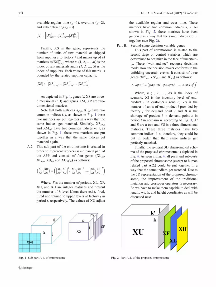
Finally, XS is the gene, represents thenumber of units of raw material m shippedfrom supplier s to factory j and makes up of Mmatrices as XS½ �ms�j, where m (1, 2, …, M) is theindex of raw materials and s (1, 2, …, S) is theindex of suppliers. Each value of this matrix isbounded by the related supplier capacity.

XS½ � : XS½ �1s�j. . . XS½ �2s�j. . . XS½ �Ms�j

h i

As depicted in Fig. 1, genes X, XS are three-dimensional (3D) and genes XM, XP are two-dimensional matrices.

Note that both matrices Xijgt, XPijt have twocommon indices i, j, as shown in Fig. 1 thesetwo matrices are put together in a way that thesame indices get matched. Similarly, XSsmjtand XMmjt have two common indices m, i, asshown in Fig. 1, these two matrices are puttogether in a way that the same indices getmatched again.

A.2. This sub-part of the chromosome is created inorder to represent workers issue based part ofthe APP and consists of four genes (XLkjt,XFkjt, XHkjt and XUkk’jt) as follows:

XL

XFjXHXU

� �¼ XL

XFjXHXU

1;

XL

XFjXHXU

2; . . . ;

XL

XFj XHXU

T !

Where, T is the number of periods. XL, XF,XH, and XU are integer matrices and presentthe number of k-level labors there exist, fired,hired and trained to upper levels at factory j inperiod t, respectively. The values of XU adjust

the available regular and over time. Thesematrices have two common indices k, j. Asshown in Fig. 2, these matrices have beengathered in a way that the same indices are fittogether (see Fig. 2).

Part B: Second-stage decision variable genesThis part of chromosome is related to the

second-stage or control variables which aredetermined to optimize in the face of uncertain-ty. These “wait-and-see” recourse decisionsmodel how the decision maker conforms to theunfolding uncertain events. It consists of threegenes (XInict, YS

nijct, and Bn

ict) as follows:

XIjBjYSð Þn ¼ XIjBjYS½ �1; XIjBjYS½ �2; . . . ; XIjBjYS½ �T� �n

Where, n (1, 2, …, N) is the index ofscenario, XI is the inventory level of end-product i in customer’s zone c, YS is thenumber of units of end-product i provided byfactory j for demand point c and B is theshortage of product i in demand point c inperiod t in scenario n. according to Fig. 3, XIand B are a two and YS is a three-dimensionalmatrices. These three matrices have twocommon indices i, c, therefore, they could beput in order that their same indices getperfectly matched.

Finally, the general 3D disassembled sche-ma of the proposed chromosome is depicted inFig. 4. As seen in Fig. 4, all parts and sub-partsof the proposed chromosome (except to humanrelated part A.2.) could be put together in away that the same indices get matched. Due tothe 3D representation of the proposed chromo-some, the improvement of the traditionalmutation and crossover operators is necessary.So we have to make them capable to deal withlength, width, and height coordinates as will bediscussed next.

Fig. 1 Sub-part A.1. of chromosome Fig. 2 Part A.2. of the proposed chromosome

774 Int J Adv Manuf Technol (2012) 58:765–782

5.2.2 Initial population

A sequential strategy is used for obtaining the initialpopulation. In the first step, part X of the first chromo-some is generated randomly considering the resourcelimitations and the expected value of demands. After that,part XS, XM and XP of the chromosome are filledrandomly too. Then the number of required workers foreach level is calculated regarding the generated pattern.Now second chromosome can be filled randomly to satisfythis requirement and constraints of the model for eachscenario. Note that chromosomes are modified during theabove mentioned steps whenever is needed. To avoidoccurrence of similar chromosomes in each generation,each solution should be compared with existing chromo-somes in the population.

5.2.3 Fitness value

The fitness value is criterion for the quality of thechromosome or feasible solution. In the proposed modelthe fitness value could be one of the objective functions, asmentioned before total cost is considered as the mainobjective function and other objectives are converted toconstraint.

5.2.4 Selection strategies

In the proposed GA, three selection strategies are used. Inthe first strategy the best chromosome among parents isdirectly transmitted to the next generation. For crossoveroperator a mating pool is first generated and parent areselected from mating pool. And finally parents are selectedfor mutation randomly.

For operating crossover it is required to select the mostpromising parents because better parent will have betteroffsprings. Thus a normalization method is used to generatemating pool. For each generation mean and standarddeviation of the objective function are calculated. Thenthe chromosomes which have less than or equal to meanvalue are transmitted to mating pool. This ensures that thebest parents make the offsprings.

5.2.5 Improved GA operators

In this paper, the chromosome structure is formed as twoand three dimensional matrixes. Thus, the GA linearoperators cannot be used to a matrix type as the traditionalforms. These operators should be improved proportional tothe matrix type. Therefore, considering the nature of matrix,each of the GA operators is considered as three named

Fig. 4 General structure of chromosome

Fig. 3 Part B of the proposedchromosome

Fig. 5 Columnar crossover

Fig. 6 Districted crossover

Int J Adv Manuf Technol (2012) 58:765–782 775

columnar, districted, and erratic which are described asfollows:

& Exercising of operation in columnar (or horizontal)direct. In this case, two numbers are first selectedrandomly for each chromosome in row and columnlimits of relevant matrix. Then, the operation (crossoveror mutation) is exercised over obtained columns. Forexample in Fig. 5, columns red and green in cube A andB of two typical chromosomes are selected randomlyand then the crossover operator is used.

& Exercising of operation as block. In this case, somenumbers in the relevant matrix column and raw limitsare selected randomly. Then, the operation (crossover ormutation) is exercised over obtained district. Forexample in Fig. 6, the red and green blocks are selectedrandomly and then the crossover operator is used.

& Exercising of operations as erratic. In this case, some cellsof matrixes are selected randomly, and then the operation(crossover or mutation) is exercised over them. (see Fig. 7)

5.2.6 Modification operation

Two kinds of modification are used in this paper, one forpart A and the other for part B:

Part A modification operator Exercising every GA oper-ators on part A, productionand workforce patterns arechanged and sometimes leadto condition that the numberof product produced in fac-tories exceeds the availableresource limits, so a modifi-cation operator is needed toconvert this infeasible solu-tion to a feasible one. There-fore, an operator is usedwhich randomly changesthese parts till the solutionbecome feasible.

Part B modification operator Exercising every GA oper-ators on part B, customerrelated constraints may beviolated. Then a flexiblemodification operator isembedded to change partB to satisfy these con-straints for each scenario.

5.2.7 GA algorithm

1. Initialize parameters U (the number of chromosomesin each generation), G (the number of generation), θ(the percentage of the crossover operation) and λ (thepercentage of elitism)

2. Generate the initial population3. Initialize counters u=1 (population counter), g=1

(generation counter)

Fig. 7 Erratic crossover

Generate N scenariosusing extended Monte

Carlo sampling method

Run GA to constructpayoff table:

Min Zj(x), k=1,…, K

Select one of the objective functions as the main one and calculate ranges for εk(r2,…,rk) by using the payoff table

Record all nondominant solutions

obtained in previousstep

Convert other objectivefunctions into constraint andrun GA to solve augmented ε

–constraint model for eachvectorof εk

Set number of gridpoints qk (k=2,..,K) forthe k-1 objectivefunctions' ranges

Fig. 8 Flowchart of the pro-posed method

776 Int J Adv Manuf Technol (2012) 58:765–782

4. Calculate the number of chromosomes which shouldbe transferred directly to the next generation:

Nelitism ¼ U � 1ð Þ � lþ 1

5. Calculate the number of times that each operation(mutation and crossover) should be used

Ncrossover ¼ U � Nelitismð Þ � q þ 1;

Nmutation ¼ U � Nelitism � Ncrossover

6. Calculate the fitness values of the current populationas F(X1

g), F(X1g), …, F(XU

g)7. Normalize population fitness as Z1, Z1, …, ZU. where

Zi ¼ Xgi �mgsg

(μg is the mean of the fitness of thepopulation and σg is the standard deviation of them)

8. Transfer the Nelitism best solutions of the previousgeneration directly to the current generation and setu=Nelitism−1

9. Choose mating pool (solutions Xi, in which Zi≤0)

10. Select two chromosomes of the pool matingrandomly

11. Operate crossover on related parts of the selectedchromosomes

12. Modify offspring till reach to feasible solutions13. If summation of offspring’s fitness values being less

than of parent’s, both of them are transferred to thenext generation and u=u+2

Else, if fitness value of one of offsprings being lessthan of both parents, just this offspring transferred tothe next generation and u=u+1

14. If u<Ncrossover+Nelitism then go to 1015. Select one of the chromosomes of the previous

population16. Operate mutation on related parts of the selected

chromosome17. Modify offspring till reaching to a feasible solution18. Transfer chromosome directly to the next generation19. If u<U then Set u=u+1 and go to15

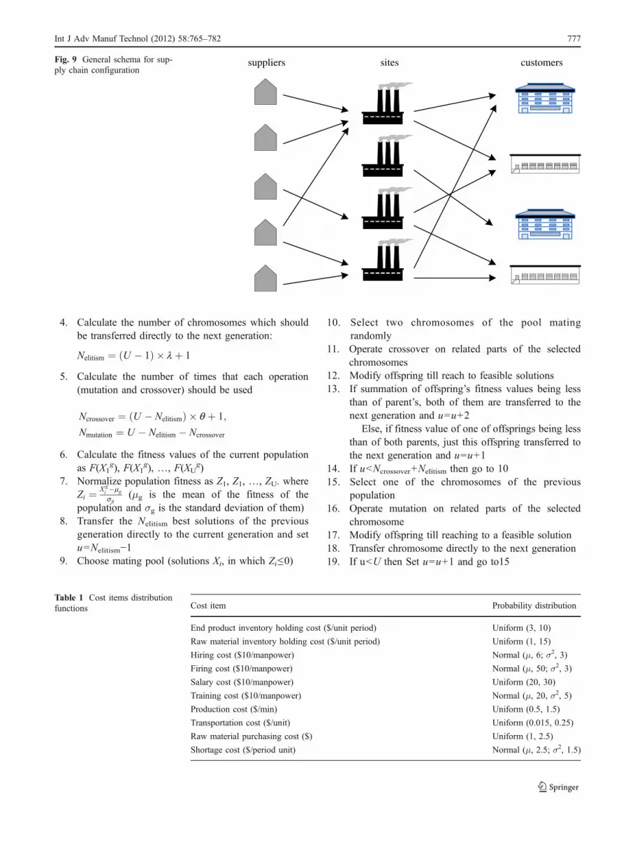
suppliers sites customersFig. 9 General schema for sup-ply chain configuration

Cost item Probability distribution

End product inventory holding cost ($/unit period) Uniform (3, 10)

Raw material inventory holding cost ($/unit period) Uniform (1, 15)

Hiring cost ($10/manpower) Normal (μ, 6; σ2, 3)

Firing cost ($10/manpower) Normal (μ, 50; σ2, 3)

Salary cost ($10/manpower) Uniform (20, 30)

Training cost ($10/manpower) Normal (μ, 20, σ2, 5)

Production cost ($/min) Uniform (0.5, 1.5)

Transportation cost ($/unit) Uniform (0.015, 0.25)

Raw material purchasing cost ($) Uniform (1, 2.5)

Shortage cost ($/period unit) Normal (μ, 2.5; σ2, 1.5)

Table 1 Cost items distributionfunctions

Int J Adv Manuf Technol (2012) 58:765–782 777

20. If g<G or stopping criteria is met then Set g=g+1 andgo to 6

21. Stop algorithm and report the best solution

5.2.8 Stopping criteria

& Number of generations: In this case, the algorithmterminates if the number of the generations exceeds apredefined number.

& Time interval: In this case, the algorithm terminates ifthe current time of the algorithm exceed a predefinedsolving time upper bound.

& Improvement of the fitness value: In this case, thealgorithm terminates if the improvement of the fitnessvalue along the last predefined number of generationsbeing less than a given percentage.

This improved genetic algorithm is used in the innerloop of the augmented ε-constraint method and also tocreate the payoff table. The general steps of the proposedmethod for solving multi-objective two-stage stochasticprogramming problem is depicted in Fig. 8.

6 Experimental result

To verify the practicability of the proposed model aswell as the performance of the hybrid algorithm, threeclasses of examples are generated: small-, medium-, andlarge-sized problems. In the first section of computa-tional examples, we solve the generated small andmedium-sized problems with the proposed hybrid algo-rithm and compare the results with global solutionsobtained by the GAMS software which uses AUGME-CON algorithm to solve such problems. At the end, theefficient frontier and the conflict between objectivefunctions are discussed.

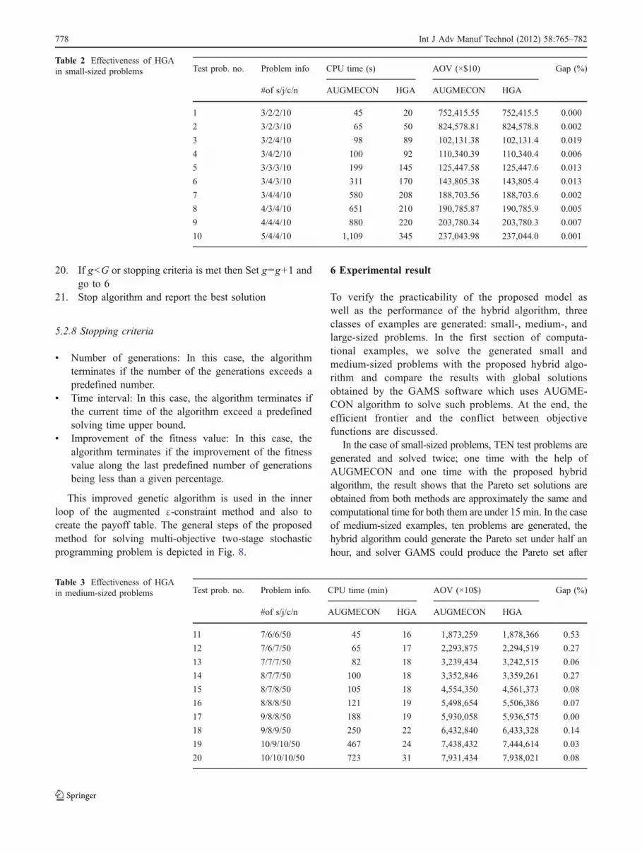
In the case of small-sized problems, TEN test problems aregenerated and solved twice; one time with the help ofAUGMECON and one time with the proposed hybridalgorithm, the result shows that the Pareto set solutions areobtained from both methods are approximately the same andcomputational time for both them are under 15 min. In the caseof medium-sized examples, ten problems are generated, thehybrid algorithm could generate the Pareto set under half anhour, and solver GAMS could produce the Pareto set after

Test prob. no. Problem info CPU time (s) AOV (×$10) Gap (%)

#of s/j/c/n AUGMECON HGA AUGMECON HGA

1 3/2/2/10 45 20 752,415.55 752,415.5 0.000

2 3/2/3/10 65 50 824,578.81 824,578.8 0.002

3 3/2/4/10 98 89 102,131.38 102,131.4 0.019

4 3/4/2/10 100 92 110,340.39 110,340.4 0.006

5 3/3/3/10 199 145 125,447.58 125,447.6 0.013

6 3/4/3/10 311 170 143,805.38 143,805.4 0.013

7 3/4/4/10 580 208 188,703.56 188,703.6 0.002

8 4/3/4/10 651 210 190,785.87 190,785.9 0.005

9 4/4/4/10 880 220 203,780.34 203,780.3 0.007

10 5/4/4/10 1,109 345 237,043.98 237,044.0 0.001

Table 2 Effectiveness of HGAin small-sized problems

Test prob. no. Problem info. CPU time (min) AOV (×10$) Gap (%)

#of s/j/c/n AUGMECON HGA AUGMECON HGA

11 7/6/6/50 45 16 1,873,259 1,878,366 0.53

12 7/6/7/50 65 17 2,293,875 2,294,519 0.27

13 7/7/7/50 82 18 3,239,434 3,242,515 0.06

14 8/7/7/50 100 18 3,352,846 3,359,261 0.27

15 8/7/8/50 105 18 4,554,350 4,561,373 0.08

16 8/8/8/50 121 19 5,498,654 5,506,386 0.07

17 9/8/8/50 188 19 5,930,058 5,936,575 0.00

18 9/8/9/50 250 22 6,432,840 6,433,328 0.14

19 10/9/10/50 467 24 7,438,432 7,444,614 0.03

20 10/10/10/50 723 31 7,931,434 7,938,021 0.08

Table 3 Effectiveness of HGAin medium-sized problems

778 Int J Adv Manuf Technol (2012) 58:765–782

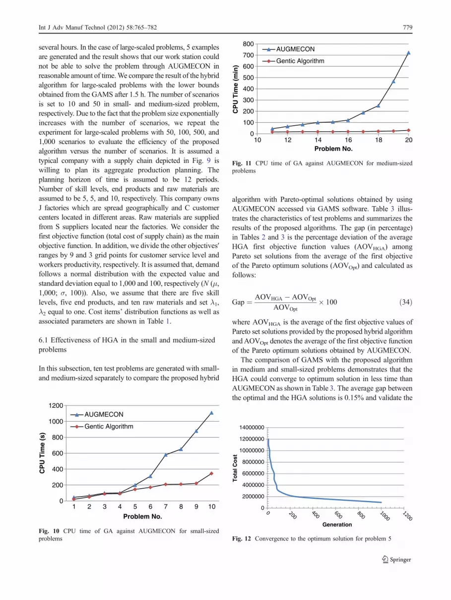
several hours. In the case of large-scaled problems, 5 examplesare generated and the result shows that our work station couldnot be able to solve the problem through AUGMECON inreasonable amount of time.We compare the result of the hybridalgorithm for large-scaled problems with the lower boundsobtained from the GAMS after 1.5 h. The number of scenariosis set to 10 and 50 in small- and medium-sized problem,respectively. Due to the fact that the problem size exponentiallyincreases with the number of scenarios, we repeat theexperiment for large-scaled problems with 50, 100, 500, and1,000 scenarios to evaluate the efficiency of the proposedalgorithm versus the number of scenarios. It is assumed atypical company with a supply chain depicted in Fig. 9 iswilling to plan its aggregate production planning. Theplanning horizon of time is assumed to be 12 periods.Number of skill levels, end products and raw materials areassumed to be 5, 5, and 10, respectively. This company ownsJ factories which are spread geographically and C customercenters located in different areas. Raw materials are suppliedfrom S suppliers located near the factories. We consider thefirst objective function (total cost of supply chain) as the mainobjective function. In addition, we divide the other objectives′ranges by 9 and 3 grid points for customer service level andworkers productivity, respectively. It is assumed that, demandfollows a normal distribution with the expected value andstandard deviation equal to 1,000 and 100, respectively (N (μ,1,000; σ, 100)). Also, we assume that there are five skilllevels, five end products, and ten raw materials and set λ1,λ2 equal to one. Cost items’ distribution functions as well asassociated parameters are shown in Table 1.

6.1 Effectiveness of HGA in the small and medium-sizedproblems

In this subsection, ten test problems are generated with small-and medium-sized separately to compare the proposed hybrid

algorithm with Pareto-optimal solutions obtained by usingAUGMECON accessed via GAMS software. Table 3 illus-trates the characteristics of test problems and summarizes theresults of the proposed algorithms. The gap (in percentage)in Tables 2 and 3 is the percentage deviation of the averageHGA first objective function values (AOVHGA) amongPareto set solutions from the average of the first objectiveof the Pareto optimum solutions (AOVOpt) and calculated asfollows:

Gap ¼ AOVHGA � AOVOpt

AOVOpt� 100 ð34Þ

where AOVHGA is the average of the first objective values ofPareto set solutions provided by the proposed hybrid algorithmandAOVOpt denotes the average of the first objective functionof the Pareto optimum solutions obtained by AUGMECON.

The comparison of GAMS with the proposed algorithmin medium and small-sized problems demonstrates that theHGA could converge to optimum solution in less time thanAUGMECON as shown in Table 3. The average gap betweenthe optimal and the HGA solutions is 0.15% and validate the

0

100

200

300

400

500

600

700

800

10 12 14 16 18 20

CP

U T

ime

(min

)

Problem No.

AUGMECON

Gentic Algorithm

Fig. 11 CPU time of GA against AUGMECON for medium-sizedproblems

0

200

400

600

800

1000

1200

1 2 3 4 5 6 7 8 9 10

CP

U T

ime

(s)

Problem No.

AUGMECON

Gentic Algorithm

Fig. 10 CPU time of GA against AUGMECON for small-sizedproblems

0

2000000

4000000

6000000

8000000

10000000

12000000

14000000

To

tal C

ost

Generation

Fig. 12 Convergence to the optimum solution for problem 5

Int J Adv Manuf Technol (2012) 58:765–782 779

efficiency of the proposed HGA and the maximum gap isrelated to test problem 11. The solution quality and time ofthe HGA vs. the AUGMECON in small and medium-sizedproblems is shown in Figs. 10 and 11. While the problemsize grows, the computational time of AUGMECON methodincreases exponentially, while it does not tangible effect onthe solution time of the proposed algorithm.

Also, convergence to the optimum solution for the testproblem 5 is shown in Fig. 12.

6.2 Effectiveness of HGA in the large-sized problems

In this section, five large-scaled test problems aregenerated to evaluate the efficiency of the proposedalgorithm versus the large number of scenarios. As wedescribed earlier, for these problems, AUGMECONmethod cannot solve the problem in reasonable amountof time. Therefore, each test problem is solved with 50,100, 500, and 1,000 scenarios and compared with lowerbounds of AUGMECON obtained after 1.5 h. Toevaluate the efficiency of the algorithm, the usual relativegap (RG) between the average of best values of firstobjective function in Pareto set solutions (AB) (obtainedfrom the proposed hybrid algorithm) and the average of

the lower bounds (AL) of the first objective function inPareto set solutions (obtained by AUGMECON after1.5 h) is used and reported in Table 4.

RG ¼ AB� AL

AL� 100 ð35Þ

Table 4 shows the characteristics of the test problemsand compares the performance obtained by HGA withdifferent scenario numbers.

The average gap of the proposed HGA for five testproblems with 50, 100, 500, and 1,000 scenarios are 1.38,1.60, 2.50, 2.38, and 2.60, respectively. Also, when thenumber of scenarios increases, the computed gap increasesaccordingly but with a decreasing slope. In addition, theCPU time is not considerable sensitive to the number ofscenarios. These comparisons show efficiency of thepresented HGA in large-sized problems.

6.3 Efficient frontiers

In multi-objective optimization, solution will be a set ofPareto-optimal possible plan alternatives representing thetradeoff among different objectives rather than a unique

Table 4 Comparison of the performance of the proposed HGA with different scenario numbers

Prob. no. Problem info. 50 scenarios 100 scenarios 500 scenarios 1,000 scenarios

No. of s/j/c CPU time (min) RG% CPU time (min) RG% CPU time (min) RG% CPU time (min) RG%

21 25/12/20 35 1.253 35 1.358 36 1.392 36 1.501

22 30/20/25 35 1.668 36 1.681 40 1.382 40 1.661

23 35/25/30 40 2.446 45 2.588 347 2.508 347 2.446

24 40/25/35 41 2.477 47 2.356 50 2.210 50 2.477

25 45/30/40 45 2.302 49 3.01 55 2.788 56 2.302

0

0.1

0.2

0.3

0.4

0.5

0.6

0.7

0.8

0.9

1

0 1 2 3 4 5 6 7 8 9 101700000

1750000

1800000

1850000

1900000

1950000

2000000

Wo

rker

s p

rod

uct

ivit

y

Solution Number

Exp

ecte

d T

ota

l co

st

Total Cost Workers Productivity

Fig. 13 Efficient frontier for workers’ productivity against total cost

1700000

1750000

1800000

1850000

1900000

1950000

2000000

0 1 2 3 4 5 6 7 8 9 100

1000

2000

3000

4000

5000

6000

7000

8000

9000

10000

Exp

ecte

d T

ota

l Co

st

Solution Number

Max

imu

m S

ho

rtag

es

Maximum Shortages Total Cost

Fig. 14 Efficient frontier for the maximum shortages against total cost

780 Int J Adv Manuf Technol (2012) 58:765–782

solution. To show the conflict there exists between theobjective functions, the efficient frontiers are given in Figs. 13and 14 for test problem 7. As can be seen, there is asignificant conflict between total cost of supply chain andcustomer service level as well as the total cost of supplychain and workers productivity. This condition arises fromthis fact that in the case of total cost, the model tries to findthe solutions that they have a minimum cost not regarding tocustomer satisfaction. For example the model never sendsthe goods to the customers’ zones far from the factoriesdue to the extra transportation cost. Conversely, in thecase of customer satisfaction, the model tries to findsolutions that the total shortages would assign to allcustomers’ zones as close as possible to each other, notregarding to the transportation cost. In the same way, theconflict between total cost and workers productivity canbe justified; in the case of total cost, the model attemptsto find solutions with minimum cost not regarding toworkers productivity as well as training courses alter-natives which imposes extra cost to the supply chain.Conversely, in the case of workers productivity, themodel tries to upgrade workers productivity throughholding training courses instead of firing them whichimposes extra cost to the supply chain.

7 Conclusions

In this paper, a new robust multi-objective multi-periodmulti-site multi-product aggregate production planning inan uncertain supply chain is presented. All cost param-eters as well as demand fluctuation is considered asuncertain parameters. Uncertainty is represented by a setof discrete scenarios. The proposed model highlightedthree significant issues of supply chain as the objectivefunctions; total cost, customer service level and workersproductivity. Due to the uncertain nature of the supplychain, first and second objective functions aim tominimize sum of the expected value and a multiple ofthe variability of total cost and customer service level,respectively. The concept of robustness is embedded inthe model by using the term of Variability which ismodeled in the form of absolute deviation. Moreoversome concept such as workers productivity and trainingcourses give this chance to decision maker to selectbetween firing previous workers and hiring new full-skilled ones or upgrading previous workers to upperlevels. To solve the proposed model, a novel hybridalgorithm is presented that is a combination of augment-ed ε-constraint method and GA. At the end, several testproblems are generated randomly to evaluate the validityof the proposed model as well as the efficiency of thehybrid algorithm.

References

1. Manzini R, Gamberi M, Regattieri A (2006) Applying mixedinteger programming to the design of a distribution logisticnetwork. Int J Ind EngTheory Appl Pract 13(2):207–218

2. Manzini R, Gamberi M, Gebennini E, Regattieri A (2008) Anintegrated approach to the design and management of supplychain system. Int J Adv Manuf Technol 37:625–640

3. Shi Y, Haase C (1996) Optimal trade-offs of aggregate productionplanning with multiple objective and multi-capacity demandlevels. Int J Oper Quant Manage 2(2):127–143

4. Hanssman F, Hess S (1960) A linear programming approach toproduction and employment scheduling. Manage Technol 1(1):46–51

5. Haehling LC (1970) Production and employment scheduling inmulti-stage production systems. Nav Res Logist Q 17(2):193–198

6. Goodman DA (1974) A goal programming approach to aggregateplanning of production and work force. Manage Sci 20(12):1569–1575

7. Masoud ASM, Hwang CL (1980) An aggregate productionplanning model and application of three multiple objectivedecision methods. Int J Prod Res 18:741–752

8. Nam SJ, Logendran R (1992) Aggregate production planning—asurvey of models and methodologies. Eur J Oper Res 61(3):255–272

9. Baykasoglu A (2001) MOAPPS 1.0: Aggregate productionplanning using the multiple-objective tabu search. Int J Prod Res39(16):3685–3702

10. Leung SCH, Tsang SOS, Ng WL, Wu Y (2007) A robustoptimization model for multi-site production planning problemin an uncertain environment. Eur J Oper Res 181(1):224–238

11. Mirzapour Al-e-hashem SMJ, Malekly H, Aryanezhad MB (2011)A multi-objective robust optimization model for multi-productmulti-site aggregate production planning in a supply chain underuncertainty. In J Prod Eco. doi:10.1016/j.ijpe.2011.01.027

12. Mark Goha c, Joseph YS Limb, Mengc F (2007) A stochastic modelfor riskmanagement in global supply chain networks. Eur J Oper Res182(1, 1):164–173

13. Mirzapour Al-e-hashem SMJ, Baboli A, Sadjadi SJ, AryanezhadMB (2011) A multi-objective stochastic production-distributionplanning problem in an uncertain environment considering riskand workers productivity. Mathematical problems in engineering.Available at: (http://www.hindawi.com/journals/mpe/aip/406398/)

14. Wang RC, Fang HH (2001) Aggregate production planning withmultiple objectives in a fuzzy environment. Eur J Oper Res 133(3):521–536

15. Wang RC, Liang TF (2004) Application of fuzzy multi-objectivelinear programming to aggregate production planning. ComputInd Eng 46(1):17–41

16. Sahinidis NV (2004) Optimization under uncertainty: state-of-the-art and opportunities. Comput Chem Eng 28(6–7):971–983

17. Escudero LF, Kamesam PV, King AJ, Wets RJB (1993) Productionplanning via scenario modeling. Ann Oper Res 43(6):309–335

18. Bakir MA, Byrne MD (1998) Stochastic linear optimization of anMPMP production planning model. Int J Prod Econ 55(1):87–96

19. Tang J, Fung RYK, Yung KL (2003) Fuzzy modeling andsimulation for aggregate production planning. Int J Syst Sci 34(1):661–673

20. Aliev RA, Fazlollahi B, Leung SCH, Tsang SOS, Ng WL, Wu Y(2007) A robust optimization model for multi-site productionplanning problem in an uncertain environment. Eur J Oper Res181(1):224–238

21. Kogut B, Kulatilaka N (1994) Operating flexibility, globalmanufacturing, and the option value of a multinational network.Manage Sci 10:123–139

22. Leung SCH, Wu Y (2004) A robust optimization model forstochastic aggregate production planning. Prod Plan Control 15(5):502–514

Int J Adv Manuf Technol (2012) 58:765–782 781

23. Kazemi-Zanjani M, Ait-Kadi D, Nourelfath M (2010) Robustproduction planning in a manufacturing environment with randomyield: a case in sawmill production planning. Eur J Oper Res 201(3):882–891

24. Feng P, Rakesh N (2010) Robust supply chain design underuncertain demand in agile manufacturing. Comput Oper Res 37(4):668–683

25. Wellons HS, Reklaitis GV (1989) The design of multiproductbatch plants under uncertainty with staged expansion. ComputChem Eng 13:11

26. Petkov SB, Maranas CD (1998) Design of single productcampaign batch plants under demand uncertainty. AIChE J44:896

27. Gupta A, Maranas D (2003) Managing demand uncertainty insupply chain planning. Comput Chem Eng 27(8–9):1219–1227

28. Poojari CA, Lucas C, Mitra G (2008) Robust solutions and riskmeasures for a supply chain planning problem under uncertainty. JOper Res Soc 59:2–12. doi:10.1057/palgrave.jors.2602381

29. Guilléna G, Melea FD, Bagajewiczb MJ, Espuna A, Puigjanera L(2005) Multi-objective supply chain design under uncertainty.Chem Eng Sci 60:1535–1553

30. Wilkinson SJ, Cortier A, Shah N, Pantelides CC (1996) Integratedproduction and distribution scheduling on a Europe-wide basis.Comput Chem Eng 20:S1275

31. Bok JK, Grossmann IE, Park S (2000) Supply chain optimization incontinuous flexible process networks. Ind EngChemRes 39:1279–1290

32. Jackson JR, Grossmann IE (2003) Temporal decompositionscheme for nonlinear multisite production planning and distribu-tion models. Ind Eng Chem Res 42:3045–3055

33. Chen CL, Lee WC (2004) Multi-objective optimization of multi-echelon supply chain networks with uncertain product demandsand prices. Comput Chem Eng 28:1131–1144

34. Oh HC, Karimi IA (2004) Global multiproduct production-distribution planning with duty drawbacks. AIChE J 50:963–989

35. Guillen G, BagajewiczM, Sequeira SE, Espuna A, Puigjaner L (2005)Management of pricing policies and financial risk as a key element forshort term scheduling optimization. Ind Eng Chem Res 44:557–575

36. Subrahmanyam S, Pekny JF, Reklaitis GV (1994) Design of batchchemical plants undermarket uncertainty. Ind Eng Chem Res33:2688–2701

37. Liu ML, Sahinidis NV (1996) Optimization of process planningunder uncertainty. Ind Eng Chem Res 35:4154

38. Shapiro A (2000) Stochastic programming by Monte Carlosimulation methods. Stochastic Program E-Prints Ser 03

39. Shapiro A, Homem-de-Mello T (1998) A simulation-basedapproach to two-stage stochastic programming with recourse.Math Program 81:301–325

40. Mak WK, Morton DP Wood RK (1999) Monte Carlo boundingtechniques for determining solution quality in stochastic programs.Oper Res Lett 24:47–56

41. You F, Wassick M, Grossmann IE (2009) Risk management for aglobal supply chain planning under uncertainty: models andalgorithms. AIChE J 55(4):931–946

42. Eppen GD, Martin RK (1989) A scenario approach to capacityplanning. Oper Res 37:517–527

43. Mulvey JM, Vanderbei RJ, Zenios SA (1995) Robust Optimiza-tion of large-scale systems. Oper Res 43:264–281

44. Ahmed S, Sahinidis NV (1998) Robust process planning underuncertainty. Ind Eng Chem Res 37:1883–1892

45. Applequist GE, Pekny JF, Reklaitis GV (2000) Risk anduncertainty in managing chemical manufacturing supply chains.Comput Chem Eng 24:2211–2222

46. Barbaro AF, Bagajewicz M (2004) Managing financial risk inplanning under uncertainty. AIChE J 50:963–989

47. Bonfill A, Bagajewicz M, Espunia A, Puigjaner L (2004) Riskmanagement in scheduling of batch plants under uncertain marketdemand. Ind Eng Chem Res 43:741–750

48. Azaron A, Brown SA, Modarres TM (2008) A multi-objectivestochastic programming approach for supply chain designconsidering risk. Int J Prod Econ 116:129–138

49. Boothby D, Dufour A, Tang J (2010) Technology adoption,training and productivity performance. Res Policy 39:650–661

50. Pan F, Nagi R (2010) Robust supply chain design under uncertaindemand in agile manufacturing. Comput Oper Res 37(4):668–683

51. Yu CS, Li HL (2000) A robust optimization model for stochasticlogistic problems. Int J Prod Econ 64(1–3):385–397

52. Rezaie K, Amalnik MS, Gereie A, Ostadi B, Shakhseniaee M(2007) Using extended Monte Carlo simulation method for theimprovement of risk management: Consideration of relationshipsbetween uncertainties. Appl Math Comput 190(2):1492–1501

53. Mavrotas G, Diakoulaki D, Florios K, Georgiou P (2008) Amathematical programming framework for energy planning inservices’ sector buildings under uncertainty in load demand: Thecase of a hospital in Athens. Energy Policy 36:2415–2429

54. Hammache A, Benali M, Aubé F (2010) Multi-objective self-adaptive algorithm for highly constrained problems: Novelmethod and applications. Appl Energy 87(8):2467–2478

55. Mavrotas G (2009) Effective implementation of the ε-constraintmethod in Multi-Objective Mathematical Programming problems.Appl Math Comput 213(2):455–465

56. Haimes YY, Wismer DA, Lasdon DS (1971) On bi-criterionformulation of the integrated systems identification and systemoptimization. IEEE Trans Syst Man Cybern SMC 1:296–297

57. Miettinen KM (1998) Nonlinear multi-objective optimization.Kluwer, Boston

58. Ehrgott M, Ryan DM (2002) Constructing robust crew scheduleswith bi-criteria optimization. J Multi-Criteria Decis Anal 11:139–150

59. Xidonas P, Mavrotas G, Psarras J (2010) Equity portfolioconstruction and selection using multi-objective mathematicalprogramming. J Glob Optim 47:185–209

782 Int J Adv Manuf Technol (2012) 58:765–782