Applied Mathematics and Computation 227 (2014) 480–493

Contents lists available at ScienceDirect

Applied Mathematics and Computation

journal homepage: www.elsevier .com/ locate /amc

Hybrid adaptive and impulsive synchronization of uncertaincomplex networks with delays and general uncertainperturbations

0096-3003/$ - see front matter � 2013 Elsevier Inc. All rights reserved.http://dx.doi.org/10.1016/j.amc.2013.11.025

⇑ Corresponding author.E-mail addresses: xinsongyang@163.com (X. Yang), jdcao@seu.edu.cn (J. Cao).

Xinsong Yang a,⇑, Jinde Cao b,c

a Department of Mathematics, Chongqing Normal University, Chongqing 301331, Chinab Department of Mathematics, Southeast University, Nanjing 210096, Chinac Department of Mathematics, Faculty of Science, King Abdulaziz University, Jeddah 21589, Saudi Arabia

a r t i c l e i n f o a b s t r a c t

Keywords:Complex networksSynchronizationUncertaintiesAdaptive controlImpulsive control

This paper is concerned with the problem of asymptotic synchronization for a class ofuncertain complex networks with delays and general uncertain perturbations. In orderto cope with the bad effects generated by the uncertain perturbations, a novel hybridadaptive and impulsive controller is designed such that the complex network can beasymptotically synchronized onto an isolate chaotic system with uncertain perturbations.All the perturbations can be different from each other. On the basis of a new lemma,squeezing rule, and Lyapunov–Krasovskii functionals, several sufficient conditions guaran-teeing the realization of the synchronization goal are derived. It is shown that the designedhybrid controllers exhibit powerful robustness. Some existing results are improved andextended. Numerical simulations verify the effectiveness of the theoretical results andthe robustness of the new controller.

� 2013 Elsevier Inc. All rights reserved.

1. Introduction

In recent years, much attention has been payed to the dynamics of complex networks. The main reason is that many realsystems can be described by complex dynamical networks, such as the internet networks [1], biological networks [2],epidemic spreading networks [3], collaborative networks [4] and social networks [5], etc.

Synchronization, as an important collective behavior of complex dynamical networks, has received particular attentiondue to its broad applications in different fields such as secure communication [6], information processing [7]. In the litera-ture, there are many results concerning synchronization of complex dynamical networks with and without delays [8–14].Along with the study of synchronization, different control techniques have also been developed. For instance, state feedbackcontrol, adaptive control, intermittent control, impulsive control, pinning control. Among these control techniques, adaptivecontrol and impulsive are attractive. Adaptive control is an effective control technique in synchronizing coupled chaotic sys-tems due to its good robustness [8,11–15,19]. The advantage of adaptive control is that the control parameters can adjustthemselves according to some suitable updating laws, which are designed according to control purpose and characteristicsof considered system. By using adaptive control, authors of [8] studied the synchronization for a class of general uncertaincoupled complex networks with delays and stochastic perturbations. Impulsive control is attractive since the it acts only atdiscrete time-points. By using impulsive control technique, control cost and the amount of the transmitted information can

X. Yang, J. Cao / Applied Mathematics and Computation 227 (2014) 480–493 481

be reduced drastically [20–24]. Recently, by integrating both the advantages of adaptive and impulsive control methods, theauthors of [25,26] investigated the synchronization for a class of uncertain complex dynamical networks. However, theauthors of [25,26] did not consider time delay. It is well known that time delays usually exist in spreading due to the finitespeeds of transmission as well as traffic congestions. Therefore, it is significant to investigate the synchronization of complexnetworks with delays.

It is worth noting that, in most of existing papers concerning synchronization of complex networks, all dynamical nodesare assumed to immune from uncertain perturbations. In practice, chaotic systems are inevitably subject to many types ofuncertainties, such as unknown parameters, unknown nonlinearities, exogenous disturbances and artificial factors, etc. Forinstance, it is reported that the famous Lorenz system is derived from partial differential equations after a series of approx-imations [27]. On the other hand, it is difficult to keep the coupled systems to be identical all the time since the parameters ofdynamical nodes may be variant due to environmental changes [28]. Thus, studying synchronization of complex networkswith uncertain perturbations is necessary and useful in both theoretical research and practical applications. In [8], synchro-nization of complex networks subject to random perturbations was studied. In [14,17], synchronization in an array of sto-chastically coupled networks was studied, However, as every one knows, not all perturbations are stochastic. The commonfeature of the perturbations in [8,14,17] is that, when synchronization has been realized, the perturbations vanish. However,if nonzero uncertain exogenous inputs are acquired by some nodes in a complex network, then the uncertain perturbationsinduced by the exogenous inputs can not disappear even all the dynamical nodes synchronize with each other. Recently,based on the passivity property and linearization method, authors of [29] studied the problems of passive control and syn-chronization of complex networks with and without coupling delay. However, their results were conditioned by the assump-tion that exogenous input to each node was zero. A natural question is: do complex networks subject to general uncertainperturbations can be controlled to synchronization? This paper will give a positive answer. Our method to deal with syn-chronization of complex networks with general uncertain perturbations is designing a new adaptive controller, which con-tains the usual adaptive controller used in [8–19,25,26] as a special case.

To sum up, this paper shall study synchronization for a class of uncertain complex dynamical networks with delays andgeneral uncertainties. In order to synchronize the considered model onto an isolate node system with different uncertainperturbations, new hybrid adaptive and impulsive controller is designed. Several synchronization criteria are derived byusing squeezing rule and Lyapunov–Krasovskii functions. The designed adaptive controller includes the usual adaptive con-troller as a special case. It is shown theoretically and numerically that the hybrid controller exhibits powerful robustness. Itcan synchronize the considered model onto a smooth trajectory even without knowing priori whether each node in the net-work is perturbed or not. Some existing results are improved and extended. Numerical simulations verify the effectiveness ofthe theoretical results.

The rest of this paper is organized as follows. In Section II, the considered model of coupled dynamical networks with uncer-tain perturbations is presented. Some necessary assumptions, definitions and lemmas are also given in this section. Section IIIdevelops several synchronization criteria for the proposed model. Synchronization rate is also estimated for the consideredmodel without delay. Then, in Section IV, a simulation example is presented to show the effectiveness and robustness of thenew controller. Finally, Section V reaches some conclusions. Future research field is also discussed in this section.

Notations: Symbols in this paper are quite standard. Rn denotes the n-dimensional Euclidean space, the superscript Tstands for the transpose of a vector, accordingly, for vector x 2 Rn, kxk ¼ xT x;Rþ ¼ ½0;þ1Þ;N denotes the set of natural num-bers, oðyÞ denotes infinitesimal of higher order than function y. sgnð�Þ is the sign function, I is an identity matrix with appro-priate dimension, kmaxðAÞ is the maximum eigenvalue of the matrix A.

2. Preliminaries

Consider a complex dynamical network consisting of N identical nodes with uncertain couplings and uncertain perturba-tions, which is described as

_xiðtÞ ¼ f1ðt; xiðtÞÞ þ f2ðt; xiðt � s1ÞÞ þ hiðx1ðtÞ; x2ðtÞ; . . . ; xNðtÞÞ þ giðx1ðt � s2Þ; x2ðt � s2Þ; . . . ; xNðt � s2ÞÞþ riðt; xiðtÞ; xiðt � s3ÞÞ; i ¼ 1;2; . . . ;N; ð1Þ

where xiðtÞ ¼ ½xi1ðtÞ; . . . ; xinðtÞ�T 2 Rn represents the state vector of the ith node. f1 and f2 : Rþ � Rn ! Rn are continuously dif-ferentiable nonlinear vector functions. s1; s2 and s3 are time delays. hi; gi : RnN ! Rn are unknown coupling functions. Vectorriðt; xiðtÞ; xiðt � s3ÞÞ ¼ ½ri1ðt; xiðtÞ; xiðt � s3ÞÞ; . . . ;rinðt; xiðtÞ; xiðt � s3ÞÞ�T 2 Rn describes the uncertain perturbations to the ithnode.

We assume that (1) has a unique continuous solution for any initial condition of the following form:xiðsÞ ¼ uiðsÞ 2 Cð½�s;0�;RnÞ; i ¼ 1;2; . . . ;N, where s ¼maxfs1; s2; s3g, Cð½�s;0�;RnÞ denotes the set of all continuous func-tions from ½�s;0� to Rn.

The delayed dynamics of an isolate node with uncertain perturbation are described by

_zðtÞ ¼ f1ðt; zðtÞÞ þ f2ðt; zðt � s1ÞÞ þ rðt; zðtÞ; zðt � s3ÞÞ; ð2Þ

where rðt; zðtÞ; zðt � s3ÞÞ ¼ ½r1ðt; zðtÞ; zðt � s3ÞÞ; . . . ;rnðt; zðtÞ; zðt � s3ÞÞ�T 2 Rn describes the uncertain perturbation on theisolate node, and zðtÞ can be any desired state: equilibrium point, a nontrivial periodic orbit, or even a chaotic orbit.

482 X. Yang, J. Cao / Applied Mathematics and Computation 227 (2014) 480–493

In order to synchronize the network (1), some controllers will be added to some of its nodes. The controlled network ispresented as

_xiðtÞ ¼ f1ðt; xiðtÞÞ þ f2ðt; xiðt � s1ÞÞ þ hiðx1ðtÞ; x2ðtÞ; . . . ; xNðtÞÞ þ giðx1ðt � s2Þ; x2ðt � s2Þ; . . . ; xNðt � s2ÞÞþ riðt; xiðtÞ; xiðt � s3ÞÞ þ Ui þ Ri; i ¼ 1;2; . . . ;N; ð3Þ

where Ui 2 Rn and Ri 2 Rn are impulsive and adaptive feedback controllers, respectively. Due to the uncertain perturbationsand general couplings of the network, N controllers are used. The aim of this paper is to design hybrid impulsive and adaptivecontrollers to synchronize all the states of the coupled nodes in network (1) onto the trajectory of (2) in the sense that

limt!þ1

kxiðtÞ � zðtÞk ¼ 0; i ¼ 1;2; . . . ;N: ð4Þ

It is assumed that when the network achieves synchronization, the couplings should vanish, i.e., hiðx1ðtÞ; x2ðtÞ; . . . ; xNðtÞÞ ¼ 0,giðx1ðt � s2Þ; x2ðt � s2Þ; . . . ; xNðt � s2ÞÞ ¼ 0.

Let eiðtÞ ¼ xiðtÞ � zðtÞ and the impulsive controllers are designed as

Ui ¼X1i¼1

Eik eiðtÞdðt � tkÞ; k 2 N; i ¼ 1;2; . . . ;N; ð5Þ

where the impulsive time instants tk satisfy 0 ¼ t0 < t1 < t2 < � � � < tk�1 < tk < � � �, and limk!þ1tk ¼ þ1, Eik 2 Rn�n are con-stant matrices to be designed later, dð�Þ is the Dirac impulsive function defined as

dðt � tkÞ ¼þ1; t ¼ tk; k 2 N;

0; t – tk;

�

under the additional condition that the area beneath it is equal to one. The Dirac function has the probing property thatR aþe

a�e gðtÞdðt � aÞdt ¼ gðaÞ for e – 0 and continuous function gðtÞ [24]. Then the controlled network (3) turns out to the follow-ing system

_xiðtÞ¼ f1ðt;xiðtÞÞþ f2ðt;xiðt�s1ÞÞþhiðx1ðtÞ;x2ðtÞ; . . . ;xNðtÞÞþgiðx1ðt�s2Þ;x2ðt�s2Þ; . . . ;xNðt�s2ÞÞþriðt;xiðtÞ;xiðt�s3ÞÞþRi; t – tk;

DxiðtkÞ¼ xiðtkÞ�xiðt�k Þ¼ Eik eiðt�k Þ; k¼1;2; . . . ; i¼1;2; . . . ;N;

(ð6Þ

where xðtkÞ ¼ xðtþk Þ ¼ limt!tþk

xðtÞ, xðt�k Þ ¼ limt!t�k

xðtÞ.

Subtracting (2) from (6) gets the following error dynamical system:

_eiðtÞ ¼ F1ðt; eiðtÞÞ þ F2ðt; eiðt � s1ÞÞ þ hiðx1ðtÞ; x2ðtÞ; . . . ; xNðtÞÞ þ giðx1ðt � s2Þ; x2ðt � s2Þ; . . . ; xNðt � s2ÞÞþriðt; xiðtÞ; xiðt � s3ÞÞ � rðt; zðtÞ; zðt � s3ÞÞ þ Ri; t – tk;

DeiðtkÞ ¼ Eik eiðt�k Þ; k ¼ 1;2; . . . ; i ¼ 1;2; . . . ;N;

8><>: ð7Þ

where F1ðt; eiðtÞÞ ¼ f1ðt; xiðtÞÞ � f1ðt; zðtÞÞ, F2ðt; eiðt � s1ÞÞ ¼ f2ðt; xiðt � s1ÞÞ � f2ðt; zðt � s1ÞÞ.

The following assumptions are used in this paper.

(H1) f1ðt;0Þ ¼ 0 and there exists positive constant a such that

kf1ðt;uÞ � f1ðt; vÞk 6 aku� vk; for any u;v 2 Rn:

(H2) f2ðt;0Þ ¼ 0 and there exists positive constant b such that

kf2ðt;uÞ � f2ðt; vÞk 6 bku� vk; for any u;v 2 Rn:

(H3) Solutions of all the nodes in the network (1) are bounded.

(H4) rijðt;0;0Þ � 0;rjðt;0;0Þ � 0ði ¼ 1;2; . . . ;N; j ¼ 1;2; . . . ;nÞ, for any positive constants A;B;A0 and B0 such thatkuk 6 A; kvk 6 B; ku0k 6 A0; kv 0k 6 B0;u;u0v ;v 0 2 Rn, there exist positive constants Mij and Mj such thatjrijðt;u;vÞj 6 Mij, jrjðt;u0; v 0Þj 6 Mj, respectively, t 2 Rþ, i ¼ 1;2; . . . ;N; j ¼ 1;2; . . . ;n.

(H5) For yj; y 2 Rnðj ¼ 1;2; . . . ;NÞ, there exist non-negative constants cij ði; j ¼ 1;2; . . . ;NÞ such that

khiðy1ðtÞ; y2ðtÞ; . . . ; yNðtÞÞ � hiðyðtÞ; yðtÞ; . . . ; yðtÞÞk 6XN

j¼1

cijkyj � yk:

(H6) For yj; y 2 Rnðj ¼ 1;2; . . . ;NÞ, there exist non-negative constants nijði; j ¼ 1;2; . . . ;NÞ such that

kgiðy1ðtÞ; y2ðtÞ; . . . ; yNðtÞÞ � giðyðtÞ; yðtÞ; . . . ; yðtÞÞk 6XN

j¼1

nijkyj � yk:

X. Yang, J. Cao / Applied Mathematics and Computation 227 (2014) 480–493 483

Remark 1. Conditions ðH3Þ and ðH4Þ are reasonable. We do not assume the usual conditions such as Lipschitz condition, dif-ferentiability for the uncertain perturbation functions. If the states of all the nodes in (1) and (2) are chaotic, then they are allbounded, and hence, according to ðH4Þ, jrijðt; xiðtÞ; xiðt � s3ÞÞj and jrjðt; zðtÞ; zðt � s3ÞÞj ði ¼ 1;2; . . . ;N; j ¼ 1;2; . . . ;nÞ arebounded. Specially, if r1 ¼ r2 ¼ � � � ¼ rN ¼ r, and r satisfies Lipschitz condition krðt;u;vÞ � rðt;u0;v 0Þk 6lku� u0k þ mkv � v 0k, where l; m are positive constants, u;v;u0;v 0 2 Rn, then krðt;u; vÞk 6 lkuk þ mkvk, then the bounded-ness of kuk and kvk implies that jrjðt;u;vÞj is bounded. In this case, the usual adaptive control techniques used in[8,11,15–19,25,26] can synchronize (1) onto (2). On the other hand, stochastic perturbation function r in [8] also belongsto this special case. However, our constriction ðH4Þ on the uncertain perturbations is very general, the adaptive control meth-ods used in [8–19,25,26] can not synchronize the network (1) onto (2).

Remark 2. Note that neither ri ði ¼ 1;2; . . . ;NÞ and r are identical nor do they satisfy Lipschitz condition. Perturbations maynot vanish even synchronization of the network has been realized and all nodes are decoupled. Obviously, synchronizing thenetwork (1) with model (2) is a hard task, and the usual adaptive controllers in [25,26] are not applicable. Therefore, weshould design some new adaptive controllers having desired robustness to cope with the difficulty induced by the generaluncertain perturbations.

In order to synchronize model (1) with model (2), hybrid adaptive and impulsive controllers will be designed such thatthe trivial solution of the error system (7) is asymptotically stable. The following Lemma 2 is useful to study the asymptoticstability of the trivial solution of the error system (7) in the case that no delay is contained. In order to get Lemma 2, we firstgive Lemma 1.

Lemma 1 (Cauchy rule [30, pp. 270]). The sufficient and necessary conditions for the convergence of infinite integrallimt!1

Rþ1a f ðsÞds are: for any e > 0, there exists G P a, such that, for any u1;u2 satisfying u1;u2 > G,

Z u2

f ðxÞdx�Z u1

f ðxÞdx���� ���� ¼ Z u2

f ðxÞdx���� ���� < e:

a a u1

Lemma 2. Suppose that function f ðtÞ defined on ½a;þ1Þ is monotonic andRþ1

a f ðtÞdt is convergent, then limt!1f ðtÞ ¼ 0, further-more, f ðtÞ ¼ o 1

t

� �ðt ! þ1Þ.

Proof. Case 1, if f ðaÞ > 0, then f ðtÞ is inevitably monotonic decreasing on ½a;þ1Þ and f ðtÞP 0. Otherwise, suppose f ðtÞ ismonotonic increasing on ½a;þ1Þ, then

Z þ1

af ðtÞdt ¼ lim

u!þ1

Z u

af ðtÞdt P lim

u!þ1

Z u

af ðaÞdt ¼ lim

u!þ1f ðaÞðu� aÞ ¼ þ1;

which is a contradiction to the convergence ofRþ1

a f ðtÞdt. If there exists b > a such that f ðbÞ < 0, then

Z þ1

bf ðtÞdt ¼ lim

u!þ1

Z u

bf ðtÞdt 6 lim

u!þ1

Z u

bf ðbÞdt ¼ lim

u!þ1f ðbÞðu� bÞ ¼ �1;

which is also a contradiction to the convergence ofRþ1

a f ðtÞdt.On the other hand, in view of the convergence of

Rþ1a f ðtÞdt and Lemma 1, for any e > 0, there exists G > a such that, for

any u satisfying u > Gþ 1 > 0,

e >Z u

Gþ1f ðtÞdt P

Z u

Gþ1f ðuÞdt ¼ ðu� G� 1Þf ðuÞ;

which implies that

0 6 f ðuÞ 6 eu� G� 1

:

Since limu!þ1e

u�G�1 ¼ 0, we have limu!þ1f ðuÞ ¼ limt!þ1f ðtÞ ¼ 0. Moreover, when u > 2ðGþ 1Þ, it is obvious thatu� ðGþ 1Þ > u� u=2 ¼ u=2, therefore,

0 6 uf ðuÞ < 2e:

One can derive from the arbitrariness of e that

limu!þ1

uf ðuÞ ¼ limt!þ1

f ðtÞ1=t¼ 0:

Hence,

484 X. Yang, J. Cao / Applied Mathematics and Computation 227 (2014) 480–493

f ðtÞ ¼ o1t

� �; ðt ! þ1Þ:

Case 2, if f ðaÞ < 0, then, by the similar deduction in Case 1, f ðtÞ is inevitably monotonic increasing on ½a;þ1Þ and f ðtÞ � 0.In view of the convergence of

Rþ1a f ðtÞdt and Lemma 1, for any e > 0, there exists G > a such that, for any u satisfying

u > Gþ 1 > 0,

e >Z u

Gþ1f ðtÞdt

���� ���� ¼ � Z u

Gþ1f ðtÞdt P �

Z u

Gþ1f ðuÞdt ¼ ðGþ 1� uÞf ðuÞ;

hence

0 6 �f ðuÞ 6 eu� G� 1

:

Since limu!þ1e

u�G�1 ¼ 0, we have limu!þ1½�f ðuÞ� ¼ limt!þ1f ðtÞ ¼ 0. Moreover, when u > 2ðGþ 1Þ, there has

0 6 �uf ðuÞ < 2e:

One can derive from the arbitrariness of e that

limu!þ1

½�uf ðuÞ� ¼ � limt!þ1

f ðtÞ1=t¼ 0:

Hence,

f ðtÞ ¼ o1t

� �; ðt ! þ1Þ:

Case 3, if f ðaÞ ¼ 0, then f ðtÞ � 0 for ½a;þ1Þ. Otherwise, there exists b > a such that f ðbÞ > 0 or f ðbÞ < 0. If the former holds,then f ðtÞ is monotonic increasing on ½a; b�. From the discussion in Case 1, one knows that f ðtÞ is monotonic decreasing on ½b;þ1Þ,which is a contradiction to the monotonicity of f ðtÞ on ½a;þ1Þ. If the latter holds, then f ðtÞ is monotonic decreasing on ½a; b�.From the discussion in Case 2, one knows that f ðtÞ is monotonic increasing on ½b;þ1Þ, which is also a contradiction to the mono-tonicity of f ðtÞ on ½a;þ1Þ. Therefore, f ðtÞ � 0 on ½a;þ1Þ, and the conclusions are obvious. This completes the proof. h

3. Synchronization of the complex network with delays

In this section, A novel hybrid adaptive and impulsive controller will be designed. By adding the designed controller to thecomplex network (1), all the node systems can be asymptotically synchronized onto the isolate system (2). Under the con-ditions ðH1Þ–ðH6Þ, the error system (7) has a zero solution. Therefore, synchronization of the complex network (2) onto sys-tem (1) is equivalent to the stability of the zero solution to the error dynamical system (7). In the proof of the followingTheorem 1, a comparison system is introduced, then squeezing rule is utilized to obtain the stability condition of the zerosolution to (7).

Consider the following comparison system:

_eiðtÞ ¼ F1ðt; eiðtÞÞ þ F2ðt; eiðt � s1ÞÞ þ hiðx1ðtÞ; x2ðtÞ; . . . ; xNðtÞÞ þ giðx1ðt � s2Þ; x2ðt � s2Þ; . . . ; xNðt � s2ÞÞþ riðt; xiðtÞ; xiðt � s3ÞÞ � rðt; zðtÞ; zðt � s3ÞÞ þ Ri; i ¼ 1;2; . . . ;N: ð8Þ

Assume system (8) has the same initial condition as that of (7). We shall prove that, under the combination of adaptivecontrol and impulsive control, asymptotical stability of the trivial solution to (8) guarantees the asymptotical stability of thezero solution to (7).

Theorem 1. Suppose that ðH1Þ–ðH6Þ hold. Then the error system (7) is asymptotically stable under the adaptive controllers

Ri ¼ �eieiðtÞ �xbisignðeiðtÞÞ; i ¼ 1;2; . . . ;N;_ei ¼ pieiðtÞT eiðtÞ; i ¼ 1;2; . . . ;N;

_bi ¼ gi

Xn

j¼1

jeijðtÞj; i ¼ 1;2; . . . ;N

8>>>><>>>>: ð9Þ

and the impulsive controllers satisfying

kmaxððI þ Eik ÞTðI þ Eik ÞÞ < 1; i ¼ 1;2; . . . ;N; k 2 N; ð10Þ

where signðeiðtÞÞ ¼ ½signðei1ðtÞÞ; . . . ; signðeinðtÞÞ�T , x > 1; pi > 0 and gi > 0 are arbitrary constants, respectively.

X. Yang, J. Cao / Applied Mathematics and Computation 227 (2014) 480–493 485

Proof. From ðH3Þ, there exists positive constant A such that kxiðtÞk 6 A, kxiðt � s3Þk 6 Aði ¼ 1;2; . . . ;NÞ. In view of ðH4Þ, thereexist positive constants Mij such that jrijðt; xiðtÞ; xiðt � s3ÞÞj 6 Mijði ¼ 1;2; . . . ;N; j ¼ 1;2; . . . ;nÞ. On the other hand, thereexists eMj such that jrjðt; zðtÞ; zðt � s3ÞÞj 6 eMj ðj ¼ 1;2; . . . ;nÞ. Take bMi ¼ maxfMij þ eMj; j ¼ 1;2; . . . ;ng ði ¼ 1;2; . . . ;NÞ anddefine the following Lyapunov–Krasovskii functional candidate:

VðtÞ ¼ V1ðtÞ þ V2ðtÞ; ð11Þ

where

V1ðtÞ ¼12

XN

i¼1

eTi ðtÞeiðtÞ þ

12

XN

i¼1

ðei � dÞ2

piþ 1

2

XN

i¼1

ð bMi � biÞ2

gi;

V2ðtÞ ¼ mXN

i¼1

Z t

t�s1

eTi ðsÞeiðsÞdsþ l

XN

i¼1

Z t

t�s2

eTi ðsÞeiðsÞds

and d;m; l are constants to be determined.Differentiating V1ðtÞ along the solution of (8) for t P 0, one obtains that

_V1ðtÞjð31Þ ¼XN

i¼1

eTi ðtÞ _eiðtÞ þ

XN

i¼1

ðei � dÞeTi ðtÞeiðtÞ �

XN

i¼1

ð bMi � biÞXn

j¼1

jeijðtÞj

¼XN

i¼1

eTi ðtÞ F1ðt; eiðtÞÞ þ F2ðt; eiðt � s1ÞÞ þ hiðx1ðtÞ; x2ðtÞ; . . . ; xNðtÞÞ þ giðx1ðt � s2Þ; x2ðt � s2Þ; . . . ; xNðt � s2ÞÞ½ �

�XN

i¼1

deTi ðtÞeiðtÞ �x

XN

i¼1

Xn

j¼1

bijeijðtÞj þXN

i¼1

eTi ðtÞðriðt; xiðtÞ; xiðt � s3ÞÞ � rðt; zðtÞ; zðt � s3ÞÞÞ

�XN

i¼1

Xn

j¼1

ð bMi � biÞjeijðtÞj: ð12Þ

Since jrijðt; xiðtÞ; xiðt � s3ÞÞj þ jrjðt; zðtÞ; zðt � s3ÞÞj 6 Mij þ eMj 6bMiði ¼ 1;2; . . . ;N; j ¼ 1;2; . . . ;nÞ, it follows that

XN

i¼1

eTi ðtÞðriðt; xiðtÞ; xiðt � s3ÞÞ � rðt; zðtÞ; zðt � s3ÞÞÞ �x

XN

i¼1

Xn

j¼1

bijeijðtÞj �XN

i¼1

Xn

k¼1

ðMi � biÞjeijðtÞj

6

XN

i¼1

Xn

j¼1

jeijðtÞjðMij þ eMjÞ � bMijeijj � ðx� 1Þbijeijjh i

6 �XN

i¼1

Xn

j¼1

ðx� 1Þbijeijj � 0: ð13Þ

According to ðH1Þ; ðH2Þ; ðH5Þ, and ðH6Þ, it is derived from (12) and (13) that

_V1ðtÞjð8Þ 6XN

i¼1

keiðtÞk akeiðtÞk þ bkeiðt � s1Þk þXN

j¼1

cijkejðtÞk þXN

j¼1

nijkejðt � s2Þk" #

�XN

i¼1

deTi ðtÞeiðtÞ

6

XN

i¼1

ða� dÞkeiðtÞk2 þ b2

XN

i¼1

ðkeiðtÞk2 þ keiðt � s1Þk2Þ þ c2

XN

i¼1

XN

j¼1

ðkeiðtÞk2 þ kejðtÞk2Þ þ n2

XN

i¼1

XN

j¼1

ðkeiðtÞk2

þ kejðt � s2Þk2Þ

¼XN

i¼1

ðaþ b2þ cN þ nN

2� dÞkeiðtÞk2 þ b

2

XN

i¼1

keiðt � s1Þk2 þ nN2

XN

i¼1

keiðt � s2Þk2; ð14Þ

where c ¼max16i;j6Nfcijg, n ¼max16i;j6Nfnijg.Differentiating V2ðtÞ along the solution to (8) for t P 0 yields that

_V2ðtÞjð8Þ ¼ ðmþ lÞXN

i¼1

eTi ðtÞeiðtÞ �m

XN

i¼1

eTi ðt � s1Þeiðt � s1Þ � l

XN

i¼1

eTi ðt � s2Þeiðt � s2Þ: ð15Þ

By (11), (14) and (15), the following inequality is derived.

_VðtÞjð8Þ 6XN

i¼1

ðaþ b2þ cN þ nN

2þmþ l� dÞkeiðtÞk2 þ b

2�m

� �XN

i¼1

keiðt � s1Þk2 þ nN2� l

� �XN

i¼1

keiðt � s2Þk2:

Take d ¼ aþ b2þ cN þ nN

2 þmþ lþ 1, m ¼ b2 and l ¼ nN

2 . Then, from the above inequality, one has

_VðtÞjð8Þ 6 �XN

i¼1

keiðtÞk2; t P 0: ð16Þ

486 X. Yang, J. Cao / Applied Mathematics and Computation 227 (2014) 480–493

The equality in (16) holds only whenPN

i¼1keiðtÞk2 ¼ 0, hence, limt!þ1keiðtÞkjð8Þ ¼ 0, limt!þ1eijð8Þ ¼ ei, limt!þ1bijð8Þ ¼ bi,where ei; bi ði ¼ 1;2; . . . ;NÞ are some constants. At the same time,

limt!þ1

VðtÞjð8Þ ¼ P; ð17Þ

where P is a nonnegative constant.On the other hand, differentiating VðtÞ along the solution of (7) for t 2 ½tk�1; tkÞ; k 2 N, one obtains by the same

discussions as above that

_VðtÞjð7Þ ¼ _VðtÞjð8Þ 6 �XN

i¼1

keiðtÞk2; t 2 ½tk�1; tkÞ; k 2 N: ð18Þ

When t ¼ tk; k 2 N, one derives from the second equation of (7), (10) and (11) that

DVðtkÞjð7Þ ¼12

XN

i¼1

eTi ðtkÞeiðtkÞ þm

XN

i¼1

Z tk

tk�s1

eTi ðsÞeiðsÞdsþ l

XN

i¼1

Z tk

tk�s2

eTi ðsÞeiðsÞds� 1

2

XN

i¼1

eTi ðt�k Þeiðt�k Þ

þmXN

i¼1

Z t�k

t�k�s1

eTi ðsÞeiðsÞdsþ l

XN

i¼1

Z t�k

t�k�s2

eTi ðsÞeiðsÞds

¼ 12

XN

i¼1

ððI þ Eik Þeiðt�k ÞÞTðI þ Eik Þeiðt�k Þ �

12

XN

i¼1

eTi ðt�k Þeiðt�k Þ ¼

12

XN

i¼1

eTi ðt�k Þ½ðI þ Eik Þ

TðI þ EikÞ � I�eiðt�k Þ

612

XN

i¼1

ðqik� 1ÞeT

i ðt�k Þeiðt�k Þ � 0;

which means that

VðtkÞjð7Þ 6 Vðt�k Þjð7Þ: ð19Þ

Since the initial conditions of (7) and (8) are identical, one can derive from (18) that

VðtÞjð7Þ ¼ VðtÞjð8Þ; t 2 ½0; t1Þ; and Vðt�1 Þjð7Þ ¼ Vðt�1 Þjð8Þ: ð20Þ

By virtue of Vðt1Þjð8Þ ¼ Vðt�1 Þjð8Þ, noticing (19) and (20), one gets that

Vðt1Þjð7Þ 6 Vðt1Þjð8Þ: ð21Þ

Again, one obtains from (18) and (21) that

VðtÞjð7Þ 6 VðtÞjð8Þ; t 2 ½t1; t2Þ: ð22Þ

Specially,

Vðt�2 Þjð7Þ 6 Vðt�2 Þjð8Þ: ð23Þ

Similarly, by virtue of Vðt2Þjð8Þ ¼ Vðt�2 Þjð8Þ, (18), (19), and (23), one derives that

VðtÞjð7Þ 6 VðtÞjð8Þ; t 2 ½t2; t3Þ: ð24Þ

By repeating the same reason, one can easily get that

VðtÞjð7Þ 6 VðtÞjð8Þ; t 2 ½tk�1; tkÞ: ð25Þ

Noticing (11) and (20)–(25), the following inequality holds:

0 6 VðtÞjð7Þ 6 VðtÞjð31Þ; t P 0: ð26Þ

One has from (17) and (26) that

0 6 limt!þ1

VðtÞjð7Þ 6 P: ð27Þ

We claim

limt!þ1

keiðtÞkjð7Þ ¼ 0; i ¼ 1;2; . . . ;N: ð28Þ

On the contrary, suppose that there exists i0 2 f1;2; . . . ;Ng such that limt!þ1kei0 ðtÞkjð7Þ – 0, then, one derives from (9) that_ei0 > 0; _bi0 > 0, hence limt!þ1ei0 ðtÞjð7Þ ¼ þ1 and limt!þ1bi0 ðtÞjð7Þ ¼ þ1. Since d; pi0

; bMi0 and gi0are constants and

X. Yang, J. Cao / Applied Mathematics and Computation 227 (2014) 480–493 487

pi0 > 0;gi0> 0, limt!þ1

ðei0ðtÞ�dÞ2

pi0jð7Þ ¼ þ1, limt!þ1

ðbMi0�bi0

ðtÞÞ2

gi0jð7Þ ¼ þ1, so, limt!þ1

12

PNi¼1ðei�dÞ2

piþ 1

2

PNi¼1ðbMi�biÞ

2

gi

� ����ð7Þ¼ þ1, this

leads to limt!þ1VðtÞjð7Þ ¼ þ1, which contradicts against (27). Therefore, (28) holds. At the same time, limt!þ1eijð7Þ ¼ bei,

limt!þ1bijð7Þ ¼ bbi, where bei; bbiði ¼ 1;2; . . . ;NÞ are some constants. This completes the proof. h

Remark 3. The designed adaptive controllers can synchronize the complex network (2) with uncertain perturbations ontosystem (1) even without impulsive control. In [29], Yao et al. studied the problems of passive control and synchronization fora class of complex networks with coupling delay and exogenous input, which is a special case of the model (29). However,synchronization criteria in [29] were obtained under the condition that every node did not effected by exogenous input.Hence, Theorem 1 improves the corresponding results in [29] to some extent.

One can see from the least restrictive conditions on uncertain perturbations that the designed adaptive controllers (9) havedesired robustness. Moreover, no matter whether there is uncertain perturbation to each node or not, the zero solution to theerror system (7) can also be asymptotically stabilized by the adaptive controller (9). In order to specify this claim, we give thefollowing two corollaries.

Suppose that some nodes have nonzero uncertain perturbations. Without loss of generality, rearrange the order of thenodes in the network, and let the first s nodes are perturbed, i.e., riðt; xiðtÞÞ– 0; i ¼ 1;2; . . . ; s,riðt; xiðtÞÞ � 0; i ¼ sþ 1; sþ 2; . . . ;N. We have the following Corollary 1.

Corollary 1. Suppose riðt; xiðtÞ; xiðt � s3ÞÞ– 0; i ¼ 1;2; . . . ; s, rðt; zðtÞ; zðt � s3ÞÞ– 0, riðt; xiðtÞ; xiðt � s3ÞÞ � 0; i ¼ sþ 1; sþ2; . . . ;N. Then, under the conditions of Theorem 1, the error system (7) is asymptotically stable under the adaptive controllers(9) and the impulsive controllers satisfying (10).

Proof. Define the Lyapunov function as

VðtÞ ¼ 12

XN

i¼1

eTi ðtÞeiðtÞ þ

12

XN

i¼1

ðei � dÞ2

piþ 1

2

Xs

i¼1

ð bMi � biÞ2

giþ V2ðtÞ;

where V2ðtÞ is defined in the proof of Theorem 1.Differentiating VðtÞ along the solution of (8) and noting that the following inequality holds:

Xs

i¼1

eTi ðtÞðriðt; xiðtÞ; xiðt � s3ÞÞ � rðt; zðtÞ; zðt � s3ÞÞÞ �x

Xs

i¼1

Xn

j¼1

bijeijðtÞj �Xs

i¼1

Xn

k¼1

ðMi � biÞjeijðtÞj �xXN

i¼sþ1

Xn

j¼1

bijeijðtÞj

6

Xs

i¼1

Xn

j¼1

jeijðtÞjðMij þ eMjÞ � bMijeijj � ðx� 1Þbijeijjh i

�xXN

i¼sþ1

Xn

j¼1

bijeijðtÞj 6 �Xs

i¼1

Xn

j¼1

ðx� 1Þbijeijj �xXN

i¼sþ1

Xn

j¼1

bijeijðtÞj

� 0;

one can easily finish this proof by the same procedure of the proof of Theorem 1. The proof is completed. h

Specially, when every node in the network and the isolate node immune from perturbation, then the considered modelbecomes the usual uncertain complex network without perturbation. We give the following corollary.

Corollary 2. Suppose riðt; xiðtÞ; xiðt � s3ÞÞ � 0; i ¼ 1;2; . . . ;N, rðt; zðtÞ; zðt � s3ÞÞ � 0. Then, under the conditions of Theorem 1,the trivial solution of the error system (7) is asymptotically stable under the adaptive controllers (9) and the impulsive controllerssatisfying (10). Moreover, the scalar x can be any non-negative constant.

Proof. Define the Lyapunov function as

eV ðtÞ ¼ 12

XN

i¼1

eTi ðtÞeiðtÞ þ

12

XN

i¼1

ðei � dÞ2

piþ V2:

Differentiating eV ðtÞ along the solution of (8) and noticing that �xPN

i¼1

Pnj¼1bijeijðtÞj � 0, one can easily complete the proof by

the same proof process as that in the proof of Theorem 1. This completes the proof. h

Remark 4. If only partial structure of a complex dynamical network with uncertain perturbations is known, the synchroni-zation goal can also be realized by using the adaptive controller (9). For example, suppose f1ðt; xiðtÞÞ in system (1) is knownand f2ðt; xiðt � s1ÞÞ is unknown, then the uncertain perturbations in (1) can be changed as~ri ¼ f2ðt; xiðt � s1ÞÞ þ riðt; xiðtÞ; xiðt � s3ÞÞði ¼ 1;2; . . . ;NÞ. In this case, it is not difficult to derive synchronization criteria sim-ilar to those in Theorem 1.

488 X. Yang, J. Cao / Applied Mathematics and Computation 227 (2014) 480–493

When there is no delay in the model (1), then the complex network (1) is reduced to the following dynamical system:

_xiðtÞ ¼ f1ðt; xiðtÞÞ þ hiðx1ðtÞ; x2ðtÞ; . . . ; xNðtÞÞ þ riðt; xiðtÞÞ þ Ui þ Ri; i ¼ 1;2; . . . ;N: ð29Þ

By Theorem 1, it is obvious that, under the adaptive controllers in (9) and the impulsive controllers in (5) satisfying the con-dition (10), the complex network (29) can be asymptotically synchronized onto the following system:

_zðtÞ ¼ f1ðt; zðtÞÞ þ rðt; zðtÞÞ: ð30Þ

The next Theorem 2 shows that, under the hybrid controllers (9) and (5), not only can the complex network (29) be asymp-totically synchronized onto the trajectory of (30), but also the synchronization rate is estimated.

Subtracting (30) from (29) yields the following controlled error dynamical system:

_eiðtÞ ¼ F1ðt; eiðtÞÞ þ hiðx1ðtÞ; x2ðtÞ; . . . ; xNðtÞÞ þ riðt; xiðtÞÞ � rðt; zðtÞÞ þ Ri; t – tk;

DeiðtkÞ ¼ Eik eiðt�k Þ; k 2 N; i ¼ 1;2; . . . ;N;

(ð31Þ

where F1ðt; eiðtÞÞ ¼ f1ðt; xiðtÞÞ � f1ðt; zðtÞÞ.Assumptions for (29) and (30) that:

(eH3) Solutions of all the nodes in the network (29) without any controller are bounded.(eH4) rijðt;0Þ � 0;rjðt;0Þ � 0 ði ¼ 1;2; . . . ;N; j ¼ 1;2; . . . ;nÞ, for any positive constants A and A0 such thatkuk 6 A; ku0k 6 A0, u;u0 2 Rn, there exist positive constants Mij and Mj such that jrijðt;uÞj 6 Mij, jrjðt;u0Þj 6 Mj, respec-tively, t 2 Rþ i ¼ 1;2; . . . ;N; j ¼ 1;2; . . . ;n.

Theorem 2. Suppose that ðH1Þ; ðeH3Þ, ðeH4Þ and ðH5Þ hold. Then the zero solution to the error system (31) is asymptotically sta-ble under the adaptive controllers in (9) and the impulsive controllers in (5) satisfying the condition (10). Moreover,

keiðtÞkjð31Þ ¼ o 1ffiffitp� �ðt ! þ1Þ; i ¼ 1;2; . . . ;N.

Proof. From ðeH3Þ one knows that there exists positive constant A such that kxiðtÞk 6 A, ði ¼ 1;2; . . . ;NÞ. In view of ðeH4Þ, thereexist positive constants Mij such that jrijðt; xiðtÞÞj 6 Mij ði ¼ 1;2; . . . ;N; j ¼ 1;2; . . . ;nÞ. Similarly, there exists Mj such thatjrjðt; zðtÞÞj 6 Mj ðj ¼ 1;2; . . . ;nÞ. Take Mi ¼maxfMij þMj; j ¼ 1;2; . . . ; ng ði ¼ 1;2; . . . ;NÞ and define the following Lyapunovfunction candidate:

V1ðtÞ ¼12

XN

i¼1

eTi ðtÞeiðtÞ þ

12

XN

i¼1

ðei � dÞ2

piþ 1

2

XN

i¼1

ðMi � biÞ2

gi; ð32Þ

where d is a constant to be determined.By the similar analysis in the proof of Theorem 1, differentiating V1ðtÞ along the solution of (31) for t 2 ½tk�1; tkÞ; k 2 N and

using ðH1Þ and ðH5Þ obtain that

_V1ðtÞjð31Þ 6XN

i¼1

keiðtÞk akeiðtÞk þXN

j¼1

cijkejðtÞk" #

�XN

i¼1

deTi ðtÞeiðtÞ

6

XN

i¼1

ða� dÞkeiðtÞk2 þ c2

XN

i¼1

XN

j¼1

ðkeiðtÞk2 þ kejðtÞk2Þ ¼XN

i¼1

ðaþ cN � dÞkeiðtÞk2: ð33Þ

where c ¼max16i;j6Nfcijg.Taking d ¼ aþ cN þ 1, one derives from (33) that

_V1ðtÞjð31Þ 6 �XN

i¼1

keiðtÞk2; t 2 ½tk�1; tkÞ; k 2 N: ð34Þ

When t ¼ tk; k 2 N, it is easy to get that

DV1ðtkÞjð31Þ 612

XN

i¼1

ðqik� 1ÞeT

i ðt�k Þeiðt�k Þ � 0;

which means that

V1ðtkÞjð31Þ 6 V1ðt�k Þjð31Þ: ð35Þ

Inequalities (34) and (35) imply that V1ðtÞ is decreasing along solution of (31) on ½0;þ1Þ. Considering V1ðtÞP 0, one knowsthat limt!þ1V1ðtÞjð31Þ exists. By the same method used in [26], one gets that

Rþ10 V1ðtÞdt is convergent along the solution of

(31). According to Lemma 2, one has limt!1V1ðtÞjð31Þ ¼ 0, and V1ðtÞjð31Þ ¼ o 1t

� �ðt ! þ1Þ, i.e.,

X. Yang, J. Cao / Applied Mathematics and Computation 227 (2014) 480–493 489

keiðtÞkjð31Þ ¼ o 1ffiffitp� �ðt ! þ1Þ; i ¼ 1;2; . . . ;N. At the same time, limt!þ1eijð31Þ ¼ eei, limt!þ1bijð31Þ ¼ ebi, whereeei; ebi ði ¼ 1;2; . . . ;NÞ are some constants. This completes the proof. h

Remark 5. The new adaptive controller of this paper has better robustness than those used in [8–19,25,26], which are usualand widely used in existing papers for adaptive chaos synchronization. The usual adaptive controllers are applicable only tosystems without perturbation (see [15,16,18,19,25,26]) or with Lipschitz-conditioned stochastic perturbations [8,17]. Onecan see from Corollary 2 and 4 that, when x ¼ 0, the designed adaptive controller turns out to the usual one. Hence, theusual adaptive controller is a special case of that of this paper.

The following two corollaries can be easily obtained from Theorem 1, we omit their proofs here.

Corollary 3. Suppose riðt; xiðtÞÞ– 0; i ¼ 1;2; . . . ; s, rðt; zðtÞÞ– 0, riðt; xiðtÞÞ � 0; i ¼ sþ 1; sþ 2; . . . ;N. Then, under the condi-tions of Theorem 1, the trivial solution of the error system (31) is asymptotically stable. Moreover,keiðtÞkjð31Þ ¼ o 1ffiffi

tp� �

ðt ! þ1Þ; i ¼ 1;2; . . . ;N.

Corollary 4. Suppose riðt; xiðtÞÞ � 0; i ¼ 1;2; . . . ;N, rðt; zðtÞÞ � 0. Then, under the conditions of Theorem 1, the trivial solution ofthe error system (31) is asymptotically stable. Moreover, keiðtÞkjð31Þ ¼ o 1ffiffi

tp� �ðt ! þ1Þ; i ¼ 1;2; . . . ;N, and the scalar x can be

relaxed to any non-negative constant.

Remark 6. The hybrid adaptive and impulsive controllers in this paper are simple. Note that no information of the linearpart of dynamical node is used and no restriction is imposed upon the impulsive distances tk � tk�1ðk 2 NÞ in this paper.Recently, authors of [25,26] studied the synchronization of (29) when r1 ¼ r2 ¼ � � � ¼ rN ¼ r � 0 by hybrid adaptive andimpulsive control scheme. However, information of the linear part of dynamical node must be known in [25,26], and theupper bounds of tk � tk�1; k 2 N should satisfy some limitative conditions in [25]. Moreover, since the Lemma 2 in this paperdoes not have so many restriction conditions on f ðtÞ as those in generalized Barbalat’s lemma in [26], the proof of Theorem 1is simpler than that of Theorem 2 in [26]. Note that the adaptive controllers in this paper are simpler and more robust thanthose used in [26]. Both of [25,26] did not give the estimation of synchronization rate. Therefore, Corollary 4 improves themain results in [25,26].

Remark 7. Note that the controller (9) is discontinuous and the phenomenon of chattering will appear [31,32]. In order toeliminate the chattering, the controller (9) can be modified as

Ri ¼ �eieiðtÞ �xbiSi; i ¼ 1;2; . . . ;N;_ei ¼ pieiðtÞT eiðtÞ; i ¼ 1;2; . . . ;N;

_bi ¼ gi

Xn

j¼1

jeijðtÞj; i ¼ 1;2; . . . ;N;

8>>>><>>>>: ð36Þ

where Si ¼ ei1ðtÞjei1ðtÞjþfi

; . . . ; einðtÞjeinðtÞjþfi

h iT, fi; i ¼ 1;2; . . . ;N, are sufficiently small positive constants, x > 1; pi > 0 and gi > 0 are arbi-

trary constants, respectively.

4. Numerical example

In this section, we provide numerical example to verify the theoretical result Theorem 1 and show the advantage of thenew adaptive controller. The other synchronization criteria are special cases of Theorem 1, we do not verify each of them.

Now we construct a random network, which obeys the scale-free distribution of the Barabási–Albert model [33]. Theparameters in the process of constructing are: initial graph is complete with m0 ¼ 5 nodes, m ¼ 5 edges are randomly addedin the network when a new node is introduced in, and the final number of nodes is N ¼ 100. Fig. 1 shows the BA scare-freenetwork.

The delayed neural network with uncertain perturbation is described as:

_zðtÞ ¼ f1ðt; zðtÞÞ þ f2ðt; zðt � sÞÞ þ rðt; zðtÞ; zðt � sÞÞ; ð37Þ

where zðtÞ ¼ ½z1ðtÞ; z2ðtÞ�T , f1ðt; zðtÞÞ ¼ CzðtÞ þ Af ðzðtÞÞ, f2ðt; zðt � s1ÞÞ ¼ Bgðzðt � sÞÞ, f ðzðtÞÞ ¼ ½tanhðz1ðtÞÞ; tanhðz2ðtÞÞ�T ,gðzðt � sÞÞ ¼ ½tanhðz1ðt � sÞÞ; tanhðz2ðt � sÞÞ�T , rðt; zðtÞ; zðt � sÞÞ is uncertain perturbation,

C ¼�1 00 �1

� ; A ¼

2 �0:1�5 4:5

� ; B ¼

�1:5 �0:1�0:2 �4

� :

0 20 40 60 80 100

10

20

30

40

50

60

70

80

90

Fig. 1. BA scale-free network initial graph is complete with m0 ¼ 5 nodes, m ¼ 5 edges are added in the network when a new node is introduced in, and thefinal number of nodes is N ¼ 100.

−1.2 −1 −0.8 −0.6 −0.4 −0.2 0 0.2 0.4 0.6 0.8−6

−4

−2

0

2

4

6

z1

z 2 z 2(a)

−1 −0.8 −0.6 −0.4 −0.2 0 0.2 0.4 0.6 0.8−8

−6

−4

−2

0

2

4

6

8

z1

−0.8 −0.6 −0.4 −0.2 0 0.2 0.4 0.6 0.8−8

−6

−4

−2

0

2

4

6

z1

z 2

(c)

−0.8 −0.6 −0.4 −0.2 0 0.2 0.4 0.6−6

−4

−2

0

2

4

6

z1

z 2

(d)

(b)

Fig. 2. Chaotic trajectories of perturbed system (37) with different perturbations.

490 X. Yang, J. Cao / Applied Mathematics and Computation 227 (2014) 480–493

Under different perturbations, the neural network (37) exhibits different chaotic behaviors. Fig. 2 shows the chaotic trajec-

tories of (37) when rðt; zðtÞ; zðt � sÞÞ takes different values ðaÞrðt; zðtÞ; zðt � sÞÞ ¼ 0; ðbÞrðt; zðtÞ; zðt � sÞÞ ¼½0:05ðz1ðt � sÞÞ2;0:2z2ðtÞ�

T, ðcÞrðt; zðtÞ; zðt � sÞÞ ¼ ½�0:1z1ðtÞ;0:2z2ðtÞ�T , ðdÞrðt; zðtÞ; zðt � sÞÞ ¼ ½�0:05ðz1ðtÞÞ2;0:2z2ðt � sÞ�

T,

respectively. It can be seen from Fig. 2 that perturbations greatly affect the chaotic behavior of (37).Consider the following uncertain complex network subject to uncertain perturbations

Fig. 4.control

X. Yang, J. Cao / Applied Mathematics and Computation 227 (2014) 480–493 491

_xiðtÞ ¼ CxiðtÞ þ Af ðxiðtÞÞ þ Bgðxiðt � sÞÞ þ 0:05X100

j¼1

gijxjðtÞ þ 0:05X100

j¼1

gijxjðt � sÞ þ riðt; xiðtÞ; xiðt � sÞÞ þ Ri; t – tk;

DxiðtkÞ ¼ xiðtkÞ � xiðt�k Þ ¼ Eik eiðt�k Þ; k ¼ 1;2; . . . ; i ¼ 1;2; . . . ;N;

8>><>>:ð38Þ

0 5 10 15 20 25 30 35−15

−10

−5

0

5

10

15

t0 5 10 15 20 25 30 35 40

−20

−15

−10

−5

0

5

10

15

20

t

Fig. 3. Time response xi1ðtÞ (left) and xi2ðtÞ (right) ð1 6 i � 100Þ of the perturbed system (38) without control.

−1 0 1 2 3 4 5 6 7 8−3

−2

−1

0

1

2

3

t−1 0 1 2 3 4 5 6 7 8

−1.5

−1

−0.5

0

0.5

1

1.5

2

2.5

3

t

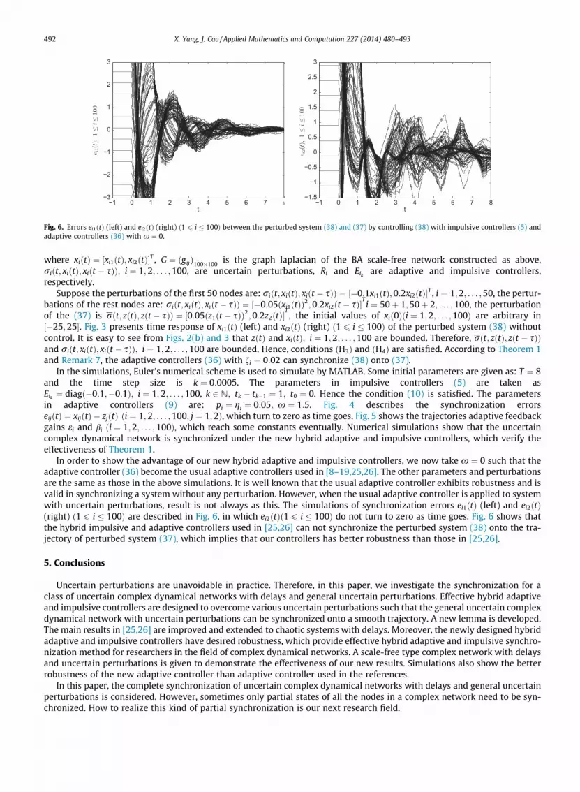
Synchronization errors ei1ðtÞ (left) and ei2ðtÞ (right) ð1 6 i � 100Þ between the perturbed system (38) and (37) by controlling (38) with impulsivelers (5) and adaptive controllers (36).

−1 0 1 2 3 4 5 6 7 81

2

3

4

5

6

7

t−1 0 1 2 3 4 5 6 7 81

1.1

1.2

1.3

1.4

1.5

1.6

1.7

1.8

1.9

t

Fig. 5. Trajectories of control gains eiðtÞð1 6 i � 100Þ (left) and biðtÞð1 6 i � 100Þ (right) for (38).

−1 0 1 2 3 4 5 6 7 8−3

−2

−1

0

1

2

3

t−1 0 1 2 3 4 5 6 7 8

−1.5

−1

−0.5

0

0.5

1

1.5

2

2.5

3

t

Fig. 6. Errors ei1ðtÞ (left) and ei2ðtÞ (right) ð1 6 i � 100Þ between the perturbed system (38) and (37) by controlling (38) with impulsive controllers (5) andadaptive controllers (36) with x ¼ 0.

492 X. Yang, J. Cao / Applied Mathematics and Computation 227 (2014) 480–493

where xiðtÞ ¼ ½xi1ðtÞ; xi2ðtÞ�T , G ¼ ðgijÞ100�100is the graph laplacian of the BA scale-free network constructed as above,

riðt; xiðtÞ; xiðt � sÞÞ; i ¼ 1;2; . . . ;100, are uncertain perturbations, Ri and Eik are adaptive and impulsive controllers,respectively.

Suppose the perturbations of the first 50 nodes are: riðt; xiðtÞ; xiðt � sÞÞ ¼ ½�0:1xi1ðtÞ;0:2xi2ðtÞ�T , i ¼ 1;2; . . . ;50, the pertur-bations of the rest nodes are: riðt; xiðtÞ; xiðt � sÞÞ ¼ ½�0:05ðxi1ðtÞÞ2;0:2xi2ðt � sÞ�

Ti ¼ 50þ 1;50þ 2; . . . ;100, the perturbation

of the (37) is rðt; zðtÞ; zðt � sÞÞ ¼ ½0:05ðz1ðt � sÞÞ2;0:2z2ðtÞ�T, the initial values of xið0Þði ¼ 1;2; . . . ;100Þ are arbitrary in

½�25;25�. Fig. 3 presents time response of xi1ðtÞ (left) and xi2ðtÞ (right) ð1 6 i � 100Þ of the perturbed system (38) withoutcontrol. It is easy to see from Figs. 2(b) and 3 that zðtÞ and xiðtÞ; i ¼ 1;2; . . . ;100 are bounded. Therefore, rðt; zðtÞ; zðt � sÞÞand riðt; xiðtÞ; xiðt � sÞÞ; i ¼ 1;2; . . . ;100 are bounded. Hence, conditions ðH3Þ and ðH4Þ are satisfied. According to Theorem 1and Remark 7, the adaptive controllers (36) with fi ¼ 0:02 can synchronize (38) onto (37).

In the simulations, Euler’s numerical scheme is used to simulate by MATLAB. Some initial parameters are given as: T ¼ 8and the time step size is k ¼ 0:0005. The parameters in impulsive controllers (5) are taken asEik ¼ diagð�0:1;�0:1Þ; i ¼ 1;2; . . . ;100, k 2 N; tk � tk�1 ¼ 1; t0 ¼ 0. Hence the condition (10) is satisfied. The parametersin adaptive controllers (9) are: pi ¼ gi ¼ 0:05; x ¼ 1:5. Fig. 4 describes the synchronization errorseijðtÞ ¼ xijðtÞ � zjðtÞ ði ¼ 1;2; . . . ;100; j ¼ 1;2Þ, which turn to zero as time goes. Fig. 5 shows the trajectories adaptive feedbackgains ei and bi ði ¼ 1;2; . . . ;100Þ, which reach some constants eventually. Numerical simulations show that the uncertaincomplex dynamical network is synchronized under the new hybrid adaptive and impulsive controllers, which verify theeffectiveness of Theorem 1.

In order to show the advantage of our new hybrid adaptive and impulsive controllers, we now take x ¼ 0 such that theadaptive controller (36) become the usual adaptive controllers used in [8–19,25,26]. The other parameters and perturbationsare the same as those in the above simulations. It is well known that the usual adaptive controller exhibits robustness and isvalid in synchronizing a system without any perturbation. However, when the usual adaptive controller is applied to systemwith uncertain perturbations, result is not always as this. The simulations of synchronization errors ei1ðtÞ (left) and ei2ðtÞ(right) ð1 6 i � 100Þ are described in Fig. 6, in which ei2ðtÞð1 6 i � 100Þ do not turn to zero as time goes. Fig. 6 shows thatthe hybrid impulsive and adaptive controllers used in [25,26] can not synchronize the perturbed system (38) onto the tra-jectory of perturbed system (37), which implies that our controllers has better robustness than those in [25,26].

5. Conclusions

Uncertain perturbations are unavoidable in practice. Therefore, in this paper, we investigate the synchronization for aclass of uncertain complex dynamical networks with delays and general uncertain perturbations. Effective hybrid adaptiveand impulsive controllers are designed to overcome various uncertain perturbations such that the general uncertain complexdynamical network with uncertain perturbations can be synchronized onto a smooth trajectory. A new lemma is developed.The main results in [25,26] are improved and extended to chaotic systems with delays. Moreover, the newly designed hybridadaptive and impulsive controllers have desired robustness, which provide effective hybrid adaptive and impulsive synchro-nization method for researchers in the field of complex dynamical networks. A scale-free type complex network with delaysand uncertain perturbations is given to demonstrate the effectiveness of our new results. Simulations also show the betterrobustness of the new adaptive controller than adaptive controller used in the references.

In this paper, the complete synchronization of uncertain complex dynamical networks with delays and general uncertainperturbations is considered. However, sometimes only partial states of all the nodes in a complex network need to be syn-chronized. How to realize this kind of partial synchronization is our next research field.

X. Yang, J. Cao / Applied Mathematics and Computation 227 (2014) 480–493 493

Acknowledgments

This work was jointly supported by the National Natural Science Foundation of China (NSFC) under Grant Nos. 61263020,61272530, 11072059, the Natural Science Foundation of Jiangsu Province of China under Grant No. BK2012741, the Special-ized Research Fund for the Doctoral Program of Higher Education under Grant Nos. 20110092110017 and 20130092110017,the Scientific Research Fund of Chongqing municipal education committee under Grant KJ130613, and the Scientific Re-search Fund of Chongqing Normal University under Grant Nos. 12XLB031 and 940115.

References

[1] B.A. Huberman, L.A. Adamic, Growth dynamics of the world-wide-web, Nature 401 (1999) 131.[2] R. Pastor-Satorras, E. Smith, R.V. Solé, Evolving protein interaction networks through gene duplication, J. Theor. Biol. 222 (2003) 199–210.[3] R. Pastor-Satorras, A. Vespignani, Epidemic spreading in scale-free networks, Phys. Rev. Lett. 86 (2001) 3200–3203.[4] A.L. Barabási, H. Jeong, Z. Néda, E. Ravasz, A. Schubert, T. Vicsek, Evolution of the social network of scientific collaborations, Phys. A 311 (2002) 590–

614.[5] F. Wang, Y. Sun, self-organizing peer-to-peer social networks, Comput. Intell. 24 (3) (2008) 213–233.[6] C. Li, X. Liao, K. Wong, Chaotic lag synchronization of coupled time-delayed systems and its applications in secure communication, Phys. D 194 (3–4)

(2004) 187–202.[7] Q. Xie, G. Chen, E. Bollt, Hybrid chaos synchronization and its application in information processing, Math. Comput. Model. 35 (1–2) (2002) 145–163.[8] W. Yu, G. Chen, J. Cao, Adaptive synchronization of uncertain coupled stochastic complex networks, Asian J. Control 13 (3) (2011) 418–429.[9] X. Wu, Synchronization-based topoligy identification of weighted general complex dynamical networks with time-varying coupling delay, Phys. A 387

(2008) 997–1008.[10] T.H. Lee, Z.-G. Wu, J.H. Park, Synchronization of a complex dynamical network with coupling time-varying delays via sampled-data control, Appl. Math.

Comput. 219 (3) (2012) 1354–1366.[11] H. Liu, J. Chen, J. Lu, M. Cao, Generalized synchronization in complex dynamical networks via adaptive couplings, Phys. A 389 (8) (2010) 1759–1770.[12] J. Wang, H. Zhang, Z. Wang, B. Wang, Local exponential synchronization in complex dynamical networks with time-varying delay and hybrid coupling,

Appl. Math. Comput. 225 (2013) 16–32.[13] W. Lu, T. Chen, Synchronization of coupled connected neural networks with delays, IEEE Trans. Circ. Syst. I 51 (12) (2004) 2491–2503.[14] X. Yang, J. Cao, Stochastic synchronization of coupled neural networks with intermittent control, Phys. Lett. A 373 (2009) 3259–3272.[15] C.C. Yang, Adaptive control and synchronization of identical new chaotic flows with unknown parameters via single input, Appl. Math. Comput. 216 (4)

(2010) 1316–1324.[16] Y. Xiao, W. Xu, S. Tang, X. Li, Adaptive complete synchronization of the noise-perturbed two bi-directionally coupled chaotic systems with time-delay

and unknown parametric mismatch, Appl. Math. Comput. 213 (2) (2009) 538–547.[17] J. Cao, Z. Wang, Y. Sun, Synchronization in an array of linearly stochastically coupled networks with time delays, Phys. A 385 (2007) 718–728.[18] J. Zhou, J. Lu, J. Lü, Adaptive pinning synchronization of a complex dynamical network, Automatica 44 (2008) 996–1003.[19] C. Zhu, Adaptive synchronization of two novel different hyperchaotic systems with partly uncertain parameters, Appl. Math. Comput. 215 (2) (2009)

557–561.[20] T. Stojanovski, L. Kocraev, U. Parlitz, Driving and synchronization by chaotic impulses, Phys. Rev. E 54 (1996) 2128–2131.[21] B. Liu, X. Liu, G. Chen, H. Wang, Robust impulsive synchronization of uncertain dynamical networks, IEEE Trans. Circuits Syst. I 52 (7) (2005) 1431–

1441.[22] P. Li, J. Cao, Z. Wang, Robust impulsive synchronization of coupled delayed neural networks with uncertainties, Phys. A 373 (1) (2006) 261–272.[23] J. Zhou, L. Xiang, Z. Liu, Synchronization in complex delayed dynamical networks with impulsive effects, Phys. A 384 (2) (2007) 684–692.[24] X. Yang, J. Cao, Z. Yang, Synchronization of reaction–diffusion neural networks with time-varying delays via pinning-impulsive controller, SIAM J.

Control Optim. 51 (5) (2013) 3486–3510.[25] K. Li, C.H. Lai, Adaptive-impulsive synchronization of uncertain complex dynamical networks, Phys. Lett. A 372 (2008) 1601–1606.[26] H.B. Jiang, Hybrid adaptive and impulsive synchronization of uncertain complex dynamical networks by the generalized Barbalat’s lemma, IET Control

Theory Appl. 3 (10) (2009) 1330–1340.[27] S. Bowong, F. Kakmeni, Chaos control and duration time of uncertain chaotic systems, Phys. Lett. A 316 (2003) 206–217.[28] H. Huang, G. Feng, Synchronization of nonidentical chaotic neural networks with time delays, Neural Networks 22 (2009) 869–874.[29] J. Yao, Z. Guan, D. Hill, Passivity-based control and synchronization of general complex dynamical networks, Automatica 45 (2009) 2107–2113.[30] S. Gao, N. Zhang, L. Hao, J. Ma, X. Kang, M. Yang, Mathematical Analysis (book) (in Chinese), Higher Education Press, Beijing, 2005.[31] C. Edwards, S. Spurgeon, R. Patton, Sliding mode observers for fault detection and isolation, Automatica 36 (2000) 541–548.[32] J. Lin, J. Yan, Adaptive synchronization for two identical generalized Lorenz chaotic systems via a single controller, Nonlinear Anal. RWA 10 (2009)

1151–1159.[33] A.L. Barabási, R. Albert, Emergence of scaling in random networks, Science 286 (5439) (1999) 509–512.