an abstract of the dissertation of arvin b. vista for
TRANSCRIPT
AN ABSTRACT OF THE DISSERTATION OF
Arvin B. Vista for the degree of Doctor of Philosophy in Forest Resources presented on June 10, 2010.
Title: Three Essays on Meta-Analysis, Benefit Transfer, and Recreation Use Valuation.
Abstract approved:
_____________________________________________________________________
Randall S. Rosenberger
This dissertation consists of three essays on meta-analysis, benefit transfer and
recreation use valuation. The first two essays were based on the sportsfishing
valuation literature in the US and Canada while the third essay was based on a study
site in the Philippines and selected study sites from the US. The first essay evaluates
the aggregation structure of primary research studies and its implications for benefit
transfer using meta-regression analysis. Results indicate that single-site and regional
studies should not be pooled without accounting for their differences in a meta-
analysis. The second essay examines the implications of addressing dependency in the
sportsfishing valuation literature using meta-regression analysis. Results indicate that
median absolute percentage transfer error is lower for the meta-regression models
based on a single value, i.e. average-set and best-set metadata than the meta-regression
models based on all-set. The average-set and best-set are two treatments of the
metadata for avoiding dependency. The third essay applies the methodological
treatments learned from the first two essays to estimate the recreational value via
benefit transfer of Taal Volcano Protected Landscape in the Philippines. Results show
that single point estimate transfer worked better than the meta-regression benefit
function transfer. Recommendations based from the three essays include: 1) the need

to account for aggregation differences among primary studies to minimize biased
value estimates in benefit transfer depending on policy settings; 2) the importance to
correct for dependency and other methodological pitfalls in meta-regression is always
warranted; 3) metadata sample selection is best guided by the goals of the meta-
analysis and perceived allowable errors in benefit transfer applications; and 4) the
conduct of primary study is still the first best strategy to recreation use valuation,
given time and resources.

©Copyright by Arvin B. Vista
June 10, 2010
All Rights Reserved
Three Essays on Meta-Analysis, Benefit Transfer, and Recreation Use Valuation
by
Arvin B. Vista
A DISSERTATION
submitted to
Oregon State University
in partial fulfillment of
the requirements for the
degree of
Doctor of Philosophy
Presented June 10, 2010
Commencement June 2011

Doctor of Philosophy dissertation of Arvin B.Vista presented on June 10, 2010.
APPROVED:
_____________________________________________________________________
Major Professor, representing Forest Resources
_____________________________________________________________________
Head of the Department of Forest Engineering, Resources and Management
_____________________________________________________________________
Dean of the Graduate School
I understand that my dissertation will become part of the permanent collection of Oregon State University libraries. My signature below authorizes release of my dissertation to any reader upon request.
_____________________________________________________________________
Arvin B. Vista, Author

ACKNOWLEDGEMENTS
I am grateful to many people for making this dissertation possible and
successful.
First, I want to thank my major professor and mentor Randall Rosenberger for
his guidance, advice and assistance in many forms throughout my PhD studies. Also, I
would like to thank William Jaeger, Jeff Kline, Kreg Lindberg, and Steven
Radosevich, for providing valuable comments and serving as my PhD committee.
Second, I would like to thank Lisa Ganio, Manuela Huso, and Robert Johnston
for their statistical advice and assistance in estimating the models using jackknife data
splitting technique. Funding for my research was supported in part by US EPA STAR
grant #RD-832-421-01 to Oregon State University (Randall Rosenberger as PI).
I am also indebted to the following people: members of Knollbrook Christian
Reformed Church through the leadership of Pastor Ken Van Shelven for continuous
encouragement and prayers; Ipat Luna for providing background information on Taal
Volcano Protected Landscape; and my mother-in-law, Loyola Viriña for providing
comments on Essay 1 and helping us during her summer 2009 visit at Corvallis,
Oregon;
Special thanks go to my wife, Loida for her support, patience, and
understanding. And to our precious son Joshua Caleb who is our joy and delight.
Finally, I exhort my gratitude to our Lord Almighty for daily provisions,
strength and grace. His words are constant source of inspiration to make things
possible and worth fulfilling.
TABLE OF CONTENTS
Page
CHAPTER 1 – INTRODUCTION ................................................................................ 1
Economic Valuation: Focus on Recreation ............................................................ 2
Why these values are important and needed? ...................................................... 13
Organization of the Dissertation .......................................................................... 15 Notes .................................................................................................................... 19 References ............................................................................................................ 20
CHAPTER 2 - ESSAY 1 Primary Study Aggregation Effects: Meta-Analysis of
Sportfishing Values in North America ................................................................. 22 Abstract ................................................................................................................ 22 Introduction .......................................................................................................... 23 Problem Definition ............................................................................................... 26 Method ................................................................................................................. 29 Model Results and Discussion ............................................................................. 48 Publication Selection Bias .................................................................................... 56 Benefit Transfer Comparison ............................................................................... 56 Conclusions .......................................................................................................... 60 Notes .................................................................................................................... 63 References ............................................................................................................ 64
CHAPTER 3 - ESSAY 2 Addressing Dependency in the Sportsfishing Valuation
Literature: Implications for Meta-Regression Analysis and In-Sample Benefit Prediction Performance ........................................................................................ 71 Abstract ................................................................................................................ 71 Introduction .......................................................................................................... 72 Approaches to Multiple Estimates ....................................................................... 74
Data Collection and Coding of Best and Average Estimates ............................... 77
Meta-Regression Model Specifications ............................................................... 85
Model Comparisons ............................................................................................. 86 Meta-Regression Results ...................................................................................... 88 In-Sample Benefit Predictions Results ................................................................. 93
Conclusions .......................................................................................................... 97 Acknowledgments ................................................................................................ 99 Notes .................................................................................................................... 99 References .......................................................................................................... 100
TABLE OF CONTENTS (Continued)
Page CHAPTER 4 - ESSAY 3 The Recreational Value of Taal Volcano Protected
Landscape: An Exploratory Benefit Transfer Application ................................. 105
Abstract .............................................................................................................. 105 Introduction ........................................................................................................ 106 The Taal Volcano Protected Landscape ............................................................. 108
Valuation Framework ......................................................................................... 113 Benefit Transfer Techniques .............................................................................. 115 Benefit Transfer Applications to TVPL ............................................................. 124
Discussions, Conclusions, and Policy Implications ........................................... 136
Notes .................................................................................................................. 140 References .......................................................................................................... 142
CHAPTER 5 - CONCLUSION ................................................................................. 147 Appendix A: Master coding sheet for recreational fishing studies. ........................... 150 Appendix B: Select characteristics of recreational angling valuation studies used in the
meta-analyses. ..................................................................................................... 156 Appendix C: Bibliography of recreational fishing valuation studies, 1969 to 2006 .. 170 Appendix D. Select characteristics of the original study used in international benefit
transfer. ............................................................................................................... 184 Appendix E: Bibliography of recreational valuation studies used in international
benefit transfer, 1958 to 2006 ............................................................................. 189
LIST OF FIGURES
Figure Page
1.1 Consumer surplus, compensating and equivalent variations for a decline in price. ................................................................................................................... 7
1.2. Compensating and equivalent surplus. ............................................................... 9
2.1. Cumulative number of estimates and studies from 1969 to 2006. ................... 31
2.2. Number of studies and estimates by document type. ....................................... 32
2.3. Number of studies and estimates by country, study aggregation level, fishing type, and valuation methodology. .................................................................... 34
2.4. Distribution of consumer surplus per person per day estimates (in 2006 dollars) for outlier-trimmed dataset (N=920). ............................................................... 35
3.1. Detection heuristics in coding ‘best’ or ‘average’ estimates for fishing studies, whether dependent or independent observations. ............................................ 79
3.2. Observed and predicted benefit estimates (in 2006 dollars) and absolute percentage transfer errors for Model A2, ranked in ascending order of the observed benefit value...................................................................................... 95
4.1. Photo and map of Taal Volcano Protected Landscape, Philippines (Vista, 2003). ............................................................................................................. 109
4.2. Conceptual composition of the Taal Volcano Protected Landscape related recreational benefits. ...................................................................................... 114
4.3. Steps to performing benefit transfers. ............................................................ 118
4.4. Map of Leyte, Region 8 showing the location of Lake Danao National Park (Garcia et al., 2005) ........................................................................................ 126
LIST OF TABLES Table Page 1.1. Hicksian monetary measures for price changes. ................................................ 6
1.2. Hicksian monetary measures for quantity changes. ........................................... 8
2.1. Meta-analysis variables and descriptive statistics. ........................................... 38
2.2. Meta-regression models. .................................................................................. 46
2.3. Hypothesis test results for panel stratification ‘by study’ (N=920; j = 140). ... 49
2.4. Unweighted random-effect meta-regression model results.............................. 50
2.5. Parameter (standard error) estimate for the sub-meta differences unweighted meta-regression model. .................................................................................... 55
2.6. Root-n meta-regression analysis of sportfishing values. .................................. 57
2.7. Out-of-sample study characteristics and benefit comparison. ......................... 59
3.1. Variables and descriptive statistics. ................................................................. 83
3.2. Meta-regression model results. ........................................................................ 89
3.3. Mean absolute percentage transfer error (PTE) in Model A2 following the jackknife data splitting technique. ................................................................... 94
3.4. Mean and median absolute percentage transfer error for the five models. ...... 96
4.1. Significant features of Taal Volcano Protected Landscape (policy site) and Lake Danao National Park (study site) and their watersheds. ....................... 127
4.2. Description of variables tested in the meta-regression analysis..................... 130
4.3. Ordinary least squares regression model result. ............................................. 132
4.4. Example adaptation of meta-regression benefit function for fishing. ............ 133
4.5. Estimated consumer surplus (CS) for different recreation activities at the policy site based on the meta-regression benefit transfer function. ............... 135

LIST OF TABLES (Continued)
Table Page 4.6. Recretional value of Taal Volcano Protected Landscape based on Filipino
resident travellers, 2006. ................................................................................ 136
THREE ESSAYS ON META-ANALYSIS, BENEFIT TRANSFER, AN D RECREATION USE VALUATION
CHAPTER 1 – INTRODUCTION
Households combine time, skill, experience, market goods (e.g. equipment),
and natural resources and facilities to produce their recreation experiences. Adapting
the household production theory, an individual (i.e. the decision-maker in the
household) is assumed to seek maximum enjoyment from all of life’s activities,
including recreation. The recreation economic rule is that an individual should
continue to participate in available recreational activities that provide the most benefit,
i.e. if the additional or marginal benefits are equal or greater than the price to
experience that activity. An individual’s participation is contingent upon their
willingness-to-pay (WTP) and ability to pay. WTP represents the economic value of
recreation, which is the amount an individual, is willing to pay rather than forego the
recreation activity. Ability to pay, a constraint on WTP, is directly affected by an
individual’s income/money, available time, effort, and opportunity costs of recreation.
Given perfect information (i.e. price = marginal value), the choices of an
individual reflect his or her value of recreational experiences. An individual’s choices
are constrained by income/money, time, experience, and/or resource availability. The
benefit derived by an individual from some recreational activities, say freshwater
fishing in a lake, is an economic measure that indicates how much pleasure, usefulness
or utility the individual obtains from the experience.
This chapter discusses 1) the basic economic theory and concepts of economic
valuation, with a focus on recreation, 2) why these values are needed and their
applications; and 3) the organization of the dissertation.
2
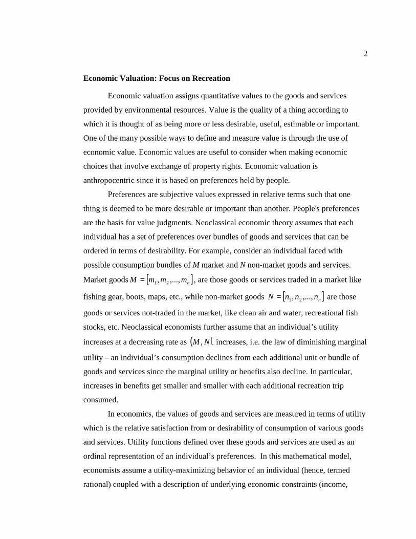
Economic Valuation: Focus on Recreation
Economic valuation assigns quantitative values to the goods and services
provided by environmental resources. Value is the quality of a thing according to
which it is thought of as being more or less desirable, useful, estimable or important.
One of the many possible ways to define and measure value is through the use of
economic value. Economic values are useful to consider when making economic
choices that involve exchange of property rights. Economic valuation is
anthropocentric since it is based on preferences held by people.
Preferences are subjective values expressed in relative terms such that one
thing is deemed to be more desirable or important than another. People's preferences
are the basis for value judgments. Neoclassical economic theory assumes that each
individual has a set of preferences over bundles of goods and services that can be
ordered in terms of desirability. For example, consider an individual faced with
possible consumption bundles of M market and N non-market goods and services.
Market goods [ ]nmmmM ,...,, 21= , are those goods or services traded in a market like
fishing gear, boots, maps, etc., while non-market goods [ ]nnnnN ,...,, 21= are those
goods or services not-traded in the market, like clean air and water, recreational fish
stocks, etc. Neoclassical economists further assume that an individual’s utility
increases at a decreasing rate as ( )NM , increases, i.e. the law of diminishing marginal
utility – an individual’s consumption declines from each additional unit or bundle of
goods and services since the marginal utility or benefits also decline. In particular,
increases in benefits get smaller and smaller with each additional recreation trip
consumed.
In economics, the values of goods and services are measured in terms of utility
which is the relative satisfaction from or desirability of consumption of various goods
and services. Utility functions defined over these goods and services are used as an
ordinal representation of an individual’s preferences. In this mathematical model,
economists assume a utility-maximizing behavior of an individual (hence, termed
rational) coupled with a description of underlying economic constraints (income,
3
supply, and time and timing of good availability). Utility is maximized when no
reallocation of one's budget can improve it.
Suppose an individual faces two bundles ( )AA NM , and ( )BB NM , , then a
utility function can be assigned to each bundle, resulting in the following utility
functions: ( )AA NMU , for bundle A and ( )BB NMU , for bundle B. A rational
individual would choose that bundle of goods and services that provides the highest
level of utility. If an individual prefers ( )AA NM , over ( )BB NM , , given that
preferences are complete, reflexive, transitive, continuous and strongly monotonic,
then ( )AA NMU , > ( )BB NMU , . However, it is difficult to measure a person's utility
or compare it with other individuals’ utilities. Instead, economists observe individual
behavior through choices made, which reflect one’s preference ordering (e.g. an
individual chooses bundle A over B). According to Holland (2002, p.17), “all choice is
basically a form of exchange.” The only way of understanding a person’s real
preference is to examine his actual choices. Hence, the relative value of a given
resource is revealed by the choices that people make (Bromley and Paavola, 2002).
Fixed monetary income, Y and prices of goods and services, ( )npppP ,...,, 21=
constrain1 the individual’s choice of bundles of goods and services( )NM , . An
individual’s problem then is to maximize utility by selecting some combination of
( )NM , , wherein the level of N is exogenously determined, subject to fixed income Y
and prices of ( )NM , . Let 0 superscript denote the initial level/status quo condition,
then the individual problem of utility maximization is written as:
MaxM ( )NMU , subject to YMP ≤* , 0NN = . Equation 1.1
Ignoring boundary problems, the utility-maximizing choice
vector ( )YNPMM ,,=∗ must meet the budget constraint with equality. The vector
( )YNPMM ,,=∗ lists the Marshallian demand function for each market good. The
demand function relates P and Y to the demanded bundle M. The function ( )YMPv ,,
4
that gives the maximum utility at prices P and income Y results in an indirect utility
function. The individual’s problem can be restated as:
( ) ( )NMUYNPv ,max,, = subject to YMP =* . Equation 1.2
The individual’s problem of utility-maximization can be written also as a cost-
minimization problem. The individual’s cost- or expenditure-minimization problem is
given by:
( ) ( )MPUNPe M *min,, 0 =
subject to ( ) ( )0,, NMUNMU ≥ Equation 1.3
where ( )UNPe ,, 0 is the expenditure function, which is the minimum cost necessary
to achieve fixed level of utility U . The solution to this cost-minimization problem is
the Hicksian vector of compensated demands ( )UNPMM H ,,= .
Hicksian (compensated) demand functions correct for the income effect
whereas Marshallian (ordinary) demand functions do not2. The demand curve for
recreational activities is negatively sloped because it is constrained by income,
presence of a substitute area, and diminishing marginal utility. A Marshallian or
Hicksian demand schedule can be derived from the demand function that shows the
number of trips taken at different prices. Prices, defined here as the summation of
transportation cost, opportunity cost of travel time, and entrance fee.
Information about the demand for recreational activities is useful for
estimating the economic value of recreation benefits (usually in a money metric
measure), predict future recreation use, and estimate the effect of different factors on
recreation use and value (e.g. entrance fee, quantity and quality changes in resources).
The money metric measure is represented in terms of surplus, i.e. the net benefit or the
difference between the benefits that an individual received from a given recreational
activity less what it costs to experience it (where costs may include non-monetary
costs, etc.). An individual chooses to engage in a given recreational activity as long as
the benefit exceeds the costs at the margin.
5
Surplus Measures
There are five measures of surplus. Consumer surplus (CS) is the usual
approximate measure of surplus. John Hicks (1941) identified four better measures of
surplus, such as compensating variation (CV), equivalent variation (EV),
compensating surplus (CoS), and equivalent surplus (ES).
Marshallian CS is a close and acceptable approximation to the Hicksian
measures of the consumer welfare effects of a price change (CV and EV) only when
the utility function is quasilinear, i.e. the function is linear in one of the goods but
(possibly) non-linear in the other goods. In estimating the change in CS, it is assumed
the there is only one good (i.e. there is no substitution effect) and the marginal utility
of income is constant.
There are two Hicksian monetary measures of the utility change associated
with price changes: 1) the CV, which is the change in the amount of income that
would compensate an individual in keeping an old/initial utility level given a new
price set, implying the status quo assignment of property right; and 2) the EV, which is
the change in the amount of income that would bring an individual to a new utility
level given old price set, implying new assignment of property right. Let 0 superscripts
denote the initial level/status quo conditions and 1 superscripts denote new conditions,
the CV measure using the indirect utility function is given by:
( ) ( )CVYNPvYNPv −= 111000 ,,,, Equation 1.4
while the EV measure is given by:
( ) ( )111000 ,,,, YNPvEVYNPv =+ . Equation 1.5
6
Using the expenditure function and considering a policy that provides a price
decrease, CV and EV measures for a price decrease for good i (such that 10ii pp > ) can
also be represented as:
( ) ( ) ( )∫ −−− =−=0
1
00000010000 ,,,,,,,,,i
i
p
p
ihiiiii dsUNPsmUNPpeUNPpeCV
Equation 1.6
( ) ( ) ( )∫ −−− =−=0
1
10010011000 ,,,,,,,,,i
i
p
p
ihiiiii dsUNPsmUNPpeUNPpeEV
Equation 1.7
where iP− refers to the price vector left after removingip , and s representsip along
the path of integration.
Another name for CV and EV welfare measures are willingness-to-pay (WTP)
and willingness-to-accept (WTA). WTP is the amount one has to offer to acquire a
good which he/she does not have legal entitlement to it. WTA is the amount the
subject asks to voluntarily give up a good. WTP is associated with a desirable change
while WTA is associated with a negative change. In WTP, an individual does not
currently have the good, while in WTA an individual has the legal entitlement to the
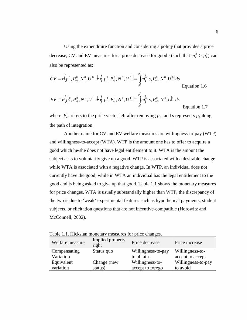
good and is being asked to give up that good. Table 1.1 shows the monetary measures
for price changes. WTA is usually substantially higher than WTP, the discrepancy of
the two is due to ‘weak’ experimental features such as hypothetical payments, student
subjects, or elicitation questions that are not incentive-compatible (Horowitz and
McConnell, 2002).
Table 1.1. Hicksian monetary measures for price changes.
Welfare measure Implied property right
Price decrease Price increase
Compensating Variation
Status quo Willingness-to-pay to obtain
Willingness-to-accept to accept
Equivalent variation
Change (new status)
Willingness-to-accept to forego
Willingness-to-pay to avoid
7
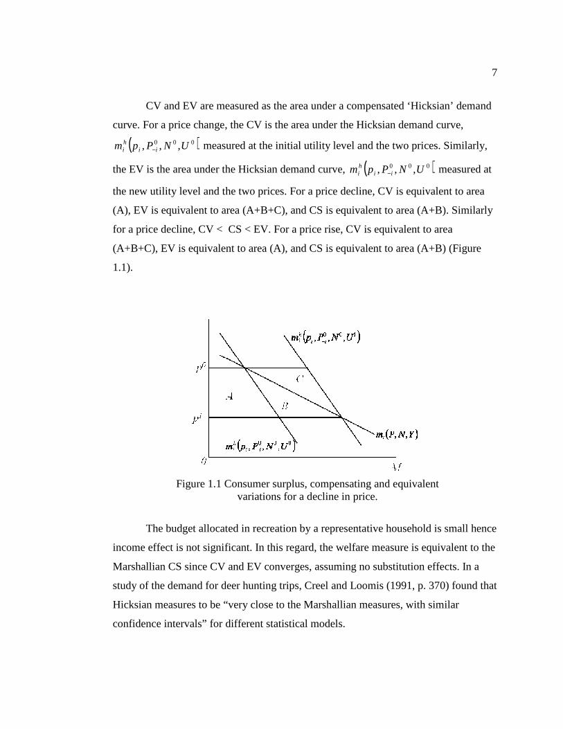
CV and EV are measured as the area under a compensated ‘Hicksian’ demand
curve. For a price change, the CV is the area under the Hicksian demand curve,
( )000 ,,, UNPpm iihi − measured at the initial utility level and the two prices. Similarly,
the EV is the area under the Hicksian demand curve, ( )000 ,,, UNPpm iihi − measured at
the new utility level and the two prices. For a price decline, CV is equivalent to area
(A), EV is equivalent to area (A+B+C), and CS is equivalent to area (A+B). Similarly
for a price decline, CV < CS < EV. For a price rise, CV is equivalent to area
(A+B+C), EV is equivalent to area (A), and CS is equivalent to area (A+B) (Figure
1.1).
Figure 1.1 Consumer surplus, compensating and equivalent variations for a decline in price.
The budget allocated in recreation by a representative household is small hence
income effect is not significant. In this regard, the welfare measure is equivalent to the
Marshallian CS since CV and EV converges, assuming no substitution effects. In a
study of the demand for deer hunting trips, Creel and Loomis (1991, p. 370) found that
Hicksian measures to be “very close to the Marshallian measures, with similar
confidence intervals” for different statistical models.

8
There are two Hicksian monetary measures of the utility change associated
with changes in quality or quantity of environmental goods and services: 1) the CoS,
which is the amount of income, either given or taken away, that would keep an
individual at his/her old utility level, given a new quantity set; and 2) the ES, which is
the amount of income, either given or taken away, that would bring an individual to a
new utility level, given old quantity set. Using the expenditure function, CoS and ES
measures for a quantity increase for good j (such that 10 nn < ) is represented as:
( ) ( ) ( )∫ −=−= −−
1
0
00000100000 ,,,,,,,,,j
j
j
n
n
vijjijji dsUNPsmUNnpeUNnpeCoS
Equation 1.8
( ) ( ) ( )∫ −− =−= −
1
0
10010101000 ,,,,,,,,,j
j
jj
n
n
vijijji dsUNPsmUNnpeUNnpeES
Equation 1.9
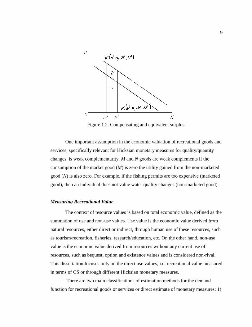
Table 1.2 summarizes the situation in regard to Hicksian monetary measures of
the utility changes associated with changes in the quality/quantity of a non-market
good. Compared to CV and EV, CS is not possible to use as approximation of CoS
and ES measures (Bockstael and McConnell, 1993). An example of quantity changes
is an increase in water flow in a river. They are shown, for the case of a quantity
increase from 0n to 1n in Figure 1.2. For a quantity increase, CoS is equivalent to area
(A) and ES is equivalent to area (A+B).
Table 1.2. Hicksian monetary measures for quantity changes.
Welfare measure Implied property right
Quantity decrease Quantity increase
Compensating Surplus
Status quo Willingness-to-accept to accept
Willingness-to-pay to get
Equivalent Surplus
Change (new status)
Willingness-to-pay to avoid
Willingness-to-accept to forego
9
Figure 1.2. Compensating and equivalent surplus.
One important assumption in the economic valuation of recreational goods and
services, specifically relevant for Hicksian monetary measures for quality/quantity
changes, is weak complementarity. M and N goods are weak complements if the
consumption of the market good (M) is zero the utility gained from the non-marketed
good (N) is also zero. For example, if the fishing permits are too expensive (marketed
good), then an individual does not value water quality changes (non-marketed good).
Measuring Recreational Value
The context of resource values is based on total economic value, defined as the
summation of use and non-use values. Use value is the economic value derived from
natural resources, either direct or indirect, through human use of these resources, such
as tourism/recreation, fisheries, research/education, etc. On the other hand, non-use
value is the economic value derived from resources without any current use of
resources, such as bequest, option and existence values and is considered non-rival.
This dissertation focuses only on the direct use values, i.e. recreational value measured
in terms of CS or through different Hicksian monetary measures.
There are two main classifications of estimation methods for the demand
function for recreational goods or services or direct estimate of monetary measures: 1)
10
revealed preference (RP) methods; and 2) stated preference (SP) methods. RP methods
are indirect approaches that infer an individual’s values by observing their behaviors
(actual choices) in related (complementary, surrogate or proxy) markets. Examples of
RP methods are travel cost models (TCM), and hedonic property value methods
(HPM). TCM are used to value recreational assets via the expenditures on traveling to
the site while HPM assume that the price of a good is a function of its attributes. TCM
recognizes that visitors to a recreation site pay an implicit price – the cost of traveling
to it, including entrance fee and the opportunity costs of their time. TCM are
oftentimes used to estimate use values for recreation activities and changes in these
use values associated with changes in environmental quality/quantity.
SP methods use surveys to directly elicit an individual’s values, based on
hypothetical or constructed markets. Examples of SP methods are contingent valuation
method (CVM) and choice modeling (CM) method. CVM uses surveys to directly
elicit individuals' preferences and WTP for non-market goods, like a direct question
“What are you willing to pay for improvements in environmental quality?” Choice
modeling seeks to secure rankings and ratings of alternatives from which WTP can be
inferred. Choice modeling is also known as choice experiments, contingent ranking,
paired comparisons, and contingent rating. If the values for individual
characteristics/attributes are required, then CM is preferable to CVM.
RP and SP methods differ in terms of the types of data used to estimate values.
RP methods rely on data based on individual’s actual choices, hence a revealed
behavior. SP methods, on the other hand, rely on data from carefully designed survey
questions asking respondents their choices for alternative levels of recreational
experience, hence an intended behavior. RP methods typically provide estimates of
Marshallian CS while SP methods can provide estimates of Hicksian surplus. SP
methods are suggested when estimating non-use values given non-use generally
precludes observable behavioral interactions with natural resources (Boyle, 2003). In
choosing which valuation technique to apply, a researcher needs to 1) determine the
management or policy question to be answered by the study; and 2) evaluate problems
11
in recreation to estimate a) the recreation benefits at existing site and quality, b)
recreation benefit with changes in quality and quantity of the resource, and c) public
benefits from preservation of resource quality.
Recreational Values Used in the Analyses
Recreational values used in the analyses in this dissertation are obtained from
primary valuation studies that reported economic measure of direct-use access value
for recreation sites and activities. Access values are measures of the current level of
benefits enjoyed by people using a resource in a recreation activity, or with versus
without the resource/site being available. Marginal WTP values are not included in the
metadata as they are measures of marginal changes in site or activity quality or
availability. These primary valuation studies reported benefit measures in terms of
compensating variation, equivalent variation, compensating surplus3, and consumer
surplus. Primary valuation studies included in the essays use revealed preference,
stated preference and combination of RP and SP methods. Primary studies reporting
the marginal value of fish are excluded in the analyses. Therefore, the recreational
values used in the analyses are derived from multiple primary studies that reported
summary statistics, such as value estimates. These estimates of recreational values are
the outcomes of empirical quantitative research. When the policy questions reported in
the primary studies are for changes in the quality or quantity of recreational experience
(e.g. an improvement in water quality that improve recreational fishing), the
recreational values encoded in the database are those representing the status quo
situation (i.e. before the improvement), if reported.
12
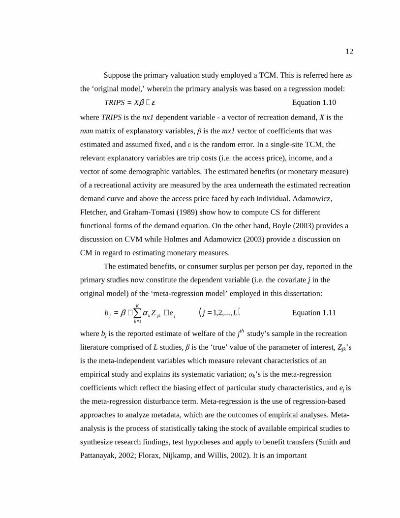
Suppose the primary valuation study employed a TCM. This is referred here as
the ‘original model,’ wherein the primary analysis was based on a regression model:
εβ += XTRIPS Equation 1.10
where TRIPS is the nx1 dependent variable - a vector of recreation demand, X is the
nxm matrix of explanatory variables, β is the mx1 vector of coefficients that was
estimated and assumed fixed, and ε is the random error. In a single-site TCM, the
relevant explanatory variables are trip costs (i.e. the access price), income, and a
vector of some demographic variables. The estimated benefits (or monetary measure)
of a recreational activity are measured by the area underneath the estimated recreation
demand curve and above the access price faced by each individual. Adamowicz,
Fletcher, and Graham-Tomasi (1989) show how to compute CS for different
functional forms of the demand equation. On the other hand, Boyle (2003) provides a
discussion on CVM while Holmes and Adamowicz (2003) provide a discussion on
CM in regard to estimating monetary measures.
The estimated benefits, or consumer surplus per person per day, reported in the
primary studies now constitute the dependent variable (i.e. the covariate j in the
original model) of the ‘meta-regression model’ employed in this dissertation:
∑=
++=K
kjjkkj eZb
1
αβ ( )Lj ,...,2,1= Equation 1.11
where bj is the reported estimate of welfare of the j th study’s sample in the recreation
literature comprised of L studies, β is the ‘true’ value of the parameter of interest, Zjk’s
is the meta-independent variables which measure relevant characteristics of an
empirical study and explains its systematic variation; αk’s is the meta-regression
coefficients which reflect the biasing effect of particular study characteristics, and ej is
the meta-regression disturbance term. Meta-regression is the use of regression-based
approaches to analyze metadata, which are the outcomes of empirical analyses. Meta-
analysis is the process of statistically taking the stock of available empirical studies to
synthesize research findings, test hypotheses and apply to benefit transfers (Smith and
Pattanayak, 2002; Florax, Nijkamp, and Willis, 2002). It is an important
13
methodological tool that can generate meaningful comparative results of empirical
data to inform policy decisions.
Why these values are important and needed?
The recreation valuation techniques presented above show that there is a real
economic value to the recreational benefits derived by a representative individual.
Recreation provides enjoyment and contributes to a well-being of the participant that
can be translated into monetary benefits, which can be compared to the costs to
manage the recreation sites. An estimate of these recreational values is one of the
criteria that may have significant influence on many recreation management decisions
and resource allocations that are made by managers. For example, Duffield (1989)
cited that estimate of the recreational value of fishing influenced the decisions by the
Montana Department of Fish, Wildlife and Parks in acquiring public access for
fishing.
One important motivation of recreational use valuation is to enable the
recreational resources to be accounted for in benefit-costs analysis (BCA). BCA is a
tool to aid decision-making and policy assessments. BCA is the process of adding up
all the gains (benefits) from a policy, program or alternative options, subtract all the
losses (costs), and choosing the option that maximizes net benefits. Benefits are
anything that contributes to the objective while costs are anything that reduces an
objective. BCA helps resource managers choose among alternative recreation
programs and projects which vary in size, design, and purpose. For example,
knowledge of the effects of stream flow on recreation for different activities and skill
levels is an important ingredient in the determination of stream flow policies. To
perform a BCA of changes in stream flow, researchers need to know how the demand
function shifts with changes in flow or flow related variables, such as fish catch.
Bishop et al., (1990) studied the release pattern that could increase the economic value
of all the multiple purposes in Glen Canyon National Recreation Area and Grand
14
Canyon National Park. Later, Congress formalized these flows when it passed the
Grand Canyon Protection Act of 1992.
Valuations also play a role in understanding the decisions made by individuals
about which recreation activities they prefer to participate in, which sites to visit and
how frequently, and if they are willing to pay higher fees or prefer not to visit.
Based on the study by McCollum et al. (1999), the Colorado Division of Wildlife
decided against proposing an increase in fishing license fees to the State Legislature
after finding out in the Colorado Angler Survey that anglers were not willing to pay
for an increased stocking. Hence, streams in certain areas of Western Colorado went to
a two-trout-per-day bag limit.
Valuation studies are also used in the relicensing decisions of the Federal
Energy Regulatory Commission (FERC). Loomis and Cooper (1990) cited that the
Pacific Gas and Electric in California relied on valuation studies that estimate the
recreation benefits associated with alternative stream flow requirements when making
their FERC license renewal applications.
Furthermore, studies on recreational activities have been used in litigation and
damage assessments. Smith (2000) cited the example of litigation over the American
Trader for an oil spill offshore of Huntington Beach, California in 1990 wherein the
jury levied $18.1 million dollars in damages and penalties against the owner of the
tanker. Of the total judgment, $12.8 million was attributed to recreation losses due to
the beach closures required by the oil spill. Estimates of the value of beach recreation
were used in this case.
Knowledge and information on the value of recreation are needed by resource
managers so that they are incorporated into planning, decision-making, and policy
issuances. For example, the technical document prepared by Rosenberger and Loomis
(2001) on benefit transfer of outdoor recreation use values supported the strategic
planning of the US Forest Service. Over the past three decades, US Forest Service has
shifted to a new paradigm, i.e. from seeing the forest as a specialized shops producing
one (timber) or few products to an emporium of multiple products and diverse
15
services (including recreation opportunities). Valuation studies on goods and services
produced on public lands managed by the US Forest Service show that the value of
recreation and wildlife services are more than timber, mineral, and range goods
(Nordhaus and Kokkelenberg, 1999).
Estimated values from primary studies are also used in benefit transfer.
Benefit transfer is the use of information from research conducted on other sites (study
sites) to inform questions or decisions at a site that lacks primary research (policy
site). Benefit transfer is considered a ‘second-best strategy’ to recreation use valuation.
Benefit transfer is suggested when time and resource constrains the conduct of
primary study. Estimated welfare values, whether by standard valuation methods or
benefit transfer, are used to aid decision-making of agencies and help justify their
decisions about how to allocate public investments. For example, primary studies that
estimated the value of recreation in coastal environments after an oil spill can be used
to inform values of recreation in coastal communities affected by a recent, but
unstudied, oil spill incident (such as the recent BP oil spill at Louisiana Gulf) using
benefit transfer. Detailed discussion of this approach is given in the body of the
dissertation.
Organization of the Dissertation
This dissertation consists of three essays on meta-analysis, benefit transfer and
recreation use valuation. The three essays focus only on the direct use values, i.e. the
economic value derived from natural resources through human use of these resources,
such as tourism/recreation, fisheries, research/education, etc. In particular, the use
values discussed herewith focus on the access value of outdoor recreation, like
sportfishing, hiking, etc., not marginal value of recreation resource.
The essays are thematically linked but can be read separately. The first two
essays were based on the sportsfishing valuation literature in the US and Canada. The
studies included in the recreation database were identified through searches of
electronic databases and formal requests for documents/references via e-mail,
16
listserve, postal mail, or phone. Other documents were obtained through private
collections and interlibrary loans. The studies were screened based on a coding
protocol template. In the creation of the sportfishing valuation database, documents
reporting the marginal value of fish were excluded. Screened primary studies
comprised the metadata, which are measured effects from primary data or empirical
studies (e.g., in economic recreation valuation, they are empirical estimates of use
values). Each primary study was encoded into the database following the master
coding sheet that contains 109 fields of information for each welfare estimate. All
study values or consumer surplus were adjusted to a ‘per person per day’ unit and
updated from their original study year values to 2006 dollars using an implicit price
deflator. After excluding possible outliers, the sportfishing metadata has 920 estimates
from 140 primary studies. The third essay was based on a study site in the Philippines
(Predo et al. 1999) and selected study sites from the broader US recreation use values
database. The study site in the Philippines was selected since there were some degree
of correspondence between the study site and policy site. Study sites included in the
metadata were selected based on recreation activity, climate, and/or site
characteristics/environment that mimics the policy site conditions.
The first essay evaluates the aggregation structure of primary research studies
and its implication for benefit transfer using meta-regression analysis. Aggregation
refers to the grouping of primary studies into single-site or regional models. Single-
site models are comprised of primary studies that are specific in their location and
scope, and may provide specific value estimates. Regional models are comprised of
studies that are broadly defined in location and scope, and may provide general value
estimates. The first essay answers the question: Are there statistical differences
between single-site and regional models? Meta-regression models were specified
following the best-practice guidelines for meta-analyses. In particular, the meta-
regression models were corrected for panel effects using a random-effect model
following by-study panel specification. Three models: a single-site model, a regional
model, and a pooled model (combined single-site and regional studies) were compared
17
based on their statistical significance, predictive power, and out-of-sample error
predictions performance. The structural shift in the metadata was investigated by
intersecting the aggregation variable with selected explanatory variables. The out-of-
sample error evaluates the convergence between consumer surplus values estimated
through meta-regression function and original out-of-sample consumer surplus values.
A log-likelihood ratio test was used to test whether the two subsamples, single-site and
regional models, are from the same population and therefore could be pooled. Essay 1
also incorporates test and correction for publication selection bias using root-n meta-
regression analysis. Publication bias is essentially a result of selective sampling, and
occurs when studies reporting statistically significant results or academic work
containing positive results are being published and others are not (Florax, Nijkamp,
and Willis, 2002).
The second essay explores the approaches in modeling and examines the
implications of treating dependency in the sportsfishing metadata when performing
meta-regression analysis and benefit transfer. Dependency or correlation refers to a
departure of two random variables from independence due to 1) multiple sampling per
study to obtain a sufficient number of observations for meta-analysis (i.e. between
study correlated observations); and 2) researchers reporting more than one benefit
measure for each primary study (i.e. multiple estimates from the same primary
study—within-study autocorrelation). Essay 2 addresses the question, “Are the meta-
regression model results statistically the same for the all-set, best-set, and average-set
metadata? The all-set metadata uses all of the available benefit measures reported in
the primary studies. Two approaches for controlling data dependency in the all-set
metadata include weighting of the metadata and using panel data estimators. Two
treatments of the metadata for avoiding dependency include a best-set metadata
(comprised of the best available benefit measures reported in a study as identified by
methodological and sample criteria) and an average-set metadata (comprised of the
average of benefit measures reported in the primary studies). Best and average
estimates, whether dependent or independent, are coded following the detection
18
heuristics discussed in Essay 2. Dependent data are multiple observations in a single
study that are derived for the same resource, using the same methods, and relying on
the same underlying sample. Independent data are single observations from
independent studies, and multiple estimates in a single study that are based on
different samples, different resources, different valuation methods (e.g., stated
preference and revealed preference data derived from the same sample), etc. The
meta-regression models are compared based on regression statistics and in-sample
benefit predictions performance (i.e. percentage transfer error) using a jackknife data
splitting technique. The jackknife technique estimates n-1 separate meta-regression
benefit functions to predict the omitted observation in each case.
The third essay applies the methodological treatments learned from the first
two essays to estimate the recreational value via benefit transfer of Taal Volcano
Protected Landscape in the Philippines. A single point estimate was derived from a
study site in the Philippines, while a meta-regression benefit function based on
existing studies in the US was used to derive the estimates of recreational value. A
benefit measure for the policy site was calculated by adapting the MR benefit function
to the specific characteristics of the ‘policy site,’ Taal Volcano Protected Landscape.
Implicit price deflators and purchasing power parities were incorporated to account for
income and cost of living differences between the study and policy sites. The different
recreational activities in the Taal Volcano Protected Landscape include hiking, day-
camping, picnicking, bird watching, horseback riding, fishing, boating, wind surfing,
sailing, rowing, and kayaking. The percentage transfer errors were computed for the
meta-regression function transfer applications, using an in-sample benefit prediction
and simple out-of-sample prediction with the single estimate from Predo et al. (1999)
as the study site original value.

19
Notes
1 For parsimonious reason, only income together with prices (i.e. excluding time,
experience and resource availability) were included in the constrained utility
maximization model. 2 Marshallian and Hicksian welfare measures are not conceptually consistent to each
other (Smith and Pattanayak, 2002). However, as Willig (1976) argues, when
income effects are small, these welfare measures tend to converge on each other.
Thus, in the metadata underlying this dissertation, conceptual differences in welfare
measures are captured by a dummy variable differentiating Marshallian from
Hicksian welfare measures.
3 Note that “access values” are ‘with’ versus ‘without’ a site and conceptually are
equivalent surplus measures. However, they are implicitly modeled through implied
changes in prices, and thus are methodologically compensating and equivalent
variation measures.
20
References
Adamowicz, W. L., J. J. Fletcher, and T. Graham-Tomasi. "Functional Form and the Statistical Properties of Welfare Measures." American Journal of Agricultural Economics 71, no. 2(1989): 414.
Bishop, R., et al. (1989) Grand Canyon and Glen Canyon Dam Operations: An
Economic Evaluation, ed. K. Boyle, and T. Heekin, Department of Agricultural and Resource Economics, University of Maine, Orono.
Bockstael, N. E., and K. E. McConnell. "Public Goods as Characteristics of Non-
Market Commodities." The Economic Journal 103, no. 420(1993): 1244-1257. Boyle, K.J. (2003). Introduction to Revealed Preference Methods. In P. Champ, K.
Boyle, and T. Brown (Eds.) A Primer on Non-Market Valuation. Boston, MA:Kluwer Academic Publishers.
Bromley, D. W., & Paavola, J. (2002). Economics, Ethics, and Environmental Policy.
In W. Bromley & J. Paavola (Eds.), Economics, Ethics, and Environmental Policy: Contested Choices. MA: Blackwell Publishing.
Creel, M. D., and J. B. Loomis. "Confidence Intervals for Welfare Measures with
Application to a Problem of Truncated Counts." The Review of Economics and Statistics 73, no. 2(1991): 370-373.
Duffield, J. (1989) Nelson Property Acquisition: Social and Economic Impact
Assessment, Report for the Montana Department of Fish, Wildlife and Parks. Helena, MT.
Florax, R., P. Nijkamp, and K. Willis (2002) Meta-analysis and value transfer:
Comparative assessment of scientific knowledge. In R. Florax, P. Nijkamp, and K. Willis (Eds). Comparative Environmental Economic Assessment. MA, USA, Edward Elgar Publishing, Inc.
Hicks, J.R. "The Rehabilitation of Consumers' Surplus." The Review of Economic
Studies 8, no. 2(1941):108-116. Holland, A. (2002). Are Choices Tradeoffs? In D. W. Bromley & J. Paavola (Eds.),
Economics, Ethics, and Environmental Policy. MA: Blackwell Publishing. Loomis, J., and J. Cooper. "Economic benefits of instream flow to fisheries: A case
study of California's Feather River." Rivers 1, no. 1(1990): 23-30.
21
McCollum, D. W., M. A. Haefele, and R. S. Rosenberger (1999) A Survey of 1997 Colorado Anglers and Their Willingness to Pay Increased License Fees (Project Report No. 39), Project Report for the Colorado Division of Wildlife. Fort Collins, CO: Colorado State University, and USDA Forest Service, Rocky Mountain Research Station.
Nordhaus, W. D., and E. C. Kokkelenberg (Eds.) (1999) Nature's Numbers:
Expanding the National Economic Accounts to Include the Environment. Washington, D.C., National Academy Press.
Predo, C. D., et al. "Non-market Valuation of the Benefits of Protecting Lake Danao
National Park in Ormoc, Philippines." Journal of Environmental Science and Management 2, no. 2(1999): 13-32.
Smith, V. K. "JEEM and Non-market Valuation: 1974-1998." Journal of
Environmental Economics and Management 39, no. 3(2000): 351-374. Smith, V., and S. Pattanayak. "Is Meta-Analysis a Noah's Ark for Non-Market
Valuation?" Environmental and Resource Economics 22, no. 1(2002): 271-296.
Willig, R.D. "Consumer's Surplus Without Apology." The American Economic Review
66, no. 4(1976):589-597
22
CHAPTER 2 - ESSAY 1 PRIMARY STUDY AGGREGATION EFFECTS: META-ANALYSIS OF
SPORTFISHING VALUES IN NORTH AMERICA
Abstract
There are many factors that affect the development, design and implementation
of primary research projects that may carry forward in applications of benefit
transfers. Meta-regression analyses have isolated and measured many patterns in the
literature, including the effects of methodology, sample designs, and geographic
region. This paper evaluates aggregation structure of primary research studies and its
implication for benefit transfer using meta-regression analysis. Aggregation structures
of primary research may be defined as single-site and regional models. Single-site
models (SM) are based on primary studies that are specific in their location and scope,
thus providing specificity in their value estimates. Regional models (RM), conversely,
are based on primary studies that are broadly defined in location and scope, thus
providing more generalized value estimates. Three meta-regression models are
evaluated, including SM, RM, and a pooled model (PM, combined SM and RM
studies). The application is applied to the sportfishing valuation literature, which
consists of 140 individual studies that span from 1969 to 2006 and provides 920
welfare measures for the US and Canada. Log likelihood-ratio test shows that SM and
RM are different from the PM in terms of how they explain welfare measures. Results
indicate that single-site and regional studies should not be pooled without accounting
for their differences in a meta-analysis. Following the ‘best practice’ guidelines for
meta-analyses and given non-random out-of-sample benefit transfer estimates, the
percent difference (i.e. comparing out-of-sample consumer surplus with meta-
regression benefit transfer consumer surplus) was lowest using RM, although this
results remain inconclusive. Not accounting for aggregation differences among
primary studies leads to biased value estimates in benefit transfer, depending on the
policy settings.
23
Introduction
Recognition of recreational benefits of ecosystem resources provides a sound
rationale for management, conservation and planning options for nature-based
recreation. Researchers have suggested that having comparable estimates of benefits
and/or costs of resources not traded in markets (i.e., without prices) can aid the
evaluation of socially efficient and welfare enhancing outcomes. Benefits are
economic measures of value derived from recreation experiences, which are also
called use values. Use values found in different studies are "more or less taken as valid
and reliable reflections of people's valuation of [ecosystem] changes" (Brouwer, 2002,
p. 101). These estimates of use values can help raise the awareness of resource users
and decision-makers in making informed choices among policy alternatives. To date,
there are numerous empirical studies on different recreation activities; so many, in
fact, that researchers and policy makers can be overwhelmed by them. In this regard,
researchers are directed to use meta-analysis, among others, to investigate the wide
range of data on the value of recreation.
Meta-analysis is the process of statistically taking the stock of available
empirical studies, with one application being the estimation of benefits from changes
in environmental resources (Smith and Pattanayak, 2002). If statisticians deal with
original observations; meta-analysts, on the other hand, statistically summarize or
synthesize past research results using meta-regression analysis (MRA) (Stanley and
Jarrell, 1989). MRA is used in bringing together empirical research findings from
different studies for purposes of comparison or hypothesis testing, synthesis,
knowledge acquisition, generalization and benefit transfer (BT) (Florax, Nijkamp, and
Willis, 2002). It offers a means to increase the effectiveness of literature reviews in
two ways: 1) it makes the process more systematic, and 2) it avoids bias in the reviews
(Stanley, 2001). The conduct of BT through MRA is feasible with the accumulation of
empirical research on resource valuation. BT is the “application of values and other
information from a ‘study site’ with data to a ‘policy site’ with little or no data"
(Rosenberger and Loomis, 2000 p. 1097). BT methods are used when policy-makers,
24
resource managers or planners cannot conduct primary research because of budget and
time constraints, or because the resource impacts are expected to be low or
insignificant. The application of MRA for the purpose of BT is preferred over other
BT methods, such as single point estimate and demand functions, since the benefit
estimates for the 'policy site' are based on the “site characteristics, user characteristics,
and temporal dimensions of recreation site and site choice” (Rosenberger and Loomis,
2001, p. 14), enabling the analyst to control for these dimensions.
Meta-analysis has a strong tradition in medicine and psychology. Pearson
(1904) first applied meta-analysis in evaluating data from many studies to conclude
that vaccination against intestinal fever was ineffective. Glass (1976) coined the word
meta-analysis, which refers to the analysis of research outcomes where the metadata
are derived from primary analyses (i.e. the original analysis of data) and secondary
analyses (reanalysis of primary data). Metadata are measured effects from primary
data or empirical studies (e.g., in economic recreation valuation, they are empirical
estimates of use values). Meta-analysis is a growing area of inquiry in education,
marketing and the social sciences. It was first applied in economics by Stanley and
Jarrell (1989) and Walsh et al. (1989). In the field of natural resource and
environmental economics, meta-analyses have been conducted for recreation values
(Smith and Kaoru, 1990; Rosenberger and Loomis, 2000b); wetland resources
(Woodward and Wui, 2001); water quality management (Van Houtven et al., 2007);
water supply and demand (Scheierling et al., 2006); endangered species and
biodiversity (Loomis and White, 1996; Brander et al., 2007); energy markets and
resources (Espey, 1996); global warming, greenhouse gases and sustainability
(Manley et al., 2005); hazardous wastes and pesticides (Florax et al., 2005);
sportfishing values of aquatic resources (Johnston et al., 2006); and forested areas
(Lindhjem, 2007), among others.
Several researchers have employed meta-analysis to estimate the sportfishing
values of aquatic resources. Sportfishing, also called recreational fishing, is fishing for
pleasure or competition. Sturtevant et al. (1996) estimated panel models to address the

25
dependency in the freshwater recreational fishing demand literature. They also
demonstrated the feasibility of meta-analysis as a benefit-transfer method using 26
freshwater fishing travel cost method (TCM) studies that span from 1980 to 1991.
Platt and Ekstrand (2001), using Ordinary Least Squares (OLS) with a Newey-West
version of White's consistent covariance estimator, estimated a national model and
region specific model for sportfishing value per person per day of water-based
recreation in the US. Koteen, Alexander and Loomis (2002) systematically analyzed
the variation in the recreational value of water in the US given changes in six water
quality parameters. Johnston et al. (20061) estimated random-effect panel models with
Huber-White standard errors and weights and found that moderator variables—
resource, context, angler attributes and study methodology—are associated with
systematic variation in willingness-to-pay (WTP) per fish among sportfishing anglers
in North America. Finally, Moeltner, Boyle and Paterson (2007) employed Bayesian
meta-regression (MR) framework in estimating welfare for freshwater sportsfishing in
the US.
This paper builds upon previous studies enumerated above by evaluating the
level of aggregation differences in welfare estimates in primary studies as a means to
minimize this potential source of error in meta-regression benefit function transfer
(MRBFT). The meta-regression protocol employed in this paper follows the ‘best-
practice’ guidelines outlined by Nelson and Kennedy (2009). Aggregation refers to the
grouping of primary studies into SM or RM. SMs are composed of primary studies
that are specific in their location and scope, and may provide specific value estimates.
For example, Jones and Stokes Associates, Inc. (1991) reported a consumer surplus
(CS) estimate of sportfishing for the municipality of Juneau, Alaska. This estimate
draws specific conclusions about this municipality. However, this estimate may only
be applicable in a BT application if the policy site matches this study site on most
salient dimensions of the valuation context. On the other hand, RMs are composed of
studies that are broadly defined in location and scope, and may provide general value
estimates. For example, Aiken and la Rouche (2003) estimated the net economic
26
values of bass, trout, and walleye fishing using a contingent valuation method for each
relevant state in the US and for the US as a whole. These estimates may be general
conclusions about each state and the US. Therefore, regional estimates may be
broadly applicable to many policy sites, but may lack the specificity of site-specific
estimates.
Thus, the levels at which welfare estimates are aggregated as reported in the
primary studies have implications when used in MRBFT. Accounting for the level of
aggregation differences may reduce transfer errors when meta-analyses are used for
the purpose of BT for a site or policy specific context. This approach is needed
because standard applications of BT methods rely on highly aggregated information
on people’s values, regardless of their aggregation differences. To address this gap,
SM is compared with RM and both with PM by systematically analyzing the causes of
variation or heterogeneity in the sportfishing metadata. This heterogeneity may be
attributed to fishing environment, study methodology, surveyed population and mode,
and study attributes in the primary studies. This approach seeks to contribute in the
refinement and testing of meta-analyses as a BT tool, since the bulk of existing
research illustrates the potential of MR models to generate BT estimates within a
broad valuation framework (Moeltner, Boyle and Peterson, 2007).
Problem Definition
Sportfishing is an important economic sector in North America's fishing and
tourism industry. In the United States, the economic activity generated by anglers is
greater than the economies of 14 states. There are nearly 40 million anglers
contributing $45.3 billion in retail sales, resulting in $125 billion in overall economic
output, $16.4 billion in state and federal taxes, and over a million jobs supported. The
National Sporting Goods Association ranked fishing sixth out of 42 recreation
activities, preceded only by walking, swimming, exercising, camping and bowling
(Southwick Associates, 2007). The 2005 survey of sportfishing in Canada reveals that
over 3.2 million anglers contributed a total of $7.5 billion (2/3 of which were directly
27
attributable to sportfishing investment and major purchases of durable goods) to
various local economies in Canadian provinces and territories (Fisheries and Oceans
Canada, 2007).
Sportfishing, among others, is an intensively studied outdoor recreational
activity in the US and Canada. The number of primary studies that quantify the value
of sportfishing is vast and continually growing. This accumulation of knowledge
through empirical research then forms the opportunity for conducting meta-analyses
and BT (Rosenberger and Stanley, 2006). The conduct of BT through MRA (i.e.
addressing the average values of parameter estimates originating from different
studies) is feasible with the accumulation of primary research on resource valuation.
With meta-analysis, 'overwhelmed' researchers and policy makers can make sense of
the vast available research findings, generate meaningful comparative assessment of
results across studies, and help inform policy decisions without the extra cost of
conducting primary studies.
A key issue in the conduct of BT is consistency across studies in terms of
valuation concept, the commodity valued, and the degree of site correspondence
(Rosenberger and Phipps, 2007). When the valuation concept, market area, or the
commodity valued is consistent or comparable across studies, BT may lead to
unbiased value estimates (Boyle and Bergstrom, 1992; Loomis and Rosenberger,
2006). Literature on BT emphasizes the importance of value transfer and function
transfer validity and reliability (Ready and Navrud, 2006; Spash and Vatn, 2006), and
the minimization of generalization and measurement errors (Rosenberger and Stanley,
2006). However, inherent heterogeneity in the primary studies, those undertaken under
varying conditions, could provoke someone to question the validity of comparative
analysis or the transferability of their results. According to Bergstrom and Cordell
(1991), the variation in recreation welfare estimates reported in empirical studies is
sensitive to differences in the characteristics of (1) the user population (e.g. income),
(2) the site characteristics (e.g. quality or suitability), and (3) the model specification
and estimation procedures of the primary studies, which are inherently transferred in
28
BT applications. Meta-analysis, by controlling for these differences across empirical
studies, may provide a means for estimating unbiased welfare values for a variety of
resource contexts, avoiding the need to find one-to-one correspondence between study
sites and a policy site.
Dependency in primary estimates of CS is common in the sportfishing
literature. Empirical studies often report multiple estimates when authors employed
different model estimators (e.g. stated preference (SP) and/or revealed preference (RP)
valuation methods), methodological treatments (e.g. different functional forms,
treatment of substitutes, different cost per mile, etc.), and estimated welfare values for
several different sites. This design in the primary studies creates panel data structure.
Panel data, when used in MRA, produces a dataset with a grouped structure with
possible intra-group error correlation (Moulton, 1986) implying biased standard error
estimates.
Study-level averages or single estimate per primary study, random selection,
and panel-data methods are suggested in dealing with correlated data (Nelson and
Kennedy, 2009). However, when estimates are averaged, there is a loss of efficiency
from increased intercorrelation among moderator variables (Brown and Nawas, 1973).
Averaging the source estimates within one study makes the variance of the error term
nonconstant (Bowes and Loomis, 1980; Vaughhan, Russell and Hazilla, 1982;
Bateman et al, 2006) and may lead to aggregation bias in the meta-regression due to
non-linear specifications (Stoker, 1993). Pooling aggregate results from heterogeneous
studies may ignore the underlying individual heterogeneity (Smith and Pattanayak,
2002), thereby violating the consistency required in MRA and BT. Moreover, the use
of aggregated2 models undervalue changes in quality at more popular sites (Lupi and
Feather, 1998). Finally, aggregating across a politically defined or economic
jurisdiction influences the estimates of aggregate value (Smith, 1993; Loomis, 2000;
Bateman et al., 2006). There are panel-data methods that address non-independence
which are discussed below. One concern not given high priority by researchers is the
29
selection of studies to include in the panel-corrected MR model that minimizes the
error. This paper fills this gap.
The conventional MR models treat summary statistics from primary studies as
units-of-observations in an aggregate regression framework, which may overlook
possibly underlying heterogeneity in the source study observations. This conventional
approach to MR model specification may lead to bias because estimates of use values
in primary studies are oftentimes a function of the choice for an estimate's 'accounting
stance, ' or 'geographic aggregation.' Estimates of use values are reported on the
following scale or aggregation level: single site or sub-site (these are coded as single-
site studies); national, ecoregional/multistate, state, county, multi-county, or multi-site
(these are coded as regional studies). There is no clear rule as to the appropriate unit of
analysis for recreation values of sportfishing, depending largely on the intended uses
motivating the primary studies. It is possible that misspecification of the proper level
of aggregation might partially explain bias in BT applications. If so, what are the
implications to BT if the estimates and standard errors of use values in primary studies
can be expressed in more than one geographic level? How do we choose the primary
studies to include in an MRBT function that reduces the transfer error? These
questions may be addressed through comparison of different MR model specifications
and answering the question: Are there statistical differences between SM and RM?
Without considering these levels of aggregation and how they affect the values
transferred, the conclusions drawn from the MRA may be unclear.
Method
Data and preliminary meta-analysis
An in-depth search was performed for written documentation or studies
reporting an economic measure of direct-use value estimates (i.e. access value only,
not marginal values) for sportfishing in the US and Canada. Documents are identified
through searches of electronic databases such as Environmental Valuation Reference
Inventory (EVRI), EconLit, AgEcon Search, dissertation/thesis abstracts, Google
30
scholar, and through formal requests for documents and/or references distributed via
e-mail, listserve, postal mail, or phone. The formal requests were sent to all graduate
degree granting economics departments in the US and Canada; US state natural
resource agencies; Canadian provincial natural resource agencies; and to academic
listserves, such as RESECON and W1133. Other documents are obtained through
private collections and interlibrary loans. The empirical fishing studies are composed
of journal articles, theses, dissertations, working papers, government agency reports,
consulting reports, and proceedings papers. Screened documents are entered into the
database based on a coding protocol template. Documents reporting the marginal
value of fish are excluded. Terminal publications (i.e. journal articles, final reports)
supercede earlier documents for specific models and outcomes. If the journal article
differs in magnitude and scope (e.g., from a broader report), then both are coded as
there is more information in the report than what is provided in the journal article.
The master coding sheet contains 109 fields of information for each of welfare
estimate (Appendix A). The main coding categories include study source, study
location, fishing activity, site characteristics, trip specific characteristics, angler-
specific characteristics, survey characteristics, valuation method, SP and RP modeling
characteristics, benefit measure, standardized CS estimates, and regression parameters.
All study values, i.e., CS, are adjusted to a ‘per person per day’ unit and updated from
their original study year values to 2006 dollars using an Implicit Price Deflator.
Studies reporting estimates in Canadian dollars are converted to US dollars.
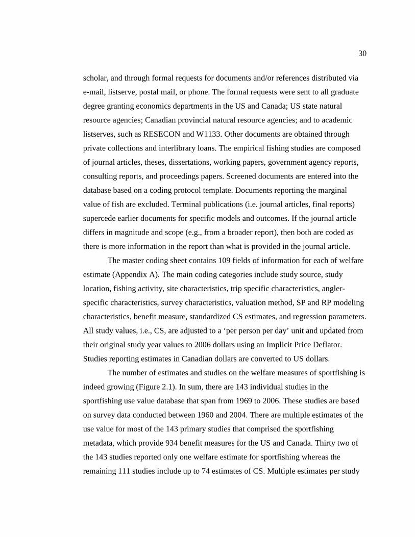
The number of estimates and studies on the welfare measures of sportfishing is
indeed growing (Figure 2.1). In sum, there are 143 individual studies in the
sportfishing use value database that span from 1969 to 2006. These studies are based
on survey data conducted between 1960 and 2004. There are multiple estimates of the
use value for most of the 143 primary studies that comprised the sportfishing
metadata, which provide 934 benefit measures for the US and Canada. Thirty two of
the 143 studies reported only one welfare estimate for sportfishing whereas the
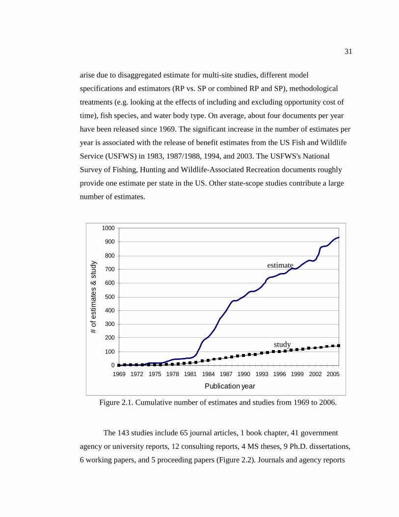
remaining 111 studies include up to 74 estimates of CS. Multiple estimates per study
31
arise due to disaggregated estimate for multi-site studies, different model
specifications and estimators (RP vs. SP or combined RP and SP), methodological
treatments (e.g. looking at the effects of including and excluding opportunity cost of
time), fish species, and water body type. On average, about four documents per year
have been released since 1969. The significant increase in the number of estimates per
year is associated with the release of benefit estimates from the US Fish and Wildlife
Service (USFWS) in 1983, 1987/1988, 1994, and 2003. The USFWS's National
Survey of Fishing, Hunting and Wildlife-Associated Recreation documents roughly
provide one estimate per state in the US. Other state-scope studies contribute a large
number of estimates.
Figure 2.1. Cumulative number of estimates and studies from 1969 to 2006.
The 143 studies include 65 journal articles, 1 book chapter, 41 government
agency or university reports, 12 consulting reports, 4 MS theses, 9 Ph.D. dissertations,
6 working papers, and 5 proceeding papers (Figure 2.2). Journals and agency reports
0
100
200
300
400
500
600
700
800
900
1000
1969 1972 1975 1978 1981 1984 1987 1990 1993 1996 1999 2002 2005
Publication year
# of
est
imat
es &
stu
dy
study
estimate
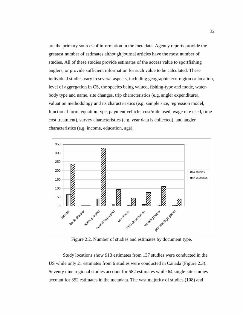
32
are the primary sources of information in the metadata. Agency reports provide the
greatest number of estimates although journal articles have the most number of
studies. All of these studies provide estimates of the access value to sportfishing
anglers, or provide sufficient information for such value to be calculated. These
individual studies vary in several aspects, including geographic eco-region or location,
level of aggregation in CS, the species being valued, fishing-type and mode, water-
body type and name, site changes, trip characteristics (e.g. angler expenditure),
valuation methodology and its characteristics (e.g. sample size, regression model,
functional form, equation type, payment vehicle, cost/mile used, wage rate used, time
cost treatment), survey characteristics (e.g. year data is collected), and angler
characteristics (e.g. income, education, age).
Figure 2.2. Number of studies and estimates by document type.
Study locations show 913 estimates from 137 studies were conducted in the
US while only 21 estimates from 6 studies were conducted in Canada (Figure 2.3).
Seventy nine regional studies account for 582 estimates while 64 single-site studies
account for 352 estimates in the metadata. The vast majority of studies (108) and
0
50
100
150
200
250
300
350
journ
al
book
/chap
ter
agen
cy re
port
cons
ulting
repo
rt
MS th
esis
PhD d
isser
tatio
n
working p
aper
proc
eeding
s pa
per
# studies
# estimates
33
estimates (807) are for freshwater fishing. Out of the 108 studies on freshwater
fishing, about 24 studies reported 330 estimates that did not specify fish species
(reported only as coldwater, coolwater, or warmwater) or reported two or more
freshwater species. Studies reporting coldwater (trout, salmon, steelhead), coolwater
fishing (pike, perch, walleye), and warmwater (bass, chub, catfish) fishing are
considered freshwater fishing in this paper. Among freshwater fish species, trout is the
most studied species (236 estimates), followed by bass (156 estimates).
RP studies (zonal travel cost, individual travel cost and random utility model)
are twice as prevalent as SP studies (open-ended, dichotomous choice, iterative
bidding, payment card, and stated choice). Four hundred eighty six estimates from 101
studies are based on RP methods, 412 estimates from 52 studies are based on SP
methods, and 36 estimates from 6 studies are based on combined SP and RP3. Study
sample sizes ranges from 7 (SP with iterative bidding elicitation method) to 46,008
(random utility model), while survey response rates from the studies ranges from 7%
to100 %.
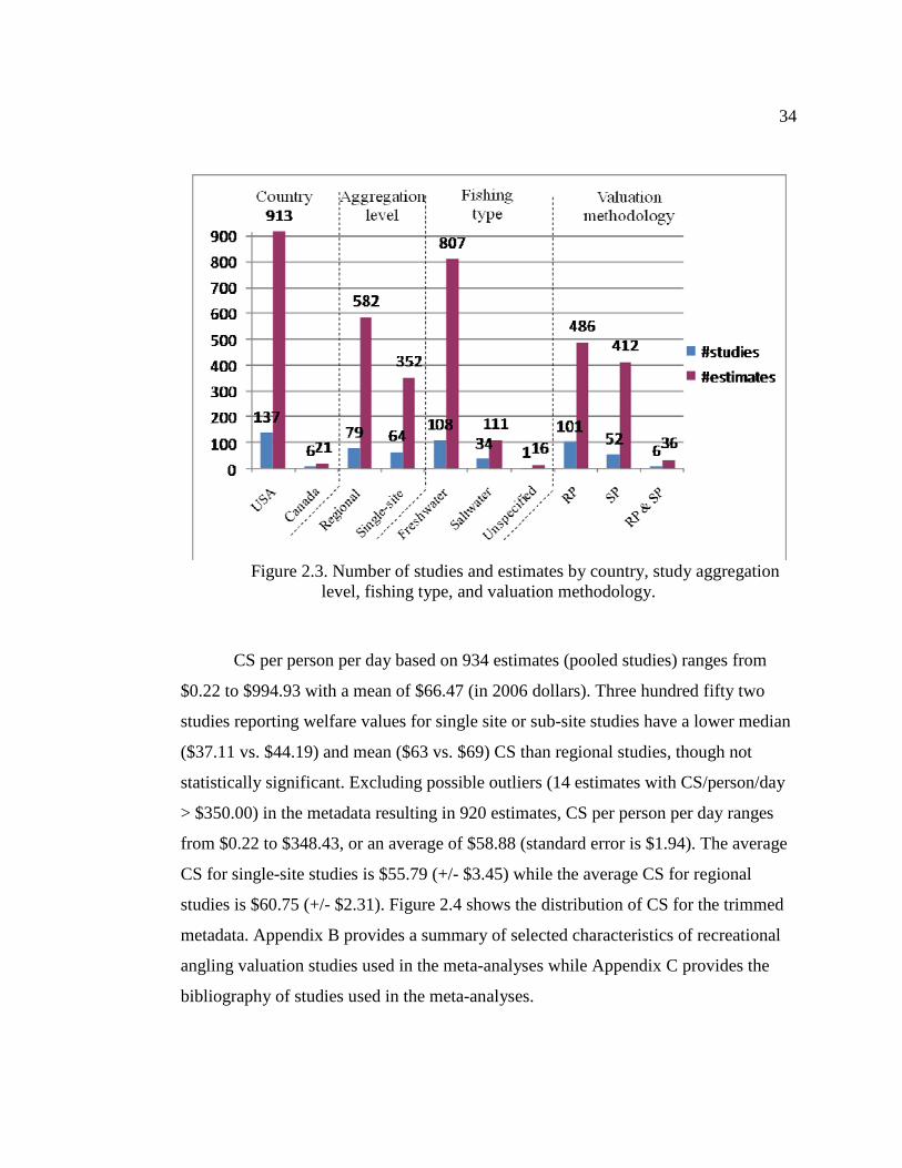
34
Figure 2.3. Number of studies and estimates by country, study aggregation level, fishing type, and valuation methodology.
CS per person per day based on 934 estimates (pooled studies) ranges from
$0.22 to $994.93 with a mean of $66.47 (in 2006 dollars). Three hundred fifty two
studies reporting welfare values for single site or sub-site studies have a lower median
($37.11 vs. $44.19) and mean ($63 vs. $69) CS than regional studies, though not
statistically significant. Excluding possible outliers (14 estimates with CS/person/day
> $350.00) in the metadata resulting in 920 estimates, CS per person per day ranges
from $0.22 to $348.43, or an average of $58.88 (standard error is $1.94). The average
CS for single-site studies is $55.79 (+/- $3.45) while the average CS for regional
studies is $60.75 (+/- $2.31). Figure 2.4 shows the distribution of CS for the trimmed
metadata. Appendix B provides a summary of selected characteristics of recreational
angling valuation studies used in the meta-analyses while Appendix C provides the
bibliography of studies used in the meta-analyses.
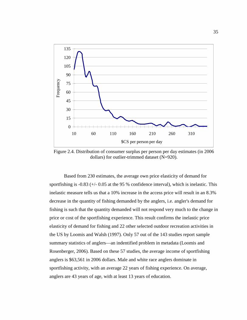
35
Figure 2.4. Distribution of consumer surplus per person per day estimates (in 2006 dollars) for outlier-trimmed dataset (N=920).
Based from 230 estimates, the average own price elasticity of demand for
sportfishing is -0.83 (+/- 0.05 at the 95 % confidence interval), which is inelastic. This
inelastic measure tells us that a 10% increase in the access price will result in an 8.3%
decrease in the quantity of fishing demanded by the anglers, i.e. angler's demand for
fishing is such that the quantity demanded will not respond very much to the change in
price or cost of the sportfishing experience. This result confirms the inelastic price
elasticity of demand for fishing and 22 other selected outdoor recreation activities in
the US by Loomis and Walsh (1997). Only 57 out of the 143 studies report sample
summary statistics of anglers—an indentified problem in metadata (Loomis and
Rosenberger, 2006). Based on these 57 studies, the average income of sportfishing
anglers is $63,561 in 2006 dollars. Male and white race anglers dominate in
sportfishing activity, with an average 22 years of fishing experience. On average,
anglers are 43 years of age, with at least 13 years of education.
0
15
30
45
60
75
90
105
120
135
10 60 110 160 210 260 310
$CS per person per day
Fre
que
ncy
36
Meta-regression model specifications
The meta-valuation function is "an envelope of a set of study site functions that
relates site values to characteristics or attributes associated with each site, including
market characteristics, physical site characteristics, spatial characteristics, and time"
(Rosenberger and Stanley, 2006, p. 374). The MR model is defined as:
iiki Xy εβα ++= Equation (1)
where y is the dependent variable, which is the vector of the natural log of CS
converted to 2006 dollars reported across the individual studies, i which indexes each
observation; X is a matrix of explanatory variables (the identifiable characteristics
among the different studies, like valuation method, etc.) that account for systematic
components explaining the variation in y; ε is a random error component with mean
zero and variance2εσ ; and α (constant term common across all observations) and β are
parameters to be estimated.
Explanatory variables
This subsection describes the explanatory variables of Equation (1) that have
been identified on the basis of theory and findings from the systematic comparison of
the studies listed in Appendix B. Other regressors one would expect to be significant
in the MR models are excluded because they are not reported, missing, or could not be
identified in many of the studies listed in Appendix B. For example, only 57 of the
143 studies report income of anglers. Income is positively related to participation in
outdoor recreation and in general, higher income households tend to participate more
days per year in recreation (Loomis and Walsh, 1997). Exclusion of these variables in
the MR models diminishes the explanatory power of the analysis but will not bias the
estimated coefficients if these variables are uncorrelated with the included set
(Kennedy, 2008).
The relevant explanatory variables are categorized into those characterizing (1)
fishing environment, (2) study methodology, (3) surveyed population and mode, and
(4) study attributes. The fishing environment attributes characterize the fishing and
37
water-body types. Fishing type differentiates fishing experience into freshwater,
saltwater or both. Water body type describes the affected water body or habitat, e.g.,
marine, estuary, lake, Great lakes, river or stream, and mixed-water body type. Study
methodology attributes describes the valuation methodology (RP, SP, or combined RP
& SP). RP variables characterize the RP types (zonal TCM, individual TCM, or
random utility model (RUM)), and if substitute price or quality and time variables are
included in the primary study regressions. SP variables include elicitation method
(open-ended, dichotomous choice, iterative bidding, payment card, and stated choice)
and if a substitute variable is included in the primary study regressions.
Surveyed populations and mode attributes distinguishes the survey type used to
collect data for estimation (mail, in-person, phone, mixed mode, or web-based and
other) and anglers’ visitor types (resident, non-resident, both resident/non-resident,
special interest group, and other). Study attributes describe the benefit unit, trend,
publication in journal, and level of aggregation. The benefit unit compares the
estimates in per day units versus per trip or per season. The trend variable is a proxy
for methodological advances that may have some effect on welfare estimates in
comparison with the rate of inflation over time. The journal variable differentiates
between peer-reviewed journal articles versus other document types such as book
chapters, government/university reports, consulting reports, dissertations, working
papers and proceeding papers. The level of aggregation differentiates between single-
site studies and regional studies as previously defined.
Table 2.1 summarizes the variables included in the analysis. SM and RM differ
in select variables of fishing environment, study methodology, surveyed population,
and literature type. For example, there are more lakes, Great Lakes, and river or
stream resources valued in the SM than RM. Likewise, more RP valuation approaches
were used in SM than RM. There are also more resident visitors and journal literature
in SM than RM. These differences in the sub-metadata are expected to affect the
estimated MR models.
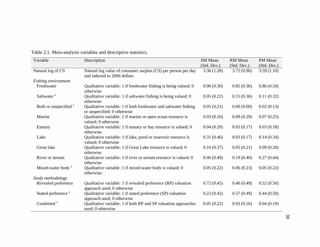
38
Table 2.1. Meta-analysis variables and descriptive statistics.
Variable Description SM Mean (Std. Dev.)
RM Mean (Std. Dev.)
PM Mean (Std. Dev.)
Natural log of CS Natural log value of consumer surplus (CS) per person per day and indexed to 2006 dollars
3.36 (1.28) 3.72 (0.96) 3.59 (1.10)
Fishing environment Freshwater Qualitative variable: 1 if freshwater fishing is being valued; 0
otherwise 0.90 (0.30) 0.85 (0.36) 0.86 (0.34)
Saltwater a Qualitative variable: 1 if saltwater fishing is being valued; 0 otherwise
0.05 (0.22) 0.15 (0.36) 0.11 (0.32)
Both or unspecified a Qualitative variable: 1 if both freshwater and saltwater fishing or unspecified; 0 otherwise
0.05 (0.21) 0.00 (0.00) 0.02 (0.13)
Marine Qualitative variable: 1 if marine or open ocean resource is valued; 0 otherwise
0.03 (0.16) 0.09 (0.29) 0.07 (0.25)
Estuary Qualitative variable: 1 if estuary or bay resource is valued; 0 otherwise
0.04 (0.20) 0.03 (0.17) 0.03 (0.18)
Lake Qualitative variable: 1 if lake, pond or reservoir resource is valued; 0 otherwise
0.31 (0.46) 0.03 (0.17) 0.14 (0.34)
Great lake Qualitative variable: 1 if Great Lake resource is valued; 0 otherwise
0.16 (0.37) 0.05 (0.21) 0.09 (0.28)
River or stream Qualitative variable: 1 if river or stream resource is valued; 0 otherwise
0.40 (0.49) 0.19 (0.40) 0.27 (0.44)
Mixed-water body a Qualitative variable: 1 if mixed-water body is valued; 0 otherwise.
0.05 (0.22) 0.06 (0.23) 0.05 (0.22)
Study methodology Revealed preference Qualitative variable: 1 if revealed preference (RP) valuation
approach used; 0 otherwise 0.72 (0.45) 0.40 (0.49) 0.52 (0.50)
Stated preference a Qualitative variable: 1 if stated preference (SP) valuation approach used; 0 otherwise
0.23 (0.42) 0.57 (0.49) 0.44 (0.50)
Combined a Qualitative variable: 1 if both RP and SP valuation approaches used; 0 otherwise
0.05 (0.22) 0.03 (0.16) 0.04 (0.19)
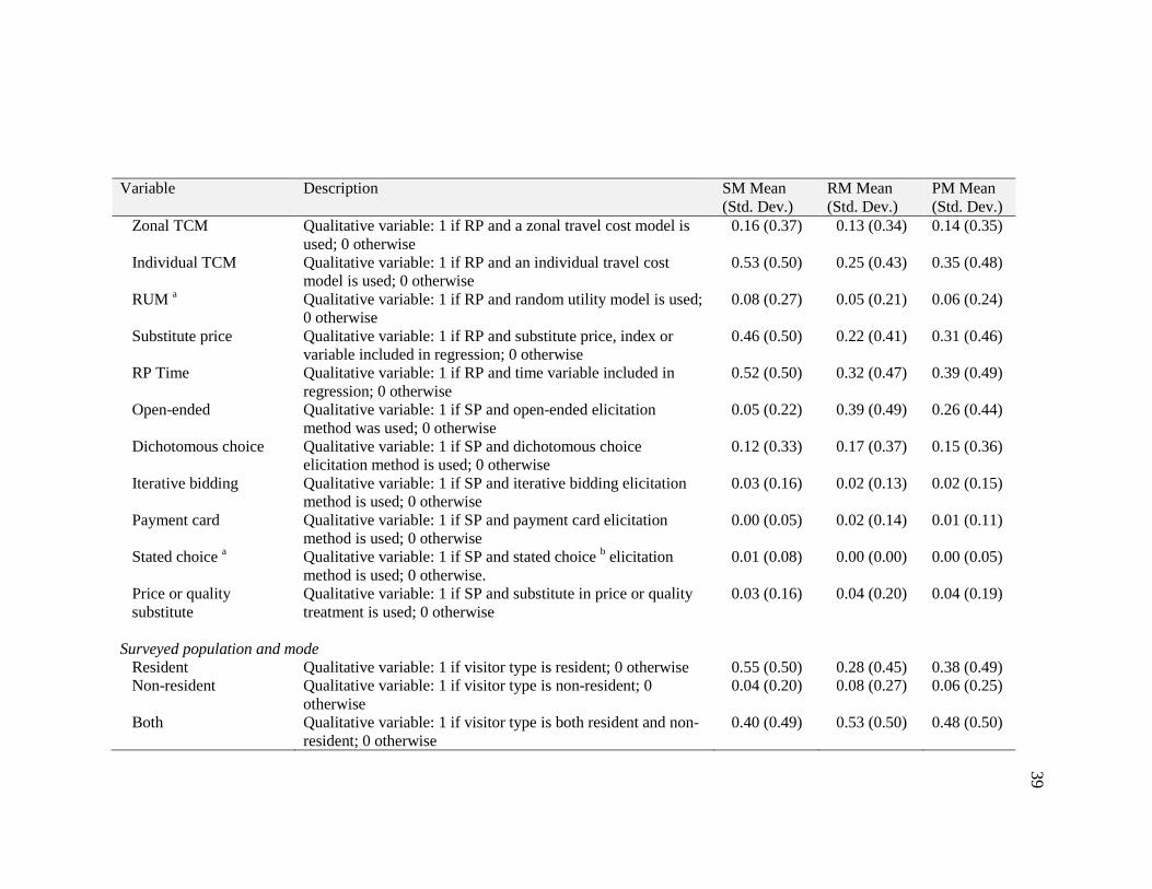
39
Variable Description SM Mean (Std. Dev.)
RM Mean (Std. Dev.)
PM Mean (Std. Dev.)
Zonal TCM Qualitative variable: 1 if RP and a zonal travel cost model is used; 0 otherwise
0.16 (0.37) 0.13 (0.34) 0.14 (0.35)
Individual TCM Qualitative variable: 1 if RP and an individual travel cost model is used; 0 otherwise
0.53 (0.50) 0.25 (0.43) 0.35 (0.48)
RUM a Qualitative variable: 1 if RP and random utility model is used; 0 otherwise
0.08 (0.27) 0.05 (0.21) 0.06 (0.24)
Substitute price Qualitative variable: 1 if RP and substitute price, index or variable included in regression; 0 otherwise
0.46 (0.50) 0.22 (0.41) 0.31 (0.46)
RP Time Qualitative variable: 1 if RP and time variable included in regression; 0 otherwise
0.52 (0.50) 0.32 (0.47) 0.39 (0.49)
Open-ended Qualitative variable: 1 if SP and open-ended elicitation method was used; 0 otherwise
0.05 (0.22) 0.39 (0.49) 0.26 (0.44)
Dichotomous choice Qualitative variable: 1 if SP and dichotomous choice elicitation method is used; 0 otherwise
0.12 (0.33) 0.17 (0.37) 0.15 (0.36)
Iterative bidding Qualitative variable: 1 if SP and iterative bidding elicitation method is used; 0 otherwise
0.03 (0.16) 0.02 (0.13) 0.02 (0.15)
Payment card Qualitative variable: 1 if SP and payment card elicitation method is used; 0 otherwise
0.00 (0.05) 0.02 (0.14) 0.01 (0.11)
Stated choice a Qualitative variable: 1 if SP and stated choice b elicitation method is used; 0 otherwise.
0.01 (0.08) 0.00 (0.00) 0.00 (0.05)
Price or quality substitute
Qualitative variable: 1 if SP and substitute in price or quality treatment is used; 0 otherwise
0.03 (0.16) 0.04 (0.20) 0.04 (0.19)
Surveyed population and mode Resident Qualitative variable: 1 if visitor type is resident; 0 otherwise 0.55 (0.50) 0.28 (0.45) 0.38 (0.49) Non-resident Qualitative variable: 1 if visitor type is non-resident; 0
otherwise 0.04 (0.20) 0.08 (0.27) 0.06 (0.25)
Both
Qualitative variable: 1 if visitor type is both resident and non-resident; 0 otherwise
0.40 (0.49) 0.53 (0.50) 0.48 (0.50)
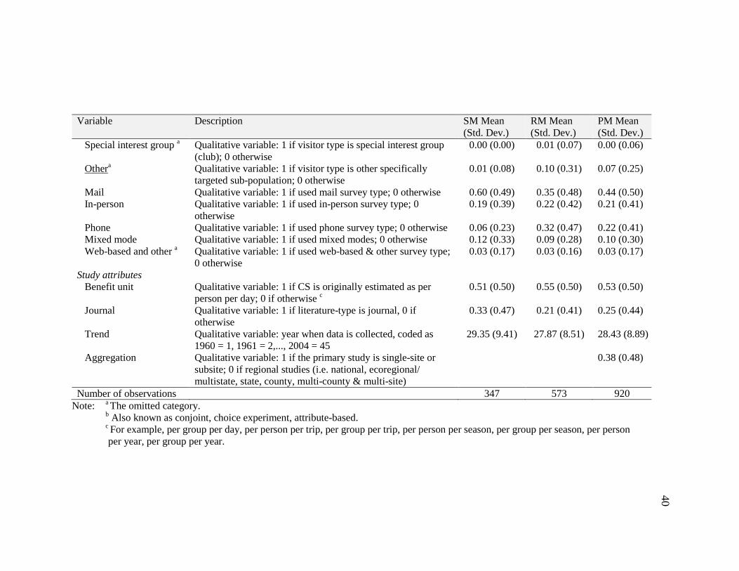
40
Variable Description SM Mean (Std. Dev.)
RM Mean (Std. Dev.)
PM Mean (Std. Dev.)
Special interest group a Qualitative variable: 1 if visitor type is special interest group (club); 0 otherwise
0.00 (0.00) 0.01 (0.07) 0.00 (0.06)
Othera Qualitative variable: 1 if visitor type is other specifically targeted sub-population; 0 otherwise
0.01 (0.08) 0.10 (0.31) 0.07 (0.25)
Mail Qualitative variable: 1 if used mail survey type; 0 otherwise 0.60 (0.49) 0.35 (0.48) 0.44 (0.50) In-person Qualitative variable: 1 if used in-person survey type; 0
otherwise 0.19 (0.39) 0.22 (0.42) 0.21 (0.41)
Phone Qualitative variable: 1 if used phone survey type; 0 otherwise 0.06 (0.23) 0.32 (0.47) 0.22 (0.41) Mixed mode Qualitative variable: 1 if used mixed modes; 0 otherwise 0.12 (0.33) 0.09 (0.28) 0.10 (0.30) Web-based and other a Qualitative variable: 1 if used web-based & other survey type;
0 otherwise 0.03 (0.17) 0.03 (0.16) 0.03 (0.17)
Study attributes Benefit unit Qualitative variable: 1 if CS is originally estimated as per
person per day; 0 if otherwise c 0.51 (0.50) 0.55 (0.50) 0.53 (0.50)
Journal Qualitative variable: 1 if literature-type is journal, 0 if otherwise
0.33 (0.47) 0.21 (0.41) 0.25 (0.44)
Trend Qualitative variable: year when data is collected, coded as 1960 = 1, 1961 = 2,..., 2004 = 45
29.35 (9.41) 27.87 (8.51) 28.43 (8.89)
Aggregation Qualitative variable: 1 if the primary study is single-site or subsite; 0 if regional studies (i.e. national, ecoregional/ multistate, state, county, multi-county & multi-site)
0.38 (0.48)
Number of observations 347 573 920 Note: a The omitted category.
b Also known as conjoint, choice experiment, attribute-based. c For example, per group per day, per person per trip, per group per trip, per person per season, per group per season, per person per year, per group per year.
41
41
Variables such as time, substitutes, and journal warrant some additional
explanation. Primary studies not incorporating time as a separate independent variable
in the demand function may underestimate CS. When time costs are included in the
demand function, anglers who incur larger direct costs or price per trip have an
incentive to increase their length of stay at the site to economize the number of long
distance trips to the site. On the other hand, primary studies not accounting for
substitutes may overestimate CS. Individuals with more choices from available
substitute sites have a flatter negative slope in the demand curve. The inclusion of the
journal variable in the MR model is a preliminary test for possible presence of bias
due to publication selection. A more formal test and correction for publication
selection bias is discussed in the next section. Peer-reviewed literature tends to report
systematically lower WTP estimates for outdoor recreation (Rosenberger and Stanley,
2006). Publication selection is influenced by the publication culture and/or
researchers' self-selections (Rosenberger and Johnston, 2009). Publication bias is
essentially a result of selective sampling, and occurs when studies reporting
statistically significant results or academic work containing positive results are being
published and others are not (Florax, Nijkamp, and Willis, 2002). Because of
publication selection, if only those studies that passed statistical cut-off points are
published, then non-published studies would be excluded from the metadata.
Moreover, many studies (consultancy, government agency reports) undertaken in
economics may not be accessible for quantitative meta-analysis. This situation results
in the inevitable exclusion of a body of valuable information, suppressing information
that may be important or relevant for BT (Smith and Pattanayak, 2002).
Weighting and selection of functional form
When more than one estimate of value is provided by a single study, the study
provides relatively more influence on model results than a study providing a single
estimate of value. Weights may be used to control for unequal influences, such as
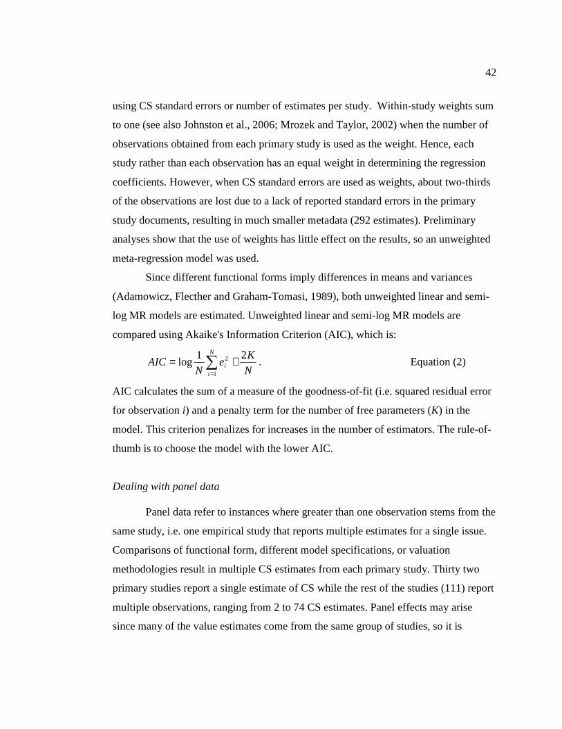
42
using CS standard errors or number of estimates per study. Within-study weights sum
to one (see also Johnston et al., 2006; Mrozek and Taylor, 2002) when the number of
observations obtained from each primary study is used as the weight. Hence, each
study rather than each observation has an equal weight in determining the regression
coefficients. However, when CS standard errors are used as weights, about two-thirds
of the observations are lost due to a lack of reported standard errors in the primary
study documents, resulting in much smaller metadata (292 estimates). Preliminary
analyses show that the use of weights has little effect on the results, so an unweighted
meta-regression model was used.
Since different functional forms imply differences in means and variances
(Adamowicz, Flecther and Graham-Tomasi, 1989), both unweighted linear and semi-
log MR models are estimated. Unweighted linear and semi-log MR models are
compared using Akaike's Information Criterion (AIC), which is:
N
Ke
NAIC
N
ii
21log
1
2 += ∑=
. Equation (2)
AIC calculates the sum of a measure of the goodness-of-fit (i.e. squared residual error
for observation i) and a penalty term for the number of free parameters (K) in the
model. This criterion penalizes for increases in the number of estimators. The rule-of-
thumb is to choose the model with the lower AIC.
Dealing with panel data
Panel data refer to instances where greater than one observation stems from the
same study, i.e. one empirical study that reports multiple estimates for a single issue.
Comparisons of functional form, different model specifications, or valuation
methodologies result in multiple CS estimates from each primary study. Thirty two
primary studies report a single estimate of CS while the rest of the studies (111) report
multiple observations, ranging from 2 to 74 CS estimates. Panel effects may arise
since many of the value estimates come from the same group of studies, so it is
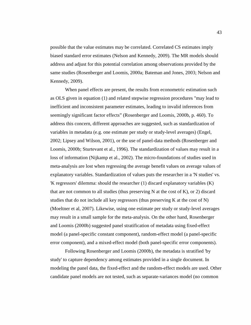
43
possible that the value estimates may be correlated. Correlated CS estimates imply
biased standard error estimates (Nelson and Kennedy, 2009). The MR models should
address and adjust for this potential correlation among observations provided by the
same studies (Rosenberger and Loomis, 2000a; Bateman and Jones, 2003; Nelson and
Kennedy, 2009).
When panel effects are present, the results from econometric estimation such
as OLS given in equation (1) and related stepwise regression procedures "may lead to
inefficient and inconsistent parameter estimates, leading to invalid inferences from
seemingly significant factor effects” (Rosenberger and Loomis, 2000b, p. 460). To
address this concern, different approaches are suggested, such as standardization of
variables in metadata (e.g. one estimate per study or study-level averages) (Engel,
2002; Lipsey and Wilson, 2001), or the use of panel-data methods (Rosenberger and
Loomis, 2000b; Sturtevant et al., 1996). The standardization of values may result in a
loss of information (Nijkamp et al., 2002). The micro-foundations of studies used in
meta-analysis are lost when regressing the average benefit values on average values of
explanatory variables. Standardization of values puts the researcher in a 'N studies' vs.
'K regressors' dilemma: should the researcher (1) discard explanatory variables (K)
that are not common to all studies (thus preserving N at the cost of K), or 2) discard
studies that do not include all key regressors (thus preserving K at the cost of N)
(Moeltner et al, 2007). Likewise, using one estimate per study or study-level averages
may result in a small sample for the meta-analysis. On the other hand, Rosenberger
and Loomis (2000b) suggested panel stratification of metadata using fixed-effect
model (a panel-specific constant component), random-effect model (a panel-specific
error component), and a mixed-effect model (both panel-specific error components).
Following Rosenberger and Loomis (2000b), the metadata is stratified 'by
study' to capture dependency among estimates provided in a single document. In
modeling the panel data, the fixed-effect and the random-effect models are used. Other
candidate panel models are not tested, such as separate-variances model (no common
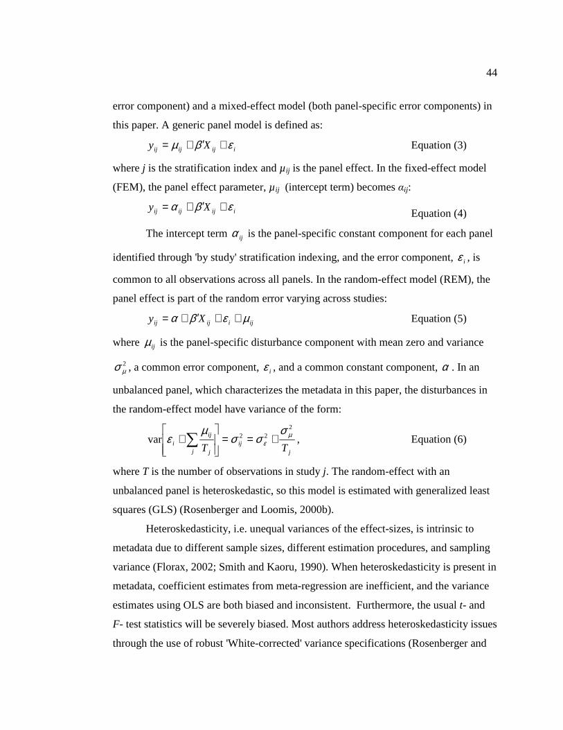
44
error component) and a mixed-effect model (both panel-specific error components) in
this paper. A generic panel model is defined as:
iijijij Xy εβµ +′+= Equation (3)
where j is the stratification index and µij is the panel effect. In the fixed-effect model
(FEM), the panel effect parameter, µij (intercept term) becomes αij:
iijijij Xy εβα +′+= Equation (4)
The intercept term ijα is the panel-specific constant component for each panel
identified through 'by study' stratification indexing, and the error component, iε , is
common to all observations across all panels. In the random-effect model (REM), the
panel effect is part of the random error varying across studies:
ijiijij Xy µεβα ++′+= Equation (5)
where ijµ is the panel-specific disturbance component with mean zero and variance
2µσ , a common error component, iε , and a common constant component, α . In an
unbalanced panel, which characterizes the metadata in this paper, the disturbances in
the random-effect model have variance of the form:
jij
j j
iji TT
222var µε
σσσ
µε +==
+∑ , Equation (6)
where T is the number of observations in study j. The random-effect with an
unbalanced panel is heteroskedastic, so this model is estimated with generalized least
squares (GLS) (Rosenberger and Loomis, 2000b).
Heteroskedasticity, i.e. unequal variances of the effect-sizes, is intrinsic to
metadata due to different sample sizes, different estimation procedures, and sampling
variance (Florax, 2002; Smith and Kaoru, 1990). When heteroskedasticity is present in
metadata, coefficient estimates from meta-regression are inefficient, and the variance
estimates using OLS are both biased and inconsistent. Furthermore, the usual t- and
F- test statistics will be severely biased. Most authors address heteroskedasticity issues
through the use of robust 'White-corrected' variance specifications (Rosenberger and
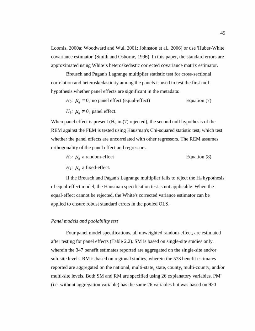
45
Loomis, 2000a; Woodward and Wui, 2001; Johnston et al., 2006) or use 'Huber-White
covariance estimator' (Smith and Osborne, 1996). In this paper, the standard errors are
approximated using White’s heteroskedastic corrected covariance matrix estimator.
Breusch and Pagan's Lagrange multiplier statistic test for cross-sectional
correlation and heteroskedasticity among the panels is used to test the first null
hypothesis whether panel effects are significant in the metadata:
H0: 0=ijµ , no panel effect (equal-effect) Equation (7)
H1: 0≠ijµ , panel effect.
When panel effect is present (H0 in (7) rejected), the second null hypothesis of the
REM against the FEM is tested using Hausman's Chi-squared statistic test, which test
whether the panel effects are uncorrelated with other regressors. The REM assumes
orthogonality of the panel effect and regressors.
H0: ijµ a random-effect Equation (8)
H1: ijµ a fixed-effect.
If the Breusch and Pagan's Lagrange multiplier fails to reject the H0 hypothesis
of equal-effect model, the Hausman specification test is not applicable. When the
equal-effect cannot be rejected, the White's corrected variance estimator can be
applied to ensure robust standard errors in the pooled OLS.
Panel models and poolability test
Four panel model specifications, all unweighted random-effect, are estimated
after testing for panel effects (Table 2.2). SM is based on single-site studies only,
wherein the 347 benefit estimates reported are aggregated on the single-site and/or
sub-site levels. RM is based on regional studies, wherein the 573 benefit estimates
reported are aggregated on the national, multi-state, state, county, multi-county, and/or
multi-site levels. Both SM and RM are specified using 26 explanatory variables. PM-
(i.e. without aggregation variable) has the same 26 variables but was based on 920
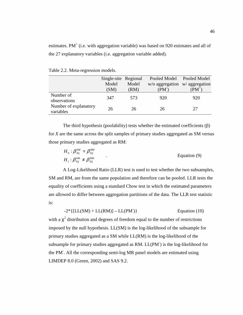
46
estimates. PM+ (i.e. with aggregation variable) was based on 920 estimates and all of
the 27 explanatory variables (i.e. aggregation variable added).
Table 2.2. Meta-regression models.
Single-site Model (SM)
Regional Model (RM)
Pooled Model w/o aggregation
(PM-)
Pooled Model w/ aggregation
(PM+) Number of observations
347 573 920 920
Number of explanatory variables
26 26 26 27
The third hypothesis (poolability) tests whether the estimated coefficients (β)
for X are the same across the split samples of primary studies aggregated as SM versus
those primary studies aggregated as RM:
RMXij
SMXij
RMXij
SMXij
H
H
ββ
ββ
≠
=
:
:
1
0 . Equation (9)
A Log-Likelihood Ratio (LLR) test is used to test whether the two subsamples,
SM and RM, are from the same population and therefore can be pooled. LLR tests the
equality of coefficients using a standard Chow test in which the estimated parameters
are allowed to differ between aggregation partitions of the data. The LLR test statistic
is:
-2*{[LL(SM) + LL(RM)] – LL(PM -)} Equation (10)
with a χ2 distribution and degrees of freedom equal to the number of restrictions
imposed by the null hypothesis. LL(SM) is the log-likelihood of the subsample for
primary studies aggregated as a SM while LL(RM) is the log-likelihood of the
subsample for primary studies aggregated as RM. LL(PM-) is the log-likelihood for
the PM-. All the corresponding semi-log MR panel models are estimated using
LIMDEP 8.0 (Green, 2002) and SAS 9.2.
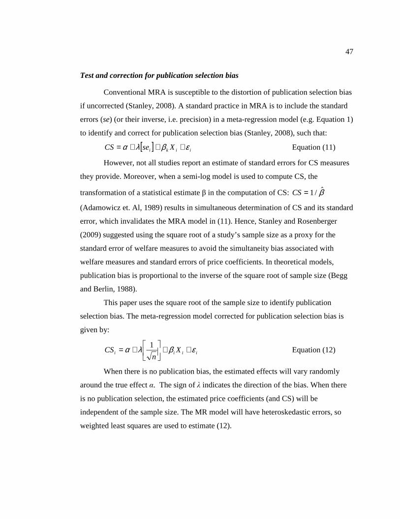
47
Test and correction for publication selection bias
Conventional MRA is susceptible to the distortion of publication selection bias
if uncorrected (Stanley, 2008). A standard practice in MRA is to include the standard
errors (se) (or their inverse, i.e. precision) in a meta-regression model (e.g. Equation 1)
to identify and correct for publication selection bias (Stanley, 2008), such that:
[ ] iiki XseCS εβλα +++= Equation (11)
However, not all studies report an estimate of standard errors for CS measures
they provide. Moreover, when a semi-log model is used to compute CS, the
transformation of a statistical estimate β in the computation of CS: CS= 1/ $β
(Adamowicz et. Al, 1989) results in simultaneous determination of CS and its standard
error, which invalidates the MRA model in (11). Hence, Stanley and Rosenberger
(2009) suggested using the square root of a study’s sample size as a proxy for the
standard error of welfare measures to avoid the simultaneity bias associated with
welfare measures and standard errors of price coefficients. In theoretical models,
publication bias is proportional to the inverse of the square root of sample size (Begg
and Berlin, 1988).
This paper uses the square root of the sample size to identify publication
selection bias. The meta-regression model corrected for publication selection bias is
given by:
iiii Xn
CS εβλα ++
+= 1 Equation (12)
When there is no publication bias, the estimated effects will vary randomly
around the true effect α. The sign of λ indicates the direction of the bias. When there
is no publication selection, the estimated price coefficients (and CS) will be
independent of the sample size. The MR model will have heteroskedastic errors, so
weighted least squares are used to estimate (12).
48
Model Results and Discussion
Unweighted linear and semi-log MR models are estimated according to the
variables listed in Table 2.1. The MR models are based on 140 original primary
studies reporting 920 estimates. The unweighted semi-log model has a lower AIC than
the linear model (2.79 vs. 10.76), so semi-log is chosen as the appropriate functional
form. As noted in Table 2.1, the dependent variable is the natural log of CS per person
per day, indexed to 2006 dollars while the independent variables4 are all linear,
resulting in a semi-log functional form. The semi-log functional form is chosen over
linear functional form because a) it fits well to the data by its ability to capture
curvature in the valuation function and b) allows explanatory variables to influence CS
in a multiplicative rather than an additive manner (Johnston et al., 2006).
The sportfishing metadata is stratified 'by study.' An unbalanced panel exists in
the sportfishing metadata since the number of observations (CS estimates) is not
constant across all studies. The number of panels (j) is 140, with each study being
indexed as a panel. The number of estimates per panel (i) ranges from 1 to 74, with
mean of 6.53 estimates and median of 3 estimates. Table 2.3 provides the result of
hypotheses test for the panel effects following the ‘by study’ stratification. For the first
hypothesis, the Lagrange multiplier statistic of 469.31 rejects the equal-effect model in
favor of a panel effect (p-value <0.01). For the second hypothesis, the Hausman test is
not successful in LIMDEP. In the literature, REM is preferred in meta-analysis over
FEM on statistical grounds. Nelson and Kennedy (2009) suggest that RE is the
appropriate model to be used because the degrees in freedom are retained in REM than
FEM resulting in more efficient estimates. The FEM has disadvantages that may limit
its applications, such as: 1) if perfect correlation exists between dummy variables, then
the slope of those moderator variables cannot be estimated; and 2) FE software will
eliminate observations from primary studies reporting only one estimate. Therefore,
unweighted REM is used as the appropriate specification for the MR models.
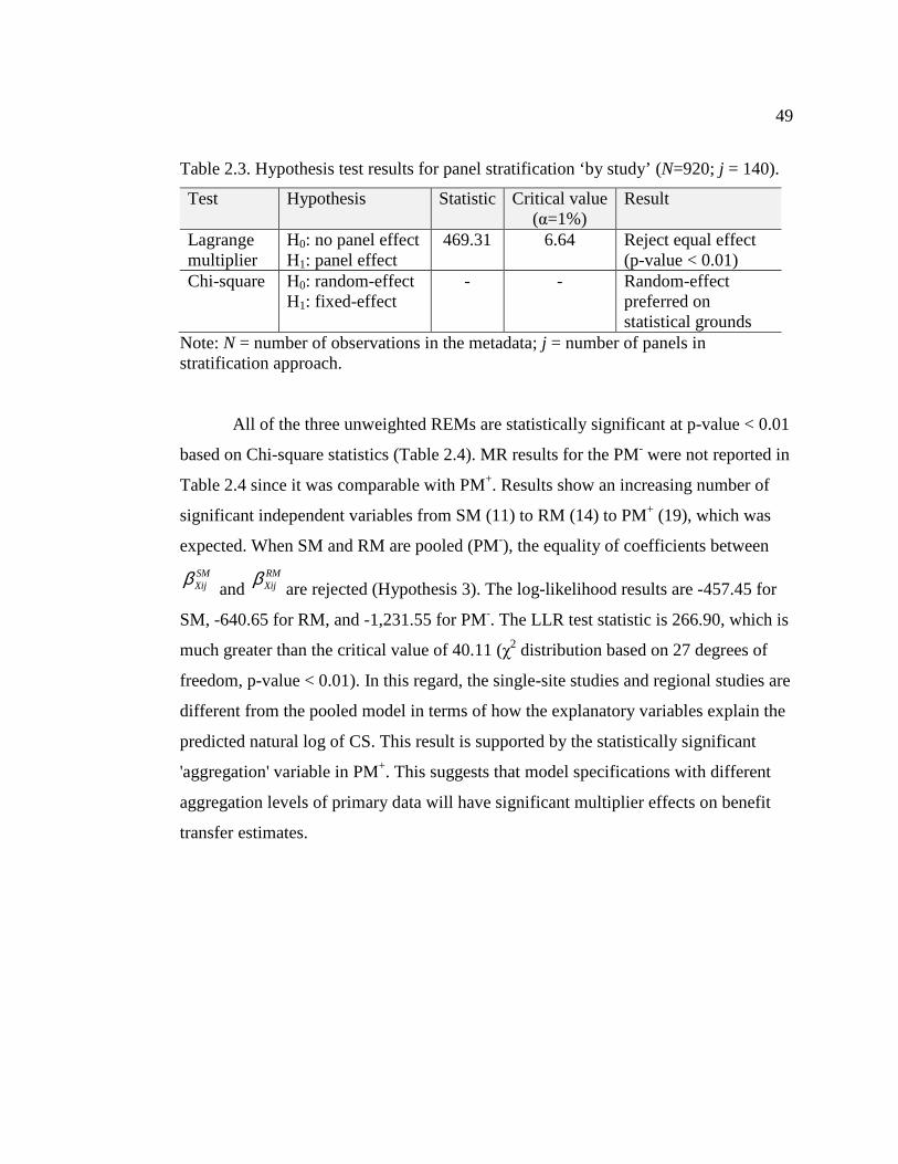
49
Table 2.3. Hypothesis test results for panel stratification ‘by study’ (N=920; j = 140).
Test Hypothesis Statistic Critical value (α=1%)
Result
Lagrange multiplier
H0: no panel effect H1: panel effect
469.31 6.64 Reject equal effect (p-value < 0.01)
Chi-square H0: random-effect H1: fixed-effect
- - Random-effect preferred on statistical grounds
Note: N = number of observations in the metadata; j = number of panels in stratification approach.
All of the three unweighted REMs are statistically significant at p-value < 0.01
based on Chi-square statistics (Table 2.4). MR results for the PM- were not reported in
Table 2.4 since it was comparable with PM+. Results show an increasing number of
significant independent variables from SM (11) to RM (14) to PM+ (19), which was
expected. When SM and RM are pooled (PM-), the equality of coefficients between
SMXijβ
and RMXijβ
are rejected (Hypothesis 3). The log-likelihood results are -457.45 for
SM, -640.65 for RM, and -1,231.55 for PM-. The LLR test statistic is 266.90, which is
much greater than the critical value of 40.11 (χ2 distribution based on 27 degrees of
freedom, p-value < 0.01). In this regard, the single-site studies and regional studies are
different from the pooled model in terms of how the explanatory variables explain the
predicted natural log of CS. This result is supported by the statistically significant
'aggregation' variable in PM+. This suggests that model specifications with different
aggregation levels of primary data will have significant multiplier effects on benefit
transfer estimates.
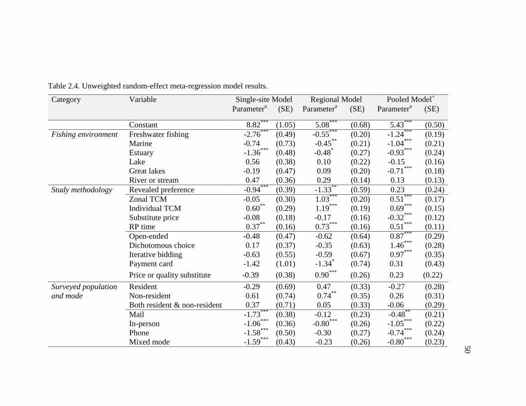
50
Table 2.4. Unweighted random-effect meta-regression model results.
Category Variable Single-site Model Regional Model Pooled Model+ Parametera (SE) Parametera (SE) Parametera (SE)
Constant 8.82*** (1.05) 5.08*** (0.68) 5.43*** (0.50) Fishing environment Freshwater fishing -2.76*** (0.49) -0.55*** (0.20) -1.24*** (0.19)
Marine -0.74 (0.73) -0.45** (0.21) -1.04*** (0.21) Estuary -1.36*** (0.48) -0.48* (0.27) -0.93*** (0.24) Lake 0.56 (0.38) 0.10 (0.22) -0.15 (0.16) Great lakes -0.19 (0.47) 0.09 (0.20) -0.71*** (0.18) River or stream 0.47 (0.36) 0.29 (0.14) 0.13 (0.13)
Study methodology Revealed preference -0.94*** (0.39) -1.33** (0.59) 0.23 (0.24) Zonal TCM -0.05 (0.30) 1.03*** (0.20) 0.51*** (0.17) Individual TCM 0.60** (0.29) 1.19*** (0.19) 0.69*** (0.15) Substitute price -0.08 (0.18) -0.17 (0.16) -0.32*** (0.12) RP time 0.37** (0.16) 0.73*** (0.16) 0.51*** (0.11) Open-ended -0.48 (0.47) -0.62 (0.64) 0.87*** (0.29) Dichotomous choice 0.17 (0.37) -0.35 (0.63) 1.46*** (0.28) Iterative bidding -0.63 (0.55) -0.59 (0.67) 0.97*** (0.35) Payment card -1.42 (1.01) -1.34* (0.74) 0.31 (0.43)
Price or quality substitute -0.39 (0.38) 0.90*** (0.26) 0.23 (0.22)
Surveyed population and mode
Resident -0.29 (0.69) 0.47 (0.33) -0.27 (0.28) Non-resident 0.61 (0.74) 0.74** (0.35) 0.26 (0.31) Both resident & non-resident 0.37 (0.71) 0.05 (0.33) -0.06 (0.29) Mail -1.73*** (0.38) -0.12 (0.23) -0.48** (0.21) In-person -1.06*** (0.36) -0.80*** (0.26) -1.05*** (0.22) Phone -1.58*** (0.50) -0.30 (0.27) -0.74*** (0.24) Mixed mode -1.59*** (0.43) -0.23 (0.26) -0.80*** (0.23)
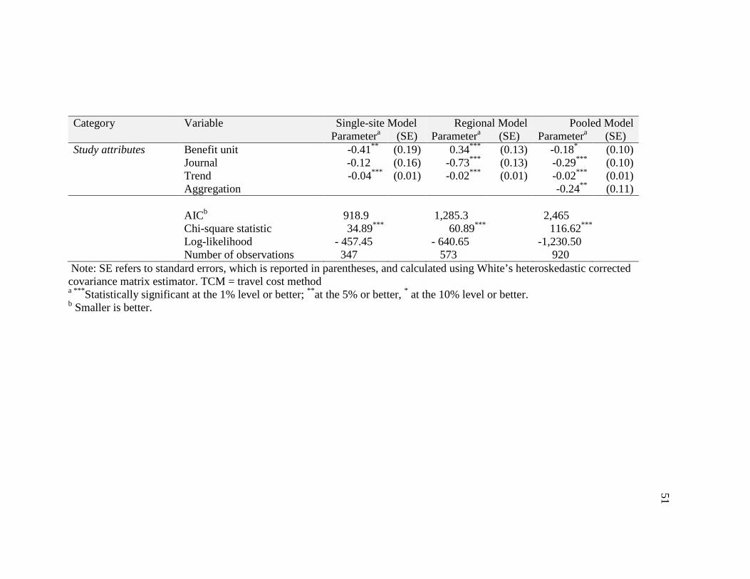
51
Category Variable Single-site Model Regional Model Pooled Model Parametera (SE) Parametera (SE) Parametera (SE)
Study attributes Benefit unit -0.41** (0.19) 0.34*** (0.13) -0.18* (0.10) Journal -0.12 (0.16) -0.73*** (0.13) -0.29*** (0.10) Trend -0.04*** (0.01) -0.02*** (0.01) -0.02*** (0.01) Aggregation -0.24** (0.11) AICb 918.9 1,285.3 2,465 Chi-square statistic 34.89*** 60.89*** 116.62*** Log-likelihood - 457.45 - 640.65 -1,230.50 Number of observations 347 573 920
Note: SE refers to standard errors, which is reported in parentheses, and calculated using White’s heteroskedastic corrected covariance matrix estimator. TCM = travel cost method a *** Statistically significant at the 1% level or better; ** at the 5% or better, * at the 10% level or better. b Smaller is better.
52
Influence of fishing environment
Freshwater fishing is negative and significant in the three MR models,
meaning that if freshwater fishing is valued, it yields lower estimates than saltwater
fishing or both freshwater and saltwater fishing combined. This result may be a
function of the underlying metadata since freshwater fishing studies account for 86%
of all the observations in the metadata. When marine is valued, it is significant in RM
and PM+, and yields lower estimates than mixed-water body. Estuary is negative and
significant for the three MR models. Great lakes variable is negative and significant
only in PM+, meaning that fishing in Great lakes yield higher estimates than fishing in
mixed-water body. Lake and river or stream variables are not statistically significant.
Influence of study methodology
Revealed preference is negative and significant in SM and RM, but not in PM+,
suggesting that lower benefit estimates are associated with RP methods when
compared with SP and combined RP/SP methods, which is not consistent with
Rosenberger and Loomis (2000a). The use of a zonal TCM in RP models is positive
and significant in RM and PM+, implying that it produces higher benefit estimates
than other valuation techniques. Moreover, the use of individual TCM in RP models is
positive and significant for all the three MR models estimated, meaning that it
produces a higher benefit estimate than other valuation techniques, which is consistent
with Shrestha and Loomis (2003), and Zandersen and Tol (2009). The inclusion of
substitute price, index or variable in RP models is negative and significant in PM+,
signifying that the when RP models correctly reflect the substitute variable, the
associated benefit estimate is lower (Rosenthal, 1987). Moreover, the inclusion of time
variable (not in $) in a regression increases the benefit estimate, which is not
consistent with Rosenberger and Loomis (2000a) and Shrestha and Loomis (2003).
The use of an open-ended elicitation method in SP models is significant and positive
53
in PM, implying that it produces a higher benefit estimates than other elicitation
methods. The same result can be said for dichotomous choice and iterative bidding
elicitation methods. On the other hand, the use of payment card in SP models
produces a significant increase in benefit estimate in RM than other elicitation
methods. Finally, the inclusion of substitute in SP models is significant and positive
in RM.
Influence of surveyed population and mode
When a non-resident visitor is coded in the RM, it produces a higher benefit
estimates than other visitor types. Resident and both resident/nonresident variables are
not statistically significant among the three MR models. The use of mail, in-person,
phone or mixed-mode appears to lower benefit estimates than other survey types (SM
and PM+). Only in-person variable was significant in RM for the survey types.
Influence of study attributes
Benefit unit is negative and significant in SM and PM+, suggesting that if the
original study estimated benefits in units such as per trip or per season, then this
tended to yield higher per day estimates than those already reported in activity day
units. On the other hand, it was positive and significant in RM. There is a significant
and negative effect on use value estimates when a dummy variable identifying those
estimates published in journals is added to the regional model, which is consistent
with Rosenberger and Stanley (2006)5. In other fishing MRA (Johnston et al. 20061),
the journal variable was not significant. The trend variable is significant and negative
for the three MR models, indicating that specific CS have generally decreased at a
greater rate than inflation over time, contrary to Rosenberger and Loomis (2001). This
is expected since researchers over time develop more prudent survey designs leading
to lower benefit measures (Johnston et al., 2005). The aggregation variable is

54
significant in PM+ (p≤0.05), meaning that if primary study is aggregated on a single-
site or sub-site level, it has negative effect on benefit estimates than when a primary
study is aggregated on a national, eco-regional/multi-state, state, county, multi-county
or multi-site level. This finding confirms the result above that the single-site and
regional sub-metadata are one of the many important sub-groups representing different
populations.
To investigate the impact of different sub-metadata on the MR model, selected
explanatory variables in the PM+ are intersected with the aggregation variable. These
intersections in the MR model accounted for structural differences between the sub-
metadata. Intersected variables that have no statistical significance are dropped,
signifying that the sub-metadata is structurally similar for that variable. Interpretations
of the coefficients in Table 2.5 are the same as in Table 2.4. When interpreting the
coefficients with a sub-metadata, the original variable measures the general effect of
the unspecified group. For example, the single-site studies aggregation effects are
measured by aggregation*freshwater fishing, aggregation*estuary, and
aggregation*mail coefficients while the original variable coefficient (aggregation)
measures the effect of the omitted metadata sample (regional site studies).
The coefficients for aggregation and aggregation*freshwater fishing are of the
opposite sign, though the magnitude of the coefficients are not statistically different
from each other. In this regard, single-site studies are more likely to provide smaller
CS estimates when reporting for freshwater fishing (aggregation*freshwater). In the
same way, aggregation*estuary is negative and statistically significant, suggesting a
negative relationship with CS estimates. Single-site studies that included time variable
in regression (aggregation*RP time) are more likely to provide smaller CS estimates.
Likewise, single-site studies that surveyed resident visitors (aggregation*resident) or
used mail survey type (aggregation*mail) are more likely to provide smaller CS
estimates. On the other hand, the coefficients for journal and aggregation* journal
were of the opposite sign, suggesting a positive relationship with CS estimates.
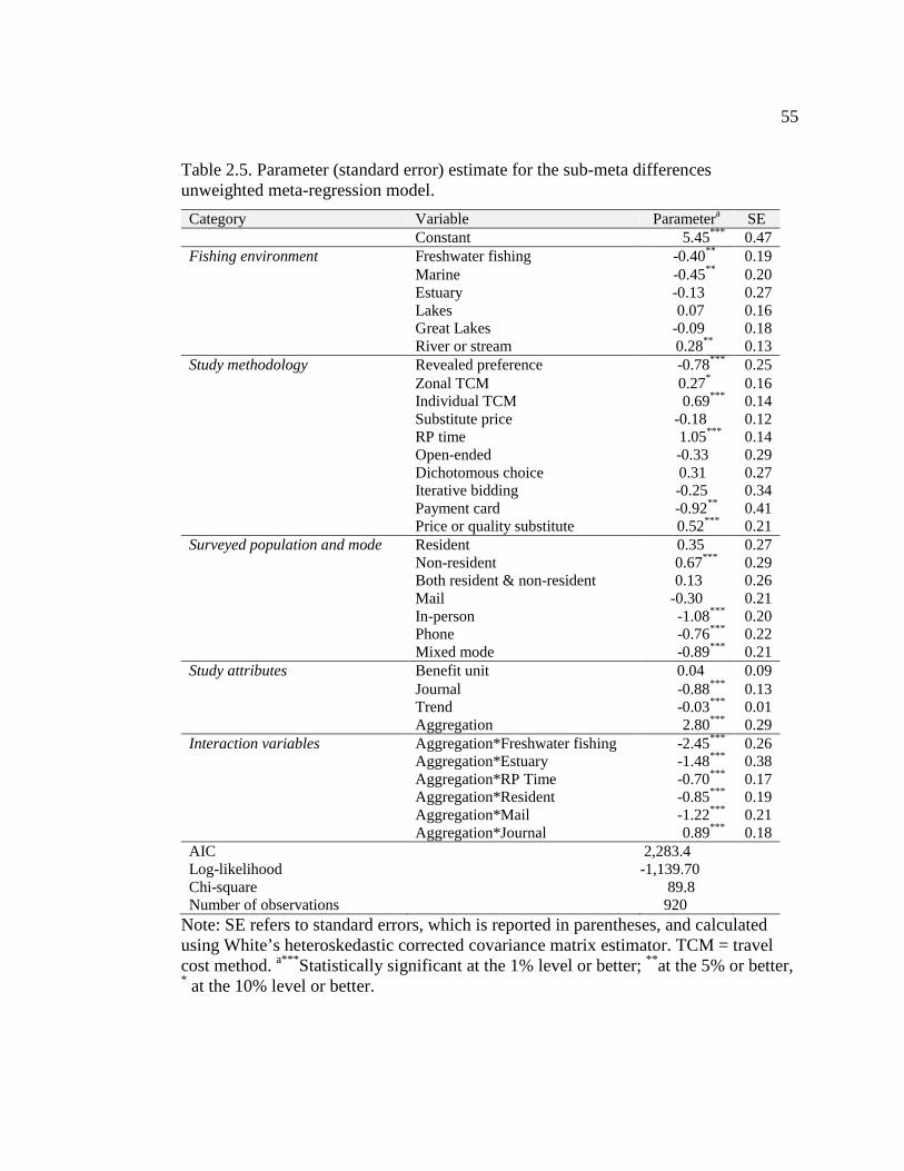
55
Table 2.5. Parameter (standard error) estimate for the sub-meta differences unweighted meta-regression model.
Category Variable Parametera SE Constant 5.45*** 0.47 Fishing environment Freshwater fishing -0.40** 0.19
Marine -0.45** 0.20 Estuary -0.13 0.27 Lakes 0.07 0.16 Great Lakes -0.09 0.18 River or stream 0.28** 0.13
Study methodology Revealed preference -0.78*** 0.25 Zonal TCM 0.27* 0.16 Individual TCM 0.69*** 0.14 Substitute price -0.18 0.12 RP time 1.05*** 0.14 Open-ended -0.33 0.29 Dichotomous choice 0.31 0.27 Iterative bidding -0.25 0.34 Payment card -0.92** 0.41 Price or quality substitute 0.52*** 0.21
Surveyed population and mode Resident 0.35 0.27 Non-resident 0.67*** 0.29 Both resident & non-resident 0.13 0.26 Mail -0.30 0.21 In-person -1.08*** 0.20 Phone -0.76*** 0.22 Mixed mode -0.89*** 0.21
Study attributes Benefit unit 0.04 0.09 Journal -0.88*** 0.13 Trend -0.03*** 0.01 Aggregation 2.80*** 0.29
Interaction variables Aggregation*Freshwater fishing -2.45*** 0.26 Aggregation*Estuary -1.48*** 0.38 Aggregation*RP Time -0.70*** 0.17 Aggregation*Resident -0.85*** 0.19 Aggregation*Mail -1.22*** 0.21 Aggregation*Journal 0.89*** 0.18
AIC 2,283.4 Log-likelihood -1,139.70 Chi-square 89.8 Number of observations 920
Note: SE refers to standard errors, which is reported in parentheses, and calculated using White’s heteroskedastic corrected covariance matrix estimator. TCM = travel cost method. a*** Statistically significant at the 1% level or better; ** at the 5% or better, * at the 10% level or better.
56
Publication Selection Bias
This section addresses the question, Is publication selection likely to cause
large biases in the sportfishing literature? If such publication selection bias exists, the
result of the root-n estimate can give us a ‘better’ true effect estimate and direction of
bias (Stanley and Rosenberger, 2009). The root-n MRA of sportfishing values, shown
in Table 2.6, is estimated using Equation (12) discussed above. Recall that the raw
average CS is $58.88 per person per day (in 2006 dollars), with a standard error of +/-
$1.94. The estimated true effect (α), i.e. the magnitude of the empirical effect
corrected for publication selection, is $98.42, with a standard error of +/- $26.12,
which is statistically different and higher CS estimate than the sportsfishing literature
mean of $58.88. There is also evidence of downward bias among sportfishing values
(λ is negative, t=3.33). By this MRA estimate, a study that uses 100 observations
underestimates CS by $10.31, while 10,000 observations imply an understatement by
$1.03. Hence, sportfishing values reported for studies included in the analysis for this
paper may be systematically underestimated.
Benefit Transfer Comparison
The results from SM, RM, and PM+, referred to as meta-regression benefit
transfer functions, are applied to predict out-of-sample CS per person per day values.
Out-of sample original CS are obtained from sportfishing valuation studies in North
America that have become available after the estimation of MRBT functions or studies
not included in the metadata. If the original benefit estimates are not reported in per
person per day, they are converted to CS per person per day. All original benefit
estimates are adjusted to 2006 US dollars using an implicit price deflator.

57
Table 2.6. Root-n meta-regression analysis of sportfishing values.
Category Variable ParameteraSE True effect α 98.42*** (26.12) Direction of bias λ -103.06*** (30.96) Fishing environment
Freshwater -68.11*** (14.93) Marine -34.53* (18.22) Estuary -54.13** (23.09) Lakes -31.71*** (7.22) Great Lakes -37.09*** (8.33) Rivers or stream 0.49 (5.47)
Study methodology Revealed Preference 56.85*** (9.82) Zonal TCM 22.81** (11.28) Individual TCM 19.77* (11.04) RP Substitute -8.94 (7.36) Open-ended 57.67*** (18.11) Dichotomous choice 68.73*** (16.89) Iterative bidding 71.74*** (20.21) Payment Card -13.28 (18.12) SP Substitute 38.07*** (11.65)
Surveyed population and mode
Resident -33.40*** (11.73) Non-resident 7.26 (16.32) Both resident and non-resident -44.44*** (11.49) Mail -7.09 (13.74) In-person -35.90*** (13.66) Phone -28.04** (13.54) Mixed-mode -19.73 (15.29)
Study attributes Benefit unit -1.69 (5.50) Journal 2.19 (6.38) Trend 0.95*** (0.34) Aggregation 3.66 (7.33)
F-statistic 10.75 Adjusted-R2 0.24 Log-likelihood -4,470.23 Number of observations 833
Note: SE refers to standard errors, which is reported in parentheses, and calculated using White’s heteroskedastic corrected covariance matrix estimator. TCM = travel cost method a*** Statistically significant at the 1% level or better; ** at the 5% or better, * at the 10% level or better.
58
The characteristics of the selected non-random out-of sample studies are
reported in Table 2.7. Three estimates from three of five out-of-sample studies belong
to the two-tails of the in-sample CS distribution reported in Figure 2.4. The original
benefit estimates ranges from $1.16 to $294.36. If high and low tails are excluded, the
original benefit estimates ranges from $18.88 to $99.96. CS values computed using
MRBTFs are estimated incorporating out-of-sample study characteristics. To do this,
relevant variables in the MRBT function are set according to the original out-of-
sample study (e.g. if freshwater fishing, this variable was set to 1, 0 otherwise). The
trend variable is set to a number to reflect the year the data is collected. Estimated CS
values using MRBTF are corrected for bias after logarithmic transformation following
Stynes, Peterson, and Rosenthal (1986).
The out-of-sample original CS estimates are compared to the MRBTF
estimated CS values, by computing the percentage difference (γ):
%100*
−=
Originall
OriginalMRBTF
CS
CSCSγ
,
where MRBTFCS is the benefit estimated using the MRBT functions while OriginalCS is
the out-of-sample original benefit estimate. The percentage difference evaluates the
convergence between the CS values estimated through MRBT functions and original
out-of-sample CS values. When the out-of-sample study reports multiple estimates, γ
is computed for each estimated CS values.
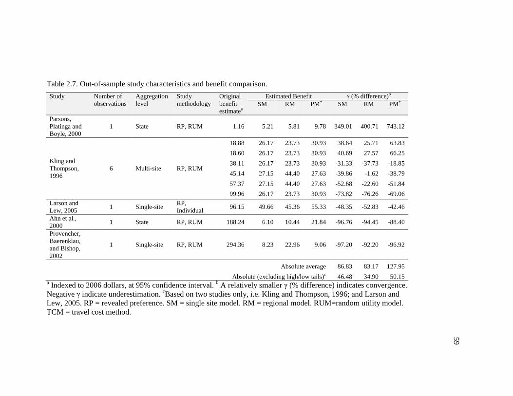
59
Table 2.7. Out-of-sample study characteristics and benefit comparison.
Study Number of observations
Aggregation level
Study methodology
Original benefit estimatea
Estimated Benefit γ (% difference)b SM RM PM+ SM RM PM+
Parsons, Platinga and Boyle, 2000
1 State RP, RUM 1.16 5.21 5.81 9.78 349.01 400.71 743.12
Kling and Thompson, 1996
6 Multi-site RP, RUM
18.88 26.17 23.73 30.93 38.64 25.71 63.83
18.60 26.17 23.73 30.93 40.69 27.57 66.25
38.11 26.17 23.73 30.93 -31.33 -37.73 -18.85
45.14 27.15 44.40 27.63 -39.86 -1.62 -38.79
57.37 27.15 44.40 27.63 -52.68 -22.60 -51.84
99.96 26.17 23.73 30.93 -73.82 -76.26 -69.06
Larson and Lew, 2005
1 Single-site RP, Individual
96.15 49.66 45.36 55.33 -48.35 -52.83 -42.46
Ahn et al., 2000
1 State RP, RUM 188.24 6.10 10.44 21.84 -96.76 -94.45 -88.40
Provencher, Baerenklau, and Bishop, 2002
1 Single-site RP, RUM 294.36 8.23 22.96 9.06 -97.20 -92.20 -96.92
Absolute average 86.83 83.17 127.95
Absolute (excluding high/low tails)c 46.48 34.90 50.15 a Indexed to 2006 dollars, at 95% confidence interval. b A relatively smaller γ (% difference) indicates convergence. Negative γ indicate underestimation. cBased on two studies only, i.e. Kling and Thompson, 1996; and Larson and Lew, 2005. RP = revealed preference. SM = single site model. RM = regional model. RUM=random utility model. TCM = travel cost method.
60
The magnitude of γ is relative upon the original benefit estimate.
Overestimation is of particular concern when original CS values are around $1 per
person per day value. Original CS values falling in the high tail distribution of the in-
sample CS result in underestimation. Excluding high and low tails, the absolute γ
values was 34.90% for RM, 46.48% for SM, and 50.15% for PM+. As expected, RM
predicted closer values of benefits with the out-of-sample CS since most values are
regional estimates. There is no definitive conclusion that can be reached from this
application given small out-of sample observation. Therefore, using certain protocol in
BT applications, either RM or SM is expected to increase the likelihood of producing
the lowest error when there is convergence in the 'study' and 'policy' sites
characteristics. On the other hand, values that are broadly applied to the region cannot
provide specific values for certain local 'policy' question of interest. Indeed, there is a
trade-off associated with this specificity versus generalizability of results.
Conclusions
This paper evaluates aggregation structure of primary research studies and
their implication for benefit transfer using meta-regression analysis. This goal is
accomplished by following the 'best-practice' guidelines for meta-analyses using the
sportfishing valuation studies. Unweighted semi-log model specification is used since
it fits the metadata best. The MR models are also corrected for panel effects using a
random-effect, following by study panel specification.
Three MR models: a single-site model, a regional model, and a pooled model
(combined single-site and regional studies) are compared based on their statistical
significance and predictive power based on out-of-sample error predictions. Structural
shifts in the metadata are mainly attributed to the following variables: freshwater
fishing, estuary, RP time, resident visitors, mail survey type and journal. Based upon
the log-likelihood ratio test result, the two sub-metadata models (single-site and
61
regional) are not from the same population. Overall, the regional model has more
significant explanatory variables than single-site model. Using the out-of-sample
validity test, results reveal that the estimated percent difference using the regional
model is lower than single-site and pooled models. By excluding high/low original CS
values for the transfer studies, the relative performance of the RM model increases
over the other two models; however, with the small set of out-of-sample studies, these
results remain inconclusive as to which model might work best in real-world policy
settings.
Following the ‘best-practice’ guidelines for meta-analysis, this paper shows
that welfare aggregation differences among primary studies influence the direction and
magnitude of biases that are carried forward in benefit transfer applications. In
particular, benefit transfer error depends on the researcher’s choice of primary studies
to include in metadata, model specification, and the unit of welfare aggregation level
to consider. The findings suggest that when doing benefit transfer based on meta-
regression benefit function, researchers should consider the appropriate level of
aggregation. Following certain protocol, it can be said that there is no single
'appropriate' level of aggregation. Depending on the available studies and objectives of
the valuation study, some construct at different levels of aggregation may be better. It
is possible that a particular unit of analysis may be appropriate in some instances.
There remain some challenges in conducting meta-analysis for benefit transfer.
The general lack of reporting about characteristics of the primary study contexts in the
literature, information which may be pertinent for benefit transfers, remains a concern
(Rosenberger and Stanley, 2006). For example, site specific characteristics are rarely
available in the primary valuation studies. Likewise, important socio-economic
variables are not reported in many of the primary studies. There might be other
variables that are significant in explaining the variation in CS values across empirical
studies, which were not reported, but these factors remain as unobserved
heterogeneity. The implication of poor reporting is that conventional and meta-
62
analytic benefit transfers might be improved with more information provided by
primary studies.
Although results indicate that the model's statistical fit is quite good, the
sportfishing metadata is heavily skewed with the abundance of freshwater primary
studies. This possible weakness in the metadata could be alleviated over time by
increasing the number of original primary studies that valued saltwater fishing.
Likewise, standardizing the types of variables to be included and facilitating access to
data from these studies is necessary. It would be interesting for future research if the
same result would come out when additional saltwater fishing studies are appended to
this growing database of sportfishing articles.
63
Notes
1 Welfare estimates are based on marginal value of fish, while this paper is based on
access value of fishing 2 Aggregation, in this paper by Lupi and Feather (1998), refers to the grouping of
individual sites into larger sites. 3 The number of studies employing each valuation methodology does not sum to the
total number of studies because some studies used different valuation methods, from
which multiple observations were derived.
4 Some variables are excluded from the model because data are incomplete or missing
from most studies in the sportfishing metadata. For example, only 57 out of 143
studies reported sample summary statistics of anglers. Some other variables are
excluded because of a clear lack of variations in some of the estimated models. 5
Care is needed in comparing the results. The metadata used in this essay is different
from the metadata in Rosenberger and Stanley (2006) meta-analysis. Rosenberger
and Stanley (2006) tested the publication dummy variables using the Rosenberger
and Loomis (2001) meta-analysis, which include literature review that spans 1967 to
1998 and covers 21 recreation activities plus a category for wilderness recreation.
6 When an OLS unweighted semi-log MR model is used instead of the random-effect
panel MR models, the absolute γ values was 53.69% for PM, 63.46% for SM and
253.09% for RM.
64
References
Ahn S., J.E., De Steiguer, R.B. Palmquist, and T.P. Holmes. Economic Analysis of the Potential Impact of Climate Change on Recreational Trout Fishing in the Southern Appalachian Mountains: An Application of a Nested Multinominal Logit Model. Climate Change 45(2000), 493-509
Adamowicz, W. L., J. J. Fletcher, and T. Graham-Tomasi. "Functional form and the
statistical properties of welfare measures." American Journal of Agricultural Economics 71, no. 2(1989): 414-421.
Bateman, I. J., and A. P. Jones. "Contrasting Conventional with Multi-Level Modeling
Approaches to Meta-Analysis: Expectation Consistency in U.K. Woodland Recreation Values." Land Economics 79, no. 2(2003): 235-258.
Bateman, I. J., et al. "The aggregation of environmental benefit values: Welfare
measures, distance decay and total WTP." Ecological Economics 60, no. 2(2006): 450-460.
Bennear, L. S., R. N. Stavins, and A. F. Wagner. "Using Revealed Preferences to Infer
Environmental Benefits:Evidence from Recreational Fishing Licenses." Journal of Regulatory Economics 28, no. 2(2005): 157-179.
Bergstrom, J. C., and H. K. Cordell. "An analysis of the demand for and value of
outdoor recreation in the United States." Journal of Leisure Research 23, no. 1(1991): 67-86.
Boyle, K. J., and J. C. Bergstrom. "Benefit Transfer Studies: Myths, Pragmatism, and
Idealism." Water Resources Research 28, no. 3(1992): 657–663. Bowes, M. D., and J. B. Loomis. "A Note on the Use of Travel Cost Models with
Unequal Zonal Populations." Land Economics 56(1980): 465-470. Brander, L. M., P. Van Beukering, and H. S. J. Cesar. "The recreational value of coral
reefs: A meta-analysis." Ecological Economics 63, no. 1(2007): 209-218. Brouwer, R. (2002) Environmental value transfer: State of the art and future prospects.
In R. Florax, P. Nijkamp, and K. Willis (Eds). Comparative Environmental Economic Assessment. MA, USA, Edward Elgar Publishing, Inc.
65
Brown, W. G., and F. Nawas. "Impact of Aggregation on the Estimation of Outdoor Recreation Demand Functions." American Journal of Agricultural Economics 55, no. 2(1973): 246.
Engel, S. (2002) Benefit function transfer versus meta-analysis as policy-making
tools: a comparison. In R. Florax, P. Nijkamp, and K. Willis (Eds). Comparative Environmental Economic Assessment. MA, USA, Edward Elgar Publishing, Inc.
Espey, M. "Explaining the variation in elasticity estimates of gasoline demand in the
United States: A meta." Energy Journal 17, no. 3(1996): 49. Fisheries and Oceans Canada (2007). Survey of Recreational Fishing in Canada 2005.
Ottawa, Ontario. Economics Analysis and Statistics Policy Sector. Florax, R. (2002) Methodological Pitfalls in Meta-analysis:Publication Bias. In R.
Florax, P. Nijkamp, and K. Willis (Eds). Comparative Environmental Economic Assessment. MA, USA, Edward Elgar Publishing, Inc.
Florax, R., P. Nijkamp, and K. Willis (2002) Meta-analysis and value transfer:
comparative assessment of scientific knowledge. In R. Florax, P. Nijkamp, and K. Willis (Eds). Comparative Environmental Economic Assessment. MA, USA, Edward Elgar Publishing, Inc.
Florax, R. J. G. M., C. M. Travisi, and P. Nijkamp. "A meta-analysis of the
willingness to pay for reductions in pesticide risk exposure." European Review of Agricultural Economics 32, no. 4(2005): 441-467.
Glass, G. V. "Primary, Secondary, and Meta-Analysis of Research." Educational
Researcher 5, no. 10(1976): 3-8. Greene, W. H. LIMDEP Version 8: Econometric Modelling Guide: Econometric
Software, Inc., 2002. Johnston, R. J., et al. "What Determines Willingness to Pay per Fish? A Meta-
Analysis of Recreational Fishing Values." Marine Resource Economics 21(2006): 1-32.
66
Johnston, R. J., et al. "Systematic Variation in Willingness to Pay for Aquatic Resource Improvements and Implications for Benefit Transfer: A Meta-Analysis." Canadian Journal of Agricultural Economics 53, no. 2-3(2005): 221-248.
Kennedy, P. A. A Guide to Econometrics. 6th ed. Malden, MA Blackwell Publishing,
2008. Kling, C.L. and C.J. Thompson. “The Implications of Model Specification for Welfare
Estimation in Nested Logit Models.” American Journal of Agricultural Economics 78(1996):103-114.
Koteen, J., S. J. Alexander, and J. B. Loomis (2002) Evaluating Benefits and Costs of
Changes in Water Quality, General Technical Report PNW-GTR-548. Portland, Oregon, US Forest Service.
Larson, D. M., and D. K. Lew. "Measuring the utility of ancillary travel: revealed
preferences in recreation site demand and trips taken " Transportation Research Part A: Policy and Practice 39, no. 2-3(2005): 237-255
Lindhjem, H. "20 years of stated preference valuation of non-timber benefits from
Fennoscandian forests: A meta-analysis." Journal of Forest Economics 12, no. 4(2007): 251-277.
Lipsey, M. W., and D. B. Wilson. Practical Meta-Analysis. Applied Social Research
Method Series. Thousand Oaks, California: Sage Publications, Inc., 2000. Loomis, J. B., and D. S. White. "Economic benefits of rare and endangered species:
summary and meta-analysis." Ecological Economics 18, no. 3(1996): 197-206. Loomis, J. B. "Vertically Summing Public Good Demand Curves: An Empirical
Comparison of Economic versus Political Jurisdictions." Land Economics 76, no. 2(2000): 312.
Loomis, J. B., and R. S. Rosenberger. "Reducing barriers in future benefit transfers:
Needed improvements in primary study design and reporting." Ecological Economics 60, no. 2(2006): 343-350.
Loomis, J. B., and R. G. Walsh. Recreation Economic Decisions: Comparing Benefits
and Costs Second ed: Venture Publishing, Inc: State College, Pennsylvania, 1997.
67
Lupi, F., and P. Feather. "Using Partial Site Aggregation to Reduce Bias in Random Utility Travel Cost Models." Water Resources Research 34, no. 12(1998): 3595-3603.
Manley, J., et al. "Creating Carbon Offsets in Agriculture through No-Till Cultivation:
A Meta-Analysis of Costs and Carbon Benefits." Climatic Change 68, no. 1(2005): 41-65.
Moeltner, K., K. J. Boyle, and R. W. Paterson. "Meta-analysis and benefit transfer for
resource valuation-addressing classical challenges with Bayesian modeling." Journal of Environmental Economics and Management 53, no. 2(2007): 250-269.
Moulton, B. R. "Random Group Effects and the Precision of Regression Estimates."
Journal of Econometrics 32(1986): 385-397. Mrozek, J. R., and L. O. Taylor. "What determines the value of life? a meta-analysis."
Journal of Policy Analysis and Management 21, no. 2(2002): 253-270. Nelson, J. P., and P. E. Kennedy. "The Use (and Abuse) of Meta-Analysis in
Environmental and Natural Resource Economics: An Assessment " Environmental and Resource Economics 42(2009): 345-377.
Nijkamp, P., et al. (2002) Environmental quality in European space: a methodology
for research synthesis. In R. Florax, P. Nijkamp, and K. Willis (Eds). Comparative Environmental Economic Assessment. MA, USA, Edward Elgar Publishing, Inc.
Parsons, G. R., A. J. Plantinga, and K. J. Boyle. "Narrow Choice Sets in a Random
Utility Model of Recreation Demand." Land Economics 76, no. 1(2000): 86-99.
Platt, J., and E. Ekstrand (2001) Meta-Analysis of Water Recreation, Report No. EC-
2001-05. Washington, DC, Bureau of Reclamation, US Department of Interior. Pearson, K. "Report on certain enteric fever inoculation statistics." British Medical
Journal 3(1904): 1243-1246. Provencher, B., K.A. Baerenklau, and R.C. Bishop. “A Finite Mixture Logit Model of
Recreational Angling with Serially Correlated Random Utility.” American Journal of Agricultural Economics 84, no. 4(2002):1066-1075.
68
Ready, R., and S. Navrud. "International benefit transfer: Methods and validity tests." Ecological Economics 60, no. 2(2006): 429-434.
Rosenberger, R. S., and J. B. Loomis. "Using meta-analysis for benefit transfer: In-
sample convergent validity tests of an outdoor recreation database." Water Resources Research 36, no. 4(2000a): 1097-1108.
Rosenberger, R. S., and J. B. Loomis. "Panel Stratification in Meta-Analysis of
Economic Studies: An Investigation of Its Effects in the Recreation Valuation Literature." Journal of Agricultural and Applied Economics 32, no. 3(2000b): 459-470.
Rosenberger, R. S., and J. B. Loomis (2001) Benefit transfer of outdoor recreation use
values: A technical document supporting the Forest Service Strategic Plan (2000 revision). Fort Collins, CO, U.S. Department of Agriculture, Forest Service, Rocky Mountain Research Station, pp. 59.
Rosenberger, R. S., and T. T. Phipps (2007) Correspondence and convergence in
benefit transfer accuracy: A meta-analytic review of the literature, ed. S. Navrud, and R. Ready. Environmental Values Transfer: Issues and Methods. Dordrecht, The Netherlands, Kluwer Academic Publishers. pp. 23-43.
Rosenberger, R. S., and T. D. Stanley. "Measurement, generalization, and publication:
Sources of error in benefit transfers and their management." Ecological Economics 60, no. 2(2006): 372-378.
Rosenberger, R. S., and R. J. Johnston. "Selection Effects in Meta-Analysis and
Benefit Transfer: Avoiding Unintended Consequences." Land Economics 85, no. 3(2009): 410-428.
Rosenthal, D. H. "The Necessity for Substitute Prices in Recreation Demand
Analyses." American Journal of Agricultural Economics 69, no. 4(1987): 828. Scheierling, S. M., R. A. Young, and G. E. Cardon. "Public subsidies for water-
conserving irrigation investments: Hydrologic, agronomic, and economic assessment." Water Resources Research 42(2006).
Shadish, W. R., and C. K. Haddock (2009) Combining Estimates of Effect Size. In H.
Cooper, L. V. Hedges, and J. C. Valentine (Eds.) The Handbook of Research Synthesis and Meta-analysis, 2nd Edition. New York, Russell Sage Foundation, pp. 257-277.
69
Shrestha, R. K., and J. B. Loomis. "Meta-Analytic Benefit Transfer of Outdoor Recreation Economic Values: Testing Out-of-Sample Convergent Validity." Environmental and Resource Economics 25, no. 1(2003): 79-100.
Smith, V. K. "Nonmarket valuation of environmental resources: An interpretive
appraisal." Land Economics 69, no. 1(1993): 1-26. Smith, V. K., and Y. Kaoru. "Signals or noise? Explaining the variation in recreation
benefit estimates." American Journal of Agricultural Economics 72, no. 2(1990): 419.
Smith, V. K., and L. L. Osborne. "Do Contingent Valuation Estimates Pass a "Scope"
Test? A Meta-analysis." Journal of Environmental Economics and Management 31, no. 3(1996): 287-301.
Smith, V., and S. Pattanayak. "Is Meta-Analysis a Noah's Ark for Non-Market
Valuation?" Environmental and Resource Economics 22, no. 1(2002): 271-296.
Southwick Associates (2007). Sportfishing in America: An Economic Engine and
Conservation Powerhouse. Produced for the American Sportfishing Association with funding from the Multistate Conservation Grant Program.
Spash, C. L., and A. Vatn. "Transferring environmental value estimates: Issues and
alternatives." Ecological Economics 60, no. 2(2006): 379-388. Stanley, T. D. "Wheat from Chaff: Meta-analysis as Quantitative Literature Review."
Journal of Economic Perspectives 15, no. 3(2001): 131-150. Stanley, T. D. "Meta-Regression Methods for Detecting and Estimating Empirical
Effects in the Presence of Publication Selection." Oxford Bulletin of Economics and Statistics 70, no. 1(2008): 103-127.
Stanley, T. D., and S. B. Jarrell. "Meta-Regression Analysis: A Quantitative method of
Literature Surveys." Journal of Economic Surveys 3, no. 2(1989): 161. Stanley, T. D., and R. S. Rosenberger (2009) Are Recreation Values Systematically
Underestimated? Reducing Publication Selection Bias for Benefit Transfer, Hendrix College and Oregon State University. Working Paper.
70
Stoker, T. M. "Empirical Approaches to the Problem of Aggregation over Individuals." Journal of Economic Literature 31(1993): 1827-1874.
Sturtevant, L. A., F. R. Johnson, and W. H. Desvousges (1996) A Meta-Analysis of
Recreational Fishing, Working Paper, Triangle Economic Research. Stynes, D.J., G.L. Peterson, and D.H. Rosenthal. 1986. "Log Transformation Bias in
Estimating Travel Cost Models." Land Economics 62(1):94-103. Van Houtven, G., J. Powers, and S. K. Pattanayak. "Valuing water quality
improvements in the United States using meta-analysis: Is the glass half-full or half-empty for national policy analysis?" Resource and Energy Economics 29, no. 3(2007): 206-228.
Vaughan, W. J., C. S. Russell, and M. Hazilla. "A Note on the Use of Travel Cost
Models with Unequal Zonal Populations: Comment." Land Economics 58, no. 3(1982): 400-407.
Walsh, R. G., D. M. Johnson, and J. R. McKean. "Issues in Nonmarket Valuation and
Policy Application: A Retrospective Glance." Western Journal of Agricultural Economics 14, no. 1(1989): 178-188.
Woodward, R. T., and Y.-S. Wui. "The economic value of wetland services: a meta-
analysis." Ecological Economics 37, no. 2(2001): 257-270. Zandersen, M., and R. S. J. Tol. "A meta-analysis of forest recreation values in
Europe." Journal of Forest Economics 15, no. 1-2(2009): 109-130.
71
CHAPTER 3 - ESSAY 2 ADDRESSING DEPENDENCY IN THE SPORTSFISHING VALUATIO N LITERATURE: IMPLICATIONS FOR META-REGRESSION ANALYS IS
AND IN-SAMPLE BENEFIT PREDICTION PERFORMANCE
Abstract
The sportfishing literature contains about 140 papers that provide benefit
estimates of the access value for fishing in the United States and Canada. This paper
examines the implications of addressing dependency in the sportsfishing valuation
literature using meta-regression analysis (MRA) and corresponding benefit-transfer
(BT) performance. Meta-analysis is applied to various treatments of data dependency
in the sportsfishing metadata. The ‘all-set’ metadata uses all of the available benefit
measures reported in the primary studies. Two approaches for controlling data
dependency in the ‘all-set’ metadata include weighting of the metadata and using
panel data estimators. Two treatments of the metadata for avoiding dependency
include a ‘best-set’ metadata (comprised of the best available benefit measures
reported in a study as identified by methodological and sample criteria) and an
‘average-set’ metadata (comprised of the average benefit measures reported in the
primary studies). Results show that the model fit is best achieved when the MRA is
based on weighting the ‘all-set’ or using the ‘average-set’, which are complementary
of each other. The weighted ‘all-set’ model resulted in the highest number of
significant variables among the models estimated. Changing the underlying structure
of the metadata changes the magnitude and sign of the estimated parameters of the
fishing environment variables. Results of in-sample BT using jackknife data splitting
technique show median absolute transfer errors of 40% to 48%. The median absolute
percentage transfer error is lower for the meta-regression (MR) models based on a
single value, i.e. ‘average-set’ and ‘best-set’ metadata than the MR models based on
‘all-set.’ Higher transfer error may be explained by dummy variables that are related
to measurement errors and publication selection bias inherent in the primary studies.
72
Introduction
Meta-analysis is an important methodological tool that can generate
meaningful comparative results of empirical data to inform policy decisions. Given its
potential applications, there has been a dramatic increase in the use of meta-analysis
over the past decade. Yet in spite of its potential contribution, Nelson and Kennedy
(2009) noted that new meta-analyses appear to ignore several basic methodological
and econometric issues that would define a complete and rigorous analysis. In
particular, several methodological pitfalls may invalidate the conclusions of a meta-
analysis when insufficient attention is given to routine problems encountered when
basic statistical procedures are applied to metadata. Heterogeneity among studies and
dependency among the observed effect sizes in the metadata are two of the
methodological pitfalls that are detrimental to the validity of meta-analysis (Glass et
al., 1981; Florax, 2002). Nelson and Kennedy (2009) emphasized the need to place a
high priority on adjusting for correlated effect-size estimates, both within and between
groups of studies. Awareness of these issues and corrections for possible biases caused
by them will help increase the validity and reliability of meta-analysis results, and be
able to detect the true effect size or true impact of moderator variables.
Heterogeneity in metadata refers to effect size estimates from primary studies
not all estimating the same population effect (Nelson and Kennedy, 2008). There is
heterogeneity in the metadata because of theoretical and modeling perspectives
(valuation method, functional form, research design), behavioral aspect (population
characteristics, income differentials) (Brouwer, 2002; Florax, 2002), and inherent data
characteristics (Stanley and Jarell, 1989). Heterogeneity in primary study variables,
estimated models, and recreation activities limit the parameters that can be included in
meta-analysis, resulting in lower coefficient of determination (R2) and higher error (ε)
in MR models (Engel, 2002), which can be carried forward in BT. Heterogeneity of
metadata may cause biased value estimates in meta-analyses due to underspecification
when used for BT predictions (Boyle and Bergstrom, 1992; Loomis and Rosenberger,
2006) and may limit the ability to measure differences within a population at a higher
73
resolution (Adamowicz and Deshazo, 2006). While heterogeneity is a fact of metadata
and proper specification is important, it is not the focus of this paper.
Dependency or correlation refers to a departure of two random variables from
independence. Correlated effect-size estimates imply biased standard error estimates
(Nelson and Kennedy, 2009). Reasons for correlation include 1) multiple sampling per
study to obtain a sufficient number of observations for meta-analysis (i.e. between
study correlated observations); and 2) researchers reporting more than one benefit
measure for each primary study (i.e. multiple estimates from the same primary
study—within-study autocorrelation). In the sportfishing metadata, the average
number of benefit estimates reported is 6.3 per primary study (median = 3) and range
from one to 74 estimates. When multiple estimates from the same study are recorded
in the metadata, meta-analysis results may be bias due to lack of independence of
observations (Wood, 2008; Strube, 1987; Glass et al., 1981). Failure to adjust for
dependency will inflate the likelihood of Type I error when comparisons are made
across studies. Likewise, dependency will inflate the likelihood of Type II error when
comparisons are made among or between different outcomes within studies (Strube,
1987). To minimize dependency, meta-analysts should use consistently defined
outcome measures (effect-sizes), and similarly defined population characteristics and
research objectives (Florax, Nijkamp, and Willis, 2002), when possible. Consistency
and comparability of primary study outcomes is an important ingredient for a robust
meta-analysis.
Since dependency and heterogeneity are inevitable in metadata, what
approaches should be employed to minimize their effects? Lipsey and Wilson (2000)
suggested two simple approaches to handle these issues. The first approach is to base
the meta-analysis only on the ‘best’ evidence (i.e. selecting a single estimate) while
the second approach is to use a single ‘mean’ value (i.e. taking the average). Other
approaches that have been used to address these issues are panel model estimators
(Rosenberger and Loomis, 2000b; Sturtevant et al., 1996), and hierarchical/multilevel
estimation procedure (Bateman and Jones, 2003; Johnston et al., 2005) on all reported
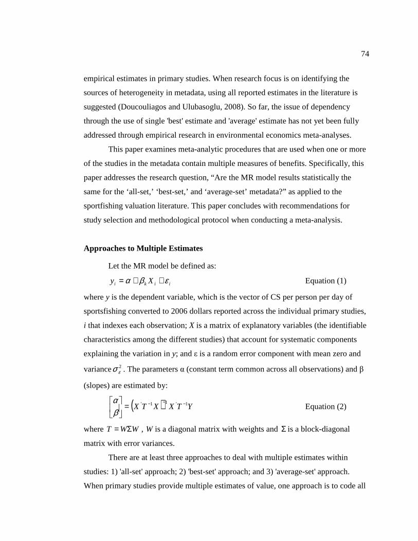
74
empirical estimates in primary studies. When research focus is on identifying the
sources of heterogeneity in metadata, using all reported estimates in the literature is
suggested (Doucouliagos and Ulubasoglu, 2008). So far, the issue of dependency
through the use of single 'best' estimate and 'average' estimate has not yet been fully
addressed through empirical research in environmental economics meta-analyses.
This paper examines meta-analytic procedures that are used when one or more
of the studies in the metadata contain multiple measures of benefits. Specifically, this
paper addresses the research question, “Are the MR model results statistically the
same for the ‘all-set,’ ‘best-set,’ and ‘average-set’ metadata?” as applied to the
sportfishing valuation literature. This paper concludes with recommendations for
study selection and methodological protocol when conducting a meta-analysis.
Approaches to Multiple Estimates
Let the MR model be defined as:
iiki Xy εβα ++= Equation (1)
where y is the dependent variable, which is the vector of CS per person per day of
sportsfishing converted to 2006 dollars reported across the individual primary studies,
i that indexes each observation; X is a matrix of explanatory variables (the identifiable
characteristics among the different studies) that account for systematic components
explaining the variation in y; and ε is a random error component with mean zero and
variance 2εσ . The parameters α (constant term common across all observations) and β
(slopes) are estimated by:
( ) YTXXTX 1'11' −−−=
βα
Equation (2)
where WWT Σ= , W is a diagonal matrix with weights and Σ is a block-diagonal
matrix with error variances.
There are at least three approaches to deal with multiple estimates within
studies: 1) 'all-set' approach; 2) 'best-set' approach; and 3) 'average-set' approach.
When primary studies provide multiple estimates of value, one approach is to code all
75
of the estimates reported in primary studies in the metadata (‘all-set’ metadata),
treating each estimates as independent observations. Independence of studies (and/or
estimates) suggests that the different studies (and/or estimates) included in the
metadata are concerned with different groups of people or with different populations.
When benefit measures are independent from each other, all the covariance terms are
zero and the estimate of the standard deviation of the linear combinations of studies is
based solely on the main diagonal of the variance-covariance matrix (Strube, 1987). In
this approach, all weights equal 1, MIW = , where MI is the identity matrix of order M
x M, and the error at the study level is assumed zero. The parameters, α and β, are
estimated via ordinary least squares (OLS).
However, not all studies are contributing the same number of estimates;
therefore, some form of weighting of the data is required. The use of weights is needed
since studies with many estimates may have a larger effect on the results of the meta-
analysis than studies with fewer estimates (Rosenthal, 1991). In this case, multiple
estimates are treated as independent weighted estimates, where weights are defined
by: JMMw jmj /= , for all =j 1, 2, …, J. When the number of estimates from each
primary study is used as the weight, the within-study weights sum to one (see also
Johnston et al., 2006; Mrozek and Taylor, 2002). Hence, each primary study, rather
than each observation, has an equal weight in determining the regression coefficients.
In other words, the sum of the weights equals the number of estimates reported within
a primary study. Weights are applied by placing the square root of the weights onto
the diagonal of an MxM matrix, thereby forming the diagonal matrix W , with zero's
as off-diagonal elements. The parameters, α and β, are estimated via weighted least
squares (WLS).
Assuming multiple estimates from a single study are independent of each other
is likely a weak assumption that can bias model results (Nelson and Kennedy, 2009).
Panel data methods are one of the recommended approaches to controlling for
dependency in metadata (Rosenberger and Loomis, 2000b; Sturtevant et al., 1996). A
general panel meta- regression model is written as:
76
ijijkji Xy εβα ++= Equation (3)
where j is the stratification index. Essay 1 provides a detailed discussion of the panel
methods and associated hypotheses tests.
With current reporting practices, estimates of covariances are generally not
given or difficult to estimate, implying greater difficulty for controlling dependency in
the presence of multiple estimates. Thus, as previously noted, two approaches are
suggested for removing data dependency due to multiple estimates from the same
source by coding a single estimate per study: 1) the use of a single 'best' estimate per
primary study (Doucouliagos and Ulubasogla, 2006; Nelson and Kennedy, 2009), or
2) the use of study-level averages (Hunter and Schmidt, 2004). In these approaches,
multiple estimates are eliminated through the selection of a single estimate or avoided
by aggregating multiple estimates (i.e., recording an average value for multiple
estimates). In either case, the resulting metadata are comprised of independent
observations that do not require the use of weights (i.e.∑= jIW = , where jI is the
identity matrix of order JxJ (Bijmolt and Pieters, 2001)) and do not have a panel data
structure. The parameters, α and β, can then be estimated via OLS.
The ’best-set’ approach uses only those studies that the analyst regards as
superior according to some criterion. Examples are estimates favored by the author
(Whitehead and Aiken, 2000), or used a particular state-of-the-art estimation
procedure (Adamowicz, Louviere and Williams, 1994). For those studies reporting a
single estimate, they are treated as best-estimates1. Although the simplest method of
using one estimate from each primary study is often recommended (Lipsey and
Wilson, 2000), it has been criticized in that results may summarize only a narrow
domain of available evidence and have less generality since the analysis is based on a
smaller sample.
The last approach in dealing with multiple estimates is to use the average
estimated value( )jCS :
77
[ ]j
ij n
CSCS ∑= Equation (4)
where n is the number of estimate for primary study j. In a study of wetlands-based
recreation, Bergstrom et al. (1990) noted that average values may be useful for
comparing aggregate values of wetland size relative to the size of the total area.
However, this standardization of estimates may result in a loss of information, i.e. the
micro-foundation of studies used in meta-analysis (Nijkamp et al., 2002). Again, if a
study reported a single estimate, then this estimate is included in the ‘average-set’
metadata. The next section discusses the collection of studies and coding of best and
average estimates.
Data Collection and Coding of Best and Average Estimates
Primary studies on the access value of outdoor recreation in the U.S. and
Canada were collected through searching databases, formally requesting documents/
references via e-mail, listserves, postal mail and/or phone, analysis of citations and
careful study of references. This study focuses on sportfishing valuation data in the
broader outdoor recreation use values database because it has sufficient previous
primary studies and reported the most number of estimates among outdoor recreation
valuation studies. The sportfishing values metadata includes 140 primary studies that
were published between 1969 and 2006 (Appendix B). Essay 1 describes the coding of
variables for the 'all-set' metadata. The discussion below describes the coding of
'average' and 'best' estimate.
Two datasets (or sub-metadata) are generated out of the sportfishing metadata
(i.e. ‘all-set’). The first dataset is the 'best-set,’ which is comprised of 'best estimates',
while the second dataset is the ' average-set', which is comprised of 'average
estimates.’ Both the ‘best-set’ and the ‘average-set’ contain independent and
dependent observations depending on primary study treatments of their underlying
sample data and the number of estimates reported. Independent data are single
observations from independent studies, and multiple estimates in a single study that
78
are based on different samples, different resources, different valuation methods (e.g.,
SP and RP data derived from the same sample), etc. Dependent data are multiple
observations in a single study that are derived for the same resource, using the same
methods, and relying on the same underlying sample. Therefore, even though some
studies report multiple estimates, it is the data structure underlying these estimates that
determines whether or not they are classified as potentially dependent.
Figure 3.1 outlines the detection heuristic in coding 'best' and 'average'
estimates reported in the primary sportfishing studies. The first step starts with
identifying studies that report a single estimate. This estimate is carried forward and
coded independently as the 'best' and the 'average' estimate for these studies. A total of
31 primary studies (or 22% of the total number of primary studies) report single
estimates of CS.
The second step evaluates primary studies reporting multiple estimates of
welfare measures, whether each estimate provided is a link to a separate sample, i.e.
multiple estimates, multiple samples, with a one-to-one correspondence. These
estimates are carried forward as independent estimates and coded as 'best' or 'average'
estimates. There are 65 primary studies (or 46% of the total number of primary
studies) that reported multiple estimates but are treated as independent samples
because of different sample sizes, geographic location, year the data is collected,
visitor-type, water-body type, fish species, or valuation methodology. For example,
Martin et al. (1974) in their study on the demand for and value of fishing in Arizona
reported 13 independent estimates, one each from 13 different samples of anglers.
Likewise, Morey et al. (2002) reported two independent estimates that correspond to
mutually-exclusive resident and non-resident populations.
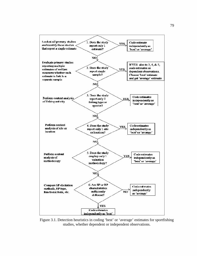
79
Figure 3.1. Detection heuristics in coding ‘best’ or ‘average’ estimates for sportfishing studies, whether dependent or independent observations.
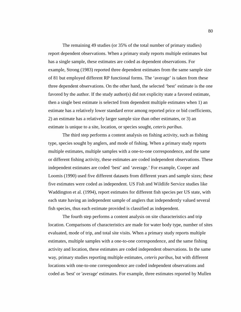
80
The remaining 49 studies (or 35% of the total number of primary studies)
report dependent observations. When a primary study reports multiple estimates but
has a single sample, these estimates are coded as dependent observations. For
example, Strong (1983) reported three dependent estimates from the same sample size
of 81 but employed different RP functional forms. The ‘average’ is taken from these
three dependent observations. On the other hand, the selected ‘best’ estimate is the one
favored by the author. If the study author(s) did not explicity state a favored estimate,
then a single best estimate is selected from dependent multiple estimates when 1) an
estimate has a relatively lower standard error among reported price or bid coefficients,
2) an estimate has a relatively larger sample size than other estimates, or 3) an
estimate is unique to a site, location, or species sought, ceteris paribus.
The third step performs a content analysis on fishing activity, such as fishing
type, species sought by anglers, and mode of fishing. When a primary study reports
multiple estimates, multiple samples with a one-to-one correspondence, and the same
or different fishing activity, these estimates are coded independent observations. These
independent estimates are coded ‘best’ and ‘average.’ For example, Cooper and
Loomis (1990) used five different datasets from different years and sample sizes; these
five estimates were coded as independent. US Fish and Wildlife Service studies like
Waddington et al. (1994), report estimates for different fish species per US state, with
each state having an independent sample of anglers that independently valued several
fish species, thus each estimate provided is classified as independent.
The fourth step performs a content analysis on site characteristics and trip
location. Comparisons of characteristics are made for water body type, number of sites
evaluated, mode of trip, and total site visits. When a primary study reports multiple
estimates, multiple samples with a one-to-one correspondence, and the same fishing
activity and location, these estimates are coded independent observations. In the same
way, primary studies reporting multiple estimates, ceteris paribus, but with different
locations with one-to-one correspondence are coded independent observations and
coded as 'best' or 'average' estimates. For example, three estimates reported by Mullen
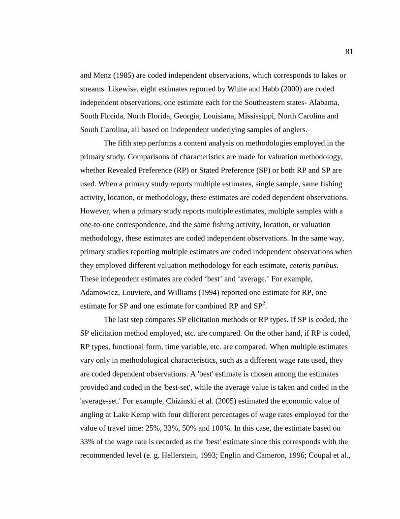
81
and Menz (1985) are coded independent observations, which corresponds to lakes or
streams. Likewise, eight estimates reported by White and Habb (2000) are coded
independent observations, one estimate each for the Southeastern states- Alabama,
South Florida, North Florida, Georgia, Louisiana, Mississippi, North Carolina and
South Carolina, all based on independent underlying samples of anglers.
The fifth step performs a content analysis on methodologies employed in the
primary study. Comparisons of characteristics are made for valuation methodology,
whether Revealed Preference (RP) or Stated Preference (SP) or both RP and SP are
used. When a primary study reports multiple estimates, single sample, same fishing
activity, location, or methodology, these estimates are coded dependent observations.
However, when a primary study reports multiple estimates, multiple samples with a
one-to-one correspondence, and the same fishing activity, location, or valuation
methodology, these estimates are coded independent observations. In the same way,
primary studies reporting multiple estimates are coded independent observations when
they employed different valuation methodology for each estimate, ceteris paribus.
These independent estimates are coded ‘best’ and ‘average.’ For example,
Adamowicz, Louviere, and Williams (1994) reported one estimate for RP, one
estimate for SP and one estimate for combined RP and SP2.
The last step compares SP elicitation methods or RP types. If SP is coded, the
SP elicitation method employed, etc. are compared. On the other hand, if RP is coded,
RP types, functional form, time variable, etc. are compared. When multiple estimates
vary only in methodological characteristics, such as a different wage rate used, they
are coded dependent observations. A 'best' estimate is chosen among the estimates
provided and coded in the 'best-set', while the average value is taken and coded in the
'average-set.' For example, Chizinski et al. (2005) estimated the economic value of
angling at Lake Kemp with four different percentages of wage rates employed for the
value of travel time: 25%, 33%, 50% and 100%. In this case, the estimate based on
33% of the wage rate is recorded as the 'best' estimate since this corresponds with the
recommended level (e. g. Hellerstein, 1993; Englin and Cameron, 1996; Coupal et al.,
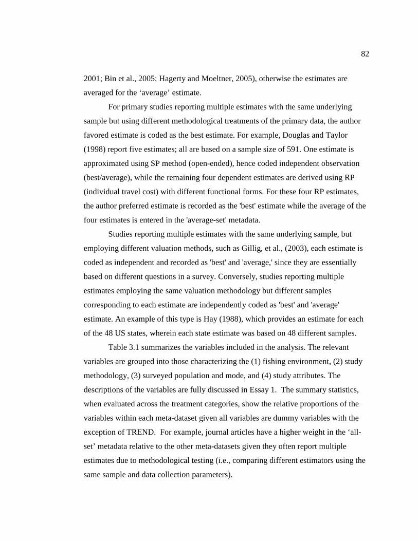
82
2001; Bin et al., 2005; Hagerty and Moeltner, 2005), otherwise the estimates are
averaged for the ‘average’ estimate.
For primary studies reporting multiple estimates with the same underlying
sample but using different methodological treatments of the primary data, the author
favored estimate is coded as the best estimate. For example, Douglas and Taylor
(1998) report five estimates; all are based on a sample size of 591. One estimate is
approximated using SP method (open-ended), hence coded independent observation
(best/average), while the remaining four dependent estimates are derived using RP
(individual travel cost) with different functional forms. For these four RP estimates,
the author preferred estimate is recorded as the 'best' estimate while the average of the
four estimates is entered in the 'average-set' metadata.
Studies reporting multiple estimates with the same underlying sample, but
employing different valuation methods, such as Gillig, et al., (2003), each estimate is
coded as independent and recorded as 'best' and 'average,' since they are essentially
based on different questions in a survey. Conversely, studies reporting multiple
estimates employing the same valuation methodology but different samples
corresponding to each estimate are independently coded as 'best' and 'average'
estimate. An example of this type is Hay (1988), which provides an estimate for each
of the 48 US states, wherein each state estimate was based on 48 different samples.
Table 3.1 summarizes the variables included in the analysis. The relevant
variables are grouped into those characterizing the (1) fishing environment, (2) study
methodology, (3) surveyed population and mode, and (4) study attributes. The
descriptions of the variables are fully discussed in Essay 1. The summary statistics,
when evaluated across the treatment categories, show the relative proportions of the
variables within each meta-dataset given all variables are dummy variables with the
exception of TREND. For example, journal articles have a higher weight in the ‘all-
set’ metadata relative to the other meta-datasets given they often report multiple
estimates due to methodological testing (i.e., comparing different estimators using the
same sample and data collection parameters).
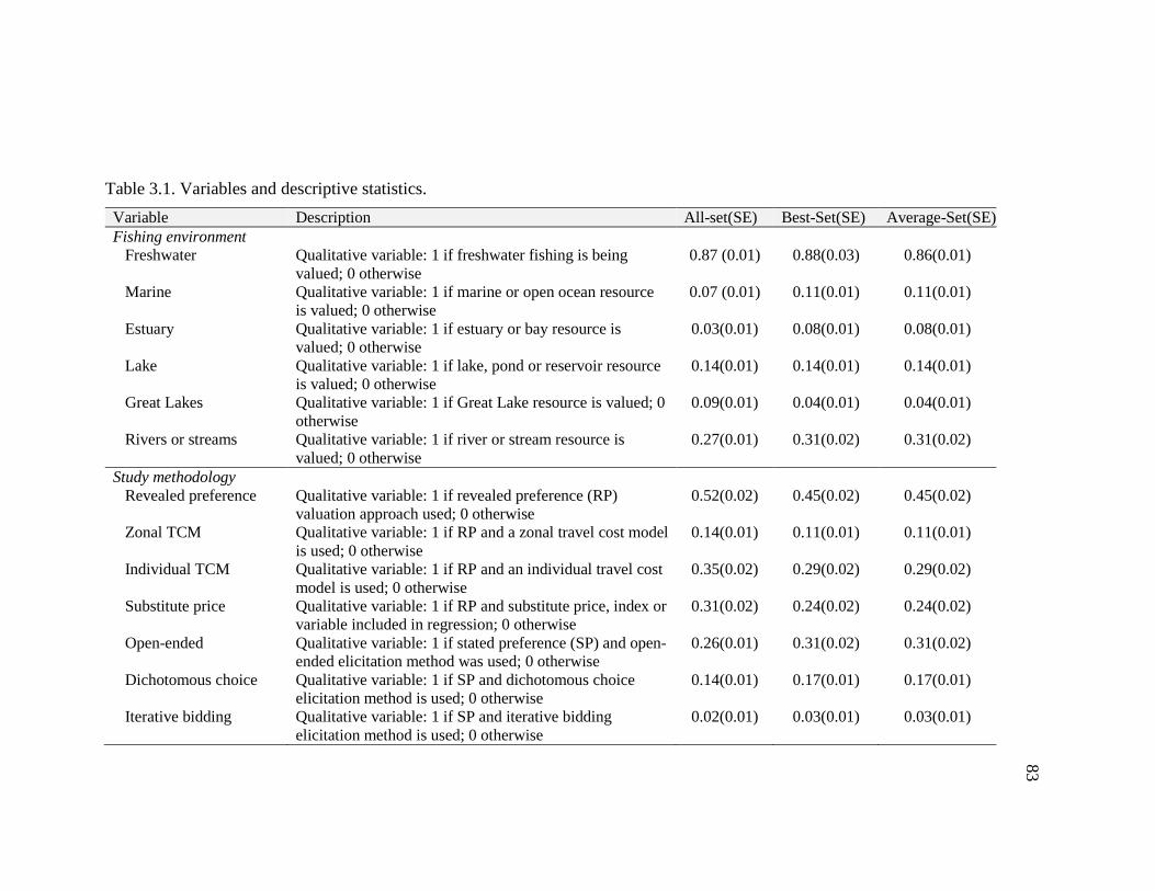
83
Table 3.1. Variables and descriptive statistics.
Variable Description All-set(SE) Best-Set(SE) Average-Set(SE) Fishing environment Freshwater Qualitative variable: 1 if freshwater fishing is being
valued; 0 otherwise 0.87 (0.01) 0.88(0.03) 0.86(0.01)
Marine Qualitative variable: 1 if marine or open ocean resource is valued; 0 otherwise
0.07 (0.01) 0.11(0.01) 0.11(0.01)
Estuary Qualitative variable: 1 if estuary or bay resource is valued; 0 otherwise
0.03(0.01) 0.08(0.01) 0.08(0.01)
Lake Qualitative variable: 1 if lake, pond or reservoir resource is valued; 0 otherwise
0.14(0.01) 0.14(0.01) 0.14(0.01)
Great Lakes Qualitative variable: 1 if Great Lake resource is valued; 0 otherwise
0.09(0.01) 0.04(0.01) 0.04(0.01)
Rivers or streams Qualitative variable: 1 if river or stream resource is valued; 0 otherwise
0.27(0.01) 0.31(0.02) 0.31(0.02)
Study methodology Revealed preference Qualitative variable: 1 if revealed preference (RP)
valuation approach used; 0 otherwise 0.52(0.02) 0.45(0.02) 0.45(0.02)
Zonal TCM Qualitative variable: 1 if RP and a zonal travel cost model is used; 0 otherwise
0.14(0.01) 0.11(0.01) 0.11(0.01)
Individual TCM Qualitative variable: 1 if RP and an individual travel cost model is used; 0 otherwise
0.35(0.02) 0.29(0.02) 0.29(0.02)
Substitute price Qualitative variable: 1 if RP and substitute price, index or variable included in regression; 0 otherwise
0.31(0.02) 0.24(0.02) 0.24(0.02)
Open-ended Qualitative variable: 1 if stated preference (SP) and open-ended elicitation method was used; 0 otherwise
0.26(0.01) 0.31(0.02) 0.31(0.02)
Dichotomous choice Qualitative variable: 1 if SP and dichotomous choice elicitation method is used; 0 otherwise
0.14(0.01) 0.17(0.01) 0.17(0.01)
Iterative bidding Qualitative variable: 1 if SP and iterative bidding elicitation method is used; 0 otherwise
0.02(0.01) 0.03(0.01) 0.03(0.01)
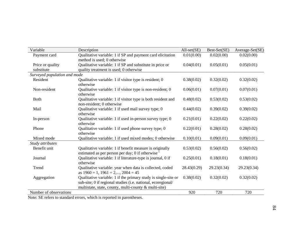
84
Variable Description All-set(SE) Best-Set(SE) Average-Set(SE) Payment card Qualitative variable: 1 if SP and payment card elicitation
method is used; 0 otherwise 0.01(0.00) 0.02(0.00) 0.02(0.00)
Price or quality substitute
Qualitative variable: 1 if SP and substitute in price or quality treatment is used; 0 otherwise
0.04(0.01) 0.05(0.01) 0.05(0.01)
Surveyed population and mode Resident Qualitative variable: 1 if visitor type is resident; 0
otherwise 0.38(0.02) 0.32(0.02) 0.32(0.02)
Non-resident Qualitative variable: 1 if visitor type is non-resident; 0 otherwise
0.06(0.01) 0.07(0.01) 0.07(0.01)
Both Qualitative variable: 1 if visitor type is both resident and non-resident; 0 otherwise
0.48(0.02) 0.53(0.02) 0.53(0.02)
Mail Qualitative variable: 1 if used mail survey type; 0 otherwise
0.44(0.02) 0.39(0.02) 0.39(0.02)
In-person Qualitative variable: 1 if used in-person survey type; 0 otherwise
0.21(0.01) 0.22(0.02) 0.22(0.02)
Phone Qualitative variable: 1 if used phone survey type; 0 otherwise
0.22(0.01) 0.28(0.02) 0.28(0.02)
Mixed mode Qualitative variable: 1 if used mixed modes; 0 otherwise 0.10(0.01) 0.09(0.01) 0.09(0.01) Study attributes Benefit unit Qualitative variable: 1 if benefit measure is originally
estimated as per person per day; 0 if otherwise c 0.53(0.02) 0.56(0.02) 0.56(0.02)
Journal Qualitative variable: 1 if literature-type is journal, 0 if otherwise
0.25(0.01) 0.18(0.01) 0.18(0.01)
Trend Qualitative variable: year when data is collected, coded as 1960 = 1, 1961 = 2,..., 2004 = 45
28.43(0.29) 29.23(0.34) 29.23(0.34)
Aggregation Qualitative variable: 1 if the primary study is single-site or sub-site; 0 if regional studies (i.e. national, ecoregional/ multistate, state, county, multi-county & multi-site)
0.38(0.02) 0.32(0.02) 0.32(0.02)
Number of observations 920 720 720 Note: SE refers to standard errors, which is reported in parentheses.
85
Meta-Regression Model Specifications
Five model specifications are estimated, Models A1, A2, A3, B, and C. The
dependent variable for all models is CS per person per day in 2006 dollars, labeled as
CS. All five models are specified with the same explanatory variables for ease of
comparisons. The explanatory variables are grouped into four different matrices that
include fishing environment in Xfe (i.e. fishing type and water-body types), the study
methodology in Xsm (i.e. RP and SP characteristics), the surveyed population and
mode in Xps (i.e. visitor and survey types), and the study attributes in Xsa (i.e. benefit
unit, journal, trend and aggregation). The estimated generic MR model is, in matrix
notation:
uXXXXCS sasapspssmsmfefei +++++= ββββα Equation (5)
where α is the constant term, µ a vector of residuals, and the vectors β containing all
the estimated coefficients of the respective explanatory variables. In this linear model,
the estimated coefficient measures the unit change in CS for a given absolute unit
change in the value of the explanatory variable, holding all other independent
variables constant.
The first three models, A1, A2 and A3 are based on the ‘all-set’ metadata with
920 estimates. Model A1 is an ‘all-set’ full specification, Model A2 is an ‘all-set’
weighted full specification, and Model A3 is an ‘all-set’ panel specification. Model B is
based on ‘best-set’ metadata while Model C is based on ‘average-set’ metadata, both
with 720 estimates. The common attribute among the five models is that they are all
estimated with datasets that contain 630 independent estimates; or 68% of all
observations for Models A1, A2 and A3, and 88% of all observations in Models B and C.
In Model A1, all estimates are treated as independent estimates and estimated
via OLS following the MR model in Equation 5. In this regard, when primary studies
reported three benefit estimates, then all three estimates are treated as independent
estimates, i.e. without correlation. In Model A2, all independent estimates are given
weights equal to one, while dependent estimates are assigned weights based on the
number of estimates within each relevant primary study. When primary studies report
86
multiple independent and dependent estimates, then the independent estimates are
given weights equal to 1 while the dependent estimates are given weight equal to the
remaining number of estimates (excluding independent estimates) for that study.
Model A2 is estimated via WLS.
Model A3 employs the panel data method to capture dependency among
estimates provided in a single document (Rosenberger and Loomis, 2000b; Sturtevant
et al., 1996). A random-effects MR model of the following linear form is estimated:
iijsajsapsjpssmjsmfejfeij euXXXXCS ++++++= ββββα Equation (6)
where j is the stratification index and µij is the panel-specific disturbance component
with mean zero and variance 2µσ . Equation 6 assumes that the source of some of the
variation in CS is due to random differences (µij) among studies that cannot be
identified. The description of the panel method and associated hypotheses test are fully
discussed in Essay 1. In this paper, the underlying data structure, and not ‘study’ is
used as the method of panel stratification. Therefore, all independent estimates are
each being indexed as a single panel, resulting in 630 panels while the rest of the
studies with dependent estimates are each being indexed as a panel, resulting in 51
panels. The total number of panels is 681, with the smallest panel size of one, largest
panel size of 44, and an average panel size of 5.2 estimates.
Finally, both Models B and C avoid dependency issues within studies by
extracting a single estimate from the dependent estimates. These models are estimated
via OLS following the MR model given in Equation 5.
Model Comparisons
To compare the performance of the five MR models, two sets of evaluation
criteria are used: 1) regression statistics (adjusted-R2, F-test, t-test); and 2) in-sample
benefit prediction performance. The adjusted-R2 (i.e., coefficient of determination)
shows the proportion of variability in the metadata that is accounted for by the model,
which is adjusted for the number of explanatory variables in the models. Based on this
criterion, the model with the largest adjusted-R2 is preferred. The F-test criterion tests
87
the null hypothesis: 0:0 ==== sapssmfeH ββββ ; i.e., testing the significance of the
26 explanatory variables in the MR model. The t-value is the coefficient (β) divided by
its standard error (SE) which is used to test whether a particular explanatory variable
(X) is a significant predictor of the dependent variable CS, over and above the other
explanatory variables (i.e. t-test Ho: βi=0).
The selection of an MR model based on regression statistics, which identify the
most efficient model, is a necessary but not a sufficient criterion for assessing whether
the estimated MR can be used for BT with any degree of confidence. In this paper, BT
is defined as the prediction of sportfishing values using the meta-regression benefit
transfer function (MRBTF). The MRBTF is a MR model estimated on the metadata
comprising the study sites and optimized for significant and salient explanatory
variables, which are then adjusted based on characteristics of the study site
(Rosenberger and Loomis, 2000a). Therefore, the five models are compared based on
their relative performances in predicting in-sample predictions of CS.
In estimating CS using the MRBTF, transfer errors are inevitable given the
inherent heterogeneity and error of the metadata (i.e. ‘study-site’ and ‘policy-site’
correspondence). Given limited characterization of sportfishing variables in the
primary studies, the use of dummy variables to characterize fishing types, water-body
types, and angler’s socio-demographics does not entirely capture the true variation in
these characteristics. Likewise, it is difficult to capture the important quality and
quantity differences of fishing sites (e.g. catch rates), since many of the primary
studies did not report complete information about them, and so these variables are not
included in the MRBTF.
The forecast performance of each model is judged using the percentage
transfer error (PTE), defined as:
%100*
−=
observed
observedestimated
CS
CSCSPTE Equation (7)
where CSestimated is the transferred (predicted) CS value from MRBTF while CSobserved
is the reported CS value in a primary study. A jackknife data splitting technique is
88
used to estimate n-1 separate MRBTFs defined above to predict the omitted
observation in each case (Loomis, 1992; Brander, Florax, and Verrmaat, 2006;
Johnston and Duke, 2009). The jackknife technique focuses on the samples that leave
out one observation at a time:
( ) ( )niii XXXXXX ,...,,..., 1121 +−= for i=1,2,… n jackknife samples. Finally, the overall
mean and median absolute PTE is generated for all the observations in the five
models.
Meta-Regression Results
Table 3.2 presents the MR results of the five models. The models are closely
and directly comparable since they all include the same explanatory variables. The
predicted mean CS is statistically the same for all the models. The adjusted-R2 value
of the five models ranges from 0.21 to 0.32, with an average of 0.25 indicating that
about one fourth of the variation in sportfishing value estimates is explained by the
explanatory variables. Model A2 has the highest adjusted-R2 value of 0.32 followed by
Model C with an adjusted-R2 value of 0.28. The adjusted-R2of Models A1, A3 and B are
similar. Care is needed in interpreting these results since adjusted-R2 from random-
effects MR model (A3) is not directly comparable to adjusted-R2 from the OLS MR
models (Models A1, B and C) and weighted MR model (Model A2).
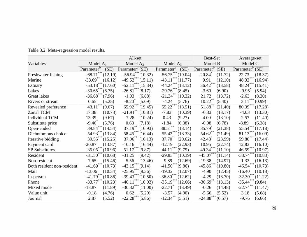
89
Table 3.2. Meta-regression model results.
Variables All-set Best-Set Average-set
Model A1 Model A2 Model A3 Model B Model C Parameterb (SE) Parameterb (SE) Parameterb (SE) Parameterb (SE) Parameterb (SE)
Freshwater fishing -68.71*** (12.19) -56.94*** (10.32) -56.75*** (10.04) -20.84* (11.72) 22.73 (18.37) Marine -33.69** (16.12) -49.52*** (15.11) -43.11*** (11.77) 9.91 (12.10) 48.32*** (16.94) Estuary -53.18*** (17.60) -52.11*** (15.34) -44.24*** (13.12) 36.42*** (13.58) 48.24*** (15.41) Lakes -30.65*** (6.75) -26.81*** (8.17) -29.76*** (8.45) -3.60 (6.90) -9.95* (5.94) Great lakes -36.68*** (7.96) -1.03 (6.88) -21.34** (10.22) 21.72 (13.72) -2.63 (8.20) Rivers or stream 0.65 (5.25) -8.20* (5.09) -4.24 (5.76) 10.22** (5.40) 3.11*** (0.99) Revealed preference 43.11*** (9.67) 65.92*** (19.45) 55.22*** (18.51) 51.88** (21.40) 80.39*** (17.28) Zonal TCM 17.38 (10.73) -21.91** (10.81) -7.83 (10.39) -6.33 (13.17) -4.03 (13.30) Individual TCM 13.39 (9.67) -7.28 (10.24) 0.43 (9.27) 4.00 (13.10) 2.57 (11.40) Substitute price -9.46* (5.76) 0.63 (7.18) -1.84 (6.38) -0.98 (6.78) -8.89 (6.38) Open-ended 39.84*** (14.54) 37.19** (16.93) 38.51** (18.14) 35.79* (21.38) 55.54*** (17.18) Dichotomous choice 54.93*** (13.84) 58.45*** (16.44) 55.42*** (18.33) 54.62** (21.49) 81.13*** (16.09) Iterative bidding 39.55*** (15.25) 37.96** (16.13) 37.70* (20.62) 42.48* (23.99) 59.80*** (17.44) Payment card -20.87 (13.87) -10.16 (16.44) -12.19 (22.93) 10.95 (22.74) 12.83 (16.10) SP Substitutes 35.05*** (10.96) 51.17*** (9.87) 44.11*** (9.79) 49.34*** (11.10) 46.59*** (10.97) Resident -31.50*** (10.68) -31.25 (9.42) -29.83*** (10.39) -45.07*** (11.14) -38.74*** (10.83) Non-resident 7.65 (15.46) 5.56 (13.46) 9.89 (12.69) -19.38 (14.97) 1.33 (16.13) Both resident non-resident -41.69*** (10.73) -43.15*** (9.14) -41.50*** (9.86) -45.86*** (10.80) -46.54*** (10.73) Mail -13.06 (10.34) -25.95*** (9.36) -19.32 (12.07) -4.90 (12.45) -16.40 (10.18) In-person -41.79*** (10.86) -39.43*** (10.50) -36.80*** (12.62) -4.29 (13.70) -32.30*** (11.22) Phone -33.77*** (10.23) -40.11*** (10.02) -35.19*** (12.66) -30.69** (13.13) -35.44*** (9.84) Mixed mode -18.87 (11.89) -30.32*** (11.00) -22.71* (13.49) -0.26 (14.48) -22.74** (11.47) Value unit -0.18 (4.76) 0.62 (5.29) -3.57 (4.90) -5.66 (5.52) 3.18 (5.68) Journal 2.87 (5.52) -22.28*** (5.86) -12.34** (5.51) -24.88*** (6.57) -9.76 (6.66)
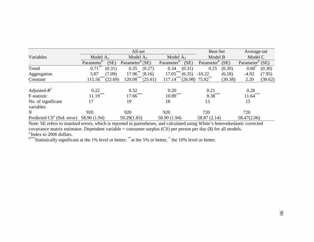
90
Variables All-set Best-Set Average-set
Model A1 Model A2 Model A3 Model B Model C Parameterb (SE) Parameterb (SE) Parameterb (SE) Parameterb (SE) Parameterb (SE)
Trend 0.71** (0.31) 0.35 (0.27) 0.34 (0.31) 0.25 (0.30) 0.60* (0.30) Aggregation 5.07 (7.09) 17.96** (8.16) 17.05*** (6.35) -10.22 (6.58) -4.92 (7.95) Constant 115.56*** (22.69) 120.08*** (25.61) 117.14*** (26.98) 75.92** (30.38) 2.20 (30.62) Adjusted-R2 0.22 0.32 0.20 0.21 0.28 F-statistic 11.19*** 17.66*** 10.89** * 8.38*** 11.64*** No. of significant variables
17 19 18 13 15
N 920 920 920 720 720 Predicted CSa (Std. error) 58.90 (1.94) 59.29(1.83) 58.90 (1.94) 58.87 (2.14) 58.47(2.06) Note: SE refers to standard errors, which is reported in parentheses, and calculated using White’s heteroskedastic corrected covariance matrix estimator. Dependent variable = consumer surplus (CS) per person per day ($) for all models. a Index to 2006 dollars. b*** Statistically significant at the 1% level or better; ** at the 5% or better, * the 10% level or better.
91
All models are statistically significant at p≤ 0.01 based on the F-tests. As
expected, the significance and magnitude of many parameter estimates vary across the
five models. Model A2 has the highest F-statistic of 17.66 while Model B has the
lowest F-statistic of 8.38. Model A2 has the highest number of significant variables
(19), based on t-values while Model B the lowest number of significant variables (13).
There are no significant changes in statistical significances (t-values) or signs of the
estimated parameters across Models A1, A2 and A3, which are based on the ‘all-set’
metadata. The same can be said between Models B and C, which are both based on
720 observations. However, there are differences in the signs of the significant
estimated parameters for the fishing environment variables between the ‘A’ models
and ‘B’ or ‘C’ models, potentially exhibiting some loss of information when dropping
observations or averaging them. The estimated constant for the models are positive
and statistically significant (p-value ≤ 0.05), except for Model C. Note that taking the
average estimate (Model C) more-or-less standardizes the data and forces it through
the origin. This changed the magnitude of the estimated parameters for Model C,
though not statistically different for all but one of the estimated parameters of Model
A2. Models A2 and C can be compared directly and are expected to be similar.
However, Model A2 has four more significant variables than Model C, may be
attributed to more observations in Model A2.
Changing the underlying structure of the metadata changes the sign and
magnitude of the estimated parameters of fishing environment variables. The
significance and magnitude of the estimated coefficient for freshwater fishing was
statistically different between the ‘A’ models (p-value ≤ 0.01) and Model B (p-value ≤
0.10). Freshwater fishing is significant in all models except Model C. As expected,
freshwater fishing tends to provide lower benefit estimates than saltwater fishing or
both freshwater and saltwater fishing combined. The estimated parameter for marine
is negative and significant for the ‘A’ models but is positive and significant for Model
C. In the same way, the estimated parameter for estuary is negative and significant for
the ‘A’ Models but is positive and significant for Models B and C. The magnitude of
92
the estimated coefficient for lake was statistically different between the ‘A’ Models
and Model C. Lake variable is negative and significant for all the models, except
Model B. The Great lakes variable is only significant and negative for Models A1 and
A3. River or stream is negative and significant in Model A2 but is positive and
significant for Models B and C.
The influences of study methodology variables are invariant to changes in the
underlying structure of the metadata. Revealed preference is positive and significant in
all models, suggesting that higher benefit estimates are associated with RP methods
when compared with SP and combined RP-SP methods, which is consistent with
Rosenberger and Loomis (2000a). For RP estimates, zonal TCM is negative and
significant only in Model A2, implying that it produces lower benefit estimates than
other valuation techniques. As expected, the inclusion of substitute price, index or
variable in the MR model is negative and significant only in Model A1, signifying that
when RP models correctly reflect substitution, the associated benefit estimate is lower
(Rosenthal, 1987). For SP parameters, the elicitation methods: open-ended,
dichotomous choice, and iterative bidding are positive and significant for all models,
suggesting a higher benefit estimate than other elicitation methods. However, the
inclusion of substitute in SP price or quality in the MR models increases the benefit
estimate, which is the opposite of theoretical expectation; but given the low proportion
of this variable in the metadata, it may be measuring some other effect (i.e. errors-in-
variables).
The influence of surveyed population and mode variables, like study
methodology variables, are also invariant to changes in the underlying structure of the
metadata. The resident and both resident/non-resident variables have lower benefit
estimates relative to non-residents, special interest groups, and other targeted sub-
population. The mail survey mode is negative and significant only in Model A2. The
other survey modes: in-person, phone, and mixed-mode have lower benefit estimates
relative to web-based and other survey modes.
93
Study attributes variables, like study methodology variables and surveyed
population and mode variables, are also invariant to changes in the underlying
structure of the metadata. The journal variable is negative and statistically significant
in Models A2, A3 and B. The trend variable is positive and significant only in Models
A1 and C, indicating that CS estimates in these models have generally increased at a
greater rate than inflation over time, similar to findings of Rosenberger and Loomis
(2001). As expected, the aggregation variable (though only significant in Models A2
and A3) increases the benefit estimates (i.e., single site studies/models tend to provide
higher estimates than regional studies/models). The value unit variable is not
significant in any of the estimated models.
In-Sample Benefit Predictions Results
The PTE are computed for all five models using a jackknife data splitting
technique. Mean absolute PTE for each of the five models is rather high, however,
they range from 0.02% to 33,282.64%. For example, Model A2 has mean absolute PTE
of 303%, median absolute PTE of 54%, and ranges from 0.02% to 21,868.96% (Table
3.3). However, looking at the mean absolute PTE for different percentiles of the data
series, ordering them by magnitude of the observed benefit estimates in ascending
order, the mean PTE decreased significantly after the initial 10th percentile of the
observations. The 1-10th percentile of the observations in Model A2 is composed of
observed benefit estimates from $0.22 to $9.50 per person per day. This result
illustrates how the same magnitude difference between observed and predicted values
can lead to substantially different PTE estimates, namely that lower observed or
predicted values are associated with higher PTEs. Figure 3.2 shows the observed and
predicted benefit estimates in $2006 (upper panel) and absolute percentage transfer
error (lower panel) associated with each observation ranked in ascending order of
observed benefit value. There is indeed a considerable difference between the
observed and predicted benefit values. About 30% of the observations show an
absolute percentage transfer error over 100%. Model A2 MRBTF systematically over-
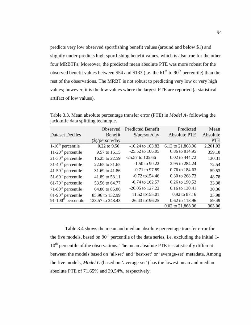
94
predicts very low observed sportfishing benefit values (around and below $1) and
slightly under-predicts high sportfishing benefit values, which is also true for the other
four MRBTFs. Moreover, the predicted mean absolute PTE was more robust for the
observed benefit values between $54 and $133 (i.e. the 61th to 90th percentile) than the
rest of the observations. The MRBT is not robust to predicting very low or very high
values; however, it is the low values where the largest PTE are reported (a statistical
artifact of low values).
Table 3.3. Mean absolute percentage transfer error (PTE) in Model A2 following the jackknife data splitting technique.
Dataset Deciles Observed
Benefit ($)/person/day
Predicted Benefit $/person/day
Predicted Absolute PTE
Mean Absolute
PTE 1-10th percentile 0.22 to 9.50 -16.24 to 103.82 6.13 to 21,868.96 2,201.03 11-20th percentile 9.57 to 16.15 -25.52 to 106.05 6.86 to 814.95 359.18 21-30th percentile 16.25 to 22.59 -25.57 to 105.66 0.02 to 444.72 130.31 31-40th percentile 22.65 to 31.65 -1.50 to 90.22 2.95 to 284.24 72.54 41-50th percentile 31.69 to 41.86 -0.71 to 97.89 0.76 to 184.63 59.53 51-60th percentile 41.89 to 53.11 -0.72 to154.46 0.30 to 268.73 48.78 61-70th percentile 53.56 to 64.77 -0.74 to 162.57 0.26 to 190.52 33.38 71-80th percentile 64.80 to 85.86 -26.05 to 127.22 0.16 to 130.41 30.36 81-90th percentile 85.96 to 132.99 11.52 to155.01 0.92 to 87.16 35.98 91-100th percentile 133.57 to 348.43 -26.43 to196.25 0.62 to 118.96 59.49 0.02 to 21,868.96 303.06
Table 3.4 shows the mean and median absolute percentage transfer error for
the five models, based on 90th percentile of the data series, i.e. excluding the initial 1-
10th percentile of the observations. The mean absolute PTE is statistically different
between the models based on ‘all-set’ and ‘best-set’ or ‘average-set’ metadata. Among
the five models, Model C (based on ‘average-set’) has the lowest mean and median
absolute PTE of 71.65% and 39.54%, respectively.
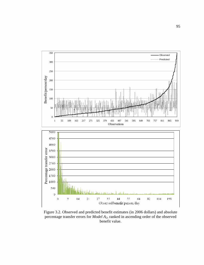
95
0
50
100
150
200
250
300
350
1 55 109 163 217 271 325 379 433 487 541 595 649 703 757 811 865 919
Observations
Observed
Predicted
Figure 3.2. Observed and predicted benefit estimates (in 2006 dollars) and absolute percentage transfer errors for Model A2, ranked in ascending order of the observed
benefit value.
Ben
efit/
pers
on/d
ay P
erce
ntag
e tr
ansf
er e
rror
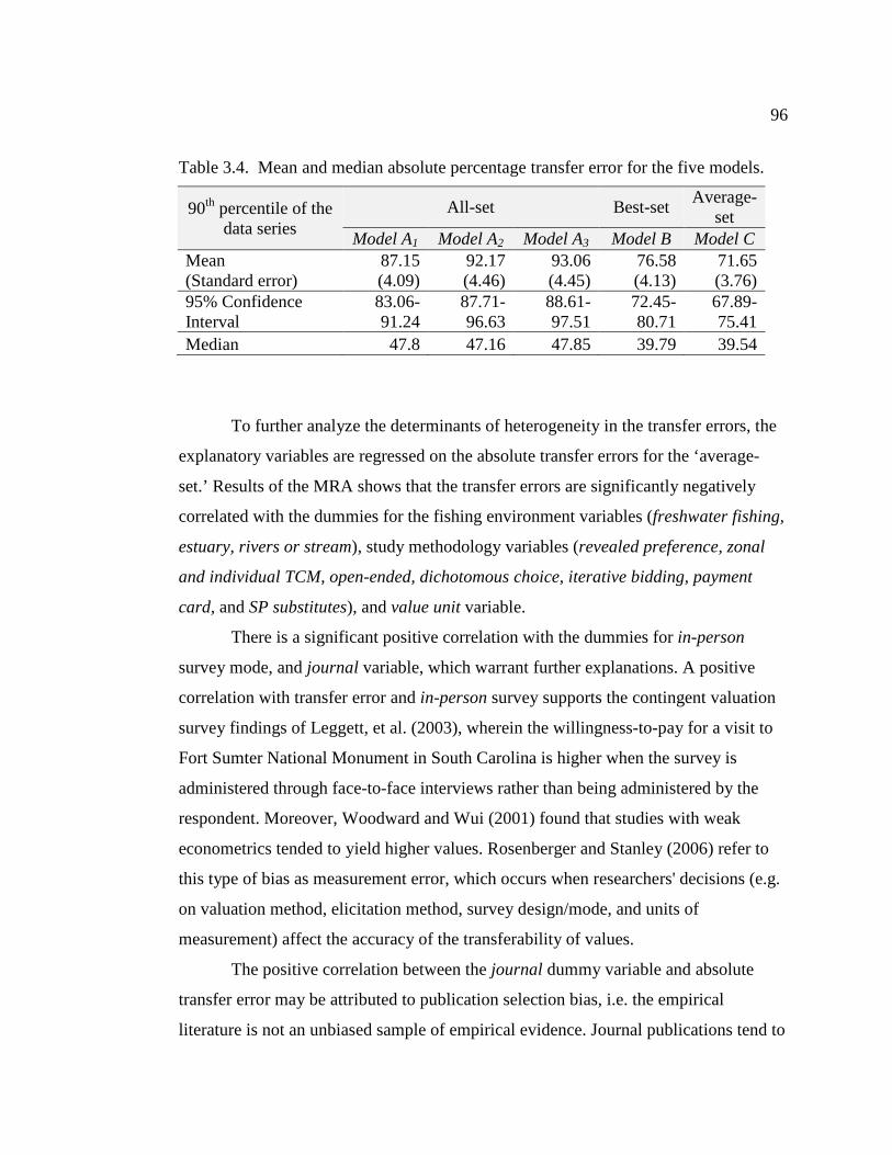
96
Table 3.4. Mean and median absolute percentage transfer error for the five models.
90th percentile of the data series
All-set Best-set Average-
set Model A1 Model A2 Model A3 Model B Model C
Mean (Standard error)
87.15 (4.09)
92.17 (4.46)
93.06 (4.45)
76.58 (4.13)
71.65 (3.76)
95% Confidence Interval
83.06-91.24
87.71-96.63
88.61-97.51
72.45-80.71
67.89-75.41
Median 47.8 47.16 47.85 39.79 39.54
To further analyze the determinants of heterogeneity in the transfer errors, the
explanatory variables are regressed on the absolute transfer errors for the ‘average-
set.’ Results of the MRA shows that the transfer errors are significantly negatively
correlated with the dummies for the fishing environment variables (freshwater fishing,
estuary, rivers or stream), study methodology variables (revealed preference, zonal
and individual TCM, open-ended, dichotomous choice, iterative bidding, payment
card, and SP substitutes), and value unit variable.
There is a significant positive correlation with the dummies for in-person
survey mode, and journal variable, which warrant further explanations. A positive
correlation with transfer error and in-person survey supports the contingent valuation
survey findings of Leggett, et al. (2003), wherein the willingness-to-pay for a visit to
Fort Sumter National Monument in South Carolina is higher when the survey is
administered through face-to-face interviews rather than being administered by the
respondent. Moreover, Woodward and Wui (2001) found that studies with weak
econometrics tended to yield higher values. Rosenberger and Stanley (2006) refer to
this type of bias as measurement error, which occurs when researchers' decisions (e.g.
on valuation method, elicitation method, survey design/mode, and units of
measurement) affect the accuracy of the transferability of values.
The positive correlation between the journal dummy variable and absolute
transfer error may be attributed to publication selection bias, i.e. the empirical
literature is not an unbiased sample of empirical evidence. Journal publications tend to
97
have smaller aggregate mean recreational use value estimates than non-journal
publications, when a dummy variable identifying those estimates published in peer-
reviewed journals is added to the MR model. Smaller benefit estimate would imply a
higher transfer error as noted above. There is also greater variation in estimates
provided across published studies than unpublished studies (Rosenberger and Stanley,
2006).
Conclusions
This paper explored approaches in modeling and treating data dependency in
the sportsfishing metadata when performing MRA and BT. The MRA is applied on
‘all-set,’ ‘best-set,’ and ‘average-set’ metadata. The ‘best-set’ and ‘average-set’
grouping of primary studies is used to avoid dependency among the observed benefit
measures in the ‘all-set’ metadata. Three MR models are considered using the ‘all-set’
metadata: 1) using all observations as independent samples; 2) using weights based on
underlying data structure; and 3) employing a random-effect panel model. The five
MR models are compared based on regression statistics and in-sample benefit
predictions performance.
The degree of explanatory power among MR models is best achieved in an
‘all-set’ weighted specification and in using an ‘average-set’ metadata, which are
complementary treatments of data dependency. When the underlying structure of the
metadata is modified as in the ‘best-set’ and ‘average-set’ treatments, the magnitude
and sign of the estimated parameters of the fishing environment variables changed too.
This result affirms the findings of Essay 1 that the structural shift in the metadata is
influenced by fishing environment variables. Other variables, such as study
methodology, surveyed population and mode, and study attributes did not change
given modification of the underlying structure in the metadata.
The median absolute percentage transfer error is lower for the MR models
based on a single value, i.e. ‘average-set’ and ‘best-set’ metadata than the MR models
based on ‘all-set’, contrary to Bijmolt and Pieters (2001). However, this increased
98
performance in in-sample predictions is not substantial. Meta-analytic procedure
representing each study with multiple estimates by an ‘average’ or ‘best’ value,
though, may result in loss of information. One significant observation from in-sample
predictions is that the absence of very low and very high estimates in the metadata will
likely result in a more robust MRBT (i.e. MRBT does not predict well in the tails of
the distribution of observed values, as expected). Caution is recommended when
selecting studies for point or function transfers that provide very low estimates. We
may be more confident with MRBT when the metadata include those observations that
fall within two standard deviations of the mean. However, in small sample MRBT,
mean CS may not be a good indicator when selecting studies to include in the
metadata since it is more sensitive to extreme benefit values (very low and very high).
Findings also suggests that the dummies related to measurement errors (in-person
survey mode) and publication selection bias (journal) are important predictors of
transfer errors. This result supports the recommendations by Stanley and Rosenberger
(2009) to detect the true effect and correct for possible publication selection bias,
when conducting a meta-analysis for BT.
Based on the results of the study, the following implications and
recommendations can be drawn. First, the importance to correct for methodological
pitfalls in MRA is always warranted. Nelson and Kennedy (2009) outline the ‘best-
practice guidelines’ in conducting a complete MRA. Second, the choice of whether to
include all estimates of primary studies or to include only the ‘average’ or ‘best’
estimates from the primary studies is best guided by the goals of the meta-analysis,
and perceived allowable errors in BT applications. When the goal of meta-analysis is
knowledge acquisition, synthesis/generalization of the literature and hypothesis testing
(e.g. explaining heterogeneity) that is beyond predicting values, metadata sample
selection may not be an issue. But when doing meta-regression benefit function
transfer, metadata sample selection is an important issue that needs to be addressed.
Third, more research is needed to analyze the implications of metadata sample
selection in the context of BT. In particular, future research should evaluate the
99
downward bias associated with the different metadata sample sizes when used in BT
applications. Further research is also warranted to know if the results found here can
be confirmed with other data dependency models, such as hierarchical/multilevel
models and clustering techniques.
Acknowledgments
The author would like to thank Lisa Ganio, Manuela Huso, and Robert
Johnston for their assistance with estimating the models using jackknife data splitting
technique. Any shortcomings of this paper are the sole responsibility of the author.
Notes
1 Selection criteria for inclusion in the ‘best-set’ metadata of single estimate studies
could be applied as well. For example, early valuation approaches did not use (or
have available) what is currently considered state-of-the-art estimators. However, we
chose to include all single estimate studies and control for their differences through
model specification (i.e., include variables that identify methodology). 2 While the latter estimate is likely partially correlated with the previous ones, it is
treated as independent in the metadata.
100
References
Adamowicz, W. L., and J. R. Deshazo. "Frontiers in Stated Preferences Methods: An Introduction." Environmental and Resource Economics 34(2006): 1-6.
Adamowicz, W., J. Louviere, and M. Williams. "Combining Revealed and Stated
Preference Methods for Valuing Environmental Amenities." Journal of Environmental Economics and Management 26, no. 3(1994): 271-292.
Bateman, I. J., and A. P. Jones. "Contrasting Conventional with Multi-Level Modeling
Approaches to Meta-Analysis: Expectation Consistency in U.K. Woodland Recreation Values." Land Economics 79, no. 2(2003): 235-258.
Bergstrom, J. C., et al. "Economic value of wetlands-based recreation." Ecological
Economics 2, no. 2(1990): 129-147. Bijmolt, T. H. A., and R. G. M. Pieters. "Meta-Analysis in Marketing when Studies
Contain Multiple Measurements." Marketing Letters 12, no. 2(2001): 157-169. Bin, O., C. E. Landry, C. Ellis, and H. Vogelsong. “Some consumer surplus estimates
for North Carolina beaches.” Marine Resource Economics 20, no. 2(2005), 145–161.
Boyle, K. J., and J. C. Bergstrom. "Benefit Transfer Studies: Myths, Pragmatism, and
Idealism." Water Resources Research 28, no. 3(1992): 657–663. Brander, L. M., R. J. G. M. Florax, and J. E. Vermaat. "The Empirics of Wetland
Valuation: A Comprehensive Summary and a Meta-Analysis of the Literature." Environmental and Resource Economics 33, no. 2(2006):223-250.
Brouwer, R. (2002) Meta-analysis and Benefit Transfer: Synergy, Lessons and
Research Agendas. In R. Florax, P. Nijkamp, and K. Willis (Eds). Comparative Environmental Economic Assessment. MA, USA, Edward Elgar Publishing, Inc.
Chizinski, C. J., et al. "Economic Value of Angling at a Reservoir with Low
Visitation." North American Journal of Fisheries Management 25, no. 1(2005): 98-104.
Coupal, R., C. Bastian, J. May, and D. Taylor. The economic benefits of
snowmobiling to Wyoming residents: A travel cost approach with market segmentation. Journal of Leisure Research 33, no. 4(2001):492–510.
101
Doucouliagos, C., and M. A. Ulubasoglu. "Economic freedom and economic growth: Does specification make a difference?" European Journal of Political Economy 22, no. 1(2006): 60-81.
Doucouliagos, H., and M. A. Ulubaşoğlu. "Democracy and Economic Growth: A
Meta-Analysis." American Journal of Political Science 52, no. 1(2008): 61-83. Douglas, A. J., and J. G. Taylor. "Riverine based eco-tourism: Trinity River non-
market benefits estimates." International Journal of Sustainable Development & World Ecology 5, no. 2(1998): 136-148.
Efron, B., and R. J. Tibshirani. An Introduction to the Bootstrap. London: Chapman
and Hall, 1993. Engel, S. (2002) Benefit function transfer versus meta-analysis as policy-making
tools: a comparison. In R. Florax, P. Nijkamp, and K. Willis (Eds). Comparative Environmental Economic Assessment. MA, USA, Edward Elgar Publishing, Inc.
Englin, J. and T. A. Cameron. “Augmenting travel cost models with contingent
behaviour data: Poisson regression analyses with individual panel data.” Environmental and Resource Economics 7(1996): 133–147.
Florax, R. (2002) Methodological Pitfalls in Meta-analysis: Publication Bias. In R.
Florax, P. Nijkamp, and K. Willis (Eds). Comparative Environmental Economic Assessment. MA, USA, Edward Elgar Publishing, Inc.
Gillig, D., et al. "Joint Estimation of Revealed and Stated Preference Data: An
Application to Recreational Red Snapper Valuation." Agricultural and Resource Economics Review 32, no. 2(2003): 209-221.
Glass, G. V., B. McGaw, and M. L. Smith. Meta-Analysis in Social Research. Beverly
Hills, CA: Sage Publications, Inc, 1981. Hagerty, D. and K. Moeltner. “Specification of driving costs in models of recreation
demand.” Land Economics 81, no. 1(2005):127–143. Hay, M. J. (1988) Net economic value for deer, elk and waterfowl hunting and bass
fishing, 1985., Report 85-1. Washington, DC: USDI Fish and Wildlife Service.
Hellerstein, D. and R. Mendelsohn. “A theoretical foundation for count data models.”
American Journal of Agricultural Economics 75, no. 3(1993):604–611.
102
Hunter, J., and F. Schmidt. Methods of Meta-Analysis: Correcting Error and Bias in Research Findings. London: Sage, 2004.
Johnston, R. J., and J. M. Duke. "Informing Preservation of Multifunctional
Agriculture when Primary Research Is Unavailable: An Application of Meta-Analysis." American Journal of Agricultural Economics 91, no. 5(2009): 1353-1359.
Johnston, R. J., et al. "Systematic Variation in Willingness to Pay for Aquatic
Resource Improvements and Implications for Benefit Transfer: A Meta-Analysis." Canadian Journal of Agricultural Economics 53, no. 2-3(2005): 221-248.
Johnston, R. J., et al. "What Determines Willingness to Pay per Fish? A Meta-
Analysis of Recreational Fishing Values." Marine Resource Economics 21(2006): 1-32.
Jones and Stokes Associates, Inc. "Southeast Alaska sport fishing economic study."
Final Research Report. December, 1991. (JSA 88-028). Prepared for Alaska Department of Fish and Game, Sport Fish Division, Research and Technical Services Section, Anchorage, AK.
Leggett, C. G., et al. "Social Desirability Bias in Contingent Valuation Surveys
Administered Through In-Person Interviews." Land Economics 79, no. 4(2003): 561-575.
Lipsey, M. W., and D. B. Wilson. Practical Meta-Analysis. Applied Social Research
Method Series. Thousand Oaks, California: Sage Publications, Inc., 2000. Loomis, J. B. "The Evolution of a More Rigorous Approach to Benefit Transfer:
Benefit Function Transfer." Water Resources Research 28, no. 3(1992): 701-705.
Loomis, J. B., and R. S. Rosenberger. "Reducing barriers in future benefit transfers:
Needed improvements in primary study design and reporting." Ecological Economics 60, no. 2(2006): 343-350.
Martin, W. E., F. H. Bollman, and R. L. Gum. "Economic Value of Lake Mead
Fishery." Fisheries 7, no. 6(1982): 20-24. Morey, E. R., et al. "Estimating recreational trout fishing damages in Montana's Clark
Fork River basin: summary of a natural resource damage assessment." Journal of Environmental Management 66, no. 2(2002): 159-170.
103
Mrozek, J. R., and L. O. Taylor. "What determines the value of life? a meta-analysis." Journal of Policy Analysis and Management 21, no. 2(2002): 253-270.
Mullen, J. K., and F. C. Menz. "The Effect of Acidification Damages on the Economic
Value of the Adirondack Fishery to New York Anglers." American Journal of Agricultural Economics 67, no. 1(1985): 112-119.
Nelson, J. P., and P. E. Kennedy. "The Use (and Abuse) of Meta-Analysis in
Environmental and Natural Resource Economics: An Assessment " Environmental and Resource Economics 42(2009): 345-377.
Nijkamp, P., et al. (2002) Environmental quality in European space: a methodology
for research synthesis. In R. Florax, P. Nijkamp, and K. Willis (Eds). Comparative Environmental Economic Assessment. MA, USA, Edward Elgar Publishing, Inc.
Rosenberger, R. S., and J. B. Loomis. "Using meta-analysis for benefit transfer: In-
sample convergent validity tests of an outdoor recreation database." Water Resources Research 36, no. 4(2000a): 1097-1108.
Rosenberger, R. S., and J. B. Loomis. "Panel Stratification in Meta-Analysis of
Economic Studies: An Investigation of Its Effects in the Recreation Valuation Literature." Journal of Agricultural and Applied Economics 32, no. 3(2000b): 459-470.
Rosenberger, R. S., and T. D. Stanley. "Measurement, generalization, and publication:
Sources of error in benefit transfers and their management." Ecological Economics 60, no. 2(2006): 372-378.
Rosenthal, R. Meta-analytic procedures for social research. Newbury Park Sage
Publications, 1991. Rosenthal, D. H. "The Necessity for Substitute Prices in Recreation Demand
Analyses." American Journal of Agricultural Economics 69, no. 4(1987): 828. Stanley, T. D., and S. B. Jarrell. "Meta-Regression Analysis: A Quantitative method of
Literature Surveys." Journal of Economic Surveys 3, no. 2(1989): 299-308. Stanley, T. D., and R. S. Rosenberger (2009) Are Recreation Values Systematically
Underestimated? Reducing Publication Selection Bias for Benefit Transfer, Department of Economics, Hendrix College and Department of Forest Ecosystems and Society, Oregon State University.
104
Strong, E. J. "A Note on the Functional Form of Travel Cost Models with Zones of Unequal Populations." Land Economics 59, no. 3(1983): 342-349.
Sturtevant, L. A., F. R. Johnson, and W. H. Desvousges (1996) A Meta-Analysis of
Recreational Fishing, Working Paper, Triangle Economic Research. Strube, M. J. "Meta-Analysis and Cross-Cultural Comparison: Sex Differences in
Child Competitiveness." Journal of Cross-Cultural Psychology 12, no. 1(1981): 3-20.
Strube, M. J. "A general model for estimating and correcting the effects of
nonidependence in meta-analysis." Multiple Linear Regression Viewpoints 16, no. 2(1987): 40-47.
Waddington, D. G., K. J. Boyle, and J. Cooper. "1991 net economic values for bass
and trout fishing, deer hunting, and wildlife watching." Washington, DC: US Fish and Wildlife Service.
Whitehead, J. C., and R. Aiken (2000) An analysis of trends in net economic values
for bass fishing from the national survey of fishing, hunting and wildlife-associated recreation, East Carolina University, Department of Economics Working Paper.
Whitehead, J. C., and T. C. Haab. "Southeast marine recreational fishery statistical
survey: distance and catch based choice sets." Marine Resource Economics 14, no. 4(2000).
Wood, J. A. "Methodology for Dealing with Duplicate Study Effects in a Meta-
Analysis." Organizational Research Methods 11, no. 1(2008): 79-95. Woodward, R. T., and Y.-S. Wui. "The economic value of wetland services: a meta-
analysis." Ecological Economics 37, no. 2(2001): 257-270.
105
CHAPTER 4 - ESSAY 3 THE RECREATIONAL VALUE OF TAAL VOLCANO PROTECTED
LANDSCAPE: AN EXPLORATORY BENEFIT TRANSFER APPLICAT ION
Abstract
Some landscapes that have significant value to people are protected through
statute. Protected landscapes that serve as popular recreational resources and
destinations hold significant use values for those people that visit them. Recognition of
these recreational benefits of protected landscapes provides a sound economic
rationale for their management. The objective of this essay is to estimate the
recreational value via benefit transfer (BT) of Taal Volcano Protected Landscape
(TVPL) in the Philippines—a major tourist attraction and designated as one of the key
priority biodiversity areas in the Philippines for priority protection. A foundation of
BT is the use of information from research conducted on other sites to inform
questions at a site that lacks primary research. In this case, the research question is
“What is the potential magnitude of recreational benefits at TVPL?” BT approaches
include transferring of values or functions from a single site or set of similar sites, and
estimating a meta-regression (MR) transfer function that can be used to predict values
for the policy site in question. One study site in the Philippines was selected and used
in a point estimate transfer application. Likewise, an MR transfer function model was
estimated based on selected ‘study sites’ from the US. Results show that single point
estimate worked better than MR benefit function transfer. While in-sample BT
prediction of the MR model show an absolute percentage transfer error (PTE) of 18%,
simple out-of-sample prediction has very high absolute PTE (1,231%). The estimated
welfare estimate of recreational access using single point estimate transfer was PHP
36 per person per trip. The aggregated recreational benefits at TVPL was PHP 9.7
million from 155,701 visitors at Batangas side and PHP118.9 million from 1,906,242
visitors at the Cavite side in 2006. These values may be used as an economic basis for
financial commitments by the institutions responsible for the TVPL management and
may inform policy issuances and ordinances, e.g. user-fee system for TVPL.
106
Introduction
The Protected Area Management Board (PAMB1), the policy and decision-
making body of the Taal Volcano Protected Landscape (TVPL), embarked on a
comprehensive 10-year (2010-2020) Management Plan. Proponents of the plan boast
of its community participation, co-management and local stakeholders’ involvement
and funding. The PAMB en banc approved the plan on September 26, 2009, with a
proposed annual administrative budget of PHP 11.7 million and a start-up cost of PHP
97.1 million. The Protected Area Superintendent (PASu), within the Department of
Environment and Natural Resources (DENR), serves as the chief operating officer of
the TVPL. One set back confronting the PASu Office is its limited staff of [seven]
persons with almost no dedicated resources (Luna and Gonzales, 2007). Funds needed
to implement the plan would be generated through available funds from the
institutions in the PAMB. These institutions are composed mainly of third, fourth, and
fifth class municipalities2, which in most cases have scarce financial resources.
Among the strong features of the plan are: (1) strong law enforcement and
agreement to comply; (2) a strong push for keeping the population levels constant for
the next ten years and beyond: (3) zoning the majority of the land area as agro-tourism
zone and setting aside forest reserves and a fish sanctuary; 4) water quality monitoring
and biodiversity survey; (5) disaster planning and climate change adaptation; (6) a
research council, center and bi-annual technical conference; and (7) institutional
development of the PASu office and the PAMB. High priority actions were identified
to address the following components: water quality and the health of Taal Lake;
aquatic living natural resources; terrestrial/watershed, recreation and cultural
resources; disaster preparedness and management; population and socio-economics;
research program and knowledge center; policy and institutional strengthening;
management zones on land and water; and work plan and budget.
One of the critical knowledge gaps identified under management requirements
is visitor’s willingness-to-pay (WTP), which could serve as basis for determining
107
future entrance fees at Taal Volcano Island and the process of fee-setting and
collection. Due to the lack of funds and limited time for the PASu and PAMB to
conduct primary research (first-best strategy), a benefit transfer (BT) application is
suggested to provide a first approximation of recreational use value. BT is the use of
recreational benefit estimates and other information from a ‘study site’ with data to a
‘policy site’ with little or no data (Rosenberger and Loomis, 2000). BT is considered a
‘second-best strategy,’ in which already existing estimates from other sites (study
sites) are used to inform decisions at the site of interest (policy site).
BT is increasingly applied to a wide variety of environmental goods and
services, such as benefits of agricultural wildlife management (Brouwer and Spaninks,
1999); water resources (Muthke and Holm-mueller, 2004); mortality risk valuation
(Krupnick, 2007); health impacts related to air and water quality (Ready et al., 2004);
air pollution and acute respiratory illness (Alberini and Krupnick, 1998); avoided
health effects from water pollution (Barton and Mourato, 2003); and outdoor
recreation (Shrestha and Loomis, 2001). Most of these authors conclude that value
transfer, i.e. single point estimate, worked better than function transfer, although
function transfers and meta-analysis transfer functions have been shown to be more
broadly accurate than value transfers (Loomis, 1992; Rosenberger and Stanley, 2006).
Shrestha and Loomis (2001) tested meta-analysis as a method for international BT
applications to recreation valuation and found that the absolute average percentage
error of meta-predictions may be within an acceptable range. There might be a trade-
off between precision and accuracy when conducting BTs using point, function, and
meta-regressions.
This paper explores both value and function transfers as a means to estimate
visitors’ recreational benefits at the TVPL, Philippines. A single point estimate is
derived from a ‘study site’ in the Philippines, while a meta-regression benefit function
based on existing studies in the US is used to derive estimates of recreational values
by adapting it to characteristics of the ‘policy site’ (i.e. TVPL). Implicit price deflators
and purchasing power parity (PPP) are incorporated to account for income and cost of
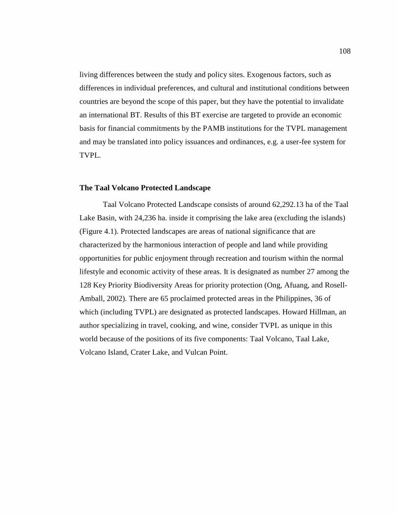
108
living differences between the study and policy sites. Exogenous factors, such as
differences in individual preferences, and cultural and institutional conditions between
countries are beyond the scope of this paper, but they have the potential to invalidate
an international BT. Results of this BT exercise are targeted to provide an economic
basis for financial commitments by the PAMB institutions for the TVPL management
and may be translated into policy issuances and ordinances, e.g. a user-fee system for
TVPL.
The Taal Volcano Protected Landscape
Taal Volcano Protected Landscape consists of around 62,292.13 ha of the Taal
Lake Basin, with 24,236 ha. inside it comprising the lake area (excluding the islands)
(Figure 4.1). Protected landscapes are areas of national significance that are
characterized by the harmonious interaction of people and land while providing
opportunities for public enjoyment through recreation and tourism within the normal
lifestyle and economic activity of these areas. It is designated as number 27 among the
128 Key Priority Biodiversity Areas for priority protection (Ong, Afuang, and Rosell-
Amball, 2002). There are 65 proclaimed protected areas in the Philippines, 36 of
which (including TVPL) are designated as protected landscapes. Howard Hillman, an
author specializing in travel, cooking, and wine, consider TVPL as unique in this
world because of the positions of its five components: Taal Volcano, Taal Lake,
Volcano Island, Crater Lake, and Vulcan Point.
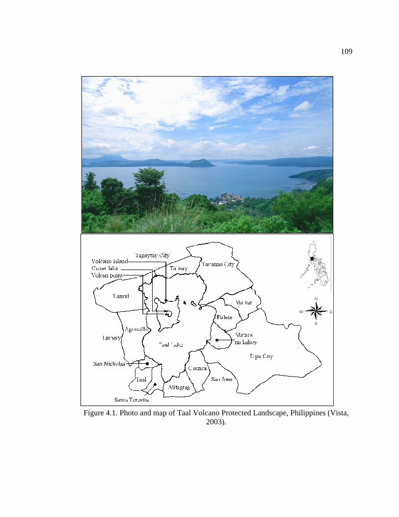
109
Figure 4.1. Photo and map of Taal Volcano Protected Landscape, Philippines (Vista, 2003).
110
The TVPL basin spans the Municipalities of Talisay, Laurel, Agoncillo, San
Nicholas, Taal, Lemery, San Jose, Santa Teresita, Alitagtag, Cuenca, Mataas na
Kahoy, Balete, Malvar, and the Cities of Lipa and Tanauan in the Province of
Batangas; and Tagaytay City in the Province of Cavite. These lakeshore municipalities
and cities have a scenic view of the volcano ridges. The ridge of the basin is in the
viewing area of the Taal Volcano Island and Lake, with Tagaytay City considered the
‘town of the ridge.’ Tagaytay City is a popular summer vacation getaway because its
climate is cooler than Manila. The municipality of Talisay is the major jump-off point
where boats are available to reach the Taal Volcano Island. TVPL watershed has 38
tributary rivers draining into the lake. The only outlet to Balayan Bay is the Pansipit
River. From the Southern Tagalog Arterial Road Tollway, and Batangas-Cavite
provincial highways, the lakeshore municipalities and cities are accessible within 15
minutes or more by vehicle. TVPL is about 60 km SSE of the capital Manila.
Taal Volcano has a crater within the Volcano island within Taal Lake within
the island of Luzon. Taal Volcano, considered the smallest volcano in the world, is
active and has erupted about 40 times from 1592 to 1977 (Hargrove, 1991). In 1967,
the Taal Volcano Island became a National Park through Proclamation No. 235. In
1993, Taal Volcano and its surrounding coastal municipalities were declared tourism
zones by virtue of Republic Act 7623. In 1996, Proclamation 235 was amended by
Presidential Proclamation 923, declaring the Taal Volcano Island, Taal Lake and the
watershed areas as a protected landscape under National Integrated protected Area
System (NIPAS3) Act of 1992. Taal Volcano Island has an area of 4,537 ha. and a
crater lake of about two kilometers in diameter at its center (Yokoyama, Alcaraz and
Peña, 1975). The main crater lake of the Volcano Island is four meters above sea level
(masl), while the highest elevation along the ridge is about 600 masl. Maximum depth
in the crater lake is about 90m. The highest elevation in the basin is 835 masl at the
peak of Mt. Maculot. The slope of the area in the Volcano Island is gentle, from four
to ten percent. The climate in the area is Type-I, i.e. dry season from November to
111
April and wet during the rest of the year. There are 47 identified cones and craters that
constitute the Volcano Island.
Taal Lake is a major tourist attraction and considered the third largest lake in
the Philippines. The lake has an average depth of 60.1 m, with a maximum depth of
198 m and a circumference of 120 km (Folledo and Cruz, 1999). The entire Taal Lake
is within a crater of a great volcano, a caldera with surrounding mountains as its walls
that are 150-304 m high. It hosts Hydrophis semperi, a freshwater sea snake, and the
Sardinella tawilis, a freshwater sardine - two of the vertebrates that are endemic to the
lake. About 20,000 fisherfolk are dependent on the lake’s resources. The lake provides
multiple and often conflicting services to various users. Current uses of the lake
include: (1) open water fishing; (2) fish cage culture of tilapia (Sarotherodon nilotica),
bangus (Chanos chanos) and maliputo (Caranx ignobilis); (3) navigation routes; (4)
recreation/tourism; (5) water source for the City of Tagaytay; and (6) a source of food
for waterfowl. The water quality in the lake is deteriorating due to nutrient pollution
from fish cages (Vista et al., 2006). Fish cage operators rely on the water of Taal Lake
as an input into ‘intensive’ fish production and as a waste repository. Excessive
amounts of nutrients (nitrogen and phosphorous) accumulating from the cages leads to
nutrient enrichment, endangering the industry itself and the general health of the lake
ecosystem.
The operational management of TVPL rests on the PASu’s Office, duly
formed by DENR. The Task Force on Environmental Law Enforcement (TFELE)
assists the PASu Office in law enforcement. The Task Force is instrumental in the
enforcement of the Unified Rules and Regulations on Fisheries, and many
environmental laws, rules and ordinances in the area.
Taal Volcano and Lake are of great interest to tourists, scientists, business
investors, and others because of their beauty and economic opportunities they provide.
Fertile land is a natural magnet for tillers, and benefits from tourism and fish cages
have attracted more occupants to the volcano. As of 2009, there are more than 5,000
people residing on Volcano Island, despite classification of the area as very high risk
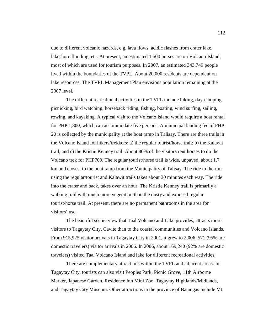
112
due to different volcanic hazards, e.g. lava flows, acidic flashes from crater lake,
lakeshore flooding, etc. At present, an estimated 1,500 horses are on Volcano Island,
most of which are used for tourism purposes. In 2007, an estimated 343,749 people
lived within the boundaries of the TVPL. About 20,000 residents are dependent on
lake resources. The TVPL Management Plan envisions population remaining at the
2007 level.
The different recreational activities in the TVPL include hiking, day-camping,
picnicking, bird watching, horseback riding, fishing, boating, wind surfing, sailing,
rowing, and kayaking. A typical visit to the Volcano Island would require a boat rental
for PHP 1,800, which can accommodate five persons. A municipal landing fee of PHP
20 is collected by the municipality at the boat ramp in Talisay. There are three trails in
the Volcano Island for hikers/trekkers: a) the regular tourist/horse trail; b) the Kalawit
trail, and c) the Kristie Kenney trail. About 80% of the visitors rent horses to do the
Volcano trek for PHP700. The regular tourist/horse trail is wide, unpaved, about 1.7
km and closest to the boat ramp from the Municipality of Talisay. The ride to the rim
using the regular/tourist and Kalawit trails takes about 30 minutes each way. The ride
into the crater and back, takes over an hour. The Kristie Kenney trail is primarily a
walking trail with much more vegetation than the dusty and exposed regular
tourist/horse trail. At present, there are no permanent bathrooms in the area for
visitors’ use.
The beautiful scenic view that Taal Volcano and Lake provides, attracts more
visitors to Tagaytay City, Cavite than to the coastal communities and Volcano Islands.
From 915,925 visitor arrivals in Tagaytay City in 2001, it grew to 2,006, 571 (95% are
domestic travelers) visitor arrivals in 2006. In 2006, about 169,240 (92% are domestic
travelers) visited Taal Volcano Island and lake for different recreational activities.
There are complementary attractions within the TVPL and adjacent areas. In
Tagaytay City, tourists can also visit Peoples Park, Picnic Grove, 11th Airborne
Marker, Japanese Garden, Residence Inn Mini Zoo, Tagaytay Highlands/Midlands,
and Tagaytay City Museum. Other attractions in the province of Batangas include Mt.
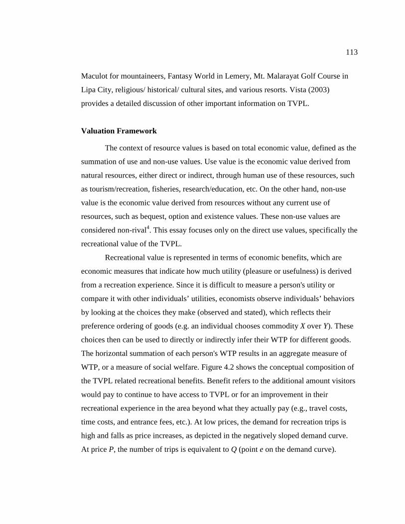
113
Maculot for mountaineers, Fantasy World in Lemery, Mt. Malarayat Golf Course in
Lipa City, religious/ historical/ cultural sites, and various resorts. Vista (2003)
provides a detailed discussion of other important information on TVPL.
Valuation Framework
The context of resource values is based on total economic value, defined as the
summation of use and non-use values. Use value is the economic value derived from
natural resources, either direct or indirect, through human use of these resources, such
as tourism/recreation, fisheries, research/education, etc. On the other hand, non-use
value is the economic value derived from resources without any current use of
resources, such as bequest, option and existence values. These non-use values are
considered non-rival4. This essay focuses only on the direct use values, specifically the
recreational value of the TVPL.
Recreational value is represented in terms of economic benefits, which are
economic measures that indicate how much utility (pleasure or usefulness) is derived
from a recreation experience. Since it is difficult to measure a person's utility or
compare it with other individuals’ utilities, economists observe individuals’ behaviors
by looking at the choices they make (observed and stated), which reflects their
preference ordering of goods (e.g. an individual chooses commodity X over Y). These
choices then can be used to directly or indirectly infer their WTP for different goods.
The horizontal summation of each person's WTP results in an aggregate measure of
WTP, or a measure of social welfare. Figure 4.2 shows the conceptual composition of
the TVPL related recreational benefits. Benefit refers to the additional amount visitors
would pay to continue to have access to TVPL or for an improvement in their
recreational experience in the area beyond what they actually pay (e.g., travel costs,
time costs, and entrance fees, etc.). At low prices, the demand for recreation trips is
high and falls as price increases, as depicted in the negatively sloped demand curve.
At price P, the number of trips is equivalent to Q (point e on the demand curve).
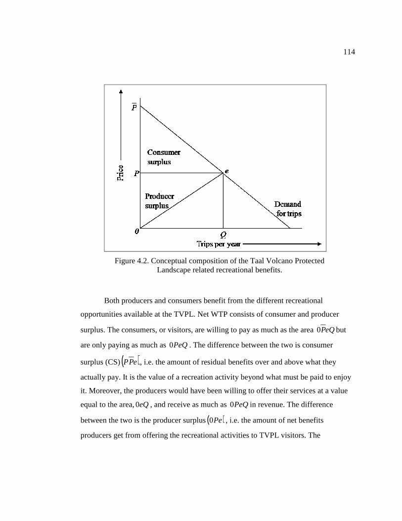
114
Figure 4.2. Conceptual composition of the Taal Volcano Protected Landscape related recreational benefits.
Both producers and consumers benefit from the different recreational
opportunities available at the TVPL. Net WTP consists of consumer and producer
surplus. The consumers, or visitors, are willing to pay as much as the area eQP0 but
are only paying as much as PeQ0 . The difference between the two is consumer
surplus (CS)( )ePP , i.e. the amount of residual benefits over and above what they
actually pay. It is the value of a recreation activity beyond what must be paid to enjoy
it. Moreover, the producers would have been willing to offer their services at a value
equal to the area,eQ0 , and receive as much as PeQ0 in revenue. The difference
between the two is the producer surplus( )Pe0 , i.e. the amount of net benefits
producers get from offering the recreational activities to TVPL visitors. The
115
recreational value of TVPL is the sum of CS and PS. Only the CS part of recreation
total value is estimated for the TVPL using BT methods.
Benefit Transfer Techniques
BT5 methods use estimated measures from study site i, VSi, to estimate the
needed measure for policy site j, VPj. When VSi is transferred to the policy site j, the
study site value becomes the transfer value, i.e. BTSi VV ⇒ (Rosenberger and Loomis,
2003). In this exercise, TVPL is the policy site, (i.e., the area or resource for which
benefit estimates are needed but do not exist). This exploratory BT exercise may also
help determine whether original research is warranted (Rosenberger and Loomis,
2003); i.e., uncertainty regarding the BT estimates and/or predicted magnitude of
recreational values.
Boyle et al. (2009, p. 1328) proposed four necessary conditions for valid BT:
a) utility must be separable in unobserved site characteristics; b) the study site and
policy site models must be correctly specified; c) people must not be sorted between
sites according to unobserved features of their preferences; and d) adequate data on the
characteristics of consumers and their choices. In addition, there should be
correspondence or similarity between study and policy sites in terms of a) resource or
commodity conditions, b) site characteristics, c) market characteristics (Desvousges,
Naughton, and Parsons, 1992), and d) welfare and empirical benefit measure (Boyle
and Bergstrom, 1992; Loomis and Rosenberger, 2006). Rosenberger and Loomis
(2001) provide a detailed list of criteria for an effective and efficient BT, reiterating
the conditions above.
Potential problems associated with the application of BT methods are provided
by Rosenberger and Loomis (2001). BT problems may be contributed by original
valuation studies their methodological applications (i.e., measurement error), and a
lack of correspondence between the study site and the policy site (i.e., generalization
error). It is important to identify the potential sources of errors that affect the accuracy
116
of BT and employ means for overcoming them (Rosenberger and Stanley, 2006). For
example, BT transfer estimates from more ‘generic study sites’ may be considered
lower bounds given the ‘uniqueness’ factor associated with TVPL. Designation of
TVPL as a ‘priority protected landscape’ may have higher values than ‘generic
protected landscapes’ due to its proximity to population centers such as Manila and
CALABARZON6 and its uniqueness. However, evidence reported in the literature
itself may not be representative of generic protected landscapes. There are many
social and political factors (e.g., highly valued, close to populations, awareness,
threatened by external factors, etc.) that may direct research resources toward certain
landscapes (Hoehn, 2006). If the literature is dominated by these research priority
sites, then use of this literature may result in upwardly biased estimates for more
generic applications (Rosenberger and Johnston, 2009).
However, being classified as a protected landscape may not always be positive
since there is an accelerated human population growth at protected area edges due to
economic opportunities they provide (Wittemyer et al. 2008). Furthermore, when a
resource site generates use value, the density of users will be higher near to that site
(Bateman et al., 2006). Resource users typically hold higher values than non-users and
we would expect average values to decay with increasing distance from a site. These
limitations and problems could lead to biased BT estimates and decreased robustness
of BT procedure, if not fully addressed.
The summarized BT procedures for estimating the access value of recreation in
TVPL, as suggested by previous studies (Boyle and Bergstrom, 1992; Brouwer, 2000;
Rosenberger and Loomis, 2001), are illustrated in Figure 4.3. The first step is to
describe the resource, commodity or context of the policy site. Here we need to specify
the theoretical definition of the value(s) to be estimated and needed at the policy site j.
In this paper, all benefit estimates, i.e. access value of recreation are expressed in
terms of CS per person per trip (PHP 2006). Primary studies reporting benefit
estimates other than CS/person/trip are adjusted to per trip units, and estimates derived
from earlier studies are converted to 2006 PHP using the Implicit Price Deflator7. The

117
information needed in this step include description of the environmental resource, and
possibly, evaluation of expected change in the resource. Moreover, factors that can
influence benefit estimates should be defined, such as socio-economic characteristics
of the affected population (e.g., income, education, age, and gender) and physical
characteristics of the policy site (e.g., environmental quality, geographic location, and
accessibility conditions). Depending on resource conditions and informational needs,
the level of required accuracy of BT estimates can be determined in this step (Kask
and Shogren, 1994).
The second step involves conducting a thorough literature search and locating
relevant study sites. Primary studies on the access value of recreation in the US and
The Philippines are collected through searching databases (EVRI, USAID
Development Experience Clearinghouse, Google Scholar), formally requesting
documents/ references via e-mail, listserves, postal mail and/or phone, analysis of
citations, and careful study of references. The primary studies are composed of journal
articles, theses, dissertations, working papers, government agency reports, consulting
reports, and proceedings papers.
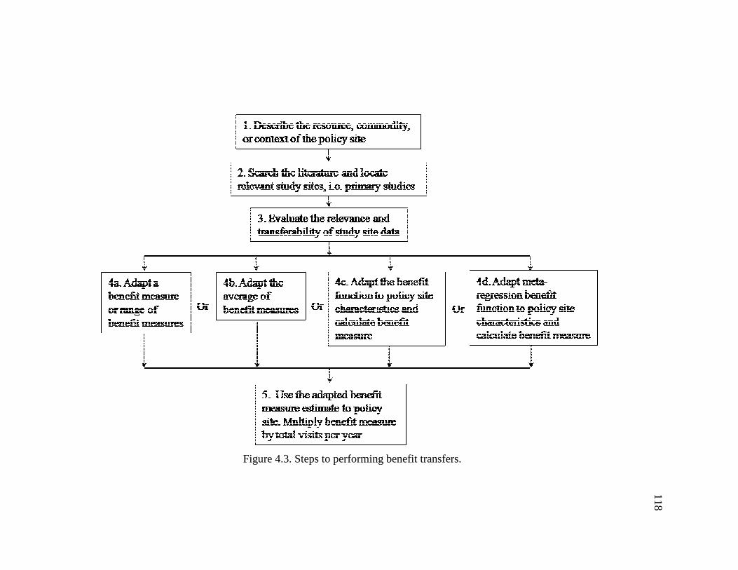
118
Figure 4.3. Steps to performing benefit transfers.
119
The third step is to evaluate study site data in terms of relevance and
transferability. Primary studies obtained from the literature search are screened
whether they are relevant to the policy site j. Transferability needs to be evaluated
using BT criteria discussed above and in terms of the overall quality of the study site
data, such as adequacy or scientific soundness. For example, unbiased estimates are
preferred for a valid BT. Some bias may be acceptable in a BT; the level of which
depends on the circumstances of decision settings and ultimate usage of BT estimates.
State-of-the-art guides on non-market valuation can be useful in this evaluation (e.g.
Champ, Boyle and Brown, 2003; Haab and McConnell, 2002).
The fourth step is to adapt the benefit measure(s) or function to policy site
characteristics. Depending on the BT approach used, whether 1) value transfer or 2)
function transfer, necessary adjustments may be needed to reflect the differences in the
study and policy sites to get a more reliable and valid BT estimates for the policy site
j. However, some potentially important characteristics may not be measured or
reported for the study or policy sites. This is an identified problem in BT (Loomis and
Rosenberger, 2006). Therefore, this missing information at the policy site may be
sourced out from other sources. For example, study sites can be supplemented with
external data like Census measures. When key characteristics of the user population
are measured using a very short and inexpensive survey, it is important that these
measures are in the study sites as well. For cases where one cannot supplement may
lead to an increased generalization errors (Rosenberger and Stanley, 2006). A more
detailed discussion of the BT approaches is given below.
The fifth step is to apply the adapted benefit measure estimate to policy site.
This is the final stage where actual BT estimates for the policy site are calculated and
can be aggregated by multiplying the benefit measure (CS/person/day in 2006 PHP)
by total visits per year (or total number of affected population).
120
Value transfer
Value transfer consists of transferring a single point estimate from study site i
or a measure of central tendency (e.g. average value) for several benefit estimates
from study site(s) i to the policy site j. Single point estimate transfer is accomplished
by using the measures of the study site value (VSi), given the context of the study site i,
(XSi), to predict the needed policy site value (VPj), given the context of the policy site j,
(XPj):
SiSiPjPj XVXV = Equation (1).
Single point estimate transfer is convergently valid when there is a
correspondence between the study and policy site in terms of the commodity, site
characteristics, and the relevant population (Ready, 2009). It is assumed that the
welfare of a representative visitor at the study site i is the same as the ‘expected’
welfare of a representative visitor at the policy site j, ceteris paribus.
Measure of central tendency is similar to point estimate transfer except for the
use of mean, median or other measure of central tendency to predict the needed policy
site value. This approach is defined as:
SiSiPjPj XVXV = Equation (2)
where SiSi XV is the measure of central tendency for all or a subset of study site
measures given each study site’s context.
Value transfer approaches are suggested when 1) the mean values of the
regression independent variables for the policy site j, or 2) the valuation regression
model of the study site, are not available or reported in the primary studies.
121
Function Transfer
Function transfers include the transfer of an entire demand or benefit function
estimated for a study site, or the use of meta-regression benefit function derived from
various study sites. Function transfers then adapt the function to fit the specifics of the
policy site, such as socioeconomic characteristics, extent of market and environmental
impact, and other measurable characteristics that systematically differ between the
study site and the policy site. The adapted function is then used to predict or forecast a
benefit measure for the policy site.
The demand or benefit function transfer is defined as:
( )PjSSPj XfV = Equation (3)
where PjV is the needed value for the policy site j, which is derived from the study site
demand or benefit function,Sf , adapted to the context of the policy site( )PjSX . To
predict a tailored policy site estimate, the regression coefficients estimated at the study
site are adjusted by the policy site measures for the associated regression variables.
Function transfer assumes that the underlying behavioral relationship between a
recreation trip and the variables representing site and population characteristics is
identical, and adjusts to the differences in these variables between the policy and study
sites.
Loomis (1992) argued that the benefit function transfer method is a more
rigorous and robust method of BT compared with point estimate transfer methods.
Benefit function transfer can be fitted to the characteristics of the policy site and more
information is effectively taken into account in the transfer. In this regard, function
transfer can result in smaller BT error than value transfers (Rosenberger and Loomis,
2003). Rosenberger and Phipps (2007) added that functional transfers have the
potential to reduce generalization errors compared to point estimate transfers.
Generalization error occurs when a measure of value is generalized to unstudied sites
122
or resources. It is hypothesized to be inversely related to the correspondence between
study sites and policy sites.
While function transfer may be better than value transfer, it is still considered a
second-best strategy for recreation valuation (Rosenberger and Loomis, 2001). One
drawback with benefit function transfer is the exclusion of relevant variables in the
WTP function estimated in a single study due to lack of variation in those variables.
There might be variables relevant to the study site but not to the policy site. To address
this problem, the study site should be chosen to be as similar as possible to the policy
site, or use meta-regression transfer function.
If benefit function transfer is based on a single study, meta-regression transfer
function, on the other hand, is based on the statistical summary or synthesis of
outcomes from several studies. The conduct of BT through MRA is feasible with the
accumulation of primary studies on recreation valuation. MRA is the statistical
summarizing or synthesizing of past research results using multivariate regression
analysis (Stanley and Jarrell, 1989). Meta-analysis has been used for synthesizing
research findings, hypothesis testing, knowledge acquisition, benefit transfer (Smith
and Pattanayak, 2002; Florax, Nijkamp, and Willis, 2002) and to improve the process
and quality of literature reviews (avoiding bias) of valuation studies (Stanley, 2001).
More detailed steps in conducting a MRA is provided by Stanley (2001).
The MRA transfer function is defined as:
( )PjSPjSPjSSPj QMXfV ,,= Equation (4)
where PjV is the needed value for the policy site j, which is a function ( )sf of the
following variables: X is a vector of site and population characteristics relevant to the
policy site j; M is a vector of methodological variables; and Q is a vector of other
quantity/quality variables. In MRA transfer function, PjV is a summary statistic
(CS/person/day) from each individual studies. This statistical function, the MRA
123
transfer function, becomes the link between the knowledge derived from applied
research and its application to policy settings.
In a meta-analysis, several original studies are analysed as a group, where the
result from each study is treated as a single observation in a regression analysis. If
multiple results from each study are used, various meta-regression specifications can
be used to account for such panel effects (Nelson and Kennedy, 2009; Rosenberger
and Loomis, 2000b).
The conduct of meta-analysis is not a perfect science. It also has its limits.
Study sites may be biased because of reliance on published sources (publication bias);
and lack of standardization in methodology. In response to these basic problems in
meta-analysis, Button (2002) described the following necessary conditions to consider
when conducting meta-analysis: a) acceptance of general values; b) sufficient previous
studies; c) compatibility of studies; d) stability of the parameters with rapidly
changing technology and tastes; e) nature of information needed; and f) independence
of studies.
The validity and reliability of applying meta-analysis to inform policy choices
is highly dependent upon the primary studies. Its contributions can be limited by the
quantity and quality of available documentation from primary research (Loomis and
Rosenberger, 2006) and the inherent heterogeneity of metadata (i.e., the literature).
Hence, meta-analysis explanatory power will usually not exceed that of the underlying
individual studies (Brouwer, 2002).
Convergent Validity of Benefit Transfer
Convergent validity is about the accuracy of generalization; i.e., measures of
the same theoretical construct correspond to each other—they converge. Validity tests
investigate the extent to which the welfare values and functions are transferable from a
statistical point of view. Convergent validity test answers the question how valid is the
measures of benefits at unstudied sites (Desvousges, Johnson and Banzhaf, 1998). For
124
example, convergent validity tests by Rosenberger and Loomis (2000b) suggest that a
national model is more robust to changes in application than regional models, in part
due to the greater coverage of the distribution of recreation values. Testing a value
transfer or function transfer model for convergent validity can be empirically done by
comparing a transfer value (VBT) to the ‘true’ value for a site (VS), where the true value
comes from an original study at the site. The associated error (ε) with the BT is
defined as:
S
BTS
V
VV −=ε Equation (5)
If more than one transfer estimates is generated, say from single point estimate and
meta-regression benefit function, these two transfer estimates can be compared to
determine if the BT method applied is invariant to judgment by the meta-analyst. If a
model has poor explanatory power for the study site, there is little confidence in the
accuracy for BT. In the same way, if there is limited convergence between ‘study site’
and ‘policy site’ estimates, there is little confidence in the BT estimation.
The ‘true’ value in itself is an estimate of an unknown value. ‘Study site’
estimates are considered the best approximation of the true value (VS). This is a
concern since there are no primary study estimates available at the policy site (TVPL).
When MR model is adapted, meta-analysis can employ an in-sample prediction
(Nelson and Kennedy, 2009) and the results are tested if the MR model supports a BT
application (Smith and Pattanayak, 2002).
Benefit Transfer Applications to TVPL
Value Transfer: Single Point Estimate
Transfers conducted within [country] perform better than transfers conducted
between [country] (Rosenberger and Loomis, 2001). In this regard, an in-depth search
for relevant study sites reporting an economic measure of direct-use value estimates
(i.e. access value only, not marginal values) for ‘nature-based’ recreation in the
125
Philippines was performed. A list of valuation studies conducted in the Philippines
between 1988 and 2002, categorized in terms of environmental services, is provided
by REECS, Inc. (2003). Three of the seven potential study sites on protected
landscape are available and were collected (Predo et al., 1999; Navarro, Paca and
Rimas, 2008; and Rosales, 2001). However, only one study site (Predo et al., 1999)
passed the relevance and transferability criteria. The studies by Navarro, Paca and
Rimas (2008) and Rosales (2001) can be excluded because these ‘potential study sites’
estimated the recreational benefits derived from a mountain ecosystem. The study by
Predo et al. (1999) estimated the recreational use, option use, existence, and bequest
values, through WTP for protection of Lake Danao National Park (LDNP) in Ormoc
City, Leyte, Philippines (Figure 4.4). The study used CVM with three WTP question
formats – open-ended, payment card, and iterative bidding. Tobit (censored
regression) model was used to analyzed the different factors affecting WTP bid for
protecting LDNP based on 210 respondents.
There is some degree of correspondence between TVPL and LDNP (Table 4.1)
in terms of the technical criteria for transferability of study sites values (Boyle and
Bergstrom, 1992). The policy site value based on Predo et al. (1999) is PHP35.65 per
person per trip or PHP62.40 per person per year (2006). At 95% confidence interval,
the policy site value ranges from PHP21 and PHP50.35/person/trip or between
PHP36.70 and PHP88.10/person/year (i.e. 41.20% margin of error (MOE)).
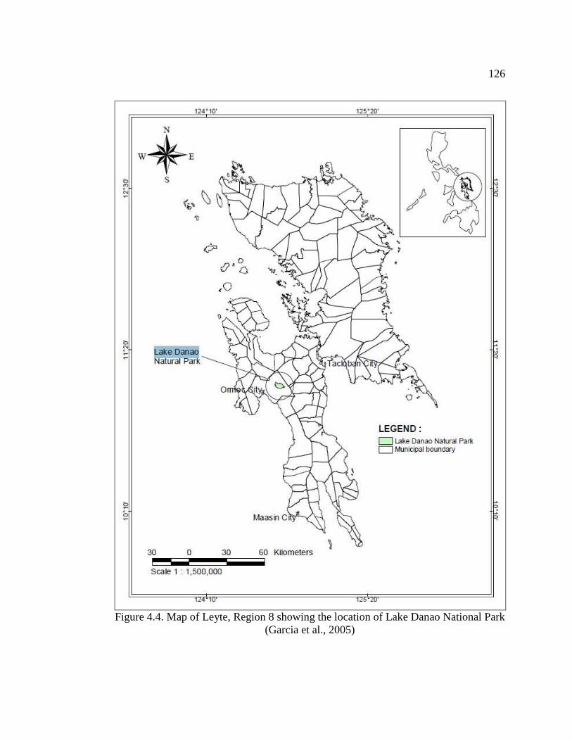
126
Figure 4.4. Map of Leyte, Region 8 showing the location of Lake Danao National Park (Garcia et al., 2005)
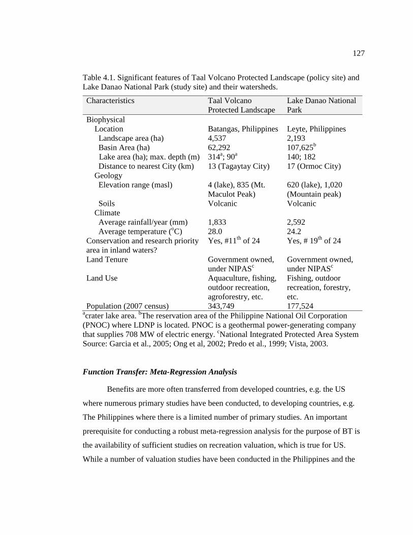
127
Table 4.1. Significant features of Taal Volcano Protected Landscape (policy site) and Lake Danao National Park (study site) and their watersheds.
Characteristics Taal Volcano Protected Landscape
Lake Danao National Park
Biophysical Location Batangas, Philippines Leyte, Philippines Landscape area (ha) 4,537 2,193 Basin Area (ha) 62,292 107,625b
Lake area (ha); max. depth (m) 314a; 90a 140; 182 Distance to nearest City (km) 13 (Tagaytay City) 17 (Ormoc City) Geology Elevation range (masl) 4 (lake), 835 (Mt.
Maculot Peak) 620 (lake), 1,020 (Mountain peak)
Soils Volcanic Volcanic Climate Average rainfall/year (mm) 1,833 2,592 Average temperature (oC) 28.0 24.2 Conservation and research priority area in inland waters?
Yes, #11th of 24 Yes, # 19th of 24
Land Tenure Government owned, under NIPASc
Government owned, under NIPASc
Land Use Aquaculture, fishing, outdoor recreation, agroforestry, etc.
Fishing, outdoor recreation, forestry, etc.
Population (2007 census) 343,749 177,524 acrater lake area. bThe reservation area of the Philippine National Oil Corporation (PNOC) where LDNP is located. PNOC is a geothermal power-generating company that supplies 708 MW of electric energy. cNational Integrated Protected Area System Source: Garcia et al., 2005; Ong et al, 2002; Predo et al., 1999; Vista, 2003. Function Transfer: Meta-Regression Analysis
Benefits are more often transferred from developed countries, e.g. the US
where numerous primary studies have been conducted, to developing countries, e.g.
The Philippines where there is a limited number of primary studies. An important
prerequisite for conducting a robust meta-regression analysis for the purpose of BT is
the availability of sufficient studies on recreation valuation, which is true for US.
While a number of valuation studies have been conducted in the Philippines and the
128
Southeast Asia region, the reality is that the vast majority of the recreation literature
originated from developed countries. For example, Zhai and Susuki (2009) studied the
possibility of using international BT to value coastal zones and found that transfer
errors are fewer when transferring from a developed country (Japan) to the developing
country (China) than vice versa. They also compared the transferability of three
attributes associated with coastal resources and found that economic promotion has
more transferability than environmental improvement and risk reduction.
In this paper, primary studies (‘study sites’) included in the metadata are based
on the broader North American recreation use values database. ‘Study sites’ are
selected based on recreation activity, climate, and/or site characteristics/environment.
The following recreation activities were selected: freshwater fishing in lakes,
swimming, boating, camping, floating/rafting/canoeing, waterskiing, hiking,
picnicking, sightseeing, and general recreation. ‘Study sites’ with hot, humid or dry
regional climate, which mimics the climate in the ‘policy site,’ are selected. These
sites include the southeast region (Florida, Georgia, Alabama, Tennessee, South
Carolina, and North Carolina); southern region (Mississippi, Louisiana, Arkansas,
Texas, and Oklahoma); and southwest region8 (Arizona, California, Nevada, New
Mexico, and Utah). After excluding five possible outliers (CS> $350), there are 213
benefit measures from 47separate primary studies in the metadata that spans from
1958 to 2006. Appendix D provides a summary of selected characteristics of the
original study used in international BT while Appendix E provides the bibliography of
recreational valuation studies used in international BT.
A linear specification fit the data better. Since the metadata resembles a panel
type, the metadata was stratified 'by study' and ‘by underlying data structure’ to
capture dependency among estimates provided in a single document. Results of
Hausman's Chi-squared statistic test, based on ‘by study’ stratification, favored fixed-
effect specification but only one of 28 study dummy variables and only one of the 42
estimated panel constants was statistically significant. On the other hand, only five of
the 28 study dummy variables were retained in the panel model when the stratification
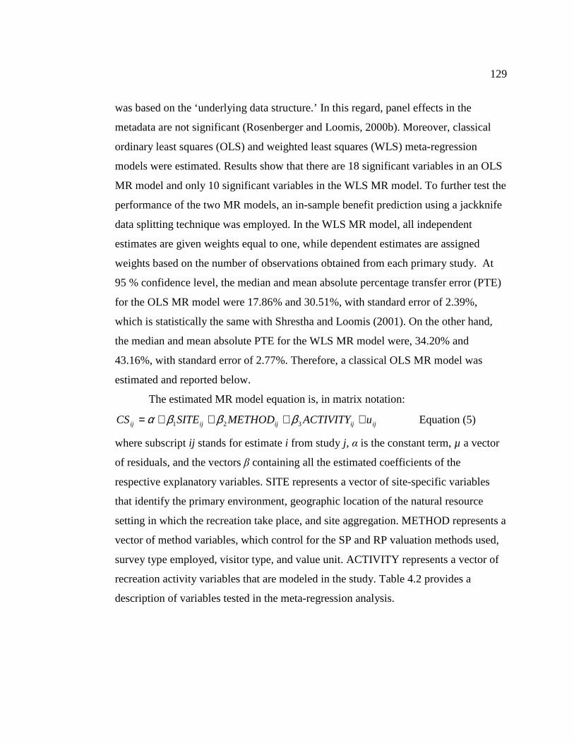
129
was based on the ‘underlying data structure.’ In this regard, panel effects in the
metadata are not significant (Rosenberger and Loomis, 2000b). Moreover, classical
ordinary least squares (OLS) and weighted least squares (WLS) meta-regression
models were estimated. Results show that there are 18 significant variables in an OLS
MR model and only 10 significant variables in the WLS MR model. To further test the
performance of the two MR models, an in-sample benefit prediction using a jackknife
data splitting technique was employed. In the WLS MR model, all independent
estimates are given weights equal to one, while dependent estimates are assigned
weights based on the number of observations obtained from each primary study. At
95 % confidence level, the median and mean absolute percentage transfer error (PTE)
for the OLS MR model were 17.86% and 30.51%, with standard error of 2.39%,
which is statistically the same with Shrestha and Loomis (2001). On the other hand,
the median and mean absolute PTE for the WLS MR model were, 34.20% and
43.16%, with standard error of 2.77%. Therefore, a classical OLS MR model was
estimated and reported below.
The estimated MR model equation is, in matrix notation:
ijijijijij uACTIVITYMETHODSITECS ++++= 321 βββα Equation (5)
where subscript ij stands for estimate i from study j, α is the constant term, µ a vector
of residuals, and the vectors β containing all the estimated coefficients of the
respective explanatory variables. SITE represents a vector of site-specific variables
that identify the primary environment, geographic location of the natural resource
setting in which the recreation take place, and site aggregation. METHOD represents a
vector of method variables, which control for the SP and RP valuation methods used,
survey type employed, visitor type, and value unit. ACTIVITY represents a vector of
recreation activity variables that are modeled in the study. Table 4.2 provides a
description of variables tested in the meta-regression analysis.
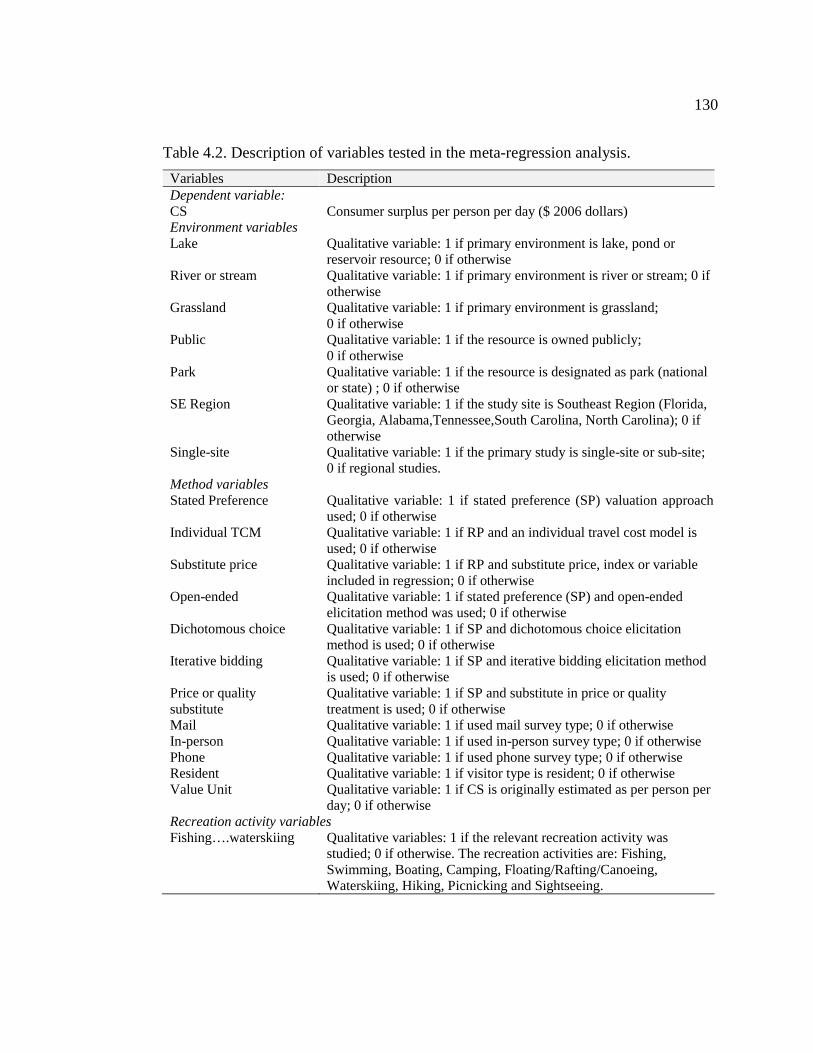
130
Table 4.2. Description of variables tested in the meta-regression analysis.
Variables Description Dependent variable: CS Consumer surplus per person per day ($ 2006 dollars) Environment variables Lake Qualitative variable: 1 if primary environment is lake, pond or
reservoir resource; 0 if otherwise River or stream Qualitative variable: 1 if primary environment is river or stream; 0 if
otherwise Grassland Qualitative variable: 1 if primary environment is grassland;
0 if otherwise Public Qualitative variable: 1 if the resource is owned publicly;
0 if otherwise Park Qualitative variable: 1 if the resource is designated as park (national
or state) ; 0 if otherwise SE Region Qualitative variable: 1 if the study site is Southeast Region (Florida,
Georgia, Alabama,Tennessee,South Carolina, North Carolina); 0 if otherwise
Single-site Qualitative variable: 1 if the primary study is single-site or sub-site; 0 if regional studies.
Method variables Stated Preference Qualitative variable: 1 if stated preference (SP) valuation approach
used; 0 if otherwise Individual TCM Qualitative variable: 1 if RP and an individual travel cost model is
used; 0 if otherwise Substitute price Qualitative variable: 1 if RP and substitute price, index or variable
included in regression; 0 if otherwise Open-ended Qualitative variable: 1 if stated preference (SP) and open-ended
elicitation method was used; 0 if otherwise Dichotomous choice Qualitative variable: 1 if SP and dichotomous choice elicitation
method is used; 0 if otherwise Iterative bidding Qualitative variable: 1 if SP and iterative bidding elicitation method
is used; 0 if otherwise Price or quality substitute
Qualitative variable: 1 if SP and substitute in price or quality treatment is used; 0 if otherwise
Mail Qualitative variable: 1 if used mail survey type; 0 if otherwise In-person Qualitative variable: 1 if used in-person survey type; 0 if otherwise Phone Qualitative variable: 1 if used phone survey type; 0 if otherwise Resident Qualitative variable: 1 if visitor type is resident; 0 if otherwise Value Unit Qualitative variable: 1 if CS is originally estimated as per person per
day; 0 if otherwise Recreation activity variables Fishing….waterskiing Qualitative variables: 1 if the relevant recreation activity was
studied; 0 if otherwise. The recreation activities are: Fishing, Swimming, Boating, Camping, Floating/Rafting/Canoeing, Waterskiing, Hiking, Picnicking and Sightseeing.
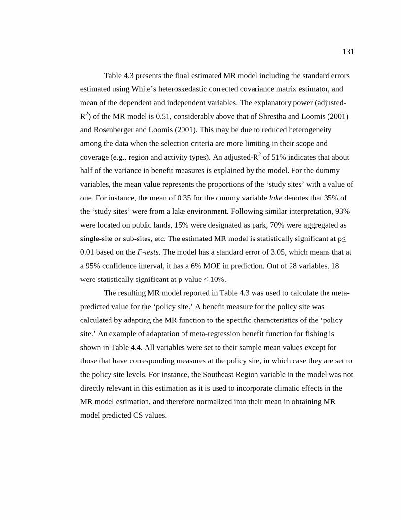
131
Table 4.3 presents the final estimated MR model including the standard errors
estimated using White’s heteroskedastic corrected covariance matrix estimator, and
mean of the dependent and independent variables. The explanatory power (adjusted-
R2) of the MR model is 0.51, considerably above that of Shrestha and Loomis (2001)
and Rosenberger and Loomis (2001). This may be due to reduced heterogeneity
among the data when the selection criteria are more limiting in their scope and
coverage (e.g., region and activity types). An adjusted-R2 of 51% indicates that about
half of the variance in benefit measures is explained by the model. For the dummy
variables, the mean value represents the proportions of the ‘study sites’ with a value of
one. For instance, the mean of 0.35 for the dummy variable lake denotes that 35% of
the ‘study sites’ were from a lake environment. Following similar interpretation, 93%
were located on public lands, 15% were designated as park, 70% were aggregated as
single-site or sub-sites, etc. The estimated MR model is statistically significant at p≤
0.01 based on the F-tests. The model has a standard error of 3.05, which means that at
a 95% confidence interval, it has a 6% MOE in prediction. Out of 28 variables, 18
were statistically significant at p-value ≤ 10%.
The resulting MR model reported in Table 4.3 was used to calculate the meta-
predicted value for the ‘policy site.’ A benefit measure for the policy site was
calculated by adapting the MR function to the specific characteristics of the ‘policy
site.’ An example of adaptation of meta-regression benefit function for fishing is
shown in Table 4.4. All variables were set to their sample mean values except for
those that have corresponding measures at the policy site, in which case they are set to
the policy site levels. For instance, the Southeast Region variable in the model was not
directly relevant in this estimation as it is used to incorporate climatic effects in the
MR model estimation, and therefore normalized into their mean in obtaining MR
model predicted CS values.
132
Table 4.3. Ordinary least squares regression model result.
Variable Coefficienta Standard errorb Mean of variable CS - - 41.75 Constant 35.25** 17.53 - Lake 26.81*** 8.98 0.35 River or stream 58.55*** 15.72 0.26 Grassland -70.75*** 20.24 0.03 Public -44.01*** 13.89 0.93 Park 41.70** 17.56 0.15 SE Region -18.75** 8.43 0.26 Stated Preference 53.54** 26.75 0.22 Individual TCM 47.55*** 11.96 0.27 Substitute price 11.90 8.50 0.47 Open-ended -68.14*** 24.13 0.07 Dichotomous choice -13.07 21.20 0.12 Iterative bidding -83.18*** 32.63 0.03 Price or quality substitute -54.63*** 18.91 0.01 Mail 38.99*** 11.12 0.36 In-person 43.98*** 9.99 0.50 Phone 30.38 23.29 0.03 Resident -27.99*** 6.63 0.41 Fishing -6.73 14.06 0.10 Camping 0.66 6.36 0.17 Hiking 19.23 14.95 0.05 Floating 5.24 18.13 0.21 Swimming -7.95 10.42 0.03 Boating -56.33*** 11.70 0.12 Picnicking 22.20* 13.18 0.03 Sightseeing 9.61 15.39 0.04 Waterskiing -19.18 16.72 0.01 Value unit -28.23*** 9.15 0.43 Single-site aggregation -8.76 10.85 0.70
Adjusted-R2 0.51 F-stat [28,184] 8.85*** Number of observations 213
Note: Dependent variable = consumer surplus (CS) per person per day ($ 2006) a*** Statistically significant at the 1% level or better; ** at the 5% or better, * the 10% level or better. bStandard errors are calculated using White’s heteroskedastic corrected covariance matrix estimator. Overall MOE is ± 6% based on standard error of 3.05 and 95% confidence interval.
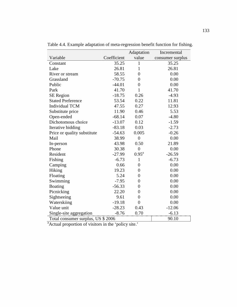
133
Table 4.4. Example adaptation of meta-regression benefit function for fishing.
Variable Coefficient Adaptation
value Incremental
consumer surplus Constant 35.25 1 35.25 Lake 26.81 1 26.81 River or stream 58.55 0 0.00 Grassland -70.75 0 0.00 Public -44.01 0 0.00 Park 41.70 1 41.70 SE Region -18.75 0.26 -4.93 Stated Preference 53.54 0.22 11.81 Individual TCM 47.55 0.27 12.93 Substitute price 11.90 0.46 5.53 Open-ended -68.14 0.07 -4.80 Dichotomous choice -13.07 0.12 -1.59 Iterative bidding -83.18 0.03 -2.73 Price or quality substitute -54.63 0.005 -0.26 Mail 38.99 0 0.00 In-person 43.98 0.50 21.89 Phone 30.38 0 0.00 Resident -27.99 0.95a -26.59 Fishing -6.73 1 -6.73 Camping 0.66 0 0.00 Hiking 19.23 0 0.00 Floating 5.24 0 0.00 Swimming -7.95 0 0.00 Boating -56.33 0 0.00 Picnicking 22.20 0 0.00 Sightseeing 9.61 0 0.00 Waterskiing -19.18 0 0.00 Value unit -28.23 0.43 -12.06 Single-site aggregation -8.76 0.70 -6.13 Total consumer surplus, US $ 2006 90.10
aActual proportion of visitors in the ‘policy site.’
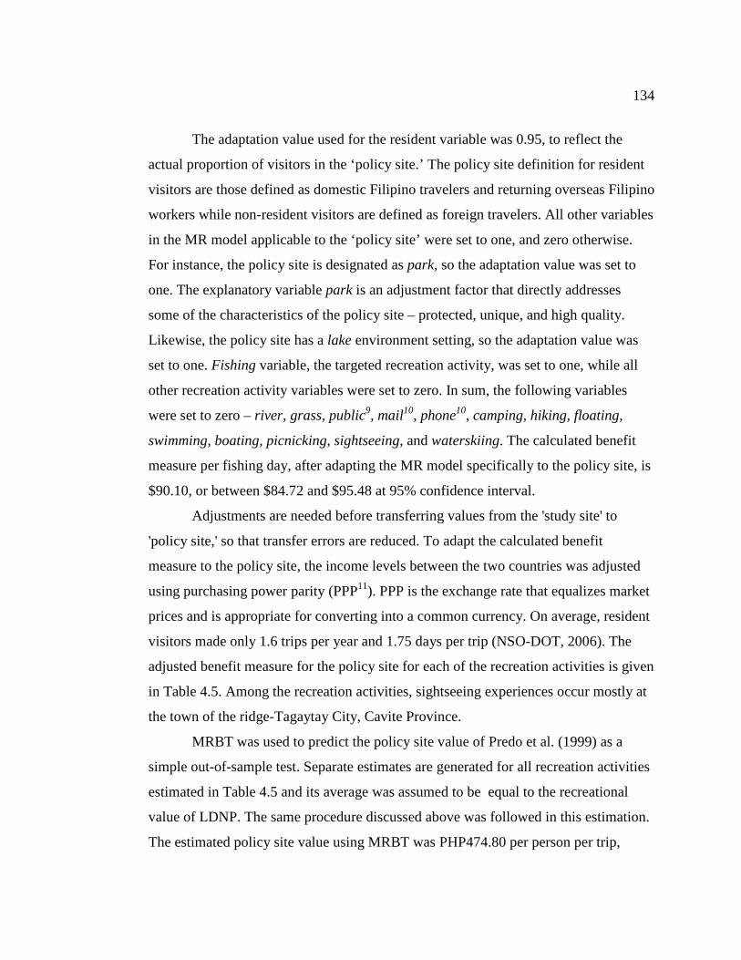
134
The adaptation value used for the resident variable was 0.95, to reflect the
actual proportion of visitors in the ‘policy site.’ The policy site definition for resident
visitors are those defined as domestic Filipino travelers and returning overseas Filipino
workers while non-resident visitors are defined as foreign travelers. All other variables
in the MR model applicable to the ‘policy site’ were set to one, and zero otherwise.
For instance, the policy site is designated as park, so the adaptation value was set to
one. The explanatory variable park is an adjustment factor that directly addresses
some of the characteristics of the policy site – protected, unique, and high quality.
Likewise, the policy site has a lake environment setting, so the adaptation value was
set to one. Fishing variable, the targeted recreation activity, was set to one, while all
other recreation activity variables were set to zero. In sum, the following variables
were set to zero – river, grass, public9, mail10, phone10, camping, hiking, floating,
swimming, boating, picnicking, sightseeing, and waterskiing. The calculated benefit
measure per fishing day, after adapting the MR model specifically to the policy site, is
$90.10, or between $84.72 and $95.48 at 95% confidence interval.
Adjustments are needed before transferring values from the 'study site' to
'policy site,' so that transfer errors are reduced. To adapt the calculated benefit
measure to the policy site, the income levels between the two countries was adjusted
using purchasing power parity (PPP11). PPP is the exchange rate that equalizes market
prices and is appropriate for converting into a common currency. On average, resident
visitors made only 1.6 trips per year and 1.75 days per trip (NSO-DOT, 2006). The
adjusted benefit measure for the policy site for each of the recreation activities is given
in Table 4.5. Among the recreation activities, sightseeing experiences occur mostly at
the town of the ridge-Tagaytay City, Cavite Province.
MRBT was used to predict the policy site value of Predo et al. (1999) as a
simple out-of-sample test. Separate estimates are generated for all recreation activities
estimated in Table 4.5 and its average was assumed to be equal to the recreational
value of LDNP. The same procedure discussed above was followed in this estimation.
The estimated policy site value using MRBT was PHP474.80 per person per trip,
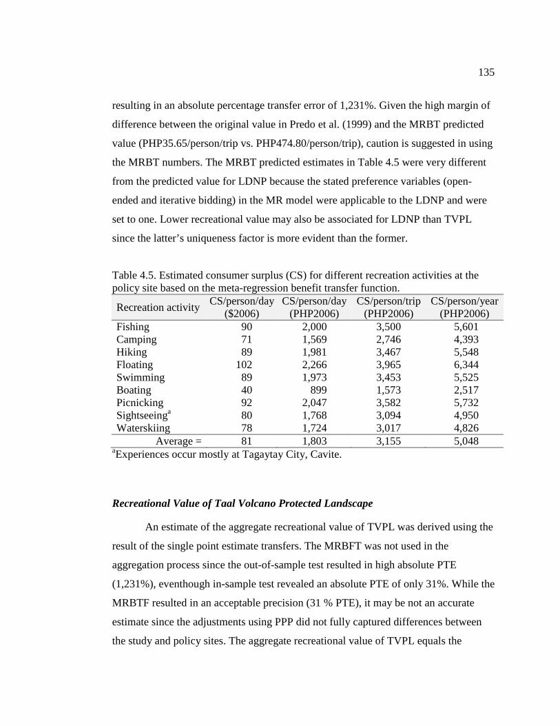
135
resulting in an absolute percentage transfer error of 1,231%. Given the high margin of
difference between the original value in Predo et al. (1999) and the MRBT predicted
value (PHP35.65/person/trip vs. PHP474.80/person/trip), caution is suggested in using
the MRBT numbers. The MRBT predicted estimates in Table 4.5 were very different
from the predicted value for LDNP because the stated preference variables (open-
ended and iterative bidding) in the MR model were applicable to the LDNP and were
set to one. Lower recreational value may also be associated for LDNP than TVPL
since the latter’s uniqueness factor is more evident than the former.
Table 4.5. Estimated consumer surplus (CS) for different recreation activities at the policy site based on the meta-regression benefit transfer function.
Recreation activity CS/person/day CS/person/day CS/person/trip CS/person/year
($2006) (PHP2006) (PHP2006) (PHP2006) Fishing 90 2,000 3,500 5,601 Camping 71 1,569 2,746 4,393 Hiking 89 1,981 3,467 5,548 Floating 102 2,266 3,965 6,344 Swimming 89 1,973 3,453 5,525 Boating 40 899 1,573 2,517 Picnicking 92 2,047 3,582 5,732 Sightseeinga 80 1,768 3,094 4,950 Waterskiing 78 1,724 3,017 4,826
Average = 81 1,803 3,155 5,048 aExperiences occur mostly at Tagaytay City, Cavite.
Recreational Value of Taal Volcano Protected Landscape
An estimate of the aggregate recreational value of TVPL was derived using the
result of the single point estimate transfers. The MRBFT was not used in the
aggregation process since the out-of-sample test resulted in high absolute PTE
(1,231%), eventhough in-sample test revealed an absolute PTE of only 31%. While the
MRBTF resulted in an acceptable precision (31 % PTE), it may be not an accurate
estimate since the adjustments using PPP did not fully captured differences between
the study and policy sites. The aggregate recreational value of TVPL equals the
136
consumer suplus per person per year times the number of resident visitors in 2006.
Non-resident visitors were excluded in the aggregation since no data was available
about their trip characteristics. In this regard, the forecasted aggregate recreational
value of TVPL is considered lower bound (conservative). Aggregate CS estimates are
provided for the Cavite (Tagaytay City) and Batangas sides since the visitation/activity
patterns for these two provinces are quite different. For the Batangas Province alone,
the estimated 2006 recreational value was about PHP9.7 million based on point
estimate transfer. For the Cavite side, the estimated 2006 recreational value was about
PHP118 million based on point estimate transfer. In sum, about PHP128 million was
estimated the value of access to TVPL in 2006. This access value is not the amount
that PASu could earn through user fees. Setting a fee and projecting fee revenue
requires the use of elasticities and other behavioral aspects of users.
Table 4.6. Recretional value of Taal Volcano Protected Landscape based on Filipino resident travellers, 2006.
No. of Visitors
No. of Resident visitors
Aggregate CS (PHP 2006) Single point estimate
Batangas 169,240 155,701 9,715,730 Cavite (Tagaytay) 2,006,571 1,906,242 118,949,529 Total 128,665,259
Discussions, Conclusions, and Policy Implications
Benefit transfer methods are increasingly used to aid decision-making,
especially when time and resource constraints the conduct of primary study. It has
many potential applications in developing countries, wherein collecting primary data
is significantly constrained by limited financial resources. This paper has used BT to
estimate the recreational value of Taal Volcano Protected Landscape, Philippines.
Two welfare measures are estimated from a 1) single point estimate transfer based on
137
a Philippines ‘study site’ and 2) meta-regression benefit function based on selected US
‘study sites.’
Following BT protocol, the adapted welfare measures, reported in PHP 2006
CS per person per trip and per year, are adjusted to the policy site conditions and
common unit. The MR transfer function was tested using in-sample benefit prediction
performance. The median and mean absolute PTE support the conclusion that the MR
transfer function model can be used to predict the welfare estimates at the policy site.
However, simple out-of-sample test of the MRBT resulted in very high absolute PTE
(1,231%). Since the absolute PTE in the out-of-sample BT prediction was greater than
the in-sample BT prediction, the estimated welfare values using MRBT were not
recommended for adaptation in TVPL. A smaller welfare estimates per person per trip
and per year (with a MOE equal to 41%) were estimated using single point estimate
than the MR transfer function model. Given with this evidence, the single point
estimate outperforms MRBT. Even though the point estimate transfer generates
second best CS estimates, the adapted welfare measure can be used to help guide
policies in the area. These values can be incorporated into resource management
decisions of PASu, PAMB, and various local governments within TVPL.
Results of this essay can inform PASu, PAMB, and the visitors of TVPL the
total value of recreational access in the area. PASu may be able to use the visitation
data and estimated aggregated value per province in the determination of financial
commitments by the different municipalities and cities within TVPL. In particular,
Tagaytay City may be asked to provide more funding towards the implementation of
the management plan since the city captures more investments and revenues
associated with tourism in the area. Tagaytay City mainly benefits from the scenic
beauty of TVPL through tourism surplus, including rise in land values, tourism-related
livelihoods, business permits, and taxes. In fact, about 80% annual revenue of the City
Government of Tagaytay are generated from tourism only. Tagaytay City is currently
a `free rider’ to the positive externalities of Taal Volcano Island and Lake, while the
DENR-PASu and other municipalities/cities within the basin pay the cost of protection
138
in the area. Interestingly, the PASu office and Provincial Government’s Task Force,
with the help of municipalities of Talisay, Laurel, Agoncillo and Tanauan City are the
ones regulating the intensive cage culture, infrastructure development, and pollution
within Taal Volcano Island and Lake but they are not shared with these tourism
suplus. Knowledge of the recreational value of TVPL creates incentives for the
Provicial Task Force on Environmental Law Enforcement and concerned local
governments to ensure protection and conservation of their unique resources. To do
this involves costs on the part of PASu, PAMB and the local governments within
TVPL.
The estimated recreational value of TVPL is not equivalent to economic
resources that can be generated when visitor use fees or recreational boat licenses are
imposed to the users. User fees should be based on a WTP study that captures public
perceptions and WTP fees, among others. If PASu would like to capture some of the
recreational value in TVPL, a user fee may be imposed on visitors at the Taal Volcano
Island. The recommended ad hoc user fee per visit is PHP86/person. This amount was
based on the budget for recreation and cultural resources priority activities from the
management plan (PHP14.62 million) divided by the number of visitors in 2006 in
Batangas Province (169,240). This amount is about twice that of the recommended fee
of PHP44 per person per visit for the Sohotan Natural Bridge National Park in Samar,
Philippines (Rosales, 2001). Higher fees at unique sites may have little or no effect on
visitation levels (Benitez, 2001). Proceeds from user fees shall go to the Integrated
Protected Areas Fund (IPAF12). Capturing monetary payments can be used to
compensate TVPL for service provisioning and maintaining the area for its scenic
beauty. Likewise, these revenues could be used to support TVPL biodiversity
conservation and funding the alternative employment opportunities for affected locals
who are barred from tilapia cage farming.
Given the time and funding, it is important to get an accurate assessment of the
value of goods and services the area provides. This can be done through conduct of
139
primary valuation studies that captures public perceptions and WTP fees, visitation
carrying capacity, etc. Moreover, future research may focus on comparing tourism
impacts on TVPL before and after management plans. In particular, after the 10-year
management plan, it is imperative to assess if the goal of maintaining the population at
TVPL is maintained below 350,000. In other protected areas in Africa and Latin
America, parks attract human settlement. There is an accelerated human population
growth at protected area edges due to economic opportunities they provide (Wittemyer
et al. 2008). If the same trend happens in TVPL, then it is imperative that economic
developments should be targeted at areas more distant from the basin that aids local
communities while simultaneously reducing human pressure on TVPL.
140
Notes
1 PAMB membership now stands at 157, with 35 Executive Committee members. 2 Municipalities are divided into income classes according to their average annual
income during the last three calendar years: First class = annual income of PHP
50,000,000 or more; Second class = annual income between PHP 40,000,000 and PHP
49,999,999; Third class = annual income between PHP 30,000,000 and PHP
39,999,999; Fourth class = annual income between PHP 20,000,000 and 29,999,999;
Fifth class = annual income between PHP 10,000,000 and PHP 19,999,999. While
most of the municipalities that spans TVPL are considered 3rd, 4th or 5th class, the
Province of Batangas ranked 6th among 77 provinces in the Philippines in terms of
Human Development Index for 2000. In 2003, Batangas ranked 16th place in HDI.
HDI is the summary measure of human development, which has three basic
dimensions: longevity, knowledge, and standard of living. 3 NIPAS law provides for the establishment and management of national integrated
protected areas system, defining its scope and coverage. These include natural park,
natural monument, wildlife sanctuary, protected landscapes and seascapes, resource
reserve, natural biotic areas, and other categories established by law, conventions or
international agreements which the Philippine Government is a signatory. The NIPAS
designation is equivalent to the International Union for Conservation of Nature and
Natural Resources (IUCN) Category V. 4 Non-rival goods are goods whose consumption by one person does not prevent
simultaneous consumption by other persons. 5 ‘Benefit’ transfer and ‘value’ transfer means the same. Other authors use the word
'value' and not 'benefit' to make a distinction between 'costs' and 'benefits.'
6 Region IV-A, portmanteau of the names of the provinces: CAvite, LAguna, BAtangas,
Rizal, QueZON. It is the second most densely populated region in the Philippines, next
to Metro Manila.

141
7 Consumer Price Index for areas outside the National Capital Region is available at
http://www.cesus.gov.ph . 8 Colorado was excluded in the selection criteria since the over-all climate of the state is
different from the targeted policy site. 9 The public variable identifies all studies conducted on recreation on public lands,
including US Forest Service, Bureau of Land Management, US Army Corps of
Engineers, county, municipality, etc. The values are typically lower than other
estimates because these sites are easily accessible and more general in nature. This
variable is not adaptable to TVPL. The variable park captures the premium for high
quality, unique protected sites. 10 Phone, mail or web-based surveys are not often used in the Philippines since many
targeted respondents don’t have access to them. Hence, in-person survey is the
dominant type of survey data collection. In developing countries, like The Philippines,
local cultures and socio-economic conditions matter [or may influence] in benefit
estimation (Alam, 2006). 11Purchasing Power Parity conversion factor used was $1=PHP22.2 (WorldBank, 2010).
There’s a caveat in PPP adjusted benefit measures since it will not be able to correct
for differences in individual preferences, and cultural and institutional conditions
between the two countries that they have the potential to invalidate an international
BT. 12Department Administrative Order No. 25, Series of 1992 – NIPAS Implementing
Rules and Regulations states that “at least 75% of the revenues generated by a
protected area shall be retained for the development and maintenance of that area
and utilized subject to the IPAF Board guidelines… with the balance being remitted
to the Central IPAF Fund.”
142
References
Alam, K. 2006. "Valuing the environment in developing countries: problems and potentials." Asia Pacific Journal on Environment and Development 13(1 & 2):27-44.
Alberini, A., and A. Krupnick. "Air Quality and Episodes of Acute Respiratory Illness
in Taiwan Cities: Evidence from Survey Data." Journal of Urban Economics 44, no. 1(1998): 68-92.
Barton, D. N., and S. Mourato. "Transferring the benefits of avoided health effects
from water pollution between Portugal and Costa Rica." Environment and Development Economics 8, no. 02(2003): 351-371.
Bateman, I. J., et al. "The aggregation of environmental benefit values: Welfare
measures, distance decay and total WTP." Ecological Economics 60, no. 2(2006): 450-460.
Benitez, S. P. (2001) Visitor User Fees and Concession Systems in Protected Areas,
Galapagos National Park, Ecuador, Tourism and Protected Areas Publication Series, The Nature Conservancy, Arlington, VA.
Boyle, K. J., and J. C. Bergstrom. "Benefit Transfer Studies: Myths, Pragmatism, and
Idealism." Water Resources Research 28, no. 3(1992): 657–663. Boyle, K. J., et al. "Necessary Conditions for Valid Benefit Transfers." American
Journal of Agricultural Economics 91, no. 5(2009): 1328-1334. Brouwer, R. "Environmental value transfer: state of the art and future prospects."
Ecological Economics 32, no. 1(2000): 137-152. Brouwer, R., and F. A. Spaninks. "The Validity of Environmental Benefits Transfer:
Further Empirical Testing." Environmental and Resource Economics 14, no. 1(1999): 95-117.
Button, K. J. (2002) An evaluation of the potential of meta-analysis in value and
function transfer. In R. Florax, P. Nijkamp, and K. Willis (Eds). Comparative Environmental Economic Assessment. MA, USA, Edward Elgar Publishing, Inc.
Champ, P. A., K. J. Boyle, and T. C. Brown (Eds.) (2003). A primer on nonmarket
valuation. Economics of non-market goods and resources Vol. 3. Dordrecht, Boston Kluwer Academic Publishers.
143
Desvousges, W. H., M. C. Naughton, and G. R. Parsons. "Benefit Transfer:
Conceptual Problems in Estimating Water Quality Benefits Using Existing Studies." Water Resour. Res. 28, no. 3(1992): 675–683.
Desvousges, W. H., F. R. Johnson, and H. S. Banzhaf. Environmental policy analysis
with limited information: principles and applications of the transfer method. Northampton, MA: Edward Elgar Publishing, 1998.
Florax, R., P. Nijkamp, and K. Willis (2002) Meta-analysis and value transfer:
Comparative assessment of scientific knowledge. In R. Florax, P. Nijkamp, and K. Willis (Eds). Comparative Environmental Economic Assessment. MA, USA, Edward Elgar Publishing, Inc.
Folledo Jr., R. A., and R. V. O. Cruz. "Taal Lake Watershed: Ecological Profile,
Sources of Ecological Perturbations and Watershed Restorations Strategies." College of Forestry and Natural Resources, University of the Philippines Los Banos, 1999.
Garcia, P. P., et al. (2005) Multi-Sectoral Watershed Planning in Lake Danao Natural
Park through Participatory Approaches: Terminal Report, Leyte State University.
Haab, T. C., and K. E. McConnell. Valuing Environmental and Natural Resources:
The Econometrics of Non-Market Valuation Northampton, Mass., USA: Edward Elgar Publishing, 2002.
Hargrove, T. R. The Mysteries of Taal: A Philippine volcano and lake, her sea life and
lost towns. Makati, Metro Manila: Bookmark, 1991. Hoehn, J. P. "Methods to address selection effects in the meta regression and transfer
of ecosystem values." Ecological Economics 60, no. 2(2006): 389-398. Kask, S. B., and J. F. Shogren. "Benefit transfer protocol for long-term health risk
valuation: A case of surface water contamination." Water Resour. Res. 30, no. 10(1994): 2813-2823.
Krupnick, A. "Mortality-risk Valuation and Age: Stated Preference Evidence." Rev
Environ Econ Policy 1, no. 2(2007): 261-282. Loomis, J. B. "The Evolution of a More Rigorous Approach to Benefit Transfer:
Benefit Function Transfer." Water Resources Research 28, no. 3(1992): 701-705.
144
Loomis, J.B., and R.S. Rosenberger. 2006. "Reducing barriers in future benefit
transfers: Needed improvements in primary study design and reporting." Ecological Economics 60(2):343-350.
Luna, M. P. G., and V. Gonzales. (2007). The Test of Effective Participation in
Management Planning. Jaipur, India. Muthke, T., and K. Holm-mueller. "National and International Benefit Transfer
Testing with a Rigorous Test Procedure." Environmental and Resource Economics 29, no. 3(2004): 323-336.
Nelson, J. P., and P. E. Kennedy. "The Use (and Abuse) of Meta-Analysis in
Environmental and Natural Resource Economics: An Assessment " Environmental and Resource Economics 42(2009): 345-377.
NSO-DOT. (2006) "2005 Household Survey on Domestic Visitors: Final Report."
National Statistics Office and Department of Tourism, Republic of the Philippines.
Ong, P. S., L. E. Afuang, and R. G. Rosell-Ambal (Eds.) (2002). Philippine
Biodiversity Conservation Priorities: A second iteration of the national biodiversity strategy and action plan. DENRPAWB, CI-Philippines, Biodiversity Conservation Program (BCP) – University of the Philippines Center for Integrative and Development Studies (UPCIDS) and Foundation for the Philippine Environment (FPE), Quezon City, Philippines.
Predo, C. D., et al. "Non-market Valuation of the Benefits of Protecting Lake Danao
National Park in Ormoc, Philippines." Journal of Environmental Science and Management 2, no. 2(1999): 13-32.
Resources Environment and Economics Center for Studies (REECS), Inc. (2003).
"Developing Pro-Poor Markets for Environmental Services in the Philippines: Final Report." International Institute for Environment and Development.
Republic Act No. 7586. National Integrated Protected Area System Act of 1992. Ready, R. C. "Advances in Environmental Benefit Transfer: Discussion." American
Journal of Agricultural Economics 91, no. 5(2009): 1351-1352. Ready, R., et al. "Benefit Transfer in Europe: How Reliable Are Transfers between
Countries?" Environmental and Resource Economics 29, no. 1(2004): 67-82.
145
REECS (Resources, Environment and Economics Center for Studies), Inc. (2003) Developing Pro-poor Markets for Environmental Services in the Philippines. Final Report prepared for the International Institute for Environment and Development.
Rosales, R. M. P. (2001) "Estimating Recreational Values of the Sohotan Natural
Bridge National Park ". US Agency for International Development. Rosenberger, R. S., and J. B. Loomis (2001) Benefit transfer of outdoor recreation use
values: A technical document supporting the Forest Service Strategic Plan (2000 revision). Fort Collins, CO, U.S. Department of Agriculture, Forest Service, Rocky Mountain Research Station, pp. 59.
Rosenberger, R. S., and J. B. Loomis (2003) Benefit Transfer: A Primer on Nonmarket
Valuation, P. A. Champ, K. J. Boyle, and T. C. Brown (Eds). Dordrecht, Netherlands: Kluwer Academic Press.
Rosenberger, R. S., and R. J. Johnston. “Selection effects in meta-analysis and benefit
transfer: Avoiding unintended consequences.” Land Economics 85, no. 3(2009): 410-428.
Rosenberger, R. S., and T. T. Phipps (2007) Correspondence and convergence in
benefit transfer accuracy: A meta-analytic review of the literature, ed. S. Navrud, and R. Ready. Environmental Values Transfer: Issues and Methods. Dordrecht, The Netherlands, Kluwer Academic Publishers. pp. 23-43.
Rosenberger, R. S., and T. D. Stanley. "Measurement, generalization, and publication:
Sources of error in benefit transfers and their management." Ecological Economics 60, no. 2(2006): 372-378.
Shrestha, R. K., and J. B. Loomis. "Testing a meta-analysis model for benefit transfer
in international outdoor recreation." Ecological Economics 39, no. 1(2001): 67-83.
Smith, V., and S. Pattanayak. "Is Meta-Analysis a Noah's Ark for Non-Market
Valuation?" Environmental and Resource Economics 22, no. 1(2002): 271-296.
Stanley, T. D. "Wheat from Chaff: Meta-analysis as Quantitative Literature Review."
Journal of Economic Perspectives 15, no. 3(2001): 131-150 Stanley, T. D., and S. B. Jarrell. "Meta-Regression Analysis: A Quantitative method of
Literature Surveys." Journal of Economic Surveys 3, no. 2(1989): 161.
146
World Bank. (2010, May 21) Purchasing power parities (PPP) conversion factor, local currency unit to international dollar. Retrieved from http://search.worldbank.org/data?qterm=ppp&language=EN&format=html
Yokoyama, I., A. Alcaraz, and O. Peña. "Gravimetric studies of Taal Volcano,
Philippines." Bulletin of Volcanology 39, no. 3(1975): 479-489. Vista, A., et al. "Nutrient Loading and Efficiency of Tilapia Cage Culture in Taal
Lake, Philippines." Philippine Agricultural Scientist 89, no. 1(2006): 48-57. Vista, A. B. "Cost-effectiveness of nutrient pollution reduction in Taal Lake,
Philippines." MS Thesis. Michigan State University, 2003. Wittemyer, G., et al. "Accelerated Human Population Growth at Protected Area
Edges." Science 321, no. 5885(2008): 123-126. Zhai, G., and T. Suzuki. "International Benefit Transfer Related to Coastal Zones:
Evidence from Northeast Asia." Marine Resource Economics 24, no. 2(2009): 171-186.
147
CHAPTER 5 - CONCLUSION
This dissertation has presented three essays on meta-analysis, benefit transfer,
and recreation use valuation. Summaries of results, contributions, conclusions and
recommendations of the three essays are presented in this section.
The goal of the first essay was accomplished by following the best-practice
guidelines for meta-analyses using the sportfishing valuation studies. Based upon the
log-likelihood ratio test, the two sub-metadata models (single-site and regional) are
not from the same population and should not be pooled without accounting for their
differences in a meta-analysis. Overall, the regional model has more significant
variables and lower percent difference (i.e. transfer error) in the out-of-sample validity
test than single-site model. When high/low original consumer surplus values for the
transfer studies were excluded in the out-of-sample validity test, the relative
performance of the regional model increases over the single-site and pooled models.
However, these results remain inconclusive as to which model might work best in
real-world policy settings given small set of out-of-sample studies. Essay 1 has shown
that welfare aggregation differences among primary studies influence the direction and
magnitude of bias that are carried forward in benefit transfer applications. In
particular, benefit transfer error depends on the meta-analyst’s choice of primary
studies to include in metadata, model specification, and the unit of welfare aggregation
level to consider. Therefore, meta-analysts should consider the appropriate level of
aggregation when doing benefit transfer based on meta-regression benefit function.
There is no single ‘appropriate’ level of aggregation. Some construct at different levels
of aggregation might be better depending on the number of available studies and
desired outcome being studies.
The second essay examined meta-analytic procedures that are used when one
or more of the studies in the metadata contain multiple measures of benefits. Results
show that the degree of explanatory power among the meta-regression models was
best achieved in an all-set weighted specification and in using an average-set
148
metadata, which are complementary treatments of data dependency. There were
changes in the magnitude and signs of the estimated parameters of the fishing
environment variables when the underlying structure of the metadata was modified
into best-set and average-set. This result affirmed the findings of Essay 1 that the
structural shift in the metadata was influenced by fishing environment variables.
Moreover, results indicate that median absolute percentage transfer error is lower for
the meta-regression models based on a single value, i.e. average-set and best-set
metadata than the meta-regression based on all-set. However, this increased in in-
sample predictions is not substantial since the single value approach may result in a
loss of information. One significant observation from in-sample predictions is that the
absence of very low and very high estimates in the metadata will likely result in more
robust meta-regression benefit transfer. Therefore, caution is recommended when
selecting studies for point or function transfers that provide very low estimates.
Instead, it is recommended to select those observations that fall within two standard
deviations of the mean, given large sample. Findings also suggest that the dummy
variables related to measurement errors and publication selection bias are important
predictors of transfer errors.
The third essay estimated the recreational value of Taal Volcano Protected
Landscape in the Philippines. Results show that single point estimate transfer worked
better than the meta-regression benefit function transfer. The meta-regression benefit
function was not used since the out-of-sample test resulted higher absolute transfer
error than in-sample test absolute transfer error. Therefore, caution is suggested in
using the estimated numbers using meta-regression benefit function. The estimated
welfare estimate of recreational access using single point estimate transfer was PHP
36 per person per trip. Given different trip characteristics of visitors, separate
aggregate estimates of recreational value were estimated for the Batangas Province
and Cavite Province. The aggregated recreational benefits at Taal Volcano Protected
Landscape was PHP 9.7 million from 155,701 visitors at Batangas side and PHP 118.9
million from 1,906,242 visitors at the Cavite side in 2006. The number of visitors
149
corresponds only to the domestic Filipino travelers and returning overseas Filipino
workers. Foreign visitors (about 5%) were excluded in the aggregation since no data
was available about their trip characteristics. The estimated PHP128.6 represents the
value of access to Taal Volcano Protected Landscape in 2006.
There remain some challenges in conducting meta-analysis for benefit transfer.
In particular, there is a general lack of reporting about characteristics of the primary
study contexts in the literature. In this regard, the following observations are
recommended when conducting meta-analysis and benefit transfer: 1) the need to
account for aggregation differences among primary studies to minimize biased value
estimates in benefit transfer depending on policy settings; 2) the importance to correct
for dependency and other methodological pitfalls in meta-regression; 3) metadata
sample selection is best guided by the goals of the meta-analysis and perceived
allowable errors in benefit transfer applications; and 4) the conduct of primary study is
still the first best strategy to recreation use valuation, given time and resources. More
research is needed to analyze the implications of metadata sample selection in the
context of benefit transfer. In particular, future research should evaluate the downward
bias associated with the different metadata sample sizes when used in benefit transfer
applications.
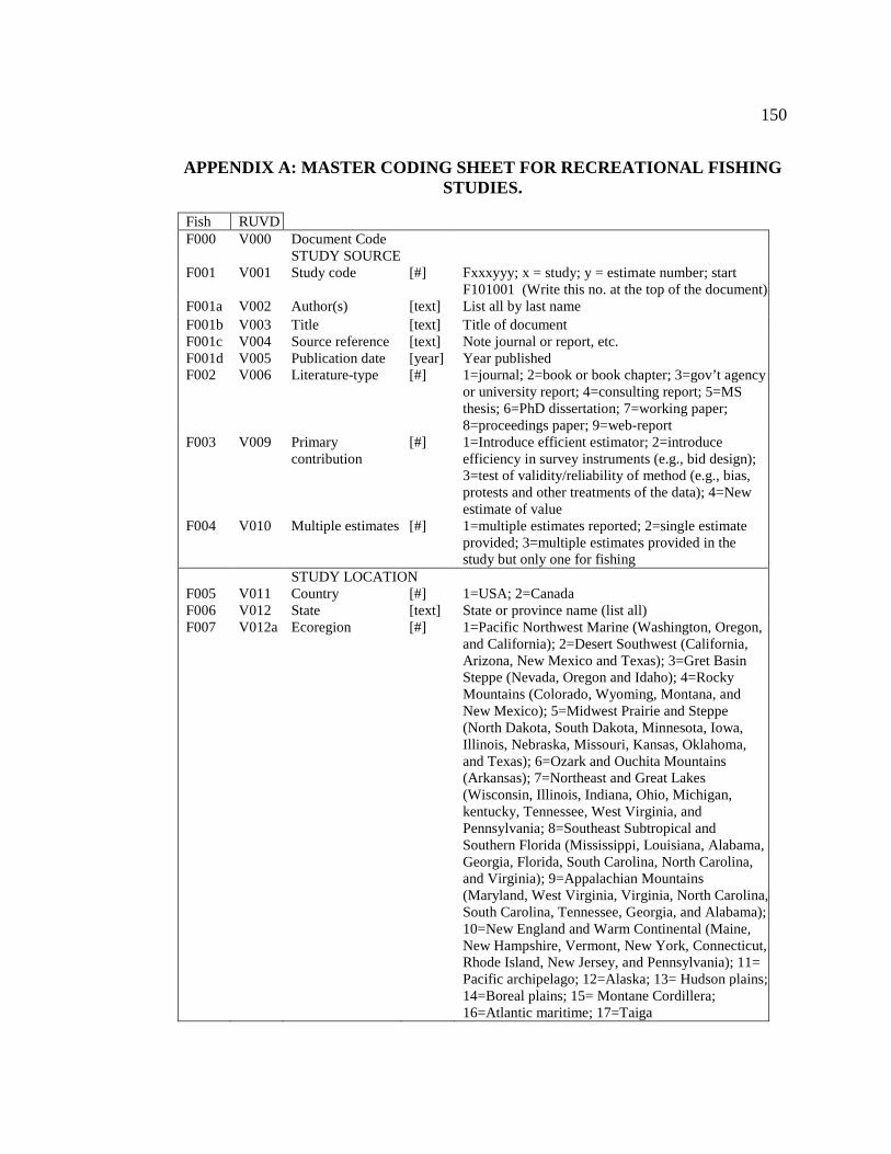
150
APPENDIX A: MASTER CODING SHEET FOR RECREATIONAL FI SHING STUDIES.
Fish RUVD F000 V000 Document Code STUDY SOURCE F001 V001 Study code [#] Fxxxyyy; x = study; y = estimate number; start
F101001 (Write this no. at the top of the document) F001a V002 Author(s) [text] List all by last name F001b V003 Title [text] Title of document F001c V004 Source reference [text] Note journal or report, etc. F001d V005 Publication date [year] Year published F002 V006 Literature-type [#] 1=journal; 2=book or book chapter; 3=gov’t agency
or university report; 4=consulting report; 5=MS thesis; 6=PhD dissertation; 7=working paper; 8=proceedings paper; 9=web-report
F003 V009 Primary contribution
[#] 1=Introduce efficient estimator; 2=introduce efficiency in survey instruments (e.g., bid design); 3=test of validity/reliability of method (e.g., bias, protests and other treatments of the data); 4=New estimate of value
F004 V010 Multiple estimates [#] 1=multiple estimates reported; 2=single estimate provided; 3=multiple estimates provided in the study but only one for fishing
STUDY LOCATION F005 V011 Country [#] 1=USA; 2=Canada F006 V012 State [text] State or province name (list all) F007 V012a Ecoregion [#] 1=Pacific Northwest Marine (Washington, Oregon,
and California); 2=Desert Southwest (California, Arizona, New Mexico and Texas); 3=Gret Basin Steppe (Nevada, Oregon and Idaho); 4=Rocky Mountains (Colorado, Wyoming, Montana, and New Mexico); 5=Midwest Prairie and Steppe (North Dakota, South Dakota, Minnesota, Iowa, Illinois, Nebraska, Missouri, Kansas, Oklahoma, and Texas); 6=Ozark and Ouchita Mountains (Arkansas); 7=Northeast and Great Lakes (Wisconsin, Illinois, Indiana, Ohio, Michigan, kentucky, Tennessee, West Virginia, and Pennsylvania; 8=Southeast Subtropical and Southern Florida (Mississippi, Louisiana, Alabama, Georgia, Florida, South Carolina, North Carolina, and Virginia); 9=Appalachian Mountains (Maryland, West Virginia, Virginia, North Carolina, South Carolina, Tennessee, Georgia, and Alabama); 10=New England and Warm Continental (Maine, New Hampshire, Vermont, New York, Connecticut, Rhode Island, New Jersey, and Pennsylvania); 11= Pacific archipelago; 12=Alaska; 13= Hudson plains; 14=Boreal plains; 15= Montane Cordillera; 16=Atlantic maritime; 17=Taiga
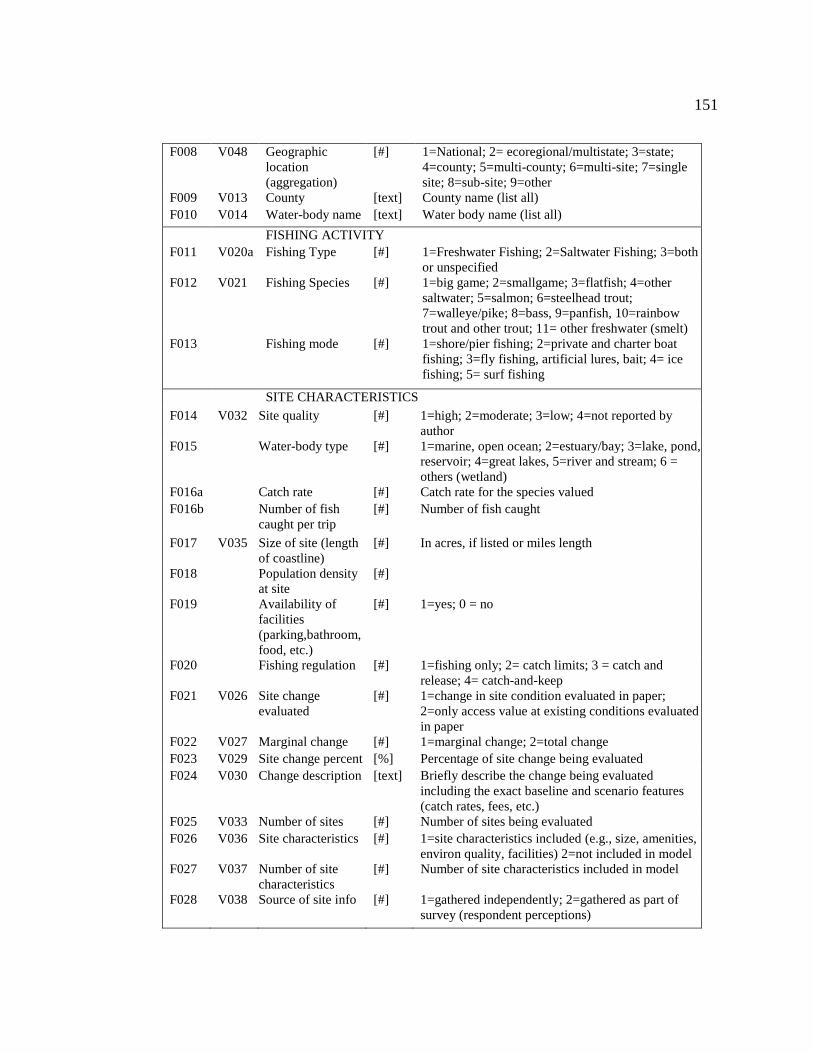
151
F008 V048 Geographic location (aggregation)
[#] 1=National; 2= ecoregional/multistate; 3=state; 4=county; 5=multi-county; 6=multi-site; 7=single site; 8=sub-site; 9=other
F009 V013 County [text] County name (list all) F010 V014 Water-body name [text] Water body name (list all)
FISHING ACTIVITY F011 V020a Fishing Type [#] 1=Freshwater Fishing; 2=Saltwater Fishing; 3=both
or unspecified F012 V021 Fishing Species [#] 1=big game; 2=smallgame; 3=flatfish; 4=other
saltwater; 5=salmon; 6=steelhead trout; 7=walleye/pike; 8=bass, 9=panfish, 10=rainbow trout and other trout; 11= other freshwater (smelt)
F013 Fishing mode [#] 1=shore/pier fishing; 2=private and charter boat fishing; 3=fly fishing, artificial lures, bait; 4= ice fishing; 5= surf fishing
SITE CHARACTERISTICS
F014 V032 Site quality [#] 1=high; 2=moderate; 3=low; 4=not reported by author
F015 Water-body type [#] 1=marine, open ocean; 2=estuary/bay; 3=lake, pond, reservoir; 4=great lakes, 5=river and stream; 6 = others (wetland)
F016a Catch rate [#] Catch rate for the species valued F016b Number of fish
caught per trip [#] Number of fish caught
F017 V035 Size of site (length of coastline)
[#] In acres, if listed or miles length
F018 Population density at site
[#]
F019 Availability of facilities (parking,bathroom, food, etc.)
[#] 1=yes; 0 = no
F020
Fishing regulation [#] 1=fishing only; 2= catch limits; 3 = catch and release; 4= catch-and-keep
F021 V026 Site change evaluated
[#] 1=change in site condition evaluated in paper; 2=only access value at existing conditions evaluated in paper
F022 V027 Marginal change [#] 1=marginal change; 2=total change F023 V029 Site change percent [%] Percentage of site change being evaluated F024 V030 Change description [text] Briefly describe the change being evaluated
including the exact baseline and scenario features (catch rates, fees, etc.)
F025 V033 Number of sites [#] Number of sites being evaluated F026 V036 Site characteristics [#] 1=site characteristics included (e.g., size, amenities,
environ quality, facilities) 2=not included in model F027 V037 Number of site
characteristics [#] Number of site characteristics included in model
F028 V038 Source of site info [#] 1=gathered independently; 2=gathered as part of survey (respondent perceptions)
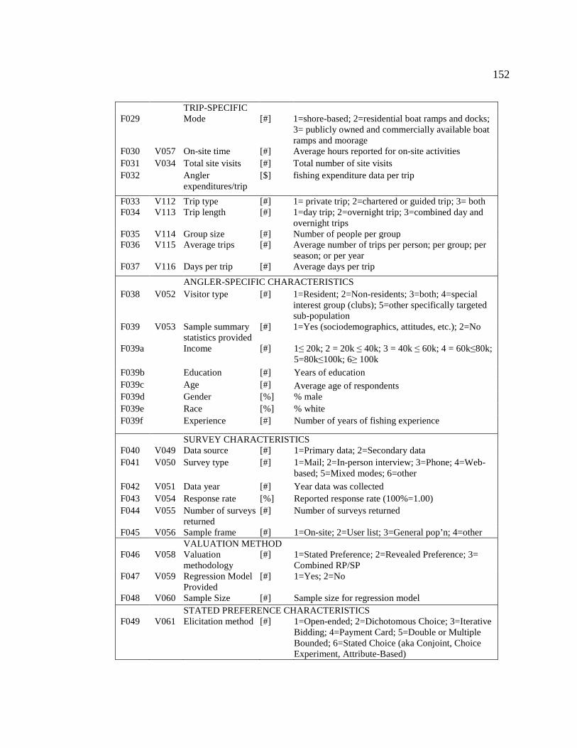
152
TRIP-SPECIFIC F029 Mode [#] 1=shore-based; 2=residential boat ramps and docks;
3= publicly owned and commercially available boat ramps and moorage
F030 V057 On-site time [#] Average hours reported for on-site activities F031 V034 Total site visits [#] Total number of site visits F032 Angler
expenditures/trip [$] fishing expenditure data per trip
F033 V112 Trip type [#] 1= private trip; 2=chartered or guided trip; 3= both F034 V113 Trip length [#] 1=day trip; 2=overnight trip; 3=combined day and
overnight trips F035 V114 Group size [#] Number of people per group F036 V115 Average trips [#] Average number of trips per person; per group; per
season; or per year F037 V116 Days per trip [#] Average days per trip
ANGLER-SPECIFIC CHARACTERISTICS F038 V052 Visitor type [#] 1=Resident; 2=Non-residents; 3=both; 4=special
interest group (clubs); 5=other specifically targeted sub-population
F039 V053 Sample summary statistics provided
[#] 1=Yes (sociodemographics, attitudes, etc.); 2=No
F039a Income [#] 1≤ 20k; 2 = 20k ≤ 40k; 3 = 40k ≤ 60k; 4 = 60k≤80k; 5=80k≤100k; 6≥ 100k
F039b Education [#] Years of education F039c Age [#] Average age of respondents F039d Gender [%] % male F039e Race [%] % white F039f Experience [#] Number of years of fishing experience
SURVEY CHARACTERISTICS F040 V049 Data source [#] 1=Primary data; 2=Secondary data F041 V050 Survey type [#] 1=Mail; 2=In-person interview; 3=Phone; 4=Web-
based; 5=Mixed modes; 6=other
F042 V051 Data year [#] Year data was collected F043 V054 Response rate [%] Reported response rate (100%=1.00) F044 V055 Number of surveys
returned [#] Number of surveys returned
F045 V056 Sample frame [#] 1=On-site; 2=User list; 3=General pop’n; 4=other VALUATION METHOD F046 V058 Valuation
methodology [#] 1=Stated Preference; 2=Revealed Preference; 3=
Combined RP/SP F047 V059 Regression Model
Provided [#] 1=Yes; 2=No
F048 V060 Sample Size [#] Sample size for regression model STATED PREFERENCE CHARACTERISTICS F049 V061 Elicitation method [#] 1=Open-ended; 2=Dichotomous Choice; 3=Iterative
Bidding; 4=Payment Card; 5=Double or Multiple Bounded; 6=Stated Choice (aka Conjoint, Choice Experiment, Attribute-Based)
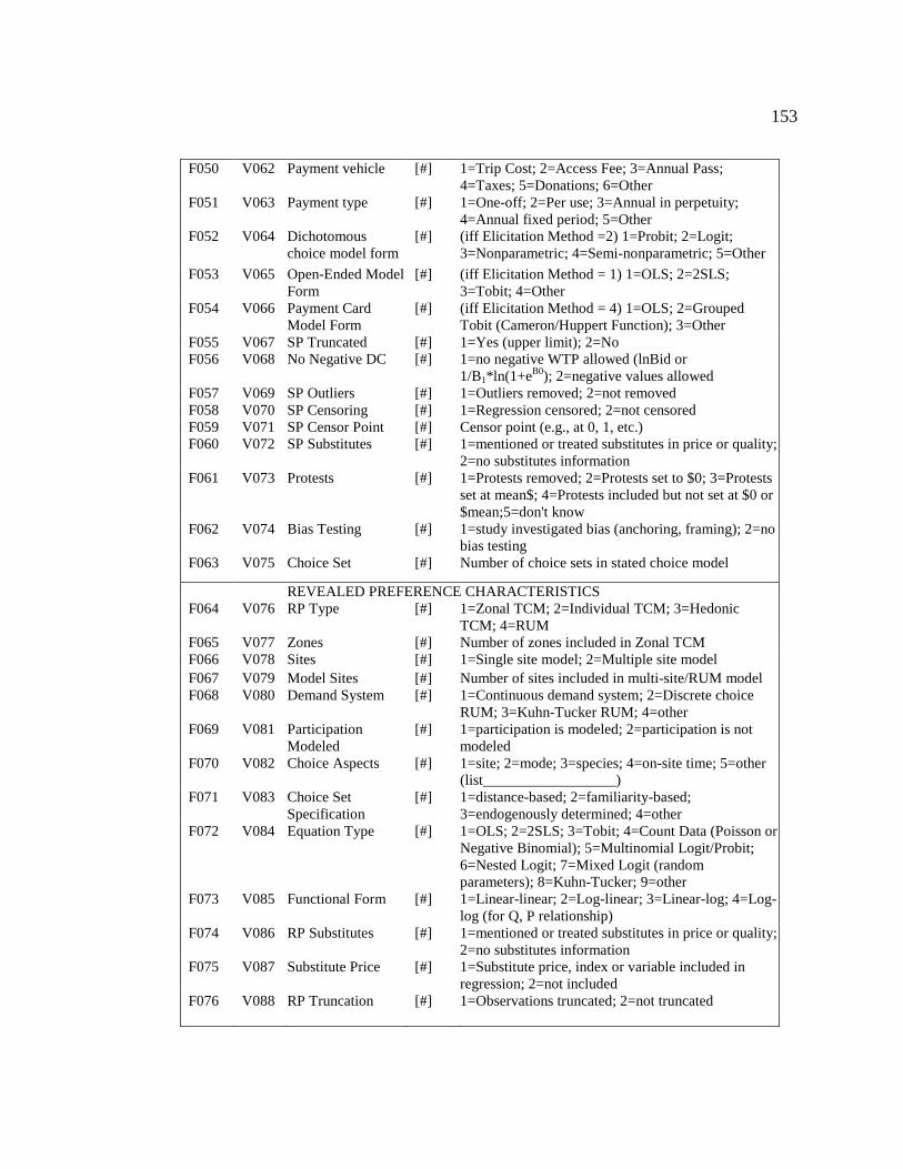
153
F050 V062 Payment vehicle [#] 1=Trip Cost; 2=Access Fee; 3=Annual Pass; 4=Taxes; 5=Donations; 6=Other
F051 V063 Payment type [#] 1=One-off; 2=Per use; 3=Annual in perpetuity; 4=Annual fixed period; 5=Other
F052 V064 Dichotomous choice model form
[#] (iff Elicitation Method =2) 1=Probit; 2=Logit; 3=Nonparametric; 4=Semi-nonparametric; 5=Other
F053 V065 Open-Ended Model Form
[#] (iff Elicitation Method = 1) 1=OLS; 2=2SLS; 3=Tobit; 4=Other
F054 V066 Payment Card Model Form
[#] (iff Elicitation Method = 4) 1=OLS; 2=Grouped Tobit (Cameron/Huppert Function); 3=Other
F055 V067 SP Truncated [#] 1=Yes (upper limit); 2=No F056 V068 No Negative DC [#] 1=no negative WTP allowed (lnBid or
1/B1*ln(1+eB0); 2=negative values allowed F057 V069 SP Outliers [#] 1=Outliers removed; 2=not removed F058 V070 SP Censoring [#] 1=Regression censored; 2=not censored F059 V071 SP Censor Point [#] Censor point (e.g., at 0, 1, etc.) F060 V072 SP Substitutes [#] 1=mentioned or treated substitutes in price or quality;
2=no substitutes information F061 V073 Protests [#] 1=Protests removed; 2=Protests set to $0; 3=Protests
set at mean$; 4=Protests included but not set at $0 or $mean;5=don't know
F062 V074 Bias Testing [#] 1=study investigated bias (anchoring, framing); 2=no bias testing
F063 V075 Choice Set [#] Number of choice sets in stated choice model
REVEALED PREFERENCE CHARACTERISTICS F064 V076 RP Type [#] 1=Zonal TCM; 2=Individual TCM; 3=Hedonic
TCM; 4=RUM F065 V077 Zones [#] Number of zones included in Zonal TCM F066 V078 Sites [#] 1=Single site model; 2=Multiple site model F067 V079 Model Sites [#] Number of sites included in multi-site/RUM model F068 V080 Demand System [#] 1=Continuous demand system; 2=Discrete choice
RUM; 3=Kuhn-Tucker RUM; 4=other F069 V081 Participation
Modeled [#] 1=participation is modeled; 2=participation is not
modeled F070 V082 Choice Aspects [#] 1=site; 2=mode; 3=species; 4=on-site time; 5=other
(list__________________) F071 V083 Choice Set
Specification [#] 1=distance-based; 2=familiarity-based;
3=endogenously determined; 4=other F072 V084 Equation Type [#] 1=OLS; 2=2SLS; 3=Tobit; 4=Count Data (Poisson or
Negative Binomial); 5=Multinomial Logit/Probit; 6=Nested Logit; 7=Mixed Logit (random parameters); 8=Kuhn-Tucker; 9=other
F073 V085 Functional Form [#] 1=Linear-linear; 2=Log-linear; 3=Linear-log; 4=Log-log (for Q, P relationship)
F074 V086 RP Substitutes [#] 1=mentioned or treated substitutes in price or quality; 2=no substitutes information
F075 V087 Substitute Price [#] 1=Substitute price, index or variable included in regression; 2=not included
F076 V088 RP Truncation [#] 1=Observations truncated; 2=not truncated
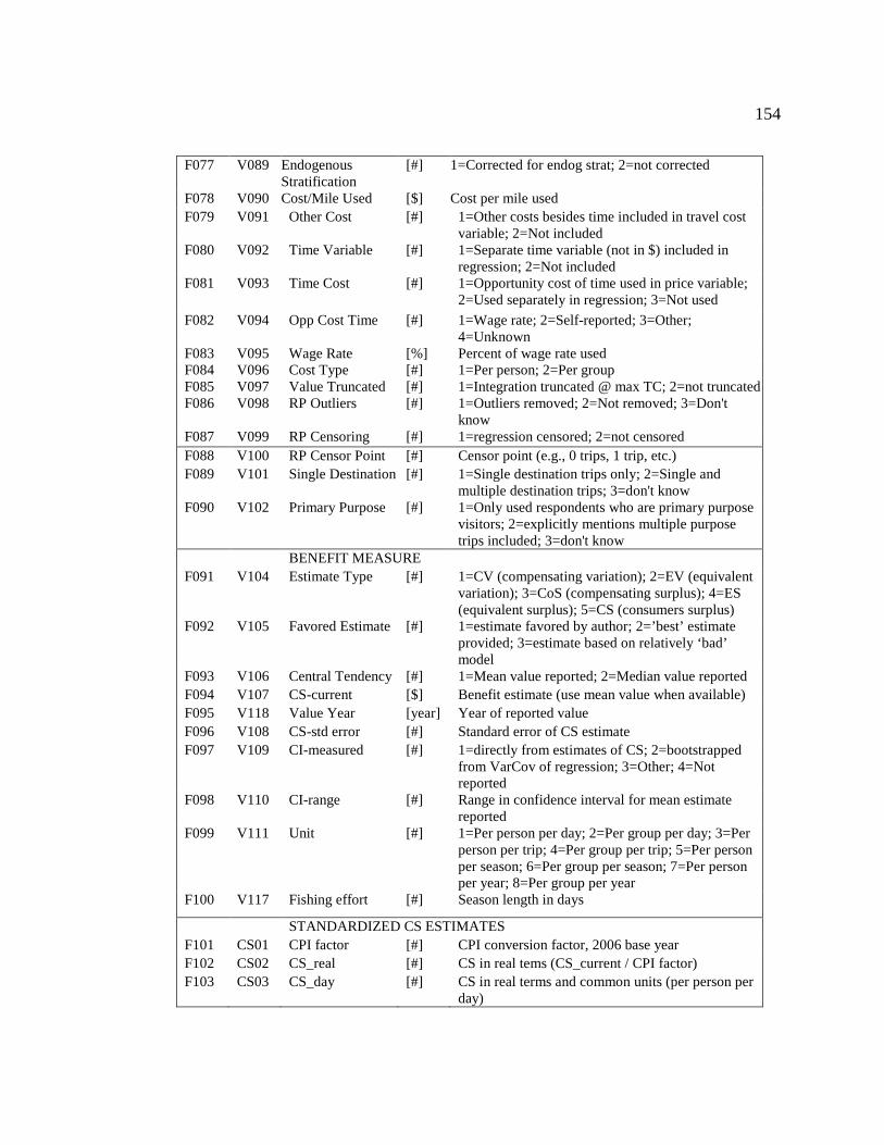
154
F077 V089 Endogenous Stratification
[#] 1=Corrected for endog strat; 2=not corrected
F078 V090 Cost/Mile Used [$] Cost per mile used F079 V091 Other Cost [#] 1=Other costs besides time included in travel cost
variable; 2=Not included F080 V092 Time Variable [#] 1=Separate time variable (not in $) included in
regression; 2=Not included F081 V093 Time Cost [#] 1=Opportunity cost of time used in price variable;
2=Used separately in regression; 3=Not used
F082 V094 Opp Cost Time [#] 1=Wage rate; 2=Self-reported; 3=Other; 4=Unknown
F083 V095 Wage Rate [%] Percent of wage rate used F084 V096 Cost Type [#] 1=Per person; 2=Per group F085 V097 Value Truncated [#] 1=Integration truncated @ max TC; 2=not truncated F086 V098 RP Outliers [#] 1=Outliers removed; 2=Not removed; 3=Don't
know F087 V099 RP Censoring [#] 1=regression censored; 2=not censored F088 V100 RP Censor Point [#] Censor point (e.g., 0 trips, 1 trip, etc.) F089 V101 Single Destination [#] 1=Single destination trips only; 2=Single and
multiple destination trips; 3=don't know F090 V102 Primary Purpose [#] 1=Only used respondents who are primary purpose
visitors; 2=explicitly mentions multiple purpose trips included; 3=don't know
BENEFIT MEASURE F091 V104 Estimate Type [#] 1=CV (compensating variation); 2=EV (equivalent
variation); 3=CoS (compensating surplus); 4=ES (equivalent surplus); 5=CS (consumers surplus)
F092 V105 Favored Estimate [#] 1=estimate favored by author; 2=’best’ estimate provided; 3=estimate based on relatively ‘bad’ model
F093 V106 Central Tendency [#] 1=Mean value reported; 2=Median value reported F094 V107 CS-current [$] Benefit estimate (use mean value when available) F095 V118 Value Year [year] Year of reported value F096 V108 CS-std error [#] Standard error of CS estimate F097 V109 CI-measured [#] 1=directly from estimates of CS; 2=bootstrapped
from VarCov of regression; 3=Other; 4=Not reported
F098 V110 CI-range [#] Range in confidence interval for mean estimate reported
F099 V111 Unit [#] 1=Per person per day; 2=Per group per day; 3=Per person per trip; 4=Per group per trip; 5=Per person per season; 6=Per group per season; 7=Per person per year; 8=Per group per year
F100 V117 Fishing effort [#] Season length in days
STANDARDIZED CS ESTIMATES F101 CS01 CPI factor [#] CPI conversion factor, 2006 base year F102 CS02 CS_real [#] CS in real tems (CS_current / CPI factor) F103 CS03 CS_day [#] CS in real terms and common units (per person per
day)
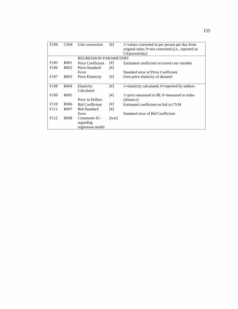
155
F104 CS04 Unit conversion [#] 1=values converted to per person per day from original units; 0=not converted (i.e., reported as CS/person/day)
REGRESSION PARAMETERS F105 R001 Price Coefficient [#] Estimated coefficient on travel cost variable F106 R002 Price-Standard
Error [#]
Standard error of Price Coefficient F107 R003 Price Elasticity [#] Own price elasticity of demand
F108 R004 Elasticity Calculated
[#] 1=elasticity calculated; 0=reported by authors
F109 R005 Price in Dollars
[#] 1=price measured in $$; 0=measured in miles (distance)
F110 R006 Bid Coefficient [#] Estimated coefficient on bid in CVM F111 R007 Bid-Standard
Error [#]
Standard error of Bid Coefficient F112 R008 Comments #2 -
regarding regression model
[text]
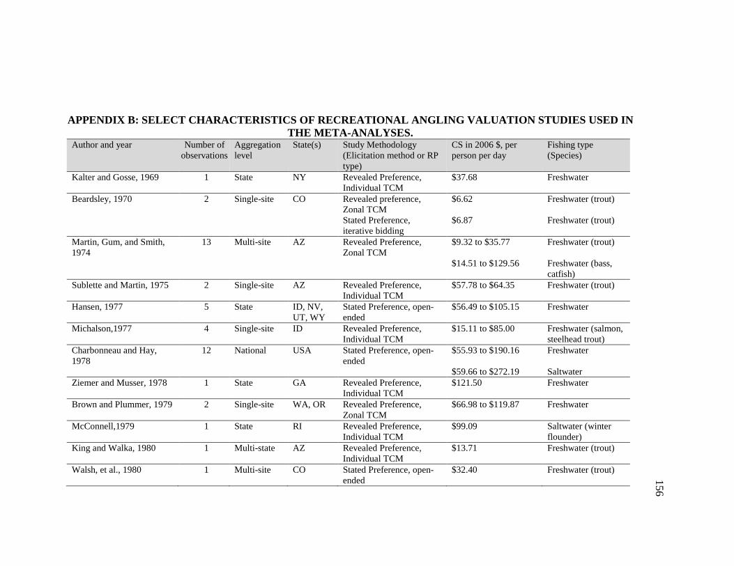
156
APPENDIX B: SELECT CHARACTERISTICS OF RECREATIONAL ANGLING VALUATION STUDIES USED IN THE META-ANALYSES.
Author and year Number of observations
Aggregation level
State(s) Study Methodology (Elicitation method or RP type)
CS in 2006 $, per person per day
Fishing type (Species)
Kalter and Gosse, 1969 1 State NY Revealed Preference, Individual TCM
$37.68 Freshwater
Beardsley, 1970 2 Single-site CO Revealed preference, Zonal TCM Stated Preference, iterative bidding
$6.62 $6.87
Freshwater (trout) Freshwater (trout)
Martin, Gum, and Smith, 1974
13 Multi-site AZ Revealed Preference, Zonal TCM
$9.32 to $35.77 Freshwater (trout)
$14.51 to $129.56 Freshwater (bass, catfish)
Sublette and Martin, 1975 2 Single-site AZ Revealed Preference, Individual TCM
$57.78 to $64.35 Freshwater (trout)
Hansen, 1977 5 State ID, NV, UT, WY
Stated Preference, open-ended
$56.49 to $105.15 Freshwater
Michalson,1977 4 Single-site ID Revealed Preference, Individual TCM
$15.11 to $85.00 Freshwater (salmon, steelhead trout)
Charbonneau and Hay, 1978
12 National USA Stated Preference, open-ended
$55.93 to $190.16 Freshwater
$59.66 to $272.19 Saltwater Ziemer and Musser, 1978 1 State GA Revealed Preference,
Individual TCM $121.50 Freshwater
Brown and Plummer, 1979 2 Single-site WA, OR Revealed Preference, Zonal TCM
$66.98 to $119.87 Freshwater
McConnell,1979 1 State RI Revealed Preference, Individual TCM
$99.09 Saltwater (winter flounder)
King and Walka, 1980 1 Multi-state AZ Revealed Preference, Individual TCM
$13.71 Freshwater (trout)
Walsh, et al., 1980 1 Multi-site CO Stated Preference, open-ended
$32.40 Freshwater (trout)
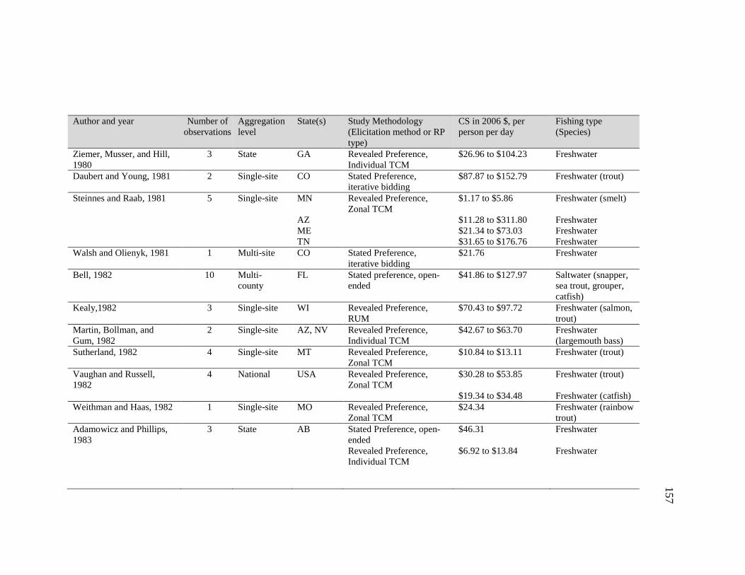
157
Author and year Number of observations
Aggregation level
State(s) Study Methodology (Elicitation method or RP type)
CS in 2006 $, per person per day
Fishing type (Species)
Ziemer, Musser, and Hill, 1980
3 State GA Revealed Preference, Individual TCM
$26.96 to $104.23 Freshwater
Daubert and Young, 1981 2 Single-site CO Stated Preference, iterative bidding
$87.87 to $152.79 Freshwater (trout)
Steinnes and Raab, 1981 5 Single-site MN Revealed Preference, Zonal TCM
$1.17 to $5.86 Freshwater (smelt)
AZ $11.28 to $311.80 Freshwater ME $21.34 to $73.03 Freshwater TN $31.65 to $176.76 Freshwater Walsh and Olienyk, 1981 1 Multi-site CO Stated Preference,
iterative bidding $21.76 Freshwater
Bell, 1982 10 Multi-county
FL Stated preference, open-ended
$41.86 to $127.97 Saltwater (snapper, sea trout, grouper, catfish)
Kealy,1982 3 Single-site WI Revealed Preference, RUM
$70.43 to $97.72 Freshwater (salmon, trout)
Martin, Bollman, and Gum, 1982
2 Single-site AZ, NV Revealed Preference, Individual TCM
$42.67 to $63.70 Freshwater (largemouth bass)
Sutherland, 1982 4 Single-site MT Revealed Preference, Zonal TCM
$10.84 to $13.11 Freshwater (trout)
Vaughan and Russell, 1982
4 National USA Revealed Preference, Zonal TCM
$30.28 to $53.85 Freshwater (trout)
$19.34 to $34.48 Freshwater (catfish) Weithman and Haas, 1982 1 Single-site MO Revealed Preference,
Zonal TCM $24.34 Freshwater (rainbow
trout) Adamowicz and Phillips, 1983
3 State AB Stated Preference, open-ended
$46.31 Freshwater
Revealed Preference, Individual TCM
$6.92 to $13.84 Freshwater
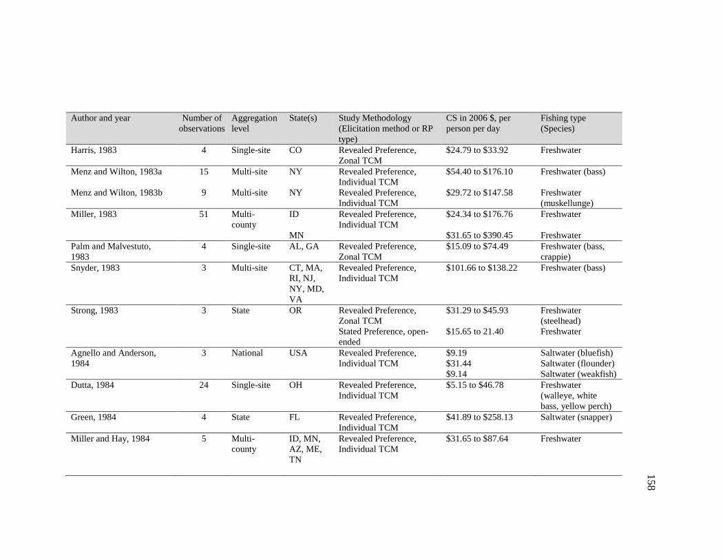
158
Author and year Number of observations
Aggregation level
State(s) Study Methodology (Elicitation method or RP type)
CS in 2006 $, per person per day
Fishing type (Species)
Harris, 1983 4 Single-site CO Revealed Preference, Zonal TCM
$24.79 to $33.92 Freshwater
Menz and Wilton, 1983a 15 Multi-site NY Revealed Preference, Individual TCM
$54.40 to $176.10 Freshwater (bass)
Menz and Wilton, 1983b 9 Multi-site NY Revealed Preference, Individual TCM
$29.72 to $147.58 Freshwater (muskellunge)
Miller, 1983 51 Multi-county
ID Revealed Preference, Individual TCM
$24.34 to $176.76 Freshwater
MN $31.65 to $390.45 Freshwater Palm and Malvestuto, 1983
4 Single-site AL, GA Revealed Preference, Zonal TCM
$15.09 to $74.49 Freshwater (bass, crappie)
Snyder, 1983 3 Multi-site CT, MA, RI, NJ, NY, MD, VA
Revealed Preference, Individual TCM
$101.66 to $138.22 Freshwater (bass)
Strong, 1983 3 State OR Revealed Preference, Zonal TCM
$31.29 to $45.93 Freshwater (steelhead)
Stated Preference, open-ended
$15.65 to 21.40 Freshwater
Agnello and Anderson, 1984
3 National USA Revealed Preference, Individual TCM
$9.19 Saltwater (bluefish) $31.44 Saltwater (flounder) $9.14 Saltwater (weakfish)
Dutta, 1984 24 Single-site OH Revealed Preference, Individual TCM
$5.15 to $46.78 Freshwater (walleye, white bass, yellow perch)
Green, 1984 4 State FL Revealed Preference, Individual TCM
$41.89 to $258.13 Saltwater (snapper)
Miller and Hay, 1984 5 Multi-county
ID, MN, AZ, ME, TN
Revealed Preference, Individual TCM
$31.65 to $87.64 Freshwater
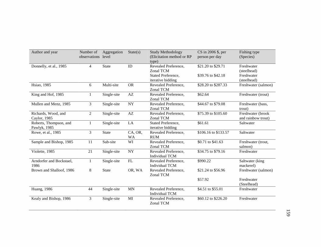
159
Author and year Number of observations
Aggregation level
State(s) Study Methodology (Elicitation method or RP type)
CS in 2006 $, per person per day
Fishing type (Species)
Donnelly, et al., 1985 4 State ID Revealed Preference, Zonal TCM
$21.20 to $29.71 Freshwater (steelhead)
Stated Preference, iterative bidding
$39.76 to $42.18 Freshwater (steelhead)
Hsiao, 1985 6 Multi-site OR Revealed Preference, Zonal TCM
$28.20 to $287.33 Freshwater (salmon)
King and Hof, 1985 1 Single-site AZ Revealed Preference, Zonal TCM
$62.64 Freshwater (trout)
Mullen and Menz, 1985 3 Single-site NY Revealed Preference, Zonal TCM
$44.67 to $79.08 Freshwater (bass, trout)
Richards, Wood, and Caylor, 1985
2 Single-site AZ Revealed Preference, Zonal TCM
$75.39 to $105.60 Freshwater (brook and rainbow trout)
Roberts, Thompson, and Pawlyk, 1985
1 Single-site LA Stated Preference, iterative bidding
$61.61 Saltwater
Rowe, et al., 1985 3 State CA, OR, WA
Revealed Preference, RUM
$106.16 to $133.57 Saltwater
Sample and Bishop, 1985 11 Sub-site WI Revealed Preference, Zonal TCM
$0.71 to $41.63 Freshwater (trout, salmon)
Violette, 1985 21 Single-site NY Revealed Preference, Individual TCM
$34.75 to $79.16 Freshwater
Arndorfer and Bockstael, 1986
1 Single-site FL Revealed Preference, Individual TCM
$990.22 Saltwater (king mackerel)
Brown and Shalloof, 1986 8 State OR, WA Revealed Preference, Zonal TCM
$21.24 to $56.96 Freshwater (salmon)
$57.92 Freshwater (Steelhead)
Huang, 1986 44 Single-site MN Revealed Preference, Individual TCM
$4.51 to $55.01 Freshwater
Kealy and Bishop, 1986 3 Single-site MI Revealed Preference, Zonal TCM
$60.12 to $226.20 Freshwater
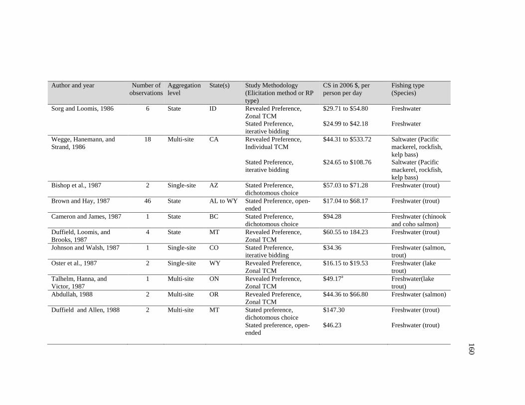
160
Author and year Number of observations
Aggregation level
State(s) Study Methodology (Elicitation method or RP type)
CS in 2006 $, per person per day
Fishing type (Species)
Sorg and Loomis, 1986 6 State ID Revealed Preference, Zonal TCM
$29.71 to $54.80 Freshwater
Stated Preference, iterative bidding
$24.99 to $42.18 Freshwater
Wegge, Hanemann, and Strand, 1986
18 Multi-site CA Revealed Preference, Individual TCM
$44.31 to $533.72 Saltwater (Pacific mackerel, rockfish, kelp bass)
Stated Preference, iterative bidding
$24.65 to $108.76 Saltwater (Pacific mackerel, rockfish, kelp bass)
Bishop et al., 1987 2 Single-site AZ Stated Preference, dichotomous choice
$57.03 to $71.28 Freshwater (trout)
Brown and Hay, 1987 46 State AL to WY Stated Preference, open-ended
$17.04 to $68.17 Freshwater (trout)
Cameron and James, 1987 1 State BC Stated Preference, dichotomous choice
$94.28 Freshwater (chinook and coho salmon)
Duffield, Loomis, and Brooks, 1987
4 State MT Revealed Preference, Zonal TCM
$60.55 to 184.23 Freshwater (trout)
Johnson and Walsh, 1987 1 Single-site CO Stated Preference, iterative bidding
$34.36 Freshwater (salmon, trout)
Oster et al., 1987 2 Single-site WY Revealed Preference, Zonal TCM
$16.15 to $19.53 Freshwater (lake trout)
Talhelm, Hanna, and Victor, 1987
1 Multi-site ON Revealed Preference, Zonal TCM
$49.17a Freshwater(lake trout)
Abdullah, 1988 2 Multi-site OR Revealed Preference, Zonal TCM
$44.36 to $66.80 Freshwater (salmon)
Duffield and Allen, 1988 2 Multi-site MT Stated preference, dichotomous choice
$147.30 Freshwater (trout)
Stated preference, open-ended
$46.23 Freshwater (trout)
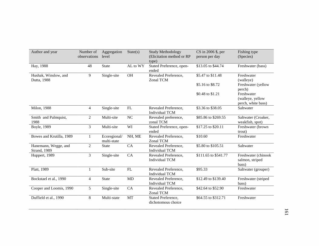
161
Author and year Number of observations
Aggregation level
State(s) Study Methodology (Elicitation method or RP type)
CS in 2006 $, per person per day
Fishing type (Species)
Hay, 1988 48 State AL to WY Stated Preference, open-ended
$13.05 to $44.74 Freshwater (bass)
Hushak, Winslow, and Dutta, 1988
9 Single-site OH Revealed Preference, Zonal TCM
$5.47 to $11.48 Freshwater (walleye)
$5.16 to $8.72 Freshwater (yellow perch)
$0.48 to $1.21 Freshwater (walleye, yellow perch, white bass)
Milon, 1988 4 Single-site FL Revealed Preference, Individual TCM
$3.36 to $38.05 Saltwater
Smith and Palmquist, 1988
2 Multi-site NC Revealed preference, zonal TCM
$85.86 to $269.55 Saltwater (Croaker, weakfish, spot)
Boyle, 1989 3 Multi-site WI Stated Preference, open-ended
$17.25 to $20.11 Freshwater (brown trout)
Bowes and Krutilla, 1989 1 Ecoregional/multi-state
NH, ME Revealed Preference, Zonal TCM
$10.60 Freshwater
Hanemann, Wegge, and Strand, 1989
2 State CA Revealed Preference, Individual TCM
$5.80 to $105.51 Saltwater
Huppert, 1989 3 Single-site CA Revealed Preference, Individual TCM
$111.65 to $541.77 Freshwater (chinook salmon, striped bass)
Platt, 1989 1 Sub-site FL Revealed Preference, Individual TCM
$95.33 Saltwater (grouper)
Bockstael et al., 1990 4 State MD Revealed Preference, Individual TCM
$12.49 to $139.40 Freshwater (striped bass)
Cooper and Loomis, 1990 5 Single-site CA Revealed Preference, Zonal TCM
$42.64 to $52.90 Freshwater
Duffield et al., 1990 8 Multi-state MT Stated Preference, dichotomous choice
$64.55 to $312.71 Freshwater
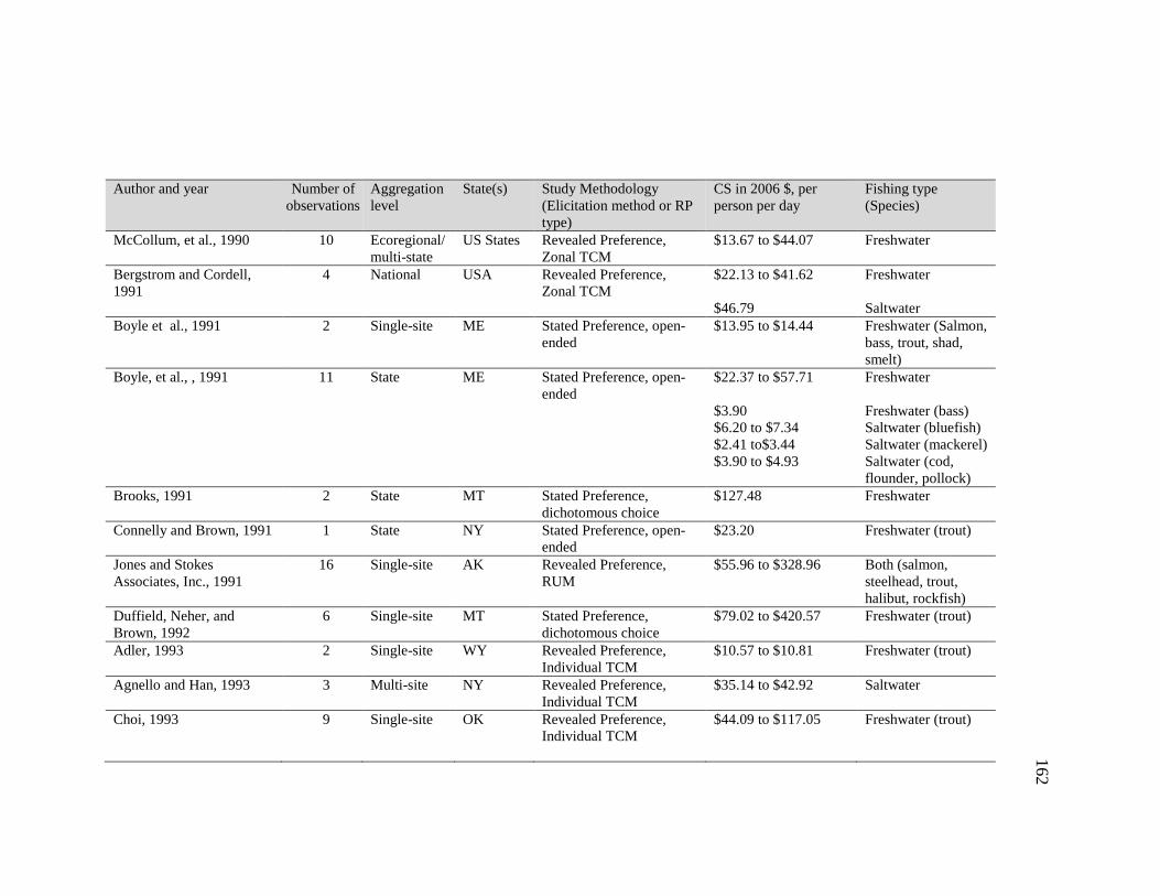
162
Author and year Number of observations
Aggregation level
State(s) Study Methodology (Elicitation method or RP type)
CS in 2006 $, per person per day
Fishing type (Species)
McCollum, et al., 1990 10 Ecoregional/ multi-state
US States Revealed Preference, Zonal TCM
$13.67 to $44.07 Freshwater
Bergstrom and Cordell, 1991
4 National USA Revealed Preference, Zonal TCM
$22.13 to $41.62 Freshwater
$46.79 Saltwater Boyle et al., 1991 2 Single-site ME Stated Preference, open-
ended $13.95 to $14.44 Freshwater (Salmon,
bass, trout, shad, smelt)
Boyle, et al., , 1991 11 State ME Stated Preference, open-ended
$22.37 to $57.71 Freshwater
$3.90 Freshwater (bass) $6.20 to $7.34 Saltwater (bluefish) $2.41 to$3.44 Saltwater (mackerel) $3.90 to $4.93 Saltwater (cod,
flounder, pollock) Brooks, 1991 2 State MT Stated Preference,
dichotomous choice $127.48 Freshwater
Connelly and Brown, 1991 1 State NY Stated Preference, open-ended
$23.20 Freshwater (trout)
Jones and Stokes Associates, Inc., 1991
16 Single-site AK Revealed Preference, RUM
$55.96 to $328.96 Both (salmon, steelhead, trout, halibut, rockfish)
Duffield, Neher, and Brown, 1992
6 Single-site MT Stated Preference, dichotomous choice
$79.02 to $420.57 Freshwater (trout)
Adler, 1993 2 Single-site WY Revealed Preference, Individual TCM
$10.57 to $10.81 Freshwater (trout)
Agnello and Han, 1993
3 Multi-site NY Revealed Preference, Individual TCM
$35.14 to $42.92 Saltwater
Choi, 1993 9 Single-site OK Revealed Preference, Individual TCM
$44.09 to $117.05 Freshwater (trout)
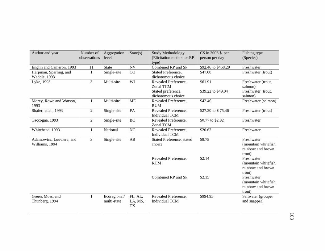
163
Author and year Number of observations
Aggregation level
State(s) Study Methodology (Elicitation method or RP type)
CS in 2006 $, per person per day
Fishing type (Species)
Englin and Cameron, 1993 11 State NV Combined RP and SP $92.46 to $458.29 Freshwater Harpman, Sparling, and Waddle, 1993
1 Single-site CO Stated Preference, dichotomous choice
$47.00 Freshwater (trout)
Lyke, 1993 3 Multi-site WI Revealed Preference, Zonal TCM
$61.91 Freshwater (trout, salmon)
Stated preference, dichotomous choice
$39.22 to $49.04 Freshwater (trout, salmon)
Morey, Rowe and Watson, 1993
1 Multi-site ME Revealed Preference, RUM
$42.46 Freshwater (salmon)
Shafer, et al., 1993 2 Single-site PA Revealed Preference, Individual TCM
$27.30 to $ 75.46 Freshwater (trout)
Taccogna, 1993 2 Single-site BC Revealed Preference, Zonal TCM
$0.77 to $2.82 Freshwater
Whitehead, 1993 1 National NC Revealed Preference, Individual TCM
$20.62 Freshwater
Adamowicz, Louviere, and Williams, 1994
3 Single-site AB Stated Preference, stated choice
$8.75 Freshwater (mountain whitefish, rainbow and brown trout)
Revealed Preference, RUM
$2.14 Freshwater (mountain whitefish, rainbow and brown trout)
Combined RP and SP $2.15 Freshwater (mountain whitefish, rainbow and brown trout)
Green, Moss, and Thunberg, 1994
1 Ecoregional/ multi-state
FL, AL, LA, MS, TX
Revealed Preference, Individual TCM
$994.93 Saltwater (grouper and snapper)
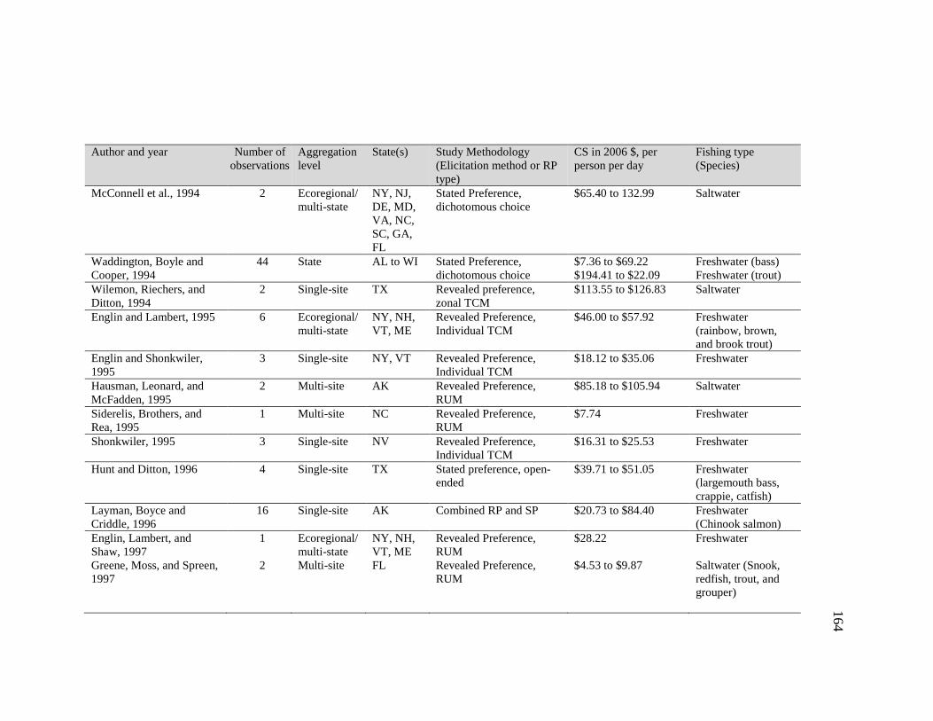
164
Author and year Number of observations
Aggregation level
State(s) Study Methodology (Elicitation method or RP type)
CS in 2006 $, per person per day
Fishing type (Species)
McConnell et al., 1994 2 Ecoregional/ multi-state
NY, NJ, DE, MD, VA, NC, SC, GA, FL
Stated Preference, dichotomous choice
$65.40 to 132.99 Saltwater
Waddington, Boyle and Cooper, 1994
44 State AL to WI Stated Preference, dichotomous choice
$7.36 to $69.22 Freshwater (bass) $194.41 to $22.09 Freshwater (trout)
Wilemon, Riechers, and Ditton, 1994
2 Single-site TX Revealed preference, zonal TCM
$113.55 to $126.83 Saltwater
Englin and Lambert, 1995 6 Ecoregional/ multi-state
NY, NH, VT, ME
Revealed Preference, Individual TCM
$46.00 to $57.92 Freshwater (rainbow, brown, and brook trout)
Englin and Shonkwiler, 1995
3 Single-site NY, VT Revealed Preference, Individual TCM
$18.12 to $35.06 Freshwater
Hausman, Leonard, and McFadden, 1995
2 Multi-site AK Revealed Preference, RUM
$85.18 to $105.94 Saltwater
Siderelis, Brothers, and Rea, 1995
1 Multi-site NC Revealed Preference, RUM
$7.74 Freshwater
Shonkwiler, 1995 3 Single-site NV Revealed Preference, Individual TCM
$16.31 to $25.53 Freshwater
Hunt and Ditton, 1996 4 Single-site TX Stated preference, open-ended
$39.71 to $51.05 Freshwater (largemouth bass, crappie, catfish)
Layman, Boyce and Criddle, 1996
16 Single-site AK Combined RP and SP $20.73 to $84.40 Freshwater (Chinook salmon)
Englin, Lambert, and Shaw, 1997
1 Ecoregional/ multi-state
NY, NH, VT, ME
Revealed Preference, RUM
$28.22 Freshwater
Greene, Moss, and Spreen, 1997
2 Multi-site FL Revealed Preference, RUM
$4.53 to $9.87 Saltwater (Snook, redfish, trout, and grouper)
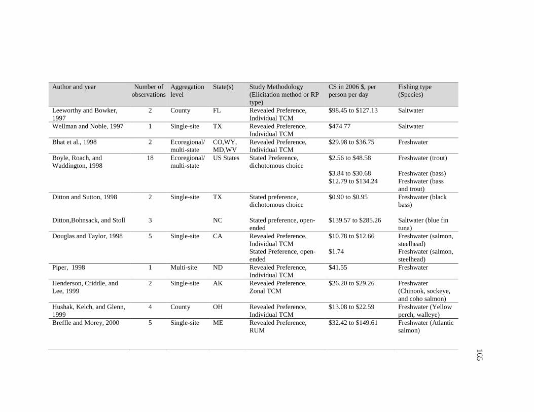
165
Author and year Number of observations
Aggregation level
State(s) Study Methodology (Elicitation method or RP type)
CS in 2006 $, per person per day
Fishing type (Species)
Leeworthy and Bowker, 1997
2 County FL Revealed Preference, Individual TCM
$98.45 to $127.13 Saltwater
Wellman and Noble, 1997 1 Single-site TX Revealed Preference, Individual TCM
$474.77 Saltwater
Bhat et al., 1998 2 Ecoregional/ multi-state
CO,WY,MD,WV
Revealed Preference, Individual TCM
$29.98 to $36.75 Freshwater
Boyle, Roach, and Waddington, 1998
18 Ecoregional/ multi-state
US States Stated Preference, dichotomous choice
$2.56 to $48.58 Freshwater (trout)
$3.84 to $30.68 Freshwater (bass) $12.79 to $134.24 Freshwater (bass
and trout) Ditton and Sutton, 1998 2 Single-site TX Stated preference,
dichotomous choice $0.90 to $0.95 Freshwater (black
bass)
Ditton,Bohnsack, and Stoll 3 NC Stated preference, open-ended
$139.57 to $285.26 Saltwater (blue fin tuna)
Douglas and Taylor, 1998 5 Single-site CA Revealed Preference, Individual TCM
$10.78 to $12.66 Freshwater (salmon, steelhead)
Stated Preference, open-ended
$1.74 Freshwater (salmon, steelhead)
Piper, 1998 1 Multi-site ND Revealed Preference, Individual TCM
$41.55 Freshwater
Henderson, Criddle, and Lee, 1999
2 Single-site AK Revealed Preference, Zonal TCM
$26.20 to $29.26 Freshwater (Chinook, sockeye, and coho salmon)
Hushak, Kelch, and Glenn, 1999
4 County OH Revealed Preference, Individual TCM
$13.08 to $22.59 Freshwater (Yellow perch, walleye)
Breffle and Morey, 2000 5 Single-site ME Revealed Preference, RUM
$32.42 to $149.61 Freshwater (Atlantic salmon)
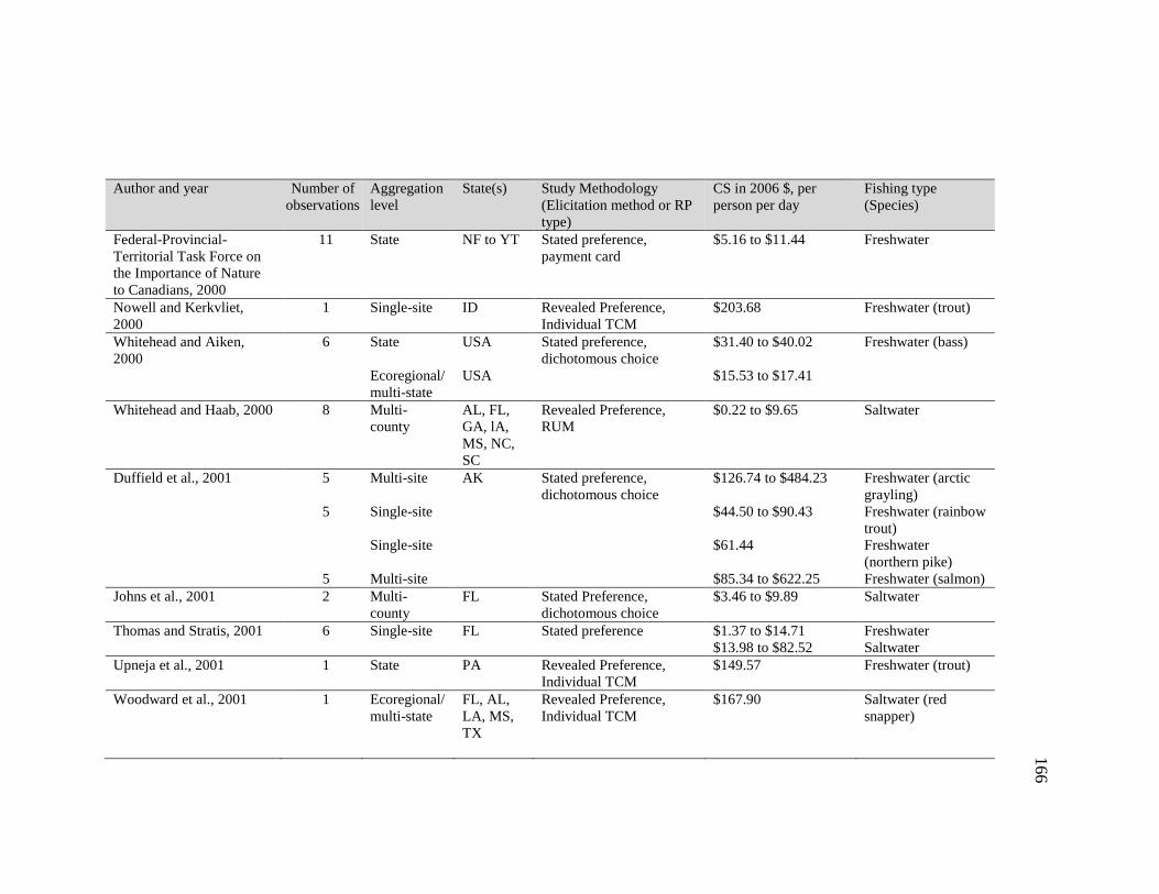
166
Author and year Number of observations
Aggregation level
State(s) Study Methodology (Elicitation method or RP type)
CS in 2006 $, per person per day
Fishing type (Species)
Federal-Provincial-Territorial Task Force on the Importance of Nature to Canadians, 2000
11 State NF to YT Stated preference, payment card
$5.16 to $11.44 Freshwater
Nowell and Kerkvliet, 2000
1 Single-site ID Revealed Preference, Individual TCM
$203.68 Freshwater (trout)
Whitehead and Aiken, 2000
6 State USA Stated preference, dichotomous choice
$31.40 to $40.02 Freshwater (bass)
Ecoregional/ multi-state
USA $15.53 to $17.41
Whitehead and Haab, 2000 8 Multi-county
AL, FL, GA, lA, MS, NC, SC
Revealed Preference, RUM
$0.22 to $9.65 Saltwater
Duffield et al., 2001 5 Multi-site AK Stated preference, dichotomous choice
$126.74 to $484.23 Freshwater (arctic grayling)
5 Single-site $44.50 to $90.43 Freshwater (rainbow trout)
Single-site $61.44 Freshwater (northern pike)
5 Multi-site $85.34 to $622.25 Freshwater (salmon) Johns et al., 2001 2 Multi-
county FL Stated Preference,
dichotomous choice $3.46 to $9.89
Saltwater
Thomas and Stratis, 2001 6 Single-site FL Stated preference $1.37 to $14.71 Freshwater $13.98 to $82.52 Saltwater Upneja et al., 2001 1 State PA Revealed Preference,
Individual TCM $149.57 Freshwater (trout)
Woodward et al., 2001 1 Ecoregional/ multi-state
FL, AL, LA, MS, TX
Revealed Preference, Individual TCM
$167.90 Saltwater (red snapper)
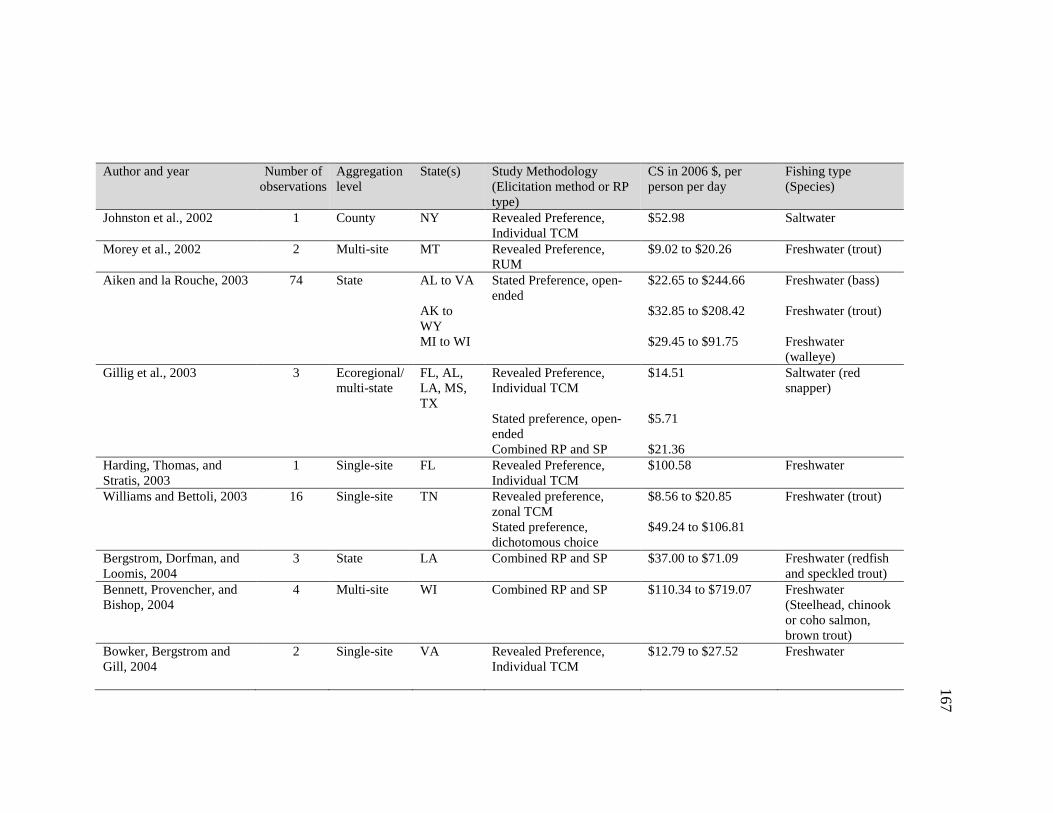
167
Author and year Number of observations
Aggregation level
State(s) Study Methodology (Elicitation method or RP type)
CS in 2006 $, per person per day
Fishing type (Species)
Johnston et al., 2002 1 County NY Revealed Preference, Individual TCM
$52.98 Saltwater
Morey et al., 2002 2 Multi-site MT Revealed Preference, RUM
$9.02 to $20.26 Freshwater (trout)
Aiken and la Rouche, 2003 74 State AL to VA Stated Preference, open-ended
$22.65 to $244.66 Freshwater (bass)
AK to WY
$32.85 to $208.42 Freshwater (trout)
MI to WI $29.45 to $91.75 Freshwater (walleye)
Gillig et al., 2003 3 Ecoregional/ multi-state
FL, AL, LA, MS, TX
Revealed Preference, Individual TCM
$14.51 Saltwater (red snapper)
Stated preference, open-ended
$5.71
Combined RP and SP $21.36 Harding, Thomas, and Stratis, 2003
1 Single-site FL Revealed Preference, Individual TCM
$100.58 Freshwater
Williams and Bettoli, 2003 16 Single-site TN Revealed preference, zonal TCM
$8.56 to $20.85 Freshwater (trout)
Stated preference, dichotomous choice
$49.24 to $106.81
Bergstrom, Dorfman, and Loomis, 2004
3 State LA Combined RP and SP $37.00 to $71.09 Freshwater (redfish and speckled trout)
Bennett, Provencher, and Bishop, 2004
4 Multi-site WI Combined RP and SP $110.34 to $719.07 Freshwater (Steelhead, chinook or coho salmon, brown trout)
Bowker, Bergstrom and Gill, 2004
2 Single-site VA Revealed Preference, Individual TCM
$12.79 to $27.52 Freshwater
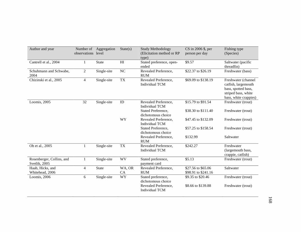
168
Author and year Number of observations
Aggregation level
State(s) Study Methodology (Elicitation method or RP type)
CS in 2006 $, per person per day
Fishing type (Species)
Cantrell et al., 2004 1 State HI Stated preference, open-ended
$9.57 Saltwater (pacific threadfin)
Schuhmann and Schwabe, 2004
2 Single-site NC Revealed Preference, RUM
$22.37 to $26.19 Freshwater (bass)
Chizinski et al., 2005 4 Single-site TX Revealed Preference, Individual TCM
$69.09 to $138.19 Freshwater (channel catfish, largemouth bass, spotted bass, striped bass, white bass, white crappies)
Loomis, 2005 32 Single-site ID Revealed Preference, Individual TCM
$15.79 to $91.54 Freshwater (trout)
Stated Preference, dichotomous choice
$38.30 to $111.40 Freshwater (trout)
WY Revealed Preference, Individual TCM
$47.45 to $132.09 Freshwater (trout)
Stated Preference, dichotomous choice
$57.25 to $158.54 Freshwater (trout)
Revealed Preference, RUM
$132.99 Saltwater
Oh et al., 2005 1 Single-site TX Revealed Preference, Individual TCM
$242.27 Freshwater (largemouth bass, crappie, catfish)
Rosenberger, Collins, and Svetlik, 2005
1 Single-site WV Stated preference, payment card
$5.13 Freshwater (trout)
Haab, Hicks, and Whitehead, 2006
4 State WA, OR Revealed Preference, RUM
$27.56 to $65.06 Saltwater CA $98.91 to $241.16
Loomis, 2006 6 Single-site WY Stated preference, dichotomous choice
$9.35 to $20.46 Freshwater (trout)
Revealed Preference, Individual TCM
$8.66 to $139.88 Freshwater (trout)
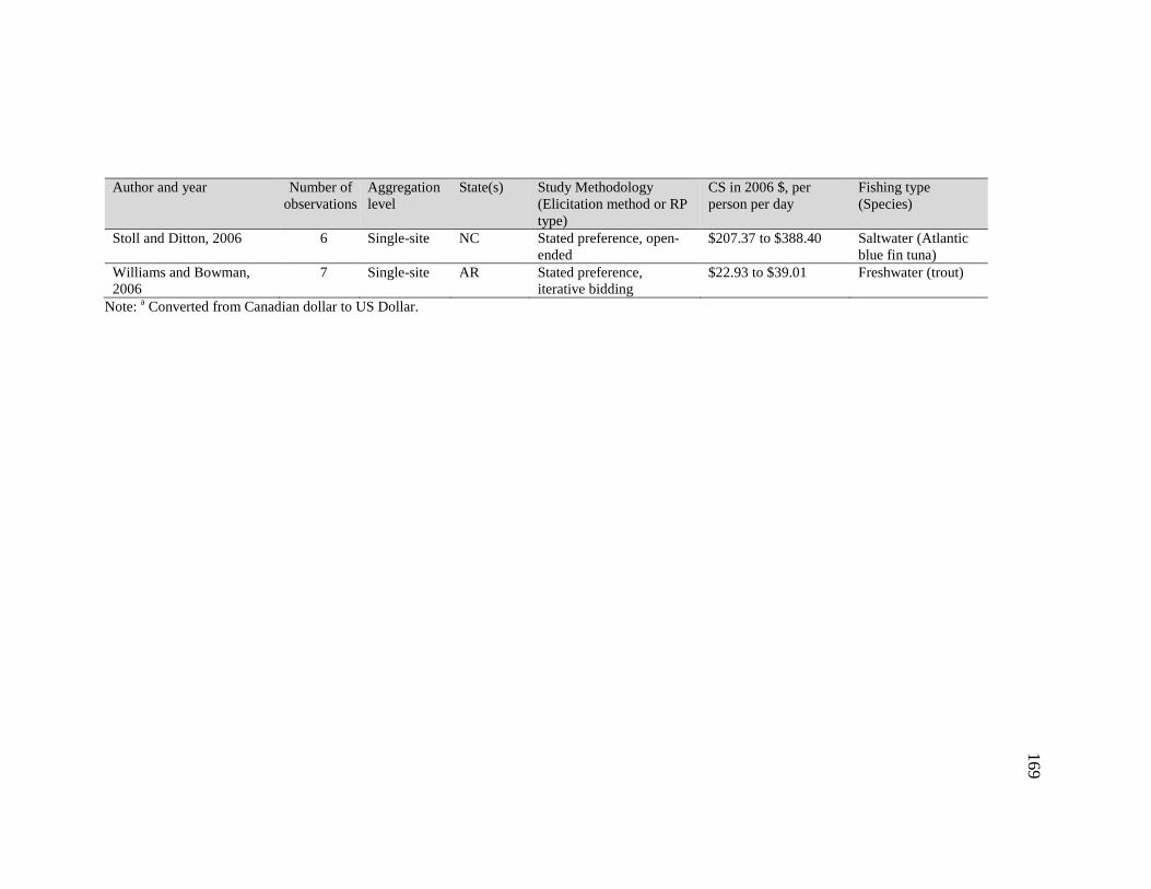
169
Author and year Number of observations
Aggregation level
State(s) Study Methodology (Elicitation method or RP type)
CS in 2006 $, per person per day
Fishing type (Species)
Stoll and Ditton, 2006 6 Single-site NC Stated preference, open-ended
$207.37 to $388.40 Saltwater (Atlantic blue fin tuna)
Williams and Bowman, 2006
7 Single-site AR Stated preference, iterative bidding
$22.93 to $39.01 Freshwater (trout)
Note: a Converted from Canadian dollar to US Dollar.
170
APPENDIX C: BIBLIOGRAPHY OF RECREATIONAL FISHING VA LUATION STUDIES, 1969 TO 2006
Abdullah, N.M. 1988. "Estimation of average and incremental economic values of
Oregon ocean sport-caught salmon: An aggregated travel cost approach." PhD dissertation, Oregon State University.
Adamowicz, W.L., and W.E. Phillips. 1983. "A comparison of extra market benefit
evaluation techniques." Canadian Journal of Agricultural Economics 31:401-412. Adamowicz, W. L., J. Louviere, and M. Williams. "Combining revealed and stated
preference methods for valuing environmental amenities." Journal of Environmental Economics and Management 26(1994): 271-292.
Adler, L. L. "Measuring the value of recreation: The impacts of substitute sites." PhD
dissertation, University of Wyoming, 1993. Agnello, R.J., and L.G. Anderson (1984) The value of fish and fishing days: A partial
solution to managing recreational fisheries with stock externalities, Working paper. University of Delaware.
Agnello, R. J., and Y. Han. "Substitute Site Measures in a Varying Parameter Model with
Application to Recreational Fishing." Marine Resource Economics 8(1993): 65-77.
Aiken, R., and G. P. la Rouche (2003) Net Economic Values for Wildlife-Related
Recreation in 2001: Addendum to the 2001 National Survey of Fishing, Hunting and Wildlife-Associated Recreation, Report 2001-3. Washington, DC: US Fish and Wildlife Service.
Arndorfer, D.J., and N. Bockstael (1986) Estimating the effects of King Mackerel bag
limits on charter boat captains and anglers, Miami, FL: National Marine Fisheries Service.
Beardsley, W. (1970) Economic value of recreation benefits determined by three
methods, Research Note Rm-176. Fort Collins, CO: USDA Forest Service, Rocky Mountain Forest and Range Experiment Station.
Bell, F.W., P.E. Sorensen, and V.R. Leeworthy (1982) The economic impact and
valuation of saltwater recreational fisheries in Florida, Florida Sea Grant College Program, Florida State University, Tallahassee, FL, Sea Grant Report ID FLSGP-T-82-005.
171
Bennett, M., B. Provencher, and R. Bishop (2004) Experience, expectations and hindsight: Evidence of a cognitive wedge in stated preference retrospectives, Staff Paper No. 468. Madison, WI: Department of Agricultural and Applied Economics, University of Wisconsin-Madison.
Bergstrom, J.C., and H.K. Cordell. 1991. "An analysis of the demand for and value of
outdoor recreation in the United States." Journal of Leisure Research 23(1):67-86.
Bergstrom, J. C., J. H. Dorfman, and J. B. Loomis. "Estuary management and
recreational fishing benefits." Coastal Management 32(2004): 417-432. Bhat, G., et al. "An ecoregional approach to the economic valuation of land- and water-
based recreation in the United States." Environmental Management 22, no. 1(1998): 69-77.
Bishop, R.C., K.J. Boyle, M.P. Welsh, R.M. Baumgartner, and P.R. Rathbun (1986) Glen
Canyon Dam releases and downstream recreation: An analysis of user preferences and economic values, Final Report to the Recreation Subteam of the Glen Canyon Environmental Studies. Madison, WI: HBRS.
Bockstael, N.E., I.E. Strand Jr., K.E. McConnel, and F. Arsanjani. 1990. "Sample
Selection Bias in the Estimation of recreation Demand Functions: An Application to Sportfishing." Land Economics 66(1):40-49.
Bowker, J. M., J. C. Bergstrom, and J. Gill (2004) The Waterway at New River State
Park, Final Report Prepared for the Virginia Department of Conservation. Athens, GA: USDA Forest Service, Southern Research Station and the University of Georgia.
Boyle, K.J., M.F. Tiesl, J. Moring, and S.D. Reiling (1991) Economic benefits accruing
to sport fisheries on the lower Kennebec River from the provision of fish passage at Edwards Dam, Staff paper. Orono, ME: Department of Agricultural and Resource Economics, University of Maine.
Boyle, K.J., S.D. Reiling, M. Teisl, and M.L. Phillips (1991) A study of the impact of
game and nongame species on Maine's economy, Staff Paper No. 423. Orono, ME: Department of Agricultural and Resource Economics, University of Maine.
172
Boyle, K. J., B. Roach, and D. G. Waddington (1998) 1996 net economic values for bass, trout and walleye fishing, deer, elk and moose hunting, and wildlife watching: Addendum to the 1996 National Survey of Fishing, Hunting and Wildlife-Associated Recreation., Report 96-2. Washington, DC: US Fish and Wildlife Service.
Bowes, M.D., and J.V. Krutilla (1989) Recreation valuation for forest planning. In M.D.
Bowes, and J.V. Krutilla (Ed.) Multiple use management: The economics of public forest lands. Washington, DC, Resources for the Future, pp. 213-247.
Boyle, K.J. 1989. "Commodity specification and the framing of contingent valuation
questions." Land Economics 65(1):57-63. Breffle, W. S., and E. R. Morey. "Investigating preference heterogeneity in a repeated
discrete-choice recreation demand model of Atlantic salmon fishing." Marine Resource Economics 15(2000): 1-20.
Brooks, R. (1991) Warm water fishing in Montana: A contingent valuation assessment of
angler attitudes and economic benefits for selected waters statewide, Helena, MT: Montana Department of Fish, Wildlife and Parks.
Brown, G. M., and M. Plummer (1978) Recreation valuation: An economic analysis of
nontimber uses of forestland in the Pacific Northwest, Pullman, WA: Forest Policy Project, Washington State University.
Brown, W.G., and F.M. Shalloof (1986) Recommended values for Columbia River
salmon and steelhead for current fishery management decisions, Final report. Corvallis, OR: Department of Agricultural and Resource Economics, Oregon State University.
Brown, G., and M.J. Hay (1987) Net economic recreation values for deer and waterfowl
hunting and trout fishing, 1980, Working Paper No. 23. Washington, DC: US Fish and Wildlife Service.
Cameron, T.A., and M.D. James. 1987. "Efficient estimation methods for "closed-ended"
contingent valuation surveys." Review of Economics and Statistics 69(2):269-276. Cantrell, R. N., et al. "Recreational anglers' willingness to pay for increased catch rates of
Pacific threadfin (Polydactylus sexfilis) in Hawaii." Fisheries Research 68(2004): 149-158.
173
Charbonneau, J. J., and M. J. Hay. "Determinants and economic values of hunting and fishing." Transactions of the North American Wildlife and Natural Resources Conference 43(1978): 391-403.
Chizinski, C. J., et al. "Economic value of angling at a reservoir with low visitation."
North American Journal of Fisheries Management 25(2005): 98-104. Choi, S. "Economic analysis of the Mountain Fork trout fishery in southeastern
Oklahoma using travel cost method." PhD dissertation, Oklahoma State University., 1993.
Connelly, N. A., and T. L. Brown. "Net economic value of the freshwater recreational
fisheries in New York." Transactions of the American Fisheries Society 120(1991): 770-775.
Cooper, J.C., and J.B. Loomis. 1990. "Pooled time-series cross-section travel cost
models: Testing whether recreation behavior is stable over time." Leisure Sciences 12:161-171.
Daubert, J. T., and R. A. Young. "Recreational demands for maintaining instream flows:
A contingent valuation approach." American Journal of Agricultural Economics 63, no. 4(1981): 666-676.
Ditton, R. B., and S. G. Sutton (1998) A Social and Economic Study of Fort Hood
Anglers, Department of Wildlife and Fisheries Sciences, Texas A&M University. Ditton, R. B., B. L. Bohnsack, and J. R. Stoll (1998) A Social and Economic Study of the
Winter recreational Atlantic Bluefin Tuna Fishery in Hatteras, North Carolina, Report prepared for the American Sportfishing Association.
Donnelly, D.M., J.B. Loomis, C.F. Sorg, and L.J. Nelson (1985) Net economic value of
recreational steelhead fishing in Idaho, Resource Bulletin RM-9. Fort Collins, CO: US Department of Agriculture, Forest Service, Rocky Mountain Forest and Range Experiment Station.
Douglas, A. J., and J. G. Taylor. "Riverine based eco-tourism: Trinity River non-market
benefits estimates." International Journal of Sustainable Development and World Ecology 5(1998): 136-148.
Duffield, J.W., J.B. Loomis, and R. Brooks (1987) The net economic value of fishing in
Montana, Helena, MT: Montana Department of Fish, Wildlife and Parks.
174
Duffield, J.W., and S. Allen (1988) Angler preference study final economics report: Contingent valuation of Montana trout fishing by river and angler subgroup, Prepared for Montana Department of Fish, Wildlife and Parks. Missoula, MT: University of Montana.
Duffield, J.W., C. Neher, D. Patterson, and S. Allen (1990) Instream flows in the
Missouri River basin: A recreational survey and economic study, Missoula, MT: Montana Department of Natural Resources and Conservation.
Duffield, J. W., C. J. Neher, and T. C. Brown. "Recreation benefits of instream flow:
Application to Montana's Big Hole and Bitterroot Rivers." Water Resources Research 28, no. 9(1992): 2169-2181.
Duffield, J. W., C. Neher, and M. Merritt (2001) Alaska Angler Survey: Use and
Valuation Estimates for 1996, with a focus on Arctic Grayling in Region III, Alaska Department of Fish and Game, Special Publication Number 01-05, Anchorage.
Duffield, J. W., C. Neher, and M. Merritt (2001) Alaska Angler Survey: Use and
Valuation Estimates for 1995, with a focus on Tanana Valley Major Stocked Waters, Alaska Department of Fish and Game, Special Publication Number 01-4, Anchorage.
Duffield, J. W., C. Neher, and M. Merritt (2001) Alaska Angler Survey: Use and
Valuation Estimates for 1997, with a focus on Salmon Fisheries in Region III, Alaska Department of Fish and Game, Special Publication Number 01-2, Anchorage.
Dutta, N. 1984. "The value of recreational boating and fishing in the central basin of
Ohio's portion of Lake Erie." MS thesis, The Ohio State University. Englin, J., and T. Cameron (1993) Comparing Observed and Multiple-Scenario
Contingent Behavior: A Panel Analysis Utilizing Poisson Regression Techniques, W-133 Proceedings, pp. 266-281.
Englin, J., and D. Lambert. "Measuring angling quality in count data models of
recreational fishing." Environmental and Resource Economics 6, no. 4(1995): 389-399.
Englin, J., and J. S. Shonkwiler. "Modeling recreation demand in the presence of
unobservable travel costs: Toward a travel price model." Journal of Environmental Economics and Management 29(1995): 14-22.
175
Englin, J., D. Lambert, and W. D. Shaw. "A structural equations approach to modeling consumptive recreation demand." Journal of Environmental Economics and Management 33, no. 1(1997): 33-43.
Federal-Provincial-Territorial Task Force on the Importance of Nature to Canadians
(2000) The Importance of Nature to Canadians: The Economic Significance of Nature-Related Activities, Ottawa, Ontario: Environment Canada.
Gillig, D., et al. "Joint estimation of revealed and stated preference data: an application to
recreational red snapper valuation." Agricultural and Resource Economics Review 32 no. 1(2003): 209-221.
Green, T.G. 1984. "Compensating and equivalent variation of the Florida saltwater tourist
fishery." PhD dissertation, Florida State University. Green, G., C. B. Moss, and E. M. Thunberg (1994) Estimation of Recreational Anglers’
Value of Reef Fish in the Gulf of Mexico, Food and Resource Economics Department, Institute of Food and Agricultural Sciences, University of Florida. SP94-12.
Greene, G., C. B. Moss, and T. H. Spreen. "Demand for Recreational in Tampa Bay,
Florida: A Random Utility Approach." Marine Resource Economics 12(1997): 293-305.
Haab, T. C., R. L. Hicks, and J. C. Whitehead (2006) The Economic Value of Marine
Recreational Fishing: Analysis of the MRFSS 1998 Pacific Add-on, Paper presented at the “Fisheries, Fisherman, and Fishing Communities: Socioeconomic perspectives on the West Coast, Alaska, and Hawaii,” Symposium during the 2005 American Fisheries Society Annual Meeting in Anchorage, Alaska.
Hanemann, W.M., T.C. Wegge, and I.E. Strand (1989) Development and application of a
predictive model to analyze the economic effects of species availability, Administrative Report SWR. Terminal Island, CA: National Marine Fisheries Service.
Hansen, C. (1977) A report on the value of wildlife: With 1979 Addendum,
Miscellaneous Pub No.1365. Harding, D., M. Thomas, and N. Stratis (2003) The Economics of Selected Florida
Wildlife Management Areas, Final Report. Tallahassee, FL: Florida Fish and Wildlife Commission.
176
Harpman, D. A., E. W. Sparling, and T. J. Waddle. "A methodology for quantifying and valuing the impacts of flow changes on a fishery." Water Resources Research 29, no. 3(1993): 575-582.
Harris, C.C. 1983. "Assessing the validity of economic methods for evaluating sport
fishery benefits: A behavioral approach." PhD dissertation, University of Michigan.
Hausman, J. A., G. K. Leonard, and D. McFadden. "A utility-consistent, combined
discrete choice and count data model: Assessing recreational use losses due to natural resource damage." Journal of Public Economics 56, no. 1(1995): 1-30.
Hay, M.J. 1988. Net economic value for deer, elk and waterfowl hunting and bass fishing,
1985: Report 85-1. Washington, DC: USDI Fish and Wildlife Service. Henderson, M. M., K. R. Criddle, and S. T. Lee. "The economic value of Alaska's Copper
River personal use and subsistence fisheries." Alaska Fishery Research Bulletin 6, no. 2(1999): 63-69.
Hsiao, C. 1985. "An evaluation of alternative estimates of demand for and benefits from
Oregon salmon sport fishing." PhD dissertation Oregon State University. Huang, C. 1986. "The recreation benefits of water quality improvement in selected lakes
in Minnesota." PhD dissertation, University of Minnesota. Hunt, K. M., and R. B. Ditton (1996) A Social and Economic Study of the Lake Fork
Reservoir Recreational Fishery, Report prepared for the Texas Parks and Wildlife Department and the Sabine River Authority of Texas. HD-608.
Huppert, D. 1989. "Measuring the Value of Fish to Anglers: Application to Central
California Anadromous Species." Marine Resource Economics 6:89-107. Hushak, L.J., J.M. Winslow, and N. Dutta. 1988. "Economic value of Great Lakes
sportfishing: The case of private-boat fishing in Ohio's Lake Erie." Transactions of the American Fisheries Society 117:363-373.
Hushak, L. J., D. O. Kelch, and S. J. Glenn. "The economic value of the Lorain County,
Ohio, artificial reef." American Fisheries Society Symposium 22(1999): 348-362. Johns, G. M., et al. (2001) Socioeconomic study of reefs in Southeast Florida, Final
Report, October 19, 2001. Hollywood, FL: Hazen and Sawyer, P.C.
177
Johnson, D.M., and R.G. Walsh (1987) Economic benefits and costs of the fish stocking program at Blue Mesa Reservoir, Colorado, Technical Report No. 49. Fort Collins, CO: Colorado Water Resources Research Institute, Colorado State University.
Johnston, R. J., et al. "Valuing estuarine resource services using economic and ecological
models: The Peconic Estuary System Study." Coastal Management 30(2002): 47-65.
Jones and Stokes Associates, Inc. (1991) Southeast Alaska sport fishing economic study,
Final Research Report. December, 1991. (JSA 88-028). Prepared for Alaska Department of Fish and Game, Sport Fish Division, Research and Technical Services Kalter, R. J., and L. E. Gosse (1969) Outdoor recreation in New York State: Projections of demand, economic value, and pricing effects for the period 1970-1985, Special Cornell Series No. 5. Ithaca, NY: Cornell University.
Kealy, M.J. 1982. "Travel cost estimates of recreation demand: Theoretical, empirical
and policy issues." PhD dissertation Madison, WI: University of Wisconsin. Kealy, M.J., and R.C. Bishop. 1986. "Theoretical and empirical specifications issues in
travel cost studies." American Journal of Agricultural Economics 68(3):660-667. King, D. A., and A. W. Walka (1980) A market analysis of trout fishing on Fort Apache
Indian Reservation, Final Report. Tucson, AZ: School of Renewable Natural Resources, University of Arizona.
King, D.A., and J.G. Hof. 1985. "Experiential commodity definition in recreation travel
cost models." Forest Science 31(2):519-529. Layman, R. C., J. R. Boyce, and K. R. Criddle. "Economic valuation of the Chinook
salmon sport fishery of the Gulkana River, Alaska." Land Economics 72, no. 1(1996): 113-128.
Leeworthy, V. R., and J. M. Bowker (1997) Linking the Economy and Environment of
Florida Keys/Florida Bay: Nonmarket Economic User Values of the Florida Keys/Key West, Monroe County Tourist Development Council.
Loomis, J. B. (2005) The economic values of recreatinoal fishing and boating to visitors
and communities along the upper Snake River, Final Report. Fort Collins, CO: Colorado State University.
178
Loomis, J. B. "A comparison of the effect of multiple destination trips on recreation benefits as estimated by travel cost and contingent valuation methods." Journal of Leisure Research 38, no. 1(2006): 46-60.
Lyke, A. J. "Discrete choice models to value changes in environmental quality: A Great
Lakes case study." PhD dissertation, University of Wisconsin-Madison, 1993. Martin, W. E., R. Gum, and A. Smith (1974) The demand for and value of hunting,
fishing, and general outdoor recreation in Arizona, Technical Bulletin 211. Tucson, AZ: Agricultural Experiment Station, University of Arizona.
Martin, W.E., F.H. Bollman, and R.L. Gum. 1982. "Economic Value of Lake Mead
Fishery." Fisheries 7(6):20-24. McCollum, D.W., G.L. Peterson, J.R. Arnold, D.C. Markstrom, and D.M. Hellerstein
(1990) The net economic value of recreation on the National Forests: Twelve types of primary activity trips across nine Forest Service Regions, Research Paper RM-289. Fort Collins, CO: USDA Forest Service, Rocky Mountain Forest and Range Experiment Station.
McConnell, K. E. "Values of marine recreational fishing: Measurement and impact of
management." American Journal of Agricultural Economics 61(1979): 921-925. McConnell, K. E., et al. (1994) The economic value of mid and south Atlantic
sportfishing, Report between the University of Maryland, the US Environmental Protection Agency, the National Marine Fisheries Service, and the National Oceanic and Atmospheric Administration. Cooperative agreement no. CR-811043-01-0. College Park, MD: University of Maryland.
Menz, F.C., and D.P. Wilton. 1983. "Alternative ways to measure recreation values by
the travel cost method." American Journal of Agricultural Economics 65:332-336. Menz, F.C., and D.P. Wilton. 1983. "An economic study of the muskellunge fishery in
New York." New York Fish and Game Journal 30(1):12-2 30(1):12-29. Michalson, E. L. (1977) An attempt to quantify the esthetics of wild and scenic rivers in
Idaho, General Technical Report NC-28. St. Paul, MN: USDA Forest Service, North Central Forest Experiment Station. pp.320-328.
Miller, J.R. (1983) On estimating the value of freshwater fishing in substate regions,
Working paper #18. Washington, DC: US Fish and Wildlife Service.
179
Miller, J.R., and M.J. Hay. 1984. "Estimating substate values of fishing and hunting." Transactions of the North American Wildlife and Natural Resources Conference 49:345-355.
Milon, J.W. 1988. "Travel cost methods for estimating the recreational use benefits of
artificial marine habitat." Southern Journal of Agricultural Economics 20(1):87-101.
Morey, E. R., R. D. Rowe, and M. Watson. "A repeated nested-logit model of Atlantic
salmon fishing." American Journal of Agricultural Economics 75, no. 3(1993): 578-592.
Morey, E. R., et al. "Estimating recreational trout fishing damages in Montana's Clark
Fork River basin: Summary of a natural resource damage assessment." Journal of Environmental Management 66(2002): 159-170.
Mullen, J.K., and F.C. Menz. 1985. "The Effect of Acidification Damages on the
Economic Value of the Adirondack Fishery to New York Anglers." American Journal of Agricultural Economics 67(1):112-119.
Nowell, C., and J. Kerkvliet. "The economic value of the Henry's Fork fishery."
Intermountain Journal of Sciences 6, no. 3(2000): 285-292. Oh, C., et al. "Understanding differences in nonmarket valuation by angler specialization
level." Leisure Sciences 27(2005): 263-277. Oster, J.M., D.T. Taylor, J.J. Jacobs, and E.B. Bradley (1987) Reservoir eutrophication
and recreational activity on Flaming Gorge Reservoir, Experiment Station Bulletin No. 908. Laramie, WY: University of Wyoming.
Palm, R.C., and S.P. Malvestuto. 1983. "Relationships between economic benefit and
sport-fishing effort on West Point Reservoir, Alabama-Georgia." Transactions of the American Fisheries Society 112:71-78.
Piper, S. "Modeling recreation decisions and estimating the benefits of North Dakota
river recreation." Rivers 6, no. 4(1998): 251-258. Platt, J.L. (1989) Estimating the Economic Impacts of Hypothetical Grouper Bag Limits
in the Destin/panama City, Florida Charterboat Fishery, NOAA Technical Memorandum NMFS-SEFC-227.
180
Richards, M.T., D.B. Wood, and D.A. Caylor (1985) Sportfishing at Lees Ferry, Arizona: User differences and economic values, Final Report to Northern Arizona University Organized Research Committee. Flagstaff, AZ: Northern Arizona University.
Roberts, K.J., M.E. Thompson , and P.W. Pawlyk. 1985. "Contingent valuation of
recreational diving at petroleum rigs, Gulf of Mexico." Transactions of the American Fisheries Society 114:214-219.
Rosenberger, R. S., A. R. Collins, and J. B. Svetlik. "Private provision of a public good:
Willingness to pay for privately stocked trout." Society and Natural Resources 18(2005): 75-87.
Rowe, R.D., E.R. Morey, A.D. Ross, and W.D. Shaw (1985) Valuing marine recreation
fishing on the Pacific Coast, Boulder, CO: Energy and Resource Consultants, Inc. Sample, K.C., and R.C. Bishop. 1985. "Estimating the value of variations in anglers'
success rates: An application of the multiple-site travel cost method." Marine Resource Economics 2(1):55-74.
Shafer, E. L., et al. "Economic amenity values of wildlife: Six case studies in
Pennsylvania." Environmental Management 17, no. 5(1993): 669-682. Schuhmann, P. W., and K. A. Schwabe. "An analysis of congestion measures and
heterogeneous angler preferences in a random utility model of recreational fishing." Environmental and Resource Economics 27(2004): 429-450.
Shonkwiler, J. S. (1995) Systems of travel cost models of recreation demand, In D.
Larson (comp), Western Regional Research Publication, W-133 Benefits and Costs Transfer in Natural Resource Planning. Eighth Interim Report. Davis, CA: University of California, Davis.
Siderelis, C., G. Brothers, and P. Rea. "A boating choice model for the valuation of lake
access." Journal of Leisure Research 27, no. 3(1995): 264-282. Smith, V.K., and R.B. Palmquist (1988) The value of recreational fishing on the
Albemarle and Pamlico Estuary, North Carolina State University and Environmental Protection Agency, EPA #88-13.
Sorg, C.F., and J.B. Loomis. 1986. "Economic value of Idaho sport fisheries with an
update on valuation technique." North American Journal of Fisheries Management 6:494-503.
181
Snyder, B.R. 1983. "Specification errors and consumer surplus values for recreational striped bass fishing." MS Thesis, University of Maryland.
Steinnes, D. N., and R. L. Raab. "The economics of a 'happening': Spring smelt fishing
on Lake Superior." Regional Science Perspectives 11, no. 1(1981): 32-41. Stoll, J., and R. Ditton. "Understanding Anglers' Willingness to Pay Under Alternative
Management Regimes." Human Dimensions of Wildlife 11, no. 1(2006): 27-42. Strong, E.J. 1983. "A note on the functional form of travel cost models with zones of
unequal populations." Land Economics 59(3):342-349. Sublette, W., and W. Martin (1975) Outdoor recreation in the Salt-Verde Basin of central
Arizona: Demand and value, Technical Bulletin 218. Tucson, AZ: Agricultural Experiment Station, University of Arizona.
Sutherland, R.J. (1982) Recreation and preservation valuation estimates for Flathead
River and Lake system, Kalispell, MT: Flathead River Basin Commission. Taccogna, G. S. "The economic value of recreation in the Seymour River corridor: A
comparison of developed and protected river reaches using the travel cost method." MS thesis, Simon Fraser University, Canada, 1993.
Talhelm, D.R., J.E. Hanna, and P. Victor. 1987. "Product travel cost approach:
Estimating acid rain damage to sport fishing in Ontario." Transactions of the American Fisheries Society 116:420-431.
Thomas, M. H., and N. Stratis (2001) Assessing the Economic Impact and Value of
Florida's Public Piers and Boat Ramps, Tallahassee, FL: Florida Fish and Wildlife Conservation Commission.
Upneja, A., et al. "Economic benefits of sport fishing and angler wildlife watching in
Pennsylvania." Journal of Travel Research 40(2001): 68-78. Vaughan, W.J., and C.S. Russel. 1982. "Valuing a fishing day: An application of a
systematic varying parameter model." Land Economics 58(4):450-463. Violette, D.M. (1985) A model to estimate the economic impacts on recreational fishing
in the Adirondacks from current levels of acidification, Proceedings of the AERE Workshop on Recreation Demand Modeling, May 17-18, 1985. Boulder, CO: Energy and Resource Consultants, Inc.
182
Waddington, D. G., K. J. Boyle, and J. Cooper (1994) 1991 net economic values for bass and trout fishing, deer hunting, and wildlife watching, Washington, DC: US Fish and Wildlife Service.
Walsh, R. G., et al. (1980) An empirical application of a model for estimating the
recreation value of instream flow, Fort Collins, CO: Colorado Water Resources Research Institute, Colorado State University.
Walsh, R.G., and J.P. Olienyk (1981) Recreation demand effects of mountain pine beetle
damage to the quality of forest recreation resources in the Colorado Front Range, Final Report to USDA Forest Service. Fort Collins, CO: Department of Economics, Colorado State University.
Wegge, T.C., W.M. Hanemann, and I.E. Strand (1986) An economic assessment of
marine recreational fishing in southern California, Sacramento, CA: Jones & Stokes Associates, Inc.
Weithman, A.S., and M.A. Haas. 1982. "Socioeconomic value of the trout fishery in Lake
Taneycomo, Missouri." Transactions of the American Fisheries Society 111:223-230.
Wellman, K. F., and B. Noble (1997) Selected recreational values of the Corpus Christi
Bay National Estuary Program study area, Publication CCBNEP-18. Corpus Christi, TX: Corpus Christi Bay National Estuary Program.
Whitehead, J. "Benefits of Quality Changes in Recreational Fishing: A Single-Site Travel
Cost Approach." Journal of Environmental Systems 21(1993): 357-364. Whitehead, J. C., and R. Aiken (2000) An analysis of trends in net economic values for
bass fishing from the national survey of fishing, hunting and wildlife-associated recreation, East Carolina University, Department of Economics Working Paper.
Whitehead, J. C., and T. C. Haab. "Southeast marine recreational fishery statistical
survey: distance and catch based choice sets." Marine resource economics 14, no. 4(2000): 283-298.
Wilemon, J. M., R. K. Riechers, and R. B. Ditton (1994) Estimating the Economic Value
of the Recreational Boat Fishery in Galveston Bay, Texas, Proceedings of the 46th Gulf and Caribbean Fisheries Institute.
Williams, J. S., and P. W. Bettoli (2003) Net value of trout fishing opportunities in
Tennessee Tailwaters, Fisheries Report 03-21. Final report submitted to the Tennessee Wildlife Resource Agency.
183
Williams, J., and D. Bowman (2006) Arkansas Trout Permit Holder Survey--2003, AGFC Trout Management Report, Report #TP-06-06. Little Rock, AR: Arkansas Game and Fish Commission.
Woodward, R. T., et al. "The Welfare Impacts of Unanticipated Trip Limitations in
Travel Cost Models." Land Economics 77, no. 3(2001): 327-338. Ziemer, R. F., W. N. Musser, and R. C. Hill. "Recreation Demand Equations: Functional
Form and Consumer Surplus." American Journal of Agricultural Economics 62, no. 1(1980): 136.
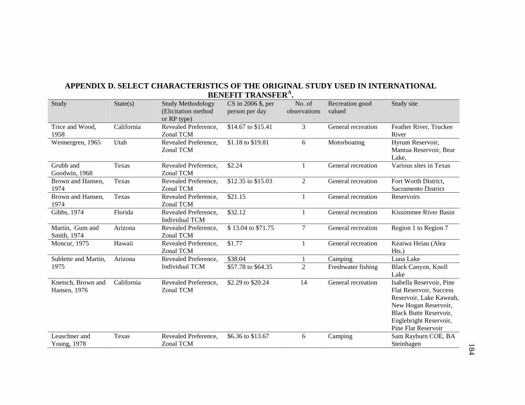
184
APPENDIX D. SELECT CHARACTERISTICS OF THE ORIGINAL STUDY USED IN INTERNATIONAL BENEFIT TRANSFER A.
Study State(s) Study Methodology (Elicitation method or RP type)
CS in 2006 $, per person per day
No. of observations
Recreation good valued
Study site
Trice and Wood, 1958
California Revealed Preference, Zonal TCM
$14.67 to $15.41 3 General recreation Feather River, Truckee River
Wennergren, 1965 Utah Revealed Preference, Zonal TCM
$1.18 to $19.81 6 Motorboating Hyrum Reservoir, Mantua Reservoir, Bear Lake,
Grubb and Goodwin, 1968
Texas Revealed Preference, Zonal TCM
$2.24 1 General recreation Various sites in Texas
Brown and Hansen, 1974
Texas Revealed Preference, Zonal TCM
$12.35 to $15.03 2 General recreation Fort Worth District, Sacramento District
Brown and Hansen, 1974
Texas Revealed Preference, Zonal TCM
$21.15 1 General recreation Reservoirs
Gibbs, 1974 Florida Revealed Preference, Individual TCM
$32.12 1 General recreation Kissimmee River Basin
Martin, Gum and Smith, 1974
Arizona Revealed Preference, Zonal TCM
$ 13.04 to $71.75 7 General recreation Region 1 to Region 7
Moncur, 1975 Hawaii Revealed Preference, Zonal TCM
$1.77 1 General recreation Keaiwa Heiau (Alea Hts.)
Sublette and Martin, 1975
Arizona Revealed Preference, Individual TCM
$38.04 1 Camping Luna Lake $57.78 to $64.35 2 Freshwater fishing Black Canyon, Knoll
Lake Knetsch, Brown and Hansen, 1976
California Revealed Preference, Zonal TCM
$2.29 to $20.24 14 General recreation Isabella Reservoir, Pine Flat Reservoir, Success Reservoir, Lake Kaweah, New Hogan Reservoir, Black Butte Reservoir, Englebright Reservoir, Pine Flat Reservoir
Leuschner and Young, 1978
Texas Revealed Preference, Zonal TCM
$6.36 to $13.67 6 Camping Sam Rayburn COE, BA Steinhagen
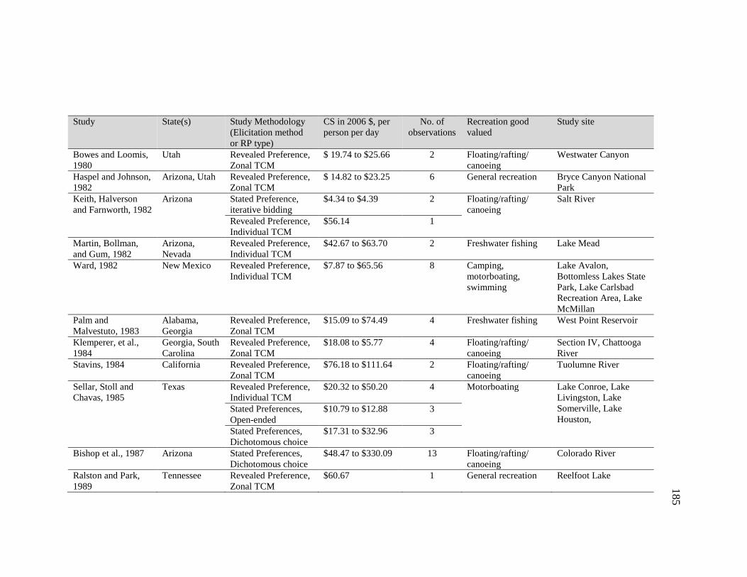
185
Study State(s) Study Methodology (Elicitation method or RP type)
CS in 2006 $, per person per day
No. of observations
Recreation good valued
Study site
Bowes and Loomis, 1980
Utah Revealed Preference, Zonal TCM
$ 19.74 to $25.66 2 Floating/rafting/ canoeing
Westwater Canyon
Haspel and Johnson, 1982
Arizona, Utah Revealed Preference, Zonal TCM
$ 14.82 to $23.25 6 General recreation Bryce Canyon National Park
Keith, Halverson and Farnworth, 1982
Arizona Stated Preference, iterative bidding
$4.34 to $4.39 2 Floating/rafting/ canoeing
Salt River
Revealed Preference, Individual TCM
$56.14 1
Martin, Bollman, and Gum, 1982
Arizona, Nevada
Revealed Preference, Individual TCM
$42.67 to $63.70 2 Freshwater fishing Lake Mead
Ward, 1982 New Mexico Revealed Preference, Individual TCM
$7.87 to $65.56 8 Camping, motorboating, swimming
Lake Avalon, Bottomless Lakes State Park, Lake Carlsbad Recreation Area, Lake McMillan
Palm and Malvestuto, 1983
Alabama, Georgia
Revealed Preference, Zonal TCM
$15.09 to $74.49 4 Freshwater fishing West Point Reservoir
Klemperer, et al., 1984
Georgia, South Carolina
Revealed Preference, Zonal TCM
$18.08 to $5.77 4 Floating/rafting/ canoeing
Section IV, Chattooga River
Stavins, 1984 California Revealed Preference, Zonal TCM
$76.18 to $111.64 2 Floating/rafting/ canoeing
Tuolumne River
Sellar, Stoll and Chavas, 1985
Texas Revealed Preference, Individual TCM
$20.32 to $50.20 4 Motorboating Lake Conroe, Lake Livingston, Lake Somerville, Lake Houston,
Stated Preferences, Open-ended
$10.79 to $12.88 3
Stated Preferences, Dichotomous choice
$17.31 to $32.96 3
Bishop et al., 1987 Arizona Stated Preferences, Dichotomous choice
$48.47 to $330.09 13 Floating/rafting/ canoeing
Colorado River
Ralston and Park, 1989
Tennessee Revealed Preference, Zonal TCM
$60.67 1 General recreation Reelfoot Lake
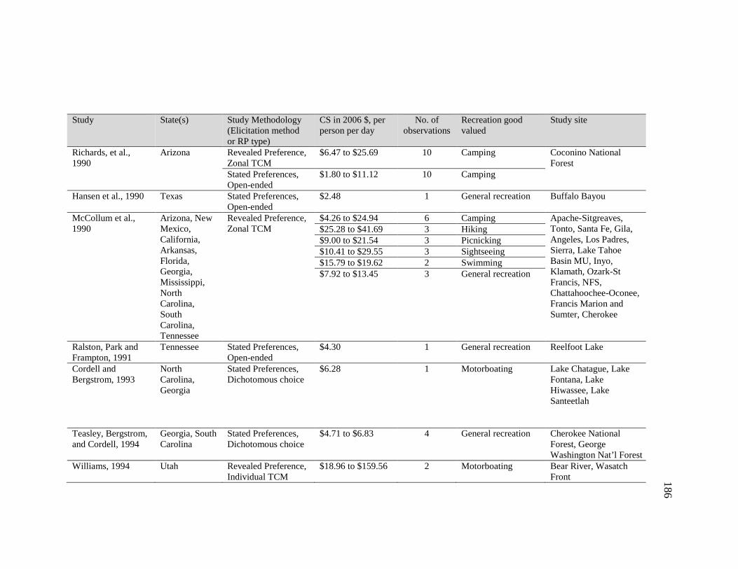
186
Study State(s) Study Methodology (Elicitation method or RP type)
CS in 2006 $, per person per day
No. of observations
Recreation good valued
Study site
Richards, et al., 1990
Arizona Revealed Preference, Zonal TCM
$6.47 to $25.69 10 Camping Coconino National Forest
Stated Preferences, Open-ended
$1.80 to $11.12 10 Camping
Hansen et al., 1990 Texas Stated Preferences, Open-ended
$2.48 1 General recreation Buffalo Bayou
McCollum et al., 1990
Arizona, New Mexico, California, Arkansas, Florida, Georgia, Mississippi, North Carolina, South Carolina, Tennessee
Revealed Preference, Zonal TCM
$4.26 to $24.94 6 Camping Apache-Sitgreaves, Tonto, Santa Fe, Gila, Angeles, Los Padres, Sierra, Lake Tahoe Basin MU, Inyo, Klamath, Ozark-St Francis, NFS, Chattahoochee-Oconee, Francis Marion and Sumter, Cherokee
$25.28 to $41.69 3 Hiking $9.00 to $21.54 3 Picnicking $10.41 to $29.55 3 Sightseeing $15.79 to $19.62 2 Swimming $7.92 to $13.45 3 General recreation
Ralston, Park and Frampton, 1991
Tennessee Stated Preferences, Open-ended
$4.30 1 General recreation Reelfoot Lake
Cordell and Bergstrom, 1993
North Carolina, Georgia
Stated Preferences, Dichotomous choice
$6.28 1 Motorboating Lake Chatague, Lake Fontana, Lake Hiwassee, Lake Santeetlah
Teasley, Bergstrom, and Cordell, 1994
Georgia, South Carolina
Stated Preferences, Dichotomous choice
$4.71 to $6.83 4 General recreation Cherokee National Forest, George Washington Nat’l Forest
Williams, 1994 Utah Revealed Preference, Individual TCM
$18.96 to $159.56 2 Motorboating Bear River, Wasatch Front
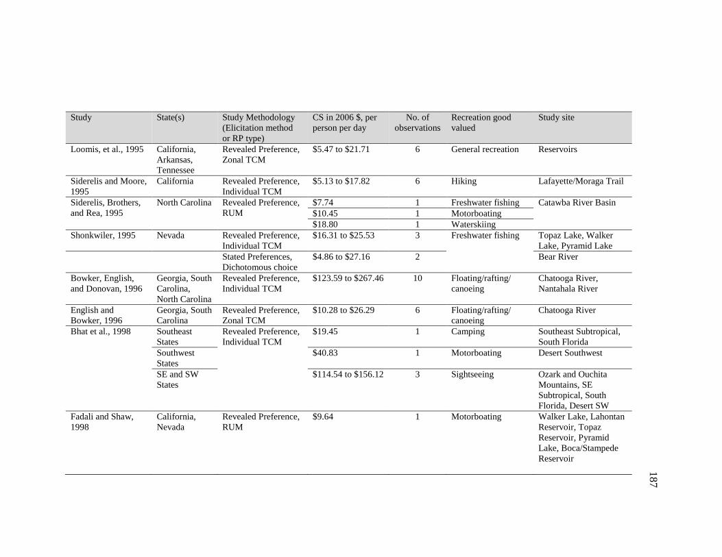
187
Study State(s) Study Methodology (Elicitation method or RP type)
CS in 2006 $, per person per day
No. of observations
Recreation good valued
Study site
Loomis, et al., 1995 California, Arkansas, Tennessee
Revealed Preference, Zonal TCM
$5.47 to $21.71 6 General recreation Reservoirs
Siderelis and Moore, 1995
California Revealed Preference, Individual TCM
$5.13 to $17.82 6 Hiking Lafayette/Moraga Trail
Siderelis, Brothers, and Rea, 1995
North Carolina Revealed Preference, RUM
$7.74 1 Freshwater fishing Catawba River Basin $10.45 1 Motorboating $18.80 1 Waterskiing
Shonkwiler, 1995 Nevada Revealed Preference, Individual TCM
$16.31 to $25.53 3 Freshwater fishing Topaz Lake, Walker Lake, Pyramid Lake
Stated Preferences, Dichotomous choice
$4.86 to $27.16 2 Bear River
Bowker, English, and Donovan, 1996
Georgia, South Carolina, North Carolina
Revealed Preference, Individual TCM
$123.59 to $267.46 10 Floating/rafting/ canoeing
Chatooga River, Nantahala River
English and Bowker, 1996
Georgia, South Carolina
Revealed Preference, Zonal TCM
$10.28 to $26.29 6 Floating/rafting/ canoeing
Chatooga River
Bhat et al., 1998 Southeast States
Revealed Preference, Individual TCM
$19.45 1 Camping Southeast Subtropical, South Florida
Southwest States
$40.83 1 Motorboating Desert Southwest
SE and SW States
$114.54 to $156.12 3 Sightseeing Ozark and Ouchita Mountains, SE Subtropical, South Florida, Desert SW
Fadali and Shaw, 1998
California, Nevada
Revealed Preference, RUM
$9.64 1 Motorboating Walker Lake, Lahontan Reservoir, Topaz Reservoir, Pyramid Lake, Boca/Stampede Reservoir
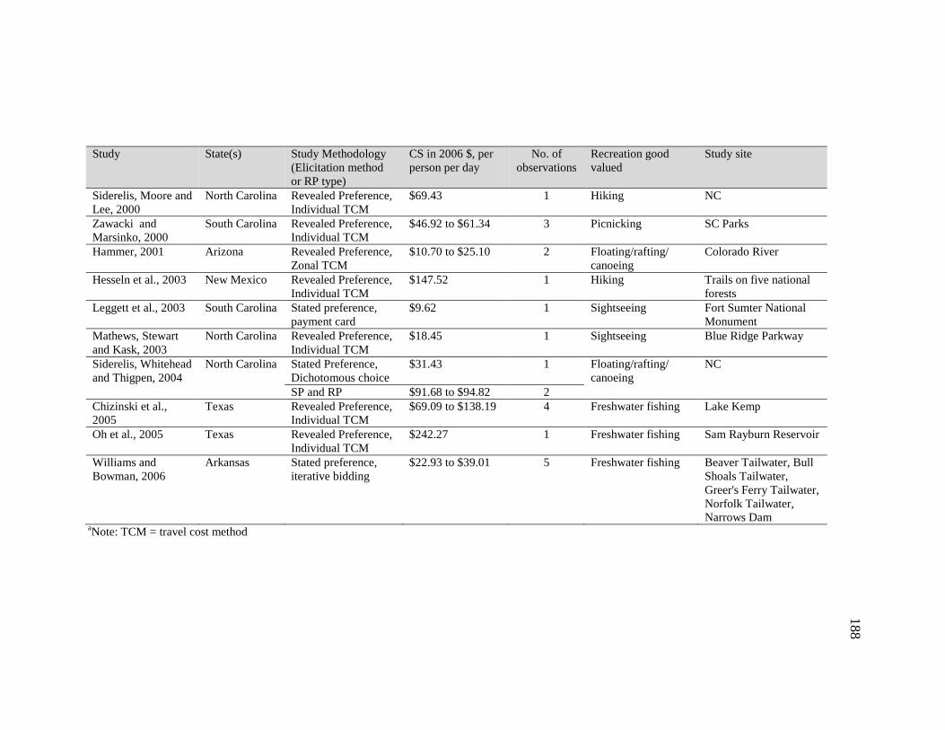
188
Study State(s) Study Methodology (Elicitation method or RP type)
CS in 2006 $, per person per day
No. of observations
Recreation good valued
Study site
Siderelis, Moore and Lee, 2000
North Carolina Revealed Preference, Individual TCM
$69.43 1 Hiking NC
Zawacki and Marsinko, 2000
South Carolina Revealed Preference, Individual TCM
$46.92 to $61.34 3 Picnicking SC Parks
Hammer, 2001 Arizona Revealed Preference, Zonal TCM
$10.70 to $25.10 2 Floating/rafting/ canoeing
Colorado River
Hesseln et al., 2003 New Mexico Revealed Preference, Individual TCM
$147.52 1 Hiking Trails on five national forests
Leggett et al., 2003 South Carolina Stated preference, payment card
$9.62 1 Sightseeing Fort Sumter National Monument
Mathews, Stewart and Kask, 2003
North Carolina Revealed Preference, Individual TCM
$18.45 1 Sightseeing Blue Ridge Parkway
Siderelis, Whitehead and Thigpen, 2004
North Carolina Stated Preference, Dichotomous choice
$31.43 1 Floating/rafting/ canoeing
NC
SP and RP $91.68 to $94.82 2 Chizinski et al., 2005
Texas Revealed Preference, Individual TCM
$69.09 to $138.19 4 Freshwater fishing Lake Kemp
Oh et al., 2005 Texas Revealed Preference, Individual TCM
$242.27 1 Freshwater fishing Sam Rayburn Reservoir
Williams and Bowman, 2006
Arkansas Stated preference, iterative bidding
$22.93 to $39.01 5 Freshwater fishing Beaver Tailwater, Bull Shoals Tailwater, Greer's Ferry Tailwater, Norfolk Tailwater, Narrows Dam
aNote: TCM = travel cost method
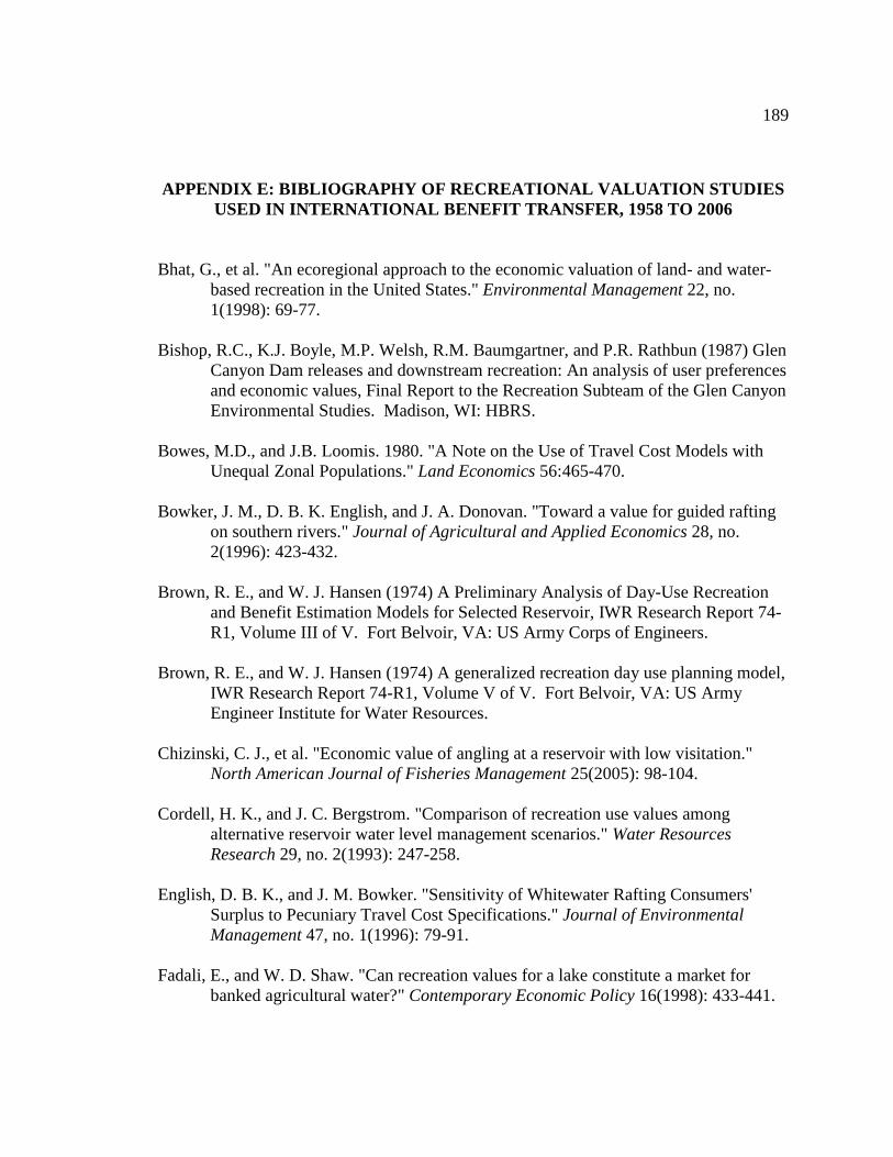
189
APPENDIX E: BIBLIOGRAPHY OF RECREATIONAL VALUATION STUDIES USED IN INTERNATIONAL BENEFIT TRANSFER, 1958 TO 200 6
Bhat, G., et al. "An ecoregional approach to the economic valuation of land- and water-
based recreation in the United States." Environmental Management 22, no. 1(1998): 69-77.
Bishop, R.C., K.J. Boyle, M.P. Welsh, R.M. Baumgartner, and P.R. Rathbun (1987) Glen
Canyon Dam releases and downstream recreation: An analysis of user preferences and economic values, Final Report to the Recreation Subteam of the Glen Canyon Environmental Studies. Madison, WI: HBRS.
Bowes, M.D., and J.B. Loomis. 1980. "A Note on the Use of Travel Cost Models with
Unequal Zonal Populations." Land Economics 56:465-470. Bowker, J. M., D. B. K. English, and J. A. Donovan. "Toward a value for guided rafting
on southern rivers." Journal of Agricultural and Applied Economics 28, no. 2(1996): 423-432.
Brown, R. E., and W. J. Hansen (1974) A Preliminary Analysis of Day-Use Recreation
and Benefit Estimation Models for Selected Reservoir, IWR Research Report 74-R1, Volume III of V. Fort Belvoir, VA: US Army Corps of Engineers.
Brown, R. E., and W. J. Hansen (1974) A generalized recreation day use planning model,
IWR Research Report 74-R1, Volume V of V. Fort Belvoir, VA: US Army Engineer Institute for Water Resources.
Chizinski, C. J., et al. "Economic value of angling at a reservoir with low visitation."
North American Journal of Fisheries Management 25(2005): 98-104. Cordell, H. K., and J. C. Bergstrom. "Comparison of recreation use values among
alternative reservoir water level management scenarios." Water Resources Research 29, no. 2(1993): 247-258.
English, D. B. K., and J. M. Bowker. "Sensitivity of Whitewater Rafting Consumers'
Surplus to Pecuniary Travel Cost Specifications." Journal of Environmental Management 47, no. 1(1996): 79-91.
Fadali, E., and W. D. Shaw. "Can recreation values for a lake constitute a market for
banked agricultural water?" Contemporary Economic Policy 16(1998): 433-441.
190
Gibbs, K.C. 1974. "Evaluation of outdoor recreational resources: A note." Land Economics 50:309-311.
Grubb, H., and J. Goodwin (1968) Economic evaluation of water oriented recreation in
the preliminary Texas water plan, Texas Water Development Board Report 84. Hammer, M. Z. "Applying the TCM with secondary data to white water boating in Grand
Canyon National Park." MS thesis, Colorado State University, 2001. Hansen, W.J., A.S. Mills, J.R. Stoll, R.L. Freeman, and C.D. Hankamer (1990) A case
study application of the contingent valuation method for estimating urban recreation use and benefits. National Economic Development Procedures Manual - Recreation, Volume III, IWR Report 90-R-11. Fort Belvoir, VA: US Army Corps of Engineers.
Haspel, A., and F.R. Johnson. 1982. "Multiple destination trip bias in recreation benefit
estimation." Land Economics 58(3):364-372. Hesseln, H., et al. "Wildfire effects on hiking and biking demand in New Mexico: A
travel cost study." Journal of Environmental Management 69(2003): 359-368. Keith, J.E., P. Halverson, and L. Farnworth (1982) Valuation of a free flowing river: The
Salt River, Arizona, Final Report to the U.S. Army Corps of Engineers for Contract No. DACW09-81-M-2439. Logan, UT: Utah State University.
Klemperer, W.D., G.J. Buhyoff, P.S. Verbyla, and L.D. Joyner (1984) Valuing white-
water river recreation by the travel cost method. Baton Rouge, LA, pp. 709-719. Knetsch, J.L., R. Brown, and W. Hansen (1976) Estimating expected use and value of
recreation sites: In C. Gearing, W. Swart, and R. Var (eds.) Planning for Tourism Development: Quantitative Approaches. New York, NY, Praeger.
Leggett, C. G., et al. "Social Desirability Bias in Contingent Valuation Surveys
Administered Through In-Person Interviews." Land Economics 79, no. 4(2003): 561-575.
Leuschner, W.A., and R. Young. 1978. "Estimating the southern pine beetle's impact on
reservoir campsites." Forest Science 24:527-537. Loomis, J. B., et al. "Testing transferability of recreation demand models across regions:
A study of Corps of Engineers reservoirs." Water Resources Research 31, no. 3(1995): 721-730.
191
McCollum, D.W., G.L. Peterson, J.R. Arnold, D.C. Markstrom, and D.M. Hellerstein (1990) The net economic value of recreation on the National Forests: Twelve types of primary activity trips across nine Forest Service Regions, Research Paper RM-289. Fort Collins, CO: USDA Forest Service, Rocky Mountain Forest and Range Experiment Station.
Martin, W.E., R. Gum, and A. Smith (1974) The demand for and value of hunting,
fishing, and general outdoor recreation in Arizona, Technical Bulletin 211. Tucson, AZ: Agricultural Experiment Station, University of Arizona.
Martin, W.E., F.H. Bollman, and R.L. Gum. 1982. "Economic Value of Lake Mead
Fishery." Fisheries 7(6):20-24. Mathews, L. G., S. Stewart, and S. Kask (2003) Blue Ridge Parkway Scenic Experience
Project, Phase 2 Final Report. Asheville, NC: University of North Carolina--Asheville, Department of Economics.
Moncur, J.E. 1975. "Estimating the value of alternative outdoor recreation facilities
within a small area." Journal of Leisure Research 7:301-311. Oh, C., et al. "Understanding differences in nonmarket valuation by angler specialization
level." Leisure Sciences 27(2005): 263-277. Palm, R.C., and S.P. Malvestuto. 1983. "Relationships between economic benefit and
sport-fishing effort on West Point Reservoir, Alabama-Georgia." Transactions of the American Fisheries Society 112:71-78.
Ralston, S. N., and W. M. Park. "Estimation of potential reductions in recreational
benefits due to sedimentation." Water Resources Bulletin 25, no. 6(1989): 1259-1265.
Ralston, S. N., W. M. Park, and E. J. Frampton. "Contingent valuation and recreational
demand." Journal of Applied Business Research 7, no. 3(1991): 116-119. Richards, M.T., D.A. King, T.C. Daniel, and T.C. Brown. 1990. "The lack of an expected
relationship between travel cost and contingent value estimates of forest recreation value." Leisure Sciences 12:303-319.
Sellar, C., J. R. Stoll, and J. Chavas. "Validation or empirical measures of welfare
change: A comparison of nonmarket techniques." Land Economics 61, no. 2(1985): 156-175.
192
Shonkwiler, J. S. (1995) Systems of travel cost models of recreation demand, In D. Larson (comp), Western Regional Research Publication, W-133 Benefits and Costs Transfer in Natural Resource Planning. Eighth Interim Report. Davis, CA:
Siderelis, C., and R. Moore. "Outdoor recreation net benefits of rail-trails." Journal of
Leisure Research 27, no. 4(1995): 344-359. Siderelis, C., G. Brothers, and P. Rea. "A boating choice model for the valuation of lake
access." Journal of Leisure Research 27, no. 3(1995): 264-282. Siderelis, C., R. Moore, and J. Lee. "Incorporating users' perceptions of site quality in a
recreation travel cost model." Journal of Leisure Research 32, no. 4(2000): 406-414.
Siderelis, C., J. Whitehead, and J. Thigpen (2004) Paddle trails and contingent fee data,
Working paper. Raleigh, NC: Department of Parks, Recreation and Tourism Management, North Carolina State University.
Stavins, R. (1984) The Tuolumne River: Preservation or development? An economic
assessment, Berkeley, CA: The Environmental Defense Fund. Sublette, W., and W. Martin (1975) Outdoor recreation in the Salt-Verde Basin of central
Arizona: Demand and value, Technical Bulletin 218. Tucson, AZ: Agricultural Experiment Station, University of Arizona.
Teasley, R.J., J.C. Bergstrom, and H.K. Cordell. 1994. "Estimating revenue-capture
potential associated with public area recreation." Journal of Agricultural and Resource Economics 19(1):89-101.
Trice, A. H., and S. E. Wood. "Measurement of recreation benefits." Land Economics
34(1958): 195-207. Ward, F.A. (1982) The demand for and value of recreational use of water in southeastern
New Mexico, Las Cruces, NM: Agricultural Experiment Station, New Mexico State University.
Wennergren, E. B. (1965) Value of water for boating recreation, Bulletin 453. Logan,
UT: Agricultural Experiment Station, Utah State University. Williams, J. T. "Utah boating and fishing survey: Applying contingent valuation and
travel cost methods to estimate recreation values in northern Utah for the Bear River water development project." MA Thesis, Utah State University, 1994.
193
Williams, J., and D. Bowman (2006) Arkansas Trout Permit Holder Survey--2003, AGFC Trout Management Report, Report #TP-06-06. Little Rock, AR: Arkansas Game and Fish Commission.
Zawacki, W., and A. Marsinko (2000) Using Geographic Information Systems with
travel cost models: A case study, In G. Kyle (comp., ed.), 2000, Proceedings of the 1999 Northeastern Recreation Research Symposium. General Technical Report NE-269. Newtown Square, PA.
