ams 206: classical and bayesian inference
TRANSCRIPT

AMS 206: Classical and Bayesian Inference
David DraperDepartment of Applied Mathematics and Statistics
University of California, Santa Cruz
[email protected]/∼draper
Lecture Notes (Part 1)
1 / 1
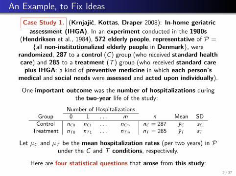
An Example, to Fix IdeasCase Study 1. (Krnjajic, Kottas, Draper 2008): In-home geriatric
assessment (IHGA). In an experiment conducted in the 1980s(Hendriksen et al., 1984), 572 elderly people, representative of P =
{all non-institutionalized elderly people in Denmark}, wererandomized, 287 to a control (C) group (who received standard healthcare) and 285 to a treatment (T ) group (who received standard care
plus IHGA: a kind of preventive medicine in which each person’smedical and social needs were assessed and acted upon individually).
One important outcome was the number of hospitalizations duringthe two-year life of the study:
Number of HospitalizationsGroup 0 1 . . . m n Mean SD
Control nC0 nC1 . . . nCm nC = 287 yC sCTreatment nT 0 nT 1 . . . nTm nT = 285 yT sT
Let µC and µT be the mean hospitalization rates (per two years) in Punder the C and T conditions, respectively.
Here are four statistical questions that arose from this study:2 / 37
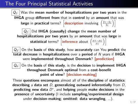
The Four Principal Statistical ActivitiesQ1: Was the mean number of hospitalizations per two years in theIHGA group different from that in control by an amount that was
large in practical terms?[description involving
(yT−yC
yC
)]Q2: Did IHGA (causally) change the mean number of
hospitalizations per two years by an amount that was large instatistical terms?
[inference about
(µT−µCµC
)]Q3: On the basis of this study, how accurately can You predict thetotal decrease in hospitalizations over a period of N years if IHGA
were implemented throughout Denmark? [prediction]Q4: On the basis of this study, is the decision to implement IHGA
throughout Denmark optimal from a cost-benefitpoint of view? [decision-making]
These questions encompass almost all of the discipline of statistics:describing a data set D, generalizing outward inferentially from D,predicting new data D∗, and helping people make decisions in thepresence of uncertainty (I include sampling/experimental design
under decision-making; omitted: data wrangling, ...).3 / 37
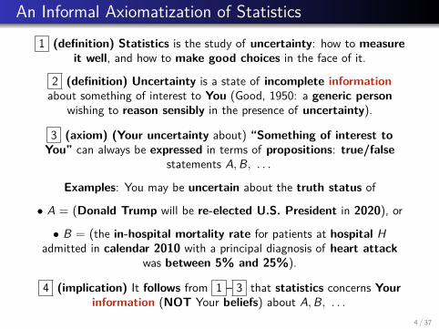
An Informal Axiomatization of Statistics1 (definition) Statistics is the study of uncertainty: how to measure
it well, and how to make good choices in the face of it.
2 (definition) Uncertainty is a state of incomplete informationabout something of interest to You (Good, 1950: a generic person
wishing to reason sensibly in the presence of uncertainty).
3 (axiom) (Your uncertainty about) “Something of interest toYou” can always be expressed in terms of propositions: true/false
statements A,B, . . .
Examples: You may be uncertain about the truth status of
• A = (Donald Trump will be re-elected U.S. President in 2020), or
• B = (the in-hospital mortality rate for patients at hospital Hadmitted in calendar 2010 with a principal diagnosis of heart attack
was between 5% and 25%).
4 (implication) It follows from 1 – 3 that statistics concerns Yourinformation (NOT Your beliefs) about A,B, . . .
4 / 37

Axiomatization (continued)
5 (axiom) But Your information cannot be assessed in a vacuum:all such assessments must be made relative to (conditional on) Yourbackground assumptions and judgments about how the world works
vis a vis A,B, . . . .
6 (axiom) These assumptions and judgments, which are themselves aform of information, can always be expressed in a finite setB = {B1, . . . ,Bb} of propositions (examples below).
7 (definition) Call the “something of interest to You” θ; inapplications θ is often a vector (or matrix, or array) of real numbers,but in principle it could be almost anything (a function, an image of
the surface of Mars, a phylogenetic tree, ...).
8 (axiom) There will typically be an information source (data set) Dthat You judge to be relevant to decreasing Your uncertainty about θ;in applications D is often again a vector (or matrix, or array) of realnumbers, but in principle it too could be almost anything (a movie,
the words in a book, ...).
5 / 37
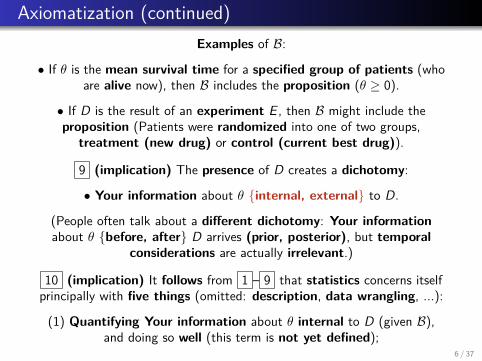
Axiomatization (continued)Examples of B:
• If θ is the mean survival time for a specified group of patients (whoare alive now), then B includes the proposition (θ ≥ 0).
• If D is the result of an experiment E , then B might include theproposition (Patients were randomized into one of two groups,
treatment (new drug) or control (current best drug)).
9 (implication) The presence of D creates a dichotomy:
• Your information about θ {internal, external} to D.
(People often talk about a different dichotomy: Your informationabout θ {before, after} D arrives (prior, posterior), but temporal
considerations are actually irrelevant.)
10 (implication) It follows from 1 – 9 that statistics concerns itselfprincipally with five things (omitted: description, data wrangling, ...):
(1) Quantifying Your information about θ internal to D (given B),and doing so well (this term is not yet defined);
6 / 37
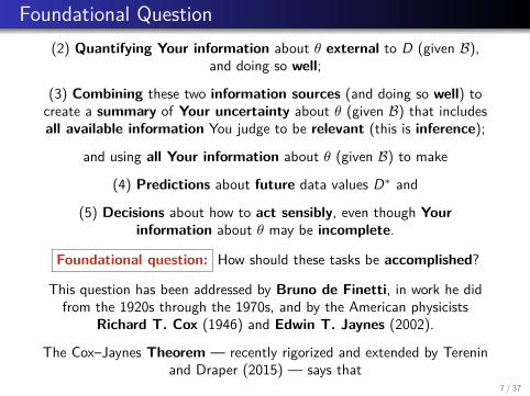
Foundational Question(2) Quantifying Your information about θ external to D (given B),
and doing so well;
(3) Combining these two information sources (and doing so well) tocreate a summary of Your uncertainty about θ (given B) that includesall available information You judge to be relevant (this is inference);
and using all Your information about θ (given B) to make
(4) Predictions about future data values D∗ and
(5) Decisions about how to act sensibly, even though Yourinformation about θ may be incomplete.
Foundational question: How should these tasks be accomplished?
This question has been addressed by Bruno de Finetti, in work he didfrom the 1920s through the 1970s, and by the American physicists
Richard T. Cox (1946) and Edwin T. Jaynes (2002).
The Cox–Jaynes Theorem — recently rigorized and extended by Tereninand Draper (2015) — says that
7 / 37
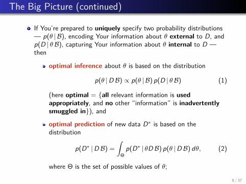
The Big Picture (continued)
If You’re prepared to uniquely specify two probability distributions— p(θ | B), encoding Your information about θ external to D, andp(D | θB), capturing Your information about θ internal to D —then
optimal inference about θ is based on the distribution
p(θ |D B) ∝ p(θ | B) p(D | θB) (1)
(here optimal = {all relevant information is usedappropriately, and no other “information” is inadvertentlysmuggled in}), and
optimal prediction of new data D∗ is based on thedistribution
p(D∗ |D B) =∫
Θp(D∗ | θD B) p(θ |D B) dθ, (2)
where Θ is the set of possible values of θ;
8 / 37
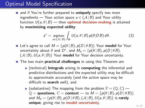
Optimal Model Specificationand if You’re further prepared to uniquely specify two moreingredients — Your action space a ∈ (A |B) and Your utilityfunction U(a, θ | B) — then optimal decision-making is attainedby maximizing expected utility:
a∗ = argmaxa∈(A |B)
∫Θ
U(a, θ | B) p(θ|D B) dθ . (3)
Let’s agree to call M = {p(θ | B), p(D | θB)} Your model for Youruncertainty about θ and D∗, and Md = {p(θ | B), p(D | θB),(A |B),U(a, θ | B)} Your model for Your decision uncertainty.The two main practical challenges in using this Theorem are
(technical) Integrals arising in computing the inferential andpredictive distributions and the expected utility may be difficultto approximate accurately (and the action space may bedifficult to search well), and(substantive) The mapping from the problem P = (Q,C) —Q = questions, C = context — to M = {p(θ | B), p(D | θB)}and Md = {p(θ | B), p(D | θB), (A |B),U(a, θ | B)} is rarelyunique, giving rise to model uncertainty.
9 / 37
Data-Science Example: A/B Testing
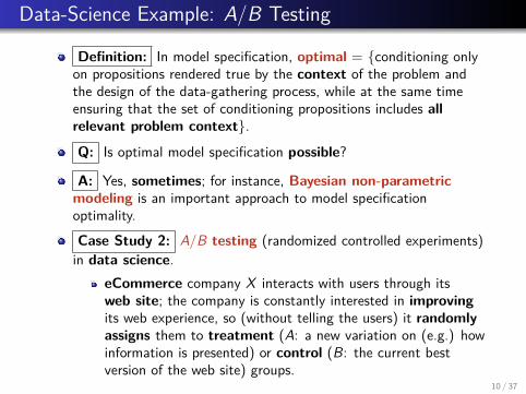
Definition: In model specification, optimal = {conditioning onlyon propositions rendered true by the context of the problem andthe design of the data-gathering process, while at the same timeensuring that the set of conditioning propositions includes allrelevant problem context}.
Q: Is optimal model specification possible?
A: Yes, sometimes; for instance, Bayesian non-parametricmodeling is an important approach to model specificationoptimality.
Case Study 2: A/B testing (randomized controlled experiments)in data science.
eCommerce company X interacts with users through itsweb site; the company is constantly interested in improvingits web experience, so (without telling the users) it randomlyassigns them to treatment (A: a new variation on (e.g.) howinformation is presented) or control (B: the current bestversion of the web site) groups.
10 / 37
A/B Testing
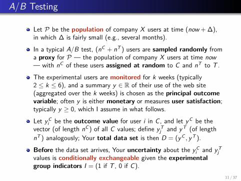
Let P be the population of company X users at time (now + ∆),in which ∆ is fairly small (e.g., several months).
In a typical A/B test, (nC + nT ) users are sampled randomly froma proxy for P — the population of company X users at time now— with nC of these users assigned at random to C and nT to T .
The experimental users are monitored for k weeks (typically2 ≤ k ≤ 6), and a summary y ∈ R of their use of the web site(aggregated over the k weeks) is chosen as the principal outcomevariable; often y is either monetary or measures user satisfaction;typically y ≥ 0, which I assume in what follows.
Let yCi be the outcome value for user i in C , and let yC be the
vector (of length nC ) of all C values; define yTj and yT (of length
nT ) analogously; Your total data set is then D = (yC , yT ).
Before the data set arrives, Your uncertainty about the yCi and yT
jvalues is conditionally exchangeable given the experimentalgroup indicators I = (1 if T , 0 if C).
11 / 37
Bayesian Non-Parametric Modeling
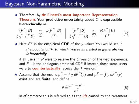
Therefore, by de Finetti’s most important RepresentationTheorem, Your predictive uncertainty about D is expressiblehierarchically as(F C | B) ∼ p(F C | B)
(yCi |F C B) IID∼ F C
(F T | B) ∼ p(F T | B)(yT
j |F T B) IID∼ F T (4)
Here F C is the empirical CDF of the y values You would see inthe population P to which You’re interested in generalizinginferentially
if all users in P were to receive the C version of the web experience,and F T is the analogous empirical CDF if instead those same userswere to counterfactually receive the T version.Assume that the means µC =
∫y dF C (y) and µT =
∫y dF T (y)
exist and are finite, and define
θ ,µT − µC
µC ; (5)
in eCommerce this is referred to as the lift caused by the treatment.12 / 37
Optimal Bayesian Model Specification(F C | B) ∼ p(F C | B)
(yCi |F C B) IID∼ F C
(F T | B) ∼ p(F T | B)(yT
j |F T B) IID∼ F T
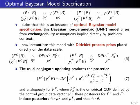
I claim that this is an instance of optimal Bayesian modelspecification: this Bayesian non-parametric (BNP) model arisesfrom exchangeability assumptions implied directly by problemcontext.I now instantiate this model with Dirichlet process priors placeddirectly on the data scale:
(F C | B) ∼ DP(αC ,F C0 )
(yCi |F C B) IID∼ F C
(F T | B) ∼ DP(αT ,F T0 )
(yTj |F T B) IID∼ F T (6)
The usual conjugate updating produces the posterior
(F C | yC B) ∼ DP(αC + nC ,
αC F C0 + n F C
nαC + nC
)(7)
and analogously for F T , where F Cn is the empirical CDF defined by
the control group data vector yC ; these posteriors for F C and F T
induce posteriors for µC and µT , and thus for θ.13 / 37
DP(n, Fn)
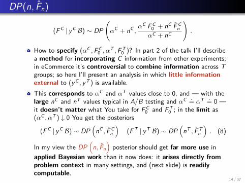
(F C | yC B) ∼ DP(αC + nC ,
αC F C0 + nC F C
nαC + nC
).
How to specify (αC ,F C0 , α
T ,F T0 )? In part 2 of the talk I’ll describe
a method for incorporating C information from other experiments;in eCommerce it’s controversial to combine information across Tgroups; so here I’ll present an analysis in which little informationexternal to (yC , yT ) is available.This corresponds to αC and αT values close to 0, and — with thelarge nC and nT values typical in A/B testing and αC .= αT .= 0 —it doesn’t matter what You take for F C
0 and F T0 ; in the limit as
(αC , αT ) ↓ 0 You get the posteriors
(F C | yC B) ∼ DP(
nC , F Cn
)(F T | yT B) ∼ DP
(nT , F T
n
). (8)
In my view the DP(
n, Fn
)posterior should get far more use in
applied Bayesian work than it now does: it arises directly fromproblem context in many settings, and (next slide) is readilycomputable.
14 / 37
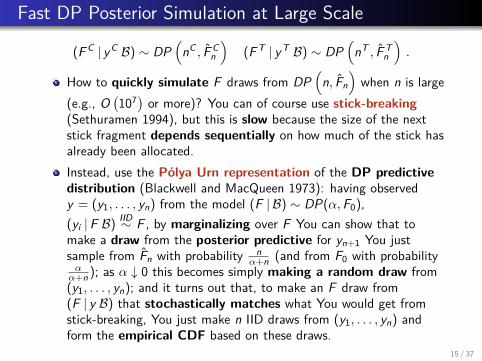
Fast DP Posterior Simulation at Large Scale
(F C | yC B) ∼ DP(
nC , F Cn
)(F T | yT B) ∼ DP
(nT , F T
n
).
How to quickly simulate F draws from DP(
n, Fn
)when n is large
(e.g., O(107) or more)? You can of course use stick-breaking
(Sethuramen 1994), but this is slow because the size of the nextstick fragment depends sequentially on how much of the stick hasalready been allocated.Instead, use the Polya Urn representation of the DP predictivedistribution (Blackwell and MacQueen 1973): having observedy = (y1, . . . , yn) from the model (F | B) ∼ DP(α,F0),(yi |F B) IID∼ F , by marginalizing over F You can show that tomake a draw from the posterior predictive for yn+1 You justsample from Fn with probability n
α+n (and from F0 with probabilityαα+n ); as α ↓ 0 this becomes simply making a random draw from(y1, . . . , yn); and it turns out that, to make an F draw from(F | y B) that stochastically matches what You would get fromstick-breaking, You just make n IID draws from (y1, . . . , yn) andform the empirical CDF based on these draws.
15 / 37
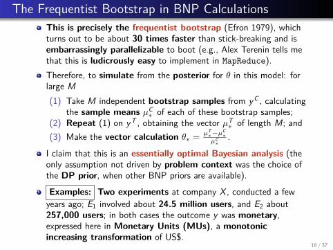
The Frequentist Bootstrap in BNP CalculationsThis is precisely the frequentist bootstrap (Efron 1979), whichturns out to be about 30 times faster than stick-breaking and isembarrassingly parallelizable to boot (e.g., Alex Terenin tells methat this is ludicrously easy to implement in MapReduce).Therefore, to simulate from the posterior for θ in this model: forlarge M(1) Take M independent bootstrap samples from yC , calculating
the sample means µC∗ of each of these bootstrap samples;
(2) Repeat (1) on yT , obtaining the vector µT∗ of length M; and
(3) Make the vector calculation θ∗ = µT∗−µ
C∗
µC∗
.
I claim that this is an essentially optimal Bayesian analysis (theonly assumption not driven by problem context was the choice ofthe DP prior, when other BNP priors are available).
Examples: Two experiments at company X , conducted a fewyears ago; E1 involved about 24.5 million users, and E2 about257,000 users; in both cases the outcome y was monetary,expressed here in Monetary Units (MUs), a monotonicincreasing transformation of US$.
16 / 37
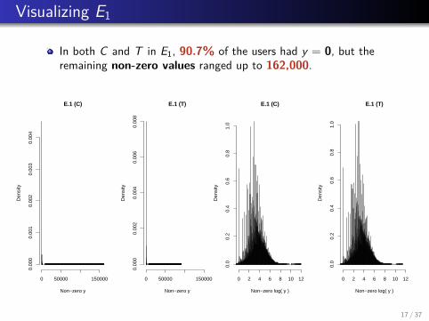
Visualizing E1
In both C and T in E1, 90.7% of the users had y = 0, but theremaining non-zero values ranged up to 162,000.
E.1 (C)
Non−zero y
Den
sity
0 50000 150000
0.00
00.
001
0.00
20.
003
0.00
4
E.1 (T)
Non−zero y
Den
sity
0 50000 150000
0.00
00.
002
0.00
40.
006
0.00
8
E.1 (C)
Non−zero log( y )
Den
sity
0 2 4 6 8 10 12
0.0
0.2
0.4
0.6
0.8
1.0
E.1 (T)
Non−zero log( y )
Den
sity
0 2 4 6 8 10 12
0.0
0.2
0.4
0.6
0.8
1.0
17 / 37
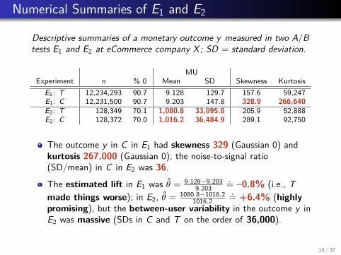
Numerical Summaries of E1 and E2
Descriptive summaries of a monetary outcome y measured in two A/Btests E1 and E2 at eCommerce company X; SD = standard deviation.
MUExperiment n % 0 Mean SD Skewness Kurtosis
E1: T 12,234,293 90.7 9.128 129.7 157.6 59,247E1: C 12,231,500 90.7 9.203 147.8 328.9 266,640E2: T 128,349 70.1 1,080.8 33,095.8 205.9 52,888E2: C 128,372 70.0 1,016.2 36,484.9 289.1 92,750
The outcome y in C in E1 had skewness 329 (Gaussian 0) andkurtosis 267,000 (Gaussian 0); the noise-to-signal ratio(SD/mean) in C in E2 was 36.
The estimated lift in E1 was θ = 9.128−9.2039.203
.= –0.8% (i.e., Tmade things worse); in E2, θ = 1080.8−1016.2
1016.2.= +6.4% (highly
promising), but the between-user variability in the outcome y inE2 was massive (SDs in C and T on the order of 36,000).
18 / 37
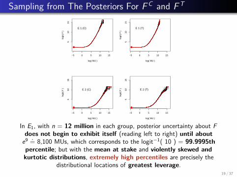
Sampling from The Posteriors For F C and F T
−5 0 5 10 15
510
15
log( MU )lo
git(
F )
E 1 (C)
●
−5 0 5 10 15
510
15
log( MU )
logi
t( F
)
E 1 (T)
●
−5 0 5 10 15
510
15
log( MU )
logi
t( F
) E 2 (C)
●
−5 0 5 10 15
510
15
log( MU )lo
git(
F ) E 2 (T)
●
In E1, with n = 12 million in each group, posterior uncertainty about Fdoes not begin to exhibit itself (reading left to right) until about
e9 .= 8,100 MUs, which corresponds to the logit−1( 10 ) = 99.9995thpercentile; but with the mean at stake and violently skewed andkurtotic distributions, extremely high percentiles are precisely the
distributional locations of greatest leverage.19 / 37
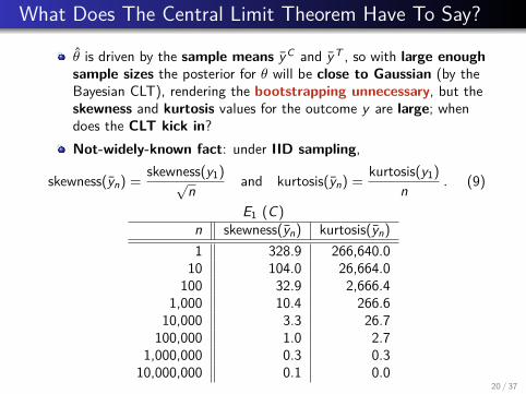
What Does The Central Limit Theorem Have To Say?
θ is driven by the sample means yC and yT , so with large enoughsample sizes the posterior for θ will be close to Gaussian (by theBayesian CLT), rendering the bootstrapping unnecessary, but theskewness and kurtosis values for the outcome y are large; whendoes the CLT kick in?Not-widely-known fact: under IID sampling,
skewness(yn) = skewness(y1)√n
and kurtosis(yn) = kurtosis(y1)n . (9)
E1 (C)n skewness(yn) kurtosis(yn)1 328.9 266,640.0
10 104.0 26,664.0100 32.9 2,666.4
1,000 10.4 266.610,000 3.3 26.7
100,000 1.0 2.71,000,000 0.3 0.3
10,000,000 0.1 0.020 / 37
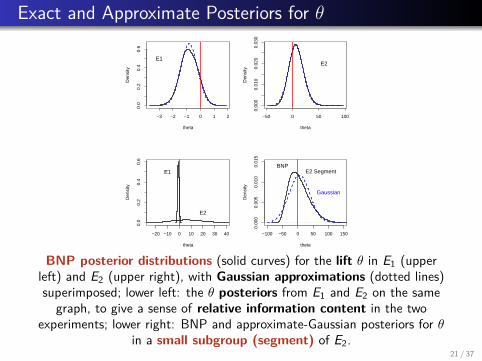
Exact and Approximate Posteriors for θ
−3 −2 −1 0 1 2
0.0
0.2
0.4
0.6
thetaD
ensi
ty
E1
−50 0 50 100
0.00
00.
010
0.02
00.
030
theta
Den
sity
E2
−20 −10 0 10 20 30 40
0.0
0.2
0.4
0.6
theta
Den
sity
E1
E2
−100 −50 0 50 100 150
0.00
00.
005
0.01
00.
015
thetaD
ensi
ty
BNP
Gaussian
E2 Segment
BNP posterior distributions (solid curves) for the lift θ in E1 (upperleft) and E2 (upper right), with Gaussian approximations (dotted lines)superimposed; lower left: the θ posteriors from E1 and E2 on the same
graph, to give a sense of relative information content in the twoexperiments; lower right: BNP and approximate-Gaussian posteriors for θ
in a small subgroup (segment) of E2.21 / 37
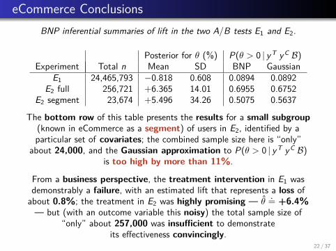
eCommerce ConclusionsBNP inferential summaries of lift in the two A/B tests E1 and E2.
Posterior for θ (%) P(θ > 0 | yT yC B)Experiment Total n Mean SD BNP Gaussian
E1 24,465,793 −0.818 0.608 0.0894 0.0892E2 full 256,721 +6.365 14.01 0.6955 0.6752
E2 segment 23,674 +5.496 34.26 0.5075 0.5637
The bottom row of this table presents the results for a small subgroup(known in eCommerce as a segment) of users in E2, identified by aparticular set of covariates; the combined sample size here is “only”
about 24,000, and the Gaussian approximation to P(θ > 0 | yT yC B)is too high by more than 11%.
From a business perspective, the treatment intervention in E1 wasdemonstrably a failure, with an estimated lift that represents a loss of
about 0.8%; the treatment in E2 was highly promising — θ.= +6.4%
— but (with an outcome variable this noisy) the total sample size of“only” about 257,000 was insufficient to demonstrate
its effectiveness convincingly.22 / 37
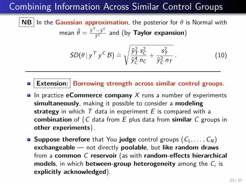
Combining Information Across Similar Control GroupsNB In the Gaussian approximation, the posterior for θ is Normal with
mean θ = yT−yC
yC and (by Taylor expansion)
SD(θ | yT yC B) .=
√y2
T s2C
y4C nC
+ s2T
y2C nT
. (10)
Extension: Borrowing strength across similar control groups.
In practice eCommerce company X runs a number of experimentssimultaneously, making it possible to consider a modelingstrategy in which T data in experiment E is compared with acombination of {C data from E plus data from similar C groups inother experiments}.
Suppose therefore that You judge control groups (C1, . . . ,CN)exchangeable — not directly poolable, but like random drawsfrom a common C reservoir (as with random-effects hierarchicalmodels, in which between-group heterogeneity among the Ci isexplicitly acknowledged).
23 / 37
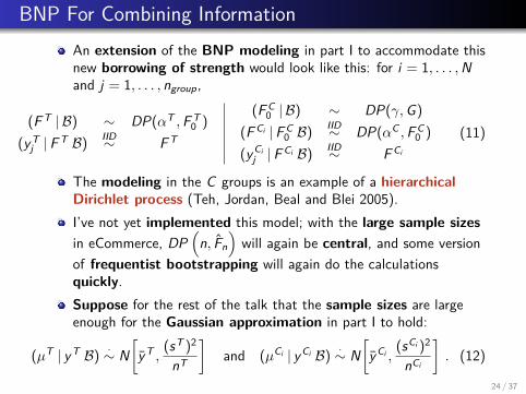
BNP For Combining InformationAn extension of the BNP modeling in part I to accommodate thisnew borrowing of strength would look like this: for i = 1, . . . ,Nand j = 1, . . . , ngroup,
(F T | B) ∼ DP(αT ,F T0 )
(yTj |F T B) IID∼ F T
(F C0 | B) ∼ DP(γ,G)
(F Ci |F C0 B) IID∼ DP(αC ,F C
0 )(yCi
j |F Ci B) IID∼ F Ci
(11)
The modeling in the C groups is an example of a hierarchicalDirichlet process (Teh, Jordan, Beal and Blei 2005).I’ve not yet implemented this model; with the large sample sizesin eCommerce, DP
(n, Fn
)will again be central, and some version
of frequentist bootstrapping will again do the calculationsquickly.Suppose for the rest of the talk that the sample sizes are largeenough for the Gaussian approximation in part I to hold:
(µT | yT B) ·∼ N[yT ,
(sT )2
nT
]and (µCi | yCi B) ·∼ N
[yCi ,
(sCi )2
nCi
]. (12)
24 / 37
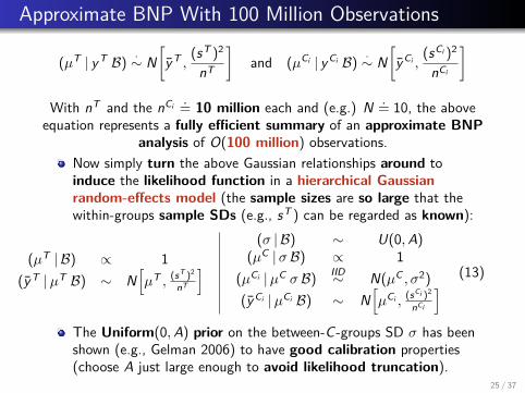
Approximate BNP With 100 Million Observations
(µT | yT B) ·∼ N[yT ,
(sT )2
nT
]and (µCi | yCi B) ·∼ N
[yCi ,
(sCi )2
nCi
]With nT and the nCi .= 10 million each and (e.g.) N .= 10, the above
equation represents a fully efficient summary of an approximate BNPanalysis of O(100 million) observations.
Now simply turn the above Gaussian relationships around toinduce the likelihood function in a hierarchical Gaussianrandom-effects model (the sample sizes are so large that thewithin-groups sample SDs (e.g., sT ) can be regarded as known):
(µT | B) ∝ 1(yT |µT B) ∼ N
[µT , (sT )2
nT
] (σ | B) ∼ U(0,A)(µC |σ B) ∝ 1
(µCi |µC σ B) IID∼ N(µC , σ2)(yCi |µCi B) ∼ N
[µCi , (sCi )2
nCi
] (13)
The Uniform(0,A) prior on the between-C -groups SD σ has beenshown (e.g., Gelman 2006) to have good calibration properties(choose A just large enough to avoid likelihood truncation).
25 / 37
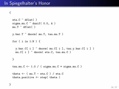
In Spiegelhalter’s Honor
{
eta.C ˜ dflat( )sigma.mu.C ˜ dunif( 0.0, A )mu.T ˜ dflat( )
y.bar.T ˜ dnorm( mu.T, tau.mu.T )
for ( i in 1:N ) {
y.bar.C[ i ] ˜ dnorm( mu.C[ i ], tau.y.bar.C[ i ] )mu.C[ i ] ˜ dnorm( eta.C, tau.mu.C )
}
tau.mu.C <- 1.0 / ( sigma.mu.C * sigma.mu.C )
theta <- ( mu.T - eta.C ) / eta.Ctheta.positive <- step( theta )
}26 / 37
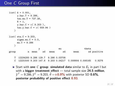
One C Group First
list( A = 0.001,y.bar.T = 9.286,tau.mu.T = 727.28,N = 1,y.bar.C = c( 9.203 ),tau.y.bar.C = c( 559.94 )
)
list( eta.C = 9.203,sigma.mu.C = 0.0,mu.T = 9.286
)y mu theta
group n mean sd mean sd mean sd positive
T 12234293 9.286 129.7 9.286 0.03708C 12231500 9.203 147.8 9.203 0.04217 0.008904 0.006165 0.9276
Start with one C group: simulated data similar to E1 in part I butwith a bigger treatment effect — total sample size 24.5 million,yT = 9.286, yC = 9.203, θ =+0.9% with posterior SD 0.6%,posterior probability of positive effect 0.93.
27 / 37
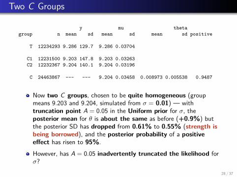
Two C Groups
y mu thetagroup n mean sd mean sd mean sd positive
T 12234293 9.286 129.7 9.286 0.03704
C1 12231500 9.203 147.8 9.203 0.03263C2 12232367 9.204 140.1 9.204 0.03196
C 24463867 --- --- 9.204 0.03458 0.008973 0.005538 0.9487
Now two C groups, chosen to be quite homogeneous (groupmeans 9.203 and 9.204, simulated from σ = 0.01) — withtruncation point A = 0.05 in the Uniform prior for σ, theposterior mean for θ is about the same as before (+0.9%) butthe posterior SD has dropped from 0.61% to 0.55% (strength isbeing borrowed), and the posterior probability of a positiveeffect has risen to 95%.
However, has A = 0.05 inadvertently truncated the likelihood forσ?
28 / 37
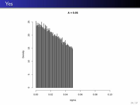
YesA = 0.05
sigma
Den
sity
0.00 0.02 0.04 0.06 0.08 0.10
05
1015
2025
29 / 37
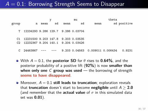
A = 0.1: Borrowing Strength Seems to Disappear
y mu thetagroup n mean sd mean sd mean sd positive
T 12234293 9.286 129.7 9.286 0.03704
C1 12231500 9.203 147.8 9.203 0.03535C2 12232367 9.204 140.1 9.204 0.03426
C 24463867 --- --- 9.203 0.04563 0.009011 0.006434 0.9231
With A = 0.1, the posterior SD for θ rises to 0.64%, and theposterior probability of a positive lift (92%) is now smaller thanwhen only one C group was used — the borrowing of strengthseems to have disappeared.
Moreover, A = 0.1 still leads to truncation; exploration revealsthat truncation doesn’t start to become negligible until A ≥ 2.0(and remember that the actual value of σ in this simulated dataset was 0.01).
30 / 37
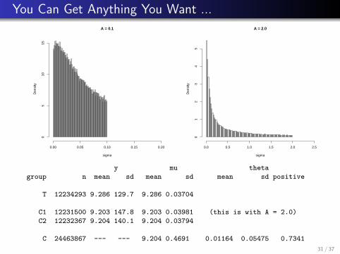
You Can Get Anything You Want ...A = 0.1
sigma
Den
sity
0.00 0.05 0.10 0.15 0.20
05
1015
A = 2.0
sigma
Den
sity
0.0 0.5 1.0 1.5 2.0 2.5
01
23
45
y mu thetagroup n mean sd mean sd mean sd positive
T 12234293 9.286 129.7 9.286 0.03704
C1 12231500 9.203 147.8 9.203 0.03981 (this is with A = 2.0)C2 12232367 9.204 140.1 9.204 0.03794
C 24463867 --- --- 9.204 0.4691 0.01164 0.05475 0.734131 / 37
Between-C -Groups Heterogeneity
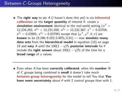
The right way to set A (I haven’t done this yet) is via inferentialcalibration on the target quantity of interest θ: create asimulation environment identical to the real-world setting (nT =12,234,293; nC1 = 12,231,500; nC2 = 12,232,367; sT = 0.03704;sC1 = 0.03981; sC2 = 0.03794) except that (µT , µC , θ, σ) areknown to be (9.286; 9.203; 0.90%; 0.01) — now simulate manydata sets from the hierarchical model in equation (10) on page19 and vary A until the 100(1− η)% posterior intervals for θinclude the right answer about 100(1− η)% of the time for abroad range of η values.
Even when A has been correctly calibrated, when the number Nof C groups being combined is small it doesn’t take muchbetween-group heterogeneity for the model to tell You that Youhave more uncertainty about θ with 2 control groups than with 1.
32 / 37
Between-C -Groups Heterogeneity (continued)
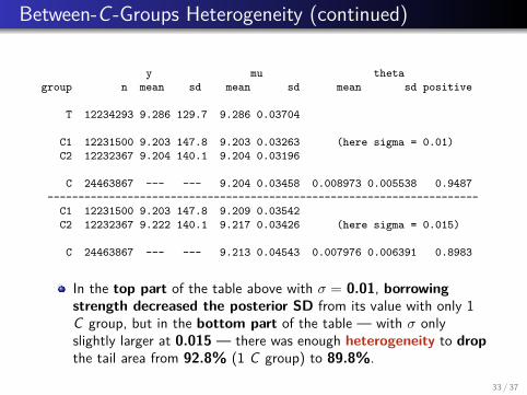
y mu thetagroup n mean sd mean sd mean sd positive
T 12234293 9.286 129.7 9.286 0.03704
C1 12231500 9.203 147.8 9.203 0.03263 (here sigma = 0.01)C2 12232367 9.204 140.1 9.204 0.03196
C 24463867 --- --- 9.204 0.03458 0.008973 0.005538 0.9487----------------------------------------------------------------------
C1 12231500 9.203 147.8 9.209 0.03542C2 12232367 9.222 140.1 9.217 0.03426 (here sigma = 0.015)
C 24463867 --- --- 9.213 0.04543 0.007976 0.006391 0.8983
In the top part of the table above with σ = 0.01, borrowingstrength decreased the posterior SD from its value with only 1C group, but in the bottom part of the table — with σ onlyslightly larger at 0.015 — there was enough heterogeneity to dropthe tail area from 92.8% (1 C group) to 89.8%.
33 / 37
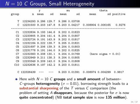
N = 10 C Groups, Small Heterogeneityy mu theta
group n mean sd mean sd mean sd positive
T 12234293 9.286 129.7 9.286 0.03708C 12231500 9.203 147.8 9.203 0.04217 0.008904 0.006165 0.9276
----------------------------------------------------------------------C1 12232834 9.193 144.6 9.202 0.01823C2 12233905 9.204 141.4 9.204 0.01807C3 12232724 9.191 143.9 9.202 0.01817C4 12232184 9.222 139.7 9.205 0.01821C5 12231697 9.206 139.3 9.204 0.01803C6 12231778 9.191 144.0 9.202 0.01825C7 12232383 9.208 130.1 9.204 0.01769 (here sigma = 0.01)C8 12232949 9.211 138.3 9.204 0.01805C9 12233349 9.209 143.0 9.204 0.01808
C10 12232636 9.197 142.2 9.203 0.01811
C 122326439 --- --- 9.203 0.01391 0.008974 0.004299 0.9817
Here with N = 10 C groups and a small amount of between–C–groups heterogeneity (σ = 0.01), borrowing strength leads to asubstantial sharpening of the T versus C comparison (theproblem of setting A disappears, because the posterior for σ is nowquite concentrated) (NB total sample size is now 135 million).
34 / 37
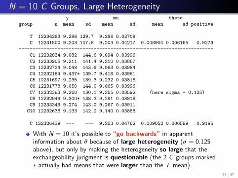
N = 10 C Groups, Large Heterogeneityy mu theta
group n mean sd mean sd mean sd positive
T 12234293 9.286 129.7 9.286 0.03708C 12231500 9.203 147.8 9.203 0.04217 0.008904 0.006165 0.9276
----------------------------------------------------------------------C1 12232834 9.082 144.6 9.094 0.03996C2 12233905 9.211 141.4 9.210 0.03867C3 12232724 9.048 143.9 9.063 0.03984C4 12232184 9.437* 139.7 9.416 0.03981C5 12231697 9.235 139.3 9.232 0.03818C6 12231778 9.050 144.0 9.065 0.03996C7 12232383 9.260 130.1 9.255 0.03592 (here sigma = 0.125)C8 12232949 9.300* 138.3 9.291 0.03818C9 12233349 9.274 143.0 9.267 0.03911
C10 12232636 9.133 142.2 9.140 0.03888
C 122326439 --- --- 9.203 0.04762 0.009052 0.006589 0.9195
With N = 10 it’s possible to “go backwards” in apparentinformation about θ because of large heterogeneity (σ = 0.125above), but only by making the heterogeneity so large that theexchangeability judgment is questionable (the 2 C groups marked∗ actually had means that were larger than the T mean).
35 / 37
Conclusions in Part II
With large sample sizes it’s straightforward to use hierarchicalrandom-effects Gaussian models — as good approximations toa full BNP analysis — in combining C groups to improveaccuracy in estimating T effects, but
When the number N of C groups to be combined is small, theresults are extremely sensitive to Your prior on thebetween–C–groups SD σ, and it doesn’t take muchheterogeneity among the C means for the model to tell Youthat You know less about θ than when there was only 1 Cgroup, and
With a larger N there’s less sensitivity to the prior for σ, andborrowing strength will generally succeed in sharpening thecomparison unless the heterogeneity is so large as to makethe exchangeability judgment that led to the C–groupcombining questionable.
36 / 37
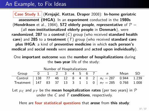
An Example, to Fix IdeasCase Study 1. (Krnjajic, Kottas, Draper 2008): In-home geriatric
assessment (IHGA). In an experiment conducted in the 1980s(Hendriksen et al., 1984), 572 elderly people, representative of P =
{all non-institutionalized elderly people in Denmark}, wererandomized, 287 to a control (C) group (who received standard healthcare) and 285 to a treatment (T ) group (who received standard care
plus IHGA: a kind of preventive medicine in which each person’smedical and social needs were assessed and acted upon individually).
One important outcome was the number of hospitalizations duringthe two-year life of the study:
Number of HospitalizationsGroup 0 1 2 3 4 5 6 7 n Mean SD
Control 138 77 46 12 8 4 0 2 nC = 287 0.944 1.239Treatment 147 83 37 13 3 1 1 0 nT = 285 0.768 1.008
Let µC and µT be the mean hospitalization rates (per two years) in Punder the C and T conditions, respectively.
Here are four statistical questions that arose from this study:37 / 37

Bayesian Qual/Quant Inference
Recall from our earlier discussion that if I judge binary(y1, . . . , yn) to be part of infinitely exchangeable sequence,to be coherent my joint predictive distribution p(y1, . . . , yn)
must have simple hierarchical form
θ ∼ p(θ)
(yi|θ)IID∼ Bernoulli(θ),
where θ = P (yi = 1) = limiting value of mean of yi ininfinite sequence.
Writing s = (s1, s2) where s1 and s2 are the numbers of 0sand 1s, respectively in (y1, . . . , yn), this is equivalent
to the model
θ2 ∼ p(θ2) (1)
(s2|θ2) ∼ Binomial(n, θ2),
where (in a slight change of notation) θ2 = P (yi = 1); i.e., inthis simplest case the form of the likelihood function
(Binomial(n, θ2)) is determined by coherence.
The likelihood function for θ2 in this model is
l(θ2|y) = c θs2
2 (1− θ2)n−s2 = c θs1
1 θs2
2 , (2)
from which it’s evident that the conjugate prior for theBernoulli/Binomial likelihood (the choice of prior having
the property that the posterior for θ2 has the samemathematical form as the prior) is the family of
Beta(α1, α2) densities
p(θ2) = c θα2−12 (1− θ2)
α1−1 = c θα1−11 θα2−1
2 . (3)
for some α1 > 0, α2 > 0.
2

Bayesian Qual/Quant Inference
With this prior the conjugate updating rule is evidently{
θ2 ∼ Beta(α1, α2)(s2|θ2) ∼ Binomial(n, θ2)
}
→ (θ2|y) ∼ Beta(α1+s1, α2+s2),
(4)where s1 (s2) is the number of 0s (1s) in the
data set y = (y1, . . . , yn).
Moreover, given that the likelihood represents a (sample)data set with s1 0s and s2 1s and a data sample size of
n = (s1 + s2), it’s clear that
(a) the Beta(α1, α2) prior acts like a (prior) data set withα1 0s and α2 1s and a prior sample size of (α1 + α2), and
(b) to achieve a relatively diffuse(low-information-content) prior for θ2 (if that’s what
context suggests I should aim for) I should try to specify α1
and α2 not far from 0.
Easy generalization of all of this: suppose the yi take onl ≥ 2 distinct values v = (v1, . . . , vl), and let s = (s1, . . . , sl)
be the vector of counts (s1 = #(yi = v1) and so on).
If I judge the yi to be part of an infinitely exchangeablesequence, then to be coherent my joint predictive
distribution p(y1, . . . , yn) must have the hierarchical form
θ ∼ p(θ) (5)
(s|θ) ∼ Multinomial(n, θ),
where θ = (θ1, . . . , θl) and θj is the limiting relativefrequency of vj values in the infinite sequence.
3
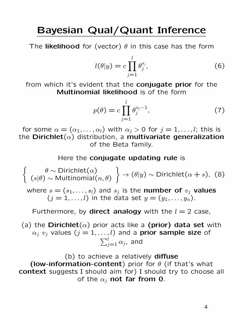
Bayesian Qual/Quant Inference
The likelihood for (vector) θ in this case has the form
l(θ|y) = c
l∏
j=1
θsj
j , (6)
from which it’s evident that the conjugate prior for theMultinomial likelihood is of the form
p(θ) = c
l∏
j=1
θαj−1j , (7)
for some α = (α1, . . . , αl) with αj > 0 for j = 1, . . . , l; this isthe Dirichlet(α) distribution, a multivariate generalization
of the Beta family.
Here the conjugate updating rule is{
θ ∼ Dirichlet(α)(s|θ) ∼ Multinomial(n, θ)
}
→ (θ|y) ∼ Dirichlet(α+ s), (8)
where s = (s1, . . . , sl) and sj is the number of vj values(j = 1, . . . , l) in the data set y = (y1, . . . , yn).
Furthermore, by direct analogy with the l = 2 case,
(a) the Dirichlet(α) prior acts like a (prior) data set withαj vj values (j = 1, . . . , l) and a prior sample size of
∑lj=1αj, and
(b) to achieve a relatively diffuse(low-information-content) prior for θ (if that’s what
context suggests I should aim for) I should try to choose allof the αj not far from 0.
4
Bayesian Qual/Quant Inference
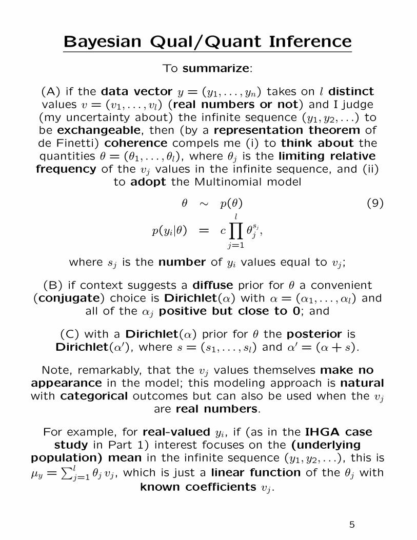
To summarize:
(A) if the data vector y = (y1, . . . , yn) takes on l distinctvalues v = (v1, . . . , vl) (real numbers or not) and I judge(my uncertainty about) the infinite sequence (y1, y2, . . .) tobe exchangeable, then (by a representation theorem ofde Finetti) coherence compels me (i) to think about thequantities θ = (θ1, . . . , θl), where θj is the limiting relativefrequency of the vj values in the infinite sequence, and (ii)
to adopt the Multinomial model
θ ∼ p(θ) (9)
p(yi|θ) = c
l∏
j=1
θsj
j ,
where sj is the number of yi values equal to vj;
(B) if context suggests a diffuse prior for θ a convenient(conjugate) choice is Dirichlet(α) with α = (α1, . . . , αl) and
all of the αj positive but close to 0; and
(C) with a Dirichlet(α) prior for θ the posterior isDirichlet(α′), where s = (s1, . . . , sl) and α′ = (α+ s).
Note, remarkably, that the vj values themselves make noappearance in the model; this modeling approach is naturalwith categorical outcomes but can also be used when the vj
are real numbers.
For example, for real-valued yi, if (as in the IHGA casestudy in Part 1) interest focuses on the (underlying
population) mean in the infinite sequence (y1, y2, . . .), this is
µy =∑l
j=1 θj vj, which is just a linear function of the θj with
known coefficients vj.
5

Bayesian Qual/Quant Inference
This fact makes it possible to draw an analogy with thedistribution-free methods that are at the heart of
frequentist non-parametric inference: when your outcomevariable takes on a finite number of real values vj,
exchangeability compels a Multinomial likelihood on theunderlying frequencies with which the vj occur; you are not
required to build a parametric model (e.g., normal,lognormal, ...) on the yi values themselves.
In this sense, therefore, model (14)—particularly with theconjugate Dirichlet prior—can serve as a kind of
low-technology Bayesian non-parametric modeling: thisis the basis of the Bayesian bootstrap (Rubin 1981).
Moreover, if you’re in a hurry and you’re already familiarwith WinBUGS you can readily carry out inference about
quantities like µy above in that environment, but there’s noneed to do MCMC here: ordinary Monte Carlo (MC)sampling from the Dirichlet(α′) posterior distribution is
perfectly straightforward, e.g., in R, based on thefollowing fact:
To generate a random draw θ = (θ1, . . . , θl) from theDirichlet(α′) distribution, with α′ = (α′
1, . . . , α′l),
independently draw
gjindep∼ Γ(α′
j, β), j = 1, . . . , l (10)
(where Γ(a, b) is the Gamma distribution with parametersa and b) and compute
θj =gj
∑lm=1 gj
. (11)
Any β > 0 will do in this calculation; β = 1 is a good choicethat leads to fast random number generation.
6

Bayesian Qual/Quant Inference
The downloadable version of R doesn’t have a built-infunction for making Dirichlet draws, but it’s easy to
write one:
rdirichlet = function( n.sim, alpha ) {
l = length( alpha )
theta = matrix( 0, n.sim, l )
for ( j in 1:l ) {
theta[ , j ] = rgamma( n.sim, alpha[ j ], 1 )
}
theta = theta / apply( theta, 1, sum )
return( theta )
}
The Dirichlet(α) distribution has the following moments: ifθ ∼ Dirichlet(α) then
E(θj) =αj
α0
, V (θj) =αj(α0 − αj)
α20(α0 + 1)
, C(θj, θj ′) = −αjαj ′
α20(α0 +1)
,
where α0 =∑l
j=1 αj (note the negative correlation between
components of θ).
This can be used to test the function above:
7
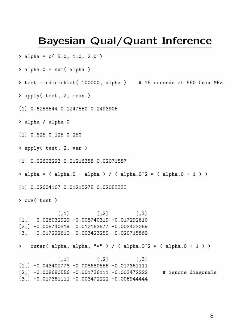
Bayesian Qual/Quant Inference
> alpha = c( 5.0, 1.0, 2.0 )
> alpha.0 = sum( alpha )
> test = rdirichlet( 100000, alpha ) # 15 seconds at 550 Unix MHz
> apply( test, 2, mean )
[1] 0.6258544 0.1247550 0.2493905
> alpha / alpha.0
[1] 0.625 0.125 0.250
> apply( test, 2, var )
[1] 0.02603293 0.01216358 0.02071587
> alpha * ( alpha.0 - alpha ) / ( alpha.0^2 * ( alpha.0 + 1 ) )
[1] 0.02604167 0.01215278 0.02083333
> cov( test )
[,1] [,2] [,3]
[1,] 0.026032929 -0.008740319 -0.017292610
[2,] -0.008740319 0.012163577 -0.003423259
[3,] -0.017292610 -0.003423259 0.020715869
> - outer( alpha, alpha, "*" ) / ( alpha.0^2 * ( alpha.0 + 1 ) )
[,1] [,2] [,3]
[1,] -0.043402778 -0.008680556 -0.017361111
[2,] -0.008680556 -0.001736111 -0.003472222 # ignore diagonals
[3,] -0.017361111 -0.003472222 -0.006944444
8

Bayesian Qual/Quant Inference
Example: re-analysis of IHGA data from Part 1; recallpolicy and clinical interest focused on η = µE
µC.
Number of HospitalizationsGroup 0 1 2 3 4 5 6 7 n Mean SD
Control 138 77 46 12 8 4 0 2 287 0.944 1.24Experimental 147 83 37 13 3 1 1 0 285 0.768 1.01
In this two-independent-samples setting I can apply deFinetti’s representation theorem twice, in parallel, on the C
and E data.
I don’t know much about the underlying frequencies of0,1, . . . ,7 hospitalizations under C and E external to the
data, so I’ll use a Dirichlet(ǫ, . . . , ǫ) prior for both θC and θEwith ǫ = 0.001, leading to a Dirichlet(138.001, . . . ,2.001)
posterior for θC and a Dirichlet(147.001, . . . ,0.001)posterior for θE (other small positive choices of ǫ yield
similar results).
> alpha.C = c( 138.001, 77.001, 46.001, 12.001, 8.001, 4.001, 0.001,
2.001 )
> alpha.E = c( 147.001, 83.001, 37.001, 13.001, 3.001, 1.001, 1.001,
0.001 )
> theta.C = rdirichlet( 100000, alpha.C ) # 17 sec at 550 Unix MHz
> theta.E = rdirichlet( 100000, alpha.E ) # also 17 sec
> print( post.mean.theta.C = apply( theta.C, 2, mean ) )
[1] 4.808015e-01 2.683458e-01 1.603179e-01 4.176976e-02 2.784911e-02
[6] 1.395287e-02 3.180905e-06 6.959859e-03
> print( post.SD.theta.C <- apply( theta.C, 2, sd ) )
[1] 0.0294142963 0.0261001259 0.0216552661 0.0117925465 0.0096747630[6] 0.0069121507 0.0001017203 0.0048757485
9
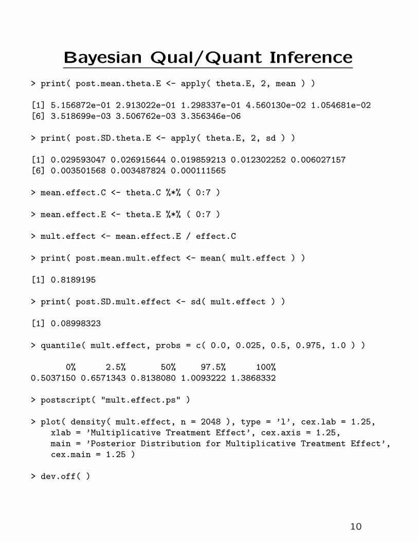
Bayesian Qual/Quant Inference
> print( post.mean.theta.E <- apply( theta.E, 2, mean ) )
[1] 5.156872e-01 2.913022e-01 1.298337e-01 4.560130e-02 1.054681e-02
[6] 3.518699e-03 3.506762e-03 3.356346e-06
> print( post.SD.theta.E <- apply( theta.E, 2, sd ) )
[1] 0.029593047 0.026915644 0.019859213 0.012302252 0.006027157[6] 0.003501568 0.003487824 0.000111565
> mean.effect.C <- theta.C %*% ( 0:7 )
> mean.effect.E <- theta.E %*% ( 0:7 )
> mult.effect <- mean.effect.E / effect.C
> print( post.mean.mult.effect <- mean( mult.effect ) )
[1] 0.8189195
> print( post.SD.mult.effect <- sd( mult.effect ) )
[1] 0.08998323
> quantile( mult.effect, probs = c( 0.0, 0.025, 0.5, 0.975, 1.0 ) )
0% 2.5% 50% 97.5% 100%
0.5037150 0.6571343 0.8138080 1.0093222 1.3868332
> postscript( "mult.effect.ps" )
> plot( density( mult.effect, n = 2048 ), type = ’l’, cex.lab = 1.25,xlab = ’Multiplicative Treatment Effect’, cex.axis = 1.25,
main = ’Posterior Distribution for Multiplicative Treatment Effect’,
cex.main = 1.25 )
> dev.off( )
10
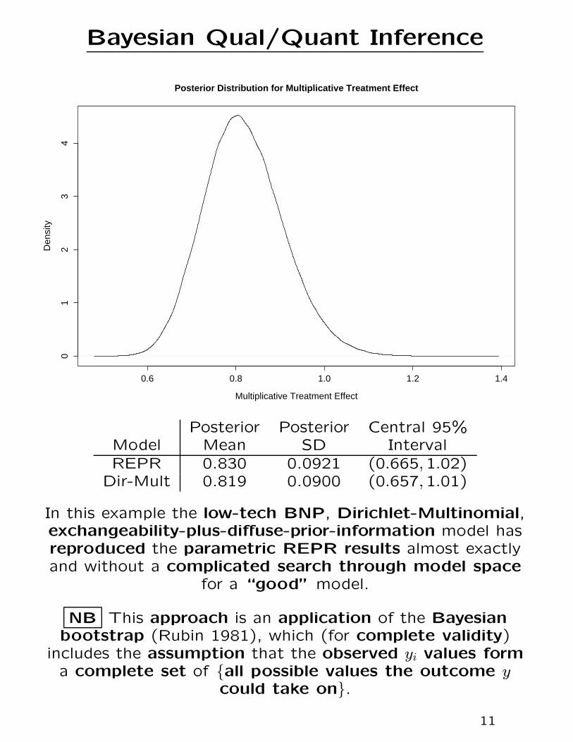
Bayesian Qual/Quant Inference
0.6 0.8 1.0 1.2 1.4
01
23
4
Posterior Distribution for Multiplicative Treatment Effect
Multiplicative Treatment Effect
Den
sity
Posterior Posterior Central 95%Model Mean SD IntervalREPR 0.830 0.0921 (0.665,1.02)
Dir-Mult 0.819 0.0900 (0.657,1.01)
In this example the low-tech BNP, Dirichlet-Multinomial,exchangeability-plus-diffuse-prior-information model hasreproduced the parametric REPR results almost exactlyand without a complicated search through model space
for a “good” model.
NB This approach is an application of the Bayesianbootstrap (Rubin 1981), which (for complete validity)
includes the assumption that the observed yi values forma complete set of {all possible values the outcome y
could take on}.
11