airflow characteristics of modulated louvered windows with
TRANSCRIPT
AIRFLOW CHARACTERISTICS OF MODULATED LOUVERED
WINDOWS WITH REFERENCE TO THE ROWSHAN OF
JEDDAH, SAUDI ARABIA
Thesis submitted in accordance with the requirements of theUniversity of Sheffield for the degree of Doctor of Philosophy by:
Amjed Abdulrahman Maghrabi
B. Arch., Umm AI-Qura University, Makkah, Saudi ArabiaM. Arch, University of Colorado at Denver, Colorado, USA
School of Architecture
University of Sheffield
August 2000

, dO...•..••·•.. .aN

6-1
~I,) ~I u.o I.........D:!Jll1u-l!
~ ~I u.o ~JlI..o JS.a ~ 0:!jJJl u-l!
~ o:s. JS ~ ~.J. ~! 0:!Jll1 u-l!
~I u-l! ... ~I~!
J,.&lII:s. (,j~1
.1..+01
Abstract
The main aim of this research project is to assess the potential of the modulatedlouvered windows (MLW) to provide ventilation as a cooling source to achieve thermalcomfort inside buildings. It presents an intensive analysis of the characteristics of airflow asfunction of the various MLW parameters in order to provide designers with practicalinformation about the performance of MLW in the control of natural ventilation inside theroom. Some initial studies suggested the significance of adjustable horizontal louveredwindows, or the MLW as they are referred to in this research, as an effective technique for thecontrol of natural ventilation beside the other Environmental issues.
In Jeddah, Saudi Arabia, the shelter adaptation to the hot-humid climate was achievedby employing a number of passive solutions, one of which, the MLW constructed in theRowshan, was considered a main elevation treatment. The Rowshan, a projected windowbay, covered in this study is constructed with adjustable louvers in a number of sashesarranged in rows and columns to control and alter breeze to the desired level inside the room.The Rowshan is also credited with controlling other environmental factors and is supposed toreflect social necessities.
This thesis has investigated the airflow characteristics of the MLW with reference tothe Rowshan of Jeddah, Saudi Arabia. After reviewing the previous efforts and predictiontechniques concerned, the research has conducted a series of experiments including laboratoryand computation fluid dynamics (CFD) appraisal stages. The laboratory stage included theevaluation of the pressure drop (L1J') and the velocity drop (v/ve%) characteristics across theMLW. The pressure drop was examined under various airflow rates (Q) using thedepressurising test chamber technique. The velocity drop (v/ve%) was examined undervarious prevailing wind conditions using the test chamber technique. This appraisal stagecovered also the room configuration and its contribution to this effect. On the other hand, theCFD measurement has examined the viability of CFD coding to simulate airflow around thereviewed MLW. The predicted results obtained from CFD were compared against thoseobtained from the laboratory. Consequently, an intensive evaluation of airflow patterns of thecommon Rowshan configurations, including the plain and projected Rowshans, employed inleddah in conjunction with various outlet types was conducted.
From the literature review, it has been concluded that the MLW played a major rolein the provision and the control of natural ventilation in the traditional architecture of leddah,Saudi Arabia. The various appraisal stages showed that parameters such as louver inclination,aperture between louver blades and the free area of the MLW were more significant variablesthan the depth of louver blades. Nevertheless, the major pressure and velocity drops were notdue to individual variable but rather to the combination of variables that wouldcomprehensively describe M and v/ve% across the MLW.
Practically, the design of the modulated louvered windows must give consideration tothose variables that play an important role in altering airflow characteristics inside the room.It should also have an element of flexibility as this enables designers to approach theirwindow treatments with a number of choices whilst retaining similar ventilationperformances. Airflow velocities in a room containing an MLW result from an interaction oflouver geometry, room geometry and prevailing wind conditions. As far as the Rowshanconfiguration was concerned, the plain Rowshan was generally better than the projectedRowshan. Yet the flow in the living zone could be enhanced by correctly sizing the projectedRowshan. Finally, CFD analysis has been successfully used to predict air velocities in theregion close to the MLW side.
- 11 -

Acknowledgment
I am particularly indebted to my parents: my Father, Abdulrahman M.
Maghrabi and my Mother, Zakiah A. Halwani. I believe that this achievement is the
result of their continuous love, support and prayers for my success. Their consent to
the absence of their son for a long period is greatly appreciated. I hope that I will
shortly compensate them for some of this.
I am also particularly indebted to both Prof. S. Sharples, myformer supervisor,
and Prof. P.R. Tregenza, my current supervisor. Their constant assistance,
supervision, and constructive criticism have played a significant role in the production
of this thesis. I am also grateful to Dr. A. C. Pitts and Mr. I.C. Ward for their help at
different phases of this research. I wish also to thank the staff, the technicians and my
colleagues in the School of Architecture for their help.
My appreciation to many people who also helped me, with great patience and
kindness, during the various phases of this research: Dr. O. Azhar, Dr. D. Suker,
Arch. A. Khoj, Dr. F. Al-Shareef, Mr. M. Limb, Dr. D. Thiam, Dr. K. AI-Barrak, Dr.
M. Gadi and others. I also owe a great deal to the continuous support, courage and
advice of my brother Dr. Aimen Maghrabi. Likewise, I cannot forget the rest of my
bothers and sisters Ms. Omaymah, Mr. Mahmoud, Ms. Eman, Mr. Hesham and Dr.
Ashraf.
Last but not the least, I am indebted to my wife who has endured a lot to keep
me relaxed and concentrated throughout in my PhD work. My children: Ammar,
Abrrar, Abdulrahman, Albarra and loujayne, in whom I see my future, have also
endured during my graduate studies, and I promise to compensate them for all of this
in the near future.
- III -

TABLE OF CONTENTS
ABSTRACT iiACKNOWLEDGEMENT iiiTABLE OF CONTENTS ivLIST OF TABLES IX
LIST OF FIGURES xLIST APPENDICES XIV
NOMENCLATURE xvi
CHAPTER 1: INTRODUCTION1.1.1.2.1.3.lA.
PREFACEAIMS OF THE RESEARCHMETHODOLOGICAL APPROACHRESEARCH APPROACH
4679
CHAPTER 2: THE REGIONAL CONTEXT2.1. INTRODUCTION. 132.2. THE CLIMATE AND ARCHITECTURE OF SAUDI ARABIA 13
2.2.1. Geographical location 132.2.2. Topography 15
2.2.2.1. Sarawat Mountains. 152.2.2.2. Tehamah Plain. 152.2.2.3. Najd Plateau. 152.2.2.4. Eastern Coastal Plain 162.2.2.5. The Empty-Quarter (Al-Rubu Al-khali) 16
2.2.3. Climatic zones and the architectural responses 162.2.3.1. Hot Dry Climatic Zone 17
2.2.3.1.1. The Climate 172.2.3.1.2. The Architecture 17
2.2.3.2. Composite Climatic Zone. 202.2.3.2.1. The Climate 202.2.3.2.2. The Architecture 20
2.2.3.3. Tropical Upland Climatic Zone 222.2.3.3.1. The Climate 222.2.3.3.2. The Architecture 22
2.2.3.4. Hot Humid Climatic Zone. 242.2.3.4.1. The Climate 242.2.3.4.2. The Architecture 24
2.3. THE CLIMATE OF JEDDAH 252.3.1. Geographical location 252.3.2. The Climatic Environment 26
2.3.2.1. Dry bulb air temperature 262.3.2.2. Relative humidity 272.3.2.3. Wind speed and directions 272.3.2.4. Precipitation 282.3.2.5. Solar radiation 28
2.3.3. Isopleths charts of climatic variables 292.3.4. The phenomenon of sea and land breezes 31
2.4. THE ARCHITECTURE OF JEDDAH 322.4.1. Construction and decoration materials 322.4.2. Layout 332.4.3. Elevations 34
- lV -
2.5.2.4.4. Social influence on traditional buildingsNATURAL VENTILATION STRATEGIES IN TRADITIONAL DWELLINGS2.5.1. Layout of the floor plan2.5.2. Elevation treatment2.5.3. Building orientation2.5.4. Urban planning layoutTHE ROWSHAN2.6.1. Historical background2.6.2. Construction components and details2.6.3. Types of Rowshans2.6.4. Rowshan ApplicationCONCLUSIONREFERENCES
2.6.
2.7.2.8.
CHAPTER 3: MODULATED LOUVERED WINDOWS (MLW)3.1. INTRODUCTION 543.2. CONVENTIONAL WINDOW TYPES 55
3.2.1. Simple openings (Holleman, 1951) 553.2.2. Vertical vane openings (Holleman, 1951) 553.2.3. Horizontal vane openings (Holleman, 1951) 563.2.4. Perforated block walls 57
3.3. LOUVER WINDOW SYSTEMS 583.4. REVIEW ON MLW APPLICATIONS IN BUILDINGS 603.5. RELATED RESEARCH 653.6. STATEMENT OF PROBLEM 743.7. REFERENCES 76
CHAPTER 4: NATURAL VENTILATION IN ARCHITECTURE
35363638394041424346464849
4.1. INTRODUCTION 814.2. AIRFLOW DYNAMICS IN BUILDINGS 82
4.2.1. Airflow in buildings 824.2.2. Wind induced natural ventilation 834.2.3. Equations of airflow mechanisms 85
4.2.3.1. Common orifice flow equation 854.2.3.2. Power law and quadratic airflow model equations 86
4.2.4. Airflow calculation models 904.2.4.1. ASHRAE model 904.2.4.2. The discharge method 914.2.4.3. British Standards (BS) 924.2.4.4. CIBSE method 94
4.2.5. Pressure characteristics around buildings 964.2.6. Laminar and turbulent flows 1004.2.7. The Reynolds number 1014.2.8. Flow regime through bounded flow 1024.2.9. Air Jets 104
4.2.9.1. Free air Jet 1044.2.9.2. Wall Jet 105
4.3. NATURAL VENTILATION AROUND BUILDINGS 1054.4. NATURAL VENTI LA TION WITHIN BUILDING 107
4.4.1. Inlet/outlet ratio (AilAo%) 1074.4.2. Window location III4.4.3. Window orientation 1134.4.4. Controls 1144.4.5. Wing-walls and projections 1154.4.6. Room configuration 1174.4.7. Internal partitioning and sub-divisions 1184.4.8. Roofs and eaves 1194.4.9. Landscape and vegetation 120
4.5. MEASURING TECHNIQUES 121- v -
4.5.1. Site Observation 1214.5.2. Wind Tunnel 1234.5.3. The test chamber 1234.5.4. Theoretical approaches 1244.5.5. Computational Fluid Dynamics (CFD) 125
4.6. CONCLUSION 1254.7. REFERENCES 127
CHAPTER 5: THE MODULATED LOUVERED WINDOWS AND THEROWSHAN PARAMETERS
5.1.5.2.
5.3.5.4.
5.5.5.6.5.7.5.8.5.9.
INTRODUCTIONREVIEW OF MLW AND ROWSHAN GEOMETRIES5.2.1. The standard criterion of the review5.2.2. MLW configurations5.2.3. The Rowshan configurationsTHE EXAMINED CONFIGURATIONSSHADING EVALUATION5.4.1. Measures of evaluation5.4.2. The discussion
5.4.2.1. Louver depth5.4.2.2. Louver aperture5.4.2.3. Inclination angle
PRIVACY AND VIEWREDUCTION OF VOLUME AS FUNCTION OF MLW PARAMETERSEXPERIMENTAL SETUPCONCLUSIONREFERENCES
136137137137139141142142143144144145145146149149151
CHAPTER 6: PRESSURE DROP ACROSS THE MODULATEDLOUVERED WINDOWS
6.1. INTRODUCTION 1546.2. EXPERIMENTAL SETUP. 155
6.2.1. The depressurising test chamber 1556.2.2. Micro-manometer 1566.2.3. The laminar volume flow-meter device 1576.2.4. Fans 1576.2.5. Pressure tappings 1576.2.6. Data-logger machine 1586.2.7. Computer 158
6.3. CALIBRATION AND MEASURING TECHNIQUES 1586.3.1. Air leakage through pressurisation chamber 1586.3.2. Positioning of pressure tappings 1596.3.3. Data-logger result conversion 1606.3.4. Timing of pressure 1606.3.5. Pressure difference at zero airflow 1616.3.6. The work ofYakubu 1616.3.7. Measuring principle 161
6.4. POWER LAW AND QUADRATIC MODEL EQUATIONS 1626.4.1. Pressure drop as a function to inclination angle «() 1636.4.2. Pressure drop as a function ratio (d/L) 1666.4.3. The comparison between both model equations 167
6.5. THE DISCUSSION 1696.5.1. The individual variables 1706.5.2. The integration of all variables 1756.5.3. Pressure drop at 600 louver inclination 176
- Vl -
6.6.6.7.
CONCLUSIONREFERENCES
CHAPTER 7: VELOCITY DROP ACROSS THE MODULATEDLOUVERED WINDOWS
7.1.7.2.
7.3.7.4.
7.5.7.6.
INTRODUCTIONEXPERIMENTAL AND CALIBRATION SETUP7.2.1. The technique7.2.2. Fans7.2.3. Velocity record instrument7.2.4. Positioning of TSI-meter device7.2.5. Timing or velocity recording7.2.6. Measuring principlesTHE ANALYSISTHE DISCUSSION
Velocity drop as function of wind speed (ve)Velocity drop as function of wind direction (w,)Velocity drop as function of room configuration7.4.3.1. Room Depth (~)7.4.3.2. Room Height (Rh)
7.4.4. Velocity drop as function ofMLW porosity (P)7.4.5. Velocity drop as function ofMLW configurations
7.4.5.1. Louver depth (L)7.4.5.2. Louver inclination angle (0)7.4.5.3. Louver aperture (d)7.4.5.4. Velocity drop as function of free area (Ar)7.4.5.5. Louver number (N)
7.4.6. The integration of all variablesCONCLUSIONREFERENCES
7.4.1.7.4.2.7.4.3.
179181
184185185187188189190191192192193196197197199200202203204205206206207208211
CHAPTER 8: SIMULATION OF VELOCITY DROP ACROSS THE MLW:CFD APPRAISAL STAGE
8.1.8.2.
8.3.
8.4.
8.5.
INTRODUCTIONLITERATURE REVIEW ON COMPUTATIONAL FLUID DYNAMICS8.2.1. Historical background8.2.2. CFD for airflow prediction in buildingsCFD APPLICATIONS IN BUILDINGS ENGINEERING8.3.1. CFD simulation software8.3.2. Basic Equations ofCFD8.3.3. Turbulence Modelling8.3.4. Physical and computational domainsBOUNDARY CONDITIONS8.4.1.1. INLET8.4.1.2. OUTLET8.4.1.3. WALL8.4.2. The iterative solution procedure8.4.3. Uncertainties in CFD8.4.4. Numerical errors8.4.5. Numerical setup8.4.6. Iterations of residualsTHE MODELS CONFIGURATIONS AND BOUNDARY SETUP8.5.1. Grid distribution8.5.2. Physical domain
8.5.2.1. Simulation model (Case-I)8.5.2.1.1. v/ve%:8.5.2.1.2. v/ve%:
8.5.2.2. Simulation model (Case-II)
- VB -
213214214215218218219220222222223223223223224224225225226226228228228229230
8.6.
8.7.
8.8.8.9.
8.5.2.3. Simulation model (Case-III)8.5.3. Boundary Conditions8.5.4. Physical Constants8.5.5. Convergence and residuals report8.5.6. Graphic outputTHE DISCUSSION8.6.1. Louver aperture8.6.2. Louver depth8.6.3. Louver inclination angle8.6.4. Room depth8.6.5. Velocity profile through louver blades (v/ve)AIRFLOW PATTERNS THROUGH MLW8.7.1. The case models8.7.2. The flow patterns
8.7.2.1. Louver inclination (0)8.7.2.2. Rowshan configurations8.7.2.3. Louver number (N)8.7.2.4. Outlet configurations.
CONCLUSIONSREFERENCES
232233233234234234235237237238239240240242242243245245247250
CHAPTER 9: CONCLUSIONS AND FURTHER RECOMMENDATIONS9.1.9.2.9.3.9.4.
AIMS OF THE RESEARCHSUMMARY OF RESULTSCONCLUSIONSFURTHER RECOMMENDATIONS
255255258259
Appendix A: Natural ventilation in Architecture 262
Appendix B: Pressure drop across the modulated louvered windows 268
Appendix C: Velocity drop across the modulated louvered windows 281
Appendix D: Computational Fluid Dynamics appraisal stage 295
- Vlll -
LIST OF TABLES
Page: 27Bover 13 years.
Page: 122techniques.
Page: 141A
Page: 169A
Page: 176A
Page: 194A
Page: 195Page:203
Page:230
Page:236
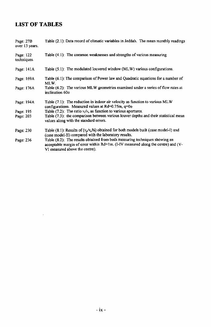
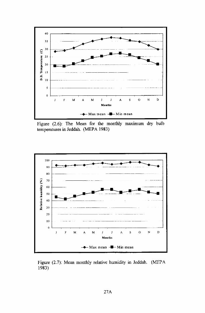
Table (2.1): Data record of climatic variables in Jeddah. The mean monthly readings
Table (4.1): The common weaknesses and strengths of various measuring
Table (5.1): The modulated louvered window (MLW) various configurations.
Table (6.1): The comparison of Power law and Quadratic equations for a number ofMLW.Table (6.2): The various MLW geometries examined under a series of flow rates atinclination 600
Table (7.1): The reduction in indoor air velocity as function to various MLWconfigurations. Measured values at Rd=0.75m, q=OoTable (7.2): The ratio v/v. as function to various apertures.Table (7.3): the comparison between various louver depths and their statistical meanvalues along with the standard errors.
Table (8.1): Results of (v/v.%) obtained for both models built (case model-I) and(case model-II) compared with the laboratory results.Table (8.2): The results obtained from both measuring techniques showing anacceptable margin of error within Rd=Im. (I-IV measured along the centre) and (V-VI measured above the centre).
- IX-

LIST OF FIGURES
Page: 14Page: 18
Page: 19
Page:21
Page:23
Page: 27APage: 27APage: 27C
Page: 28APage: 28APage: 28BPage: 28BPage: 30A
Page:31Page: 33APage: 34A
Page:37
Page:38
Page:40Page:41
Page:44Page:45
Page: 56
Page: 57Page: 57A
Page: 58Page: 59A
Page:60
Page:61
Page: 62APage: 63Page: 64
Figure (2.1): The geographical map of Saudi Arabia.Figure (2.2): Diagrammatic explanation of the three climatic phases (at night, noonand afternoon).Figure (2.3): The architectural response to the hot arid climatic zone where found thecourtyard house, smaller apertures on the exterior walls and the compact urban formsurrounded by thick layers of palm trees to protect against frequent sandstorm.Figure (2.4): The Composite climatic zone where found the wind towers (badjirs) tocatch the maximum breeze and direct it downwards.Figure (2.5): Typical houses in the composite climatic zone where flat stone piecesare put together in rows to protect mud walls from solar radiation and from heavyrain in summer and winter seasons respectively.Figure(2.6): The Mean for the monthly maximum dry bulb temperatures in Jeddah.Figure (2.7): Mean monthly relative humidity in Jeddah.Figure (2.8): The four seasonal maps of air circulation over Saudi Arabia showing theyear-round predomination of sea breeze blowing from the northwest and west inJeddah.Figure (2.9): Mean monthly wind speeds in Jeddah.Figure (2.10): The wind rose of Jeddah.Figure (2.11): Mean monthly precipitations in Jeddah.Figure (2.12): Sunpath diagram for 210 N latitude.Figure (2.13): The isopleths charts of various climatic variables, [a: dry bulbtemperature (C)], [b: relative humidity (%)], Cc:wind speed and direction (mls)].Figure (2.14): The phenomenon of sea and land breezes.Figure (2.15): A typical traditional house in Jeddah (Noorwali house).Figure (2.16): The main elevation treatments in Jeddah where the modulatedlouvered windows are commonly used in all of them.Figure (2.17): A sketch of the vertical and horizontal airflow patterns in a typicalhouse in Jeddah.Figure (2.18): At the upper most floor (Al-Mabit) is normally covered withmodulated louver windows.Figure (2.19): The master plan of old Jeddah.Figure (2.20): The hourly temperature variations obtained from Jeddah traditionalstreet, modem street and the meteorological station on 18/7/1987.Figure (2.21): The various types of Rowshans found in Jeddah.Figure (2.22): The various elements of the Rowshan.
Figure (3.1): The conventional window types classified under the three maincategories including simple opening, vertical vane opening and horizontal vaneopening.Figure (3.2): The MLW has a quality of directing air to different levels indoors.Figure (3.3): The patterns of airflow indoors based on various block types examinedunder wind speed=1 Omls and perpendicular wind direction(900). Block C I offeredthe maximum resistance to air velocity and hence, showed the poorest performancewhile C2 and C3 tend to straighten the flow indoors regardless of wind direction.Figure (3.4): The various louver window systems.Figure (3.5): Velocity drop as function to the various louver systems includingcombine, vertical and horizontal.Figure (3.6): Horizontal louver systems carry preference over the vertical virtue of anumber of functions. (a): the capability to alter the louvers angle to the sun altitude,(b): distribution of airflow to various level in the room, (c): protection from rain and(d): larger range of view.Figure (3.7): Flow coefficients for both observed and predicted curves with wallporosity of 46%.Figure (3.8): Different examples ofMLW applications in apertures.Figure (3.9): The use ofMLW in wind towers and roof ridges.Figure (3.10): The modem application of MLW for natural ventilation.
- x -
Page:66
Page: 67
Page: 68A
Page: 69A
Page: 70
Page: 71
Page: 72
Page:73
Page:93Page:95Page:96Page:98Page: lOOPage: 103Page: 106
Page: 108
Page: 109
Page: 110
Page: 112Page: 113
Page: 116
Page: 117
Page: 139
Page: 140Page: 141
Page: 142Page: 143APage: 1438Page: 143CPage: 143DPage: 143EPage: 145A
Page: 156Page: 157APage: 168
Page: 169APage: 170Page: 170A
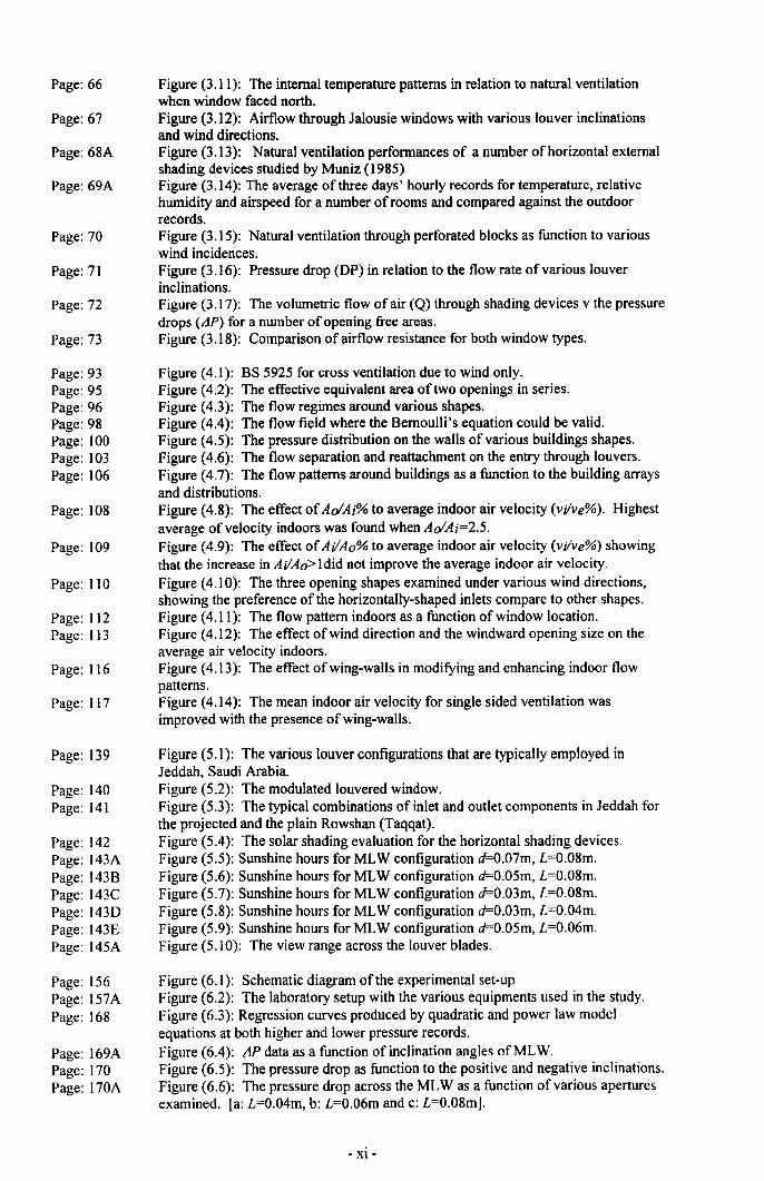
Figure (3.11): The internal temperature patterns in relation to natural ventilationwhen window faced north.Figure (3.12): Airflow through Jalousie windows with various louver inclinationsand wind directions.Figure (3.13): Natural ventilation performances of a number of horizontal externalshading devices studied by Muniz (1985)Figure (3.14): The average of three days' hourly records for temperature, relativehumidity and airspeed for a number of rooms and compared against the outdoorrecords.Figure (3.15): Natural ventilation through perforated blocks as function to variouswind incidences.Figure (3.16): Pressure drop (DP) in relation to the flow rate of various louverinclinations.Figure (3.17): The volumetric flow of air (Q) through shading devices v the pressuredrops (LiP) for a number of opening free areas.Figure (3.18): Comparison of airflow resistance for both window types.
Figure (4.1): BS 5925 for cross ventilation due to wind only.Figure (4.2): The effective equivalent area of two openings in series.Figure (4.3): The flow regimes around various shapes.Figure (4.4): The flow field where the Bernoulli's equation could be valid.Figure (4.5): The pressure distribution on the walls of various buildings shapes.Figure (4.6): The flow separation and reattachment on the entry through louvers.Figure (4.7): The flow patterns around buildings as a function to the building arraysand distributions.Figure (4.8): The effect of AoIA;% to average indoor air velocity (vvve%). Highestaverage of velocity indoors was found when AoIA;=2.5.Figure (4.9): The effect of AvAo% to average indoor air velocity (vvve%) showingthat the increase in AvAo> ldid not improve the average indoor air velocity.Figure (4.10): The three opening shapes examined under various wind directions,showing the preference of the horizontally-shaped inlets compare to other shapes.Figure (4.11): The flow pattern indoors as a function of window location.Figure (4.12): The effect of wind direction and the windward opening size on theaverage air velocity indoors.Figure (4.13): The effect of wing-walls in modifying and enhancing indoor flowpatterns.Figure (4.14): The mean indoor air velocity for single sided ventilation wasimproved with the presence of wing-walls.
Figure (5.1): The various louver configurations that are typically employed inJeddah, Saudi Arabia.Figure (5.2): The modulated louvered window.Figure (5.3): The typical combinations of inlet and outlet components in Jeddah forthe projected and the plain Rowshan (Taqqat).Figure (5.4): The solar shading evaluation for the horizontal shading devices.Figure (5.5): Sunshine hours for MLW configuration d=0.07m, L=0.08m.Figure (5.6): Sunshine hours for MLW configuration d=0.05m, L=0.08m.Figure (5.7): Sunshine hours for MLW configuration d=0.03m, L=0.08m.Figure (5.8): Sunshine hours for MLW configuration d=0.03m, L=0.04m.Figure (5.9): Sunshine hours for MLW configuration d=0.05m, L=0.06m.Figure (5.10): The view range across the louver blades.
Figure (6.1): Schematic diagram of the experimental set-upFigure (6.2): The laboratory setup with the various equipments used in the study.Figure (6.3): Regression curves produced by quadratic and power law modelequations at both higher and lower pressure records.Figure (6.4): AP data as a function of inclination angles ofMLW.Figure (6.5): The pressure drop as function to the positive and negative inclinations.Figure (6.6): The pressure drop across the MLW as a function of various aperturesexamined. [a: L=0.04m, b: L=0.06m and c: L=0.08m].
- xi-
Page: 171Page: 172
Page: 173Page: 174Page: 179
Page: 177
Page: 187Page: l88A
Page: 192A
Page: 193Page: 195APage: 195B
Page: 196A
Page: 198
Page: 200APage:20lPage:202Page: 204A
Page:207
Page: 2l7A
Page: 222A
Page: 227A
Page: 227APage: 230A
Page: 232APage: 235A
Page: 235A
Page: 235B
Page: 235B
Page: 235C
Page: 235C
Page: 235D
Page: 235D
Page: 236A
Figure (6.7): The pressure drop as function to the aperture dimensions.Figure (6.8): Some of the MLW where there was a significant effect of the louverdepths. [a: d=O.02m and b: d=0.03m].Figure (6.9): Pressure drop as function of louver number at louver inclination ()=60°.Figure (6.10): Pressure drop as function of various d/L%.Figure (6.11): Pressure drop as a function of various MLW configurations at louverinclination 60°.Figure (6.12): The predicted against the observed values of &'. based on thestatistical model equation (6.26).
Figure (7.1): A schematic diagram of the velocity measurements experimental set-upFigure (7.2): The experimental setup of velocity drop measurements showing thevarious equipments employed in the experiment.Figure (7.3): The comparison between the quadratic and the power law statisticalcurve fitsFigure (7.4): The polynomial curves for two louver apertures at Rcr=0.75mFigure (7.5): The reduction of velocity as function of louver depth.Figure (7.6): The correlation between various apertures and wind speeds at variouslocations inside the roomFigure (7.7): The effect on wind angles of incidence on velocity reduction near theMLW, Rd=0.25.Figure (7.8): The ratio of velocity reduction along the room with reference toR;=0.25m.Figure (7.9): The reduction of velocity as function of porosity percentage (p).Figure (7.10): The phenomenon of relationship between v/villo and vlv.%.Figure (7.11): The v/ve% and vlve% against various porosity percentages examinedFigure (7.12): The comparison of various louver depths effect in relation to the roomdepthFigure (7.13): The correlation between observed and predicted values of vi/ve%based on equation 7.1.
Figure (8.1): Some examples of various problem scales covered by the CFDtechnique. [a: A multi storey building (Robinson et al. 1999)], [b: Mechanicalairflow systems.Figure (8.2): Both grid coordinates systems constructed using by FLUENT. [a, b, c:Cartesian grids coordinate system], [d: Body-fitted grids coordinate system]Figure (8.3.a): The model initially constructed to carry out the simulation process(case model I).Figure (S.3.b): The modified model constructed (case model II).Figure (8.4): Curves of both CFD (case model-I) and CFD (case model-Il) plottedagainst results obtained form the laboratory showing comparable curves with anacceptable margin of error, ()=Oo.Figure (8.5): The CFD model (case model-III) built to carry on the simulation.Figure (S.6.a): The colour-filled contours of airflow for the model d=O.02m andL=O.06mFigure (S.6.b): Regression curves of both CFD and Laboratory (LAB) along the roomfor the model d=0.02m and L=0.06mFigure (S.7.a): The colour-filled contours of airflow for the model d=O.03m andL=O.OSm.Figure (S.7.b): Regression curves of both CFD and Laboratory (LAB) along the roomfor the model d=O.03m and L=O.OSm.Figure (S.S.a): The colour-filled contours of airflow for the model d=O.05m andL=O.OSm.Figure (8.S.b): Regression curves of both CFD and Laboratory (LAB) along the roomfor the model d=O.05m and L=O.OSm.Figure (8.9.a): The colour-filled contours of airflow for the model d=O.07m andL=O.OSm.Figure (S.9.b): Regression curves of both CFD and Laboratory (LAB) along the roomfor the model Page: d=O.07m and L=O.OSm.Figure (S.l O.a) the colour-filled contours of airflow at angle d=O.03m, L=O.OSm..
- XII-
Page: 236A
Page: 236BPage: 236B
Page: 236C
Page: 241A
Page:244
Page:245
Figure (S.IO.b): Regression curves of both CFD and laboratory (LAB) near the MLWmodels, d=O.03m, L=O.OSmFigure (S.ll.a) the colour-filled contours of airflow at angle d=O.07m, L=O.OSm.Figure (S.ll.b): Regression curves of both CFD and laboratory (LAB) near the MLWmodels, d=O.07m, L=O.OSm.Figure (S.12): The comparison between results achieved from Laboratory and CFD.q=OoFigure (S.13): The Rowshan combinations simulated with the three outlet types andthe evaluated zones under which vertical velocity profiles were examined along theroom.Figure (S.14): The flow pattern showing that modifying the projected Rowshancould force air flow to move in the occupants' zones rather than the ceiling, (J=60,Rd=1.5m. [a: Inlet-V][b: Inlet-IV][c: Inlet-II].Figure (S.15): The effect of the outlet type over the flow pattern of air near the outlet(0.25m near outlet), (J=O°
- xiii -
LIST OF APPENDICES
Appendix A: Natural ventilation in Architecture
Page:263
Page:264Page:264Page:265Page:265Page:266
Page:267Page:267
Appendix (A. I): The flow regimes and pressure fields around a streamed-lines and abluff body.Appendix (A.2): The four regions of the free jet air.Appendix (A.3): The two regions of the wall jet effect.Appendix (AA): The velocity profiles of various types of terrain.Appendix (A.5): The characteristics of terrain roughness.Appendix (A.6): The effect of the eaves (horizontal projection) and the wing-walls(vertical projections) on indoor air velocity.Appendix (A.7 .a): The various roof configurations examined.Appendix (A.7.b): Indoor air velocity as a function to various roof shapes measured ata height of 1.35m and along the centre section. The wind inclinations are (a=OO),(b=300), (c=450), (d=euo), (e=900).
Page:269
Appendix B: Pressure drop across the modulated louvered windows.
Page:270
Page:27l
Page:27l
Page:272
Page:272
Page:273
Page:274Page:274Page:275Page:275Page:276Page:277Page:278Page:278Page:279Page:279Page:280
Appendix (B. I): The conversion of the data-logger results into pressure drops (DP) atboth high and low pressure limits.Appendix (B.2): The coefficient of determinations (r2) with the standard errors of allMLW examined with both model equations.Appendix (B.3.a): Measured values of volume flow (Qmeas) compared to calculatedvalues (Qeale) identified from the Eq.(6.5) for MLW L=0.06m and d=0.02mAppendix (B.3.b): Measured values of volume flow (Qmeas) compared to calculatedvalues (Qeak) identified from the Eq.(6.5) for MLW L=0.06m and d=0.035mAppendix (B.3.c): Measured values of volume flow (Qmeas) compared to calculatedvalues (Qeak) identified from the Eq.(6.5) for MLW L=0.06m and d=0.05mAppendix (BA): Measured values of volume flow (Qmeas) compared to calculatedvalues (Qcale) identified from the Eq.(6.5)Appendix (B.5): Differential Pressures as function of various dlL ratios. [a: dlL=0.5,b:dlL= 0.75 and c: dlL=I]Appendix (B.6.a): The statistical analysis of the louver inclination effectAppendix (B.6.b): The statistical analysis of the louver aperture effectAppendix (B.6.c): The statistical analysis of the louver depth effectAppendix (B.6.d): The statistical analysis of the louver number effectAppendix (B.6.e): The statistical analysis of the louver free area effectAppendix (B.7): The statistical analysis of the integration of overall variables.Appendix (B.8.a): The statistical analysis of the louver depth at 8=600
Appendix (B.8.b): The statistical analysis of the louver aperture at 8=600
Appendix (B.S.c): The statistical analysis of the louver free area at 0=600
Appendix (B.8.d): The statistical analysis of the louver number at 8=600
Appendix (B.9): The statistical analysis of integration of the overall variables at 8=600
Appendix C: Velocity drop across the modulated louvered windows.
Page:282Page:282Page: 283
Page:284
Page:285Page:286Page:287Page:2S8Page:289
Appendix (C. I): The calibration of the air velocity transducer.Appendix (C.2): The various wind speed required indoors.Appendix (C.3): The reduction in indoor air velocity as function to various MLWconfigurations. Measured values at Rd=0.75m.Appendix (CA): The ratio v/v. as function to various MLW configurations. Measuredvalues at Rd=0.75m.Appendix (C.5): The ratio of wv, as function to room depth along and above centreAppendix (C.6): The ratio ofv/ve as function to room depth along and above centreAppendix (C.7): The ratio ofv/ve as function to room depth along and above centreAppendix (C.8): The ratio ofv/ve as function to room depth along and above centreAppendix (C.9): The ratio of wv, as function to room depth along and above centre
- xiv-
Page:290
Page:291
Page:292Page:292Page:293Page:293Page:294
Appendix (C.1O): The velocity drop across room (along the centre) for the variousMLW configurations examined.Appendix (C. II): The velocity drop across room (above the centre) for the various •MLW configurations examined.Appendix (C.l2.a): The statistical analysis of the louver inclination effectAppendix (C.l2.b): The statistical analysis of the louver inclination effectAppendix (C.l2.c): The statistical analysis of the louver free area effectAppendix (C.l2.d): The statistical analysis of the louver number effectAppendix (C.l3): The statistical analysis of the integration of overall variables.
Page:296
Appendix D: Computational Fluid Dynamics appraisal stage.
Page:297
Page:298
Page:299
Page: 300
Page: 301
Page: 302
Page: 303
Page: 304
Page: 305
Page: 306
Page: 307
Page: 308
Page: 309
Page: 310
Page: 311
Page: 312
Page: 313
Appendix (D. I): The velocity profile within the louver blades at various inclinations,L=0.08m, d=0.07m 0=0°, 30 0, and 60 0.
Appendix (D.2): Airflow patterns at various locations inside the room depth at louverinclination angle 0=0°, Projected Rowshan (inlet-II), (outlet-I), d=0.07m, L=0.08m.Appendix (D.3): Airflow patterns at various locations inside the room depth at louverinclination angle 0=0°, Projected Rowshan (inlet-V), (outlet-I), d=0.07m, L=0.08m.Appendix (D.4): Airflow patterns at various locations inside the room depth at louverinclination angle 0=0°, Projected Rowshan (inlet-V), (outlet-II), d=0.07m, L=0.08m.Appendix (D.S): Airflow patterns at various locations inside the room depth at louverinclination angle 0=0°, Projected Rowshan (inlet-V), (outlet-III), d=0.07m, L=0.08m.Appendix (D.6): Airflow patterns at various locations inside the room depth at louverinclination angle 0=30°, Plain Rowshan (inlet-I), (outlet-I), d=0.07m, L=0.08m.Appendix (D.7): Airflow patterns at various locations inside the room depth at louverinclination angle 0=30°, Plain Rowshan (inlet-III), (outlet-I), d=0.07m, L=0.08m.Appendix (D.S): Airflow patterns at various locations inside the room depth at louverinclination angle 0=30°, Projected Rowshan (inlet-V), (outlet-III), d=0.07m, L=0.08m.Appendix (D.9): Airflow patterns at various locations inside the room depth at louverinclination angle 0=60°, Projected Rowshan (inlet-II), (outlet-I), d=0.07m, L=0.08m.Appendix (D. I0): Airflow patterns at various locations inside the room depth at louverinclination angle 0=60°, Projected Rowshan (inlet-IV), (outlet-I), d=0.07m, L=O.08m.Appendix (D.!l): Airflow patterns at various locations inside the room depth at louverinclination angle 0=30°, Projected Rowshan (inlet-V), (outlet-I), d=0.07m, L=0.08m.Appendix (D.!2): Airflow patterns at various locations inside the room depth at louverinclination angle 0=60°, Plain Rowshan (inlet-I), (outlet-I), d=0.07m, L=O.08m.Appendix (D.13): Airflow patterns at various locations inside the room depth at louverinclination angle 0=60°, Plain Rowshan (inlet-III), (outlet-I), d=0.07m, L=0.08m.Appendix (D.!4): Airflow patterns at various locations inside the room depth at louverinclination angle 0=60°, Plain Rowshan (inlet-III), (outlet-III), d=0.07m, L=O.OSm.Appendix (D. IS): Airflow patterns at various locations inside the room depth at louverinclination angle 0=60°, Projected Rowshan (inlet-II), (outlet-I), d=0.07m, L=O.OSm.Appendix (D.16): Airflow patterns at various locations inside the room depth at louverinclination angle 0=60°, Projected Rowshan (inlet-IV), (outlet-I), d=0.07m, L=O.OSm.Appendix (D.17): Airflow patterns at various locations inside the room depth at louverinclination angle 0=60°, Projected Rowshan (inlet-V), (outlet-III), d=O.07m, L=0.08m.Appendix (D.lS): Airflow patterns at various locations inside the room depth at louverinclination angle 0=60°, Projected Rowshan (inlet-V), (outlet-I), d=0.07m, L=O.OSm.
- xv-

NOMENCLATURE
a Constant proportional to the effective leakage area of the crack (m3/s Pa),
A Opening area (m2) or Flow coefficient for fully developed laminar friction losses[CPas)/m3] (depending on application).
Aj Free area (rrr')
A; Inlet area (rrr')
A2 Internal opening area (m2)
An Outlet area (m2)
B Coefficient of entry, exit and turbulent flow losses [(pa s2)/m6].
C Coefficient obtained from experimental measurements
Cc Turbulence model constant
Cd Discharge coefficient of an opening.
Cp Static pressure coefficient
Cpt Leeward pressure coefficient
Cpw Windward pressure coefficient
CQ Flow coefficient
d Gap thickness between louver plates (m)I
D Summation of gaps between louvers L d (m).n
f Expansion Factor
Fj External body forces (N)
g Gravitational acceleration (m/s'')
G; Rate of production of turbulent kinetic energy.
K Head loss
L Breadth of the plate or structure (depending on application) (m)
Le Segment length
m V Mill-voltage signals
n Number of openings in series or an exponent (depending on application).
N Number of louvers
Ne Number of cells in the segment
p porosity percentage (%)
P Pressure (Pa)
r; Wind pressure (Pa)
Q Volumetric flow of air (m3/s)
Qi Flow rate due to infiltration (m3/s).
- xvi-
QI Total flow rate including infiltration (m3/s)
,2 Coefficient of determination
Rd Room depth (m)
Sh Sash height (m)
S, Sash length (m)
Sw Sash width (m)
t Time (s) or plate thickness(m) (depending on application)
T Temperature(C) or Summation of louver thickness (m) (dependingonapplication)
T; internal temperature(C)
To External (outside) temperature (C)
u Axial velocity (m/s)
v, External air velocity (m/s)
Vi internal air velocity (m/s)
vp Velocity reduction due to porosity of an MLW(m/s)
VL Volume of louvers (nr')
Vnew Volume reduction due to louvers (nr')
V Wind speed at opening level (m/s) or volume (nr') (dependingon application)
Vz Mean wind velocity at z height above the ground (roof level) (m/s)
v/ve% Ratio of internal to external air velocity (%)
Wi Wind angle of incidence HY Factor depending on crack geometry.
z Plate length (m) or height above a horizontal reference datum (m) (depending onapplication)
Greek symbols
Lt Increment (dimensionless)
a Slope constant determined by the linear regression.
P Intercept constant determined by the linear regression.
c Intercept constant determined by the linear regression.
K Thermal conductivity (W/m-K)
p Air density (Kg/m3)
f.J Dynamic viscosity (Kg/ms)
f.J1 Turbulent viscosity (Kg/ms)
3 Shadow angle 0o Inclination angle e)
- xvii-

a Stefan-Boltzmann constant (5.67xIO-8 W/m2_K4)
e Dissipation of K(m2/s3)
L Summation of an element.
- xviii-

CHAPTER 1: INTRODUCTION


1.1. Preface
Architectural responses to climate have, throughout the history of building
evolution, varied from one climatic zone to another. In hot humid climates, the
environmental stresses and climatic hazards had influenced the architectural elements of
the shelter into being more responsive. Techniques found in this climatic zone are of
significance in producing comfort by using the natural means available in the environment.
They were handed down through the generations and allowed to evolve through the
process of elimination and adaptation. This man-made architecture was also governed by
the social structure of the inhabitants and the availability of the natural resources in the
settlement.
In modem architecture, people in the tropics have suffered from architectural
solutions proposed by designers and engineers for whom the idea of respecting
environment is quite alien. Those solutions were presumed to originate from the earlier
forms, but the irony is that they turned out to be inappropriate for the climate. Nowadays,
building production in the tropics is associated with a major increase in labour, materials,
and huge energy waste to meet human standards of comfort, which in tum influences the
environment and its quality.
Recently, the prevailing trend towards a sustainable environment has become a
global task. People working in areas related to environment have been urged to review
their approaches and methods to resolve the problems unintentionally caused to the
environment. In architecture this task is implemented in the process of developing passive
and low energy alternatives in the building engineering. Wind-induced natural ventilation
is one of the alternatives to relieve climatic stress and at the same time to reduce energy
- 4 -
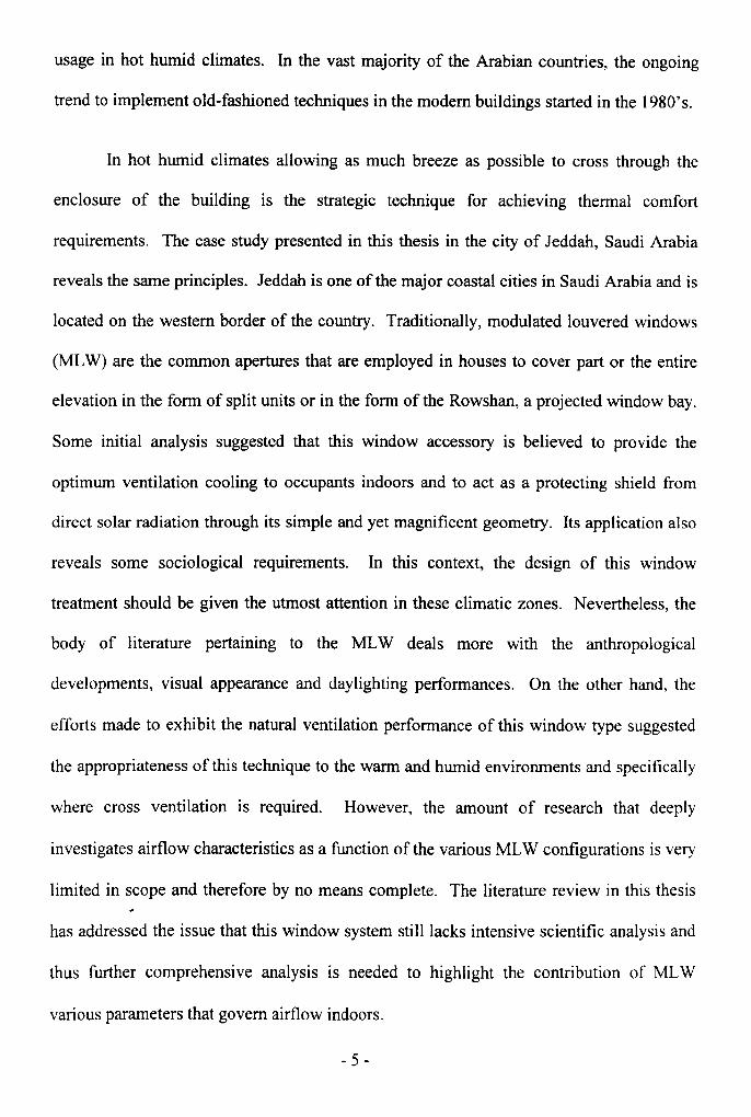
usage in hot humid climates. In the vast majority of the Arabian countries, the ongoing
trend to implement old-fashioned techniques in the modern buildings started in the 1980's.
In hot humid climates allowing as much breeze as possible to cross through the
enclosure of the building is the strategic technique for achieving thermal comfort
requirements. The case study presented in this thesis in the city of Jeddah, Saudi Arabia
reveals the same principles. Jeddah is one of the major coastal cities in Saudi Arabia and is
located on the western border of the country. Traditionally, modulated louvered windows
(MLW) are the common apertures that are employed in houses to cover part or the entire
elevation in the form of split units or in the form of the Rowshan, a projected window bay.
Some initial analysis suggested that this window accessory is believed to provide the
optimum ventilation cooling to occupants indoors and to act as a protecting shield from
direct solar radiation through its simple and yet magnificent geometry. Its application also
reveals some sociological requirements. In this context, the design of this window
treatment should be given the utmost attention in these climatic zones. Nevertheless, the
body of literature pertaining to the MLW deals more with the anthropological
developments, visual appearance and daylighting performances. On the other hand, the
efforts made to exhibit the natural ventilation performance of this window type suggested
the appropriateness of this technique to the warm and humid environments and specifically
where cross ventilation is required. However, the amount of research that deeply
investigates airflow characteristics as a function of the various MLW configurations is very
limited in scope and therefore by no means complete. The literature review in this thesis
has addressed the issue that this window system still lacks intensive scientific analysis and
thus further comprehensive analysis is needed to highlight the contribution of MLW
various parameters that govern airflow indoors.
- 5 -
This study sets out to ascertain that MLW was a major climatic control in hot
humid climates to produce cross ventilation within various parts of the building and
therefore the potential and the parametric performance of the MLW as a mean of
alleviating airflow within in the traditional architecture of Jeddah, Saudi Arabia is needed
to be investigated further.
1.2. Aims of the research
Two sources of wind-induced natural ventilation including the pressure drop (LiP)
and the velocity drop (vlve%) across the MLW are the criterion element of this study. The
research is assessing the potential of the modulated louvered windows to provide
ventilation as a cooling source to achieve thermal comfort inside the buildings.
The research aims and objectives were divided into a number of areas as follow:
• Encourage the use of natural ventilation techniques:
1. Review the methods to control natural ventilation that have been employed in
the traditional house in Jeddah.
2. Address the main architectural element that enhanced cross ventilation within
the traditional house.
• Present technical analysis of the potentials of the MLW:
1. Deeply investigate the various parameters of the modulated louvered windows
(MLW) and their contribution to the governing of airflow characteristics
indoors with respect to pressure and velocity drops.
-6-
2. The thorough investigation of the overall performance in relation to integrating
all variables of the MLW.
• Present practical information for the designers:
1. Address the critical MLW geometry at which airflow characteristics would
experience a significance reduction.
2. The velocity drop as function of prevailing wind conditions as well as the room
depth up to certain distance behind louvers.
3. The schematic analysis of the patterns of airflow inside the room as function of
the common Rowshan configurations employed in Jeddah is studied in
conjunction with a number of outlet types. This is to find out the optimum
configuration of the Rowshan from natural ventilation perspective.
The above aims and objectives of the investigation could not be accomplished
without a suitable investigation and analysis tool. Therefore, within this context certain
objectives are added:
1. To analyse the results obtained from the pressure drop appraisal stage using the
two common model equations, the Power law and the Quadratic, and further to
examine the coefficients embedded into them theoretically.
2. To examine the viability of using computational fluid dynamics (CFO) coding
to simulate the airflow around the reviewed modulated louver windows.
1.3. Methodological approach
The author has followed the following methodological approach:
- 7 -
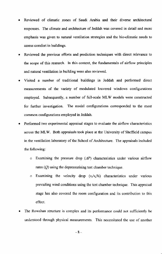
• Reviewed of climatic zones of Saudi Arabia and their diverse architectural
responses. The climate and architecture of Jeddah was covered in detail and more
emphasis was given to natural ventilation strategies and the bio-climatic needs to
assess comfort in buildings.
• Reviewed the previous efforts and prediction techniques with direct relevance to
the scope of this research. In this context, the fundamentals of airflow principles
and natural ventilation in building were also reviewed.
• Visited a number of traditional buildings in Jeddah and performed direct
measurements of the variety of modulated louvered windows configurations
employed. Subsequently, a number of full-scale MLW models were constructed
for further investigation. The model configurations corresponded to the most
common configurations employed in Jeddah.
• Performed two experimental appraisal stages to evaluate the airflow characteristics
across the MLW. Both appraisals took place at the University of Sheffield campus
in the ventilation laboratory of the School of Architecture. The appraisals included
the following:
o Examining the pressure drop (LiP) characteristics under varIOUS airflow
rates (Q) using the depressurising test chamber technique.
o Examining the velocity drop (v/ve%) characteristics under varIOUS
prevailing wind conditions using the test chamber technique. This appraisal
stage has also covered the room configuration and its contribution to this
effect.
• The Rowshan structure is complex and its performance could not sufficiently be
understood through physical measurements. This necessitated the use of another
-8 -
technique in the field. The computational fluid dynamics (CFD) technique was
then selected with an initial attempt to examine the viability of CFD coding to
simulate the airflow around the reviewed modulated louver windows.
Consequently, an intensive evaluation of the Rowshan components in conjunction
of various outlet types was then studied.
• Drawn up conclusions and recommendations that will be guidelines for further
research.
1.4. Research Approach
Chapter One is an introduction of the problem upon which the hypothesis is built.
In this, the author is describing the scale of the problem in the modem architectural
approaches in hot humid zones. The research aims and methodology is discussed in this
chapter.
Chapter Two is devoted to highlighting the climatic adaptation to architecture for
the regional context and in particular to natural ventilation approaches seeking to adapt the
micro and macroclimate environments in Jeddah. It is believed that they would allow a
better understanding of the bio-climatic environment and the thermal comfort
requirements. The analysis of Rowshan's various components and configurations is also
discussed in this chapter.
Chapter Three reviews the application of the modulated louvered windows in
architecture and their preference over other window treatments. The literature review on
the related research pertaining to the scope of current research along with its contributions
and critiques are also discussed in the chapter. The conclusions derived from Chapter Two
- 9 -
and Chapter Three set the problem statement of the work in hand and stress the need for
further analysis of this window treatment.
The principles in architectural aerodynamics including the common mathematical
representations of wind-induced natural ventilation around and within buildings are
established in Chapter Four. These will be taken as guidelines to establish the ground for
further laboratorial and CFD appraisals carried out in the subsequent chapters.
Chapter Five sets out the various components of the MLW and the Rowshan
obtained from the two visits to Jeddah conducted by the author as well from the available
literature. Consequently, the various configurations of the full-scale MLW as well as the
Rowshans that will be further examined are highlighted. The shading performance of the
MLW examined and its effect on day lighting potentials based on solar data of sunpath
diagram of Jeddah will be examined later in the chapter. A brief presentation of the
reduction in the view angle as a function of the MLW configurations will then be followed.
The chapter ends up with the arithmetical representations of each parameter as a function
of the total reduction in volumetric flow.
The two laboratorial appraisals stages of pressure and velocity characteristics as
functions of the reviewed MLW are placed respectively in Chapter Six and Chapter Seven
of this thesis. Since the measuring technique was different, the experimental setup
including calibrations of various instrumentations used and measuring principles will be
discussed separately in each chapter. Similarly, the analysis and discussion of the
contribution of MLW various parameters as well as the integration of the overall variables
to this effect are discussed in details in each chapter.
- 10-
Attempts to examine the CFD coding to simulate the airflow around the reviewed
modulated louver windows is discussed in Chapter Eight. The first part of the chapter
reviews the application of CFD in predicting airflow in buildings, the theory of numerical
modelling, the range of CFD software packages used for simulation and justification of the
selected CFD package. The second part is devoted to discussing the set up of MLW
models configurations, the boundary conditions and the comparison of both CFD and
velocity results obtained from Chapter Seven. This chapter ends up by highlighting the
patterns of airflow within the room based on a number of common Rowshan
configurations adapted in Jeddah.
The last chapter summarises the main conclusions and contributions of the thesis to
the field of natural ventilation and emphasizes recommendations that are concluded from
this research.
- 11 -

CHAPTER 2: THE REGIONAL CONTEXT
- 12 -

2.1. Introduction.
Wind-induced natural ventilation is a fundamental technique to achieve human
comfort in humid climates. This chapter is devoted to highlighting the climatic adaptation
of architecture to the regional context and in particular to natural ventilation approaches
seeking to adapt the micro and macroclimate environments in Jeddah. A brief background
is given first to the climatic features and their adaptations in the architecture of Saudi
Arabia. Then comes the climate and architecture of Jeddah where the climatic variables
are discussed more deeply since it is believed that they would allow a better understanding
of the bio-climatic environment and its thermal comfort requirements. The traditional
architecture and its distinguishing features will be discussed here, followed by the
manipulation of natural ventilation approaches on the simple house scale as well as on the
spatial structure of the entire settlement, Le. macroclimate. The analysis of Rowshan's
various components and configurations is discussed in the last section in this chapter as the
main elevation treatment that served both climatic and social requirements.
2.2. The Climate and Architecture of Saudi Arabia
2.2.1. Geographicallocation
Saudi Arabia is one of the world's largest oil producers and exporters. It is one of
the Middle-East countries and is located within the latitudes 16° N to 32° N at the border of
the Asian continent near to Africa with an area of nearly 2,240,OOOsq.Km. Along the west
border of Saudi Arabia there is the Red Sea which connects it to the African, European,
North and South American continents. It is the longest border, approximately 1700Km,
and extends from the Gulf of Aqaba in the north to Maydi in the south. To the East there is
- 13 -

the Arabian Gulf that extends from Ras-Mish'ab to Qatar and is 450Km long. Both
northern and southern borders are land borders (Figure 2.1). Northern Saudi shares
borders, which total 1300Km, with Jordan, Iraq and Kuwait. Oman and Yemen share the
southern borders of Saudi Arabia which are 1200Km long. The geographical location and
economical status of Saudi Arabia, added to its religious status as the home to Islam's two
holiest shrines, shape its political agenda and give Saudi Arabia its uniqueness to the rest
of the world.
P,,'t, t •• rJ 11Ad~~
eN- eP* ,.,,~
.....
R
if. L
Figure (2.1): The geographical map of Saudi Arabia, (Microsoft Enearta WorldAtlas, 1997)
- 14-

2.2.2. Topography
Saudi Arabia is a tropical country that lies within the narrow belt between the
Tropic of Cancer and the Tropic of Capricorn. It is mainly desert with few green spots and
green areas with no permanent bodies of water or main rivers (AI Shareef, 1996).
Regarding its topographical features, they are classified as follows:
2.2.2.1. Sarawat Mountains.
The mountains of Sarawat are located between Najd plateau and Tehamah plain.
They are high mountains broken by great valleys such as Wadi-Fatimah and Wadi-Bishah.
The Sarawat extend from the north with a height of 1,000m to the south near Asir where
peaks rise up to 3,000m and stretch by the city of Madinah. They are the longest chain of
mountains in Saudi Arabia.
2.2.2.2. Tehamah Plain.
This contains two plains; Tehamah and Hedjaz. This narrow plain is located along
the western border of Saudi Arabia and lies parallel to the Red Sea. The maximum width
of the plain is 40 miles in the south and narrows gradually, reaching 10 miles near the city
of Al-Wajh in the north. The plain then extends towards The Gulf of Aqabah with a
similar width. The plain and the mountains of Sarawat act as deflectors to the wind that is
prevailing from the Red Sea (Al-Ansari et al. 1985).
2.2.2.3. Najd Plateau.
This is located in the middle of Saudi Arabia east of the Sarawat Mountains. Its
peak reaches up to 2,000m above sea level with the elevation drops reaching nearly 700m
- 15 -

near AI-Dahna towards the Arabian Gulf. The plateau extends to the south towards Wadi
AI-Dawaser and runs deep parallel to the Empty-Quarter (AI-Rubu Al-khali) (Figure2.1).
More fertile lands are found on the Najd Plateau such as those in Qaseem, Kharj and Aflaj.
To the north, the Najd Plateau extends for nearly 1500Km where there are a nwnber of
famous mountains such as the mountains of Aja, Salma and Towik. Further north stretch
huge sandy hills, called the AI-Nufoud, which join the Iraqi and Jordanian borders.
2.2.2.4. Eastern Coastal Plain
This is a sandy plain that extends along the Arabian Gulf from north to south and
shares borders with both AI-Dahna and the Empty-Quarter.
2.2.2.5. The Empty-Quarter (AI-Rubu AI-khali)
The world's largest area of continuous sand dunes is found in the Empty-Quarter
(AI Shareef, 1996). It is a desert with no evidence of life as only minimwn annual
precipitation occurs.
2.2.3. Climatic zones and the architectural responses
Saudi Arabia is generally classified as a tropical climate where hot temperatures are
predominant, "Arid, desert land, with long, hot summers, and short, cool, winters" (AI-
Ansari et al. 1985).
The month of March marks the beginning of swnmer and October and November
mark the beginning of winter (Al-Ansari et al. 1985). However, the distribution of land
and sea masses and land heights has produced large varieties of climatic zones in Saudi
- 16 -
Arabia. The climatic zones, and hence the architectural responses to climate on dwelling
and urban layout scales, are discussed here in brief.
2.2.3.1. Hot Dry Climatic Zone
2.2.3.1.1. The Climate
The desert that covers most parts of the region is mainly characterized by a hot dry
climate. Arid and semi-arid desert climates are classified by the percentage of vegetation
(Konya, 1980). Cities with hot dry and arid climates such as Riyadh and Makkah
generally have two seasons; summer and winter. Humidity is low and temperatures range
between 25 and 45°C during the day and night in summer, and between 20-30°C during
winter. Skies are clear, no clouds most of the year and annual rainfall is insignificant. As
a result, direct solar radiation is intense and is augmented by radiation reflected from
barren, light-coloured terrain. The wind blows slowly during the morning; dust storms
occur frequently in the afternoon.
2.2.3.1.2. The Architecture
Internal courtyards are constructed everywhere in hot arid regions (Winterhalter,
1982). A courtyard house simply acts as a central core connecting all other elements of the
house. Besides privacy needs, the courtyard operates as a climate moderator as well as a
natural lighting source. In a courtyard house, the daily temperature difference between
inside and outside may reach up to lOoC (Maghrabi, 1993). This difference is crucial to
the generation of an acceptable microclimate indoors when higher temperatures exist. In
these regions, the body moisture evaporates easily since the relative humidity is very low,
and hence, direct wind currents are not desirable (Evans, 1979). As stated by Kaizer
- 17 -
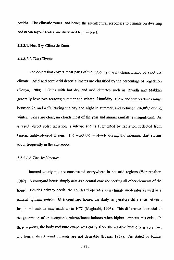
(1984), the courtyard in these climatic regions has three regular daily phases (Figure 2.2).
The first occurs during night when cool air descends into the courtyard and fills
surrounding rooms. As a result, walls, floors, columns, roofs, etc. remain cool until late
afternoon. Then comes the second phase around noon. When the sun hits the courtyard
floor, cool air sinks through surrounding rooms. While heat penetrates the thick walls, a
pleasant and comfortable temperature is maintained inside. The last phase occurs in the
afternoon when the courtyard and rooms become warmer. Then, as the sun sets in the
Noon Afternoon
Figure (2.2): Diagrammatic illustrations of the three climatic phases (at night,noon and afternoon). (Kaizer, 1984)
Night
desert, air temperature falls rapidly and colder air begins to flow. Thus, a new cycle
begins. So, large interior openings overlooking the courtyard are found and smaller ones
are located on exterior walls. An example of this could be found in Riyadh traditional
dwellings (Hemeid, 1999). However, when larger openings are desired on exterior walls,
such as those found in traditional dwellings in Makkah, Rowshans are used to allow cross
ventilation, to provide privacy and to shelter occupants from direct sun radiations.
On the urban scale, several examples of compact urban form courtyard architecture
can be found in Saudi Arabia. To shelter from solar radiation, courtyard houses are
grouped together, sharing two or three walls with one another and forming narrow streets.- 18 -
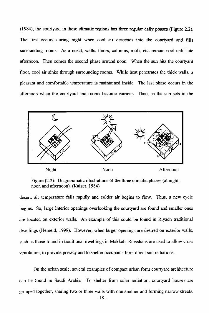
This arrangement allows walls to be less exposed to the sun. The compact urban form also
helps reduce the effect of sand storms. In some cities, the neighbourhood is usually
surrounded by a thick growth of palm trees which protect houses from sand storms (Figure
2.3)
Small openings on the exterior walls
Figure (2.3): The architectural response to the hot arid climatic zone where found thecourtyard house, smaller apertures on the exterior walls and the compact urban formsurrounded by thick layers of palm trees to protect against frequent sandstorm. (Al-Hussaini and Al-Shoaibi 1989)
- 19 -

2.2.3.2. Composite Climatic Zone.
2.2.3.2. J. The Climate
Composite or monsoon climates are " Neither consistently hot dry, nor warm and
humid, ". so they, "Altering between long hot, dry periods to shorter periods of concentrated
rainfall and high humidity "(Koenigsberger et al. 1977). Eastern region of Saudi Arabia falls
under this climatic zone where almost direct sun radiation with relatively low humidity during
summer and rainfall is high during winter causing high humidity records(Kaizer, 1984).
2.2.3.2.2. The Architecture
Since climatic conditions fluctuate between hot dry during summer and hot humid
during winter, the composite climate poses a great challenge for the building environment.
Traditional design responses differ considerably from one place to another. Courtyards,
thick walls of mud or stone, wind towers (badjirs) and terraces for sleeping are the main
elements that compose the dwelling unit. The badjirs are meaningful to those who live in a
composite climate. This is a vertical decorative element that works as cooling ventilators
for both lower and upper levels of the structure. The mouth of a badjir usually extends
some meters higher than the building and is opened towards the prevailing wind. From the
ventilation point of view, wind towers have some preference over windows since
prevailing wind speed or direction is not altered ahead of the tower (Al-Megren, 1987).
The dampness occurring at lower floors is treated with cross ventilation through the
Rowshans and other elevation apertures. For upper levels, which are usually the family
living section, air entering through badjirs enhances comfort and reduces humidity (Figure
2.4). When natural ventilation is not desired, during extreme winter or summer conditions
or sand storms, the badjir is closed with operable louvers or wooden boards.
- 20-
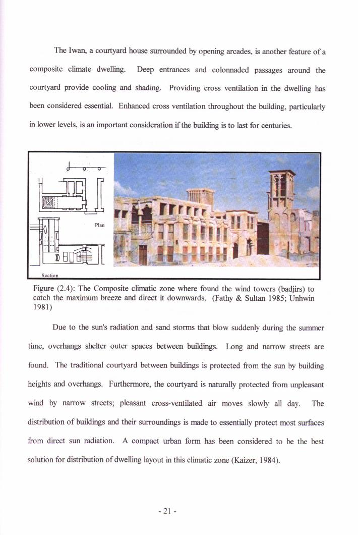
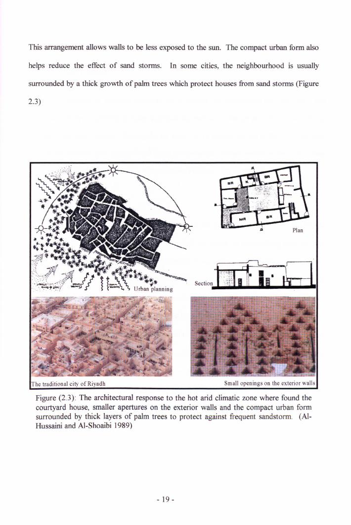
The Iwan, a courtyard house surrounded by opening arcades, is another feature of a
composite climate dwelling. Deep entrances and colonnaded passages around the
courtyard provide cooling and shading. Providing cross ventilation in the dwelling has
been considered essential. Enhanced cross ventilation throughout the building, particularly
in lower levels, is an important consideration if the building is to last for centuries.
J 0
Section
o
Figure (2.4): The Composite climatic zone where found the wind towers (badjirs) tocatch the maximum breeze and direct it downwards. (Fathy & Sultan 1985; Unhwin1981)
Due to the sun's radiation and sand storms that blow suddenly during the summer
time, overhangs shelter outer spaces between buildings. Long and narrow streets are
found. The traditional courtyard between buildings is protected from the sun by building
heights and overhangs. Furthermore, the courtyard is naturally protected from unpleasant
wind by narrow streets; pleasant cross-ventilated air moves slowly all day. The
distribution of buildings and their surroundings is made to essentially protect most surfaces
from direct sun radiation. A compact urban form has been considered to be the best
solution for distribution of dwelling layout in this climatic zone (Kaizer, 1984).
- 21 -
2.2.3.3. Tropical Upland Climatic Zone
2.2.3.3.1. The Climate
This climate can be found in the southern region of Saudi Arabia. Although it is
uncommon in the Arabian region, its influence on traditional architecture has been
significant. Most of the zone lies at an average of 1,OOO-2,OOOmabove sea level.
Widespread mountainous and plateau areas are found in the region. Examples of the cities
located in this climatic zone are Abha and Khamis Meshait in southern Saudi Arabia. The
highest temperature might rise to over 40°C whereas the mean temperature is around 2SoC.
Due to considerable annual rainfall, humidity rises seasonally. Dew is heavy at night, and
the ground has frosts in winter.
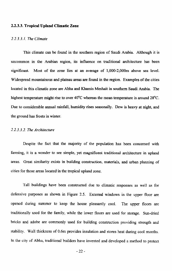
2.2.3.3.2. The Architecture
Despite the fact that the majority of the population has been concerned with
farming, it is a wonder to see simple, yet magnificent traditional architecture in upland
areas. Great similarity exists in building construction, materials, and urban planning of
cities for those areas located in the tropical upland zone.
Tall buildings have been constructed due to climatic responses as well as for
defensive purposes as shown in Figure 2.5. External windows in the upper floor are
opened during summer to keep the house pleasantly cool. The upper floors are
traditionally used for the family, while the lower floors are used for storage. Sun-dried
bricks and adobe are commonly used for building construction providing strength and
stability. Wall thickness of O.6mprovides insulation and stores heat during cool months.
In the city of Abha, traditional builders have invented and developed a method to protect
- 22-
thick adobe walls from regular heavy rainfalls. Flat stone pieces are put together in rows
to protect mud walls from sun radiation during summer and from heavy rain in winter
(Figure 2.5).
Figure (2.5): Typical houses in the tropical upland climatic zone where flat stonepieces are put together in rows to protect mud walls from solar radiation and fromheavy rain in summer and winter seasons respectively. (Mauger 1996)
Classifying the urban planning of upland areas is difficult because it is affected by
the presence of extensive hills and mountain slopes. Villages are small, sometimes
containing five or six houses spread in a valley. Larger villages may be located on the
slopes of a hill with the lower slopes used for farming while the hilltops are used for
buildings. The character of tall buildings, 3 to 6 floors, in such villages creates narrow
alleyways connected to one another through open spaces. Open spaces are usually shaded
during the summer by high-rise buildings.
- 23 -
2.2.3.4. Hot Humid Climatic Zone.
2.2.3.4.1. The Climate
Coastal cities have widely different temperatures from one area to another,
depending upon latitude and exposure to the sea. The climate of linear cities located on the
seashore differs from that of cities that extend inland. Mean temperature falls between 25-
38°C in summer and 17-2SoC in winter (Koenigsberger et al. 1977). Because of the
influence of the sea, relative humidity is very high, at 70-100%. Based on the percentage
of relative humidity, annual rainfall varies from one location to another. Winds are
stronger in settlements located on the seashore rather than those inland. The wind energy
atlas of Saudi Arabia (Al-Ansari et al. 1985) indicates that the strongest wind speeds occur
during April- June while the weakest occur during October and December.
2.2.3.4.2. The Architecture
The architecture in the hot humid climatic zone has traditionally followed three
main construction practices including establishing tall ventilated structures that allow cross
ventilation, constructing large openings covered by projected bay windows (Rowshans)
and plastering walls with coral or gypsum for protection against heavy rain and humidity
as gypsum works as a sealant for water proofing. The courtyard is replaced by a high,
raised building (Kaizer, 1984). Three to six story buildings catch the offshore and onshore
breezes near the sea. Large openings enhance cross ventilation through the structure as
they are necessary to reduce humidity inside the building. Preferred orientation of
structures has been towards the seaside. In some cases, a back or front yard serves the
essential need for relaxation.
- 24-
On the city urban planning scale, cities located in this climatic zone differ from
those found in other climatic zones. The urban planning of hot humid climates has been
developed through years of trial and error experience to enhance desirable wind
penetration through and between buildings. The wider apertures oriented towards the sea
create a remarkable wind movement. This solution helps considerably in reducing
humidity and in cooling down streets temperatures. Unlike the compact urban form, wide
and long streets separate buildings. This climatic zone will be discussed in more details in
the following sections.
2.3. The Climate of Jeddah
2.3.1. Geographicallocation
Jeddah is one of the western region and coastal cities that is overlooking the Red
Sea and is located at 21019' north and 390 12' east with an elevation ranging from 3 tol5m
above sea level. The width of Tehamah Plain near Jeddah is approximately 30Km; it is
relatively flat and rises gradually eastward from the sea. The Red Sea shapes the western
border of Jeddah whilst continuous lines of foothills are found towards the East. Makkah,
the city with the holiest shrine to all Muslims, is the nearest major city to Jeddah and is
located 80Km eastwards. Therefore Jeddah shapes the access for most Muslims aiming to
reach Makkah. Additionally, Jeddah is classed as the capital city of trade since its harbor
is the link with the African, European and American continents. Figure 2.1 shows the
location of Jeddah within Saudi Arabia.
- 25 -
2.3.2. The Climatic Environment
Jeddah has a maritime-desert climate (hot humid) and hence the relative humidity is
reasonably high (Najib, 1987). The data recorded between 1970 and 1983 by the
Meteorology and Environmental Protection Administration (MEPA) are used here to
exhibit the climatic conditions in Jeddah (1983). The long-term data are much more
comprehensive than the short-term data collection (Said and Al-Zaharnah, 1994). It is
worth mentioning that the data collected did not include the year 1976, and hence the data
in hand covered 1970-1975 and 1977-1983. The daily- 24 hours- records were averaged to
yield mean monthly readings over 13years.
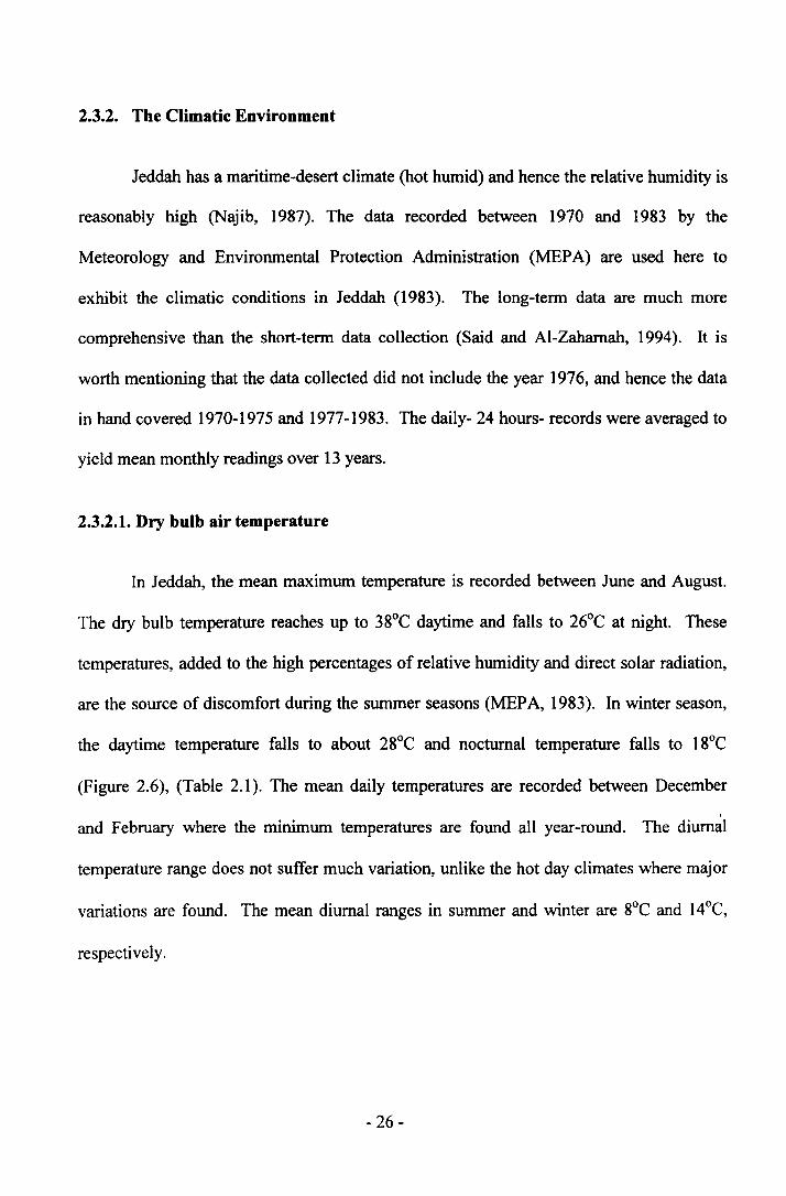
2.3.2.1.Dry bulb air temperature
In Jeddah, the mean maximum temperature is recorded between June and August.
The dry bulb temperature reaches up to 38°C daytime and falls to 26°C at night. These
temperatures, added to the high percentages of relative humidity and direct solar radiation,
are the source of discomfort during the summer seasons (MEPA, 1983). Inwinter season,
the daytime temperature falls to about 28°C and nocturnal temperature falls to 18°C
(Figure 2.6), (Table 2.1). The mean daily temperatures are recorded between December
and February where the minimum temperatures are found all year-round. The diurnal
temperature range does not suffer much variation, unlike the hot day climates where major
variations are found. The mean diurnal ranges in summer and winter are 8°C and 14°C,
respectively.
- 26-
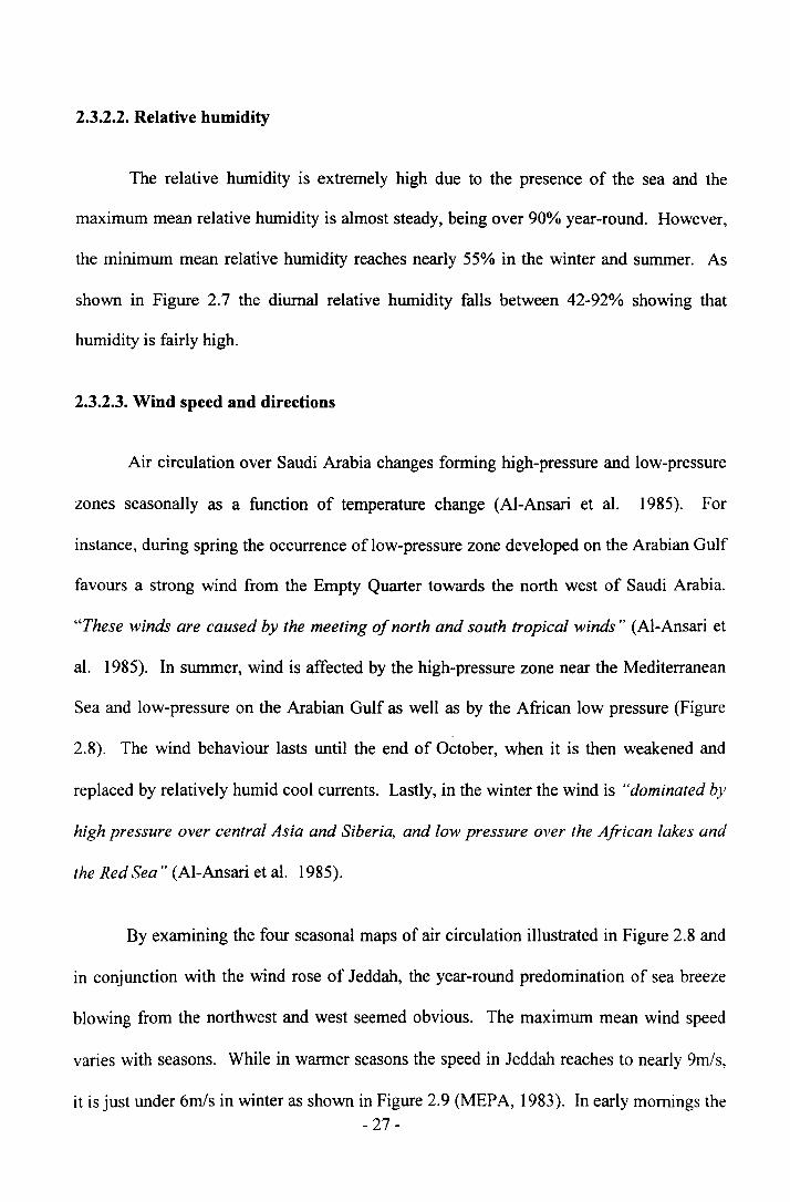
2.3.2.2. Relative humidity
The relative humidity is extremely high due to the presence of the sea and the
maximum mean relative humidity is almost steady, being over 90% year-round. However,
the minimum mean relative humidity reaches nearly 55% in the winter and summer. As
shown in Figure 2.7 the diurnal relative humidity falls between 42-92% showing that
humidity is fairly high.
2.3.2.3. Wind speed and directions
Air circulation over Saudi Arabia changes forming high-pressure and low-pressure
zones seasonally as a function of temperature change (Al-Ansari et al. 1985). For
instance, during spring the occurrence of low-pressure zone developed on the Arabian Gulf
favours a strong wind from the Empty Quarter towards the north west of Saudi Arabia.
"These winds are caused by the meeting of north and south tropical winds" (Al-Ansari et
al. 1985). In summer, wind is affected by the high-pressure zone near the Mediterranean
Sea and low-pressure on the Arabian Gulf as well as by the African low pressure (Figure
2.8). The wind behaviour lasts until the end of October, when it is then weakened and
replaced by relatively humid cool currents. Lastly, in the winter the wind is "dominated by
high pressure over central Asia and Siberia, and low pressure over the African lakes and
the Red Sea" (AI-Ansari et al. 1985).
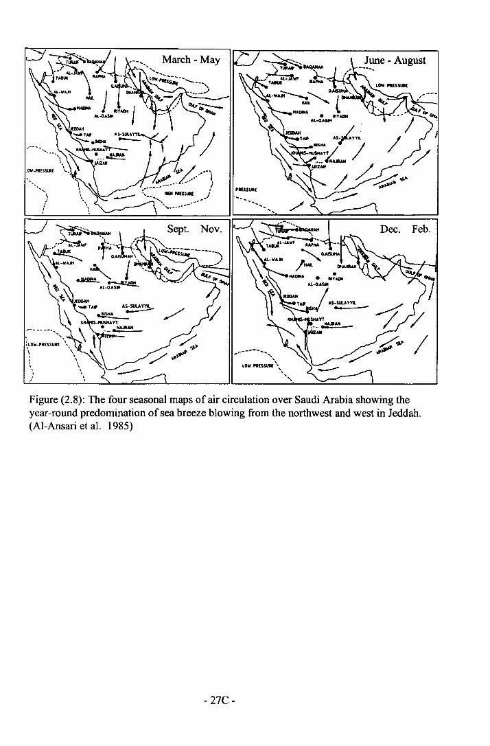
By examining the four seasonal maps of air circulation illustrated in Figure 2.8 and
in conjunction with the wind rose of Jeddah, the year-round predomination of sea breeze
blowing from the northwest and west seemed obvious. The maximum mean wind speed
varies with seasons. While in warmer seasons the speed in Jeddah reaches to nearly 9m/s,
it is just under 6m1s in winter as shown in Figure 2.9 (MEPA, 1983). In early mornings the- 27-
~ 30 r.~~p-"~-~~ 25e..~ 20~~~~_'~-E~ 15
=iQ 10
5
N Ds oM M AAF
Months
-+- Max mean .._ Min mean
Figure (2.6): The Mean for the monthly maximum dry bulbtemperatures in Jeddah. (MEPA 1983)
80~~ 70._,!' 60 -l--------i§ 50..:..E 40.!!~ 30
20 ._-- -----_ ..
10
s o N DF M A M A
Months
-+- Max mean .._ Min mean
Figure (2.7): Mean monthly relative humidity in Jeddah. (MEPA1983)
27A
i!
--......
--f"')000\......Iof'.0'1
\o\oo"! ooooooor-0\...0 N d d-
---00000000-
N N N N - 0 0 0 0 0 - N
N ~ ~ ~ 00 N ~ ~ N M ~MMMMM.,r.,r NNNN
00 \0 0\ 00 N ~ 0\ ~ r- ~ \0 00ori ...0...0 r-: 00 00 r-:...o ori
O\r-~N~~r-NNNNOoOd~.,rori...or-:...o.,rNN
N ,~ N N N N N N N
~ 0\ ~ ~ \0 r- N 00 0\ ~ 0000 0\ d M ~ ...0 r-: r-: ori .,r N 0\NN~~~~M~~M~N
- 27B-
- 0
N 0
-====<
-, -," "):,
Dec. Feb .
.,-- ..- --......,~ ". ,,lOW-PAE:SSURf ,, ,\ \I,,I,
------- ........ -,,
lOW PRlSSUIII '\,".
Figure (2.8): The four seasonal maps of air circulation over Saudi Arabia showing theyear-round predomination of sea breeze blowing from the northwest and west in Jeddah.(Al-Ansari et al. 1985)
- 27C-
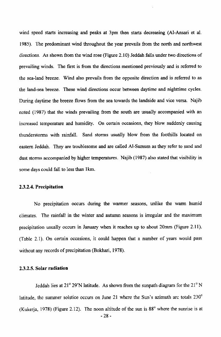
wind speed starts increasing and peaks at 3pm then starts decreasing (Al-Ansari et al.
1985). The predominant wind throughout the year prevails from the north and northwest
directions. As shown from the wind rose (Figure 2.10) Jeddah falls under two directions of
prevailing winds. The first is from the directions mentioned previously and is referred to
the sea-land breeze. Wind also prevails from the opposite direction and is referred to as
the land-sea breeze. These wind directions occur between daytime and nighttime cycles.
During daytime the breeze flows from the sea towards the landside and vice versa. Najib
noted (1987) that the winds prevailing from the south are usually accompanied with an
increased temperature and humidity. On certain occasions, they blow suddenly causing
thunderstorms with rainfall. Sand storms usually blow from the foothills located on
eastern Jeddah. They are troublesome and are called AI-Samum as they refer to sand and
dust storms accompanied by higher temperatures. Najib (1987) also stated that visibility in
some days could fall to less than 1km.
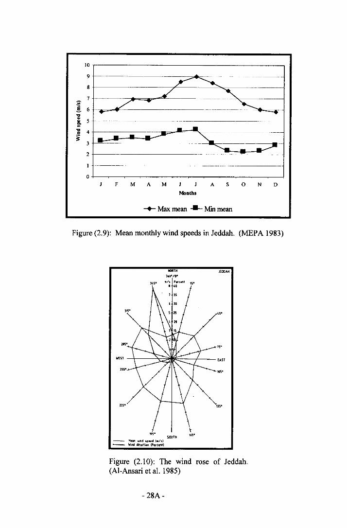
2.3.2.4. Precipitation
No precipitation occurs during the warmer seasons, unlike the warm humid
climates. The rainfall in the winter and autumn seasons is irregular and the maximum
precipitation usually occurs in January when it reaches up to about 20mm (Figure 2.11),
(Table 2.1). On certain occasions, it could happen that a number of years would pass
without any records of precipitation (Bokhari, 1978).
2.3.2.5. Solar radiation
Jeddah lies at 210 29'N latitude. As shown from the sunpath diagram for the 210 N
latitude, the summer solstice occurs on June 21 where the Sun's azimuth arc totals 2300
(Kukerja, 1978) (Figure 2.12). The noon altitude of the sun is 880 where the sunrise is at- 28-
10
9
8
-- 7~!. 6'a..
5Ko'"'a 4=~
3
2
... .._-_.
~
/ <,/ -... ,..... ....
-...--~--.--
::::-----.. • -~-.--- ---~~--____. • ~-------~--•~ • V
oJ F M A M J
Months
s oA N D
-+- Max mean --- Minmean
Figure (2.9): Mean monthly wind speeds in Jeddah. (MEPA 1983)
Hun ....ind sp.ed 1m/51- Wind direction IP.,conrJ
Figure (2.10): The wind rose of Jeddah.(Al-Ansari et al. 1985)
- 28A-
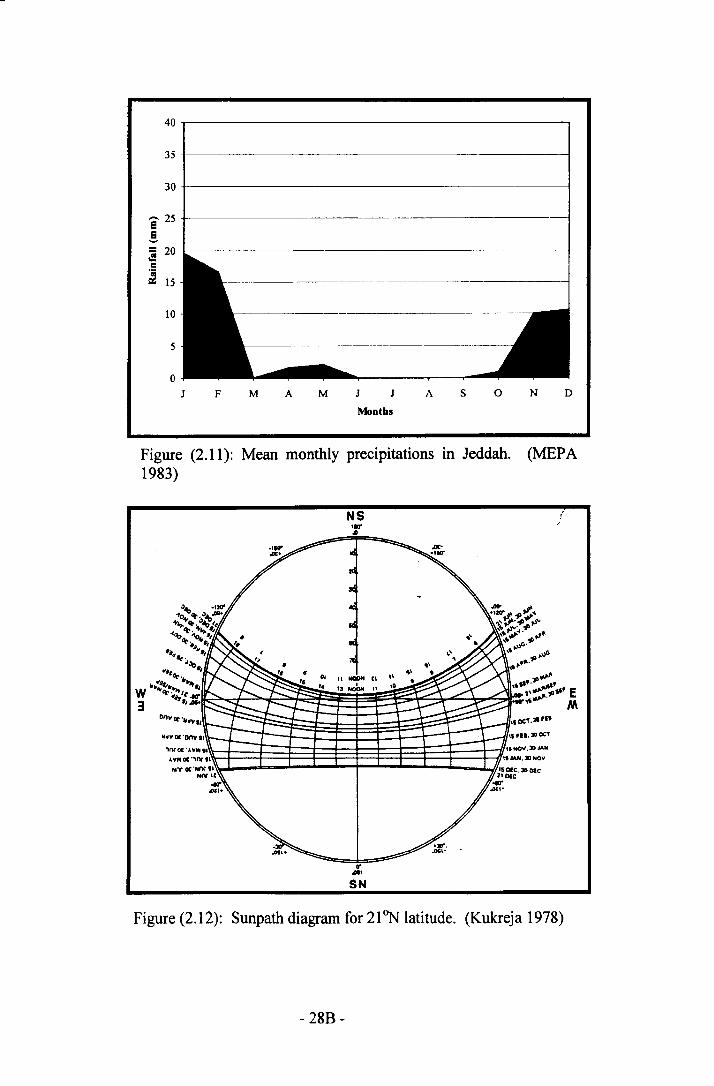
40
35
30
E 25!~ 201:1
~ 15
10
5
0J F M A M J A S 0 N D
Montbs
Figure (2.11): Mean monthly precipitations in Jeddah. (MEPA1983)
NS (....JJ
11'.....SN
Figure (2.12): Sunpath diagram for 21~ latitude. (Kukreja 1978)
- 28B-
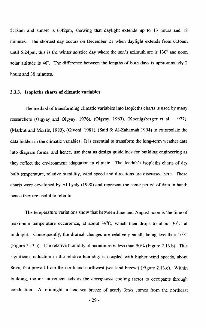
5: l8am and sunset is 6:42pm, showing that daylight extends up to 13 hours and 18
minutes. The shortest day occurs on December 21 when daylight extends from 6:36am
until 5:24pm; this is the winter solstice day where the sun's azimuth arc is 130° and noon
solar altitude is 46°. The difference between the lengths of both days is approximately 2
hours and 30 minutes.
2.3.3. Isopleths charts of climatic variables
The method of transforming climatic variables into isopleths charts is used by many
researchers (Olgyay and Olgyay, 1976), (Olgyay, 1963), (Koenigsberger et al. 1977),
(Markus and Morris, 1980), (Givoni, 1981), (Said & Al-Zahamah 1994) to extrapolate the
data hidden in the climatic variables. It is essential to transform the long-term weather data
into diagram forms, and hence, use them as design guidelines for building engineering as
they reflect the environment adaptation to climate. The Jeddah's isopleths charts of dry
bulb temperature, relative humidity, wind speed and directions are discussed here. These
charts were developed by A1-Lyaly (1990) and represent the same period of data in hand;
hence they are useful to refer to.
The temperature variations show that between June and August noon is the time of
maximum temperature occurrence, at about 39°C, which then drops to about 30°C at
midnight. Consequently, the diurnal changes are relatively small, being less "than 10°C
(Figure 2.13.a). The relative humidity at noontimes is less than 50% (Figure 2.13.b). This
significant reduction in the relative humidity is coupled with higher wind speeds, about
8m/s, that prevail from the north and northwest (sea-land breeze) (Figure 2.13.c). Within
building, the air movement acts as the energy-free cooling factor to occupants through
conduction. At midnight, a land-sea breeze of nearly 3m/s comes from the northeast
- 29-
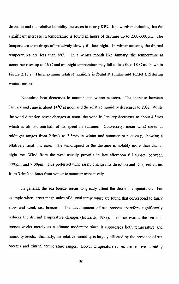
direction and the relative humidity increases to nearly 85%. It is worth mentioning that the
significant increase in temperature is found in hours of daytime up to 2:00-3:00pm. The
temperature then drops off relatively slowly till late night. In winter seasons, the diurnal
temperatures are less than gOC. In a winter month like January, the temperature at
noontime rises up to 26°C and midnight temperature may fall to less than 18°Cas shown in
Figure 2.13.a. The maximum relative humidity is found at sunrise and sunset and during
winter seasons.
Noontime heat decreases in autumn and winter seasons. The increase between
January and June is about 14°Cat noon and the relative humidity decreases to 20%. While
the wind direction never changes at noon, the wind in January decreases to about 4.5m1s
which is almost one-half of its speed in summer. Conversely, mean wind speed at
midnight ranges from 2.5m1s to 3.5m1s in winter and summer respectively, showing a
relatively small increase. The wind speed in the daytime is notably more than that at
nighttime. Wind from the west usually prevails in late afternoon till sunset, between
3:00pm and 7:00pm. This preferred wind rarely changes its direction and its speed varies
from 3.5m1s to 6m1s from winter to summer respectively.
In general, the sea breeze seems to greatly affect the diurnal temperatures. For
example when larger magnitudes of diurnal temperature are found that correspond to fairly
slow and weak sea breezes. The development of sea breezes therefore significantly
reduces the diurnal temperature changes (Edwards, 1987). In other words, the sea-land
breeze works merely as a climate moderator since it suppresses both temperature and
humidity levels. Similarly, the relative humidity is largely affected by the presence of sea
breezes and diurnal temperature ranges. Lower temperature raises the relative humidity
- 30-
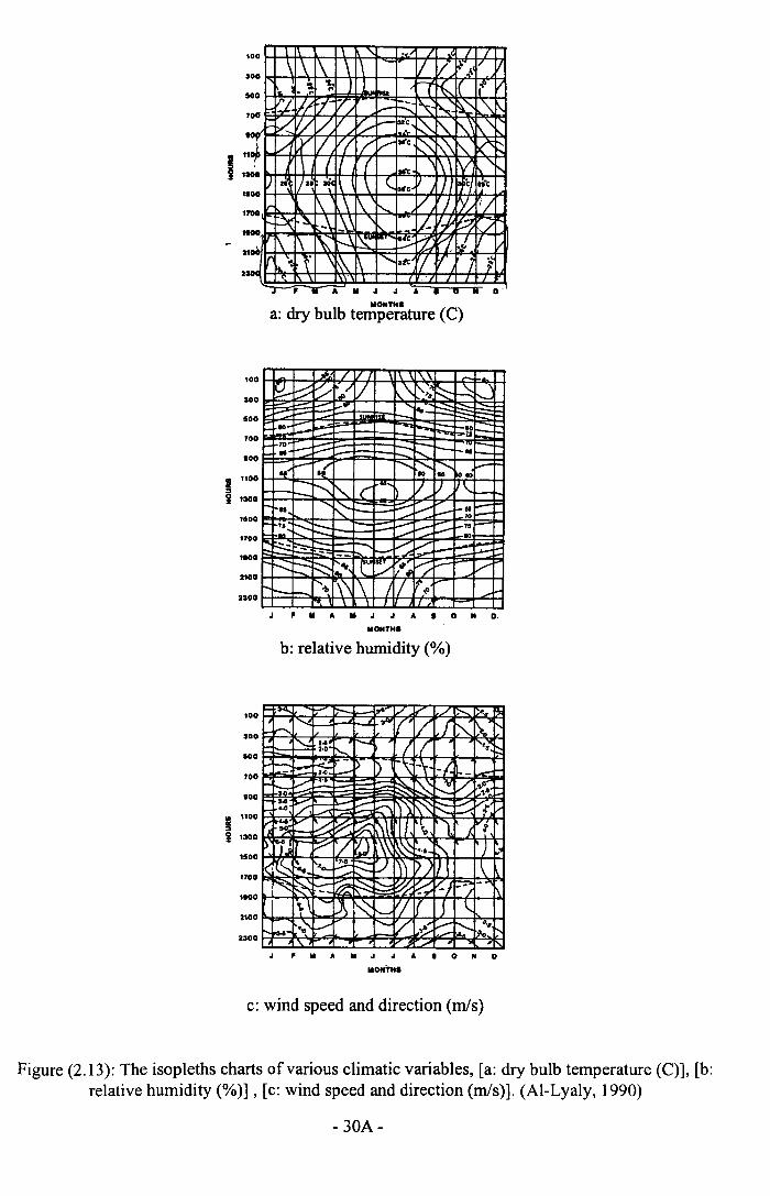
a
,00 \ ".'" / .~I I_\ '1 1\ \ 1\ V ;- l: I
~OO ~500 '. ~ 1: 1L I1rr ~ fl
''[l/~V~v/ f..- b:l~ ~ ~"".'\:--.700
;.(V/v:V ~ I-- ~'e,~ \_ '\_, \.'
~,/ V II V( rV :We
~ \\ -, >(":"( ( I"'e
,.\ v1lOCI) .e: II •• "{ \ \ <..~.II J reI ....e
100
1\ \ 1\ <, V / y/ ij700 --~ .~ -\ l' lI- ;-,? ")- \ .\ ~ N~ '"'' I-~ ttln c! I /100 x.. l \ ~ ~
<, •tr!rl 'f j ~:IO~
T , T A III J J A ... II D'
• 1!ii 1
MOIITH.
a: dry bulb temperature (C)
,00 ~ / \.\ ....g_ ~ ~ ~,/V "-[';:~ ~ I'-
...p .. ::3:: :::::, :::::::-eo -.... _I"""- ~ :;.U.....-: ::::-,.
--: c-- -~ t-- -.. -..-0(-~{ ......... ;.::--- ....--~ r-, (' r ..... / ~ \.,__ -~.. .....~ ,..- / I- _II ::::10
.::'~ F=:: - ~ --::: t::-1-'.-..~S E--- -- ~ ~ -r:::.-- ::,... r-- i-'-:....:::::~ ~ :;,.... c: ::;..- V~4' 1-"'"/ V-""--
1'." \\ \ III l',o ,..-I..... -
300
600
700
'00
= "00
"i 1:100
'.00
1700
,.00
2100
2300
J 'IIIAIIIJJA.OIIO.
MOIITH.
b: relative humidity (%)
100 ~ ;- V ./ ~ #..
\.~..... ..... .-If / I ~ ).,"'-! ... ~ I .f .....,..
• .0 t>-.~-.
_~ D '\ -\. -/._:-: .~I.-- -~
~ :..--:: r'" .
~ ~ ~ ~ ~Sl~..U /, ~ kl~)~ t::::; ~ ~~ .........,
f--.
Ij(~~v
~ ~ ~ ~\l'II, '\ I, /. t::--<l)iiJ -~ '/ (J l\'\~ ~ ) ,,'··s
!""~ ~ ",,-~ s:V' DJ )/~i \..-:~ ~ --:::~ ~ ~ ~ ~ Vol ~~I
_\
To\ "-'P\ ~ VI { J \..r---- .;;.~ ......_~ ...;.~ t-- 'Jy,~P--
" ./ ,
300
500
700
800
= 1100
"i 1300
1500
1100
.,00
.300
J'MAMJJA.OIID
MOIITH.
c: wind speed and direction (m/s)
Figure (2.13): The isopleths charts of various climatic variables, [a: dry bulb temperature (C)], [b:relative humidity (%)], [c: wind speed and direction (m/s)]. (AI-Lyaly, 1990)
- 30A-
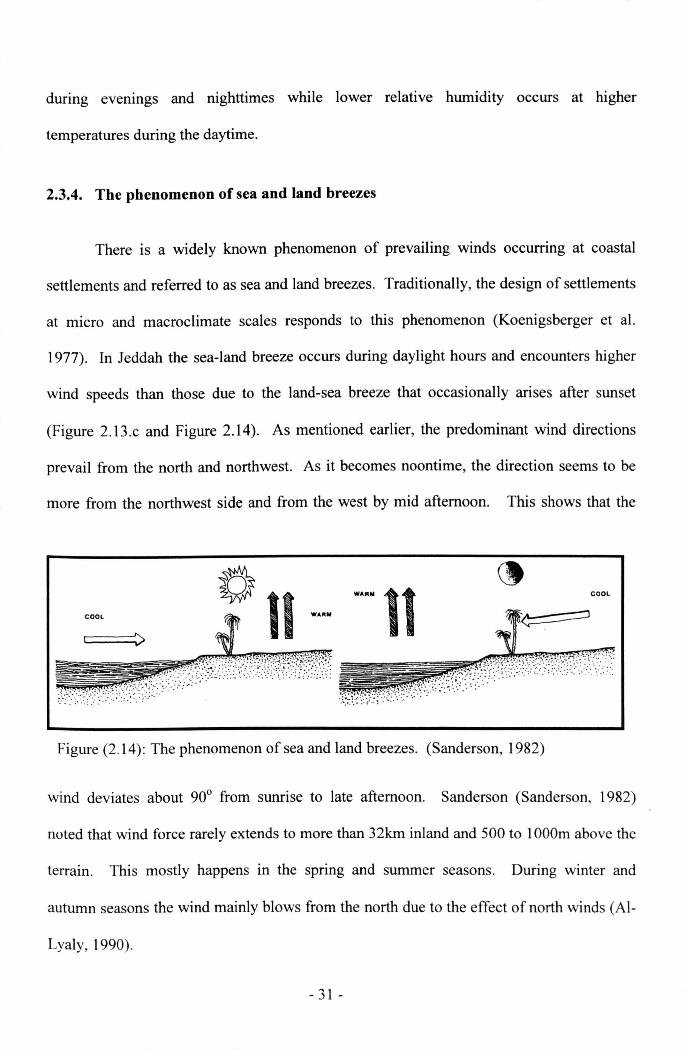
during evenings and nighttimes while lower relative humidity occurs at higher
temperatures during the daytime.
2.3.4. The phenomenon of sea and land breezes
There is a widely known phenomenon of prevailing winds occurring at coastal
settlements and referred to as sea and land breezes. Traditionally, the design of settlements
at micro and macroclimate scales responds to this phenomenon (Koenigsberger et al.
1977). In Jeddah the sea-land breeze occurs during daylight hours and encounters higher
wind speeds than those due to the land-sea breeze that occasionally arises after sunset
(Figure 2.13.c and Figure 2.14). As mentioned earlier, the predominant wind directions
prevail from the north and northwest. As it becomes noontime, the direction seems to be
more from the northwest side and from the west by mid afternoon. This shows that the
COOL WA .. M....11 COOL
Figure (2.14): The phenomenon of sea and land breezes. (Sanderson, 1982)
wind deviates about 90° from sunrise to late afternoon. Sanderson (Sanderson, 1982)
noted that wind force rarely extends to more than 32km inland and 500 to 1000m above the
terrain. This mostly happens in the spring and summer seasons. During winter and
autumn seasons the wind mainly blows from the north due to the effect of north winds (AI-
Lyaly, 1990).
- 31 -

The land-sea breeze occurs during nighttime and prevails mainly from northeast
and east. The directions are consistent and are not affected by the monthly climatic
variations. The highest speed of wind does not exceed 4.5m/s with a mean of
approximately 2.7m/s. Another land-sea wind direction blows from the south and
southeast directions. While it rarely blows, the wind is always coupled with dust and
storm and, therefore unwelcome.
2.4. The Architecture of Jeddah
2.4.1. Construction and decoration materials
Historically, Jeddah is well known for commerce, and hence, the flourishing trade in
Jeddah exerts a direct influence on the architectural formation of the city. The
architectural characteristics are greatly inspired by those originated in Turkey and Egypt
(Mani', 1980). The skills and techniques were brought through migrations and gradually
implemented in Jeddah during the Ottoman era (Al-Lyaly, 1990). Some building materials
were also imported from abroad. For example the qandal, which is extensively used in
Jeddah for construction and wall reinforcements, was the famous timber imported from
India (Bokhari, 1978). Al-Lyaly (1990) suggested that the importing of this wood
coincided with the construction of tall buildings since qandal increases the structural
solidity and prevents uneven settling. Alternatively, the Jawi (teak wood) was mainly used
for decoration. Its name refers to the country where it was brought from, Java. It is more
expensive and of higher quality than the qandal and is widely used by craftsmen for
decorating facades, main doors and windows. Rowshans that are mainly made with Jawi
wood are believed to offer more resistance to humidity and insects (Bokhari, 1978). Wood
- 32 -
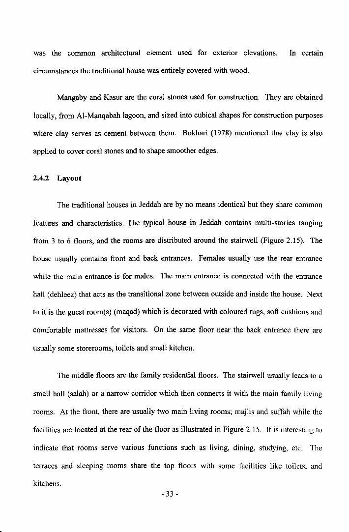
was the common architectural element used for exterior elevations. In certain
circumstances the traditional house was entirely covered with wood.
Mangaby and Kasur are the coral stones used for construction. They are obtained
locally, from Al-Manqabah lagoon, and sized into cubical shapes for construction purposes
where clay serves as cement between them. Bokhari (1978) mentioned that clay is also
applied to cover coral stones and to shape smoother edges.
2.4.2 Layout
The traditional houses in Jeddah are by no means identical but they share common
features and characteristics. The typical house in Jeddah contains multi-stories ranging
from 3 to 6 floors, and the rooms are distributed around the stairwell (Figure 2.15). The
house usually contains front and back entrances. Females usually use the rear entrance
while the main entrance is for males. The main entrance is connected with the entrance
hall (dehleez) that acts as the transitional zone between outside and inside the house. Next
to it is the guest room(s) (maqad) which is decorated with coloured rugs, soft cushions and
comfortable mattresses for visitors. On the same floor near the back entrance there are
usually some storerooms, toilets and small kitchen.
The middle floors are the family residential floors. The stairwell usually leads to a
small hall (salah) or a narrow corridor which then connects it with the main family living
rooms. At the front, there are usually two main living rooms; majlis and suffah while the
facilities are located at the rear of the floor as illustrated in Figure 2.15. It is interesting to
indicate that rooms serve various functions such as living, dining, studying, etc. The
terraces and sleeping rooms share the top floors with some facilities like toilets, and
kitchens.- 33 -
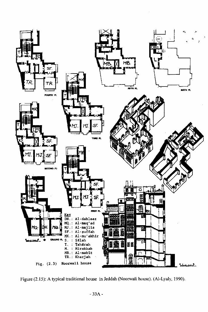
FOlImt PI.
SECOND. PI.!
Ku1IY1",,,+=:JIpI&'.l-li DH.: AI- dahleez
KQ.: AI- maq , ad. tu.: Al-majlisSF.: Al-liluffahKK.: AI-mu' akhir
, H •-. '._. GIII»IO R. S. : ~ilahT. : TaharahM. : MirakkabMB.: Al-mabltTR.: Kharj ah
Fig. (2.3) Noorwali house
_..
SIXTH Fl
~·H·J •..
Figure (2.15): A typical traditional house in Jeddah (Noorwali house). (Al-Lyaly, 1990).
- 33A-

2.4.3. Elevations
In his journey over the Arabian Peninsula, Lawrence (Lawrence of Arabia)
described Jeddah as a remarkable city (Khan, 1986). He wrote:
"The streets were alleys, wood roofed in the main bazaar, but
elsewhere open to the sky in the little gap between the tops of the lofty
white-walled houses. These were built four or jive stories high, the coral
rag tied with square beams and decorated by wide bow-windows running
from the ground to (top)floor in gray woodenpanel".
The elevations in Jeddah are the main distinguishing feature of its architecture, from the
remarkably carved wooden main doors to the astonishingly decorated windows
representing what is locally known by Rowshans, mashrabiah and taqqat (Figure 2.16).
The extensive decorations were made by the professional local craftsmen to reflect the
family living standard. The Rowshan and mashrabiah are cantilever elements projecting
from the walls to form a projected window bay jutting out of the main body of the
building. The Rowshan is commonly used in Jeddah while the mashrabiah are mostly used
in hot dry climates (AI Shareef, 1996). Al Shareef added:
" The name Mashrabiah is used for an opening with a wooden
lattice screen composed of small wooden balusters that are circular in
section and arranged at specific regular intervals, often in a decorative and
intricate geometric patterns".
The Rowshan configurations will be discussed in details later in this chapter. On the top
floors are found the terraces which breakup the continuity of Rowshans that extend from
the ground, shaping the staggered and uneven skylines of the structure elevation.
- 34 -
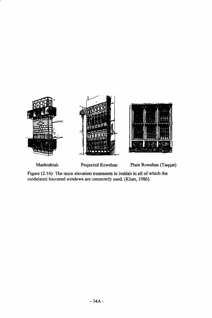
Mashrabiah Projected Rowshan Plain Rowshan (Taqqat)
Figure (2.16): The main elevation treatments in Jeddah in all of which themodulated louvered windows are commonly used. (Khan, 1986).
- 34A-
2.4.4. Social influence on traditional buildings
Social values are given very significant consideration in the Islamic architecture,
and hence, the traditional building in Jeddah reveals the same principles. Hospitality,
neighbour-to-neighbour relations and the extended family structure shape the integrations
between levels of privacy and are replicated in the traditional dwellings. The woman's
status within the family is also given great importance.
Two dimensions of privacy are found within the traditional house, vertical and
horizontal. The social obligations towards guests created a vertical dimension of privacy
between the visitors and the rest of the family. As mentioned earlier, the house master's
hospitality to guests and all the related facilities are situated on the ground floor (semi-
private zone), whilst the upper floors are more private, as they are out of bounds for the
guests. Within the upper floors is found another degree of privacy sanctioned in the
segregation between the sleeping and living zones. The living zones are usually found in
the middle floors, and the sleeping zone is located at the uppermost floors. The concept of
the extended family structure also carries some levels of privacy. In the case of a married
son living with his parents, he is usually allocated a certain floor or a quarter within the
floor. This creates a specific zone of privacy that does not interfere with the daily
activities of other family members. Parents would normally live above the floor of their
married son (Al-Lyaly, 1990). The floor layout reveals some horizontal levels of privacy
as well. For example the stairwell is usually located near the rear entrance to enable family
members and women in particular to go to the upper floors freely and without passing by
the guests. The small hall connecting the stairwell with other rooms provides a degree of
privacy within the floor.
- 35 -
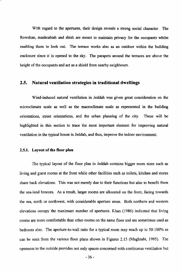
With regard to the apertures, their design reveals a strong social character. The
Rowshan, mashrabiah and shish are meant to maintain privacy for the occupants whilst
enabling them to look out. The terrace works also as an outdoor within the building
enclosure since it is opened to the sky. The parapets around the terraces are above the
height of the occupants and act as a shield from nearby neighbours.
2.5. Natural ventilation strategies in traditional dwellings
Wind-induced natural ventilation in Jeddah was given great consideration on the
microclimate scale as well as the macroclimate scale as represented in the building
orientations, street orientations, and the urban planning of the city. These will be
highlighted in this section to trace the most important element for improving natural
ventilation in the typical house in Jeddah, and thus, improve the indoor environment.
2.5.1. Layout of the floor plan
The typical layout of the floor plan in Jeddah contains bigger room sizes such as
living and guest rooms at the front while other facilities such as toilets, kitchen and stores
share back elevations. This was not merely due to their functions but also to benefit from
the sea-land breezes. As a result, larger rooms are allocated on the front, facing towards
the sea, north or northwest, with considerable aperture areas. Both northern and western
elevations occupy the maximum number of apertures. Khan (1986) indicated that living
rooms are more comfortable than other rooms on the same floor and are sometimes used as
bedroom also. The aperture-to-wall ratio for a typical room may reach up to 50-100% as
can be seen from the various floor plans shown in Figures 2.15 (Maghrabi, 1995). The
openness to the outside provides not only spaces concerned with continuous ventilation but
- 36-
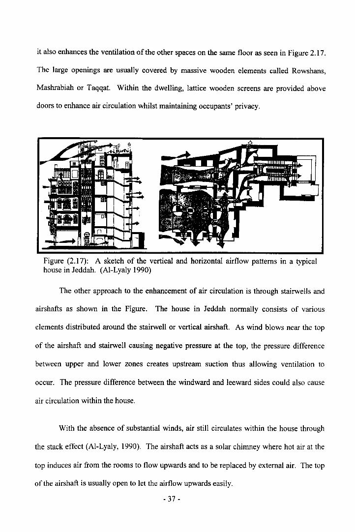
it also enhances the ventilation of the other spaces on the same floor as seen in Figure 2.17.
The large openings are usually covered by massive wooden elements called Rowshans,
Mashrabiah or Taqqat. Within the dwelling, lattice wooden screens are provided above
doors to enhance air circulation whilst maintaining occupants' privacy.
Figure (2.17): A sketch of the vertical and horizontal airflow patterns in a typicalhouse in Jeddah. (Al-Lyaly 1990)
The other approach to the enhancement of air circulation is through stairwells and
airshafts as shown in the Figure. The house in Jeddah normally consists of various
elements distributed around the stairwell or vertical airshaft. As wind blows near the top
of the airshaft and stairwell causing negative pressure at the top, the pressure difference
between upper and lower zones creates upstream suction thus allowing ventilation to
occur. The pressure difference between the windward and leeward sides could also cause
air circulation within the house.
With the absence of substantial winds, air still circulates within the house through
the stack effect (AI-Lyaly, 1990). The airshaft acts as a solar chimney where hot air at the
top induces air from the rooms to flow upwards and to be replaced by external air. The top
of the airshaft is usually open to let the airflow upwards easily.
- 37 -
2.5.2. Elevation treatment
The Rowshan is a main elevation treatment in Jeddah. It extends vertically or
horizontally to cover part, or the whole, of the building's facade, Khan (1986) indicated
that the use of Rows hans reflects the elegance of the house owner. Additionally he stated:
"Practically, the Rowshan is considered window to the external
world, veilfrom the Sun's glare, source of ventilation in buildings andpiece
of furniture in the house which sometimes extends to cover a number of
"rooms.
Figure (2.18): The uppermost floor (Al-Mabit) is normally covered withmodulated louver windows. (Khan, 1986).
The above description reflects the importance of the Rowshan as the main source of cross
ventilation in the buildings. It contains adjustable louvers which allow breeze to penetrate
at the desired inclination. Occasionally, small screens are found near the top of the
- 38 -
Rowshan that serve another important role. When air penetrates through the screens it
extracts the excessive humidity and heat near ceiling level.
The modulated louvered windows (MLW) are also employed on the top floors
where the sleeping area and terrace are found. The sleeping rooms are surrounded by
wooden louvers on two or three sides, giving the impression of an air pavilion as illustrated
in Figure 2.18 (AI-Lyaly, 1990). This is merely made to favour continuous circulation of
air within the room even at very low wind speed. The terraces located at the upper floors
in Jeddah replace the central courtyard (Hariri, 1993). They are surrounded by high-
perforated parapets and open to the sky, acting as an outdoor environment within the
building.
2.5.3. Building orientation
Freestanding structures that are penetrated by a number of alleys to channel air
through are one of the most favorable solutions in humid climates (Koenigsberger et al.
1977). Houses distributions and orientations in Jeddah have arisen from the same
perception. Indeed the concept was optimized after long-term experience of trial and error
technique (AI Shareef, 1996). The tall buildings rarely share any walls and are often
surrounded by a number of alleys to enhance cross ventilation. As mentioned earlier,
rooms located on the north and the west elevations are widely opened and facilitated with
Rowshans while the house shares only a single wall with the neighbour. This was
necessary since the inflowing air between buildings will take the moisture away. In turn, it
increases the house's durability. The traditional dwellings therefore faced the seafront.
Such orientation is certainly joyful to the occupants who benefit from the continuous
breeze.
- 39-
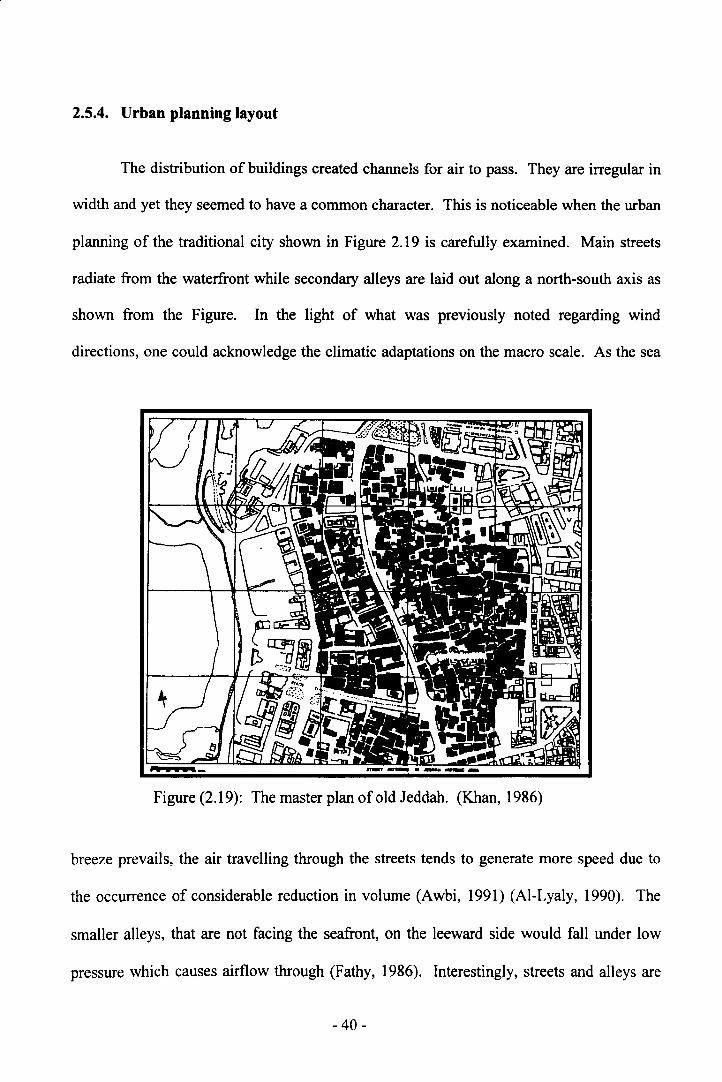
2.5.4. Urban planning layout
The distribution of buildings created channels for air to pass. They are irregular in
width and yet they seemed to have a common character. This is noticeable when the urban
planning of the traditional city shown in Figure 2.19 is carefully examined. Main streets
radiate from the waterfront while secondary alleys are laid out along a north-south axis as
shown from the Figure. In the light of what was previously noted regarding wind
directions, one could acknowledge the climatic adaptations on the macro scale. As the sea
Figure (2.19): The master plan of old Jeddah. (Khan, 1986)
breeze prevails, the air travelling through the streets tends to generate more speed due to
the occurrence of considerable reduction in volume (Awbi, 1991) (Al-Lyaly, 1990). The
smaller alleys, that are not facing the seafront, on the leeward side would fall under low
pressure which causes airflow through (Fathy, 1986). Interestingly, streets and alleys are
- 40-
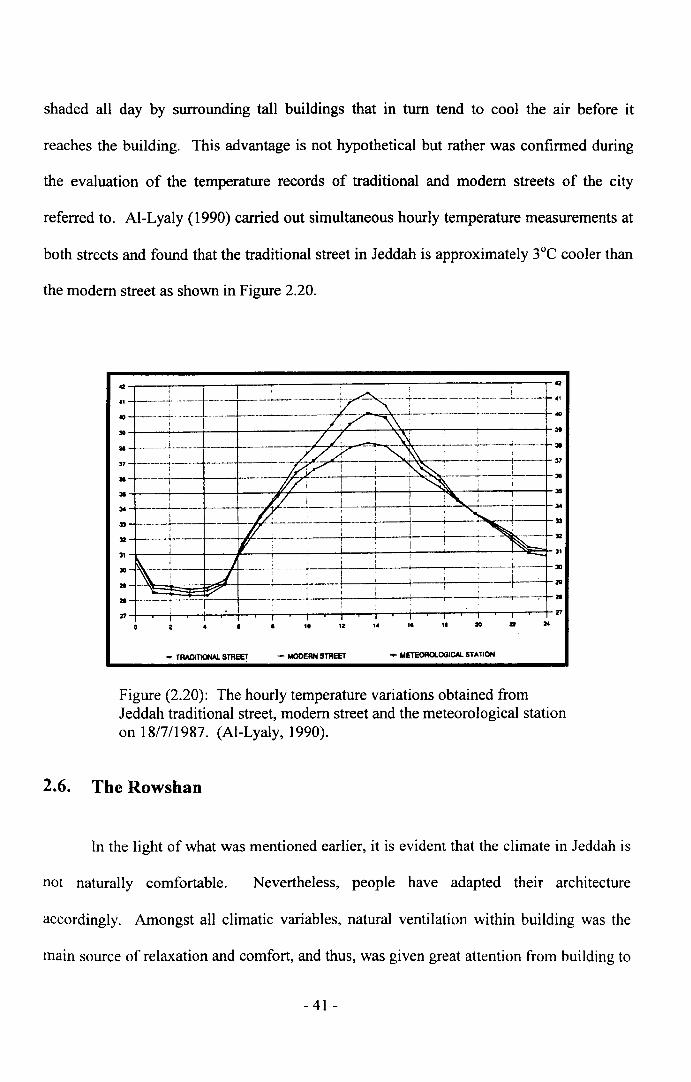
shaded all day by surrounding tall buildings that in turn tend to cool the air before it
reaches the building. This advantage is not hypothetical but rather was confirmed during
the evaluation of the temperature records of traditional and modem streets of the city
referred to. Al-Lyaly (1990) carried out simultaneous hourly temperature measurements at
both streets and found that the traditional street in Jeddah is approximately s-e cooler than
the modem street as shown in Figure 2.20 .
.---,---,---,---~--~--~------~----------~--T~
: =:::+:=r=T.----=--=:=~_/r.-7'~.~--~--~--4---~----~~--~~~--c---~--~--T·
.---- ..-.•-- ...~-.--~----... 31
.a •z •• .. ••
- TRAOOlONAL STREET - MODERN STREET ... METEOROlOGICAl. STA TlON
Figure (2.20): The hourly temperature variations obtained fromJeddah traditional street, modem street and the meteorological stationon 18/7/1987. (AI-Lyaly, 1990).
2.6. The Rowshan
In the light of what was mentioned earlier, it is evident that the climate in Jeddah is
not naturally comfortable. Nevertheless, people have adapted their architecture
accordingly. Amongst all climatic variables, natural ventilation within building was the
main source of relaxation and comfort, and thus, was given great attention from building to
- 41 -

the urban planning scale. The Rowshan is the major window type adopted in Jeddah as it
answered the climatic and social needs of the occupants inside the dwelling. The
Rowshan's origination, configuration, types and applications are discussed in the following
subsections.
2.6.1. Historical background
The projected window bay- the Rowshan- does not only glorify the traditional
architecture in Jeddah but it is rather a distinctive feature replicated in many structures
across the world:
"The distinguishing external features of the old houses of the Red
Sea and some other Islamic and Indian styles are the large casement
windows jutting-out into the street to catch the slightest passing breeze, "
(Greenlaw, 1976).
Its name may differ but its role remains similar: an environmental modulator. In other
words, it is a transition between harsh outdoor and comfortable indoor environments,
acting as a shield against direct solar radiation and glare, insects, dust and undesired flows.
Equally, it is designed to exploit natural breeze through its detailed apertures. Its
development also reflects occupants' social values.
The origin of Rowshan is still debatable. Some refer it back to the ancient castles
built thousands of years ago when Rowshans were used merely for defensive purposes,
while others refer its origin to Turkey or India (AI Shareef, 1996). But according to Khan
(1986), the Rowshan is primarily an Islamic technique that has been modified and adapted
by many others later. This argument is also supported by some Islamic literature. Back in
1100AD, the prominent scholar Ibn AL-Qaim AL-Joziah (1997) cited the word
- 42-
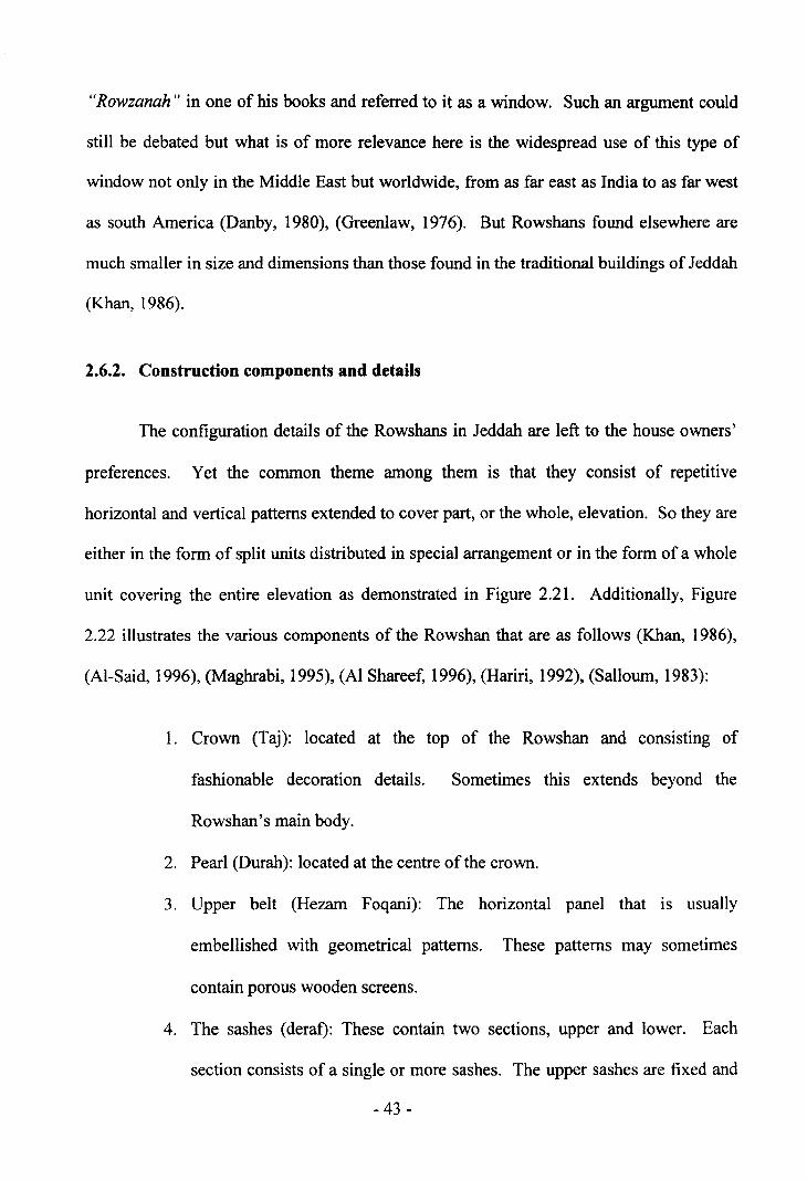
"Rowzanah" in one of his books and referred to it as a window. Such an argument could
still be debated but what is of more relevance here is the widespread use of this type of
window not only in the Middle East but worldwide, from as far east as India to as far west
as south America (Danby, 1980), (Greenlaw, 1976). But Rowshans found elsewhere are
much smaller in size and dimensions than those found in the traditional buildings of Jeddah
(Khan, 1986).
2.6.2. Construction components and details
The configuration details of the Rowshans in Jeddah are left to the house owners'
preferences. Yet the common theme among them is that they consist of repetitive
horizontal and vertical patterns extended to cover part, or the whole, elevation. So they are
either in the form of split units distributed in special arrangement or in the form of a whole
unit covering the entire elevation as demonstrated in Figure 2.21. Additionally, Figure
2.22 illustrates the various components of the Rowshan that are as follows (Khan, 1986),
(AI-Said, 1996), (Maghrabi, 1995), (AI Shareef, 1996), (Hariri, 1992), (Salloum, 1983):
1. Crown (Taj): located at the top of the Rowshan and consisting of
fashionable decoration details. Sometimes this extends beyond the
Rowshan's main body.
2. Pearl (Durah): located at the centre of the crown.
3. Upper belt (Hezam Foqani): The horizontal panel that is usually
embellished with geometrical patterns. These patterns may sometimes
contain porous wooden screens.
4. The sashes (deraf): These contain two sections, upper and lower. Each
section consists of a single or more sashes. The upper sashes are fixed and
- 43 -
the one underneath moves up and down behind the sash above through side
grooves and rests on two hinges leaving a complete aperture. Every sash
contains a number of horizontal wooden slats (louver blades). These are
J/~'tr'
Figure (2.21): The various types of Rowshans found in Jeddah.(Khan, 1986).
movable in circular manner around their axes. They are called Qalaleeb,
referring to the modulated louver windows (MLW). Al-Shareef (1996)
indicated that every sash contains 12-18 louver blades.
- 44-
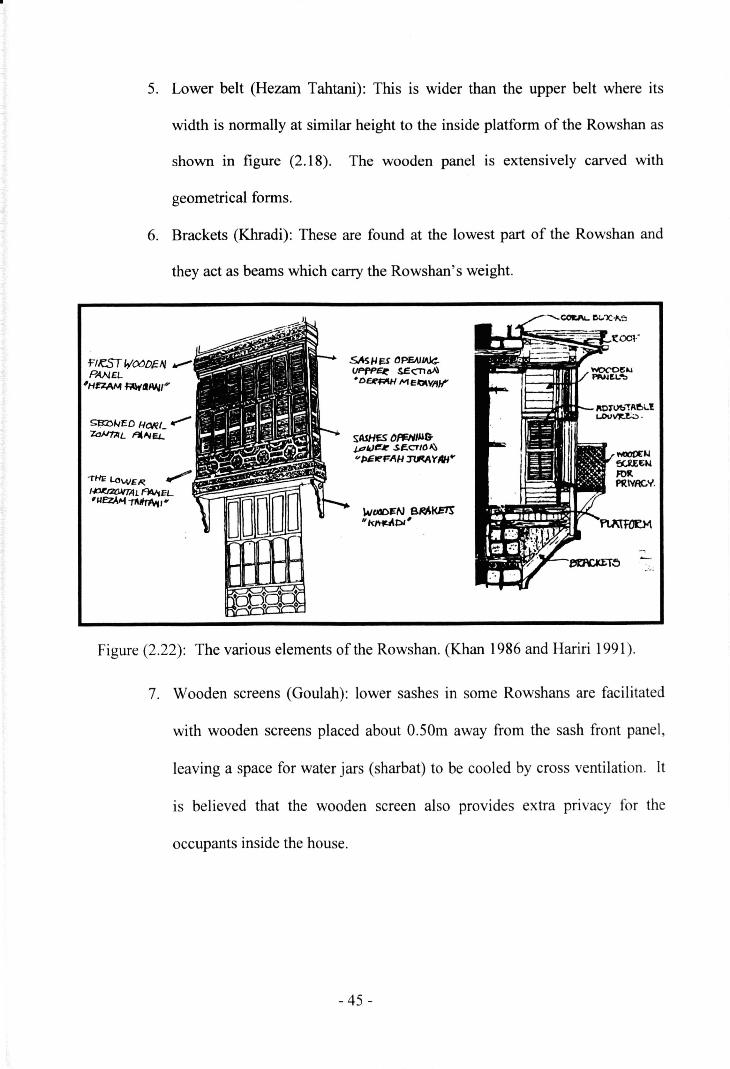
5. Lower belt (Hezam Tahtani): This is wider than the upper belt where its
width is normally at similar height to the inside platform of the Rowshan as
shown in figure (2.18). The wooden panel is extensively carved with
geometrical forms.
6. Brackets (Khradi): These are found at the lowest part of the Rowshan and
they act as beams which carry the Rowshan' s weight.
~11eST 1,.j000Dt=NPANEL
'H~~IIANI4"
s:t3::2)NE. D HOI( t: .--Za)./"f;t/ L I'll ~ tu:
SAsHI:S llPlWW<:.UPf'P~ SEcnGA\'DElrR4H ME~VIlIt'
SASHES ()~//J&JP"'~ se.atO""'-.,/lEI('FAH :rIM 'f1fH"
Figure (2.22): The various elements of the Rowshan. (Khan 1986 and Hariri 1991).
7. Wooden screens (Goulah): lower sashes in some Rowshans are facilitated
with wooden screens placed about O.SOm away from the sash front panel,
leaving a space for water jars (sharbat) to be cooled by cross ventilation. It
is believed that the wooden screen also provides extra privacy for the
occupants inside the house.
- 45 -
2.6.3. Types of Rowshans
Khan (1986) and Hariri (1992) agree that the classification of Rowshans falls under
two main types including the split unit and the vertical long Rowshan (Figure 2.21). The
latter extends to a number of floors to cover most of or the entire elevation. In some cases
it extends from the ground level till reaching the uppermost floors or ends just under the
terrace parapet located on the uppermost floor. The split units Rowshans are isolated to
cover part of the room and are distributed in certain arrangements to shape the overall
elevation. According to Salloum (1983), the Rowshans in Jeddah are either in the form of
a simple window opening covered by wooden screens of modulated louvers, or are the
extended wind bay projecting from the elevation and offering an extension to the interior
spaces. Another type is on the uppermost floors, Al-Mabit, where the room is surrounded
by wooden louvers on two or three sides as stated previously in this chapter (Figure2.18).
2.6.4. Rowshan Application
Through the various louver apertures, the Rowshan serves the following functions:
1. Natural ventilation: Cooling the occupants within the traditional dwelling
through louver apertures is part of the significance of the Rowshan as it acts
as a modulator to the airflow pattern, to its velocity and to the flow rate of
passing au. The occupants are cooled through positioning the louver
apertures at body level so that even at higher air temperature there is
cooling by sweat evaporation (Al-Lyaly, 1990), (Sharma and Sharafat,
1986), (Oliveira and Bittencourt, 1998).
- 46-
2. Humidity: The continuous cross ventilation is extremely important as it
controls humidity within the space (Koenigsberger et al. 1977).
Additionally, a local craftsman indicated that the Rowshans in Jeddah
reduce air-moisture passing through their apertures, .....due to the wood
types used, " (Maghrabi, 1995).
3. Solar shading: Generally, the direct solar radiation in Jeddah is
undesirable, especially in the summer periods (AI Shareef, 1996). Shading
is then desired to control the large amount of radiation, and yet, let interiors
be daylit. As indicated by Khan (1986) the daylight penetrating through
louvers and various screen geometries reflect an attractive play of light and
shadow in the room and the patterns are altered throughout the day
4. Privacy: The Rowshan cantilevers from the building into the outdoor, and
yet, provides a high level of visual privacy. From inside, the Rowshan
platform sometimes rises from floor level and women enjoy observing the
daily life in the streets while still invisible to people outdoors. Also,
difference of illumination levels between indoor and outdoor favours more
privacy. As explained by Al-Lyaly (1990):" ...when looking towards the
Rowshan from the outside, the solid areas formed by the wooden louvers
would be bright and in contrast the gaps in between would be dark
prohibiting a view of the interior. "
- 47-
2.7. Conclusion
This chapter has highlighted the climatic adaptation to architecture in the regional context
and in particular to natural ventilation approaches seeking to adapt the micro and
macroclimate environments in Jeddah.
Saudi Arabia generally falls under tropical climate zones. However, when the
climate was observed it was found that the distribution of land and sea masses, added to
the land topographies, have created some sub-climatic zones that mayor may not refer to
the general climate. This has led to various styles of traditional architecture that reveal
deep responses to climatic variations. When Jeddah's climate and architecture were
closely observed, the following points were concluded:
1. The climate of Jeddah is not naturally comfortable and the wind-induced
natural ventilation was considered to control the excessive heat and
humidity as a treatment to achieve comfort and relaxation. This is reflected
on both micro and macroclimate scales.
2. Within the scale of a typical dwelling, the modulated louvered windows
(MLW) found in Rowshans, Mashrabiah, Taqqat or other apertures
components are believed to be the main solution to controlling the breezes
needed to release climatic stresses and bring comfort within the dwelling.
These types of windows answer bio-climatic necessities as well as social
requirements. The MLW will be discussed in detail in the next chapter.
- 48-

2.S. References
1. MS Encarta World Atlas. Anonymous (1997) 97. USA: Microsoft.
2. AI-Ansari, J., Bakhsh, H. and Madni, I. (1985) Wind energy atlas for the Kingdom of Saudi
Arabia. p.S6p King Abdulaziz City for Science and Technology.
3. AI-Joziah, I.A.-Q. (1997) Iqhthat AI-Lahfan Min Makaa'd AI-Shatian, 2 edn. Dar AI-Kitab
AI-Arabi.
4. AI-Lyaly, S.M. (1990) The traditional house of Jeddah: A study of the interaction between
climate, form, and living patterns. University of Edinburgh. Unpublished Ph.D.
5. AI-Megren, K. (1987) Wind towers for passive ventilation cooling in hot-arid regions. The
University of Michigan. Unpublished Doctor of Architecture.
6. AI-Said, M. (1996) The Rowshan in the Western Province. SED-308/l4l6, King
Abdulaziz University: School of Environmental Design.
7. AI Shareef, F.M. (1996) Natural light control in Hedjazi Architecture; An investigation of
the Rowshan performance by computer simulation. University of Liverpool. Unpublished
Ph.D. thesis.
8. Awbi, H.B. (1991) Ventilation of Buildings, London: E & FN Spon.
9. Bokhari, A. (1978) Jeddah, a study in urban formation. University of Pennsylvania,
Philadelphia. Unpublished Ph.D.
10. Danby, M. (1980) "The Islamic architectural tradition and the house, with special reference
to the Middle East". p.200-208, Dammam, Saudi Arabia: King Faisal University.
- 49-

11. Edwards, F. (1987) Climate and Oceanography. In: Edwards, A. and Head, S., (Eds.) Red
Sea, London: Pergamon Press.
12. Evans, B. H. (1979) "Energy conservation with natural air flow through windows". (5), 2
edn. p.641-650, ASHRAE Transactions.
13. Fathy, H. (1986) Natural Energy and Vernacular Architecture, Chicago: Chicago press.
14.Fathy, H. and Sultan, A.A. (1985) "AI Malkaf: A traditional cooling and ventilation system".
Sun World 9-(2),
15. Givoni, B. (1981) Man, Climate and Architecture, 2nd edn. London: Applied Science
Publishers Ltd.
16. Greenlaw, J. (1976) The Coral Buildings of Suakin, London: Oriel Press.
17. Hariri, M. (1992) "The design of the Rowshan and its importance to the dwelling". Journal
ofUmm Al-Qura University (5), p.175-237.
18. Hariri, Majdi (1993) ""Kharijah"". p.22p, Cairo: Third International Science Conference.
19. Hemeid, A.A. (1999) Desirable courtyard orientation and proportion for the Riyadh region.
pp.2B-36-2B-64. King Saud University.
20. Kaizer, T. (1984) Shelter in Saudi Arabia., London: Academy Editions.
21. Khan, S. (1986) Jeddah Old Houses, Saudi Arabia: King Abdulaziz City for Science and
Technology.
22. Kilical, A.A. (199) Traditional architecture in Riyadh. pp.52-57. Riyadh: King Saud
University.
- 50 -

23. Koenigsberger, 0., Ingresoll, T., Mayhew, A. and Szokolay, S. (1977) Manual of Tropical
Housing. Part One: Climatic Design, London: Longman Group Ltd.
24. Konya, A. (1980) Design primer for hot climates, London: Architectural Press.
25. Kukerja, C. (1978) Tropical Architecture, New Delhi: Tata McGrow-Hill Publishing
Company ltd.
26. Maghrabi, A. (1993) The revival of adobe architecture in the Arabian region. Unpublished
report.
27. Maghrabi, A. (1995). Personal communication with local craftsman. leddah, Saudi Arabia.
28. Mani', M. (1980) The Architectural features to old leddah. vo!.l, pp.l 00-1 08. leddah: AI-
Salam.
29. Markus, T.A. and Morris, E.N. (1980) Buildings, Climate and Energy, London: PITMAN.
30. Mauger, T. (1996) Impressions of Arabia, Paris, France: Flammarrion
31. MEPA 1983. Meteorology & Environmental Protection Administration. leddah:
Meteorology & Environmental Protection Administration.
32. Najib, A. (1987) The climate in Jeddah: the Bridge of the Red Sea, Cairo: The Arabian
publishing house for Encyclopedias.
33. Olgyay, V. and Olgyay, A. (1976) Design with climate; Bio-c1imatic approach to
Architectural regionalism, Princeton N.J.: Princeton University Press.
34. Olgyay, V. (1963) Design with climate, Princeton N.J.: Princeton University Press.
- 51 -
35. Oliveira, F. and Bittencourt, L. S. (1998) "Air flow through louvered windows in small
rooms". PLEA I 98. Lisbon, Portugal, p.393-396,
36. Said, S.-A. and AI-Zaharnah, E.T. (1994) "Development of comfort zone charts using the
Isopleth charts technique". Building and Environment 29 (1), p.13-20.
37. Salloum, A. (1983) "EI-Rowashin ofJeddah, Saudi Arabia". p.245-252, Crete, Greece:
Passive and Low Energy Architecture (PLEA).
38. Sanderson, R. (1982) Meteorology at Sea, London: Sanford Maritime.
39. Sharma, M.R. and Sharafat, A. (1986) "Tropical summer index - a study of thermal comfort
ofIndian subjects". Building and Environment 21 (1), p.11-24.
40. Winterhalter, C.P. (1982) "Environmental control in the indigenous architecture of the
Eastern Province of Saudi Arabia". The Arabian journal for science and Engineering. 7 (2),
p.112-121.
- 52 -
CHAPTER 3: MODULATED LOUVERED WINDOWS
(MLW).
3.1. Introduction
This chapter reviews the current research and contribution made to observe
modulated louvered windows (MLW) as a source of natural ventilation in buildings. In
addition, it sets out the approach to the theoretical thrust of this research. The first section
reviews the conventional window types and highlights some of their ventilation
characteristics. Then follows the discussion of the louver window systems including the
horizontal, vertical and combined systems. The third section is devoted to the review of
the relevant research carried out in relation to MLW and to addressing closely the
evaluation and critique of each one of them.
The chapter ends up by stating the problem of the current research based on the
review of the aforementioned chapters concerning the climate and architecture in Jeddah as
well as on the review of modulated louvered windows as the source of natural ventilation
in buildings.
- 54-
3.2. Conventional window types
Back In 1951, Holleman (1951) carried out research on airflow through
conventional window openings and concluded that airflow characteristics differ
significantly due to these different opening types. Holleman and Evans (1979) agreed that
common windows used are classified under three basic types; simple opening, vertical
vane and horizontal vane as illustrated in Figure 3.1. These categories seem valid and
cover most of the types commonly employed in buildings. The perforated block walls are
of porous elements that are widely employed in the tropics; they discussed here along with
other window types.
3.2.1. Simple openings (Holleman, 1951)
Simple openings include the single-hung, the double-hung and the horizontal-hung.
The direction of passing air was not affected and continued in the same wind direction.
However, a noticeable significant change of speed was evident near the window. This was
referred to as the squeeze of air and Holleman recommended this type to be used directly
in living zones. The maximum opening area is one-half the total window area: 50%
opening. These windows are recommended directly in the occupied zone since neither the
direction nor the speed of air was altered.
3.2.2. Vertical vane openings (Holleman, 1951)
Vertical vane openings include such openings as side-hinged casement, the folding
casement, and the vertical pivot. These windows allow complete opening area: 100%
opening. Generally they provide alteration of airflow at horizontal level and it was
recommended to allocate them directly to the occupied zone.- 55 -
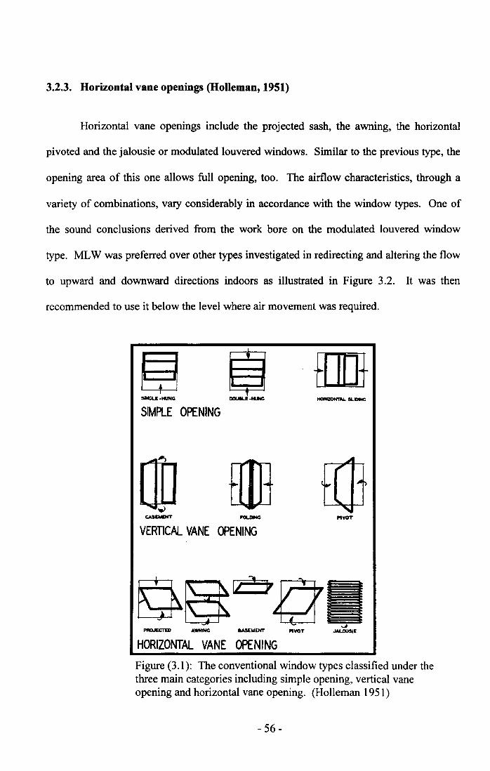
3.2.3. Horizontal vane openings (Holleman, 1951)
Horizontal vane openings include the projected sash, the awning, the horizontal
pivoted and the jalousie or modulated louvered windows. Similar to the previous type, the
opening area of this one allows full opening, too. The airflow characteristics, through a
variety of combinations, vary considerably in accordance with the window types. One of
the sound conclusions derived from the work bore on the modulated louvered window
type. MLW was preferred over other types investigated in redirecting and altering the flow
to upward and downward directions indoors as illustrated in Figure 3.2. It was then
recommended to use it below the level where air movement was required.
I'tYOT
SINCl.! -HUNG
SIMPLE OPENING
ODVERTICAL VANE OPENING
HORIZONTAL VANE OPENINGFigure (3.1): The conventional window types classified under thethree main categories including simple opening, vertical vaneopening and horizontal vane opening. (Holleman 1951)
- 56-
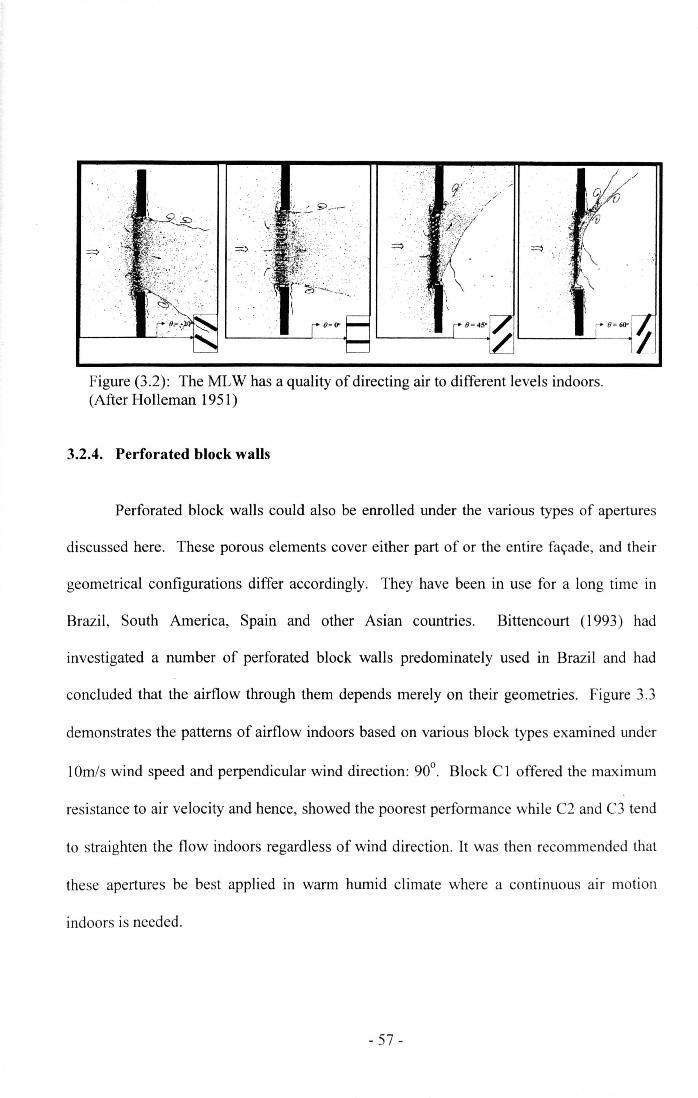
Figure (3.2): The MLW has a quality of directing air to different levels indoors.(After Holleman 1951)
3.2.4. Perforated block walls
Perforated block walls could also be enrolled under the various types of apertures
discussed here. These porous elements cover either part of or the entire facade, and their
geometrical configurations differ accordingly. They have been in use for a long time in
Brazil, South America, Spain and other Asian countries. Bittencourt (1993) had
investigated a number of perforated block walls predominately used in Brazil and had
concluded that the airflow through them depends merely on their geometries. Figure 3.3
demonstrates the patterns of airflow indoors based on various block types examined under
10mls wind speed and perpendicular wind direction: 90°. Block Cl offered the maximum
resistance to air velocity and hence, showed the poorest performance while C2 and C3 tend
to straighten the flow indoors regardless of wind direction. It was then recommended that
these apertures be best applied in warm humid climate where a continuous air motion
indoors is needed.
- 57 -
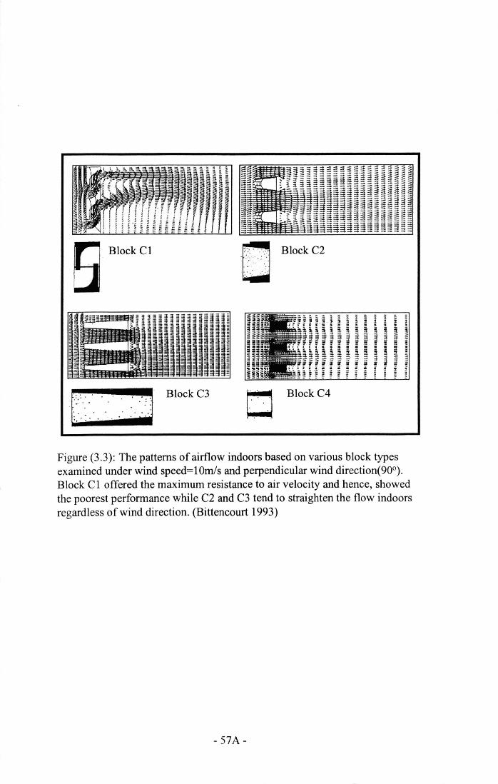
Block Cl
t...:...·f·.· .
'.J Block C3
l'i:] Block C2
~~
Block C4
Figure (3.3): The patterns of airflow indoors based on various block typesexamined under wind speed=lOmls and perpendicular wind directioru'Xr').Block Cl offered the maximum resistance to air velocity and hence, showedthe poorest performance while C2 and C3 tend to straighten the flow indoorsregardless of wind direction. (Bittencourt 1993)
- 57A-
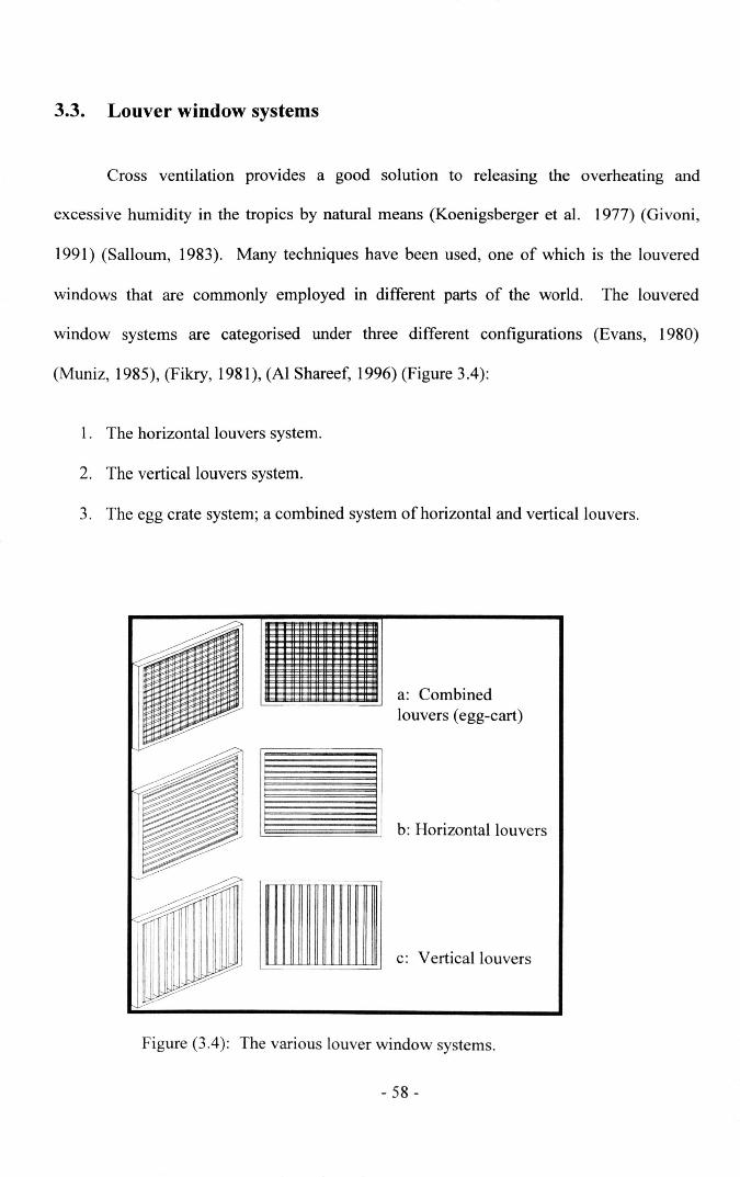
3.3. Louver window systems
Cross ventilation provides a good solution to releasing the overheating and
excessive humidity in the tropics by natural means (Koenigsberger et al. 1977) (Givoni,
1991) (Salloum, 1983). Many techniques have been used, one of which is the louvered
windows that are commonly employed in different parts of the world. The louvered
window systems are categorised under three different configurations (Evans, 1980)
(Muniz, 1985), (Fikry, 1981), (AI Shareef, 1996) (Figure 3.4):
1. The horizontal louvers system.
2. The vertical louvers system.
3. The egg crate system; a combined system of horizontal and vertical louvers.
a: Combinedlouvers (egg-cart)
b: Horizontal louvers
c: Vertical louvers
Figure (3.4): The various louver window systems.
- 58 -
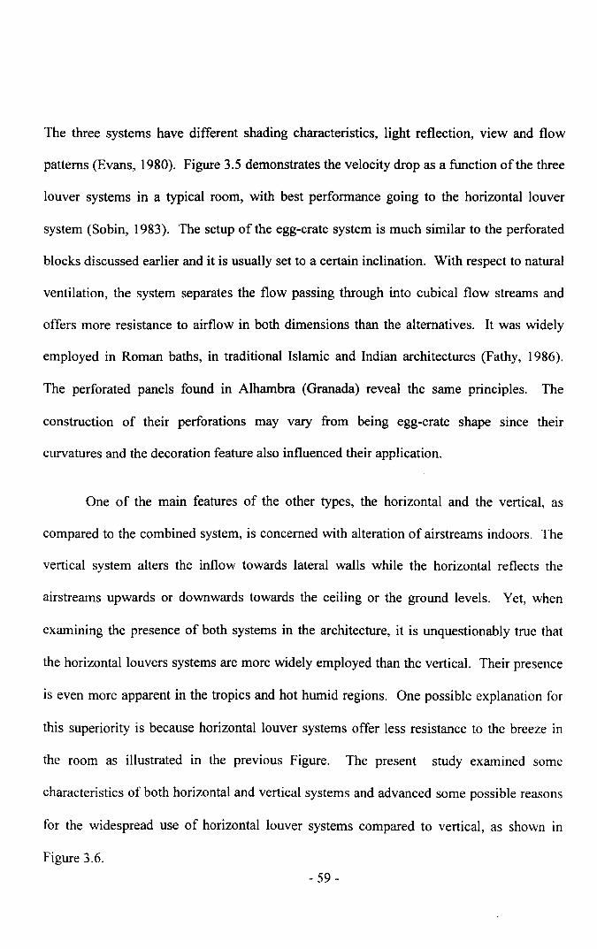
The three systems have different shading characteristics, light reflection, view and flow
patterns (Evans, 1980). Figure 3.5 demonstrates the velocity drop as a function of the three
louver systems in a typical room, with best performance going to the horizontal louver
system (Sobin, 1983). The setup of the egg-crate system is much similar to the perforated
blocks discussed earlier and it is usually set to a certain inclination. With respect to natural
ventilation, the system separates the flow passing through into cubical flow streams and
offers more resistance to airflow in both dimensions than the alternatives. It was widely
employed in Roman baths, in traditional Islamic and Indian architectures (Fathy, 1986).
The perforated panels found in Alhambra (Granada) reveal the same principles. The
construction of their perforations may vary from being egg-crate shape since their
curvatures and the decoration feature also influenced their application.
One of the main features of the other types, the horizontal and the vertical, as
compared to the combined system, is concerned with alteration of airstreams indoors. The
vertical system alters the inflow towards lateral walls while the horizontal reflects the
airstreams upwards or downwards towards the ceiling or the ground levels. Yet, when
examining the presence of both systems in the architecture, it is unquestionably true that
the horizontal louvers systems are more widely employed than the vertical. Their presence
is even more apparent in the tropics and hot humid regions. One possible explanation for
this superiority is because horizontal louver systems offer less resistance to the breeze in
the room as illustrated in the previous Figure. The present study examined some
characteristics of both horizontal and vertical systems and advanced some possible reasons
for the widespread use of horizontal louver systems compared to vertical, as shown ill
Figure 3.6.- 59 -
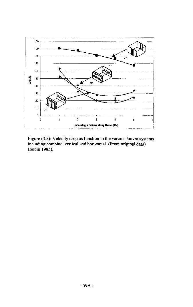
100
90 •80
70
60~ 50"~;:..
40
30
20·
10 ~ __ ~~-
~-~ --.---... -
~~----==---~-··--·I~----! -~----I
-------.-.---- ----Io 0---··-·-·-.--------;--~···__;_·---,-4 --~-~-;--~-···--1
. ....._ .. .__. ~a~~~~1IS a~~ ROCI~(R_~_... IIt,
Figure (3.5): Velocity drop as function to the various louver systemsincluding combine, vertical and horizontal. (From original data)(Sobin 1983).
- 59A-
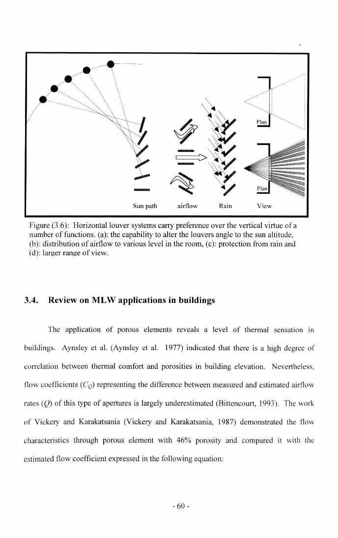
-Sun path
\.
airflow Rain View
Figure (3.6): Horizontal louver systems carry preference over the vertical virtue of anumber of functions. (a): the capability to alter the louvers angle to the sun altitude,(b): distribution of airflow to various level in the room, (c): protection from rain and(d): larger range of view.
3.4. Review on MLW applications in buildings
The application of porous elements reveals a level of thermal sensation In
buildings. Aynsley et al. (Aynsley et al. 1977) indicated that there is a high degree of
correlation between thermal comfort and porosities in building elevation. Nevertheless,
flow coefficients (CQ) representing the difference between measured and estimated airflow
rates (Q) of this type of apertures is largely underestimated (Bittencourt, 1993). The work
of Vickery and Karakatsania (Vickery and Karakatsania, 1987) demonstrated the flow
characteristics through porous element with 46% porosity and compared it with the
estimated flow coefficient expressed in the following equation:
- 60-
(3.1)
where
CQ= Flow coefficient
Q = Volumetric flow of air (m3/s)
A = Opening area (m2)
V= Wind speed at opening level (m/s)
e. Z~ ,---6"'-.......-,-----,~ / --.
·'.~~ItCl\
"\'\\\\
0."Co
0.0'
I"
0.0' L with win; waif.(P ·'6%
'wlnd Ingl. 0
._._.
\ o
30' 60·
Figure (3.7): Flow coefficients for both observed and predictedcurves with wall porosity of 46%. (Vickery & Karakatsania19R7t
From Figure 3.7, the observed values were obviously less than those predicted values for
wind indices between 20° and 90° while in perpendicular wind (0°) both were nearly
similar. Also the critical drop in both curves was present with skewed inclinations- when
B> 45°- where they may then produce errors that seriously lead to mistaken readings. The
- 61 -
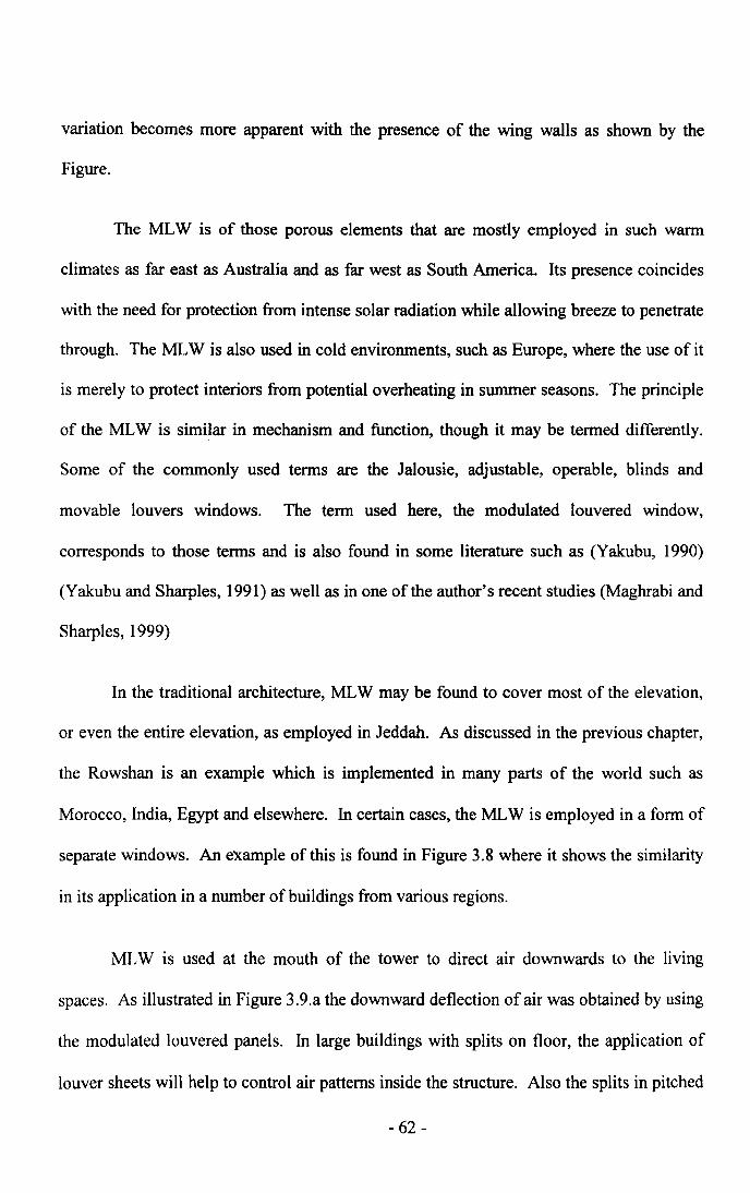
variation becomes more apparent with the presence of the wing walls as shown by the
Figure.
The MLW is of those porous elements that are mostly employed in such warm
climates as far east as Australia and as far west as South America. Its presence coincides
with the need for protection from intense solar radiation while allowing breeze to penetrate
through. The MLW is also used in cold environments, such as Europe, where the use of it
is merely to protect interiors from potential overheating in summer seasons. The principle
of the MLW is similar in mechanism and function, though it may be termed differently.
Some of the commonly used terms are the Jalousie, adjustable, operable, blinds and
movable louvers windows. The term used here, the modulated louvered window,
corresponds to those terms and is also found in some literature such as (Yakubu, 1990)
(Yakubu and Sharples, 1991) as well as in one of the author's recent studies (Maghrabi and
Sharples, 1999)
In the traditional architecture, MLW may be found to cover most of the elevation,
or even the entire elevation, as employed in Jeddah. As discussed in the previous chapter,
the Rowshan is an example which is implemented in many parts of the world such as
Morocco, India, Egypt and elsewhere. In certain cases, the MLW is employed in a form of
separate windows. An example of this is found in Figure 3.8 where it shows the similarity
in its application in a number of buildings from various regions.
MLW is used at the mouth of the tower to direct air downwards to the living
spaces. As illustrated in Figure 3.9.a the downward deflection of air was obtained by using
the modulated louvered panels. In large buildings with splits on floor, the application of
louver sheets will help to control air patterns inside the structure. Also the splits in pitched
- 62-
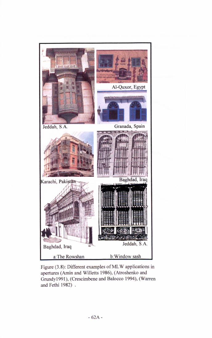
a:The Rowshan b:Window sash
Figure (3.8): Different examples ofML W applications inapertures (Amin and Willetts 1986), (Atroshenko andGrundy1991), (Crescimbene and Balocco 1994), (Warrenand Fethi 1982) .
- 62A-
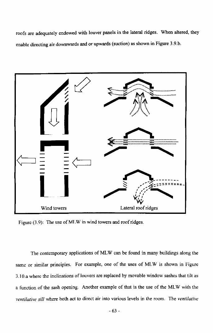
roofs are adequately endowed with louver panels in the lateral ridges. When altered, they
enable directing air downwards and or upwards (suction) as shown in Figure 3.9.b.
Dr-I
(=J ¢==J
l__JWind towers
c.. :].~. ~ ....•........:•....:..................~ ~ ..~ ~ M····~···························
~\!A~'=' ...· .. .· .. .· ., ...•. .... .... ..•.r» ',,'," 't
"----------... './'... 'L - - - - - - - - -, ~-----------, ", :t:!:"..
I ' .. ~I "I I\!~,,'-WtLateral roof ridges
Figure (3.9): The use ofMLW in wind towers and roof ridges.
The contemporary applications of MLW can be found in many buildings along the
same or similar principles. For example, one of the uses of MLW is shown in Figure
3.1O.a where the inclinations of louvers are replaced by movable window sashes that tilt as
a function of the sash opening. Another example of that is the use of the MLW with the
ventilative sill where both act to direct air into various levels in the room. The ventilative
- 63 -
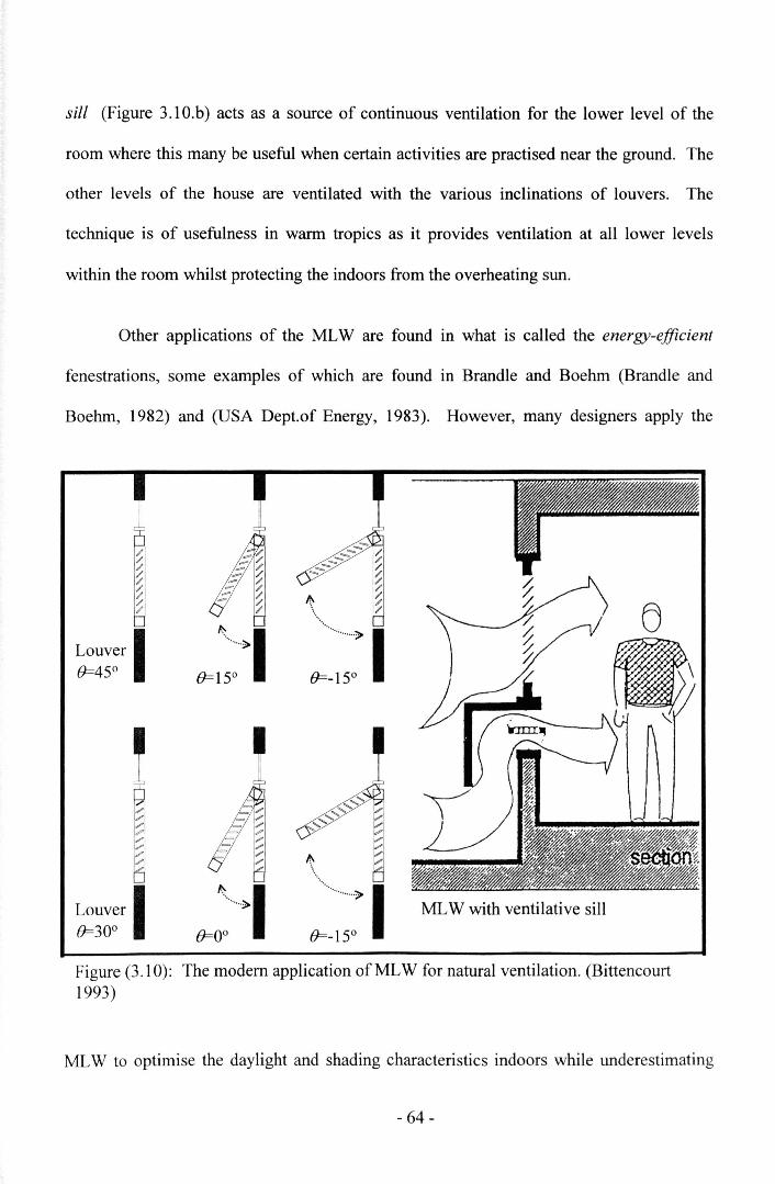
sill (Figure 3.10.b) acts as a source of continuous ventilation for the lower level of the
room where this many be useful when certain activities are practised near the ground. The
other levels of the house are ventilated with the various inclinations of louvers. The
technique is of usefulness in warm tropics as it provides ventilation at all lower levels
within the room whilst protecting the indoors from the overheating sun.
Other applications of the MLW are found in what is called the energy-efficient
fenestrations, some examples of which are found in Brandle and Boehm (Brandle and
Boehm, 1982) and (USA Dept.of Energy, 1983). However, many designers apply the
Louver0=450
LouverI0=300
~..........>
A
\ >
A
:~1:~I MLWwith ventilative sill
Figure (3.10): The modem application of MLW for natural ventilation. (Bittencourt1993)
MLW to optimise the daylight and shading characteristics indoors while underestimating
- 64-
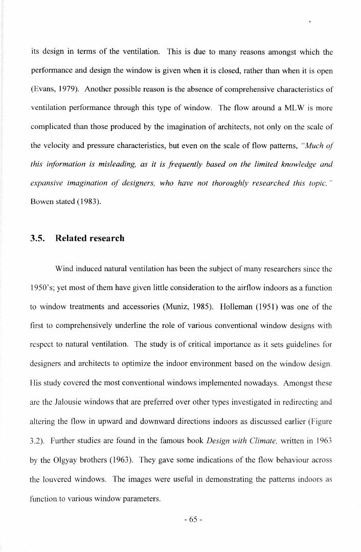
its design in terms of the ventilation. This is due to many reasons amongst which the
performance and design the window is given when it is closed, rather than when it is open
(Evans, 1979). Another possible reason is the absence of comprehensive characteristics of
ventilation performance through this type of window. The flow around a MLW is more
complicated than those produced by the imagination of architects, not only on the scale of
the velocity and pressure characteristics, but even on the scale of flow patterns, "Much of
this information is misleading, as it is frequently based on the limited knowledge and
expansive imagination of designers, who have not thoroughly researched this topic, "
Bowen stated (1983).
3.5. Related research
Wind induced natural ventilation has been the subject of many researchers since the
1950's; yet most of them have given little consideration to the airflow indoors as a function
to window treatments and accessories (Muniz, 1985). Holleman (1951) was one of the
first to comprehensively underline the role of various conventional window designs with
respect to natural ventilation. The study is of critical importance as it sets guidelines for
designers and architects to optimize the indoor environment based on the window design.
His study covered the most conventional windows implemented nowadays. Amongst these
are the Jalousie windows that are preferred over other types investigated in redirecting and
altering the flow in upward and downward directions indoors as discussed earlier (Figure
3.2). Further studies are found in the famous book Design with Climate, written in 1963
by the Olgyay brothers (1963). They gave some indications of the flow behaviour across
the louvered windows. The images were useful in demonstrating the patterns indoors as
function to various window parameters.
- 65 -
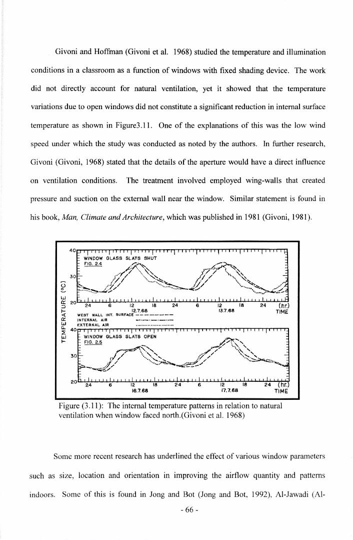
Givoni and Hoffman (Givoni et al. 1968) studied the temperature and illumination
conditions in a classroom as a function of windows with fixed shading device. The work
did not directly account for natural ventilation, yet it showed that the temperature
variations due to open windows did not constitute a significant reduction in internal surface
temperature as shown in Figure3.11. One of the explanations of this was the low wind
speed under which the study was conducted as noted by the authors. In further research,
Givoni (Givoni, 1968) stated that the details of the aperture would have a direct influence
on ventilation conditions. The treatment involved employed wing-walls that created
pressure and suction on the external wall near the window. Similar statement is found in
his book, Man, Climate and Architecture, which was published in 1981 (Givoni, 1981).
oo
WINDOW GLASS SLATS SHUT
FIG. 2.4 /-.:-;'~\" r...I.I~;i~~,''1'' / '." " )./ / \""(' / ....'" i/ / .~./// :~~ ~. / .,.... ."
...... /7'./ ·····..·'·~ .•i../ ..:::::......._.~~......... ~.__.:,... '.."..~~-
Figure (3.11): The internal temperature patterns in relation to naturalventilation when window faced north.(Givoni et al. 1968)
Some more recent research has underlined the effect of various window parameters
such as size, location and orientation in improving the airflow quantity and patterns
- 66-
indoors. Some of this is found in long and Bot (long and Bot, 1992), Al-Jawadi (Al-
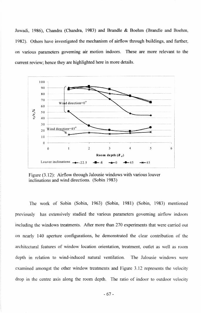
Jawadi, 1986), Chandra (Chandra, 1983) and Brandle & Boehm (Brandle and Boehm,
1982). Others have investigated the mechanism of airflow through buildings, and further,
on various parameters governing air motion indoors. These are more relevant to the
current review; hence they are highlighted here in more details.
10090807060
~ 50"~ 40;:..
3020
10
00 2 3 4 5 6
Room depth (R d)
Louver inclinations -+--22.5 -8 ...... 0 ""_45 -.-45
Figure (3.12): Airflow through Jalousie windows with various louverinclinations and wind directions. (Sobin 1983)
The work of Sobin (Sobin, 1963) (Sobin, 1981) (Sobin, 1983) mentioned
previously has extensively studied the various parameters governing airflow indoors
including the windows treatments. After more than 270 experiments that were carried out
on nearly 140 aperture configurations, he demonstrated the clear contribution of the
architectural features of window location orientation, treatment, outlet as well as room
depth in relation to wind-induced natural ventilation. The Jalousie windows were
examined amongst the other window treatments and Figure 3.12 represents the velocity
drop in the centre axis along the room depth. The ratio of indoor to outdoor velocity
- 67-
(V/Ve%) near the window was 90% for the louvers inclinations 0°, -8° and -22.5°, while a
clear reduction was observed with the presence of steeper inclinations. The study also
demonstrated the significance of the wind direction for the reduction of the ratio of internal
velocity with respect to external (v/ve%). The reduction along the room was obviously
smoother with the perpendicular wind incidence. In addition, the study gave some
indications of the effect of louver angle of inclination with respect to v/ve% as illustrated in
the Figure. Nevertheless, his work disregarded the effect of various parameters of the
louvered windows on the flow indoors. Furthermore, it did not emphasise the flow rate
(Q) with respect to the pressure drop (9) across the window.
Muniz (Muniz, 1985) examined the effect of shading device geometries on natural
ventilation, daylight and thermal comfort. The study was extensive in that it provided
designers with an analytical model in which they could compare various shading
geometries in order to optimise the indoor environment. There were three shading devices
that covered horizontal, vertical and combined geometries. The velocity characteristics
with respect to the former types were generally less marked in perpendicular than In
oblique winds (Figure 3.13).
But when this work is examined in light of the hypothesis of the of current study,
some critical limitations become apparent:
1. The study was limited to only a single wind speed.
2. The louver configurations covered, including louver depth and aperture,
were too large compared with those reviewed in this investigation. The
depth ranged from 0.35m to nearly I.20m; the flow characteristics could not
therefore represent those carried out here.
- 68-
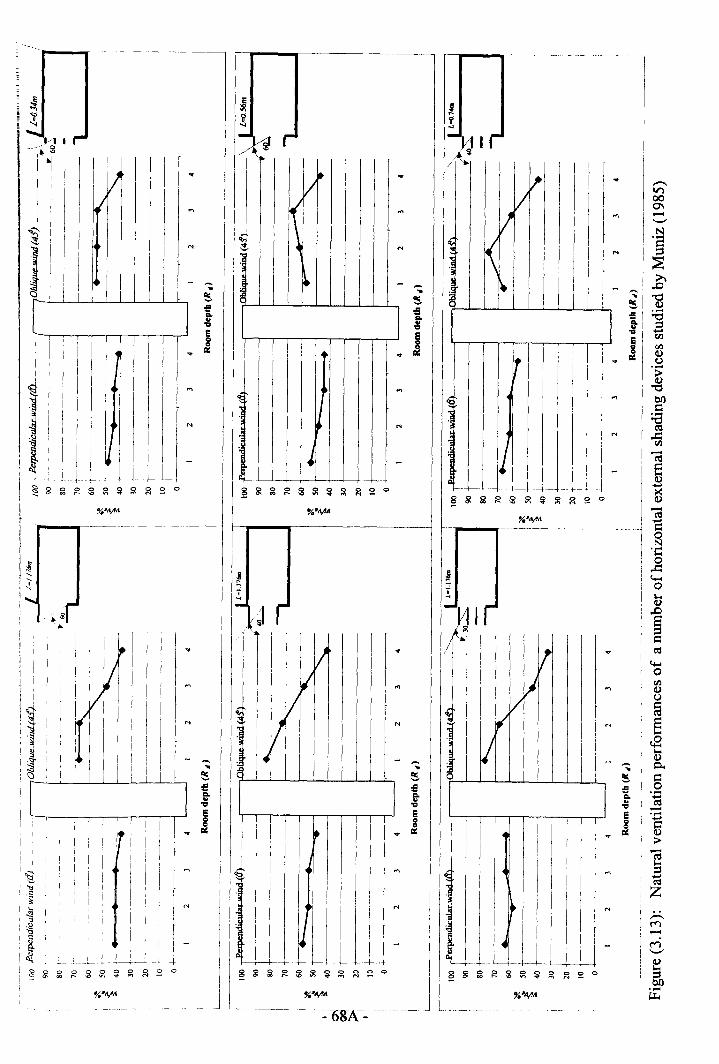
11I lJ II '
I II /i
1 II.~I(
I
I:
II I I
II 1, i
I I
~l:
!
f i-_ --- -f_ -L,-I ~ ~ ill :2
fII
I~i~I
o 0 0 0 000I,() V"I "'" fO'l N -
,,----------------, 11,--....---------------
R'i....l--fJ I/ ..
If
V'/
'"
I~ K I M
1~
r ..
f--\--- ---- -- -- -- -- -----
§ ~ £ g ss ~ ~ g R ~ 0
N
~ 0
11
,..-----~---------- r--.,.--...--------
~ ~i ~....
J 1-~I.. ~~/ ..
I ..,
. f ~
II I : l
I ' II' LJ"-+------1-----+----
i III II 1 I
I,I I, I ,
! I II I i
t I IIIr- -lifl ll,- _§ & ~ g ~ ~ ~ ~ ~ ~ 0
I
I
--In000'1-'-'N'§~»
~ ..c... "ds <I)
i!I....."dQ, E..
"Cl
E til
g til<I)II: U.....;>
l,g01)
.5'i~til
-;~...~<I)-t'::I1::0N.~0~
4-<0
~..c§~t'::I
- ~s
j i!ICo.."Cl
Eg.. II:
..,
N
-
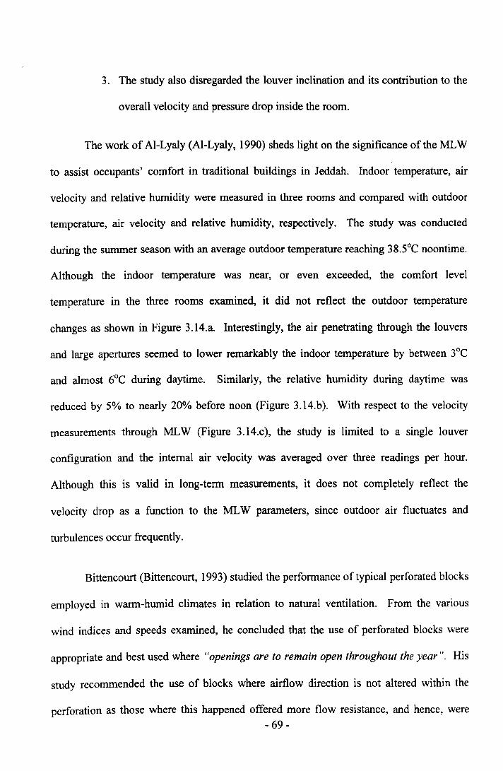
3. The study also disregarded the louver inclination and its contribution to the
overall velocity and pressure drop inside the room.
The work of AI-Lyaly (AI-Lyaly, 1990) sheds light on the significance of the MLW
to assist occupants' comfort in traditional buildings in Jeddah. Indoor temperature, air
velocity and relative humidity were measured in three rooms and compared with outdoor
temperature, air velocity and relative humidity, respectively. The study was conducted
during the summer season with an average outdoor temperature reaching 38.5°C noontime.
Although the indoor temperature was near, or even exceeded, the comfort level
temperature in the three rooms examined, it did not reflect the outdoor temperature
changes as shown in Figure 3.14.a. Interestingly, the air penetrating through the louvers
and large apertures seemed to lower remarkably the indoor temperature by between 3°C
and almost 6°C during daytime. Similarly, the relative humidity during daytime was
reduced by 5% to nearly 20% before noon (Figure 3.14.b). With respect to the velocity
measurements through MLW (Figure 3.14.c), the study is limited to a single louver
configuration and the internal air velocity was averaged over three readings per hour.
Although this is valid in long-term measurements, it does not completely reflect the
velocity drop as a function to the MLW parameters, since outdoor air fluctuates and
turbulences occur frequently.
Bittencourt (Bittencourt, 1993) studied the performance of typical perforated blocks
employed in warm-humid climates in relation to natural ventilation. From the various
wind indices and speeds examined, he concluded that the use of perforated blocks were
appropriate and best used where "openings are to remain open throughout the year". His
study recommended the use of blocks where airflow direction is not altered within the
perforation as those where this happened offered more flow resistance, and hence, were- 69-
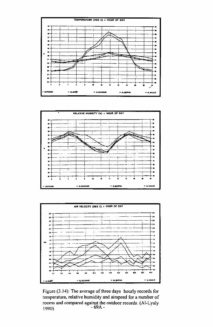
TEMPERATURE IDEO Cl • HOUR OF DAY
..••>1
••....
" •....••~••
, I I i , ,i /'l : I- ~
I i : I /~" Ii : / V i "l.'\ i
I i// --l---' "\\/y I '\ :
: iC"i I I...:::::.;.. '\ i
! , /Y ~ ! :--I
I:=. ,I \.' ---=,
.//1 ~ ~I I I~ I I I ~
, : I I :
I ,I I i I
,I ,.. II I. II " • . ..
/'-Al._-OUTDOOII
RELATIVE HUMIDITY 1%1 • HOUR OF DAY
• --.----;--i,r---:', ~~~ " ,.. ------.--·-·--r------·--I-·'·~-~·------·--,-"-------,._---,--_.,..4---+--~----+_--~----~-_,_--~--~----+_--~--_r•
II II .. •II ""-AI. .........- OUTDOOII
AIR VELOCITY IDEO Cl • HOUR OF DAY
~------~--------_,_--~--~-------------------~----r"I ,I__ ~_~_~-~~_-- __~".-__,-- __ I -'--------- U-t ----L- _j._-,---_;_-- -------- ...
..U
to
U..U
U
,~OWl
,.I
to....lA
'.1..ID
- Al ...MIT
~--~--~----,_--~--~--4----~--f---~---+--_1~--r~·
--+---------'----i----+----+---+----t---¥~---------~-t_ •.•+--,-:,,-,,__----_!_------ lA
.. .. .. 11.0 , .... tu lU •.• II.CI
- Al.. .... \lAKHIR
Figure (3.14): The average of three days hourly records fortemperature, relative humidity and airspeed for a number ofrooms and compared against the outdoor records. (Al-Lyaly1990) - 69A-
•••17
••....•"•••'D
••
•
....
..
....
unable to produce the minimum ventilation required for comfort in that climatic region
(Figure 3.15). Essentially, the previous statement reflects the importance of MLW in
warm and humid climates where it offers flexibility in adjusting airflow entering the room.
80807060
-so.!,Cl) 40} 30
20
10
°0 1 2 3 4 5 6
,\I,,\
22 DEG ~c,UAU Cl
:::g! 60___ o.s mi.-so.!,Cl) 40~s 30
20
70
wind speed (m/s)
45 OEG~C'UAUC2..... Cl~g:'. mi·
10
°0 2 3 ~ 5 6wind speed (m/s)
90 DEG~ClUAUC2
\,~~m/',
~'i 2 '3 ? 5 6wind speed (m/s)
Figure (3.15): Natural ventilation through perforated blocks asfunction to various wind incidences. (Bittencourt 1993)
Perhaps the most relevant studies in the review are found in (Yakubu, 1990),
(Yakubu and Sharples, 1991), (Pitts and Georgiadis, 1994), (Oliveira and Bittencourt,
1998) and (White, 1999). The work of Yakubu (Yakubu, 1990) and (Yakubu and Sharples,
1991) was conducted under similar louver configurations and measurements setup. Like
the current study, the work investigated the performance of louver window systems under a
series of air extractions. Figure 3.16 illustrates the pressure drop (LiP) across the MLW as
function to volumetric flow of air (Q). The inclination angles selected for this work ranged
-70 -
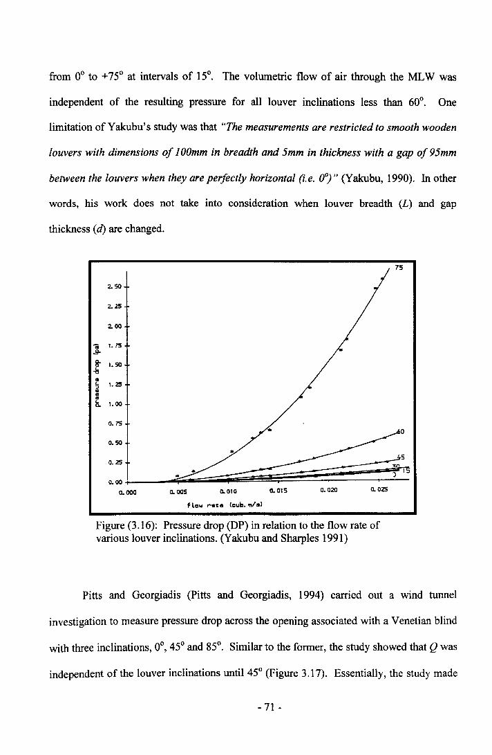
from 0° to +75° at intervals of 15°. The volumetric flow of air through the MLW was
independent of the resulting pressure for all louver inclinations less than 60°. One
limitation of Yakubu's study was that "The measurements are restricted to smooth wooden
louvers with dimensions of JOOmmin breadth and 5mm in thickness with a gap of 95mm
between the louvers when they are perfectly horizontal (i.e. 0°)" (Yakubu, 1990). In other
words, his work does not take into consideration when louver breadth (L) and gap
thickness (d) are changed.
2.50
2.25
2.00
di 1.75E-
s- 1.50-t;II<- 1.25:l......<- 1.00Q.
0.75
0.50
0.25
0.000.000
..0. 005 0.010 0.015 0.020 0.025
flow ~.ca (cub.m/a>
Figure (3.16): Pressure drop (DP) in relation to the flow rate ofvarious louver inclinations. (Yakubu and Sharples 1991)
Pitts and Georgiadis (Pitts and Georgiadis, 1994) carried out a wind tunnel
investigation to measure pressure drop across the opening associated with a Venetian blind
with three inclinations, 0°, 45° and 85°. Similar to the former, the study showed that Q was
independent of the louver inclinations until 45° (Figure 3.17). Essentially, the study made
- 71 -
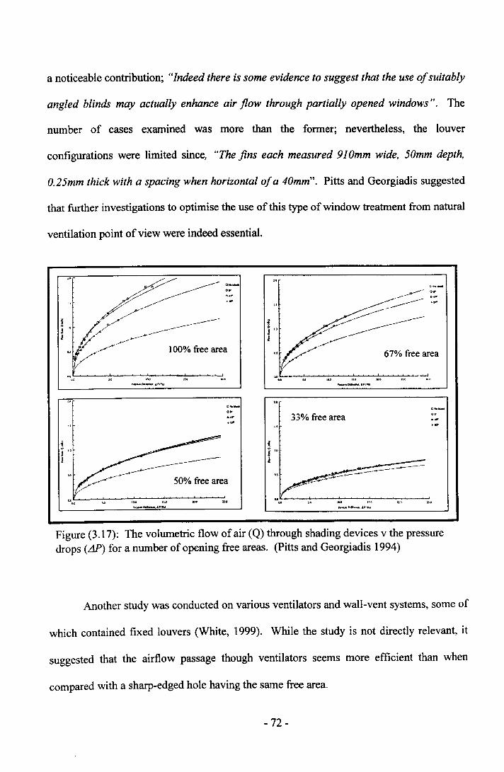
a noticeable contribution; "Indeed there is some evidence to suggest that the use of suitably
angled blinds may actually enhance air flow through partially opened windows". The
number of cases examined was more than the former; nevertheless, the louver
configurations were limited since, "The fins each measured 910mm wide, 50mm depth,
O.25mmthick with a spacing when horizontal of a 40mm". Pitts and Georgiadis suggested
that further investigations to optimise the use of this type of window treatment from natural
ventilation point of view were indeed essential.
",L, ~_""'_'~~--'-".~~'_'_~~_'.._.",_,4.! ....
t'"
r s
67% free area
~~--~--~'''~~~~~~.... .. ~4'1JWj
....0"''''''''o c-33% free area
Figure (3.17): The volumetric flow of air (Q) through shading devices v the pressuredrops (LiP) for a number of opening free areas. (Pitts and Georgiadis 1994)
Another study was conducted on various ventilators and wall-vent systems, some of
which contained fixed louvers (White, 1999). While the study is not directly relevant, it
suggested that the airflow passage though ventilators seems more efficient than when
compared with a sharp-edged hole having the same free area.
- 72-
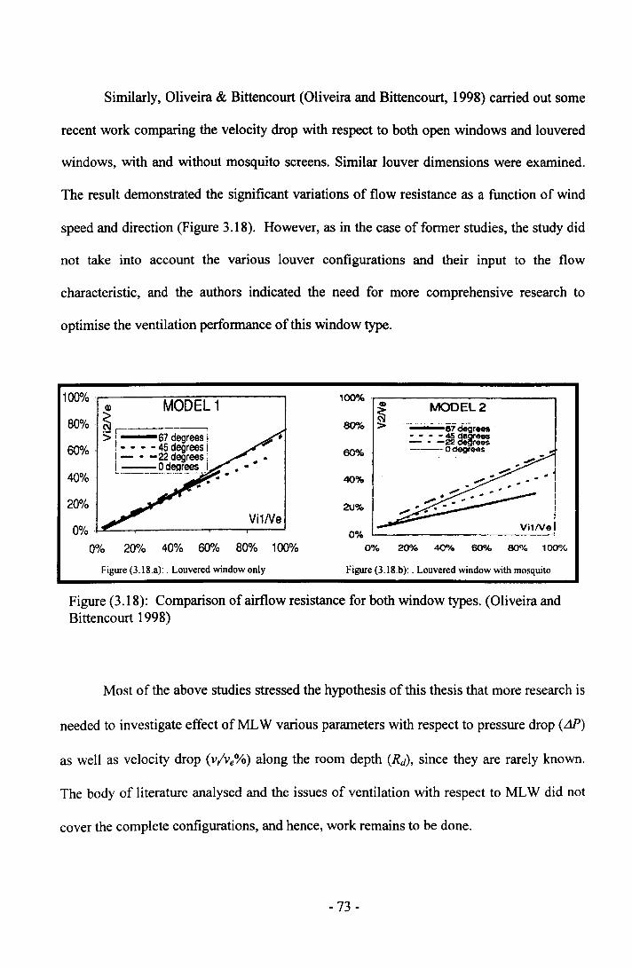
Similarly, Oliveira & Bittencourt (Oliveira and Bittencourt, 1998) carried out some
recent work comparing the velocity drop with respect to both open windows and louvered
windows, with and without mosquito screens. Similar louver dimensions were examined.
The result demonstrated the significant variations of flow resistance as a function of wind
speed and direction (Figure 3.18). However, as in the case of former studies, the study did
not take into account the various louver configurations and their input to the flow
characteristic, and the authors indicated the need for more comprehensive research to
optimise the ventilation performance of this window type.
1~h~W----~M~O=D~E=L-1~----~80% ~s r, 67 degrees i
I - - - - 45 degrees I1- • -22 degrees il===Q~.~~.1
,~ '~---------------------,CD
80%~
MOOEL2
60% 60%
40% 40%
20% 20%Vi1Ne
0%0% 20% 40% 60% 80% 100% 0% 200/0 40"'" 6()<'k 80% 100%
Figure (3.18.a): . Louvered window only Figure (3.18.b): . Louvered window with mosquito
Figure (3.18): Comparison of airflow resistance for both window types. (Oliveira andBittencourt 1998)
Most of the above studies stressed the hypothesis of this thesis that more research is
needed to investigate effect of MLW various parameters with respect to pressure drop (..1P)
as well as velocity drop (vlve%) along the room depth (Rd), since they are rarely known.
The body of literature analysed and the issues of ventilation with respect to MLW did not
cover the complete configurations, and hence, work remains to be done.
- 73 -
3.6. Statement of problem
This section is devoted to setting the hypothetical statement of the current research
based on the review in the aforementioned chapters concerning the climate and architecture
in Jeddah as well as the review on the modulated louvered windows as the source of
natural ventilation in building.
From the literature review it was found that Jeddah is located in a hot-humid
climatic zone and wind-induced ventilation is a main source of human comfort by natural
means. Various ventilation strategies to improve the indoor climate were employed,
amongst which the MLW, as part of Rowshan, was given the most attention. The
application of MLW systems is also found elsewhere. The body of literature pertaining to
this window accessory dealt with its solar control performance and the optimization of its
various dimensions and configurations in relation to natural ventilation is far from being
satisfactory. A number of studies have addressed the need for a comprehensive analysis of
this issue.
In this context, the design of MLW acquires special importance as air mainly flows
inside buildings through its (MLW) apertures. There is a need to move a step forward to
trace more carefully the significance of various MLW components with respect to natural
ventilation. Entire parametric studies are still needed to investigate pressure and velocity
characteristics as function of MLW various components. Therefore the present study will,
through its various appraisal stages, enable the researcher to elaborate on the pressure and
velocity characteristics as functions of the MLW parameters. These are highlighted as the
following:
- 74-
• The role of the modulated louvered windows parameters, such as louver
depth (L), aperture (d), angle of inclination (0), free area (AI)' d/L% and
others.
• The thorough investigation of the overall performance In relation to
integrating all variables.
• The external prevailing wind conditions represented in wind speed and
direction.
• The critical MLW configuration when the flow characteristics would
experience major alteration and resistance.
• The room configuration and its contribution to this effect.
• The airflow patterns in relation to the common Rowshan configurations
employed Jeddah.
- 75-
3.7. References
1. Al-Jawadi, M.H. (1986) Window optimisation for Iraqi houses. Department of
Architecture and building science, University of Strathclyde. Unpublished Ph.D. Thesis.
2. AI-Lyaly, S.M. (1990) The traditional house of Jeddah: A study of the interaction between
climate, form, and living patterns. University of Edinburgh. Unpublished Ph.D.
3. AI Shareef, F.M. (1996) Natural light control in Hedjazi Architecture; An investigation of
the Rowshan performance by computer simulation. University of Liverpool. Unpublished
Ph.D. thesis.
4. Aynsley, R.M., Melbourne, W. and Vickery, B.l. (1977) Architectural Aerodynamics,
London: Applied Science Publishers Ltd.
5. Bittencourt, L.S. (1993) Ventilation as a cooling resource for warm -humid climates: An
investigation on perforated block wall geometry to improve ventilation inside low-rise
buildings. Architectural Association Graduate School. Unpublished Ph.D. thesis.
6. Bowen, A (1983) "Design guidelines on lateral through and around buildings". p.517-533,
Crete, Greece: 2nd International PLEA Conference.
7. Brandle, K. and Boehm, P. E. (1982) "Airflow windows: Performance and application".
p.361-379, ASHRAE Trans.
8. Chandra, Subrato (1983) "A Design procedure to size windows for naturally ventilated
rooms". p.l 05-110, USA: American Solar Energy Society, Inc.
9. Evans, B. H. (1979) "Energy conservation with natural air flow through windows". (5), 2
edn. p.641-6S0, ASHRAE Transactions.
10. Evans, M. (1980) Housing, Climate, and comfort, London: Architectural press.
-76 -

11. Fathy, H. (1986) Natural energy and vernacular architecture, Chicago: Chicago press.
12. Fikry, A.A. (1981) An Investigation into window shading devices to optimize the control
of the internal environment. University of Sheffield. Unpublished Ph.D.
13. Givoni, B. (1968) Ventilation problems in hot countries. Haifa: Research report ofFord
foundation, Building research station, technion.
14. Givoni, B. (1981) Man, Climate and Architecture, 2nd edn. London: Applied Science
Publishers Ltd.
15. Givoni, B. (1991) "Performance and Applicability of Passive and Low Energy Cooling
Systems". Energy and Buildings (17)-
16. Givoni, B., Neeman, E., Hoffman, M.E. and Becker, M. (1968) Effect of orientation and
details of windows and fixed shading devices upon indoor temperature and illumination
conditions of classroom. Haifa, Israel: Building research station.
17. Holleman, T.R. (1951) Air flow through conventional window openings. 33, p.45 Texas:
Texas Engineering Experiment Station, College Station.
18. Jong, T. and Bot, G.P.A. (1992) "Flow characteristics of one-side mounted windows".
Energy and Buildings (19)-p.105-112.
19. Koenigsberger, 0., Ingresoll, T., Mayhew, A. and Szokolay, S. (1977) Manual of Tropical
Housing. Part One: Climatic Design, London: Longman Group Ltd.
20. Maghrabi, Amjed and Sharples, S. (1999) "Air flow characteristics through Modulated
Louvered Windows". (I), p.507-514, Brisbane, Australia: PLEA.
21. Muniz, P.A. (1985) The geometry of external shading devices as related to natural
ventilation, daylighting and thermal comfort, with particular reference to tropical hot-
humid climates. Unpublished Ph.D.
- 77-

22. Olgyay, V. (1963) Design with climate, Princeton N.J.: Princeton University Press.
23. Oliveira, F. and Bittencourt, L. S. (1998) "Air flow through louvered windows in small
rooms". p.393-396, Lisbon, Portugal: PLEA' 98.
24. Pitts, A. C. and Georgiadis, S. (1994) "Ventilation air flow through window openings in
combination with shading devices". 15th AIVC Conference edn. p.432-439, AIVC.
25. Salloum, A. (1983) "EI-Rowashin of Jeddah, Saudi Arabia". p.245-252, Crete, Greece:
Passive and Low Energy Architecture.
26. Sobin, H. (1963) "Post-Graduate Research: Air movement study". Architectural
Association Journal (78)-871, p.31 0-311.
27. Sobin, Harris (1981) "window design for passive ventilative cooling: An experimental
model-scale study". p.191-195, Miami Beach, Florida, USA:
28. Sobin, H. (1983) Analysis of wind tunnel data on naturally ventilated models. p.287
Tucson, Arizona, USA: Harris Sobin & Associates.
29. USA Dept. of Energy (1983) Energy efficient windows. A key to energy performance. 8p
USA: Us Department of Energy.
30. Vickery, B. J. and Karakatsania, C. (1987) "External wind pressure distribution and
induced ventilation flow in low rise industrial and domestic structures". (2), USA:
ASHRAE Trans.
31. White, M. (1999) "Ventilators: Ventilation and acoustic Effectiveness". ERE (IP4/99)-
p.I-8.
32. Yakubu, G.S. (1990) Modulated solar shielding of buildings: A study ofa solar radiation
control strategy for low energy buildings in hot dry and semi-arid climates. University of
Sheffield. Unpublished PhD.
- 78 -

33. Yakubu, O.S. and Sharples, S. (1991) "Airflow through modulated louver systems".
Building Services Engineering Research and Technology (12)-p.151-155.
- 79-
CHAPTER 4: NATURAL VENTILATION IN
ARCHITECTURE
- 80-
4.1. Introduction
This chapter reviews ventilation and airflow research within buildings with an
emphasis on wind induced natural ventilation. Besides the introduction, it contains four
sections including airflow dynamics in buildings, airflow around buildings, ventilation
within buildings and ends up by highlighting some common techniques employed In
ventilation research.
The first section underlines the basic principles in architectural aerodynamics
including the common mathematical representations of wind induced natural ventilation
around and within buildings. This establishes the ground for the laboratory appraisal of
airflow characteristics across the modulated louvered windows (MLW) that is carried out in
Chapters 6 and 7. The pressure characteristicsaround the structure as a function of wind are
also covered here. Then comes the wind movement around buildings with respect to a
number of determinants including the urban fabric, the topography, building surroundings,
and building geometry in altering the characteristicsof airstreams.
The discussion in respect to natural ventilation within buildings is of importance to
comprehend the various building components and their contribution to natural ventilation
indoors. More emphasis in this section is given to the window as a main source of natural
ventilation in buildings. Window treatments and controls as well as indoor and outdoor
modifications, such as wing-walls and partitions, are also considered. The last section
reviews some of the most common techniques employed in ventilation research and sheds
light on the features and drawbacks of each technique.
- 81 -
II
4.2. Airflow dynamics in buildings
Architectural aerodynamics in buildings involve a number of complications in the
real environment. As a result a number of mathematical representations of airflow
characteristics within the building are established to assist an understanding of the
dynamics of airflow in buildings. It is worth mentioning that most of the researchers agree
those theoretical representations of flow components are treated with some simplicity and
assumptions (Etheridge and Sandberg, 1996) (Awbi, 1991) (Koenigsberger et al. 1977)
(Aynsley et al. 1977) (Massey, 1989) (Maghrabi and Sharples, 1999) (Bittencourt, 1993) .
Despite the fact that in practice they may differ, the assumptions made in the mathematical
models considers that airflow is in steady state and is isothermal. Nevertheless, most of
the equations discussed in the following subsections are considered accurate enough to
examine the airflow around and within the buildings.
4.2.1. Airflow in buildings
The dynamics of airflow within and around buildings is basically caused by the
following variables:
• Wind induced natural ventilation.
• Buoyancy forces caused by temperature difference (stack effect).
The phenomenon of wind induced natural ventilation is simply understood when an
obstacle, such as a building, obstructs the wind causing pressure difference (..1P) across the
windward and leeward sides. When apertures are provided on both walls, cross ventilation
through the building occurs. This depends on many variables discussed in this chapter.
The temperature difference between outside (To) and inside (Ti) the building will also
- 82-
contribute to ventilation rates as a function of AT. In low-rise buildings a 10°C
temperature difference could result in an indoor air speed of O.SmJs (Bittencourt, 1993).
The vertical magnitude of temperature differences between different levels within a
building could result in significant ventilation. The phenomenon is known as the stack
effect whereby air ascends to higher floors, and low-pressure zones in lower levels cause
air suction. However, "Stack effect ventilation is not a powerful ventilation mechanism
and has several limitations that reduce its applicability" (Abrams, 1986). In addition, in
warm and hot humid climates the effect of temperature is not significant since external
temperature almost nears or even exceeds limits of comfort zones all year-round. So T;
and To do not suffer much variation. The typical temperature difference ranges from 2°C
to 5°C depending on the thermal mass of building and other variables (Aynsley et aI.
1977), (Fleury, 1990), (Bittencourt, 1993) and (Van Straatan et al. 1965). Wind-induced
natural ventilation is therefore the main factor in assessing thermal comfort in building by
natural means while the stack effect is negligible with the presence of even a slight breeze.
Thus, the effect of stack effect is excluded and not examined in the following discussion.
Evans (1979) has indicated that thermal comfort in buildings relies, to a high extent, on the
energy-free source; i.e. natural ventilation.
4.2.2. Wind induced natural ventilation
The blowing of wind on a structure creates positive and negative pressure zones on
windward and leeward sides, respectively. Low-pressure zones are also created along the
sides of the building and above the roof with the presence of higher wind velocities
(Abrams, 1986). It is important to indicate at this stage that in a hot humid climate, it is the
airflow which should be taken into consideration when assessing human comfort, not the
air changes (Muniz, 1985). Although models identifying air changes per hour (ACH) are- 83 -
important in ventilation research they are not addressed here for the above-mentioned
reason.
The highest-pressure drop arises when wind is perpendicular to the building
(Evans, 1979). The American Society of Heating, Refrigerating, and Air-conditioning
Engineers (ASHRAE) Handbook of Fundamentals (1985) states that wind pressure (Pw) is
a function of the square of wind velocity (V) and expressed as follows:
(4.1)
where
Pw = wind pressure (Pa)
Cp = static pressure coefficient
p = air density (Kg/m3)
v = wind speed at datum level (rn/s)
The magnitude of pressure on windward side for a square or a rectangular structure
varies from 0.5 to 0.9 times the velocity pressure (Pw). On the downwind side, the pressure
is negative from -0.3 to -0.9 the velocity pressure (Abrams, 1986). The ASHRAE
Handbook of Fundamentals (1985) and the Chartered Institution of Building Services
Engineers (CIBSE) (1976) have similar values for these figures. The magnitude of
pressure is usually described as the pressure coefficient (Cp) and is the ratio of the total
Wind pressure acting on the building. It is dependent mainly on the type of flow, whether
turbulent or laminar, and building geometry as will be mentioned later here (Etheridge and
- 84-
Sandberg, 1996). The surroundings such as topography and terrain type, may also have
some effects on the pressure (BRE, 1978) and (Awbi, 1991). Pressure coefficient
represents only a single point on building surface and is obtained through direct
measurements or through wind tunnel models. Values of Cp on a number of buitnings
geometries are found in (BS, 1980) and in (Liddament, 1986) and others.
4.2.3. Equations of airflow mechanisms
The mathematical models to calculate the volumetric fluid flow (Q) across an
orifice are related to a large extent to the pressure difference (AP) across the orifice. These
models are represented in a form of flow network consisting of a number of nodes where
each node is then represented by a number of equations. Some of these models are
mentioned in the following subsections.
4.2.3.1. Common orifice flow equation
In buildings with large apertures, the airflow (Q) seems turbulent under normal
pressure (Awbi, 1991). The common orifice flow equation represents the turbulent airflow
with large openings in the building as being proportional to the square root of the pressure
difference across the aperture. It is expressed as follows:
(4.2)
where
Cr discharge coefficient of an opening.
A = openings area (rrr')
- 85 -
L1P= pressure drop across the opening (Pa)
p = air density (Kg/mJ)
The discharge coefficient (Cd) for a sharp-edged orifice flow is 0.61 and is independent of
the Reynolds number (Re) (see section 4.2.7). Etheridge (1977) noted that Cd is not
observed in most buildings due to the configuration of the openings and the variations in
pressure difference depending on inside and outside building conditions determining the
effective leakage areas, Cd A, either through pressurisation and depressurisation tests or
directly from the ASHRAE Handbook of Fundamentals (1985).
4.2.3.2. Power law and quadratic airflow model equations
The validity of the power law and quadratic airflow model equations have been
investigated by many researchers in ventilation studies to set standards for building envelopes,
ventilation requirements and many other infiltration models. Both calculation methods have
been broadly accepted and the discussion as which is the most suitable one to apply is still
ongoing. In general the power law equation has been widely used to describe the relationship
between differential pressure (LiP) and the volumetric flow rate (Q) through various ranges of
apertures in buildings such as gaps around doors and windows, cracks, slits, etc, (Sherman et
al. 1979), (Liddament, 1987), (ASTM Standard E779, 1982), (CGSB Standard 149.l0-M86,
1986), (ISO Standard, 1995), (Awbi, 1991) and (Etheridge and Sandberg, 1996). (Liddament,
1987) considers the power law function as best to fit measurements of air infiltration within
buildings. The power law function is expressed as:
L1P = aQ" (4.3)
where:
- 86-
M = pressure drop across orifice (Pa)
a' = is a constant proportional to the effective leakage area of the crack (rrr'Is Pa),
Q = is the volwne flow rate (m3/s) n = is the exponent.
But equations of this type, however, are not dimensionally homogeneous because they do not
obey Reynolds law of similitude (Etheridge, 1987). Equation 4.3 gives the function of
pressure drop for a known Q. Alternatively, the flow rate can be expressed in another form:
Q=a·(Mt (4.4)
where a = fT~d
The flow exponent n was determined to be the square root of pressure as the flow rate is
almost proportional to the square root of M (Shennan et al. 1979), (Dick, 1950). On the other
hand, Walker et al. (1998) suggested that n has a value of 0.5 for fully developed turbulent
flows and I for laminar flow. This formulation is called the square law. But this relationship
does not fit in practice for a number ofreasons(Hopkins and Hansford 1974):
• Due to distortion of the crack, the increase in M would be accompanied by an
increase in aperture area.
• The value of the Cd of the orifice plate equation that is used to estimate the
leakage area was asswned constant. Hence, any change in the discharge
coefficient would result in deviation from the theory.
• The approximation in square law equation could not be applied for all types of
cracks and their various configurations and differential pressures.
- 87 -
Alternatively, other researchers in the field applied the quadratic model equation.
Etheridge (1987) (1997) (Etheridge and Sandberg, 1996) prefer the quadratic equation
method to determine the air infiltration. Baker et al. (1987) stated "Although the quadratic
disregards the existence of a critical velocity of transition between streamline and turbulence
flow, it has the practical advantage that at both extremes, i.e. Q ~ 0 and Q ~ C(), it gives the
correct forms corresponding respectively to laminar flow and to complete turbulence. The
coefficients A and B remain independent to the rate offlow", This formulation is expressed as
follows:
M=AQ+BQ2 (4.5)
where
A = the flow coefficient for fully developed laminar friction losses [CPasj/m"].
B = the coefficient of entry, exit and turbulent flow losses [CPas2)/m6].
Practitioners have also found that the quadratic is better in estimating leakage areas
through cracks and that it gives a better fit to the data obtained from their pressurisation and
depressurisation experimental results as found in (Thomas and Evans, 1951), (Baker et al.
1987), (Yakubu, 1990), (Yakubu and Sharples, 1991) and recently in Maghrabi and Sharples
(1999). The quadratic equation had some theoretical validity by using the basic flow equation
for laminar flow through infinite parallel plates and it is dimensionally homogenous (Fox and
MacDonald, 1978).
Coefficients A and B are determined by the standard fluid mechanics principles:
- 88-
(4.6)
(4.7)
where
J.i = the dynamic viscosity (kg/ms)
z = the plate length (m)
L= the breadth of the plate (m)
d = the gap thickness(m)
p = the fluid density (kg/nr')
Y = a factor depending on crack geometry.
Substituting coefficients A and B in Eq. (4.5):
(4.8)
The factor of loss coefficient as a function of crack geometry is assumed to be 1.5, 2.5
and 3.5 for straight crack, L-shaped crack and double crack respectively (Baker et al. 1987).
Hence, loss coefficient is increasing with a value of 1 for each sharp bend (Baker et al. 1987).
Awbi (1991) pointed out that some researchers had compared these models equations at
higher pressures and they found that both equations in the form of quadratic and power-law
models were identical. He added, "However, this study was by no means conclusive and
- 89-
more test cases are needed before a true assessment of the two equations can be achieved at
low pressure ranges H. The latter quotation establishes a solid base for the further comparison
between these models with respect to the type of window in hand: the modulated louvered
windows.
4.2.4. Airflow calculation models
A number of calculation models are reported here with several references. As it
was indicated previously, these model equations are developed with some simplifications.
4.2.4.1. ASHRAE model
The ASHRAE model (1985) of the volumetric flow of air is expressed as follows:
where
Q = volumetric air flow (m3/s)
Cd= effectiveness of the opening (discharge coefficient), 0.5 to 0.6 for perpendicular wind
and 0.25 to 0.35 for diagonal wind.
A= free area of inlet opening (m2)
V=wind velocity (m/s)
One advantage of this model is that only two variables are involved; wind velocity
and area of the opening. However, the simplicity of this equation may have some
drawbacks when applied in prediction. The equation does not take into account cases
- 90-
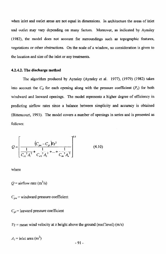
when inlet and outlet areas are not equal in dimensions. In architecture the areas of inlet
and outlet may vary depending on many factors. Moreover, as indicated by Aynsley
(1982), the model does not account for surroundings such as topographic features,
vegetations or other obstructions. On the scale of a window, no consideration is given to
the location and size of the inlet or any treatments.
4.2.4.2. The discharge method
The algorithm produced by Aynsley (Aynsley et al. 1977), (1979) (1982) takes
into account the Cd for each opening along with the pressure coefficient (Pc) for both
windward and leeward openings. The model represents a higher degree of efficiency in
predicting airflow rates since a balance between simplicity and accuracy is obtained
(Bittencourt, 1993). The model covers a number of openings in series and is presented as
follows:
Q=
0.5
(4.10)
where
Q = airflow rate (m3/s)
Cpw = windward pressure coefficient
Cpt = leeward pressure coefficient
Vz =mean wind velocity at z height above the ground (rooflevel) (m/s)
- 91 -
A2 = internal opening area (m2)
n = number of openings in series
Cd= discharge coefficient of an opening
The wind incidence would have an effect on the inlet area (AI). The AI is then
corrected with respect to the projection of the opening area that is perpendicular to wind
speed. But when wind incidence is greater than 60° then the representation of AI becomes
more complicated (Aynsley, 1988). In addition, wind pressure characteristics could be
estimated directly for a solid building or with a wall opening less than 10% of wall area
(Lee et al. 1980). However, in cases where the opening area exceeds 20% of wall area Cp
could not be estimated except from real measurements or wind tunnel tests. The difficulty
of obtaining Cp inside the building when the flow is divided into a number of branches
adds another disadvantage to the model equation (Al-Megren, 1987).
4.2.4.3. British Standards (BS)
The formula of airflow rate due to wind developed by the British Standards (BS
5925) (1980) for single sided ventilation is represented as:
Q= 0.025AV (4.11 )
where
Q = airflow rate (m3/s)
A = inlet area (m2)
- 92-
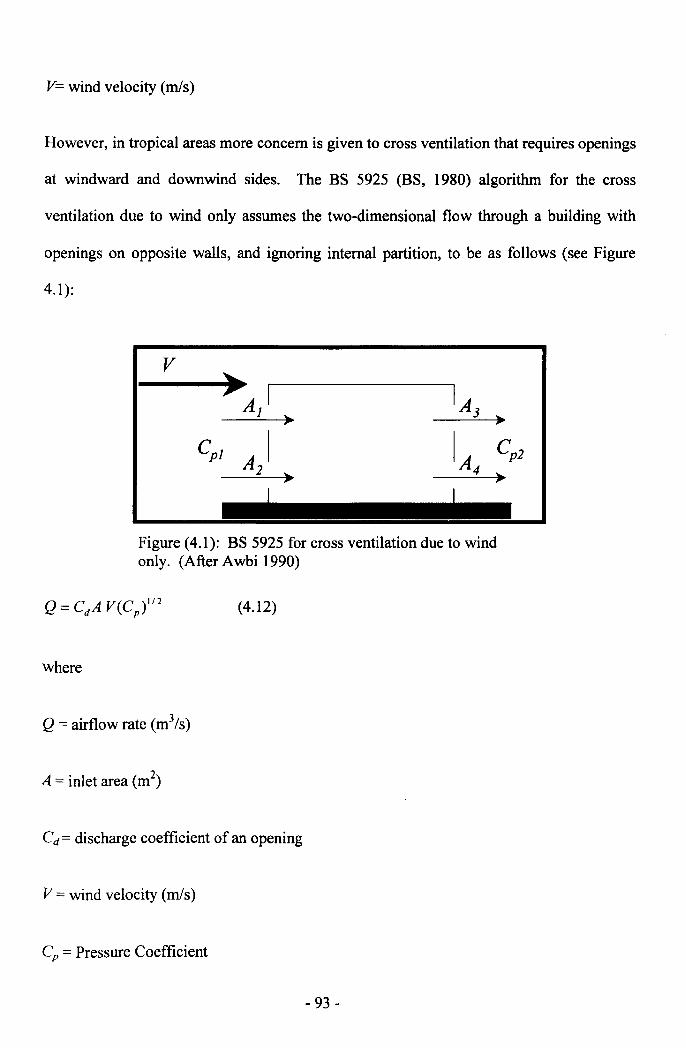
V=wind velocity (mls)
However, in tropical areas more concern is given to cross ventilation that requires openings
at windward and downwind sides. The BS 5925 (BS, 1980) algorithm for the cross
ventilation due to wind only assumes the two-dimensional flow through a building with
openings on opposite walls, and ignoring internal partition, to be as follows (see Figure
4.1):
where
v
Figure (4.1): BS 5925 for cross ventilation due to windonly. (After Awbi 1990)
(4.12)
Q = airflow rate (m3/s)
A = inlet area (m2)
Cd= discharge coefficient of an opening
v = wind velocity (mls)
C; = Pressure Coefficient
- 93 -
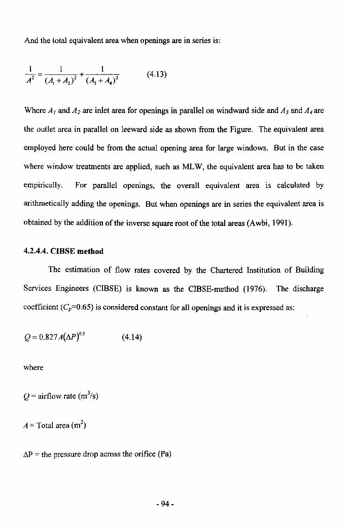
And the total equivalent area when openings are in series is:
(4.13)
Where AJ and A2 are inlet area for openings in parallel on windward side and A3 and A4 are
the outlet area in parallel on leeward side as shown from the Figure. The equivalent area
employed here could be from the actual opening area for large windows. But in the case
where window treatments are applied, such as MLW, the equivalent area has to be taken
empirically. For parallel openings, the overall equivalent area is calculated by
arithmetically adding the openings. But when openings are in series the equivalent area is
obtained by the addition of the inverse square root of the total areas (Awbi, 1991).
4.2.4.4. CIBSE method
The estimation of flow rates covered by the Chartered Institution of Building
Services Engineers (CIBSE) is known as the CIBSE-method (1976). The discharge
coefficient (Cp=0.65) is considered constant for all openings and it is expressed as:
Q = 0.827 A(MtS (4.14)
where
Q = airflow rate (m3/s)
A = Total area (rrr')
~P = the pressure drop across the orifice (Pa)
- 94-
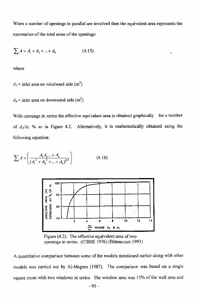
When a number of openings in parallel are involved then the equivalent area represents the
summation of the total areas of the openings:
(4.15)
where
Al = inlet area on windward side (m')
An = inlet area on downwind side (rrr')
With openings in series the effective equivalent area is obtained graphically for a number
of A/AI % as in Figure 4.2. Alternatively, it is mathematically obtained using the
following equation:
(4.16)
2 . ,. 6 8 ·10. 12 I"
-< 100
- ...~o~~ 90w II)er< -c0(
w 0 80"'> II)
;: II)
u ~... ......... ><w w 70
/1/--7
~: WHERE A2 .. AI
Figure (4.2): The effective equivalent area of twoopenings in series. (CIBSE 1976) (Bittencourt 1993)
A quantitative comparison between some of the models mentioned earlier along with other
models was carried out by Al-Megren (1987). The comparison was based on a single
square room with two windows in series. The window area was 15% of the wall area and
- 95 -
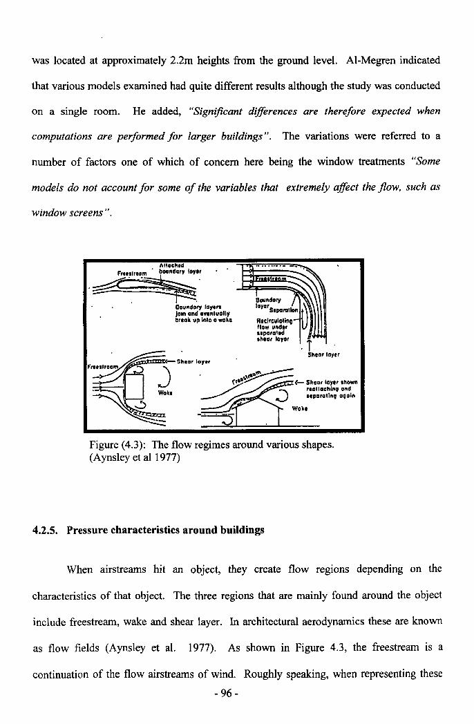
was located at approximately 2.2m heights from the ground level. AI-Megren indicated
that various models examined had quite different results although the study was conducted
on a single room. He added, "Significant differences are therefore expected when
computations are performed for larger buildings". The variations were referred to a
number of factors one of which of concern here being the window treatments "Some
models do not account for some of the variables that extremely affect the flow, such as
window screens".
IIlIochtd
.d:-···~":;;;.-- .'.
. .Ooundoty lay.,.lOInand oyonluall,bllok up Inlo 0 woko
BoulldD'1loyarSiparolion
Rlclrculolinoflow under•• paralldshlar layar
·TShoar layer
Figure (4.3): The flow regimes around various shapes.(Aynsley et al 1977)
4.2.5. Pressure characteristics around buildings
When airstreams hit an object, they create flow regions depending on the
characteristics of that object. The three regions that are mainly found around the object
include freestream, wake and shear layer. In architectural aerodynamics these are known
as flow fields (Aynsley et al. 1977). As shown in Figure 4.3, the freestream is a
continuation of the flow airstreams of wind. Roughly speaking, when representing these
- 96-
airstreams of wind into graphical parallel lines, they become more condense as function of
building shape. The shear-layer is formed as a separation between the freestream and the
wake zone where re-circulation and vortex form behind the shear layer. Around a
streamed-lined body (see Appendix A.l), the free stream moves adjacent to the body and
the pressure increases depending on the curvature of the body. The wake region is
minimized and the pressure around it contributes to lift and drag forces (Aynsley et al.
1977). The forces are components of the wind velocity force over the body. Lift-forces
tend to deflect airstreams in perpendicular to wind direction, and drag-forces are dragged
parallel to the airstreams direction. The developments of the three regions are more
obvious with bluff bodies and sharp-edged elements (Appendix A.l). In architecture, the
bluff bodies represented in square or rectangular building shapes are employed more than
the streamlined building forms. Therefore, some detailed description of the pressure fields
around bluff bodies is mentioned, bearing in mind that the presence of more than 20% of
aperture to wall area will have different pressures characteristics (Lee et al. 1980).
The pressure fields are formed as function of flow separations as well as of the
building shape. As shown in Appendix A.1, "The algebraic sum of the pressure, kinetic
energy per unit volume, potential energy per unit volume has the same value of any two
points on a streamline" (Bittencourt, 1993). The equation is expressed as follows:
- 97-
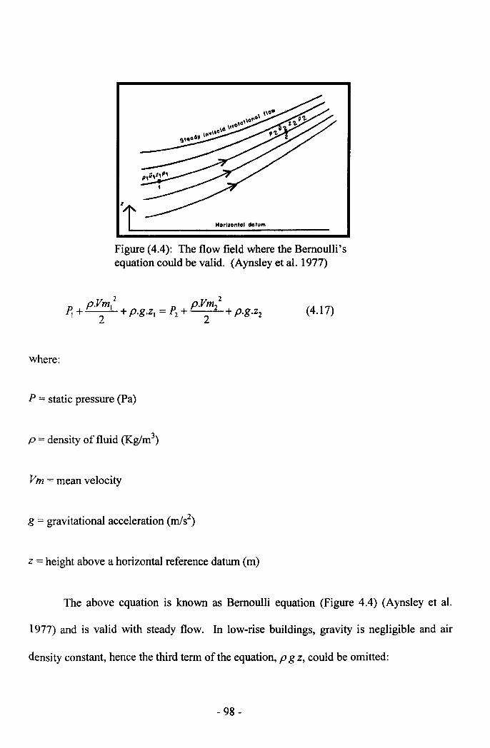
Horizontal dotu,"
Figure (4.4): The flow field where the Bernoulli'sequation could be valid. (Aynsley et al. 1977)
2 2p.VmJ D p.Vm2P; + +p.g.z, = £2 + +P·g,Z22 2
where:
P = static pressure (Pa)
(4.17)
p = density of fluid (Kg/m3)
Vm =mean velocity
g = gravitational acceleration (m/s')
z = height above a horizontal reference datum (m)
The above equation is known as Bernoulli equation (Figure 4.4) (Aynsley et al.
1977) and is valid with steady flow. In low-rise buildings, gravity is negligible and air
density constant, hence the third term of the equation, pg z, could be omitted:
- 98-
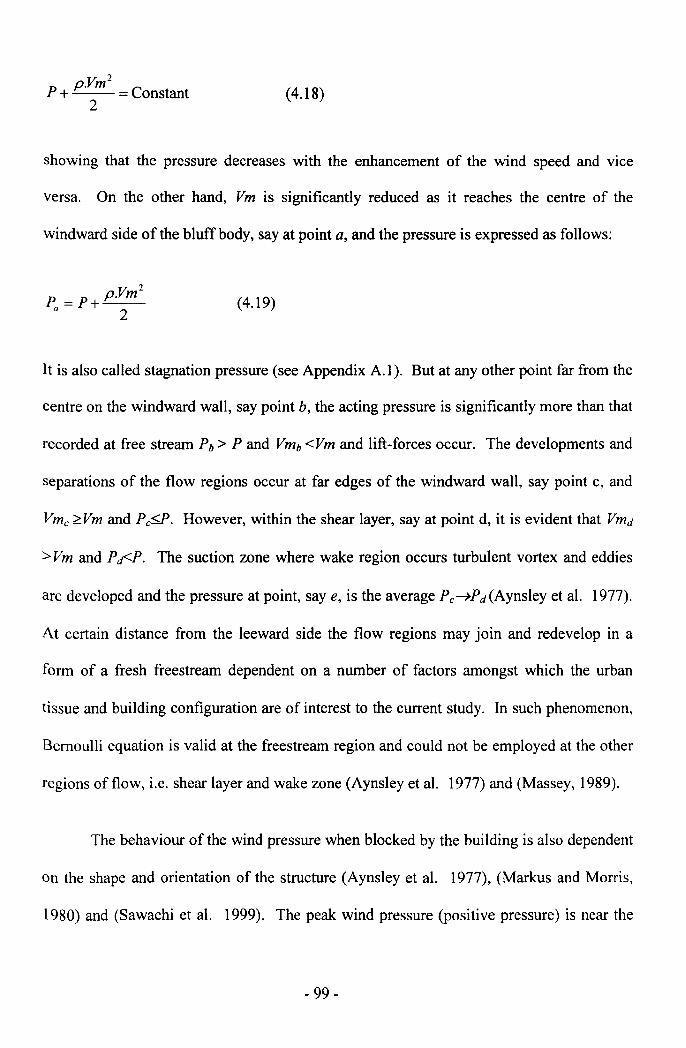
pVm2
P +' = Constant2
(4.18)
showing that the pressure decreases with the enhancement of the wind speed and vice
versa. On the other hand, Vm is significantly reduced as it reaches the centre of the
windward side of the bluff body, say at point a, and the pressure is expressed as follows:
(4.19)
It is also called stagnation pressure (see Appendix A.l). But at any other point far from the
centre on the windward wall, say point b, the acting pressure is significantly more than that
recorded at free stream Ph> P and Vm; <Vm and lift-forces occur. The developments and
separations of the flow regions occur at far edges of the windward wall, say point c, and
Vme '2:Vm and Peg. However, within the shear layer, say at point d, it is evident that Vmd
:>Vm and P~P. The suction zone where wake region occurs turbulent vortex and eddies
are developed and the pressure at point, say e, is the average Pe-)P d (Aynsley et al. 1977).
At certain distance from the leeward side the flow regions may join and redevelop in a
form of a fresh freestream dependent on a number of factors amongst which the urban
tissue and building configuration are of interest to the current study. In such phenomenon,
Bernoulli equation is valid at the freestream region and could not be employed at the other
regions of flow, i.e. shear layer and wake zone (Aynsley et al. 1977) and (Massey, 1989).
The behaviour of the wind pressure when blocked by the building is also dependent
on the shape and orientation of the structure (Aynsley et al. 1977), (Markus and Morris,
1980) and (Sawachi et al. 1999). The peak wind pressure (positive pressure) is near the
- 99-
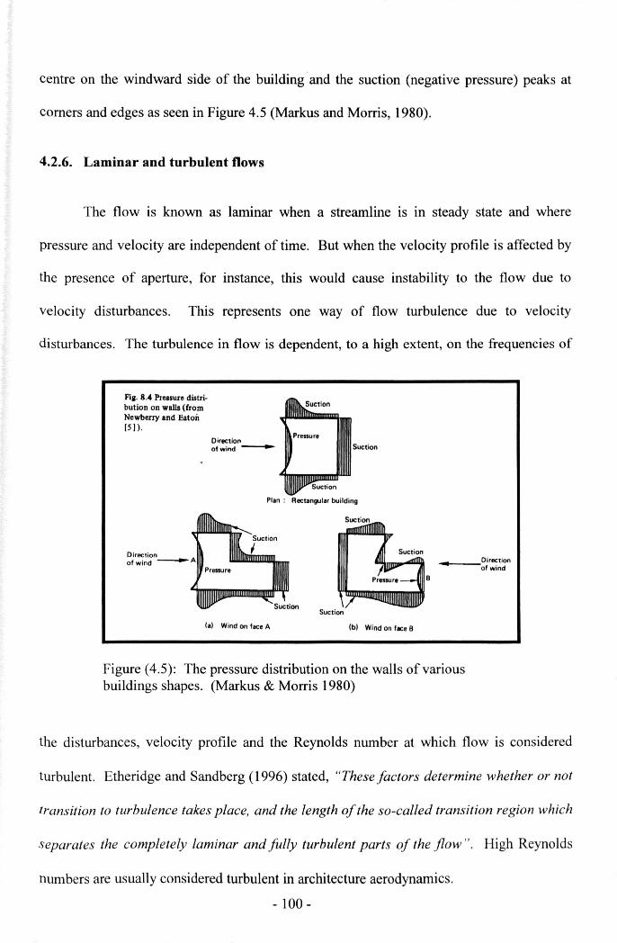
centre on the windward side of the building and the suction (negative pressure) peaks at
Comers and edges as seen in Figure 4.5 (Markus and Morris, 1980).
4.2.6. Laminar and turbulent flows
The flow is known as laminar when a streamline is in steady state and where
pressure and velocity are independent of time. But when the velocity profile is affected by
the presence of aperture, for instance, this would cause instability to the flow due to
velocity disturbances. This represents one way of flow turbulence due to velocity
disturbances. The turbulence in flow is dependent, to a high extent, on the frequencies of
Fill. 8.4 Pressure distri-bution on walls (fromNewberry and Eaton[5 J).
SuctionDirectlo~of wind --.....
Plan: Rectangular building
Directionof wind ----
B
(a) Wind on face A (b) Wind on face B
Figure (4.5): The pressure distribution on the walls of variousbuildings shapes. (Markus & Morris 1980)
the disturbances, velocity profile and the Reynolds number at which flow is considered
turbulent. Etheridge and Sandberg (1996) stated, "These factors determine whether or not
transition to turbulence takes place, and the length of the so-called transition region which
separates the completely laminar and fully turbulent parts of the flow". High Reynolds
numbers are usually considered turbulent in architecture aerodynamics.
- 100 -
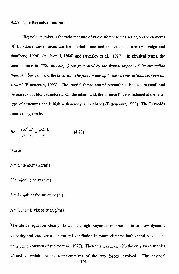
4.2.7. The Reynolds number
Reynolds number is the ratio measure of two different forces acting on the elements
of air where these forces are the inertial force and the viscous force (Etheridge and
Sandberg, 1996), (Al-Jawadi, 1986) and (Aynsley et al. 1977). In physical terms, the
inertial force is, "The blocking force generated by the frontal impact of the streamline
against a barrier" and the latter is, "Theforce made up to the viscous actions between air
strata" (Bittencourt, 1993). The inertial forces around streamlined bodies are small and
increases with blunt structures. On the other hand, the viscous force is reduced at the latter
type of structures and is high with aerodynamic shapes (Bittencourt, 1993). The Reynolds
number is given by:
Re = p.U2.L2 = p.U.Lf./..U.L f./.
(4.20)
where
p = air density (Kg/m3)
U = wind velocity (m/s)
L = Length of the structure (m)
u = Dynamic viscosity (Kg/ms)
The above equation clearly shows that high Reynolds number indicates low dynamic
viscosity and vice versa. In natural ventilation in warm climates both p and f./. could be
considered constant (Aynsley et al. 1977). Then this leaves us with the only two variables
U and L which are the representatives of the two forces involved. The physical- 101 -
interpretation of this in architecture aerodynamics is that the blockage caused by L
dimension could, to a high extent, determine the behaviour of the flow from laminar to
fully turbulent.
The value under which the Re is considered laminar or turbulent is not fixed.
Depending on the frictional forces, it is ranged from 105 to 3.6x10⁶ and is called the
critical Re (Melaragno, 1982) (Etheridge and Sandberg, 1996). Above this, the range of
transition indicates that boundary layer is turbulent as the functional increase of frictional
forces. In the opposite, low critical Re indicates reduction in the frictional forces and the
boundary layer is more likely laminar.
The Re of the structure differs from that across an aperture or those smaller
components. The flow through MLW is more likely a piped flow and the critical value of
Re to consider laminar or turbulent flow is also not fixed. In most cases if Re value
exceeds 2000 then the jet flow is considered turbulent. Etheridge and Sandberg (1996)
mention that some studies showed that fully turbulent flow could be of about 4000.
Similarly, Massey (1989) indicated that the critical Re for the later flow regime ranged
from 2000 to 4000.
4.2.8. Flow regime through bounded flow
Amongst the flow regimes through an aperture, the regime of flow through the
reviewed MLW seemed to fall under the piped flow regime or bounded flow regime. A
number of factors affect the flow regime through piped object. Frictional losses are the
most important in causing resistance to the fluid flow as a function of pipe roughness,
kinematics' viscosity and pipe shape (Etheridge and Sandberg, 1996), (Awbi, 1991). Entry
and exit diameters of an inlet added to any diversion of flow within the pipe, such as elbow- 102-
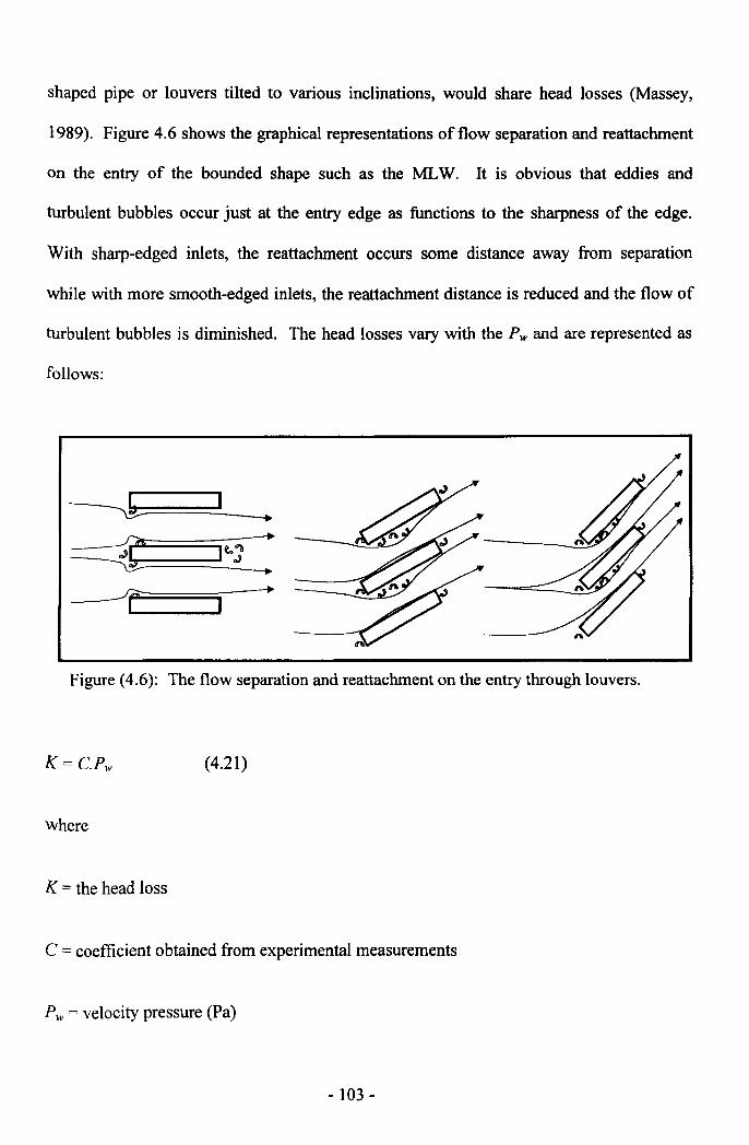
shaped pipe or louvers tilted to various inclinations, would share head losses (Massey,
1989). Figure 4.6 shows the graphical representations of flow separation and reattachment
on the entry of the bounded shape such as the MLW. It is obvious that eddies and
turbulent bubbles occur just at the entry edge as functions to the sharpness of the edge.
With sharp-edged inlets, the reattachment occurs some distance away from separation
while with more smooth-edged inlets, the reattachment distance is reduced and the flow of
turbulent bubbles is diminished. The head losses vary with the Pw and are represented as
follows:
Figure (4.6): The flow separation and reattachment on the entry through louvers.
K=CPw (4.21)
where
K = the head loss
C = coefficient obtained from experimental measurements
Pw = velocity pressure (Pa)
- 103 -
The value of C differs from the entry and exit of an inlet. Baker et al. (1986)
investigated the airflow through perforated screens at small-scale pressure difference and
recommended that the value of C at entry side of an inlet be 0.5 and at exit side of the inlet
1. The latter value of C is correspondent to exit losses when the airstreams within the pipe
leave it into the freestream inside the room or the enclosure. The governing principles of
the flow regime at exiting side of an inlet are discussed in the following section.
4.2.9. Air Jets
The principles of air jets are mainly encountered with the mechanical ventilation
systems where, "Air jets are used to mix the processed air from the plant with the room
air" (Awbi, 1991). Similar principles of air jets are encountered with cross ventilation.
Roughly there are two types of jets, namely the free air jet and the wall jet. Both
phenomena are discussed here since they are directly relevant to the flow regime
encountered through the reviewed modulated louvered windows.
4.2.9.1.Free air Jet
The free air jet occurs when air leaves an aperture or a nozzle and travels into the
space where no solid boundaries affect the flow patterns. "The static pressure within the
jet is the same as the static pressure of the surrounding space" (Awbi, 1991). The velocity
magnitude increases at the jet centerline and a free shear layer is developed around the
edges of the regime. The shear layers from both sides shape jet boundaries as an indication
of the velocity discontinuity and they expand as function of distance from the opening.
The downstream flow becomes more turbulent as function of the distance from the opening
due to the velocity reduction in air jet. Four zones of free jets are developed depending on
the variation of velocity centerline caused by distance from the opening; potential core
- 104-
region, characteristic decay region, asymmetric decay region and terminal decay region
(Appendix A.2).
4.2.9.2. Wall Jet
The Wall jet effect occurs when the fluid inside the space flow is adjacent to a flat
surface and the velocity magnitude moves parallel to that surface. This phenomenon is
widely know as Coanda effect (Awbi, 1991), (Etheridge and Sandberg, 1996), where the
jet keeps attached to the surface recording the highest velocity near it till reaching the
opposite wall where it then deflects downward in the room. The shear layer here is
developed only from the other side of the surface and expands in a proportional and similar
fashion to the free air jet. In architectural aerodynamics, the wall jet could produce some
sort of draught within the living room specifically when the re-circulation of air, such as
cross ventilation, is not present. In this case, two zones of wall jets are developed
including potential core and the characteristics decay (see Appendix A.3).
4.3. Natural ventilation around buildings
There are a number of parameters affecting airflow around buildings. Some are
referred to the environment and surroundings while others are related to the building
geometry. Of the first determinant, the type of terrain, topography, streets and alleys, and
landscape are of most significance. On the other hand, building determinants include array
and distribution of buildings, building shape and orientation. These are discussed here in
brief as they are not directly relevant to the current study.
The global wind circulation in the atmosphere follows two dominant directions of
circulation, horizontal and vertical, and each circulation dimension is dependent on the
- 105 -
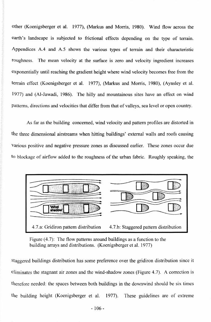
other (Koenigs berger et al. 1977), (Markus and Morris, 1980). Wind flow across the
earth's landscape is subjected to frictional effects depending on the type of terrain.
Appendices A.4 and A.S shows the various types of terrain and their characteristic
roughness. The mean velocity at the surface is zero and velocity ingredient increases
exponentially until reaching the gradient height where wind velocity becomes free from the
terrain effect (Koenigsberger et al. 1977), (Markus and Morris, 1980), (Aynsley et al.
1977) and (AI-Jawadi, 1986). The hilly and mountainous sites have an effect on wind
patterns, directions and velocities that differ from that of valleys, sea level or open country.
As far as the building concerned, wind velocity and pattern profiles are distorted in
the three dimensional airstreams when hitting buildings' external walls and roofs causing
various positive and negative pressure zones as discussed earlier. These zones occur due
to blockage of airflow added to the roughness of the urban fabric. Roughly speaking, the
4.7.a: Gridiron pattern distribution 4.7.b: Staggered pattern distribution
Figure (4.7): The flow patterns around buildings as a function to thebuilding arrays and distributions. (Koenigsberger et al. 1977)
staggered buildings distribution has some preference over the gridiron distribution since it
eliminates the stagnant air zones and the wind-shadow zones (Figure 4.7). A correction is
therefore needed: the spaces between both buildings in the downwind should be six times
the building height (Koenigsberger et al. 1977). These guidelines are of extreme
- 106 -
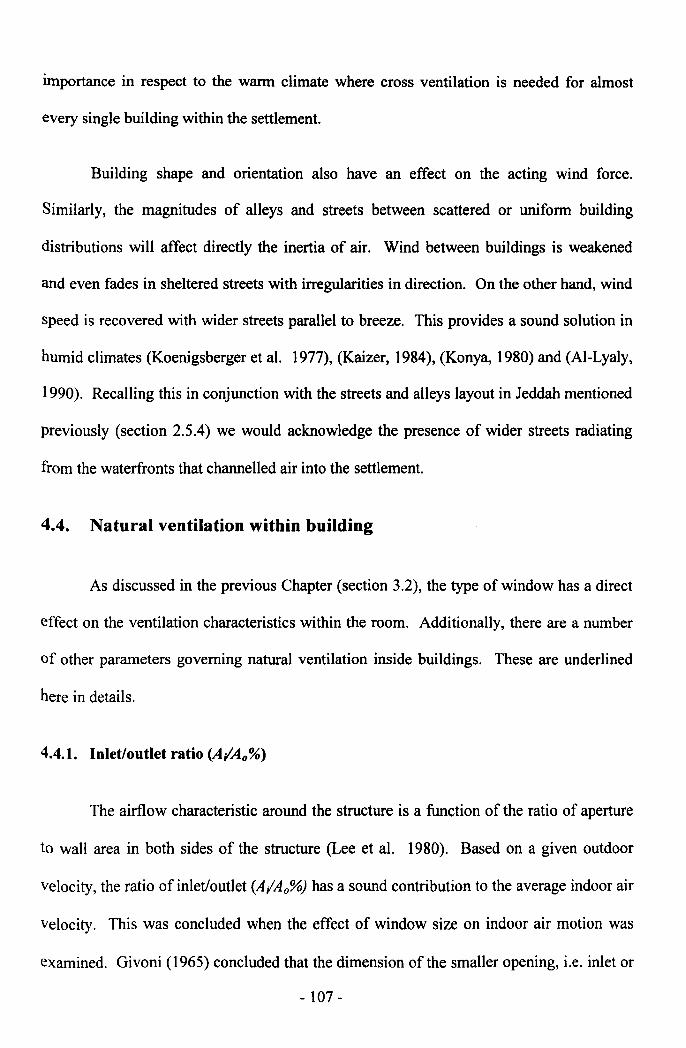
importance in respect to the warm climate where cross ventilation is needed for almost
every single building within the settlement.
Building shape and orientation also have an effect on the acting wind force.
Similarly, the magnitudes of alleys and streets between scattered or uniform building
distributions will affect directly the inertia of air. Wind between buildings is weakened
and even fades in sheltered streets with irregularities in direction. On the other hand, wind
speed is recovered with wider streets parallel to breeze. This provides a sound solution in
humid climates (Koenigsberger et al. 1977), (Kaizer, 1984), (Konya, 1980) and (Al-Lyaly,
1990). Recalling this in conjunction with the streets and alleys layout in Jeddah mentioned
previously (section 2.5.4) we would acknowledge the presence of wider streets radiating
from the waterfronts that channelled air into the settlement.
4.4. Natural ventilation within building
As discussed in the previous Chapter (section 3.2), the type of window has a direct
effect on the ventilation characteristics within the room. Additionally, there are a number
of other parameters governing natural ventilation inside buildings. These are underlined
here in details.
4.4.1. Inlet/outlet ratio (A/Ao%)
The airflow characteristic around the structure is a function of the ratio of aperture
to wall area in both sides of the structure (Lee et al. 1980). Based on a given outdoor
velocity, the ratio of inlet/outlet (A/Ao%) has a sound contribution to the average indoor air
Velocity. This was concluded when the effect of window size on indoor air motion was
examined. Givoni (1965) concluded that the dimension of the smaller opening, i.e. inlet or
- 107 -
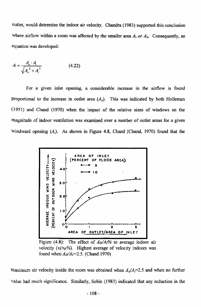
outlet, would determine the indoor air velocity. Chandra (1983) supported this conclusion
where airflow within a room was affected by the smaller area Ai or Ao. Consequently, an
equation was developed:
(4.22)
For a given inlet opening, a considerable increase in the airflow is found
proportional to the increase in outlet area (Ao). This was indicated by both Holleman
(1951) and Chand (1970) when the impact of the relative sizes of windows on the
magnitude of indoor ventilation was examined over a number of outlet areas for a given
windward opening (Ai). As shown in Figure 4.8, Chand (Chand, 1970) found that the
W I-\.II ZCl I.LIa: v~ a:Cl'; 00 I 2 ~
AREA OF OUTLET/AREA OF .IN UT
1I>- ut: gg ~-J
W 0> :r:o ~zi ~oa: 0o ....o ;:,o 0z
AREA OF INLET(PERC~.NT OF FLOOR AREA)
- 540~IO
o
u,o
Figure (4.8): The effect of AoIAi% to average indoor airvelocity (vi/ve%). Highest average of velocity indoors wasfound when AoIAi=2.S. (Chand 1970)
maximum air velocity inside the room was obtained when AJAF2.S and when no further
value had much significance. Similarly, Sobin (1983) indicated that any reduction in the
- 108 -
inlet area to the outlet area would have major contribution to average indoor speed. Sobin
found that the highest average values of velocity indoors were for AJA; ranges from 1.0-
2.25. In contrast, when the size of the inlet is larger than the outlet, a more uniform pattern
of air distribution was found (see Figure 4.9) and the speed increased as it approached the
outlet (Chand, 1970).
In general, larger outlets favour air speed to increase near the inlet and vice versa
(Abrams, 1986). Yet, larger windward openings are preferred with the presence of wind
incidences or when the flow through the entire room was required (Koenigs berger et al.
1977). The latter provides an optimum alternative for the warm and humid climates where
cross ventilation is needed for almost every single space within the structure.
'>-....
t l-t.) AREA OF OUTLET0 (PERCENT OF FLOOR AREA)~
-l0I- U.!0 >0
Cl~ -- 5tU Z> ~ 1030 --Clz a:s 0
0Cl
a: !:; 2000 0Cl u.:z 0w t-
.10u. zCl: usa: uw a:> U.! 0et 0..- 0 I 2 3
AP.EA OF INUT/ AREA OF OUTLET..Figure (4.9): The effect of Ai/Ao% to average indoor airvelocity (vi/ve%) showing that the increase in Ai/Ao> l didnot improve the average indoor air velocity. (Chand1970)
- 109-
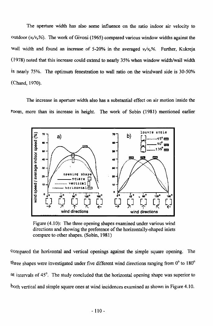
The aperture width has also some influence on the ratio indoor air velocity to
outdoor (v/ve%). The work of Givoni (1965) compared various window widths against the
wall width and found an increase of 5-20% in the averaged v/ve%. Further, Kukreja
(1978) noted that this increase could extend to nearly 35% when window width/wall width
is nearly 75%. The optimum fenestration to wall ratio on the windward side is 30-50%
(Chand, 1970).
The increase in aperture width also has a substantial effect on air motion inside the
room, more than its increase in height. The work of Sobin (1981) mentioned earlier
;i" 70a- a) b)
opening shape_-_!lquare 0
..................vert-leal 0- hOClzontaU:::::J
o 00
[J~
45° 10° 131° 110°
[J [J [J [J71 l' '" ~wind directions
70louvre angle
(.,) 4Som[.J - 90° II1IIlJ-'_1JS°mJI
10
~J [1'J [J [J'" ~wind directions
Figure (4.10): The three opening shapes examined under various winddirections and showing the preference of the horizontally-shaped inletscompare to other shapes. (Sobin, 1981)
compared the horizontal and vertical openings against the simple square opening. The
three shapes were investigated under five different wind directions ranging from 0° to 180°
at intervals of 45°. The study concluded that the horizontal opening shape was superior to
both vertical and simple square ones at wind incidences examined as shown in Figure 4.10.
- 110 -
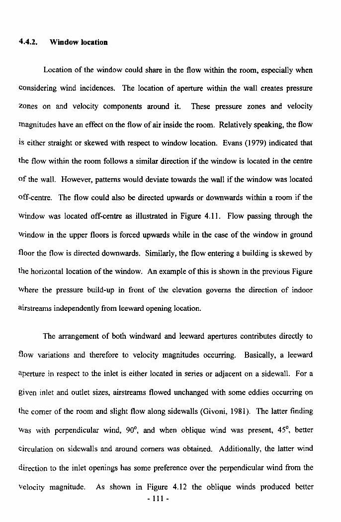
4.4.2. Window location
Location of the window could share in the flow within the room, especially when
considering wind incidences. The location of aperture within the wall creates pressure
zones on and velocity components around it. These pressure zones and velocity
magnitudes have an effect on the flow of air inside the room. Relatively speaking, the flow
is either straight or skewed with respect to window location. Evans (1979) indicated that
the flow within the room follows a similar direction if the window is located in the centre
of the wall. However, patterns would deviate towards the wall if the window was located
off-centre. The flow could also be directed upwards or downwards within a room if the
Window was located off-centre as illustrated in Figure 4.11. Flow passing through the
window in the upper floors is forced upwards while in the case of the window in ground
floor the flow is directed downwards. Similarly, the flow entering a building is skewed by
the horizontal location of the window. An example of this is shown in the previous Figure
where the pressure build-up in front of the elevation governs the direction of indoor
airstreams independently from leeward opening location.
The arrangement of both windward and leeward apertures contributes directly to
flow variations and therefore to velocity magnitudes occurring. Basically, a leeward
aperture in respect to the inlet is either located in series or adjacent on a sidewall. For a
given inlet and outlet sizes, airstreams flowed unchanged with some eddies occurring on
the corner of the room and slight flow along sidewalls (Givoni, 1981). The latter finding
Was with perpendicular wind, 90°, and when oblique wind was present, 45°, better
circulation on sidewalls and around corners was obtained. Additionally, the latter wind
direction to the inlet openings has some preference over the perpendicular wind from the
Velocity magnitude. As shown in Figure 4.12 the oblique winds produced better-III -
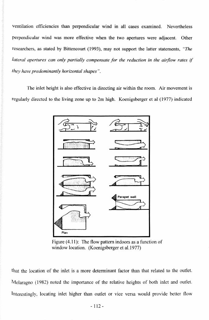
ventilation efficiencies than perpendicular wind in all cases examined. Nevertheless
perpendicular wind was more effective when the two apertures were adjacent. Other
researchers, as stated by Bittencourt (1993), may not support the latter statements, "The
lateral apertures can only partially compensate for the reduction in the airflow rates if
they have predominantly horizontal shapes".
The inlet height is also effective in directing air within the room. Air movement is
regularly directed to the living zone up to 2m high. Koenigsberger et al (1977) indicated
Plan
~
S·:;''''?i:
Figure (4.11): The flow pattern indoors as a function ofwindow location. (Koenigsberger et al.1977)
that the location of the inlet is a more determinant factor than that related to the outlet.
Melaragno (1982) noted the importance of the relative heights of both inlet and outlet.
Interestingly, locating inlet higher than outlet or vice versa would provide better flow
- 112-
regimes in all vertical layers in the space including flow around body level or living zone.
On the other hand, positioning the outlet in various heights affected neither the incoming
air nor the pattern of the flow (Holleman, 1951), (Givoni, 1981), (Olgyay and Olgyay,
1976).
The vertical location and type are the main controls of indoor flow patterns (Muniz,
1985). Bowen (Bowen, 1983) demonstrated a number of sketches of flow patterns within
the room as a function of various parameters mentioned in the section.
27 3t 32 41 81 38 37 31 72 . 88 54 30 83 7734
32 38 58 30 81 44 44 29 29 &0 &4 28 31 25 8339 42 89 34 62 37 25 28 29 38 43 32 30 34 78
38 32 79 33 44 33 25 31 29 30 49 31 311 37 78
38 27 137 30 32 34 29 31 29 37 58 34 32 30 82
~ Ave... :44% 1tAvereg& :35% 1{Avtnge: 47%
38 24 24 28 84 38 32 27 62 121 44 3& 51 87 77
31 28 26 24 93 42 42 29 81 128 68 32 30 86 8829 24 27 39 78 68 36 29 71 103 69 32 30 86 88
30 27 27 109 28 68 28 48 81 118. 87 34 43 102 10924 28 71 162 29 67 32 51 68 137 56 152 78 78 115
(::JAverege:44% l=J Avtnge :69'110 ~ Average:86%
Figure (4.12): The effect of wind direction and the windwardopening size on the average air velocity indoors. (Koenigsberger etal.I977), (Givoni 1981)
4.4.3. Window orientation
Building orientation is a significant task for designers when considering the
environmental variables. Similarly the window design, on the scale of an aperture, is of
appreciable importance. The orientation of a window in relation to the wind angle of
- 113 -
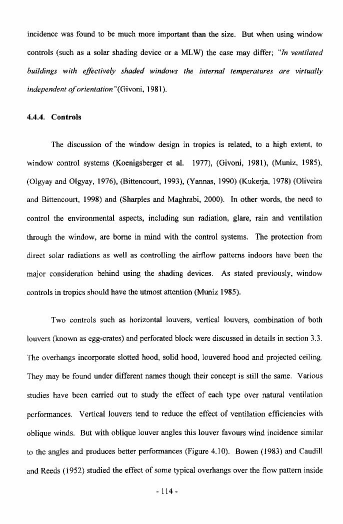
incidence was found to be much more important than the size. But when using window
controls (such as a solar shading device or a MLW) the case may differ; "In ventilated
buildings with effectively shaded windows the internal temperatures are virtually
independent of orientation "(Givoni, 1981).
4.4.4. Controls
The discussion of the window design in tropics is related, to a high extent, to
window control systems (Koenigsberger et al. 1977), (Givoni, 1981), (Muniz, 1985),
(Olgyay and Olgyay, 1976), (Bittencourt, 1993), (Yannas, 1990) (Kukerja, 1978) (Oliveira
and Bittencourt, 1998) and (Sharples and Maghrabi, 2000). In other words, the need to
control the environmental aspects, including sun radiation, glare, rain and ventilation
through the window, are borne in mind with the control systems. The protection from
direct solar radiations as well as controlling the airflow patterns indoors have been the
major consideration behind using the shading devices. As stated previously, window
controls in tropics should have the utmost attention (Muniz 1985).
Two controls such as horizontal louvers, vertical louvers, combination of both
louvers (known as egg-crates) and perforated block were discussed in details in section 3.3.
The overhangs incorporate slotted hood, solid hood, louvered hood and projected ceiling.
They may be found under different names though their concept is still the same. Various
studies have been carried out to study the effect of each type over natural ventilation
performances. Vertical louvers tend to reduce the effect of ventilation efficiencies with
oblique winds. But with oblique louver angles this louver favours wind incidence similar
to the angles and produces better performances (Figure 4.10). Bowen (1983) and Caudill
and Reeds (1952) studied the effect of some typical overhangs over the flow pattern inside
- 114 -
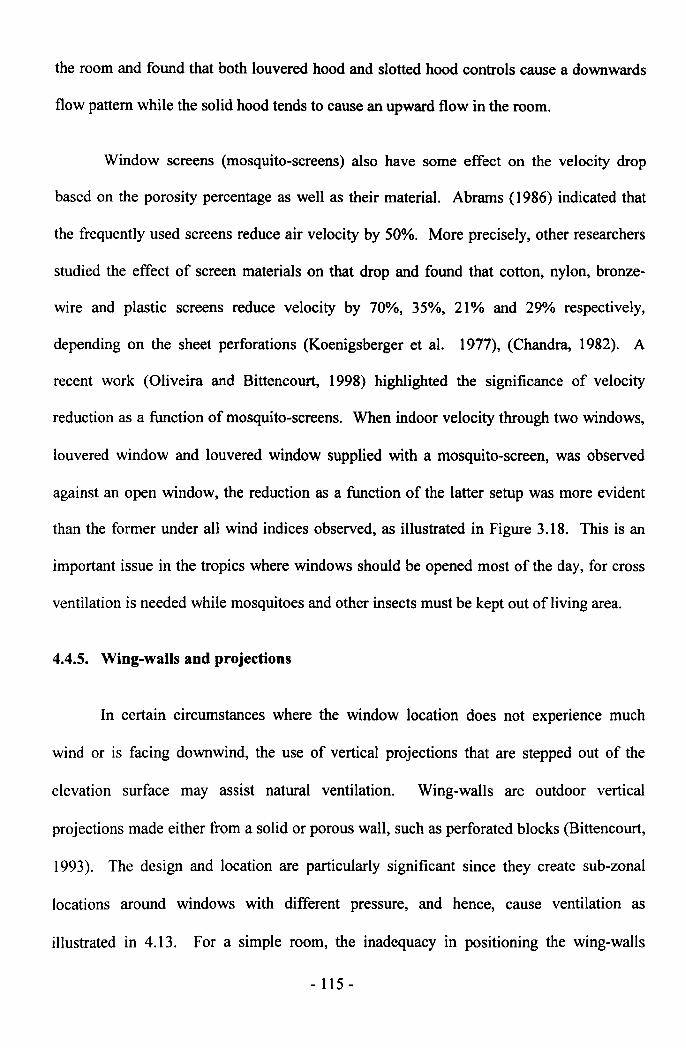
the room and found that both louvered hood and slotted hood controls cause a downwards
flow pattern while the solid hood tends to cause an upward flow in the room.
Window screens (mosquito-screens) also have some effect on the velocity drop
based on the porosity percentage as well as their material. Abrams (1986) indicated that
the frequently used screens reduce air velocity by 50%. More precisely, other researchers
studied the effect of screen materials on that drop and found that cotton, nylon, bronze-
wire and plastic screens reduce velocity by 70%, 35%, 21% and 29% respectively,
depending on the sheet perforations (Koenigsberger et al. 1977), (Chandra, 1982). A
recent work (Oliveira and Bittencourt, 1998) highlighted the significance of velocity
reduction as a function of mosquito-screens. When indoor velocity through two windows,
louvered window and louvered window supplied with a mosquito-screen, was observed
against an open window, the reduction as a function of the latter setup was more evident
than the former under all wind indices observed, as illustrated in Figure 3.18. This is an
important issue in the tropics where windows should be opened most of the day, for cross
ventilation is needed while mosquitoes and other insects must be kept out of living area.
4.4.5. Wing-walls and projections
In certain circumstances where the window location does not experience much
wind or is facing downwind, the use of vertical projections that are stepped out of the
elevation surface may assist natural ventilation. Wing-walls are outdoor vertical
projections made either from a solid or porous wall, such as perforated blocks (Bittencourt,
1993). The design and location are particularly significant since they create sub-zonal
locations around windows with different pressure, and hence, cause ventilation as
illustrated in 4.13. For a simple room, the inadequacy in positioning the wing-walls
- 115-
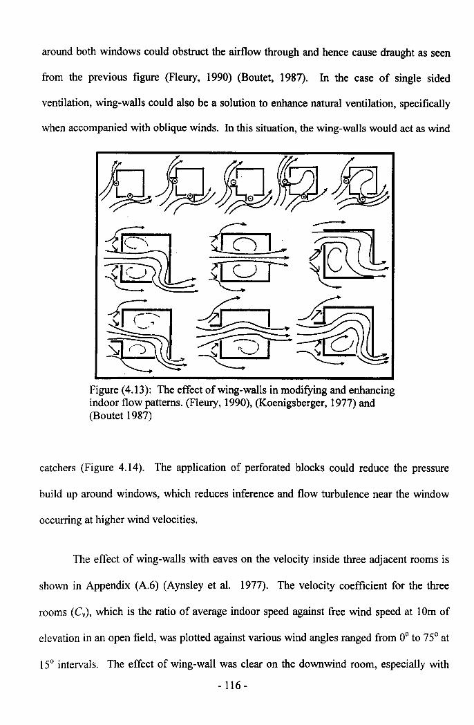
around both windows could obstruct the airflow through and hence cause draught as seen
from the previous figure (Fleury, 1990) (Boutet, 1987). In the case of single sided
ventilation, wing-walls could also be a solution to enhance natural ventilation, specifically
when accompanied with oblique winds. In this situation, the wing-walls would act as wind
Figure (4.13): The effect of wing-walls in modifying and enhancingindoor flow patterns. (Fleury, 1990), (Koenigsberger, 1977) and(Boutet 1987)
catchers (Figure 4.14). The application of perforated blocks could reduce the pressure
build up around windows, which reduces inference and flow turbulence near the window
occurring at higher wind velocities.
The effect of wing-walls with eaves on the velocity inside three adjacent rooms is
shown in Appendix (A.6) (Aynsley et al. 1977). The velocity coefficient for the three
rooms (Cv), which is the ratio of average indoor speed against free wind speed at 10m of
elevation in an open field, was plotted against various wind angles ranged from 0° to 75° at
IS° intervals. The effect of wing-wall was clear on the downwind room, especially with
- 116 -
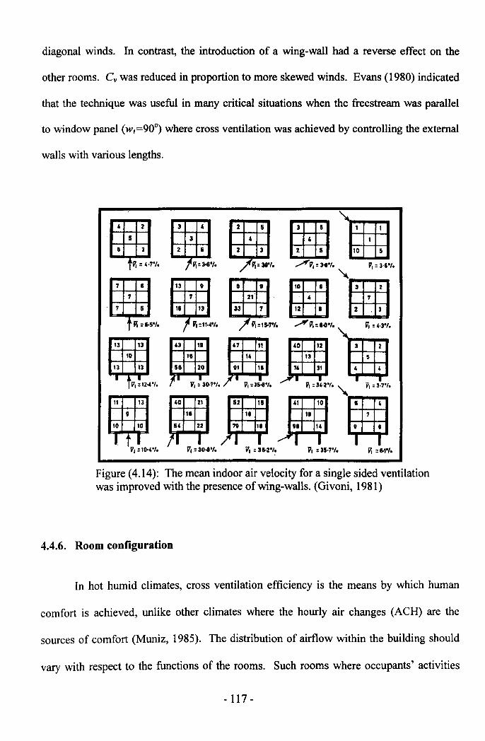
diagonal winds. In contrast, the introduction of a wing-wall had a reverse effect on the
other rooms. C;was reduced in proportion to more skewed winds. Evans (1980) indicated
that the technique was useful in many critical situations when the freestream was parallel
to window panel (w;=900) where cross ventilation was achieved by controlling the external
walls with various lengths.
13
3 ,3
13
10
13 ,
7
Figure (4.14): The mean indoor air velocity for a single sided ventilationwas improved with the presence of wing-walls. (Givoni, 1981)
II 13
I v.:11·"1.43 11
11
13 13 5& 20
• tv, ~IWI. ,I V, ~ 3()'7'1.
g13 40 21
11
54 22
II IV,.:30,.·I.
4.4.6. Room configuration
11
ID 10
In hot humid climates, cross ventilation efficiency is the means by which human
comfort is achieved, unlike other climates where the hourly air changes (ACH) are the
sources of comfort (Muniz, 1985). The distribution of airflow within the building should
vary with respect to the functions of the rooms. Such rooms where occupants' activities
- 117 -
occur at set locations should have concentrated flow regimes (Bittencourt, 1993). An
example of this is the bedroom or bathroom where concentrated airflow with higher
velocities is required. Other enclosures such as the living room require a uniform
distribution of air. Thus the design of such a space should provide adequate and uniform
distribution of air and avoid wind-shadowed or still-air areas within the room (Caudill and
Reed, 1952), (Bittencourt, 1993).
When endowing the room with appropriate openings, then the room depth, length
and height would have little effect on the airflow as was quoted by both Caudill and Reed
(1952) and Muniz (1985). The effect on the length may have some significance for
diagonal winds as indicated by Caudill and Reeds (1952). This, however, is not supported
by other research findings. For example, Givoni's (1981) showed that the velocity
reduction is dependent on the room depth as shown in Figure (4.12). Additionally another
study has shown the influence of ceiling height and depth on the flow pattern indoors
(Sharples and Maghrabi, 2000). When using controls that deflect air towards the ceiling,
the stack effect will be negligible due to the breeze speed. Evans (1979) noted that flow
near the ceiling helps remove the hot air build-up but may not necessarily cause a cooling
sensation to occupants. As discussed before in section (4.2.9.2) this is due to the Coanda
effect when air flows adjacently to the ceiling until reaching the outlet and is not diverted
into the living zone.
4.4.7. Internal partitioning and sub-divisions
Most airflow studies are conducted using a single room with windward and leeward
openings. However, airflow within a building normally passes by a number of zones
before reaching the outlet. These zones are usually divided by walls or partitions which
- 118 -
sub-divide the building, and hence, would have a major effect on branching and
channelling the flow indoors. Internal partitions have a great effect on flow pattern,
direction and speed of air before leaving through the outlet. Givoni (1981) studied the
effect of sub-divisions on the distribution of average internal speed (Vi) and found that the
reduction ranged from 44.5% to 30.5%. He concluded that higher average Vi was obtained
when the partitions were placed near the outlet as compared to the inlet. One solution
suggested to reduce flow resistance caused by partitions was the application of porous
partitions (Koenigsberger et al. 1977), (Al-Lyaly, 1990), (Bittencourt, 1993). This
recommendation is not new but rather was employed in traditional architectures in the
tropics such as in Jeddah, Yemen, Brazil, etc. However, the application of porous
partitions may interfere with other aspects such as privacy and noise controls as noted by
Bittencourt (1993).
4.4.8. Roofs and eaves
A number of studies have investigated the criterion of roof and eaves design in
regards to flow patterns within building. Bahadori & Haghighat (1985) studied the
doomed roof design in respect to reduced air temperature in buildings. They concluded
that doomed roof with a crown opening on its crest is a sound alternative to asses natural
ventilation in arid regions (Bahadori and Haghighat, 1985). A more recent study was
conducted on the effect of roof shape on cross ventilation in a room using numerical
simulation: Computational Fluid Dynamics (CFD) (Kindangen et al. 1997). The roof
shape examined covered a number of possible roof shapes in tropical architecture including
pitched, pyramidal, prism-shaped and semi-cylindrical roofs and was measured with
reference to flat roof, with and without overhangs (eaves) (Appendix A.7.a). The
significance of eaves on the flat roof depended, to a high function, on the wind inclination- 119 -
angle. An amplification of 39%, 10% and 7% was found with the presence of respectively
0°,30°,45° of wind incidence. Any increase beyond that was negligible (Appendix A.7.b).
However, eaves on outdoors flow pattern and specifically on the percentage of wind
shadow (wake depth) was minor (Evans, 1973) (Boutet, 1987). The roof height was also
significant with steeper wind indices, " For large wind angles (60~(}:590)at the inlet, act
to increase the exposed projected area on the windward side, followed by the positive
pressure of the windward side" (Kindangen et al. 1997). Interestingly, in all cases
examined, the measured cell on outlet surface experienced higher speed than the adjacent
cell inside the room. Similarly, wake depth as function of pitched roof height was
increasingly proportional and obviously increases pressure difference between building
enclosures (Boutet, 1987).
4.4.9. Landscape and vegetation
The proper positioning of plants around a building or an opening will appreciably
enhance and correct flow patterns inside the room. Where window orientation does not
appreciate wind currents or is not facing the freestream then hedges and trees could solve
the problem (Evans, 1979). The hedges act as wing-walls and create sub-zonal locations
with difference in pressures between inlet and outlet, and thus, ventilation occurs.
However, Bittencourt (1993) and Chandra (1989) argued that most literature on the
influence of plants on the airflow within buildings was based on a model study carried out
by White in 1957 and the model does not realistically represent the plants' ''porosity'' or
"bending and alignment of leaves due to wind".
The influence of hedges on flow inside the room will be more effective than trees.
The height and location of the hedges in relation to the building are important for " The
- 120 -
reduction in air motion reaches its peak when the hedges are located about 7 times its
height from the building, but decreases sharply when the hedges are planted near the
building or awayfrom it" (Bittencourt, 1993), (Van Straatan et a1. 1965).
4.5. Measuring techniques
Ventilation contribution through an opening encounters a number of complications
in the real environment. Some of these are related to the physics of the fluid and others are
related to the aperture and surroundings as discussed previously in this chapter. The
calculation method or measuring technique selected is considerably important to decide the
optimum technique for a specific task. The principle of airflow measurement would
determine to a large extent the appropriateness of the technique selected. The various
techniques and calculation methods implemented in ventilation research are discussed
here. Table (4.1) sheds light on the advantages and disadvantages of each technique.
4.5.1. Site Observation
Perhaps the most pragmatic and most primitive technique is the site observation
where the investigation procedure is conducted on a full-scale building or on an enclosure
in the real environment. It may not necessarily be named site observations since it has
been used on the basis of trai/-and-error experience to treat the built environment.
Aynsley (1999) indicated that the empirical knowledge obtained from observations to
utilise natural ventilation in buildings goes some thousands years back; "Ancient records
from Egyptian times refer to orientation of buildings to prevailing winds as do Greek,
Romans, and Chinese records". He added, "It was not until the development of
instruments to measure atmospheric pressure and wind speed that there was an
- 121 -
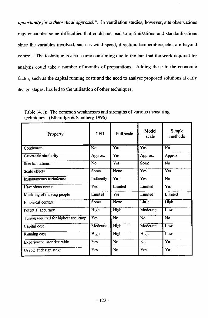
opportunity for a theoretical approach". In ventilation studies, however, site observations
may encounter some difficulties that could not lead to optimisations and standardisations
since the variables involved, such as wind speed, direction, temperature, etc., are beyond
control. The technique is also a time consuming due to the fact that the work required for
analysis could take a number of months of preparations. Adding these to the economic
factor, such as the capital running costs and the need to analyse proposed solutions at early
design stages, has led to the utilisation of other techniques.
Table (4.1): The common weaknesses and strengths of various measuringtechniques. (Etheridge & Sandberg 1996)
Property CFD Full scaleModel Simplescale methods
Continuum No Yes Yes No
Geometric similarity Approx. Yes Approx. Approx.
Size limitations No Yes Some No
Scale effects Some None Yes Yes
Instantaneous turbulence Indirectly Yes Yes No
Hazardous events Yes Limited Limited Yes
Modeling of moving people Limited Yes Limited Limited
Empirical content Some None Little High
Potential accuracy High High Moderate Low
Tuning required for highest accuracy Yes No No No
Capital cost Moderate High Moderate Low
Running cost High High High Low
Experienced user desirable Yes No No Yes
Usable at design stage Yes No Yes Yes
- 122 -
4.5.2. Wind Tunnel
The wind tunnel is an empirical scale-model approach that is widely established in
ventilation research. This technique, along with others, has some preference over site
observation in regards to its usefulness at an early design stage before finalising the
scheme and further developing various solutions. It allows examination of different
alternatives. Carey and Etheridge (1999) indicated that direct wind tunnel approach has
more potential for the examination of wind effects on buildings than the theoretical
approaches. The boundary layer in the wind tunnels, depending on the surface roughness,
presents a good representation of wind characteristics in the real environment before
reaching the proposed building; and also of how the building will influence other buildings
in the downwind direction as found in Lee et al (1980), Abdulrahman et al. (1998) and
Olwi et al (1988). The wind tunnel is also used to examine airflow through a particular
space or a number of spaces within the building as found in (Gadi and Ward, 1989),
(Warren and Parkins, 1984) and more recently in (Carey and Etheridge, 1999). Pressure
and velocity drops and airflow visualisation are obtained with the use of appropriate
instrumentations and equipments. In 1950's, the wind tunnels were the only available tool
for testing complex cases in ventilation (Koenigsberger et al. 1977).
4.5.3. The test chamber
Another laboratorial approach is the test chamber. This is widely employed in
testing building components such as a window, a door or some of their particular
components, like infiltration due to cracks. The technique is widely used in measuring the
volumetric flow of fluid (Q) through a component, and therefore the differential pressure
(LiP) occurring (Etheridge and Sandberg, 1996). The approach has also a history in
- 123 -
ventilation research that goes back to 1920's. Houghton and O'Connell (1928) carried out
air leakage measurements in metal windows in 1928 using the latter approach. Some
recent research applied this technique to determine airflow characteristics through cracks
(Baker et al. 1987) or flow characteristics through louvered windows as found in
Maghrabi and Sharples (1999), Yakubu and Sharples (1991), Sharples and Maghrabi
(2000). In this study, velocity and pressure drops as functions of various MLW
configurations will be carried out using the latter technique; Le. full-scale test chamber
approach.
4.5.4. Theoretical approaches
Theoretical approaches to calculate airflow within and around buildings were
discussed in more details in section (4.2) and subsequent sub-sections. The assumptions
are employed to answer some of the complexities accruing in practice since the full
understanding of these complexities is not yet complete: "In this approach the better
models are the ones which make the more justifiable assumptions and which employ the
experimental in the more appropriate manner" (Etheridge and Sandberg, 1996). The
assumptions corrections are more evident with the presence of empirical studies. In 1950,
Dick (1950), when investigating air infiltration while using both techniques, reported that
theoretical estimations shared a good agreement with site observation. Since then, more
efforts have been made to validate the theoretical approaches with other empirical studies.
Some of the most recent ones are found in (Said et al. 1995), (Wang, 1995), (Kindangen
and Krauss, 1996), (Alexander et al. 1997), (Chung and Dunn-Rankin, 1998), (Sharples
and Maghrabi, 2000) and others. However, theoretical techniques usually require a highly
sophisticated knowledge of fluid mechanics principles and user expertise.
- 124-
4.5.5. Computational Fluid Dynamics (CFD)
Computational fluid dynamics (CFD) is one of the theoretical approaches that have
been widely accepted in recent years. The advancement in computational power has
influenced the developments in wind engineering. In the 1970's, CFD software was
feasible and was accompanied with research in the field of ventilation. CFD models are
governed by the principles of fluid dynamics including conversion of mass, momentum
and thermal energy represented in set of equations to solve some more complicated
situations than any other measuring technique. CFD will be discussed in more details in
Chapter 8 of this thesis.
4.6. Conclusion
Wind-induced natural ventilation is the main natural and free source of human
comfort in hot humid climates. Its potential to cool the indoor environment as well as the
occupants ensures research interest. In this chapter the airflow characteristics as a function
of various elements around and within buildings were reviewed. Also, the mathematical
representations of the airflow characteristics with respect to natural ventilation in buildings
were highlighted. Some conclusions are derived from this review:
• The varieties of mathematical models related to airflow characteristics
within buildings are treated with some simplicity and assumptions; yet they
are widely accepted in ventilation research since the entire representations
of flow complexities are agreed to be unfeasible. Nevertheless, the validity
of most of them is based on a complete open aperture. When any treatment
is involved, such as the reviewed MLW, their appropriateness is questioned,
- 125 -
and thus, the need for direct measurements will be more reliable than the
theoretical models.
• Window accessories and controls, such as MLW, are very essential in
tropical climate as they serve more than one function. Nevertheless, the
relevant research conducted with respect to their contribution in the overall
ventilation effectiveness and flow patterns indoors is far from being
satisfactory. Also, the values for pressure and velocity magnitudes are rare
in the literature. The previous statement was argued in both Chapters 3 and
4 and therefore, further research is needed to identify the coefficients of
pressure and velocity magnitudes as functions to these treatments and their
configurations.
• The observed measunng techniques to solve ventilation problems in
buildings are widely acceptable and the selection of the appropriate
technique depends on the scale and the problem, and the degree of accuracy
required. From this perspective the standardisation of characterising airflow
around MLW is believed to be better conducted through wind tunnels or test
chambers as compared with the site observation technique. Both techniques
have also preference over the theoretical models, specifically when related
to MLW as discussed before. The work in Chapters 6 and 7 will be then
carried out using the test chamber at the University of Sheffield Campus.
- 126-

4.7. References
1. Abdulrahman, S., Kannan, K. S., and Ramli, A. H. (1998) "Prediction of indoor air
movement of naturally ventilated classrooms in schools in Malaysia". (3), p.1411-1414,
Florence (Italy): Proc. World Renewable Energy Congress V.
2. Abrams, D. (1986) Low-Energy Cooling, New York, USA: Van Nostrand Reinhold
Company.
3. AI-Jawadi, M.H. (1986) Window optimisation for Iraqi houses. Department of Architecture
and Building Science, University of Strathclyde. Unpublished PhD thesis.
4. AI-Lyaly, S.M. (1990) The traditional house of Jeddah: A study of the interaction between
climate, form, and living patterns. University of Edinburgh. Unpublished Ph.D thesis.
5. AI-Megren, K. (1987) Wind towers for passive ventilation cooling in hot-arid regions. The
University of Michigan. Unpublished Doctor of Architecture thesis.
6. Alexander, D. K., Jenkins, H G, and Jones, P. J. (1997) "A comparison of wind tunnel and
CFD methods applied to natural ventilation design. ". p.321-326, Prague, Czech Republic:
Proc. International Building Performance Simulation Association.
7. ASHRAE (1985) ASH RAE Handbook of Fundamentals, Georgia, Atlanta: American
Society of Heating, Refrigerating, and Air-Conditioning Engineers.
8. ASTM Standard E779 (1982) Measuring air leakage by fan infiltration pressurisation
method,
9. Awbi, H.B. (1991) Ventilation of Buildings, London: E & FN Spon.
10. Aynsley, R. M. (1979) "Wind-generated natural ventilation of housing for thermal comfort
in hot humid climates". (1), p.243-254, Proc. 5th International Conference Fort Collins.
- 127 -
11. Aynsley, R M. (1982) "Natural Ventilation model studies". Gaithersburg, USA:
Proceedings of the International Workshop on Wind Tunnel Modeling Criteria and
Techniques in Civil Engineering Application.
12. Aynsley, R. M. (1988) "A Resistance Approach to Estimating Airflow Through Buildings
With Large Openings Due To Wind". (94), 2 edn. p.1661-1668, ASHRAE transactions.
13. Aynsley, R M. (1999) "Unresolved issues in natural ventilation for thermal comfort". p.36-
44, Darlington, NSW, Australia: proceedings of Hybvent Forum '99.
14. Aynsley, R.M., Melbourne, W. and Vickery, B.J. (1977) Architectural Aerodynamics,
London: Applied Science Publishers Ltd.
15. Bahadori, M.N. and Haghighat, F. (1985) "Passive cooling in hot, arid regions in
developing countries by employing domed roofs and reducing the temperature of internal
surfaces.". Building and Environment 20-(2), p.l 03-113.
16. Baker, P.H., Heap, RD. and Sharples, S. (1986) "Airflow through perforated screens at
small pressure differences.". Building Serv Eng Res Technolp.96-97.
17. Baker, P.H., Sharples, S. and Ward, I.C. (1987) "Airflow through cracks". Building and
Environment 22-(4), p.293-304.
18. Bittencourt, L.S. (1993) Ventilation as a cooling resource for warm -humid climates: An
investigation on perforated block wall geometry to improve ventilation inside low-rise
buildings. Architectural Association Graduate School. Unpublished Ph.D. thesis.
19. Boutet, T.S. (1987) Controlling air movement: A Manual/or Architects and Builders, New
York: McGraw-Hili.
20. Bowen, A (1983) "Design guidelines on lateral through and around buildings". p.517-533,
Proc. of 2nd International PLEA Conference.
- 128 -
21. BRE (1978) Principles of natural ventilation. no.210, UK: Building Research
Establishment.
22. BS (1980) Code of Practice and designing of buildings: Ventilation principles and
designing for natural ventilation. no. 5925, London: British Standards Institution.
23. Carey, P.S. and Etheridge, D.W. (1999) "Direct wind tunnel modelling of natural ventilation
for design purposes ". Building Serv.Eng.Res. Technol. (20)-3, p.131-142.
24. Caudill, W.W. and Reed, B.H. (1952) Geometry of classrooms as related to natural light
and natural ventilation. 36, p.53 Texas: Texas Engineering Experiment Station; College
Station.
25. CGSB Standard 149.10-M86 inventor Canadian General Standards Board, (1986)
Determination of airtightness of building envelopes by fan pressurisation method. 149.10-
M86. 149.10-M86.
26. Chand, I. (1970) "Effect of the distribution of fenestration area on the quantum of natural
ventilation in buildings ". Architect and Science Review 13-(4), p.130-133.
27. Chandra, S. (1982) A Handbook for Designing naturally ventilated buildings, Florida,
USA: Florida Solar Energy Centre.
28. Chandra, S. (1989) Ventilative cooling. In: Cook, J., (Ed.) Passive Cooling, Cabridge,
Massachusetts: MIT Press.
29. Chandra, Subrato (1983) "A Design procedure to size windows for naturally ventilated
rooms ". p.l 05-11 0, USA: American Solar Energy Society, Inc.
30. Chung, I.-P. and Dunn-Rankin, D. (1998) "Using numerical simulation to predict ventilation
efficiency in a model room ". Energy and buildings (28)-p.43-S0.
- 129-
31. CIBSE (1976) Infiltration. Guide A4- Infiltration, London, UK: The Chartered Institute
of Building Services Engineers.
32. Dick, J.B. (1950) "The Fundamentals of Natural Ventilation in Houses". JIHVE (18)-p.123-
134.
33. Etheridge, D.W. (1977) "Crack Flow Equation and Scale Effect". Building and
Environment (12)-p.181-l89.
34. Etheridge, D.W. (1987) Air infiltration review. 4,
35. Etheridge, D.W. (1997) "A note on crack flow equations for ventilation modelling".
Building and Environment 33-(5), p.325-328.
36. Etheridge, D. and Sandberg, M. (1996) Building Ventilation: Theory and Measurements,
John Willy & Sons.
37. Evans, B. (1973) Natural air flow around buildings. Lecture notes: Teaching the teachers
on building climatology. Stockholm: The National Swedish Institute for Building Research.
38. Evans, B. H. (1979) "Energy conservation with natural air flow through windows". (5),
p.641-650, ASHRAE Transactions.
39. Evans, M. (1980) Housing, Climate, and Comfort, London: Architectural press.
40. Fleury, B. (1990) "Ventilative cooling". Ispra, CEC, Joint research centre: Paper presented
at the workshop on passive cooling.
41. Fox, D.W. and MacDonald, A.T. (1978) Introduction to Fluid Mechanics, 2nd edition edn.
New York: Wiley.
42. Gadi, M. and Ward, I. C. (1989) "An investigation into the ventilation and thermal
performance of contemporary housing in North Africa.". -p.143-146, Paris, France:
- 130-
proceedings "Second European conference on architecture: science and technology at the
service of architecture".
43. Givoni, B. (1965) "Laboratory study of the effect of window size and location on indoor air
motion". Architectural science review 8-(2), p.42-45.
44. Givoni, B. (1981) Man, Climate and Architecture, 2nd edn. London: Applied Science
Publishers Ltd.
45. Holleman, T.R. (1951) Air flow through conventional window openings. 33, pA5 Texas:
Texas engineering experiment station, College station.
46. Hopkins, M. H. and Hansford, B. (1974) "Air flow through cracks". (42), p.123-129,IHVE
Ventilation of housing symposium.
47. Houghton, F. C. and 0' Connel (1928) "Air leakage studies in metal windows in a modem
office building". 34 edn. p.321-336, USA: ASHVE Trans.
48. ISO Standard inventor International organisation for standardisation, (1995) Thermal
insulation-determination of building airtightness-fan pressurisation method. 9972.
49. Kaizer, T. (1984) Shelter in Saudi Arabia., London: Academy Editions.
so. Kindangen, J. and Krauss, G. (1996) "Investigation of natural ventilation with
computational fluid dynamics. A comparison study with wind tunnel results. " .
Architectural science review (39)-p.l13-119.
51. Kindangen, 1., Krauss, G. and Depecker, P. (1997) "Effect of roof shape on wind-induced
air motion inside buildings". Building and Environment 32-(1), p.I-II.
52. Koenigsberger, 0., Ingresoll, T., Mayhew, A. and Szokolay, S. (1977) Manual of Tropical
Housing. Part One: Climatic Design, London: Longman Group Ltd.
- 131 -
53. Konya, A. (1980) Design Primer for Hot Climates, London: Architectural Press.
54. Kukerja, C. (1978) Tropical Architecture, New Delhi: Tata McGrow-Hill Publishing
Company ltd.
55. Lee, B.E., Hussain, M. and Soliman, B. (1980) Predicting natural ventilation forces upon
low-rise buildings. Sheffield: Building Science Unit, University of Sheffield.
56. Liddament, M.W. (1986) Air Infiltration calculation techniques-An Application Guide.
Coventry, UK: AIVC.
57. Liddament, M.W. (1987) Air infiltration review. 4,
58. Maghrabi, Amjed and Sharples, S. (1999) "Air flow characteristics through Modulated
Louvered Windows". (1), p.507-514, Brisbane, Australia: PLEA.
59. Markus, T.A. and Morris, E.N. (1980) Buildings, Climate and Energy, London: Pitman.
60. Massey, B.S. (1989) Mechanics of Fluids, 6th edn. London: Chapman and Hall Ltd.
6l. Melaragno, M.G. (1982) Wind in architectural and environmental design, New York: Van
Nostrand Reinhold Co.
62. Muniz, P.A. (1985) The geometry of external shading devices as related to natural
ventilation, daylighting and thermal comfort, with particular reference to tropical hot-humid
climates. Unpublished Ph.D. Thesis.
63. Olgyay, V. and Olgyay, A. (1976) Design with climate; Bio-climatic approach to
Architectural regionalism, Princeton N.J.: Princeton University Press.
64. Oliveira, F. and Bittencourt, L. S. (1998) "Air flow through louvered windows in small
rooms". p.393-396, Lisbon, Portugal: PLEA I 98.
- 132-
65. OLwi, LA., Ghazi, M.A. and Mohsen, M.A. (1988) "Wind tunnel simulation of airflow
through rows of attached buildings". Solar & Wind Technology 5-(4), p.445-450.
66. Said, M. N. A., Shaw, C. Y., Zhang, J. S., and Christianson, L. L. (1995) "Computation of
room air distribution". ,Chicago, USA: proceedings of ASHRAE Centennial Conferencep.l065-1077.
67. Sawachi, T., Kiyota, N., and Kodama, Y. (1999) "Airflow and wind pressure around a full-
size cubical building model in a wind tunnel: Basic data for developing a quantitative tool
for cross ventilation design". (2), Brisbane, Australia: PLEA.
68. Sharples, S and Maghrabi, Amjed (2000) "Airflow through louvers: an experimental and
CFD study". The Hague, Netherlands: Proc. 21st. AIVC Conference (To be published).
69. Sherman, M., Grimsrud, D.T. and Sonderegger, R.C. (1979) Low pressure leakage function
ofa building. LBL-9162, Lawrence Berekely Lab.
70. Sobin, Harris (1981) "Window design for passive ventilative cooling: An experimental
model-scale study". Miami Beach, Florida, USA: Proc. International passive and hybrid
cooling conference, p.19l-195.
71. Sobin, H. (1983) Analysis of wind tunnel data on naturally ventilated models. p.287
Tucson, Arizona, USA: Harris Sobin & Associates.
72. Thomas and Evans (1951) Proposed interior classroom. pp.l-57. Texas: Texas
Engineering Experiment Station, College Station.
73. Van Straatan, J.F., Richards, SJ. , Lotz, F.J. and Deventer, E.N. (1965) Ventilation and
thermal considerations in school building Design. Pretoria: National building research
institute-CSIR.
- 133 -
74. Walker, I.S., Wilson, D.J. and Sherman, M. (1998) "A comparison of the power law to
quadratic formulations for air infiltration calculations". Energy and buildings (27)-p.293-
299.
75. Wang, Z. (1995) "Study of cross-ventilation in apartment with large openings - comparisons
between wind tunnel tests and simulations". (2), p.449-455, Canada: Second International
Conference.
76. Warren, P. R. and Parkins, L.M. (1984) "Single-sided ventilation through open windows.".
p.p.487, Goteborg Sweden: Proc. "Windows in building design and maintenance".
77. Yakubu, G.S. (1990) Modulated solar shielding of buildings: A study of a solar radiation
control strategy for low energy buildings in hot dry and semi-arid climates. University of
Sheffield. Unpublished PhD thesis.
78. Yakubu, G.S. and Sharples, S. (1991) "Airflow through modulated louver systems".
Building Services Engineering Research and Technology 12-(4), p.151-155.
79. Yannas, S. (1990) "Solar control techniques". p.75-98, Proceedings of workshop on Passive
Cooling. London, UK.
- 134 -
CHAPTER 5: THE MODULATED LOUVERED
WINDOWS AND THE ROWSHAN PARAMETERS
- 135 -
5.1. Introduction
This chapter is the outcome of the literature review carried out in Chapters 2 and 3 as
well as of a number of site measurements conducted by the author to observe the modulated
louvered windows as well as the Rowshan various configurations that are commonly
employed in Jeddah, Saudi Arabia. The first section reviews the MLW and the Rowshan
geometries and the criterion employed for the review. Then comes the MLW configurations
which will be examined later in Chapters 6,7 and 8. The potential of the various selected
MLW configurations for controlling solar shading and view is then discussed in brief. The
shading evaluation examines the shading masks for four months, representing the four
seasons of the year followed by the privacy and view evaluation as functions of the MLW
various geometries. The chapter ends up with highlighting the mathematical contribution of
each variable involved in the reduction of airflow across the modulated louvered window
systems.
- 136 -
5.2. Review of MLWand Rowshan geometries
5.2.1. The standard criterion of the review
The review of MLW as well as of the Rowshan's vanous components and
geometries discussed in this chapter and examined in Chapters 6,7, 8 and 9 are based on
the aforementioned Chapters as well as on some other sources of information. These are
set out as follows:
• Onsite measurements on a number of typical houses in Jeddah carried out by
the author to trace the MLW and Rowshan geometries.
• The Rowshan and MLW characteristics found in the work of Hariri (Hariri,
1992) as well as the recent work of Al-Shareef (AI Shareef, 1996).
• An interview with a local craftsman (Maghrabi, 1995) who has experience of
constructing this type of windows.
• In addition, other sources in the literature that have highlighted the
construction and geometry of the window system in hand. Amongst these
references are Al-Lyaly, (1990), Al-Said (1996), Attieh (1990), Banajah
(1995), Khan (1986), Maghrabi (1995), Mani' (1980), Salloum (1983), Al-
Kahtani (1996), Greenlaw (1976), Hajj Research Centre (1994) and Zahran
(1995).
5.2.2. MLW configurations
The construction of modulated louvered windows does not fall under a strict rule or
specification. Therefore, an attempt was made to examine a number of MLW configurations
that would cover most employed parameters.
- 137-
The thickness of the louver (t) has slight variations with a mean thickness ofO.OIm.
Thus the thickness examined in this study was chosen to be O.OIm. As far as the values of
aperture between louvers (cl) and depth of louver (L) were concerned, there were no specific
dimensions of these values; and yet they were set in proportion. This was concluded after the
onsite measurements that was carried out in addition to those found in the literature review
such as Al Shareef (AI Shareef, 1996) and Greenlaw (Greenlaw, 1976). When the MLW is
completely closed, the louvers are set into three different proportions. The maximum aperture
is obtained when the external edge of the louver overlaps just over the internal edge of the
louver underneath when it is closed with the maximum value of d obtained. A local
craftsman stated, "The distance between the two, when the louvers are completely open at (j'
inclination, should not exceed the total depth or breadth of the louver" (Maghrabi, 1995).
This overlap could also be 1f4 or Y2of the louver underneath. The proportions were examined
graphically and resulted in three-overlap proportions that represent the approximate ratios of
d/L which are 1,0.75 and 0.50 respectively, as illustrated in Figure 5.1. The depth of the sash
frame (SI) has the same length as the L. The number of louvers (N) within sash frame is
determined by sash height (Sh), d and L. The location of the window, the orientation and the
function of the room determine the width (Sw) of the sash (Figure 5.2).
The porosity (P) of the MLW depends on the geometry and the number of louver
blades in each unit. When blades are in perfect horizontal position, i.e. ()== 0, P IS
considered at its maximum and diminishes according to the degree of inclination, say po·
The MLW has its own significant mechanism that allows louvers to incline from 0°
angle- when the window is totally open- up to the degree, say eo, when the outer edge of
the louver will overlap the inner edge underneath where d == Om. The louver depth,
number and gaps between louver blades in the frame also determine the angle where the
sash unit is considered closed.
- 138 -
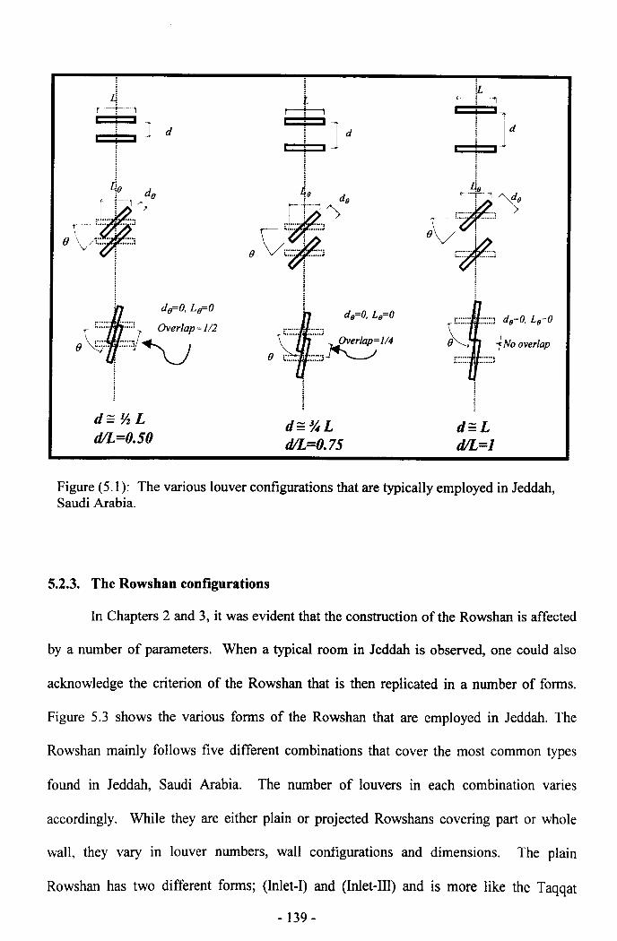
1! ,
IL~--t 1
In Chapters 2 and 3, it was evident that the construction of the Rowshan is affected
by a number of parameters. When a typical room in Jeddah is observed, one could also
~ l::::::' . ::::::: dfJ=O. LfJ=O
NiNo overlap
d~ Yz Ld/L=O.50
d~Ld/L=l
acknowledge the criterion of the Rowshan that is then replicated in a number of forms.
Figure (5.1): The various louver configurations that are typically employed in Jeddah,Saudi Arabia.
5.2.3. The Rowshan configurations
Figure 5.3 shows the various forms of the Rowshan that are employed in Jeddah. The
Rowshan mainly follows five different combinations that cover the most common types
found in Jeddah, Saudi Arabia. The number of louvers in each combination varies
accordingly. While they are either plain or projected Rowshans covering part or whole
wall, they vary in louver numbers, wall configurations and dimensions. The plain
Rowshan has two different forms; (Inlet-I) and (Inlet-III) and is more like the Taqqat
- 139-
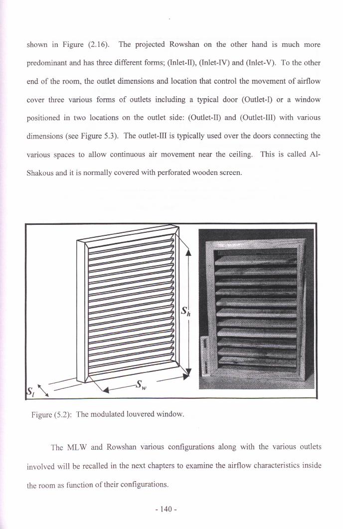
shown in Figure (2.16). The projected Rowshan on the other hand is much more
predominant and has three different forms; (Inlet-II), (Inlet-IV) and (Inlet-V). To the other
end of the room, the outlet dimensions and location that control the movement of airflow
cover three various forms of outlets including a typical door (Outlet-I) or a window
positioned in two locations on the outlet side: (Outlet-II) and (Outlet-III) with various
dimensions (see Figure 5.3). The outlet-III is typically used over the doors connecting the
various spaces to allow continuous air movement near the ceiling. This is called Al-
Shakous and it is normally covered with perforated wooden screen.
Figure (5.2): The modulated louvered window.
The MLW and Rowshan various configurations along with the various outlets
involved will be recalled in the next chapters to examine the airflow characteristics inside
the room as function of their configurations.
- 140-
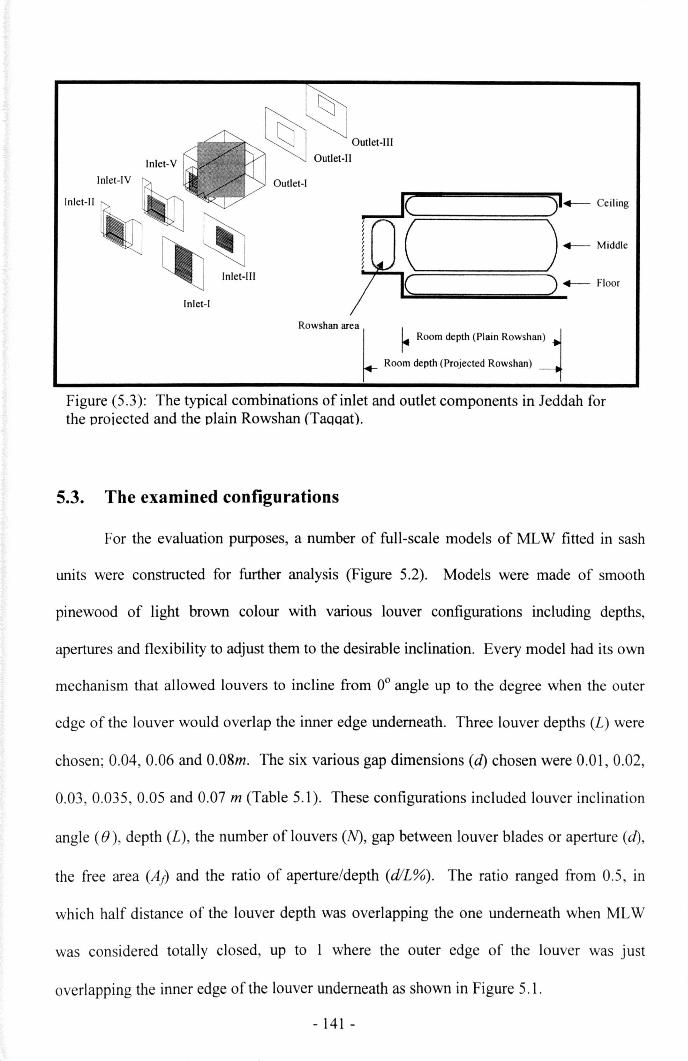
)1.-- Ceiling
':;=====~) __ Middl,
,)======~.-- Floor
Inlet-I
Rowshan areaI ~ Room depth (Plain Rowshan) ~r- Room depth (Projected Rowshan) --1
Figure (5.3): The typical combinations of inlet and outlet components in Jeddah forthe projected and the plain Rowshan (Taqqat).
5.3. The examined configurations
For the evaluation purposes, a number of full-scale models of MLW fitted in sash
units were constructed for further analysis (Figure 5.2). Models were made of smooth
pinewood of light brown colour with various louver configurations including depths,
apertures and flexibility to adjust them to the desirable inclination. Every model had its own
mechanism that allowed louvers to incline from 00 angle up to the degree when the outer
edge of the louver would overlap the inner edge underneath. Three louver depths (L) were
chosen; 0.04,0.06 and 0.08m. The six various gap dimensions (d) chosen were 0.01,0.02,
0.03, 0.035, 0.05 and 0.07 m (Table 5.1). These configurations included louver inclination
angle (B), depth (L), the number of louvers (N), gap between louver blades or aperture (d),
the free area (Aj) and the ratio of aperture/depth (d/L%). The ratio ranged from 0.5, in
which half distance of the louver depth was overlapping the one underneath when MLW
was considered totally closed, up to 1 where the outer edge of the louver was just
overlapping the inner edge of the louver underneath as shown in Figure 5.1.
- 141 -
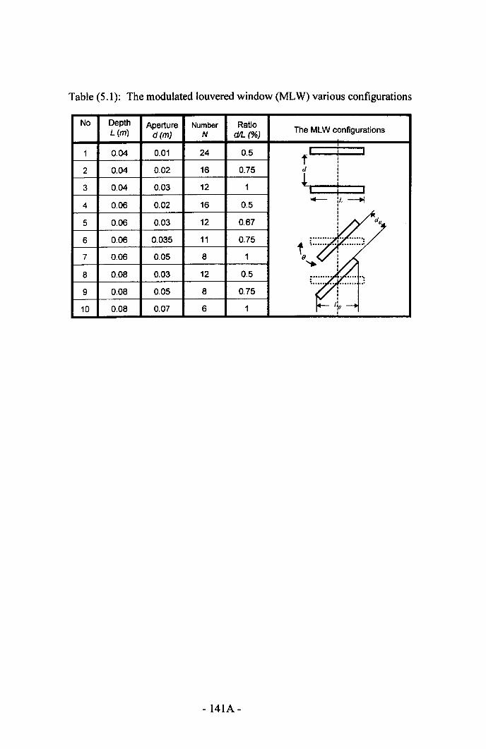
Table (5.1): The modulated louvered window (MLW) various configurations
No Depth Aperture Number RatioL(m) d(m) N d/L (%) The MLW configurations
1 0.04 0.01 24 0.5 fI i I
III
2 0.04 0.02 16 0.75 d I
~III
3 0.04 0.03 12 1 I
I i I
4 0.06 0.02 16 0.5 14- :L~IIII
d5 0.06 0.03 12 0.67 IIII
6 0.06 0.035 11 0.75 I ........• I •
to \...... .. ..........8 1
I
7 0.06 0.05 II
~ II
0.08 0.03 12 0.5I
8 : •••••••• Jo ••••• :~,..... I.9 0.08 0.05 8 0.75 I
III
10 0.08 0.07 6 1 40 -+I
- 141A-
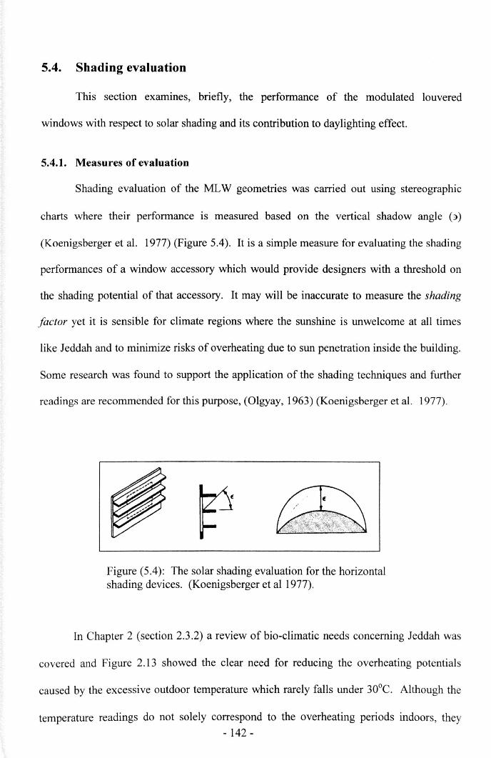
5.4. Shading evaluation
This section examines, briefly, the performance of the modulated louvered
windows with respect to solar shading and its contribution to daylighting effect.
5.4.1. Measures of evaluation
Shading evaluation of the MLW geometries was carried out using stereo graphic
charts where their performance is measured based on the vertical shadow angle (3)
(Koenigsberger et al. 1977) (Figure 5.4). It is a simple measure for evaluating the shading
performances of a window accessory which would provide designers with a threshold on
the shading potential of that accessory. It may will be inaccurate to measure the shading
factor yet it is sensible for climate regions where the sunshine is unwelcome at all times
like Jeddah and to minimize risks of overheating due to sun penetration inside the building.
Some research was found to support the application of the shading techniques and further
readings are recommended for this purpose, (Olgyay, 1963) (Koenigsberger et al. 1977).
Figure (5.4): The solar shading evaluation for the horizontalshading devices. (Koenigs berger et al 1977).
In Chapter 2 (section 2.3.2) a review of bio-climatic needs concerning Jeddah was
covered and Figure 2.13 showed the clear need for reducing the overheating potentials
caused by the excessive outdoor temperature which rarely falls under 30°C. Although the
temperature readings do not solely correspond to the overheating periods indoors, they- 142 -
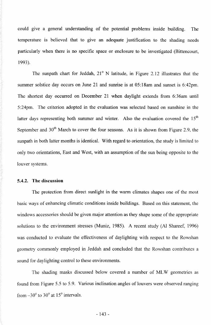
could give a general understanding of the potential problems inside building. The
temperature IS believed that to give an adequate justification to the shading needs
particularly when there is no specific space or enclosure to be investigated (Bittencourt,
1993).
The sunpath chart for Jeddah, 210 N latitude, in Figure 2.12 illustrates that the
summer solstice day occurs on June 21 and sunrise is at 05:18am and sunset is 6:42pm.
The shortest day occurred on December 21 when daylight extends from 6:36am until
5:24pm. The criterion adopted in the evaluation was selected based on sunshine in the
latter days representing both summer and winter. Also the evaluation covered the is"
September and so" March to cover the four seasons. As it is shown from Figure 2.9, the
sunpath in both latter months is identical. With regard to orientation, the study is limited to
only two orientations, East and West, with an assumption of the sun being opposite to the
louver systems.
5.4.2. The discussion
The protection from direct sunlight in the warm climates shapes one of the most
basic ways of enhancing climatic conditions inside buildings. Based on this statement, the
windows accessories should be given major attention as they shape some of the appropriate
solutions to the environment stresses (Muniz, 1985). A recent study (AI Shareef, 1996)
was conducted to evaluate the effectiveness of daylighting with respect to the Rowshan
geometry commonly employed in Jeddah and concluded that the Rowshan contributes a
sound for daylighting control to these environments.
The shading masks discussed below covered a number of MLW geometries as
found from Figure 5.5 to 5.9. Various inclination angles of louvers were observed ranging
from -300 to 300 at 150 intervals.
- 143 -
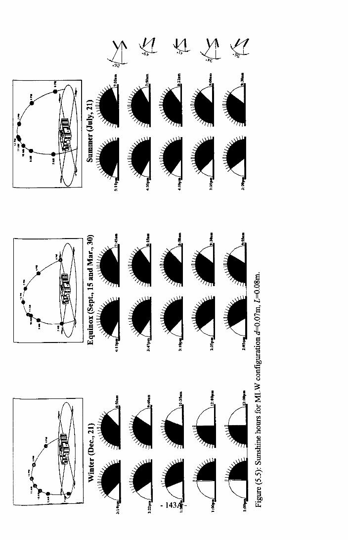
- I= i~'"..:~
~"CCl S=II'l 00~ 0
.J' 1?c.Qj
~rJ'J e'-"IlOl
e--e 0
Cl~.-=C'"
~ s=0
• ·1t+=:s=0(.)
• ~g.
~~M
~
- ~~N
0
'"..c:
UQ)
Qj ]B ell
... S~Cl
Cl)
.- -~
onon--Q)~.-~
,>;

Iir--e>
"..:=~"'0&:I E~II) 00
0...-4 clII~S~
~ lJ')
0Q cl&:I.... 4=0" a s=~ ... 0::l ~ .....,;; ;.; ~ro~
t+:4s=0o
e ~Ii .....4;:!l ::B= ! I-<
t8~;:::l0
...t::Q)s=.....
...t::Vl
~ §~ Vl....Cl .-._
'"~ lJ')'-'Q)
~e e en........ ... ~ r.,I..
- 143~ -on:n ~
\\
-.Cl~
r-..:~~"0
= S~In
00~ 0
r- 0...,J IIC.~ ~00 s'-'~ M
Q0
= 0....= -11="~ ~.. 0. ....
oii ~I-<
51~~0o~
e ~~. ~I-<.aCIl
-. I-<
~ ::sN
0
r-..c:
c,; Q)
CI.I~
~ :E'-'
tf.l
... §CI.I.... C/J
=.... -.~
r---\r)'-'Q)I-<
5bii:
::!
- 143C -
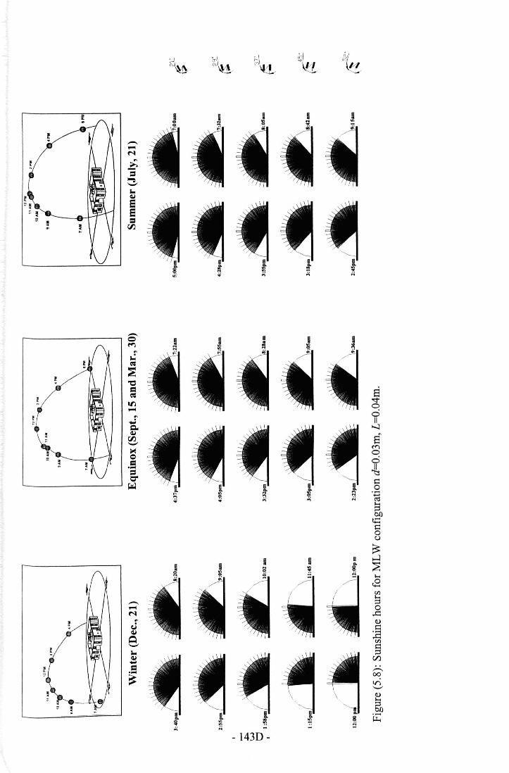
-Q a iM~ ~,.:~~-eCl
~~If')
"""0
~ 0.... IIc.. ~~00 S~--~ t"'l
00
Cl 0....= 40"~ s:::::
0.~~OJ)
tHs:::::0C,)
~e ~... ::;s8~ I-<
t8rJ)-- ~
"""N 0
~ ..d
UQ)
~ s:::::
a :ErJ)
,.. §~.... Cl')
Cl.... -:s 00tr)'-'Q)
~~ ~
~- 143D-
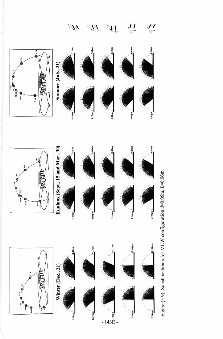
-Q('f')~..:=
~"CCl S=I£) \0
0- 0II
>...::l
ErV')
00
-11a :::0- 0~ .-N ~
~l+=i:::0C)
~E a
~E 0- .... ~ ~~ N ...
I-<..sVJ
~0.s::~::::.aVJ
J... §Cl) C/)....Cl -.- 0\~ V)
'-'~~Cl)
on ~...N
- 143E -
5.4.2.1. Louver depth
The shading masks reflect the increasing potential of shading as a function to the
louver depth. With the same model's geometry, the increase in depth is found appropriate
to reduce the cutoff angle of the louvers which increase the masking periods. For instance,
with louver depth L=0.08m, the effective shading started early morning in the summer
(8:22am). This was extended to more than an hour with the presence of -30°. However,
this was corrected by the increase in louver depth as airflow may be directed downwards
with the interior being under complete shade from early morning (around 8:30am).
Similarly, in September, the shading mask started one hour earlier with L=0.03m rather
than 0.07m for the same cutoff angle. In winter, when the noon solar altitude is 46°, there
is a big potential for over heating when the 8=-30°. Both depths 0.08m and 0.06m hardly
created any mask till noon since the respective cutoff angles 56" and 51" were more than
the solar altitude. Meanwhile the increase in depth provided some release to the indoor
environment since the cutoff angle was slightly under the sun's solar altitude; bearing in
mind that in winter direct sun may be needed at day time to assist cooling the structure.
In general, it is the increase in louver depth that would assist controlling the
penetration of direct solar light, which would contribute to the thermal environment
indoors.
5.4.2.2. Louver aperture
The aperture also contributed to this effect since the cutoff angle was corrected
according to the decrease of d. The comparison between similar MLW geometries with
various apertures have shed light on the possibilities of overheating indoors. The decrease
d from 0.07m to 0.05m would reduce the shading mask time from 30 minutes to more than
one hour before and afternoon. While this may be acceptable during early morning, the
- 144-
afternoon overheating may be increased where the sun due to the increase in cutoff angles
accompanied by higher temperature (from 1:OOpmtill 4:00pm).
5.4.2.3. Inclination angle
The effect of louver inclination angle is clearer than the other variables. The
attempt to examine the negative inclinations was to observe the possibility to determine the
extent of these inclinations when altered to negative or positive angles. With louver being
perfectly horizontal, the minimum summer shading period was between 8:30am and
3:3Opmwith the MLW with largest d and L dimensions. The shading period covers the
most unwelcome sunlight that is around noon and afternoon periods. The time was even
expanded with the alteration of even a small segment of louver inclination as shown in the
Figures. The tilt of louver to -30 inclination is questionable since it limits the shading
periods, which may cause the potential overheating indoors. In general, the other
dimensions of the MLW are corrected with the presence of louver inclination even at the
hottest periods of the year. Generally, to control the indoor environment, the cutoff angle
should not exceed the solar altitude in the hot seasons and more specifically in the
afternoons where higher temperatures are present.
The flexibility in controlling cutoff angles of the louvers is another advantage
added to this window system which, on the other hand, exhibit the preference of this type
of window accessories as they demonstrated a stronger potential to control the daylight in
buildings.
5.5. Privacy and view
In the literature, a number of studies indicated the importance of louvers from
privacy and view perspectives as the MLW design reveals some social requirements.
Privacy is the main sociological factor that a Rowshan posses. This issue was thoroughly
- 145 -
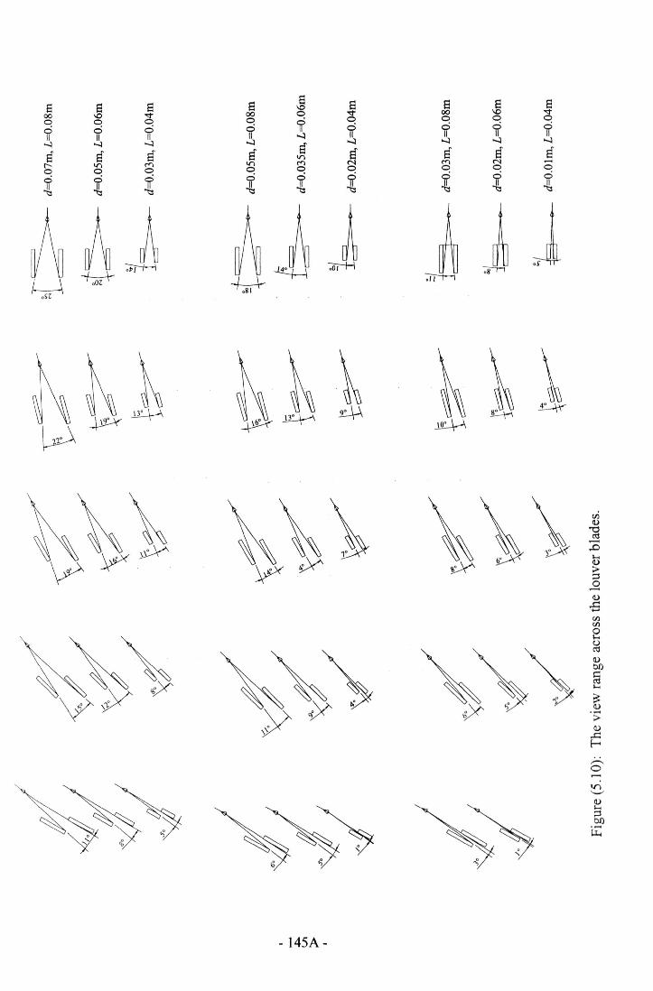
~h1 h1~ ~~~~
Cl.)
;Stiltil
f--;
--.o.......If)
~~~~~ ~~ J- 145A-
investigated by other studies such as (Hariri, 1992), (Al-Lyaly, 1990), (Al-Said, 1996)
(Banajah, 1995), (Khan, 1986), (Salloum, 1983) and others, and therefore will not be
covered in the following discussion.
The view within the louvers blades of the Rowshan is important since at certain
stage the Rowshan louvers geometry could cause conflict with the climatic requirements.
The MLW setup allows different viewing angles to the outdoor environment. The
reference viewpoint determines the angle of viewing. Here the point is about 0.08m away
from inside louver blades. The simple diagrams that are demonstrated in Figures (5.10)
gives a number of interpretations of the viewing characteristics through louver apertures.
The initial notion of the above figures demonstrates the effect of inclination of
louver as a considerable factor which will diminish view angle. The view angle is
diminished by almost 60% when louver is inclined to 45°. In practice this is of crucial
importance since it may contradict with the solar shading requirements during noon
periods in summer. Similarly, the louver aperture is also a measure to control the view
through. The diminishing of louver apertures is accompanied with a reduction of view
angle which ranges from 5-25% when ()=Oo. The Figure also shows some effect of the
louver depth where its increase is accompanied with some limitation of view angle based
on the other MLW geometries.
In general, there is a significant contribution of the MLW various geometries to the
view behaviour across them. Therefore, the design of MLW should give also some
concern to these variables since at certain stage they may sufficiently obstruct the view
through.
5.6. Reduction of volume as function ofMLW parameters
- 146-
The louvers' various variables including d, L and e are factors that determine the
flow patterns as well as the volume of the flow passing through a sash window. An
attempt is made here to mathematically define these functions to the total reduction in
volumetric flow.
Assuming a sash window with a complete open aperture and with a volume of:
where
V = the sash volume (rrr')
Sh = the sash height (m)
S; = the sash width (m)
SI = the sash length (m)
when this window is facilitated with louver sheets and the total volume of louvers is:
where
VL = volume of louvers (rrr')
1
T = the summation of louver thickness Lt. (m)n
L = the louver depth (m)
then the new volume as a function oflouvers' volume is expressed as follows
V - D·S -Snew - I w (5.3)
where
I
D = the summation apertures between louvers Id.n
Vnew = V - VL (5.4)
where
- 147 -
Vnew = volume reduction due to louvers (rrr')
For a number of louvers (n) of V[., the above equation is written as follows:
(5.5)n
Substituting both equations, (5.1) and (5.2):
This is when the louver at inclination O> 00; L = S, and Lis:
L = Sh -T (5.7)v"ew . s;
Representing Vnew in equation 5.3:
L = --=-1 _ ____:.:.n __
(Ld.L.Sw2)
(5.8)
n
(5.9)
n
L = n (5.10)
n
(5.11)
With the presence of louver inclination angle B:
Lo = L'cose (5.12)
1 1Ido = Id ·cosen n
(5.13)
- 148 -
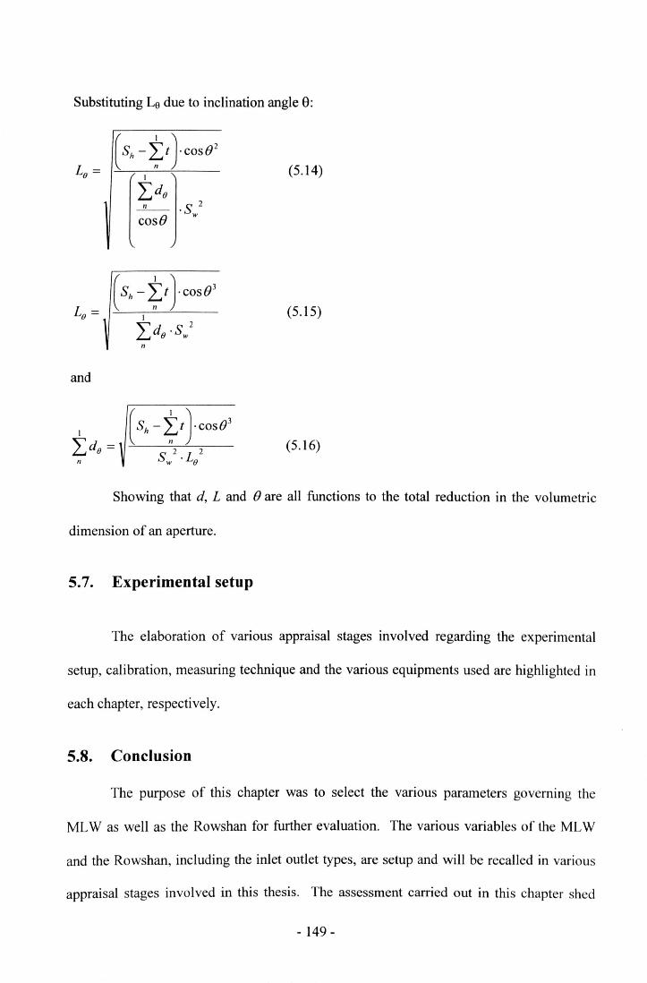
Substituting Le due to inclination angle 8:
(s, -t,leoso'I
Ide_n__ .S 2
cose w
(5.14)
(s, - t}osOJIIde 'Sw
2(5.15)
n
and
(5.16)
Showing that d, L and e are all functions to the total reduction in the volumetric
dimension of an aperture.
5.7. Experimental setup
The elaboration of various appraisal stages involved regarding the experimental
setup, calibration, measuring technique and the various equipments used are highlighted in
each chapter, respectively.
5.S. Conclusion
The purpose of this chapter was to select the various parameters governing the
MLW as well as the Rowshan for further evaluation. The various variables of the MLW
and the Rowshan, including the inlet outlet types, are setup and will be recalled in various
appraisal stages involved in this thesis. The assessment carried out in this chapter shed
- 149-
light. on the potentials of the reviewed MLW to control other factors that share a its
function considerably. The control of sunshine hours in various seasons is easily done by
the simple configurations of the MLW. Both louver depth and angle of inclination showed
some level of significance to controlling shading masks indoors, and hence to managing
indoor overheating during summer times. In the meantime, the aperture was less important
in this respect.
With reference to view consideration, the assessment indicted the importance of
various MLW parameters in affecting the view through louvers that may contradict, at
certain stage, the other functions of the MLW.
These configurations of MLW and Rowshan will be recalled in the following
chapters to carry out the various appraisal stages of this research.
- 150-

5.9. References
1. Kahtani, A.M. (1996) AI-Khasab: The wood. SED-309/1415, King Abdulaziz University:
School of Environmental Design.
2. AI-Lyaly, S.M. (1990) The traditional house of leddah: A study of the interaction between climate,
form, and living patterns. University of Edinburgh. Unpublished Ph.D thesis.
3. AI-Said, M. (1996) The Rowshan in the western province. SED-30S/1416, King Abdulaziz
University: School of Environmental Design.
4. AI Shareef, F.M. (1996) Natural light control in Hedjazi Architecture; An investigation of the
Rowshan performance by computer simulation. University of Liverpool. Unpublished Ph.D.
thesis.
5. Attieh, A.M.A. (1990) Review and analysis of housing in Jeddah, Saudi Arabia. Dundee.
Unpublished Ph.D. thesis.
6. Banajah, A. (1995) The Rowshan; AI-Mashrabiah. SED-30911415, King Abdulaziz
University: School of Environmental Design.
7. Bittencourt, L.S. (1993) Ventilation as a cooling resource for warm -humid climates: An
investigation on perforated block wall geometry to improve ventilation inside low-rise buildings.
Architectural Association Graduate School. Unpublished Ph.D. thesis.
S. Greenlaw, I. (1976) The Coral Buildings of Sua kin, London: Oriel Press.
9. Hajj Research Centre (1994) Samples ofMakkan traditional houses, Makkah: Hajj Research
Centre, Umm AI-Qura University.
10. Hariri, M. (1992)" The design of the Rowshan and its importance to the dwelling". Journal of
Umm Al-Qura University (3rd year)-S, p.175-237.
- 151 -

11. Khan, S. (1986) Jeddah Old Houses, Saudi Arabia: King Abdulaziz City for Science ad
Technology.
12. Koenigsberger, 0., Ingresoll, T., Mayhew,A. and Szokolay, S. (1977) Manual a/Tropical Housing.
Part One: Climatic Design, London: Longman Group Ltd.
13. Maghrabi, A. (1995). Personal communication with local craftsman.
14. Mani', M. (1980) The Architectural features to old Jeddah. pp.l 00-1 08. Jeddah: AI-Salam
Publications.
15. Muniz, P.A. (1985) The geometry of external shading devices as related to natural ventilation,
daylighting and thermal comfort, with particular reference to tropical hot-humid climates.
Unpublished Ph.D. Thesis.
16. Olgyay, V. (l963)DesignwithClimate, Princeton N.J.: Princeton University Press.
17. Salloum, A. (1983) " El-Rowashin of Jeddah, Saudi Arabia ". Crete, Greece: Passive and Low
Energy Architecture, p.245-252.
18. Zahran, W. (1995) Al-Khasab: The wood. SED-309/1415, King Abdulaziz University:
School of Environmental Design.
- 152-
CHAPTER 6: PRESSURE DROP ACROSS THE
MODULATED LOUVERED WINDOWS
- 153 -
6.1. Introduction
The first appraisal stage of this study is concerned with the pressure drop
characteristics across the modulated louver windows and is discussed in this chapter. It is
devoted to exploring the drop as function of the MLW various parameters reviewed in the
previous chapter.
The first section sheds light on the experimental setup as well as the various
instrumentation and equipment employed. The procedure followed to allocate and
calibrate the equipment in addition to the measuring principles is discussed in the second
section. The analysis of the observed data based on the two model equations in the form of
power law and the quadratic is discussed later. At this stage, the work covers the analysis
of the mathematical representations of the coefficients embedded in the equation in the
quadratic form. This section also covers the mathematical representations of other
variables involved in this study that are not integrated in the basic quadratic model
equation.
The results discussion of this chapter is divided into three subsections including
individual-variable appraisal, overall-variables appraisal and the critical inclination
appraisal where major airflow reduction was present. Based on critical inclination, a
statistical model is developed which represents pressure drop across the MLW as function
of the other variables concerned.
- 154 -
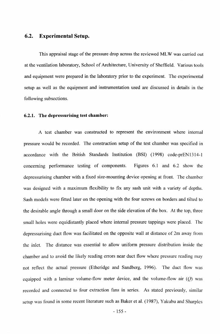
6.2. Experimental Setup.
This appraisal stage of the pressure drop across the reviewed MLW was carried out
at the ventilation laboratory, School of Architecture, University of Sheffield. Various tools
and equipment were prepared in the laboratory prior to the experiment. The experimental
setup as well as the equipment and instrumentation used are discussed in details in the
following subsections.
6.2.1. The depressurising test chamber:
A test chamber was constructed to represent the environment where internal
pressure would be recorded. The construction setup of the test chamber was specified in
accordance with the British Standards Institution (BSI) (1998) code-prEN1314-1
concermng performance testing of components. Figures 6.1 and 6.2 show the
depressurising chamber with a fixed size-mounting device opening at front. The chamber
was designed with a maximum flexibility to fix any sash unit with a variety of depths.
Sash models were fitted later on the opening with the four screws on borders and tilted to
the desirable angle through a small door on the side elevation of the box. At the top, three
small holes were equidistantly placed where internal pressure tappings were placed. The
depressurising duct flow was facilitated on the opposite wall at distance of 2m away from
the inlet. The distance was essential to allow uniform pressure distribution inside the
chamber and to avoid the likely reading errors near duct flow where pressure reading may
not reflect the actual pressure (Etheridge and Sandberg, 1996). The duct flow was
equipped with a laminar volume-flow meter device, and the volume-flow air (Q) was
recorded and connected to four extraction fans in series. As stated previously, similar
setup was found in some recent literature such as Baker et al. (1987), Yakubu and Sharples
- 155 -
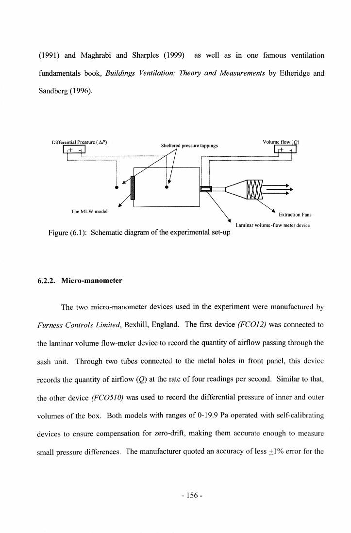
(1991) and Maghrabi and Sharples (1999) as well as in one famous ventilation
fundamentals book, Buildings Ventilation; Theory and Measurements by Etheridge and
Sandberg (1996).
Differ~:al ~~r.~r.~.~.~.) ~.hleltered pressure t:.~.~:.~.~~ ~.~.I~.r.l:ow ~ ]), ·.. · · 1 I I r · · · · · · · · l
I I! !. ~~~
The MLW modelExtraction Fans
Laminar volume-flow meter device
Figure (6.1): Schematic diagram of the experimental set-up
6.2.2. Micro-manometer
The two micro-manometer devices used in the experiment were manufactured by
Furness Controls Limited, Bexhill, England. The first device (FC012) was connected to
the laminar volume flow-meter device to record the quantity of airflow passing through the
sash unit. Through two tubes connected to the metal holes in front panel, this device
records the quantity of airflow (Q) at the rate of four readings per second. Similar to that,
the other device (FC0510) was used to record the differential pressure of inner and outer
volumes of the box. Both models with ranges of 0-19.9 Pa operated with self-calibrating
devices to ensure compensation for zero-drift, making them accurate enough to measure
small pressure differences. The manufacturer quoted an accuracy of less ±l % error for the
- 156 -
devices. Data from both devices were transferred to the computer through the data-logger
connected.
6.2.3. The laminar volume flow-meter device
This device was used to record the quantity of airflow through the reviewed MLW
(Figure 6.2). It is designed for smaller Reynolds number to preserve the laminar flow of
the fluid; Re is less than 2000. The device is based on the linear-law correlations between
Q and !.1P as in laminar flow (Awbi, 1991). While the flow is passing through the parallel
flat plates, it considers the flow rate in relation to the pressure drop taken from upstream
and downstream of the meter by linear relationship calibration stated by the manufacturer.
6.2.4. Fans
Four fans used for depressurisation were connected in series at the other end. The
diameter of each fan was 0.48m (19 inches) and contained blades of 14° pitch capable of
1440 r.p.m. and performed under fluid temperatures of up to 40° C. Each fan was made to
control the speed alteration separately from other fans. Woods of Colchester Limited
manufactured the fans.
6.2.5. Pressure tappings
Internal and external pressure tappings were positioned away from the influence of
flow through the opening. In the measurement, there was no need to make a second
upstream chamber of the component such as that found in Baker et al (1987) since the
laboratory pressure fluctuations, when measured, were found negligible. Shield pressure
tappings were enough to measure pressure both outside and inside the test chamber.
- 157 -
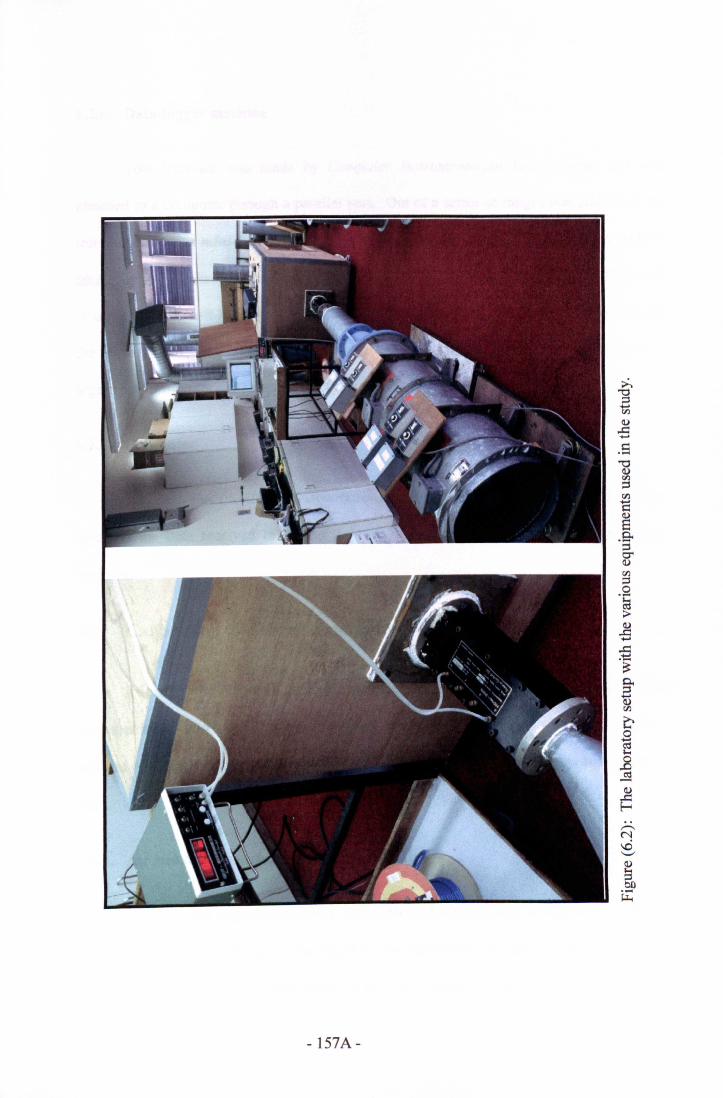
- 157A-

6.2.6. Data-logger machine
This interface was made by Computer Instrumentation Ltd, England and was
attached to a computer through a parallel port. Out of a series of ranges manufactured, the
interface used was mini-POD 100- 8 Channel high speed A-D converter that is capable of
taking up to 4 channel differential inputs or 8 single-ended channels. The mini-POD 100
is supplied with soft-logger and soft-scope software for DOS & Windows, together with
the Virtual Multi-meter. The data from both micro-manometers were transferred to data-
logger into millivolts (mV) signals via wires connecting both devices.
6.2.7. Computer
The data was transferred to a computer through the Data-logger, the software that
converts the data received to a CSV format for loading into a spreadsheet for further
analysis.
6.3. Calibration and measuring techniques
Prior to the analysis, it was essential to start with a number of routine
measurements and calibrations. These included the calibrations of various
instrumentations, data conversion, selecting the appropriate location of pressure tappings,
etc.
6.3.1. Air leakage through pressurisation chamber
The chamber edges were sealed with rubber silicon and tape along both its internal
and external edges. Seals were also made for the three holes on top. In addition, the sash
unit was firmly sealed after being fitted on the front panel of the chamber with rubber and
- 158 -
tape around the edges. All these precautions were made to minimise any possible
infiltration that may result from air extraction. Initial measurements were carried with the
box being totally sealed, including the opening in the front panel, and resulted in L1P at
extremely low flow rates, i.e Q,=O.0038. The flow rate due to infiltration (Q;) was
measured according to testing installation conditions and uncertainty characteristics noted
by BSI code-prEN 1314-1 (1998). The actual flow rate passing through the louver was
then adjusted using the following equation:
Q=Q-Q (6.1)
where
Q = the actual flow rate passing through the MLW (m3/s)
Qt= the total flow rate (m3/s)
Qi = the flow rate due to infiltration (m3/s).
6.3.2. Positioning of pressure tappings
The pressurisation chamber was designed with the flexibility to allocate the
pressure tappings in many locations and, thus, achieve most accurate results. The fact that
the location of the pressure tappings might influence the data reading to be analysed further
(Etheridge and Sandberg, 1996) was taken into consideration. For this purpose, pressure
readings were taken under two airflow rates for six different locations in the pressurisation
chamber. They found that positioning pressure tappings at the centre would be the most
appropriate.
- 159-
6.3.3. Data-logger result conversion
The micro-manometer transferred the data to the data-logger via connecting wires.
The software then received the data in its raw format, i.e. mV, and represented them into
series of tables for loading into spreadsheet software. Later, this data was calibrated from
mV signals into e and volume-airflow Q. Series of airflow records run first and then
micro-manometer transferred the data to the computer. The calibrations were made for
both pressure limits of pressure bands, high and low as shown in Appendix (B. I ). The
results were in linear regression of raw data mV into pressure readings from the micro-
manometers expressed in the following equation:
/)J'=a·mV+b (6.2)
where
a = the slope constant determined by the linear regression (Appendix B.l).
b = the intercept constant determined by the linear regression (Appendix 8.1).
6.3.4. Timing of pressure
Adjusting proper timing for each average reading is an essential technique which
has been taken into consideration prior to the evaluation stage. In the case of ventilation,
the researcher needs to give positive timing for the flow to reach its steady state where
pressure fluctuations are minimised. Too short a timing of an average reading might be
less effective and does not represent the actual alteration in the pressure drop where long
timing might be redundant and is time consuming. The micro-manometers and software
were adjusted to give the average reading of various timings, 1, 2, 3 minutes at four
- 160-
readings per second, under series of air extractions. The 2 minutes average readings were
found to be the appropriate timing to carry out the rest of the analysis.
6.3.5. Pressure difference at zero airflow
For accuracy, the author aimed to examine the pressure variations due to volume
variations between outside and inside of the pressurisation chamber. So the micro-
manometers recorded L1P at Q = Om3/s. Records were taken with respect to three time
periods: 20 minutes, 1 hour and 2 hours and the L1P were almost the same; L1P=0.019 Pa.
Though this drop was not significant it was taken into consideration in this study.
6.3.6. The work of Yakubu
The initial setup and measuring technique was similar to the work found in Yakubu
and Sharples (1991). The rest of the experiment was carried out after ensuring comparable
results were found in the relevant study.
6.3.7. Measuring principle
Controlling the circuit of fan systems would result in air flowing into the chamber
through louvers on the other edge. As these are already pre-set at particular angles this
causes differential pressure across the modulated louver window. The previous and the
volume-airflow readings were both transferred when the reading had stabilised. The
pervious step is repeated over a range of pressure drops obtained from the combined power
of the 4 axial fans. It was ensured that the laboratory temperature was about 20°C (White,
1999), the temperature that was programmed for both micro-manometers. The procedure
of the test measurement can be summarised in the following steps:
- 161 -
1. Various equipment to be used in the measurement were first switched on.
n. The micro-manometers were set to zero and left some time to stabilise.
UI. A MLW unit was fitted onto the chamber and sealed. Further, an
adjustment to tilt louvers to the desired angle took place. The inclination
was flexibly adjusted through a vertical wood panel connecting all louver
blades within the sash unit.
IV. After ensuring that only air entering the pressure chamber was flowing
through the sash, adding to the room infiltration, the fan was switched on
and controlled to the desired setting.
v. The data of both pressure drop and the volume-flow were taken after
ensuring stability of volume flow. As stated previously, one reading is a
representation of averaged two-minute records at 4 readings per second.
VI. Fan speed was set to various extraction rates to create ranges of differential
pressures. Step (v) was repeated before any further readings were taken.
vu. Fans were later switched off and the louvers adjusted to the next desired
angle. Step (iv) and (v) were then repeated for each setting.
viii. Nine various settings of angles, ranging from 60° to -60° at intervals of 15°,
were observed before installing other MLW unit.
IX. The software was programmed to record only the required data to be loaded
later into a spreadsheet package.
6.4. Power law and Quadratic Model equations
The validity of the power law and quadratic equations has been reviewed in the
previous chapter (section 4.2.4.3). Both calculation methods have been broadly accepted
- 162 -
and the debate about which of the two is more suitable still goes on. The results were
analysed using both model equations in order to find the more appropriate model. The
power law function is expressed as:
M = a .Qn (6.3)
And the quadratic model equation is expressed as:
M= AQ+BQ2 (6.4)
For ventilation research, some correlation is needed to identify the flow rates as a
function in relation to pressure difference due to wind, stack effect, .etc, which is expressed
as follows (ASTM Standard E779, 1982):
-A±.JA2 +4BMQ= 2B (6.5)
The values of A and B in the quadratic form could be directly measured as they
refer to gap thickness between louvers (d) and the breadth of louver (L) in equations (4.6)
and (4.7). However, the louver inclination Band the ratio of d/L were not considered in the
model equation. The following subsections are attempts to represent these effects in
mathematical forms.
6.4.1. Pressure drop as a function to inclination angle (9)
For modulated louvers, pressure difference could be a function to vertical
inclination angles of louver assuming that two louver blades are placed at a distance d with
a breadth of a blade L at initial inclination position 0°, when the two blades are perfectly
- 163 -
horizontal as shown in Figure (5.1). When louvers at initial setup were tilted positively or
negatively to angle, say e, this would be accompanied with a decrease in the effective gap
thickness between louvers da and the breadth of louver Lo, bearing in mind that the
following formulations could only be true if friction along dimension z was considered
constant for all louvers' vertical inclination angles (Yakubu, 1990). The following is the
interplay of the (da) and (La) at vertical angle e:
de =dcose (6.6)
Le = Lcose (6.7)
hence, the total pressure drop for the vertical angle e derived from Eq.(6.4):
(6.8)
or
:. the values of Aa and B«
A = 12.uz (6.10)(J L d 3e e
B = pY (6.11)(J 2d 2L 2e e
- 164-
Substituting the values of both de (Eq 6.6) and Le (Eq 6.7) in the latter equations, one
obtains:
(6.12)
12.uz 1= Ld3 • cos04
(6.13)
(6.14)
pY 1= 2L2d2 • cos04
(6.15)
By replacing both coefficients A and B for the blades when they are perfectly horizontal in
latter equations (6.13) and (6.15), one gets:
A = A ._I---:-e cos04
(6.16)
1s, = B· -co-s-O-:-4 (6.17)
:. Ma is given as:
1 1 2M, =A· Q+B·--4Qo cos (}4 cos 0
(6.18)
= (AQ+BQ2)._I_cos04
(6.19)
- 165 -
It is evident from the pressure difference for the parallel plate theory, and when angle e = 0°
that M = AQ + BQ2. ThenMe would be representedas follow:
(6.20)
From the above equations it was apparent that a vertical angle e would be a
parameter to measure pressure drop function across the modulated louvers systems, in
addition to other constants embodied in coefficients A and B.
6.4.2. Pressure drop as a function ratio (dIL)
The ratio of the gap thickness between louvers over the breadth of louver (d/L) is
also another parameter considered in determining the function of measured pressure drop
at any angle e. In this study, this ratio was strictly divided into three categories from
which all model configurations were selected. To simplify, these categories were
represented in numerical numbers as (d/L= 0.5), (d/L = 0.75) and (d/L= 1), respectively
(Figure 5.1).
So, from Eq. (6.19) it is apparent that pressure difference at any angle e was
represented as follows:
(6.21)
(12,uz pY 2) 1
= Ld3 Q+ 2d2 L2 Q cose4 (6.22)
Adding to the above equation a function of (Ld\
- 166-
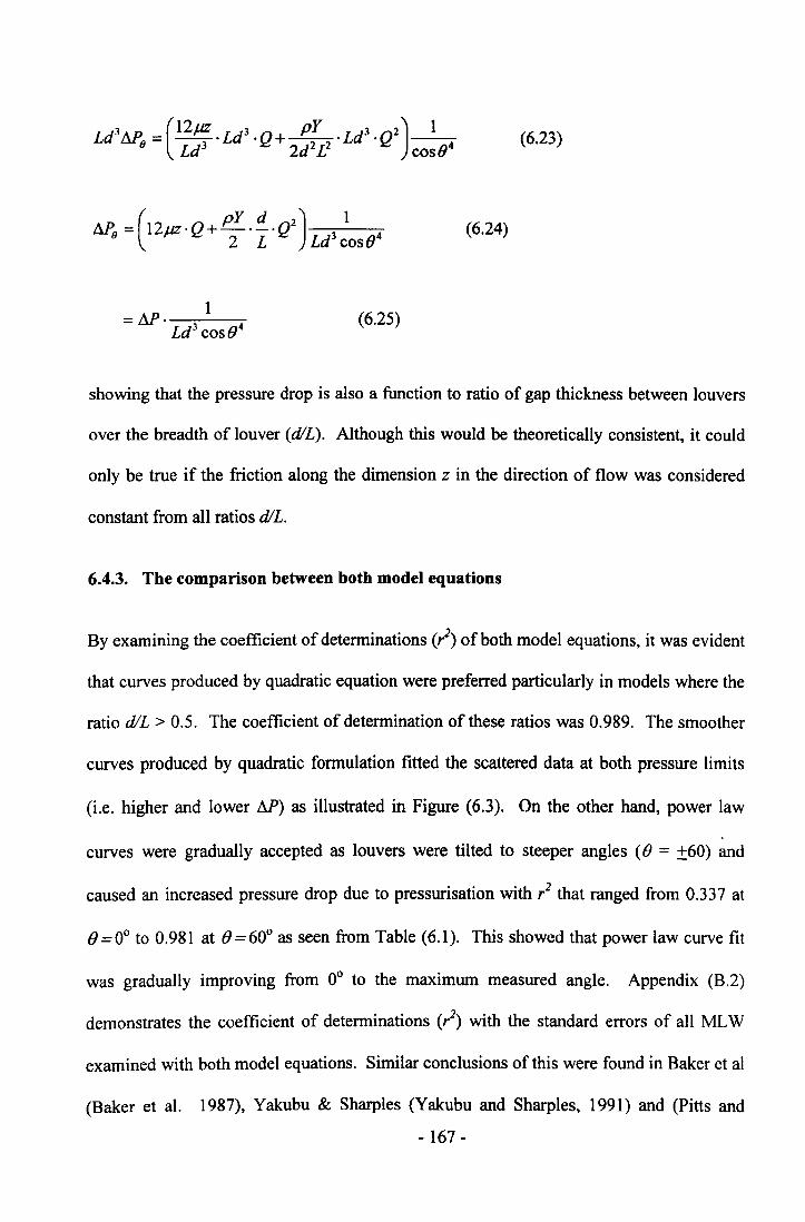
(6.23)
(pY d 2) 1M, = 12,uz·Q+-·_·Q
8 2 L Ld3 cos04(6.24)
(6.25)
showing that the pressure drop is also a function to ratio of gap thickness between louvers
over the breadth of louver (d/L). Although this would be theoretically consistent, it could
only be true if the friction along the dimension z in the direction of flow was considered
constant from all ratios d/L.
6.4.3. The comparison between both model equations
By examining the coefficient of determinations (r2) of both model equations, it was evident
that curves produced by quadratic equation were preferred particularly in models where the
ratio d/L > 0.5. The coefficient of determination of these ratios was 0.989. The smoother
curves produced by quadratic formulation fitted the scattered data at both pressure limits
(i.e. higher and lower M) as illustrated in Figure (6.3). On the other hand, power law
curves were gradually accepted as louvers were tilted to steeper angles (0 = ±60) and
caused an increased pressure drop due to pressurisation with / that ranged from 0.337 at
()=OO to 0.981 at 0=60° as seen from Table (6.1). This showed that power law curve fit
was gradually improving from 0° to the maximum measured angle. Appendix (B.2)
demonstrates the coefficient of determinations (r2) with the standard errors of all MLW
examined with both model equations. Similar conclusions of this were found in Baker et al
(Baker et al. 1987), Yakubu & Sharples (Yakubu and Sharples, 1991) and (Pitts and
- 167-
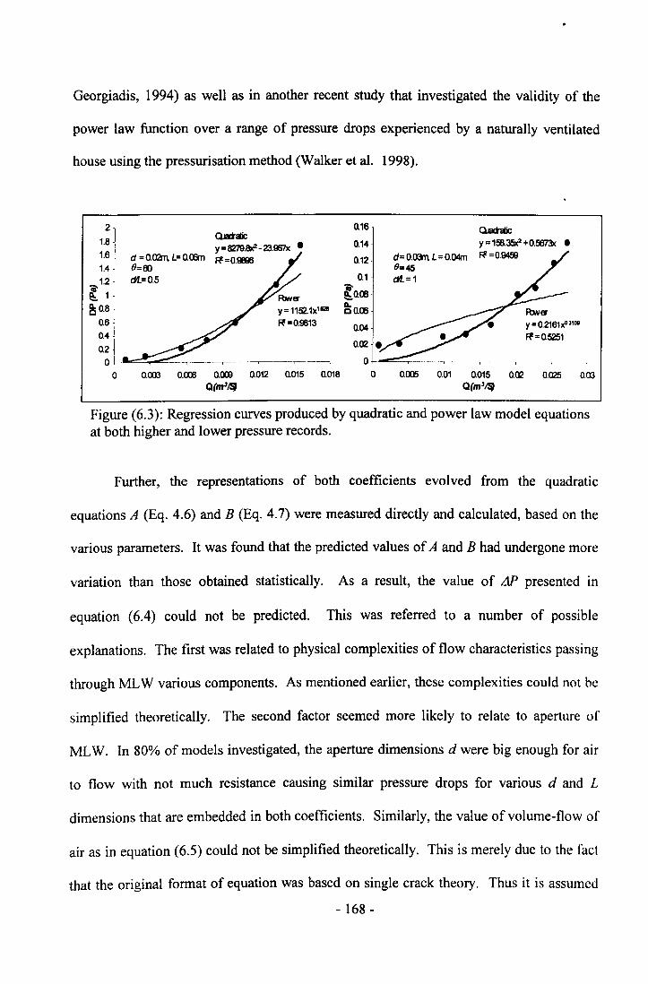
Georgiadis, 1994) as well as in another recent study that investigated the validity of the
power law function over a range of pressure drops experienced by a naturally ventilated
house using the pressurisation method (Walker et a1. 1998).
0.16
0.14
0.12
0.1
~0.(IJ
~o.oo0.04
2
1.81.61.412
11....~0.8
0.60.4
0.200
Qa:hIticy = 158.35)(2+O.~ •
d=O.canL=O.04m R!=0.94fi919=45cH..= 1
Qa:hIticy = 8279.SXZ - 23.967x •
d =0.02rn L= o.am R!=0.9!Il619=00cH..=0.5
y = 1152.1xUI211
R!=0.9813 y = 0.2161xO3'011R!=0.5251
0.003 0.000 0.00l 0.012 0.Q15 0.018Q(m1~
o 0.00> 0.01 0015 0.02 0.025 0.03Q(m1~
Figure (6.3): Regression curves produced by quadratic and power law model equationsat both higher and lower pressure records.
Further, the representations of both coefficients evolved from the quadratic
equations A (Eq. 4.6) and B (Eq. 4.7) were measured directly and calculated, based on the
various parameters. It was found that the predicted values of A and B had undergone more
variation than those obtained statistically. As a result, the value of & presented in
equation (6.4) could not be predicted. This was referred to a number of possible
explanations. The first was related to physical complexities of flow characteristics passing
through MLW various components. As mentioned earlier, these complexities could not be
simplified theoretically. The second factor seemed more likely to relate to aperture of
MLW. In 80% of models investigated, the aperture dimensions d were big enough for air
to flow with not much resistance causing similar pressure drops for various d and L
dimensions that are embedded in both coefficients. Similarly, the value of volume-flow of
air as in equation (6.5) could not be simplified theoretically. This is merely due to the fact
that the original format of equation was based on single crack theory. Thus it is assumed
- 168 -
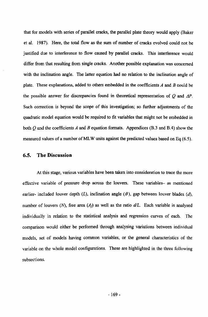
that for models with series of parallel cracks, the parallel plate theory would apply (Baker
et al. 1987). Here, the total flow as the sum of number of cracks evolved could not be
justified due to interference to flow caused by parallel cracks. This interference would
differ from that resulting from single cracks. Another possible explanation was concerned
with the inclination angle. The latter equation had no relation to the inclination angle of
plate. These explanations, added to others embedded in the coefficients A and B could be
the possible answer for discrepancies found in theoretical representation of Q and iJP.
Such correction is beyond the scope of this investigation; so further adjustments of the
quadratic model equation would be required to fit variables that might not be embedded in
both Q and the coefficients A and B equation formats. Appendices (B.3 and B.4) show the
measured values ofa number ofMLW units against the predicted values based on Eq (6.5).
6.5. TheDiscussion
At this stage, various variables have been taken into consideration to trace the more
effective variable of pressure drop across the louvers. These variables- as mentioned
earlier- included louver depth (L), inclination angle (B), gap between louver blades (d),
number of louvers (N), free area (AI) as well as the ratio d/L. Each variable is analysed
individually in relation to the statistical analysis and regression curves of each. The
comparison would either be performed through analysing variations between individual
models, set of models having common variables, or the general characteristics of the
variable on the whole model configurations. These are highlighted in the three following
subsections.
- 169 -
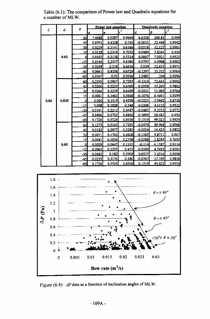
Table (6.1): The comparison of Power law and Quadratic equations fora number ofMLW.
d (JL
0.06 0.035
0.02
0.05
1.8 T--~--------.-------~-----.-1.6 t-------
I • -'\-- (}_ =± 60°1.4 -r---~--
Ii1.2 -4- ----- ------
1 l---------i
o
• ..i>:•-------~~
• • •• •
0.005 0.01 0.015 0.02 0.030.025
flow rate (mJ/s)
Figure (6.4): AP data as a function of inclination angles ofMLW.
- 169A-
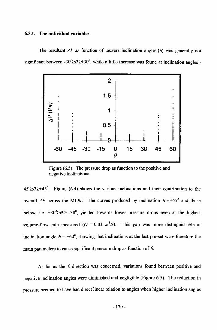
6.5.1. The individual variables
The resultant L1P as function of louvers inclination angles (8) was generally not
significant between -30o~B e+-30°, while a little increase was found at inclination angles -
2
1.5CO'o, 1-o,-<l i .0.5 - .Li I.
I
Ji I
i n i .r. l\J
-60 -45 -30 -15 0 15 30 45 60()
Figure (6.5): The pressure drop as function to the positive andnegative inclinations.
45°~B e+-45°. Figure (6.4) shows the various inclinations and their contribution to the
overall L1P across the MLW. The curves produced by inclination B=±45° and those
below, i.e. +30o~B:? -30°, yielded towards lower pressure drops even at the highest
volume-flow rate measured (Q == 0.03 m3/s). This gap was more distinguishable at
inclination angle B = ±60°, showing that inclinations at the last pre-set were therefore the
main parameters to cause significant pressure drop as function of B.
As far as the B direction was concerned, variations found between positive and
negative inclination angles were diminished and negligible (Figure 6.5). The reduction in
pressure seemed to have had direct linear relation to angles when higher inclination angles
- 170-
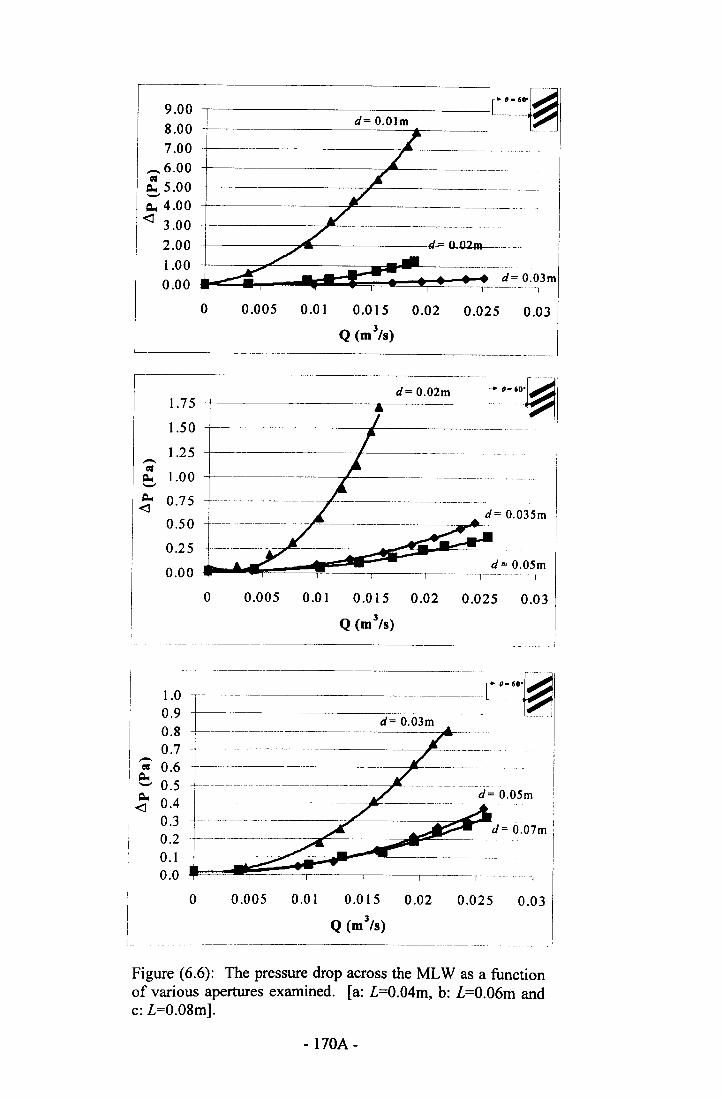
-,------d=-O.-Olm--=--=--- ..•r:....~9.008.007.00
_6.00""~ 5.00'-"'
~ 4.00<j 3.00
2.001.000.00
0
d= O.03m.. "1
0.005 0.01 0.015 0.02 0.025 0.03
Q (m3/s)
+- .-a-_d_=_O.02m_['."~1.75
1.50
1.25-""~ 1.00'-"'~ 0.75<j
0.50
0.25
0.00
0
-t------------.t-------- ..-- .....-.
d= O.035m
0.005 0.01 0.015 0.02 0.025 0.033Q (m Is)
f·-··---------·
I
o 0.005 0.01 0.015 0.02 0.025 0.03IIi __
3Q (m Is)
Figure (6.6): The pressure drop across the MLW as a functionof various apertures examined. [a: L=O.04m, b: L=O.06m andc: L=O.OSm].
- 170A-
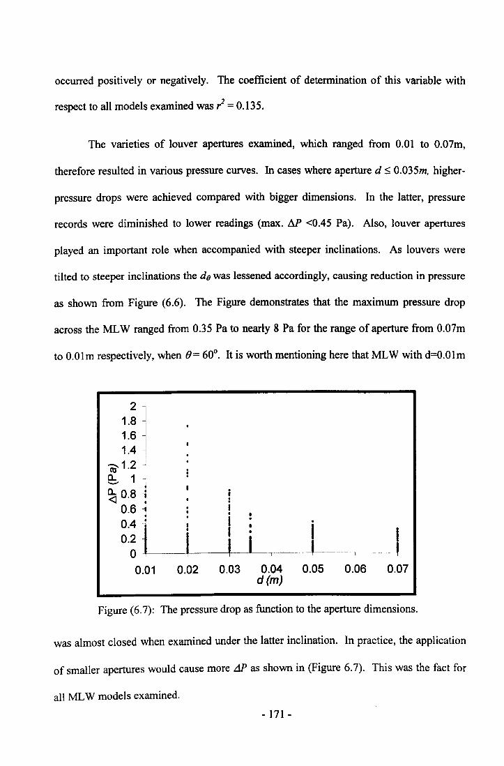
occurred positively or negatively. The coefficient of determination of this variable with
respect to all models examined was r2 = 0.135.
The varieties of louver apertures examined, which ranged from 0.01 to 0.07m,
therefore resulted in various pressure curves. In cases where aperture d $; 0.035m, higher-
pressure drops were achieved compared with bigger dimensions. In the latter, pressure
records were diminished to lower readings (max. !1P <0.45 Pa). Also, louver apertures
played an important role when accompanied with steeper inclinations. As louvers were
tilted to steeper inclinations the de was lessened accordingly, causing reduction in pressure
as shown from Figure (6.6). The Figure demonstrates that the maximum pressure drop
across the MLW ranged from 0.35 Pa to nearly 8 Pa for the range of aperture from O.07m
to O.OImrespectively, when B= 60°. It is worth mentioning here that MLW with d=O.Olm
1.~ 11.61.4
_jet;' 1.2~1~ 0.8
0.6
I-~
0.07
0.40.2o +------+---------'1--------,----+--- -----,
0.01 0.050.03 0.04d(m)
0.060.02
Figure (6.7): The pressure drop as function to the aperture dimensions.
was almost closed when examined under the latter inclination. In practice, the application
of smaller apertures would cause more L1P as shown in (Figure 6.7). This was the fact for
all MLW models examined.
- 171 -
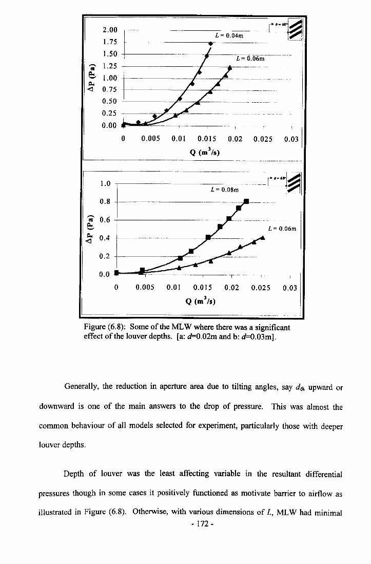
2.001.751.50- 1.25•~ 1.00-~-e 0.750.50 ~---
0.250.00
0 0.005
L__ ~ ~~.~_~ __ ~
1.0
0.8- 0.6•~-~ 0.4<I
0.2
0.0
0
C'"~-+-------------------~---
L= O.04m
-+------------..~----=------~~-------.~.~~-~--~L= O.06m
0.01 0.015 0.02 0.025 0.03
Q (m3/s)
--~-------~-----r O-.60'..j~.,--------~--~-------.--~- ~
L= O.08m
L= O.06m
0.005 0.01 0.015 0.02 0.025 0.033Q (m Is)
Figure (6.8): Some of the MLW where there was a significanteffect of the louver depths. [a: d=O.02m and b: d=O.03m].
Generally, the reduction in aperture area due to tilting angles, say do. upward or
downward is one of the main answers to the drop of pressure. This was almost the
common behaviour of all models selected for experiment, particularly those with deeper
louver depths.
Depth of louver was the least affecting variable in the resultant differential
pressures though in some cases it positively functioned as motivate barrier to airflow as
illustrated in Figure (6.8). Otherwise, with various dimensions of L, MLW had minimal- 172 -
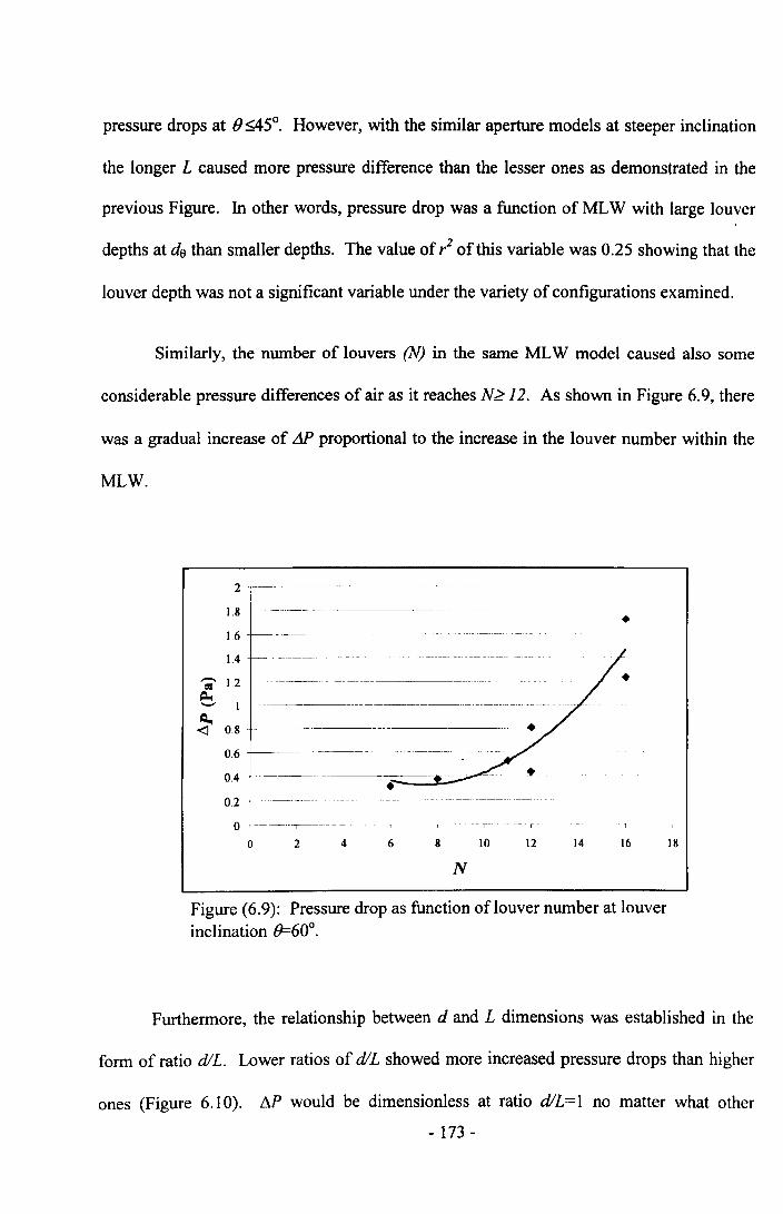
pressure drops at 0 :$;45°. However, with the similar aperture models at steeper inclination
the longer L caused more pressure difference than the lesser ones as demonstrated in the
previous Figure. In other words, pressure drop was a function of MLW with large louver
depths at de than smaller depths. The value of,2 of this variable was 0.25 showing that the
louver depth was not a significant variable under the variety of configurations examined.
Similarly, the number of louvers (N) in the same MLW model caused also some
considerable pressure differences of air as it reaches N;? 12. As shown in Figure 6.9, there
was a gradual increase of AP proportional to the increase in the louver number within the
MLW.
21~-~----~-~---1.8
1.4
.- 1.2~~--a.;-o
0.6
0.4
0.2
o --- ----~,--~--- --~---.- --r-------··o.- .....,.
1810 12 14 16
Furthermore, the relationship between d and L dimensions was established in the
4 6 8
form of ratio d/L. Lower ratios of d/L showed more increased pressure drops than higher
o 2
ones (Figure 6.10). !1P would be dimensionless at ratio d/L=t no matter what other
- 173 -
N
Figure (6.9): Pressure drop as function of louver number at louverinclination fF600.
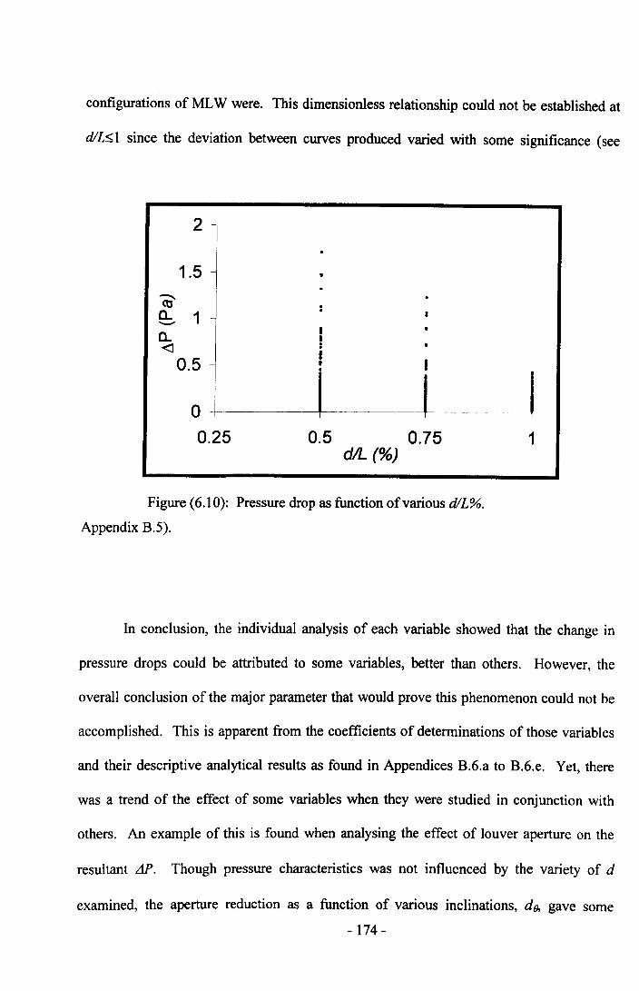
configurations of MLW were. This dimensionless relationship could not be established at
d/L~1 since the deviation between curves produced varied with some significance (see
2 -
I
1.5
<il'e:. 1-o,<l0.5 I
o +-------+-----10.25 0.5 0.75 1
dlL (%)
Figure (6.10): Pressure drop as function of various d/L%.
Appendix B.5).
In conclusion, the individual analysis of each variable showed that the change in
pressure drops could be attributed to some variables, better than others. However, the
overall conclusion of the major parameter that would prove this phenomenon could not be
accomplished. This is apparent from the coefficients of determinations of those variables
and their descriptive analytical results as found in Appendices B.6.a to B.6.e. Yet, there
was a trend of the effect of some variables when they were studied in conjunction with
others. An example of this is found when analysing the effect of louver aperture on the
resultant M. Though pressure characteristics was not influenced by the variety of d
examined, the aperture reduction as a function of various inclinations, do, gave some
- 174-
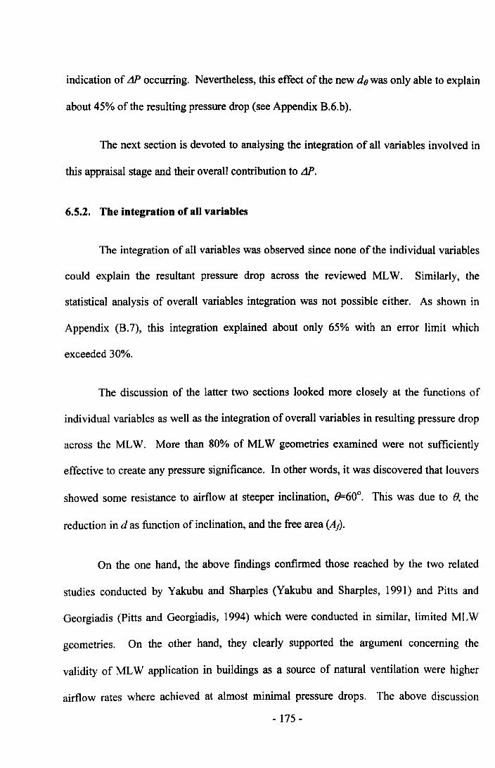
indication of AP occurring. Nevertheless, this effect of the new do was only able to explain
about 45% of the resulting pressure drop (see Appendix B.6.b).
The next section is devoted to analysing the integration of all variables involved in
this appraisal stage and their overall contribution to AP.
6.5.2. The integration of all variables
The integration of all variables was observed since none of the individual variables
could explain the resultant pressure drop across the reviewed MLW. Similarly, the
statistical analysis of overall variables integration was not possible either. As shown in
Appendix (B.7), this integration explained about only 65% with an error limit which
exceeded 30%.
The discussion of the latter two sections looked more closely at the functions of
individual variables as well as the integration of overall variables in resulting pressure drop
across the MLW. More than 80% of MLW geometries examined were not sufficiently
effective to create any pressure significance. In other words, it was discovered that louvers
showed some resistance to airflow at steeper inclination, 8=600• This was due to 8, the
reduction in d as function of inclination, and the free area (AI)'
On the one hand, the above findings confirmed those reached by the two related
studies conducted by Yakubu and Sharples (Yakubu and Sharples, 1991) and Pitts and
Georgiadis (Pitts and Georgiadis, 1994) which were conducted in similar, limited MLW
geometries. On the other hand, they clearly supported the argument concerning the
validity of MLW application in buildings as a source of natural ventilation were higher
airflow rates where achieved at almost minimal pressure drops. The above discussion
- 175 -
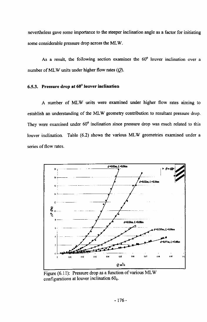
nevertheless gave some importance to the steeper inclination angle as a factor for initiating
some considerable pressure drop across the MLW.
As a result, the following section examines the 60° louver inclination over a
number of MLW units under higher flow rates (Q).
6.5.3. Pressure drop at 60° louver inclination
A number of MLW units were examined under higher flow rates aiming to
establish an understanding of the MLW geometry contribution to resultant pressure drop.
They were examined under 60° inclination since pressure drop was much related to this
louver inclination. Table (6.2) shows the various MLW geometries examined under a
series of flow rates.
~ 10---------Q"~
0.115 0.116 0.07 009001 010.01 0.02 0.03 0.04
Figure (6.l1): Pressure drop as a function of various MLWconfigurations at louver inclination 600.
- 176-
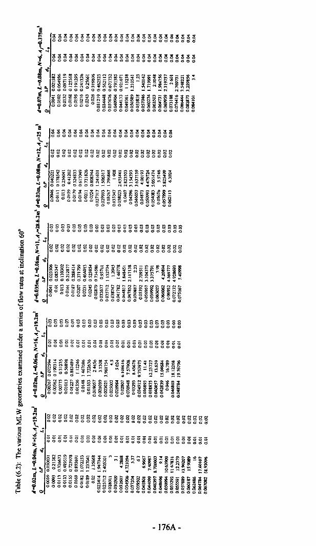
8ssaaaaaaaaaaaaaaaasaaaaOOOOOOOOOOOQoooooooooooo
08oao~oao~oBo8BBB88B8B8BBB88BB800000000000000000
BBSSBBBBBBSSSSBSBBBSSSSSSSSBBodoOdddOdddOdddddddodddddddd~
- 176A-
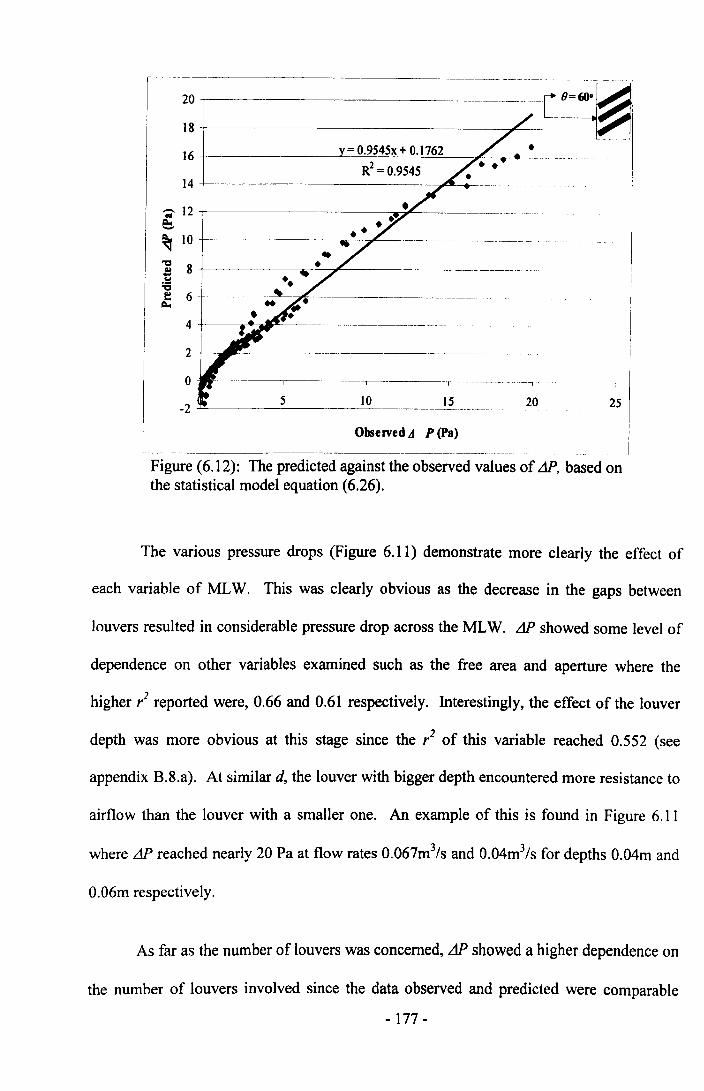
20
18
16
14
-;- 12~~ 10
"a 8~.~"ae 6 ----
Q.,
4
2
0
-2
= 0.9545x + 0.1762
R2 = 0.9545
~---"'-------,----------.-~----.---~ -,5 10 15
-=------------'-------------~~---- 20 25
Observed A P (pa)L_ ~ .
Figure (6.12): The predicted against the observed values of t1P, based onthe statistical model equation (6.26).
The various pressure drops (Figure 6.11) demonstrate more clearly the effect of
each variable of MLW. This was clearly obvious as the decrease in the gaps between
louvers resulted in considerable pressure drop across the MLW. t1P showed some level of
dependence on other variables examined such as the free area and aperture where the
higher r2 reported were, 0.66 and 0.61 respectively. Interestingly, the effect of the louver
depth was more obvious at this stage since the r2 of this variable reached 0.552 (see
appendix 8.8.a). At similar d, the louver with bigger depth encountered more resistance to
airflow than the louver with a smaller one. An example of this is found in Figure 6.11
where t1P reached nearly 20 Pa at flow rates 0.067m3/s and O.04m3/sfor depths O.04mand
O.06mrespectively.
As far as the number of louvers was concerned, t1P showed a higher dependence on
the number of louvers involved since the data observed and predicted were comparable
- 177 -
with ,2=0.75, with a high level of significance. Appendices B.8.a to B.8.d demonstrate the
statistical analysis of each variable with respect to the observed data.
Nevertheless, the integration of all variables involved in this study was needed to
establish the overall relationship of the factors mentioned earlier. The predicted value of
L1P with respect to the observed laboratorial data aimed to trace this effect. So, a statistical
model equation was developed which corresponds to the integration relationship of
variables involved in the latter inclination. This was essential to demonstrate the effect of
various parameters of MLW at the critical inclination; Le. 60°. The linear correlation of
the observed L1P is plotted against the predicted value in Figure 6.12 and is represented in
the following equation:
M = c+a.Q+ Pi.do +Xi·At +c5i·N+6i·Lo +l(ap)ij ·Q.do +(ax)y ·Q.Af +(ac5)ij ·Q.N +(ac),/ 'Q.L(}j(6.27)
where:
c = the intercept defined from the linear curve estimate in Figure 6.12 (0.1762).
a = a constant value for volume flow (141.046 )
f3, X, 8, E and ¢J are the numerical representations of the variables do. Afi N. Lo and ()
respectively.
The equation fitted the data observed with high degree of linear correlation (/ == 0.95)
(Appendix 13.8), with standard error of less than 5%, bearing in mind that the equation is
examined merely on the data obtained from Table (6.2). The aim was to highlight the
critical inclination where the pressure across the reviewed MLW would encounter a
- 178-
considerable drop. A further observation of this equation to fit larger number of MLW
parameters was beyond the aim of this research even through it represents one of the
author's future tasks. Therefore, it is not covered here.
6.6. Conclusion
This study investigated the pressure characteristics across the reviewed modulated
louvered windows that are typically employed in Jeddah. The appraisal measurement
showed that enhancements in pressure drops between inner and outer volumes could, at
certain point, be a function to some variables involved in this analysis. Nevertheless, the
major enhancement in differential pressure was not due to individual variables but rather to
the combination of variables that would comprehensively describe M. The considerable
pressure drop could not be achieved except when reaching ±60° of inclination, where
MLW offered a considerable resistance to the airflow. This was verified since more than
80% of the total cases observed have fallen under extremely low-pressure drops. The
statement, in light with the hypothesis of the current study, addresses the significance of
modulated louvered windows as a source on natural ventilation in buildings. Airflow
across the MLW has shown independence to the MLW where 0<±60o, regardless of the
other configurations involved. In other words, this chapter has demonstrated the critical
angle ofMLW under which major airflow reduction will exist.
In addition to the above, there are a number of other conclusions derived from this
chapter. They are highlighted as follow:
• The quadratic model equation suggested the best curves fits compared to
those produced by power law regressions. The quadratic curves were in the
- 179-

form of M = AQ + BQ2. However, further adjustments of the theoretical
representations of coefficients A and B that are embedded in the equation in
the quadratic form would be required to fit other variables such as number
of gaps between louvers, inclination angles B, and the ratio d/L%.
• The effect of louver depth showed some significance when accompanied
with steeper inclinations only.
• No major variations on drops were found between louvers positive and
negative inclinations.
There is some evidence to suggest that the flexibility in the design of MLW which
will not encounter much reduction in airflow passing louver blades. Next chapter is the
next appraisal stage to evaluate the velocity drop across the reviewed MLW.
- 180-
6.7. References
1. ASTM Standard E779 (1982) Measuring air leakage by fan infiltration pressurisation
method.
2. Awbi, H.B. (1991) Ventilation of Buildings, London: E & FN Spon.
3. Baker, P.H., Sharples, S. and Ward, I.C. (1987) "Airflow through cracks". Building and
Environment 22-(4), p.293-304.
4. BSI (1998) Ventilation for buildings - Performance testing of components/products for
residential ventilation - Part 1: Externally and internally mounted air transfer device. PrEN-
1314-1, p.18pp London: British Standards Institution.
5. Etheridge, D. and Sandberg, M. (1996) Building Ventilation: Theory and Measurements,
John Willy & Sons.
6. Maghrabi, Amjed and Sharples, S. (1999) "Air flow characteristics through Modulated
Louvered Windows". (1), p.507-514, Brisbane, Australia: PLEA99.
7. Pitts, A. C. and Georgiadis, S. (1994) "Ventilation air flow through window openings in
combination with shading devices". 15th AIVC Conference. p.432-439, AIVC.
8. Walker, I.S., Wilson, DJ. and Sherman, M. (1998)!lA comparison of the power law to
quadratic formulations for air infiltration calculations". Energy and Buildings 27-p.293-299.
9. White, M. (1999) "Ventilators: Ventilation and acoustic Effectiveness". BRE (IP4/99)-p.l-
8.
10. Yakubu, G.S. (1990) Modulated solar shielding of buildings: A study ofa solar radiation
control strategy for low energy buildings in hot dry and semi-arid climates. University of
Sheffield. Unpublished PhD thesis.
- 181 -

11. Yakubu, G.S. and Sharples, S. (1991) "Airflow through modulated louver systems".
Building Services Engineering Research and Technology 12-(4), p.lSI-155.
- 182 -
CHAPTER 7: VELOCITY DROP ACROSS THE
MODULATED LOUVERED WINDOWS
- 183 -
7.1. Introduction
This chapter covers the experimental work carried out to investigate the velocity
drop across the reviewed modulated louvered Windows. The louver depths (L), inclination
angles (0), apertures (d), and porosity percentage (P) of MLW are investigated here in
depth. In addition, room configurations, height (R,J and depth (RaJ, and prevailing wind
conditions including angle of incidence (Wi) and speed of wind (ve) are also studied at this
stage. The experimental setup and the calibration technique are considered first before
being followed by the analysis technique selected by comparing curves produced by the
power-law and quadratic statistical curve fits.
The discussion of the results is undertaken in a number of stages. First, the wind
data, including wind speed and direction, are highlighted. Then follows the velocity drop
as function of the room configurations. The parameters of MLW mentioned earlier are
discussed in the last section of the chapter, followed by the integration of all variables in
respect to the velocity drop across the MLW.
- 184-
7.2. Experimental and Calibration setup
The experiment took place at Ventilation laboratory, School of Architecture,
University of Sheffield. The velocity reading, which is further analysed as a function of
the earlier mentioned variables, is expressed as a percentage representing the ratio between
the mean indoor air velocity (vJ and mean outdoor wind speed (v.). The aim of this is to
establish a relationship between louvers' various configurations and that of the percentage
of (v/ve). It is necessary to mention at this stage that the wind speeds ranged from 0.6 to
3m/s. However, for simplicity some variables were investigated under fixed wind speed of
v,=2m1s, unless otherwise stated. The setup and calibration of various equipments and
instrumentation used in this study are discussed here in more detail.
7.2.1. The technique
The type of measurement undertaken in this chapter requires a deep analysis of the
air velocity reduction as function of the MLW variables noted in chapter 5. In addition, a
number of variables are also investigated here including the room configuration, wind data
and external reduction of velocity near the MLW as function of porosity percentage (p). In
here, the wind flow through the window is expressed as the fraction of wind speed near the
window level. The technique is appropriate for the scale of measurement in hand. Chand
et al. (Chand et al. 1988) studied the profile of wind speed on airflow rates through a
cross-ventilated enclosure by identifying the wind speed near the window level and
"Without introducing practically significant errors in the results due to a variation in the
type of terrain". In addition, a recent research is conducted by the Sharples and Maghrabi
(Sharples and Maghrabi, 2000) which includes the same measuring technique.
- 185 -
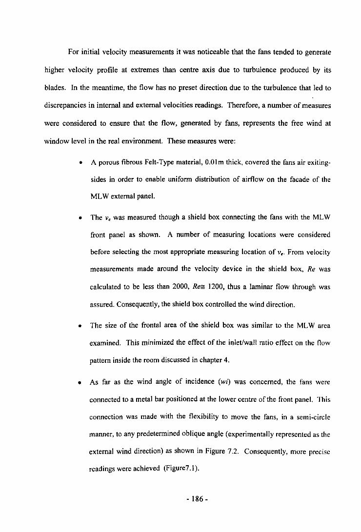
For initial velocity measurements it was noticeable that the fans tended to generate
higher velocity profile at extremes than centre axis due to turbulence produced by its
blades. In the meantime, the flow has no preset direction due to the turbulence that led to
discrepancies in internal and external velocities readings. Therefore, a number of measures
were considered to ensure that the flow, generated by fans, represents the free wind at
window level in the real environment. These measures were:
• A porous fibrous Felt-Type material, O.Olm thick, covered the fans air exiting-
sides in order to enable uniform distribution of airflow on the facade of the
MLW external panel.
• The v, was measured though a shield box connecting the fans with the MLW
front panel as shown. A number of measuring locations were considered
before selecting the most appropriate measuring location of Ve. From velocity
measurements made around the velocity device in the shield box, Re was
calculated to be less than 2000, Res 1200, thus a laminar flow through was
assured. Consequently, the shield box controlled the wind direction.
• The size of the frontal area of the shield box was similar to the MLW area
examined. This minimized the effect of the inlet/wall ratio effect on the flow
pattern inside the room discussed in chapter 4.
• As far as the wind angle of incidence (wi) was concerned, the fans were
connected to a metal bar positioned at the lower centre of the front panel. This
connection was made with the flexibility to move the fans, in a semi-circle
manner, to any predetermined oblique angle (experimentally represented as the
external wind direction) as shown in Figure 7.2. Consequently, more precise
readings were achieved (Figure7.1).
- 186-
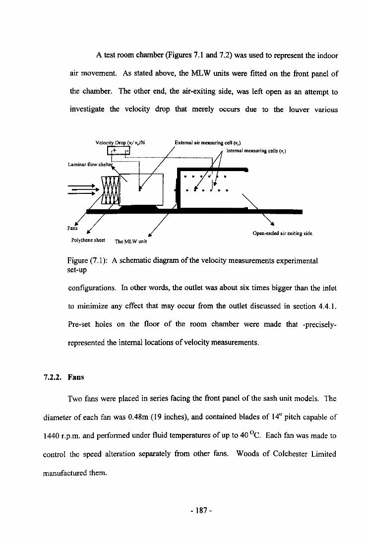
A test room chamber (Figures 7.1 and 7.2) was used to represent the indoor
air movement. As stated above, the MLW units were fitted on the front panel of
the chamber. The other end, the air-exiting side, was left open as an attempt to
investigate the velocity drop that merely occurs due to the louver various
External air measuring cell (v,)Internal measuring cells (v,)
Laminar flow
•
Open-ended air exiting side.Polythene sheet The MLW unit
Figure (7.1): A schematic diagram of the velocity measurements experimentalset-up
configurations. In other words, the outlet was about six times bigger than the inlet
to minimize any effect that may occur from the outlet discussed in section 4.4.1.
Pre-set holes on the floor of the room chamber were made that -precisely-
represented the internal locations of velocity measurements.
7.2.2. Fans
Two fans were placed in series facing the front panel of the sash unit models. The
diameter of each fan was 0.48m (19 inches), and contained blades of 14° pitch capable of
1440 r.p.m. and performed under fluid temperatures of up to 40 QC. Each fan was made to
control the speed alteration separately from other fans. Woods of Colchester Limited
manufactured them.
- 187-
7.2.3. Velocity record instrument
The machine used to record the indoor air velocity (vJ and the outdoor wind speed
(veJ was Model 8910 DisplaylPower Supply, manufactured by TSI Incorporated, USA
(Figure 7.2). It was designed specifically to work with TSI air velocity transducers to
provide a convenient readout of air velocity. Depending on the range selected, this
machine accepts a signal of 0 to 5 volts DC and displays an output that is linearly
proportional to the signal. The connected TSI air velocity transducer in the same hand is
calibrated to provide a linear output of 0 to 5 volts DC. It is a precise instrument designed
to measure air mass velocity in fixed installations as quoted by manufacturer. Mass
velocity is a measure of air velocity with reference to standard conditions of about 20°C,
the laboratory temperature under which the experiment took place. As the flow of air
passes the heated sensor of the velocity transducer which is kept at a constant elevated
temperature by means of electronics, more electrical power is required to maintain the
sensor at the elevated temperature. Monitoring the power supplied to the sensor provides a
signal that is related to the amount of air flowing past the sensor. This signal is
automatically displayed in the power supply machine in terms of velocity (mls) and
transferred to the computer in voltage signals through wiring and data-logger connecting
them.
The air velocity transducer was calibrated by the manufacture (refer to TSI device
manual). In the laboratory, the author correlated the readings of series of air velocity (m/s)
displayed from TSI machine relative to the voltage signals recorded by the data-logger.
The chart developed showed linear correlation between velocity and voltages signal that
ensured consistently accurate output display against that of voltage signals (see appendix
C.l). The coefficient of determination of the linear regression was (r2 = l).
- 188 -
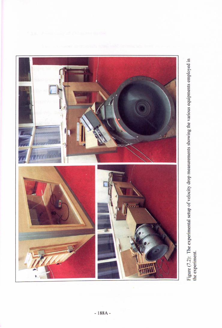
- 188A-
7.2.4. Positioning of TSI-meter device
Two TSI-meter instruments were used to measure both external and internal air
velocities. The first was placed outside room chamber at five different measuring locations
at a pre-set distance from the centre axis of the MLW unit. A number of routine
measurements took place before the final measuring location was chosen. It was evident
that the resistance to airflow caused by both front panel and MLW units had resulted in
interruptions to velocity reading and caused discrepancies in the O.50m next to the panel.
Beyond this, the distance towards the fans was a more appropriate location to measure
external air velocity as discrepancies were diminished. The centre of shield box was
finally recommended as the optimum measuring location from which wind velocity was
recorded.
As far as internal velocity was concerned, detailed analysis was attempted of
velocity drops along the vertical and horizontal sectional directions of flow. Therefore, six
different locations with two various heights each were selected for measurements along
height and depth of the chamber. Along the room depth, the six measuring locations were
set at O.25mdistance from each other and the vertical location was at O.325m(Figure 7.1).
The selection of the first measuring location inside the room chamber was chosen far from
free-jet flow or turbulence caused by louver geometry. The series of runs that took place
first showed that at a distance less than RtFO.25m, there were turbulences and jet flows that
interrupted flow measurements being taken, and hence, the first measuring location was
selected.
At a later stage, the TSI-meter instrument was positioned on the external surface of
MLW for comparison with the reviewed inclination angles for the various MLW units in
order to study the velocity drop as function of porosity percentage (P) of the MLW.
- 189-
7.2.5. Timing or velocity recording
As stated in Chapter 6, there is a need to give positive time for the flow to reach its
steady state and to avoid any turbulence before inscribing any reading (Etheridge and
Sandberg, 1996). While too short a timing may be less effective, along timing might be
redundant and is time consuming. Contrary to site measurements, wind could be adjusted
at any pre-set speed and direction in laboratory measurements. This advantage could save
time and therefore result in better representation of the average readings to be recorded
therefore (Yousoufian, 1992). Another advantage of the latter technique is related to the
time lag between internal and external readings. Time lag is the time required for
measuring internal velocity to correspond with the external one (Bittencourt, 1993). Onsite
observations with improper consideration of time lag could result in discrepancies found in
data collected. On certain occasions, at lower air velocities and wind turbulence, the
discrepancies could exceed the margin of error percentage, thus results may not be
accurate, especially when v/ve% is of considerable importance in the analysis. In the
laboratory, errors resulting from time lag are diminished since external wind is controlled
at a pre-set velocity and direction. Hence, the ratio v/ve% is more likely to represent the
actual drop in air velocity.
The software was adjusted to give an average reading of various timings, 30 sec, I
min and 2 min at four readings per second under series of air velocities. The first average
timing (30 sec) was chosen as no major variations resulted from the three timings
examined.
- 190-
7.2.6. Measuring principles
Both internal and external velocity readings from the combined power of both axial
fans were transferred to the computer attached when readings had stabilised. Similar to the
pressure drop appraisal stage, this step was repeated over ranges of velocity drops as well
as different measuring locations involved. Steps were taken to ensure that the laboratory
temperature was about 20 C (White, 1999). The procedure of the test measurement can be
summarised in the following steps:
I. Various equipment used in the measurement were first switched on.
II. The TSI-meter devices were set to zero and left some time to stabilise after.
being fitted in the pre-set measuring locations.
III. A MLW unit is fitted onto the chamber front panel facing fan systems with
adjusting louvers to the desired inclination angle.
IV. The fan is switched on and controlled to the desired setting.
V. The data of both internal and external velocities were then taken after
ensuring stabilised readings.
VI. The fans were set to various wind speeds in order to create ranges of air
velocities and step (v) was repeated.
VII. The TSI-meter device used to measure internal velocity was then moved to
another pre-set location, vertically or horizontally, and the last two steps
were then repeated.
VIII. The MLW unit was then adjusted to the next desired angle and the last
three steps were then repeated for each setting.
IX. Wind speed covered from 0 to around 3 mls.
- 191 -
x. External velocity was measured at the centre axis of the MLW and internal
velocity was taken at the preset locations noted earlier.
7.3. The analysis
A reduced-sample of data was first analysed using the two statistical curve fits
including power law and quadratic (based on the least square method). At this stage, the
three curve fits were analysed based on the reduction in velocity due to external wind
speed and the reduction in v/ve% due to room depth and the ,-2 of both model equations
were examined as shown in Figure 7.3. It is important to mention at this stage that data
obtained were not based on scattered data but rather on clear trend of curve fits since
measurements were carried out in the laboratory.
As shown in Figure 7.3, the regression lines developed by the two curve fits
corresponded to the data measured at both maximum and minimum aperture dimensions.
The preference of quadratic cure fit was obvious with data representing the reduction due
to room depth at both higher and lower ratios v/ve, as well as with the presence of louver
inclinations. Therefore, the recommendation was to carryout the discussion of results of
this chapter using the curve fits in the quadratic form.
7.4. The discussion
This study investigated the velocity drop across the reviewed MLW. The louver
depths (L), inclination angles (0), apertures (d), ratio of (d1L) and free area (Aj, porosity
percentage (P) of MLW are investigated here. The room configurations, height (R;J and
depth (RcJJ and wind angle of incidence (Wi) were considered.
The internal velocity patterns would vary in accordance with the varieties of louver
inclinations as well as other variables involved. Some measurements were taken at louver
- 192 -
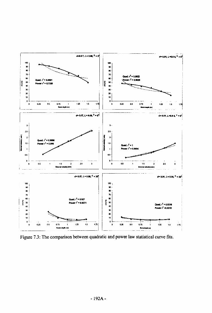
I d-o.O 7, L- 0.01, e _
lOO 100
Igo go
110 110
70 70I
110Quad. " - 0.9801
eo
i 50 _"-0.7321 ~ 50
40 ~ 40
30 30
20 20
10 10
o -~--~~~~-o 025 0.5 125
------ ..--~~-~~~~~~~~--~~~~---,
r---------~.-.--.-- ..---..-~·"'....··1I
QuIll. " - 0.t122,~,,-O ...."
II
IIIIIi
171
-,, ...
+--~--~-- ..~-----,..1.7 025 0.5 1.25 1.5
---------
2.5
if 15
I0.5
0 ----,._----,--
0 0.5
100
90
110
70
601
50I40
30
20J
10 !o 1-.0 025
1.5 2-_.-, 2.5
- -----.----------~.-----,
Quad. ,. - D.927_?--0.1571
~ -.~0.5 1.2.5 1.5
----_ .. -~-----------~---~-
2.5
ff 1.5
QuIll. ?-- 1I _"-0.18140.5
0.5 1.5 2--.-, 2.5
,------~-----------.- ..
1.75
,--------- _----._-- ... _ .•.-d- 0.01, L- O.IM,e _ ~
Ii
100
go
110
70
. , ....
110
40QuIll. ?-- 0.1211_?--O.1311
30
20
10 ...__ . . ~0.25 0.5o 1.25 1.5 1.75
Figure 7.3: The comparison between quadratic and power law statistical curve fits.
- 192A-
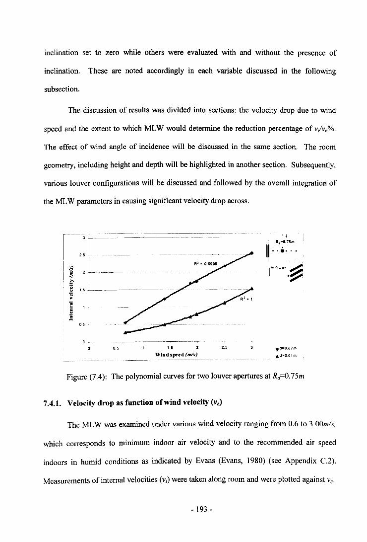
inclination set to zero while others were evaluated with and without the presence of
inclination. These are noted accordingly in each variable discussed in the following
subsection.
The discussion of results was divided into sections: the velocity drop due to wind
speed and the extent to which MLW would determine the reduction percentage of v/ve %.
The effect of wind angle of incidence will be discussed in the same section. The room
geometry, including height and depth will be highlighted in another section. Subsequently,
various louver configurations will be discussed and followed by the overall integration of
the MLW parameters in causing significant velocity drop across.
1-,:l----- .----I ii ~ 2r-I
'- ,.~
I !l,sl---~-------'-; j
I... 1·-
::l !
oSo.s i--~
II° ; -- ---~-~-'T-~--~-----·~------
o.s 1,S 2 2,5 3 .d·007m
Ad-O,OlmWind speed (ntis)
Figure (7.4): The polynomial curves for two louver apertures at Rcr=0.7Sm
7.4.1. Velocity drop as function of wind velocity (ve)
The MLW was examined under various wind velocity ranging from 0.6 to 3.00mls.
which corresponds to minimum indoor air velocity and to the recommended air speed
indoors in humid conditions as indicated by Evans (Evans, 1980) (see Appendix C.2).
Measurements of internal velocities (Vi) were taken along room and were plotted against Ve.
- 193 -
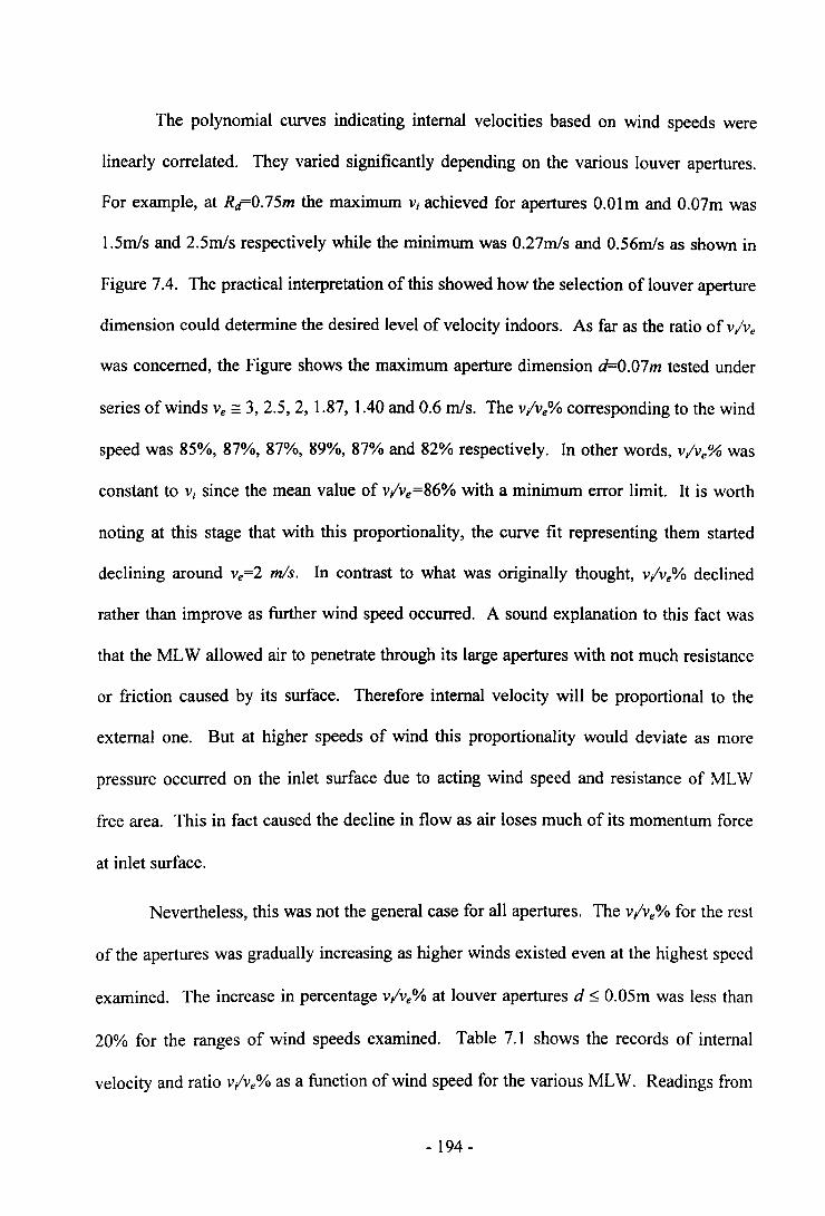
The polynomial curves indicating internal velocities based on wind speeds were
linearly correlated. They varied significantly depending on the various louver apertures.
For example, at RcFO.75m the maximum Vi achieved for apertures O.Olm and 0.07m was
1.5m1s and 2.5m1s respectively while the minimum was 0.27m1s and 0.56m1s as shown in
Figure 7.4. The practical interpretation of this showed how the selection of louver aperture
dimension could determine the desired level of velocity indoors. As far as the ratio of v/ve
was concerned, the Figure shows the maximum aperture dimension d=0.07m tested under
series of winds v, == 3, 2.5, 2, 1.87, 1.40 and 0.6 mls. The v/ve% corresponding to the wind
speed was 85%, 87%, 87%, 89%, 87% and 82% respectively. In other words, v/ve% was
constant to Vi since the mean value of v/ve=86% with a minimum error limit. It is worth
noting at this stage that with this proportionality, the curve fit representing them started
declining around ve=2 m/s. In contrast to what was originally thought, v/ve% declined
rather than improve as further wind speed occurred. A sound explanation to this fact was
that the MLWallowed air to penetrate through its large apertures with not much resistance
or friction caused by its surface. Therefore internal velocity will be proportional to the
external one. But at higher speeds of wind this proportionality would deviate as more
pressure occurred on the inlet surface due to acting wind speed and resistance of ML W
free area. This in fact caused the decline in flow as air loses much of its momentum force
at inlet surface.
Nevertheless, this was not the general case for all apertures. The v/v/Yo for the rest
of the apertures was gradually increasing as higher winds existed even at the highest speed
examined. The increase in percentage v/ve% at louver apertures d ~ 0.05m was less than
20% for the ranges of wind speeds examined. Table 7.1 shows the records of internal
velocity and ratio v/ve % as a function of wind speed for the various MLW. Readings from
- 194-
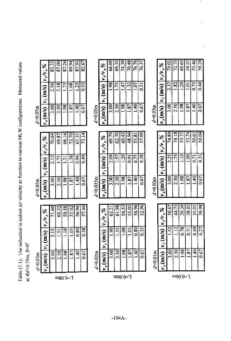
VJaJ::stil>"'0aJ
'""::sVJcOaJ
~vic::0.~ s'"" t-::s ~01)t;:: 0c:: II0 ~u
~...l~Cl)
::s0·ccO>0....c::.s....uc::cBVJ ScO In~ ~·u 00 IIQ) ~>'""·ca'""00"'0.s.sc::.s....u::s"'0aJ 0
'"" 0aJ II..c CDf- a a~,.-... In 0r-- 0r-- 0 II'-" II ~aJ '1::l- ~~f- ~
trl 0 \0 "<t" M r--~ M 0 C"! 0\ ~ \0
trl ~ r- a\ r-- ~\I 00 00 00 00 00 00
~;;..- \0 00 ~ 00 M trl~ trl ..... t- ~ C"! trle ('.I e-i ..... ..... ..... 0-._;;..
0 0 00 r- 0 e-- ~ trl ~ 00 ~ ~~ ~a M ..... - ..... 0-\I;;..
'<:t t- \0 0 ..... '<:t
~ ~ 00 ..... r-- M .....0 a\ \0 M r-- M
\I r-- \0 \0 r-- \0 r--~;;..- C"I trl ..... 00 "<t" 0\~ ..... r-- M M ~ '<:ta C"I - ..... - 0 0-._;;..
0 0 00 r-- 0 r--- 0 trl ~ 00 ~ ~~e ~ ('.I ..... ..... -' 0-\I;;..
0 ('.I 00 ('.I \0 \0
~ ~ ~ trl 0 0\ ~..... 0 0\ In -.0 r--\I t- \0 trl In trl trl
~;;..
In ..... 00 M 0 00- - In ..... 0 00 M~ ~ 0e - ..... -' 0-._;;..0 0 00 r-- 0 r--- 0 In 0\ 00 ~ ~~e ~ ('.I ..... ..... -' 0-\I;;..
W80·0=1
StrlooII~
0\ M 0\ 00 \0 t--
~ 0 ~ ~ '<:t t- ~-.0 0\ "<t" 0 -.0 -c
\I \0 \0 t- r- r- e--~....;;..
'{i;'00 ~ t- ('.I r- .....~ l'; ~ ~ ~ trle - ..... ..... ..... ..... 0-....;;..0 0 00 r-- O e--- ~ trl ~ 00 ~ \0~ 0a M C"I - ..... .....-\I;;..
son~ooII~
0\ 0 ~ '<:t ..... 0~ l'; t- '<:t ~ ~ ~
0\ ~ 0 00 ~ t-\I \0 \0 \0 '<:t trl trl
~;;..- 0\ t- o ..... trl 00~ 0 trl C"! 0\ l'; ~a ~ - ..... 0 0 0-....;;..
0 0 00 t- o t-- ~ trl ~ 00 ~ \0~ 0e ~ ('.I ..... ..... .....-\I;;..
sC"IooII~
- 00 M ('.I \0 \0
~ C"! ~ trl ~ 0\ 0\~ ..... ~ trl -c ~
\I \0 \0 trl trl trl trl
~....;;..- 0 trl 00 ~ 0 trl~ 0\ trl 0 0 00 ~e ..... ..... ..... ..... 0 0-....;;..
0 0 00 t- O t-- ~ trl ~ 00 ~ \0~ ~ 0e ~ ..... ..... .....-\I;;..
W90'O=1
-194A-
M trl trl trl \0 0\
~ ~ e- ~ C"I ~ C"I0\ C"I 0 -.i M a\
\I r-- t- \0 trl trl trl
~....;;..- r- ('.I 0 ..... trl 0~ ~ 00 C"! ~ r-- '<:te C"I ..... ..... ..... 0 0-....;;..
0 0 00 r-- 0 r--- 0 trl 0\ 00 ~ \0~e ~ C"I - - - 0-\I;;..
0\ 00 ('.I '<:t - '<:t
~ 00 ..... l'; l'; \0 0~ 0 trl M 0 0
\I r-- r-- trl on trl on~._;;..- trl trl 0 0 ..... M~ C"! r-- - 0 r-- ~e C"I - ..... - 0 0-._;;..
0 0 00 r-- 0 r--- ~ "1 ~ 00 ~ \0
l ~ ('.I ..... ..... - 0-\I;;..
ooII~
r-- ~ 0\ on on 00
~ \0 t- M 0 0 0\0 ~ a\ 00 In 0\
\I trl ~ ~ ~ M
~._;;..- N N 00 - 0\ r--~ trl - r-- r-- "<t" C"Ie - - 0 0 0 0-._;;..
0 0 00 r-- 0 r--- 0 trl 0\ 00 ~ \0~e ~ ~ ..... - - ci-\I;;..
wVO'O=l
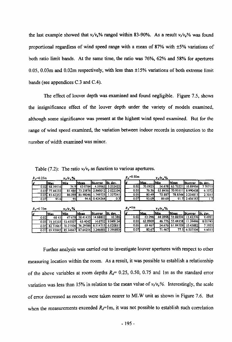
the last example showed that v/ve% ranged within 83-90%. As a result v/ve% was found
proportional regardless of wind speed range with a mean of 87% with ±5% variations of
both ratio limit bands. At the same time, the ratio was 76%, 62% and 58% for apertures
0.05, 0.03m and 0.02m respectively, with less than ±15% variations of both extreme limit
bands (see appendices C.3 and C.4).
The effect of louver depth was examined and found negligible. Figure 7.5, shows
the insignificance effect of the louver depth under the variety of models examined,
although some significance was present at the highest wind speed examined. But for the
range of wind speed examined, the variation between indoor records in conjunction to the
number of width examined was minor.
Table (7.2): The ratio v/ve as function to various apertures.
R =025m R =050md . '. 0
Id IMu IMin Mun ISt.error SI. dey.
0.02 68.39516 14.9 63.0184 4.59962 3.2524220.03 11.44133 81.486 13.23816 2.860012 2.0223340.05 83.62352 86.098 80.98046 1.149123 1.2312410.01 95.6 95 94.6 0.424264 0.3
d 'iJ '. 0
Id M.~ MI .. Mun St..rrnr St. d.v0.02 10.0923 54.618 63.75221 10.89956 1.707150.03 76.56 63.8456 70.93111 8.990438 6.35120.05 80.49 15.887 78.8544 3.254813 230150.07 93.09 89.69 91.1 2.404163 1.7
R =0 15m v Iv 0;. R -1m Ivo;.d • 0
Id IMax IMin IMean ISt.error 1St.d.v.
0.02 68.45 47.678 58.41433 14.68802 10.386
0.03 73.35333 53.45507 63.4042 14.0702 9.949134
0.05 82.31667 70.27504 76.29586 8.514713 6.020811
0.07 89.93845 85.34667 87.64256 3.246883 2.295893
d- VI. r; 0
Id 1M... IMln IMnn ISt.rrnr 1st. dey.0.02 63.098 44.0998 53.88594 13.43376 9.49910.03 62.8909 46.776 55.44158 11.39496 8.057450.05 69.461 54.676 61.84709 10.45882 739550.07 80.67 71.467 77.3 6.507504 4.6015
Further analysis was carried out to investigate louver apertures with respect to other
measuring location within the room. As a result, it was possible to establish a relationship
of the above variables at room depths Rc 0.25, 0.50, 0.75 and 1m as the standard error
variation was less than 15% in relation to the mean value ofv/ve%. Interestingly, the scale
of error decreased as records were taken nearer to MLW unit as shown in Figure 7.6. But
when the measurements exceeded Rc1m, it was not possible to establish such correlation
- 195 -
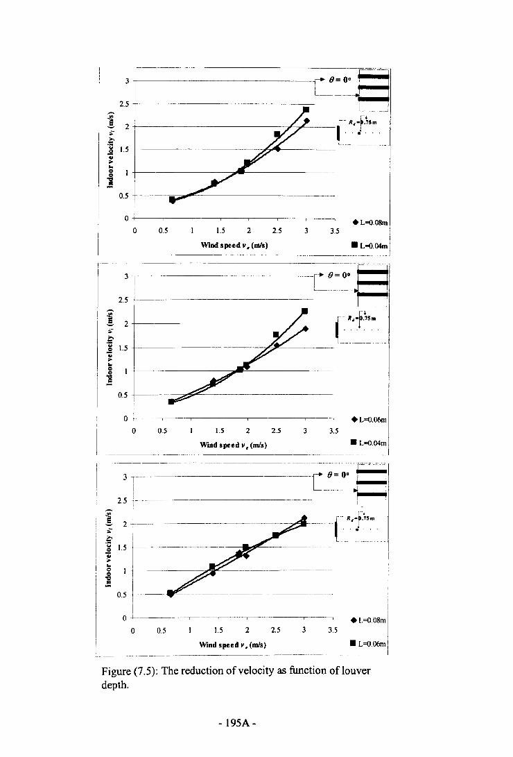
~----.----,------,,----.---,----,-----,.L=<l.08m
1.5 2 2.5 3 3.5
Wind speed v. (mls) • L=<l.04m
o 3.S.L=<l.06m
O.S I.S 2 2.5 3
Wind speed v. (mls) • L=<l.04m
3~i
2.5 +--~---. ,-------~ I! 2 I--,.--------~i: 1
.€ 1.5 rl=- -_g..~..g 1 .. -----'=""'0=- o.s 1--.
• I
Io .i. --,---~- ---,,----,.----,----,-
o 32 2.5 3.S0.5 1.5
Wind speed v. (mls) • L=O.06m
Figure (7.5): The reduction of velocity as function of louverdepth.
- 195A-
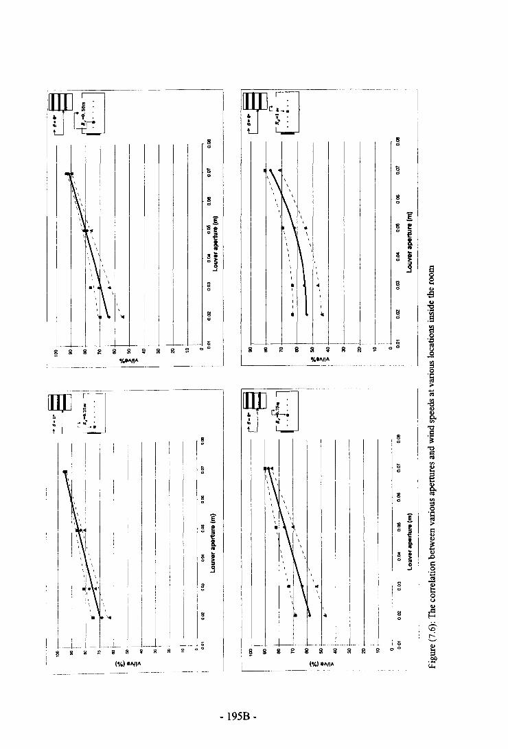
%811f111
!0
~
80
:[!l e" ..
1:!...
~..~...9
s0
!'l
"
000
- 195B-
~cill~
""', ~I
I
\, ~
II
'~'I' ~!
'Kofl..
I I 1StI
I ,I
,,~I ,
I~
I ,I ,
• 1 •
I\'i B
0I II
I I
II
,.. s"
'1'\' ,I ,, ,
\K\I II ,
I..I \I
II ..I II
I
I
10
%811f111'------------ -------
.-------------------- -
~tl
("I.1811f111
s~ 0
0
8es
q°
Bo
as error percentages increased beyond the acceptable limits; over 25%. Hence, polynomial
regression curves were produced representing that correlation for louver apertures
investigated at various room depths. Table 7.2 shows the various MLW units examined
with their standard errors and standard deviations. Although louver aperture O.OIm
behaved like other apertures, it was not included in the later Figure since its correlation had
fallen significantly different from the rest of louver depths.
7.4.2. Velocity drop as function of wind direction (wtJ
Measurements covered three incidences of wind directions (WI) 90", 75"and 60"with
blades in perfect horizontal position. The first direction is referred to as the wind
perpendicular to the windward side. As mentioned earlier, the metal bar connecting both
room chamber and fans made it flexible to alter fans (in a semi-circle manner) to any
predetermined direction. Polynomial curves produced by the two latter directions, w;=7s"
and 60"were compared with the referenced direction w,=90"at RrO.25m.
The average reduction in velocity as function to wind incidence angle is illustrated
in Figure 7.7 where in average it yielded nearly 21% due to tilting wind from perpendicular
to incident 60". In other words, the Figure suggested that a 30" deviation in wind angle of
incident would consequently reduce 20% of initial velocity recorded at perpendicular, i.e.
w;=90". This was the general behaviour with MLW of various aperture dimensions
examined, with some reservation at d=O.Olm.
The case was not proportional as measurements took place further. These
percentages were further enhanced as room depth increased depending on each model
configuration. Gaps between curves at wind incidences 90", 75" and 60" were gradually
increasing as velocity was measured along room depth. At 60", the reduction reached its
- 196-
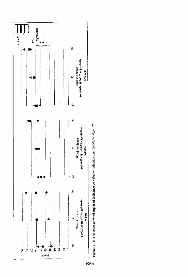
Jif'I0U..L"= •I :u:~.... , 0a-
I er--0
'if8~ij. E"0 e 00
• '0 :8 c11"1 <::ir- .e'if II
"O~ "-l.e.~ e
M00
JII-e•
0'D
o 0o 0\
,1 ! r
•I II ! I
I \ I I I! IJ. +11--1 -* 1- ,---+ ~
•
000 0 0 0 0 0 000 r- \0 V'l ~ "'"' N
II
I ... 1
---.-----~------,- ..-------- ..--.------.-.---
- 196A-
minimum readings in the middle of the room with some reservations at models with
d=O.07m. Hence, it was thought that as further wind directions were examined, the breeze
flow along room depth would be less effective for all models examined, with exception of
measuring location RtFO.25m. Generally, it was evident that velocity drop due to
deviation in wind direction was significant when accompanied with room depth and varied
in accordance with various d selected.
7.4.3. Velocity drop as function of room configuration
The observation mainly covered the horizontal velocity magnitude represented in
the room depth. In this section, vertical velocity magnitude is also highlighted. As noted
before, one of the main advantages of employing the MLW is the possibility to control the
flow patterns to various sections within the room, including ceiling, living and ground
zones. The following is the discussion of each of these effects.
7.4.3.1. Room Depth (Rd)
Some of the studies reviewed in the literature, such as Givoni (Givoni, 1981), Sobin
(Sobin, 1983), Muniz (Muniz, 1985) and others, showed the effect of velocity drop as
function of room depth. Here the six measuring locations along room (Rd) were taken at
distance of 0.25m each.
The relation between Rd and v/ve% contained two approaches of evaluation
including the percentage of velocity reduction along room depth with reference to
RtFO.25m and the effective ventilation along room. As for the former, readings at
RtFO.25m were taken as a reference to trace the percentage of reduction at other measuring
locations examined when the external wind velocity was ve=2mJs. In fact it was found that
along room depth the flow of air had lost 30% - SO%of its momentum force at RtF 1.SOm.
- 197 -
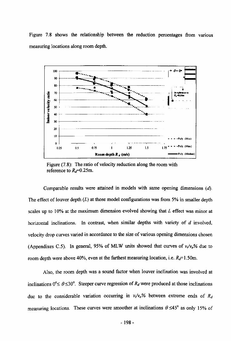
Figure 7.8 shows the relationship between the reduction percentages from various
measuring locations along room depth.
- - - ·Poly (Min)
....,-----~~-
R-. 0= O·1_- .
(t-_:·~<WI.R.-O.lSao
.....
100
90
80
! 70e£ 60...~ 5041>.. 40Cl
-8a 30-20
10
0 -----
0.25 0.5 0.75 1.25 I.S 1.7S - - - .Poly.(Max)
Room depth R " (mlS) -Poly (Madlan)
Figure (7.8): The ratio of velocity reduction along the room withreference to Rr0.25m.
Comparable results were attained in models with same opening dimensions (d).
The effect of louver depth (L) at those model configurations was from 5% in smaller depth
scales up to 10% at the maximum dimension evolved showing that L effect was minor at
horizontal inclinations. In contrast, when similar depths with variety of d involved,
velocity drop curves varied in accordance to the size of various opening dimensions chosen
(Appendixes C.5). In general, 95% of MLW units showed that curves of v/ve% due to
room depth were above 40%, even at the farthest measuring location, i.e. Rr I.SOm.
Also, the room depth was a sound factor when louver inclination was involved at
inclinations Oo~B~30°. Steeper curve regression of Rd were produced at those inclinations
due to the considerable variation occurring in v/ve% between extreme ends of Rd
measuring locations. These curves were smoother at inclinations B ~45° as only 15% of
- 198-
data were scattered above 20% of vlve at various MLW configurations examined. Thus,
MLW greater than 30° of inclination would be ineffectual in producing velocity drop
variations along the centre axis of room depth (Appendices C.S to C.II).
7.4.3.2. Room Height (Rh)
Velocity measured at certain height above was taken at 0.0725m above and below
MLW frame edges and at a distance of 0.18Sm away from ceiling to shelter against
discrepancies occurring due to wall jet phenomenon (Awbi, 1991) (Etheridge and
Sandberg, 1996).
The inclination 8= 0° showed the poorest performances since incoming air was not
deflected upwards and continued in a similar direction. Similarly, the result found at 8=
60° was not effective, with the exception of the first measuring location, RcFO.25m.
However, other inclination angles showed higher percentages of vlve% inclinations at the
specific room height. For example, the highest records of vlve were found at RcFI.OOmat
inclination angle of 15°. Meanwhile, room depth at distance of O.SOmwas the optimum
measuring location for all models examined when louvers were tilted to 30° angle. Also,
The maximum ranges of data achieved were found at distance of 0.25m for both
inclinations, 45° and 60°. All these findings demonstrate that the velocity distribution
patterns inside a space would vary according to MLW configurations beside other
variables such as wind data and room configuration (Appendix C.S to C.Il). This is more
likely the reason why curve patterns of vlve% would vary at various room heights (Rh) and
depths (Rd) indoors. Finally, the vlve was found to be less than SO%at nearly 92% of data
examined, showing that the maximum ratio indoors, with the presence of wind inclination
will not reached more than half of the wind speed. This figure even becomes more critical
with the presence of steeper louver inclinations as seen in the Appendices.
- 199-
7.4.4. Velocity drop as function ofMLW porosity (P)
The porosity (P) of the MLW depends on the geometry and the number of louver
blades in each unit. When blades are in perfect horizontal position, i.e. 0: 0, P is
considered at its maximum and diminishes according to the degree of inclination, say PfJ.
Thus, data measured of (V/ve%) represent the ratio of velocity drop at the external front
panel of MLW on the windward side (vp) against the actual wind velocity (ve) (Figure 7.1).
The porosities ranged from 50% to 87% and were calculated on the basis of the ratio of
inlet opening over the total area of the MLW unit when 0:0. The aim was to find out how
much resistance was offered by the geometry of MLW different configurations on external
reduction of airflow speed.
There was a strong relationship between porosity of MLW geometry against
v/Ye%. The ratio v/ve: 62% when selecting the MLW units with minimum porosity
percentage, i.e. p=50%. This would in other words suggest that air stream lost
approximately 40% of its momentum velocity before reaching the inlet external surface
due to the resistance caused by inlet porosity percentage. However, the loss decreases as
the development in porosity percentage occurs. As found at the other extreme porosity
percentage, p=87%, the loss was less than 5% as the ratio v/Ye was found to be
approximately 96%, as demonstrated in Figure (7.9).
In addition, it was interesting to underline that when measuring the velocity drop at
RrFO.25m for the same model unit both porosity percentage and the ratio v/Ye were almost
identical, i.e. v/ve%:V/Ve%. A more defined description of this phenomenon is illustrated
in Figure (7.10) which shows that, as a laminar flow of air passes inlet surface of the
louvers, it generates its speed along the louver depth causing a free-jet flow with higher
speed on the outlet surface than that on the inlet. This speed along the centreline of the
..200 ..
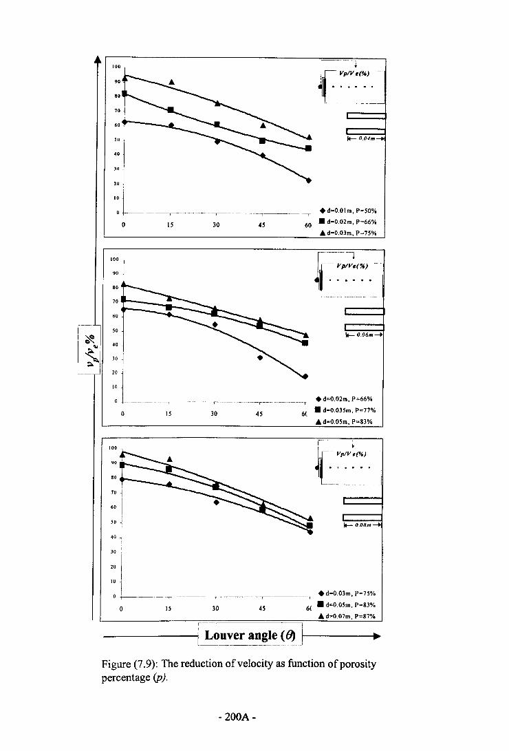
100
10
-~--.----,-----~-- -----,-----------,--- +r-
o 15 30 4S
k-- O.04m
+ d=O.Olm, P=SO%
60 • d~O.02m, P-66%
• d=O.03m, P-7S%
100
90
80
70
60
r-~ 50
" 40
~ 30;:.
20
10
0 4S
t------1- VpIVe(")
.~--~-.- ...
I+- O.06m-+
+d=0.02m, P=66%
6( • d-0.03Sm, P~77%
• d-O.OSm, P=83%3015
·----,------.--------r
I+- O.ORm
30 45
+d=O.03m, P=7S%
6( • d~O.OSm, P=83%
• d=O.07m, P=87%o 15
---------ir_L_OU~_er_a_ng_I!_!_~]I------~~
Figure (7.9): The reduction of velocity as function of porositypercentage (P),
- 200A-
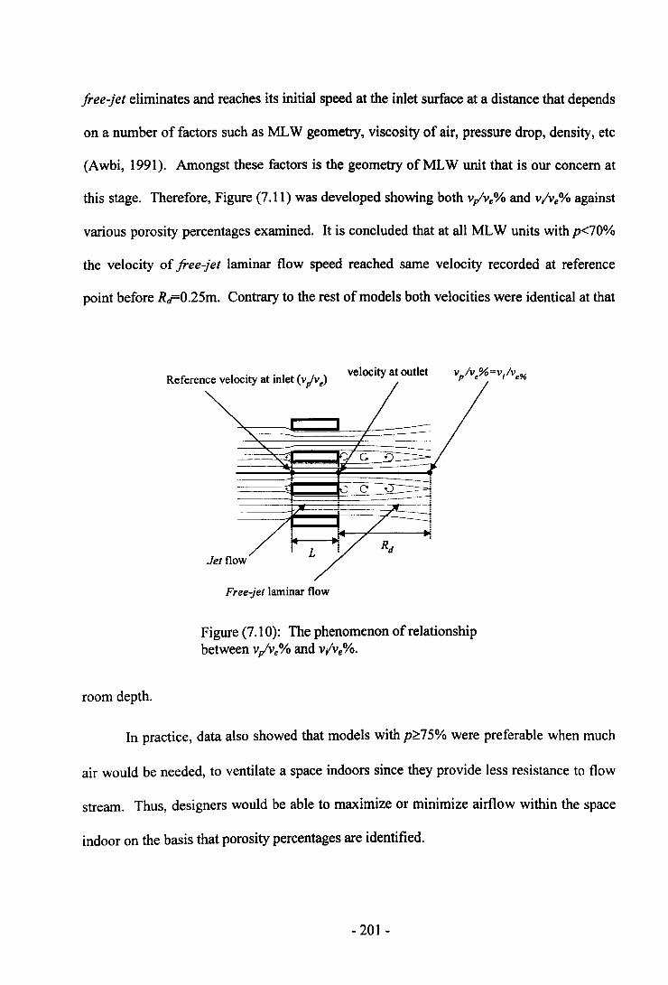
free-jet eliminates and reaches its initial speed at the inlet surface at a distance that depends
on a number of factors such as MLW geometry, viscosity of air, pressure drop, density, etc
(Awbi, 1991). Amongst these factors is the geometry ofMLW unit that is our concern at
this stage. Therefore, Figure (7.11) was developed showing both v/ve% and v/ve% against
various porosity percentages examined. It is concluded that at all MLW units with p<70%
the velocity of free-jet laminar flow speed reached same velocity recorded at reference
point before R,F0.25m. Contrary to the rest of models both velocities were identical at that
Reference velocity at inlet (v,Ive)velocity at outlet
Jet flowL
Free-jet laminar flow
Figure (7.10): The phenomenon of relationshipbetween v/ve% and v/ve%.
room depth.
In practice, data also showed that models with p~75% were preferable when much
air would be needed, to ventilate a space indoors since they provide less resistance to flow
stream. Thus, designers would be able to maximize or minimize airflow within the space
indoor on the basis that porosity percentages are identified.
- 201 -
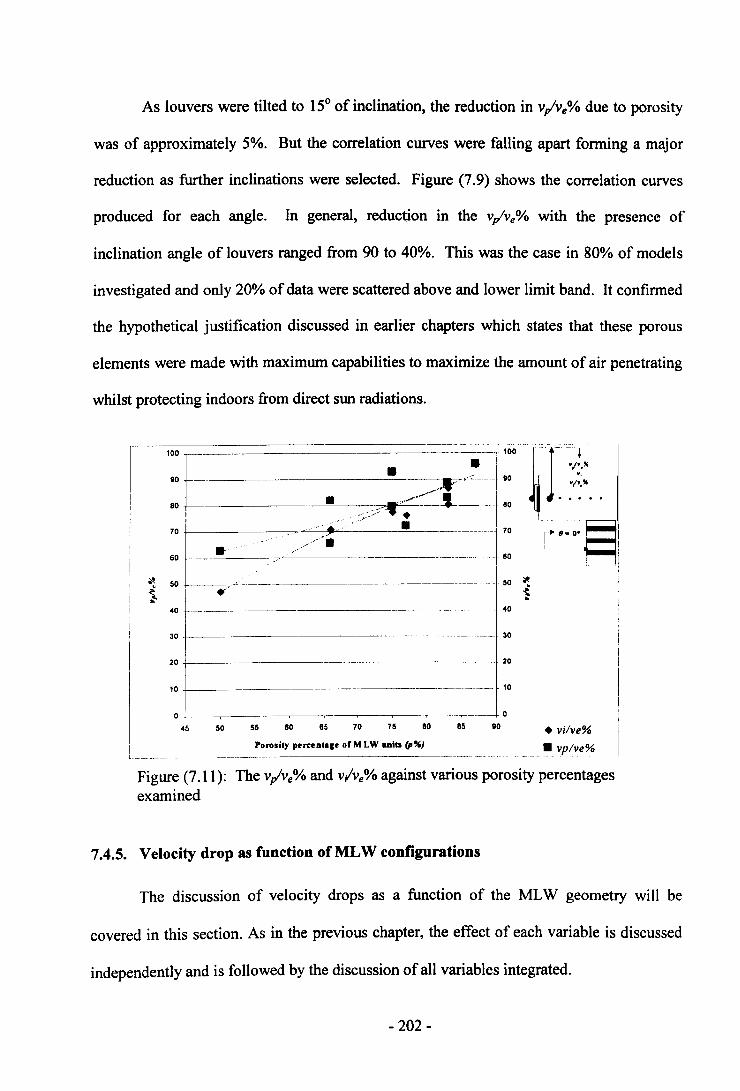
As louvers were tilted to 15°of inclination, the reduction in v/ve% due to porosity
was of approximately 5%. But the correlation curves were falling apart forming a major
reduction as further inclinations were selected. Figure (7.9) shows the correlation curves
produced for each angle. In general, reduction in the v/ve% with the presence of
inclination angle of louvers ranged from 90 to 40%. This was the case in 80% of models
investigated and only 20% of data were scattered above and lower limit band. It confirmed
the hypothetical justification discussed in earlier chapters which states that these porous
elements were made with maximum capabilities to maximize the amount of air penetrating
whilst protecting indoors from direct sun radiations.
III,
1:: :=-=~~-_-_-_-_-_-__-_-_-_-_-_-_-_-_-_-_-_~-_.~~_~-~-;:-~,.~ - ~~ ~ 1- ~k• - _.,...-- .J_ • . . . .
80+---------=---_..-_.:.--::::c-:::::-"'OI-.~p:-c>~__ -- -- 80
70 +---------:c~ -,:'-- • ---------170 -II· ,.o·R"../r.60+--·---7~------------ ----- I 80
~ 50 +--~-"'~ ------------------------
i ..t--.-------------:: -1--1 -----------------::
10 I 10
O~_~-~-~-~-~-~- 0
40
80 85 807565 70805550 • vilve%• vplve%
45
Porosity percent_le or MLW units (P")--------------------
Figure (7.11): The v/ve% and v/ve% against various porosity percentagesexamined
7.4.5. Velocity drop as function of MLW configurations
The discussion of velocity drops as a function of the MLW geometry will be
covered in this section. As in the previous chapter, the effect of each variable is discussed
independently and is followed by the discussion of all variables integrated.
·202·
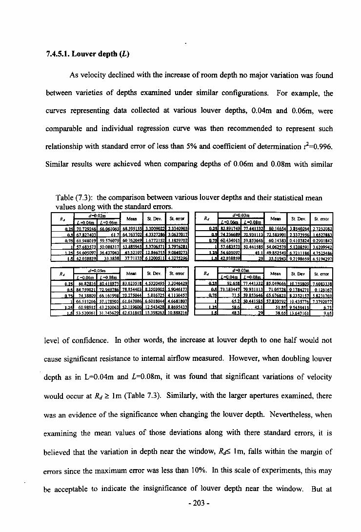
7.4.5.1. Louver depth (L)
As velocity declined with the increase of room depth no major variation was found
between varieties of depths examined under similar configurations. For example, the
curves representing data collected at various louver depths, O.04m and 0.06m, were
comparable and individual regression curve was then recommended to represent such
relationship with standard error of less than 5% and coefficient of determination r=0.996.
Similar results were achieved when comparing depths of 0.06m and 0.08m with similar
Table (7.3): the comparison between various louver depths and their statistical meanvalues along with the standard errors.
level of confidence. In other words, the increase at louver depth to one half would not
cause significant resistance to internal airflow measured. However, when doubling louver
depth as in L=0.04m and L=0.08m, it was found that significant variations of velocity
would occur at Rd ~ 1m (Table 7.3). Similarly, with the larger apertures examined, there
was an evidence of the significance when changing the louver depth. Nevertheless, when
examining the mean values of those deviations along with there standard errors, it is
believed that the variation in depth near the window, RQ5. lrn, falls within the margin of
errors since the maximum error was less than 10%. In this scale of experiments, this may
be acceptable to indicate the insignificance of louver depth near the window. But at
- 203-
Rd>1m, this homogenous relationship was not possible since velocity drops were clearly
falling apart from one depth to another. The curves would even fall apart more
significantly as room depth increases as shown in Figure (7.12).
Results were homogenous with the presence of louver inclinations ISo~ B~600, the
coefficient of determination of those curves was r=0.999 at 9S% models examined with
standard error of mean less than S% (see appendices C.6 to C.9). This homogenous
relationship was also found with the presence of various MLW units observed.
The general statistical value of this variable to contribute any adjustment to indoor
velocity ratio was the least affecting variable since the r2::O.2.
7.4.5.2. Louver inclination angle (9)
The reduction of air velocity at 0=00 was relatively smooth and the curves along the
room had not shown considerable or sudden drop. Nevertheless, the curves produced for
other inclinations showed some significant drops relative to the inclination selected. For
instance, the effective flow at ISOwas present up to distance Rd =0.7Sm. Subsequently a
major airflow velocity drop was shown for all models examined, i.e. vi/ve<20%. This drop
was even closer to MLW unit when both inclinations of 30° and 4Soexisted as the effective
flow was found only around the first measuring location near the MLW. 60° Angle
showed the poorest performance amongst other examined inclinations since maximum
vilve < 30% regardless of the rest ofMLW variables (see Appendices C.S to C.9).
The situation was clearly different as flow above the centre axis was considered.
Measurements of various inclinations carried out with the presence of room height were
quite distinct from those measured at the centre. As noted before, while the flow at 0=0°
was found very minor and negligible, both louver inclinations of ISOand 30° were quite
- 204-
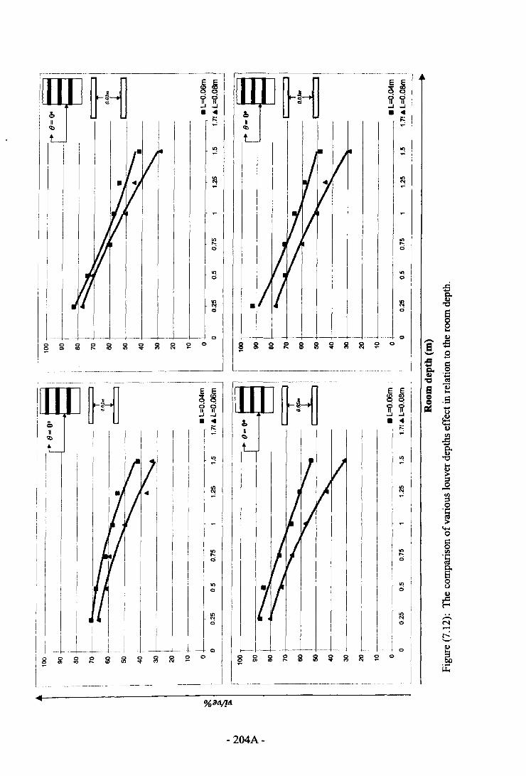
---------------------~ ----.-,---.-.-----~---.--.-
E E ~1 E ~s flO er;0 00 ? ? ?II..J ..J ..J ..J• 4 • 4
;:; ~- -~ ~- -~ ~-
~ It>,.._ci ci
on onci ci
~ ~ci ci
- - C>
~ g ~ ~ 2 ~ ~ ~ ~ ~ C>
----------~-----------------______j
1 I I
-- -----1- L--l--+----+---Ig ~ ~ R g g ~ ~ ~ ~ C>-
'---------------------
E Eer; s00II II..J ..J• 4
;:.;
----------~~---------------------
C>
@ ~? ?..J ..J• 4
~-
onQ
- 204A-
i3fr"0
~Cl)
i 05- B;: §g..Cl) ·C'C t':I
S 'Ee I::::
~........U
~Cl)ell
05~1-0Cl);:.-::s0-ell::s0.~;:.-
......0sell.~
s-ouCl)
~,.-..N.....-,;.._.,
~....~
on,._ci
onci
accepted as room depth increased. The highest records for angle of 15°was found around
the measuring location ReF 0.75m and 1m with smooth decline in flow after them.
Similarly, the effective velocity at 8=30° was found around Rd = O.SOmand 0.75m away
from the MLW. Finally, at the first O.SOmof room depth it was found that the optimum
velocity resulted from both inclination 45° and 60° as shown in (see appendices C.8 and
C.9). This was to ensure that the vertical velocity profile within a space would vary
according to the change in louver inclination angle.
Interestingly, it was possible to trace the significant contribution of the louver
inclination angle when examining its coefficient of determination from statistical
perspective. As seen in Appendix C.l2.a, the statistical behaviour of (}with respect to
vilve% revealed some significance since ,2 = 0.736 for the variety of MLW geometries
along the room depths examined.
7.4.5.3. Louver aperture (d)
Internal velocity as a function of aperture distance between louver blades shaped
the major factor to the total velocity reduction indoors. It varied in accordance with the
size of various opening dimensions chosen. At this stage no consideration was given to
louver depth since the increase to one half would be less effective to velocity readings
indoor, up to ReFlm.
At the maximum aperture examined, air lost nearly 20% of its initial speed after
reaching Rd=lm while it lost 50% at Rd =1.5m. Likewise, only 5% was lost at ReFO.25m
showing that this model configuration may be recommended where cross ventilation may
be necessary. Obviously the MLW with minimum aperture showed the poorest
performance since 50% of wind speed was lost at first measured location and almost 90%
was lost at 1.5m of room depth as seen in Appendix (C.5). Additionally, it was found that
- 205-
the decrease ofO.02m in d=0.07m would be accompanied with a decrease in v/Ye =10-15%
near the window.
In general, curves ofv/ve% due to room depth were above 40% even at the farthest
measuring location when d=O.Olm is excluded. Figure (7.6) shows the correlation curves
produced for the louver apertures measured up to Rd =1m.
However, the do variable was only sufficient to explain about 38% of the total
reduction in velocity drop for all models selected. As seen from the Appendix (C.l2.b),
this has some effect on the reduction of flow, yet its effect was less significant than the
inclination angle effect.
7.4.5.4. Velocity drop as function of free area (A,,)
The free area was found to be a more appropriate variable corresponding to the
velocity drop across the ML W rather than d(J. Based on the various configurations
selected, the AI which ranged from approximately 33 to 85% were gradually accepted as
the result of vilve%. The general effect showed that AI explained nearly 65% of the air
velocity characteristics inside the room as the coeffiecnt of determination exceeded 0.60
(see Appendix C.12.c). Hence, the free area was a better factor than MLW aperture.
7.4.5.5. Louver number (N)
The general behaviour of louver number was not sufficiently possible to determine
the indoor velocity reduction across the ML W since the r2=0.2 as seen in Appendix
(C.12.d).
- 206-
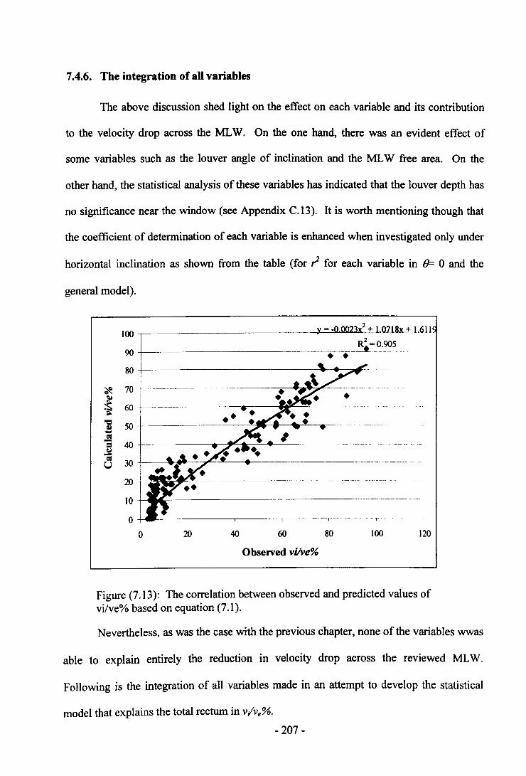
7.4.6. The integration of all variables
The above discussion shed light on the effect on each variable and its contribution
to the velocity drop across the MLW. On the one hand, there was an evident effect of
some variables such as the louver angle of inclination and the MLW free area. On the
other hand, the statistical analysis of these variables has indicated that the louver depth has
no significance near the window (see Appendix C.13). It is worth mentioning though that
the coefficient of determination of each variable is enhanced when investigated only under
horizontal inclination as shown from the table (for'; for each variable in B= 0 and the
general model).
~~~~~~~~~~~~~~+y-==~-01lo..OO""",23.llXL-'2 +1.0718x ±_L611190
00r 2t _~~=O.905
80 +-~-~ 70 t·-----------~~----.--+ ...~:-
~ :+r_-_-_--_--_-_--_-~_· _~_~~~~~ ___-.!B 40 +-~~--_____._~_t_~_+_-:-~---.-.-.--.- ..--.--.- -. -
-;U 30+--~ ..~~~~-.~-20+-~~~~~~~~~~~-
10~.w~-~~~~~~~~~~~--
•
o - r-
100 12040 60 80o 20
Observed vVve%
Figure (7.13): The correlation between observed and predicted values ofvi/ve% based on equation (7.1).
Nevertheless, as was the case with the previous chapter, none of the variables wwas
able to explain entirely the reduction in velocity drop across the reviewed MLW.
Following is the integration of all variables made in an attempt to develop the statistical
model that explains the total rectum in v/ve%.
- 207-
The statistical model was developed with error percentage less than 15% and with
,2 =0.905. Meanwhile, when including the various inclinations involved in this study, the
model (Eq 7.1) was the best to sufficiently explain the velocity reductions function to
various MLW geometries examined. Figure (7.13) and Appendix C.13 demonstrate the
correlation between the observed values of vlve% compared with the predicted value
which corresponds to the following equation:
where:
c = the intercept defined from the linear curve estimate in Figure 7.1 (1.6119).
a, f3, Xand cS are the numerical representations of the variablesa, Band N, respectively.
A further observation of this equation to fit larger number of MLW parameters was
beyond the aim of this research though it represents one of the author's future tasks.
Therefore, it is not covered here.
As seen from the Appendix C.l3, all variables selected in the model were
statistically significant, bearing in mind that some variation may occur if variables not
covered by this study were to be included, such as roughness or other variables noted
previously.
7.5. Conclusion
This chapter has examined the velocity flow characteristics with respect to the
reviewed MLW. In addition, it has highlighted the velocity drop as function to the room
configurations and wind data. The conclusions derived from the investigation are as
follow:
- 208-
• Louver angle of inclination is found a main variable to control this while
louver depth was the least affecting variables in this phenomenon except
with the presence of steeper louver inclination. Nevertheless, the major
indoor velocity drop was not due to individual variables but rather to
combination of variables that would comprehensively describe v/ve% as
concluded from the various evaluation stages conducted throughout this
chapter.
• The description of flow characteristics as function to the free area was
found more appropriate than that related to louver aperture. While both
variables showed some level of significance, the effect of the former was
more practical than the latter.
• The mean indoor velocity (v/ve%) was increasing as a function of wind (ve)
and the maximum increase was less than 15%. This was the general
behaviour of MLW under various apertures examined yet when d>O.05m
the v/ve% was proportional to Ve.
• Wind direction has also some significance on indoor air velocity since
normally a 20% reduction in v/ve% near the window was found when wind
was to deviate 30" from perpendicular.
• The vertical and the horizontal velocity profiles along the room height and
depth respectively are much related to the MLW configurations examined.
• The porosity percentage is a sound alternative to evaluate the performance
of MLW as it gave an understanding of the flow characteristics at the
windward side near the modulated louvered windows.
- 209-
• Airflow velocities in a room containing an MLW result from an interaction
of louver geometry, room geometry and prevailing wind conditions.
• It was possible to establish a dimensionless relationship of velocity
characteristics as function to various MLW parameters involved near the
window, Rds lm, Therefore, these results will be the base of the further
evaluation stages that will be covered next chapter using the computational
fluid dynamics (CFD) technique.
The appraisal stage has demonstrated the flexibility of the MLW design in relation
to accomplishing similar results. In another words, similar airflow characteristics were
achieved with a number of MLW configurations. There is some evidence to suggest that
the flexibility in the design of MLW that will not encounter much reduction in airflow
passing louver blades. These could be guidelines to be implemented in practise for further
implementation in production. Some of the conclusions attained from Chapters 6 and 7
were sound and considered key elements to recall the traditional louvers geometric
reviewed in earlier chapters.
- 210-
7.6. References
1. Awbi, H.B. (1991) Ventilation oj Buildings, London: E & FN Spon.
2. Bittencourt, L.S. (1993) Ventilation as a cooling resource for warm -humid climates: An
investigation on perforated block wall geometry to improve ventilation inside low-rise
buildings. Architectural Association Graduate School. Unpublished Ph.D. thesis.
3. Chand, l., Bhargave, P.K., Sharma, V.K. and Krishak, N.L. (1988) "Studies on the effect of
mean wind speed profile on rate of air flow through cross-ventilated enclosures".
Architectural science review (35)-p.83-88.
4. Etheridge, D. and Sandberg, M. (1996) Building Ventilation: Theory and Measurements,
John Willy & Sons.
5. Evans, M. (1980) Housing, Climate, and Comfort, London: Architectural press.
6. Givoni, B. (1981) Man, Climate and Architecture, 2nd edn. London: Applied Science
Publishers Ltd.
7. Muniz, P.A. (1985) The geometry of external shading devices as related to natural
ventilation, daylighting and thermal comfort, with particular reference to tropical hot-humid
climates. Unpublished Ph.D. Thesis.
8. Sharples, S and Maghrabi, Amjed (2000) "Airflow through louvers: an experimental and
CFD study". The Hague: Proc. 21st. AIVC Conference (To be published).
9. Sobin, H. (1983) Analysis of wind tunnel data on naturally ventilated models. p.287
Tucson, Arizona, USA: Harris Sobin & Associates.
10. White, M. (1999) "Ventilators: Ventilation and acoustic Effectiveness". BRE (IP4/99)-p.l-
8.
11. Yousoufian, H.H. (1992) "Correlation of residual velocity with throw terminal velocity
from a louver-faced unidirectional diffuser". ASHRAE Transactions (2)-p.1-8.
- 211 -
CHAPTER 8: SIMULATION OF VELOCITY DROP
ACROSS THE MLW: CFD APPRAISAL STAGE.
- 212 -
8.1. Introduction
This chapter is devoted to exploring and extending investigations carried out in the
previous chapter. On the one hand it examines the CFD coding to simulate airflow around
the reviewed modulated louver windows; on the other hand it highlights the airflow
patterns around the MLW and the subsequent flow within the room, based on MLW and
inlet configurations as well as outlet configurations that are typically found in Jeddah. It
was not possible to examine them in the previous chapter due to the dimension of the
physical model under which laboratory measurements were carried out. A description is
first given of the historical background to the theory of numerical modelling and the
application of CFD in predicting airflow in buildings. The range of CFD software
packages used for simulation and justification of CFD code selection is discussed here.
Basic conservation equations, turbulence modelling and other CFD requirements for
simulation are also covered. The set up of MLW model configurations and the boundary
conditions are discussed before the comparison of both CFD and laboratory results takes
place. The chapter ends up by highlighting patterns of airflow through MLW with
reference to both inlet and outlet configurations implemented in Jeddah, Saudi Arabia.
- 213 -
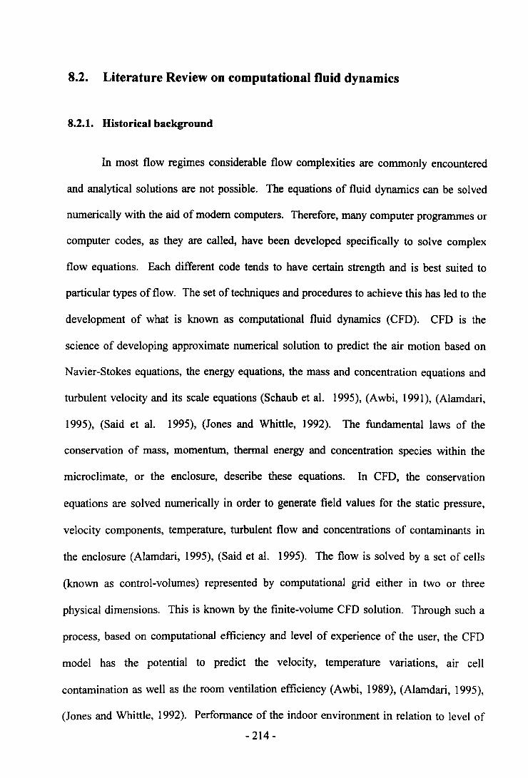
8.2. Literature Review on computational fluid dynamics
8.2.1. Historical background
In most flow regimes considerable flow complexities are commonly encountered
and analytical solutions are not possible. The equations of fluid dynamics can be solved
numerically with the aid of modem computers. Therefore, many computer programmes or
computer codes, as they are called, have been developed specifically to solve complex
flow equations. Each different code tends to have certain strength and is best suited to
particular types of flow. The set of techniques and procedures to achieve this has led to the
development of what is known as computational fluid dynamics (CFD). CFD is the
science of developing approximate numerical solution to predict the air motion based on
Navier-Stokes equations, the energy equations, the mass and concentration equations and
turbulent velocity and its scale equations (Schaub et al. 1995), (Awbi, 1991), (Alamdari,
1995), (Said et al. 1995), (Jones and Whittle, 1992). The fundamental laws of the
conservation of mass, momentum, thermal energy and concentration species within the
microclimate, or the enclosure, describe these equations. In CFD, the conservation
equations are solved numerically in order to generate field values for the static pressure,
velocity components, temperature, turbulent flow and concentrations of contaminants in
the enclosure (Alamdari, 1995), (Said et al. 1995). The flow is solved by a set of cells
(known as control-volumes) represented by computational grid either in two or three
physical dimensions. This is known by the finite-volume CFD solution. Through such a
process, based on computational efficiency and level of experience of the user, the CFD
model has the potential to predict the velocity, temperature variations, air cell
contamination as well as the room ventilation efficiency (Awbi, 1989), (Alamdari, 1995),
(Jones and Whittle, 1992). Performance of the indoor environment in relation to level of
- 214-
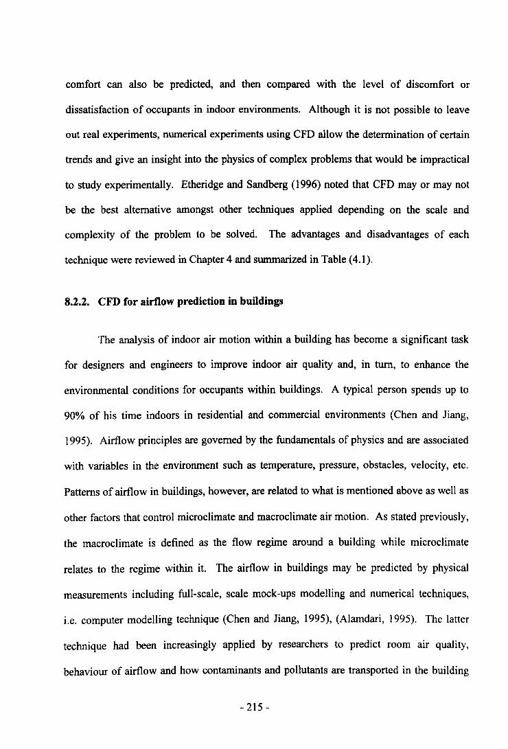
comfort can also be predicted, and then compared with the level of discomfort or
dissatisfaction of occupants in indoor environments. Although it is not possible to leave
out real experiments, numerical experiments using CFD allow the determination of certain
trends and give an insight into the physics of complex problems that would be impractical
to study experimentally. Etheridge and Sandberg (1996) noted that CFD mayor may not
be the best alternative amongst other techniques applied depending on the scale and
complexity of the problem to be solved. The advantages and disadvantages of each
technique were reviewed in Chapter 4 and summarized in Table (4.1).
8.2.2. CFD for airflow prediction in buildings
The analysis of indoor air motion within a building has become a significant task
for designers and engineers to improve indoor air quality and, in turn, to enhance the
environmental conditions for occupants within buildings. A typical person spends up to
90% of his time indoors in residential and commercial environments (Chen and Jiang,
1995). Airflow principles are governed by the fundamentals of physics and are associated
with variables in the environment such as temperature, pressure, obstacles, velocity, etc.
Patterns of airflow in buildings, however, are related to what is mentioned above as well as
other factors that control microclimate and macroclimate air motion. As stated previously,
the macroclimate is defined as the flow regime around a building while microclimate
relates to the regime within it. The airflow in buildings may be predicted by physical
measurements including full-scale, scale mock-ups modelling and numerical techniques,
i.e. computer modelling technique (Chen and Jiang, 1995), (Alamdari, 1995). The latter
technique had been increasingly applied by researchers to predict room air quality,
behaviour of airflow and how contaminants and pollutants are transported in the building
- 215 -
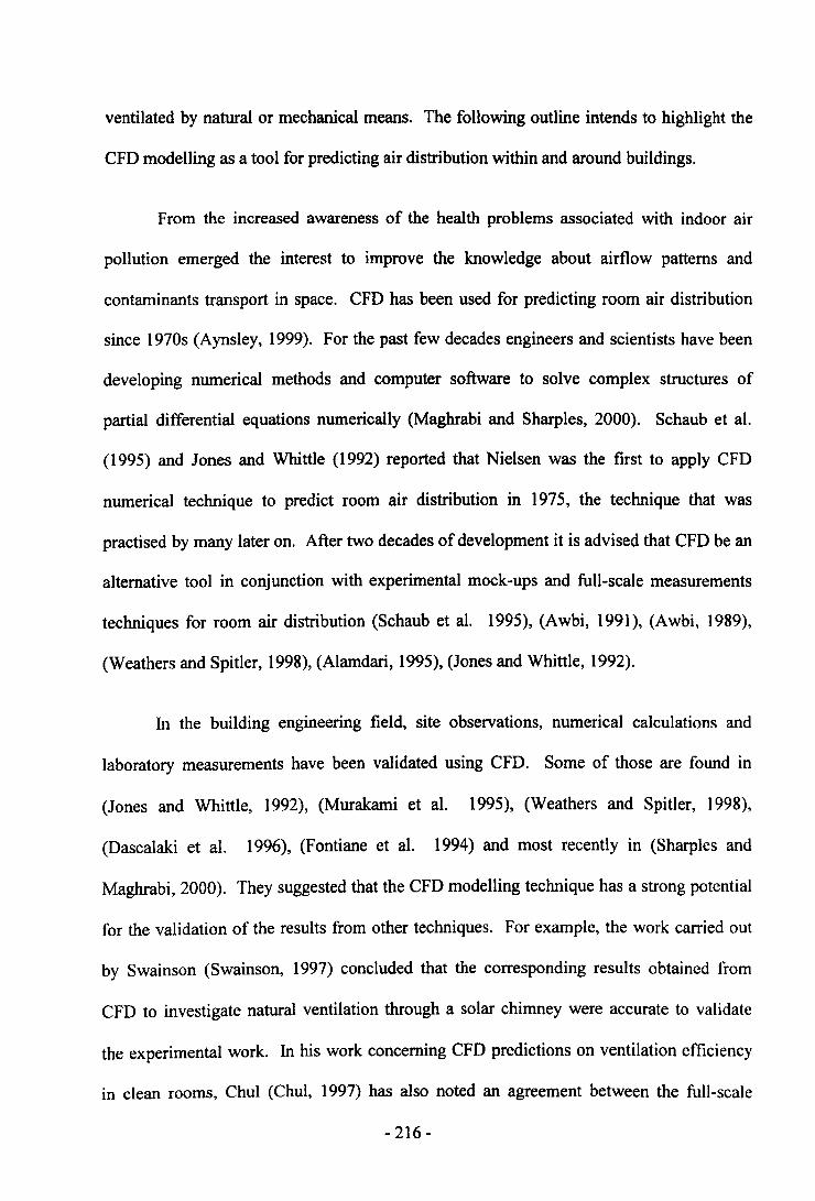
ventilated by natural or mechanical means. The following outline intends to highlight the
CFD modelling as a tool for predicting air distribution within and around buildings.
From the increased awareness of the health problems associated with indoor air
pollution emerged the interest to improve the knowledge about airflow patterns and
contaminants transport in space. CFD has been used for predicting room air distribution
since 1970s (Aynsley, 1999). For the past few decades engineers and scientists have been
developing numerical methods and computer software to solve complex structures of
partial differential equations numerically (Maghrabi and Sharples, 2000). Schaub et al.
(1995) and Jones and Whittle (1992) reported that Nielsen was the first to apply CFD
numerical technique to predict room air distribution in 1975, the technique that was
practised by many later on. After two decades of development it is advised that CFD be an
alternative tool in conjunction with experimental mock-ups and full-scale measurements
techniques for room air distribution (Schaub et al. 1995), (Awbi, 1991), (Awbi, 1989),
(Weathers and Spitler, 1998), (Alamdari, 1995), (Jones and Whittle, 1992).
In the building engineering field, site observations, numerical calculations and
laboratory measurements have been validated using CFD. Some of those are found in
(Jones and Whittle, 1992), (Murakami et al. 1995), (Weathers and Spitler, 1998),
(Dascalaki et al. 1996), (Fontiane et al. 1994) and most recently in (Sharples and
Maghrabi,2000). They suggested that the CFD modelling technique has a strong potential
for the validation of the results from other techniques. For example, the work carried out
by Swainson (Swainson, 1997) concluded that the corresponding results obtained from
CFD to investigate natural ventilation through a solar chimney were accurate to validate
the experimental work. In his work concerning CFD predictions on ventilation efficiency
in clean rooms, Chul (Chul, 1997) has also noted an agreement between the full-scale
- 216 -
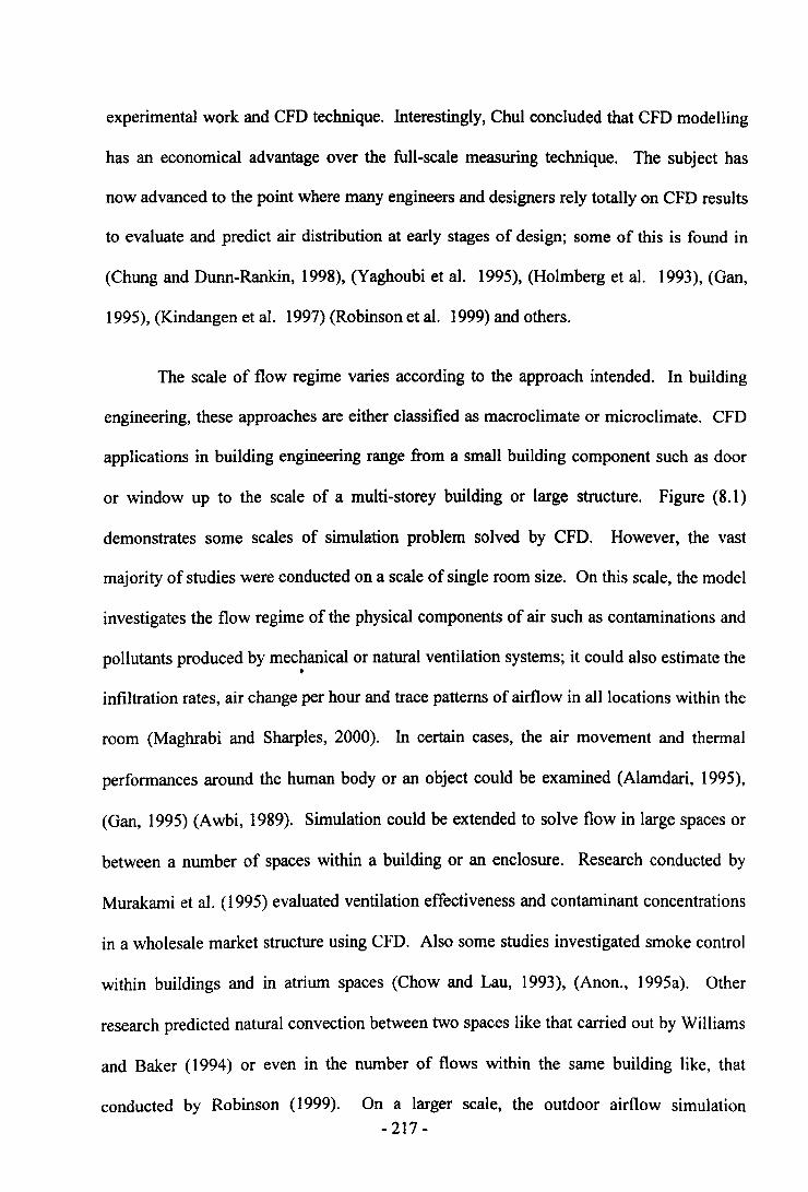
experimental work and CFD technique. Interestingly, Chul concluded that CFD modelling
has an economical advantage over the full-scale measuring technique. The subject has
now advanced to the point where many engineers and designers rely totally on CFD results
to evaluate and predict air distribution at early stages of design; some of this is found in
(Chung and Dunn-Rankin, 1998), (Yaghoubi et al. 1995), (Holmberg et al. 1993), (Gan,
1995), (Kindangen et al. 1997) (Robinson et al. 1999) and others.
The scale of flow regime varies according to the approach intended. In building
engineering, these approaches are either classified as macroclimate or microclimate. CFD
applications in building engineering range from a small building component such as door
or window up to the scale of a multi-storey building or large structure. Figure (8.1)
demonstrates some scales of simulation problem solved by CFD. However, the vast
majority of studies were conducted on a scale of single room size. On this scale, the model
investigates the flow regime of the physical components of air such as contaminations and
pollutants produced by mechanical or natural ventilation systems; it could also estimate the•
infiltration rates, air change per hour and trace patterns of airflow in all locations within the
room (Maghrabi and Sharples, 2000). In certain cases, the air movement and thermal
performances around the human body or an object could be examined (Alamdari, 1995),
(Gan, 1995) (Awbi, 1989). Simulation could be extended to solve flow in large spaces or
between a number of spaces within a building or an enclosure. Research conducted by
Murakami et al. (1995) evaluated ventilation effectiveness and contaminant concentrations
in a wholesale market structure using CFD. Also some studies investigated smoke control
within buildings and in atrium spaces (Chow and Lau, 1993), (Anon., 1995a). Other
research predicted natural convection between two spaces like that carried out by Williams
and Baker (1994) or even in the number of flows within the same building like, that
conducted by Robinson (1999). On a larger scale, the outdoor airflow simulation- 217 -
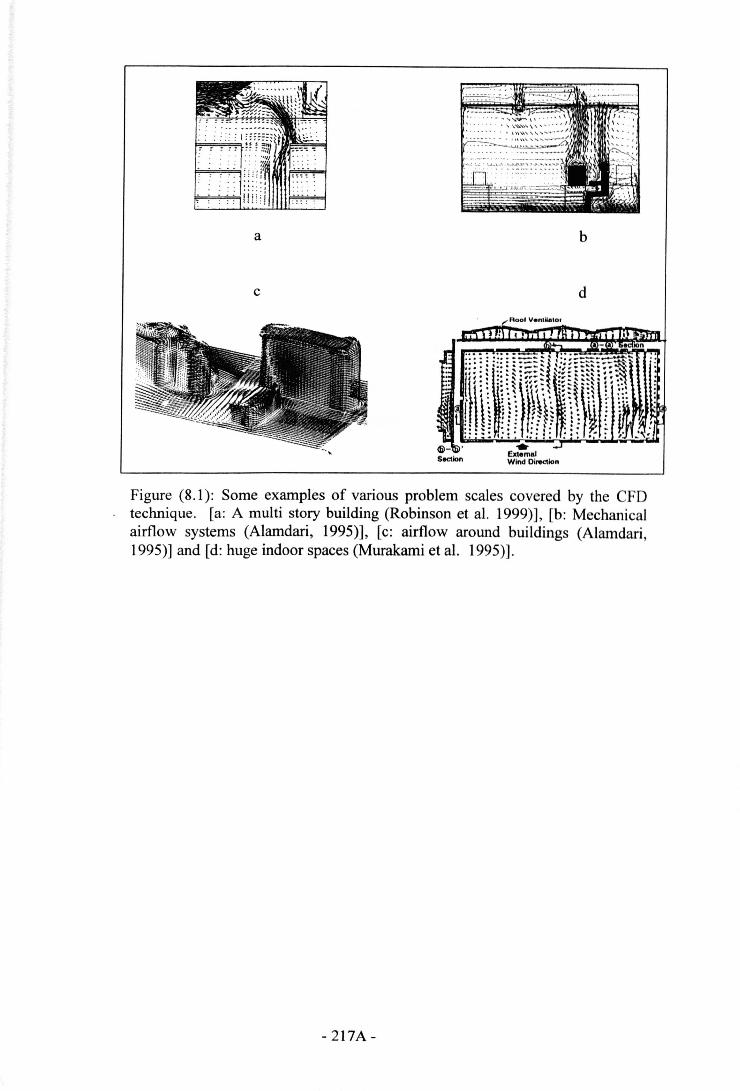
a b
c d
@-Section
Figure (8.1): Some examples of various problem scales covered by the CFDtechnique. [a: A multi story building (Robinson et al. 1999)], [b: Mechanicalairflow systems (Alamdari, 1995)], [c: airflow around buildings (Alamdari,1995)] and [d: huge indoor spaces (Murakami et al. 1995)].
-217A-

encounters other complications in addition to those discussed at indoor airflow simulations
such as wind forces, directions and other environmental factors that could not be solved at
certain stage of simulation.
In general, the application of CFD in building engineering IS increasingly
advancing with the enhancement in computational power. While empirical measurements
should not be underestimated, CFD offers an alternative tool for building engineering
problems that cannot be easily traced by other measuring techniques. A recent review
work carried out by Maghrabi and Sharples (2000) indicated the challenges of using
modelling technique for designers and architects in the field.
8.3. CFD applications in buildings engineering
8.3.1. CFD simulation software
There are several commercial CFD packages available at present that have the
capability of modelling a wide range of fluid flow problems; amongst these packages are
FLOVENT, FLUENT, FLINT, PHOENICS, STARCD and FLOW3D. They suggest
similar capabilities, hence the choice of package which is most suitable for the study
depends on a number of factors including the appropriateness to the fluid flow problem,
the software and hardware requirements in relation to cost and user skills. Help facilities
and technical user support services should also be considered.
The present work required facilities for single-phase flow and two-dimensional
modelling. FLUENT software was the code chosen to perform solutions of the problem in
hand. This software is used heavily in airflow simulation in buildings. Further details arc
available in the FLUENT user manual (1999). FLUENT was already available on site
- 218 -
(University network and University network remote access) with technical user support
services, and the University of Sheffield network is frequently updated with the latest
version of FLUENT. That is why the simulation was carried out using the FLUENT
version 4.5, and hence, its description in some detail in this chapter. It is worth
emphasising that not all the available options of FLUENT are mentioned here, but only
those relevant to this work.
8.3.2. Basic Equations of CFD
The first step in numerical modelling is to establish the basic conservation
equations based on the principles of fluid mechanics and relevant components such as heat
and flow, etc. These equations constitute a system of non-linear simultaneous partial
differential equations that can be solved numerically. The equations used in this numerical
modelling are presented here.
The main problem of fluid dynamics is the determination of the velocity and state
of the fluid subject to certain imposed conditions. Throughout this work it has been
assumed that the fluids are gases at ambient pressure that behave ideally. No consideration
was given of the case of chemical reactions, air contaminations or heat transfer since the
aim was to investigate the air quantity rather than quality. The equations that allow the
solution of the most general case of ideal gas mixture are the following:
Mass conservation:
ap +~(pu,)=O (8.1)at Ox,
- 219-
Momentum conservation:
a a a [ (~. ~j)] iP-(pu)+-(pu.u.)=- I-l -' +- --+pg. +F.at } & '} & & &. &. } }, '}'}
(8.2)
The left side of the equation represents the convection term, and the terms on the
other side represent, in sequence, the diffusion, pressure body forces, and the momentum
interaction between forces.
The continuity and momentum equations are non-linear partial differential
equations and, together with appropriate boundary conditions, provide a complete
description of flows for which the density is uniform.
8.3.3. Turbulence Modelling
Turbulence is one of the remaining unsolved theoretical problems in fluid
mechanics (Yang, 1989). Nevertheless, there are different approaches in dealing with
engineering problems. The most rigorous treatment is for predicting complex turbulent
flows. As discussed in the earlier chapters, turbulence is measured based on the Reynolds
number, Navier-stokes, x-s model equations and others. The derivation of these equations
is not detailed here but some references are suggested to that effect (Etheridge and
Sandberg, 1996), (Alamdari, 1995), (Chow, 1995), (Ruyssevelt et al. 1995), (Anon.,
1995b), (Anon., 1995c), (Yang, 1989). It is worth mentioning that many engineers have
relied on the /C-B model equation to predict flow around the buildings (Kindangen et al.
1997), and hence, /C-B model was used in this study.
The above equations describe the time-averaged flow when applied to a finite
number of discrete control volumes. The effects of turbulence can be included by
- 220-
substituting an 'effective' viscosity in the equations consisting of the molecular viscosity
augmented by its turbulent counterpart, !J.t. The differential transport equations for the
kinetic energy of turbulence K and its dissipation rate E are:
(8.3)
and
o ( ) 0 ( ) o}lt OE E E2- oe +- pu,e =---+C -G -C p-a ax I ax ax 1& k Ie 2& kI I U& I
(8.4)
where Gk is the generation term of k and is given by:
(8.5)
The turbulent viscosity, !J." is related to K and E, by
e!J., = pCp- (8.6)e
where CIl) C2l) C)b Uk and Ue are empirical constants, with values 1.44, 1.92, 0.09, 1.0 and
1.3 respectively.
The equations mentioned above are transformed into a set of algebraic equations
that can be solved iteratively. This transformation, also called discretisation, involves the
following.
• The domain is divided into cells or control volumes.
• The governing equations are integrated over each cell.- 221 -
• The algebraic equations so obtained are solved by iteration as described
later. In this section consideration is given to the discretisation procedure.
8.3.4. Physical and computational domains
FLUENT requires detailed specification of flow mechanism and its boundaries in
addition to the model of turbulence. The identification of physical and computational
domains added to the boundary conditions shape the complicated part of the simulation
procedure (Maghrabi and Sharples, 2000).
In order to perform the discretisation of the governing equations the physical space
must be subdivided into a number of cells by means of a structured grid. The cells can be
built using Cartesian or Body-fitted grid coordinate systems as shown in Figure (8.2). The
latter is much complicated and sophisticated to make curves and cylindrical shapes while
Cartesian coordinate system is widely used in the rectangular domains (Alamdari, 1995),
(FLUENT, 1999). In this research, a two-dimensional Cartesian grid was generated either
directly from FLUENT or FLINT (2000). FLINT code is used only to construct the
models when simulating louver inclination angle since it was more complicated to use the
body-fitted grids coordinate in FLUENT. Permission was given to use it by FLINT's
author, as it was not yet commercialised. The node points, i.e. points where the grid lines
intersect, define the cells generated. The space where the integer numbers are used is
called the computational domain.
8.4. Boundary conditions
- 222-
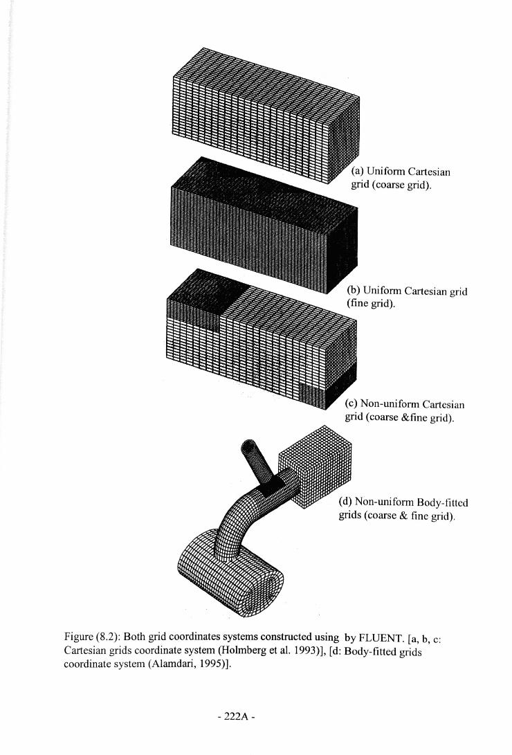
(c) Non-uniform Cartesiangrid (coarse &fine grid).
(d) Non-uniform Body-fittedgrids (coarse & fine grid).
Figure (8.2): Both grid coordinates systems constructed using by FLUENT. [a, b, c:Cartesian grids coordinate system (Holmberg et al. 1993)], [d: Body-fitted gridscoordinate system (Alamdari, 1995)].
- 222A-
FLUENT allows for a number of different types of boundary conditions. The
following are the terms identified by FLUENT and various data were input to solve the
problem. Data mentioned here are those related to the work in hand.
8.4.1.1. INLET
At which conditions of flow components are identified such as velocity, turbulence
and composition of the flow.
8.4.1.2. OUTLET
FLUENT does not allow adjustments of the OUTLET specifications. But the
normal velocities are adjusted at OUTLET boundary to satisfy an overall mass balance and
no velocity gradients should exist. For precise results, it is recommended that air should be
fully developed before reaching the OUTLET.
8.4.1.3. WALL
Including walls, floor and ceiling. At these boundaries, the normal velocity
component vanishes. Temperature, conduction or heat fluxes were not specified as they
were not of concern in the current solution. The pressure gradient is zero. If the
dimensionless distance becomes less than a certain value, then a laminar expression is used
instead.
8.4.2. The iterative solution procedure
The equations are not solved simultaneously at all nodes. Instead, a line-by-line
solution procedure is made. The last step in the calculation is the inclusion of the
interaction terms between the second phase and the fluid phase, as discussed in the chapter.
- 223-
8.4.3. Uncertainties in CFD
The overall uncertainties involved in CFD modelling could be due to several
sources. The CFD coding to represent complexities could be a main cause of this.
Complexities occurring in a' real environment could not - sometimes- be represented
numerically as stated earlier. Additional uncertainties are referred to other factors:
• Modelling errors (the inaccuracy inherent in the mathematical model of certain
physical phenomena), domain dependency errors, i.e. errors arising from finite
representation of a domain.
• Inaccurate implementation of the boundary and initial conditions.
• Iterative convergence errors (i.e. incomplete convergence).
• Grid convergence errors (errors due to insufficient grid refinement, i.e,
discretisation errors).
• Lack of user skills and experience in dealing with CFD solution.
8.4.4. Numerical errors
In 1993, the issue was raised concerning the ability of programmes to produce
dependable predictions (Anon., 1995b). Different CFD models have different codes that
can have significant errors when applied in prediction procedures. While the debate
continues, this can be a significant issue not only for unskilled users, but embedded errors
are not - sometimes- easily discovered even by highly sophisticated skilful users (Maghrabi
and Sharples, 2000). Some of these errors refer to the fact that some of the complexities in
the real environment cannot be simplified numerically (Etheridge and Sandberg, 1996)
(Awbi, 1989). Error then must be reduced to a reasonable level before accepting solution.
Cost may limit the resources that can be brought to bear on a problem. In such a case,
- 224-
compromise or another approach is necessary. The distribution of grids in the domain
could reduce the percentage of error. In other words, the use of finer grids near INLET,
OUTLET and WALL (Figure 8.2.c and 8.2.d) would usually increase the solution accuracy
and this while increasing computation power and solution timing (Awbi, 1991), (Maghrabi
and Sharples, 2000).
8.4.5. Numerical setup
FLUENT necessitates definitions of parameters in order to run proper solutions.
Memory allocation, dimension of computational domain (2 dimensions in this solution),
size of the computational domain and number of cells must be identified first. Other
parameters also must be identified to FLUENT: physical models used, fluid specifications
(viscosity, density, etc,) and boundary conditions of INLET, OUTLET and WALL. As
earlier stated, fluid temperature was not specified since it was not concerned in this
solution.
8.4.6. Iterations of residuals
Once the set up and construction of the model took place and was ready to run, the
solution parameter would then depend on the number of iterations of the solver. The
residuals of iterations reflect the accuracy of obtainable results. It is applicable either to
determine the number of iterations counted or by time-dependence. To activate the time-
dependent option, time varying data must be carefully identified, such as flow fluctuations,
before running the solution. However, in counts iteration the FLUENT is set to reach
satisfactory convergence at (1x 10⁻⁴) of residual iterations and would stop counting,
assuming that results are accurate to depend upon, and hence, save computational timing.
- 225-
In some studies, the residual of iteration counts would be adjusted to converge at (1x 10⁻³),
as found in (Kindangen et al. 1997), and still be acceptable.
8.5. The Models configurations and boundary setup
The general procedure employed to set up geometry, two-dimensional Cartesian
grid coordinates system, specification of the boundary conditions and physical constants
are discussed here. It is worth mentioning that this stage contained flaws as it is the first of
trial calculations but, as always, they are used as a learning process and are improved in the
subsequent specifications of the calculations.
8.5.1. Grid distribution
The consideration was taken into account to examine the CFD coding through
solving and representing the airflow around the MLW. A two dimensional rectangular
physical boundary was therefore constructed. FLUENT grid-based geometry was used, in
which the geometry of the domain was determined by control volumes defined by the grid.
This is with horizontal louvers blades evolved. As stated early, FLINT code was merely
used to construct the two-dimensional domain when louver inclinations were present and
the simulation process was carried out using FLUENT. Cartesian coordinates were used in
which the grid lines were aligned with the Cartesian (x, y) coordinates.
The overall domain size of the room chamber and location of reference wind (ve)
were defined. A non-uniform grid aimed to enhance the accuracy of the solution. A fine
non-uniform grid allowed the grid to cluster more densely in areas where the flow is
complex or of interest such as louver blades, ceiling and floor locations. It also allowed
the use of grid lines apart in regions that were of lesser interest. Therefore, non-uniform
- 226-
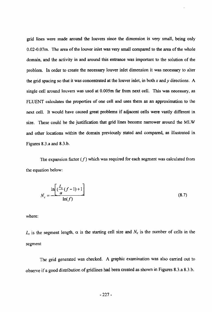
grid lines were made around the louvers since the dimension is very small, being only
O.02-0.07m. The area of the louver inlet was very small compared to the area of the whole
domain, and the activity in and around this entrance was important to the solution of the
problem. In order to create the necessary louver inlet dimension it was necessary to alter
the grid spacing so that it was concentrated at the louver inlet, in both x and y directions. A
single cell around louvers was used at O.005mfar from next cell. This was necessary, as
FLUENT calculates the properties of one cell and uses them as an approximation to the
next cell. It would have caused great problems if adjacent cells were vastly different in
size. These could be the justification that grid lines become narrower around the MLW
and other locations within the domain previously stated and compared, as illustrated in
Figures 8.3.a and 8.3.b.
The expansion factor (/) which was required for each segment was calculated from
the equation below:
N ~ ~(~(f -1)+1]
c In(/)(8.7)
where:
Le is the segment length, a is the starting cell size and Ne is the number of cells in the
segment
The grid generated was checked. A graphic examination was also carried out to
observe if a good distribution of gridlines had been created as shown in Figures 8.3.a 8.3.h.
- 227-
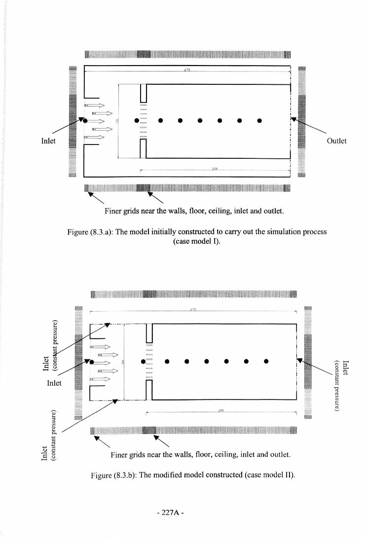
D.= • • • • • •II
200
I
I
1
Finer grids near the walls, floor, ceiling, inlet and outlet.
Outlet
Figure (8.3.a): The model initially constructed to carry out the simulation process(case model I) .
mllllllllllllllllllllllllllllllllllllllllllllllllllillIIIIIIII-.
•= • • •• • •
111111111111111111111111111111111111111111111111111111111111111111111111111111111111111111111111111111111111111111111111111111111111111111111111111111111111111111111111111111111 ~
<,Finer grids near the walls, floor, ceiling, inlet and outlet.
Figure (8.3.b): The modified model constructed (case model II).
- 227A-
8.S.2. Physical domain
The construction of the physical domain usually anticipates some flaw. So these
errors were the learning process that improved subsequent specifications of calculations.
Initial set up of the laboratory was simulated and both v/ve% and v/ve% were examined.
The appropriateness of the model selected to carry out validation stage is described here
taking into consideration points stated earlier in this chapter. The procedure followed to
consider the appropriate model under which comparison took place was in three stages of
modelling. Each case model is described next.
8.S.2.1. Simulation model (Case-I)
This case is similar to the laboratory set up (Figure 8.3.a). The test chamber was
located between domains INLET and OUTLET as they shaped the vertical edges of the
domain while the room chamber with the louvers was floating within them. The reference
wind speed (ve) was located at a distance similar to that noted in section 7.2.1 away from
MLW models similar to the laboratory location and all characteristics of the physical
domain discussed earlier were clearly specified to the model. Both v/ve% and v/ve% were
obtained and compared to the physical measurements.
8.5.2.1.1. v/ve%:
The attempt was made to determine the flow resistance zone created at the
windward side outside the room due to the MLW. Inevitably, CFD confirmed that MLW
models had offered resistance to airflow. This zone however was depending on the MLW
tested. In general, the flow resistance zone ranged from O.35mto O.60mon the windward
side. Results of v/ve% obtained from both measuring techniques were comparable as
- 228-
shown by Figure (8.4) and Table (8.1). The error limit between both curves produced from
a number of MLW configurations was less than 10%.
8.5.2.1.2. v/ve%:
The first observations of colour-filled contour and regression curve plotted for
results obtained from both measuring techniques encountered major discrepancies. The
indoor air ratio of mean indoor velocity v/ve% obtained from CFD was undoubtedly
illogical and improper, and the measured cells inside the box accompanied by higher error
and discrepancies. On the one hand, the observation showed that as air passed the louver
blades its kinetic momentum increased dramatically, causing a higher percentage of errors
along the room chamber with a very slight decrease in the v/ve%. Furthermore, the regime
of airflow fluctuated and was obviously illogic. Various endeavours were then performed
to correct it. However, it was found that neither increasing the non-uniform computational
grid cells around louvers and inside the compartment nor considering the surface
roughness of the louvers corrected it. Boundary specifications on the other hand were
specified correctly. Locating reference wind speeds at various positions, far from louvers,
did not correct the error either. In addition, a consultation from the technical support was
sought. It was then suggested that errors resulting in vlve% could be due to number of
factors:
• The flow regime between various zones with dramatic change in their
dimensions as found in the case in hand. The area of air gap (d) between
louvers examined was much smaller when compared to the area of airflow
outside (windward) or inside the room chamber simulated. In such dramatic
change in flow volume the jet flow was as/if moving from free-jet condition to
wall-jet, to free-jet condition again. All of this occurred through the number- 229-
of cells within louver blades and the flow encountered dramatic changes in the
fluid components. Even though during the laboratory measurement this
phenomenon was found only in CFD, it caused an increasing change in the
kinetic force as it was based on mathematical representations of the flow.
This force then affected the other adjacent cells around, which led to such
error.
• Another reasonable justification of this was concerned with CFD numerical
coding. In practice, the flow of air within and around porous elements such as
louvers would be accompanied with dramatic complexities occurring in
physical properties of air such as air viscosity, static pressure, velocity, etc.
These could not be simplified theoretically, and correcting them was beyond
the scope of the laboratory experiment. Therefore. the CFD equations
representing them may not represent the complication in the real environment.
Additionally, most available CFD packages deal with issues related to
ventilation aspects in simplistic ways and may not necessarily reflect those
types of complexities as noted before.
8.5.2.2. Simulation model (Case-H)
This case was similar to the latter except that the outlet was replaced by an INLET
with a constant pressure (IP) (0 pressure difference at IP) that permitted air to float at inlet
boundaries according to velocity and direction of a fluid (Figure 8.3.b). While this
solution did not correct the problem, it gave more assurance to the accuracy of measured
V/Ve% at laboratory (Table 8.1), (Figure 8.4).
The anticipated flaws that emerged from the two models cases discussed earlier led
to the conclusion that errors emerged inside the modelled test chamber. where the vlve%- 230-
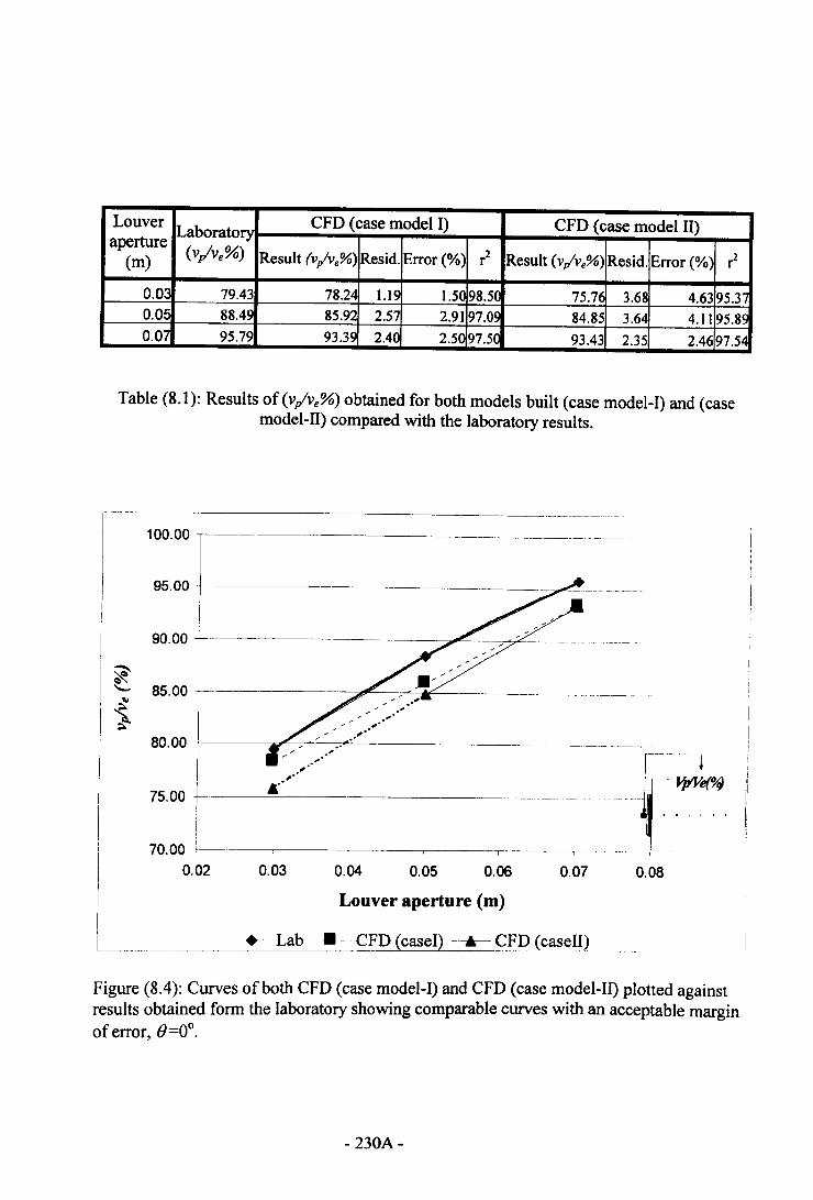
Louver Laboratory CFD (case model I) CFD (case model II)aperture
(m) (v/ve%) Result (v/ve%) Resid. Error (%) r2 Result (v/ve%) Resid. Error (%) r2
0.03 79.43 78.24 l.l<; 1.5~98.5C 75.7f 3.68 4.63 95.370.05 88.49 85.92 2.57 2.91 97.09 84.85 3.64 4.11 95.8(0.07 95.79 93.39 2.4C 2.5~ 97.5~ 93.43 2.35 2.46 97.54
l_~_~_
Table (8.1): Results of (v/ve%) obtained for both models built (case model-I) and (casemodel-II) compared with the laboratory results.
-----------------------
100.00 -,-----
95.00
.',...,..'
::: l--£~·-·--~---.---0.02
,-----.~ -- -I----~~--·
0.03 0.04 0.05 0.06 0.07 0.08
Louver aperture (m)
--+- Lab - • - CFD (easel) -_._- C£Q_ (c;~_e_II)
Figure (8.4): Curves of both CFD (case model-I) and CFD (case model-II) plotted againstresults obtained form the laboratory showing comparable curves with an acceptable marginof error, ()=Oo.
- 230A-
examined was due to the airflow complexities occurring within the louver blades. This led
to the errors found within the simulated chamber. On the other side, the flow readings
outside the box, towards the windward side were less affected by that error. As shown in
Figure 8.4, v/ve% recorded from both model cases built have supported the findings
obtained from laboratory measurements. The choice was suggested of the velocity drop
due to the porosity percentages (vp've%) obtained from the physical measurements as the
reference velocity at the INLET. Such decision was taken into consideration because of a
number of factors:
• The comparable v/ve% achieved from both techniques used as mentioned
earlier
• Reducing of the complications of the model which, in tum, would reduce the
error percentage.
• Scaling the volume from which airflow passed through, i.e. airflow from within
the louvers to the room.
• Other works in the field of CFD technique support the decision taken to
consider the data of v/ve% obtained from laboratory as a reference of values for
inlet wind speed. For example, Murakami et. al. (1995) applied wind tunnel
results obtained at the window to characterise the openings boundaries in CFD
stage. Also, Weathers and Spitler (1998) conducted a comparative study
between numerical predictions using CFD and full-scale measurements to study
room airflow, and used the measured data to specify the boundary conditions of
the inlet. Interestingly, the previous work highlighted that in ventilation
research velocity distribution over the inlet area is assumed to be uniform. This
is even applied with the predicting flow performance from mechanical
- 231 -
ventilation systems as found in Gan (1995). The work Gan conducted to
evaluate room air distribution systems using CFD showed that the inlet was
characterised with some simplicity rather than fully characterised. Similar
justification could be found in the work carried out by Holmberg et al (1993).
Nielsen (1992) carried out a much relevant research on various diffusers. In his
work concerning the description of supply openings in numerical models for
room air distribution, the author investigated various techniques to specify the
boundary conditions at the supply openings (INLET) including direct
description, box method, prescribed velocity method and computer generated
supply condition method. The author stated, " The flow profiles in the openings
of the diffusers can now be used as inlet profiles for the prediction of the flow in
the room". Thus, the characterisation of INLET was represented by readings
obtained form the laboratory measurements, hence the full validation stage and
airflow pattern study were carried out based on this justification.
8.5.2.3. Simulation model (Case-III)
This model was constructed as a third stage of creating the proper computational domain.
In this solution, velocity speed vlve% obtained from laboratory measurements was applied
at the INLET reference speed because a strong potential for CFD to represent the
laboratory results of vlve% was found (Figure 8.4). The model was built considering that
air INLET as the first vertical grid cells between louver blades and the other side of the
room chamber was the OUTLET as illustrated in Figure 8.5. The actual shape of the
louver with inlets was accurately modelled under the Cartesian coordinates. This reduced
the geometry complications to predict the flow regime around MLW, and in-turn, reduced
error percentage and computational timing. Consequently, precise results were achieved.
- 232-
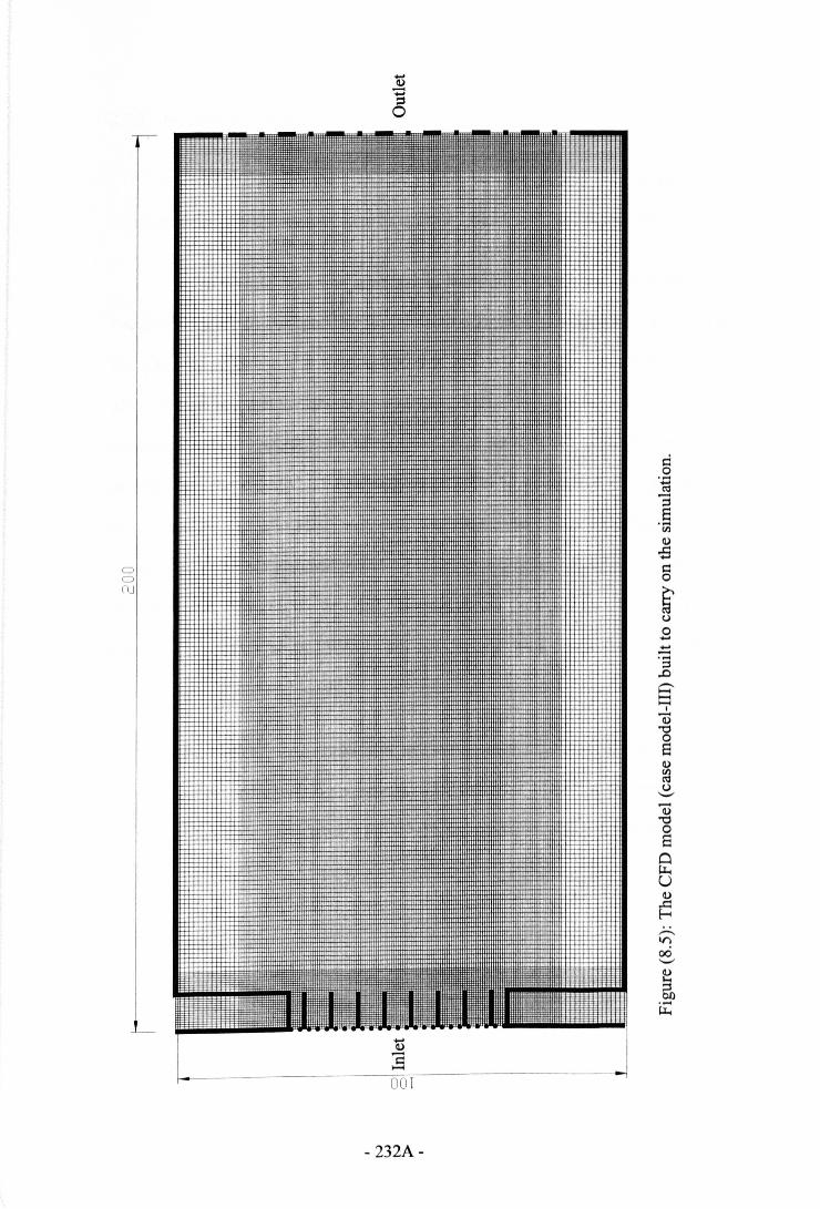
d0..g:i.§Cl)
a.>-BI::l0
0
~
0cu
o0..........-.....;::S..0~~I
Q)"008a.>~o'-"-a.>"00Elfi:ua.>
~,-....V")
00<;»
a.>
~.-~
- 232A-
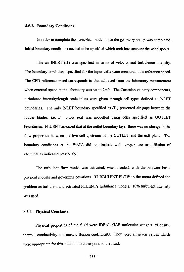
8.5.3. Boundary Conditions
In order to complete the numerical model, once the geometry set up was completed,
initial boundary conditions needed to be specified which took into account the wind speed.
The air INLET (II) was specified in terms of velocity and turbulence intensity.
The boundary conditions specified for the input-cells were measured at a reference speed.
The CFD reference speed corresponds to that achieved from the laboratory measurement
when external speed at the laboratory was set to 2m/s. The Cartesian velocity components,
turbulence intensity/length scale inlets were given through cell types defined at INLET
boundaries. The only INLET boundary specified as (11) presented air gaps between the
louver blades, i.e. d. Flow exit was modelled using cells specified as OUTLET
boundaries. FLUENT assumed that at the outlet boundary layer there was no change in the
flow properties between the live cell upstream of the OUTLET and the exit plane. The
boundary conditions at the WALL did not include wall temperature or diffusion of
chemical as indicated previously.
The turbulent flow model was activated, when needed, with the relevant basic
physical models and governing equations. TURBULENT FLOW in the menu defined the
problem as turbulent and activated FLUENT's turbulence models. 10% turbulent intensity
was used.
8.5.4. Physical Constants
Physical properties of the fluid were IDEAL GAS molecular weights, viscosity,
thermal conductivity and mass diffusion coefficients. They were all given values which
were appropriate for this situation to correspond to the fluid.
- 233 -
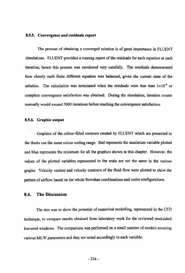
8.5.5. Convergence and residuals report
The process of obtaining a converged solution is of great importance in FLUENT
simulations. FLUENT provided a running report of the residuals for each equation at each
iteration; hence this process was monitored very carefully. The residuals demonstrated
how closely each finite different equation was balanced, given the current state of the
solution. The calculation was terminated when the residuals were less than 1x 10⁻⁴ or
complete convergence satisfaction was obtained. During the simulation, iteration counts
normally would exceed 5000 iterations before reaching the convergence satisfaction.
8.5.6. Graphic output
Graphics of the colour-filled contours created by FLUENT which are presented in
the thesis use the same colour coding range. Red represents the maximum variable plotted
and blue represents the minimum for all the graphics shown in this chapter. However, the
values of the plotted variables represented in the scale are not the same in the various
graphs. Velocity vectors and velocity contours of the fluid flow were plotted to show the
pattern of airflow based on the whole Rowshan combinations and outlet configurations.
8.6. The Discussion
The aim was to show the potential of numerical modelling, represented in the CFD
technique, to compare results obtained form laboratory work for the reviewed modulated
louvered windows. The comparison was performed on a small number of models covering
various MLW parameters and they are noted accordingly in each variable.
- 234-
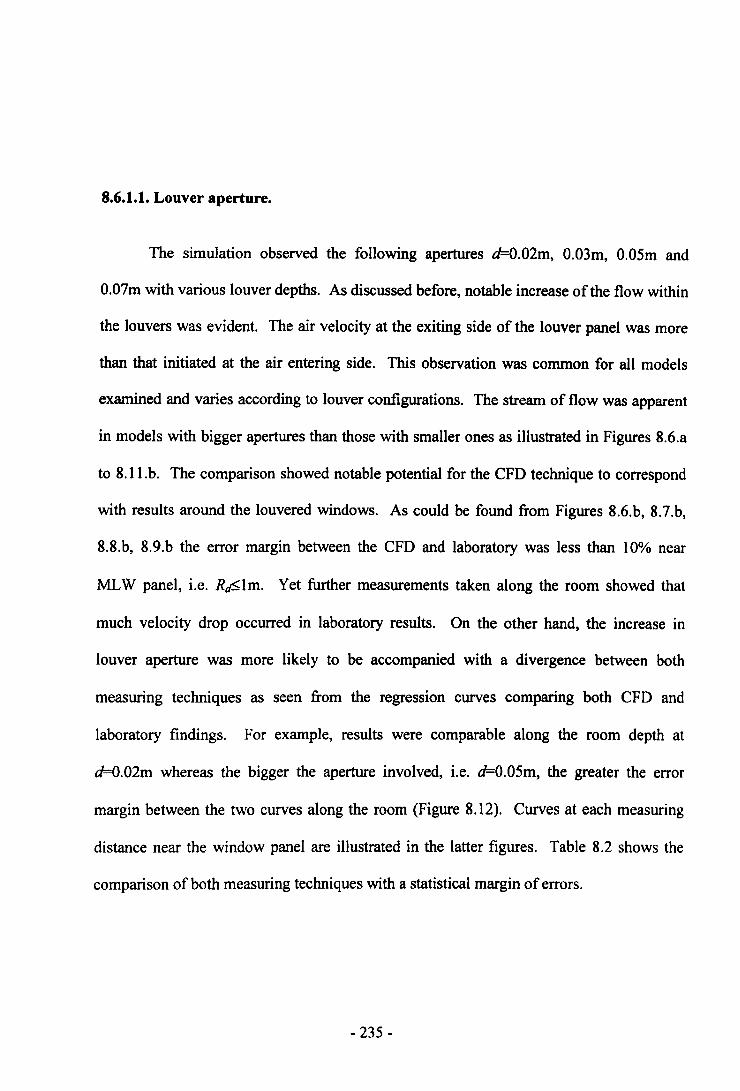
8.6.1.1.Louver aperture.
The simulation observed the following apertures d=0.02m, 0.03m, 0.05m and
0.07m with various louver depths. As discussed before, notable increase of the flow within
the louvers was evident. The air velocity at the exiting side of the louver panel was more
than that initiated at the air entering side. This observation was common for all models
examined and varies according to louver configurations. The stream of flow was apparent
in models with bigger apertures than those with smaller ones as illustrated in Figures 8.6.a
to 8.II.b. The comparison showed notable potential for the CFD technique to correspond
with results around the louvered windows. As could be found from Figures 8.6.b, 8.7.b,
8.8.b, 8.9.b the error margin between the CFD and laboratory was less than 10% near
MLW panel, i.e. RcJ$lm. Yet further measurements taken along the room showed that
much velocity drop occurred in laboratory results. On the other hand, the increase in
louver aperture was more likely to be accompanied with a divergence between both
measuring techniques as seen from the regression curves comparing both CFD and
laboratory findings. For example, results were comparable along the room depth at
d=0.02m whereas the bigger the aperture involved, Le. d=O.05m, the greater the error
margin between the two curves along the room (Figure 8.12). Curves at each measuring
distance near the window panel are illustrated in the latter figures. Table 8.2 shows the
comparison of both measuring techniques with a statistical margin of errors.
- 235-
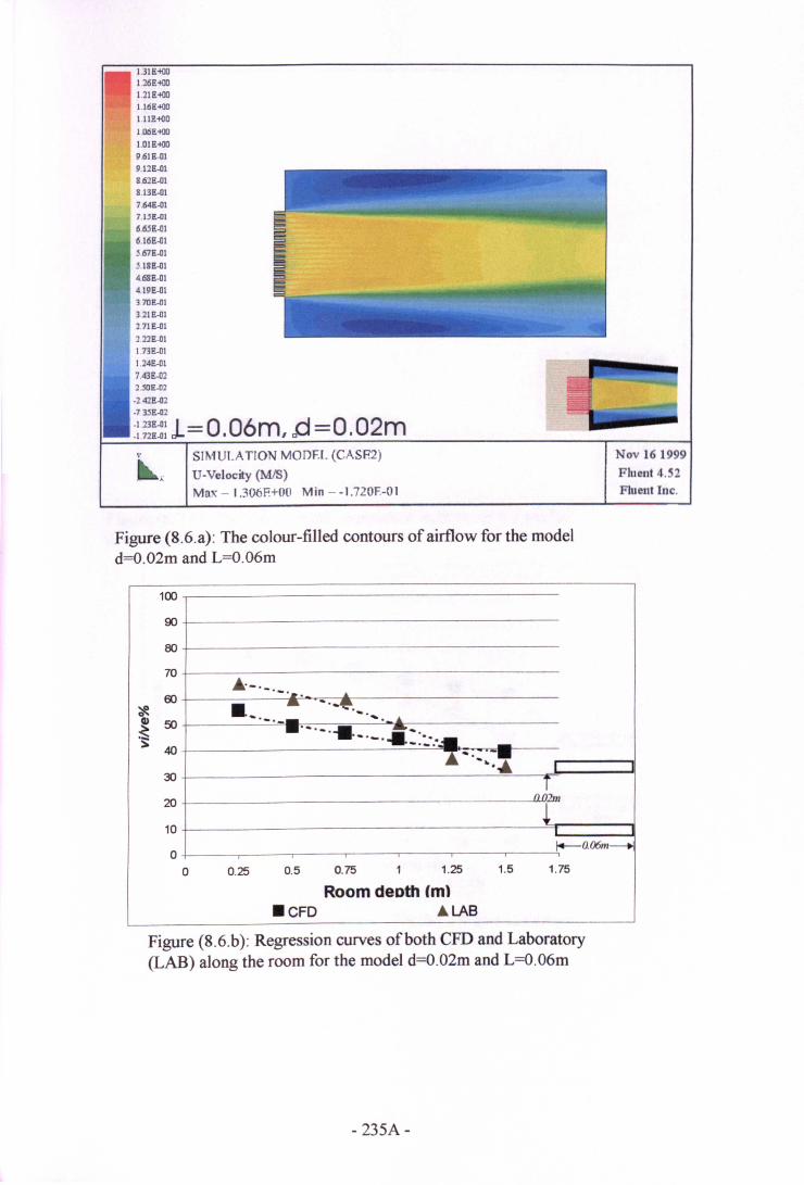
SIf\fUI.A TION MODEL (CASE2)
U-Velocity (MIS)Max - 1.306F.+Oll Min - -1.720F.-Ol
Nov 161999Fluent 4.52Fluent Inc,
1.21 E-+OO1.16E-+OOI.1I1HilO1.00E-+OO1.00E-+!l09.6IE-0I9.12E-018.62E-018.13E-017.64E-017.I.lE-016.65E-016.16E-0I.I.67E-01.1.18£-014.68E-014.19E-01370E-013.21E-012.7IE-012.22E-01173E-Ol1.24E-Ol7.43E-022..lOE-02-242£-02.735£-02
::;~~~:!=O.06m, aCt =O.02m\'
~x
Figure (S.6.a): The colour-filled contours of airflow for the modeld=O.02m and L=O.06m
100
90
80
70 .-._ ..60'_' ..
~ .- ....... 4!l'. ...'"Cl) 50
-._._- '.~
_...... ~ ... '.... '.._.
:> -. ..40
- ..... -,. .......:%I
30
nJ2m20~
10
0l+-o.06m--+i
0 0.25 0.5 0.75 1 1.25 1.5 1.75
Room deoth 1m).CFD .LAB
Figure (S.6.b): Regression curves of both CFD and Laboratory(LAB) along the room for the model d=O.02m and L=O.06m
- 235A-
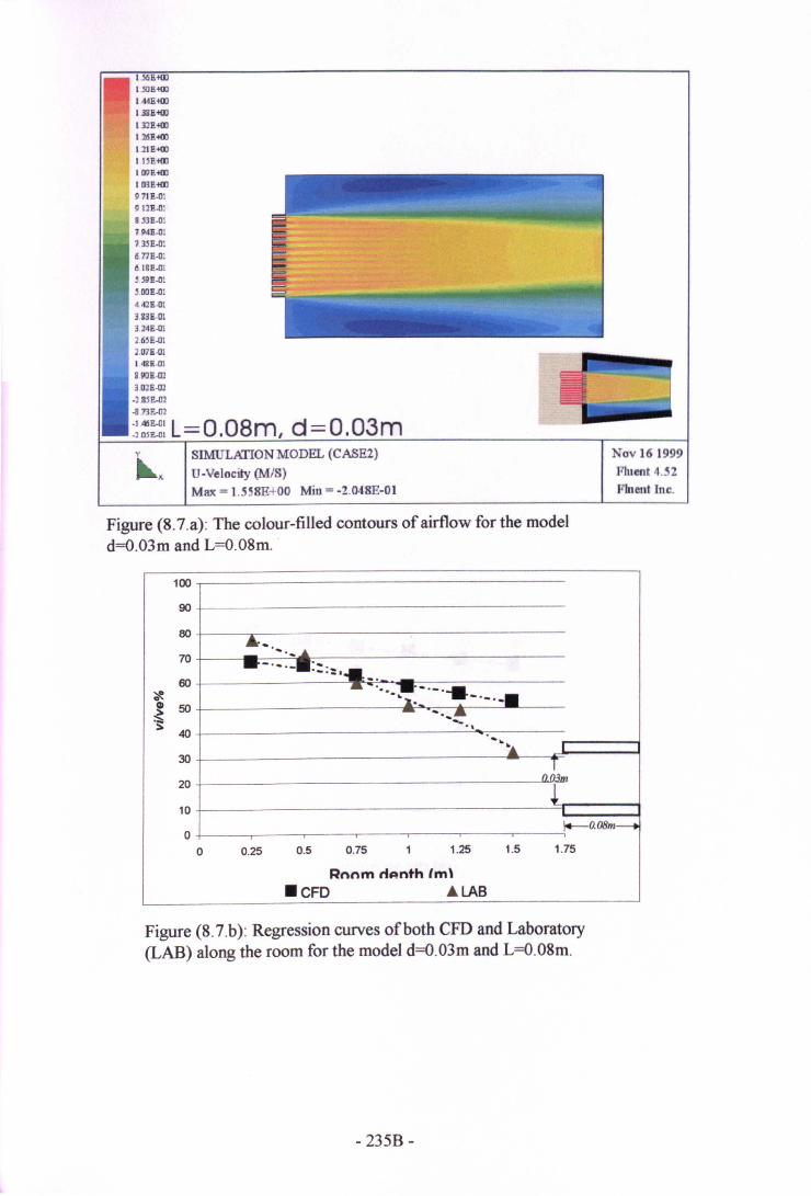
13S£<ID132£<ID126P.<ID1.21E<ID1 UP.<IDI D9E<ID103E<IDP 71P.-OlP 12P.-Ol8 SlE.Ol794£-017.35£-016.n£·016 18E-Ol5 S9E-Ol5.00E.01441E-Ol
U31l·01324£-012.65£-012.07£·0114118·01
81J01l-0210JE·OJ.2851l-02
-873E.-OJ
:~:~:L=O.08m, d=O.03mSIMULATION MODEL (CASE2)
U-Velocity (MIS)Max = 1.558E+OO Min = -2.048E-Ol
Nov 161999Fluent 4. 2Fluent Inc.
Figure (8.7.a): The colour-filled contours of airflow for the modeld=O.03m and L=O.08m ..
100
90
80£..... ..
70 - .......-.-.-.:.... _-.:.60 - .---~.-.-.-II
'*'~ 50~1' -'-,-11
~- ........
"'- .,40 ..,.-:..
I
30 +20
10
0 I+--O.08m--t
0 0.25 0.5 0.75 1 1.25 1.5 1.75
Rnnm rip-nth fm\.CFD A LAB
Figure (8.7.b): Regression curves of both CFD and Laboratory(LAB) along the room for the model d=O.03m and L=O.08m.
- 235B-
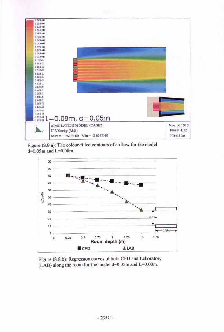
I S6Et{I)1 oI9Et{I)I 43Et{I)136Et{I)129Et{I)I 221!.t{I)I 16l!t{I)I D9l!t{I)1 D2l!t{I)953£.01g,86E.olS ISE.ol7,51E.olQ,g31!..o16,16E.oI5,4IIE-III4,81E.oI414l!.o13 46E-Ol279l!.o121111.011,44E.oI7,66E-029 12E.Q3
-.l,B3E.-D2·1,2IIE.-DI
:~::~~:L-O.OBm d=O.05mNov 161999Fluent 4.52Fluent Inc,
SIMULATION MODEL (eASE2)U -Velocity (MiS)Max = 1.762E+OO Min = -2.606E-Ol
Figure (8.8.a): The colour-filled contours of airflow for the modeld=O.05m and L=O.08m.
100
90
80 -_···:;·-:I:'•. '-'-'1IJ .~ .70
.-. -._.. -...... ----.-._ ....60 .
'$.....
III 50.....
~ ":> 40
....\,'....
30nISm
20~.
10
0I--O.08m-+
0 0.25 0.5 0.75 1 1.25 1.5 1.75
Room depth (m).CFD .LAB
Figure (8.8.b): Regression curves of both CFD and Laboratory(LAB) along the room for the model d=O.05m and L=O.08m.
- 235C-
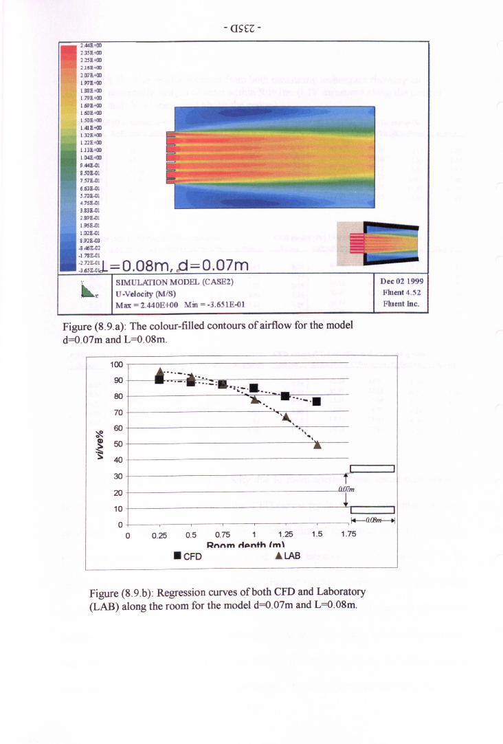
- Q!;£l-
SIMULATION MODEL (CASE2)U -Velocity (MIS)Max = 2.440E+OO Min = ·3.651E-Ol
Dec 02 1999Fluent 4. 2Fluent Inc.
2.25E-flD:l.l~E4!D
2D7E-IlII1.97E<OOl.88E-IlIIl.79E-flD1.59E-IlII1.ISOE-IlIII.SOE-IlIIl.41 E<OO132E-IlIIU2E-IlII1.I3E-IlIIl.04E-IlII
=O.08m =O.07m
Figure (S.9.a): The colour-filled contours of airflow for the modeld=O.07m and L=O.OSm.
100 •..._.~...90 ... ._._ ...-:•.:._.•80
". ....-
-~" ....._ .•70
.''_ ,
~60 ",
s ..\
50 I:;:..S 40
I
30 nl_20
.~
10
0I+-QaJm--..\
0 0.25 0.5 0.75 1 1.25 1.5 1.75~nnm tipn+h Im\
.CFD A LAB
Figure (S.9.b): Regression curves of both CFD and Laboratory(LAB) along the room for the model d=O.07m and L=O.OSm.

Table (8.2): The results obtained from both measuring techniques showing anacceptable margin of error within Rd=lm. (I-IVmeasured along the centre)and CV-VImeasured above the centre).
CFD model (I) L=O.08m, d=O.07m and q=Oo CFD model (II) L-O.08m, d-G.OSm and q-OoReI(m) LAB (vllve%) CFD (vllve%) SL deviation SL error Rd(.) LAB ("live") CFD (vllve") SL deviation SI. error
0.25 95.60 89.85 4.06 2.87 0.25 80.42 80.26 0.11 0.080.50 91.70 88.09 2.55 1.81 0.50 72.95 76.98 2.85 2.020.75 87.26 86.32 0.66 0.47 0.75 66.16 73.70 533 1771.00 77.30 83.80 4.59 3.25 1.00 57.18 72.19 10.61 7.50U5 66.59 78.75 8.60 6.08 1.25 43.25 68.65 17.96 12.701.50 48.55 75.21 18.86 13.33 1.50 31.74 66.63 24.67 17.44
CFD model (III) L=O.08m, d=O.Olm and q=Oo CFD model (IV) L=O.06m, d=O.Olm and q-OoRd(.) LAB (vllve%) CFD ("live·"') SL deviation SL error Rd(.) LAB ("live") CFD (vilv.%) St.d ..... tin SI.... ror
0.25 77.44 68.15 6.57 4.65 0.25 66.06 55.02 7.81 5.520.50 70.93 66.63 3.04 2.15 0.50 59.68 48.51 7.90 5.580.75 59.85 62.59 1.94 1.37 0.75 59.58 46.04 9.57 6.771.00 50.44 58.05 5.38 3.80 1.00 50.09 43.51 4.65 3.291.25 48.70 55.02 4.47 3.16 1.25 36.44 41.04 3.25 2301.50 31.59 51.99 14.43 10.20 1.50 33.38 38.57 3.66 2.59
CFD model (V) L=O.06m, d=O.03m and q=30o CFD model (VI) L-O.08m, d-O.07m and q .... SoReI(m) LAB (vllve") CFD (vllve%) SL deviatiol SL error ReI(.) LAB (vilve%) crn ("iIv.") SI. dev .. tlon St. error
0.25 37.17 38.57 0.99 0.70 0.25 42.59 37.05 3.92 2.770.50 58.62 45.89 9.00 6.37 0.50 55.89 32.26 16.71 11.820.75 44.81 40.99 2.70 1.91 0.75 23.49 10.60 9.12 6.451.00 38.30 26.25 8.52 6.03 1.00 12.79 9.99 1.98 1.401.25 35.30 19.34 11.29 7.98 1.25 17.13 11.05 4.30 3041.50 29.93 12.00 12.68 8.96 1.50 10.72 7.57 2.23 1.58
In general, the decline of velocity due to room aperture was found comparable in
both techniques. It was also notable that CFD curves produced were smoother than those
produced at the laboratory. In other words, the decline of regression curves produced by
CFD was generally less than that produced in the laboratory. Such variations in the
regression curves were within the acceptable limit of validation when examined at smaller
apertures. The same holds for bigger apertures, with some reservation found at the last two
locations measured along room, i.e. Rd~I.25m. As shown in Table 8.3 the standard error
was less than 10% when examined for the smaller apertures along the room while it
increased to nearly 18% with bigger apertures. The author referred this to a number of
- 236-
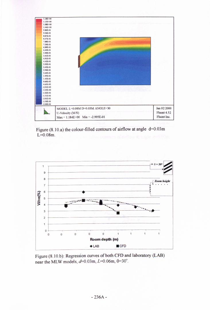
~x
MODEL L=O.08M D=O.03M ANGLE=30
U- Velocity (MIS)Max = 1.184E+00 Min = -2.995E-Ol
Jan 02 2000Fluent4.52Fluent Inc.
93~18.8~1837E.()17.88E'()1739£.016.89E'()16.40£.01S.90E'()1SAIE.()l4.91£.014.42E'()13.93E'()13.43E'()12.94E'()12.44E.()1I.9SE'()11.45E.()19.60E.()24.65E.()2·2.9IE'()3·S.23E.()2.1.02E'()1·1.51E.()1·2.01£.01·2.s0£.Ol·3.00£.01
Figure (8.10.a) the colour-filled contours of airflow at angle d=O.03mL=0.08m.
1 e=30.~I
~9
8Room height
7 • ..,- 6,
~ -. l0
(jj 5~ •. _-_._--.&_ _..:,..: .... _ .._ -._- .....> 4
.... ::'.'- ---. .. .. - .........• .. •.', -.....3
...... ..... ....•• -."lr
2
1
00 0 0 0 0 1 1 1 1
Room depth (m)
+LAB .CFD
Figure (8.10.b): Regression curves of both CFD and laboratory (LAB)near the MLW models, d=O.03m, L=0.06m, 8=30°.
- 236A-
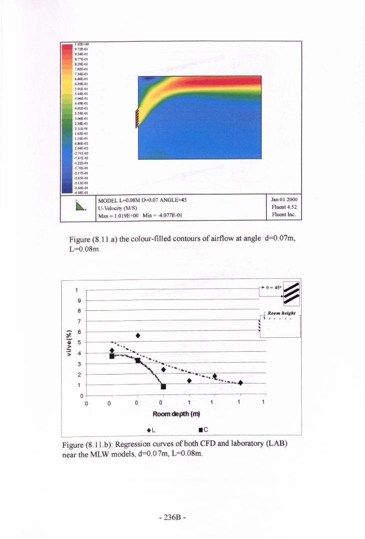
MODEL L=O.08M 0=0.07 ANGLE=45U- Velocity (MIS)Max = 1.019E+OO Min = 4.077E-OI
Jan 012000
Fluent 4.52Fluent Inc.
1.02E+009.72E.QI9.24E.QI&.71E.QI&.29E.QI7.81E.QI734E.QI6.86E.QI639E.QIS9IE.QIS.44E.QI
Figure (S.1l.a) the colour-filled contours of airflow at angle d=O.07m,L=O.08m.
1 I-'·"·~9
8'---
7 0.-. 6~ •~Gl 5 ..> • .\::: 4
...> "-'~~•.''''
3 '." '.• ....
2....
\. ... ~. ..... ...1
.._•
00 0 0 0 1 1 1 1
Room depth (m)
+L .cFigure (S.ll.b): Regression curves of both CFD and laboratory (LAB)near the MLW models, d=O.07m, L=O.OSm.
- 236B-
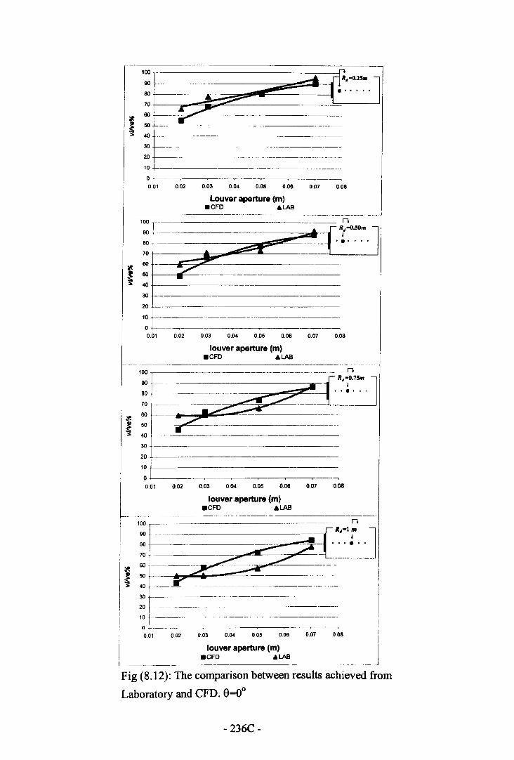
-
L._~~.~~_
Fig (8.12): The comparison between results achieved fromLaboratory and CFD. 9=00
+--------------~~-.-.--~.---~+---~-------~- --------------
0.05 0.06 0.07 0.08
Louver aperture (m).CFD .LAB
c--100
90
80
70 ....-~ 60 -..........~
50 -40
30 --20
nr RJ-G.50m -
II .•....I
10+--------------------o ---~--1-----~-~--~---~---~
0.02 0.03 0.04 0.05 0.060.01 0.07 0.08
louver aperture (m).CFD .LAB
-----------~~--------~---~--------.-.----lOO90
80
70
~ 60
~50
40
30
20
10
00.01
r--.--------------~.--.-----.- n
-- . m~~'r~. J..;z--C==:-
0.06 0.07 0.060.03 0.04 0.050.02
louver aperture (m).CFD .LAB
-~---------------~--.~--.----100 __ n
r RJ-I m90 ---~----------------.I Ieo ·----- ----c~-..,.!!!:-.~-II.....70~~~-----~~~-~ ~~~-~-----~
60 ~--50 ~~
40 f-~- _I"'_. . ~.. ~ _~~
II
II
: r===~--·--. -----~--------~-:::~~~10 L-.---·~- -----~
oL-.0.07 0.080.05 0.060.01 0.02 0.03 0.04
louver aperture (m).CFD .LAB
- 236C-
reasons, one of which was related to the laboratory. The hot-wire transducers were
carefully allocated in their appropriate positions; however, the change in flow was altered
in a scale of millimetres inside the box, and flow regime is so delicate that any minor
alteration in the positioning of the transducer would change the readings accordingly.
Although pre-set holes were made to exactly allocate the device it is agreed that this type
of errors are inevitable and hence always justifiable. Another reason thought of was the
neglect of louver friction. However, when this was activated the CFD results achieved
were very much similar. Also the CFD algorithms and numerical equations shared this
type of variations as they tended to simplify the complications occurring in actual flow
mechanism in the environment.
8.6.2. Louver depth
The sample of louver depths measured confirmed what was stated in the previous
chapters concerning the louver depth, i.e. L was found to be the least variable to form a
considerable drop in velocity. The three depths examined were L=0.04m, 0.06m and
0.08m, with a fixed aperture, i.e. d=0.03m, and it was found that the increase in this
variable would be less effective than other variables.
8.6.3. Louver inclination angle
The three louver inclinations examined included 0°, 30° and 45° and the results
plotted which were investigated were those above the MLW near the ceiling (Figures 8.1Oa
to 8.II.b. Results due to louver inclination were evidently taken with confidence, near the
MLW. Higher velocities however were found near the ceiling due to the wall jet effect
with the presence of steeper inclinations. The data were obtained at exact room height
along the room (Figure 7.1). In the laboratory, the wall jet effect was not investigated but
- 237-
the motivation of wall effect influenced by the ceiling height was discussed in some related
references such as (Awbi, 1991) and (Etheridge and Sandberg, 1996). Two variable
heights were examined, including the room chamber height under which laboratory
measurements were taken and ceiling height of 2m. While both results obtained were
comparable with what was observed with the physical measurements results within
Rd~0.75m any further measurements taken should acknowledge the fact of wall effect.
Within Rd~0.75m both measuring techniques were comparable with an acceptable margin
of error, up to 15%. Additionally, the error limit was even minimised when obtained at
horizontal louvers. As for further locations measured, the comparison was accompanied
with a higher error margin, 20% Table 8.3. However, this error percentage would be
acceptable showing that one could rely upon the results obtained from CFD near the
MLW.
8.6.4. Room depth
The increase in room depth was accompanied with an increase in error percentage
at horizontal and inclined louvers and variations between both techniques were examined.
However, the readings obtained at the first measured location indoor showed a positive
potential for the CFD technique. As shown in Figures 8.6 to 8.11, models examined were
comparable and within the acceptable margin of error, i.e less than 20%, with and without
the presence of a louver inclination. These harmonized results were stable and within the
acceptable margin of error up to RrO.75m or 1m either at the centre axis measured or
above MLW.
- 238-
8.6.5. Velocity profile through louver blades (vlve)
The schematic patterns of the two-dimensional flow distribution within louver
blades were plotted (see Appendix D.l) with an aim to study the effect of louver
inclinations in causing these patterns. While this was uneasily accomplished in the
laboratory measurements, simulation offers an alternative tool to deeply study these
profiles within blades. The comparison was limited to one louver configuration (d=0.07m
and L=0.08m) with three various inclinations, 0=0°, 30°, and 60°. It was understood that
the velocity profile would differ if other MLW configurations or wind speeds were
selected. However, the importance here was given to the general flow patterns occurring
because of the inclination of louvers as seen in Appendix D.I. Also, in the simulation
process the louver roughness was not specified, assuming smooth material with minimum
friction parentage similar to what was examined at the laboratory, i.e. smooth pinewood.
At 0=0°, the flow at centre axis along L dimension seemed to be increasing as
plotted deeper towards blades exiting side. The increment was nearly 5-10% more than
that recorded at v/ve%. On the contrary, a reduction of flow was found at adjacent cells
located underneath and above louvers. It ranged from nearly vyve=25% at the first
measured location along L up to vyve=55% near air exiting side. In other words, the flow
increased at the centre of d whilst decreasing near blade surface along L dimension.
Velocity profiles across both dimensions were obviously altered when referenced to
louver inclinations effect. As mentioned in earlier chapter, the tilting of louvers to 3011
degrees of inclination, for instance, caused loss of about 25% in velocity near blades due to
the MLW porosity, i.e v/ve=76%. Interestingly, this reduction which continued unchanged
at the centre axis of new aperture occurred due to inclination, say de: 30°; however, it
- 239-
decreased significantly when measured underneath louver blades, and increased above
them. The decrease of MLW configuration in hand reached up to 50% (approximately
vlve=lmls). This was the minimum cell recorded and developed proportionally across the
cells towards the surface of other louver. When air reached the cell measured at the other
surface of the blade vlve=105% it showed that the wall effect added to the jet effect had
altered the velocity profile within the louvers on both directions due to the noted
inclination.
At inclination fJ=60°, the significance in the velocity speed was also found at cells
above the louver blades. However, the increase compared to other measured cells was
considerable. For example, when the profile was measured at the middle of L0=60,
vlve=1.92m1s above louver blade and vlve=0.46m1s underneath. Meanwhile the cell
measured at centre axis showed vlve=l.lOmls showing that it was almost similar along
L0=60°. At air exiting side it was noticed that facts mentioned here for both above and
underneath louvers were altered.
In practice, the flow of air within louvers was very much influenced by the desired
degree of inclination. While horizontal inclination provides occupants with the direct flow
inside the living space, one could acknowledge the alteration of louver to maximize the
flow at certain regions within the room if direct air was not desired.
8.7. Airflow Patterns through MLW
8.7.1. The case models
The simulation at this stage covered the patterns of airflow within a room based on
louvers inclinations, wall inlet (windward) and outlet configurations. It is worth
- 240-
mentioning that CFD simulation is well established to represent velocity directions and
pattern of airflow across a room, as it is a valid alternative with the wind tunnel or smoke
testing techniques in case of full-scale measurements as stated by (Kindangen et al. 1997),
(Shaw, 1995), (Awbi, 1989) and others. The decision was then made to evaluate the
effectiveness of MLW to produce patterns of airflow within indoors. These were traced
with the influence of the five different combinations reviewed in Chapter 5 (section 5.2.3)
that are typically found in the reference study, i.e. Jeddah, Saudi Arabia. The number of
louvers in each combination varied accordingly. Figure 8.13 illustrates the five wall
combinations at windward side. While they were either plain or projected Rowshan
covering part or whole wall, they varied in louver numbers, wall configurations and
dimensions. The plain Rowshan has two different forms; (Inlet-I) and (Inlet-III) and the
projected Rowshan has three different forms; (Inlet-II), (Inlet-IV) and (Inlet-V).
Furthermore, the outlet dimensions and location to control the movement of airflow in a
room were also studied. Three various forms of outlets were considered, including a
typical door (Outlet-I) or a window positioned in two locations on the outlet side; (Outlet-
II) and (Outlet-III) with various dimensions.
The evaluation process of the flow patterns was made into three levels within the
room. These included ceiling, middle and ground zones and were added to the Rowshan
sitting zone when the projected Rowshans were examined (Inlet-Il; Inlet-IV and Inlet-V).
In Jeddah, it was mentioned that both middle and floor zones are considered the occupants'
living zones (AI-Lyaly, 1990). A two-dimensional physical domain was made and
previous procedures of setting up the model and physical domain were followed. The
variety of inlet and outlet configurations were studied under three various louver
inclinations; f)=00, 30° and 60°. The following discussion is based on the results shown in
Appendices D.2 to D.18.- 241 -
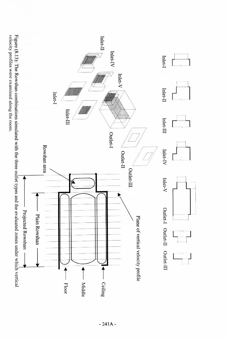
2:(l)......I..........
T__
o(l).....-~.
- 241A-
oS[I
~.....
~ t-,:j'7.....
J:="",,~_L,,_
tl• __ ,.1 ,_
-L'_ j---r-'-l
8.7.2. The flow patterns
8.7.2.1. Louver inclination (8)
The flow pattern was more effective at the middle zone with horizontal inclinations
and diversities of flow were shown in relation to the degree of inclination. The pattern and
maximum velocities at a particular location within the room were easily controlled by the
louver angle as the various inclinations involved in the solution had noticeably changed
results obtained. The most rigorous solution to enhance ventilation indoor in the occupied
living zone was observed at the inclination 8=0° as wind direction was not deflected or
altered, shaping the most preferable flow regime at the middle zone in both plain and
projected Rowshans. The Rowshan sitting zone was evenly ventilated, being next to the
louvers. This solution is ideal when the maximum ventilation or direct flow to the
occupant zone was desired. However, airflow at ceiling and floor showed the poorest
performances. This was corrected with the increase of louver numbers as found in inlet-l
and inlet-II, which enhanced the flow in the various zones. It also depends on proper
selection of louver aperture d. As discussed previously maximizing louver aperture would
minimize the percentage loss in the v/ve% and vice versa. However it is important to
consider that when higher wind speeds are present, direct flow in the occupied zone may
not be the optimum choice and may cause feeling of discomfort. It was noted by Evans
(1980), that when air exceeds certain speed indoors it becomes undesirable and leads to
occupants' discomfort. Thus the control of air could be through selecting the appropriate
louver aperture when the louver inclination is at {}= 0°.
The presence of louver inclination had directly altered the airflow pattern in the
room. When the louver inclination was set to 8=30°, the flow near the Rowshan was
maximized at ceiling and Rowshan area. Occupants' living zone was also ventilated near
- 242-
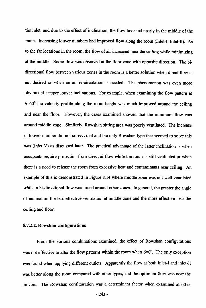
the inlet, and due to the effect of inclination, the flow lessened nearly in the middle of the
room. Increasing louver numbers had improved flow along the room (Inlet-I, Inlet-II). As
to the far locations in the room, the flow of air increased near the ceiling while minimizing
at the middle. Some flow was observed at the floor zone with opposite direction. The bi-
directional flow between various zones in the room is a better solution when direct flow is
not desired or when an air re-circulation is needed. The phenomenon was even more
obvious at steeper louver inclinations. For example, when examining the flow pattern at
(F60o the velocity profile along the room height was much improved around the ceiling
and near the floor. However, the cases examined showed that the minimum flow was
around middle zone. Similarly, Rowshan sitting area was poorly ventilated. The increase
in louver number did not correct that and the only Rowshan type that seemed to solve this
was (inlet-V) as discussed later. The practical advantage of the latter inclination is when
occupants require protection from direct airflow while the room is still ventilated or when
there is a need to release the room from excessive heat and contaminants near ceiling. An
example of this is demonstrated in Figure 8.14 where middle zone was not well ventilated
whilst a bi-directional flow was found around other zones. In general, the greater the angle
of inclination the less effective ventilation at middle zone and the more effective near the
ceiling and floor.
8.7.2.2. Rowshan configurations
From the various combinations examined, the effect of Rowshan configurations
was not effective to alter the flow patterns within the room when (FOo. The only exception
was found when applying different outlets. Apparently the flow at both inlet-I and inlet-II
was better along the room compared with other types, and the optimum flow was near the
louvers. The Rowshan configuration was a determinant factor when examined at other
- 243-
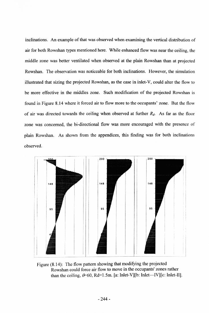
inclinations. An example of that was observed when examining the vertical distribution of
air for both Rowshan types mentioned here. While enhanced flow was near the ceiling, th
middle zone was better ventilated when observed at the plain Rowshan than at projected
Rowshan. The observation was noticeable for both inclinations. However, the simulati n
illustrated that sizing the projected Rowshan, as the case in inlet-V, could alter the flow to
be more effective in the middles zone. Such modification of the projected Rowshan is
found in Figure 8.14 where it forced air to flow more to the occupants' zone. But the flow
of air was directed towards the ceiling when observed at further Rd. As far as the flo r
zone was concerned, the bi-directional flow was more encouraged with the presen e f
plain Rowshan. As shown from the appendices, this finding was for both inclinations
observed.
Figure (8.14): The flow pattern showing that modifying the projectedRowshan could force air flow to move in the occupants' zones ratherthan the ceiling, 0=60, Rd=1.5m. [a: Inlet-V][h: Inlet-IV][c: Inlet-II].
- 244-
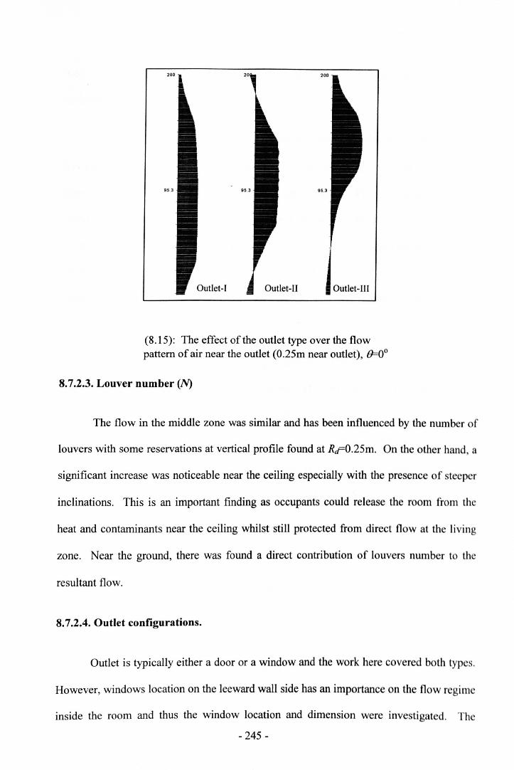
200
95.3
Outlet-II Outlet-Ill
(8.15): The effect of the outlet type over the flowpattern of air near the outlet (0.25m near outlet), 8=0°
8.7.2.3. Louver number (N)
The flow in the middle zone was similar and has been influenced by the number of
louvers with some reservations at vertical profile found at RrO.25m. On the other band, a
significant increase was noticeable near the ceiling especially with the presence of steeper
inclinations. This is an important finding as occupants could release the room from the
heat and contaminants near the ceiling whilst still protected from direct flow at the living
zone. Near the ground, there was found a direct contribution of louvers number to th
resultant flow.
8.7.2.4. Outlet configurations.
Outlet is typically either a door or a window and the work here covered both typ s.
However, windows location on the leeward wall side has an importance on the flow regim
inside the room and thus the window location and dimension were investigated. The
- 245-
location of the room outlet was made to stress the natural flow at the ceiling zones between
different spaces in the building.
When examined under horizontal inclination, no major influence of various outlets
was shown near the inlet, Le. at R« slm. On the contrary, at approximately O.2Smaway
from outlet the flow was very much shaped to outlet configuration. An example of this is
found with the vertical velocity profile near the three outlets (Figure 8.15). The similarity
dwindled when traced deeper, with some exception to the door. Additionally, the vertical
velocity profile for the inlet-Vat Rd>lm was driven near the ceiling due to the outlet
location with only minor bi-directional flow near the floor. Obviously the middle zone in
all outlet types was ventilated more than other zones.
Similarly, with the presence of steeper inclinations the flow was neither changed
near inlet nor changed in the middle of the room. The variation of flow regime found at
the ceiling level was minor and negligible. But the previous fact was shown in the
projected Rowshan (inlet-Il, inlet-IV and inlet-V). On the other hand, when the vertical
velocity profile was plotted for the plain Rowshan (inlet-I) the case changed. The flow
near ground was induced to create more bi-directional near floor in outlet-III than that
achieved from the door for example.
The valid conclusion derived from this in addition to what was mentioned earlier is
the following. As the incoming air follows the same wind direction, only the middle zone
would be well ventilated. An improvement to ventilate the flow near the ceiling could be
achieved by adjusting the outlet configuration, for example by locating the outlet near the
ceiling. The solution will in fact improve the flow at the ceiling location but with some
reduction of flow in the middle zone. The utilisation of louver inclination is of importance
for the designers to create various flow patterns in the room. For various louver apertures,- 246-
maximising the flow in a certain location within the room could be through the use of
louver inclination. The Rowshan configuration also played a main role in the flow pattern
inside the room. While plain Rowshan performed generally better than the projected
Rowshan, the simulation showed that the modification in the projected Rowshan (as in
inlet-V) could help direct the flow downwards towards the living space rather than the
ceiling. As far as the airflow near the floor was concerned, the simulation of flow patterns
had shown that tilting the louvers to steeper angles would be proportional to the percentage
of bi-directional flow near the ground whilst flow in the middle zone is minimised. This
provides an absolute solution for getting rid of the excessive heat and humidity near the
ceiling and provides breeze of flow near the ground level. This flow near the floor is even
much better when the outlet is controlled. The simulation has shown that using the-
window near the ceiling, as is typically used in Jeddah, is an optimum solution to improve
the flow near ground, which would improve the feeling of comfort in the room. Finally at
any positive inclination, the vertical flow profile was increasing as traced upwards.
8.8. Conclusions
Computational fluid dynamics has increasingly been used as a useful tool to
comprehend the complications existing in the real environment. Recently, more
researchers have relied on the results achieved by CFD packages, bearing in mind the
limitations and restrictions embedded into them. This chapter gave a brief description to
the historical background about the theory of numerical modelling and the basic equations
used by CFD. Then there followed the importance of CFD in airflow predictions within
buildings. In the process of evaluating the velocity results achieved from the laboratory,
models were constructed using CFD to compare results from both techniques.
- 247-
Additionally, the simulation covered the patterns of airflow within a room based on inlet
and outlet room configurations. The following points of conclusions are obtained:
1. CFD is a reliable tool to simulate the flow near the Modulated louvered windows at
the windward side, i.e. velocity drop due to porosity percentage (V/ve%). The
correction made to the INLET boundary conditions, by replacing the reference v,
with v/ve%, was a good alternative to assess velocity results across the MLW. The
technique has some validation in ventilation research and it reduced the model
complications as well as the computational timings that, in turn, resulted in more
accurate and comparable results.
2. CFD coding was a reliable tool to examine the velocity components in the room
near the MLW. However. CFD results measured away from the MLW were
accompanied with a level of error percentage higher than those obtained near the
MLW. The errors were referred to a number of points discussed earlier in this
chapter. Nevertheless within the scope of this study CFD results are acceptable
since the error was less than 20% at the farthest measuring location, i.e. RtF I.Sm.
3. The simulation of vertical velocity profile within the room was the technique used
to evaluate the patterns along both room dimensions and some conclusions were
derived from the evaluation:
• The presence of steeper louver inclinations angles induced a bi-directional
flow within the room unlike the horizontal inclination. The latter
inclination however is the optimum when direct ventilation at occupants
living zone is desired.
• The outlet type applied controls the flow behaviour and percentage of bi-
directional flow.
- 248-

• The plain Rowshan is generally a better choice than the projected Rowshan.
Yet the flow in the living zone could be obtained be correctly sizing the
projected Rowshan.
- 249-
8.9. References
1. AI-Lyaly, S.M. (1990) The traditional house of Jeddah: A study of the interaction
between climate, form, and living patterns. University of Edinburgh. Unpublished Ph.D
thesis.
2. Alamdari, F. (1995) "Modelling airflow in buildings by computational fluid dynamics".
Building Services Engineering Research and Technology 16-(4), p.B44-B49
3. Anon. (1995a) Relationships for smoke control in atria. Technical Memoranda TMl9,
London: Chattered Institution of Building Engineers.
4. Anon. (1995b) "Simulation models: Towers of Babel or the promised land?". Building
services (January)-p.23-25.
5. Anon. (I995c) "Testing time". Building services (January)-p.26-28.
6. Awbi, H.B. (1989) "Application of computational fluid dynamics in room ventilation".
Building and Environment 24-(1), p.73-84.
7. Awbi, H.B. (1991) Ventilation of Buildings, London: E & FN Spon.
8. Aynsley, R. M. (1999) "Unresolved issues in natural ventilation for thermal comfort ".
p.36-44, Darlington, NSW, Australia: proceedings of Hybvent Forum '99.
9. Chen, Q. and Jiang, Z. (1995) "Significant questions in predicting room air motion". 9-
(1). p.929-939, ASHRAE Transactions.
10. Chow, W.K. (1995) "Ventilation design: Use of computational fluid dynamics as a study
tool ". Building Services Engineering Research and Technology 16-(2), p.63-76.
11. Chow, W. K. and Lau, K. W. (1993) "Field tests on atrium smoke control systems".
p.461-469, USA: ASHRAE Transactions.- 250-
12. Chul, C.Y. (1997) Experimental, theoretical and computational modelling of airflow to
investigate the thermalhydraulic performance and ventilation efficiency in a clean room.
Bristol. Unpublished Ph.D. thesis.
13. Chung, I.-P. and Dunn-Rankin, D. (1998) "Using numerical simulation to predict
ventilation efficiency in a model room". Energy and buildings (28)-p.43-50.
14. Dascalaki, E., Santamouris, M., Argiriou, A., Helmis, C., Asimakopoulos, D.N.,
Papadopoulos, K. and Soilemes, A. (1996) "On the combination of air velocity and flow
measurements in single sided natural ventilation configuration.". Energy and
buildings24, p.155-165.
15. Etheridge, D. and Sandberg, M. (1996) Building Ventilation: Theory and Measurements,
John Willy & Sons. London
16. Evans, M. (1980) Housing, Climate, and Comjort, London: Architectural press.
17. FLINT. FLINT (2000) version 4.1. Unpublished software.
18. FLUENT. FLUENT (1999) version 4.51. New Hampshire, USA: Fluent Inc.
19. Fontiane,1. R., Rapp, R., Serieys, 1. C., and Aubertin, G. (1994) "Aerosol transport in
room turbulent air flow- experimental and numerical flows". Carcow, Poland:
Proceedings of Roomvent '94.
20. Gan, G. (1995) "Evaluation of room air distribution systems using computational fluid
dynamics". Energy and buildings (23)-p.83-93.
21. Holmberg, Y.L., Paprocki, A. and Tang, Y.-Q. (1993) "Simulation of room flows with
small ventilation openings by a local grid-refinement technique". Building Services
Engineering Research and Technology 15-(1), p.I-iO.
- 251 -
22. Jones, P.J. and Whittle, G.E. (1992) "Computational Fluid Dynamics for building asr
flow prediction-Current status and capabilities". Building and EnvironmenI27-(3),
p.321-338.
23. Kindangen, J., Krauss, G. and Depecker, P. (1997) "Effect of roof shape on wind-
induced air motion inside buildings". Building and EnvironmenI32-(1), p.l-Ll ,
24. Maghrabi, A. and Sharples, S. (2000) "Significant limitations in applying
Computational Fluid Dynamics (CFD) to predict room air distribution" .(To be
published).
25. Murakami, S., Kato, S., Deguchi, K., Takahashi, T., Makimura, I., and Kondo, Y (1995)
"Natural ventilation of a large-scale wholesale market building". p.44-55, USA:
ASHRAE Trans.
26. Neilsen, P.V. (1992) "Description of supply openings in numerical models for room air
distribution". ASHRAE Transactions 9-(4), p.963-97I.
27. Robinson, D., Cook, M. J., Lomas, K., and Bowman, N. T. (1999) "The design and
control of buildings with passive downdrought evaporative cooling". (1), p.453-458,
Brisbane, Australia: PLEA99.
28. Ruyssevelt, P., Stankovi, S., Wilson, A., Lomas, K., Bloomfield, D. and Gouph, M.
(1995) "Simulation modelling: Lessons for the future". Building services (Jaouary)-
p.31-36.
29. Said, M. N. A., Shaw, C. Y., Zhang, J. S., and Christianson, L. L. (1995) "Computation
of room air distribution". p.l065-I077, Chicago, USA: proceedings of ASHRAE
Centennial Conference.
30. Schaub, E. G., Kelso, R. M., and Baker, A. 1. (1995) "Comparing the continuity-
constraint algorithm results with a full-scale laboratory test". (2), p.1 041-1 053, USA:
ASHRAE Transactions.
- 252-
31. Sharples, S and Maghrabi, Amjed (2000) "Airflow through louvers: an experimental and
CFD study". The Hague: Proc. 21st. AIVC Conference (To be published).
32. Shaw, M. (1995) "Computer modelling as a design tool for predicting building
performance: Part 1". Building Services Engineering Research and Technology 16-(4),
p.B41-B41
33. Swainson, M.J. (1997) Evaluation of the potential of solar chimneys to derive natural
ventilation in non domestic buildings. Cranfield. Unpublished Ph.D. thesis.
34. Weathers, J. W. and Spitler, J. D. (1998) "A comparative study of room airflow:
Numerical prediction using computational fluid dynamics and full-scale experimental
measurements". p.144-157, USA: ASHRAE Trans.
35. Williams, P. T. and Baker, A. J. (1994) "CFD Characterization of natural convection in a
two-cell enclosure with a "Door"". (3), p.685-696, USA: ASHRAE Trans.
36. Yaghoubi, M., Knappmiller, K. and Kirkpatrick, A. (1995) "Three-dimensional
numerical simulation of air contamination dispersal in a room". ASH RAE Transactions
(1)-p.1 031-1 040.
37. Yang, Z. (1989) Numerical simulation of incompressible and compressible flow.
University of Sheffield. Unpublished Ph.D.
- 253 -

CHAPTER 9: CONCLUSIONS AND FURTHER
RECOMMENDATIONS
9.1. Aims of the research
The research assessed the potential of the modulated louvered windows to
provide ventilation as a cooling source to achieve thermal comfort inside the ,
buildings. A number of aims and objectives were established and investigated.
throughout the chapters of this thesis. The main aim was to encourage the use of .
natural ventilation techniques by reviewing the methods of controlling natural
ventilation to address the main architectural element that enhanced cross ventilation
within the traditional house in Jeddah. Another aim was to present technical analysis
of the potentials of the MLW in order to achieve the central aim of this thesis, i.e. to
present designers with practical information concerning the airflow characteristics
across this type of window accessories.
9.2. Summary of results
Dealing with the MLW geometries to achieve the acceptable air velocity
indoors is quite complex. The review, analysis and discussion carried out in the
earlier chapters are recalled and summarised here.
From the literature review it was noticeable that a number of strategies were
considered in Jeddah on both microclimate and macroclimate scales (section 2.5).
Within the microclimate scale, the MLW found in the Rowshan or any other aperture
component is believed to be the main solution to control the breezes.
The review also showed that varieties of mathematical models related to
airflow characteristics within buildings are treated with some simplicity and
assumptions whose validity, for most of them, is based on a complete, open aperture.
- 254-
When any treatment is involved, such as the reviewed MLW, their appropriateness
becomes questionable; hence the need for direct measurements was recommended by
a number of investigations more reliable than the theoretical models.
Dealing with the pressure and velocity drops as the main functions to control
the indoor airflow characteristics was a sound choice since the temperature was
found, by other research, to be less effective in controlling air movement indoors with
the presence of even a slight breeze. The pressure characteristics between inner and
outer volumes showed that the enhancements in pressure drops could, at certain point,
be a function to some variables involved in this analysis. The adjustment of louvers
to steeper blade inclination as well as the reduction of aperture and free area are main
causes of poor ventilation inside the room. The considerable pressure drop could not
be achieved except when reaching ±60° of louver inclination, the critical angle of the
MLW under which major airflow reduction was found (section 6.5.3). Similarly, the
control of velocity drop across the MLW was more related to the aforementioned
variables. The louver angle of inclination was found to be a main variable to control
this, while louver depth was the least affecting variable in this phenomenon, except
with the presence of steeper louver inclination.
Interestingly, the major indoor velocity and pressure drop was not due to
individual variables but rather to a combination of variables that would
comprehensively describe AP and v/ve% as concluded from the evaluation stages
conducted in sections 6.5.3 and 7.4.6.
Wind direction has also some significance on indoor air velocity smce
normally a 20% reduction in v/ve% near the window was found when wind was to
- 255-
deviate 30" from perpendicular (see section 7.4.2). In addition, the vertical and the
horizontal velocity profiles, along the room height and depth respectively, are much
related to the MLW configurations examined as shown in sections 7.4.3.1 and 7.4.3.2.
As far the room depth was concerned, it was possible to establish a dimensionless
relationship of velocity characteristics as function to various MLW parameters
involved near the window, RtPlm (see section 7.4.1 and Figure 7.6).
The reduction in air velocity near the windward side of the MLW, expressed
as the porosity percentage (v/ve%), was a sound alternative to evaluate the
performance of MLW as it gave an understanding of the flow characteristics at the
windward side near the modulated louvered windows (section 7.4.4.).
The CFD appraisal stage conducted in Chapter 8 examined the viability of
CFD coding to simulate airflow around the MLW and established the schematic
airflow patterns based on MLW and Rowshan configurations as well as outlet
configurations that are typically found in Jeddah. With or without the presence of
inclination angles, CFD had successfully represented results obtained from laboratory
near louvers inside the room, i.e. R~lm (section 8.6.1.1). However, CFD data
obtained far from the MLW could only be accepted with some reservations. On the
other hand, results of the schematic airflow patterns were as follow:
• The presence of steeper louver inclination angles induced a bi-
directional flow within the room unlike the horizontal inclination. The
latter inclination however is the optimum when direct ventilation at
occupants living zone was desired as discussed in section 8.7.2.1.
- 256-
• Both types of Rowshans, the plain and the projected, showed good
performances to the airflow patterns inside the room. Nevertheless, the
bi-directional flow was with the presence of the plain Rowshan
generally better than the projected type. Within the context of the
projected Rowshan, the flow pattern enhanced with the presence of
split units Rowshan, particularly with steeper louver inclinations, as
the airflow pattern was directed towards living zone rather than the
ceiling (section 8.7.2.2).
9.3. Design guidelines
One of the main aims of this research was to provide designers and architects
with practical information concerning the airflow characteristics across this type of
window accessory. A number of design guidelines are noted here.
• This window accessory has a high degree of design flexibility where a
number of MLW geometries could be proposed to offer similar
ventilation performances. This on the other hand would assist
designers and architects to propose a number of MLW configurations
to optimise their window treatments.
• Optimum ventilation performance inside the room is achieved when
horizontal inclinations of louvers are employed.
• Inclination {P-60° was accompanied with poor ventilation performance
inside the room, and thus is considered the critical MLW geometry that
should be avoided. However, when this inclination is necessarily
- 257-
employed, larger dimensions of louver apertures are then
recommended, i.e. d/L= 1.
• Steeper louver inclinations, 8>30°,will lessen ventilation performance
in the living zone whilst improve it near the ceiling. In addition,
airflow near the ground level is improved at those inclinations when
properly sizing the outlet.
• The variation in louver depths of an MLW has no considerable effect
on the ventilation performance inside the room.
• Room depth has a considerable effect on the reduction of air velocity
inside the room.
• The plain Rowshan showed was generally a better performance than
the projected Rowshan. In addition, sizing the projected Rowshan
from top will enhance airflow in the living zone.
• Smaller outlets are recommended when bi-directional flow between
various heights inside the room is required.
9.4. Conclusions
This thesis has investigated the airflow characteristics of the modulated
louvered windows (MLW) with reference to the Rowshan of Jeddah, Saudi Arabia.
The results obtained from the study can be implemented in other settlements in any
part of the world. Throughout the various stages of the research, a number of
conclusions were derived that answered the aims and objectives of the research.
- 258-
1. From the literature review, the MLW was the most important element and played
the major role in the provision and control of natural ventilation in the traditional
architecture of Jeddah, Saudi Arabia.
2. The adjustment of louvers to steeper blade inclination as well as the reduction of
aperture and free area are the main causes of poor ventilation indoors. On the
other hand, the depth of louver blades does not have the same significance and is
the least important variable. Nevertheless, the major pressure and velocity drops
are not due to individual variables but rather to a combination of variables that
would comprehensively describe !:J.P and v/ve% across the reviewed MLW.
3. Airflow velocities in a room containing an MLW result from an interaction of
louver geometry, room geometry and prevailing wind conditions.
4. The ventilation performance of the plain Rowshan was generally better than the
projected Rowshan. Yet the flow in the living zone could be enhanced by
correctly sizing the projected Rowshan.
5. The quadratic model equation produced better curves fits to the data compared to
those produced by power law regressions. The quadratic curve was in the form of
I1P = AQ + BQ2. However, further adjustments of the theoretical representations
of equation in the quadratic form would be required to fit other variables such as
number of louvers and their inclination angles.
6. CFD coding was a reliable tool to examine the velocity components in the room
near the MLW. But it was less successful in predicting air velocities towards the
rear of the room at some distance from the louver opening Nevertheless within the
scope of this study CFD results are acceptable since the error was less than 20% at
the farthest measuring location.
- 259-

9.5. Further recommendations
1. The design of the modulated louvered windows must give a consideration to
the variables as they play an important role in altering airflow characteristics
inside the room.
2. There is no consideration allowed to the frictional factor and the roughness of
the louver blades. Also, there is no barrier or medium, such as a mosquito
screen or a glass, which may affect the ventilation performance across the
reviewed MLW. Therefore, more research is needed to include such factors in
the investigation of the MLW and Rowshan performances.
3. Further research could be conducted to investigate the effect of obstacles
either inside the Rowshan in the room (such as furniture or human bodies) or
around the building on the windward side (such as wing-walls or plants).
These issues fall beyond the scope of the current thesis, and thus further
research is needed.
4. Further work comparing the laboratory and CFD results with measurements in
real rooms is needed.
5. Due to the limitations of the number and characteristics of the Rowshan
structure covered in the thesis, investigations are recommended to cover cases
of more complex forms of the Rowshan. This also may include the airflow
through the sides of the projected Rowshan under various prevailing wind
conditions.
6. Further adjustments of the theoretical representations of the equation in the
quadratic form are required to fit other variables such as number of louvers
and their inclination angles as noted previously.
- 260-
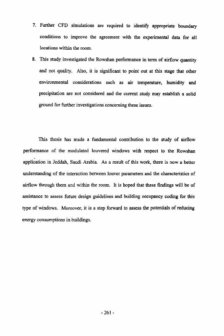
7. Further CFD simulations are required to identify appropriate boundary
conditions to improve the agreement with the experimental data for all
locations within the room.
8. This study investigated the Rowshan performance in term of airflow quantity
and not quality. Also, it is significant to point out at this stage that other
environmental considerations such as air temperature, humidity and
precipitation are not considered and the current study may establish a solid
ground for further investigations concerning these issues.
This thesis has made a fundamental contribution to the study of airflow
performance of the modulated louvered windows with respect to the Rowshan.
application in Jeddah, Saudi Arabia. As a result of this work, there is now a better
understanding of the interaction between louver parameters and the characteristics of
airflow through them and within the room. It is hoped that these findings will be of
assistance to assess future design guidelines and building occupancy coding for this
type of windows. Moreover, it is a step forward to assess the potentials of reducing
energy consumptions in buildings.
- 261 -

Appendix A: Natural ventilation in Architecture
Page:263
Page:264Page:264Page:265Page:265Page:266
Page:267Page:267
Appendix (A. I): The flow regimes and pressure fields around a streamed-lines and abluff body.Appendix (A.2): The four regions of the free jet air.Appendix (A.3): The two regions of the wall jet effect.Appendix (A.4): The velocity profiles of various types of terrain.Appendix (A.5): The characteristics of terrain roughness.Appendix (A.6): The effect of the eaves (horizontal projection) and the wing-walls(vertical projections) on indoor air velocity.Appendix (A.7.a): The various roof configurations examined.Appendix (A.7.b): Indoor air velocity as a function to various roof shapes measured ata height of 1.35m and along the centre section. The wind inclinations are (a=Oo),(b=Juo), (c=450), (d=600), (e=90o).
- 262-
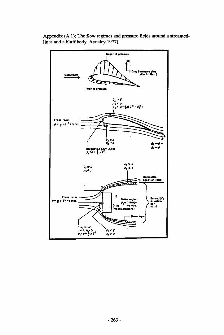
Appendix (A. I ): The flow regimes and pressure fields around a streamed-lines and a bluff body. Aynsley 1977)
Free,tream
¥,t.4 Dra, (prtllUre piu,
'kin friction I
Po.iti". pre.ure
ii3 > iiPs< PPs = p+ip(81! -811
1/z< 8Pz>P
Stqnatian point it: 0ptop +i pi/I!
Fr.estream ---p+ t P i2 =const. --==' Bernoulli',
equationnatvalid
- 263-
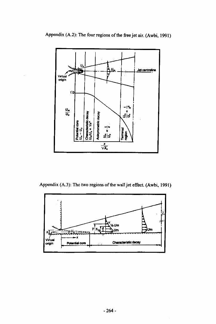
Appendix (A.2): The four regions of the free jet air. (Awbi, 1991)
Appendix (A.3): The two regions of the wall jet effect. (Awbi, 1991)
Virtualorigin
- 264-
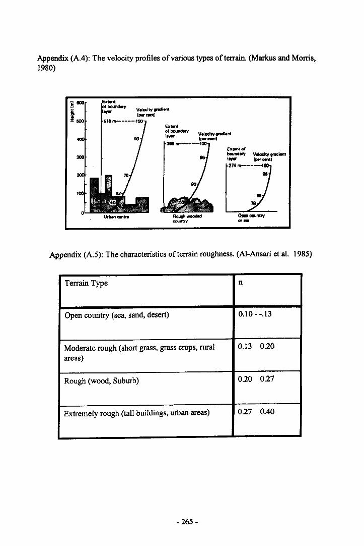
Appendix (A.4): The velocity profiles of various types of terrain. (Markus and Morris,1980)
exlMltofboundwy Vtlooity pllntII¥« (PI!' OIIItl274m------·100
81
()pin coumry« ...Urbln centnt Routh woodId
country
Appendix (A.S): The characteristics of terrain roughness. (AI-Ansari et al. 1985)
Terrain Type n
Open country (sea, sand, desert) 0.10--.13
Moderate rough (short grass, grass crops, rural 0.13 0.20areas)
Rough (wood, Suburb) 0.20 0.27
Extremely rough (tall buildings, urban areas) 0.27 0.40
- 265-
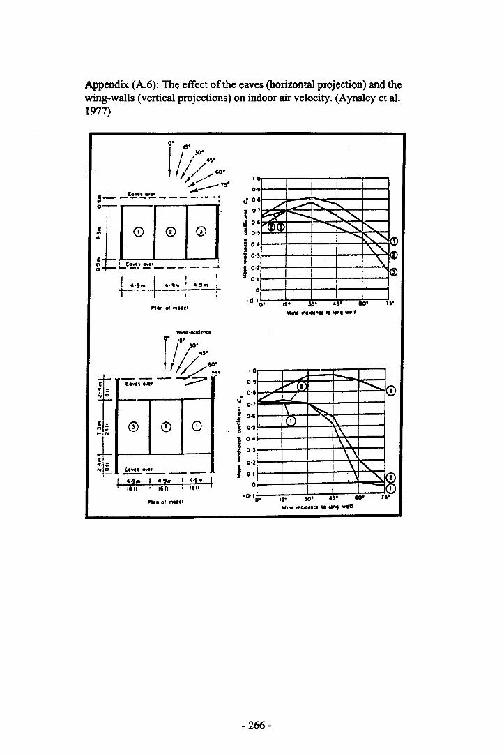
Appendix (A.6): The effect of the eaves (horizontal projection) and thewing-walls (vertical projections) on indoor air velocity. (Aynsley et al.1977)
~ .~.1///:·..·
~..../ 7!·..A---I-'- t-E!!I!..~__ - _'_ -'.. ! I I0--
ji
lL'...
:. I Eov., OWl'o t-- _.
1 I ! '. ,.,... 4·,,,,' ,.,... :-t-- .._.•..------;-I , I ;
0 CD 6)
,
1"'. " ",.del
itI'1-... -..I":'i:~
0,,7 ./ .,....., i'..--"~,~ -- .......~"s 'Q)Q) ...........~-'~
...........~,I ,,"-l, '\.,- :• . •
e-~oi e-~ 0§ e-! 04t1 e-J 0·'
0·,
o·0 '0.
IS. ~ '. 10w.,., ,ftc,*ftC, 111
71
---...;..,..-~(0•• ' over
CD ® 0
£Olt" oye,-----4"'" I 4·,,,, ! Hili.," . .". "1"
I'... of 1IIOIIt'
.0090·' ....V (2 ............... (!)
~ ./
'"o ":\\\\\\\\ 1"-.. , ~ro
" -I~. . .':"
•U 0.7ii 0·6
1 0·'
I 04... O·l
I 0.2
j O.o
'5· SO· 45 60w,•• I.c,d,.et ., "., .111
- 266-
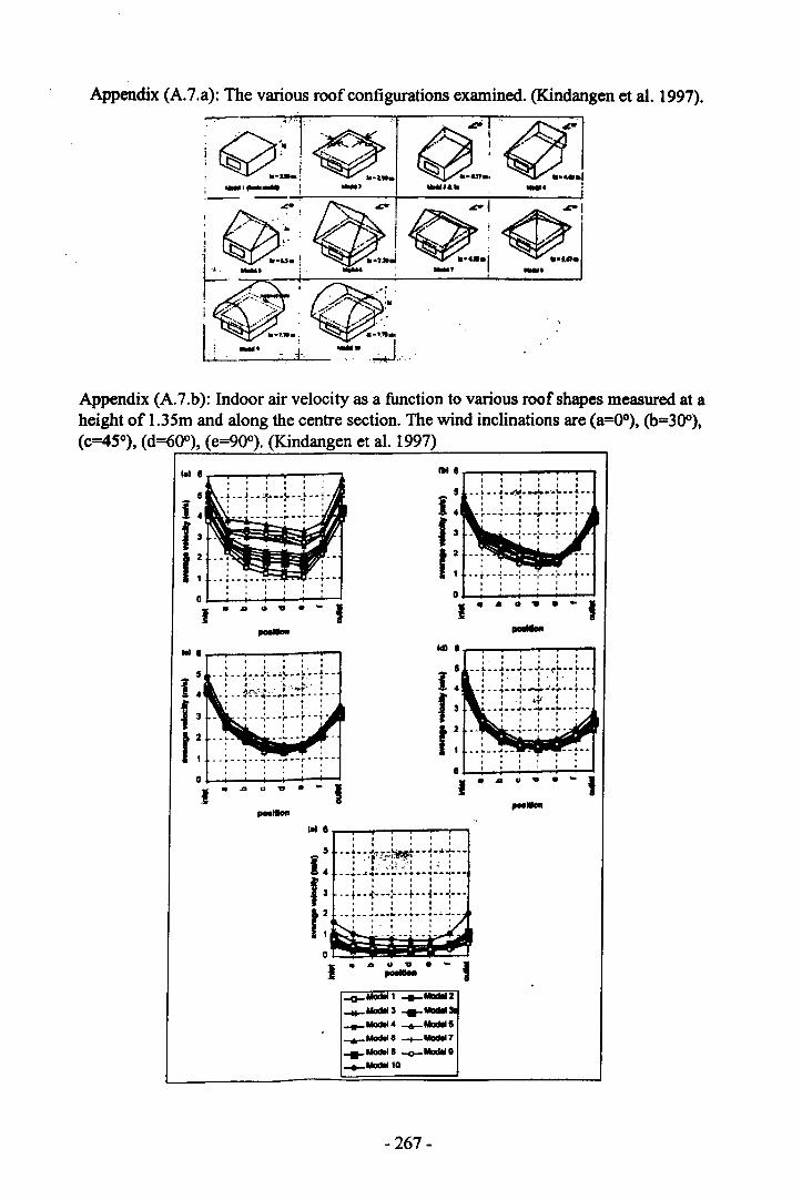
Appendix (A.7.a): The various roof configurations examined. (Kindangen et al. 1997).
~~~"~;~-__"".-/...,.-X~l'.A--,-----.,.,~·, ~---l ~&_ ~u •• : ~_.I
.. 4 :
Appendix (A.7.b): Indoor air velocity as a function to various roof shapes measured at aheight of 1.35m and along the centre section. The wind inclinations are (a=OO),(b=300),(c=45°). (d=600), (e=900). (Kindangen et al. 1997)
1M • _ ...... _ ..... _- __ ..,I I I • I I, • I I I •
........ -"."".., ...... -'-~., .. &._-• I " I I II I I • t •I I , I I •
.. r" -., .. -1 ..--r,·-~·..9'-I It' • ,
I I I I
_ 5
I.f 3
r : ....r ....-i ..... -; ... -,- .... :- .... t ...., , ,, , ,O~+- __~~ ~o ow ... II··I · .a
.. ..l1li • r--_"""'__''''---'..,._--~-.--...........-,
I I • I I •
I , I I ' .•
-~r::~~:tJ;;EJ:t , , I
" t • '-~--~---~--}--~-,
, , ,, , ,--~--1-·~··~-·~~··~··• I I I •. I• • I .,' ,
.. r » » ~--1'·~"·~·-""'": : : ,l": :....... --~..---......... -• , I I •• I I I·
.... ~.... ~.... .., .... -"" .... ,. ..... ~...., , ,, , ,
........-- !III • r- .........,..__,........-_..,....,I , I I I II .. I , I I--!:~r~~1rr:--rtr-
- ~~.. - ~-- -• " I I • ,
1 I I I I I
-- f--{---:-- -r-- ~---:---• I • • I I
I I I I
I·";"':'·~I~ModeIl __ ModI! Z__ ModeI3 ...... ModI!__ Model. __ MadII5__ ModoIII __ ModoI7
...... Model 8 -0- MadIll__ ModoIl0
- 267-
Page:269
Appendix B: Pressure drop across the modulated louvered windows.
Page:270
Page: 271
Page:271
Page: 272
Page:272
Page:273
Page:274Page:274Page:275Page:275Page:276Page:277Page:278Page:278Page:279Page:279Page:280
Appendix (B. I): The conversion of the data-logger results into pressure drops (OP) atboth high and low pressure limits.Appendix (B.2): The coefficient of determinations (r2) with the standard errors of allMLW examined with both model equations.Appendix (B.3.a): Measured values of volume flow (Q_as) compared to calculatedvalues (Qca/c) identified from the Eq.(6.5) for MLW L=O.06m and d=O.02mAppendix (B.3.b): Measured values of volume flow (Qmeas) compared to calculatedvalues (Qca/c) identified from the Eq.(6.5) for MLW L=0.06m and d=O.035mAppendix (B.3.c): Measured values of volume flow (Qmeas) compared to calculatedvalues (Qca/c) identified from the Eq.(6.5) for MLW L=0.06m and d=O.05mAppendix (B.4): Measured values of volume flow (QmeD.l") compared to calculatedvalues (Qca/c) identified from the Eq.(6.5)Appendix (B.5): Differential Pressures as function of various dlL ratios. [a: dlL=0.5,b:dlL= 0.75 and c: dlL=I]Appendix (B.6.a): The statistical analysis of the louver inclination effectAppendix (B.6.b): The statistical analysis of the louver aperture effectAppendix (B.6.c): The statistical analysis of the louver depth effectAppendix (B.6.d): The statistical analysis of the louver number effectAppendix (B.6.e): The statistical analysis of the louver free area effectAppendix (B.7): The statistical analysis of the integration of overall variables.Appendix (B.8.a): The statistical analysis of the louver depth at 8=60
0
Appendix (B.8.b): The statistical analysis of the louver aperture at 8=600
Appendix (B.8.c): The statistical analysis of the louver free area at 8=600
Appendix (B.8.d): The statistical analysis of the louver number at tJ=60°Appendix (B.9): The statistical analysis of integration of the overall variables at 8=600
- 268-
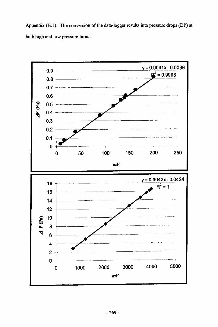
Appendix (B. I): The conversion of the data-logger results into pressure drops (DP) at
both high and low pressure limits.
y= 0.0041x- 0.0_0392 = 0.99930.9
0.80.70.6- 0.5
~
~0.40.30.20.1o -
0 50 100 150 200mV
18l16
!
14 -12 +-----------::;;,_.-----------
~ 10=-- 8"" 6 +---------:;ot'---- ------
I
-----~------------_--------
---,--------,------,------------ ---- - -,
o 1000 2000 3000 4000 5000mV
- 269-
250
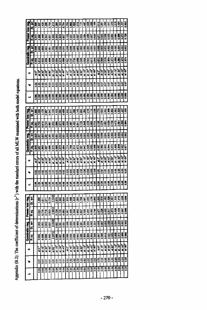
II51 a~ ~~ ~~ Sl~ ~.I~ ~t; ~~ z ~ ~~~a> ~~ ~~- .... ~ - ~ ~~ -1ft "'0 <'!~
tiS": - - _0 - - ~o - - - - - - - - ~ ...: - - ~~ - - _0
IIi~ ~~ ~~ §Ii §i ~~ ~~ Ii :s~ a~~!~i i~.~II::~ ~~ Iii..,00 00 00 00 00 00 00 00 od od 00 00 00
i51 !!"I- NN "1- a~ 88 88 §§ 8 I §§ ijij88 ijij~~ :!I:!I :!la
tiSci 00 00 00 00 00 00 00 00 00 00 00
s§ ;;i II!i ~I ~~ !!a>~ i; !§I;i~ li ~~~"": 1.II::ci cici 00 00 00 00 00 00 00 od 00 00 00
'b'lo ~~ o '10 ~'Io ~ 1:,~ ~~ ~~ ~~ ~ 'b'lo ~~ ~~ ~~~Cl> lii :i! , ."t .1;•• •• 1i1i • cali iiii .ii .11 'iii 'iii1ii 'iii1ii 1ii1i1ii
"Q ~~ sa S~ "''''''' a~ ~~ :!l:!l :!l~:!l ~~ ~~ ~~~ ... ~
000 00 ~~:00 00 00 000 00 00 00 000 00 00
... ii i ii i i ii ~~ ii ~~ ~~ i ii !!ii iii00 0 00 0 0 00 00 00 00 0.0 0 00 00 000
It ~~ ~~ i~ ~~ ~!~~ S~ "IN ~~ I~ 99 ~~ ~~ 9~~.-: 8:';: ~.-:
J tiS": ...:~ ci ci ":0 - - 0"':' - - - - -0
It~ "8 ... '" ~~ 15 ~ ~ iii-~~!!§~ lila> -,;: ~I!! i~ i-.ta~ cc!"-: ;..., .. r;; ~"l "":'l1li:II:: cio 00 00 ci .0 o 0 00 00 cio 00 00 00 00 0
t ~ 88 "1_ _"I _ "I- 1ft ~§ ijij ...... "IN 81 i§ ij§ 88 ~:!I:!I ~~ :!I :!I 88 ~~ :!I:!I
ItiS 00 00 00 o 0 00 00 00 dei 00 00 00
Ii Ift~ Ii IE :I!~ i ~::"I - ~!iil ~I !ids ii ~,;: !~..~~ G! G! ....... ~~ 1... ~G! Ii;II:: 00 00 o ci 00 o 0 00 00 00 00 00 00 00 00 0
'b'lo ~~ i!?o '10 ~~'b~ ~~ i~~!? ~ 'b'lo ~~ ~~ ~~~Cl> ~"tiii•• Cia; ••• 161i 1I'iii Cl. cs. 1i .1; .1i lit. 1ii1i
~a N N N N aaa ~~ lIIlII lIIlII lIIalll ~~ :!;l~ :!l:!l :!l:!l:!l"Q c!c! 00 C!C! C!q q .C!
00 00 cid 000 00 00 00 000 00 00 00 000
... ~ ~~ 88 88 :!!~ :!!~ :!!:!! ~~ 88 ~ ~~ 88 !!!! !!!!~0 00 00 00 00 00 00 00 00 0 00 00 00 000
t~ co
~§ - .SI!! i~ ~~ 1!3'" .- 8~ i § CON !II" $!~ ~IoJ::: .... ~~ ~:g ~~ :::!! :!:J CiS ..: 0 00 cio e- -
0"':' - - o ..: - -J
N
51 .....~~ ~~ ~!...... !i ~~
_N SJ::: ~~~.,
~~ ~I~;:: ~~ ~:ll - ..."! .... I'o:~ .qcqII:: od ci d 00 00 00 00 00 00 o 0 00 00 00 00
~cot 88 N _ 8- 8g 88 88 88 88 e- 1ft 88 88 !!88:!I a .8 a a
ItiS 00 00 00 00 00 cid 00 cici o 0 00 cia 00
N
51 II ii .... :8 ... 3l "':Il ",N IIIi Ii ~;iiiiIi II.~ ... 9l"! is .. 131II:: 00 00 00 00 00 00 00 00 00 00 00 cio 00
• '10 ~~o '10
~It) 'btn ~~ o '10 1i!to r-~ • to ~~ ~~ ~~~Cl> 0_ li!, ."t
10 ~:i!oo; ."t 0_
1i. ti ti ti • •• •• ••- - ii -. _'iii'iii 'iii 1ii'iiili.. ..
s c; C;o - - ;;c; NN "IN NN NNN sa .,,,, ss ~~~b 00 00 00 ~C! ~C!q C!C!
00 00 00 ci ci 00 00 00 000 00 00 00 000
~~ ~ ~ c;c; c;c; c; c; ~~ ~~ ~~ ~ ~ ~~ ~~ ~~ ~~00 00 oei 00 00 00 00 00 o 0 00 00 00 00
....
- 270-
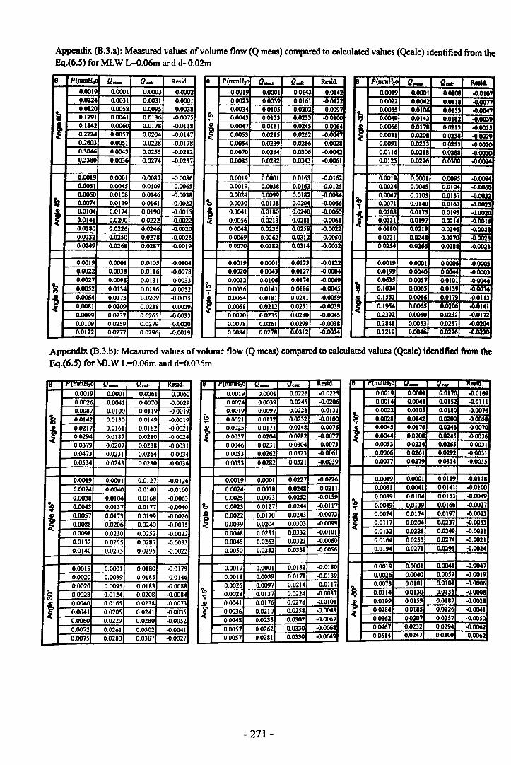
Appendix (B.3.a): Measured values of volume flow (Q meas) compared to calculated values (Qcalc) identified from theEq.(6.S) for MLW L=O.06m and d=O.02m
18 P(DmIH~ Q- Q- Resid.0.0019 0.0001 0.0003 .().00020.0224 0.0031 0.0031 0.00010.0120 0.0058 0.0095 .().0038
k 0.1291 0.0061 0.0136 .().0075
t 0.1142 0.0060 0.0178 .().01180.2224 0.0057 0.0204 .().01470.2603 0.0051 0.0228 .().01780.3046 0.0043 0.0255 .().02120.33SO 0.0036 0.0274 .().0237
0.0019 0.0001 0.0087 .().00860.0031 0.0045 0.0109 .().00650.0060 0.0108 0.0146 .().0038, 0.0074 0.0139 0.0161 .().0022
t 0.0104 0.0174 0.0190 .().00150.0146 0.0200 0.0222 .().0022O.OISO 0.0226 0.0246 .().00200.0232 0.0250 0.0278 .().00280.0249 0.0268 0.0287 .().0019
0.0019 0.0001 O.OIOS .().01040.0022 0.0038 0.0116 .().00780.0027 0.0098 0.0131 .().0033
II 0.0052 0.0134 0.0186 .().0052
t 0.0064 0.0173 0.0209 .().003S0.0081 0.0209 0.0238 .().00290.0099 0.0232 0.0265 .().00330.0109 0.0259 0.0279 .().00200.0122 0.0277 0.0296 .().0019
le I rv·uII .. :!' Q- 0.;;; RuIcI.O.OOIS 0.0 .o:OtOi
-0.0110.002J O. 0.0111 -0.1)0'
I; 0.0035 0.1 0.0153 -0.1)000.0049 0] 0.01140.0066 0.021o:ooiI 0.( O.IllU0.0091 0:0: 0.1IllS3o:om 0.0.: 0.1:128. -0.0.0125 0.0.: 0.030( -0,1 I~
0.0019 o.OO!li 0.0095 -0.1 ~0.002<4 0.0045 0: 10<4 -0.
i; 0.0047 O:OIM O. 13' -0.0:0071 0.0140 O. 16: -0,0.0108 0.0175 0. 19! -0.0.0131 0.0197 0.' 11' -0.1o:ot.~ 0.0219 0.024j -0.10.0221 0.024. O~0271l -0.o.Offi 0.02~ 0.021' -0.'
0.0019 o']OOJ O.OOCM -0.1 050.0199 0.0040 o.0ii44 -0. 03
I; 0.0635 0.0057 0.0101 -0.1 4<1-o.ioji 0.0065 0.0139 ,~0.1553 O.~ O:Of~0.1954 0.0065 0.0206 .0o:ill2 0.0060 0.0232 00.2848 0.0053 0.0251 -0.0:10.3219 0.004d 0.0276 -0.02:
Appendix (B.3.b): Measured values of volume flow (Q meas) compared to calculated values (Qcalc) identified from theEq.(6.S) for MLW L=O.06m and d=O.03Sm
ID I Y\lUlJut:zO !t_ lleM< KesK1.
0.0019 0.0001 0.0061 .().00600.0026 0.0041 0.0070 .().00290.0087 0.0100 0.0119 .().0019
~ 0.0142 0.0130 0.0149 .().0019
f 0.0217 0.0161 0.0182 .().00210.0294 0.0187 0.0210 .().OO240.0379 0.0207 0.0238 .().00310.0473 0.0231 0.0264 .().OO340.0534 0.0245 0.0280 .().0036
0.0019 0.0001 0.0127 .().01260.0024 0.0040 0.0140 .().01000.0038 0.0104 0.0168 .().0063
!1 0.0043 0.0137 0.0177 .().0040
f 0.0057 0.0173 0.0199 .().00260.0088 0.0206 0.0240 .().003S0.0098 0.0230 0.0252 .().00220.0132 0.0255 0.0287 .().00330.0140 0.0273 0.0295 .().0022
0.0019 0.0001 0.0180 .().01790.0020 0.0039 0.0185 .().01460.0020 O.OO9S 0.0183 .().0088
~ 0.0028 0.0124 0.0208 .().0084
J 0.0040 0.0165 0.0238 .().00730.0041 0.0205 0.0241 .().OOlS0.0060 0.0229 0.0280 .().00520.0072 0.0261 0.0302 .().00410.OO7S 0.0280 0.0307 .().0027
III I Y (11IIIItI:zO Il_ Il_ Resid.
0.0019 0.0001 0.0226 .().022S
0.0024 0.0039 0.0245 .().02060.0019 0.0097 0.0228 .().0J3J
~ 0.0021 0.0132 0.0232 .().OIOO
J! 0.0025 0.0171 0.0248 -0.0076
~ 0.0037 0.0204 0.0282 .().oon0.0046 0.0231 0.0304 .().0073
0.0053 0.0262 0.0323 .().0061
0.0053 0.0282 0.0321 .().OO39
0.0019 0.0001 0.0227 .().0226
0.0024 0.0038 0.0248 -0.0211
0.0025 0.0093 0.0252 .().0159
b 0.0023 0.0127 0.0244 .().OJl7
f 0.0022 0.0170 0.0243 .().0073
0.0039 0.0204 0.0303 -0.0099
0.0048 0.0231 0.0332 .().0101
0.0045 0.0263 0.0323 .().0060
0.0050 0.0282 0.0338 .().0056
0.0019 0.0001 0.0181 .().0180
0.0018 0.0039 0.0178 .().0139
0.0026 0.0097 0.0214 -0.0117~ 0.0028 0.0137 0.0224 .().OO87-. 0.0278 .().0101J! 0.0041 0.0176s 0.0036 0.0210 0.0258 .().0048
0.0048 0.0235 0.0302 .().0067
0.0057 0.0262 0.0330 .().00680.0057 0.0281 0.0330 .().0049
- 271 -
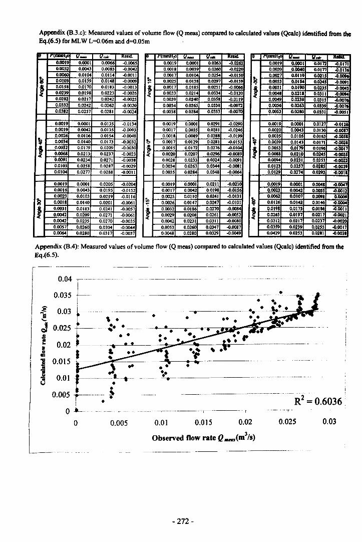
Appendix (B.3.c): Measured values of volume flow (Q meas) compared to calculated values (Qcalc) identified from theEq.(6.S) for MLW L=O.06m and d=O.OSm
~ "lmmn2ll il_ il_ KalIL
0.0019 0.0001 0.0066 .(1.00650.0032 0.0043 0.0085 .(1.00420.0060 0.0104 0.0114 .(1.0011
k 0.0103 0.0139 0.0148 .(1.0009
f 0.0158 0.0170 0.0183 .(I.OOJ30.0239 0.0198 0.0223 .(1.00260.0282 0.0217 0.0242 .(1.00250.0332 0.0242 0.0262 .(1.00200.0382 0.0257 0.0281 .(1.0024
0.0019 0.0001 0.0135 .(1.01340.0019 0.0042 0.0135 .(1.00930.0026 0.0106 0.0154 .(1.0048
~ 0.0034 0.0140 0.0173 .(1.0032
f 0.0052 0.0179 0.0209 .(1.00300.0068 0.0213 0.0237 .(1.00230.0091 0.0234 0.0271 .(1.00380.0103 0.0258 0.0287 .(1.00290.0104 0.0277 0.0288 .(1.0011
0.0019 0.0001 0.0205 .(1.02040.0016 0.0043 0.0195 .(1.01520.0023 0.0103 0.0219 .(1.0116
k 0.0018 0.0140 0.0201 .(1.0061
f 0.0031 0.0183 0.0241 .(1.00570.0042 0.0209 0.0271 .(1.00610.0042 0.0235 0.0270 .(1.00350.0057 0.0260 0.0304 .(1.00440.0064 0.0280 0.0317 .(1.0037
II YlmmttzO il_ "'- KeSId.
0.0019 0.0001 0.0263 .(1.02620.0018 0.0039 0.0260 .(I.ono0.0017 0.0104 0.0254 .(1.0150
~ 0.0025 0.0138 0.0297 .(I.01S9~..t! 0.0017 0.0185 0.0251 .(1.0066
~ 0.0033 0.0214 0.0334 .(1.01200.0039 0.0240 0.0358 .(I.01l90.0034 0.0265 0.0338 .(1.00720.0038 0.0284 0.0353 .(1.0070
0.0019 0.0001 0.0291 .(1.02900.0017 0.0035 0.0281 .(1.02460.0018 0.0089 0.0288 .(1.0199
'b 0.0017 0.0129 0.0281 .(I.OIS3
f 0.0015 0.0172 0.0276 .(1.01040.0020 0.0207 0.0296 .(1.00890.0028 0.0233 0.0324 .(1.00910.0034 0.0263 0.0344 .(1.00810.0035 0.0284 0.0348 .(1.0064
0.0019 0.0001 0.0211 .(1.02100.0017 0.0042 0.0198 .(1.01560.0025 0.0110 0.0241 .(1.0131
~ 0.0026 0.0147 0.0247 ..0.0101e-.0.0270 ..0.0084..t! 0.0032 0.0186
~ 0.0029 0.0208 0.0261 .(1.00520.0042 0.0231 0.0311 .(1.00800.0053 0.0260 0.0347 .(1.00870.0048 0.0280 0.0329 .(1.0049
III 111'_ X'" KIIId.0.0019 0.0001 o.om ..0.01710.0020 0.0040 0.0177 ..0.0136
~0.0027 0.0119 0.0215 ..o.OOH0.0033 0.0154 0.0245 ..0.0091
f 0.0031 0.0190 0.0235 ..0.00450.0048 0.0218 0.0311 ..0.00940.0049 0.0239 0.0315 ..0.00760.0056 0.0263 0.0339 ..o.OO"H0.0053 0.0210 0.0331 ..0.0051
0.0019 0.0001 0.0127 ..0.01260.0020 0.0043 0.01l0 ..0.0087
~0.0035 0.0105 0.0163 ..0.00510.0039 0.0143 0.0171 ..0.0021
f 0.0053 0.0179 0.0196 ..0.00170.0088 0.0210 0.0245 ..0.00350.0094 0.0231 0.0253 ..0.00220.0123 0.0257 0.0215 ..0.00290.0129 0.0274 0.0292 ..0.0011
0.0019 0.0001 0.0041 ..0.00470.0023 0.0042 0.0055 ..0.0012
~0.0062 0.0107 0.009. 0.00090.0126 0.0142 0.0146 ..0.0004
f 0.0198 0.0175 0.0116 ..0.00110.0265 0.0197 0.0217 ..0.00210.0312 0.0217 0.0237 ..0.00200.0359 0.0239 0.0255 ..0.00170.0429 0.0253 0.0211 ..0.0021
Appendix (8.4): Measured values of volume flow (Q meas) compared to calculated values (Qcalc) identified from theEq.(6.5).
----- -----_---- --~--.----.---_
~04 ,-==-~=~~=~'~--~~----.~_-..-.----.----.I0.0351--------I
0.03 ,.~~ ~.---_.___._~----..----. ....--:--...~~~~.,~~.••
--.-__j·~·L-----~~.......=-~..---___1iR------------· -
0.025
0.02
0.015
0.01 ••~•0.005•I
I
o ¥-o 0.005
• •
••
- 272-
----------._---- ..--.-._ ....
R2=O.6036,
0.01 0.015
...-.~, -----------r·------r-----.- .._-.--.-.T - ..
0.02 0.025 0.03
--- --------------------
• .,
--------------
3Observed flow rate Q.MS(m Is)
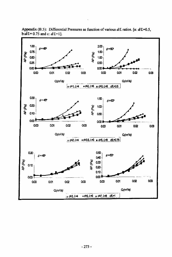
Appendix (B.5): Differential Pressures as function of various d/L ratios. [a: dlL=O.S,b:dlL= 0.75 and c: d/L=l].
1.00 200
r a75 'i' 1.s)..... as) ~ 1.00~ (2) ~ as)
aoo aoo _._-_ ...,
aoo a01 aC12 am aoo a01 aC12 am
Q(m3..s) Q(m3..s)
I. cF1,L=4 • cJ::!2, L=6 • d=3, L~ dL=Q5 I
a:l) 1.s)(}=fIP
'i' (2) 'i' 1.00e;, ~~ a10 ~ as)
aoo aoo --------_.---,
aoo a01 0C12 am 000 a01 Oal amQ(m3..s) Q(m'..s)
,--------------dL:(l75 II. d=2,L=4 .d=3.5, L=6 • d=6, L=8
Cla)l oS)(}=.fI!J' a4)
'iii' i Qi' 03)e;_ I (ha10 ~~ I ~ (2)
I 010aoo 000--~
aoo 001 0C12 am 000 a01 aal am
Q(m3..s) Q(m3..s,J
lA d:G, L=4 .d=6, L=6 • d=7, L=8 dL=1 I
- 273-
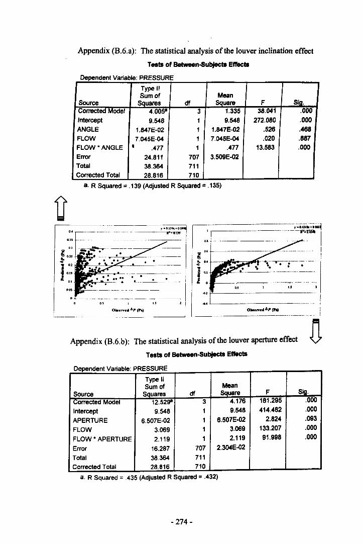
Appendix (B.6.a): The statistical analysis of the louver inclination effect
Tests of Between-Subjects Effects
Dependent Variable' PRESSURE
Type "Sum of Mean
Source Squares df Square F 51a.Corrected Model 4.005- 3 1.335 38.041 .000Intercept 9.548 1 9.548 272.080 .000ANGLE 1.B47E-02 1 1.B47E-02 .526 .468FLOW 7.045E-04 1 7.045E-04 .020 .887FlOW*ANGlE I .477 1 .477 13.583 .000Error 24.811 707 3.509E-02Total 38.364 711Corrected Total 28.816 710
a. R Squared = .139 (Adjusted R Squared = .135)
r------~~ ..~----.---___,y·O.I)".O.
R'-0.U9
---,--:0-._;0 .,~---.--~ II0.'
'i' 0.'@:... 0-4~..i 01
I. 0
.4.1
I I ....0., I,'
0' I
0111..... "",. (hi--_.------_. __ .-
OlIo ...... 6p (h) IL_ . . ..
Appendix (B.6.b): The statistical analysis of the louver aperture effect
Tests of Between-Subjects Effects
Dependent Variable' PRESSURE
Type IISum of Mean
Source Squares df Square F Sig.
Corrected Model 12.529'1 3 4.176 181.295 .000Intercept 9.548 1 9.548 414.482 .000
APERTURE 6.507E-02 1 6.507E-02 2.824 .093
FLOW 3.069 1 3.069 133.207 .000
FLOW * APERTURE 2.119 1 2.119 91.998 .000
Error 16.287 707 2.304E-02
Total 38.364 711Corrected Total 28.816 710
a. R Squared = .435 (Adjusted R Squared = .432)
- 274-
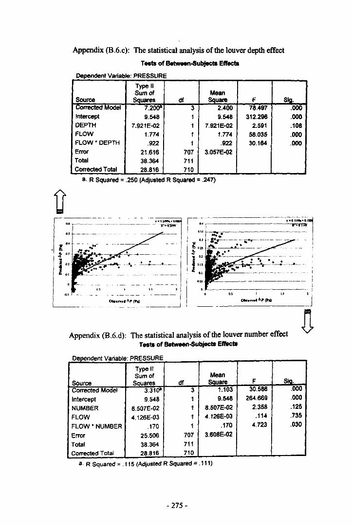
Appendix (B.6.c): The statistical analysis of the louver depth effect
Tests of Between-8ubjectll E«ec«s
Dependent Variable' PRESSURE
Type IISum of Mean
Source Squares df Square F Slo.." ed Model 7.2Q08 3 2.400 78.497 .000
Intercept 9.548 1 9.548 312.296 .000DEPTH 7.921E-02 1 7.921E-02 2.591 .108FLOW 1.774 1 1.774 58.035 .000FLOW" DEPTH .922 1 .922 30.164 .000Error 21.616 701 3.057E-02Total 38.364 711Corrected Total 28.816 710
a. R Squared = .250 (Adjusted R Squared = .247)
us
lO .•I ~ OJ t...;-'~---.-:;,o~.;....
i I02
E. D.,
• •
11
L-_n_: _o 9._1_0I00_O_"O_._4"_IPIIl__ U .Jn-------------'
Appendix (B.6.d): The statistical analysis of the louver number effectTests of 8etween-8ubjects Effects
Dependent Variable: PRESSURE
Type "Sum of Mean
Source SQuares df SQuare F 510.Corrected Model 3.31Q8 3 1.103 30.586 .000Intercept 9.548 1 9.548 264.669 .000
NUMBER 8.S07E-02 1 8.507E-02 2.358 .125
FLOW 4.126E-03 1 4.126E-03 .114 .735
FLOW • NUMBER .170 1 .170 4.123 .030
Error 25.506 707 3.608E-02
Total 38.364 711Corrected Total 28.816 710
a. R Squared = .115 (Adjusted R Squared = .111)
- 275-
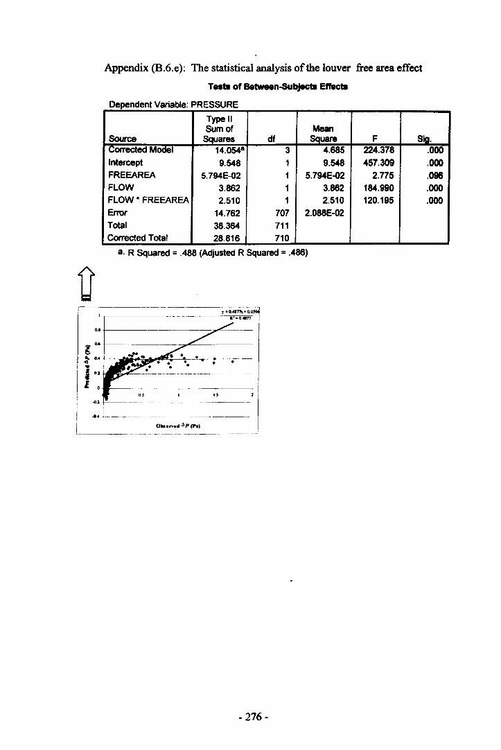
Appendix (B.6.e): The statistical analysis of the louver free area effect
T.... of Between-Subjecta Effec ..
Dependent Variable' PRESSURE
Type IISum of Mean
Source Squares df SQuare F Sla.Corrected Model 14.054- 3 4.685 224.378 .000Intercept 9.548 1 9.548 457.309 .000FREEAREA 5.794E-02 1 5.794E-02 2.775 .096FLOW 3.862 1 3.862 184.990 .000FLOW * FREEAREA 2.510 1 2.510 120.195 .000Error 14.762 707 2.088E-02Total 38.364 711Corrected Total 28.816 710
a. R Squared = .488 (Adjusted R Squared = .486)
D~ G.
~G.4
1.. 0.>
I. 0
- 276-
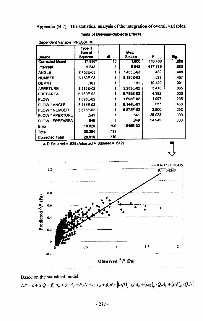
Appendix (B.7): The statistical analysis of the integration of overall variables.
T.... of 8etwMn-Subjects Etracts
Dependent Variable' PRESSURE
Type IISwnof Mean
Source ~ ...... df ~,_"" F Sig.(;Ofi~ Model 17.9W 10 1.800 116.430 .000Intercept 9.548 1 9.548 617.739 .000
ANGLE 7.453E-03 1 7.453E-03 .482 .488
NUMBER 8.18OE-03 1 8.180E-03 .529 .467
DEPTH .161 1 .161 10.429 .001APERTURE 5.283E-02 1 5.283E-02 3.418 .065FREEAREA 6.789E-02 1 6.789E-02 4.392 .036FLOW 1.695E-02 1 1.695E-02 1.097 .295
FLOW-ANGLE 8.144E-03 1 8.144E-03 .527 .468
FLOW • NUMBER 5.873E-02 1 5.873E-02 3.800 .052
FLOW • APERTURE .541 1 .541 35.023 .000
FLOW • FREEAREA .849 1 .849 54.942 .000
Error 10.820 700 1.546E-02
Total 38.364 711
Corrected Total 28.816 710
a. R Squared = .625 (Adjusted R Squared = .619)
1.2y = 0.6245x + 0.043~-------nz--~---.-.- I
R = 0.6245
- 0.8ell~-Q.. 0.6
<l"CII.. 0.4~:ae~ 0.2
0
-0.2
•
..--- .__...~__~, -·-~~"·____r__·--·-·-~---·-l - .----- -_..
0.5 1.5 2
Observed t1p (pa)
Based on the statistical model:
M = c+a.Q+ p,.do +X,·Af +8,.N +&,.Lo +¢;.O+l(ap)" ·Q.do +(ax)" .Q.Af +(a8)" 'Q.NJ
- 277-
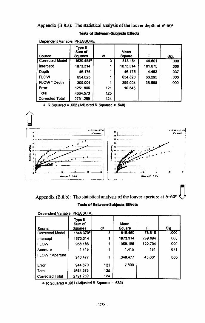
Appendix (B.8.a): The statistical analysis of the louver depth at 8=:600
Tests of Between-SubJects Effect8
Dependent Variable: PRESSURE
Type IISum of Mean
Source Squares df Square F Sig.Corrected Model 1539.454· 3 513.151 49.601 .000Intercept 1873.314 1 1873.314 181.075 .000Depth 46.175 1 46.175 4.463 .037FLOW 654.823 1 654.823 63.295 .000FLOW· Depth 399.004 1 399.004 38.568 .000Error 1251.805 121 10.345Total 4664.573 125Corrected Total 2791.259 124
a. R Squared = .552 (Adjusted R Squared = .540)
y ·0.55161<+ I. y • O.MI,b;. I 1I~Il'-OMU !
I1Ilc= R'.O.5516
::j---~--------------14 t----:12~~-----_.~~~~---
~IO~--~-~-~~~----
I:~~-.~-.-2 - __ --- --- J__ _111___ _u__ _lII__ _____lj
- -----_-----------_----
Appendix (B.S.b): The statistical analysis of the louver aperture at (P60" nTests of Between-Subjects Effects
Dependent Variable' PRESSURE
Type IISum of Mean
Source SQuares df Square F Sia.Corrected Model 1846.37ga 3 615.460 78.815 .000Intercept 1873.314 1 1873.314 239.894 .000FLOW 958.186 1 958.186 122.704 .000Aperture 1.415 1 1.415 .181 .671FLOW • Aperture 340.477 1 .340.477 43.601 .000
Error 944.879 121 7.809Total 4664.573 125Corrected Total 2791.259 124
a. R Squared = .661 (Adjusted R Squared = .653)
- 278-
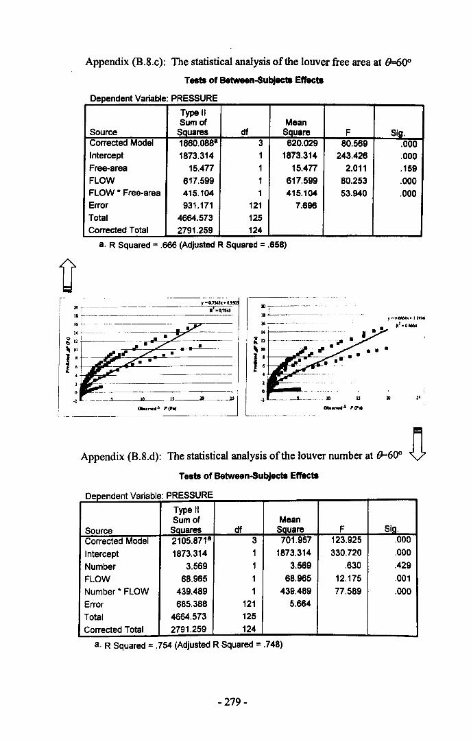
Appendix (B.S.c): The statistical analysis of the louver free area at 9=60°
Tests of Between-SubJects Etracts
Dependent Variable: PRESSURE
Type IISum of Mean
Source SQuares df Square F Sio.Corrected Model 1860.088- 3 620.029 80.569 .000Intercept 1873.314 1 1873.314 243.426 .000Free-area 15.477 1 15.477 2.011 .159FLOW 617.599 1 617.599 80.253 .000FLOW * Free-area 415.104 1 415.104 53.940 .000Error 931.171 121 7.696Total 4664.573 125Corrected Total 2791.259 124
a. R Squared = .666 (Adjusted R Squared = .658)
:~=-_-_~ R_'_O.'I54.S_
16 +--~----~-14 -------------
e; 12+-----~IO~-_= __ ~_=~~~~·---I:~~---..
3II~--
11+-----16
14+----
: 12
~ 10I:~~4
·2 10 u lOO"-~-.zL--~
-------------------____j
Appendix (B.8.d): The statistical analysis of the louver number at 0=600
Te.ts of Between-SubJects Effects
o d tV . bl PRESSUREepen en ana e:
Type IISum of Mean
Source Sauares df SQuare F 51Q.Corrected Model 2105.871- 3 701.957 123.925 .000Intercept 1873.314 1 1873.314 330.720 .000Number 3.569 1 3.569 .630 .429FLOW 68.965 1 68.965 12.175 .001Number * FLOW 439.489 1 439.489 77.589 .000Error 685.388 121 5.664Total 4664.573 125Corrected Total 2791.259 124
a. R Squared = .754 (Adjusted R Squared = .748)
- 279-
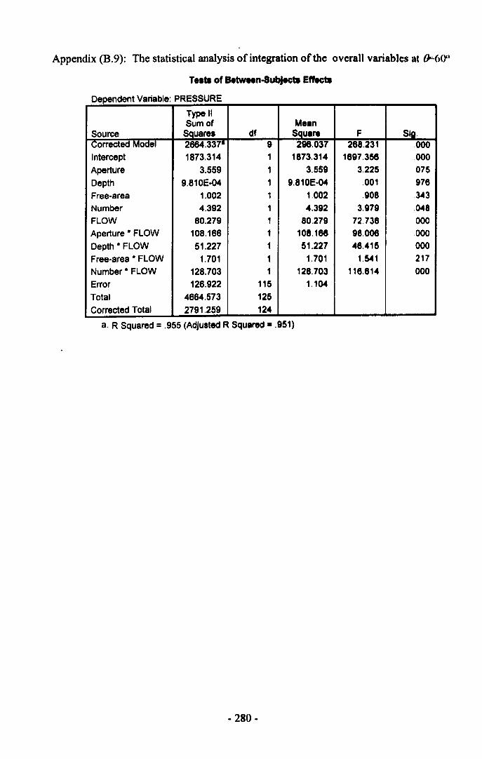
Appendix (B.9): The statistical analysis of integration of the overall variables at f).,()()"
T•• ta of Betw .. n-8ubject8 Eft'ecta
Dependent Variable' PRESSURE
Type IISum of M.an
Source Squares df SQuare F SIQcorrected Model 2664.337· 9 296.037 268.231 .000Intercept 1873.314 1 1873.314 1697.358 .000Aperture 3.559 1 3.559 3.225 075Depth 9.810E-04 1 9.810E·04 .001 976Free-area 1.002 1 1.002 908 ~3Number 4.392 1 4.392 3.979 048FLOW 80.279 1 80.279 72.738 000Aperture * FLOW 108.186 1 108.188 98.006 000
Depth * FLOW 51.227 1 51.227 46.415 000Free-area * FLOW 1.701 1 1.701 1.541 217Number * FLOW 128.703 1 128.703 116.614 000Error 126.922 115 1.104Total 4664.573 125Corrected Total 2791.259 124
a. R Squared = .955 (Adjusted R Squared· .951)
- 280-
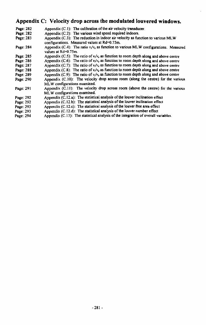
Appendix C: Velocity drop across the modulated louvered windows.Page:282Page:282Page:283
Page:284
Page:28SPage:286Page:287Page:288Page:289Page:290
Page:291
Page:292Page:292Page:293Page:293Page:294
Appendix (C. I): The calibration of the air velocity transducer.Appendix (C.2): The various wind speed required indoors.Appendix (C.3): The reduction in indoor air velocity as function to various MLWconfigurations. Measured values at Rd=O.7Sm.Appendix (CA): The ratio v/v. as function to various MLW configurations. Measuredvalues at Rd=O.7Sm.Appendix (e.S): The ratio ofv/v, as function to room depth along and above centreAppendix (C.6): The ratio ofvlv. as function to room depth along and above centreAppendix (C.7): The ratio ofvlv. as function to room depth along and above centreAppendix (e.8): The ratio ofvlv. as function to room depth along and above centreAppendix (C.9): The ratio of v/v, as function to room depth along and above centreAppendix (C.lO): The velocity drop across room (along the centre) for the variousML W configurations examined.Appendix (C. I I): The velocity drop across room (above the centre) for the variousMLW configurations examined.Appendix (C.12.a): The statistical analysis of the louver inclination effectAppendix (C.12.b): The statistical analysis of the louver inclination effectAppendix (C.12.c): The statistical analysis of the louver free area effectAppendix (C.12.d): The statistical analysis of the louver number effectAppendix (C.13): The statistical analysis of the integration of overall variables.
- 281 -
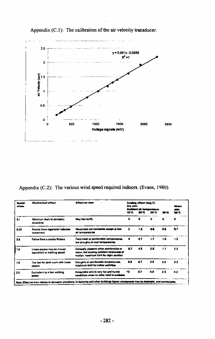
Appendix (C.l): The calibration of the air velocity transducer.
2.5y. 0.001x· 0.0205
If ·12
Wi'!1.5
I...;0.5
oo 1000 1500
VolbIgl.Ign." (mV)
500 2000 2500
Appendix (C.2): The various wind speed required indoors. (Evans, 1980).
....... M...... n..... eff.ct EHect on "*' c:o.IIIIa .......... ClnIIl ... Dry .... Molle,_..... ............. ....
,,·C IO'C ..·c III"C .·e0.1 Minimum likely In domeat.c MIY '"I aNffy 0 0 0 0 0
"tuition.
G.25 Smoke .from clgenm.) IndlceteI Movement not notIoNbIe ...apt lliow I U 0.' 0.' 0.7movemlnt Ilr tlmp_tuIN
o.a Flame !tom • candle flIckeR Fee",,", lI~ttllftpaq ...... 4 U U ,.0 1.1but drlughty It _, ..1IIf*IlUt'II
11.0 LOGII plpere may be moved. G,n.rally plttatnt when oomlortlble or 1.7 U U u UequlVllllnt to wllkl"lltpeed Wlnn. bu. 01"."11--.nt ew_ of
motion. maJdmum .",'t for nigII. 00Iftf0rt.---- ..-..., ...,-.~.~
1.5 Too t•• t for d•• work with 1_ Draughty It comfortablt .empeFllt" ..... 1.1 '.7 U J.O Upapers mllldmum"nIh for ~ tctMUet
.~-.~.,._-" .. ,-~---2.0 Equlv.'.nt to I , .. t wilking AccIpttbll only In very hoI end humid 10 '.7 4.0 U U
tpeed oondItione whin no o1hIt ,..,., la tve ......---~"--.....
Note: EffKt on min rellt.I'o domestic Iltultlon .. In ftctorlet end ottltf bulldIntIlIIgher Willdllli I CIt -. 1M............... ~.
- 282-
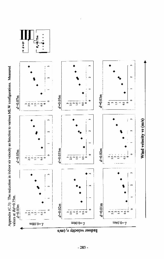
Cl)
::so.~>sc:o'B~~.e(,)
oU>'"'·ta
• r .... •!
• i •I
t r N ~!
• I •r -• ! •
8 8r-- I/')
0 0 0 0
0 """lI"\NI.I"1-tnO 17 f'f"IV\Ntn-'f')O
II N - 0 N ...: 0~ ~
8C"IooII~
••••••
N
--~1•
I,
811/')'01.,1r1~, :
~• I ....I• I I
I I, f N !I• I
• - I
•••••
.....
o
•N
I!
_____________________ J
- ----------,,-- --.---,- ..-~-----.--I
• .... I
W90'O=7
•••
•N
•~ I"• I I
~ -
~-~--~~..•·~loJt""lV')NV1-lnON _: d
--~--~
w80'O=7
•,••
,--T-- -T-- --r-'- '---T-- 0
",",'I"'IN"'-"'ON .....; 0
. ....
•N,
••8-o
1f~
WvO'O=7
SIW) 1" AlPO(aA ~OOPUI
- 283-
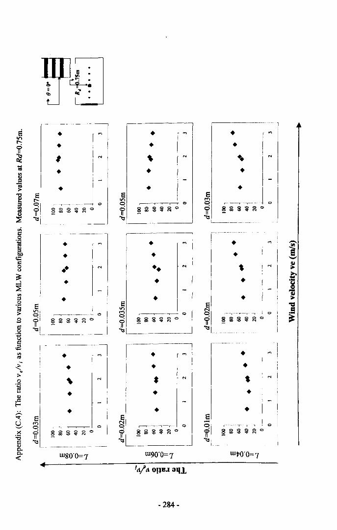
•=uq,
t_
elr\oclII"t!
••
••
....
••••••e
lr\("0")o1f"t! L _
w90'O=7
••..••
••
••••
~ I
••
••••
....
e-oen>~
••
o
o
000 0 0 0:: QC >0 "" .....
N
I------~
II :•••
oo 0M
•
••••s
("0")~ 01r g~~~~o~
wgO'O=7
- 284-
wVO'O=7
N
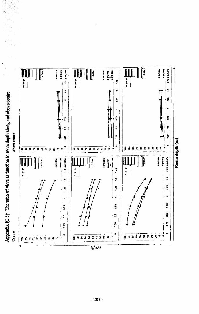
1 ~
~~ -I~ 5~ ~
1 ~i-
l',-, // I.;.;II, '~.
t II l;~.f.! ,
i II •r I
IiI :
.1 • ~~~~~~~:
It II• • .. I
II)..,
IIIo
- 285-
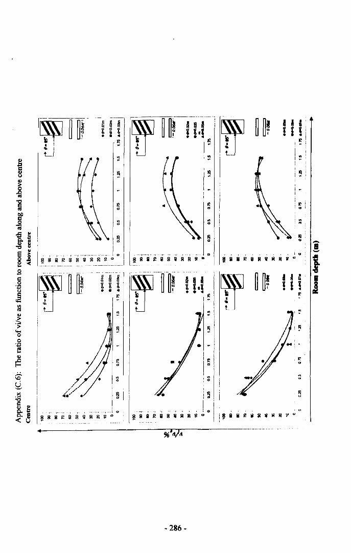
"' --...-~.'-".~-.•.-~.-- - .
~
~ ~~
g ~ B
~
~ ~~ I 1.1~
~~,• I ~t t t !I!.. .. ....~ iC ~~
~ on .:~
~ ~,IQ, ~
r'-"""--"'-- -.,~.....-r- -" ..•. , -,' ". 0
~
~i'i~ i S ~ ~ 2 ~ 0
0
1
o
- 286-
. , , • , ... , . I ..@ i i ~i R ~ M ~ V u
I I C!I!
~
....illlo -a-
, ,.
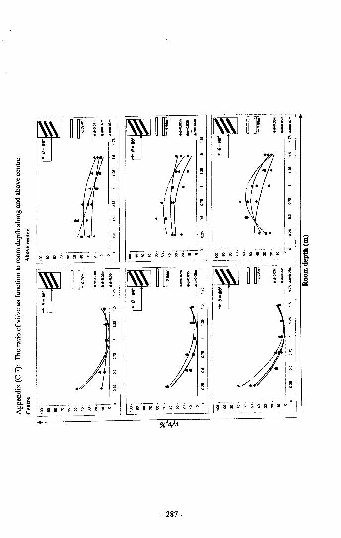
/t.,!!i ...I ,
~II'.1
.. 1.....I!, .i.\.4.
Ili~~iS! ~ g_!il_~_O_o_
---~----.-------E !:IcE O~I,~.. ..
.--r-·T~·'---"·- - •
~ 8 i ~S S! i ~~o
51 0
It i. . ..~
onoono
o
..
!--,- -'-'"--,
~ 8 i ~ S S! ~ ~ !il
;!?o
'--------------
"1o
- 287·
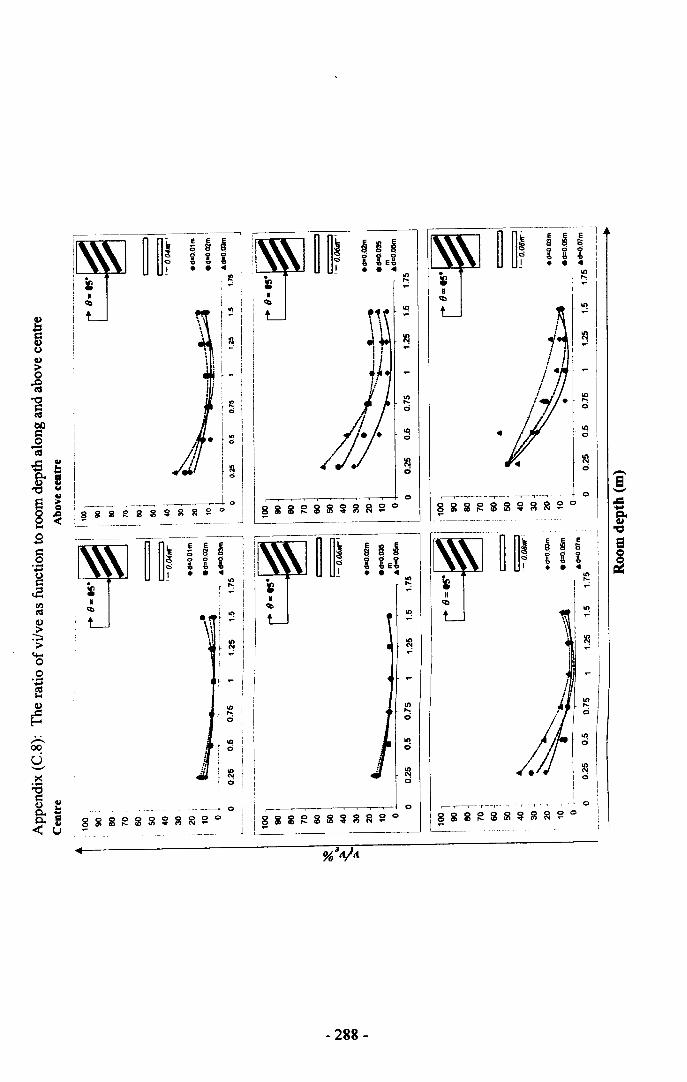
i
f ~I.~~1°~~1°!
I ~~_~ .. _~ __ .--~~~_J °18g2gli!li!~g!il~o I~---=----'"--~--.----.--------. ----- _ __________j
-- -------- ----~ ,
~ ~'" s ~ ~ I IC3 ~ 0 0 I
Q ~" II .... i- ~ i
r""= i
_ .~.. __. .-.-.....----.-.-0
~ ~ ~ ~ g ~ ~ ~ ~ ~ 0
-------~-------
~ ~~~ ~ ~
~ ~~
e ~ eB S~ <> ~<> ~ e~
.I!,,• • .. • • ..
'" '"..., ...,
"! ~-II) ~"!-II)...,0
"! .. '"0.,;
~ Iq.,; 0
'i0 0 --r---,...----,.-----1 - -.--- ----,---r----" '_-
~i 2 ~ i ~~~~~0 § i 2 ~ li! ~ ~ ~ ~ ~ 0.=~Cl.._--,---"'_ -._ --- ~"Cl
~ ~~~ 8 ~
~ ~~~ ~ e e!:i
i t et ~ ~ ~~• • .. • • ..
on II)... ...,.-' e-
"! "!-'" '""I "!.-'
I - II
",I"". I,_ I
i
- IIiI
~••••••••• ~-:_j
'"...,;'".,;
- 288-
II)III... ...,
.,; 0
III "!.,; 0
III
I~I
'-'---'-._ T __ ,__ ._, , , , , I 0
~i 2 ~ li! ~ ~ ~ ~ ~ 0
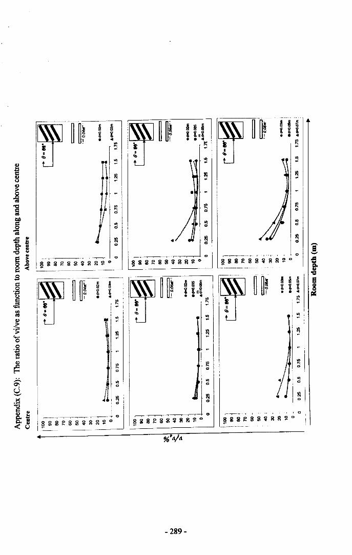
t•j1 ~: \• .1. ~IT ~: fH ~Ii:j_ &0ell "":Ii 0
1'/~~<>
~-~·~~·It.lIT U L r~I
q, ~u ~'I it.. ~
Ii"
II)....o
-.- ..•.,- ..~-_ -, .-
fit• • 4~~
~. ~~ IIi• • 4II>....,.;
~
~-
"1o
~1°I
r----r"'--'T"" ",·---.'1' "T' -.,- " , , I 0 '
§ i 2 ~ ~ ~ ~ ~ ~ ~ 0
- 289-
II>.;
~II
o
II>.;
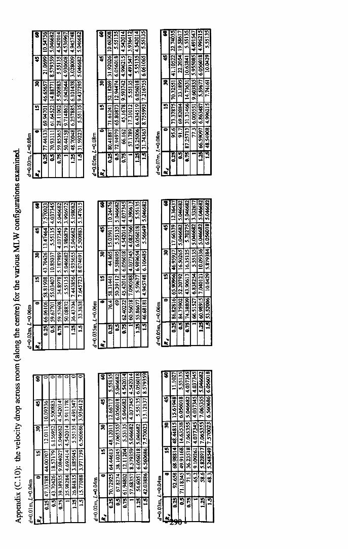
S \0 N ~r- 00 Non 00 (;~ .. 00
~~N \0 1;;::8
o . ~:ri ;1;~-on -i-i -i",
VI ~~ on 00 O\N~ ....0 8~S~ ViS 00 \0...:C::; on ....S~· 0\N . on .00 ..M.n
:;: r- - =~00 onon e-- ....0\~to "N
8M - r-\0 00 on~ 0 ......o-i -~..- vi"'; ..00\
:!l - N §~ on onOM 00 ....r- on 00 -;1;$ -~ r-- onon ono\_: · r- N .
00 . ..0'"\0\0 NO\= .... - '" 00 00 ........ -\0 on~ N
~ - .... - 8 N~ :2~ 0\r- V)
e- 0 0\0 00 -r- e-- on on • ....~ :! ~ - ~ II}
~ -= -...l1li
s ....on NN N '"N" 00 r- oo -g~ \00\ 0\0\0\0 00 r-r- ....~~ ~:!onor..:-i vi~ ",vi
VI $~ onO\ N ...... ~r- 00 00,,- ...., 00 ::800r- on r-\O• on ....,00~~Mvi C!~- "M '" '":;: \0 r- .... M '" -
~~00 00 onO\....\0 \0\0r- \0 on "r- 00 ~~
M r-"';0 ~C!..- on on .00VI 00 r- OO on \0 M- ~~ r- M onN0\- 00 r-- .... 00 on ....on00 0 · on ~$oO~ " .M""on on r- r-= S 00 N " 000 ~ .... 0 M- r- OO r- OO8 ~ r- OO M ....
'" 0 " ...;..0 0\ 0\ 0 ..0 ....\0 on .,., on .....~
III III - III II}c:i r- f'!~ -Q -...
l1li
i 00 00 00
III \0"'" ~OO r-N... ....00 _ r- ,,-....00 0- ~$g;g N-., - 0\ ..... on "1~ ~~o .- on ., .... ., ....
= - N ......, .,., \0,.., - .,., 00 (; .... 000 0\\0 - \0\0 \0 ..... .,., ~N ~~
., II"!- on .,., on1.C:i"'; ~ ..0
III r- 0\ r- ., .,., 0\- 0 r- .....~ • ....r- -0 0\ r-g r-" ....on -onoo 0\00 r-
~'0 ~"'< ~00 .-0\ " .... ....
= 00 \0 on" on 0000
~.... 00 ,..., 00r- ....N 00 0...., 00 00 " r-.... r- ...., .... 00 r-
r..: ...; 0\", ..0 '"..,. ..,. ........ M -. III II} on - on II}f'! = r- N -= ~ ...:...
l1li
s 00 on "N .. on0 ....~i - ........ - 0-~~ Non
~Sl ~""!0'" . on- ........ ..,.
III \000 on e- on on.. N - M~ :::!S~$ s:i on -~:g :ri~;:;:;~ .-i \0~ .... ..,. N on 00 on
~i..... - onr- - ~~.... on0\ on on -NN on . C!f'!. onon - .... \Cl e--
on - ...., 00 N 0\ ,...,- "r- r- - ;;;8:NOO ~~-0 .. on\000 ..... ,...,on.....:.,.; on . ~r-:.r-r-\O
_ \0 00
= r- ....fi:1 ~ 8~00r-00 .... !::-~~on ..
~~ r..: ~f"o;0 ..... on ,..., -00 e-- ..,...,·
~II} ;!! - ~ II}= c:i --...
l1li
i \0 ......,., ,..., on Nr-OO .. - ....00
~~ ~~ ~~0"'"o .~.on .- on on
III - on :!:::8000\.. - ...., $~0\-~~....onoon :gil"!
vi vi II"!C! . on- .." \0= .,.,on 00 on ~lQ,.., \0 ....-"00\0 ~~ !)8~;.,., ....,
00 0\ -0\ ..o~ ..0..0III _N "00 r-OO- ~::
_ 00 r- ..oon \0 r-- .... ~§ O\on.... ...., :ri~000 on .on on ..,.r- ..,.= .. $~ 00 i-..0 $ 00
r-~ -on ~fi:1 g '" ~on
· ~ :! ~ ~ II}- -c:i -...l1li
~ on ....." .. 000\....,00
~~- on
Vi::8 $~:ri~ :gl;;
on ~~ \Ci00on r-OO Non on r-.. r::$ 00;;1; ...., ....
::8r- ~N~~ ~8 on-N . "'~ 'lif"i_\0 -
= - on .,., ..... ..... ....f'I - on ,...,00 00 N
0"'" ;;;::8~~
N '"_\0~~00C!.. r- on on r-
III ,...,on~~ 00\0- -~ -00;~N M~~-0\_r-
$~. on oonN . \Ci\Ci_ 00
= on~ iI;; - \Cl
~ ~00.... 00N 00 00~r-
~\0
~g ::0 r..: ~on· 11111} III - ~
II}:;le ~ -
...l1li
i onr- on r- on on.... - :::!~ - ....~~ N-on _~~r- on on 0\
No\ "':N -.on
~ ~~_ on 000\Gteo - N:g~ .... ~ $~
-:N ~~ on .00- ..... o • \Ci-.. _ on
~ - on - on r- -onO\ ........ r-\Oon eo \0 00 ~:;N - ~$,..., . on e--. ...., ",r..:ON " .e-- -0\on ~i ~~
r-on... 00 _r-N - on~i....00:~"';0\r-\O .... \0 \O~
= \Or- ....,M
~~'I"i"': r::~0\01 onr-<'! II"!~r- ::8~eo
~ :J I!l - ~ II}-= ......
l1li
S r-N I~II~iN .-on on ....on on
~ OIN on .....il....00~I~~r- . "'on on\Ci-on:;: r-on on on ~Gt,...,\0N ....O\N :n:;:; §~~~ ....on
~~ ~V'i 00'!-onIII I~:::!~
_ 01- N"'"~~ -~
onM '00 ~c:i\0'" ~\Ci r..:-
= \ON~
r-on
~Oii~ ..... -onO\Non Vi~oor- ....,;g ~ rt. ~ ~ ...;on~II}
~ -~II}c:i= -...
...l1li
i r-on .,..onil......... ;;1;;;1;0--on r-r-_:"} 88- on -i-i "'\CiIII eooo i~~i.. -a;-
iO~ ~ .onC!_\0 on. r-\O
:;: on eo on on on ...._ M
~;;I; onNooon ~8~:d onr-~!~~ 8&;
r- .. r..:r..:on :!:~ 00- r-O\.... -\0 ;:~00 - on .....~;: ::::g 00 eo~~ ~;~~11\11\
= 00 on on .....~:l:2;;1; "':'1\. 00 r-\O on~~-:-r-~
II}~ ....~
It)=c:i -
...l1li .~
;'7
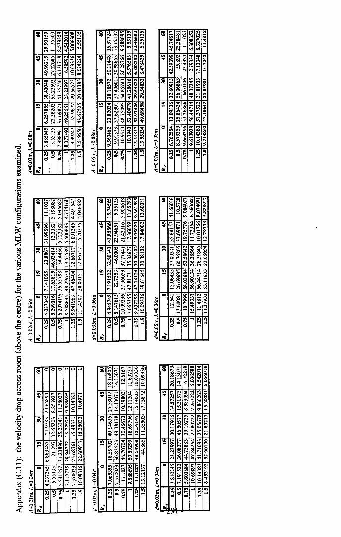
~ a- "" a- ~ 00 .,..11'\ 0 11'\ s 0 "".,.. .... "" ;;:;~ .,.. 0- <'I >D
"! I'- ~ 8 "l~ :: 11'\ .,.. .,..M 00 ~ .,.;
VI 11'\ .,.. 00 M >D ~• N 00 - a- .... M>D I'- 11'\ "" M
>D M ;;; 00 a- ~a- M .,.. 0 M
~ r-: - -0 ~ 0~ M -0 00
0 00 "" >D I'- .... "".... ~ a- .,.. a- M 00.,.. I'- a- .,.. "".... .... .,.. .... >D~ M "! M .,.. ~00 .,.; ~ M 0 0.... .,.. <'I M M
VI .,.. "" r:: :0 I'- 11'\- 00 0 I'- M00 M 00 11'\ >D .,..I'- 00 0- 11'\ a- I'-11'\ "" >D M .,.; >DM .... r-: ~ .,.. 00-0 M "" ~ ~
0 .,.. .,.. ;;: M "" >D~ "" a- ~ 11'\a- - 0- ~ M 11'\.,.. .,.. 00 I'- a- a-00 .,.. 0- I'- a-00 .,.; 0- "" ~ 11'\
M r-: 00 r-:. on VI ~ - on IIIN => ~ -=> cl -...~
E00o'if"-l
E....o'ii'"1:s
0 I'- M M :0 I'- M
'" M 00 00 ~ 000 0 >D ~ .,.. -c
00 >D ;;: >D- a- ~ I'- ~- - I'- ~.,.; .,.; ~ ~ .,..VI -c M M "" V> V>.. a- 00 00 00 ~ I'-
V> "" "" 00 "" Ma- M M 8 ;;: 0~ .... ~ I'-- - .,.. 0 .,.;"" .,.; .,.; -0
0 I'- ~ >D 0- I'- I'-.... -c .... 00 - -00 ~ ~ V> I'- I'-00 ..., .,.. -c >D.... a- ~ V> -c >DM -0 .... '" .... ....~ - - -
~ 11'\ V> 00 ~ ~ -11'\ 00 a- I'- 0 V>0 I'- -c ~~ .... .... 0- 0
>D 11'\ M ~ 0
r-: r-: -0 00 r-: 00- .... ~ ~ ....0 .,.. >D 0- .,.. .... I'-~ 0- >D 0.... 0 '" >D 0- ""I'- 0- I'- 00 :!:M 0- 0 00 ~
0 M M 11'\ 0- -~ .,.; -0 '" ~ -on ~ on - VI IIIN I'- ~ ...cl cl ...
...~
eo8CIlCIl
~
!c.-()o-4):>.s
~ 0 0 0 0 00
on '" I'- I'- 11'\ "" -~ 0- M M 0- 00 I'-00 0- 0 >D .... a->D -c 00 00 ~ ~~ on ""! 00 -:0.... ~ - 11'\ 0 -M 00 - '" -0 .... .... -;;. 11'\ - M.... 00 0 I'- .... .....I'- M ..... 0- ..... 0~ on ..... M 0- V>- -c M I'- ~ MM .... .,.; -0 .,.; -0..... M - - -
on I'- I'- -c M - .....- 00 0- 0- I'- >D ;;:~ "'! 00 M I'-..... - ..... '" 00 55-c N "'! 0- -c00 - 00 .,.; ....-0 .... M N M
0 11'\ V> I'- 11'\ .... -c~ ..... on I'- N ......... - M I'- 8 .....I'- on 0 0-.... "l ~ - I'- 00 on on - V> 0~ .,.; r-: r-:
. I(') on I(') ... I(') III... cl I'- "'1 ...cl => -...
~
----
~ ~ I'- VI V> M .,..M .... 0- .... 00 ""I'- - -c- -c -I'- M 00 .,.. >D .,.."" - 00 .,..
~.,..
.,.; !:).,.. . .,.;. .,...... 0- .,..
on 00 .... -c .... N .,.... :)::g -c 00 III ~I'- .,.. ....-00 00 -c 00 00NO- M I'- g I'-
00 0 .,.. ~III .... M .,.; -0 00
0 N $ .... >D N N.... I'- ~ - .... ....VI I'- :g 00 0000 ~
.,.. ~ ~- 00 M VI
00 I'- ~....: ~ ~<'I .,.. .,..~ M
VI ~ ;; .,.. 0- -c 00- .., SS; MVI0 .... ~;;tM M VlO
f;;'Cl00 -c I'-~M r-: oOM .... 0-M .... ~VI .,..~
0 N .... .... .... I'-~-c I'- - ~ ~ ....~ 10 .,.. 0- 000
"" ;;: 0- .... ~VI>D :!e .... .,..VI 0\ P'i""';~ - -. on III on ... on III~ 0 r-: "'1 ...0 0 -...
~
E00o'ii'"-l
E.,..o'ii'"1:s
~ VI - I'- I'- 10 -c0 I'- -c .... .... ""00 0 I'- .... ""'" .... >D 0 0- g- - .... 'Cl 000 ~ .... .... 0 0- -
on M - .., ~ VI M.. ;; I'- 0 0 I'-0 00 M ~ 00
00 .... 0- - VIVI VI - - ....r-: ~ 0 .... .,.; r-:M - - - .... -
0 .,.. 00 M >D I'- ........ "" I'- I'- 0- :! 010 - >D I'- .,..:!: 00 .,.. 0- 0- .,...... ~ '" VI "!0 ~ 0 00 .... -~ ~ .... .... - -
on M .... ~ 0- 00 VI- 0 M 0- ~ >DI'- .,.. I'- M 000- .... 0 0- ~ ~VI 00 I"- VI .,..00 0 -0 0 00- "" ~
.,.. ~0 .,.. "" I"- VI l"- I"-.,.. M M 0- M ........ 0 0 -c 0 .....,.. 0 - 00 - M
:8 I"- .... 00 - -.,.. .... V> .... Mr-: r-: ~ -. on on VI - on IIIN cl r-: ~ -cl 0 -...~
~ ~ - ~ M VI M00 VI M 0000 ;;t ~ ",,0~ 00 I'- "':I"- .... - OM -.,.; .,.; - .... .., -~ M -000
on ~ ~ .... ~ 00 ~... M .... ~.... 00 0- "" .... M0- .,.; ~ 0- "" I"-III V> M I"- .... ~~ M .... ~-
~ "" .... :8 .,.. ....~-10 ~ ""~8 c:; M 0-
I'-OC!
...:g .., 00
.... -0 00 - .,.;M VI ~ "" M
III -c ~ :g :! M I"-- .... M M ~""~ 00 I'- .,..goo -c :): I"- 00
"" "! -0"'; M -0 .... ~_M 11'\ .,.. VI
0 ~ 0\ ~ 0- .... MVI .,.. ~ 001011'\ ... ... ... 00M 0\
~ "" ~~'" I"- \O~ r:::l"- V>-0 00 '" .0 '"0--
on III on ... :q IIIN ~=> 0 --...~
~ -c 00 I"- >D ;;: I"-
"" M M 00 ;;:~ I"- 0 -c >DV> .,. ~ ~ 00
'Cl ~ 00 ~ M
-;;. C! III 000\ -0 00 .,.;
on .... .... 10 ~~ ~• V> l"- I'- ....~
00 I'- "" I"- ....0- 11'\ .... - 0\-c I"- r-O r-
.,.; r-: 0\ ~ci ~V> "" .... .... ....0 - V> M~ ~~.... - 0
"" M ~II'\
S >D 00 00 ;;;~I'- .,.. M
r-: g .... -0 -OM"" VI .... M M
III .,.. VI ~ ~ :! ....... .... 0- 00 "" ....8$ '" - I'- 'D.... ~~ -0 -"';-0 00 -c-c M- M VI .,.. VI .,..
0 ~oo 0- - M ...0- "" 00 ....
~~0- .... 0-r- 0- "': I"-
~ "': - "'!"" VI ... ...... ... .... VI III ;!! ... VI IIIN ~=> 0 => ...-...
~
~ "" r::: 00 00 :! 00r- ... 00 §-c 0 M 11'\ 000 ::::! M 'D M... I'- .... ~ VI
0 ~ -0 0 VI 0M .,.; ~ -0
on r- V> '" M .... ...... V> r- 0\ M -c 00M .,.. 0 M M §r- ... .... !O >D00 M 00 -c~ .,.; 0\ M 00 M"" ... 00 r-: ~ -
0 -c I'- V> M 00 ....... ;;: ... M M r- NV> M r- '"~ 0 >D 0 11'\ V>V> .... 00 C! ~0 -0 '" r-: V> ........ ~ ... M M M
on l"- I"- ... ~ "" '"- 8: I"- 00 VI 00 V>
"" 00 M ~ §"" 00 .... ;;tM C! l"- t-:M '" ~ r-: -;;. ....M .... ~ ....
0 VI M ;;t r- "" M~ M 0- QC 0-M .,.. '" QC "" -~ ... .... 0- :! ....
0- 0 >D 11'\00 .... ~ ~ 0 .,.M r-: .,.. ... 00
. lQIIl on - lQ IIIcl° ~ ..: -
,;, "...d
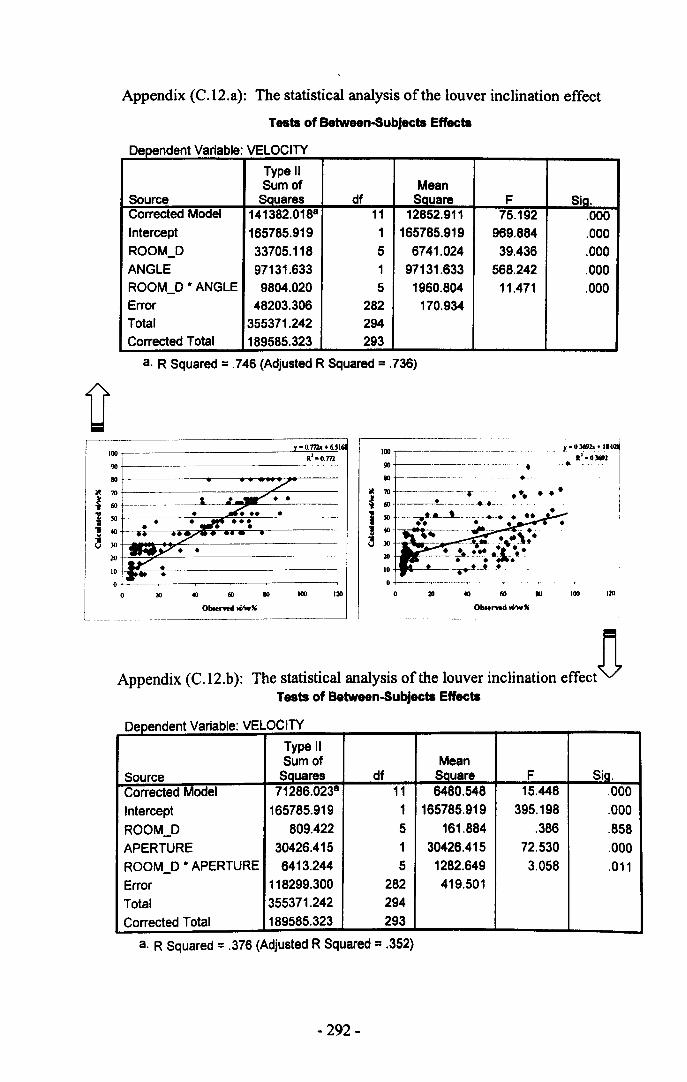
Appendix (C.12.a): The statistical analysis of the louver inclination effect
Tests of Between-8ubJects Effects
Ddt V . bl VELOCITYepen en ana e:
Type IISum of Mean
Source SQuares df Sauare F Sia.Corrected Model 141382.0188 11 12852.911 75.192 .000Intercept 165785.919 1 165785.919 969.884 .000ROOM_D 33705.118 5 6741.024 39.436 .000ANGLE 97131.633 1 97131.633 568.242 .000ROOM_D * ANGLE 9804.020 5 1960.804 11.471 .000Error 48203.306 282 170.934Total 355371.242 294Corrected Total 189585.323 293
a. R Squared = .746 (Adjusted R Squared = .736)
U100
90III
~ 70
Ii ~
I I 40
I U JO
20
10
0
r-------~--- _-
III
100 ~------------
90III
~ 70
~ IIO+-~-...L....-
1 ~'! 40+--=_~
;, 30 +--'--~=--~
_ 1" 0l69h ._I.C~
_e ."01691 Ie- -
• e. ee·
60 100
:co10
o ~----~----.-----------.-:co 40 fill III 100 110120
Oboerwd """''' O........ d"""'''----------------
Appendix (C.12. b): The statistical analysis of the louver inclination effectnTests of Between-8ubJects Effects
Ddt V . bl VELOCITYepen en aria e:
Type IISum of Mean
Source Sauares df Sauare F Sia.Corrected Model 71286.0238 11 6480.548 15.448 .000Intercept 165785.919 1 165785.919 395.198 .000ROOM_D 809.422 5 161.884 .386 .858APERTURE 30426.415 1 30426.415 72.530 .000ROOM_D * APERTURE 6413.244 5 1282.649 3.058 .011Error 118299.300 282 419.501Total 355371.242 294Corrected Total 189585.323 293
a. R Squared = .376 (Adjusted R Squared = .352)
- 292-
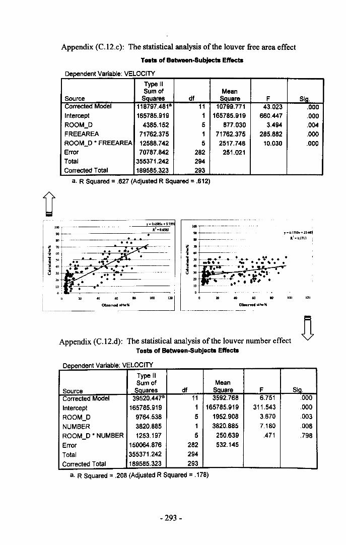
Appendix (C.12.c): The statistical analysis of the louver free area effect
Tests of Between-Subjects Effects
Dependent Variable: VELOCITY
Type IISum of Mean
Source SQuares df SQuare F Sla.Corrected Model 118797.4818 11 10799.771 43.023 .000Intercept 165785.919 1 165785.919 660.447 .000ROOM_D 4385.152 5 877.030 3.494 .004FREEAREA 71762.375 1 71762.375 285.882 .000ROOM_D * FREEAREA 12588.742 5 2517.748 10.030 .000Error 70787.842 282 251.021Total 355371.242 294Corrected Total 169565.323 293
a. R Squared = .627 (Adjusted R Squared = .612)
R' -0.651$y -D'71". J"•.~
.a.J.0.171.1
y - 0.651$. + 9.7
20 ID 100 120 60 lOll
Obs...... d_" Obsorwd Ktw"
Appendix (C.12.d): The statistical analysis of the louver number effectTests of Between-SubJects Effects
Ddt V . bl VELOCITYepen en ana e:
Type IISum of Mean
Source SQuares df Sauare F Sic.Corrected Model 39520.4478 11 3592.766 6.751 .000
Intercept 165765.919 1 165765.919 311.543 .000
ROOM_D 9764.538 5 1952.908 3.670 .003
NUMBER 3820.885 1 3820.885 7.180 .008ROOM_D * NUMBER 1253.197 5 250.639 .471 .798Error 150064.676 282 532.145
Total 355371.242 294Corrected Total 189565.323 293
a. R Squared = .206 (Adjusted R Squared = .176)
- 293-
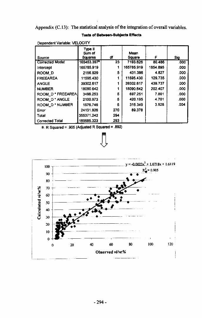
Appendix (C.13): The statistical analysis of the integration of overall variables.
Tests of Between-SubJects Effects
Dependent Variable' VELOCITY
Type IISum of Mean
Source SQuares cif SQuare F Sig.Corrected Model 165453.39]8 23 7193.626 80.486 .000Intercept 165785.919 1 165785.919 1854.895 .000ROOM_D 2156.929 5 431.386 4.827 .000FREEAREA 11595.430 1 11595.430 129.735 .000ANGLE 39302.617 1 39302.617 439.737 .000NUMBER 18090.642 1 18090.642 202.407 .000ROOM_D • FREEAREA 3486.253 5 697.251 7.801 .000ROOM_D • ANGLE 2100.973 5 420.195 4.701 .000ROOM_D • NUMBER 1576.746 5 315.349 3.528 .004Error 24131.926 270 89.378Total 355371.242 294Corrected Total 189585.323 293
a. R Squared = .905 (Adjusted R Squared = .892)
lOO~--------------~---W+---------------------80~-- ------------~
~ 70 ---------------------...:-4~~~-
~ 60~"C~ 50 +----------___:_--~ _ _.~It_.:'lI':--._------- -..-; 40u-;U 30 +---~ .. -:-~~---+--------------
2010 H.. ~------------------------ ------
•
oo 20 40 60 80 120100
Observed vVve%------- -- ---------------------
- 294-
Page:296
Appendix D: Computational Fluid Dynamics appraisal stage.
Page:297
Page:29S
Page:299
Page:300
Page:301
Page:302
Page:303
Page: 304
Page:305
Page:306
Page: 307
Page:308
Page: 309
Page:310
Page: 311
Page: 312
Page: 313
Appendix (D. I}: The velocity profile within the louver blades at various inclinations,L=0.08m, d=O.07m fF=ft, 30°, and 60°.Appendix (0.2): Airflow patterns at various locations inside the room depth at louverinclination angle fFOo, Projected Rowshan (inlet-Il), (outlet-I), d=0.07m, L=0.08m.Appendix (0.3): Airflow patterns at various locations inside the room depth at louverinclination angle fFO°, Projected Rowshan (inlet-V), (outlet-I), d=0.07m, L=0.08m.Appendix (0.4): Airflow patterns at various locations inside the room depth at louverinclination angle (F00, Projected Rowshan (inlet-Y), (outlet-II), d=O.07m, L=O.08m.Appendix (0.5): Airflow patterns at various locations inside the room depth at louverinclination angle (F00, Projected Rowshan (inlet-V), (outlet-III), d=O.07m, L=0.08m.Appendix (0.6): Airflow patterns at various locations inside the room depth at louverinclination angle fF30°, Plain Rowshan (inlet-I), (outlet-I), d=0.07m, L=0.08m.Appendix (0.7): Airflow patterns at various locations inside the room depth at louverinclination angle fF30°, Plain Rowshan (inlet-III), (outlet-I), d=O.07m, L=O.08m.Appendix (0.8): Airflow patterns at various locations inside the room depth at louverinclination angle fF30°, Projected Rowshan (inlet-V), (outlet-III), d=O.07m, L=O.08m.Appendix (0.9): Airflow patterns at various locations inside the room depth at louverinclination angle fF60o, Projected Rowshan (inlet-II), (outlet-I), d=0.07m, L=0.08m.Appendix (0.10): Airflow patterns at various locations inside the room depth at louverinclination angle fF60°, Projected Rowshan (inlet-IV), (outlet-I), d=O.07m, L=O.08m.Appendix (0.11): Airflow patterns at various locations inside the room depth at louverinclination angle fF30°, Projected Rowshan (inlet-V), (outlet-I), d=O.07m, L=O.OSm.Appendix (0.12): Airflow patterns at various locations inside the room depth at louverinclination angle fF60°, Plain Rowshan (inlet-I), (outlet-I), d=O.07m, L=O.OSm.Appendix (D.13): Airflow patterns at various locations inside the room depth at louverinclination angle fF60°, Plain Rowshan (inlet-III), (outlet-I), d=O.07m, L=O.OSm.Appendix (0.14): Airflow patterns at various locations inside the room depth at louverinclination angle fF60o, Plain Rowshan (inlet-III), (outlet-III), d=O.07m, L=O.OSm.Appendix (0.15): Airflow patterns at various locations inside the room depth at louverinclination angle fJ=60°, Projected Rowshan (inlet-Il), (outlet-I), d=O.07m, L=0.08m.Appendix (0.16): Airflow patterns at various locations inside the room depth at louverinclination angle fJ=60°, Projected Rowshan (inlet-IV), (outlet-I), d=0.07m, L=0.08m.Appendix (0.17): Airflow patterns at various locations inside the room depth at louverinclination angle fJ=60°, Projected Rowshan (inlet-V), (outlet-lIl), d=O.07m, L=0.08m.Appendix (D. IS): Airflow patterns at various locations inside the room depth at louverinclination angle fJ=60°, Projected Rowshan (inlet-V), (outlet-I), d=0.07m, L=0.08m.
- 295-
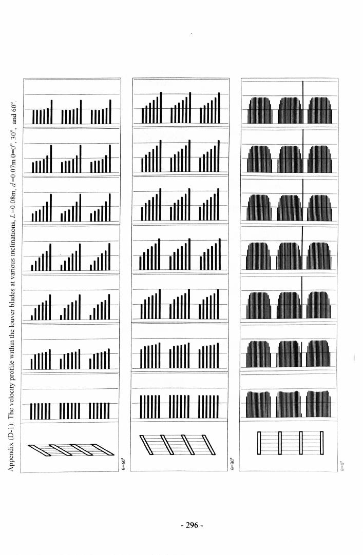
o·o\0"0§
o 'oM
IIIIII IIIIII IIIIII
IIIIII IIIIII IIIIII
IIIIII IIIIII IIIIII
IIIIII IIIIII IIIIII
IIIIII IIIIII IIIIII
IIIIII IIIIII IIIIII
lllTiI 111111 111111
~3§§Z§L~
ooII
CD
Et'-ooII~{00ooII"--l
'0'"II<l>
IIIIII IIIIII IIIIII
IIIIII IIIIII IIIIII
IIIIII IIIIII IIIIII
IIIIII IIIIII IIIIII
IIIIII IIIIII IIIIII
IIIIII IIIIII IIIIII
IIIIII IIIIII IIIIII'n. ..\."
" ,~ " ."
- 296-
oo'"it, '---_._
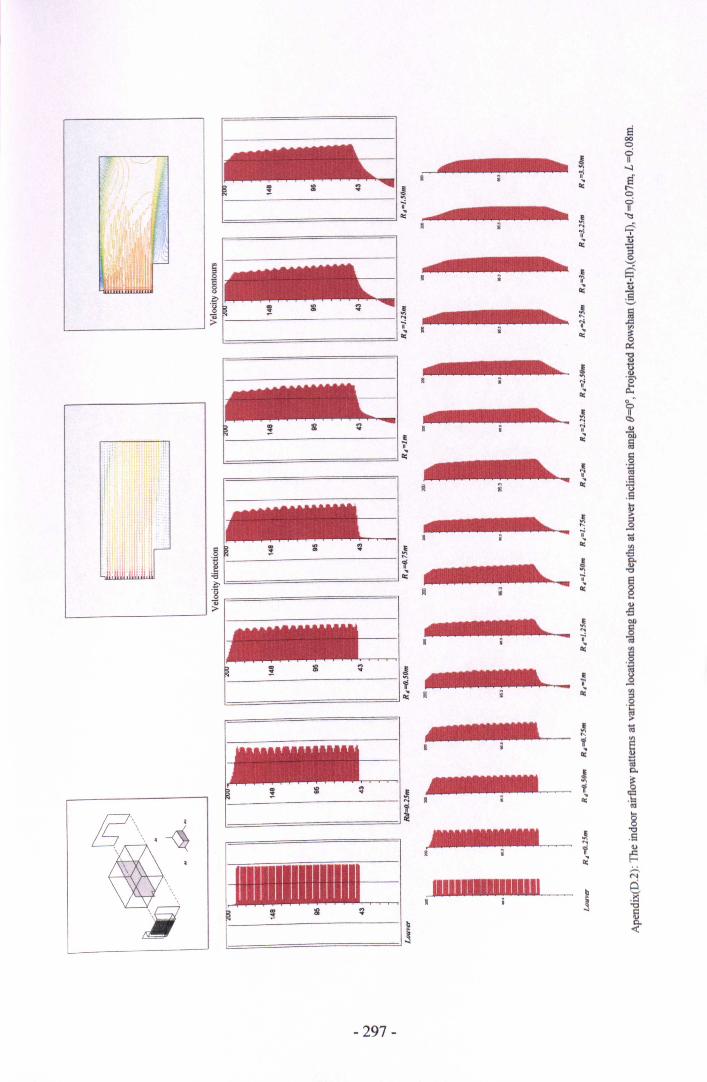
~J~--~---------------- i
~==========l~
~~1~-___:___------- ~ .......___~~
- 297-
K 11111111111,111111 !
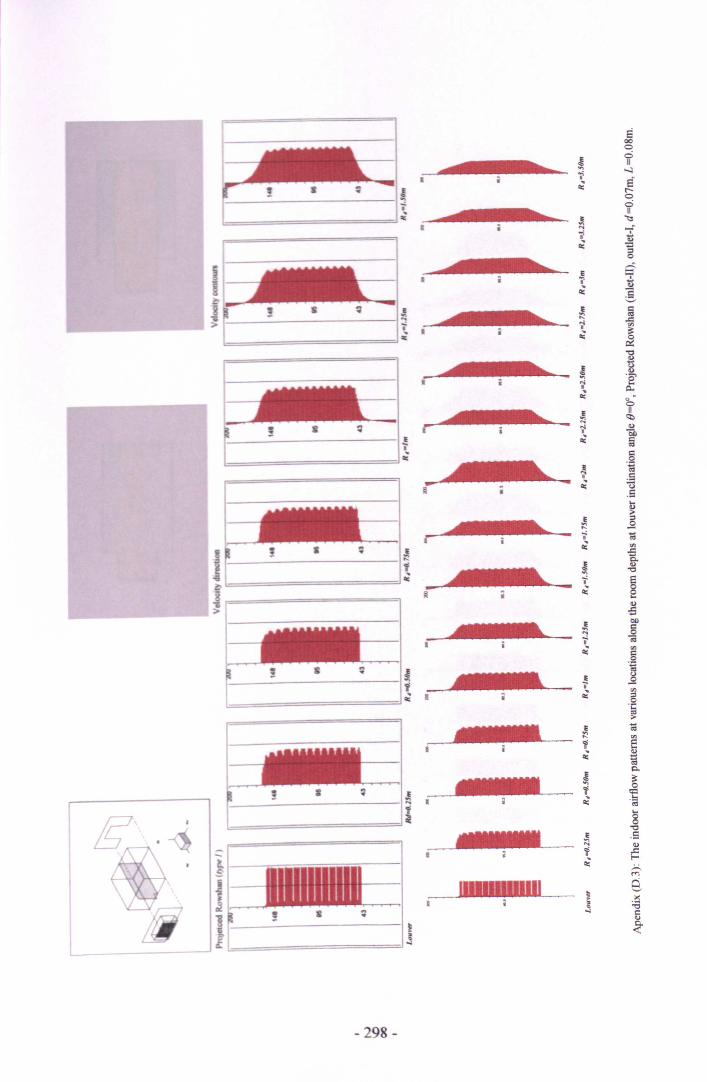
::::...........=====
~==============_I~
- 298-
r
800eoII"-.lE"r-eoII~
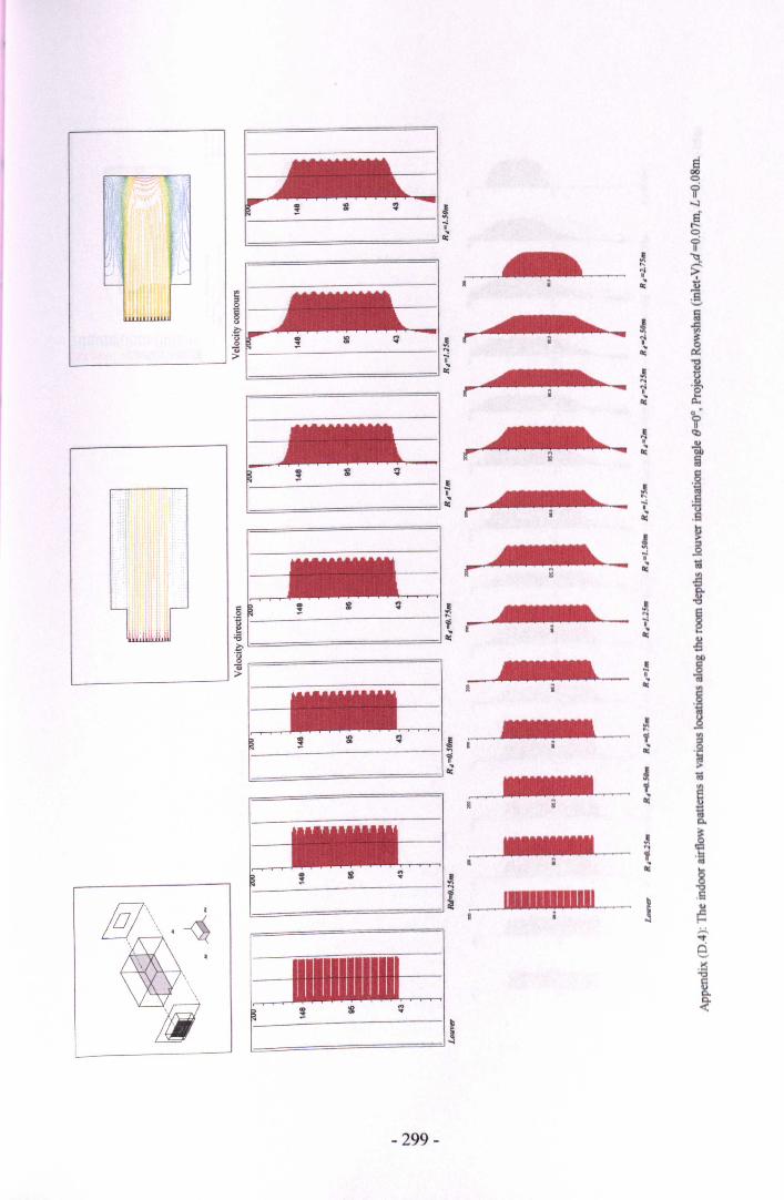
§l_'\,\ I
, ,.~.
•'.
"....
Ifi
- 299-
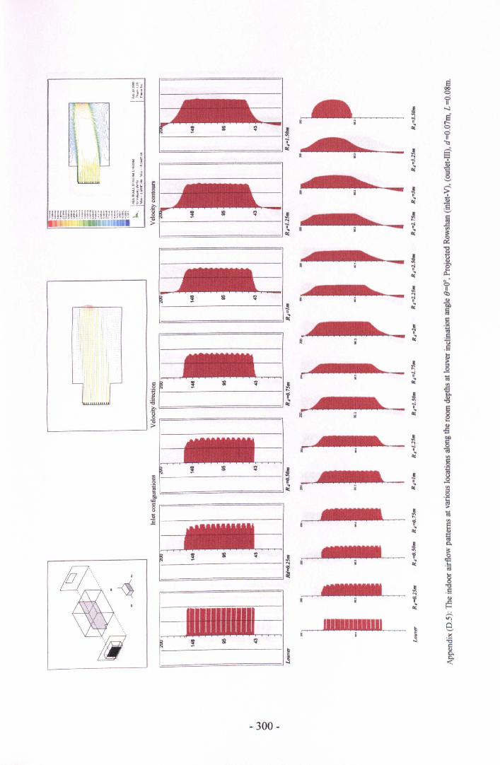
:__ __:___ ----- ~ ..-.. ~·i ~~~~~=====i===========ji --====~~=-
11111111111111; j
§!\\ .~.
\ .g- 300-
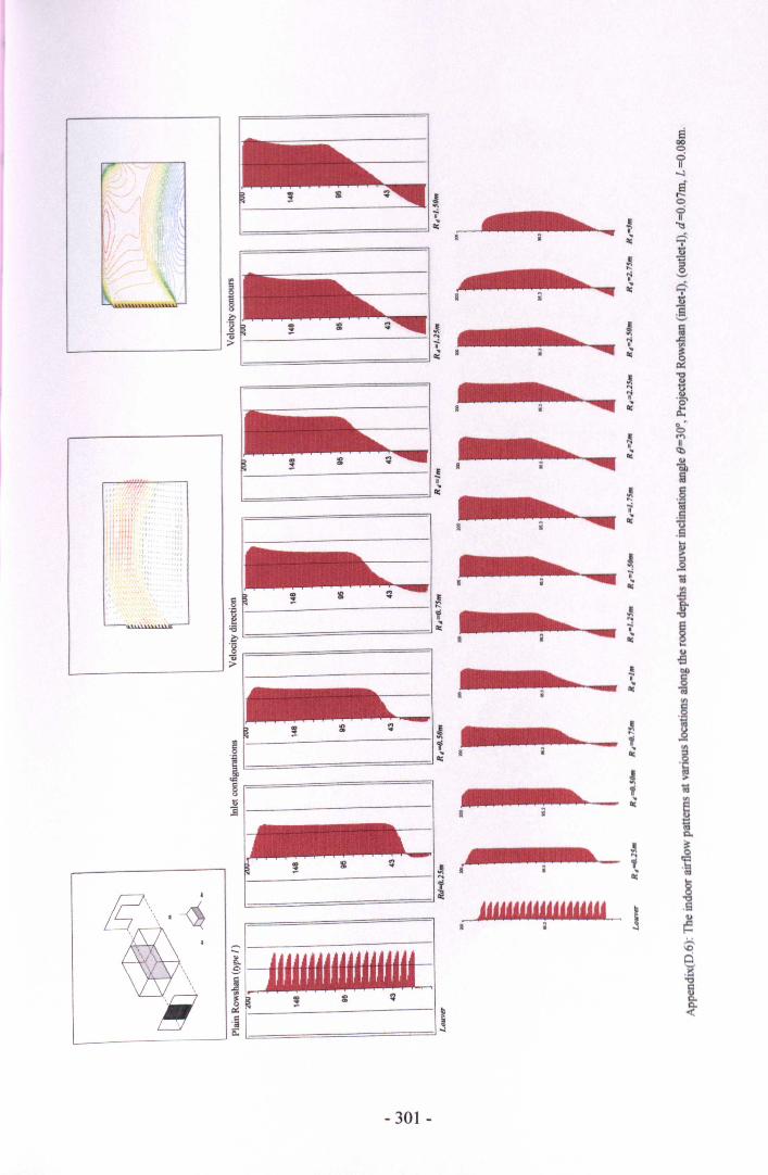
El00<:>
?"-l
El'~ t'
<:>'" ?1
~cC ~
Ii' "1::l
~ 9-';)
~ ';::l
~~
'it ~g cC 9-'" ~8l;>
] ~'-'
~l~
]s i 'itcC ~ ~
~
l~
Ji 1'"'it~ '0'
t!::~.
l~
~MII<:t>.. G.l
~Obla, ';"://. ,. cC I :i, ,
"
~
~icC u
.8.,
l~
! I"7: '01~
§ ~ .s.~ 11 l-.-.. • 6-:q "'Q
:a ~ 7:~]: re ...G.l
u i3;;.
~! bI)II §re 01
J:~
~l!l 1 "0 re ·11 cC
~c '018 ,.....,...._ 'IIII
~ I:9..
Cl.
~ ~...~E 'II
'" ~'"11~!f:\""" ~
iil 4"."" ••"" ••,,, ] .8G.l
iI t=:
~. G-o ::::-, .. ~~~~~~~'~j~~~~j~j~j~\ ~.........
J "'Q\,
~ ., : J§ ~ ~ ! ~ ~~]
0.. ~
- 301 -
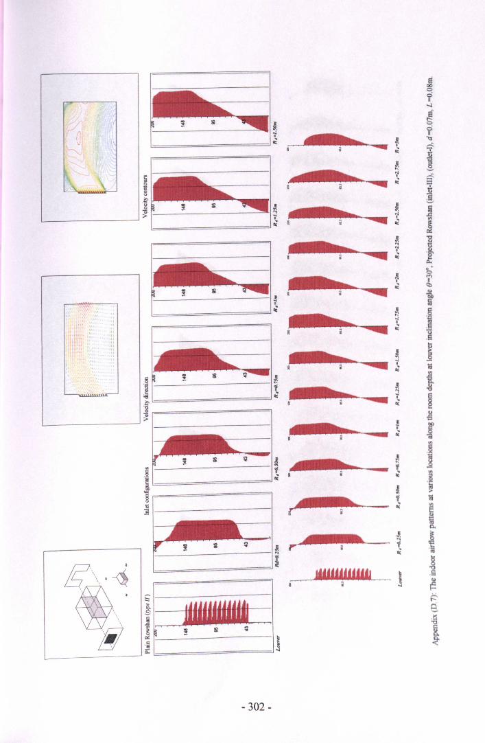
Ei000
'it-..l
8'l'-
Ji 0., 'iti
~~ ~ """6~ '.
~ ~;::: 0
~'i "-'
~ ~]
Ji ~ '-'
'"~
.,~ii II
~ ~ !I~
~ 1..•~ l~ b
~
!"'\,~~ <>
E "6br fa~ • ·1
M~
;:::..;•~ ~
,9
I~
l j..;• la~
~ I,I~
~~ :!
~,~
I~1----- 00ii~~
Ji- ~ I., t'if
'I~ I • oc
~
~
., «l~ I
Cl,
~ ~Ji r 1 ~'" ~~ ~
I...........~ ! ,9
• ~¢e.~
! I
, ?,:,f' II
" ,_
l~=======iF=================i---------
I~''''jj'''~~fl. ,i • i
~ ~ i£ ~
~""\\.~
•.
\
........
"\,
jjl
- 302-
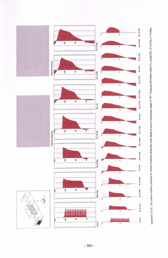
.!-____::_-----I! ~!
..'I
--- QC
,~~~'~~U~~l,-,~
, I I , , ... i£ ~
~ ;:!:
J-
- 303 -
,.'",.,,.'.,
El00oi-4er
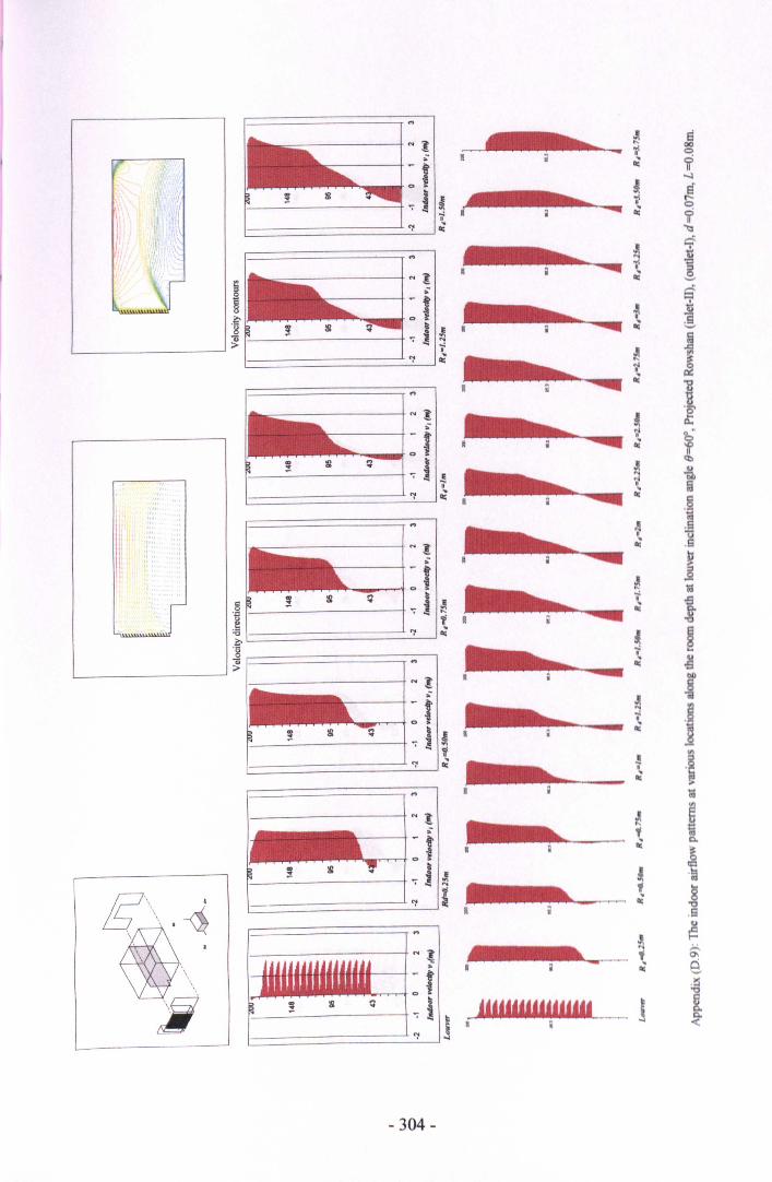
"'"1/",I, .,
"J ~
-----i"'l ..,.------, - t-,,,,,,,_0 ~
~__::::...__----I -;!~~ ~
'" l§ ..- t=~8
0g J ~'"-; ::."il ,:>
"I ~
'" l..- t0 i~-; ! ~
'H"I ~
,--------- I'" l
,--------, : f~__::_---~ -;j
...l.: t-;i I:
'"'""I l
- 304-
JAIU."....._.,_·"~.. _,,.__• _ !• •
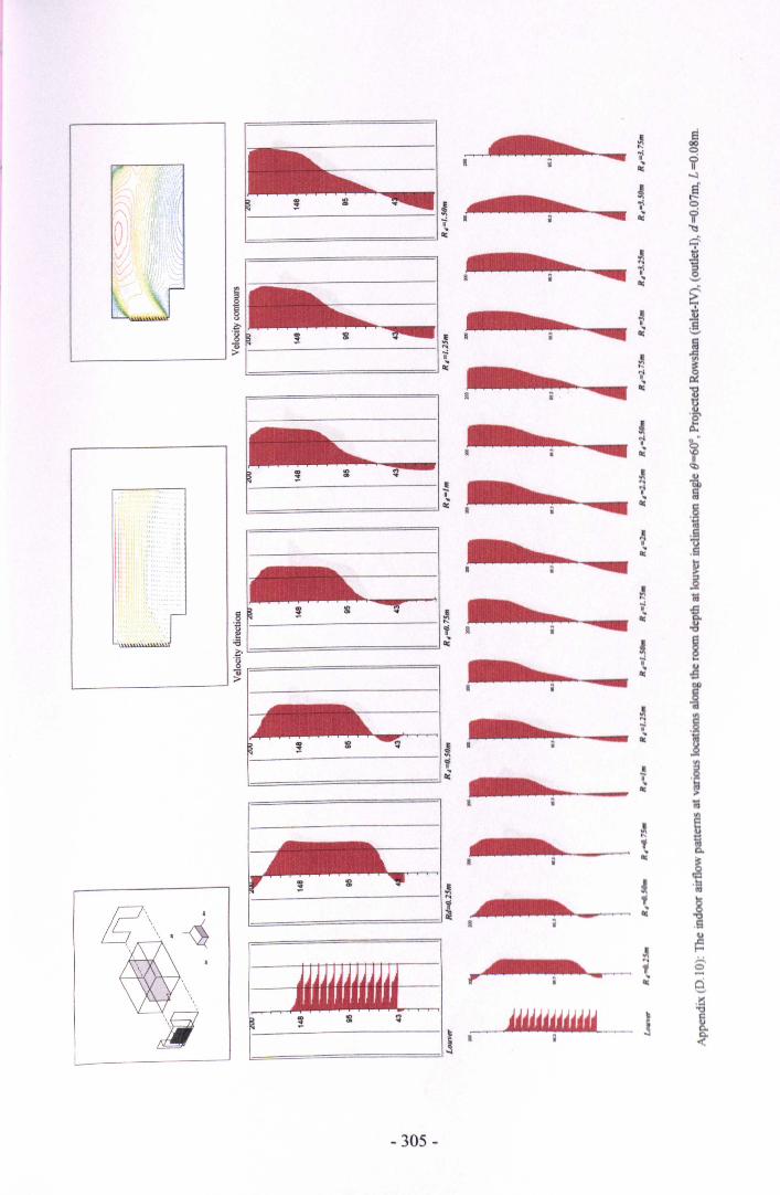
-
n,
U'U
IJ, •
'"II, "1/1,
1111'1'1" ,.,n
",u"\ ....
- 305 -
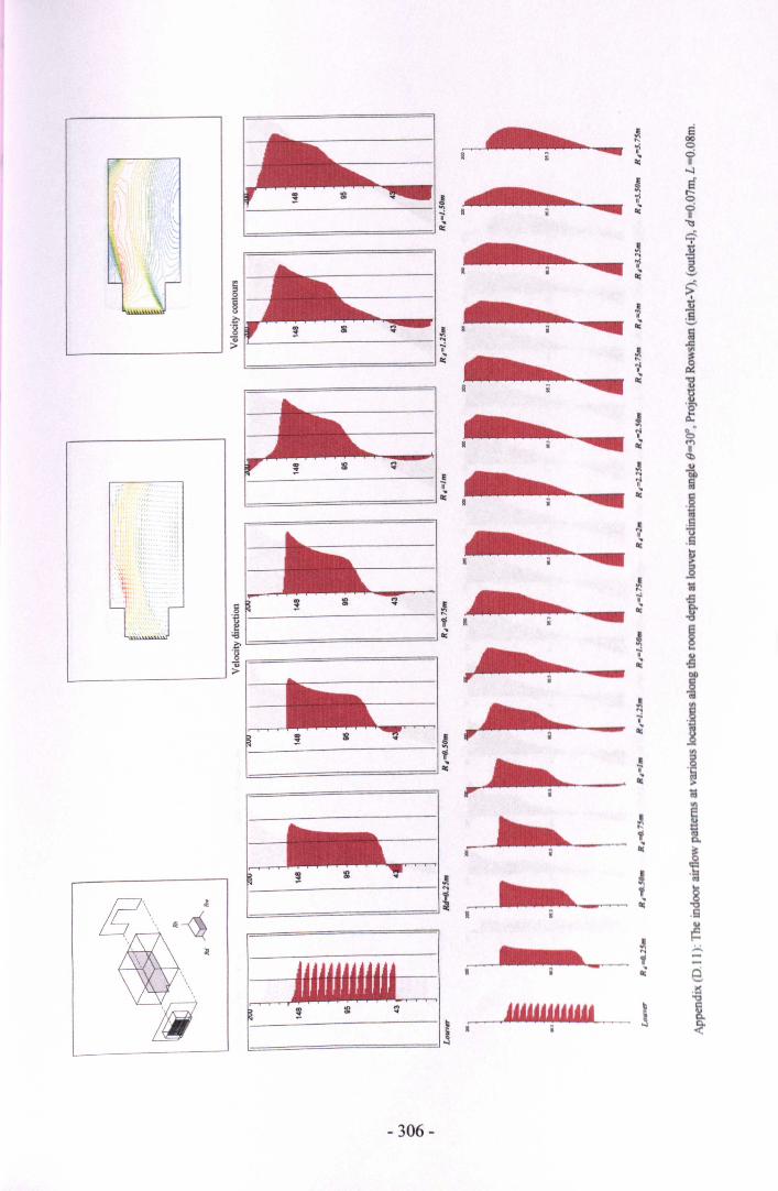
p' ~b_\,,\~~
..
~,
"
11 , , , , , <D ill ~
~ ;!
- 306-
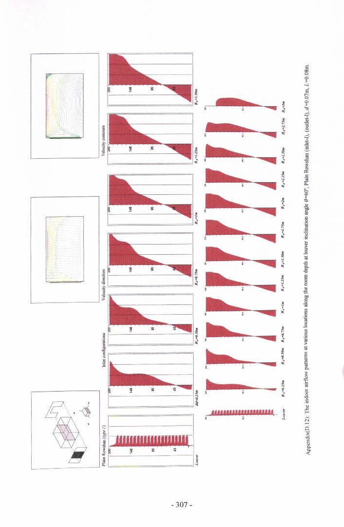
'" I .:~\ --,~,
",r .....
.r:n
"", ' '", lrr
!,,1:
. """, 1\1I' "t-i •~,\
\
."," ,,
IIII!IIIIIIIIIIIIIII'___ -. :!l !J l'
=======~j
- 307-
."".",,~.,.,..,.,.!II <,
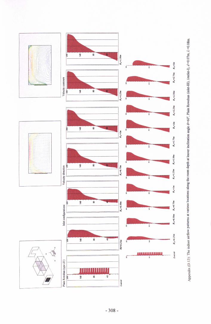
/ ,;~;.II 'n
!.'1
I,'111
\\\
\\" \I<
" II",ll
1\.\
I<.1<
" ... L I: ," l
\,'.\'
!IIIIIIIIIIIII
- 308-
~..,C
....II
~
Jl...C
~~
. . !'1"'111'111"
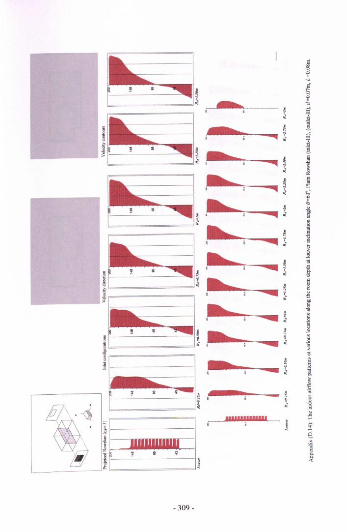
1----------------------- ~ ~AI.......... -------"i
~=====================~
~-;l==============d ~
Ii'j
~=============~~
IIIIIIIIIIIIII~' .. .
:! :!l ~
- 309-
'111..11..'111
800ooII
o....l
Sr-ooII~
I
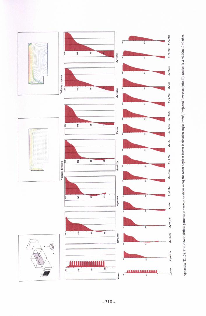
• ~"oC" ~..,
"'"
~
i ~oCIt0:;
.~ ~'it'oC
~
~......• "ii'oC~
''Vo,
.~ ~oC
~.~ ~i
" oC~i
~".
oC ::;
,~."
• ifoC
&•~i •oC
l1li~ ~ ._.,
'"~ill
IIIIIIIIIIIIIIII~ ,f ~ :II ~
- 310-
~••... ... i?
Cl ~
-
"""."".""(
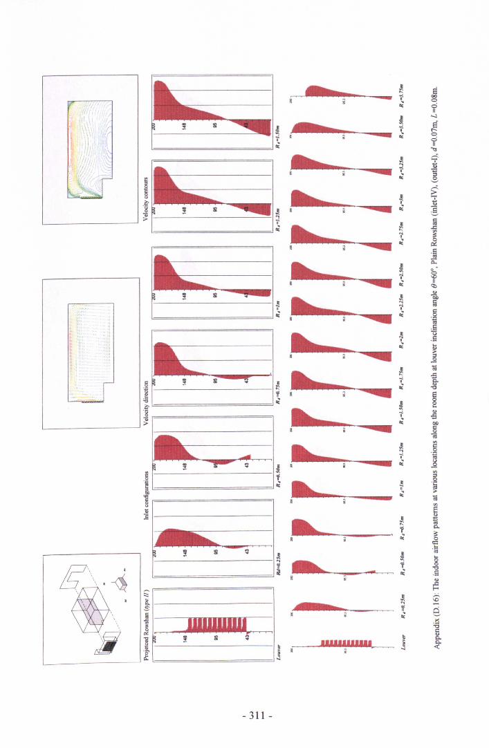
IIIa ~0 ~'1 ~ III'§8 ~
":5 laM
~ J1'" •~ill -
:,~:u
"11, ..ru
11111111
OTlIJ~~:"
s.~1-------------1.l:l;~======================~'gu r-=======================4
L- ~>
~IIIII~IIIII'I:'~ ~ OJ ~
- 311 -
n l El~- i 00
~ 00II
~ '-4.., 8;; r--~ 0
611
"'::s
.!i 1....- jji~ :;
~
l ~,. ..,~ ]_~ a
.Cl... ~"G ~ ~
.S'"
~ 0::.., 0... 0
" '"a ~ 11Q:)
~ ib... fil" 1'1a ~ .~
.Sl UIi' .S~ ~Q .§~ ~
-:3i: e-a ~ -e
~~.., ....if
..,-:3~ OIl=0t;l
l '"'" §....if 'n~ ]
'";:s.! .~
"~ ;.~'"
l~1:~ '"1 c,
~ ~<;:l.=
~ '"....'" g1 -e~ .S..,
~Ji ;..:..... '"1i' B~ .!S~
~ep..
~ ~..,....,....
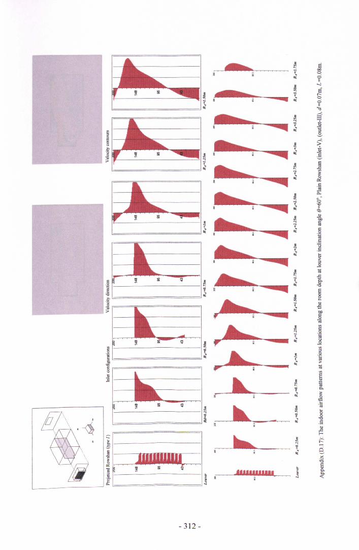
- -
ffl\\ .~..
\,
",
II """"I'I~
- 312 -
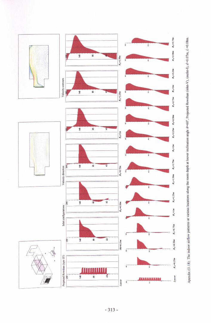
• Jl...C ;;
~
l1li EIi'
Q ~E~~...;
~• •~ 'i~.. !..,'ia ~Jl.. .....;~"i~~
i
AI 'iI'~
Q
~ -jl-------
i1--il~IIITIIlr.Illlmllrnlll;-'-..:~ ! :!l -e ~] ~F__ -_=-___________ .u ~
IL=====-----~,4''''''''''1. .s
- 313-

PUBLISHED ACADEMIC PAPERS
ENERGY, ECOLOGY, ARCHITECTUREPROCEEDINGS OF THE 16m INTERNATIONAL PLEA (PASSIVE AND
LOW ENERGY ARCHITECTURE)BRISBANE, AUSTRALIA, 22-24 SEPTEMBER 1999
PLEA'99
AIR FLOW CHARACTERISTICS THROUGH MODULATEDLOUVERED WINDOWS
A A Maghrabi* and S Sharples'·School of ArchitectureUniversity of Sheffield, Sheffield, SI 0 21N, United KingdomTel: (0114) 2220399Fax: (0114) 2798276e-mail: [email protected]
'Centre for the Built Environment, School of Environment and DevelopmentSheffield Hallam University, Sheffield, SI 1WB, United Kingdome-mail: [email protected]

Sustaining the future
ENERGYECOLOGYARCHITECTUREPLEA'99Proceedings of the sixteenth international PLEA(Passive and Low Energy Architecture) conferenceBrisbane, Australia22·24 September 1999
volume 1
edited bySteven V Szokolay
published by PLEA Internationalin conjunction withthe Department of Architecture, The University of QueenslandBrisbane
III
PLEA'99 Conference Refereed paper
AIR FLOW CHARACTERISTICS THROUGH MODULATEDLOUVERED WINDOWS.
A A Maghrabi* and S Sharples"*Department of ArchitectureUniversity of Sheffield, Sheffield, S10 2TN, United Kingdomtel: (0114) 222 0399fax: (0114) 279 8276e-mail: [email protected]. uk
'scnoo' of ConstructionSheffield Hallam University, Sheffield. S11WB. United Kingdome-mail: [email protected]
ABSRACT This study investigated the pressure flow characteristics over a number of full-scale modulated louvered windows (MLW). The various MLW parameters included louverinclination angle ({)), depth (L). aperture (d) .and the ratio of aperture/depth (d/L%). Airflowmodels were developed using both power law and quadratic model equations. By examiningthe coefficient of detennination (t) for both model equations. it was evident that the quadraticmodel equation suggested the best curves fit. The pressure flow characteristics as a functionof louver inclination angle ({)) in conjunction with (dlL) were presented in dimensionlessform. It was concluded that the pressure flow characteristics could be controlled if properconfigurations of MLW were to be chosen.
1 Introduction •~
Airflow within and around buildings has been a rich topic of research for many years. Henceseveral inv,stigations have been carried out on the mechanism of airflow through buildingsand- further - on various parameters governing air motions indoors. The Modulated LouverWindows (MLW) have been used for centuries as tool to achieve thermal comfort in buildingsby natural means. Although the body of literature pertaining to the MLW dealt with its solarcontrol performance. the optimization of its various dimensions and configurations in relation toventilation is far from being satisfactory. On the same hand, available studies were limited inscope (Yakubu & Sharples 1991, Tsangrassoulis et al. 1997, Pitts & Georgiadis 1994). In thiscontext, the design of window acquires special importance as air mainly flow inside buildingsthrough its apertures. Entire parametric studies are still needed to investigate the pressure andvelocity drops as functions of MLW various components.
Nevertheless, most of the available CFD packages deal with ventilation aspects in simplisticways and may not necessarily reflect complexities occurring in physical circumstance.Furthermore, theoretical representations of airflow passing through a window could not besimplified. Calculation methods in building ventilation tend to rely upon simple experimentaldata and general assumptions since precise calculations of unsteady flow characteristics ofopenings within building are rarely known. Hence it is more preferable to undertake laboratorymeasurements as the steady flow characteristic is a significant parameter to establish anyventilation measurements (Etheridge & Sandberg 1996).
'5(17
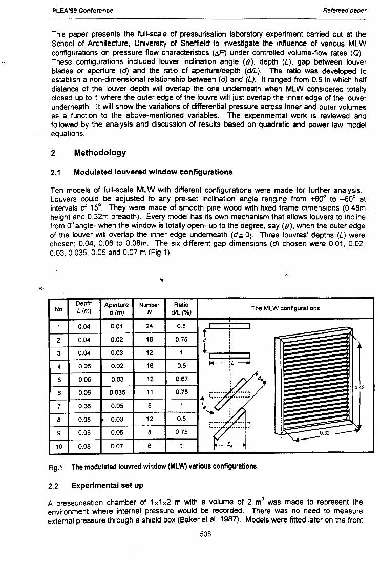
PLEA'99 Conference Refereed paper
..
This paper presents the full-scale of pressurisation laboratory experiment carried out at theSchool of Architecture, University of Sheffield'to investigate the influence of various MLWconfigurations on pressure flow charaCteristics (6P) under controlled volume-flow rates (Q).These configurations included louver inclination angle (8), depth (L), gap between louverblades or aperture (d) and the ratio of aperture/depth (dIL). The ratio was developed toestablish a non-dimensional relationship between (d) and (L). It ranged from 0.5 in which halfdistance of the louver depth will overlap the one underneath when MLW considered totallyclosed up to 1 where the outer edge of the louvre will just overlap the inner edge of the louverunderneath. It will show the variations of differential pressure across inner and outer volumesas a function to the above-mentioned variables. The experimental work is reviewed andfollowed by the analysis and discussion of results based on quadratic and power law modelequations.
2 Methodology
2.1 Modulated louvered window configurations
Ten models of full-scale MLW with different configurations were made for further analysis.Louvers could be adjusted to any pre-set inclination angle ranging from +60° to -60° atintervals of 15°. They were made of smooth pine wood with fixed frame dimensions (0.48mheight and 0.32m breadth). Every model has its own mechanism that allows louvers to inclinefrom 0° angle- when the window is totally open- up to the degree, say (8), when the outer edgeof the louver will overlap the inner edge underneath (d == 0). Three louvres' depths (L) werechosen; 0.04, 0.06 to 0.08m. The six different gap dimensions (d) chosen were 0.01, 0.02,0.03,0.035,0.05 and 0.07 m (Fig.1).
Depth Aperture Number Ratio The MLW configurationsNo L (m) d (m) N dIL (%)
I I1 0.04 0.01 24 0.5 , -t ,, ;-~2 0.04 0.02 16 0.75 d
,, -!, - -, --::, ~0.04 0.03 12 1 , --:3 I i I ~ ~
I+- :L~ ---: -4 0.06 0.02 16 0.5 , -,I""""':, ~, I""""":
5 0.06 0.03 12 0.67 , d, I'""""':::,, ~ -, 0.486 0.06 0.035 11 0.75 .......... .. ....... I""""':: ;;;... , . I"""""'::t .................... -, ~ -7 0.06 0.05 8 1 , I""""': ~e , ~..... , ~ -, -8 0.08 ~ 0.03 12 0.5 , -: ....,_.
:0 •••••••• " ••••• ''': "'"""'"=~
................ ..'9 0.08 0.05 8 0.75 , ..--,,,10 0.08 0.07 6 1 1.:" ~,
Fig.1 The modulated louvred window (MLW)various configurations
2.2 Experimental set up
A pressurisation chamber of 1x 1x2 m with a volume of 2 m3 was made to represent theenvironment where internal pressure would be recorded. There was no need to measureexternal pressure through a shield box (Baker et al. 1987). Models were fitted later on the front
508
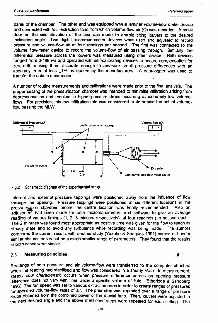
PLEA'99 Conference Refereed paper
panel of the chamber. The other end was equipped witt! a laminar volume-flow meter deviceand connected with four extraction fans from which volume-flow air (0) was recorded. A smalldoor on the side elevation of the box was made to enable tilting louvers to the desiredinclination angle. Two digital micromanometer devices were used and adjusted to recordpressure and volume-flow air at four readings per second. The first was connected to thevolume flow-meter device to record the volume-flow of air passing through. Similarly, thedifferential pressure across the louvers was measured using other device. Both devicesranged from 0-199 Pa and operated with self-calibrating devices to ensure compensation forzero-drift, making them accurate enough to measure small pressure differences with anaccuracy error of less ±1% as quoted by the manufacturers. A data-logger was used totransfer the data to a computer.
A number of routine measurements and calibrationswere made prior to the final analysis. Theproper sealing of the pressurisation chamber was intended to minimise infiltration arising fromdepressurisation and resulted in higher-pressure drops occurring at extremely low volume-flows. For precision, this low infiltration rate was considered to determine the actual volume-flow passing the MLW.
Sheltered pressure tappingsVolume now (Q)
1,+ "1 1! J
The MLW model i !l.-- 1m ~i 2m
Extraction
Laminar volume- now meter device
Fig.2 Schematic diagram of the experimental setup
Intemal and external pressure tappings were positioned away from the influence of flowthrough the opening. Pressure tappings were positioned at six different locations in thepressurig!ion ~mber before the cen~re location was finally recommen.ded. Also anadjustment· had been made for both rmcrcrnanometers and software to give an averagereac!lng of various timings (1, 2, 3 minutes respectively), at four readings per second each.The 2 minutes was found most appropriate as positive time was given for the flow to reach itssteady state and to avoid any turbulence while recording was being made. The authorscompared the current results with another study (Yakubu & Sharples 1991) carried out undersimilar circumstances but on a much smaller range of parameters. They found that the resultsin both cases were similar.
2.3 Measuring principles ,Readings of both pressure and air volume-flow were transferred to the computer attachedwhen the reading had stabilised and flow was considered in a steady state. In measurement,steady flow characteristic occurs when pressure difference across an opening pressuredifference does not vary with time under a specific volume of fluid (Etheridge & Sandberg1996). The fan speed was set to various extraction rates in order to create ranges of pressuresfor specified volume-flow rates of air. The prior step was repeated over a range of pressuredrops obtained from the combined power of the 4 axial fans. Then, louvers were adjusted tothe next desired angle and the above mentioned steps were repeated for each setting. The
509
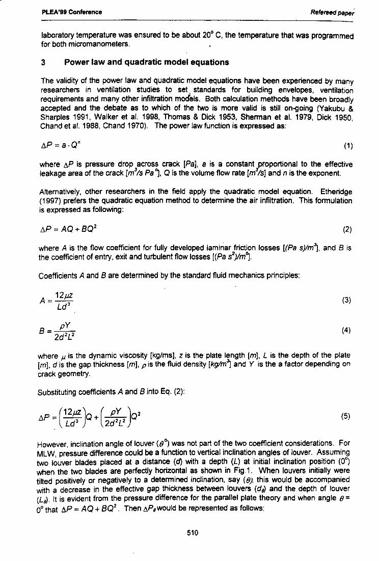
PLEA'99 Conference Refereed pape~
laboratory temperature was ensured to be about 20° C. the temperature that was programmedfor both micromanometers.
3 Power law and quadratic model equations
The validity of the power law and quadratic model equations have been experienced by manyresearchers in ventilation studies to set .. standards for building envelopes. ventilationrequirements and many other infiltration models. Both calculation methods have been broadlyaccepted and the debate as to which of the two is more valid is still on-going (Yakubu &Sharples 1991. Walker et al. 1998. Thomas & Dick 1953. Sherman et al. 1979. Dick 1950.Chand et al. 1988. Chand 1970). The power law function is expressed as:
f1p = eo" (1)
where ~P is pressure drop across crack [Pal. s is a constant proportional to the effectiveleakage area of the crack [m31s Pa j. Q is the volume flow rate [m3ls] and n is the exponent.
Alternatively, other researchers in the field apply the quadratic model equation. Etheridge(1997) prefers the quadratic equation method to determine the air infiltration. This formulationis expressed as following:
(2)where A is the flow coefficient for fully developed laminar friction losses [(Ps s)/m1, and B isthe coefficient of entry. exit and turbulent flow losses [CPa s2)lm~.
Coefficients A and B are determined by the standard fluid mechanics principles:
(3)
(4)
where jJ is the dynamic viscosity [kg/ms]. z is the plate length [m]. L is the depth of the plate[m]. d is the gap thickness [m]. p is the fluid density [kglm1 and Y is the a factor depending oncrack geometry.
Substituting coefficients A and B into Eq. (2):
(5)
However. inclination angle of louver (0) was not part of the two coefficient considerations. ForMLW, pressure difference could be a function to vertical inclination angles of louver. Assumingtwo louver blades placed at a distance (d) with a depth (L) at initial inclination position (0°)when the two blades are perfectly horizontal as shown in Fig.1. When louvers initially weretilted positively or negatively to a determined inclination. say (0). this would be accompaniedwith a decrease in the effective gap thickness between louvers (ds) and the depth of louver(Ls). It is evident from the pressure difference for the parallel plate theory and when angle 0 =0° that 6P = AQ + BQ2. Then ~Pewould be represented as follows:
510
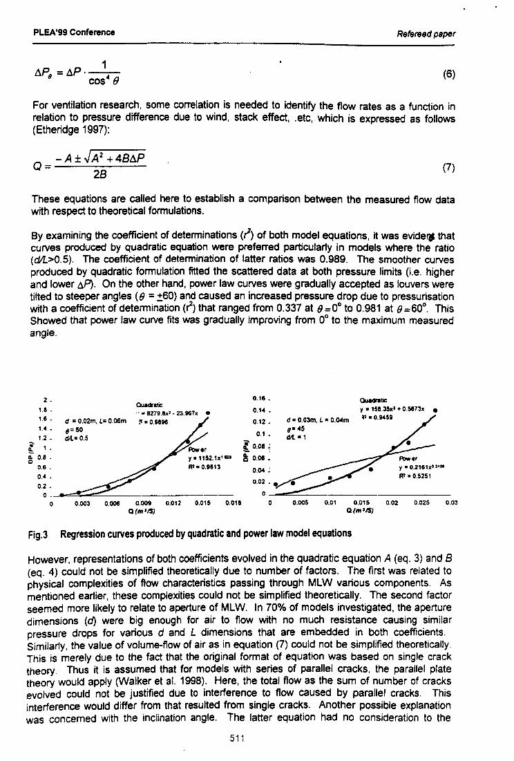
PLEA'99 Conference Refereed paper
1~P(l =~p. 4COS o (6)
For ventilation research, some correlation is needed to identify the flow rates as a function inrelation to pressure difference due to wind, stack effect, .etc, which is expressed as follows(Etheridge 1997):
Q = - A ± .JA 2 + 4B~P2B (7)
These equations are called here to establish a comparison between the measured flow datawith respect to theoretical formulations.
By examining the coefficient of determinations (I) of both model equations, it was evide'_ thatcurves produced by quadratic equation were preferred particularly in models where the ratio(dIL>O.S). The coefficient of determination of latter ratios was 0.989. The smoother curvesproduced by quadratic formulation fitted the scattered data at both pressure limits (i.e. higherand lower tlp). On the other hand, power law curves were gradually accepted as louvers weretilted to steeper angles (e = :t60) and caused an increased pressure drop due to pressurisationwith a coefficient of determination «() that ranged from 0.337 at e =0° to 0.981 at e =60°. ThisShowed that power law curve fits was gradually improving from 0° to the maximum measuredangle.
2.1.8 _1.6 _
1.4 •1.2 _
'i'!!:. 1.~ 0.8.
0.6 _
0.4.
0.2 "o __ ~~~ . _
o
Quadratic... 8279.Bx'· 23.967x •
d = 0.02m. L= O.06m ~ • 0.9896(1=80dII.= 0.5
0.16.
0.14 "
0.12 •
0.1 •
d • O.Olm. L • O.04m(1.45dII. • 1
Quadraticy II 1S8.35xl + 0.5e73x •~ -0.9459
y ·1152.1xIlZIRi·0.U13
l 0.08 ~
~ 0.01 ~
0.04 ; y ·0.2161x· ....
Ri·0.5251
0.003 0.008 0.009 0.012 0.015 0.01aQ(m'lS)
0.005 0.01 0.015 0.02 0.025 0.03Q(m'lS)
Fig.3 Regression curves produced by quadratic and power law model equations
However, representations of both coefficients evolved in the quadratic equation A (eq. 3) and B(eq. 4) could not be simplified theoretically due to number of factors. The first was related tophysical complexities of flow characteristics passing through MLW various components. Asmentioned earlier, these complexities could not be simplified theoretically. The second factorseemed more likely to relate to aperture of MLW. In 70% of models investigated, the aperturedimensions (d) were big enough for air to flow with no much resistance causing similarpressure drops for various d and L dimensions that are embedded in both coefficients.Similarly, the value of volume-flow of air as in equation (7) could not be Simplified theoretically.This is merely due to the fact that the original format of equation was based on single cracktheo~. Thus it is assumed that for models with series of parallel cracks, the parallel platetheory would apply (Walker et al. 1998). Here, the total flow as the sum of number of cracksevolved could not be justified due to interference to flow caused by parallel cracks. Thisinterference would differ from that resulted from single cracks. Another possible explanationwas concerned with the inclination angle. The latter equation had no consideration to the
511
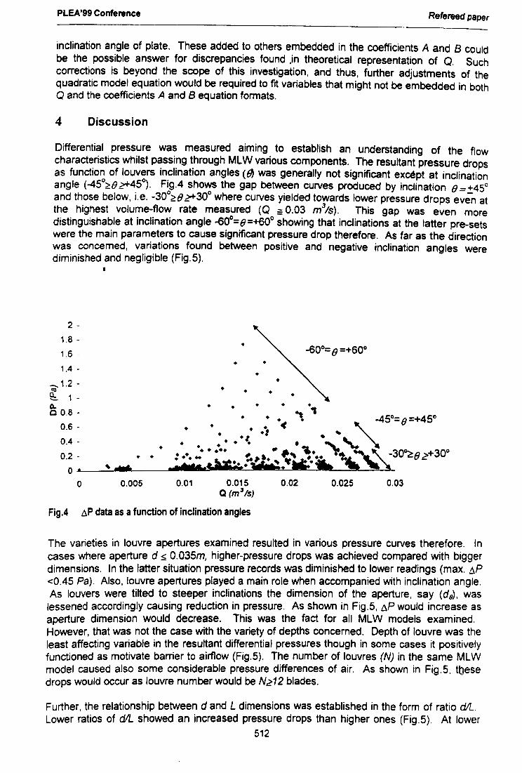
PLEA'99 Conference Refereed paper
inclination angle of plate. These added to others embedded in the coefficients A and B couldbe the possible answer for discrepancies found ,in theoretical representation of Q. Suchcorrections is beyond the scope of this investigation, and thus, further adjustments of thequadratic model equation would be required to fit variables that might not be embedded in bothQ and the coefficients A and B equation formats.
4 Discussion
Differential pressure was measured aiming to establish an understanding of the flowcharacteristics whilst passing through MLW various components. The resultant pressure dropsas function of louvers inclination angles (~ was generally not significant except at inclinationangle (-4So~O~4So). Fig.4 shows the gap between curves produced by inclination 0=+450
and those below, i.e. -300~O~30° where curves yielded towards lower pressure drops even atthe highest volume-flow rate measured (Q == 0.03 m3/s). This gap was even moredistinguishable at inclination angle -60°=0=+60° showing that inclinations at the latter pre-setswere the main parameters to cause significant pressure drop therefore. As far as the directionwas concerned, variations found between positive and negative inclination angles werediminished and negligible (Fig.S).
•
2 -1.8 -1.6 .
1.4 -
-.. 1.2 -lae:.. 1-
a.. • • • • •C 0.8 - • •• ~.. -450= ()=+4So
0.6 - ••• • <tt ~• .t • 4t.
0.4 - • • • • • •• ~ .,. "-0.2 - ..: •••• : • ••• !.,.a•... , ,... 1'''-.~ ,\-30~O ,?+30°
OL. __ ~~~tMd~ .as.td~'~4~h~.~~~·~fi~.r~~u.~~~tt~I·~1t~~~,.~~,_~-~__~~o
• -60°= 0 =+60°• •
• •• • • •
0.015Q (m3/s)
Fig.4 ~p dataasafunctionof inclinationangles
0.005 0.01 0.02 0.025 0.03
The varieties in louvre apertures examined resulted in various pressure curves therefore. Incases where aperture o s 0.03Sm, higher-pressure drops was achieved compared with biggerdimensions. In the latter situation pressure records was diminished to lower readings (max. ~P<0.45 Pa). Also, louvre apertures played a main role when accompanied with inclination angle.As louvers were tilted to steeper inclinations the dimension of the aperture, say (de), waslessened accordingly causing reduction in pressure. As shown in Fig.S, tP would increase asaperture dimension would decrease. This was the fact for all MLW models examined.However, that was not the case with the variety of depths concerned. Depth of louvre was theleast affecting variable in the resultant differential pressures though in some cases it positivelyfunctioned as motivate barrier to airflow (Fig.S). The number of louvres (N) in the same MLWmodel caused also some considerable pressure differences of air. As shown in Fig.S, thesedrops would occur as louvre number would be N,?12 blades.
Further, the relationship between d and L dimensions was established in the form of ratio d/L.Lower ratios of dlL showed an increased pressure drops than higher ones (Fig.S). At lower
512
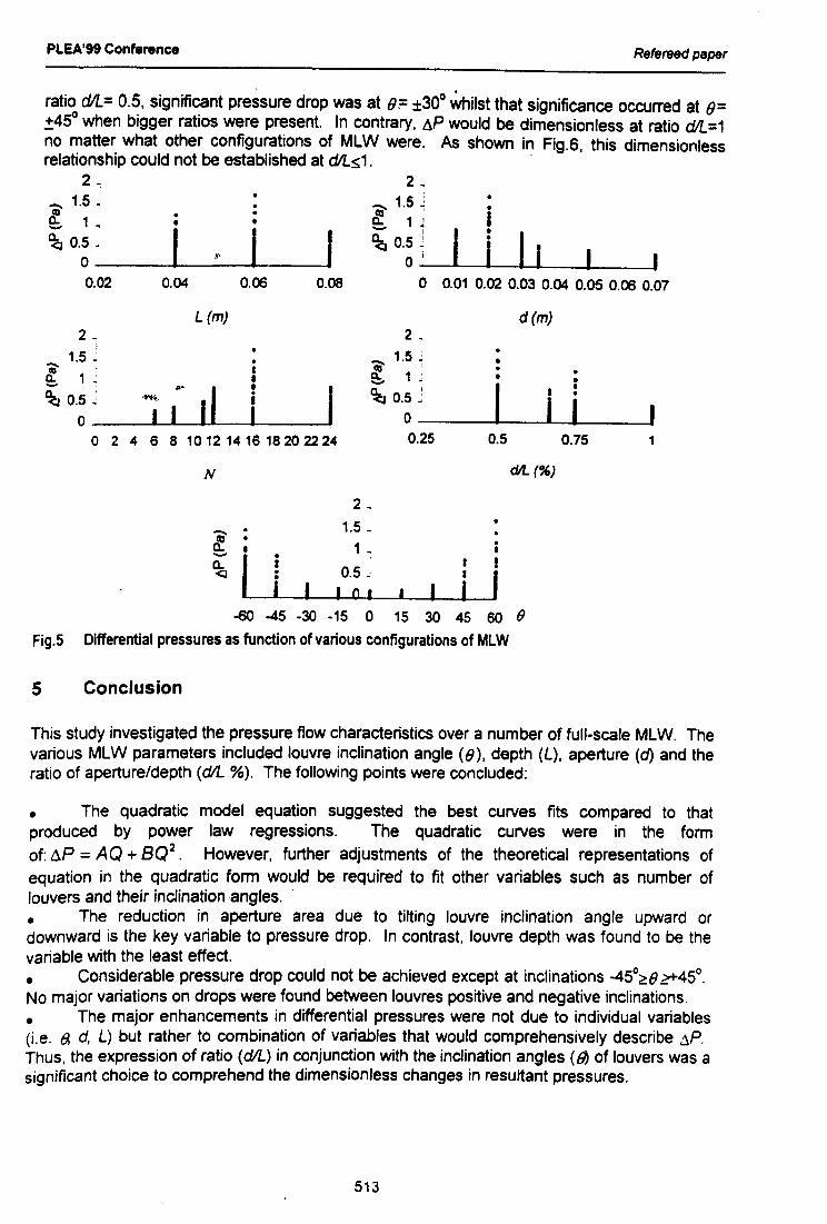
PLEA'99 Conference Refereed paper
ratio d/L= 0.5. significant pressure drop was at B~ ±30o ~ilst that significance occurred at B=.:t45° when bigger ratios were present. In contrary. 6.P would be dimensionless at ratio d/L=1no matter what other configurations of MLW were. As shown in Fig.6. this dimensionlessrelationship could not be established at dlLs;1. .
2 ~ 2 _-.. 1.5_ · ~ 1.5 jl 1_ . · ~ 1 I• • - ~I I I I
~ 0.5- ~ 0.5 ~0
~, o I
0.02 0.04 0.06 0.08 0
L(m)2 ~ 2 _
i1.5 ~ · -.. 1.5 J
~ I ~ 1:1 ~ • - -..... ...II
• I ~ 0.5 ~~ 0.5 ~ 'w~. i0 I I I 00 2 4 6 8 1012 14 16 182022 24 0.25
•
Ii•i II I I
0.01 0.02 0.03 0.04 0.05 0.06 0.07
d(m)
•· •• •
I I ••I I
0.5 0.75 1
dIl ("JN
2 _
iii' · 1.5 _•c; • 1 _- I •
Cl. r 0.5 ~<J ·•i I I o •-60 -45 -30 -15 0
•
·•I Ir II I
15 30 45 60 (J
Fig.5 Differential pressures as function of various configurations of MLW
5 Conclusion
This study investigated the pressure flow characteristics over a number of full-scale MLW. Thevarious MLW parameters included louvre inclination angle (B), depth (L). aperture (d) and theratio of aperture/depth (dIL %). The following points were concluded:
• The quadratic model equation suggested the best curves fits compared to thatproduced by power law regressions. The quadratic curves were in the formof: tlP = AQ + BQ2. However. further adjustments of the theoretical representations ofequation in the quadratic form would be required to fit other variables such as number oflouvers and their inclination angles. .• The reduction in aperture area due to tilting louvre inclination angle upward ordownward is the key variable to pressure drop. In contrast, louvre depth was found to be thevariable with the least effect.• Considerable pressure drop could not be achieved except at inclinations -45°~():?+45°.No major variations on drops were found between louvres positive and negative inclinations.• The major enhancements in differential pressures were not due to individual variables(i.e. 8. d, L) but rather to combination of variables that would comprehensively describe ,1P.Thus. the expression of ratio (dIL) in conjunction with the inclination angles (fIJ of louvers was asignificant choice to comprehend the dimensionless changes in resultant pressures.
513
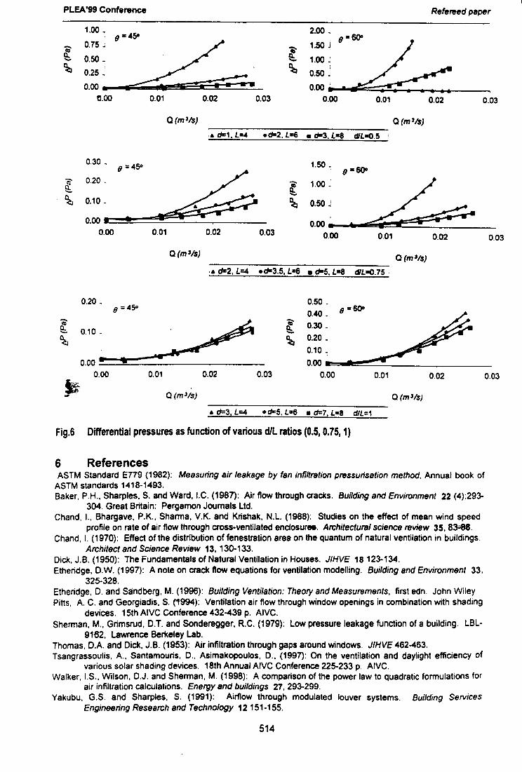
PLEA'99 Conference Refereed paper
1.00 - SO
0.75~ (J~=4
0.50 _ .
~::~~Cl.OO 0.01 0.02 0.03
2.00 ,
1.50J 8=~6()D1.00 ~
0.50 "0.00 ••
0.00 0.01 0.02 0.03
Q(m'~) Q(ml~),a eta1, L... .0-2, L-=6 .11-3. L-B dlLrcO.5
0.30,(J=4SO 1.50_
k(J=6()D
~0.20. 'i' 1.00_
~
.._ ~~ 0.10 _ ~ 0.50 J
0.00 • • 0.00 • ~0.00 0.01 0.02 0.03 0.00 0.01 0.02 0.03
Q (m'/s)
·6 cfc2. L=4 .d=3.5, L-=6 • d-5, L-B dlLrcO.75.
Q (m'!s)
0.20 _
0.00 0.01 0.02
0.50 _0.40 _ (J = 6()D
L'i' 0.30 _~~
0.20 _0.10 _0.00 .. •
0.03 0.00 0.01 0.02 0.03
a (m'!s)
(J = 450
a (m'!s)
6 d=3, L=4 .dz5, L·S • d=7, La8 dlL=1
Fig.6 Differential pressures as function of various dlL ratios (0.5, 0.75, 1)
6 ReferencesASTM Standard E779 (1982): Measuring air leakage by fan infiltration pressurisation method. Annual book ofASTM standards 1418-1493.Baker. P.H., Sharples. S. and Ward, I.C. (1987): Air flow through cracks. Building and Environment 22 (4):293-
304. Great Britain: Pergamon Journals Ltd.Chand, I.. Bhargave, P.K., Shanna, V.K. and Krishak. N.L. (1988): Studies on the effect of mean wind speed
profile on rate of air flow through cross-ventilated enclosuree. Architectural science review 35. 8J:.188.Chand. I. (1970): Effect of the distribution of fenestration area on the quantum of natural ventilation in buildings.
Architect and Science Review 13,130-133.Dick. J.B. (1950): The Fundamentals of Natural Ventilation in Houses. JIHVE 18123-134.Etheridge, D.W. (1997): A note on crack flow equations for ventilation modelling. Building and Environment 33.
325-328.Etheridge, D. and Sandberg. M. (1996): Building Ventilation: Theory and Measurements, first edn. John WileyPitts, A. C. and Georgiadis, S. (1994): Ventilation air flow through window openings in combination with shadIng
devices. 15th AIVC Conference 432-439 p. AIVC.Sherman, M., Grimsrud, D.T. and Sonderegger, R.C. (1979): Low pressure leakage function of a building. LBL-
9162, Lawrence Berkeley Lab.Thomas, D.A. and Dick, J.B. (1953): Air infiltration through gaps around windows. JIHVE 462-463.Tsangrassoulis, A., Santamouris, D., Asimakopoulos, D., (1997): On the ventilation and daylight efficiency of
various solar shading devices. 18th Annual AIVC Conference 225-233 p. AIVC.Walker, I.S., Wilson, D.J. and Shennan, M. (1998): A comparison of the power law to quadratic formulations for
air infiltration calculations. Energy and buildings 27,293-299.Yakubu, G.S. and Sharples, S. (1991): Airflow through modulated louver systems. Building Services
Engineering Research and Technology 12151·155.
514

INNOVATIONS IN VENTILATION TECHNOLOGY21sT ANNUAL CONFERENCE
THE HAGUE, NETHERLANDS, 26-29 SEPTEMBER 2000
AIRFLOW THROUGH LOUVERS: AN EXPERIMENTALAND CFD STUDY
S Sharples* and A A Maghrabi t
.Centre for the Built Environment, School of Environment and DevelopmentSheffield Hallam University, Sheffield, SI 1WB, United Kingdome-mail: [email protected]
"School of ArchitectureUniversity of Sheffield, Sheffield, SI 0 2TN, United KingdomTel: (0114) 2220399Fax: (0114) 2798276e-mail: [email protected]
SYNOPSISIn this study a series of parametric laboratory measurements were made of the velocitiesoutside, Ve, and inside, Vi, a full-scale louver positioned in a rectangular opening located in avertical wall forming part of a 1m x 1m x 2m deep model room. The louver parametersexamined, for external incident wind speeds from 0.6 to 2.5 mis, included louver blade depth(L), aperture (d) and distance from the louver in to room (Rd). For this initial study the bladesof the louvers for each experiment were horizontal with an inclination angle e of 0°. It wasconcluded that louver aperture dimensions and distance from louver both played major rolesin determining the magnitude of the velocity drop, whilst the effect on v;lve of louver depthdimensions was smaller. Experimental results were compared against velocity drop valuespredicted by the computational fluid dynamics (CFD) program FLUENT. A comparisonbetween the experimental data and the CFD predicted results showed a generally goodagreement for positions close to the internal surface of the louver. Further in to the room thecomparisons showed a greater divergence.
INTRODUCTIONIn recent years there has been a renewed interest in the use of natural ventilation systems inbuildings as a sustainable means of supplementing or replacing mechanical ventilation and airconditioning (see, for example, NatVent[l]). For large, non-domestic buildings, in particular,the natural ventilation inlets will often consist of large wall openings with louvered covers.Night-time ventilation of buildings can also make use of secure louvered openings.
A recent study of through-the-wall ventilators was performed at the Building ResearchEstablishment (White et al[2]). This indicated that interactions between components in theventilators, such as louvers, insect screens and internal flowpaths, meant that the airflowperformances of the ventilators were highly variable and not easily described by standardflow equations. One way of gaining a better understanding of these interactions is throughanalysis of the performance of the individual components. For louvers there is only limiteddesign information on the airflow performance of louvers and how louver parameters (suchas blade depth, blade thickness, spacing between blades and blade orientation) interact toproduce the overall louver flow and velocity characteristics. This study sort to gain a betterunderstanding of some of these interactions.
A number of researchers have investigated the effect of various window opening parameters,such as size, location and orientation, on improving indoor airflow quantity and distribution,for example Brandle and Boehm[3], Jong and Bot[4] and Sobin[5]. Others have investigatedthe specific mechanisms of airflow through louvers and the various parameters governingindoor air motion such as louver depth, aperture and inclination angle. Yakubu andSharples[6] and Pitts and Georgiadis[7] focused on pressure drops across the louvers.Recently, Maghrabi and Sharples[8] investigated the influence of various louverconfigurations on pressure flow characteristics CM) under controlled volume-flow rates (Q).They used a pressurised room chamber technique, originally developed by Baker et al[9], toinvestigate airflow through cracks. Recent louver airflow work was carried out by Oliveiraand Bittencourt[lO], who used louvers with dimensions similar to those of the present study.
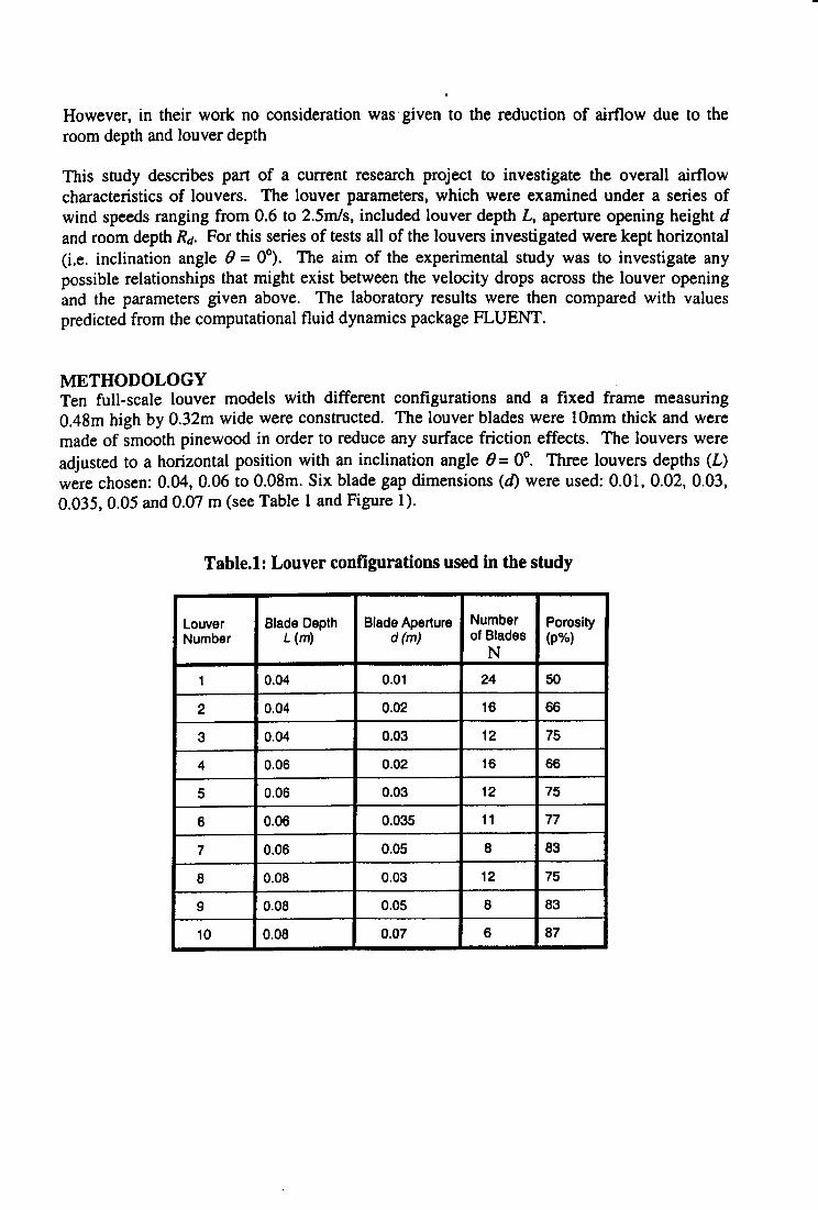
However, in their work no consideration was' given to the reduction of airflow due to theroom depth and louver depth
This study describes part of a current research project to investigate the overall airflowcharacteristics of louvers. The louver parameters, which were examined under a series ofwind speeds ranging from 0.6 to 2.5m/s, included louver depth L, aperture opening height dand room depth Rd. For this series of tests all of the louvers investigated were kept horizontal(i.e. inclination angle ()= 0°). The aim of the experimental study was to investigate anypossible relationships that might exist between the velocity drops across the louver openingand the parameters given above. The laboratory results were then compared with valuespredicted from the computational fluid dynamics package FLUENT.
METHODOLOGYTen full-scale louver models with different configurations and a fixed frame measuring0.48m high by 0.32m wide were constructed. The louver blades were 10mm thick and weremade of smooth pinewood in order to reduce any surface friction effects. The louvers wereadjusted to a horizontal position with an inclination angle ()= 0°. Three louvers depths (L)were chosen: 0.04, 0.06 to 0.08m. Six blade gap dimensions (d) were used: 0.01, 0.02, 0.03,0.035,0.05 and 0.07 m (see Table 1 and Figure 1).
Table.1: Louver configurations used in the study
Louver Blade Depth Blade Aperture Number PorosityNumber L (m) d(m) of Blades (p%)
N
1 0.04 0.Q1 24 50
2 0.04 0.02 16 66
3 0.04 0.03 12 75
4 0.06 0.02 16 66
5 0.06 0.03 12 75
6 0.06 0.035 11 77
7 0.06 0.05 8 83
8 0.08 0.03 12 75
9 0.08 0.05 8 83
10 0.08 0.07 6 87
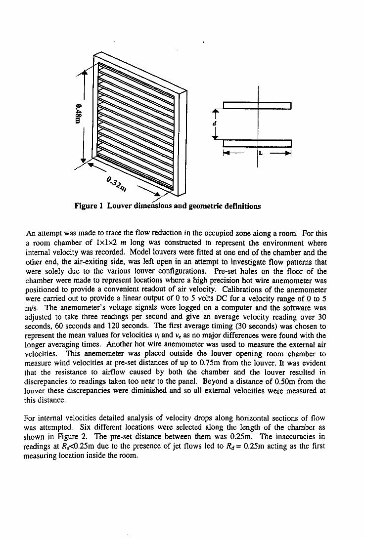
a..J<IQ ~ .
.....:.--Figure 1 Louver dimensions and geometric definitions
fL
d
An attempt was made to trace the flow reduction in the occupied zone along a room. For thisa room chamber of lxlx2 m long was constructed to represent the environment whereinternal velocity was recorded. Model louvers were fitted at one end of the chamber and theother end, the air-exiting side, was left open in an attempt to investigate flow patterns thatwere solely due to the various louver configurations. Pre-set holes on the floor of thechamber were made to represent locations where a high precision hot wire anemometer waspositioned to provide a convenient readout of air velocity. Calibrations of the anemometerwere carried out to provide a linear output of 0 to 5 volts DC for a velocity range of 0 to 5mls. The anemometer's voltage signals were logged on a computer and the software wasadjusted to take three readings per second and give an average velocity reading over 30seconds, 60 seconds and 120 seconds. The first average timing (30 seconds) was chosen torepresent the mean values for velocities Vj and Ve as no major differences were found with thelonger averaging times. Another hot wire anemometer was used to measure the external airvelocities. This anemometer was placed outside the louver opening room chamber tomeasure wind velocities at pre-set distances of up to 0.75m from the louver. It was evidentthat the resistance to airflow caused by both the chamber and the louver resulted indiscrepancies to readings taken too near to the panel. Beyond a distance of 0.50m from thelouver these discrepancies were diminished and so all external velocities were measured atthis distance.
For internal velocities detailed analysis of velocity drops along horizontal sections of flowwas attempted. Six different locations were selected along the length of the chamber asshown in Figure 2. The pre-set distance between them was 0.25m. The inaccuracies inreadings at Rtt<O.25m due to the presence of jet flows led to Rd = 0.25m acting as the firstmeasuring location inside the room.
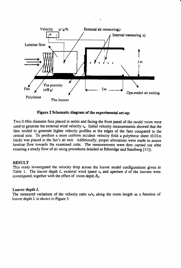
External air measuring)Internal measuring vJ
Laminar flow
t• • 1m
2mOpe-ended air exiting
PolytheneThe louver
Figure 2 Schematic diagram of the experimental set-up.
Two 0.48m diameter fans placed in series and facing the front panel of the model room wereused to generate the external wind velocity Ye. Initial velocity measurements showed that thefans tended to generate higher velocity profiles at the edges of the fans compared to thecentral axis. To produce a more uniform incident velocity field a polythene sheet (O.OImthick) was placed at the fan's air exit. Additionally, proper alterations were made to assurelaminar flow towards the examined units. The measurements were then carried out afterensuring a steady flow of air using procedures detailed in Etheridge and Sandberg [lI]).
RESULTThis study investigated the velocity drop across the louver model configurations given inTable 1. The louver depth L, external wind speed Ve and aperture d of the louvers wereinvestigated, together with the effect of room depth Rd.
Louver depth LThe measured variations of the velocity ratio v/ve along the room length as a function oflouver depth L is shown in Figure 3.
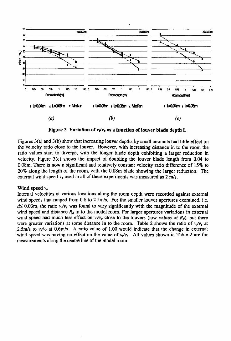
mr-----------------~mr-------------------m~------------------._~~~~~~--~-...•-----------
•'." "......,.......,..•'I .
.......~ I
im.~ ••••~~r---------.~...~- ..~~~----~~I~-----------··-··~·.~·-··~··~___
:. , ..~~--------------~---~~-------------------
~ .....•.•. "". j •••••.,
" ".
~~-------------------Or-~~~~~--~~~o ~ ~ ~ ~ ~ ~o ~ ~ ~ 125 ~ \15 0 ~ 05 Oit; 125 ~ \15
(a) (b) (c)
Figure 3 Variation of vJve as a function of louver blade depth L
Figures 3(a) and 3(b) show that increasing louver depths by small amounts had little effect onthe velocity ratio close to the louver. However, with increasing distance in to the room theratio values start to diverge, with the longer blade depth exhibiting a larger reduction invelocity. Figure 3(c) shows the impact of doubling the louver blade length from 0.04 toO.OBm.There is now a significant and relatively constant velocity ratio difference of 15% to20% along the length of the room, with the O.OBmblade showing the larger reduction. Theexternal wind speed Ve used in all of these experiments was measured as 2 mls.
Wind speed v,Internal velocities at various locations along the room depth were recorded against externalwind speeds that ranged from 0.6 to 2.5m1s. For the smaller louver apertures examined, Le.d'5 0.03m, the ratio v/ve was found to vary significantly with the magnitude of the externalwind speed and distance Rd in to the model room. For larger apertures variations in externalwind speed had much less effect on v/ve close to the louvers (low values of Rd), but therewere greater variations at some distance in to the room. Table 2 shows the ratio of v/ve at2.5mJs to v/ve at 0.6m1s. A ratio value of 1.00 would indicate that the change in externalwind speed was having no effect on the value of v/ve• All values shown in Table 2 are formeasurements along the centre line of the model room
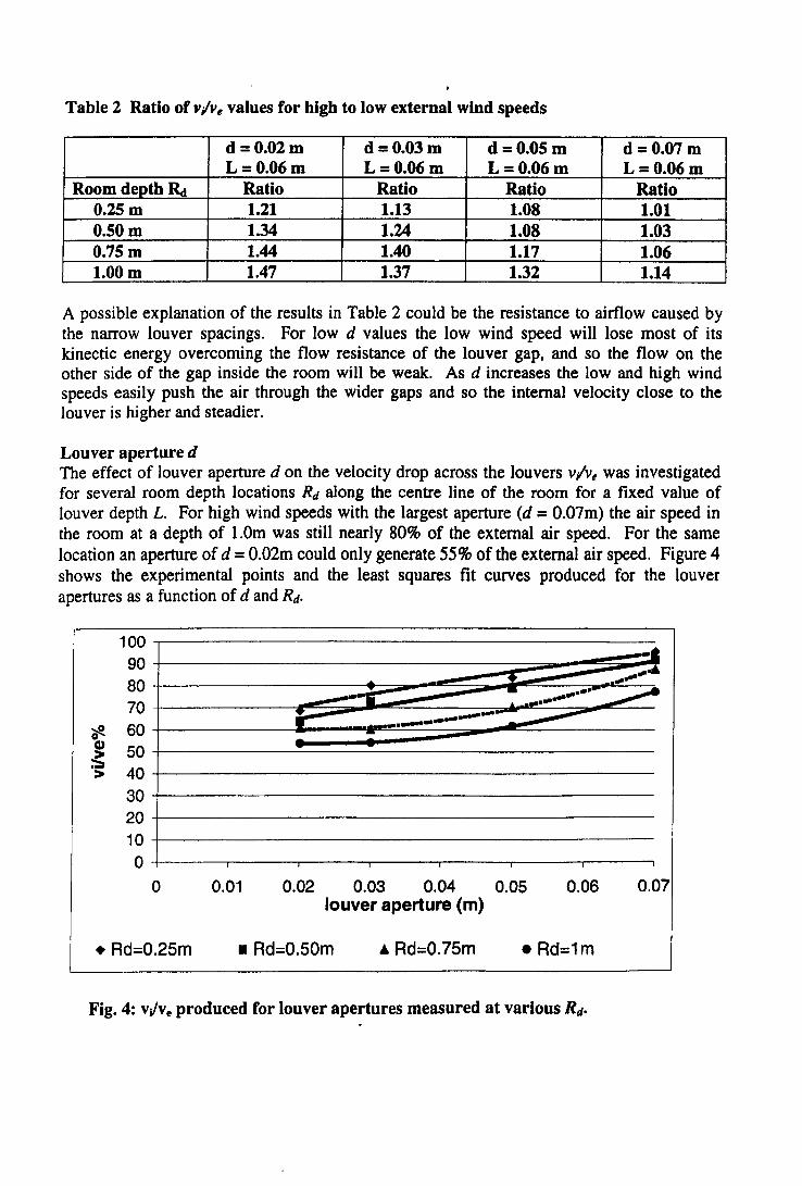
Table 2 Ratio of v/ve values for high to low external wind speeds
d =0.02m d = 0.03 m d =0.05 m d = 0.07 mL =0.06m L=0.06 m L=0.06m L =0.06 m
Room depth R.t Ratio Ratio Ratio Ratio0.25 m 1.21 1.13 1.08 1.010.50m 1.34 1.24 1.08 1.030.75m 1.44 1.40 1.17 1.061.00m 1.47 1.37 1.32 1.14
A possible explanation of the results in Table 2 could be the resistance to airflow caused bythe narrow louver spacings. For low d values the low wind speed will lose most of itskinectic energy overcoming the flow resistance of the louver gap, and so the flow on theother side of the gap inside the room will be weak. As d increases the low and high windspeeds easily push the air through the wider gaps and so the internal velocity close to thelouver is higher and steadier.
Louver aperture dThe effect of louver aperture d on the velocity drop across the louvers vlve was investigatedfor several room depth locations R« along the centre line of the room for a fixed value oflouver depth L. For high wind speeds with the largest aperture (d = 0.07m) the air speed inthe room at a depth of 1.Omwas still nearly 80% of the external air speed. For the samelocation an aperture of d = O.02mcould only generate 55% of the external air speed. Figure 4shows the experimental points and the least squares fit curves produced for the louverapertures as a function of d and Rd.
100908070
~ 600Cl) 50~> 40
3020100
_,........ • ..........
_.---r:: - ........-~...........• ...--~r ._.--_ ..--
0.02 0.03 0.04 0.05louver aperture (m)
0.06 0.07o 0.01
• Rd=O.75m• Rd=O.50m • Rd=1m• Rd=O.25m
Fig. 4: wv, produced for louver apertures measured at various Rd.
CFD APPRAISAL.Computational Fluid Dynamics (CFD) can be used to predict the indoor velocities and overallventilation effectiveness of natural or mechanical air distribution systems. In this studyFLUENT [12] software was used for the CFD simulation of the louver-room configuration.A number of case studies were tested first to simulate the laboratory work. The specificationof boundary conditions was carefully established as the assumed boundary conditions playavital role in the results predicted from the simulations. A refined grid domain of 250 x 100nodes was established in the room and the vicinity of the louvers. The k-e model wasimplemented in the simulation to represent the flow turbulence. The k-e model is a widelyused method to represent turbulence in CFD (Jones and Whittle, [13]). The results of velocityreadings were taken when the simulation process was fully converged or when the globalabsolute residuals from the iterations reached a very low limit (approximately less thanlxlO-4).
The CFD analysis was used to predict the ratio of v;lve for comparison with the experimentaldata. Two sets of comparisons were made. In the first the measured and predicted values ofv;lve were compared at a point close to the louver (Rd = 0.25m) for louver (L, d) values of (4,2), (6, 3.5) and (8, 5). The results from this are presented in Figure 5. There is goodagreement for the reasonably strong airflows encountered very close to the room side of thelouvers, which gives encouragement that CFD can be used to predict the local air velocitiesaround louvers. In the second comparison the room depth was varied from 0.25 to 1.5m andthe v;lve ratios from CFD and experiment were examined. The results for two louver settings(L=0.08, d=0.03 and L=0.08, d=O.07 ) are shown in Figure 6. These results are representativeof the trends observed in other louver combinations The agreement is still good close to thelouver, and the general form of the variation with Rd is similar. However, there is a markeddivergence between CFD and experimental results as Rd increases, and towards the back ofthe room model the differences become very large (around 50%). The design of the roommodel left the back of the model open with no obstructing wall. It may be that this boundarycondition needs to be better defined in future studies as the airflows in this location will beweaker and so more susceptible to large variations over small spatial distances.
CONCLUSIONSThis parametric and CFD study of airflow through louvers has highlighted the following:
• airflow velocities in a room containing a louver covered opening result from aninteraction of louver geometry, room geometry and prevailing wind conditions
• the key parameters for louver performance are the aperture opening (distance betweenlouver blades) and the distance from the louvers in to the room
• small changes in the depth of the louver blade do not have a significant effect on airflowvelocities
• CFD analysis has been successfully used to predict air velocities in the region close to theroom side of the louvers
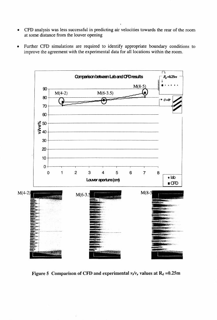
• CFD analysis was less successful in predicting air velocities towards the rear of the roomat some distance from the louver opening
• Further CFD simulations are required to identify appropriate boundary conditions toimprove the agreement with the experimental data for all locations within the room.
nOJ. JDiscn IEtv.eEn Lm cn:I CFDres.fts r-~~ -
~IM(8-51 ~ • I •• ••
00 "M(4-2) M(6-3.5) ----~00()_ r_'
~70
-\;_)
00
~50G)
~40
3)
a>10
00 1 2 3 4 5 6 7 8
I..o.IIe' ~(~.Icb.0=0
Figure 5 Comparison of CFD and experimental v/ve values at RI =O.25m
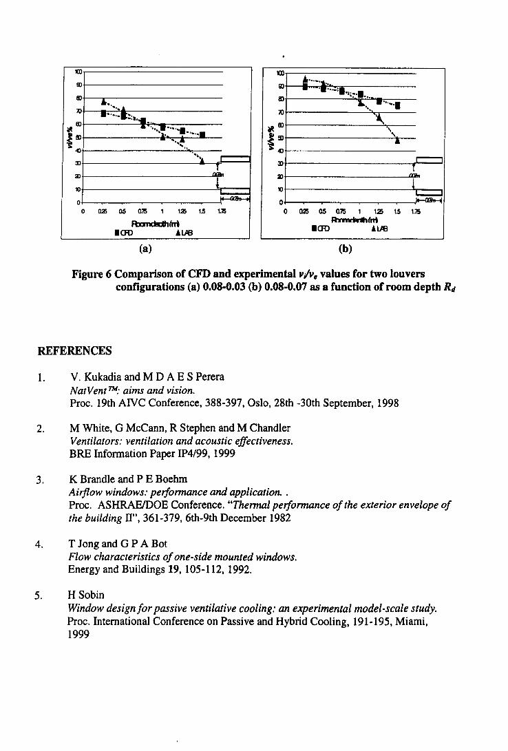
mII)
8)
j".,. "10 •.....•~....-.•.
~8) •.... :-r •.•.••~!D
'1· •.•.••- ',,~-o .,3J
..~~
a:l ~
10l
00 Q2i as 075 1 1.25 1.5 t75
FbllhcaJl.lrrlICfD 'LJe
(a)
1(J) !.....'ll••II) - ......:•.8)
·,t:-·.....I..........
10 ".
~ID.~.
"
~!D"•
4l
3J r---1
1..a:l
10 t0 ~0 Q2i as Q75 1 13 1.5 1.75
R"allddhlmICfD !IJIB
(b)
Figure 6 Comparison of CFD and experimental v/v. values for two louversconfigurations (a) 0.08-0.03 (b) 0.08-0.07 as a function of room depth Rd
REFERENCES1. V. Kukadia and M D A E S Perera
NatVentTM.· aims and vision.Proc. 19th AIVC Conference, 388-397, Oslo, 28th -30th September, 1998
2. M White, G McCann, R Stephen and M ChandlerVentilators: ventilation and acoustic effectiveness.BRE Information Paper IP4/99, 1999
3. K Brandle and P EBoehmAirflow windows: performance and application ..Proc. ASHRAFJDOE Conference. "Thermal performance of the exterior envelope ofthe building TI", 361-379, 6th-9th December 1982
4. T Jong and G P A BotFlow characteristics of one-side mounted windows.Energy and Buildings 19, 105-112, 1992.
5. H SobinWindow design for passive ventilative cooling: an experimental model-scale study.Proc. International Conference on Passive and Hybrid Cooling, 191-195, Miami,1999
6. G S Yakubu and S SharplesAirflow through modulated louver systems.Building Services Engineering Research and Technology 12 (4), 151-155, 1991.
7. A C Pitts and S GeorgiadisVentilation air flow through window openings in combination with shading devices.Proc. 15th AIVC Conference, 432-439, Buxton, UK, 27th-30th September, 1994.
8. A A Magbrabi and S SharplesAir flow characteristics through Modulated Louvered Windows.Proc. PLEA Conference, 507-514, Brisbane, 22nd-24th September, 1999.
9. PH Baker, S Sharples and I C WardAir flow through cracks.Building and Environment 22 (4), 291-304, 1987
10. F Oliveira and L S BittencourtAir flow through louvered windows in small rooms.Proc. PLEA Conference, 393-396, Lisbon, Ist-3rd June, 1998.
11. D Etheridge and M SandbergBuilding Ventilation: Theory and Measurements.John Wiley & Sons, 1996.
12. FLUENT (version 4.51). 1999. New Hampshire, USA, Fluent Inc.
13. P J Jones and G E WhittleComputational Fluid Dynamics for building air flow prediction-current status andcapabilities.Building and Environment 27 (3), 321-338. 1992.