the airflow over mountains - wmo library
TRANSCRIPT
WORLD METEOROLOGICAL ORGANIZATION
TECHNICAL NOTE No. 34
THE AIRFLOW OVER MOUNTAINSReport of a working group of the Commission for Aerology
prepared by P. Queney, Chairman – G.A. CORBY –
N. GERBIER – H. KOSCHMIEDER – J. ZIEREP
Edited and co-ordinated by
M.A ALARA
of the WMO Secretariat
WMO-No. 98. TP. 43
Secretariat of the World Meteorological Organization – Geneva – Switzerland
WORLD METEOROLOGICAL ORGANIZATION
TECHNICAL NOTE No. 34
THE AIRFLOW OVER MOUNTAINS Report of a working group of the Commission for Aerology
prepared by P. QuENEY, chairman - G. A. CoRBY - N. GERBIER -H. KoscHMIEDER - J. ZIEREP
Edited and co-ordinated by
M. A . ALAKA
of the WMO Secretariat
PRICE : Sw. fr. 22.-
-c 1-i t:: ... ~_ l , r '-- .-··' .
y t'
.~~ ;\~; :c ' v
', {' ,., ~· , . ;:.,, fi.~"> '<.~
WMO- No. 93. TP. 43 I
Secretariat of the World Meteorological Organization • Geneva • Switzerland 1960
S"~\.\'s2. ,(1
\._;\., ""· "
WMO q~ TP ~~
c..- · 'L ..

THE AIRFLOW OVER MOUNTAINS
Table of Contents
Page
Foreword _ - _ _ _ _ _ 0 0 o o o o o o vn 2 0 50 2 01 Techniques and instrumentation 0
Introduction (English, French, Russian, Spanish) IX
Part I - Observational Resnlts and Field
Investigations
1 0 History o
2 o Different obserrational sources
2 01 Clouds
1
2 0 50 2 0 2 Main results
2 0 50 3 Forchtgott's work 0 2 0 50 3 01 Techniques and instrumenta
tion 0
2 0 5 0 3 0 2 Main results
2 0 50 4 Larsson's observations
2 0 50 5 Sierra Wave Project 0 2 2 0 50 5 o1 Techniques and instrumen-2 tation 0
2 0101 Cap clouds 0 __ 2 2 o 5 o 5 o 2 Main results 0
2 o1. 2 Rotoreloud~(
2 010 3 Lenticular clouds
2 010 3 01 Stratocumulus
2 010 3 0 2 Altocumulus 0
2 010 3 o 3 Cirrus 0
2 010 3 o 4 Nacreous clouds
2 0 2 Gliders 0
2 o 3 Powered aircraft
2 0 4 Other auxiliary observations
2 0 4 01 Forest blowdowns and crop damage
2 0 4 0 2 The flight of birds 0
2 0 4 0 3 The transport of particles by mountain winds
2 0 4 0 4 Miscellaneous effects 0
2 0 5 Some organized field investigations
2 0 5 01 The early work of Kuettner o
2 0 5 0101 Techniques and instrumentation 0
2 0 5 010 2 Main results
2 0 50 2 Manley's study of the Helm Wind of Crossfell
2 0 50 50 2 01 Sailplane flights 2 2. 5 0 5 0 2 0 2 Aircraft flights o 9 2 0 5 0 5 0 2 0 3 Synoptic fields o 9
9
10 19
19
20
22
22
22
23
23
23
24
24 24
27
20506 Studies in the French Alps
2 0 50 6 01 Techniques and instrumentation
2050602 205060201 205060202
Main results
Effect of topography
The character of the airstream
20506020201 Wind 0 2 o 5o 6 o 2 o 2 o 2 Static stability 0 2o5o6o2o3 Rotor phenomena
3 0 General interpretation of the obserrational evidence
3 01 The general structure of lee waves 0
3 0 2 The meteorological conditions relevant for lee waves
3 o 2 o1 Static stability
30202 Wind
3 0 3 Some particular characteristics of lee waves
3o4 Turbulence 0
Page
27 27 29
29 29 30 32
32 33 33 37 38
39
40 41 41
42 42 44
45
46
46
47
47
47
48 48
:\
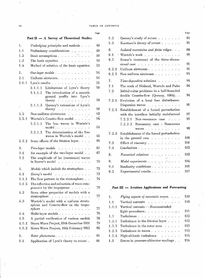
IV TABLE OF CONTENTS
1.
1.1
1.2
1.3
1.4
2.
2.1
2.1.1
Part 11 - A Survey of Theoretical Studies
Underlying principles and methods
Preliminary considerations
Basic assumptions .
The basic equation
..
Method of solution of the basic equation
One-layer models .
Uniform airstream.
Lyra's results .
2 .1.1.1 Limitations of Lyra's theory
2 .1.1. 2 The introduction of a smooth ground profile into Lyra's theory
2 .1.1. 3 Queney's extensions of Lyra's theory
2 . 2 Non -uniform· airstreams
2. 2.1 Wurtele's Couette-flow model
2. 2 .1.1 The free waves in Wurtele's model ...
2. 2 .1. 2 The determination of the free waves in Wurtele's model
2. 2. 2 Some effects of the friction layer.
3. Two-layer models
3.1 An example of the two-layer model
3. 2 The amplitude of lee (resonance) waves in Scorer's model
4. Models which include the stratosphere
4.1 Zierep's model
Page
49
49
50
50
52
54
54
55
58
59
60
62 64
64
65
66
67
67
70
72
73
4 .1.1 The flow pattern in the stratosphere . . 7 4
4 .1. 2 The reflection and refraction of wave components by the tropopause 76
4. 2 Some other properties of models with a stratosphere . . . . . . . . . . . . 77
4. 3 Wurtele's model with a uniform stratosphere and Couette-flow in the tropo-sphere . . . . . . . . . . . . . . . 77
4.4 Multi-layer models ..... ; . . . . 78
4. 5 A partial verification of various models 78
4. 5.1 Sierra Wave Project, 18th December 1951 79
4.5 .2 Sierra Wave Project, 16th February 1952 80
5 . Rotor phenomena. . . . . . . . . . 81
5.1 Application of Lyra's theory to rotors · 81
5.2
5.3
6. 6.1
6.2
6.2.1
6.2.2
7. 7.1
Queney's study of rotors
Kuettner's theory of rotors
Isolated mountains and finite ridges.
·· Wurtele's work
Scorer's treatment of the three-dimen
sional case
Uniform airstream.
Non-uniform airstream
Time-dependent solutions
The work of Hoiland, Wurtele and Palm
7. 2 Initial-value problems in a half-bounded
double Couette-flow (Queney, 1954).
7. 2 .1 Evolution of a local free disturbance.
Dispersion waves . . , . . . . . . ..
7. 2. 2 Establishment of a forced perturbation
with the interface initially undeformed
7 . 2 . 2 .1 Non -resonance case
7. 2. 2. 2 Resonance case - Resonance
waves.
7. 2. 3 Establishment of the forced perturbation
Page
84
85
88
88
91
91
93
94
94
94
95
97
97
99
in the general case 100
7. 3 Effect of viscosity 101
7. 4 Conclusions . . . . 102
8. Numerical solutions . . . . . . . . . 103
9. Model experiments . . 104
9 .1 Similarity conditions . 105
9. 2 Experimental results . 107
Part m - Aviation Applications and Forecasting
1. Flying aspects of mountain wares. 110
1.1 Vertical currents 110
1.1.1 Vertical currents ~·Recommended
flight procedures. 111
1.2 Turbulence . 112
1.2.1 Turbulence in the friction layer _112
1.2.2 Turbulence in the rotor zone 113
1.2.3 Turbulence in waves . 113
1.2.4 High-altitude turbulence 114
1.3 Errors in pressure-altimeter readings . 114
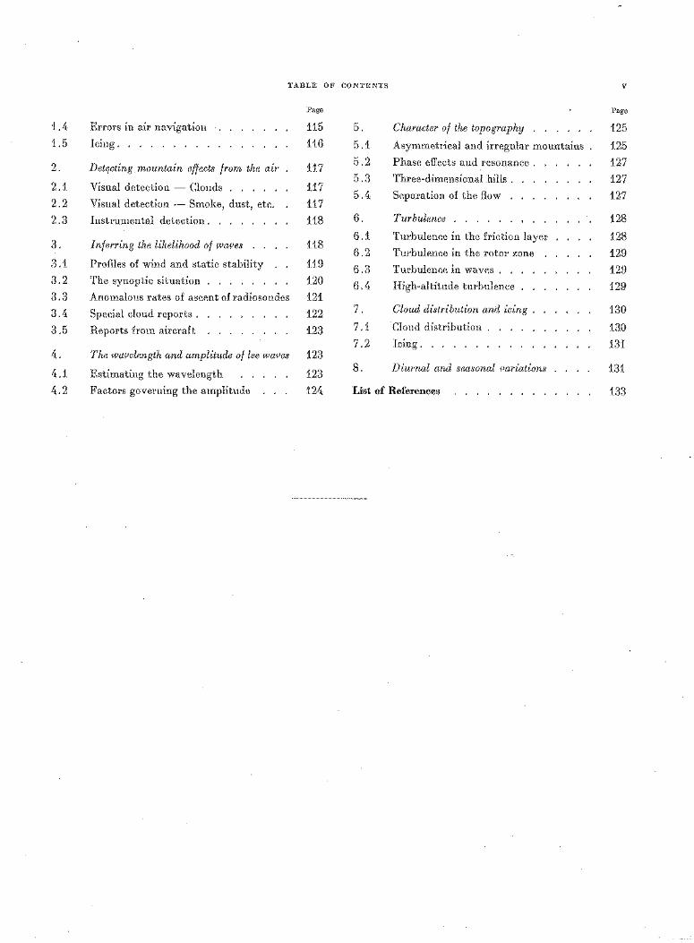
TABLE OF CONTENTS V
Page Page
1.4 Errors in air navigation 115 5. Character of the topography 125 1.5 Icing. 116 5.1 Asymmetrical and irregular mountains 125
2. Detrtcting mountain effects from the air 117 5.2 Phasr. effects and resonance . 127 5.3 Three-dimensional hills . 127
2.1 Visual detection - Clouds . 117 5.4 Separation of the flow 127
2.2 Visual detection - Smoke, dust, etc. 117 2.3 Instrumental detection . 118 6. Turbulence . 128
6.1 Turbulence in the friction layer 128 3. Inferring the likelihood of wares 118
6.2 Turbulence in the rotor zone 129 3.1 Profiles of wind and static stability 119 6.3 Turbulence in waves . 129 3.2 The synoptic situation . 120 6.4 High-altitude turbulence 129 3.3 Anomalous rates of ascent of radiosondes 121 3.4 Special cloud reports . 122 7. Cloud distribution and icing . 130
3.5 Reports from aircraft 123 7.1 Cloud distribution . 130 7.2 Icing. 131
4. The warelength and amplitude of lee wares 123
4.1 Estimating the wavelength 123 8. Diurnal and seasonal fJariations 131
4.2 Factors governing the amplitude 124 List of References 133
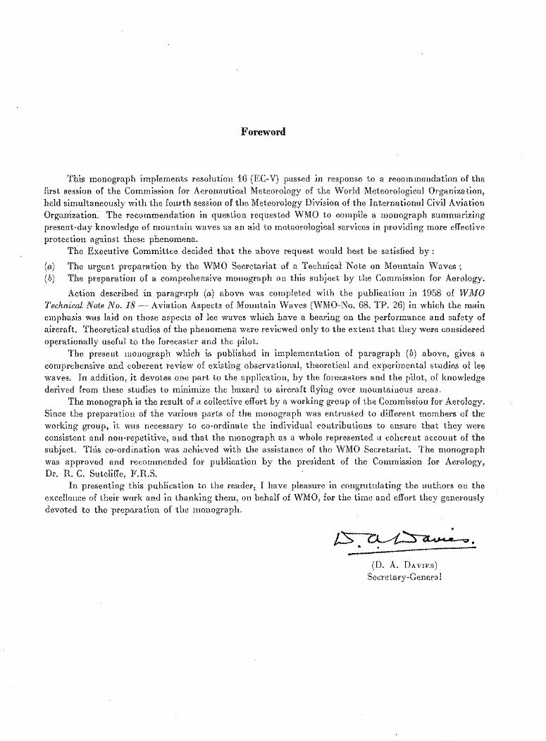
Foreword
This monograph implements resolution 16 (EC-V) passed in response to a recommendation of the first session of the Commission for Aeronautical Meteorology of the World Meteorological Organization, held simultaneously with the fourth session of the Meteorology Division of the International Civil Aviation Organization. The recommendation in question requested WMO to compile a monograph summarizing present-day knowledge of mountain waves as an aid to meteorological services in providing more effective protection against these phenomena.
The Executive Committee decided that the above request would best be satisfied by :
(a) The urgent preparation by the \VMO Secretariat of a Technical Note on Mountain Waves; (b) The preparation of a comprehensive monograph on this subject by the Commission for Aerology.
Action described in paragraph (a) above was completed with the publication in 1958 of W MO Technical Note No. 18 ~Aviation Aspects of Mountain Waves (WMO-No. 68. TP. 26) in which the main emphasis was laid on those aspects of lee waves which have a bearing on the performance and safety of aircraft. Theoretical studies of the phenomena were reviewed only to the extent that they were considered operationally useful to the forecaster and the pilot.
The present monograph which is published in implementation of paragraph (b) above, gives a comprehensive and coherent review of existing observational, theoretical and experimental studies of lee waves. In addition, it devotes one part to the application, by the forecasters and the pilot, of knowledge derived from these studies to minimize the hazard to aircraft flying over mountainous areas.
The monograph is the result of a collective effort by a working group of the Commission for Aerology. Since the preparation of the various parts of the monograph was entrusted to different members of the working group, it was necessary to co-ordinate the individual contributions to ensure that they were consistent and non-repetitive, and that the monograph as a whole represented a coherent account of the subject. This co-ordination was achieved with the assistance of the WMO Secretariat. The monograph was approved and recommended for publication by the president of the Commission for Aerology, Dr. R. C. Sutcliffe, F.R.S.
In presenting this publication to the reader, I have pleasure in congratulating the authors on the excellence of their work and in thanking them, on behalf of WMO, for the time and effort they generously devoted to the preparation of the monograph.
(D. A. DAVIES) Secretary-General
ACKNOWLEDGMENTS
We are greatly indebted to :
The Royal Meteorological Society, London, for permission to reproduce figures 1.1-9-11-12-15-16-17-18-19-20, II .11-13-14-15-26 and III: 1-2-3 ; and for the loan of certain blocks.
Mr. H. Klieforth for permission to reproduce the figures taken from the "Sierra Wave Report" ;
Many individuals, who kindly authorized the reproduction of their photographs and diagrams and to those who placed the originals at our disposal.
Figure I .1 (British Crown Copyright) is reproduced with permission of the Controller of Her Britannic Majesty's Stationery Office.
Figures I. 2-3-6-10-21-22 are reproduced from the International Cloud Atlas.
THE AIRFLOW OVER MOUNTAINS
Introduction
Since the early days of meteorology it has been known that the airflow over mountainous terrain is often more disturbed than over level country, but in the textbooks of the past one naturally finds little information about the nature of the disturbances, apart from simple statements assigning an empirical limit to their maximum height. However, over the last few decades observational data from a variety of sources have accumulated in considerable quantities and more recently research effort has been devoted specifically to the problem in many countries. Whether investigated theoretically or in the field, the problem of how the airflows over mountains is a very complex one which has its own peculiar difficulties. I£ the disturbances to the airflow were entirely of a random, turbulent character, progress would probably have been limited to results of a statistical nature, but the airflow is often deformed systematically. Disturbances of the latter kind have yielded substantially before the pressure of theoretical attack and the most recent theoretical models are capable of predicting very closely most aspects of the observed flow.
Although the subject has great intrinsic interest, the practical importance is currently bound up almost entirely with aviation. There is no doubt that amongst the effects which occur in the airflow over mountains are several which can be a serious hazard to aircraft and, indeed, there is also no doubt that many past aircraft disasters in mountain areas, which at the time were unexplained, were in fact due to such effects. Accordingly, although the present monograph is a fairly comprehensive general summary of the available knowledge to date on the airflow over mountains, including theory, the emphasis wherever appropriate is towards the aviation aspects. Very large mountain barriers such as the Rockies and Himalayas do, of course, impose disturbances of all scales on the airflow around the globe, from the scale of the long waves down through that of lee depressions to minor turbulent eddies. Synoptic scale effects of mountains have been omitted from the monograph and in line with the emphasis on effects relevant to aviation, most attention is paid to the quasi-stationary gravity waves initiated by mountains and having a horizontal wavelength in the approximate range one to twenty kilometres and also to the turbulence sometimes associated therewith. The vertical currents in such waves have carried gliders to the stratosphere and can in many parts of the world attain a magnitude greater than the maximum rate of climb of many aircraft still in regular use. The importance of mountain waves for aviation is, therefore, beyond question.
In order to make quite clear the nature of the phenomena which occur over mountains, the observational evidence is reviewed in some detail in Part I of the monograph. Some of the evidence has arisen as a by-product of other activities, e.g. the rewarding occupations of cloud study and soaring, whilst other evidence has come from specific field investigations. To link the observational evidence from various sources into a coherent whole, some general interpretation of the evidence is given at the end of Part I. For any theory to be satisfactory and useful it must account for these observed facts.
Part II is a critical survey of theoretical studies, ranging from the early applications of perturbation theory to a uniform airstream, up to recent work using a multi-layer approximation to the atmosphere. Theoretical results are still subject to notable limitations, but in view of the complexities of the problem, it is remarkable how successfully the most refined theories are ea pable of predicting the observed phenomena.
In Part Ill the flying aspects of mountain waves, viz.: vertical currents, turbulence, altimeter errors, icing, etc. are discussed and some attempt is made to indicate ways in which current knowledge on the phenomena can be exploited in forecasting for flights across mountains and in avoiding the worst hazards.
L'ECOULEMENT DE L'AIR SUR LE RELIEF
Introduction
Depuis les debuts de la meteorologic, l'on sait que de l'air qui s'ecoule au-dessus d'une regwn montagneuse est souvent plus perturbe qu'au-dessus d'un terrain plat, mais I' on ne trouve clans les anciens manuels que peu de renseignements sur la nature des perturbations, sauf quelques indications sur la limite empirique de !'altitude maximale a laquelle elles se produisent. Au cours des dernieres decennies toutefois, on a recueilli un nombre considerable de donnees d' observation de sources diverses et, plus recemment, des travaux de recherche ont ete consacres specialement a ce probleme clans de nombreux pays. Qu'il soit aborde theoriquement ou pr1;1tiquement, le probleme de l'ecoulement de l'air sur le relief est des plus complexes et presente des difficultes particulieres. Si les perturbations de l' ecoulement de l'air avaient ete entierement accidentelles, on n'aurait probablement obtenu que des resultats d'ordre statistique, mais il arrive souvent que l'ecoulement de l'air soit deforme systematiquement. L'etude theorique des perturbations du dernier type a permis d' obtenir des resultats substantiels et les modeles theoriques les plus recents permettent de predire avec une grande precision la plupart des aspects du flux observe,
Bien que la question offre un grand interet intrinseque, son importance pratique releve pour le moment presque uniquement du domaine de !'aviation. Plusieurs effets des mouvements ondulatoires dus au relief peuvent sans aucun doute constituer un grave danger pour les areonefs et, en fait, il est peu douteux que de nombreuses catastrophes aeriennes, qui ont eu lieu anterieurement clans des regions montagneuses et qui etaient demeurees inexpliquees, aient ete dues en realite a ces effets. C'est pourquoi, bien que la presente monographic fasse le point de toutes les connaissances actuelles concernant l'ecoulement de l'air sur le relief (y compris les theories), !'accent est mis chaque fois que cela est possible sur les aspects qui interessent plus particulierement I' aviation. De tres vastes cha'ines montagneuses, comme les montagnes Rocheuses et l'Himalaya provoquent, evidemment, toutes sortes de perturbations sur la circulation autour du globe, depuis les grands mouvements ondulatoires jusqu'aux petits mouvements tourbillonnaires, en passant par les depressions sous le vent. La monographic ne neglige pas les effets a echelle synoptique du relief et, comme l'accent est mis sur les phenomenes qui interessent particulierement !'aviation, elle accorde une grande attention aux ondes de gravite quasi-stationnaires dues au relief, dont la longueur d'onde est comprise approximativement entre un et vingt kilometres, ainsi qu'a la turbulence qui y est quelquefois associee. · Les courants verticaux au sein de ces mouvements ondulatoires ont porte des planeurs jusqu'a la stratosphere et clans de nombreuses parties du globe leur vitesse peut etre superieure a la vitesse ascensionnelle maximale de bon nombre d'aeronefs qui sont encore en service actuellemEmt. L'importance que les ondes de relief presentent pour !'aviation ne fait done pas de doute.
Afin de definir clairement la nature des phenomenes qui se produisent au-dessus des montagnes, la premiere partie de la monographic etudie en detail les donnees d'observation recueillies. Certaines des donnees sont des sous-produits d'autres activites (par exemple, etude des nuages et vol a voile), tandis que d'autres sont le resultat de recherches speciales sur le terrain. On trouvera a la fin de la premiere partie une analyse generale de la documentation recueillie, qui permet de coordonner en un tout coherent lcs donnees d'observation provenant de diverses sources. En effet, toute theorie, pour qu'elle soit valable et utile, doit tenir compte des faits observes.
La deuxieme partie examine de faQon critique diverses etudes theoriques, qui vont des premieres applications de la theorie des perturbations a un courant atmospherique uniforme aux travaux recents utilisant des modeles a plusieurs couches de !'atmosphere. Les resultats theoriques presentent encore d'importantes failles, mais eu egard a la complexite du probleme, il est remarquable de constatcr le succes avec lequel les theories les plus avancees permettent de predire les phenomenes observes.
La troisieme partie etudie les aspects des ondes de relief qui interessent !'aviation (c'est-a-dire, les mouvements verticaux, la turbulence, les erreurs altimetriques, le givrage, etc.) et recherche les moyens permettant d'exploiter les connaissances actuelles de ces phenomenes pour prevoir des conditions de vol au-dessus des montagnes et pour eviter les dangers les plus graves.
B03,II;YIIIHhiE TEqEHHH HA,II; rOPHhiMI1 PAffOHAMI1
BBe;:~;enne
C MOMBHTa ITORBJIBHMH MBTBOpOJIOrH'IBCII:OM HaJRM 6niJIO MBBBCTHO, 'ITO B03)l;JIIIHbiB 'l'B'IBHMH Hap;
ropnniMM pai:i:ormMM '!aCTO 6nmaiO'l' 6oJiee 6ypHhlMM, 'IBM Ha,n; paBHMnoi:i:, o.n;naRo B yqe6rumax Toro
BpBMBHM MOiKHO 6hlJIO Hai!ITM MaJIO CBB,[\BHMM 0 xapaRTepe BTMX BOBMJIIIBHMM sa MCRJIIO'IBHMBM JIMillh
«JlopMJJIMpOBOR, onpe,n;eJIRIOII\MX t>MnMpM'Iecr-tyro rpaHMI1Y MX MaRcMMaJihHOM BhiCOThl. B Te'IeHMe nocJie,n;
HMX ,[\BCJITMJIBTMM 6niJIO HaROITJieiW 3Ha'IHTBJihHOB ROJIM'IBCTBO p;aHHhlX, ITOJIJ~IBHHhlX H3 paBJIH'IHhlX
MCTO'Il!MROB, a BO MHOrMX CTpaHaX HaJ'IHhlB JCHJIMJI ITOCJIB;D;HHX JIBT 6hlJIH HanpaBJIBHhl Ha MBJ'IBHMB
tlTOrO CITBI1M«JlM'IBCROrO BOnpoca. flpo6JieMa npOXOiK;D;BHMH B03;D;JIDHhlX ITOTOROB 'Iepes ropni, paCCMa
TpMBaBTCH JIM OHa C TO'IRM BpeHMH TeopeTM'IBCROrO MCCJIB)l;OBaHMH MJIM C TO'IRM BpeH.IiJ:H npaRTM'IBCROrO
na6mD,n;eHMH, HBJIHBTCH qpeBBhi'Iai:i:no cJiomnoi:i: u MMeeT oco6hle TPY;D;HOCTH. EcJIM 6nr BOBMyru;enMH,
npOMCXO;D;HII(Me B BOB;D;JIDHOM ITOTORe HOCHJIM CJIJ'IaMHhlM, 'l'yp6yJieHTHbiM xapai-tTep, 'l'O nporpecc
orpaHM'IMBaJICH 6hl pBBJJihTaTaMM c•raTHCTM'IBCROrO xapaRTepa, O)l;HaRO BOB;D;JIDHhlB ITOTORM ;n;e«JlopMM
pJIOTCH CMCTBMaTH'IBCRM. 8TH HBJIBHIIJI JCTJITMJIM B 8Ha'IMTBJihHOM CTBITBHM nepep; HaJROM, TaR 'ITO
npMMeHJIJI HaM60Jiee COBpBMBHHhlB TeOpMH CTaJIO BOBMOiKHbiM nporHOBMpOBaHHB C 60JibillOM TO'IHOCTbiO
MHOrHX acneRTOB BOB)l;JIDHOrO TB'IBHHH.
XoTH 9TOT Bonpoc u npe;n;cTaBJIHBT 6oJinmoi:i: HHTepec no cyru;ecTBY, npaR'l'M'IBCRoe sna'IeHMe ero
B HaCTOHru;ee BpBMJI ITO'ITH ITOJIHOCTbiO CBJISaHO C aBMai~HeM. HeT COMHBHMM, 'ITO cpep;M HBJIBHHM,
npOHCXO;D;HII~J!IX B BOB;rl;JIDHOM ITOTORB Hap; ropHhlMll pai:i:OIIaMH, MMBIDTCH TaRHe, ROTOpbiB npep;CTaBJIJIIDT
cepnesnym onacnocTh ;D;JIH anMa1IHM H cei:i:'Iac, nanpnMep, RCI-IO, 'ITO Mnorr1e anapnn, MMeBmMe MecTo
paHbillB B ropHhlX pai:i:OHaX, M ROTOphle B TO BpBMH HMRai-t He 06'bJICHJIJIMCh, npOMCXO;D;MJIM MMBHHO MB-Ba
9THX .HBJIBHMM. TaRMM o6pasoM, HBCMOTPH Ha TO, 'ITO HacTOHII\aH MOHorpa«Jlua- 9TO no.n;po6Hoe pesroMe
COBpBMBHHbiX SHai-IHM 0 BOB)l;JillHbiX TB'IBHMHX, npOXO;D;HIIIMX 'Iepes ropHhlB xpe6Thl, BI-tJIIO'Ia.H TeopeTM
'IBCRHB acneRThl, BO Bcex MBCTax y;n;apeHMe ;n;eJiaeTCH Ha aBHa1IMOHHhre acneRThi. TaRMe 6oJihmMe ropHhle
6apnephl I\aR CI-taJIMCThlB ropnl M rMMaJiaM 6esycJIOBHO Bhl3hlBaiOT BOBMyru;eHMJI B BOB,ll;JillHbiX TB'IBHMHX
BORpyr BCero 3BMHOrO mapa, ROTOpbiB BapnnpyiOTCH OT ;D;JIMHHhlX BOJIH 'Iepes HBBHa'IMTBJibHhlB ;n;enpec
CI1H ;n;o ne6oJihiDMX Typ6yJieHTHhlX ;n;E«Jl«Jlym-ri:i:. CMHOITTH'IeCRMe acneRThi BJIMHHI1H ropHhlX MaCCIIBOB
6hlJIM BhlllJIIIBHhl MS MOHOrpa«JlnM B COOTBBTCTBliiM C ITOCTaBJIBHHOM sap;aqei:i: o6paru;aTh OCHOBHOB BHMMaHMB
na anMal1I10HHhle acneRThl. Mnoro BHMMaHMH y;n;eJIHeTcH TaRme HBasMcTa1IHOHapnnrM rpaBnTa1IMOHHhiM
BOJIHaM, BOBHMRaiOII\HM B ropHbiX pai:i:onax M HMBIOII\MM ropHBOHTaJibHJIO ;D;JIMHJ, ROJIB6JIIOIIIJIOCJI B
pa;n;nyce OT O)l;HOrO ;D;O 20 RM, a Tai-tme Typ6yJieHTHOCTh, ROTOpaH Sa'IaCTJIO CBHBaHa C 9THM JIBJIBHMBM.
BepTHRaJibHhle TB'IBHMJI B TaRMX BOJIHaX SaHOCHT ITJiaHephl Ha TaRyiO BhlCOTJ, ROTOpaH BO MHOrMX
'IaCTHX 3BMHOrO mapa MOiKBT )l;OCTMraTb 66JihilliiX BHa'IBHMM, 'IBM npep;eJihl ITO)l;'hBMa MHOrMX COBpe
MBHHbiX CaMOJIBTOB. l1ot>TOMJ BaiKHOCTh rOpHhlX BOJIH ;D;JIH aBMa1IMM HaXOP;IITCJI BHB BCJIRHX COMHBHIIM.
qT06hl ,n;aTh Jicnoe o6'bJicneHne xapaHTepy t>Toro HBJieHnH, 'IaCTh I MOHorpa«JlMn nocnHru;ena
o6sopy .n;anHhlX Ha6mo.n;er-nm. HeROTOphle ;n;anHhie 6hlJIII noJiyqeHhl cJiyqai:i:no BO npeMH npone,n;eHMJI
;n;pyrux Ha6mo;n;eHni:i:, HanpiiMep, B Ra'IeCTBe nosaarpam:a;eanJI sa MBy'Ienne o6Jia'IHOCTM, B TO npeMH
Hal-t ;n;pyrne p;aHHhlB 6hlJilil ITOJIJ'IBHhi ITOCpB;D;CTBOM npOBB)l;BHMJI CITBI1IIaJihHhiX liiCCJIB;D;OBaHIIM. qT06bi
06'bB;D;MHMTb BCB Ha6JIIO;D;BHHH, ITOJIJ'IBHHhiB liB paSHhlX liiCTO'IHliiROB B O)l;HO CBHBHOB lii llOCJIB;D;OBaTBJihHOB
1IBJIOe, B ROHI1e 'IaCTH I npnBO;D;MTCH o6ru;aH liiHTepnpeTa1IHH ,n;aHHhlX. ,II;JIH Toro, 'IT06nr mD6aH TeopHH
6hlJia Ha;D;en-tHOM lii ITOJIBSHOM, OIIa )l;OJiiKHa OITMpaTbCJI Ha «JlaRTII<IeCRliiB p;aHHhiB I-Ia6JIIO,[\BHIIH.
B 'IaCTM II ;n;aeTCH RpHTM'IBCRM:i1: o6sop TeopeTH'IeCRIIM MCCJie;n;onannHM, naqnnaH OT npnMeHei-IMH
pa!II-IBM TBOpHlil nepeMBIDHBaHMH R B;D;IIHOMJ B03;D;JIDHOMJ TB'IBI-IIIIO BITJIOTh )l;O Hep;amiliiX pa60T, r;n;e
ncnoJinByeTCH Teoprur MHorocJio:i1:rm:i1: anpORCMMal1Mlil. TeopeTII'IBCRIIe pa6oThi eru;e HMBIDT cepneBI-Ibre
HB;D;OCTaTRlil, Op;HaRO, J'IMThiBaH BCB CJIOiKI-IOCTM np06JIBMhl, Bhl;D;aiOru;liiMCH MOiKHO C'IliiTaTh TO, 'ITO Haii60JIBB
oTpa6oTaHHhle Teopnn MoryT c ycnexoM npMMeHHThCH npn npornosnpoBaHIIII t>Toro HBJIBHliiH.
B 'IaC'l'H Ill onHChlBaiDTCH JieT.Eihre acneRThi ropnnrx BOJIH, Tai-tne I-taR : nepTima.rrhHhre TB'IBHIIH,
Typ6eJIBHTHOCTh, norpemHOCTlil BbiCOTOMepa, 06Jie)l;ei-IeHlile li T. )1;. j B TOM me 'IaCTII p;eJiaBTCH IIOIThlTRa
JRaSaTh ITJTlil lil B03MOiKHOCTII, npH RO'rOphlX COBpeMeHHhlB BHaHliiH tlTOl'O JIBJIBHIIJI MOrJilil 6hl HaH60JIBB
t>«Jl«Jlei-tTIIBHO MCITOJihBOBaThCH npii nporHOBHpOBaHliiH ITOJIBTOB Rap; ropHhlMII pai:i:OHaMM C TBM, 'IT06bi
IIs6eraTh nan6oJiee onacHhle ;D;JIH caMoJieTa JIBJieHYIH.
PASO DE LAS CORRIENTES DE AIRE SOBRE LAS MONTANAS
Introduccion
Desde los primeros tiempos de la meteorologia se sabia que las corrientes de aire, al pasar por encima de terrenos montafiosos, suelen experimentar mas perturbaciones que al pasar sobre terreno llano ; pero, como es l6gico, en los antiguos libros de texto encontramos muy poca informaci6n sobre la naturaleza de esas perturbaciones, apenas unas meras declaraciones para asignar espiricamente un limite maximo a su altura. Sin embargo, en las ultimas decadas se han acumulado cantidades considerables de datos procedentes de fuentes diversas y, mas recientemente, en muchos paises se han consagrado esfuerzos a este problema especifico.
El problema del paso de las corrientes de aire por encima de las montafias es muy complejo, tanto para las investigaciones te6ricas como experimentales, y entrafia dificultades peculiares. Si las perturbaciones de las corrientes de aire fuesen de un caracter meramente turbulento y fortuito, los progresos se limitarian probablemente a resultados estadisticos, pero ocurre que, muchas veces, las corrientes de aire se deforman de manera sistematica. Datos de observaci6n sobre csta ultima clase de perturbaciones se habian acumulado antes de que se comenzase el ataque te6rico del problema y los · esquemas te6ricos mas recientes permiten una previsi6n muy exacta de los aspectos principales de las corrientes observadas.
Aunque el tema es de gran interes por si mismo, su importancia practica suele estar ligada casi exclusivamente a la aviaci6n. No cabe duda de que algunos de los efectos del paso de una corriente de aire sobre las montafias pueden constituir un peligro para la aviaci6n y tambien es indudable que muchas de las catastrofes aereas del pasado, ocurridas en zonas montafiosas y para las que no se encontr6 en aquella epoca una explicaci6n, fueron causadas por dichos efectos. Por eso, aunque la presente monografia es un resumen general bastante completo de los conocimientos disponibles hoy dia acerca de las corrientes de aire sobre las montafias, incluida la teoria, se insiste especialmente, cuando procede, en los aspectos relativos a la aviaci6n. Las grandes barreras montafiosas, como las Montafias Rocosas o el Himalaya, producen indudablemente perturbaciones de todas las magnitudes en las corrientes de aire que circulan alrededor del globo, pasando en escala descendente desde las ondas largas hasta los remolinos turbulentos menores, a traves de las depresiones de sotavento. En la monografia se han omitido los efectos de escala sin6ptica que producen las montafias y, dado el interes que se pone en los efectos importantes para la aviaci6n, se ha prestado mayor atenci6n a las ondas de gravedad semi-estacionarias que se inician en las rnontafias y que tienen una longitud de onda horizontal de un orden aproximado de 20 kil6metros, asi corno a las perturbaciones que suelen ir asociadas con el}as. Las corrientes verticales de esas ondas han llevado a algunos planeadores hasta la estratosfera y en muchas partes del rnundo pueden alcanzar una magnitud mayor que el indice ascensional maximo de muchos de los aviones que, aun hoy, prestan servicio regularmente. Asi pues, resulta evidente la importancia que tienen para la aviaci6n las ondas producidas por las montafias.
A fin de poner bien en claro la naturaleza de los fen6menos que se producen encima de las montafias, en la Parte I de la monografia se estudia:n con cierto detalle los resultados de las observaciones. Algunos de esos resultados son el producto secundario de otras actividades, como por ejemplo, las tareas fructuosas del estudio de las nubes y de los vuelos sin motor, mientras que otros proceden de investigaciones de campo especificamente dedicadas a ese fin. Para formar un todo coherente con los resultados procedentes de observaciones diversas, en la Parte I se procede a una cierta interpretaci6n general de los resultados. Para ser satisfactoria y util, cualquier teoria habra de tener en cuenta esos hechos observados.
La Parte 11 constituye un examen critico de los diversos metodos de estudio te6rico, desde las primitivas aplicaciones de la teoria de perturbaci6n a una corriente de aire uniforme, hasta los trabajos recientes en los que se utiliza un rnodelo de capas multiples como representaci6n de la atm6sfera. Los resultados te6ricos estan todavia sujetos a grandes limitaciones pero, teniendo en cuenta la complejidad del problema, resulta notable el exito con que las teorias mas perfeccionadas permiten predecir los fen6-rnenos observados.
En la Parte Ill se exarninan los aspectos de importancia para la aviaci6n de las oridas producidas encima de las montafias, o sea : corrientes verticales, turbulencia, errores del altimetro, formaci6n de hielo, etc., y se trata de indicar en que forma se pueden aprovechar los conocimientos actuales de esos fen6menos en las predicciones meteorol6gicas destinadas a los vuelos sobre zonas montafiosas, y para evitar los principales peligros.
PART I
OBSERVATIONAL RESULTS AND FIELD INVESTIGATIONS
1. History
Probably the earliest work at all related to the problem of lee waves was that of Rayleigh and Kelvin who in the latter part of the last century carried out theoretical studies of the flow of streams of water over obstacles on the bed. Their work satisfactorily explained the standing waves often seen on the surface of running water in such circumstances. Although the problem of the airflow over mountains is a good deal more complicated, owing inter alia to the stratification and compressibility of the atmosphere, theoretical studies of the problem have followed much the same mathematical techniques as those evolved by Rayleigh and Kelvin.
Apart from a theoretical work published by Pockels in 1901, the nature of the flow in the vicinity of hills received little attention until the 1920's when interest in the subject was awakened and a number of papers were published, e.g. by Koschmieder, Georgii and others. These described observations with balloons, both free lift and zero lift, and to a limited extent with gliders. Attempts were made at a tentative interpretation of the observations and there was early recognition that ascending currents are often to .
. be found on the lee as well as the windward side of hills. In 1928 some organized observations were sponsored by the German Glider Research Institute at the Rossitten dunes near Kaliningrad (formerly Konigsberg) ; these threw further light on the nature of the flow to the lee of obstacles.
From this time on it was natural that the small but enthusiastic band of glider pilots in Europe should come into the picture, as their art depended essentially on the successful exploitation of ascending currents in the atmosphere. Probably many of them soared in hill waves without being aware of it, but the first successful lee-wave flights are usually attributed to Deutschmann and Hirth, who in March 1933 successfully glided in what must have been lee waves in the Hirschberger Valley in Silesia.
There followed a period in the late 1930's when several adventurous glider pilots achieved many climbs into the high troposphere. These flights were at the time viewed with astonishment because they were accomplished not on the windward side of mountain ridges where ascending air would have been accepted with little surprise, but on the leeward side. Notable amongst these flights were those of Kuettner who in 1937 attained about 8,000 m on several occasions in the Riesengebirge and of Kloclmer who in 1939 reached 11,400 m in the East Alps. Even to the lee of the much smaller hills of Cumberland in the British Isles, McLean in 1939 reached about 3,500 m in standing waves.
The next two decades saw mountain waves probed and exploited to an ever-increasing extent by glider pilots in many parts of the world. Slowly but steadily there was built up a body of mainly qualitative, descriptive information about the character of the airflow near mountains, until a fairly clear picture of the characteristics of mountain lee waves was established. In the meantime theoretical workers had not been idle. Indeed, Queney in his paper Influence du relief sur les elements meteorologiques, published in 1936, can claim to have predicted mountain waves before their occurrence in the atmosphere had been properly appreciated- a rare event in meteorological progress. Sirice then the theory has been continuously developed and elaborated by many workers including Lyra, Queney, Stiimke, Scorer, Zierep, Hoiland; Long, Palm, Wurtele and many others. The observations of glider pilots, coupled in recent years with
2 OBSERVATIONAL RESULTS AND FIELD INVESTIGATIONS
those from the pilots of powered aircraft and from other miscellaneous sources, contributed jointly with
the theory in bringing about a state of knowledge on this subject which, although far from complete,
forms a coherent and consistent whole.
2. Different observational sources
2.1 Clouds
The deformation of airstreams by hills and mountains is often visibly revealed in a variety of beautiful
orographic clouds whose form and characteristics sometimes tell us a great deal about the nature of the airflow. In particular, such clouds indicate the location of ascending currents and to some extent of regions
of turbulence. As they are linked to the terrestrial relief below, they generally remain nearly stationary
or at any rate move much more slowly than the wind. Most orographic clouds are continually reforming at the upwind edge and dissolving at the downwind edge. They occur at all heights from the surface to
Cirrus levels and indeed there is little doubt that the astonishing nacreous (mother-of-pearl) clouds at 20 to 30 km are also caused by topography. Orographic clouds fall naturally into certain distinct types
which are briefly described and illustrated in the following paragraphs.
2 .1.1 Cap clouds
Cap clouds comprise the simplest examples of forced ascent leading to saturation and cloud forma
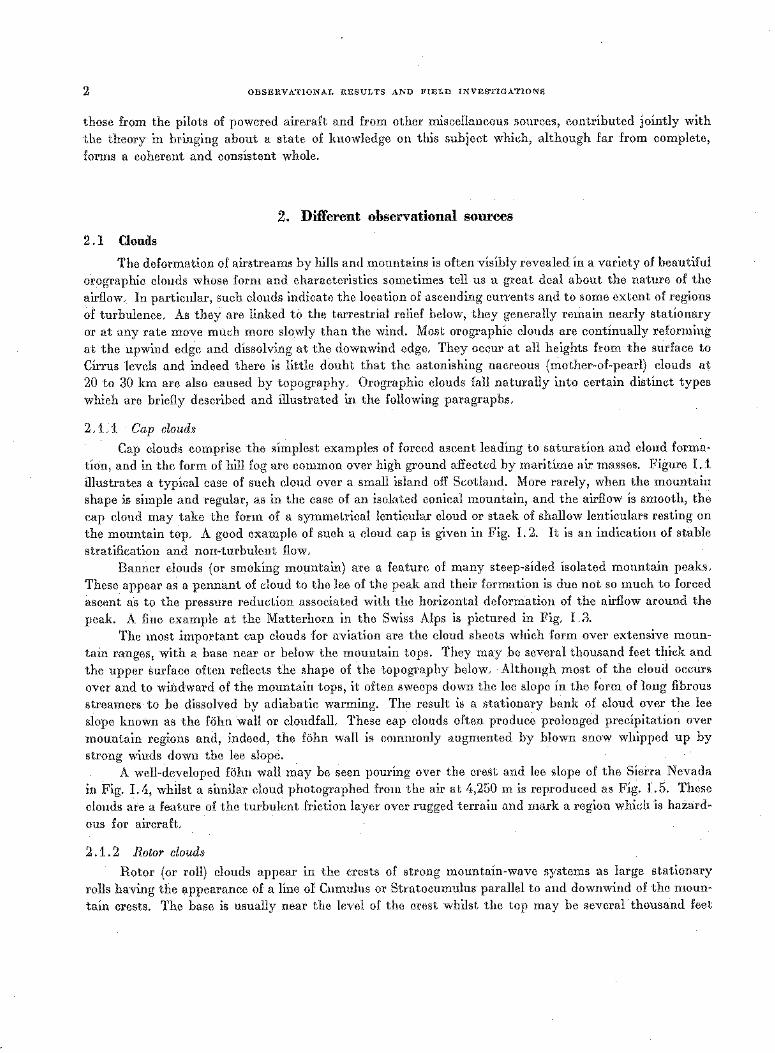
tion, and in the form of hill fog are common over high ground affected by maritime air masses. Figure I .1 illustrates a typical case of such cloud over a small island off Scotland. More rarely, when the mountain shape is simple and regular, as in the case of an isolated conical mountain, and the airflow is smooth, the
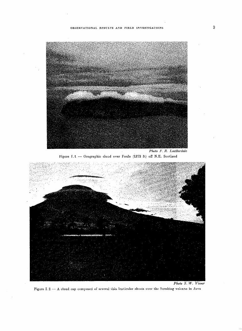
cap cloud may take the form of a symmetrical lenticular cloud or stack of shallow lenticulars resting on the mountain top. A good example of such a cloud cap is given in Fig. I. 2. It is an indication of stable
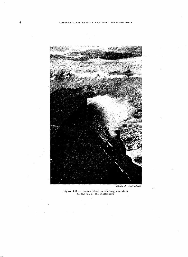
stratification and non-turbulent flow. Banner clouds (or smoking mountain) are a feature of many steep-sided isolated mountain peaks.
These appear as a pennant of cloud to the lee of the peak and their formation is due not so much to forced ascent as to the pressure reduction associated with the horizontal deformation of the airflow around the peak. A fine example at the Matterhorn in the Swiss Alps is pictured in Fig. 1.3.
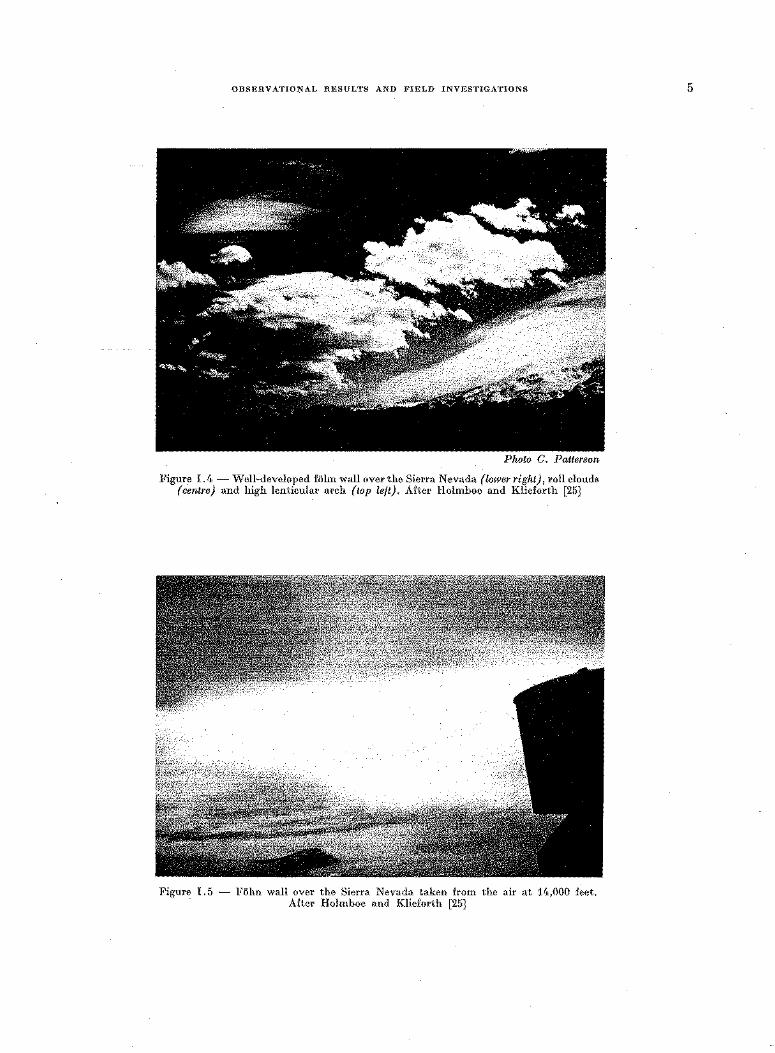
The most important cap clouds for aviation are the cloud sheets which form over extensive mountain ranges, with a base near or below the mountain tops. They may be several thousand feet thick and
the upper surface often reflects the shape of the topography below. Although most of the cloud occurs over and to windward of the mountain tops, it often sweeps down the lee slope in the form of long fibrous streamers to be dissolved by adiabatic warming. The result is a stationary bank of cloud over the lee
slope known as the fohn wall or cloudfall. These cap clouds often produce prolonged precipitation over mountain regions and, indeed, the fohn wall is commonly augmented by blown snow whipped up by
strong winds down the lee slope. A well-developed fohn wall may be seen pouring over the crest and lee slope of the Sierra Nevada
in Fig. I. 4, whilst a similar cloud photographed from the air at 4,250 m is reproduced as Fig. I. 5. These clouds are a feature of the turbulent friction layer over rugged terrain and mark a region which is hazard
ous for aircraft.
2 . 1. 2 Rotor clouds
Rotor (or roll) clouds appear in the crests of strong mountain-wave systems as large stationary rolls having the appearance of a line of Cumulus or Stratocumulus parallel to and downwind of the mountain crests. The base is usually near the level of the crest whilst the top may be several· thousand feet
OBSERVATIONAL RESULTS AND FIELD INVESTIGATIONS
Photo F. R. Leatherdale
Figure 1.1 -- Orographic cloud over Foula (1373 ft) ofl' N.E. Scotland
Photo S. W. Visser
Figure 1.2- A cloud cap composed of several thin lenticular sheets over the Sumbing volcano in Java
3
4 OBSERVATIONAL RESULTS AND FIELD INVESTIGATIONS
Photo 1. Galimberti
Figure I. 3 ~ Banner cloud or smoking mountain to the lee of the Matterhorn
OBSERVATIOr-(AL RESULTS AND FIELD INVESTIGATIONS
Photo C. Patterson
Figure I. 4 -Well-developed fiihn wall over the Sierra Nevada (lower right), roll clouds (centre) and high lenticular arch (top left). After Holmboe and Klieforth [25]
Figure I.5 - Fiihn wall over the Sierra Nevada taken from the air at 14,000 feet. · After Holmboe and Klieforth [25]
5
6 OBSERVATIONAL RESULTS AND FIELD INVESTIGATIONS
Photo R. Symons
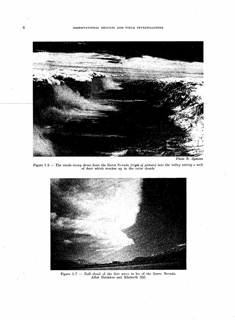
Figure I. 6 - The winds sweep down from the Sierra Nevada (right of picture) into the valley raising a wall of dust which reaches up to the rotor clouds
Figure I. 7 - Roll cloud of the first wave to lee of the Sierra Nevada. After Holmboe and Klieforth [25]
OBSERVATIONAL RESULTS AND FIELD INVESTIGATIONS
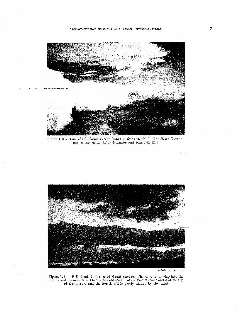
Figure I.8- Line of roll clouds as seen from the air at 16,000 ft. The Sierra Nevada are to the right. After Holmboe and Klieforth [25]
Photo S. S~tzuki
Figure I. 9 - Roll clouds in the lee of Mount Suzuka. The wind is blowing into the picture and the mountain is behind the observer. Part of the first roll cloud is at the top
of the picture and the fourth roll is partly hidden by the third
7
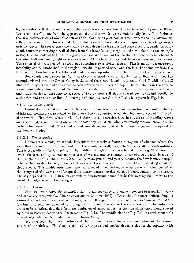
ll[ QQ0 ' 0~ 1 11 0 fJ l! 1l! ~ I (pnnp a/JJ}J_IIll} .ll!JI1 :l 1JII .l l 'IJ OOLU~ :l ll,l,
'"1'"·'·1 '( ll.LI ·11c; ~ 1 11 ]" ·1 ·11 · " 11 111 ·' -"'·" 1 ~· 1 !) ·" 11 ] 0 J ~.). i. l ·" 11 111 ~ 1' 1 "'1:) · 11 ' 1 ,> .IILil 1.-l
J.'"'l " -''1' J i" 'l ·" J q 1 s. I.J.\u J p11u 1J .1J dd11 JO JJJ q s v ·pullu.l.<i>tJcq
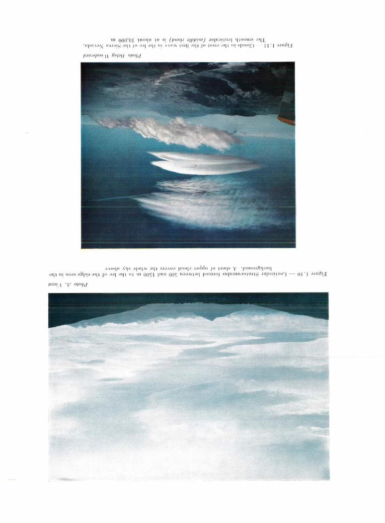
d lj1 ll l UJ.JS al5 p 1.1-. J 'Ii J U JJ i J 41 UJ lll oo s ~ pu B OO S' UJJ.\\J J q paLU.IUJ ' "l'lLLIII J U]Il ,IJ S .II.!Jil :l iJll d' J - ()~' I J,lll,jlid
)111)1 . I ' I-" O)Olfcf
OBSERVATIONAL RESULTS AND FIELD INVESTIGATIONS 9
higher ; indeed roll clouds in the lee of the Sierra Nevada have been known to extend beyond 9,000 m. The term "rotor" stems from the appearance of rotation which these clouds usually have. This is due to the large positive vertical wind shear through the cloud, the upper part of which appears to be continuously rolling over ahead of the lower cloud. Rotor clouds seem to be a natural consequence of very large amplitude lee waves. In severe cases the airflow sweeps down the lee slope and rises steeply towards the rotor cloud, sometimes carrying a wall of dust from the lower lee slopes up into the roll cloud, as for example in Fig. I. 6. In contrast to the strong gusty winds near the foot of the lee slope the surface winds beneath the rotor itself are usually light or even reversed. At the base of the cloud, however, reversed flow is rare. The region of the rotor cloud is turbulent, sometimes to a violent degree. This is mainly because great instability can be established in the region, but the large wind shear and the fact that some air from the turbulent friction layer of the fohn wall finds its way up into the roll cloud, no doubt also play a part.
Roll clouds can be seen in Fig. I. 4, already referred to as an illustration of fohn wall. Another example, viewed from the Owens Valley in the lee of the Sierra Nevada, is given in Fig. I. 7, whilst Fig. I. 8 illustrates a typical line of roll clouds as seen from the air. These all depict the roll clouds in the first lee wave immediately downwind of the mountain crests. I£, however, a train of lee waves of sufficient amplitude develops, there may be a series of two or more roll clouds spaced out downwind parallel to each other and to the crest line. An example of such a succession of roll clouds is given in Fig. I. 9.
2. 1. 3 Lenticular clouds Unmistakable visual evidence of the wave motions which occur in the airflow over and to the lee
of hills and mountains is provided by the quasi-stationary lenticular clouds which are observed in all parts of the world. They form where air is lifted above its condensation level in the crests of standing waves and accordingly remain poised above the topography whilst the wind continually streams through them perhaps for hours on end. The cloud is continuously regenerated at the upwind edge and dissipated at the downwind edge.
2 . 1. 3 .1 Stratocumulus Unlike rotor clouds, orographic lenticulars are mostly a feature of regions of airspace where the
wave flow is smooth and lamin:;tr and thus the clouds generally have characteristically smooth outlines. This is especially so for lenticulars in the middle and high troposphere but at lower, e.g. Stratocumulus levels, the form and quasi-stationary nature of wave clouds is commonly less obvious, partly because if there is cloud at all at those levels it is usually more general and partly because the flow is more complicated at low levels. In fact, the effect of waves at these levels is often to modify pre-existing clouds or cloud sheets. The modification may take the form of quasi-stationary clear areas or lanes located in the troughs of the waves, and/or quasi-stationary darker patches of cloud corresponding to the crests. The sky depicted in Fig. I .10 is an example of Stratocumulus modified in this way by the airflow to the lee of the ridge seen in the background.
2. 1. 3. 2 Alto cumulus At these levels, wave clouds display the typical lens shape and· smooth outlines to a marked degree
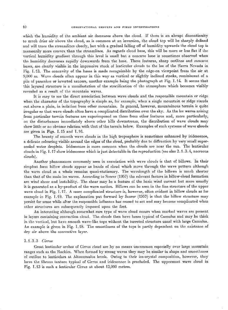
and are easily recognizable. The observations of Larsson (1954) indicate that the most definite shape is assumed when the ambient relative humidity is low (30-60 per cent). The most likely explanation is that the low humidity confines the cloud to the regions of maximum ascent in the wave crests and the lenticulars are seen in isolation, detached from the confusion of other clouds. A striking single-wave cloud caused by a hill in Eastern Scotland is illustrated in Fig. I .12. The middle cloud in Fig. I .11 is another example of a clearly detached lenticular over the Owens Valley.
We have seen that the smoothness of the outlines of wave clouds is an indication of the laminar nature of the airflow. The sharp clarity of the upper-cloud outline depends also on the rapidity with
10 OBSERVATIONAL RESULTS AND FIELD INVESTIGATIONS
which the humidity of the ambient air decreases above the cloud. If there is an abrupt discontinuity
to much drier air above the cloud, as is common at an inversion, the cloud top will be sharply defined
and will trace the streamlines closely, but with a gradual falling off of humidity upwards the cloud top is necessarily more convex than the streamlines. As regards cloud base, this will be more or less flat if the
vertical humidity gradient through this level is small but a concave base is sometimes observed when the humidity decreases rapidly downwards from the base. These features, sharp outlines and concave
bases, are clearly visible in the impressive stack of lenticular clouds to the lee of the Sierra Nevada in Fig. I .13. The concavity of the bases is made recognizable by the edge-on viewpoint from the air at
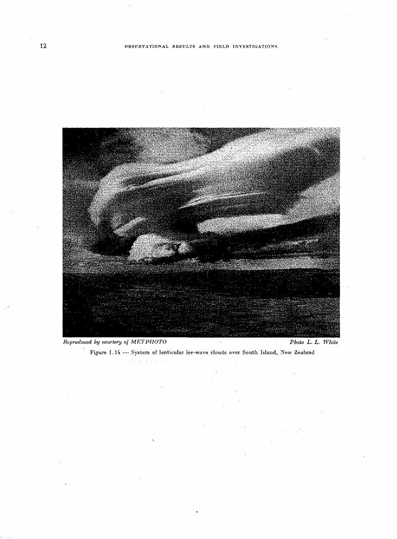
9,000 m. Wave clouds often appear in this way as vertical or slightly inclined stacks, reminiscent of a pile of pancakes or inverted saucers, another example being the photograph at Fig. I .14. It seems that
this layered structure is a manifestation of the stratification of the atmosphere which becomes visibly
revealed as a result of the mountain waves. It is easy to see the direct association between wave clouds and the responsible mountain or ridge
when the character of the topography is simple as, for example, when a single mountain or ridge stands out above a plain, in isolation from other mountains. In general, however, mountainous terrain is quite
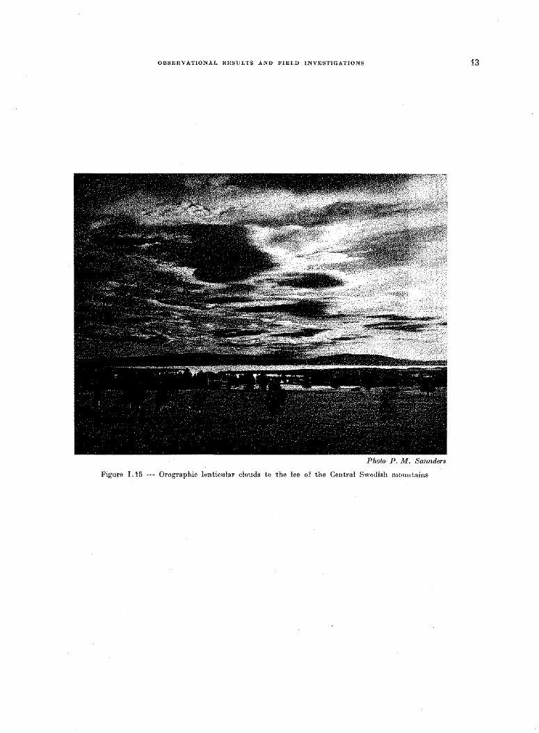
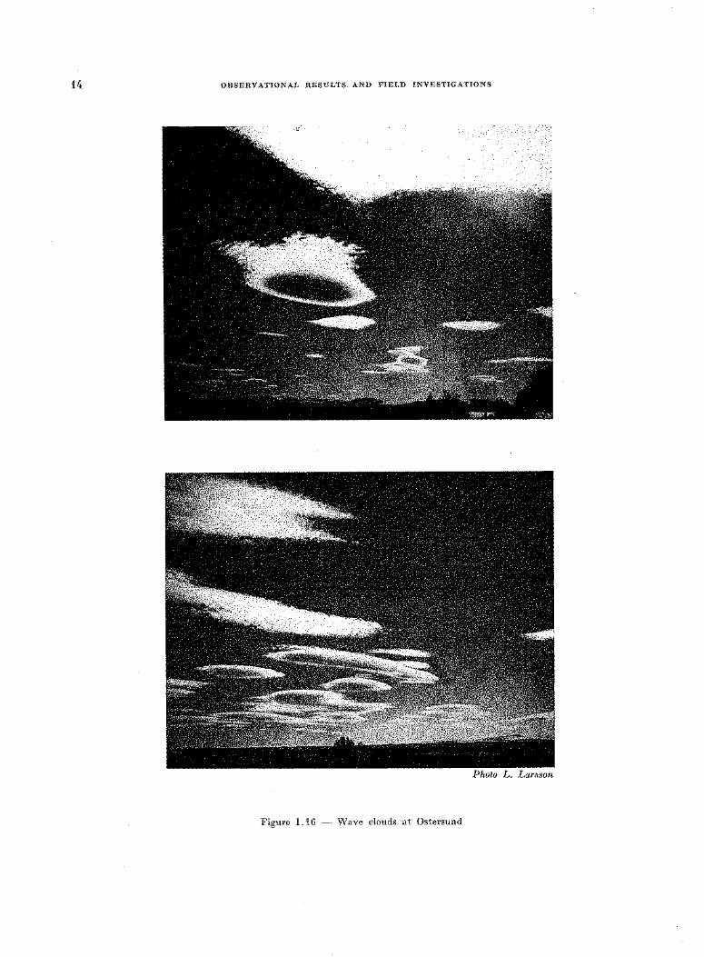
irregular so that wave clouds often have a complicated distribution over the sky. As the lee waves arising from particular terrain features are superimposed on those from other features and, more particularly,
on the disturbances immediately above other hills downstream, the distribution of wave clouds may show little or no obvious relation with that of the terrain below. Examples of such systems of wave clouds
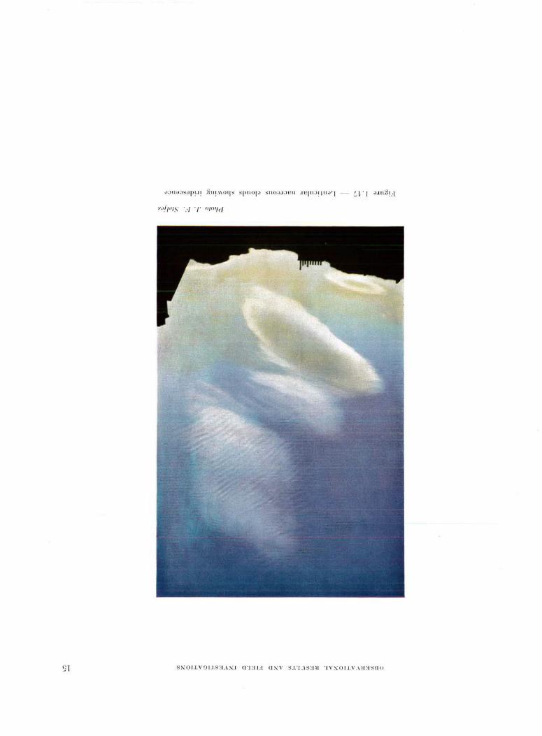
are given in Figs. I. 15 and I .16. The beauty of smooth wave clouds in the high troposphere is sometimes enhanced by iridescence,
a delicate colouring visible around the edges of the cloud, probably due to diffraction by very small super
cooled water droplets. Iridescence is more common when the clouds are near the sun. The lenticular: clouds in Fig. I .17 show iridescence which is just detectable in the reproduction (see also 2. 1. 3. 4, nacreous clouds).
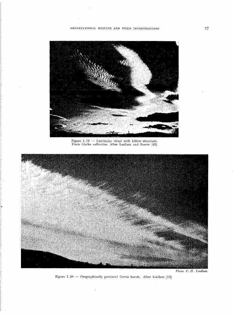
Another phenomenon commonly seen in association with wave clouds is that of billows. In their simplest form billow clouds appear as bands of cloud which move through the wave pattern although the wave cloud as a whole remains quasi-stationary. The wavelength of the billows is much shorter
than that of the main lee waves. According to Scorer (1957) the relevant factors in billow-cloud formation are wind shear and instability. The shear may be a feature of the basic wind current but more usually it is generated as a by-product of the wave motion. Billows can be seen in the fine structure of the upper
wave cloud in Fig. 1.17. A more complicated structure is, however, often evident in billow clouds as for example in Fig. 1.19. The explanation put forward by Scorer (1957) is that the billow structure may persist for some while after the responsible influence has ceased to act and may become complicated when
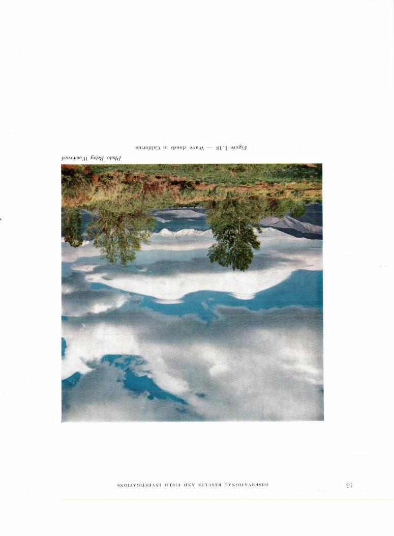
other structures are subsequently imposed upon the first. An interesting although somewhat rare type of wave cloud occurs when marked waves are present
in layers containing convection cloud. The clouds then have bases typical of Cumulus and may be thick in the vertical, but have smooth wave-like tops without the turreted structure usual with large Cumulus. An example is given in Fig. I. 18. ·The smoothness of the tops is partly dependent on the existence of
dry air above the convective layer.
2 . 1. 3. 3 Cirrus
Great lenticular arches of Cirrus cloud are by no means uncommon especially over large mountain ranges such as the Rockies. When formed by strong waves they may be similar in shape and smoothness
of outline to lenticulars at Altocumulus levels. Owing to their ice-crystal composition, however, they have the fibrous texture typical of Cirrus and iridescence is precluded. The uppermost wave cloud in Fig. I .13 is such a lenticular Cirrus at about 12,000 metres.
OBSERVATIONAL RESULTS AND FIELD INVESTIGATIONS
Photo Terence Horsley
Figure 1.12 - A single-wave cloud, seen from 12,000 ft and caused by Lundie Hill (U.K.) visible bottom left of picture
Photo T. Henderson
Pigure I .13 - Roll clouds and lenticulars at five levels in the first lee wave downwind of the Sierra Nevada photographed from 30,000 ft.
After Holmboe and Klieforth [25)
11
12 OBSERVATIONAL RESULTS AND FIELD INVESTIGATIONS
Reproduced by courtery of METPHOTO Photo L. L. White
Figure 1.14- System of lenticular lee-wave clouds over South Island, New Zealand
OBSERVATIONAL RESULTS AND FIELD INVESTIGATIONS
Photo P. M. Saunders
Figure I .15 - Orographic lenticular clouds to the lee of the Central Swedish mountains
13
14 OBSERVATIONAL RESULTS AND FIELD INVESTIGATIONS
Photo L. Larsson
Figure 1.16 -Wave clouds at Ostersund
ST
ll!UJOJ !fll:J ur spnop ~-' l'.J\,\ - 8 ~ · I ~.rn il r ,·I
p.tlh HJ100 Il l fi S /Of{ 0 / 0lfd
S.\:O I.I.Y ::J I.I. S:·J.\ !\:1 O ' L ILI CI!\:Y S .I .'J.l S :o!ll 1\'!\:0 J.I . \' .\ll ci SHO gr,
OBSERVATIONAL RESULTS AND FIELD INVESTIGATIONS
Figure I. 19 - Lenticular cloud with billow structure. From Clarke collection. After Ludlam and Scorer [l•3]
Figure I. 20 - Orographically produced Cirrus bands. After Ludlam [42]
17
Photo F. I-1. Ludlam
lnJSB JY . 1 ~.\0 sp nop J-l l~ad-JO-.W 'f1 DJ\ - ~(; · J J.l n.ll •:T
.1;/ 11/.l,!?/S' 'Q O]Olf c[
OBSERVATIONAL RESULTS AND FIELD INVESTIGATIONS 19
As is explained elsewhere in this monograph, there is sometimes considerable turbulence associated
with mountain waves near the tropopause and this is sometimes revealed by the structure of any lenticular
Cirrus clouds at these levels. The highest wave cloud in Fig. I .11, at about 12,000 m, has a fibrous and
turbulent structure in marked contrast to the very smooth lenticular water cloud below it.
It must not be thought from the foregoing examples that orographic Cirrus is only formed over
very large mountains. From a series of careful observations over the British Isles, Ludlam (1952) has
demonstrated conclusively that waves caused by hills only 300 m or so high may have sufficient amplitude
at Cirrus levels to form cloud. Very often the vertical air displacerrtents at these high levels must be much
greater than the height of the responsible hills. It appears from Ludlam's work that due to the physics of
Cirrus clouds, there is often an interesting aspect in the subsequent behaviour of the cloud once formed.
Over the British Isles cloudless air at these levels is commonly supersaturated with respect to ice but
not with respect to water. Orographic waves in the airflow lead to saturation with respect to water and
thus to cloud formation. The cloud rapidly becomes a predominantly ice-crystal cloud and, owing to the
supersaturation with respect to ice, fails to dissolve when the air descends to its original level. This results
sometimes in the production of long bands or streamers of Cirrus extending downwind for perhaps hundreds
of km, and beginning with a sharply defined upwind encl. where the cloud is being continuously formed
above some terrain feature. The bands of Cirrus in Fig. I. 20 extended from hills in the west of England to
at least the east coast. The mechanism makes it possible for hills to exert a profound influence over the
general high cloud cover above considerable areas to the lee.
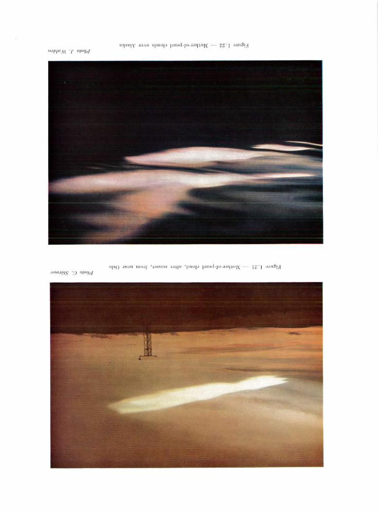
2 . 1 . 3 . 4 Nacreous clouds
These, perhaps the most astonishing of all orographic clouds, occur, albeit rarely, in the stratosphere
at heights from 20 to 30 km, viz. at about twice the height of Cirrus cloud. They have the smooth lenticular
form characteristic of wave clouds in mid-troposphere and often exhibit marked iridescence. Owing to
their great height they appear brightly illuminated for some time after sunset and before sunrise at the
ground. At these times the dark sky provides an ideal background against which to view the colouring _
due to iridescence, and no doubt the description "mother-of-pearl" clouds is highly appropriate.
Mother-of-pearl clouds have been seen in Norway, Scotland, Iceland and Alaska but there have been
few systematic observations except those of Stormer in Norway. However, there seems little doubt that
an essential requirement for the occurrence of these clouds is a strong deep airstream having a component
across a substantial mountain chain extending to heights of 30 km or more. These conditions are occa
sionally provided in the strong westerly currents to the south of intense high-latitude depressions during
the northern hemisphere winter. What other conditions may also be necessary can only be inferred from
theoretical considerations, but clearly there must be sufficient moisture in the high stratosphere. Further
more, if the cloud physics of the troposphere is at all applicable we are tempted to conclude from the iri
descence of nacreous clouds that they must be water clouds at a temperature above -40°C.
Two beautiful examples of mother-of-pearl clouds are illustrated in Figs. I. 21 and I. 22.
2. 2 Gliders
We have mentioned that some of the first observational evidence relating to waves over and to
the lee of mountains came from glider pilots during the period of adventurous activity in this sport in
the 1930's. That this should be so is not surprising ; in order to climb and stay aloft, glider pilots must
_______ -~xploit the up-currents which occur naturally in the atmosphere, and experienced glider pilots are often
remarkably skilful at locating rising_air. In the very beginning of gliding the main source of vertical
motion was the up-slope motion to be found on the windward side of hills and ridges, whilst somewhat
later thermal up-currents were exploited. The great attraction and interest of soaring in mountain waves
20 OBSERVATIONAL RESULTS AND FIELD INVESTIGATIONS
stems from the fact that they provide a means of continuous soaring to considerable heights in regions to the lee of hills. From the glider pilot's point of view once he has reached the rising air of a mountain wave he knows that he has every prospect of maintaining himself aloft for a few hours if desired, because the vertical motion he is exploiting is much less transitory than that associated with thermals.
There is available in the literature of gliding an abundance of descriptive, and to some extent quantitative, material on the nature and characteristics of mountain waves, because the pilots using every gliding site near hills or mountains naturally take steps to gain experience of the potentialities of their locality for wave soaring. This material provides a fairly complete picture of the properties of waves requiring explanation.
A modern glider is very efficient aerodynamically in that the sinking speed in still air for a given airspeed is very low - of the order of 1 m/sec. Furthermore the relation between sinking speed and airspeed can be determined by calibration fairly exactly for any particular machine. Gliders are also able to fly comparatively slowly, e.g. around 40 kt without reaching stalling speed. By recording the altitude at frequent intervals and allowing for the rate of sink in still air, vertical air currents can be obtained, whilst the available range of airspeed enables a glider flown into wind to hover above a fixed point on the ground. These qualities of the glider make it a valuable research tool for the investigation of mountain waves and as we shall see in later sections they have played an important part in a number of field investigations.
2. 3 Powered aircraft
Aircraft have been flying over hills and mountains since aviation came into being, but it is· only during the last decade or so that an awareness of the dangerous phenomena which can occur over mountains has begun to develop amongst pilots. The high proportion of aircraft accidents which have occurred in the past in mountainous terrain constitute a tragic pointer to the hazards of which pilots in the past could have had but a vague knowledge. At the time, many such accidents were attributed to errors of navigation coupled with an inadequate height margin to clear high ground near the intended track, accompanied perhaps by additional adverse circumstances such as cloud, darkness, icing. It seems probable, however, that the deceptive vertical currents which are now known to occur near mountains must have been the dominant factor in many of these accidents. Thanks to the numerous observations which have been made and research work which has been conducted in many countries during the last few years, there is now a much better understanding of the nature of the airflow over mountains. Reports from the pilots of aircraft have contributed substantially to this improved understanding. They confirm that areas of lift and sink are commonly to be found over and to the lee of mountains. Mild lee waves may easily escape the notice of the pilot of a powered aircraft because they are not necessarily accompanied by any turbulence effects ; indeed, many pilots mention the remarkably smooth flying conditions in waves. One of the main hazards is that even powerful waves may pass unnoticed unless a close watch on the altimeter is maintained and a region of turbulence may then be encountered suddenly when the height clearance above the terrain has become marginal.
Undoubtedly the most spectacular incident on record has been that mentioned by Colson (1954) of the experience of the pilot of a P-38 aircraft who found on arrival over the Owens Valley in the Sierra Nevada that rising dust whipped up by strong surface winds prevented his landing at Bishop Airport. The mountain wave operating at the time was of such intensity that the pilot was able. to feather the airscrews and soar this heavy fighter aircraft as a glider for over an hour whilst awaiting an opportunity to land. The implied vertical currents (of the order of 40 m/sec) were quite exceptional even for this unique location and the reports from the pilots of transport aircraft mostly imply vertical currents ranging up to about 10 m/sec.
OBSERVATIONAL RESULTS AND FIELD INVESTIGATIONS 21
Numerous reports of this type are on record in the literature and some of them may be found m
the following references: Austin (1952), Corby (1957), French (1951), Georgii (1956), Kuettner and Jenkins (1953), Mason (1954), Pilsbury (1955), Radok (1954) and Turner (1951).
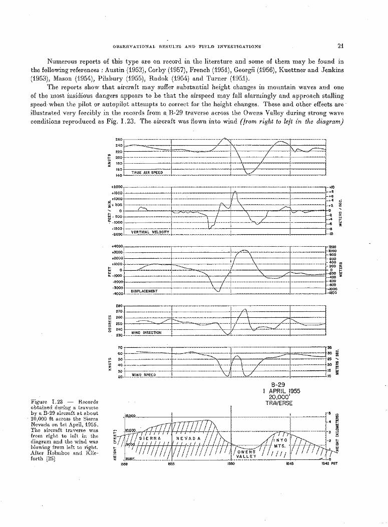
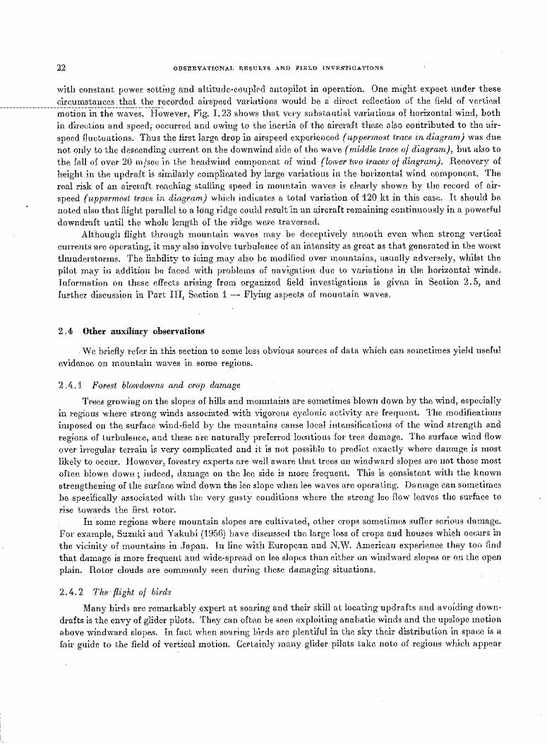
The reports show that aircraft may suffer substantial height changes in mountain waves and one
of the most insidious dangers appears to be that the airspeed may fall alarmingly and approach stalling speed when the pilot or autopilot attempts to correct for the height changes. These and other effects are ·
illustrated very forcibly in the records from a B-29 traverse across the Owens Valley during strong wave
conditions reproduced as Fig. I. 23. The aircraft was flown into wind (from right to left in the diagram)
Figure I. 23 - Records obtained during a traverse by a B-29 aircraft at about 20,000 ft across the Sierra Nevada on 1st April, 1955. The aircraft traverse was from right to left in the diagram and the wind was blowing from left to right. After Holmboe and Klieforth [25]
'T I Ll ~t~ 240 --=:::::::: ---.... 2 \ 7 ~
% j~t .. ""'"" : \; 140
+2000
+1500
. +1000 z i .. 500
.... 0
E- soo ""-1000
-1500
-2000
+4000
+3000
+2000
+1000
t;; 0
"' ... -1000
-2000
-3000
-4000
280
270
260
250
240
230
60
~ 50 70j
0 40 z " 30
20
" 1/ \ " \
£-\ /V " ---....._ I \ \ I \ \,.-'
VERTICAL VELOCITY
...-... _L \ / \
/ ----- ~ .L \ ./_ \ I
DISPLACEMENT ~
/'-I
/ '"'
\ '\., L_ ...______...
,~ -
r--
+10 .a +6 +4 +2 0 2 4 6
8 10
200 1000 800 600 400 200 0
-200 1-400
600 600 1000 1200 _.
.,:::}f+=<Vkf#l WIND SPEED
~\JGGzjjjj~ 8-29
APRIL 1955 20,000'
TRAVERSE
5 ~ &! 15000 4 ~
;: "' "' ...
1559 1555 1550 1545
"' "' 3 :::! ~
22 OBSERVATIONAL RESULTS AND FIELD INVESTIGATIONS
with constant power setting and altitude-couplPd autopilot in operation. One might expect under these
circumstances that _the _E_ecorded airspeed variations would be a direct reflection of the field of vertical
motion in the waves. However, Fig. I. 23 shows that very substantial variations of horizontal wind, both
in direction and speed; occurred and owing to the inertia of the aircraft these also contributed to the air
speed fluctuations. Thus the first large drop in airspeed experienced (uppermost trace in diagram) was due
not only to the descending current on the downwind side of the wave (middle trace of diagram), but also to
the fall of over 20 m/sec in the headwind component of wind (lower two traces of diagram). Recovery of
height in the updraft is similarly complicated by large variations in the horizontal wind component. The
real risk of an aircraft reaching stalling speed in mountain waves is clearly shown by the record of air
speed (uppermost trace in diagram) which indicates a total variation of 120 kt in this case. It should be
noted also that flight parallel to a long ridge could result in an aircraft remaining continuously in a powerful
downdraft until the whole length of the ridge were traversed. Although flight through mountain waves may be deceptively smooth even when strong vertical
currents are operating, it may also involve turbulence of an intensity as great as that generated in the worst
thunderstorms. The liability to icing may also be modified over mountains, usually adversely, whilst the
pilot may in addition be faced with problems of navigation due to variations in the horizontal winds.
Information on these effects arising from organized field investigations is given in Section 2. 5, and
further discussion in Part Ill, Section 1 - Flying aspects of mountain waves.
2 . 4 Other auxiliary observations
We briefly refer in this section to some less obvious sources of data which can sometimes yield useful
evidence on mountain waves in some regions.
2. 4. 1 For est blowdowns and crop damage
Trees growing on the slopes of hills and mountains are sometimes blown down by the wind, especially
in regions where strong winds associated with vigorous cyclonic activity are frequent. The modifications
imposed on the surface wind-field by the mountains cause local intensifications of the wind strength and
regions of turbulence, and these are naturally preferred locations for tree damage. The surface wind flow
over irregular terrain is very complicated and it is not possible to predict exactly where damage is most
likely to occur. However, forestry experts are well aware that trees on windward slopes are not those most
often blown down ; indeed, damage on the lee side is more frequent. This is consistent with the known
strengthening of the surface wind down the lee slope when lee waves are operating. Damage can sometimes
be specifically associated with the very gusty conditions where the strong lee flow leaves the surface to
rise towards the first rotor. In some regions where mountain slopes are cultivated, other crops sometimes suffer serious damage.
For example, Suzuki and Yak ubi ( 1956) have discussed the large loss of crops and houses which occurs in
the vicinity of mountains in Japan. In line with European and N.W. American experience they too find
that damage is more frequent and wide-spread on lee slopes than either on windward slopes or on the open
plain. Rotor clouds are commonly seen during these damaging situations.
2. 4. 2 The flight of birds
Many birds are remarkably expert at soaring and their skill at locating updrafts and avoiding down
drafts is the envy of glider pilots. They can often be seen exploiting anabatic winds and the upslope motion
above windward slopes. In fact when soaring birds are plentiful in the sky their distribution in space is a
fair guide to the field of vertical motion. Certainly many glider pilots take note of regions which appear
OBSERVATIONAL RESULTS AND FIELD INVESTIGATIONS 23
to be favoured by birds and to some extent it appears that birds sometimes abandon one area in favour of
another being used by gliders. According to the gliding press, however, there is little doubt that birds are
superior to glider pilots when it comes to anticipating the end of an updraft ; they abandon the area in
good time. The term "dynamic soaring" is not to be confused with the straightforward use of rising air. Dynamic
soaring is the technique used by some birds, notably maritime types, for exploiting the vertical gradient
of horizontal wind to gain height.
2. 4. 3 The transport of particles by mountain winds
In order to spread particles distances of many miles, we require up-currents of sufficient magnitude
near the ground to support the particles, coupled with sufficient wind for the horizontal transport. Further
more these conditions need to be maintained for several hours or a day or more to bring about any consi
derable transport from one area to another. Thermals provide only small up-currents near the ground
and would not usually result in preferred areas for the deposit of particles. The airflow in the vicinity of
mountains can provide all the factors to support particles and transport them. There would be a tendency
for such material to be deposited in areas where the wind became lighter. The process is rather like that
which brings about snow drifts to the lee-of sheltering obstructions such as hedges, buildings etc. Indeed,
on tnelarger scale-tne immeuiatelee slopes of mountains areuftmru~:muded of lying snow by strong winds
which deposit the snow further downstream.
In an unusual study Forchtgott ( 1950) considered the flow to the lee of the Ohre mountains in Silesia
and concluded that there would be a tendency for airborne material to be deposited in the valley of the
River Ohre, especially in the Louny sector. This conclusion was strikingly borne out, in the course of
plant protection research, by the discovery of a strong and persistent centre of colorado beetle activity in
this sector.
2 . 4. 4 Miscellaneous effects
The distribution of rainfall in mountainous regions is influenced markedly by the topography. In
this context the time spent by the air in flowing through lee waves is too short for the processes relevant
for the production of rain to be effective. We are therefore concerned with the flow over mountain ranges
as a whole rather than with that over individual ridges. Sawyer (1956) has considered this question and
shown what factors result in a vertical motion field over mountains suitable for heavy orographic rain.
Double-theodolite pilot-balloon ascents are quite adequate to reveal the vertical motions in waves
and have been made use of in some investigations (see, for example, Colson, 1954 and Laird, 1952). The
microbarograph, too, has its uses and, in particular, as moving eddies are accompanied by pressure fluctua
tions, the incidence and intensity of eddying motion can be assessed indirectly from microbarograph
records. Such studies are most appropriate to mountain observatories.
Finally there are numerous natural indicators of surface wind, e.g. the movement of smoke, dust,
trees, corn, grasses, etc. It is sometimes possible to infer a good deal about the flow near hills by observing
the surface wind at a distance by means of such indicators. Phenomena such as separation of the flow,
and standing eddies can sometimes be detected in this way. Disturbances on the surface of lakes amongst
mountains and on the sea near cliffs can be similarly revealing.
2 . 5 Some organized field investigations
The study of mountain airflow effects in the field can take the form of systematic observations of
clouds, surface wind, smoke drift, etc. from the ground and certainly such studies can be profitable and are
24 OBSERVATIONAL RESULTS AND FIELD INVESTIGATIONS
not to be despised. Indeed, certain specific aspects of the airflow over mountains are best studied by such means. It is natural, however, that some ambitious workers in the field should wish to measure as comprehensively as possible the three-dimensional field of flow over and to the lee of mountains. Studies on this scale pose some formidable problems and call for considerable experimental skill, comprehensive instrumentation and a well-organized team. Since the effects it is desired to study do not occur to order, the team may need to remain in the field location for a whole season, or more, unless they are so dispositioned that they can go into action at short notice.
Methods which have been used include the tracking of calibrated and instrumented sailplanes through mountain waves, flights by specially instrumented aircraft, the tracking of balloons, including large "no-lift" balloons carrying radiosonde transmitters, etc. In the following sub-sections, we summarize the techniques and results of some of the more notable field investigations which have been carried out.
2. 5.1 The early work of Kuettner
In the present section we are concerned with Kuettner's work during the 1930's, the bulk of which was published in two substantial papers in 1939. (The Sierra Wave Project, in which Kuettner also participated, is discussed in 2. 5. 5.) The work was carried out in the European Alps, favoured locations being the Riesengebirge range and the Hirschberger Valley to the lee of the Schneekoppe ridge.
2. 5 .1.1 Techniques and instrumentation
This work did not comprise one specific field project with well-defined aims. Rather it is an account of a variety of personal studies, observations and experience acquired during a period when Kuettner himself was amongst the pioneer glider pilots exploring mountain waves in Europe. Like Manley (see 2. 5. 2), Kuettner was concerned mainly with achieving a detailed description of phenomena, which up to that time had been inadequately documented, although naturally he also attempted a measure of interpretation whenever possible.
One of his principal techniques was the detailed observation of mountain clouds as regards their characteristic forms, their mainly stationary quality and their position relative to the mountains. His papers contain a very comprehensive collection of photographs, taken both from the air and from the ground, and including superb examples of almost every type of mountain cloud. In addition, his graphic descriptions of the cloud forms are most illuminating.
Data from glider flights provided the other main source of data. The gliders usually carried a barograph, providing a pressure/time plot of each flight, but were not otherwise specially instrumented. However, there were sufficient data to allow a fairly detailed study of the airflow on a number of particular occasions. Conventional synoptic data were also used.
2 . 5 .1. 2 Main results
Kuettner's main achievement at this time was to produce a precise and really comprehensive account of his own and other observations of mountain wave phenomena. .There would today be few significant criticisms of the correctness of his description, which speaks highly of the thoroughness of his original interpretation o£ the observations.
Kuettner recognized the existence of powerful gravity waves over and to the lee of mountains, and noted their quasi-stationary character which makes the topographical connexion inescapable. He found that the vertical currents involved were sufficient to carry gliders to the high troposphere and he himself reached 8,000 m on more than one occasion (e.g. 14 March 1937). Experience in different localities indicated that the phenomena were not peculiar to one particular mountain but occurred generally.
In an attempt at the classification of mountain waves, he drew a distinction between cases with "lee eddies" and "£ohn waves". In the former case some form o£ eddying motion takes place immediately
OBSERVATIONAL RESULTS AND FIELD 1NYESTlGA'riONS 25
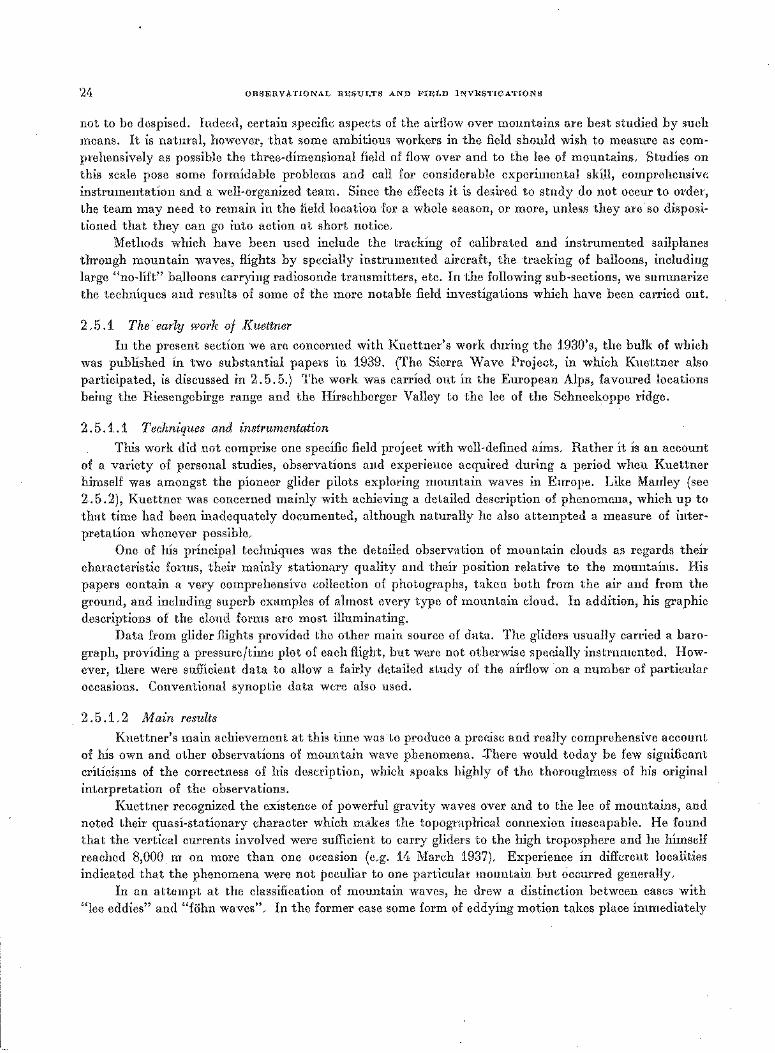
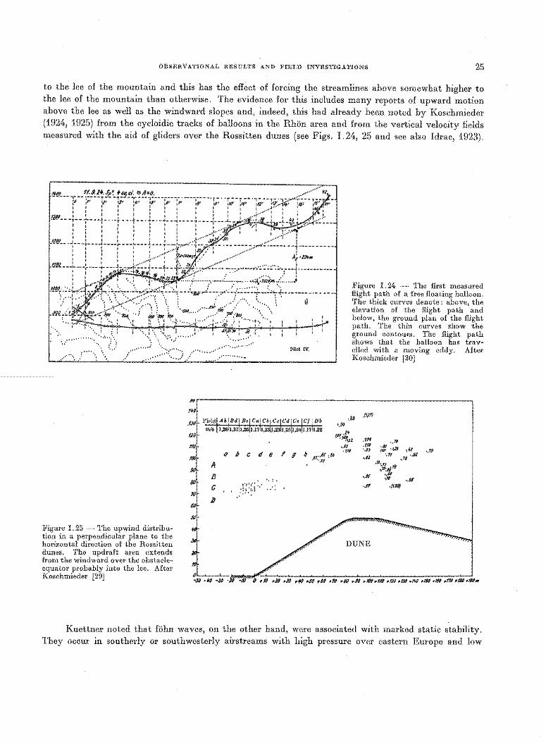
to the lee of the mountain and this has the effect of forcing the streamlines above somewhat higher to the lee of the mountain than otherwise. The evidence for this includes many reports of upward motion above the lee as well as the windward slopes and, indeed, this had already been noted by Koschmieder (1924, 1925) from the cycloidic tracks of balloons in the Rhon area and from the vertical velocity fields measured with the aid of gliders over the Rossitten dunes (see Figs. I. 24, 25 and see also ldrac, 1923).
.. ····· ... _.· .····-·----
t~l/1/ ff.$.2 .. .fp~ ~&v,e,: 0/l=o. . .. ···············,z, ----- -;, --:;,---r,;- -11,---~;--:;;--:;--:-;;--·-:~;--·:9:-- r,;- r,;, "-;;;- -1,J:=-~~;-:--·-~;,-- iti'- f1
1-
1 I I : : : I I I I I 1 I , ••• J.•' I I 14of. I
fJID : : : 1 I : : : : : : : ••• ·+···· : : : ~ J. --- ---1---:-- --"! .. ---t .. --f .. -- j--- ~- -i- .. -- ~- ... --:-- ~-~~J~~ o/~-· ·::- '»-~-~:- ~-)~~-:.·~ ...... : ! : : : : : : : .... L··:·W : I : ).~-=-4 I I I I I I I I , ... 1{. ,,•''1 :
f2dtl 1 1 I I 1 : I 1 •• +·· JP';}. ;]21 ,.,••'' i ,_- -----,- ... -;- ---:----r- ---~--- 1--- y-~~~-"; .... ~ -1;o- -, ,------- -.:::.:;~·-------- -1-- .. -------: : : : : : ... ·····r· .:?d'•INMt~ /, 1
••••••••••••• A~•l.?fcm
~;:J;l;;.~~~;~i~,-J~t~~~i;-~~,;f§:r:!::~~:::::-_ .900 :t~, .9So ... •'li_oq ~.. .. ! ' • , IS0~~·· •• 'fsl."lt;g \ •
---~~-~: •. -.::~· ~~·-: '._', : '111{\J. ~ f \~: ~-:-~---~ ... ~'··'~~~i .... -~:) : ·--···-:-·,, '•,: : I :
I I : i : I •• •• : ... :,; : !· : JJ Jl I J6 ·l' I ··.'---:·. ... ... 'tJ\ :~·- _,./'
........ () ./·······~~-~ .. :-::· .. ::::::) ...... .. ......... _.
Pilot IV.
Figure I. 24 - The first measured flight path of a free floating balloon. The thick curves denote: above, the elevation of the flight path and below, the ground plan of the flight path. The thin curves show the ground contours. The flight path shows that the balloon has travelled with a moving eddy. After Koschmieder [30]
mr------------------------------------------------------------,
Figure I. 25 - The upwind distribution in a perpendicular plane to the horizontal direction of the Rossitten dunes. The updraft area extends from the windward over the obstacleequator probably into the lee. After Koschmieder [29]
1~0
.fJO
fJO
!fO,
ff)
ll B c D
u/Jcde
·. :. : ~;: ~: i ...
f !I " ,61.:::: :86
•,89 •.90
or·.ll f ·1-'!,)z
,,.9J o(f0
.(1,11}
.tal
.1,18 ".IJ
•• Q1
•• JI
•,Sf
,,11
.,JJ •I.J$ •,11 ftrJo.,.,, .,1J •.81
•71
:,'1J •.1b .,'11~61
::: ··" •(!SO)
.,'?!I
.... _ .... J-- ...
Kuettner noted that fohn waves, on the other hand, were associated with marked static stability. They occur in southerly or southwesterly airstreams with high pressure over eastern Europe and low
26 OBSERVATIONAL RESULTS AND FIELD INVESTIGATIONS
pressure in the British Isles region. He drew a further distinction between the anticyclonic fohn and the
cyclonic fi.ihn, the main difference being that the full gamut of mountain wave clouds (cap, wave and rotor)
were not produced in the former case owing to the dryness of the subsiding air in the anticyclonic stream.
Other descriptive terms used by Kuettner, e.g. "rising waves" and "sinking waves" to distinguish cases
having opposite vertical motion above the lee slope are somewhat ambiguous and have not come into
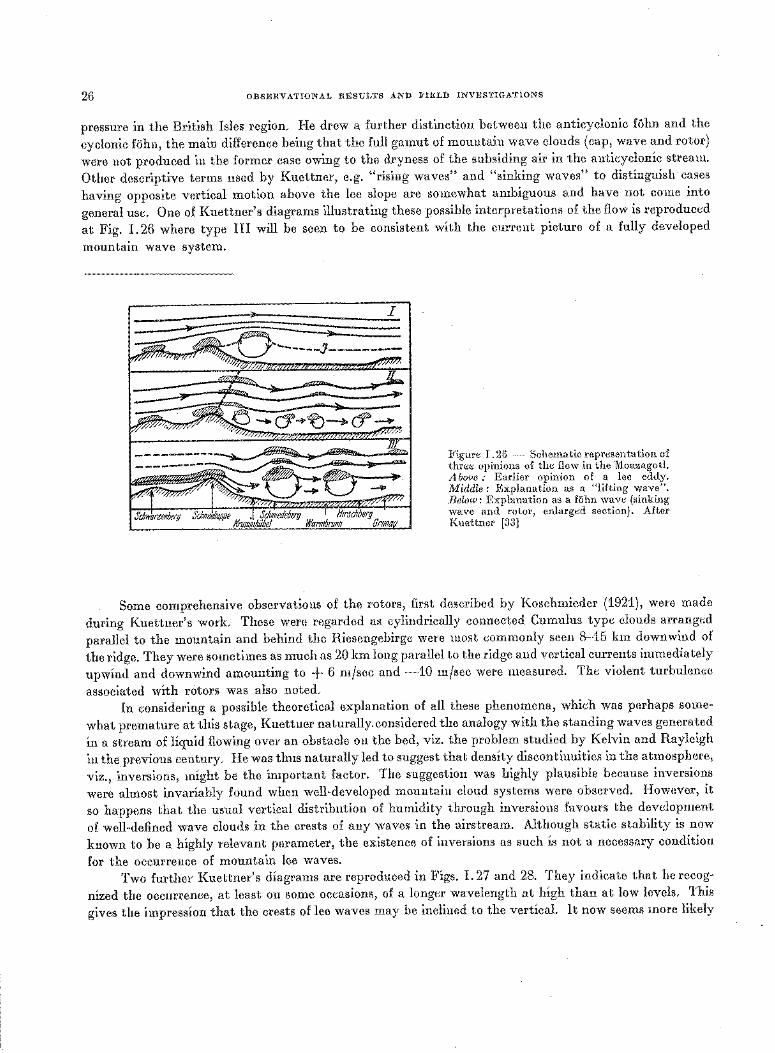
general use. One of Kuettner's diagrams illustrating these possible interpretations of the flow is reproduced
at Fig. I. 26 where type Ill will be seen to be consistent with the current picture of a fully developed
mountain wave system.
I
Figure I. 26 - Schematic representation of three opinions of the flow in the Moazagotl. Above : Earlier opinion of a lee eddy. Middle: Explanation as a "lifting wave". Below: Explanation as a fohn wave (sinking wave and rotor, enlarged section). After Kuettner [33]
Some comprehensive observations of the rotors, first described by Koschmieder (1921), were made
during Kuettner's work. These were regarded as cylindrically connected Cumulus type clouds arranged
parallel to the mountain and behind the Riesengebirge were most commonly seen S-15 km downwind of
the ridge. They were sometimes as much as 20 km long parallel to the ridge and vertical currents immediately
upwind and downwind amounting to + 6 m/sec and -10 m/sec were measured. The violent turbulence
associated with rotors was also noted.
In considering a possible theoretical explanation of all these phenomena, which was perhaps some
what premature at this stage, Kuettner naturally. considered the analogy with the standing waves generated
in a stream of liquid flowing over an obstacle on the bed, viz. the problem studied by Kelvin and Rayleigh
in the previous century. He was thus naturally led to suggest that density discontinuities in the atmosphere,
viz., inversions, might be the important factor. The suggestion was highly plausible because inversions
were almost invariably found when well-developed mountain cloud systems were observed. However, it
so happens that the usual vertical distribution of humidity through inversions favours the development
of well-defined wave clouds in the crests of any waves in the airstream. Although static stability is now
known to be a highly relevant parameter, the existence of inversions as such is not a necessary condition
for the occurrence of mountain lee waves. Two further Kuettner's diagrams are reproduced in Figs. I. 27 and 28. They indicate that he recog
nized the occurrence, at least on some occasions, of a longer wavelength at high than at low levels. This
gives the impression that the crests of lee waves may be inclined to the vertical. It now seems more likely
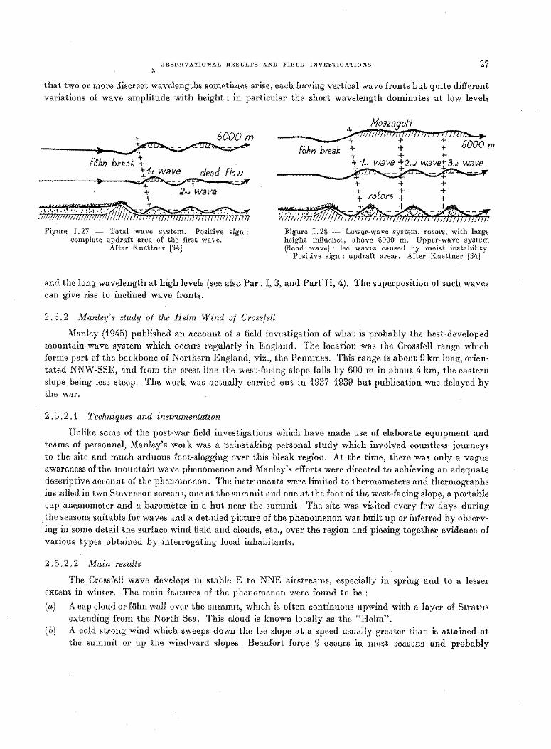
OBSERVATIONAL RESULTS AND FIELD INVESTIGATIONS 27 :,
that two or more discreet wavelengths sometimes arise, each having vertical wave fronts but quite different variations of wave amplitude with height ; in particular the short wavelength dominates at low levels
6000m
Figure I. 27 - Total wave system. Positive sign : complete updraft area of the first wave.
After Kuettner [3!>]
Figure I. 28 - Lower-wave system, rotors, with large height influence, above 6000 m. Upper-wave system (flood wave) : lee waves caused by moist instability.
Positive sign : updraft areas. After Kuettner [34]
and the long wavelength at high levels (see also Part I, 3, and Part II, 4). The superposition of such waves can give rise to inclined wave fronts.
2 . 5. 2 M anley' s study of the Helm Wind of Crossfell
Manley (1945) published an account of a field investigation of what is probably the best-developed mountain-wave system which occurs regularly in England. The location was the Crossfell range which forms part of the backbone of Northern England, viz., the Pennines. This range is about 9 km long, orientated NNW-SSE, and from the crest line the west-facing slope falls by 600 m in about 4 km, the eastern slope being less steep. The work was actually carried out in 1937-1939 but publication was delayed by the war.
2. 5. 2.1 Techniques and instrumentation
Unlike some of the post-war field investigations which have made use of elaborate equipment and teams of personnel, Manley's work was a painstaking personal study which involved countless journeys to the site and much arduous foot-slogging over this bleak region. At the time, there was only a vague awareness ofthe mountain wave phenomenon and Manley's efforts were directed to achieving an adequate descriptive account of the phenomenon. The instruments were limited to thermometers and thermographs installed in two Stevenson screens, one at the summit and one at the foot of the west-facing slope, a portable cup anemometer and a barometer in a hut near the summit. The site was visited every few days during the seasons suitable for waves and a detailed picture of the phenomenon was built up or inferred by observing in some detail the surface wind field and clouds, etc., over the region and piecing together evidence of various types obtained by interrogating local inhabitants.
2.5.2.2 Main results
The. Crossfell wave develops in stable E to NNE airstreams, especially in spring and to a lesser extent in winter. The main features of the phenomenon were found to be :
(a) A cap cloud or fohn wall over the summit, which is often continuous upwind with a layer of Stratus extending from the North Sea. This cloud is known locally as the "Helm".
(b) A cold strong wind which sweeps down the lee slope at a speed usually greater than is attained at the summit or up the windward slopes. Beaufort force 9 occurs in most seasons and probably
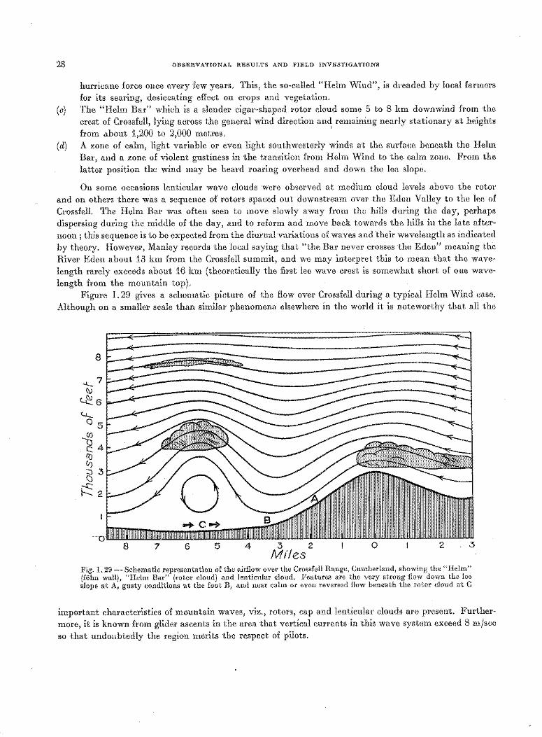
28 OBSERVATIONAL RESULTS AND FIELD INVESTIGATIONS
hurricane force once every few years. This, the so-called "Helm Wind", is dreaded by local farmers
for its searing, desiccating effect on crops and vegetation.
(c) The "Helm Bar" which is a slender cigar-shaped rotor cloud some 5 to 8 km downwind from the
crest of Crossfell, lying across the general wind direction and remaining nearly stationary at heights I
from about 1,200 to 2,000 metres.
(d) A zone of calm, light variable or even light southwesterly winds at the surface beneath the Helm
Bar, and a zone of violent gustiness in the transition from Helm Wind to the calm zone. From the
latter position the wind may be heard roaring overhead and down the lee slope.
On some occasions lenticular wave clouds were observed at medium cloud levels above the rotor
and on others there was a sequence of rotors spaced out downstream over the Eden V alley to the lee of
Crossfcll. The Helm Bar was often seen to move slowly away from the hills during the day, perhaps
dispersing during the middle of the day, and to reform and move back towards the hills in the late after
noon ; this sequence is to be expected from the diurnal variations of waves and their wavelength as indicated
by theory. However, Manley records the local saying that "the Bar never crosses the Eden" meaning the
River Eden about 13 km from the Crossfell summit, and we may interpret this to mean that the wave
length rarely exceeds about 16 km (theoretically the first lee wave crest is somewhat short of one wave
length from the mountain top). Figure I. 29 gives a schematic picture of the flow over Crossfell during a typical Helm Wind case.
Although on a smaller scale than similar phenomena elsewhere in the world it is noteworthy that all the
t..J....... Os
~ c:4 (\]
~ 3 CJ
~2
8 7 6 5 4 3 2 Miles
0 2 3
Fig. I. 29- Schematic representation of the airflow over the Crossfell Range, Cumber land, showing the "Helm" (fohn wall), "Helm Bar" (rotor cloud) and lenticular cloud. Features are the very strong flow down the lee slope at A, gusty conditions at the foot B, and near calm or even reversed flow beneath the rotor cloud at C
important characteristics of mountain waves, viz., rotors, cap and lenticular clouds are present. Further
more, it is known from glider ascents in the area that vertical currents in this wave system exceed 8 m/sec
so that undoubtedly the region merits the respect of pilots.
OBSERVATIONAL RESULTS AND FIELD INVESTIGATIONS 29
2. 5. 3 F orchtgott' s work
Forchtgott's work, the most important results of which are contained in his 1949 paper, constitutes an excellent example of what can be done by the shrewd interpretation of. gliding experience and personal observation in mountainous areas. It was carried out at several different localities in the rugged mountain country of Czechoslovakia and his results are not therefore peculiar to one particular mountain ridge.
2. 5. 3. 1 Techniques and instrumentation
Forchtgott's activities included the occasional function of gliding instructor in mountain regions and in most of his field work he was able to obtain observations from several gliders simultaneously, the gliders being equipped with barographs and thermometers as well as the conventional flight instruments. He also had available observations from light aircraft which enabled more prolonged investigations in regions inconvenient or impossible for the gliders. The flight data were supplemented by observations from an expanded network of synoptic reporting stations, and by a study of the drift of smoke in the area and of the behaviour, etc. of soaring birds.
2.5.3.2 Main results
Forchtgott found that the shape of the lee slope was of primary importance and that organized flow patterns to the lee were only established if (i) the wind direction was roughly perpendicular to the ridge and varied little with height and (ii) the air mass was stable. Subject to these conditions being satisfied, he found that the type of flow depended on the wind regime. Fi:irchtgott's most important result is probably his classification of mountain airflow types according to the wind and its variation with height. This is therefore summarized below and illustrated in Fig. I. 30.
(a) Laminar streaming
\JVith very light winds, the flow comprises a smooth shallow wave over the ridge, providing only feeble vertical currents and no downstream phenomena.
(b) Standing eddy streaming
With somewhat stronger winds there is often evidence of a large semi-permanent eddy to the lee of the mountain ; above this the air flows smoothly through a shallow wave. This implies reversed flow up the lee slope, a phenomenon often observed in hilly country and confirmed by the drift of smoke, the flight of birds, etc. The presence of such eddies has important repercussions on the flow at greater heights, since the effective shape of the mountain is modified by the presence of the eddy.
(c) W a>->e streaming
With stronger winds increasing with height Forchtgott finds that a lee-wave system develops downwind of the mountain ridge. He depicts lenticular clouds in the crests of the waves and rotor clouds at lower levels.
(d) Rotor streaming
This type arises when the wind is very strong and extends through a restricted vertical depth, comparable with the height of the mountain. Such a stream can occur when there is a strong reversed thermal wind or, as we are really concerned with the component of wind perpendicular to the mountain ridge, when the wind direction varies markedly with height. Under-these conditions-Forchtgott frequently found severe turbulence to the lee of the mountain and from its nature concluded that the flow comprised a system of quasi-stationary vortices rotating in opposite directions. Outside
30 OBSERVATIONAL RESULTS AND FIELD INVESTIGATIONS
Fi:irchtgott's own work there are few documented examples of severe turbulence which one is forced
to attribute to this particular mechanism, but two such cases were reported by Corby (1957). In
both, a number of aircraft encountered severe turbulence in the lowest few thousand feet of the
atmosphere over and to the lee of high ground in the British Isles. The structure of the wind shear
was such as to provide a streaming layer of limited depth and in both cases the turbulence occurred
in a deep, almost isothermal, layer where convection could be ruled out as the operative mechanism.
As will be seen from Part 11, Fi:irchtgott's conclusions are consistent with the predictions of theory,
so far as they are comparable, but the value of his work lies also in the light thrown on the nature of the
flow when it is non-laminar, conditions so far not treated by theory.
In a recent contribution to the literature, Fi:irchtgott (1957) describes a non-stationary feature of
the flow to the lee of mountains, which has so far not been reported on elsewhere. He has on many
occasions observed lee-wave clouds and the associated rotors to move slowly downstream for some
appreciable fraction of a wavelength, followed by an apparent rapid jump back upstream towards the
mountains. The time for the downwind movement is of the order o£ minutes whilst the upwind jump is
accomplished in a matter of seconds. This sequence of events is sometimes repeated several times with
remarkable regularity. Variations of surface wind, and of the locations of up drafts and regions of turbulence
as noted by glider pilots also occur in association with the periodic shifts of the wave clouds. The explana
tion of this phenomenon must necessarily be speculative, but that put forward by Scorer (1955) is plausible
and accounts for all the observed facts. He suggests that when the conditions are critical for separation
of the flow to occur near the crest of the mountain, an eddy may form from time to time in the lee. As
this gradually grows in size, the effective size of the mountain is enlarged downstream, so giving rise to
the slow displacement downwind of the lee waves. When the eddy reaches some limiting size, it is shed
from the mountain and moves off downstream. This allows laminar flow down the lee slope to be suddenly
although temporarily resumed, thus causing the lee waves to jump back upstream to their original position.
The cycle is then repeated. It is probable that careful observation would reveal that the phenomenon occurs in other areas.
2. 5. 4 Larsson' s obserfJations
A remarkable example of the value of the intelligent study of lenticular clouds is provided by the
observations of Larsson (1954). Cloud observations, both visual and photographic (including time-lapse
films), both from the ground and the air, were made over a period of three years in the region of the central
Swedish mountains. In this area orographic lenticulars most often occur in the layer 4,000-7,000 m and
Larsson gives an informative description of their general form and characteristics. He describes having
observed on many occasions spectacular piles of wave clouds arranged one above the other to considerable
heights. The piles are usually vertical, but sometimes inclined, and on one occasion the pile comprised
25 distinct lenticulars. The explanation of the humidity stratification of the oncoming airstream which
this implies is an interesting side issue which we will not dwell on here. The main conclusions which Larsson
was able to draw from his observations were the following :
(a) The ascending currents on the upwind side of wave clouds are often much greater than the descending
currents on the downwind side, implying an asymmetrical structure to the waves.
(b) Sometimes a wave cloud does not continuously dissolve at the downwind edge but forms instead a
fibrous veil or ice-crystal cloud which may extend for a considerable distance downstream. The
phenomenon is most common at high levels and can be explained in terms of cloud physics (see
2.1.3.3).
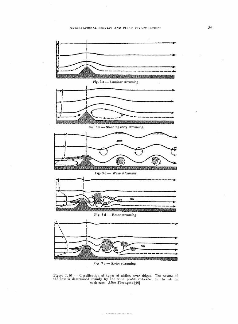
OBSERVATIONAL RESULTS AND FIELD INVESTIGATIONS
Fig. 3 a - Laminar streaming
-----------+ Fig. 3 b- Standing eddy streaming
Fig. 3 c - Wave streaming
Fig. 3d- Rotor streaming
Fig. 3 e- Rotor streaming
Figure I. 30 - Classification of types of airflow over ridges. The nature of the flow is determined mainly by the wind profile indicated on the left in
each case. After Forchgott [16]
31
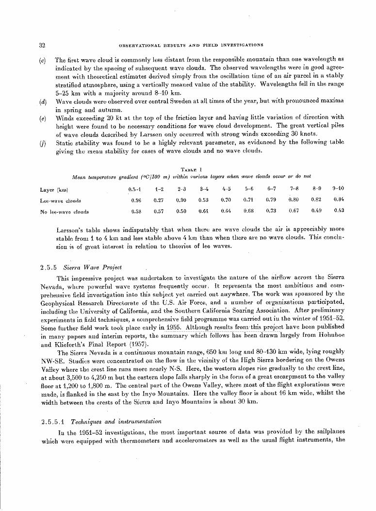
32 OBSERVATIONAL RESULTS AND FIELD INVESTIGATIONS
(c) The first wave cloud is commonly less distant from the responsible mountain than one wavelength as
indicated by the spacing of subsequent wave clouds. The observed wavelengths were in good agree
ment with theoretical estimates derived simply from the oscillation time of an air parcel in a stably
stratified atmosphere, using a vertically meaned value of the stability. Wavelengths fell in the range
5-25 km with a majority around 8-10 km.
(d) Wave clouds were observed over central Sweden at all times of the year, but with pronounced maxima
in spring and autumn.
(e) Winds exceeding 20 kt at the top of the friction layer and having little variation of direction with
height were found to be necessary conditions for wave cloud development. The great vertical piles
of wave clouds described by Larsson only occurred with strong winds exceeding 30 knots.
(f) Static stability was found to be a highly relevant parameter, as evidenced by the following table
giving the mean stability for cases of wave clouds and no wave clouds.
TABLE I
Mean temperature gradient (°C [100 m) within l-'arious layers when W(We clouds occur 01' do not
Layer (km) 0.5-1 1-2 2-3 3-t.o 4-5 5-6 6-7 7-8 8-9 9-10
Lee-wave clouds 0.96 0.27 0.30 0.53 0.70 0.71 0.79 0.80 0.82 0.84o
No lee-wave clouds 0.58 0.57 0.50 0.61 0.6t. 0.68 0.73 0.67 0.49 0.43
Larsson's table shows indisputably that when there are wave clouds the air is appreciably more
stable from 1 to 4 km and less stable above 4 km than when there are no wave clouds. This conclu
sion is of great interest in relation to theories of lee waves.
2. 5. 5 Sierra Wave Project
This impressive project was undertaken to investigate the nature of the airflow across the Sierra
Nevada, where powerful wave systems frequently occur. It represents the most ambitious and com
prehensive field investigation into this subject yet carried out anywhere. The work was sponsored by the
Geophysical Research Directorate of the U.S. Air Force, and a number of organizations participated,
including the University of California, and the Southern California Soaring Association. After preliminary
experiments in field techniques, a comprehensive field programme was carried out in the winter of 1951-52.
Some further field work took place early in 1955. Although results from this project have been published
in many papers and interim reports, the summary which follows has beeh drawn largely from Holmboe
and Klieforth's Final Report (1957). The Sierra Nevada is a continuous mountain range, 650 km long and 80--130 km wide, lying roughly
NW-SE. Studies were concentrated on the flow in the vicinity of the High Sierra bordering on the Owens
Valley where the crest line runs more nearly N-S. Here, the western slopes rise gradually to the crest line,
at about 3,500 to 4,250 m but the eastern slope falls sharply in the form of a great escarpment to the valley
floor at 1,200 to 1,800 m. The central part of the Owens Valley, where most of the flight explorations were
made, is flanked in the east by the lnyo Mountains. Here the valley floor is about 16 km wide, whilst the
width between the crests of the Sierra and lnyo Mountains is about 30 km.
2. 5. 5 .1 Techniques and instrumentation
In the 1951-52 investigations, the most important source of data was provided by the sailplanes
which were equipped with thermometers and accelerometers as well as the usual flight instruments, the
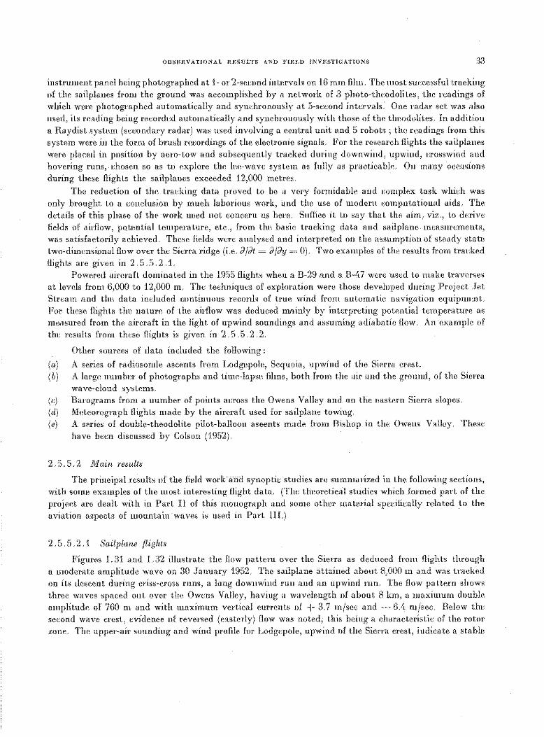
OBSERVATIONAL RESULTS AND FIELD INVESTIGATIONS 33
instrument panel being photographed at 1- or 2-second intervals on 16 mm film. The most successful tracking of the sailplanes from the ground was accomplished by a network of 3 photo-theodolites, the readings of which were photographed automatically and synchronously at 5-second intervals: One radar set was also used, its reading being recorded automatically and synchronously with those of the theodolites. In addition a Raydist system (secondary radar) was used involving a central unit and 5 robots ; the readings from this system were in the form of brush recordings of the electronic signals. For the research flights the sailplanes were placed in position by aero-tow and subsequently tracked during downwind, upwind, crosswind and hovering runs, chosen so as to explore the lee-wave system as fully as practicable. On many occasions during these flights the sailplanes exceeded 12,000 metres. .
The reduction of the tracking data proved to be a very formidable and complex task which was only brought to a conclusion by much laborious work, and the use of modern computational aids. The details of this phase of the work need not concern us here. Suffice it to say that the aim, viz., to derive fields of airflow, potential temperature, etc., from the basic tracking data and sailplane measurements, was satisfactorily achieved. These fields were analysed and interpreted on the assumption of steady state two-dimensional flow over the Sierra ridge (i.e. JfJt = JjJy = 0). Two examples of the results from tracked flights are given in 2. 5. 5. 2 .1.
Powered aircraft dominated in the 1.955 flights when a B-29 and a B-47 were used to make traverses at levels from 6,000 to 12,000 m. The techniques of exploration were those developed during Project Jet Stream and the data included continuous records of true wind from automatic navigation equipment. For these flights the nature of the airflow was deduced mainly by interpreting potential temperature as measured from the aircraft in the light of upwind soundings and assuming adiabatic flow. An example of the results from these flights is given in 2. 5. 5. 2. 2.
Other sources of data included the following :
(a) A series of radiosonde ascents from Lodgepole, Sequoia, upwind of the Sierra crest. (b) A large number of photographs and time-lapse films, both from the air and the ground, of the Sierra
wave-cloud systems. (c) Barograms from a number of points across the Owens Valley and on the eastern Sierra slopes. (d) Meteorograph flights made by the aircraft used for sailplane towing. (e) A series of double-theodolite pilot-balloon ascents made from Bishop in the Owens Valley. These
have been discussed by Colson (1952).
2. 5. 5. 2 M a in results
The principal results of the field wor1Cand synoptic studies are summarized in the following sections, with some examples of the most interesting flight data. (The theoretical studies which formed part of the project are dealt with in Part 11 of this monograph and some other material specifically related to the aviation aspects of mountain waves is used in Part Ill.)
2. 5. 5. 2 .1 Sailplane flights
Figures I. 31 and I. 32 illustrate the flow pattern over the Sierra as deduced from flights through a moderate amplitude wave on 30 January 1952. The sailplane attained about 8,000 m and was tracked on its descent during criss-cross runs, a long downwind run and an upwind run. The flow pattern shows three waves spaced out over the Owens Valley, having a wavelength of about 8 km, a maximum double amplitude of 760 m and with maximum vertical currents of + 3. 7 m/sec and ~ 6.4 m/sec. Below the second wave crest, evidence of reversed (easterly) flow was noted, this being a characteristic of the rotor zone. The upper-air sounding and wind profile for Lodgepole, upwind of the Sierra crest, indicate a stable
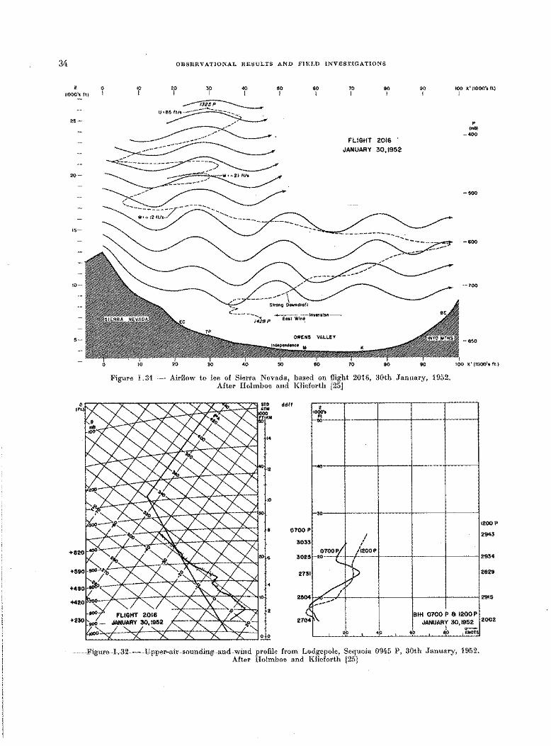
34
(lOOO's ft.}
25-
20-
15-
10-
5-
0 I
OBSERVATIONAL RESULTS AND FIELD INVESTIGATIONS
10 20 30 40 50 60 10 80 90 100 X' UOOO's fl) I I I I I I I I I I
~ __..---:::.~-Uz
/ p
---(mb)
-400 FLIGHT 2016
JANUARY 30,.1952
-500
-600
-700
-850
Figure !.31 - Airflow to lee of Sierra Nevada, based on flight 2016, 30th January, 1952. After Holmboe and Klieforth [25]
ddfl
0700 p
3033
2 IOOO't
~~---~------1-------i-------t------.
40-----+--------+--------r-------+------__,
~~----~-----~------~-----+-----__,
/ I
1200P
2943
/1200P ,---4~~~--~------~~----~----~2934
27!111 I I I 12829
20 4p
2915
IBIH 0700 P 8 1200 P JANUARY 30,1952 12002
I u-60 80 , KNOTS!
--Eiglll'e-I-.-32 -- Upper~air-sounding-and-wind profile from Lodgepole, Sequoia 0945 P, 30th January, 1952. After Holmboe and Klieforth [25]
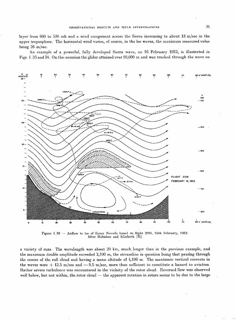
OBSERVATIONAL RESULTS AND FIELD INVESTIGATIONS 35
layer from 660 to 530 mb and a wind component across the Sierra increasing to about 18 m/sec in the
upper troposphere. The horizontal wind varies, of course, in the lee waves, the maximum measured value
being 26 m/sec. An example of a powerful, fully developed Sierra wave, on 16 February 1952, is illustrated in
Figs. I. 33 and 34. On this occasion the glider attained over 10,000 m and was tracked through the wave on
! 0 IIOOO'sft)
3&-
10 I
20 I
30 I
40 I
&0 I
60 I
70 I
80 I
90 I
100 I
110 I
FLIGHT 2018
FEBRUARY 16, 1952
1fo x' uooo'• ft)
p (mb}
-300
-400
-500
-600
-700
-eso
1:0 1J0 X' (10001.s ft)
Figure 1.33 - Airflow to lee of Sierra Nevada based on flight 2018, 16th February, 1952. After Holmboe and Klieforth [25]
a variety of runs. The wavelength was abc;mt 20 km, much_ longer than in the previous example, and
the maximum double amplitude exceeded 2,100 m, the streamline in question being that passing through
the centre of the roll cloud and having a mean altitude of 4,100 m. The maximum vertical currents in
the waves were + 12.5 m/sec and - 9.5 m/sec, more than sufficient to constitute a hazard to aviation.
Rather severe turbulence was encountered in the vicinity of the rotor cloud. Reversed flow was observed
well below, but not within, the rotor cloud- the apparent rotation in rotors seems to be due to the large
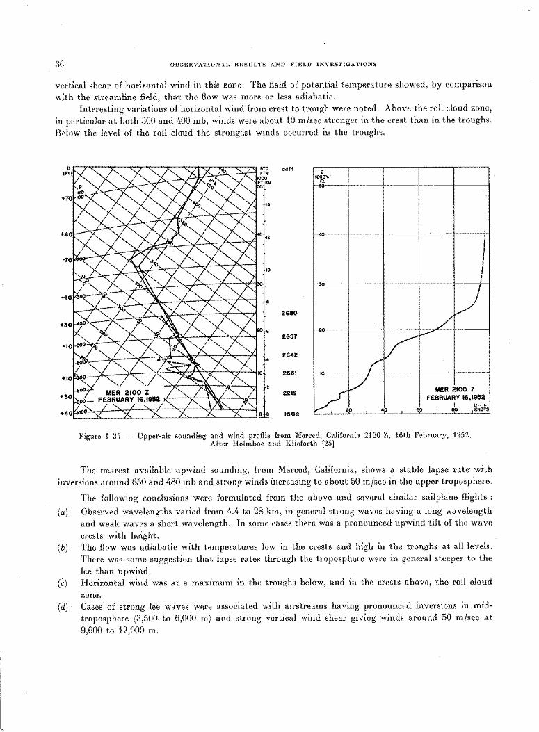
36 OBSERVATIONAL HESULTS AND FIELD INVESTIGATIONS
vertical shear of horizontal wind in this zone. The field of potential temperature showed, by comparison
with the streamline field, that the flow was more or less adiabatic.
Interesting variations of horizontal wind from crest to trough were noted. Above the roll cloud zone,
in particular at both 300 and 400 mb, winds were about 10 m/sec stronger in the crest than in the troughs.
Below the level of the roll cloud the strongest winds occurred in the troughs.
ddff f
1000 .. Ft.
I-50
l-40 I I I I I I f I I I
f-30 I
I
I I
2680
2657
/ v'
l-20
/ _...,
r 2642
2631
I
HO L/ MER 2100 Z
V..o' FEBRUARY 16,19521 I u-
4p '
6p 1 ep 1t<NOTS
2219
1508
Figure I. 3ft ~ Upper-air sounding and wind profile from Merced, California 2100 Z, 16th February, 1952. After Holmboe and Klieforth [25)
The nearest available upwind sounding, from Merced, California, shows a stable lapse rate with
inversions around 650 and 480mb and strong winds increasing to about 50 m/sec in the upper troposphere.
The following conclusions were formulated from the above and several similar sailplane flights :
(a) Observed wavelengths varied from 4.4 to 28 km, in general strong waves having a long wavelength
and weak waves a short wavelength. In some cases there was a pronounced upwind tilt of the wave
crests with height.
(b) The flow was adiabatic with temperatures low in the crests and high in the troughs at all levels.
There was some suggestion that lapse rates through the troposphere were in general steeper to the
lee than upwind. (c) Horizontal wind was at a maximum in the troughs below, and in the crests above, the roll cloud
zone. (d) Cases of strong lee waves were associated with airstreams having pronounced inversions in mid
troposphere (3,500 to 6,000 m) and strong vertical wind shear giving winds around 50 m/sec at
9,000 to 12,000 m.
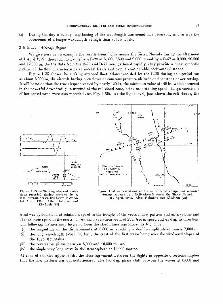
OBSERVATIONAL RESULTS AND FIELD INVESTIGATIONS 37
(e) During the day a steady lengthening of the wavelength was sometimes observed, as also was the occurrence of a longer wavelength at high than at low levels.
2. 5. 5. 2. 2 Aircraft flights
We give here as an example the results from flights across the Sierra Nevada during the afternoon of 1 April1955; these included runs by a B-29 at 6,000, 7,500 and 9,000 m and by a B-47 at 9,000, 10,500 and 12,000 m. As the data from the B-29 and B-47 were gathered rapidly, they provide a quasi-synoptic picture of the flow characteristics at several levels and over a considerable horizontal distance.
Figure I. 35 shows the striking airspeed fluctuations recorded by the B-29 during an upwind run at about 6,000 m, the aircraft having been flown at constant pressure altitude and constant power setting. It will be noted that the true airspeed varied by nearly 120 kt, the minimum value of 145 kt, which occurred in the powerful downdraft just upwind of the roll-cloud zone, being near stalling speed. Large variations of horizontal wind were also recorded (see Fig. I. 36). At the flight level, just above the roll clouds, the
i - 220 :=:=:-=--.. ...,...:){ \ 1 V'J ,_.,
180 -------+--1+1---+-----
1~------~---1--+------
40
B-29 I APRIL 1955
2.0,000FT.
STATUTE MILES
Figure I. 35 -- Striking airspeed variations recorded during traverse by a B-29 aircraft across the Sierra Nevada, 1st April, 1955. After Holmboe and
Klieforth [25]
119°1
/
PROJECT JET STREAM
B -29 FLIGHT 39
I APRIL 1955
20,000 FEET"' 195 MPH I.A. S.
37°30'
JIB a 117'1~
,.aQ~I'I''~ ~~~\..E.~c't. 1541 1/z ~~-- ... I 1Jv- •--- ' yY ~ I ,,. ~~ Q~~~1;
37• N
36°301
Figure I. 36 - Variations of horizontal wind component recorded during traverse by a B-29 aircraft across the Sierra Nevada,
1st April, 1955. After Holmboe and Klieforth [25]
wind was cyclonic and at minimum speed in the troughs of the vertical flow pattern and anticyclonic and at maximum speed in the crests. These wind variations reached 25 m/sec in speed and 45 deg. in direction. The following features may be noted from the streamlines reproduced as Fig. I. 37 :
(i) the magnitude of the displacements at 6,000 m, reaching a double-amplitude of nearly 2,000 m; (ii) the long wavelength (about 20 km), the crest of the first wave being over the windward slopes of
the Inyo Mountains ; (iii) the reversal of phase between 6,000 and 10,500 m; and (iv) the single very long wave in the stratosphere at 12,000 metres.
At each of the two upper levels, the close agreement between the flights in opposite directions implies that the flow pattern was quasi-stationary. The 1.80 deg. phase shift between the waves at 6,000 and
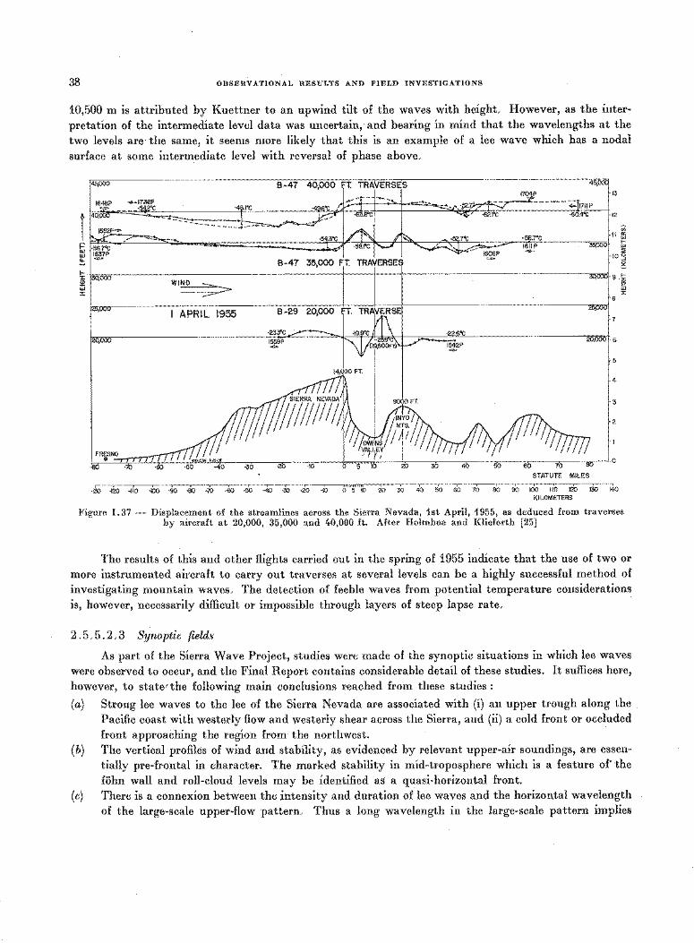
38 OBSERVATIONAL RESULTS AND FIELD INVESTIGATIONS
10,500 m is attributed by Kuettner to an upwind tilt of the waves with height. However, as the inter
pretation of the intermediate level data was uncertain,· and bearing in mind that the wavelengths at the
two levels are· the same, it seems more likely that this is an example of a lee wave which has a nodal surface at some intermediate level with reversal of phase above.
45,000 B-47 40,000 F.T. TRAVERSE:S 45,.
1704P 13
12
:t~ l ~~ ~~ B __ 1s11 P 35,< w _.... 1606P 4=>
"- B-47 35,000 FT. TRAVERSES =-
WIND
~ I APRIL 1955 B-29 20,000
·233'C
1559P -7
-22.6"C
1542P 20;0001-6 -
4
3
I q,·P=n;-r-rrn I I I I '·!";' .. ,.... ~ . '$I I I -s6 -70 -oo -5o -4o -30 -2b -1o' "5 ' · M -- -- .- -- "" o
MILES
-130 -120 -110 -100 -90 -80 -70 -60 -50 -40 -30 -20 -10 0 5 10 20 30 40 50 60 70 80 90 100 110 120 130 140 KILOMETERS
Figure I. 37 - Displacement of the streamlines across the Sierra Nevada, 1st April, 1955, as deduced from traverses by aircraft at 20,000, 35,000 and 40,000 ft. After Holmboe and Klieforth [25]
The results of this and other flights carried out in the spring of 1955 indicate that the use of two or more instrumented aircraft to carry out traverses at several levels can be a highly successful method of
investigating mountain waves. The detection of feeble waves from potential temperature considerations is, however, necessarily difficult or impossible through layers of steep lapse rate.
2. 5. 5. 2. 3 Synoptic fields
As part of the Sierra Wave Project, studies were made of the synoptic situations in which lee waves
were observed to occur, and the Final Report contains considerable detail of these studies. It suffices here, however, to staterthe following main conclusions reached from these studies :
(a) Strong lee waves to the lee of the Sierra Nevada are associated with (i) an upper trough along the Pacific coast with westerly flow and westerly shear across the Sierra, and (ii) a cold front or occluded front approaching the region from the northwest.
(b) The vertical profiles of wind and stability, as evidenced by relevant upper-air soundings, are essentially pre-frontal in character. The marked stability in mid-troposphere which is a feature of· the
fohn wall and roll-cloud levels may be identified as· a quasi-horizontal front. (c) There is a connexion between the intensity and duration of lee waves and the horizontal wavelength
of the large-scale upper-flow pattern. Thus a long wavelength in the large-scale pattern implies
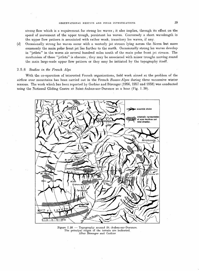
OBSERVATIONAL HESULTS AND FIELD INVESTIGATIONS 39
strong flow which is a requirement for strong lee waves ; it also implies, through its effect on the speed of movement of the upper trough, persistent lee waves. Conversely a short wavelength in the upper flow pattern is associated with rather weak, transitory lee waves, if any.
(d) Occasionally strong lee waves occur with a westerly jet stream lying across the Sierra but more commonly the main polar front jet lies further to the north. Occasionally strong lee waves develop in "jetlets" in the warm air several hundred miles south of the main polar front jet stream. The mechanism of these "jetlets" is obscure ; they may be associated with minor troughs moving round the main large-scale upper flow pattern or they may be initiated by the topography itself.
2. 5. 6 Studies in the French Alps
With the co-operation of interested French organizations, field work aimed at the problem of the airflow over mountains has been carried out in the French Bas11es-Alpes during three successive winter seasons. The work which has been reported by Gerbier and Bercnger (1956, 1957 and 1958) was conducted using the National Gliding Centre at Saint-Auban-sur-Durance as a base (Fig. I. 38).
Figure I. 38 - Topography around St.-Auban-sur-Durance. The principal ridges of the terrain are indicated.
After Berenger and Gerbier
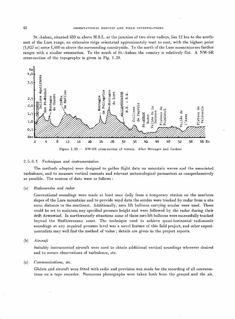
40 OBSERVATIONAL RESULTS AND FIELD INV:ESTIGATIONS
St.-Auban, situated 450 m above M.S.L. at the junction of two river valleys, lies 12 km to the southeast of the Lure range, an extensive ridge orientated approximately west to east, with the highest point (1,827 m) some 1,400 m above the surrounding countryside. To the north of the Lure mountains are further ranges with a similar orientation. To the south of St.-Auban the country is relatively flat. A NW-SE cross-section of the topography is given in Fig. I. 39.
Km 4,0. fll
'<Il H
3.51- ~ ., (J) (J) ::l .-1 s:: s:: s:: Q) Cij :.. O'<I> ro .,~~ OJ· '<I>~ <I> .-1 ~~+'...:! <1!1<: fll-rl~Jl $:;:1 ~<I>§(J) g. fll
2.5 r § ~ ~ Jl <~ ~ .,., ;::j ~ 'd 0 • ·rl
;::j ~ +' 0 0 § &; J ~ ~ ::l Q) (J) Q)
2,0 ~. " \~ ~ • " ~ ~ .s ~ z ~ 0 " ~ ~ \ I ..-1 V\ P.,
~
0 4 8 12 16 20 24 28 32 36 40 44 48 52 56 60Km
Figure I. 39 - NW-SE cross-section of terrain. After Berenger and Gerbier
2. 5. 6.1 Techniques and instrumentation
The methods adopted were designed to gather flight data on mountain waves and the associated turbulence, and to measure vertical currents and relevant meteorological parameters as comprehensively as possible. The sources of data were as follows :
(a) Radiosondes and radar
Conventional soundings were made at least once daily from a temporary station on the southern slopes of the Lure mountains and to provide wind data the sondes were tracked by radar from a site some distance to the southeast. Additionally, zero lift balloons carrying sondes were used. These could be set to maintain any specified pressure height and were followed by the radar during their drift downwind. In northwesterly situations some of these zero lift balloons were successfully tracked beyond the Mediterranean coast. The technique used to achieve quasi-horizontal radiosonde soundings at any required pressure level was a novel feature of this field project, and other experimentalists may well find the method of value ; details are given in the project reports.
(b) Aircraft
Suitably instrumented aircraft were used to obtain additional vertical soundings wherever desired and to secure observations of turbulence, etc.
(c) Communications, etc.
Gliders and aircraft were fitted with radio and provision was made for the recording of all conversations on a tape recorder. Numerous photographs were taken both from the ground and the air.
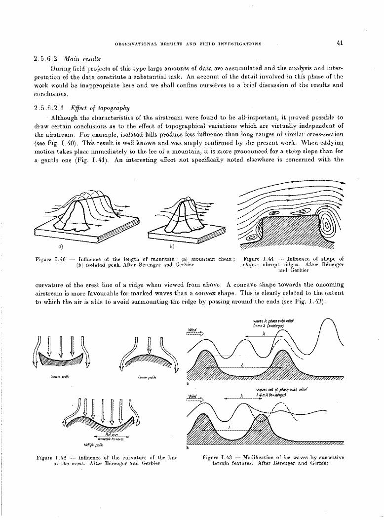
OBSERVATIONAL RESULTS AND FIELD INVESTIGATIONS 41
2.5.6.2 Main results
During field projects of this type large amounts of data are accumulated and the analysis and inter
pretation of the data constitute a substantial task. An account of the detail involved in this phase of the
work would be inappropriate here and we shall confine ourselves to a brief discussion of the results and
conclusions.
2. 5. 6. 2.1 Effect of topography
Although the characteristics of the airstream were found to be all-important, it proved possible to
draw certain conclusions as to the effect of topographical variations which are virtually independent of
the airstream. For example, isolated hills produce less influence than long ranges of similar cross-section
(see Fig. I. 40). This result is well known and was amply confirmed by the present work. When eddying
motion takes place immediately to the lee of a mountain, it is more pronounced for a ste'ep slope than for
a gentle one (Fig. I. 41). An interesting effect not specifically noted elsewhere is concerned with the
a.) h)
Figure I. 40 - Influence of the length of mountain : (a) mountain chain ; (h) isolated peak. After Berenger and Gerhier
Figure I. 41 - Influence of shape of slope : abrupt ridges. After Berenger
and Gerbier
curvature of the crest line of a ridge when viewed from above. A concave shape towards the oncoming
airstream is more favourable for marked waves than a convex shape. This is clearly related to the extent
to which the air is able to avoid surmounting the ridge by passing around the ends (see Fig. I. 42).
~~\ ~ Concave profile Convex profile
~\ ravoursiie for waves
Mu//iple profile
Figure I. 42 - Influence of the curvature of the line of the crest. After Berenger and Gerbier
a
waves in phase w1!h relief l•nx).. (n<~ilfe99r}
Figure I .l>3 - Modification of lee waves by successive terrain features. After Berenger and Gerbier
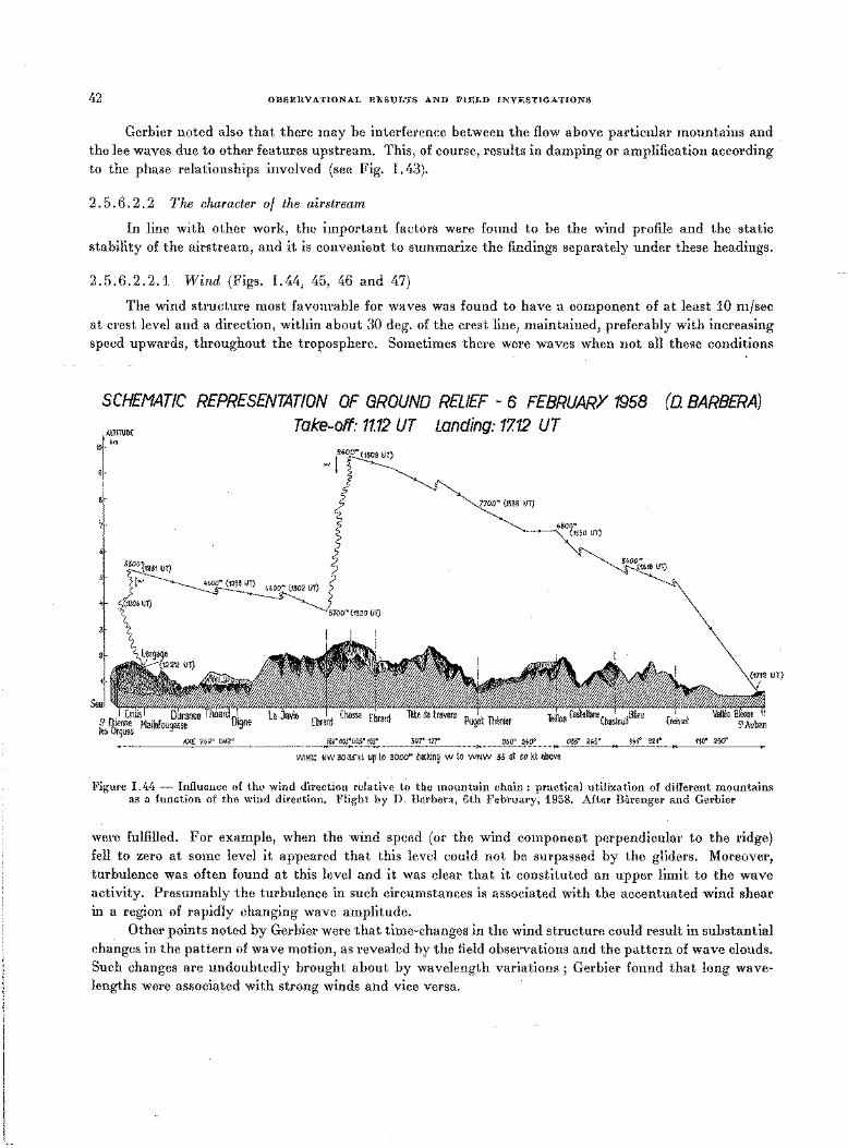
42 OBSERVATIONAL RESULTS AND FIELD INVESTIGATIONS
Gerbier noted also that there may be interference between the flow above particular mountains and the lee waves due to other features upstream. This, of course, results in damping or amplification according to the phase relationships involved (see Fig. I. 43).
2. 5. 6. 2. 2 The character of the airstream
In line with other work, the important factors were found to be the wind profile and the static stability of the airstream, and it is convenient to summarize the findings separately under these headings.
2.5.6.2.2.1 Wind (Figs. I.44, 45, 46 and 47)
The wind structure most favourable for waves was found to have a component of at least 10 m/sec at crest level and a direction, within about 30 deg. of the crest line, maintained, preferably with increasing speed upwards, throughout the troposphere. Sometimes there were waves when not all these conditions
SCHEMATIC REPRESENTATION OF GROUND RELIEF - 6 FEBRUARY 1958
ALTITUDE 10' km
AXE 262" 082"
Take-off: 11.12 UT Landing: 17.12 UT
135'005'005'185' 307" 127" 060' 2'0' 085' 265' 1-'tf) 921°
WIND: NW 30·3Skt up to 3ooo• backing w to WNW 35 at so kt above
(QBARBERA)
UT)
110" 290'
Figure I. 44 -- Influence of the wind direction relative to the mountain chain : practical utilization of different mountains as a function of the wind direction. Flight by D. Barbera, 6th February, 1958. After Berenger and Gerbier
were fulfilled. For example, when the wind speed (or the wind component perpendicular to the ridge) fell to zero at some level it appeared that this level could not be surpassed by the gliders. Moreover, turbulence was often found at this level and it was clear that it constituted an upper limit to the wave activity. Presumably the turbulence in such circumstances is associated with the accentuated wind shear in a region of rapidly changing wave amplitude.
Other points noted by Gerbier were that time-changes in the wind structure could result in substantial changes in the pattern of wave motion, as revealed by the field observations and the pattern of wave clouds. Such changes are undoubtedly brought about by wavelength variations ; Gerbier found that long wavelengths were associated with strong winds and vice versa.
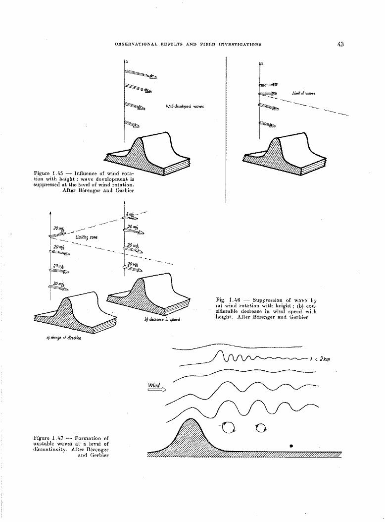
OBSERVATIONAL RESULTS AND FIELD INVESTIGATIONS 43
z
Figure I. t.5 - Influence of wind rotation with height : wave development is suppressed at the level of wind rotation.
After Berenger and Gerbier
----------20mfs
----.--· Limiting zone
-------- ----- ---
a) change of direction
Figure I.47 - Formation of unstable waves at a level of discontinuity. After Berenger
and Gerbier
Well-developed waves
-----
,Wind:>
z
limif of waves
Fig. I. t.6 - Suppression of wave by (a) wind rotation with height ; (b) considerable decrease in wind spee-d -with height. After Berenger and Gerbier
-----
~A<2km
0
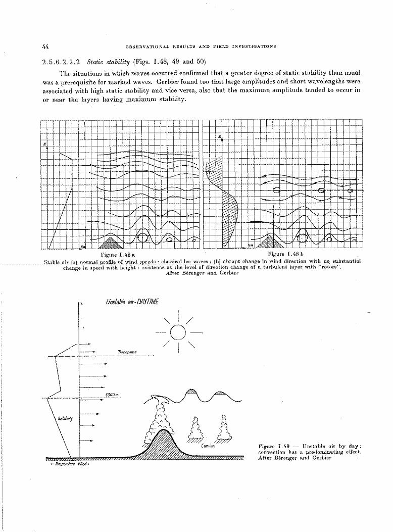
44 OBSERVATIONAL RESULTS AND FIELD INVESTIGATIONS
2. 5. 6. 2. 2. 2 Static stability (Figs. I. 48, 49 and 50)
The situations in which waves occurred confirmed that a greater degree of static stability than usual
was a prerequisite for marked waves. Gerbier found too that large amplitudes and short wavelengths were
associated with high static stability and vice versa, also that the maximum amplitude tended to occur in
or near the layers having maximum stability.
z
.z
"' 1--r- -... -~--- ....... -... 1-/ % t-r- f.-- r-
'-l._ / - 1'---- _t:;r:::: ~
....... - -- \:% % ?% 1-- rl
}._ V r-. / 1-\-. 1- '< ,..... t-1- _... !'-'
I 1---..... :>: ......- ..-r- <.:;iil
t- I-V t-- % V:: f-.. - ....... 1- v --f- H
I vr--- /: r::--t:l 1--1/ ....... / I./ f"- !-
1- V 1\ % ~a ....... / '-... .......~--...
%~ / \ :;;;;;
I r-......_ / / I'-.. f-., %V:: " \. " ~
1--- f:;-:::7
+-~ I ..11\ D"-. ~ 1-
......._
1/ % VA ~"
V~ "'--! c./ -H /'( . )\] 'r0... H
? V Kt ~ ---.d ~ ..-' '--~
Figure I. 48 a Figure I. 48 b
_______ _.S,__t.,.a,..b~l"'e--'a"'i"'r---~-"'(a,) normal 2rofile of wind s2eeds : classical lee waves ; (b) abrupt change in wind direction with no substantial change in speed with height: existence at the level of direction change of a turbulent layer with "rotors".
After Berenger and Gerbier
Unstable air- DAYTIME
"" I / -0-
- - --- !!_•f_'J'!.':_se_--/1""
!iOOOm
t;;}J Cumulus
+-- li!mperature Wind-
Figure I ,!,9 - Unstable air by day: convection has a predominating effect. After Berenger and Gerbier
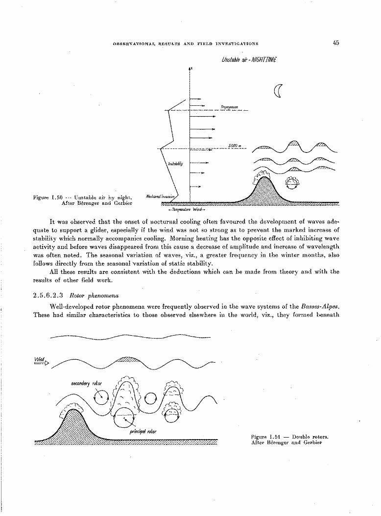
OBSERVATIONAL RESULTS AND FIELD INVESTIGATIONS 45
Unsfa/Jie air- NIGH TT/ME
er -+-----~I'!!E~·--
Figure 1.50 - Unstable air by night. After Berenger and Gerbier
~remperslure Wind-
It was observed that the onset of nocturnal cooling often favoured the development of waves adequate to support a glider, especially if the wind was not so strong as to prevent the marked increase of stability which normally accompanies cooling. Morning heating has the opposite effect of inhibiting wave activity and before waves disappeared from this cause a decrease of amplitude and increase of wavelength was often noted. The seasonal variation of waves, viz., a greater frequency in the winter months, also follows directly from the seasonal variation of static stability.
All these results are consistent with the deductions which can be made from theory and with the results of other field work.
2. 5. 6. 2. 3 Rotor phenomena
Well-developed rotor phenomena were frequently observed in the wave systems of the Basses-Alpes. These had similar characteristics to those observed elsewhere in the world, viz., they formed beneath
~~" ,4'7//~,
secondery rolor 0~ (G~~\'0 Dt&'
principal rolor
~ Figure I. 51 - Double rotors. After Berenger and Gerbier
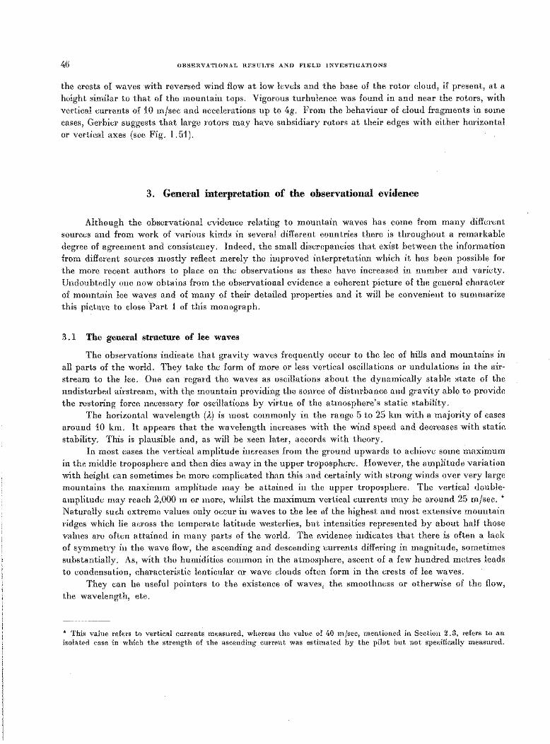
46 OBSERVATIONAL RESULTS AND FIELD INVESTIGATIONS
the crests of waves with reversed wind flow at low levels and the base of the rotor cloud, if present, at a
height similar to that of the mountain tops. Vigorous turbulence was found in and near the rotors, with
vertical currents of 10 m/sec and accelerations up to 4g. From the behaviour of cloud fragments in some
cases, Gerbier suggests that large rotors may have subsidiary rotors at their edges with either horizontal
or vertical axes (see Fig. I.51).
3. General interpretation of the observational evidence
Although the observational evidence relating to mountain waves has come from many different
sources and from work of various kinds in several different countries there is throughout a remarkable
degree of agreement and consistency. Indeed, the small discrepancies that exist between the information
from different sources mostly reflect merely the improved interpretation which it has been possible for
the more recent authors to place on the observations as these have increased in number and variety.
Undoubtedly one now obtains from the observational evidence a coherent picture of the general character
of mountain lee waves and o£ many of their detailed properties and it will be convenient to summarize
this picture to close Part I of this monograph.
3. l The general structure of lee waves
The observations indicate that gravity waves frequently occur to the lee o£ hills and mountains in
all parts of the world. They take the form of more or less vertical oscillations or undulations in the air
stream to the lee. One can regard the waves as oscillations about the dynamically stable state of the
undisturbed airstream, with th.e mountain providing the source of disturbance and gravity able to provide
the restoring force necessary for oscillations by virtue of the atmosphere's static stability.
The horizontal wavelength (.A) is most commonly in the range 5 to 25 km with a majority of cases
around 10 km. It appears that the wavelength increases with the wind speed and decreases with static
stability. This is plausible and, as will be seen later, accords with theory.
In most cases the vertical amplitude increases from the ground upwards to achieve some maximum
in the middle troposphere and then dies away in the upper troposphere. However, the amplitude variation
with height can sometimes be more complicated than this and certainly with strong winds over very large
mountains the maximum amplitude may be attained in the upper troposphere. The vertical double
amplitude may reach 2,000 m or more, whilst the maximum vertical currents may be around 25 m/sec. * Naturally such extreme values only occur in waves to the lee of the highest and most extensive mountain
ridges which lie across the temperate latitude westerlies, but intensities represented by about half those
values are often attained in many parts of the world. The evidence indicates that there is often a lack
of symmetry in the wave flow, the ascending and descending ·currents differing in magnitude, sometimes
substantially. As, with the humi.dities common in the atmosphere, ascent of a few hundred metres leads
to condensation, characteristic lenticular or wave clouds often form in the crests of lee waves.
They can be useful pointers to the existence of waves, the smoothness or otherwise of the flow,
the wavelength, etc.
* This value refers to vertical currents measured, whereas lhe value of t,Q m/sec, mentioned in Section 2. 3, refers to an isolated case in which the strength of the ascending current was estimated by the pilot but not specifically measured.
OBSERVATIONAL RESULTS AND FIELD INVESTIGATIONS 47
When lee waves are operating the spacing of the streamlines is such that the strongest surface winds are commonly to be found sweeping down the lee slope. These winds may carry the cap cloud down the
lee slope during the process of dispersal by adiabatic warming, so that the cloud resembles a waterfall
known as the "cloud fall" or "fohn wall". Vvhen lee waves are of large amplitude, the flow may contain rotors in the crests of the waves, at
about the level of maximum amplitude. Owing to the large vertical wind shear in the region, the characteristic rotor or roll cloud which forms commonly has the appearance of rotating about a horizontal axis.
The low-level winds beneath rotors are observed to be much lighter than elsewhere and indeed may even be reversed. Violent turbulence is liable to be encountered in the vicinity of rotor clouds.
A succession or train of several lee waves may be formed, especially if the obstacle is a mountain ridge of considerable length lying across the airstream. In contrast, the waves to the lee of an isolated
hill or mountain quickly die away downstream and there may be only one or two observable lee waves. Several authors remark that the first lee wave is usually less than one wavelength downstream from the
mountain crest ; this is consistent with theory which predicts 3f4,l as the downstream displacement of the first lee wave crest. In this connexion we must remember that the flow downstream of a ridge may
be further complicated by the disturbances arising from other hills or mountains, when the terrain is irregular.
Above the level of maximum amplitude the horizontal winds are strongest in the crests and weakest
in the troughs. The reverse holds below that level. This is of course an automatic consequence of the
vertical variations of lee-wave amplitude.
3 . 2 The meteorological conditions relevant fm· lee waves
From the studies of mountain clouds, pilots' reports and from specific field investigations, the
meteorological factors which are relevant for lee-wave formation emerge clearly. We may summarize them as follows :
3. 2. 1 Static stability
The atmosphere is more often than not stably stratified. In airstreams containing lee waves, there
is evidence that the air has greater static stability than the average at low levels surmounted by air of lesser stability above. Deep stable layers, often isothermal (and sometimes inversions), are frequently
noted in airstreams with lee waves. It seems an essential requirement, at least for strong waves, that there should be marked stability at levels where the air is disturbed by the mountain. In the case of very
large mountains (e.g. Sierra Nevada), the high stability is seen in mid-troposphere (say, around 4,000 to 5,000 m), but for smaller mountains it is more usually observed in the lower troposphere. Over small hills and mountains, diurnal variations of static stability near the surface can exert a pronounced influence
on the incidence, amplitude and wavelength of lee waves, but such variations play a much smaller part when the mountains are very large. There is evidence that the maximum amplitude in lee waves is usually
attained somewhere in or near the layers of maximum static stability. The relevance and effect of static stability as summarized above will be found to be consistent with
theory (see Part 11).
3.2.2 Wind
For waves to the lee of a mountain ridge, the airstream must be blowing more or less perpendicularly across the ridge or at any rate must have a substantial component across the ridge, and this must be
maintained through a considerable depth of the troposphere. The most powerful waves occur in deep
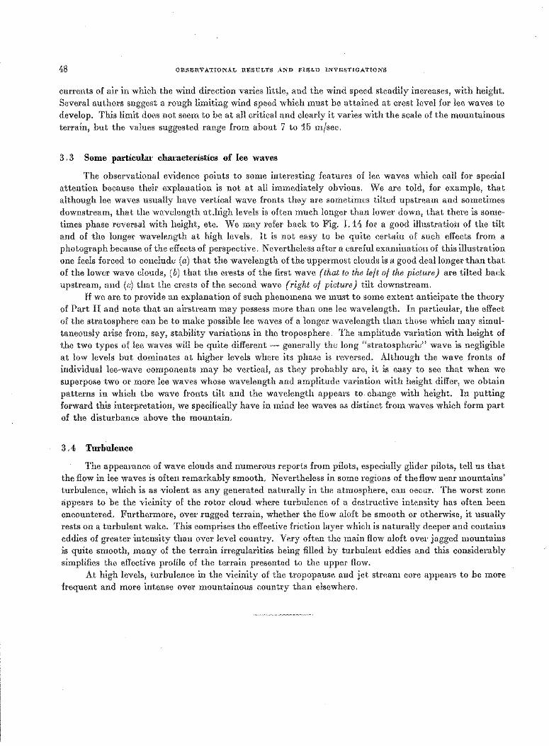
48 OBSERVATIONAL RESULTS AND FIELD INVESTIGATIONS
currents of air in which the wind direction varies little, and the wind speed steadily increases, with height. Several authors suggest a rough limiting wind speed which must be attained at crest level for lee waves to develop. This limit does not seem to be at all critical and clearly it varies with the scale of the mountainous terrain, but the values suggested range from about 7 to 15 m/sec.
3 . 3 Some particular characteristics of lee waves
The observational evidence points to some interesting features of lee waves which call for special attention because their explanation is not at all immediately obvious. We are told, for example, that although lee waves usually have vertical wave fronts they are sometimes tilted upstream and sometimes downstream, that the wavelength at.high levels is often much longer than lower down, that there is sometimes phase reversal with height, etc. We may refer back to Fig. I.14 for a good illustration of the tilt and of the longer wavelength at high levels. It is not easy to be quite certain of such effects from a photograph because of the effects of perspective. Nevertheless after a careful examination of this illustration one feels forced to conclude (a) that the wavelength of the uppermost clouds is a good deal longer than that of the lower wave clouds, (b) that the crests of the first wave (that to the left of the picture) are tilted back upstream, and (c) that the crests of the second wave (right of picture) tilt downstream.
If we are to provide an explanation of such phenomena we must to some extent anticipate the theory of Part I1 and note that an airstream may possess more than one lee wavelength. In particular, the effect of the stratosphere can be to make possible lee waves of a longer wavelength than those which may simultaneously arise from, say, stability variations in the troposphere. The amplitude variation with height of the two types of lee waves will be quite different - generally the long "stratospheric" wave is negligible at low levels but dominates at higher levels where its phase is reversed. Although the wave fronts of individual lee-wave components may be vertical, as they probably are, it is easy to see that when we superpose two or more lee waves whose wavelength and amplitude variation with height differ, we obtain patterns in which the wave fronts tilt and the wavelength appears to change with height. In putting forward this interpretation, we specifically have in mind lee waves as distinct from waves which form part of the disturbance above the mountain.
3. 4 Turbulence
The appearance of wave clouds and numerous reports from pilots, especially glider pilots, tell us that the flow in lee waves is often remarkably smooth. Nevertheless in some regions of the flow near mountains' turbulence, which is as violent as any generated naturally in the atmosphere, can occur. The worst zone appears to be the vicinity of the rotor cloud_ where turbulence of a destructive intensity has often been encountered. Furthermore, over rugged terrain, whether the flow aloft be smooth or otherwise, it usually rests on a turbulent wake. This comprises the effective friction layer which is naturally deeper and contains eddies of greater intensity than over level country. Very often the main flow aloft over jagged mountains is quite smooth, many of the terrain irregularities being filled by turbulent eddies and this considerably simplifies the effective profile of the terrain presented to the upper flow.
At high levels, turbulence in the vicinity of the tropopause and jet stream core appears to be more frequent and more intense over mountainous country than elsewhere.
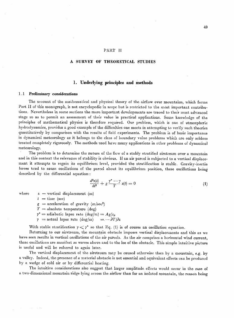
49
PART II
A SURVEY OF THEORETICAL STUDIES
I. Underlying principles and methods
1 . 1 Preliminary considerations
The account of the mathematical and physical theory of the airflow over mountains, which forms Part II of this monograph, is not encyclopedic in scope but is restricted to the most important contributions. Nevertheless in some sections the more important developments are traced to their most advanced stage so as to permit an assessment of their value in practical applications. Some knowledge of the principles of mathematical physics is therefore required. Our problem, which is one of atmospheric hydrodynamics, provides a good example of the difficulties one meets in attempting to verify such theories quantitatively by comparison with the results of field experiments. The problem is of basic importance in dynamical meteorology as it belongs to the class of boundary value problems which are only seldom treated completely rigorously. The methods used have many applications in other problems of dynamical meteorology.
The problem is to determine the nature of the flow of a stably stratified airstream over a mountain and in this context the relevance of stability is obvious. If an air parcel is subjected to a vertical displace· ment it attempts to regain its equilibrium level, provided the stratification is stable. Gravity-inertia forces tend to cause oscillations of the parcel about its equilibrium position, these oscillations being described by the differential equation :
where
d2z(t) + y* - y ( ) _ 0 dt2 g-T-zt-
z = vertical displacement (m) =time (sec)
g = acceleration of gravity (m/sec2)
T = absolute temperature ( deg) y* =adiabatic lapse rate (deg/m) = Agfcp y = actual lapse rate ( deg/m) =.- JT fJz
With stable stratification y < y* so that Eq. (1) is of course an oscillation equation.
(1)
Returning to our airstream, the moun!ain obstacle imposes vertical displacements and this as we have seen results in vertical oscillations of the air parcels. As the air comprises a horizontal wind current, these oscillations are manifest as waves above and to the lee of the obstacle. This simple intuitive picture is useful and will be referred to again later.
The vertical displacement of the airstream may be caused otherwise than by a mountain, e.g. by a valley. Indeed, the presence of a material obstacle is not essential and equivalent effects can be produced by a wedge of cold air or by differential heating.
The intuitive considerations also suggest that larger amplitude effects would occur in the case of a two-dimensional mountain ridge lying across the airflow than for an isolated mountain, the reason being
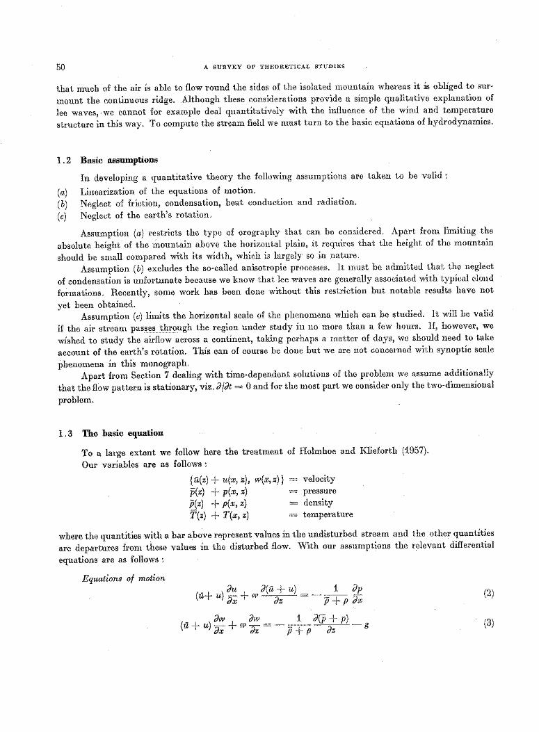
50 A SURVEY OF THEORETICAL STUDIES
that much of the air is able to flow round the sides of the isolated mountain whereas it is obliged to sur
mount the continuous ridge. Although these considerations provide a simple qualitative explanation of
lee waves, ·we cannot for example deal quantitatively with the influence of the wind and temperature
structure in this way. To compute the stream field we must turn to the basic equations of hydrodynamics.
1. 2 Basic assumptions
In developing a quantitative theory the following assumptions are taken to be valid :
(a) Linearization of the equations of motion.
(b) Neglect of friction, condensation, heat conduction and radiation.
(c) Neglect of the earth's rotation.
Assumption (a) restricts the type of orography that can be considered. Apart from limiting the
absolute height of the mountain above the horizontal plain, it requires that the height of the mountain
should be small compared with its width, which is largely so in nature.
Assumption (b) excludes the so-called anisotropic processes. It must be admitted that the neglect
of condensation is unfortunate because we know that lee waves are generally associated with typical cloud
formations. Recently, some work has been done without this restriction but notable results have not
yet been obtained. Assumption (c) limits the horizontal scale of the phenomena which can be studied. It will be valid
if the air stream passes through the region under study in no more than a few hours. If, however, we
wished to study the airflow across a continent, taking perhaps a matter of days, we should need to take
account of the earth's rotation. This can of course be done but we are not concerned with synoptic scale
phenomena in this monograph. Apart from Section 7 dealing with time-dependent solutions of the problem we assume additionally
that the flow pattern is stationary, viz. JjJt = 0 and for the most part we consider only the two-dimensional
problem.
1 . 3 The basic equation
To a large extent we follow here the treatment of Holmboe and Klieforth (1957).
Our variables are as follows :
{ u(z) + u(x, z), w(x, z)} p(z) + p(x, z) p(z) + p(x, z) T(z) + T(x, z)
- velocity pressure
- density - temperature
where the quantities with a bar above represent values in the undisturbed stream and the other quantities
are departures from these values in the disturbed flow. With our assumptions the relevant differential
equations are as follows :
Equations of motion Ju J(u + u) ___ 1_ Jp
(u+ u) Jx + w {)z - P + P Jx (2)
_ dW dW _ _ _1_ J(p + p) _ g ( u + u) Jx + w {)z - p + p {)z (3)
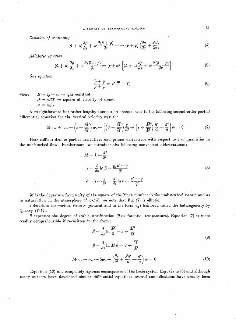
A SURVEY OF THEORETICAL STUDIES
Equation of oontmuuy Jp J(p + P) ~- (] + P) Jx + Jz . . (du dw) (u + u) dx + w Jz
Adiabatic equation
where
Gas equation
(u + u) dp + w J(p + p) = (c + c) 2 [(a+ u) dp + w J(p + p)J dx dz dx dz
P + P = R(f + T) fi+P
R = Cp - Cv = gas constant c2 = KRT = square of velocity of sound
1C = Cp/Cv
51
(4)
(5)
(6)
A straightforward but rather lengthy elimination process leads to the following second-order partial
differential equation for the vertical velocity w(x, z) :
- ( M') [( lfii') g ( M') _, _,] Mwxx + Wzz- s + M Wz + a+ M . u2 + 8 + M ~ - ~ w = 0 (7)
Here suffixes denote partial derivatives and primes derivatives with respect to z of quantities in
the undisturbed flow. Furthermore, we introduce the following convenient abbreviations :
M=i-u} c2
s = .!:_In p = gfR- y dz T
- - g d - y*- y a= s-=-= -In()=---
c2 dz T
(8)
M is the departure from unity of the square of the Mach number in the undisturbed stream and as
in natural flow in the atmosphere u2 < < c2, we note that Eq. (7) is elliptic. s describes the vertical density gradient and in the form ~ s has been called the heterogeneity by
Queney ( 194 7). a expresses the degree of stable stratification (() = Potential temperature). Equation (7) IS more
readily comprehensible if re-written in the form:
- d M _ M' S= -ln=-=s+-=
dz p M (9)
- d -- _ M' fJ=-lnM()=a+--=
dz M
(/3- s-_, _,) - - g u u
Mwxx + Wzz- Swz + -=2 + --- ---;;- W = 0 u u u
(10)
Equation (10) is a completely rigorous consequence of the basic system Eqs. (2) to (6) and although many authors have developed similar differential equations several simplifications have usually been
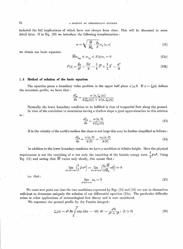
52 A SURVEY OF THEORETICAL STUDIES
included the full in::iplications of which have not always been clear. This will be discussed m more detail later. If in Eq. (10) we introduce the following transformation :
• ~wl(x,z) w=y Mu ·jj (11)
we obtain our basic equation
Mw1 + w1 + F(z)w1 = 0 XX ZZ
(12a)
F(z) = ifg + Sa' - ~ Il + ~ s' - u" a2 a 4 2 a (12b)
1. 4 Method of solution of the basic equation
The equation poses a boundary value problem in the upper half plane z::::::,. 0. If z = ( 0(x) defines the mountain profile, we have that:
IS :
d(0 w [x, (0 (x)] dx = i1[(0 (x)] + u[x, ( 0 (x)]
Naturally the lower boundary condition to be fulfilled is that of tangential flow along the ground. In view of the restriction to mountains having a shallow slope a good approximation to this relation
d(o dx
w(x, 0) i1((0 (x))
(13)
If in the vicinity of the earth's surface the shear is not large this may be further simplified as follows :
d(0 w (x, 0) w1 (x, 0) dx = il (0) = il (0) (14)
In addition to the lower boundary condition we have a condition at infinite height. Here the physical
requirement is not the vanishing of w but only the vanishing of the kinetic Eq. (11) and noting that M varies only slowly, this means that :
1_ 2 u. energy term 2 p w . smg
lim (! p w2) = lim (Po!! w~) = 0 x'+z'~oo 2 x'+z'-+oo 2M0
I.e. that: lim w1 = 0 (15)
x2+z2-+oo
We must now point out that the two conditions expressed by Eqs. (14) and (15) are not in themselves sufficient to determine uniquely the solution of our differential equation (12a). The particular difficulty arises in other applications of meteorological flow theory and is now considered.
We represent the ground profile by the Fourier integral:
00
( 0 (x) = a2 Rej.exp (ikx- kb) dk = na~b .n, 0
(b > 0) (16)
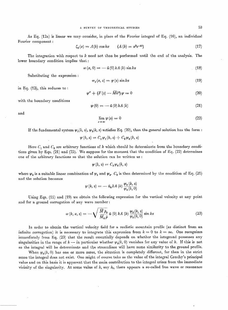
A SURVEY OF THEORETICAL STUDIES 53
As Eq. (12a) is linear we may- consider, in place of the Fourier integral of Eq. (16), an individual Fourier component :
( 0 (x) = A(k) cos kx (A (k) = a2e-kb) (17)
The integration with respect to k need not then be performed until the end of the analysis. The lower boundary condition implies that :
w(x, 0) = -u(O)kA(k) sinkx (18)
Substituting the expressiOn : wdx, z) = lf/ (z) sin kx (19)
in Eq. (12), this reduces to : lf/" + (F (z) - Mk2
) lf/ = 0 (20)
with the boundary conditions lf/ (O) = - a (O) kA (k) (21)
and lim lf/ (z) = 0 (22)
Z-+00
If the fundamental system lf/1(k, z), lf/2(k, z) satisfies Eq. (20), then the general solution has the form:
lf/ (k, z) = C1 lf/1 (k, z) + C2 lf/2 (k, z)
Here C1 and C2 are arbitrary functions of k which should be determinate from the boundary conditions given by Eqs. (21) and (22). We suppose for the moment that the condition of Eq. (22) determines one of the arbitrary functions so that the solution can be written as :
lf/ (k, z) = C3 lf/3 (k, z)
where lf/a is a suitable linear combination of lf/1 and lf/2• C3 is then determined by the condition of Eq. (21) and the solution becomes
lf/ (k, z) = - ilo kA (k) If/a (k, z) If/a (k, ~·
Using Eqs. (11) and (19) we obtain the following expression for the vertical velocity at any point
and for a ground corrugation of any wave number :
w (k, x, z) = - · fiFio_ a (0) kA (k) If/a~:·:) sin kx V Mj lf/3 r, (23)
In order to obtain the vertical velocity field for a realistic mountain profile (as distinct from an infinite corrugation) it is necessary to integrate this expression from k = 0 to k = oo. One recognizes immediately from Eq. (23) that the result essentially depends on whether the integrand possesses any
singularities in the range of k - in particular whether lf/3(k, 0) vanishes for any value of k. If this is not so the integral will be determinate and t:Q.e streamlines will have some similarity to the ground profile.
When If/a (k, 0) has one or more zeros, the situation is completely different, for then in the strict sense the integral does not exist. One might of course take as the value of the integral Cauchy's principal value and on this basis it is apparent that the main contribution to the integral arises from the immediate vicinity of the singularity. At some value of lr, say k., there appears a so-called free wave or resonance
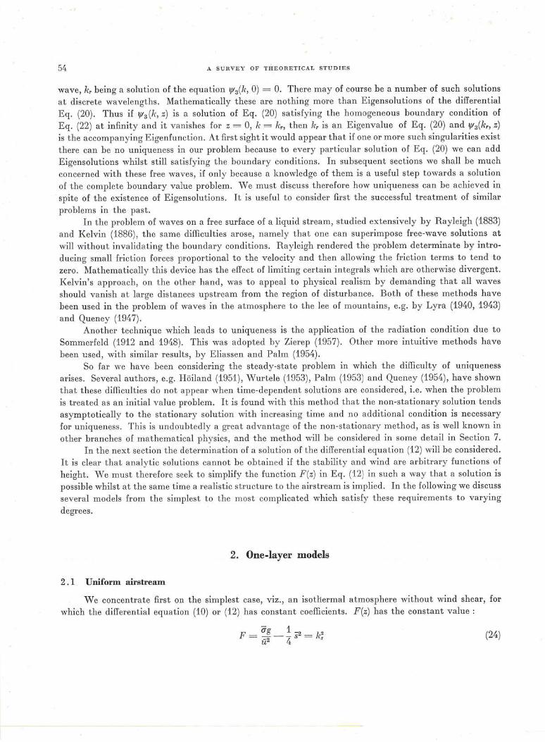
54 A SURVEY OF THEORETICAL STUDIES
wave, k, being a solution of the equation lfl3(k, 0) = 0. There may of course be a number of such solutions
at discrete wavelengths. Mathematically these are nothing more than Eigensolutions of the differential
Eq. (20). Thus if lfl3 (k, z) is a solution of Eq. (20) satisfying the homogeneous boundary condition of
Eq. (22) at infinity and it vanishes for z = 0, k = k,, then k, is an Eigenvalue of Eq. (20) and 1f13(k,, z)
is the accompanying Eigenfunction. At fi rst sight it would appear that if one or more such singularities exist
there can be no uniqueness in our problem because to every particular solution of Eq. (20) we can add
Eigensolutions whilst still satisfying the boundary conditions. In subsequent sections we shall be much
concerned with these free waves, if only because a knowledge of them is a useful step towards a solution
of the complet e boundary value problem. W e must discuss therefore how uniqueness can be achieved in
spite of the existence of Eigensolutions. It is useful to consider fi rst the successful treatment of similar
problems in the past. In the problem of waves on a free surface of a liquid stream, studied extensively by Rayleigh (1883)
and Kelvin (1886), the same difficulties arose, namely that one can superimpose free-wave solutions at
will without invalidating the boundary conditions. R ayleigh rendered the problem determinate by intro
ducing small friction forces proportional to the velocity and then allowing the friction terms to t end to
zero. Mathematically this device has the effec t of limiting certain integrals which are otherwise divergent.
Kelvin's approach, on the other hand, was to appeal to physical realism by demanding that all waves
should vanish at large distances upstream from the region of disturbance. Both of these methods have
been used in the problem of waves in t he atmosphere to the lee of mountains, e.g. by Lyra (1940, 1943)
and Queney (1947). Another technique which leads to uniqueness is the application of the radiation condition due to
Sommerfeld (1912 and 1948) . This was adopted by Zierep (1957). Other more intuitive methods have
been used, with similar results, by Eliassen and Palm (1954).
So far we have been considering the steady-state problem in which the difficulty of uniqueness
arises . Several authors, e.g. Hiiiland (1951), Wurtele (1953), Palm (1953) and Queney (1954), have shown
that these difficulties do not appear when time-dependent solutions are considered, i.e. when the problem
is treated as an initial value problem. It is found with this method that the non-stationary solution tends
asymptotically to the stationary solution with increasing time and no additional condition is necessary
for uniqueness . This is undoubtedly a great advantage of the non-stationary method, as is well known in
other branches of mathematical physics, and the method will be considered in some detail in Section 7.
In the next section the determination of a solution of the differential equation (12) will be considered.
It is clear that analytic solutions cannot be obtained if the stability and wind are arbitrary functions of
height. We must therefore seek to simplify the function F (z) in Eq. (12) in such a way that a solution is
possible whilst at the same time a realistic structure to the airstream is implied. In the following we discuss
several models from the simplest to the most complicated which satisfy these requirements to varying
degrees.
2. One-layer models
2.1 Uniform airstream
We concentrate first on the simplest case, viz., an isotliermal atmosphere without wind shear, for
which the differential equation (10) or (12) has constant coefficients. F(z) has the constant value :
F - ag 1 - 2 - k2 ---s - u2 4 - s (24)
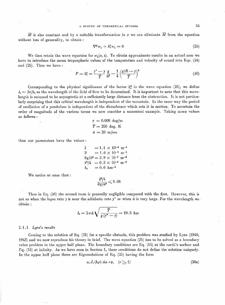
A SURVEY OF THEORETICAL STUDIES 55
M is also constant and by a suitable transformation in x we can eliminate M from the equation
without loss of generality, to obtain :
'\72 H\ + k~ w1 = 0 (25)
We thus retain the wave equation for w1(x, z). To obtain approximate results in an actual case we have to introduce the mean tropospheric values of the temperature and velocity of sound into Eqs. (24) and (25). Thus we have:
F=k~= y*=-y 1__!(gfR-y)2
T u2 4 T (26)
Corresponding to the physical significance of the factor Is.; in the wave equation (25), we define As= 2nfk, as the wavelength of the field of flow to be determined. It is important to note that this wavelength is assumed to be asymptotic at a sufficiently large distance from the obstruction. It is not particu
larly surprising that this critical wavelength is independent of the mountain. In the same way the period of oscillation of a pendulum is independent of the d{sturbance which sets it in motion. To ascertain the
order of magnitude of the various terms we now consider a numerical example. Taking mean values as follows:
y = 0.006 deg/m
T = 250 deg. K
a = 20 m/sec
then our parameters have the values :
We notice at once that:
s = 1.1 X 10⁻⁴ m-1
a = 1.6 X 10⁻⁵ m-1
agfu2 = 3.9 X 10⁻⁷ m-2
82/4 = 0.3 X 10⁻⁸ m-2
ks = 0.6 km-1
82/4 agfu2 < o.o1
Thus in Eq. (26) the second term is generally negligible compared with the first. However, this is not so when the lapse rate y is near the adiabatic rate y* or when u is very large. For the wavelength we obtain:
-v T As = 2 nu ( * , = 10. 5 km g y -y
2. 1. 1 Lyra's results
Coming to the solution of Eq. (25) for a specific obstacle, this problem was studied by Lyra (1940, 1943) and we now reproduce his theory in brief. The wave equation (25) has to be solved as a boundary
value problem in the upper half plane. The boundary conditions are Eq. (14) at the earth's surface and Eq. (15) at infinity. As we have seen in Section 1, these conditions do not define the solution uniquely. In the upper half plane there are Eigensolutions of Eq. (25) having the form
avlv(k,r) sin rrp, (r ~ 1) (26a)
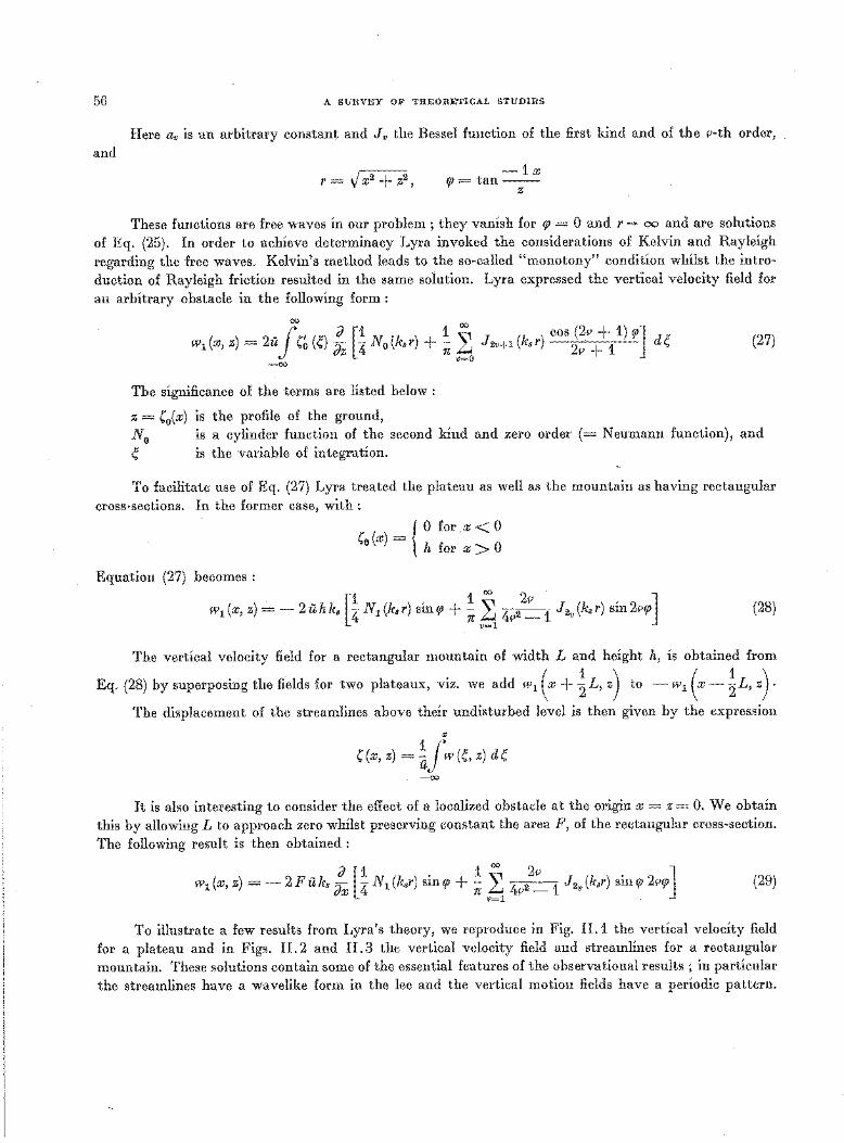
56
and
A SURVEY OF THEORETICAL STUDIES
Here av is an arbitrary constant and J. the Bessel function of the first kind and of the p-th order,
1' = vx2 + z2, rp= tan -1x z
These functions are free waves in our problem ; they vanish for rp = 0 and r -+ oo and are solutions
of Eq. (25). In order to achieve determinacy Lyra invoked the considerations of Kelvin and Rayleigh
regarding the free waves. Kelvin's method leads to the so-called "monotony" condition whilst the intro
duction of Rayleigh friction resulted in the same solution. Lyra expressed the vertical velocity field for
an arbitrary obstacle in the following form :
00 -J 1 d [1 1 ~ COS (21/ + 1) rp] w1 (x, z) = 2u Co (~) (}z 4 N0 (ka r) + 17: 1:'o J2v+l (lr,r) 2P + 1 d~
-00
The significance of the terms are listed below :
z = C0(x) is the profile of the ground,
(27)
N 0 is a cylinder function of the second kind and zero order (= Neumann function), and
~ is the variable of integration.
To facilitate use of Eq. (27) Lyra treated the plateau as well as the mountain as having rectangular
cross-sections. In the former case, with :
Equation (27) becomes :
(x _ { 0 for x < 0 Co ) - h for x > 0
wi(x, z) · - 2uhka [~ N1 (kar) sinrp + ~ ~ 41/22:__ 1 J2.(k,r) sin2Prp J (28)
The vertical velocity field for a rectangular mountain of width L and height h, is obtained from
Eq. (28) by superposing the fields for two plateaux, viz. we add w1 ( x + ~ L, z) to - w1 ( x - ~ L, z) . The displacement of the streamlines above their undisturbed level is then given by the expression
"' 11' C(x, z) =a w(~, z) d~ -00
It is also interesting to consider the effect of a localized obstacle at the origin x = z = 0. We obtain
this by allowing L to approach zero whilst preserving constant the area F, of the rectangular cross-section.
The following result is then obtained :
wdx, z) =- 2Fuk, Jx l~ Ndkar) sinrp + ~ ~ 41/22:__ 1 J 2.(7r,r) sinrp 2Prp] (29)
To illustrate a few results from Lyra's theory, we reproduce in Fig. II.1 the vertical velocity field
for a plateau and in Figs. II. 2 and II. 3 the vertical velocity field and streamlines for a rectangular
mountain. These solutions contain some of the essential features of the observational results ; in particular
the streamlines have a wavelike form in the lee and the vertical motion fields have a periodic pattern.
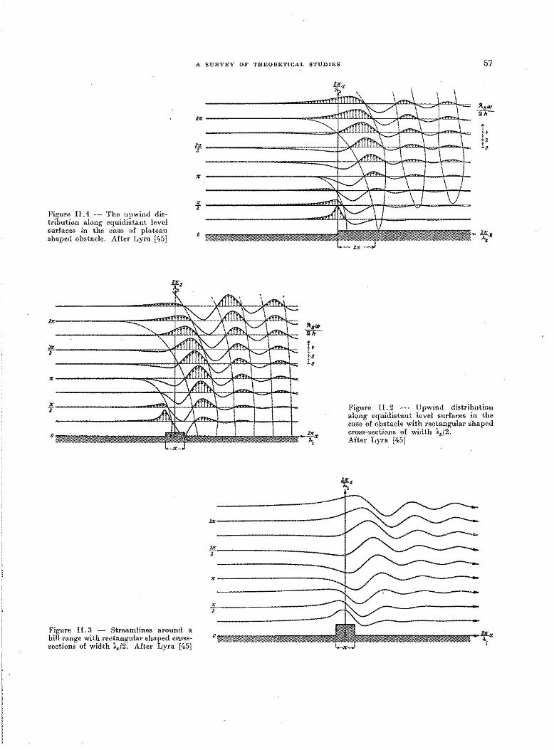
A SURVEY OF THEORETICAL STUDIES
2-n:z .a.,
57
!'I sat
z-n: -_"T""ffl'["'ll!!llll~,... ~----=-~-= an
J7t 1::7<:"'[1111!1"(~~) 1~1 T ~ 1-=1 \- f! /r
-1- -n:rrrt)t'\: - ::;;.\ l--===- V \./ Figure Il .1 - The upwind distribution along equidistant level surfaces in the case of plateau shaped obstacle. After Lyra [45]
z;r:2 .t,
Q
2JC ._ ~ "'-../ )<" 1.111 N \Affil,\ \: 1\: 7\ 1""":::
3Jt -J(fi I I I~'\:: )(' I I TNK :;)('f7tt~ z
.'71: c::::::-=:: 1 :;;¥''"''T'IJK yxr,..\~ ........... \<
f S"£"2\ 1- X'IIIT~i-"'"-1 I I
!'I slAt an
I;
o~~~~#llf#B' ~x
Figure 11. 3 - Streamlines around a hill range with rectangular shaped crosssections of width "A,/2. After Lyra [45]
27<---------------------------
7&---------------------~
OW#$#,@1$$.@'.-m'.#SM~,@
27< :( ks
Figure Il. 2 - Upwind distribution along equidistant level surfaces in the case of obstacle with rectangular shaped cross-sections of width ).8 /2. After Lyra [45]
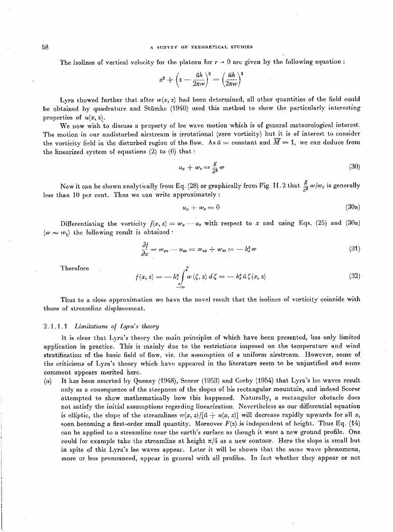
58 A SUHVEY OF THEOHETICAL STUDIES
The isolines of vertical velocity for the plateau for r --+ 0 are given by the following equation :
x2 + (z _ uh )2
= ( uh )2
2nw 2nw
Lyra showed further that after w(x, z) had been determined, all other quantities of the field could be obtained by quadrature and Stiimke (1940) used this method to show the particularly interesting
properties of u(x, z). We now wish 'to discuss a property of lee wave motion which is of general meteorological interest.
The motion in our undisturbed airstream is irrotational (zero vorticity) but it is of interest to consider
the vorticity field in the disturbed region of the flow. As il = constant and M = 1, we can deduce from
the linearized system of equations (2) to (6) that :
g Ux + Wz= 1 W
c (30.)
Now it can be shown analytically from Eq. (28) or graphically from Fig. I I. 2 that ~ wfw. is generally
less than 10 per cent. Thus we can write approximately : c
Ux + Wz = 0 (30a)
Differentiating the vorticity f(x, z) = Wx- u. with respect to x and using Eqs. (25) and (30a)
(w """' w1) the following result is obtained :
Therefore
Jf Jx = Wxx- Uzx = Wxx + Wzz = - k~ w
X
f(x, z) =- k! r w (~, z) d~ =- k!il((x, z) 0/
-00
(31)
(32)
Thus to a close approximation we have the novel result that the isolines of vorticity coincide with
those of streamline displacement.
2. 1. 1.1 Limitations of Lyra's theory
It is clear that Lyra's theory the main principles of which have been presented, has only limited
application in practice. This is mainly due to the restrictions imposed on the temperature and wind stratification of the basic field of flow, viz. the assumption of a uniform airstream. However, some of
the criticisms of Lyra's theory which have appeared in the literature seem to be unjustified and some comment appears merited here. (a) It has been asserted by Queney (1948), Scorer (1953) and Corby (1954) that Lyra's lee waves result
only as a consequence of the steepness of the slopes of his rectangular mountain, and indeed Scorer attempted to show mathematically how this happened. Naturally, a rectangular obstacle does not satisfy the initial assumptions regarding linearization. Nevertheless as our differential equation
is elliptic, the slope of the streamlines w(x, z)/[il + u(x, z)] will decrease rapidly upwards for all x, soon becoming a first-order small quantity. Moreover F(z) is independent of height. Thus Eq. (14) can be applied to a streamline near the earth's surface as though it were a new ground profile. One
could for example take the streamline at height n/4 as a new contour. Here the slope is small but in spite of this Lyra's lee waves appear. Later it will be shown that the same wave phenomena,
more or less pronounced, appear in general with all profiles. In fact whether they appear or not
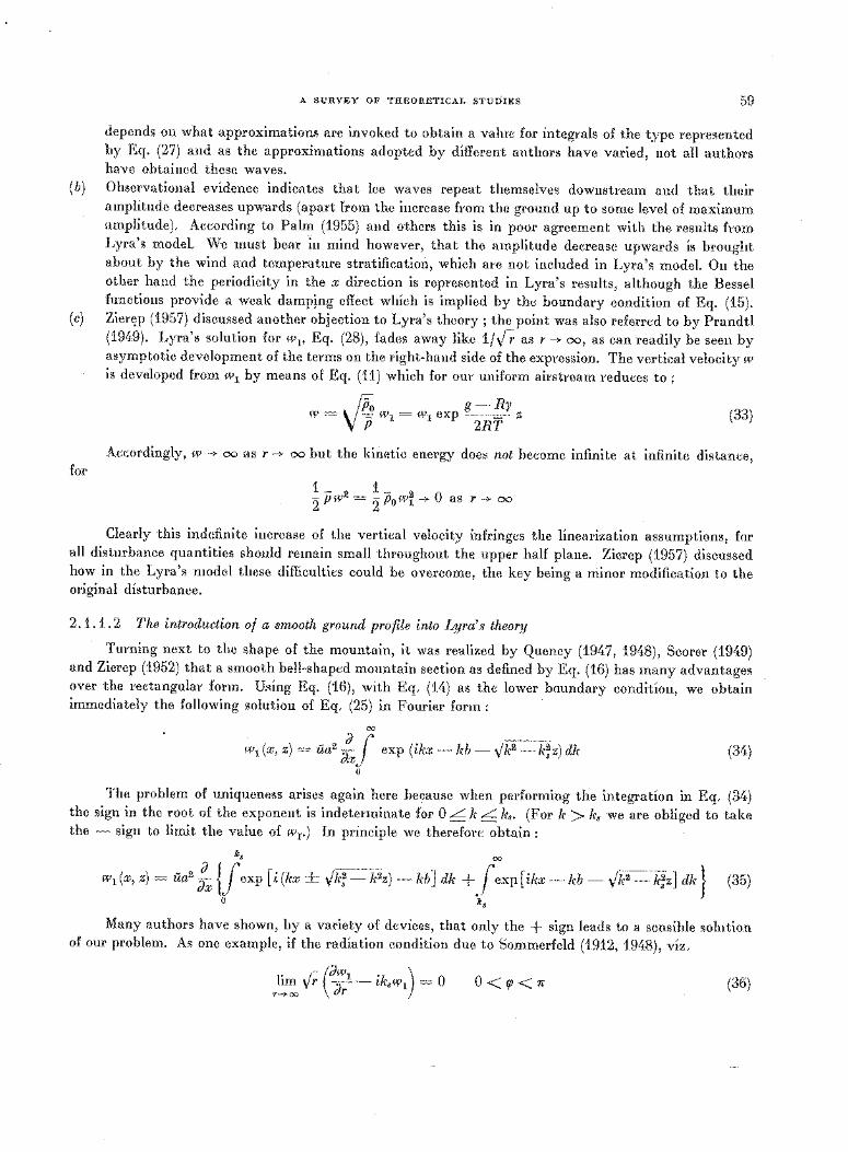
(b)
(c)
for
A SURVEY OF THEORETICAL STUDIES 59
depends on what approximations are invoked to obtain a value for integrals of the type represented by Eq. (27) and as the approximations adopted by different authors have varied, not all authors have obtained these waves. Observational evidence indicates that lee waves repeat themselves downstream and that their amplitude decreases upwards (apart from the increase from the ground up to some level of maximum amplitude). According to Palm (1955) and others this is in poor agreement with the results from Lyra's model. W-e must bear in mind however, that the amplitude decrease upwards is brought about by the wind and temperature stratification, which are not included in Lyra's model. On the other hand the periodicity in the x direction is represented in Lyra's results, although the Bessel functions provide a weak dampjng effect which is implied by the boundary condition of Eq. (15). Zier~p (1957) discussed another objection to Lyra's theory ; the point was also referred to by Prandtl (1949). Lyra's solution for wv Eq. (28), fades away like 1/ V-;. as r--+ oo, as can readily be seen by asymptotic development of the terms on the right-hand side of the expression. The vertical velocity w is developed from w1 by means of Eq. (11) which for our uniform airstream reduces to :
. /Po g -- Ry w = V p w1 = w1 exp
2RT- z (33)
Accordingly, w -+ oo as r -+ oo but the kinetic energy does not become infinite at infinite distance,
1- 1 2 p w2 = 2 Po wi -+ 0 as r -~ oo
Clearly this indefinite increase of the vertical velocity infringes the linearization assumptions, for all disturbance quantities should remain small throughout the upper half plane. Zierep (1957) discussed how in the Lyra's model these difficulties could be overcome, the key being a minor modification to the original disturbance.
2. 1. 1. 2 The introduction of a smooth ground profile into Lyra's theory
Turning next to the shape of the mountain, it was realized by Queney (1947, 1948), Scorer (1949) and Zierep (1952) that a smooth bell-shaped mountain section as defined by Eq. (16) has many advantages over the rectangular form. Using Eq. (16), with Eq. (14) as the lower boundary condition, we obtain immediately the following solution of Eq. (25) in Fourier form:
00
w1 (x, z) = ua2 J~ ( exp (ikx- kb- Vk2- k;z) dk
0 (34)
The problem of uniqueness arises again here because when performing the integration in Eq. (34) the sign in the root of the exponent is indeterminate for 0 L. k L. k8 • (For k >Jr. we are obliged to take the - sign to limit the value of w1.) In principle we therefore obtain :
~ 00
wdx, z) = ua2 :X {Jexp [i (kx + vk;- k2z) -- kb] dk +,(exp [ikx- kb- vk2- k;z] dk} (35)
0 ~
Many authors have shown, by a variety of devices, that only the + sign leads to a sensible solution of our problem. As one example, if the radiation condition due to Sommerfeld (1912, 1948), viz.
lim V; ({);:'1 - ik.w1) = 0 r-)- 00 {/r
O<qJ<n (36)
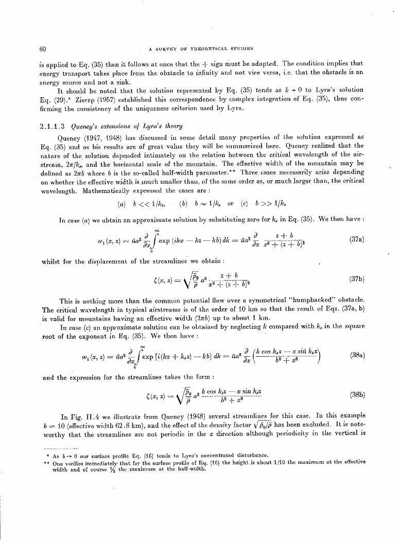
60 A SURVEY OF THEORETICAL STUDIES
is applied to Eq. (35) then it follows at once that the + sign must be adopted. The condition implies that
energy transport takes place from the obstacle to infinity and not vice versa, i.e. that the obstacle is an
energy source and not a sink. It should be noted that the solution represented by Eq. (35) tends as b + 0 to Lyra's solution
Eq. (29). * Zierep (1957) established this correspondence by complex integration of Eq. (35), thus con
firming the consistency of the uniqueness criterion used by Lyra.
2. 1.1. 3 Queney' s extensions of Lyra's theory
Queney (1947, 1948) has discussed in some detail many properties of the solution expressed as
Eq. (35) and as his results are of great value they will be summarized here. Queney realized that the
nature of the solution depended intimately on the relation between the critical wavelength of the air
stream, 2rcfk,, and the horizontal scale of the mountain. The effective width of the mountain may be
defined as 2rcb where b is the so-called half-width parameter.** Three cases necessarily arise depending
on whether the effective width is much smaller than, of the same order as, or much larger than, the critical
wavelength. Mathematically expressed the cases are :
(a) b<<1fk,, (b) b = 1fk, or (c) b >> 1fk,
In case (a) we obtain an approximate solution by substituting zero fork, in Eq. (35). We then have:
00
w1 (x, z) = ua2 ffxf exp (ikx- kz- kb) dk = ua2 ffx
0
whilst for the displacement of the streamlines we obtain :
./Po 2 z+b ((x, z) =V p ax ~2c--+~(-z -;-+ b)2
z+b (37a)
x2 + (z + b) 2
(37b)
This is nothing more than the common potential flow over a symmetrical "humpbacked" obstacle.
The critical wavelength in typical airstreams is of the order of 10 km so that the result of Eqs. (37a, b)
is valid for mountains having an effective width (2rcb) up to about 1 km.
In case (c) an approximate solution can be obtained by neglecting k compared with k, in the square
root of the exponent in Eq. (35). We then have:
00
J f . J (b cos k,z- x siii k,z) wdx, z) = ua2
;;--;;; exp [£(kx + k,z)- kb] dk = ua2 Jx b2 + x2 (38a)
0
and the expression for the streamlines takes the form :
((x, z)= • ffi a2 b cos k,z- x sin k,z V P b2 + x2
(38b)
In Fig. II. 4 we illustrate from Queney ( 1948) several streamlines for this case. In this example
b = 10 (effective width 62.8 km), and the effect of the density factor V p0 fp has been excluded. It is note
worthy that the streamlines are not periodic in the x direction although periodicity in the vertical is
* As b-+ 0 our surface profile Eq. (16) tends to Lyra's concentrated disturbance.
** One verifies immediately that for the surface profile of Eq. (16) the height is about 1/10 the maximum at the effective
width and of course ~ the maximum at the half-width.
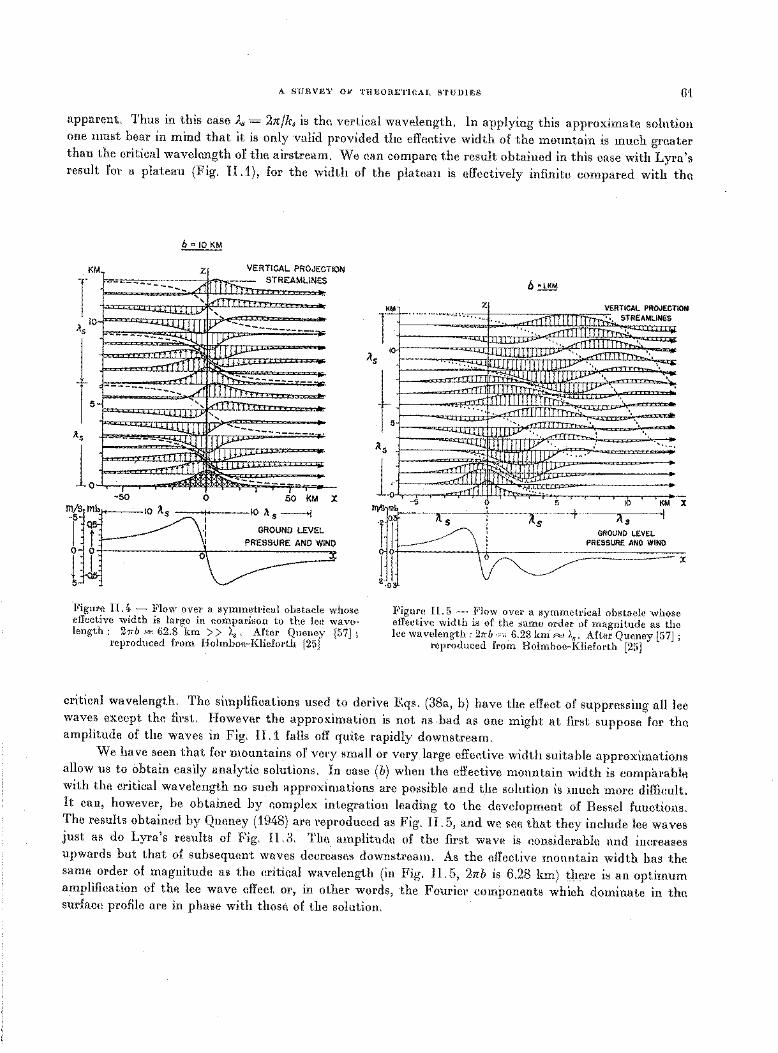
A SURVEY OF THEORETICAL STUDIES 61
apparent. Thus in this case As= 2njk. is the vertical wavelength. In applying this approximate solution one must bear in mind that it is only valid provided the effective width of the mountain is much greater than the critical wavelength of the airstream. We can compare the result obtained in this case with Lyra's result for a plateau (Fig. II .1), for the width of the plateau is effectively infinite compared with the
KM
110 ~5
5
.ls
L
b = 10 KM
z VERTICAL PROJECTION
- ---------,A LCtrr STREAMLINES
... 'V£
' ', '-U..I..lU I V ------------- -
---------~[ ~ ~ fj!JJJ-'
-rfffl ....-rfl [~----------------------- .,.( l _)TfT-r
',V£ -"',
.!..llllJ V ------------- . --- -----~ ll I~
-50
T l J.J.l-1-l rrrff ~
-----------0 50 KM X
-~>-~----10 ll s ------>!
GROUND LEVEL
Figure 11.4 - Flow over a symmetrical obstacle whose effective width is large in comparison to the lee wavelength: 27rb = 62.8 km > > ),8 • After Queney [57] ;
reproduced from Holmboe-Klieforth [25]
h •lKM
KM- z
~s 10
i ----~lllllllllJJJ-IY'•,,~\
t. its
l =:mllli'i'tffi Ill I V~ I I I=--.; ---
l~ -5 9 5 10 KM X
a ! ~ I i'ls GROUND LEVEL
PRESSURE AND WIND
X
Figure 11. 5 - Flow over a symmetrical obstacle whose effective width is of the same order of magnitude as the lee wavelength : 27rb ·= 6.28 km"""" ).8 • After Queney [57] ;
reproduced from Holmboe-Kiieforth [25]
critical wavelength. The simplifications used to derive Eqs. (38a, b) have the effect of suppressing all lee waves except the first. However the approximation is not as bad as one might at first suppose for the amplitude of the waves in Fig. II .1 falls off quite rapidly downstream.
We have seen that for mountains of very small or very large effective width suitable approximations allow us to obtain easily analytic solutions. In case (b) when the effective mountain width is comparable with the critical wavelength no such approximations are possible and the solution is much more difficult. It can, however, be obtained by complex integration leading to the development of Bessel functions. The results obtained by Queney (1948) are reproduced as Fig. II. 5, and we see that they include lee waves just as do Lyra's results of Fig. II. 3. The amplitude of the first wave is considerable and increases upwards but that of subsequent waves decreases downstream. As the effective mountain width has the same order of magnitude as the critical wavelength (in Fig. II. 5, 2nb is 6.28 km) tpere is an optimum amplification of the lee wave effect or, in other words, the Fourier components which dominate in the surface profile are in phase with those of the solution.
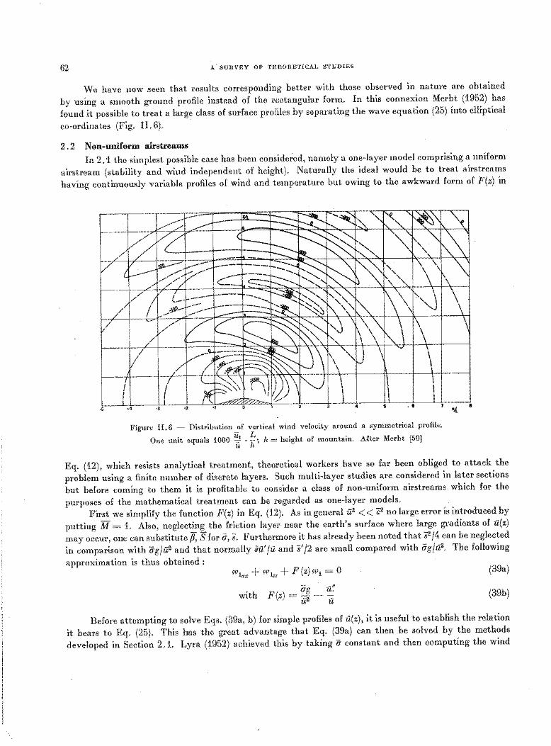
62 A. SURVEY OF THEORETICAL STUDIES
We have now seen that results corresponding better with those observed in nature are obtained
by using a smooth ground profile instead of the rectangular form. In this connexion Merbt (1952) has
found it possible to treat a large class of surface profiles by separating the wave equation (25) into elliptical
co-ordinates (Fig. 11. 6). .
2. 2 Non-uniform airstreams
In 2.1 the simplest possible case has been considered, namely a one-layer model comprising a uniform
airstream (stability and wind independent of height). Naturally the ideal would be to treat airstreams
having continuously variable profiles of wind and temperature but owing to the awkward form of F(z) in
/
/
-5 ";{_
Figure II. 6 - Distribution of vertical wind velocity around a symmetrical profile.
One unit equals 1000 ~ · ~; h =height of mountain. After Merbt [50]
Eq. (12), which resists analytical treatment, theoretical workers have so far been obliged to attack the
problem using a finite number of discrete layers. Such multi-layer studies are considered in later sections
but before coming to them it is profitable to consider a class of non-uniform airstreams which for the
purposes of the mathematical treatment can be regarded as one-layer models.
First we simplify the function F(z) in Eq. (12). As in general u2 < < c2 no large error is introduced by
putting M= 1. Also, neglecting the friction layer near the earth's surface where large gradients of il(z)
may occur, one can substitute 7f, S for ii, 8. Furthermore it has already been noted that 82/4 can be neglected
in comparison with agfu2 and that normally sil'/il and 8'/2 are small compared with iigfu2• The following
approximation is thus obtained : wl.,., + wlzz + F(z)wl = 0 (39a)
with F(z) = ag _ il~' f12 -=-u
(39b)
Before attempting to solve Eqs. (39a, b) for simple profiles of il(z), it is useful to establish the relation
it bears to Eq. (25). This has the great advantage that Eq. (39a) can then be solved by the methods
developed in Section 2 .1. Lyra (1952) achieved this by taking a constant and then computing the wind
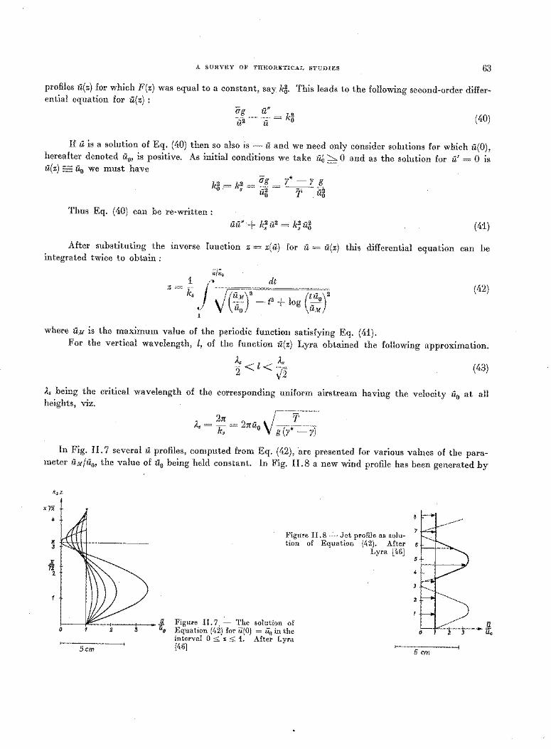
A SURVEY OF THEORETICAL STUDIES 63
profiles a(z) for which F(z) was equal to a constant, say kg. This leads to the following second-order differential equation for a(z) :
- -n
~-~=~ a2 a (40)
If a is a solution of Eq. (40) then so also is- a and we need only consider solutions for which a(O), hereafter denoted a0, is positive. As initial conditions we take a0 :::::::,. 0 and as the solution for a' = 0 is a(z) _ a0 we must have
k2 = k2 = ag - y* - Y g 0 . s -2 - . ---_- . -uo T a5
Thus Eq. (40) can be re-written:
aa"+ k~a2 ~ k~a~ (41)
After substituting the inverse function z = z(a) for a = u(z) this differential equation can be integrated twice to obtain :
;;;;,0
,~ t. / ·-
dt (42)
(aM)2 (tu )2 ilo - t2 + log u;
where UA£ is the maximum value of the periodic function satisfying Eq. (41). For the vertical wavelength, l, of the function u(z) Lyra obtained the following approximation.
~<l<~~ (43)
As being the critical wavelength of the corresponding uniform airstream having the velocity a0 at all heights, viz.
2n • / T As= k, = 2na0 V g(y* -y)
In Fig. II. 7 several u profiles, computed from Eq. (42), are presented for various values of the parameter ilM/110, the value of u0 being held constant. In Fig. 11.8 a new wind profile has been generated by
ks z
1C-yi
* n: [ \.\ 1• I I J
Jr n 2
Figure II. 8 _:_ Jet profile as solu-7
tion of Equation (42). After 6 t 1 =--.., Lyra ['•6] ~
5 I I ..;
2
1 liP= 1 1 • $ Figure II. 7. - The solution of "o Equation (42) for U:(O) = ii0 in the
interval 0 s z s 1. After Lyra [46]
i1 1 j_......= 1 I "' Uo 0 2 3 11
5cm 5 cm
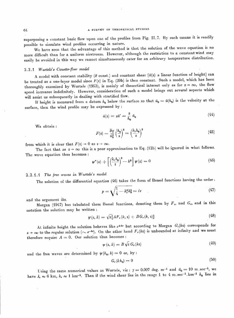
64 A SURVEY OF THEORETICAL STUDIES
superposing a constant basic flow upon one of the profiles from Fig. 11. 7. By such means it is readily
possible to simulate wind profiles occurring in nature.
We have seen that the advantage of this method is that the solution of the wave equation is no
more difficult than for a uniform airstream. However, although the restriction to a constant wind may
easily be avoided in this way we cannot simultaneously cater for an arbitrary temperature distribution.
2 . 2 . 1 W urtele' s C ouette- flow model
A model with constant stability (a const.) and constant shear [u(z) a linear function of height] can
be treated as a one-layer model since F(z) in Eq. (39b) is then constant. Such a model, which has been
thoroughly examined by Wurtele (1953), is mainly of theoretical interest only as for z--+ =, the flow
speed increases indefinitely. However, consideration of such a model brings out several aspects which
will assist us subsequently in dealing with stratified flow.
If height is measured from a datum h0 below the surface so that u0 = u(h0) is the velocity at the
surface, then the wind profile may be expressed by :
We obtain:
z u(z) = zu' = h iio
0
F(z) =~;(~or= c·zhoy
from which it is clear that F(z) --+ 0 as z--+ OC>.
(44)
(45)
The fact that as z--+ = this is a poor approximation to Eq. (12b) will be ignored in what follows.
The wave equation thus becomes:
'fl" (z) + [ (k.zhoy- k2J 'fl(z) = o (46)
2. 2 .1.1 The free wares in W urtele' s model
The solution of the differential equation ( 46) takes the form of Bessel functions having the order :
p = v~-k~h~= iv (47)
and the argument ikz. Morgan (1947) has tabulated these Bessel functions, denoting them by Fv, and Gv, and in this
notation the solution may be written :
lfi(Z, k) = V;-[AFv(k, z) + BGv(k, z)] (48)
At infinite height the solution behaves like e±kz but according ·to Morgan Gv(kz) corresponds for
z-+ OC> to the regular solution(,""-! e-kz). On the other hand Fv(kz) is unbounded at infinity and we must
therefore require A = 0. Our solution thus becomes :
If/ (z, k) = B Vz Gv (kz) (49)
and the free waves are determined by lfl(h0 , k) = 0 or, by:
Gv(kho) = 0 (50)
Using the same numerical values as Wurtele, viz: y = 0.007 deg. m-1 and u0 = 10 m.sec-1, we
have As ~ 6 km, k. ~ 1 km-1. Then if the wind shear lies in the range 1 to 4 m. sec-1 . km-1 ho lies in
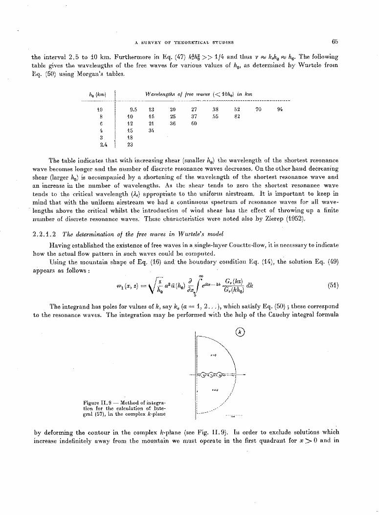
A SURVEY OF THEORETICAL STUDIES 65
the interval 2.5 to 10 km. Furthermore in Eq. (47) krh~ >> 1/4 and thus v ~ k,h0 ~ h0• The following
table gives the wavelengths of the free waves for various values of h0, as determined by Wurtele from
Eq. (50) using Morgan's tables.
h0 (km) Wavelengths of free waves ( < 10h0 ) in km
10 9.5 13 20 27 38 52 70 94,
8 10 16 25 37 55 82 G 12 21 36 60 4, 15 34,
3 18 2.4, 23
The table indicates that with increasing shear (smaller h0) the wavelength of the shortest resonance
wave becomes longer and the number of discrete resonance waves decreases. On the other hand decreasing
shear (larger h0) is accompanied by a shortening of the wavelength of the shortest resonance wave and
an increase in the number of wavelengths. As the shear tends to zero the shortest resonance waye
tends to the critical wavelength (A..) appropriate to the uniform airstream. It is important to keep in
mind that with the uniform airstream we had a continuous spectrum of resonance waves for all wave
lengths above the critical whilst the introduction of wind shear has the effect of throwing up a finite
number of discrete resonance waves. These characteristics were noted also by Zierep (1952).
2. 2 .1. 2 The determination of the free wares in W urtele' s model
Having established the existence of free waves in a single-layer Couette-flow, it is necessary to indicate
how the actual flow pattern in such waves could be computed.
Using the mountain shape of Eq. (16) and the boundary condition Eq. (14), the solution Eq. (49)
appears as follows : - 00
( ) _. J Z 2 -(h){)! ikx-kb Gv(kz) dk wl x, z - V ho a u o {)x e Gv (kho) (51)
0
The integrand has poles for values of k, say ka (a= 1, 2 ... ), which satisfy Eq. (50); these correspond
to the resonance waves. The integration may be performed with the help of the Cauchy integral formula
Figure II. 9 -Method of integration for the calculation of Integral (57), in the complex k-plane
~~ ®
LJ : ._ ..... ..,.,...=.. .. "!r ....... ::·::.~ ... ~.,~~
' J I t.t:.O ,/
: /,/
' ,' L ________ ........... ...
-,-,_--
by deforming the contour in the complex k-plane (see Fig. II. 9). In order to exclude solutions which
increase indefinitely away from the mountain we must operate in the first quadrant for x > 0 and in
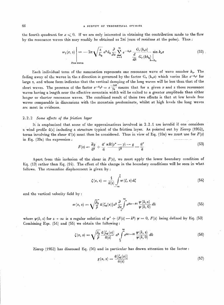
66 A SURVEY OF THEORETICAL STT.:DIES
the fourth quadrant for x < 0. I£ we are only interested in obtaining the contribution made to the flow
by the resonance waves this may readily be obtained as 2ni (sum of residues at the poles). Thus:
. fz 2 - !!__ ~ e-Tcab _!!.::.. (/ra!)__ sin kax wl (x, z) I = - 2n V ho a uo Jx L.J !!__ G (kh ) J
0 a~l dk V 0/c~lca (52) .
Free waves
Each individual term of the summation represents one resonance wave of wave number ka. The
fading away of the waves in the z direction is governed by the factor G. (kaz) which varies like e-ka• for
large z, and whose form indicates that the vertical damping of the long waves will be less than that of the -21lb
short waves. The presence of the factor e-kab = e ~ means that for a given x and z those resonance
waves having a length near the effective mountain width will be exited to a greater ;1mplitude than either
longer or shorter resonance waves. The combined result of these two effects is that at low levels free
waves comparable in dimensions with the mountain predominate, whilst at high levels the long waves
are most in evidence.
2 . 2 . 2 Some effects of the friction layer
It is emphasized that some of the approximations involved in 2. 2.1 are invalid if one considers
a wind profile u(z) including a structure typical of the friction layer. As pointed out by Zierep (1952),
terms involving the shear ii'(z) must then be considered. Thus in view of Eq. (10a) we must use for F(z) in Eq. (39a) the expression: ----- -
F(z) = ~g + u' KR(y*- y)- g u" u2 ii c2 - u
(53)
Apart from this inclusion of the shear in F(z), we must apply the lower boundary condition of
Eq. (13) rather than Eq. (14). The effect of this change in the boundary conditions will be seen in what
followR. The streamline displacement is given by :
X
((x, z) = u~z) J w (~, z)d~ (54)
-00
and the vertical velocity field by :
w(x, z) = 0i ii[(0 (x)Ja2 ;xLfeikx-kb ~~~:~) dk (55)
0
where !fl(k, z) for z-+ oo is a regular solution of lf/ 11 + (F(z)- k2) 1f1 = 0, F(z) being defined by Eq. (53)
Combining Eqs. (54) and (55) we obtain the following:
- 00
((x z) = • /& ii[Co(x)] a2feik:r-kb !fl(k, z) ~k ' V jj u(z) . !fl(k, 0)
0
Zierep (1952) has discussed Eq. (56) and in particular has drawn attention to the factor:
g(x, z) = u[Co(x)J u(z)
(56)
(57)
A SURVEY OF THEORETICAL STUDIES 67
As can be seen from Fig. II .10 this factor exerts a considerable damping where the mountain lies
in the friction layer and the wind increases rapidly upwards. Where the mountain extends above the
friction layer, g--+ 1. These considerations are therefore most relevant for smaller obstacles.
3. Two-layer models
We have so far been concerned with the simplest types of airstreams, namely those which could
be regarded for our purpose as effectively comprising one layer, i.e. F(z) in Eq. (39b) constant. Thus,
except to a limited extent in the Couette-flow model (2. 2 .1) it has not been possible to deal with realistic
I I
z --+-----0 I
I I I I
Xo
z z
L--~ _ ___L_ _ _l__ a X U(~alX0l) iJ.{l0 )
5 cm
Figure 11.10 - }'or illustration and for graphical construction of the
factor g (x, z) = u ~0( (x) )] in Equations (!•3) and (4A). After Zierep [85] u z
profiles of temperature and wind. As continuous profiles cannot in general be treated analytically it is
natural to consider the value of approximating to real airstreams by a number of layers each having a
constant but different value of F(z). This approach was first adopted by Scorer (1949) who used an
_atmosphere divided into two layers. Although this representation of the stratification of the atmosphere
is crude, the results are illuminating and practically useful and this has stimulated extensive study of the
two-layer model.
3. 1 An example of the two-layer model
To illustrate the method we now quote an example from Scorer (1949). His airstream comprised
the following two layers :
(a) Upper Constant wind velocity Constant lapse rate
Thus:
a= 15 m.sec-1
Y = 0.008 deg.m-1
ag F 2 = --;;z = k~ = 0.33 km-2,
u
(b) Lower
A2 = 11 km (58)
The lower layer consisted strictly speaking of two parts buLas_E(.z_) was _ariang_e_d to have the
same value throughout, dynamically it could be considered as one layer. At the surface Scorer
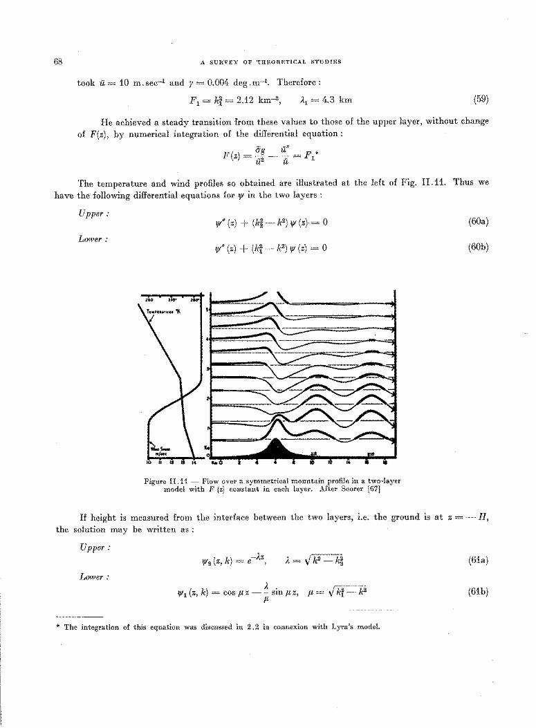
68 A SURVEY OF THEORETICAL STUDIES
took a= 10 m.sec-1 and y = 0.004 deg.m-1. Therefore:
F 1 = ki = 2.12 km-2, A1 = 4.3 km (59)
He achieved a steady transition from these values to those of the upper layer, without change
of F(z), by numerical integration of the differential equation: - _,
F (z) = ~~ - u_ = F / u u
The temperature and wind profiles so obtained are illustrated at the left of Fig. II .11. Thus we
have the following differential equations for lfl in the two layers :
Upper:
Lower:
lf/ 11 (z) + (k~- k2) lfl (z)· = 0
lfl" (z) + (ki- k2) lfl (z) = 0
Figure II .11 - Flow over a symmetrical mountain profile in a two-layer model with F (z) constant in each layer. After Scorer [67]
(60a)
(60b)
I£ height is measured from the interface between the two layers, i.e. the ground is at z = - H, the solution may be written as :
Upper:
Lower:
lf/z (z, lr) ....:... e -Az , A= vk2 -k~
lf/1 (z, k) =cos flZ- ~sin flZ, f1 = V kf- k2
f1
* The integration of this equation was discussed in 2. 2 in connexion with Lyra's model.
(61a)
(61b)
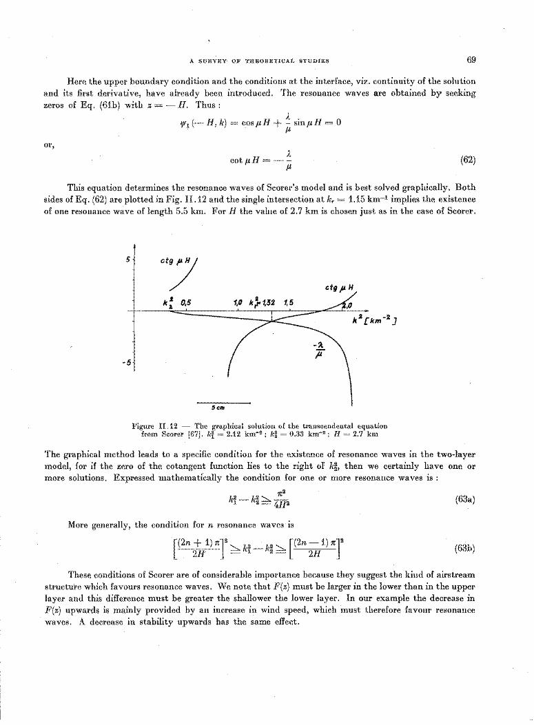
A SURVEY OF THEORETICAL STUDIES 69
Here the upper boundary condition and the conditions at the interface, viz. continuity of the solution and its first derivative, have already been introduced. The resonance waves are obtained by seeking zeros of Eq. (61b) with z =-H. Thus:
or,
lf/1 (- H, k) =cos pH+~ sin pH= 0 J.l
cot pH=-~ J.l
(62)
This equation determines the resonance waves of Scorer's model and is best solved graphically. Both sides of Eq. (62) are plotted in Fig. 11.12 and the single intersection at kr = 1.15 km-1 implies the existence of one resonance wave of length 5.5 km. For H the value of 2. 7 km is chosen just as in the case of Scorer.
5
-5
"'7 1,0
k • 0,5 :r;::::::==-~ k 2 {km -• 1 ~ I j
5cm
Figure Il .12 - The graphical solution of the transcendental equation from Scorer [67]. k~ = 2.12 km-2 ; k~ = 0.33 km-2 ; H = 2.7 km
The graphical method leads to a specific condition for the existence of resonance waves in the two-layer model, for if the zero of the cotangent function lies to the right of k~, then we certainly have one or more solutions. Expressed mathematically the condition for one or more resonance waves is :
2
k~- k~::::,. 4~2 (63a)
More generally, the condition for n resonance waves is
[(2n + 1) n]2::::,. k2 _ k2::::,. [(2n -1) n]2
2H - 1 2 - 2H (63b)
These conditions of Scorer are of considerable importance because they suggest the kind of airstream structure which favours resonance waves. We note that F(z) must be larger in the lower than in the upper layer and this difference must be greater the shallower the lower layer. In our example the decrease in F(z) upwards is mainly provided by an increase in wind speed, which must therefore favour resonance waves. A decrease in stability upwards has the same effect.
70 A SURVEY OF THEORETICAL STUDIES
After these comments about the free waves, we turn to the problem of obtaining a complete solution
of the boundary value problem for a specific obstacle. Analogous to Eq. (51), the vertical velocity field
is given by: 00
wdx, z) = a2 il (-H) fx Jexp (ikx- kb) IJI~, 2 (z:_k~, dk (64)
. 0
Once again it is necessary to evaluate this expression by complex integration and Scorer obtained
the result:
x>O
- d w1 (x, z) = a2u (-H) dx
x<O
b + ix b2 + x2
IJI1,2 (z, 0) , lfld- H O) + 2m exp (ikrx- k b) IJI1,2 (z, kr) ' r d
dkr lf/1 (- H, kr)
I _b_ Uo.N' 'Y 1,;.: \ ..... , V I
(65)
In Eq. (65) the term for the contribution of the single resonance wave in our example is exact;
the remaining term however is an approximation only, obtained by putting k = 0 in part of the integrand
on the strength of the exponential factor e-kb. The terms may easily be calculated by substituting for
1J11(k, z) from Eq. (61b). The resonance-wave term is of particular interest and in the lower layer (z L 0)
it takes the form :
d I V k2- k2 w1 (x, z) = a2il(--H) dx - 2n H ~
+ ,; k:- k~
e-krb I · k; · sin V k~- k; (H + z) · sin krx (66)
The factors in Eq. (66) governing the amplitude of resonance waves are discussed in Section 3. 2.
To calculate the complete field of flow from Eq. (65) we substitute the expressions of Eq. (61) for lf/,
using (61a) for the upper layer and (61b) for the lower layer, In the upper layer the previously discussed
difficulty is again encountered as to the choice of sign for the A root when k < h2• Scorer, erroneously in
our opinion, took the negative sign in these circumstances implying that the mountain acts as an energy
sink (see 2 .1.1. 2). His computed flow pattern is reproduced as Fig. II .11 and had he made the opposite
choice the powerful wave which appears for z > 3 km above and to -windward of the obstacle would have
appeared, more realistically, on the lee side.
In subsequent work Scorer (1953) applied his methods to a three-layer model having an adiabatic
lower layer in which F(z) = 0. This is a realistic model in the sense that a well-mixed layer near the
surface is a common feature in conditions of strong wind. Scorer (1954) also studied the effect of inversions
of varying intensity on the amplitude of resonance waves.
3. 2 The amplitude of lee (resonance) waves in Scorer's model
Some interesting conclusions, having some practical value, have been deduced by Corby and
Wallington (1956) concerning the amplitude of the resonance waves arising in the Scorer type model. To
avoid misunderstanding it must be emphasized that they studied the lee-wave term of Eq. (65) in isolation.
However, the first term which is non-periodic "in x may have a large effect in the immediate vicinity of
the mountain so that their conclusions apply strictly to lee waves over level ground well downstream of
the mountain.
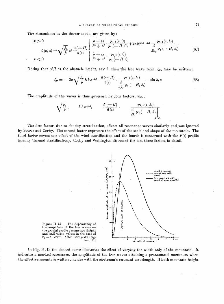
A SURVEY OF THEORETICAL STUDIES 71
The streamlines in the Scorer model are given by :
x>O
( (x, z) = · I ~o a2 il (-H) V p --,
b + ix . lf/1 2 (z 0) b
2 • ' ' +2 . ( + x2 lfll ( _ H, O) . rneikrx-krb d lf/1, 2 z, k,)
die, lf/1 (- H, k,) (67) b + ix 1{11, 2 (z, 0)
x<O b2 + x2. lfll (-H, 0)
Noting that a2 fb is the obstacle height, say h, then the free wave term, (1,, may be written:
(fr =- 2n • I ~0 h b e-k,b • il (-H) . lf/1.2 (z, k,) V P ~~ d dkr lf/1 (- H, k,)
· sin k,x
The amplitude of the waves is thus governed by four factors, viz. :
.!Po V!i'
h b g-krb, u(-H)
il (z) lf/1,2 (z, k,)
d dk lfld- H, k) I
k=kr
(68)
The first factor, due to density stratification, affects all resonance waves similarly and was ignored by Scorer and Corby. The second factor expresses the effect of the scale and shape of the mountain. The third factor covers one effect of the wind stratification and the fourth is concerned with the F(z) profile (mainly thermal stratification). Corby and Wallington discussed the last three factors in detail.
Figure 11.13 - The dependency of the amplitude of the free waves on the ground profile parameters (height and half-width value) in the case of k 0 = 1 km-1. After Corby-Walling-
ton [11]
0&
'i ~
i:' 104 ..0 ~
i j: 03
"0
-t 1 -a. E 0·2 Q
~ ~
Ht0"19ht of mOJnlcun ---- con!J.,n!-,only Ylld~h
varied -- Bofh hll•<)ht and wJI-1,
vdlriod 10 sarn~a proportia'l
t\ I \ I \ I I I \ I I I \ I \
I • \ I { \
I § \ I - \ I o \ I -" \ I :::0 \ I I ~ \ I E \ I > \
E ' i.. ',, 0 ',
................ __ _ 3 4 ~ Bkm
Holf . w•d•h of mountCIIn
In Fig. II .13 the dashed curve illustrates the effect of varying the width only of the mountain. It indicates a marked resonance, the amplitude of the free waves attaining a pronounced maximum when the effective mountain width coincides with the airstream's resonant wavelength. If both mountain height
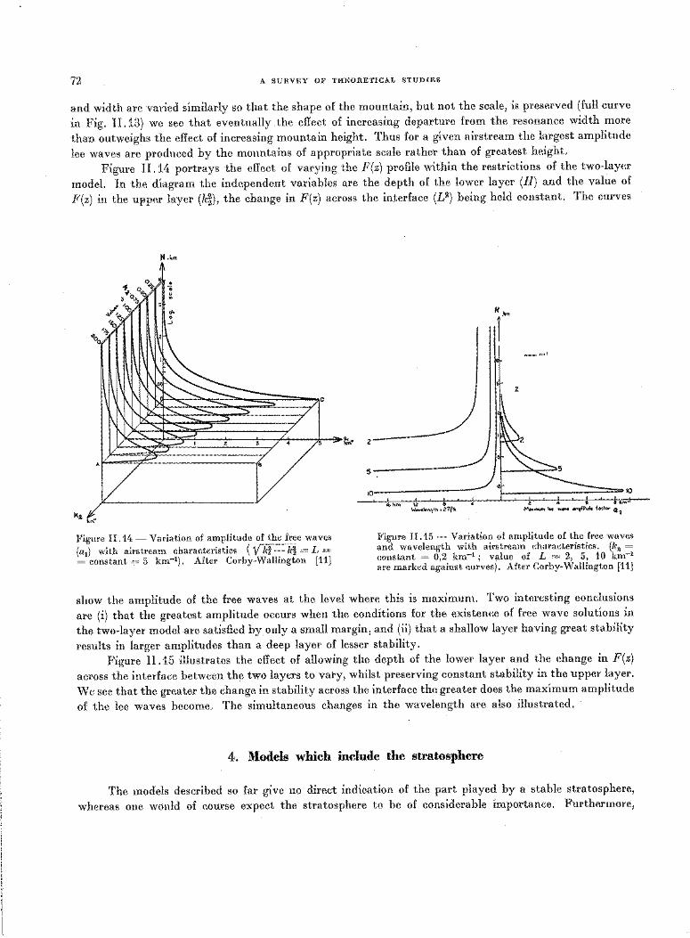
72 A SURVEY OF THEORETICAL STUDIES
and width are varied similarly so that the shape of the mountain, but not the scale, is preserved (full curve
in Fig. II .13) we see that eventually the effect of increasing departure from the resonance width more
than outweighs the effect of increasing mountain height. Thus for a given airstream the largest amplitude
lee waves are produced by the mountains of appropriate scale rather than of greatest height.
Figure 11.14 portrays the effect of varying the F(z) profile within the restrictions of the two-layer
model. In the diagram the independent variables are the depth of the lower layer (H) and the value of
F(z) in the U)'lper layer (k~), the change in F(z) across the interface (£2) being held constant. The curves
"·""
~::-~s:::::;--=:; /le
H ~~~m
r I
_n•l
2.
_k ~-~ ! • /, I '>\\o --------- ; • /. :::;illl" kin:' 2
Figure II. 14 - Variation of amplitude of the free waves
(a1) with airstream characteristics (V ·k'f- k~ = L = =constant= 5 km-1). After Corby-Wallington [11]
s------~
~------------------- ~
"'''" 12 8 ~.l .. "qtt ... 20/t..
-;z----4-- 6 a km"'
M .. .rrun IM w..,. •,Pih.cla factor Q 1
Figure II .15 - Variation of amplitude of the free waves and wavelength with airstream characteristics. (k2 = constant = 0,2 km-1 ; value of L = 2, 5, 10 km-1
m·e marked against curves). After Corby-Wallington [11]
show the amplitude of the free waves at the level where this is maximum. Two interesting conclusions
are (i) that the greatest amplitude occurs when the conditions for the existence of free wave solutions in
the two-layer model are satisfied by only a small margin, and (ii) that a shallow layer having great stability
results in larger amplitudes than a deep layer of lesser stability.
Figure 11.15 illustrates the effect of allowing the depth of the lower layer and the change in F(z)
across the interface between the two layers to vary, whilst preserving constant stability in the upper layer.
We see that the greater the change in stability across the interface the greater does the maximum amplitude
of the lee waves become. The simultaneous changes in the wavelength are also illustrated.
4. Models which include the stratosphere
The models described so far give no direct indication of the part played by a stable stratosphere,
whereas one would of course expect the stratosphere to be of considerable importance. Furthermore,
A ,SURVEY OF THEORETICAL STUDIES 73
we know from the observational evidence that waves due to orography occur at very great heights in the
atmosphere (cf. mother-of-pearl clouds). It is desirable, therefore, to consider the results obtained with
models including the stratosphere.
4 .1 Zierep's model
The simplest possible model in this category effectively comprises two layers separated by the
tropopause and each having a constant value of F(z). The model was exhaustively studied by Zierep
(1956). As for Scorer's two-layer model, the differential equations for the two layers take the form :
Stratosphere :
Troposphere :
lf/11 (z) + (k:- k2
) If/ (z) = 0
If/" (z) + (M- k2) 1f1 (z) = 0
Zierep used the following numerical values :
a = 15 m.sec-1 , Yt = 0.0006 deg.m-1
,(y* - y). = 0.01 deg.m-1, (y* - Y)t = 0.004 deg.m-1
T = { 230oK (s) 260oK (t)
Surface temperature = 290°K
H = height of tropopause = 10 km
leading to the following critical wavelengths :
k. = 1.38 km-1
ke ___.:. 0.82 km-1
In the troposphere the elementary solutions are :
As= 4.55 km
Ae = 7.66 km
lf/1 = A exp V k2 - k; z , lf/2 = B exp (- Vk2-k;z), (OLk<oo)
Thus the solution for the standard obstacle expressed by Eq. (16) is :
00
(69a)
(69b)
(70)
(71)
wdx, z) = ua2 Jx j[A (k) exp (ikx + V k2 - k; z) + B (k) exp (ikx- V k2 - M z)] dk (72)
0
The lower boundary condition g1ves :
A (k) + B (k) = e-kb
whilst the conditions at the tropopause provide the second boundary condition required.
The elementary solution for the stratosphere takes the form :
J C exp (- V k2 - k: z)
If/= \ C exp ( + i V k:- lc2 z)
le> k.
k<k.
(73)
(74)
Here we have already ensured that the solution remains finite and satisfies the radiation condition
as z-+ oo. Subsequently the form w = C exp (- v lc2 - k~ z) will be used to denote the function Eq. (74).
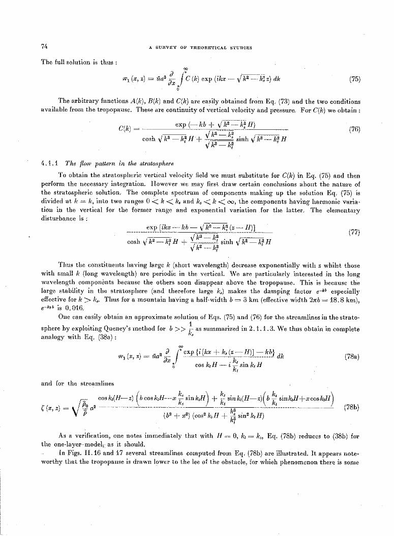
74 A SURVEY OF THEORETICAL STUDIES
The full solution is thus : 00 .
{) " w1 (x, z) = ila2 dx .J C (k) exp (ikr- V k2 - k; z) dk (75)
0
The arbitrary functions A(k), B(k) and C(k) are easily obtained from Eq. (73) and the two conditions available from the tropopause. These are continuity of vertical velocity and pressure. For C(k) we obtain :
C(k) = exp (- kb + ,1 k2- k~H) .jk2-k2 . ,---
cosh · 1 k2 - k2 H · + s smh · 1 k2 - lr2 H V t V k2-k~ V t
(76)
4 .1. 1 The flow pattern in the stratosphere
To obtain the stratospheric vertical velocity field we must substitute for C(k) in Eq. (75) and then perform the necessary integration. However we may first draw certain conclusions about the nature of the stratospheric solution. The complete spectrum of components making up the solution Eq. (75) is divided at k = ks into two ranges 0 < k < k, and ks < k < oo, the components having harmonic variation in the vertical for the former range and exponential variation for the latter. The elementary disturbance is :
exp [ikx -lrb- V k2 - k; (z- H)] ---- vk2-k2 v
cosh · 1 k2 - k2 H + s sinh k2 - k2 H V t V k2- k; t
(77)
Thus the constituents having large k (short wavelength) decrease exponentially with z whilst those with small k (long wavelength) are periodic in the vertical. We are particularly interested in the long wavelength components because the others soon disappear above the tropopause. This is because the large stability in the stratosphere (and therefore large k.) makes the damping factor e-kb especially effective fork> lr8• Thus for a mountain having a half-width b = 3 km (effective width 2nb = 18.8 km), e-ksb is 0.016.
One can easily obtain an approximate solution of Eqs. (75) and (76) for the streamlines in the strato-
sphere by exploiting Queney's method for b > > f as summarized in 2 .1.1. 3. We thus obtain in complete analogy with Eq. (38a) : •
00
w1
(x, z) = ua2 !.__ J~ exp {i [kx + lrs (z- H)]- kb} h k ~
o cos lre H - i __! sin ke H kt
(78a)
and for the streamlines
VjJ coske(H-z) ( bcoskeH-x ~: sinlr1H) + ~ sinkt(H-z)( b ~ sink1H+xcoskeH)
( (x, z) = ! a2 k2 .. (78b) P (b2 + x2
) (cos2 k1H + k; sin2 kef!) t
As a verification, one notes immediately that with H = 0, k1 = k., Eq. (78b) reduces to (38b) for the one-layer--model~ as it should.
In Figs. II.16 and 17 several streamlines computed from Eq. (78b) are illustrated. It appears noteworthy that the tropopause is drawn lower to the lee of the obstacle, for which phenomenon there is some
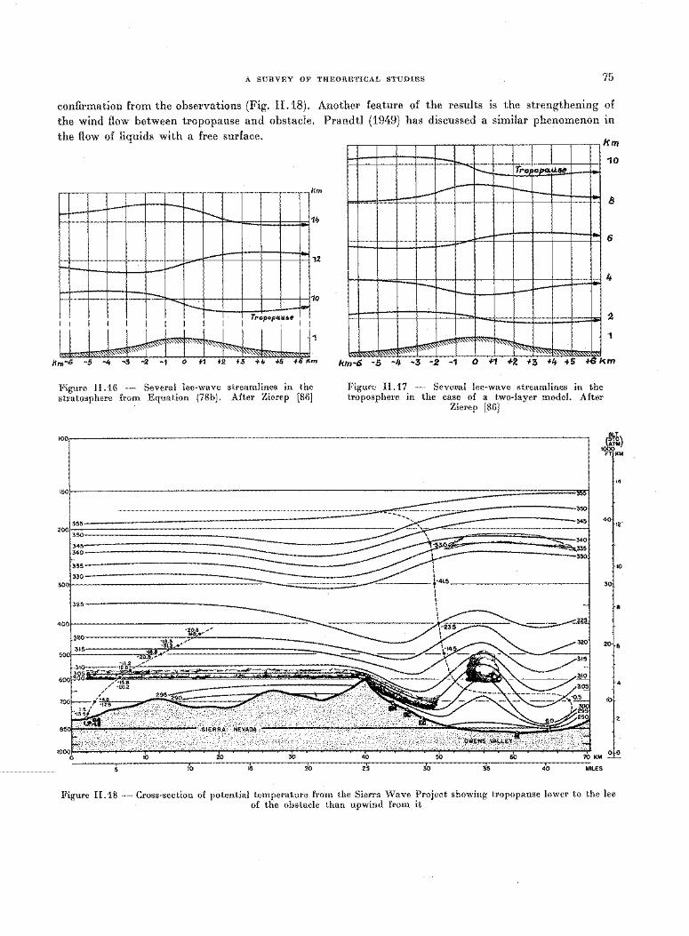
A SURVEY OF THEORETICAL STUDIES 75
confirmation from the observations (Fig. 11.18). Another feature of the results is the strengthening of the wind flow between tropopause and obstacle. Prandtl (1949) has discussed a similar phenomenon in the flow of liquids with a free surface.
Hm - 10 r-- Tro ooor.l.\4.,
km ,...- -t---I-- ,... ll - r-- -... ......__ 1ft
J..--- 6 - 12 1- ...........
4
- -~-- - -t--- -~ 10
UJjJ~~+++4JlJJJ '"~ ~
2
1
Jlm•6 -5 ·4 •3 -'.2 -1 o f1 +2 +3 +4 -1-5 +6 l<m hm-6 -5 -1+ ·3 -2 -1 0 ?1 +2. +3 +4 +5 +Bkm
Figure II .16 - Several lee-wave streamlines in the stratosphere from Equation (78b). After Zierep [86]
Figure II .17 - Sl'veFal lel'-wave streamlines in the troposphere in the case of a two-layer model. After
Zierep [86]
IOOr----------------------------------------------------------------------------------------------------------,
-:~ -345
~~340 ~335 --330 ..
150r-----------------------------------------------------------------------------------~========================
~55 ==================== 200 350 345--------------------------------340----------------------------~=
335= 330--------------------------------
300 -
ALT
~D) TM I
FT! KM
14
1 40H2-
r 30
•
20~6
4
10
- 10 20 30 40 SO 60 70 KM 0-1-0
IU 15 20 2 5 30 35 40 MILES
Figure II .18 - Cross-section of potential temperature from the Sierra Wave Project showing tropopause lower to the lee of the obstacle than upwind from it
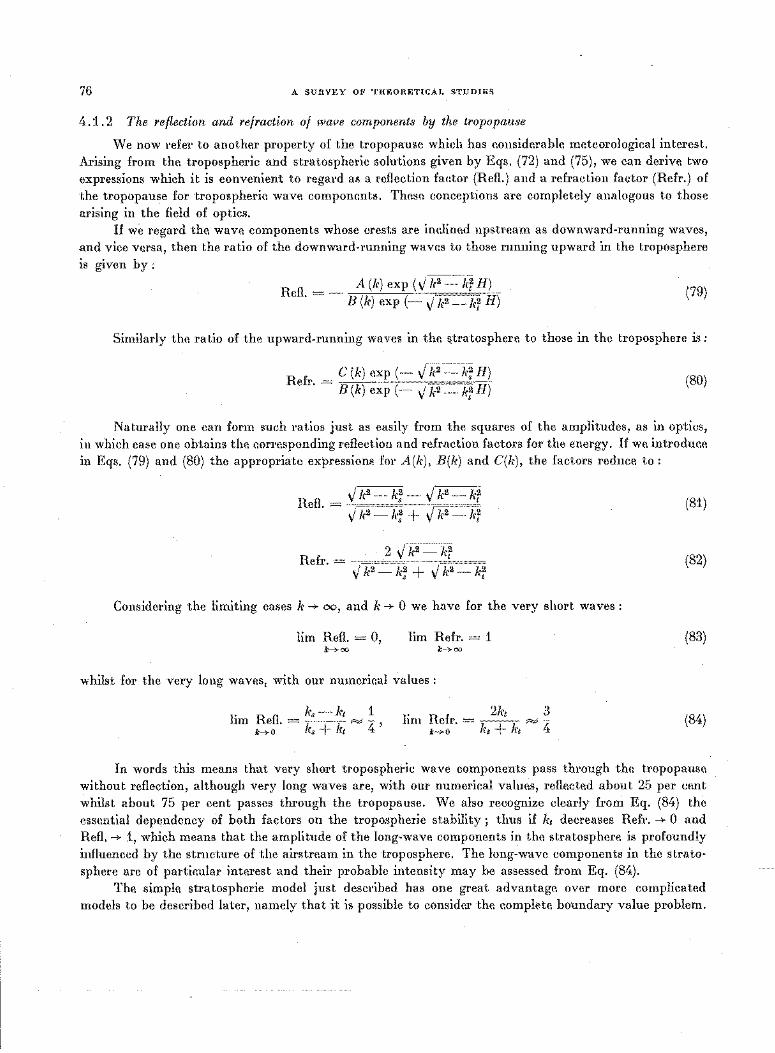
76 A SURVEY OF THEORETICAL STUDIES
4 .1. 2 The reflection and refraction of wave components by the tropopause
We now refer to another property of the tropopause which has considerable meteorological interest.
Arising from the tropospheric and stratospheric solutions given by Eqs. (72) and (75), we can derive two
expressions which it is convenient to regard as a reflection factor (Refl.) and a refraction factor (Refr.) of
the tropopause for tropospheric wave components. These conceptions are completely analogous to those
arising in the field of optics. If we regard the wave components whose crests are inclined upstream as downward-running waves,
and vice versa, then the ratio of the downward-running waves to those running upward in the troposphere
is given by:
Refl. = _ A(k) exp (V k2 -k~H) B (k) exp (-V k2 -k~ H)
(79)
Similarly the ratio of the upward-running waves in the ~tratosphere to those in the troposphere is :
Refr. = C (k) exp (- J k2- k~ H)
B (k) exp (- V k2 _ k~ H) (80)
Naturally one can form such ratios just as easily from the squares of the amplitudes, as in optics,
in which case one obtains the corresponding reflection and refraction factors for the energy. If we introduce
in Eqs. (79) and (80) the appropriate expressions for A(k), B(k) and C(k), the factors reduce to :
.!~-~-,!~-~ Refl. = V I t
.1~-~+J~-~ V I t
(81)
Refr. = 2 J k2- kr v k2
- k~ + v k2 - lrr
(82)
Considering the limiting cases k -+ oo, and k -+ 0 we have for the very short waves :
lim Refl. = 0, lim Refr. = 1 (83) k-+oo k-+oo
whilst for the very long waves, with our numerical values :
lim Refl. = k1 - kt 1 k-+0 kl + kt Pd 4 '
lim Refr. = 2kt 3 k-+0 kl + kt Pd 4 (84)
In words this means that very short tropospheric wave components pass through the tropopause
without reflection, although very long waves are, with our numerical values, reflected about 25 per cent
whilst about 75 per cent passes through the tropopause. We also recognize clearly from Eq. (84) the
essential dependency of both factors on the tropospheric stability ; thus if k1 decreases Refr. -+ 0 and
Refl. -+ 1, which means that the amplitude of the long-wave components in the stratosphere is profoundly
influenced by the structure of the airstream in the troposphere. The long-wave components in the strato
sphere are of particular interest and their probable intensity may be assessed from Eq. (84).
The simple stratospheric model just described has one great advantage over more complicated
models to be described later, namely that it is possible to consider the complete boundary value problem.
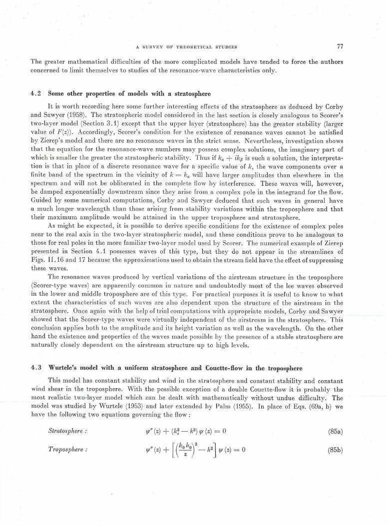
A SURVEY OF THEORETICAL STUDIES 77
The greater mathematical difficulties of the more complicated models have tended to force the authors concerned to limit themselves to studies of the resonance-wave characteristics only.
4 . 2 Some other properties of models with a stratosphere
It is worth recording here some further interesting effects of the stratosphere as deduced by Corby and Sawyer (1958). The stratospheric model considered in the last section is closely analogous to Scorer's two-layer model (Section 3 .1) except that the upper layer (stratosphere) has the greater stability (larger value of F(z )) . Accordingly, Scorer's condition for the existence of resonance waves cannot be satisfied by Zierep's model and there are no resonance waves in the strict sense. Nevertheless, investigation shows that the equation for the resonance-wave numbers may possess complex solutions, the imaginary part of which is smaller the greater the stratospheric stability . Thus if ka + ikp is such a solution, the interpretation is that in place of a discrete resonance wave for a specific value of k, the wave components over a finite band of the spectrum in the vicinity of k = ka will have larger amplitudes than elsewhere in the spectrum and will not be obliterated in the complete flow by interference. These waves will, however, be damped exponentially downstream since they arise from a complex pole in the integrand for the flow. Guided by some numerical computations, Corby and Sawyer deduced that such waves in general have a much longer wavelength than those arising from stability variations within the troposphere and that their maximum amplitude would be attained in the upper troposphere and stratosphere .
As might be expected, it is possible to derive specific conditions for the existence of complex poles near to the real axis in the two-layer stratospheric model, and these conditions prove to be analogous to those for real poles in the more familiar two-layer model used by Scorer. The numerical example of Zierep presented in Section 4.1 possesses waves of this type, but they do not appear in the streamlines of Figs. II .16 and 17 because the approximations used to obtain the stream field have the effect of suppressing these waves .
The resonance waves produced by vertical variations of the airstream structure in the troposphere (Scorer-type waves) are apparently common in nature and undoubtedly most of the lee waves observed in the lower and middle troposphere are of this t ype. For practical purposes it is useful to know to what extent the characteristics of such waves are also dependent upon the structure of the airstream in the stratosphere. Once again with the help of trial computations with appropriate models, Cor by ~nd Sawyer showed that the Scorer-type waves were virtually independent of the airstream in the stratosphere . This conclusion applies both to the amplitude and its height variation as well as the wavelength. On the other hand the existence and properties of the waves made possible by the presence of a stable stratosphere are naturally closely dependent on the airstream structure up to high levels.
4. 3 Wurtele's model with a uniform stratosphere and Couette-flow in the troposphere
This model has constant stability and wind in the stratosphere and constant stability and constant wind shear in the troposphere. vVith the possible exception of a double Couette-flow it is probably the most realistic two-layer model which can be dealt with mathematically without undue difficulty. The model was studied by Wurtele (1953) and later extended by Palm (1955) . In place of Eqs . (69a, b) we have the following two equations governing the flow :
Stratosphere : lj/11 (z) + (k;- k2) ljl (z) = 0 (85a)
Troposphere : '~'" (z) + [ (ko;loy _ kz] '~' (z) = o (85b)
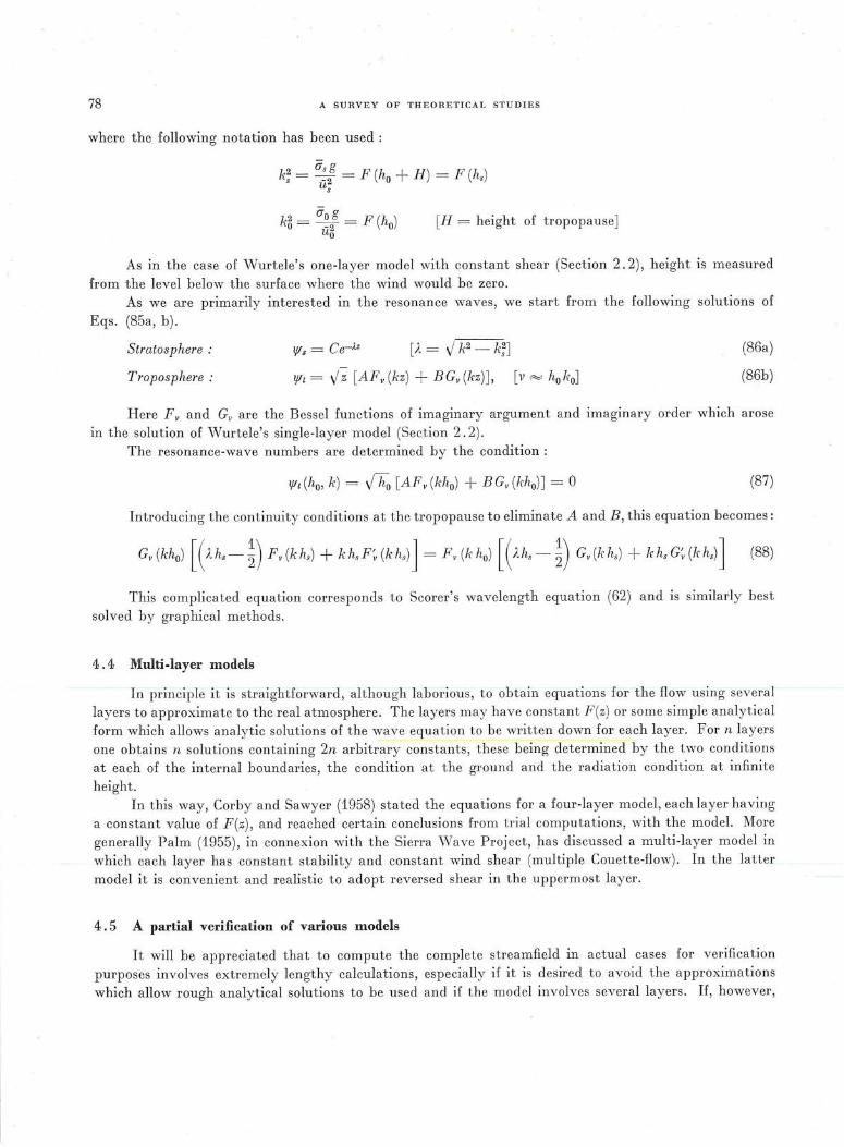
78 A SURVEY OF THEORETICAL STUDIES
where the following notation has been used :
k; =a~!= F(h0 +H) = F(h.) u,
k~ = a~2g = F (h0) uo
[H =height of tropopause]
As in the case of Wurtele's one-layer model with constant shear (Section 2 . 2), height is measured
from the level below the surface where the wind would be zero.
As we are primarily interested in the resonance waves, we start from the following solutions of
Eqs. (85a, b ).
Stratosphere :
Troposphere :
If/ s = C e-A2 [A = y k2 - k;]
lf/t = ,; -; [AFv(kz ) + BGv(kz )], [v ""=" h0 k0]
(86a)
(86b)
Here Fv and Gv are the Bessel functions of imaginary argument and imaginary order which arose
in the solution of Wurtele's single-layer model (Section 2. 2).
The resonance-wave numbers are determined by the condition :
lf!t(ho, k) = /-ho [AFv (kh0) + BGv (kh0) ] = 0 (87)
Introducing the continuity conditions at the tropopause to eliminate A and B, this equation becomes:
Gv (kho) [(A.h.-~) Fv (kh,,) + khs F~(khs) J = Fv (kh0) [(u. -~) Gv (khs) + khs G~ (khs) ] (88)
This complicated equation corresponds to Scorer's wavelength equation (62) and is similarly best
solved by graphical methods.
4. 4 Multi-layer models
In principle it is straightforward , although laborious, to obtain equations for the flow using several
layers to approximate to the real atmosphere. The layers may have constant F (z) or some simple analytica l
form which allows analytic solutions of the wave equation to be written down for each layer. For n layers
one obtains n solutions containing 2n arbitrary constants, these being determined by the tvvo conditions
at each of the internal boundaries, the condition at the ground and the radiation condition at infinite
height. In this way, Corby and Sawyer (1958) stated the equations for a four-layer model, each layer having
a constant value of F (z), and reached certain conclusions from trial computations, with the model. More
generally Palm (1955), in connexion with the Sierra \Vave Project, has discussed a multi-layer model in
which each layer has constant stability and constant wind shear (multiple Couette-flow). In the latter
model it is convenient and realistic to adopt reversed shear in the uppermost layer.
4. 5 A partial verification of various models
It will be appreciated that to compute the complete streamfield in actual cases for verification
purposes involves extremely lengthy calculations, especially if it is desired to avoid the approximations
which allow rough analytical solutions to be used and if the model involves several layers. If, however,
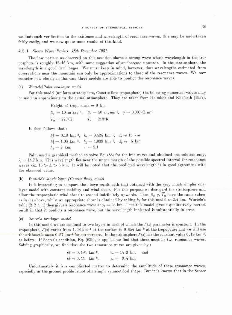
A SURVEY OF THEORETICAL STUDIES 79
we limit such verification to the existence and wavelength of resonance waves , this may be undertaken
fairly easily, and we now quote some results of this kind.
4. 5 . 1 Sierra Wave Project, 18th December 1951
The flow pattern as observed on this occasion shows a strong wave whose wavelength in the tro
posphere is roughly 15-16 km, with some suggestion of an increase upwards. In the stratosphere, the
wavelength is a good deal longer. \Ve must keep in mind, however, that wavelengths estimated from
observations near the mountain can only be approximations to those of the resonance waves. We now
consider how closely in this case three models are able to predict the resonance waves .
(a) WurtelefPalm two-layer model
For this model (uniform stratosphere, Couette-flow troposphere) the following numerical values may
be used to approximate to the actual atmosphere. They are taken from Holmboe and Klieforth (1957).
Height of tropopause = 8 km
u0 = 10 m. sec-1 , Us = 50 m. sec-1, y = 0.007°C. m-1
T0 = 273oK, Ts = 218oK
It then follows that :
k; = 0.18 km- 2, ks = 0.424 km-1, As R::> 15 km
k~ = 1.08 km- 2, k0 = 1.039 km- 1, A.0 R::> 6 km
h0 = 2 km, V = 2.1
Palm used a graphical method to solve Eq. (88) for the free waves and obtained one solution only,
A,.= 14.7 km. This wavelength lies near the upper margin of the possible spectral interval for resonance
waves viz. 15 > },, > 6 km. It will be noted that the predicted wavelength is in good agreement with
the observed value.
(b) Wurtele's single-layer ( Couette- flow) model
It is interesting to compare the above result with that obtained with the very much simpler one
layer model with constant stability and wind shear. For this purpose we disregard the stratospher e and
allow the tropospheric wind shear to extend indefinitely upwards. Thus u0 , y, T0 have the same values
as in (a) above, whilst an appropriate shear is obtained by taking h0 for this model as 2.4 km. Wurtele's
table (2 . 2 .1 .1) then gives a resonance wave at y, = 23 km. Thus this model gives a qualitatively correct
result in that it predicts a r esonance wave, but the wavelength indicated is substantially in error.
(c) Scorer' s two-layer model
In this model we are confined to two layers in each of which the F (z) parameter is constant. In the
troposphere, F (z) varies from 1. 08 km-2 at the surface to 0 . 054 km- 2 at the tropopause and we will use
the arithmetic mean 0. 57 km- 2 for our purpos-e-:- h r thestratosphere F(z) has the constant value 0.18 km- 2,
as before. If Scorer's condition, Eq. (63b), is applied we find that there must be two resonance waves.
Solving graphically, we find that the two resonance waves are given by :
k~ = 0.194 km-2,
k~ = 0 . 44 km- 2,
Ar = 14.3 km
}" = 9.4 km
and
Unfortunately it is a complicated matter to determine the amplitude of these resonance waves,
especially as the ground profile is not of a simple symmetrical shape. But it is known that in the Scorer
80 A SURVEY OF THEORETICAL STUDIES
model when more than one resonance wave occurs, the one having the longest wavelength generally has
by far the greatest amplitude. However, whether this is so in a particular case depends also on the
dominant ·wavelength components in the ground profile. Vve cannot therefore claim, without further
calculation, that the predicted resonance vvave at 14.3 km in the model would necessarily dominate the
one at 9 . 4 km, although this is very likely .
In these tests of three models, (a) and (c) appear satisfactory and we note that both these models
include the stratosphere . Test (b) of the single-layer Couette-flow model was however unsuccessful in
this case, although as in (a) the tropospheric variation of F(z) due to wind shear was included. It would
seem, therefore, that in this case the change in F(z ) across the tropopause was the essential feature.
4.5.2 Sierra Wa(Je Project, 16th February 1952
On this occasion a powerful wave occurred and was investigated during the Sierra 'Nave Project. The
case was discussed in Part I, 2. 5 . 5 and is illustrated in Figs. I. 33 and 34. The lee wave, which had a
large amplitude through a considerable depth of the troposphere, had a wavelength of about 20 km. \Ve
now test two models on this case.
(a) WurtelefPalm tHJo-layer model
We use the following numerical values from Holmboe and Klieforth (1957) :
Height of tropopause = 9 km
ti0 = 7. 7 m. sec-1, Lis = 67 m. sec-1, y = 0.0073°C. m-1
T0 = 283.7oK, 7'. = 218oK
These values lead to
k~ = 0.10 km-2, ks = 0.315 km-1, A ~ 20 km
kg= 1.56 km-2, k0 = 1.25 km-1, Ao ~ 5 km
h0 = 1.17 km, V ~ lf0 h0 = 1.46
As before, Palm used a graphical method to examine Eq. (88) and, surprisingly, found that
no free-wave solutions were indicated. _Thus in spite of the powerful wave observed, this particular
model fails to predict any resonance waves in this case. Palm expresses the opinion that the observed
wave might be the resultant of a continuous spectral band of supercritical wave components with
A> As, which is equivalent to suggesting that Eq. (88) might have a complex root near the real k
axis (see 4. 2). The suggestion is highly plausible and shows up the limitations of this kind of rough
verification.
(b) Scorer's two-layer model
We use the mean value 0.794 km-2 for F (z) in the troposphere and the value 0.10 km-2 in the
stratosphere, as before. The graphical solution for the resonance-wave numbers leads to the following
values: k~ = 0. 700 km-2,
k; = 0.425 km-2,
A,.= 7.51 km
}.,. = 9.65 km
Neither of these values accords with the observed wavelength of 20 km. However, the wave
length equation is quite sensitive to small changes in the airstream and one can deduce that a small
change in ki (the tropospheric value of F(z)) could result in an additional solution near k2 = 0.1.
This would lead to a free wave of length A,. ~ 20 km.
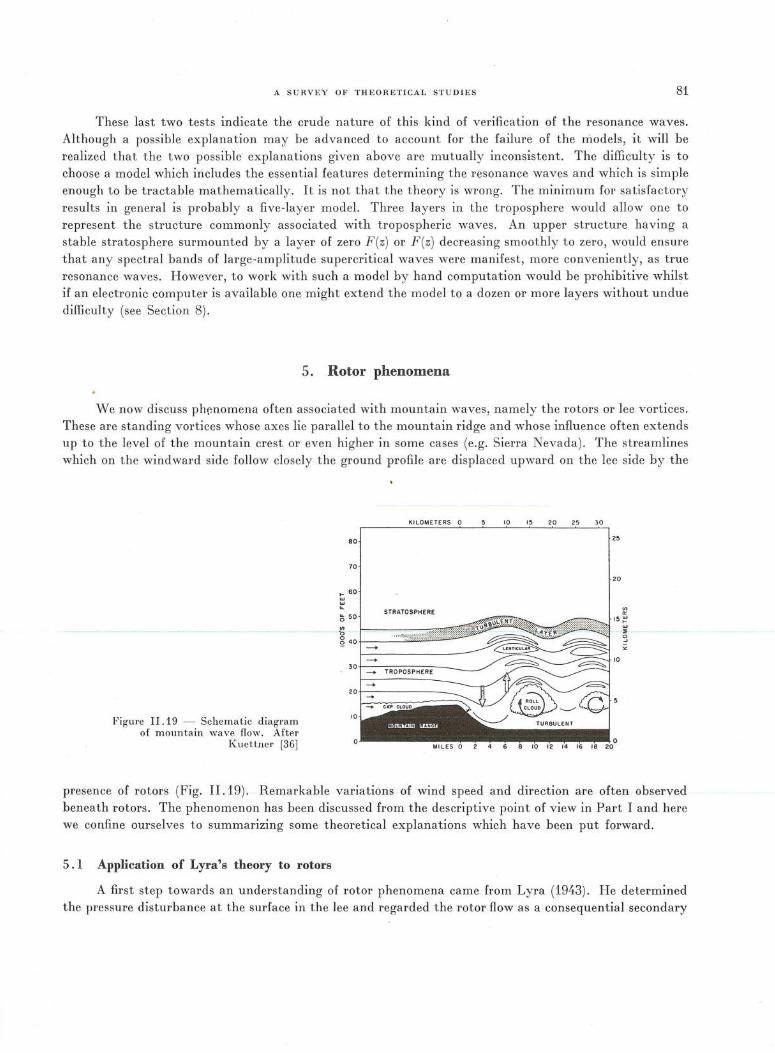
A SURVEY OF THEORETICAL STUDIES 81
These last two tests indicate the crude nature of this kind of verification of the resonance waves. Although a possible explanation may be advanced to account for the failure of the models, it will be realized that the two possible explanations given above are mutually inconsistent. The difficulty is to choose a model which includes the essential features determining the resonance waves and which is simple enough to be tractable mathematically. It is not that the theory is wrong. The minimum for satisfactory results in general is probably a five-layer model. Three layers in the troposphere would allow one to represent the structure commonly associated with tropospheric waves. An upper structure having a stable stratosphere surmounted by a layer of zero F (z) or F (z) decreasing smoothly to zero, would ensure that any spectral bands of large-amplitude supercritical waves were manifest, more conveniently, as true resonance waves. However, to work with such a model by hand computation would be prohibitive whilst if an electronic computer is available one might extend the model to a dozen or more layers without undue difficulty (see Section 8).
5. Rotor phenomena
'Ne now discuss ph~nomena often associated with mountain waves, namely the rotors or lee vortices. These are standing vortices whose axes lie parallel to the mountain ridge and whose influence often extends up to the level of the mountain crest or even higher in some cases (e.g. Sierra Nevada ). The streamlines which on the windward side follow closely the ground profile are displaced upward on the lee side by the
Figure I I . 19 - Schema tic diagram of mountain wave flow. After
Kuettner [36]
70
~ 60
00
"'
KILOMETERS
STRATOSPHERE
"§ 4 0 . ....... ~::~::
10 15 20 25 30
25
20
w ,._ '3 "
presence of rotors (Fig. II .19). Remarkable variations of wind speed and direction are often observed beneath rotors. The phenomenon has been discussed from the descriptive point of view in Part I and here we confine ourselves to summarizing some theoretical explanations which have been put forward.
5. 1 Application of Lyra's theory to rotors
A first step towards an understanding of rotor phenomena came from Lyra (1943). He determined the pressure disturbance at the surface in the lee and regarded the rotor flow as a consequential secondary
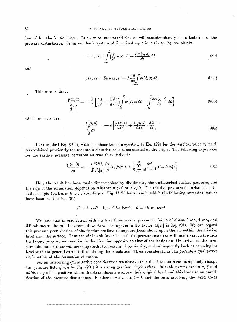
82 A SURVEY OF THEORETICAL STUDIES
flow within the friction layer. In order to understand this we will consider shortly the calculation of the
pressure disturbance. From our basic system of linearized equations (2) to (6), we obtain :
X
u (x, z) = J (~ w ( ~, z) _ dw ~~, z) d~ (89)
-00
and X
p(x, z) = puu(x, z)- p ~l~f w(~, z) d~ (90a)
-00
This means that : X X
p ~x, z) = _ ~ [(! + ~ du)Jw (~, z) d~ -j'Jw (~, z) d~J p _
2 u c2 u dz {)z
2u -oo -oo
(90b)
which reduces to : p (x, z) = _ 2 [u (x, z) + ( (x, z) . du] p -2 u(z) u(z) dz 2u
(90c)
_ .. _ ~Yl'[l f\ppli~d "E;g. (90b), with the shear terms neglected, to Eq. (29) for the vertical velocity field.
As explained previously the mountain disturbance is concentrated at the origin. The following expression
for the surface pressure perturbation was thus derived :
p (:> 0) =- u2'!!k• [~ Nl(k.!xl) + ~ ~ 4v;v2 1 F2v(k.lxl)] Po RT0 lxl v=l
(91)
Here the result has been made dimensionless by dividing hy the undisturbed surface pressure, and
the sign of the summation depends on whether x > 0 or x < 0. The relative pressure disturbance at the
surface is plotted beneath the streamlines in Fig. 11. 20 for a case in which the following numerical values
have been used in Eq. (91) :
F = 3 km2, ks = 0.82 km-1, u = 15 m. sec-1
We note that in association with the first three waves, pressure minima of about 5 mb, 1 mb, and
0.6 mb occur, the rapid decrease downstream being due to the factor 1/l xI in Eq. (91). We can regard
this pressure perturbation of the frictionless flow as imposed .from above upon the air within the friction
layer near the surface. Thus the air in this layer beneath the pressure maxima will tend to move towards
the lowest pressure minima, i.e. in the direction opposite to that of the basic flow. On arrival at the pres
sure minimum the air will move upwards, for reasons of continuity, and subsequently back at some higher
level with the general current, thus closing the circulation. These considerations can provide a qualitative
explanation of the formation of rotors. For an interesting quantitative consideration we observe that the shear term can completely change
the pressure field given by Eq. (90c) if a strong gradient dujdz exists. In such circumstances u, ( and
dujdz may all be positive where the__g.:tr_e_amlines are above their original level and this leads to an ampli
fication of the pressure disturbance. Further downstream ( -+ 0 and the term involving the wind shear
A SURVEY OF THEORETICAL STUDIES 83
vanishes but at least the first pressure minimum should be stronger than indicated by Lyra. A simple numerical example serves to indicate the influence of the shear term. Thus if :
(= 1 km dil dz = 5 m.sec-1 . km-1, and u = 5 m.sec-1
then we see that the shear term ( ~~ = 5 n. ~flc-1 has the same value as the u-term in Eq. (90c). Thus
here it would double the effect. Particularly useful in this connexion is an alternative form of the pressure formula Eq. (90). Thus if Eq. (89) is used together with the streamline equation,
"' il (z) ( (x, z) = J w (~, z) d~
-00
then it follows (see also Zierep, 1952) that :
,)!__ = 2 ({)'- g l) f!_ u2 {)z (i2
2
(92)
In this equation the pressure disturbance is linked with the vertical rate of change of streamline displacement {}(j{}z, which one can recognize intuitively as a highly relevant quantity in the formation of rotors. We realize immediately from Eq. (92) that the larger {}(j{)z is, the larger will be the pressure
Figure II. 20 - Distribution of relative pressure disturbances on the ground in the case of a small obstacle. After
Lyra [45]
·~----------------------
¥------v
f-------
0 W'$#$$)i$$$'N#$$!R$M$B'h!Y#~$M#$Mf$#$,@, I
_./!_
r ~· '
<.11 _.-/, r " '(' •(' '"x •. ,.~ _, I t '\ _r---.._._ _-- • -x;
-1-XJ
-J·to-J
-5·1Q·J'
disturbance, p, and accordingly the greater will be the likelihood of reversed flow near the surface and the formation of rotors. In nature the pressure disturbance may be further augmented in several ways ; for example in the Sierra Nevada strong heating over the lee ground is probably relevant and this will be referred to in 5. 3, concerned with Kuettner's theory.
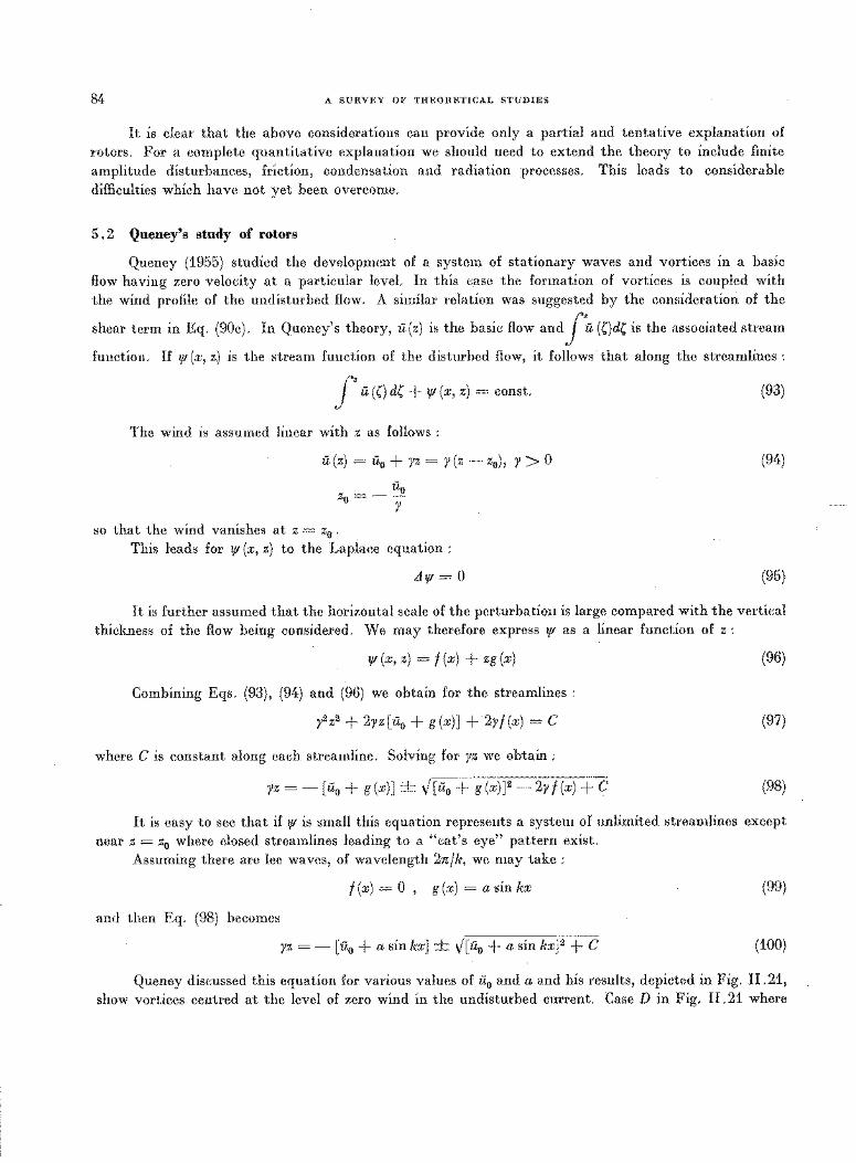
84 A SURVEY OF THEORETICAL STUDIES
It is clear that the above considerations can provide only a partial and tentative explanation of
rotors. For a complete quantitative explanation we should need to extend the theory to include finite
amplitude disturbances, friction, condensation and radiation processes. This leads to considerable
difficulties which have not yet been overcome.
5. 2 Queney's study of rotors
Queney (1955) studied the development of a system of stationary waves and vortices in a basic
flow having zero velocity at a particular level. In this case the formation of vortices is coupled with
the wind profile of the undisturbed flow. A similar relation was suggested by the consideration of the
shear term in Eq. (90c). In Queney's theory, u (z) is the basic flow and J~ (()d( is the associated stream
function. If 1f1 (x, z) is the stream function of the disturbed flow, it follows that along the streamlines :
j' u(()d( + lfl(x, z) = const.
The wind is assumed linear with z as follows :
u(z)=u0 +yz=y(z-z0 ), y>O
iio Zo=--y
so that the wind vanishes at z = z0 •
This leads for 1f1 (x, z) to the La place equation :
Lll{l = 0
(93)
(94)
(95}
It is further assumed that the horizontal scale of the perturbation is large compared with the vertical
thickness of the flow being considered. We may therefore express 1f1 as a linear function of z:
If/ (x, z) = f (x) + zg (x)
Combining Eqs. (93), (94) and (96) we obtain for the streamlines:
y2z2 + 2yz[u0 + g(x)] + 2yf(x) = C
where C is constant along each streamline. Solving for yz we obtain :
(96)
(97)
yz =- [u0 + g(x)] + \f'[u0 + g(x)] 2 -2yf(x) + C (98)
It is easy to see that if 1f1 is small this equation represents a system of unlimited streamlines except
near z = z0 where closed streamlines leading to a "eat's eye" pattern exist. Assuming there are lee waves, of wavelength 2njk, we may take:
f (x) = 0 , g (x) = a sin kx (99)
and then Eq. (98) becomes
yz = - [ u0 + a sin kx] + V[ u0 + a sin kx ]2 + C (100)
Queney discussed this equation for various values of u0 and a and his results, depicted in Fig. 11. 21,
show vortices centred at the level of zero wind in the undisturbed current. Case D in Fig. 11.21 where
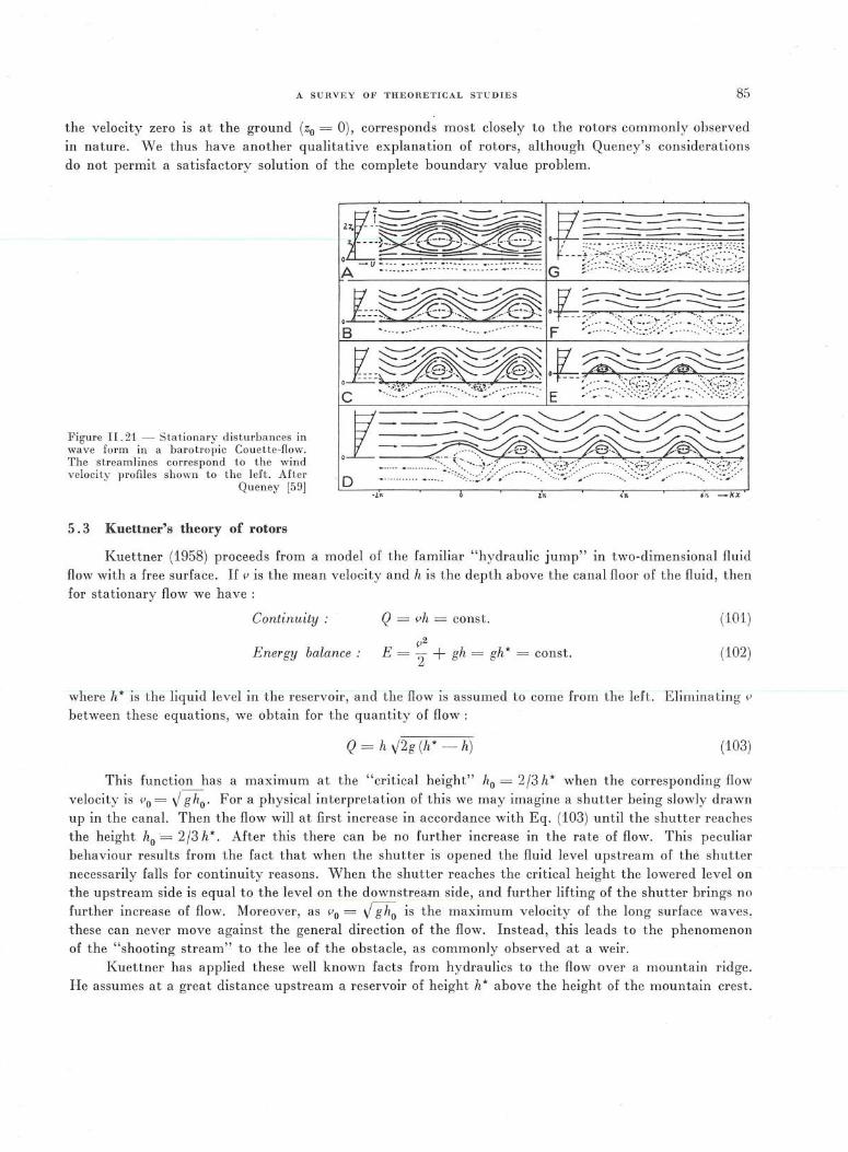
A SURVEY OF TH E OR ETICAL STV DI ES 85
the velocity zero is at the ground (z0 = 0), corresponds most closely to the rotors commonly observed in nature. We thus have another qualitative explanation of rotors, althou gh Queney's considerations do not permit a satisfactory solution of the complete boundary value problem.
Fi gure Il. 21 - Stationa ry disturba nces in wave form in a barotropic Couette-flow. The streamlines correspond to the wind velocity profil es shown to the left. After
Queney [59)
5 . 3 Kuettner's theory of rotors
f z - -- - ---- ,;- -2~~~,,~~ A - u ~-~-~-~-~ G:-- -f/><i::~\~L~~-;~~:f;~~~:~~E:;:;
0 [::~~~:i@? '~~~--=~ B ·------------- -----. ___ --------- ·---- F . - :-- -- <<:-: :: .~-.-::-..-:.-- -. ::·-::::-.-.::-:-;:
~ ~~~~ ti.......-::-:--.'---....---......----,L=~~~~ ,~~G~;:;~~~ C --:.-~~•!:·.-· ;:::-.. ~:::· .. ::~-i:·~.--;::: -~ _-_- :· E ::-:-·:.:_-:::-':::~~:~:-.;:)·:-- -_-_. ::-_:::_::~~~::>;
21---~ ~ ~ ~
.L==-~~~~ D :: _-_-_ ~- ::: --~--·:::::-.-,::;_:~:::}./·· .. ~~-~:-_· --~~:'~<-~~?:-_··. ·_. ~.: :::_:::_:j~~-:/::: -_·_·_ ~- ~---. -~·~:'~{':
-l• '" 4R , -r-. -kx
Kuettner (1958) proceeds from a model of the familiar " hy draulic jump" in two-dimensional fluid flow with a free surface. If v is the mean velocity and his the depth above the canal floor of the fluid , then for stationary flow we have :
Continuity : Q = vh = const. (101)
Energy balance : v2
E = 2 + gh = gh * = const. (102)
where h* is the liquid level in the reservoir, and the flow is assumed to come from the left. Eliminating v
between these equations, we obtain for the quantity of flow :
Q=h v2g(h* - h) (103)
This function ha s a maximum at the "critical height" h0 = 2f3 h* when the corresponding flow velocity is v0 = ,1 g h0 • For a physical in terpretation of this we may imagine a shutter being slowly drawn up in the canal. Then the flow will at fir st increase in accordance with Eq. (103) until the shutter r eaches the height h0 ·_ 2/3 h*. After this there can be no further increase in the rate of flow. This peculiar behaviour results from the fact that when the shutter is opened the fluid level upstream of the shutter necessarily falls for continuity reasons. When the shutter reaches the critical height the lowered level on the upstream side is equal to the level on the downstream side, and further lifting of the shutter brings no further increase of flow. Moreover , as v0 = ,1 gh0 is the maximum velocity of the long surface waves , these can never move against the general direction of the flow. Instead, this leads to the phenomenon of the "shooting stream" to the lee of the obstacle, as commonly observed at a weir.
Kuettner has applied these well known facts from hy draulics to the flow over a mountain ridge. He assumes at a great distance upstream a reservoir of height h * above the height of the mountain crest.
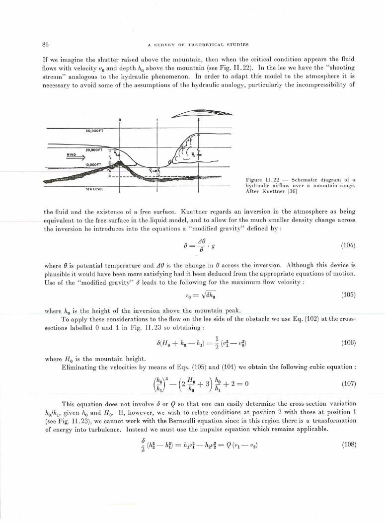
86 A SURVEY OF THEORETICAL STUDIES
If we imagine the shutter raised above the mountain, then when the critical condition appears the fluid
flows with velocity v0 and depth h0 above the mountain (see Fig. 11 . 22). In the lee we have the "shooting
stream" analogous to the hydraulic phenomenon. In order to adapt this model to the atmosphere it is
necessary to avoid some of the assumptions of the hydraulic analogy, particularly the incompressibility of
0
30.000Ft
SEA LEVEL
~~* .... 2
Figure IJ. 22 - Schematic diagram of a hydraulic a irflow over a mountain range. After Kuettner [36)
the fluid and the existence of a free surface. Kuettner regards an inversion in the atmosphere as being
equivalent to the free surface in the liquid model, and to allow for_ the much smaller density change across
the inversion he introduces into the equations a "modified gravity" defined by:
r5 = L18 e·g (104)
where e is potential temperature and L18 is the change in e across the inversion. Although this device is
plausible it would have been more satisfying had it been deduced from the appropriate equations of motion.
Use of the "modified gravity" r5 leads to the followin g for the maximum flow velocity :
~'o = y r5ho (105)
where h0 is the height of the inversion above the mountain peak.
To apply these considerations to the flow on the lee side of the obstacle we use Eq. (102) at the cross
sections labelled 0 and 1 in Fig. 11. 23 so obtaining :
r5(H 0 + h0 - h1) = ~ (v~ - v~) (106)
where H0 is the mountain height.
Eliminating the velocities by means of Eqs. (105) and (101) we obtain the following cubic equation :
(~)3
- ('2 Ho + 3) ~ + 2 = 0 hi ho hl
(107)
This equation does not involve r5 or Q so that one can easily determine the cross -section variation
h0 /h11 given h0 and H 0 • If, however, we wish to relate conditions at position 2 with those at position 1
(see Fig. 11. 23), we cannot work with the Bernoulli equation since in this region there is a transformation
of energy into turbulence. Instead we must use the impulse equation which remains applicable.
r5 2 (h~- h~) = h1vi- h2v~ = Q (v1 - v2) (108)
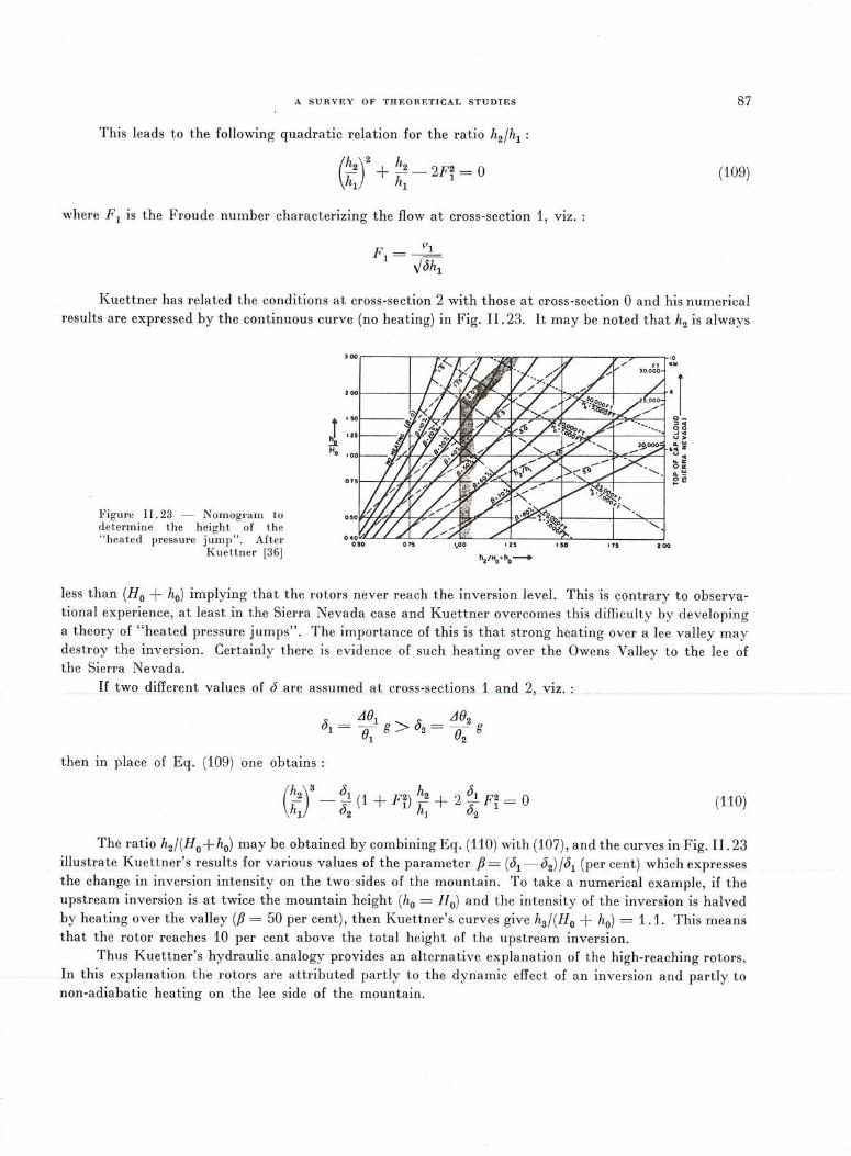
A SURVEY OF THEORETICAL STUDIES
This leads to the following quadratic relation for the ratio h2 /h1 :
(h2)2 + h2 - 2Fi = 0 hi hi
where F1 is the Froude number characterizing the flow at cross-section 1, VIZ . :
~-'I
FI = yJhi
87
(109)
Kuettner has related the conditions at cross-section 2 with those at cross-section 0 and his numerical results are expressed by the continuous curve (no heating) in Fig. 11. 23. It may be noted that h2 is always
Figure II.23 - Nomogram to de termine the height of the " heated pressure jump" . After
Kuettner (36]
J :.;g, Ho
r--------r---;~-.r--n--~~r-~------r-----~--?-----~~~
.... y , I -. ~ /I I / t-· r ;;J, , r .:C"_>: ,
c=>4 OD -'4 V> .....
14 z --~b/ I:,L ;: '('t}' ~ r(--..,,.- I ~ =
h2JH0
• h0
____,.
oa: o.!o! ~!!!
less than (H0 + h0 ) implying that the rotors never reach the inversion level. This is contrary to observational experience, at least in the Sierra Nevada case and Kuettner overcomes this difficulty by developing a theory of "heated pressure jumps". The importance of this is that strong heating over a lee valley may destroy the inversion. Certainly there is evidence of such heating over the Owens Valley to the lee of the Sierra Nevada.
If two different values of J are assumed at cross-section_Li .Jind 2, _viz. : _
LJ(}I LJ(}2 Jl = - g > J2 = - g
(}I (}2
then in place of Eq. (109) one obtains:
(~)3
- ~ (1 + F~) ~ + 2 J1 Fi = 0 hi J2 hl J2
(110)
The ratio h2 f (H 0 +h0 ) may be obtained by combining Eq. (110) with (107), and the curves in Fig. 11.23 illustrate Kuettner's results for various values of the parameter fJ = (J1 - J2) fJI (per cent) which expresses the change in inversion intensity on the two sides of the mountain. To take a numerical example, if the upstream inversion is at twice the mountain height (h0 = H 0 ) and the intensity of the inversion is halved by heating over the valley (fJ = 50 per cent), then Kuettner's curves give h3 f (H 0 + h0 ) = 1.1. This means that the rotor reaches 10 per cent above the total height of the upstream inversion.
Thus Kuettner' s hydraulic analogy provides an alternative explanation of the high-reaching rot ors. In this explanation the rotors are attributed partly to the dynamic effect of an inversion and partly to non-adiabatic heating on the lee side of the mountain .
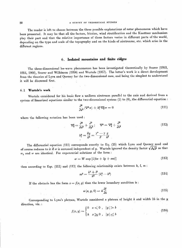
88 A SURVEY OF THEORETICAL STUDIES
The reader is left to choose between the three possible explanations of rotor phenomena which have
been presented. It may be that all the factors, friction, wind stratification and the Kuettner mechanism
play their part and that the relative importance of these factors varies in different parts of the world,
depending on the type and scale of the topography and on the kinds of airstreams, etc. which arise in the
different regions.
6. Isolated mountains and :finite ridges
The three-dimensional lee-wave phenomenon has been investigated theoretically by Scorer (1953,
1954, 1956), Scorer and Wilkinson (1956) and Wurtele (1957). The latter's work is a direct development
from the theories of Lyra and Queney for the two-dimensional case, and being the simplest to understand
it will be discussed first.
6 .1 Wurtele's work
Wurtele considered for his basic flow a uniform airstream parallel to the axis and derived from a
system of linearized equations similar to the two-dimensional system (2) to (6),. the differential equation:
()2 - ('iJ2 w) +. k2 'V 2 w = 0 ()x2 s 2
where the following notation has been used :
()2 {)2
'V~ = ()x2 + {)y2 '
()2 v2 = 'V~ + ()z2
k2 = erg = y* - Y JL • u,2 F u2
(111)
(112)
The differential equation (111) corresponds exactly to Eq. (25) which Lyra and Queney used and
of course reduces to it if w is assumed independent of y. Wurtele ignored the density factor .J p0fp so that
w1 and w are identical. For exponential solutions of the form :
w = W exp [i(kx + ly + mz)]
then according to Eqs. (111) and (112) the following relationship exists between k, l, m:
2 = k2 + l2 (k2 - l 2) m k2 s r
If the obstacle has the form z = f(x, y) then the lower boundary condition is :
- Jf 1v(x, y, 0) = u {)x
(113)
(114)
(115)
Corresponding to Lyra's plateau, Wurtele considered a plateau of height h and width 2b in the y
direction, viz. :
10 x<.O, JyJ>b
f(x, y) = h x::::,;.o, jyjLb
(116)
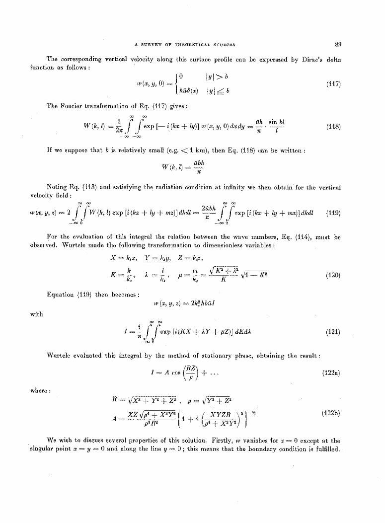
A SURVEY OF THEORETICAL STUDIES 89
The corresponding vertical velocity along this surface profile can be expressed by Dirac's delta function as follows :
w(x, y, O) ~ ~ :M(x)
The Fourier transformation of Eq. (117) gives :
00 00
JyJ> b
JyJLb
1 r J . uh sin bl W(k, l) = '2n. exp [- ~(k.'lJ + ly)] w(x, y, O)dxdy = n · -l--oo -oo
If we suppose that b is relatively small (e.g.< 1 km), then Eq. (118) can be written:
w (k, l) = ubh n
(117)
(118)
Noting Eq. (113) and satisfying the radiation condition at infinity we then obtain for the vertical velocity field :
00 00 00 00
w (x, y, z) = 2 .f.(w (k, l) exp [i (kx + ly + mz)] dkdl = 2~bh J.{exp [i (ltx + ly + mz)] dkdl (119)
-00 0 -00 0
For the evaluation of this integral the relation between the wave numbers, Eq. (114), must be observed. Wurtele made the following transformation to dimensionless variables :
with
X = k,x, Y_ lf_._y_, Z = k,z,
k K= ks'
Equation (119) then becomes :
A. = __::_ _ m .j K2 + ..1,2 . k, ' ll - k, ~ K .j. ---
w (x, y, z) = 2k;hbill
00 00
I=~ J j'exp [i(KX + A.Y + pZ)] dKdA. -00 0
Wurtele evaluated this integral by the method of stationary phase, obtaining the result:
I = A cos ( R:) + ...
where:
R = ..;x2 + p + z2 , P = .j¥2 + z2
_ XZ ..}p4 + X 2 Y2 { ( XYZR ) 2 (-¥2
A- 3R2 1 + 4 4 + X2¥2 f p - p
(120)
(121)
(122a)
(122b)
We wish to discuss several properties of this solution. Firstly, w vanishes for z = 0 except at the . singular point x = y = 0 and along the line y = 0 ; this means that the boundary condition is fulfilled. ·
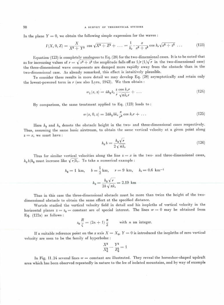
90 A SURVEY OF THEORETICAL STUDIES
In the plane Y = 0, we obtain the following simple expression for the waves :
I (X, 0, Z ) = V9. .::- V9. cos vX2 + Z2 + 0 0 0 = ~ 0
_ 9. ~ _9. cos k, vx2 + z2 (123)
Equation (123) is completely analogous to Eq. (28) for the two-dimensional cases. It is to be noted that
as for increasing values of r = V x2 + z2 the amplitude falls off as 1 Jr (1/ V-;. in the two-dimensional case)
the three-dimensional wave components are damped more rapidly away from the obstacle than in the
two-dimensional case. As already remarked, this effect is intuitively plausible.
To consider these results in more detail we may develop Eq. (28) asymptotically and retain only
the lowest-powered term in r (see also Lyra , 1943). We then obtain:
_ z cos k, r w 1 (x,z) = uh2 k, -~ +
r ,lnk,r
By comparison, the same treatment applied to Eq. (123) leads to:
X w (x, 0, z) = 2uh3 bk, 2 cos k, r + ...
r
(124)
(1.25)
Here h2 and h~ denote the obstacle height in the two- and three-dimensional cases respectively.
Thus, assuming the same basic airstream, to obtain the same vertical velocity at a given point along
z = x, we must have : h .r
h3
b = 2_vr 2 ,i-;J; s
(126)
Thus for similar vertical velocities along the line z = x in the two- and three-dimensional cases,
h3 bjh2 must increase like v r fk, . To take a numerical example:
h2 = 1 km, 1
b = 2 km, r = 9 km,
h2 V r = 2.19 km h3 = 2b V nk,
k, = 0.6 km-1
Thus in this case the three-dimensional obstacle must be more than twice the height of the two
dimensional obstacle to obtain the same effect at the specified distance.
Wurtele studied the vertical velocity field in detail and his isopleths of vertical velocity in the
horizontal planes z = z0 = constant are of special interest. The lines w = 0 may be obtained from
Eq. (122a) as follows : n
!!_ = (2n + 1) 2 zo ( with n an integer.
If a suitable reference point on the x axis X= X 0, Y = 0 is introduced the isopleths of zero vertical
velocity are seen to be the family of hyperbolae :
X2 Y2 X2- Z2 = 1
0 0
In Fig. 11.24 several lines w = constant are illustrated. They reveal the horseshoe-shaped updraft
area which has been observed repeatedly in nature to the lee of isolated mountains, and by way of example
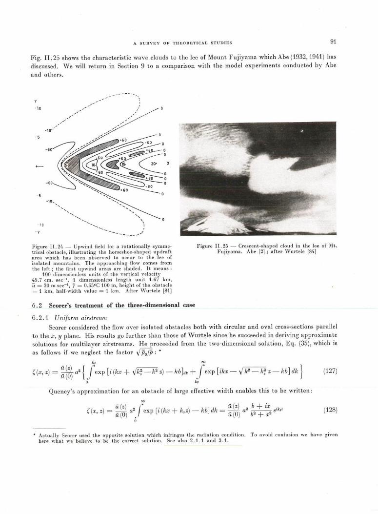
A SURVEY OF THEORETICAL STUDIES 91
Fig. 11.25 shows the characteristic wave clouds to the lee of Mount Fujiyama which Abe (1932, 1941) has
discussed. We will return in Section 9 to a comparison with the model experiments conducted by Abe
and others.
y
. 10
. 5
+-
· s
. 10
-y
·10-'
-6C
-60
-10,
,. ..... "' ..
', ',,
~
~
.... , ', ',
,-
.......................
...................... ,
.... __ ---
', ' ' ' \
1
' /
0
0
Figure II. 24 - Upwind fie ld for a rotation ally symmetrical obstacle, illustrating the horseshoe-shaped updraft area which has been observed to occur to the lee of isolated mountains. The approaching flow comes from the left; the first upwind areas are shaded. It m eans :
Figure II. 25 - Crescent-shaped cloud in the lee of :\It.
100 dimension less units of the vertical velocity 45.7 cm. sec-1, 1 dimensionless length unit 1.67 km, u = 20 m sec-1, Y = 0.65°C 100 m, height of the obstacle = 1 km , half-width value = 1 km. After Wurtele [81]
6. 2 Scorer's treatment of the three-dimensional case
6. 2. 1 Uniform airstream
Fujiyama. Abe [2] ; after Wurtele [84]
Scorer considered the flow over isolated obstacles both with circular and oval cross-sections parallel
to the x, y plane. His results go further than those of Wurtele since he succeeded in deriving approximate
solutions for multilayer airstreams. He proceeded from the two-dimensional solution, Eq. (35), which is
as follows if we neglect the factor y /50 //5 : * ~ 00
( (x, z) = ~ i~) a2 Lfexp [i (kx + yk; - k2 z)- kbLk + Jexp [ikx- y k2- 1r; z - lrb] dk} (127)
0 ks
Queney's approximation for an obstacle of large effective width enables this to be written:
00
r ( ) - u (z) 2 r [. (k. k ) - kb] dk - u (z) 2 b + ix ik,z ., x, z - u (O) a . exp L x + ,z - u (O) a b2 + x2 e (128)
* Actually Scorer used the opposite solution which infringes the radiation condition. To avoid confusion we have given here what we believe to be the correct solution. See also 2 .1.1 and 3 .1.
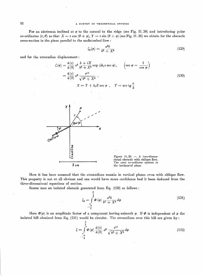
92 A SURVEY OF THEORETICAL STUDIES
For an airstream inclined at rp to the normal to the ridge (see Fig. 11. 26) and introducing polar co-ordinates (r, 8) so that X= r cos (8 + rp), Y = r sin (8 + rp) (see Fig. 11. 26) we obtain for the obstacle cross-section in the plane parallel to the undisturbed flow:
(o(ffJ) = .A a2b b • -•n
and for the streamline displacement :
_ a (z) 2 b + iX . ( (rp) - a (O) a L9. 1 v 2 exp (Lksz sec rp), (sec rp = co: rp)
a(z) eiX = -a2 '
a(O) v b2 + x2
~
X = T + k.Z sec rp ,
cu ~ .....
11) <IJ l;
Scm
p
.... "" ,.
.... ""
X
X T = arctg b
Figure II. 26 - A two-dimensional obstacle with oblique flow. The used co-ordinate system in the horizontal plane
(129)
(130)
Here it has been assumed that the streamlines remain in vertical planes even with oblique flow. This property is not at all obvious and one would have more confidence had it been deduced from the three-dimensional equations of motion.
Scorer uses an isolated obstacle generated from Eq. (129) as follows :
" 2
f a2b '0 = ifJ (rp) 19, 1 V9. drp (131)
" -2
Here rP(rp) is an amplitude factor of a component having azimuth rp. I£ ifJ is independent of rp the isolated hill obtained from Eq. (131) would be circular. The streamlines over this hill are given by:
" 2 _ ( ) eiX d
f uz ., qJ ( = ifJ (rp) a(O) a~ V b2 + xz (132)
" -2
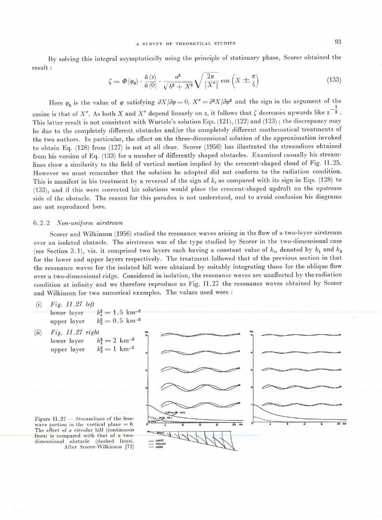
A SUHYEY OF THEORETICAL STUDIES 93
By solving this integral asymptotically using the principle of stationar.Y phase, Scorer obtained the
result :
_ . u (z) . ____!!!___ . ( 2n ( ,. + ~) (- c;[> (cpo) u(O) Jh2+ X2 V IX"I cos X - 4 (133)
Here cp0
is the value of q> satisfying {)X j()cp = 0, X"= d2X fdcp 2 and the sign in the argument of the 1
cosine is that of X". As both X and X" depend linearly on z, it follows that (decreases upwards like z -- 2 .
This latter result is not consistent with Wurtele's solution Eqs. (121 ), (122) and (123) ; the discrepancy may
be due to the completely different obstacles and/or the completely 9-ifferent mathematical treatments of
the two authors. In particular, the effect on the three-dimensional solution of the approximation invoked
to obtain Eq. (128) from (127) is not at all clear. Scorer (1956) has illustrated the streamlines obtained
from his version of Eq. (133) for a number of differently shaped obstacles. Examined casually his stream
lines show a simi larity to the field of vertical motion implied by the crescent-shaped cloud of Fig. Il. 25.
However we must remember that the solution he adopted did not conform to the radiation condition.
This is manifest in his treatment by a reversa l of the sign of k, as compared with its sign in Eqs. (128) to
(133), and if this were corrected his solutions would place the crescent-shaped updraft on the upstream
side of the obstacle. The reason for this paradox is not understood, and to avoid confusion his diagrams
are not reproduced here.
6. 2. 2 Non-uni form airstream
Scorer and Wilkinson (1956) studied the resonance waves arising in the flow of a two-layer airstream
over an isolated obstacle. The airstream was of the type studied by Scorer in the two-dimensional case
(see Section 3.1), viz. it comprised two layers each having a constant value of k., denoted by k1 and lr2
for the lower and upper layers respectively. The treatment followed that of the previous section in that
the resonance waves for the isolated hill were obtained by suitably integrating those for the oblique flow
over a two-dimensional ridge. Considered in isolation, the resonance waves are unaffected by the radiation
condition at infinity and we therefore reproduce as Fig. I I. 27 the resonance waves obtained by Scorer
and \ iVilkinson for two numerical examples. The values used were :
(i) Fig. I I. 27 le ft lower layer lrr = -1. 5 km-2-
upper layer k~ = 0 . 5 km-2
(ii) Fig. I I. 27 right
lower layer lrr = 2 km-2
.. • ~';
upper layer k~ = 1 km-2
~·l~
~ ~
~ ~
~ ~
Figure I I. 27 - St•·eamlines of the free-wave portion in the vertical plane = 0. o 4 l J ~ "' ,. o· ~ 20 ..
· The efl'ect of a circular hill (continuous .. , =-...=--,---.----,---.-----.--.----,------, lines) is compared- with that of a two---- -· - - · - '·. \ dimensio na l obs tacle (dashed li nes ). ::::: =" ·,, \
After Scorer-Wilkinson [72) - "oo' ·
94 A SURVEY OF THEORETICAL STUDIES
In both cases the lower layer was 2 km deep. The very interesting result was obtained that the free waves excited by an isolated hill are confined
to a wedge-shaped region to the lee, the apex of the wedge being at the hill top. The total angle subtended by the wedge was found to be 24.6° and 15.6° in examples (i) and (ii) respectively. There is a clear analogy in this respect with the waves comprising the wash of a ship.
7 . Time-dependent solutions
The assumption of a basic wind independent of time, made by practically every author of a mountainwaves theory, was mainly introduced in order to simplify the mathematics. If dissipation factors are taken into account they lead for the mountain perturbation to one unique solution, also independent of time, and it is logical to adopt this solution as the perturbation to be observed after a sufficient time (theoretically infinite) whatever may be the initial distribution of the wind disturbance. This limit solution may be called the "forced perturbation" due to the mountain, though it is more usually referred to as the "mountain-perturbation".
However the actual wind is never steady, and if it is subject to a rapid variation in the lower layers the observed mountain perturbation may be quite different from the forced one corresponding to the mean wind distribution. On the other hand it is important to know how the forced perturbation is established when the wind becomes practically steady after a period of more or less rapid variation.
7.1 The work of HOiland, Wurtele and Palm
A first attempt concerning time-dependent mountain perturbations was made by Hoiland (1951) : taking the classical case of a constant-density incompressible flow over a corrugated bed, with a free surface and no vertical shear, he showed that if the motion starts from certain prescribed simple initial conditions, it will approach the forced perturbation asymptotically with time. The same work was continued by Wurtele (1953 c), who used a more convenient method for deriving the asymptotic motion, and in addition considered the case of a basic system consisting of two barotropic Couette-flows, which is mathematically simpler and at the same time quite similar as far as the behaviour of the waves is concerned. An analogous investigation was made by Palm (1953). The next year the same problem was considered independently by Queney (1954), who obtained not only the asymptotic behaviour but more generally the complete evolution of the perturbation in several cases. In the following we shall start with an abstract of this latter work, and then try to draw some practical conclusions.
7. 2 Initial-value problems in a half-hounded double Couette-flow (Queney, 1954)
The assumptions made in this work are as follows :
(i) The motion is two-dimensional in a vertical plane (xz- plane), and the density has a constant value everywhere (barotropic motion).
(ii) The basic flow, above the ground level z = 0, consists of two Couette-flows (constant-shear layers) with a discontinuity of the shear at the interface but no discontinuity in the velocity U.
(iii) The viscosity is infinitesimal and there is no initial disturbance of vorticity in each Couette-flow, whence it follows that the same remains true at any time (since the vorticity is a constant in each layer).
(iv) The amplitude of the perturbation is infinitesimal.
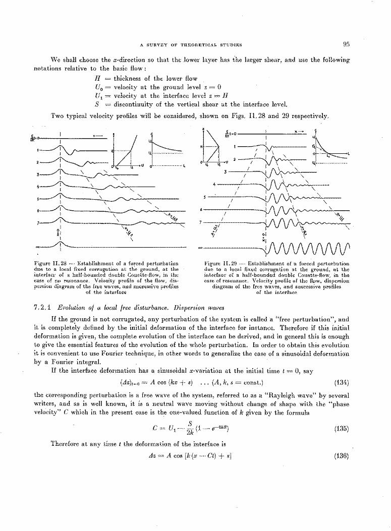
A SURVEY OF THEORETICAL STUDIES 95
We shall choose the x-direction so that the lower layer has the larger shear, and use the following notations relative to the basic flow :
H = thickness of the lower flow U0 = velocity at the ground level z = 0 U 1 = velocity at the interface level z = H S = discontinuity of the vertical shear at the interface level.
Two typical velocity profiles will be considered, shown on Figs. 11.28 and 29 respectively.
4___..,,~ \ "-
t=z ~ ~t•O ><-
l.\ H ··············, 1 :
4. ~~ ; 2~1
I '-o L 0 U. u U I ' I \ "\.
3 I I A\-..~-~ I "\J v\~ -- '\.
-~ " ~
ub CL __ _
~ ... :>~ ............. L
At·:-~----,..i----"--n· I
2 .../i"-..... - ; - i ~-------- u. ~ u
~ I ' ""- 4 I
I
\ " \ \ " ~
.\ " 5 I
I
" I'-- \ " I \ 7____., ['..._ \ """· ~~
I ~I '"'"· 'f,.
I \ I I
Figure II. 28 - Establishment of a forced perturbation due to a local fixed corrugation at the ground, at the interface of a half-bounded double Couette-flow, in the case of no resonance. Velocity profile of the flow, dispersion diagram of the free waves, and successive profiles
of the interface
"
6 I
~I
~ -1-;
I I
"' 't·~
'{{
"
Figure II. 29 - Establishment of a forced perturbation due to a local fixed corrugation at the ground, at the interface of a half-bounded double Couette-flow, in the case of resonance. Velocity profile of the flow, dispersion
diagram of the free waves, and successive profiles of the interface
7. 2 .1 Evolution of a local free disturbance. Dispersion waves
If the g~ound is not corrugated, any perturbation of the system is called a "free perturbation", and it is completely defined by the initial deformation of the interface for instance. Therefore if this initial deformation is given, the complete evolution of the interface can be derived, and in general this is enough to give the essential features of the evolution of the whole perturbation. In order to obtain this evolution it is convenient to use Fourier technique, in other words to generalize the case of a sinusoidal deformation by a Fourier integral.
If the interface deformation has a sinusoidal x-variation at the initial time t = 0, say
(L1z)e~o = A cos (kx + s) ... (A, lr, s = const.) (134)
the corresponding perturbation is a free wave of the system, referred toas a "Rayleigh wave" by several writers, and as is well known, it is a neutral wave moving without change of shape with the "phase velocity" C which in the present case is the one-valued function of k given by the formula
C = U 1- ~k ( 1 - e-2kH) (135)
Therefore at any time t the deformation of the interface is
L1z =A cos [k(x-Ct) + s] (136)
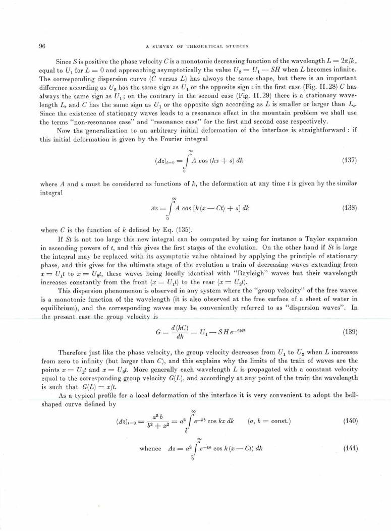
96 A SU RVE Y OF THEORETICAL STUDIES
Since S is positive the phase velocity C is a monotonic decreasing function of the wavelength L = 2nfk, equal to U1 for L = 0 and approaching asymptotically the value U2 = U1- SH when L becomes infinite.
The corresponding dispersion curve (C versus L ) has always the same shape, but there is an important
difference according as U2 has the same sign as U1 or the opposite sign: in the first case (Fig. 11. 28) C has
always the same sign as U1 ; on the contrary in the second case (Fig. 11 . 29) there is a stationary wave
length Ls and C has the same sign as U1 or the opposite sign according as Lis smaller or larger than L8 •
Since the existence of stationary waves leads to a resonance effect in the mountain problem we shall use
the terms "non-resonance case" and "resonance case" for the first and second case respectively .
Now the ·generalization to an arbitrary initial deformation of the interface is straightforward : if
this initial deformation is given by the Fourier integra l
00
(Liz )t=O =.!A cos (kx + s) dk 0
(137)
where A and s must be considered as fun ctions of k, t he deformation at any time t is given by the similar
integral 00
Llz =.!A cos [k (x- Ct) + s] dk 0
where C is the function of k defined by Eq. (135).
(138)
If St is not too large this new integra l can be computed by using for instance a Taylor expansion
in ascending powers of t, and this gives the first stages of the evolution . On the other hand if St is large
the integral may be replaced with its asymptotic value obtained by applying t he principle of stationary
phase, and this gives for the ultimate stage of the evolution a train of decreasing waves extending from
x = U1t to x = U2t , these waves being locally identical with "Rayleigh" waves but their wavelength
increases constantly from t he front (x = U1t) to the rear (x = U2t). This dispersion phenomenon is observed in any system where the "group velocity" of the free waves
is a monotonic function of the wavelength (it is also observed at the free surface of a sheet of water in
equilibrium), and the corresponding waves may be conveniently referred to as "dispersion waves". In
the present case the group velocity is
G= d (kC) = U1-SHe-2kH dk
(139)
Therefore just like the phase velocity, the group velocity decreases from U1 to U2 when L increases
from zero to infinity (but larger than C), and this explains why the limits of the train of waves are the
points x = U 1t and x = U 2t. More generally each wavelength L is propagated with a constant velocity
equal to the corresponding group velocity G(L), and accordingly at any point of the train the wavelength
is such that G(L ) = xft. As a typical profile for a local deformation of the interface it is very convenient to adopt the bell
shaped curve defined by 00
(Liz)t=O = b2a:b x2 = a2Je-kb cos kx dk
0
00
(a, b = const. )
whence Llz = a2,{e- kb cos k (x- Ct) dk
0
(140)
(141)
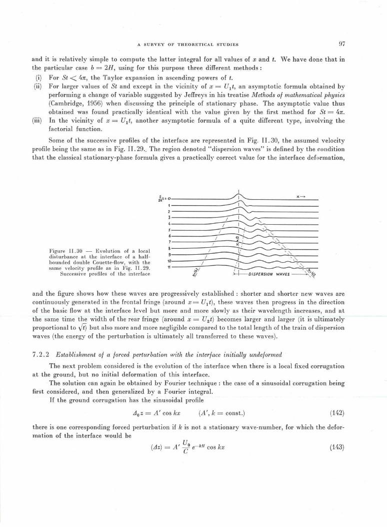
A SURVEY OF THEORETICAL STUDIES 97
and it is relatively simple to compute the latter integral for all values of x and t. We have done that in the particular case b = 2H, using for this purpose three different methods :
(i) For St < 4n, the Taylor expansion in ascending powers of t. (ii) For larger values of St and except in the vicinity of x = U1 t, an asymptotic formula obtained by
performing a change of variable suggested by Jeffreys in his treatise Methods of mathematical physics (Cambridge, 1956) when discussing the principle of stationary phase . The asymptotic value thus obtained was found practically identical with the value given by the first method for St = 4n.
(iii) In the vicinity of X = ul t, another asymptotic formula of a quite different type, involving the factorial function.
Some of the successive profiles of the interface are represented in Fig. II. 30, the assumed velocity profile being the same as in Fig. II. 29._ The region denoted "dispersion waves" is defined by the r.ondition that the classical stationary-phase formula gives a practically correct value for the interface deformation,
Figure II.30 - Evolution of a local disturbance at the interface of a halfbounded double Couette-flow, with the sam e velocity profile as in F ig. II. 29.
Successive profiles of t he interface
kl:O------------------' 1----------------2
3 I
4~ 5~ 6~ 7 I ~ 8 I
I
x~
' ,'-. ','-. 10 I , __ _
11 , I ' '" ;;:I .' I ' 'f k/ .'+-I- DISPERSION WAVES ________::.<~
and t he figure shows how these waves are progressively established : shorter and shorter new waves are continuously generated in the frontal fringe (around x = U1 t), these waves t hen progress in t he direction of the basic flow at t he interface level but more and more slowly as their wavelength increases, and at the same t ime the width of t he rear fringe (around x = U2 t} becomes larger and larger (it is ultimately proportional to Vi) but also more and more negligible compared to the total length of the train of dispersion waves (the energy of the perturbation is ultimately all transferred to these waves).
7. 2. 2 Establishment of a forced perturbation with the interface initially undeformed ·
The next problem considered is the evolution of the interfa ce when there is a local fixed corrugation at the ground, but no initial deformation of this interface.
The solution can again be obtained by Fourier technique : the case of a sinusoidal corrugation being first considered, and then generalized by a Fourier integral.
If the ground corrugation has the sinusoidal profile
Ll 0 z = A ' cos kx (A', k = const.) (142)
t here is one corresponding forced perturbation if k is not a stationary wave-number, for which the deformation of the interface would be
(Liz) = A ' Uo e-kH cos kx c (143)
98 A SURVEY OF THEORETICAL STUDIES
where C is the value defined by Eq. 135. Therefore in order to have L1z = 0 when t = 0 we must add to
it the free perturbation defined by the condition that the initial interface deformation is opposite to (L1z),
and this gives for this deformation at any time t
L1z = A' ~0 e - kH [cos kx - cos k (x- Ct )] (144)
In the particular case k = k, (= 2nfL,) Eq. (143) would give for (L1z) an infinite value (resonance
effect), but Eq. (144) still gives a finite value for L1z, namely
L1z =-A' U0 e - ksll k,t sin k,t (145)
and therefore Eq. (144) is valid in any case, so that its generalization by a Fourier integral involves no
difficulty. It is again convenient to choose as the profile of a typical local corrugation the bell-shaped
curve 00
- a'2 b' - '2}' -kb' L1 0 z- ·u 2 , _ 2 - a e cos kxdk ... (a', b' = const .)
0
and then we get, for the interface deformation at time t,
00
L1z = a'2J~o e-k(b'+H) [cos kx - cos k (x- Ct)] dk
0
However it is necessary to consider separately the non-resonance and the resonance case.
7. 2. 2.1 Non-resonance case (velocity profile of Fig. 11. 28)
with
In this case we can write
L1z = L1 1z- L1 2 z
00
L1 1 z = a'2j~o e-k(b'+H) cos kx dk
0
00
L1 2z = a'2JUo e-k(b'+H) cos k (x- Ct) dk e 0
(146)
(147)
(148)
(149)
(150)
Since C does not vanish in the range of integration the integcals are one-valued, and obviously L11z
represents the stationary deformation corresponding to the forced perturbation, or "forced deformation",
and L1 2z represents the deformation corresponding to the free perturbation defined by the same initial
deformation : in other words we have exactly the same result as for a sinusoidal corrugation, and this is
true with any ground corrugation. It is relatively easy to compute L1 1z by means of proper expansions, and just as the ground corrugation
this forced deformation has a symmetrical bell-shaped profile, but a larger width scale since this scale is
represented by ( b' + H) instead of b' . Accordingly the evolution of the free deformation L1 2 z is quite
similar to that of the local deformation Eq. (140) considered in the preceding problem, and its ultimate
stage has already been described : the deformation is transformed into a system of dispersion waves
A SURVEY OF THEORETICAL STUDIES' 99
extending from X= U2t to X= Ult, and since u2 has the same sign as ul this system is completely separated from the forced deformation and located at a larger and larger distance ahead of it.
The complete evolution of the interface has been computed in the case where b' =Hand U2 = U1 /2, and some of the successive profiles are reproduced in Fig. II. 28, the last one (for t = =) being the forced deformation itself. It appears that the two components L11z and L1 2z are already practically separated when St = 8n, and therefore we can say that the establishment of the forced perturbation is a relatively fast process in this case. On the contrary the damping of the free perturbation is rather slow, but this is obviously unimportant for the mountain problem.
7. 2. 2. 2 Resonance case (velocity profile of Fig. II. 29). Resonance wares
We shall again discuss this case with the assumption of the same ground corrugation, given by Eq. (146).
The equations (148), (149) and (150) can again be used, but since the integrals are many-valued as a result of the vanishing of C for k = k,, it is necessary to specify that one has to take for instance their principal values, defined as follows :
J 1~[]: !J (151) 0 o ks+-'
In other words the vicinity of k = k, is excluded from the range of integration, and this can be done since_in (149_)_and (150) the integrands have the same residue (in (147) the integrand has no pole).
Now we can write, denoting by G. the value of the group velocity fork= lf8 , or "resonance group velocity",
00 00
L11 z = a'2 ks Uo e-ks(b'+H)J 2
ks cos kx dk +jf (k) cos kx dk G., k2 -k; (152)
0 0 with
u 2k2 u I (k) = a'2 _____!)_ e-lc(b' +H) _ a'2 · ·' o e-k8(b' +H)
C G. (k2 -k;) (153)
and it is easy to verify that f(k.) is finite-, so that the second integrarin Eq. (152) represents a local deformation. On the other hand we have
whence
00 00
f 2k,, d !cos kx dk ( ) . lf2 _ k; cos kx k = k _ k. = - sgn x n sm k.x 0 -00
00 .
L1 1 z =- (sgn x)a' 2 nk. Uo e-ks(b'+H) sin k,x +jf(k) coskx dk G, 0
and the same transformation applied to L1 2z gives 00
(154)
(155)
-------LJ2Z-=~sgn-(x- G.tj-a'2 nkG~o e-ks(b'+H) sin k.x + Jt (k) cos k (x- Ct) dk + F (x, t) (156) 0
where F(x, t) represents a local deformation around x = G,t Accordingly we can write
Llz = Ll~z- Ll~z + eL13 z (157)
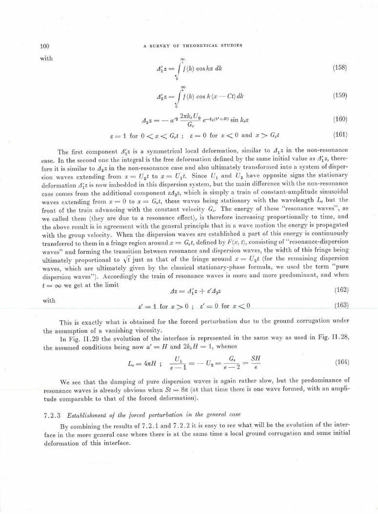
100
with
A SURVEY OF THEORETICAL STUDIES
00
Ll~z = j'f(lr) coskx dk
0 00
Ll~z = jf (k) cos k (x - Ct) dk
0
2nk, Uo -k,(b'+H) sin k.x '2 e Llaz = -a "
e = 1 for 0 < x < G,t ; e = 0 for x < 0 and x > G,t
(158)
(159)
(160)
(161)
The first component Ll~z is a symmetrical local deformation, similar to Ll1 z in the non-resonance
case. In the second one the integral is the free deformation defined by the same initial va lue as Ll~ z, there
fore it is similar to Ll 2 z in the non-resonance case and also ultimately transformed into a system of disper
sion waves extending from X= U2t to X= Ult . Since ul and u2 have opposite signs the stationary
deformation Ll~z is now imbedded in this dispersion system, but the main difference with the non-resonance
case comes from the additional component eLI 3z, which is simply a train of constant-amplitude sinusoidal
waves extending from x = 0 to x = G,t, these waves being stationary with the wavelength L, but the
front of the train advancing with the constant velocity G,. The energy of these "resonance waves" , as
we called them (they are due to a resonance effect), is therefore increasing proportionally to t ime, and
the above result is in agreement with the general principle that in a wave motion the energy is propagated
with the group velocity. When the dispersion waves are established a part of this energy is continuously
transferred to them in a fringe region around x = G,t, defined by F (x, t), consisting of "resonance-dispersion
waves" and forming the transition between resonance and dispersion waves, the width of this fringe being
ultimately proportional to \/t just as that of the fringe around x = U2 t (for the remaining dispersion
waves, which are ultimately given by the classical stationary-phase formula , we used the term "pure
dispersion waves") . Accordingly the train of resonance waves is more and more predominant, and when
t = = we get at the limit Llz = Ll{z + e'LI3z (162)
with e' = 1 for x > 0 ; e' = 0 for x < 0 (16QJ
This is exactly what is obtained for the forced perturbation due to the ground corrugation under
the assumption of a vanishing viscosity.
In Fig. 11.29 the evolution of the interface is represented in the same way as used in Fig. 11 . 28,
the assumed conditions being now a'= H and 2k,H = 1, whence
L , = 4nH; G,
ul =- u2 = e- 2 e -1
SH e
(164)
'vVe see that the damping of pure dispersion waves is again rather slow, but the predominance of
resonance waves is already obvious when St = 8n (at that time there is one wave formed, with an ampli
tude comparable to that of the forced deformation).
7. 2. 3 Establishment of the forced perturbation in the general case
By combining the results of 7. 2.1 and 7. 2. 2 it is easy to see what will be the evolution of the inter
face in the more general case where there is at the same time a local ground corrugation and some initial
deformation of this interface. ·
A SURVEY OF THEORETICAL STUDIES 101
Obviously the perturbation can be obtained by superposing two components :
(i) The free perturbation defined by the initial deformation of the interface (obtained in 7. 2 .1). (ii) The perturbation resulting from the ground deformation under the assumption of no initial defor
mation of the interface (obtained in 7. 2. 2).
Therefore the asymptotic behaviour of the perturbation is still the same as in the absence of initial interface deformation, the only parameters to be modified being the amplitude and the phase of the pure dispersion waves. Accordingly after a rather short time the prominent feature is again the forced component in the non-resonance case and the system of resonance waves in the resonance case. In both cases the perturbation becomes identical with the forced perturbation when t = =·
7 . 3 Effect of viscosity
In a recent paper the effect of viscosity on the free waves of an unbounded double Couette-flow was studied by Queney (1958), and the rather unexpected result was obtained that these waves become unstable (amplified with time) if their wavelength is short enough, the longer waves alone being damped. In other words the combined effects of viscosity and vertical variation of the shear lead to a dynamic instability, and it may be that the transformation of mountain waves into rotors has something to do with this phenomenon.
However, and though we have not considered what happens if the flow is bounded by a corrugated ground, it seems probable that if the viscosity is small its net effect on a mountain perturbation is always a damping effect whatever the structure of the basic wind . If this is accepted the following consequence is to be expected when resonance waves are formed : instead of growing indefinitely, the energy of the perturbation tends towards a limit, corresponding to a balance between the gain by resonance and the loss by viscous friction (since the rate of the gain remains constant, while the loss increases with the length of the train of resonance waves). Therefore the perturbation becomes practically stationary after a certain time, and in the final regime (which is necessarily identical with the forced perturbation) the amplitude of the resonance waves is continuously decreasing downwind and practically negligible beyond a certain distance. The smaller the viscosity, the longer will be the time required for its complete building, and therefore if the viscosity is very small it is correct to say that it can be neglected provided what is happening at a great distance is not taken into consideration.
From this discussion it follows that viscosity is only a secondary factor in the mountain problem, and more particularly the fact that the resonance waves usually develop on the lee side of the mountain has nothing to do with the effect of viscosity. Actually we have obtained this result in 7. 2. 2. 2 under the assumption of a viscosity strictly equal to zero, and in that case the resonance waves are on the lee side simply because the resonance group velocity Gs has the same sign as the wind velocity U1 at the interface level. Similarly in the case of the gravity waves at the free surface of a river Gs has the same sign as the velocity of the water, and again this explains why the stationary waves due to a corrugation at the bed of the river are always observed on the lee side of the corrugation. But if these waves are controlled by capillarity instead of gravity they are located on the opposite side, in agreement with the fact that in this case Gs has the opposite sign.
The result is quite general and can be stated as follows :
In the perturbation due to a corrugation in the bed of a stationary flow, the resonance wares derelop on the lee side of this corrugation or on the opposite side according as the group relocity of these wares (when
considered as free wares) has the same direction as the flow, or the opposite direction.
102 A SURVEY OF THEORETICAL STUDIES
From the relation
G, =-La(~~). (165)
it is also obvious that an equivalent condition for the resonance waves to be lee waves is that C must be
a decreasing function of L in the vicinity of L = L 8 , when the positive direction is that of the flow.
This discussion proves that the only correct way of treating the problem of mountain waves is to
consider it as an initial-value problem. If as usual it is treated as a problem of stationary motion, an
infinity of solutions are obtained when viscosity or other dissipative factors are neglected, and if these
factors are taken into account the problem becomes very difficult mathematically. All these well-known
difficulties are quite artificial, and they completely disappear if one starts from initial conditions.
7 . 4 Conclusions
It is obvious that the model of basic flow u sed in the preceding study is very different from the actual
wind structure in the lower atmosphere, and therefore it seems impossible to make any quantitative
application of the results obtained. It would be at least necessary to generalize the theory in two direc
tions : first by introducing a static stability, then by considering the case of a time-dependent basic flow.
As is well known , the introduction of static stability in a system of Couette-flows results in a profound
modification of the dispersion formula for the free waves, since it makes possible a resonance even in the
case of a unique Couette-flow. However if the two parameters L, and G, are given, all the evolution of
the resonance waves is probably the same as without stability, so that a quantitative application of the
theory is actually possible if the basic wind is independent of time. The time-dependence of the wind is also a very important factor, but here again we can get at least
a rough understanding of what may happen by considering the case of a discontinuous variation : assuming
for instance a basic flow increasing abruptly from a negligible value, then remaining steady for a certain
time, then changing again discontinuously to another steady regime, and so on.
A. Assuming no initial motion above the corrugated ground, any abrupt establishment of a basic flow
will necessary produce a purely local perturbation, and if this basic current is a barotropic double Couette
flow there will be no vorticity dist urbance in the absence of viscosity. Therefore if the wind becomes
steady after this sudden change we are brought back to the problem discussed in 7. 2. 3, and we know
what is going to happen in a resonance case : a first resonance lee-wave will predominate after a time that
we may take equal to T = L,f G., a train of two waves will be formed when t = 2T, three waves when
t = 3T, and this process will go on as long as the wind remains steady.
Taking for instance G. = 0.42 U1 (case of Fig. II . 29) , L. = 5 km and U1 = 10 mfs, we get
T = 20 minutes.
B. Let us now assume that at time t = 3T for instance the basic flow changes abruptly to another
double Couette-flow with the same height H for the interface , and then remains again steady. In general
the stationary wavelength and the corresponding group velocity take new values L; and G;, so that the
system of three waves already formed will no longer remain stationary ; it will move downwind or upwind
according as L.' is larger or smaller than L,. At the same time it will become progressively dispersed at
about the same rate as that of its formation, and a new system of stationary lee waves of wavelength L; will develop at the rate defined by the new time-scale T I= L;/ G;. This new system will interfere with
the former one, but become more and more predominant : the first-formed waves will have practically
disappeared when t = 6T, and if T' is smaller than T there will be more than three lee waves at that time.
A SURVEY OF THEORETICAL STUDIES 103
C. If a further abrupt change occurs in the basic flow the result will be a new period of interference
eventually followed by a new period of regular lee waves, and the interference may be very complex since
the first-formed waves may not have completely disappeared. All the eventual subsequent changes in
the basic wind will have similar consequences. Of course this discussion is purely idealistic, but it shows the complexity that may result, for the
evolution of the perturbation, from the time-variation of the wind. Finally it seems that we may conclude as follows :
(i) A system of regular lee waves is likely to occur only in the cases where the time-scale of the variation
of L , (resulting from the variation of the wind) is large as compared with T = Ls/ G., the time
required for the formation of one wave. The principal dispersive factor limiting the number of waves
is probably the internal static stability of the airflow, rather than eddy-viscosity. (ii) If the time-scale of the variation of L, is comparable with T, the evolution of the mountain perturba
tion is very complex, and when it shows a wavelike pattern the waves are no longer stationary and
not necessarily on the lee side of the mountain. (iii) The usual order of magnitude of T is probably 10 to 30 minutes.
8 . Numerical solutions
Theoretical studies of the airflow over mountains have, up to the time of writing, been almost
entirely confined to the derivation and interpretation of analytical solutiop.s of the relevant linearized
equations. Except in very special circumstances, the linearization restricts the validity of the solutions to
small-amplitude disturbances. Numerical computation has so far only been involved for the evaluation
of solutions which it has been possible to express in analytical form. This has limited published results
to very simple model airstreams and mountain obstacles having a very simple idealized shape. In spite
of such simplifications, the analytical solutions have not been evaluated exactly even in the simplest case,
except for the resonance waves considered in isolation . For example, in the evaluation of certain integrals
which arise, further approximations have been found necessary and the effect of these is often somewhat
obscure and has certainly not been demonstrated quantitatively. These remarks are not intended to
decry the value of the existing theory, for our subject is after all a difficult and complex one, but to remind
the reader of the theory's limitations. Many of these limitations would be avoided or considerably minimized if the resources of electronic
computing were available so that heavy computation ceased to be an obstacle. Indeed, the approach to
the problem may be substantially modified by the advent of electronic computers. High-powered
computing may be used either to extend and exploit more fully the results inherent in existing analytical
solutions, or to obtain numerical solutions of the basic equations. Some work of the former type has
already been done. For example, Wallington and Portnall (1958) showed how the wavelengths and ampli
tude factors of the resonance waves could be computed for any airstream, the structure of which they
specified by means of temperatures and winds at 50 mb intervals up to 200 mb. This represents an escape
from simple airstreams comprising a small number of discrete layers and a move towards greater generality.
In another contribution, Wallington (1958) showed how the available conclusions, regarding the
dependence of the resonance waves on the mountain shape, could be extended to asymmetrical mountains
and to those of quite irregular shape. This involved determining by electronic computation the break
down of the given ground profile into a number of idealized ridges each having a different height, width,
104 A SURVEY OF THEORETICAL STUDIES
and phase. The method enables one to determine inter alia the wavelengths most likely to be excited by
any particular terrain. Another valuable line of action would of course be the more accurate evaluation of the complete
field of flow given by the analytical solutions than has been achieved hitherto. This is particularly relevant
if one wishes to study the nature of the flow in the immediate vicinity of the mountain, which is of course
important for aviation. Another approach which is known to be receiving active attention is based on the initial value
formulation of the problem summarized in the previous section. This approach avoids the problems of
uniqueness which arise in the steady state formulation. The method would amount to integrating numeri
cally in time, starting from an arbitrary initial flow (in practice that of the airstream as revealed by radio
sondefradiowind data ) and continuing the process until some steady state, or limited oscillatory state,
were established. However, the ultimate aim of numerical work must clearly be to evolve computational techniques
to obtain the complete flow for any given basic flow, for finite amplitudes, for any ground contour and
preferably in three dimensions. Such an aim is no longer completely unrealistic and the publication of
new work in this direction is awaited with interest.
9 . Model experiments
In view of the great difficulties in achieving practically useful results in this subject, whether by
theoretical studies or fi eld work, it is natural that some workers should explore the possibilities of simulating
the flow of the atmosphere over mountains by means of model experiments on the laboratory scale. In
such work, however, we encounter the difficulty of achieving dynamical similarity between the two flow
patterns, which are necessarily on vastly different scales.
Suppose for example we consider placing a model of our mountain obstacle in a wind tunnel and
suppose for the moment that friction may be neglected in the model as well as in the atmosphere. Then
if the obstacle height is denoted by h it can be shown by transferring to dimensionless variables (see
Seorer, 1953 and C01·by, 1954) that the following dimensionless function must have the same values in both scales of flow in corresponding points :
Scorer function : S = h2 (~~ - ~') (166)
If we neglect the shear term in Eq. (166) and insert typical values for the atmosphere, viz . :
y = 0.006oC m- 1 , T = 250oK , u = 20 m. sec-1
we obtain G-gfu2 = 0.4 km-2 for the atmosphere. It follows that we must have :
((ig) - 0 4 l -2 h2atmos -=--2 - • UTI - 2--U model h model
For a geometric scaling in the ratio 1 : 3 X 10⁻⁵, we should therefore require iigfu2 for the model
to be 4.4 X 10² m-2• Now, even if it were possible to maintain the very large temperature gradient of
1 °C cm-1 in the model, we should require a flow speed of only 9 cm. sec-1 . For smaller temperature gradients,
even slower flow speeds in the model would be necessary. Such flows with large temperature gradients
A SURVEY OF THEORETICAL STUDIES 105
and very low flow speeds cannot be accomplished, at least in conventional wind tunnels. Furthermore, at such low velocities (small Reynold's number) considerable boundary layer effects would arise near the tunnel walls, and the assumption of no friction would be invalidated.
The above considerations indicate that model experiments in a wind tunnel using air as the streaming medium would be useless if it is desired to accomplish quantitative similarity. As we shall see, however, the situation is completely different with a streaming fluid of much greater density e.g. water.
9 . l Similarity conditions
In order to deal rigorously with the conditions for similarity between the flow of the atmosphere and that of an incompressible liquid over an obstacle, it is necessary to proceed from the basic equations for the two classes of motion. We will follow essentially the work of Batchelor (1953) and Sawyer (1955).
(a) Atmosphere
Using the vector notation :
U = { u, ~ } , V = { :x ' ~ } ' g = { 0, - g }
the appropriate equations (of motion, continuity and energy) may be written:
1 du = g -- V p dt p
1 dp _-V ·U p dt -
~(E)= o dt P"
(167)
(168)
(169)
We denote the density and pressure in an atmosphere having an adiabatic lapse rate by Pa and pa respectively, the values in the actual atmosphere at the same height z being p and p. Sawyer (1955) shows that the followin g expressions are good approximations in our particular case :
From Eqs. (169) and (170) we obtain:
p- Pa << 1 Pa
p -pa << 1 Pa
1 dp 1 1 dp 1 dpa 1 OPa 1 gpa -- = ---P:d--=-w- =- --w p dt K p dt Pa dt Pa Jz K pa
(170a)
(170b)
This is because with p = pa it follows from Eq. (169) that P/Pa is approximately constant along the streamlines and we can thus write Eq. (168) in the form :
V . u = gpa -w Kpa
(171)
106 A SURVEY OF THEORETICAL STUDIES
Now if we introduce (p- pa) and (p - Pa) as new variables in Eqs. (167), (169) and (171) and use
the fact that Vpa = pag, we obtain :
(p - Pa + 1) du _ p - Pa 1 n ( ) - - - - g ---- v p-pa
Pa dt , Pa Pa
V.U = gpa -w Kpa
!':_ (p - Pa) = 0 dt Pa
(172)
(173)
(174)
We now transfer to dimensionless variables by introducing the units length x0 , velocity u0, density p0
and pressure p0 and indicate the dimensionless variables by dashes, thus : U1
= uju0. Vve then
obtain, if (p - Pa)/Pa is neglected in comparison with 1 [Eq. (170b)] :
du1
_ x0 p0 P1
- P~ g _ X~Po V (p 1 _ p~) (JZ- u~ Pa UoPa
V.U 1 = g pa X W 1
Kpa 0
:i (PI I p~) = 0 dt Pa
(175)
(176)
(177)
(b) Incompressible liquid model
It might appear at first to be impossible to achieve similarity without using a compressible fluid
having the same value of K = cpfcv as in the atmosphere. Sawyer showed, however, that a system
of equations precisely analogous to Eqs. (175), (176) and (177) could be derived for an incompressible
liquid model, provided the tank width across the flow varied suitably with height. The motion can
still be regarded as two-dimensional and compressibility is simulated by variations in the depth of
a given layer of the liquid as it moves from one level to another in the tank. This effect appears in
the mathematics as a modification of the continuity equation. Thus Saw)'er obtain..ed the following
equations for such a model having a variable channel width a(z) :
dU1
_ Xm Pm ( 1 _ 1 ) _ XmPm V( 1 _ 1 )
dt - u2 p P Pam g u2 p P Pam m am ·m um
V 0 U1 = - Xm da I
a dz w
~ (P1
-: P~m) = 0 dt Pam
(178)
(179)
(180)
Comparing these equations with Eqs . (175), (176) and (177) for the atmosphere, we obtain the
following conditions for similarity :
gxoPo -u5Pa
gxmPm U~Pam
XoPo Xmpm -2- = -2-UoPa UmPam
(181)
(182)
A SURVEY OF THEORETICAL STUDIES 107
gpaXo _ Xm da (183) Kpa - --;;: dz
As the pressure is not involved in our initial or boundary conditions we may disregard the condition of Eq. (182). However an interesting deduction can be obtained from Eq. (183). Thus if dz* is the height increment in the atmosphere corresponding to dz in the model, so that:
then Eq. (183) becomes :
and therefore :
dz* = Xo dz Xm
da g Pa d * 1 dp 1 dpa - = -- z = - -"""- -a K Pa K Pa K Pa
a (z) = Apa1/K = Bpa (184)
Thus the compressibi li ty of the atmosphere can be simulated by arranging for the width of the channel to vary with height in proportion to the density at corresponding heights in the atmosphere. The remaining condition, Eq. (181), requires the Froude number of the atmospheric and rqodel flow to be matched. Assuming the flow speeds to be independent of height the latter condition requires a match between the density gradients and this can be achieved in many cases by using a stratified salt solution in the model. Thus if the geometric scaling is in the ratio 1 : 10-4 and the percentage density gradients are made equal, atmospheric flow speeds within the range 10 m. sec-1 < Ua < 50 m . sec-1 would require model flow speeds in the range 10 cm. sec-1 < Um < 50 cm. sec-1, which is a convenient range from the experimental point of view. 'Ne should of course also require for the obstacle itself geometric similarity between the two scales .
The only remaining difficulty concerns the upper boundary which is of course quite different in the two cases, the liquid model having a free surface. In relevant work by Corby and Sawyer (1958) it was found that with a rigid upper boundary the flow at low levels could be made to approach that for an unbounded atmosphere as closely as desired by placing the rigid upper boundary sufficiently high. Undoubtedly_ the same considerations apply in the present context. _ _
9 . 2 Experimental results
So far no model experiments have been carried out which comply with both the similarity requirements expressed by Eqs. (181) and (184). However, some experiments have been carried out, e.g. in a wind tunnel by Abe (1942) and in a liquid channel by Long (1953, 1954, 1955) and by Suzuki and Yabuki (1956), and it is useful to refer to these briefly and state their limitations.
Abe (1932, 1941) studied over a lengthy period the unusual cloud forms caused by Mount Fujiyama, which is an almost conical mountain, and experimented in a wind tunnel with a geometrically similar model scaled in the ratio 1 : 2 X 10⁻⁵. He was careful to carry out the experiments at the same Reynold's number, on the assumption that molecular viscosity in the model corresponded to eddy viscosity in the atmosphere. He also introduced wind and temperature stratification into his model but these factors were not matched quantitatively on the two scales in accordance with Eq. (181). In spite of this his model flow, revealed by the use of incense smoke, indicated qualitative agreement with the characteristic cloud of Mount Fujiyama ; this is clearly seen from the photograph of the model flow reproduced as Fig. 11 . 31.
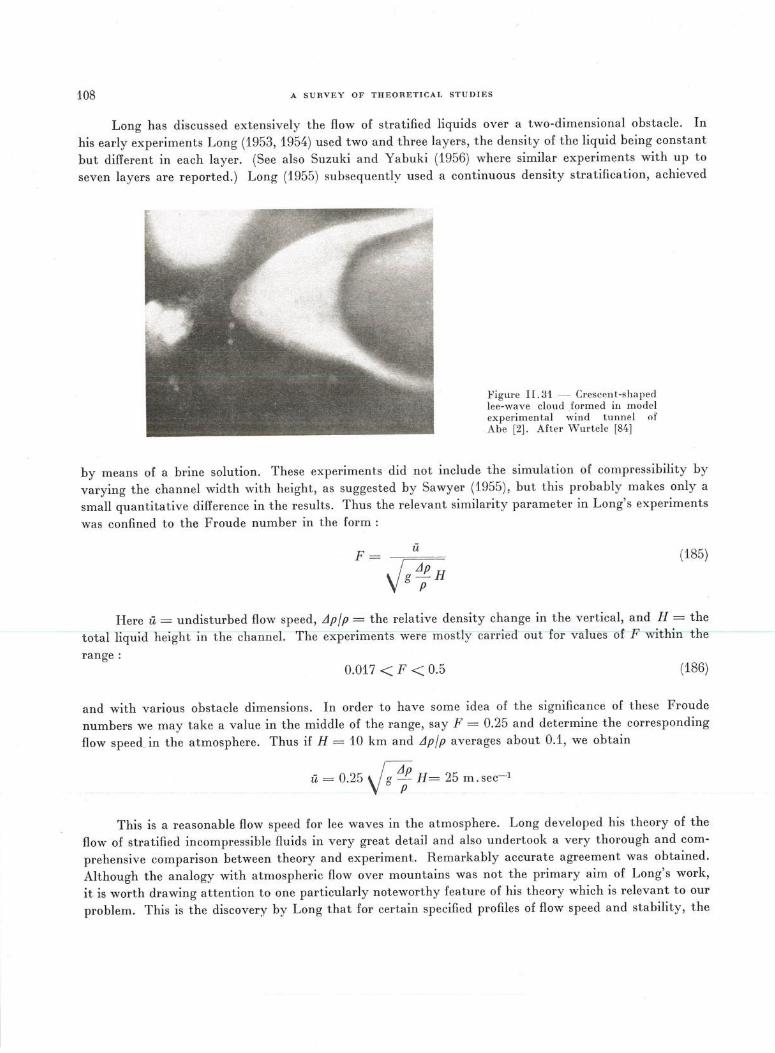
108 A SURVEY OF THEORETICAL STUDIES
Long has discussed extensively the flow of stratified liquids over a two-dimensional obstacle. In
his early experiments Long (1953, 1954) used two and three layers , the density of the liquid being constant
but different in each layer. (See also Suzuki and Yabuki (1956) where similar experiments with up to
seven layers are reported.) Long (1955) subsequently used a continuous density stratification, achieved
Figure IL31 -- C1·escent-shaped lee-wave cloud form ed iu mod el experim ental wind tunnel of Abe (2]. After Wurtele [84]
by means of a brine solution. These experiments did not include the simulation of compressibility by
varying the channel width with height, as suggested by Sawyer (1955), but this probably makes only a
small quantitative difference in the results. Thus the relevant similarity parameter in Long's experiments
was confined to the Froude number in the form :
u F~~ (185)
Here u =undisturbed flow speed, L1pfp = the relative density change in the vertical, and H =the
total liquid height in theChannel. The experiments were mostly carried out for valueso f F wirlrin the
range: 0.017 < F < 0.5 (186)
and with various obstacle dimensions. In order to have some idea of the significance of these Froude
numbers we may take a value in the middle of the range, say F = 0.25 and determine the corresponding
flow speed in the atmosphere. Thus if H = 10 km and L1pfp averages about 0.1, we obtain
ii = 0.25 ~ H= 25 m.sec-·1
This is a reasonable flow speed for lee waves in the atmosphere. Long developed his theory of the
flow of stratified incompressible fluids in very great detail and also undertook a very thorough and com
prehensive comparison between theory and experiment. Remarkably accurate agreement was obtained.
Although the analogy with atmospheric flow over mountains was not the primary aim of Long's work,
it is worth drawing attention to one particularly noteworthy feature of his theory which is relevant to our
problem. This is the discovery by Long that for certain specified profiles of flow speed and stability, the
A SURVEY OF THEORETICAL STUDIES 109
equations are linear even for finite amplitudes. Thus, Long's basic equation in our notation may be written:
2 y 1 [( d Y)2 2 J(ld l (--)2 g dp y Y'2., + - gra ., + - -- n pu = -::-:= -- ., 2 ~ ~ ~p~ (187)
when p is the streamline displacement above the original.level. Now, if· the basic flow is such that pu2 = constant and dpjdz = constant, Eq. (187) reduces to the simple wave equation:
V'g + a2( = 0, a 2 = .f r ~ dp 1 = const u2 p dz (188)
This means that fpr this particular class of basic flow fields, the linearized (perturbation) equations are valid for finite amplitudes. The reader will note the correspondence between Eq. (188) and Eq. (25) for the atmospheric case. Even the parameter :
a2 = .f I d log p I u2 dz IS fully equivalent to :
Jr2 = .f y* - Y _ g d log 1J • u2 T - u2 ----;rz
which figures in the theory of Lyra and others. Here one may note the correspondence, which has been known for some time, between the potential temperature in the atmosphere and the density in the incompressible fluid. This follows from Eq. (8) which is valid for the compressible atmosphere in the form :
d - d g - ln e + - In j5 + - = 0 dz dz c2 (189)
To change to an incompressible model flow (c2 -+ CXJ) it is only necessary to replace d(log iJ)fdz by - d(log p)fdz.
In his experiments Long used nearly linear density gradients without velocity shear. Although the analogy with atmospheric mountain waves is hindered by the presence of a free surface in the model, Long's experiments have made an important contribution to the atmospheric problem and no doubt there will be further contributions through improvements in the model. In particular one would like to see similar experiments with a variable channel width to simulate compressibility and with a large depth of liquid in the model to minimize effects due to the upper boundary differences.
110
PART Ill
AVIATION APPLICATIONS AND FORECASTING
1. Flying aspects of mountain waves
In this section we discuss the flying aspects of mountain waves with the point of view of pilots and
forecasters especially in mind. Familiarity on the part of pilots with the kind of hazard which can occur
over mountains goes some way towards minimizing the dangers, and makes it more likely that the pilot
will act wisely when some action is urgently called for. The subject is very complicated and inevitably
forecasts of mountain airflow effects must be limited in scope, often not specific and on occasions unreliable.
Much depends, therefore, on the pilot being able to recognize and assess the characteristics of waves,
rotors, etc., whilst in flight. Moreover, the pilot can contribute useful data on the subject by reporting
his experiences when flying over mountainous terrain.
1 . 1 Vertical currents
It is natural to think of the wind as flowing predominantly horizontally but the numerous observa
tions recorded in Part I show that over mountains there may be considerable vertical currents, sometimes
exceeding the maximum rate of climb of many aircraft in current use. The vertical currents associated
with mountain waves may be quite extensive and are insidious because fl ying conditions in much of the
affected airspace are usually quite smooth, so that there may be no positive indication of their existence
except that provided by the altimeter. It is probably easy for a pilot to fly through mountain waves of
moderate amplitude without being aware of it.
A pilot flying across mountain waves experi~ces altern~e regions of lift and sink. Even over quite
small hills the vertical currents involved may reach a few m/sec whilst 10 m/sec h.as been encountered.
over and to the lee of mountains in the British Isles little more ~han 1 km high. In the powerful wave
systems of the Sierra Nevada in California, vertical velocities in the two main downdraft areas, viz., over
the lee slope and on the downwind side of the rotor zone, commonly attain 10 m/sec, whilst in severe
cases 25 m/sec or more has been observed. Very few aircraft could remain in such a region for long ·without
being brought down dangerously near the mountains or into layers of severe turbulence. Although the
waves of this particular location have been more c·ompletely measured and documented than those of
other regions, there is little doubt that waves of comparable intensity must occur over many other large
mountain ranges, especially those which lie across the temperate latitude westerlies .
As is explained in Part I, 2. 3, attempts to maintain altitude during fli ght through waves , whether
by pilots' action or by altitude-coupled auto-pilot, are fraught with the danger of stalling. There is plenty
of evidence for the large changes of airspeed which may be suffered on this account , and they constitute a
real hazard. In the past the statement has sometimes been made that high ground has no disturbing effect on
the airflow at more than three times its height, but it is as well for the pilot to ignore this statement.
Over the hills and mountains of Europe, waves of the most common type attain their maximum amplitude
at some level which is most often below about 4,000 m. Over large mountain ranges such as the Rockies
AVIATION APPLICATIONS AND FORECASTING 111
the maximum amplitude may be at a somewhat higher level. Above this level the amplitude decreases,
albeit rather slowly on some occasions. Less commonly, there may be waves which are dominant in the
high troposphere and lower stratosphere but these are clearly of much less danger to aircraft than those
which dominate in the middle or lower troposphere. It may be useful for a pilot to realize that when crossing a mountain range parallel to the wind, the
aircraft's height fluctuations will be in phase or out of phase with those of the airstream according as he is
fl ying downwind or upwind. Furthermore, when flying across the wind along the lee side of a lengthy
mountain ridge, an aircraft could remain continuously in a down current until the whole length of the
ridge were traversed, with catastrophic loss of height.
1. 1. 1 Vertical currents - Recommended fli ght procedures
Kuettner, in a section of the Sierra Wave Final Report (1957), has proposed certain safety rules
and we shall make use of his considerable experience in the course of the suggestions which follow.
If minor waves, resulting in only small involuntary changes of height , are encountered when flying
at a considerable height above hilly terrain, there is clearly no necessity for the pilot to take any special
immediate action. He would be well advised to watch his altimeter, however, particularly if he is passing
over the foothills of larger mountains which lie ahead on his route. He may then obtain evidence of larger
effects ahead, suggesting the desirability of flight at a greater height than previously intended over the
higher ground to come. The greatest need for action arises when strong effects are encountered at a height which does not
provide any special margin for large height changes. Kuettner recommends that if it is not feasible to fly
around an area of obvious wave activity, the mountain range should be crossed at a level which is at least
50 per cent higher than the height of the mountain range above the surrounding terrain. The pilot should
bear in mind that long ranges lying across the general wind are more productive of powerful and extensive
waves than isolated hills or mountains. For flights over the Rockies and mountains of comparable scale,
Kuettner proposes 7,500 m as an optimum flight level from the point of view of minimizing dangers due
to vertical currents. It is obvious that such dangers are greater during flight in cloud and/or darkness
and it is accordingly unwise to penetrate strong mountain waves on instrument flight.
Powerful waves are almost always associated with strong winds and accordingly the time spent by
an aircraft in downdraft regions varies considerably according as tile aircraft is flying upwind or downwind.
Thus long ridges are best crossed transversely , and if an aircraft becomes trapped in a strong downdraft
it is best for the pilot to change course quickly to the opposite direction, to give himself an opportunity
to assess the situation. It is useful to exploit updraft regions (especially the one upwind of the rotor zone)
in order to gain altitude reserve to cope with the next downdraft area. Kuettner makes the point that
high speed aircraft should not be flown into strong waves (below about 6,000 m in the case of the Rockies)
especially not in the downwind direction ; this is presumably because for such an aircraft the stresses
imposed on the aircraft are of greater importance than any height fluctuations.
Special consideration is required for light aircraft, for which flight over mountains can be more
hazardous. Indeed, there may sometimes be no alternative but to abandon such a flight in a light aircraft.
This is because of the much slower speed, and in many cases the lower rate of climb and limited ceiling
attainable. In view of what has been said of the vertical currents which can occur over mountains, it is
clear that it may be impossible for a light aircraft to cross a large ridge even though this is well within its
theoretical ceiling. It is unnecessary to elaborate further except to say that the worst circumstance will
be flight across a substantial ridge against strong headwinds when vigorous waves are operating.
With regard to aircraft which operate at high altitude, it must be admitted that the nature of the
flow at great heights over mountains is less well understood than that at middle and low levels. However
112 AVIATION APPLICATIONS AND FORECASTING
it is known that mountain waves occasionally have significant amplitudes even in the high troposphere
and lower stratosphere. In the absence of turbulence (see next section), the smooth vertical currents
associated with high-level waves are unlikely to be as dangerous for high altitude aircraft as those which
affect aircraft in mid-troposphere. This is partly because of the much greater height margin above high
ground and partly because the waves at high levels usually have a much longer wavelength with, accord
ingly, reduced speed of vertical currents ; furthermore, high altitude aircraft normally have a greater
reserve of power. As a final word on vertical currents, it may be remarked that pilots should not discount the dangers
of mountain waves because they have had no direct personal experience of them ; glider pilots have
reached the stratosphere in many parts of the world by exploiting the updrafts and po>vered pilots must
respect the corresponding down currents .
1 . 2 Turbulence
It has frequently been noted that flight through mountain waves is remarkably smooth ; indeed
some glider pilots have claimed that they can sense the existence of waves from the unusually smooth
"feel" of wave flight. However, violent turbulence can also occur in association with waves in some regions
of the airspace, and the transition from smooth to turbulent flow can be quite abrupt. Although turbulence
can occur at any height, it is possible to give some guidance as to the most dangerous locations.
1. 2 .1 Turbulence in the fri ction layer
Over irregular mountainous terrain the friction layer is usually more variable in depth than over
level country. The irregularities of the terrain cause separation of the flow from the surface and the forma
tion of lee eddies to occur here and there, so that many of the terrain irregularities are filled in by some
form of turbulent wake. As one would expect, therefore, turbulence within the friction layer is likely
to be more vigorous over mountains than elsewhere, even when smooth waves are operating aloft. The
existence of such turbulence is often indicated by the form of Stratocumulus cloud. \i\lhere a substantial
and lengthy lee slope exists in a region of large mountains (e.g., Sierra Nevada) the turbulence may be
rendered spectacularly visible by the cloud fall (fohn wall) sweeping down the lee slope. Kuettner regards
the proper control of an aircraft in this turbulent region as virtually impossible and recommends that
flight in this zone should always be avoided. However, aside from the serious dangers which arise in
special locations amongst the highest mountain ranges of the world, pilots are often obliged to fly at times
within the friction layer above moderate-sized hills and mountains. In such circumstances, the factors
which determine the degree of turbulence, viz. wind strength, static stability and surface roughness, are
the same as those which are relevant over the level coun try.
The degree of bumpiness experienced in an aircraft in a given state of turbulence varies widely
according to the size, speed and characteristics of the particular aircraft ; furthermore, quantitative
predictions of turbulence are not yet possible in everyday aviation forecasting. It is, however, appropriate
for pilots to expect rather more vigorous turbulence in the friction layer above hilly country than in the
same airstream above flat country. Pilots should bear in mind that a potentially dangerous situation may
arise when flying at a height providing only marginal clearance above mountains. It is then possible
for height to be lost when it can ill be spared, owing to smooth sink in waves, so that the aircraft suddenly
encounters turbulence when the clearance above the high ground has become inadequate.
The phenomenon called by Forchtgott "rotor streaming" and described in Part I, 2. 5. 3, can be
regarded as a severe but semi-organized kind of mechanical turbulence which arises in the friction layer
when an airstream of limited depth crosses mountainous country. The requirements appear to be high
AVIATION APPLICATIONS AND FORECASTING 113
static stability and strong winds confined to a limited layer no more than about 1 Yz times the height of the hills. Forchtgott's work contains some well-documented cases of this particular variety of turbulence, but the sparsity of similar observations from elsewhere suggests that the phenomenon is rare , presumably because of the lack of suitable airstreams in other regions.
1. 2. 2 Turbulence in the rotor zone
Forchtgott's so -called "rotor streaming" is not to be confused with the rotor or roll cloud zone which often forms an important part of the waveflow over moderate and large mountains. Such zones comprise something akin to large standing eddies and lie beneath the crest of lee waves, the most powerful rotor being that beneath the first lee wave crest downstream of the mountain ridge (see Part I, 2 .1. 2, 2. 5. 5, and 2. 5. 6 for fuller descriptive information and illustrations).
The rotor zone gives rise to the most severe turbulence to be found in the airflow over mountains, and on occasions this can be more violent than that occurring in the worst thunderstorms. During the field investigations of the Sierra \Vave Project (see Part I, 2 . 5. 5), many traverses were made near and under the rotor zone in the course of aero-towing the gliders. The intensity of the turbulence often made the experience alarming and its nature suggested the existence of large horizontal as well as vertical gusts in this zone. Vertical accelerations of 2g 'to 4g, were common and 7g was exceeded on one occasion when on tow. On another occasion one of the project gliders disintegrated and the pilot narrowly escaped with his life. As Kuettner remarks, ordinary boats must stay away from the Niagara Falls and conventional aircraft must avoid the rotor zone when it is present in fully developed form. The main danger zones are roll clouds with unusually high tops (extreme observed value at the Sierra Nevada about 10,000 m) and very strong winds evidenced by the roll clouds extending unusually far downwind and surface dust being carried up into the roll cloud.
Away from the Sierra Nevada and other locations amongst very high mountains productive of powerful effects, the rotor zone manifests itself in less violent form. Nevertheless it always merits the respect of the pilot. For example, during the course of the field studies in the French Alps by Gerbier and Berenger (summarized in Part I, 2. 5 . 6), rotor structure was frequently observed downwind of the montagne de Lure (1,400 m above surrounding terrain) with large and rapid variations of both the horizontal and vertical wind component. These variations corresponded to accelerations of 2g to 4g, more than sufficient to constitute a serious hazard to conventional transport aircraft.
The nest insurance against encountering rotor zone turbulence is an adequate height margin above the mountain peaks. If there are reasons to expect strong effects, e.g., from the forecast, the appearance of the clouds or from the pilots' experience, the flight level should be at least 1 Yz times the height of the mountains above surrounding terrain and preferably higher. Particular care should be taken when flying across mountains on instrument flight .
1. 2 . 3 Turbulence in waves
As has been noted previously, flight in the tropospheric part of wave flow, outside the friction layer and the rotor zone, is often characterized by marked smoothness . This, however, is not always the case. In 66 examples of waves encountered by pilots over the British Isles and ana lysed by Pilsbury (1955), 20 were associated with some turbulence although this was mainly of the slight "cobblestone" variety. The explanation is possibly that the perturbations of hor·izontal wind within the waves generate additional shears in the general airstream. Gerbier noted during. his field studies in the French Alps that similar turbulence was not infrequently found near the upper limit of wave activity . This would be a region of more or less rapidly decreasing wave amplitude in the vertical, and accordingly increased wind shear.
This explanation is scarcely adequate to account for the turbulence associated with waves which has been reported from other parts of the world. Kuettner, for example, describes how smooth wave
~~~-
114 AVIATION APPLICATIONS AND FORECASTING
clouds sometimes assume quite suddenly a ragged, torn appearance indicative of the sudden breakdown
of smooth wave flow into vigorous turbulence. It appears that sometimes this breakdown operates
throughout the vertical depth of the wave system. Similar rapid transitions from smooth flow to turbu
lence, sometimes intense, have been reported from several parts of the world. This breakdown phenomenon
may be associated with slight changes in the airstream characteristics when conditions are near the critical
for waves to occur. One would also expect the ratio amplitude/wavelength to be r elevant ; indeed Gerbier
has noted that turbulence in ·waves is frequently associated with a short wavelength < 2 km (see Part I,
2. 5. 6). Such explanations are speculative and do not provide any basis for forecasting. It is necessary,
therefore, for pilots to be always on their guard for the sudden onset of turbulence during flight through
waves over mountains.
1. 2. 4 Hi gh-altitude tw·bulence
A statistical association between the occurrence of high-altitude clear air turbulence and the proximity
of the tropopause and jet stream core has been amply demonstrated to exist over Europe, the U.S. and
elsewhere (see, for example, Bannon, 1952). The cold side of the jet core appears to be a preferred location
for such turbulence. Forecasting in precise terms is so far not possible ; the statistical evidence can only
be exploited to indicate to pilots the degree of risk or probability involved. Kuettner, in his contribution
to the Sierra Vvave Project, makes the point that over mountains hi gh-altit ude clear air turbulence is
more frequent and intense than elsewhere; he records that the spatial distribution of the up and down
currents of 15 to 20 m/sec encountered at high levels above the Sierra Nevada seemed to indicate the
presence of large turbulent eddies having a characteristic size of about 2 km. Other authors have suggested
at least a partial association between high altitude turbulence and topography but any explanation of the
mechanism responsible for the turbulence is necessarily speculative at present.
l . 3 Errors in pressure-altimeter readings
There have from time to time been alarming accounts of very large altimeter errors claimed to
have been experienced by pilots flying over mountainous t errain. The observations from the Sierra 'Vave
Project, coupled with a sober theoretical assessment of the altimeter error problem, have shown these
accounts to be gross exaggerations which arose due to misinterpretation of the evidence. Altimeter errors
occur but they are by no means the principal hazard accompanying flight over mountains.
The hydrostatic approximation, which is a highly accurate one for most meteorological purposes,
is necessarily implicit in the use of pressure altimeters in aircraft. Height is determined on the assumption
that the air pressure is solely due to the "weight" of the air. This air pressure is converted to height on
the basis of some st~ndard atmosphere, allowing for the departure of surface pressure from that of the
standard atmosphere. The altimeter itself is subject to several instrumental errors which have been discussed in detail in
a report of the International Air Transport Association (1953). By far the largest of these is that due to
hysteresis which can give rise to errors amounting to about 1 per cent of the height. However, an even
more important error is non-instrumental and due to departures of the temperature profile of the true
atmosphere from that of the standard atmosphere used to calibrate the altimeter. If the atmosphere is
colder than standard the altimeter reads too high and vice versa. The maximum error from this cause
would be about 3 per cent of the height. If all these errors were of the same sign and at their maximum,
an improbable combination, the total error at 3,000 m could reach about 300 m and it is emphasized that
this is a limitation to which pressure altimeters are subject in general, irrespective of any special mountain
effects.
AVIATION APPLICATIONS AND FORECASTING 115
The quasi-steady wave-like flow over mountains affects altimeter readings in two ways. Firstly, the pressure is not solely a reflection of hydrostatic conditions but is partly determined by the vertical accelerations of the air in the non-horizontal flow. It has been estimated that in one case of strong Sierra lee waves, the integrated effect of these accelerations produced at 300 mb an apparent height difference between wave crests and troughs amounting to 195 m . Secondly, as the flow is practically adiabatic, the crests are cold and the troughs warm. These departures from the undisturbed temperature profile produce errors which are of nearly the same magnitude (204 m in this case) as those due to the vertical accelerations, but of opposite sign. Conveniently, therefore, the two sources of error are nearly self-compensating and this can be shown to be generally true. It follows that the additional altimeter errors which arise during flight over mountains are negligible compared with the errors to which pressure altimeters are always subject. The main error is a feature of the air mass in which the aircraft is flying and is due to departures of the mean t emperature of the atmosphere from the standard on which the altimeter is calibrated. It so happens, therefore, that in winter the altimeter usually reads too high and this becomes obvious and important when it is being used for terrain clearance purposes over mountains. The actua1 magnitude of the error is much more a function of the air mass than of the terrain.
Reported large altimeter errors are probably due to the following factors :
(a) During an upwind approach to a mountain ridge the pilot checks his altimeter and then, perhaps unknowingly, enters the powerful downdraft of a wave and soon finds himself approaching the mountainside at a height obviously much lower than intended . The loss of height is then qvite genuine and not an indication that the altimeter previously lied.
(b) An adverse combination of ·what may be regarded as the " normal" altimeter errors, viz. both instrumental and those due to an atmosphere colder than standard and an altimeter setting too high for the region. At Sierra crest level these could lead to an extreme total error of about 300 metres.
(c) An optical illusion brought about by lack of an adequate horizon and/or refraction effects due to an InversiOn.
It should be mentioned that in unsteady flow, especially, for example, near the rotor zone, strong short-lived vertical accelerations occur but then the associated turbulence constitutes a far greater hazard than do any altimeter fluctuations.
l . 4 Errors in air navigation
It should be unnecessary to emphasize that accurate navigation is especially important when flying over mountains, particularly at night, in cloud and when ground clearance is limited. The vertical currents in waves are accompanied by variations in both direction and speed of the horizontal wind, this being an automatic consequence of changes with height of the wave amplitude. Thus if the amplitude is increasing with height, as is usual in the lower troposphere, the horizontal wind is necessarily stronger in the troughs and weaker in the crests. Above the level of maximum amplitude, where the amplitude is decreasing upwards, the strongest winds are in the crests. These variations of horizontal wind can be quite substantial. They have been nicely demonstrated by the radar tracking of zero lift balloons over the French Alps by Gerbier (see Part I, 2. 5. 6 and Gerbier and Berenger, 1956). In these measurements, total variations of horizontal wind amounting to 10 m /sec were attained from crests to troughs, and this figure is probably typical of the variations to be expected over European scale mountains.
Much larger wind fluctuations have been measured in the wave systems of the Sierra Nevada ; on one occasion these reached 25 m /sec in speed and 45 deg. in direction (see Part I, 2.5.5.6 and Fig. I.36). Owing to the inertia of large heavy aircraft and the rapidity with which such wind changes can be met by
116 AVIATION APPLI CATIONS AND FORECASTING
an aircraft, the wind changes have a large effect on the aircraft's airspeed. This is aggravated by the
phase relationship between the vertical currents and the horizontal wind perturbations which acts so as
to make the airspeed variations from the two causes additive. The total airspeed variations during flight
through waves have reached nearly 50 m/sec over Europe and 60 m /sec over the U.S. Thus the variations
of horizontal wind contribute indirectly to the danger of stalling.
From the point of view of navigation, the largest errors are likely to arise when an aircraft is flying
parallel to a long ridge lying across the general wind. The aircraft might then remain for some time in a
region where the wind was materially different from the general value. When waves are operating, there
fore, pilots should not place too much reliance on forecast winds which inevitably cannot take account
of perturbations in waves, these being local in the synoptic sense. Furthermore, winds measured from an
aircraft over mountains, even very recently, may be similarly unreliable.
1. 5 Icing
We have seen that the air may undergo substantial vertical displacements in the neighbourhood of
high ground, especially when the situation favours the occurrence of orographic waves. These displace
ments may occur over quite short horizontal distances of the order of a few km and we should expect
that the time taken for such motions to occur would be short enough for the motions to be very nearly
adiabatic. That this is so in mountain waves has been amply demonstrated by Gerbier's field studies over
the French Alps (see Part I, 2 .5.6), by the Sierra Vvave Project measurements (see Part I, 2.5.5) and
by other work. Accordingly, the level of the 0°C isotherm is modified during the passage of an airstream
across a ridge of hills or mountains. The effect is often important because for ·waves of a given amplitude
the temperature perturbation at a particular level will be greater the greater the static stability and it is
precisely in layers of high static stability that the waves assume their largest amplitude. It is common
for the level of the 0°C isotherm to be lowered on this account by a few hundred metres in the crests of
waves, and extreme displacements in powerful waves may reach 1,000 m or more. It is clearly necessary
for the pilot to remain aware, during flight over mountains in cloudy conditions, that icing may occur
at substantially lower levels than in the same air mass over level country.
Apart from the possible lowering of the 0°C isotherm, mountains can also have a significant adverse
effect on the intensity of icing. The problem is a complicated one involving several parameters both
meteorological and aerodynamic. The most important of the meteorological variables is the concentration
of supercooled liquid water in the potential icing cloud. Such measurements of this quantity as have
been made from aircraft rarely reach values greater than 1 gmfm3, ·whereas at mountain observatories
values four times greater have been obtained. These higher values confirm what one would expect, viz.
that the liquid water content of clouds is often augmented above mountains by the additional ascent
which the air may be forced to undergo . Furthermore, in individual clouds in the free air, the cloud is
diluted by entrainment of clear air from the sides ; when air is forced to ascend a long mountain ridge
this does not occur and this is another reason for expecting higher liquid water contents in the clouds
above mountains. The pilot must therefore bear in mind that icing, if it occurs over mountains, is liable
not only to be met at a lower altitude, but also is likely to be of a greater intensity than elsewhere.
As to recommended flight procedures from the icing point of view, every situation requires consi
deration according to the individual circumstances, but the most difficult situation arises when the 0°C
isotherm is not far above the hilltops (as is sometimes the case during the European winter) and it is
contemplated to fly in the layer between it and the hills. If flight below the 0°C isotherm is considered
unsafe because of probable height changes in waves, the main alternatives are then :
(a) To fly high enough to avoid both the airflow effects and the icing liability .
AVIATION APPLICATIONS AND FORECASTING 117
(b) To fly above the level of the 0°C isotherm but within a potential icing layer- this may be acceptable if the distance is short and adequate modern de-icing equipment is available.
(c) To choose an alternative route avoiding the high ground , if such a route exists.
(d) To abandon the flight.
2. Detecting mountain effects fl'om the ail'
Quite apart from his knowledge of what to expect during a flight across mountains, based on his experience of the region in given synoptic situations and on what may be indicated in his flight forecast, the pilot has opportunities to detect mountain airflow effects from the air. By exploiting these opportunities he can, therefore, to some extent forewarn himself of the dangers . The means of detection may be either visual or instrumental or both.
2 . l Visual detection - Clouds
By far the most revealing visual evidence of wave efiects is that provided by the variety of special clouds which owe their character to the nature of the airflow. Part I, 2 .1 comprises a fairly detailed description of mountain clouds with several illustrations, some of them from the air. The pilot who regularly flies across mountains should naturally become familiar with these cloud types and their significance.
Lenticular wave clouds in the middle and high troposphere are easily recognized from their shape and smooth outlines. They may be accepted as reliable evidence that waves are operating and if seen well before the mountains are reached the pilot has an opportunity to assess the situation and decide upon any change of fli ght level or course which may appear prudent. Occasionally the outline of wave clouds is seen to break down and assume a ragged, instead of the usual smooth, appearance. This can be taken to indicate the onset of turbulence in the r elevant layer and flight in or near the cloud should be avoided .
Cap clouds, including the cloud fall or fi:ihn wall, should also be avoided. They are usually turbulent, sometimes violently so ; they have strong downdrafts, and flight within them involves limited clearance above obscured terrain - clearly a hazardous procedure.
Rotor clouds, too, are commonly turbulent to a severe degree and should be given a wide berth, particularly the first rotor cloud downwind of a substantial mountain ridge in conditions of strong wind. The presence of well-developed rotor clouds indicates , in addition to the turbulence near and within them , the existence of powerful downdraughts especially above the lee slope of the mountain ridge and immediately downwind of the rotor cloud.
2 . 2 Visual detection - Smoke, dust, etc.
Although cloud provides the most useful visible evidence of disturbances to the airflow caused by mountains, these disturbances are not always accompanied by cloud. In such cases the behaviour and movement of smoke and dust can sometimes be helpful to pilots. In Fig. I . 6 for example, the airflow is clearly revealed by the flow of dust down the lee slope and up into the rotor zone. It is in fact the very large variations in surface wind beneath rotors which are most likely to show up and be noticed by a pilot who observes that surface dust is being raised by the wind. In particular, a local reversal of surface wind
118 AVIATION APPLICATIONS AND FORECASTING
may be shown by dust movement, and this usually means that waves and rotors exist aloft. Smoke from
fires can be equally as helpful as dust for this purpose. Landing at airfields sited amongst mountains can be hazardous during conditions of strong wind,
and the character of the drift of dust or smoke can then be particularly useful. At such airfields it is
common for more than one windsock to be installed so that the pilot can see the variations of surface
wind over the airfield in the absence of smoke or dust.
2 . 3 Instrumental detection
When fl ying in cloud or at night over mountains the pilot must depend on his instruments for indi
cations of mountain waves. As explained in Part I, outside certain turbulent regions flight in waves is
commonly quite smooth, even when there are substantial vertical currents, so that the need to maintain
a close watch on the instruments is of the greatest importance. Although, as we have seen from 1. 3, the readings of a pressure altimeter over mountains may be
as much as 300 m in error at 3,000 m, such errors are mostly a result of the general limitations of pressure
altimeters rather than of any special mountain effects. Consequently, altimeter corrections for the
departure of the actual atmosphere from the standard must be applied carefully, especially when the
flight level does not provide for generous terrain clearance . The altimeter is of most value in indicating
rapid changes of height in waves and the desirability of a frequent inspection of the altimeter needs
stressing no further. An efficient radio altimeter would be a useful additional instrument for flights over
mountains. The rate of change of height of an aircraft during flight through waves may often exceed considerably
the rates of change during normal climb or descent manreuvres. The rate-of-climb indicator is quite
adequate, therefore, to reveal the height fluctuations in waves and like the altimeter should be inspected
frequently. Flight with an altitude-coupled autopilot in operation deserves special mention. Under these
circumstances neither the altimeter nor the rate-of-climb indicator may give any indication of the presence
of waves , provided the vertical currents are not so large as to render impossible full compensation by the
automatic system. The instrumental indication will then be given by the airspeed indicator as the aircraft
is mad~_to climb or descend to correct for vertical currents. The total variation of airspeed may exceed
100 kt so that the pilot cannot afford to leave the flight to the autopilot but must be prepared to take
appropriate action to avoid stalling.
3. Inferring the likelihood of waves
The aviation forecaster who must attempt to predict the occurrence of waves over mountains is
faced with a difficult problem. The nature of the airflow even over mountains of simple shape may be
very complicated and although the observational experience and theoretical understanding built up over
the last two or three decades represent considerable progress in the subject, the formulation of a fully
reliable and easily applied forecasting system is not yet possible. Furthermore, typical mountainous
terrain is not simple but is generally irregular and complex which renders the prediction problem even
more formidable. Fortunately, however, it is possible to provide helpful advice to pilots even though
the flow above mountains cannot be predicted in quantitative detail. In common with most aspects of
forecasting it is necessary to weigh the probabilities suggested by all the relevant evidence and come to
AVIATION APPLICATIONS AND FORECASTING 119
the conclusion which seems most likely. Experience is naturally valuable in forecasting for air routes which cross mountain ranges, and forecasters should lose no opportunities to discuss with pilots the effects encountered by them.
In the succeeding paragraphs we discuss how the likelihood of mountain lee waves may be inferred from the evidence which may be available.
3 . 1 Profiles of wind and static stability
It is well established that given suitable mountainous terrain lying across the airs tream, the incidence and characteristics of mountain lee waves are determined by the profiles of wind and static stability possessed by the airstream. This emerges clearly from a variety of fi eld investigations and sets of observa tions of different t ype and is a fundamental result of the theory developed by Scorer (see Part Ill, Section 3). For the commonest t ype of lee wave, viz., that whose amplitude increases upward from the ground to attain a maximum somewhere in the lower troposphere (sometimes the upper troposphere in the case of very large mountains), and decreases at higher levels, the stability and wind requirements are as follows : (a) Stability. The air mass must be statically stable and more particularly there should be marked
stability, such as an isothermal layer or an inversion, at levels where the airstream is disturbed by the mountains, i. e., within several hundred metres of their crest level. At higher levels the stability should be less. As any forecaster will appreciate, this structure is typically frontal in character and may be easily recognized from a representative upper-air sounding. The proximity of a front is not, however, a necessary condition for the occurren ce of mountain lee waves ; it is merely that the neighbourhood of fronts is one of the commonest places for the right t ype of air mass to occur.
(b) Wind. \iVhatever the stability structure we cannot expect waves to develop to the lee of a mountain ridge unless we have a definite wind current across the region. It seems that an airstream blowin g very obliquely against a ridge is rarely productive of waves and generally speaking it is necessary for the ·wind to be within about 30 deg. of the perpendicular to the ridge. The minimum speed at crest level is not particularly critical but values around 7 m /sec appear to be required in the case of small mountains, rising to about 15 m /sec for large mountains such as the Rockies. It is of greater importance that the airstream should comprise a deep current of air in whiCh tne direction changes little with height and the speed increases upwards through the troposphere. Cert ainly the most powerful waves are confined to such airstreams, which are common in the temperate latitude westerlies.
If a forecaster recognizes successfully airstreams complying with the above requirements, he will be able to advise pilots with a fair degree of confidence as to the likelihood of well-marked mountain lee waves. Although these requirements have general application, the forecaster will natura lly need to take account also of such experience as may have been gained about other factors, both topographical and meteorological, which may have been found significant in particular regions.
The forecaster will often be in . some difficulty because the stability /wind conditions given above are only partially satisfied, e.g., if the wind is strong, unidirectional and increases markedly with height but a stable layer in the lower or middle troposphere is only feebly indicated. In such cases it may be advantageous to appeal more specifically to theory. The theoretical requirement for the lee waves to be possible, discussed in Part 11, is that a function of height given approximately by
F(z) = ag u2 '
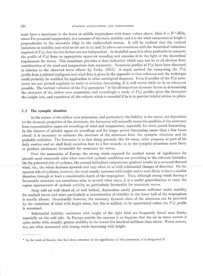
120 AVIATION APPLICATIONS AND FORECASTING
must have a maximum in the lower or middle troposphere with lesser values above. Here a = B- 1 dBj{Jz,
where 8 is potential temperature, is a measure of the static stability and il is the wind component at height z
perpendicular to the mountain ridge in the undisturbed stream. It will be realized that the vertical
variations in stability and wind as set out in (a) and (b) above are consistent with the theoretical variations
required of F(z), but the two factors are not independent. In doubtful cases it is often profitable to compute
the profile of F (z) from an appropriate upper-air sounding and examine it in the light of the theoretical
requirement for waves. This sometimes provides a clear indication which may not be at all obvious from
consideration of the wind and temperature data separately. Numerous profiles of F(z) have been discussed
in relation to the observed wave effects by Corby (1957). A rapid method for computing the F (z)
profile from a plotted tephigram and wind data is given in the appendix to that reference and the technique
could probably be modified for application to other aerological diagrams. Even if profiles of the F (z) para
meter are not plotted regularly to assist in aviation forecasting, it is well worth while to do so whenever
possible. The vertical variation of the F(z) parameter * is the all-important dynamic factor in determining
the character of the airflow over mountains, and accordingly a study of F(z) profiles gives the forecaster
the insight into, and experience of, the subject which is essential if he is to provide helpful advice to pilots.
3 . 2 The synoptic situation
As the nature of the airflow over lTIOuntains, and particularly the liability to lee waves, are dependent
on the dynamic properties of the airstream, the forecaster will naturally assess the qualities of the airstream
from representative upper-air soundings of wind and temperature, especially for short period forecasting.
In the absence of suitable upper-air soundings and for longer period forecasting (more than a few hours
ahead) it is necessary to estimate the structure of the airstream from the synoptic situation and its
probable evolution. The forecaster is in fact doing precisely this for many other purposes as part of his
daily routine and we shall limit ourselves here to a few remarks as to the synoptic situations most likely
to produce airstreams favourable for mountain lee waves.
Over the mountains of Europe the strong winds required for marked waves of significance for
aircraft most commonly arise when unsettled cyclonic conditions are prevailing in the relevant latitudes.
On the poleward side of cyclones, the normal latitudinal temperature gradient results in a reversed thermal
wind, viz., thew inds decrease upwards and may often do soWith substantial changes of direction. On the
equator side of cyclones, however, the wind usually increases with height and is more likely to have a similar
direction through at least a considerable depth of the troposphere. Thus, although strong winds having a
favourable structure can sometimes arise in several other ways, it is a useful generalization to treat the
region equatorward of cyclonic activity as particularly favourable for mountain waves.
Deep cold air well ahead of, or well behind, depressions rarely possesses sufficient static stability
for marked waves and more particularly a concentration of stability in the lower half of the troposphere
is usually absent. Occasionally however, the necessary dynamic state of the airstream can be provided
by the variations of wind with height alone, but this is unlikely to be appreciated unless the F(z) profile
is examined.
Substantial stability variations with height of the right kind are frequently found near fronts,
especially on the cold side. In Europe outside the summer it so happens that the air in warm sectors is
quite stable with, usually, greater stability in the lowest few hundred millibars than above. \iVarm sectors,
too, are often associated with strong winds increasing with height.
* In the work of Scorer, who first drew attention to the significance of this parameter, it is designated £2.
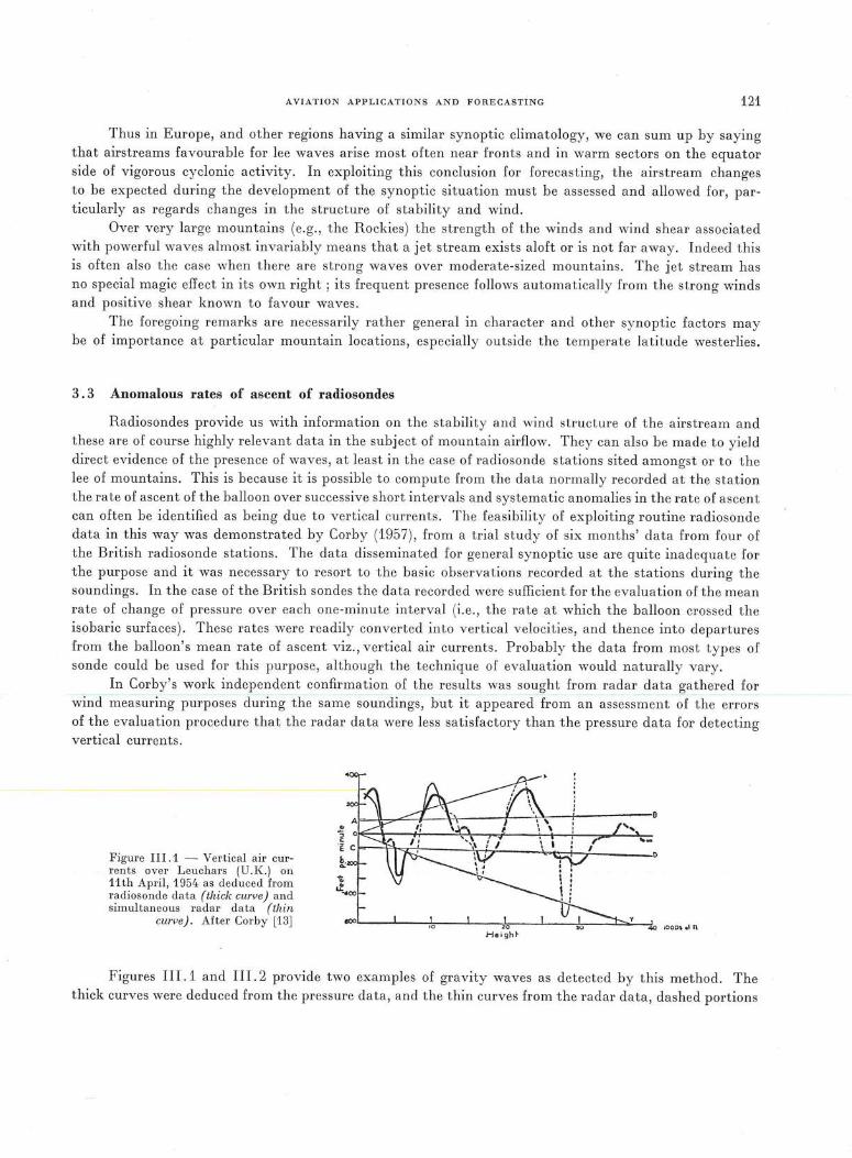
AVIATION APPLICATIO NS AND FORECASTING 121
Thus in Europe, and other regions having a similar synoptic climatology, we can sum up by saying that airstreams favourable for lee waves arise most often near front s and in warm sectors on the equator side of vigorous cyclonic activity. In exploiting this conclusion for forecasting, the airstream changes to be expected during the development of the synoptic situation must be assessed and allowed for , particularly as regards changes in the structure of stability and wind.
Over very large mountains (e.g., the Rockies) the strength of the winds and wind shear associated with powerful waves almost invariably means that a jet stream exists aloft or is not far away. Indeed this is often also the case when there are strong waves over moderate-sized mountains. The jet stream has no special magic effect in its own right ; its frequent presence follows automatically from the strong winds and positive shear known to favour waves.
The foregoing remarks are necessarily rather general in character and other synoptic fa ctors may be of importance at particular mountain locations, especially outside the temperate latitude westerlies.
3 . 3 Anomalous rates of ascent of radiosondes
Radiosondes provide us with information on the stability and wind struct ure of the airstream and these are of course highly relevant data in the subj ect of mountain airflow. They can also be made to yield direct evidence of the presence of waves, at least in the case of radiosonde stations sited amongst or to the lee of mountains. This is because it is possible to compute from the data normally recorded at the station the rate of ascent of the balloon over successive short intervals and systematic anomalies in the rate of ascent can often be identified as being due to vertical currents. The feasibility of exploiting routine radiosonde data in this way was demonstrated by Corby (1957), from a trial study of six months' data from four of the British radiosonde stations. The data disseminated for general synoptic use are quite inadequate for the purpose and it was necessary to resort to the basic observations recorded at the stations during the soundings. In the case of the British sondes the data recorded were sufficient for the evaluation of the mean rate of change of pressure over each one-minute interval (i. e., the rate at which the balloon crossed the isobaric surfaces). These rates were readily converted into vertical velocities, and thence into departures from the balloon's mean rate of ascent viz., vertical air currents. Probably t he data from most t ypes of sonde could be used for this purpose, although the technique of evaluation would naturally vary.
In Corby's work independent confirmation of the results was sought from radar data gathered for wind measuring purposes during the same soundings, but it appeared from an assess~nent of -the error~ of the evaluation procedure that the radar data were less satisfactory than the pressure data for detecting vertical currents.
Figure I II . 1 - Vertical air currents over Leuchars (U. K .) on 11th April, 1954 as deduced from radiosonde data {thick curve) and simultaneous radar data {thin
curve). Af ter Corby (13]
... ... .. _ t= ~~~ ·,~, ,7' \. ~i 71
0
10 2n ""' .q0 1000\ oi I\
Figures III.1 and Ill. 2 provide two examples of gravity waves as detected by this method . The thick curves were deduced from the pressure data, and the thin curves from the radar data, dashed portions
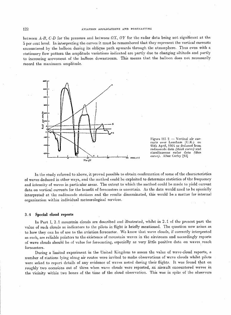
122 AVIATION APPLICATIONS AND FORECASTING
between A-B, C-D for the pressure and between OX, OY for the radar data beii1g not significant at the
5 per cent level. In interpreting the curves it must be remembered that they represent the vertical currents
encountered by the balloon during its oblique path upwards through the atmosphere. Thus even with a
stationary flow pattern the amplitude variations indicated are partly due to changing altitude and partly
to increasing movement of the balloon downstream. This means that the balloon does not necessarily
record the maximum amplitude.
"
Figure Ill. 2 - Vertical air currents over Leuchars (U.K.) on 15th April, 1954 as deduced from radiosonde data (thick curve} and simultaneous radar data (thin curve). After Corby [13]
In the study referred to above, it proved possible to obtain confirmation of some of the characteristics
of waves deduced in other ways, and the method could be exploited to determine statistics of the frequency
and intensity of waves in particular areas. The extent to which the method could be made to yield current
data on vertical currents for the benefit of forecasters is uncertain. As the data would need to be specially
interpreted at the radiosonde stations and the results disseminated, this would be a matter for internal
organization within individual meteorological services.
3 . 4 Special cloud reports
In Part I, 2 .1 mountain clouds are described and illustrated, whilst in 2. 1 of the present part the
value of such clouds as indicators to the pilots in flight is briefly mentioned. The question now arises as
to how they can be of use to the aviation--forecaster. We know that wave clouds, if correctly interpreted
as such, are reliable pointers to the existence of mountain waves in the airstream and accordingly reports
of wave clouds should be of value for forecasting, especially as very little positive data on waves reach
forecasters. During a limited experiment in the United Kingdom to assess the value of wave-cloud reports, a
number of stations lying along air routes were invited to make observations of wave clouds whilst pilots
were asked to report details of any evidence of waves noted during their flights. It was found t_hat on
roughly two occasions out of three when wave clouds were reported,- an aircraft encountered waves in
the vicinity within two hours of the time of the cloud observation. This was in spite cif the observers
A V!ATION APPLICATIONS AND FORECASTING 123
having been given only brief written instructions regarding the recognition of such clouds. The experiment confirms that when they are seen from the ground, wave clouds provide a useful indication of wave activity sufficient to affect aircraft. On the other hand, on only one occasion in five or six of those when pilots reported waves were any wave clouds reported from the nearest ground stations. Thus the absence of wave clouds does not mean that there are no waves.
In view of the paucity of other relevant data on a current basis, it is probably worth while for meteorological services to arrange for the special reporting of orographic clouds at appropriate stations and for the reports to be disseminated amongst their aviation forecast offices. In addition, there is probably a case for special provision in the synoptic codes for the reporting of orographic wave clouds in more detail than the present codes permit.
3 . 5 Reports from aircraft
Although the good forecaster is always attempting to predict the onset of precipitation, fog, thunderstorms, etc., in advance of their appearance in the area he is concerned with, nevertheless actual reports of the phenomena are vital. They add to the forecaster's confidence and to the precision which he can achieve in dealing with the subsequent developments. Furthermore, actual reports may indeed sometimes surprise the forecaster by indicating phenomena which he was not expecting.
In the problem of mountain waves, the forecaster may assess the properties of the airstream and form an opinion as to the likelihood of waves (see 3.1), he may have some relevant evidence in the form of cloud reports (see 3. 4), or data on vertical currents from radiosonde stations (see 3. 3), but the only direct observations of waves he is likely to receive on a day to day basis will be those from aircraft. As the forecasting problem is very difficult and positive data are hard to come by, it is essential that maximum use should be made of aircraft reports.
A regular reporting scheme can only be established successfully if aviation forecasters specifically discuss mountain waves with pilots at briefing and appeal for in-flight reports , impressing on them their great value. Such di scussions are bound to be mutually beneficial. In particular, pilots can be asked to avoid ambiguity by making clear in their reports whether the effects observed occurred with the aircraft "riding the waves" freely (in which case the main effects are height changes) or whether the aircraft was on altitude-coupled autopilot (in which case the main effects are airspeed changes). Information on turbulence should naturally be included also. The standard codes currently in operation for aircraft reports do not allow adequate reporting of mountain airflow effects and the reports must necessarily be of the plain language type.
4. The wavelength and amplitude of lee waves
4. 1 Estimating the wavelength
The horizontal scale of the disturbance imposed on an airstream immediately above a mountain ridge is determined almost entirely by the scale of the ridge and the question of estimating the wavelength in this vicinity does not arise. In contrast the wavelength of any lee waves above level ground downstream of the ridge is directly dependent on the characteristics of the airstream and is therefore amenable to calculation, in theory at least. However the amount of calculation would be quite prohibitive for routine application, except given the resources of an electronic computer. Fortunately it is possible to obtain a fair estimate of the lee wavelength, which is quite adequate for many purposes, in a simple fashion .
124 AVIATION APPLICATIONS AND FORECASTING
As explained in 3 .1, the relevant parameter expressing the dynamical state of the airstream at any
level is given by
F(z) = ag az
where a is the static stability and u is the horizontal wind speed. The theory indicates that the wave
length of any lee waves will lie somewhere between the maximum and minimum values of 2nfvF(z) or
2naj,lga through the troposphere. Now althou gh the static stability in shallow layers varies widely from
one air mass to another, the mean stability through the whole troposphere does not. Thus we should
expect the lee wavelength to be approximately proportional to the mean tropospheric wind speed. If
we assume a mean stability corresponding to about half the adiabatic lapse rate we obtain for the lee
wavelength :
where ?.. is in km and u in m/sec.
1 -}, = 2 u (1)
In support of this rough theoretical estimate, Corby (1957) found, in the study of waves from routine
radiosonde soundings referred to in 3. 3, a correlation coefficient of 0.91 between the observed wavelength
and the mean tropospheric wind speed. The regression relation was :
?.. (km) = 0.585 u (m /sec) - 2.8 (2)
This relation is not far removed from the approximate theoretical formula at Eq. (1). Larsson (1954)
also found in his study of wave clouds (see Part I, 2. 5 . 4) that simple estimates of the wavelength obtained
by this approach showed good agreement with observations. As the wavelength is rarely of vital importance
in aviation forecasting such estimates should suffice when they are required.
The above wavelength considerations apply to lee waves of the most common type, viz. those which
have their greatest amplitude in the lower or middle troposphere and decrease above. Occasionally lee
waves occur with their greatest amplitude in the upper troposphere or lower stratosphere. Once again
the general wavelength equation cannot be solved rapidly but by treating the stratosphere as of infinite
stability one obtains an approximate value of the wavelength from the relations :
?.. = 2nfk
h V F (z) - k2 = n ) (3)
where h is the height of the tropopause and F(z) is a mean for the troposphere as before. Equations (3) are
consistent with observations in that with typical values they suggest much longer wavelengths for this
type of wave, but the relation has not been verified in any detail.
Although the point may only rarely be of importance in aviation forecasting it is appropriate to
mention here that the crest of the first lee wave downstream of a mountain ridge is commonly observed
to be less than one wavelength from the mountain crest. Indeed for a symmetrical ridge theory indicates
that the spacing should be % },,
4. 2 Factors governing the amplitude
The amplitude of any lee waves is naturally of the greatest importance for aviation but is unfortu
nately almost intractable from the forecasting point of view. This is because the amplitude depends in
a complex way on both the topography as well as the properties of the airstream. These aspects were the
subject of a theoretical study by Cm·by and Wallington (1956) briefly described in Part 11, Section 3.
AVIATION APPLICATIONS AND FORECASTING 125
However, although it is not yet possible to predict the lee wave amplitude quantitatively, a knowledge of the relevant factors is valuable background knowledge for a forecaster.
For symmetrical mountain ridges the lee wave amplitude depends on the height of the ridge above the surrounding countryside and also on the horizontal scale of the ridge. The dependence on height, viz. approximate proportionality, is to be expected. The dependence on horizontal scale may be regarded as a resonance effect . The power spectrum of the mountain cross-section necessarily has one or more concentrations in the vicinity of particular wavelengths (of the usual idealized symmetrical cross-section often adopted in theoretical work there is of course only one such concentration). If the topography possesses one of these maxima near the natural wavelength of the airstream, then the lee wave amplitude will be much greater than otherwise. Put in another way, we may say that if the horizontal scale of the mountain roughly coincides with the lee wavelength, the wave amplitude will be much larger than for both broader and narrower mountains. In P art II , Fig. II .13 illustrates this effect, which is moderately critical. It follows that for a given airstream flowin g over mountainous terrain the largest amplitude waves will not necessarily be found to the lee of the largest mountains. In making use of this result , we must bear in mind that most mountainous terrain contains irregularities on a wide range of scales and in particular broad mountains often have superposed short wavelength features . Furthermore, broad mountains may have steep lee slopes (e .g. Sierra Nevada) and it is of course the character of the lee slope which is of most importance.
As regard the dependence of lee wave amplitude on the airstream characteristics, the main theoretical results are given in Part II, Section 3. The plain language interpretation may be stated as follows. The amplitude of lee waves is subject to wide variations even amongst airstreams having similar profiles of wind and stability because of the critical way in which the amplitude depends on the airstream characteristics. Other things being equal, the largest amplitude lee waves occur when the airstream satisfies the condition for waves by only a small margin, and in this region large changes in amplitude may result from small changes in the airstream. Apart from the question of this sensitive region, it may be said that larger amplitude waves are theoretically more likely in airstreams containing a shallow layer of great stability than in conditions of lesser stability through a deep layer .
A theoretical result which can be exploited in forecasting is concerned ·with the amplitude variation of lee waves with height. Generally speaking, the maximum amplitude is attained in or near the layer of maximum stability. If the stability is concentrated in a shallow layer , as for example at an inversion, The amplitude has a sharper maximum near th!Slevel and falls off rapidly hoth above andbelow. If the stability maximum is diffuse the variation of lee wave amplitude with height follows the same pattern but is more gentle. This result is well supported by observations and enables forecasters to provide useful advice as to choice of flight level.
5. Character of the topography
We have already noted (Section 4. 2) that if the horizontal scale of a symmetrical mountain ridge roughly matches the wavelength of the airstream, the lee wave amplitude will be greater than for narrower or broader mountains. Vve now record other results of this t ype and indicate further ways in which the lee wave characteristics are influenced by the shape and scale of the mountains.
5 . 1 Asymmetrical and irregular mountains
By means of electronic computation Wallington (1958) has been able to draw some conclusions relating to more realistic mountain profiles than the simple symmetrical shape commonly used in most
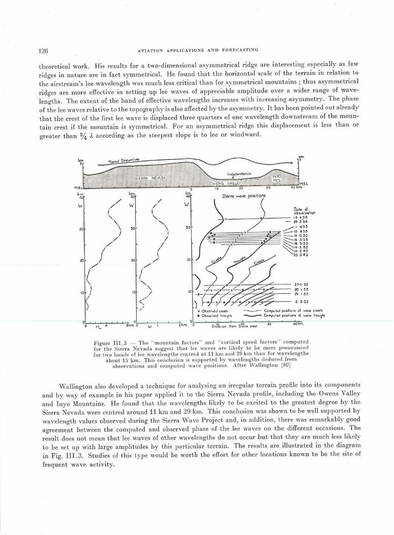
126 AVIATION APPLICATIONS AND FORECASTING
theoretical work. His results for a two-dimensional asymmetrical ridge are interesting especially as few
ridges in nature are in fact symmetrical. He found that the horizontal scale of the t errain in relation to
the airstream's lee wavelength was much less critical than for symmetrical mountains ; thus asymmetrical
ridges are more effective in setting up lee waves of appreciable amplitude over a wider range of wave
lengths. The extent of the band of effective wavelengths increases with increasing asymmetry. The phase
of the lee waves relative to the topography is also affected by the asymmetry. It has been pointed out already
that the crest of the first lee wave is displaced three quarters of one wavelength downstream of the moun
tain crest if the mountain is symmetrical. For an asymmetrical ridge this displacement is less than or
greater than % A according as the steepest slope is to lee or windward.
km. kJiB ':w· ~or // /
'W w / ! i Dote of
" .,
'\ '· 30~ \ 30 \ :30
/ i / I
/ / / I ! \
20~ I 20 ./ // /
I I \
I 10 .. j
/ \ I
0 0
I i ........
j~·-·"---;7" 27-11 · ~2 ., 10 j 10 x-e~x-- 30 · 1 · ~2
/' )·-r-. 2'J I ~2
~ 3 3·~2 ' ·, ;'
j
x Observed cre:!ls --- Computed po5itions oF wdYe crests
0 Observed troughs -.........-- Comp._Jted positiO'"'IS cJ. wdve rrougbs
0 0
M... 4 a km. o w I 2km. 0 D i~&nc.e from S~e~r"d cres~ 30 40km.
Figure Ill. 3 - The " mountain factors " and " vertical speed factors " computed
for the Sierra Nevada suggest that lee waves are likely to b e more pronounced
for two bands of lee wavelengths centred at 11 km and 29 km than for wavelengths
about 15 km. This conclu sion is supported by wavelengths deduced from
observations and computed wave positions. After \Vallington [80]
' Vallington also developed a technique for analysing an irregular terrain profile into its components
and by way of example in his paper applied it to the Sierra Nevada profile, including the Owens Valley
and Inyo Mountains. He found that the wavelengths likely to be excited to the greatest degree by the
Sierra Nevada were centred around 11 km and 29 km. This conclusion was shown to be well supported by
wavelength values observed during the Sierra Wave Project and, in addition, there was remarkably good
agreement between the computed and observed phase of the lee waves on the different occasions. The
result does not mean that lee waves of other wavelengths do not occur but that they are much less likely
to be set up with large amplitudes by this particular terrain. The results are illustrated in the diagram
in Fig. Ill. 3. Studies of this type would be worth the effort for other locations known to be the site of
frequent wave activity.
AVIATION APPLICATIONS AND FORECASTING 127
5 . 2 Phase effects and resonance
It is often convenient to regard the displacement of the streamlines above mountains as being made up of two parts, viz., the deformation due t o any mountain in the vicinity below and that due to the lee waves . For any given airstream the former deformation is closely dependent on t he mountain profile, but it so happens that when the airstream favours lee waves the deformation immediately above a moun tain has a larger amplitude than otherwise and also has its maximum amplitude at roughly the same level as that of the lee waves.
The lee waves arising from different terrain features will interfere, but in this connexion it is to be noted that the superposition of two waves of the same wavelength but of different phase and amplitude still results in a wave of the same wavelength. In addition t here will be interference between the deformation above particular mountains and the lee waves from other mountains upstream.
A further complication arises because occasionally an airstream can contain two wavelengths neither of which completely dominates the other for all terrain features. vVe have in mind that the large mountains will excite mainly the longer, and the small mountains the shorter , lee wavelength. In these circumstances the variation of lee wave amplitude with height may be quite different for the two sets of waves.
It is for reasons such as the above that t he pattern of vertical currents, and similarly of wave clouds, above very irregular terrain may be so complicated as to bear no obvious relation to the t errain itself. Clearly, also, quite small changes in the characteristics of t he airstream may result in large changes in the location and magnitude of vertical currents. Thus over a region of very irregular hills the forecaster cannot as yet hope to do more than indicate the general character and intensity of the ·wave activity to be expected .
5. 3 Three-dimensional hills
Certain conclusions have been drawn regarding the effect of individual hills of various shapes, as distinct from infinite two-dimensional ridges ; these are of more than passing interest from the forecasting point of view.
Both theory and observation show that individual hills are much less effective in giving rise to lee waves than are- very long ridges of similar cross -section lying across -the, vind-:- In particular-the first lee wave is of smaller amplitude and the waves die away much more rapidly downstream. The effect of oval hills and short ridges lying across the wind is intermediate in character between these alternatives . This is due to the air flowing partly around as well as over the three-dimensional obstacle . An additional effect is that the amplitude of any lee waves produced by an isolated hill falls oiT much more rapidly with height than those due to a long ridge. As a consequence of these effects, forecasters and pilots can aiTord to pay much less attention to isolated mountains in comparison with long ridges of similar height.
Gerbier found in the course of his field work in the French Alps (see Part I, 2 . 5. 6) that the shape of the crest line, when viewed in plan , was a relevant factor. A ridge having a crest line which is concave towards the upstream direction is more favourab le for lee waves than one having a convex crest line. This is clearly also related to the ease with which some of the air is able to avoid flowing over the summit by passing around the sides of the ridge.
5 . 4 Separation of the flow
Sometimes over mountainous terrain there are departures from streamline flow on a much larger scale than we usually have in mind when considering turbulence. An example of this is the so-called
128 AVIATION APPLICATIONS AND FORECASTING
"standing-eddy streaming" of Fi:irchtgott's classification (see Part I, 2. 5. 3) where the dimensions of the
large lee eddy may run into kilometres. This kind of phenomenon concerns what is known as separation ;
the lowest streamline leaves the surface completely and returns subsequently. That separation is com
mon in mountainous terrain is well known. It can often be observed from the low-level wind field as
revealed by the movement of smoke or dust. In the absence of natural indicators it can sometimes be
neatly demonstrated by releasing smoke or zero-lift balloons from the top of an abrupt escarpment or
cliff top when the general wind is away from the cliff. Indeed, this leads us to the main topographical
factor favouring separation of the flow, namely the existence of a sharp-edged escarpment having the
character of a cliff. In such a case separation takes place much more readily than over a smooth rounded
summit. As regards the meteorological factors, high static stability at low levels obviously tends to inhibit
separation. Separation is important because it may have large repercussions on the flow at higher levels. If a
large eddy fills the space to the lee of a mountain, the streamlines above are smoothed out and we may
regard the effective shape of the mountain as being completely modified by the presence of the eddy. If
a mountain is to have its maximum potential effect on the flow aloft, the low-level flow must be induced
to follow the contours ; any process which prevents this will reduce the mountain's effect . Thus in practice,
although the generalization that "steep lee slopes favour lee waves" is mostly true, if they are too steep
and have a sharp-edged summit, lee waves may often be negligible owing to the effect of separation of
the flow. Actually it is not always easy to separate cause and effect in this context because an essential
feature accompanying lee waves is strong flow down the lee slope and in marginal cases it may in fact be the
onset of lee waves which brings separation of the flow to an end.
6 . Tmbulence
Part Ill, Section 1 (Flying aspects of mountain waves) contains a mainly descriptive account (in
1. 2) of the distribution and intensity of turbulence to be expected in association with the airflow over
mountains . The information given is also essential knowledge for the forecaster and we shall confine
ourselves here to some additional- remarks direct-ed specifically to -the -forecasting problem.
At the outset we must remember that in current aviation forecasting, turbulence, however caused,
is only predicted in a rough qualitative fashion. For a given state of turbulence in the atmosphere, there
is necessarily enormous variation in the behaviour of different aircraft. Assuming the turbulence comprises
a broad spectrum of eddy sizes, an aircraft is highly selective in responding to these eddies ; the aircraft
acts as a kind of filter, and is affected much more by some eddy sizes than others. The response charac
teristics of the aircraft depend on its size, speed and several aerodynamic parameters. Thus even if the
turbulence structure could be stated in precise quantitative form, the information would be of little use
to the pilot in the absence of elaborate data on his aircraft. For general turbulence forecasting, therefore,
judicious use of the descriptive terms light, moderate or severe is about as far as the forecaster is normally
able to go.
6. l Turbulence in the friction layer
Quite apart from the phenomena of waves, rotors, etc., we must expect the greater degree of surface
roughness of hilly terrain to bring about an intensification of turbulence in the friction layer in comparison
with flat country. As turbulence forecasting is highly subjective and only qualitative, the forecaster can
AVIATION APPLICATIONS AND FORECASTING 129
best cover this by predicting turbulence over high ground to one degree higher on the descriptive scale than is expected over flat country, unless he has definite reasons to the contrary, e.g., aircraft reports. For example, if in a strong, unstable airstream moderate turbulence is expected generally in the friction layer and in Cumulus cloud, the forecaster may add appropriately "but locally severe over high ground". If severe turbulence is being forecast generally, he might add "especially over high ground".
If the air route passes over a substantial mountain ridge in conditions favouring powerful waves, etc., the forecaster will need to draw special attention to the violent turbulence liable to be encountered immediately above the ridge and in the fohn wall region. Naturally, however, the pilot should not in normal circumstances plan to fly in the friction layer under such conditions.
6 . 2 Turbulence in the rotor zone
The characteristics of the rotor zone have been fully described elsewhere in this monograph (e.g. Part I, 2. 5. 5 and 2. 5. 6) and have been discussed from the flying point of view in Part Ill, 1. 2. 2. The violence of the turbulence to be found in this region has been amply established and the inescapable conclusion appears to be that aircraft must at all costs avoid flying through this zone. In order properly to discharge his responsibilities, the forecaster must acquire experience of the liability to strong rotors at the mountain ridges along the air routes for which he has to forecast. The pilot too should possess this experience, but it is for the forecaster to warn him of the specific occasions when and where well-developed rotors are likely to be operating.
6. 3 Turbulence in waves
We have seen that outside the regions of waveflow known to be often associated with severe turbulence, flight through waves is commonly quite smooth. It is, however, sometimes turbulent and it appears that this type of turbulence is caused by the additional wind shears which may be imposed on the airstream in the region of waveflow. Such turbulence cannot be predicted in any detail or with any reliability, but forecasters can often indicate the height at which it is most likely to occur. The shear will be greatest where the wave amplitude is changing most rapidly with height. When the air mass possesses a strong inversion this is likely to be the level of maximum amplitude and a particularly rapid decrease of amplitude with height is then to be expected in the layers immediately above the inversion.
The abrupt breakdown of smooth waveflow into chaotic turbulence through a considerable depth of the troposphere is a phenomenon which is known to occur occasionally, but the process is imperfectly understood and the available explanations are speculative. There is therefore no basis as yet for forecasting such developments and an awareness on the part of pilots that this sometimes happens must for the time being suffice.
6. 4 High-altitude turbulence
The occurrence of high-altitude turbulence in general is a troublesome problem, mainly because there is no adequate dynamical theory providing a satisfactory explanation. The statistical evidence points clearly to an association with the jet stream core, particularly the cold side, but can only be exploited by forecasters to indicate the approximate probability and preferred location of any high-altitude turbulence. As regards the additional effect of high ground, evidence is accumulating that over mountains, high-altitude turbulence (clear air or otherwise) is more frequent and intense than elsewhere, especially
130 AVIATION APPLICATIONS AND FORECASTING
when the mountains are large. This is of course highly plausible and forecasters can do little more than
bear this in mind during their aviation work.
7 . Cloud distribution and icing
Cloud is formed by the ascent of moist air, the most familiar forms of ascent being on the scale of
fronts or other synoptic systems and of convection clouds. As mountains impose their own field of vertical
motion on the airstreams flowing over them, they also influence the distribution of cloud and the liability
to aircraft icing.
7. 1 Cloud distribution
The various types of individual mountain clouds are fully described in Part I, Section 2.1 but in
aviation forecasting we do not normally predict individual clouds. We are concerned here with the general
cloud cover on a rather larger scale than that of individual clouds. That mountains have a profound effect
on the general cloud cover is well known and is borne out by the close correspondence between rainfall
isopleths and geographical contours. For general aviation purposes, the forecaster requires to know the meteorological conditions in which
the cloud amount over ranges of hills and mcuntains will be greatly augmented and the vertical depth
of cloud greatly increased. Obvious conditions for this are a moist air mass, such as those which reach
coastal mountain barriers from the ocean, and a wind current perpendicular to the mountains. Maximum
lifting of the air mass is also encouraged if the mountain chain is an extensive one having a considerable
length across the airstream. To achieve a greatly increased depth of general cloud over mountains, naturally the air mass requires
to be moist in depth butin this context the wind and stability structure are also relevant. The theory of
the airflow over mountains indicates that the vertical velocity of the air above is subject to a vertical
variation such that upward motion in the lowest levels may be reversed at some level above and replaced
by downward motion. Further reversals may take place at still higher levels. Sawyer (1956) has considered
this effect in relation to the orogr~phic rainfall over mountain barriers of overall width 50 km or more
and his conclusions have direct application to the question of cloud cover. Clearly if a mountain barri~r is to cause continuous cloud in great depth, the height at which the upward motion first ceases- must be
as high as possible. He found that the factors favouring this were :
(a) a lapse rate which is near neutral stability, without markedly stable layers or inversions, and
(b) a vertical wind profile with d2ii,fdz2 positive (as is often found beneath a jet stream).
Sawyer was able to find support for this thesis from synoptic studies. If the conditions are not
realized, there may well be continuous low cloud formed over the mountains and some other layers above,
but there is unlikely to be continuous and dense orographic cloud through a substantial depth of the
troposphere. There are several other ways in which mountains influence the cloud cover above them. For example,
the lifting of a potentially unstable air mass at a mountain barrier may give rise to wide-spread thundery
cloud ; a fi:ihri effect may maintain a complete absence of cloud on the lee side ; the valleys may fill up with
fog· on quiet radiation nights ; the sunny slopes are often favourable locations for thermal currents and
cumuhrs cloud formation. Howeviw most such phenomena are only indirectly connected with the character
AVIATION APPLICATIONS A N D FORECASTI NG 131
of the airflow over mountains and they are already part of the stock-in-trade of forecasters concerned with mountain regions. They will not therefore be discussed here.
7.2 Icing
The flying aspects of icing in cloud over mountains have been r eferred to in Part II I, Section 1. 5 and we assume that the aviation forecaster is familiar with these. The latter is concerned with three aspects, viz. modifications to the level of the 0°C isotherm, which must be specified as a routine in forecasts , modifications to the general cloud cover, already discussed in 7.1 above, and changes in the intensity of icing caused by mountains.
Now, given a representative upper-air sounding plotted on an aerological diagram it is a straightforward matter to ascertain the effect of lifting the whole air mass in a specified manner. As, however , it is impracticable to determine the pattern of vertical motion above mountains in any detail, we are obliged to adopt some compromise in forecasting. A reasonable basis for the present purpose is to assume that the air at all levels follows the shape of the high ground. The maximum effect on the level of the 0°C isotherm may then be assessed from the aerological diagram. The choice of upper-air sounding should be such that the sounding itself is unlikely to have been affected by any similar mot ions. This constitutes a reasonable basis on which to forecast the lowering of the OoC isotherm especially if good waves are reasonably certain. Actually high ground can cause waves having an amplitude greater than that of the topography, even at heights a few thousand metres above the surface. However, if the height of the highest ground is used in applying the procedure, including that of individual peaks, some additional tolerance will automatically be included. The procedure yields plausible values when applied to moderate-sized mountains but if applied arbitrarily to very large mountains (e.g., higher than 3,000 m ) the results may appear somewhat absurd ; in such cases t he values must of course be tempered by common sense.
The intensity of icing is always a difficult matter. This is because the relevant parameters, e.g., drop size, liquid water concentration and certain aerodynamic characteristics of the aircraft , are not known to the forecaster and cannot t hemselves be predicted. Thus, as in the case of turbulence, predictions of icing intensity are necessarily qualitative and subj ective, being confined to the descriptive terms light, moderate, severe (or icing index low, moderate , high). However, in view of the greater liquid water content known to obtain in clouds over mountains, if the forecaster expects some degree of icing generally he will be well advised to indicate a greater liability and intensity over mountains whatever kind of airflow is expect ed. If it so happens that the levels where icing is expected coincide with a layer where waves are likely to occur with large amplit ude, he can predict worse icing conditions with more confidence.
8 . Diurnal and seasonal variations
The probability of mountain waves will naturally be assessed by the forecaster in the light of the current situation and type of airstream, etc. However , it is useful to be aware of the diurnal and seasonal variations to be expect ed in mountain wave activity . These follow quite naturall y from the known variations of the relevant meteorological factors but depend also, of course, on the synoptic climatology of the particular region.
The lower layers of the atmosphere are subject to large diurnal variations of both stability and wind structure. The radiational cooling which sets in towards dusk on clear days has the effect of increasing
132 AVIATION APPLICATIONS AND FORECASTING
stability and decreasing wind speed in the surface layers ; accordingly the value of F (z) (see Part Ill,
Section 3 .1 ) is increased at these levels and the result is sometimes that waves become possible during
the evening when this may not have been the case during the day. They may continue during the night
and beyond sunrise until warming on the following morning decreases the stability and also F (z), provided
other changes do not prevent waves. This kind of eiTect is important for lee waves produced by small hills
but although often exploited by evening glider pilots in Europe such waves are mostly only of academic
interest for powered aviation. For moderate-sized hills and mountains the most important diurnal eiTect
is probably that of katabatic winds which ensure that the shape of the mountain is communicated to the
general airflow aloft (see also Section 5). For very large mountains diurnal eiTects are almost irrelevant;
the development of waves then depends on the whole troposphere and the waves form when the evolution
of the synoptic situation results in a suitable airstream, irrespective of the time of day or night.
As regards seasonal variations, the greater tendency during winter for low-level stability and
situations in which the wind is strong and increases markedly with height, suggests that orographic waves
should be more common during winter than at other seasons. The observations certainly indicate a marked
deficiency of waves during summer but the maximum is not in high winter in all regions ; there is some
times a double maximum in spring and autumn. Such diiTerences in the seasonal liability of mountain
waves merely reflect diiTerences in the synoptic climatology of the various regions.
List of References
1. Abe, M., 1932- The formation of cloud by the obstruction of Mount Fuji. Geophys. Mag., Tokyo, 6, pp. 1-10.
2. Abe, M., 1941 - Mountain clouds, their forms and connected air current. Part II. Bull. Central Met. Observatory of Japan, VII, 3, pp. 93-145.
3. Abe, M., 1942 - An attempt to make visible the mountain air current. J. Met. Soc., Tokyo, p. 69.
4. Austin, A.R.I., 1952 - Wave clouds over southern England. Weather, 7, pp. 50-53.
5. Bannon, J. K., 1952 - Weather systems associated with some occasions of severe turbulence at high altitude. Met. Mag., London, 81, pp. 97-101.
-----6~Batshe1or-,-G.--K.,---1-9S*l--'l'he-conditions for dynamical similarity of motions of a frictionless perfect-gas atmosphere. Quart. J. R. Met. Soc., 79, pp. 224-235.
7. Berenger, M. et Gerbier, N., 1956 - Les mouvements ondulatoires a St-Auban-sur-Durance (Basses-Alpes) ; premiere campagne d'etudes et de mesures. Janvier 1956. Monographic N° 4 de la Meteorologic N ationale.
8. Cols on, De V er, 1952 - Results of double-theodolite observations at Bishop, Cal., in connection with the "Bishop-wave" phenomena. Bull. Amer. Met. Soc., 33, pp. 107-116.
9. Colson, De V er, 1954 - Meteorological problems in forecasting mountain waves. Bull. Amer. Met. Soc., 35, pp. 363-371.
10. Corby, G. A., 1954 - The airflow over mountains. Quart. J. R. Met. Soc., 80, pp. 491-521.
11. Corby, G. A. and Wallington, C. E., 1956 - Airflow over mountains : the lee-wave amplitude. Quart. J. R. Met. Soc., 82, pp. 266-274.
--' 12. Cor by, G. A., 1957 - Airflow over mountains: notes l'or forecasters and pilots. Met. Rep., No. 18, H.M. Stationery Offwe.
13. Cor by, G. A., 1957 - A preliminary study of atmospheric waves using radiosonde data. Quart. J. R. Met. Soc., 83, pp. 49-60.
14. Corby, G. A. and Sawyer, J. S., 1958- The airflow over a ridge : the effects of the upper boundary and highlevel conditions. Quart. J. R. Met. Soc., 84, pp. 25-37.
15. Eliassen, A. and Palm, E., 1954 - Energy flux for combined gravitational-sound waves. Institute for weather and climate research, Oslo, Pub!. No. 1.
16. Fiirchtgott, J., 1949- Wave streaming in the lee of mountain ridges. Bull. Met. Czech., Prague, 3, p. t,9.
17. Fiirchtgott, J., 1950--=- The transport of small particles or insects over the Ore Mountains. Bull. Met. Czech., Prague, 4, pp. 14-16.
18. lfiirchtgott, J., 1957- Active turbulent layer downwind of mountain ridges. Schweizer Aero-Revue, Bern, 32, pp. 324-335.
19. French, G. M., 1951- Mountain waves and their effects on flight. Civil Aeronautics Board, Bureau of Safety Investigation, Safety Bulletin, 186-51. Washington D. C.
20. Georgii, W., 1956 - Flugmeteorologie. Akademische Verlagsgesellschaft M. B. H., Frankfurt am Main, 2. neubearbeitete Aufl., p. 332.
21. Gerbier, N. et Berenger, M., 1957 - Les ondes dues au relief dans les Basses-Alpes fran-.;aises. 2° campagne d'etudes et de mesures, janvier-fevrier 1957. Direction de la Meteorologic N ationale.
22. Gerbier, N. et Berenger, M., 1958 - Ondes de ressaut dans les Alpes franqaises. 3° campagne d'etudcs, janvier-fevrier 1958. Direction de la Meteorologic Nationale.
23. Hiiiland, E., 1951 - Fluid flow over a corrugated bed. Appendix A, fifth Progress Report, Contract No. AF 19 (122) - 263. Air Force Cambridge Research Center, Cambridge, Mass.
24. Holmboe, ,J. and Klieforth, H., 1957- Investigations of mountain lee waves and the air flow over the Sierra Nevada. Dept. Met. Univ. California.
25. Holmboe, J. and Klieforth, H., 1957- Investigations of mountain lee waves and the air flow over the Sierra Nevada. Final Report, Contract No. AF 19(604) -728. 290 p.
26. Idrac, P., 1923- Etude sur les conditions d'ascendance du vent favorable au vol a voile. Off. Nat. Met. de France, Paris, Memorial N° 7, 16 p.
27. Kelvin, 1886 - On stationary waves in flowing water. Philos. Mag., 5, 22, pp. 353-357, 445-452, 517-530.
28. Koschmieder, H., 1921 - Zwei bemerkenswerte Beispiele horizontaler Wolken-Schlauche. Beitr. Phys. frei. Atmos., 9, pp. 176-180.
29. Koschmieder, H., 1924 - Die Arbeiten des Messtrupps wahrend des 2. Segelflug-Wettbewerbes in Rossitten. Z. F. Flugtechnik und Motorluftschiffahrt, 15, pp. 236-242, 257-258.
30. Koschmieder, H., 1925 - Zur Kenntnis des Stromfeldes in Lee. Z. F. Flugtechnik und Motorluftschiffahrt, 16, pp. 240-2llll.
31. Koschmieder, H., 1951 - Dynamische Meteorologic, Akademische Verlagsgesellschaft, Leipzig, 3. Aufl., pp. 327-341.
32. Krug-Pielsticker, U., 1942- Beobachtungen der hohen Fiihnwelle an den Ostalpen. Beitr. Phys. frei. Atmos., 27, pp. 140-164.
33. Kuettner, J., 1939 - Moazagotl und Fiihnwelle. Beitr. Phys. frei Atmos., 25, pp. 79-114.
34. Kuettner, J., 1939 - Zur Entstehung der Fiihnwelle. Beitr. Phys. frei. Atmos., 25, pp. 251-299.
35. Kuettner, J. and Jenkins, C. F., 1953- Flight aspects of the mountain wave. Air Force Cambridge Research Center, Surveys in geophysics, Techn. Report No. 35.
134 LIST OF REFERENCES
36. Kuettner, J., 1958 - The rotor flow in the lee of mounta ins. Schweizer Aero-Revue, Bern, 33, pp. 208-215.
37. Laird, A. R., 1952 - Standing wave at Aberporth, .Met. Mag., London, 81, pp. 337-339.
38. Larsson, L ., 1954. - Observations of lee wave clouds in the Jiimtland Mountains, Sweden. T ellus, 6, pp. 124-138 .
39. Long, R. R., 1953 - Some aspects of the flow of stratified fluids. I : A theoretical investigation. Tellus, 5 , pp . 42-58.
40. Long, R. R., 1954 - Some aspec~s of the flo w of stratified fluids. II : Experiments of a two-fluid system. T ellus, 6, pp. 97-115.
41. Long, R. R., 1955 - Some aspects of the flow of stratified fluids. III : Continuous density gradients. Tellus, 7, pp. 341-357.
42. Ludlam, F. H., 1952 - Orographic Cirrus clouds. Quart. J. R. Met. Soc., 78, pp. 55lt-562 .
43. Ludlam, F. H. and Scorer, R. S., 1957 - Cloud s tudy: a pictorial guide . J . Murray, London. 80 p.
4ft. Lyra, G., 1940 - Ueber den Einfluss vonBodenerhebungen auf die Str6mung einer stabil geschichteten Atmosphiire. Beitr. Phys. frei. Atmos., 26, pp. 197-206.
45 . Lyra, G., 1943 -- Theorie der stationiiren L eewellenstr6mung in freier Atmosphii re. Z. angew. Math. Mech., 23, pp. 1-28.
46. Ly ra, G., 1952 - Bemerkungen iiber eine gewisse Klasse nicht-konstanter Anstromprofile beim L eewellenproblem. Vortrag auf der OSTIV-Tagung in Madrid. Beitr. Phys. Atmos., 31, pp. 147-151.
47. iVIagnus, \V., 1949 - Fragen der Eindeutigkeit und des Verhal tens im Unendlichen fur Lostmgen von /:;u + k 2 u = 0. Abh. Math. Sem. Univ. Hamburg, Bd. 16, H eft 1 /2, p. 77.
48. Manley, G., 1945- The Helm Wind of Crossfell, 1937-1939. Quart. J. R. Met. Soc., 71, pp.197-219.
49 . Mason, D., 195ft - Hill standing waves and safety heights. \Veather , 9, pp. 45-55 .
50. Merbt, H., 1952 - Solution of the two-dimensional lee-wave equation for arbitrary mountain profiles, and some remarks on the horizontal wind component in mountain flow. Vortrag auf der OSTIV-Tagung in Madrid. Beitr. Phys. Atmos., 31, pp. 152-161.
51 . Morgan, S. P., 1947 - Tables of Bessel functions of imaginary order and imaginary argument. California, Institute of Technology, Pasadena.
52. Palm, E., 1953 - On the formation of surface waves in a fluid flowing over a corrugated bed and on the development of mountain waves. Astrophysica Norvegica, 5, No. 3.
53. Palm, E., 1955 -Multiple-layer mountain wave models with constant stabili ty and shear. Scientific R ep. No. 3, Contract No. AF 19 (60!•)-728. Air Force Cambridge Research Center, Cambridge, Mass.
54. Pi lsbury, R. K., 1955 - A preliminary analysis of standing-wave reports received at N ortholt during .the winter of 1953-1954. Met. Mag., 84, pp . 313-318.
55. Prandtl, L., 1949 - Fiihrer durch die Str6mungslehre. Friedr. Vieweg u. Sohn , Braunschweig. 3. Aufl.
56. Queney, P ., 194 7 - Theory of perturba tions in stratified currents with a pplication to a irflow over mountain barri ers. The University of Chicago Press, l\I isc. Rep., No. 23.
57. Queney, P., 1948 - The problem of airflow over mountains : A summ a t·y of theo retical s tudies. Bull. Amer. l\Iet . Soc ., 29, pp . 16-26.
58. Queney, P., ·I95lt- Initial value problems in a double Couette-flow. Autobarotropic Flow Project, Scientific Rep. No. 1, Contract No. AF 19 (604)-728. Air Force Cambridge R esearch Center, Cambridge, Mass.
59. Queney , P ., 1955 - Rotor phenomena in the lee of mountains . Tellus, 7, pp. 367-371.
60 . Queney, P., 1958 - Effect of viscosity on Rayleigh waves: dynamics of s imple atmosp here flow. Scientific R ep . No . 2, Contract No . AF 19 (604)-728. Air Force Cambridge Research Center, Cambridge, Mass .
61. Radok, U ., 1954 - A pt·ocedure for studying mountain effects at low level. Bull. Amer. Met. Soc., 35, pp. !,12-416.
62. Rayleigh, R. J., 1883 - The form of standing waves on the surface of runnin g water. Proc. London Math. Soc ., 15, pp. 69-78.
63 . Rellich, F., 1943 - Ueber das asymptotische Verhalten von Losungen von /:; u + k 2 u = 0 in unendlichen Gebieten. Jahresber. Dt. l\Iath. Ver. , 55 .
64. Sawyer, J. S., 1955 - Dynamical similarity in an incompressible fluid mode l of two-dimensional airflow over a ridge. l\I.R.P. 935 . Air Ministry Meteorological Research Committee.
65 . Sawyer, J. S., 1956 - The physical a nd dynamical problems of orographic rain. Weather, 11, pp. 375- 381.
66 . Sawyer, J . S. and Hinds, l\I. K., 1957 - Numerical calculations of the a irflow over a ridge fo r small amplitudes. M.R.P. 1041 . Air Ministry Meteorological Research Committee.
67. Scorer, R. S., 19lt9 - Theory of waves in the lee of mountains. Quart. J. R. Met. Soc., 75, pp. 41-56 .
68. Scorer, R. S. , 1953- Theory of airflow over mountains. II: The flow over a ridge. Quart. J. R . Met. Soc., 79, pp. 70- 83.
69. Scorer, R. S., 1954.- Theory of airflow over mountains. III: Airstream characteristics . Quart. J. R. Met. Soc., 80, pp. 417-428.
70. Scorer, R. S., 1955 -Theory of airflow over mountains. IV : Separation of airflow from the surface. Quart. J. R. Met. Soc. , 81 . pp. 340-350.
71. Scorer, R. S., 1956 - Airflow over an isolated hill. Quart. J. R. Met. Soc., 82, pp . 75-81.
72 . Scorer, R. S. and vVi lkinson, M., 1956 - \Vaves in the lee of an isolated hil l. Quart. J. R. Met. Soc. , 82, pp. 419-427.
73. Scorer, R. S. (Voir Lucllam and Scorer).
74. Sommerfeld, A., 1912 - Die Greensche Funk lion der Schwingungsgleichung. Jahres ber. Dt. Math. Ve1·., 21 .
75. Sommerfelcl , A., 1948 - Vorlesungen iib er theoretische Physik. VI. Akademische Verlagsgesellschaft, Leipzig. Zweite neubearbeitete Aufla ge, p. 191.
LIST OF REFERE NCES 135
76. Stiimke, H., 19lt0 - Bem erkungen iiber di e h orizontalen Stromungsgeschwindigk eit en der in v ors tehender Arbeit (Lyra) behandelten Stromun g. Beitr. Phys. frei . Atmos., 26, pp . 207-2"10 .
77. Suzuki , S. and Yabuki, K ., 1956 - The airflow crossing over the m ountain range. Geophys. Mag., Tokyo, 27, pp . 273-291.
78 . Turner, H. S., 1951 - Standing waves and powered flight. Met. Mag., 80, pp. 106-109.
79 . Wallington, C. E., 1953 - OPS-ENG R epor t. Intern a t ional Air Transport Asso ciation .
80 . Wallington, C. E., 1958 - A numerical study of the topographical fa ctor in lee-wave amplitudes. Quart. J. R. Met. Soc., 84, pp . 428-433 .
81 . Wurtele, M., 1953- The initial-value lee-wave problem fo r the isothermal atmosph ere. Scientific R ep. No. 3, Sierra VVave Project, Contract No. AF 19 (122)-263. Air Force Cambridge R esearch Center , Cambridge, Mass.
82. vVurtele, M., 1953- Stud ies of lee waves in atmospheric models with continuously distributed s tatic s tabil ity . Scientifi c R ep. No . 4, Contract No. AF 19 (122)-263. Air Force Cambridge Research Cen ter , Cambridge, Mass .
83 . \Vurtele, JVI. , 1953 - On lee waves in the interface separating two barotropic layers. Final Report, Sierra Wave Project, Contract No. AF 19 (122)-263. Air Force Cambridge R esearch Center, Cambridge, Mass.
84 . Wurtele, M., 1957 - The t hree dimensional lee wave. Beitr. Phys. frei . Atmos ., 29, pp . 24.2-252.
85 . Zierep, J ., 1952 - L eewellen bei geschichteter Anstriimun g. Ber. Deutsch . \Vett erd. U. S. Zone, Nr . 35 , pp. 85-90.
86. Zierep, J ., 1956- Das Verhalten der Leewellen in der Stratosph iire. Beitr. Phys . Atmos. , 29, pp. 10-20 .
87 . Zierep, J., 1957- Neue Forschungsergebnisse a us dem Gebiet der atmosphiirischen Hinderniswellcn. Beitr. Phys . Atmos ., 29, pp. 1tt3-153.