afale e fi lw - vtechworks - virginia tech
TRANSCRIPT
A Bayesian Statistics Approach to Updating Finite Element Models
with Frequency Response Data
by
Brian E. Lindholm
Dissertation submitted to the Faculty of the
Virginia Polytechnic Institute and State University
in partial fulfillment of the requirements for the degree of
Doctor of Philosophy
in Mechanical Engineering
APPROVED:
Dr. Robert L. West, Jr
Afale E fi LW Dr. Charles E. Raiey /
Mele Oh bili he Dr. Larry D. Mitchell Dr. Alfred L. Wicks
August, 1996
Blacksburg, Virginia
Keywords: bayesian, regression, parameter estimation, model updating

A BAYESIAN STATISTICS APROACH TO UPDATING FINITE ELEMENT MODELS
WITH FREQUENCY RESPONSE DATA
by
Brian E. Lindholm
Dr. Robert L. West, Jr. Chairman Mechanical Engineering
(ABSTRACT)
This dissertation addresses the task of updating finite element models with
frequency response data acquired in a structural dynamics test. Standard statistical
techniques are used to generate statistically qualified data, which is then used in a
Bayesian statistics regression formulation to update the finite element model. The
Bayesian formulation allows the analyst to incorporate engineering judgment (in the
form of prior knowledge) into the analysis and helps ensure that reasonable and
realistic answers are obtained. The formulation includes true statistical weights
derived from experimental data as well as a new formulation of the Bayesian
regression problem that reduces the effects of numerical ill-conditioning.
Model updates are performed with a simulated free-free beam, a simple steel
frame, and a cantilever beam. Improved finite element models of the structures are
obtained and several statistical tests are used to ensure that the models are improved.

Acknowledgements
Many thanks are owed to my advisor, Dr. Robert West, for his unfailing support
and belief in what I was doing. His ability to see “the bigger picture” helped me go
further than I ever thought possible.
I thank Dr. Larry Mitchell for his guidance on the experimental work, and I thank
Dr. Rakesh Kapania, Dr. Charles Knight, and Dr. Alfred Wicks for helping me keep
some perspective on what I was trying to do. I also thank all of them for helping me
make sure that my work applied to the tricky cases as well as the friendly ones.
Special thanks are also due to Dr. Jeffrey Birch, who taught me so much of the
statistics that I use, and to Dr. Calvin Ribbens, who taught me how to do big matrix
problems on the computer. I also thank Dr. David Montgomery, who got me started
on the signa] processing statistics, and Randall Mayes of Sandia National Labs, who
helped me try out my ideas on a “real-world” structure.
And finally, I would like to thank my friends Elizabeth Besteman and David Coe
for their friendship and emotional support during the crunch at the end.
This material is based upon work supported in part under a National Science
Foundation Graduate Fellowship. Any opinions, findings, conclusions, or
recommendations expressed in this publication are those of the author and do not
necessarily reflect the views of the National Science Foundation.
Acknowledgements ili
Table of Contents
Abstract .......0 0... cc cc ee ew ee ee te ee te ee ete ii
Acknowledgements ...........-- eee eee eee eee te tee iti
Table of Contents ............ 0... eee eee et eee eee iv
List of Figures... 2... ee ee ee ee viii
List of Tables .. 0... . ee ee eee eens x
Nomenclature ... 0... 2.0... ccc ee ee ee eens xii
Part |: Introduction and Literature Review
Chapter 1: Introduction ........ ccc c ence cere ncnnssnnscees 2
1.1: Model Updating ............ cee eee ee ees 2
1.2: Research Goals ......... 0... ccc ee ee teens 4
1.3: Research Hypothesis .......... 0... 0c cee ee ees 4
1.4: Research Objectives ....... 0.0... cee ee ee ees 5
1.5: Scope of Research ........ 0... 0.00. cee eee es 7
1.6: Contributions of Research ......... 0... 0.0... fe)
1.7: Structure of the Dissertation ....................2000- 11
Chapter 2: Literature Review ............. 0c cece nace neee 14
2.1: Model Update Categorization ..................2.-200. 14
2.2: Recent Work in the Literature .................0000005 19
2.3: Comments on the Literature ............ 0... 0. 2000 ee 29
2.4: Other Relevant Work ......... 0... 00 cece eee ee eee 32
Part ll: Basic Statistical Theory
Chapter 3: Bayesian Statistics ........ 0.00 ccc cence ences 35
3.1: Ordinary Least-Squares .......... 0... 0c cece ees 35
3.2: Maximum Likelihood Estimation....................0.. 37
3.3: Maximum a Posterior Estimation ..................000. 42
3.4: Additional Comments on Statistics ..............00 cease 47
3.5: The Core Equations .......... 0.0... cece eee eee eee 50
Table of Contents
Chapter 4: Update Parameters ...........00c cee ccucecees 51
4.1: Model Update Parameters ................. eee ae 51
4.2: Bayesian Priors .......... eee ee ees 53
Chapter 5: Sine-Dwell Statistics .......... 00.0 cc eee eeeees 56
5.1: Sine-Dwell Test Data ......... 2.0.2... cee eee ee ee 56
5.2: Relative Response Statistics ....................2028, 60
5.3: Is Sine-Dwell Data Normally Distributed? ................ 65
5.4: Assembling Sine-Dwell Data ...................--200- 70
Chapter 6: Frequency Response Function Statistics .......... 73
6.1: FRF Test Data... 0.0... ee eee 73
6.2: FRF Statistics 2.0.0... ee eee 75
6.3: The FRF Data Normally Distributed? ................... 81
6.4: Assembling FRF Data... ....... 0.0... 00 cee eee eee eee 82
Chapter 7: Finite Element Predictions .................+06- 85
7.1: Finite Element Modeling .................-. 020s eee 85
7.2: Generating the Prediction Vector ...................... 87
7.3: Generating the Sensitivity Matrix ..................00208 91
7.4: Concluding Remarks ........... 0.00 eee eee eee 93
Part Ill: “Quality Control” Issues
Chapter 8: Computational Issues ............2002000 cee 95
8.1: Matrix Decompositions ........... 0.0.00. 96
8.2: Parameter Rescaling ............... 222.2. 97
8.3: Bayesian Regression Reformulation ................... 99
8.4: Step Size Determination ............... 0.00000 e eee 101
8.5: Convergence Testing ..............c cece eee e ee eens 102
8.6: Computation Time ......... 2.0.0... cc ee ees 103
8.7: Concluding Remarks on Numerical Issues .............. 104
Chapter 9: Model Update Verification ..............0ccee: 106
9.1: Time-Invariance Testing ........... 0.0202 eee eee enee 106
9.2: Lack-of-Fit Testing ........... 0. cee eee eee ene 110
9.3: Parameter Consistency Testing ...............0020005 113
9.4: Cross-Validation Testing ............ 0... cee eee eee 115
Table of Contents
Chapter 10: Visualization Statistics ...........02 cece eeeee 117
10.1: Sine-Dwell Visualization Statistics ........... eee eee 117
10.2: FRF Visualization Statistics ............ 2.2... 0 eee eee 119
Part IV: Case Studies
Chapter 11: The Simulated Beam .... 1.1... 2c sence ec ccnes 121
11.1: Simulation Overview .......... 00 cece ee ee eee 121
11.2: Simulation Results ........ 0.0... cee eee eee te eee 124
Chapter 12: The Sandia Test Frame .............2000200 129
12.1: Preliminary Issues ......... 0... 0. eee eee eee ees 129
12.2: Sine-Dwell Study ..... 0... 0.0.00. c ccc eens 134
12.3: FRF Study ........ 0... ccc cc ee eens 144
12.4: Concluding Remarks on Sandia Test Frame ............ 152
Chapter 13: The Cantilever Beam .......... 000 cscenneeee 154
13.1: Preliminary Issues ......... 0.0... ee eee ee ee 154
13.2: Model Updating Results ............. 0... eee eee 163
13.3: Concluding Remarks on the Cantilever Beam ........... 171
Part V: Conclusions and Recommendations
Chapter 14: Conclusions and Recommendations ........... 174
14.1: Conclusions ... 0.0... 0.0.00. ee ee ee ees 174
14.2: Recommendations for Future Work .................. 176
References 2.0... ccc cw cee eee eee eee teens 180
Appendices
Appendix A: Estimation Methodologies ..................-. 190
Maximum Likelihood Estimation (MLE) .................... 190
Maximum a Posterier (MAP) Estimation ................... 191
Appendix B: FFT Orthogonality ............00cccneeecaes 194
Appendix C: Model Update Algorithm .............c0ee005 197
Appendix D: Using the Scanning LDV ..............ec000: 199
Table of Contents vi

Appendix E: Cantilever Beam Priors ............-0000000: 201
Clamp Stiffmesses ........... 0... ccc eee eee Lees 201
Beam Thickness and Width ............... 0.200 eee eee 202
Tip Inertias 2... 0... ee ee ee eens 202
Stinger Stiffness ... 0... 0... ccc ee ee 204
Vita. ccc tcc cee eect eee eee eee teat eee 205
Table of Contents vii
List of Figures
Figure 2.1: Categories of Model Updating Algorithms .......... 15
Figure 2.2: Regression Analysis Choices ...............2005 18
Figure 2.3: Model Updates Using Modal Data................ 29
Figure 2.4: Model Updates Using FRF Data ................. 31
Figure 3.1: Ordinary Least-Squares Solutions ................ 40
Figure 3.2: Weighted Least-Squares Solutions ............... 41
Figure 3.3: Confidence Region from Weighted Regression....... 45
Figure 3.4: Confidence Region from Prior Knowledge .......... 45
Figure 3.5: Confidence Region from Bayesian Regression ....... 46
Figure 5.1: Sample Time-Series Data...................... 57
Figure 5.2: Monte Carlo Simulations, Set #1 ................. 66
Figure 5.3: Monte Carlo Simulations, Set #2 ................. 68
Figure 5.4: Sample y Vector from Sine-Dwell Data ............ 71
Figure 5.5: Sample f Vector from Sine-Dwell Data ............ 72
Figure 6.1: FRF Monte Carlo Results ....................6. 78
Figure 6.2: FRF Variance Comparison ................0000- 78
Figure 6.3: Sample y Vector from FRF Data................. 83
Figure 6.4: Sample f Vector from FRF Data................. 84
Figure 7.1: Sensor Orientation Example ...................- 88
Figure 9.1: Force Amplitude Residuals .................... 108
Figure 11.1: Analytical Beam Model ...................2.. 121
Figure 11.2: Visualization Statistics before Update ........... 125
Figure 11.3: Visualization Statistics after Update ............. 126
Figure 12.1: Sandia Test Frame ................ 0020 cece 129
Figure 12.2: NASTRAN Model of Frame ................... 131
Figure 12.3: Variances of Sine-Dwell Data ................. 136
Figure 12.4: Visualization Statistics from Initial Model ......... 138
Figure 12.5: Visualization Statistics after Preliminary Update .... 139
List of Figures viii
Figure 12.6: Visualization Statistics after Intermediate Update ... 140
Figure 12.7: Visualization Statistics after Final Update ......... 141
Figure 12.8: Variances of FRF Data...................040. 146
Figure 12.9: Initial Model FRF Comparison ................. 147
Figure 12.10: Additional Initial Model FRF Comparison ........ 148
Figure 12.11: Final Model FRF Comparison ................ 149
Figure 12.12: Additional Final Model FRF Comparison ........ 149
Figure 13.1: Cantilever Beam Setup ................ 0000: 155
Figure 13.2: Clamp Schematic ............. 0.0. e eee eee 155
Figure 13.3: FE Model of CantileverBeam ................. 156
Figure 13.4: Data Acquisition Pattern ........... 0.0. ee eee 159
Figure 13.5: Variances of Data from Cantilevered Beam ....... 160
Figure 13.6: Evidence of Time-Variation in 450 Hz Data ....... 162
Figure 13.7: Visualization Statistics from Initial Model ......... 166
Figure 13.8: Visualization Statistics after Final Update ......... 167
Figure 13.9: Low Frequency Response Shape .............. 168
Figure 13.10: High Frequency Response Shape ............. 168
Figure E.1: Test Configuration for Effective Mass Testing ...... 203
List of Figures
List of Tables
Table 1.1: Key Questions for Model Updating ................ 4
Table 3.1: Data for Weighted Regression Example ............ 39
Table 3.2: Priors for Regression Example ................... 44
Table 4.1: Example of Prior Information .................... 54
Table 5.1: The Multivariate Delta Method ................... 62
Table 9.1: Durbin-Watson Critical Values .................. 109
Table 9.2: Critical Chi-Squared Values .................... 115
Table 11.1: Update Parameter Target Values ............... 122
Table 11.2: Excitation Frequencies .............2 0000 ee eee 122
Table 11.3: Prior Knowledge about Parameters ............. 123
Table 11.4: Simulation Results ............. 0.00. cee eee 124
Table 11.5: Improved Prior Knowledge .................... 128
Table 11.6: Update Results from Improved Priors ............ 128
Table 12.1: Sandia Test Frame Update Parameters .......... 132
Table 12.2: Excitation Frequencies ...................004- 135
Table 12.3: Parameter Estimates from Sine-Dwell Test ........ 142
Table 12.4: Reduced Parameter Results: Sine-Dwell .......... 143
Table 12.5: Parameter Estimates from FRF Test............. 150
Table 12.6: Reduced Parameter Results: FRF .............. 151
Table 13.1: Cantilever Beam Update Parameters ............ 157
Table 13.2: Excitation Frequencies ...................008- 158
Table 13.3: Time-Invariance Testing Results ................ 161
Table 13.4: Parameter Estimates from CantileverBeam ....... 164
Table 13.5: Reduced Parameter Results: CantileverBeam ..... 165
Table 13.6: Cantilever Beam Natural Frequencies ............. 170
List of Tables
Table B.1: FFT / Least-Squares Equivalency Script ........... 194
Table B.2: Equivalency Script Output ............. eee eee 195
Table C.1: Model Update Algorithm ...................... 197
Table D.1: LDV Registration Results ...................06. 200
List of Tables xi
Nomenclature
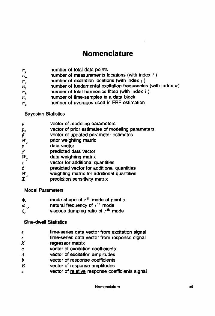
n, number of total data points Nn number of measurements locations (with index i ) n, number of excitation locations (with index j ) ny number of fundamental excitation frequencies (with index k)
nN, number of total harmonics fitted (with index / ) n, number of time-samples in a data block n number of averages used in FRF estimation
Bayesian Statistics
vector of modeling parameters vector of prior estimates of modeling parameters vector of updated parameter estimates prior weighting matrix data vector predicted data vector
data weighting matrix vector for additional quantities
predicted vector for additional quantities weighting matrix for additional quantities prediction sensitivity matrix
vs 'S
OQ
WN
wet
ay
ENN
go
= be
Modal Parameters
d, mode shape of r' mode at point s @,, natural frequency of r' mode ¢, viscous damping ratio of r mode
Sine-dwell Statistics
time-series data vector from excitation signal time-series data vector from response signal regressor matrix vector of excitation coefficients vector of excitation amplitudes vector of response coefficients
vector of response amplitudes vector of relative response coefficients signal OP ty
SFR A
De TO
Nomenclature xii
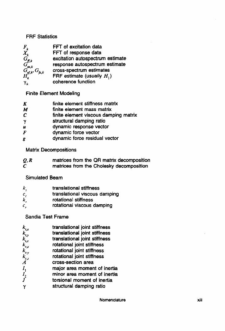
FRF Statistics Q OOP
wes
:= >
<i
FFT of excitation data FFT of response data excitation autospectrum estimate response autospectrum estimate cross-spectrum estimates FRF estimate (usually H, )
coherence function
Finite Element Modeling
mM YES
QRH
finite element stiffness matrix finite element mass matrix
finite element viscous damping matrix structural damping ratio dynamic response vector dynamic force vector dynamic force residual vector
Matrix Decompositions
Q,R C
matrices from the QR matrix decomposition matrices from the Cholesky decomposition
Simulated Beam
~
an)
~
“ ia)
~
translational stiffness translational viscous damping rotational stiffness rotational viscous damping
Sandia Test Frame
y <=
Ok a PT
2
5 %e N
<< So
mh
translational joint stiffness transiational joint stiffness translational joint stiffness rotational joint stiffness rotational joint stiffness rotational joint stiffness cross-section area major area moment of inertia minor area moment of inertia torsional moment of inertia structural damping ratio
Nomenclature xiii

Cantilever Beam
Le JES
OD Yes translational clamp stiffness
rotational clamp stiffness modulus of rigidity density
structural damping ratio thickness of beam width of beam effective transducer mass effective transducer rotatory inertia stinger rotational stiffness
Nomenclature Xiv

PART I:
Introduction and Literature Review
Chapter 1: Introduction
1.1 MODEL UPDATING
When accounting for the dynamic behavior of a structure in engineering design, it
is helpful to have a finite element model of the structure available for prediction
purposes. This enables the designer to determine the effects of changes made to the
structure without having to actually build a modified structure. Indeed, this is one of
the main objectives of using the finite element method.
However, finite element models of structures do not always accurately predict the
behavior of the structure. This can happen if there are modeling errors present in the
finite element model. Examples of such errors include the use of inaccurate estimates
of material properties, the use of poor thickness or dimension estimates, or improper
modeling of the boundary conditions of the system. If errors are present in the model,
then errors will be present in predictions made by the model. The model will not be
suited for quantitative behavior prediction; at best, it can only be used for qualitative
behavior prediction. In extreme cases, it may not even be good for qualitative predic-
tion purposes.
Unfortunately, it is not easy for the analyst to create a sufficiently accurate finite
element model of a given structure. This is especially true when there is considerable
uncertainty present in the modeling parameters used to build the finite element. For
example, the elastic modulus of the structure material may not be precisely known, or
Chapter 1: Introduction 2
the boundary condition model that should be used to model a clamp holding the struc-
ture may not be known.
One method of dealing with these difficulties is to update the modeling parameters
using data from a structural dynamics test. An effective model update procedure will
cause the revised model to better predict the experimental data acquired in the test.
Additionally, the model update procedure should provide evidence that the model has
genuinely been improved, as opposed to having been manipulated to fit only the
specific set of data used to perform the model update.
Using Bayesian Statistics with frequency response data is a particularly suitable
framework for performing such model updates. Bayesian statistics provides a formal
methodology for incorporating prior knowledge about a system into the model update
process, and it also provides a framework for describing how good the results of the
model update process are. These considerations help ensure that reasonable and
realistic changes are made to the finite element model.
A significant amount of research has been dedicated to this problem in the past,
but most of it has been oriented around approaches utilizing the results of experiment-
al modal analysis. An overview of relevant literature on the FE update problem is
presented in Chapter 2. While most of the techniques in the literature work with
modal test data, the use of frequency response data lends itself more easily to a
formal statistical analysis, as will be shown in Part II of the dissertation.
Chapter 1: Introduction 3
1.2 RESEARCH GOALS
The primary goal of the research presented in this dissertation is to substantially
improve the predictive capability of a finite element model by updating the model with
frequency response data acquired in a structural dynamics test. However, the process
of updating a model with test data is not simple, and there are a number of questions
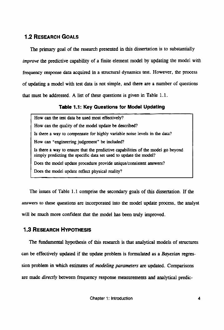
that must be addressed. A list of these questions is given in Table 1.1.
Table 1.1: Key Questions for Model Updating
How can the test data be used most effectively?
How can the quality of the model update be described?
Is there a way to compensate for highly variable noise levels in the data?
How can “engineering judgement” be included?
Is there a way to ensure that the predictive capabilities of the model go beyond simply predicting the specific data set used to update the model?
Does the model update procedure provide unique/consistent answers?
Does the model update reflect physical reality?
The issues of Table 1.1 comprise the secondary goals of this dissertation. If the
answers to these questions are incorporated into the model update process, the analyst
will be much more confident that the model has been truly improved.
1.3 RESEARCH HYPOTHESIS
The fundamental hypothesis of this research is that analytical models of structures
can be effectively updated if the update problem is formulated as a Bayesian regres-
sion problem in which estimates of modeling parameters are updated. Comparisons
are made directly between frequency response measurements and analytical predic-
Chapter 1: Introduction 4
tions of those same measurements, with statistical weights being used to make the
comparison as efficient as possible (minimizing errors in the final parameter esti-
mates). Prior information concerning the design parameters is also incorporated,
helping ensure that parameter estimates are reasonable and realistic. The Bayesian
formulation also provides a framework for describing the quality of the updated
parameter estimates and for performing statistical tests that help ensure the validity of
the model update.
1.4 RESEARCH OBJECTIVES
In order to meet the goals of this research, a number of objectives must be
achieved. The bulk of the work is oriented around the model update problem formula-
tion with a Bayesian statistics framework. Also, consideration is given to the para-
meter selection and modeling process.
Identify Design Parameters
The identification of erroneous modeling parameters is perhaps the most important
part of the model update process. These modeling parameters typically concern struc-
ture size and shape, material properties, and boundary conditions. Unfortunately ,
there are no simple guidelines for selecting the parameters to be updated, and the
issue must be addressed on a case-by-case basis.
Comparing Test Results to Analysis
The method used to compare test data to finite element model predictions is the
defining characteristic of a model update algorithm. In this research, Bayesian statis-
Chapter 1: Introduction 5
tical theory is used to develop a weighted sum-of-squares error term that represents
the differences between the test and analysis. The resulting formulation for estimating
modeling parameter values is called a Bayesian regression formulation.
incorporate Sources of Uncertainty
The model update formulation will be most effective if it accounts for as many
sources of uncertainty into the process as possible. These sources include variable
noise levels on the data and uncertainty in parameter estimates used to generate the
initial model. Statistical tools such as the multivariate delta method are used to gener-
ate estimates of mean and variance for the data, while Bayesian priors contain esti-
mates of the mean and variance of the initial parameter estimates used to generate the
model. A lack-of-fit analysis is used to compensate for sources of uncertainty that
may have been neglected, such as miscalibration errors or model form errors.
Describe Quality of Results
The Bayesian regression formulation provides standard methods for computing
confidence intervals and correlation matrices for the updated parameter estimates.
Visualization techniques are also developed in order to demonstrate how well the
model predicts the shape and amplitude of the dynamic response of the structure.
Verify Results
Methods of verifying the model update include performing data quality tests and
cross-validation tests. Specifically, time-invariance tests are performed before the
model update to ensure that the data used is valid. Cross-validation techniques are
Chapter 1: Introduction 6
used after the model update to ensure that the updated mode is capable of fitting other
data sets beyond the specific set used to perform the model update. Parameter consist-
ency checks are also performed after the model update to help ensure that reasonable
and realistic parameter estimates have been obtained.
Perform Model Updates on Actual Problems
The Bayesian regression formulation developed in this dissertation is used on three
different model update problems. The first problem is a simulated beam in which
boundary condition parameters are updated. The second is a steel frame in which joint
stiffness and beam cross-section parameters are updated. The third problem is a
cantilever beam in which boundary condition parameters representing a clamp are
updated.
1.5 SCOPE OF RESEARCH
The potential scope of research involving model updating is very broad. However,
the research performed for this dissertation was strategically restricted in order that
the most relevant research items could be investigated thoroughly.
Structure complexity
The test articles used in this research were of relatively simple geometry, i.e.,
beams or simple frames. Updating a finite element model of a more complex structure
would have been more interesting and intellectually satisfying, but for purposes of
testing a new model update methodology, it was best to start with simple and well-
understood problems.
Chapter 1: Introduction 7
Modeling technique
The only modeling technique used in this research was the finite element method.
Transfer matrix methods or Rayleigh-Ritz methods could also have been used, but the
basic model update formulation would not have changed.
Testing methodology
Data was obtained from the test structures using broad-band FRF testing (accomp-
lished with an impact from a modal test hammer) and single frequency sine-dwell
testing (accomplished with a sinusoidally driven electromagnetic shaker). Other testing
techniques such as swept-sine testing or burst-random testing could have been used,
but these would not have changed the model update formulation.
Transducer types
Data was acquired from structures using either accelerometers or a scanning laser-
Doppler vibrometer (SLDV). Other types of experimental data, such as strain gauge
measurements, could have been incorporated but were not due to time considerations.
Parameter types
The update parameters included isotropic material properties, beam cross-section
properties, and structural damping coefficients. Boundary condition parameters were
also included. While this is a fairly complete list, most of these parameters focus on
global properties of the structure. An element-by-element model update (requiring one
or more parameters for each element) would be very useful for damage detection pur-
poses, as would a thickness-profiling study based on spline control-point parameters,
Chapter 1: Introduction 8
but these problems are large and complex enough to be addressed in dissertations of
their own. They are not addressed here.
1.6 CONTRIBUTIONS OF RESEARCH
Development of a True Bayesian Statistics Formulation
The Bayesian statistics regression formulation has appeared in numerous papers in
the literature. However, many of these methods are done only in a Bayesian statistics
“style” rather than in a true Bayesian formulation. Specifically, the Bayesian statistics
approach requires weighting matrices for both data and prior information. In much of
the literature, arbitrary weighting matrices such as W=J are used, or the issue of
weighting matrices is ignored entirely. In this research, the data weighting matrix
comes from the initial signal processing done on the raw time signals, while the
weighting matrix for the Bayesian priors comes from variance estimates describing the
initial quality of the parameters used to model the system under study. Other measure-
ments taken from the system can also be incorporated into the analysis. |
Using a data-based weighting matrix is statistically optimal in the sense that it uses
the data as efficiently as possible, providing minimum variance parameter estimates.
Additionally, it allows the analyst to use data with highly variable noise levels without
user intervention. This capability is particularly useful with working with scanning
laser-Doppler vibrometer (SLDV) data and shaker-based FRF data. In the case of
SLDV data, time-domain response signal drop-outs can be a problem, while
Chapter 1: Introduction 9
frequency-domain force autospectrum drop-outs can be a problem in shaker-based
FRF data.
Statistics for Multi-Frequency Sine-Dwell Data
A second major contribution of this work is the development of statistically
qualified response coefficients that are used to describe time-series data coming from
a structural dynamics test in which multiple excitation frequencies are used. Prior
work has focused on cases in which only a single excitation frequency is used.
Reformulation of the Bayesian Statistics Problem
In order to implement the Bayesian regression formulation on a computer, the
problem has to be reformulated to alleviate the effects of ill-conditioning. This is
accomplished with the use of modern matrix decompositions and a reformulation of
the Bayesian regression problem that makes it numerically equivalent to an ordinary
least-squares problem.
Development of a Lack-of-fit Testing and Compensation
A third contribution of the work presented in this dissertation is the lack-of-fit
test. This test provides a statistically rigorous method of determining whether or not it
is possible to better fit the data. If the test statistic comes out as insignificant, the
analyst can conclude that the model fits the model as well as can possibly be expect-
ed, and that there is no point in trying to further refine the model. However, a signifi-
cant test statistic indicates that there may still be a model that better matches the data.
Chapter 1: Introduction 10
Additionally, it is possible to downweight data residuals in the Bayesian regression
formulation to compensate for the presence of lack-of-fit. This ensures that the prior
information provided by the analyst still has an effect in the analysis and that
unrealistically small confidence interval sizes are not computed. This is particularly
important in evaluating the model in cases where the number of data points over-
whelmingly outnumbers the number of pieces of prior information.
Model Update Verification Procedures
A fourth area of contribution includes two model verification tests used to ensure
that the model update is valid. The first test is a time-invariance test performed on the
test data before the model update, which helps ensure that the data are valid. The
second is a cross-validation test performed after the model update to ensure that the
model has predictive capabilities that go beyond the specific data set used to update
the model.
1.7 STRUCTURE OF THE DISSERTATION
This dissertation is broken into five major parts: (I) introduction and literature
review; (II) basic statistical theory used to update models; (III) issues concerning
“quality control,” including computer implementation issues and statistical techniques
used to verify the model update; (IV) model update case studies, both simulated and
experimental; and (V) conclusions and recommendations.
Part I of the dissertation consists of Chapter 1 (this introductory chapter) and
Chapter 2, the literature review. In the literature review, an overview of the many
Chapter 1: Introduction 11
model update algorithms that exist is presented. Particular attention is paid to those
algorithms that address statistical issues. |
Part II deals with the basic statistical theory used to update finite element models.
Specifically, Chapter 3 provides an introduction to the use of Bayesian statistics in
regression problems, which is the basic framework on which this dissertation is
based. Chapter 4 provides an explanation of the update parameters typically used in a
model update approach based on Bayesian statistics. This chapter also explains what
statistical priors are and how they are obtained. Chapter 5 discusses how time-series
data from a sine-dwell test is processed to generate statistically-qualified (having both
mean and variance information available) frequency response data to be used by the
model update algorithm. Chapter 6 presents similar results for broad-band frequency
response function (FRF) data. Finally, Chapter 7 discussed how the finite element
method is used to compute analytical predictions of the test data along with parameter
sensitivities of the predictions.
Part III of the dissertation deals with “quality control” issues, both numerical and
Statistical. Chapter 8 discusses a number of computational and numerical concerns
relating to the computer-based implementation of the Bayesian statistics model update
formulation. Chapter 9 presents a number of statistics-based tools for testing the
quality of the input data and for determining whether or not the updated model has
been improved. Finally, Chapter 10 presents a number of visualization statistics that
help provide insight into the changes made to the model.
Chapter 1: Introduction 12

Part IV of the dissertation presents three case studies, one using simulated data
and two using experimental data. Chapter 11 presents a simulated study in which
boundary condition parameters are estimated using sine-dwell data. A Monte Carlo
study is also performed to confirm variance estimates. Chapter 12 presents an
experimental study in which joint stiffness parameters used in a finite element model
of a frame are updated using both sine-dwell data and FRF data. Chapter 13 presents
an experimental study in which boundary condition parameters representing the effects
of a steel clamp on a cantilever beam are estimated using sine-dwell data. This study
is more complete than the steel frame study of Chapter 12, as more of the statistical
tests of Chapter 9 are used here.
Part V, consisting of only Chapter 14, provides a brief summary of conclusions
and a list of recommendations for future work.
Chapter 1: Introduction 13
Chapter 2: Literature Review
INTRODUCTION
The subject of updating finite element models using experimental test data is well
represented in the literature, with hundreds of papers being available on the subject.
In this chapter, a general overview of these various model update techniques is pre-
sented, followed by a more detailed discussion concerning recent work in this area.
The chapter concludes with references to other works relating to the research present-
ed in this dissertation.
2.1 MODEL UPDATE CATEGORIZATION
The numerous model update procedures discussed in the literature can be categor-
ized according the type of algorithms used. Specifically, there are three basic charac-
teristics that can be used to categorize a model update algorithm: (1) the type of test
data used; (2) the means by which test data are compared to analysis; and (3) the
methodology used to updating the finite element (FE) model. The primary options for
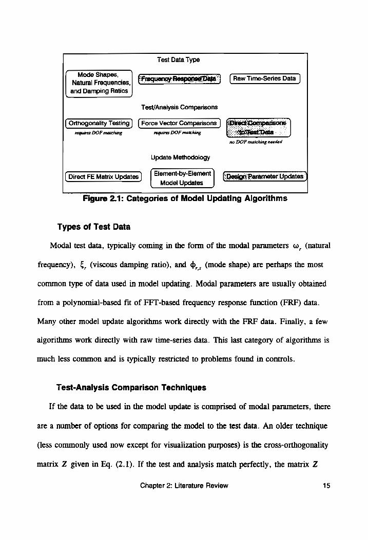
each of these selections is shown below in Figure 2.1. Highlighted in gray are the
options used in this disseration.
Chapter 2: Literature Review 14
Test Data Type
ponse’Data’] { Raw Time-Series Data |
Natural Frequencies
Mode Shapes,
and Damping Ratios
Test/Analysis Comparisons
( Orthogonality Testing | { Force Vector Comparisons | Comparison:
one DOR mans repares DOF matching <Atefest Data no DOF matching needed
Update Methodology
(Direct FE Matrix Updates} | Element-by-Element| fh ecicn Parameter Updates ) Model Updates
Figure 2.1: Categories of Model Updating Algorithms
Types of Test Data
Modal test data, typically coming in the form of the modal parameters w, (natural
frequency), € (viscous damping ratio), and o,, (mode shape) are perhaps the most
common type of data used in model updating. Modal parameters are usually obtained
from a polynomial-based fit of FFT-based frequency response function (FRF) data.
Many other model update algorithms work directly with the FRF data. Finally, a few
algorithms work directly with raw time-series data. This last category of algorithms is
much less common and is typically restricted to problems found in controls.
Test-Analysis Comparison Techniques
If the data to be used in the model update is comprised of modal parameters, there
are a number of options for comparing the model to the test data. An older technique
(less commonly used now except for visualization purposes) is the cross-orthogonality
matrix Z given in Eq. (2.1). If the test and analysis match perfectly, the matrix Z
Chapter 2: Literature Review 15
will equal an identity matrix. A model update algorithm used here would have the
objective of minimizing the differences between Z and J (most often in a Frobenius n, Nn,
norm sense, i.e., minimize SSE = © x (z,-5,) where 6,,=1 for i=j and 6, =0 i=1je1
for 1 #/).
Z= Dig M Dory (2.1)
It should be noted that using Eq. (2.1) requires that the test and analysis degrees-
of-freedom (DOF) be matched, since there are normally many more analytical DOF
(which include both translation and rotation values at FE nodes) than experimental
DOF (which typically include only translation measurements from small number of
accelerometer locations). Degree-of-freedom matching is accomplished with either
modal expansion, which expands the test data to match the analysis DOF, or with the
use of model reduction, which collapses the finite element DOF to match those of the
test. This will be discussed in more detail in Section 2.3.
Another comparison technique that can be used is the dynamic force residual. This
comparison takes advantage of the fact that the excitation force and system response
are related by the fundamental equation of motion of the system. For modal parameter
data there are no applied loads, since modes correspond to free vibration. Thus, the
force residual vector g,, defined in Eq. (2.2) for mode r , should be zero. Force resi-
duals can also be computed for dynamic response shapes u, , which can be extracted
directly from the FRF at frequency w, with an applied force of F, at the appropriate
location. This response-based force residual is defined in Eq. (2.3).
Chapter 2: Literature Review 16
g, =(K- w,M)o, ~0 | (2.2)
g, = (K+iw,C - o,M)u, - F, ~ 0 (2.3)
As with the cross-orthogonality matrix of Eq. (2.1), the objective of a model
update algorithm would be to minimize the vector g, typically by minimizing (g'g)
in a least-squares fashion. Again, degree-of-freedom matching is required via either
modal expansion or model reduction.
A third approach to comparing test data to the finite element model is to directly
compare model predictions to the test data, typically in a sum-of-squares error
fashion. In a modal approach, this might involve direct comparisons between natural
n,
frequencies, e.g., (Wgaa ~ © rem) r=]
comparisons between natural frequencies, mode shapes, and damping ratios simul-
2 or a more generalized approach involving direct
taneously. With FRF data, analytical FRFs predicted using the model would be direct-
ly compared to the measured FRFs. Time-series data can compared to analysis in this
fashion as well. In many direct comparison techniques, the residuals are weighted.
Model Update Methodologies
The final option used to categorize model update methods is the means by which
the finite element model is updated. Many of the simplest update methods make direct
modifications to individual entries of the FE mass and stiffness matrices. These
methods are usually very efficient computationally, but have fallen somewhat out of
favor because the results of direct matrix updates are difficult to interpret. The ever-
Chapter 2: Literature Review 17
increasing power of computers has also reduced the need for such computationally
efficient algorithms. |
An alternative to direct mass and stiffness matrix updates are methods that update
models at the finite element level. These algorithms are most often used for damage
detection purposes. The computational expense is increased, but the results are easier
to understand.
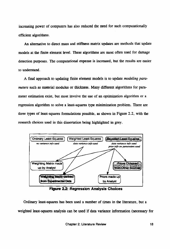
A final approach to updating finite element models is to update modeling para-
meters such as material modulus or thickness. Many different algorithms for para-
meter estimation exist, but most involve the use of an optimization algorithm or a
regression algorithm to solve a least-squares type minimization problem. There are
three types of least-squares formulations possible, as shown in Figure 2.2, with the
research choices used in this dissertation being highlighted in grey.
( Ordinary Least-Squares ] [ Weighted Least-Squares } (Bayesian ares.,)
no variance info used data variance info used data variance info used Prior info on parameters used
Weighting Matrix made
up by Analyst
Priors made up
by Analyst
Figure 2.2: Regression Analysis Choices
Ordinary least-squares has been used a number of times in the literature, but a
weighted least-squares analysis can be used if data variance information (necessary for
Chapter 2: Literature Review 18
computing weights) is available. Furthermore, if prior information is available for the
parameters being estimated, a Bayesian statistics analysis can be used.
2.2 RECENT WORK IN THE LITERATURE
Overviews of Model Updating
Imregun and Visser [1] presented an extensive overview of model updating that
began with common comparison techniques such as the modal assurance criterion
(MAC) [2] and the coordinate modal assurance criterion (COMAC) [3], along with
different model reduction and data expansion techniques. Direct FE matrix update
methods were discussed, followed by methods using force residuals and orthogonality,
and then by sensitivity-based parameter update methods. A preference for FRF-based
parameter update approaches was indicated, since the FRF contains information on
out-of-band modes and the lengthy modal analysis procedure is eliminated.
Baker [4] presented an overview that included test-analysis comparison techniques,
model reduction techniques, direct matrix update algorithms, and parameter update
algorithms. The bulk of the methods discussed involve the use of modal data, but
reference was also made to methods using FRF data. The paper concluded with a
number of practical suggestions for performing model updates with modal test data
and recommended that model updates be used with simple, rapidly-solved models
rather that large, detailed models.
Mottershead and Friswell [5] provided a very extensive survey of model updating
that included direct matrix updates and various least-squares type analyses for use
with both modal and FRF data (including the Bayesian statistics approach). The
Chapter 2: Literature Review 19
survey also included discussions of error localization techniques, which are used to
identify erroneous parameters or regions in a finite element model: incompleteness
issues, where effective linear dependencies present in the data can interfere with
effective parameter estimation; and weighting matrices to be used in weighted and
Bayesian regression techniques. The paper ended with recommendations that more
research be performed with larger, complex models, along with more research
concerning the selection of a “most suitable” initial model from a set of candidate
models. A slight preference for parameter estimation approaches that utilitize
regularization and error localization techniques was indicated.
Link [6] provided an extensive list of possible sources of error in model update
procedures. Experimental errors can arise from wrong measurements (perhaps caused
by defective or miscalibrated tranducers), the influence of test equipment on results
(such as tranducer mass-loading effects), inaccurate measurements (caused by random
noise), and incomplete measurements (typically caused by insufficient spatial DOF or
excitation frequencies). Modeling errors can arise from discretization errors, invalid
element connectivity, improper modeling of a non-linear system as linear, physical
modeling errors (such as incorrect material properties, inertias, and stiffnesses), and
mismatched boundary conditions between the test and the model. All of these prob-
lems must be eliminated if good results are to be obtained, and statistics techniques
can deal only with random noise in measurements and physical modeling errors.
Dascotte [7] discussed some of the issues that must be addressed in updating finite
element models using modal test data. The importance of matching mode shapes from
Chapter 2: Literature Review 20
test and analysis was stressed. A preference for model update methods that use design
parameters instead of direct matrix updates was also indicated, as these methods
provide more physical insight into the changes made. It was also recommended that
sensitivity analyses be performed with the modeling parameters in order to determine
which parameters should be excluded from the model update process.
Natke [8] presented an overview of model update techniques based on Bayesian
statistics. Data types included FRF data, FRF-based dynamic force residuals, modal
test data, and mode-based dynamic force residuals. The importance of having
Statistical weights was stressed, but no discussion of where weighting matrices might
come from was included. Zhang [9] showed how update methods based on direct
comparisons of modal data or FRF data can be formulated similarly, and how other
approaches based on dynamic force residuals and orthogonality coefficients can also
be formulated in a consistent fashion.
Degree-of-Freedom Matching
Although the research presented in this dissertation does not utilitize a degree-of-
freedom (DOF) matching technique, many model update algorithms do and they are
thus discussed here. DOF matching typically is needed for algorithms utilize cross-
orthogonality measurements or dynamic force residuals, as mentioned in the previous
section. The DOF matching techniques can be broken into two categories: (1) finite
element model reduction techniques, and (2) experimental mode shape expansion
techniques.
Chapter 2: Literature Review 21
Model reduction techniques generate reduced finite element matrices that are
called test-analysis models (TAMs), referring to the fact that the reduced model has
degrees-of-freedom that correspond exactly with the test. The oldest model reduction
method is the static TAM, developed by Guyan [10]. This method produces exact
results for static loads, but errors are generated for dynamic loads. Kammer [11]
developed the modal TAM, in which the analyst picks mode shapes from the original
analytical model that the reduced model will match exactly. Kammer later updated the
modal TAM to account for mode shapes not included in the reduced model by includ-
ing mode shapes from the static TAM [12]. O’Callahan [13] developed the improved-
reduced system (IRS) TAM, which is similar to the static TAM but includes correc-
tion terms that account for the inertial effects of the missing DOF. Gordis [14]
studied the IRS TAM and concluded that it was most effective when the natural
frequencies of the omitted DOF are higher than those of the DOF included in the
reduced model.
Freed and Flanigan [15] compared the static, modal, hybrid, and IRS TAMs using
two numerical and two experimental case studies. They concluded that the IRS and
hybrid TAMs work best, achieving accuracy and robustness more often than the other
two. The topic of test-analysis models was studied further by Avitabile and Foster
[12], who investigated test-analysis models in the context of performing comparisons
with the MAC, COMAC, enhanced COMAC [16], and cross-orthogonality matrix.
An alternative approach to model reduction is mode shape expansion, where the
DOF of the test data are expanded to match those of the finite element model. Lieven
Chapter 2: Literature Review 22
and Ewins [17] discussed three expansion techniques: (1) using cubic splines for
interpolation; (2) modeling the test modes as linear combinations of FEM modes; and
(3) inverting the static reduction process. The inverted static reduction process proved
most effective. O’Callahan et al [18] later developed the System Equivalent Reduction
Expansion Process (SEREP), which is a more generalized procedure that can be used
for either data expansion or model reduction. The process was later extended such
that expanded mode shapes were smoothed consistently [19].
Update Methods using Modal Data
Model update techniques which use modal test data are the most common. Earlier
techniques performed direct updates of the finite element mass and stiffness matrices,
resulting in very efficient algorithms that often matched the test data perfectly. Baruch
and Bar Itzhack [20] developed one of the earliest direct matrix update algorithms,
which did not preserve the structure of the original FE matrices. Kabe [21] developed
an improved technique that preserved the connectivity of the finite element model but
sometimes resulted in a loss of positive definiteness in the FE matrices. O’Callahan
[22] presented four different direct matrix update techniques which updated mass and
stiffness matrices based on various combinations of mode shape and natural frequency
data. Aiad ef al [23] used simulated complex-valued mode shapes and natural
frequencies to perform global updates of finite element matrices. Conti and Bretl [24]
developed a direct matrix update approach for using experimental modal data to
determine the rigid-body properties in addition to mount stiffnesses. A more recent
Chapter 2: Literature Review 23
work by Ahmadian et al [25] utilized a formulation that preserves the connectivity
between nodes and retains the positive definiteness of the FE system matrices.
Analysts using orthogonality-based model update approaches include Niedbal and
Luber [26], who combined orthogonality products and energy methods with
substructuring techniques to perform model updates.
Analysts using least-squares type analyses (sometimes called inverse
eigensensitivity techniques) include Jung and Ewins [27], who updated design
parameters using direct eigenvalue and eigenvector comparisons. Ladeveze et al [28]
used a similar approach, except that the residuals were downweighted by response
magnitudes. Nobari and Ewins [29] discussed the effectiveness of using only natural
frequencies in a least-squares type analysis rather than using both natural frequency
and mode shape information. Lindholm and West [30] used only mode shape ~
information in an ordinary least-squares context to determine boundary condition
parameters.
Farhat and Hemez [31] used a least-squares type analysis with mode-based
dynamic force residuals. FE models were updated using an element-by-element
approach designed for damage detection purposes. Hemez [32] later updated the
approach to use FRF data, and then extended the approach further [33] to also include
Static test data.
Bayesian Approaches using Modal Data
As shown in Figure 2.2, an alternative to the ordinary least-squares regression
formulation is the Bayesian regression formulation, which is sometimes called extend-
Chapter 2: Literature Review 24
ed weighted least-squares, regularized least-squares, or maximum a posterior estima-
tion. Hasselman [34] provided an explanation of the philosophy behind Bayesian
statistics in addition to providing detailed guidelines for interpreting the results of a
Bayesian statistical analysis. Topics discussed included model improvement vs.
manipulation, uniqueness of solutions, and qualification of the model for future use.
Beliveau [35] provided formulations for using Bayesian Statistics with modal data,
FRF data, and raw time-series data. Sensitivity results were developed for all three
data types. Link [36] discussed some issues concerning the Bayesian statistics
formulation, including discretization errors, faulty modeling assumptions, and
inconsistent boundary conditions. Dascotte et al [37] presented a number of different
options for weighting matrices to use in a Bayesian statistics style formulation.
Hasselman and Chrostowski [38] used the Structural System Identification (SSID)
code (developed at Sandia National Laboratories to update models with a Bayesian
Statistics formulation [39]) to perform model updates with modal test data coming
from a large space truss. Martinez et al [40] discussed the use of different optimiza-
tion algorithms within SSID to perform parameter estimation using Bayesian statistics.
Other work using the SSID code was performed by Nefske and Sung [41], who
updated joint stiffness parameters in a model of an engine cradle.
Antonacci and Vestroni [42] used the Bayesian statistics approach to update
lumped-mass models of civil engineering structures. Link et al [43] updated a bridge
model using a Bayesian statistics formulation with modal test data. Alvin [44]
generalized the element-by-element formulation of Farhat and Hemez [31] to a
Chapter 2: Literature Review 25
Bayesian statistics parameter update approach. Variance estimates on the original
modal data were carried through the modal expansion procedure and transformed to
determine variance estimates for the computed dynamic force residuals.
Update Methods using FRF Data
As shown in Figure 2.1, FRF data can be used for model updating instead of
modal test data. Authors using direct FE matrix updates with FRF data include
Larsson and Sas [45], who used a reduced model to generate a dynamic stiffness
matrix (DSM) which was compared to the inverse of an FRF matrix generated from
multi-frequency FRF data. Kritzen and Kiefer [46] used QR decomposition techniques
with FRF data to localize errors in the FE mass and stiffness matrices. A more recent
direct matrix update method presented by Zimmerman et al [47] uses rank-one modi-
fications of the FE stiffness matrix for purposes of damage detection.
Berger et al [48] used dynamic force residuals, as given in Eq. (2.3), with
expanded mode shapes to localize and correct errors in substructures. Missing DOF in
the experimental data were filled in using static deflections in an expansion approach
similar to an inverse of Kammer’s hybrid TAM [12]. Also using FRF-based force
residuals were Yang and Brown [49], who used a model reduction technique to study
different methods of reducing the sensitivity of the model update process to the
presence of damping in the structure, which is often difficult to model accurately.
Schulz et al [50] used dynamic force residuals coming from FRF data in a weighted
least-squares formulation to update a model of a truss. A similar formulation was
presented by Schulz et al (51] for purposes of structural damage detection.
Chapter 2: Literature Review 26
Friswell and Penny [52] used FRF data with the Kammer’s modal TAM in a
weighted least-squares problem in which damping and joint stiffness parameters were
updated. A similar technique was developed by Conti and Donley [53], who used a
TAM with FRF data to develop a linear least-squares model update formulation.
Imregun [54] compared model update results obtained with modal test data (using
the inverse eigensensitivity technique of Zhang et al [55]) to model update results
obtained with FRF data (using the dynamic force residual method of Visser and
Imregun [56]). The effectiveness of each method was dependent on which modes or
FRF lines were selected for use as data. Hybrid approaches, in which one technique
was used to find preliminary parameter estimates for the other, were also investi-
gated. The approach was expanded by Imregum ef al [57] to utilize complex-valued
FRF data in an element-by-element approach and was tested by Imregum ef al [58] in
a joint stiffness parameter estimation problem.
Cogan et al [59] presented a least-squares approach to updating finite element
models with FRF data in which residuals were scaled by the original FRF magni-
tudes. This approach is equivalent to a weighted least-squares formulation in which
noise levels are assumed to be proportional to magnitude. The importance of having a
good initial model was particularly stressed.
Reix et al [60] predicted global damping coefficients using a two-staged weighted
least-squares formulation that directly compared measured FRF data to the analytically
predicted FRF. In the first stage, global mass and stiffness properties such as modulus
and density were manually updated to make the model match the results of modal
Chapter 2: Literature Review 27
parameters fitted from the FRF. The FRF data was then directly used in a weighted
least-squares analysis to obtain the damping coefficients.
Bayesian Approaches using FRF Data
A couple of the papers using modal data in a Bayesian formulation also discussed
how FRF data would be used in a Bayesian formulation. These included the works by
Beliveau [35] and Link et al [43]. Additionally, Mottershead and Foster [61] used the
Bayesian statistics approach with FRF data to improve the conditioning of a weighted
least-squares process developed to estimate element stiffnesses in a cantilever beam.
Update Methods using Time-Series Data
Ibrahim et al [62] developed a method which used displacement, velocity, and
acceleration measurements at a few instants in time to directly update the system
matrices of the FE model. Harmonic excitation is used in order that velocity and
displacement data can be derived directly from acceleration data. Bronowicki et
al [63] proposed a Bayesian statistics formulation in which time-series data was
directly used to update a model. Eigensolutions coming from the finite element model
were used to predict the time-series data. Koh and See [64] use the extended Kalman
filter (a controls-based time-series formulation that is equivalent to the Bayesian
Statistics formulation [65]) to estimate structural parameters from time-series data.
Their procedure incorporated an adaptive filter that adjusted data variance estimates to
ensure statistical consistency and to prevent underestimation of confidence interval
sizes.
Chapter 2: Literature Review 28
Model Updates with Other Types of Data
Mahnken and Stein [66] used strain measurements instead of displacement
measurements for purposes of estimating viscoplastic damping parameters. The
problem was initially formulated as a weighted least-squares problem, but regulari-
zation terms were then added that made the problem equivalent to a Bayesian statistics
formulation.
2.3 COMMENTS ON THE LITERATURE
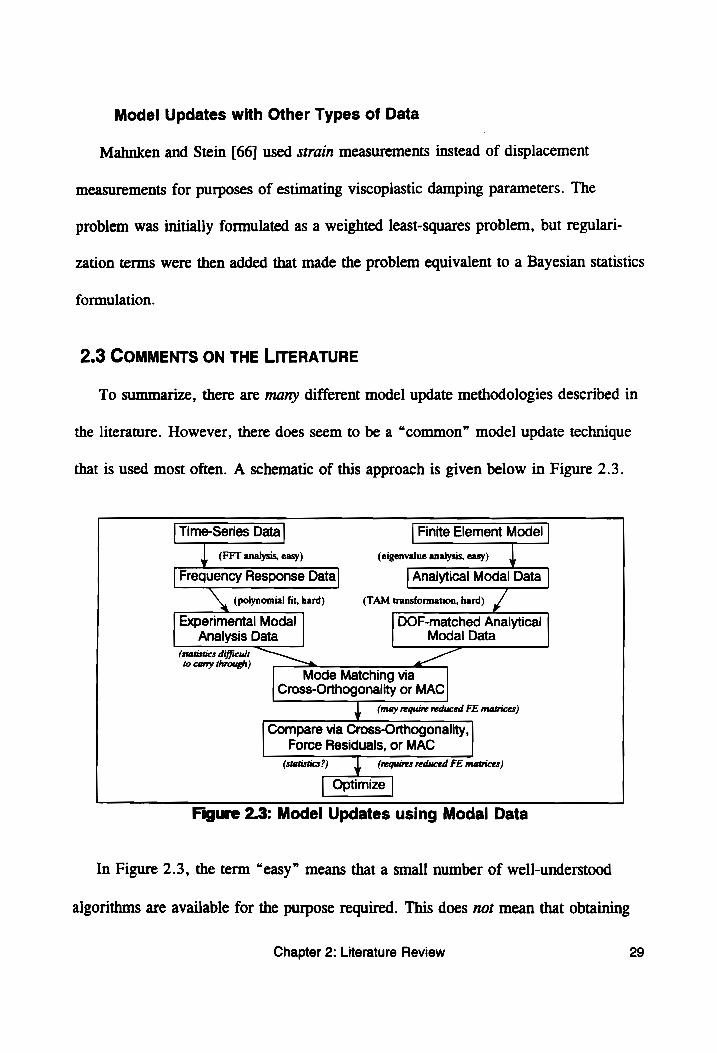
To summarize, there are many different model update methodologies described in
the literature. However, there does seem to be a “common” model update technique
that is used most often. A schematic of this approach is given below in Figure 2.3.
| Time-Series Data | | Finite Element Model |
(FFT analysis, easy) (eigenvalue analysis, easy)
| Frequency Response Data] | Analytical Modal Data |
\ (polynomial fit, hard) (TAM transformation, hard) go
Experimental Modal DOF-matched Analytical Analysis Data Modal Data
(statistics difficul:
Mode Matching via Cross-Orthogonality or MAC
(may require reduced FE matrices)
Compare via Cross-Orthogonality, Force Residuals, or MAC
(Statistics?) (requires reduced FE matrices)
Figure 2.3: Model Updates using Modal Data
In Figure 2.3, the term “easy” means that a small number of well-understood
algorithms are available for the purpose required. This does not mean that obtaining
Chapter 2: Literature Review 29
unbiased FRF estimates from time-series data and computing eigensolutions for
massive FE system matrices are trivial tasks. Indeed, there are several methods for
estimating FRFs and several algorithms for computing the eigenvalues of large scale
matrices, and these must be used properly. However, a competent analyst should be
able to obtain correct results for these parts of the problem for almost any system.
The “hard” tasks, on the other hand, can become intractably difficult for certain
systems. Extraction of modal parameters is typically performed with a polynomial-
based fit, and a large number of algorithms exist for the purpose of performing that
fit. These algorithms work quite well for many systems, but systems that have densely
packed modes, nearly coupled modes, or heavy/non-proportional damping can cause
modal analysis algorithms to fail. Additionally, only a few modal analysis algorithms
carry through the statistics necessary to describe of the quality of the modal
parameters extracted. One algorithm that does so was presented by Yoshimura and
Nagamatsu [67].
Likewise, performing effective model reductions or test mode expansions can be
very difficult for real-world structures. A poorly implemented TAM can fail to
predict the natural frequencies and mode shapes of the original model; it can even
introduce spurious modes into the analysis. This is particularly likely to happen if data
is not acquired at a sufficient number of spatial locations or at improper locations.
Mode shape expansion algorithms have similar problems. A final difficulty with the
“common” approach is that it is difficult to carry statistical measures of quality all the
way through the update process.
Chapter 2: Literature Review 30
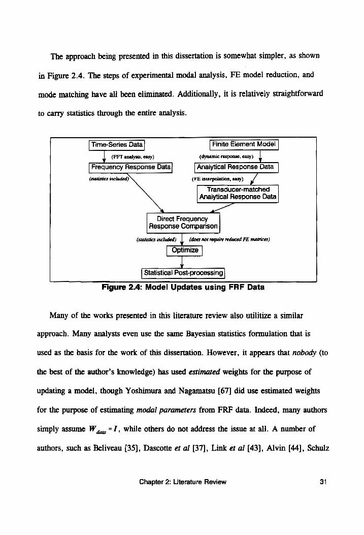
The approach being presented in this dissertation is somewhat simpler, as shown
in Figure 2.4. The steps of experimental modal analysis, FE model reduction, and
mode matching have all been eliminated. Additionally, it is relatively straightforward
to carry statistics through the entire analysis.
| Time-Series Data] | Finite Element Model |
(FFT analysis, easy) (dynamic response, easy)
| Frequency Response Data| | Analytical Response Data |
(statistics included) (FE interpolation, easy) J
Transducer-matched Analytical Response Data
Direct Frequency Response Comparison
(statistics included) (does not require reduced FE matrices)
Opti
mize
| Statistical Post-processing |
Figure 2.4: Model Updates using FRF Data
Many of the works presented in this literature review also utilitize a similar
approach. Many analysts even use the same Bayesian statistics formulation that is
used as the basis for the work of this dissertation. However, it appears that nobody (to
the best of the author’s knowledge) has used estimated weights for the purpose of
updating a model, though Yoshimura and Nagamatsu [67] did use estimated weights
for the purpose of estimating modal parameters from FRF data. Indeed, many authors
simply assume W,,,=1, while others do not address the issue at all. A number of
authors, such as Beliveau [35], Dascotte et al [37], Link et al [43], Alvin [44], Schulz
Chapter 2: Literature Review 31
et al [50], and Koh and See [64], address the issue of weighting matrices in
considerable detail and present a number of schemes for generating them, but none
describe how to estimate weights directly from experimental data.
2.4 OTHER RELEVANT WORK
A key step in obtaining experimentally estimated weights is a statistical analysis of
frequency response data. For sine-dwell data, this was addressed by Montgomery and
West [68], who developed a method of variance estimation for frequency response
coefficients coming from a sine-dwell test. Excitation and response signals are
analyzed separately and then combined into statistically qualified relative response
coefficients using the multivariate delta method. Montgomery et al [69] later verified
the results using Monte Carlo simulations. Zeng and Wicks [70] compared the use of
discrete Fourier transform techniques and linear regression techniques to fit sine-dwell
data. Lopez Dominguez [71] also studied the issue of fitting sine-dwell data, using
robust regression techniques to deal with time-domain drop-outs in time-series data
coming from a laser Doppler vibrometer. A triggering strategy was used to estimate
phase angle information.
Other authors have addressed the issue of estimating variances for FRF data.
Bendat [72] developed a large number of formulae for estimating variances for FRF
magnitude, phase angle, and coherence for the H, FRF estimator. Yoshimura and
Nagamatsu [67] derived similar variance estimators for the 1, FRF estimator, though
only for magnitude. The results were used as a source of statistical weights in a
weighted least-squares modal parameter estimation procedure. Cobb [73] studied the
Chapter 2: Literature Review 32
statistics of a three-channel FRF estimator in addition to providing guidelines on when
certain variance estimators broke down. | |
Deaton et al [74] wrote a significant work on the use of estimated error variances
in regression problems. They provided guidelines for when estimated weights should
be used in a regression analysis and when they should not be used. Other works on
this subject include papers by Williams [75] and Jacquez and Morusis [76]. Both
provide guidelines for using estimated weights in least-squares problems.
Other basic references used in this work include a reference on basic statistics by
Walpole and Myers [77], a reference on statistical regression techniques by Myers
[78], a reference on parameter estimation by Beck and Arnold [79], a reference on
large-scale matrix computations by Golub and Van Loan [80], a reference on signal
processing techniques by Bendat [81], a reference on modal analysis by Ewins [82], a
reference on the Monte Carlo method by Rubinstein [83], and references on the finite
element method by Przemieniecki [84] and Bathe [85].
Chapter 2: Literature Review 33

PART Il:
Basic Statistical Theory
Chapter 3: Bayesian Statistics
INTRODUCTION
As discussed in the introduction, this dissertation is concerned with the task of
updating finite element models with experimental data. More specifically, modeling
parameters are to be updated using direct comparisons between experimentally
acquired frequency response data and FEM-based analytical predictions of that same
data. To this end, there are three common regression techniques that can be used to
obtain statistically qualified parameters estimates: (1) ordinary least-squares regres-
sion; (2) maximum likelihood estimation (which is also known as weighted least-
squares regression); and (3) maximum a posterior estimation (which is also known as
Bayesian regression or regularized regression).
3.1 ORDINARY LEAST-SQUARES
Basic Theory
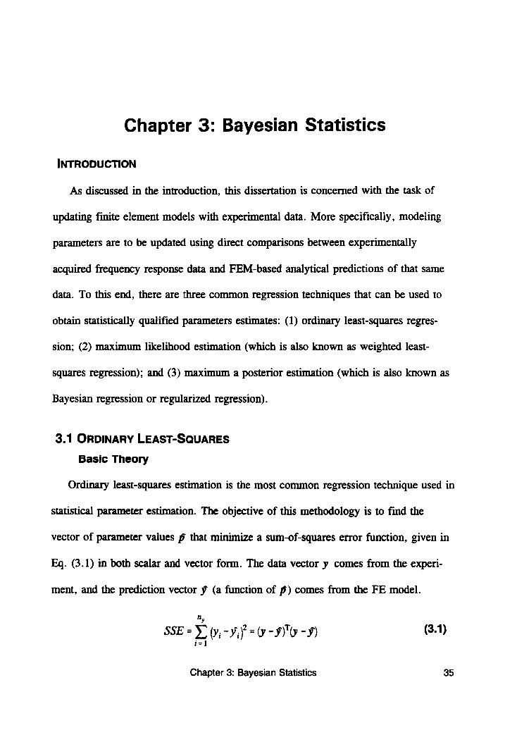
Ordinary least-squares estimation is the most common regression technique used in
Statistical parameter estimation. The objective of this methodology is to find the
vector of parameter values p that minimize a sum-of-squares error function, given in
Eq. (3.1) in both scalar and vector form. The data vector y comes from the experi-
ment, and the prediction vector ¥ (a function of f) comes from the FE model.
ny
SSE = ¥" v,-¥i) = 0-0-9) (3.1) i=]
Chapter 3: Bayesian Statistics 35
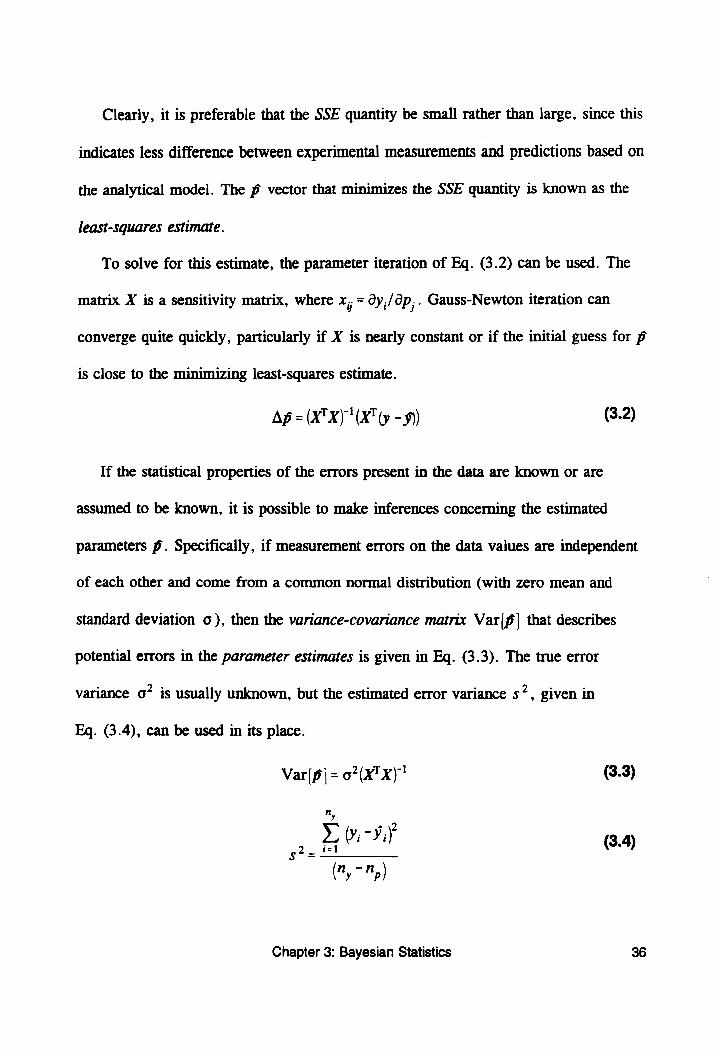
Clearly, it is preferable that the SSE quantity be small rather than large, since this
indicates less difference between experimental measurements and predictions based on
the analytical model. The p vector that minimizes the SSE quantity is known as the
least-squares estimate.
To solve for this estimate, the parameter iteration of Eq. (3.2) can be used. The
matrix X is a sensitivity matrix, where x, = dy,/dp,. Gauss-Newton iteration can
converge quite quickly, particularly if X is nearly constant or if the initial guess for p
is close to the minimizing least-squares estimate.
Ap = (X™X)"(X"(y - 9) (3.2)
If the statistical properties of the errors present in the data are known or are
assumed to be known, it is possible to make inferences concerning the estimated
parameters p. Specifically, if measurement errors on the data values are independent
of each other and come from a common normal distribution (with zero mean and
standard deviation 0), then the variance-covariance matrix Var|p| that describes
potential errors in the parameter estimates is given in Eq. (3.3). The true error
variance o” is usually unknown, but the estimated error variance s”, given in
Eq. (3.4), can be used in its place.
Var [pf] = 0?(X™X)" (3.3)
2 (3.4) ny-n,)
Chapter 3: Bayesian Statistics 36
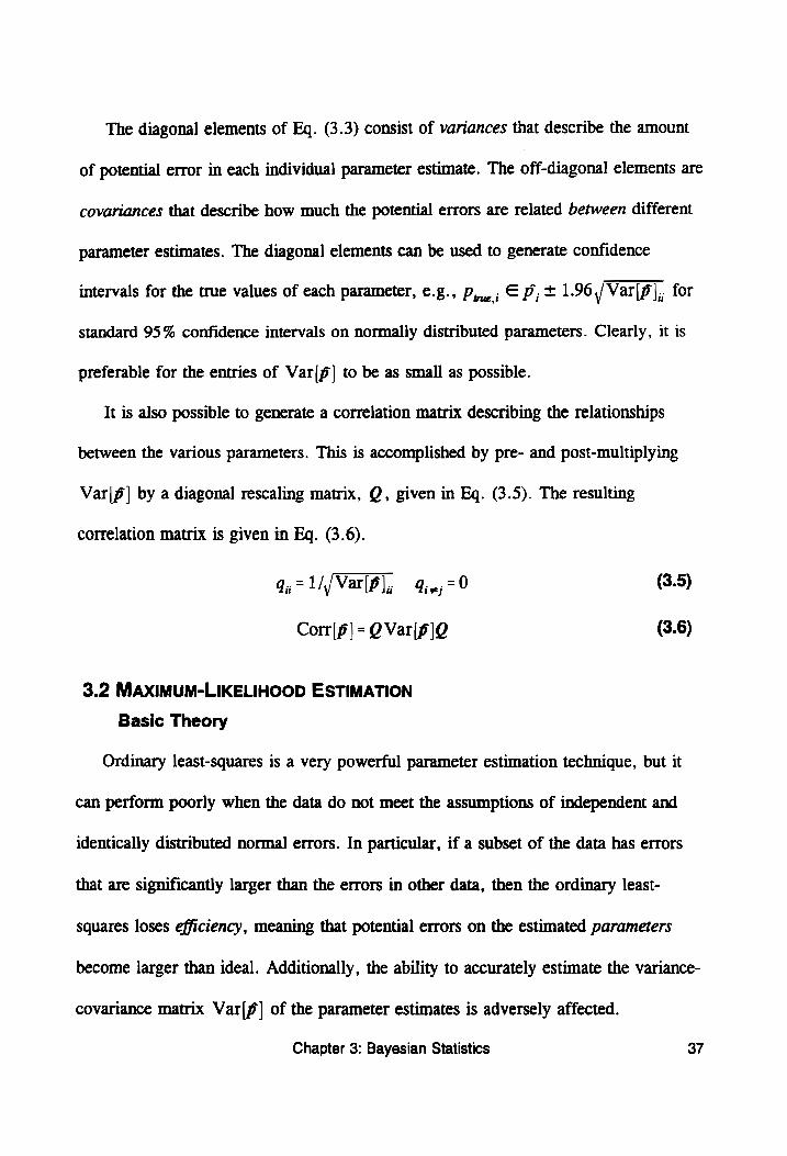
The diagonal elements of Eq. (3.3) consist of variances that describe the amount
of potential error in each individual parameter estimate. The off-diagonal elements are
covariances that describe how much the potential errors are related between different
parameter estimates. The diagonal elements can be used to generate confidence
intervals for the true values of each parameter, e.g., D,,; © P; + 1.96,/ Var[p];, for
standard 95% confidence intervals on normally distributed parameters. Clearly, it is
preferable for the entries of Var([p] to be as small as possible.
It is also possible to generate a correlation matrix describing the relationships
between the various parameters. This is accomplished by pre- and post-multiplying
Var([p| by a diagonal rescaling matrix, @, given in Eq. (3.5). The resulting
correlation matrix is given in Eq. (3.6).
q;, = 1/,/ Var|p]; inj = 9 (3.5)
Corr[f] = QVar([p]O (3.6)
3.2 MAXIMUM-LIKELIHOOD ESTIMATION
Basic Theory
Ordinary least-squares is a very powerful parameter estimation technique, but it
can perform poorly when the data do not meet the assumptions of independent and
identically distributed normal errors. In particular, if a subset of the data has errors
that are significantly larger than the errors in other data, then the ordinary least-
squares loses efficiency, meaning that potential errors on the estimated parameters
become larger than ideal. Additionally, the ability to accurately estimate the variance-
covariance matrix Var|p| of the parameter estimates is adversely affected.
Chapter 3: Bayesian Statistics 37
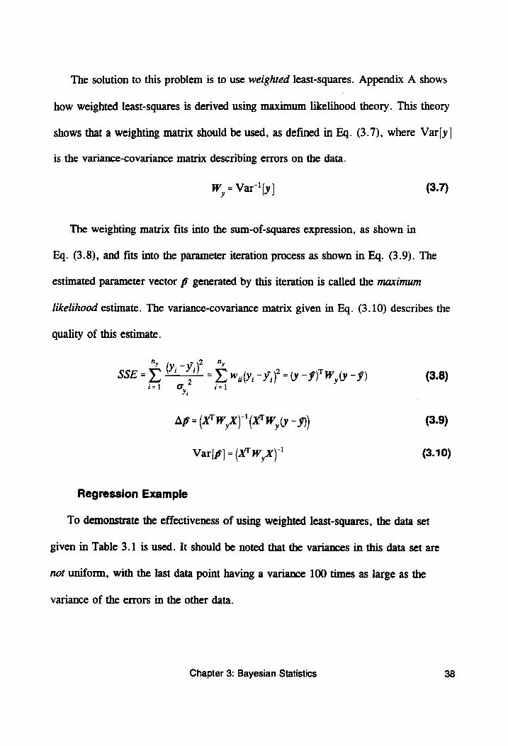
The solution to this problem is to use weighted least-squares. Appendix A shows
how weighted least-squares is derived using maximum likelihood theory. This theory
shows that a weighting matrix should be used, as defined in Eq. (3.7), where Var[y|
is the variance-covariance matrix describing errors on the data.
W, = Var‘ [y] (3.7)
The weighting matrix fits into the sum-of-squares expression, as shown in
Eq. (3.8), and fits into the parameter iteration process as shown in Eq. (3.9). The
estimated parameter vector f generated by this iteration is called the maximum
likelihood estimate. The variance-covariance matrix given in Eq. (3.10) describes the
quality of this estimate.
"Ny fy -y\?
SSE =" Y - v1) Yew Vif =O -IFW,0-9) (3.8) t= vj i=
Ap = (X™W,X)" (XW, (y -9)) (3.9)
Var[p]=(X'W,X)" (3.10)
Regression Example
To demonstrate the effectiveness of using weighted least-squares, the data set
given in Table 3.1 is used. It should be noted that the variances in this data set are
not uniform, with the last data point having a variance 100 times as large as the
variance of the errors in the other data.
Chapter 3: Bayesian Statistics 38
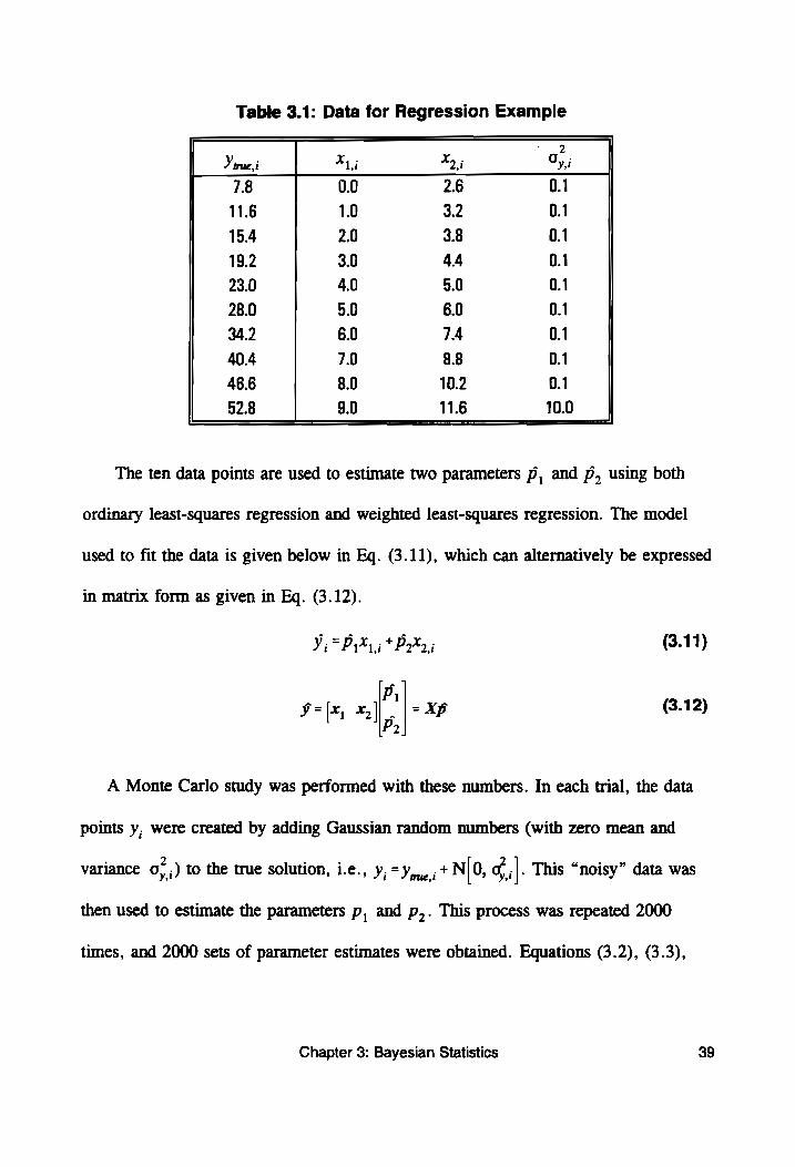
Table 3.1: Data for Regression Example
Y rue, i 1 i 9 5, 7.8 0.0 2.6 0.1
11.6 1.0 3.2 0.1
15.4 2.0 3.8 0.1
19.2 3.0 44 0.1
23.0 4.0 5.0 0.1
28.0 5.0 6.0 0.1
34.2 6.0 7.4 0.1
40.4 7.0 8.8 0.1
46.6 8.0 10.2 0.1
52.8 _ 9.0 11.6 10.0 |
The ten data points are used to estimate two parameters p, and p, using both
ordinary least-squares regression and weighted least-squares regression. The model
used to fit the data is given below in Eq. (3.11), which can alternatively be expressed
in matrix form as given in Eq. (3.12).
Y= PX, ;+ PX); (3.11)
= Xp (3.12)
A Monte Carlo study was performed with these numbers. In each trial, the data
points y, were created by adding Gaussian random numbers (with zero mean and
variance oy) to the true solution, i.e., y,=y,,,,+N [0, |. This “noisy” data was
then used to estimate the parameters p, and p,. This process was repeated 2000
times, and 2000 sets of parameter estimates were obtained. Equations (3.2), (3.3),
Chapter 3: Bayesian Statistics 39
and (3.4) were used for the ordinary least-squares analysis, while Eqs. (3.8), (3.9),
and (3.10) were used for the weighted least-squares analysis. |
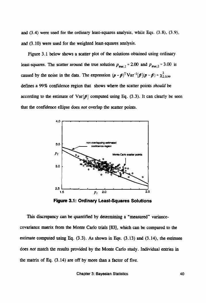
Figure 3.1 below shows a scatter plot of the solutions obtained using ordinary
least-squares. The scatter around the true solution p,,, , = 2.00 and p,,, . = 3.00 is
caused by the noise in the data. The expression (p - pf)! Var '[p](p - p) = 3.0.99
defines a 99% confidence region that shows where the scatter points should be
according to the estimate of Var[p] computed using Eq. (3.3). It can clearly be seen
that the confidence ellipse does not overlap the scatter points.
4.0
3.5 [
P2
3.0 }
2.5 15 Pp; 20 25
Figure 3.1: Ordinary Least-Squares Solutions
This discrepancy can be quantified by determining a “measured” variance-
covariance matrix from the Monte Carlo trials [83], which can be compared to the
estimate Computed using Eq. (3.3). As shown in Eqs. (3.13) and (3.14), the estimate
does not match the results provided by the Monte Carlo study. Individual entries in
the matrix of Eq. (3.14) are off by more than a factor of five.
Chapter 3: Bayesian Statistics 40
p 0.0207 -0.0093 Var| _ | | (3.13)
Pali co [70-0093 +0.0080
p +0.1316 -0.0998 Var| -s2xy'-| | (3.14)
By. -0.0998 +0.0777
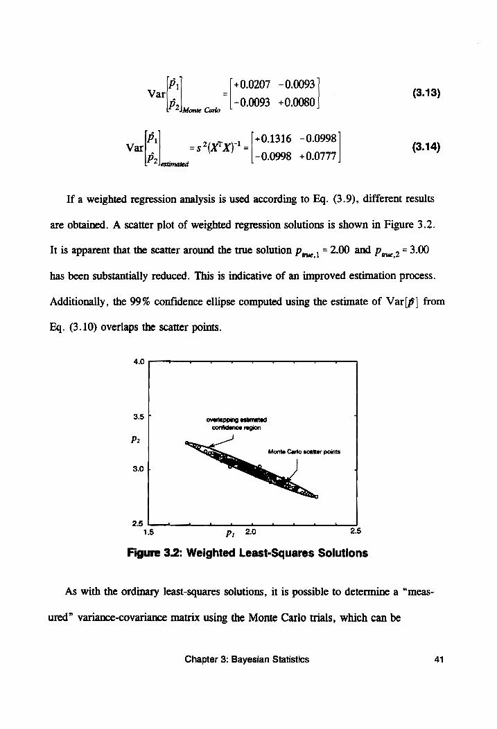
If a weighted regression analysis is used according to Eq. (3.9), different results
are obtained. A scatter plot of weighted regression solutions is shown in Figure 3.2.
It is apparent that the scatter around the true solution p,,, , = 2.00 and p,_, , = 3.00
has been substantially reduced. This is indicative of an improved estimation process.
Additionally, the 99% confidence ellipse computed using the estimate of Var(p] from
Eq. (3.10) overlaps the scatter points.
4.0 .s _ v me ¥ —_- =
3.5 [
P2
3.0 +
2.5 Lo 15 Pp, 20 2.5
Figure 3.2: Weighted Least-Squares Solutions
As with the ordinary least-squares solutions, it is possible to determine a “meas-
ured” variance-covariance matrix using the Monte Carlo trials, which can be
Chapter 3: Bayesian Statistics 41
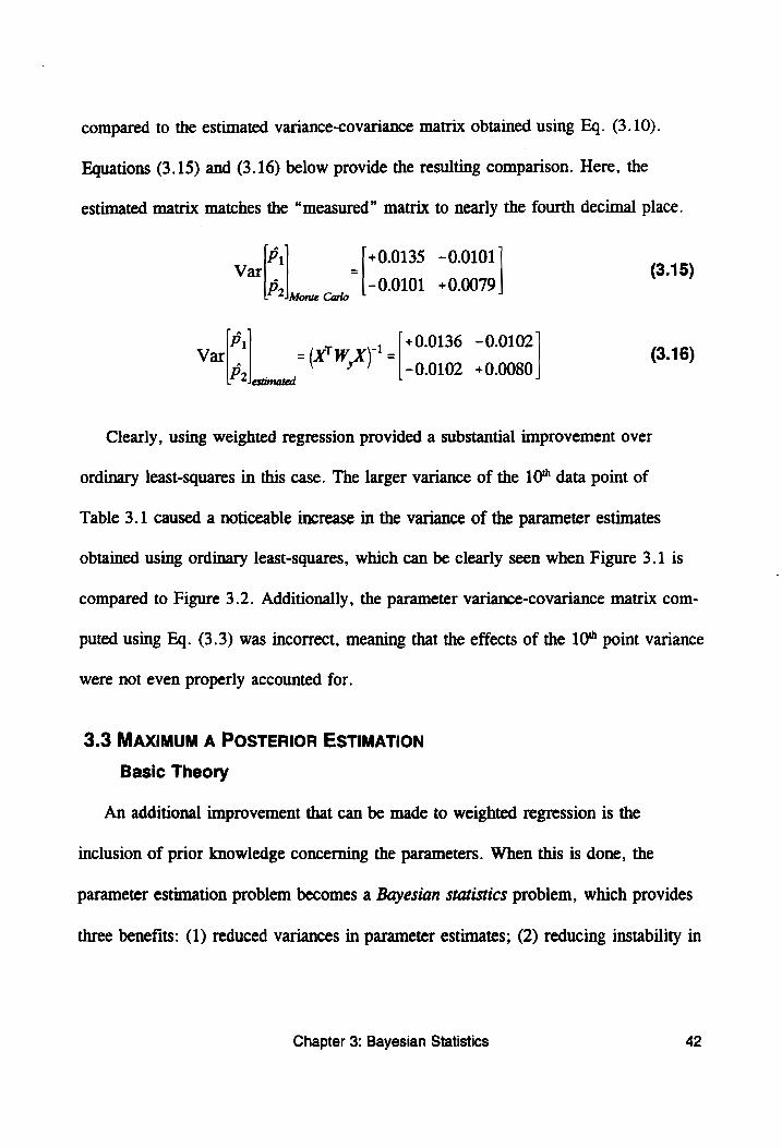
compared to the estimated variance-covariance matrix obtained using Eq. (3.10).
Equations (3.15) and (3.16) below provide the resulting comparison. Here, the
estimated matrix matches the “measured” matrix to nearly the fourth decimal place.
A
p 0.0135 -0.0101 Var| | | | (3.15) Pali coup {70.0101 +0.0079
p +0.0136 -0.0102 Var| =a W,x)" =| | (3.16) Pl. -0.0102 +0.0080
Clearly, using weighted regression provided a substantial improvement over
ordinary least-squares in this case. The larger variance of the 10" data point of
Table 3.1 caused a noticeable increase in the variance of the parameter estimates
obtained using ordinary least-squares, which can be clearly seen when Figure 3.1 is
compared to Figure 3.2. Additionally, the parameter variance-covariance matrix com-
puted using Eq. (3.3) was incorrect, meaning that the effects of the 10" point variance
were not even properly accounted for.
3.3 MAXIMUM A POSTERIOR ESTIMATION
Basic Theory
An additional improvement that can be made to weighted regression is the
inclusion of prior knowledge concerning the parameters. When this is done, the
parameter estimation problem becomes a Bayesian statistics problem, which provides
three benefits: (1) reduced variances in parameter estimates; (2) reducing instability in
Chapter 3: Bayesian Statistics 42
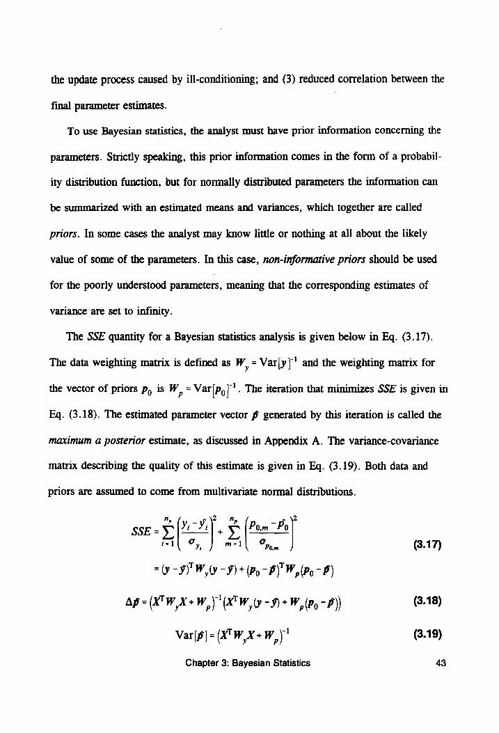
the update process caused by ill-conditioning; and (3) reduced correlation between the
final parameter estimates. |
To use Bayesian statistics, the analyst must have prior information concerning the
parameters. Strictly speaking, this prior information comes in the form of a probabil-
ity distribution function, but for normally distributed parameters the information can
be summarized with an estimated means and variances, which together are called
priors. In some cases the analyst may know little or nothing at all about the likely
value of some of the parameters. In this case, non-informative priors should be used
for the poorly understood parameters, meaning that the corresponding estimates of
variance are set to infinity.
The SSE quantity for a Bayesian statistics analysis is given below in Eq. (3.17).
The data weighting matrix is defined as W,= Var[y]’ and the weighting matrix for
the vector of priors p, is W, = Var|[Po| The iteration that minimizes SSE is given in
Eq. (3.18). The estimated parameter vector f generated by this iteration is called the
maximum a posterior estimate, as discussed in Appendix A. The variance-covariance
matrix describing the quality of this estimate is given in Eq. (3.19). Both data and
priors are assumed to come from multivariate normal distributions.
2
sse-5) NE a (3.17)
=(y -$)' W,(y - 9) + (Do - B)'W, (Py - B)
Ap=(X™W,X+W,\'(X'W (y -9)+ W, (po - B)) (3.18)
Var[p] = (X'W,X+W, i. (3.19)
Chapter 3: Bayesian Statistics 43
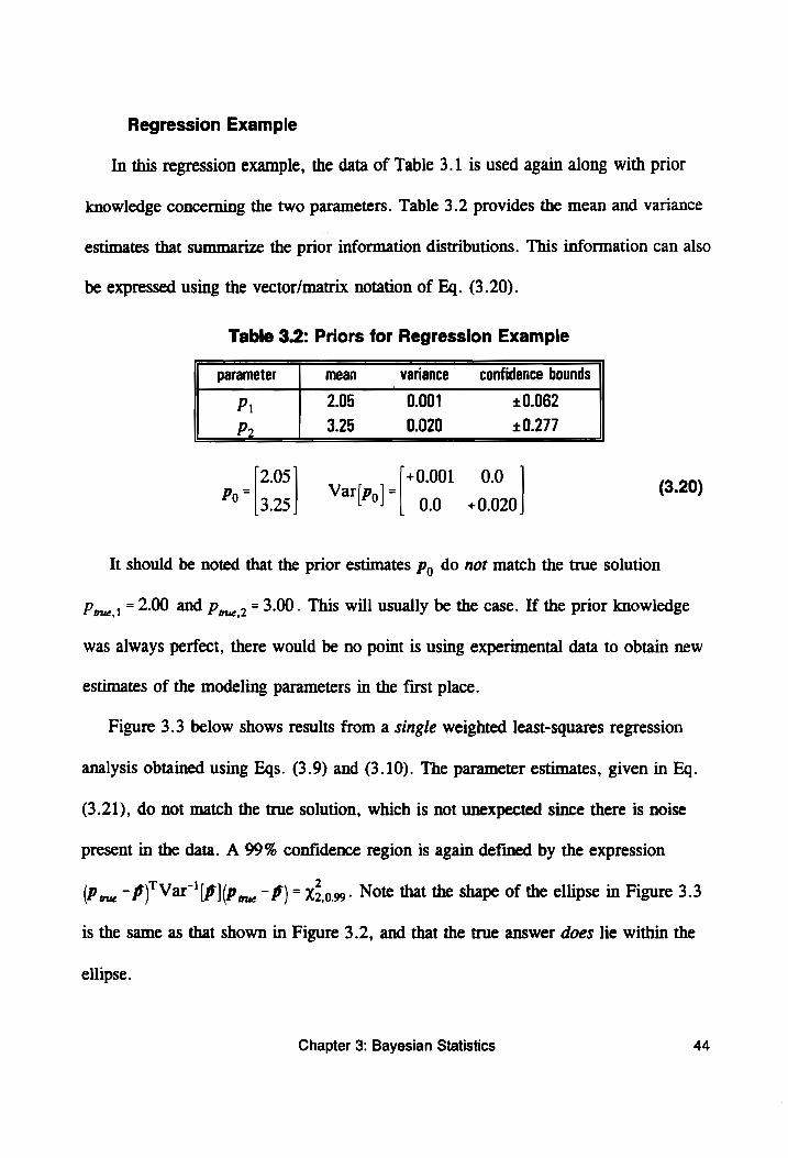
Regression Example
In this regression example, the data of Table 3.1 is used again along with prior
knowledge concerning the two parameters. Table 3.2 provides the mean and variance
estimates that summarize the prior information distributions. This information can also
be expressed using the vector/matrix notation of Eq. (3.20).
Table 3.2: Priors for Regression Example Ts
parameter mean . variance confidence bounds
P, 2.05 0.001 +0.062
P» 3.25 0.020 +0.277
2.05 +0.001 0.0 = V = (3.20)
Po sel arlPol"| go somo
It should be noted that the prior estimates p, do not match the true solution
Prue, = 2-00 and p,,, . = 3.00. This will usually be the case. If the prior knowledge
was always perfect, there would be no point is using experimental data to obtain new
estimates of the modeling parameters in the first place.
Figure 3.3 below shows results from a single weighted least-squares regression
analysis obtained using Eqs. (3.9) and (3.10). The parameter estimates, given in Eq.
(3.21), do not match the true solution, which is not unexpected since there is noise
present in the data. A 99% confidence region is again defined by the expression
(P rue ~ P)' Var [6 |(P ye - P) = X2,099- Note that the shape of the ellipse in Figure 3.3
is the same as that shown in Figure 3.2, and that the true answer does lie within the
ellipse.
Chapter 3: Bayesian Statistics 44
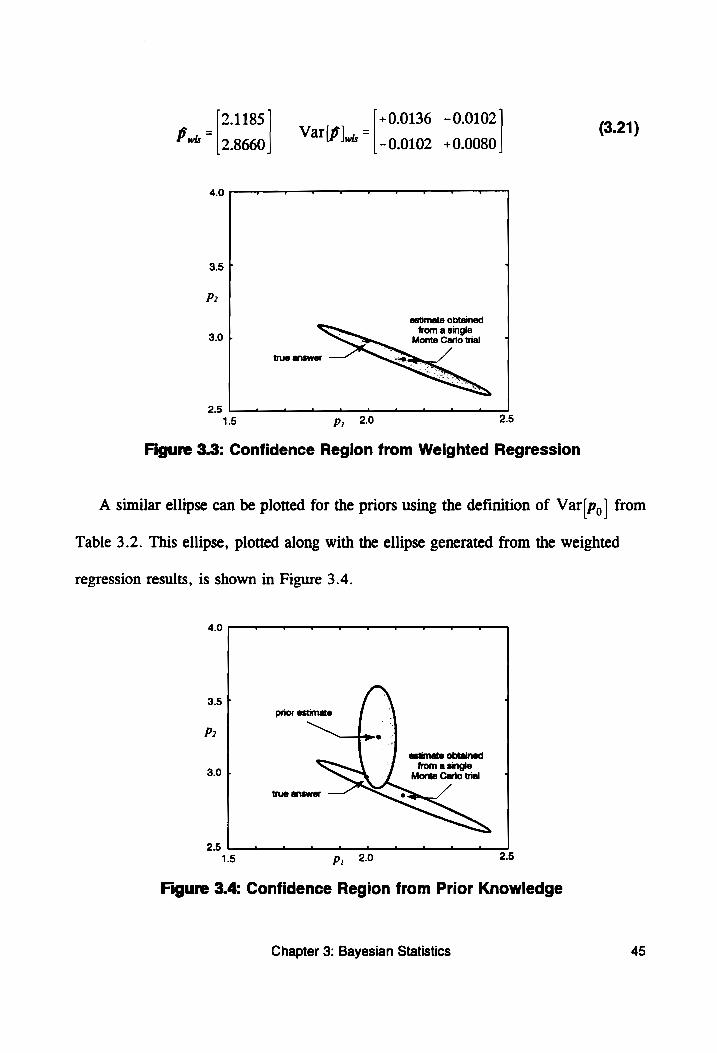
2.1185 Vv +0.0136 -0.0102 (3.21) = a = : «
Pus | 5 8660 TIP lw) 9.0102 +0.0080
4.0 , . — . — ’ r
3.5
P2
estimate obtained
from a single 3.0 + Monte Cario trial
true answer
25 a an hh
15 p; 20 2.5
Figure 3.3: Confidence Region from Weighted Regression
A similar ellipse can be plotted for the priors using the definition of Var [Po| from
Table 3.2. This ellipse, plotted along with the ellipse generated from the weighted
regression results, is shown in Figure 3.4.
4.0 r T r r r T a
3.5 7
P?
3.0 +
25 fs 15 Pp, 20 2.5
Figure 3.4: Confidence Region from Prior Knowledge
Chapter 3: Bayesian Statistics 45
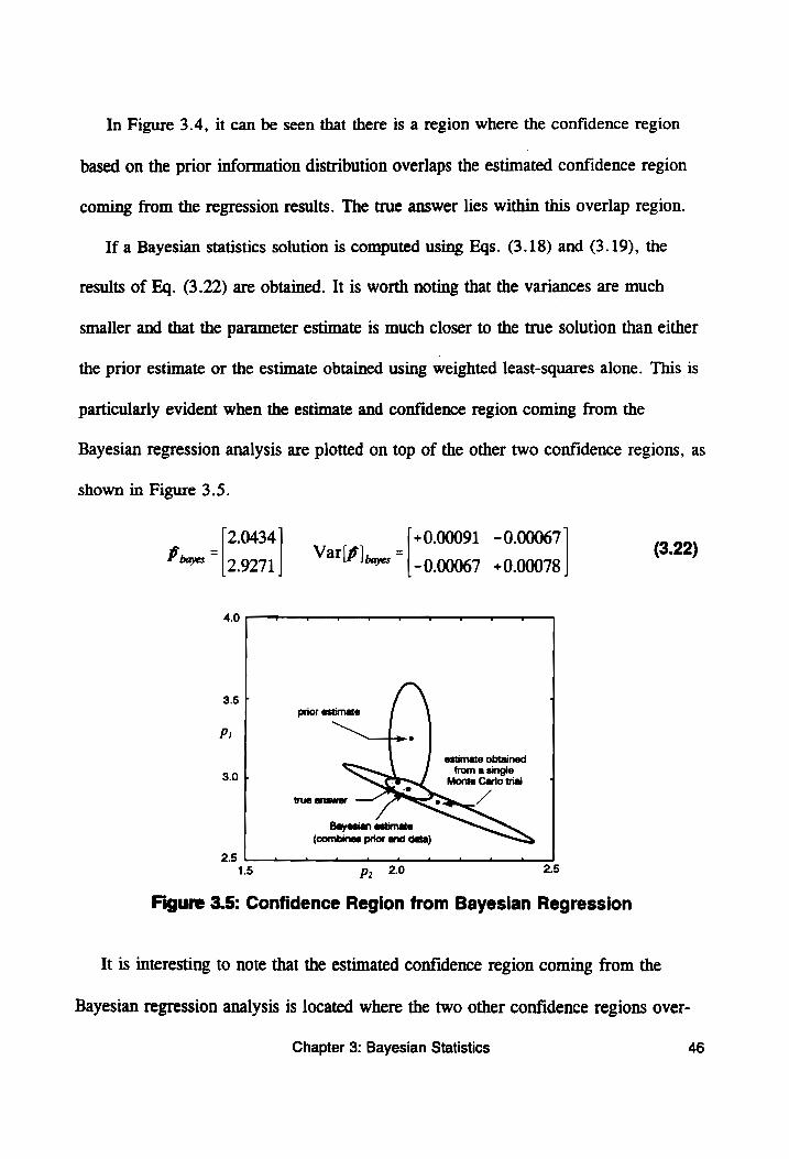
In Figure 3.4, it can be seen that there is a region where the confidence region
based on the prior information distribution overlaps the estimated confidence region
coming from the regression results. The true answer lies within this overlap region.
If a Bayesian statistics solution is computed using Eqs. (3.18) and (3.19), the
results of Eq. (3.22) are obtained. It is worth noting that the variances are much
smaller and that the parameter estimate is much closer to the true solution than either
the prior estimate or the estimate obtained using weighted least-squares alone. This is
particularly evident when the estimate and confidence region coming from the
Bayesian regression analysis are plotted on top of the other two confidence regions, as
shown in Figure 3.5.
+0.00091 -0.00067 - 3.22 aT1P lee nae? +0.00078 e2)
2.0434
bayes 19.9271
4.0 ¥ —_ — — r me ~ e r ms
3.57
3.0
2.5 — 1.5
Figure 3.5: Confidence Region from Bayesian Regression
It is interesting to note that the estimated confidence region coming from the
Bayesian regression analysis is located where the two other confidence regions over-
Chapter 3: Bayesian Statistics 46
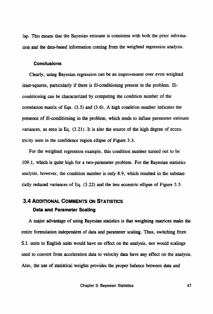
lap. This means that the Bayesian estimate is consistent with both the prior informa-
tion and the data-based information coming from the weighted regression analysis.
Conclusions
Clearly, using Bayesian regression can be an improvement over even weighted
least-squares, particularly if there is ill-conditioning present in the problem. Ill-
conditioning can be characterized by computing the condition number of the
correlation matrix of Eqs. (3.5) and (3.6). A high condition number indicates the
presence of ill-conditioning in the problem, which tends to inflate parameter estimate
variances, as seen in Eq. (3.21). It is also the source of the high degree of eccen-
tricity seen in the confidence region ellipse of Figure 3.3.
For the weighted regression example, this condition number turned out to be
109.1, which is quite high for a two-parameter problem. For the Bayesian statistics
analysis, however, the condition number is only 8.9, which resulted in the substan-
tially reduced variances of Eq. (3.22) and the less eccentric ellipse of Figure 3.5.
3.4 ADDITIONAL COMMENTS ON STATISTICS
Data and Parameter Scaling
A major advantage of using Bayesian statistics is that weighting matrices make the
entire formulation independent of data and parameter scaling. Thus, switching from
S.I. units to English units would have no effect on the analysis, nor would scalings
used to convert from acceleration data to velocity data have any effect on the analysis.
Also, the use of statistical weights provides the proper balance between data and
Chapter 3: Bayesian Statistics 47
priors. Without the weights, the analyst would have to assign a scaling coefficient to
the residuals from the priors to ensure that they influence the analysis sufficiently.
Normality of Data
In all three types of parameter estimation (ordinary least-squares, weighted
regression, and Bayesian regression), the errors on the data are assumed to come
from a multivariate normal (Gaussian) distribution. If this assumption is not met, it
decreases the efficiency of the estimation process and renders the parameter variance-
covariance matrix estimators of Eqs. (3.3), (3.10), and (3.19) inaccurate. Rarely do
we have any guarantees that the errors on raw time-series data meet this assumption.
However, if a large amount of data is available (as is the case with structural
dynamics testing results), the central limit theorem [77] indicates that statistical
quantities based on linear combinations of the data will approach normality, even if
errors on the data are not normally distributed. Typically, 30 or more data points
must be used for this approximation to hold.
As will be described in later chapters, the data used in the model update procedure
described in this dissertation are not actually raw time-series data, but are rather the
results of signal processing performed on the time-series data. In this signal process-
ing, a large amount of time-series data is condensed into a few numbers that effective-
ly describe the time-series data. For low noise levels, this data condensation process
is effectively linear, meaning that the results of signal processing become normally
distributed. This normality of the signal processing results indicates that a sum-of-
squares error is the appropriate quantity to use for comparison purposes.
Chapter 3: Bayesian Statistics 48
Other Measurable Quantities
Typically, the data used for parameter estimation consists of processed dynamic
response data. However, there may be other measurable quantities that can be
included as well. For example, if the mass of the test structure is known to weigh
15.05 + 0.05 kg, then the FE model should predict a weight within that range. Strain
gauge measurements could be used as well. These additional quantities, z , can be
included in the problem as shown in Eq. (3.23). The data weighting matrix is defined
by W,= Var"'[y], the weighting matrix for prior information is defined by
Wi Var"'[Po| , and the weighting matrix for the additional measurements is defined
by W, = Var"[z].
ny
_w\2 2” _w lt % _s \ SSE=¥° Yi~Y; +y Pom ~ Po ye 2-2 m
izi| oy m=1\ 9%, k=1| (3.23)
=(y -9)'W,(y - 9) + (Py -B)'W, (Po -P) + (z - 2) W, (2-2)
Of course, measurements of quantities can be considered simply as additional
data, as the y vector does not have to be restricted to signal processing results.
Therefore, the z vector can be appended to the y vector, and the W, matrix can be
appended to the W,, forming a generalized y vector and W, matrix pair as shown in
Eq. (3.24). This means that Eq. (3.17) can be used in place of Eq. (3.23).
y Varly] 0 Veins “|"} Vat) penn" ; vate (3.24)
Chapter 3: Bayesian Statistics 49
Comparing Different Models
The Bayesian statistics formulation for solving regression problems is also well-
suited for comparing how different models fit the same data. This can be accom-
plished by simply determining which model provides the smallest SSE value, as
defined in Eq. (3.17). The model with the smallest SSE value will be the model that
best fits the data.
3.5 THE CORE EQUATIONS
To summarize this chapter, there are four equations that describe the Bayesian
Statistics approach for updating parameters in a model. As mentioned in Section 3.1,
the FEM-based 9 data prediction vector is computed using the parameter estimate
vector f. A vector f of force amplitudes (to be described in Chapters 5 and 6) is also
required. Equation (3.17) gives the objective function that is to be minimized.
Equation (3.18) provides the basic iteration that is used to perform the function
minimization/parameter estimation. Equation (3.19) gives the variance-covariance
matrix that describes the quality of the resulting parameter estimates.
At the beginning of each chapter in this section, these four equations will be listed
again, along with a description of which vectors/matrices have already been derived,
which ones are being derived in that particular chapter, and which ones remain to be
derived in later chapter.
Chapter 3: Bayesian Statistics 50
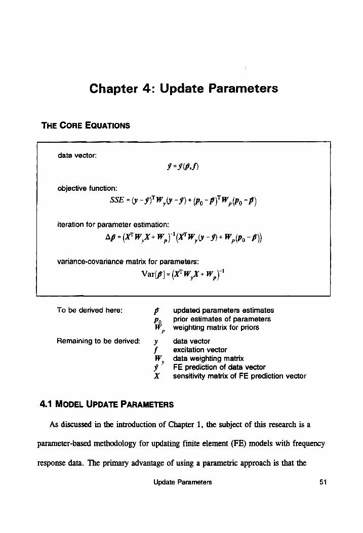
Chapter 4: Update Parameters
THE CORE EQUATIONS
data vector:
I=IWDS)
objective function:
SSE = (y - §)" Wy -9) + (Po - DB)" W, (Po -P)
iteration for parameter estimation:
Ap =(XTW,X+W,)(X'W,(y -9) + W, (Po - B)
variance-covariance matrix for parameters:
_ {yt -1 Var[p] = (X'W,X+W,)
To be derived here: Pp _updated parameters estimates P) _ Prior estimates of parameters W, weighting matrix for priors
Remaining to be derived: = y data vector f excitation vector W, data weighting matrix y FE prediction of data vector X _ sensitivity matrix of FE prediction vector
4.1 MODEL UPDATE PARAMETERS
As discussed in the introduction of Chapter 1, the subject of this research is a
parameter-based methodology for updating finite element (FE) models with frequency
response data. The primary advantage of using a parametric approach is that the
Update Parameters 51

updated parameters provide insight into the changes made to the model. Clearly, one
of the main tasks the analyst initially has (in addition to building the initial FE model)
is to pick the parameters that are to be updated. The parameter vector p contains one
entry for each parameter to be updated. The updated parameter estimates that come
from the regression analysis are designated pf, with the “hat” indicating that they are
estimated quantities.
Since finite element models can be used to model a wide range of systems, there
are virtually no restrictions on what constitutes a valid parameter, aside from the fact
that they must be independent. For example, if the analyst is modeling a beam with a
solid rectangular cross-section, he cannot select width b, thickness h , and cross-
section area A, since A = bh. Unfortunately, this lack of independence will not
always be obvious to the analyst.
Additionally, it is preferable that the parameters consist of values that are easily
measured or interpreted. Parameters such as these include material parameters such as
density and elastic modulus, global geometric properties such as length and thickness,
and boundary condition values such as effective mass and effective stiffness. An
example of parameters that are difficult to measure or interpret are individual entries
in the finite element mass and stiffness matrices.
Trade-offs can sometimes be made between parameter ease-of-use and intuitive-
ness. For example, when working with a rectangular cross section of a beam (with a
fixed width), it is easier to work with the area moment of inertia J , since the FE
stiffness matrix is linear with respect to J]. However, it is more intuitive to work with
Update Parameters 52
thickness ¢ and width w, since these are the parameters that the analyst can actually
measure and are the quantities that would be modified in a design change. Parameters
that required remeshing of the FE model should be avoided, since repeatedly remesh-
ing the FE model greatly increases the expense of performing the model update. In
the research of this dissertation, choices between intuitiveness and ease-of-use went
both ways.
Ideally, the set of parameters will be as small as possible, while being complete
enough to include the dominant sources of uncertainty in the model. Thus, when the
parameters are properly updated, the uncertainty in the model will have been signifi-
cantly reduced and the predictive capability of the model will have been improved.
4.2 BAYESIAN PRIORS
An additional benefit of using design parameters is that the update problem can be
formulated as a Bayesian statistics problem. In this statistical framework, any prior
knowledge the analyst has concerning the values of the design parameters can be
formally incorporated into the update process. This knowledge, usually consisting of
independent measurements of the the parameters, is called prior information.
In the Bayesian statistics approach, prior information is described by the a priori
probability distribution function (PDF). This PDF is typically summarized with esti-
mates of mean and variance for parameters coming from a normal distribution. The
estimated mean and variance together are called a prior.
If the update parameters are selected properly, priors can be easily obtained. For
example, if one of the parameters is thickness, the analyst can measure the thickness
Update Parameters 53
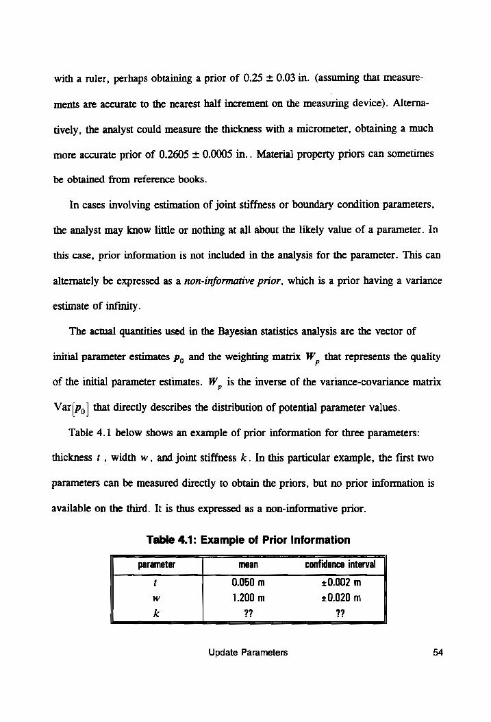
with a ruler, perhaps obtaining a prior of 0.25 + 0.03 in. (assuming that measure-
ments are accurate to the nearest half increment on the measuring device). Alterna-
tively, the analyst could measure the thickness with a micrometer, obtaining a much
more accurate prior of 0.2605 + 0.0005 in.. Material property priors can sometimes
be obtained from reference books.
In cases involving estimation of joint stiffness or boundary condition parameters,
the analyst may know little or nothing at all about the likely value of a parameter. In
this case, prior information is not included in the analysis for the parameter. This can
alternately be expressed as a non-informative prior, which is a prior having a variance
estimate of infinity.
The actual] quantities used in the Bayesian statistics analysis are the vector of
initial parameter estimates p, and the weighting matrix W, that represents the quality
of the initial parameter estimates. W,, is the inverse of the variance-covariance matrix
Var [Po| that directly describes the distribution of potential parameter values.
Table 4.1 below shows an example of prior information for three parameters:
thickness ¢ , width w, and joint stiffness k. In this particular example, the first two
parameters can be measured directly to obtain the priors, but no prior information is
available on the third. It is thus expressed as a non-informative prior.
Table 4.1: Example of Prior Information
parameter mean confidence interval
t 0.050 m +0.002 m
w 1.200 m +0.020 m
k ?? ??
Update Parameters 54
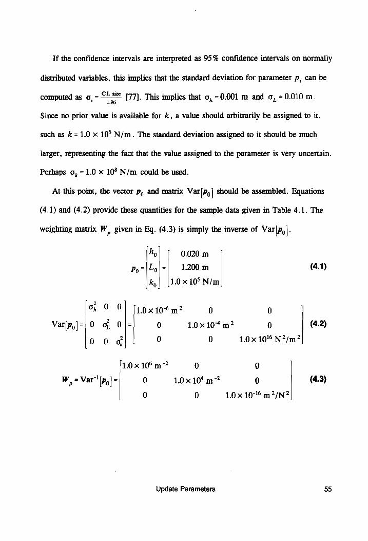
If the confidence intervals are interpreted as 95% confidence intervals on normally
distributed variables, this implies that the standard deviation for parameter p, can be
computed as a, = —= [77]. This implies that o, = 0.001 m and a, =0.010 m.
Since no prior value is available for k , a value should arbitrarily be assigned to it,
such as k = 1.0 x 10° N/m. The standard deviation assigned to it should be much
larger, representing the fact that the value assigned to the parameter is very uncertain.
Perhaps o, = 1.0 x 10° N/m could be used.
At this point, the vector p, and matrix Var|Po| should be assembled. Equations
(4.1) and (4.2) provide these quantities for the sample data given in Table 4.1. The
weighting matrix W, given in Eq. (4.3) is simply the inverse of Var|Do|-
Ng 0.020 m Po= Ly |= 1.200 m (4.1)
ky 1.0 x 10° N/m
% 9 Of [19x%10% m2 0 0 Var[p]=|0 o, 0|= 0 1.0x 10“ m? 0 (4.2)
006 0 0 1.0 x 10'° N?/m?
1.0 x 10⁶ m 0 0 W, = Var"'[py|= 0 1.0x 10* m * 0 (4.3)
0 0 1.0x 10° m?/N?
Update Parameters 55
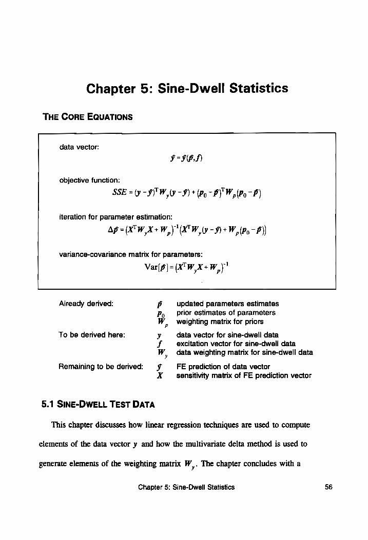
Chapter 5: Sine-Dwell Statistics
THE CORE EQUATIONS
data vector:
¥ =I.)
objective function:
SSE = (y -§)'W,(y -9) + (Py - B)' W,, (Po -P)
iteration for parameter estimation:
Ap =(X"W,X+W,)'(X"W,(y -9) + W, (Po - 8)
variance-covariance matrix for parameters:
- {yr -1 Var[p]=(X'W,X+W, )
Already derived: updated parameters estimates prior estimates of parameters
weighting matrix for priors <3
data vector for sine-dwell data
excitation vector for sine-dwell data
data weighting matrix for sine-dwell data
To be derived here:
yo
FE prediction of data vector
sensitivity matrix of FE prediction vector Remaining to be derived:
be Ss
5.1 SINE-DWELL TEST DATA
This chapter discusses how linear regression techniques are used to compute
elements of the data vector y and how the multivariate delta method is used to
generate elements of the weighting matrix W,. The chapter concludes with a
Chapter 5: Sine-Dwell Statistics 56
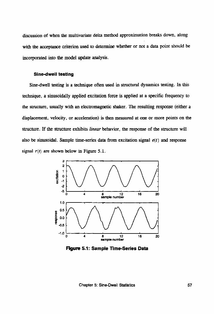
discussion of when the multivariate delta method approximation breaks down, along
with the acceptance criterion used to determine whether or not a data point should be
incorporated into the model update analysis.
Sine-dwell testing
Sine-dwell testing is a technique often used in structural dynamics testing. In this
technique, a sinusoidally applied excitation force is applied at a specific frequency to
the structure, usually with an electromagnetic shaker. The resulting response (either a
displacement, velocity, or acceleration) is then measured at one or more points on the
structure. If the structure exhibits Jinear behavior, the response of the structure will
also be sinusoidal. Sample time-series data from excitation signal e(t) and response
signal r(t) are shown below in Figure 5.1.
excitation
3 i a |
0 4 8 12 16 20 sampie number
1.0 5 v OU Ue
o 25F a” ¢
8 0.0
2 0.5 4
-1.0 : —— —- ‘ 0 4 8 12 16 20
sample number
Figure 5.1: Sample Time-Series Data
Chapter 5: Sine-Dwell Statistics 57
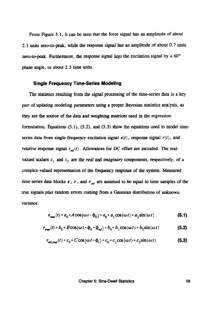
From Figure 5.1, it can be seen that the force signal has an amplitude of about
2.1 units zero-to-peak, while the response signal has an amplitude of about 0.7 units
zero-to-peak. Furthermore, the response signal lags the excitation signal by a 60°
phase angle, or about 2.5 time units.
Single Frequency Time-Series Modeling
The statistics resulting from the signal processing of the time-series data is a key
part of updating modeling parameters using a proper Bayesian statistics analysis, as
they are the source of the data and weighting matrices used in the regression
formulation. Equations (5.1), (5.2), and (5.3) show the equations used to model time-
series data from single-frequency excitation signal e(t), response signal r(t), and
relative response signal r,,(t). Allowances for DC offset are included. The real-
valued scalars c, and c, are the real and imaginary components, respectively, of a
complex-valued representation of the frequency response of the system. Measured
time-series data blocks e, r, and r,,, are assumed to be equal to time samples of the
true signals plus random errors coming from a Gaussian distribution of unknown
variance.
Cie (t) = Ag+ A COS(Wt- by) = ay+ a, COS(Wt) + a, sin (Wt) (5.1)
Tmue(t) = Dy+ BCOs(w t~ y- ,,,) = by+ b, cos (wt) + b,sin (wt) (5.2)
Tret mue(t) = p+ CC0S(wt-,) = cy+ c, cos (wt) +c,sin(w?) (5.3)
Chapter 5: Sine-Dwell Statistics 58
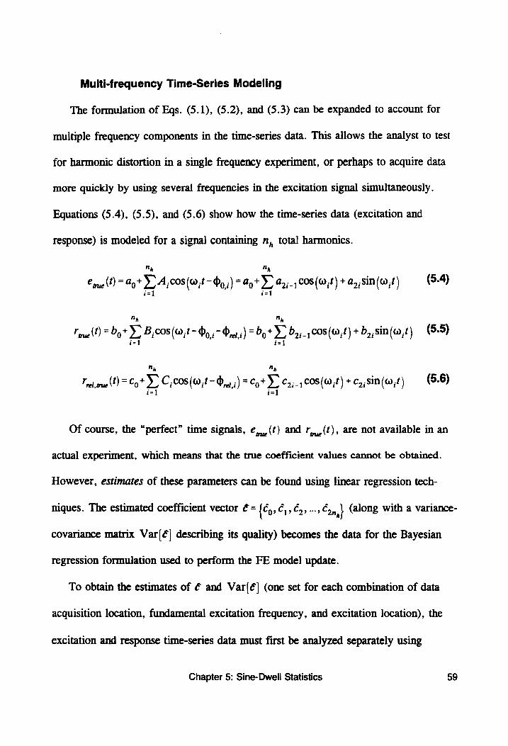
Multi-frequency Time-Series Modeling
The formulation of Eqs. (5.1), (5.2), and (5.3) can be expanded to account for
multiple frequency components in the time-series data. This allows the analyst to test
for harmonic distortion in a single frequency experiment, or perhaps to acquire data
more quickly by using several frequencies in the excitation signal simultaneously.
Equations (5.4), (5.5), and (5.6) show how the time-series data (excitation and
response) is modeled for a signal containing n, total harmonics.
n, n,
Cmue(t) =4y+ )A;COS(W;t- Yo ;) = Ag+) @p;_,COS(W,t) + a,,Sin(w,t) (5.4) i=] i=]
nh n,
Time (t) = Dy+ Y B;COS(W,t~ Op ;~ Dyes ;) = Dg + Y- by;-1C08(w;t) + b,,8in(w,t) (5-5) i=] i=l
np ny
ret mue(t) = €9+ ¥, C,COS(w,t- 1 ;) = Co+ ¥. Ca;-1CO8(W,t)+C,,Sin(w,t) (5.6) i=l i=l
Of course, the “perfect” time signals, e,_(¢) and r,(t), are not available in an
actual experiment, which means that the true coefficient values cannot be obtained.
However, estimates of these parameters can be found using linear regression tech-
niques. The estimated coefficient vector ¢ = {Cos C19 Cay oy Con,} (along with a variance-
covariance matrix Var|¢| describing its quality) becomes the data for the Bayesian
regression formulation used to perform the FE model update.
To obtain the estimates of ¢ and Var|é] (one set for each combination of data
acquisition location, fundamental excitation frequency, and excitation location), the
excitation and response time-series data must first be analyzed separately using
Chapter 5: Sine-Dwell Statistics 59
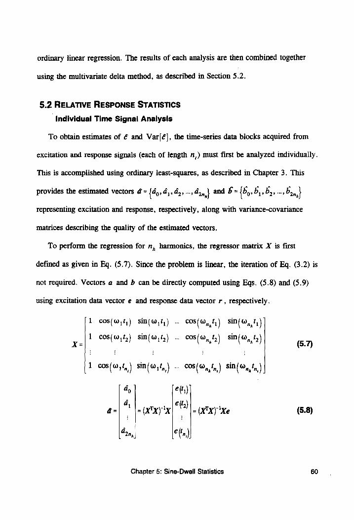
ordinary linear regression. The results of each analysis are then combined together
using the multivariate delta method, as described in Section 5.2.
5.2 RELATIVE RESPONSE STATISTICS
Individual Time Signal Analysis
To obtain estimates of ¢ and Var[é], the time-series data blocks acquired from
excitation and response signals (each of length n,) must first be analyzed individually.
This is accomplished using ordinary least-squares, as described in Chapter 3. This
provides the estimated vectors @ = {do, d,,4,, ~»o,,} and 5 = {bo by, Ba, «5 Bon}
representing excitation and response, respectively, along with variance-covariance
matrices describing the quality of the estimated vectors.
To perform the regression for n, harmonics, the regressor matrix X is first
defined as given in Eq. (5.7). Since the problem is linear, the iteration of Eq. (3.2) is
not required. Vectors a and b can be directly computed using Eqs. (5.8) and (5.9)
using excitation data vector e and response data vector r , respectively.
1 cos(W,t,) sin(@,t,) .. COs(@,,, £1) sin(@, £,)
y- 1 cos(@,t,) sin(@,t,) ... Cos (W,,, £5) sin(,,t2) (5.7)
1 COS (1, ) sin(©,t,, ) -- COS(O,, f, | sin(©,, t,,)
a, e(t,)
i, me-ty| &(E2) 1 G = = (X™X)'X a (X™X) 'Xe (5.8)
Gon, e(,
Chapter 5: Sine-Dwell Statistics 60
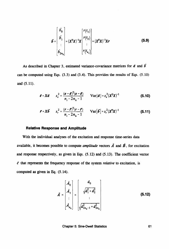
°Q “
mt,
~
oma
~
a
B= 7" | =cxtxytx| 8?) = (xx) xr (5.9)
Pan, r(Fn,) As described in Chapter 3, estimated variance-covariance matrices for @ and b
can be computed using Eqs. (3.3) and (3.4). This provides the results of Eqs. (5.10)
and (5.11).
-6\"(p- e=xa 522-978) Varig) =5?(xTx)" (5.10)
n,-2n,-1
f=-X6 s°= (r-#)'(r-F) Var(b] =s,(X™x)" (5.11) n,-2n,-1
Relative Response and Amplitude
With the individual analyses of the excitation and response time-series data
available, it becomes possible to compute amplitude vectors A and B, for excitation
and response respectively, as given in Eqs. (5.12) and (5.13). The coefficient vector
é that represents the frequency response of the system relative to excitation, is
computed as given in Eq. (5.14).
[4 | a A, 0 A a+a
A-| l- — (5.12)
An, Gon,-1* Fn Chapter 5: Sine-Dwell Statistics 61
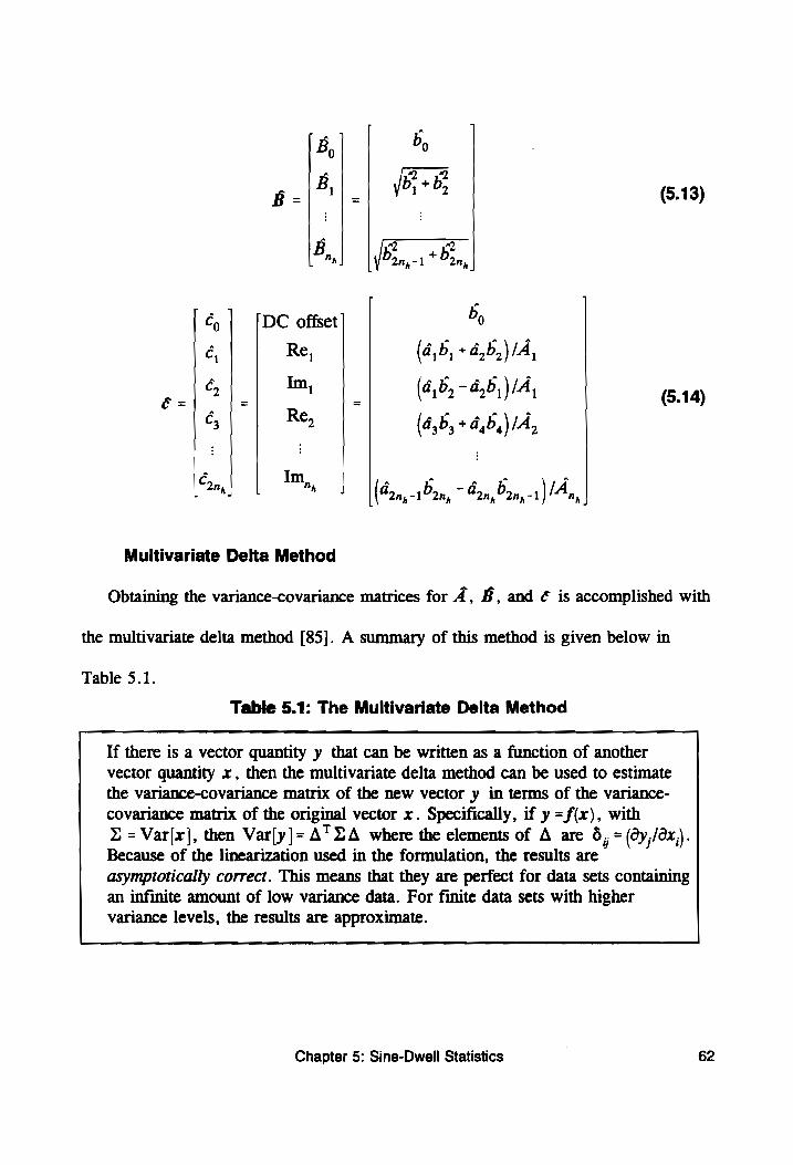
r A rp 3 b
B, 0 - be + Be
B _ | _ 7 2 (5.13)
a a2 2)
B.. Don,-1 2n, |
fé, | [DC offset’ 0 | a | | Re, 6,6, +4,6,)/A, Fae i ee GU ea (5.14)
C; Re, (4, 5 +a, », LA,
C. Im,, 7 ). I ) { | 2p | | , (4on,-1P2n, ~ 8, Pant) !Any, Multivariate Delta Method
Obtaining the variance-covariance matrices for 4, B, and ¢ is accomplished with
the multivariate delta method [85]. A summary of this method is given below in
Table 5.1.
Table 5.1: The Multivariate Delta Method
If there is a vector quantity y that can be written as a function of another vector quantity x, then the multivariate delta method can be used to estimate
the variance-covariance matrix of the new vector y in terms of the variance- covariance matrix of the original vector x. Specifically, if y = f(x), with = = Var[x], then Var[y]= A™ZA where the elements of A are 6, =(dy,/x)). Because of the linearization used in the formulation, the results are asymptotically correct. This means that they are perfect for data sets containing an infinite amount of low variance data. For finite data sets with higher
variance levels, the results are approximate.
Chapter 5: Sine-Dwell Statistics 62
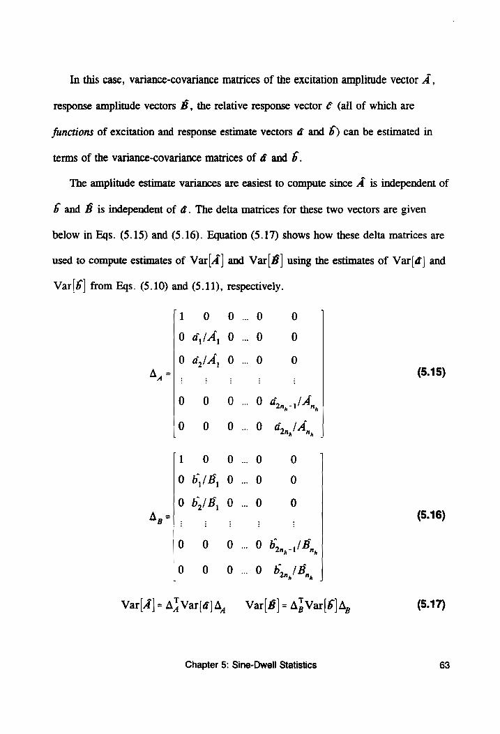
In this case, variance-covariance matrices of the excitation amplitude vector A,
response amplitude vectors B, the relative response vector ¢ (all of which are
functions of excitation and response estimate vectors @ and 6) can be estimated in
terms of the variance-covariance matrices of @ and b.
The amplitude estimate variances are easiest to compute since A is independent of
5 and B is independent of @. The delta matrices for these two vectors are given
below in Eqs. (5.15) and (5.16). Equation (5.17) shows how these delta matrices are
used to compute estimates of Var|A| and Var|#] using the estimates of Var{d] and
Var|6| from Eqs. (5.10) and (5.11), respectively.
[4
0
SO oO
&
Var|A] = A} Var[4]
0
a,/A,
a,/A,
a a
b/B, b,/B,
A
0...
0...
0 0
0 0
. 0 0
0 d,, /A,,
0 dy, |An
0 0
0 0
. 0 0
. 0B, 4/8,
0 5, /B,
Var|B] = A; Var|b] A,
Chapter 5: Sine-Dwell Statistics
(5.15)
(5.16)
(5.17)
63
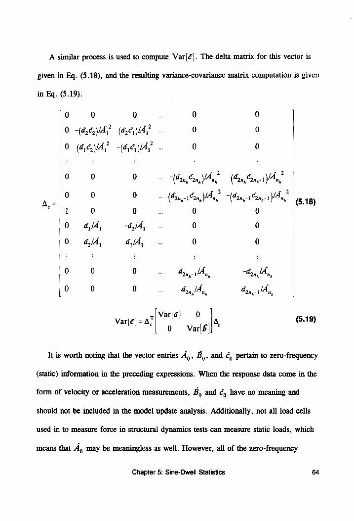
A similar process is used to compute Var(¢|. The delta matrix for this vector is
given in Eq. (5.18), and the resulting variance-covariance matrix computation is given
in Eq. (5.19).
OQ 0 0 0 0 :
0 -(4,6,/A, (d,¢,/A? 0 ° 0 (4,¢,)/A," -(4,6,)/A," ° °
a o ; 2 7 { * 0 0 0 ™ “(42n, (on, VA, (42n, Cony 1 "4,
a 2 ; * { ?
A. 0 0 0 wee (42n,-1©2n,\/An, ~(42n,-1©2n,-1 An, (5.18)
0 4,/A, -d,/A, 0 ° 0 G,/A, a, /A, “ 0 °
0 0 0 . Gon, 1 IA, “Fan, An,
0 0 0 . dy, A, bany-1!An,
Var|@ 0 var(e]= a7 [a] A (5.19) 0 Var|b]
It is worth noting that the vector entries A,, B,, and ¢, pertain to zero-frequency
(static) information in the preceding expressions. When the response data come in the
form of velocity or acceleration measurements, B, and ¢, have no meaning and
should not be included in the model update analysis. Additionally, not all load cells
used in to measure force in structural dynamics tests can measure static loads, which
means that A, may be meaningless as well. However, all of the zero-frequency
Chapter 5: Sine-Dwell Statistics 64
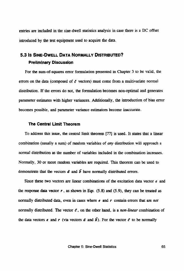
entries are included in the sine-dwell statistics analysis in case there is a DC offset
introduced by the test equipment used to acquire the data.
5.3 Is SINE-DWELL DATA NORMALLY DISTRIBUTED?
Preliminary Discussion
For the sum-of-squares error formulation presented in Chapter 3 to be valid, the
errors on the data (composed of ¢ vectors) must come from a multivariate normal
distribution. If the errors do not, the formulation becomes non-optimal and generates
parameter estimates with higher variances. Additionally, the introduction of bias error
becomes possible, and parameter variance estimators become inaccurate.
The Central Limit Theorem
To address this issue, the central limit theorem [77] is used. It states that a linear
combination (usually a sum) of random variables of amy distribution will approach a
normal distribution as the number of variables included in the combination increases.
Normally, 30 or more random variables are required. This theorem can be used to
demonstrate that the vectors ¢ and 6 have normally distributed errors.
Since these two vectors are linear combinations of the excitation data vector e and
the response data vector r , as shown in Eqs. (5.8) and (5.9), they can be treated as
normally distributed data, even in cases where e and r contain errors that are not
normally distributed. The vector €, on the other hand, is a non-linear combination of
the data vectors e and r (via vectors @ and 6). For the vector ¢ to be normally
Chapter 5: Sine-Dwell Statistics 65
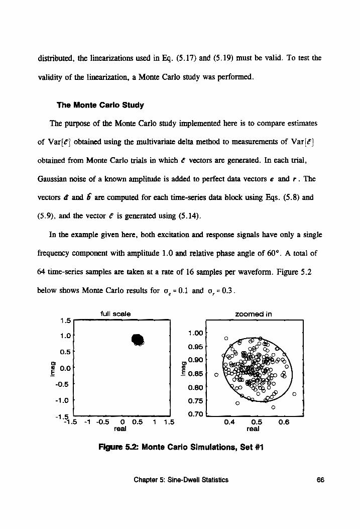
distributed, the linearizations used in Eq. (5.17) and (5.19) must be valid. To test the
validity of the linearization, a Monte Carlo study was performed.
The Monte Carlo Study
The purpose of the Monte Carlo study implemented here is to compare estimates
of Var/¢] obtained using the multivariate delta method to measurements of Var|¢|
obtained from Monte Carlo trials in which ¢ vectors are generated. In each trial,
Gaussian noise of a known amplitude is added to perfect data vectors e and r. The
vectors @ and 6 are computed for each time-series data block using Egs. (5.8) and
(5.9), and the vector ¢ is generated using (5.14).
In the example given here, both excitation and response signals have only a single
frequency component with amplitude 1.0 and relative phase angle of 60°. A total of
64 time-series samples are taken at a rate of 16 samples per waveform. Figure 5.2
below shows Monte Carlo results for o,=0.1 and o,=0.3.
full scale zoomed in 1.5 ~ - -
1.0f @ 1.00 j -
| 0.95 [ 0.5] |
© ool @ 0-90
E° £0.85}
-0.5 - : 0.80 t
-1.0 Tf ’ 0.75 f
-1.5 0.70 t
1.5 -1 05 005 1 1.5 0.4 0.5 0.6 real real
Figure 5.2: Monte Carlo Simulations, Set #1
Chapter 5: Sine-Dwell Statistics 66
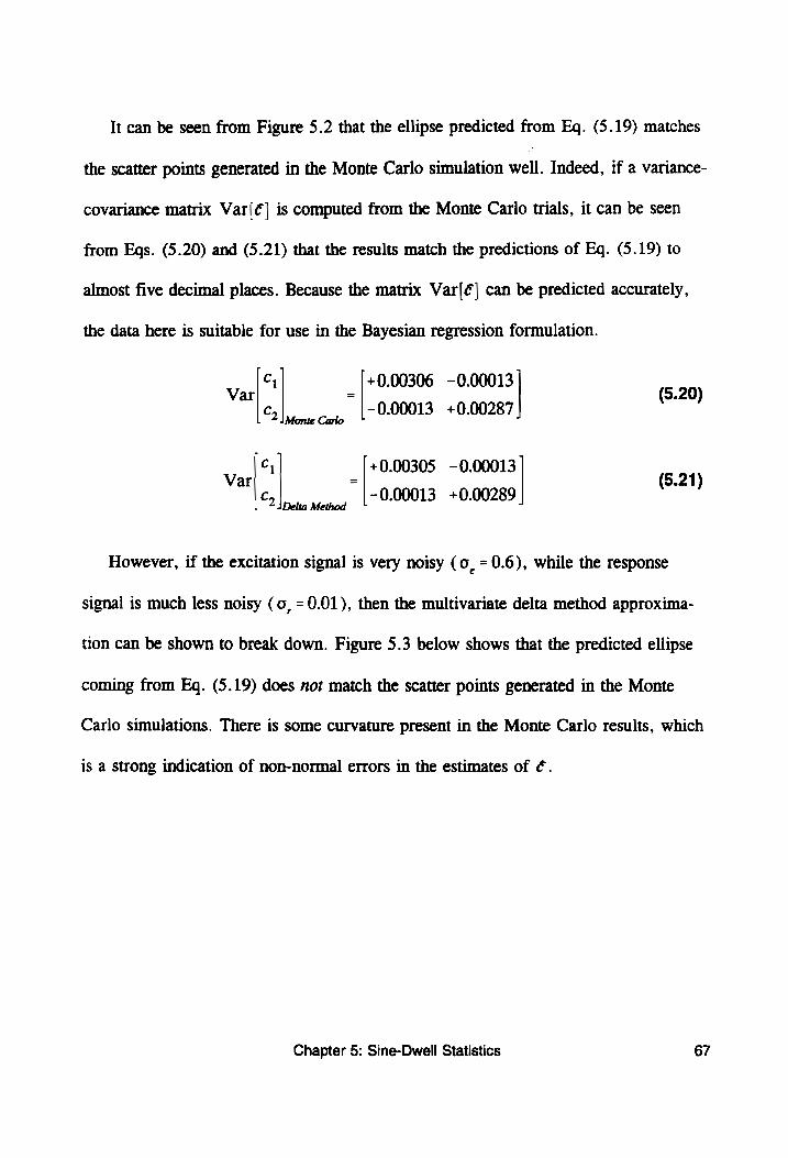
It can be seen from Figure 5.2 that the ellipse predicted from Eq. (5.19) matches
the scatter points generated in the Monte Carlo simulation well. Indeed, if a variance-
covariance matrix Var(¢] is computed from the Monte Carlo trials, it can be seen
from Eqs. (5.20) and (5.21) that the results match the predictions of Eq. (5.19) to
almost five decimal places. Because the matrix Var/¢] can be predicted accurately,
the data here is suitable for use in the Bayesian regression formulation.
y Cy +0.00306 “camer (5.20) ar = °
C5 -0.00013 +0.00287 Monte Carlo
y Cy +0.00305 eel 6.21) ar = .
C, -0.00013 +0.00289 Delta Method
However, if the excitation signal is very noisy (0, = 0.6), while the response
signal is much less noisy (0, = 0.01), then the multivariate delta method approxima-
tion can be shown to break down. Figure 5.3 below shows that the predicted ellipse
coming from Eq. (5.19) does not match the scatter points generated in the Monte
Carlo simulations. There is some curvature present in the Monte Carlo results, which
is a strong indication of non-normal errors in the estimates of ¢.
Chapter 5: Sine-Dwell Statistics 67
full scale zoomed in
1.5
1.1 1
1.0} ma,
0.5! | 1.0 LS
oD m 0.9 1 E 0.0 | £
05 | | 0.8
-1.0 | 0.7 | @
-1.5 0.6 15 -1-05 005 1 =1.5 0.2 0.4 0.6
real real
Figure 5.3: Monte Carlo Simulations, Set #2
If a variance-covariance matrix Var[é] is computed from the Monte Carlo trials
in this case [83], it can be seen from Eqs. (5.22) and (5.23) that the results match the
predictions of Eq. (5.19) only to three decimal places. Because the matrix Var|¢]
cannot be predicted accurately and because there is evidence of non-normality, the
data here is not suitable for use in the Bayesian regression formulation of Chapter 3
and must be dropped from the analysis.
y Re=c, +0.00832 ee (6.22) ar = .
Im =c, |, -0.00475 +0.00280
y Re =c, +0,00844 ieee (6.28) ar = 2
Im =c -0.00487 +0.00282 2 | Delta Method
Chapter 5: Sine-Dwell Statistics 68
Data Acceptance Criteria
From the discussion in the previous section, it is apparent that some test data and
statistical weights (some of the vectors ¢ and corresponding matrices W = Var ![é])
may not be suitable for use in a least-squares type formulation. To determine whether
or not data from a particular point (data acquisition location/excitation location/
frequency set combination) is valid, the criteria of Eqs. (5.24) and (5.25) must be
met. In these equations, the quantities A, and B, are the elements of the A and B
vectors of Eqs. (5.8) and (5.9) corresponding to the /“ harmonic. The corresponding
variances are the /"" diagonal entries of the two variance-covariance matrices given in
Eq. (5.17).
vain / a co. (5.24)
A,
- 2 [| 5] 5 VarlA, - /Var/B, (5.25)
A, B,
The first rule, Eq. (5.24), is a limit that ensures that phase angle errors are not
too large and do not cause too much curvature. The second rule, Eq. (5.25), ensures
that curvature effects caused by errors in the excitation signal are small enough to be
masked by effects caused by errors in the response signal. These criteria came from
observations of many Monte Carlo studies in which different noise levels were tested
on both the excitation and response data.
Chapter 5: Sine-Dwell Statistics 69
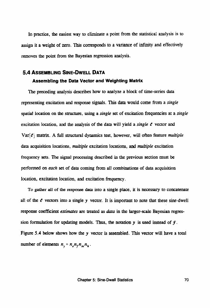
In practice, the easiest way to eliminate a point from the statistical analysis is to
assign it a weight of zero. This corresponds to a variance of infinity and effectively
removes the point from the Bayesian regression analysis.
5.4 ASSEMBLING SINE-DWELL DATA
Assembling the Data Vector and Weighting Matrix
The preceding analysis describes how to analyze a block of time-series data
representing excitation and response signals. This data would come from a single
spatial location on the structure, using a single set of excitation frequencies at a single
excitation location, and the analysis of the data will yield a single € vector and
Var[é] matrix. A full structural dynamics test, however, will often feature multiple
data acquisition locations, multiple excitation locations, and multiple excitation
frequency sets. The signal processing described in the previous section must be
performed on each set of data coming from all combinations of data acquisition
location, excitation location, and excitation frequency.
To gather all of the response data into a single place, it is necessary to concatenate
all of the € vectors into a single y vector. It is important to note that these sine-dwell
response coefficient estimates are treated as data in the larger-scale Bayesian regres-
sion formulation for updating models. Thus, the notation y is used instead of ¥.
Figure 5.4 below shows how the y vector is assembled. This vector will have a total
number of elements n, = n,n,n,,n, . ef" m
Chapter 5: Sine-Dwell Statistics 70
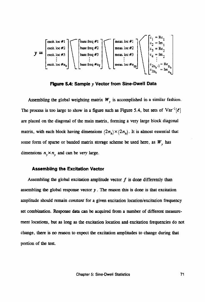
rc i= Re, ] excit. loc #1 base freq #1 meas. loc #1 cy =Im
1 excit. loc #2 base freq #2 meas. loc #2 Ca = Re,
Y = | excit. loc #3 base freq #3 meas. loc #3 C4 = Im,
excit. loc #n, base freq #n¢ meas. loc #n_, C2n, = Ren
“2n, = Nh Figure 5.4: Sample y Vector from Sine-Dwell Data
Assembling the global weighting matrix W, is accomplished in a similar fashion.
The process is too large to show in a figure such as Figure 5.4, but sets of Var™'(é]
are placed on the diagonal of the main matrix, forming a very large block diagonal
matrix, with each block having dimensions (2n,)x(2n,\. It is almost essential that
some form of sparse or banded matrix storage scheme be used here, as W,, has
dimensions n,n, and can be very large.
Assembling the Excitation Vector
Assembling the global excitation amplitude vector f is done differently than
assembling the global response vector y . The reason this is done is that excitation
amplitude should remain constant for a given excitation location/excitation frequency
set combination. Response data can be acquired from a number of different measure-
ment locations, but as long as the excitation location and excitation frequencies do not
change, there is no reason to expect the excitation amplitudes to change during that
portion of the test.
Chapter 5: Sine-Dwell Statistics 71
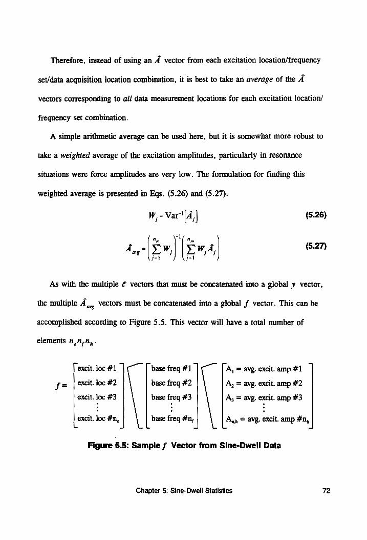
Therefore, instead of using an A vector from each excitation location/frequency
set/data acquisition location combination, it is best to take an average of the 4
vectors corresponding to ali data measurement locations for each excitation location/
frequency set combination.
A simple arithmetic average can be used here, but it is somewhat more robust to
take a weighted average of the excitation amplitudes, particularly in resonance
situations were force amplitudes are very low. The formulation for finding this
weighted average is presented in Eqs. (5.26) and (5.27).
W,= Var"! (A, | (5.26)
(5.27) A a=
Nn “1 Ain
Sw] [$04 j=l j=l
As with the multiple ¢ vectors that must be concatenated into a global y vector,
the multiple 4 ag Vectors must be concatenated into a global f vector. This can be
accomplished according to Figure 5.5. This vector will have a total number of
elements n.n,N,.
| excit. loc #1 | | base freq #1 ] TA, = avg. excit. amp #1 |
f= excit. loc #2 base freq #2 A, = avg. excit. amp #2
excit. loc #3 base freq #3 A, = avg. excit. amp #3
excit. loc #n, base freq #n, A, = avg. excit. amp #n, L - L - L -
Figure 5.5: Sample f Vector from Sine-Dwell Data
Chapter 5: Sine-Dwell Statistics 72
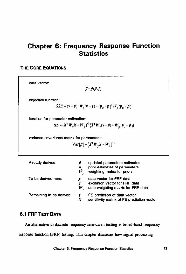
Chapter 6: Frequency Response Function Statistics
THE CORE EQUATIONS
data vector:
¥=IOS)
objective function:
SSE = (y -§)"W,(y -9) + (Py - B)' (Po -P)
iteration for parameter estimation:
Ap =(X"W,X+W,) (XW, -9)+ W, (Po -B))
variance-covariance matrix for parameters:
— {yt -1 Var|p|= (X WX + W,)
Already derived: Pf _updated parameters estimates Py) Prior estimates of parameters
W, weighting matrix for priors
To be derived here: y data vector for FRF data f excitation vector for FRF data W, data weighting matrix for FRF data
Remaining to be derived: ff FE prediction of data vector X _ sensitivity matrix of FE prediction vector
6.1 FRF Test DATA
An alternative to discrete frequency sine-dwell testing is broad-band frequency
response function (FRF) testing. This chapter discusses how signal processing
Chapter 6: Frequency Response Function Statistics 73
techniques and standard FRF estimators are used to compute elements of the FRF data
vector § and how a statistical analysis of the FRF estimate is used to generate the
associated weighting matrix W,. The chapter concludes with a discussion of when the
variance estimators for the FRF break down, along with the acceptance criterion used
to determine whether or not a data point should be included in the Bayesian regression
formulation for updating models.
Frequency Response Function Testing
The excitation used for broad-band FRF testing typically comes from a modal test
hammer impact or burst-random excitation coming from an electromagnetic shaker.
Standard FFT-based signal processing routines are used to generate a complex-valued
FRF along with a coherence function that describes the quality of the FRF (81, 82].
As with the sine-dwell results, the FRF and measures of its quality become the data
for the Bayesian regression formulation for updating models.
Basic FRF Signal Processing
When acquiring data for FFT-based signal processing, a number of blocks of
time-series data (n, = 30+) are normally taken such that averages can be computed.
Equations (6.1), (6.2), (6.3), and (6.4) show the relationships used to compute auto-
and cross-spectra estimates, FRF estimates, and coherence estimates at frequency
f =(j-1)At/n, (At = time sample interval, n, = block size of FFT) [81].
X, and F, are results from the k™ spectral line of FFT results obtained from the
response data vector r and the excitation data vector e , respectively. Gy ke Gy ke
Chapter 6: Frequency Response Function Statistics 74
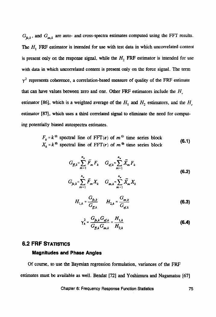
Geek 9
The H, FRF estimator is intended for use with test data in which uncorrelated content
and G,, , are auto- and cross-spectra estimates computed using the FFT results.
is present only on the response signal, while the H, FRF estimator is intended for use
with data in which uncorrelated content is present only on the force signal. The term
y* represents coherence, a correlation-based measure of quality of the FRF estimate
that can have values between zero and one. Other FRF estimators include the H,
estimator [86], which is a weighted average of the H, and H, estimators, and the H.
estimator [87], which uses a third correlated signal to eliminate the need for comput-
ing potentially biased autospectra estimates.
F,,=k™ spectral line of FFT(e) of m™ time series block
th . th a: . (6.1) X,=k"™ spectral line of FFT(r) of m"™ time series block
Cpa do Fn Fi Ci = mx
(6.2)
Gay FX Go = mk
G G H,,=—2* = H,,=—z# (6.3)
1,k Gey 2,k Gry
yp= esSae - Ai (6.4) Ge Gur Ah,
6.2 FRF STATISTICS
Magnitudes and Phase Angles
Of course, to use the Bayesian regression formulation, variances of the FRF
estimates must be available as well. Bendat [72] and Yoshimura and Nagamatsu [67]
Chapter 6: Frequency Response Function Statistics 75
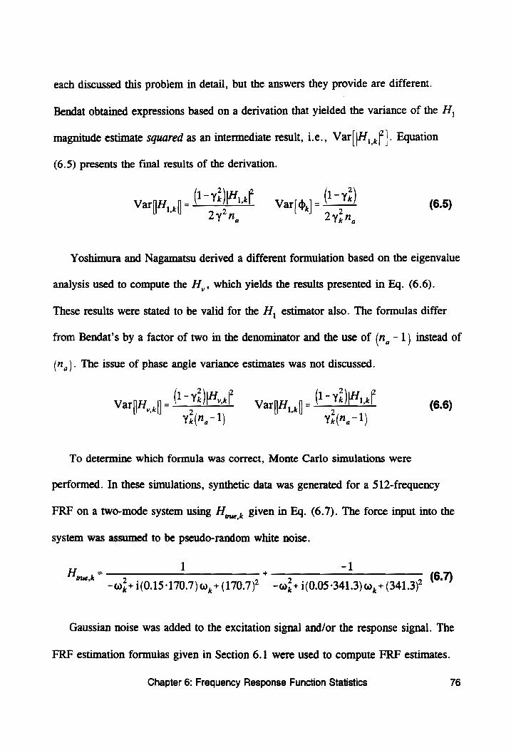
each discussed this problem in detail, but the answers they provide are different.
Bendat obtained expressions based on a derivation that yielded the variance of the H,
magnitude estimate squared as an intermediate result, i.e., Var{|H, if]. Equation
(6.5) presents the final results of the derivation.
1- ¥ i- v
Vary, j= & eal a Var[,]= NE e°)
Yoshimura and Nagamatsu derived a different formulation based on the eigenvalue
analysis used to compute the H,, which yields the results presented in Eq. (6.6).
These results were stated to be valid for the H, estimator also. The formulas differ
from Bendat’s by a factor of two in the denominator and the use of (n, - 1) instead of
(n,). The issue of phase angle variance estimates was not discussed.
VarjH,,j= ONE vary j= OH (6.6) ¥;,(",~ 1) ¥;,(",-1)
To determine which formula was correct, Monte Carlo simulations were
performed. In these simulations, synthetic data was generated for a 512-frequency
FRF on a two-mode system using H,,, , given in Eq. (6.7). The force input into the
system was assumed to be pseudo-random white noise.
1 -1 nt a 7 IT 2 (6.7)
-@,+ 1(0.15-170.7) 0, + (170.7) = -w,+1(0.05-341.3) w, + (341.3)
Gaussian noise was added to the excitation signal and/or the response signal. The
FRF estimation formulas given in Section 6.1 were used to compute FRF estimates.
Chapter 6: Frequency Response Function Statistics 76
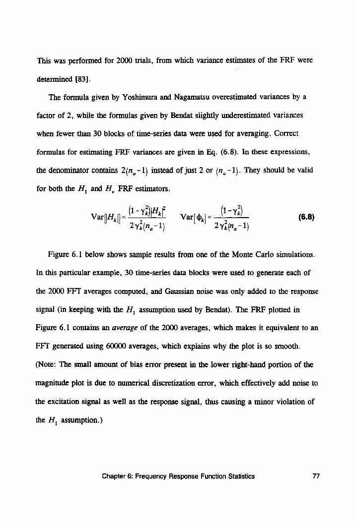
This was performed for 2000 trials, from which variance estimates of the FRF were
determined [83].
The formula given by Yoshimura and Nagamatsu overestimated variances by a
factor of 2, while the formulas given by Bendat slightly underestimated variances
when fewer than 30 blocks of time-series data were used for averaging. Correct
formulas for estimating FRF variances are given in Eq. (6.8). In these expressions,
the denominator contains 2(n,-1) instead of just 2 or (n,-1\. They should be valid
for both the H, and H, FRF estimators.
Var[|H,||- (i-wa)Faf Var[,]= _[tn) (6.8) 24 (",-1) 24 (7, ~1)
Figure 6.1 below shows sample results from one of the Monte Carlo simulations.
In this particular example, 30 time-series data blocks were used to generate each of
the 2000 FFT averages computed, and Gaussian noise was only added to the response
signal (in keeping with the H, assumption used by Bendat). The FRF plotted in
Figure 6.1 contains an average of the 2000 averages, which makes it equivalent to an
FFT generated using 60000 averages, which explains why the plot is so smooth.
(Note: The small amount of bias error present in the lower right-hand portion of the
magnitude plot is due to numerical discretization error, which effectively add noise to
the excitation signal as well as the response signal, thus causing a minor violation of
the H, assumption.)
Chapter 6: Frequency Response Function Statistics 77
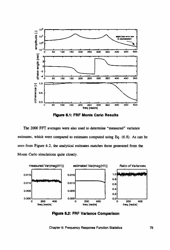
® 401 slight bias error due 3 to discretization | = & 10° E
GS 1071 __ _ __ 2 __ 8 af 4 it ts _| —_
0 50 100 150 200 250 300 350 400 450 500
¥ 4 v Te qv a ' oF ¥ r ¥
=< ‘
2 r \ ;
oO) c oO c PN
g -2 bh a
2 4 ll 2 a | ll a nil ll a | ell 2S
QO. 0 50 100 150 200 250 300 350 400 450 500
—10 oO a T T
® Oo
5 0s - : he ®
6 Oo 0.0 oval 4 1 mull. 4 anal ft ail | |
Oo 50 100 150 200 250 300 350 400 450 500
freq [rad/s]
Figure 6.1: FRF Monte Carlo Results
The 2000 FFT averages were also used to determine “measured” variance
estimates, which were compared to estimates computed using Eq. (6.8). As can be
seen from Figure 6.2, the analytical estimates matches those generated from the
Monte Carlo simulations quite closely.
measured Var(mag(H1))
0.015
0.010
0.005
0.000
Hardener
oO
200 400
freq [rad/s]
estimated Var(mag(H1))
0.015 1.0
0.8 0.010 ™ 06
0.005 0.4 0.2
0.000 0.0 O 200 400
treq [rad/s]
Ratio of Variances
ine
0 200
freq [rad/s]
400
Figure 6.2: FRF Variance Comparison
Chapter 6: Frequency Response Function Statistics 78
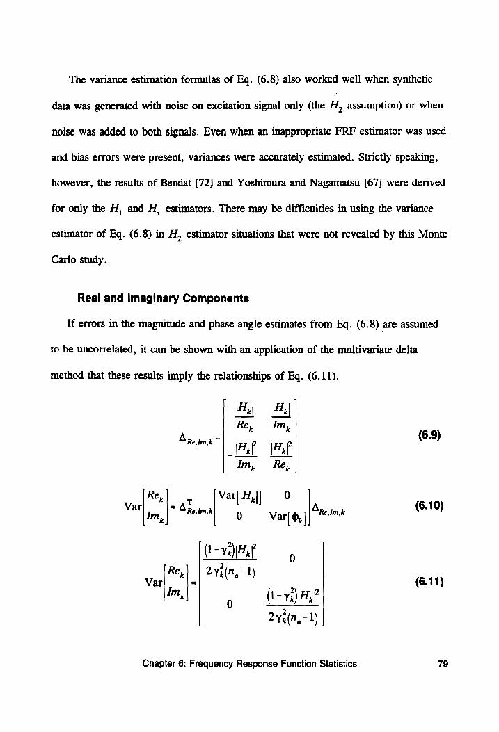
The variance estimation formulas of Eq. (6.8) also worked well when synthetic
data was generated with noise on excitation signal only (the H, assumption) or when
noise was added to both signals. Even when an inappropriate FRF estimator was used
and bias errors were present, variances were accurately estimated. Strictly speaking,
however, the results of Bendat [72] and Yoshimura and Nagamatsu [67] were derived
for only the H, and H, estimators. There may be difficulties in using the variance
estimator of Eq. (6.8) in Hf, estimator situations that were not revealed by this Monte
Carlo study.
Real and Imaginary Components
If errors in the magnitude and phase angle estimates from Eq. (6.8) are assumed
to be uncorrelated, it can be shown with an application of the multivariate delta
method that these results imply the relationships of Eq. (6.11).
Fal |F
Re, Im, 6.9
A Re,Im,k = H (6.9) et Pal
Im, Re,
Re, Var(|H,|| 0 V = 6.10 ar Im, A Re,im,k 0 Var|,] Are. im,k (6.10)
| (1 ~ Ye) AP 0
Re 2yu(n -1 Var| | =| 7k (6.11)
m 0 (1 Yi)}ef 2y;(n,-1) |
Chapter 6: Frequency Response Function Statistics 79
Bendat [81] shows that Cov/|G,.,4> o, |; Cov]|G¢, «|» o; |; Cov||G,,,> ar
Cov||G,,|, ,] are all zero for H, ,, with , being the phase angle of #, . Since
H, , is simply the cross-spectrum estimate G, , rescaled by the real-valued
autospectrum estimate Gy , the off-diagonal terms of the Var||FT, ,|, o,,| matrix are
zero. This happens because rescalings of uncorrelated random variables do not cause
correlation between the variables. Thus, for the H, FRF estimator (and perhaps the
H,, estimator), the Cov |i, kl? o, | =( assumption that went into the multivariate delta
analysis has been verified. However, the estimator H, , is the autospectrum estimate
G,,,, divided by the complex-valued cross-spectrum estimate G,,,. This is not a
simple rescaling, and thus, the assumption of Cov/|H,|, $,|=0 is probably not true
for the H, estimator.
These results are valid for information coming from a single spectral line of the
FRF. It is also desirable to show that there are no correlations between results coming
from different spectral lines. This is done by showing that the basic FFT algorithm is
equivalent to a orthogonal least-squares fit of sine and cosine terms (see Appendix B),
which in turn implies that errors in the FFT results are uncorrelated from one spectral
line to the next.
It is important to note here that these FRF statistics are valid only for signal
processing performed with a rectangular window. If other data windows (such as the
Hanning) are used, it is likely that the statistics of the problem will be altered. Using
pseudo-random or periodic chirp excitation would eliminate the need for windowing.
The effects of leakage on FRF statistics are also unknown.
Chapter 6: Frequency Response Function Statistics 80
6.3 Is FRF DATA NORMALLY DISTRIBUTED?
Preliminary Discussion
As with the sine-dwell data of Chapter 5, it is necessary to establish that errors in
the elements of the data vector y come from a normal distribution. This is
accomplished by examining Eqs. (6.1) through (6.3). If errors on the time-series data
themselves are normally distributed, then X, and F, of Eq. (6.1) will have normally
distributed errors, since the FFT operation is a linear operation. Linear operations
performed on normal data preserve the normality.
Even if the errors on the time-series data are not normally distributed, the
summation of Eq. (6.2) will cause errors on the auto- and cross-spectra estimates
G G fe,k? xx,k?
G fk? and Gy , tO approach normality for 30 averages or more as
predicted by the central limit theorem [77]. If errors on these auto- and cross-spectra
terms are small enough, the non-linear division operation used to generate H,, of
Eq. (6.3) can effectively be linearized (via a Taylor series expansion). This means
that errors on the FRF estimate will be normally distributed, as they are effectively
linear combinations of the errors on the auto- and cross-spectra estimates.
Data Acceptance Criteria
Cobb [73] performed an extensive study of the statistics of FRF estimators, noting
that the distribution of [FY «| approaches the Rayleigh distribution (the distribution of
z= \xr +x? , where x, and x, are Gaussian random variables with mean zero and
variance One) as variance levels increase on the real and imaginary parts of the FRF
estimate. In high noise cases, this causes the FRF estimates to exhibit non-nommality
Chapter 6: Frequency Response Function Statistics 81

and causes the approximations used in computing Eq. (6.5) to break down. The FRF
data will not be properly suited for the Bayesian regression formulation of Chapter 3
and should not be included in the analysis.
To determine whether or not data from a particular data acquisition location/
excitation location/spectral line combination is valid, the criterion of Eq. (6.12) must
be met. Var||H «| should be estimated using Eq. (6.8). The acceptance criterion alter-
natively can be written as shown in Eq. (6.13), which can be derived by plugging
Eq. (6.8) into Eq. (6.12). Thus, for n, = 30, ve would have to have a value of at
least 0.63 for the results from the k‘ frequency bin to be included in the Bayesian
regression formulation for updating FE models.
yVar LE <0.1 (6.12)
FA, |
y > ——! *" (1 +0.02(n, - 1))
(6.13)
6.4 ASSEMBLING FRF DATA
Assembling the Data Vector and Weighting Matrix
As with the sine-dwell data, the FRF results obtained at different data acquisition
locations using different excitation locations must be assembled into a single data
vector y. Here, however, the basic unit of data comes in much larger pieces, as the
FRF contains a real and imaginary part for each of n, spectral lines. These subsets of
data are assembled into a global y vector as shown in Figure 6.3.
Chapter 6: Frequency Response Function Statistics 82
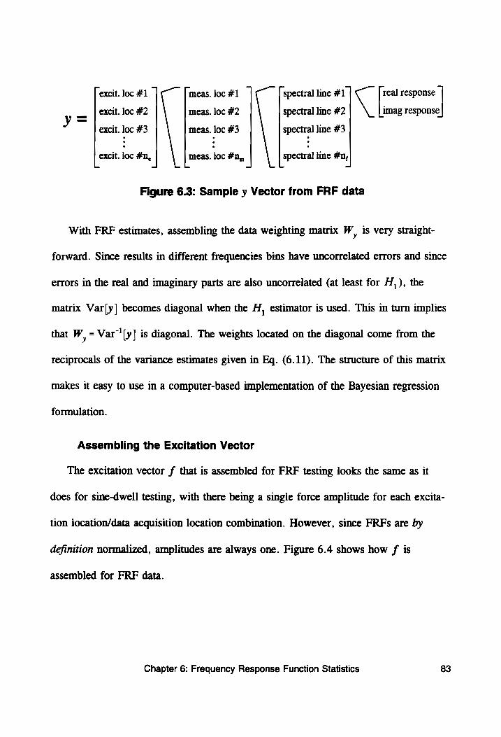
excit. loc #1 meas. loc #1 spectral line #1 real response
excit. loc #2 meas. loc #2 spectral line #2 imag response
excit. loc #3 meas. loc #3 spectral line #3
excit. loc #n, meas. loc #n,, spectral line #n,
Figure 6.3: Sample y Vector from FRF data
With FRF estimates, assembling the data weighting matrix W, is very straight-
forward. Since results in different frequencies bins have uncorrelated errors and since
errors in the real and imaginary parts are also uncorrelated (at least for H,), the
matrix Var/y| becomes diagonal when the H, estimator is used. This in turn implies
that W, = Var"'|y] is diagonal. The weights located on the diagonal come from the
reciprocals of the variance estimates given in Eq. (6.11). The structure of this matrix
makes it easy to use in a computer-based implementation of the Bayesian regression
formulation.
Assembling the Excitation Vector
The excitation vector f that is assembled for FRF testing looks the same as it
does for sine-dwell testing, with there being a single force amplitude for each excita-
tion location/data acquisition location combination. However, since FRFs are by
definition normalized, amplitudes are always one. Figure 6.4 shows how f is
assembled for FRF data.
Chapter 6: Frequency Response Function Statistics 83
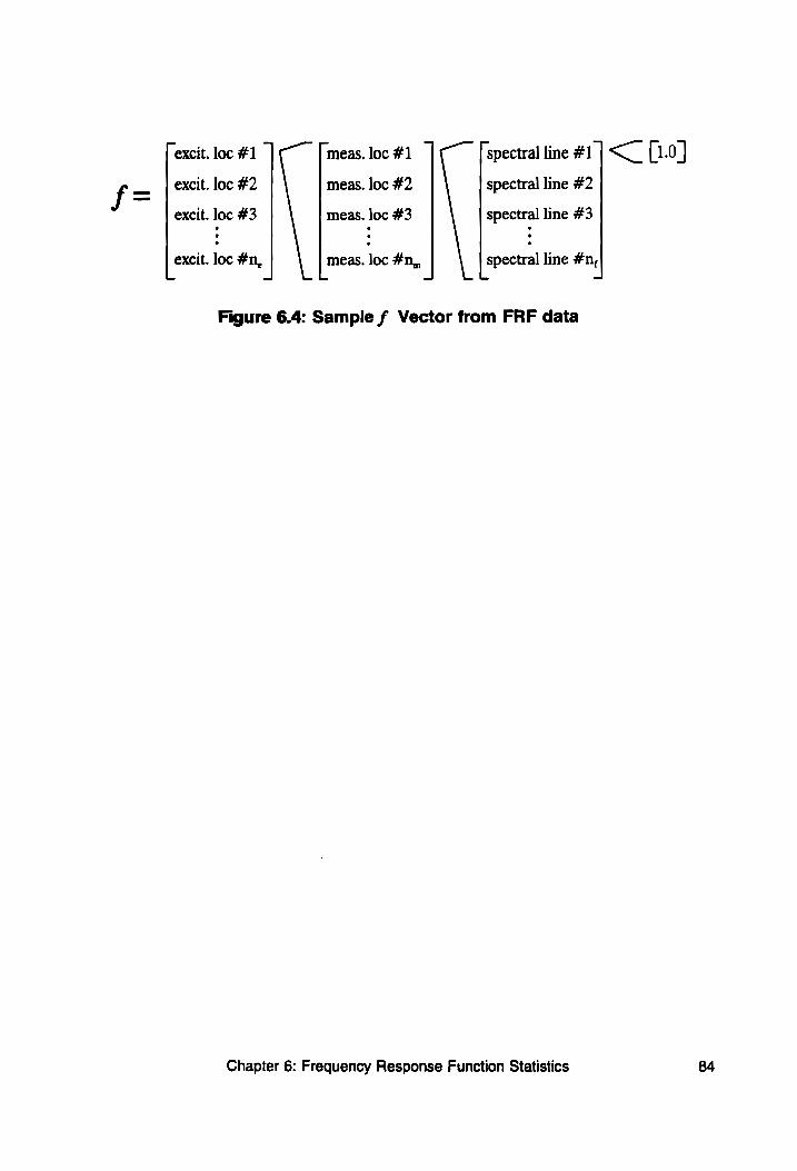
excit. loc #2
excit. loc #3
excit. loc #n,
Texcit. loc #1 |
meas. loc #2
meas. loc #3
meas. loc #n,,
Tmeas. loc #1
spectral line #1 |
spectral line #2
spectral line #3
spectral line #n, Figure 6.4: Sample f Vector from FRF data
Chapter 6: Frequency Response Function Statistics
<= [10]
84
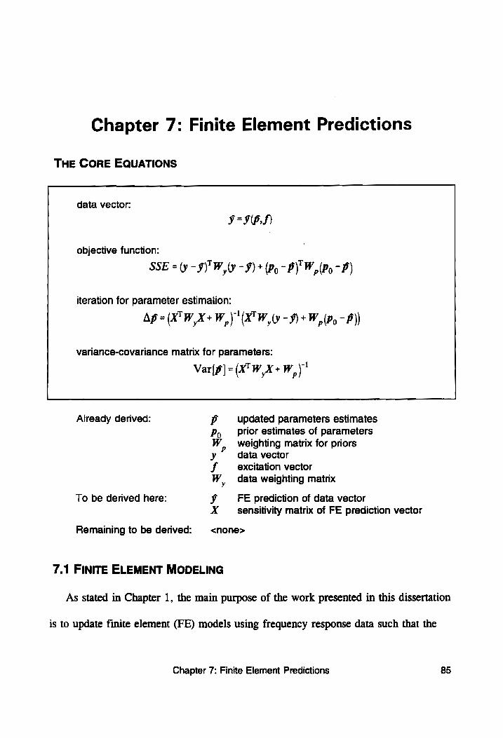
Chapter 7: Finite Element Predictions
THE CORE EQUATIONS
data vector:
¥ =F)
objective function:
SSE = (y -§)"W,(y - 9) + (Py) -B)'W,, (Pp -B)
iteration for parameter estimation:
Ap = (X"W,X+ W,) (XW, -J)* W,(Po -P))
variance-covariance matrix for parameters:
_/{yT -1 Var |p} = (X W X+ W,,)
Already derived: updated parameters estimates prior estimates of parameters
weighting matrix for priors data vector
excitation vector data weighting matrix SO
s SE
To be derived here: FE prediction of data vector sensitivity matrix of FE prediction vector be
SS
Remaining to be derived: <none>
7.1 FINITE ELEMENT MODELING
As stated in Chapter 1, the main purpose of the work presented in this dissertation
is to update finite element (FE) models using frequency response data such that the
Chapter 7: Finite Element Predictions 85
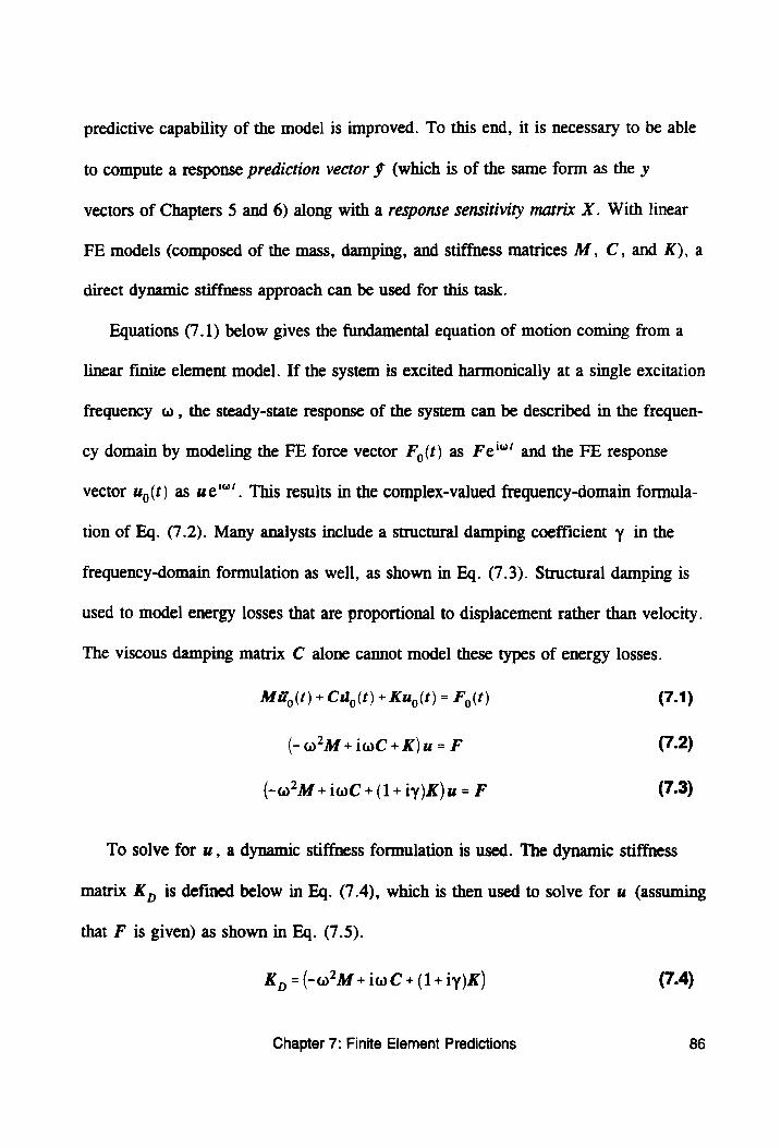
predictive capability of the model is improved. To this end, it is necessary to be able
to compute a response prediction vector § (which is of the same form as the y
vectors of Chapters 5 and 6) along with a response sensitivity matrix X . With linear
FE models (composed of the mass, damping, and stiffness matrices M, C, and K), a
direct dynamic stiffness approach can be used for this task.
Equations (7.1) below gives the fundamental equation of motion coming from a
linear finite element model. If the system is excited harmonically at a single excitation
frequency w, the steady-state response of the system can be described in the frequen-
cy domain by modeling the FE force vector F,(t) as Fe'®‘ and the FE response
vector U,(t) as ue'®’. This results in the complex-valued frequency-domain formula-
tion of Eq. (7.2). Many analysts include a structural damping coefficient y in the
frequency-domain formulation as well, as shown in Eq. (7.3). Structural damping is
used to model energy losses that are proportional to displacement rather than velocity.
The viscous damping matrix C alone cannot model these types of energy losses.
Mii, (t) + Cu,(t) + Ku,(t) = F(t) (7.1)
(-w?M+iwC+K)u=F (7.2)
(-w?*M +iwC +(1+iy)K)u=F (7.3)
To solve for wu, a dynamic stiffness formulation is used. The dynamic stiffness
matrix K,, is defined below in Eq. (7.4), which is then used to solve for u (assuming
that F is given) as shown in Eq. (7.5).
K y= (-w?M + iwC + (1+ iy)K) (7.4)
Chapter 7: Finite Element Predictions 86
K,u=F wu=K)F | (7.5)
The dynamic response vector uw is complex-valued, with the real part representing
the portion of the response that is in phase with the excitation force and the imaginary
part representing the portion that is out of phase with the force. Note that the vector
u may provide several displacements (both translational and rotational) at a single
nodal DOF. If velocity or acceleration predictions are required, u must be multiplied
by iw or -w’, respectively.
7.2 GENERATING THE PREDICTION VECTOR
In order to compare the predictions of the finite element model to the data
collected in a structural dynamics test, a data prediction vector ~ must be computed
from the model that corresponds exactly to the y vector that comes from the signal
processing results described in Chapters 5 and 6 (see Figure 5.4 and Figure 6.3).
Additionally, the model must be built according to the current values of the estimated
modeling parameters p.
If data was acquired from the structure at spatial locations corresponding to finite
element nodal points, then construction of the prediction vector ¥ is straightforward.
First, a force amplitude A ,, (corresponding to the j™ excitation location and the 7"
harmonic of the k“ excitation frequency set) must be extracted from the force vector
f of Figure 5.5 or Figure 6.4. This amplitude must then be placed in the entry of the
F vector of the FE model that corresponds to the excitation location.
Chapter 7: Finite Element Predictions 87
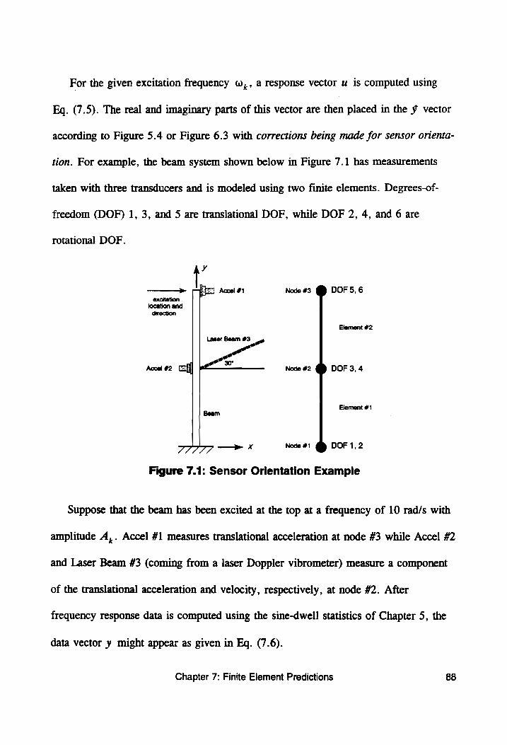
For the given excitation frequency ,, a response vector u is computed using
Eg. (7.5). The real and imaginary parts of this vector are then placed in the y vector
according to Figure 5.4 or Figure 6.3 with corrections being made for sensor orienta-
tion. For example, the beam system shown below in Figure 7.1 has measurements
taken with three transducers and is modeled using two finite elements. Degrees-of-
freedom (DOF) 1, 3, and 5 are translational DOF, while DOF 2, 4, and 6 are
rotational DOF.
t
——_—> qa Accel #1 Node #3 ® DOF 5, 6 excitation
location and direction
Element #2
Laser Beam #3
a oe
Accel #2 aii pee ones @ DOF 4
Element #1 Beam WITT —> * Node #1 @ DOF 1,2
Figure 7.1: Sensor Orientation Example
Suppose that the beam has been excited at the top at a frequency of 10 rad/s with
amplitude A,. Accel #1 measures translational acceleration at node #3 while Accel #2
and Laser Beam #3 (coming from a laser Doppler vibrometer) measure a component
of the translational acceleration and velocity, respectively, at node #2. After
frequency response data is computed using the sine-dwell statistics of Chapter 5, the
data vector y might appear as given in Eq. (7.6).
Chapter 7: Finite Element Predictions 88
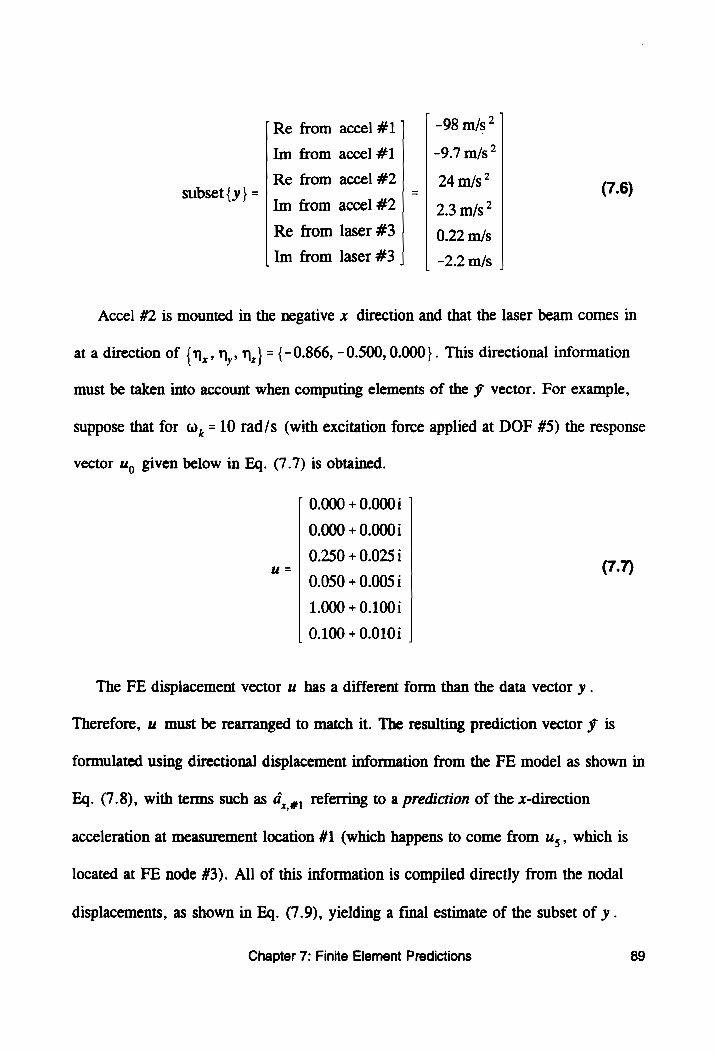
[Re from accel #1 | | -98 m/s?
Im from accel #1 -9.7 m/s”
Re from accel #2 24 2 subset{y}=| pl" m/s (7.6)
om acce 2.3 m/s? Re from laser #3 0.22 m/s
| Im from laser #3 | -2.2 m/s | Accel #2 is mounted in the negative x direction and that the laser beam comes in
at a direction of {n,, n,,N1,} = {-0.866, - 0.500, 0.000}. This directional information
must be taken into account when computing elements of the ¥ vector. For example,
suppose that for w, = 10 rad/s (with excitation force applied at DOF #5) the response
vector u, given below in Eq. (7.7) is obtained.
. 0.000 + 0.000: |
0.000 + 0.0001
0.250 + 0.0251 u = come (7.7)
0.050 + 0.0051
1.000 + 0.1001
| 0.100 + 0.0103 | The FE displacement vector uw has a different form than the data vector y.
Therefore, u must be rearranged to match it. The resulting prediction vector ¥ is
formulated using directional displacement information from the FE model as shown in
Eq. (7.8), with terms such as @, ,, referring to a prediction of the x-direction
acceleration at measurement location #1 (which happens to come from u,, which is
located at FE node #3). All of this information is compiled directly from the nodal
displacements, as shown in Eq. (7.9), yielding a final estimate of the subset of y.
Chapter 7: Finite Element Predictions 89
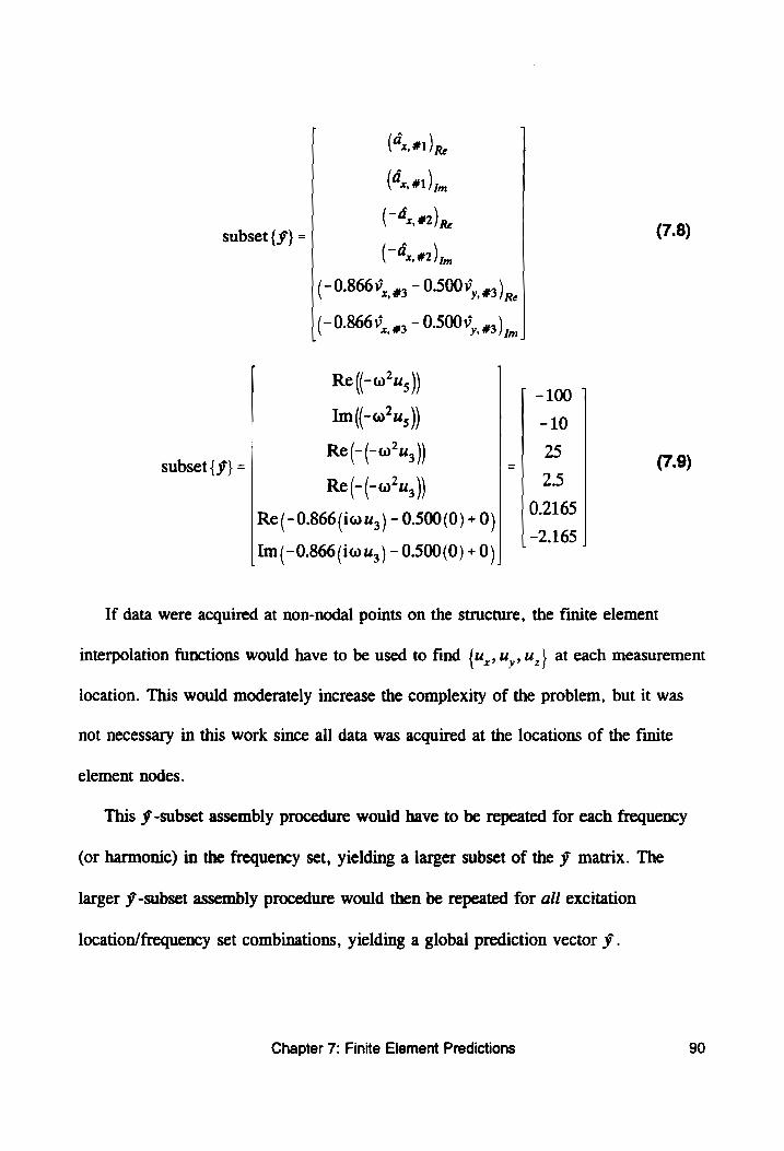
(4, #1) pe
(4, 91 ) ion
(-4,, #2) subset { ¥} = / Re (7.8)
(4, #2) 5
(-0.866¥,, 4, - 0.5009, #3) pe
(-0.866¥, 4, - 0.5000, #3) in
Re ((-w7u (-o?4) a Im (-w7u, )) -10
| Re(-(-w*u 25 subset { 9} = ( ( 3)) _ (7.9)
Re(-(-w7u,)) 2.5
Re (- 0.866 (iw u, ) - 0.500(0) + 0) 0.2165 ~2.165
Im (- 0.866 (iw x, ) - 0.500(0) +0), . , If data were acquired at non-nodal points on the structure, the finite element
interpolation functions would have to be used to find {u,; uy, u,} at each measurement
location. This would moderately increase the complexity of the problem, but it was
not necessary in this work since all data was acquired at the locations of the finite
element nodes.
This ¥-subset assembly procedure would have to be repeated for each frequency
(or harmonic) in the frequency set, yielding a larger subset of the y matrix. The
larger ¥-subset assembly procedure would then be repeated for all excitation
location/frequency set combinations, yielding a global prediction vector y.
Chapter 7: Finite Element Predictions 90
7.3 GENERATING THE SENSITIVITY MATRIX
In addition to the ¥ matrix, it is necessary to compute a sensitivity matrix X,
which has entries x,, = (dy;/dp ,). One method of computing this matrix is to use the
finite difference method. Equation (7.10) below shows how this matrix would be
assembled. The term ¥,,,, , refers to a ¥ vector computed for a p,,,, ; parameter
vector, where p, is replaced with (p,- Ap,). The term ¥,,,, ; would be computed
similarly, except with (p ;+ Ap) in place of p;.
Snigh,1 Siow,
ZAP, X=
___ [Sait ~Ftowsny (7.10) 2 Ap, 26,
[a ~Siow,2
The finite difference method is simple and robust. The only input required by the
analyst is the selection of the finite difference steps Ap,. Unfortunately, the finite |
difference method is also expensive computationally, making it worthwhile to seek an
alternative for computing X.
This other alternative is to compute analytical derivatives. The basic theory for
this analysis comes directly from Eq. (7.3). If this equation is differentiated with
respect to p,, the expression of Eq. (7.11), or alternatively, Eq. (7.12), results.
Simply premultiplying Eq. (7.12) by K, yields the desired expression of (ou/op i)
found in Eq. (7.13). Note: (@F/dp;) is usually zero.
0? OM gg 2E 4 (1+ iy) SK u + (-w?M +iwC + (1+ iy)K) 2H = OF (7.11) Op; = OP; Op; Op, Op,
OK —?u+K Ou _ OF (7.12) 8, OP, OP,
Chapter 7: Finite Element Predictions 91
OKy aF u+—
Ou -1 K _
| Op, Op, a
Op;
(7.13)
Of course, the expression (ou /op;) is not precisely what is needed to generate the
X matrix; rather, (dy /ap i) is required. Therefore, it is necessary to use the entries of
each (du/dp;) vector to compose (o¥/op;), just as the entries of u were used to
compose y. This includes selecting the appropriate DOF and making corrections for
sensor orientation, just as was shown in Egs. (7.7), (7.8), and (7.9).
Finding expressions such as (0K/dp;,) is highly dependent on how the problem is
formulated. For certain systems, the FE system matrices can be factored into “ele-
mentary” matrices. For example, if K can be expressed as a sum of the matrices K),
K,, and K,,, as shown in Eq. (7.14), then matrix partial derivatives can be found
quite easily as demonstrated in Eq. (7.15).
3
K= 27K, +k, K, +K, (7.14)
OK Eh? OK Ebh? OK OK — = —=K
Ky K, Ok, 1 Ok, K, a 12° oh 4 - (7.15)
This type of FE matrix formulation allows the FE matrices K and M (and deriva-
tives of these matrices) to be calculated easily and quickly. However, if the formula-
tion of the FE system matrices is more complex, it may be necessary to perform the
differentiation at the matrix entry level. This can be substantially more expensive
computationally, at which point the finite difference method may become the more
attractive alternative.
Chapter 7: Finite Element Predictions 92
7.4 CONCLUDING REMARKS
With the completion of this discussion on ¥ and X, all parts of the Bayesian
regression formulation have been defined, and the basic theory of the model update is
complete. This work included the Bayesian statistical theory used to formulate the
regression problem, the sources of prior information used in the analysis, the signal
processing necessary to generate statistically qualified frequency response data, and
the use of a dynamic stiffness formulation to quickly and effectively generate finite
element predictions of the data.
In the next part of the dissertation, Part III, a number of “quality control” issues
are discussed, including computational issues, update verification statistics, and visual-
ization Statistics.
Chapter 7: Finite Element Predictions 93

PART Ill:
“Quality Control” Issues
94
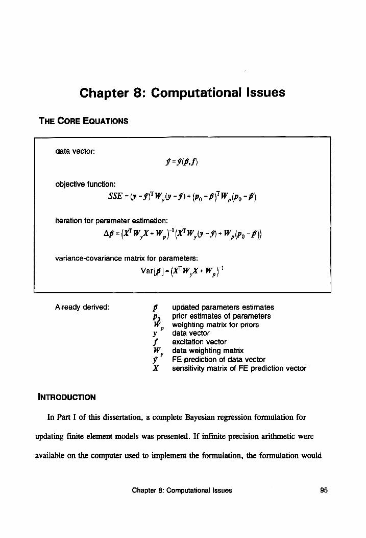
Chapter 8: Computational Issues
THE CORE EQUATIONS
data vector:
I=ID.f)
objective function:
SSE = (y -§)"W,(y ~9) + (Py) -B)' W, (Po -B)
iteration for parameter estimation:
Ap = (XTW,X+W,)'(X"W,(y -9) + W, (PB)
variance-covariance matrix for parameters:
_~ {yt -1 Var|p] = (x Wx + W,)
Already derived: p updated parameters estimates Py) _ Prior estimates of parameters W, weighting matrix for priors y data vector f excitation vector W, data weighting matrix y FE prediction of data vector X _ sensitivity matrix of FE prediction vector
INTRODUCTION
In Part I of this dissertation, a complete Bayesian regression formulation for
updating finite element models was presented. If infinite precision arithmetic were
available on the computer used to implement the formulation, the formulation would
Chapter 8: Computational Issues 95
be complete. However, with only finite precision arithmetic available, several
computational issues must be addressed. These issues include proper use of modern
matrix decompositions, parameter rescaling, reformulation of the problem to use
matrix decompositions, step size determination, and convergence testing. The chapter
concludes with a discussion of computation times.
8.1 MATRIX DECOMPOSITIONS
There are two modern matrix decompositions that are used in implementing the
Bayesian regression formulation of Chapter 3. The first is the Cholesky decomposi-
tion. With this decomposition, a symmetric positive-definite matrix W,,,, is repre-
sented with an upper triangular matrix C where W=C'C. This decomposition is nxn?
often used in solving certain systems of simultaneous linear equations (such as linear
FE statics problems) and has applications in statistics as well. This will be discussed
in more detail in Section 8.3.
The second decomposition is the QR decomposition. Here, the rectangular matrix
X xn (with n <m) is represented by the orthogonal matrix Q and the upper men
triangular matrix R where X= QR . Since Q is orthogonal, Q'Q=T,,.,. nxn?
Equations (8.1), (8.2), and (8.3) show how QR decomposition is used to solve an
ordinary least-squares regression problem.
Ap = (X'X)'X"(y -¥) = (R'OTOR) RQ" ly -¥) (8.1)
Ap = (RTR)'R'Q"(y -§) = R'R™R'Q'(y -J) (8.2)
Ap = R'Q"\y -9) (8.3)
Chapter 8: Computational Issues 96
Performing the regression using the QR decomposition provides several numerical
benefits. First and foremost is the fact that R can be inverted instead of (X'X). R is
considerably better conditioned than (X'X). Indeed, it can be shown that the condition
numbers of R and (X'X) are related by the expression Cond (R) = ¥Cond(X'X). This
reduces the number of significant digits required for matrix computations by half.
Additionally, R is an upper triangular matrix, which means that a simple back-
substitution algorithm can be used to solve for Ap instead of using a more complex
algorithm for solving linear systems.
An added benefit of using QR decomposition is reduced computation time in cases
where multiple regression problems are to be solved using the same X matrix. In this
Situation, the QR decomposition can be computed and stored ahead of time, to be
used with all regression problems having the same X matrix. The sine-dwell statistics
of Chapter 5 were implemented with LAPACK [88] using this strategy. The QR
decomposition is also used in the reformulation of the Bayesian regression procedure
discussed in Section 8.3.
8.2 PARAMETER RESCALING
A second computational issue which must be addressed is parameter rescaling.
When working with parameters that represent engineering quantities, large variations
in scale sometimes result. For example, in Chapter 12, the density parameter p has a
value of 7.85 x 10° Mg/mm?° while the rotational joint stiffness parameter k, , has a
value of 2.53 x 10° N-mm. These values differ in scale by more than 16 orders of
magnitude. Variations such as this cause extreme ill-conditioning in the X matrix.
Chapter 8: Computational issues 97
Even a QR decomposition-based regression algorithm may fail due to numerical
difficulties in this case. An algorithm based on the inversion of (X'X) will almost
certainly fail.
To deal with this problem, the parameters must be rescaled. One possible
rescaling would consist of dividing all of the parameters by their nominal values (the
prior values of Chapter 4), which would be p; = o The scaled parameters fp” would
then represent the fraction change in the parameters p.
An alternative rescaling is to use parameters p’ that represent the number of
standard deviations the parameters is away from its nominal value. This rescaling was
used in the computer implementation of the Bayesian regression algorithm. Eq. (8.4)
gives the formal definition of the parameter rescaling. A more general formulation is
given in Eq. (8.5), where C p is the Cholesky decomposition of the inverse of the
prior variance-covariance matrix, i.e., Cyc p= W,= Var" [Po]- Equation (8.5) is only
necessary if there is correlation between prior estimates, which normally is not the
case. When Var"[Po| is a diagonal matrix, the two expressions yield identical results.
at (P; ~ Po.) P; oO (8.4)
p= C (8 - Po) (8.5)
With this rescaling, the vector of normalized prior estimates pj (corresponding to
prior estimate vector p,) becomes zero. The matrix Var|po | becomes an identity
matrix, as shown in Eq. (8.6).
Chapter 8: Computational Issues 98
Var|p"] = C,Var[p]C, = C,C,C,, Ch = Ih xn (8.6)
8.3 BAYESIAN REGRESSION REFORMULATION
One problem with using QR decomposition to solve regression problems is that it
was not designed to include weighting matrices or prior information. To use QR
decomposition with all aspects of the Bayesian regression formulation of Chapter 3.
Specifically, the problem must be reformulated such that an ordinary least-squares
algorithm based on QR decomposition can be used. To this end, a new X” and y’ are
defined as given in Eqs. (8.7) and (8.8). C, is the Cholesky decomposition of the
data weighting matrix W,, i.e., C,C,=W, = Var"[y], and C, is again the Cholesky
decomposition of the prior weighting matrix W,, i.e., cic >= W,= Var™"[po|-
c.xc'| {ce xc x=| 7 "I ; , (8.7)
CC, n,Xn,
Cyy | |C,y| Ie C,y | |e ye} 7 fel fe) 2? J (8.8)
C,C,Po| | Po 0 ‘Ic (Coe | r
If these expressions are plugged into the standard ordinary least-squares iteration
shown in Eq. (8.9), it can be shown the process is mathematically equivalent to the
Bayesian regression iteration shown in Eq. (3.18) of Chapter 3. This is demonstrated
in Eqs. (8.10) through (8.14). The expansion J = C, C5C,C, is used as a part of this
derivation.
Ap =(X TX XT (y* -¥*) (8.9)
Chapter 8: Computational Issues 99
- - ~] - T
C,Ap= (C, X'C,C,XC, +I) (C,X"C,C,(y - 9) +C, (D9 - p))
C,Ap=(C,X"C\C,XC, +(C, C,C,C, \"
(Cy X™C,C,(y -9) + (Cp C,C,Cy )C,(Py - B))}
C,Ap=[C,'(X7C,C,X+C5C,)C, |"
Cp [ACC -9) + CC, (Po B)
C, AP =C,(X'W,X+W,)'C,C, (XW, (y - 9) + W, (Po -B))
Ap = (X'WX + W,)" (TW, ~¥)+W,(Po “B))
been greatly reduced.
given below in Eqs. (8.15) and (8.16).
p= Cr + Po
Var[p] = C;, Var[p" JC,
Chapter 8: Computational Issues
(8.10)
(8.11)
(8.12)
(8.13)
(8.14)
Note that the final result, shown in Eq. (8.14), is exactly the same as the standard
Bayesian regression iteration given in Eq. (3.18) and in the core equations, which is
the desired result. The reformulated X” and y* should be used with QR decomposi-
tion to obtain Q’R’ =X". The iteration Ap” = R*'Q"'(y* - y*) can then be used to
obtain parameter estimate vector p” and an estimated variance-covariance matrix
Var|p" |=(R*™R’). In addition, the effects of numerical ill-conditioning will have
At the end of the parameter estimation process, it is necessary to transform back
to the original parameters p. Expressions for f and its variance-covariance matrix are
(8.15)
(8.16)
100
8.4 STEP SIZE DETERMINATION
The final computational issue that must be addressed is that of iteration conver-
gence. If the matrix X" is constant (not a function of p”), then the iteration of
Eq. (8.10) converges in a single step to the value of p* that minimizes SSE.
However, if X” is not constant (meaning that the regression problem is nonlinear),
multiple steps will be required to reach the minimum. If the non-linearity is extreme
enough, the p* vectors generated by the iteration Ap* = R"™!Q*'(y* -y*) may not
reduce the SSE value at all, in which case the iteration will fail to converge. It should
be noted that the model update formulation of Part II of the dissertation is nonlinear
despite the fact that the finite element model is assumed to be linear. This is caused
by use of the inverse of the dynamic stiffness matrix K, of Chapter 7.
To ensure convergence, one must first note the fact that the step defined by
Eq. (8.10) always points in a direction (in normalized parameter space) that reduces
SSE, in other words, it is a descent direction. However, this direction is only
guaranteed to be a descent direction at the f° at which X° is computed. If X* changes
enough over the course of the step, the SSE values may rise instead.
Therefore, when a step is generated that increases the SSE value, the step size
should be reduced, as shown in Eq. (8.17). This expression is the same as found in
Eq. (8.10), except that a step size modifier B , which always has a value less than
one, has been included. Similar results are given for the QR decomposition based
iteration from Eq. (8.18).
Ap’ = B(X™X) XT (y* -y) (8.17)
Chapter 8: Computational issues 101
Ap’ = BR™Q"(y" -y") | (8.18)
A number of different schemes exist for determining the optimal f [89].
However, it is sufficient to repeatedly halve 6 until the SSE value obtained has been
decreased. Additionally, it is sometimes desirable to limit the initial step size before
checking to see if the new p* yields a reduced SSE value. This is particularly true in
systems where the X” matrix is ill-conditioned, which can potentially generate large
parameter changes. The expression given in Eq. (8.19) provides a restriction on the
initial size of the step, effectively limiting the average change (in an RMS sense) in a
parameter to one standard deviation.
if (Ap*? Ap*) > n,, then f, = ——+ , else B,=1 (8.19) Ap 4
8.5 CONVERGENCE TESTING
When using any iterative least-squares procedure, the analyst should run the
procedure multiple times with different initial parameter estimates (which is not the
same as different prior estimates, as described in Chapter 4). If all of the initial
estimates converge to the same final parameter estimate, the analyst can be confident
that the unique SSE-minimizing estimate has been obtained. Unique in this context
means unique for the Bayesian regression formulation with a particular set of data and
set of prior information. It does not mean that all other model update formulations
and data sets would give identical answers.
Chapter 8: Computational Issues 102
If the different initial estimates converge to two or three different final parameter
estimates, the analyst may be having difficulties with local minima, which are points
in parameter space that appear to be error-minimizing solutions, but are not. The
analyst can choose the best of the different parameter estimates simply by picking the
one that provides the lowest SSE value, as given in Eq. (3.17).
If the regression iteration never converges to a final parameter estimate, or
converges to a different estimate every time, then there is a problem with either the
model update formulation (typically poor parameter choices) or a defect in the Bayes-
ian regression implementation or the FE model. In this case, the analyst must re-
examine everything carefully.
8.6 COMPUTATION TIME
One disadvantage to using a Bayesian statistics formulation over some other model
update formulations (e.g., direct matrix update methods) is a greatly increased need
for computing power. In these iterative approaches, the finite element is rebuilt and
resolved repeatedly, sometimes hundreds of times. This is particularly true when the
dynamic response of a structure is computed at multiple frequencies, as described in
Chapters 5 and 6. Indeed, a dynamic response must be computed for each frequency.
This can represent a significant amount of computational work, particularly when
FRF data is used.
Of course, it is possible to significantly reduce computation times with strategic
use of matrix decompositions [80]. A modal summation approach for FRF predictions
might also be worth considering. In this approach, an eigensolution would be com-
Chapter 8: Computational issues 103
puted for the finite element model, providing natural frequencies and mode shapes.
This is expensive to compute, but once it is finished, standard modal summation can
then be used to quickly predict FRF values at as many frequencies as desired [82].
However, there are three difficulties with this approach: (1) modal truncation becomes
an issue; (2) computation of FRF sensitivities becomes more complex; and (3) the
types of damping models that can be used in the finite element model are restricted.
None of these difficulties is intractable, but all represent disadvantages over the direct
computation of frequency response. In cases in which sine-dwell data excitation is
used, it is probably not cost effective to use modal summation.
8.7 CONCLUDING REMARKS ON NUMERICAL ISSUES
Clearly, there were a number of numerical concerns in the Bayesian statistics
formulation that were addressed in the course of performing this research. However,
all of these steps were necessary to ensure rapid and reliable convergence of the
Bayesian regression iteration. The parameter rescaling and step size determination in
particular were very important. The use of the QR and Cholesky decompositions with
the reformulated X” and y" further increased stability and computation speed.
The issue of frequency response prediction computation times was not handled as
well in this work. All of the examples presented in this dissertation were implemented
in MATLAB [90], which is a high-level programming environment that provides
many routines for use with general matrices. However, MATLAB does not provide
routines for optimal use of matrix decompositions (especially routines that take
advantage of certain matrix properties, such as symmetry, bandedness, or positive
Chapter 8: Computational issues 104

definiteness). An implementation that used a modern matrix computation library such
as LAPACK [88] would run faster and provide more accurate results. However, the
amount of programming and debugging required would be greatly increased as well.
Chapter 8: Computational Issues 105

Chapter 9: Model Update Verification
Once the model update has been accomplished, it is desirable to perform a number
of tests to ensure that the updated model is representative of the behavior of the
structure. There are four different categories of tests available: (1) data stationarity
testing; (2) lack-of-fit testing and compensation; (3) parameter consistency testing; and
(4) cross-validation testing. These tests increase confidence that data was acquired
correctly, that the model fits the data, that the updated model parameters make sense,
and that the model is capable of predicting other data sets besides the specific set used
to update the model.
9.1 TIME-INVARIANCE TESTING
There are two implicit assumptions that are made whenever a model update is
performed with experimental data: (1) the data is acquired correctly; and (2) the
dynamic properties of the structure/test apparatus do not change over the course of
testing. Ensuring that data is obtained correctly is best accomplished by using proper
experimental technique. If the structure does not change over the course of testing,
the data should be time-invariant, which means that the statistical properties of the
data do not change over time. An autocorrelation test can be performed as a test of
this characteristic [77].
Chapter 9: Model Update Verification 106
Specifically, if data is acquired in a sequential fashion during a discrete-frequency
test (usually a scanning LDV test), a large amount of force data can be obtained.
Clearly, the amplitude of this force signal should remain constant for the entire
duration of the test. If it does not, the structure or test equipment has probably
experienced some change, often due to changes in the ambient temperatures
surrounding the system [91].
The Durbin-Watson Statistic
During the course of a laser-Doppler vibrometer test, a block of excitation data is
acquired with each block of response data. This means that if a block of velocity
measurements is taken at each of 45 data acquisition locations, 45 blocks of force data
will be available as well. 45 estimates of force amplitude A, (each corresponding to
data acquisition location () can be computed according to Eq. (5.12).
These 45 A ; vectors should all be the same (if the system is time-invariant), plus
or minus some small error caused by noise on the excitation time-series data. Addi-
tionally, the errors in the estimates should be uncorrelated, since the errors present in
one time-series data block should be completely unrelated to errors present in another
time-series data block.
To estimate the errors in the 45 force amplitude vectors A ;» the average force
amplitude vector 4 ag is computed, as described in Eq. (5.27), and then subtracted
from each of the A, vectors. If the true force amplitude is not constant, there will be
a trend to the residuals. The top plot of Figure 9.1 shows uncorrelated errors (with no
Chapter 9: Model Update Verification 107
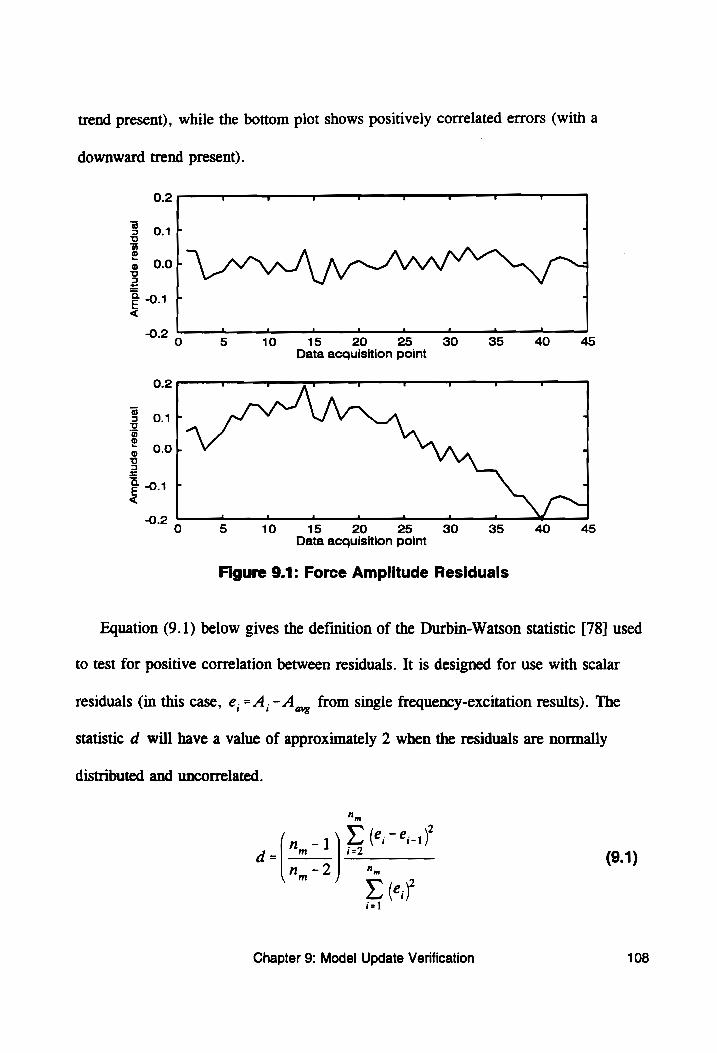
trend present), while the bottom plot shows positively correlated errors (with a
downward trend present).
0.2 a F v ' a 7 v tT
8 o1f , 3S G 2 o OO A VY o 2
2 0.1 F : &
0.2 O 5 10 15 20 25 30 35 40 45 Data acquisition point
Ampl
itud
e re
sidu
al
0.2 ell aA a rt nll. of lh
0 5 10 15 20 25 30 35 40 45 Data acquisition point
Figure 9.1: Force Amplitude Residuals
Equation (9.1) below gives the definition of the Durbin-Watson statistic [78] used
to test for positive correlation between residuals. It is designed for use with scalar
residuals (in this case, e,=A,-A ag ‘rom single frequency-excitation results). The
Statistic d will have a value of approximately 2 when the residuals are normally
distributed and uncorrelated.
n -1)4 (;-e4) ‘-| m | (9.1)
Chapter 9: Model Update Verification 108
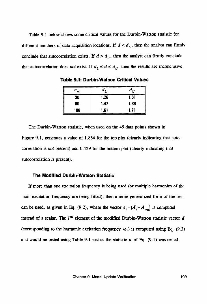
Table 9.1 below shows some critical values for the Durbin-Watson statistic for
different numbers of data acquisition locations. If d <d, , then the analyst can firmly
conclude that autocorrelation exists. If d >d,,, then the analyst can firmly conclude
that autocorrelation does nor exist. If d, sd <d_,,, then the results are inconclusive.
Table 9.1: Durbin-Watson Critical Values
| Nm da, dy
30 1.26 1.61
60 1.47 1.66
100 1.61 1.71 The Durbin-Watson statistic, when used on the 45 data points shown in
Figure 9.1, generates a value of 1.854 for the top plot (clearly indicating that auto-
correlation is not present) and 0.129 for the bottom plot (clearly indicating that
autocorrelation is present).
The Modified Durbin-Watson Statistic
If more than one excitation frequency is being used (or multiple harmonics of the
main excitation frequency are being fitted), then a more generalized form of the test
can be used, as given in Eq. (9.2), where the vector e,=(4,-A,,,\ is computed
instead of a scalar. The /‘ element of the modified Durbin-Watson statistic vector d
(corresponding to the harmonic excitation frequency w,) is computed using Eq. (9.2)
and would be tested using Table 9.1 just as the statistic d of Eq. (9.1) was tested.
Chapter 9: Model Update Verification 109
Mm
- (i17%i-14) d {* | =a (9.2) ~ n n,-2
(.:) 1 ~,
A similar test can be performed on the driving point response (if it is available),
except that ¢ vectors are used in place of the A vectors. The real and imaginary
components of the frequency response should exhibit time-invariance, which is
equivalent to requiring that magnitude and phase angle exhibit time-invariance.
Other Comments on Time-invariance
Performing these tests to ensure that the structure has not changed during the
course of data acquisition is relatively easy. However, it is more difficult to ensure
that the structure does not change between tests. The only way to statistically test for
changes of this sort is to repeat at least a portion of all previous tests (same excitation
frequency, force levels, and response measurement locations) and compare statistical-
ly. Both the force and response signals should be the same for repeated portions of
the tests. Unfortunately, this significantly increases the amount of work required and
was not done in this research.
9.2 LACK-OF-FIT TESTING
Once it has been established that data was taken properly and that the structure did
not change during the course of testing, the model update can be performed. After the
model update, a lack-of-fit (LOF) test can be performed. This test determines whether
Chapter 9: Model Update Verification 110
or not the updated model fits the data as well as possible. This test can only be
performed in the context of a weighted least-squares formulation in which estimated
weighting matrices (like those of Chapters 5 and 6) are used.
The lack-of-fit statistic is the SSE term of Eq. (3.17). With proper weights, the
SSE term becomes equivalent to a sum of independent z* statistics, where z is a
Gaussian random variable with zero mean and unit variance [77]. A z? is equivalent
to a chi-squares statistic with one degree of freedom, i.e., Xi: If n of these 1
statistics are added together, a chi-squares statistic with n degrees of freedom results,
1.€., x. [77]. When a degree-of-freedom for each fitted parameter is subtracted off,
the relationship of Eq. (9.3) results, which means that the SSE term comes from a Xn,
distribution. Because of this, the relationships of Eq. (9.4) also apply.
2 XLor = SSE = (y -yWy J) + (Po - py W,@, - Pp)
2 2 ~ Xny+n,-n ~ Xn
P y
(9.3)
E[SSE]=n, Var(SSE]=2n, (9.4)
For a large number of data points (n, > 30), the distribution of the SSE/LOF
Statistic approach normality, as predicted by the central limit theorem [77]. Knowing
this, the statistic can be normalized into a z-score, as shown in Eq. (9.5).
(SSE ny) i (9.5)
2n y
If Z, or has a value in excess of some critical z, value (1.96 for 97.5% confi-
dence), the model can be said to exhibit lack-of-fit. This means that the model is not
Chapter 9: Model Update Verification 411
fitting the data as well as could be expected, and that the SSE value has been
artificially inflated. This lack-of-fit can be the result of model form errors, data
acquisition errors unaccounted for by the signal processing statistics, or poor/incom-
plete parameter selection. Examples of modeling form errors include bad boundary
condition models and discretization errors, while data acquisition errors might be
caused by misplaced or miscalibrated transducers, FRF leakage, or over-filtering of
time-series data.
If Z, or <2, there is no statistical evidence for lack-of-fit and no statistical reason
to expect that amy model could fit the data any better. Unfortunately, the power [77]
of the LOF test becomes very great for a large n,, which means that even the
slightest lack of agreement between the model and data will cause a z, 5, greater than
1.96 to be generated. Only if the FE model, data acquisition procedure, and signal
processing technique are all perfect will lack-of-fit not be detected by the test. Thus,
instead of insisting that a model pass the lack-of-fit test (which is virtually
impossible), it is better to compensate for lack-of-fit.
When lack-of-fit occurs, the quantity SSE, = (y - yt W, y -9) is artificially inflated
relative to the priors, “drowning out” SSE, = (p - py W (Pp - p). This keeps the priors
from influencing the analysis as much as they should. To compensate for this SSE
inflation, the data residuals can be downweighted, restoring the effect of residuals
from the priors. Equations (9.6), (9.7), and (9.8) show how the sum-of-squares error,
the Gauss-Newton step, and the estimated parameter variance-covariance matrix are
Chapter 9: Model Update Verification 112
reformulated with the downweighted data. The lack-of-fit compensation coefficient a
has value less than one.
SSE = ay - $)'W,(y - 9) + (Pp - BP) Wo - B) (9.6)
Ap = (0?2X"W, X+W,)'(0?X"W,(y - 9) + W, (pp - B)) (9.7)
Var[p]=(0?X*W,X+W,)" (9.8)
Two reasonable schemes for computing « exist, each developed with a slightly
different objective in mind. The first coefficient, given in Eq. (9.9), eliminates the
artificial SSE inflation by appropriately scaling down the data residuals. Koh and
See [64] used a similar downweighting scheme in a Kalman filtering context. The
second coefficient, given in Eq. (9.10), keeps confidence intervals from becoming
arbitrarily small (even in the presence of infinite data) by downweighting the data
more strongly as more data is included. Both of the lack-of-fit compensation
coefficients were tried in the case studies of Chapters 12 and 13.
a. = a (9.9) ' \| SSE
z+1 u (9.10) a, =
Zor * 1
9.3 PARAMETER CONSISTENCY TESTING
As mentioned above, using Bayesian statistics is supposed to generate a parameter
estimate that is consistent with both data and prior information. This statement can be
Chapter 9: Model Update Verification 113
tested with the statistical tests given in Eqs. (9.11) and (9.12), with 7 p being the
number of parameters and Xnp1-a being a critical chi-squared value. (Note: Strictly
speaking, an F-test should be used when comparing to data-based parameter esti-
mates. However, the chi-squared test becomes an increasingly good approximation as
the number of data points used in the regression increases [78]. Typically, at least 30
data points must be used for the approximation to be valid. Thousands of data points
are often used in model update problems.)
. 2
if (P hayes ~ P data) W data (B bayes ~ B data) > Xing. 1-a> (9.11) then declare inconsistent with data
if (P sayes Po) W p(B tyes ~ Po) > Ange tw (9.12) then declare inconsistent with prior
The quantity p,,,, Tefers to a parameter estimate obtained without using any prior
information (computed using the weighted least-squares iteration of Eq. (3.9)), while
P ayes refers to the normal Bayesian regression parameter estimate. The data
weighting matrix W,,,, is equal to (X7 WX y , and the prior weighting matrix is
again W, = Var" '[Po| , as described in Chapter 4. Table 9.2 below provides critical
values for Xing It for different values of n, at the 95% significance level [77].
Chapter 9: Model Update Verification 114
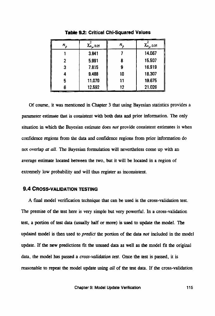
Table 9.2: Critical Chi-Squared Values
n x. n x. P Patty, 0.05 P Mos 0.05
1 3.841 7 14.067
2 5.991 8 15.507
3 7.815 g 16.919
4 9.488 10 18.307
5 11.070 11 19.675
6 12.592 12 21.026 |
Of course, it was mentioned in Chapter 3 that using Bayesian statistics provides a
parameter estimate that is consistent with both data and prior information. The only
situation in which the Bayesian estimate does not provide consistent estimates is when
confidence regions from the data and confidence regions from prior information do
not overlap at all. The Bayesian formulation will nevertheless come up with an
average estimate located between the two, but it will be located in a region of
extremely low probability and will thus register as inconsistent.
9.4 CROSS-VALIDATION TESTING
A final model verification technique that can be used is the cross-validation test.
The premise of the test here is very simple but very powerful. In a cross-validation
test, a portion of test data (usually half or more) is used to update the model. The
updated model is then used to predict the portion of the data not included in the model
update. If the new predictions fit the unused data as well as the model fit the original
data, the model has passed a cross-validation test. Once the test is passed, it is
reasonable to repeat the model update using all of the test data. If the cross-validation
Chapter 9: Model Update Verification 115
test is not passed, there is probably a model form error or an important parameter has
been left out of the analysis. |
An acceptance criterion for determining if an updated model (based on fitted data
subset #1) effectively predicts a different set of data (unfitted data subset #2) is given
in Eq. (9.13). The selected critical value of 2.0 provides a small allowance for varia-
tions in relative noise levels in the data sets. The ideal result of Eq. (9.13) is 1.0,
while results much larger than 2.0 mean that the model is incapable of predicting data
beyond the specific set used to update the model.
ny subset #1
SSE subset #1
SSE spset #2 | < 9 (9.1 3)
ny subset #2
Chapter 9: Model Update Verification 116
Chapter 10: Visualization Statistics
The model update procedure described in Part II of this dissertation is complete.
The only statistical quantity strictly required for interpreting the results is the sum-of-
squares error term of Eq. (3.17). However, it is helpful to have a number of test-
analysis visualization statistics available. These statistics allow the analyst to better
understand the results of the model update. They can also be used as tools to locate
problems with the model and/or data, either in terms of spatial location or excitation
frequency.
Three visualization schemes are presented in this chapter. The first two are
intended for use with sine-dwell test data, while the third is intended for use with
broad-band FRF data.
10.1 SINE-DWELL VISUALIZATION STATISTICS
The Correlation Coefficient
In order to better determine how well an updated model predicts sine-dwell test
data, two visualization statistics were developed. The first is a correlation coefficient
re. Here, a subset of the data measurements, y,, is compared to a prediction of the
same subset, ¥,, using the correlation function given in Eq. (10.1). Values for r, can
fall between zero and one.
72 = ly; Wid ) k (10.1) VM IIe MI)
Chapter 10: Visualization Statistics 117
A variety of subset definitions can be used, but the most useful way to break
down the data is by frequency. Thus, y, would correspond to the subset of the data
that was generated with the excitation frequency w,. The purpose of the test would
then be to compare response shapes, independent of scaling. If the results of test and
analysis match perfectly, ry will have a value of 1.0. Values less than one indicate
response shape discrepancies at the excitation frequency W,.
Using the r, Statistic in this manner makes it very similar to the modal assurance
criterion (MAC) [2] commonly used in modal testing to compare mode shapes. With
the MAC, results are often compared between different frequencies as well, since
mode shapes corresponding to different natural frequencies are expected to be
orthogonal. However, there is no point in computing these off-diagonal terms in a
dynamic response setting, since there is no reason for any given pair of response
shapes to exhibit orthogonality. When used in this context, the term r, is Called the
frequency response assurance criterion (FRAC) [41].
The Scaling Factor
A second comparison that can be made is one between measured and predicted
response amplitudes. Again, this can be done with any subset of the data, but it is
most useful to have y, and ¥, correspond to the data and predictions generated using
excitation frequency w,. The statistic that is computed here is the scaling factor c,
given in Eq. (10.2), which effectively gives the constant by which the actual data y,
would have to be multiplied to have amplitudes comparable to the predicted data J, .
Chapter 10: Visualization Statistics 118
T
_ EW iI (10.2) Ck T VW Nk
As with the correlation coefficient, c, will have a value of 1.0 if the model
matches the data perfectly. Values other than one indicate a response amplitude
discrepancy. It should be noted that there is no restriction on the possible values for
C,, as there are with the correlation coefficient ry. Any value can potentially be
obtained. This type of comparison is normally not done with mode shapes, since they
are usually rescaled according to some normalization criterion, but it can be a
valuable statistic to use with dynamic response shapes.
10.2 FRF VISUALIZATION STATISTICS
It is possible to compute r? and c, statistics for FRF data, but a much simpler
means of visually comparing test and analysis is to plot FRFs from both test and
analysis on the same chart. This can be done with real and imaginary components of
the FRF, but it is usually more intuitive to look at magnitude and phase angle, since
the positive-valued magnitudes can be plotted on a semi-logarithmic chart.
Chapter 10: Visualization Statistics 119

PART IV:
Case Studies
120
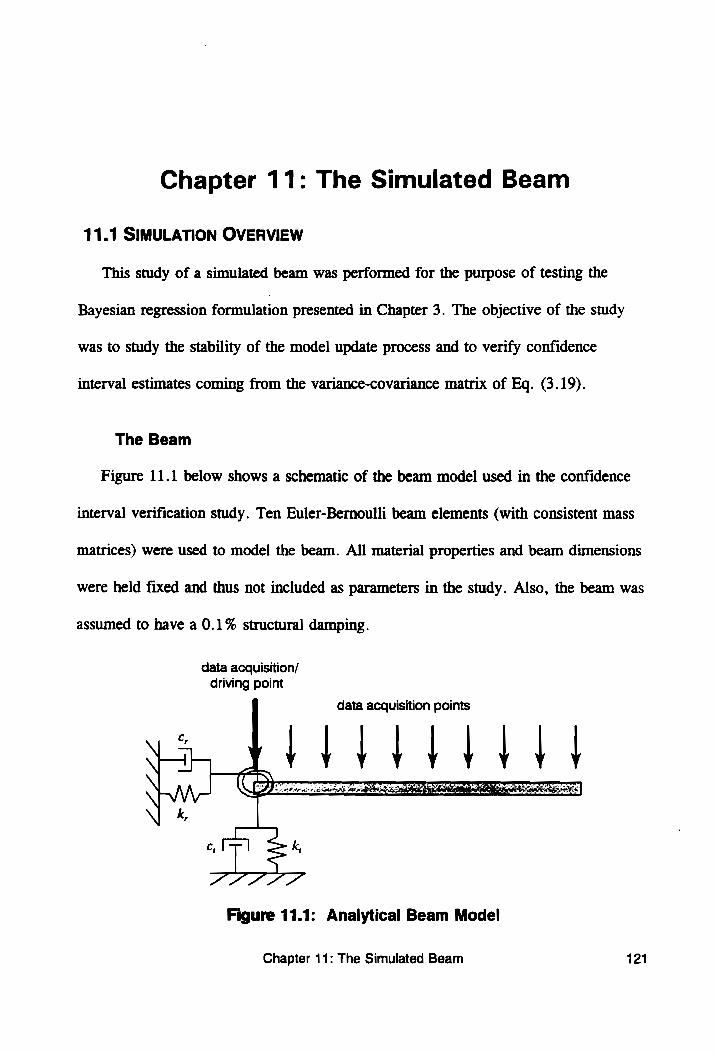
Chapter 11: The Simulated Beam
11.1 SIMULATION OVERVIEW
This study of a simulated beam was performed for the purpose of testing the
Bayesian regression formulation presented in Chapter 3. The objective of the study
was to study the stability of the model update process and to verify confidence
interval estimates coming from the variance-covariance matrix of Eq. (3.19).
The Beam
Figure 11.1 below shows a schematic of the beam model used in the confidence
interval verification study. Ten Euler-Bernoulli beam elements (with consistent mass
matrices) were used to model the beam. All material properties and beam dimensions
were held fixed and thus not included as parameters in the study. Also, the beam was
assumed to have a 0.1% structural damping.
data acquisition/
driving point
data acquisition points
ryy eed dt
Figure 11.1: Analytical Beam Model
Chapter 11: The Simulated Beam 121
The four unknowns in the problem consisted of the springs and dampers shown in
Figure 11.1, which might represent an elastic shock cord suspending the beam and a
metallic stinger connecting a shaker to the top of the beam. The four parameters c_,
c,, k,, and k, are estimated using the Bayesian regression formulation of Chapter 3.
Obtaining “Experimental” Data
In order to obtain “experimental” data, it was necessary to first choose “true”
values for the four update parameters. The values shown in Table 11.1 below were
selected. The stiffness values were based on previous research [92] concerning the
particular beam and suspension system under test, while damping values were
arbitrarily picked such that damping effects were noticeable (but not dominant) in a
driving point FRF.
Table 11.1: Update Parameter Target Values
Translational stiffness, k, = 87.56 Nim (0.50 Ibf/in) Translational damping, c, = 3.503 N-s/m (0.020 Ibf-sec/in) Rotational stiffness, k, = 0.339 N-m/rad (3.0 lbfin/rad) Rotational damping, c, =0.0Nm-s/rad (0.0 Ibf in-sec/rad)
“Experimental data” was generated analytically by computing the dynamic
response of the system at eight different excitation frequencies using Eq. (7.5), and
then adding a known level of Gaussian noise to the response shapes obtained. The
excitation frequencies of Table 11.2 were used.
Table 11.2: Excitation Frequencies
| near mode 1 [Hz] | near mode 2 [Hz] | near mode 3 [Hz] | near mode 4 [Hz] ]
17.30 17.35 | 47.55 4852 | 93.20 95.09 | 154.07 157.18 |
Chapter 11: The Simulated Beam 122
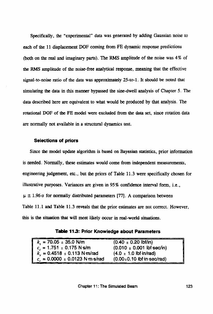
Specifically, the “experimental” data was generated by adding Gaussian noise to
each of the 11 displacement DOF coming from FE dynamic response predictions
(both on the real and imaginary parts). The RMS amplitude of the noise was 4% of
the RMS amplitude of the noise-free analytical response, meaning that the effective
signal-to-noise ratio of the data was approximately 25-to-1. It should be noted that
simulating the data in this manner bypassed the sine-dwell analysis of Chapter 5. The
data described here are equivalent to what would be produced by that analysis. The
rotational DOF of the FE model were excluded from the data set, since rotation data
are normally not available in a structural dynamics test.
Selections of priors
Since the model update algorithm is based on Bayesian statistics, prior information
is needed. Normally, these estimates would come from independent measurements,
engineering judgement, etc., but the priors of Table 11.3 were specifically chosen for
illustrative purposes. Variances are given in 95% confidence interval form, i.e.,
yt + 1.960 for normally distributed parameters [77]. A comparison between
Table 11.1 and Table 11.3 reveals that the prior estimates are not correct. However,
this is the situation that will most likely occur in real-world situations.
Table 11.3: Prior Knowledge about Parameters
= (0.40 + 0.20 Ibf/in) = 1.751 + 0.175 Ns/m (0.010 + 0.001 Ibf-sec/in) = 0.4518 + 0.113 N-m/rad (4.0 + 1.0 Ibfin/rad)
c, = 0.0000 + 0.0123 N-m-s/rad (0.00+0.10 Ibfin-sec/rad)
Chapter 11: The Simulated Beam 123
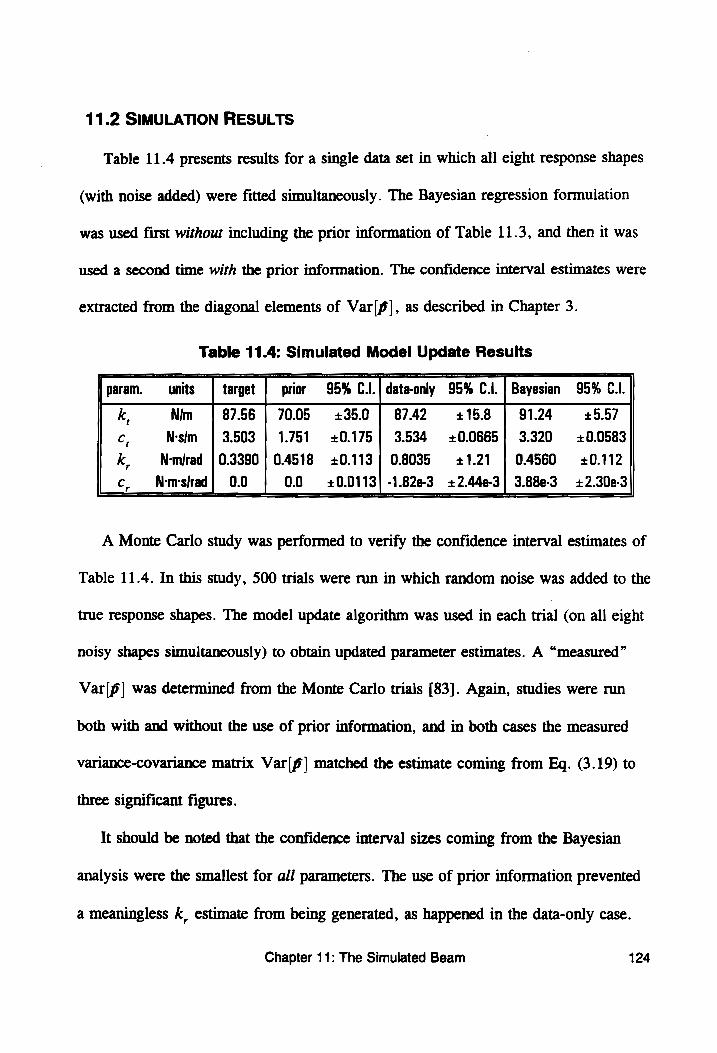
11.2 SIMULATION RESULTS
Table 11.4 presents results for a single data set in which all eight response shapes
(with noise added) were fitted simultaneously. The Bayesian regression formulation
was used first without including the prior information of Table 11.3, and then it was
used a second time with the prior information. The confidence interval estimates were
extracted from the diagonal elements of Var[p], as described in Chapter 3.
Table 11.4: Simulated Model Update Results
param. units | target | prior 95% C.l.| data-only 95% C.l. | Bayesian 95% CLI.
k Nim | 87.56 | 70.05 +35.0 | 87.42 +158 | 91.24 +5.57 t
C, N-sim | 3.503 | 1.751 +0.175| 3.534 +0.0665/ 3320 +0.0583
kK, N-mirad | 0.3390 | 0.4518 +0.113} 0.8035 +121 | 0.4560 +0.112
c, Nmrsijrad} 0.0 0.0 = +0.0113) -1.82e-3 +2.44e-3| 3.88e-3 +2.30e-3|
A Monte Carlo study was performed to verify the confidence interval estimates of
Table 11.4. In this study, 500 trials were run in which random noise was added to the
true response shapes. The model update algorithm was used in each trial (on all eight
noisy shapes simultaneously) to obtain updated parameter estimates. A “measured”
Var([p] was determined from the Monte Carlo trials [83]. Again, studies were run
both with and without the use of prior information, and in both cases the measured
variance-covariance matrix Var[p| matched the estimate coming from Eq. (3.19) to
three significant figures.
It should be noted that the confidence interval sizes coming from the Bayesian
analysis were the smallest for all parameters. The use of prior information prevented
a meaningless k, estimate from being generated, as happened in the data-only case.
Chapter 11: The Simulated Beam 124
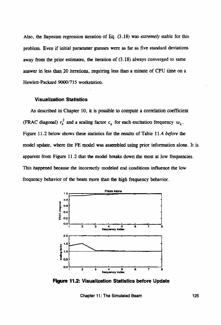
Also, the Bayesian regression iteration of Eq. (3.18) was extremely stable for this
problem. Even if initial parameter guesses were as far as five standard deviations
away from the prior estimates, the iteration of (3.18) always converged to same
answer in less than 20 iterations, requiring less than a minute of CPU time on a
Hewlett-Packard 9000/715 workstation.
Visualization Statistics
As described in Chapter 10, it is possible to compute a correlation coefficient
(FRAC diagonal) r? and a scaling factor c, for each excitation frequency w,.
Figure 11.2 below shows these statistics for the results of Table 11.4 before the
model update, where the FE model was assembled using prior information alone. It is
apparent from Figure 11.2 that the model breaks down the most at low frequencies.
This happened because the incorrectly modeled end conditions influence the low
frequency behavior of the beam more than the high frequency behavior.
Priors Alone ————n
0.8F
F g 0.6r
3 oO 0.4fr
€ o2f 0.0 af a} = nd
1 2 3 4 5 6 7 & frequency index
2.0 -
i ow
2 1.0 =
§ ost 1
0.0 alles all el ani. ——— | ani
2 3 4 5 6 7 8 frequency index
Figure 11.2: Visualization Statistics before Update
Chapter 11: The Simulated Beam 125
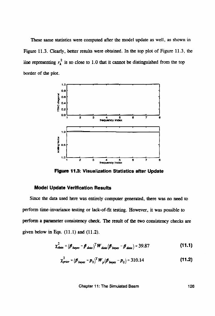
These same statistics were computed after the model update as well, as shown in
Figure 11.3. Clearly, better results were obtained. In the top plot of Figure 11.3, the
line representing re is so close to 1.0 that it cannot be distinguished from the top
border of the plot.
0.8 ,
z 4 5 0.6
£ oat 3 04 /
$ z 0.2 ; 0.0 a = ont ol
4 2 3 4 5 6 7 8 frequency index
1.0
; 2 OS a 8
1.0 A ft anil al el ai
1 2 3 4 5 6 7 8 frequency index
Figure 11.3: Visualization Statistics after Update
Model Update Verification Results
Since the data used here was entirely computer generated, there was no need to
perform time-invariance testing or lack-of-fit testing. However, it was possible to
perform a parameter consistency check. The result of the two consistency checks are
given below in Eqs. (11.1) and (11.2).
Kata = (B paves ~ P data * W deta (P tenes ~ B sata) = 39-87 (11.1)
Xprior = (P hayes ~ Po)" W p(B payes ~ Po) = 310.14 (11.2)
Chapter 11: The Simulated Beam 126
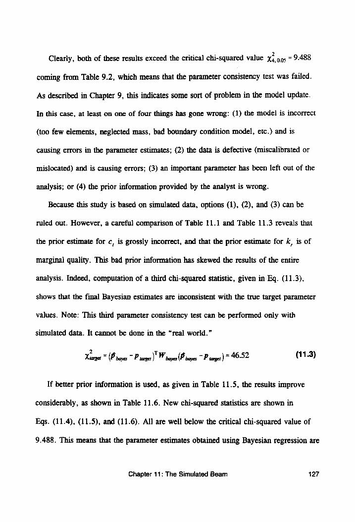
Clearly, both of these results exceed the critical chi-squared value Xi. 0.05 = 9-488
coming from Table 9.2, which means that the parameter consistency test was failed.
As described in Chapter 9, this indicates some sort of problem in the model update.
In this case, at least on one of four things has gone wrong: (1) the model is incorrect
(too few elements, neglected mass, bad boundary condition model, etc.) and is
causing errors in the parameter estimates; (2) the data is defective (miscalibrated or
mislocated) and is causing errors; (3) an important parameter has been left out of the
analysis; or (4) the prior information provided by the analyst is wrong.
Because this study is based on simulated data, options (1), (2), and (3) can be
ruled out. However, a careful comparison of Table 11.1 and Table 11.3 reveals that
the prior estimate for c, is grossly incorrect, and that the prior estimate for k, is of
marginal quality. This bad prior information has skewed the results of the entire
analysis. Indeed, computation of a third chi-squared statistic, given in Eq. (11.3),
shows that the final Bayesian estimates are inconsistent with the true target parameter
values. Note: This third parameter consistency test can be performed only with
simulated data. It cannot be done in the “real world.”
2 Ww Xiarget = (P payes ~ P target) W ayes (P vayes ~ P target) = 46-52 (11.3)
If better prior information is used, as given in Table 11.5, the results improve
considerably, as shown in Table 11.6. New chi-squared statistics are shown in
Egs. (11.4), (11.5), and (11.6). All are well below the critical chi-squared value of
9.488. This means that the parameter estimates obtained using Bayesian regression are
Chapter 11: The Simulated Beam 127
consistent with the data, with prior information, and most importantly, with the true
values. Indeed, this is the entire point of the exercise.
Table 11.5: Improved Prior Knowledge
k, = 70.05 + 35.0 N/m (0.40 + 0.20 Ibf/in) c, = 3.590 + 0.175 Ns/m (0.0205 + 0.0010 Ibf-sec/in) k, = 0.3953 + 0.113 N-m/rad (3.5 + 1.0 Ibfin/rad) c, = 0.0000 + 0.0123 Nms/rad = (0.00+0.10 Ibf in-sec/rad)
Table 11.6: Update Results from Improved Priors —————
param. units | target | prior 95% C.|.} data-only 95% C1. Bayesian 95% C.I.
k, Nim | 87.56 | 70.05 +35.0 | 8742 +158 | 91.24 +5.57
C, N-sim | 3.503 | 3.590 +0.175| 3.534 +20.0665| 3.320 +0.0583
k. = N-mirad | 0.3390 | 0.3953 20.113 | 0.8035 +121 | 0.4560 +0.112
c, Nmrsijrad; 0.0 0.0 +0.0113| -1.82e-3 +2.44e-3/ 3.88e-3 +2.30e-3
Xaata new = (P rayes,new ~ P data)" ¥ data bayes, new ~ P daw ) = 0-49 (11.4)
Xprior,new = (hayes, new ~ Po)" © p(Bhayes, new ~ Po) = 1-93 (11.5)
Xearget,new = (Poayes,new ~ P target)’ Wayes (Preys, new ~ P targer) = 6-79 (11.6)
These results support the hypothesis of Chapter 1, which states that the use of
Bayesian statistics is an effective framework for performing updates of finite element
models. In this simulated study, the inclusion of prior information considerably
improved the quality of the parameter estimates obtained. Additionally, the statistical
tools of Chapter 9 were used to detect a problem with the model update, which was
eliminated when improved prior information was used.
Chapter 11: The Simulated Beam 128

Chapter 12: The Sandia Test Frame
This chapter contains the results of two model updates performed on a single finite
element model of a test frame used in research at Sandia National Laboratories [44].
The first update was performed with sine-dwell data taken from the structure, and the
second was performed with FRF data taken from the structure. Issues relating to both
update problems are discussed initially, with sine-dwell and FRF results following.
The chapter concludes with a comparison of the two sets of update results.
12.1 PRELIMINARY ISSUES
The Test Structure
The Sandia test frame was a frame built specifically for the purpose of developing
joint models in structures made of tubular steel. A schematic of the test frame is
shown in Figure 12.1. The frame was approximately one meter tall and weighed
approximately 20 kg.
main beam section —,
Figure 12.1: Sandia Test Frame
Chapter 12: The Sandia Test Frame 129
Test Configuration
To acquire dynamic response data, sixteen sets of triaxial accelerometers (for a
total of 48) were mounted on the frame as shown in Figure 12.1 and Figure 12.2.
Two dynamic response tests were performed. The first utilized harmonic excitation
delivered through an electromagnetic shaker, generating data appropriate for the sine-
dwell statistical analysis of Chapter 5. The second utilized broad-band excitation
delivered through the impact of a modal test hammer, generating data appropriate for
the FRF statistical analysis of Chapter 6. All excitation was delivered from the rear
the frame in the positive z direction. Details on data acquisition are presented in the
individual sections concerning the sine-dwell results and the FRF results.
Also, the weight of test frame was measured twice (once each on two different
scales), generating two additional pieces of data to be used according to Eq. (3.23).
The measurements were 20.06 + 0.11 kg and 20.18 + 0.11 kg.
The Finite Element Model
A finite element model of the frame was built in NASTRAN using beam elements.
Figure 12.2 shows the node and element locations (units are in mm). Also shown are
the four double node locations at which four sets of six springs (three translational
and three rotational) were inserted between the beam elements. These springs
represent the effective joint stiffness of the welds. The elements between the double
nodes and main beam sections were assigned zero mass, since the connecting beams
do not reach to the neutral axes of the main beam sections. To account for the effect
of the accelerometers being offset from the neutral axes of the beams, rigid elements
Chapter 12: The Sandia Test Frame 130
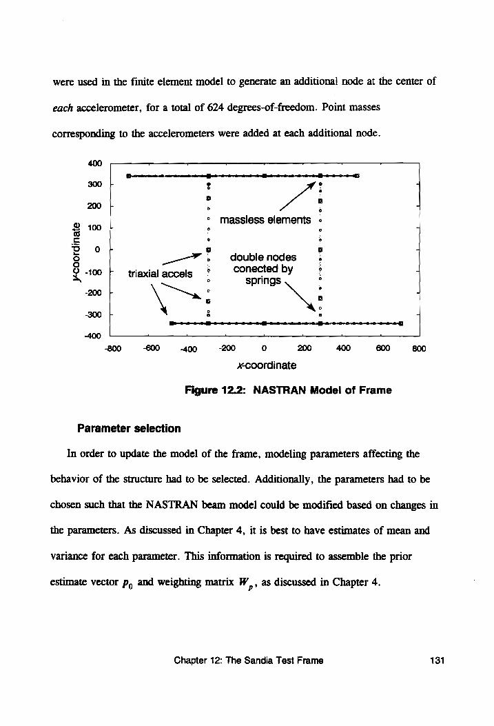
were used in the finite element model to generate an additional node at the center of
each accelerometer, for a total of 624 degrees-of-freedom. Point masses
corresponding to the accelerometers were added at each additional node.
400 — . , Y —
& 2 ~o- > a wo
300 + ® ° -
6 8 a 8
© ° massless elements ° —_ 100 L 9 ° 7
o c 6 °
ob OF a a , o _—” . double nodes e
¢ -100 fF triaxial accels ° conected by ° : 0 springs ° .
-200 [+ \: \ c
300 g ° / = gy =i} o. —> eo
-400 — , _ — — 4 —
-800 -600 -400 -200 0 200 400 600 800
xcoordinate
Figure 12.2: NASTRAN Model of Frame
Parameter selection
In order to update the model of the frame, modeling parameters affecting the
behavior of the structure had to be selected. Additionally, the parameters had to be
chosen such that the NASTRAN beam model could be modified based on changes in
the parameters. As discussed in Chapter 4, it is best to have estimates of mean and
variance for each parameter. This information is required to assemble the prior
estimate vector p, and weighting matrix W,, as discussed in Chapter 4.
Chapter 12: The Sandia Test Frame 131

The 16 parameters listed in Table 12.1 were selected as possible parameters to be
used in the model update process. These parameters can be broken up into five
groups: joint stiffness parameters, cross-section property parameters, material
property parameters, damping parameters, and a force miscalibration adjustment
parameter. Also listed with the parameters are the nominal values and confidence
intervals (estimated means and variances) that define the prior for each parameter. All
four joints were assumed to be the same, thus requiring only 6 parameters for joint
modeling instead of 24. Parameters such as J, and J, were used instead of thickness
and width parameters because the NASTRAN system matrices were linear with
respect to J, and I,. This made interfacing with NASTRAN and computing sensitiv-
ity matrices significantly easier. Also, these were the same parameters as used in
prior research [44] concerning the test frame.
Table 12.1: Sandia Test Frame Update Parameters
bneg
2: minor area moment of inertia
J : torsional moment of inertia
E: modulus of rigidity p: density a,: damping proportional to K
k,,: translational joint stiffness 6.01e6 N/mm (+20000%) k, ,: translational joint stiffness 6.01e6 N/mm (+20000%) k,,: transiational joint stiffness 6.01e6 N/mm (+20000%) k, ,: rotational joint stifiness 2.53e8 N.mm (+20000%) ky: rotational joint stiffness 1.96e8 N.mm (+20000%) k, ,: rotational joint stiffness 4.80e8 N.mm (+20000%) A: cross-section area 737 mm? (+3%) I,: major area moment of inertia 3.11e5 mm* (+6%)
5.89e5 mm* (+6%) 6.15e5 mm* (+15%) 2.07e5 N/mm? (+5%) 7.85 Mg/mm? (+5%) 0.00 (+0.002)
a,,: damping proportional to M 0.00 (+20) y : Structural damping ratio 0.00 (+0.2) c: force miscalibration factor 1.00 (+0.05)
Chapter 12: The Sandia Test Frame
132
The a, and o,, parameters are used to form a proportional viscous damping
matrix C= a,K+a,,M, while y is used to form a complex stiffness matrix (1+i7)K
for structural damping. The force miscalibration correction factor is included to
account for a possible miscalibration of the force transducer. If miscalibrated force
signals are used, bias errors in all other parameters could result. Ideally, a calibration
parameter would be included for every transducer used in the test, but this would
result in far too many parameters (and extreme ill-conditioning) when 48 accelero-
meters are used.
If the parameters of Table 12.1 are considered carefully, it becomes evident that
changes in certain parameters may have nearly (or even exactly) the same effects that
changes in other parameters have. This would be manifested in the X matrix of
Chapter 7 as a linear dependency which will cause the Bayesian regression formula-
tion to fail. Because of this, it is probably not possible to realistically update the
model by changing all 16 parameters. Indeed, in preliminary testing, all 16 para-
meters were used and completely unrealistic updates were obtained, even though the
data was fitted well. Thus, the set of parameters was restricted, as explained below.
Since the effects of material property changes were highly correlated with the
effects of beam cross-section property changes, the material property parameters were
excluded from the study. Similarly, a, and a,, have effects highly correlated with y
effects and were also left out. Finally, the force miscalibration correction factor c
was excluded because it was likely to be highly correlated with many of the
parameters. After these parameters were dropped, the six joint stiffnesses, four cross-
Chapter 12: The Sandia Test Frame 133
section properties, and one structural damping ratio remained, leaving a total of 11
parameters to be updated.
12.2 SINE-DWELL STUDY
The NASTRAN model of the frame was first updated using sine-dwell test data.
The sine-dwell statistics developed in Chapter 5 were used to provide statistically
qualified data (estimates ¥ and weights W,) for the model update algorithm. A
summary of the test and the analysis follow.
Data Acquisition
There are basically two “categories” of excitation frequency for sine-dwell exci-
tation. The first is near-resonance, where a small force generates a large response.
The response at near-resonant frequencies is very sensitive to most structural para-
meters, including damping and any parameters that might shift natural frequencies.
The second category is off-resonance, where a large force generates a small response.
The response at off-resonance frequencies is less sensitive to most structural
parameters. In particular, damping has almost no effect on off-resonance behavior.
Table 12.2 below lists the 13 excitation frequencies used in the test, along with the
category into which each frequency fits.
Chapter 12: The Sandia Test Frame 134
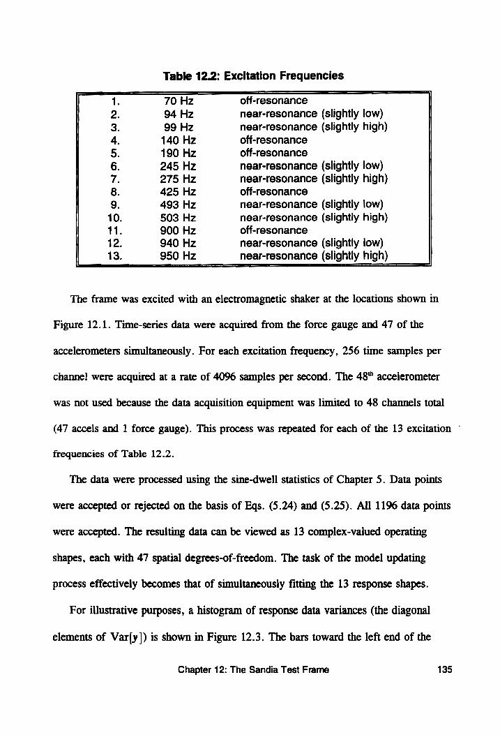
Table 12.2: Excitation Frequencies
1. 70 Hz off-resonance
2. 94 Hz near-resonance (slightly low) 3. 99 Hz near-resonance (slightly high) 4. 140 Hz off-resonance 5. 190 Hz off-resonance 6. 245 Hz near-resonance (slightly low) 7. 275 Hz near-resonance (slightly high) 8. 425 Hz off-resonance 9. 493 Hz near-resonance (slightly low) 10. 503 Hz near-resonance (slightly high) 11. 900 Hz off-resonance 12. 940 Hz near-resonance (slightly low) 13. 950 Hz near-resonance (slightly high)
The frame was excited with an electromagnetic shaker at the locations shown in
Figure 12.1. Time-series data were acquired from the force gauge and 47 of the
accelerometers simultaneously. For each excitation frequency, 256 time samples per
channel were acquired at a rate of 4096 samples per second. The 48" accelerometer
was not used because the data acquisition equipment was limited to 48 channels total
(47 accels and 1 force gauge). This process was repeated for each of the 13 excitation ~
frequencies of Table 12.2.
The data were processed using the sine-dwell statistics of Chapter 5. Data points
were accepted or rejected on the basis of Eqs. (5.24) and (5.25). All 1196 data points
were accepted. The resulting data can be viewed as 13 complex-valued operating
shapes, each with 47 spatial degrees-of-freedom. The task of the model updating
process effectively becomes that of simultaneously fitting the 13 response shapes.
For illustrative purposes, a histogram of response data variances (the diagonal
elements of Var(y|) is shown in Figure 12.3. The bars toward the left end of the
Chapter 12: The Sandia Test Frame 135
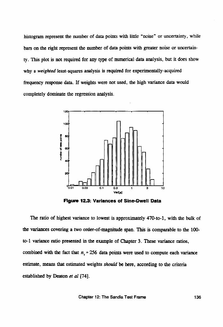
histogram represent the number of data points with little “noise” or uncertainty, while
bars on the right represent the number of data points with greater noise or uncertain-
ty. This plot is not required for any type of numerical data analysis, but it does show
why a weighted least-squares analysis is required for experimentally-acquired
frequency response data. If weights were not used, the high variance data would
completely dominate the regression analysis.
120
100 a ,
—
|p 7 5 So
1 7 : 40r 7 1
7 _ 20 ] ]
0.01 0.03 0.1 0.3 ‘ 3 10
Var[y]
Figure 12.3: Variances of Sine-Dwell Data
The ratio of highest variance to lowest is approximately 470-to-1, with the bulk of
the variances covering a two order-of-magnitude span. This is comparable to the 100-
to-1 variance ratio presented in the example of Chapter 3. These variance ratios,
combined with the fact that n, = 256 data points were used to compute each variance
estimate, means that estimated weights should be here, according to the criteria
established by Deaton et al [74].
Chapter 12: The Sandia Test Frame 136
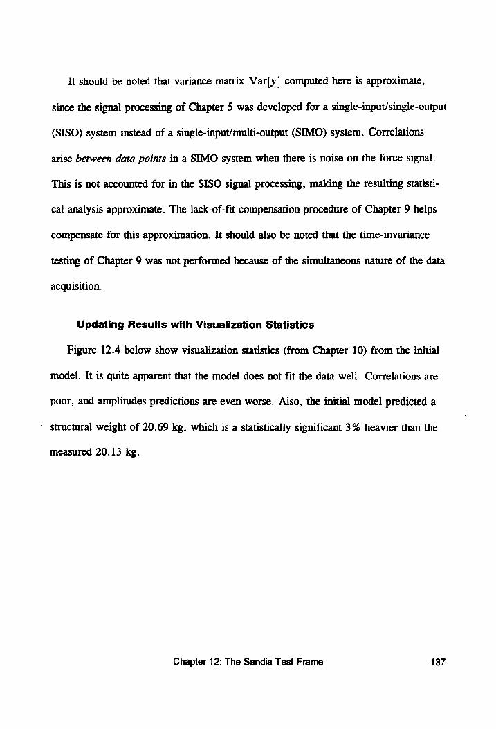
It should be noted that variance matrix Var[y] computed here is approximate,
since the signal processing of Chapter 5 was developed for a single-input/single-output
(SISO) system instead of a single-input/multi-output (SIMO) system. Correlations
arise between data points in a SIMO system when there is noise on the force signal.
This is not accounted for in the SISO signal processing, making the resulting statisti-
cal analysis approximate. The lack-of-fit compensation procedure of Chapter 9 helps
compensate for this approximation. It should also be noted that the time-invariance
testing of Chapter 9 was not performed because of the simultaneous nature of the data
acquisition.
Updating Results with Visualization Statistics
Figure 12.4 below show visualization statistics (from Chapter 10) from the initial
model. It is quite apparent that the model does not fit the data well. Correlations are
poor, and amplitudes predictions are even worse. Also, the initial model predicted a
' structural weight of 20.69 kg, which is a statistically significant 3% heavier than the
measured 20.13 kg.
Chapter 12: The Sandia Test Frame 137
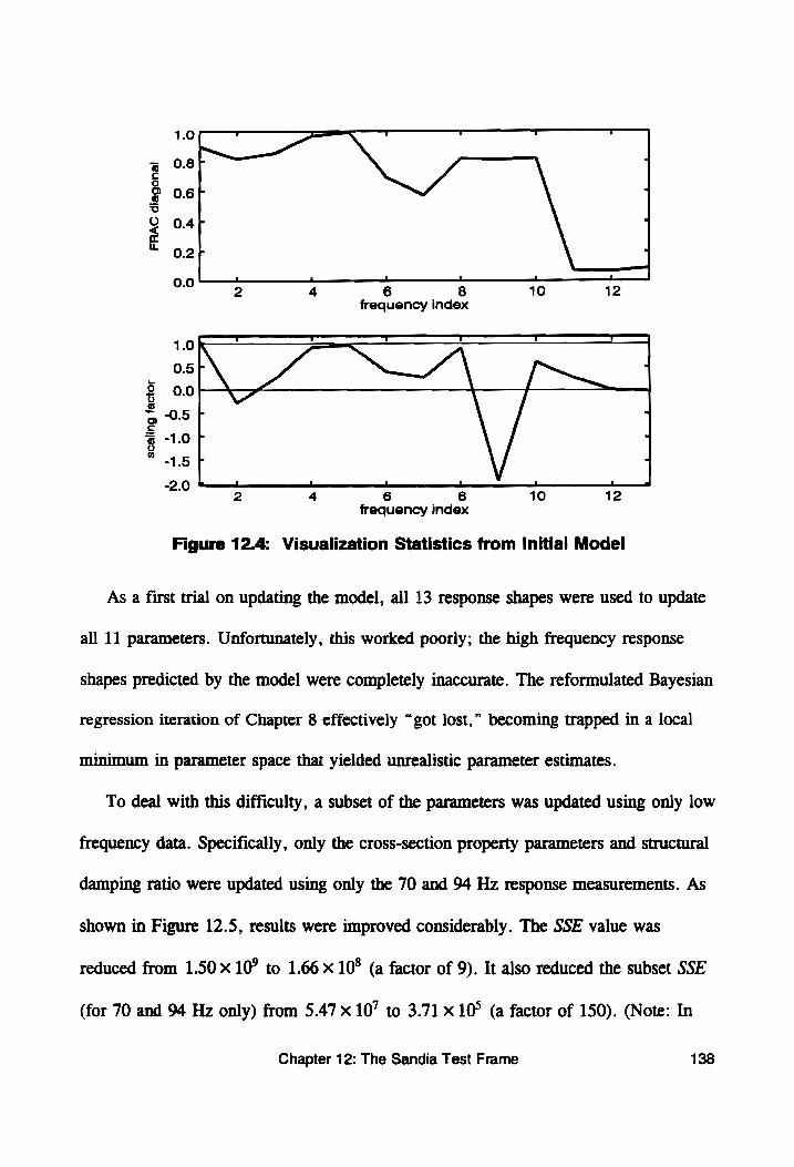
FRAC di
agon
al
0.02 4 6 8 10 12
frequency index
t c z
1.0 \ - — =
0.5 Sf ~~ *\ , 00ot-\> [-—~_
0.5 f
scal
ing
factor
-1.5 7
-2.0 al ell anal. ol
4 6 8 10 12 frequency index
hen
Figure 12.4: Visualization Statistics from Initial Model
As a first trial on updating the model, all 13 response shapes were used to update
all 11 parameters. Unfortunately, this worked poorly; the high frequency response
shapes predicted by the model were completely inaccurate. The reformulated Bayesian
regression iteration of Chapter 8 effectively “got lost,” becoming trapped in a local
minimum in parameter space that yielded unrealistic parameter estimates.
To deal with this difficulty, a subset of the parameters was updated using only low
frequency data. Specifically, only the cross-section property parameters and structural
damping ratio were updated using only the 70 and 94 Hz response measurements. As
shown in Figure 12.5, results were improved considerably. The SSE value was
reduced from 1.50 x 10° to 1.66 x 10° (a factor of 9). It also reduced the subset SSE
(for 70 and 94 Hz only) from 5.47 x10’ to 3.71 x 10° (a factor of 150). (Note: In
Chapter 12: The Sandia Test Frame 138
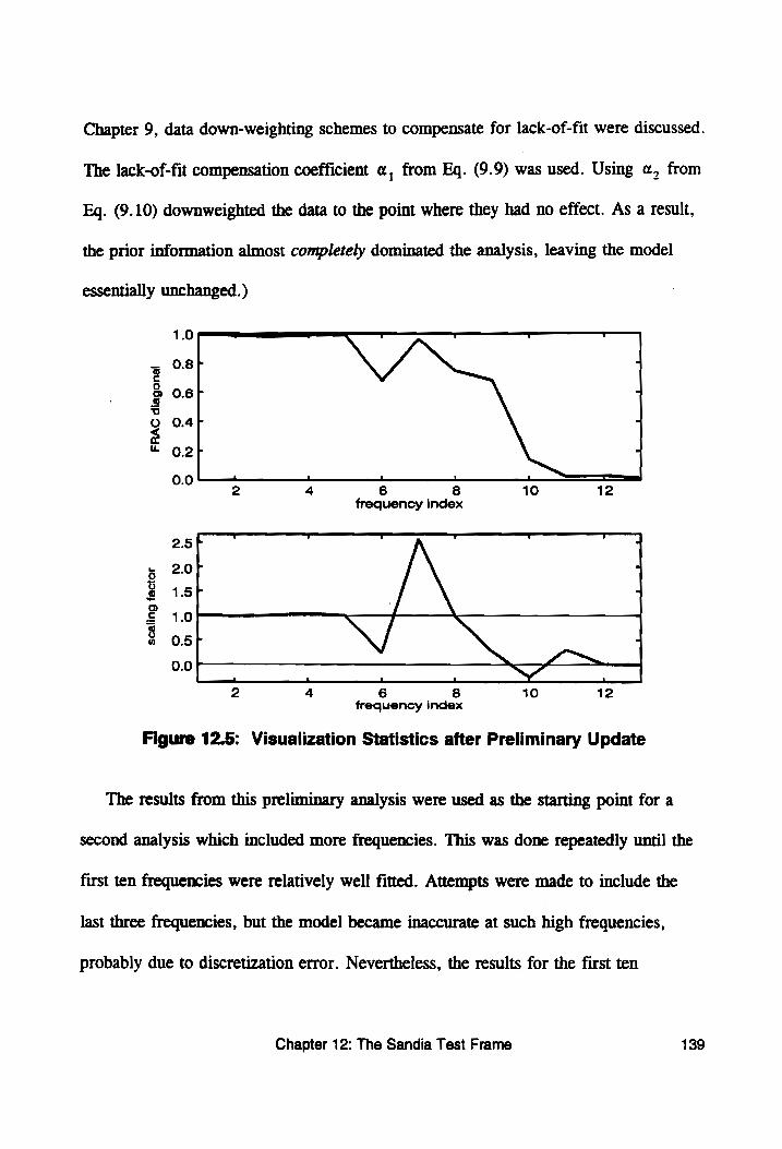
Chapter 9, data down-weighting schemes to compensate for lack-of-fit were discussed.
The lack-of-fit compensation coefficient a, from Eq. (9.9) was used. Using «, from
Eq. (9.10) downweighted the data to the point where they had no effect. As a result,
the prior information almost completely dominated the analysis, leaving the model
essentially unchanged.)
1.0 [eee
0.8F
0.6 F
0.4F
FRAC di
agon
al
0.27
0.0 nll a | 4 ell
2 4 6 8 10 12 frequency index
— T r La
2.57
2.07
1.5F
1.0
0.51 \/ Iw f —~
. . . NY _. 4 8 10 12
scal
ing
fact
or
0.0
2 6 frequency index
Figure 12.5: Visualization Statistics after Preliminary Update
The results from this preliminary analysis were used as the starting point for a
second analysis which included more frequencies. This was done repeatedly until the
first ten frequencies were relatively well fitted. Attempts were made to include the
last three frequencies, but the model became inaccurate at such high frequencies,
probably due to discretization error. Nevertheless, the results for the first ten
Chapter 12: The Sandia Test Frame 139
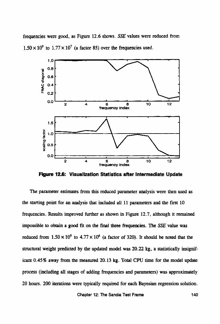
frequencies were good, as Figure 12.6 shows. SSE values were reduced from
1.50 10° to 1.7710’ (a factor 85) over the frequencies used.
1.0
0.8fF
0.6 fF
0.4F
FRAC diagonal
0.25 0.0
frequency index
1.5/7 _ /\ A
1.0
0.5f A
scal
ing
fact
or
0.0 -—— —; = = os 2 4 6 8 10 12
frequency index
Figure 12.6: Visualization Statistics after Intermediate Update
The parameter estimates from this reduced parameter analysis were then used as
the starting point for an analysis that included all 11 parameters and the first 10
frequencies. Results improved further as shown in Figure 12.7, although it remained
impossible to obtain a good fit on the final three frequencies. The SSE value was
reduced from 1.50 x 10° to 4.77 x 10° (a factor of 320). It should be noted that the
structural weight predicted by the updated model was 20.22 kg, a statistically insignif-
icant 0.45% away from the measured 20.13 kg. Total CPU time for the model update
process (including all stages of adding frequencies and parameters) was approximately
20 hours. 200 iterations were typically required for each Bayesian regression solution.
Chapter 12: The Sandia Test Frame 140
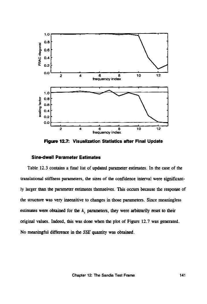
1.0
0.6Fr
0.47
FRAC di
agon
al
0.27 0.0 — — -
frequency index
v t v “! mn _
1.0 a
0.8F
0.6F
0.4F 5
0.2F
0.0
scal
ing
fact
or
nll lh. all. nl. nll
2 4 6 8 10 12 frequency index
Figure 12.7: Visualization Statistics after Final Update
Sine-dwell Parameter Estimates
Table 12.3 contains a final list of updated parameter estimates. In the case of the
translational stiffness parameters, the sizes of the confidence interval were significant-
ly larger than the parameter estimates themselves. This occurs because the response of
the structure was very insensitive to changes in those parameters. Since meaningless
estimates were obtained for the k, parameters, they were arbitrarily reset to their
original values. Indeed, this was done when the plot of Figure 12.7 was generated.
No meaningful difference in the SSE quantity was obtained.
Chapter 12: The Sandia Test Frame 141
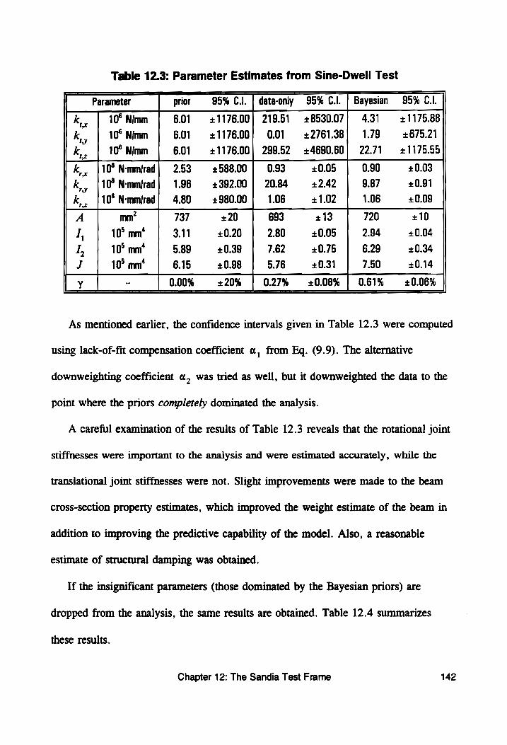
Table 12.3: Parameter Estimates from Sine-Dwell Test
As mentioned earlier, the confidence intervals given in Table 12.3 were computed
Parameter prior 95% C.I. | data-only 95% C.l. | Bayesian 95% Cll.
k, x 10° Nimm 6.01 +1176.00) 219.51 +8530.07; 4.31 + 1175.88
k, y 10° Nimm 6.01 +117600; O01 +2761.38| 1.79 +675.21
k, 2 10° Nimm 6.01 +1176.00) 299.52 +4690.60) 22.71 +1175.55
k,. 10° N-mmirad| 2.53 +588.00 | 0.93 +0.05 0.90 +0.03
ky 10° N-mmirad| 1.96 +392.00 | 20.84 +2.42 9.87 +0.91
k, 2 10° N-mmirad| 4.80 +980.00 1.06 + 1.02 1.06 +0.09
A mm’ 737 +20 693 +13 720 +10
IL 10° mm‘ 3.11 +0.20 2.80 +0.05 2.94 +0.04
L, 10° mm‘ 5.89 +0.39 7.62 +0.75 6.29 +0.34
J 10° mm‘ 6.15 +0.98 5.76 +0.31 7.50 +0.14
Y 0.00% +20% 0.27% +0.08% | 0.61% +0.06%
using lack-of-fit compensation coefficient a, from Eq. (9.9). The alternative
downweighting coefficient a, was tried as well, but it downweighted the data to the
point where the priors completely dominated the analysis.
A careful examination of the results of Table 12.3 reveals that the rotational joint
stiffnesses were important to the analysis and were estimated accurately, while the
translational joint stiffnesses were not. Slight improvements were made to the beam
cross-section property estimates, which improved the weight estimate of the beam in
addition to improving the predictive capability of the model. Also, a reasonable
estimate of structural damping was obtained.
If the insignificant parameters (those dominated by the Bayesian priors) are
dropped from the analysis, the same results are obtained. Table 12.4 summarizes
these results.
Chapter 12: The Sandia Test Frame 142
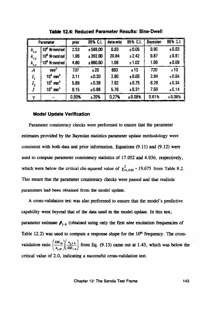
Table 12.4: Reduced Parameter Results: Sine-Dwell
— eee See =
Parameter prior 95% C.J. | data-only 95% C.l. | Bayesian 95% CLI.
kK 110° N-mmijrad} 2.53 +588.00) 0.93 +0.05 0.90 +0.03
k 10° N-mmirad} 1.96 +392.00 | 20.84 +2.42 9.87 +0.91
k. 110° N-mmjrad} 4.80 +980.00} 1.06 + 1.02 1.06 +0.09
A mm? 737 +20 693 +13 720 +10
rx
ny
V,Z
I 10° mm‘ 3.11 +0.20 2.80 +0.05 2.94 +0.04
I 10° mm‘ 5.89 +0.39 7.62 +0.75 6.29 +0.34
J
Y
No
10° mm‘ 6.15 +0.98 5.76 +0.31 7.50 +0.14
0.00% +20% 0.27% +0.08% | 0.61% +0.06% a ee _
Model Update Verification
Parameter consistency checks were performed to ensure that the parameter
estimates provided by the Bayesian statistics parameter update methodology were
consistent with both data and prior information. Equations (9.11) and (9.12) were
used to compute parameter consistency statistics of 17.052 and 4.036, respectively,
which were below the critical chi-squared value of 131,005 = 19.675 from Table 9.2.
This meant that the parameter consistency checks were passed and that realistic
parameters had been obtained from the model update.
A cross-validation test was also performed to ensure that the model’s predictive
capability went beyond that of the data used in the model update. In this test,
parameter estimate f,. (obtained using only the first nine excitation frequencies of
Table 12.2) was used to compute a response shape for the 10" frequency. The cross-
validation ratio (Se) [2 | from Eq. (9.13) came out at 1.43, which was below the My 19 J\ SSE, 5
critical value of 2.0, indicating a successful cross-validation test.
Chapter 12: The Sandia Test Frame 143
A second cross-validation test was performed in which p,_,, (the same as given in
Table 12.3) was used to compute response shapes for the 11", 12", and 13" frequen-
cies (900, 940, and 950 Hz). In this case, the cross-validation ratio (Ses) [22
came out at 280, failing the test. These results imply that the predictive capability of
the model is valid up to 500 Hz, but does not go much beyond that. A finer FE mesh
or improved joint model would probably be required for accurate higher frequency
predictions.
12.3 FRF Stupy
A second test was conducted on the Sandia test frame with impact excitation (from
a modal test hammer) being used instead of harmonic excitation. Statistically-qualified
FRF data (coming from the H, signal processing discussed in Chapter 6) was
acquired from the same 48 accelerometers. The same 11 parameters were updated.
Data acquisition
A modal test hammer was used at four points on the structure, as shown in
Figure 12.1 and Figure 12.2. Thirty averages were taken at each point. With each
impact, 9192 time samples were taken on each channel at a rate of 4096 samples per
second. This allowed for FFT computation of H, FRF estimates with 0.5 Hz resolu-
tion up to 2048 Hz. Due to time considerations, however, only a subset of the
frequency lines was used. Specifically, one out of every 32 lines (every 16 Hz) was
used up to 500 Hz, with the upper frequency limit being based on the results of the
sine-dwell study of Section 12.2. However, there is no fundamental theoretical reason
Chapter 12: The Sandia Test Frame 144
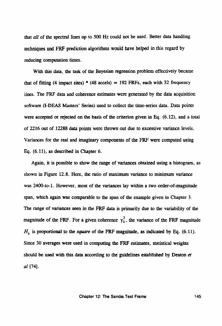
that all of the spectral lines up to 500 Hz could not be used. Better data handling
techniques and FRF prediction algorithms would have helped in this regard by
reducing computation times.
With this data, the task of the Bayesian regression problem effectively became
that of fitting (4 impact sites) * (48 accels) = 192 FRFs, each with 32 frequency
lines. The FRF data and coherence estimates were generated by the data acquisition
software (I-DEAS Masters’ Series) used to collect the time-series data. Data points
were accepted or rejected on the basis of the criterion given in Eq. (6.12), and a total
of 2216 out of 12288 data points were thrown out due to excessive variance levels.
Variances for the real and imaginary components of the FRF were computed using
Eq. (6.11), as described in Chapter 6.
Again, it is possible to show the range of variances obtained using a histogram, as
shown in Figure 12.8. Here, the ratio of maximum variance to minimum variance
was 2400-to-1. However, most of the variances lay within a two order-of-magnitude
span, which again was comparable to the span of the example given in Chapter 3.
The range of variances seen in the FRF data is primarily due to the variability of the
magnitude of the FRF. For a given coherence Y; , the variance of the FRF magnitude
Hi, is proportional to the square of the FRF magnitude, as indicated by Eq. (6.11).
Since 30 averages were used in computing the FRF estimates, statistical weights
should be used with this data according to the guidelines established by Deaton et
al [74].
Chapter 12: The Sandia Test Frame 145
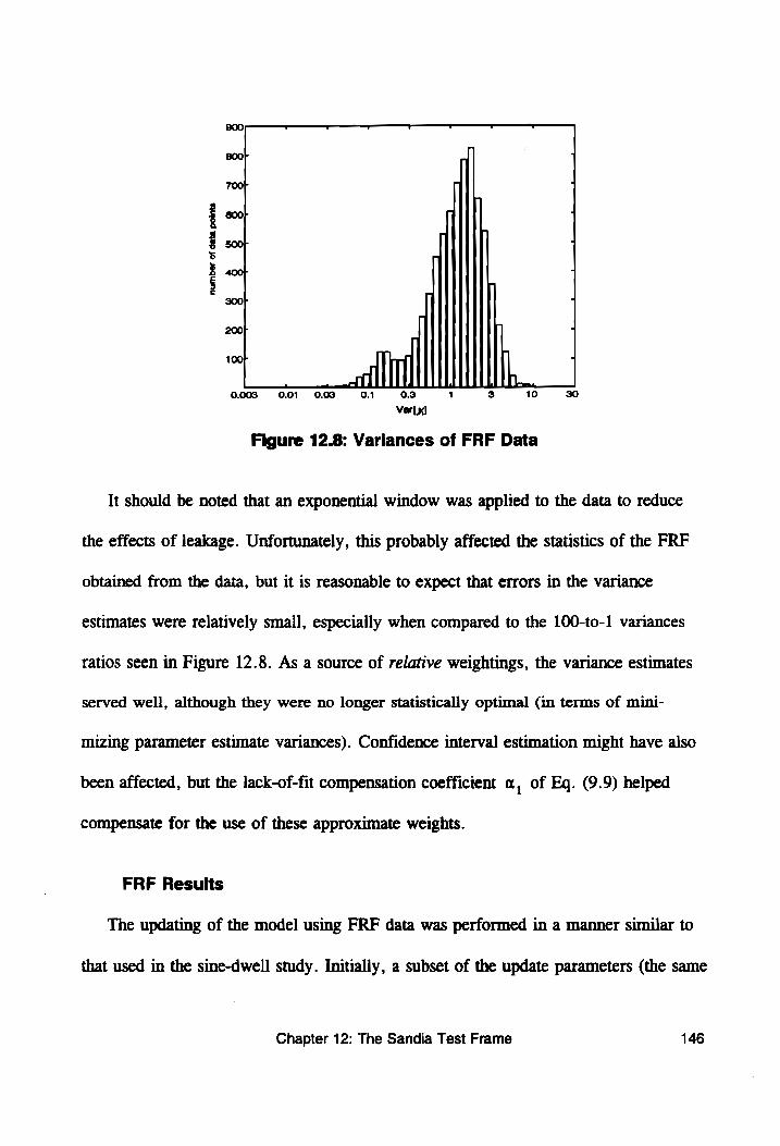
g 8 4
8 8
8 8
8 nn
g 4 anh
0.003 0.01 0.03 01 03 | 1 3 10 30
VarLy]
Figure 12.8: Variances of FRF Data
It should be noted that an exponential window was applied to the data to reduce
the effects of leakage. Unfortunately, this probably affected the statistics of the FRF
obtained from the data, but it is reasonable to expect that errors in the variance
estimates were relatively small, especially when compared to the 100-to-1 variances
ratios seen in Figure 12.8. As a source of relative weightings, the variance estimates
served well, although they were no longer statistically optimal (in terms of mini-
mizing parameter estimate variances). Confidence interval estimation might have also
been affected, but the lack-of-fit compensation coefficient «, of Eq. (9.9) helped
compensate for the use of these approximate weights.
FRF Results
The updating of the model using FRF data was performed in a manner similar to
that used in the sine-dwell study. Initially, a subset of the update parameters (the same
Chapter 12: The Sandia Test Frame 146
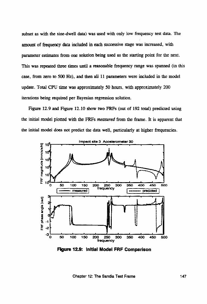
subset as with the sine-dwell data) was used with only low frequency test data. The
amount of frequency data included in each successive stage was increased, with
parameter estimates from one solution being used as the starting point for the next.
This was repeated three times until a reasonable frequency range was spanned (in this
case, from zero to 500 Hz), and then all 11 parameters were included in the model
update. Total CPU time was approximately 50 hours, with approximately 200
iterations being required per Bayesian regression solution.
Figure 12.9 and Figure 12.10 show two FRFs (out of 192 total) predicted using
the initial model plotted with the FRFs measured from the frame. It is apparent that
the initial model does not predict the data well, particularly at higher frequencies.
Zz 2 n ~~
E E ® 3 2 € D @ E Le va uw
Impact site 3 Accelerometer 30 ™ 107
1 i i. nll. 4S = nll nll 5 nll
Oo 50 100 150 200 250 300 350 400 450 500
[———"measured] ene = preated —
j
a
6
FR
F phase
angl
e [r
ad]
2
ST
3 a A ell ell anil ll ell anit
O SO 100 150 200 250 300 350 400 450 500 frequency
Figure 12.9: Initial Model FRF Comparison
Chapter 12: The Sandia Test Frame 147
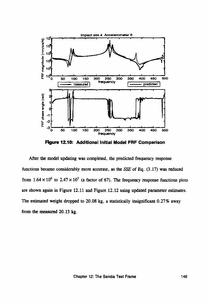
Impact site 4 Accelerometer 6 v . J
FRF
magnitude (mm/s/s/N]
1 a | ani af. ani. nt. aol. =
Oo 50 4100 150 200 250 300 350 400 450 500
frequency oe
fgg
sn
oe
Re
ew
od
FRF
phas
e an
gle
[rad
]
35 50 100 150 200 250 300 350 400 450 £500 frequency
Figure 12.10: Additional Initial Model FRF Comparison
After the model updating was completed, the predicted frequency response
functions became considerably more accurate, as the SSE of Eq. (3.17) was reduced
from 1.64 x10? to 2.47 x 10’ (a factor of 67). The frequency response functions plots
are shown again in Figure 12.11 and Figure 12.12 using updated parameter estimates.
The estimated weight dropped to 20.08 kg, a statistically insignificant 0.27% away
from the measured 20.13 kg.
Chapter 12: The Sandia Test Frame 148
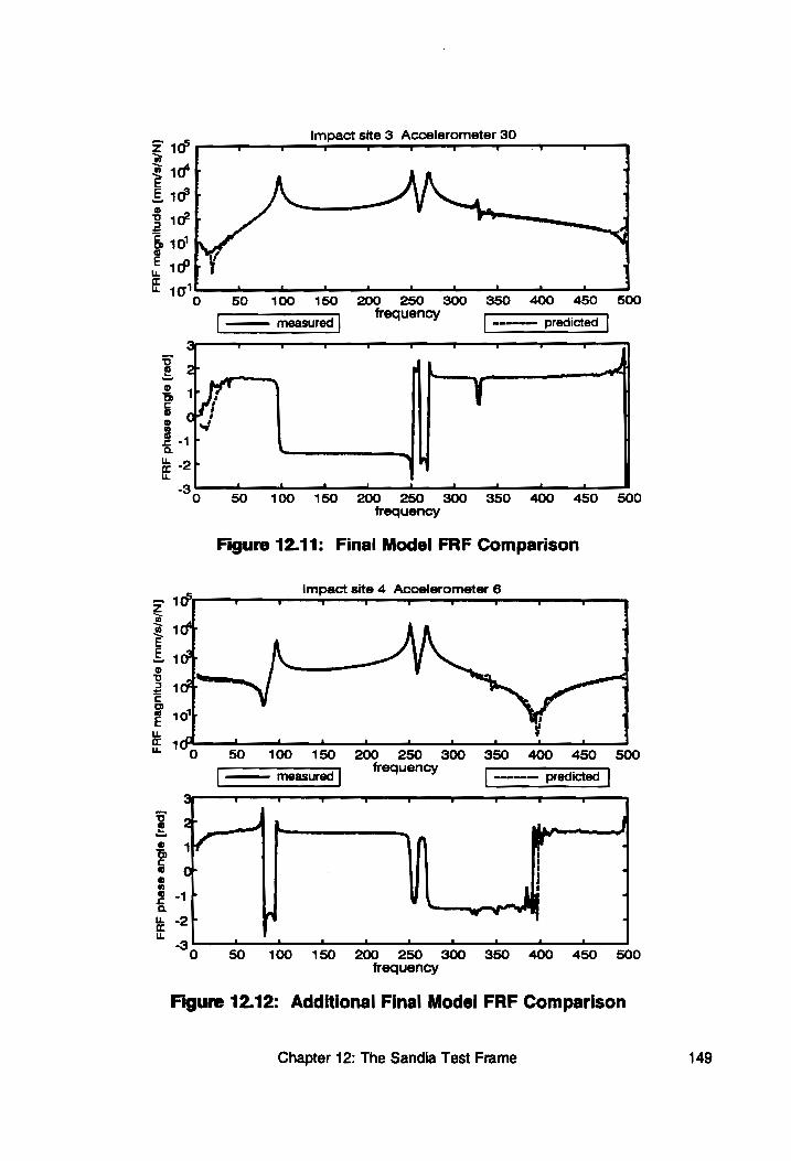
FRF
magnitude
[(mm
/s/s
/N]
FRF
phase an
gle
[rad
]
Impact site 3 Accelerometer 30
Z 10 a o
E E @ ug
2 <
Oo
E uo ™ | a E Lk. 10' — | ai _ — i a | af a_i, i
Oo 50 100150 200 250 300 350 400 450 500
saweney
o o 2 2 oS ®
3 £
Qa
ua cr
u 4 a ail nll a el ah a | a
‘3050 100.150 200 250 300 350 400 450 500 frequency
Figure 12.11: Final Model FRF Comparison
ie Impact site 4 Accelerometer 6
’ 1 el ll af a | a | i hh all a J
O50 100180 200 rey rr 30 400450500
mameney
2
1
or
at -2
30 50.100 150 200 250 300 350 400 450 500 frequency
Figure 12.12: Additional Final Model FRF Comparison
Chapter 12: The Sandia Test Frame 149
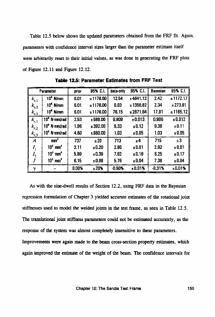
Table 12.5 below shows the updated parameters obtained from the FRF fit. Again,
parameters with confidence interval sizes larger than the parameter estimate itself
were arbitrarily reset to their initial values, as was done in generating the FRF plots
of Figure 12.11 and Figure 12.12.
Table 12.5: Parameter Estimates from FRF Test
| Parameter prior 95% C.l. | data-only 95% C.I. | Bayesian 95% CLI.
ky 10° Nimm 6.01 +1176.00) 12.54 +4641.12) 2.42 1172.17
ko 10° Nimm 6.01 +1176.00; O03 +1356.82| 2.34 +273.91
k, 3 10° Nimm 6.01 +1176.00| 76.15 +2671.64) 17.91 +1165.12
k, 10° N-mmirad} 2.53 +588.00 | 0.909 +0.013 | 0.906 +0.012
k, 2 10° N-mmirad| 1.96 +392.00 9.33 +0.12 9.38 +0.11
k, 5 10° N-mmirad| 4.80 + 980.00 1.03 +0.05 1.03 +0.05
A mm’ 737 +20 713 +4 715 +3
L, 10° mm‘ 3.11 +0.20 2.80 +0.01 2.92 +0.01
L, 10° mm‘ 5.89 +0.39 7.62 +0.19 6.25 +0.17
J 10° mm‘ 6.15 +0.98 5.76 +0.04 7.38 +0.04
y 0.00% +20% 0.50% +0.01% | 031% +0.01% As with the sine-dwell results of Section 12.2, using FRF data in the Bayesian
regression formulation of Chapter 3 yielded accurate estimates of the rotational joint
stiffnesses used to model the welded joints in the test frame, as seen in Table 12.5.
The translational joint stiffness parameters could not be estimated accurately, as the
response of the system was almost completely insensitive to these parameters.
Improvements were again made to the beam cross-section property estimates, which
again improved the estimate of the weight of the beam. The confidence intervals for
Chapter 12: The Sandia Test Frame 150
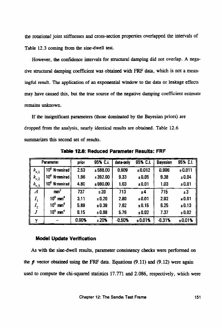
the rotational joint stiffnesses and cross-section properties overlapped the intervals of
Table 12.3 coming from the sine-dwell test. |
However, the confidence intervals for structural damping did not overlap. A nega-
tive structural damping coefficient was obtained with FRF data, which is not a mean-
ingful result. The application of an exponential window to the data or leakage effects
may have caused this, but the true source of the negative damping coefficient estimate
remains unknown.
If the insignificant parameters (those dominated by the Bayesian priors) are
dropped from the analysis, nearly identical results are obtained. Table 12.6
summarizes this second set of results.
Table 12.6: Reduced Parameter Results: FRF
Parameter
k,, |10°Nmmirad] 2.53 +588.00] 0909 +0.012 | 0906 +0.011
2 [10° Nmmirad| 1.96 +392.00} 933 +005 | 9.38 +£0.04 3 [10° N-mmjrad} 4.80 +980.00]} 103 +0.01 1.03 +0.01
k,
k,
A mm’ 737 +20 713 +4 715 +3
I
I, J
10° mm‘ 3.11 +0.20 2.80 +0.01 2.92 +0.01
10° mm‘ 5.89 +0.39 7.62 +0.15 6.25 +0.13
10° mm‘ 6.15 +0.98 5.76 +0.02 7.37 +0.02
0.00% +20% | -0.50% +0.01% | 0.37% +0.01% :
Model Update Verification
As with the sine-dwell results, parameter consistency checks were performed on
the p vector obtained using the FRF data. Equations (9.11) and (9.12) were again
used to compute the chi-squared statistics 17.771 and 2.086, respectively, which were
Chapter 12: The Sandia Test Frame 151
less than the critical chi-squared value of 171,005 = 19.675 from Table 9.2. Thus, the
Bayesian parameter estimates passed the parameter consistency check.
Since only a subset of the FRF data was used in the model update, performing a
cross-validation test here was even easier. The original data came from frequency set
#1, which consisted of the frequencies {5 Hz, 17 Hz, 29 Hz, -., 497 Hz}. The results
from this set were used to predict FRF values at frequency set #2, which consisted of
the frequencies {7 Hz, 19 Hz, 31 Hz, --, 499 Hz}. The cross-validation ratio
(==) [ze] of Eq. (9.13) came out at 1.002, which is a nearly ideal result that
easily passes the cross-validation test. For frequency interpolation purposes, this
updated model is almost ideal.
12.4 CONCLUDING REMARKS ON SANDIA TEST FRAME
If the results from Table 12.5 are compared to those of Table 12.3, it will be
noticed that the confidence intervals obtained from the FRF data are smaller than
those obtained from the sine-dwell data. The smaller size of the confidence intervals
is due primarily to the increased amount of data available for the update (10072 points
vs. 974 points). As pointed out in Chapter 9, however, ever-increasing amounts of
data will cause confidence intervals to become arbitrarily small, possibly around the
wrong answer if there is a significant lack-of-fit problem with the model. The lack-of-
fit compensation factor «, was developed to deal with this problem, but the compen-
sation it provided was too strong, effectively eliminating the data from the analysis.
Therefore, only «, was used, possibly resulting in Table 12.5 having smaller confi-
dence intervals than it should.
Chapter 12: The Sandia Test Frame 152

Fortunately, even if the sizes of intervals are off somewhat due to lack-of-fit, they
are still correct relative to each other. This helps the analyst determine which vari-
ables are most important to the model update analysis and which are not. Fortunately,
the confidence intervals from both studies overlapped (except for the structural
damping coefficient y ) in this study, which adds credibility to the results.
Chapter 12: The Sandia Test Frame 153
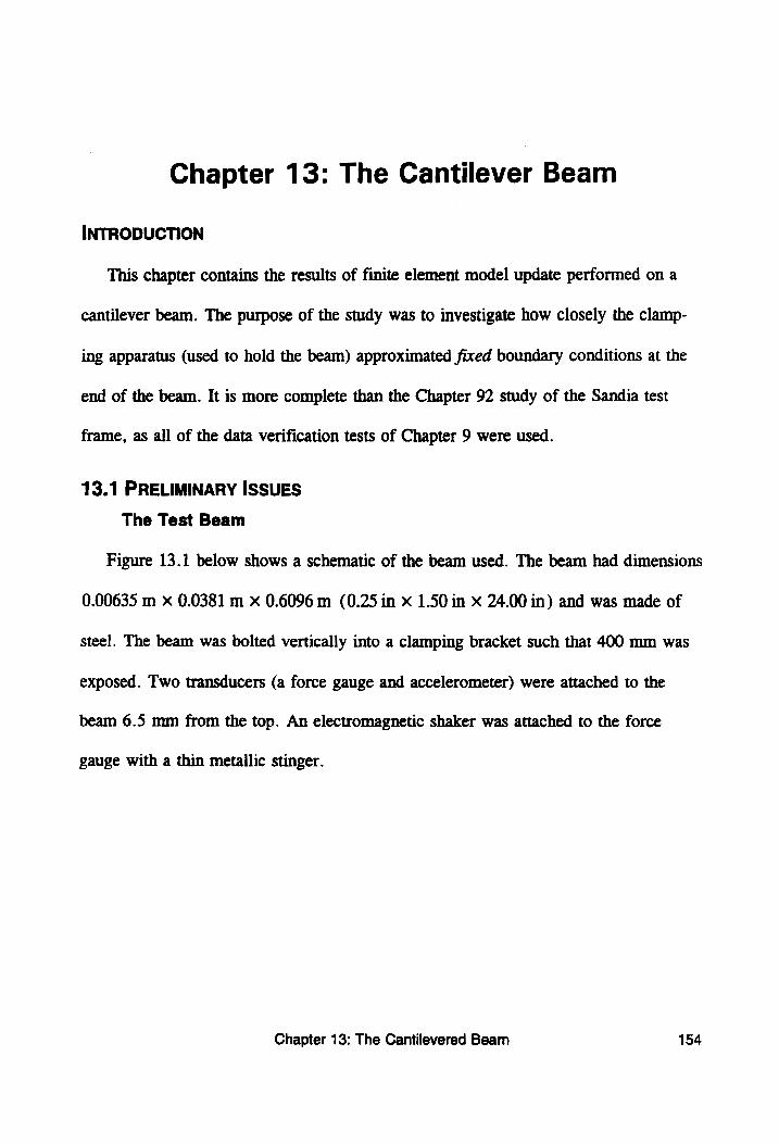
Chapter 13: The Cantilever Beam
INTRODUCTION
This chapter contains the results of finite element model update performed on a
cantilever beam. The purpose of the study was to investigate how closely the clamp-
ing apparatus (used to hold the beam) approximated fixed boundary conditions at the
end of the beam. It is more complete than the Chapter 92 study of the Sandia test
frame, as all of the data verification tests of Chapter 9 were used.
13.1 PRELIMINARY ISSUES
The Test Beam
Figure 13.1 below shows a schematic of the beam used. The beam had dimensions
0.00635 m x 0.0381 m x 0.6096 m (0.25 in x 1.50 in X 24.00 in) and was made of
steel. The beam was bolted vertically into a clamping bracket such that 400 mm was
exposed. Two transducers (a force gauge and accelerometer) were attached to the
beam 6.5 mm from the top. An electromagnetic shaker was attached to the force
gauge with a thin metallic stinger.
Chapter 13: The Cantilevered Beam 154
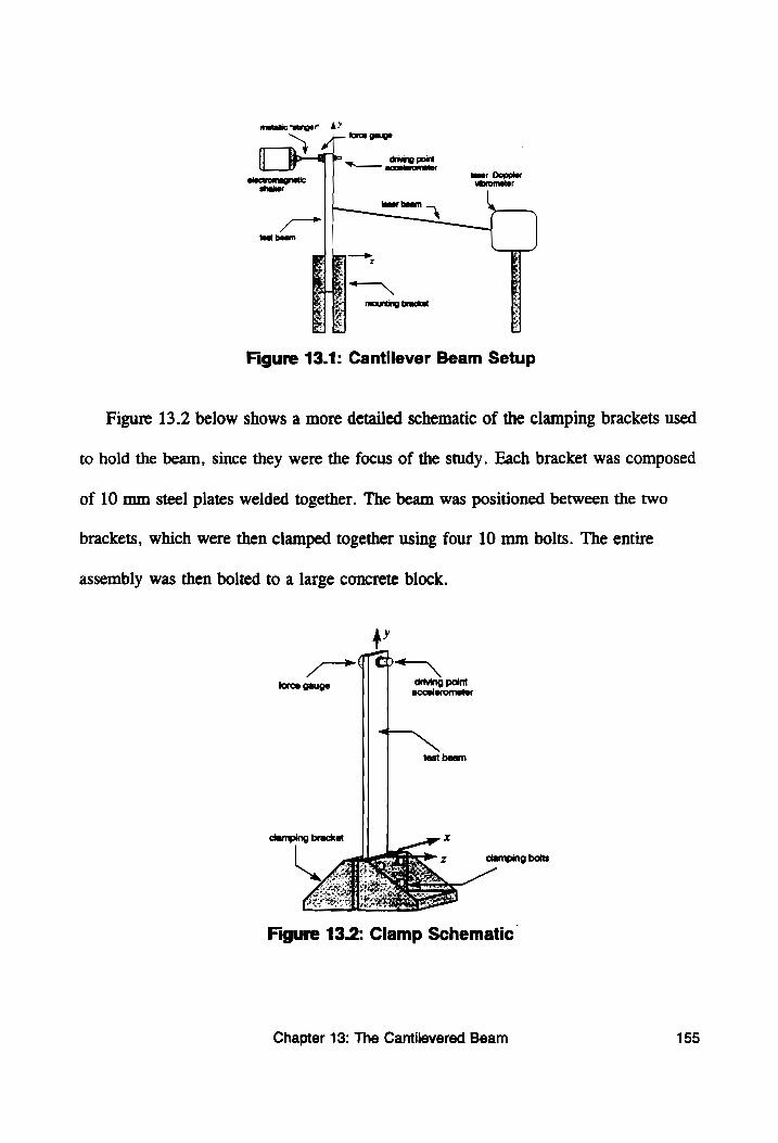
Figure 13.1: Cantilever Beam Setup
Figure 13.2 below shows a more detailed schematic of the clamping brackets used
to hold the beam, since they were the focus of the study. Each bracket was composed
of 10 mm steel plates welded together. The beam was positioned between the two
brackets, which were then clamped together using four 10 mm bolts. The entire
assembly was then bolted to a large concrete block.
> Ne
aN "
A orn force gauge Seng point
test beam
Figure 13.2: Clamp Schematic
Chapter 13: The Cantilevered Beam 155
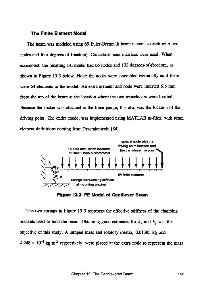
The Finite Element Model
The beam was modeled using 65 Euler-Bernoulli beam elements (each with two
nodes and four degrees-of-freedom). Consistent mass matrices were used. When
assembled, the resulting FE model had 66 nodes and 132 degrees-of-freedom, as
shown in Figure 13.3 below. Note: the nodes were assembled essentially as if there
were 64 elements in the model. An extra element and node were inserted 6.5 mm
from the top of the beam at the location where the two transducers were located.
Because the shaker was attached to the force gauge, this also was the location of the
driving point. The entire model was implemented using MATLAB m-files, with beam
element definitions coming from Przemieniecki [84].
special node with the
_— driving point location and 15 data acquisition locations the transducer masses for laser Doppler vibrometer
RRARARARRAEARE, LEE TTT YT)
65 finite elements
springs representing stiffness
of mounting bracket
Figure 13.3: FE Model of Cantilever Beam
The two springs in Figure 13.3 represent the effective stiffness of the clamping
brackets used to hold the beam. Obtaining good estimates for k, and k, was the
objective of this study. A lumped mass and rotatory inertia, 0.01385 kg and
4.248 x 10° kg-m? respectively, were placed at the extra node to represent the mass
Chapter 13: The Cantilevered Beam 156
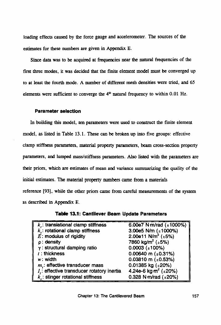
loading effects caused by the force gauge and accelerometer. The sources of the
estimates for these numbers are given in Appendix E.
Since data was to be acquired at frequencies near the natural frequenciés of the
first three modes, it was decided that the finite element model must be converged up
to at least the fourth mode. A number of different mesh densities were tried, and 65
elements were sufficient to converge the 4" natural frequency to within 0.01 Hz.
Parameter selection
In building this model, ten parameters were used to construct the finite element
model, as listed in Table 13.1. These can be broken up into five groups: effective
clamp stiffness parameters, material property parameters, beam cross-section property
parameters, and lumped mass/stiffness parameters. Also listed with the parameters are
their priors, which are estimates of mean and variance summarizing the quality of the
initial estimates. The material property numbers came from a materials
reference [93], while the other priors came from careful measurements of the system
as described in Appendix E.
Table 13.1: Cantilever Beam Update Parameters
k_: translational clamp stiffness 6.00e7 Nm/rad (+1000%) k,: rotational clamp stiffness 3.00e5 N/m (+1000%) E: modulus of rigidity 2.00611 N/m? (+5%) p: density 7860 kg/m? (+5%) y : structural damping ratio 0.0003 (+100%) t : thickness 0.00640 m (+0.31%) w: width 0.03810 m (+0.53%) m,: effective transducer mass 0.01385 kg (+20%) I: effective transducer rotatory inertia 4.24e-6 kg-m* (+20%)
Chapter 13: The Cantilevered Beam 157
Data Acquisition
As with the Sandia test frame of Chapter 12, two categories of excitation
frequency were used for sine-dwell excitation. The first was near-resonant, where a
small force generates a large response, while the second was off-resonant, where a
large force generates a small response. Table 13.2 below lists the 12 excitation
frequencies used in the test, along with the category into which each frequency fits.
Table 13.2: Excitation Frequencies
1 15 Hz off-resonance 2 26.25 Hz near-resonance (slightly low)
3 28.25 Hz near-resonance (slightly high) 4 50 Hz off-resonance 5 90 Hz off-resonance 6 170 Hz near-resonance (slightly low) 7. 180 Hz near-resonance (slightly high) 8. 250 Hz off-resonance
9 400 Hz off-resonance 10 450 Hz near-resonance (slightly low) 11 470 Hz near-resonance (slightly high) 12 530 Hz off-resonance
Blocks of time-series data were acquired from the force gauge, the accelerometer,
and the scanning laser Doppler vibrometer (SLDV) for each of the 45 data acquisition
points, as shown in Figure 13.4. The y-axis values were picked such that data was
acquired at FE nodes {#5, #9, #13, --, #61} (one in every four FE nodes), while
X-axis values were arbitrarily set at {-12.7 mm, 0.0mm, 12.7 mm}. Appendix D
describes how the SLDV was registered in space relative to the beam and how
scanning angles were computed to hit the desired points. For each excitation
frequency, 250 time samples were acquired at a rate of 2000 samples per second.
Chapter 13: The Cantilevered Beam 158
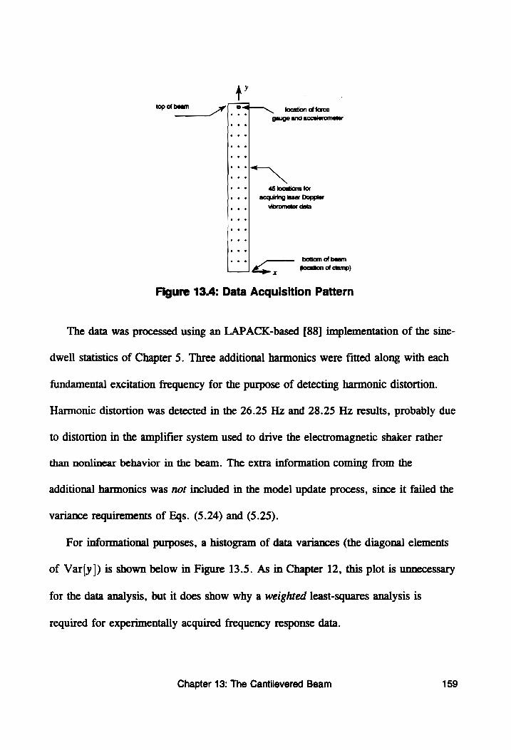
A?
top of beam | 2—~_ ovation of force .* gauge and accelerometer
Figure 13.4: Data Acquisition Pattern
The data was processed using an LAPACK-based [88] implementation of the sine-
dwell statistics of Chapter 5. Three additional harmonics were fitted along with each
fundamental excitation frequency for the purpose of detecting harmonic distortion.
Harmonic distortion was detected in the 26.25 Hz and 28.25 Hz results, probably due
to distortion in the amplifier system used to drive the electromagnetic shaker rather
than nonlinear behavior in the beam. The extra information coming from the
additional harmonics was not included in the model update process, since it failed the
variance requirements of Eqs. (5.24) and (5.25).
For informational purposes, a histogram of data variances (the diagonal elements
of Var[y]) is shown below in Figure 13.5. As in Chapter 12, this plot is unnecessary
for the data analysis, but it does show why a weighted least-squares analysis is
required for experimentally acquired frequency response data.
Chapter 13: The Cantilevered Beam 159
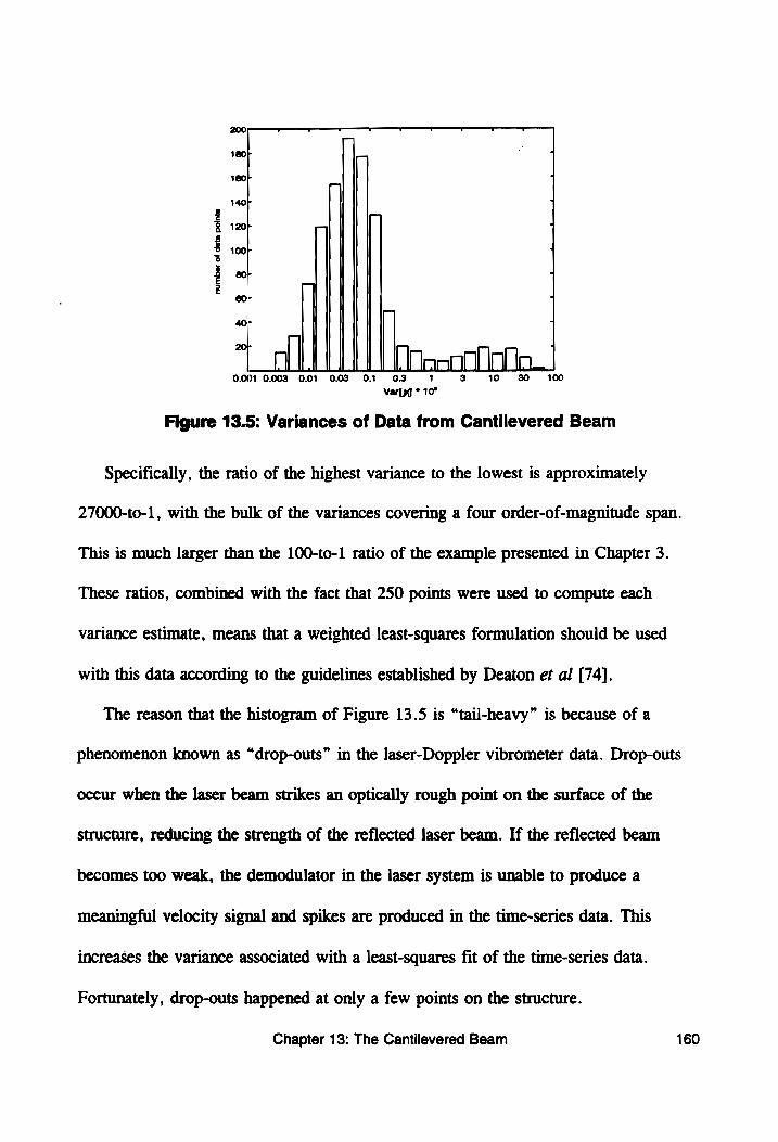
180P _ : ]
160°r
140r
1207 a
number
of da
ta points
wb
8 8
8 8
]
dl breecetict | 0.001 0.003 0.01 0.03 0.1 03 1 100
Var[yJ * 10°
Figure 13.5: Variances of Data from Cantilevered Beam
Specifically, the ratio of the highest variance to the lowest is approximately
27000-to-1, with the bulk of the variances covering a four order-of-magnitude span.
This is much larger than the 100-to-1 ratio of the example presented in Chapter 3.
These ratios, combined with the fact that 250 points were used to compute each
variance estimate, means that a weighted least-squares formulation should be used
with this data according to the guidelines established by Deaton et al [74).
The reason that the histogram of Figure 13.5 is “tail-heavy” is because of a
phenomenon known as “drop-outs” in the laser-Doppler vibrometer data. Drop-outs
occur when the laser beam strikes an optically rough point on the surface of the
structure, reducing the strength of the reflected laser beam. If the reflected beam
becomes too weak, the demodulator in the laser system is unable to produce a
meaningful velocity signal and spikes are produced in the time-series data. This
increases the variance associated with a least-squares fit of the time-series data.
Fortunately, drop-outs happened at only a few points on the structure.
Chapter 13: The Cantilevered Beam 160
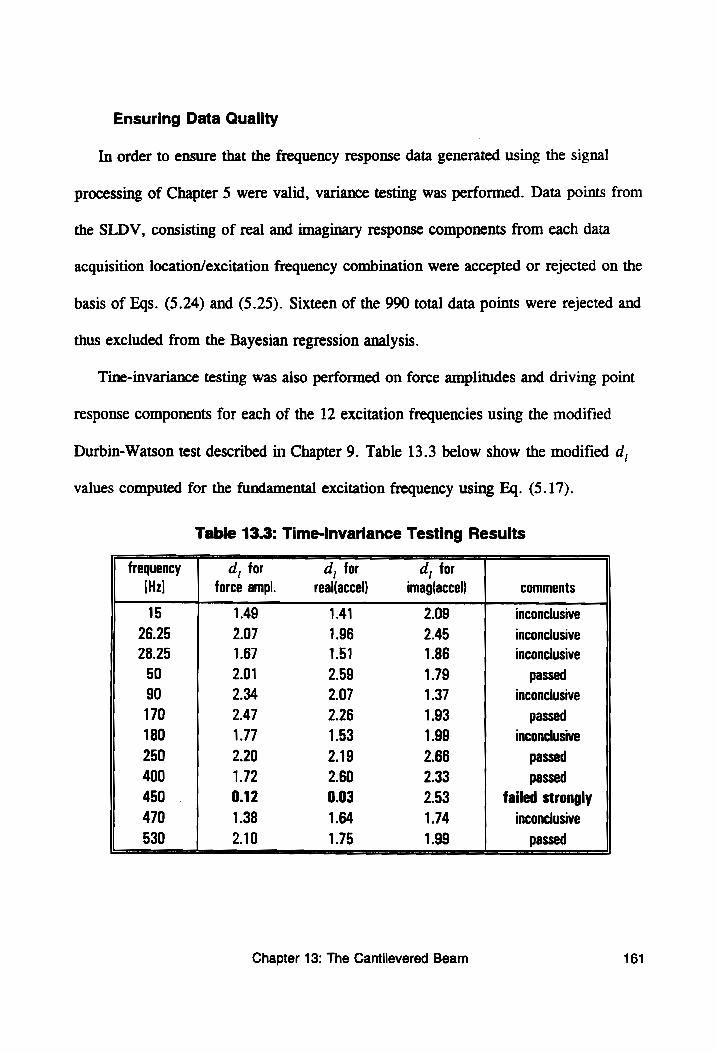
Ensuring Data Quality
In order to ensure that the frequency response data generated using the signal
processing of Chapter 5 were valid, variance testing was performed. Data points from
the SLDV, consisting of real and imaginary response components from each data
acquisition location/excitation frequency combination were accepted or rejected on the
basis of Eqs. (5.24) and (5.25). Sixteen of the 990 total data points were rejected and
thus excluded from the Bayesian regression analysis.
Tine-invariance testing was also performed on force amplitudes and driving point
response components for each of the 12 excitation frequencies using the modified
Durbin-Watson test described in Chapter 9. Table 13.3 below show the modified d,
values computed for the fundamental excitation frequency using Eq. (5.17).
Table 13.3: Time-invariance Testing Results
Chapter 13: The Cantilevered Beam
frequency d, for d, for d, for {Hz] force amopl. real(accel) imag(accel) comments
15 1.49 1.41 2.09 inconclusive
26.25 2.07 1.96 2.45 inconclusive
28.25 1.67 1.51 1.86 inconclusive
50 2.01 2.59 1.79 passed
90 2.34 2.07 1.37 inconclusive
170 2.47 2.26 1.93 passed
180 1.77 1.53 1.99 inconclusive
250 2.20 2.19 2.66 passed
400 1.72 2.60 2.33 passed
450 0.12 0.03 2.53 failed strongly
470 1.38 1.64 1.74 inconclusive
161
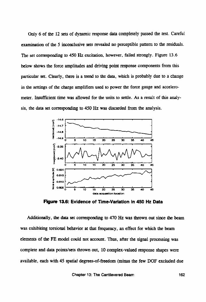
Only 6 of the 12 sets of dynamic response data completely passed the test. Careful
examination of the 5 inconclusive sets revealed no perceptible pattern to the residuals.
The set corresponding to 450 Hz excitation, however, failed strongly. Figure 13.6
below shows the force amplitudes and driving point response components from this
particular set. Clearly, there is a trend to the data, which is probably due to a change
in the settings of the charge amplifiers used to power the force gauge and accelero-
meter. Insufficient time was allowed for the units to settle. As a result of this analy-
sis, the data set corresponding to 450 Hz was discarded from the analysis.
-14.6 - ¥ r v v v ¥ Oe
-14.7 fF 4
-14.8 fF .
real
(acc
el)
(m/s
’]
force
amplitude
(N]_
imag(accel)
[m/s"]
0.605 ani. li eel A. ell. A malls a |
° 5 10 15 20 25 30 35 40 45
data acquisition location
Figure 13.6: Evidence of Time-Variation in 450 Hz Data
Additionally, the data set corresponding to 470 Hz was thrown out since the beam
was exhibiting torsional behavior at that frequency, an effect for which the beam
elements of the FE model could not account. Thus, after the signal processing was
complete and data points/sets thrown out, 10 complex-valued response shapes were
available, each with 45 spatial degrees-of-freedom (minus the few DOF excluded due
Chapter 13: The Cantilevered Beam 162
to variance considerations). The task of model updating effectively became that of
simultaneously fitting the 10 response shapes.
Data acquired from the accelerometer was also included in the model update
process. Instead of using multiple accelerometer-based ¢ vectors, an average response
vector was computed for each excitation frequency using Eq. (5.27), where accelero-
meter-based ¢ vectors were used instead of @ vectors). A measurement of the weight
of the beam, 1158.5+0.3 g, was also included.
13.2 MODEL UPDATING RESULTS
The procedure that was used to estimate parameters for the Sandia test frame was
used again with the cantilevered beam. Initially, only a subset of the frequency
response data was used with a subset of the parameters; in this case, it was the first
five excitation frequencies with parameters k,, k,, E, and p. More frequencies were
added until all 10 shapes had been fitted, and then all 10 parameters were included.
The SSE term of Eq. (3.17) was reduced from 4.57 x 10° to 5.20 x 10° (a factor
of 880).
Total computing time required was on the order of 3 hours. A small convergence
study was performed by plugging different numbers (up to five standard deviations
away from the priors for all parameters except clamp stiffnesses) in at the beginning
of the process. This was performed 10 times, and the results converged to the same
result all 10 times, although the number of iterations required for convergence
differed in each case.
Chapter 13: The Cantilevered Beam 163
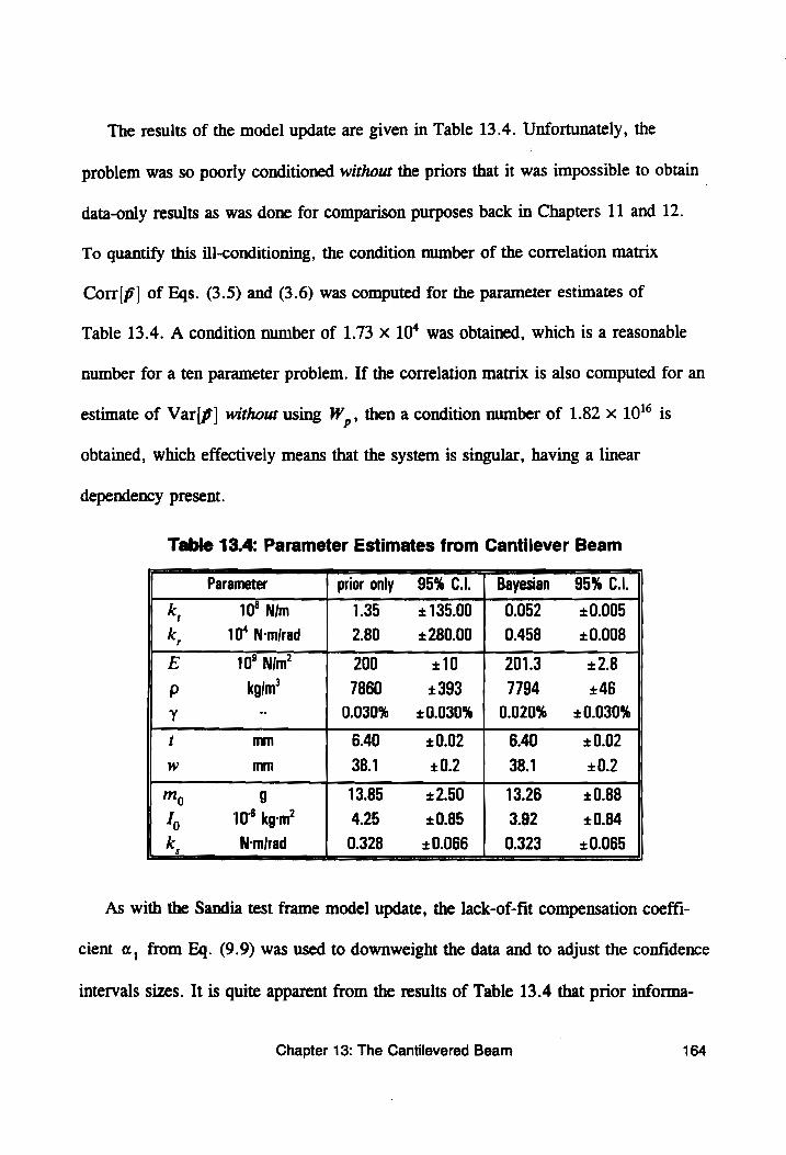
The results of the model update are given in Table 13.4. Unfortunately, the
problem was so poorly conditioned without the priors that it was impossible to obtain |
data-only results as was done for comparison purposes back in Chapters 11 and 12.
To quantify this ill-conditioning, the condition number of the correlation matrix
Corr[p] of Eqs. (3.5) and (3.6) was computed for the parameter estimates of
Table 13.4. A condition number of 1.73 x 10* was obtained, which is a reasonable
number for a ten parameter problem. If the correlation matrix is also computed for an
estimate of Var[f] without using W, , then a condition number of 1.82 x 10'° is
obtained, which effectively means that the system is singular, having a linear
dependency present.
Table 13.4: Parameter Estimates from Cantilever Beam
Parameter prior only 95% Cul. Bayesian 95%
k, 10° Nim 1.35 + 135.00 0.052 +0.005
k. 10° N-mirad 2.80 +280.00 | 0.458 +0.008
E 10° Nim? 200 +10 201.3 +2.8 p kgim’ 7860 +393 7794 +46 Y -- 0.030% +0.030% | 0.020% +0.030%
t mm 6.40 +0.02 6.40 +0.02
w mm 38.1 +0.2 38.1 +0.2
mM, 9 13.85 +2.50 13.26 +0.88
I, 10° kg-m? 4.25 +0.85 3.92 +0.84
k, N-mirad 0.328 +0.066 0.323 +0.065
As with the Sandia test frame model update, the lack-of-fit compensation coeffi-
cient «, from Eq. (9.9) was used to downweight the data and to adjust the confidence
intervals sizes. It is quite apparent from the results of Table 13.4 that prior informa-
Chapter 13: The Cantilevered Beam 164
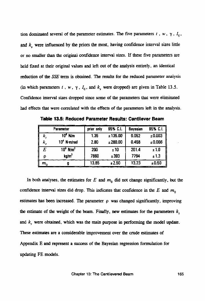
tion dominated several of the parameter estimates. The five parameters t, w, y, J,,
and k, were influenced by the priors the most, having confidence interval sizes little
or no smaller than the original confidence interval sizes. If these five parameters are
held fixed at their original values and left out of the analysis entirely, an identical
reduction of the SSE term is obtained. The results for the reduced parameter analysis
(in which parameters tf, w, y, J,, and k, were dropped) are given in Table 13.5.
Confidence interval sizes dropped since some of the parameters that were eliminated
had effects that were correlated with the effects of the parameters left in the analysis.
Table 13.5: Reduced Parameter Results: Cantilever Beam
Parameter prior only 95% C.l. | Bayesian 95% C.l.
k, 10° Nim 1.35 +13500 [ 0052 +0.003 k. 10* N-mirad 2.80 +280.00 | 0.458 +0.006
E 10° Nim? 200 +10 201.4 +1.0 p kgim’ 7860 +393 7794 +1.3
mM, g 13.85 +2.50 13.23 +0.50
In both analyses, the estimates for E and m, did not change significantly, but the
confidence interval sizes did drop. This indicates that confidence in the E and m,
estimates has been increased. The parameter p was changed significantly, improving
the estimate of the weight of the beam. Finally, new estimates for the parameters k,
and k, were obtained, which was the main purpose in performing the model update.
These estimates are a considerable improvement over the crude estimates of
Appendix E and represent a success of the Bayesian regression formulation for
updating FE models.
Chapter 13: The Cantilevered Beam 165
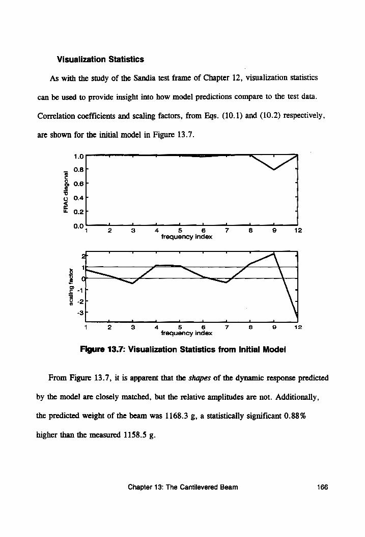
Visualization Statistics
As with the study of the Sandia test frame of Chapter 12, visualization statistics
can be used to provide insight into how model predictions compare to the test data.
Correlation coefficients and scaling factors, from Eqs. (10.1) and (10.2) respectively,
are shown for the initial model in Figure 13.7.
1.0 t 7 v eal ae NS
_ O.8F " o
5 coal J @ 0.6 & 3 © 0.4F 2
e 0.2 b> 4
0.0, 2 3 4 5 6 7 8 9 12 frequency index
2 Ss a om me a\
. 1 —_pf
& i a
> 5 4 £ -1
5 -2P 3 r
1 2 3 4 5 6 7 8 9 12 frequency index
Figure 13.7: Visualization Statistics from Initial Model
From Figure 13.7, it is apparent that the shapes of the dynamic response predicted
by the model are closely matched, but the relative amplitudes are not. Additionally,
the predicted weight of the beam was 1168.3 g, a statistically significant 0.88%
higher than the measured 1158.5 g.
Chapter 13: The Cantilevered Beam 166
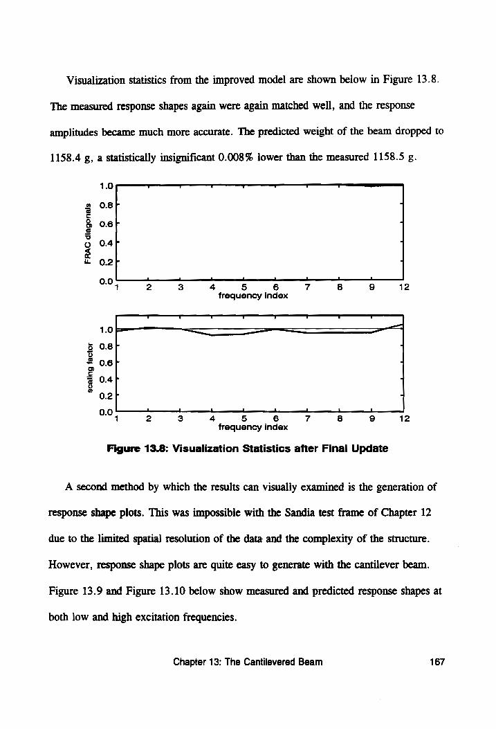
Visualization statistics from the improved model are shown below in Figure 13.8.
The measured response shapes again were again matched well, and the response
amplitudes became much more accurate. The predicted weight of the beam dropped to
1158.4 g, a Statistically insignificant 0.008% lower than the measured 1158.5 g.
1.0 vw v e ve v a Lo
» O8F J © c & O6F : ®
TG
g 0.4 fr 4
k O.2F "
0.0 , 2 ogo 4 45S 6 7 8 9 12 frequency index
1.0 LL ———————— —
5 08 4
o = 06 4 >
= 0.4 . 8 °
0.2
0.0, 2 3 4 5 6 7 8 9 12
frequency index
Figure 13.8: Visualization Statistics after Final Update
A second method by which the results can visually examined is the generation of
response shape plots. This was impossible with the Sandia test frame of Chapter 12
due to the limited spatial resolution of the data and the complexity of the structure.
However, response shape plots are quite easy to generate with the cantilever beam.
Figure 13.9 and Figure 13.10 below show measured and predicted response shapes at
both low and high excitation frequencies.
Chapter 13: The Cantilevered Beam 167
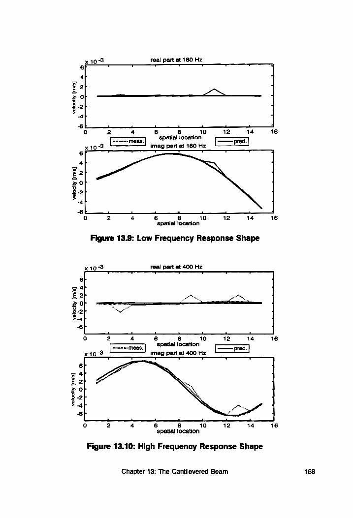
x 10 3 real part at 180 Hz
6 T T . ' 4
4r .
@ 2 a «
E > of = aN |
8a . >
~4P , -6 L a | a | fl ok __ fo Ss i *
0 2 4 6 8 _ 10 12 14 16 spatial location pred.
x10°3 imag part at 180 Hz 6 7 me we e v ' t al
4 a
z ol E 2 OF 1 8 -2 P
*
$ ~4F “
6 s ell nll ell oll ell dl
0 2 4 6 8 10 12 14 16 spatial location
Figure 13.9: Low Frequency Response Shape
x10°3 real part at 400 Hz
6r 4
ze 47 1 £ 2 r wea ee, 1
2 or PE FE el teeemees a 8 2 5 tn J
f4 4 P
-6F 4
oO 2 4 6 8 10 12 14 16
[== reas] Seana coaton =n x 10°73 imag part at 400 Hz
6 a
w 47 — 2r ,
2 Or 1 8 -2F 1 ® > -~4 al a
& P
4
° w al
6 8 10 12 14 16 spatial location
Figure 13.10: High Frequency Response Shape
Chapter 13: The Cantilevered Beam 168
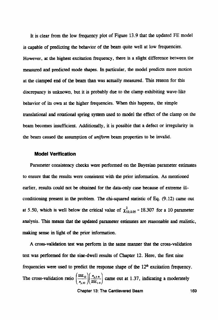
It is clear from the low frequency plot of Figure 13.9 that the updated FE model
is capable of predicting the behavior of the beam quite well at low frequencies.
However, at the highest excitation frequency, there is a slight difference between the
measured and predicted mode shapes. In particular, the model predicts more motion
at the clamped end of the beam than was actually measured. This reason for this
discrepancy is unknown, but it is probably due to the clamp exhibiting wave-like
behavior of its own at the higher frequencies. When this happens, the simple
translational and rotational spring system used to model the effect of the clamp on the
beam becomes insufficient. Additionally, it is possible that a defect or irregularity in
the beam caused the assumption of uniform beam properties to be invalid.
Model Verification
Parameter consistency checks were performed on the Bayesian parameter estimates
to ensure that the results were consistent with the prior information. As mentioned
earlier, results could not be obtained for the data-only case because of extreme ill-
conditioning present in the problem. The chi-squared statistic of Eq. (9.12) came out
at 5.50, which is well below the critical value of X40,0.08 = 18.307 for a 10 parameter
analysis. This means that the updated parameter estimates are reasonable and realistic,
making sense in light of the prior information.
A cross-validation test was perform in the same manner that the cross-validation
test was performed for the sine-dwell results of Chapter 12. Here, the first nine
frequencies were used to predict the response shape of the 12" excitation frequency.
The cross-validation ratio (2) [ came out at 1.37, indicating a moderately ny 2 SSE 1-9
Chapter 13: The Cantilevered Beam 169
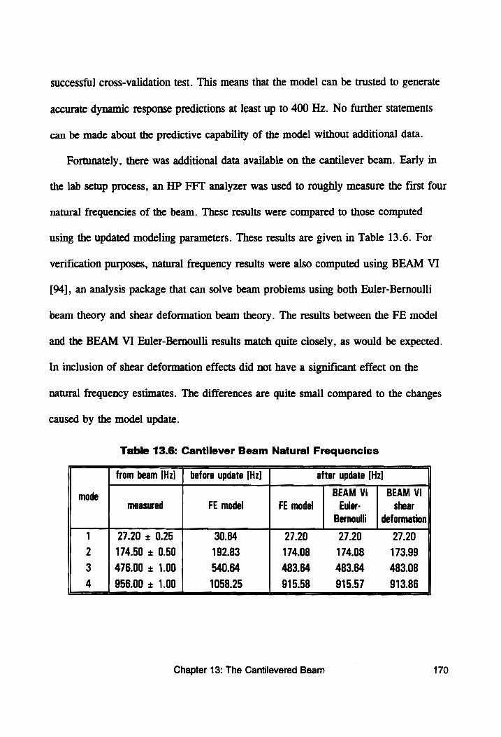
successful cross-validation test. This means that the model can be trusted to generate
accurate dynamic response predictions at least up to 400 Hz. No further statements
can be made about the predictive capability of the model without additional data.
Fortunately, there was additional data available on the cantilever beam. Early in
the lab setup process, an HP FFT analyzer was used to roughly measure the first four
natural frequencies of the beam. These results were compared to those computed
using the updated modeling parameters. These results are given in Table 13.6. For
verification purposes, natural frequency results were also computed using BEAM VI
[94], an analysis package that can solve beam problems using both Euler-Bernoulli
beam theory and shear deformation beam theory. The results between the FE model
and the BEAM VI Euler-Bernoulli results match quite closely, as would be expected.
In inclusion of shear deformation effects did not have a significant effect on the
natural frequency estimates. The differences are quite small compared to the changes
caused by the model update.
Table 13.6: Cantilever Beam Natural Frequencies
Chapter 13: The Cantilevered Beam
from beam [Hz] | before update [Hz] | after update (Hz] |
mode BEAM Vi | BEAM Vi
measured FE model FE model Euler- shear
Bernoulli | deformation
1 27.20 + 0.25 30.64 27.20 27.20 27.20
2 174.50 + 0.50 192.83 174.08 174.08 173.99
3 476.00 + 1.00 540.64 483.64 483.64 483.08
4 956.00 + 1.00 1058.25 915.58 915.57 913.86 170
From Table 13.6, it is apparent that the updated model predicted the natural
frequencies of the first two modes much more accurately that the original model did.
However, the updated model does not predict the natural frequencies of the third and
fourth modes very accurately. Curiously, it overpredicted the third natural frequency
and underpredicted the fourth natural frequency. As with the response shape plots, the
reason for the inaccurate frequency predictions is not known, but they are probably
due to wave-like behavior in the clamp or irregularities in the beam. It should be
noted that the response shape plot of Figure 13.10 comes from an excitation
frequency that is above the third natural frequency, which is a high enough frequency
for the model to begin breaking down. The resulting difference between test and
analysis can be seen in this plot.
13.3 CONCLUDING REMARKS ON TEST BEAM
The use of the Bayesian regression model update formulation appeared to work
quite well for the cantilevered beam. Accurate estimates for unknown parameters k,
and k, were obtained, which was the primary purpose of the exercise. Additionally,
estimates for E, p, and m, were either improved or verified. The data provided
little information on the parameters y, ¢ , w, J,, and k,, but the use of prior
information prevented the Bayesian regression formulation from generating meaning-
less estimates for these parameters. Indeed, leaving these parameters out of the
analysis did not change the results, except to drop confidence interval sizes somewhat.
Time-invariance tests were used to determine whether or not the data were
suitable for use in the model update. Parameter consistency checks were used to
Chapter 13: The Cantilevered Beam 171
ensure that the parameter estimates obtained were reasonable and realistic. The cross-
validation test was used to confirm that the model did more than just predict the
specific data set used in the model update.
The net conclusion of these tests was that the model could be used to predict the
behavior of the cantilever beam up to 400 Hz. However, a study of the first four
natural frequencies of the beam revealed that the model broke down at higher
frequencies. The reason for this breakdown is unknown, but it is probably due to
wave-like behavior in the clamp or irregularities in the beam. Nevertheless, for low
frequencies, the predictive capability of the beam model was substantially improved.
Chapter 13: The Cantilevered Beam 172

PART V:
Conclusions and Recommendations
173
Chapter 14: Conclusions and Recommendations
14.1 CONCLUSIONS
Comments on Model Updating
This dissertation presented a Bayesian regression formulation for updating the
modeling parameters used to build a finite element (FE) model. The model update
procedure yields a model with substantially improved predictive capability along with
Statistically-qualified estimates of the updated modeling parameters.
With this information available, the analyst can determine whether or not the
updated model is sufficiently correct for the modeling task at hand. If it is sufficiently
correct, the analyst will have an improved basis on which to perform structural
modification or optimization. If it is not sufficiently correct, the analyst knows that
more modeling work or experimental work will be required to obtain a sufficiently
correct model.
Summary of Dissertation
In Part I of this dissertation, the Bayesian regression formulation for model
updating was introduced and placed in context with other model update formulations.
In Part II, the complete Bayesian regression formulation was presented, covering the
basic Bayesian regression theory, the signal processing techniques used to generate
statistically-qualified frequency response data (both sine-dwell and FRF), and the
Chapter 14: Conclusions and Recommendations 174
modeling techniques used to make finite element predictions of the data. Part III
presented the numerical and statistical issues that must be addressed to develop a
robust computer implementation of the model update process and to ensure that a
valid model update is obtained.
Part IV of the dissertation provided three case studies involving implementations
of the Bayesian regression formulation. The first study, which involved the successful
update of a beam model using simulated data, was performed to verify confidence
interval estimation procedures. In the second study, joint stiffness and beam cross-
section parameters in a finite element model of a steel frame were updated to improve
its predictive capability. Good results were obtained with both sine-dwell and FRF
data. In the third study, stiffness parameters representing a clamp holding a cantilever
steel beam were updated, as were other modeling parameters used to build the beam
model. Significant improvements were made to several of the parameters, while the
Bayesian regression formulation prevented the regression procedure from generating
meaningless estimates for the non-significant parameters.
Contributions to the Field
Advancements made in this work include: (1) the formulation of a true Bayesian
statistics analysis; (2) the use of experimentally-derived statistical weights; (3) the
development of lack-of-fit compensation procedures; (4) the matrix-decomposition
based reformulation of the Bayesian regression problem to improve numeric condi-
tioning; and (5) the development of time-invariance tests and cross-validation tests.
Chapter 14: Conclusions and Recommendations 175
Final Comments
To summarize, most of the goals of this research were met. The primary goal of
updating finite element models with frequency response was accomplished success-
fully. Key to this goal were the sine-dwell and FRF statistics of Chapters 5 and 6, and
with the Bayesian regression reformulation of Chapter 8. Without these parts of the
research, none of the results of Chapters 11 through 13 would have been possible.
The visualization and model verification statistics also worked well, although the
performance of the lack-of-fit compensation coefficients of Chapter 9 was not entirely
satisfactory.
It was discovered in the course of this research that parameter selection is
extremely important to the task of model updating. Poor parameter selection can cause
numerous difficulties when estimating parameters. It is also helpful to having accurate
prior information.
14.2 RECOMMENDATIONS FOR FUTURE WORK
Expand Sine-Dwell Statistics
The sine-dwell statistics presented here were formulated for unscaled real and
imaginary components of the single frequency response. A different formulation
would use an amplitude/phase angle representation instead of the complex number
representation. This formulation would work better in the resonance situations where
the complex number formulation fails (see Chapter 5). However, dealing with phase
angle wraparound becomes an issue, and the task of computing response sensitivities
become more difficult. Scaled sine-dwell statistics (in which the response is divided
Chapter 14: Conclusions and Recommendations 176
by the force amplitude) would also be worth investigating, as would multi-input multi-
output (MIMO) formulations. These formulations would enable the analyst to use data
many different form in additional to providing for more accurate data acquisition.
Expand FRF Statistics
A second area of investigation concerns statistics of the FRF. Bendat [72] and
Yoshimura and Nagamatsu [67] addressed this issue in considerable detail, but the
effects of leakage and data windowing techniques on variance estimates were not
addressed. These considerations would allow proper weighting matrices to be used in
the Bayesian regression formulation, instead of the approximate weighting matrices
used in the FRF study of Chapter 12.
Lack-of-Fit Compensation
Another potential area of investigation would be techniques used to compensate
for lack-of-fit. Two data rescaling coefficients were presented in this dissertation (see
Chapter 9). Coefficient «, clearly worked better than «, in the case studies
presented in Chapters 12 and 13, but coefficient «, has more “philosophical appeal.”
Resolving this difficulty might require alternative approaches to adjusting the data
weighting matrix or even alternative approaches to computing confidence intervals.
Incorporate Robust Regression Techniques
The use of robust regression techniques [71] to fit time-series data coming from a
sine-dwell test would also be worth investigating. The ordinary least-squares fit
described in Chapter 5 works quite well for data having errors that are approximately
Chapter 14: Conclusions and Recommendations 177
Gaussian. However, the scanning laser Doppler vibrometer (SLDV) can sometimes
generate dropouts, which are brief duration spikes in the data having variances levels
much greater than that found in the rest of the data. The use of robust regression
techniques would increase the quality of the fit and reduce parameter variance esti-
mates, allowing the data to contribute more to the Bayesian regression formulation.
Incorporate Spatial Error
Before a scanning LDV can be used to acquire test data from a structure, it must
be registered in space relative to the structure. Specifically, this means determining
the position and orientation (three translations and three rotations) of the SLDV
assembly in structural coordinates. Earlier works by Zeng et al [95] and Montgomery
and West [96] used a direct solution technique in which estimated ranges play in key
role in solving this problem. Later works by Zeng [97] and Lindholm [98] use non-
linear regression to estimate six laser locations parameters (three translations and
three rotations). Because there are errors in the data used to estimate the position and
orientation of the SLDV, estimates of where the laser beam measures velocities and
the direction at which is measures can also have errors. A more complete model
update algorithm would account for these potential sources of error.
Use Non-Gaussian Priors
In this dissertation, all prior information was assumed to come from Gaussian
distributions. However, for parameters such as damping coefficients, more realistic
Chapter 14: Conclusions and Recommendations 178
distributions such as the chi-squared or Weibull [77] might be useful, as they restrict
allowable parameter values to positive numbers. |
The primary disadvantage of using non-Gaussian priors is increased complexity in
the Bayesian regression implementation. The SSE term of Eq. (3.17) would gain
terms significantly more complicated than the squared/weighted residuals, and the SSE
minimization would require a constrained optimization algorithm substantially more
sophisticated than the simple parameter iteration of Eq. (3.18).
Final Comments
Of the recommendations for future work, incorporating spatial error is probably
the most important. Spatial error is the most significant source of uncertainty not
addressed in the research presented in this dissertation. The use of non-Gaussian
priors and improved lack-of-fit compensation would also be a substantial improve-
ments. The other recommendations are minor modifications to the Bayesian regression
formulation that would enable the analyst to use test data more efficiently or to collect
it more quickly.
Chapter 14: Conclusions and Recommendations 179
[1]
[2]
[3]
[4]
(5)
[6]
[7]
[8]
[9]
[10]
References
Imregun, M. and Visser, W. J., “A Review of Model Updating Techniques,” Shock
and Vibration Digest, Vol. 23, No. 1, January 1991, pp. 9-20.
Allemang, R. J. and Ewins, D. J., “A Correlation Coefficient for Modal Vector
Analysis,” Proceedings of the Ist International Modal Analysis Conference, IMAC-I,
SEM, 1983, pp. 110-116.
Lieven, N. A. J and Ewins, D. J., “Spatial Correlation Coefficient of Mode Shapes,
the Coordinate Modal Assurance Criterion (COMAC),” Proceedings of the 6th Inter-
national Modal Analysis Conference, IMAC-VI1, SEM, Kissimmee, FL, February 1988,
pp. 690-695.
Baker, M., “Review of Test/Analysis Correlation Methods and Criteria for Validation of Finite Element Models for Dynamic Analysis,” Proceedings of the 10th International
Modal Analysis Conference, IMAC-X, SEM, San Diego, CA, February 1992, pp. 985-
991.
Mottershead, J. E. and Friswell, M. I., “Model Updating in Structural Dynamics: A Survey,” Journal of Sound and Vibration, Vol. 167, No. 2, 1993, pp. 347-375.
Link, M., “Identification and Correction of Errors in Analytical Models using Test
Data,” Proceedings of the &th International Modal Analysis Conference, IMAC-VIII,
SEM, Kissimmee, FL, February 1990, pp. 570-578.
Dascotte, E., “Practical Applications of Finite Element Model Tuning Using
Experimental Modal Data,” Proceedings of the 8th International Modal Analysis
Conference, IMAC-VIII, SEM, Kissimmee, FL, February 1990, pp. 1032-1037.
Natke, H. G., “Updating Computational Models in the Frequency Domain based on Measured Data: a Survey,” Probabilistic Engineering Mechanics, Vol. 3, No. 1, March
1988, pp. 28-35.
Zhang, L., “A Consistent Derivation and Assessment of Different Model Updating Procedures,” Proceedings of the 14th International Modal Analysis Conference, IMAC-XIV, SEM, Detroit, MI, February 1996, pp. 769-775.
Guyan, R. J., “Reduction of Stiffness and Mass Matrices,” AAA Journal, Vol. 3,
No. 2, February 1965.
References 180
[11]
[12]
[13]
[14]
[15]
[16]
[17]
[18]
[19]
[20]
[21]
[22]
Kammer, D. C., “Test-Analysis Model Development Using an Exact Modal
Reduction,” International Journal of Analytical and Experimental Modal Analysis,
Society for Experimental Mechanics, Vol. 2, No. 4, Bethel, CT, October 1987, pp.
174-179.
Avitabile, P. and Foster, T. J., “Evaluation of Degree of Freedom Based Vector
Correlation Methods,” Proceedings of the 14th International Modal Analysis
Conference, IMAC-XIV, SEM, Detroit, MI, February 1996, pp. 1048-1056.
O’Callahan, J., “A Procedure for an Improved Reduced System (IRS) Model,”
Proceedings of the 7th International Modal Analysis Conference, IMAC-VII, SEM, Las
Vegas, NV, February 1989, pp. 17-21.
Gordis, J. H., “An Analysis of the Improved Reduced System Modal Reduction Procedure,” Proceedings of the 10th International Modal Analysis Conference, SEM,
IMAC-X, San Diego, CA, February 1992, pp. 471-487.
Freed, A. M. and C. C. Flanigan, “A Comparison of Test-Analysis Reduction Methods,” Proceedings of the 8th International Modal Analysis Conference, IMAC-
Vil, SEM, Kissimmee, FL, 1990, pp. 1344-1351.
Hunt, D. L., “Application of an Enhanced Coordinate Modal Assurance Criterion,”
Proceedings of the 10th International Modal Analysis Conference, IMAC-X, SEM, San Diego, CA, February 1992, pp. 66-71.
Lieven, M. A. J., and D. J. Ewins, “Expansion of Modal Data for Correlation,” Proceedings of the 8th International Modal Analysis Conference, SEM, IMAC-VIII, Kissimmee, FL, February 1990, pp. 605-609.
O’Callahan, J., Avitable, P., and Rimer, R., “System Equivalent Reduction Expansion
Process (SEREP),” Proceedings of the 7th International Modal Analysis Conference, IMAC-VII, SEM, Las Vegas, NV, February 1989, pp. 29-37.
O’Callahan, J. and Li, P., “SEREP Expansion,” Proceedings of the 14th International Modal Analysis Conference, IMAC-XIV, SEM, Detroit, MI, February 1996, pp. 1258-
1264.
Baruch, M. and Bar Itzhack, Y., “Optimal Weighted Orthogonalization of Measured Modes,” AIAA Journal, Vol. 16, No. 4, April 1978, pp. 346-351.
Kabe, A. M, “Stiffness Matrix Adjustment Using Mode Data,” AIAA Journal, Vol. 23, No. 9, September 1985, pp. 1431-1436.
O’Callahan, J., “Determination of Analytical Model Differences Using Modal Updating,” Proceedings of the 8th International Modal Analysis Conference, IMAC-VIII, SEM, Kissimmee, FL, February 1990, pp. 999-1003.
References 181
[23] Aiad, A., Level, P., and Ravalard, Y., “A Global Updating Procedure to Improve Finite Element Models,” Proceedings of the 10th International Modal Analysis Conference, IMAC-X, SEM, San Diego, CA, February 1992, pp. 1051-1056.
[24] Conti, P. and Bretl, J., “Mount Stiffness and Inertia Properties for Modal Test Data,” Modal Testing and Analysis, Proceedings of the 11th Biennal Conference on Mechanical
Noise and Vibration, ASME, Vol. 3, December 1987, pp. 11-16.
[25] Ahmadian, H., Ismail, F., and Gladwell, G. M. L., “Acceptable Element Matrices for
Finite Element Model Updating,” ed. Bui, H. D., et al, Inverse Problems in
Engineering Mechanics (reprinted from Proceedings of the 2nd International Symposium on Inverse Problems, ISIP ’°94, Paris, November 1994), A. A. Balkema, Rotterdam,
1994, pp. 209-213.
[26] Niedmal, M. and Luber, W., “Updating a Finite-Element Model by Means of Normal Mode Parameters,” Proceedings of the 8th International Modal Analysis Conference, IMAC-VIII, SEM, Kissimmee, FL, February 1990, pp. 586-592.
[27] Jung, H. and Ewins, D.J., “Error Sensitivity of the Inverse Eigensensitivity Method for Model Updating,” Proceedings of the 10th International Modal Analysis Conference, IMAC-X, SEM, San Diego, CA, February 1992, pp. 992-998.
[28] Ladeveze, P., Nedjar, D., and Reynier, M., “Updating of Finite Element Models Using Vibrations Tests,” AIAA Journal, Vol 32., No. 7, July 1994, pp. 1485-1491.
[29] Nobari, A. S. and Ewins, D. J., “On the Effectiveness of Using Only Eigenvalues of
Structural Model Updating Problems,” Shock and Vibration, Vol. 1, No. 4, 1994, pp.
339-348.
[30] Lindholm, B. E. and West, R. L., “Determination of Suspension Effects by Direct
Experiments and Comparisons to an Analytical Model,” Proceedings of the 12th
International Modal Analysis Conference, IMAC-XI1, Honolulu, February 1994, pp. 262-268.
[31] Farhat, C. and Hemez, F. M., “Updating Finite Element Dynamic Models Using an
Element-by-Element Sensitivity Methodology,” AZAA Journal, Vol. 31, No. 9, Septem- ber 1993, pp. 1702-1711.
[32] Hemez, F. M., “Closing the Gap Between Modal Parameter Based and Frequency
Response Function Based Updating Methods,” Proceedings of the 13th International Modal Analysis Conference, IMAC-XIII, SEM, Nashville, TN, February 1995, pp. 171-178.
[33] Hemez, F. M., “Advanced Tools for Updating Damped Finite Element Models Using Static, Modal, and Flexibility Data,” Proceedings of the 14th International Modal Analysis Conference, IMAC-XIV, SEM, Detroit, MI, February 1996, pp. 511-517.
References 182
[34]
[35]
[36]
[37]
[38]
[39]
[40]
[41]
[42]
[43]
Hasselman, T. K., “A Perspective on Dynamic Model Verification,” Modal Testing and Model Refinement, ASME, Applied Mechanics Division, Vol. 59, November 1983, pp. 101-118.
Beliveau, J. G., “System Identification of Civil Engineering Structures,” Canadian Journal of Civil Engineering, Vol. 14, No. 1, January 1987, pp. 7-18.
Link, M., “Requirements for the Structure of Analytical Models Used for Parameter
Identification,” ed. Tanaka, H. and Bui, H. D., Inverse Problems in Engineering Mechanics (from Proceedings of IUTAM Symposium, Tokyo, 1992), Springer-Verlag, New York, 1992, pp. 133-146.
Dasacotte, E., Strobbe, J., and Hua, H., “Sensitivity-based Model Updating Using
Multiple Types of Simultaneous State Variables,” Proceedings of the 13th International
Modal Analysis Conference, IMAC-XIII, SEM, Nashville, TN, February 1995, pp. 1035-1040.
Hasselman, T. K. and Chrostowski, J. D., “A Recent Case Study in System
Identification,” Proceedings of the 32nd AIAA/ASME/ASCE/AHS/ASC Structures, Structural Dynamics, and Materials Conference, SDM-32, AIAA, Baltimore, MD,
April 1991, pp. 2154-2168.
Engineering Mechanics Associates, “SSID -- A Computer Code for Structural System Identification,” Technical Report No. TR-91-1134-1, Sandia National Laboratories, Albuquerque, NM, March 1991.
Martinez, D. R., Red-Horse, J. R., and Allen, J. J., “System Identification Methods
for Dynamic Structural Models of Electronic Packages,” Proceedings of the 32nd AIAA/ASME/ASCE/AHS/ASC Structures, Structural Dynamics, and Materials Conference, SDM-32, AIAA, Baltimore, MD, April 1991, pp. 2336-2346.
Nefske, D. J. and Sung, S. H., “Correlation of a Coarse-Mesh Finite Element Model using Structural System Identification and a Frequency Response Assurance Criterion,” Proceedings of the 14th International Modal Analysis Conference, IMAC-XIV, SEM, Detroit, MI, February 1996, pp. 597-602.
Antonacci, E. and Vestroni, F., “Updating of Finite Element Models through Nonlinear Parametric Estimation,” ed. Bui, H. D., et al, Inverse Problems in Engineering Mechanics (reprinted from Proceedings of the 2nd International Symposium on Inverse Problems, ISIP °94, Paris, November 1994), A. A. Balkema, Rotterdam, 1994, pp. 215-222.
Link, M., Rohrmann, R. G., and Pietrzko, S., “Experience with Automated Procedures
for Adjusting the Finite Element Model of a Complex Highway Bridge to Experimental Modal Data,” Proceedings of the 14th International Modal Analysis Conference, IMAC-
XIV, SEM, Detroit, MI, February 1996, pp. 218-223.
References 183
[44]
[45]
[46]
[47]
[48]
[49]
[50]
[51]
[52]
[53]
[54]
[55]
Alvin, K. F., “Finite Element Model Update via Bayesian Estimation and Minimization of Dynamic Force Residuals,” Proceedings of the 14th International Modal Analysis Conference, IMAC-XIV, SEM, Detroit, MI, February 1996, pp. 561-567.
Larrson, P. O. and Sas, P., “Model Updating Based on Forced Vibration Testing Using
Numerically Stable Formulations,” Proceedings of the 10th International Modal Analysis Conference, IMAC-X, SEM, San Diego, CA, February 1992, pp. 966-974.
Fritzen, C. P. and Kiefer, T., “Localization of Correction of Errors in Analytical
Models,” Proceedings of the 10th International Modal Analysis Conference, IMAC-X, SEM, San Diego, February 1992, pp. 1064-1071.
Zimmerman, D. C., Simmermacher, T., and Kaouk, M., “Structural Damage
Detection using Frequency Response Functions,” Proceedings of the 13th International Modal Analysis Conference, IMAC-XIII, SEM, Nashville, TN, February 1995, pp. 179-184.
Berger, H., et al, “Parametric Updating of Finite Element Models Using Experimental
Simulation - A Dynamic Reaction Approach,” Proceedings of the 8th International Modal Analysis Conference, IMAC-VIII, SEM, Kissimmee, FL, February 1990, pp. 180-184.
Yang, M. and Brown, D., “An Improved Procedure for Handling Damping During
Finite Element Modal Updating,” Proceedings of the 14th International Modal Analysis Conference, IMAC-XIV, SEM, Detroit, MI, February 1996, pp. 576-584.
Schulz, M. J. and Thyagarajan, S. K., “Inverse Dynamic Design Technique for Model Correction and Optimization,” AJAA Journal, Vol. 33, No. 8, August 1995, pp. 1486-
1491.
Schulz, M. J., Pai, P. F., and Abdelnaser, A. S., “Frequency Response Function
Assignment Technique for Structural Damage Detection,” Proceedings of the 14th
International Modal Analysis Conference, IMAC-XIV, SEM, Detroit, MI, February
1996, pp. 105-111.
Friswell, M. I. and Penny, J. E. T., “Updating Modal Parameters Directly from Frequency Response Function Data,” Proceedings of the 8th International Modal Analysis Conference, IMAC-VIII, SEM, Kissimmee, FL, February 1990, pp. 843-849.
Conti, P. and Donley, M., “Test-Analysis Correlation Using Frequency Response Functions,” Proceedings of the 10th International Modal Analysis Conference, IMAC-X, SEM, San Diego, CA, February 1992, pp. 724-729.
Imregun, M., “Three Case Studies in Finite Element Model Updating,” Shock and Vibration, Vol. 2, No. 2, 1995, pp. 119-131.
Zhang, Q., et al, “A Complete Procedure for the Adjustment of a Mathematical Modal from Identified Complex Modes,” Proceedings of the 5th International Modal Analysis
References 184
[56]
[57]
[58]
[59]
[60]
[61]
[62]
[63]
[64]
[65]
[66]
Conference, IMAC-V, SEM, London, February 1987, pp. 1183-1190.
Visser, W.J. and Imregun, M., “A Technique to Update Finite Element Models Using Frequency Response Data,” Proceedings of the 9th International Modal Analysis
Conference, IMAC-IX, SEM, February 1991, pp. 462-468.
Imregum, M., Visser, W. J., and Ewins, D. J., “Finite Element Model Updating Using
Frequency Response Function Data — I. Theory and Initial Investigation,” Mechanical
Systems and Signal Processing, Vol. 9, No. 2, March 1995, pp. 187-202.
Imregum, M., Sanliturk, K. Y., and Ewins, D. J., “Finite Element Model Updating Using Frequency Response Function Data — II. Case Study on a Medium-Sized Finite
Element Model,” Mechanical Systems and Signal Processing, Vol. 9, No. 2, March
1995, pp. 203-213.
Cogan, S., et al, “An Improved Frequency Response Residual for Model Correction,” Proceedings of the 14th International Modal Analysis Conference, IMAC-XIV, SEM,
Detroit, MI, February 1996, pp. 568-575.
Reix, C., et al, “Updating the Damping Matrix using Frequency Response Data,” Proceedings of the 14th International Modal Analysis Conference, IMAC-XIV, SEM,
Detroit, MI, February 1996, pp. 585-590.
Mottershead, J. E., and Foster, C. D., “On the Treatment of Il-conditioning in Spatial Parameter Estimation from Measured Vibration Data,” Mechanical Systems and Signal Processing, Vol. 5, No. 2, March 1991, pp. 139-154.
Ibrahim, S. R., “Direct Updating on Non-Conservative Finite Element Models using Measured Input/Output Data,” Proceedings of the 10th International Modal Analysis Conference, IMAC-X, SEM, San Diego, CA, February 1992, pp. 202-210.
Bronowicki, A. J., Likich, M. S., and Kuritz, S. P., “Application of Physical
Parameter Identification to Finite Element Models,” Proceedings of the Ist NASA/DOD
CSI Technology Conference, NASA, Norfolk, VA, November 1986, pp. 187-206.
Koh, C. G. and See, L. M., “Identification and Uncertainty Estimation of Structural Parameters,” Journal of Engineering Mechanics, Vol. 120, No. 6, June 1994, pp.
1219-1237.
Brown, R. G. and Hwang, P. Y. C., Introduction to Random Signals and Applied Kalman Filtering, 2nd Edition, John Wiley & Sons, Inc., New York, NY, 1983.
Mahnken, R. and Stein, E., “Gradient-Based Methods for Parameter Identification of Viscoplastic Materials,” ed. Bui, H. D., et al, Inverse Problems in Engineering
Mechanics (reprinted from Proceedings of the 2nd International Symposium on Inverse
Problems, SIP ’94, Paris, November 1994), A. A. Balkema, Rotterdam, 1994, pp.
137-144.
References 185
[67]
[68]
[69]
[70]
[71]
[72]
[73]
[74]
[75]
[76]
[77]
Yoshimura, T. and Nagamatsu, A., “Estimation of Variance of the Frequency Response
Function and its Application to the Curve Fit,” Japanese Society of Mechanical Engi-
neering International Journal, JSME, Series TI, Vol. 34, No. 2, 1991, pp. 227-232.
Montgomery, D. M. and West, R. L., “Identification of Estimated Error Variance in Time Signal Coefficients of Laser Doppler Vibrometer Data,” Proceedings of the 13th International Modal Analysis Conference, IMAC-XIII, SEM, Nashville, TN, February
1995, pp. 728-734.
Montgomery, D. E., Lindholm, B. E., and West, R. L., “Monte Carlo Verification of
the Multivariate Delta Method Variance Estimation of Harmonic Dynamic Response Coefficients,” Symposium on Optical Methods in Vibration and Noise, 15th ASME Biennial Conference on Mechanical Vibration and Noise, Boston, MA, 1995.
Zeng, X. and Wicks, A. L., “A Comparison of Two Methods for Estimating the Mag-
nitude and Phase Angle of a Harmonic Wave,” Proceedings of the 11th International Modal Analysis Conference, IMAC-XI, SEM, Kissimmee, FL, February 1993, pp. 906- 912.
Lopez Dominguez, J. C., Reconstruction of 3-D Structural Dynamic Response Fields:
an Experimental, Laser-Based Approach with Statistical Emphasis, Department of Mechanical Engineering Ph.D. dissertation, Virginia Polytechnic Instititue and State University, Blacksburg, VA, August 1994.
Bendat, J. S., “Statistical Errors in Measurement of Coherence Functions and
Input/Output Quantities,” Journal of Sound and Vibration, Vol. 59, No. 3, August 1978, pp. 405-421.
Cobb, R. E., Confidence Bands, Measurement Noise, and Multiple Input - Multiple
Output Measurements Using the Three-Channel Frequency Response Function Estimator, Department of Mechanical Engineering Ph.D. dissertation, Virginia Polytechnic Institute and State University, Blacksburg, VA, May 1988.
Deaton, M. L., Reynolds, M. R., and Myers, R. H., “Estimation and Hypothesis
Testing in Regression in the Presence of Nonhomogeneous Error Variances,” Communications in Statistics: Simulation and Computation, Vol. 12, No. 1, March
1983, pp. 45-66.
Williams, J. S., “The Variance of Weighted Regression Estimators,” Journal of the
American Statistical Association, Vol. 62, 1967, pp. 1290-1301.
Jacquez, J. A. and Norusis, M, “Sampling Experiments on the Estimation of Parameters in Heteroscedastic Linear Regression,” Biometrics, Vol. 29, No. 4,
December 1973, pp. 771-779.
Walpole, R. E. and Myers, R. H., Probability and Statistics for Engineers, 4th Edition, Macmillan Publishing Co., New York, 1989.
References 186
[78]
[79]
[80]
[81]
[82]
[83]
[84]
[85]
[86]
[87]
[88]
[89]
[90]
[91]
[92]
Myers, R. H., Classical and Modern Regression with Applications, 2nd Edition, PWS-
Kent Publishing Co., Boston, MA, 1990.
Beck, J. V. and Arnold, K. J., Parameter Estimation in Engineering and Science, John
Wiley & Sons, New York, NY, 1977.
Golub, G. H. and Van Loan, C. F., Matrix Computations, 2nd Edition, Johns Hopkins University Press, Baltimore, MR, 1989.
Bendat, J. S. and Piersol, A. G., Random Data, Analysis and Measurement Procedures,
John Wiley & Sons, New York, NY, 1986.
Ewins, D. J., Model Testing: Theory and Practice, Research Studies Press, Letchworth,
Hertfordshire, England, 1984.
Rubinstein, R. Y., Simulation and the Monte Carlo Method, John Wiley & Sons, New York, NY, 1981.
Przemienicki, J. S., Theory of Matrix Structural Analysis, 2nd Edition, McGraw-Hill
Book Publishing Co., New York, NY, 1985.
Bathe, K., Finite Element Procedures in Engineering Analysis, Prentice-Hall, Inc., Englewood Cliffs, NJ, 1982.
Rocklin, G. T., Crowley, J., and Vold, H., “A Comparison of H,, H, and H,
Frequency Response Functions,” Proceedings of the 3rd International Modal Analysis Conference, IMAC-II, SEM, February 1985, pp. 272-278.
Mitchell, L. D. and Deel, J. C., “An Unbiased Frequency Response Function
Estimator,” Proceedings of the 5th International Modal Analysis Conference, IMAC-V, SEM, London, February 1987, pp. 364-373.
Dongarra, J., et al, LAPACK Users’ Guide -- Release 2.0, Society for Industrial and
Applied Mathematics, Philadelphia, PA, 1995.
Grace, A., MATLAB Optimization Toolbox, version 1.0b, The Mathworks, South
Natick, MA, 1991.
MATLAB 4.2c Users Manual, for UNIX Workstations, The Mathworks, Inc., Natick,
MA, 1994.
Woon, C. E. and Mitchell, L. D., “Variations in Structural Dynamic Characteristics Caused by Changes in Ambient Temperatures: I. Experimental,” Proceedings of the 14th International Modal Analysis Conference, IMAC-XIV, SEM, Detroit, MI,
February 1996, pp. 963-971.
Lindholm, B. E., Reconciliation of a Rayleigh-Ritz Beam Model with Experimental Data, Department of Mechanical Engineering M.S. thesis, Virginia Polytechnic
References 187
[93]
[94]
[95]
[96]
(97]
[98]
Institute and State University, Blacksburg, VA, September 1994.
Budinski, K. G., Engineering Materials: Properties and Selection, Third Edition, Prentice-Hall, Englewood Cliffs, NJ, 1989.
Mitchell, L. D., et al, BEAM VI (software), Department of Mechanical Engineering,
Virginia Polytechnic Institute and State University, Blacksburg, VA, 1992.
Zeng, X., Mitchell, L. D., and Agee, B. L., “A Laser Position Determination
Algorithm for an Automated Mechanical Mobility Measurement System,” Proceedings
of the 11th International Modal Analysis Conference, TMAC-XI, Kissimmee, FL,
February 1993, pp. 122-129.
Montgomery, D. E. and West, R. L., “Position Registration of Scanning Lasers for Experimental Spatial Dynamics Modeling,” Proceedings of the ASME Conference on
Design Automation, ASME, 1994.
Zeng, X., The Estimation and Statistical Inferences of the Position and Orientation of a Scanning Laser Doppler Vibrometer, Department of Mechanical Engineering Ph.D. dissertation, Virginia Polytechnic Institute and State University, Blacksburg, VA,
November, 1994.
Lindholm, B. E., “Three-Dimensional Position Registration of a Laser Doppler
Vibrometer,” Proceedings of the 14th International Modal Analysis Conference,
IMAC-XIV, Detroit, MI, February 1996, pp. 830-836.
References 188

Appendices
189
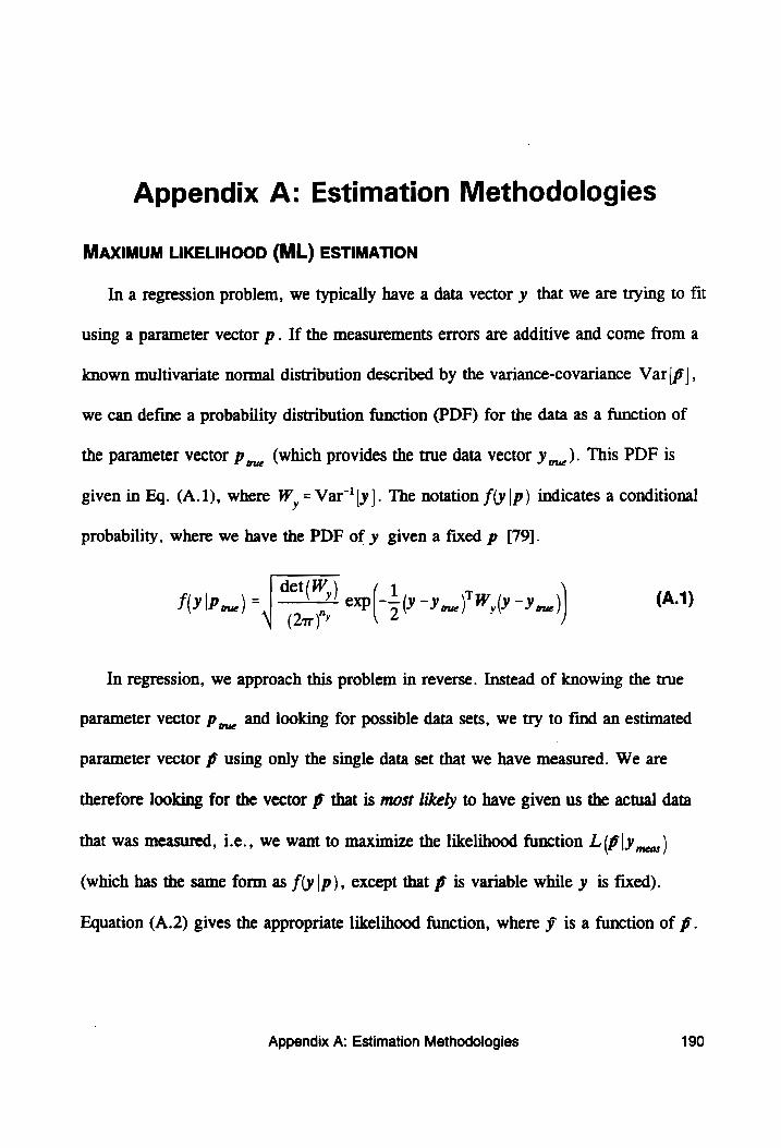
Appendix A: Estimation Methodologies
MAXIMUM LIKELIHOOD (ML) ESTIMATION
In a regression problem, we typically have a data vector y that we are trying to fit
using a parameter vector p. If the measurements errors are additive and come from a
known multivariate normal distribution described by the variance-covariance Var|p}|,
we can define a probability distribution function (PDF) for the data as a function of
the parameter vector p,_, (which provides the true data vector y,,). This PDF is
given in Eq. (A.1), where W, = Var™'[y]. The notation f(y|p) indicates a conditional
probability, where we have the PDF of y given a fixed p [79].
det (
(2ary"
XS
AUP P ne) = | ne e019 Vane) Wy l9 Ye (A.1)
“e
In regression, we approach this problem in reverse. Instead of knowing the true
parameter vector p,,, and looking for possible data sets, we try to find an estimated
parameter vector f using only the single data set that we have measured. We are
therefore looking for the vector pf that is most likely to have given us the actual data
that was measured, i.e., we want to maximize the likelihood function L (DY ,,24s)
(which has the same form as f(y|p), except that f is variable while y is fixed).
Equation (A.2) gives the appropriate likelihood function, where ¥ is a function of p.
Appendix A: Estimation Methodologies 190
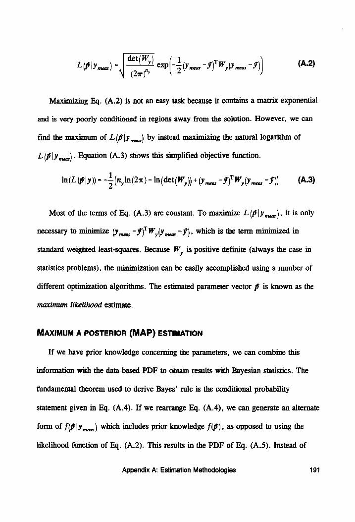
det(W,
(2ar)"” L(B\Y meas ) = exp 5 meas 7 I) WY meas -¥) (A.2)
Maximizing Eq. (A.2) is not an easy task because it contains a matrix exponential
and is very poorly conditioned in regions away from the solution. However, we can
find the maximum of L(p|y,,..,) by instead maximizing the natural logarithm of
L(P\Y meas)~ Equation (A.3) shows this simplified objective function.
In(L (f|y)) = -=(n,In(2m) - In(det(W, )) + (¥ meas I) Wy(¥ meas F)) (A-3) 1 2
Most of the terms of Eq. (A.3) are constant. To maximize L(p | Y meas)? it is only
necessary to minimize (y,..,-¥)'W,(¥ meas J)» Which is the term minimized in
standard weighted least-squares. Because W, is positive definite (always the case in
statistics problems), the minimization can be easily accomplished using a number of
different optimization algorithms. The estimated parameter vector f is known as the
maximum likelihood estimate.
MAXIMUM A POSTERIOR (MAP) ESTIMATION
If we have prior knowledge concerning the parameters, we can combine this
information with the data-based PDF to obtain results with Bayesian statistics. The
fundamental theorem used to derive Bayes’ rule is the conditional probability
statement given in Eq. (A.4). If we rearrange Eq. (A.4), we can generate an alternate
form of f(b | Y meas) Which includes prior knowledge f(p), as opposed to using the
likelihood function of Eq. (A.2). This results in the PDF of Eq. (A.5). Instead of
Appendix A: Estimation Methodologies 191
assuming a fixed parameter vector, we assume that it is a random variable, just as we
do with the data vector. The “reversal” in thinking used with the maximum likelihood
approach is no longer necessary.
F(E\Y meas )F(Y meas) = F(Y meas |P) FP) (A.4)
F(P|Y meas) = Powtl (A.5)
Again, the PDF f(Y jas |) has the exact same form as Eq. (A.2). The PDF F(p)
(representing our knowledge of the parameters before analyzing any data) is given
below in Eq. (A.6), where W, = Var" [po]. The parameters are assumed to come
from a multivariate normal distribution. The vector p, and matrix Var [Po| specify a
set of estimated means and variances that comprise our prior knowledge. This is also
called a priori knowledge.
det(W,)
(2ar)"?
No
| =
fl) = exp (- (Py - BY WP, -A) (A.6)
Bayes’ theorem combines information coming from the data with the prior know-
ledge to form the a posterior distribution. If we find the parameter vector that maxi-
mizes the values of this PDF, we will have found the maximum a posterior estimate.
Again, this can be accomplished most easily by taking the natural logarithm of Eq.
(A.5), as shown in Eg. (A.7).
In(f(p|y)) = -3[(n, +7, in(2x) - In(det(W,)) - In(det(W,)
* (Vmeas I)" Wy (¥ meas ~ 9) * (Po - BW p(Po -B)]| - nif) (A.7)
Appendix A: Estimation Methodologies 192

And again, most of the terms in this expression are constant with respect to the
parameters. Therefore, to maximize f(p|y), we need to minimize only the expression
(Y meas 3)" W,(Y meas ~3)* (Po ~ P\'W, (Pp - P), which can be readily accomplished
using a number of different optimization algorithms.
Appendix A: Estimation Methodologies 193
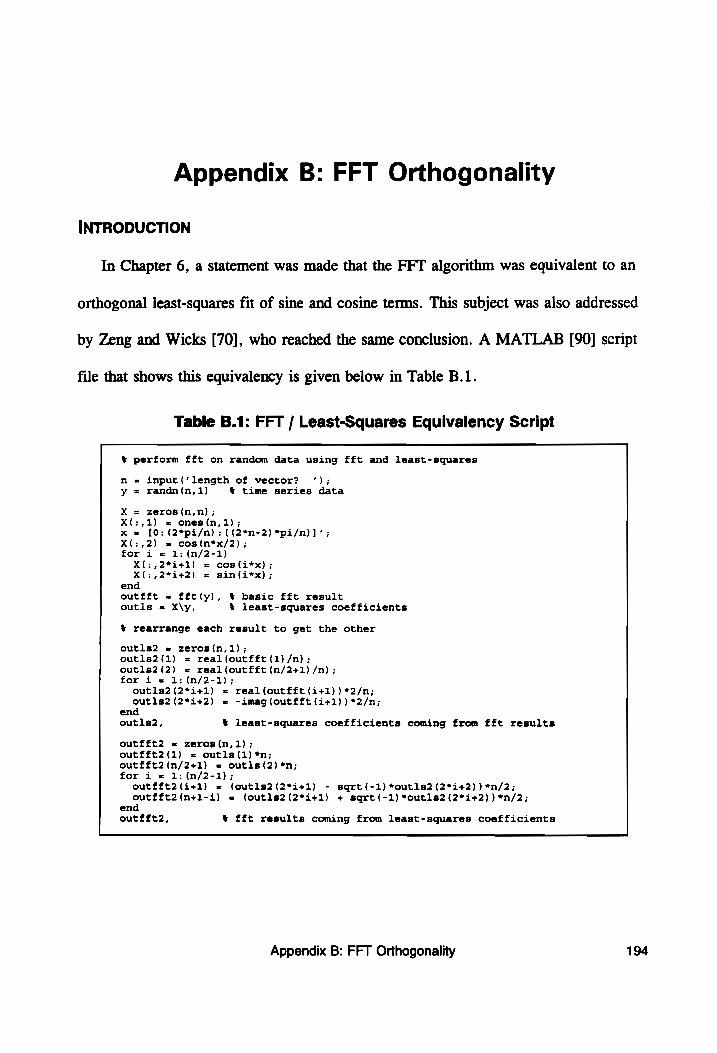
Appendix B: FFT Orthogonality
INTRODUCTION
In Chapter 6, a statement was made that the FFT algorithm was equivalent to an
orthogonal least-squares fit of sine and cosine terms. This subject was also addressed
by Zeng and Wicks [70], who reached the same conclusion. A MATLAB [90] script
file that shows this equivalency is given below in Table B.1.
Table B.1: FFT / Least-Squares Equivalency Script
%& perform fft on random data using fft and least-squares
n = input (‘length of vector? ‘); y = randnin,1) % time series data
X = zeros(n,n); X(:,1) = ones(n,1);
x = [0:(2*pi/n) : ((2*n-2) *pi/n)]'; X(:,2) = cos(n*x/2); for i = 1: (n/2-1)
X(:,2*i+1) = cos (i*x); X(:,2*1+2) = sin(i*x) ;
end outfft = fftly), * basic fft result outls = X\y, % least-squares coefficients
& rearrange each result to get the other
outls2 = zeros(n,1); outls2(1) = real (outfft (1) /n); outls2(2) = real (outfft (n/2+1) /n) ; for i = 1:(n/2-1);
outls2(2*i+1) = real (outfft (i+1))*2/n; outls2 (2*i+2) = -imag(outfft (i+1))*2/n;
end
outls2, % least-squares coefficients coming from fft results
outfft2 = zerosin,1); outff£t2(1) = outls(1)*n; outfft2(n/2+1) = outls(2)*n; for i = 1: (n/2-1);
outff£t2(i+1) = (outls2(2*i+1) - sqrt (-1) *outls2 (2*i+2))*n/2; outfft2(n¢+1-i) = (outls2(2*i+1) + sqrt (-1) *outls2 (2%i+2))*n/2;
end outfft2, & fft results coming from least-squares coefficients
Appendix B: FFT Orthogonality 194
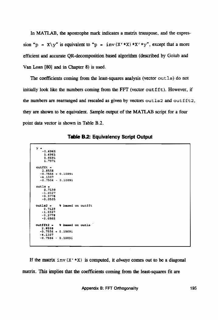
In MATLAB, the apostrophe mark indicates a matrix transpose, and the expres-
sion “p = X\y” is equivalent to “p = inv(X’*X) *X’*y”, except that a more
efficient and accurate QR-decomposition based algorithm (described by Golub and
Van Loan [80] and in Chapter 8) is used.
The coefficients coming from the least-squares analysis (vector out1s) do not
initially look like the numbers coming from the FFT (vector out ff£t). However, if
the numbers are rearranged and rescaled as given by vectors out1s2 and out fft2,
they are shown to be equivalent. Sample output of the MATLAB script for a four
point data vector is shown in Table B.2.
Table B.2: Equivalency Script Output
-0.6965 1.6961 0.0591 1.7971
outfft =
2.8558 -0.7556 + 0.10091
-4.1307 -0.7556 - 0.10091
outils =
0.7139 -1.0327
-0.3778 -0.0505
outls2 = * based on outfft 0.7139
-1.0327
-0.3778 -0.0505
outfft2 = & based on outils 2.8558
-0.7556 + 0.10091 -4.1307
-0.7556 - 0.10093
If the matrix inv (X‘*X) is computed, it always comes out to be a diagonal
matrix. This implies that the coefficients coming from the least-squares fit are
Appendix B: FFT Orthogonality 195
statistically independent, meaning that potential errors from one coefficient to the next
are uncorrelated. This, in turn, means that terms coming from an FFT analysis will
also have uncorrelated errors, even between real and imaginary parts.
Because FFT results corresponding to a given frequency are never recombined
with results corresponding to any other frequency during the signal processing compu-
tations, each spectral line bin of the resulting FRF remains statistically independent
from all other spectral lines. This argument cannot be applied to the real and
imaginary parts from a single spectral line, since they are multiplied together during
the signal processing computations. However, using arguments from Bendat [81], it
can be shown that the final real and imaginary components of the FRF are statistically
independent for the H, FRF estimator, as was done in Chapter 6.
Appendix B: FFT Orthogonality 196
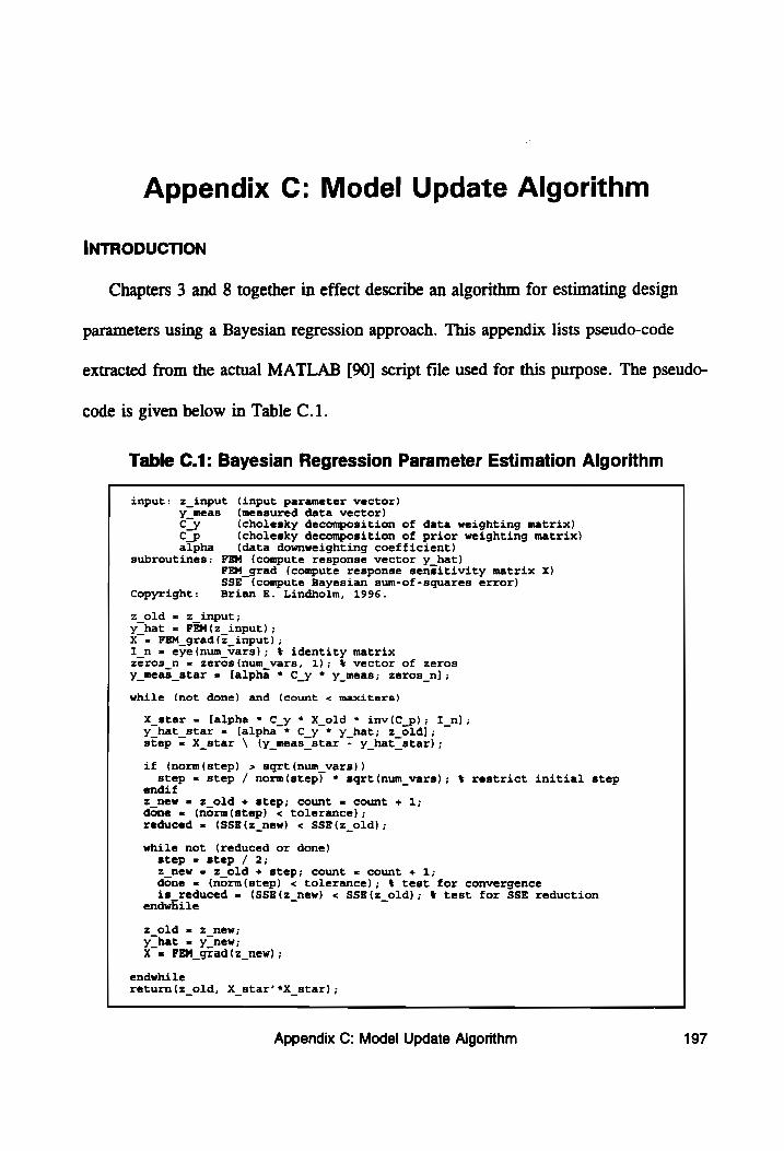
Appendix C: Model Update Algorithm
INTRODUCTION
Chapters 3 and 8 together in effect describe an algorithm for estimating design
parameters using a Bayesian regression approach. This appendix lists pseudo-code
code is given below in Table C.1.
Table C.1: Bayesian Regression Parameter Estimation Algorithm
input: z_input (input parameter vector) y_meas (measured data vector) cy (cholesky decomposition of data weighting matrix) Cp (cholesky decomposition of prior weighting matrix) alpha (data downweighting coefficient)
subroutines: FEM (compute response vector y hat) FEM _grad (compute response sensitivity matrix X) SSE (compute Bayesian sum-of-squares error)
Copyright : Brian E. Lindholm, 1996.
z_old = z_ input; y_hat = FEM(z_ input) ; X = PEM _grad(z input); I_n = eye(num_vars); % identity matrix zeros _n = zeros(num_vars, 1); * vector of zeros y_meas_star = {alpha * C_y * y meas; zeros_n];
while (not done) and (count < maxiters)
X_star = [alpha * C_y * X_old * inv(C_p); I_n]; y_hat_star = [alpha * C_y * y_hat; z_old); step = X_star \ (y_meas_star - y hat_star);
if (norm(step) > sqrt (num_vars) ) step = step / norm(step) * sqrt (num_vars); % restrict initial step
endif z_new = z_old + step; count = count + 1; done = (norm(step) < tolerance) ; reduced = (SSE(z_new) < SSE(z_old);
while not (reduced or done) step = step / 2; z_new = z old + step; count = count + 1; done = (norm(step) < tolerance); % test for convergence is_reduced = (SSE(z_new) < SSE(z_old); * test for SSE reduction
endwhile
z_old = z_new; y_hat = y_new; X = FEM_grad(z_new) ;
endwhile return(z_old, X_star’*X_star);
extracted from the actual MATLAB [90] script file used for this purpose. The pseudo-
Appendix C: Model Update Algorithm 197

As mentioned in Appendix B, in MATLAB the apostrophe mark indicates a matrix
transpose, and expressions similar to “step = X\y” are equivalent to the least-
squares “step = inv(X’*X) *X’*y”, except that MATLAB uses a more efficient
_ and accurate QR-decomposition based algorithm (described by Golub and Van Loan
[80] and used in Chapter 8) instead of matrix inversion.
The algorithm given in Table C.1 utilizes line searches, parameter rescaling, and
the QR decomposition algorithm. It is quite robust and will always converge to a
solution, although the solution can sometimes be a non-optimal local minimum rather
than the global minimum.
Appendix C: Model Update Algorithm 198
Appendix D: Using the Scanning LDV
SCANNING LDV REGISTRATION
In order to use the scanning laser-Doppler vibrometer (LDV) for data acquisition
purposes (as was done in Chapter 13), it is necessary to register the location of the
LDV unit in space relative to the test structure. Without this information, it is
impossible to determine at what point on the structure data is being acquired or at
what angle the laser beam is striking the structure. This information is required if
predictions are to be made of what the laser beam “sees.”
To locate the LDV in space, the laser beam was “manually” aimed at seven
different points of known location on the structure. The scanning angle pair for each
point was carefully recorded and used to estimate the location of the LDV in space
relative to the structure. This was accomplished with a MATLAB-based implemen-
tation of a registration algorithm developed by Lindholm [98]
Once this was done, it became possible to use the registration information to com-
pute the scanning angles required to hit other points on the structure, as also
described by Lindholm [98]. In Chapter 13, this procedure was used to acquire data
at points on the structure corresponding a subset of the FE model nodal points.
Table D.1 below shows the results of the LDV registration procedure.
Chapter D: Using the Scanning LDV 199
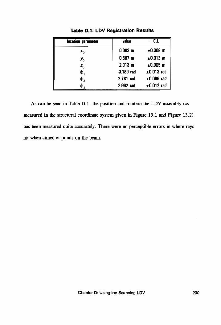
Table D.1: LDV Registration Results
location parameter “value C.l.
Xp 0.003 m +0.009 m
Yo 0.587 m +0.013 m
2 2.013 m +0.005 m
d, -0.189 rad +0.013 rad
d, 2.781 rad +0.006 rad
, 2.962 rad +0.012 rad
As can be seen in Table D.1, the position and rotation the LDV assembly (as
measured in the structural coordinate system given in Figure 13.1 and Figure 13.2)
has been measured quite accurately. There were no perceptible errors in where rays
hit when aimed at points on the beam.
Chapter D: Using the Scanning LDV
Appendix E: Cantilevered Beam Priors
INTRODUCTION
In Chapter 13, priors for several parameters had to be obtained. These included
the effective translational stiffness k, and rotational stiffness k, of the clamp, beam
thickness ¢ and width w, the effective mass m, and rotatory inertia J, of the
transducers, and the effective rotational stiffness k, of the stinger.
EFFECTIVE CLAMP STIFFNESSES
To find the effective translational stiffness of the clamp, k,, the clamp was
crudely modeled as a pinned-pinned beam (length 0.1 m, width 0.05 m, thickness
0.015 m) with a load applied in the center. For a material modulus of elasticity of
2.0 x 10'' N/m?, an effective translational stiffness of 1.35 x 10° N/m is obtained.
For the effective rotational stiffness of the clamp, k,, the clamp was crudely
modeled as a cantilever beam of the same dimensions. In this case, an effective
rotational stiffness of 2.8 x 10* N-m/rad was obtained. These results were summar-
ized below in Eq. (E.1). It should be noted that these estimates are quite rough and
probably cannot be trusted to be accurate within even a factor of 10. Thus, confidence
interval sizes of +10000% were assigned to these parameters.
k, = 1.35 x 10⁸ N/m (+ 10000 %) E.1
k, = 2.8 x 10* N-m/rad (+ 10000 %) 1)
Appendix E: Cantilevered Beam Priors 201

BEAM THICKNESS AND WIDTH
The thickness of the beam (nominally 0.25 in.) was carefully measured with a
micrometer at a number of locations, while the width of the beam (nominally
1.50 in.) was measured with a tape measure. The results are given in Eq. (E.2), with
confidence interval sizes assumed to be half the size of the smallest increment on the
measuring devices.
t = 0.00640 m (+0.00002 m)
w = 0.0381 m (+0.0002 m) (E.2)
TIP MASS AND ROTATORY INERTIA
The mass of the force gauge was measured to be 23.1+0.1 2g, while the mass of
the accelerometer was measured to be 2.3+0.1g. In a standard test configuration,
half of the force gauge mass is isolated from the system because it is on the other side
of the piezoelectric core of the transducer. Thus, only half of the force gauge mass is
added to the tip of the beam, while the entire mass of the accelerometer is added. Out
of these considerations comes the prior estimate given in Eq. (E.3) below. The broad
confidence interval of +20% was arbitrarily picked as a safe estimate of how far the
true effective mass of the force gauge might be away from a perfect 50% effective
mass.
m, = 0.01385 kg (+ 20%) (E.3)
Appendix E: Cantilevered Beam Priors 202
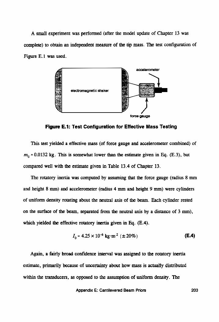
A small experiment was performed (after the model update of Chapter 13 was
complete) to obtain an independent measure of the tip mass. The test configuration of
Figure E.1 was used.
accelerometer
electromagnetic shaker
force gauge
Figure E.1: Test Configuration for Effective Mass Testing
This test yielded a effective mass (of force gauge and accelerometer combined) of
m, = 0.0132 kg. This is somewhat lower than the estimate given in Eq. (E.3), but
compared well with the estimate given in Table 13.4 of Chapter 13.
The rotatory inertia was computed by assuming that the force gauge (radius 8 mm
and height 8 mm) and accelerometer (radius 4 mm and height 9 mm) were cylinders
of uniform density rotating about the neutral axis of the beam. Each cylinder rested
on the surface of the beam, separated from the neutral axis by a distance of 3 mm),
which yielded the effective rotatory inertia given in Eq. (E.4).
I, = 4.25 x 10° kg-m? (+20%) (E.4)
Again, a fairly broad confidence interval was assigned to the rotatory inertia
estimate, primarily because of uncertainty about how mass is actually distributed
within the transducers, as opposed to the assumption of uniform density. The
Appendix E: Cantilevered Beam Priors 203

assumptions of perfectly cylindrical geometry and the rough dimension measurements
were also potential sources of error in the estimate.
STINGER STIFFNESS
For purposes of estimating rotational stiffness, the metallic stinger used to attach
the electromagnetic shaker to the force gauge was modeled as a cantilever beam with
a@ moment applied at the end. With a cylindrical cross-section (diameter 1 mm) and a
length of 32 mm, the estimated rotational stiffness of the stinger was computed,
yielding the result given in Eq. (E.5). Again, a confidence interval size of +20% was
assigned.
k, = 0.328 N-m/rad (+20 %) (E.5)
Appendix E: Cantilevered Beam Priors 204

Vita
Brian Eric Lindholm was born November 8, 1967 in Jacksonville, Arkansas. His
early childhood was spent in Chattanooga, Tennessee, while his later childhood years
were spent in Midlothian, Virginia. He graduated from Clover Hill High School in
June of 1986.
He then enrolled at Virginia Tech, where he completed his B.S. degree in
Mechanical Engineering in May of 1991. He continued at Virginia Tech and com-
pleted his M.S. degree in Mechanical Engineering in September of 1994 and his
Ph.D. degree in Mechanical Engineering in August of 1996. Later that month, he
began work with the Corporate Research and Development division of the General
Electric Company in Schenectady, New York.
Vita 205