ld5655.v855_1986.s867.pdf - vtechworks

Modeling Phosphorus Transport in Surface Runoff From Agricultural

Watersheds For Nonpoint Source Pollution Assessment

by

Daniel Eugene Storm

Thesis submitted to the F acuity of the

Virginia Polytechnic Institute and State University

in partial fulfillment of the requirements for the degree of

Master of Science

Saied Mostaghimi

Tamim M. Younes

in

Agricultural Engineering

APPROVED:

Theo A. Dillaha, III, Chairman

September, 1986

Blacksburg, Virginia

Vernon 0. Shanholtz

G. V. Loganathan

Modeling Phosphorus Transport in Surface Runoff From Agricultural

Watersheds For Nonpoint Source Pollution Assessment

by

Daniel Eugene Storm

Theo A. Dillaha, III, Chairman

Agricultural Engineering

(ABSTRACT)

Nonpoint source pollution from cropland has been identified as the primary source of nitrogen

and sediment, and a significant source of phosphorus in the Chesapeake Bay. These pollutants,

whether from point or nonpoint sources, have been found to be the primary cause of declining

water quality in the Bay. Numerous studies have indicated that, for many watersheds, a few critical

areas are responsible for a disproportionate amount of the nutrient and sediment yield. Conse-

quently, if pollution control activities are concentrated in these critical areas, then a far greater im-

provement in downstream water quality can be expected with limited funds.

In this research a phosphorus transport model is incorporated into ANSWERS, a distributed

parameter watershed model. The version of ANSWERS used has an extended sediment transport

model which is capable of simulating the transport of individual particle classes in a sediment

mixture during the overland flow process. The phosphorus model uses a nonequilibrium

desorption equation to account for the desorption of phosphorus from the soil surface into surface

runoff. The sediment-bound phosphorus is modeled as a function of the specific surface area of the

soil and transported sediment. The equilibrium between the soluble and sediment-bound

phosphorus is modeled using a Langmuir isotherm.

The extended ANSWERS model was verified using water quality data collected from rainfall

simulator plot studies conducted on the Prices Fork Research Farm in Blacksburg, Virginia. The

plots consisted of four 5.5 m wide by 18.3 m long strips with average slopes ranging from 6.2 to

11 percent. Two of the plots were tilled conventionally, and the remaining two were no-till. Sim-

ulated rainfall at an intensity of 5 cm/h was applied to the plots and runoff samples were analysed

for sediment and phosphorus. The model was then verified by comparing the simulated responce

with the observed data. The results of the verification runs ranged from satisfactory to excellent.

Also developed is a technique for selecting a design storm for ANSWERS. The technique

creates an n-year recurrence interval storm with a duration equal to the time of concentration of the

watershed. The intensity pattern is simulated on a ten-minute interval using a first-order Markov

model with a lognormal distribution.

Using a two-year recurrence interval design storm, the use of the model is demonstrated for

evaluating the application of conservation practices to critical areas on a Virginia watershed. Ap-

plication of BMP's to critical areas is shown to be substantially more cost effective in terms of

pollutant reduction than nonselective placement of BMP's if cost sharing funds are involved.

Acknowledgements

I would like to thank each member of my examining committee, Dr. Theo A. Dillaha, Dr.

Vernon 0. Shanholtz, Dr. Saied Mostaghimi, Dr. Tamitn M. Younos, and Dr. G. V. Loganathan

for their guidance and support. In particular, I would like to thank Dr. Theo A. Dillaha for his

continuous support and suggestions, and his previous development of the advanced sediment

transport model used in ANSWERS. This critical piece of work enabled the development of the

phosphorus transport model. I would also like to acknowledge Dr. David B. Beasley, Dr. Larry

F. Huggins, and Dr. Edward J. Monke for their work in the initial development of the ANSWERS

model.

Special thanks goes to Dr. Frank Woeste for his encouragement and guidance with the devel-

opment of the stochastic processes involved with the design storm. Without his assistance, this

work would not have been possible.

I would also like to thank Kris Bailey for her endless devotion and countless hours of work

in the development of the ANSWERS data bases, for copying literature from the library, for

washing thousands of pieces of laboratory glassware, and for her other assorted laboratory assist-

ance and office work.

Thanks goes to the Agricultural Engineering Water Quality Laboratory, and in particular

Helen Castros and Craig Eddleton for their patience and assistance in making a me pseudo chemist

in three weeks. Without their assistance the required laboratory work for the development of the

phosphorus transport model would never had happened.

Thanks also goes to Dr. Saied Mostaghimi for providing the field data used in verifying the

model. I would like to thank Mark Bennett for his assistance in surveying the research plots at the

Prices Fork Research Farm, and Peter Newkirk for running the particle size distributions on the

Acknowledgements iv

laboratory soil samples. I would also like to thank Sharon Akers for her endless secretarial assist-

ance.

Many thanks to the other graduate and undergraduate students for the good times and

friendships, and assistance during my course work as well as my research. I would like to thank

my wife, Amy for her kindness and understanding on the many evenings and nights I spent away

from her at the computer terminals.

A very special thanks goes to Jan Carr for his hundreds of hours of assistance with my

countless computer problems. His invaluable assistance saved months of work.

Finally, I wish to acknowledge the financial support provided by the Department of Agricul-

tural Engineering, Virginia Polytechnic Institute and State University and the Virginia Division of

Soil and Water Conservation.

Acknowledgements V

Table of Contents

IN'TRODUCTION . . . . . . . . . . . . . . . . . . . . . . . . . . . . . . . . . . . . . . . . . . . . . . . . . . . . . . . 1

Background . . . . . . . . . . . . . . . . . . . . . . . . . . . . . . . . . . . . . . . . . . . . . . . . . . . . . . . . . . 1

Research Objectives . . . . . . . . . . . . . . . . . . . . . . . . . . . . . . . . . . . . . . . . . . . . . . . . . . . . . 3

LITERATURE REVIEW . . . . . . . . . . . . . . . . . . . . . . . . . . . . . . . . . . . . . . . . . . . . . . . . . . S

Current Methods for the Analysis of Watersheds . . . . . . . . . . . . . . . . . . . . . . . . . . . . . . . . S

Methods for Watersheds with Historical Records . . . . . . . . . . . . . . . . . . . . . . . . . . . . . . S

Methods for Watersheds without Historical Records . . . . . . . . . . . . . . . . . . . . . . . . . . . 6

Lumped Parameter Models . . . . . . . . . . . . . . . . . . . . . . . . . . . . . . . . . . . . . . . . . . . . . . 7

Distributed Parameter Models . . . . . . . . . . . . . . . . . . . . . . . . . . . . . . . . . . . . . . . . . . . 7

Description of Some Phosphorous Transport Models . . . . . . . . . . . . . . . . . . . . . . . . . . . . 8

ARM ............................................................. 8

NPS . . . . . . . . . . . . . . . . . . . . . . . . . . . . . . . . . . . . . . . . . . . . . . . . . . . . . . . . . . . . . 10

CREAMS ......................................................... 11

The ANSWERS Model . . . . . . . . . . . . . . . . . . . . . . . . . . . . . . . . . . . . . . . . . . . . . . . . . 12

Model Description . . . . . . . . . . . . . . . . . . . . . . . . . . . . . . . . . . . . . . . . . . . . . . . . . . . 12

Critique of the ANSWERS Model . . . . . . . . . . . . . . . . . . . . . . . . . . . . . . . . . . . . . . . 13

Forms and Availability of Phosphorus . . . . . . . . . . . . . . . . . . . . . . . . . . . . . . . . . . . . . . 14

Modeling Sediment-Bound Phosphorus . . . . . . . . . . . . . . . . . . . . . . . . . . . . . . . . . . . . . 17

Vegetation as a Source of Phosphorus . . . . . . . . . . . . . . . . . . . . . . . . . . . . . . . . . . . . . . 18

Modeling Phosphorous Transport Using Chemical Kinetics . . . . . . . . . . . . . . . . . . . . . . . 19

First-Order Chemical Kinetics . . . . . . . . . . . . . . . . . . . . . . . . . . . . . . . . . . . . . . . . . . 19

Table of Contents vi

Equilibrium Chemical Kinetic Models . . . . . . . . . . . . . . . . . . . . . . . . . . . . . . . . . . . . . 20

Nonequilibrium Chemical Kinetic Models . . . . . . . . . . . . . . . . . . . . . . . . . . . . . . . . . . 23

MODEL DEVELOPMENT . . . . . . . . . . . . . . . . . . . . . . . . . . . . . . . . . . . . . . . . . . . . . . . 26

Sediment Transport Model .............................................. 26

Sediment-Bound Phosphorus Transport Model ................................ 33

Soluble Phosphorus Transport . . . . . . . . . . . . . . . . . . . . . . . . . . . . . . . . . . . . . . . . . . . . 36

Model Development . . . . . . . . . . . . . . . . . . . . . . . . . . . . . . . . . . . . . . . . . . . . . . . . . 36

Soluble Phosphorus Transport Model ..................................... 41

Equilibrium Phosphorus Adsorption/Desorption Process . . . . . . . . . . . . . . . . . . . . . . . . . 44

Model Development . . . . . . . . . . . . . . . . . . . . . . . . . . . . . . . . . . . . . . . . . . . . . . . . . 44

Equilibrium Phosphorus Adsorption/Desortion Model . . . . . . . . . . . . . . . . . . . . . . . . . 56

MODEL VERIFICATION . . . . . . . . . . . . . . . . . . . . . . . . . . . . . . . . . . . . . . . . . . . . . . . . 66

Plot Descriptions and Data Collection . . . . . . . . . . . . . . . . . . . . . . . . . . . . . . . . . . . . . . 66

Plot Simulations . . . . . . . . . . . . . . . . . . . . . . . . . . . . . . . . . . . . . . . . . . . . . . . . . . . . . . 68

Results and Discussion . . . . . . . . . . . . . . . . . . . . . . . . . . . . . . . . . . . . . . . . . . . . . . . . . 83

SENSITIVITY ANALYSIS . . . . . . . . . . . . . . . . . . . . . . . . . . . . . . . . . . . . . . . . . . . . . . . 87

WATERSHED SIMULATIONS ........................................... 92

Design Storm . . . . . . . . . . . . . . . . . . . . . . . . . . . . . . . . . . . . . . . . . . . . . . . . . . . . . . . . 92

Nomini Creek Simulation . . . . . . . . . . . . . . . . . . . . . . . . . . . . . . . . . . . . . . . . . . . . . . 103

Watershed Description . . . . . . . . . . . . . . . . . . . . . . . . . . . . . . . . . . . . . . . . . . . . . . . 103

Scenario Descriptions . . . . . . . . . . . . . . . . . . . . . . . . . . . . . . . . . . . . . . . . . . . . . . . . 103

Results and Discussion . . . . . . . . . . . . . . . . . . . . . . . . . . . . . . . . . . . . . . . . . . . . . . . 108

SUMMARY AND CONCLUSIONS . . . . . . . . . . . . . . . . . . . . . . . . . . . . . . . . . . . . . . . 116

Table of Contents vii

Summary . . . . . . . . . . . . . . . . . . . . . . . . . . . . . . . . . . . . . . . . . . . . . . . . . . . . . . . . . . 116

Conclusions . . . . . . . . . . . . . . . . . . . . . . . . . . . . . . . . . . . . . . . . . . . . . . . . . . . . . . . . 117

RECOMMEND A TIO NS . . . . . . . . . . . . . . . . . . . . . . . . . . . . . . . . . . . . . . . . . . . . . . . . 119

REFERENCES . . . . . . . . . . . . . . . . . . . . . . . . . . . . . . . . . . . . . . . . . . . . . . . . . . . . . . . 122

APPENDICES . . . . . . . . . . . . . . . . . . . . . . . . . . . . . . . . . . . . . . . . . . . . . . . . . . . . . . . . 127

APPENDIX A: Variable Glossary . . . . . . . . . . . . . . . . . . . . . . . . . . . . . . . . . . . . . . . . . . 127

APPENDIX B: Computer Program Listing . . . . . . . . . . . . . . . . . . . . . . . . . . . . . . . . . . . 137

APPENDIX C: Computer Simulation Data Files . . . . . . . . . . . . . . . . . . . . . . . . . . . . . . . 171

Prices Fork Farm Plots . . . . . . . . . . . . . . . . . . . . . . . . . . . . . . . . . . . . . . . . . . . . . . . . 171

Plot 1 . . . . . . . . . . . . . . . . . . . . . . . . . . . . . . . . . . . . . . . . . . . . . . . . . . . . . . . . . . . 171

Plot 6

Plot A

Plot D

172

172

173

Nomini Creek Watershed . . . . . . . . . . . . . . . . . . . . . . . . . . . . . . . . . . . . . . . . . . . . . . . 174

APPENDIX D: Sample Output . . . . . . . . . . . . . . . . . . . . . . . . . . . . . . . . . . . . . . . . . . . 198

Vita . . . . . . . . . . . . . . . . . . . . . . . . . . . . . . . . . . . . . . . . . . . . . . . . . . . . . . . . . . . . . . . . 202

Table of Contents viii

List of Illustrations

Figure 1.

Figure 2.

Figure 3.

Figure 4.

Figure 5.

Figure 6.

Figure 7.

Distributed parameter watershed representation showing subdivision into cells. . . . 9

Block diagram of soil-water-phosphorus interactions (Novotny and Chesters, 1981). . . . . . . . . . . . . . . . . . . . . . . . . . . . . . . . . . . . . . . . . . . . . . . . . . . . . . . 16

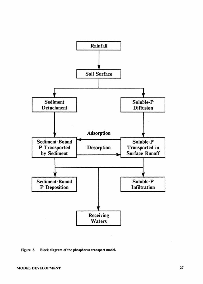
Block diagram of the phosphorus transport model. . . . . . . . . . . . . . . . . . . . . . . 27

Langmuir isotherm for Groseclose silt loam orignial fraction with its 95% confi-dence intervals for Equation 82. . . . . . . . . . . . . . . . . . . . . . . . . . . . . . . . . . . . 48



Langmuir coefficient Qo as a function of specific surface area for Grosclose silt loam soil. . ........................................... , . . . . . . . . . . . . 59

Figure 8. Langmuir coefficient b as a function of Qo for Grosclose silt loam soil. . . . . . . . 60

Figure 9. Observed and simulated runoff hydrographs for Plot 1. . . . . . . . . . . . . . . . . . . . 72

Figure 10. Observed and simulated runoff hydrographs for Plot 6. . . . . . . . . . . . . . . . . . . . 73

Figure 11. Observed and simulated runoff hydrographs for Plot A. . . . . . . . . . . . . . . . . . . 74

Figure 12.

Figure 13.

Figure 14.

Figure 15.

Figure 16.

Figure 17.

Figure 18.

Figure 19.

Observed and simulated runoff hydrographs for Plot D. . . . . . . . . . . . . . . . . . . 75

First order serial correlation coefficients for the Pony Mountain Branch watershed for three time intervals. . . . . . . . . . . . . . . . . . . . . . . . . . . . . . . . . . . . . . . . . . . 94

Histogram of May rainfall intensity transformed by the cube root for ten-minute intervals, with a lognormal distribution fit to the data. . . . . . . . . . . . . . . . . . . . 97

Actual and simulated rainfall intensity histograms for the month of May. . . . . . 102

Westmoreland County watershed partitioned into one-hectare grids with flow di-rections and channel elements. . . . . . . . . . . . . . . . . . . . . . . . . . . . . . . . . . . . 104

Simulated intensity pattern. . . . . . . . . . . . . . . . . . . . . . . . . . . . . . . . . . . . . . . 107

Land use distribution for the Nomini Creek watershed. . . . . . . . . . . . . . . . . . . 110

Critical area distribution for the Nomini Creek watershed. . . . . . . . . . . . . . . . . 114

List of Illustrations ix

List of Tables

Table 1.

Table 2.

Table 3.

Table 4.

Table 5.

Table 6.

Table 7.

Table 8.

Table 9.

Table 10.

Table 11.

Table 12.

Table 13.

Table 14.

Table 15.

Table 16.

Physical and chemical properties for the composite Groseclose silt loam and Suffolk sandy loam soil samples. . . . . . . . . . . . . . . . . . . . . . . . . . . . . . . . . . . . . . . . . . 37

Extactable phosphorus levels for the composite Groseclose silt loam and Suffolk sandy loam soil samples. . . . . . . . . . . . . . . . . . . . . . . . . . . . . . . . . . . . . . . . . . 39

Estimates for the coefficients in the phosphorus desorption Equation 68. . . . . . . 40

Total phosphorus levels and pH for the composite Groseclose silt loam and Suffolk sandy loam soil samples. . . . . . . . . . . . . . . . . . . . . . . . . . . . . . . . . . . . . . . . . . 45

Langmuir isotherm paramter estimates for Equation 82 .................... 47

Langmuir isotherm paramter estimates using Equation 83. . . . . . . . . . . . . . . . . . 49

Nonlinear regression estimates for Langmuir isotherm coefficients using Equation 17. . . . . . . . . . . . . . . . . . . . . . . . . . . . . . . . . . . . . . . . . . . . . . . . . . . . . . . . . . 51

Model comparison for Langmuir isotherm coefficiet estimates. . . . . . . . . . . . . . . 53

Particle size distributions for composite Groseclose silt loam and Suffolk sandy loam soil samples. . . . . . . . . . . . . . . . . . . . . . . . . . . . . . . . . . . . . . . . . . . . . . . . . . . 57

Coefficient estimates for Langmuir coefficients Qo as a function of specific surface area and b as a function of Qo. . . . . . . . . . . . . . . . . . . . . . . . . . . . . . . . . . . . . . 58

Rainfall simulator summary statistics. . . . . . . . . . . . . . . . . . . . . . . . . . . . . . . . . 67

Soil moisture, bulk density, and nutrient summary for Prices Fork Farm plot soil samples. . .................................................... 69

Suggested and calibrated parameters for Holtan's infiltration equation. . . . . . . . . 71

Aggregate and primary soil particle size distributions for Prices Fork farm 0-5 cm soil samples. . .................................................... 80

Sediment particle class decription and composition for 0-5 cm plot soil samples from Prices Fork Farm. . . . . . . . . . . . . . . . . . . . . . . . . . . . . . . . . . . . . . . . . . . 84

Simulated and observed yields and their relative error for the Prices Fork Farm plot computer simulations. . . . . . . . . . . . . . . . . . . . . . . . . . . . . . . . . . . . . . . . . . . . 85

Table 17. Sensitivity anlaysis results with reference to one second time step simulations. . . . 88

Table 18. Sensitivity analysis percent deviation summary. . . . . . . . . . . . . . . . . . . . . . . . . . 89

Table 19. Parameter sensitivity and relative sensitivity. . . . . . . . . . . . . . . . . . . . . . . . . . . . 90

Table 20. Estimated Parameters for a lognormal distribution for Pony Mountain Branch watershed for truncated data without zero intensities. . . . . . . . . . . . . . . . . . . . . . 96

List of Tables X

Table 21. Estimated parameters for a first-oder Markov model with a lognormal distribution for Pony Mountain Branch watershed for transformed data. . . . . . . . . . . . . . . . . 99

Table 22. Estimated parameters for first ten-minute intensity model for Pony Mountain Branch watershed for transformed data. . . . . . . . . . . . . . . . . . . . . . . . . . . . . . . 10 I

Table 23. Average s~il p~osphorus levels for the Nomini Creek watershed in Westmoreland County, V rrguua. . . . . . . . . . . . . . . . . . . . . . . . . . . . . . . . . . . . . . . . . . . . . . . 106

Table 24. Land use and tillage practice scenario description. . . . . . . . . . . . . . . . . . . . . . . 109

Table 25. Nomini Creek watershed simulation results.

Table 26. Nomini Creek watershed simulation analysis.

Table 27. Comparison of alternative cost share stratagies for maximizing the cost effectiveness

111

112

of allocating cost share monies. . . . . . . . . . . . . . . . . . . . . . . . . . . . . . . . . . . . . 115

List of Tables xi

INTRODUCTION

Background

Recent studies on the decline of the Chesapeake Bay have concluded that both point and

nonpoint source pollution are responsible for water quality degradation in the Bay (USEPA, 1983).

In recent years, significant progress has been made in developing technology for controlling point

sources, while nonpoint sources of pollution have been relatively neglected.

Nonpoint source pollution is transported primarily by runoff from urban, agricultural and

mining areas, and construction sites. Runoff carries sediment, organic matter, bacteria, pesticides,

metals, nutrients, and other chemicals. Nutrients, primarily nitrogen and phosphorus, can be a

major problem because they cause eutrophic algae growth. As the algae die and decay, they utilize

dissolved oxygen, which reduces the oxygen available to living organisms. In addition, excess algae

increases the turbidity of water and reduces the available sunlight to submerged aquatic vegetation,

a valuable food source and breeding ground for aquatic organisms.

The Environmental Protection Agency (EPA) Chesapeake Bay study concluded that nitrogen

and phosphorus are the primary pollutants responsible for declining water quality in the Bay

(USEPA, 1983). The EPA Chesapeake Bay Watershed Model estimated that nonpoint sources

were responsible for approximately 39 percent of the phosphorus and 67 percent of the nitrogen

during an average year. Furthermore, cropland was estimated to be responsible for 27 and 60 per-

cent of the phosphorus and nitrogen from nonpoint sources, respectively (USEPA, 1983).

Cropland, therefore, is the primary source of nitrogen and a major source of phosphorus in the Bay.

INTRODUCTION

Sediment as a nonpoint source pollutant causes many problems. Sediment increases the

turbidity of water and its deposition can kill submerged aquatic vegetation, as well as reduce the

storage volume of waterways. In addition, a large percentage of the phosphorus and pesticides that

enter waterways are adsorbed onto soil particles. Thus, the processes of soil erosion and sediment

transport play a significant role in the water quality decline.

A reduction in soil erosion from cropland would result in a significant decrease in the quantity

of nutrients entering the Bay. One method of reducing soil erosion is through the use of Best

Management Practices (BMPs). This has been the approach taken by national soil and water

conservation programs, whose goal is maintaining or improving agricultural productivity. These

programs now have an additional benefit, that of improving downstream water quality. Encour-

aging farmers to implement BMPs, however, has not always been successful. In Virginia, the tra-

ditional approach has been to provide technical assistance to farmers who request it, and to provide

financial incentives to farmers who implement approved BMPs. Unfortunately, funds have always

been limited. As a result, BMPs are not as widely used as they could be.

Numerous studies have indicated that, for many watersheds, a few critical areas are responsible

for a disproportionate amount of the nutrient and sediment loadings to downstream waters. Con-

sequently, if pollution control activities can be concentrated in the critical areas, then far greater

improvements in downstream water quality can be expected with limited funds. A methodology

for identifying potentially critical source areas is currently under development by the Departments

of Agricultural Engineering and Landscape Architecture at Virginia Tech. The system, Virginia

Geographical Information System (VirGIS), includes topography, soils, and land use data. It is

being used to identify potentially critical source areas of nonpoint source pollution using the Uni-

versal Soil Loss Equation and simple sediment delivery algorithms. Once the potentially critical

areas are identified, there is a need for a more precise technique to evaluate the sediment and nu-

trient yields from these critical areas and to evaluate the effectiveness of various BMPs in reducing

these yields.

Before sediment and nutrients from nonpoint source pollution can be controlled, a method for

describing the transport of the pollutants must first be available. The transport of sediment and

INTRODUCTION 2

nutrients is an extremely difficult process to model because of the complexities of overland flow

processes. The model presented in this research and other models, are only rough approximations

of the actual processes.

Several different methods have been developed to describe gross sediment and nutrient losses

from disturbed lands. Most of the methods treat the watershed as a lumped system and depend

on empirical equations. The development of these equations require large amounts of historical

data and their predictions are only valid for watersheds with similar histories and hydrologic char-

acteristics. Current research emphasis is shifting to physically based models which simulate the

hydrologic, and sediment and nutrient transport processes on a series of small hydrologically uni-

form areas. The response of these small areas are then combined and routed through a hydro logic

event. This is the approach taken by Huggins and Monke (1966), Simons, et al. (1975), and Ross,

et al. (1982). The model presented in this research is an extension of the work of Huggins and

Monke (1966), Beasley (1977), Dillaha (1981) and Amin-Sichani (1982).

Research Objectives

The objectives of this research are:

1. Develop a phosphorus transport model and incorporate it into ANSWERS (Dillaha,

1981), a distributed parameter watershed model. The model will account for both the

soluble and sediment-bound phosphorus phases, as well as the equilibrium conditions

between them.

2. Evaluate the accuracy of the model by comparing its predictions with observed data

from rainfall simulator plot studies.

3. Study the sensitivity of the model to various input parameters that affect the transport

processes.

INTRODUCTION 3

4. Develop a technique for generating a design storm of a given duration and recurrence

interval for the geographic area of interest.

5. Demonstrate the use of ANSWERS in evaluating the effects of conservation tillage on

phosphorus and sediment yields on a Virginia watershed.

INTRODUCTION 4

LITERATURE REVIE\V

Current Methods for the Analysis of Watersheds

Models can be classified as deterministic, parametric, stochastic, or a combination of the three,

with most models consisting of varying combinations of the three. Deterministic models are based

on underlying physical processes and do not require calibration for their application. Parametric

models are deterministic in the sense that once the model parameters are determined, the model

always produces the same output for a given input. Stochastic models are those whose outputs are

predicted only in a statistical sense (Haan, 1977). Models may also be classified as to whether they

are lumped or distributed parameter models. The type of model to be used generally depends upon

the intended use of the model, and the available data.

Methods for Watersheds with Historical Records

For many situations, water quality planners only need information concerning average or ex-

treme water quality data. If this is all that is required and historical data is available, then the his-

torical records can be analyzed stochastically and long term averages, trends and extreme event

probabilities identified.

Another general method of analysis requiring historical data is correlation analysis. With this

procedure, one seeks to establish a functional relationship between watershed characteristics, pre-

cipitation parameters and the response of the watershed to various storm events. Regression anal-

LITERATURE REVIEW 5

ysis is then used to estimate the values of the coefficients of these parameters which result in the

highest correlation between the historical records and the model's response. The Universal Soil

Loss Equation (USLE) (Wischmeier and Smith, 1978) is an excellent example of correlation anal-

ysis.

The validity of a stochastic model depends directly on the characteristics of the data used to

estimate the model's parameters. The model can be no better than the data used to develop it. The

data must also have been collected during periods and situations similar to those for which the

model will be used. For example, a model developed for disturbed forest conditions will not be

valid for estimating the soil loss from construction sites. Care must also be taken to insure that the

hydrologic data which drives the soil loss processes are homogeneous over time or can be adjusted

for any nonhomogeneities that may exist (Haan, 1977). Causes of nonhomogeneity are

urbanization, deforestation or reforestation, stream channelization, and construction of dams, res-

ervoirs, and sediment basins, to name but a few.

Methods/or Watersheds without Historical Records

Methods for analysis of watersheds without historical data are generally deterministic or em-

pirical. The deterministic models used are generally precalibrated during their development, and

as long as they are not applied outside the range of constraints for which they were developed their

predictions can be quite satisfactory. Deterministic models are useful for planning purposes because

they can simulate the response of a watershed to changes in topography, land use, soil cover, and

management, to changes for which there are no historical precedents. Empirical models, such as

the USLE, which was developed using thousands of plot years of soil loss data, are also satisfactory

if used for the purposes for which they were designed. Empirical models have the advantage that

they are not as complex numerically as the deterministic models, and thus are quicker and easier

to use. Deterministic models, conversely, often require considerable data input to adequately de-

scribe the watershed which is being simulated. Deterministic models are only as good as the com-

LITERATURE REVIEW 6

ponent processes which make up the overall model. Without adequate and accurate data inputs,

the component process models fail and the overall model suffers.

Lumped Parameter Models

The vast majority of models developed to date are of the lumped parameter type. Lumped

parameter models assume that the areal and temporal distribution and variability of rainfall and

watershed parameters have limited influence on the watershed response. The magnitude of the error

associated with this method is a function of the degree and distribution of the nonuniformities

within the watershed, and thus vary from one watershed to another and even between storms on a

given watershed (Huggins and Monke, 1966).

The degree of complexity in lumped parameter models varies greatly. Two of the simplest

examples are the USLE for estimating soil loss and the Rational Method for predicting peak runoff

rate. A more complex lumped parameter model is Agricultural Runoff Model (ARM) (Davis and

Donigian, 1979), which was developed from the Stanford Watershed Model (Donigian and

Crawford, 1976).

Distributed Parameter Models

Distributed parameter models differ from lumped models in that they include spatial variations

in the inputs, parameters and dependant variables. They consist of a partial differential equation

or a system of such equations (Woolhiser, 1973). Parameters in a deterministic model, unlike those

of lumped system models, have some physical significance and can usually be evaluated by inde-

pendent measurements. As a result, a distributed parameter model has a much greater potential

for increasing accuracy as opposed to a lumped parameter model.

Distributed parameter models can be advantageous in sediment and phosphorous modeling

because they can account for spatial variations in soil types, cover materials and land slopes. In

LITERATURE REVIEW 7

addition, they have the ability to better simulate the hydrologic behavior of the watershed, which

is the driving force for sediment detachment and transport. The potential increase in accuracy of

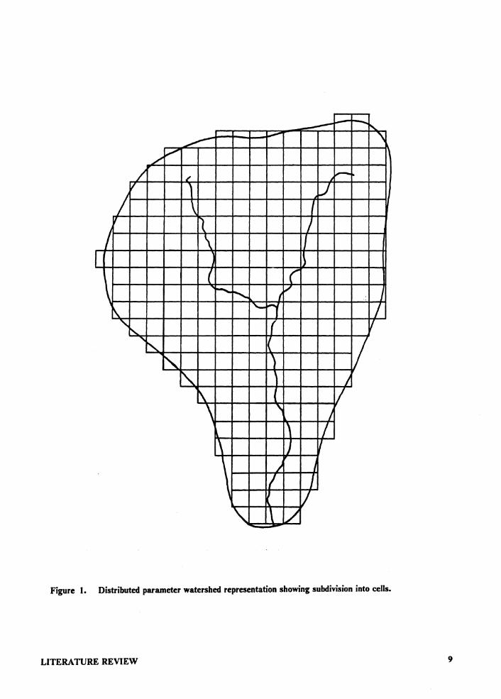
distributed parameter models is not without its costs, however. The distributed approach requires

that the watershed under study be divided into a finite number of small independent cells, as shown

in Figure I. The shape of the cells depends upon the particular model, and some models allow

cell size and shape to vary throughout a watershed. Figure I is a representation of a watershed as

it is perceived by the ANSWERS model. Important hydrologic and soil loss parameters must be

identified for each cell. The cells should be sufficiently small that all significant factors affecting

hydrology and soil loss are uniform within the boundaries of the cell (Huggins and Monke, 1966).

The collection of this data for large watersheds can be a time consuming task, but the increase in

accuracy over lumped models may be significant.

Distributed parameter models also are well suited to .. what if? .. type analyses. The effects of

changing management practices in small, critical portions of the watershed can be easily evaluated

by changing the input parameters of the cells affected. This allows many different management

scenarios to be evaluated quickly and accurately with minimal additional effort.

Description of Some Phosphorous Transport Models

ARM

The Agricultural Runoff Management (ARM) model (Davis and Donigian, 1979; Donigian

and Davis, 1978; Donigian, et al. 1977; Donigian, 1976) simulates surface runoff, interflow,

phosphorus, nitrogen, and pesticide loading into stream channels from both surface and subsurface

sources. The hydrologic components of the model are based on the Stanford Watershed Model

(James, I 970; Ross, I 970), with the runoff component of the ARM model driven by rainfall as well

as snow melt. The erosion component of the model uses Negev's equations for sediment

LITERATURE REVIEW 8

---- \ _.,,,-/

i.,,,,-"""

/ ,,, ,i.---" 7 ' L/ I \ I

I il I I \

I j

( ( \ I'"'- ........ ,7

j

'-= n I ' I/ "'-

' I I\. j

r\ I I \ ' ) , I

' I j

I

\ j

7 I I/

' \ / -

Figure I. Distributed parameter watershed representation showing subdivision into cells.

LITERATURE REVIEW 9

detachment and transport (Negev, 1967). The ARM model is a lumped parameter model and must

be calibrated for a particular watershed. Crawford and Donigian (1973) found that a minimum of

two years of historical data were required for adequate calibration. The model assumes uniform

land use, and is thus only applicable to watersheds with uniform cropping management practices.

No channel processes are included, which limits the model's application to watersheds in which

channel processes are negligible. Donigian and Davis ( 1978) suggest that as a general rule,

watersheds greater than 200 to 500 hectare are approaching the upper limit of the model.

Phosphorous transformations in the ARM model use first-order kinetics, and are corrected for

temperature using a modified Arrhenius equation. Davis and Donigian ( 1979) found that the ARM

model predicted satisfactory monthly simulations of phosphorus in runoff, but storm event simu-

lations of soluble phosphorus were unsatisfactory.

NPS

The Nonpoint Source (NPS) model (Donigian and Crawford, 1979; Donigain and Crawford,

1977; Donigian and Crawford, 1976) is a lumped parameter, continuous simulation model. The

model simulates surface and subsurface hydrologic processes, erosion processes, and nonpoint

source pollutant transport and accumulation into a stream channel. The hydrologic and erosion

components are identical to those in the ARM's model. The NPS model also does not simulate

channel processes. Donigian and Crawford ( 1978) sugges~ that the watershed size be limited to 250

to 500 hectare, and that a minimum of 3 to 5 years of historical records be used to calibrate the

model. However, many of the input parameters for the various processes are physically based, and

may not require calibration.

The NPS model can handle up to five different land uses. However, the hydrologic simulation

separates the watershed into pervious and nonpervious areas without regard to the land use. The

model simulates water temperature, dissolved oxygen, sediment, and up to five user-specified con-

stituents. The model simulates pollutant transport by using a simple potency factor, which is de-

LITERATURE REVIEW 10

fined as the mass of pollutant per mass of transported sediment. The pollutant loading is then

estimated by multiplying the transported sediment by the potency factor.

The NPS model allows monthly variation in land cover and pollutant accumulation and re-

moval. During a storm event the model simulates hydrologic and water quality conditions on a

15-minute time interval. Between storm events the model operates on a combination of 15-minute,

hourly, and daily time intervals to simulate evapotranspiration and percolation to determine the soil

moisture status. Donigian and Crawford (1976) tested the NPS model and found that the

hydrologic simulation gave good results. However, the nonpoint source pollutants gave only fair

to good results.

CREAMS

The Chemical, Runoff, and Erosion from Agricultural Management Systems (CREAMS)

model (Knisel, 1980) simulates the transport of sediment, nitrogen, phosphorus, and pesticides.

CREAMS is a field scale model that assumes homogeneous land use and soil characteristics, and

thus can not be applied to larger nonhomogeneous areas, such as a watershed. If daily rainfall data

is used, surface runoff is calculated using the Soil Conservation Service curve number method, and

if hourly data is available, an infiltration based model is used to estimate surface runoff. The ero-

sion components of the model uses the USLE, along with a sediment transport capacity model for

overland flow. In addition, CREAMS has a channel erosion and deposition component.

The phosphorous transport component assumes that the transfer of phosphorus from the soil

into surface runoff occurs in the top one centimeter of the soil. Soluble forms of phosphorus from

the soil, plant residues, and surface-applied fertilizers are assumed to be completely mixed in the top

one centimeter. The amount of soluble phosphorus transported by the surface runoff is calculated

using an empirical extraction coefficient, and the amount of sediment-bound phosphorus trans-

ported is estimated using phosphorous enrichment ratios.


The ANSWERS Model

Mode/ Description

ANSWERS (Areal Nonpoint Source Watershed Environmental Response Simulation) is a

distributed parameter, deterministic, watershed model developed for predicting the hydrologic re-

sponse of watersheds to storms and the erosion and sediment response of watersheds to different

agricultural management systems. The basic hydrologic model, developed by Huggins and Monke

(1966), describes the processes of interception, infiltration, surface storage, interflow and surface

runoff. The hydrologic model is described in more detail by Beasley (1977), Beasley et al. (1980),

and Beasley and Huggins (1980). Beasley (1977) expanded the model to include erosion, sediment

transport, tile drainage and channel flow. The current model also simulates parallel tile outlet ter-

races, sediment basins, grassed waterways, and field borders (Beasley and Huggins, 1981). Dillaha

(1981) developed an extended version of the sediment transport model, which is capable of simu-

lating the transport of individual particle size classes in a sediment mixture during the overland flow

process.

The ANSWERS model requires that a watershed be divided into a grid of small square ele-

ments. Within each element, the hydrologic parameters (slope direction and magnitude, vegetation,

soil type, surface condition, rainfall and management practices) are assumed to be uniform, and the

hydrologic processes are treated as independent functions of the parameter characteristics. The

degree of uniformity of these parameters is used to determine the limiting element size. The output

from each element is routed to its downslope neighboring elements, and eventually is routed to the

watershed outlet.


Critique of the ANSWERS Model

The most obvious disadvantage of using this type of approach is the large amount of compu-

tational time required for simulation. Numerically, this method requires the calculations equivalent

to an entire lumped parameter simulation be performed on each individual element in the

watershed. The increase in computer time required to accomplish this, as opposed to the lumped

parameter approach, is substantial, and would not be possible without the help of digital comput-

ers. Depending upon the type of computer used, there is a limit to the number of elements that a

watershed can be divided into. This problem can be partially overcome by increasing element sizes,

but a point is reached where the elemental areas are no longer representative of the nonhomogenity

of the watershed and the simulation accuracy suffers.

Another possible disadvantage of this type of analysis is the large amount of input data re-

quired to describe the conditions within each element of the watershed. For the hydrologic portion

of the model, approximately four to seven parameters must be specified for each individual element.

These data may be collected on an element by element basis from soil surveys, topographic maps,

land use maps and/or field surveys and sound engineering estimates. With the development of

digital remote sensing techniques and other computerized inventory surveys, this time consuming

task is being reduced considerably. It must be remembered, however, that the results of this type

of analysis are potentially much more accurate and useful than the lumped parameter approaches.

If added accuracy and planning flexibility are important, then this type of analysis may be necessary.

ANSWERS allows channel aggredation, but degradation of only the previously deposited

sediment. This limitation may be a problem if channel erosion is significant, which may occur as

the size of the watershed increases.

The greatest advantage of ANSWERS, and other similar models, is that they can be used to

predict the response of watersheds to changes in conditions within small areas of the watershed.

In conjunction with its erosion and sediment transport model, ANSWERS can identify critical

areas within a watershed that have high erosion rates and determine whether or not the soil losses

from these areas contribute substantially to the total sediment yield of the watershed. The model


is thus an excellent planning tool for quantitatively evaluating the advantages of various BMP see-

Finally, this type of analysis has the ability to isolate particular component processes. The

ability to isolate a particular component process makes possible the evaluation of the sensitivity of

the watershed to changes in the parameter values of the various components. This allows those

components and parameters having the greatest impact on model accuracy to be identified. Time

can then be allocated more efficiently to improve those parameters and component relationships

to which the model is most sensitive.

Forms and Availability of Phosphorus

Most past work involving phosphorus has dealt with the chemistry of phosphorus in soil, with

an emphasis on the processes of phosphorus availability to agricultural crops. More work is needed

to understand the chemical and physical processes of phosphorus transport from agricultural soils

into surface runoff.

Soils generally contain approximately 0.0 l to 0.13 percent phosphorus, and surface runoff

contains approximately 0.01 to 1.0 ppm (Frere, et al., 1980). Phosphorus existing in the soil and

surface waters can be classified as sediment-bound and soluble, or as organic and inorganic.

Schaller and Bailey ( 1983) categorized sediment-bound phosphorus into the following categories:

1. Adsorbed: labile and exchangeable phosphorus.

2. Organic: various forms including phytins, phospholipids.

3. Precipitates : formed from the reaction of phosphates with Ca, Fe, Al, and other

cations.

4. Minerals: amorphous, short-range order and crystalline minerals with Ca, Fe, Al, and

other cations.


Soluble phosphorus exists as orthophosphate, inorganic polyphosphates, or as organic

phosphorous compounds, while total phosphorus is the sum of sediment-bound and dissolved

forms. Approximately two-thirds of the phosphorus occurring in the soil is inorganic (Shaller and

Bailey, 1983), but the actual percentage is constantly changing due to the microbial decomposition

of plant residue and other organic compounds within the soil system. Organic phosphorus is de-

composed by microorganisms and mineralized to inorganic phosphate ions, which are available to

plants. Conversely, plants and bacteria can immobilize these phosphate ions by converting them

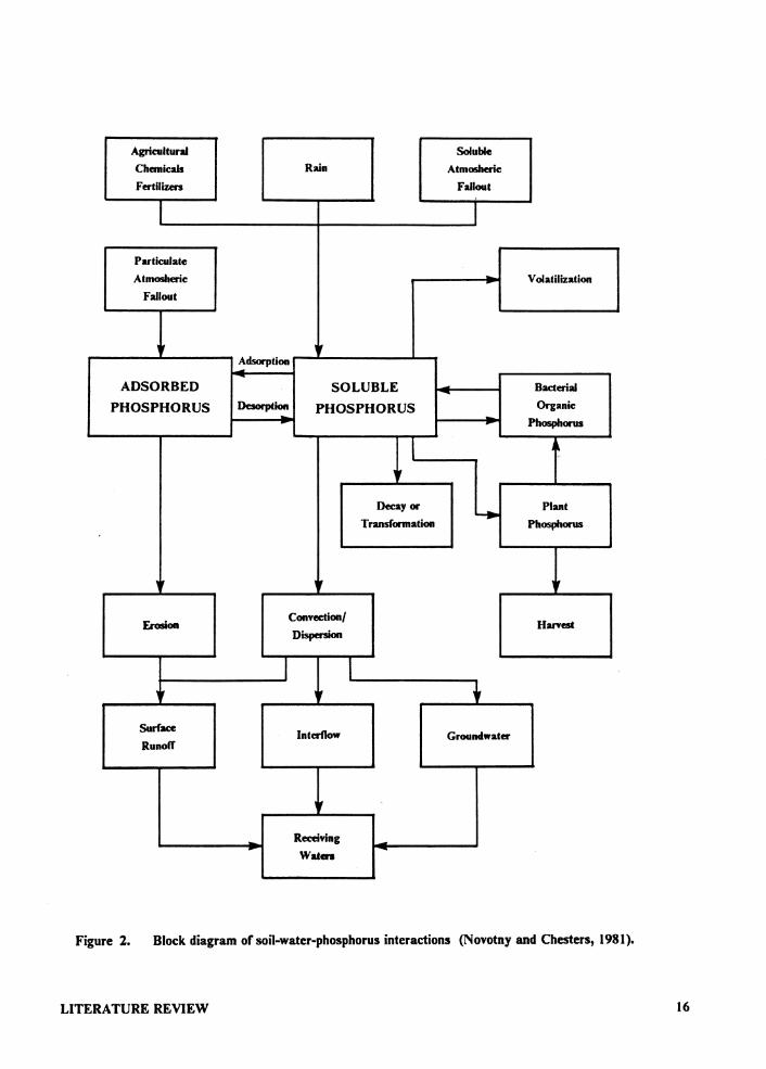
back to organic phosphorus. A block diagram of the soil-water-phosphorus interactions is shown

in Figure 2.

The form of phosphorus entering surface waters is very important in determining the quantity

of available phosphorus for aquatic vegetation. Soluble inorganic phosphorus is readily available

while sediment-bound phosphorus is generally considered unavailable for algae growth in aquatic

systems. Soluble phosphorus is transported by surface runoff and insoluble phosphorus is adsorbed

to the soil particles and is transported with the eroded soil. During the transport process, there is

a dynamic equilibrium between the soluble and sediment-bound phases of phosphorus. For ex-

ample, a high concentration of soluble phosphorus and a low concentration of sediment-bound

phosphorus, can result in the adsorption of the soluble phosphorus by the sediment. Conversely,

under certain conditions sediment-bound phosphorus can be desorbed into solution.

A portion of the phosphorus in the soil is bound to the soil particles and is not readily plant

available. To increase agricultural productivity, commercial fertilizers are often applied to the soil

to increase the plant available phosphorus. However, when the fertilizer comes in contact with the

soil, it is quickly converted to less available forms which are adsorbed to the soil particles. The soil

pH governs the forms to which phosphorus is converted. In acidic soils phosphates are converted

to iron and aluminum phosphates, and in alkaline soils calcium phosphates are formed (Novotny

and Chesters, 1981 ). The method of fertilizer application, surface application or subsurface in-

jection, and the type of fertilizer, liquid or solid, also influences the rate at which the phosphorus

is converted. Other factors include tillage practice, temperature, vegetation, soil moisture, and soil

LITERATURE REVIEW IS

Agricultural Soluble Chemicals Rain Atmosheric Fertilizers FallCNJt

Particulate Atmosheric . Volatilization

FallCNJt

,, ,, Adsorption

ADSORBED SOLUBLE - Bacterial --PHOSPHORUS Desorption PHOSPHORUS Organic

-- Phosphorus

,l

1f

Decay or -. Plant Transformation Phosphorus

, , '.

F.rosion Convection/ Han-est Dispersion

I I ,, 1, +

Surface Interflow Groundwater Runoff

1lf

- Receiving -- -Wuen

Figure 2. Block diagram of soil-water-phosphorus interactions (Novotny and Chesters, 1981).


type. Because of the high affinity of soil for phosphorus, the downward movement of phosphorus

in the soil profile is very slow. Thus, phosphorus is rarely a significant contaminate in groundwater.

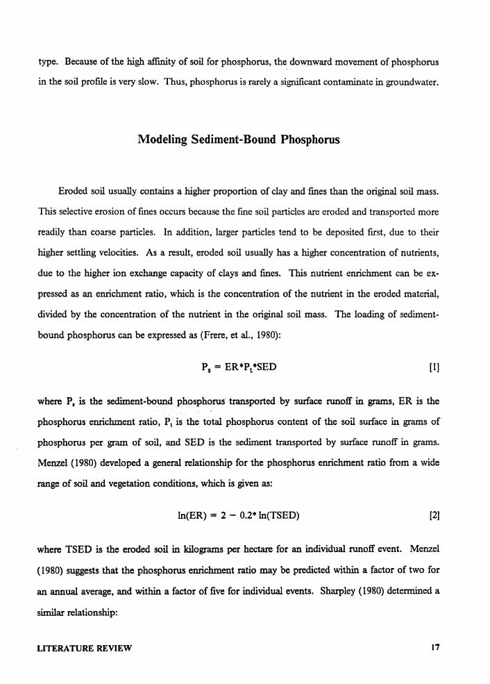
Modeling Sediment-Bound Phosphorus

Eroded soil usually contains a higher proportion of clay and fines than the original soil mass.

This selective erosion of fines occurs because the fine soil particles are eroded and transported more

readily than coarse particles. In addition, larger particles tend to be deposited first, due to their

higher settling velocities. As a result, eroded soil usually has a higher concentration of nutrients,

due to the higher ion exchange capacity of clays and fines. This nutrient enrichment can be ex-

pressed as an enrichment ratio, which is the concentration of the nutrient in the eroded material,

divided by the concentration of the nutrient in the original soil mass. The loading of sediment-

bound phosphorus can be expressed as (Frere, et al., 1980):

[ l I

where P1 is the sediment-bound phosphorus" transported by surface runoff in grams, ER is the

phosphorus enrichment ratio, Pt is the total phosphorus content of the soil surface in grams of

phosphorus per gram of soil, and SED is the sediment transported by surface runoff in grams.

Menzel ( 1980) developed a general relationship for the phosphorus enrichment ratio from a wide

range of soil and vegetation conditions, which is given as:

ln(ER) = 2 - 0.2• ln(TSED) [2]

where TSED is the eroded soil in kilograms per hectare for an individual runoff event. Menzel

( 1980) suggests that the phosphorus enrichment ratio may be predicted within a factor of two for

an annual average, and within a factor of five for individual events. Sharpley ( 1980) determined a

similar relationship:


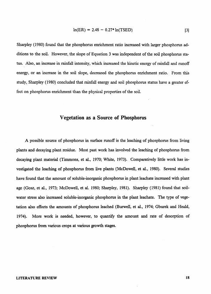
ln(ER) = 2.48 - 0.27"' ln(TSED) [3]

Sharpley ( 1980) found that the phosphorus enrichment ratio increased with larger phosphorus ad-

ditions to the soil. However, the slope of Equation 3 was independent of the soil phosphorus sta-

tus. Also, an increase in rainfall intensity, which increased the kinetic energy of rainfall and runoff

energy, or an increase in the soil slope, decreased the phosphorus enrichment ratio. From this

study, Sharpley (1980) concluded that rainfall energy and soil phosphorus status have a greater ef-

fect on phosphorus enrichment than the physical properties of the soil.

Vegetation as a Source of Phosphorus

A possible source of phosphorus in surface runoff is the leaching of phosphorus from living

plants and decaying plant residue. Most past work has involved the leaching of phosphorus from

decaying plant material (Timmons, et al., 1970; White, 1973). Comparatively little work has in-

vestigated the leaching of phosphorus from live plants (McDowell, et al., 1980). Several studies

have found that the amount of soluble-inorganic phosphorus in plant leachate increased with plant

age (Gosz, et al., 1973; McDowell, et al. 1980; Sharpley, 1981). Sharpley (1981) found that soil-

water stress also increased soluble-inorganic phosphorus in the plant leachate. The type of vege-

tation also effects the amounts of phosphorus leached (Burwell, et al., 1974; Gburek and Heald,

1974). More work is needed, however, to quantify the amount and rate of desorption of

phosphorus from various crops at various growth stages.


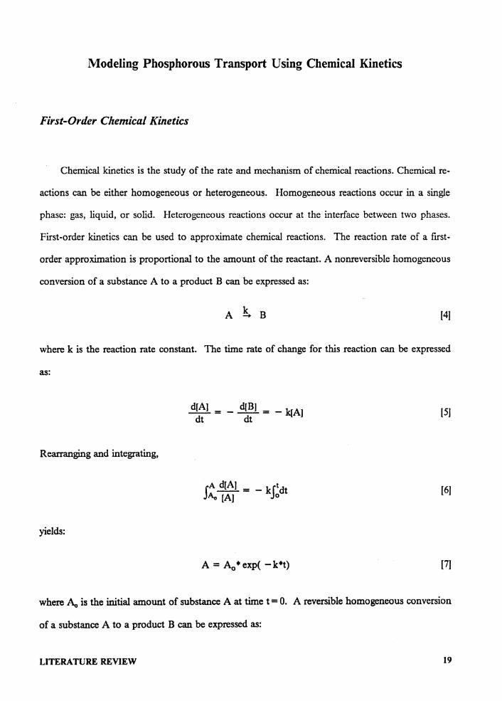
Modeling Phosphorous Transport Using Chemical Kinetics

First-Order Chemical Kinetics

Chemical kinetics is the study of the rate and mechanism of chemical reactions. Chemical re-

actions can be either homogeneous or heterogeneous. Homogeneous reactions occur in a single

phase: gas, liquid, or solid. Heterogeneous reactions occur at the interface between two phases.

First-order kinetics can be used to approximate chemical reactions. The reaction rate of a first-

order approximation is proportional to the amount of the reactant. A nonreversible homogeneous

conversion of a substance A to a product B can be expressed as:

A t B [4)

where k is the reaction rate constant. The time rate of change for this reaction can be expressed

as:

[5)

Rearranging and integrating,

[6)

yields:

[7]

where Ao is the initial amount of substance A at time t = 0. A reversible homogeneous conversion

of a substance A to a product B can be expressed as:


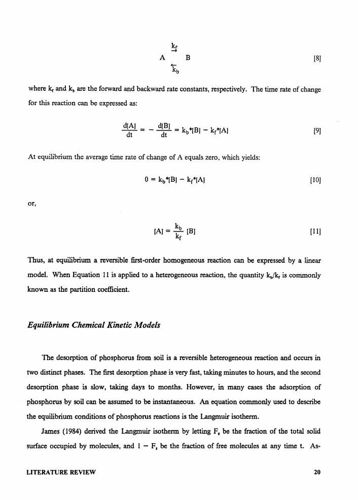
A B [8]

where k, and kb are the forward and backward rate constants, respectively. The time rate of change

for this reaction can be expressed as:

At equilibrium the average time rate of change of A equals zero, which yields:

or,

k [AJ = .....2... [BJ

kr

(9)

(10)

(11)

Thus, at equilibrium a reversible first-order homogeneous reaction can be expressed by a linear

model. When Equation 11 is applied to a heterogeneous reaction, the quantity kb/k, is commonly

known as the partition coefficient.

Equilibrium Chemical Kinetic Models

The desorption of phosphorus from soil is a reversible heterogeneous reaction and occurs in

two distinct phases. The first desorption phase is very fast, taking minutes to hours, and the second

desorption phase is slow, taking days to months. However, in many cases the adsorption of

phosphorus by soil can be assumed to be instantaneous. An equation commonly used to describe

the equilibrium conditions of phosphorus reactions is the Langmuir isotherm.

James (1984) derived the Langmuir isotherm by letting F1 be the fraction of the total solid

surface occupied by molecules, and 1 - FI be the fraction of free molecules at any time t. As-


suming that the rate at which the molecules are adsorbed is proportional to the available surface

area, and that the rate of desorption is proportional to the surface covered yields:

I 121

dNd -- = k2•F dt s

(13)

where k1 and k2 are the adsorption and desorption rate constants, respectively, C is the concen-

tration of absorbent in solution, and N1 and Nd are the number of molecules adsorbed and

desorbed, respectively. At equilibrium, the average time rate of change equals zero, which yields:

(14)

Which can be rearranged to:

[15]

Letting b = ki/k2, and multiplying through by a rate constant, k, gives:

[ 16]

The Langmuir equation is often written in the form (Tchobanoglous and Schroeder, 1985):

[17]

where xis the mass of material adsorbed (adsorbate) on the solid phase in grams, mis the mass

of solid (adsorbent) on which adsorption occurs in grams, c. is the equilibrium concentration of

adsorbate in mg/L, Q0 is the adsorption maximum in grams of phosphorus per g of soil, and b is

an empirical constant in L/mg.


The Langmuir equation was initially derived to describe the adsorption of gases by solids

(Langmuir, 1918). The equation is valid for a monomolecular layer and assumes a constant energy

of adsorption, which is independent of surface coverage. The equation also assumes no interaction

between adsorbate molecules, and that a maximum adsorption exists when the reactive adsorbent

surface of the monomolecular layer is filled. The coefficients Q0 and b may be estimated exper-

imentally, or from general relationships developed by Ryden, et al. (1972):

Q0 = -3.5 + 10.7*(percent clay) + 49.S*(percent organic C) [18]

b = 0.061 + 169832 x 10·PH + 0.027*(percent clay) + 0.76*(percent organic C) (19]

The major advantage of the Langmuir isotherm is that the equation has an adsorption maxi-

mum, and can thus be used to describe the adsorption capacity of soil for phosphorus. However,

the Langmuir equation assumes a constant energy of adsorption with increasing surface coverage,

which is not likely to occur in nature. However, according to Bohn, et al. (1979), in some cases

as the reaction sites are filled the energy of adsorption decreases, and the interaction of the

adsorbent molecules increases. These two effects tend to cancel each other, which results in an

approximately constant energy of adsorption. On a practical basis, when the Langmuir equation

applies, it is limited to the range of the experimental data.

Another commonly used adsorption equation, developed by Freundlich (1926), can be ex-

pressed as (Tchobanoglous and Schroeder, 1985):

..!.. = K+cl/n m e (20]

where K and n are an empirical coefficients.

The Freundlich equation assumes that the energy of adsorption decrease logarithmically as the

reactive adsorption surface increases, which is due to the surface heterogeneity. The Freundlich

equation has fit experimental data very well for a wide variety of conditions. This may be due to

transforming the data by the natural logarithm, which is only appropriate when the coefficient of

variation is constant throughout the data. When the coefficient of variation is not constant, trans-


forming the data by the natural logarithm masks the variability, resulting in an apparent better fit.

Even when the logarithmic transformation is appropriate, this does not ensure accuracy, especially

when extrapolating beyond the range of the data, because the equation does not predict a finite

surface adsorption maximum.

Nonequilihrium Chemical Kinetic Models

The desorption of sediment-bound phosphorus is important in the modeling of phosphorus

desorption from the soil surface to surface runoff. By assuming that phosphorous desorption from

the soil to surface runoff is diffusion controlled, Sharpley, et al. (1981a) developed a desorption

equation of the form:

(21)

where Pd is the cumulative phosphorus desorbed in µg phosphorus/g soil, P0 is the initial amount

of desorbable phosphorus in µg/g soil, t is contact time in minutes, WS is the water to soil ratio in

L/kg, and K, a, and p are empirical constants. The parameters K, a, and Pin Equation 21 are

dependant on the soil characteristics, and can be estimated experimentally in the lab. Sharpley

( 1983) developed general expressions for estimating these parameters using 43 different acid soils

from across the United States, which correlate the parameters to the clay and organic carbon con-

tent of the soil. The expressions are:

LITERATURE REVIEW

KL= 1.327*(percent clay/organic C)-o.so 6

KB = 0.732*(percent clay/organic C)- 0•748

a = 0.779*(percent clay/organic q- 0•526

p = 0.143*(percent clay/organic C) +0. 4 t 9

[22)

[23]

[24]

[25)

23

where KL is the coefficient K corresponding to labile phosphorus status of the soil measured using

isotrophic dilution with 32P (Sharpley, 1983), and K8 is the coefficient K corresponding to Bray-Pl

available soil phosphorus status, measured using procedures from Bray and Kurtz ( 1945).

Sharpley, et al. (1981a) and Ahuja, et al. (1982) developed an expression to describe the rate

of phosphorous desorption by taking the derivative of Equation 21 with respect to time, which

yields:

Letting,

dPd = dt

(26]

[27]

where dPd/dt is the time rate of change of phosphorus desorbed in µg phosphorus/g soil/sec, C is

the concentration of soluble phosphorus in runoff in mg/L, EDI is the effective depth of interaction

in mm, I is the rainfall intensity in mm/min, and Pb is the soil bulk density in g/cm3• Solving for

the phosphorous concentration in solution yields:

(28)

The desorption of phosphorus from the soil surface into surface runoff is initiated by turbulent

mixing caused by raindrop impact and overland flow. In Equation 28, EDI represents the thin layer

of soil that interacts with rainfall to release soluble phosphorus into solution. For the conditions

studied, Sharpley (1985) found EDI to range from 1.3 to 37 mm. Ahuja, et al (1981) used 32P, a

relatively immobile tracer, to determine the depth of interaction for phosphorous desorption. They

found that EDI increased with time, and concluded that EDI was more dependant on the storm

duration, than on the soil type. In a similar study using a bromide tracer, Ahuja and Lehman (1983)

found that the contribution of chemicals released into surface runoff decreased exponentially with

soil depth. Sharpley (1985) found that EDI increased exponentially with increasing slope, increased


linearly with increasing rainfall intensity, and found that these increases were independent of soil

type. Sharpley (1985) and Sharpley, et al. (1981a) found that the degree of soil aggregation also

effected EDI, as well as the magnitude of the effect of rainfall intensity and slope on EDI. Sharpley

(1985) found that EDI was not related to the degree of aggregation when wheat straw was incor-

porated into the soil, and found that as the percent cover increased, EDI decreased. Ahuja (1982)

also found that soil cover decreased EDI.

Ahuja and Lehman (1983) hypothesized that the transport mechanism of phosphorus to sur-

face runoff is a turbulent diffusion process caused by rainfall impact. This mechanism implies that

as the hydraulic conductivity of the soil increases, the depth of phosphorus contribution from the

soil increases, along with the total amount transferred. In addition, as the canopy and ground cover

increase, the amount of phosphorus transferred decreases. A general expression for estimating EDI

was developed by Sharpley ( 1985) over a wide range of rainfall and management practices, and is

given as:

ln(EDI) = - 3.130 + 0.071 •(soil aggregation) + 0.576•1n(soil loss) [29]

On a practical note, when modeling the desorption process EDI is usually assumed constant.

As Sharpley (1985) points out, a constant EDI is a simplification of a complex physio-chemical

process, and will not exist over an entire watershed under normal conditions. However, for many

applications a constant EDI must still be used until more complex quantitative expressions for EDI

are developed.

LITERATURE REVIEW 2S

MODEL DEVELOPMENT

The ANSWERS model was chosen to incorporate the phosphorous transport model because

the model is deterministic with modular component process subroutines. It is, therefore, a relatively

straight forward task to add additional subroutines to the model, and does not require recalibration

of other components of the model. In addition, the sediment transport and hydrologic portions

of the model have been extensively tested and verified on watersheds in Illinois, Indiana, Iowa,

Ohio, Oklahoma, Texas, Virginia, Pennsylvania, and Ontario, Canada. The ANSWERS model is

also well suited for simulating the effects of changing topography, land use, and soil type on

sediment yields and the particle size distribution of eroded sediment.

A block diagram of the proposed model is shown in Figure 3. The model, as presented in the

following sections, accounts for the desorption of soluble inorganic phosphorus from the soil sur-

face into surface runoff, the transport of sediment-bound phosphorus, and the equilibrium between

the soluble and sediment-bound phases. The model is written in FORTRAN 77 with its equations

in the finite-difference form. A list of the variables and a computer program listing are given in

Appendices A and B, respectively.

Sediment Transport Model

The transport of sediment in and out of each overland flow element and channel segment in

ANSWERS is modeled in SUBROUTINE SEO. Version 4.840815 of ANSWERS used in this

research includes an extended sediment transport model, developed by Dillaha (1981), which sim-

MODEL DEVELOPMENT 26

Rainfall

, , Soil Surface

Sediment Soluble-P Detachment Diffusion

' , Adsorption ,, Sediment-Bound Soluble-P P Transported Desorption Transported in by Sediment - Surf ace Runoff

-, , ' , Sediment-Bound Soluble-P

P Deposition Infiltration

, , Receiving Waters

Figure 3. Block diagram of the phosphorus transport model.


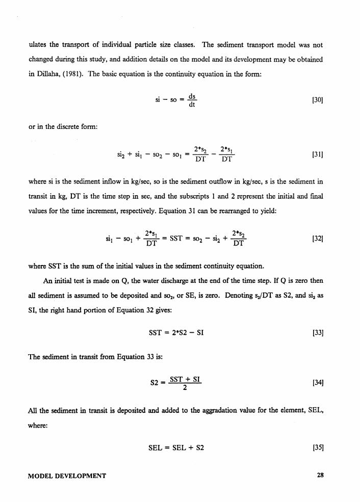
ulates the transport of individual particle size classes. The sediment transport model was not

changed during this study, and addition details on the model and its development may be obtained

in Dillaha, (1981). The basic equation is the continuity equation in the form:

or in the discrete form:

si - so= .4§.. dt

. . 2*s2 2*s1 s12 + s11 - so2 - so1 = -- - --DT DT

(30]

(31]

where si is the sediment inflow in kg/sec, so is the sediment outflow in kg/sec, s is the sediment in

transit in kg, DT is the time step in sec, and the subscripts 1 and 2 represent the initial and final

values for the time increment, respectively. Equation 31 can be rearranged to yield:

. • 2*s1 ST . 2*s2 Slt - SOt + -- = S = SO2 - Sl2 + --DT DT

[32)

where SST is the sum of the initial values in the sediment continuity equation.

An initial test is made on Q, the water discharge at the end of the time step. If Q is zero then

all sediment is assumed to be deposited and so2, or SE, is zero. Denoting s2/DT as S2, and si2 as

SI, the right hand portion of Equation 32 gives:

SST = 2*S2 - SI

The sediment in transit from Equation 33 is:

52 = SST+ SI 2

[33)

[34]

All the sediment in transit is deposited and added to the aggradation value for the element, SEL,

where:

SEL = SEL + S2 [35]


For the next time period, outflow and storage are zero, thus SST can be calculated as:

SST= SI [36]

These calculations are repeated for each particle size class separately.

If Q is positive the detachment rates, DETR and DETF, are calculated as (Dillaha, 1981;

Beasley, 1977; Wischemeir, 1969):

DETR = 6.539 x 106*CDR *SKDR *R2

AREA2

DETF = 1.05l*CDR*SKDR*SL*Q*DX

[37]

[38]

where DETF is the sediment detachment rate due to overland flow in kg/sec, DETR is the sediment

detachment rate due to rainfall impact in kg/sec, CDR and SKDR are the Cand K factors as de-

fined in the USLE, R is the rainfall intensity in m3 /sec, AREA2 is the elemental area in m2, SL is

the slope steepness in m/m, Q is the discharge in m 3 /sec, and DX is the flow width in m. The

model then branches depending upon whether washload or larger particles are being routed.

For the washload particles the maximum available inflow rate, DS, is:

DS = SI+ F*(DETR + DETF) (39]

where F is the fraction of particles of class i in the detached sediment. The sediment in transit at

the end of the time period, S2 is:

s2 = SST+ DS 1 + _g_ s

(40]

where S is the volume of stored water in the element per unit time at the beginning of the time

increment.

Equation 40 was derived from Equation 31, the continuity equation as follows. The conti-

nuity equation can be expressed as:


SST = SE - DS + S2 [41]

where SE = so2, DS = si2 and S2 is redefined as 2*s2/DT. SE can be calculated as the product of

the sediment concentration and the outflow rate or:

SE= s2*0 s [42]

where s = S*DT/2, the storage volume at the end of the time increment. Substituting for s2 and s

in Equation 42 and simplifying yields:

SE= S2*Q s [43]

This equation is then substituted into Equation 41 which is then rearranged to give Equation 40.

The aggradation value, SELm, for the element m is:

SELm = SELm - F*(DETR + DETF) [44]

This process is repeated for each washload particle class.

Equations 40, 39, and 43 also are used to find SE for larger sediment particles. The transport

capacity, TF, is then calculated and compared with SE. If TF is less than SE, there is a potential

transport deficit unless transport capacity is available from other particle classes.

If TF is greater than or equal to SE then the transport excess, TF-SE, is summed for all par-

ticle size classes with TF greater than SE to get the total transport excess, TFXCES. The value

of each TF is then set equal to SE. If there is any transport excess, it is divided between the particle

size classes with potential deficits according to the following equation:

TF = TF + TFXCES*DELTA SDEL

[45]

where DELTA is the amount of sediment in transport for particle class i, and SDEL is the total

sediment transportability. SDEL is calculated as the sum of all particle classes with potential defi-


cits. This process is repeated until all the transport excess has been distributed among the particle

size classes.

The new transport capacity of each of the larger particle size classes is then compared with SE

again. If TF equals SE, maximum rainfall and flow detachment occur and there is no deposition.

The sediment is then routed using Equations 39, 40, and 43.

If SE is greater than TF, the potential exists for deposition. TF is then compared with SE!,

the value of SE with only rainfall detachment included. If TF is less than SEl then deposition

occurs and there is no flow detachment. The potential amount of deposition for particle class i,

DP, is:

DP= RE•(SEl - TF)

where RE, the fraction of particles of particle class i depositing, is calculated as:

RE = FV* AREA2 Q

[46]

(47]

where FV is the fall velocity of particle size class i in m/s. The new sediment discharge rate, SE,

from the element is SEI-DP. The sediment is then routed using the following form of Equation

41:

SST= SE - si2 + S•SE Q

(48]

where DS has been replaced by si2 and S2 was replaced by a rearranged form of Equation 42.

Equation 48 can be rearranged to give:

212 = SE*(l + S/Q) - SST (49]

where 212, or si2, is the rate of sediment movement inflow plus erosion at the end of the time step.

The accumulation on, or loss of sediment from the element is then the difference between the total

sediment inflow, 212, and the inflow from adjacent elements, SI. The amount of deposition (or

aggradation) is then calculated as:


SELm = SELm + SI - 212 (50)

and SST, for the next time period, is derived from the left half of Equation 32 as:

SST= 212 + SE•(S/Q - 1) [51)

where so1 = SE, si1 = 212, and s1 = s1 since the end of the current time step is the beginning of the

next time step.

If TF is greater than SEl;, but less than SE2, the value of SE with both rainfall and flow

detachment, then flow detachment is allowed to occur until the sediment load and transport ca-

pacity are equal.

The basic assumptions of the sediment transport model are (Dillaha, 1981):

1. The particle size distribution of detached sediment is the same as the weight fraction

of the soil particles in the original soil mass (no enrichment during detachment).

2. Rainfall detachment is not limited by the transport capacity of the flow or by flow

inundation.

3. Flow detachment occurs if there is excess transport capacity and can never exceed the

transport capacity excess.

4. Deposition and flow detachment never occur at the same time for the same particle size

class.

5. Washload transport is independent of the transport capacity of the flow and does not

influence the transport of the larger particles.

6. Deposited sediment requires the same amount of energy as in the original detachment

to become redetached.

7. Enrichment is controlled by the deposition process.

8. The rate at which a particle will deposit is proportional to its fall velocity.

9. Channel erosion does not occur.

10. Subsurface or tile drainage produces no sediment.


Sediment-Bound Phosphorus Transport Model

Sediment-bound phosphorus transport for an individual element is derived from the

sediment transport model, and is in SUBROUTINE PSED. Initially the phosphorus content

of the transported sediment at the beginning of the time interval is calculated as:

and

PTl = PI SI

PT2 = PSTOLD STOLD

[52}

[53}

where PTl and PT2 are the phosphorus contents of the incoming sediment and the sediment

in transit, respectively, at the beginning of the time interval in kg phosphorus/kg soil, PI is the

incoming phosphorus at the beginning of the time interval in kg, PSTOLD is the phosphorus

in storage at the beginning of the time interval, and STO LD is the sediment in storage at the

beginning of the time interval.

An initial test is made on the discharge at the end of the time interval, Q2. If Q2 is equal

to zero, then the sediment-bound phosphorus at the end of the time interval, PE, is assumed

to deposit, and set to zero. The sediment-bound phosphorus in transit, P2, is calculated as:

P2 = STNEW•PT [54}

with

PT = PTl + PT2 (55] 2

where PT is the average phosphorus content of the sediment. This sediment-bound

phosphorus is deposited and added to the phosphorus aggradation value, PSELm, for element

m where:


[56]

Next, newly transported sediment that is detached during the time interval, SEDNEW,

is calculated. If there is maximum rainfall and flow detachment of sediment with no deposi-

tion, SEDNEW is calculated as:

SEDNEW = F*(DETR + DETF) [57)

However, with rainfall and partial or no flow detachment of sediment, SEDNEW is calculated

as:

SEDNEW = 212 - SI

If NEWSED is zero, then PE is calculated from:

with

PT= PTl + PT2 2

(58]

[59]

[60]

If NEWSED is greater than zero, then the amount of newly generated sediment-bound

phosphorus, PG, is calculated from:

PG= P0*SEDNEW (61]

where PO is the sediment-bound phosphorus content of the original soil for particle class i.

PE and PT are calculated as:

PT= PI+ PSTOLD + PG SEDNEW +SI+ STOLD

[62]

and


PE= PT*SE (63]

The sediment-bound phosphorus aggradation value is then calculated from:

PSELm = PSELm - PG (64]

These calculations are repeated for each sediment particle size class separately.

The sediment-bound phosphorus content of the original soil for particle class i, P0j, is

calculated by first assuming that the sediment-bound phosphorus is distributed throughout the

sediment in proportion to the specific surface area of the particles, such that:

PSSA = P0SOIL x 10- 9

SSAT (65]

where PSSA is the phosphorus content of the soil in kg/m2, P0SOIL is the total phosphorus

content for the original soil in µg phosphorus/g soil, and SSAT is the specific surface area of

the original soil in m2/g. P01 is then calculated as:

P0i = SSAi*PSSA (66]

where SS.Ai is the specific surface area for particle class i.

The basic assumptions of the sediment-bound phosphorus transport model are:

1. The sediment transport model and its assumptions are appropriate.

2. Sediment-bound phosphorus is distributed throughout the soil particles in proportion

to the specific surface area of the soil particles.

3. Eroded soil has the properties of the element from which the soil is eroded.


Soluble Phosphorus Transport

Model Development

The phosphorus desorption Equation 21 developed by Sharpley, et al. (1981a), was cho-

sen to model the desorption of sediment-bound phosphorus to inorganic soluble phosphorus

in surface runoff .. Equation 21 was selected because recent work (Sharpley, 1983; Sharpley et

al., 1981a) has shown that the phosphorus desorption process is highly dependent on contact

time, the water to soil ratio, and the initial soil phosphorus level. Equation 21 can be rewritten

as:

[67)

where Pext is the initial extractable phosphorus level of the soil in µg/g soil, tis the contact time

in minutes, WS is the water to soil ratio in L/kg, and Kext• a, P , and y are empirical constants.

The empirical constants were determined experimentally for the two soils used in verifying

the phosphorus transport model. The first soil was a Groseclose silt loam taken from the

Prices Fork Research Farm in Blacksburg, Virginia. The soil was a composite sample taken

from the top 10 cm of the soil profile from around the experimental plots. The second soil,

a Suffolk sandy loam, was also a composite sample from the top 10 cm of the soil profile, and

was taken from the Nomini Creek watershed in Westmoreland County, Virginia. A summary

of the physical properties of the two soil samples are given in Table 1. The extractable K,

Ca, Mg, and percent organic matter tests were performed by the Soil Testing and Plant Anal-

ysis Laboratory at Virginia Polytechnic Institute and State University, Blacksburg, Virginia.

The particle distributions were measured using the pipette method (Day, 1965), and the soil

pH was measured with a glass electrode using a 1:1 soil to solution ratio made with a 0.0lM

CaC12 solution.


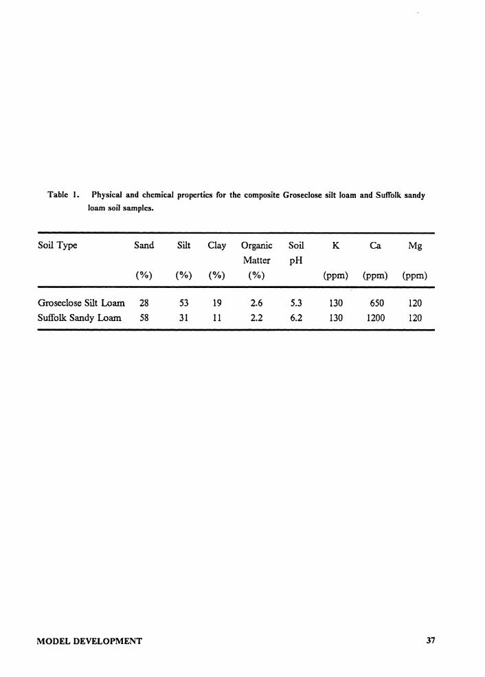
Table 1. Physical and chemical properties for the composite Groseclose silt loam and Suffolk sandy loam soil samples.

Soil Type Sand Silt Clay Organic Soil K Ca Mg Matter pH

(%) (%) (%) (%) (ppm) (ppm) (ppm)

Groseclose Silt Loam 28 53 19 2.6 5.3 130 650 120 Suffolk Sandy Loam 58 31 11 2.2 6.2 130 1200 120


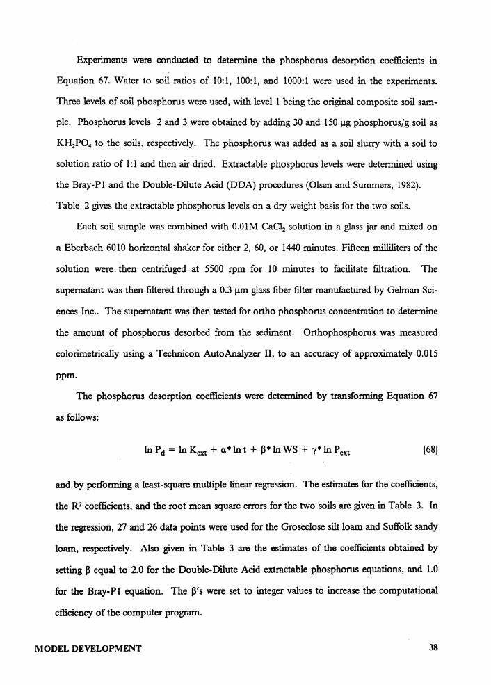
Experiments were conducted to determine the phosphorus desorption coefficients in

Equation 67. Water to soil ratios of 10:1, 100:1, and 1000:1 were used in the experiments.

Three levels of soil phosphorus were used, with level 1 being the original composite soil sam-

ple. Phosphorus levels 2 and 3 were obtained by adding 30 and 150 µg phosphorus/g soil as

KH2PO4 to the soils, respectively. The phosphorus was added as a soil slurry with a soil to

solution ratio of 1:1 and then air dried. Extractable phosphorus levels were determined using

the Bray-Pl and the Double-Dilute Acid (DDA) procedures (Olsen and Summers, 1982).

Table 2 gives the extractable phosphorus levels on a dry weight basis for the two soils.

Each soil sample was combined with 0.0lM CaC12 solution in a glass jar and mixed on

a Eberbach 6010 horizontal shaker for either 2, 60, or 1440 minutes. Fifteen milliliters of the

solution were then centrifuged at 5500 rpm for 10 minutes to facilitate filtration. The

supernatant was then filtered through a 0.3 µm glass fiber filter manufactured by Gelman Sci-

ences Inc.. The supernatant was then tested for ortho phosphorus concentration to determine

the amount of phosphorus desorbed from the sediment. Orthophosphorus was measured

colorimetrically using a Technicon AutoAnalyzer II, to an accuracy of approximately 0.015

ppm.

The phosphorus desorption coefficients were determined by transforming Equation 67

as follows:

168]

and by performing a least-square multiple linear regression. The estimates for the coefficients,

the R2 coefficients, and the root mean square errors for the two soils are given in Table 3. In

the regression, 27 and 26 data points were used for the Groseclose silt loam and Suffolk sandy

loam, respectively. Also given in Table 3 are the estimates of the coefficients obtained by

setting~ equal to 2.0 for the Double-Dilute Acid extractable phosphorus equations, and 1.0

for the Bray-Pl equation. The Ws were set to integer values to increase the computational

efficiency of the computer program.


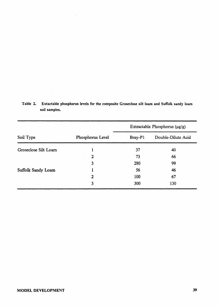
Table 2. Extactable phosphorus levels for the composite Groseclose silt loam and Suffolk sandy loam soil samples.

Extractable Phosphorus (µg/g)

Soil Type Phosphorus Level Bray-Pl Double-Dilute Acid

Groseclose Silt Loam l 37 40 2 73 66 3 280 99

Suffolk Sandy Loam 1 56 46 2 100 67 3 300 130


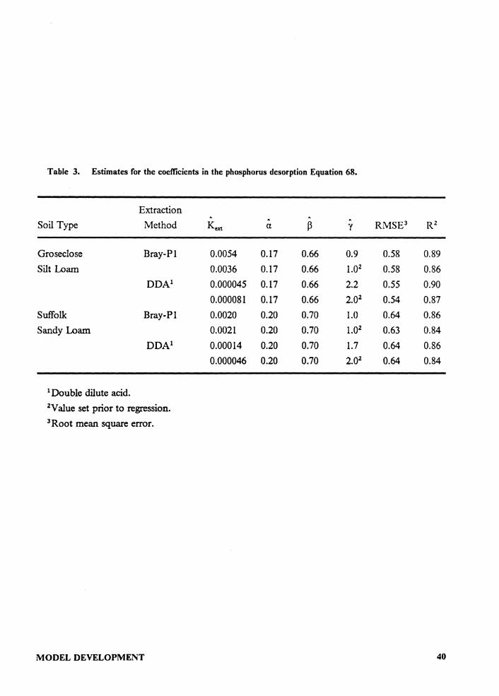
Table 3. Estimates for the coefficients in the phosphorus desorption Equation 68.

Extraction A

Soil Type Method Kext a A

y RMSE 3 R2

Groseclose Bray-Pl 0.0054 0.17 0.66 0.9 0.58 0.89 Silt Loam 0.0036 0.17 0.66 1.02 0.58 0.86

DDA 1 0.000045 0.17 0.66 2.2 0.55 0.90 0.000081 0.17 0.66 2.02 0.54 0.87

Suffolk Bray-Pl 0.0020 0.20 0.70 1.0 0.64 0.86 Sandy Loam 0.0021 0.20 0.70 1.02 0.63 0.84

DDA 1 0.00014 0.20 0.70 1.7 0.64 0.86 0.000046 0.20 0.70 2.02 0.64 0.84

1 Double dilute acid. 2V alue set prior to regression. 3 Root mean square error.


Soluble Phosphorus Transport Model

Natural sources of soluble inorganic phosphorus in surface runoff include: precipitation,

living and decomposing plant material, soil water, and soil particles. Soluble phosphorus from

precipitation and the water in the soil matrix was assumed to be negligible. Soluble

phosphorus from living and decomposing plant material was not incorporated into the model

due to the lack of available information on the amount and rate of desorption of phosphorus

from different crops at various growth stages.

The primary source of soluble phosphorus was assumed to be from the soil particles at

the soil surface. During a storm event surface runoff can be divided into three distinct periods.

1. Period I: Infiltration rate exceeds the rainfall rate, and surface runoff and storage are

zero.

2. Period II: Surface storage occurs, but surface runoff is zero.

3. Period III: Surface runoff and surface storage both occur.

During period I when the infiltration rate exceeds the rainfall rate, the outflow rate, PSO2, in kg/sec

is zero.

When the rainfall rate exceeds the infiltration rate, phosphorus will be desorbed from the soil

surface into the rainfall excess according to Equation 28. The concentration of the phosphorus in

the rainfall excess, CGEN in kg/m3, is calculated as:

with

and

CGEN = CGENl •wsBETA+TIME(ALPHA-1) SSTOR

MODEL DEVELOPMENT

[69]

[70)

41

WS = l000*SSTOR DETR+ DETF [71)

where WS is the water to soil ratio in L/kg, ALPHA, BETA, IGAM, and PK are constants for a

given soil, TIME is the contact time between the rainfall excess and the soil surface in minutes,

EXTP is the extractable phosphorus level for the soil in element m in µg phosphorus/g soil, BD

is the bulk density of the soil in g/cml , and SSTOR is the runoff in transit at the end of the time

interval in ml/ sec. TIME is calculated as:

with

and

TIME= FLOWL 60*OFVEL

s OFVEL = DX*DEP

DEP = S*DT DX2

(72]

(73]

[74)

where FLOWL is the length of flow prior to concentrated flow in meters, OFVEL is the overland

flow velocity in m/s, S is the runoff volume in transit at the start of the time increment in m3 /s, and

DEP is the uniform depth of flow over the element in meters. The rate of soluble phosphorus

desorption from the soil to surface storage and surface runoff, PSG, in kg/sis calculated as:

PSG = CGEN*QGEN [75)

QGEN = R - FIL [76)

where R is the net rainfall rate in m3/s, and FIL is the inftltration rate in ml/ sec.


In period II the outflow is still zero, but storage is occurring within the element. Letting

PSS NEW be the soluble phosphorus in transit at the end of the time increment in kg/s, PSS NEW

can be calculated as:

PSSNEW = PSI+ PSSOLD + PSG *SSTOR QI+ QS + QGEN [77]

where PSI is the inflow of soluble phosphorus at the beginning of the time increment in kg/s,

PSSOLD is the soluble phosphorus in transit at the beginning of the time increment, QI is the

runoff inflow at the beginning of the time increment in m 3 /s, and QS is the runoff in transit at the

beginning of the time increment in m3 /s.

During period III the runoff outflow rate is greater than zero. Assuming that the concentration

of soluble phosphorus outflow and the soluble phosphorus in transit at the end of the time interval

are equal, the resulting concentration, CPS02, in kg/m3 can be calculated as:

CPS0 2 = PSI+ PSSOLD + PSG QI+ QS + QGEN

The outflow soluble phosphorus rate, PS02, can be calculated as:

PS02 = CPS02*Q2

[78]

[79]

where Q2 is the runoff outflow rate at the end of the time increment in m3 /s. PSSNEW can then

be calculated as:

PSSNEW = CPS02*SSTOR [80)

For periods II and III, the accumulated amount of net soluble phosphorus from the element,

PPSEL, is calculated as:

PSSEL = PSSEL - PSG [81]

The basic assumptions of the soluble phosphorus model are:


1. Precipitation, living and decomposing plant material, and the soil water are negligible

sources of soluble phosphorus.

2. The soil matrix is an infinite sink for infiltrating phosphorus.

3. The phosphorus level in the soil remains constant during a storm event.

4. The phosphorus desorption process is diffusion controlled.

Equilibrium Phosphorus Adsorption/Desorption Process

Model Development

The Langmuir isotherm given in Equation 17 was chosen to describe the equilibrium condi-

tions between the sediment-bound and soluble phosphorus phases. The Langmuir isotherm was

selected due to its good fit with lower soluble phosphorus concentrations. The adsorption maxi-

mum, Q0 , and the empirical constant, b, were determined experimentally for the Groseclose silt

loam and the Suffolk sandy loam described previously. The experimental procedure was the same

as the nonequilibrium phosphorus desorption equation, except that the samples were shaken for

24 hours. In addition to the original composite soil samples, the two soils were separated into two

fractions, course and fine, by dry sieving with a #400, 0.037 mm opening, sieve after breaking up

the aggregates with a rubber tipped pestle and mortar. Soil pH was measured as described previ-

ously, and the total phosphorus content of the soils were determined using a perchloric acid digest

(Sommers and Nelson, 1972; Murphy and Riley, 1962). The results are given in Table 4.

Equilibrium phosphorus concentrations were determined experimentally for various condi-

tions. The soluble initial phosphorus concentration consisted of 0.0, 0.1, or 1.0 ppm as KH2PO4•

The tests were performed with water to soil ratios of 10: 1, 100: 1, and 1000: 1, for each of the soil

fractions. The final ortho phosphorus concentration was determined as previously described.


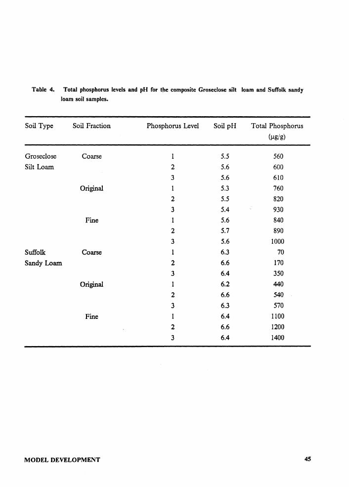
Table 4. Total phosphorus levels and pH for the composite Groseclose silt loam and Suffolk sandy loam soil samples.

Soil Type Soil Fraction Phosphorus Level Soil pH Total Phosphorus (µg/g)

Groseclose Coarse I 5.5 560 Silt Loam 2 5.6 600

3 5.6 610 Original l 5.3 760

2 5.5 820 3 5.4 930

Fine l 5.6 840 2 5.7 890 3 5.6 1000

Suffolk Coarse l 6.3 70 Sandy Loam 2 6.6 170

3 6.4 350 Original l 6.2 440

2 6.6 540 3 6.3 570

Fine I 6.4 1100 2 6.6 1200 3 6.4 1400


Knowing the initial sediment-bound phosphorus level, the initial and final concentrations of soluble

phosphorus, the final sediment-bound phosphorus was calculated.

There are several forms the Langmuir isotherm can take to estimate its coefficients. The most

common method is to linearize the equation as follows:

[82)

A linear least-square regression was performed to estimate Q0 and b for each of the three particle

fractions separately. The results are given in Table 5, and Figure 4 shows the equation for the

original Groseclose silt loam fraction with its 95 percent confidence intervals. It is important to

note that Ce occurs on both sides of Equation 82, and since Ce and x/m are possitively correlated,

the variance of the regression is reduced. Thus, the true variability of the data is not apparent.

An alternative approach is too perform a least-square linear regression using the following

form:

[83)

The results of this regression are given in Table 6, and Figure 5 shows the equation for the original

Groseclose silt loam soil fraction with its 95 percent confidence intervals.

The third approach was to use a nonlinear regression scheme on Equation 17. The Marquardt

nonlinear regression technique was used on each of the three soil fractions for the two soils, with

initial parmameter estimates obtained from Table 5. The results are given in Table 7, and

Figure 6 shows the equation for the original Groseclose silt loam soil fraction with its 95 percent

confidence intervals.

A summary of the estimated coefficients for the three models is given in Table 8. The type

of model used to estimate the coefficients has a large impact on the b coefficient, and to a lesser

degree on Q0 • For the linear regressions, estimates for the inverse and the inverse of the products

of the coefficients are being estimated, and not the coefficients. However, with the nonlinear re-

gression, the coefficients are being estimated directly. Even though nonlinear regression techniques


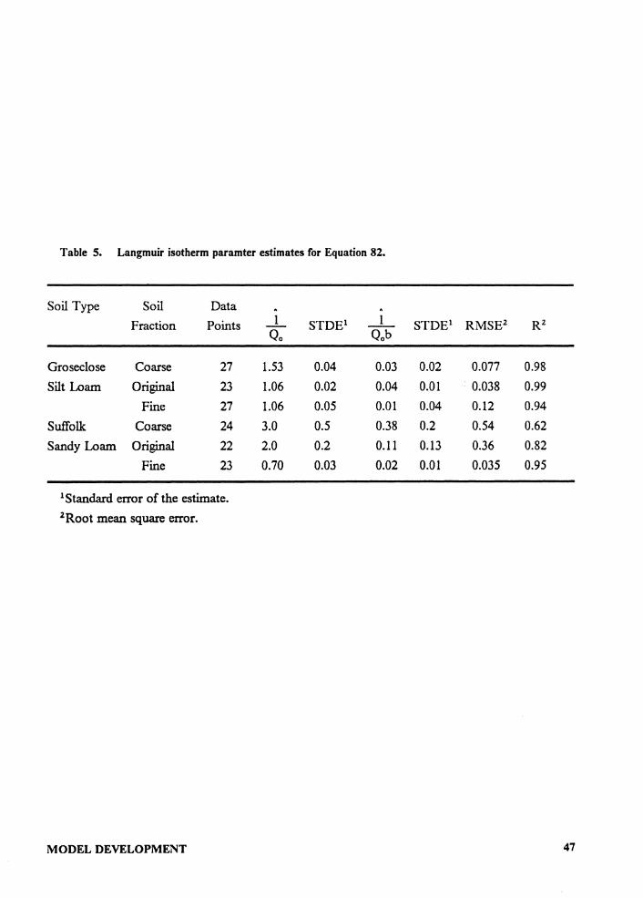
Table 5. Langmuir isotherm paramter estimates for Equation 82.

Soil Type Soil Data Fraction Points 1 STDE 1 1 STDE 1 RMSE 2 Rz

Oo Oob

Groseclose Coarse 27 1.53 0.04 0.03 0.02 0.077 0.98 Silt Loam Original 23 1.06 0.02 0.04 0.01 0.038 0.99

Fine 27 1.06 0.05 0.01 0.04 0.12 0.94 Suffolk Coarse 24 3.0 0.5 0.38 0.2 0.54 0.62 Sandy Loam Original 22 2.0 0.2 0.11 0.13 0.36 0.82

Fine 23 0.70 0.03 0.02 0.01 0.035 0.95

1 Standard error of the estimate. 2Root mean square error.


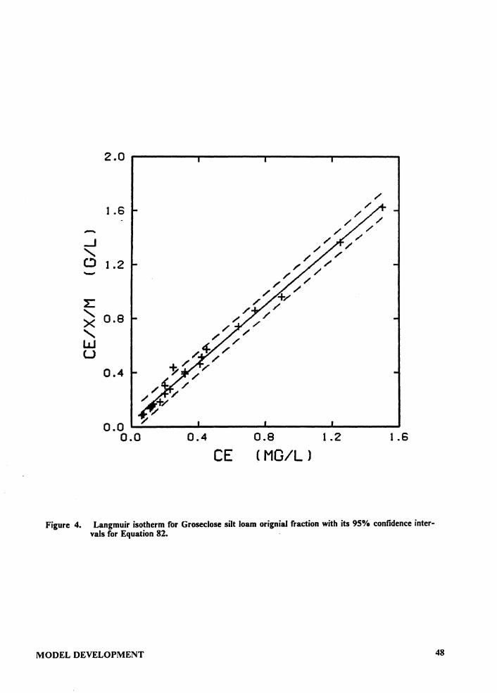
2.0

/

J.6

-_J

' CJ 1.2 -l:: T/

' 0.8 X

' w u 0.4

0.0 7

0.0 0.4 0.8 1.2 1.6

CE CMG/Ll

Figure 4. Langmuir isotherm for Groseclose silt loam orignial fraction with its 95% confidence inter-vals for Equation 82.


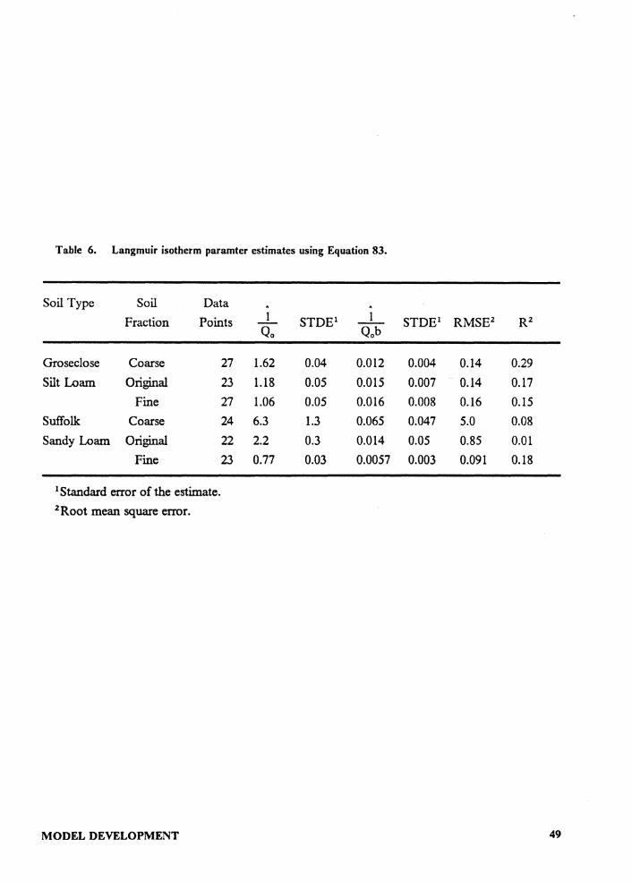
Table 6. Langmuir isotherm paramter estimates using Equation 83.

Soil Type Soil Data Fraction Points 1 STDE 1 1 STDE 1 RMSE 2 R2

Oo Oob

Groseclose Coarse 27 1.62 0.04 0.012 0.004 0.14 0.29 Silt Loam Original 23 1.18 0.05 0.015 0.007 0.14 0.17

Fine 27 1.06 0.05 0.016 0.008 0.16 0.15 Suffolk Coarse 24 6.3 1.3 0.065 0.047 5.0 0.08 Sandy Loam Original 22 2.2 0.3 0.014 0.05 0.85 0.01

Fine 23 0.77 0.03 0.0057 0.003 0.091 0.18

1 Standard error of the estimate. 2 Root mean square error.


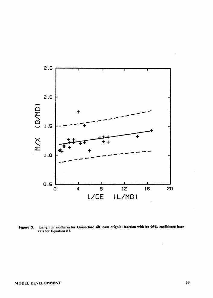
2.5

2.0 -C) l:

' C) ....... 1.5

X

' l: 1.0

0.5 0

+ ---------- ---_..,.. .... - + ..+

•:I= I + 1t ++ ++ -=It-.flt.+ + .,. ---- --__ __.------.. --

4

----

8

1/CE 12

CL/MGJ 16 20

Figure 5. Langmuir isotherm for Groseclose silt loam orignial fraction with its 950/o confidence inter-vals for Equation 83.


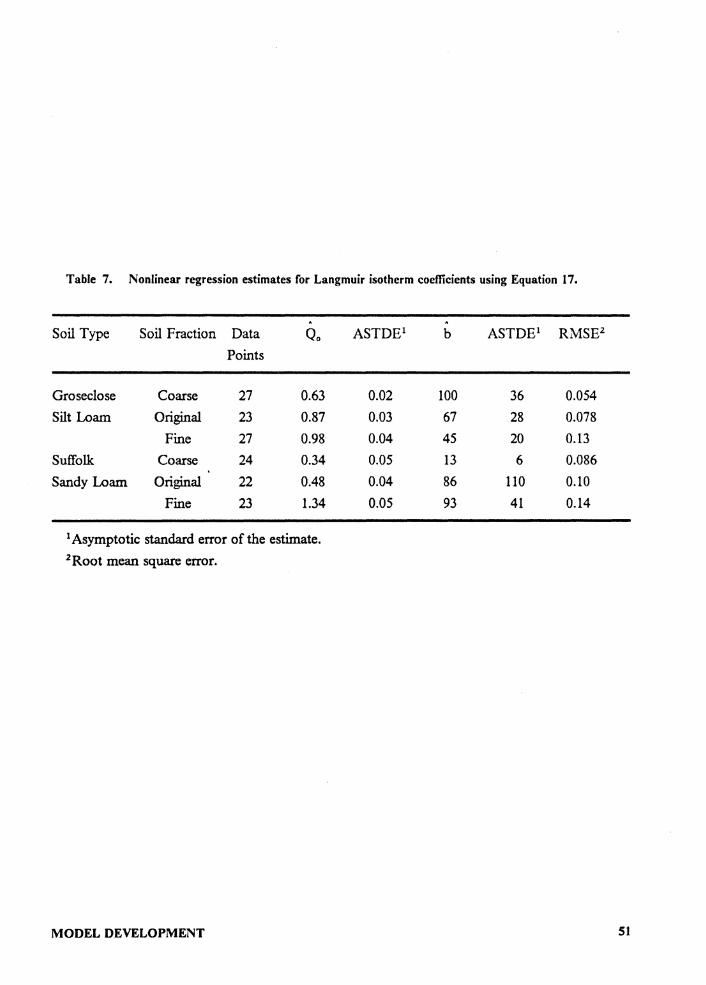
Table 7. Nonlinear regression estimates for Langmuir isotherm coefficients using Equation 17.

Soil Type Soil Fraction Data Oo ASTDE 1 b ASTDE 1 RMSE 2

Points

Groseclose Coarse 27 0.63 0.02 100 36 0.054 Silt Loam Original 23 0.87 0.03 67 28 0.078

Fine 27 0.98 0.04 45 20 0.13 Suffolk Coarse 24 0.34 0.05 13 6 0.086 Sandy Loam Original 22 0.48 0.04 86 110 0.10

Fine 23 1.34 0.05 93 41 0.14

1 Asymptotic standard error of the estimate. 2 Root mean square error.


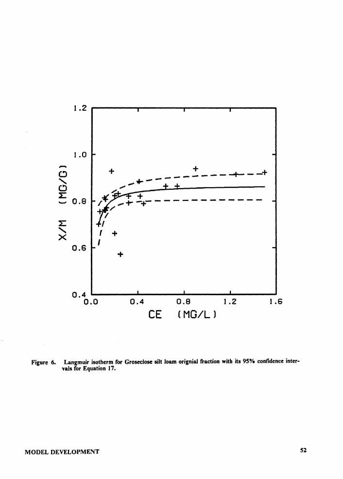
1.2 ,------.----------...-----

-C)

' C) 2: -2:

' X

1.0

0.8

0.6

0.4 0.0

+

0.4 0 .8 1 .2 1.6

CE CMG/Ll

Figure 6. Langmuir isotherm for Groseclose silt loam orignial fraction with its 95% confidence inter-vals for Equation 17.


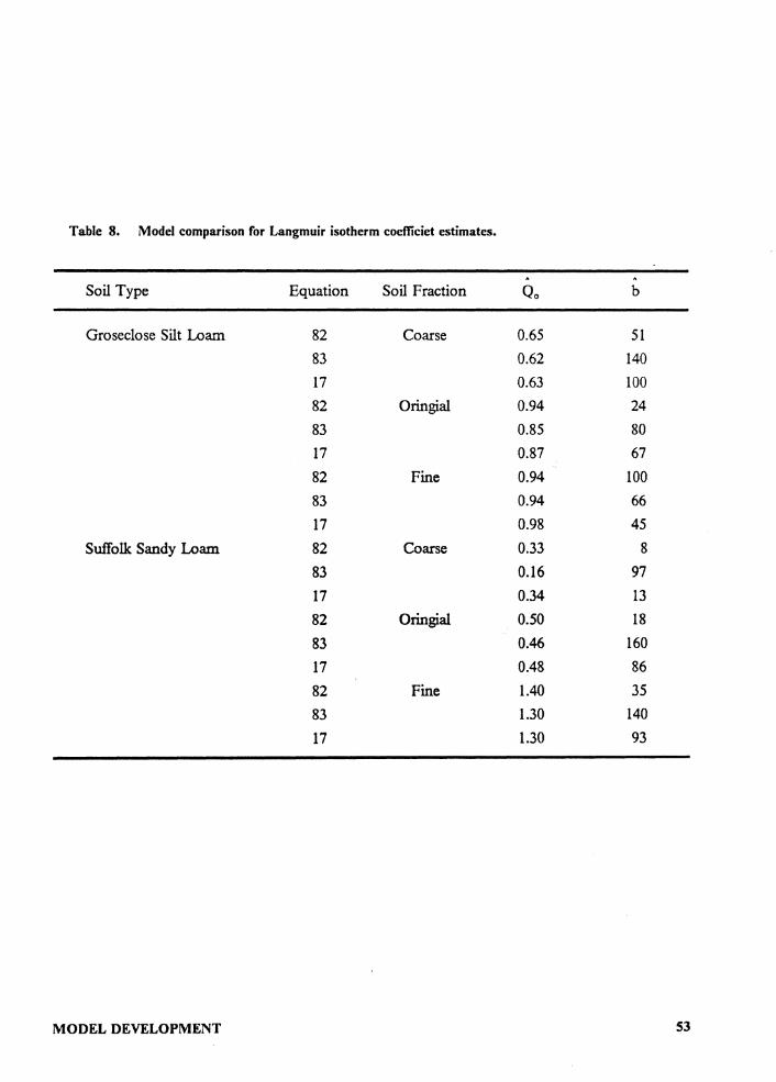
Table 8. Model comparison for Langmuir isotherm coefficiet estimates.

Soil Type Equation Soil Fraction Oo b

Groseclose Silt Loam 82 Coarse 0.65 51 83 0.62 140 17 0.63 100 82 Oringial 0.94 24 83 0.85 80 17 0.87 67 82 Fine 0.94 100 83 0.94 66 17 0.98 45

Suffolk Sandy Loam 82 Coarse 0.33 8 83 0.16 97 17 0.34 13 82 Oringial 0.50 18 83 0.46 160 17 0.48 86 82 Fine 1.40 35 83 1.30 140 17 1.30 93

MODEL DEVELOPMENT S3

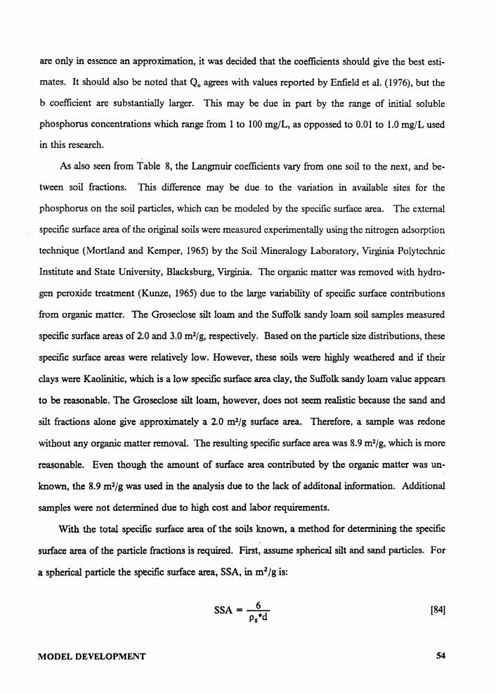
are only in essence an approximation, it was decided that the coefficients should give the best esti-

mates. It should also be noted that Q0 agrees with values reported by Enfield et al. (1976), but the

b coefficient are substantially larger. This may be due in part by the range of initial soluble

phosphorus concentrations which range from 1 to 100 mg/L, as oppossed to 0.01 to 1.0 mg/L used

in this research.

As also seen from Table 8, the Langmuir coefficients vary from one soil to the next, and be-

tween soil fractions. This difference may be due to the variation in available sites for the

phosphorus on the soil particles, which can be modeled by the specific surface area. The external

specific surface area of the original soils were measured experimentally using the nitrogen adsorption

technique (Mortland and Kemper, 1965) by the Soil Mineralogy Laboratory, Virginia Polytechnic

Institute and State University, Blacksburg, Virginia. The organic matter was removed with hydro-

gen peroxide treatment (Kunze, 1965) due to the large variability of specific surface contributions

from organic matter. The Groseclose silt loam and the Suffolk sandy loam soil samples measured

specific surface areas of 2.0 and 3.0 m2/g, respectively. Based on the particle size distributions, these

specific surface areas were relatively low. However, these soils were highly weathered and if their

clays were Kaolinitic, which is a low specific surface area clay, the Suffolk sandy loam value appears

to be reasonable. The Groseclose silt loam, however, does not seem realistic because the sand and

silt fractions alone give approximately a 2.0 m2/g surface area. Therefore, a sample was redone

without any organic matter removal. The resulting specific surface area was 8.9 m2/g, which is more

reasonable. Even though the amount of surface area contributed by the organic matter was un-

known, the 8.9 m2/g was used in the analysis due to the lack of additonal information. Additional

samples were not determined due to high cost and labor requirements.

With the total specific surface area of the soils known, a method for determining the specific

surface area of the particle fractions is required. First, assume spherical silt and sand particles. For

a spherical particle the specific surface area, SSA, in m2 /g is:

[84)


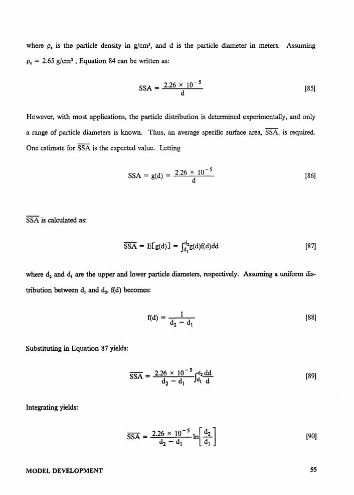
where p1 is the particle density in g/cm.3, and d is the particle diameter in meters. Assuming

p1 = 2.65 g/cm3 , Equation 84 can be written as:

2.26 X 10-S SSA = ~;;..;;,___.;; ___ _ d

[85)

However, with most applications, the particle distribution is determined experimentally, and only

a range of particle diameters is known. Thus, an average specific surface area, SSA, is required.

One estimate for SSA is the expected value. Letting

SSA is calculated as:

2.26 X 10-S SSA= g(d) = ..;;;.=...;;;..__..;;;..;;._

d

SSA = E[g(d)] = s::g(d)f(d)dd

[86)

[87]

where(½ and d1 are the upper and lower particle diameters, respectively. Assuming a uniform dis-

tribution between d1 and (½, f( d) becomes:

[88)

Substituting in Equation 87 yields:

[89)

Integrating yields:

[90]

MODEL DEVELOPMENT ss

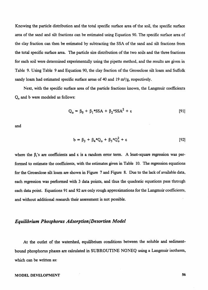
Knowing the particle distribution and the total specific surface area of the soil, the specific surface

area of the sand and silt fractions can be estimated using Equation 90. The specific surface area of

the clay fraction can then be estimated by subtracting the SSA of the sand and silt fractions from

the total specific surface area. The particle size distribution of the two soils and the three fractions

for each soil were determined experimentally using the pipette method, and the results are given in

Table 9. Using Table 9 and Equation 90, the clay fraction of the Groseclose silt loam and Suffolk

sandy loam had estimated specific surface areas of 40 and 19 m2/g, respectively.

Next, with the specific surface area of the particle fractions known, the Langmuir coefficients

Q0 and b were modeled as follows:

[91]

and

[92]

where the P/s are coefficients and & is a random error term. A least-square regression was per-

formed to estimate the coefficients, with the estimates given in Table 10. The regression equations

for the Groseclose silt loam are shown in Figure 7 and Figure 8. Due to the lack of available data,

each regression was performed with 3 data points, and thus the quadratic equations pass through

each data point. Equations 91 and 92 are only rough approximations for the Langmuir coefficients,

and without additional research their assessment is not possible.

Equilibrium Phosphorus Adsorption/ Desortion Mode[

At the outlet of the watershed, equilibrium conditions between the soluble and sediment-

bound phosphorus phases are calculated in SUBROUTINE NONEQ using a Langmuir isotherm,

which can be written as:


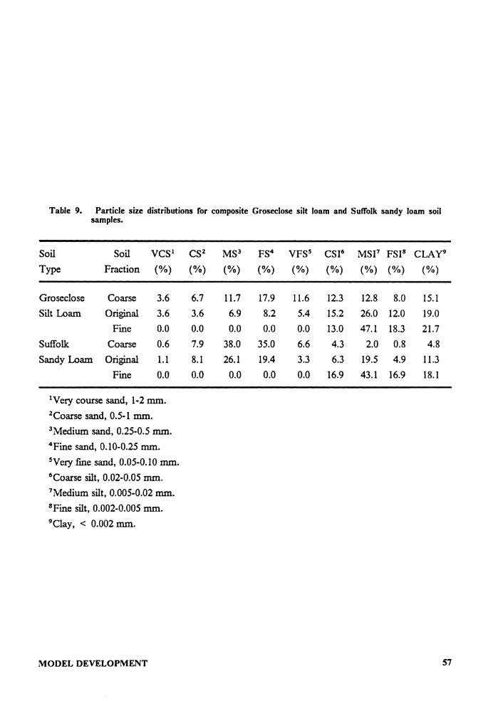
Table 9. Particle size distributions for composite Groseclose silt loam and Suffolk sandy loam soil samples.

Soil Soil vcs1 cs2 MS3 FS4 VFS 5 CSl 6 MSF FSl 8 CLAY 9

Type Fraction (%) (%) (%) (%) (%) (%) (%) (%) (%)

Groseclose Coarse 3.6 6.7 11.7 17.9 11.6 12.3 12.8 8.0 15. 1 Silt Loam Original 3.6 3.6 6.9 8.2 5.4 15.2 26.0 12.0 19.0

Fine 0.0 0.0 0.0 0.0 0.0 13.0 47.1 18.3 21.7 Suffolk Coarse 0.6 7.9 38.0 35.0 6.6 4.3 2.0 0.8 4.8 Sandy Loam Original 1.1 8.1 26.l 19.4 3.3 6.3 19.5 4.9 11.3

Fine 0.0 0.0 0.0 0.0 0.0 16.9 43.1 16.9 18. 1

1Very course sand, 1-2 mm. 2 Coarse sand, 0.5-1 mm. 3 Medium sand, 0.25-0.5 mm. 4 Fine sand, 0.10-0.25 mm. 5Very fine sand, 0.05-0.10 mm. 6 Coarse silt, 0.02-0.05 mm. 7 Medium silt, 0.005-0.02 mm. 8 Fine silt, 0.002-0.005 mm. 9 Clay, < 0.002 mm.


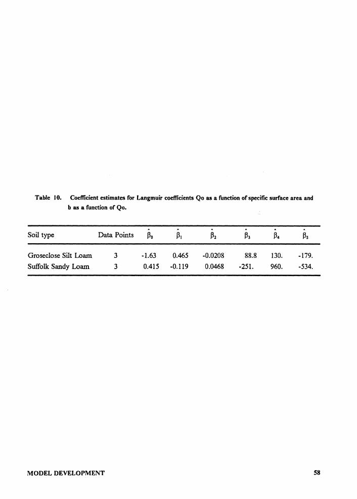
Table IO. Coefficient estimates for Langmuir coefficients Qo as a function of specific surface area and b as a function of Qo.

. Soil type Data Points Po P1

Groseclose Silt Loam 3 -1.63 0.465 Suffolk Sandy Loam 3 0.415 -0.119

MODEL DEVELOPMENT

-0.0208 0.0468

88.8 -251.

130. 960.

Ps

-179. -534.

58

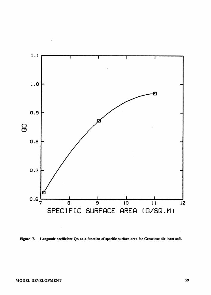
0 C,

1.0

0.9

0.8

0.7

8 9 10

SPECIFIC SURFACE AREA 1 1

CG/SQ.Ml 12

Figure 7. Langmuir coefficient Qo as a function of specific surface area for Grosclose silt loam soil.


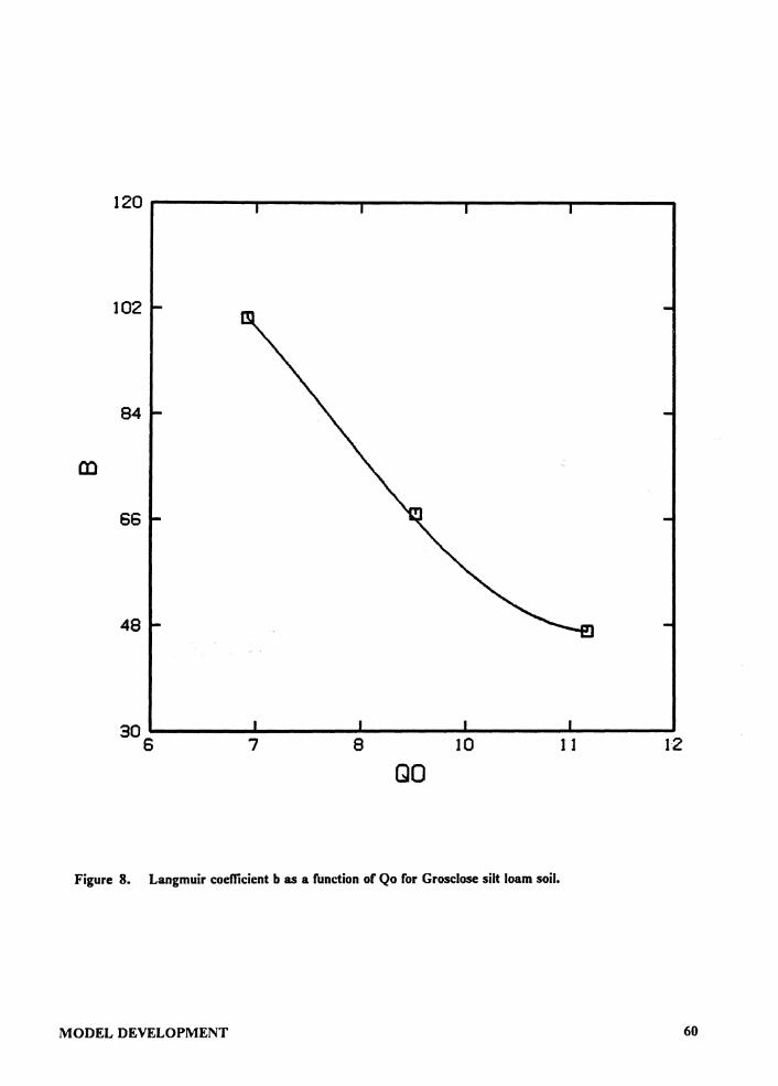
102

84

66

48

30 ---------------------------6 7 8 10 1 1 12

QO

Figure 8. Langmuir coefficient b as a function of Qo for Grosclose silt loam soil.


or rewritten as:

PO+ DELP SEDT

PO+ DELP SEDT

= QO"'BO"'(CO - DELP) V + BO"'(CO - DELP)

[93]

[94]

where PO is the initial sediment-bound phosphorus in mg, DELP is the amount of phosphorus

moving between phases, QO is an adsorption maximum constant, BO is an empirical constant, CO

is the initial soluble phosphorus in mg, and V is the volume of flow in liters. To solve for the

equilibrium conditions, DELP must be determined. Equation 94 can be rewritten as a quadratic

equation:

where

and

B = PO - l - CO - SEDT"'QO BO

Using the quadratic formula, the appropriate solution for DELP was found to be:

[95)

[96]

[97]

[98]

The equilibrium sediment-bound phosphorus, PF, and the equilibrium soluble phosphorus, CF,

are calculated as:


PF= PO+ DELP (99)

and

CF= CO - DELP (100)

The coefficients Q0 and BO are estimated from:

Q0 = Q0Cl + Q0C2*SSASED + Q0C3*SSASED2 (101)

and

BO= B0Cl + B0C2*Q0 + B0C3*Q02 (102)

where SSASED is the specific surface area of the transported sediment in m2/g, and Q0Cl, Q0C2,

Q0C3, B0Cl, B0C2, and B0C3 are constants. SSASED is calculated as:

SSASED = SA0 2 SEDT

(103)

where SAO2 is the transported sediment surface area outflow at the end of the time interval. To

avoid potential errors in determining Q0 and BO, SSASED is bounded by a minimum allowable

specific surface area, SSAMIN, and a maximum specific surface area, SSAMAX.

The surface area of the sediment in transit for an individual element is calculated in SUB-

ROUTINE SACAL and is derived from the continuity equation which can be expressed as:

or written in a discrete form as:

MODEL DEVELOPMENT

sai - sao = dsa dt

(104]

[105]

62

where sai is the surface area of the sediment inflow in m2 /sec, sao is the surface area of sediment

outflow in m2/sec, sa is the surface area of sediment in transit in m2, DT is the time step in sec, and

the subscripts 1 and 2 represent the initial and final values for the time increment, respectively.

Rearranging Equation 105 yields:

[106]

where SAT is the sum of the initial values for the sediment surface area continuity equation.

When the discharge, Q, from an element is zero, all sediment in the element is assumed to be

deposited and the sediment surface area outflow, sao2 = 0 .

sa2/DT = SA2 , Equation 106 becomes:

Letting sai2 = SAi and

SAT = 2"'SA2 - SAi

and the surface area of sediment in transit, SA2, can be calculated from Equation 107 as:

SA2 = SAT+ SAi 2

[107]

[108]

The surface area of sediment in storage, SA2, is deposited. For the next time interval the outflow

and storage are zero, and SAT= SAi.

When the discharge, Q, from an element is greater than zero, Equation 106 becomes:

SAT = sao2 - sai2 + 2"'SA2 [109]

The surface area of sediment inflow at the end of the time step can be expressed as:

sai2 = SAi + SAG [110]

where SAG is the sediment surface area from the newly transported sediment from the element

during the time interval in m2/ sec , and is calculated as:


NPART SAG= L SSAi"'SEDNEWi [l llj

i= 1

where SSA is the specific surface area of the original soil for particle class i for the element in

kg/m2• If SA2 is zero, then SAO2 is calculated from:

SAO2 =SAT+ SAI + SAG (112)

When SA2 > 0, sao2 = SAO2, and assuming the specific surface area of SAO2 and SA2 are equal

yields:

or,

SAO2 = SA2 SET S2T

SAO2 = SA2*SET S2T

(113]

[ 114)

where S2T and SET are the sediment in transit and the sediment outflow at the end of the time step

and are calculated as:

NPART S2T = L STNEWi

i=l

NPART SET= L SEi

i= 1

Combining Equations II0, 111, and ll4 with Equation 109 yields:

SAT = SA2*SET - SAI - SAG + 2•SA2 S2T

and solving for SA2 yields:

SA2 = l.+[sA T + SA + SAG - SA2*SET ] 2 S2T

MODEL DEVELOPMENT

(115)

[116]

[117]

[118]

64

SA02 is then calculated form Equation 114. For the next time step SAT becomes:

SAT= SAi + SAG - SA02 + 2*SA2 I 1191

MODEL DEVELOPMENT 6S

MODEL VERIFICATION

The ultimate test of a mathematical model is a comparison of the simulated and observed re-

sponses of the physical system to a variety of input conditions. To evaluate the effectiveness of the

model developed in this research, the model's predictions are compared with observed sediment,

soluble phosphorus, and sediment-bound phosphorus yields from rainfall simulator plot studies.

Plot Descriptions and Data Collection

A field study in the fall of 1985 at the Prices Fork Research farm in Blacksburg, Virginia was

conducted to validate the phosphorus transport model. The plots used in the analysis included two

conventional disk plowed plots, and two no-till plots planted in winter rye. Conventional till and

no-till plots were used in the verification process to simulate the extremes of conditions expected

to be encountered in future applications of the model. All four plots were 5.5 meters (18 feet) wide

and 18.3 meters (60 feet) long. The no-till plots, plots 1 and 6, had average slopes of 6.2 and 11

percent, respectively. The conventional tillage plots, plots A and D, had average slopes of 6.3 and

6.5 percent, respectively.

A rainfall simulator (Shanholtz et al., 1981; Neff, 1979) was used to produce runoff which

transported phosphorus and sediment. Three runs were made on each plot. The first run was 60

minutes; runs 2 and 3 were 30 minutes with 30 minutes between runs, and were made 24 hours after

run 1. For each plot the rainfall was measured with 12 volumetric rain gauges, and runoff was

measured with a 15 cm (6 inch) H-flume. A summary of the rainfall simulator average intensities,

MODEL VERIFICATION 66

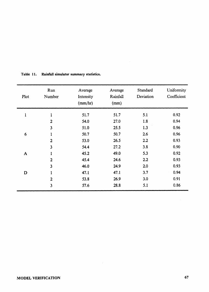
Table I I. Rainfall simulator summary statistics.

Run Average Average Standard Uniformity Plot Number Intensity Rainfall Deviation Coefficient

(mm/hr) (mm)

1 1 51.7 51.7 5.1 0.92 2 54.0 27.0 1.8 0.94 3 51.0 25.5 1.3 0.96

6 1 50.7 50.7 2.6 0.96

2 53.0 26.5 2.2 0.93

3 54.4 27.2 3.8 0.90

A 1 45.2 49.0 5.3 0.92

2 45.4 24.6 2.2 0.93

3 46.0 24.9 2.0 0.93

D 1 47.1 47.1 3.7 0.94

2 53.8 26.9 3.0 0.91

3 57.6 28.8 5.1 0.86


rainfall volumes, and uniformity coefficients is given in Table 11.

The winter rye planted in Plots 1 and 6 was killed with paraquat prior to the runs, and the

plant residue measured after run 3 was 3400 and 1900 kg/ha for plots 1 and 6, respectively. Soil

moisture and soil samples used for nutrient measurements were taken before and after each run to

a depth of 30 cm at 5 cm intervals. Bray-Pl and Double-Dilute Acid extractable phosphorus, and

total phosphorus were determined as previously described for the 0-5 cm samples. A summary of

this data is given in Table 12.

Plot Simulations

The first step in creating the required data base for the plot simulations was to divide each plot

into uniform square elements. Due to the shape of the plots, 5 square elements with 3.66 m (12

feet) sides were chosen. Thus, for comparative purposes the observed nutrient, runoff volume, and

sediment yields were reduced by 33 percent.

The next step in the simulation was to calibrate the predicted runoff hydrographs of the AN-

SWERS model to the observed data. The runoff hydrographs were calibrated in an attempt to

minimize the effects of differences in surface runoff on phosphorus transport. This allowed a more

accurate evaluation of the phosphorus transport model by reducing the effects of surface runoff.

During the calibration process, the observed runoff hydrographs and rainfall intensies were assumed

accurate, and were not altered. Antecedent soil moisture was also assumed accurate, however it

was necessary to assume the downslope elements had higher moisture contents to match the ob-

served runoff hydrographs. Surface roughness, crop constants, and drainage and groundwater

constants were estimated as recommended by Beasley and Huggins ( 1981 ). Field capacity estimates

were obtained from Shanholtz and Lillard (1968).

The ANSWERS model uses a form of Holtan's infiltration equation (Holtan, 1961; Overton,

1965) given as:


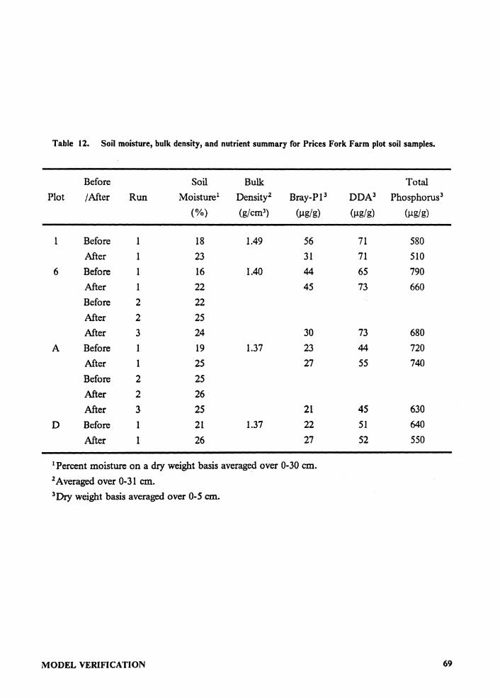
Table 12. Soil moisture, bulk density, and nutrient summary for Prices Fork Farm plot soil samples.

Before Soil Bulk Total Plot /After Run Moisture 1 Density2 Bray-Pl 3 DDA 3 Phosphorus 3

(%) (g/cm 3) (µg/g) (µg/g) (µg/g)

1 Before 18 1.49 56 71 580 After 1 23 31 71 510

6 Before 1 16 1.40 44 65 790 After 1 22 45 73 660 Before 2 22 After 2 25 After 3 24 30 73 680

A Before 1 19 1.37 23 44 720 After 1 25 27 55 740 Before 2 25 After 2 26 After 3 25 21 45 630

D Before 1 21 1.37 22 51 640 After 1 26 27 52 550

1 Percent moisture on a dry weight basis averaged over 0-30 cm. 2Averaged over 0-31 cm. 3Dry weight basis averaged over 0-5 cm.


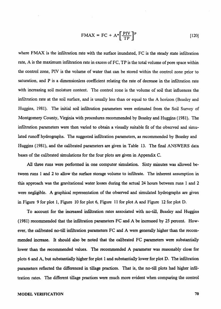
[1201

where FMAX is the infiltration rate with the surface inundated, FC is the steady state infiltration

rate, A is the maximum infiltration rate in excess of FC, TP is the total volume of pore space within

the control zone, PIV is the volume of water that can be stored within the control zone prior to

saturation, and P is a dimensionless coefficient relating the rate of decrease in the infiltration rate

with increasing soil moisture content. The control zone is the volume of soil that influences the

infiltration rate at the soil surface, and is usually less than or equal to the A horizon (Beasley and

Huggins, 1981). The initial soil infiltration parameters were estimated from the Soil Survey of

Montgomery County, Virginia with procedures recommended by Beasley and Huggins (1981). The

infiltration parameters were then varied to obtain a visually suitable fit of the observed and simu-

lated runoff hydrographs. The suggested infiltration parameters, as recommended by Beasley and

Huggins (1981), and the calibrated parameters are given in Table 13. The final ANSWERS data

bases of the calibrated simulations for the four plots are given in Appendix C.

All three runs were performed in one computer simulation. Sixty minutes was allowed be-

tween runs 1 and 2 to allow the surface storage volume to infiltrate. The inherent assumption in

this approach was the gravitational water losses during the actual 24 hours between runs 1 and 2

were negligible. A graphical representation of the observed and simulated hydrographs are given

in Figure 9 for plot l, Figure 10 for plot 6, Figure 11 for plot A and Figure 12 for plot D.

To account for the increased infiltration rates associated with no-till, Beasley and Huggins

(1981) recommended that the infiltration parameters FC and A be increased by 25 percent. How-

ever, the calibrated no-till infiltration parameters FC and A were generally higher than the recom-

mended increase. It should also be noted that the calibrated FC parameters were substantially

lower than the recommended values. The recommended A parameter was reasonably close for

plots 6 and A, but substantially higher for plot 1 and substantially lower for plot D. The infiltration

parameters reflected the differenced in tillage practices. That is, the no-till plots had higher infil-

tration rates. The different tillage practices were much more evident when comparing the control


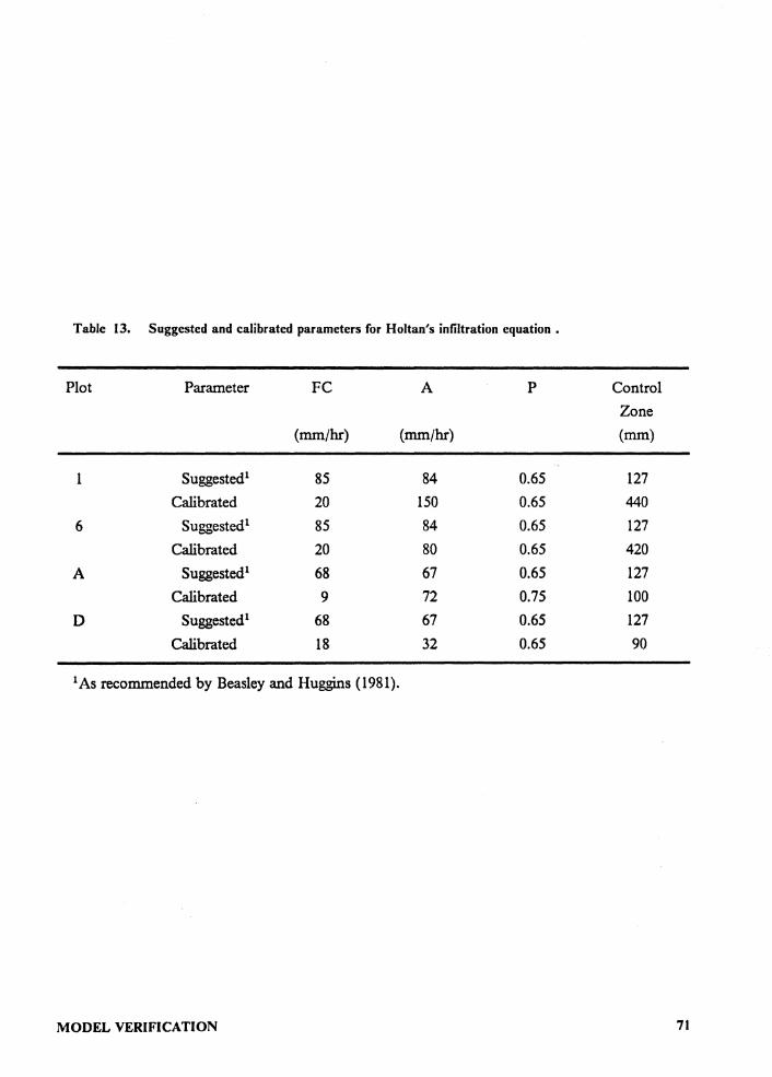
Table 13. Suggested and calibrated parameters for Holtan's infiltration equation .

Plot Parameter FC A p Control Zone

(mm/hr) (mm/hr) (mm)

1 Suggested1 85 84 0.65 127 Calibrated 20 150 0.65 440

6 Suggested1 85 84 0.65 127 Calibrated 20 80 0.65 420

A Suggested1 68 67 0.65 127 Calibrated 9 72 0.75 100

D Suggested1 68 67 0.65 127 Calibrated 18 32 0.65 90

1As recommended by Beasley and Huggins (1981).


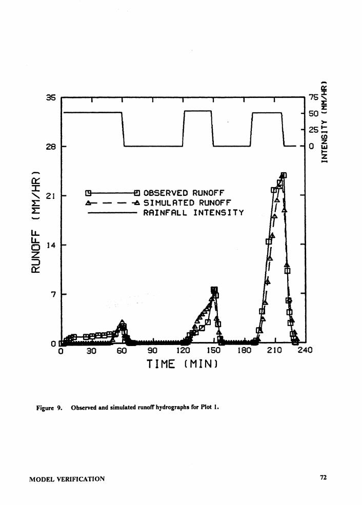
.... 35 75~ :z: :z:

\ I \ so-

I L >-25 !:

(J)

28 o z I.LI I-z --0:: :c C!3 l:!J OBSERVED RUNOF'f' ' 21

l: A- -- -!!. SIMULATED RUNOFF' :I: RAINF'ALL INTENSITY -LL LL 14 0 z ::) 0::

7

0 0 30 60 90 120 150 180 210 240

TIME CMINJ

Figure 9. Observed and simulated runoff hydrographs for Plot 1.


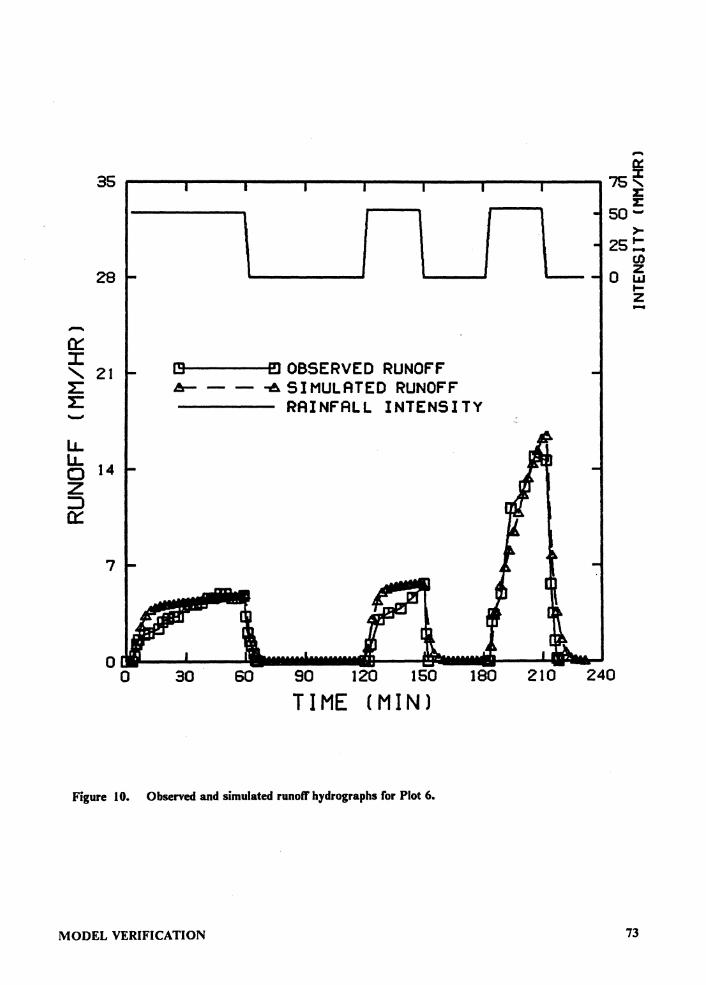
..... 0:

35 75~ 2: 2:

\ I \ I L so->-

25 !: rJ)

28 0 z uJ t-z --0::: :c CJ E!l OBSERVED RUNOFF ' 21 -- -6 SIMULATED RUNOFF

RAINFALL INTENSITY ...... LL LL 14 0 z ::) 0:::

7

90 120 150 180 240

TIME (MIN)

Figure 1 0. Observed and simulated runoff hydrographs for Plot 6.


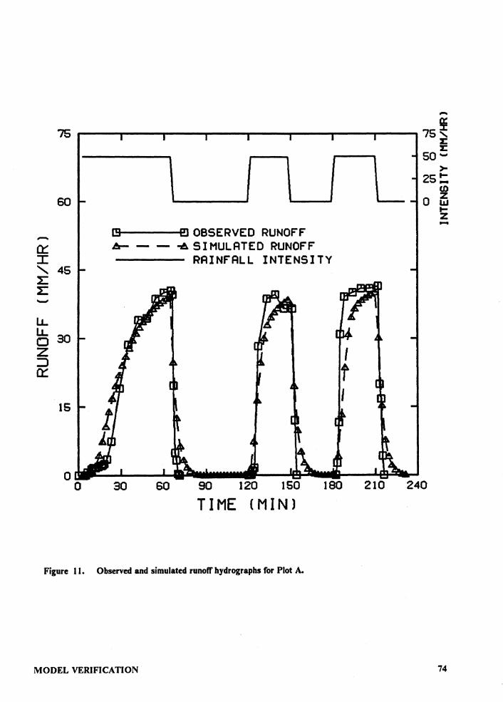
75

60 \ I \ I - [9 EJ OBSERVED RUNOFF ct: A- - - -1!. SI MULATEO RUNOFF I RAINFALL INTENSITY

' 45 :I: :I: -LL LL 30 0 z ct:

15

0 0 30 60 90 120 150

TIME (MINl

Figure 11. Observed and simulated runoff hydrographs for Plot A.

MODEL VERIFICATION

I t I

180

..... 75~ :c :c

L so->-

25~ co

0 z laJ t-z -

210 240

74

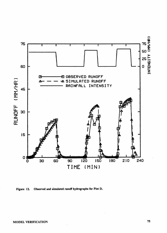
-75 75~ z:

I l z:

I \ so-

\ >-

25 !: UJ

60 0 z 1'J I-z -[9 E!l OBSERVED RUNOFF -0::: b- - - -6 SIMULATED RUNOFF

:r: RAINFALL INTENSITY

' 45 l: l: -LL /i LL 30 CJ z ::J 0:::

15

I

0 0 30 60 90 120 150 180 210 240

TIME CMIN)

Figure 12, Observed and simulated runoff hydrographs for Plot D.


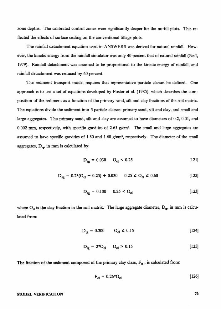
zone depths. The calibrated control zones were significantly deeper for the no-till plots. This re-

flected the effects of surface sealing on the conventional tillage plots.

The rainfall detachment equation used in ANSWERS was derived for natural rainfall. How-

ever, the kinetic energy from the rainfall simulator was only 40 percent that of natural rainfall (Neff,

1979). Rainfall detachment was assumed to be proportional to the kinetic energy of rainfall, and

rainfall detachment was reduced by 60 percent.

The sediment transport model requires that representative particle classes be defined. One

approach is to use a set of equations developed by Foster et al. (1985), which describes the com-

position of the sediment as a function of the primary sand, silt and clay fractions of the soil matrix.

The equations divide the sediment into 5 particle classes: primary sand, silt and clay, and small and

large aggregates. The primary sand, silt and clay are assumed to have diameters of 0.2, 0.01, and

0.002 mm, respectively, with specific gravities of 2.65 g/cm3• The small and large aggregates are

assumed to have specific gravities of 1.80 and 1.60 g/cm3, respectively. The diameter of the small

aggregates, D,,, in mm is calculated by:

Dsg = 0.030 Oc1 < 0.25 (121)

Dsg = 0.2•(Oc1 - 0.25) + 0.030 0.25 s: Oc1 s: 0.60 (122]

Dsg = 0.100 0.25 < Oc1 [123]

where Odis the clay fraction in the soil matrix. The large aggregate diameter, D11, in mm is calcu-

lated from:

D1g = 0.300 Oc1 S: 0.15 [124)

[125]

The fraction of the sediment composed of the primary clay class, F d , is calculated from:

F cl = 0.26•Oc1 (126]


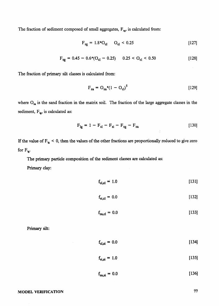
The fraction of sediment composed of small aggregates, F,,, is calculated from:

[1271

Fsg = 0.45 - 0.6+(Ocl - 0.25) 0.25 < Ocl < 0.50 [128]

The fraction of primary silt classes is calculated from:

[1291

where o .. is the sand fraction in the matrix soil. The fraction of the large aggregate classes in the

sediment, F11, is calculated as:

[130]

If the value of F11 < 0, then the values of the other fractions are proportionally reduced to give zero

for F1,.

The primary particle composition of the sediment classes are calculated as:

Primary clay:

fcl,cl == 1.0 [131I

fsi,cl = 0.0 [1321

fsa,cl = 0.0 [133)

Primary silt:

fcl,si = 0.0 [134)

fsi,si = 1.0

fsa,si = 0.0 (136)


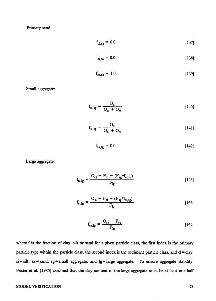
Primary sand:

Small aggregate:

Large aggregate:

fcl,sa = 0.0

fsi,sa = 0.0

fsa,sa = 1.0

Ocl fcl,sg = 0 + 0

cl si

fsa,sg = 0.0

[137]

[138)

[139]

[140)

[ 141)

[142]

[143]

(144]

(145)

where f is the fraction of clay, silt or sand for a given particle class, the first index is the primary

particle type within the particle class, the second index is the sediment particle class, and cl= clay,

si==silt, sa=sand, sg=small aggregate, and lg=large aggregate. To ensure aggregate stability,

Foster et al. (1985) assumed that the clay content of the large aggregate must be at least one-half


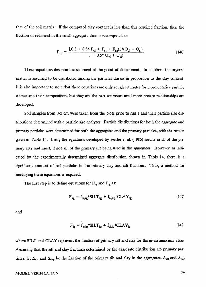
that of the soil matrix. If the computed clay content is less than this required fraction, then the

fraction of sediment in the small aggregate class is recomputed as:

(146)

These equations describe the sediment at the point of detachment. In addition, the organic

matter is assumed to be distributed among the particles classes in proportion to the clay content.

It is also important to note that these equations are only rough estimates for representative particle

classes and their composition, but they are the best estimates until more precise relationships are

developed.

Soil samples from 0-5 cm were taken from the plots prior to run 1 and their particle size dis-

tributions determined with a particle size analyzer. Particle distributions for both the aggregate and

primary particles were determined for both the aggregates and the primary particles, with the results

given in Table 14. Using the equations developed by Foster et al. (1985) results in all of the pri-

mary clay and most, if not all, of the primary silt being used in the aggregates. However, as indi-

cated by the experimentally determined aggregate distribution shown in Table 14, there is a

significant amount of soil particles in the primary clay and silt fractions. Thus, a method for

modifying these equations is required.

The first step is to define equations for F,1 and F11 as:

(147)

and

(148)

where SILT and CLAY represent the fraction of primary silt and clay for the given aggregate class.

Assuming that the silt and clay fractions determined by the aggregate distribution are primary par-

ticles, let A,ilt and Ac1ay be the fraction of the primary silt and clay in the aggregates. Asiit and Ac1ay


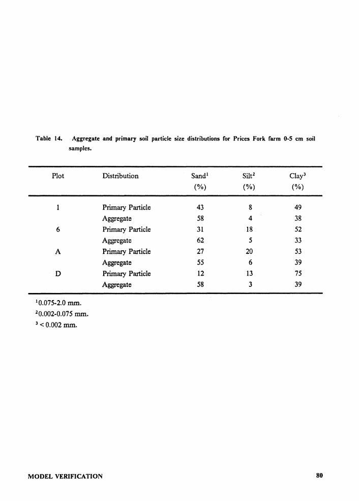
Table 14. Aggregate and primary soil particle size distributions for Prices Fork farm 0-5 cm soil samples.

Plot

1

6

A

D

10.075-2.0 mm. 20.002-0.075 mm. 3 <0.002mm.

Distribution

Primary Particle Aggregate Primary Particle Aggregate Primary Particle Aggregate Primary Particle Aggregate

MODEL VERIFICATION

Sand 1

(%)

43 58 31 62 27 55 12 58

Silt2 Clay3

(%) (%)

8 49 4 38 18 52 5 33

20 53 6 39 13 75 3 39

80

are calculated as the difference between the primary and aggregate distribution fractions for the silt

and clay fractions, respectively, and are also defined as:

(149)

and

(150)

The fraction of the original primary particles can be defined as:

(151]

(152]

Osa = F sa + fsa,lg *SAND1g (153)

Next, assume that the primary clay and silt in the aggregates are distributed in proportion to Foster

et al. ( 1985) equations, such that:

Rearranging Equation 154 yields:

and

= fcl,sg *CLA y sg

fcl,lg *CLA Y1g

F *f -1 SILT = SILT • sg si,g sg lgp+f

lg si,sg

F +f CLA y = CLA y • sg cl,lg

sg lgp+f lg cl,sg

Putting Equations 155 and 156 into Equations 149 and 150 and rearranging yields:

MODEL VERIFICATION

[154)

[155)

[156]

81

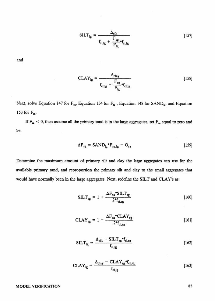
SILT1g = ~silt [ 157) Fsg

fsi,lg + F+fsi,lg lg

and

CLAY1g = ~clay (158)

Fsg fcl,lg + F+fcl,lg

lg

Next, solve Equation 147 for Fs,, Equation 154 for F1,, Equation 148 for SAND1,, and Equation

153 for Fsa·

If F sa < 0, then assume all the primary sand is in the large aggregates, set F n equal to zero and

let

1159)

Determine the maximum amount of primary silt and clay the large aggregates can use for the

available primary sand, and reproportion the primary silt and clay to the small aggregates that

would have normally been in the large aggregates. Next, redefine the SILT and CLAY's as:

MODEL VERIFICATION

~Fsa•SILTsg SILT5g = 1 + -----

2•rsi,sg

~Fsa•CLAYsg CLAYsg = 1 + ----~

2+fcl,sg

~silt - SILTsg +fsi,sg SILT1g = ---------

fsi,lg

6clay - CLAY sg +fcl,sg CLA Y1g = _ _,;;_ _______ ....;;... fcl,lg

(160)

[161)

(162)

[163)

82

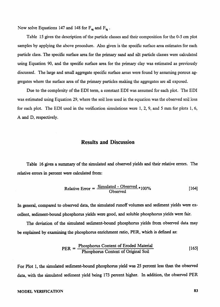
Now solve Equations 147 and 148 for F,, and F,, .

Table 15 gives the description of the particle classes and their composition for the 0-5 cm plot

samples by applying the above procedure. Also given is the specific surface area estimates for each

particle class. The specific surface area for the primary sand and silt particle classes were calculated

using Equation 90, and the specific surface area for the primary clay was estimated as previously

discussed. The large and small aggregate specific surface areas were found by assuming porous ag-

gregates where the surface area of the primary particles making the aggregates are all exposed.

Due to the complexity of the EDI term, a constant EDI was assumed for each plot. The EDI

was estimated using Equation 29, where the soil loss used in the equation was the observed soil loss

for each plot. The EDI used in the verification simulations were 1, 2, 9, and 5 mm for plots 1, 6,

A and D, respectively.

Results and Discussion

Table 16 gives a summary of the simulated and observed yields and their relative errors. The

relative errors in percent were calculated from:

Relative Error = Simulated - Observed • IOO¾ Observed

[164]

In general, compared to observed data, the simulated runoff volumes and sediment yields were ex-

cellent, sediment-bound phosphorus yields were good, and soluble phosphorus yields were fair.

The deviation of the simulated sediment-bound phosphorus yields from observed data may

be explained by examining the phosphorus enrichment ratio, PER, which is defined as:

Phosphorus Content of Eroded Material PER = _ __;: ______ -,--..,.....,.......,-~ Phosphorus Content of Original Soil

[165]

For Plot 1, the simulated sediment-bound phosphorus yield was 25 percent less than the observed

data, with the simulated sediment yield being 173 percent higher. In addition, the observed PER


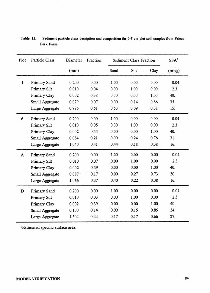
Table 15. Sediment particle class decription and composition for 0-5 cm plot soil samples from Prices Fork Farm.

Plot Particle Class Diameter Fraction Sediment Class Fraction SSA1

(mm) Sand Silt Clay (m2/g)

1 Primary Sand 0.200 0.00 1.00 0.00 0.00 0.04 Primary Silt 0.010 0.04 0.00 1.00 0.00 2.3 Primary Clay 0.002 0.38 0.00 0.00 1.00 40. Small Aggregate 0.079 0.07 0.00 0.14 0.86 35. Large Aggregate 0.986 0.51 0.53 0.09 0.38 15.

6 Primary Sand 0.200 0.00 1.00 0.00 0.00 0.04 Primary Silt 0.010 0.05 0.00 1.00 0.00 2.3 Primary Clay 0.002 0.33 0.00 0.00 1.00 40. Small Aggregate 0.084 0.21 0.00 0.24 0.76 31. Large Aggregate 1.040 0.41 0.44 0.18 0.38 16.

A Primary Sand 0.200 0.00 1.00 0.00 0.00 0.04 Primary Silt 0.010 0.07 0.00 1.00 0.00 2.3 Primary Clay 0.002 0.39 0.00 0.00 1.00 40.

Small Aggregate 0.087 0.17 0.00 0.27 0.73 30.

Large Aggregate 1.066 0.37 0.40 0.22 0.38 16.

D Primary Sand 0.200 0.00 1.00 0.00 0.00 0.04

Primary Silt 0.010 0.03 0.00 1.00 0.00 2.3

Primary Clay 0.002 0.39 0.00 0.00 1.00 40.

Small Aggregate 0.100 0.14 0.00 0.15 0.85 34. Large Aggregate 1.504 0.44 0.17 0.17 0.66 27.

1 Estimated specific surface area.


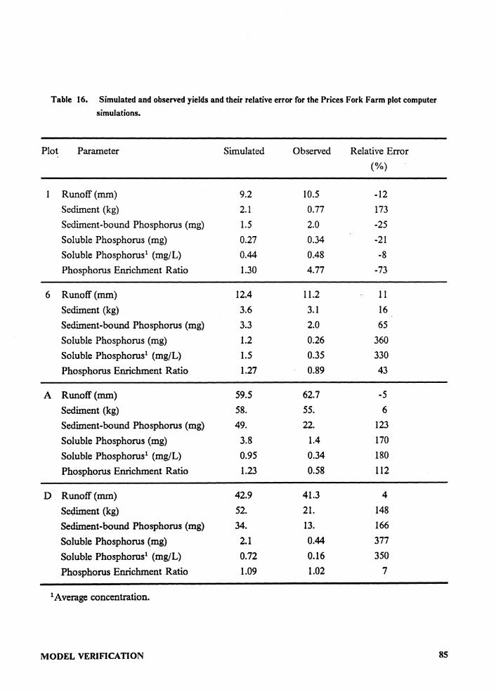
Table 16. Simulated and observed yields and their relative error for the Prices Fork Farm plot computer simulations.

Plot Parameter Simulated Observed Relative Error (%)

I Runoff (mm) 9.2 10.5 -12 Sediment (kg) 2.1 0.77 173 Sediment-bound Phosphorus (mg) 1.5 2.0 -25 Soluble Phosphorus (mg) 0.27 0.34 -21 Soluble Phosphorus 1 (mg/L) 0.44 0.48 -8 Phosphorus Enrichment Ratio 1.30 4.77 -73

6 Runoff (mm) 12.4 I 1.2 11 Sediment (kg) 3.6 3.1 16 Sediment-bound Phosphorus (mg) 3.3 2.0 65 Soluble Phosphorus (mg) 1.2 0.26 360 Soluble Phosphorus 1 (mg/L) 1.5 0.35 330 Phosphorus Enrichment Ratio 1.27 0.89 43

A Runoff(mm) 59.5 62.7 -5 Sediment (kg) 58. 55. 6 Sediment-bound Phosphorus (mg) 49. 22. 123 Soluble Phosphorus (mg) 3.8 1.4 170 Soluble Phosphorus 1 (mg/L) 0.95 0.34 180 Phosphorus Enrichment Ratio 1.23 0.58 112

D Runoff (mm) 42.9 41.3 4 Sediment (kg) 52. 21. 148 Sediment-bound Phosphorus (mg) 34. 13. 166 Soluble Phosphorus (mg) 2.1 0.44 377 Soluble Phosphoros 1 (mg/L) 0.72 0.16 350 Phosphorus Enrichment Ratio 1.09 1.02 7

1 Average concentration.


was substantially higher than the simulated, which can be explained by a low soil phosphorus

content estimate. This would appear reasonable because the observed PER of 4. 77 is relatively

high. A low soil phosphorus content estimate would also explain the low simulated sediment-

bound phosphorus yield with the high sediment yield.

For plots 6 and A, the simulated sediment-bound phosphorus yields were over predicted, while

the simulated sediment yields were very close to observed values. However, the observed PER were

less than one, which is unreasonable. This implies the soil phosphorus levels were over estimated,

which would explain the over predicted sediment-bound phosphorus yields.

The simulated PER for plot D was very close to the observed value. The over predicted

sediment-bound phosphorus can be attributed to the over predicted sediment yield.

The over predicted soluble phosphorus yields may be attributed to the over predicted

sediment-bound phosphorus yields. As the concentration of sediment-bound phosphorus increases,

the soluble phosphorus concentration increases as well. Thus, a reduction in the sediment-bound

phosphorus concentration results in a lower soluble phosphorus concentration and a lower soluble

phosphorus yield.

Comparing the two tillage practices, the conventional tillage plots had observed runoff,

sediment, and sediment-bound phosphorus yields at least an order of magnitude higher than the

no-till plots, which was reflected in the predicted responses. Compared to the no-till plots, the

conventional tillage plots were expected to have higher soluble phosphorus yields and lower soluble

phosphorus concentrations. This was reflected in both the observed and predicted responces.


SENSITIVITY ANALYSIS

A sensitivity analysis of the ANSWERS model for the phosphorus component processes is

necessary to evaluate the sensitivity of the model to changes in the input parameter values. Thus,

the component processes and the parameter values having the greatest impact on the model output

can be identified, and additional research can be performed in these areas to increase the model's

accuracy.

A sensitivity analysis was performed for Plot A, with the results referenced to a simulation time

step of one second. Table 17 gives the sediment and phosphorus yields for the sensitivity analysis

simulations. The selected parameters were varied by a percentage based upon the expected pa-

rameter variability. Table 18 gives the percent deviation for each of the reference simulations.

Another approach to determine the sensitivity of the parameters is to use a technique presented by

Douglas and Burges, (1982). A sensitivity index, S, is defined as:

S = aR oP

[166]

where R is the model results and P is the value of the parameter being investigated. The relative

sensitivity, Sr, is defined as:

s = ..f.. aR r R ap [167)

Table 19 gives the sensitivity and relative sensitivity for the selected parameters.

As seen from Table 19, the soluble phosphorus model is extremely sensitive to BETA, mod-

erately sensitive to Kext, ALPHA, EXTP, EDI, FLOWL and N, slightly sensitive to P0SOIL and

DELT, and insensitive to K, C, Q0, BO, and the specific surface area of the clay fraction. However,

SENSITIVITY ANALYSIS 87

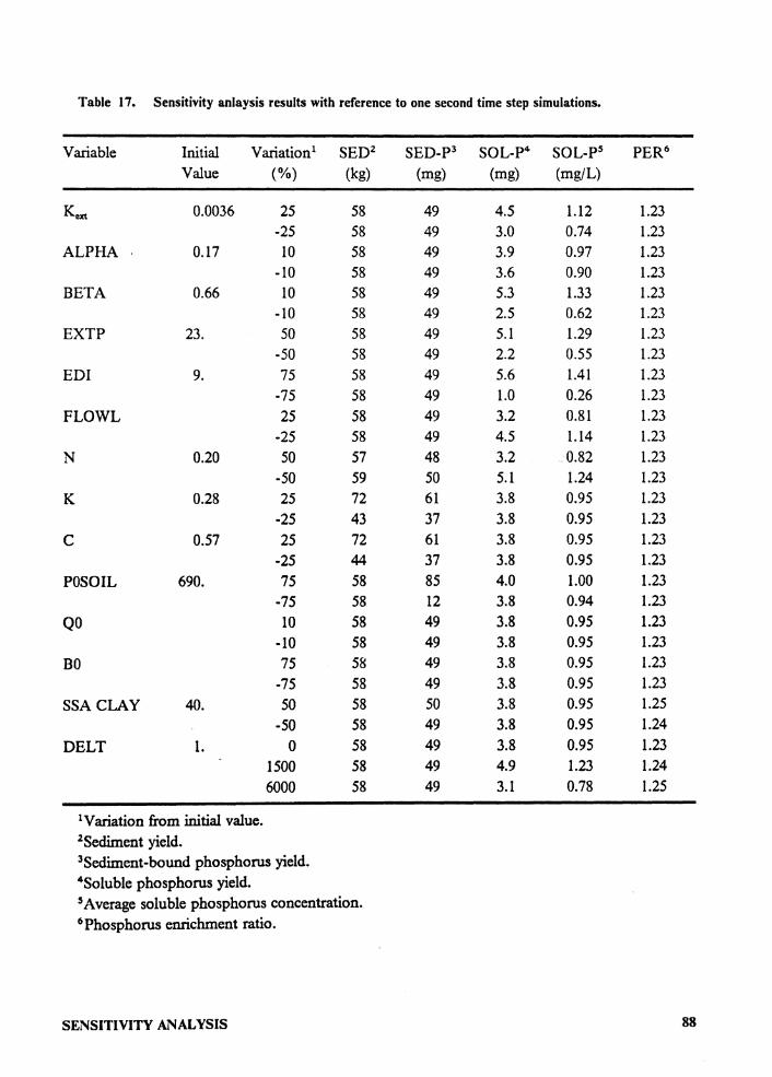
Table 17. Sensitivity anlaysis results with reference to one second time step simulations.

Variable Initial Variation 1 SED 2 SED-P 3 SOL-P 4 SOL-P 5 PER 6

Value (%) (kg) (mg) (mg) (mg/L)

Kexi 0.0036 25 58 49 4.5 1.12 1.23 -25 58 49 3.0 0.74 1.23

ALPHA 0.17 10 58 49 3.9 0.97 1.23 -10 58 49 3.6 0.90 1.23

BETA 0.66 10 58 49 5.3 1.33 1.23 -10 58 49 2.5 0.62 1.23

EXTP 23. 50 58 49 5.1 1.29 1.23 -50 58 49 2.2 0.55 1.23

EDI 9. 75 58 49 5.6 1.41 1.23 -75 58 49 1.0 0.26 1.23

FLOWL 25 58 49 3.2 0.81 1.23 -25 58 49 4.5 1.14 1.23

N 0.20 50 57 48 3.2 0.82 1.23 -50 59 50 5.1 1.24 1.23

K 0.28 25 72 61 3.8 0.95 1.23 -25 43 37 3.8 0.95 1.23

C 0.57 25 72 61 3.8 0.95 1.23 -25 44 37 3.8 0.95 1.23

P0SOIL 690. 75 58 85 4.0 1.00 1.23 -75 58 12 3.8 0.94 1.23

Q0 10 58 49 3.8 0.95 1.23 -10 58 49 3.8 0.95 1.23

BO 75 58 49 3.8 0.95 1.23 -75 58 49 3.8 0.95 1.23

SSA CLAY 40. 50 58 50 3.8 0.95 1.25 -50 58 49 3.8 0.95 1.24

DELT 1. 0 58 49 3.8 0.95 1.23 1500 58 49 4.9 1.23 1.24 6000 58 49 3.1 0.78 1.25

1Variation from initial value. 2Secliment yield. 3Sediment-bound phosphorus yield. 4 Soluble phosphorus yield. 5 Average soluble phosphorus concentration. 6 Phosphorus enrichment ratio.


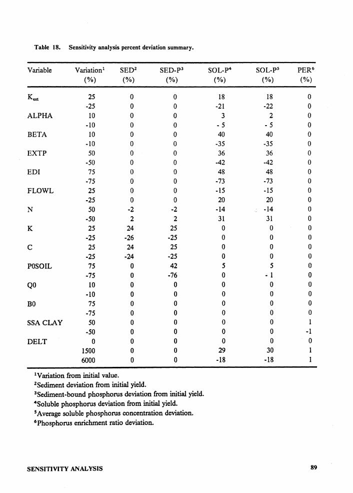
Table 18. Sensitivity analysis percent deviation summary.

Variable Variation 1 SED2 SED-P 3 SOL-P 4 SOL-P 5 PER 6

(%) (%) (%) (%) (%) (%)

Kex1 25 0 0 18 18 0 -25 0 0 -21 -22 0

ALPHA 10 0 0 3 2 0 -10 0 0 - 5 - 5 0

BETA 10 0 0 40 40 0 -10 0 0 -35 -35 0

EXTP 50 0 0 36 36 0 -50 0 0 -42 -42 0

EDI 75 0 0 48 48 0 -75 0 0 -73 -73 0

FLOWL 25 0 0 -15 -15 0 -25 0 0 20 20 0

N 50 -2 -2 -14 -14 0 -50 2 2 31 31 0

K 25 24 25 0 0 0 -25 -26 -25 0 0 0

C 25 24 25 0 0 0 -25 -24 -25 0 0 0

P0SOIL 75 0 42 5 5 0 -75 0 -76 0 - 1 0

QO 10 0 0 0 0 0 -10 0 0 0 0 0

BO 75 0 0 0 0 0 -75 0 0 0 0 0

SSA CLAY 50 0 0 0 0 1 -SO 0 0 0 0 -1

DELT 0 0 0 0 0 0 1500 0 0 29 30 1 6000 0 0 -18 -18 1

1 Variation from initial value. 2 Sediment deviation from initial yield. 3Sediment-bound phosphorus deviation from initial yield. 4 Soluble phosphorus deviation from initial yield. 5 Average soluble phosphorus concentration deviation. 6 Phosphorus enrichment ratio deviation.


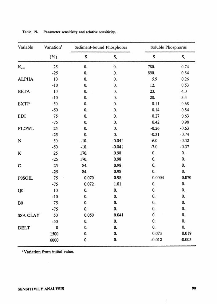
Table 19. Parameter sensitivity and relative sensitivity.

Variable Variation 1 Sediment-bound Phosphorus Soluble Phosphorus

(%) s s, s s,

Kex1 25 0. 0. 780. 0.74 -25 0. 0. 890. 0.84

ALPHA IO 0. 0. 5.9 0.26 -10 0. 0. 12. 0.53

BETA 10 0. 0. 23. 4.0 -10 0. 0. 20. 3.4

EXTP 50 0. 0. 0.11 0.68 -50 0. 0. 0.14 0.84

EDI 75 0. o. 0.27 0.63 -75 o. 0. 0.42 0.98

FLOWL 25 o. o. -0.26 -0.63 -25 0. 0. -0.31 -0.74

N 50 -10. -0.041 -6.0 -0.32 -50 -10. -0.041 -7.0 -0.37

K 25 170. 0.98 0. 0. -25 170. 0.98 0. 0.

C 25 84. 0.98 0. 0. -25 84. 0.98 0. 0.

P0SOIL 75 0.070 0.98 0.0004 0.070 -75 0.072 1.01 0. 0.

Q0 10 0. 0. 0. 0. -10 o. 0. 0. 0.

BO 75 0. o. 0. 0. -75 o. 0. 0. 0.

SSA CLAY 50 0.050 0.041 0. 0. -50 0. 0. 0. 0.

DELT 0 o. 0. 0. 0. 1500 0. o. 0.073 0.019 6000 0. 0. -0.012 -0.003

1 Variation from initial value.


it should be noted that potential inaccuracies due to large time steps can be eliminated by using a

relatively small DELT. The sediment-bound phosphorus model is moderately sensitive to N, K,

C, and P0SOIL, and slightly sensitive to the specific surface area of the soil in the clay fraction.


WATERSHED SIMULATIONS

Design Storm

The major driving force for any runoff related model is precipitation. Rainfall impact influ-

ences soil detachment and transport by adding to the turbulence of overland flow. The time dis-

tribution of precipitation also governs the extent and magnitude of surface runoff. The use of event

oriented models like ANSWERS requires the careful selection of a design storm.

Determining an appropriate rainfall distribution for ANSWERS can be approached in several

ways. One approach is to use the rainfall distribution from a series of actual storm events. Disad-

vantages of this approach include high computational costs and added complexity to the analysis

by adding uncertainties concerning the recurrence interval for the storm events selected. AN-

SWERS can also use a generalized storm distribution as presented by Kent (1968). However, these

distributions are for large areas and localized effects may be significant.

The approach taken in this study is to utilize a simulated intensity pattern developed from

historical data, which is characteristic of the watershed being investigated. The design storm dura-

tion is taken as the time of concentration of the watershed, which results in a storm with the highest

possible intensities and peak runoff for a given recurrence interval. The time of concentration of

the watershed, Tc (min), is calculated using:

[168)

WATERSHED SIMULATIONS 92

where L. is the maximum length of channel flow (m), L0 is the maximum length of overland flow

(m), Sc and So are the channel and overland flow slopes (m/m) associated with L. and L0 respec-

tively, and n is Mannings roughness coefficient. The first part of Equation 168 was developed to

describe channel flow (Schwab et al.,1981), while the second part describes the travel time for

overland flow (Kerby, 1959). A rainfall amount for the calculated storm duration can then be ob-

tained from United States Weather Bureau (USWB) Technical Paper (TP) No. 29 or other ap-

propriate sources for the desired recurrence interval.

Next, a probability density function was used to model the rainfall intensities. To demonstrate

the procedure for estimating the required parameters for the design storm, rainfall intensities from

the Pony Mountain Branch watershed in Culpeper County, Virginia were obtained from Virginia

break-point precipitation data presented by Shanholtz and Burford (1976). The data was divided

into storm events, which were defined as any period having less than one hour without rainfall. It

was also assumed that rainfall events less than 0.635 cm (0.25 inch) would not produce significant

runoff and erosion and were thus not included in the data base. Next, the storm events were par-

titioned into uniform time intervals of either 5, 10, or 15 minutes, and the first-order serial corre-

lation Figure 13 shows the first-order serial correlation coefficients for each of the time intervals

on a monthly basis. A ten-minute interval was selected, and due to the monthy variation of the

first-order serial correlation coefficients, each month was analysed separately.

The next step was to determine the underlying distribution of the intensity pattern for each

month. The probability distributions investigated were normal, folded normal, lognormal, two-

parameter gamma, two-parameter Weibull, and exponential. Transformations investigated included

x114, X1/3, x 112 , X2/3, X314, ln(X), ln(X + 1), and ln(X + 1)0•33• The distribution parameters were

estimated using the method of maximum likelihood if the procedures were available, other wise the

method of moments was used. A Chi-Square goodness of fit test and a K-S goodness of fit test

were performed for the distributions and transformations investigated. It should be noted that in

all cases, both the Chi-Square and K-S tests were rejected, which was due to the large number of

data points. However, the test were used as a guideline for determining the best fit. The distrib-


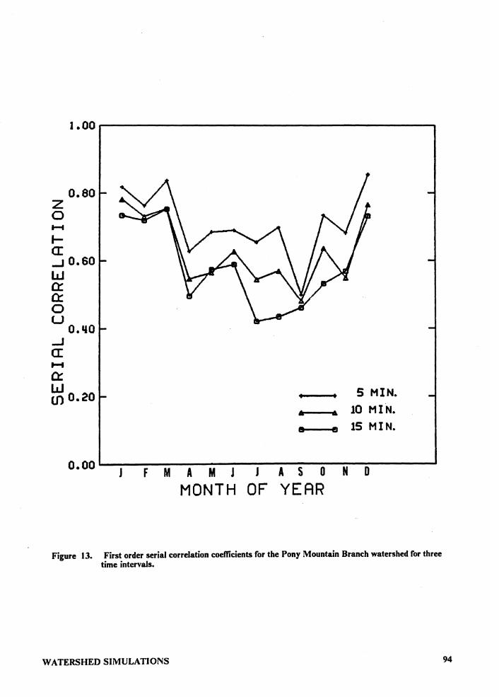
1.00,------------------------

o.ao z 0 1--t l-a: ..J 0.60 w a: a: 0 u

O.&&O ..J a: t-1 a: w (I) 0.20 S MIN.

... ---.... 10 MIN. ••--e 1S MIN.

0.00'--J--F-M--A-M--J-J--A-S--O-N--0-----J

MONTH OF YEAR

Figure 13. First order serial correlation coefficients for the Pony Mountain Branch watershed for three time intervals.


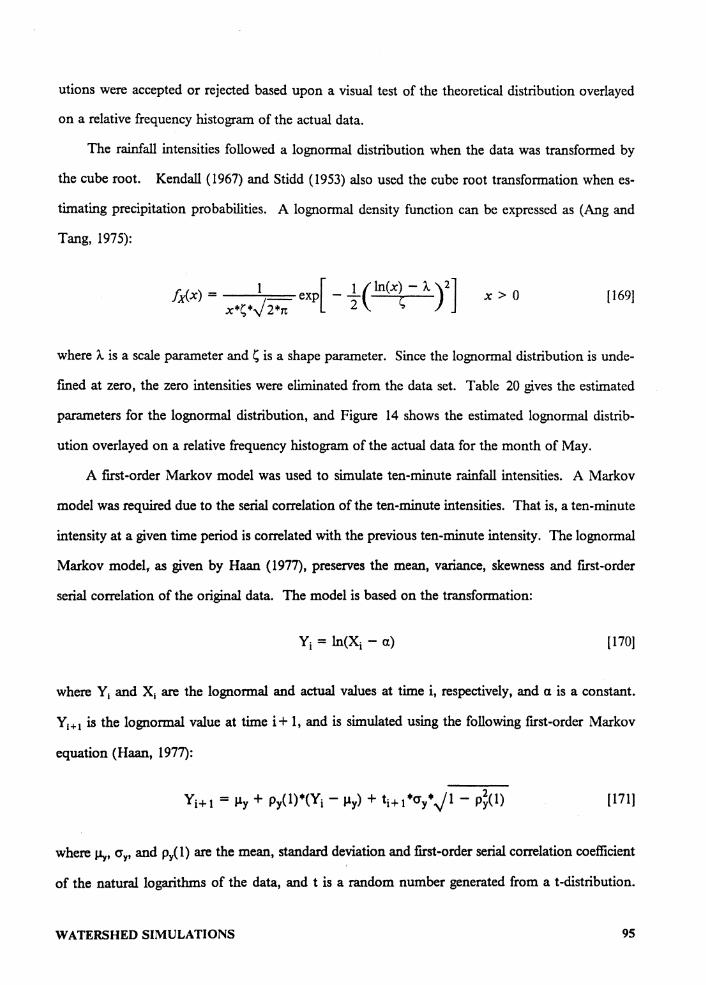
utions were accepted or rejected based upon a visual test of the theoretical distribution overlayed

on a relative frequency histogram of the actual data.

The rainfall intensities followed a lognormal distribution when the data was transformed by

the cube root. Kendall (1967) and Stidd (1953) also used the cube root transformation when es-

timating precipitation probabilities. A lognormal density function can be expressed as (Ang and

Tang, 1975):

fx(x) = 1 exp[ - 1.( ln(x) - "-)2] 2

x>O [169]

where"- is a scale parameter ands is a shape parameter. Since the lognormal distribution is unde-

fined at zero, the zero intensities were eliminated from the data set. Table 20 gives the estimated

parameters for the lognormal distribution, and Figure 14 shows the estimated lognormal distrib-

ution overlayed on a relative frequency histogram of the actual data for the month of May.

A first-order Markov model was used to simulate ten-minute rainfall intensities. A Markov

model was required due to the serial correlation of the ten-minute intensities. That is, a ten-minute

intensity at a given time period is correlated with the previous ten-minute intensity. The lognormal

Markov model, as given by Haan ( 1977), preserves the mean, variance, skewness and first-order

serial correlation of the original data. The model is based on the transformation:

Yi = ln(Xi - a) [170]

where Y1 and X1 are the lognormal and actual values at time i, respectively, and a is a constant.

Y1+ 1 is the lognormal value at time i + 1, and is simulated using the following first-order Markov

equation (Haan, 1977):

(171]

where~. cry, and Py(l) are the mean, standard deviation and first-order serial correlation coefficient

of the natural logarithms of the data, and t is a random number generated from a t-distribution.


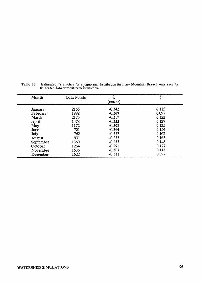
Table 20. Estimated Parameters for a lognormal distribution for Pony Mountain Branch watershed for truncated data without zero intensities.

Month Data Points j_ (cm/hr)

January 2165 -0.342 0.115 February 1992 -0.309 0.097 March 2173 -0.317 0.122 April 1478 -0.333 0.127 May 1172 -0.308 0.135 June 721 -0.264 0.154 July 762 -0.287 0.162 August 931 -0.283 0.163 September 1360 -0.287 0.148 October 1264 -0.291 0.127 November 1536 -0.307 0.118 December 1622 -0.311 0.097


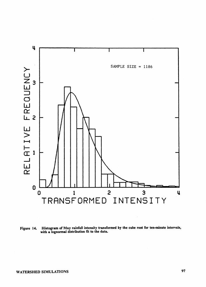
>-u Z3 w ::J d w 0:: LL 2

w > 1--1

l-a: 1 _J

w Cl::

0 0 1 2 TRANSFORMED

SAMPLE SIZE= 1186

3 INTENSITY

Figure 14. Histogram of May rainfall intensity transformed by the cube root for ten-minute intervals, with a lognormal distribution tit to the data.


To preserve the statistical properties of the original data, the following equations must be solved

(Haan, 1977):

exp(3*er;) - 3* exp(er;) + 2 Yx = ----------

[ exp( er;) - 1 ]1-5

exp(er;"'Py(l)) - 1 px(l) = ------

exp(er;) - 1

[172]

[173]

[174]

(175]

In these equations; Jlx, er~, Yx , and px(l) are the mean, variance, coefficient of skew and the first-

order serial correlation coefficient of the original data, respectively, and are estimated by x, s~ , C5x

and rx(l). The values of ~,ery, py(l), and a are estimated using Equations 172 thru 175, and are

then used in Equation 171 to generate a value of Y1+ 1• These estimated parameters for the Pony

Mountain Branch watershed are given in Table 21. The value of X1+ 1 is then calculated using:

.. Xi+ 1 = exp(Yi+ 1) + a (176]

The value of XI+ 1 becomes X1 and is transformed by Equation 170, put into Equation 171 to sim-

ulate the next Y1 + 1 , and the process continues.

Use of the Markov model requires an initial ten-minute intensity, 110 (cm/hr), to initiate a

storm sequence. The initial ten-minute intensity was found to be a function of both total rainfall

amount, A (cm), and storm duration, D (hr). An appropriate model of the general form was de-

termined to be:

[177]


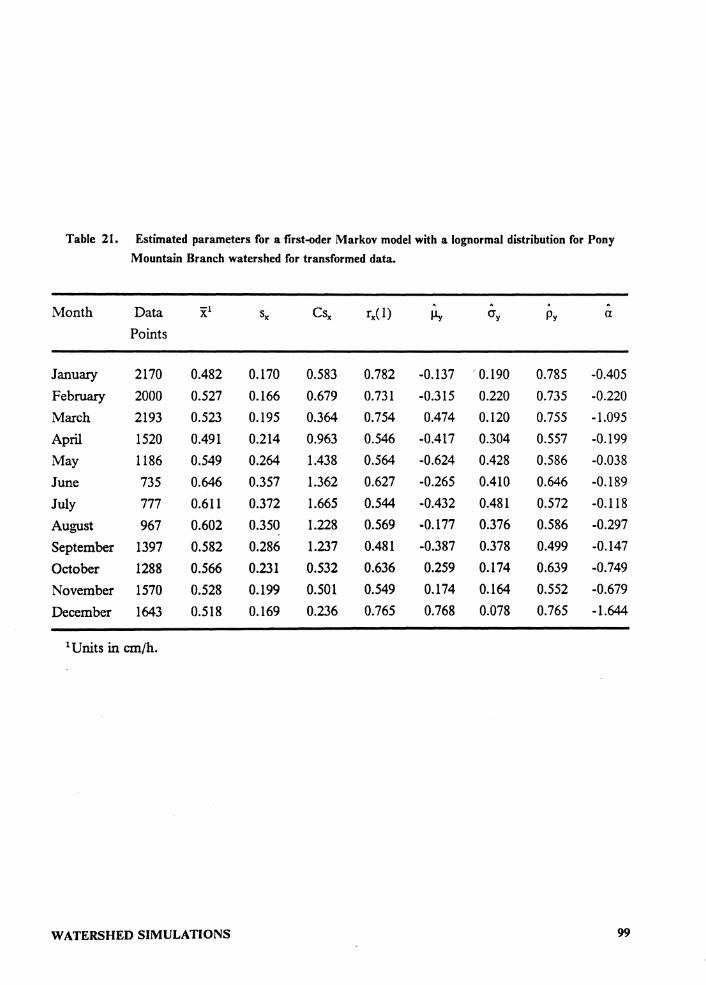
Table 21. Estimated parameters for a first-oder Markov model with a lognormal distribution for Pony Mountain Branch watershed for transformed data.

Month Data x:1 Csx rx(l) .

Sx Jly (Jy Py a

Points

January 2170 0.482 0.170 0.583 0.782 -0.137 , 0.190 0.785 -0.405 February 2000 0.527 0.166 0.679 0.731 -0.315 0.220 0.735 -0.220 March 2193 0.523 0.195 0.364 0.754 0.474 0.120 0.755 -1.095 April 1520 0.491 0.214 0.963 0.546 -0.417 0.304 0.557 -0.199 May 1186 0.549 0.264 1.438 0.564 -0.624 0.428 0.586 -0.038 June 735 0.646 0.357 1.362 0.627 -0.265 0.410 0.646 -0.189 July 777 0.611 0.372 1.665 0.544 -0.432 0.481 0.572 -0.118 August 967 0.602 0.350 1.228 0.569 -0.177 0.376 0.586 -0.297 September 1397 0.582 0.286 1.237 0.481 -0.387 0.378 0.499 -0.147

October 1288 0.566 0.231 0.532 0.636 0.259 0.174 0.639 -0.749

November 1570 0.528 0.199 0.501 0.549 0.174 0.164 0.552 -0.679

December 1643 0.518 0.169 0.236 0.765 0.768 0.078 0.765 -1.644

1 Units in cm/h.


where Po, P1, and P1 are coefficients, and & is a random error term. Random values for 110 are sim-

ulated with the following equation:

.. .. " 110 = exp[Po + P1•1n(D) + P2•1n(A) + s•N(0,1)] (178)

where s is the estimated residual standard deviation of the natural logarithm of 110 and N(O, 1) is a

random value generated from a standard normal distribution (Haan, 1977). The estimated coef-

ficients are given in Table 22.

To check the accuracy of the approach, the actual and simulated relative frequency histograms

were plotted together and visually compared (Woeste et al., 1979). Figure 15 shows the actual and

simulated histograms for the month of May. This figure, along with the remaining months, are very

similar indicating adequate model accuracy.

The procedure for generating a design storm can be summarized as follows:

1. Determine the statistical parameters for the geographic region of interest.

2. Determine the time of concentration of the watershed using Equation 168.

3. From USWB TP-29 find a rainfall amount for an n-year recurrence interval for a du-

ration equal to the time of concentration of the watershed.

4. Simulate a first ten-minute intensity using Equation 178.

5. Using the first ten-minute intensity as a seed, simulate the number of ten-minute in-

tensities equal to the storm duration using Equation 171.

6. Multiply each simulated ten-minute intensity by the original storm amount divided by

the simulated storm amount.

Step 5 is necessary in order to obtain the original storm amount. The multiplication of the simu-

lated intensities by a constant preserves the coefficient of skew and first-order serial correlation of

the simulated data.

The design storm reflects the characteristics of the watershed being investigated, and thus al-

lows different watersheds to be compared with the same recw;rence interval storm. Therefore,


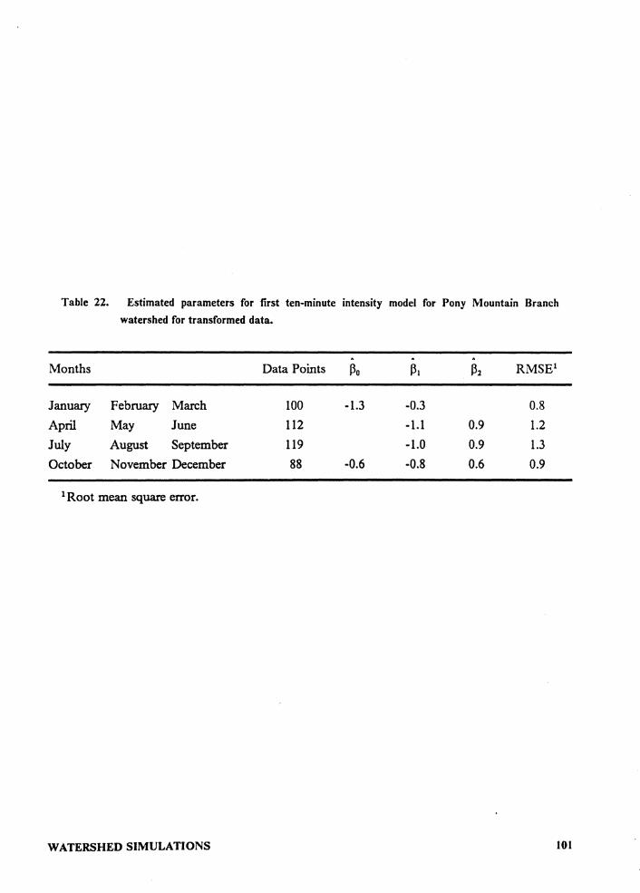
Table 22. Estimated parameters for first ten-minute intensity model for Pony Mountain Branch watershed for transformed data.

Months Data Points Po P1 P2 RMSE 1

January February March 100 -1.3 -0.3 0.8 April May June 112 -1.1 0.9 1.2 July August September 119 -1.0 0.9 1.3 October November December 88 -0.6 -0.8 0.6 0.9

1 Root mean square error.


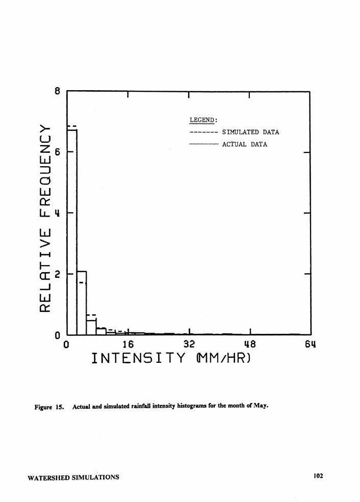
>-u

8

Zs w :::J d w 0::: LL 11

w > 1-t

l-a: 2 _J

w a::

0 0

LEGEND: ------- SIMULATED DATA --- ACTUAL DATA

16 32 INTENSITY

Figure IS. Actual and simulated rainfall intensity histograms for the month of May.


combining ANSWERS with the design storm results in an excellent planning tool for evaluating

the impacts of changing land use in watersheds. The design storm can also be used to assess the

impact of the intensity pattern on ANSWERS. This can be accomplished by simulating a series

of storm events, running ANSWERS for each of the simulated storm events, and then investigating

the variability of the output.

Nomini Creek Simulation

Watershed Description

The Nomini Creek watershed, used to demonstrate the use of ANSWERS, is located in

Westmoreland County, Virginia. This watershed was selected because the Virginia Division of Soil

and Water Conservation had identified it as a potentially critical source of nonpoint pollution. The

watershed will be monitored over the next 10 years to assess the long-term water quality impacts

of BMP implementation. The watershed contains approximately 1500 hectares (3700 acres), with

land use being approximately half agriculture and half forested. The upland areas with mild slopes

are generally in row crops. Steep areas and the lowlands are forested. The watershed is character-

ized by well drained sandy and loamy soils.

Scenario Descriptions

The watershed was partitioned into one hectare elements, as shown in Figure 16. The arrows

in each element in Figure 16 indicate the slope direction or direction of flow for that element. The

darker arrows designate channel elements. Soils, topographic and land use data required by the

ANSWERS model were obtained from soil surveys and 1:24000 scale United States Geological

Survey topographic maps. Other hydrologic parameters required by ANSWERS were estimated


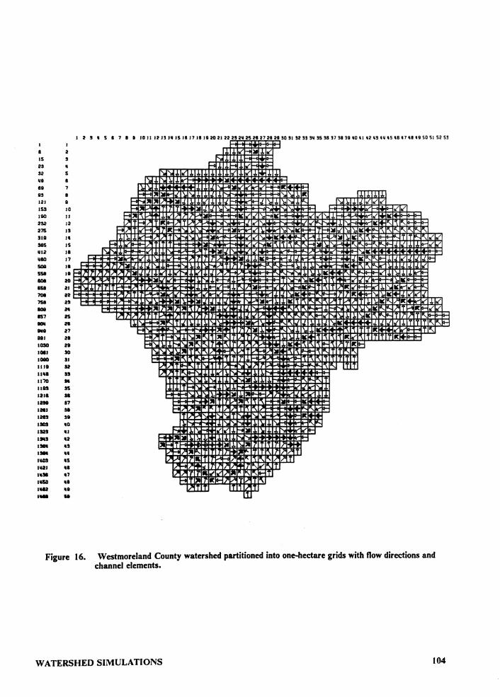
I 2 S I 5 S 7 I I 10 II U lS II 15 JI 17 111120 21 22 n 2¥ 25 2127 28 29 90 SJ !2 93 !V 35 SB '7 '8 9910 II ,2 •H• ,s 18 '7 U 19 SD SJ 52 53 I I

• 2 J. 15 s J. 21 I H - ,t'H S2 5 ' J. .l .l Vt g '- .l ', l I lll It 7 l \. .i .. as • -'""' "llll- 7 ,. ",, « l .1 .1 121 a ........ "" ,. lll T J J. \. .L \." 11... \, \ I

JSS ID ..... ,. ..... T 'l' T lll \. \, '\.. ....... ... 110 II -t,. 'I .... .l' --'lll If:,.(,.(\, " ,I'/'-,,, ,.( " 232 12 ..,, .... .,, «--- )II i, ' -,l"' ,I'~ ..... " ~, ~,_ >-I>-

275 IS ..... Jf' 1 7llt'-'\.\. .... ,t'r-- lllll""llr' ,I' .,. )I' If: ,_ T~lill 1..- \." .... ""'"-~ "" SUI II .1.1 l.. I .,..-i "TI',-..,', I- lll .... '"' \, " .... , .. Jill "'I '\ 1 "'-"- ,.(1./1

SIS JS _, I ,_ 7' lll '"' ICI'\ '11"'-1"-,_, lll \, .t q12 JI .,. Jill " qlQ 17 lit.- ... ,.( ~- l ., , ll .:- --1.L .I. IC'u ,I' J'd-

SOIi JI 17 lllJ '-'--'- l ,..,. } ........... I 1. '- .... " l"i I", ~; ..... ., ,/

558 It - l' 7 / ,. 1'lll 1.,, 1 u-.., -:-; -, ,,,. .... ,; .. 1--, " 1. \. " '" "' I I-- 20 -,,. ,,. 111)' ,,. lit.I,., .... _ ' l I'> r-, \. If: ""I ... .,,.,1., i,- ,......, II:.,_ I- ...

1sa 21 - ...... ., '-'-',. 11 .... ,( 1"'-1/ lrll >-t- .._...,.IC.,_ I, _; « ,( .. .,_ ,.,- I ', 11:....-,( ... 708 22 ,,, lll l'>,11: 7' It ... \, \." I/ ,t' .r J 758 2! ,,,. ..... " I',\.. lll' ll J. ,...Jill "i '\ ;; ..,., J' ! l \. If: "- 1,; It .,..~ I.L ,.( - 21 ,.,,,.r,. 17' ll If."\_ r,,,..a- M 'lo""" "- IJ' , -' It 157 25 !)II ,. / J1c,, , J' ,,,. ,K II: l"i 1 7 'l' T - ,. l,,__..,.,..,_, l ,K J. 1.1 IC l..l 1 T TT "' ... "-' .... 27 M " lll - I',. \. " 1 « ......... _, T I~ tal 21 ,__ 1)11, '- .._" ,. I/" \. IC 11 , 1 It ........ 1030 211 .... '\.. -,,.111:1(" ,,. IC '\ It I-

1081 90 "' \ 'i T .,.. ... lll '\ ... "' I\. 1080 SI ........ ,.~~ ,. '\ Ii 1 11111 S2 11qa H

~,} ... , ... ,. }' I", • ! ..,, }' It .,; " I 'l,N

11'10 .. T It It \. 1 I"> ll Ii 1109 ss I , ..... .... " .. .11 1211 - ...,j .... i"\ \ lrl ... J. J 12911 S7 "

,,,. '\ " ... 1281 SI

... .,, ,,,,. .. ,,. i" ,.......,

12n SIi \, « ISO! 10 ', ... lS2S u .... l 'I...,. ,( - » .,,, I-

1311! 12 ... ). .1 19111 IS I,. - T )I " ·- II .,. -i )',. ... r .. T UIO, 15 J' • " "' }'

IV2J II I., "" / I It "\.

IVSI 17 I; ... f I", >- I

1115D II ..... 'l'lt ... , llv '\ 111&2 II l I 11/

I- u J

Figure 16. Westmoreland County watershed partitioned into one-hectare grids with flow directions and channel elements.


using procedures discussed by Beasley and Huggins (1981). Soil samples from the top one centi-

meter of the soil were taken from the Nomini creek watershed in February of 1986 and tested for

total and Bray-P 1 phosphorus levels. Average phosphorus levels and approximate ED Is for each

tillage practice and land use used in the computer simulations, are given in Table 23. As given

previously, the phosphorus desorption and Langmuir isotherm parameters were determined in the

laboratory using a composite Suffolk sandy loam soil sample taken from the top IO cm of the ag-

ricultural fields. The representative particle distributions were determined as previously discussed

using information obtained from the Westmoreland County Soil Survey.

The closest available precipitation data to fit the intensity distribution for the design storm

was from the Pony Mountain Branch watershed in Culpeper County, Virginia, which is located

approximately 70 miles Northwest of the Nomini Creek watershed. For this study, the time of

concentration of the watershed was found to be 130 minutes using Equation 168. A rainfall amount

for a given storm duration and recurrence interval was obtained from the United States Weather

Bureau (USWB) Technical Paper (TP) No. 29. In this study a two-year recurrence interval storm,

occurring during mid to late spring when cropland is most susceptible to erosion, was chosen for

the design storm. Using USWB TP-29, the rainfall amount for a two-year recurrence interval storm

with a 130-minute duration was found to be 53 mm (2.1 in.). For this example, an initial ten-

minute storm intensity of 9.5 mm/hr (0.37 in/hr) was simulated using Equation 178. The first-order

Markov model was then used to simulate the intensity pattern given in Figure 17, which was used

as the design storm.

Using this design storm, computer simulations were conducted for eight early spring scenarios.

For each of the scenarios the antecedent soil moisture content was assumed to be 75 percent of

saturation. All forested land and pasture was assumed to be in good managed condition, and the

agricultural soils were assumed to be classified as having good productivity. The cropland was as-

sumed to be planted in either com or soybeans and follow a simple two-year com and soybean

rotation. Both crops were considered to be in the seed-bed cropstage. In this area com is usually

planted from the beginning to middle April and emerges in early May. Soybeans are planted to-

wards the end of April and have not emerged by the beginning of May.


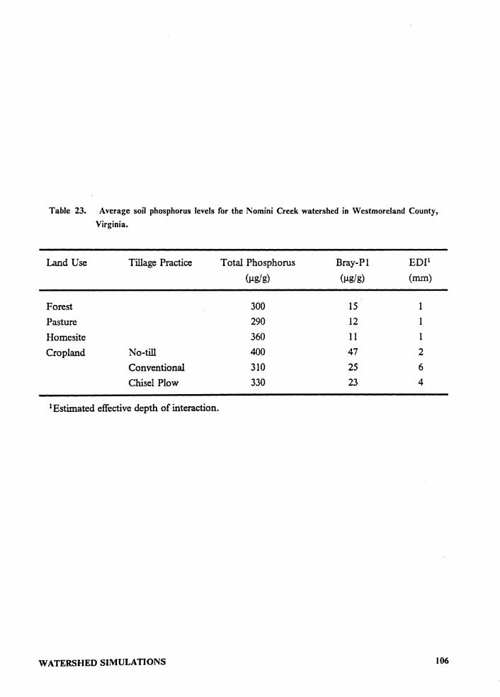
Table 23. Average soil phosphorus levels for the Nomini Creek watershed in Westmoreland County, Virginia.

Land Use Tillage Practice Total Phosphorus Bray-Pl EDI1 (µg/g) (µg/g) (mm)

Forest 300 15 1 Pasture 290 12 1 Homesite 360 11 1 Cropland No-till 400 47 2

Conventional 310 25 6 Chisel Plow 330 23 4

1 Estimated effective depth of interaction.


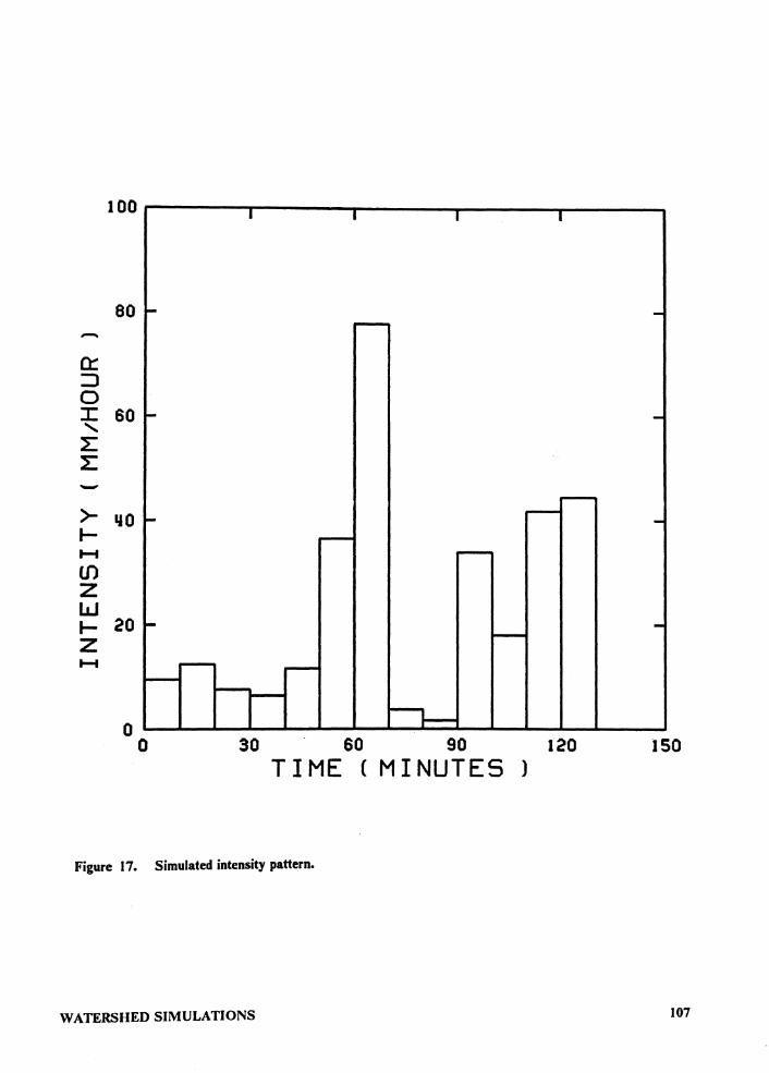
80 -0:: ::J 0 :r: 60

' l: l: ->- 110 I-t-1 U) z w I- 20 z t-1

30 60 90 120 150 TIME C MINUTES J

Figure 17. Simulated intensity pattern.


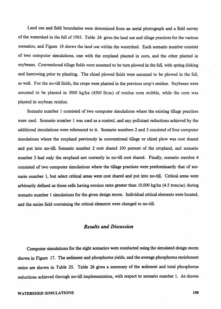
Land use and field boundaries were determined from an aerial photograph and a field survey

of the watershed in the fall of 1985. Table 24 gives the land use and tillage practices for the various

scenarios, and Figure 18 shows the land use within the watershed. Each scenario number consists

of two computer simulations, one with the cropland planted in corn, and the other planted in

soybeans. Conventional tillage fields were assumed to be turn plowed in the fall, with spring disking

and harrowing prior to planting. The chisel plowed fields were assumed to be plowed in the fall,

as well. For the no-till fields, the crops were planted in the previous crop's residue. Soybeans were

assumed to be planted in 5000 kg/ha (4500 lb/ac) of residue corn stubble, while the corn was

planted in soybean residue.

Scenario number 1 consisted of two computer simulations where the existing tillage practices

were used. Scenario number 1 was used as a control, and any pollutant reductions achieved by the

additional simulations were referenced to it. Scenario numbers 2 and 3 consisted of four computer

simulations where the cropland previously in conventional tillage or chisel plow was cost shared

and put into no-till. Scenario number 2 cost shared 100 percent of the cropland, and scenario

number 3 had only the cropland not currently in no-till cost shared. Finally, scenario number 4

consisted of two computer simulations where the tillage practices were predominantly that of sce-

nario number 1, but select critical areas were cost shared and put into no-till. Critical areas were

arbitrarily defined as those cells having erosion rates greater than 10,000 kg/ha (4.5 tons/ac) during

scenario number 1 simulations for the given design storm. Individual critical elements were located,

and the entire field containing the critical elements were changed to no-till.

Results and Discussion

Computer simulations for the eight scenarios were conducted using the simulated design storm

shown in Figure 17. The sediment and phosphorus yields, and the average phosphorus enrichment

ratios are shown in Table 25. Table 26 gives a summary of the sediment and total phosphorus

reductions achieved through no-till implementation, with respect to scenario number 1. As shown


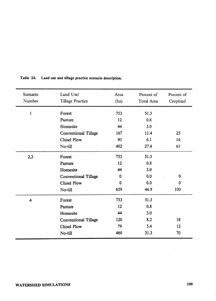
Table 24. Land use and tillage practice scenario description.

Scenario Land Use/ Area Percent of Percent of Number Tillage Practice (ha) Total Area Cropland

1 Forest 753 51.3 Pasture 12 0.8 Homesite 44 3.0 Conventional Tillage 167 11.4 25 Chisel Plow 90 6.1 14 No-till 402 27.4 61

2,3 Forest 753 51.3 Pasture 12 0.8 Homesite 44 3.0 Conventional Tillage 0 0.0 0 Chisel Plow 0 0.0 0 No-till 659 44.9 100

4 Forest 753 51.3 Pasture 12 0.8 Homesite 44 3.0 Conventional Tillage 120 8.2 18 Chisel Plow 79 5.4 12 No-till 460 31.3 70


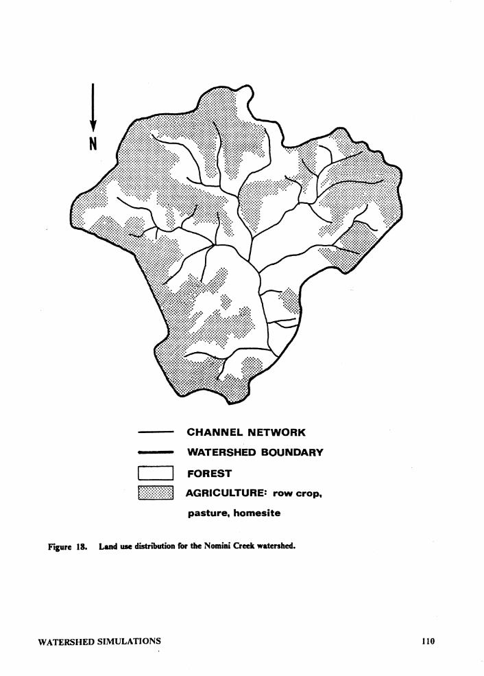
! N

CHANNEL NETWORK

WATERSHED BOUNDARY

I I FOREST

Pt?}{:J AGRICULTURE= row crop,

pasture, homesite

Figure 18. Land use distribution for the Nomini Creek watershed.


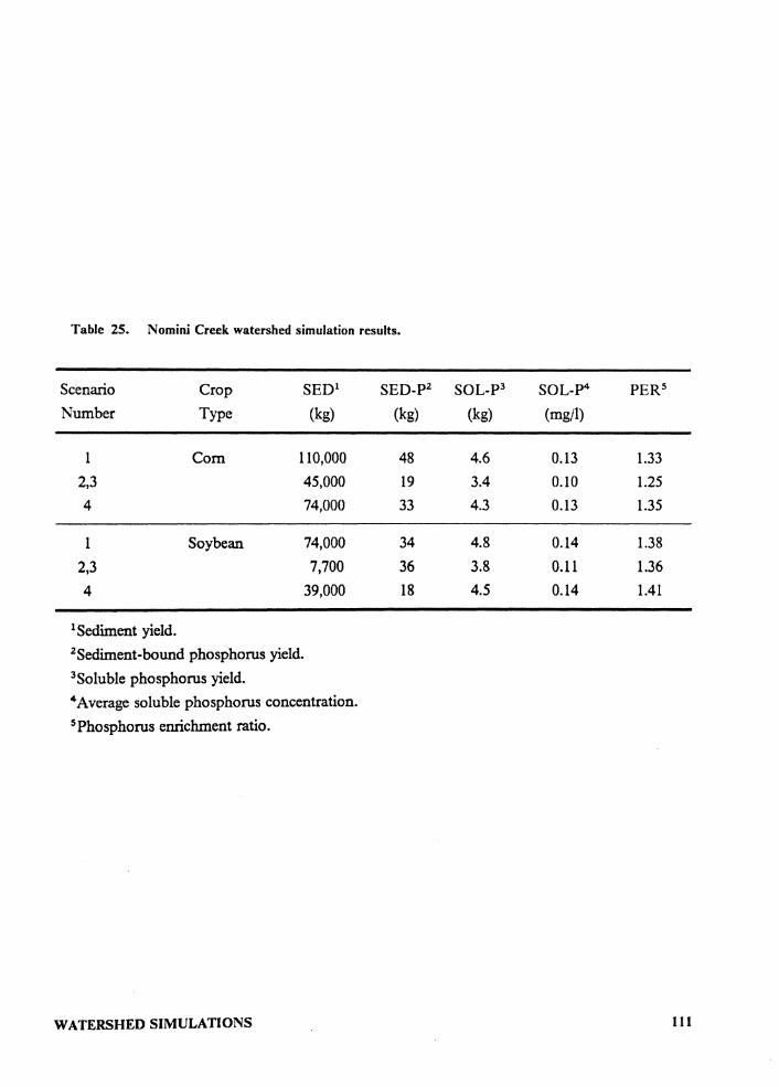
Table 25. Nomini Creek watershed simulation results.

Scenario Crop SED 1 SED-P 2 SOL-P 3 SOL-P 4 PER 5

Number Type (kg) (kg) (kg) (mg/1)

1 Com 110,000 48 4.6 0.13 1.33 2,3 45,000 19 3.4 0.10 1.25 4 74,000 33 4.3 0.13 1.35

1 Soybean 74,000 34 4.8 0.14 1.38 2,3 7,700 36 3.8 0.11 1.36 4 39,000 18 4.5 0.14 1.41

1 Sediment yield. 2Sediment-bound phosphorus yield. 3Soluble phosphorus yield. 4 Average soluble phosphorus concentration. 5Phosphorus enrichment ratio.


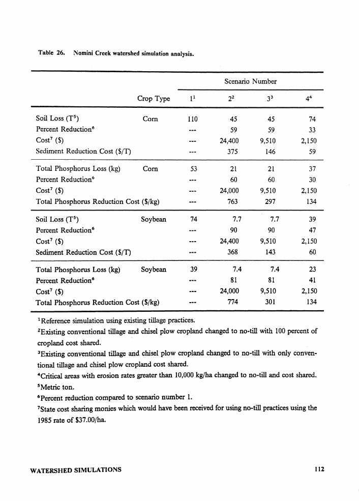
Table 26. Nomini Creek watershed simulation analysis.

Scenario Number

Crop Type l1 22. 33 44

Soil Loss (T 5) Corn 110 45 45 74 Percent Reduction 6 59 59 33 Cost 7 ($) 24,400 9,510 2,150 Sediment Reduction Cost ($/T) 375 146 59

Total Phosphorus Loss (kg) Corn 53 21 21 37 Percent Reduction 6 60 60 30 Cost7 ($) 24,000 9,510 2,150 Total Phosphorus Reduction Cost ($/kg) 763 297 134

Soil Loss (T 5) Soybean 74 7.7 7.7 39 Percent Reduction 6 90 90 47 Cost7 ($) 24,400 9,510 2,150 Sediment Reduction Cost ($/T) 368 143 60

Total Phosphorus Loss (kg) Soybean 39 7.4 7.4 23 Percent Reduction 6 81 81 41 Cost7 ($) 24,000 9,510 2,150 Total Phosphorus Reduction Cost ($/kg) 774 301 134

1 Reference simulation using existing tillage practices. 2Existing conventional tillage and chisel plow cropland changed to no-till with 100 percent of cropland cost shared. 3Existing conventional tillage and chisel plow cropland changed to no-till with only conven-tional tillage and chisel plow cropland cost shared. 4Critical areas with erosion rates greater than 10,000 kg/ha changed to no-till and cost shared. 5Metric ton. 6 Percent reduction compared to scenario number 1. 7State cost sharing monies which would have been received for using no-till practices using the

1985 rate of $37.00/ha.


in Table 26, for scenario numbers 2 and 3, the implementation of additional no-till practices on

cropland in the watershed reduced predicted soil loss by 59 and 90 percent, and predicted total

phosphorus yields by 60 and 81 percent for the no-till com and soybean scenarios, respectively.

In scenario number 4, when additional no-till practices were used only on those fields containing

areas with erosion rates greater than 10,000 kg/ha, soil loss was reduced 33 and 47 percent, and total

phosphorus yields were reduced by 30 and 41 percent for the critical area no-till corn and soybean

scenarios, respectively. The critical areas are shown in Figure 19

In 1985, cost share funds for using no-till were $37.00 per hectare. Using this rate, the cost

of reducing sediment and total phosphorus losses for scenarios 2 and 3 were $375 and $146 per

metric ton of soil loss reduced, and $763 and $297 per kg of total phosphorus reduced, respectively.

For the critical area scenario number 4, the cost of reducing sediment was $59 per metric ton of soil

loss reduced, and $134 per kg of total phosphorus reduced. The reason for this dramatic reduction

in cost is because scenario number 2 cost shared 100 percent of the cropland, scenario number 3

cost shared 39 percent, and scenario number 4 only cost shared 9 percent of the cropland. As

shown in Table 27, the cost effectiveness of the cost share program could be improved 61 and 84

percent in terms of sediment loss, and 61 and 83 percent in terms of total phosphorus for senarios

3 and 4, respectively. Similar cost reductions were achieved for the soybean scenarios.

It is important to note that these projections were based upon the results of a single design

storm. If cost per ton of soil loss prevented were determined on an annual basis for all the storms

that might be expected to occur throughout the year, then the cost per ton would be reduced sig-

nificantly because of the greater annual soil loss. It is also important to note that these projections

were based upon a critical area being defined as a field containing an element with an erosion rate

greater than 10,000 kg/ha for the given design storm. Selection of different erosion rates for critical

area identification could change these projections significantly.

WATERSHED SIMULATIONS ll3

" " ,.

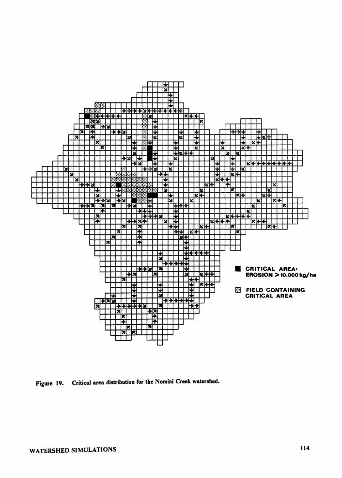
... :ill

lll I.& -lll""' 1,.1,

-t lll .i.

h _. •. ··: :••• •••• ··:• :.·

,_. _. lll lll ::::::::::· -111-1 :,II :,II :,II 1-t lll .... , ...

" ,_. lll

" .. " "' ,. .. ,I,

lll

-II -t lll " .. " " " .. ,I, lll

I .. :,II )I

" . lll " " " R

"' R ,. " R

.... --.... '-

lll ,I

I.I + IC ,I ... ,I ,_ .. 12' lll

"' 12' ++ IC :ill

,I,

IC

lll .. lll

lll +

:i:11 +

++++

lll

.I

Figure 19. Critical area distribution for the Nomini Creek watershed.

WATERSHED SIMULATIONS

lll

1-1 + .i, + :.i; +IC .. ,. IC 4-ric+

Ile .I.

IC

'--

CRITICAL AREA:

7 I

EROSION > 10,000 kg/ha

Q FIELD CONTAINING CRITICAL AREA

114

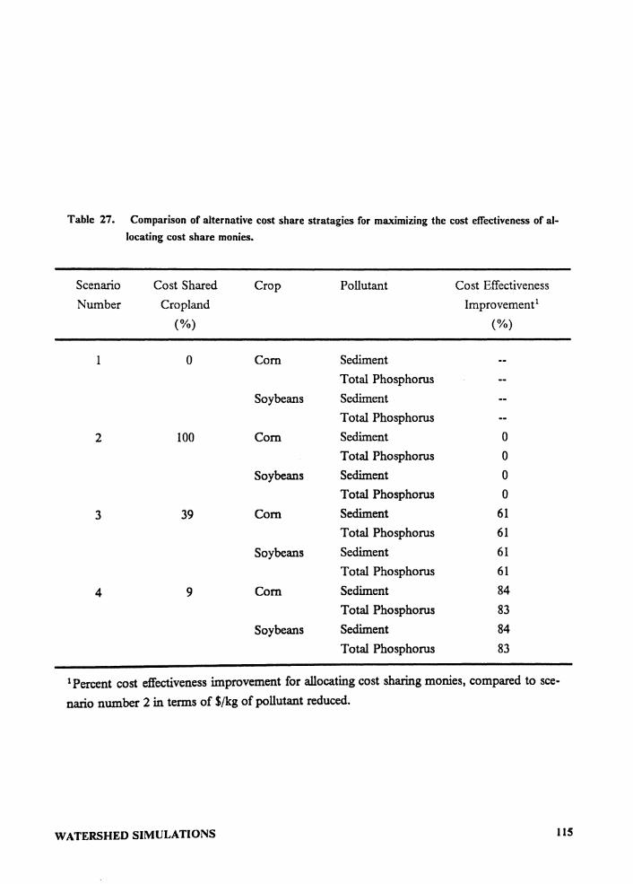
Table 27. Comparison of alternative cost share stratagies for maximizing the cost effectiveness of al-locating cost share monies.

Scenario Cost Shared Crop Pollutant Cost Effectiveness Number Cropland Improvement1

(%) (%)

I 0 Com Sediment Total Phosphorus

Soybeans Sediment Total Phosphorus

2 100 Com Sediment 0 Total Phosphorus 0

Soybeans Sediment 0 Total Phosphorus 0





1 Percent cost effectiveness improvement for allocating cost sharing monies, compared to see-nario number 2 in terms of $/kg of pollutant reduced.

WATERSHED SIMULATIONS ll5

SUMMARY AND CONCLUSIONS

Summary

A distributed parameter watershed model has been developed to simulate the transport of

soluble and sediment-bound phosphorus during the overland flow process. The phosphorus model

uses a nonequilibrium desorption equation to account for the desorption of soluble phosphorus

from the soil surface to surface runoff. The sediment-bound phosphorus is modeled as a function

of the specific surface area of the soil and transported sediment. The equilibrium conditions be-

tween the soluble and sediment-bound phases are modeled using a Langmuir isotherm.

The version of ANSWERS used has an extended sediment transport model which simulates

the transport of individual particle size classes in a sediment mixture. The erosion process is limited

to the overland flow regime, because the model does not account for channel erosion. The model

describes the processes of overland flow, subsurface drainage, sedimentation, and phosphorus

chemical kinetics. The continuity equation is then used to integrate the individual elemental re-

sponses into a system response that describes the watershed as a whole. The computer program

in written in Fortran 77.

The model was verified using experimental plot data, where the simulated results were in good

agreement with the observed data. The model was then used to demonstrate the use of ANSWERS

in studying the effects of no-till implementation on phosphorus and sediment yield reductions. The

demonstration used a technique developed for selecting a design storm. The technique creates an

n-year recurrence interval storm with a duration equal to the time of concentration of the

SUMMARY AND CONCLUSIONS 116

watershed. The intensity is simulated on a ten-minute interval using a first-order Markov model

with a lognormal distribution.

Conclusions

The phosphorus transport model simulated the response of the research plots fairly well. The

soluble phosphorus was usually overestimated which can, at least in part, be attributed to the over

estimation of the sediment-bound phosphorus. The over estimated sediment-bound phosphorus

can be attributed to over estimating the transported sediment or over estimating the soil phosphorus

levels.

The phosphorus processes, and the detachment and transport of sediment in overland flow are

very complex. The phosphorus and sediment processes used in this research are only rough ap-

proximations of the actual processes. However, the sediment transport equation appears to be one

of the better equations for describing overland flow. The phosphorus equations also appear to be

the best available equations. To date, this expanded version of ANSWERS is the most compre-

hensive computer model to describe the transport and chemical kinetics of the phosphorus and

sediment transport processes within an agricultural watershed.

The major obstacle encountered during this research was the lack of theoretical background

for describing the phosphorus and sediment transport processes, and the lack of available data for

describing the existing theory. Therefore, as a result of this research, it is evident that additional

research is required to develop more physically based relationships for estimating the input param-

eters. However, it is important to note that the existing model is still an excellent tool for simu-

lating a wide variety of soil, crop and topographic conditions and for evaluating the effects of

changing land use on phosphorus and sediment yields.

As shown from the Nomini Creek Watershed simulations, the model is an excellent planning

tool for evaluating the cost effectiveness of various conservation tillage scenarios on a watershed

scale. It should also be noted that for a given scenario, there is probably a significant amount of

SUMMARY AND CONCLUSIONS ll7

error associated with the pollutant yields, but the error in the relative differences between scenarios

is should be minimal. The model is therefore useful and adequate for planning purposes.

It should also be noted that ANSWERS is not cost-effective when applied to large areas be-

cause of the costs of data base generation and high computational costs. Data base generation costs

are greatly reduced if there is an existing geographical information system containing the required

data. For various portions of Virginia a geographical information system, VirGIS, is currently

available, which greatly facilitates the use of the model in Virginia.

SUMMARY AND CONCLUSIONS 118

RECOMMENDATIONS

During the course of this research, many assumptions were made to simplify complex physical

processes due to the lack of available data and/or the lack of theoretical background. Therefore,

the following recommendations are presented to guide future research in phosphorus and sediment

transport in agricultural watersheds.

1. A potential source of phosphorus not taken into account by the model is living and

decomposing plant material. Research on the plant material as a source of phosphorus

is becoming increasingly important with the implementation of no-till and other min-

imum tillage techniques. Use of these new tillage practices result in plant residue being

left on the soil surface, which may become a significant source of phosphorus.

2. Other potential sources of phosphorus not taken into account by the model are pre-

cipitation and the soil water. Both the soluble and particulate-bound phosphorus

from precipitation need to be addressed. In addition, the soluble phosphorus in the

soil water should be taken into account. However, its magnitude as a source of soluble

phosphorus is dependant on existing soil moisture conditions as well as various soil

physical properties.

3. Another area which requires additional research is in estimating the Langmuir isotherm

coefficients based on soil texture and the specific surface area of the transported

sediment. Most of the previous work with the Langmuir isotherm has dealt with the

soil matrix and phosphorus availability to plants, which typically has soluble

phosphorus concentrations of 1.0 to 100 ppm. However, soluble phosphorus con-

centrations in surface runoff from agricultural areas are typically 0.01 to 1.0 ppm.

RECOMMENDATIONS 119

Therefore, new relationships need to be developed, and if possible they need to be

physically based and not empirical.

4. Physically based relationships for determining the phosphorus desorption equation

coefficients need to be developed. They need to account for soil texture, soil properties

and soil chemistry.

5. Software needs to be developed to interface ANSWERS and simular models with ge-

ographic information systems such as VIRGIS. Emphasis also should be placed on

making the system personal computer (PC) based. For the model to be used to its

fullest, requires a PC based system that is Huser friendly."

6. Additional research in the area of soil detachment is required. To date, soil detachment

has been dealt with as gross detachment. The detachment process needs to be sepa-

rated into rill and interrill components. In addition, further research is required to

investigate the particle size distribution of sediment as detached and as a function of

soil type, texture, and soil chemistry. Also, additional data on the specific gravity of

detached particles is needed if their transport is to be modeled.

7. Aggregate stability during the transport process is another area that needs research.

8. Sediment transport models need to be developed to model overland flow in the rill and

interrill areas separately.

9. A channel erosion component needs to be incorporated into the current ANSWERS

model. In many watersheds the channel erosion may be the dominate erosion process.

Thus, the current model is not applicable to watersheds were channel erosion is sig-

nificant.

10. The surface sealing process should be researched to better quantify its effects on infil-

tration, subsurface drainage and overland flow. Knowledge concerning surface sealing

will allow the infiltration process to be modified to reflect changing surface conditions

throughout the storm event.

11. Additional research is needed to better estimate the effective depth of interaction based

upon the tillage practice, soil texture, and soil physical and chemical properties.

RECOMMENDATIONS 120

12. Finally, additional model verification over a wide range of conditions is required.

Factors which should be considered include various methods of fertilizer application,

crop conditions, surface slopes, and rainfall conditions. In addition, the model should

be verified on a watershed scale.

RECOMMENDATIONS 121

REFERENCES

Ahuja, L.R. 1982. Release of soluble chemicals from soil to runoff. TRANSACTIONS of the ASAE 25:948-953,960.

Ahuja, L.R., and O.R. Lehman. 1983. The extent and nature of rainfall-soil interaction in the release of soluble chemicals to runoff. J. Environ. Qual. 12:34-40.

Ahuja, L.R., A.N. Sharpley, and O.R. Lehman. 1982. Effect of soil slope and rainfall char-acteristics on phosphorus in runoff. J. Environ. Qual. 11:9-13.

Ahuja, L.R., A.N. Sharpley, M. Yamamoto, and R.G. Menzel. 1981. The depth of rainfall-runoff-soil interaction as determined by 32P . Water Resources Research 17:969-974.

Amin-Sichani, S. 1982. Modeling of phosphorus transort in surface runoff from agricultural watersheds. Ph. D. Thesis. Purdue University, West Lafayette, IN. 157 p.

Ang, A. H-S and W. H. Tang. 1975. Probability concepts in engineering planning and design. John Wiley and Sons, New York, N.Y., 409 p.

Beasley, D.B. 1977. ANSWERS: A mathematical model for simulating the effects of land use and management on water quality. Ph. D. Thesis. Purdue University, West Lafayette, IN. 266 p.

Beasley, D.B., L.F. Huggins. 1981. ANSWERS (Areal Nonpoint Source Watershed Environ-mental Response Simulation) User Manual. Department of Agricultural Engineering, Purdue University, West Lafayette, IN. 55 p.

Beasley, D.B., L.F. Huggins, and EJ. Monke. 1980. ANSWERS: A model for watershed planning. Transactions of the ASAE. 23:938-944.

Bohn, H., B. McNeal, G.A. O'Conner. 1979. Soil Chemistry. John Wiley and Sons, Inc., New York.

Bray, R.H., and L.T. Kurtz. 1945. Determination of total, organic, and available forms of phosphorus in soil. Soil Sci. 59:39-45.

Burwell, R.E., G.E. Schuman, R.F. Piest, R.G. Spomer, and T.M. Mccalla. 1974. Quality of water discharged from two agricultural watersheds in southwestern Iowa. Water Re-sources Research 10:359-365.

Crawford, N .H., and A.S. Donigian. 1973. Pesticide transport and runoff model for agricultural lands. EPA-600/2-74-013, Environmental Research Laboratory, U.S. Environmental Protection Agency, Athens, GA. 293 p.

Davis, H.H., Jr., and A.S. Donigian, Jr. 1979. Simulating nutrient movement and transf-ormations with the ARM model. Transactions of the ASAE 22( 1 ): 151-154.

Day, P.R. 1965. Particle fractionation and particle size analysis. In: C.A. Black, et al. (ed.) Methods of Soil Analysis Part I. Agronomy Monograph 9:545-567. Am. Soc. of Agron., Madison, Wis.

REFERENCES 122

Dillaha, T.A. 1981. Modeling the particle size distribution of eroded sediments during shallow overland flow. Ph. D. Thesis. Purdue University, West Lafayette, IN. 189 p.

Donigian, A.S. Jr. 1976. Modeling pesticides and nutrients on agricultural lands. EPA-600/2-76-043, Environmental Research Laboratory, U.S. Environmental Protection Agency, Athens, GA. 293 p.

Donigian, A.S. Jr., and N.H. Crawford. 1976. Modeling nonpoint pollution from the land surface. EPA-600/3-76-083, Environmental Research Laboratory, U.S. Environmental Protection Agency, Athens, GA. 293 p.

Donigian, A.S. Jr., and N.H. Crawford. 1979. Users Manual for the nonpoint source (NPS) model. EPA-600/6-79-343, Environmental Research Laboratory, U.S. Environmental Protection Agency, Athens, GA. 95 p.

Donigian, A.S. Jr., and N.H. Crawford. 1977. Simulation of nutrient loadings in surface runoff with the NPS model. EPA-600/3-77-065, Environmental Research Laboratory, U.S. En-vironmental Protection Agency, Athens, GA. 95 p.

Donigian, A.S. Jr., and J.H. Davis. 1978. Users Manual for Agricultural runoff management (ARM) model. EPA-600/3-78-080, Environmental Research Laboratory, U.S. Environ-mental Protection Agency, Athens, GA. 293 p.

Donigian, A.S. Jr., D.C. Beyerlein, J.H. Davis, Jr., and N.A. Crawford. 1977. Agricultural runoff management (ARM) model. Version II: refinement and testing. EPA-600/3-77-098, Environmental Research Laboratory, U.S. Environmental Protection Agency, Athens, GA. 293 p.

Foster, G.A., R.A. Young, and W.H. Neibling. 1985. Sediment composition for nonpoint source pollution analyses. Transactions of the ASAE 28(1):133-139, 146.

Frere, R.G., J.D. Ross, and LJ. Lane. 1980. The nutrient submode!. In: Knisel, W.G. (ed), CREAMS. A Field Scale Model for Chemicals, Runoff, and Erosion from Agricultural Management Systems. Conservation Res. Report No. 26, USDA-SEA. pp. 65-87.

Freundlich, H. 1926. Colloid and Capillary Chemistry. Methven & Company, London.

Gburek, W.J., and W.R. Heald. 1974. Soluble phosphate output of an agricultural watershed in Pennsylvania. Water Resou. Res. 10:113-119.

Gosz, J.R., G.E. Likens, and F.H. Bormann. 1973. Nutrient release from decomposing leaf and branch litter on the Hubbard Brook Experimental Forest,New Hampshire. Ecological Monograph. 43: 173-I 91.

Haan, C. T. 1977. Statistical Methods in Hydrology. The Iowa State University Press, Ames, Iowa, 378 p.

Huggins, L.F., and EJ. Monke. 1966. The mathematical simulation of small watersheds. Technical Report 1. Water Resources Research Center, Purdue University, West Lafayette, IN. 70 p.

James, A. 1984. An Introduction to Water Quality Modeling. John Wiley and Sons, New York. 234 p.

James, L.D. 1970. An evaluation of relationships between streamflow patterns and watershed characteristics through the use of OPSET: A self-calibrating version of the Stanford

REFERENCES 123

watershed model. University of Kentucky, Water Resources Institute, Research Report No. 36. Lexington, KY.

Kendall, G.R. 1967. Probability distribution of a single variable. In: Statistical Methods in Hydrology. Proceedings of Hydrology Symposium 5. McGill University, Feb. 24 and 25, 1966. Queen's Printer, Ottawa, Canada.

Kent, K. M. 1968. A method of estimating volume and rate of runoff in small watersheds. USDA Soil Conservation Service, SCS-TP-149. 40 p.

Kerby, W.S. 1959. Time of concentration for overland flow. Civil Engineering. 29:6.

Knisel, W.G. 1980. CREAMS. A Field Scale Model for Chemicals, Runoff, and Erosion from Agricultural Management Systems. Conservation Research Report No. 26, USDA-SEA.

Kunze, G.W. 1965. Pretreatment for mineral analysis. In: C.A. Black, et al. (ed.) Methods of Soil Analysis Part I. Agronomy Monograph 9:568-577. Am. Soc. of Agron., Madison, Wis.

Langmuir, I. 1918. The adsorption of gases on plane surfaces of glass, mica, and platinum. J. Am. Chem. Soc. 40: 1361.

McDowell, D.L., J.D. Schreiber, and H.B. Pionke. 1980. Estimating soluble (P0 4-P) and labile phosphorus in runoff from croplands. In: Knisel, W.G. (ed), CREAMS. A Field Scale Model for Chemicals, Runoff, and Erosion from Agricultural Management Systems. Conservation Res. Report No. 26, USDA-SEA. pp. 509-533.

Menzel, R.G. 1980. Enrichment ratios for water quality modeling. In: Knisel, W.G. (ed.), CREAMS. A Field Scale Model for Chemical, Runoff, and Erosion from Agricultural Management Systems. Conservation Research Report No. 26, USDA-SEA. pp. 486-492.

Mortland, M.M., and W.D. Kemper. 1965. Specfic surface. In: C.A. Black, et al. (ed.) Methods of Soil Analysis Part I. Agronomy Monograph 9:532-544. Am. Soc. of Agron., Madison, Wis.

Murphy; J., and J.P. Riley. 1962. A modified single solution method for determination of phosphate in natural wastes. Anal. Chem. Acta. 27:31-36.

Neff, E. L.. 1979. Simulator activities - Sidney, Montana. In Proceeding: The Rainfall Simu-lator Workshop. USDA-ARS, ARS-W-10, p. 160-161.

Negev, M.A. 1967. Sediment model on a digital computer. Department of Civil Engineering, Stanford University, Technical Report No. 76. Standford, CA. 109p.

Novotny, V., and G. Chesters. 1981. Handbook of Nonpoint Pollution Sources and Manage-ment. Van Nostrand Reinhold Company, New York.

Olsen, S.R. 1982. Methods of soil analysis. In: C.A. Black, et al. (ed.) Methods of Soil Anal-ysis Part II. Agronomy Monograph 9:403-430. Am. Soc. of Agron., Madison, Wis.

Ross, G .A. 1970. The Stanford watershed model: The correlation of parameter values selected by a computerized procedure with measurable physical characteristics of the watershed. Water Resources Institute Research Report No. 35. University of Kentucky, Lexington, KY. 178 p.

REFERENCES 124

Ross, B.B., M.L. Wolfe, V.O. Shanholtz, M.D. Smolen, and D.N. Contractor. 1982. Model for simulating runoff and erosion in ungaged watersheds. Virginia Water Resorces Re-search Center, Bulletin 130, Virginia Polytechnic Institute and State Univeristy, Blacksburg, Virginia. 72 p.

Ryden, J.C., Syers, J.K., and R.F. Harris. 1972. Potential on an eroding urban soil for the phosphorus enrichment of streams. J. Enviro. Qual. 1:430.

Schaller, F.W., and G.W. Bailey. 1983. Agricultural management and water quality. Iowa State University Press, Ames, Iowa.

Schwab,G. 0., R. K. Frevert, T. W. Edminster, and K. K. Barnes. 1981. Soil and water conservation engineering. 3rd Edition, John Wiley & Sons, New York, N.Y. 525 p.

Shanholtz, V. 0. and J. B. Burford. 1967. Computer systems for reduction and analysis of hydrologic data. USDA Agricultural Research Service, ARS 41-132. 90 p.

Shanholtz, V.O. and J.H. Lillard. 1968. Hydrologic aspects of no-tillage versus conventional tillage systems for corn production. Virginia Water Resorces Research Center, Bulletin 14, Virginia Polytechnic Institute and State Univeristy, Blacksburg, Virginia. 31 p.

Shanholtz, V.O., M. D. Smolen, D. F. Amos, and J.B. Burger. 1981. Predicting soil loss from surface mined areas. State Mining and Mineral Resourse Research Institute, VPI & SU, Blacksburg, Virginia.

Sharpley, A.N. 1985. Depth of surface soil-interaction as affected by rainfall, soil slope, and management. Soil Sci. Soc. Am. J. 49:1010-1015.

Sharpley, A.N. 1983. Effect of soil properties on the kinetics of phosphorus desorption. Soil Sci. Soc. Am. J. 47:462-467.

Sharpley, A.N. 1981. The contribution of phosphorus leached from crop canopy to losses in surface runoff. J. Environ. Qual. 10:160-165.

Sharpley, A.N. 1980. The enrichment ratio of soil phosphorus in runoff sediments. J. Enviro. Quality 9(3):521-525.

Sharpley, A.N., L.R. Ahuja, and R.G. Menzel. 1981. The release of soil phosphorus to runoff in relation to the kinetics of desorption. J. Environ. Qual. 10:386-391.

Sharpley, A.N., L.R. Ahuja, M. Yamamoto, and R.G. Menzel. 1981b. The kinetics of phosphorus desorption from soil. Soil Science. 45:493-496.

Simons, D.B., R.M. Li, and M.A. Stevens. 1975. Development of models for predicting water and sediment routing and yield from storms on small watersheds. CER-75-DBS-RML-MAS-24. Colorado State University, Fort Collins, Colorado. 130 p.

Stidd, C.K. 1953. Cube root normal precipitation distributions. Transactions Geophysical Union. 34(1):31-35.

Summers, L.E., and D.W. Nelson. 1972. Determination of total phosphorus in soils: a rapid perchloric acid digestion procedure. Soil Sci. Soc. Am. Proc. 36:902-904.

Tchobanoglous, G., and I.D. Schroeder. 1985. Water Quality Management. Addision-Wesley Publishing Company, Reading, MA.

REFERENCES 125

Timmons, D.R., and R.F. Holt. 1970. Leaching of crop residues as a source of nutrients in surface runoff waters. Water Resources Research. 6:1367-1375.

USEPA. 1983. Chesapeake Bay: A framework for action. Chesapeake Bay Program, U.S. Environmental Protection Agency, Annapolis, Maryland. 186 p.

White, E.M., and E.J. Williamson. 1973. Plant nutrient concentrations in runoff fertilized cultivated erosion plots and prairie in eastern South Dakota. J. Environ. Qual. 2:453-455.

Wischmeier, W.H. and D.D. Smith. 1978. Predicting Rainfall erosion losses. Agricultural Handbook No. 537, USDA-Science and Education Administration, 58 p.

Woeste, F.E., S.K. Suddarth and W.L. Galligan. 1979. Simulation of correlated lumber prop-erties data - a regression approach. Wood Science. 12(2):73-79.

Woolhiser, D.A. 1973. Hydrology and watershed modeling - state of the art. Transactions of the ASAE. 16(3):553-559.

REFERENCES 126

APPENDICES

APPENDIX A: Variable Glossary

NAME TYPE MAIN USE DEFINITION

A R ARRAY Infiltration coefficient in Holtan's equations for element i ADIR R VARIABLE Retention depth on volume per unit area, m AGRAV R VARIABLE Acceleration of gravity is m/s2

ALPHA R ARRAY Exponent for TIME in soluble phosphorus desorption equation for soil type i

ANG R VARIABLE Slope direction of element in degrees counter- clockwise from positive row axis

AREA R VARIABLE Catchment area as sum of element areas, ha AREA2 R VARIABLE Element or channel area, m2

ASM R EQVARRAY Antecedent soil moisture as a fraction of pore space for soil i ASMBAR R VARIABLE Average ASM AVGER R VARIABLE Average phosphorus enrichment ratio AVGP0 R VARIABLE Avarage soil phosphorus content, µg/g B R ARRAY Conveyance in Manning's equation BO R VARIABLE Coefficient related to the binding strength of the material for the

Langmuir isotherm. BOC! R VARIABLE Coefficeint in Langmuir isotherm related equation as a function

Q0 B0C2 R VARIABLE Coefficeint in Langmuir isotherm related equation as a function

ofQ0 B0C3 R VARIABLE Exponent in Langmuir isotherm related equation as afunction of

Q0 BD R ARRAY Soil bulk density, g/cm.3

BETA R ARRAY Exponent for WS in phosphorus the desorption equation for soil type i

Cl-6 R VARIABLE Product of CDR and SKDR for element CBAR R EQVARRAY Percent of watershed in crop i CD R VARIABLE Drag coefficient used in determining particle full velocity CDR R ARRAY Erosion parameter for crop management practice i

APPENDICES 127

CE3-6 R VARIABLE Constants in erosion equations CGEN R ARRAY Concentration of soluble phosphorus from the soil surface, kg/m3

CGENl R ARRAY Part of soluble phosphorus desorption equation for element m CHAN I EQV ARRAY Constant indicating presence of absence of channel in an element CHDR R VARIABLE Groundwater discharge into a channel segment CHN R VARIABLE Number of channel segments CN R EQV ARRAY Manning's "n" for channel type i CONST R VARIABLE Flow depth units conversion factor CONY R VARIABLE Catchment conversion constant for mm/h to m 3/s CPSO2 R VARIABLE Concentration of soluble phosphorus outflow after time step,

kg/m3

CROP R EQV ARRAY Alphanumeric name of crop i cu R VARIABLE Element conversions constant for mm/h to m 3 /s CUI R VARIABLE Element conversion constant for mm to m3

CU2 R VARIABLE Element conversion constant for twice m3

CWID R EQVARRAY Width of channel segment i CYI-5 R ARRAY Simplifying constants used in transport equation D R VARIABLE Depth increment in segmented depth curve DATE R EQVARRAY Date of event being simulated DC R VARIABLE Tile drainage coefficient DD R VARIABLE Portion of tile drainage fl.owing in a row direction DELTA R ARRAY Variable in transport equation DEP R VARIABLE Storage depth on element in volume per unit area, m DETF R VARIABLE Rainfall detachment, kg/s DETR R VARIABLE Rainfall detachment, kg/s DF R EQV ARRAY Infiltration control zone depth for soil i, mm

PI R VARIABLE Simulation time minus rainfall histogram change time, s

DIA R ARRAY Particle diameter, m DIAMM R EQVARRAY Particle diameter, mm

DIN R EQV ARRAY Accumulated tile drainage rate in element i, m DIR R EQVARRAY Retention depth for cropping practice i, m 3 /s

DIRM R EQVARRAY Maximum physical retention depth for cropping practice i, mm

DP R VARIABLE Deposition rate kg/s

DR R ARRAY Vertical drainage loss from control zone of element i, m3/s

DRA R VARIABLE Incremental increase in outflow from element in row direction, m3/s

DRANE R VARIABLE Rate of tile drainage in element, m3/s

APPENDICES 128

DRFT DS DSl DS2 DT DTM DTMIN DX DX2 EDI EDMM EQSDIA ER ERG ERP

EXTP

F FC

FCAP FH FHS FIL FILTS FLIN FLINS

R VARIABLE R VARIABLE R ARRAY R ARRAY R VARIABLE R VARIABLE R VARIABLE R VARIABLE R VARIABLE R ARRAY R ARRAY R ARRAY R ARRAY R VARIABLE R ARRAY

R ARRAY

R ARRAY R ARRAY

Sum of rainfall and flow detachment, kg/s Maximum rate of sediment inflow and erosion in element, kg/s DS with only rainfall detachment, kg/s DS with rainfall and flow detachment, kg/s Simulation time increment in seconds Simulation time increment in minutes Minimum time increment in any hyetograph Length of side of square element, m Area of element, m2

Effective depth of interaction for soluble phosphorus model, mm Equivalent sand diameter of particle i, mm Equivalent sand diameter of particle i, m Amount of particle type i leaving watershed, kg/s Sum of ER for all particle classes, kg/s Sediment bound phosphorus leaving watershed for particle class i, kg Extractable phosphorus level for soil m element m, µg - P/g - soil Fraction of particles of type i in original soil Minimum, supply unlimited infiltration capacity for soil i, m3/s (input as mm/h)

R EQV ARRAY Field capacity for soil i as a fraction of pore space R VARIABLE Maximum physical water depth in element, m R VARIABLE FLINS plus FLIN R VARIABLE Infiltration into element during time increment, m3 /s. R EQV ARRAY Infiltration capacity for element i, m3/s R VARIABLE Net rate of flow into an element less losses, m3/s R ARRAY Storage, inflow and outflow for element i at start of time incre-

ment, m3/s FLODEP R VARIABLE Depth of flow in element or channel, m FMAX

FPBAR FRA FV FWA GRF

R VARIABLE Maximum infiltration capacity, surface inundated, m3/s (input as mm/h)

R VARIABLE R ARRAY R ARRAY R VARIABLE R VARIABLE

P in Holtans equation Fraction of catchment area covered by rain gauge i Fall velocity of particle type i, m/s Fraction of surface area of element covered by water Fractional rate of baseflow release

APPENDICES 129

GWC R ARRAY Volume of air filled pore space at field capacity for soil i, m HU R ARRAY Maximum height differential on soil surface, mm 11-3 I VARIABLE Counter ICR I VARIABLE Number of cropping practices IEL I EQVARRAY Array for data manipulation IG I EQV ARRAY Alphanumeric number for rain gauge IGAM I ARRAY Exponent for EXTP in phosphorus desorption equation. II I VARIABLE Number of channel segments IRR I EQVARRAY Number of rainfall intensity readings for rain gauge i IS I VARIABLE Soil type for current element JSR I VARIABLE Number of soil types ISTL I VARIABLE Comparator for sensing presence of drain tile in element ISTRUC I VARIABLE Counter for structural practices ITEMP I EQVARRAY Array for input data manipulation ITR I VARIABLE Rainfall histogram counter IX I VARIABLE Constant to indicate presence of a channel in an element IY I VARIABLE Segment number on segmented discharge curve Jl-3 I VARIABLE Counters JJ, JK I VARIABLE Counters JMAX I VARIABLE Dimension in IEL JS I VARIABLE Column number for last column on current element row, plus I JTR I ARRAY Current rainfall intensity histogram period for rain gauge i

K I VARIABLE Number of values in rainfall hyetograph and Surface type of cur-rent element

Kl I VARIABLE Counter

KK I VARIABLE Soil type for current element

KPR I VARIABLE Number of time increment routings between print lines

L I VARIABLE Number of last element in row and a Counter

M I VARIABLE Element number counter and Slope direction quadrant

MOUT I VARIABLE Catchment outflow overland flow element number

N I VARIABLE Number of overland flow elements

NI I VARIABLE N+l

N2 I VARIABLE Number of overland flow plus channel elements

NC I ARRAY Number of element receiving outflow from element i in a column direction

NOT I VARIABLE Number of lines of hydrograph print

APPENDICES 130

NEXP I VARIABLE Exponent in equation controlling drainage rate from infiltration control zone

NF I ARRAY Down-Counter from NF 1 NFI I VARIABLE Maximum number of time increments between infiltration recal-

culations NIOUT NJOUT NMAX NN NPAR NPART NPM NR

I VARIABLE Row number of catchment outflow element I VARIABLE Column number of catchment outflow element I VARIABLE Maximum number of elements I VARIABLE N2 + 1 I VARIABLE Dimension of IEL and !TEMP I VARIABLE Number of particle size classes I VARIABLE NPART - NWASHl I ARRAY Number of element receiving outflow from element i in a row di-

rection NRG I VARIABLE Number of rain gauges NSTR UC I EQV ARRAY Type of structural practice NW ASH I VARIABLE Number of washload particle classes NW ASH 1 I VARIABLE NW ASH + 1 OLDSED R VARIABLE Previous transported sediment after time step for particle class i,

kg/sec OUTSID R VARIABLE Area of watershed border elements which drain outside of

watershed p R ARRAY PO R ARRAY

P0SOIL R ARRAY

P2 R ARRAY

PE R ARRAY

Parameter in Holtan' s equation for surface condition i Total Phosphorus content of the soil for an element for particle class i, kg-p/kg-soil Total phosphorus content of the soil for element m, µg - p/µg - soil Term in sediment-bound phosphorus continuity equation for particle class i for storage term, kg/sec Sediment-bound phosphorus outflow after time increment for particle class i, kg/sec

PER R ARRAY Fraction of element area covered by foliage for surface type i PET R VARIABLE Total sediment-bound phosphorus outflow for element i, kg/sec PG R ARRAY Sediment-bound phosphorus eroded from the soil surface during

a time step for particle class i, kg/sec PI R ARRAY Sediment-bound phosphorus inflow from adjacent elements for

particle class i, kg/sec

APPENDICES 131

PI2

PIT PIV PIV2 PK

pp PPT

R ARRAY

R ARRAY R ARRAY R VARIABLE R ARRAY

R ARRAY R ARRAY

Sediment-bound phosphorus inflow after time increment for par-ticle class i, kg/ sec Interception storage for cover for surface type i, mm Volume of air filled pore space in control zone in element i Same as PIV Constant in soluble phosphorus desorption equation for soil type 1

Alphanumeric unit description Sum of initial values in sediment-bound phosphorus continuity equation, elements for particle class i, kg/sec

PRA R VARIABLE Sediment-bound phosphorus leaving element and flowing in a row

PRACT PREC PRI

I VARIABLE R VARIABLE R VARIABLE

direction Counter for structural practices Accumulated depth of precipitation, mm PR comparator for print of hyetograph(s)

PS R ARRAY Variable in transport equation PS2 R VARIABLE Storage component m continuity equation for soluble

phosphorus, kg/sec PSCON R ARRAY Soluble phosphorus concentration at print line, mg/1. PSEL R ARRAY Accumuative sediment-bound phosphorus for element i, kg/sec. PSPT R VARIABLE Accumulative sediment-bound phosphorus loss from catchment

at previous time, kg PSER R VARIABLE Soluble phosphorus leaving watershed, kg/sec PSG R VARIABLE Rate of soluble phosphorus desorbed from the soil surface from

a given element after the time step, kg/sec PSI PSIG PSINF PSLSI PSLSIY PSLST PS02 PSRA

PSSA PSSEL PSSI

R ARRAY Soluble phosphorus inflow from adjacent elements, kg/s R VARIABLE Sum of PSI values for previous interval, kg/s R VARIABLE Soluble phosphorus infiltrating into element i, kg/sec R VARIABLE Soluble phosphorus yield at outlet in kg R VARIABLE Soluble phosphorus yield at outlet in kg/ha R VARIABLE Accumulative soluble phosphorus at outlet, kg/sec R VARIABLE Soluble phosphorus leaving element after time step, kg/sec. R VARIABLE Amount of soluble phosphorus leaving element and flowing in a

row direction R VARIABLE Phosphorus content of soil type i, kg-p/m2

R ARRAY Accumulative soluble phosphorus for element i, kg/sec R ARRAY Sediment-bound phophorus at print line, mg.

APPENDICES 132

PSSIG R VARIABLE Sum of PSSI values for previous interval, kg/s PSSIY R VARIABLE Sediment-bound phosphorus yield at outlet, in kg PSSPT R VARIABLE Accumulative soluble phosphorus loss from catchment at previ-

oustime,kg PSTOLD R ARRAY Specific surface area of sediment leaving watershed, kg/s PTl R ARRAY Sediment-bound phosphorus content for inflow sediment for par-

ticle class i at the start of the time step, kg-p/kg-soil PT2 R ARRAY Sediment-bound phosphorus content for transported and outflow

sediment for particle class i at the end of the time step, kg-p/kg-soil Q R ARRAY Outflow from element i at start of time increments, m3/s Q0 R VARIABLE Adsorption maximum for the Langmuir isotherm Q0Cl R VARIABLE Coefficeint in Langmuir isotherm related equation as as function

of specific surface area. Q0C2 R VARIABLE Coefficeint in Langmuir isotherm related equation as as function

of specific surface area. Q0C3 R VARIABLE Exponent in Langmuir isotherm related equation as as function

of specific surf ace area. Ql R VARIABLE Discharge from catchment at ith hydrograph line, mm/h QlMl R VARIABLE Ql(i-1) Q2 R VARIABLE Outflow from element at end of time increment, m3/s QA R ARRAY Incremental depth power values for segmented curve QD R VARIABLE Differential in discharge on curve segment QI R ARRAY Inflow to element i from adjacent elements m3/s QL R VARIABLE Discharge at lower end of segment IY on discharge curve R R ARRAY Net rainfall rate for rain gauge ion surface type j m.3/s RAIN R VARIABLE Effective rainfall rate, m3 /s RANE I EQVARRAY Number of rain gauge applicable to element i RATE R ARRAY Gauge rainfall rate at rainfall gauge i, m3/s RC R ARRAY Rainfall intensity for gauge i, histogram period j, m3/s

RE R VARIABLE Particle removal efficiency during deposition

REYN R VARIABLE Particle Reynolds number

RFL R ARRAY Fraction of discharge from element flowing in a row direction

RIT R VARIABLE Interception during time increment, m3/s

RN R ARRAY Manning's "'n"" for surface type 1

ROUGH R ARRAY Surface depth-storage parameter for surface i

RW R VARIABLE Average rainfall intensity over catchment at ith hydrograph print time

APPENDICES 133

s R ARRAY Storage at start chime increment for element i, m3/s S2 R VARIABLE Variable in sediment continuity equation S22 R ARRAY Variable in sediment continuity equation SAi R ARRAY Sediment surface area inflow from adjacent elements, m2

SAIG R VARIABLE Sum of SAi values for previous interval, m2

SA02 R VARIABLE Sediment surface area leaving element after time step, m2 /s SAPT R VARIALBE Accumulated sediment surface area loss from catchment at previ-

ous time interval, m2

SAT R ARRAY Sum of the initial values for the sediment surface area continuity equation

SB R VARIABLE Average overland flow conveyance coefficient SBAR R VARIABLE Average catchment slope SC R VARIABLE Depth increment for segmented curve SCBAR R VARIABLE Variable used for determining mean value of SS and SSI SCMAX R VARIABLE Maximum value of SS and SSI SCMIN R VARIABLE Minimum value of SS and SSI SDEL R VARIABLE Summation of DELTA SDR R VARIABLE Accumulated groundwater storage, m3/s SE R ARRAY Rate of sediment movement from element, kg/s SEl-2 R ARRAY Rate of sediment movement from element with and without flow

detachment, kg/s SEDNEW R ARRAY Newly transported sediment after time step for particle class i,

kg/sec SEL R EQVARRAY Accumulated sediment aggradation in element i kg/s SF R VARIABLE Segment factor. Maximum projected catchment discharge SG R ARRAY Specific gravity of particle type i SGD2 R VARIABLE SQRT (AGRAV/2) SI R EQVARRAY Rate of sediment inflow into element i from adjacent elements,

kg/s SIG R VARIABLE Sum of SI values for all particle classes, kg/s SIGMA R VARIABLE Coefficient in transport equation SKDR R ARRAY Erosion parameter for soil type i SL R ARRAY Slope of overland flow element or channel segment i SMAX R VARIABLE Final accumulated sediment loss from catchment, kg

SMDIR R VARIABLE S-DIR

SMIN R VARIABLE Minimum elemental and channel slope in watershed

SOIL I EQVARRAY Soil type for element i

APPENDICES 134

SPADEP R VARIABLE Maximum elemental aggradation value, kg/ha SPAERO R VARIABLE Minimum elemental aggradation value, kg/ha SPASD R VARIABLE Standard deviation of SEL SPASS R VARIABLE Variable used in detennining SPASD SPASUM R VARIABLE Sum of SEL values used to calculate SPASD SPER R EQVARRAY Steady state infiltration rate, mm/h SPT R VARIABLE Accumulated sediment loss from catchment at previous time, kg SR R ARRAY Rainfall rate from previous calculation, m3/s SRA R VARIABLE Portion of sediment leaving element and flowing in a row direction ss R ARRAY Incremental increase in storage on element i SSA R ARRAY Total specific surface area for element m, for particle class i, m2 /kg

(input/output in m2 /g) SSASED R VARIABLE Specific surface area of sediment leaving watershed, m2 /kg SSAT R ARRAY Total specific surface area for soil type i, m2 /g SSCON R VARIABLE Sediment concentration at print line i, mg/1 SSI R VARIABLE Accumlated sediment loss from catchment at print line i SSII R VARIABLE Same as SSI SSlMl R VARIABLE SSI at previous time step SST R EQVARRAY Sum of initial values in sediment continuity equation, kg/s SSTOR R ARRAY Storage on element at end of time increment, m3/s STD R VARIABLE Total inflow into tile lines during DT STNEW R ARRAY Sediment in particle class i in storage at the end of the time step,

to be saved for next time step, kg/sec STOLD R ARRAY Sediment in particle class i in storage at the beginning of the time

step, kg/sec STRNAM R ARRAY Name of structure STRUC R VARIABLE Flag for e;itistence of structure SUPP R VARIABLE Available supply for infiltration during time increment SUR R EQVARRAY Surface type on element i SWH20 R VARIABLE Specific weight water, kg/m3

T R ARRAY Real time TBAR R VARIABLE Percent of elements tiled TC R ARRAY Time of jth histogram period for rain gauge i TEST R VARIABLE Comparison for correct data input check TF R ARRAY Sediment transport capacity, kg/s

TFMSE2 R ARRAY TF-SE2

TFXCES R VARIABLE Transport capacity excess, kg/s

APPENDICES 135

TIAL I EQV ARRAY Value of 1 denotes element is tile drained TIME R ARRAY Contact time in soluble phosphorus desorption equation for soil

type i, input in tenths of a second and converted to minutes. TINT R VARIABLE Time interval in hyetograph TITLE R EQVARRAY Simulation title TMAX R VARIABLE Maximum time value given in any hyetograph TMIN R VARIABLE Minimum tine value given in any hyetograph TP R EQV ARRAY Porosity for soil type i TPCON R ARRAY Total phosphorus concentration leaving watershed, mg/1 TRAP R VARIABLE Trap efficiency of ponds UN R VARIABLE Comparison for units UNITS R VARIABLE Type of input-output units VISCOS R VARIABLE Kinematic viscosity of water, m2/s VOL R VARIABLE Accumulated runoff depth from catchment vs R ARRAY Simplification variable used in transport equation VSTAR R VARIABLE Shear velocity, m/s WID R ARRAY Width of type 1 channel, m ws R ARRAY Water to soil ratio, 1/kg X R VARIABLE Overland flow width across overland flow element, m Xl-4 R VARIABLE Simplifying variables used in SUBROUTINE SED XDIR R VARIABLE Same of DIR XPR R VARIABLE Real value of KPR XR R VARIABLE Same as R xzw R VARIABLE Element or channel width, m y R VARIABLE Number of appropriate increment on segmented discharge curve.

Depth at initial value of this curve segment YALCON R VARIABLE Yalin's Constant YCR R VARIABLE Dimensionless critical shear stress from Shield's diagram Z12 R VARIABLE Rate of sediment inflow plus erosion at end of time increment

APPENDICES 136

APPENDIX B: Computer Program Listing

C*********************************************************************** C***** ****** C***** ****** C***** A N S W E R S ****** C***** ****** C***** (AREAL NONPOINT SOURCE WATERSHED ****** C***** ENVIRONMENT RESPONSE SIMULATION) ****** C***** ****** C***** ****** C***** DISTRIBUTED PARAMETER MATHEMATICAL MODEL OF A RAINFALL ****** C***** EVENT ON A CATCHMENT, WITH EROSION AND DEPOSITION AS A ****** C***** FUNCTION OF PARTICLE SIZE. ****** C***** ****** C***** ****** C***** ****** C***** AUTHOR: DANIELE. STORM ****** C***** INCORPORATION OF EXTENDED SEDIMENT MODEL BY ****** C***** DILLAHA INTO CURRENT ANSWERS MODEL FOR FORTRAN ****** C***** 77 COMPILER FOR VIRGINIA TECH SYSTEM. ****** C***** FEBURARY 17, 1986. ****** C***** ****** C***** DEVELOPMENT AND INCORPORATION OF SOLUBLE AND ****** C***** SEDIMENT-BOUND PHOSPHORUS MODEL. ****** C***** LAST MODIFY DATE: JUNE 29, 1986 ****** C***** ****** C***** AUTHOR: THEO DILLAHA ****** C***** DEVELOPMENT OF AND INITIAL INCORPORATION OF ****** C***** EXTENDED SEDIMENT MODEL ****** C***** LAST MODIFY DATE: SEPTEMBER 1, 1981 ****** C***** ****** C***** AGRICULTURAL ENGINEERING DEPARTMENT, VIRGINIA TECH ****** C***** BLACKSBURG, VIRGINIA 24061 703-961-6813 ****** C***** ****** C***** ****** C***** AUTHORS: D. B. BEASLEY, L. F. HUGGINS, AND J. R. BURNEY ****** C***** HYDROLOGIC COMPONENTS AND BMP SUBROUTINES ****** C***** ****** C***** AGRICULTURAL ENGINEERING DEPARTMENT, PURDUE UNIVERSITY ****** C***** WEST LAFAYETTE, INDIANA 47907 ****** C***** ****** C***** ****** C***** ****** C*********************************************************************** C*********************************************************************** c-----------------------------------------------------------------------c----- ------c----- IMPORTANT NOTICE: ALL INPUT UNITS MUST BE METRIC ------c----- ------c-----------------------------------------------------------------------C*********************************************************************** C*********************************************************************** C***** ****** C***** CURRENT MODIFICATION DATE TO MAIN PROGRAM: AUGUST 15,1984 ****** C***** ****** C***** THE COMPONENTS CONTAINED IN THIS PROGRAM HAVE BEEN ****** C***** THOROUGHLY TESTED USING OBSERVED INFORMATION FROM ****** C***** BOTH PLOT AND WATERSHED RESEARCH AREAS, SINCE THE ****** C***** MODEL IS STILL UNDERGOING DEVELOPMENT, THE ADDITION ****** C***** OR MODIFICATION OF COMPONENT RELATIONSHIPS SHOULD ****** C***** BE EXPECTED FROM ONE RELEASE TO ANOTHER. BECAUSE OF ****** C***** THIS, SLIGHTLY DIFFERENT SIMULATION RESULTS MAY BE ****** C***** OBTAINED. ALWAYS USE THE MOST CURRENT RELEASE!! ****** C***** ****** C*********************************************************************** C*********************************************************************** C***** ******

APPENDICES 137

C***** THIS VERSION OF ANSWERS CONTAINS: ****** C***** ****** C***** 1) MEMORY CONSERVATION EQUIVALENCING ****** C***** 2) 3-PER-PASS ALGORITHM ****** C***** 3) IMPROVED DATA VERIFICATION DIAGNOSTICS ****** C***** 4) STRUCTURAL PRACTICES ****** C***** 5) MODIFIED INPUT FORMATS (SEE USER'S MANUAL) ****** C***** 6) MODIFIED DETACHMENT AND TRANSPORT RELATIONSHIPS ****** C***** 7) MODIFIED OUTPUT FORMATS ****** C***** ****** C***** THE FOLLOWING ARE NEW WITH THIS RELEASE: ****** C***** ****** C***** 8) 1977 ANSI STANDARD FORTRAN CODING ****** C***** (SHOULD YOUR PARTICULAR COMPILER NOT BE ANSI- ****** C***** 1977 COMPATIBLE, SIMPLY REMOVE THE CHARACTER ****** C***** DEFINITION STATEMENTS AT THE BEGINNING OF THE ****** C***** MAIN PROGRAM AND ALL SUBROUTINES) ****** C***** ****** C*********************************************************************** C***** ****** C***** TO CHANGE FROM DOUBLE TO SINGLE PRECISION ON IBM SYSTEM: ****** C***** ****** C***** 1. COMMENT OUT ALL IMPLICIT REAL*8 STATEMENTS. ****** C***** 2. CHANGE: DLOG TO ALOG; DEXP TO EXP; DSQRT TO SQRT. ****** C***** 3. CHANGE: IFIX(SNGL(DT)) TO IFIX(DT). ****** C***** ****** C*********************************************************************** C*********************************************************************** C C C ****** DISTRIBUTED PARAMETER MATHEMATICAL MODEL OF A RAINFALL C ****** EVENT ON A CATCHMENT, WITH EROSION AND DEPOSITION. C

IMPLICIT REAL*8 (A-H,O-Z) C C **** MAXIMUM NUMBER OF SOIL TYPES IS 20. C

COMMON /CSOIL/ A(20),P(20),FC(20),GWC(20),SKDR(20) C C **** MAXIMUM NUMBER OF SURFACE AND CROP TYPES IS 20. C

COMMON /CROUGH/ ROUGH(20),HU(20),DIR(21),PIT(5,20),PER(20),CDR(20) C C **** MAXIMUM NUMBER OF RAINGAGES IS 8 WITH 35 VALUES PER GAGE, C

C

COMMON /CRGAGE/ RC(8,35),TC(8,35),R(8,20),FRA(8),JTR(8),RATE(8),SR 1(8),NF(8)

C .... PARAMETERS USED IN THE EXTENDED SEO SUBROUTINE C

C

COMMON /ZSEDI/ NPART,NWASH,NWASH1 COMMON /ZSEDR/ VISCOS,AGRAV,SWH20,YALCON,SE(8),VS(2000),DIA(8),SG

1(8),FV(8),CY1(8),CY2(8),CY4(8),DIAMM(8),EQSDIA(8),EDMM(8),F(10,8) 2,CE1,CE2,CE3,CE4,CE5,CE6

C---- PARAMATERS FOR THE PHOSPHORUS TRANSPORT MODELS C

C

COMMON /IPHOS/ IGAM(20) COMMON /PHOS/ PE(8),Pl(2010,8),PSl(2010),PPT(2000,8),PSSOLD(2000),

1SEDNEW(2000,8),ALPHA(20),BETA(20),P0(2000,8),BD(20),CGEN1(20), 2EXTP(2000),FLOWL(2000),STOLD(2000,8),STNEW(2000,8),SSA(20,8), 3POSOIL(2000),SSAT(20),PSEL(2000),PSSEL(2000),EDl(2000),PK(20),QOC1 4,QOC2,QOC3,BOC1,BOC2,BOC3,DRFT,SAT(2000),SAl(2000),PSTOLD(2000,8) 5,SSAMIN,SSAMAX

C **** MAXIMUM NUMBER OF OVERLAND ELEMENTS PLUS CHANNEL ELEMENTS C **** IS 2000 = NMAX. C C C C C

****** ****** ****** ******

IT IS EXPECTED THAT ARRAY "IEL" ( IN SUBROUTINE DATA) WILL BE OF SUCH A SIZE THAT IT Will OVERLAY (BE EQUIVALENCED TO) THE SPACE IN ARRAYS SI AND QI TOGETHER. THEREFORE IT IS NECESSARY THAT THESE TWO ARRAYS BE KEPT ADJACENT IN THEIR

APPENDICES 138

BOf!!*fHECOBfflOftLBNOBBER OF ELEMENTS THAT C ****** CAN BE DIMENSIONED IN IEL WILL DEPEND ON THE WORD LENGTH C ****** OF THE MACHINE BEING USED, E.G. ON A MACHINE WHICH USES C ****** A SINGLE WORD INTEGER AND A DOUBLE WORD REAL, THE NUMBER C ****** OF ELEMENTS IN IEL CAN BE FOUR TIMES THE NUMBER OF ELEMENTS C ****** IN ARRAY SI. C

C

COMMON /CFLOW/ Q(2000),RFL(2000),FLINS(2000),SS(2000),PIV(2000),B( 12000),NR(2000),NC(2000),DR(2000),S(2000),SL(2000),SEL(2000),S1(201 20,8),Ql(2010),DIN(2000),SST(2000,8)

C ****** ARRAYS SI AND QI MUST BE DIMENSIONED TO A SIZE= NMAX+ISTRUC+2 C ****** TO HOLD, IN ORDER, SEDIMENT AND FLOW FROM THE WATERSHED OUTLET C ****** ELEMENT, STRUCTURAL PRACTICES AND ANY "LEAKY" ELEMENTS. C

C

EQUIVALENCE (FILTS(1),CWID(1)) DIMENSION CWID(2000), FILTS(2000) EQUIVALENCE (TIAL(1),RANE(1)), (SUR(1),SOIL(1)) COMMON /CSURF/ SUR(2000),RANE(2000) INTEGER SUR,SOIL(2000),TIAL(2000),RANE

C **** NUMBER OF PRINT AND PLOT POINTS IS 101 MAXIMUM. C

DIMENSION T(101),Q1(101),RW(101),SSl(101),SSCON(101),ER(8),PP(14), 1QA(300),TT(20),PSSl(101),PSCON(101),PTCON(101),TPCON(101),ERP(8) CHARACTER*4 PP, TT CHARACTER*50 FILE DATA PP(1),PP(2),PP(3),PP(4)fPP(5!,PP(6)fPP(7),PPIB),PP(9),PPl10),

1PP(11!,PP(12!,PP(13!,PP(14!/ IN. ,'/HR. ,' AC.', FT.',' LB. , 2 1 PPM ,'/AC ,' MM ,'/H ,'HA',' M ',' KG','MG/L' ,'/HA 'I

C **** NEW TRANSPORT AND DETACHMENT CONSTANTS. C C **** DETACHMENT COEFFICIENT CE3 (RAINFALL) WAS INCREASED BY A FACTOR C **** OF 4 IN THE MARCH 15, 1982 VERSION OF ANSWERS. THE REASON FOR C **** THIS LARGE INCREASE WAS THAT A NUMBER OF THE RAINFALL SIMULATOR C **** PLOTS THAT WERE USED IN COEFFICIENT CALCULATION HAD DEPOSITION C **** AREAS. HOWEVER, AFTER CLOSER EXAMINATION OF PHOTOGRAPHS AND C **** SURVEY INFORMATION, THE DETACHMENT COEFFICIENT WAS DEEMED TO C **** BE TOO HIGH. THUS, THE CURRENT ACCEPTED VALUE OF CE3 IS TWICE C **** THE ORIGINAL VALUE (GASP-IV VERSION OF ANSWERS). C C **** DETACHMENT COEFFICIENT CE4 (FLOW) WAS INCREASED BY A FACTOR OF C **** 50 IN THE MARCH 15, 1982 VERSION OF ANSWERS. THE REASON FOR C **** THIS DRAMATIC INCREASE WAS SOME RAINFALL SIMULATOR DATA THAT C **** SHOWED THE DIFFERENCE BETWEEN RAINFALL-ONLY AND RAINFALL PLUS C **** UPSLOPE FLOW SEDIMENT YIELDS. WHILE THE YIELDS INCREASED C **** SUBSTANTIALLY WITH THE INCREASED FLOW, IT APPEARS THAT THE C **** MAJOR SOURCE OF SEDIMENT WAS WASHOFF OF UNATTACHED PARTICLES, C **** NOT DETACHMENT OF COHESIVE PARTICLES. A RE-EXAMINATION OF THE C **** FLOW DETACHMENT EQUATION HAS LED TO THE CONCLUSION THAT THE C **** FLOW DETACHMENT COEFFICIENT SHOULD BE APPROXIMATELY 5 TIMES C **** GREATER THAN THE ORIGINAL VALUE (NOT 50 TIMES). C C **** WHILE THE C AND K FACTORS IN THE USLE ARE USED TO DESCRIBE C **** THE RELATIVE DEGREE OF ERODIBILITY OF A PARTICULAR SOIL IN C **** THIS MODEL, THE IMPACTS OF SURFACE COMPACTION, ROUGHNESS, C **** TEMPERATURE, ETC. ARE NOT TAKEN INTO ACCOUNT. THUS, WHILE C **** THE EROSION EQUATIONS WORK FOR THOSE SOIL SERIES FOR WHICH C **** WE HAVE RAINFALL SIMULATOR AND WATERSHED DATA, THEY MAY NOT C ****DOAN ADEQUATE JOB ON OTHER TYPES OF TOPOGRAPHY, SOIL TEXTURE, EO~*fHESBRRAff60B8~Dt~JOft~DE~E~ SHOULD C **** BE CONSIDERED AS POTENTIAL VARIABLES. RESEARCH NOW BEING C **** CONDUCTED SHOULD YIELD BETTER DESCRIPTIONS OF THE DETACHMENT C **** PROCESS AND THE COEFFICIENTS ASSOCIATED WITH IT. WHILE IT C **** IS NOT POSSIBLE TO GIVE EXACT INSTRUCTIONS ON MODIFICATIONS C **** THAT SHOULD BE MADE TO COEFFICIENTS WHEN SIMULATED AND OBSERVED C **** RESULTS DON'T AGREE, WE WILL CERTAINLY BE WILLING TO DISCUSS C **** THE PROBLEM AND MAKE SUGGESTIONS FOR LOGICAL MODEL MODIFICATIONS. C C **** TO EITHER MAKE SUGGESTIONS OR RECEIVE FURTHER INFORMATION, CONTACT: C C **** DAVID B. BEASLEY, PH.D., P.E.

APPENDICES 139

C **** C **** C **** C **** C

AGRICULTURAL ENGINEERING DEPARTMENT PURDUE UNIVERSITY WEST LAFAYETTE, IN 47907 PHONE: (317) 494-1198

C c---- PRINT OUT A HEADER FILE FOR BATCH JOBS c

READ(l,999) FILE WRITE(2,999) FILE

999 FORMAT(A50) C **** ENGLISH UNITS. C

C

CE1=5603. CE2=4.26 CE3=62208.0 CE4=0.1 CE5=.00833333 CE6=62.3174 READ (1,280) (TT(l),1=1,19) WR I TE (2,290) ( TT ( I ) , I= 1, 19)

C **** READ, TRANSFORM AND RETURN INPUT INFORMATION. C

CALL DATA (NDT,KPR,N,CONV,CU,SF,IT,NN,ICR,NFl,CU2,ISTRUC,SB,TMIN,T 1MAX,NRG,DX,GRF,NEXP,DC,PP,FILTS,CWID,AREA,DT,NMAX)

C C **** COMPUTE THE PIECE-WISE LINEAR SEGMENTS FOR USE IN MANNING'S C **** EQUATION. C

SC=((SF*CONV/SB)**.6)/300. D=O. DO 10 1=1,300 QA( I )=D**l .66667

10 D=D+SC SC=1./SC

C C **** INITIALIZE VARIABLES. C **** SET RAINFALL INITIAL VALUES. C

C

DO 20 1=1,NRG JTR( I )=1 IF (TC(l,2).EQ.TMIN) JTR(l)=2 SR( I )=O.

20 NF ( I ) =NF I Nl=N+l N2=NN-1 CHN=N2-N

C **** EROSION CONSTANTS. C

IF (IT.LE.O) GO TO 30 C C **** METRIC UNITS. C

C

CE1=9.66155E+5 CE2=2.0847E+1 CE3=6.53864E+6 CE4=5.25545E+1 CE5=7.7419E-4 CE6=1.E+3

C **** INITIALIZE VALUES. C

30 VOL=O. SSl(l)=O. SDR=O. CHDR=O. SSCON(l)=O. RW( 1)=0. Ql(l)=O. RMAX=O.

APPENDICES 140

C

QMAX=O. CMAX=O. PREC=O. DTM=DT/60. T(l)=TMIN

C .... INITILIZATION OF DATA EXTENDED SED SUBROUTINE C •

C

SIG=O. ERG=O. DO 31 11=1,8

3 1 ER ( I 1 ) =O . YALCON=0.635

C---- INITIALIZE PARAMETERS FOR THE PHOSPHORUS TRANSPORT MODELS C

C C

SAIG=O. PSIG=O. PSSIG=O. PSS I ( 1) =O. PSCON(l)=O. TPCON(l)=O. DO 32 IC=l,NPART

32 ERP( IC)=O, PSER=O. AVGPO=O. DO 33 M=l,N AVGPO=AVGPO+POSOIL(M) ISOIL=SOIL(M)/256 PSEL(M)=O. PSSEL(M)=O. PSSOLD(M)=O. FLOWL(M)=FLOWL(M)/600. CGENl(M)=ALPHA( ISOIL)*PK(ISOIL)*

lEXTP(M)**IGAM( ISOIL)*BD(ISOIL)*DX*DX/120.*EDl(M)*l.E-6 PSSA=(POSOIL(M)/SSAT( ISOIL))*l.E-9 DO 33 IC=l,NPART PO(M,IC)=SSA(ISOIL,IC)*PSSA

33 CONTINUE AVGPO=AVGPO/FLOAT(N) J=NMAX+ISTRUC+2 DO 34 1=1,J PSl(l)=O. SAi ( I )=0. SAT( I )=O. DO 34 IC=1,NPART STOLD( I, IC)=O. PSTOLD( I, IC)=O, STNEW( I, IC)=O. PPT(l,IC)=O. P I ( I , I C ) =O .

34 CONTINUE

C **** WRITE HYDROGRAPH HEADING AND INITIAL VALUE. C WRITE (2,300) PP( IT+6),PP( IT+1),PP(IT+2),PP(IT+1),PP(IT+2),PP( IT+S

1 ) WRITE (2,310) T(1),RW(1),Q1(1),SSl(1),PSSl(1),SSCON(1),PSCON(1),

1TPCON( 1) C C **** START COMPUTATION FOR EACH HYDROGRAPH PRINT LINE AT DT*KPR. C

DO 220 L=2,NDT LMl=L-1 T(L)=T(LM1)

C C **** CONTINUITY EQUATION FOR TIME INCREMENTS DT. C

c----DO 170 J=l,KPR

SAPT=SAI (NN)

APPENDICES 141

PSSPT=PSl(NN) SPT=O. PSPT=O. DO 35 IC=1,NPART PSPT=PSPT+Pl(NN,IC)

35 SPT=SPT+Sl(NN,IC) c----T(L)=T(L)+DTM

C C **** CALCULATE NET RAINFALL FOR EACH GAGE AND SURFACE CONDITION AND C **** UPDATE INFILTRATION CAPACITIES WITHIN GAGE AREA ON TIME OR NET C **** RAINFALL CHANGE. C

C

DO 90 JJ=1,NRG NF(JJ)=NF(JJ)-1 ITR=JTR(JJ) ITRM1=1TR-1 IF (T(L)-TC(JJ,ITR)) 60,60,40

40 IF (T(L)-TMAX) 50,230,230 C **** NEW RAINFALL RATE, ALLOW FOR DTM BRIDGING TC VALUE. C

C

50 Dl=T(L)-TC(JJ,ITR) ITRP1=1TR+l RATE(JJ)=CU*(RC(JJ,ITRP1)*Dl+RC(JJ,ITR)*(DTM-Dl))/DTM JTR(JJ)=JTR(JJ)+l ITR=ITRP1

C **** ADD WHOLE HISTOGRAM BLOCK TO TOTAL PRECIPITATION IN C **** PROPORTION TO WATERSHED AREA COVERED. C

PREC=PREC+RC(JJ,ITR)*(TC(JJ,ITR)-TC(JJ,ITR-l))*FRA(JJ)/60. C C **** CALCULATE NET RAINFALL FOR EACH COVER. C

C

60 DO 70 1=1,ICR R ( JJ, I ) =RAIN ( RATE ( JJ) , PIT ( JJ, I ) , PER ( I ) ) IF (R(JJ,l).EQ.SR(JJ).AND.NF(JJ).GT.O) GO TO 70 SR(JJ)=R(JJ,I) NF(JJ)=-NFI

70 CONTINUE RATE(JJ)=RC(JJ,ITR)*CU IF (NF(JJ).GT.O) GO TO 90

C **** CALCULATION OF INFILTRATION CAPACITY FOR EACH OVERLAND ELEMENT. C

C

DO 80 M=l,N IF (MOD(RANE(M),256).NE.JJ) GO TO 80 K=MOD(SUR(M),256) KK=SOIL(M)/256 FILTS(M)=FILT(A(KK),PIV(M),P(KK),FC(KK),GWC(KK),DR(M),S(M),R(JJ,K)

1,CU2,ROUGH(K),HU(K),NEXP) 80 CONTINUE

NF(JJ)=NFI 90 CONTINUE

C **** CONTINUITY EQUATION EXPLICIT SOLUTION FOR EACH ELEMENT DURING C **** TIME INCREMENT, DT. C

C

DO 170 M=1,N2 SSTOR=S(M)+SS(M) IF (SSTOR.LT.O.) SSTOR=O. IF (M.GT.N) GO TO 100

C **** OVERLAND ELEMENT. C

l=MOD(RANE(M),256) K=MOD(SUR(M),256) KK=SOIL(M)/256 SUPP=.5*SSTOR+Ql(M)+R( l,K) FIL=FILTS(M) IF (FIL.GT.SUPP) FIL=SUPP

APPENDICES 142

C

PIV(M)=PIV(M)+DR(M)-FIL SDR=SDR+DR(M) FLIN=Ql(M)+R(l,K)-FIL GO TO 110

C **** CHANNEL ELEMENT. C

C

100 K=21 FLIN=Ql(M)+CHDR+DIN(M)

C **** COMBINE INITIAL INFLOW, OUTFLOW AND STORAGE WITH ACCUMULATED C **** INFLOW. C

110 FHS=FLINS(M)+FLIN IF (SSTOR.GT.DIR(K)) GO TO 130

C C **** NO RUNOFF FROM ELEMENT. c----

120 QS=S(M)/2. Q2=0. SSTOR=FHS

c----S(M)=FHS SS(M)=O. FLINS(M)=FLIN+FHS IF (Q(M).EQ.O.) GO TO 170 D=-Q(M) Q(M)=O. GO TO 150

C C **** DIRECT SOLUTION OF CONTINUITY EQUATION BY LINEARIZATION. C

130 Y=SC*(SSTOR-DIR(K)) IY=Y+1. IF ( IY.LT.300) GO TO 140 WRITE (2,330) M STOP

140 Y=IY-1 QL=B(M)*QA( IY) QD=B(M)*(QA( IY+1)-QA( IY)) SSTOR=(FHS-QL+QD*(Y+DIR(K)*SC))/(1,+QD*SC) IF (SSTOR.LE.DIR(K)) GO TO 120 Q2=QL+QD*((SSTOR-DIR(K))*SC-Y) D=Q2-Q(M) Q(M)=Q2 SS(M)=SSTOR-S(M)

c----QS=S(M)/2.

c----S(M)=SSTOR FLINS(M)=FLIN+SSTOR-Q2

C C ..... SEDIMENT CALCULATION ..... C

150 IF (M.LE.N) GO TO 156 C C ...... COMPUTE TRANSPORT/DEPOSITION FOR CHANNEL FLOW C

CALL SED(CWID(M),0.,1.,0.,M,N,KK,DX) C c---- COMPUTE SOLUBLE AND SEDIMENT-BOUND PHOSPHORUS FOR CHANNEL FLOW C

C

CALL SACAL (Q2,M,KK,SA02) DO 151 IC=1,NPART CALL PSED(Q2,P I (M, IC) ,PE( IC) ,PO(M, IC) ,SI (M, IC) ,SE( IC),

1SEDNEW(M,IC),STOLD(M,IC),STNEW(M,IC),PSEL(M),PSTOLD(M,IC)) S I ( M , I C ) =O .

151 CONTINUE CALL PSOL(Q2,SSTOR,PSl(M),PS02,CGEN1(M),DRFT,R( l,K),FIL,BETA(KK)

1,PSSEL(M),M,N,PSSOLD(M),QS,Ql(M),DT,DX,FLOWL(M),ALPHA(KK))

APPENDICES 143

C ...... REMEMBER ALL CHANNEL FLOW MOVES WITH ITS "COLUMN" DESIGNATOR C

152

154 C

K=NC(M) Q I ( K ) =Q I ( K ) +D I F ( Q I ( K ) . LT . 0 . ) Q I ( K ) =O . PSl(K)=PSl(K)+PS02 SAl(K)=SAl(K)+SA02 DO 152 IC=1,NPART

Pl(K,IC)=Pl(K,IC)+PE(IC) S I ( K, IC) =S I ( K, IC) +SE ( IC)

CONTINUE IF(M.NE.N2) GO TO 170 PSER=PSER+PS02 DO 154 IC=1,NPART

ERP( IC)=ERP( IC)+PE( IC) ER( IC)=ER( IC)+SE( IC)

CONTINUE GO TO 170

C ..... COMPUTE TRANSPORT/DEPOSITION FOR OVERLAND FLOW C

156 C=CDR(K)*SKDR(KK) CALL SED(DX,R( I ,K) ,C,DIR(K) ,M,N,KK,DX)

C C---- COMPUTE SOLUBLE AND SEDIMENT-BOUND PHOSPHORUS C

CALL SAGAL (Q2,M,KK,SA02) DO 157 IC=1,NPART CALL PSED(Q2,P I (M, IC) ,PE( IC) ,PO(M, IC) ,SI (M, IC) ,SE( IC),

1SEDNEW(M,IC),STOLD(M,IC),STNEW(M,IC),PSEL(M),PSTOLD(M,IC)) S I ( M, I C ) =O .

157 CONTINUE CALL PSOL(Q2,SSTOR,PSl(M),PS02,CGEN1(M),DRFT,R( l,K),FIL,BETA(KK)

1,PSSEL(M),M,N,PSSOLD(M),QS,Ql(M),DT,DX,FLOWL(M),ALPHA(KK)) C C ...... PROPORTION OUTFLOW AND SEDIMENT TO DOWNSLOPE ADJACENT ROW C ............ AND COLUMN ELEMENTS .... . C c---- PROPORTION SOLUBLE AND SEDIMENT-BOUND PHOSPHORUS C

IF(M.LT.N2) GO TO 160 PSER=PSER+PS02 DO 158 IC=1,NPART

ERP(IC)=ERP( IC)+PE(IC) ER(IC)=ER(IC)+SE(IC)

158 CONTINUE 160 CONTINUE

l=NR(M) K=NC(M) ZRFL=RFL(M) DRA=D*ZRFL Q I ( I ) =Q I ( I ) +DRA QI (K)=QI (K)+D-DRA I F ( Q I ( I ) . LT . 0 . ) Q I ( I ) =O . IF(QI (K) .LT.O. )QI (K)=O. PSRA=PS02*ZRFL PSI ( I )=PSI ( I )+PSRA PSl(K)=PSl(K)+PS02-PSRA SARA=SA02*ZRFL SAi( l)=SAI( l)+SARA SAl(K)=SAl(K)+SA02-SARA DO 162 IC=1,NPART

PRA=PE( IC)*ZRFL Pl( 1,IC)=PI( l,IC)+PRA P I ( K , I C) =P I ( K , I C) +PE ( I C) -PRA SRA=SE( IC)*ZRFL SI( l,IC)=SI( l,IC)+SRA Sl(K,IC)=Sl(K,IC)+SE(IC)-SRA


IF (CHN.LT.1 .. 0R.SDR.EQ.O.) GO TO 180 C

APPENDICES 144

C **** CALCULATE TILE DRAINAGE AND GROUNDWATER CONTRIBUTION. C

C

XPR=KPR CALL DRAIN (DR,DC,DIN,N,N1,N2,STD,TIAL,RFL,NR,NC) SDR=SDR-STD*XPR CHDR=SDR*GRF/XPR/CHN SDR=SDR*(1.-GRF)

C **** OUTPUT PRINT SECTION. C

C

180 Q1(L)=Ql(NN)/CONV SIG=O. DO 185 LC=1,NPART

185 SIG=SIG+Sl(NN,IC) SS I (L)=S I G*DT IF (Ql(NN).GT.O.) GO TO 190 SSCON(L)=O. GO TO 200

190 SSCON(L)=(SIG-SPT)/(SIG-SPT+Ql(NN)*CE6)*1000000. 200 IF (Q1(L).GT.QMAX) QMAX=Q1(L)

IF (SSCON(L).GT.CMAX) CMAX=SSCON(L) VOL=VOL+Q1(L) RW(L)=O. DO 210 1=1,NRG J=JTR (I)

210 RW(L)=RW(L)+RC(l,J)*FRA( I) IF (RW(L).GT.RMAX) RMAX=RW(L)

c---- DETERMINE EQUILIBRIUM CONDITIONS FOR SOLUBLE AND SEDIMENT BOUND C PHOSPHORUS AT OUTLET DURING OUTPUT PRINT SECTION C

C

PSSIG=PSl(NN) PSIG=O. DO 215 IC=1,NPART

215 PSIG=PSIG+Pl(NN,IC) SA I G=SA I ( NN) IF(SAIG.LE.SAPT.OR.SIG.LE.SPT) GOTO 216 SSASED=(SAIG-SAPT)/(SIG-SPT)/1000. CALL NONEQ (SIG,SPT,Ql(NN),PSIG,PSPT,PSSIG,PSSPT,SSASED,SSAMIN,

1SSAMAX,QOC1,QOC2,QOC3,BOC1,BOC2,BOC3) PSI (NN)=PSSIG PI ( NN, 1) =PS I G IF(NPART.EQ.1) GOTO 216 DO 225 IC=2,NPART

225 PI ( NN, IC) =O. C---- OUTPUT PRINT SECTION PHOSPHORUS MODELS C

C

216 PSSl(L)=PSIG*DT*1.E+6 IF(Ql(NN).LE.O.) GOTO 218 PSCON(L)=(PSSIG-PSSPT)/Ql(NN)*lOOO. TPCON(L)=(PSIG-PSPT)/Ql(NN)*1000.+PSCON(L) GOTO 219

218 PSCON(L)=O. TPCON(L)=O.

C **** PRINT ONE HYDROGRAPH LINE ..... C

C

219 WRITE (2,310) T(L),RW(L),Q1(L),SSl(L),PSSl(L),SSCON(L),PSCON(L), 1TPCON(L)

220 CONTINUE C **** END OF HYDROGRAPH. PRINT TOTAL RUNOFF AND RAINFALL. C •

L=NDT+1 230 VOL=(VOL-.5*Q1(L-1))*DT*FLOAT(KPR)/3600.

X1=SSl(L-1)/AREA WRITE (2,320) PREC,PP(IT+1),VOL,PP(IT+1),X1,PP(IT+5),PP(IT+7)

C cc .... PRINT PARTICLE SIZE DISTRIBUTION OF ERODED SEDIMENT.;,, C

DO 232 IC=1,NPART

APPENDICES 145

ERG=ERG+ER ( IC) 232 CONTINUE

IF(ERG.LE.O.) GO TO 238 DO 234 IC=1,NPART

ER( IC)=ER( IC)/ERG*100. 234 CONTINUE

WRITE(2,405) WRITE(2,410)( IC,ER( IC),IC=1,NPART)

238 CONTINUE C C **** DISPLAY STRUCTURAL PRACTICE EFFECTIVENESS. C

K=NMAX+2 M=K+ISTRUC-1 DO 240 l=K,M SIG=O. DO 235 IC=1,NPART

235 SIG=SIG+SI( l,IC) IF (SIG.EQ.O.) GO TO 240 SIG=SIG*DT J=I-K+1 WRITE (2,370) J,SIG,PP(IT+5)

240 CONTINUE C C **** INDIVIDUAL ELEMENT SEDIMENT LOSS (-)ORGAIN (+). C

X=10000./DX/DX IF (IT.EQ.O) X=X*4.356 WRITE (2,340) (PP(IT+5),PP(IT+7),1=1,4)

C C **** OUTPUT INDIVIDUAL ELEMENT NET SEDIMENTATION AMOUNTS AND GROSS C **** STATISTICAL VALUES. C

C

SPAERO=O. SPADEP=O. SPASUM=O. SPASS=O.

C **** COMPUTE STATISTICS ON OVERLAND FLOW ELEMENTAL SEDIMENT YIELDS. C

DO 250 1=1,N SEL( I )=SEL( I )*DT*X IF (SEL( l).GT.SPADEP) SPADEP=SEL(I) IF (SEL( l).LT.SPAERO) SPAERO=SEL( I) SPASUM=SPASUM+SEL(I)

250 SPASS=SPASS+SEL(l)*SEL( I) WRITE (2,360) ( I ,SEL( I), 1=1,N) NM1=N-1 SPASD=DSQRT((SPASS-SPASUM*SPASUM/FLOAT(N))/FLOAT(NM1)) SPAERO=-SPAERO WRITE (2,350) SPAERO,PP(IT+5),PP( IT+7),SPADEP,PP(IT+5),PP(IT+7),SP

1ASD,PP(IT+5),PP(IT+7),PP( IT+S) C C **** NOW, OUTPUT NET DEPOSITION FOR CHANNEL AREAS. C

J=N+1 DO 260 l=J,N2

260 SEL( I )=SEL( I )*DT WR I TE (2,360) (NR( I ),SEL( I), l=J,N2)

C C----- SUMMARY OF POLLUTANT LOADINGS C

PSSIY=PSSl(L-1)*1.E-6 X2=PSSl(L-1)/AREA*1.E-6 PSLSl=PSl(NN)*DT X3=PSLSI/VOL/AREA*100. PSLSIY=PSLSI/AREA WRITE (2,420) SSl(L-1),X1,PSSIY,X2,PSLSl,PSLSIY,X3 AVGER=PSSIY/SSl(L-1)/AVGP0*1.E+6 WRITE(2,460) AVGPO,AVGER

C WRITE(2,470) KPR*DT/60. C

APPENDICES 146

C---- INDIVIDUAL ELEMENT PHOSPHORUS LOSS(-) OR GAIN(+) C

C

265 267

DO 265 1=1,N PSEL( l)=PSEL(l)*DT*X PSSEL( l)=PSSEL( l)*DT*X CONTINUE DO 267 l=J,N2 PSEL( l)=PSEL( l)*DT WRITE(2,430) WRITE(2,440) WRITE(2,455) ( l,PSEL(l),1=1,N) WRITE(2,445) WRITE(2,440) WRITE(2,455) ( l,PSEL(l),l=J,N2) WRITE(2,447) WRITE(2,450) WRITE(2,455) ( l,PSSEL( 1),1=1,N)

C **** PLOTTING SECTION, THIS SECTION OF CODE WILL CREATE THE INPUT C **** FILE FOR SUBROUTINE HYPLT ON DEVICE 8. SOME OF THE COMMANDS C **** ARE MACHINE DEPENDENT AND ALL ARE PRESENTLY DISABLED. TO USE, C **** SIMPLY REMOVE THE C IN COLUMN 1, ADD SUBROUTINE HYPLT TO THE C **** PROGRAM, AND APPEND THE CALCOMP LIBRARY TO THE INPUT FILE. C **** THERE ARE TWO FORMAT STATEMENTS (380 AND 390) THAT MUST ALSO C **** HAVE THE COMMENT DESIGNATION REMOVED! C C C C C C C C C C

C

L=L-1 REWIND 8 WRITE (8,380) L1,RMAX,QMAX,CMAX,IT,PP

**** COPY HYDROGRAPH TO STORAGE TAPE,

D0270 1=1,L 270 WRITE (8,390) T(l),RW(l),Q1(1),SSCON(I)

CALL HYPLT (L1,T,RW,Q1,SSCON,RMAX,QMAX,CMAX,IT,PP) STOP

C **** FORMATS. C

280 FORMAT (19A4) 290 FORMAT (1H1,52H DISTRIBUTED HYDROLOGIC AND WATER QUALITY SIMULATIO

1N/16X,23HBY ANSWERS VER 4.840815/19A4) 300 FORMAT (/25X,'OUTLET HYDROGRAPHS--VER 4.840815'/32X,' YIELDS

112X 'CONCENTRATIONS--MG/L'/26X '----------------------' 1X 2 1 --!--------------------------! 1 /3X,'TIME RAINFALL RUNOFF' 4X, 3 1SEDIMENT SEDIMENT SEDIMENT SOLUBLE-P TOTAL-P'/3X, 1MIN.f ,4X, 4 1MM/H MM/H' ,8X, 1KG1 ,7X, 1 BOUND-P-MG')

C 310 FORMAT (1X,F7.1,F8.2,F10,4,F11,0,E11.2,E11,2,E10,2,F10,4) 310 FORMAT (1X,F7.1,F8.2,F10.4,F11,0,F12.2,F11,0,F8,4,F9.2) 320 FORMAT (4X,28HRUNOFF VOLUME PREDICTED FROM,F7.2,A4,14H OF RAINFALL

1 =,F7.3,A4/15X,19HAVERAGE SOIL LOSS =,F7.0,1X,2A4) 330 FORMAT (///5X,48HMEAN FLOW DEPTH GREATER THAN EXPECTED AT ELEMENT,

115/56H CONDITION OCCURRED BECAUSE THIS ELEMENT'S SLOPE IS MUCH,31H 2 LESS THAN WATERSHED AVERAGE OR,/,28H CIRCULAR FLOW PATTERNS ARE , 358H PRESENT IN THIS VICINITY. RECOMMENDED CORRECTIVE ACTION:,/60H 4 INCREASE EXPECTED PEAK RUNOFF VALUE (SF) IN SUBROUTINE DATA,10H 0 5R MODIFY,/,24HELEMENT FLOW DIRECTIONS.)

340 FORMAT (//19X,36HINDIVIDUAL ELEMENT NET SEDIMENTATION/1X,4(2X,16HE 1LEMENT SEDIMENT)/1X,4(4X,3HNO, 3X,2A4))

350 FORMAT (1X,'MAX EROSION RATE =f ,F7.0,2A4,2X,'MAX DEPOSITION RATE= 1' ,F7.0,2A4,/,23X,'STD. DEV.=' fF7.0,2A4,//,24X,'CHANNEL DEPOSITION 2 --' ,A4,/,4(4X,'NO. AMOUNT))

360 FORMAT (4(17,F11.0)) 370 FORMAT (21H STRUCTURAL PRACTICE,13,32H REDUCED TOTAL SEDIMENT YIE

1LD BY,F9.0,A4) C 380 FORMAT (14,2F7,2,F7.0,13/12A4) C 390 FORMAT (3F10.2,F10.0)

405 FORMAT(/20X,26HPARTICLE SIZE DISTRIBUTION/ *24X,18HOF ERODED SEDIMENT/)

410 FORMAT(17X,15HPARTICLE CLASS ,11,2H =,F6,2,8H PERCENT) 420 FORMAT(//5X,'POLLUTANT' ,19X,'YIELD AT OUTLET AVG. YIELD AVG. 1

1,'CONC.'/40X,'KG' ,12X,'KG/HA' ,8X,'MG/L'//5X,'SEDIMENT' ,20X,E15.3,

APPENDICES 147

C

2E13.3//5X,'SEOIMENT-BOUND PHOSPHORUS' ,3X,E15.3,E13.3//5X, 3 1SOLUBLE PHOSPHORUS' ,10X,E15.3,E13.3,E12.3///)

430 FORMAT(' INDIVIDUAL ELEMENT NET SEDIMENT-BOUND PHOSPHORUS RATE') 440 FORMAT(/' ELEM SEO-BOUND ELEM SEO-BOUND ELEM SEO-BOUND'

1' ELEM SEO-BOUND'/' NO. PHOSPHORUS NO. PHOSPHORUS', 2 1 NO. PHOSPHORUS NO. PHOSPHORUS'/' KG/HA 3 1 KG/HA KG/HA KG/HA 1 / /)

445 FORMAT('CHANNEL NET SEDIMENT-BOUND PHOSPHORUS RATE') 447 FORMAT('INDIVIDUAL ELEMENT NET SOLUBLE PHOSPHORUS RATE') 450 FORMAT(/' ELEM SOLUBLE ELEM SOLUBLE ELEM SOLUBLE',

1' ELEM SOLUBLE'/' NO. PHOSPHORUS NO. PHOSPHORUS', 2 1 NO. PHOSPHORUS NO. PHOSPHORUS'/' KG/HA 1

3' KG/HA KG/HA KG/HA'//) 455 FORMAT(4(17,E11.3)) _ 460 FORMAT(//5X,'AVERAGE SOIL PHOSPHORUS CONTENT=' ,F10.0,

1'UG-P/G-SOIL 1//11X,'AVERAGE ENRICHMENT RATIO=' ,F7.3//) 470 FORMAT(//5X,'PHOSPHORUS EQUILIBRIUM CONDITIONS CALCULATED OVER'

1,13, 1 MINUTES'//) END SUBROUTINE DATA (NDT,KPR,N,CONV,CU,SF,IT,NN,ICR,NFl,CU2,ISTRUC,SB,

1TMIN,TMAX,NRG,DX,GRF,NEXP,DC,PP,FILTS,CWID,AREA,DT,NMAX) IMPLICIT REAL*8 (A-H,O-Z)

C C---- PARAMATERS FOR THE PHOSPHORUS TRANSPORT MODELS C

C


1SEDNEW(2000,8),ALPHA(20),BETA(20),P0(2000,8),BD(20),CGEN1(20), 2EXTP(2000),FLOWL(2000),STOLD(2000,8),STNEW(2000,8),SSA(20,8), 3POSOIL(2000),SSAT(20),PSEL(2000),PSSEL(2000),EDl(2000),PK(20),QOC1 4,QOC2,QOC3,BOC1,BOC2,BOC3,DRFT,SAT(2000),SAl(2000),PSTOLD(2000,8) 5,SSAMIN,SSAMAX

C ****** SUBROUTINE TO INPUT WATERSHED DATA. C

C

COMMON /ZSEOI/ NPART,NWASH,NWASH1 COMMON /ZSEDR/ VISCOS,AGRAV,SWH20,YALCON,SE(8),VS(2000),DIA(8),SG

1(8),FV(8),CY1(8),CY2(8),CY4(8),DIAMM(8),EQSOIA(8),EDMM(8),F(10,8) 2,CE1,CE2,CE3,CE4,CE5,CE6

C **** MAXIMUM NUMBER OF SOIL TYPES IS 20. C

C

COMMON /CSOIL/ A(20),P(20),FC(20),GWC(20),SKOR(20) DIMENSION TP(20), DF(20), ASM(20), FCAP(20)

C **** MAXIMUM NUMBER OF SURFACE AND CROP TYPES IS 20. C

COMMON /CROUGH/ ROUGH(20),HU(20),DIR(21),PIT(5,20),PER(20),COR(20) C C **** MAXIMUM NUMBER OF OVERLAND ELEMENTS PLUS CHANNEL ELEMENTS C **** IS 50. C C ****** IT IS EXPECTED THAT ARRAY 11 1EL11 ( IN SUBROUTINE DATA) WILL C ****** BE OF SUCH A SIZE THAT IT WILL OVERLAY (BE EQUIVALENCED TO) C ****** THE SPACE IN ARRAYS SI AND QI TOGETHER. THEREFORE IT IS C ****** NECESSARY THAT THESE TWO ARRAYS BE KEPT ADJACENT IN THEIR BOf~t*f"ECABfflOALB~OBBER OF ELEMENTS THAT C ****** CAN BE DIMENSIONED IN IEL WILL DEPEND ON THE WORD LENGTH C ****** OF THE MACHINE BEING USED, E.G. ON A MACHINE WHICH USES C ****** A SINGLE WORD INTEGER AND A DOUBLE WORD REAL, THE NUMBER C ****** OF ELEMENTS IN IEL CAN BE FOUR TIMES THE NUMBER OF ELEMENTS C ****** IN ARRAY SI. C

C

COMMON /CFLOW/ Q(2000),RFL(2000),FLINS(2000),SS(2000),PIV(2000),B( 12000),NR(2000),NC(2000),DR(2000),S(2000),SL(2000),SEL(2000),Sl(201 20,8),Ql(2010),DIN(2000),SST(2000,8)

C ****** ARRAYS SI AND QI MUST BE DIMENS-IONED TO A SIZE= NMAX+ISTRUC+2 C ****** TO HOLD, IN ORDER, SEDIMENT AND FLOW FROM THE WATERSHED OUTLET C ****** ELEMENT, STRUCTURAL PRACTICES AND ANY "LEAKY" ELEMENTS. C

APPENDICES 148

C

EQUIVALENCE (TP(1),SST(1,1)),(DF(1),SST(21,1)),(ASM(1),SST(41,1)) EQUIVALENCE (FCAP(1),SST(61,1)), ( ITEMP(1),SST(81,1)) EQUIVALENCE (IRR(1),SST(101,1)) EQUIVALENCE (RN(1),SEL(1)) EQUIVALENCE (WID(1),SEL(41)), (CN(1),SEL(51)) EQUIVALENCE (CBAR(1),SEL(80)), (SPER(1),SEL(101)), (CROP(l,1),SEL

1(121)), (NSTRUC(1),SEL(161)) DIMENSION CROP(20,2), RN(20), DIRM(20), CBAR(20), SPER(20), NSTRUC

1(4), STRNAM(3,4) EQUIVALENCE (DIRM(1),DIR(1))

C **** MAXIMUM NUMBER OF RAINGAGES IS 4 WITH 35 VALUES PER GAGE. C

C

COMMON /CRGAGE/ RC(8,35),TC(8,35),R(8,20),FRA(8),JTR(8),RATE(8),SR 1 ( 8) , NF ( 8) D I MENS I ON I RR ( 4) , I G ( 4) , DATE ( 2) EQUIVALENCE ( IEL(1,1,1),Sl(1,1)) DIMENSION IEL(3,103,15), ITEMP(15) DIMENSION IELC(3,103,2), ITEMPC(2) DIMENSION FILTS(2000), CWID(2000) EQUIVALENCE (TIAL(1),RANE(1)), (SUR(1),SOIL(1)) EQUIVALENCE (DIN(1),CHAN(1)) COMMON /CSURF/ SUR(2000),RANE(2000) INTEGER SUR,SOIL(2000),TIAL(2000),RANE,CHAN(2000)

C **** MAXIMUM NUMBER OF CHANNEL TYPES IS 10. C

C

DIMENSION WID(10), CN(10), PP(14), TITLE(11) LOGICAL STRUC CHARACTER*4 Cl, C2, C3, C4, C5, C6, PRI, UN, UNITS, PR, TEST CHARACTER*4 PP, TITLE, STRNAM, DATE CHARACTER*2 IG, IELC, ITEMPC, ISTL CHARACTER JBEG DATA C1,C2,C3,C4,C5,C6,PRl,UN/ 1 RAI',' SI',' SO',' SU',' CH',

1 1 EL' ,'PRIN' 'METR'/ DATA ISTL/'TI f;

C **** NOW, STORE THE NAMES OF THE STRUCTURAL PRACTICES. C

C

DATA STRNAM/'PTO 1 ,'TERR' ,'ACES' ,'POND' ,'S, L' ,'AKES' ,'G. W','ATER 1 1 ,'WAYS' ,'FIEL' ,'D BO' ,'RDER'/ STRUC=.FALSE.

C ****** NUMBER OF STRUCTURAL PRACTICES PERMITTED. ARRAYS STRNAM AND C ****** NSTRUC MUST BE REDIMENSIONED IF ISTRUC IS MODIFIED. ALSO, THE C ****** ADITIONAL STRUCTURE NAMES MUST BE ADDED TO THE DATA STATEMENT. C

C

ISTRUC=4 IT=O OUTSID=O. TMAX=O. TMIN=1.E+10

C **** INPUT UNITS USED IN SIMULATION AND OUTPUT PRINT CONTROL. C

C

READ (1,800) UNITS,PR IF(UNITS.NE. 'METR') GOTO 595

C **** INPUT NUMBER OF RAINGAGES AND DATE OF EVENT. C

C

READ (1,810) TEST,NRG,DATE IF (NRG.GT.8) GO TO 540 IF (TEST.NE.Cl) GO TO 580

C **** INPUT SEPARATE RAINFALL HYETOGRAPHS FOR EACH RAINGAGE. C

DTMIN=900. TINT=DTMIN DO 20 1=1,NRG FRA(l)=O. READ (1,830) IG( I) K=2

APPENDICES 149

C

KM1=1 10 READ (1,740) JBEG,TC(l,K),RC(l,K)

IF (K.GT.2) TINT=TC(l,K)-TC(l,KM1) IF (TINT.LT.DTMIN) DTMIN=TINT K=K+1 KM1=K-1 IF (JBEG.EQ. 1 1 .OR.JBEG.EQ. 1 0 1 ) GO TO 10 IF (JBEG.NE. 1 11 ) GO TO 570 IF (K.GT.35) GO TO 540 IF ( TC ( I , 2) . LT. TM IN) TM I N=TC ( I , 2) IF (TC( l,KM1).GT.TMAX) TMAX=TC( l,KM1)

20 IRR ( I )=K

C **** INSERT SAME START AND FINISH TIME FOR EACH RAINGAGE RECORD. C

C C C C C C C C C C C C C C C C

DO 30 1=1,NRG K= I RR( I) KM1=K-1 TC ( I , 1 ) =TM I N RC(l,1)=0. IF (TC(l,KM1).EQ.TMAX) IRR(l)=IRR(l)-1 TC( 1,K)=TMAX

30 RC( I ,K)=O.

****** ****** ****** ****** ****** ****** ****** ****** ****** ****** ****** ****** ****** ******

DEFINE DEFAULT SIMULATION REQUIREMENTS. MAXIMUM NUMBER OF HYDROGRAPH PRINT POINTS IS 101 (THIS IS THE NUMBER THAT WILL BE OUTPUT). NORMAL TIME STEP IS 60 SECONDS AND NORMAL TIME STEP FOR INFILTRATION IS 180 SECONDS. MAXIMUM EXPECTED RUNOFF RATE IS 2 INCHES (50.8 MM) PER HOUR. IF A SEGMENTED CURVE ERROR OCCURS DURING SIMULATION, INCREASE SF BY 50 PERCENT UNTIL THAT PROBLEM CEASES ( IT MAY NOT BE THE ONLY PROBLEM, THOUGH). FOR WATERSHEDS WITH LARGE ELEMENTS (GREATER THAN 5 ACRES), MILD TOPOGRAPHY (LESS THAN 1 PERCENT AVERAGE SLOPES), OR MANY ELEMENTS (MORE THAN 1000), THE SIMULATION TIME STEP, DT, SHOULD BE INCREASED TO NO MORE THAN 300 SECONDS (5 MINUTES). SIMILARLY, FOR SMALL ELEMENTS (LESS THAN 1 ACRE), SEVERE TOPOGRAPHY, OR WATERSHEDS WITH ONLY A FEW ELEMENTS, THE SIMULATION TIME STEP SHOULD BE DECREASED TO 15 - 30 SECONDS,

C .... INPUT SIMULATION REQUIREMENTS C

C

C

READ (1,810) TEST IF (TEST.NE.C2) GOTO 580 READ (1,1030) NDT,DT,NFl,SF IF (UNITS.EQ.UN) IT=7 IF (PRI.NE.PR) GO TO 50 WRITE (2,660) DATE 0040 1=1,NRG L= I RR (I)

40 WRITE (2,670) IG(l),PP(IT+1),PP(IT+2),(TC(l,K),RC(l,K),K=2,L) 50 IF (DT.GT.DTMIN*60.) WRITE (2,880)

KPR=(TMAX-TMIN)/OT/FLOAT(NDT)*60,+1. IF (PRI.EQ.PR) WRITE(2,630) DT,NFl,SF,PP(IT+1),PP(IT+2) NFl=NFI/IFIX(SNGL(DT))

C **** INPUT INFILTRATION AND SOIL DATA. C

c----c----

READ (1,810) TEST IF (TEST.NE.C3) GO TO 580 READ (1,780) ISR IF (PRI.EQ,PR) WRITE (2,750) PP(IT+1),PP(IT+2),PP(IT+1),PP(IT+2),P

1P(IT+1) IF (ISR.GT.20) GO TO 530 ASMBAR=O. FPBAR=O. DO 60 1=1, ISR READ (1,790) TP(l),FCAP(l),FC(l),A(l),P(l),DF(l),ASM(l),SKOR(I) SPER( I )=O.

BD( I )=2.65*( 1.-TP( I))

APPENDICES 150

C

IF (PRI ~EQ.PR) WRITE (2,640) I ,TP( I) ,FCAP( I) ,FC( I) ,A( I) ,P( I) ,OF( I) 1,ASM( I) ,SKDR( I)

cc ..... WATER TEMPERATURE ASSUMED TO BE 20 DEG.C. (68 DEG.F.) .... . cc .......... AT OTHER TEMPERATURES ADJUST VISCOS AND SWH20 ......... . C

AGRAV=32.174 VISCOS=0.0000108 SWH20=62.32 IF(UNITS.NE.UN) GO TO 58 AGRAV=9.8066352 VISCOS=0.000001003352832

C SWH20=9789.69088

C

SWH20=999.1677535 58 CONTINUE 60 CONTINUE

C .... ADDITIONAL CALCULATIONS FOR EXTENDED SEDIMENT MODEL C

WRITE(2,1040) READ(1,1050)NPART,NWASH WRITE(2,1060)NPART,NWASH NWASH1=NWASH+1 IF(NWASH.EQ.NPART) NWASH1=1 VISCOS=l./VISCOS READ ( 1 , 1070) ( D I AMM ( IC) , SG ( IC) , FV ( IC) , IC= 1 , NP ART) DO 70 IC=l,NPART

IF(UNITS.EQ.UN) GO TO 61 DIA( IC)=DIAMM( IC)*.0032808399 GO TO 62

61 DIA(IC)=DIAMM( IC)*0.001 62 IF(FV( IC).LE.0.00000001) GO TO 63

GO TO 70 C cc ......... CALCULATION OF PARTICLE FALL VELOCITIES ......... . C

C

63 FV( IC)=AGRAV*(SG(IC)-1.)*VISCOS*DIA( IC)**2/18. Xl=DIA(IC)*VISCOS REYN=FV( IC)*Xl IF(REYN.LE.0.1) GO TO 70 X2=DSQRT(4.*AGRAV*(SG(IC)-1.)*DIA(IC)/3.) D069 1=1,10

CD=24./REYN+3./DSQRT(REYN)+.34 FV(IC)=X2/DSQRT(CD) REYN=FV(IC)*X1


cc ......... CALCULATION OF EQUIVALENT SAND DIAMETERS ........ . C

DO 78 IC=1,NPART IF(SG( IC).GT.2.645) GO TO 77 X4=FV( IC)*VISCOS DS=DSQRT(10.90909091*FV( IC)/(AGRAV*VISCOS)) REYN=X4*DS IF(REYN.LE.0.1) GO TO 76 X3=FV( IC)**2/(AGRAV*2.2) DO 75 I 1=1,20

DS=X3*(24./REYN+3./DSQRT(REYN)+.34) REYN=X4*DS

75 CONTINUE 76 EQSDIA(IC)=DS

GO TO 78 77 EQSDIA(IC)=DIA(IC) 78 CONTINUE

X3=304.8 IF(UNITS.EQ.UN) X3=1000. DO 79 IC=l,NPART

79 EDMM( IC)=EQSDIA( IC)*X3 WRITE(2,1080)PP(IT+4) WRITE(2,1090)(IC,DIAMM( IC),EDMM( IC),SG(IC),FV(IC),IC=l,NPART) WR I TE ( 2, 1100)

APPENDICES ISi

READ(1,1105) DO 85 J=1, ISR READ(1,1110)(F(J,l),1=1,NPART)

85 WRITE(2,1120)J,(F(J,l),1=1,NPART) C C---- INPUT SPECIFIC SURFACE AREAS FOR PHOSPHORUS MODEL C

WR I TE ( 2, 1150) READ ( 1, 1105) DO 86 J=l, I SR

READ (1,1140) SSAT(J),(SSA(J,1),1=1,NPART) WRITE (2,1160) J,SSAT(J),(SSA(J,1),1=1,NPART) DO 86 1=1,NPART SSA(J,l)=SSA(J,1)*1000.

86 CONTINUE C C---- INPUT PHOSPHORUS DESORPTION CONSTANTS C

C

READ (1,1105) WR I TE ( 2, 1180) DO 93 J=1,ISR

READ (1,1170) PK(J),ALPHA(J),BETA(J),IGAM(J) WRITE (2,1190) J,PK(J),ALPHA(J),BETA(J),IGAM(J)

93 CONTINUE C---- INPUT PHOSPHORUS ADS/DESORPTION CONSTANTS FOR LANGMUIR ISOTHERM C

C

READ ( 1, 1105) READ (1,1200) QOC1,QOC2,QOC3,BOC1,BOC2,BOC3,SSAMIN,SSAMAX WRITE (2,1210) QOC1,QOC2,QOC3,BOC1,BOC2,BOC3,SSAMIN,SSAMAX

C **** INPUT DRAINAGE AND GROUNDWATER CONSTANTS. C

READ (1,980) NEXP,DC,GRF IF (PRI .EQ.PR) WRITE (2,990) NEXP,DC,PP( IT+1),GRF

C C **** INPUT CROP AND SURFACE ROUGHNESS DATA. C

C

READ (1,810) TEST IF (TEST.NE.C4) GO TO 580 READ (1,940) ICR IF (PRI .EQ.PR) WRITE (2,950) PP(IT+1),PP(IT+1),PP(IT+1) IF (ICR.GT.20) GO TO 550 DO 87 I =1, I CR CBAR( I )=O. READ (1,620) CROP( l,1),CROP(l,2),PIT(1,l),PER(l),ROUGH(l),HU(l),RN

1( l),DIRM(l),CDR(I) IF (ROUGH( l).GT.1.0.0R.ROUGH(l).LE.O.) GO TO 590 IF (PR I .EQ.PR) WRITE (2,960) I ,CROP( I, 1) ,CROP( I ,2) ,PIT( 1, I) ,PER( I)

1,ROUGH( l),HU(l),RN( l),DIRM( l),CDR(I) 87 CONTINUE

C **** INPUT CHANNEL DATA. C

C

READ (1,810) TEST IF (TEST.EQ.C6) GO TO 80 IF (TEST.NE.CS) GO TO 580 READ (1,920) M IF (M.GT.10) GO TO 510 READ (1,760) (WID(l),CN(l),1=1,M) IF (PRI.EQ.PR) WRITE (2,650) PP(IT+4),(1,WID(l),CN(l),1=1,M)

C **** INPUT OUTFLOW ELEMENT POSITION. C

READ (1,820) TEST,TITLE IF (TEST.NE.C6) GO TO 580

80 READ (1,610) DX,NIOUT,NJOUT C C **** EVALUATE CONSTANTS FOR USE WITH METRIC OR ENGLISH UNITS. C **** METRIC UNITS. C

DX2=DX*DX

APPENDICES 152

C

AREA=DX2/1.E+4 CU1=DX2/1.E+3 CU2=DT/DX2*500. CU=DX2/3.6E+6 CONST=DX/(2./DT*DX2)**1.6667 IF (UNITS.EQ.UN) GO TO 90

C **** CONVERT TO ENGLISH UNITS. C

C

CU1=CU1/.012 CU=CU/.012 CU2=CU2*.012 CONST=1.486*CONST AREA=AREA/4.3560

C **** INPUT INDIVIDUAL ELEMENT TOPOGRAPHICAL DATA. C

90 NPAR=17 NPAR2=15

C C **** CHANGE DIMENSION STATEMENT BELOW IF JMAX IS CHANGED. C

C

JMAX=103 NMAX=2000 N=O 11=0 SCMIN=9. SCMAX=O. SCBAR=O. SMIN=9. SMAX=O. SBAR=O. TBAR=O. DO 100 J=1,JMAX

100 IEL(3,J,3)=0 C **** INPUT FIRST ROW OF ELEMENTAL DATA. C

READ (1,680) (ITEMP(K),K=1,7),(ITEMPC(L),L=1,2),(ITEMP(K),K=8,15) CALL RELEM ( IEL,ITEMP,N,MOUT,NIOUT,NJOUT,ISR,ICR,NMAX,JMAX,NPAR,

11ELC,ITEMPC,NPAR2) C C **** PUT WATERSHED ELEMENTAL DATA INTO SINGLE DIMENSIONED ARRAYS. C

C

110 CALL RELEM (IEL,ITEMP,N,MOUT,NIOUT,NJOUT,ISR,ICR,NMAX,JMAX,NPAR, 11ELC,ITEMPC,NPAR2) JS=IEL(2,1,2) DO 270 J=1,JS JM1=J•1 l=IEL(2,J,3) IF (I.EQ.O) GO TO 270 SL( f)=FLOAT( IEL(2,J,4))/1000. IF (SL( l).LT.SMIN) SMIN=SL(I) IF (SL( l).GT.SMAX) SMAX=SL( I) SBAR=SBAR+SL ( I) CHAN(l)=IEL(2,J,6)/100 IF (CHAN( l).GT.10) WRITE (2,1020) CHAN(l),I SS(l)=FLOAT( IEL(2,J,8))/1000.

C---- PUT PHOSPHORUS VARIABLES INTO ARRAYS C

EXTP(l)=IEL(2,J,12) POSOIL(l)=IEL(2,J,13) FLOWL( l)=IEL(2,J,14) EDl(l)=IEL(2,J,15)

C C **** IF CHANNEL SLOPE NOT SPECIFIED, ASSUME IT'S HALF OVERLAND SLOPE. C

IF (SS(l).LE.O.) SS(l)=.5*SL(I) TIAL( I )=0 IF (IELC(2,J,2).NE.ISTL) GO TO 120 T I AL ( I ) =256

APPENDICES 153

TBAR=TBAR+1. 120 M=FLOAT(IEL(2,J,5))/90.+1.

MM1=M-1 C C **** EVALUATE OUTFLOW PROPORTIONS TO ADJACENT COLUMN AND ROW ELEMENTS. C

C

ANG=(FLOAT( IEL(2,J,5))-90.*FLOAT(MM1))*.01745329 X=SIN(ANG)+COS(ANG) IX=CHAN( I) IF (IX.EQ,O) GO TO 130

C **** EVALUATE CONVEYANCE FOR CHANNEL ELEMENTS. C

11=11+1 CW I D ( I I ) =W I D ( I X) SS ( I I ) =SS ( I ) I F ( SS ( I ) . LT, SCM I N ) SCM I N=SS ( I ) IF (SS( l).GT.SCMAX) SCMAX=SS( I) SCBAR=SCBAR+SS( I) PIV( I l)=CONST/CN( IX)/X*(DX/WID(IX)/X)**0.6667*DSQRT(SS(I))

C C **** NOW DETERMINE THE ELEMENT(S) THAT RECEIVE OUTFLOW FROM THE C **** CURRENT ELEMENT. NOTE: IT IS LEGAL FOR AN ELEMENT WITH A C **** SHADOW CHANNEL ELEMENT TO SHOW FLOW, AT THIS TEST POINT, THAT C **** WOULD OTHERWISE BE OUTSIDE THE CATCHMENT. C

C

130 GO TO (140,150,150,140,140), M 140 IF ( ( J. GE. JMAX. OR. I EL ( 2, J+ 1 , 3) . EQ. 0) . AND, CHAN ( I ) , EQ, 0, AND, I EL ( 2, J,

15),NE.270.AND.I.NE.MOUT) WRITE (2,770) IEL(2,J,1),J NR(t)=IEL(2,J+1,3) GO TO (160,160,170,170,160), M

150 IF ( (J,LE.1,0R, IEL(2,JM1 ,3) .EQ.O) .AND, IEL(2,J,5) .NE.90.AND. I .NE.MO 1UT,AND.CHAN( l).EQ.O) WRITE (2,770) IEL(2,J,1),J NR( l)=IEL(2,JM1,3) GO TO (160,160,170,170,160), M

160 IF ( I EL ( 1 , J, 3) . EQ. 0. AND. I EL ( 2, J, 5) . NE. 0. AND. CHAN ( I ) . EQ. 0. AND. I EL ( 2 1,J,5) .NE.360.AND. I .NE.MOUT) WRITE (2,770) IEL(2,J, 1) ,J NC(l)=IEL(1,J,3) GO TO 180

170 IF ( IEL(3,J,3).EQ.O,AND. IEL(2,J,5).NE.180.AND.I.NE.MOUT.AND.CHAN( I 1).EQ.O) WRITE (2,770) IEL(2,J,1),J

NC ( I ) = I EL ( 3, J, 3) 180 IF (ANG.GT .. 78539816) GO TO 190

RFL( l)=.5*SIN(ANG)/COS(ANG) GO TO 200

190 RFL( 1)=1.-.5*SIN(1.5707963-ANG)/COS(1.5707963-ANG) 200 GO TO (210,220,210,220,210), M 210 RFL(l)=1.-RFL(t)

C **** ELIMINATE FALSE RECEIVING ELEMENTS WHICH MAY CAUSE OUT-OF-RANGE C **** SUBSCRIPTS FOR SOME BOUNDARY ELEMENTS. C

C

220 IF ( RFL ( I ) . LT.0.01 ) NR ( I ) =NC ( I ) IF (RFL(l).GT.0.99) NC(l)=NR(I)

C **** "LEAKY" ELEMENTS (THOSE WITH PARTIAL FLOW OUTSIDE THE WATERSHED) C **** MUST DIVERT THAT PARTIAL FLOW INTO A SPECIAL PSUEDO ELEMENT. C

IF (NC(l).GT.O.OR.I .EQ,MOUT) GO TO 230 C C **** THIS ELEMENT LEAKS, DIVERT IT INTO SPECIAL "BOTTOMLESS PIT". C

NC(l)=NMAX+ISTRUC+2 C C **** ADD TO TOTAL NON-CONTRIBUTING AREA. C

C

OUTSID=OUTSID+1.-RFL(I) 230 IF (NR(l),GT.O.OR. I.EQ.MOUT) GO TO 240

NR( l)=NMAX+ISTRUC+2 OUTSID=OUTSID+RFL(I)

APPENDICES 154

C **** GET CROP/MGMT NUMBER. C

240 11=1EL(2,J,7) CBAR( 11)=CBAR(l1)+1.

C C **** PUT CROP/MANAGEMENT NUMBER IN LOW BYTE AND SOIL TYPE NUMBER IN C **** NEXT BYTE OF (SOIL:SUR). C

C

K=MOD ( I EL ( 2, J, 6) , 100) SPER(K)=SPER(K)+1. SOIL( I )=(K*256)+11 ASMBAR=ASMBAR+ASM(K) FPBAR=FPBAR+FCAP(K) B( l)=CONST*DSQRT(SL(l))*X/RN(l1)

C **** MAKE SPECIAL ADJUSTMENTS TO ACCOUNT FOR STRUCTURAL PRACTICES, C **** BUT FIRST SEE IF ANY ARE PRESENT IN THIS ELEMENT. C

C

IF ( IEL(2,J,9) .NE.O) CALL STRUCT ( 1,J,NC( I) ,NR( I) ,RFL( I), IEL,JMAX, 1NPAR,NMAX,STRUC,NSTRUC, ISTRUC,X,DX,WID,SS( 11+1) ,SS( I) ,P IV( I 1+1) ,CN 2,CWID( I 1+1),CHAN(l),CONST,SL( 1),1 I ,SCMIN,SCMAX,SCBAR,ANG,IELC,NPAR 32)

C **** RENUMBER RAINGAGES TO 1,2, .. ,NRG IN ORDER OF HYETOGRAPH INPUTS. C

C

DO 250 K=1,NRG I F ( I ELC ( 2, J, 1 ) . EQ. I G ( K) ) GO TO 260

250 CONTINUE WRITE (2,600) IELC(2,J,1),IEL(2,J,1),J,IG(1) K=1

C **** PUT RAINGAGE NUMBER IN LOW BYTE AND TILE NUMBER IN NEXT BYTE C **** OF (TIAL:RANE). C

C

260 RANE ( I ) =TI AL ( I ) +K 270 CONTINUE

JS=IEL(3,1,2) IF ( ITEMP(3).NE.999.AND.IEL(3,JS,1).NE.ITEMP(1)) GO TO 110 ITEMP(3)=999 IF (JS.NE.JMAX) GO TO 110 IF (N+I I .GT.NMAX) GO TO 520 X=N ASMBAR=ASMBAR/X FPBAR=FPBAR/X SB=AREA AREA=AREA*(X-OUTSID) CONV=CU*(X-OUTSID) SBAR=SBAR/X IF (II .GT.O) SCBAR=SCBAR/FLOAT(I I) NN=N+1

C **** OUTPUT STATISTICAL SUMMARY OF WATERSHED CHARACTERISTICS. C

TBAR=TBAR/X WRITE (2,690) TITLE,SB,PP(IT+3),N,I l,AREA,PP(IT+3),SMIN,SBAR,SMAX,

1SCMIN,SCBAR,SCMAX,TBAR,DC,PP( IT+1),ASMBAR,FPBAR,GRF,MOUT,NIOUT,NJO 2UT WR I TE ( 2 , 700 ) PP ( I T + 1 ) , PP ( I T +2) , PP ( I T+ 1 ) , PP ( I T+2) , PP ( I T + 1 ) DC=DC*CU/24. SB=CONST*DSQRT(SBAR)/RN(1) J=O • DO 330 1=1,ICR IF (CBAR(l).LE.O .. AND.I.LT.ICR) GO TO 330 CBAR( I )=CBAR( I )/X IF (J.GE.ISR) GO TO 320

280 J=J+1 DO 300 JJ=J, I SR IF (SPER(JJ).LE.O.) GO TO 300 FPBAR=FC(JJ)+A(JJ)*(1.-ASM(JJ))**P(JJ) SPER(JJ)=SPER(JJ)/X IF (CBAR( l).LE.O.) GO TO 290 WRITE (2,710) CROP(l,1),CROP(l,2),CBAR(l),PER(l),RN(l),CDR(l),JJ,S

APPENDICES 155

C

1PER(JJ),FC(JJ),FPBAR,DF(JJ),SKDR(JJ) CBAR( I )=O, GO TO 310

290 WRITE (2,720) JJ,SPER(JJ),FC(JJ),FPBAR,DF(JJ),SKDR(JJ) GO TO 310

300 CONTINUE J=ISR GO TO 320

310 J=JJ IF (I ,LT, ICR) GO TO 330 IF (J.LT. ISR) GO TO 280

320 IF (CBAR(l).GT.O.) WRITE (2,730) CROP(l,1),CROP(l,2),CBAR(l),PER(I 1 ) , RN ( I ) , CDR ( I )

330 CONTINUE NR(MOUT)=NN NC(MOUT)=NN IF ( 11.NE.O) GO TO 340 N2=N GO TO 410

C **** DETERMINE SHADOW ELEMENT CONTINUITY, C **** FIND CHANNEL SEGMENTS. C

340 DO 350 J=1,N IF (CHAN(J).EQ.O) GO TO 350

C C **** USE THE ROW FLOW POINTER TO REMEMBER ORIGINAL ELEMENT NUMBER C **** OF THIS CHANNEL ELEMENT, SINCE THE FLOW COMPONENT IN THE ROW C **** DIRECTION IS 0. C

NR(NN)=J NN=NN+1

350 CONTINUE C C **** MOVE CHANNEL PARAMETERS TO END OF ARRAYS. C

C

N2=NN-1 N1=N+1 DO 390 l=N1,N2 11= 1-N B ( I ) =PI V( 11) CWID(l)=CWID(l1) SL ( I ) =SS ( I 1 ) J=NR (I) I 1=NC( J) 12=NR(J)

C **** IF CERTAIN STRUCTURES ARE PRESENT IN AN ELEMENT WITH A SHADOW C **** ELEMENT, IT IS LIKELY THAT THE RECEIVING CHANNEL ELEMENT WILL C **** NOT BE GETTING THE MAJOR OUTFLOW. C

C

IF (11,GT.NMAX) GO TO 360 IF ( 12.GT.NMAX) GO TO 380

C **** THIS ELEMENT DOES NOT CONTAIN A STRUCTURE; THEREFORE, THE C **** RECEIVING CHANNEL ELEMENT SHOULD BE IN THE DIRECTION OF THE C **** PREDOMINANT FLOW COMPONENT. C

C

IF (RFL(J).LT.0.207107) GO TO 380 IF (RFL(J),GT.0.792893) GO TO 360

C **** FLOW DIRECTION IS PREDOMINANTLY DIAGONAL. C ****** IF ROW FLOW DESTINATION NUMBER IS LESS THAN CURRENT ELEMENT C ****** NUMBER, THE DIAGONAL POINTS TO THE LEFT AND THE DIAGONAL C ****** DESTINATION ELEMENT CAN BE COMPUTED BY SUBTACTING ONE FROM C ****** THE CONVENTIONAL OVERLAND FLOW COLUMN DESTINATION NUMBER. C

IF (12.LT.J) GO TO 370 11=11+1 GO TO 380

360 11=12 GO TO 380

APPENDICES 156

370 11=11-1 C C **** MAKE CERTAIN THE RECEIVING ELEMENT IS A CHANNEL ELEMENT. C

380 IF (CHAN( 11).LT.1.AND.J.NE.MOUT) GO TO 560 C C **** TEMPORARILY ASSIGN THE ORIGINAL OVERLAND FLOW ELEMENT NUMBER C **** AS THE DESTINATION FOR THE SHADOW OUTFLOW, THIS IS NECESSARY C **** UNTIL NEW NUMBERS ARE ASSIGNED TO ALL SHADOW ELEMENTS. C

NC(1)=11 C C **** MAKE ALL OVERLAND FLOW FROM THIS ELEMENT GO INTO ITS SHADOW C **** ELEMENT, UNLESS IT CONTAINS A STRUCTURAL PRACTICE. C

IF (NR(J).LE.NMAX) NR(J)=I IF (NC(J).LE.NMAX) NC(J)=I

390 CONTINUE C C **** FIND REAL CHANNEL SEGMENT NUMBER INTO WHICH EACH CHANNEL C **** SEGMENT FLOWS. C

C

DO 400 J=N1,N2 l=NC(J) NC ( J) =NR ( I )

C **** IF THIS ELEMENT CONTAINS A STRUCTURAL MEASURE, ITS CORRECT C **** CHANNEL ELEMENT NUMBER MAY BE PRESENT ONLY IN ARRAY NC. C

IF (NC(J).GT.NMAX) NC(J)=NC(I) C C **** FORCE ALL CHANNEL FLOW TO USE ONLY COLUMN FLOW DIRECTIONS. C

C

400 RFL(J)=O. J=NR(MOUT) NC(J)=NN

C **** OUTPUT DATA CONCERNING ANY STRUCTURAL PRACTICES. C

410 IF (.NOT.STRUC) GO TO 430 WR I TE ( 2 , 1000) DO 420 1=1,ISTRUC IF (NSTRUC(l).NE.O) WRITE (2,1010) l,(STRNAM(J,l),J=1,3),NSTRUC(I)

420 CONTINUE C C **** EVALUATE INITIAL CONDITIONS. C

C

430 DO 440 1=1,N2 S( I )=O.

440 FLI NS( I )=O. C **** CONVERT SOIL CONSTANTS. C

DO 450 1=1, ISR FC( I )=CU*FC( I) TP(l)=TP(l)*CU1*DF( I) A( l)=CU*A( l)*(DT/TP(l))**P( I)

450 GWC( 1)=(1.-FCAP(l))*TP( 1)/DT C C **** INITIALIZE VALUES SPECIFIC TO INDIVIDUAL ELEMENTS. C

C

Y=1./X DO 460 1=1,N K=2 I S=SO I L ( I ) /256 IC=MOD(SUR( 1),256) PIV(1)=(1.-ASM(IS))*TP( IS)/DT

C **** CONTINUE FOR SURFACE INITIAL CONDITION. C

J=MOD(RANE( 1),256) IF (TC(J,2).LT.(TMIN+1.1)) K=3

APPENDICES 157

FRA(J)=FRA(J)+Y SUPP=RC(J,K)*(1.-PER(IC))*CU X=F ILT(A( IS) ,P IV( I) ,P( IS) ,FC( IS) ,GWC( IS) ,DR( I) ,S( I) ,SUPP ,CU2,ROUGH

1 ( IC) ,HU( IC) ,NEXP) FIL TS( I )=X IF (X.GT.SUPP) X=SUPP

460 FLINS( l)=SUPP-X C C **** CONVERT SURFACE VALUES. C

C

C

470 480

DO 480 1=1, ICR DIRM( I )=0.10*HU( I) DO 470 J=1,NRG PIT(J,l)=PIT(1,l)*CU1/DT AD IR=HU( I )*ROUGH( I )*(D IRM( I )/HU( I))**( 1 ./ROUGH( I)) DIR( l)=ADIR*2.*CU1/DT

C **** SET CHANNEL RETENTION TO ZERO. C

C

DIR(21)=0. J=NMAX+ISTRUC+2 DO 500 1=1,J IF ( I .GT.NMAX) GO TO 490 Q( I )=O. SS ( I ) =O. SEL( I )=O. DO 484 IZ=1,NPART

484 SST( l,IZ)=O. DIN ( I) =O.

490 QI ( I )=O. DO 494 IZ=l,NPART

494 Sl(l,IZ)=O. 500 CONTINUE

cc .... CALCULATION OF COEFFICIENTS FOR YALINS EQUATION ....... . C

DO 505 IC=l,NPART CY1( IC)=EQSDIA( IC)*VISCOS CY2( IC)=1.65*AGRAV*EQSDIA( IC) CY4(1C)=2.65*EQSDIA( IC)*SWH20

505 CONTINUE SGD2=DSQRT(AGRAV*.5) DO 506 IC=1,N

K=MOD(SUR( IC),256) VS( IC)=SGD2*DSQRT(SL(IC)*DT/DX2)

506 CONTINUE IF(N2.EQ.N) GO TO 508 DO 507 IC=N1,N2

VS( IC)=SGD2*DSQRT(SL(IC)*DT/(DX*CWID(IC))) 507 CONTINUE 508 CONTINUE

RETURN C C **** ERROR MESSAGES. C

510 WRITE (2,930) STOP





560 WRITE (2,890) J STOP

570 WRITE (2,900) NRG,J STOP

580 WRITE (2,910) TEST STOP

590 WRITE (2,970) ROUGH(l),CROP(l,1),CROP(l,2)

APPENDICES 158

STOP 595 WRITE (2,1130)

STOP C C **** FORMATS. C

600 FORMAT (1X,27HRAIN DATA MISSING FOR GAGE ,A2,12H, AT ELEMENT,14,1H 1,,14,7H: GAGE ,A2,10H DATA USED)

610 FORMAT (16X,F7.2/17X,14,8X,14) 620 FORMAT (11X,2A4,6X,F3.2,6X,F3.2,5X,F3.2,4X,F4.2,3X,F4.3,6X,F5.3,

*3X,F5.4) 630 FORMAT (/1X,27HSIMULATION TIME INCREMENT =,F6.1,8H SECONDS/1X,

*38HINFILTRATION CAPACITY CALCULATED EVERY,15,8H SECONDS/1X, *22HEXPECTED RUNOFF PEAK =,F5.1,2A4)

640 FORMAT ( 14,2PF9.1,F11.1,0PF11.2,F8.2,F7.2,F9.1,2PF10.1,0PF9.2) 650 FORMAT (/1X,18HCHANNEL PROPERTIES/1X,4HTYPE,3X,5HWIDTH,3X,11HMANNI

1NG'S N/9X,A4/( 14,F8.1,F11.3)) 660 FORMAT (//5X,33HRAINFALL HYETOGRAPH FOR EVENT OF ,2A4) 670 FORMAT (/5X,12HGAGE NUMBER ,A2/5X,11HTIME - MIN.,7X,15HRAINFALL RA

1TE -,2A4/(F14.1,F24.2)) 680 FORMAT (213,12,13,314,3X,A2,1X,A2,2X,14,13,214,216,17 115) 690 FORMAT (/,5X,11A4,/,5X,'WATERSHED CHARACTERISTICS',/, NUMBER OF',

1F8.4,A4,' OVERLAND FLOW ELEMENTS=' ,15/1X,'NUMBER OF CHANNEL SEG 2MENTS = 1 ,13,/,1X,'AREA OF CATCHMENT=' ,F10.3,A4/1X, 1CATCHMENT SL 30PE: MIN=' ,2PF7.2, 1 AVE=' ,F7.2, 1 MAX=' ,F7.2,' PERCENT' 1/,1X,' 4CHANNEL SLOPE: MIN=' ,F7.2,' AVE=' ,F7.2,' MAX=' ,F7.2, PERCE 5NT' ,/,1X,'PERCENT OF AREA TILED=' ,F6.1,' WITH A D.C. OF' ,OPF5.2,A 64,'/24H' ,/,' MEAN ANTECEDENT SOIL MOISTURE=' ,2PF4.0,', FIELD CAPA 7CITY =' ,F4.0,' PERCENT SATURATION' ,/, 1 GROUNDWATER RELEASE FRACTIO 8N =' ,OPF7.4,/,1X, 10UTLET IS ELEMENT' ,15, 1 AT ROW' ,14 1 COL' ,14)

700 FORMAT(/,' SURFACE COVER/MANAGEMENT CONDITIONS' ,8X! 1so1L ASSOCIAT 110N PROPERTIES' ,/,3X,'CROP PERCENT PERCENT N' ,4X, C' ,5X,'NO. PER 2CENT FC' 14X,'INITIAL CONTROL K' ,/,9X,'PRESENT COVER' ,18X, 1 PRE 3SENT' ,4A4, DEPTH' ,A4)

710 FORMAT (1X,2A4,2PF6.1,F7.0,0PF6.3,F7.4,14,2PF7.1,0PF7.1,1X,2F8.1,F 17.2)

720 FORMAT (139,2PF7.1,0PF7.1,1X,2F8.1,F7.2) 730 FORMAT (1X,2A4,2PF6.1,F7.0,0PF6.3,F6.2) 740 FORMAT (A1,F9.0,F10.0) 750 FORMAT (//1X,15HSOIL PROPERTIES/1X,4HSOIL,2X,8HPOROSITY,2X,10HFIEL

10 CAP.,2X,22HINFILTRATION CONSTANTS,2X,7HCONTROL,2X,10HANTECEDENT, 21X,7HEROSION/7X,8H(PERCENT,3X,8H(PERCENT,6X,2HFC,7X,1HA,6X,1HP,5X, 34HZONE,5X,8HMOISTURE,3X,6HCONST./9X,5HVOL,),6X,5HSAT.),4X,2A4,2A4, 49X,A4,3X,13H(PERCENT SAT))

760 FORMAT (18X,F4.0,27X,F5.0) 770 FORMAT (8H ELEMENT,14,1H,,14,27H FLOWS OUT OF THE WATERSHED) 780 FORMAT (18X,14) 790 FORMAT (10X,F3,2,6X,F3.2,6X,F5.2,5X,F5.3,5X,F3.2,6X,F5,1,7X,F3.2,5

1X,F3.2) 800 FORMAT (1X,A4,52X,A4) 810 FORMAT (A4,15X,11,25X,2A4) 820 FORMAT (A4,24X,11A4) 830 FORMAT (16X,A2) 840 FORMAT (37H NUMBER OF SHED+CHAN ELEMENTS EXCEEDS,10H DIMENSION) 850 FORMAT (32H RAINFALL DATA EXCEEDS DIMENSION) 860 FORMAT (31H NO. OF SOILS EXCEEDS DIMENSION) 870 FORMAT (36H NO. OF CROPS EXCEEDS DIMENSION SPEC) 880 FORMAT (47H ANALYSIS IS NOT ACCURATE IF RAINFALL INTENSITY,28H INT

1ERVALS ARE LESS THAN OT.) 890 FORMAT (39HCHANNELS DISCONTINUOUS NEAR ELEMENT N0.,15) 900 FORMAT (1X,37HHYETOGRAPH DATA MISSING OR INCORRECT,,24H FIRST COLU

1MN NOTO OR 1/14,40H GAGES REQUESTED. BAD LINE BEGINS WITH: ,A2) 910 FORMAT (24HINCORRECT INPUT SEQUENCE,36H OR HEADER CARD. CARD BEGI

1NS WITH: ,A4) 920 FORMAT (30X,13) 930 FORMAT (39H NO. OF CHANNEL TYPES EXCEEDS DIMENSION) 940 FORMAT (31X,13) 950 FORMAT (/7H COVER /20HMANAGEMENT PRACTICES/3X,4HCROP,6X,

19HMAX. POT.,3X,7HPERCENT,2X,6HROUGH.,2X,6HROUGH.,2X, 29HMANNING'S,2X,9HMAX. RET.,2X,7HEROSION/11X,12HINTERCEPTION, 33X,5HCOVER,3X,6HCOEFF.,2X,6HHEIGHT,6X,1HN,8X,5HDEPTH,5X, 46HCONST./14X,A4,25X,A4,16X,A4)

APPENDICES 159

C

C

960 FORMAT (1X,12,1X,2A4,F7.2,2PF12.0,0PF8,2,F8.1,F10.3,F10.2,F10.2) 970 FORMAT (20H ROUGHNESS COEFF. OF,F8,2,27H IS OUT OF RANGE FOR CROP:

1 ,2A4) 980 FORMAT (20X,12/39X,F5,2/31X,E10.3) 990 FORMAT (/1X,19HDRAINAGE EXPONENT =,12/1X,22HTILE DRAINAGE COEFF. =

1,F5.2,A4,4H/24H/1X,30HGROUNDWATER RELEASE FRACTION =,E10.3) 1000 FORMAT (/3X,28HSTRUCTURAL MEASURES INCLUDED,/10X,4HTYPE,9X,6HNUMBE

1R) 1010 FORMAT (17,2X,3A4,16) 1020 FORMAT (1X,11HCHANNEL N0,,15,15H AT ELEMENT N0.,15) 1030 FORMAT (39X,14/17X,F5.l/39X,15/23X,F5.2) 1040 FORMAT(/20X,31HPARTICLE SIZE DISTRIBUTION DATA/) 1050 FORMAT(/36X,12/36X,12/) 1060 FORMAT(14X,37H NUMBER OF PARTICLE SIZE CLASSES =,12/

*14X,37H NUMBER OF WASHLOAD CLASSES =,12) 1070 FORMAT(1X,F15.8,F15.3,F15.7) 1080 FORMAT(3X,5HCLASS,3X,6HDIA,MM,7X,9HEQSAND,MM,10X,2HSG,3X,

*14HFALL VELOCITY,,A4,2H/S) 1090 FORMAT(5X,11,4X,F6.3,2F15.3,F15.7) 1105 FORMAT( 1X) 1110 FORMAT(1X,8F6.3) 1100 FORMAT(//1X,47HPARTICLE SIZE DISTRIBUTION OF SOILS AS DETACHED/

*2X,52HCLASS 1 2 3 4 5 6 7 8) 1120 FORMAT(1X,4HSOIL,12,8F6.3) 1130 FORMAT ('MUST INPUT IN METRIC UNITS ONLY!!!!!!!!!!!!!!!!!!!') 1140 FORMAT(5X,9F8.4) 1150 FORMAT(//1X,1SPECIFIC SURFACE AREA

1'0F SOILS AS DETACHED1/2X,'CLASS 2'3 4 5 6 7

1160 FORMAT(lX,'SOIL=' ,12,9F8.4)

FOR PARTICLE SIZE DISTRIBUTION' TOTAL 1 2 '

8')

1170 FORMAT(5X 3(8X,E10.3),8X,11) 1180 FORMAT(//1PHOSPHORUS DESORPTION COEFFCIENTS1/17X,

11 PK ALPHA BETA IGAM') 1190 FORMAT(1X,'SOIL=' ,12,3E15,3,112) 1200 FORMAT(3(10X,E10.3)/3(10X,E10.3)/10X,F6.2,14X,F6.2) 1210 FORMAT(//'PHOSPHORUS ADSORPTION/DESORPTION LANGMUIR ISOTHERM',

1'COEFFICIENTS1 / 1 QOC1=' ,E10,3, 1 QOC2=' ,E10.3, 1 QOC3=' ,E10.3/ 2 1 BOC1=' ,E10.3, 1 BOC2=' ,E10,3,' BOC3=' ,E10.3/ 3 1 MINIMUM SPECIFIC SURFACE AREA=' ,E10.3/ 4' MAXIMUM SPECIFIC SURFACE AREA=' ,E10.3)

END SUBROUTINE STRUCT (l,J,NC,NR,RFL,IEL,JMAX,NPAR,NMAX,STRUC,NSTRUC,I

1STRUC,X,DX,WID,SSI l,SSl,PIV,CN,CWtD,CHAN,CONST,SL,I l,SCMIN,SCMAX,S 2CBAR,ANG,IELC,NPAR2)

IMPLICIT REAL*8 (A-H~o~z,

C ****** SUBROUTINE TO ADJUST PARAMETERS TO REFLECT STRUCTURAL PRACTICES C ****** INSTALLED WITHIN AN ELEMENT. C

C

DIMENSION IEL(3,JMAX,NPAR2), NSTRUC(ISTRUC), WID(10), CN(10) DIMENSION IELC(3,JMAX,2) INTEGER CHAN,PRACT LOGICAL STRUC CHARACTER*2 IELC

C **** SWITCH TO APPROPRIATE HANDLER FOR EACH STRUCTURAL TYPE. C

C

PRACT=IEL(2,J,9) IF (PRACT.GT.ISTRUC.OR.PRACT.LT.O) GO TO 90 STRUC=.TRUE. NSTRUC(PRACT)=NSTRUC(PRACT)+1 GO TO (10,60,70,80), PRACT

C **** HANDLE PONDS AND TILE-OUTLET TERRACES BY USING A TRAP EFFICIENCY C **** APPROACH, FOR BOTH SEDIMENT AND WATER. C C **** CASE 1 IS FOR A PTO. C

10 TRAP=.90 C

APPENDICES 160

C **** CHECK FOR A POSSIBLE SHADOW CHANNEL ELEMENT. C

20 IF (CHAN.EQ.O) GO TO 40 C C **** IT'S A CHANNEL ELEMENT, DOES IT REQUIRE DIAGONAL FLOW? C

IF (ANG.LT .. 3926991.0R.ANG.GT,1,178097) GO TO 40 C C **** FLOW IS DIAGONAL, CHANGE DESTINATION ELEMENT NUMBERS. C

IF (NR.LT.I) GO TO 30 NR=NC+1 NC=NC+1 GO TO 40

30 NR=NC-1 NC=NC-1

C C **** THE PREDOMINANT OVERLAND DIRECTION IS MAINTAINED AND THAT C **** ELEMENT WILL RECEIVE THE UNTRAPPED FLOW AND SEDIMENT. C

C

40 IF (RFL.GT,,5) GO TO 50 RFL=TRAP NR=NMAX+ 1+PRACT RETURN

50 RFL=1.-TRAP NC=NMAX+1+PRACT RETURN

C **** PONDS ARE SIMILAR TO PTO'S, BUT HAVE A HIGHER TRAP EFFICIENCY. C

60 TRAP=.95 GO TO 20

C C **** GRASSED WATERWAYS DIRECTLY AFFECT ONLY THE VEGETAGED AREA OF C **** THE ELEMENT IN WHICH THEY ARE LOCATED, BUT THEY MUST ALSO ASSURE C **** THAT THIS ELEMENT HAS A SHADOW CHANNEL ELEMENT. C

70 IF (CHAN.NE.O) GO TO 80 C C **** CURRENT ELEMENT DOES NOT HAVE A SHADOW CHANNEL ELEMENT, MAKE ONE. C

C

CHAN=IEL(2,J,11) IF (CHAN.EQ.O) CHAN=1 11=11+1 CWID=WID(CHAN) PIV=CONST/CN(CHAN)/X*(DX/CWID/X)**.6667*DSQRT(SSI) SS I l=SS I IF (SSI .LT.SCMIN) SCMIN=SSI IF (SSI.GT.SCMAX) SCMAX=SSI SCBAR=SCBAR+SSI

C **** NOW ACCOUNT FOR VEGETATED AREA BY REDUCING THE SEDIMENT C **** DETACHMENT BY FLOW FOR THIS ELEMENT BY AN AMOUNT PROPORTIONAL C **** TO THE VEGETATED AREA. SINCE FLOW DETACHMENT IS DIRECTLY C **** PROPORTIONAL TO THE OVERLAND SLOPE, ADJUST THAT PARAMETER. C C **** FIELD BORDERS HAVE A SIMILAR EFFECT TO THE VEGETATED AREA C **** OF GRASSED WATERWAYS. C

80 TRAP=FLOAT(IEL(2,J,10))/DX IF (TRAP,GT .. 5) TRAP=,5 SL=SL*(1,-TRAP) RETURN

C C **** CHECK TO SEE IF IT'S A MANAGEMENT PRACTICE BEFORE SPOUTING OFF. C

C

90 IF (PRACT.GT,10.AND.PRACT.LT,13) RETURN WRITE (2,100) IEL(2,J,9),IEL(2,J,1),J RETURN

100 FORMAT (14H PRACTICE N0.,13,7H IN ROW,14,5H, COL,14,20H ILLEGAL A

APPENDICES 161

C

C

1ND IGNORED) END SUBROUTINE DRAIN (DR,DC,DIN,N,N1,N2,STD,TIAL,RFL,NR,NC) IMPLICIT REAL*8 (A-H,0-Z)

C ****** SUBROUTINE FOR SUBSURFACE DRAINAGE. C

C

DIMENSION DR(2000), DIN(2000), RFL(2000) INTEGER NR(2000),NC(2000),TIAL(2000)

C **** SET ALL CHANNEL INFLOWS TO ZERO. C

C

DO 10 l=N1,N2 1 0 D I N ( I ) =O .

STD=O. C **** ROUTE DRAINAGE FROM TILES. C

C

C

DO 50 1=1,N DRANE=O. IF (TIAL( l).LT.256) GO TO 40 IF (DR(l).GT.DC) GOT020 DRANE=DR ( I ) GO TO 30

20 DRANE=DC 30 STD=STD+DRANE 40 DRANE=DRANE+DIN( I)

DD=RFL( I )*DRANE J=NR (I) K=NC( I) DIN(J)=DIN(J)+DD DIN(K)=DIN(K)-DD+DRANE

50 D I N ( I ) =O . RETURN

END FUNCTION FILT(A,PIV,P,FC,GWC,DR,S,R,CU2,ROUGH,HU,NEXP) IMPLICIT REAL*8 (A-H,O•Z)

C ****** CALCULATION OF INFILTRATION CAPACITY. C C **** POTENTIAL INFILTRATION CAPACITY -- WHOLE SURFACE COVERED. C

IF (PIV) 30,40,10 C C **** UNSATURATED INFILTRATION ZONE. C

10 FMAX=A*PIV**P+FC IF (PIV.LT.GWC) GO TO 20 DR=O. GO TO 50

20 DR=FC*(1.-PIV/GWC)**NEXP GO TO 50

C C **** INFILTRATION ZONE SATURATED. C

30 PIV=O. 40 DR=FC

FMAX=FC C C **** ADJUST INFILTRATION ACCORDING TO FRACTION OF AREA INUNDATED, C **** REMAINING AREA INFILTRATES AT RAINFALL RATE, C

50 IF (R,GE.FMAX.OR,HU.LE.O.) GO TO 70 DEP=S*CU2 IF (DEP.GT,1,E-10) GO TO 60 FWA=O. GO TO 90

60 FH=DEP/HU/ROUGH IF (FH.LT.1.) GO TO 80

C

APPENDICES 162

C **** ENTIRE SURFACE INUNDATED OR RAINFALL RATE EXCEEDS SOIL C **** INFILTRATION CAPACITY. C

C

70 FILT=FMAX RETURN

C **** INFILTRATION CAPACITY REDUCED BELOW ITS POTENTIAL VALUE. 80 FWA=FH**(1.-ROUGH)

C

C

90 FILT=FWA*FMAX+(1,-FWA)*R RETURN END FUNCTION RAIN(RATE,PIT,PER) IMPLICIT REAL*8 (A-H,O-Z)

C ****** DETERMINATION OF NET RAINFALL RATE. C

C

IF (PIT) 40,50,10 10 RIT=PER*RATE

IF (RIT-PIT) 20,30,30 20 RAIN=RATE-RIT

PIT=PIT-RIT RETURN

30 RAIN=RATE-PIT PIT=O. RETURN

40 PIT=O. 50 RAIN=RATE

RETURN END SUBROUTINE RELEM (IEL,ITEMP,N,MOUT,NIOUT,NJOUT,ISR,ICR,NMAX,JMAX,N

1PAR,IELC,ITEMPC,NPAR2) IMPLICIT REAL*8 (A-H,O-Z)

C ****** SUBROUTINE TO SET UP NEXT ROW OF WATERSHED ELEMENTAL DATA. C **** INTO THE PROPER POSITION OF THE 113-ROW PER PASS" ARRAY. C

C

DIMENSION IEL(3,JMAX,NPAR2), ITEMP(NPAR2) DIMENSION IELC(3,JMAX,2), ITEMPC(2) CHARACTER*2 IELC, ITEMPC

C **** "RIPPLE" ROW 2 INTO ROW 1 AND ROW 3 INTO ROW 2, THEN ZERO C **** THE THIRD ROW. C

C

DO 20 J=1,JMAX NZZ=NPAR-2 DO 10 1=1,NZZ IEL(1,J,l)=IEL(2,J,I)

10 IEL(2,J,l)=IEL(3,J,1) 20 IEL(3,J,3)=0

DO 25 J=1,JMAX 0023 1=1,2 IELC(1,J,l)=IELC(2,J,I)

23 IELC(2,J,l)=IELC(3,J,I) 25 CONTINUE

C ****SETUP POSSIBLE LAST ROW TEST FLAG. C

IEL(3,1,2)=JMAX IF (ITEMP(3).EQ.999) RETURN

C C **** NOW TRANSFER CURRENT WATERSHED ELEMENTAL DATA INTO THE THIRD C **** ROW OF THE "3-ROW PER PASS" ARRAY. C C ****** IEL(l,J,3) CONTAINS THE POSITION NUMBER FOR THAT ELEMENT IN C ****** THE SINGLE DIMENSION ARRAYS USED FOR SIMULATION ANALYSIS. C ****** IEL(l,1,2) CONTAINS THE COLUMN NUMBER OF THE LAST WATERSHED C ****** ELEMENT IN THE ROW. C

30 J=ITEMP(2) K=MOD( ITEMP(6),100) ITEMP(6)=1TEMP(6)/100*100+K

APPENDICES 163

C

IF (K.LE.O.OR.K.GT.ISR) GO TO 80 IF ( I TEMP ( 7) . LE. 0. OR. I TEMP ( 7) . GT. I CR) GO TO 90 IF (J.GT.JMAX) GO TO 50

C **** TRANSFER PARAMETER DATA FROM A SINGLE ELEMENT. C

C

NZZ=NPAR-2 DO 40 I = 1 , NZZ

40 I EL ( 3, J, I ) = I TEMP ( I ) DO 45 1=1,2

45 IELC(3,J,l)=ITEMPC( I) C **** REMEMBER AS POSSIBLE LAST ELEMENT IN CURRENT ROW. C

IEL(3,1,2)=J C C **** REMEMBER ROW NUMBER OF THIS ELEMENT. C

IC=ITEMP(l) C C **** SAVE ELEMENT'S SEQUENCE NUMBER. C

C

N=N+1 IF (N.GT.NMAX) GO TO 60 IEL(3,J,3)=N IF ( ITEMP(1).EQ.NIOUT.AND.J.EQ.NJOUT) MOUT=N IF ( ITEMP(3).NE.O) RETURN

C **** NOW READ PARAMETERS FOR NEXT ELEMENT. C

C C C

C

C

C C

READ (1,100) ( ITEMP(K),K=1,7),( ITEMPC(L),L=1,2),( ITEMP(K),K=8,15) If ( ITEMP(1).LT.IC.OR.ITEMP(1).GT.IC+1.0R.(ITEMP(2).LE.J.AND.ITEMP

1 ( 1) . EQ. IC) ) GO TO 70 IF ( ITEMP(1).EQ.IC) GO TO 30 RETURN

50 WR I TE ( 2, 110 ) I TEMP ( 1 ) , J STOP

**** ERROR MESSAGES.

60 WRITE (2,120) ITEMP(1),J STOP

70 WRITE (2,130) ITEMP(1),ITEMP(2) STOP

80 WRITE (2,140) K, I TEMP ( 1 ) , J STOP

90 WRITE (2,150) ITEMP(7),ITEMP(1),J STOP

100 FORMAT (213,12,13,314,3X,A2,1X,A2,2X,14,13,214,216,17,15) 110 FORMAT (23H COLUMN NO. FOR ELEMENT,14,1H,,14,24H EXCEEDS IEL() DIM

1ENS ION) . 120 FORMAT (45H NO. OF ELEMENTS EXCEEDS DIMENSION AT ELEMENT,14,1H,,14

1) 130 FORMAT (40H ELEMENT DATA OUT OF SEQUENCE AT ELEMENT,14,1H,,14) 140 FORMAT (1X,9HSOIL TYPE,14,22H SPECIFIED FOR ELEMENT,14,1H,,14,15H

11S NOT DEFINED) 150 FORMAT (1X,9HCROP TYPE,14,22H SPECIFIED FOR ELEMENT,14,1H,,14,15H

11S NOT DEFINED)

END

cc ....... SHIELDS DIAGRAM EXTENDED BY MANTZ (1977) ............... . C

FUNCTION SHIELD(REYN) IMPLICIT REAL*8 (A-H,0-Z) IF(REYN.LE. 1. ) GO TO 30 IF(REYN.LE. 6.0) GO TO 40 IF(REYN.LE. 20. ) GO TO 50 IF(REYN.LE.450. ) GO TO 20

10 CONTINUE

APPENDICES 164

C

C

SHIELD=.06 RETURN

20 SHIELD=DEXP(-3.9793+.19212*DLOG(REYN)) RETURN

30 SHIELD=.1*REYN**(-.3) RETURN

40 SHIELD=DEXP(-2.3026-.5546*DLOG(REYN)) RETURN

50 SHIELD=0.033 RETURN END

SUBROUTINE SED(XZW,XR,C,XDIR,M,N,KK,DX) IMPLICIT REAL*8 (A-H,0-Z)


C

C

C

C


1SEDNEW(2000,8),ALPHA(20),BETA(20),P0(2000,8),BD(20),CGEN1(20), 2EXTP(2000),FLOWL(2000),STOLD(2000,8),STNEW(2000,8),SSA(20,8), 3POSOIL(2000),SSAT(20),PSEL(2000),PSSEL(2000),ED1(2000),PK(20),QOC1 4,QOC2,QOC3,BOC1,BOC2,BOC3,DRFT,SAT(2000),SAl(2000),PSTOLD(2000,8) 5,SSAMIN,SSAMAX

COMMON /ZSEDI/ NPART,NWASH,NWASHl COMMON /ZSEDR/ VISCOS,AGRAV,SWH20,YALCON,SE(8),VS(2000),DIA(8),SG


COMMON /CFLOW/ Q(2000),RFL(2000),FLINS(2000),SS(2000),PIV(2000),B( 12000),NR(2000),NC(2000),DR(2000),S(2000),SL(2000),SEL(2000),Sl(201 20,8),Ql(2010),DIN(2000),SST(2000,8)

DIMENSION SE1(8),SE2(8),DELTA(8),PS(8),TF(8),TFMSE2(8) *,DS1(8),DS2(8),S22(8)

NP=l IF(Q(M).GT.O.) GO TO 30

C ....... NO OUTFLOW, ALL SEDIMENT ASSUMED DEPOSITED ........... . C

GO TO 10 5 NP=NWASHl

10 CONTINUE DO 20 IC=NP,NPART

SEL(M)=SEL(M)+.5*(SST(M,IC)+Sl(M,IC)) SST(M,IC)=Sl(M,IC) SE( IC)=O.

C---- Sl(M,IC)=O. c----

c----STNEW(M, IC)=O. SEDNEW(M,IC)=O.

20 CONTINUE

C

IF(NP.EQ.NWASHl.AND.NWASH.NE.O) GO TO 65 RETURN

C ....... OUTFLOW .............................................. . C

C

30 CONTINUE SMDIR=S(M)-XDIR IF(SMDIR.LE.O.) GO TO 10

C ....... CALCULATE TRANSPORT CAPACITY FOR EACH ........•.. C ................ PART I CLE S I ZE CLASS .................... . C

SDEL=O. VSTAR=VS(M)*DSQRT(SMDIR) CY5=VSTAR*XZW DO 50 IC=NWASHl,NPART

REYN=CY1( IC)*VSTAR YCR=SHIELD(REYN)

APPENDICES 165

C

C

DELTA( IC)=VSTAR**2/(CY2(1C)*YCR)-1.0 IF(DELTA(IC),LE.O) GO TO 45 SIGMA=1.65908*DELTA( IC)*DSQRT(YCR) PS( IC)=YALCON*DELTA( IC)*(1.-DLOG(1.+SIGMA)/SIGMA) SDEL=SDEL+DELTA(IC) GO TO 50

45 CONTINUE DELTA( IC)=O. PS( IC)=O.

50 CONTINUE IF(SDEL.LE.O.) GO TO 5 DO 60 IC=NWASH1,NPART

TF( IC)=PS( IC)*DELTA(IC)/SDEL*CY5*CY4(1C) 60 CONTINUE

65 CONTINUE AREA2=DX*XZW IF(M.GT.N) GO TO 70

cc .... CALCULATE RAINFALL DETACHMENT & POTENTIAL FLOW DETACHMENT .... C C C C C

NOTE: WHEN SIMULATING THE VIRGINIA TECH RAINFALL SIMULATOR DATA, ASSUME THAT THE KINETIC ENERGY OF THE RAINFALL IS PROPORTIONAL TO THE RAINFALL DETACHMENT, THUS REDUCE DETR BY 60% (NEFF, 1979).

DETR=CE3*C*XR*XR/AREA2 C DETR=CE3*C*XR*XR/AREA2*0.40

DETF=CE4*C*SL(M)*Q(M)*DX GO TO 75

70 DETR=O. DETF=O.

75 CONTINUE DRFT=DETR+DETF X1=Q(M)/S(M) X2=1./( 1 .+X1) IF(NP.EQ.NWASH1.AND.NWASH.NE.O) GO TO 310 X3=X1*X2 X4=1./X1 DO 80 IC=NWASH1,NPART

DS1( IC)=Sl(M,IC)+F(KK,IC)*DETR DS2(1C)=DS1(1C)+F(KK,IC)*DETF S22( IC)=(SST(M,IC)+DS2(1C))*X2 SE 1 ( IC)= ( SST ( M, IC) +DS 1 ( IC) ) *X3 SE2( IC)=S22(1C)*X1

80 CONTINUE C C ......... APPORTION ANY TRANSPORT EXCESS TO DEFICITS ......... . C

NPM=NPART-NWASH 90 11=0

12=0 13=0 SDEL=O. TFXCES=O. DO 150 IC=NWASH1,NPART

TFMSE2(1C)=TF(IC)-SE2(1C) IF(TFMSE2( IC)) 130,140,110

C C ............ TRANSPORT > SE2 ....................... . C

C

110 11=11+1 TFXCES=TFXCES+TFMSE2(1C) TF( IC)=SE2( IC) GO TO 150

C ............ TRANSPORT < SE2 . ..... ·• ....... , . , • • • • • • • C

130 140 150

13=13+1 SDEL=SDEL+DELTA( IC) 12=12+1

CONTINUE IF(SDEL.LE.O.) GO TO 200

APPENDICES 166

IF(l1.EQ.NPM.OR.12.EQ.NPM.OR. 13.EQ.NPM) GO TO 200 DO 160 IC=NWASH1,NPART

IF(TFMSE2(1C).GE.O .. OR.DELTA(IC).LE.O.) GO TO 160 TF( IC)=TF( IC)+TFXCES*DELTA( IC)/SDEL IF ( I 3. EQ. 1) GO TO 170

160 CONTINUE GO TO 90

170 IF ( TF ( IC) . GT. SE2 ( IC) ) TF ( IC) =SE2 ( IC) C C ......... SOLVE CONTINUITY EQUATION FOR SEDIMENT TRANSPORT .... . C

200

C

CONTINUE DO 300 IC=NWASH1,NPART

IF(TF(IC).LT.SE1(1C)) GO TO 240 IF(TF( IC).LT.SE2( IC)) GO TO 220

C .......... MAX I MUM RA I NF ALL AND FLOW DETACHMENT ............. .. C ................... NO DEPOSITION ............................ . C

SST(M,IC)=DS2( IC)-SE2( IC)+S22( IC) SE( IC)=SE2( IC) SEL(M)=SEL(M)-F(KK,IC)*DRFT c----STNEW(M,IC)=S22( IC)/2. SEDNEW(M,IC)=F(KK,IC)*DRFT

c----GO TO 295

C C .......... MAXIMUM RAINFALL, PARTIAL FLOW DETACHMENT ......... . C ..................... NO DEPOSIT I ON .......................... . C

220 Zl2=TF(IC)*(1.+X4)-SST(M,IC) SEL(M)=SEL(M)+Sl(M,IC)-Zl2 SST(M,IC)=Zl2+TF( IC)*(X4-1.) SE( IC)=TF( IC) c----STNEW(M,IC)=TF( IC)*X4/2.

c----GO TO 290

C C .......... DEPOSITION, NO FLOW DETACHMENT .................... . C

240 RE=FV( IC)*AREA2/Q(M) IF(RE.GT.1.) RE=1. DP=RE*(SE1(1C)-TF(IC)) SE(IC)=SE1(1C)-DP Zl2=SE(IC)*(1.+X4)-SST(M,IC) IF(Zl2.LT.O.) Zl2=0. SEL(M)=SEL(M)+Sl(M,IC)-Zl2 SST(M,IC)=Zl2+SE(IC)*(X4-1.)

c----290 295

c----c----

300 C

STNEW(M,IC)=SE(IC)*X4/2. SEDNEW(M,IC)=Zl2-Sl(M,IC) IF(SEDNEW(M,IC).LT.O.) SEDNEW(M,IC)=O.

SI (M, IC)=O. IF(SE(IC).LT.O.) SE(IC)=O. IF(SST(M,IC).LT.O.) SST(M,IC)=O.

CONTINUE IF(NWASH.EQ.O) GO TO 410

C ... , WASH LOAD CALCULATIONS. , , ....................•.•..•... , . C

310 CONTINUE

c----

DO 400 IC=l,NWASH DS=Sl(M,IC)+F(KK,IC)*DRFT S2=(SST(M,IC)+DS)*X2 SE(IC)=S2*X1 SST(M,IC)=DS-SE( IC)+S2 IF(SST(M,IC).LT.O.)SST(M,IC)=O. SEL(M)=SEL(M)-F(KK,IC)*(DETR+DETF)

APPENDICES 167

c----c----

STNEW(M,IC)=S2/2. SEDNEW(M,IC)=F(KK,IC)*DRFT S I ( M , I C ) =O .

C

400 410

CONTINUE CONTINUE RETURN END SUBROUTINE PSED(Q2,Pl,PE,PO,Sl,SE,SEDNEW,STOLD,STNEW,PSEL,PSTOLD) IMPLICIT REAL*8 (A-H,O-Z)

C---- SUBROUTINE TO DETERMINE THE SEDIMENT-BOUND PHOSPHORUS------------C

C

PTl=O. I F ( S I . GT. 0. ) PTl =P I /S I PT2=0. IF(STOLD.GT.O.) PT2=PSTOLD/STOLD IF(Q2,GT.O.) GOTO 10

C---- FOR DISCHARGE LESS THAN ZERO---------------------------C

C

PT=(PT1+PT2)/2. PSEL=PSEL+STNEW*PT PT=O. PE=O. GOTO 40

C---- FOR DISCHARGE GREATER THEN ZERO------------------------C C---- ZERO NEWLY ERODED SEDIMENT C

C

10 IF(SEDNEW.GT.O.) GOTO 20 PT=( PT1+PT2) /2. PE=PT*SE GOTO 40

C---- NEWLY ERODED SEDIMENT C

C

20 PG=PO*SEDNEW PT=(Pl+PSTOLD+PG)/(SEDNEW+Sl+STOLD) PE=PT*SE PSEL=PSEL-SEDNEW*PO

C---- RESET VARIABLES----------------------------------------C

40 Pl=O.

C c----c

C

STOLD=STNEW PSTOLD=PT*STNEW RETURN END

SUBROUTINE PSOL(Q2,SSTOR,PSl,PS02,CGEN1,DRFT,R,FIL,BETA, 1PSSEL,M,N,PSSOLD,QS,Ql,DT,DX,FLOWL,ALPHA)

IMPLICIT REAL*8 (A-H,0-Z)

C---- SUBROUTINE TO CALCULATE THE SOLUBLE PHOSPHORUS-------------------C c---- PERIOD I, NO RUNOFF AND NO SURFACE STORAGE-------------C

C

SSTOR2=SSTOR/2. QGEN=R-FIL IF(QGEN.LT.O.) QGEN=O. IF (Q2,GT,O .. OR,SSTOR2,GT,O,) GOTO 10 PSSOLD=O. PS02=0. PSl=O. RETURN

C---- CHECK FOR CHANNEL ELEMENT-------------------------------C

APPENDICES 168

C

10 IF(M.LE.N) GOTO 15 PSG=O. GOTO 18

C---- PERIODS I I AND I I I --------------------------------------C

C

15 IF(DRFT.GT.O .. AND.SSTOR2.GT.O .. AND.QGEN.GT.O.) GOTO 17 PSG=O. GOTO 18

17 WS=SSTOR2/DRFT*1000. IF(WS.GT.1000.)WS=1000. DEP=QS*DT/DX/DX OFVEL=QS/DX/DEP TIME=FLOWL/OFVEL CGEN=CGEN1*WS**BETA/SSTOR2*TIME**(ALPHA-1.) IF(CGEN.GT.2.E-3)CGEN=2.E-3 PSG=CGEN*QGEN

18 IF (Q2.GT.O.) GOTO 20 C---- PERIOD I I, SURFACE STORAGE AND NO RUNOFF C

C

PSSNEW=(PSl+PSSOLD+PSG)/(Ql+QS+QGEN)*SSTOR2 PS02=0.0 GOTO 30

c---- PERIOD I I I, SURFACE STORAGE AND SURFACE RUNOFF C

C

20 CPS02=(PSl+PSSOLD+PSG)/(Ql+QS+QGEN) PS02=CPS02*Q2 PSSNEW=CPS02*SSTOR2

c---- SOLVE CONTINUITY EQUATION-----------------------------------------C

C C

30 PSSEL=PSSEL-PSG PSSOLD=PSSNEW PSl=O. IF(PS02.LT.O.) PS02=0. RETURN END SUBROUTINE NONEQ(SIG,SPT,Ql,PSIG,PSPT,PSSIG,PSSPT,SSASED,

1SSAMIN,SSAMAX,QOC1,QOC2,QOC3,BOC1,BOC2,BOC3) IMPLICIT REAL*8 (A-H,O-Z) RETURN

c----c----c----PROGRAM TO CALCULTATE THE EQUILIBRIM CONDITIONS BETWEEN SEDIMENT BOUND PHOSPHORUS AND SOLUBLE PHOSPHORUS USING A NONEQUILIBRIUM LANGMUIR ISOTHERM

c

C

IF(SSASED.LT.SSAMIN)SSASED=SSAMIN IF(SSASED.GT.SSAMAX)SSASED=SSAMAX QO=QOC1+QOC2*SSASED+QOC3*SSASED*SSASED BO=BOC1+BOC2*QO+BOC3*QO*QO

C---- SOLVE FOR DELP AND CALCULATE THE PHOSPHORUS EQUILIBRUIM CONDITIONS C

V=Ql*1000. CO=(PSSIG-PSSPT)*1.E+6 PO=(PSIG-PSPT)*1.E+6 SED=(SIG-SPT)*1.E+3 BB=PO-QO*SED-V/BO-CO CC=CO*(SED*QO-PO)-PO*V/BO DELP=(-BB-DSQRT(BB*BB-4.*CC))/2. PF=PO+DELP CF=CO-DELP IF (CF.GT.O.) GOTO 5 PF=PF+CF CF=O.

5 PSIG=PF*1.E-6+PSPT PSSIG=CF*1.E-6+PSSPT IF(PSIG.LT.PSPT) WRITE(2,10)

10 FORMAT(10X,'WARNING: SEDIMENT-BOUND PHOSPHORUS LE 0. IN NONEQ') RETURN

APPENDICES 169

C

END SUBROUTINE SACAL (Q2,M,KK,SA02) IMPLICIT REAL*8 (A-H,O-Z)

C---- SUBROUTINE TO CALCULATE THE SURFACE AREA OF TRANSPORTED SEDIMENT C C C .... PARAMETERS USED IN THE EXTENDED SED SUBROUTINE C

C

COMMON /ZSEDI/ NPART,NWASH,NWASH1 COMMON /ZSEDR/ VISCOS,AGRAV,SWH20,YALCON,SE(8),VS(2000),DIA(8),SG



C

COMMON /IPHOS/ IGAM(20) COMMON /PHOS/ PE(8),P1(2010,8),PSl(2010),PPT(2000,8),PSSOLD(2000),

1SEDNEW(2000,8),ALPHA(20),BETA(20),P0(2000,8),BD(20),CGEN1(20), 2EXTP(2000),FLOWL(2000),STOLD(2000,8),STNEW(2000,8),SSA(20,8), 3POSOIL(2000),SSAT(20),PSEL(2000),PSSEL{2000),EDl(2000),PK(20),QOC1 4,QOC2,QOC3,BOC1,BOC2,BOC3,DRFT,SAT(2000),SAl(2000),PSTOLD(2000,8) 5,SSAMIN,SSAMAX

IF(Q2.GT.O.) GOTO 10 SAT{M)=SAl(M) SA02=0. SAl(M)=O. RETURN

10 S2T=O. SET=O. SAG=O. DO 20 IC=1,NPART S2T=S2T+STNEW(M,IC) SET=SET+SE(IC) SAG=SAG+SSA(KK,IC)*SEDNEW(M,IC)

20 CONTINUE IF(S2T.GT.O.) GOTO 30 SA02=SAT(M)+SAG+SAl(M) SA2=0. GOTO 40

30 SA2=(SAT(M)+SAl(M)+SAG-SA2*SET/S2T)/2. SA02=SA2*SET/S2T

40 SAT(M)=SAl(M)+SAG-SA02+2.*SA2 SAl(M)=O. IF(SAT(M).LT.O.) SAT(M)=O. IF(SA02,LT.O.) SA02=0. RETURN END

APPENDICES 170

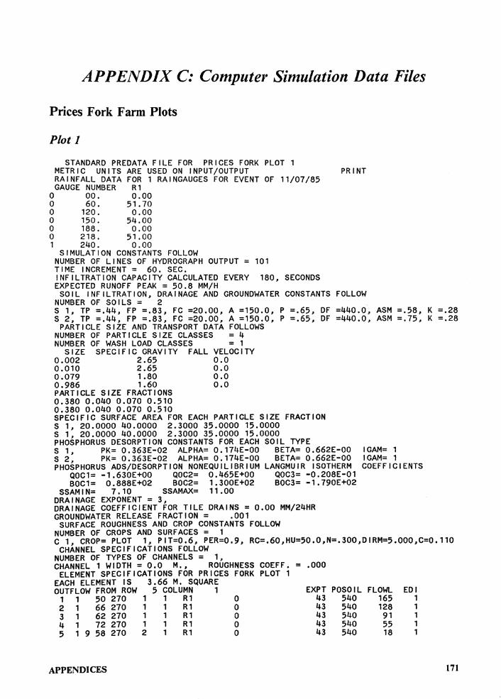
APPENDIX C: Computer Simulation Data Files

Prices Fork Farm Plots

Plot I

STANDARD PREDATA FILE FOR PRICES FORK PLOT 1 METRIC UNITS ARE USED ON INPUT/OUTPUT RAINFALL DATA FOR 1 RAINGAUGES FOR EVENT OF 11/07/85 GAUGE NUMBER R1

0 00. 0.00 0 60. 51. 70 0 120. 0.00 0 150. 54.00 0 188. 0.00 0 218. 51.00 1 240. 0 .00

SIMULATION CONSTANTS FOLLOW NUMBER OF LINES OF HYDROGRAPH OUTPUT= 101 TIME INCREMENT= 60. SEC. INFILTRATION CAPACITY CALCULATED EVERY 180, SECONDS EXPECTED RUNOFF PEAK= 50.8 MM/H

PRINT

SOIL INFILTRATION, DRAINAGE AND GROUNDWATER CONSTANTS FOLLOW NUMBER OF SOILS= 2 S 1, TP =.44, FP =.83, FC =20.00, A =150.0, P =,65, OF =440.0, ASM =.58, K =.28 S 2, TP =.44, FP =.83, FC =20.00, A =150.0, P =.65, OF =440.0, ASM =.75, K =.28

PARTICLE SIZE AND TRANSPORT DATA FOLLOWS NUMBER OF PARTICLE SIZE CLASSES = 4 NUMBER OF WASH LOAD CLASSES = 1

SIZE SPECIFIC GRAVITY FALL VELOCITY 0.002 2.65 0.0 0.010 2.65 0.0 0.079 1.80 0.0 0.986 1.60 0.0 PARTICLE SIZE FRACTIONS 0.380 0.040 0.070 0.510 0.380 0.040 0.070 0.510 SPECIFIC SURFACE AREA FOR EACH PARTICLE SIZE FRACTION S 1, 20.0000 40.0000 2.3000 35.0000 15.0000 S 1, 20.0000 40.0000 2.3000 35.0000 15.0000 PHOSPHORUS DESORPTION CONSTANTS FOR EACH SOIL TYPE S 1, PK= 0.363E-02 ALPHA= 0.174E-OO BETA= 0.662E-OO IGAM= 1 S 2, PK= 0.363E-02 ALPHA= 0.174E-OO BETA= 0.662E-OO IGAM= 1 PHOSPHORUS ADS/DESORPTION NONEQUILIBRIUM LANGMUIR ISOTHERM COEFFICIENTS

QOC1= -1.630E+OO QOC2= 0.465E+OO QOC3= -0.208E-01 BOC1= 0.888E+02 BOC2= 1.300E+02 BOC3= -1.790E+02

SSAMIN= 7.10 SSAMAX= 11.00 DRAINAGE EXPONENT= 3, DRAINAGE COEFFICIENT FOR TILE DRAINS= 0.00 MM/24HR GROUNDWATER RELEASE FRACTION= .001

SURFACE ROUGHNESS AND CROP CONSTANTS FOLLOW NUMBER OF CROPS AND SURFACES= 1 C 1, CROP= PLOT 1, PIT=0.6, PER=0.9, RC=.60,HU=50.0,N=.300,DIRM=5.000,C=0.110

CHANNEL SPECIFICATIONS FOLLOW NUMBER OF TYPES OF CHANNELS= 1, CHANNEL 1 WIDTH= 0.0 M., ROUGHNESS COEFF. = ,000

ELEMENT SPECIFICATIONS FOR PRICES FORK PLOT 1 EACH ELEMENT IS 3.66 M. SQUARE OUTFLOW FROM ROW 5 COLUMN 1

1 1 50 270 1 1 Rt 2 1 66 270 1 1 R 1 3 1 62 270 1 1 R1 4 1 72 270 1 1 R1 5 1 9 58 270 2 1 Rt

APPENDICES

0 0 0 0 0

EXPT 43 43 43 43 43

POSOIL 540 540 540 540 540

FLOWL 165 128 91 55 18

EDI 1 1 1 1 1

171

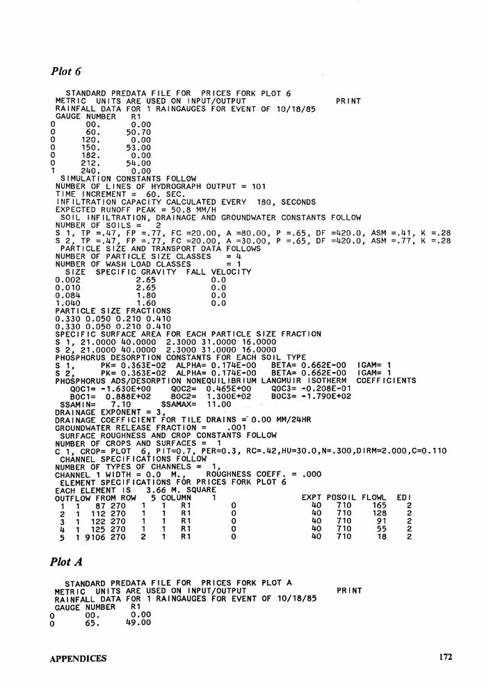
Plot 6

STANDARD PREDATA FILE FOR PRICES FORK PLOT 6 METRIC UNITS ARE USED ON INPUT/OUTPUT RAINFALL DATA FOR 1 RAINGAUGES FOR EVENT OF 10/18/85 GAUGE NUMBER R1

0 00. 0.00 0 60. 50. 70 0 120. 0.00 0 150. 53.00 0 182. 0.00 0 212. 54.00 1 240. 0.00


PRINT

SOIL INFILTRATION, DRAINAGE AND GROUNDWATER CONSTANTS FOLLOW NUMBER OF SOILS= 2 S 1, TP =.47, FP =.77, FC =20.00, A =80.00, P =.65, DF =420.0, ASM =.41, K =.28 S 2, TP =.47, FP =.77, FC =20.00, A =30.00, P =.65, DF =420.0, ASM =.77, K =.28


SIZE SPECIFIC GRAVITY FALL VELOCITY 0.002 2.65 0.0 0.010 2.65 0.0 0.084 1.80 o.o 1.040 1.60 0.0 PARTICLE SIZE FRACTIONS 0.330 0.050 0.210 0.410 0.330 0.050 0.210 0.410 SPECIFIC SURFACE AREA FOR EACH PARTICLE SIZE FRACTION S 1, 21.0000 40.0000 2.3000 31.0000 16.0000 S 2, 21.0000 40.0000 2.3000 31.0000 16.0000 PHOSPHORUS DESORPTION CONSTANTS FOR EACH SOIL TYPE S 1, PK= 0.363E-02 ALPHA= 0.174E-OO BETA= 0.662E-OO IGAM= 1 S 2, PK= 0.363E-02 ALPHA= 0.174E-OO BETA= 0.662E-OO IGAM= 1 PHOSPHORUS ADS/DESORPTION NONEQUILIBRIUM LANGMUIR ISOTHERM COEFFICIENTS

QOC1= -1.630E+OO QOC2= 0.465E+OO QOC3= -0.208E-01 BOC1= 0.888E+02 BOC2= 1,300E+02 BOC3= -1.790E+02

SSAMIN= 7.10 SSAMAX= 11.00 DRAINAGE EXPONENT= 3, ORA I NAGE COEFFICIENT FOR Tl LE ORA I NS =~ 0. 00 MM/24HR GROUNDWATER RELEASE FRACTION= .001

SURFACE ROUGHNESS AND CROP CONSTANTS FOLLOW NUMBER OF CROPS AND SURFACES= 1 C 1, CROP= PLOT 6, PIT=0.7, PER=0.3, RC=.42,HU=30.0,N=.300,DIRM=2.000,C=0.110

CHANNEL SPECIFICATIONS FOLLOW NUMBER OF TYPES OF CHANNELS= 1, CHANNEL 1 WIDTH= 0.0 M., ROUGHNESS COEFF. = .000

ELEMENT SPECIFICATIONS FOR PRICES FORK PLOT 6 EACH ELEMENT IS 3.66 M. SQUARE OUTFLOW FROM ROW 5 COLUMN 1

1 1 87 270 1 1 R1 2 1 112 270 1 1 R1 3 1 122 270 1 1 R1 4 1 125 270 1 1 R1 5 1 9106 270 2 1 R1

Plot A

0 0 0 0 0

STANDARD PREDATA FILE FOR PRICES FORK PLOT A METRIC UNITS ARE USED ON INPUT/OUTPUT

EXPT 40 40 40 40 40

RAINFALL DATA FOR 1 RAINGAUGES FOR EVENT OF 10/18/85 GAUGE NUMBER R1

0 00. 0.00 0 65. 49.00

APPENDICES

POSOIL 710 710 710 710 710

PRINT

FLOWL 165 128 91 55 18

EDI 2 2 2 2 2

172

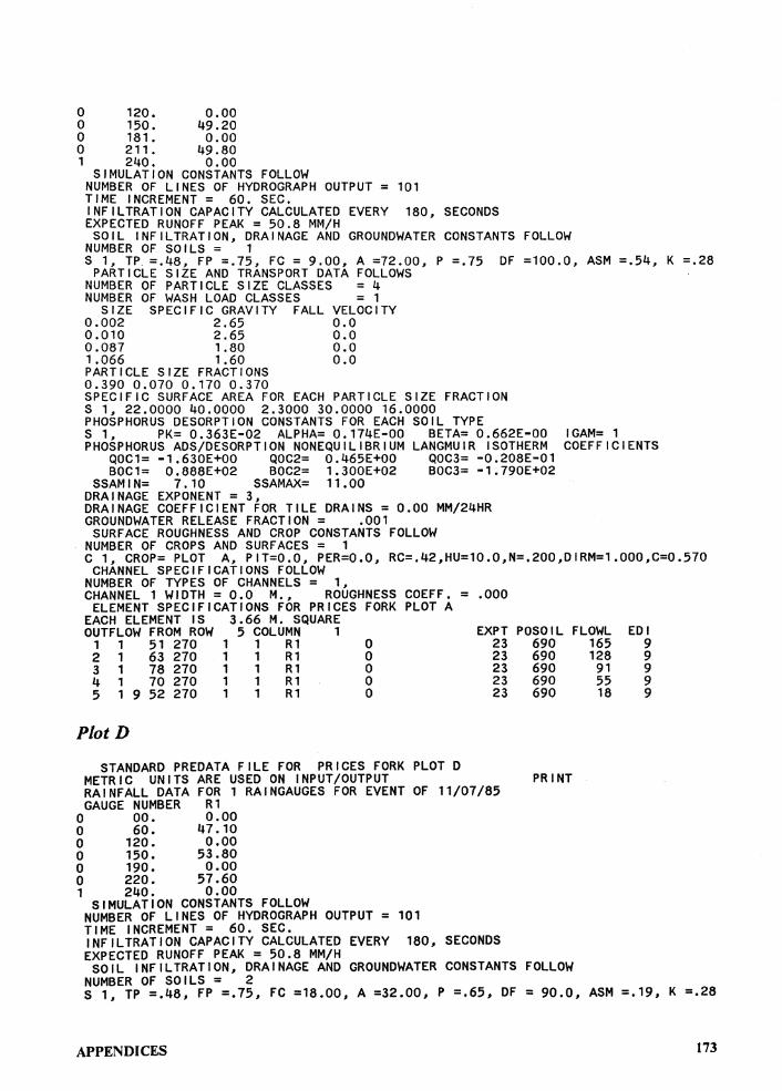
0 0 0 0 1

120. 0, 00 150. 49 ,20 181, 0.00 211. 49. 80 240. 0.00

SIMULATION CONSTANTS FOLLOW NUMBER OF LINES OF HYDROGRAPH OUTPUT= 101 TIME INCREMENT= 60. SEC, INFILTRATION CAPACITY CALCULATED EVERY 180, SECONDS EXPECTED RUNOFF PEAK= 50.8 MM/H

SOIL INFILTRATION, DRAINAGE AND GROUNDWATER CONSTANTS FOLLOW NUMBER OF SOILS= 1 S 1, TP. =,48, FP =.75, FC = 9.00, A =72.00, P =.75 DF =100.0, ASM =.54, K =.28


SIZE SPECIFIC GRAVITY FALL VELOCITY 0.002 2.65 0.0 0.010 2.65 o.o 0.087 1.80 0.0 1.066 1,60 0.0 PARTICLE SIZE FRACTIONS 0.390 0.070 0.170 0.370 SPECIFIC SURFACE AREA FOR EACH PARTICLE SIZE FRACTION S 1, 22,0000 40.0000 2.3000 30.0000 16.0000 PHOSPHORUS DESORPTION CONSTANTS FOR EACH SOIL TYPE S 1, PK= 0.363E-02 ALPHA= 0.174E-OO BETA= 0.662E-OO IGAM= 1 PHOSPHORUS ADS/DESORPTION NONEQUILIBRIUM LANGMUIR ISOTHERM COEFFICIENTS


SSAMIN= 7.10 SSAMAX= 11,00 DRAINAGE EXPONENT= 3, DRAINAGE COEFFICIENT FOR TILE DRAINS= 0.00 MM/24HR GROUNDWATER RELEASE FRACTION= .001

SURFACE ROUGHNESS AND CROP CONSTANTS FOLLOW NUMBER OF CROPS AND SURFACES= 1 C 1, CROP= PLOT A, PIT=O.O, PER=O.O, RC=.42,HU=10.0,N=.200,DIRM=1.000,C=0.570

CHANNEL SPECIFICATIONS FOLLOW NUMBER OF TYPES OF CHANNELS= 1, CHANNEL 1 WIDTH= 0.0 M., ROUGHNESS COEFF. = .000

ELEMENT SPECIFICATIONS FOR PRICES FORK PLOT A EACH ELEMENT IS 3.66 M, SQUARE OUTFLOW FROM ROW 5 COLUMN 1

1 1 51 270 1 1 R 1 2 1 63 270 1 1 R1 3 1 78 270 1 1 R1 4 1 70 270 1 1 R1 5 1 9 52 270 1 1 R1

Plot D

0 0 0 0 0

STANDARD PREDATA FILE FOR PRICES FORK PLOT D

EXPT 23 23 23 23 23

POSOIL 690 690 690 690 690

METRIC UNITS ARE USED ON INPUT/OUTPUT PRINT RAINFALL DATA FOR 1 RAINGAUGES FOR EVENT OF 11/07/85 GAUGE NUMBER R1

0 00. 0.00 0 60. 47.10 0 120. 0.00 0 150. 53.80 0 190. 0.00 0 220. 57.60 1 240. 0.00


FLOWL 165 128 91 55 18

EDI 9 9 9 9 9

SOIL INFILTRATION, DRAINAGE AND GROUNDWATER CONSTANTS FOLLOW NUMBER OF SOILS= 2 S 1, TP =.48, FP =.75, FC =18.00, A =32.00, P =.65, DF = 90.0, ASM =.19, K =.28

APPENDICES 173

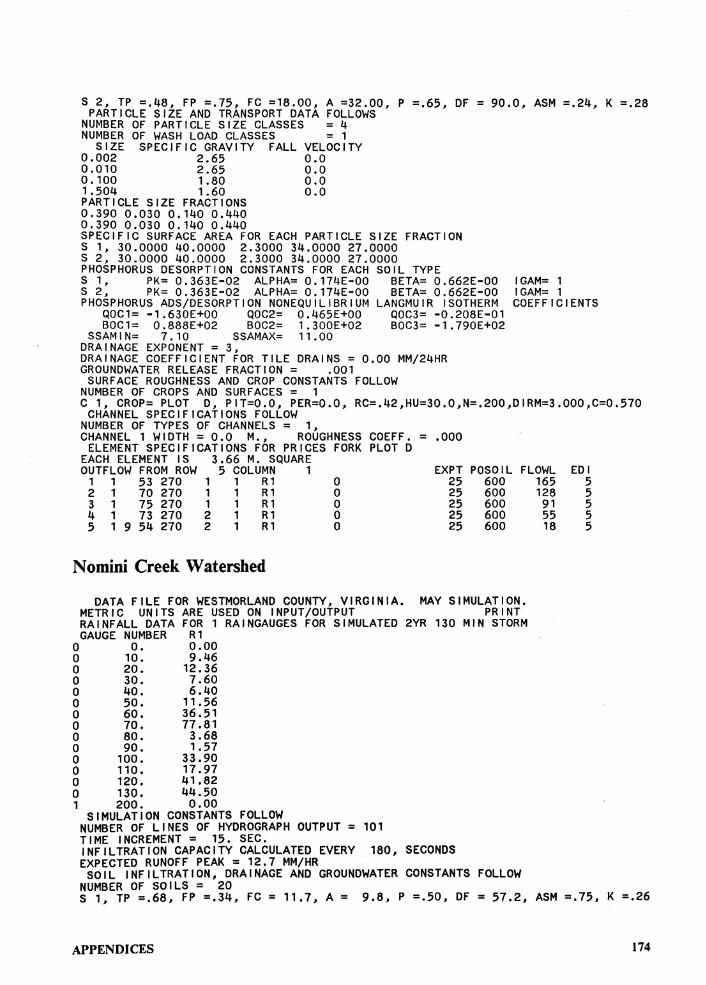
S 2, TP =.48, FP =,75, FC =18.00, A =32.00, P =.65, OF= 90.0, ASM =.24, K =.28 PARTICLE SIZE AND TRANSPORT DATA FOLLOWS

NUMBER OF PARTICLE SIZE CLASSES = 4 NUMBER OF WASH LOAD CLASSES = 1

SIZE SPECIFIC GRAVITY FALL VELOCITY 0.002 2.65 0.0 0.010 2.65 0.0 0.100 1.80 0.0 1 .504 1.60 0.0 PARTICLE SIZE FRACTIONS 0.390 0.030 0.140 0.440 0.390 0.030 0.140 0.440 SPECIFIC SURFACE AREA FOR EACH PARTICLE SIZE FRACTION S 1, 30.0000 40.0000 2.3000 34.0000 27.0000 S 2, 30.0000 40.0000 2.3000 34.0000 27.0000 PHOSPHORUS DESORPTION CONSTANTS FOR EACH SOIL TYPE S 1, PK= 0.363E-02 ALPHA= 0.174E-OO BETA= 0.662E-OO IGAM= 1 S 2, PK= 0.363E-02 ALPHA= 0.174E-OO BETA= 0.662E-OO IGAM= 1 PHOSPHORUS ADS/DESORPTION NONEQUILIBRIUM LANGMUIR ISOTHERM COEFFICIENTS


SSAMIN= 7.10 SSAMAX= 11.00 DRAINAGE EXPONENT= 3, DRAINAGE COEFFICIENT FOR TILE DRAINS= 0.00 MM/24HR GROUNDWATER RELEASE FRACTION= .001

SURFACE ROUGHNESS AND CROP CONSTANTS FOLLOW NUMBER OF CROPS AND SURFACES= 1 C 1, CROP= PLOT D, PIT=O.O, PER=O.O, RC=.42,HU=30.0,N=.200,DIRM=3.000,C=0.570

CHANNEL SPECIFICATIONS FOLLOW NUMBER OF TYPES OF CHANNELS= 1, CHANNEL 1 WIDTH= 0.0 M., ROUGHNESS COEFF. = ,000

ELEMENT SPECIFICATIONS FOR PRICES FORK PLOT D EACH ELEMENT IS 3.66 M. SQUARE OUTFLOW FROM ROW 5 COLUMN 1

1 1 53 270 1 1 R1 2 1 70 270 1 1 R1 3 1 75 270 1 1 R1 4 1 73 270 2 1 R1 5 1 9 54 270 2 1 R1

Nomini Creek Watershed

0 0 0 0 0

EXPT 25 25 25 25 25

POSOIL 600 600 600 600 600

FLOWL 165 128 91 55 18

DATA FILE FOR WESTMORLAND COUNTY, VIRGINIA, MAY SIMULATION. METRIC UNITS ARE USED ON INPUT/OUTPUT PRINT RAINFALL DATA FOR 1 RAINGAUGES FOR SIMULATED 2YR 130 MIN STORM GAUGE NUMBER R1

0 o. 0.00 0 10. 9.46 0 20. 12.36 0 30. 7 .60 0 40. 6.40 0 50. 11.56 0 60. 36.51 0 70. 77 .81 0 80. 3.68 0 90. 1.57 0 100. 33.90 0 110. 17.97 0 120. 41.82 0 130. 44.50 1 200. 0.00

SIMULATION CONSTANTS FOLLOW NUMBER OF LINES OF HYDROGRAPH OUTPUT= 101 TIME INCREMENT= 15. SEC. INFILTRATION CAPACITY CALCULATED EVERY 180, SECONDS EXPECTED RUNOFF PEAK= 12.7 MM/HR SOIL INFILTRATION, DRAINAGE AND GROUNDWATER CONSTANTS FOLLOW

NUMBER OF SOILS= 20

EDI 5 5 5 5 5

S 1, TP =.68, FP =,34, FC = 11.7, A= 9.8, P =.50, DF = 57.2, ASM =.75, K =.26

APPENDICES 174

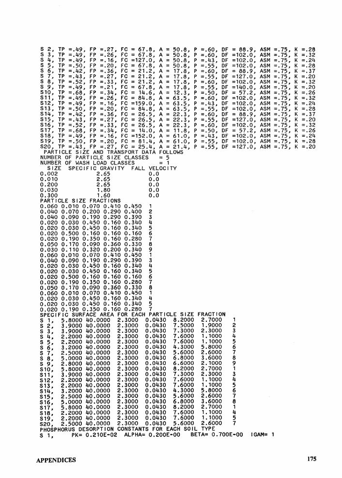
S 2, TP =.49, FP =,27, FC = 67.8, A= 50.8, P S 3, TP =.49, FP =.26, FC = 67.8, A= 50.8, P S 4, TP =.49, FP =.16, FC =127.0, A= 50.8, P S 5, TP =.50, FP =.20, FC = 67.8, A= 50.8, P S 6, TP =.42, FP =,36, FC = 21.2, A= 17.8, P S 7, TP =.43, FP =,27, FC = 21.2, A= 17.8, P S 8, TP =.52, FP =,33, FC = 21.2, A= 17.8, P S 9, TP =.49, FP =.21, FC = 67.8, A= 17.8, P SlO, TP =.68, FP =.34, FC = 14.6, A= 12.3, P Sll, TP =.49, FP =.26, FC = 84.8, A= 63.5, P S12, TP =.49, FP =.16, FC =159.0, A= 63.5, P S13, TP =.50, FP =,20, FC = 84.8, A= 63.5, P S14, TP =,42, FP =,36, FC = 26.5, A= 22.3, P S15, TP =.43, FP =.27, FC = 26.5, A= 22.3, P S16, TP =.52, FP =.33, FC = 26.5, A= 22.3, P S17, TP =.68, FP =.34, FC = 14.0, A= 11.8, P S18, TP =.49, FP =.16, FC =152.0, A= 61.0, P S19, TP =.50, FP =,20, FC = 81.4, A= 61.0, P S20, TP =.43, FP =.27, FC = 25.4, A= 21.4, P


SIZE SPECIFIC GRAVITY FALL VELOCITY 0.002 2.65 0.0 0.010 2.65 o.o 0.200 2.65 o.o 0.030 1.80 0.0 0.300 1.60 0.0 PARTICLE SIZE FRACTIONS 0.060 0.010 0.070 0.410 0.450 1 0.040 0.070 0.200 0.290 0.400 2 0.040 0.090 0.190 0.290 0.390 3 0.020 0.030 0.450 0.160 0.340 4 0.020 0.030 0.450 0.160 0.340 5 0.020 0.500 0.160 0.160 0.160 6 0.020 0.190 0.350 0.160 0.280 7 0.050 0.170 0.090 0.360 0.330 8 0.030 0.110 0.320 0.200 0.340 9 0.060 0.010 0.070 0.410 0.450 1 0.040 0.090 0.190 0.290 0.390 3 0.020 0.030 0.450 0.160 0.340 4 0.020 0.030 0.450 0.160 0.340 5 0.020 0.500 0,160 0.160 0.160 6 0,020 0.190 0.350 0.160 0.280 7 0.050 0.170 0,090 0.360 0.330 8 0.060 0.010 0.070 0.410 0.450 1 0.020 0.030 0.450 0.160 0.340 4 0.020 0.030 0.450 0.160 0.340 5 0.020 0.190 0,350 0.160 0.280 7

=.60, DF =.60, DF =.43, DF =.55, DF =.60, DF =.55, DF =.60, DF =.55, DF =.50, DF =.60, DF =.43, DF =.55, DF =.60, DF =.55, DF =.60, DF =.50, DF =.43, DF =.55, DF =.55, DF

SPECIFIC SURFACE AREA FOR EACH PARTICLE SIZE FRACTION S 1, 5.8000 40.0000 2.3000 0.0430 8.2000 2.7000 S 2, 3.9000 40.0000 2.3000 0.0430 7.5000 1.9000 S 3, 3.9000 40.0000 2.3000 0.0430 7.3000 2.3000 S 4, 2.2000 40.0000 2,3000 0.0430 7.6000 1.1000 S 5, 2.2000 40.0000 2.3000 0.0430 7.6000 1.1000 S 6, 3.2000 40.0000 2.3000 0.0430 4.3000 5.8000 S 7, 2.5000 40.0000 2.3000 0.0430 5.6000 2.6000 S 8, 5.0000 40.0000 2.3000 0.0430 6.8000 3.6000 S 9, 2.8000 40.0000 2.3000 0.0430 6.6000 2.1000 S10, 5,8000 40.0000 2.3000 0.0430 8.2000 2.7000 S11, 3.9000 40.0000 2.3000 0.0430 7.3000 2.3000 S12, 2.2000 40.0000 2,3000 0.0430 7.6000 1.1000 S13, 2.2000 40.0000 2.3000 0.0430 7.6000 1.1000 S14, 3.2000 40.0000 2.3000 0.0430 4.3000 5.8000 S15, 2.5000 40.0000 2.3000 0.0430 5.6000 2.6000 S16, 5,0000 40.0000 2.3000 0.0430 6.8000 3.6000 S17, 5.8000 40.0000 2.3000 0.0430 8.2000 2.7000 S18, 2.2000 40.0000 2.3000 0.0430 7.6000 1.1000 S19, 2.2000 40.0000 2.3000 0.0430 7.6000 1.1000 S20, 2.5000 40.0000 2.3000 0.0430 5.6000 2.6000 PHOSPHORUS DESORPTION CONSTANTS FOR EACH SOIL TYPE

= 88.9, =102.0, =102.0, =102.0, = 88.9, =127.0, =102.0, =140.0, = 57.2, =102.0, =102.0, =102.0, = 88.9, =127.0, =102.0, = 57.2, =102.0, =102.0, =127.0,

1 2 3 4 5 6 7 8 9 1 3 4 5 6 7 8 1 4 5 7

ASM =.75, K ASM =.75, K ASM =.75, K ASM =.75, K ASM =.75, K ASM =.75, K ASM =,75, K ASM =.75, K ASM =.75, K ASM =.75, K ASM =.75, K ASM =.75, K ASM =.75, K ASM =.75, K ASM =.75, K ASM =.75, K ASM =.75, K ASM =.75, K ASM =.75, K

S 1, PK= 0,210E-02 ALPHA= 0.200E-OO BETA= 0.700E-OO IGAM= 1

APPENDICES

=.28 =.32 =.24 =.28 =.37 =.20 =.32 =.20 =.26 =.32 =.24 =.28 =.37 =.20 =.32 =.26 =.24 =.28 =.20

175

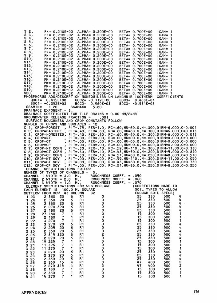
S 2, PK= 0.210E-02 ALPHA= 0.200E-OO S 3, PK= 0.210E-02 ALPHA= 0.200E-OO S 4, PK= 0.210E-02 ALPHA= 0.200E-OO S 5, PK= 0.210E-02 ALPHA= 0.200E-OO S 6, PK= 0.210E-02 ALPHA= 0.200E-OO S 7, PK= 0,210E-02 ALPHA= 0.200E-OO S 8, PK= 0.210E-02 ALPHA= 0.200E-OO S 9, PK= 0.210E-02 ALPHA= 0.200E-OO S10, PK= 0.210E-02 ALPHA= 0.200E-OO S11, PK= 0.210E-02 ALPHA= 0.200E-OO S12, PK= 0.210E-02 ALPHA= 0.200E-OO S13, PK= 0.210E-02 ALPHA= 0.200E-OO S14, PK= 0.210E-02 ALPHA= 0.200E-OO S15, PK= 0.210E-02 ALPHA= 0.200E-OO S16, PK= 0.210E-02 ALPHA= 0.200E-OO S17, PK= 0.210E-02 ALPHA= 0.200E-OO S18, PK= 0.210E-02 ALPHA= 0.200E-OO S19, PK= 0.210E-02 ALPHA= 0.200E-OO S20, PK= 0.210E-02 ALPHA= 0.200E-OO PHOSPHORUS ADS/DESORPTION NONEQUILIBRIUM

QOC1= 0.415E+OO QOC2= -0.119E+OO BOC1= -0.252E+03 BOC2= 0.960E+03

SSAMIN= 1.20 SSAMAX= 5,80 DRAINAGE EXPONENT= 3,

BETA= 0.700E-OO BETA= 0.700E-OO BETA= 0.700E-OO BETA= 0.700E-OO BETA= 0. 700E-OO BETA= 0.700E-OO BETA= 0.700E-OO BETA= 0.700E-OO BETA= 0.700E-OO BETA= 0.700E-OO BETA= 0.700E-OO BETA= 0.700E-OO BETA= 0.700E-OO BETA= 0.700E-OO BETA= 0.700E-OO BETA= 0.700E-OO BETA= 0.700E-OO BETA= 0.700E-OO BETA= 0.700E-OO

LANGMUIR ISOTHERM QOC3= 0.468E-01 BOC3= -0.534E+03

DRAINAGE COEFFICIENT FOR TILE DRAINS= 0.00 MM/24HR GROUNDWATER RELEASE FRACTION= .001

SURFACE ROUGHNESS AND CROP CONSTANTS FOLLOW NUMBER OF CROPS AND SURFACES= 12

GAM= 1 GAM= 1 GAM= 1 GAM= 1 GAM= 1 GAM= 1 GAM= 1 GAM= 1 GAM= 1 GAM= 1 GAM= 1 GAM= 1 GAM= 1 GAM= 1 GAM= 1 GAM= 1 GAM= 1 GAM= 1 GAM= 1

COEFFICIENTS

C 1, CROP=FOREST , PIT=.75, PER=1.0, C 2, CROP=PASTURE , PIT=.40, PER=,80, C 3, CROP=HOMESTED, PIT=.40, PER=.80, C 4, CROP=NT , PIT=.00, PER=.00, C 5, CROP=CT , PIT=.00, PER=.00, C 6, CROP=CP , PIT=.00, PER=.00, C 7, CROP=NT CORN, PIT=.30, PER=,10, C 8, CROP=CT CORN, PIT=.30, PER=.10, C 9, CROP=CP CORN , PIT=.30, PER=.10, C10, CROP=NT SOY , PIT=.00, PER=.00, C11, CROP=CT SOY , PIT=.00, PER=.00, C12, CROP=CP SOY , PIT=.00, PER=.00,

RC=.60,HU=60.0,N=.300,DIRM=6.000,C=0.001 RC=.60,HU=60.0,N=.300,DIRM=6.000,C=0.013 RC=.60,HU=60.0,N=.300,DIRM=6,000,C=0.013 RC=.OO,HU=OO.O,N=.000,DIRM=O.OOO,C=O.OOO RC=.OO,HU=OO.O,N=.OOO,DIRM=O.OOO,C=0.000 RC=.OO,HU=OO.O,N=.OOO,DIRM=O.OOO,C=0.000 RC=,59,HU=110.,N=.300,DIRM=11.00,C=0.330 RC=.43,HU=50.0,N=.200,DIRM=5.000,C=0.810 RC=,51,HU=80.0,N=.250,DIRM=8.000,C=0.510 RC=.59,HU=110.,N=.300,DIRM=11.00,C=0.050 RC=.43,HU=60.0,N=.200,DIRM=6.000,C=0.730 RC=,51,HU=85.0,N=.250,DIRM=8.500,C=0.250

CHANNEL SPECIFICATIONS FOLLOW NUMBER OF TYPES OF CHANNELS= 3, CHANNEL 1 WIDTH= 3.0 M., ROUGHNESS COEFF. = CHANNEL 2 WIDTH= 2.0 M., ROUGHNESS COEFF. = CHANNEL 3 WIDTH= 1.0 M., ROUGHNESS COEFF. =

ELEMENT SPECIFICATIONS FOR WESTMORLAND EACH ELEMENT IS 100.0 M. SQUARE OUTFLOW FROM ROW 43 COLUMN 32

1 23 2 360 20 6 R1 1 24 2 360 20 6 R1 1 25 2 360 20 6 R1 1 26 2 270 320 6 R1 1 27 2 180 20 6 R1 1 28 27 180 7 1 R1 1 29 2 180 7 1 R1 2 22 3 270 7 1 R1 2 23 3 270 20 6 R1 2 24 2 225 20 6 R1 2 25 2 360 20 6 R1 2 26 2 315 320 6 R1 2 27 2 270 20 6 R1 2 28 19 225 7 1 R1 3 21 11 326 7 1 R1 3 22 11 270 7 1 R1 3 23 3 270 20 6 R1 3 24 2 270 20 6 R1 3 25 2 360 20 6 R1 3 26 2 360 15 4 R1 3 27 2 270 315 4 R1 3 28 2 180 7 1 R1 4 20 2 360 7 1 R1 4 21 14 270 7 1 R1

APPENDICES

0 0 0 2 0 0 0 0 0 0 0 2 0 0 0 0 0 0 0 0 2 0 0 0

.050

.060

.070 (CORRECTIONS MADE TO SOIL TYPES TO ALLOW ENOUGH SOIL SPECS)

25 330 500 25 330 500 25 330 500 25 330 500 25 330 500 15 300 500 15 300 500 15 300 500 25 330 500 25 330 500 25 330 500 25 330 500 25 330 500 15 300 500 15 300 500 15 300 500 25 330 500 25 330 500 25 330 500 47 400 500 47 400 500 15 300 500 15 300 500 15 300 500

4 4 4 4 4 1 1 1 4 4 4 4 4 1 1 1 4 4 4 2 2 1 1 1

176

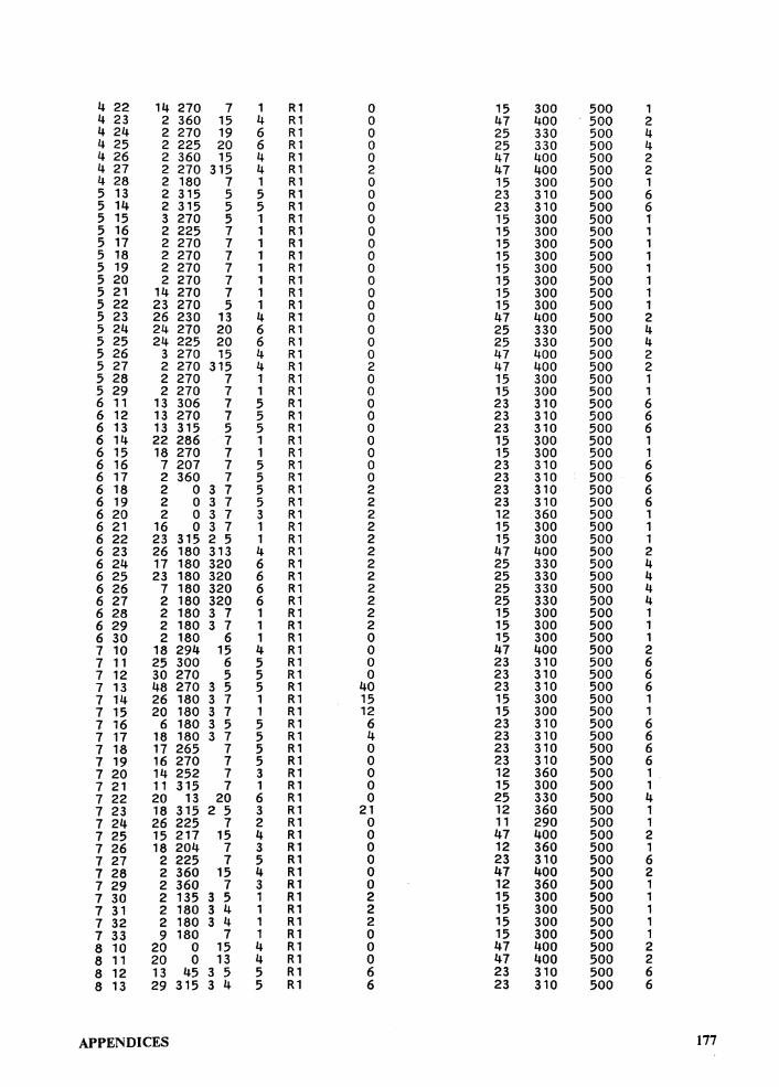
4 22 14 270 7 1 R1 0 15 300 500 1 4 23 2 360 15 4 R1 0 47 400 500 2 4 24 2 270 19 6 R1 0 25 330 500 4 4 25 2 225 20 6 R1 0 25 330 500 4 4 26 2 360 15 4 R1 0 47 400 500 2 4 27 2 270 315 4 R1 2 47 400 500 2 4 28 2 180 7 1 R1 0 15 300 500 1 5 13 2 315 5 5 R1 0 23 310 500 6 5 14 2 315 5 5 R1 0 23 310 500 6 5 15 3 270 5 1 R1 0 15 300 500 1 5 16 2 225 7 1 R1 0 15 300 500 1 5 17 2 270 7 1 R1 0 15 300 500 1 5 18 2 270 7 1 R1 0 15 300 500 1 5 19 2 270 7 1 R1 0 15 300 500 1 5 20 2 270 7 1 R1 0 15 300 500 1 5 21 14 270 7 1 R1 0 15 300 500 1 5 22 23 270 5 1 R1 0 15 300 500 1 5 23 26 230 13 4 R1 0 47 400 500 2 5 24 24 270 20 6 R1 0 25 330 500 4 5 25 24 225 20 6 R1 0 25 330 500 4 5 26 3 270 15 4 R1 0 47 400 500 2 5 27 2 270 315 4 R1 2 47 400 500 2 5 28 2 270 7 1 R1 0 15 300 500 1 5 29 2 270 7 1 R1 0 15 300 500 1 6 11 13 306 7 5 R1 0 23 310 500 6 6 12 13 270 7 5 R1 0 23 310 500 6 6 13 13 315 5 5 R1 0 23 310 500 6 6 14 22 286 7 1 R1 0 15 300 500 1 6 15 18 270 7 1 R1 0 15 300 500 1 6 16 7 207 7 5 R1 0 23 310 500 6 6 17 2 360 7 5 R1 0 23 310 500 6 6 18 2 0 3 7 5 R1 2 23 310 500 6 6 19 2 0 3 7 5 R1 2 23 310 500 6 6 20 2 0 3 7 3 R1 2 12 360 500 1 6 21 16 0 3 7 1 R1 2 15 300 500 1 6 22 23 315 2 5 1 R1 2 15 300 500 1 6 23 26 180 313 4 R1 2 47 400 500 2 6 24 17 180 320 6 R1 2 25 330 500 4 6 25 23 180 320 6 R1 2 25 330 500 4 6 26 7 180 320 6 R1 2 25 330 500 4 6 27 2 180 320 6 R1 2 25 330 500 4 6 28 2 180 3 7 1 R1 2 15 300 500 1 6 29 2 180 3 7 1 R1 2 15 300 500 1 6 30 2 180 6 1 R1 0 15 300 500 1 7 10 18 294 15 4 R1 0 47 400 500 2 7 11 25 300 6 5 R1 0 23 310 500 6 7 12 30 270 5 5 R1 0 23 310 500 6 7 13 48 270 3 5 5 R1 40 23 310 500 6 7 14 26 180 3 7 1 R1 15 15 300 500 1 7 15 20 180 3 7 1 R1 12 15 300 500 1 7 16 6 180 3 5 5 R1 6 23 310 500 6 7 17 18 180 3 7 5 R1 4 23 310 500 6 7 18 17 265 7 5 R1 0 23 310 500 6 7 19 16 270 7 5 R1 0 23 310 500 6 7 20 14 252 7 3 R1 0 12 360 500 1 7 21 11 315 7 1 R1 0 15 300 500 1 7 22 20 13 20 6 R1 0 25 330 500 4 7 23 18 315 2 5 3 R1 21 12 360 500 1 7 24 26 225 7 2 R1 0 11 290 500 1 7 25 15 217 15 4 R1 0 47 400 500 2 7 26 18 204 7 3 R1 0 12 360 500 1 7 27 2 225 7 5 R1 0 23 310 500 6 7 28 2 360 15 4 R1 0 47 400 500 2 7 29 2 360 7 3 R1 0 12 360 500 1 7 30 2 135 3 5 1 R1 2 15 300 500 1 7 31 2 180 3 4 1 R1 2 15 300 500 1 7 32 2 180 3 4 1 R1 2 15 300 500 1 7 33 9 180 7 1 R1 0 15 300 500 1 8 10 20 0 15 4 R1 0 47 400 500 2 8 11 20 0 13 4 R1 0 47 400 500 2 8 12 13 45 3 5 5 R1 6 23 310 500 6 8 13 29 315 3 4 5 R1 6 23 310 500 6

APPENDICES 177

8 14 42 190 4 1 R1 0 15 300 500 1 8 15 22 236 4 1 R1 0 15 300 500 1 8 16 14 297 7 3 R1 0 12 360 500 1 8 17 11 315 4 5 R1 0 23 310 500 6 8 18 16 270 4 5 R1 0 23 310 500 6 8 19 16 270 12 4 R1 0 47 400 500 2 8 20 16 248 15 4 R1 0 47 400 500 2 8 21 12 270 15 4 R1 0 47 400 500 2 8 22 9 329 20 6 R1 0 25 330 500 4 8 23 54 344 4 3 R1 0 12 360 500 1 8 24 48 270 2 7 2 R1 9 11 290 500 1 8 25 8 191 15 4 R1 0 47 400 500 2 8 26 23 184 7 5 R1 0 23 310 500 6 8 27 3 180 7 5 R1 0 23 310 500 6 8 28 2 360 13 4 R1 0 47 400 500 2 8 29 2 360 7 3 R1 0 12 360 500 1 8 30 2 315 13 4 R1 0 47 400 500 2 8 31 24 310 12 4 R1 0 47 400 500 2 8 32 38 277 6 1 R1 0 15 300 500 1 8 33 20 135 3 6 1 R1 2 15 300 500 1 8 41 2 270 7 1 R1 0 15 300 500 1 8 42 2 270 7 1 R1 0 15 300 500 1 8 43 2 270 7 1 R1 0 15 300 500 , 8 44 2 270 7 1 R1 0 15 300 500 1 9 9 2 360 7 1 R1 0 15 300 500 1 9 10 14 342 15 4 R1 0 47 400 500 2 9 11 20 45 313 4 R1 3 47 400 500 2 9 12 9 45 3 7 5 R1 6 23 310 500 6 9 13 24 45 15 4 R1 0 47 400 500 2 9 14 3 0 215 4 R1 3 47 400 500 2 9 15 44 315 2 7 1 R1 3 15 300 500 1 9 16 51 258 7 1 R1 0 15 300 500 1 9 17 39 281 4 5 R1 0 23 310 500 6 9 18 32 270 4 5 R1 0 23 310 500 6 9 19 22 231 12 4 R1 0 47 400 500 2 9 20 6 270 15 4 R1 0 47 400 500 2 9 21 15 270 15 4 R1 0 47 400 500 2 9 22 12 247 20 6 R1 0 25 330 500 4 9 23 67 357 4 5 R1 0 23 310 500 6 9 24 56 270 2 7 5 R1 15 23 310 500 6 9 25 16 209 15 4 R1 0 47 400 500 2 9 26 23 184 7 3 R1 0 12 360 500 1 9 27 5 252 7 5 R1 0 23 310 500 6 9 28 22 304 13 4 R1 0 47 400 500 2 9 29 23 270 15 4 R1 0 47 400 500 2 9 30 20 302 12 4 R1 0 47 400 500 2 9 31 43 321 12 4 R1 0 47 400 500 2 9 32 19 270 14 4 R1 0 47 400 500 2 9 33 27 149 6 1 R1 0 15 300 500 1 9 38 11 315 7 1 R1 0 15 300 500 1 9 39 27 286 7 1 R1 0 15 300 500 1 9 40 34 270 5 1 R1 0 15 300 500 1 9 41 27 254 5 1 R1 0 15 300 500 1 9 42 13 234 4 1 R1 0 15 300 500 1 9 43 2 225 19 6 R1 0 25 330 500 4 9 44 2 225 20 6 R1 0 25 330 500 4

10 9 11 0 7 1 R1 0 15 300 500 1 10 10 7 45 315 4 R1 2 47 400 500 2 10 11 25 25 15 4 R1 0 47 400 500 2 10 12 24 90 3 7 3 R1 6 12 360 500 1 10 13 28 84 7 3 R1 0 12 360 500 1 10 14 44 74 15 4 R1 0 47 400 500 2 10 15 69 84 14 4 R1 0 47 400 500 2 10 16 58 0 2 7 1 R1 3 15 300 500 1 10 17 35 0 2 7 1 R1 9 15 300 500 1 10 18 30 315 2 4 1 R1 9 15 300 500 1 10 19 48 252 1 1 R1 0 15 300 500 1 10 20 40 241 7 1 R1 0 15 300 500 1 10 21 18 301 15 4 R1 0 47 400 500 2 10 22 24 315 20 6 R1 0 25 330 500 4 10 23 77 342 4 5 R1 0 23 310 500 6 10 24 72 270 2 7 5 R1 12 23 310 500 6

APPENDICES 178

10 25 24 180 15 4 R1 0 47 400 500 2 10 26 20 180 7 5 R1 0 23 310 500 6 10 27 8 349 7 5 R1 0 23 310 500 6 10 28 42 330 12 4 R1 0 47 400 500 2 10 29 40 270 315 4 R1 29 47 400 500 2 10 30 41 324 15 4 R1 0 47 400 500 2 10 31 39 312 12 4 R1 0 47 400 500 2 10 32 56 270 3 4 1 R1 12 15 300 500 1 10 33 11 188 7 1 R1 0 15 300 500 1 10 34 5 180 7 1 R1 0 15 300 500 1 10 37 2 360 15 4 R1 0 47 400 500 2 10 38 16 0 15 4 R1 0 47 400 500 2 10 39 17 0 2 7 1 R1 18 15 300 500 1 10 40 22 0 2 4 1 R1 12 15 300 500 1 10 41 46 270 2 7 1 R1 12 15 300 500 1 10 42 55 214 4 1 R1 0 15 300 500 1 10 43 3 0 20 6 R1 0 25 330 500 4 10 44 2 270 220 6 R1 2 25 330 500 4 10 45 3 180 19 6 R1 0 25 330 500 4 10 46 20 225 19 6 R1 0 25 330 500 4 10 47 13 225 5 1 R1 0 15 300 500 1 11 8 16 0 7 1 R1 0 15 300 500 l 11 9 10 45 3 7 1 Rl 2 15 300 500 l 11 10 7 117 20 6 Rl 0 25 330 500 4 11 11 23 28 20 6 Rl 0 25 330 500 4 11 12 18 90 320 6 Rl 6 25 330 500 4 11 13 5 270 15 4 Rl 0 47 400 500 2 11 14 8 225 15 4 R1 0 47 400 500 2 11 15 5 45 15 4 Rl 0 47 400 500 2 11 16 11 56 15 4 R1 0 47 400 500 2 11 17 24 55 7 l R1 0 15 300 500 l 11 18 58 23 7 l Rl 0 15 300 500 1 11 19 22 315 2 1 1 Rl 8 15 300 500 1 11 20 46 180 7 1 R1 0 15 300 500 1 11 21 17 355 7 1 R1 0 15 300 500 1 11 22 13 0 20 6 R1 0 25 330 500 4 11 23 72 356 4 5 R1 0 23 310 500 6 11 24 93 225 2 7 1 R1 12 15 300 500 1 11 25 13 225 7 1 R1 0 15 300 500 1 11 26 24 230 15 4 R1 0 47 400 500 2 11 27 22 309 7 5 R1 0 23 310 500 6 11 28 42 350 12 4 R1 0 47 400 500 2 11 29 44 225 315 4 R1 15 47 400 500 2 11 30 33 0 15 4 R1 0 47 400 500 2 11 31 44 0 12 4 R1 0 47 400 500 2 11 32 70 270 2 7 1 R1 12 15 300 500 1 11 33 17 185 5 1 R1 0 15 300 500 1 11 34 2 225 7 1 R1 0 15 300 500 1 11 35 6 225 20 6 R1 0 25 330 500 4 , 1 36 6 315 15 4 R1 0 47 400 500 2 11 37 7 270 15 4 R1 0 47 400 500 2 11 38 9 360 15 4 R1 0 47 400 500 2 11 39 16 22 12 4 Rl 0 47 400 500 2 11 40 33 22 12 4 R1 0 47 400 500 2 11 41 30 270 3 7 l R1 11 15 300 500 l 11 42 72 198 4 l Rl 0 15 300 500 1 11 43 24 225 4 1 R1 0 15 300 500 1 11 44 2 270 312 4 Rl 22 47 400 500 2 11 45 4 225 220 6 Rl 14 25 330 500 4 11 46 22 180 220 6 Rl 13 25 330 500 4 11 47 24 180 7 1 Rl 0 15 300 500 1 11 48 6 180 7 1 Rl 0 15 300 500 1 11 49 7 180 7 1 R1 0 15 300 500 1 . 12 8 7 45 7 1 Rl 0 15 300 500 1 12 9 13 90 7 1 R1 0 15 300 500 1 12 10 2 360 7 3 Rl 0 12 360 500 1 12 11 9 45 20 6 R1 0 25 330 500 4 12 12 8 90 20 6 Rl 0 25 330 500 4 12 13 4 135 320 6 Rl 7 25 330 500 4 12 14 8 180 15 4 R1 0 47 400 500 2 12 15 6 45 15 4 R1 0 47 400 500 2 12 16 6 90 7 5 Rl 0 23 310 500 6

APPENDICES 179

12 17 13 36 15 4 R1 0 47 400 500 2 12 18 43 42 12 4 R1 0 47 400 500 2 12 19 56 22 4 1 R1 0 15 300 500 1 12 20 39 270 2 4 1 R1 8 15 300 500 1 12 21 7 333 7 1 R1 0 15 300 500 1 12 22 20 321 18 6 R1 0 25 330 500 4 12 23 52 270 218 6 R1 12 25 330 500 4 12 24 82 190 7 1 R1 0 15 300 500 1 12 25 18 246 7 1 R1 0 15 300 500 1 12 26 17 218 15 4 R1 0 47 400 500 2 12 27 11 315 7 5 R1 0 23 310 500 6 12 28 32 270 3 4 1 R1 15 15 300 500 1 12 29 40 184 7 1 R1 0 15 300 500 1 12 30 7 333 12 4 R1 0 47 400 500 2 12 31 72 359 10 4 R1 0 47 400 500 2 12 32 60 270 2 7 1 R1 9 15 300 500 1 12 33 44 234 7 1 R1 0 15 300 500 1 12 34 19 225 7 1 R1 0 15 300 500 1 12 35 7 153 20 6 R1 0 25 330 500 4 12 36 25 330 15 4 R1 0 47 400 500 2 12 37 24 270 312 4 R1 20 47 400 500 2 12 38 17 275 15 4 R1 0 47 400 500 2 12 39 13 315 15 4 R1 0 47 400 500 2 12 40 25 353 4 1 R1 0 15 300 500 1 12 41 47 270 3 7 1 R1 9 15 300 500 1 12 42 50 200 4 1 R1 0 15 300 500 1 12 43 48 225 2 7 1 R1 17 15 300 500 1 12 44 2 180 215 4 R1 14 47 400 500 2 12 45 11 135 7 3 R1 0 12 360 500 1 12 46 26 111 7 5 R1 0 23 310 500 6 12 47 22 135 7 3 R1 0 12 360 500 1 12 48 9 180 15 4 R1 0 47 400 500 2 12 49 9 180 7 1 R1 0 15 300 500 1 12 50 7 180 7 1 Rl 0 15 300 500 1 13 7 13 0 8 1 R1 0 15 300 500 1 13 8 5 45 20 6 R1 0 25 330 500 4 13 9 16 90 20 6 R1 0 25 330 500 4 13 10 2 225 20 6 R1 0 25 330 500 4 13 11 2 360 20 6 R1 0 25 330 500 4 13 12 2 45 20 6 R1 0 25 330 500 4 13 13 5 72 20 6 R1 0 25 330 500 4 13 14 4 135 320 6 R1 7 25 330 500 4 13 15 2 360 7 3 R1 0 12 360 500 1 13 16 9 315 7 5 R1 0 23 310 500 6 13 17 18 294 15 4 R1 0 47 400 500 2 13 18 39 312 7 1 R1 0 15 300 500 1 13 19 68 337 4 1 R1 0 15 300 500 1 13 20 43 270 2 4 1 R1 18 15 300 500 1 13 21 54 223 7 1 R1 0 15 300 500 1 13 22 24 0 20 6 R1 0 25 330 500 4 13 23 66 315 217 6 R1 9 25 330 500 4 13 24 87 192 7 1 R1 0 15 300 500 1 13 25 14 198 7 1 R1 0 15 300 500 1 13 26 13 225 15 4 R1 0 47 400 500 2 13 27 14 288 12 4 R1 0 47 400 500 2 13 28 44 270 3 4 1 R1 29 15 300 500 1 13 29 51 203 1 1 R1 0 15 300 500 1 13 30 48 310 1 1 R1 0 15 300 500 1 13 31 46 323 7 1 R1 0 15 300 500 1 13 32 74 225 2 7 1 R1 15 15 300 500 1 13 33 55 180 7 1 R1 0 15 300 500 1 13 34 33 180 7 1 R1 0 15 300 500 1 13 35 8 79 7 1 R1 0 15 300 500 1 13 36 30 0 7 1 R1 0 15 300 500 1 13 37 22 315 320 6 R1 20 25 330 500 4 13 38 30 233 18 6 R1 0 25 330 500 4 13 39 30 311 12 4 R1 0 47 400 500 2 13 40 53 303 5 1 R1 0 15 300 500 1 13 41 32 225 2 7 1 R1 17 15 300 500 1 13 42 46 180 2 7 1 R1 26 15 300 500 1 13 43 54 164 7 1 R1 0 15 300 500 1 13 44 14 117 7 1 R1 0 15 300 500 1

APPENDICES 180

13 45 22 129 7 1 R1 0 15 300 500 1 13 46 15 143 7 1 R1 0 15 300 500 1 13 47 4 135 15 4 R1 0 47 400 500 2 13 48 9 135 15 4 R1 0 47 400 500 2 13 49 1.7 142 15 4 R1 0 47 400 500 2 13 50 15 127 15 4 R1 0 47 400 500 2 14 7 32 273 20 6 R1 0 25 330 500 4 14 8 28 292 20 6 R1 0 25 330 500 4 14 9 27 270 20 6 R1 0 25 330 500 4 14 10 9 211 20 6 R1 0 25 330 500 4 14 11 2 360 20 6 R1 0 25 330 500 4 14 12 2 45 20 6 R1 0 25 330 500 4 14 13 2 45 20 6 R1 0 25 330 500 4 14 14 2 90 20 6 R1 0 25 330 500 4 14 15 2 315 15 4 R1 0 47 400 500 2 14 16 18 336 15 4 R1 0 47 400 500 2 14 17 37 315 4 1 R1 0 15 300 500 1 14 18 18 301 4 1 R1 0 15 300 500 1 14 19 47 0 7 1 R1 0 15 300 500 1 14 20 80 315 2 1 1 R1 6 15 300 500 1 14 21 77 195 4 1 R1 0 15 300 500 1 14 22 22 164 7 1 R1 0 15 300 500 1 14 23 105 14 17 6 R1 0 25 330 500 4 14 24 89 270 2 7 1 R1 9 15 300 500 1 14 25 11 225 7 1 R1 0 15 300 500 1 14 26 13 225 15 4 R1 0 47 400 500 2 14 27 37 315 10 4 R1 0 47 400 500 2 14 28 75 270 3 4 1 R1 15 15 300 500 1 14 29 87 225 2 7 1 R1 15 15 300 500 1 14 30 46 180 2 7 1 R1 12 15 300 500 1 14 31 32 180 2 7 1 R1 20 15 300 500 1 14 32 82 158 7 1 R1 0 15 300 500 1 14 33 22 124 7 1 Rl 0 15 300 500 1 14 34 14 18 7 1 Rl 0 15 300 500 1 14 35 6 270 7 1 Rl 0 15 300 500 1 14 36 20 13 7 1 Rl 0 15 300 500 1 14 37 38 32 20 6 R1 0 25 330 500 4 14 38 22 315 318 6 Rl 24 25 330 500 4 14 39 60 294 18 6 Rl 0 25 330 500 4 14 40 13 225 2 5 1 Rl 8 15 300 500 1 14 41 59 125 5 1 Rl 0 15 300 500 1 14 42 56 119 7 1 R1 0 15 300 500 1 14 43 30 165 7 1 Rl 0 15 300 500 1 14 44 14 180 7 1 Rl 0 15 300 500 1 14 45 15 180 15 4 Rl 0 47 400 500 2 14 46 7 153 15 4 Rl 0 47 400 500 2 14 47 6 90 15 4 Rl 0 47 400 500 2 14 48 11 90 15 4 Rl 0 47 400 500 2 14 49 20 153 15 4 Rl 0 47 400 500 2 14 50 13 126 15 4 Rl 0 47 400 500 2 14 51 13 225 13 4 Rl 0 47 400 500 2 14 52 9 225 20 6 Rl 0 25 330 500 4 15 6 6 360 4 3 Rl 0 12 360 500 1 15 7 11 270 4 3 Rl 0 12 360 500 1 15 8 7 225 20 6 Rl 0 25 330 500 4 15 9 30 180 20 6 R1 0 25 330 500 4 15 10 9 180 20 6 Rl 0 25 330 500 4 15 11 2 45 20 6 R1 0 25 330 500 4 15 12 2 90 20 6 Rl 0 25 330 500 4 15 13 2 90 19 6 R1 0 25 330 500 4 15 14 2 90 15 4 R1 0 47 400 500 2 15 15 2 0 15 4 Rl 0 47 400 500 2 15 16 18 0 7 3 Rl 0 12 360 500 1 15 17 39 0 7 1 R1 0 15 300 500 1 15 18 26 0 3 7 1 Rl 34 15 300 500 1 15 19 56 315 3 4 1 Rl 26 15 300 500 1 15 20 98 341 4 1 Rl 0 15 300 500 1 15 21 58 270 2 1 1 Rl 9 15 300 500 1 15 22 72 198 4 1 Rl 0 15 300 500 1 15 23 123 353 17 6 Rl 0 25 330 500 4 15 24 84 270 2 7 1 Rl 9 15 300 500 1 15 25 19 225 7 1 Rl 0 15 300 500 1

APPENDICES 181

15 26 1 1 225 15 4 R1 0 47 400 500 2 15 27 69 335 10 4 R1 0 47 400 500 2 15 28 20 225 2 7 1 R1 13 15 300 500 1 15 29 111 114 7 1 R1 0 15 300 500 1 15 30 107 101 7 1 R1 0 15 300 500 1 15 31 77 108 7 1 R1 0 15 300 500 1 15 32 54 142 5 1 R1 0 15 300 500 1 15 33 17 135 7 1 R1 0 15 300 500 1 15 34 40 360 7 1 R1 0 15 300 500 1 15 35 17 315 3 7 1 R1 23 15 300 500 1 15 36 27 301 4 1 R1 0 15 300 500 1 15 37 6 315 20 6 R1 0 25 330 500 4 15 38 61 13 4 1 R1 0 15 300 500 1 15 39 24 270 218 6 R1 5 25 330 500 4 15 40 60 135 7 1 R1 0 15 300 500 1 15 41 33 143 4 1 R1 0 15 300 500 1 15 42 15 180 7 1 R1 0 15 300 500 1 15 43 17 135 7 1 R1 0 15 300 500 1 15 44 18 149 7 1 R1 0 15 300 500 1 15 45 13 166 15 4 R1 0 47 400 500 2 15 46 8 259 15 4 R1 0 47 400 500 2 15 47 11 236 15 4 R1 0 47 400 500 2 15 48 2 270 15 4 R1 0 47 400 500 2 15 49 14 270 15 4 R1 0 47 400 500 2 15 50 11 188 13 4 R1 0 47 400 500 2 15 51 11 225 13 4 R1 0 47 400 500 2 15 52 17 225 15 4 R1 0 47 400 500 2 16 5 8 315 7 5 R1 0 23 310 500 6 16 6 26 320 4 3 R1 0 12 360 500 1 16 7 15 270 4 1 R1 0 15 300 500 1 16 8 20 180 7 1 R1 0 15 300 500 1 16 9 26 170 20 6 R1 0 25 330 500 4 16 10 3 180 20 6 R1 0 25 330 500 4 16 11 2 225 20 6 R1 0 25 330 500 4 16 12 2 270 20 6 R1 0 25 330 500 4 16 13 2 270 13 4 R1 0 47 400 500 2 16 14 2 315 15 4 R1 0 47 400 500 2 16 15 2 360 15 4 R1 0 47 400 500 2 16 16 7 27 15 4 R1 0 47 400 500 2 16 17 24 360 15 4 R1 0 47 400 500 2 16 18 44 31 7 1 R1 0 15 300 500 1 16 19 49 86 7 1 R1 0 15 300 500 1 16 20 78 0 3 7 1 R1 26 15 300 500 1 16 21 43 315 2 4 1 R1 9 15 300 500 1 16 22 92 246 4 1 R1 0 15 300 500 1 16 23 112 315 1 1 R1 0 15 300 500 1 16 24 91 270 2 1 1 R1 8 15 300 500 1 16 25 22 231 7 1 R1 0 15 300 500 1 16 26 22 236 10 4 R1 0 47 400 500 2 16 27 101 270 2 4 1 R1 12 15 300 500 1 16 28 110 183 7 1 R1 0 15 300 500 1 16 29 41 163 7 1 R1 0 15 300 500 1 16 30 14 207 7 1 R1 0 15 300 500 1 16 31 8 169 7 1 R1 0 15 300 500 1 16 32 18 180 7 1 R1 0 15 300 500 l 16 33 24 162 7 1 Rl 0 15 300 500 1 16 34 50 38 7 1 R1 0 15 300 500 1 16 35 38 21 7 1 R1 0 15 300 500 1 16 36 41 270 3 4 1 R1 41 15 300 500 1 16 37 41 219 20 6 R1 0 25 330 500 4 16 38 63 350 4 1 R1 0 15 300 500 1 16 39 17 270 2 5 1 Rl 6 15 300 500 1 16 40 41 174 4 1 R1 0 15 300 500 1 16 41 28 315 7 1 R1 0 15 300 500 1 16 42 43 225 315 4 R1 24 47 400 500 2 16 43 30 180 315 4 R1 30 47 400 500 2 16 44 23 180 315 4 R1 19 47 400 500 2 16 45 2 180 315 4 Rl 6 47 400 500 2 16 46 2 180 315 4 R1 2 47 400 500 2 16 47 8 180 315 4 R1 2 47 400 500 2 16 48 7 180 3 7 3 R1 2 12 360 500 1 16 49 10 180 315 4 R1 2 47 400 500 2

APPENDICES 182

16 50 11 180 313 4 R1 2 47 400 500 2 16 51 9 180 7 5 R1 0 23 310 500 6 16 52 13 180 15 4 R1 0 47 400 500 2 17 3 6 0 7 5 R1 0 23 310 500 6 17 4 25 0 7 3 R1 0 12 360 500 1 17 5 6 360 7 5 R1 0 23 310 500 6 17 6 23 0 4 5 R1 0 23 310 500 6 17 7 4 315 3 4 1 R1 10 15 300 500 1 17 8 30 204 7 1 R1 0 15 300 500 1 17 9 26 190 20 6 R1 0 25 330 500 4 17 10 2 225 20 6 R1 0 25 330 500 4 17 11 3 270 20 6 R1 0 25 330 500 4 17 12 15 307 12 4 R1 0 47 400 500 2 17 13 20 270 15 4 R1 0 47 400 500 2 17 14 13 225 15 4 R1 0 47 400 500 2 17 15 2 360 15 4 R1 0 47 400 500 2 17 16 3 360 15 4 R1 0 47 400 500 2 17 17 22 45 15 4 R1 0 47 400 500 2 17 18 32 73 7 5 R1 0 23 310 500 6 17 19 30 75 15 4 Rl 0 47 400 500 2 17 20 33 68 7 1 Rl 0 15 300 500 1 17 21 88 45 4 1 Rl 0 15 300 500 1 17 22 98 0 2 7 1 R1 6 15 300 500 1 17 23 89 0 2 4 1 R1 9 15 300 500 1 17 24 44 315 2 4 1 R1 8 15 300 500 1 17 25 104 267 1 1 R1 0 15 300 500 1 17 26 123 271 4 1 R1 0 15 300 500 1 17 27 54 225 2 7 1 R1 12 15 300 500 1 17 28 110 180 4 1 R1 0 15 300 500 1 17 29 37 180 7 1 R1 0 15 300 500 1 17 30 20 193 15 4 R1 0 47 400 500 2 17 31 11 262 15 4 Rl 0 47 400 500 2 17 32 26 249 12 4 R1 0 47 400 500 2 17 33 52 195 13 4 R1 0 47 400 500 2 17 34 24 18 15 4 R1 0 47 400 500 2 17 35 69 6 4 5 R1 0 23 310 500 6 17 36 34 270 3 4 1 R1 28 15 300 500 1 17 37 40 180 7 5 R1 0 23 310 500 6 17 38 80 351 12 4 R1 0 47 400 500 2 17 39 41 270 2 4 1 R1 3 15 300 500 1 17 40 49 254 7 1 R1 0 15 300 500 1 17 41 23 225 3 7 2 R1 28 11 290 500 1 17 42 41 141 7 2 R1 0 11 290 500 1 17 43 30 139 15 4 R1 0 47 400 500 2 17 44 21 180 15 4 R1 0 47 400 500 2 17 45 12 270 15 4 R1 0 47 400 500 2 17 46 10 252 15 4 R1 0 47 400 500 2 17 47 9 225 15 4 R1 0 47 400 500 2 17 48 10 252 15 4 R1 0 47 400 500 2 17 49 16 241 13 4 R1 0 47 400 500 2 17 50 16 248 15 4 R1 0 47 400 500 2 17 51 17 180 7 5 R1 0 23 310 500 6 18 2 9 0 7 5 R1 0 23 310 500 6 18 3 9 0 7 5 R1 0 23 310 500 6 18 4 11 0 15 4 R1 0 47 400 500 2 18 5 15 37 15 4 R1 0 47 400 500 2 18 6 20 63 4 5 R1 0 23 310 500 6 18 7 22 56 4 1 R1 0 15 300 500 1 18 8 15 315 2 1 1 R1 13 15 300 500 1 18 9 58 247 4 1 R1 0 15 300 500 1 18 10 54 262 20 6 R1 0 25 330 500 4 18 11 35 247 15 4 R1 0 47 400 500 2 18 12 22 315 12 4 R1 0 47 400 500 2 18 f3 13 270 15 4 Rl 0 47 400 500 2 18 14 16 180 7 1 R1 0 15 300 500 1 18 15 2 360 15 4 Rl 0 47 400 500 2 18 16 13 324 13 4 Rl 0 47 400 500 2 18 17 24 288 7 5 Rl 0 23 310 500 6 18 18 21 270 7 5 Rl 0 23 310 500 6 18 19 11 304 7 5 Rl 0 23 310 500 6 18 20 5 342 7 5 Rl 0 23 310 500 6 18 21 26 40 15 4 Rl 0 47 400 500 2

APPENDICES 183

18 22 34 90 7 1 R1 0 15 300 500 1 18 23 92 60 7 1 R1 0 15 300 500 1 18 24 134 73 7 1 R1 0 15 300 500 1 18 25 91 0 2 4 1 R1 8 15 300 500 1 18 26 37 270 1 4 1 R1 6 15 300 500 1 18 27 111 164 7 1 R1 0 15 300 500 1 18 28 76 140 7 1 R1 0 15 300 500 1 18 29 33 143 7 1 R1 0 15 300 500 1 18 30 25 173 15 4 R1 0 47 400 500 2 18 31 12 360 15 4 R1 0 47 400 500 2 18 32 16 292 15 4 R1 0 47 400 500 2 18 33 65 270 12 4 R1 0 47 400 500 2 18 34 63 284 13 4 R1 0 47 400 500 2 18 35 76 323 1 1 R1 0 15 300 500 1 18 36 34 270 3 1 1 R1 29 15 300 500 1 18 37 38 209 1 1 R1 0 15 300 500 1 18 38 112 347 12 4 R1 0 47 400 500 2 18 39 50 225 2 7 1 R1 6 15 300 500 1 18 40 50 180 3 7 1 R1 36 15 300 500 1 18 41 68 124 7 2 R1 0 11 290 500 1 18 42 33 127 7 3 R1 0 12 360 500 1 18 43 9 149 7 3 R1 0 12 360 500 1 18 44 9 211 15 4 R1 0 47 400 500 2 18 45 5 288 7 5 R1 0 23 310 500 6 18 46 6 270 15 4 R1 0 47 400 500 2 18 47 16 259 15 4 R1 0 47 400 500 2 18 48 16 259 15 4 R1 0 47 400 500 2 18 49 16 259 9 5 R1 0 23 310 500 6 18 50 17 232 7 5 R1 0 23 310 500 6 19 1 4 0 7 5 R1 0 23 310 500 6 19 2 9 59 7 5 R1 0 23 310 500 6 19 3 10 72 7 5 R1 0 23 310 500 6 19 4 11 56 15 4 R1 0 47 400 500 2 19 5 11 56 12 4 R1 0 47 400 500 2 19 6 11 45 15 4 R1 0 47 400 500 2 19 7 15 45 4 1 R1 0 15 300 500 1 19 8 34 63 4 1 R1 0 15 300 500 1 19 9 30 315 2 1 1 R1 13 15 300 500 1 19 10 48 252 1 1 R1 0 15 300 500 1 19 11 56 248 1 1 R1 0 15 300 500 1 19 12 44 270 10 4 R1 0 47 400 500 2 19 13 37 225 7 1 R1 0 15 300 500 1 19 14 28 270 4 1 R1 0 15 300 500 1 19 15 24 225 15 4 R1 0 47 400 500 2 19 16 47 331 4 5 R1 0 23 310 500 6 19 17 22 270 7 5 R1 0 23 310 500 6 19 18 2 225 7 5 R1 0 23 310 500 6 19 19 7 270 4 5 R1 0 23 310 500 6 19 20 5 252 7 5 R1 0 23 310 500 6 19 21 2 45 7 5 R1 0 23 310 500 6 19 22 2 45 7 5 R1 0 23 310 500 6 19 23 2 360 15 4 R1 0 47 400 500 2 19 24 26 36 15 4 R1 0 47 400 500 2 19 25 106 16 7 1 R1 0 15 300 500 1 19 26 63 270 1 1 1 R1 6 15 300 500 1 19 27 130 183 4 1 R1 0 15 300 500 1 19 28 57 185 7 1 R1 0 15 300 500 1 19 29 22 141 7 1 R1 0 15 300 500 1 19 30 15 143 15 4 R1 0 47 400 500 2 19 31 23 337 15 4 R1 0 47 400 500 2 19 32 13 324 12 4 R1 0 47 400 500 2 19 33 39 281 12 4 R1 0 47 400 500 2 19 34 126 295 1 1 R1 0 15 300 500 1 19 35 141 283 4 1 R1 0 15 300 500 1 19 36 107 225 2 4 1 R1 6 15 300 500 1 19 37 111 180 2 7 1 R1 6 15 300 500 1 19 38 43 180 212 4 R1 8 47 400 500 2 19 39 91 135 7 1 R1 0 15 300 500 1 19 40 59 141 7 1 R1 0 15 300 500 1 19 41 19 162 7 1 R1 0 15 300 500 1 19 42 3 180 15 4 R1 0 47 400 500 2 19 43 3 180 15 4 R1 0 47 400 500 2

APPENDICES 184

19 44 2 225 15 4 Rl 0 47 400 500 2 19 45 6 270 7 5 R1 0 23 310 500 6 19 46 11 304 12 4 R1 0 47 400 500 2 19 47 9 270 12 4 R1 0 47 400 500 2 19 48 14 264 13 4 R1 0 47 400 500 2 19 49 14 207 3 5 R1 0 23 310 500 6 19 50 14 180 7 5 R1 0 23 310 500 6 20 1 2 360 7 5 R1 0 23 310 500 6 20 2 2 45 15 4 R1 0 47 400 500 2 20 3 4 45 5 1 R1 0 15 300 500 1 20 4 7 27 5 1 Rl 0 15 300 500 1 20 5 7 27 5 1 Rl 0 15 300 500 1 20 6 12 90 7 1 Rl 0 15 300 500 1 20 7 20 63 7 1 R1 0 15 300 500 1 20 8 11 45 4 1 R1 0 15 300 500 1 20 9 55 34 4 1 R1 0 15 300 500 1 20 10 63 0 2 4 1 R1 8 15 300 500 1 20 11 39 0 2 4 1 R1 9 15 300 500 1 20 12 52 315 2 4 1 R1 9 15 300 500 1 20 13 87 239 4 1 R1 0 15 300 500 1 20 14 43 225 7 1 R1 0 15 300 500 1 20 15 32 183 15 4 R1 0 47 400 500 2 20 16 80 348 4 5 R1 0 23 310 500 6 20 17 54 270 3 6 5 R1 30 23 310 500 6 20 18 5 288 7 5 R1 0 23 310 500 6 20 19 24 320 4 5 R1 0 23 310 500 6 20 20 24 270 7 5 R1 0 23 310 500 6 20 21 3 180 7 5 R1 0 23 310 500 6 20 22 8 349 7 5 R1 0 23 310 500 6 20 23 4 270 7 5 R1 0 23 310 500 6 20 24 5 18 15 4 R1 0 47 400 500 2 20 25 97 6 12 4 R1 0 47 400 500 2 20 26 87 270 1 1 1 R1 6 15 300 500 1 20 27 125 181 4 1 R1 0 15 300 500 1 20 28 66 181 7 1 R1 0 15 300 500 1 20 29 27 180 15 4 R1 0 47 400 500 2 20 30 3 90 15 4 R1 0 47 400 500 2 20 31 22 315 7 1 Rl 0 15 300 500 1 20 32 50 340 7 1 R1 0 15 300 500 1 20 33 115 310 1 1 R1 0 15 300 500 1 20 34 28 225 1 7 1 R1 8 15 300 500 1 20 35 63 180 1 4 1 Rl 8 15 300 500 1 20 36 72 108 7 1 Rl 0 15 300 500 1 20 37 87 105 7 1 Rl 0 15 300 500 1 20 38 30 90 3 4 1 R1 29 15 300 500 1 20 39 78 191 4 1 Rl 0 15 300 500 1 20 40 15 225 4 1 R1 0 15 300 500 1 20 41 24 235 15 4 R1 0 47 400 500 2 20 42 15 233 15 4 R1 0 47 400 500 2 20 43 8 191 15 4 R1 0 47 400 500 2 20 44 11 180 15 4 R1 0 47 400 500 2 20 45 22 352 4 5 R1 0 23 310 500 6 20 46 34 297 12 4 R1 0 47 400 500 2 20 47 29 225 315 4 R1 26 47 400 500 2 20 48 8 180 15 4 R1 0 47 400 500 2 20 49 19 180 11 4 R1 0 47 400 500 2 20 50 12 180 15 4 R1 0 47 400 500 2 21 1 2 360 15 4 R1 0 47 400 500 2 21 2 4 315 15 4 Rl 0 47 400 500 2 21 3 3 270 7 1 Rl 0 15 300 500 1 21 4 5 72 7 1 Rl 0 15 300 500 1 21 5 13 76 7 1 R1 0 15 300 500 1 21 6 12 90 15 4 R1 0 47 400 500 2 21 7 16 11 4 1 R1 0 15 300 500 1 21 8 36 0 4 1 R1 0 15 300 500 1 21 9 14 45 7 1 R1 0 15 300 500 1 21 10 18 90 7 1 R1 0 15 300 500 1 21 11 28 49 7 1 R1 0 15 300 500 1 21 12 89 31 4 1 R1 0 15 300 500 1 21 13 6 270 2 1 1 R1 8 15 300 500 1 21 14 96 205 4 1 R1 0 15 300 500 1 21 15 33 214 6 1 R1 0 15 300 500 1

APPENDICES 185

21 16 81 352 12 4 R1 0 47 400 500 2 21 17 43 270 3 4 1 R1 24 15 300 500 1 21 18 63 269 7 5 R1 0 23 310 500 6 21 19 32 273 7 5 R1 0 23 310 500 6 21 20 32 183 7 5 R1 0 23 310 500 6 21 21 4 225 7 5 R1 0 23 310 500 6 21 22 6 360 7 5 R1 0 23 310 500 6 21 23 2 270 5 5 R1 0 23 310 500 6 21 24 19 135 2 5 R1 0 23 310 500 6 21 25 84 46 14 4 R1 0 47 400 500 2 21 26 151 315 1 4 1 R1 6 15 300 500 1 21 27 112 187 4 1 R1 0 15 300 500 1 21 28 81 191 4 2 R1 0 11 290 500 1 21 29 22 231 7 2 R1 0 11 290 500 1 21 30 24 235 15 4 R1 0 47 400 500 2 21 31 24 310 7 1 R1 0 15 300 500 1 21 32 78 349 4 1 R1 0 15 300 500 1 21 33 96 225 1 4 1 R1 9 15 300 500 1 21 34 107 165 7 1 R1 0 15 300 500 1 21 35 61 90 7 1 R1 0 15 300 500 1 21 36 92 114 7 1 R1 0 15 300 500 1 21 37 61 90 7 1 R1 0 15 300 500 1 21 38 65 45 7 1 R1 0 15 300 500 1 21 39 30 135 3 4 1 R1 23 15 300 500 1 21 40 43 225 12 4 R1 0 47 400 500 2 21 41 15 180 15 4 R1 0 47 400 500 2 21 42 15 180 15 4 R1 0 47 400 500 2 21 43 9 211 15 4 R1 0 47 400 500 2 21 44 25 277 12 4 R1 0 47 400 500 2 21 45 50 315 4 5 R1 0 23 310 500 6 21 46 10 225 312 4 R1 24 47 400 500 2 21 47 14 198 15 4 R1 0 47 400 500 2 21 48 28 225 15 4 R1 0 47 400 500 2 21 49 26 190 15 4 R1 0 47 400 500 2 21 50 9 149 15 4 R1 0 47 400 500 2 22 1 2 360 15 4 R1 0 47 400 500 2 22 2 4 0 15 4 R1 0 47 400 500 2 22 3 5 0 7 1 R1 0 15 300 500 1 22 4 2 0 7 1 R1 0 15 300 500 1 22 5 2 360 15 4 R1 0 47 400 500 2 22 6 2 360 15 4 R1 0 47 400 500 2 22 7 13 36 15 4 R1 0 47 400 500 2 22 8 47 58 7 1 R1 0 15 300 500 1 22 9 42 90 7 1 R1 0 15 300 500 1 22 10 11 82 15 4 R1 0 47 400 500 2 22 11 10 18 12 4 R1 0 47 400 500 2 22 12 51 17 12 4 R1 0 47 400 500 2 22 13 84 315 2 4 1 R1 6 15 300 500 1 22 14 81 214 1 1 R1 0 15 300 500 1 22 15 83 232 1 1 R1 0 15 300 500 1 22 16 74 332 10 4 R1 0 47 400 500 2 22 17 48 270 3 1 1 R1 36 15 300 500 1 22 18 44 211 1 1 R1 0 15 300 500 1 22 19 34 225 4 1 R1 0 15 300 500 1 22 20 13 194 4 5 R1 0 23 310 500 6 22 21 17 225 5 5 R1 0 23 310 500 6 22 22 2 360 7 5 R1 0 23 310 500 6 22 23 22 270 3 6 5 R1 17 23 310 500 6 22 24 46 197 6 5 R1 0 23 310 500 6 22 25 27 360 14 4 R1 0 47 400 500 2 22 26 158 11 4 1 R1 0 15 300 500 1 22 27 29 270 1 1 1 R1 6 15 300 500 1 22 28 157 212 7 2 R1 0 11 290 500 1 22 29 35 263 1 2 R1 0 11 290 500 1 22 30 44 254 1 2 R1 0 11 290 500 1 22 31 140 306 4 1 R1 0 15 300 500 1 22 32 155 225 1 4 1 R1 9 15 300 500 1 22 33 61 180 1 4 1 R1 9 15 300 500 1 22 34 120 174 7 1 R1 0 15 300 500 1 22 35 26 144 7 1 R1 0 15 300 500 1 22 36 35 165 7 1 R1 0 15 300 500 1 22 37 27 360 7 1 R1 0 15 300 500 1

APPENDICES 186

22 38 26 69 7 1 R1 0 15 300 500 1 22 39 59 69 7 1 R1 0 15 300 500 1 22 40 41 135 3 7 1 R1 29 15 300 500 1 22 41 13 180 3 7 1 R1 29 15 300 500 1 22 42 23 191 12 4 R1 0 47 400 500 2 22 43 32 315 12 4 R1 0 47 400 500 2 22 44 70 297 4 5 R1 0 23 310 500 6 22 45 32 225 2 7 5 R1 14 23 310 500 6 22 46 14 180 2 5 1 R1 14 15 300 500 1 22 47 25 256 5 1 R1 0 15 300 500 1 22 48 26 225 5 1 R1 0 15 300 500 1 22 49 44 216 7 1 R1 0 15 300 500 1 22 50 25 245 15 4 R1 0 47 400 500 2 23 2 2 360 15 4 R1 0 ·47 400 500 2 23 3 2 360 7 1 R1 a 15 300 500 1 23 4 2 360 15 4 R1 0 47 400 500 2 23 5 2 360 15 4 R1 0 47 400 500 2 23 6 2 360 15 4 R1 0 47 400 500 2 23 7 2 45 15 4 R1 0 47 400 500 2 23 8 3 360 13 4 R1 0 47 400 500 2 23 9 22 326 13 4 R1 0 47 400 500 2 23 10 19 279 12 4 R1 0 47 400 500 2 23 11 54 313 12 4 R1 0 47 400 500 2 23 12 70 297 7 1 R1 0 15 300 500 1 23 13 50 0 3 4 1 R1 16 15 300 500 1 23 14 12 0 1 4 1 R1 6 15 300 500 1 23 15 70 315 1 4 1 R1 6 15 300 500 1 23 16 94 292 12 4 R1 0 47 400 500 2 23 17 39 0 1 7 1 R1 4 15 300 500 1 23 18 70 315 1 4 1 R1 4 15 300 500 1 23 19 112 248 1 1 R1 0 15 300 500 1 23 20 68 253 1 5 R1 0 23 310 500 6 23 21 51 258 4 5 R1 0 23 310 500 6 23 22 48 246 4 5 R1 0 23 310 500 6 23 23 20 270 3 6 5 R1 33 23 310 500 6 23 24 44 196 6 1 R1 0 15 300 500 1 23 25 26 315 14 4 R1 0 47 400 500 2 23 26 85 30 4 1 R1 0 15 300 500 1 23 27 145 315 1 4 1 R1 6 15 300 500 1 23 28 134 201 4 1 R1 0 15 300 500 1 23 29 147 283 1 2 R1 0 11 290 500 1 23 30 186 270 4 1 R1 0 15 300 500 1 23 31 82 225 1 4 1 R1 6 15 300 500 1 23 32 66 99 7 1 R1 0 15 300 500 1 23 33 119 119 7 1 R1 0 15 300 500 1 23 34 99 139 7 1 R1 0 15 300 500 1 23 35 39 138 7 1 R1 0 15 300 500 1 23 36 20 122 7 1 R1 0 15 300 500 1 23 37 22 39 7 1 R1 0 15 300 500 1 23 38 13 90 7 1 R1 0 15 300 500 1 23 39 11 34 7 1 R1 0 15 300 500 1 23 40 11 45 4 1 R1 0 15 300 500 1 23 41 2 90 7 1 R1 0 15 300 500 1 23 42 42 280 12 4 R1 0 47 400 500 2 23 43 81 299 12 4 R1 0 47 400 500 2 23 44 15 225 2 7 5 R1 20 23 310 500 6 23 45 66 144 7 1 R1 0 15 300 500 1 23 46 43 42 7 1 R1 0 15 300 500 1 23 47 38 135 2 7 1 R1 10 15 300 500 1 23 48 12 180 2 5 1 R1 10 15 300 500 1 23 49 30 204 7 1 R1 0 15 300 500 1 23 50 24 220 15 4 R1 0 47 400 500 2 23 51 12 270 7 3 R1 0 12 360 500 1 23 52 11 225 7 1 R1 0 15 300 500 1 24 5 2 360 15 4 R1 0 47 400 500 2 24 6 2 360 16 4 R1 0 47 400 500 2 24 7 6 0 16 4 R1 0 47 400 500 2 24 8 24 0 15 4 R1 0 47 400 500 2 24 9 19 0 15 4 R1 0 47 400 500 2 24 10 11 0 3 7 3 R1 18 12 360 500 1 24 11 36 0 3 7 3 R1 28 12 360 500 1 24 12 59 45 3 7 1 R1 28 15 300 500 1

APPENDICES 187

24 13 57 63 4 1 R1 0 15 300 500 1 24 14 66 45 3 7 1 R1 25 15 300 500 1 24 15 93 58 7 1 R1 0 15 300 500 1 24 16 72 45 1 7 1 R1 6 15 300 500 1 24 17 121 108 7 1 R1 0 15 300 500 1 24 18 122 66 7 1 R1 0 15 300 500 1 24 19 28 0 1 7 1 R1 6 15 300 500 1 24 20 69 315 1 4 1 R1 6 15 300 500 1 24 21 116 270 1 1 R1 0 15 300 500 1 24 22 115 230 1 1 R1 0 15 300 500 1 24 23 43 270 3 4 1 R1 36 15 300 500 1 24 24 47 259 4 1 R1 0 15 300 500 1 24 25 43 252 12 4 R1 0 47 400 500 2 24 26 28 319 6 1 R1 0 15 300 500 1 24 27 141 13 4 1 R1 0 15 300 500 1 24 28 4 270 1 1 1 R1 5 15 300 500 1 24 29 54 180 1 4 2 R1 4 11 290 500 1 24 30 56 180 1 4 1 R1 4 15 300 500 1 24 31 108 135 7 1 R1 0 15 300 500 1 24 32 83 120 7 1 R1 0 15 300 500 1 24 33 56 131 7 1 R1 0 15 300 500 1 24 34 22 164 7 1 R1 0 15 300 500 1 24 35 32 188 7 1 R1 0 15 300 500 1 24 36 3 270 7 1 R1 0 15 300 500 1 24 37 8 349 4 1 R1 0 15 300 500 1 24 38 14 333 4 1 R1 0 15 300 500 1 24 39 12 293 4 1 R1 0 15 300 500 1 24 40 19 315 4 1 R1 0 15 300 500 1 24 41 36 298 4 1 R1 0 15 300 500 1 24 42 54 315 12 4 R1 0 47 400 500 2 24 43 22 225 215 4 R1 15 47 400 500 2 24 44 70 144 7 1 R1 0 15 300 500 1 24 45 25 150 7 , R1 0 15 300 500 1 24 46 15 45 15 4 R1 0 47 400 500 2 24 47 15 90 7 1 R1 0 15 300 500 1 24 48 30 15 7 1 R1 0 15 300 500 1 24 49 16 135 3 5 1 R1 10 15 300 500 1 24 50 26 180 13 4 R1 0 47 400 500 2 24 51 4 225 5 3 R1 0 12 360 500 1 24 52 9 225 15 4 R1 0 47 400 500 2 25 7 6 45 16 4 R1 0 47 400 500 2 25 8 25 60 11 4 R1 0 47 400 500 2 25 9 34 45 15 4 R1 0 47 400 500 2 25 10 35 56 15 4 R1 0 47 400 500 2 25 11 26 80 7 3 R1 0 12 360 500 1 25 12 23 90 4 3 R1 0 12 360 500 1 25 13 51 30 4 1 R1 0 15 300 500 1 25· 14 51 90 3 7 1 R1 33 15 300 500 1 25 15 68 56 15 4 R1 0 47 400 500 2 25 16 88 90 4 1 R1 0 15 300 500 1 25 17 68 126 4 1 R1 0 15 300 500 1 25 18 79 56 7 1 R1 0 15 300 500 1 25 19 127 73 4 1 R1 0 15 300 500 1 25 20 148 78 4 1 R1 0 15 300 500 1 25 21 119 0 1 1 1 R1 9 15 300 500 1 25 22 33 270 1 4 1 R1 9 15 300 500 1 25 23 124 270 3 4 1 R1 74 15 300 500 1 25 24 119 267 1 1 R1 0 15 300 500 1 25 25 113 254 12 4 R1 0 47 400 500 2 25 26 65 229 12 4 R1 0 47 400 500 2 25 27 73 42 4 1 R1 0 15 300 500 1 25 28 132 270 1 4 1 R1 6 15 300 500 1 25 29 69 139 4 1 R1 0 15 300 500 1 25 30 108 129 5 1 R1 0 15 300 500 1 25 31 78 135 7 1 R1 0 15 300 500 1 25 32 32 139 7 1 R1 0 15 300 500 1 25 33 15 143 7 1 R1 0 15 300 500 1 25 34 15 135 4 1 R1 0 15 300 500 1 25 35 20 184 7 1 R1 0 15 300 500 1 25 36 11 225 4 1 R1 0 15 300 500 1 25 37 24 325 4 1 R1 0 15 300 500 1 25 38 50 308 4 1 R1 0 15 300 500 1

APPENDICES 188

25 39 59 279 4 1 R1 0 15 300 500 1 25 40 56 279 4 5 R1 0 23 310 500 6 25 41 78 307 4 5 R1 0 23 310 500 6 25 42 47 225 212 4 R1 15 47 400 500 2 25 43 63 125 7 1 R1 0 15 300 500 1 25 44 31 147 7 1 R1 0 15 300 500 1 25 45 10 162 5 3 R1 0 12 360 500 1 25 46 3 90 15 4 R1 0 47 400 500 2 25 47 7 63 15 4 R1 0 47 400 500 2 25 48 28 49 7 1 R1 0 15 300 500 1 25 49 34 90 7 1 R1 0 15 300 500 1 25 50 22 135 7 1 R1 0 15 300 500 1 25 51 3 180 15 4 R1 0 47 400 500 2 25 52 6 180 15 4 R1 0 47 400 500 2 25 53 2 180 15 4 Rl 0 47 400 500 2 26 9 22 278 11 4 R1 0 47 400 500 2 26 10 17 315 15 4 R1 0 47 400 500 2 26 11 3 360 7 3 R1 0 12 360 500 1 26 12 3 360 7 3 R1 0 12 360 500 1 26 13 26 45 3 7 3 R1 18 12 360 500 1 26 14 28 139 15 4 R1 0 47 400 500 2 26 15 3 90 13 4 R1 0 47 400 500 2 26 16 7 243 15 4 R1 0 47 400 500 2 26 17 59 291 12 4 R1 0 47 400 500 2 26 18 74 270 4 1 Rl 0 15 300 500 1 26 19 55 284 4 1 R1 0 15 300 500 1 26 20 120 308 4 1 R1 0 15 300 500 1 26 21 115 302 4 1 R1 0 15 300 500 1 26 22 23 0 1 4 1 Rl 14 15 300 500 1 26 23 45 0 1 4 1 R1 9 15 300 500 1 26 24 23 0 1 4 1 R1 5 15 300 500 1 26 25 57 315 1 1 1 Rl 5 15 300 500 1 26 26 138 207 4 1 Rl 0 15 300 500 1 26 27 65 300 4 1 R1 0 15 300 500 1 26 28 135 270 1 4 1 R1 6 15 300 500 1 26 29 121 168 4 1 R1 0 15 300 500 1 26 30 70 144 5 1 R1 0 15 300 500 1 26 31 24 130 4 1 R1 0 15 300 500 1 26 32 9 239 7 1 R1 0 15 300 500 1 26 33 22 254 4 1 R1 0 15 300 500 1 26 34 50 281 1 1 Rl 0 15 300 500 1 26 35 61 270 1 1 R1 0 15 300 500 1 26 36 48 252 4 1 R1 0 15 300 500 1 26 37 132 311 4 1 R1 0 15 300 500 1 26 38 107 225 1 4 1 Rl 12 15 300 500 1 26 39 34 180 1 7 1 Rl 12 15 300 500 1 26 40 22 180 1 7 5 R1 12 23 310 500 6 26 41 70 180 2 4 1 R1 12 15 300 500 1 26 42 69 180 3 7 1 R1 58 15 300 500 1 26 43 39 259 4 1 R1 0 15 300 500 1 26 44 45 250 12 4 R1 0 47 400 500 2 26 45 36 239 13 4 R1 0 47 400 500 2 26 46 15 233 15 4 R1 0 47 400 500 2 26 47 3 270 15 4 R1 0 47 400 500 2 26 48 3 90 7 1 R1 0 15 300 500 1 26 49 6 90 7 1 R1 0 15 300 500 1 26 50 6 90 7 1 Rl 0 15 300 500 1 26 51 7 135 7 3 R1 0 12 360 500 1 26 52 24 135 7 3 Rl 0 12 360 500 1 26 53 24 180 15 4 Rl 0 47 400 500 2 27 10 5 0 7 3 R1 0 12 360 500 1 27 11 2 315 15 4 Rl 0 47 400 500 2 27 12 3 360 15 4 Rl 0 47 400 500 2 27 13 2 90 315 4 Rl 18 47 400 500 2 27 14 5 162 15 4 R1 0 47 400 500 2 27 15 2 315 13 4 Rl 0 47 400 500 2 27 16 3 360 15 4 Rl 0 47 400 500 2 27 17 45 0 12 4 Rl 0 47 400 500 2 27 18 52 339 4 1 R1 0 15 300 500 1 27 19 72 0 2 7 1 Rl 12 15 300 500 1 27 20 49 0 2 4 1 Rl 21 15 300 500 1 27 21 94 45 2 4 1 R1 12 15 300 500 1

APPENDICES 189

27 22 92 90 3 7 1 R1 38 15 300 500 1 27 23 84 95 7 1 R1 0 15 300 500 1 27 24 102 63 4 1 R1 0 15 300 500 1 27 25 96 65 4 1 R1 0 15 300 500 1 27 26 54 315 1 4 1 R1 5 15 300 500 1 27 27 109 277 1 1 R1 0 15 300 500 1 27 28 68 270 1 4 1 R1 6 15 300 500 1 27 29 165 172 4 1 R1 0 15 300 500 1 27 30 33 143 4 1 R1 0 15 300 500 1 27 31 47 312 4 1 R1 0 15 300 500 1 27 32 55 270 1 1 R1 0 15 300 500 1 27 33 133 301 1 1 R1 0 15 300 500 1 27 34 168 275 4 1 R1 0 15 300 500 1 27 35 157 225 1 4 1 R1 11 15 300 500 1 27 36 142 180 1 7 1 R1 11 15 300 500 1 27 37 45 180 1 4 1 R1 11 15 300 500 1 27 38 91 90 3 4 1 R1 58 15 300 500 1 27 39 81 119 4 1 R1 0 15 300 500 1 27 40 51 107 7 1 R1 0 15 300 500 1 27 41 34 90 4 1 R1 0 15 300 500 1 27 42 35 92 4 1 R1 0 15 300 500 1 27 43 34 135 312 4 R1 14 47 400 500 2 27 44 26 180 315 4 R1 17 47 400 500 2 27 45 14 180 315 4 R1 20 47 400 500 2 27 46 22 219 15 4 R1 0 47 400 500 2 27 47 11 214 15 4 R1 0 47 400 500 2 27 48 3 180 15 4 R1 0 47 400 500 2 27 49 2 360 15 4 R1 O' 47 400 500 2 27 50 2 90 15 4 R1 0 47 400 500 2 27 51 3 135 15 4 R1 0 47 400 500 2 28 11 2 360 15 4 R1 0 47 400 500 2 28 12 2 45 15 4 R1 0 47 IWO 500 2 28 13 3 90 15 4 R1 0 47 400 500 2 28 14 2 360 13 4 R1 0 47 400 500 2 28 15 4 315 13 4 R1 0 47 400 500 2 28 16 3 270 12 4 R1 0 47 400 500 2 28 17 45 315 12 4 R1 0 47 400 500 2 28 18 80 45 2 4 1 R1 13 15 300 500 1 28 19 71 135 4 1 R1 0 15 300 500 1 28 20 40 99 4 1 R1 0 15 300 500 1 28 21 43 45 3 4 1 R1 57 15 300 500 1 28 22 65 135 7 1 R1 0 15 300 500 1 28 23 41 84 7 1 R1 0 15 300 500 1 28 24 47 45 7 1 R1 0 15 300 500 1 28 25 78 79 7 1 R1 0 15 300 500 1 28 26 135 59 4 1 R1 0 15 300 500 1 28 27 65 0 1 4 1 R1 5 15 300 500 1 28 28 13 270 1 1 1 R1 5 15 300 500 1 28 29 153 194 1 1 R1 0 15 300 500 1 28 30 102 283 1 1 R1 0 15 300 500 1 28 31 126 295 1 1 R1 0 15 300 500 1 28 32 123 271 4 1 R1 0 15 300 500 1 28 33 75 225 1 4 1 R1 7 15 300 500 1 28 34 110 180 1 7 1 R1 7 15 300 500 1 28 35 148 98 7 1 R1 0 15 300 500 1 28 36 147 109 7 1 R1 0 15 300 500 1 28 37 111 106 7 1 R1 0 15 300 500 1 28 38 39 101 7 1 R1 0 15 300 500 1 28 39 25 135 3 4 1 R1 7 15 300 500 1 28 40 30 217 12 4 R1 0 47 400 500 2 28 41 23 118 15 4 R1 0 47 400 500 2 28 42 32 93 7 1 R1 0 15 300 500 1 28 43 31 84 7 1 R1 0 15 300 500 1 28 44 31 96 15 4 R1 0 47 400 500 2 28 45 32 87 15 4 R1 0 47 400 500 2 28 46 26 135 315 4 R1 17 47 400 500 2 28 47 11 180 315 4 R1 17 47 400 500 2 28 48 3 180 15 4 R1 0 47 400 500 2 28 49 2 180 15 4 R1 0 47 400 500 2 29 11 2 360 15 4 R1 0 47 400 500 2 29 12 2 315 13 4 R1 0 47 400 500 2 29 13 5 288 13 4 R1 0 47 400 500 2

APPENDICES 190

29 14 3 270 13 4 R1 0 47 400 500 2 29 15 5 342 13 4 R1 0 47 400 500 2 29 16 43 312 13 4 R1 0 47 400 500 2 29 17 65 45 2 4 1 R1 20 15 300 500 1 29 18 22 135 7 1 R1 0 15 300 500 1 29 19 65 137 7 1 R1 0 15 300 500 1 29 20 39 79 4 1 R1 0 15 300 500 1 29 21 56 90 3 4 1 R1 29 15 300 500 1 29 22 47 122 7 1 R1 0 15 300 500 1 29 23 23 79 7 1 R1 0 15 300 500 1 29 24 46 53 7 1 R1 0 15 300 500 1 29 25 30 45 4 1 R1 0 15 300 500 1 29 26 60 45 4 1 R1 0 15 300 500 1 29 27 138 27 4 1 R1 0 15 300 500 1 29 28 37 0 1 4 1 R1 6 15 300 500 1 29 29 93 270 1 1 1 R1 2 15 300 500 1 29 30 99 274 4 1 R1 0 15 300 500 1 29 31 24 225 1 7 1 R1 7 15 300 500 1 29 32 69 180 1 7 1 R1 7 15 300 500 1 29 33 142 113 7 1 R1 0 15 300 500 1 29 34 110 124 7 1 R1 0 15 300 500 1 29 35 22 106 7 1 R1 0 15 300 500 1 29 36 42 170 7 1 R1 0 15 300 500 1 29 37 5 108 7 1 R1 0 15 300 500 1 29 38 26 50 3 1 R1 0 15 300 500 1 29 39 38 83 7 1 R1 0 15 300 500 1 29 40 35 135 315 4 R1 29 47 400 500 2 29 41 19 180 15 4 R1 0 47 400 500 2 30 12 4 315 15 4 R1 0 47 400 500 2 30 13 2 315 13 4 R1 0 47 400 500 2 30 14 22 309 13 4 R1 0 47 400 500 2 30 15 59 296 12 4 R1 0 47 400 500 2 30 16 42 45 2 7 1 R1 18 15 300 500 1 30 17 34 95 4 1 R1 0 15 300 500 1 30 18 67 131 7 1 R1 0 15 300 500 1 30 19 26 130 7 1 R1 0 15 300 500 1 30 20 2 45 7 1 R1 0 15 300 500 1 30 21 2 90 3 7 1 R1 29 15 300 500 1 30 22 3 180 7 1 R1 0 15 300 500 1 30 23 2 135 7 1 R1 0 15 300 500 1 30 24 15 37 7 1 R1 0 15 300 500 1 30 25 26 90 7 1 R1 0 15 300 500 1 30 26 33 34 4 1 R1 0 15 300 500 1 30 27 123 7 4 1 R1 0 15 300 500 1 30 28 70 36 4 1 R1 0 15 300 500 1 30 29 45 315 1 1 1 R1 2 15 300 500 1 30 30 80 180 2 4 1 R1 2 15 300 500 1 30 31 115 119 4 1 R1 0 15 300 500 1 30 32 93 113 7 1 R1 0 15 300 500 1 30 33 39 169 7 1 R1 0 15 300 500 1 30 34 23 180 7 1 R1 0 15 300 500 1 30 35 23 113 7 1 R1 0 15 300 500 1 30 36 26 140 7 1 R1 0 15 300 500 1 30 37 2 90 3 1 R1 0 15 300 500 1 30 38 2 90 3 1 R1 0 15 300 500 1 30 39 4 135 3 1 R1 0 15 300 500 1 30 40 4 135 3 1 R1 0 15 300 500 1 31 12 4 0 15 4 R1 0 47 400 500 2 31 13 11 0 15 4 R1 0 47 400 500 2 31 14 38 0 13 4 R1 0 47 400 500 2 31 15 20 45 212 4 R1 22 47 400 500 2 31 16 57 124 7 1 Rl 0 15 300 500 1 31 17 47 111 4 1 R1 0 15 300 500 1 31 18 20 141 7 1 R1 0 15 300 500 1 31 19 3 180 15 4 R1 0 47 400 500 2 31 20 5 18 7 1 Rl 0 15 300 500 1 31 21 22 90 3 7 1 R1 26 15 300 500 1 31 22 29 93 7 1 Rl 0 15 300 500 1 31 23 22 82 15 4 Rl 0 47 400 500 2 31 24 16 68 15 4 Rl 0 47 400 500 2 31 25 2 270 7 1 Rl 0 15 300 500 1 31 26 40 0 7 1 R1 0 15 300 500 1

APPENDICES 191

31 27 78 29 7 1 R1 0 15 300 500 1 31 28 88 34 4 1 R1 0 15 300 500 1 31 29 80 9 1 1 R1 0 15 300 500 1 31 30 94 270 1 4 1 R1 2 15 300 500 1 31 31 94 205 7 1 R1 0 15 300 500 1 31 32 32 177 7 1 R1 0 15 300 500 1 31 33 50 104 7 1 R1 0 15 300 500 1 31 34 52 118 7 1 R1 0 15 300 500 1 31 35 33 124 7 1 R1 0 15 300 500 1 31 36 25 97 3 1 R1 0 15 300 500 1 31 37 28 96 3 1 R1 0 15 300 500 1 31 38 28 84 3 1 R1 0 15 300 500 1 31 39 18 90 3 1 R1 0 15 300 500 1 31 40 11 90 3 1 R1 0 15 300 500 1 32 13 13 36 15 4 R1 0 47 400 500 2 32 14 37 45 15 4 R1 0 47 400 500 2 32 15 28 90 13 4 R1 0 47 400 500 2 32 16 39 169 7 1 R1 0 15 300 500 1 32 17 4 135 7 1 R1 0 15 300 500 1 32 18 6 90 7 5 R1 0 23 310 500 6 32 19 9 315 7 5 R1 0 23 310 500 6 32 20 14 90 15 4 R1 0 47 400 500 2 32 21 23 90 7 1 R1 0 15 300 500 1 32 22 2 45 15 4 R1 0 47 400 500 2 32 23 11 352 15 4 R1 0 47 400 500 2 32 24 13 324 15 4 Rl 0 47 400 500 2 32 25 9 315 7 1 R1 0 15 300 500 1 32 26 24 50 7 1 R1 0 15 300 500 1 32 27 52 69 7 1 R1 0 15 300 500 1 32 28 119 29 4 1 Rl 0 15 300 500 1 32 29 118 14 1 1 Rl 0 15 300 500 1 32 30 74 270 1 4 1 R1 2 15 300 500 1 32 31 102 180 4 1 R1 0 15 300 500 1 32 32 54 164 4 1 R1 0 15 300 500 1 32 33 26 177 7 1 R1 0 15 300 500 1 32 34 12 157 7 1 R1 0 15 300 500 1 32 35 16 158 7 1 R1 0 15 300 500 1 32 36 7 117 3 1 R1 0 15 300 500 1 32 37 2 135 3 1 R1 0 15 300 500 1 32 39 5 90 3 1 R1 0 15 300 500 1 32 40 2 90 3 1 R1 0 15 300 500 1 33 13 4 45 15 4 R1 0 47 400 500 2 33 14 13 54 13 4 R1 0 47 400 500 2 33 15 24 90 13 4 R1 0 47 400 500 2 33 16 22 135 7 1 R1 0 15 300 500 1 33 17 6 180 7 5 R1 0 23 310 500 6 33 18 2 315 7 5 R1 0 23 310 500 6 33 19 6 270 15 4 R1 0 47 400 500 2 33 20 15 270 15 4 Rl 0 47 400 500 2 33 21 24 220 15 4 Rl 0 47 400 500 2 33 22 10 288 15 4 R1 0 47 400 500 2 33 23 15 323 15 4 R1 0 47 400 500 2 33 24 14 333 4 1 Rl 0 15 300 500 1 33 25 24 270 3 4 1 R1 70 15 300 500 1 33 26 43 278 4 1 R1 0 15 300 500 1 33 27 57 281 4 , R1 0 15 300 500 1 33 28 82 338 4 1 R1 0 15 300 500 1 33 29 140 360 1 1 R1 0 15 300 500 1 33 30 66 270 1 4 1 R1 2 15 300 500 1 33 31 123 180 3 4 , Rl 94 15 300 500 1 33 32 45 180 3 7 1 R1 91 15 300 500 1 33 33 27 180 3 5 1 Rl 61 15 300 500 1 33 34 20 180 3 5 1 R1 61 15 300 500 1 33 35 13 180 5 1 R1 0 15 300 500 1 33 36 2 180 3 1 Rl 0 15 300 500 1 34 14 4 90 15 4 Rl 0 47 400 500 2 34 15 2 90 15 4 R1 0 47 400 500 2 34 16 4 135 15 4 Rl 0 47 400 500 2 34 17 2 135 7 3 Rl 0 12 360 500 1 34 18 2 315 15 4 Rl 0 47 400 500 2 34 19 5 288 13 4 R1 0 47 400 500 2 34 20 15 315 13 4 R1 0 47 400 500 2

APPENDICES 192

34 21 28 270 7 1 R1 0 15 300 500 1 34 22 17 270 13 4 R1 0 47 400 500 2 34 23 11 315 4 1 R1 0 15 300 500 1 34 24 50 320 7 1 R1 0 15 300 500 1 34 25 99 315 3 4 1 R1 52 15 300 500 1 34 26 126 284 4 1 R1 0 15 300 500 1 34 27 130 273 4 1 R1 0 15 300 500 1 34 28 84 275 1 1 R1 0 15 300 500 1 34 29 120 349 1 1 R1 0 15 300 500 1 34 30 42 270 1 4 1 R1 2 15 300 500 1 34 31 145 183 4 1 R1 0 15 300 500 1 34 32 65 169 4 1 R1 0 15 300 500 1 34 33 22 129 4 1 R1 0 15 300 500 1 34 34 16 158 13 4 R1 0 47 400 500 2 34 35 2 135 7 1 R1 0 15 300 500 1 34 36 2 90 3 1 Rl 0 15 300 500 1 35 14 7 270 15 4 R1 0 47 400 500 2 35 15 7 270 15 4 R1 0 47 400 500 2 35 16 2 90 7 5 R1 0 23 310 500 6 35 17 2 360 15 4 R1 0 47 400 500 2 35 18 2 315 13 4 R1 0 47 400 500 2 35 19 4 315 13 4 R1 0 47 400 500 2 35 20 17 0 5 1 R1 0 15 300 500 1 35 21 17 270 4 1 R1 0 15 300 500 1 35 22 25 300 4 1 R1 0 15 300 500 1 35 23 43 278 4 1 R1 0 15 300 500 1 35 24 30 345 4 5 R1 0 23 310 500 6 35 25 93 9 4 1 R1 0 15 300 500 1 35 26 82 0 2 4 1 R1 22 15 300 500 1 35 27 145 0 2 7 1 R1 29 15 300 500 1 35 28 78 0 1 4 1 R1 31 15 300 500 1 35 29 69 0 1 4 1 R1 2 15 300 500 1 35 30 22 270 1 4 1 R1 2 15 300 500 1 35 31 163 189 4 1 R1 0 15 300 500 1 35 32 66 216 4 1 R1 0 15 300 500 1 35 33 48 235 15 4 Rl 0 47 400 500 2 35 34 23 208 15 4 R1 0 47 400 500 2 35 35 6 315 15 4 Rl 0 47 400 500 2 35 36 6 270 15 4 Rl 0 47 400 500 2 36 14 2 0 15 4 Rl 0 47 400 500 2 36 15 2 360 7 5 R1 0 23 310 500 6 36 16 2 360 7 5 R1 0 23 310 500 6 36 17 2 315 7 5 Rl 0 23 310 500 6 36 18 7 297 13 4 Rl 0 47 400 500 2 36 19 26 306 13 4 R1 0 47 400 500 2 36 20 26 291 7 1 R1 0 15 300 500 1 36 21 24 0 3 7 1 R1 15 15 300 500 1 36 22 32 0 2 7 1 R1 15 15 300 500 1 36 23 43 315 2 4 1 Rl 15 15 300 500 1 36 24 64 273 4 5 R1 0 23 310 500 6 36 25 39 45 2 7 1 R1 20 15 300 500 1 36 26 63 166 7 1 R1 0 15 300 500 1 36 27 15 180 7 1 R1 0 15 300 500 1 36 28 140 45 4 1 R1 0 15 300 500 1 36 29 144 58 4 1 Rl 0 15 300 500 1 36 30 56 270 1 1 1 R1 2 15 300 500 1 36 31 123 214 4 1 Rl 0 15 300 500 1 36 32 126 245 4 1 R1 0 15 300 500 1 36 33 102 210 4 1 Rl 0 15 300 500 1 36 34 28 216 12 4 Rl 0 47 400 500 2 36 35 17 275 15 4 R1 0 47 400 500 2 36 36 14 270 15 4 Rl 0 47 400 500 2 37 15 2 0 7 5 Rl 0 23 310 500 6 37 16 2 360 7 5 Rl 0 23 310 500 6 37 17 3 360 7 5 Rl 0 23 310 500 6 37 18 10 342 7 5 Rl 0 23 310 500 6 37 19 15 0 3 7 1 Rl 17 15 300 500 1 37 20 32 45 3 7 5 Rl 12 23 310 500 6 37 21 34 90 7 1 R1 0 15 300 500 1 37 22 41 77 7 1 R1 0 15 300 500 1 37 23 66 36 7 1 R1 0 15 300 500 1 37 24 46 45 2 7 1 Rl 15 15 300 500 1

APPENDICES 193

37 25 68 117 7 1 R1 0 15 300 500 1 37 26 63 104 7 1 R1 0 15 300 500 1 37 27 38 119 7 1 R1 0 15 300 500 1 37 28 41 0 4 5 R1 0 23 310 500 6 37 29 107 360 4 5 R1 0 23 310 500 6 37 30 86 315 1 1 1 R1 2 15 300 500 1 37 31 32 180 4 1 R1 0 15 300 500 1 37 32 76 180 4 1 R1 0 15 300 500 1 37 33 91 225 3 4 1 R1 46 15 300 500 1 37 34 100 180 315 4 R1 74 47 400 500 2 37 35 52 180 315 4 R1 86 47 400 500 2 37 36 8 180 11 4 R1 0 47 400 500 2 38 15 4 0 7 5 R1 0 23 310 500 6 38 16 5 45 7 5 R1 0 23 310 500 6 38 17 6 45 7 5 R1 0 23 310 500 6 38 18 11 45 3 7 1 Rl 16 15 300 500 1 38 19 9 121 7 5 R1 0 23 310 500 6 38 20 4 135 7 1 R1 0 15 300 500 1 38 21 3 90 7 1 R1 0 15 300 500 1 38 22 4 45 15 4 R1 0 47 400 500 2 38 23 45 48 15 4 R1 0 47 400 500 2 38 24 57 90 7 1 R1 0 15 300 500 1 38 25 37 114 7 5 R1 0 23 310 500 6 38 26 13 126 7 5 R1 0 23 310 500 6 38 27 9 45 7 5 R1 0 23 310 500 6 38 28 55 6 7 5 R1 0 23 310 500 6 38 29 101 0 4 1 R1 0 15 300 500 1 38 30 86 0 1 1 Rl 0 15 300 500 1 38 31 40 270 1 4 1 Rl 2 15 300 500 1 38 32 61 180 3 4 1 R1 76 15 300 500 1 38 33 58 157 4 1 R1 0 15 300 500 1 38 34 54 135 4 1 R1 0 15 300 500 1 38 35 34 207 11 4 R1 0 47 400 500 2 38 36 37 180 15 4 Rl 0 47 400 500 2 39 16 9 90 7 5 R1 0 23 310 500 6 39 17 9 45 7 5 R1 0 23 310 500 6 39 18 7 27 7 5 R1 0 23 310 500 6 39 19 24 315 5 1 Rl 0 15 300 500 1 39 20 26 270 3 7 1 Rl 40 15 300 500 1 39 21 2 315 15 4 Rl 0 47 400 500 2 39 22 2 315 15 4 Rl 0 47 400 500 2 39 23 2 90 15 4 R1 0 47 400 500 2 39 24 13 324 12 4 R1 0 47 400 500 2 39 25 13 270 315 4 Rl 61 47 400 500 2 39 26 2 315 7 5 R1 0 23 310 500 6 39 27 17 315 7 5 R1 0 23 310 500 6 39 28 41 354 4 5 R1 0 23 310 500 6 39 29 93 23 7 1 R1 0 15 300 500 1 39 30 108 22 1 1 R1 0 15 300 500 1 39 31 25 270 1 4 1 R1 2 15 300 500 1 39 32 84 175 4 1 R1 0 15 300 500 1 39 33 94 135 3 7 1 Rl 30 15 300 500 1 39 34 25 180 3 3 1 R1 41 15 300 500 1 39 35 32 180 3 7 1 Rl 20 15 300 500 1 40 16 5 288· 7 5 R1 0 23 310 500 6 40 17 7 333 7 5 Rl 0 23 310 500 6 40 18 8 349 7 5 R1 0 23 310 500 6 40 19 51 343 5 1 R1 0 15 300 500 1 40 20 52 270 3 7 5 Rl 29 23 310 500 6 40 21 3 270 4 5 R1 0 23 310 500 6 40 22 2 315 7 5 R1 0 23 310 500 6 40 23 4 315 15 4 R1 0 47 400 500 2 40 24 39 334 12 4 Rl 0 47 400 500 2 40 25 41 270 312 4 Rl 61 47 400 500 2 40 26 56 279 4 5 R1 0 23 310 500 6 40 27 101 299 4 5 Rl 0 23 310 500 6 40 28 88 270 4 5 R1 0 23 310 500 6 40 29 26 315 4 1 Rl 0 15 300 500 1 40 30 142 2 1 1 R1 0 15 300 500 1 40 31 11 270 1 4 1 R1 2 15 300 500 1 40 32 108 188 4 1 R1 0 15 300 500 1 40 33 94 190 4 1 R1 0 15 300 500 1

APPENDICES 194

40 34 9 135 5 1 R1 0 15 300 500 1 40 35 25 155 5 1 R1 0 15 300 500 1 41 15 22 344 7 5 R1 0 23 310 500 6 41 16 14 270 3 7 5 R1 10 23 310 500 6 41 17 13 284 7 5 R1 0 23 310 500 6 41 18 28 311 5 3 R1 0 12 360 500 1 41 19 32 357 4 5 R1 0 23 310 500 6 41 20 39 270 3 4 5 R1 29 23 310 500 6 41 21 45 225 4 5 R1 0 23 310 500 6 41 22 43 225 4 5 R1 0 23 310 500 6 41 23 2 270 15 4 R1 0 47 400 500 2 41 24 57 352 12 4 R1 0 47 400 500 2 41 25 87 315 3 4 1 R1 75 15 300 500 1 41 26 123 277 4 5 R1 0 23 310 500 6 41 27 102 297 4 1 R1 0 15 300 500 1 41 28 78 270 4 1 R1 0 15 300 500 1 41 29 111 268 4 1 R1 0 15 300 500 1 41 30 116 326 1 1 R1 0 15 300 500 1 41 31 24 270 1 1 1 Rl 9 15 300 500 1 41 32 99 212 4 1 R1 0 15 300 500 1 41 33 119 220 4 1 R1 0 15 300 500 1 41 34 87 180 5 1 R1 0 15 300 500 1 42 13 13 0 5 3 R1 0 12 360 500 1 42 14 36 0 3 5 5 R1 10 23 310 500 6 42 15 25 45 3 5 5 R1 10 23 310 500 6 42 16 24 315 313 4 Rl 24 47 400 500 2 42 17 48 288 13 4 R1 0 47 400 500 2 42 18 58 293 4 5 R1 0 23 310 500 6 42 19 56 279 4 1 R1 0 15 300 500 1 42 20 81 270 3 4 1 R1 28 15 300 500 1 42 21 57 275 4 1 Rl 0 15 300 500 1 42 22 60 270 4 1 R1 0 15 300 500 1 42 23 34 270 12 4 Rl 0 47 400 500 2 42 24 101 327 12 4 Rl 0 47 400 500 2 42 25 91 329 7 1 R1 0 15 300 500 1 42 26 32 0 1 4 1 Rl 24 15 300 500 1 42 27 11 0 1 4 1 Rl 18 15 300 500 1 42 28 11 0 1 4 1 Rl 12 15 300 500 1 42 29 24 0 1 4 1 R1 9 15 300 500 1 42 30 44 0 1 4 1 R1 9 15 300 500 1 42 31 26 270 1 1 1 R1 9 15 300 500 1 42 32 67 196 1 1 R1 0 15 300 500 1 42 33 82 180 4 1 R1 0 15 300 500 1 43 13 10 45 3 7 5 R1 10 23 310 500 6 43 14 44 0 5 5 R1 0 23 310 500 6 43 15 25 90 5 5 Rl 0 23 310 500 6 43 16 45 0 7 5 Rl 0 23 310 500 6 43 17 32 0 3 4 5 Rl 27 23 310 500 6 43 18 11 0 2 4 1 R1 9 15 300 500 1 43 19 36 0 2 4 1 R1 9 15 300 500 1 43 20 39 0 2 7 1 R1 9 15 300 500 1 43 21 4 0 2 7 1 R1 9 15 300 500 1 43 22 69 315 2 5 1 Rl 9 15 300 500 1 43 23 115 274 5 1 R1 0 15 300 500 1 43 24 98 309 5 1 R1 0 15 300 500 1 43 25 22 45 1 4 1 R1 18 15 300 500 1 43 26 79 71 4 1 R1 0 15 300 500 1 43 27 113 90 5 1 R1 0 15 300 500 1 43 28 153 96 5 1 R1 0 15 300 500 1 43 29 179 78 7 1 R1 0 15 300 500 1 43 30 154 57 4 1 Rl 0 15 300 500 1 43 31 69 0 1 4 1 Rl 9 15 300 500 1 43 32 36 0 1 1 1 R1 9 15 300 500 1 44 14 45 40 7 5 R1 0 23 310 500 6 44 15 43 0 7 1 R1 0 15 300 500 1 44 16 43 48 4 1 R1 0 15 300 500 1 44 17 32 45 3 4 3 R1 21 12 360 500 1 44 18 59 145 4 1 Rl 0 15 300 500 1 44 19 61 84 7 1 R1 0 15 300 500 1 44 20 78 84 7 1 R1 0 15 300 500 1 44 21 99 79 7 1 R1 0 15 300 500 1 44 22 104 63 19 6 R1 0 25 330 500 4

APPENDICES 195

44 23 72 0 2 5 1 R1 12 15 300 500 1 44 24 55 45 1 5 1 R1 15 15 300 500 1 44 25 57 153 4 1 R1 0 15 300 500 1 44 26 41 84 4 1 R1 0 15 300 500 1 44 27 98 90 4 1 R1 0 15 300 500 1 44 28 76 127 5 1 R1 0 15 300 500 1 44 29 81 67 7 1 R1 0 15 300 500 1 44 30 149 49 4 1 R1 0 15 300 500 1 44 31 163 37 4 1 R1 0 15 300 500 1 44 32 39 90 4 1 R1 0 15 300 500 1 45 14 8 45 7 5 R1 0 23 310 500 6 45 15 20 32 7 5 R1 0 23 310 500 6 4516 33 56 7 1 R1 0 15 300 500 1 45 17 52 69 7 1 R1 0 15 300 500 1 45 18 67 135 3 4 5 R1 28 23 310 500 6 45 19 24 90 7 5 R1 0 23 310 500 6 45 20 17 75 7 1 R1 0 15 300 500 1 45 21 14 18 7 1 R1 0 15 300 500 1 45 22 63 359 20 6 R1 0 25 330 500 4 45 23 22 45 19 6 R1 0 25 330 500 4 45 24 54 90 3 7 1 R1 44 15 300 500 1 45 25 75 135 4 1 R1 0 15 300 500 1 45 26 74 109 4 1 R1 0 15 300 500 1 45 27 86 134 15 4 R1 0 47 400 500 2 45 28 4 135 15 4 R1 0 47 400 500 2 45 29 77 45 4 1 R1 0 15 300 500 1 45 30 128 45 7 1 R1 0 15 300 500 1 45 31 78 90 4 1 R1 0 15 300 500 1 46 15 11 45 7 3 R1 0 12 360 500 1 46 16 5 0 7 3 R1 0 12 360 500 1 46 17 6 45 7 1 R1 0 15 300 500 1 46 18 19 90 3 7 1 R1 40 15 300 500 1 46 19 22 236 7 1 R1 0 15 300 500 1 46 20 5 72 7 1 R1 0 15 300 500 1 46 21 25 60 7 1 R1 0 15 300 500 1 46 22 65 51 7 1 R1 0 15 300 500 1 46 23 50 45 4 1 R1 0 15 300 500 1 46 24 46 90 3 7 1 R1 44 15 300 500 1 46 25 22 74 4 1 R1 0 15 300 500 1 46 26 56 135 4 1 R1 0 15 300 500 1 46 27 54 220 15 4 R1 0 47 400 500 2 46 28 22 135 15 4 R1 0 47 400 500 2 46 29 60 90 12 4 R1 0 47 400 500 2 47 15 4 45 7 3 R1 0 12 360 500 1 47 16 4 45 7 5 R1 0 23 310 500 6 47 17 8 79 7 1 R1 0 15 300 500 1 47 18 13 76 7 1 R1 0 15 300 500 1 47 19 17 135 3 7 1 R1 2 15 300 500 1 47 20 9 225 7 1 R1 0 15 300 500 1 47 21 2 225 7 1 R1 0 15 300 500 1 47 22 17 45 15 4 R1 0 47 400 500 2 47 23 65 45 3 7 1 R1 59 15 300 500 1 47 24 44 126 15 4 R1 0 47 400 500 2 47 25 57 135 4 1 R1 0 15 300 500 1 47 26 32 135 7 1 R1 0 15 300 500 1 47 27 37 185 15 4 R1 0 47 400 500 2 47 28 11 90 15 4 R1 0 47 400 500 2 48 16 9 0 7 5 R1 0 23 310 500 6 48 17 10 90 7 5 R1 0 23 310 500 6 48 18 16 45 315 4 R1 2 47 400 500 2 48 19 10 72 7 3 R1 0 12 360 500 1 48 20 5 135 3 7 1 R1 2 15 300 500 1 48 21 25 180 15 4 R1 0 47 400 500 2 48 22 22 56 15 4 R1 0 47 400 500 2 48 23 24 35 7 1 R1 0 15 300 500 1 48 24 23 86 15 4 R1 0 47 400 500 2 48 25 41 42 15 4 R1 0 47 400 500 2 48 26 32 90 7 1 R1 0 15 300 500 1 48 27 28 131 15 4 R1 0 47 400 500 2 49 17 8 45 15 4 R1 0 47 400 500 2 49 18 5 90 15 4 R1 0 47 400 500 2 49 19 16 90 12 4 R1 0 47 400 500 2

APPENDICES 196

49 23 21 90 13 49 24 35 92 13 49 25 45 48 15 49 26 23 90 15 50 25 9 43 90 15

APPENDICES

4 R1 4 Rl 4 R1 4 R1 4 Rl

0 0 0 0 0

47 47 47 47 47

400 400 400 400 400

500 500 500 500 500

2 2 2 2 2

197

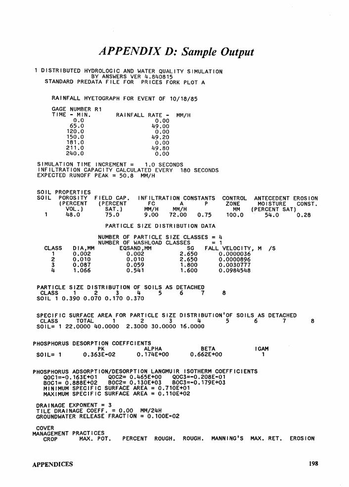
APPENDIX D: Sample Output 1 DISTRIBUTED HYDROLOGIC AND WATER QUALITY SIMULATION

BY ANSWERS VER 4.840815 STANDARD PREDATA FILE FOR PRICES FORK PLOT A

RAINFALL HYETOGRAPH FOR EVENT OF 10/18/85 GAGE NUMBER Rl TIME - MIN. o.o

65.0 120.0 150.0 181 .0 211.0 240.0

RAINFALL RATE - MM/H 0.00

49.00 0.00

49.20 0.00

49.80 0.00

SIMULATION TIME INCREMENT= 1.0 SECONDS INFILTRATION CAPACITY CALCULATED EVERY 180 SECONDS EXPECTED RUNOFF PEAK= 50.8 MM/H

SO IL PROP ERTi ES SOIL POROSITY

(PERCENT VOL.)

FIELD CAP. (PERCENT

SAT.) 75.0

INFILTRATION CONSTANTS CONTROL ANTECEDENT EROSION FC A P ZONE MOISTURE CONST.

MM/H MM/H MM (PERCENT SAT) 1 48.0 9.00 72.00 0.75 100.0 54.0 0.28

CLASS 1 2 3 4

DIA,MM 0.002 0.010 0.087 1 .066

PARTICLE SIZE DISTRIBUTION DATA

NUMBER OF PARTICLE NUMBER OF WASHLOAD

EQSAND,MM 0.002 0.010 0.059 0.541

SIZE CLASSES= 4 CLASSES = 1

SG FALL VELOCITY, 2.650 0.0000036 2.650 0.0000896 1.800 0.0030777 1.600 0.0984548

PARTICLE SIZE DISTRIBUTION OF SOILS AS DETACHED CLASS 1 2 3 4 5 6 7 8

SOIL 1 0.390 0.070 0.170 0.370

M /S

SPECIFIC SURFACE AREA FOR PARTICLE SIZE DISTRIBUTION'OF SOILS AS DETACHED CLASS TOTAL 1 2 3 4 5 6 7 8

SOIL= 1 22.0000 40.0000 2.3000 30.0000 16.0000

PHOSPHORUS DESORPTION COEFFCIENTS PK ALPHA

SOIL= 1 0.363E-02 0.174E+OO BETA

0.662E+OO IGAM

1

PHOSPHORUS ADSORPTION/DESORPTION LANGMUIR ISOTHERM COEFFICIENTS QOC1=-0.163E+01 QOC2= 0.465E+OO QOC3=-0.208E-01 BOCl= 0.888E+02 BOC2= 0.130E+03 BOC3=-0.179E+03 MINIMUM SPECIFIC SURFACE AREA= 0.710E+01 MAXIMUM SPECIFIC SURFACE AREA= 0.110E+02

DRAINAGE EXPONENT= 3 TILE DRAINAGE COEFF. = 0.00 MM/24H GROUNDWATER RELEASE FRACTION= 0.100E-02

COVER MANAGEMENT PRACTICES

CROP MAX. POT. PERCENT ROUGH. ROUGH. MANNING'S MAX. RET. EROSION

APPENDICES 198

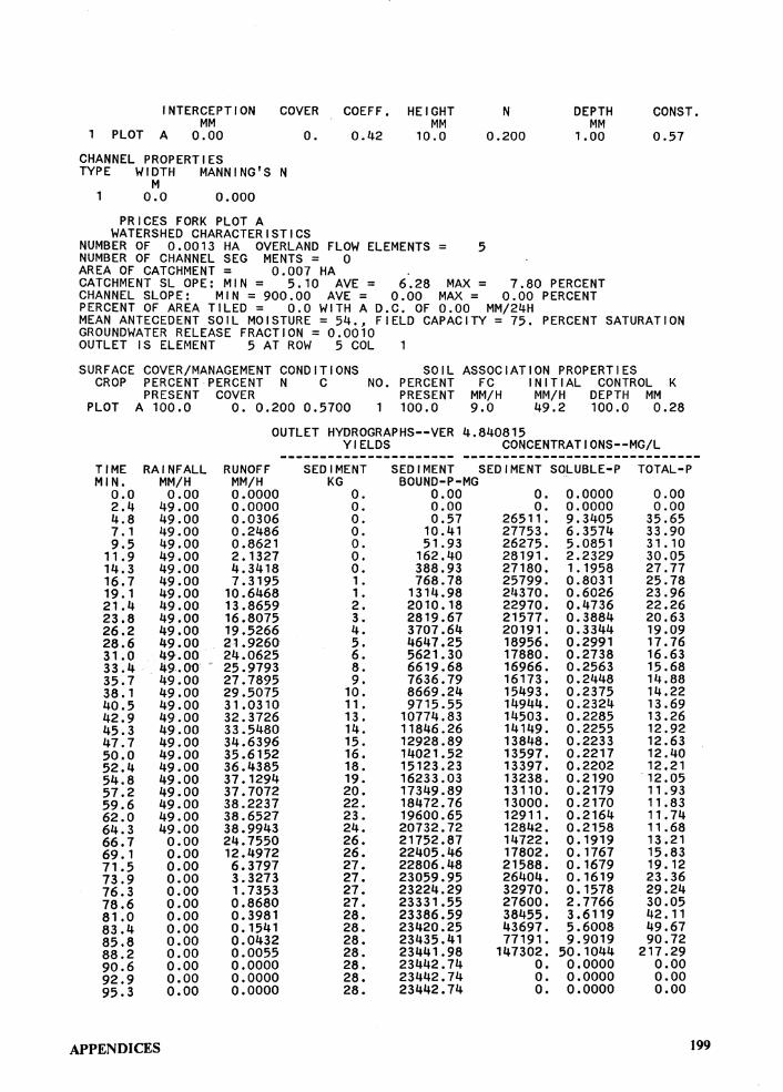
INTERCEPTION COVER MM

1 PLOT A 0.00 0.

CHANNEL PROPERTIES TYPE WIDTH MANNING'S N

M 1 0.0 0.000

PRICES FORK PLOT A WATERSHED CHARACTERISTICS

COEFF. HEIGHT MM

0.42 10.0

NUMBER OF 0.0013 HA OVERLAND FLOW ELEMENTS= 5 NUMBER OF CHANNEL SEG MENTS = 0 AREA OF CATCHMENT= 0.007 HA

N

0.200

DEPTH MM

1.00

CATCHMENT SL OPE: MIN= 5.10 AVE= 6.28 MAX= 7.80 PERCENT CHANNEL SLOPE: MIN= 900.00 AVE= 0.00 MAX= 0.00 PERCENT PERCENT OF AREA TILED= 0.0 WITH A D.C. OF 0.00 MM/24H

CONST.

0.57

MEAN ANTECEDENT SOIL MOISTURE= 54., FIELD CAPACITY= 75. PERCENT SATURATION GROUNDWATER RELEASE FRACTION= 0.0010 OUTLET IS ELEMENT 5 AT ROW 5 COL

SURFACE COVER/MANAGEMENT CONDITIONS SOIL ASSOCIATION PROPERTIES CROP PERCENT PERCENT N C NO. PERCENT FC INITIAL CONTROL K

PRESENT COVER PRESENT MM/H MM/H DEPTH MM PLOT A 100.0 O. 0.200 0.5700 1 100.0 9.0 49.2 100.0 0.28

OUTLET HYDROGRAPHS--VER 4.840815

TIME MIN.

0.0 2.4 4.8 7. 1 9,5

11.9 14.3 16.7 19. 1 21.4 23.8 26.2 28.6 31.0 33.4 35.7 38. 1 40.5 42.9 45.3 47.7 50.0 52.4 54.8 57.2 59.6 62.0 64.3 66.7 69. 1 71.5 73.9 76.3 78.6 81.0 83.4 85.8 88.2 90.6 92.9 95.3

RAINFALL MM/H

0.00 49.00 49.00 49.00 49.00 49.00 49.00 49.00 49.00 49.00 49.00 49.00 49.00 49.00 49.00, 49.00 49.00 49.00 49.00 49.00 49.00 49.00 49.00 49.00 49.00 49.00 49.00 49.00 o.oo o.oo o.oo

0.00 0.00 o.oo o.oo 0.00 0.00 0.00 o.oo o.oo o.oo

APPENDICES

RUNOFF MM/H 0.0000 0.0000 0.0306 0.2486 0.8621 2.1327 4.3418 7.3195

10.6468 13.8659 16.8075 19.5266 21. 9260 24.0625 25.9793 27.7895 29.5075 31.0310 32.3726 33.5480 34.6396 35.6152 36.4385 37. 1294 37.7072 38.2237 38.6527 38.9943 24.7550 12.4972 6.3797 3.3273 1.7353 0.8680 0.3981 0. 1541 0.0432 0.0055 0.0000 0.0000 0.0000

YIELDS CONCENTRATIONS--MG/L

SEDIMENT KG o. o. o. o. o. o. o.

1. ,. 2. 3. 4. 5. 6. 8. 9.

10. 1,. 13. 14. 15. 16. 18. 19. 20. 22. 23. 24. 26. 26. 27. 27. 27. 27. 28. 28. 28. 28. 28. 28. 28.

SEDIMENT SEDIMENT SOLUBLE-P BOUND-P-MG

0.00 0.00 0.57

10.41 51.93

162.40 388.93 768.78

1314.98 2010. 18 2819.67 3707.64 4647.25 5621.30 6619.68 7636.79 8669.24 9715.55

10774.83 11846.26 12928.89 14021.52 15123.23 16233.03 17349.89 18472.76 19600.65 20732.72 21752.87 22405.46 22806.48 23059.95 23224.29 23331.55 23386.59 23420.25 23435.41 23441.98 23442.74 23442.74 23442.74

o. 0.

26511. 27753. 26275. 28191. 27180. 25799. 24370. 22970. 21577. 20191. 18956. 17880. 16966. 16173. 15493. 14944. 14503. 14149. 13848. 13597. 13397. 13238. 13110. 13000. 12911. 12842. 14722. 17802. 21588. 26404. 32970. 27600. 38455. 43697. 77191.

147302. o. o. o.

0.0000 0.0000 9.3405 6. 3574 5.0851 2.2329 1.1958 0.8031 0.6026 0.4736 0.3884 0.3344 0.2991 0.2738 0.2563 0.2448 0.2375 0.2324 0.2285 0.2255 0.2233 0.2217 0.2202 0.2190 0.2179 0.2170 0.2164 0.2158 0.1919 0.1767 0.1679 0.1619 0.1578 2.7766 3.6119 5,6008 9.9019

50. 1044 0.0000 0.0000 0.0000

TOTAL-P

0.00 0.00

35.65 33.90 31.10 30.05 27. 77 25.78 23.96 22.26 20.63 19.09 17.76 16.63 15.68 14.88 14.22 13.69 13.26 12.92 12.63 12.40 12.21 12.05 11.93 11. 83 11.74 11.68 13.21 15.83 19. 12 23.36 29.24 30.05 42.11 49.67 90.72

217.29 o.oo o.oo 0.00

199

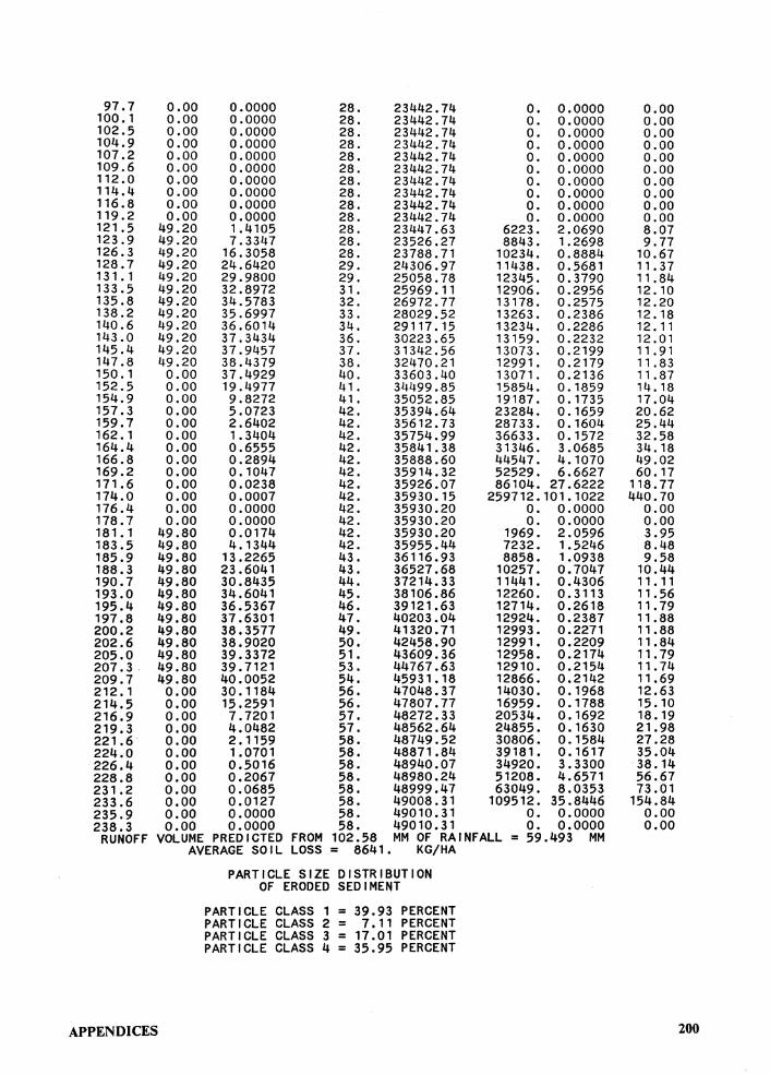
97.7 o.oo 0.0000 28. 23442.74 o. 0.0000 0.00 100. 1 0.00 0.0000 28. 23442.74 o. 0.0000 0.00 102.5 0.00 0.0000 28. 23442.74 o. 0.0000 0.00 104.9 0.00 0.0000 28. 23442.74 0. 0.0000 0.00 107.2 0.00 0.0000 28. 23442.74 o. 0.0000 0.00 109.6 o.oo 0.0000 28. 23442.74 o. 0.0000 0.00 112.0 0.00 0.0000 28. 23442.74 o. 0.0000 0.00 114.4 0.00 0.0000 28. 23442.74 o. 0.0000 0.00 116.8 o.oo 0.0000 28. 23442.74 o. 0.0000 0.00 119.2 0.00 0.0000 28. 23442.74 o. 0.0000 0.00 121.5 49.20 1 .4105 28. 23447.63 6223. 2.0690 8.07 123.9 49.20 7.3347 28. 23526.27 8843. 1.2698 9.77 126.3 49.20 16.3058 28. 23788.71 10234. 0.8884 10.67 128.7 49.20 24.6420 29. 24306.97 11438. 0.5681 11.37 131 . 1 49.20 29.9800 29. 25058.78 12345. 0.3790 11.84 133.5 49.20 32.8972 31. 25969.11 12906. 0.2956 12. 10 135.8 49.20 34.5783 32. 26972.77 13178. 0.2575 12.20 138.2 49.20 35.6997 33. 28029.52 13263. 0.2386 12. 18 140.6 49.20 36.6014 34. 29117.15 13234. 0.2286 12. 11 143.0 49.20 37.3434 36. 30223.65 13159. 0.2232 12.01 145.4 49.20 37.9457 37. 31342.56 13073. 0.2199 11 . 91 147.8 49.20 38.4379 38. 32470.21 12991. 0.2179 11. 83 150. 1 0.00 37.4929 40. 33603.40 13071. 0.2136 11.87 152.5 0.00 19.4977 41. 34499.85 15854. 0. 1859 14. 18 154.9 0.00 9.8272 41. 35052.85 19187. 0. 1735 17.04 157.3 0.00 5.0723 42. 35394.64 23284. 0. 1659 20.62 159.7 0.00 2.6402 42. 35612.73 28733. 0. 1604 25.44 162. 1 0.00 1.3404 42. 35754.99 36633. 0.1572 32.58 164.4 0.00 0.6555 42. 35841.38 31346. 3.0685 34. 18 166.8 0.00 0.2894 42. 35888.60 44547. 4. 1070 49.02 169.2 0.00 0. 1047 42. 35914.32 52529. 6.6627 60.17 171.6 0.00 0.0238 42. 35926.07 86104. 27.6222 118.77 174.0 0.00 0.0007 42. 35930.15 259712.101.1022 440.70 176.4 o.oo 0.0000 42. 35930.20 o. 0.0000 0.00 178.7 0.00 0.0000 42. 35930.20 0. 0.0000 0.00 181. 1 49.80 0.0174 42. 35930.20 1969. 2.0596 3.95 183.5 49.80 4.1344 42. 35955.44 7232. 1.5246 8.48 185.9 49.80 13.2265 43. 36116.93 8858. 1 .0938 9.58 188.3 49.80 23.6041 43. 36527.68 10257. 0.7047 10.44 190.7 49.80 30.8435 44. 37214.33 11441. 0.4306 11. 11 193.0 49.80 34.6041 45. 38106.86 12260. 0.3113 11.56 195.4 49.80 36.5367 46. 39121.63 12714. 0.2618 11.79 197.8 49.80 37.6301 47. 40203.04 12924. 0.2387 11.88 200.2 49.80 38.3577 49. 41320.71 12993. 0.2271 11.88 202.6 49.80 38.9020 50. 42458.90 12991. 0.2209 11.84 205.0 49.80 39.3372 51. 43609.36 12958. 0.2174 11.79 207 .3. 49.80 39.7121 53. 44767.63 12910. 0.2154 11.74 209.7 49.80 40.0052 54. 45931.18 12866. 0.2142 11.69 212. 1 0.00 30.1184 56. 47048.37 14030. 0. 1968 12.63 214.5 0.00 15.2591 56. 47807.77 16959. 0. 1788 15. 10 216.9 0.00 7.7201 57. 48272.33 20534. 0. 1692 18. 19 219.3 0.00 4.0482 57. 48562.64 24855. 0.1630 21. 98 221.6 0.00 2. 1159 58. 48749.52 30806. 0. 1584 27.28 224.0 0.00 1.0701 58. 48871.84 39181. 0.1617 35.04 226.4 0.00 0.5016 58. 48940.07 34920. 3.3300 38. 14 228.8 o.oo 0.2067 58. 48980.24 51208. 4.6571 56.67 231.2 o.oo 0.0685 58. 48999.47 63049. 8.0353 73.01 233.6 0.00 0.0127 58. 49008.31 109512. 35.8446 154.84 235.9 0.00 0.0000 58. 49010.31 o. 0.0000 0.00 238.3 0.00 0.0000 58. 49010. 31 o. 0.0000 0.00

RUNOFF VOLUME PREDICTED FROM 102.58 MM OF RAINFALL = 59,493 MM AVERAGE SOIL LOSS= 8641. KG/HA

PARTICLE SIZE DISTRIBUTION OF ERODED SEDIMENT

PARTICLE CLASS 1 = 39.93 PERCENT PARTICLE CLASS 2 = 7. 11 PERCENT PARTICLE CLASS 3 = 17 .01 PERCENT PARTICLE CLASS 4 = 35.95 PERCENT

APPENDICES 200

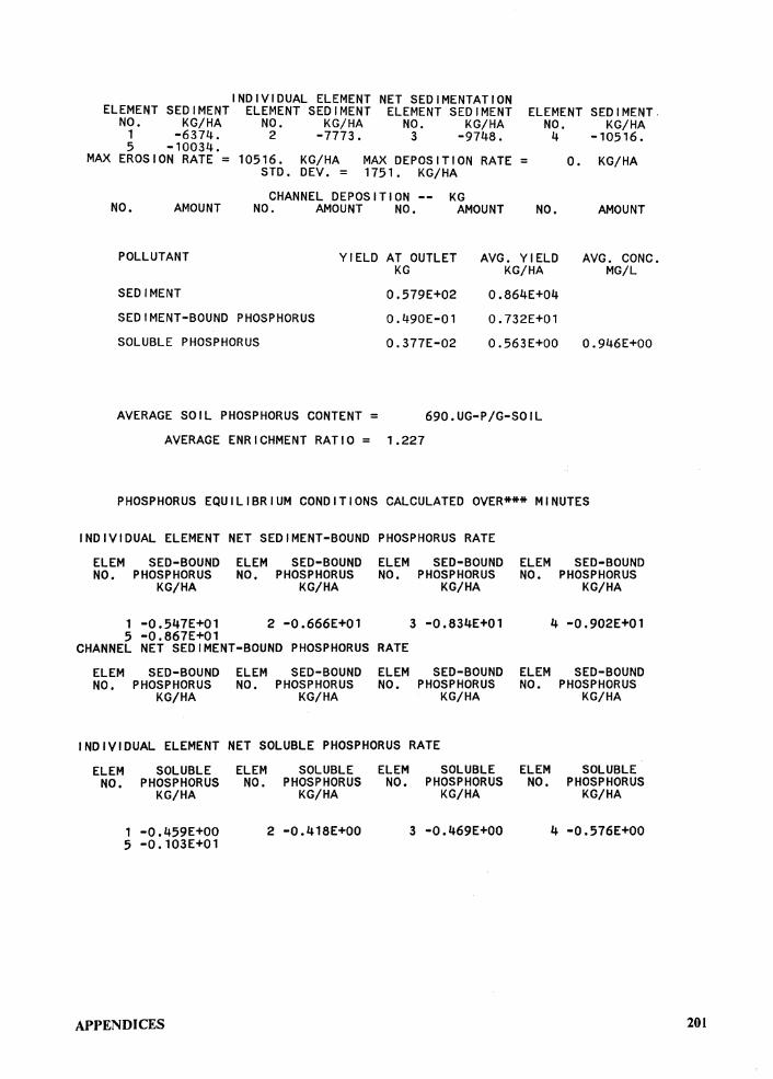
NET SEDIMENTATION INDIVIDUAL ELEMENT ELEMENT SEDIMENT ELEMENT SEDIMENT ELEMENT SEDIMENT ELEMENT SEDIMENT.

NO. KG/HA NO. KG/HA 1 -6374. 2 -7773.

NO. KG/HA NO. KG/HA 3 -9748. 4 -10516.

5 -10034. MAX EROSION RATE= 10516. KG/HA MAX DEPOSITION RATE=

STD. DEV. = 1751. KG/HA CHANNEL DEPOSITION -- KG

NO. AMOUNT NO. AMOUNT NO. AMOUNT

o. KG/HA

NO. AMOUNT

POLLUTANT YIELD AT OUTLET AVG. YIELD AVG. CONC. KG KG/HA MG/L

SEDIMENT 0.864E+04 0.732E+01 SEDIMENT-BOUND PHOSPHORUS

SOLUBLE PHOSPHORUS

0.579E+02 0.490E-01 0.377E-02 0.563E+OO 0.946E+OO

AVERAGE SOIL PHOSPHORUS CONTENT= 690.UG-P/G-SOIL AVERAGE ENRICHMENT RATIO= 1.227

PHOSPHORUS EQUILIBRIUM CONDITIONS CALCULATED OVER*** MINUTES

INDIVIDUAL ELEMENT NET SEDIMENT-BOUND PHOSPHORUS RATE

ELEM SEO-BOUND ELEM SEO-BOUND ELEM SEO-BOUND ELEM SEO-BOUND NO. PHOSPHORUS NO. PHOSPHORUS NO. PHOSPHORUS NO. PHOSPHORUS

KG/HA KG/HA KG/HA KG/HA

1 -0.547E+01 2 -0.666E+01 3 -0.834E+01 4 -0.902E+01 5 -0.867E+01

CHANNEL NET SEDIMENT-BOUND PHOSPHORUS RATE

ELEM SEO-BOUND ELEM SEO-BOUND ELEM SEO-BOUND ELEM SED-BOUND NO. PHOSPHORUS NO. PHOSPHORUS NO. PHOSPHORUS NO. PHOSPHORUS


INDIVIDUAL ELEMENT NET SOLUBLE PHOSPHORUS RATE

ELEM SOLUBLE ELEM SOLUBLE ELEM SOLUBLE ELEM SOLUBLE NO. PHOSPHORUS NO. PHOSPHORUS NO. PHOSPHORUS NO. PHOSPHORUS


1 -0.459E+OO 2 -0.418E+OO 3 -0.469E+OO 4 -0.576E+OO 5 -0.103E+01

APPENDICES 201

The vita has been removed from the scanned document

ld5655.v855_1986.s867.pdf - vtechworks

Documents