chapter 7 bunsen burner model - vtechworks
TRANSCRIPT
Chapter 7
Bunsen Burner Model
85
7.1 Purpose of the Bunsen Type Burner Model
The Bunsen type burner with co–flow is a very simple experimental configuration
that avoids many complications of modern gas turbine combustors such as complex
fluid mechanics and high levels of turbulence. The laminar Bunsen flame is however
a non–ideal burning environment that also shows similarities to the gas turbine com-
bustor environment. The flame is stabilized by a delicate balance between heat–loss
and fluid mechanical strain. The flame is surrounded by a shroud of dilution air that
affects the burning.
The Bunsen type burner model shows that global chemiluminescence measure-
ments can be modeled and understood using simple physical principles without detail
information about the exact burning process. Through the understanding of chemi-
luminescence several other aspects of the burning process can be elucidated, at the
very least at a qualitative level.
7.2 Modeling Approach
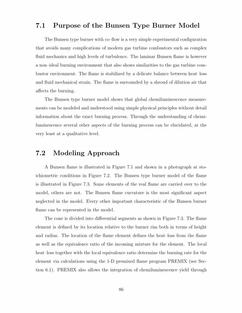
A Bunsen flame is illustrated in Figure 7.1 and shown in a photograph at sto-
ichiometric conditions in Figure 7.2. The Bunsen type burner model of the flame
is illustrated in Figure 7.3. Some elements of the real flame are carried over to the
model, others are not. The Bunsen flame curvature is the most significant aspect
neglected in the model. Every other important characteristic of the Bunsen burner
flame can be represented in the model.
The cone is divided into differential segments as shown in Figure 7.3. The flame
element is defined by its location relative to the burner rim both in terms of height
and radius. The location of the flame element defines the heat–loss from the flame
as well as the equivalence ratio of the incoming mixture for the element. The local
heat–loss together with the local equivalence ratio determine the burning rate for the
element via calculations using the 1-D premixed flame program PREMIX (see Sec-
tion 6.1). PREMIX also allows the integration of chemiluminescence yield through
86
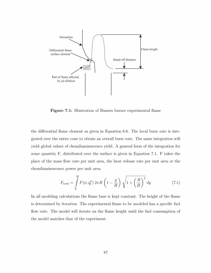
Figure 7.1: Illustration of Bunsen burner experimental flame
the differential flame element as given in Equation 6.6. The local burn–rate is inte-
grated over the entire cone to obtain an overall burn–rate. The same integration will
yield global values of chemiluminescence yield. A general form of the integration for
some quantity F, distributed over the surface is given in Equation 7.1. F takes the
place of the mass flow–rate per unit area, the heat–release rate per unit area or the
chemiluminescence power per unit area.
Ftotal =
H∫0
F (φ, q′′l ) 2πR
(1 − y
H
) √1 +
(R
H
)2
dy (7.1)
In all modeling calculations the flame base is kept constant. The height of the flame
is determined by iteration. The experimental flame to be modeled has a specific fuel
flow–rate. The model will iterate on the flame height until the fuel consumption of
the model matches that of the experiment.
87
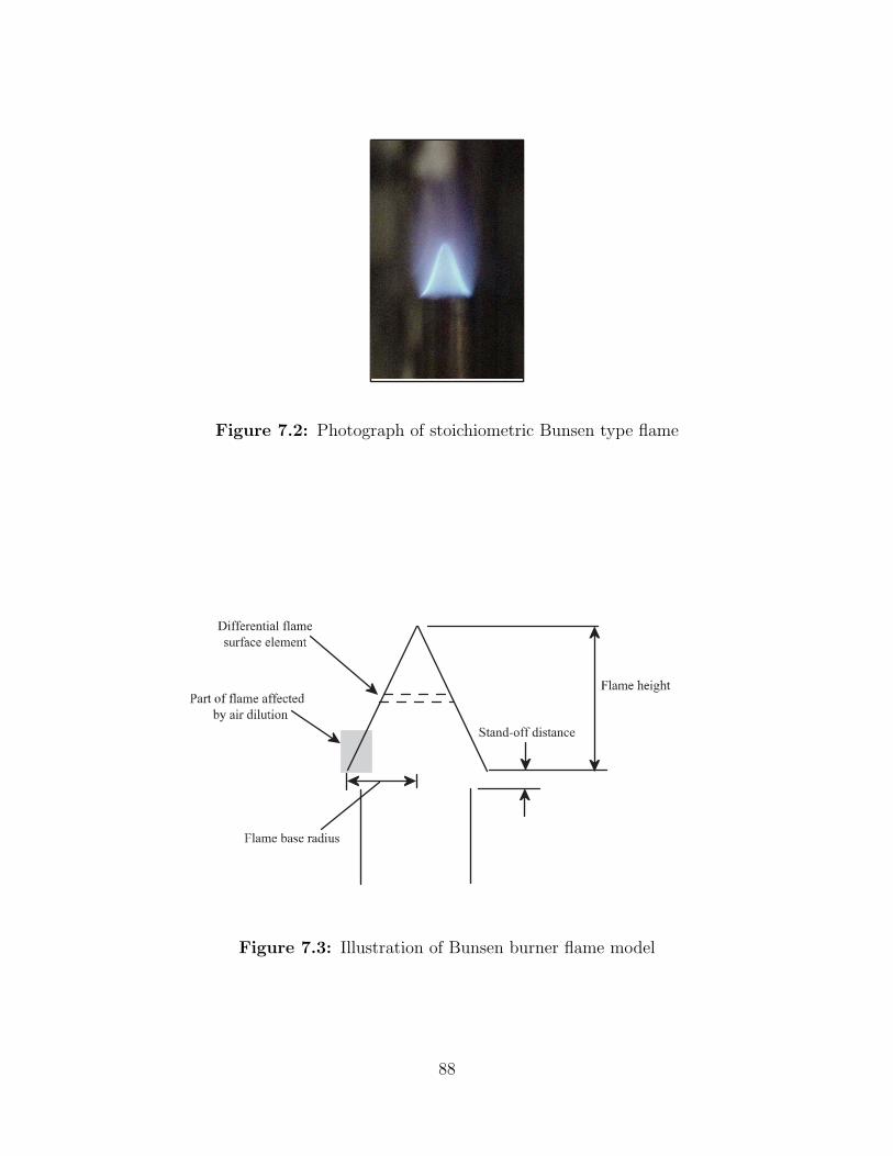
Figure 7.2: Photograph of stoichiometric Bunsen type flame
Figure 7.3: Illustration of Bunsen burner flame model
88
7.3 Bunsen Type Burner Model Components
To provide closure for the model, relationships between the position of the flame
element and all other flame relevant quantities must be obtained. The model will
translate the position into both heat–loss and local equivalence ratio using a low-
order approximation of the heat–transfer and mixing observed in the flame. The local
heat–loss and equivalence ratio will then determine all other flame–related quantities
such as chemiluminescence yield and burn–rate through the calculations performed
using PREMIX.
7.3.1 Semi-empirical mixing model
The local chemiluminescence measurements revealed that significant mixing be-
tween the co–flow of air and the main premixed fuel and air stream exists. To model
the effect, a variation of the local equivalence ratio along the height of the flame is
prescribed in the model. The form of the variation is given in Equation 7.2. The con-
stants in the equation may vary with main–stream equivalence ratio. φl represents
the leanest equivalence ratio at the edge of the flame. b is a parameter governing how
evenly the equivalence ratio increases from φl to the main stream equivalence ratio
φo. b is kept constant for all calculations at a value of 30. hch is the height at which
the main stream equivalence ratio is reached. Beyond hch, the equivalence ratio does
not change. The formula shown in Equation 7.2 is a crude model of the complex
mixing processes that actually occur but the modeling results given in Section 7.4
will show that the model is sufficient to capture the major experimental influences
of the co–flow of air. The model is termed ”semi–empirical” because the variation of
parameters φl and hch with equivalence ratio is determined by attempting to match
modeling results to experimental data.
φlocal(y) =
φo−φl
ebhch−1
(eb y − 1
)+ φl for y < hch
φo for y > hch
(7.2)
89
7.3.2 Semi-empirical heat–loss model
Heat–loss from the Bunsen burner flame is by radiation and conduction. PRE-
MIX, as used in the Bunsen burner modeling calculations does not account for radi-
ation heat–loss. The formula given in Equation 7.3 assumes that both heat–loss by
radiation and conduction are based on the flame temperature, Tflame. The major heat
sink for the Bunsen burner flame is the stainless steel burner rim with a temperature
of Trim. The conductivity λ, is kept constant at a value of 0.04 W/ (m-Ko). The final
parameter governing the conduction heat–loss is the stand–off distance of the edge
of the flame, dst. The radiation sink, Tsink was assumed black with temperature of
298Ko. The emissivity of the flame, ε is considered constant at 0.005.
q′′l (y) = λTflame − Trim
y + dst
+ εσ
(T 4
flame − T 4sink
)(7.3)
7.3.3 PREMIX 1-D flame results
Heat–loss and local equivalence ratio determine all other flame variables such
as local burn–rate, chemiluminescence and flame temperature through PREMIX cal-
culations. PREMIX calculations were originally performed in the two–dimensional
parameter space of burner flow–rate and equivalence ratio. Burner flow–rate is re-
lated directly to heat–loss, and due to the application of the PREMIX results in the
Bunsen burner flame model, heat–loss is considered the independent variable.
All of the PREMIX calculations resolve the computational domain with at least
200 points to achieve the desired accuracy in the chemiluminescence species mole–
fraction variation through the flame. The chemiluminescence species variation through
the flame is the last to converge as the computational grid is refined because of the
extremely low mole–fractions observed for the chemiluminescence species. The max-
imum mole–fraction for excited species is on the order of 10−13.
Flame temperature
The flame temperature is defined to be the maximum temperature observed in
the computational domain of the PREMIX calculation. The flame temperature is
90
0 25000 50000 75000 100000Heat Loss (W/sq.m)
1500
1600
1700
1800
1900
2000
2100
2200
Fla
me
Tem
pera
ture
(K)
Equivalence Ratio = 0.75Equivalence Ratio = 0.85Equivalence Ratio = 1.00
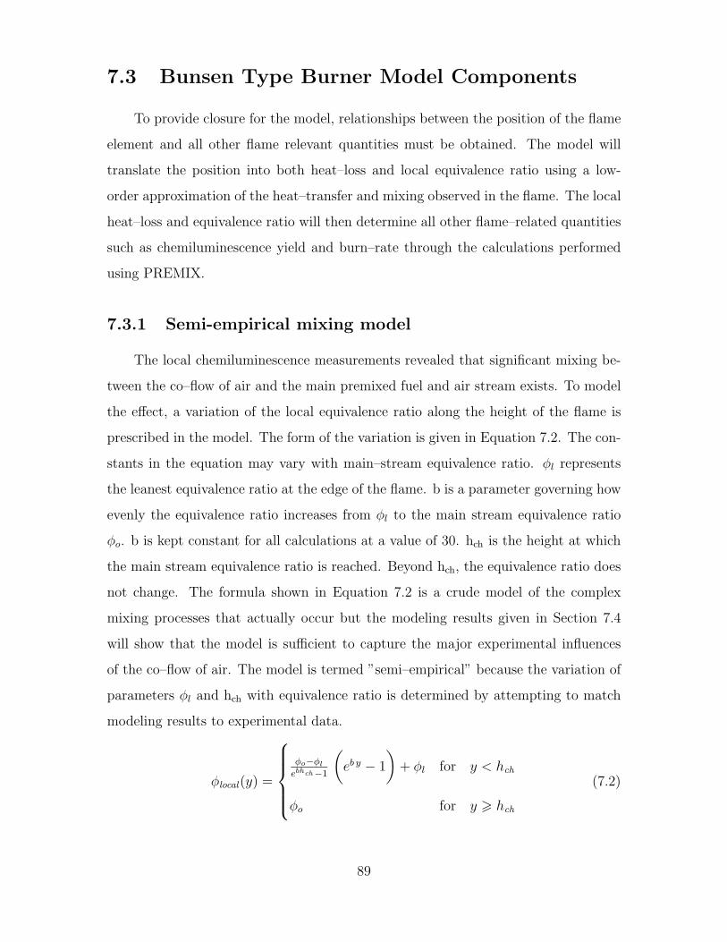
Figure 7.4: Flame temperature as a function of heat–loss
shown as a function of heat–loss for three equivalence ratios in Figure 7.4. Flame
temperature is most sensitive to heat–loss at lower equivalence ratios, as can be
expected due to the fact that less heat is liberated at these equivalence ratios.
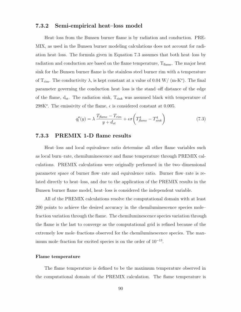
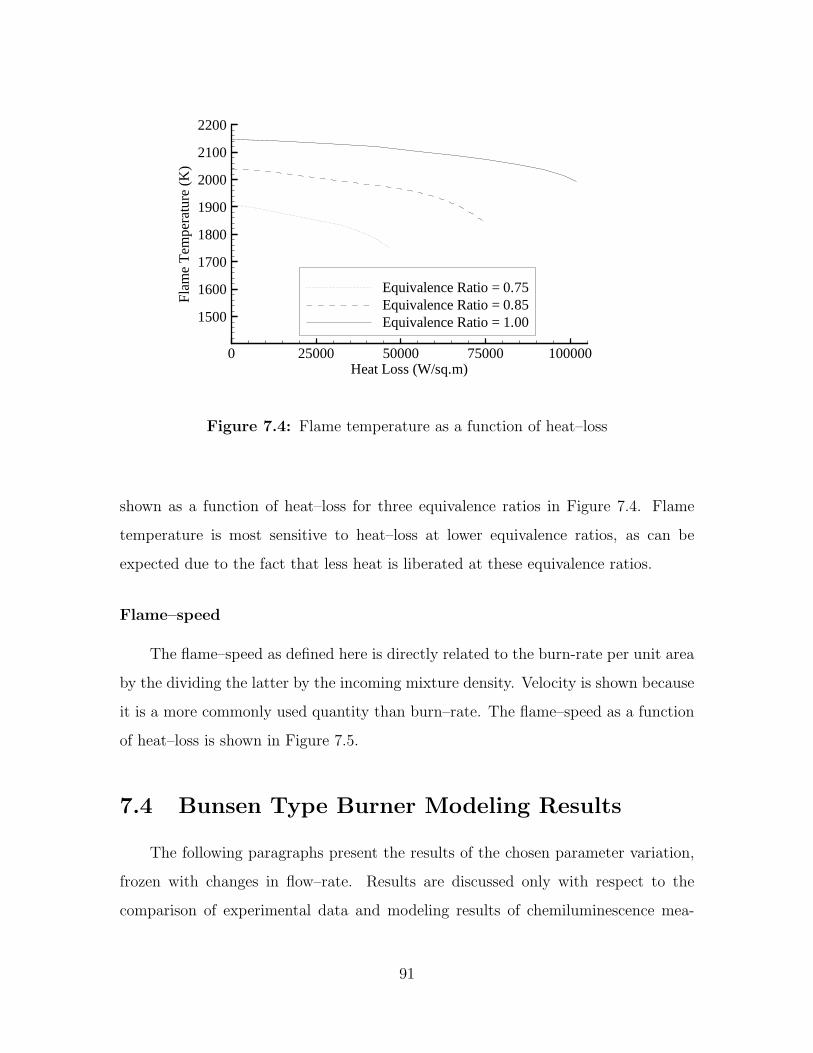
Flame–speed
The flame–speed as defined here is directly related to the burn-rate per unit area
by the dividing the latter by the incoming mixture density. Velocity is shown because
it is a more commonly used quantity than burn–rate. The flame–speed as a function
of heat–loss is shown in Figure 7.5.
7.4 Bunsen Type Burner Modeling Results
The following paragraphs present the results of the chosen parameter variation,
frozen with changes in flow–rate. Results are discussed only with respect to the
comparison of experimental data and modeling results of chemiluminescence mea-
91
0 25000 50000 75000 100000Heat Loss (W/sq.m)
10
20
30
40
50
60
Fla
me
Spe
ed(c
m/s
ec)
Equivalence Ratio = 0.75Equivalence Ratio = 0.85Equivalence Ratio = 1.00
Figure 7.5: Flame–speed as a function of heat–loss
surements. Detail analysis and evaluation of chemiluminescence as a heat–release
rate indicator is given in Section 10.2.1.
7.4.1 Summary of modeling procedure
Before presenting the modeling results, the procedure used to obtain these results
is summarized. The parameters defined above in Section 7.3.1 and Section 7.3.2
are set by matching, to the best of the model’s ability the OH∗ chemiluminescence
experimental data for a flow–rate of 60 cc/sec of air. The conversion factor from the
units of experimentally measured chemiluminescence (cV-A) to the yield calculated in
PREMIX, is determined at an equivalence ratio of 0.90 and held constant for all other
data points. Once the parameter values are determined as a function of equivalence
ratio for one flow–rate they are not changed for the other flow–rates.
92
0.75 0.8 0.85 0.9 0.95 1 1.05 1.1 1.15 1.2Equivalence Ratio
5E-05
0.0001
0.00015
0.0002
0.00025
0.0003
0.00035
Che
milu
min
esce
nce
Yie
ld
Experimental DataModelling Results
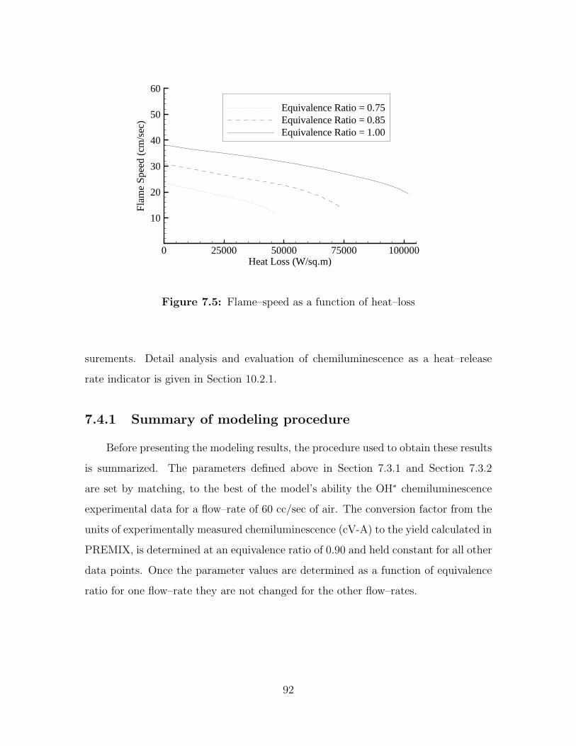
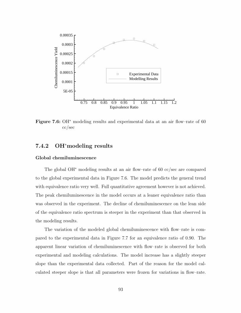
Figure 7.6: OH∗ modeling results and experimental data at an air flow–rate of 60cc/sec
7.4.2 OH∗modeling results
Global chemiluminescence
The global OH∗ modeling results at an air flow–rate of 60 cc/sec are compared
to the global experimental data in Figure 7.6. The model predicts the general trend
with equivalence ratio very well. Full quantitative agreement however is not achieved.
The peak chemiluminescence in the model occurs at a leaner equivalence ratio than
was observed in the experiment. The decline of chemiluminescence on the lean side
of the equivalence ratio spectrum is steeper in the experiment than that observed in
the modeling results.
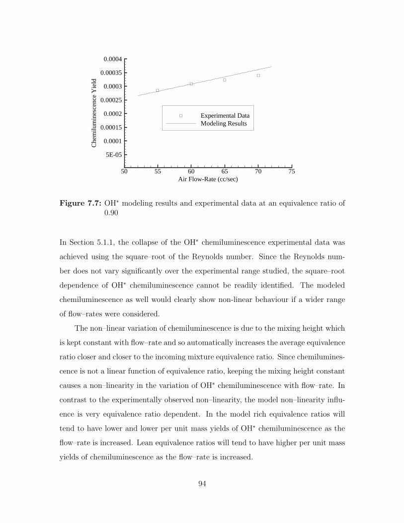
The variation of the modeled global chemiluminescence with flow–rate is com-
pared to the experimental data in Figure 7.7 for an equivalence ratio of 0.90. The
apparent linear variation of chemiluminescence with flow–rate is observed for both
experimental and modeling calculations. The model increase has a slightly steeper
slope than the experimental data collected. Part of the reason for the model cal-
culated steeper slope is that all parameters were frozen for variations in flow–rate.
93
50 55 60 65 70 75Air Flow-Rate (cc/sec)
5E-05
0.0001
0.00015
0.0002
0.00025
0.0003
0.00035
0.0004
Che
milu
min
esce
nce
Yie
ld
Experimental DataModeling Results
Figure 7.7: OH∗ modeling results and experimental data at an equivalence ratio of0.90
In Section 5.1.1, the collapse of the OH∗ chemiluminescence experimental data was
achieved using the square–root of the Reynolds number. Since the Reynolds num-
ber does not vary significantly over the experimental range studied, the square–root
dependence of OH∗ chemiluminescence cannot be readily identified. The modeled
chemiluminescence as well would clearly show non-linear behaviour if a wider range
of flow–rates were considered.
The non–linear variation of chemiluminescence is due to the mixing height which
is kept constant with flow–rate and so automatically increases the average equivalence
ratio closer and closer to the incoming mixture equivalence ratio. Since chemilumines-
cence is not a linear function of equivalence ratio, keeping the mixing height constant
causes a non–linearity in the variation of OH∗ chemiluminescence with flow–rate. In
contrast to the experimentally observed non–linearity, the model non–linearity influ-
ence is very equivalence ratio dependent. In the model rich equivalence ratios will
tend to have lower and lower per unit mass yields of OH∗ chemiluminescence as the
flow–rate is increased. Lean equivalence ratios will tend to have higher per unit mass
yields of chemiluminescence as the flow–rate is increased.
94

Local chemiluminescence
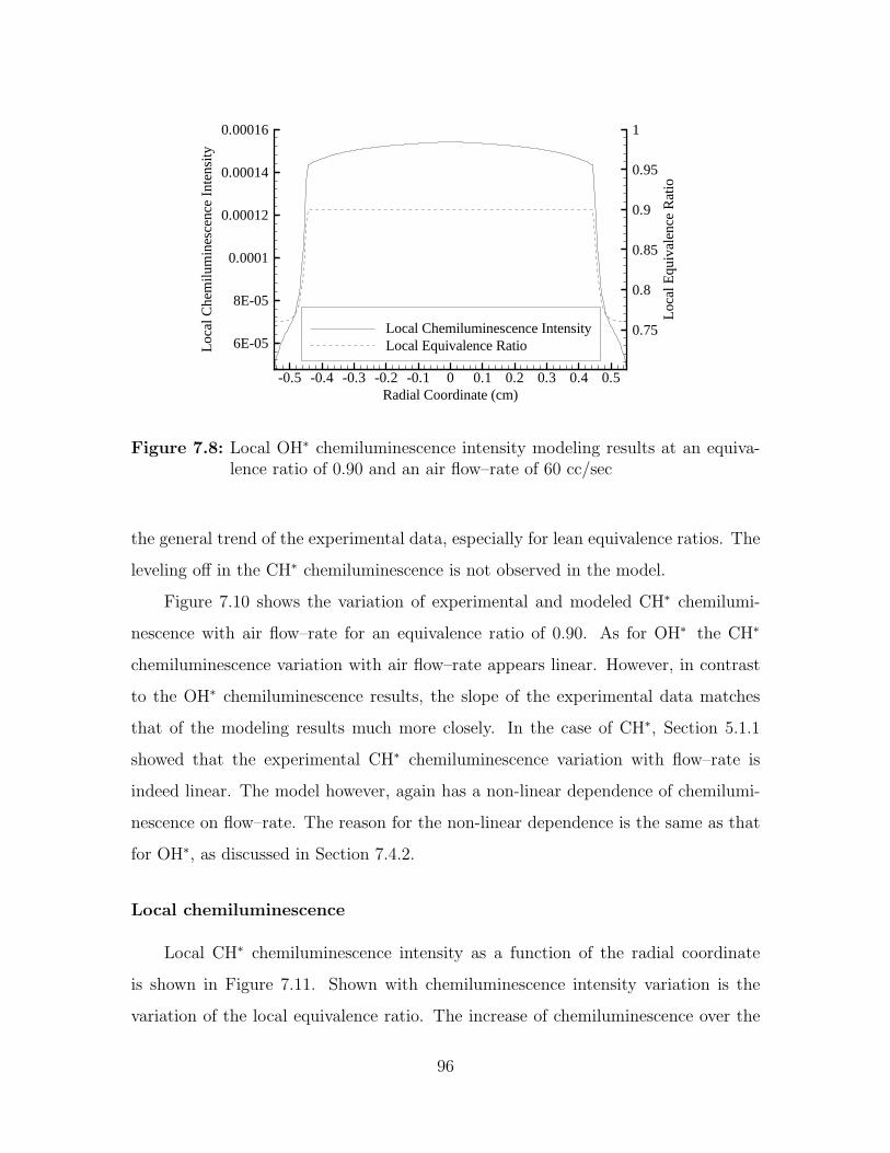
Local OH∗ chemiluminescence intensity as a function of the radial coordinate
is shown in Figure 7.8. Shown with chemiluminescence intensity variation is the
variation of the local equivalence ratio. The increase of chemiluminescence over the
radius is similar in magnitude to that observed in the experimental data shown in
Figure 5.8 for example. The model chemiluminescence variation is however mostly due
to the variation of the local equivalence ratio over the radius of the flame. Heat losses
appear only to be important in the immediate vicinity of the burner rim. Curvature
effects, which contribute significantly to the shape observed experimentally are not
considered in the model. Similarly, the local minimum of chemiluminescence intensity
observed in the center of the flame is not observed in the model, because the diffusion
and pressure influences are not considered by the model. Section 7.5.3 addresses
burning at the flame center in greater detail.
It is important to reiterate that the goal of the model is not to provide a complete
model of the Bunsen flame in air co–flow but rather to model the general behaviour
of the flame in order to provide a basis for the interpretation of chemiluminescence
measurements in terms of heat–release rate. The modeling success for global chemi-
luminescence shows that the level of complexity in the model is adequate to attain
the goal of the model.
The units of the displayed local chemiluminescence are that of yield intensity
since the values have not been integrated over the flame area to give an overall
chemiluminescence yield.
7.4.3 CH∗modeling results
Global chemiluminescence
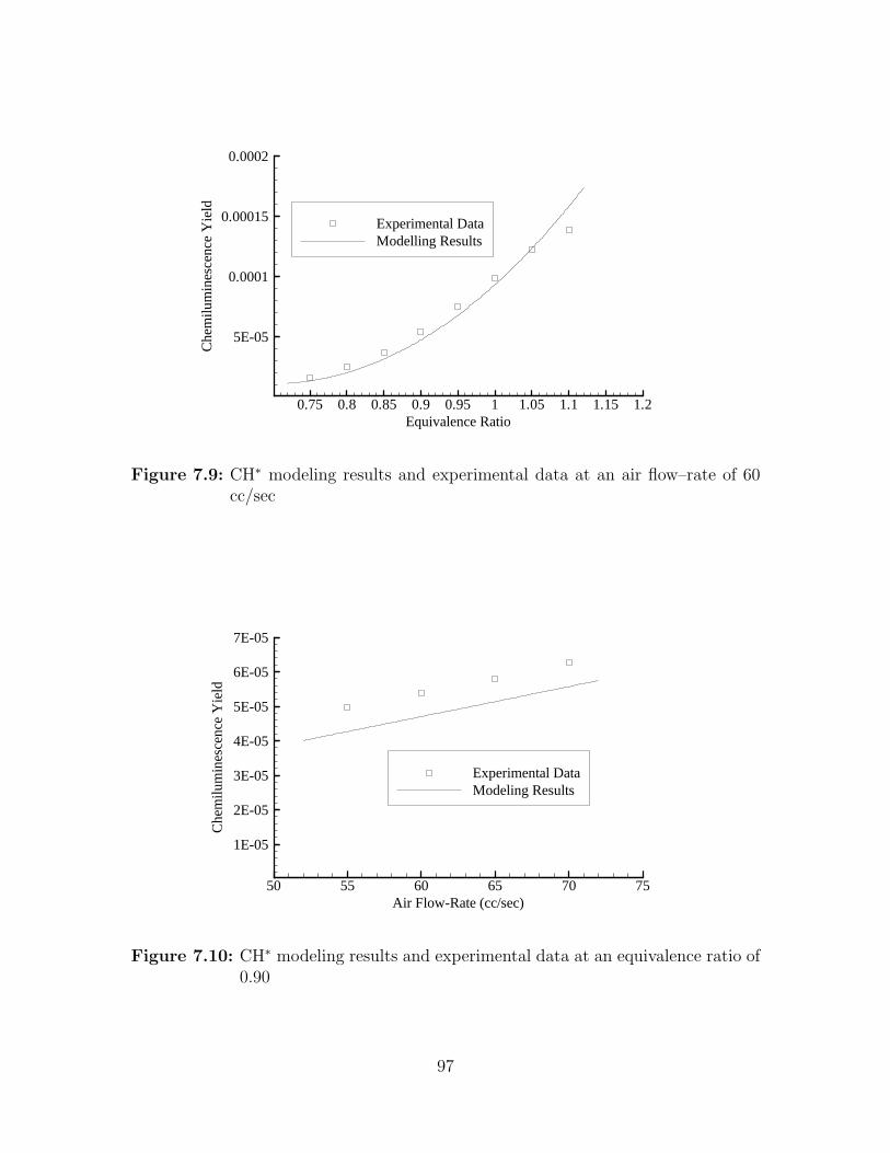
The same conversion factor used above to compare OH∗ chemiluminescence ex-
perimental data with modeling results is used to compare the CH∗ experimental data
to the modeling results. The experimental and modeled variation of CH∗ chemilumi-
nescence is shown in Figure 7.9 for an air flow–rate of 60 cc/sec. The model captures
95
-0.5 -0.4 -0.3 -0.2 -0.1 0 0.1 0.2 0.3 0.4 0.5Radial Coordinate (cm)
6E-05
8E-05
0.0001
0.00012
0.00014
0.00016
Loc
alC
hem
ilum
ines
cenc
eIn
tens
ity
0.75
0.8
0.85
0.9
0.95
1
Loc
alE
quiv
alen
ceR
atio
Local Chemiluminescence IntensityLocal Equivalence Ratio
Figure 7.8: Local OH∗ chemiluminescence intensity modeling results at an equiva-lence ratio of 0.90 and an air flow–rate of 60 cc/sec
the general trend of the experimental data, especially for lean equivalence ratios. The
leveling off in the CH∗ chemiluminescence is not observed in the model.
Figure 7.10 shows the variation of experimental and modeled CH∗ chemilumi-
nescence with air flow–rate for an equivalence ratio of 0.90. As for OH∗ the CH∗
chemiluminescence variation with air flow–rate appears linear. However, in contrast
to the OH∗ chemiluminescence results, the slope of the experimental data matches
that of the modeling results much more closely. In the case of CH∗, Section 5.1.1
showed that the experimental CH∗ chemiluminescence variation with flow–rate is
indeed linear. The model however, again has a non-linear dependence of chemilumi-
nescence on flow–rate. The reason for the non-linear dependence is the same as that
for OH∗, as discussed in Section 7.4.2.
Local chemiluminescence
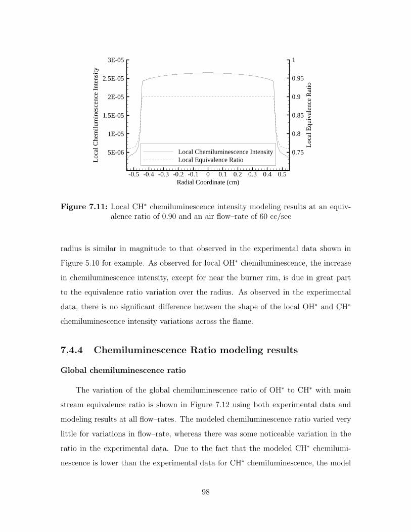
Local CH∗ chemiluminescence intensity as a function of the radial coordinate
is shown in Figure 7.11. Shown with chemiluminescence intensity variation is the
variation of the local equivalence ratio. The increase of chemiluminescence over the
96
0.75 0.8 0.85 0.9 0.95 1 1.05 1.1 1.15 1.2Equivalence Ratio
5E-05
0.0001
0.00015
0.0002
Che
milu
min
esce
nce
Yie
ldExperimental DataModelling Results
Figure 7.9: CH∗ modeling results and experimental data at an air flow–rate of 60cc/sec
50 55 60 65 70 75Air Flow-Rate (cc/sec)
1E-05
2E-05
3E-05
4E-05
5E-05
6E-05
7E-05
Che
milu
min
esce
nce
Yie
ld
Experimental DataModeling Results
Figure 7.10: CH∗ modeling results and experimental data at an equivalence ratio of0.90
97
-0.5 -0.4 -0.3 -0.2 -0.1 0 0.1 0.2 0.3 0.4 0.5Radial Coordinate (cm)
5E-06
1E-05
1.5E-05
2E-05
2.5E-05
3E-05
Loc
alC
hem
ilum
ines
cenc
eIn
tens
ity
0.75
0.8
0.85
0.9
0.95
1
Loc
alE
quiv
alen
ceR
atio
Local Chemiluminescence IntensityLocal Equivalence Ratio
Figure 7.11: Local CH∗ chemiluminescence intensity modeling results at an equiv-alence ratio of 0.90 and an air flow–rate of 60 cc/sec
radius is similar in magnitude to that observed in the experimental data shown in
Figure 5.10 for example. As observed for local OH∗ chemiluminescence, the increase
in chemiluminescence intensity, except for near the burner rim, is due in great part
to the equivalence ratio variation over the radius. As observed in the experimental
data, there is no significant difference between the shape of the local OH∗ and CH∗
chemiluminescence intensity variations across the flame.
7.4.4 Chemiluminescence Ratio modeling results
Global chemiluminescence ratio
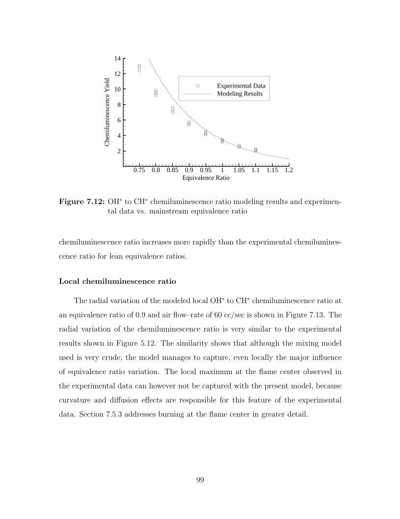
The variation of the global chemiluminescence ratio of OH∗ to CH∗ with main
stream equivalence ratio is shown in Figure 7.12 using both experimental data and
modeling results at all flow–rates. The modeled chemiluminescence ratio varied very
little for variations in flow–rate, whereas there was some noticeable variation in the
ratio in the experimental data. Due to the fact that the modeled CH∗ chemilumi-
nescence is lower than the experimental data for CH∗ chemiluminescence, the model
98
0.75 0.8 0.85 0.9 0.95 1 1.05 1.1 1.15 1.2Equivalence Ratio
2
4
6
8
10
12
14
Che
milu
min
esce
nce
Yie
ld
Experimental DataModeling Results
Figure 7.12: OH∗ to CH∗ chemiluminescence ratio modeling results and experimen-tal data vs. mainstream equivalence ratio
chemiluminescence ratio increases more rapidly than the experimental chemilumines-
cence ratio for lean equivalence ratios.
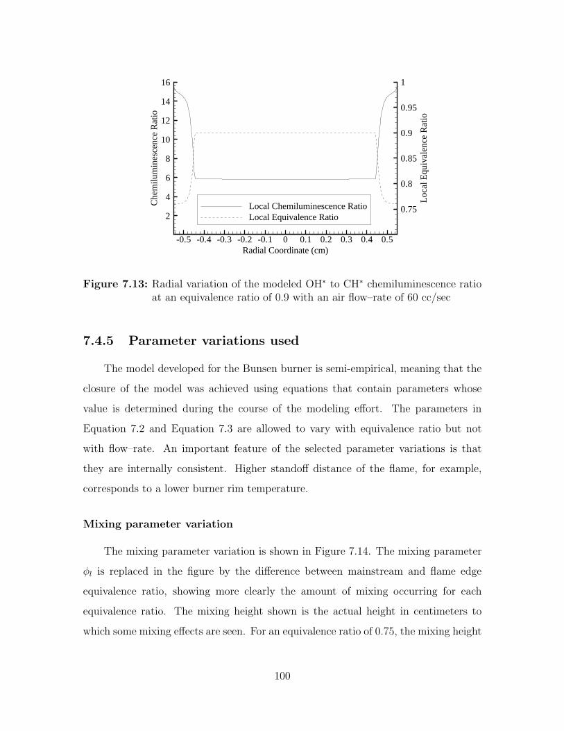
Local chemiluminescence ratio
The radial variation of the modeled local OH∗ to CH∗ chemiluminescence ratio at
an equivalence ratio of 0.9 and air flow–rate of 60 cc/sec is shown in Figure 7.13. The
radial variation of the chemiluminescence ratio is very similar to the experimental
results shown in Figure 5.12. The similarity shows that although the mixing model
used is very crude, the model manages to capture, even locally the major influence
of equivalence ratio variation. The local maximum at the flame center observed in
the experimental data can however not be captured with the present model, because
curvature and diffusion effects are responsible for this feature of the experimental
data. Section 7.5.3 addresses burning at the flame center in greater detail.
99
-0.5 -0.4 -0.3 -0.2 -0.1 0 0.1 0.2 0.3 0.4 0.5Radial Coordinate (cm)
2
4
6
8
10
12
14
16
Che
milu
min
esce
nce
Rat
io
0.75
0.8
0.85
0.9
0.95
1
Loc
alE
quiv
alen
ceR
atio
Local Chemiluminescence RatioLocal Equivalence Ratio
Figure 7.13: Radial variation of the modeled OH∗ to CH∗ chemiluminescence ratioat an equivalence ratio of 0.9 with an air flow–rate of 60 cc/sec
7.4.5 Parameter variations used
The model developed for the Bunsen burner is semi-empirical, meaning that the
closure of the model was achieved using equations that contain parameters whose
value is determined during the course of the modeling effort. The parameters in
Equation 7.2 and Equation 7.3 are allowed to vary with equivalence ratio but not
with flow–rate. An important feature of the selected parameter variations is that
they are internally consistent. Higher standoff distance of the flame, for example,
corresponds to a lower burner rim temperature.
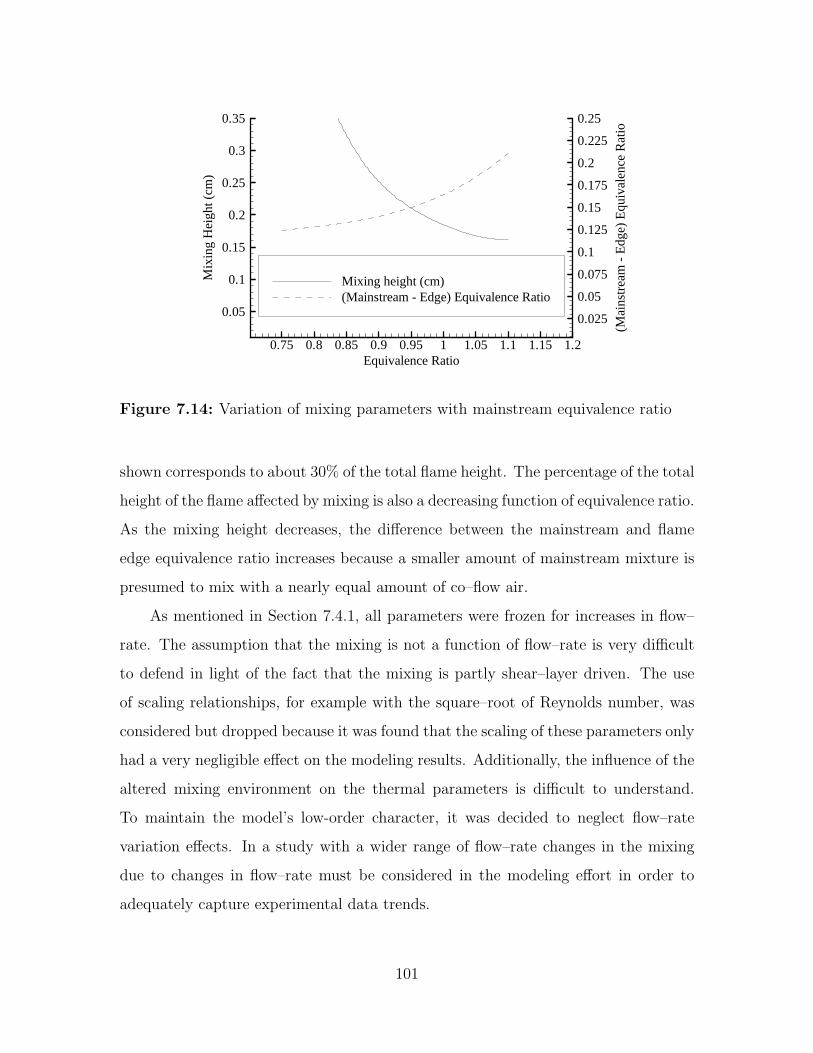
Mixing parameter variation
The mixing parameter variation is shown in Figure 7.14. The mixing parameter
φl is replaced in the figure by the difference between mainstream and flame edge
equivalence ratio, showing more clearly the amount of mixing occurring for each
equivalence ratio. The mixing height shown is the actual height in centimeters to
which some mixing effects are seen. For an equivalence ratio of 0.75, the mixing height
100
0.75 0.8 0.85 0.9 0.95 1 1.05 1.1 1.15 1.2Equivalence Ratio
0.05
0.1
0.15
0.2
0.25
0.3
0.35
Mix
ing
Hei
ght(
cm)
0.025
0.05
0.075
0.1
0.125
0.15
0.175
0.2
0.225
0.25
(Mai
nstr
eam
-E
dge)
Equ
ival
ence
Rat
io
Mixing height (cm)(Mainstream - Edge) Equivalence Ratio
Figure 7.14: Variation of mixing parameters with mainstream equivalence ratio
shown corresponds to about 30% of the total flame height. The percentage of the total
height of the flame affected by mixing is also a decreasing function of equivalence ratio.
As the mixing height decreases, the difference between the mainstream and flame
edge equivalence ratio increases because a smaller amount of mainstream mixture is
presumed to mix with a nearly equal amount of co–flow air.
As mentioned in Section 7.4.1, all parameters were frozen for increases in flow–
rate. The assumption that the mixing is not a function of flow–rate is very difficult
to defend in light of the fact that the mixing is partly shear–layer driven. The use
of scaling relationships, for example with the square–root of Reynolds number, was
considered but dropped because it was found that the scaling of these parameters only
had a very negligible effect on the modeling results. Additionally, the influence of the
altered mixing environment on the thermal parameters is difficult to understand.
To maintain the model’s low-order character, it was decided to neglect flow–rate
variation effects. In a study with a wider range of flow–rate changes in the mixing
due to changes in flow–rate must be considered in the modeling effort in order to
adequately capture experimental data trends.
101
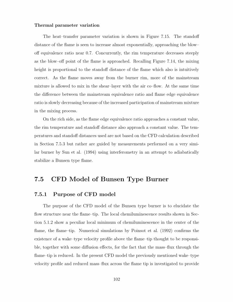
Thermal parameter variation
The heat–transfer parameter variation is shown in Figure 7.15. The standoff
distance of the flame is seen to increase almost exponentially, approaching the blow–
off equivalence ratio near 0.7. Concurrently, the rim temperature decreases steeply
as the blow–off point of the flame is approached. Recalling Figure 7.14, the mixing
height is proportional to the standoff distance of the flame which also is intuitively
correct. As the flame moves away from the burner rim, more of the mainstream
mixture is allowed to mix in the shear–layer with the air co–flow. At the same time
the difference between the mainstream equivalence ratio and flame edge equivalence
ratio is slowly decreasing because of the increased participation of mainstream mixture
in the mixing process.
On the rich side, as the flame edge equivalence ratio approaches a constant value,
the rim temperature and standoff distance also approach a constant value. The tem-
peratures and standoff distances used are not based on the CFD calculation described
in Section 7.5.3 but rather are guided by measurements performed on a very simi-
lar burner by Sun et al. (1994) using interferometry in an attempt to adiabatically
stabilize a Bunsen type flame.
7.5 CFD Model of Bunsen Type Burner
7.5.1 Purpose of CFD model
The purpose of the CFD model of the Bunsen type burner is to elucidate the
flow structure near the flame–tip. The local chemiluminescence results shown in Sec-
tion 5.1.2 show a peculiar local minimum of chemiluminescence in the center of the
flame, the flame–tip. Numerical simulations by Poinsot et al. (1992) confirms the
existence of a wake–type velocity profile above the flame–tip thought to be responsi-
ble, together with some diffusion effects, for the fact that the mass–flux through the
flame–tip is reduced. In the present CFD model the previously mentioned wake–type
velocity profile and reduced mass–flux across the flame tip is investigated to provide
102
0.75 0.8 0.85 0.9 0.95 1 1.05 1.1 1.15 1.2Equivalence Ratio
0.05
0.1
0.15
0.2
0.25
0.3
0.35
Sta
ndof
fD
ista
nce
(cm
)
350
400
450
500
550
600
650
Rim
Tem
pera
ture
(K)
Standoff Distance (cm)Rim Temperature (K)
Figure 7.15: Variation of heat transfer parameters with mainstream equivalence ra-tio
a further physical foundation for the observed chemiluminescence variation in the
flame–tip region.
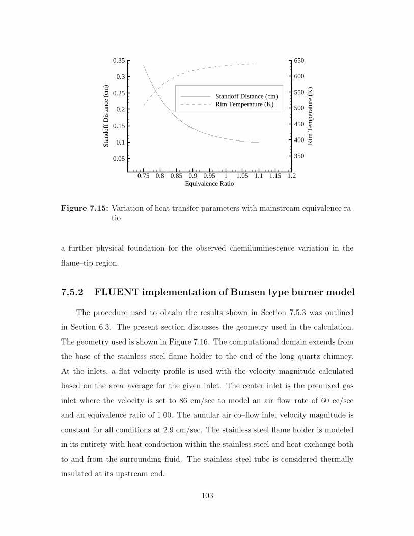
7.5.2 FLUENT implementation of Bunsen type burner model
The procedure used to obtain the results shown in Section 7.5.3 was outlined
in Section 6.3. The present section discusses the geometry used in the calculation.
The geometry used is shown in Figure 7.16. The computational domain extends from
the base of the stainless steel flame holder to the end of the long quartz chimney.
At the inlets, a flat velocity profile is used with the velocity magnitude calculated
based on the area–average for the given inlet. The center inlet is the premixed gas
inlet where the velocity is set to 86 cm/sec to model an air flow–rate of 60 cc/sec
and an equivalence ratio of 1.00. The annular air co–flow inlet velocity magnitude is
constant for all conditions at 2.9 cm/sec. The stainless steel flame holder is modeled
in its entirety with heat conduction within the stainless steel and heat exchange both
to and from the surrounding fluid. The stainless steel tube is considered thermally
insulated at its upstream end.
103
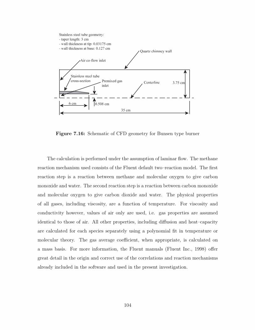
Figure 7.16: Schematic of CFD geometry for Bunsen type burner
The calculation is performed under the assumption of laminar flow. The methane
reaction mechanism used consists of the Fluent default two–reaction model. The first
reaction step is a reaction between methane and molecular oxygen to give carbon
monoxide and water. The second reaction step is a reaction between carbon monoxide
and molecular oxygen to give carbon dioxide and water. The physical properties
of all gases, including viscosity, are a function of temperature. For viscosity and
conductivity however, values of air only are used, i.e. gas properties are assumed
identical to those of air. All other properties, including diffusion and heat–capacity
are calculated for each species separately using a polynomial fit in temperature or
molecular theory. The gas average coefficient, when appropriate, is calculated on
a mass basis. For more information, the Fluent manuals (Fluent Inc., 1998) offer
great detail in the origin and correct use of the correlations and reaction mechanisms
already included in the software and used in the present investigation.
104
0.005 0.01Radial Coordinate (m)
0.06
0.0625
0.065
0.0675
0.07
0.0725
0.075
0.0775
0.08
Axi
alC
oord
inat
e(m
)
9.18.57.97.26.66.05.44.84.23.63.02.41.81.20.6
arbitrary units
Figure 7.17: Contour plot of the methane consumption reaction rate in Bunsen typeburner CFD simulation
7.5.3 Results of FLUENT Bunsen type burner model
The flame–tip wake phenomenon observed by Poinsot et al. (1992) is also found
in the presently described CFD investigation. Figure 7.17 shows a contour plot for
the rate of the first reaction. The outline of flame can thus be easily identified.
The contour plot clearly shows that the reaction rate, as expected, is highest at the
flame–tip. The contour plot also allows the flame base radius to be quantified along
with the flame stand–off distance from the burner rim. The flame base diameter is
only slightly larger than the stainless steel flame–holder inside exit diameter which is
not surprising considering that the CFD calculation suggests that the flame stand–off
distance is only 0.5 mm. The calculation also shows the significant curvature variation
along the Bunsen burner flame front. The flame has a stabilizing concave curvature
near the flame–tip and a flame de–stabilizing convex curvature near the flame base.
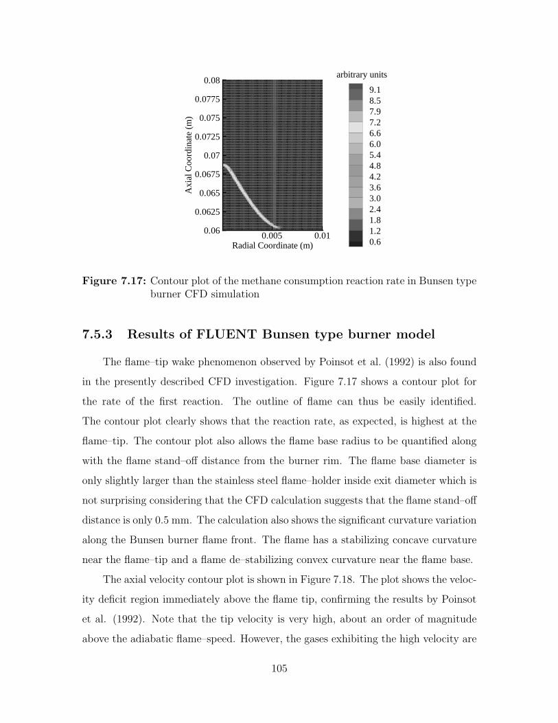
The axial velocity contour plot is shown in Figure 7.18. The plot shows the veloc-
ity deficit region immediately above the flame tip, confirming the results by Poinsot
et al. (1992). Note that the tip velocity is very high, about an order of magnitude
above the adiabatic flame–speed. However, the gases exhibiting the high velocity are
105
0.005 0.01Radial Coordinate (m)
0.06
0.0625
0.065
0.0675
0.07
0.0725
0.075
0.0775
0.08
Axi
alC
oord
inat
e(m
)
3.83.53.33.02.72.52.21.91.71.41.20.90.60.40.1
m/sec
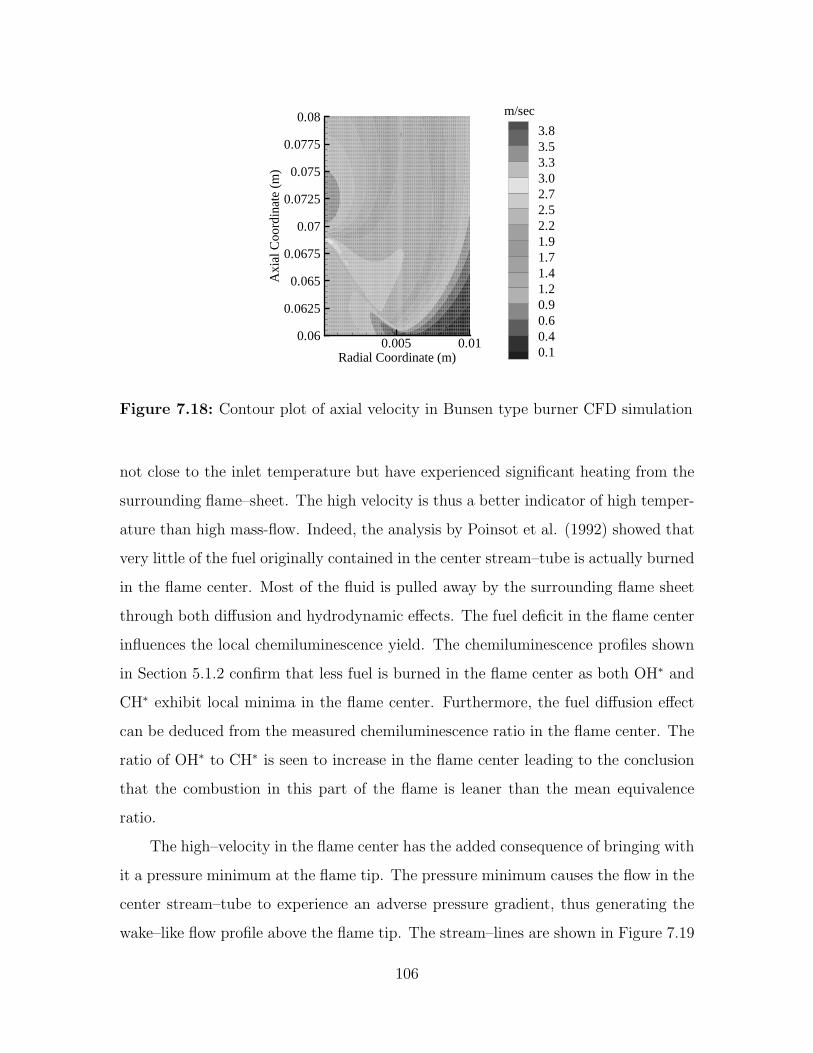
Figure 7.18: Contour plot of axial velocity in Bunsen type burner CFD simulation
not close to the inlet temperature but have experienced significant heating from the
surrounding flame–sheet. The high velocity is thus a better indicator of high temper-
ature than high mass-flow. Indeed, the analysis by Poinsot et al. (1992) showed that
very little of the fuel originally contained in the center stream–tube is actually burned
in the flame center. Most of the fluid is pulled away by the surrounding flame sheet
through both diffusion and hydrodynamic effects. The fuel deficit in the flame center
influences the local chemiluminescence yield. The chemiluminescence profiles shown
in Section 5.1.2 confirm that less fuel is burned in the flame center as both OH∗ and
CH∗ exhibit local minima in the flame center. Furthermore, the fuel diffusion effect
can be deduced from the measured chemiluminescence ratio in the flame center. The
ratio of OH∗ to CH∗ is seen to increase in the flame center leading to the conclusion
that the combustion in this part of the flame is leaner than the mean equivalence
ratio.
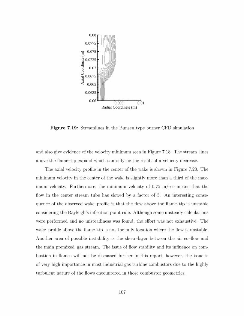
The high–velocity in the flame center has the added consequence of bringing with
it a pressure minimum at the flame tip. The pressure minimum causes the flow in the
center stream–tube to experience an adverse pressure gradient, thus generating the
wake–like flow profile above the flame tip. The stream–lines are shown in Figure 7.19
106
0.005 0.01Radial Coordinate (m)
0.06
0.0625
0.065
0.0675
0.07
0.0725
0.075
0.0775
0.08
Axi
alC
oord
inat
e(m
)
Figure 7.19: Streamlines in the Bunsen type burner CFD simulation
and also give evidence of the velocity minimum seen in Figure 7.18. The stream–lines
above the flame–tip expand which can only be the result of a velocity decrease.
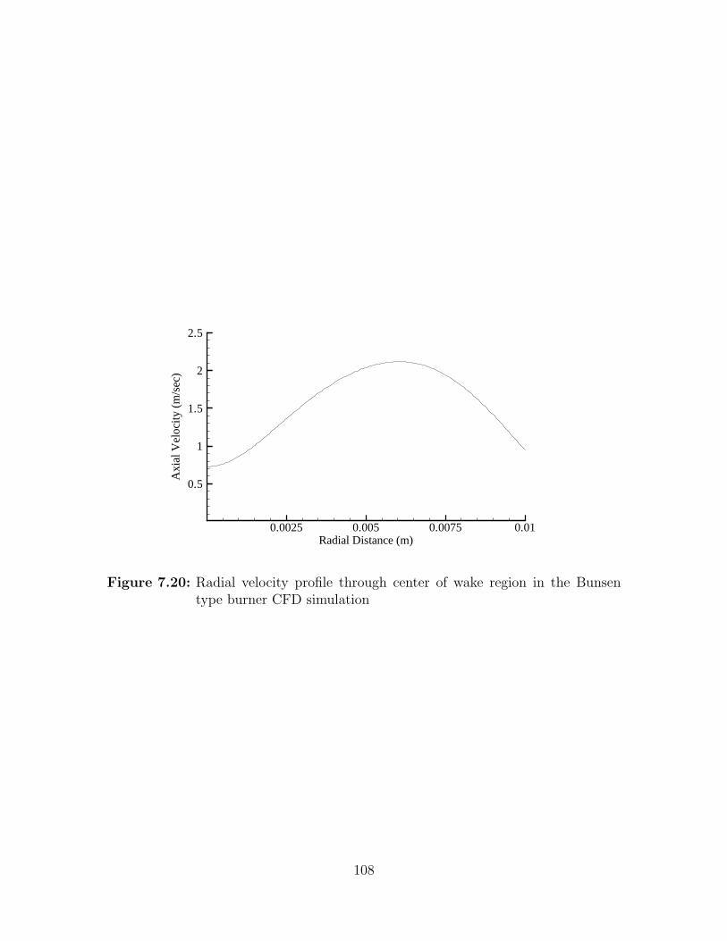
The axial velocity profile in the center of the wake is shown in Figure 7.20. The
minimum velocity in the center of the wake is slightly more than a third of the max-
imum velocity. Furthermore, the minimum velocity of 0.75 m/sec means that the
flow in the center stream tube has slowed by a factor of 5. An interesting conse-
quence of the observed wake–profile is that the flow above the flame–tip is unstable
considering the Rayleigh’s inflection point rule. Although some unsteady calculations
were performed and no unsteadiness was found, the effort was not exhaustive. The
wake–profile above the flame–tip is not the only location where the flow is unstable.
Another area of possible instability is the shear–layer between the air co–flow and
the main premixed–gas stream. The issue of flow stability and its influence on com-
bustion in flames will not be discussed further in this report, however, the issue is
of very high importance in most industrial gas turbine combustors due to the highly
turbulent nature of the flows encountered in those combustor geometries.
107
0.0025 0.005 0.0075 0.01Radial Distance (m)
0.5
1
1.5
2
2.5
Axi
alV
eloc
ity(m
/sec
)
Figure 7.20: Radial velocity profile through center of wake region in the Bunsentype burner CFD simulation
108