continuous hmm connected digit ... - vtechworks
TRANSCRIPT
CONTINUOUS HMM CONNECTED DIGIT RECOGNITION
by
Ananth Padmanabhan
Thesis submitted to the Faculty of the Bradley Department of Electrical Engineering
Virginia Polytechnic Institute and State University
in partial fulfillment of the requirements for the degree of
Master of Science
in
Electrical Engineering
APPROVED
Dr. A. A. (Louis) Beex, Chairman
] i i! Jeffrey H. Reed ¢ Dr. John S. Bay /
September 1996 Blacksburg, Virginia
Keywords: Recognition, HMM, Hidden Markov Model, Continuous HMM, Connected
Digit Recognition
Sess
Vass
\AAG
PAAG
a2
CONTINUOUS HMM CONNECTED DIGIT RECOGNITION
by
Ananth Padmanabhan
Dr. A. A. (Louis) Beex, Chairman
Bradley Department of Electrical Engineering
(ABSTRACT)
In this thesis we develop a system for recognition of strings of connected digits that can
be used in a hands-free telephone system. We present a detailed description of the
elements of the recognition system, such as an endpoint algorithm, the extraction of
feature vectors from the speech samples, and the practical issues involved in training and
recognition, in a Hidden Markov Model (HMM) based speech recognition system.
We use continuous mixture densities to approximate the observation probability density
functions (pdfs) in the HMM. While more complex in implementation, continuous
(observation) HMMs provide superior performance to the discrete (observation) HMMs.
Due to the nature of the application, ours is a speaker dependent recognition system
and we have used a single speaker’s speech to train and test our system. From the
experimental evaluation of the effects of various model sizes on recognition performance,
we observed that the use of HMMs with 7 states and 4 mixture density components yields
average recognition rates better than 99% on the isolated digits. The level-building
algorithm was used with the isolated digit models, which produced a recognition rate of
better than 90% for 2-digit strings. For 3 and 4-digit strings, the performance was 83 and

64% respectively. These string recognition rates are much lower than expected for
concatenation of single digits. This is most likely due to uncertainties in the location of the
concatenated digits, which increases disproportionately with an increase in the number of
digits in the string.

Acknowledgments
If there is any part of me that I am proud of, I owe it all to my parents. This thesis is a
small but important step in my efforts to live up to the standards, of being a good human
being, that they have set. I cannot thank them enough for making me capable of doing
whatever I am doing now.
The very thought of having Vasu, my brother, be my best friend gives me great pride.
Almost every endeavor of mine has included Vasu and, strangely, I feel Vasu has not left
me alone in my work towards my degree. I have spent many hours talking to my sister, Pri
(even when I am alone), and every moment has been intellectually replenishing. If I have
found the motivation to complete this work, it is solely due to the association with such
magnetic personalities as Pri. I also feel great about having Sampath as a close friend
during the course of this work.
I would like to thank Dr. A. A. (Louis) Beex for his guidance and help in completing
this work. Association with him has given me the confidence that being good at Digital
Signal Processing ensures the capacity to solve problems arising within the realms of a
wide range of fields. I hope to, someday, become as impressive as him.
I thank Dr. Jeff Reed from whom I have learnt to derive intellectual satisfaction
through Digital Signal Processing. I thank Dr. Reed and Dr. Bay for their time and effort
in reviewing this work.
Finally, I thank the Center for Innovative Technology, Herndon VA, and Comdial
Corporation, Charlottesville VA, for their support in this research.
iv
Table of Contents
ADSUraCt o.oo ceccccccccccccnececceseeseeeseeeecesseeeesessaeeesesseesecesssecesssseesceesssescesssseeceessseecesesseeeens il
Acknowledgments .00.....0.....0cccccccssecccssseceseeseeseeeceseeeseseeesseessesseeessaeecesseesessueeeestaeseeseeeeas iv Table of Contents 2.0.0.0... cccccccccccccccssseeeeeeececsaeeeccesessaeeeeeesessssceeeeeesseessasseeseseeetsssseeeees V
List Of Figures ....0.0...ccccccccccccccccccesesceceesseeeseesssessesucccusesseesesessseseessseeseseesssseceessnesesesstess vii
List Of Tables. .......0.cccccccccccccsscccesesseeeccesseeecessseeeecssseccessseeecensseeecesaeseseceeseseesstseseeenseess 1x
Vo Tmtroductton ooo... cece cccceeenceceecenssnneeeeeesesseeeeceseseeeescessesseeeeseeseeessaeeeeeesseesaeeeeens 1
2 Background 20.0... ccc cece cece cece cece cece eeeeeeeeeeeeeeeeeeeeeeeceeseceeeeseeseeecceseeesueeeeeess 7
2.1 Approaches to Speech Recognition ..0.0....00.ccccccccccscceeeceeeeeeeeeesesnensssaeeees 7
2.1.1 Acoustical Signal Approach oo... cccecccccccceeeeeeeeeseeeeseeesseseees 7
2.1.2 Speech Production Approach.........0.00..cccccccccccceccsssseeeeseeesssseeeseeeepinaes 9
2.1.3 Sensory Reception Approach ........0...cccceccccesceccseeeeesteeeeenseeeenteeeeaes 12
2.1.4 Speech Perception Approach ..........00..ccccecceccccccssssateeeeeeseeesaseseeeeeesaes 13
2.2 Elements of a Speech Recognition system................c:ccccsccccceeseeenneteceeeeenteeees 15
2.2.1 Pre-PproCeSSOP ....... eee ccccceeeneeeeceeeesceceeceeceeeeeaaeauaeeeeeeeeeceeeeeauneeeeeenees 15
2.2.2 Feature Extraction ...........0ccccccccccccccccceessnseeeeeceeeseeceeesseseteeeeeesesensaes 16
2.2.3 Pattern Matching and Unit Identification ...............0 0 eeeeeeeeeeeeeees 16
2.2.4 Structural Composer ...........0.0c cece ccecenccecceceeessteeeeeseeesseneaeeeeeens 17
3 Feature Extraction o.......0..ccccceccccccccccccssecceecessseneeccesenneeeeeeeesssesseeeceteesnenaeeeeeeeessnsaeees 19
3.1 Endpoint Detection .0.........00..0.ccccccccecceeeeeceeseecesteesseessseeeeseesseeeseeeseseseseeeeeeeees 20
3.2 Feature Amalysis 2.0.0.0... cccccceccccccceeceeeeeeeeeeeeestanaseeeeeeeeeeeeeeeeeeseeennssenanees 22
3.2.1 Cepstral Features ........... ccc ccccccceccscscecseeceeceeeeceeeeseesssssssseeeeerees 24
3.2.2 Delta Cepstral Features .........00000 ccc ceeccceccceceeseesneeeeeeeettesseeeeene 25
4 The Hidden Markov Model .........0...00cccccc cc ccccccccecceteeeeeeeceeesnseeeeeseesesasseeseeesensaeees 27
4.1 Introduction 00.0.0... ccccccccccc cece cceteneceeceeeeeeeeeseeeeeessseesaaeeeeeeeeeesteeeeeenessanees 28
4.2 Discrete and Continuous Hidden Markov Models ......000..0.0......ccceeceeeeeees 33
4.3. The Continuous Hidden Markov Model...0........0.....ccccccceseseecteeceeeeeeeeeeeeeenes 35
A.3.1 ReCOgmition 0.0... ccccccccccecceccceeceeessestsssseseeeeeeeeeeeesesenttssasaeees 36
4.3.1.1 Forward-Backward Method ...0.00.......ccccccccceeeeteeeeeeeeentteeeees 37
4.3.1.2 Viterbi Method... ccccccccceesesnneeeeeeeeentaeteeeeenenteeeeees 4]
A3.2 Training... ccc ccc cece ccccccsccecesaceeeeseeeceeesseeseseseeeeeesseeeeessetens 48
4.3.2.1 Baum-Welch Reestimation .........0....cccccccccecceeseesceeesneeeeeeeees 49
Table of Contents V
4.3.3 Viterbi Reestimation ..........0...0...cccccccccccccccccccccccucceucccusecucceuscesceuseseaes 55
4.4 Implementation ....0..... ccc cece cecensensceeeeeeeeeeeeeeeeesssssseeeeeeeeeeeeeeeseeeenas 58
4.4.1 Structure of the HMM ...0........ occ ccc ccecceeeeeeseststeessessseeeeeeeeeenns 59
A AQ Tratming nn... ccc cccccceccceccecccssseccecceeseeeeeeeeesesseseeesecesseettaneeeesens 60
4.4.3 ReCORMIION 000... cceccceceeesnnneceeeesesteeeeeeeeeeensseeeesecceesstieeeeeseenegs 63
5 Testing of the Recognition System ..........0...ccccccccccccccscceeceeeeeceeesseeeceeeseseeeeeseeesensas 65
5.1 Results on Known Models.................cccccccccccccccccceseesesseeceeeeseeeeceeeeesssstenseaaaees 65
5.2 Results on Words 2000... ccccccccecccceecessceeeessaeeecensceseesesseeeeeessaeescesaseeeseneaeeees 75
6 Connected Digit Recognition .......... ccc ccc cc cece cece ccceceeceecceeeeeeeseeeeeseeeeseeneeenss 83
6.1 Introduction 0... ccceccccccc ccc eecceeeeessceeeeeeeeeeeeceeseeesssssseeaaueeeeeeeeeseeeeeenags 83
6.2 Recognition of a String using the LB Algorithm «0.0.0.0... cece 84
6.3 Results of Recognition of Strings... ccecccecccecccecceeeeseeeeeseeseettsaaeess 91
7 Conclusions and Further Research .................ccccccccccccccesceeeseesssseeseeeeeeeeeeeeseeseesssaaaes 95
B Appendix An icc ccecceecceccescneeeeeesenneneeeeseesnneeeeeessesneeeeeeeseeniaaeeeeserseinneeeesenens 98
Q Appendix Bou... ccccccceeccc cece ee eeeeeeeessseaeeeeeeeeeeceeetesssseseseeeseeeeeeeeceeseseenneeaaaes 104
10 Bibliography 2.0.0.0 cccccccccssseeeececeeaeececeecesssseeecesesssaeeeeseeseestssseeeesesenssaaees 116
DD Vita ccc cece eee eeenn nee e eee net te ee Ee eEEE LE EEEE ENOL EEGEEE;E SELIG GEESE Eee EA AGE EESEEeE Enea aGEEES 119
Table of Contents Vi
Figure 1.
Figure 2.
Figure 3.
Figure 4.
Figure 5.
Figure 6.
Figure 7.
Figure 8.
Figure 9.
Figure 10.
Figure 11.
Figure 12.
Figure 13.
Figure 14.
Figure 15.
Figure 16.
Figure 17.
Figure 18.
Figure 19.
Figure 20.
Figure 21.
List of Figures
List of Figures
Block Diagram of Acoustical Signal Approach to Speech Recognition.............. 8
Discrete Time Speech Model. ..0.............cccccccccccscccesssscecessssseeesensseeseestseeeenseees 11
Model of Speech Perception. ........00.0000cccccceccsescccsceceecceceseeeseeeetenssssseeeeesenens 14
A typical Speech Recognition System. ...0...........cccceecceseesceeceeceeseeeceeseeseeeeneeneesens 15
Feature Extractor. .............cccccccccccccccceeeeneeeeneneeeeeeeeeeeeeeeasaaeseeeeeeeseeeesaaaaaesaaeees 19
Plot of the word "TWO" before and after endpoint detection. ....................00... 21
Feature Analysis Unit 000000000 ccccccccccccccccccceseeenssssssseseeeeeeeeeeeeseeesesesseaeeeseess 22
A typical 3-state HMM... ccccccccceccenscccenseceesseeeesteeeeesssescnseeeesseeensaees 30
Grid for the HMM viewed with DP framework................0::c:cccccccceceseeeeeenttseees 43
Block diagram of the training algorithm............0.0.00.00ccccccceeeeeeeteeeeeeeeeneeees 61
Block diagram of the recognition algorithm ....0...00...00.......c0cccccceeeeeeeeeseeeeeeeenns 64
Model distances for successive iterations ...........0...cccccccccccceeeeeteceeeeeenestsestenens 67
Histogram for State 1 (non-overlapping mixture components). ....................... 69
Histogram for State 2 (non-overlapping mixture components). ...................6. 70
Histogram for State 3 (non-overlapping mixture components). ...................6. 71
True and Reestimated Observation PDFs for State 1 (non-overlapping
MIXtUTE COMPONENHS). ......eeeeccceeececeeseeeeeeeeeeceseneeeeeessnseecesseeeeeeeeseeeeerseeteenss 72
True and Reestimated Observation PDFs for State 2 (non-overlapping
MIXCUTE COMPOMENES) ........ eee cc ccececceceeeeteeeeecesateeeeeeseestsaeeseeeeeeaeietseesensaes 73
True and Reestimated Observation PDFs for State 3 (non-overlapping
MIXtUTE COMPONENHS) o.oo. ee eee cence eeneeeeeeeeeceeeeceeeeestaeeeeeneeessneeesnteeentteess 73
Plot of error rate percentages for different number of states with varying
number of mixture densities 00.00.0000. ccecceeneceeeeeeeeseeeeseeeeesesesensseeenseeens 80
Plot of error rate percentages for different number of mixture densities with
varying number Of states... cceccccccecesccececeeeeesssceececsecseeeeeeeseessesaeeeeessenaes 81
Implementation of LB based on HMMs for each isolated word...................00. 85
vii
Figure 22.
Figure 23.
Figure 24.
Figure 25.
Figure 26.
Figure 27.
List of Figures
True and Reestimated Observation PDFs for State 1 (overlapping mixture
components)..... ccssessssvesssessasessssecsstessstesssucssivesssessivessissssessitesssesssessasessssessssees 99
True and Reestimated Observation PDFs for State 2 (overlapping mixture
COMPOMENS) .0..... eee ccceesceceesseseeecesceeeessseecceesseeeesesseueeeceesseeeeeeesteteesteneeeens 100
True and Reestimated Observation PDFs for State 3(overlapping mixture
COMPOMNENtS) 02... ccececescecsesessessessseseesseeseeeseeseesesessesececeeseceseeceeeeeeny 100
Histogram for State 1 (overlapping mixture components) .................00::c00 101
Histogram for State 2 (overlapping mixture components). .............0......000005 102
Histogram for State 3 (overlapping mixture components). ............0.....00::e6 103
Vili
List of Tables
Table 1 Recognition rates for the dummy words................cccccccccssseceeeesseeeeestteeeeens 74
Table 2 Recognition rates for M = 4, S = 7 (training sets). .............cccccceeesessteeeeees 78
Table 3 Recognition rates for M = 4, S = 7 (testing sets). 0.0.0.0... eccecceeeeteteeees 78
Table 4 Error rates in recognition (training Sets)................cc:cccceccccceceeeeeeseenseetteeeees 82
Table 5 Error rates in recognition (testing Sets) 00.0.2... ccccscceseeeeeeesseeeseeeenenaaes 82
Table 6 Recognition rates for 2-digit strings .........00..ccccccecesceeeeeseeeeeeeeeaeeeeestneeeeeens 92
Table 7 Recognition rates for 3-digit Strings ................cccccccceecccceecceeeeesesesnnsstteeeeeees 92
Table 8 Recognition rates for 4-digit strings .................ccccccccccccceeeeeeeeeseeneesssteaeeeetees 93
Table 9-10 Recognition rates for M = 1, S = 5 (testing and training sets). .................. 104
Table 11-12 Recognition rates for M = 2, S = 5 (testing and training sets)................... 105
Table 13-14 Recognition rates for M = 4, S = 5 (testing and training sets)................... 106
Table 15-16 Recognition rates for M = 1, S = 6 (testing and training sets)................... 107
Table 17-18 Recognition rates for M = 2, S = 6 (testing and training sets)................... 108
Table 19-20 Recognition rates for M = 4, S = 6 (testing and training sets)................... 109
Table 21-22 Recognition rates for M = 1, S = 7 (testing and training sets)................... 110
Table 23-24 Recognition rates for M = 2, S = 7 (testing and training sets).................. 111
Table 25-26 Recognition rates for M = 4, S = 7 (testing and training sets)................... 112
Table 27-28 Recognition rates for M = 1, S = X (testing and training sets). ................. 113
Table 29-30 Recognition rates for M = 2, S = X (testing and training sets).................. 114
Table 31-32 Recognition rates for M = 4, S = X (testing and training sets).................. 115
Table 33. Number of states in S =X occ ccc ccennneeeeeeeeesteeeeeeseeeenseeeeeens 115
List of Tables ix

1. Introduction
Speech is the most dominant mode of communication among human beings. It has
been a part of every civilization that has been discovered. Another mode by which
complex information is exchanged is by writing. However, since reading and writing
require literacy, they are less universal than speaking. Lately, with the advent of resources
such as the internet, communication by typing has been on the increase. Typing and
writing, however, suffer from the disadvantage that they are much slower means of
communication than speaking. On the other hand, man-machine communication is
dominated by typing. This is because, although writing and speaking are potentially more
efficient modes of man-machine communication, they require the machine to be able to
recognize handwriting and speech. Research in these areas has not yet reached such a
high level of maturity. Speech, however, offers the advantage of being the fastest and the
most natural form of human communication. Man-machine communication through speech
also promises an environment where the hands and eyes are free; the speaker and listener
can enjoy unconstrained movement and remote access. These have been the main
motivation for research into automatic speech recognition. The ultimate goal of automatic
speech recognition is to build machines that can "hear," "understand," and "act upon"
spoken input. For this, the machine must be capable of extracting information from a
speech wave. The information content in a speech wave can vary between the level of
being just a sound, to the level of being a tone, to the identity of the speaker and to a
Chapter 1 1
meaningful communication between humans. This information is stored in the machine’s
internal model of the speech process. The fundamental problem of modeling speech is that
it is a continuous stream of sounds with no clear boundaries between the words. Yet,
humans perceive speech as a sequence of words. Hence, it is necessary to segment this
continuous stream of sounds into words, subwords and gaps. The large variability in the
acoustic signals corresponding to the same linguistic unit also complicates the modeling
process. Speech recognizers can be classified into varying levels of complexity based on
criteria such as speaker-dependency, nature and size of vocabulary, and continuity of the
speech.
In a speaker-dependent system, the utterances of a single speaker are used to model
the speech process. This process of characterizing speech by models is called “training.”
The purpose of a speaker-dependent system would be to recognize the speech uttered by
the person whose speech was used in the training process. A speaker-independent system
is trained by multiple speakers and is used to recognize the speech uttered by multiple
speakers, some of who could be outside the training population. Due to larger variability
involved, a speaker-independent system is less accurate than a speaker-dependent system.
However, the speaker-dependent system needs to be retrained each time it is to be used
with a new speaker.
Based on the size of the vocabulary involved, speech recognition systems can be
classified as small, medium and large vocabulary systems. Typically, vocabulary sizes of 1-
99, 100-999, and 1000 or more words are called small, medium, and large vocabularies
Chapter 1 2
respectively. The performance and speed of recognition decrease as the vocabulary size
increases. Moreover, the memory requirements and the number of confusable items in the
vocabulary increase as the vocabulary size increases. The larger vocabulary recognition
systems need to employ many complex constraints, such as linguistic constraints, rather
than train, store and search exhaustively for each word. They also use models of subword
units rather than of whole words.
Based on the continuity of the speech involved in the application, speech recognizers
can be isolated-word, connected-word or continuous speech recognizers. In isolated-word
recognition, the speech involved is constrained to be uttered with a sufficiently long pause
(typically 200 msec) between words. With this constraint, techniques such as end-point
detection can successfully locate the boundaries between the words. This simplifies the
task of speech recognition. Continuous speech is much more complex to recognize due to
the absence of any such simplifying constraints. The recognizer must be capable of taking
care of the large variability in the articulation associated with flowing speech. Moreover,
the continuous speech recognizer must deal with unknown temporal boundaries in the
speech. Connected word recognition is a technique to recognize continuous speech. It is
used in small vocabulary, continuous speech applications. This technique characterizes a
sentence as a concatenation of models of individual words.
Let us now briefly look into the history of speech recognition systems. The earliest
speech recognition systems were based upon the fact that the information required for
recognizing speech existed in the acoustic signal. This was because different spoken words
Chapter 1 3
were observed to give rise to different acoustic patterns. Most of the speech recognition
systems employed a wide variety of filter banks to divide the speech signal into frequency
bands. The outputs of the filter banks were then cross-correlated with patterns of spoken
words obtained by a similar treatment of training utterances. These early systems were
improved by adjusting the mean level of the speech signal so that loud speech and quiet
speech have roughly the same intensity. There were also recognition systems that divided
the speech signal into smaller units such as voiced and unvoiced sounds, fricatives and
plosives such that a single phoneme was isolated. The recognition was then performed
based on the combination of the various phonemes present. The early systems, however,
did not perform very accurately. Further research suggested that the simple matching of
the acoustic patterns was not enough to achieve high performance speech recognition. The
same word, spoken by the same person at different times, or by different persons, varied in
duration, intensity, and frequency content. So researchers began to consider the speech
recognition problem as a pattern-recognition problem. Recognizers were built that
attempted to normalize the intensity level, the duration, and the formant frequencies in the
speech before matching with stored patterns. These methods performed better in terms of
accuracy and the number of speakers whose speech was recognized. The idea of pattern-
recognition also motivated researchers to employ artificial neural networks for speech
recognition. However, all the early speech recognition systems were built to recognize
small speech units such as vowels and not words or sentences. Later, the employment of
linguistic constraints enabled development of systems that recognized words and
Chapter 1 4
sentences. Recognition systems involved extraction of prosodic features (or the tonal and
rhythmic aspects of speech) from the speech. This was crucial to the development of
continuous speech recognition systems. The use of lexical, syntactic, semantic and
pragmatic knowledge further improved the performance of continuous speech recognition
systems. More recently, the uses of dynamic programming techniques, such as Dynamic
Time Warping (DTW) and stochastic modeling, such as hidden Markov modeling, have
led to encouraging results in the development of isolated and connected word recognition
systems.
This thesis attempts to develop a connected-digit speech recognition system that can
be used in applications like the hands-free telephone. The various issues investigated in
this thesis include the effects of the model sizes on the recognition performance, the use of
isolated word patterns for connected speech recognition, and other issues regarding the
convergence of the training algorithm, such as the initial estimate and the stopping
conditions. This thesis suggests a method that provides good initial models for the training
procedure. We also discuss a procedure for obtaining good estimates for the stopping
conditions involved in the training process. In the connected digit recognition system that
we have developed in this thesis, we have incorporated the word duration statistics in a
manner that is different but simpler than in many of the existing techniques. The existing
techniques use an empirically scaled word duration likelihood [2]. The choice of the scale
factor is crucial to successful recognition and requires a lot of trials to arrive at a “good”
scale factor. The technique that we have implemented does not involve any such empirical
Chapter 1 5
scale factors and consequently does not require trial and error. The development of this
connected-digit recognition system involves hidden Markov models (HMM) extensively
and dynamic programming strategies to a lesser extent. Before proceeding to the details of
the developed system, the following chapter provides a background on the various
approaches to speech recognition and the elements of a speech recognition system.
Chapter 3 discusses the feature extraction block of the recognition system. In Chapter 4,
we provide the necessary theoretical background about Hidden Markov Models and other
issues such as training and recognition using HMMs. In Chapter 5 we demonstrate the
recognition performance that we obtained when we used our system for isolated digit
recognition. Chapter 6 describes the level-building algorithm that we used to perform
connected digit recognition and discusses the recognition performance on strings of digits.
Chapter 1 6
2. Background
In this chapter we bring out the various approaches to speech recognition and the
elements of a typical speech recognition system.
2.1 Approaches to Speech Recognition
It is fundamental to speech recognition to extract the information from the speech
signal. Hence, it becomes necessary to model the speech signal so that the parameters of
the model characterize the information and discard any redundancy in the speech. The
various approaches to speech recognition differ largely in the philosophy behind modeling
of the information in speech. During speech communication, linguistic messages are
converted into acoustic waveforms and transmitted. These are then received by the
auditory system and converted back to a linguistic message by the speech perception
system. Based on these stages of speech communication, we can identify four viewpoints
of speech recognition. A combination of these four approaches can also be used in the
development of a speech recognition system.
2.1.1 Acoustical Signal Approach
This approach views the speech signal as just another waveform. Therefore, we can
apply various signal analysis techniques such as Fourier analysis, principal component
analysis, and other mathematical methods to identify the input to the recognizer. The
Chapter 2 7
principal focus of this method is the mathematical representation of the input-output
characteristic of the recognizer. Each input is compared with the stored examples or
templates of each class of inputs. The class that is closest to the input (in terms of an
appropriate distance measure) is chosen as the identity of the input. This is the basis of
various statistical modeling and pattern recognition schemes. These methods do not
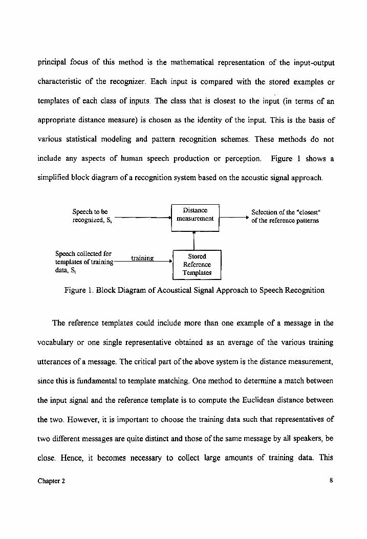
include any aspects of human speech production or perception. Figure 1 shows a
simplified block diagram of a recognition system based on the acoustic signal approach.
Speech to be Distance Selection of the "closest" recognized, S; measurement ” of the reference patterns
Speech collected for trainin Stored templates of training ——T2e —_, Reference data, S, Templates
Figure 1. Block Diagram of Acoustical Signal Approach to Speech Recognition
The reference templates could include more than one example of a message in the
vocabulary or one single representative obtained as an average of the various training
utterances of a message. The critical part of the above system is the distance measurement,
since this is fundamental to template matching. One method to determine a match between
the input signal and the reference template is to compute the Euclidean distance between
the two. However, it is important to choose the training data such that representatives of
two different messages are quite distinct and those of the same message by all speakers, be
close. Hence, it becomes necessary to collect large amounts of training data. This
Chapter 2 8
increases the cost of the system in terms of storage requirements and effort needed to
collect training data. This method treats every part of the speech wave as if it is equally
important. However, we can provide different levels of significance to different aspects of
the waveform. For example, we can provide a higher level of significance to the higher
signal levels because they are less susceptible to noise. Such differential weighting can be
achieved by choosing an appropriate distance measure or by extracting certain features (or
parameters) from the signal and comparing only those features. These features can be
extracted by many of the signal processing techniques used in waveform analysis. Due to
differences in the duration of different messages or various utterances of the same
message, time-warping provides a better method of comparison of the templates. Time
warping can be achieved either by a simple method of time normalization of the templates
before matching or by more complex methods such as Dynamic Time Warping (DTW).
2.1.2 Speech Production Approach
This approach views the information in the speech wave as a characteristic of the
manner in which it was produced by the human vocal system. We now suggest a brief
mechanism by which speech can be produced with the vocal apparatus. To inhale air, the
rib cage expands and the diaphragm is lowered. This draws air into the lungs. Then the rib
cage expands and the diaphragm is raised increasing the air pressure in the lungs. The
increase in pressure forces out air through the wind pipe. In the wind pipe the air passes
through the larynx, which contains the vocal cords. Due to the Bernoulli effect, the air
Chapter 2 9
flow causes a drop in the pressure. This causes the laryngeal muscles to close the glottis,
thereby interrupting the air flow. This interruption increases the air pressure which in turn
forces the vocal cords apart. The cycle then repeats, which produces a train of glottal
pulses. The vocal tract, and the oral and nasal passages pass the harmonics of the glottal
waveform that are close to their natural resonances while attenuating the others. This
acoustic wave radiates from the lips as speech. Some sounds such as the consonants are
produced without involving the glottis. These sounds are produced by constricting the
vocal tract. The constriction causes a turbulence and the air then flows out through the
oral and nasal passages resulting in speech. Thus speech is produced by the excitation of
the vocal tract, and/or the oral and nasal passages. Based on the nature of the excitation,
speech can be broadly classified into voiced and unvoiced speech. The glottal excitation of
the vocal tract produces voiced sounds. Vowels are examples of voiced sounds. Sounds
produced by the constriction of the vocal tract are known as unvoiced sounds, consonants
for example. When humans convey a linguistic message in the form of speech, they
construct a phrase or sentence by selecting a set of sounds from a finite collection of
mutually exclusive sounds. This basic set of sounds consists of the phonemes. However,
due to various factors, such as accents, gender, and coarticulatory effects, a given
phoneme will have a different manifestation under different conditions. These
manifestations of the phonemes of a language are called phones.
Having provided the basics of speech production, we now go into the aspect of
modeling speech from the production point of view. Various models have been proposed
Chapter 2 10
for modeling speech [1]. Of all these models, a popular model for speech is the Discrete
Time Model that is shown in Figure 2.
Gain
Glottal
Pulse Filter
G(z)
Impulse
train at —” pitch period
Vocal Lip Voiced/Unvoiced __{ Tract Filter »| Radiation |-» Speech s(n)
switch THz) Filter R(z)
Random
Noise
Generator
Gain
Figure 2. Discrete Time Speech Model
According to this model, the glottal pulse shaping, the human vocal tract, and the lips
are modeled by the Glottal Pulse Filter G(z), the Vocal Tract Filter H(z), and the Lip
Radiation Filter R(z), respectively. The voiced sounds are produced as a result of
excitation by an impulse train at the pitch period and the unvoiced sounds by random noise
excitation. The random noise excitation is used to model unvoiced speech because it is
produced as a result of noise-like flow of air through a constriction in the vocal tract.
Thus we can model the Z-transform of speech as
S(z) = E,(z)G(z)H(z)R(z) ; for voiced speech with E,(z) representing an impulse train
= E,(z)H(z)R(z) __; for unvoiced speech with E,(z) representing noise
In general, to obtain the above system to model speech, we require an ARMA filter.
However, the presence of very powerful computational techniques for deriving an all-pole
Chapter 2 11
model from speech [3] provides a very good motivation for modeling speech with an all-
pole transfer function. Moreover, we can obtain an all-pole filter that matches the
magnitude spectrum of the speech [3]. For the purposes of coding, recognition, and
synthesis, it has been found that modeling the magnitude spectrum of speech is sufficient.
2.1.3 Sensory Reception Approach
Since the sensory reception of spee is an integral part of human speech
communication, its understanding could provide us with useful clues for developing a
good speech recognizer. The ear is the sensory reception organ in the human body. It can
be divided into three regions; the outer ear, the middle ear and the inner ear [1]. The pinna
in the outer ear receives the speech. It then transmits the speech to the eardrum in the
middle ear through the meatus. The eardrum is attached to a system that transduces the
acoustic vibrations to mechanical vibrations. This transducer system consists of the
malleus, the incus and the stapes that act like a hammer, an anvil, and the stirrup,
respectively. The mechanical vibrations are set up in the inner ear (cochlea). The cochlea
is a coil-like structure containing two channels called the scalae. The scalae are filled with
a liquid called the perilymph. The movement of the stapes sets up a traveling wave in the
perilymph. This then causes the basilar membrane to vibrate. The basilar membrane is
about 35 mm long and tapers along its length. Due to this taper, the basilar membrane
exhibits a resonance property that varies along its length. We can think of the basilar
membrane as a broad band-pass filter with the successive points on the membrane having
Chapter 2 12
an approximately constant Q characteristic. The width of the filter is inversely proportional
to its resonance frequency. The basilar membrane is attached to the organ of corti. This
contains the hair cells which transduce the mechanical vibrations to neural impulses. The
ear thus performs acoustic to neural transduction and broad-band frequency analysis.
Based on the functions of the ear in speech reception, we can arrive at the auditory
representations of speech [1, 4]. However, the method by which the human speech
reception system extracts parameters and classifies patterns is quite complex and difficult
to duplicate. Hence, the sensory reception approach has not had a great impact on the
development or improvement of speech recognition systems.
2.1.4 Speech Perception Approach
It has been experimentally found that certain features in speech, such as the voice
onset times, formant transitions, etc., are important to the perception of speech by human
beings. The speech perception approach suggests that a recognition system could
duplicate the human perception system in extracting the above features. To achieve this,
we have to make some sort of a perceptual categorization of the contents of speech.
Experiments with perception of speech have suggested that the speech signal can be
broken down into a finite number of discrete message elements [5]. It has been found that
human beings are very sensitive to differences in the frequency or intensity of the different
sounds provided to them. However, a listener has been found to have difficulties in
identifying a single tone in isolation. Hence we can conclude that human beings exhibit
Chapter 2 13
different information capacity for differential and absolute discrimination. Experiments
with speech perception [5] indicate certain cues to identify certain features of speech such
as consonant voicing, vowel identity, etc. Some of these cues are the voice onset time,
formant transitions and single equivalent formants. The ability of a listener to identify a
sound is affected by the time he or she is allowed to "learn" the sound and other linguistic
constraints. The linguistic constraints help in reducing the set of sounds, from which the
choice has to be made, for recognition. Although the human perception system has not
been understood and modeled completely, one view of modeling considers the problem to
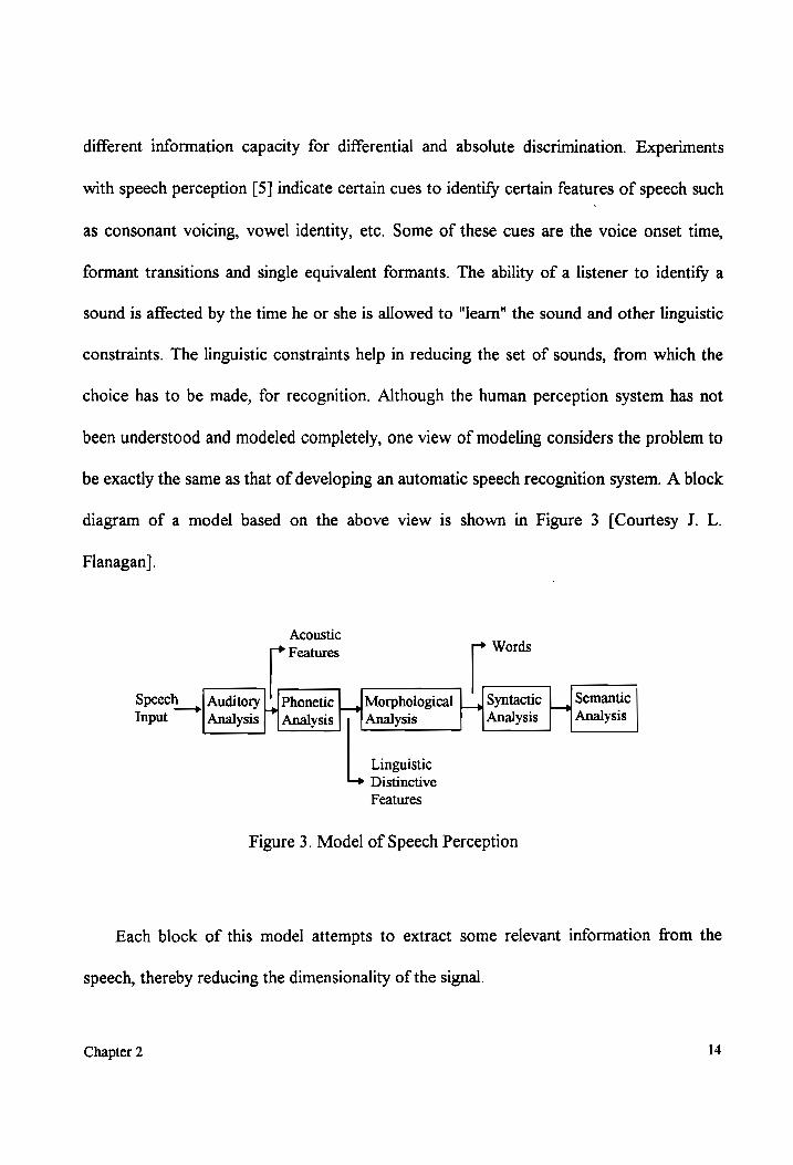
be exactly the same as that of developing an automatic speech recognition system. A block
diagram of a model based on the above view is shown in Figure 3 [Courtesy J. L.
Flanagan].
Speech Input
Auditory Analysis
Acoustic ; Features Words
Phonetic |_,|Morphological |_, Syntactic Semantic
Analysis Analysis Analysis Analysis
Linguistic Distinctive
Features
Figure 3. Model of Speech Perception
Each block of this model attempts to extract some relevant information from the
speech, thereby reducing the dimensionality of the signal.
Chapter 2 14
Having looked at the four philosophies of speech recognition, we now briefly describe
the elements of a typical speech recognition system.
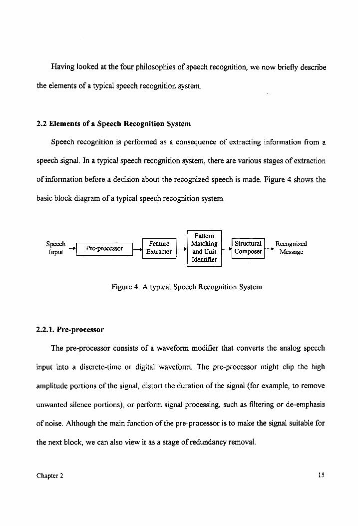
2.2 Elements of a Speech Recognition System
Speech recognition is performed as a consequence of extracting information from a
speech signal. In a typical speech recognition system, there are various stages of extraction
of information before a decision about the recognized speech is made. Figure 4 shows the
basic block diagram of a typical speech recognition system.
Pattern
Speech Feature Matching Structural Recognized Input Pre-processor Extractor and Unit Composer Message
Identifier Figure 4. A typical Speech Recognition System
2.2.1. Pre-processor
The pre-processor consists of a waveform modifier that converts the analog speech
input into a discrete-time or digital waveform. The pre-processor might clip the high
amplitude portions of the signal, distort the duration of the signal (for example, to remove
unwanted silence portions), or perform signal processing, such as filtering or de-emphasis
of noise. Although the main function of the pre-processor is to make the signal suitable for
the next block, we can also view it as a stage of redundancy removal.
Chapter 2 15
2.2.2 Feature Extraction
This block extracts certain specific aspects of the speech wave that facilitate
recognition. This extraction might result in a parametric representation of the speech
wave. The parameters that are popular in speech recognition systems are the energies in
frequency bands, the linear prediction coefficients (LPC), the cepstral coefficients, etc. To
obtain some of these features, the feature extractor splits the speech segment into various
frames by windowing. The features may also include information such as the fundamental
frequency of the voice, or the number of zero crossings, or the voicing characteristic of
the frame of speech. The feature extraction block also achieves data compression,
resulting in reduced memory requirements. The feature extractor is sometimes called the
parameter extractor.
2.2.3. Pattern Matching and Unit Identification
The pattern matching block attempts to identify certain linguistic units present in the
speech to be recognized. Typically, the pattern matching block has some models of the
speech units it is designed to identify. These speech units could be single words or smaller
units like phonemes or syllables. These models could be simple templates of features of the
speech units in the vocabulary or stochastic models such as the Hidden Markov Models
(HMM). These models present in the pattern matching block are constructed as a result of
a "training" procedure so that they represent the various patterns associated with the
vocabulary in context. When the features are presented, the pattern matching system
determines the extent to which each of the models represents the features. For example, in
Chapter 2 16
the case of template matching, the test features are compared with the stored reference
features using techniques like DTW. If HMM is used, the likelihood of generating the
given features, by each of the models, is computed. The unit identifier chooses the model
that produces the best match. Before making a decision about the recognized output, the
unit identifier could use some linguistic constraints or analyze for some of the perceptual
aspects of speech.
2.2.4. Structural Composer
Finally, the structural composer assembles the identified speech units into larger units
that correspond to a complete message. The structural composer combines the smaller
speech units with the help of a set of rules. These rules could be a set of syntactic,
semantic, and/or pragmatic constraints. A structural composer could either combine words
to form phrases and sentences, or work with words as the subunits. Finally, the message in
the speech waveform is output.
We have provided a brief overview of the various approaches to speech recognition
and the basic building blocks of a speech recognition system. Next we describe in detail
the various elements of the connected-digit recognition system developed in this thesis
towards the specific application of hands-free dialing of a telephone. We also present the
procedures, and other design issues, involved in the training and recognition parts of the
system. The following chapter provides a description of the feature extraction system. In
many speech recognition systems, the pre-processor is also assumed to be a part of the
Chapter 2 17

feature extractor. We make this assumption and discuss the details regarding pre-
processing and feature extraction in the following chapter.
Chapter 2 18
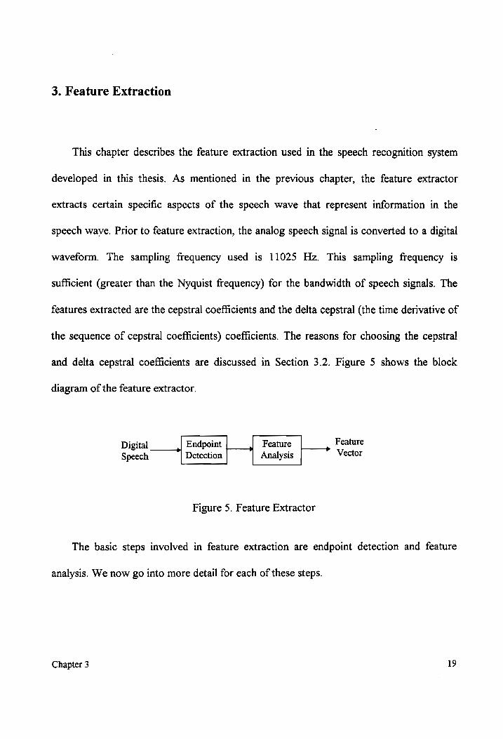
3. Feature Extraction
This chapter describes the feature extraction used in the speech recognition system
developed in this thesis. As mentioned in the previous chapter, the feature extractor
extracts certain specific aspects of the speech wave that represent information in the
speech wave. Prior to feature extraction, the analog speech signal is converted to a digital
waveform. The sampling frequency used is 11025 Hz. This sampling frequency is
sufficient (greater than the Nyquist frequency) for the bandwidth of speech signals. The
features extracted are the cepstral coefficients and the delta cepstral (the time derivative of
the sequence of cepstral coefficients) coefficients. The reasons for choosing the cepstral
and delta cepstral coefficients are discussed in Section 3.2. Figure 5 shows the block
diagram of the feature extractor.
Digital___,} Endpoint Speech Detection
Figure 5. Feature Extractor
Feature
Analysis
Feature
Vector
The basic steps involved in feature extraction are endpoint detection and feature
analysis. We now go into more detail for each of these steps.
Chapter 3 19
3.1 Endpoint Detection
The endpoint detection unit detects the boundaries of the spoken word. It is
important to detect the boundary of the spoken word so that we can cut the unwanted
portions out of the speech signal we have recorded. This removes the redundancies (such
as silence portions or background noise) so that they do not affect the recognition
performance of the entire system. Another advantage of endpoint detection is that it
reduces the amount of subsequent processing. A simple algorithm is used to achieve end-
point detection [6]. The algorithm is based on two measures: short-time energy and zero-
crossing rate. The recorded string of digits is first split into m frames of 10 msec each. We
then compute the energy in each frame by
n 2
E(m) = > [Sn(K)] , 1sms<N (3.1) k=l
where 7 is the number of samples in a frame and N is the number of frames. We keep track
of the frame where the energy exceeds a particular threshold (four times the minimum
frame energy for this word [6]) and the frame where it falls below the same threshold and
remains below it for more than 150 ms [6]. For the words we consider, a gap of more than
150 ms does not occur within the word and hence 150 ms is a reasonably good estimate of
the duration of the silent portions at the end of the word. For each frame, we also
compute the number of zero-crossings of the speech signal. As with the frame energies,
Chapter 3 20
we obtain an estimate of the boundaries of the word from the number of zero-crossings.
At this point we have two starting points and two final points. As an estimate of the
endpoints of the words, we choose the starting point and the final point which yield the
shortest duration for the word. The use of both criteria (frame energy and number of zero-
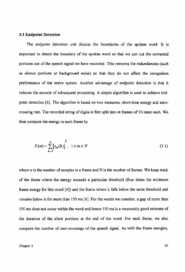
crossings) improves the accuracy of detection [6]. Figure 6 shows the waveforms before
and after the endpoint detection for the word "two" using both of the criteria mentioned
above.
“T¥¥O" before end-point detection"
0 9000 10000 15000
“2 500 1000 1500 2000 2500 3000 3500
xo
Samples
Figure 6. Plot of the word "TWO" before and after end-point detection.
Chapter 3 21
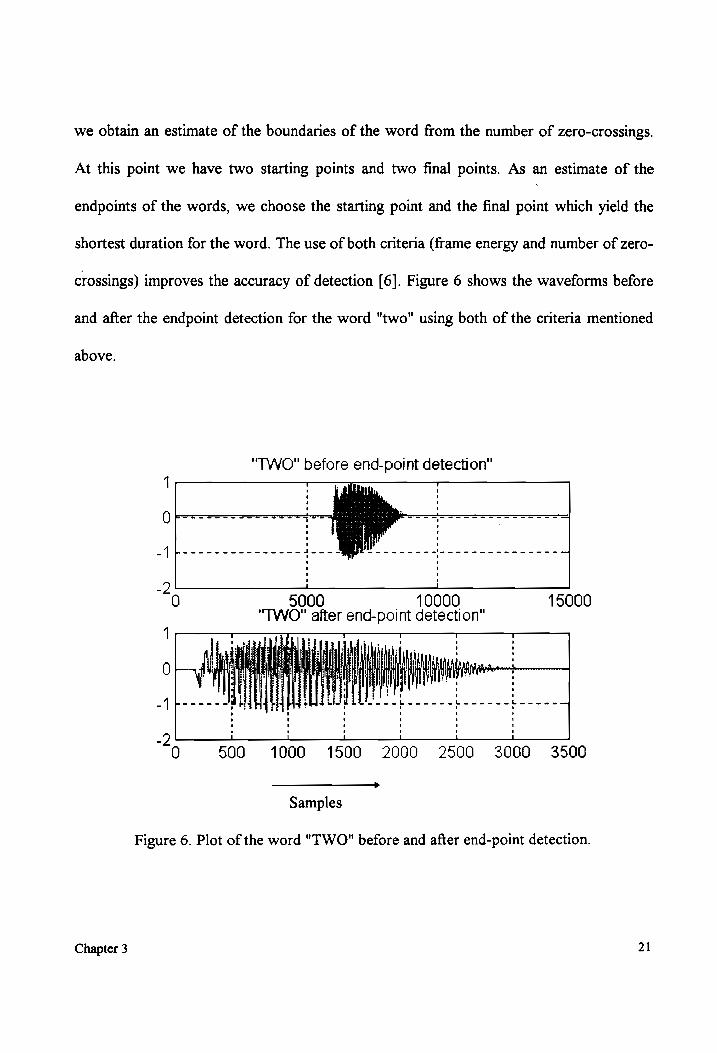
3.2 Feature Analysis
This is the next step of extracting the relevant (for understanding) information in the
speech waveform. As discussed in the previous chapter, one of the approaches to speech
recognition is based on modeling the speech waveform from the speech production point
of view. The all-pole model or the autoregressive (AR) model can be shown to be an
appropriate model for speech recognition purposes [3]. The AR modeling of speech
results in a set of parameters representing the magnitude spectral dynamics in the speech
waveform. Figure 7 shows the block diagram of the feature analysis unit.
Calculation of Cepstral
Speech_, !preemphasis Windowing -}—> Anaicig —>| and Delta Vector Input y Cepstral Coefficients
Figure 7. Feature Analysis Unit
First, we perform preemphasis of the speech by passing it through a high pass filter of
the form l-az", where a = 0.95. Most of the information in speech, for recognition
purposes, lies in the vocal tract characteristics. Since the speech signal contains the glottal
pulse characteristics too, we require preemphasis to cancel one of the poles of the glottal
pulse so that AR modeling of the speech can model the vocal tract characteristics better.
Another way to look at preemphasis is that it emphasizes the higher frequency portions of
Chapter 3 22
the speech spectrum so that the higher frequency formants become more significant than
before.
Parameterization of signals frequently calls for the signal to be stationary. However,
speech is a non-stationary signal. Hence, before we parameterize, we split the speech
signal into frames wherein the speech is considered to be quasi-stationary. We use
windowing to split the speech into frames. Associated with windowing, we come across
two issues: the length of the window and the type of window [3]. A longer window tends
to produce a better spectral picture of the signal while inside the stationary region,
whereas a shorter window provides better resolution in time. However, improvements in
spectral and time resolution are in conflict with each other. Past research suggests that a
window length of 45 msec is appropriate for speech signals [24]. For a given window
length, we again have two competing factors in the choice of the window. We need to
avoid any distortion in the selected points. Also, a window with abrupt transitions at the
boundary has significantly high sidelobes in its spectrum and, when convolved with the
signal in the frequency domain, brings a lot of undesirable spectral energy into the
resulting spectrum. Hence, we need to choose a window that has smoother discontinuities
at the boundaries. As found appropriate by past research [7], we use a Hamming window
with 66% overlap.
After windowing, we obtain the tenth order AR model for the speech frames by using
the Levinson-Durbin Algorithm for Linear Predictive Coding (LPC) of speech [8]. It has
been found that the model order of ten is appropriate for speech [3]. The LPC analysis
Chapter 3 23
obtains the AR model of speech in the process of determining a filter that predicts a future
sample of speech from its past samples. In this process of prediction, it achieves data
compression or removal of redundancies or extraction of the relevant information.
3.2.1 Cepstral Features
The set of cepstral features or coefficients is the complex cepstrum of the LP model
of speech. It has been found that the use of a cepstral technique instead of the LPC
coefficients improved speech recognition performance [9, 10]. This is because the cepstral
coefficients derived from the LPC coefficients can be manipulated (for example, weighted)
so that the feature vector is less affected by the glottal dynamics than the LPC coefficients
[3]. Another motivation for using the cepstral parameters is that we can use the Euclidean
metric between two cepstral parameter sets as a reasonably good measure of the spectral
similarity of the corresponding models [3].
We use the following recursions [10] to compute the cepstral coefficients c(/) from
the LPC coefficients a(z).
c(1) = -a(1), (3.2)
c(i) = -a(i) - x (1 _ "lackyet —k),1<i<p (3.3) k=1~ =!
Chapter 3 24
The variable p is the order of the AR model. The number of cepstral coefficients has to be
greater than the number of LPC coefficients. We have obtained 12 cepstral coefficients.
The cepstral coefficients are then weighted by a function given by,
OQ .{™ w,(m) = 1+ "> sin 0. , l<m<sQ (3.4)
where Q is equal to the number of cepstral coefficients used in (3.3). It has been found
that weighting reduces the effect of the glottal pulse characteristics on speech modeling
and thus improves the performance of speech recognition [25].
3.2.2. Delta Cepstral Features
In order to include information about the spectral changes that have occurred since
the previous frame, we compute another set of features called the delta cepstral features.
The delta cepstral coefficients are the derivative of the cepstral coefficients. We compute
the delta cepstral coefficients by considering a window of several frames and calculating
the difference in the cepstral coefficients from one frame to another within the window.
The delta cepstral coefficients are computed using
L
Ac,(m) = >, key_;,(m) G, l<m<Q (3.5)
k=-L
Chapter 3 25
where (2£+1) is the length of the window. We have chosen L=2. G is a gain chosen such
that the variances of the delta cepstral coefficients and the cepstral coefficients are
approximately equal. We include the gain to ensure that one set of parameters does not
dominate over the other when using the Euclidean metric on the final feature vector
formed by appending the set of delta cepstral coefficients to the set of cepstral
coefficients. This feature vector is such that it has fewer redundancies than the speech
waveform we started with.
We next present the Hidden Markov Model (HMM) and other issues, such as the
training and the recognition algorithm used. We have used the HMM as the model for
each word for the purposes of pattern matching and unit identification.
Chapter 3 26
4, The Hidden Markov Model
As mentioned earlier, one of the elements of a speech recognition system is the
pattern matching block which identifies the presence of certain linguistic units present in
the speech. Fundamental to speech pattern matching is representing the patterns in speech
as models. Knowledge of the structure of speech together with many reference tokens
(multiple utterances of the same speech) of the speech are used to obtain appropriate
models. We can then compare unknown patterns of speech against these models to
determine how well the available models match them. The models have to be generated
from the reference data such that they accommodate the inherent variability of speech and
are able to recognize speech patterns that have not been observed previously. The
simplest model is a set of templates formed by storing the parameterized form (cepstral
coefficients) of an utterance of each word in the vocabulary. One or more templates can
be used to model each word in the vocabulary. Unknown utterances can be matched
against these templates through techniques such as dynamic time warping (DTW) [11].
DTW is a good scheme to compare tokens (utterances of the same speech) of different
durations. However, DTW uses the speech data in a deterministic way. Although it has
been used in many practical systems, DTW requires a large number of templates to
account for the large variability associated with speech. This increases the computational
cost of searching to inconvenient proportions. If templates of subword units are used, the
number of templates used can be decreased. However, in the presence of coarticulatory
Chapter 4 27
effects, as encountered in connected-speech recognition, standardization of the subword
units becomes difficult. Intuitively, a stochastic model can accommodate acoustic
variability in a better way than simple template based approaches. Research in stochastic
modeling of speech patterns has proceeded in two directions: the Hidden Markov Models
and the Artificial Neural Networks (ANN). Hidden Markov Models were first studied by
statisticians and were applied to characterize stochastic processes for which incomplete
observations were available. In the mid 70s, researchers looked into applying the HMM to
model speech for recognition purposes [12, 13]. Although the HMM was adapted to the
speech recognition problem rather slowly (3 decades), it has had a great impact on the
speech recognition schemes that have been incorporated into practical systems. In
contrast, the application of ANN techniques has had lesser impact on speech recognition
because research in this direction is very young. The fundamental aim of ANN techniques
is to explore computing architectures that resemble the massively parallel computing found
in biological neural systems. The following section introduces the HMM and provides the
various notations used in this thesis.
4.1. Introduction
As mentioned above the HMM is applied to characterize random processes for which
incomplete observations are available. The HMM is a means to model the problem as an
observable stochastic process produced as a result of an underlying unobservable (hidden)
stochastic process. In this sense, the HMM is a doubly embedded stochastic process. The
Chapter 4 28
HMM is used to model speech utterances as a stochastic finite state automaton which
generates the speech utterances as a result of generating a "hidden" state sequence which
can be observed through an observation sequence. Typically, in small vocabulary systems
the HMM models a whole word and in large vocabulary systems, the HMM models a
subword unit. Since the connected digit recognition system developed in this thesis is a
small vocabulary system, we have used the HMMs to model whole words.
We recall that HMM is used in the pattern matching unit and the speech utterance at
this point is a string of feature vectors (in our case, the feature vector is formed by the
cepstral features concatenated with the delta cepstral features). In this chapter, we will
treat the string of feature vectors as an observation sequence. We denote an observation
sequence as follows:
yi), y(2), vB), . , W(t), ..... , X(T).
where y(.) is a feature vector, ¢ is the frame index, and 7 is the total number of
observations in the sequence.
An HMM is always associated with an observation sequence which it is more likely to
generate than any other HMM. The likelihood that a given HMM generates a given
observation sequence is a quantitative measure of how well the observation sequence
"matches" the HMM. In the pattern matching block of the speech recognition system, we
have the HMMs representing each word in the vocabulary. Given a word (or a string of
feature vectors) to recognize, we compute the likelihood that each of the HMMs available
would have generated the string. We find the recognized word as the one whose HMM
Chapter 4 29
produces the maximum likelihood. Usually, the highest likelihood is significantly (>107)
larger than the next highest likelihood. Since the highest likelihood “stands out”
prominently, we can expect the correct model to yield the highest likelihood, even if the
speech to be recognized were a little noisy. The HMM corresponding to each word in the
vocabulary is formed by a process of "training," by which many utterances of a word are
used to obtain the statistical makeup of the observations associated with that word.
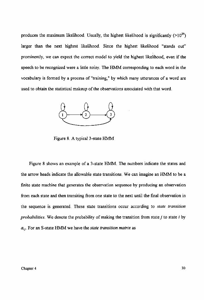
Figure 8. A typical 3-state HMM
Figure 8 shows an example of a 3-state HMM. The numbers indicate the states and
the arrow heads indicate the allowable state transitions. We can imagine an HMM to be a
finite state machine that generates the observation sequence by producing an observation
from each state and then transiting from one state to the next until the final observation in
the sequence is generated. These state transitions occur according to state transition
probabilities. We denote the probability of making the transition from state j to state 7 by
aj;. For an S-state HMM we have the state transition matrix as
Chapter 4 30
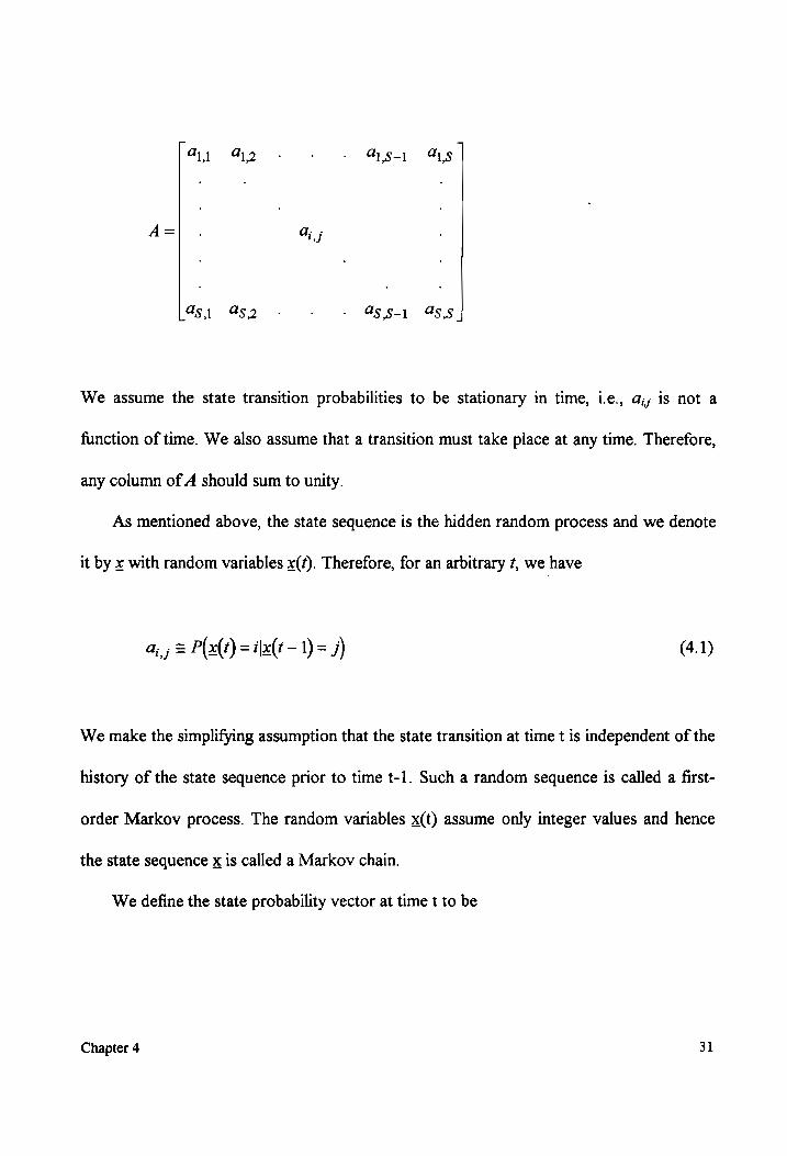
a1 a2 . . . a S-1 as
| as 4 a5 2 . . as S-1 as 8 |
We assume the state transition probabilities to be stationary in time, i.e., aj; is not a
function of time. We also assume that a transition must take place at any time. Therefore,
any column of A should sum to unity.
As mentioned above, the state sequence is the hidden random process and we denote
it by x with random variables x(f). Therefore, for an arbitrary 4, we have
a; ; = P(x(2) = i|x(¢ - 1) = j) (4.1)
We make the simplifying assumption that the state transition at time t is independent of the
history of the state sequence prior to time t-1. Such a random sequence is called a first-
order Markov process. The random variables x(t) assume only integer values and hence
the state sequence x is called a Markov chain.
We define the state probability vector at time t to be
Chapter 4 31
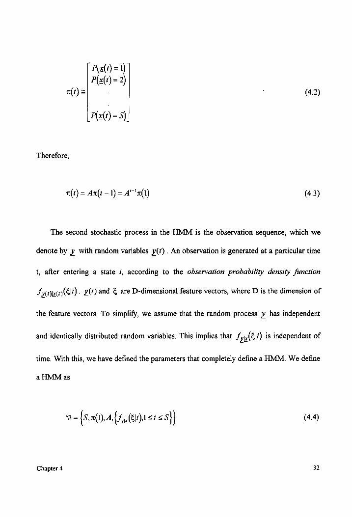
| (x(t) =1) | P{x(*) = 2)
n(t) = (4.2)
P (x(7 )= ).
Therefore,
n(t) = An(t —1) = A*'x(1) (4.3)
The second stochastic process in the HMM is the observation sequence, which we
denote by y with random variables y(t). An observation is generated at a particular time
t, after entering a state i, according to the observation probability density function
Sy pixce)(Elé) . y() and € are D-dimensional feature vectors, where D is the dimension of
the feature vectors. To simplify, we assume that the random process y has independent
and identically distributed random variables. This implies that Fyre(El) is independent of
time. With this, we have defined the parameters that completely define a HMM. We define
a HMM as
m={S,n(1),A,{ fe(Elisi ssl} (4.4)
Chapter 4 32
We can realize two issues regarding the use of HMM for speech recognition. Firstly,
we have to obtain the parameters of the HMM from a series of training observations. This
is the problem of training the HMM to model a given word. Secondly, we have to
compute the likelihood that a particular HMM produced the given speech observation
sequence. This is the problem of recognition.
4.2 Discrete and Continuous Hidden Markov Models
Depending upon the form of the observation pdf's, we have two types of HMMs that
can be used for speech recognition: discrete (observation) HMM and continuous
(observation) HMM. The discrete observation HMM uses a discrete pdf for the
observation pdf. This means that only a finite set of observations is allowed. After the
feature extraction stage, the feature vectors have to be vector quantized to one of the
permissible set of (say K) observation vectors. Since only K vectors are allowed, it is
possible to assign to every observation vector a scalar and, consequently, the random
process y becomes a scalar random variable with scalar random variables y(t) which can
take only integer values in [1, K]. The observation pdf, being a discrete pdf, is completely
specified by the set of weights on the impulses forming the pdf or, in other words, the
probabilities of the K possible observations. The observation probability is given by
b(kli) = P(y(4) = klx(4) =?) (4.5)
Chapter 4 33
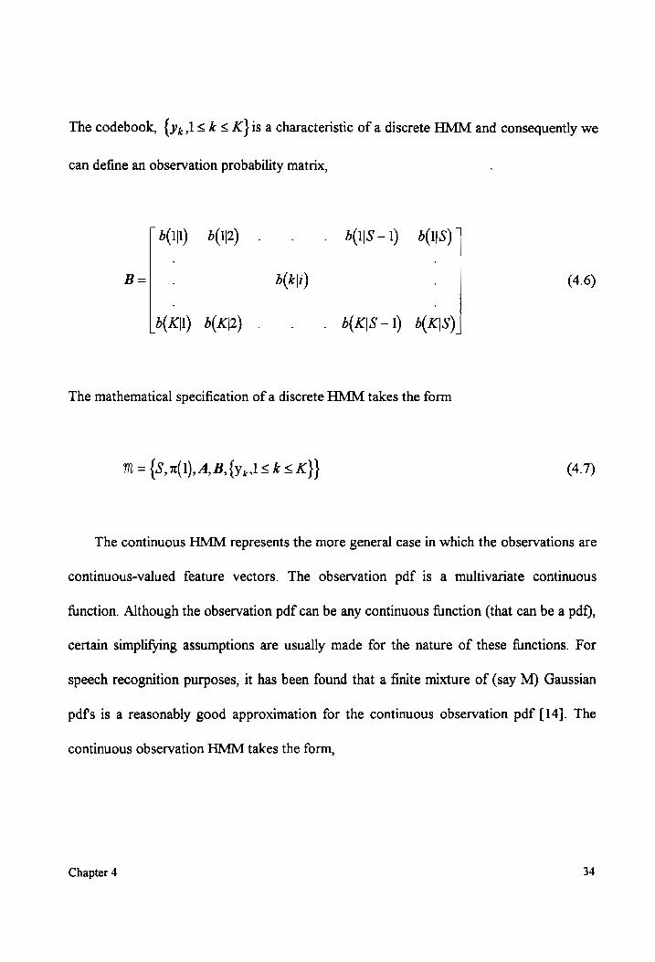
The codebook, { yylsks K} is a characteristic of a discrete HMM and consequently we
can define an observation probability matrix,
bil) B(j2) . eS -1) BAIS)
B= | b(k\i) | (4.6)
b(K|l) b(K(2) . . , B(K |S — 1) b(K|S)
The mathematical specification of a discrete HMM takes the form
m = {S,n(1), A,B, {y,,1<k < K}} | (4.7)
The continuous HMM represents the more general case in which the observations are
continuous-valued feature vectors. The observation pdf is a multivariate continuous
function. Although the observation pdf can be any continuous function (that can be a pdf),
certain simplifying assumptions are usually made for the nature of these functions. For
speech recognition purposes, it has been found that a finite mixture of (say M) Gaussian
pdf's is a reasonably good approximation for the continuous observation pdf [14]. The
continuous observation HMM takes the form,
Chapter 4 34
m= {s, n(1), A, { Fyx(Eli),1 <i < s} (4.8)
The following section provides details of the continuous HMM used in this thesis with
respect to issues such as training and recognition.
4.3 The Continuous Hidden Markov Model
In this thesis, the continuous HMM is used with the observation pdf approximated by
a mixture (sum) of M multivariate Gaussian functions. The observation pdf is of the form
Fye(Elé) = Ye mE ims Cim (4.9)
where Cim iS the coefficient for the mth component of the mixture for state 7, N(.) is a
multivariate Gaussian pdf with mean sj», and covariance matrix Cj, The mixture
coefficients are non-negative and satisfy the constraint
Sm = 1, 1<i<S (4.10)
For simplicity of notation we define a likelihood function
Chapter 4 35
b(Eli) = Fy (El) (4.11)
Having provided the necessary introduction to HMM, we now present the details
regarding the training of the HMM and recognition using the HMM. Of these two
problems, the recognition problem is easier and the concepts therein serve as a convenient
background to understanding the training problem. Hence, we deal with the recognition
problem first.
4.3.1. Recognition
Given an observation sequence, the recognition problem deals with computing the
likelihood that the models available (as a result of training) produce that observation
sequence. We define some notation that will help in understanding and establishing the
concepts of recognition.
We denote a partial sequence of observations in time as
Ve = {y(4),9(4 + 1), v(t, + 2),.... ¥(t)} (4.12)
The particular sequence of observations
¥{ = {y(1),9(2),.... 91D} (4.13)
is called the forward partial sequence of observations at time t and
Chapter 4 36
yee {y(¢ +1), y(t + 2),..-,(T)} (4.14)
is called the backward partial sequence of observations at time t. The complete sequence
of observations is
yt ={y(1),9(2),--.9(Z)} (4.15)
and, for the sake of simplicity of notation, we define
y=yp (4.16)
We proceed to discuss the computation of the likelihood that a given model produces a
given observation sequence.
4.3.1.1 Forward-Backward Method
The Forward-Backward (F-B) method to compute the likelihood is also called the
"any path" method because it computes the likelihood that the observations could have
been produced using any state sequence through the given model. Let us consider a
particular state sequence of length T to be J = {i, bh, . . ., ir}. The likelihood of the
observation sequence being produced from this state sequence is
Chapter 4 37
L(y|3,M) = b(y(1)\A,).5(9(2)Ii2)..---2(v(D iz) (4.17)
Since we use the functional values of the pdf, the left hand side of (4.17) is a likelihood.
The likelihood of the state sequence is
£(3|M) = n(i Jain, i la(i;,2y).....a(i7,ip_)) (4.18)
Therefore,
L(y, 3M) = b(y(Dli, )O((2)lé)....-(v(Dlir) oe yn , (4.19)
xX (i )a(is, i, a(iz,1,).....a(iz,i7_))
The sum of the above likelihood over all possible sequences provides the likelihood of the
given model producing the observation sequence through any state sequence as
£(y|m) = >> 2(y,3|M) (4.20) all 3
Equation (4.20) gives a "brute force" method to compute (y|M). It has been found
that this approach requires a prohibitively high amount of computation [3]. The forward-
backward algorithm developed by Baum computes the above likelihood in an efficient
recursive manner. The forward-backward algorithm uses a "forward-going" and a
"backward-going" likelihood. We define these likelihoods as
Chapter 4 38
o( y{.i) = 2(yt = vf.x() = am) | (4.21)
B(vfvilé) = 2(¥7,, = yalx(s) = i,m) (4.22)
respectively. In equations (4.21) and (4.22), y? denotes a partial sequence of random
variables. Since the observation sequence could have reached state i at time ¢ from any of
the S possible states at time ¢-/, we have
S
a(yt.i)= a(y{, jay, (x!) (4.23) J=1
Clearly, (4.23) provides a recursive algorithm for computing the a's with the algorithm
initiated by
a(x. i) = n()B(y(1)LJ) i<j<S (4.24)
Similarly, the backward recursion can be defined as
B(yzal) = 5 8(yZal/}a,,0(9( +1)/) (4.25) j=l
Chapter 4 39
with the recursion initiated by the fictitious partial sequence Vous used in
1, ifiisalegal final state T |: = 4.26
B(yrsa) i. otherwise ( )
where a legal final state is one at which a path through the model may end.
With the definitions of a and B we have, for a particular state i,
Ay, x(t) =11m) = of yf 7)B( v7) (4.27)
Therefore,
- T (ym) = Yo »f,7)B( yal) (4.28) i=]
The likelihood in (4.28) can be computed at any time slot, ¢. If we operate at the final
time, t = 7, we obtain
¢(y|m) = Ya(y? JA)B(y7 sil) (4.29) i=l
Chapter 4 40
Using (4.26) in (4.29) we obtain
Aym= Y — alyzi) (4.30) alllegal finali
It can be shown that the forward-backward algorithm considerably reduces the
number of computations to obtain the desired likelihood as compared to the brute force
method of (4.20) [3]. The following section describes the Viterbi approach to estimating
the likelihood that a particular model generated a given observation sequence.
4.3.1.2 Viterbi Method
Unlike the "any path" method described above, the Viterbi approach to recognition is
based on computing the likelihood that a particular HMM generated the given observation
sequence through the best possible state sequence. The best state sequence is the one of
all possible state sequences that produces the maximum likelihood. Hence the Viterbi
approach seeks £(y,J |12) such that,
3” = argmax £(y, 5M) (4.31) J
Chapter 4 41
where J is any possible state sequence. Although this method involves the added
complexity of determining the best state sequence, it reduces the number of computations
required to estimate the desired likelihood.
The problem of determining the best possible state sequence can be solved efficiently
within the framework of dynamic programming (DP). Towards this end, consider a grid as
shown in Figure 9, where the observations (from a sequence of observations) are laid out
on the abscissa, and the states along the ordinate. Each point in the grid indexed by the
time, state index pair (¢, i). The best possible state sequence is determined as a
consequence of grid searches for the path that results in an optimal objective cost function
subject to some constraints.
The observations and the states are laid out along the abscissa and the ordinate
respectively. The constraints are
1. Every path must advance in time by one, and only one, step for each path
segment.
2. The final grid points on any path must be of the form (T,ig) where ig is a legal final
state in the model.
We can assign two kinds of costs as we traverse along any path in the grid. They are
1. Type N cost to any node: dy(t,i)= b(y(t)\i) (4.32)
2. Type T cost to any transition: dr|(t,i\(¢ ~1, j)| za; ;t>l (4.33)
Chapter 4 42
si Legal final
states
d
io}
& 2 a
A
3 =
2 ime
lr
__| J >
] 23 4 =: , os T
Frame index, t
Figure 9. Grid for the HMM viewed within DP framework
The accumulated cost associated with any transition from (f-/,/) to (47) is
d|(ti(t —1, jl = dr|(t,\(¢ - 1 Ajay 3) 41>] (4.34) =a; > y(t)i)
|
For simplicity of notation we assume that all the paths originate from a fictitious costless
node (0,0). All paths make a transition from (0,0) with a transition cost m(7) and arrive at
(1,/). Therefore for ¢ = 1, the accumulated cost is
Chapter 4 43
a (1,)\(0,0)] = dy[(1,4)\(0,0)]ay/(1,)
= x(i)0(¥(")) (4.35)
Given an observation sequence between ¢ = 1 and ¢ = 7 and a particular HMM, the
joint likelihood of the observation sequence and a particular state sequence J, of the same
length, is the product of the accumulated costs of all the nodes in the path. The total cost
of a path is of the form
T
D=JJal(t.i Me -L4-)] t=]
T
= [Ta 5, Ari) (4.36) t=1
= L(y, 3|m)
where
Qj, 5, = %,,0 = Mi) (4.37)
The best state sequence J’ is the one that produces the maximum cost D’.
The cost of the paths in (4.34)-(4.36) takes the form of a product of likelihoods,
which in many instances becomes a very small number, which can lead to numerical
problems. By using negative logarithms, we can convert these products to a process of
Chapter 4 44
summation. In addition to reducing the numerical problems, a summation is
computationally less expensive than a multiplication. Taking the negative logarithm
converts (4.34)-(4.36) respectively to
d{(d(t-1,7)] =4r[(c(t-1L. A] + ay (t1) 4.38
= [-log(a; ,)] + [-log((»(t)\/))] C88)
a[(1,7(0,0)| = 4r[(1,1)1(0,0)] + ay(1) faq (4.39)
=[-log(x(i))]+[-log((y(A)] |
D=S [Gi i(t- Li.) (4.40) t=]
We note that by taking the negative logarithm the cost function becomes a negative
likelihood and the objective of the DP converts to finding the path that produces the
lowest cost function. We now describe the use of DP to determine the path resulting in the
lowest objective cost function (negative likelihood).
Let
Dmin(t,i,) = distance from (0,0) to (4,4) over the best path. (4.41)
Chapter 4 45
Using Bellman's Optimality principle [3], we have
Drin(ti)= , min {Pain - Lips) +4[(Ci)(t-Lia)]}s t> 1 (4.42) (t-1,i,.,
Equation (4.42) uses the fact that the only legal predecessor nodes to (¢,i,) are of the form
(t-1,i;1). Moreover, all legal predecessors to (47,) come from the same time slot, (f-1).
Therefore, (4.42) is essentially a minimization over only the previous states and hence
Denin(tsi¢) = min{ Drrn( - Liga) +4[(4it- Lind}; > 1 (4.43)
Using (4.38) in (4.43)
Dyrin(tyi) = min Daunl 11-1) +]-loe(q, ,,,)] +[-loa(vi)} (4.44)
with
Dmin(0,0)=0 ; fort=1 (4.45)
The search ends resulting in the quantity
Chapter 4 46
D’ = min| Dain(7 it)} 'r (4.46)
= —log(z(y,2 |)
where
ip = argmin{ Dyin( 7 sip) (4.47) egal i,
Equation (4.46) provides the negative logarithm of the joint likelihood of occurrence
of the observation sequence and the best state sequence. The negative logarithm of the
likelihood can be used for comparisons between various models just as well as the
likelihood itself. As we will discuss later, in Section 4.3.2, describing training, it is
sometimes required to obtain the state sequence that results in the least cost function. We
can obtain this state sequence by backtracking from the best last state in the DP grid. Let
w(+,i,) = the best last state on the optimal partial path ending at (¢,i,)
= arin Daal —1,i,_,)+ |-los(a, i ) + [-loa( (oii) (4.48)
apie a)
Chapter 4 47
The best state sequence can be obtained by backtracking from v(Z , it)
This method of determining the likelihood using DP is known as the Viterbi
Algorithm, since it was first suggested by A. J. Viterbi. It can be shown that the Viterbi
method is computationally less expensive than the forward-backward approach [15]. It
should be noted that the best state sequence as obtained through the Viterbi method is
only an estimate of the underlying state sequence because there is no way of accurately
obtaining the hidden state sequence.
Having provided the theory behind the recognition process, we now present the
theory behind the training process before describing the implementation of these two
processes.
4.3.2. Training
While the recognition problem dealt with computing the likelihood that a particular
model produces a given observation sequence, there is the need to come up with a model
which will represent its designated word. In other words, we have to obtain models that
will have a greater likelihood of generating the modeled word than any other model. This
is the process of training. To train an HMM for a particular word, we need many strings
of feature vectors extracted from training utterances of the word. Let these training
feature strings be of the form y = y/ = { y(]),..., 9(T )}. The problem of training deals with
using these training utterances of a word to obtain the state transition matrix A, and the
Chapter 4 48
observation pdfs in the HMM for that word. Although there is no analytical way to obtain
the HMM parameters, an iterative procedure exists to estimate them. The forward-
backward algorithm (also known as Baum-Welch Reestimation) developed by Baum et al,
which we introduced in Section 4.3.1.1, can be extended to provide a method that
iteratively converges to a model such that the likelihood 2(y|M) is locally maximized [16].
Similarly, an extension of the Viterbi approach to recognition also provides an efficient
method for estimating the parameters of an HMM. In both methods, the training
procedure starts from an arbitrary initial model and recursively uses the training utterances
of a word to "reestimate" or update the model until the model converges to a local
optimum of the likelihood that it produces the observation sequence.
4.3.2.1. Baum-Welch Reestimation
Without going into the details of its theoretical development, we now describe the
Baum-Welch Reestimation algorithm [16]. Towards this end, we introduce some notation
that is needed to understand the procedure. We begin by using a single observation
sequence for the reestimation. Let u be a random process, with random variables u(t),
that models the state transitions at time ¢ with
uj; = label for transition from state 7 to state 7 (4.49)
u,, = set of transitions entering state j (4.50)
uy = set of transitions exiting state / (4.51)
Chapter 4 49
Let y 5 1<j<8&, be a random process with random variables y (2) modeling the
observations emitted from state j at time ¢. We start with an arbitrary model, 17. For a
given training observation sequence, y= ye , we compute the following likelihoods:
E(i, jt) = 2(u(t) = u,,| y,m)
_ i(u(t) = Uy \y ,m) 4.52 Aylm) (4.52)
a( yl ia, b(y(t + DL)B(ys2L/) 2(y|m) , t=,....,T-1
other ¢
where a, @, and £ are defined in (4.1), (4.21), and (4.22) respectively and 5 is defined in
(4.11) where the continuous-valued pdf takes the form in (4.9).
VGH = Au(t) euyly, m)
- 2st jt) (4.53)
a yf,i) B(y/\)
ay) 3 prereg
Chapter 4 50
vi; t, 2) = 4(x(#) = il, [y(4) produced due to mixture density i)
(4.54)
__ Ay )Blyiall) en(Estusy) Die A)B(ViilZ) DoeimM(Es Hin>Cin)
We derive the following from (4.52)-(4.54):
T-1 (i, 7:) = (ul) =uyly,M) = YEGI (4.55)
t=1
-1 vi) = Au(>) Euyly, m) = Vy(ét) (4.56)
Vi; 2) = 4(x() = i|m,[y© produced due to mixture density /])
(4.57) - > vn)
With these definitions, the HMM parameters for the new model, ™ are reestimated as
_ Expected number of transitions from state / to state
Expected number of transitions from state i
E(i, js) v(G,)
Ji
(4.58)
Chapter 4 51
( Expected number of times the path is in) state 7 using /th mixture component CG; =
i!” Expected number of times the path is in state i (4.59)
__ Wa!) eat
Dim) m=]
weighted time average of observation vectors
_ __| weighted according to the likelihood of their
Ba having been produced by mixture density / in
state I.
(4.60) T
VEDIO _ t=1
vis /)
r T DME DVO - Bally - Ba]
C, = (4.61)
Vis.)
Usually, a particular state is designated as the initial state for the model and consequently
there is no need to estimate the initial state probabilities. It can be shown that the new
model ™ is such that £(y|%)2>2(y|M)[17]. The reestimated models can be used
iteratively in equations (4.58)-(4.61) until a local maximum is reached. Since 2(y|M) is a
highly nonlinear function of many parameters, it may have many local maxima.
Chapter 4 52
Consequently, for the training procedure to result in a good model, it is necessary to
perform the iterations from different initial conditions and choose the model that
corresponds to the largest of all the local maxima for £( y|™).
We recall that, in the above reestimation procedure, we have used only one training
observation sequence. However, it is insufficient to model just one observation sequence.
It is essential to train a HMM with many utterances of the same word so that the statistical
variations present across utterances are more completely modeled. We denote each of the
I multiple (say, Z) observation sequences as y) = | yf ) where the superscript / indicates
the /th observation sequence. We recall that in (4.58)-(4.61) the numerators and
denominators represent an average number of certain events. Hence, it is appropriate to
extend (4.58)-(4.61) to the multiple observation case by summing the events over all
observations. The reestimation formulas for the multiple observation case then are
E t
YeOGs) l=1
L
YG.) {=1
aa (4.62)
L » W(i:.,n)
Cn = = ———_ (4.63)
Pe) [= Lm=1
Chapter 4 53
LT
LEwWE.IMO py = Le! . (4.64) L
yw) l=1
L To TY
ew (iy (1) - wy [> (t)- Ha C, = =e! 7
WED [=]
(4.65)
A basic problem associated with the forward-backward algorithm, as we have seen
with recognition and training, is that the intermediate variables (a, B, &, y and v) involve a
large number of multiplications of numbers less than unity. This could lead to underflow
problems during computation. One way to circumvent this numerical problem is by scaling
the forward and backward variables (a and 8). The scaling is done so that the HMM
parameter values are not affected throughout the reestimation procedure. We multiply
ar( yi i) and B(yia ) by a scaling factor
c(t) = — (4.66)
ol)
so that
Chapter 4 54
a(y{./) = al yf ‘) x e(t) | (4.67)
B( vial) = Bl yest) x (2) (4.68)
where B and & are the scaled versions of 6B and a respectively. It can be shown that the
use of these scaled values in the reestimation does not affect the HMM parameter values
as the scale factors cancel out in the reestimation formulas [3]. Another drawback with the
Baum-Welch reestimation method is that the maximum-likelihood estimates of the means,
yl, are very sensitive to the initial estimate [14]. In the following section, we describe the
Viterbi reestimation procedure which is simpler than the Baum-Welch procedure yet
equally efficient.
4.3.2.2 Viterbi Reestimation
The Viterbi reestimation is based on the Viterbi decoding approach to recognition.
Since the need for using multiple observations was mentioned in the previous section, the
following discussion of Viterbi reestimation uses multiple observations. As with the Baum-
Welch reestimation, we start with an arbitrary initial model 1!) and Z training sequences
l yp) = yf My <1< ZL corresponding to L utterances of a particular word. We segment
each of these Z observation sequences into S states using the model 7, and Viterbi
Chapter 4 55
decoding and backtracking as described in Section 4.3.1.2. As a result, we determine the
following numbers:
nu si) = number of transitions uj, (4.69)
n(u,) = number of transitions exiting state i (4.70)
From (4.69)-(4.70) estimates of the state transition probabilities are
. i 4.71 i , (4.71) Al Tl
Also, for each of the S states, we have a set of observations (from the L training
sequences) that occur within the state. Alternatively, at this point we have the histogram
of the observations that occur within each state from which we can obtain estimates of the
parameters in the observation pdf of the state. To this end we use a segmental k-means
procedure to cluster the observation vectors, occurring within a single state, into M@
clusters. As a result, we obtain / clusters for each of the S states [18, 19]. Estimates of
the observation pdf parameters from these clusters are
a, = number of vectors in cluster & of the jth state
ik “number of vectors observed in the /th state (4.72)
Chapter 4 56
Hj, = sample mean of the vectors in cluster k of jth state (4.73)
Cr = sample covariance matrix of the vectors in cluster & of jth state (4.74)
Instead of using the sample means and covariance matrices, it is possible to use other
methods of statistical data analysis to provide estimates for the means and covariance
matrices of the HMM [20]. The resulting model is then compared with the previous
model ™ in terms of a distance measure that reflects the statistical similarity of the
HMMs. One such distance measure is [21]
D'(m,M) = [log £(y|m) - log 2(17)| (4.75)
my]
—
where jis a length 7 observation sequence generated by %. It should be noted that D'
doesnt conform to the requirements of a metric, since it is an asymmetric distance measure
in the sense that
D'(m,M) # D'(Hi,M) (4.76)
To obtain a distance which is symmetric with respect to the models, we use
Chapter 4 57
D'(i,m) + D'(m,M) 2 D(m,M) = (4.77)
If the model distance at the end of an iteration is greater than a threshold, then we replace
the old model ™ with the new model 7 and repeat the process of reestimation until the
distance falls below the threshold, at which point model convergence is assumed. The
Viterbi reestimation using the segmental k-means method is faster than the Baum-Welch
reestimation method. Although it is possible to use Viterbi reestimation to provide a
"good" initial model for the Baum-Welch reestimation, it has been found that the HMMs
resulting from both reestimation methods mentioned here yield almost the same
likelihoods [2]. In this sense, we can circumvent the drawbacks of the Baum-Welch
method by the exclusive use of the Viterbi reestimation method.
Having discussed the theory behind training and recognition using HMMs, in the next
section we present the implementation of the training and recognition algorithms for the
HMMs used in our recognition system.
_ 4.4 Implementation
The implementation of the training and recognition procedures, described in the
previous sections, and as applied to our recognition system, deals with various issues.
These include assumptions regarding the structure of the HMM, the initial guesses for the
models, and appropriate stopping conditions for checking convergence of the models.
Chapter 4 58
4.4.1 Structure of the HMM
The structure of the HMM includes the pattern of allowable state transitions, the
number of states, and the number of mixture densities used in the HMM. An ergodic
model as introduced in Section 4.1 is one which allows unconstrained state transitions.
Since the main motivation for using the HMM is to model the underlying acoustic
phenomena, there is the need for the so called /eft-to-right model to represent the
sequential ordering of events associated with speech utterances which vary in time from
left to right [22]. For the case where there is a repetition of events in time, we can use
more number of states and still use the left-to-right model. If the states are numbered
sequentially from left to right, then the left-to-right model that we have used satisfies the
constraints
a, ,;=0, foralli<j, andfori>j+1 (4.78)
In other words, we allow transitions from state j only to itself or to state j+1. We also
make the following assumptions regarding the initial and final states:
ag 5 =1 (4.79)
1 fori=1 ‘\— 4.80
n(i) ‘ forl<i<S ( )
Chapter 4 59
The assumption in (4.80) removes the need for estimating the initial state probabilities as
parameters for the HMM. Apart from the propriety of the assumptions made here
regarding the state transition probabilities, we have reduced the number of non-trivial
entries in the state transition matrix, A. This provides a computational advantage. We have
approximated the observation pdfs by Gaussian mixture densities, as in (4.9).
When continuous (observation) HMMs are used to model whole words, it is typical
to use one state per analysis frame [3]. We have obtained HMMs using various numbers
of states. We have also investigated the use of different numbers of states for the different
digits. The number of mixture densities in (4.9) has been constrained to be a power of two
to simplify the clustering algorithm used in the segmental k-means method. Various
numbers of mixture densities have been used to study the effect of the number of mixture
densities on recognition performance. Chapter 6 deals with the results of comparison
between models with different numbers of states and different numbers of mixture density
components.
4.4.2 Training
After the decision regarding the structure and the size of the HMM to be used in the
implementation, we need to obtain "good" models to represent the words in our
vocabulary, which are the nine digits for now. As mentioned in Section 4.3.2, we use
multiple recordings of each word to provide the multiple observation sequences for the
Chapter 4 60
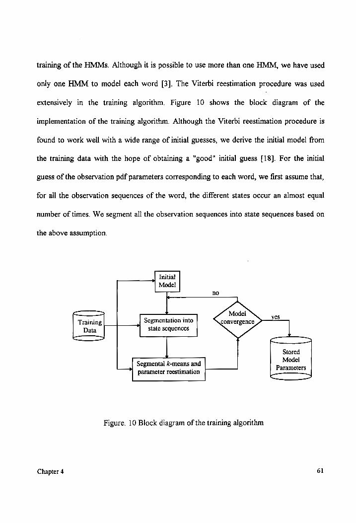
training of the HMMs. Although it is possible to use more than one HMM, we have used
only one HMM to model each word [3]. The Viterbi reestimation procedure was used
extensively in the training algorithm. Figure 10 shows the block diagram of the
implementation of the training algorithm. Although the Viterbi reestimation procedure is
found to work well with a wide range of initial guesses, we derive the initial model from
the training data with the hope of obtaining a "good" initial guess [18]. For the initial
guess of the observation pdf parameters corresponding to each word, we first assume that,
for all the observation sequences of the word, the different states occur an almost equal
number of times. We segment all the observation sequences into state sequences based on
the above assumption.
Initial Model
no
Training Segmentation into Data State sequences
Stored
Segmental k-means and P oe
parameter reestimation
Figure. 10 Block diagram of the training algorithm
Chapter 4 61
As a result, we have a set of observations that occur within each state. As mentioned
in Section 4.3.2.2, we use the segmental k-means method to cluster the observations that
occur within each state. From each cluster of vectors, we obtain a set of estimates
(say, é, pand C) for the observation pdf parameters of the state using (4.72)-(4.74). We
use these estimates as a seed for generating random initial guesses according to
C=C (4.81)
aS tri (4.82)
C= La r€ (4.83)
where r is random scalar variable, uniformly distributed between 0 and 1, used to generate
the different initial guesses.
For the initial estimate for the state transition probabilities, we have used random
values satisfying the constraints in Section 4.4.1 and the constraint that the entries of the
state transition matrix must add up to unity along every column.
In order to obtain a solution as close as possible to the global optimum during the
iterations, we start the reestimation from 25 different initial conditions. As a result we
have, at the end of the iterations, 25 candidates (7; 1<ks<25) for the final estimate of the
HMM for a particular word. As the best candidate, we choose the model that provides the
Chapter 4 62
"best" average (over all training sequences) likelihood of producing the training sequences
according to the following equation
toe -(»0r,) m =argmin| 7 1<k<25 (4.84)
My
where Z is the total number of training observation sequences available for each word.
To check for model convergence, we have used the distance measure given in (4.77).
We found that the model distance does not decrease monotonically with each iteration.
However, the distance goes below a particular value and remains below it for a significant
number of successive iterations. We choose this value as the threshold for stopping the
iterations. Since there is scope for model distances to increase after some iterations, it is
crucial to fix a suitable threshold. We have chosen a model distance of 0.1, calculated
according to (4.77), between the models of two successive iterations as the stopping
condition, based on experimental evaluation of the performance of the various models.
The final model 1" is then chosen to represent the word during recognition.
4.4.3 Recognition
At the end of the training process, we have a model for each word in the vocabulary.
If we have a total of W words in the vocabulary, we end up with W HMMs at the end of
Chapter 4 63
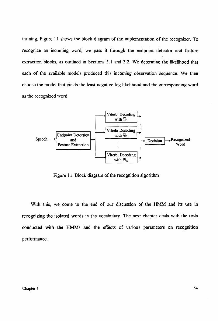
training. Figure 11 shows the block diagram of the implementation of the recognizer. To
recognize an incoming word, we pass it through the endpoint detector and feature
extraction blocks, as outlined in Sections 3.1 and 3.2. We determine the likelihood that
each of the available models produced this incoming observation sequence. We then
choose the model that yields the least negative log likelihood and the corresponding word
as the recognized word.
Viterbi Decoding |_,
with 77),
Viterbi Decoding Endpoint Detection with 1,
Speech —> and > +} Decision /-»Recognized Feature Extraction Word
| Viterbi Decoding m4
with Ty
Figure 11. Block diagram of the recognition algorithm
With this, we come to the end of our discussion of the HMM and its use in
recognizing the isolated words in the vocabulary. The next chapter deals with the tests
conducted with the HMMs and the effects of various parameters on recognition
performance.
Chapter 4 64
5. Testing of the Recognition System
Having discussed the various aspects of the speech recognition system developed in
this thesis, such as feature extraction and HMM training and recognition, in this chapter
we present the results of the tests conducted with the training and the recognition
algorithms. While the tests conducted on the training process were used to provide
insights into the nature of the convergence of the training algorithm, the results of
recognition can be used to discuss the effects of the number of states and the number of
mixture components on the performance of the overall recognition system.
5.1 Results on Known Models
Due to the lack of knowledge of the true HMMs for the digits, we used simplified,
known models to initially test the training algorithm. These known models were used to
generate observation sequences based on the following procedure [14]:
i) The state index is initialized to 7 = 1 and the time index to t = 1.
ii) The unit interval is partitioned proportional to Cj, 1<m<M. A random number,
uniform on [0, 1], is generated and a mixture density component, 7 1s selected
according to the subinterval in which the random number falls.
iii) A D-dimensional normal deviate, y, of zero mean and covariance Cj, is generated.
iv) The observation O, = y + py.
Chapter 5 65
v) A unit interval is partitioned proportional to az, 1< & < S.A random number uniform
on [0, 1] is generated and the next state, 7, is selected according to the subinterval in
which the random number falls. |
vi) The time index, ¢, is incremented to ¢+1.
vii) Steps ii through vi are repeated until a maximum allowable ¢ is reached or the final
state is generated for the maximum allowable number of times.
For a test case, the following model parameters were assumed.
S=3 M=2 D=1
08 0 0
A=|02 03 0
0 07 1
p,.=[1 19] p,.=[7 25] u,,=[13 31]
The covariance matrix was taken to be a diagonal matrix containing the variances of the
observation vector elements, and all the variances were taken to be equal to 2.
0.7 03
c=|05 O05
0.2 08
The above model was used to generate 100 observation sequences that were used as
training data. This training data was then used as input to the training procedure. The
training procedure was started from arbitrary initial models and we observed the distance
between the models (according to (4.77)), out of two successive iterations for a number of
Chapter 5 66
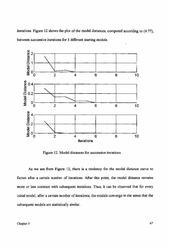
iterations. Figure 12 shows the plot of the model distances, computed according to (4.77),
between successive iterations for 3 different starting models.
®
Q2 3 ” uLA 0) \
GO
20 8) 2 4 6 8 10
@
20.4 8 ”
3 Poo™S = 0 2 4 6 8 10
®
24
3
@® \ wT
20 — 0 2 4 6 8 10
terations
Figure 12. Model distances for successive iterations
As we see from Figure 12, there is a tendency for the model distance curve to
flatten after a certain number of iterations. After this point, the model distance remains
more or less constant with subsequent iterations. Thus, it can be observed that for every
initial model, after a certain number of iterations, the models converge in the sense that the
subsequent models are statistically similar.
Chapter 5 67

For the test case used in Figure 12, the model distance converges to a value of zero.
However, we found that with real speech data, due to the larger dimensions of the
problem, it takes a prohibitively long time for the iterations to reach a model distance of
zero. Hence, we have attempted to arrive at a convenient threshold for assuming
convergence and stopping the iterations. The plots in Figure 12 show a general tendency
for the model distance to decrease with successive iterations. After a number of iterations
with the simple, known models it was decided that, for speech data, a threshold of 0.1 for
the model distances could be used as a reasonable stopping condition for assuming
convergence. As we will see from the results discussed in the next section, this threshold is
quite reasonable from a recognition performance point of view.
The training with the 100 observation sequences (generated from the known HMMs),
resulted in the following estimates for the various model parameters (5, M, and D were
assumed to be the same as the true S, M, and D respectively):
§ =3 M=2 D=l1
077 0 O
A=|023 034 0
0 066 1
~
fi, =[108 188] fi, =[69 25] p,=[126 31]
07 03 é=(049 051
0.19 081
C.=[16 18] C,=[23 18] C,=(21 23]
Chapter 5 68
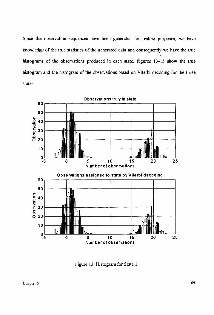
Since the observation sequences have been generated for testing purposes, we have
knowledge of the true statistics of the generated data and consequently we have the true
histograms of the observations produced in each state. Figures 13-15 show the true
histogram and the histogram of the observations based on Viterbi decoding for the three
states.
Observations truly in state 60
50 Cc
2 40
e © 30 ur a
“ ly
2 AUT o 20 al
10 HALT mu mi Ni | 0 | J hoo fl
-5 0 § 10 15 20 25 Number of observations
Observations assigned to state by Viterbi decoding 60
50 Aj
c | 2 40
S | @o 30 Tt
g
” i" fl &
© 20 iH | CH
10 7 UM = A
0 fli I Do fl
-§ 0 5 10 15 20 25 Number of observations
Figure 13. Histogram for State 1
Chapter 5 69
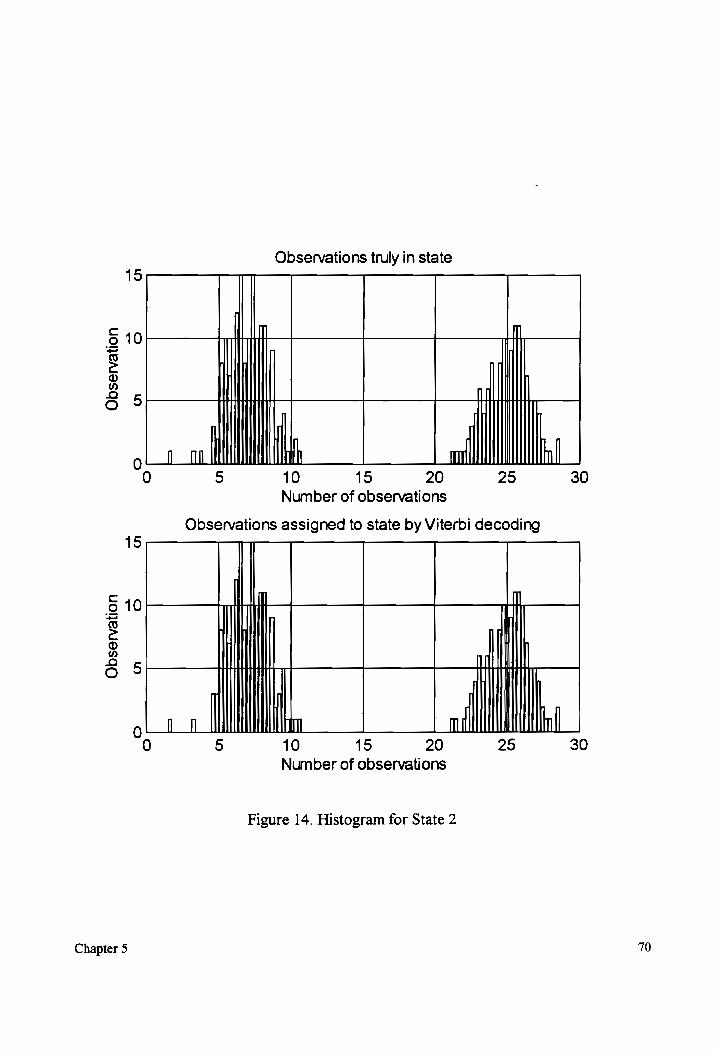
Observations truly in state
15
6 10 | > (Uh rT a | 6 5
| o_o th Hh 0 5 10 15 20 25 30
Number of observations
Observations assigned to state by Viterbi decoding 15
]
6 10 @ ] e I I
Ww i
5 5
Lao ll “Ail 0 5 10 15 20 25 30
Number of observations
Chapter 5
Figure 14. Histogram for State 2
70
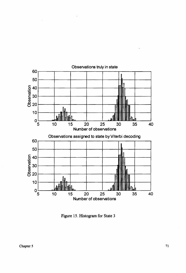
Observations truly in state
® Oo
On
oe)
oO
Observat
ion
ND
ow
A Oo
oO
—
Oo . all
Oo
on
Obse
rvat
ion
—
NO
Ww ao
Oo
Oo)
oO Oo
oO oO
oO Oo
Oo
Chapter 5
10 15 20 25 30 35 40
Number of observations
Observations assigned to state by Viterbi decoding
. hn. all
nn
10 15 20 25 30 35 40
Number of observations
Figure 15. Histogram for State 3
71
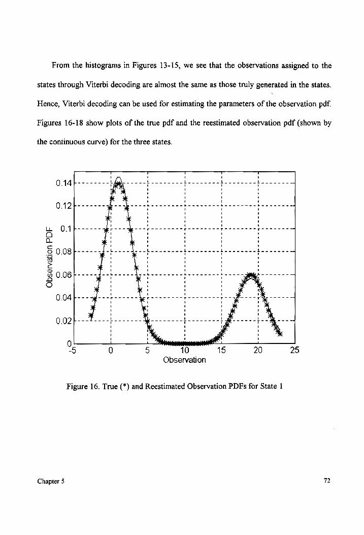
From the histograms in Figures 13-15, we see that the observations assigned to the
states through Viterbi decoding are almost the same as those truly generated in the states.
Hence, Viterbi decoding can be used for estimating the parameters of the observation pdf.
Figures 16-18 show plots of the true pdf and the reestimated observation pdf (shown by
the continuous curve) for the three states.
0.14}-------- tbe - = --- beeen beeen beeen eee beeen eee 4
0.12;------- f -- sp ----b-- 2-22 tanner eee toon eens boven een
i O0.1b------ teehee eee eee teen neee tees tod G ! : oO ! 5 t i t
6 0.08t-----+f- Lew--de-- ban nnn nn ben nee n nn bene nnn e beeen nee . 3 ! < 2 0.06 }-----y-- ena bene e cn tenn nn ne b= = Bigs = = =o ° ! ! : | ¥ 4
0.04 F---34---r------ poccctee povscccce aa rocco 1
0.02}---4----1 w eae Me nen cee bocce ig eee bBo
“5 0 5 1015 20 25 Observation
Figure 16. True (*) and Reestimated Observation PDFs for State 1
Chapter 5 72
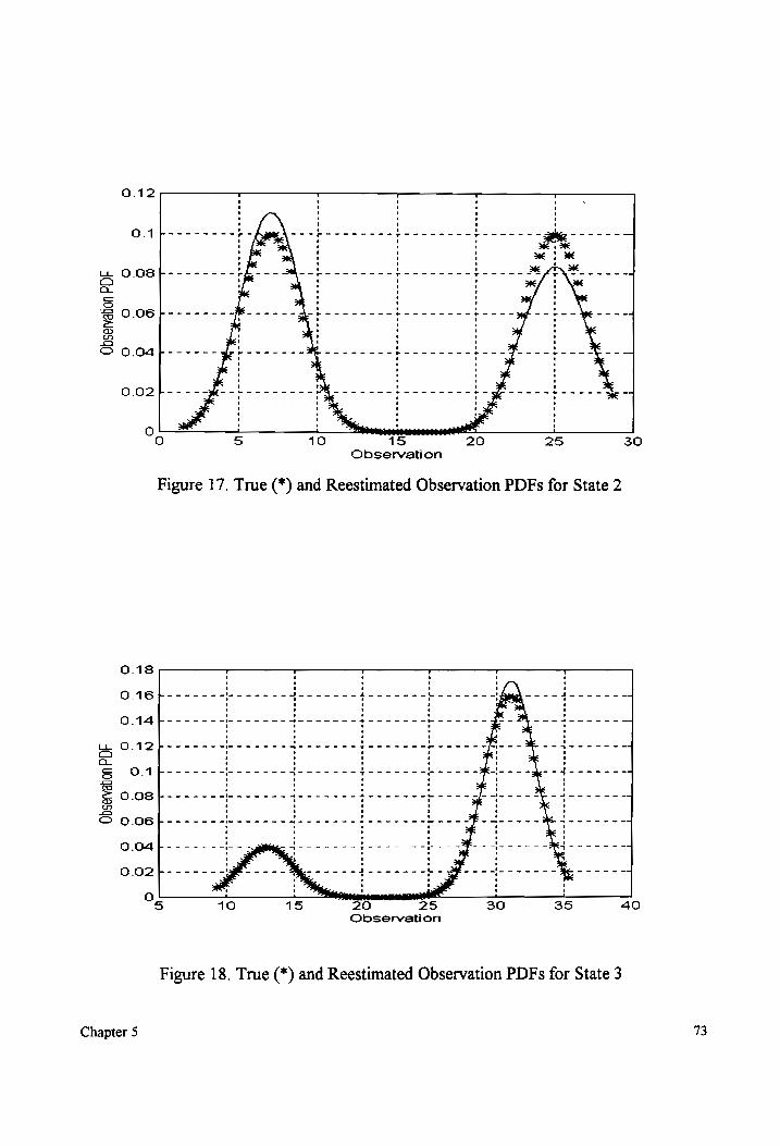
30
40
Aer ewe we Ke ee
HH ew
meee tee tee pee
ee wee Qe ene
ee
35
]j- eye eee ewe =
a
> me Zt
25
rm
a
i
4
‘ '
, wer r err mtr em temp rr crm mmr pr scm rece
a ' t
i} 1
' were ew we ee wm Pee KH ew em ee KM Pe KH eK
!
a
1
a 1
4 =~ePe wr wm ew ewe MP wm ee eww ew eM em em HM eee Ke
Pec ens PWR
wn ape tre meee
me tee eee
eee
we ew
wwe
30
20
25
woven whew mma
a dees wwe
Oe
ee
i wow epee
ae epee
we det
ee hee
ewe peewee
nae
15
Observation
Observation 20
“wy, ee ee ew ee et eee ww ee ee
cer goctcc occ
10
15
eee eee ee
rc
r.
weebaawmne
a
10
Figure 17. True (*) and Reestimated Observation PDFs for State 2
0
O.1}---------
0.02}-----
O
0.16}-------
O.14}-------
0.12[;-------
O.1}-------
0.08}-------
‘ ' ' ; t o Oo
0.12
0.08} --------
0.06|--------}
0.18 0d
UOnEAES GQ) 41g VONEAIOSGQ
Figure 18. True (*) and Reestimated Observation PDFs for State 3
73 Chapter 5
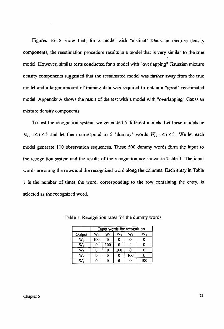
Figures 16-18 show that, for a model with "distinct" Gaussian mixture density
components, the reestimation procedure results in a model that is very similar to the true
model. However, similar tests conducted for a model with "overlapping" Gaussian mixture
density components suggested that the reestimated model was farther away from the true
model and a larger amount of training data was required to obtain a "good" reestimated
model. Appendix A shows the result of the test with a model with "overlapping" Gaussian
mixture density components.
To test the recognition system, we generated 5 different models. Let these models be
Mm, 1<i<S and let them correspond to 5 "dummy" words W,; 1<i<5S. We let each
model generate 100 observation sequences. These 500 dummy words form the input to
the recognition system and the results of the recognition are shown in Table 1. The input
words are along the rows and the recognized word along the columns. Each entry in Table
1 is the number of times the word, corresponding to the row containing the entry, is
selected as the recognized word.
Table 1. Recognition rates for the dummy words.
Input words for recognition
Output W, W, W; W, W;
WwW, 100 | 0 0 0 0
Ww? 0 | 100} 0 0 0
W;3 0 0 | 100] 0 0
W, 0 0 0 | 100 0
Ws 0 0 0 0 100
Chapter 5 74
We observe that, for the test case, the recognition system successfully recognizes all
the "dummy" observation sequences. Thus, if the true models corresponding to the
observation sequences are available, the recognition system is capable of successful
recognition.
Thus, the results of the tests on known models provide the proof of concept for the
implementations of the training and the recognition algorithms. We now present the results
of recognition with the words in the vocabulary, which are the digits 0 through 9, in our
case.
5.2 Results on Words
Since the objective of this thesis is to develop a speaker dependent recognition
system, we recorded two sets of 50 utterances of each digit, by a single speaker, on two
different days. In order to include the variability of the recorded words, for each digit we
formed the training set of 50 utterances using 25 recordings each from the two sets. Thus
we have a training set of 50 utterances per digit and a testing set of 50 utterances per
digit. The training sets were used to train the HMMs for the 10 digits in the vocabulary.
The results of recognition on the words help us to evaluate the performance of the
recognition system and to study the effects of the number of states and the number of
mixture density components on recognition performance.
As with the dummy words, the results of recognition on the training and the testing
sets are presented in the form of tables, where the input words are along the columns and
Chapter 5 75
the recognized words along the rows. Each entry in the table is the number of times the
word, corresponding to the row containing the entry, is selected as the recognized word.
We varied the number of states between 5, 6, and 7, and the number of mixture density
components between 1, 2, and 4. We also attempted to use 8 mixture density components.
However, the segmental k-means clustering that we use for Viterbi reestimation resulted in
many clusters being empty. This indicates that using 8 mixture density components leads
to over-parameterization. Moreover, since the Viterbi reestimation method obtains the
statistics of each mixture density component from each of the clusters, empty clusters lead
to numerical problems during reestimation. We first present the results of recognition for
the models with 7 states (S = 7) and 4 mixture density components (M = 4). The results
with the models with other values of S and M are provided in Appendix B. We use these
results to discuss the effects of S and M on performance. As an alternative to using the
same number of states and mixture density components in the models for all the words in
the vocabulary, we have also used different values for S and M for different words. Since
it is customary to use as many states as the average number of frames in a word, for the
case with a different number of states for the different digits, for each word, we have
chosen the number of states to be equal to the number of frames in the shortest training
utterance of that word. The results of recognition, for models with different values for S
and M for different words, are also provided in Appendix B.
We have associated a figure of merit with each recognition table. The figure of merit
is the sum of the elements of the diagonal in the tables. This figure of merit gives an idea
Chapter 5 76
of the average percentage of correct recognition (figure of merit divided by 5) for all the
words in the vocabulary.
Table 2 shows the recognition rates for the training utterances for M = 4 and S = 7.
The figure of merit for Table 2 is 500 and corresponds to an average recognition rate of
100%. We can expect such a high recognition rate for the training data, as the models
have been trained to "tune" to the training utterances. Table 3 shows the recognition rates
for the testing utterances for M = 4 and S = 7. The figure of merit for Table 3 is 496 and
corresponds to an average recognition rate of 99.2%. The recognition rate for the testing
set can be expected to be less than that for the training set, as the representative models
may not be tuned to some of the variability in the testing set. Hence, as expected, the
trained models are a poorer representative of the testing set than of the training set. From
Tables 2 and 3 and Appendix B, we see that it is possible to decrease the error rate
associated with the recognition of any one word by changing the value of © and S.
However, the overall recognition rate as indicated by the figure of merit, as we have
chosen, depends on all the models being "good" and this figure of merit has to be
observed, to arrive at a suitable value for S and M/ for the recognition system.
To study the effects of S and M on recognition performance, we next generalize the
results obtained using 5, 6, 7, and a varying number of states. Figure 19 shows the average
error percentages across the digits for the training and the testing data sets. We observe
the downward trend in the error percentages with varying a number of mixture density
components for a particular number of states.
Chapter 5 77
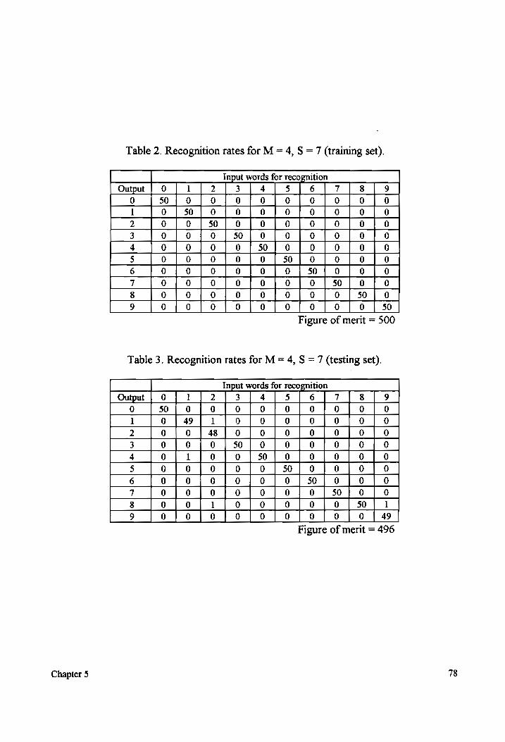
Table 2. Recognition rates for M = 4, S = 7 (training set).
Input words for recognition
Output | 0 1 2 3 4 5 6 7 8 9 0 50 | 0 0 0 0 0 0 0 0 0 1 0 | 50} 0 0 0 0 0 0 0 0
2 0 0 | 50] 0 0 0 0 0 0 0 3 0 0 0 |} 50 j 0 0 0 0 0 0
4 0 0 0 0 | 50; 0 0 0 0 0
5 0 0 0 0 0 | 50} 0 0 0 0
6 0 0 0 0 0 0; 50 { 0 0 0
7 0 0 0 0 0 0 0 | 50] 0 0
8 0 0 0 0 0 0 0 0 | 50 | 0
9 0 0 0 0 0 0 0 0 0 | 50
Figure of merit = 500
Table 3. Recognition rates for M = 4, S = 7 (testing set).
Input words for recognition
Output | 0 1 2 3 4 5 6 7 8 9 0 50 | 0 0 0 0 0 0 0 0 0
1 QO | 49 l 0 0 0 0 0 0 0
2 0 0 | 48 | 0 0 0 0 0 0 0
3 0 0 0 50 | 0 0 0 0 0 0
4 0 1 0 0 | 50 | 0 0 0 0 0
5 0 0 0 0 0 50 | 0 0 0 0
6 0 0 0 0 0 0 | 50; 0 0 0
7 0 0 0 0 0 0 0 | 50} 0 0
8 0 0 1 0 0 0 0 0 50 1 9 0 0 0 0 0 0 0 0 0 | 49
Figure of merit = 496
Chapter 5
The curves marked by 'S = X' represent the models with a different number of states
for the different digits. We see that an increase in the number of mixture components
generally decreases the error rates, for each of the different number of states. Figure 20
shows the trend in the average error percentages across the digits for the training and the
testing data sets, with a varying number of states for a particular number of mixture
density components. Although the error percentage decreases monotonically with an
increase in the number of states for the testing set, there is no such trend with the training
set. However, in general, an increase in the number of states seems to decrease the error
rates. However, after a particular point, an increase in the number of states adversely
affects the performance because, due to the larger number of parameters involved, the
training algorithm may not converge to very "good" models.
We see that the decrease in error percentages with changes in the number of mixture
density components is more pronounced than that with changes in the number of states.
Tables 4 and 5 indicate that the trends of the recognition performance in the testing set,
with changes in S and M, more or less follow the pattern in the training set. In Table 5, we
see that the error rate increases when we change from using 7 states to a varying number
of states. This is because, in general, in the models for the case S = X, the number of
states used by each digit is more than 7. Hence, the increase in the number of states has
increased the number of parameters to be reestimated. Since an increase in the number of
parameters tends to increase the variance involved with each of the parameters, the
Chapter 5 79
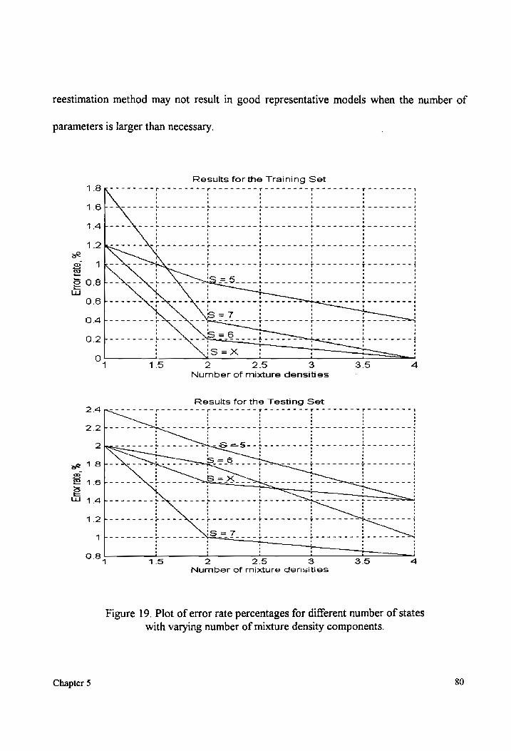
reestimation method may not result in good representative models when the number of
Results for the Training Set
parameters is larger than necessary.
ey
pocorn gst
pes tsps
ss sess SP DEE
1 '
' t
1 t
' '
' '
' '
' i
I t
t '
1 1
' '
’ '
' 1
1 1
' '
! 1
1 '
t '
' '
( t
t '
i 1
i '
! 1
' '
( 1
! '
' '
' 1
’ '
t 1
1 '
' '
' !
Leenehecedacent 0
Lecscbeceedecesatessetfeefleceedecaaben 1
J l
«m '
t '
1 '
1 1
1 '
' 1
' I
' '
' i
' 1
I t
’ '
' !
' t
' '
1 {
t t
t '
' ‘
' '
' '
' '
1 1
' '
' i
' '
' I
t '
' !
1 1
' '
' '
1 '
v)
roo ;
@ $.
+ «
« fr
dyoa 4
es |
re eo
m+
“) mwa
e be mend
awen abe
fon bha nf
ode cnc nh
cen eb
aw nee
' !
' 0
’ ’
' '
' 1
t 1
t !
' c
Or
' '
' 1
i !
' '
' ’
@ c
' '
' t
! '
' '
rd
; U
Broo ot
Uf Ot
Pa '
1 '
@ Q!
' 1
t '
1 '
' 1
t 5
k t
t '
t i
t I
’ '
Lecce pete
feb dO Eg
Lect feeteecebeceetfee
' !
N=
£1
' '
' '
I 1
' !
£ i
1 \
' \
' '
' .
5 '
‘ yf
' '
'
! !
6 e1
' |
Pot '
t 0
Vi J
' ()
' '
q! !
1 =
' '
1 t
€
a '
' '
1 '
0
. a a
tecnethen pave t !
ze
ff, of)
1 '
t '
i '
' '
t I
I ’
1 '
t !
1 '
' !
i i
1 '
' !
L lO
Leceefeceed (deveechaccobeces
l -
t 1
1 !
' i
1 {
' '
' 1
' '
’ ’
’ I
’ '
' '
' t
' 1
' '
I ‘
1 '
i '
' '
1 '
’ '
1 '
' 1
' '
t 1
1 '
i) '
f t
t '
i)
r -
a i
l i
l
© TN
N YT
N ©
® 7
N N
a c
vc Oo
% '9Je)
JONI %
‘aed JONI
80
2 2.5 3 3.5 Number of mixture densities
1.5
with varying number of mixture density components.
Figure 19. Plot of error rate percentages for different number of states
Chapter 5
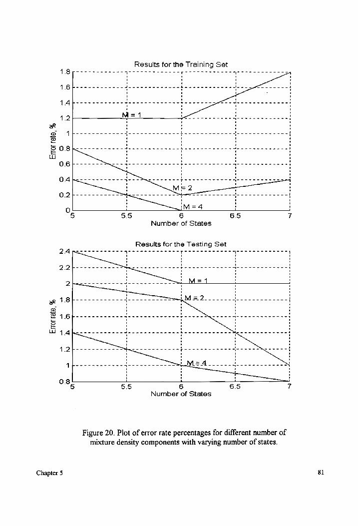
Results for the Training Set
wee
en ree
ee ee
eee p
enn eee
mM '
' t
t '
\ '
' '
' {
i '
' t
i i)
i) 1
L} a
'
' t
' '
1 1
' '
' '
' '
' ‘
' \
t i]
i 1
t '
i] i]
' 1
' i)
i) !
t 1
' t
' '
‘ '
' t
t I
' l]
1 i]
t
i] '
1 I
I 1
' t
' t
' 1
1 '
i '
' '
' ‘
i '
\ '
eed
ete th
td
ae i
’ 7
i t
i i
i '
' '
' 1
t '
’ <e)
' ‘
\ '
‘ 1
' '
' '
' '
' '
1 '
4 '
l t
i) i)
1
i) '
t i]
' '
1 '
' '
\ '
i '
' t
' '
' '
i 1
t i]
t 1
1 I
i) 1
1 i]
i] 1
' 1
t '
i) '
1 '
i] '
i) L)
i] '
1 t
J I
t '
i) '
' '
' ‘
' '
' t
le ew
we de ee
we eh
ew
he eee ee
ee ek
O
U t
i] 1)
t t
t
' 1
1’ '
1 i]
'
t '
' '
' i)
4
' t
' '
' '
‘ '
\ '
1 '
' '
' '
' ‘
1 \
' '
1 5
' i
1 '
( i
i I
i) '
1
t '
' 1
' \
‘ '
' ‘
\ '
1 '
It '
am '
' 1
' (
t ‘
" ‘
i '
4 Te
i) J
’ t
' i)
i]
rue eye
rere zee ere
PTT TTT
OT OTM
Frew
Ke ye wean
: \
' '
=
' \
' ‘
' re)
t '
' i
’ '
' ‘
' t
t t
\ \
t t
' '
' ‘
' t
' \
' '
i 1
t \
' (
1! t
i) '
' i]
4
' '
i '
' '
' ’
! i]
i] '
1 i]
t i
I l
' I
t t
' '
' '
t ’
' 1
' '
t i]
i] !
i) t
' t
\ ’
' \
\ '
1 '
LN
l Ll
LL i
1 wo
oOo
tT NH
© OT
AN O
baad -
-
-
7) oO
OQ ©
% '9]es
JOUS
Number of States
Results for the Testing Set
wee eee
1.6}
1+
0.8
T <
’ t ‘ ' ’ ' ' t ' ' ’ ' ' Ke)
meee Pree grr cpr
pid
' '
©
' t
' '
’ J
' ’ '
’ '
’ 1
5 '
' t
1 '
' '
wae wef eee
baweed
©
’ '
’ 1
' '
' '
' '
' '
1 ’
1 ’
' '
t '
' '
' '
' '
' ’
' '
' '
’ ’
’ '
t '
i) re
Tur
yr rrr gern pete
. !
' '
' )
' '
' '
4 '
‘ '
\ ’
' '
1 '
' !
' '
' ’
’ '
J '
{ '
' t
\ '
' '
' '
' '
' ‘
' '
t '
' '
i 8)
0 bs
‘g]21 JOU
Number of States
Figure 20. Plot of error rate percentages for different number of mixture density components with varying number of states
81 Chapter 5
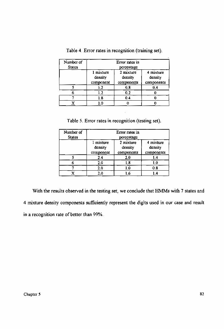
Table 4. Error rates in recognition (training set).
Number of Error rates in
States percentage 1 mixture 2 mixture 4 mixture
density density density
component components | components 5 1.2 0.8 0.4
6 1.2 0.2 0 7 1.8 0.4 0
XxX 1.0 0 0
Table 5. Error rates in recognition (testing set).
Number of Error rates in
States percentage
1 mixture 2 mixture 4 mixture
density density density
component components | components
5 2.4 2.0 1.4
6 2.0 1.8 1.0
7 2.0 1.0 0.8
xX 2.0 1.6 1.4
With the results observed in the testing set, we conclude that HMMs with 7 states and
4 mixture density components sufficiently represent the digits used in our case and result
in a recognition rate of better than 99%.
Chapter 5 82
6. Connected Digit Recognition
In the last two chapters, we presented the design of an isolated word recognition
algorithm and demonstrated the recognition of the ten digits 0 through 9. The focus of this
thesis was to develop a system that is capable of recognizing strings of digits, as in a
"hands-free" telephone system. In this chapter, we present the implementation of a
connected digit recognition algorithm and discuss the results of recognition on strings of
digits.
6.1 Introduction
As mentioned in Chapter 1, connected digit recognition is a technique used to
recognize continuous speech in a small-vocabulary application. In connected digit
recognition, a string of digits is modeled as a concatenation of the models built from
isolated digits. Since we use HMMs to model the isolated digits, the connected digit
recognition system attempts to select the string of models that best matches the string of
digits in a maximum likelihood sense. The most popular method to find the optimum set of
models is a method known as the level-building (LB) method [3]. The main challenge
behind finding an optimum set of digits is to determine the boundary between the words in
the string. In continuous speech, this boundary is not distinct. Hence there is a need to
incorporate the statistics regarding the duration of individual words, into the HMMs. It
has been found in past research that a simple Gaussian duration model can be assumed for
Chapter 6 83
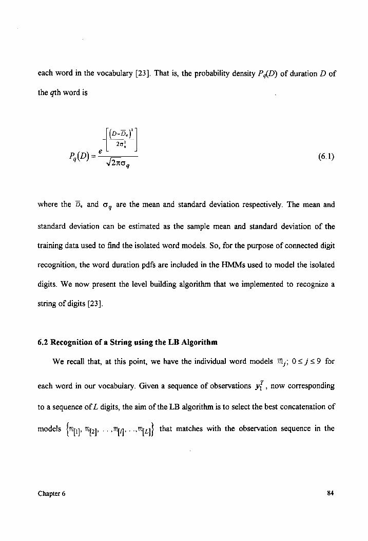
each word in the vocabulary [23]. That is, the probability density P,(D) of duration D of
the gth word is
P,(D) = faa, (6.1)
where the D, and co, are the mean and standard deviation respectively. The mean and
standard deviation can be estimated as the sample mean and standard deviation of the
training data used to find the isolated word models. So, for the purpose of connected digit
recognition, the word duration pdfs are included in the HMMs used to model the isolated
digits. We now present the level building algorithm that we implemented to recognize a
string of digits [23].
6.2 Recognition of a String using the LB Algorithm
We recall that, at this point, we have the individual word models 1,; O< 7 <9 for
each word in our vocabulary. Given a sequence of observations ye , how corresponding
to a sequence of L digits, the aim of the LB algorithm is to select the best concatenation of
models {mi May -- Map - tr} that matches with the observation sequence in the
Chapter 6 84
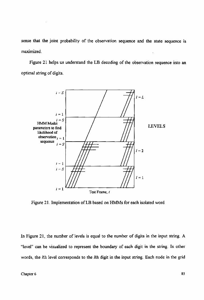
sense that the joint probability of the observation sequence and the state sequence is
maximized.
Figure 21 helps us understand the LB decoding of the observation sequence into an
optimal string of digits.
i=]
HMM Model
parameters to find likelihood of observation ; _ 1
sequence
LEVELS
Test Frame, tf
Figure 21. Implementation of LB based on HMMs for each isolated word
In Figure 21, the number of levels is equal to the number of digits in the input string. A
“level” can be visualized to represent the boundary of each digit in the string. In other
words, the /th level corresponds to the /th digit in the input string. Each node in the grid
Chapter 6 85
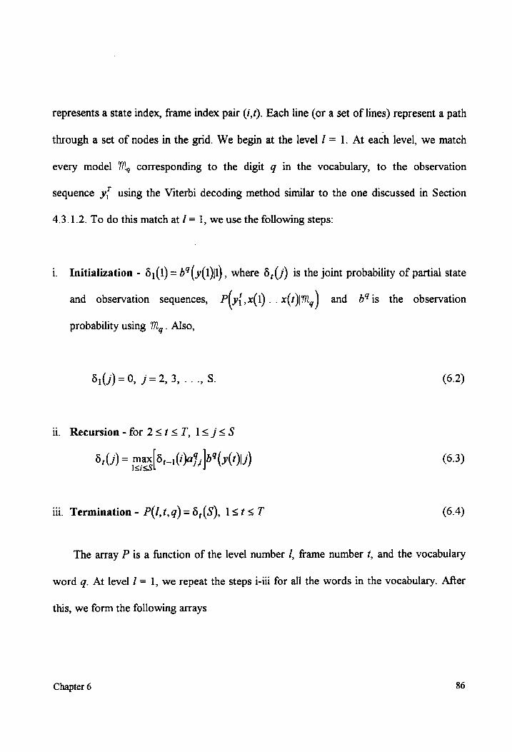
represents a state index, frame index pair (i,f). Each line (or a set of lines) represent a path
through a set of nodes in the grid. We begin at the level / = 1. At each level, we match
every model 17/1, corresponding to the digit g in the vocabulary, to the observation
sequence y, using the Viterbi decoding method similar to the one discussed in Section
4.3.1.2. To do this match at / = 1, we use the following steps:
i. Initialization - 5,(1) = b4( y(1)il), where 5,(/) is the joint probability of partial state
and observation sequences, P(yf ,x(1).. x(1)|M,y) and 5b7is the observation
probability using 1, . Also,
5\(/)=0, j=2,3,...,8. | (6.2)
li. Recursion - for 2<¢t<7,1<j<S
5,(/) = max{3,-(i)49,|6%(»(U) (6.3)
iii. Termination - P(/,t,q)=5,(S), l1<t<T (6.4)
The array P is a function of the level number /, frame number ¢, and the vocabulary
word g. At level / = 1, we repeat the steps i-iii for all the words in the vocabulary. After
this, we form the following arrays
Chapter 6 86
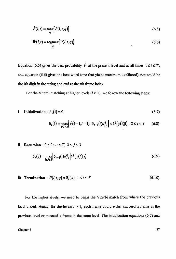
P(t) = max{ P(/,1,4)] (6.5)
W(i,t) = argmax| P(/, t, q)| (6.6) 4
Equation (6.5) gives the best probability P at the present level and at all times 1<¢<T,
and equation (6.6) gives the best word (one that yields maximum likelihood) that could be
the /th digit in the string and end at the ‘th frame index.
For the Viterbi matching at higher levels (/ > 1), we follow the following steps:
i. Initialization - 5,(1) =0 (6.7)
5,(1) = max| P(!-1,¢-1), 5,-s()a},|xd%(y(Mn), 2<¢<T (6.8)
li. Recursion - for 2<t<7,2<j<S
6,(j) = max 8 ,-1()a9,[6%(y()L/) (6.9)
iii. Termination - P(/,t,q)=5,(S), 1<t<T (6.10)
For the higher levels, we need to begin the Viterbi match from where the previous
level ended. Hence, for the levels / > 1, each frame could either succeed a frame in the
previous level or succeed a frame in the same level. The initialization equations (6.7) and
Chapter 6 87
(6.8) let the level pick up at the most appropriate (of the above two possibilities) place
from the previous level. We repeat steps i-iii for all the words in the vocabulary and then
form the following arrays
P(t) = max] P(/,t,4)| (6.11)
W (i,t) = argmax| P(/,1,q)| (6.12) q
for all the levels, 1</<LZ, where L is the total number of levels which equals the
expected number of digits in the observation string.
After we reach the highest level, Z, we have W , which is the array containing the best
estimate of the digit ending at a particular frame, for all the frames and for all the levels.
We have to obtain estimates of the boundaries of the digits corresponding to the various
levels. We begin with the first level / = 1. We assume that all the digits in the string are
equally long. Based on this assumption, we can obtain an initial estimate of the boundaries
of the first digit in the string. This provides an estimate of the temporal region occupied by
the level. We then examine the array W and determine the digit which occurs the
maximum number of times within the boundaries that we have estimated. We have the
mean and the standard deviation of the statistics of the duration of this digit. We now
change the estimate of the temporal region occupied by the level to vary between the
frames D, —3o, and D, +3o,. The array W is again examined for the digit that occurs
Chapter 6 88

the maximum number of times. This process (of searching for the digit that occurs a
maximum number of times within the present boundary estimates) is repeated until the
digits selected for two successive boundary estimates are the same.
Once the digit for level / is chosen, we let the initial estimate of the lower boundary
(in terms of the frame index) of the next higher level (/+1) be the frame D, . where qd is
the digit estimated to occupy level 1. We then proceed to examine W and select the digit
for the next level, 7+ 1 in a manner similar to that for level /.
After we go through all the levels, we have an estimate of the string of digits
corresponding to the input observation sequence. In the next section, we discuss the
results of recognition on test strings.
Let us look at an example of choosing the digits in the string from the array W . Let
us consider a string of 2 digits. Hence, we use 2 levels (LZ = 2). For a test case, we have
chosen the digit string “one two", to be recognized. The string we have chosen is 24
frames long. At the end of the LB algorithm, we have the following array
pary-|? °° SO EEE EEE EERE EEE EEE
“10 000003333321188727222222
We begin with level 1. We first assume that the first digit (level 1) is 12 frames long. So
our initial boundary estimates for the 1st digit of the string are the frames 1 and 12.
Between frame indices 1 and 12, we look for the digit of maximum occurrence. That is the
Chapter 6 89
digit "one" (in the lst row of W). We also know that the mean duration of the digit "one"
is 15 frames and the standard deviation is approximately 3 frames. So we modify the
boundary estimates for the Ist digit as the 6th (D, —3o0,) and the 24th frame
(D, +30, ). We again search for the digit of maximum occurrence within frames 6 and
24. We can see that it is still the digit "one". Hence we conclude that the Ist digit of the
string is "one". Therefore, we now have | (i.e. Z-1) digits remaining in the string, and yet
to be recognized. For the next level, /; we start the search from frame 15 (i.e. D. ). We i-i
assume that the remaining (Z-1) digits of the string are equally long. Hence, we choose the
initial boundaries of the second digit as 15 and 24 and we repeat the process. We look for
the digit of maximum occurrence. That is the digit "two" (in the 2nd row of W). We also
know that the mean duration of the digit "two" is 15 frames and the standard deviation is
approximately 5 frames. According to the LB algorithm, we modify the boundary
estimates (to search for the digit of maximum occurrence) for the 2nd digit to
D, . +D,—30, and D, . +D,+3o,. However, since the maximum frame index is 24, i-l i-1
and the length of the first digit is 15 frames, we modify the boundary estimates for the 2nd
digit as the 15th and the 24th frame and search for the digit of maximum occurrence. We
see that it is still the digit “two". Hence we conclude that the 2nd digit of the string is
"two". Thus, we see that the string “one two” is correctly recognized.
It should be noted that knowledge of the number of digits in the string is extremely
crucial to the connected digit algorithm that we have implemented. However, the HMMs,
Chapter 6 90
when used within the framework of DP, have a self normalization feature [3] in the sense
that irrespective of the number of levels in the LB algorithm, the length of the search path
is always equal to the number of frames in the input string. This allows us to execute the
LB algorithm on the same string using different values of Z and choosing the set of HMMs
that result in the best overall likelihood of having produced the input string. However, due
to the larger amount of variability involved as compared to the situation where knowledge
of the number of digits in the input string is available, we can expect the speech
recognition system to yield poorer performance when the number of digits in the string is
not available.
6.3 Results of recognition of strings
We now present the recognition rates observed with the recognition of strings of 2, 3,
and 4 digits. We form the test strings by concatenating the observation sequences
corresponding to isolated digits. We recall that we have 100 recordings of each digit
(including training and testing sets). For each string length (number of digits in a string),
we formed a testing set of 100 strings by randomly choosing the digits of the string from
the recordings of isolated digits.
For each string length, we present the results where the isolated digit HMMs
containing 1, 2, and 4 mixture density components, and 5, 6, and 7 states and a different
number of states for different digits. Tables 6, 7 and 8 provide the string recognition rates
Chapter 6 91
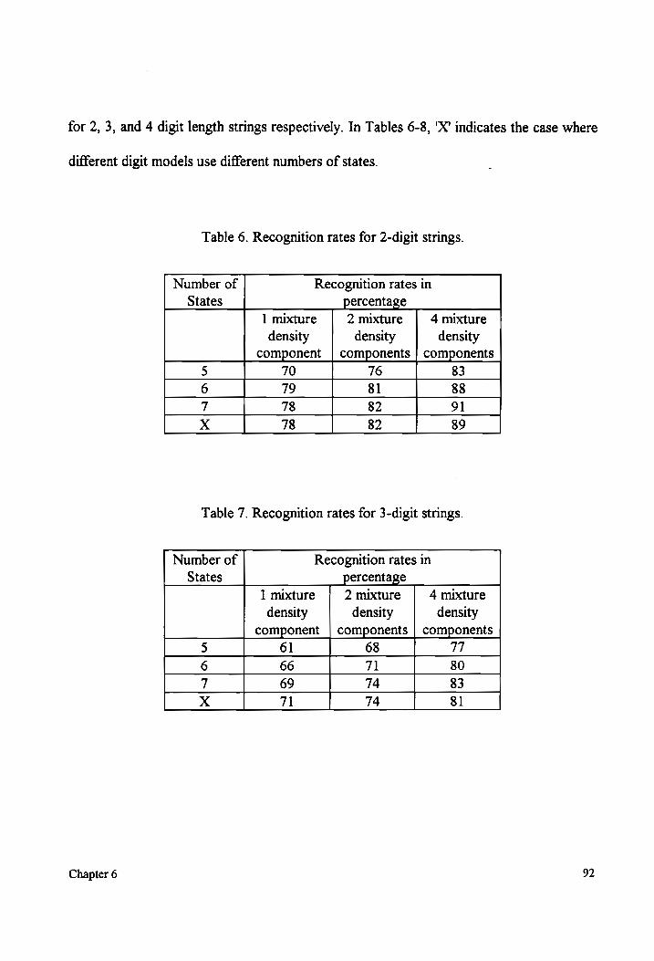
for 2, 3, and 4 digit length strings respectively. In Tables 6-8, 'X' indicates the case where
different digit models use different numbers of states.
Chapter 6
Table 6. Recognition rates for 2-digit strings.
Number of Recognition rates in
States percentage
1 mixture 2 mixture 4 mixture
density density density
component | components | components
5 70 76 83
6 79 81 88
7 78 82 91
X 78 82 89
Table 7. Recognition rates for 3-digit strings.
Number of Recognition rates in States percentage
1 mixture 2 mixture 4 mixture
density density density
component | components | components 5 61 68 77
6 66 71 80 7 69 74 83
XxX 71 74 81
92
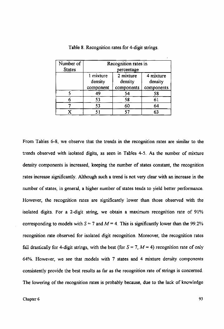
Table 8. Recognition rates for 4-digit strings.
Number of Recognition rates in States ercentage
1 mixture 2 mixture 4 mixture
density density density
component | components | components 5 49 54 58 6 53 58 61
7 53 60 64 x 51 57 63
From Tables 6-8, we observe that the trends in the recognition rates are similar to the
trends observed with isolated digits, as seen in Tables 4-5. As the number of mixture
density components is increased, keeping the number of states constant, the recognition
rates increase significantly. Although such a trend is not very clear with an increase in the
number of states, in general, a higher number of states tends to yield better performance.
However, the recognition rates are significantly lower than those observed with the
isolated digits. For a 2-digit string, we obtain a maximum recognition rate of 91%
corresponding to models with S = 7 and M = 4. This is significantly lower than the 99.2%
recognition rate observed for isolated digit recognition. Moreover, the recognition rates
fall drastically for 4-digit strings, with the best (for S = 7, Af = 4) recognition rate of only
64%. However, we see that models with 7 states and 4 mixture density components
consistently provide the best results as far as the recognition rate of strings is concerned.
The lowering of the recognition rates is probably because, due to the lack of knowledge
Chapter 6 93
regarding the individual digit boundaries (unlike in isolated digit recognition), some
observations belonging to adjacent digits may be included in the process of determining
the best word at each level. This can lead to a wrong digit being picked to be a part of the
string; it certainly would make recognition worse than for the correct individual digit.
Further more, uncertainty about the boundaries of digits increases faster, relative to those
on either absolute end of the string, for digits in between digits with uncertain locations.
The increased uncertainty in the boundaries cannot but worsen the recognition rates for
the nested digits. The consequence is a string recognition rate that is much less than for a
concatenation of isolated digits with known boundaries (Based on our results: (0.99)” for
an L-digit string).
Chapter 6 94
7. Conclusions and Further Research
The motivation for this thesis has been to develop a speaker dependent speech
recognition system that can be used to recognize strings of digits; for example, to be
employed in an environment with a hands-free telephone system. In Chapters 3-6 we
presented the theoretical background, the implementation, and the performance results of
the recognition system. In Chapter 3, we discussed feature extraction. Chapter 4 delved
into the theory behind the HMM and its application to the problem of speech recognition.
We also discussed the various issues involved in the implementation of the training and the
recognition algorithms in Chapter 4. In Chapter 5 we presented the results of recognition
with isolated digits and discussed the effects of the number of states and the number of
mixture density components on the recognition performance and error rates.
Based on the results presented in Chapter 5 and Appendix B, we concluded in
Chapter 5 that HMMs with 7 states and 4 mixture density components resulted in the
highest recognition rates as far as isolated digit recognition is concerned. We obtained a
better than 99% recognition rate on the test data which were not used in the training
process. This is significantly higher than the recognition rates obtained using a discrete
HMM approach [26]. K. A. Rangarajan [26] has employed the FB algorithm and Baum-
Welch reestimation for recognition and training respectively. However, to extend this
system to a speaker independent or a larger vocabulary system, a larger amount of training
data is needed. In such a case, although the basic structure of the recognition system can
be maintained as it is here, some linguistic constraints may have to be included to achieve
Chapter 7 95
similar performance. Chapter 7 details the implementation of the level-building algorithm
to recognize strings of more than one digit. While we obtained better than 90%
recognition rates for 2-digit strings, for a 4-digit string the recognition rates were no
better than 64%. Thus, the system implemented here can be used as an isolated word
recognizer, providing very high recognition rates, or it can be used to recognize 2-digit
strings, at moderately high recognition rates.
To use the system for situations involving longer strings we have to involve some
additional aspects into the word models. For example, the training data for each digit can
be obtained from strings containing the digit [2]. As an extension to the system
implemented in this thesis, to improve performance, different state and word duration
models can be experimented with and employed [23]. In addition to state and word
duration models, the HMMs can include models for the word energies. The latter has also
been found to improve recognition performance to some extent [2].
Although other techniques that use empirical constraints to determine the boundaries
between the digits in a string yield higher string recognition rates, the manner in which the
digits are selected at the various levels is simpler in our system [2, 23].
In view of future real time implementation of the recognition system we observed,
using MATLAB for a 10-digit vocabulary using 7 state and 4 mixture density component
HMMs, that the number of flops required to perform recognition of a single isolated digit
is approximately 10 million. To recognize a 3-digit string approximately 13 million
operations are needed. Hence, if a Digital Signal Processor such as the ADSP-2181 (a 32
Chapter 7 96

MIPS processor) is used, a 3-digit string can be recognized in approximately a third of a
second and an isolated digit in less time. This is reasonably fast for the recognition system
to be useful in many real-time applications. The memory requirement of the recognition
system using 7 states and 4 mixture densities is for approximately 14000 words (16 bit).
Chapter 7 97
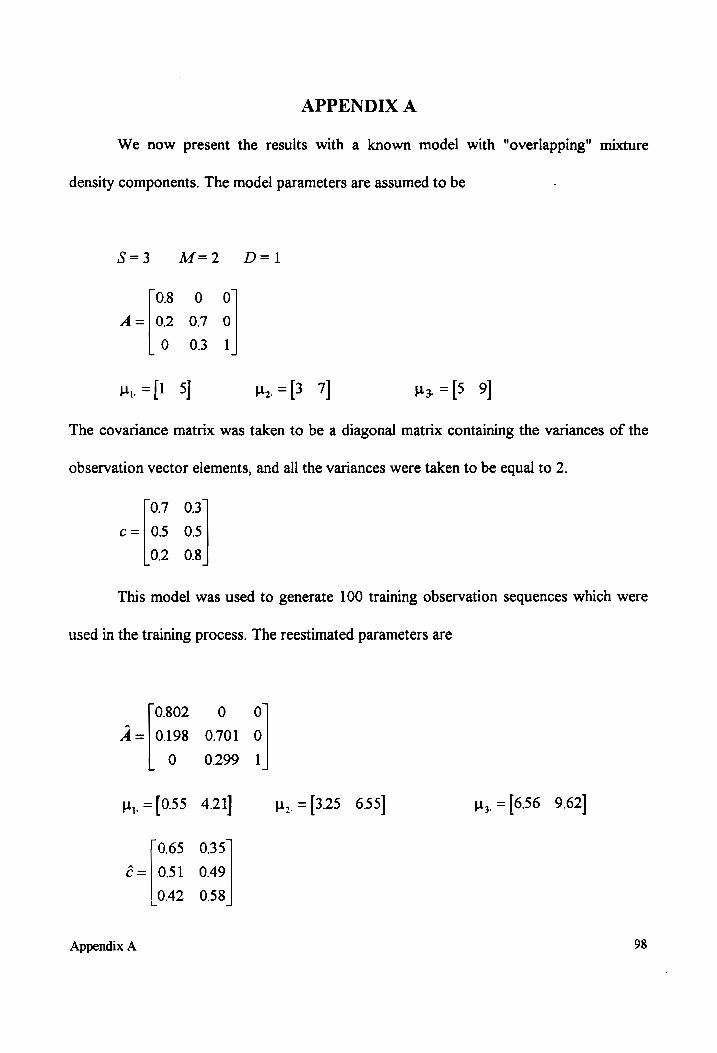
APPENDIX A
We now present the results with a known model with "overlapping" mixture
density components. The model parameters are assumed to be
S=3 M=2 D=1
08 0 0
A=|02 07 O
0 03 1
w=[1 5] b= [3 7] Hs =[5 9]
The covariance matrix was taken to be a diagonal matrix containing the variances of the
observation vector elements, and all the variances were taken to be equal to 2.
0.7 03
c=105 O5
0.2 08
This model was used to generate 100 training observation sequences which were
used in the training process. The reestimated parameters are
0802 0 0
A=|0198 0701 0
0 0299 1
,=[055 4.21] p,, =[3.25 655] p,,=[656 9.62]
0.65 0.35
c=|051 0.49
0.42 058
Appendix A 98
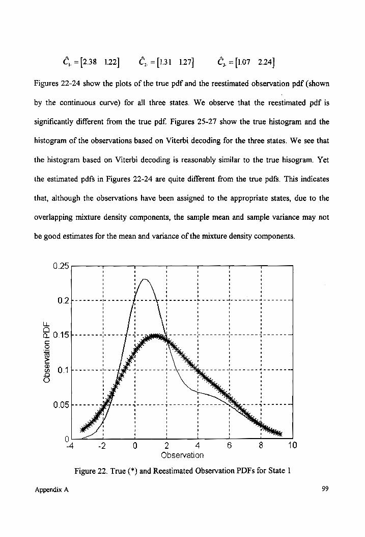
C,=[238 122] 9 C, =[131 127] C,.=[107 2.24]
Figures 22-24 show the plots of the true pdf and the reestimated observation pdf (shown
by the continuous curve) for all three states. We observe that the reestimated pdf is
significantly different from the true pdf. Figures 25-27 show the true histogram and the
histogram of the observations based on Viterbi decoding for the three states. We see that
the histogram based on Viterbi decoding is reasonably similar to the true hisogram. Yet
the estimated pdfs in Figures 22-24 are quite different from the true pdfs. This indicates
that, although the observations have been assigned to the appropriate states, due to the
overlapping mixture density components, the sample mean and sample variance may not
be good estimates for the mean and variance of the mixture density components.
0.25 ™— —
0.2f-------bo=--- toeseeecbeeeeedeceeedeecceey
" 3 a : Q 0.15t------- tone pig l------- Loe e---- 2 ---d-------
Ss x a 5 : ! ! 8 O.1----------- x -------4
© ! :
0.05}------ By ----4o-- eo ! jeveeeee
0 _ 4 = ! -4 -2 0 2 4 6 8 10
Observation
Figure 22. True (*) and Reestimated Observation PDFs for State 1
Appendix A 99
0.18
Ad UONENeSgO
i
4 i
i i
i i
i t
I '
' !
' '
‘ '
' '
' '
’ ’
t '
' '
' 1
t '
t t
' '
' ;
' ¥
' '
! i
' t
’ SON
' ‘
1 1
' '
' .t
Pats
qyr etre ssp
ayewea pen
mae, ar
F4 '
i '
’ i
' 7
’ '
1 !
t '
t ‘
' '
! '
t 1
2 '
' t
t '
’ '
i '
' '
‘ 4
1 ’
l I
' '
on '
’ '
' t
1)
' 1
’ eee
PTT TM TTT OTP
ae TT Py
as
' !
t ..
’ '
t ‘
t '
1 t
' i
' !
t '
' '
' '
’ ’
! '
' '
1 '
' '
emcee game denne
ee
wn else
we damm obseneb
snow
dtonan
! I
’ ’
] '
' t
' t
' t
' 1
t '
' '
' '
' '
' '
’ t
' '
t ee
wt et
mr gett
net eee epee
tee ens
' '
' '
1 '
' t
' 1
t t
t t
t !
' i
! ’
' t
l !
’ ’
t '
a '
' ’
' Perey
ttt
et rae
eS Bert terpenes
! '
t '
Ab '
' '
' '
t '
y 1
' t
1 ‘
' {
’ '
i '
' '
y= '
' 1
! '
t t
1 7K,
I t
t i
' '
! é
1
een
dee ee
ee tee
+...
! 1
' ’
t !
t Bet
' '
' ‘
' 1
1 Am
| '
' 1
' !
I '
' {
' '
t '
' i
' '
' '
' t
l 1
' '
1 '
! '
1 '
' i
t '
' !
’ ’
i L
——l,
l l
l i
ah
oy
N -
YD ©
gz Nn
Oo =
= =
CEO FD
OC ,
2 oO
©
1) ©
Oo 7)
©
12 10 6
Observation
4 -2
Figure 23. True (*) and Reestimated Observation PDFs for State 2
45
bee ee
wena bee ee he ee ene De eee apo
ee we
ow
10
ewe t erm eee em ee Pw ee ale
a
eee ee
fo ee
ee ee
ee rr ie
0.2}-----------------
15
O.1}-----------------
1
O
4dq UODeNeSqC
Observation
Figure 24. True (*) and Reestimated Observation PDFs for state 3
100 Appendix A
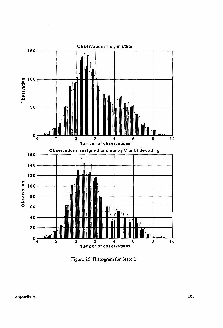
Observations truly in state 150
ill
ob So oS
Observation
an
oS
-4
|
-2
Observations assigned to state by Viterbi decoding
0 2 4 6 Number of observations
10
160
Lal 140
120
ok
So So
Observation
60 40 20
~4 -2
Appendix A
0 2 4 6
Number of observations
Figure 25. Histogram for State 1
10
101
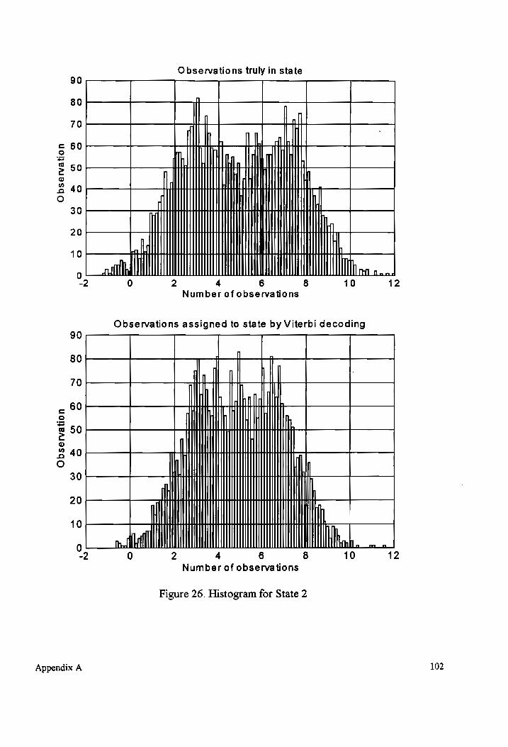
Observations truly in state 90
80
70
60 30
40
Observation
30
20
10 i | I TA non
0 2 4 6 8 10 12
Number of observations
Observations assigned to state by Viterbi decoding 90
80
70
60
50 40
Observation
30 20
10
Appendix A
2 4 6 8 10 12
Number of observations
Figure 26. Histogram for State 2
102
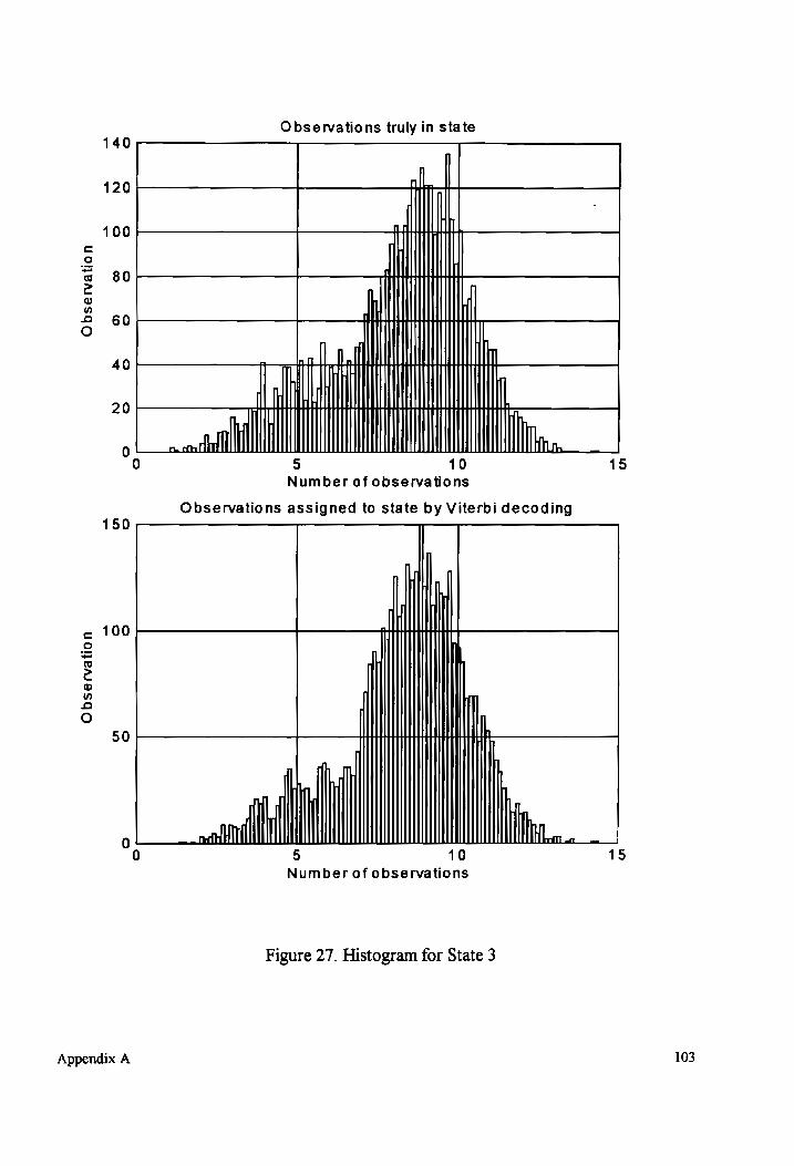
Observations truly in state 140
fl
120
100
80
Observation
60
40 20
n 7]
eri Wht
5 10 15
Number of observations
Observations assigned to state by Viterbi decoding 150
100
Observation
nn
oO
0
Appendix A
ll Mine 10 15
Number of observations
Figure 27. Histogram for State 3
103
APPENDIX B
We now present all the results obtained during testing of the performance of our recognition system. The results presented are for the training set and the testing set.
Table 9. Recognition rates for M = 1, S = 5 (training set).
Input words for recognition
Output | 0 1 2 3 4 5 6 7 8 9 0 49 | 0 0 0 0 0 0 0 0 0
1 0 | 49 1 0 0 0 0 0 0 0
2 0 0 | 48 { 0 0 0 0 0 0 0 3 0 0 0 50 | 0 0 0 0 0 0
4 0 0 0 0 50 | 0 0 0 0 0
5 0 0 0 0 0 49 |} 0 0 0 0
6 0 0 0 0 0 0 50 | 0 0 0
7 0 0 0 0 0 0 0 50 | 0 0
8 1 1 1 0 0 1 0 0 50 1 9 0 0 0 0 0 0 0 0 Oo | 49
Figure of merit = 494
Table 10. Recognition rates for M = 1, S = 5 (testing set).
Input words for recognition
Output | 0 1 2 3 4 5 6 7 8 9
0 49 0 0 0 0 0 0 0 0 0
1 0 47 1 0 0 0 0 0 0 0
2 0 1 46 0 0 0 0 0 0 0
3 0 0 0 50 0 0 0 0 0 0
4 0 2 2 0 49 0 0 0 0 0
5 0 0 0 0 0 50 0 0 0 0
6 0 0 0 0 0 0 49 0 0 0
7 0 0 0 0 0 0 0 50 0 0
8 1 0 1 0 1 0 1 0 50 2
9 0 0 0 0 0 0 0 0 0 48
Appendix B
Figure of merit = 488
104
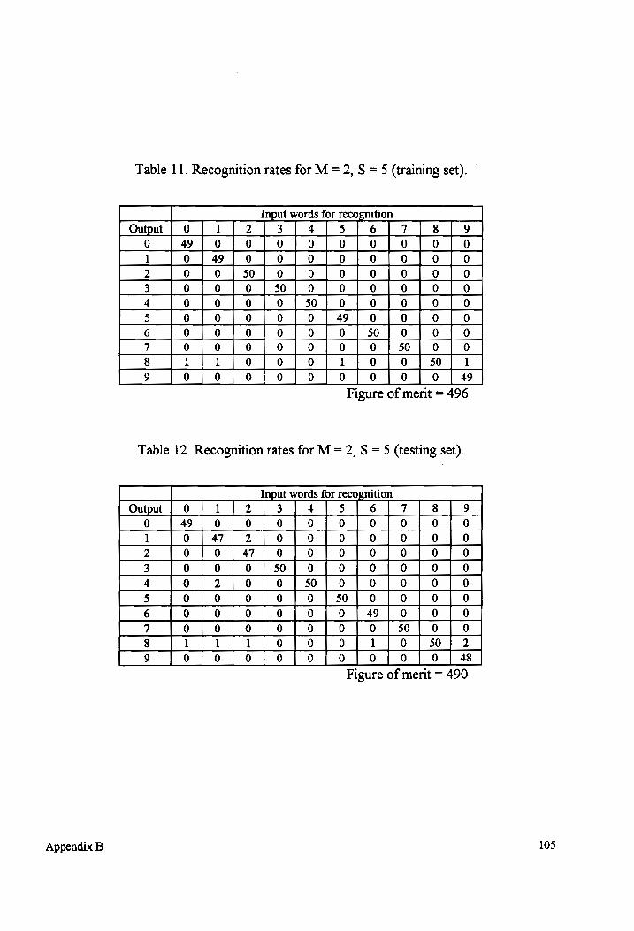
5 (training set). © =2,S= Table 11. Recognition rates for M
49
30
Input words for recognition
49
ut
a
Figure of merit = 496
5 (testing set). =2,S= Table 12. Recognition rates for M
Input words for recognition
48
50
49
Output
Figure of merit = 490
105 Appendix B
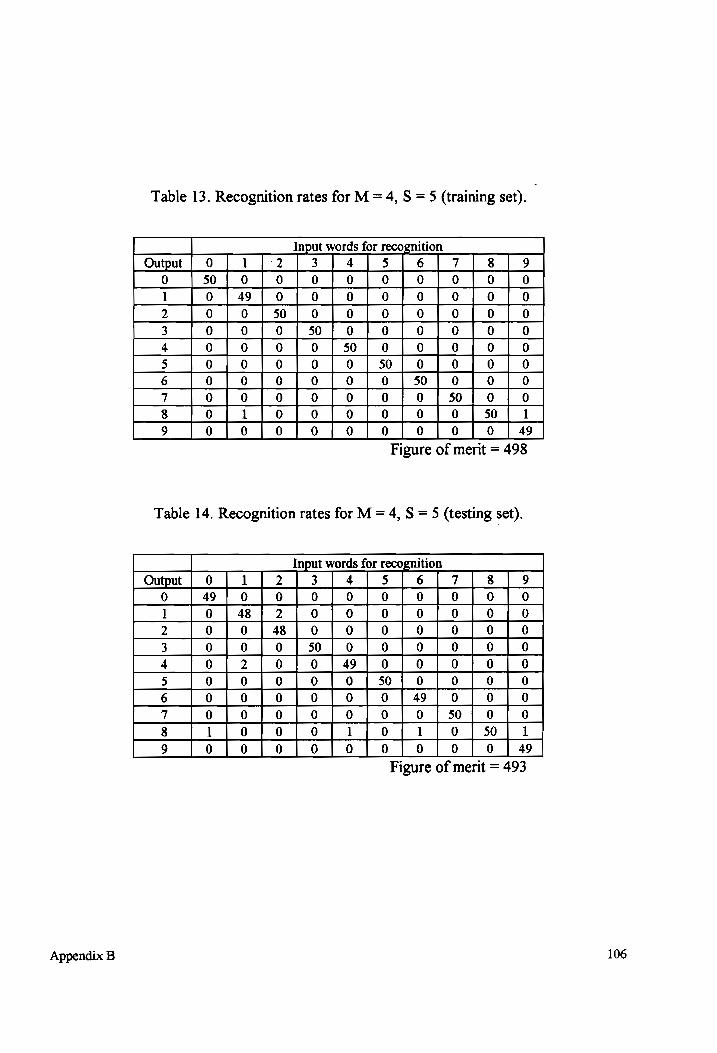
= 5 (training set). =4,S Table 13. Recognition rates for M
49
50
Input words for recognition
50
ut
a
Figure of merit = 498
=4,S= Table 14. Recognition rates for M
5 (testing set).
49
50
Input words for recognition
0 49
Output
Figure of merit = 493
106 Appendix B
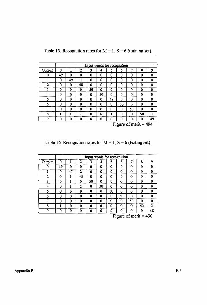
6 (training set). Table 15. Recognition rates for M = 1, S
49
50
Input words for recognition
49
ut
,
Figure of merit = 494
6 (testing set). Table 16. Recognition rates for M = 1, S
48
50
ition
Input words for reco
49
ut
Figure of merit = 490
107 Appendix B
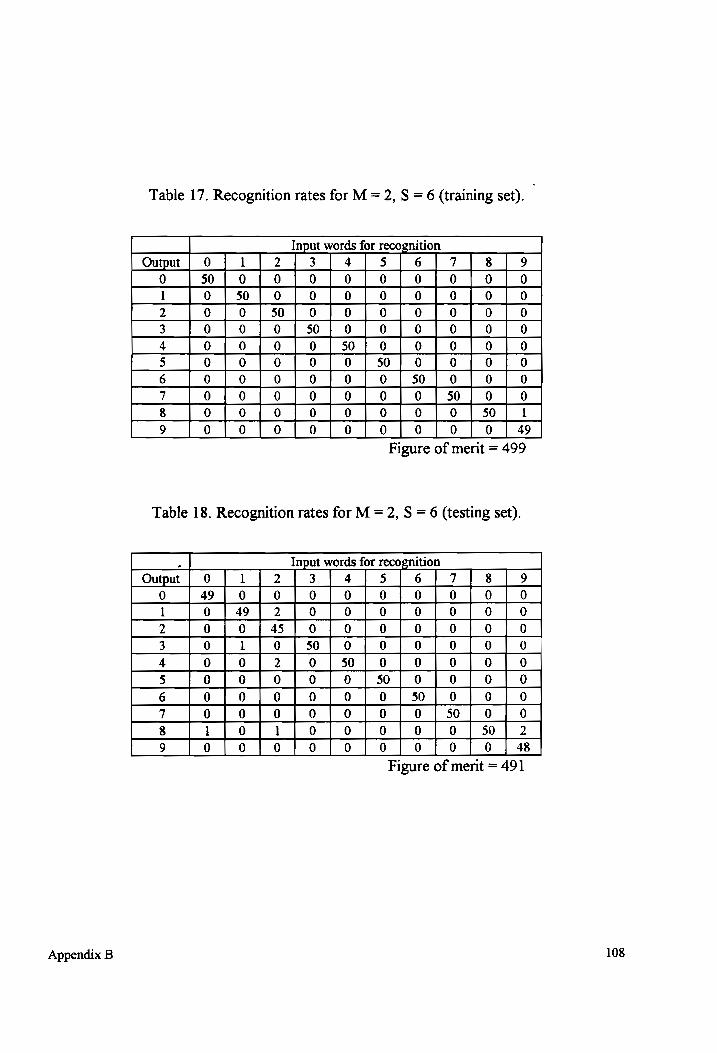
Appendix B
Table 17. Recognition rates for M = 2, S = 6 (training set).
Input words for recognition
Output | 0 1 2 3 4 5 6 7 8 9
0 50 0 0 0 0 0 0 0 0 0
1 0 50 0 0 0 0 0 0 0 0
2 0 0 50 0 0 0 0 0 0 0
3 0 0 0 50 0 0 0 0 0 0
4 0 0 0 0 50 0 0 0 0 0
5 0 0 0 0 0 50 | 0 0 0 0
6 0 0 0 0 0 0 50 0 0 0
7 0 0 0 0 0 0 0 50 0 0
8 0 0 0 0 0 0 0 0 50 1
9 0 0 0 0 0 0 0 0 0 49
Figure of merit = 499
Table 18. Recognition rates for M = 2, S = 6 (testing set).
Input words for recognition
Output | 0 1 2 3 4 5 6 7 8 9 0 49 0 0 0 0 0 0 0 0 0
1 0 49 2 0 0 0 0 0 0 0
2 0 0 45 0 0 0 0 0 0 0
3 0 1 0 350 | 0 0 0 0 0 0
4 0 0 2 0 50 0 0 0 0 0
5 0 0 0 0 0 50 | 0 0 0 0
6 0 0 0 0 0 0 50 | 0 0 0
7 0 0 0 0 0 0 0 50 0 0
8 1 0 1 0 0 0 0 0 50 2
9 0 0 0 0 0 0 0 0 0 48
Figure of merit = 491
108
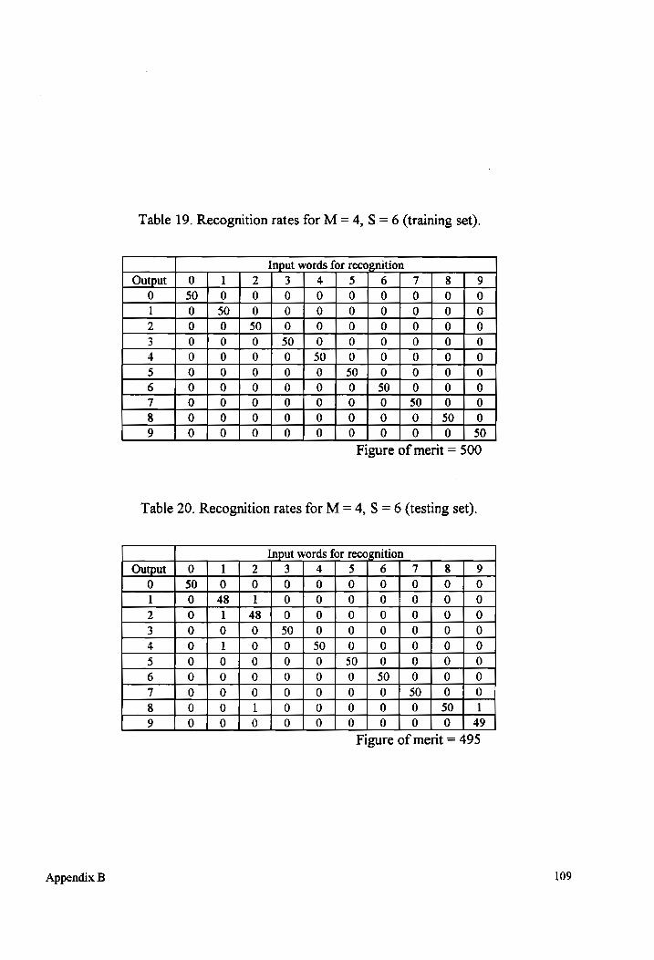
6 (training set). =4,S= Table 19. Recognition rates for M
ition Input words for reco
50
50
0
50
Output
Figure of merit = 500
= 6 (testing set). =4,8 Table 20. Recognition rates for M
ition Input words for reco
49
50
0
50
Output
Figure of merit = 495
109 Appendix B
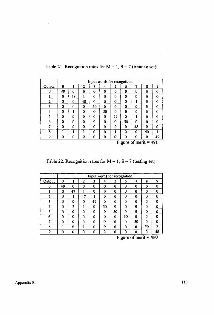
7 (training set). Table 21. Recognition rates for M= 1, S
49
50
Input words for recognition
0 49
Output
Figure of merit = 491
7 (testing set). Table 22. Recognition rates for M= 1, S
48
50
ition
Input words for reco
]
0
49
Output
Figure of merit = 490
110 Appendix B
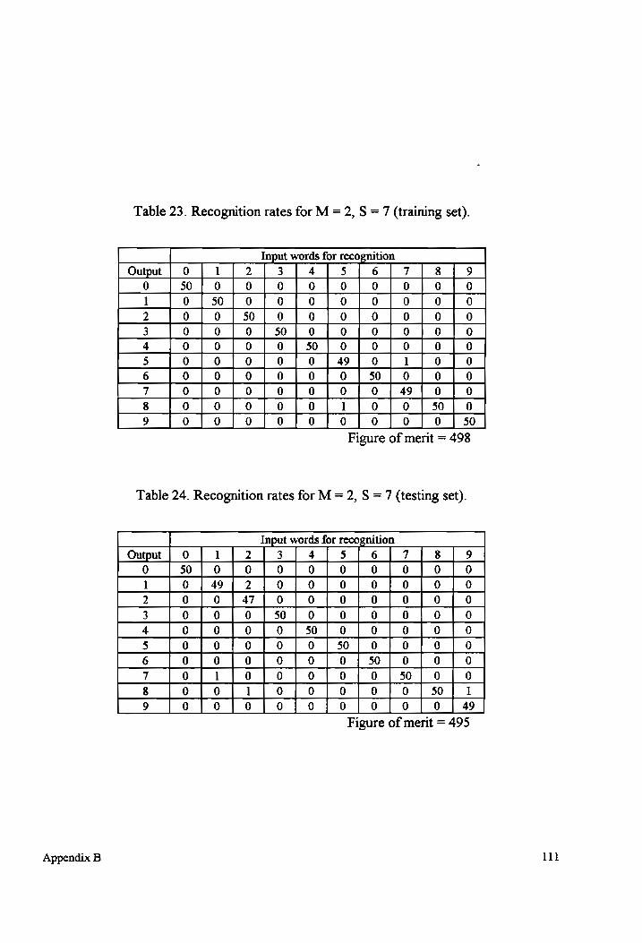
Appendix B
Table 23. Recognition rates for M = 2, S = 7 (training set).
Input words for recognition
Output | 0 1 2 3 4 5 6 7 8 9
0 50 | 0 0 0 0 0 0 0 0 0
1 0 350 | 0 0 0 0 0 0 0 0
2 0 0 50 0 0 0 0 0 0 0
3 0 0 0 50 0 0 0 0 0 0
4 0 0 0 0 50 0 0 0 0 0
5 0 0 0 0 0 49 | 0 1 0 0
6 0 0 0 0 0 0 50 | 0 0 0
7 0 0 0 0 0 0 0 49 0 0
8 0 0 0 0 0 1 0 0 50 0
9 0 0 0 0 0 0 0 0 0 50 Figure of merit = 498
Table 24. Recognition rates for M = 2, S = 7 (testing set).
Input words for recognition
Output | 0 1 2 3 4 5 6 7 38 9 0 50 | 0 0 0 0 0 0 0 0 0
1 0 49 | 2 0 0 0 0 0 0 0
2 0 0 47 | 90 0 0 0 0 0 0
3 0 0 0 50 | 0 0 0 0 0 0
4 0 0 0 0 50 0 0 0 0 0
5 0 0 0 0 0 50 | 0 0 0 0
6 0 0 0 0 0 0 50 | G 0 0
7 0 1 0 0 0 0 0 50 | 0 0
8 0 0 ] 0 0 0 0 0 50 1
9 0 0 0 0 0 0 0 0 0 | 49
Figure of merit = 495
111
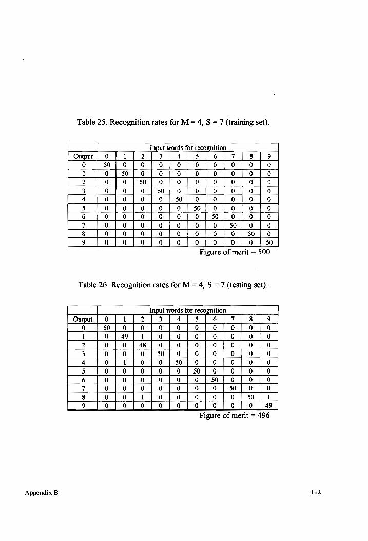
Appendix B
Table 25. Recognition rates for M = 4, S = 7 (training set).
Input words for recognition
Outpt | 0 | 1 | 2 [3 1 4[5]6/7/)8 719 0 sof ofofolf]ofolfotlolfot!lo 1 o | s50/ofofof]of]of]o0f]o0]0 2 o{[ofso{fofofofof{olfo [0 3 ofofofs0/ofofofofoT]o 4 o[ofofo{sfofot!]ot{o {[o 5 ofofofolfol]s{ofo!o !{o 6 o][ofofofofofs0/fofo [| o 7 o{[ofofojfofolfo]sol[o [ 0 8 o]|ofofofofol]ot]o =! solo 9 o[ofofofof{ofotl]ol]o { so
Figure of merit = 500
Table 26. Recognition rates for M = 4, S = 7 (testing set).
Input words for recognition
Output| o | 17273 /[4]5]6 [7 {383/19 0 5o{o0]o]o]ofo]o]o0]o0 | 0 1 o {| 49{[1]o0]o0fo0fo]o0]{0 1 0 2 0 {| of[4sfof]ofofol]o!{o{[o 3 o{[ofofso{lofofol]|{ol]|oT! o 4 o/1if]ofo0!fs0/o0f]o0fo0fo0]o0 5 o{f[ofof]ofot{solofo|o lo 6 o/ofofofofofso]o]{o {| o 7 o|ofofof{olfotl{o=t!]so{o]|o 8 o/[of1f{ofof]of]o]oT!{s0{41 9 o/[ofofofofolfot!lo={o {a9
Figure of merit = 496
112
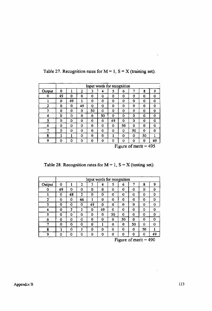
Table 27. Recognition rates for M = 1, S = X (training set).
Input words for recognition Output 0 1 2 3 4 5 6 7 8 9
0 49 | 0 0 0 0 0 0 0 0 0 1 0 49 1 0 0 0 0 0 0 0
2 0 0 49 0 0 0 0 0 0 0
3 0 0 0 50 0 0 0 0 0 0
4 0 0 0 0 50 0 0 0 0 0
5 0 0 0 0 0 49 0 0 0 0
6 0 0 0 0 0 0 50 0 0 0
7 0 0 0 0 0 0 0 50 0 0
8 1 1 0 0 0 1 0 0 | 50{ 1
9 0 0 0 0 0 0 0 0 0 49
Figure of merit = 495
Table 28. Recognition rates for M = 1, S = X (testing set).
Input words for recognition
Output | 0 1 2 3 4 5 6 7 8 9
0 49 | 0 0 0 0 0 0 0 0 0
1 0 | 48 | 2 0 0 0 0 0 0 0
2 0 0 | 46 1 0 0 0 0 0 0
3 0 0 0 | 49} 0 0 0 0 0 0
4 0 2 l 0 | 49 | 0 0 0 0 0
5 0 0 0 0 0 50 | 0 0 0 0
6 0 0 0 0 0 0 | 50; 0 0 0 7 0 0 0 0 1 0 0 50 0 0
8 1 0 1 0 0 0 0 0 50 1 9 0 0 0 0 0 0 0 0 0 49
Appendix B
Figure of merit = 490
113
Appendix B
Table 29. Recognition rates for M = 2, S = X (training set).
Input words for recognition
Output] 0 | 172/73 14/15 )]6/7+)]8i/19 0 so{o]ofofofolflofolfoljo l o [sol ofofofofotlflofolo 2 o|ofs0]0fof]ofofofol]o 3 o{[ofol]so{ofofofofof]o 4 0 |/o]ofo]|so0]o0]of]ofot!]o 5 o{|ofofofof{solofofo | o 6 o[ofolflofolflof{sol[ofol]|o 7 ofofofofolofot[so[o]o 8 o{[ofofofolfofo=Z[o [so] o 9 o[ofofofo]ol]of{fo]|o j 50
Figure of merit = 500
Table 30. Recognition rates for M = 2, S = X (testing set).
Input words for recognition
Output | 0 | 11273 {[4]s5)]6)]7)8 19 0 53 /o0f]ofofofoflofofolfo 1 o|49/2{[ofofo]of]o0]o0]o0 2 o|o|46/1{[o0]o0]o0]o0][o0T]0 3 o|oj]of49/ofof]of}otfotlo 4 o|ofi{of49/o0f]of]ofo!]o 5 o{|of1{o!ofsolofofo!]{o 6 o/[of]ofofolflolsolojfofo 7 o!ofofof1f]ofo/{s0{o [0 8 o{[1i1f]ofo]o]ofo0]o0]{s50] 1 9 0/|ofofofofolotlfo=t!|o {a9
Figure of merit = 492
114
Table 31. Recognition rates for M = 4, S = X (training set).
Input words for recognition .
Output {/ 0 {| 1 {2/3 | 4] 5 {[6{7]8 {9 0 50 | 0 0 0 0 0 0 0 0 0
1 0 | 50} 0 0 0 0 0 0 0 0
2 0 0 50 0 0 0 0 0 0 0
3 0 0 0 | 50 | 0 0 0 0 0 0 4 0 0 0 0 50 0 0 0 0 0
5 0 0 0 0 0 | 50] 0 0 0 0 6 0 0 0 0 0 0 50 0 0 0
7 0 0 0 0 0 0 0 | 50 | 0 0 8 0 0 0 0 0 0 0 0 50 0
9 0 0 0 0 0 0 0 0 0 | 50
Figure of merit = 500
Table 32. Recognition rates for M = 4, S = X (testing set).
Input words for recognition
Output | 0 1 2 3 4]5 | 6 |7 gs | 9 0 50/0]0]{0f]0f{]0)]0)]0{]07;0 1 0 | 49 | 3 0o|ofofot!|o 0 | 0 2 0|/0]46/]0]0f{]o0/f/0f0]0 {0 3 0o{o]}] 0 ] 50] 1 0o]}/0;]0]o0;] 0 4 0 | 0 1 01,49} 0{0]0{0/ 0 5 0o/o0};0f0]0 {50} 0 | o | 0 |] O 6 0o/o]o0of]o}o0 {0} 50] 0] 0 {| 0 7 o/o}o]o0o)]0f0] 0] 50] 0 | Oo 8 o{oj]of]of]o0f]o0f]0 fo; 50] 1 9 0 1 0o};o0fofo0fo0]0 1] 0 | 49
Figure of merit = 493
where S = X indicates that different number of states have been used for the different
digits according to the following table.
Table 33. Number of States in S = X
Digit 0 1 2 3 4 5 6 7 8 9
# States 18 7 10 10 10 10 7 7 15 14
Appendix B 115
[1]
[2]
[3]
[4]
[5]
[6]
[7]
[8]
[9]
[10]
[11]
[12]
Bibliography
J. L. Flanagan, Speech, Analysis Synthesis and Perception, Springer-Verlag, 1983.
Lawrence R. Rabiner, Jay G. Wilpon, and Frank K. Soong, High Performance Connected Digit Recognition Using Hidden Markov Models, TEEE Transactions
on Acoustics, Speech, and Signal Processing, vol. 37, no. 8, pp. 1214-1225, Aug. 1989.
John R. Deller Jr., John G. Proakis, and John H. L. Hansen, Discrete Time
Processing of Speech Signals, Macmillan, 1993.
Geoff Bristow, Electronic Speech Recognition, Collins, 1986.
W. A. Ainsworth, Speech Recognition By Machine, Peter Peregrinus Ltd., 1988.
L. R. Rabiner and M. R. Sambur, Speech Endpoint Algorithm, Bell System Technical Journal, vol. 54, pp. 302-315, Feb. 1975.
Alan V. Oppenheim and R. W. Schafer, Discrete Time Processing of Signals, Prentice Hall, 1975.
Leland B. Jackson, Digital Filters and Signal Processing, Kluwer Academic
Publishers, 1996.
S. B. Davis and P. Mermelstein, Comparison of parametric representations for monosyllabic word recognition in continuously spoken sentences, TEEE Transactions on Acoustics, Speech, and Signal Processing, vol. 28, pp. 357-366,
Aug. 1980.
B. S. Atal, Effectiveness of Linear Prediction characteristics for speech
recognition, JASA, vol. 55, no. 6, pp. 1304-1312, June 1974.
C. S. Myers, L. R. Rabiner, and A. E. Rosenberg, Performance tradeoffs in dynamic time warping algorithms for isolated word recognition, IEEE
Transactions on Acoustics, Speech, and Signal Processing, vol. 28, pp. 622-635, Dec. 1980.
J. K. Baker, Stochastic modeling for automatic speech understanding, In D. R.
Reddy, ed., Speech Recognition, New York: Academic Press, pp. 521-542, 1975.
Bibliography 116
[13]
[14]
[15]
[16]
[17]
[18]
[19]
[20]
[21]
[22]
[23]
[24]
F. Jelinek, L. R. Bahl, and R. L. Mercer, Design of a linguistic statistical decoder for the recognition of continuous speech, IEEE Transactions on Information Theory, vol. 21, pp. 250-256, May 1975.
L. R. Rabiner, B. H. Juang, S. E. Levinson, and M. M. Sondhi, Some properties of Continuous Hidden Markov Model Representations, AT&T Technical Journal, vol. 64, no. 6, pp. 1251-1270, July-Aug. 1985.
J. Picone, Continuous speech recognition using hidden Markov Models, IEEE
Acoustics, Speech, and Signal Processing Magazine, vol. 7, pp. 26-41, July 1990.
L. E. Baum, T. Petrie, G. Soules, A maximization technique occurring in
statistical analysis of probabilistic functions of Markov chains, Ann. Math. Stat., vol. 41, no. 1, pp. 164-171, 1970.
L. E. Baum and G. R. Sell, Growth functions for transformations on manifolds, Pacific Journal of Mathematics, vol. 27, pp. 211-227, 1968.
L. R. Rabiner, B. H. Juang, S. E. Levinson, and M. M. Sondhi, Recognition of isolated digits using hidden Markov models with continuous mixture densities, AT&T Technical Journal, vol. 64, pp. 1211-1234, July-Aug. 1985.
J. Makhoul, S. Roucos, and H. Gish, Vector quantization in speech coding, Proceedings of the IEEE, vol. 73, pp. 1551-1588, Nov. 1985.
S. S. Rao, Optimization Theory and Applications, Wiley-Eastern Ltd. 1984.
B. H. Juang and L. R. Rabiner, A probabilistic distance measure for hidden Markov models, AT&T System Technical Journal, vol. 64, pp. 391-408, Feb. 1985.
R. Bakis, Continuous speech word recognition via centisecond acoustic States, Proceedings of the 91st Annual Meeting of the Acoustical Society of America, Washington, D.C., 1976.
L. R. Rabiner and S. E. Levinson, A speaker-independent, syntax-directed, connected word recognition system based on hidden Markov models and level
building, TEEE Transactions on Acoustics, Speech, and Signal Processing, vol. ASSP-33, no. 3, pp. 561-573, June 1985.
L. R. Rabiner, A Tutorial on Hidden Markov Models, TEEE Proceedings, vol. 77, pp. 257-285, Feb. 1989.
Bibliography 117
[25] Y. Tokhura, A weighted cepstral distance measure for speech recognition, TEEE
Transactions on Acoustics, Speech, and Signal Processing, vol. 35, pp. 1414-1422, Oct. 1987.
[26] K.A. Rangarajan, Discrete HMM isolated digit recognition, M.S. Thesis, Virginia
Polytechnic Institute and State University, Blacksburg, Virginia 24061, July 1996.
Bibliography 118
Vita
Ananth Padmanabhan graduated from the Regional Engineering College, Calicut, India,
with a Bachelor degree in Electrical Engineering in 1994. He attended Virginia
Polytechnic Institute and State University in Blacksburg, Virginia, completing a Masters
of Science in Electrical Engineering specializing in telecommunications in 1996. His
research interests are in the area of digital signal processing. He is employed as an
Engineer in the Systems Engineering Division with Qualcomm Inc. located in San Diego,
California.
CL fhe aataeathe.
“
119