Centre for Vision Speech & Signal ProcessingUniversity of Surrey, Guildford GU2 7XH.

HMM tutorial 1by Dr Philip Jackson

• Fundamentals• Markov models• Hidden Markov models

- Likelihood calculation- Optimum state sequence (Viterbi)- Re-estimation (Baum-Welch)

• Output probabilities• Extensions and applications

http://www.ee.surrey.ac.uk/Personal/P.Jackson/tutorial/

Fundamentals

• Least-squares parameter estimation

• Likelihood equation and ML estimation

• Bayes’ theorem and MAP

• Discrete vs. continuous observations

• Probability distribution functions

2

Scientific inference

Steps of scientific investigation:

1. develop experimental apparatus

2. perform measurements

3. analyse data

Levels of inference:

1. parameter estimation

2. classification

3. recognition

3

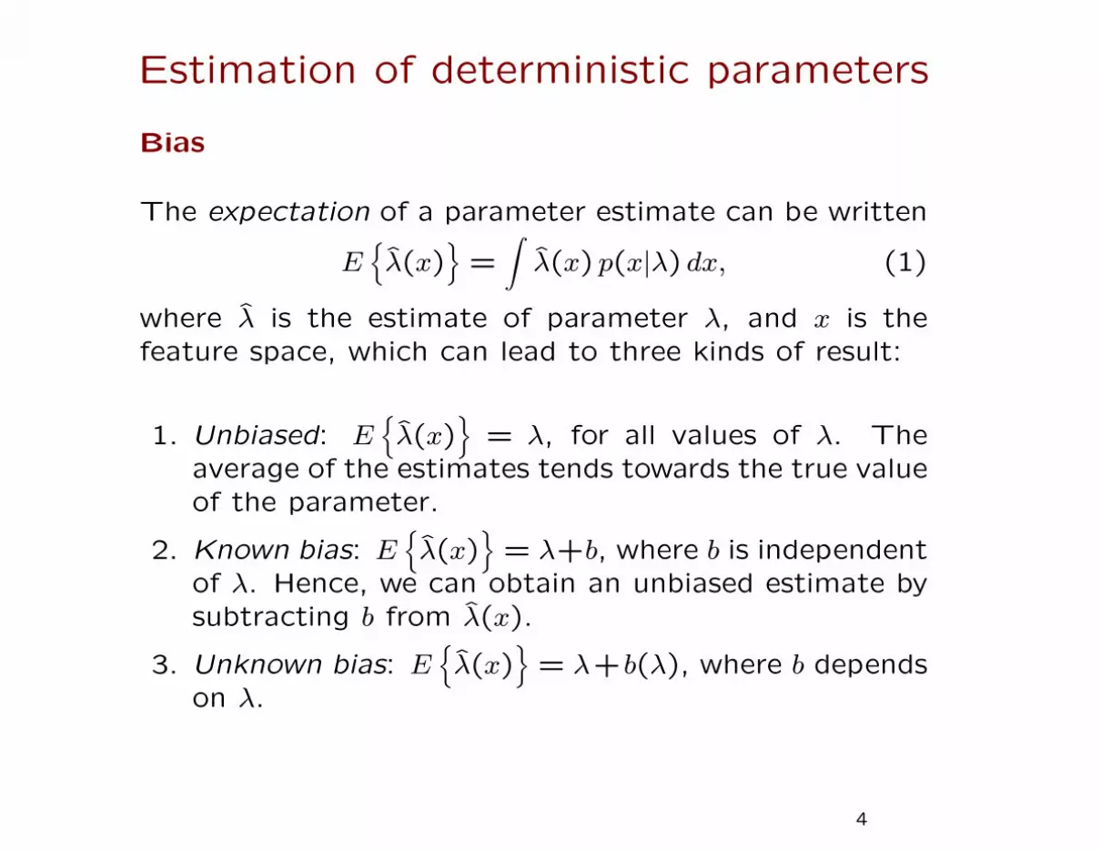
Estimation of deterministic parameters

Bias

The expectation of a parameter estimate can be written

E{λ̂(x)

}=

∫λ̂(x) p(x|λ) dx, (1)

where λ̂ is the estimate of parameter λ, and x is thefeature space, which can lead to three kinds of result:

1. Unbiased: E{λ̂(x)

}= λ, for all values of λ. The

average of the estimates tends towards the true valueof the parameter.

2. Known bias: E{λ̂(x)

}= λ+b, where b is independent

of λ. Hence, we can obtain an unbiased estimate bysubtracting b from λ̂(x).

3. Unknown bias: E{λ̂(x)

}= λ+b(λ), where b depends

on λ.

4

Variance

The variance of the estimation error,

var[λ̂(x)− λ

]= E

{[λ̂(x)− λ

]2}− b2(λ), (2)

describes the spread of the error.

In general, we want unbiased estimates with minimum

variance, but no simple procedure exists to find them.

However, one approach to improving the quality of our

estimates is to use maximum likelihood.

5

Maximum likelihood

Motivation for the most likely

Consider these two different probability distribution func-

tions (pdfs):

1

2

o

p(o)

6

Maximum likelihood estimation

We try to use as our estimate the value of λ that most

likely caused a given value of o to occur. We denote the

value obtained by using such a procedure as a maximum

likelihood (ML) estimate, λ̂ML(o). The ML estimate is

obtained by differentiating ln p(o|λ) with respect to λ and

setting the result equal to zero:

∂Lo(λ)

∂λ=

∂ ln p(o|λ)

∂λ= 0. (3)

This equation is called the likelihood equation.

7

Bayesian inference

Value of prior knowledge

Let us suppose there are two conditional pdfs, as follows:

12

o

p(o,i)

8

Conditional probability

Now imagine two dependent events:

Event AEvent B True False

True 0.1 0.3False 0.4 0.2

The probability of both events occurring can be ex-pressed as

P (A, B) = P (A)P (B|A), (4)

but also as

P (A, B) = P (A|B)P (B). (5)

which leads us to the theorem proposed by Rev. ThomasBayes (C.18th).

9

Bayes’ theorem

Equating the RHS of eqs. 4 and 5 gives

P (B|A) =P (A|B)P (B)

P (A), (6)

which can be interpreted as

posterior =likelihood× prior

normalisation factor. (7)

10

Interpretation

Consider the occurrence of entities λ and O,

p(λ|O) =p(O|λ) p(λ)

p(O), (8)

where O denotes a series of measured or observed data,

and λ comprises a set of model parameters.

p(λ|O) is the posterior probability

p(O|λ) is the likelihood

p(λ) is the prior probability

p(O) is the evidence

11

Discrete and continuous pdfs

Discrete probability distribution functions

Continuous probability distribution functions

12

Markov models

Ergodic model:

21

3

For a first-order discrete-time Markov chain, probability

of state occupation depends only on the previous step:

P (xt = j|xt−1 = i, xt−2 = h, . . .) = P (xt = j|xt−1 = i).

(9)

13

Modelling stochastic time series

Left-right Markov model:

1 2 3 4

If we assume that the RHS of eq. 9 is independent of

time, we can express the state-transition probabilities,

aij = P (xt = j|xt−1 = i), 1 ≤ i, j ≤ N, (10)

with the properties

aij ≥ 0, andN∑

j=1

aij = 1. (11)

14

Weather predictor example of a Markov model

State 1: rainState 2: cloudState 3: sun

1 2

3

0.4 0.6

0.8

0.10.3

0.2

0.3

0.20.1

State-transition probabilities,

A ={aij

}=

0.4 0.3 0.30.2 0.6 0.20.1 0.1 0.8

(12)

15

Weather predictor calculation

Given today is sunny (i.e., x1 = 3), what is the probabil-

ity of “sun-sun-rain-cloud-cloud-sun” with model M?

P (X|M) = P (X = {3,3,1,2,2,3}|M)

= P (x1 = 3)P (x2 = 3|x1 = 3)

P (x3 = 1|x2 = 3)P (x4 = 2|x3 = 1)

P (x5 = 2|x4 = 2)P (x6 = 3|x5 = 2)

= π3 a33 a31 a12 a22 a23

= 1 · (0.8)(0.1)(0.3)(0.6)(0.2)

= 0.00288

where the initial state probability for state i is

πi = P (x1 = i). (13)

16

State duration probability

As a consequence of the first-order Markov model, the

probability of occupying a state for a given duration, τ ,

is exponential:

p(X|M, x1 = i) = (aii)τ−1 (1− aii) . (14)

0 5 10 15 200

0.05

0.1

0.15

0.2

duration

prob

abili

ty

a11

= 0.8

17

Summary of Markov models

1 2 3 4

Transition probabilities:

A ={aij

}=

0.6 0.4 0 0

0 0.9 0.1 00 0 0.2 0.80 0 0 0.5

and π = {πi} =[

1 0 0 0].

Probability of a given state sequence X:

P (X|M) = πx1 ax1x2 ax2x3 ax3x4 . . .

= πx1

T∏t=2

axt−1xt. (15)

18

Hidden Markov Models

Urns and balls example (Ferguson)

21

3

b1 b2

b3

Probability of state i producing an observation ot is:

bi(ot) = P (ot|xt = i), (16)

which can be discrete or continuous in o.

19

Elements of a discrete HMM, λ

1. Number of states N , x ∈ {1, . . . , N};

2. Number of events K, k ∈ {1, . . . , K};

3. Initial-state probabilities,

π = {πi} = {P (x1 = i)} for 1 ≤ i ≤ N ;

4. State-transition probabilities,

A = {aij} = {P (xt = j|xt−1 = i)} for 1 ≤ i, j ≤ N ;

5. Discrete output probabilities,B = {bi(k)} = {P (ot = k|xt = i)} for 1 ≤ i ≤ N

and 1 ≤ k ≤ K.

20

Hidden Markov model example

a45π1

a11 a22 a33 a44

a34a23a12

o1 o2 o3 o4 o5 o6

b (o )11

b (o )21

b (o )32

b (o )43

b (o )53

b (o )64

1 2 43

with state sequence X = {1,1,2,3,3,4},

P (O|X, λ) = b1(o1) b1(o2) b2(o3) b3(o4) b3(o5) b4(o6)

P (X|λ) = π1 a11 a12 a23 a33 a34 (17)

P (O, X|λ) = π1b1(o1) a11b1(o2) a12b2(o3) . . . (18)

21

Continuous output probabilities

For a Gaussian pdf, the output probability of an emitting

state, xt = i, is

bi(ot) = N (ot;µi,Σi), (19)

where N (·) is a multivariate Gaussian pdf with mean

vector µi and covariance matrix Σi, evaluated at ot,

bi(ot) =

1√(2π)M |Σi|

exp(−

1

2(o− µi)

′Σ−1i (o− µi)

)(20)

where M is the dimensionality of the observed data o.

22

HMM as observation generator

1. Initialise t = 1;

2. If t = 1, choose state x1 using πi;

Else, transit to xt according to aij;

3. Choose ot = k according to bj(k);

4. Increment t, and repeat from 2 until t > T .

23

Today’s summary

• Fundamentals:

– Least-squares and ML estimation

– Bayes’ theorem and MAP

– Discrete vs. continuous pdfs

• Markov models

• Hidden Markov models

24

Three HMM problems for next time

1. Compute P (O|λ);

2. Find best X;

3. Re-estimate models Λ = {λ}.

Further reading

L. R. Rabiner. A tutorial on HMM and selected applica-

tions in speech recognition. In Proc. IEEE, Vol. 77,

No. 2, pp. 257–286, 1989.

25