Reprinted from I~EC Vol. 61, December 1969 Copyright 1969 b ' Pages 14-28 S . y the Am . oClety and reprinted b enc.an. Chemical the copyright owner y permission of

General theory of creep flow is proposed which indicates permeability

tensor can be represented in terms of only four scalar constants

Advances in Theory of

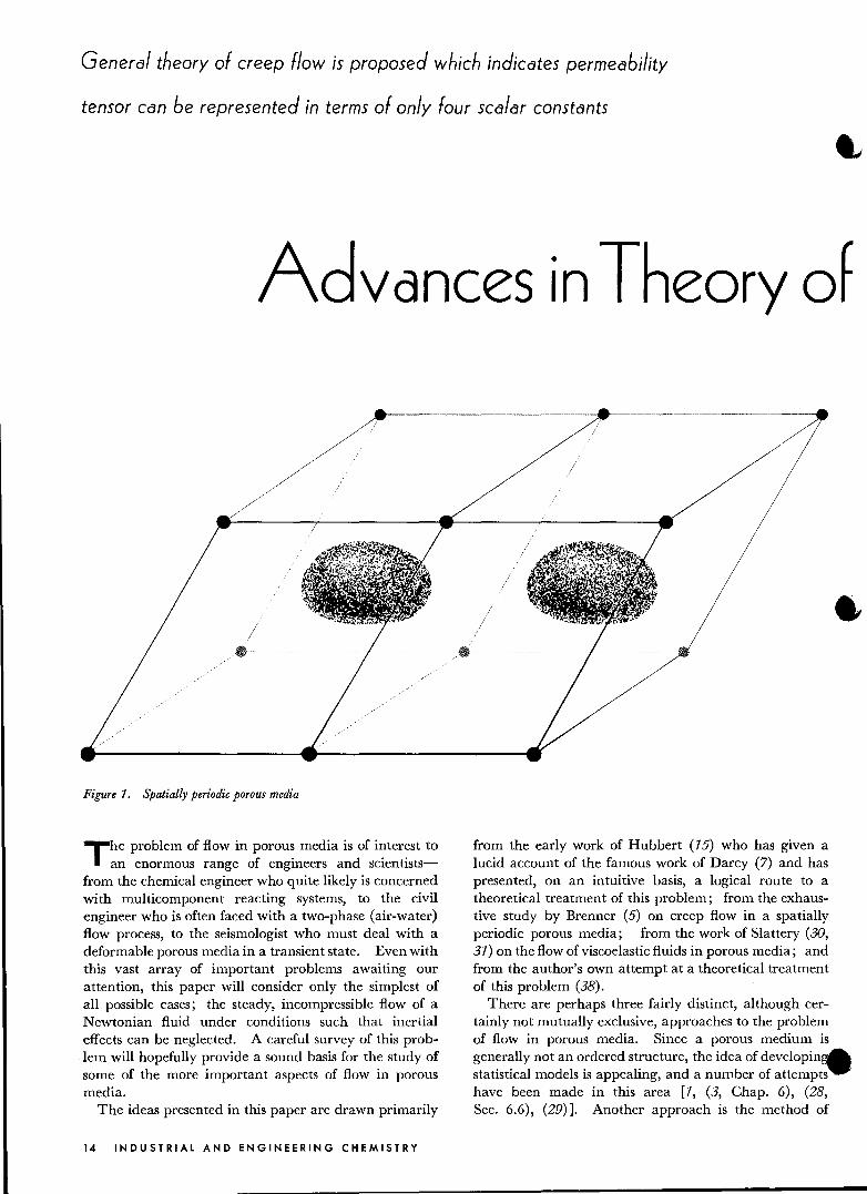
Figure 1. Spatially periodic porous media

T he problem of flow in porous media is of interest to an enormous range of engineers and scientists­

from the chemical engineer who quite likely is concerned with multicomponent reacting systems, to the civil engineer who is often faced with a two-phase (air-water) flow process, to the seismologist who must deal with a deformable porous media in a transient state. Even with this vast array of important problems awaiting our attention, this paper will consider only the simplest of all possible cases; the steady, incompressible flow of a Newtonian fluid under conditions such that inertial effects can be neglected. A careful survey of this prob-

.lem will hopefully provide a sound basis for the study of some of the more important aspects of flow in porous media.

The ideas presented in this paper are drawn primarily

14 INDUSTRIAL AND ENGINEERING CHEMISTRY

from the early work of Hubbert (75) who has given a lucid account of the famous work of Darcy (7) and has presented, on an intuitive basis, a logical route to a theoretical treatment of this problem; from the exhaus­tive study by Brenner (5) on creep flow in a spatially periodic porous media; from the work of Slattery (30, 37) on the flow of viscoelastic fluids in porous media; and from the author's own attempt at a theoretical treatment of this problem (38).

There are perhaps three fairly distinct, although cer­tainly not mutually exclusive, approaches to the problem of flow in porous media. Since a porous medium is generally not an ordered structure, the idea of developin~ statistical models is appealing, and a number of attempts have been made in this area [7, (3, Chap. 6), (28, Sec. 6.6), (29)]. Another approach is the method of

FLOW THROUGH POROUS MEDIA SYMPOSIUM

Fluid Motion in Porous Media

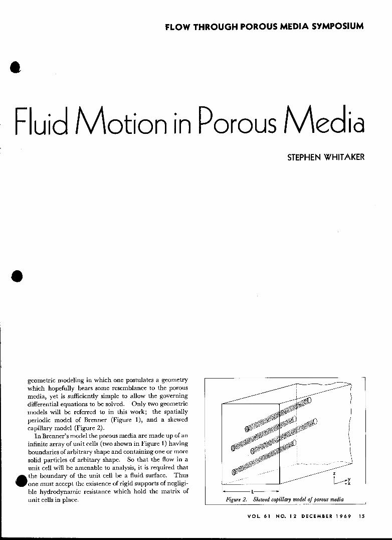
geometric modeling in which one postulates a geometry which hopefully bears some resemblance to the porous media, yet is sufficiently simple to allow the governing differential equations to be solved. Only two geometric models will be referred to in this work; the spatially periodic model of Brenner (Figure 1), and a skewed capillary model (Figure 2).

In Brenner's model the porous media are made up of an infinite array of unit cells (two shown in Figure 1) having boundaries of arbitrary shape and containing one or more solid particles of arbitary shape. So that the flow in a unit cell will be amenable to analysis, it is required that

_ the boundary of the unit cell be a fluid surface. Thus • one must accept the existence of rigid supports of negligi­

ble hydrodynamic resistance which hold the matrix of unit cells in place.

STEPHEN WHITAKER

I, .1 Figure 2. Skewed capillary model of porous media

VOL 6 1 N O. 1 2 0 E C E M B E R 1 9 6 9 15

The skewed capillary model shown in Figure 2 is a minor variation of the well-known straight capillary model (28, page 114), but it cannot be obtained from that model by a simple transformation of coordinates because the boundary conditions, which may be imposed on the flow, also change under a coordinate transforma­tion. A third approach, which lies somewhere between statistical models and geometric models, is the develop­ment of correct averaged forms of the governing differ­ential equations. These equations should be valid for any geometry, thus the results obtained for specific geometric models must satisfy the averaged equations. In addition, any statistical model should be in accord with the averaged equations. All three methods lead to unspecified param­eters which must be determined experimentally, and the primary objective of theoretical work in this general area is to aid in the interpretation of experimental data.

In attacking the problem of incompressible flow in porous media, one is confronted with the fact that the final result is pretty well established-i.e., Darcy's law gives an accurate description of the flow. Because of this, it is easy to proceed along a variety of ap­proaches, some of which might well be erroneous or wholly intuitive, to the correct final result. We will try to avoid this pitfall in the present study and establish as carefully as possible a logical, correct route to the final result.

1. The Problem

We are concerned here with the incompressible, creep flow of a constant viscosity Newtonian fluid in a rigid porous media. The equations governing this process are:

1. The continuity equation

v . V = ° (1-1)

The velocity, V, and position vector, r, are measured relative to an inertial frame imbedded in the porous media; thus the porous media may move with a con­stant velocity, U, relative to a frame that is stationary with respect to the fixed stars.

2. The equations of motion

° = - Vp + pg + JJ.V2v (1-2)

The restriction of constant viscosity is imposed by the form of Equation 1-2.

3. The void volume distribution function

( ) = {1, if r lies in the fluid region a r 0, if r lies in the solid region

(1-3)

If the function a(r) were known it would be possible, in principle, to solve the governing equations and thus determine completely the pressure and velocity fields. However, a(r) is never known and we are obviously forced into a different type of analysis-i.e., a derivation of the volume averaged equations. In this approach we associate with every point in space an averaging

16 INDUSTRIAL AND ENGINEERING CHEMISTRY

volume V which contains a volume of fluid V f. The volume porosity is given by

(1-4)

or more explicitly in terms of the void volume distri- -bution function

cp = _1 r a(r)dV V Jv (1-5)

Throughout this work we will require that the averaging volume be constant in time and space; however, the magnitude of the fluid volume V f may vary with position subject to certain restrictions to be discussed later.

Before attacking the problem at hand-i.e., obtaining the averaged forms of the governing equations-we must establish some ideas about area and volume averages and what is meant by a "meaningful average," and we must develop an averaging theorem to relate averages of derivatives to the derivatives of averages.

2. Averages In treating problems of flow in porous media, we

assume that some microscopic characteristic length, d, exists which is representative of the distance over which significant variations in the point velocity, V, take place. Similarly, we designate the macroscopic characteristic length as L, and assume it is representative of the dis­tance over which significant variations in the volume averaged velocity, (v), take place. In general, one associates d with the poorly defined but intuitively A appealing mean pore diameter, and L with some .. macroscopic dimension representative of the process under consideration. In Darcy's original work one would consider d to be on the order of magnitude of the "diameter" of the sand grains used in the filter, while L would be associated with the diameter of the filter bed.

Letting if; be some point quantity (tensor of any order) associated with the fluid (velocity, density), we define the volume average of if; as

(if;) = ~ r if;dV V Jv! (2-1)

One can now ask whether the average (if;) is a function that is suitable to use in analyzing flow in porous media. If we were to plot (if;) versus V we might obtain a function similar to that in Figure 3. Such a curve would be obtained if the point associated with V was in the solid region; thus V f would be zero for small values of V. As V becomes larger, portions of the fluid are contained within V and the average increases from zero going through some fluctuations representative of the varia­tions in the point value of if;. For values of V larger than V* the microscopic variations in if; are essentially smoothed out, but the value of (if;) need not become con­stant. It should be clear that (if;) is a continuous func- _ tion for any value of V, but for values of V larger than _ V* the volume average (if;) becomes "smooth," and thus amenable to the type of analysis we have in mind.

Figure 3. Dependence of average on averaging volume

If we let l be a characteristic length for the averaging volume, we can impose our first restriction (throughout this paper restrictions will be denoted by R.1, R.2, and assumptions by A.1, A.2, and so forth).

R.1

In addition to this restriction we will require that the average of the average be equal to the average, a concept perhaps more dearly expressed by

(2-2)

This is an important restriction, for it must be true if the average is to be a useful quantity with which to work. A similar situation occurs in the time averaging of turbulent fields (39, pp 187, 209). In considering (1/;), we note that it is defined everywhere in space, not just in the space occupied by the fluid. Thus the proper average of this function is given by

«I/;» = _1 r (l/;)dV V Jv

(2-3)

For convenience only, we choose the point with which we associate (I/;) to be the centroid of V and expand (I/;) in a Taylor series (32, p 228) choosing the centroid as the origin of our coordinate system. (Here Xi is the position vector in index notation. Repeated indices are summed from 1 to 3.)

(2-4)

Here the subscript zero indicates that the function is evaluated at Xi = O. Forming the average of (I/;) indicated by Equation 2-3 yields

(2-5)

The linear term in Equation 2-4 has dropped out since Xi

is measured from the centroid of V, thus

Iv XidV = 0 (2-6)

If (I/;) is a linear function of Xi> Equation 2-2 is immedi­ately satisfied; however, we wish to consider a some­what more general case.

An order of magnitude estimate of the first integral in Equation 2-5 can be expressed as,

_1_ r xixjdV = 0 ([2) V Jv (2-7)

and the order of magnitude estimate for the second derivative of (I/;) is given by

( 02(1/;») = 0 «I/;)/V)

ox/ox} 0

(2-8)

Neglecting the higher order terms in Equation 2-5, we express the average of the average as

«I/;» = (I/;) + O[(I/;)(l/L)2] (2-9)

Clearly our analysis must be bound by the restriction

R.2

in order that Equation 2-2 be satisfied.

AREA AVERAGES

Subject to restriction R.2, it will be of interest to com­pare area averages with volume averages to determine any possible differences between the area and volume averaged forms of the basic equations. To make a com­parison, it is necessary to choose an averaging volume V which can bound a plane averaging area Au .k) such that the area is always constant. As an example, we choose V to be a cube of volume [3 and AU,k) to be an area of magnitude [2 parallel to the (j, k) plane. We let the center of the cube be the origin of our coordinate system, the sides of the cube being orthogonal to the coordinate axes. The area average of I/; at the origin is given by

1I0U,k) = _1_ r I/;dA AU,k) J AI

(2-10)

Here A, represents the fluid area contained within A(j,k), the dependence of A, on the particular coordinate surface under consideration being understood. The volume average can now be expressed as

1 iXC') = + 1/2 (1/;)0 = - lIU,k)dx(i)

l XC') = - 1/2

where (i), (j), and (k) are distinct. if;U,k) in a Taylor series in X (ih we obtain

(2-11 )

If we expand

(2-12)

VOL. 6 1 N O. 1 2 0 E C E M B E R 1 9 6 9 1 7

where the summation convention does not apply to indices in parentheses. Substituting Equation 2-12 into Equation 2-11 and evaluating the integrals yield

(2-13)

Estimating the order of magnitude of the second deriva­tive as

(CA/(J,k») -2- = O(if;U,k)/V)

OX (t) 0

(2-14)

we can express Equation 2-13 as

(2-15)

Thus if our analysis is to be restricted by I « L, it follows that volume and area averages are essentially equivalent.

It is of some interest to apply this result to the void volume distribution function, a, which leads us to

(a) ~ c':u ,k) (2-16)

Since the volume average of a is the volume porosity, <P, while the area average is the plane porosity, we find that our restriction I «L requires the volume porosity be essentially equal to the three plane porosities

(2-17)

This relation between the porosities applies in general to anisotropic porous media; however, it is not necessarily valid for a highly structured porous media in which the order of magnitude estimate given by Equation 2-14 might not apply to aU ,k). Note that if porous media are homogeneous or uniform, Equation 2-17 takes the form

<P = a(1,2) = a(2.3) = a(3,1) (2-18)

regardless of whether or not the medium is isotropic.

3. SlaHery's Averaging Theorem

Up to this point we have been discussing the averaging of some point function if;; however, in developing the averaged form of the basic equations we will be dealing

AUTHOR Stephen Whitaker is Associate Professor in the Department of Chemical Engineering, University of California, Davis, CalzJ. This work was supported by the National Science Foundation, Grant GK-477. The author also acknowl­edges the courtesy of the hand-written notes made available to him by Professor Howard Brenner, Carnegie-Mellon Univer­sity, and the helpful discussions with Professor J. C. Slattery, Northwestern University. This paper was presented as part of the Symposium on Flow Through Porous Media, The Carnegie Institution, Washington, D.C., June 9-17, 7969.

18 INDUSTRIAL AND ENGINEERING CHEMISTRY

with gradients of point functions, and we need to explore the problem of averaging gradients of functions for we are interested in obtaining gradients of averages rather than averages of gradients.

A general relationship between gradients of averages and averages of gradients for functions defined in both the solid and the liquid phase and suffering a jump dis­continuity at the phase interface has been presented by the author (36); however, the result (37) is not available in the readily accessible literature, and furthermore the development is a rather heavy-handed one. A similar result has been obtained by Slattery (30) for functions defined in the fluid phase by a rather ingenious applica­tion of the general transport theorem [(35, p 347), (39, p 88)]. Since the original presentation given by Slattery is rather terse, and since the development has value in the analysis of more complex systems than the one treated here, we will present a detailed version of the theoretical development.

The general transport theorem can be written as

d i i oif; f - ifidV = - dV + if;w·ndA dt Vet) Vet) ot A(t)

(3-1)

where Vet) is a volume bounded by the surface A(t) moving at a velocity w which may be different from the velocity of the fluid, v. If w is taken to be equal to V

the volume Vet) is the region occupied by a body and Equation 3-1 is referred to as the Reynolds' transport theorem (2, p 84). To apply the general transport theorem to the problem of averaging gradients, we consider a point in the porous media (in either the fluid or solid) located on an arbitrary, continuous curve, the arc length measured along this curve being s. With each point on the curve, we associate an averaging volume V(s) bounded by a surface A(s). Of this volume, a portion is occupied by the fluid; we designate this portion by VIes) and its bounding surface by A!(s). The local volume porosity is then given by

<p(s) = V!(s) V(s)

(3-2)

We consider now how the integral over VIes) of some quantity if; changes as a function of s. Although the transport theorem is generally viewed as a rule for taking the time derivative of an integral having limits which are functions of time, the analysis can be carried over directly to the problem of obtaining the directional derivative (16, p 107). Thus, from Equation 3-1, we may proceed directly to

- if;dV = - dV + if; - . ndA d i i (Oif;) f (dT) ds· VI(S) VI(S) OS AI(s) ds

(3-3)

where n is the outwardly directed unit normal for AAs).

Figure 4. Physical significance of derivative of volume integral with respect to s

The formal mathematical development of Equation 3-3 is obtained by replacing t in the derivation of the transport theorem with the arc length, s. This simply means that we assume a continuous and invertible mapping exists

r = r[~, s]

~ = r(s = 0)

which maps V,(s = 0) into V,(s). Here r and ~ are comparable to spatial and material position vectors (39, p 76). We will concern ourselves with quantities which are explicit functions of time and the spatial coordinates only, thus 01/l/os = 0 giving us

- 1/Ids = 1/1 - • ndA d ~ f (dr) ds Vr(s) Ar(s) ds

(3-4)

To clarify the dependence of 1/1 upon s, we note that 1/1 is, in general, a function of the spatial coordinates and time, 1/1 = 1/1 (Xj, t), and the spatial dependence may be represented in terms of the arc-length s along an arbi­trary curve to give, 1/1 = 1/I[Xj(s), t]. It should be clear that the total derivative of 1/1 with respect to s is generally nonzero and given by

(dVt) (01/1 ) (dXj) ds OXj ds

(3-5)

while the partial derivative is zero since 1/1 does not A depend explicitly upon s. The physical significance of ,. the derivative of the volume integral with respect to s

is shown in Figure 4. It is clear from that figure that dr / ds over the solid-fluid interface is a tangent vector

to the interface, thus

(~). n = 0, on the solid-fluid interface (3-6)

We may express the area A,(s) as

(3-7)

where Ae(s) represents the area of the entrances and exits on the surface A(s), and Aj(s) represents the area of the solid-fluid interface contained within V(s). In view of Equations 3-6 and 3-7, we may write Equation 3-4 as

d i i (dr) - 1/IdV = 1/1 - 'ndA ds Vr(s) A.(s) ds

(3-8)

Letting ToeS) be the position vector locating the reference point on the arbitrary curve and pes) the position vector locating points on A,(s) relative to the reference point (which is at the center of a sphere for the case illustrated in Figure 4), we can write

res) = Toe s) + pes) (3-9)

The directional derivative (39, p 232) can be expressed in terms of ToeS) as -

~ = (dro) . V ds ds

(3-10)

Substituting Equations 3-9 and 3-10 into Equation 3-8 yields

(dro). V r 1/IdV = r 1/1 (dro) . ndA + ds J Vr(s) J A,(s) ds

i (dP) 1/1 - ·ndA A,(s) ds

(3-11 )

Since dro/ ds is not a function of the limits of integration for a fixed value of s, we may remove dro/ ds from the integral sign to obtain

dro

ds ( V r 1/IdV - r 1/IndA) J Vr(s) J A.(s)

fA.(S) 1/Ie~) . ndA (3-12)

Provided the volume V(s) is translated without rotation along the arbitary curve C, any differential variation in P is a tangent vector to the surface of the volume (21, p 168)-i.e.,

(dP) _ {a unit tangent vector} ds - to the surface Ae(s)

(3-13)

Thus dp/ ds and n are orthogonal and the right-hand

VOL. 6 1 N O. 1 2 0 E C E M B E R 1 9 6 9 1 9

side of Equation 3-12 is zero. Since dro/ ds is an arbitary vector, we obtain

v r if;dV = r if;ndA Jv! JA, (3-14)

Here the dependence of V f and Ae upon s has been omitted; however, we must remember that the fluid volume V, contained within the averaging volume V very definitely depends upon the spatial coordinates. The same may also be said of A •.

The above result, due to Slattery (30), can be used to provide a useful expression for the average of a deriva­tive in terms of the derivative of the average. Making use of the divergence theorem,

r Vif;dV = r if;ndA + r if;ndA Jv, JAi JA. (3-15)

we may write Equation 3-14 as

r Vif;dV = V r if;dV + r if;ndA Jv! Jv! JAi (3-16)

Remembering that the volume average is defined as

(if;) = ~ r if;dV V Jv

we may divide Equation 3-16 by V (remember that V is a constant) in order to obtain

(3-17)

A more general form of this result, relating the average of the derivative to the derivative of the average, has been presented elsewhere by the author (37). We must remember that there was one important restriction made in the derivation of Equation 3-17 namely

The averaging volume V is constant, and its orienta­tion relative to some inertial frame remams un­changed R.3

Having discussed averages and averages of derivatives, we are now in a position to proceed with our analysis of flow in porous media.

4. Darcy's Law The governing equations that we wish to analyze

are given by Equations 1-1 and 1-2. The volume averaged form of the continuity equation may be written as

2.- r V. vdV = 0 V Jv! (4-1)

and by our averaging theorem, Equation 3-17, we obtain

V . (v) + _1 r V· ndA = 0 V JAi (4-2)

if the porous media is fixed in space v = 0 over At and the second term in Equation 4-2 is zero. If the

20 I N 0 U S T R I A LAN 0 ENG I NEE R I N G C HEM 1ST R Y

porous media is moving at a constant velocity u, we must remember that V is to be interpreted as the relative velocity which is also zero over Ai. With this in mind we write Equation 4-2 as

V . (v) = 0 (4-3)

where it is understood that (v) is the average fluid velocity relative to the constant porous media velocity, u.

Before attacking the equations of motion we define a piezometric pressure, P, as

P = p - po + PI{! (4-4)

where po is some reference pressure and I{! is the gravita­tional potential function which must satisfy the condi­tion

g = -VI{! (4-5)

Equation 4-5 specifies I{! to within an arbitrary constant, and we will choose this constant so that I{! = 0 when p = po. In terms of Equation 4-4, the equations of motion can be written as

o = -VP + p,V2v (4-6)

Again, it should be kept in mind that v is the velocity relative to u. Taking the divergence of Equation 4-6 and making use of the continuity equation show that P must satisfy the Laplace equation

(4-7)

If we now operate on Equation 4-6 with the Laplacian, the velocity must satisfy the biharmonic equation

(4-8)

In addition, the velocity must satisfy the "no slip" condition at the solid-fluid interface.

v = 0 on At of V (4-9)

If we were to specify v over the entrances and exits of any averaging volume V-i.e.,

v = f(x) on A. of V (4-10)

a unique solution for v would result (77, Chap. 2) in the region V. It follows that Equations 4-8, 4-9, and 4-10 are sufficient to determine (v) for the particular region in question. Thus, these three equations lead to

(v) = g(ro) (4-11)

where ro is the point with which the averaging volume is associated.

Now we are going to assume that this problem can be, in effect, turned around and stated in the following way:

,

Given the governing differential equation (Eq. 4-8), the no-slip condition (Equation 4-9), and the average velocity (Equation 4-11), the veloc-ity field is uniquely determined A.l t

One can prove this for a number of flows. For example, the one-dimensional flow in a capillary tube is uniquely

determined by the equations of motion, the no-slip condition at the walls of the capillary, and the average velocity. Flow past a sphere is uniquely determined by the equations of motion, the no-slip condition, and the average velocity, provided the velocity is uniform at infinity. Brenner (5) has been able to prove assumption Ai, provided the flow is spatially periodic. It seems doubtful that a general proof of assumption Ai will ever be given, for in each case where we know it holds, there is always one additional requirement placed on the flow-i.e., the flow is one-dimensional, or uniform at infinity, or spatially periodic. Still, assumption Ai has some intuitive appeal, and, one way or another, it appears in all previous theoretical treatments of this problem.

Since v and (v) are continuous and defined every­where in the region under consideration, we can map (v) into v-i.e.,

v = M . (v) (4-12)

where M is the transformation which maps the average velocity into the point velocity. (Tensors are indicated by capital letters in boldface type, while vectors are represented by lower case letters in boldface type.) By the assumption Ai, the mapping is unique although not necessarily linear. If we substitute the above expression for v into Equation 4-8 we obtain

(4-13 )

From previous order of magnitude arguments, it is clear that V4(v) is negligible and the transformation matrix is determined by

,

(4-14a)

We must keep in mind here that Equation 4-14a follows rigorously from Equation 4-13 if (v) is a constant vector or depends on the spatial coordinates to the third order or less. For the more general case, we need only re­member that significant variations in (v) take place over a distance L and significant variations in M take place over a distance d where d < < < L.

M = OonA;

(M) = U at ro

(4-14b)

( 4-14c)

where Equation 4-14c is a logical extension of assump­tion A1. From Equations 4-14 we conclude that M is independent of (v), thus the point velocity is a linear vector function of the average velocity. From Halmos (13, p 62) we know that a linear transformation is invertible if, and only if, M . (v) = 0 implies that (v) = 0; however, v = 0 everywhere in the solid regardless of the value of (v). Thus we cannot say that M has an inverse.

Returning now to Equation 4-6, we form the scalar product with :A.

(4-15)

where :A. is a tangent vector to some arbitrary curve lying wholly within the fluid region. Letting s be the arc

length measured along this curve and substituting Equation 4-12 for v allow us to write

dP - = p.:A. • (V"lM) . (v) ds

(4-16)

Here we have used the relation :A. . V = d/ ds and used the same order of magnitude arguments that were im­posed between Equation 4-13 and Equation 4-14. (This step and several subsequent ones are all rigorous if (v) is a constant vector or is a linear function of the spatial coordinates. For the general case, we constantly invoke the argument that the spatial variations in (v) are small compared to those of M.) Integrating from s = 0 where P = Po to any point on the arbitrary curve yields

{

r~=8(T) }

per) = Po + p. J~=o [:A.' (V2M) ]d'l) . (v) ( 4-17)

The term in braces depends only on the geometry through Equation 4-14 and on the position vector r through the upper limit of integration. Somewhat more simply we can state that P is determined to within an arbitrary constant by the expression

P = -p.m· (v) (4-18)

where m depends on the position vector r in addition to the detailed structure of the porous media. (The minus sign is included in Equation 4-18 so that the perme­ability for isotropic porous media will be positive.)

Returning now to Equation 3-14, we can substitute P for if! on the left-hand side and - p'm • (v) for if! on the right-hand side and divide by sides by V to obtain

V [ ~ fv,PdvJ = - ~i, p'm . (v)ndA

This can be expressed as

V(P) = _p.K-1 . (v)

where K -1 is given by

K-1 = ~ r nmdA V JA,

( 4-19)

(4-20)

(4-21 )

We are now confronted with the question as to whether K -1 has an inverse. We know that if P is constant, the pressure variation is hydrostatic, the point velocity is zero, and (v) = O. The same line of reasoning does not necessarily follow if (P) is constant; however, it is intuitively appealing, and we will make the assumption

V(P) = 0 implies (v) = 0 A2

The theorem of Halmos (13, p 62) then indicates that K -1 has an inverse which we designate by K so that Eq ua tion 4-19 takes the form

1 (v) = -- [K V(P)]

p. (4-22)

VOL. 61 NO. 12 DECEMBER 1969 21

Up to this point we have dealt with the equations of motion in a form which kept the analysis as neat as possible. Now we would like to express the result in a form which is more directly applicable to the interpreta­tion of experimental data. Substitution of Equation 4-4 yields

(v) = (4-23)

Here we have removed the density from the average since we are considering only incompressible flows. To within an arbitrary constant, we can express the gravitational potential function as

'" = -r· g

and the average becomes

("') = - _1 r (r. g)dV V Jv!

We note that g is constant which reduces to

(4-24)

(4-25)

(4-26)

where r is the position vector locating the centroid of the fluid volume, V,. Because of the restrictions we have placed on the variation of the porosity, r can be con­sidered essentially identical to ro, the position vector locating the centroid of the averaging volume, V.

An experimental measurement of the fluid pressure in a porous medium would probably determine the quantity (p - po), which is defined

(p - po), = v1 r (p - po)dV , Jv! (4-27)

Thus the average pressure III Equation 4-23 can be written as

(p - po) = <I>(p - po), (4-28)

Substitution of Equations 4-26 and 4-28 into Equation 4-23 yields

1 (v) = - - K . {V[<I>«P - Po), - pr·g)J} (4-29)

J.I.

The general interpretation of the quantity Vr is

Vr = U (4-30)

where U is the unit tensor. In taking the gradient of averaged functions, we think of these functions as being defined at points in space, and if we associate the centroid of the averaging volume it appears consistent to write

Vro = U (4-31)

In as much as r is essentially identical to To we can ex­press the body force term in Equation 4-29 as

V[-<I>pi· g] = -<I>pg - pi . gV<I> (4-32)

22 IN 0 U 5 T R I A LAN 0 ENG I NEE R I N G C HEM 1ST R Y

In general then, Equation 4-29 takes the form

1 (v) = - -K {<I>[V(p - po), - pg] +

J.I.

[(P - po),- pr· g]V<I>} (4-33) '-"

We have already restricted the analysis to porous media having only slowly changing physical properties, thus the practical form of Equation 4-32 is

<l>K (v) = -- [V(p - po), - pg] (4-34)

J.I.

Note that the average form used for the velocity has been chosen with the idea that volumetric flow rates can be readily calculated by the relation

Q = Is (v) . ndS (4-35)

while the pressure and body force terms are given in a form most suitable for interpretation by the experi­mentalist. (Here the surface area S must be large compared to [2 so that the integrals accurately represent the volumetric flow rate.) Massarani (20) has experi­mentally verified Equation 4-34 for one-dimensional flow in a nonhomogeneous porous media.

We can carry out analysis just a bit further by examin­ing Equation 4-21 and noting that an order of magnitude estimate gives

thus

K-l = O(d-2)

and the inverse of K -1 has an order of magnitude given by

We can define a dimensionless permeability tensor It by the equation

and express Equation 4-34 as

(<I>d2) _

(v) = - ----;; K· [V(p - po), - pg] (4-36)

At this point we can say little about K. except that it depends on the structure of the porous media. In general, the determination of the scalar components ofK. represents an enormous experimental task, although geometric models can be helpful in shedding some light on this problem. In particular, one can argue from the capillary model of Kozeny (4, p 196) that It should be proportional to <1>2/(1 - <1»2, thus the difficulty in corre­lating data is reduced. The spatially periodic model of Brenner (5) indicates that K. should be symmetric; thus the results of those investigators who have tacitly assumed this to be self-evident become more credulous, 6. and the experimentalist is faced with six undetermined ... components instead of nine. The experimental deter­mination of the scalar components of K. indeed repre-

sents a formidable task and in the next section we would like to address this problem.

5. The Permeability Tensor

a In discussing the problem of the experimental deter-• mination of the scalar components of K or K, we will

consider two geometric models: Brenner's spatially periodic model shown in Figure 1 and the skewed capillary model shown in Figure 2. For the former, Brenner has proved that K is symmetric even if the porous media is anisotropic. The skewed capillary model shown in Figure 2 has apparently never been analyzed, presumably because it appears to be nothing more than a minor variation of the straight capillary tube model. This is quite true-still there is something to be learned from the analysis.

The skewed capillary model consists of a slab of thick­ness L, infinite in the y- and z-directions, and embedded with capillary tubes of diameter d. We require that the tube diameter be much smaller than the slab thickness, d «< L, so that our requirements for meaningful aver­ages are satisfied. The flow occurring in the capillaries will be one-dimensional, laminar, and will satisfy assump­tions A.l and A.2. Thus the average pressure gradient will be related by Darcy's law, Equation 4-22, to the average velocity.

In analyzing the flow that takes place in the capil­laries, we imagine that either the pressure or the pressure gradient can be maintained at some constant value over y-z planes at x = 0 and x = L. Under these circum-

a stances we can consider three distinct flow processes ., given by

I.

II.

III.

o(P)

ox

o(P) __ o(P) -Cl , oy oz

(V)(l) uo(l)(ia + j/3 + ky)

UO(l) Cl (arP/32j.1.)

o

o(P) = o(P) = 0 o(P) = _ C2

ox oz 'oy

(V)(2) = uo(2)(ia + j/3 + k'Y)

Uo (2) = C2(/3rP /32j.1.)

o(P) = o(P) = 0 ox oy ,

(V) (3)

o(P) = -C3

oz

Here a, /3, and 'Y represent the direction cosines for the orientation of the capillary tube, and Uo represents the magnitude of the average velocity determined by the Hagen-Poiseuille law. Substituting these expressions for the pressure gradients and average velocities into

.6 Equation 4-22 allows us to determine the scalar compo­~ents ofK given by

Ktj = G~) AtAj (5-1)

where At are the scalar components of the unit vector pointing in the direction of the capillary tubes-i.e., Al = a, A2 = /3, and A3 = 'Y. Here we have found that the permeability tensor is symmetric, an interesting result especially in light of Brenner's analysis of spatially periodic porous media. In that structure, the anisot­ropy results from the geometry and orientation of a solid particle within a unit cell; thus the orientation occurs on a length scale comparable to t. The situation is quite different in the skewed capillary model where the orientation occurs over a length scale on the order of L. Since these two rather different types of porous media have symmetric permeability tensors, it is appealing to assume that K is always symmetric, and a number of investigators have presented arguments in support of this point of view [11,25, (27, p 625) J.

Our next step is to try to put forth some general ideas about the analysis of anisotropic porous media and to offer a proof, suggested by Slattery (37), that the perme­ability tensor is always symmetric.

Following the work of Ericksen (8, 9), we will assume at the outset that there is a unique orientation vector w,

representing a preferred direction, which describes the anisotropic nature of the porous media:

K = K(w) (5-2)

Subject to the constraints on the porous media listed in Sec. 2, the vector, w, may depend on the spatial co­ordinates. For isotropic porous media, w will clearly be zero, and for the skewed capillary model, w is ob­viously parallel to the capillaries. If the particles in Brenner's spatially periodic porous media are ellipsoids, w would be parallel to the major axis, but what can we say about the orientation vector for the more general porous media? Very little, it seems, at this point; however, we will overlook for the present the fact that the three scalar components of w may have to be determined experimentally and proceed.

If a porous media is symmetric about one plane, then a change of coordinates of the type

(5-3)

should leave the permeability tensor unchanged, thus

Kij = Ktj

for the transformation given by Equation 5-3. This requires that

K12 = K21 = K31 = Kl3 = 0

and the array of coefficients becomes

Ktj = (~11 ~22 ~23) o K32 K33

(5-4)

(5-5)

If the media are symmetric about two orthogonal planes, a coordinate transformation of the form,

(5-6)

in addition to the transformation given by Equation 5-3, leaves the permeability tensor unchanged. In addition

VOL. 6 1 NO. 1 2 0 E C E M B E R 1 96 9 23

to the restrictions given by Equation 5-4, we now require that

Kn = Ka2 = 0 (5-7)

and the array of coefficients becomes

(

Kll

Kij = ~ (5-8)

Clearly porous media symmetric about two orthogonal planes must be symmetric about a third orthogonal plane so that only the diagonal elements are nonzero in the principal axis coordinate system established by the three orthogonal planes of symmetry. Such ma­terials are called orthotropic (72, p 159) and K is com­pletely specified by the principal values K ll, K 22, and Kaa. One can easily show that if K is symmetric in one coordinate system it is symmetric in all coordinate systems; thus the permeability tensor for orthotropic materials is symmetric. The skewed capillary model represents an or tho tropic material-one plane of sym­metry being perpendicular to the direction of the capil­laries and the other two planes being orthogonal to the first.

If, in addition to the transformations given by Equa­tions 5-3 and 5-6, the permeability tensor is unchanged by a transformation of the type

Xl = Xl cos 8 + X2 sin 8

X2 = -Xl sin 8 + X2 cos 8 (5-9)

Xa = Xa

the porous media are said to be transversely isotropic (12, p 159) and we find that

K22 = Kaa

At this point we have learned nothing about how one might expect the orientation vector, (0), to depend on the nature of the porous media. For orthotropic, transversely isotropic, and isotropic media, one might guess the form of (0) to be

[ KllV3 ] [K22 V3 ]

(0) = e(l) _ I 1 + e(2) _ ~ - 1 + V KijKij V KijKij

[Ka3v'3 ]

e(3) - 1 v'KijKij

(5-10)

to within a constant multiplier. Here K ll, K 22, Ka3

represent the principal values. Here also e(l), e(2h and e(3) are the orthogonal base vectors for the principal directions. For isotropic porous media, Kll = K22 = K 33, and (0) equals zero as required. For transversely isotropic media, the angle between (0) and e(3) (in our example) would depend on the ratio of Kll to K 22 .

For the skewed capillary model, (0) would be parallel to the capillary tubes as required. The general problem seems to indicate that (0) must be measured experi­mentally; however, it would seem that good intuition and some ingenious modeling might lead to some general rules regarding the nature of (0).

24 I N D U 5 T R I A LAN DEN GIN E E R I N G C HEM 1ST R Y

To put our analysis of the dependence of K upon (0)

on a sound basis, we first note that the vector (0) can be represented by the skew-symmetric tensor 0 by the relation

1 Wi = 2 eijSljk or Q jk = ejkiWi (5-11)

The functional dependence of the scalar components of K can therefore be expressed as

(5-12)

We now assume that Kij can be expressed as a poly­nomial in Qnp, and apply the Caley-Hamilton theorem (74, p 64) to obtain a closed-form expression.

Kij = Ail + AijmnIlQmn + AijmnIllQmpQpn (5-13)

Here the A-tensors are polynomial functions of the single scalar invariant of Qmn-i.e., the magnitude of w. Sub­stituting Equation 5-11 into Equation 5-13 yields

(5-14)

With a little algebraic effort we can show that

(5-15)

Since the A-tensors are unspecified we can redefine and regroup these terms to obtain

(5-16)

where once again the B-tensors are polynomial functions of the magnitude of w. In going from Equations 5-14 and 5-15 we have replaced (0) with wJ.. where J.. is the unit orientation vector. No generality is lost in this step since the B-tensors are already functions of w. If J.. is indistinguishable from - J.., as it will be for any ortho­tropic material, the second term must vanish to yield

(5-17)

for orthotropic porous media. If the porous media is isotropic, J.. = 0 and BiF must be an isotropic second­order tensor and we obtain

(5-18)

for isotropic porous media. At this point we proceed with a development sug­

gested by Slattery (31) and require that Darcy's law satisfy the principle of material frame-indifference [(22), (34, P 41)]. This follows from the fact that Darcy's law is nothing more than a balance of forces, and forces are regarded as being frame-indifferent (33, p 27). Thus the equation

~ [B .1 o(P) + BIn. o(P) + i] ;". ijk "k ;".

}Jo VXj VXj

B Ill\. \. O(P)] ijmn "m"n Ox j (5-19) e.,

must be frame-indifferent. The most general change of frame is given by (34, p 41)

x* c(t) + Q(t) . [x - Xo]

t*=t-a

(5-20)

(5-21)

where c(t) is a time-dependent point, Q(t) is a time­dependent orthogonal tensor, Xo is a fixed point that is mapped into c(t). The time-dependent orthogonal transformation, Q(t), represents a rotation and, possibly, a reflection from a right-(left)-handed coordinate system to a left-(right)-handed coordinate system. A vector b is said to be frame-indifferent if it satisfies the condition

b* = Q(t) . b (5-22)

In considering Equations 5-19 we express the functional dependence of <v) upon ~ and V<P) as

<v) = F(~, V<P» (5-23)

and require that (33, p 34)

<v)* = F(~*, V<P)*) (5-24)

This expression means that the material properties of the porous media-i.e., the relationships among velocity, orientation, and pressure gradient are indifferent to the choice of observer. In writing Equation 5-24 we have used the fact that the relative velocity is frame-indifferent. We also regard forces-i.e., V<P)-as being frame­indifferent (33, p 27), and we assume that the orientation vector ~ is frame-indifferent. Thus ~ must be thought of as the gradient of some scalar property of the media.

Equation 5-24 requires that the B-tensors satisfy the conditions e Bi/* = Bi/

Bjj"Il* = Bjj"Il (5-25)

B IIl* - B III ijmn - ijmn

which leads to the restriction that the B-tensors must be isotropic (not that the porous media are isotropic) (34, p 23), and we conclude

Bd = BIOij

Bij"Il = 0

(5-26a)

(5-26b)

BjjmnIII = B(l)IIlOjjOmn + B(2)IIl(OijOmn + OimOjn) + B(3)1II(OjjOmn - OinOjm) (5-26c)

We note here that the third-order tensor ejj" is isotropic only to right-(left)-handed transformations and must be considered a hemitropic tensor-valued function, if reflections are to be allowed (34, p 24).

Subject to Equations 5-26, we write Equation 5-19 as

1 O<P) <Vi) = -- [B(l)Oij + B(2)AjAj] ~

~ UXj

(5-27)

Putting this result in the form expressed by Equation 4-36, we obtain our final form of Darcy's law for aniso­tropic porous media

e <v) = _(if>:) (BmU + B(2)~~) . [V<p - po) f - pg]

(5-28)

This result is consistent with that given by Slattery (31) and indicates that the permeability tensor is symmetric. If Bm = 0, we obtain the proper form of Darcy's law for the skewed capillary model, and the symmetry requirement is in accord with the spatially periodic model. From the experimentalist's point of view, the problem has been reduced to measuring four scalars (B(1), B(2h A1, A2) although the problem could be simpli­fied if a method of making a good guess about the nature of ~ could be developed. Our guess, given by Equation 5-10 is not entirely out of line with the result obtained here. Comparing Equation 5-28 and Equation 4-36, we find

(5-29)

Taking the trace of this expression allows us to solve for B(2)

(5-30)

For orthotropic materials, we can put Equation 5-29 in the principal axis coordinate system and solve for ~

~ _ e ~ Kll/ B(l) - 1 + - (1) _ _ / _ )

(KijKij B(l) - 3

e J (K22/B(1» - 1 + e J (R3a1B(l» - 1 (2)" _ _ / _ ) (3) "( _ _ _ )

(KijKij Bm - 3 KijKij/B(1) - 3

We must keep in mind that two assumptions were made in the course of this development:

The anisotropic nature of a porous media can be uniquely described by a single orientation vector, II)

A.3

The principle of material frame-indifference applies to Darcy's law A.4

6. Transient Creep Flow

For transient creep flow our governing equations take the form

ov p ot -VP + ~V1-v

v . v = 0

(6-1)

(6-2)

We can follow the analysis of Sections 4 and 5, provided assumption A.1 can still be applied; a reasonable proce­dure only if the flow is quasi-steady. This means that the left-hand side of Equation 6-1 is negligible and the time dependence of <v) and <P) enters the problem only through the boundary conditions. We can examine the problem of transient flow in a tube (4, p 129) to gain some insight as to when the quasi-steady assumption might be valid. If a tube filled with fluid is subjected to a sudden change in the pressure drop, essentially steady flow occurs for times greater than to where

(6-3)

Here d is the tube diameter and v is the kinematic viscosity. For the purpose of estimating microscopic transient times in porous media, a practical lower

VOL. 6 1 NO. 1 2 DEC E M B E R 1 96 9 2S

bound on II is 10-2 cm2/sec, and an upper bound on d might be on the order of 10-1 cm. This gives a micro­scopic transient time on the order of 1 sec, and if the transient time for the macroscopic process is much larger (say on the order of minutes), we should be able to treat the flow as quasi-steady and the analysis presented in Sections 4 and 5 will be valid. This means that Equation 5-28 and Equation 4-3 are to be solved subject to boundary conditions of the type

(v) = g(r, t) over S (6-4)

where S is the surface of some macroscopic region. If the left-hand side of Equation 6-1 is not negligible,

we reformulate the problem so the governing equation for v is

and the boundary conditions are

v = 0 on At of V

v = /(r, t) on Ae of V

(6-5)

(6-6)

(6-7)

The solution of Equation 6-5, subject to these boundary conditions, is unique (17, Chap. 4), thus Equations 6-5, 6-6, and 6-7 are sufficient to determine (v) for the region in question, and we write

(v) = g(ro, t)

Following the development in Section 4, we assume

Given the governing differential equation (Equation 6-5), the no slip condition (Equa­tion 6-6), and the average velocity (Equation

(6-8)

6-8), the velocity field is uniquely determined A,l'

This assumption has less appeal than assumption A,1, primarily because we do not have a set of special cases for which we know it holds true. Nevertheless, once the assumption is made we can express V in terms of (v) by the unique mapping, M

v = M . (v) (6-9)

Substitution of Equation 6-9 into the governing differen­tial equation yields

[(~ - IIV2)~M ] . (v) +

M . [(~ - II~ )V2(V) ] = 0 (6-10)

Following the arguments given in Section 4, we may conclude that V2(v) is negligible and M must satisfy the equation

(~-II~)~M = 0

subject to the boundary conditions of

M = 0 on Ai

(M) = U at ro

(6-11)

(6-12)

(6-13)

26 I N 0 U 5 T R I A LAN 0 ENG IN E E R I N G C HEM 1ST R Y

Since the boundary conditions are independent of time, we conclude that M cannot depend on time, but only on the structure of the porous media. This immediately leads us to the conclusion that the time dependence of the point velocity is completely determined by the time dependence of the average velocity-i.e.,

v = M . g(ro, t) (6-14)

This, of course, is the quasi-steady flow condition, and it is not reasonable at all for the conditions we are now considering. This unhappy condition is brought about by the assumption A,l', for in making that assumption the time dependence of Equation 6-7 is replaced by the time dependence of Equation 6-8. We might consider the simplification in going from Equation 6-10 to Equation 6-11 as a possible error in our analysis; however, this simplification is quite reasonable, and is strictly satisfied if (v) is a linear function of the spatial coordinates. As an example, consider the case of one­dimensional, transient, incompressible flow in homo­geneous porous media. For such a flow, the average velocity (v) is always independent of the spatial coordi­nates, being a function of time alone, and Equation 6-11 logically follows from Equation 6-10.

If we were to throw caution to the winds, we might discard assumption A,l' but retain Equation 6-9, allow­ing M to be a function of time. Under these circum­stances we can modify the development given in Section 4 as follows. Beginning at Equation 4-15 we would write

A . V P = P.A . ~v - PA . (~:) (6-15)

Substitution of Equation 6-9, keeping in mind that M is a function of time leads to

~: = P.A . (v2M) . (v) - {A . e:) ] . (v) -

p(A . M) . o(v) (6-16) ot

As usual, we assume negligible spatial variation of (v) and o(v)/ot to obtain

{

f~=8(T) [

P(r) = Po + p. J~=o A . (V2M) -

Here we see that, to within an arbitrary constant, P is given by

P = -p.m· (v) - pb . o~:) (6-18)

Here we must remember that m is a function of II and t, _ and that b is a function of t. Rearranging and sub­stituting into Equation 3-14 yield

V[~ f (p - b . p ()(V») dV] = -~ f p.m· (v)ndA V J VI ()t V J A.

(6-19)

This can be expressed as

[ ()(v) 1 V(P) - V (b) . p Tt = _p.K-l . (v) (6-20)

If the spatial variation of (b) is large compared to the spatial variation of ()(v)/()t, we could express Equation 6-20 as

()(v) V(P) - B . p - = _p.K-l . (v)

()t (6-21)

The existence of an inverse for K -1 is not so easy to argue in favor of as it was in the case of steady flow, neverthe­less we will assume it exists and write Equation 6-21 as

(v) = - ! [K . V(P) - (Kt) . p ()(v)] p. ()t

(6-22)

where K . B has been replaced by K '. It must be remembered that both K and K' are time dependent. Several workers (19, 23, 24, 34) have suggested forms similar to this, but have assumed that K' = K which requires that B be equivalent to the unit tensor. It should be remembered that two assumptions were re­quired to arrive at Equation 6-22.

A unique time-dependent mapping M exists which maps (v) into V A.S

The time-dependent tensor K -1 has an inverse A.6

Further theoretical work and experimental studies are certainly needed to confirm or reject the intuitive de­velopment outlined here. If assumptions A.S and A.6 prove to be satisfactory, the principle of material frame­indifference can again be invoked to put K and K' in the simplified form suggested by Equation S-28.

7. Inertial Effects In considering inertial effects, we restrict our analysis

to incompressible flows so that the governing equations are

p(~: + v . vv) = -VP + p.~v (7-1)

V· V = 0 (7-2)

The volume averaged continuity equation quickly becomes

V • (v) = 0 (7-3)

while the volume averaged Navier-Stokes equations may be written as

e~~) + (v . VV») =

e -V(P) + ~ f PndA + p.(V2v) (7-4) V JA;

We can define a new velocity Ii which represents the

deviations of the local point velocity from the local average velocity

v = (v) + iJ (7-S)

Substituting this expression into Equation 7-4 and noting «v» = (v) and therefore (fJ) = 0, we find

pe~~) + (v) . V(V») = -V(P) + p.(~v) +

~ f PndA - pV . (iJfJ) (7-6) V JAi

Assuming that (v) = 0 if, and only if, v is everywhere equal to zero, a mapping of (v) into v exists which cannot be linear nor is it likely to be unique, and we can write

v = M . (v) (7-7)

Expressing the last two terms in Equation 7-6 as a force I, we can write

pe~~) + (v) . V(V») =

-V(P) + p.(~M) . (v) + I (7-8)

If (v) = 0 implies I = 0 we can map (v) into I by the expression

I = A . (v) (7-9)

and rewrite Equation 7-8 in the form

()(V) ) p Tt + (v) . V(v) = - V(P) + R . (v) (7-10)

Here we have written R = p.(~M) + A where R is a total resistance tensor. It will depend upon the struc­ture of the porous media, the local velocity, and perhaps velocity gradients, in addition to the viscosity and density of the fluid. In general we would expect the compo­nents of R to be proportional to the viscosity at low Reynolds numbers and proportional to the density and velocity at high Reynolds. This generalized type of approach to the analysis of high Reynolds number flows does not appear to have been considered previously, probably because such flows are usually one-dimensional and one need only determine a friction factor or drag coefficient to characterize the macroscopic flow field.

Conclusions

The development presented in this paper has as the primary objective a careful listing of the assumptions and restrictions that must be imposed if the point equa­tions describing steady, incompressible, creep flow in a rigid porous media can be integrated over an averaging volume to produce Darcy's law. The functions to be averaged must behave in a manner such that the follow­ing restriction is satisfied

d«I«L

and the averaging must be performed in such a way that

The averaging volume is constant and main-tains a fixed orientation relative to an inertial frame

VOL. 6 1 N O. 1 2 0 E C E M B E R 1 9 6 9 27

Here d, I, and L represent characteristic lengths for: (1) the structure of the porous media, (2) the averaging volume, and (3) the macroscopic process. With these restrictions placed on the averaging process, Darcy's law can be derived from the point equations on the basis of two assumptions

v is a unique function of (v) V(P) = 0 implies (v) = 0

On the basis of two additional assumptions

The anisotropic nature of a porous media can be uniquely represented by a single orienta­tion vector, (,) Darcy's law must satisfy the principle of ma­terial indifference

one can prove that the permeability tensor is symmetric and takes the form

Kij = B(l)~ij + B(2)W/WJ

The analysis of transient flow indicates that the relation­ship between velocity, pressure gradient, and local acceleration is an extremely complex one, and further theoretical study is obviously needed.

Nomenclature Roman Letters

g K i. K-I k Kij

L [

M m

n p po p

P T

To

R s S U u V VI V

(v) Xi

surface of the averaging volume, cm~ surface ofthe fluid volume contained within the averaging

volume, cm~ area of entrances and exits of A" cm~ area of solid-fluid interface of AI, cm~

= an averaging area parallel to the (j, k) plane, cm~ fluid area contained within A(j.kh cm~

characteristic length for the structure of the porous media, cm

gravity vector, cm/sec~ permeability tensor, cm2

dimensionless permeability tensor inverse of the permeability tensor, cm-2

isotropic permeability, cm~ permeability tensor in index notation, cm2

characteristic length for the macroscopic process, cm characteristic length for the averaging volume, cm the tensor mapping (v) into v a vector relating the average pressure to the average

velocity, cm-I

outwordly directed unit normal for V and VI pressure, dyne/cm2

reference pressure, dyne/cm2

position vector relative to the centroid of the averaging volume, cm

piezometric pressure, dyne/cm2

position vector, cm position vector locating the centroid of the averaging

volume, cm position vector locating the centroid of the fluid volume

contained within the averaging volume, cm resistance tensor, dyne-sec/cm4

arc length, cm surface area of a macroscopic region, cm~ unit tensor constant porous media velocity, cm/sec. averaging volume, cc fluid volume contained within the averaging volume, cc velocity vector, cm/sec

= volume averaged velocity vector, cm/sec position vector for rectangular Cartesian coordinates in

index notation, cm

Greek Letters

a(X) (a)

28

= void volume distribution function = volume porosity

INDUSTRIAL AND ENGINEERING CHEMISTRY

a(i. k ) plane porosity for the (j, k) plane p fluid density, g/cc <p gravitational potential function, cm2/sec2

<I> volume porosity (= (a» '" any tensor valued function associated with the fluid j" unit tangent vector to an arbitrary curve, unit orientation

vector " kinematic viscosity, cm2/sec Il coefficient of viscosity, dyne sec/cm2

w = orientation vector o skew-symmetric orientation tensor Ii = reference position vector, cm

REFERENCES

(1) Aranow, R. H., "Statistical approach to flow through porous media," Phys. Fluids, 9,1721 (1966).

(2) Aris, Rutherford, "Vectors, Tensors, and the Basic Equations of Fluids Me­chanics," 1962, Prentice-Hall, Englewood Clifts, N. J.

(3) Beran, M. J., H Statistical Continuum Theories," 1968, Interscience, New York, N.Y.

(4) Bird, R. B., Stewart, W. E., and Lightfoot, E. N., "Transport Phenomena,.' 1960, Wiley & Sons, Inc.,NewYork,N. Y.

(5) Brenner, Howard, "Elements of transport processes in porous media,1I to be published as a monograph by Springer-Verlag.

(6) Brenner, Howard, "The Stokes resistance of an arbitrary particle," Chern. Engr. Sci., 18, 1 (1963).

(7) Darcy, Henry, "Les Fontaines Publiques de la Ville de Dijon," 1856, Victor Dalmont, Paris.

(8) Ericksen, J. L.," Anisotropic fluids," Archive Rat. Mech. Anal., 4, 231 (1959-60). (9) Ericksen, J. L., "General solutions in the hydrostatic theory of liquid crystals,"

Trans. Soc. Rheol., 11, 5 (1967). (10) Ericksen, J. L., "Tensor fields,1I "Handbuch cler Physik," 1960, Vol. III,

Pt. 1, Springerw Verlag, Berlin. (11) Ferrandon, J., Le Genie Civil, 125, 24 (1948). (12) Green, A. E., and Zerna, W., "Theoretical Elasticity," 1963, Oxford Press. (13) Halmos, P. R., "FinitewDimensional Vector Spaces," 2nd ed., 1958, D. van

Nostrand Co., Princeton, N. J. (14) Hildebrand, F. B., "Methods of Applied Mathematics," 1952, Prentice-Hall,

Englewood Cliffs, N. J. (15) Hubbert, M. K., "Darcy's law and the field equations of the flow of under ..

ground fluids," A.I.M.E. Petrol. Trans., 207, 222 (1956). (16) Kaplan, Wilfred, "Advanced Calculus," 1952, AddisonwWesley, Reading,

Mass. (17) Ladyzhenskraya, O. A., "The Mathematical Theory of Viscous Incompressible

Flow," 1963, Gordon and Breach, New York, N. Y. (18) Landau, L. D., and Lifshitz, E. M., "Fluid Mechanics," 1959, Addison ..

Wesley, Reading, Mass. (19) Lapwood, E. R., PTOC. Camb. Phil. Soc., 44, 508 (1948). a (20) Massarani, GiuHo, "Criticism on the validity of the law of Darcy in hetero- •

geneous media," Compt. Rend., 265, 19, 587a (1967). (21) McConnell, A. J., "Applications of Tensor Analysis," 1957, Dover Pub.,

New York, N. Y. (22) Noll, W.," On the continuity of the solid and fluid states," J. Rat. Meeh. Anal.,

4,3(1955). (23) Orovy Ann, T. and Sil'vyann, E., Rev. Mecan. Appl., 5, 215 (1960). (24) Paria, G., Appl. Mech. Rev., 16,421 (1963). (25) Polubarinova-Kochin P. Ya., "Theory of Ground Water Movement," 1960,

Princeton University Press, Princeton, N. J. (26) Poreh, M. and C. Elata, "Analytical Derivation of Darcy's Law," Israel J.

Tech., 4, 214 (1966). (27) Scheidegger, A. E., "Handbuch der Physik," 1960, Vol 3, Part I, Springer­

Verlag, Berlin. (28) Scheidegger, A. E., "The Physics of Flow Through Porous Media," 1960,

Macmillan,NewYork,N. Y. (29) Scheidegger, A. E., "Statistical theory of flow through porous media," Trans.

Soc. Rheol., 9, 313 (1965). (30) Slattery, J. C.," Flow of viscoelastic fluids through porous media," A.I.Ch.E. J.,

13,1066 (1967). (31) Slattery, J. C., "Single-phase flow through porous media," in press, A.I.Ch.E.

J. (32) Taylor, A. E., "Advanced Calculus," 1955, Ginn and Co., New York, N. Y. (33) Truesdell, C., "The Elements of Continuum Mechanics," 1966, Springer ...

Verlag, New York, N. Y. (34) Truesdell, C., and Noll, W., "The nonwlinear field theories of mechanics,'­

"Handbuch der Physik," 1965, Vol. 3, Pt. 3, Springer-Verlag, Berlin. (35) Truesdell, C., and Toupin, R., "The classical field theories," ibid., 1960, Vol.

3, Pt. 1. (36) Whitaker, S., "Diffusion and dispersion in porous media," A.I.Ch.E. J., 13,

420 (1967). (37) Whitaker, S., Document 9234 deposited with the American Documentation

Institute, Photociuplication Service, Library of Congress, Washington 25, D. C. (38) Whitaker, S., "The equations of motion in porous media," Chern. Engr. Sci.,

21, 291 (1966). (39) Whitaker, S., "Introduction to Fluid Mechanics," 1968, Prentice-Hall, Engle­

wood Cliffs, N. J.