ADVANCES IN WATERDESALINATION

WILEY SERIES ON ADVANCES IN WATERDESALINATION

NOAM LIOR, Series Editor

Editorial Board

Miriam Balaban

Editor in Chief of Desalination and Water Treatment;Secretary General of the European Desalination Society

University Campus Bio-Medico of Rome, Faculty of Engineering; ItalyCenter for Clean Water and Energy, Department of Mechanical Engineering,MIT, Cambridge, MA, USA

Mohammad A. Darwish

Professor Emeritus, Kuwait University, Kuwait

Consultant, Qatar Environment and Energy Research Institute, Doha, Qatar

Osamu Miyatake

Professor Emeritus of Kyushu University, JapanSpecial Advisor of JDA (Japan Desalination Association)Fukuoka, Japan

Shichang Wang

Professor, Tianjin University, Tianjin, China

Mark Wilf

Membrane Technology Consultant, San Diego, CA, USA

ADVANCES IN WATERDESALINATION

Edited by

Noam LiorUniversity of Pennsylvania

A JOHN WILEY & SONS, INC., PUBLICATION

Cover Images: (large photo) © Airyelf/iStockphoto; (circle 1) © BlankaBoskov/iStockphooto; (circle 2) Photograph shows the 127 million m3/year ROdesalination plant in Hadera, Israel. Courtesy of IDE Technologies, the builder andoperator of the plant; (circle 3) Photograph shows the 23,500 m3/day per unit MSFdesalination plant in Al-Jobail, Saudi Arabia. Courtesy of Sasakura Engineering Ltd., thebuilder of the plant; (circle 4) Line art depicting filtration.

Copyright © 2013 by John Wiley & Sons, Inc. All rights reserved

Published by John Wiley & Sons, Inc., Hoboken, New JerseyPublished simultaneously in Canada

No part of this publication may be reproduced, stored in a retrieval system, or transmittedin any form or by any means, electronic, mechanical, photocopying, recording, scanning,or otherwise, except as permitted under Section 107 or 108 of the 1976 United StatesCopyright Act, without either the prior written permission of the publisher, orauthorization through payment of the appropriate per-copy fee to the Copyright ClearanceCenter, Inc., 222 Rosewood Drive, Danvers, MA 01923, (978) 750-8400, fax (978)750-4470, or on the web at www.copyright.com. Requests to the Publisher for permissionshould be addressed to the Permissions Department, John Wiley & Sons, Inc., 111 RiverStreet, Hoboken, NJ 07030, (201) 748-6011, fax (201) 748-6008, or online athttp://www.wiley.com/go/permission.

Limit of Liability/Disclaimer of Warranty: While the publisher and author have used theirbest efforts in preparing this book, they make no representations or warranties with respectto the accuracy or completeness of the contents of this book and specifically disclaim anyimplied warranties of merchantability or fitness for a particular purpose. No warranty maybe created or extended by sales representatives or written sales materials. The advice andstrategies contained herein may not be suitable for your situation. You should consult witha professional where appropriate. Neither the publisher nor author shall be liable for anyloss of profit or any other commercial damages, including but not limited to special,incidental, consequential, or other damages.

For general information on our other products and services or for technical support, pleasecontact our Customer Care Department within the United States at (800) 762-2974, outsidethe United States at (317) 572-3993 or fax (317) 572-4002.

Wiley also publishes its books in a variety of electronic formats. Some content thatappears in print may not be available in electronic formats. For more information aboutWiley products, visit our web site at www.wiley.com.

Library of Congress Cataloging-in-Publication Data:

Advances in water desalination / edited by Noam Lior.p. cm.

Includes bibliographical references and index.ISBN 978-0-470-05459-8 (hardback)

1. Saline water conversion. I. Lior, Noam.TD479.A36 2012628.1′67–dc23

2012006128

Printed in the United States of America

10 9 8 7 6 5 4 3 2 1

CONTENTS

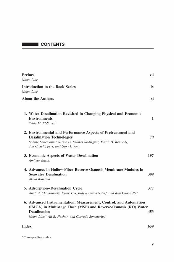
Preface viiNoam Lior

Introduction to the Book Series ixNoam Lior

About the Authors xi

1. Water Desalination Revisited in Changing Physical and EconomicEnvironments 1Yehia M. El-Sayed

2. Environmental and Performance Aspects of Pretreatment andDesalination Technologies 79Sabine Lattemann,∗ Sergio G. Salinas Rodriguez, Maria D. Kennedy,Jan C. Schippers, and Gary L. Amy

3. Economic Aspects of Water Desalination 197Amitzur Barak

4. Advances in Hollow-Fiber Reverse-Osmosis Membrane Modules inSeawater Desalination 309Atsuo Kumano

5. Adsorption–Desalination Cycle 377Anutosh Chakraborty, Kyaw Thu, Bidyut Baran Saha,∗ and Kim Choon Ng∗

6. Advanced Instrumentation, Measurement, Control, and Automation(IMCA) in Multistage Flash (MSF) and Reverse-Osmosis (RO) WaterDesalination 453Noam Lior,∗ Ali El-Nashar, and Corrado Sommariva

Index 659

∗Corresponding author.

v

This page intentionally left blank

PREFACE

This volume contains a wide spectrum of principal and timely information about(1) advances in fundamentals of desalination analysis and design when taking intoconsideration the increasing concerns about environmental and fuel cost effectson the processes, (2) an evaluation of the state of the art of pretreatment anddesalination technologies considering environmental and performance aspects,(3) a critical comprehensive survey of the economic aspects of water desalination,(4) a review of advances in hollow-fiber reverse-osmosis membrane modules,(5) an introduction and review of the emerging adsorption desalination process,and (6) a comprehensive review of advanced instrumentation, measurements,control, and automation in the MSF (Multi-Stage Flash) and RO (ReverseOsmosis) desalination processes.

Perhaps the current main leading challenge in water desalination is its sustain-ability. The first three chapters in the book address two of the three sustainabilitypillars: environmental impact and economics. Economics became a growing con-cern due to the rapidly increasing and wildly fluctuating prices of energy, which isbecoming a more dominant fraction of the produced water cost.

I note with great sorrow that the author of Chapter 1, Dr. Professor YehyaEl-Sayed, has passed away before the printing of this book. As one of the world’sleading and well-acknowledged thermodynamicists, he brought the science to engi-neering practice in general and to water desalination in particular, especially in hisseminal work on applications of exergy and exergo-economic analysis to this field.His life-work and this chapter demonstrates his foresight in dealing scientificallywith water desalination sustainability, and will remain a permanent tribute to hismemory.

I would like to acknowledge the essential contributions of the chapter authorswho shared with us their precious knowledge and experience, of the book seriesEditorial Board members who are international leading desalination experts,Ms. Miriam Balaban, Dr. Professor Mohamed Ali Darwish, Dr. Professor OsamuMiyatake, Dr. Professor Shichang Wang and Dr. Mark Wilf who providedvaluable guidance and review, and of Dr. Arza Seidel of John Wiley & Sonswho has patiently and professionally overseen the creation of this book series andvolume.

vii

viii PREFACE

Some material for Chapter 1 is not included in the book (in its various formats)and may be downloaded at http://booksupport.wiley.com. For more informationabout Wiley products, including a variety of print and electronic formats, visitwww.wiley.com.

Professor Noam LiorUniversity of PennsylvaniaPhiladelphia, PA 19104-6315, USAlior@seas.upenn.eduEditor-in-ChiefPhiladelphia, 17 March 2012

INTRODUCTION TO THE BOOK SERIESADVANCES IN WATER DESALINATION

Rapidly increasing scarcity of water usable for drinking, irrigation, industry, andgeneral sanitation, caused by rising use and pollution of existing fresh watersources, has created an enormous rise (lately of around 12%/year) in water desali-nation. Water desalination consists of separation processes that produce new freshwater from seawater and other water sources which are too saline for use. Largecommercial scale desalination began in 1965 and had a worldwide capacity ofonly about 8000 m3/day in 1970. It now produces about 72 million m3/day ofdesalted water by about 16,000 facilities worldwide. Within 10 years, productionis forecasted to triple with an expected investment of around $60 billion.

Water desalination is accomplished by a variety of different technologies,which are gradually changing to reduce capital costs, energy consumption andenvironmental impacts. It consumes large amounts of energy and materials,and has an associated important and increasingly recognized impact on theenvironment. Research and development, improved construction, operation, costallocation in multi–purpose plants, and financing methods, and education andinformation exchange must continue to be advanced to reduce the cost of thewater produced and improve process sustainability.

Advances in Water Desalination is designed to meet the knowledge needs inthis rapidly advancing field. One book volume is published per year, and contains5–7 invited, high quality timely reviews, each treating in depth a specific aspect ofthe desalination and related water treatment field and the chapters are written andreviewed by top experts in the field. All aspects are addressed and include science,technology, economics, commercialization, environmental and social impacts, andsustainability.

The series will be useful for desalination practitioners in industry and business,scientists and researchers, and students.

The series is advised and directed by an international Editorial Board of desali-nation and water experts from academia and industry.

ix

x INTRODUCTION TO THE BOOK SERIES

I am grateful to Dr. Arza Seidel of John Wiley & Sons who has patiently andprofessionally overseen the creation of this book series.

Professor Noam LiorUniversity of PennsylvaniaPhiladelphia, PA 19104-6315, USAlior@seas.upenn.eduEditor-in-ChiefPhiladelphia, 17 March 2012

ABOUT THE AUTHORS

Prof. Gary Amy is Director of the Water Desalinationand Reuse Research Center and Named Professor of Envi-ronmental Science and Engineering at the King AbdullahUniversity of Science and Technology (KAUST) in theKingdom of Saudi Arabia.

Prof. Amy’s research focuses on membrane technol-ogy, innovative adsorbents, ozone/advanced oxidation, riverbank filtration and soil aquifer treatment, natural organicmatter and disinfection by-products, and organic and inor-ganic micropollutants.

Dr. Amitzur Ze’ev Barak born 1938 in Israel, got both hisB.Sc. in Mechanical & Energy Engineering/Nuclear Engi-neering [1960] and his Doctor of Sciences-in-Technology,Civil Engineering/Hydro-Sciences [1974] at the Technion,the Israel Institute of Technology. Joined the desalinationcommunity [1962] as the Research Desalination Engineerat the IDE-Israel Desalination Engineering Ltd. Coinventorand development-manager of two low-temperature evapo-rative desalination processes—LTMVC [mechanical vaporcompression, 1964] and LTMED [multieffect-distillation,1969]. For these activities, he received the Israeli “Prime-

Minister Award for Applied Research” [1976].Manager of the Thermal Desalination R&D Department at IDE Ltd

[1968–1974].Manager of the “Joint US-Israel Desalination Program,” and director of all the

Israeli governmental R&D activities on desalination [1976–1981].Senior staff engineer for planning at the Israeli Atomic Energy Commission

[1982–2003]. Since 2003, Professor of Chemical Engineering, Civil Engineering,and Mechanical Engineering at the Ariel University Center of Samaria, Israel.Consultant to the IAEA (International Atomic Energy Agency), the CERN, anddozen other entities on energy and desalination. Published over 60 papers and hassix patents on desalination and solar energy.

xi

xii ABOUT THE AUTHORS

Anutosh Chakraborty received his B.Sc. Eng. fromBUET, Bangladesh, in 1997. He obtained his M. Engg.and Ph.D. degrees from the National University of Singa-pore (NUS) in 2001 and 2005, respectively. He workedas a JSPS Fellow at the interdisciplinary Graduate Schoolof Engineering Sciences of Kyushu University, Japan.At present, he is working at the School of Mechanicaland Aerospace Engineering, Nanyang Technological Uni-versity (NTU), Singapore, as an Assistant Professor. Hisresearch interests focus on micro/nanoscale transport phe-nomena, thin-film thermoelectric device; adsorption ther-

modynamics, adsorption cooling, gas storage, and desalination; and CO2-basedcooling system. At present, Dr. Chakraborty has published about 100 articlesin peer-reviewed journals and international conference proceedings and holds sixpatents.

Dr. Ali El Nashar is a mechanical engineer withspecialization in the fields of energy and desalination andwith a special interest in solar desalination and powergeneration. He received his Ph.D. degree in nuclearengineering from the Queen Mary College, Universityof London, UK, in 1968. His work experience coversapplied research and development work at both academicand industrial institutions. He has been involved inteaching and research at several academic institutions inEgypt, UK, and USA, among them are the Universityof Alexandria and University of Mansoura in Egypt; the

Queen Mary College, London University and Lanchester Polytechnic in the UnitedKingdom; and the Clemson University and Florida Institute of Technology in theUnited States. He has worked as the manager of cogeneration and desalinationdepartment at the Abu Dhabi Water & Electricity Authority (ADWEA) from1982 to 2002, where his department participated in the commissioning of newdesalination and power plants as well as monitoring the performance of existingplants operated by the ADWEA. He was also in charge of the solar desalinationresearch program in the ADWEA during this period, where he supervised theinstallation, commissioning, and testing of the solar desalination demonstrationplant in Umm Al Nar, which was designed and operated as a part of a jointresearch program with Japan’s New Energy Development Organization (NEDO).He has been a member of several professional organizations, including the ASME,IDA, and ISE, and the editor of the IDA, Energy, and ISE. He has consultedfor a number of international organizations, including the United NationsEnvironmental Program (UNEP); Arab Agency for Industrial Development

ABOUT THE AUTHORS xiii

(AAID); Technology International, Inc. (USA); CH2M-Hill, Inc. (USA); ScienceApplications, Inc. (USA); Dow Chemical Europe (Switzerland); and IndustrialCenter for Water & Energy Systems (ICWES), Abu Dhabi. Dr. El-Nashar hasmore than 50 published papers, reports, and book chapters in his field of interest.

Dr. Yehia El-Sayed 1928–2010. Yehia El-Sayed wasborn in Alexandria, Egypt, on September 13, 1928. Hereceived his bachelor’s degree from Alexandria Univer-sity and his doctorate in Mechanical Engineering fromManchester University in England. He taught and con-ducted research at Assiut University (Egypt), KansasState University, Dartmouth College, Glasgow Univer-sity (Scotland), Tripoli University (Libya), and the Mas-sachusetts Institute of Technology. His legacy persists inthe thousands of students and colleagues whose careersand intellectual development he has influenced. He wasa recognized international authority in desalination, ther-

modynamics, and thermoeconomics. He authored two books and numerous scien-tific papers. A Life Fellow of the American Society of Mechanical Engineering,he was a two-time recipient of ASME’s prestigious Edward F. Obert Award, inaddition to a Best Paper Award from the International Desalination Association.Dr. El-Sayed’s contributions brought the fundamentals of science to usefulness inengineering practice across the spectrum of energy conversions systems, providingprinciples for optimizing their technical and economic efficiency.

Editor-in-Chief’s note: Yehia El-Sayed submitted his chapter but regrettablypassed away before the publication of this book. His wisdom, kindness, and friend-ship will be missed by the desalination and thermodynamics scientific communities,including me.

Prof. Maria D Kennedy Ph.D., is the Professor of WaterTreatment Technologies at UNESCO-IHE. She is a boardmember of the European Desalination Society. She has 18years of research experience and currently specializes inresearch and development in the field of membrane tech-nology. Her research areas of interest include membranefouling (indices), scaling and cleaning, and modeling ofmembrane systems. She has been involved in internationaltraining projects in Israel (West Bank), Jordan, Oman, St.Maarten, and Yemen in the field of desalination and waterreuse.

xiv ABOUT THE AUTHORS

Dr. Atsuo Kumano is a professional engineer Japan, andin charge of technical matters in the Desalination Mem-brane Department in Toyobo Co., Ltd. Dr. Kumano’sresearch and development focus on membrane technol-ogy and its engineering, for water treatment membranessuch as reverse osmosis membrane for seawater desali-nation, and wastewater treatment including hollow fibreconfiguration module analysis.

Dr. Kumano holds a Ph.D. in Chemical Science andEngineering from Kobe University, Japan, 2011; an M.S.in Environmental Engineering from Osaka University,

Japan, 1983; and a B.S. in Environmental Engineering from Osaka University,Japan, 1981.

Dr. Sabine Lattemann is a part-time Research Scientistat the Water Desalination and Reuse Center (WDRC) ofthe King Abdullah University of Science and Technology(KAUST) in the Kingdom of Saudi Arabia.

Sabine has over 10 years of experience in environ-mental impact assessment (EIA) studies. Her main areasof interest include the desalination of seawater, offshorewind energy development projects, and maritime ship-ping impacts. From 2007 to 2010, Sabine worked on thetopic of environmental impacts and life cycle assessmentof seawater desalination plants within the European

research project “MEDINA.” From 2004 to 2007, she chaired the environmentalworking group of the World Health Organization Project “Desalination for safewater supply.”

Sabine holds a Postgraduate Diploma in Marine Science from Otago University(New Zealand), an M.Sc. in Marine Environmental Science from the Universityof Oldenburg (Germany), and a doctorate degree from the UNESCO-IHE Institutefor Water Education and Delft University of Technology (The Netherlands).

Dr. Noam Lior is a Professor of Mechanical Engineeringand Applied Mechanics at the University of Pennsylvania,where he is also a member of the Graduate Group of Inter-national Studies, Lauder Institute of Management andInternational Studies (MA/MBA program); of the Insti-tute for Environmental Science; and of the Initiative forGlobal Environmental Leadership (IGEL) at the Whar-ton Business School. He did his Ph.D. work on waterdesalination at the Seawater Conversion Laboratory ofthe University of California, Berkeley, and thus startedactive research, teaching, and consulting in this field in

1966. His editorships include the following.

ABOUT THE AUTHORS xv

Editor-in-Chief:

Advances in Water Desalination book series, John Wiley, since 2006.Energy, The International Journal , 1998–2009.

Board of Editors Member:

Desalination, The International Journal of Desalting and Water Purification ,since 1988;

Energy Conversion and Management Journal , since 1994;

Desalination and Water Treatment—Science and Engineering , journal, Desali-nation Publications–International Science Services, since 2008;

Frontiers of Energy and Power Engineering , Springer, since 2008;

The Energy Bulletin , an international quarterly published by the InternationalSustainable Energy Development Center (ISEDC, under UNESCO auspices),Moscow, Russian Federation, since 2011;

Thermal Science and Engineering Journal (Japan), 1999–2008;

The ASME Journal of Solar Energy Engineering , 1983–1989;

The International Desalination & Water Reuse Quarterly , 1997–2003.

He has more than 350 technical publications, many of which are in the energyand desalination fields, and is the editor of the book Measurements and Control inWater Desalination (Elsevier, 1986).

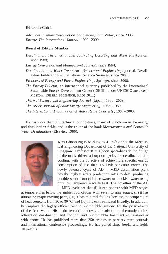
Kim Choon Ng is working as a Professor at the Mechan-ical Engineering Department of the National University ofSingapore. Professor Kim Choon specializes in the designof thermally driven adsorption cycles for desalination andcooling, with the objective of achieving a specific energyconsumption of less than 1.5 kWh per cubic meter. Thenewly patented cycle of AD + MED desalination planthas the highest water production rates to date, producingpotable water from either seawater or brackish-water usingonly low temperature waste heat. The novelties of the AD+ MED cycle are that (i) it can operate with MED stages

at temperatures below the ambient conditions with seven to nine stages, (ii) it hasalmost no major moving parts, (iii) it has minimal fouling because the temperatureof heat source is from 50 to 80 ◦C, and (iv) it is environmental friendly. In addition,he employs the highly efficient ozone microbubble systems for the pretreatmentof the feed water. His main research interests are adsorption thermodynamics,adsorption desalination and cooling, and microbubble treatment of wastewaterwith ozone. He has published more than 250 articles in peer-reviewed journalsand international conference proceedings. He has edited three books and holds10 patents.

xvi ABOUT THE AUTHORS

Bidyut Baran Saha obtained his B.Sc. (Hons.) and M.Sc.degrees from Dhaka University of Bangladesh in 1987and 1990, respectively. He received his Ph.D. in 1997from Tokyo University of Agriculture and Technology,Japan. He worked as an Associate Professor at the inter-disciplinary Graduate School of Engineering Sciences ofKyushu University until 2008. He worked as a SeniorResearch Fellow at the Mechanical Engineering Depart-ment of the National University of Singapore before join-ing the Mechanical Engineering Department of KyushuUniversity in 2010 as a Professor. He also holds a Profes-

sor position at the Thermophysical Properties Division of the International Institutefor Carbon-Neutral Energy Research (WPI-I2CNER), Kyushu University. His mainresearch interests are thermally powered sorption systems, adsorption desalination,heat transfer enhancement, and energy efficiency assessment. He has publishedmore than 200 articles in peer-reviewed journals and international conference pro-ceedings. He has edited three books and holds seven patents. Recently, he servedas the Guest Editor for the Heat Transfer Engineering journal for a special issue onthe Recent Developments of Adsorption Technologies for Energy Efficiency andEnvironmental Sustainability. He is also serving as the Managing Guest Editor ofApplied Thermal Engineering . He worked as the General Chairman for the Innova-tive Materials for the Processes in Energy Systems (IMRES) for Fuel Cells, HeatPumps and Sorption Systems, 2010 Singapore, and will organize IMPRES2013 atFukuoka, Japan.

Sergio G Salinas Rodriguez Ph.D., M.Sc, is a Lecturerin Water Treatment Technology at UNESCO-IHE. He hassix years of experience in research and in integrated mem-brane systems. He has performed research in the fields offouling indices and organic matter characterization forseawater reverse osmosis systems.

Prof. Jan C Schippers Ph.D., M.Sc, is a member ofthe Water Supply Group at UNESCO-IHE and a pro-fessor at the Wageningen University. He has extensiveprofessional experience in drinking and industrial watersupply projects in Morocco, Qatar, Libya, Gabon, CapeVerde, Namibia, Uzbekistan, Chile, France, and manyother countries. Prof. Schippers is the past president ofthe European Desalination Society and the chairman ofscientific and program committees of numerous interna-tional conferences and workshops of the IWA and EDS.

ABOUT THE AUTHORS xvii

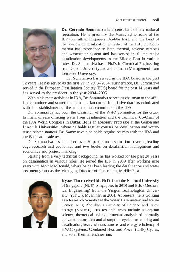
Dr. Corrado Sommariva is a consultant of internationalreputation. He is presently the Managing Director of theILF Consulting Engineers, Middle East, and the head ofthe worldwide desalination activities of the ILF. Dr. Som-mariva has experience in both thermal, reverse osmosisand wastewater system and has served in all the majordesalination developments in the Middle East in variousroles. Dr. Sommariva has a Ph.D. in Chemical Engineeringfrom Genoa University and a diploma in Management fromLeicester University.

Dr. Sommariva has served in the IDA board in the past12 years. He has served as the first VP in 2003–2004. Furthermore, Dr. Sommarivaserved in the European Desalination Society (EDS) board for the past 14 years andhas served as the president in the year 2004–2005.

Within his main activities in IDA, Dr. Sommariva served as chairman of the affil-iate committee and started the humanitarian outreach initiative that has culminatedwith the establishment of the humanitarian committee in the IDA.

Dr. Sommariva has been the Chairman of the WHO committee for the estab-lishment of safe drinking water from desalination and the Technical Co-Chair ofthe IDA World Congress in Dubai. He is an honorary Professor at the Genoa andL’Aquila Universities, where he holds regular courses on desalination and water-reuse-related matters. Dr. Sommariva also holds regular courses with the IDA andthe Bushnaq academy.

Dr. Sommariva has published over 50 papers on desalination covering leadingedge research and economics and two books on desalination management andeconomics and project financing.

Starting from a very technical background, he has worked for the past 20 yearson desalination in various roles. He joined the ILF in 2009 after working nineyears with Mott MacDonald, where he has been leading the desalination and watertreatment group as the Managing Director of Generation, Middle East.

Kyaw Thu received his Ph.D. from the National Universityof Singapore (NUS), Singapore, in 2010 and B.E. (Mechan-ical Engineering) from the Yangon Technological Univer-sity (Y.T.U.), Myanmar, in 2004. At present, he is workingas a Research Scientist at the Water Desalination and ReuseCenter, King Abdullah University of Science and Tech-nology (KAUST). His research areas include adsorptionscience, theoretical and experimental analysis of thermallyactivated adsorption and absorption cycles for cooling anddesalination, heat and mass transfer and energy efficiency ofHVAC systems, Combined Heat and Power (CHP) Cycles,and solar thermal engineering.

CHAPTER 1

Water Desalination Revisited inChanging Physical and EconomicEnvironments

YEHIA M. EL-SAYED∗

1.1 Introduction 31.1.1 Past and Present Desalination 31.1.2 The Emerged Concern 41.1.3 The Emerged Energy Analysis Methodologies 5

1.2 The Methodology Used in this Study 61.2.1 Improved Thermodynamic Analysis 6

1.2.1.1 The Exergy Function 71.2.2 Improved Costing Analysis 8

1.2.2.1 The Quantification of the Manufacturing and OperationResources for a Device 8

1.2.2.2 Correlating the Manufacturing Resources of a Device inTerms of Thermodynamic Variables 9

1.2.3 Enhanced Optimization 101.2.3.1 Two Simplifying Assumptions 101.2.3.2 The Conditions of Device-by-Device Optimization 111.2.3.3 The Form of Ai min and Di of a Device 121.2.3.4 Convergence to System Optimum 131.2.3.5 Optimization of System Devices by One Average

Exergy Destruction Price 131.2.3.6 Global Decision Variables 14

1.3 The Scope of Analysis 141.3.1 Desalination Related to Physical and Economic Environments 141.3.2 The Systems Considered 15

∗Dr. El-Sayed has regrettably passed away prior to the publication of this chapter. Final proofreadingand some updating were done by the Editor. A tribute to his life was published as Testimonial, YehiaM. El-Sayed, Energy 36 2315 (2011).

Advances in Water Desalination, First Edition. Edited by Noam Lior.© 2013 John Wiley & Sons, Inc. Published 2013 by John Wiley & Sons, Inc.

1

2 WATER DESALINATION REVISITED IN CHANGING PHYSICAL AND ECONOMIC ENVIRONMENTS

1.4 The Analyzed Systems in Detail 341.4.1 Gas Turbine/Multistage Flash Distillation Cogeneration

Systems 341.4.1.1 Flow Diagram 341.4.1.2 Major Features of the Results 34

1.4.2 The Simple Combined Cycle Systems 351.4.2.1 Flow Diagram 351.4.2.2 Major Features of the Results 35

1.4.3 Vapor Compression Systems Driven by the Figure 1.2 SimpleCombined Cycle 361.4.3.1 Flow Diagrams 361.4.3.2 Major Features of the Results 36

1.4.4 Reverse Osmosis Desalination Systems Driven by the Figure 1.2Simple Combined Cycle 361.4.4.1 Flow Diagrams 361.4.4.2 Major Features of the Results 40

1.4.5 Photovoltaic/Reverse-Osmosis (PV/RO) Solar Systems 411.4.5.1 Flow Diagram 411.4.5.2 Major Features of Results 41

1.4.6 Photovoltaic/Electrodialysis Solar System 421.4.6.1 Major Features of the Results 42

1.4.7 Osmosis Power Systems 421.4.7.1 Flow Diagram 421.4.7.2 Major Features of the Results 44

1.4.8 Future Competitiveness of Combined Desalination Systems 451.4.8.1 Prediction Criteria 451.4.8.2 Predicted Competitiveness 45

1.5 Recommended Research Directions 461.5.1 Avoiding CO2 Emissions 461.5.2 Reducing CO2 Emissions 461.5.3 Desalination of Zero Liquid Discharge 46

1.6 Conclusions 471.7 The Software Programs Developed by the Author for System Analysis 47

1.7.1 Four Programs Developed and Their Entries 471.7.2 Major Ingredients of Each Program 491.7.3 The Software 49Appendix 501.A.1 Brief Description of the Thermodynamic Model of a System and

the Design Models of Its Main Components 501.A.1.1 Thermodynamic Model 501.A.1.2 Sample Design Models 50

1.A.2 The Capital and Fuel Costing Equations of some commonDevices (Tables 1.A.1 and 1.A.2) 54

1.A.3 Some Useful Forms of Flow Exergy Expressions 591.A.3.1 Equations 591.A.3.2 Balances 63

1.A.4 Theoretical Separation Work Extended to Zero LiquidDischarge 64

INTRODUCTION 3

Selected References for Section 1.1–1.3 72Further Reading 73

1.F.1 International Symposia on Energy Analysis 731.F.2 Selected International Symposia on Desalination 751.F.3 Books on Thermodynamics 751.F.4 Books on Optimization and Equation Solvers 751.F.5 Books on Design of Energy Conversion Devices 761.F.6 Books on Optimal Design 761.F.7 Books on Emerging Technologies (Fuel/Solar Cells and Selective

Membranes) 761.F.8 General Additional Reading for Section 1.2 761.F.9 General Additional Reading for Section 1.4 771.F.10 Literature on Design Models 78

1.1 INTRODUCTION

The topic of water desalination is revisited because of the negative impact of therising oil price index on the economic environment and the adverse effects ofthe increasing carbon footprint on the physical environment. In this introductorychapter, these negative factors are discussed with respect to their impact on pastand present desalination methods. The impact of these factors on the design andoperation practices of desalination and energy-intensive systems in general is high-lighted. The energy analysis methodologies developed during the last two decades,including the methodology discussed in the present study, are summarized. Generalreferences on the subject matter are listed in the Further Reading section at the endof this chapter.

The software mentioned in this chapter may be downloaded at http://booksupport.wiley.com.

1.1.1 Past and Present Desalination

Interest in water desalination began in the late 1950s and early 1960s when theprice of oil was only $3 per barrel (bl). A number of desalting processes andsystems were considered that sought to minimize the cost of water production. Forseawater, the leading methods were multistage flash distillation, vapor compressionand freezing. Other processes, such as electrodialysis and reverse osmosis, laggedsomewhat behind. Balancing the cost of the resources utilized in fueling a systemand the resources utilized in making its devices favored moderate efficiencydevices. For example, multistage flash distillation (MSF) in a cogeneration system

4 WATER DESALINATION REVISITED IN CHANGING PHYSICAL AND ECONOMIC ENVIRONMENTS

used a maximum temperature of around 190◦F (∼80◦C) in 8–12 stages. Costallocated to water was as low as $0.3/m3. Environmental constraints were virtuallyabsent.

As the oil price index increased to $25/bl, the number of the stages of conven-tional MSF increased to about 20 and the cost allocated to water rose to about$1/m3. At the same time, the awareness and concern regarding increased CO2emissions also increased.

Present desalination methods are facing a continuing increase in oil prices anda continuing increase of CO2 content in the air. This creates a serious concern todesigners and operators of desalination plants, power plants, and energy-intensiveplants in general. Innovative ideas, along with expanded R&D in certain directions,will be essential to boost prevailing technological advances to achieve higher-efficiency devices at lower cost.

Unfortunately, if the efficiencies of these devices are not high enough and theircosts are not low enough, then promoting conservation may be necessary in orderto reduce demand, followed by undesirable rationing.

1.1.2 The Emerged Concern

Early traditional approaches to the synthesis and design of energy-intensive systemsrelied on the intuition of experienced engineers and designers. Modest concern wasgiven to fuel consumption, and no concern was given to the environment or to wastemanagement.

The continuing rise in oil prices and the continuing increase in thecarbon footprint did, indeed, create a concern. Today the concern is at its peak,fueled by an increase in world population looking for a higher standard ofliving.

The concern regarding the environment did rise to a global level and did posea difficult challenge for the designers and operators of energy-intensive systems.Cost-effective fuel conservation became a focus of attention in the design and in theoperation of these systems. The design aspects became a complex multidisciplinaryprocess requiring specialized knowledge in each discipline. The operation aspectsbecame more responsive to any missmanagement of energy, emissions, and wastedisposal. Many research and development (R&D) projects emerged to target a newgeneration of energy systems to meet the challenge at both the producer end andthe consumer end.

There was an increased demand for improved methods of system analysis toachieve lower cost and higher efficiency, to facilitate the work of system designers.The methods of improved energy analysis influenced the design and the manufac-ture of energy conversion devices. Devices are now designed for the system asa whole rather than being selected from lines of preexisting components. Man-ufacture models are developed for the devices to reduce overall cost. The lowcost of “number crunching” has enhanced the development of energy-intensiveanalysis.

INTRODUCTION 5

Almost all methods developed involve optimization and seek innovation throughenergy-intensive analysis. Common tools are modeling and computational algo-rithms. However, the tendency for models to involve assumptions and view thesame system from different perspective has created variations in the quality andreliability of the developed models. It is, therefore, important that models be verifiedand also that both designers and operators be aware of the purpose of each modeland its limitations.

1.1.3 The Emerged Energy Analysis Methodologies

The interaction between cost and efficiency has always been recognized qualita-tively. However, the interest in formulating the interaction was first highlighted inconnection with seawater distillation in the 1960s to gain insight into the interac-tion between the surface of separation requirement and energy requirement. Thefirst landmark of the work on thermoeconomics [1] dealt with seawater desalinationprocesses. Further development followed in 1970 [2,3]. Professor Tribus coined theword thermoeconomics . Professor Gaggioli [4,5] generated interest in extending thedevelopment to all kinds of energy-intensive systems.

Since then the interest spread nationally and internationally by a large numberof investigators, and the development is still continuing. Various schools of thoughtregarding optimal system design have evolved in the last 30 years with the follow-ing common objectives:

• Increasing the ability to pinpoint and quantify energy inefficiencies.• Providing further insight into possible improvements in system design and

operation.• Automation of certain aspects of the search for improvement.

Investigators differ with respect to the techniques of managing system complexity.Four techniques may be identified, all of which allow changes in system structuredirectly or indirectly:

• Construct an internal system economy as a system decomposition strategy.Most of the work by these techniques falls under the heading of either ther-moeconomics or exergoeconomics [6–8].

• Consider a composite heat exchange profile of all heat exchange processesto identify where to add or reject heat and to produce and/or supply workappropriately. All work performed using this technique is termed “pinch tech-nology” [9].

• Let the computer automate the analysis by supplying it with a large database ofdevices and their characteristics. All the work performed using this techniqueis classified as expert systems or artificial intelligence [10].

• Consider evolutionary techniques based on the survival-of-the-fittest theory[11,12] to identify the desired system.

6 WATER DESALINATION REVISITED IN CHANGING PHYSICAL AND ECONOMIC ENVIRONMENTS

The author recommended the references listed in Sections 1.F.1–1.F.7 at the endof this chapter as useful readings for the preceding material.

1.2 THE METHODOLOGY USED IN THIS STUDY

The methodology discussed in this chapter, termed thermoeconomics , begins withsimple thermodynamic computations of a given system configuration on a trajec-tory leading to an optimal design via multidisciplinary computations involving thedisciplines of design, manufacture, and economics, in addition to thermodynamics.

In a typical thermodynamic model, the cost factor is absent. Decision variablesare mainly efficiency parameters of the processes involved, along with a few param-eters such as pressure, temperature, and composition. The computations target fuelconsumption, overall system efficiency, and duty parameters of the system devices.Evaluating cost involves input resources from the disciplines of design and man-ufacture in a prevailing economic environment. This, in turn, requires formulatedcommunications among the participating disciplines.

Thermoeconomic analysis targets minimized production costs and is based onthree main principles:

• Improved thermodynamic analysis, through the concept of exergy, to addtransparency to the distribution of lost work (exergy destructions) throughouta system configuration.

• Improved costing analysis, by quantifying the manufacturing and operatingcosts of the devices of a system, to add transparency to the interaction betweencost and efficiency.

• Enhanced optimization, via reasonable simplifying assumptions, to reachimproved design points for alternative and evolving system configurations.

1.2.1 Improved Thermodynamic Analysis

Improved thermodynamic analysis extends the conventional thermodynamic com-putations to include the second law of thermodynamics quantitatively rather thanqualitatively . The extended computations are simply entropy balance computa-tions in addition to property computations and the conventional mass, energy, andmomentum balances. Entropy is conserved in an ideal process and is created in areal process. The ideal adiabatic work of a compressor or a turbine (isentropic), forexample, is obtained when the entropy remains constant. Actual adiabatic work isassociated with entropy creation. The adiabatic efficiency relates the actual workto the ideal. The process inefficiency (irreversibility) measured as a lost workpotential = T0 S c, where T0 is an ultimate sink temperature.

The main advantage of extended computations is that they enable assignment offuel consumption to each process in a system. Fuel here means the input energyresource often applied at one location within the system boundaries. The energyresource may be fossil fuel, power, heat, solar, wind, or any other driving resource.

THE METHODOLOGY USED IN THIS STUDY 7

Thus, the manner in which a fuel is utilized throughout a system is revealed.Processes of high fuel consumption are identified. Means of fuel saving are inspiredby a structural change of the system or/and by a design point change. New avenuesof research and development are discovered.

It is important to note that engineers previously did not recognize the needto perform entropy balances. They could perform the thermodynamic analysisusing property computations, and efficiency-related variables of a process such aspressure or heat loss, adiabatic efficiency, and heat exchange effectiveness. Theymissed the advantage of the distribution of fuel consumption throughout a givensystem.

A more complete picture of efficiencies and inefficiencies is obtained by using ageneral potential work function known as exergy . For simple chemical systems, thisrepresents the maximum useful work relative to a dead-state environment definedby pressure P0, temperature T0, and composition {Xc0}. Exergy also representsthe minimum amount of work needed to create the system from the dead-stateenvironment.

1.2.1.1 The Exergy Function The exergy function is a general potentialwork function for simple chemical systems. The function evolved from the workof Carnot and Clausius, and is due to Gibbs [13]. The function is expressed asfollows:

E s = U + P0V − T0S −∑

μc0Nc (1.1)

Here, E s is the maximum work that could be obtained from a sample of matter ofenergy U , volume V , number of moles (or mass) of each matter species Nc whenthe sample of matter is allowed to come to equilibrium with an environment ofpressure P0, temperature T0, and chemical potential μc0 for each species Nc. Thesame expression measures the least work required to create such a sample of matterfrom same environment. A form useful to second-law computations for systems inthe steady state is

E f = H − T0S −∑

μc0Ni (1.2a)

where E f is flow exergy. For convenience, it is often expressed as the sum oftwo changes: (1) a change under constant composition {Xc} from the state atP and T to a state at a reference point between P0 and T0 and (2) a changeunder constant P0 and T0 from composition {Xc} to a state at reference {Xc0}. Thestate at P0 + T0 + {Xc0} defines the reference dead-state environment for computingexergy

E f = (H − H 0) − T0(S − S ◦) +

∑(μc − μc0)Nc (1.2b)

where (H 0 − T0S ◦) P0,T0,Xc

= (∑

μcNc) P0·T0is used.

8 WATER DESALINATION REVISITED IN CHANGING PHYSICAL AND ECONOMIC ENVIRONMENTS

All special forms of potential workfunctions such as Carnot work, Keenam’savailability, Helmholz free energy, and Gibbs free energy are obtainable from idealinteraction between a simple chemical system and large dead state environmentusing mass, energy and entropy balances as given by El-Sayed [14].

Section 1.A.3 (in the end-of-chapter Appendix) gives some useful forms of flowexergy in terms of measurable parameters and discusses the selection of the dead-state environment(s). Two or more dead-state environments may be used wheneverthere is no interest in their relative work potential. A known equilibrium chemicalreaction may be introduced to establish the equivalent equilibrium composition ofa missing species in a selected dead state environment.

1.2.2 Improved Costing Analysis

Most engineering activities seek the extreme of an objective function, which isusually a multicriterion function. Some criteria can be quantified in terms ofmonetary values such as fuel, equipment, and maintenance costs. Others involvenonunique assumptions regarding quantification of economic factors such as envi-ronmental impact, reliability, safety, and public health. In the design phase ofan energy system, however, concern peaks around two criteria— fuel and equip-ment —without violating other desired criteria. A closer look at the interactionbetween fuel and equipment (products of specified materials and shapes) nowfollows to establish an improved costing analysis along with the improved thermo-dynamic analysis—in other words, to establish a thermoeconomic analysis.

Even when the objective function focuses on fuel and equipment only as costs,the analysis becomes multidisciplinary in nature. At least four disciplines of knowl-edge participate in information exchange: thermodynamics, design, manufacture,and economics. A communication protocol has to be established among the partic-ipating disciplines to provide cost with a rational basis.

Unfortunately, bidding information and some engineering practices for estimat-ing the capital costs of major energy conversion devices are not helpful in theimprovement of system design. The estimations are often oversimplified by a dutyparameter for a group of devices such as a simple gas turbine unit costs of $500/kW.Such costs are not responsive to efficiency changes. The obvious way to recovermissed information is to communicate with designers and manufacturers or to applytheir practices encoded by suitable mathematical models.

1.2.2.1 The Quantification of the Manufacturing and OperationResources for a Device Any energy conversion device requires tworesources: those needed to manufacture it, Rmanuf, and those needed to operateit Roperate. These two resources increase with the device duty (capacity andpressure–temperature severity) and are in conflict with the device performingefficiency (one or more efficiency parameters). Since both resources are expensive,their minimum sum is sought.

1.2.2.1.1 The Manufacturing Resources The leading manufacturing activi-ties are materials, R&D, design, and construction. Exergy destruction associated

THE METHODOLOGY USED IN THIS STUDY 9

with the performed activities of these activities are difficult to trace back or evalu-ate. The capital cost of a device Z in monetary units is an indicator of the performedactivities, if not the best indicator. The capital cost, in turn, may be expressed byone or more characterizing parameters and their unit-dimensional costs:

Z = �cai Ai + k (1.3)

Usually one characterizing surface Ai of unit surface cost cai is an adequatequantification of Z . Ai is evaluated by an updated design model. The unit cost caiis a manufacturing cost evaluated by an updated manufacture model. The rate ofthe manufacturing resources then becomes

Rmanuf = Z = cz ca(Vmanuf)A(Vdesign) (1.4)

where Z is the capital cost rate and cz is the capital recovery rate.

1.2.2.1.2 Operating Resources The primary operation resources are related tofueling and other maintenance materials and activities. The fueling resource is whatthe device pulls or draws from the fueling supply point. In other words, it is simplythe exergy destruction performed by the device. Engineers, however, use efficiencyparameters (pressure loss ratio, adiabatic efficiency, effectiveness, etc.) to accountfor exergy destruction. All devices destroy exergy for their operation, dependingon their performance efficiency. Only ideal devices (operating at 100% efficiency),which do not exist, have zero exergy destruction when performing their duties. Therates of operating resources that do not go to the products are directly quantifiedby the rates of exergy destruction. In monetary units, the operating resources canbe expressed as

Roperate = cdD({Vduty}, {Vefficiency}) (1.5)

where D is the rate of exergy destruction of a device depending on its duty and effi-ciency and cd is the cost of its exergy destruction; cd depends on the cost of the fuelfeeding the system and on the position of the device within the system configuration.The objective function Ji of a device i to minimize at the device level is

Ji = Rmanuf + Roperate

= czi cai (Vmanufacture)Ai (Vdesign) + cdiDi ({Vduty}, {Vefficiency}) (1.6)

1.2.2.2 Correlating the Manufacturing Resources of a Device in Termsof Thermodynamic Variables Communication between the thermodynamicand the design models makes it possible to express Ai as a minimized surfaceAi min({Vduty}, {Vefficiency}), and communication between the design and themanufacture models allows one to express cai = Zmin(Vmanuf)/A(Vdesign) as aminimized unit surface price ca min({Vduty}, {Vefficiency}).

10 WATER DESALINATION REVISITED IN CHANGING PHYSICAL AND ECONOMIC ENVIRONMENTS

State-of-the-art or updated design and manufacture models are sought for majorsystem devices. A conventional thermodynamic model delivers to each deviceits respective {Vduty}, {Vefficiency} obtained from one feasible system solution. Thedesign model of the device minimizes the characterizing surface of the deviceby adjusting the design dimensions of the design model that represent its designdegrees of freedom. The minimized surface Amin is sent to the manufacture modelto minimize the manufacturing cost of the device design blueprint by adjustingthe decision variables of the manufacture model, which represent its manufactur-ing degrees of freedom. The minimized unit surface cost ca min is the minimizedmanufacturing cost/Amin.

This process is repeated over a range of feasible system solutions of interest tooptimal system design. A matrix of rows representing feasible system solutions asrelated to a device and of columns representing thermodynamic duty and efficiencyvariables, design decision variables, and manufacture decision variables allows themanufacturing cost of a device in terms of design and manufacturing variables tobe correlated in terms of thermodynamic variables.

A device objective function in terms of thermodynamic variables can beexpressed as

Ji = Rmanuf + Roperate

= cz cai min({Vduty}, {Vefficiency})Ai min({Vduty}, {Vefficiency})+ cdi Di ({Vduty}, {Vefficiency}) (1.7)

where caimn, Ai min, and Di are all functions of {Vduty} and {Vefficiency}, tending, ingeneral, to increase with duty, and are at conflict with efficiency.

Communication between the system thermodynamic model and the designmodels of its devices has been applied to a fair number of any conversiondevices as given in Section 1.A.1. An example of such communication forforced-convection heat exchangers, in which the manufacturing cost of a heatexchanger is expressed in terms of thermodynamic variables, is given in Section1.A.2.

However, the communication between design and manufacture is still lagging.The unit surface manufacture cost is derived, at the moment, from published costinformation rather than by manufacturing models. The communication betweendesign and manufacture models of devices is still being formulated.

1.2.3 Enhanced Optimization

1.2.3.1 Two Simplifying Assumptions The optimization of an energysystem configuration is most expedient when the system devices are optimizedone by one with respect to the decision variables of the system. Improvedthermodynamic and costing analyses have two basic features that qualify a systemfor device-by-device optimization:

• The assignment of fuel consumption to each device of the system establishesthe operating costs of the system devices.

THE METHODOLOGY USED IN THIS STUDY 11

• Most of the decision variables are efficiency parameters whose major impactis on the local manufacturing costs of their respective devices.

Two simplifying assumptions are introduced to allow device-by-device optimiza-tion with respect to efficiency decisions as explained in the following paragraphs:

• An average exergy destruction cost applies to all devices.• Efficiency decisions are local to their devices followed by a correction for

their effect on other devices.

1.2.3.2 The Conditions of Device-by-Device Optimization The objec-tive function of a device is expressed in Equation (1.7). The objective function ofa system configuration, in terms of {Vduty, Vefficiency}, given a sizing parameter forthe production rate and having one fueling resource, is

Minimize Js = cF F +n∑

i=1

ZT + CR

= cF F +n∑

i=1

Zi + CR

= cF F +n∑

i=1

Czi Zi + CR

= cF F ({Vduty, Vefficiency}) +n∑

i=1

czi caiAi ({Vduty, Vefficiency}) + CR (1.8)

where F is fuel rate; ZT the total capital cost recovery rate; Zi the capital costrecovery rate of a device; n , the number of devices; and Zi , the capital cost of eachdevice represented by one characterizing dimension Ai . CR is a constant remaindercost as far as the system design is concerned. When a design becomes a project,CR may become a variable with respect to other non-system-design decisions.

To express the cost objective function of a system [Eq. (1.8)] in terms of thefunctions of the manufacturing and operating resources of its devices [Eq. (1.7)],the following condition must apply to a device i after dropping the constant CR:

∂Js

∂Yj= ∂Ji

∂Yj= 0 (1.9)

where Yj is a system decision variable, Js is the objective function of the system,and Ji is that function of a device i in the system:

∂Js

∂Yj= cf

(∂EF

∂Di

)(∂Di

∂Yj

)+

(∂ZT

∂Zi

) (∂Zi

∂Yj

)= cfKe ji

∂Di

∂Yj+ Kzji

(∂Zi

∂Yj

)

= ∂Ji

∂Yj(1.10)

12 WATER DESALINATION REVISITED IN CHANGING PHYSICAL AND ECONOMIC ENVIRONMENTS

where

cFF = cfEF (1.11a)

Ke ji =(

∂EF

∂Di

)by a small change in Yj (1.11b)

Kzji =(

∂ZT

∂Zi

)by a small change in Yj (1.11c)

IF Ke ji and Kzji are independent of Yj or at least weak functions of Yj , thenEquation (1.9) gives the objective function of a device as follows:

Ji = cfKe ji Di + Kzji Zi (1.12a)

= cd i Di + czi caiAi (1.12b)

Then cd i = cfKeji , and the capital cost rate is modified by Kzji .The condition that a device can be self-optimized in conformity with the objec-

tive function of its system is that Ke ji and Kzji can be treated as constants.The major effects of most efficiency decision variables on their respective

devices (Ke ji = Ke ii), converging to the condition of Equation (1.9) with Kzii = 1.They are denoted as local YL. Few efficiency decisions have their major effect onmore than one device such as heat exchange effectiveness of two heat exchangers inseries. These are identified as global YG. Their values {Ke ji and Kzji } will continueto change, leading to random fluctuations of the system objective function with nosign of convergence. A slower optimization routine, often gradient-based, has tobe used for these few global decisions. Because most efficiency decision variablesare designated as local, it is worthwhile to utilize the piecewise optimization ofthe system devices, to gain insight into possible improvements and to ensure rapidoptimization.

1.2.3.3 The Form of Ai min and Di of a Device A suitable form to expressAi min and Di in terms {Viduty} and {Viefficiency}, particularly for optimization, is aform extracted from geometric programming:

Ai min = ka

n∏j=1

(Vi duty)daj

(Vi efficiency)eaj

(1.13)

Di = kd

n∏j=1

(Viduty)ddj

(Vi efficiency)edj

(1.14)

where ka and kd are constants; n is the number of correlating variables, and da, ea,dd, and ed are exponents. For the local decisions

Ji = cfKei Di (YLi ) + Kzi czi cai Ai (YLi ) (1.15)

THE METHODOLOGY USED IN THIS STUDY 13

where the exergy destruction price cd i = cfKe i and Kei = δEF/δDi through achange δYLi and is always a positive quantity. Ke i converges to a constant, andK zi converges to 1.

Equation (1.15) boils down, as far as the optimization of YLi is concerned, to ageneralized form of a Kelvin optimality equation:

Ji = keYL ine + kz YLi

nz (1.16)

where ke and kz are lumped energy and the capital factors, considered weak func-tions of YLi, and ne and nz are exponents of opposite signs. The Kelvin optimalityequation has the exponents 1 and −1. If ke and kz were precisely constants, thenthe optimum is reached in one system computation by the analytical solution

YL i opt =[−(kz nz )

(kene)

]1/(ne−nz)

(1.17)

1.2.3.4 Convergence to System Optimum The decisions idealized as localare not in complete isolation from the rest of the system. They influence the dutiespassed over from their devices, as mass rates, heat rates, or power, to other devices.The effect of these duties on cost within the range of system optimization is linear.To allow for this mild variation to adjust and converge to the system optimum,system computations are repeated using the analytical solutions of Equation (1.17)as an updating equation.

Substituting Di and Ai for ke and kz , we obtain the updating equation forconvergence:

YL i new = YLi old

[(−nm/ne)(czi cai Ai )

cd i Di

]1/(ne−nm)

(1.18)

Equation (1.18) happens to converge to a system’s optimum in seconds (four tosix iterations).

1.2.3.5 Optimization of System Devices by One Average ExergyDestruction Price According to Equation (1.15), each device i has its ownexergy destruction price cd i . With Kzi converging to 1, we obtain

∑cd i Di = cfEf = cf

(∑Di +

∑Dj +

∑Ep

)(1.19)

where {Ep, Ef) are exergies of feeds and products, {D} are exergy destruction bythe devices, and {Ej } exergy of wasted streams and cf is fuel price per unit exergy.Then, introducting an average cda such that

cda

∑Di =

∑cd i Di = cfEf = cf

(∑Di +

∑Dj +

∑Ep

)

14 WATER DESALINATION REVISITED IN CHANGING PHYSICAL AND ECONOMIC ENVIRONMENTS

we obtain

cda = cf(1 +∑

Dj /∑

Di +∑

Ep/∑

Di ) (1.20)

A slightly higher cd than cda often improves further the desired objective function.

1.2.3.6 Global Decision Variables Few decision variables belong to thesystem as a whole and are considered global. Operating pressure and temperaturelevels of a system are examples of global decisions. Occasionally a local decisionsuch as a temperature difference has a global effect. Devices are not decomposedwith respect to these decisions. A nonlinear programming algorithm may be invokedto solve for the optimum of these decisions simultaneously. If the range of varia-tion of global decisions is narrow, manual search may be sufficient. For automatedoptimization, a simplified gradient-based method that ignores cross second deriva-tives may also be sufficient. This simplified method avoids singular matrices, whichblock solutions and often occur in systems of process-oriented description. It alsoconverges, if guided to differentiate between a maximum and a minimum, as shownby the following updating equations for a global decision YG:

YG new = YG old ± �Y (1.21a)

�Y = ABS

[δY

(g2 − g1)(−g1)

](1.21b)

g1 = (J1 − J0)

δY(1.21c)

g2 = (J2 − J1)

δY(1.21d)

δY = YG1 − YG0 = YG2 − YG1 (1.21e)

The updating equation [Eq. (1.21)] requires three system computations to obtainthree neighboring values of the objective function assuming, for example,YG0, YG0 + δY and YGO + 2δY for each global decision. After {�Y } of thesimultaneous solution has been obtained, the ± sign is then assigned to guide thechange in the favored direction because zero gradient represents both maximumand minimum.

References listed in Section 1.F.8 at the end of this chapter are additional usefulreadings for the preceding Section 1.2.

1.3 THE SCOPE OF ANALYSIS

1.3.1 Desalination Related to Physical and Economic Environments

Desalted water is either coproduced with power production where the combinedsystem is fossil-fuel-driven or self-produced, driven indirectly by fossil fuelby engines or by power from the grid. Most grid power is fossil-fuel-driven.The remaining grid power is driven by renewable sources of energy or bynuclear energy.

THE SCOPE OF ANALYSIS 15

When desalted water is fossil-fuel-driven, two streams are to be dumped inthe environment: an exhaust gas stream and a concentrated brine stream. Whenthe exhaust is dumped in air CO2 emission occurs. When concentrated brine isdumped back into the sea, marine life is damaged; and when dumped underground,the salinity of the underground water rises fast because of the limited amount ofunderground water. Dumping waste directly in the physical environment is thecheapest way to dispose of waste, but at the expense of the environment.

When desalted water is driven by solar, wind, or tidal energy, only the brinestream needs to be dumped. Exhaust gases are absent as well as CO2 emission.Thus, in terms of CO2 emission, renewable-energy-driven desalination systemsare the most ecofriendly.1

For fossil-fuel-driven desalination systems, the higher the efficiency of thesystem, the lower the fuel burning and hence the CO2 emission for the sameproduced product(s). This pattern continues until cost loses its competitiveness inthe market as a limit to the reduction of CO2 emission. The economic environmentimposes the limit.

In view of the points discussed above, a number of desalination systems willbe evaluated in terms of efficiency, cost, and CO2 emission, assuming that directdumping of concentrated brine is tolerated.

The avoidance of direct brine dumping will be treated by going to zero liquiddischarge where more desalted water is obtained and solid salts can be safelytransported isolated dumping locations. Predumping treatment is another option tosafe dumping but is not considered in this study.

The idea of generating power by the concentration difference between concen-trated brine and seawater will be investigated as a source of power though it doesavoid the effect of direct dumping.

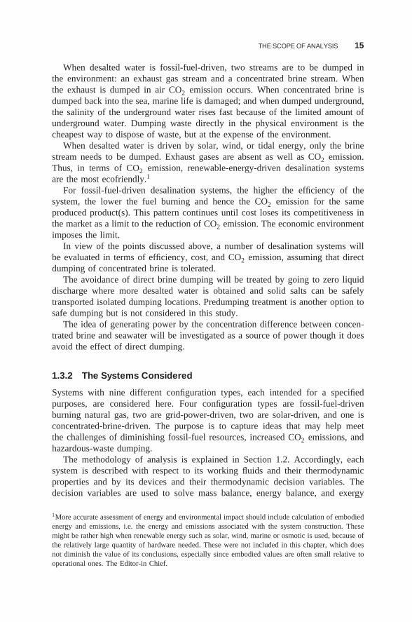
1.3.2 The Systems Considered

Systems with nine different configuration types, each intended for a specifiedpurposes, are considered here. Four configuration types are fossil-fuel-drivenburning natural gas, two are grid-power-driven, two are solar-driven, and one isconcentrated-brine-driven. The purpose is to capture ideas that may help meetthe challenges of diminishing fossil-fuel resources, increased CO2 emissions, andhazardous-waste dumping.

The methodology of analysis is explained in Section 1.2. Accordingly, eachsystem is described with respect to its working fluids and their thermodynamicproperties and by its devices and their thermodynamic decision variables. Thedecision variables are used to solve mass balance, energy balance, and exergy

1More accurate assessment of energy and environmental impact should include calculation of embodiedenergy and emissions, i.e. the energy and emissions associated with the system construction. Thesemight be rather high when renewable energy such as solar, wind, marine or osmotic is used, because ofthe relatively large quantity of hardware needed. These were not included in this chapter, which doesnot diminish the value of its conclusions, especially since embodied values are often small relative tooperational ones. The Editor-in Chief.

16 WATER DESALINATION REVISITED IN CHANGING PHYSICAL AND ECONOMIC ENVIRONMENTS

balance equations leading to a feasible solution with the lower number of itera-tive loops. A characterizing surface of heat transfer, mass transfer, or momentumtransfer is identified for each device. The cost of the device is rated per unitmanufacturing cost of the characterizing surface. Decision variables are changedmanually to minimize a cost objective function of the system.

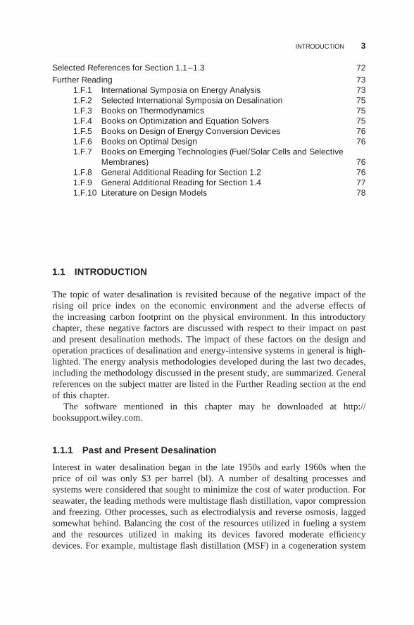
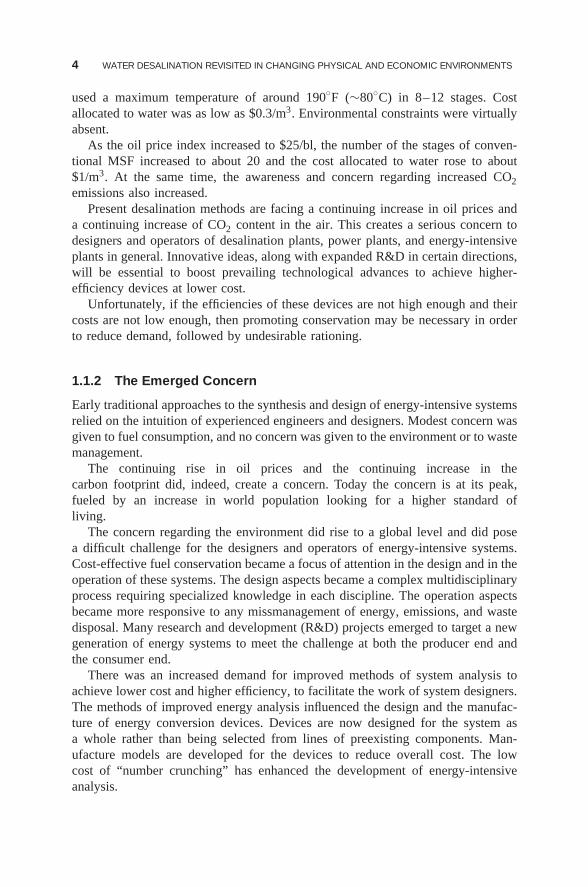
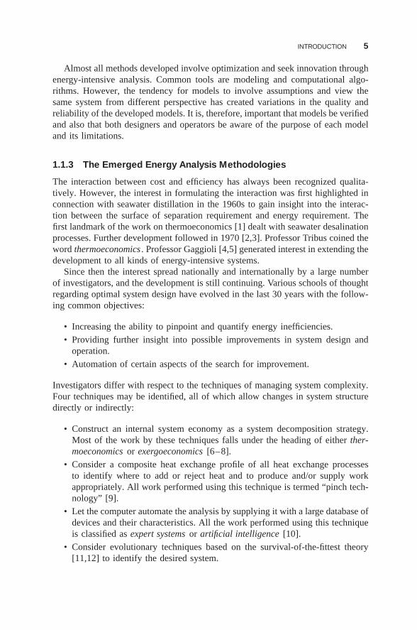
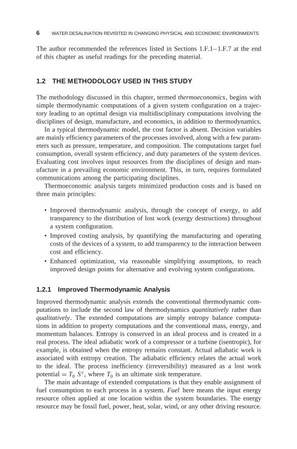
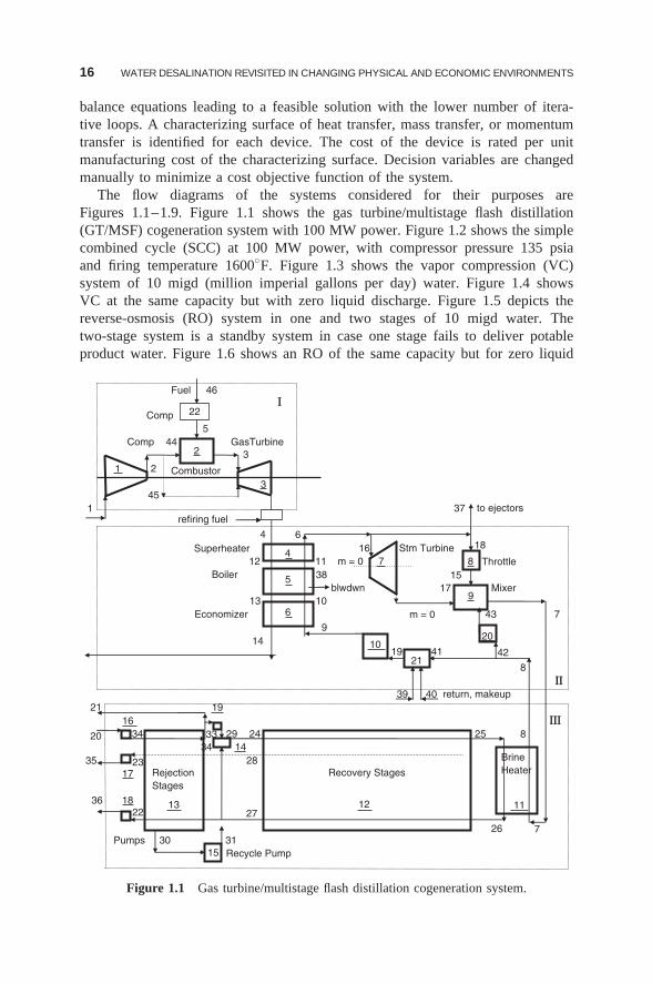
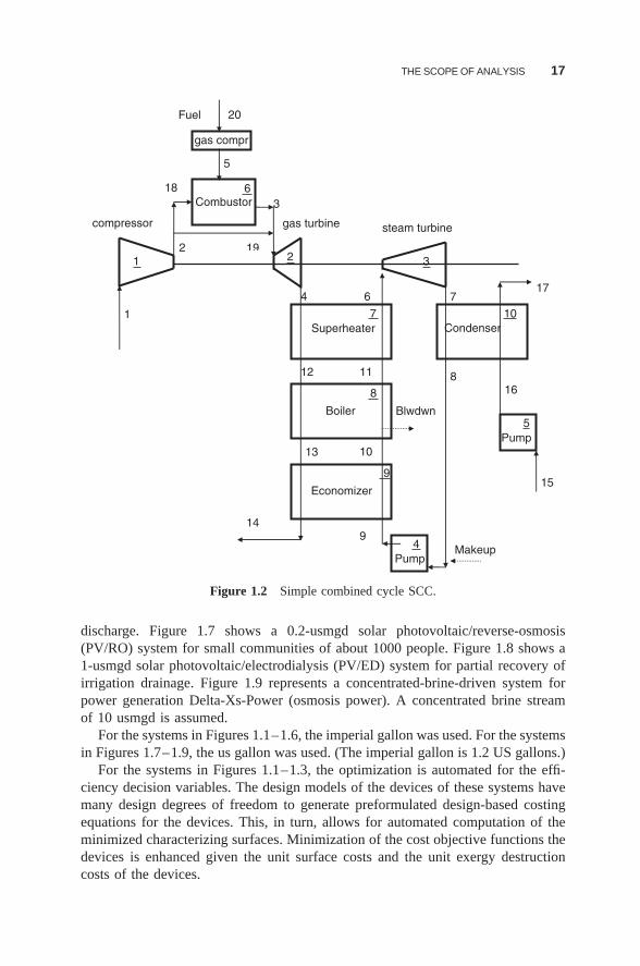
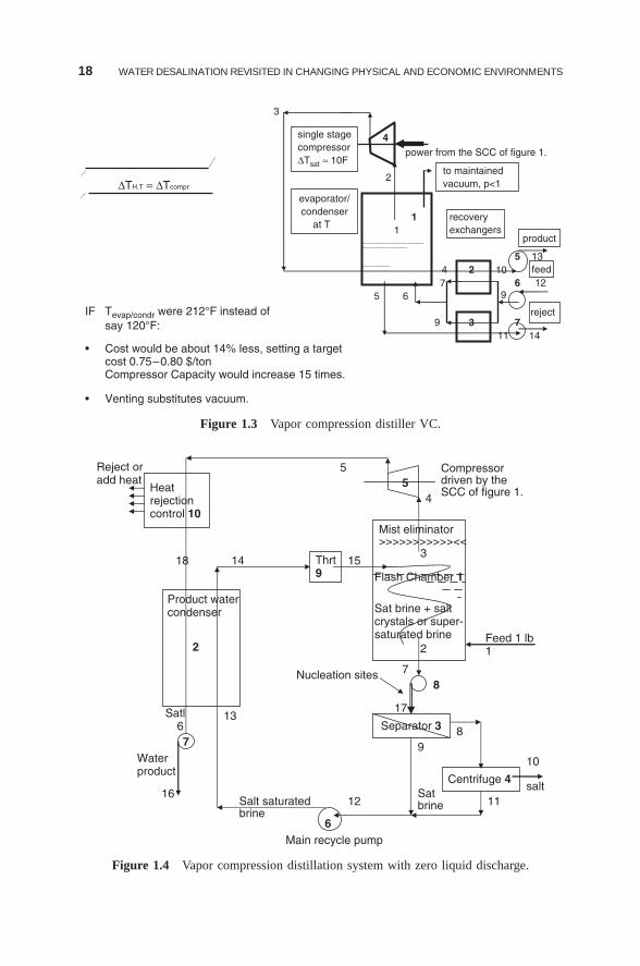
The flow diagrams of the systems considered for their purposes areFigures 1.1–1.9. Figure 1.1 shows the gas turbine/multistage flash distillation(GT/MSF) cogeneration system with 100 MW power. Figure 1.2 shows the simplecombined cycle (SCC) at 100 MW power, with compressor pressure 135 psiaand firing temperature 1600◦F. Figure 1.3 shows the vapor compression (VC)system of 10 migd (million imperial gallons per day) water. Figure 1.4 showsVC at the same capacity but with zero liquid discharge. Figure 1.5 depicts thereverse-osmosis (RO) system in one and two stages of 10 migd water. Thetwo-stage system is a standby system in case one stage fails to deliver potableproduct water. Figure 1.6 shows an RO of the same capacity but for zero liquid

Fuel 46Ι

Comp5

Comp

345

4 6

1

1

23

37refiring fuel

Throttle 15

17 Mixer

424119

8ΙΙ

return, makeup19

39 40

16 ΙΙΙ8

Recycle Pump

21

10

BrineHeater

11

RejectionStages

15

5

6

48

9

20

44 GasTurbine

Combustor

to ejectors

Superheater

Economizer

16 Stm Turbine 18

12 11 m = 0

m = 0

7

Pumps 30

36

1735 23 28

18 1322 27

12

26 7

Recovery Stages

31

34 1420 34 33 29 24 25

21

14

13 1043 7

9

blwdwnBoiler 38

22

2

Figure 1.1 Gas turbine/multistage flash distillation cogeneration system.

THE SCOPE OF ANALYSIS 17

3

2

Superheater

8

Boiler

9

Economizer

10 Condenser

4Pump

5Pump

6Combustor

Makeup

Blwdwn

gas compr

Fuel 20

18

19

1

9

5

12

6

7

8

4

14

21 3

compressor gas turbine steam turbine

15

16

17

13

11

10

7

Figure 1.2 Simple combined cycle SCC.

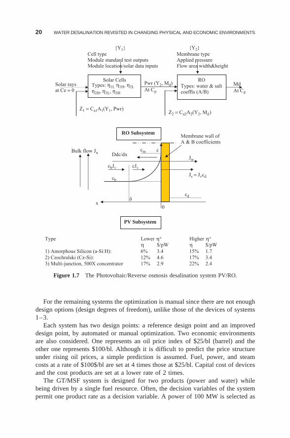
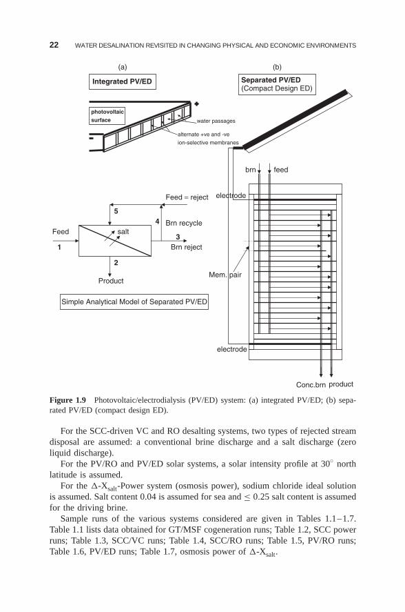
discharge. Figure 1.7 shows a 0.2-usmgd solar photovoltaic/reverse-osmosis(PV/RO) system for small communities of about 1000 people. Figure 1.8 shows a1-usmgd solar photovoltaic/electrodialysis (PV/ED) system for partial recovery ofirrigation drainage. Figure 1.9 represents a concentrated-brine-driven system forpower generation Delta-Xs-Power (osmosis power). A concentrated brine streamof 10 usmgd is assumed.

For the systems in Figures 1.1–1.6, the imperial gallon was used. For the systemsin Figures 1.7–1.9, the us gallon was used. (The imperial gallon is 1.2 US gallons.)

For the systems in Figures 1.1–1.3, the optimization is automated for the effi-ciency decision variables. The design models of the devices of these systems havemany design degrees of freedom to generate preformulated design-based costingequations for the devices. This, in turn, allows for automated computation of theminimized characterizing surfaces. Minimization of the cost objective functions thedevices is enhanced given the unit surface costs and the unit exergy destructioncosts of the devices.

18 WATER DESALINATION REVISITED IN CHANGING PHYSICAL AND ECONOMIC ENVIRONMENTS

3

2

4power from the SCC of figure 1.

1

5 13 4 2 107 6 12

9

9

5 6

3 7

single stagecompressorΔTsat ≈ 10F

to maintainedvacuum, p<1

evaporator/condenser

at T recoveryexchangers

product

feed

rejectIF Tevap/condr were 212°F instead of say 120°F:

ΔTH.T = ΔTcompr

1

11 14• Cost would be about 14% less, setting a target cost 0.75–0.80 $/ton Compressor Capacity would increase 15 times.

• Venting substitutes vacuum.

Figure 1.3 Vapor compression distiller VC.

10

Reject oradd heat

Satbrine12 11

89

17

7

613

16

151418

5

4

Feed 1 lb1

8

5

Main recycle pump

Salt saturated brine

Satl

Waterproduct

salt

Compressor driven by the SCC of figure 1.

Mist eliminator >>>>>>>>>>><<

3

Flash Chamber 1

Sat brine + saltcrystals or super-saturated brine

2

Product watercondenser

2

Heatrejectioncontrol 10

Thrt9

Separator 3

Centrifuge 4

Nucleation sites

6

7

Figure 1.4 Vapor compression distillation system with zero liquid discharge.

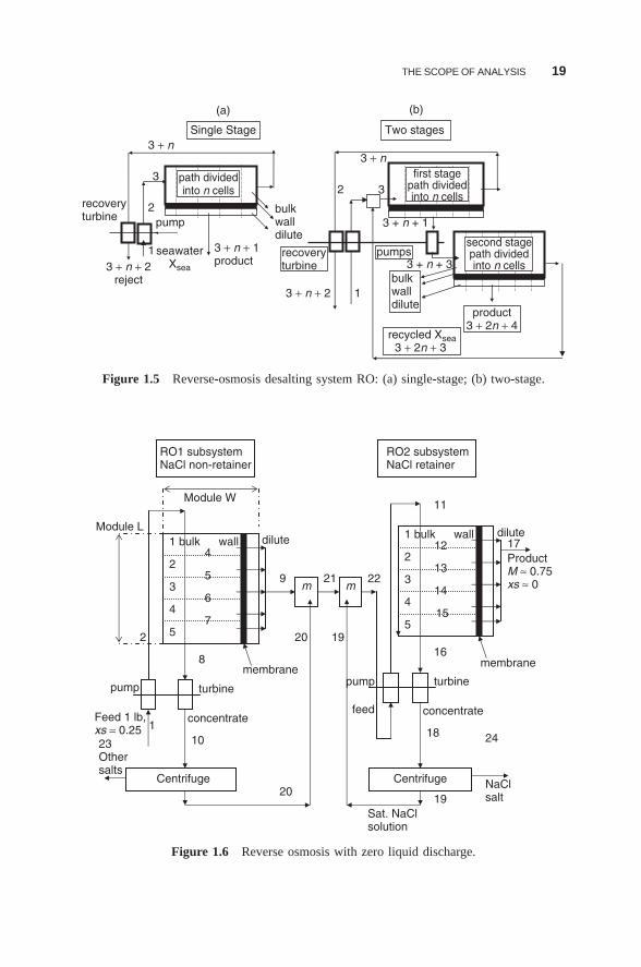
THE SCOPE OF ANALYSIS 19

23 + n + 1

13 + n + 3

bulkwalldilute

path dividedinto n cells

3 + n + 2reject

3 + n + 1product

Single Stage

pump

recoveryturbine

pumpsrecoveryturbine

first stagepath dividedinto n cells

second stagepath dividedinto n cells

bulkwalldilute

product3 + 2n + 4

recycled Xsea3 + 2n + 3

Two stages

seawaterXsea

32 3

3 + n3 + n

3 + n + 2 1

(a) (b)

Figure 1.5 Reverse-osmosis desalting system RO: (a) single-stage; (b) two-stage.

24

17ProductM ≈ 0.75xs ≈ 0

Module L

feed

pump

NaClsalt

20

10

9 22

dilute

19

Module W

19

pump

Sat. NaClsolution

21

20

18

11

Centrifuge

m

Centrifuge

m

RO1 subsystemNaCl non-retainer

RO2 subsystemNaCl retainer

1 bulk wall 4 2 5 3 6 4 7 52

8

turbine

concentrate1

membrane

12 2

13 3

14 4

155

16

turbine

concentrateFeed 1 lb,xs = 0.25

membrane

23Othersalts

dilute1 bulk wall

Figure 1.6 Reverse osmosis with zero liquid discharge.

20 WATER DESALINATION REVISITED IN CHANGING PHYSICAL AND ECONOMIC ENVIRONMENTS

Type η° η°Higher

η $/pW $/pWη1) Amorphous Silicon (a-Si:H):

Membrane typeApplied pressureFlow area width&height

{Y1} {Y2}

Cell typeModule standard test outputsModule location/solar data inputs

Solar raysat Ce = 0

Z1 = Ca1A1(Y1, Pwr)Z2 = Ca2A2(Y2, Md)

Pwr (Y2, Md)

At Cp

Md

At Cd

0

δ

Ddc/dx

Js = Jvcd

Jw

cbJv

cd

cb

cJv

cm

x

c

Membrane wall ofA & B coefficients

Bulk flow Ju

Types: water & saltcoeffts (A/B)

Types: η1L η1H, η2L

η2H, η3L, η3H

PV Subsystem

RO Subsystem

Solar Cells RO

Lower

6% 3.4 15% 1.7

2) Czochralski (Cz-Si): 12% 4.6 17% 3.4

3) Multi-junction, 500X concentrator 17% 2.9 22% 2.4

Figure 1.7 The Photovoltaic/Reverse osmosis desalination system PV/RO.

For the remaining systems the optimization is manual since there are not enoughdesign options (design degrees of freedom), unlike those of the devices of systems1–3.

Each system has two design points: a reference design point and an improveddesign point, by automated or manual optimization. Two economic environmentsare also considered. One represents an oil price index of $25/bl (barrel) and theother one represents $100/bl. Although it is difficult to predict the price structureunder rising oil prices, a simple prediction is assumed. Fuel, power, and steamcosts at a rate of $100$/bl are set at 4 times those at $25/bl. Capital cost of devicesand the cost products are set at a lower rate of 2 times.

The GT/MSF system is designed for two products (power and water) whilebeing driven by a single fuel resource. Often, the decision variables of the systempermit one product rate as a decision variable. A power of 100 MW is selected as

THE SCOPE OF ANALYSIS 21

Zone of currentgeneration technologies

Argued range of η limits

Carnot η limit

Current η limit

1H

3H

3L2H

2L

$3.0/pW$4.0/pW

$2.0/pW

$1.0/pW$0.5/pW$0.1/pW

0 100 200 300 400 500 600 700 800 900 1000

1

0.6

0.7

0.8

0.9

0.5

0.4

0.3

0.2

0.1

0

Cel

l sta

ndar

d te

st e

ffici

ency

ηo

$/m2

1L

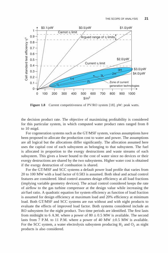
Figure 1.8 Current competitiveness of PV/RO system [18]. pW: peak watts.

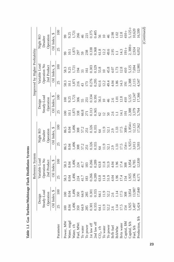
the decision product rate. The objective of maximizing profitability is consideredfor this particular system, in which computed water product rates ranged from 8to 10 migd.

For cogeneration systems such as the GT/MSF system, various assumptions havebeen proposed to allocate the production cost to water and power. The assumptionsare all logical but the allocations differ significantly. The allocation assumed hereuses the capital cost of each subsystem as belonging to that subsystem. The fuelis allocated in proportion to the exergy destructions and waste streams of eachsubsystem. This gives a lower bound to the cost of water since no devices or theirexergy destructions are shared by the two subsystems. Higher water cost is obtainedif the exergy destruction of combustion is shared.

For the GT/MSF and SCC systems a default power load profile that varies from20 to 100 MW with a load factor of 0.583 is assumed. Both ideal and actual controlfeatures are considered. Ideal control assumes design efficiency at all load fractions(implying variable geometry devices). The actual control considered keeps the rateof airflow to the gas turbine compressor at the design value while increasing theair/fuel ratio. A quadratic equation for system efficiency as function of load fractionis assumed for design efficiency at maximum load and 20% efficiency at minimumload. Both GT/MSF and SCC systems are run without and with night products toevaluate the effects of improved load factor. Both systems considered include anRO subsystem for the night product. Two time periods are identified. The first lastsfrom midnight to 6 A.M. where a power of 80 ± 0.5 MW is available. The secondlasts from 7 P.M. to 11 P.M. where a power of 40 MW ±0.5 MW is available.For the SCC system, a water electrolysis subsystem producing H2 and O2 as nightproducts is also considered.

22 WATER DESALINATION REVISITED IN CHANGING PHYSICAL AND ECONOMIC ENVIRONMENTS

electrode

electrode

54

3

2

1

Product

Feed

Feed = reject

Brn recycle

Brn reject

Mem. pair

Conc.brn product

feedbrn

photovoltaic

surface

alternate +ve and -ve

ion-selective membranes

water passages

Separated PV/ED(Compact Design ED)

Integrated PV/ED

salt

Simple Analytical Model of Separated PV/ED

(a) (b)

Figure 1.9 Photovoltaic/electrodialysis (PV/ED) system: (a) integrated PV/ED; (b) sepa-rated PV/ED (compact design ED).

For the SCC-driven VC and RO desalting systems, two types of rejected streamdisposal are assumed: a conventional brine discharge and a salt discharge (zeroliquid discharge).

For the PV/RO and PV/ED solar systems, a solar intensity profile at 30◦ northlatitude is assumed.

For the �-Xsalt-Power system (osmosis power), sodium chloride ideal solutionis assumed. Salt content 0.04 is assumed for sea and ≤ 0.25 salt content is assumedfor the driving brine.

Sample runs of the various systems considered are given in Tables 1.1–1.7.Table 1.1 lists data obtained for GT/MSF cogeneration runs; Table 1.2, SCC powerruns; Table 1.3, SCC/VC runs; Table 1.4, SCC/RO runs; Table 1.5, PV/RO runs;Table 1.6, PV/ED runs; Table 1.7, osmosis power of �-Xsalt.

Tabl

e1.

1G

asTu

rbin

e/M

ulti

stag

eF

lash

Dis

tilla

tion

Syst

ems

Ref

eren

ceSy

stem

Impr

oved

byH

ighe

rPr

ofita

bilit

y

Des

ign

Var

iabl

eL

oad

Nig

htR

OD

esig

nV

aria

ble

Loa

dN

ight

RO

Stea

dy-L

oad

Ope

ratio

nN

oD

esal

ter

Stea

dy-L

oad

Ope

ratio

nN

oD

esal

ter

Ope

ratio

n2n

dPr

oduc

tO

pera

tion

Ope

ratio

n2n

dPr

oduc

tO

pera

tion

Oil

Inde

x,$

Oil

Inde

x,$

Oil

Inde

x,$

Oil

Inde

x,$

Oil

Inde

x,$

Oil

Inde

x,$

Para

met

er25

100

2510

025

100

2510

025

100

2510

0

Pow

er,

MW

100

100

58.3

58.3

86.5

86.5

100

100

58.3

58.3

9999

Wat

er,

mig

d8.

048.

048.

048.

048.

048.

0410

.19.

2510

.19.

2510

.19.

25W

ater

,t/h

1,49

61,

496

1,49

61,

496

1,49

61,

496

1,87

11,

721

1,87

11,

721

1,87

11,

721

Fuel

,M

Wt

350

350

224

224

308

308

338

306

216

194

297

266

Tow

ater

64.9

64.9

41.7

41.7

57.2

57.2

66.8

5543

3359

46To

pow

er28

528

518

318

325

125

127

125

117

316

123

822

11s

tla

wef

f0.

301

0.30

10.

266

0.26

60.

326

0.32

60.

313

0.33

40.

276

0.30

30.

338

0.37

52n

dla

wef

f0.

355

0.35

50.

289

0.28

90.

355

0.35

50.

365

0.39

10.

295

0.32

90.

368

0.40

5C

O2,

t/h64

.164

.163

.863

.864

6462

56.1

61.6

55.8

61.8

56To

wat

er11

.911

.911

.811

.811

.911

.912

1012

.210

12.2

10To

pow

er52

.252

.251

.951

.952

.152

.150

4649

.445

.849

.646

lb/lb

fuel

2.6

2.6

4.04

4.04

2.9

2.9

2.6

2.6

4.04

4.07

2.95

2.98

lb/k

Whe

1.14

1.14

1.96

1.96

1.33

1.33

1.1

1.01

1.86

1.73

1.1

1.02

lb/tn

wat

er17

.517

.517

.417

.417

.517

.514

.112

.814

.312

.814

.312

.8C

apita

l,$M

154

308

154

308

154+

308+

191

410

191

410

191+

410+

Cap

ital,

$/h

1,92

53,

854

1,92

53,

854

1,92

5+3,

854+

2,38

85,

125

2,38

85,

125

2,38

8+5,

125+

Fuel

,$/

h3,

497

13,9

872,

196

8,78

53,

013

12,1

253,

379

12,2

472,

115

7,69

42,

924

10,6

20Pr

oduc

tion,

$/h

5,42

417

,840

4,17

112

,830

5,59

317

,562

5,76

417

,366

4,54

712

,981

6,05

216

,599

(Con

tinu

ed)

23

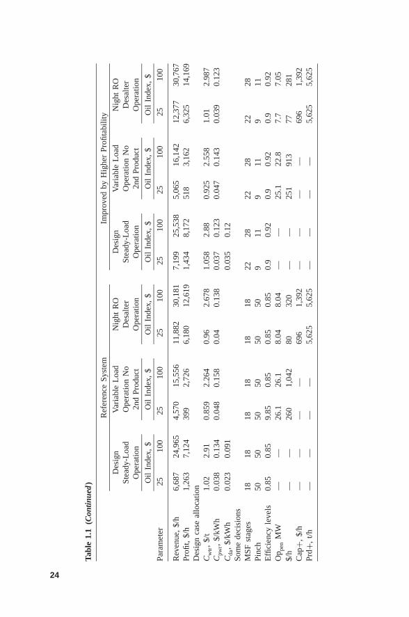
Tabl

e1.

1(C

ontin

ued

)

Ref

eren

ceSy

stem

Impr

oved

byH

ighe

rPr

ofita

bilit

y

Des

ign

Var

iabl

eL

oad

Nig

htR

OD

esig

nV

aria

ble

Loa

dN

ight

RO

Stea

dy-L

oad

Ope

ratio

nN

oD

esal

ter

Stea

dy-L

oad

Ope

ratio

nN

oD

esal

ter

Ope

ratio

n2n

dPr

oduc

tO

pera

tion

Ope

ratio

n2n

dPr

oduc

tO

pera

tion

Oil

Inde

x,$

Oil

Inde

x,$

Oil

Inde

x,$

Oil

Inde

x,$

Oil

Inde

x,$

Oil

Inde

x,$

Para

met

er25

100

2510

025

100

2510

025

100

2510

0

Rev

enue

,$/

h6,

687

24,9

654,

570

15,5

5611

,882

30,1

817,

199

25,5

385,

065

16,1

4212

,377

30,7

67Pr

ofit,

$/h

1,26

37,

124

399

2,72

66,

180

12,6

191,

434

8,17

251

83,

162

6,32

514

,169

Des

ign

case

allo

catio

nC

wtr,

$/t

1.02

2.91

0.85

92.

264

0.96

2.67

81.

058

2.88

0.92

52.

558

1.01

2.98

7C

pwr,

$/kW

h0.

038

0.13

40.

048

0.15

80.

040.

138

0.03

70.

123

0.04

70.

143

0.03

90.

123

Cda

,$/

kWh

0.02

30.

091

0.03

50.

12So

me

deci

sion

sM

SFst

ages

1818

1818

1818

2228

2228

2228

Pinc

h50

5050

5050

509

119

119

11E

ffici

ency

leve

ls0.

850.

859.

850.

850.

850.

850.

90.

920.

90.

920.

90.

92O

p pen

MW

——

26.1

26.1

8.04

8.04

——

25.1

22.8

7.7

7.05

$/h

——

260

1,04

280

320

——

251

913

7728

1C

ap+,

$/h

——

——

696

1,39

2—

——

—69

61,

392

Prd+

,t/h

——

——

5,62

55,

625

——

——

5,62

55,

625

24

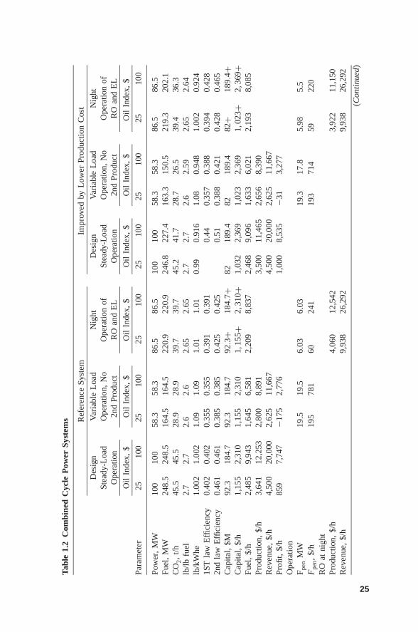
Tabl

e1.

2C

ombi

ned

Cyc

leP

ower

Syst

ems R

efer

ence

Syst

emIm

prov

edby

Low

erPr

oduc

tion

Cos

t

Des

ign

Var

iabl

eL

oad

Nig

htD

esig

nV

aria

ble

Loa

dN

ight

Stea

dy-L

oad

Ope

ratio

n,N

oO

pera

tion

ofSt

eady

-Loa

dO

pera

tion,

No

Ope

ratio

nof

Ope

ratio

n2n

dPr

oduc

tR

Oan

dE

LO

pera

tion

2nd

Prod

uct

RO

and

EL

Oil

Inde

x,$

Oil

Inde

x,$

Oil

Inde

x,$

Oil

Inde

x,$

Oil

Inde

x,$

Oil

Inde

x,$

Para

met

er25

100

2510

025

100

2510

025

100

2510

0

Pow

er,

MW

100

100

58.3

58.3

86.5

86.5

100

100

58.3

58.3

86.5

86.5

Fuel

,M

W24

8.5

248.

516

4.5

164.

522

0.9

220.

924

6.8

227.

416

3.3

150.

521

9.3

202.

1C

O2,

t/h45

.545

.528

.928

.939

.739

.745

.241

.728

.726

.539

.436

.3lb

/lbfu

el2.

72.

72.

62.

62.

652.

652.

72.

72.

62.

592.

652.

64lb

/kW

he1.

002

1.00

21.

091.

091.

011.

010.

990.

916

1.08

0.94

81.

002

0.92

41S

Tla

wE

ffici

ency

0.40

20.

402

0.35

50.

355

0.39

10.

391

0.44

0.35

70.

388

0.39

40.

428

2nd

law

Effi

cien

cy0.

461

0.46

10.

385

0.38

50.

425

0.42

50.

510.

388

0.42

10.

428

0.46

5C

apita

l,$M

92.3

184.

792

.318

4.7

92.3

+18

4.7+

8218

9.4

8218

9.4

82+

189.

4+C

apita

l,$/

h1,

155

2,31

01,

155

2,31

01,

155+

2,31

0+1,

032

2,36

91,

023

2,36

91,

023+

2,36

9+Fu

el,

$/h

2,48

59,

943

1,64

56,

581

2,20

98,

837

2,46

89,

096

1,63

36,

021

2,19

38,

085

Prod

uctio

n,$/

h3,

641

12,2

532,

800

8,89

13,

500

11,4

652,

656

8,39

0R

even

ue,

$/h

4,50

020

,000

2,62

511

,667

4,50

020

,000

2,62

511

,667

Profi

t,$/

h85

97,

747

−175

2,77

61,

000

8,53

5−3

13,

277

Ope

ratio

nF p

enM

W19

.519

.56.

036.

0319

.317

.85.

985.

5F

pen,

$/h

195

781

6024

119

371

459

220

RO

atni

ght

Prod

uctio

n,$/

h4,

060

12,5

423,

922

11,1

50R

even

ue,

$/h

9,93

826

,292

9,93

826

,292

(Con

tinu

ed)

25

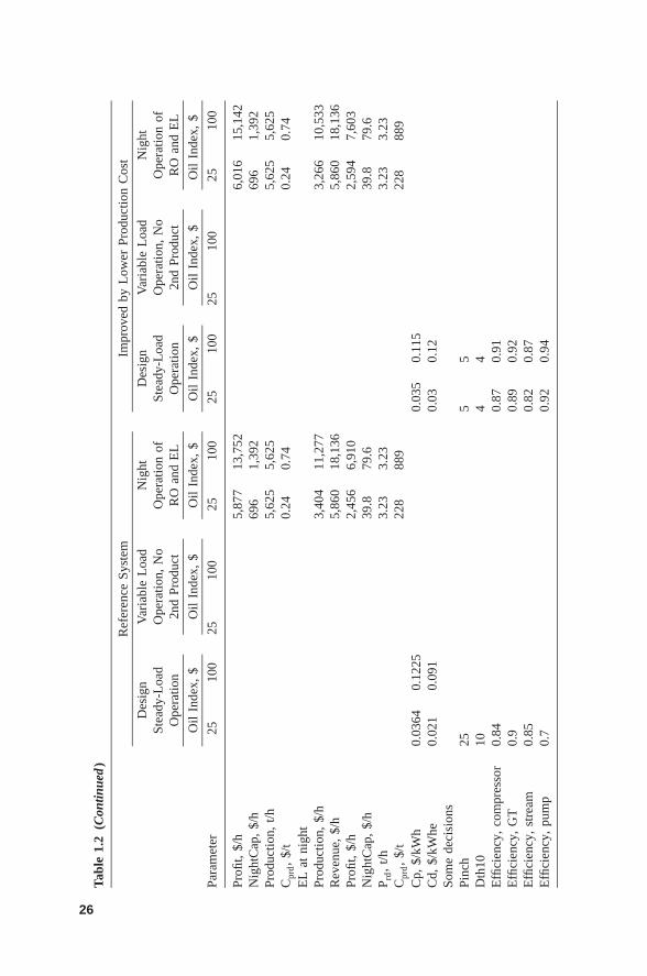
Tabl

e1.

2(C

ontin

ued

)

Ref

eren

ceSy

stem

Impr

oved

byL

ower

Prod

uctio

nC

ost

Des

ign

Var

iabl

eL

oad

Nig

htD

esig

nV

aria

ble

Loa

dN

ight

Stea

dy-L

oad

Ope

ratio

n,N

oO

pera

tion

ofSt

eady

-Loa

dO

pera

tion,

No

Ope

ratio

nof

Ope

ratio

n2n

dPr

oduc

tR

Oan

dE

LO

pera

tion

2nd

Prod

uct

RO

and

EL

Oil

Inde

x,$

Oil

Inde

x,$

Oil

Inde

x,$

Oil

Inde

x,$

Oil

Inde

x,$

Oil

Inde

x,$

Para

met

er25

100

2510

025

100

2510

025

100

2510

0

Profi

t,$/

h5,

877

13,7

526,

016

15,1

42N

ight

Cap

,$/

h69

61,

392

696

1,39

2Pr

oduc

tion,

t/h5,

625

5,62

55,

625

5,62

5C

prd,

$/t

0.24

0.74

0.24

0.74

EL

atni

ght

Prod

uctio

n,$/

h3,

404

11,2

773,

266

10,5

33R

even

ue,

$/h

5,86

018

,136

5,86

018

,136

Profi

t,$/

h2,

456

6,91

02,

594

7,60

3N

ight

Cap

,$/

h39

.879

.639

.879

.6P r

d,

t/h3.

233.

233.

233.

23C

prd,

$/t

228

889

228

889

Cp,

$/kW

h0.

0364

0.12

250.

035

0.11

5C

d,$/

kWhe

0.02

10.

091

0.03

0.12

Som

ede

cisi

ons

Pinc

h25

55

Dth

1010

44

Effi

cien

cy,

com

pres

sor

0.84

0.87

0.91

Effi

cien

cy,

GT

0.9

0.89

0.92

Effi

cien

cy,

stre

am0.

850.

820.

87E

ffici

ency

,pu

mp

0.7

0.92

0.94

26

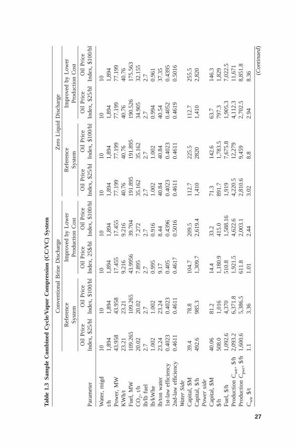
Tabl

e1.

3Sa

mpl

eC

ombi

ned

Cyc

le/V

apor

Com

pres

sion

(CC

/VC

)Sy

stem

Con

vent

iona

lB

rine

Dis

char

geZ

ero

Liq

uid

Dis

char

ge

Ref

eren

ceIm

prov

edby

Low

erR

efer

ence

Impr

oved

byL

ower

Syst

emPr

oduc

tion

Cos

tSy

stem

Prod

uctio

nC

ost

Oil

Pric

eO

ilPr

ice

Oil

Pric

eO

ilPr

ice

Oil

Pric

eO

ilPr

ice

Oil

Pric

eO

ilPr

ice

Para

met

erIn

dex,

$25/

blIn

dex,

$100

/bl

Inde

x,25

$/bl

Inde

x,$1

00/b

lIn

dex,

$25/

blIn

dex,

$100

/bl

Inde

x,$2

5/bl

Inde

x,$1

00/b

l

Wat

er,

mig

d10

1010

1010

1010

10t/h

1,89

41,

894

1,89

41,

894

1,89

41,

894

1,89

41,

894

Pow

er,

MW

43.9

5843

.958

17.4

5517

.455

77.1

9977

.199

77.1

9977

.199

KW

h/t

23.2

123

.21

9.21

69.

216

40.7

640

.76

40.7

640

.76

Fuel

,M

W10

9.26

510

9.26

543

.995

639

.704

191.

895

191.

895

190.

526

175.

563

CO

2,

t/h20

.02

20.0

27.

895

7.27

235

.162

35.1

6234

.905

32.1

55lb

/lbfu

el2.

72.

72.

72.

72.

72.

72.

72.

7lb

/kW

he1.

002

1.00

20.

995

0.91

61.

002

1.00

20.

994

0.96

1lb

/ton

wat

er23

.24

23.2

49.

178.

4440

.84

40.8

440

.54

37.3

51s

t-la

wef

ficie

ncy

0.40

230.

4023

0.40

50.

4396

0.40

230.

4023

0.40

520.

4395

2nd-

law

effic

ienc

y0.

4611

0.46

110.

4617

0.50

160.

4611

0.46

110.

4619

0.50

16W

ater

Side

Cap

ital,

$M39

.478

.810

4.7

209.

511

2.7

225.

511

2.7

255.

5C

apita

l,$/

h49

2.6

985.

31,

309.

72,

619.

41,

410

2820

1,41

02,

820

Pow

ersi

deC

apita

l,$M

40.0

681

.214

.433

.271

.314

2.6

63.7

146.

3$/

h50

8.0

1,01

61,

180.

941

5.0

891.

71,

783.

579

7.3

1,82

9Fu

el,

$/h

1,09

2.6

4,37

051

0.8

1,58

8.16

1,91

97,

675.

81,

905.

37,

022.

5Pr

oduc

tion

Cw

tr,

$/h

2,09

3.2

6,37

1.8

1,92

1.5

4,62

2.6

4,22

0.5

12,2

794,

112.

311

,671

Prod

uctio

nC

pwr,

$/h

1,60

0.6

5,38

6.5

611.

82,

003.

12,

810.

69,

459

2,70

2.5

8,85

1.8

Cw

tr$/

t1.

13.

361.

012.

443.

028.

82.

948.

36 (Con

tinu

ed)

27

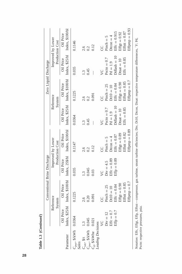
Tabl

e1.

3(C

ontin

ued

)

Con

vent

iona

lB

rine

Dis

char

geZ

ero

Liq

uid

Dis

char

ge

Ref

eren

ceIm

prov

edby

Low

erR

efer

ence

Impr

oved

byL

ower

Syst

emPr

oduc

tion

Cos

tSy

stem

Prod

uctio

nC

ost

Oil

Pric

eO

ilPr

ice

Oil

Pric

eO

ilPr

ice

Oil

Pric

eO

ilPr

ice

Oil

Pric

eO

ilPr

ice

Para

met

erIn

dex,

$25/

blIn

dex,

$100

/bl

Inde

x,25

$/bl

Inde

x,$1

00/b

lIn

dex,

$25/

blIn

dex,

$100

/bl

Inde

x,$2

5/bl

Inde

x,$1

00/b

l

Cpw

r,$/

kWh

0.03

640.

1225

0.03

50.

1147

0.03

640.

1225

0.03

50.

1146

Sale

sC

wtr,

$/t

1.3

2.6

1.3

2.6

1.3

2.6

1.3

2.6

Cpw

r,$/

kWh

0.04

50.

200.

045

0.2

0.45

0.2

0.45

0.2

Cd,

$/kW

he0.

021

0.09

10.

030.

12—

0.09

1—

0.12

Lea

ding

Dec

isio

ns VC

CC

VC

CC

VC

CC

VC

CC

Dtv

=12

Pinc

h=

25D

tv=

4.5

Pinc

h=

5Ps

ctn

=0.

7Pi

nch

=25

Psct

n=

0.7

Pinc

h=

5E

ffc

=0.

7D

t10

=10

Eff

c=

0.89

Dtc

on=

4Pd

=1.

9D

t10

=10

Pd=

1.9

Dtc

on=

4E

ffp

=0.

7E

ffc

=0.

84E

ffp

=0.

89E

ffc

=0.

87D

tflas

h=

10E

ffc

=0.

84D

tflas

h=

10E

ffc

=0.

915

Eff

gt=

0.90

Eff

gt=

0.89

Dts

at=

10E

ffgt

=0.

90D

tsat

=10

Eff

gt=

0.92

Eff

stt=

0.85

Eff

stt=

0.82

Eff

c=

0.85

Eff

stt=

0.85

Eff

c=

0.85

Eff

stt=

0.87

Eff

pmp

=0.

7E

ffpm

p=

0.89

Eff

pmp

=0.

7E

ffpm

p=

0.93

Not

atio

n:E

ffc,

Eff

gt,

Eff

p,E

ffss

t—co

mpr

esso

r,ga

stu

rbin

e,st

eam

turb

ine

effic

ienc

ies;

Dtv

,D

t10,

Dtc

on,

Dts

at:

resp

ectiv

ete

mpe

ratu

redi

ffer

enec

es,

◦ F;Pd

,Ps

ctn:

resp

ectiv

epr

essu

res,

psia

.

28

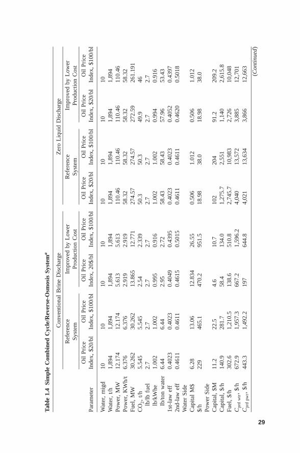
Tabl

e1.

4Si

mpl

eC

ombi

ned

Cyc

le/R

ever

se-O

smos

isSy

stem

a

Con

vent

iona

lB

rine

Dis

char

geZ

ero

Liq

uid

Dis

char

ge

Ref

eren

ceIm

prov

edby

Low

erR

efer

ence

Impr

oved

byL

ower

Syst

emPr

oduc

tion

Cos

tSy

stem

Prod

uctio

nC

ost

Oil

Pric

eO

ilPr

ice

Oil

Pric

eO

ilPr

ice

Oil

Pric

eO

ilPr

ice

Oil

Pric

eO

ilPr

ice

Para

met

erIn

dex,

$20/

blIn

dex,

$100

/bl

Inde

x,20

$/bl

Inde

x,$1

00/b

lIn

dex,

$20/

blIn

dex,

$100

/bl

Inde

x,$2

0/bl

Inde

x,$1

00/b

l

Wat

er,

mig

d10

1010

1010

1010

10W

ater

,t/h

1,89

41,

894

1,89

41,

894

1,89

41,

894

1,89

41,

894

Pow

er,

MW

12.1

7412

.174

5.61

35.

613

110.

4611

0.46

110.

4611

0.46

Pow

er,

KW

h/t

6.37

66.

376

2.91

92.

919

58.3

258

.32

58.3

258

.32

Fuel

,M

W30

.262

30.2

6213

.865

12.7

7127

4.57

274.

5727

2.59

261.

191

CO

2,

t/h5.

545

5.54

52.

542.

339

50.3

50.3

49.9

46lb

/lbfu

el2.

72.

72.

72.

72.

72.

72.

72.

7lb

/kW

he1.

002

1.00

20.

995

0.91

61.

002

1.00

20.

994

0.91

6Ib

/ton

wat

er6.

446.

442.

952.

7258

.43

58.4

357

.96

53.4

31s

t-la

wef

f0.

4023

0.40

230.

4049

0.43

950.

4023

0.40

230.

4052

0.43

972n

d-la

wef

f0.

4611

0.46

110.

4615

0.50

150.

4611

0.46

110.

4620

0.50

18W

ater

Side

Cap

ital

M$

6.28

13.0

612

.834

26.5

50.

506

1.01

20.

506

1.01

2$/

h22

946

5.1

470.

295

1.5

18.9

838

.018

.98

38.0

Pow

erSi

deC

apita

l,$M

11.2

22.5

4.6

10.7

102

204

91.2

209.

2C

apita

l,$/

h14

0.9

281.

758

.413

4.0

1,27

5.7

2,55

11,

140

2,61

5.8

Fuel

,$/

h30

2.6

1,21

0.5

138.

651

0.8

2,74

5.7

10,9

832,

726

10,0

48C

prd

wtr,

$/h

672.

91,

957.

366

7.2

1,59

6.2

4,04

013

,572

3,88

512

,701

Cpr

dpw

r,$/

h44

3.3

1,49

2.2

197

644.

84,

021

13,6

343,

866

12,6

63

(Con

tinu

ed)

29

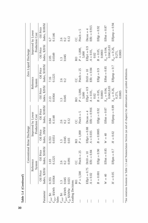
Tabl

e1.

4(C

ontin

ued

)

Con

vent

iona

lB

rine

Dis

char

geZ

ero

Liq

uid

Dis

char

ge

Ref

eren

ceIm

prov

edby

Low

erR

efer

ence

Impr

oved

byL

ower

Syst

emPr

oduc

tion

Cos

tSy

stem

Prod

uctio

nC

ost

Oil

Pric

eO

ilPr

ice

Oil

Pric

eO

ilPr

ice

Oil

Pric

eO

ilPr

ice

Oil

Pric

eO

ilPr

ice

Para

met

erIn

dex,

$20/

blIn

dex,

$100

/bl

Inde

x,20

$/bl

Inde

x,$1

00/b

lIn

dex,

$20/

blIn

dex,

$100

/bl

Inde

x,$2

0/bl

Inde

x,$1

00/b

l

Cw

tr,

$/t

0.35

51.

030.

353

0.84

2.13

7.16

2.05

6.7

Cpw

r,$/

kWh

0.03

640.

1225

0.03

510.

1148

0.03

640.

1225

0.03

490.

1146

Sale

sC

wtr,

$/t

1.3

2.6

1.3

2.6

1.3

2.6

1.3

2.6

Cpw

r,$/

kWh

0.04

50.

20.

045

0.2

0.04

50.

20.

045

0.2

Cd,

$/kW

he0.

021

0.09

10.

030.

120.

12L

eadi

ngD

ecis

ions RO

CC

RO

CC

RO

CC

RO

CC

—P

=1,

500

Pinc

h=

25P

=1,

000

Pinc

h=

5P

=1,

000,

5,00

0Pi

nch

=25

P=

1,00

0,5,

000

Pinc

h=

5

—E

ffp/

t=0.

75D

t10

=10

Eff

p/t=

0.88

Dtc

on=

4E

ffp/

t=0.

9D

t10

=10

Eff

p/t=

0.9

Dtc

on=

4—

A=

0.02

Eff

c=

0.84

A=

0.03

5E

ffc

=0.

916

A=

0.01

,0.

02E

ffc

=0.

84A

=0.

01,

0.02

Eff

c=

0.91

5

—B

=0.

001

Eff

gt=

0.90

B=

0.00

05E

ffgt

=0.

92B

=0.

05,

0.00

03E

ffgt

=0.

9B

=0.

05,

0.00

03E

ffgt

=0.

92

—W

=40

Eff

stt=

0.85

W=

40E

ffst

t=0.

87X

s1=

0.04

,0.

041,

0.03

Eff

stt=

0.85

Xs1

=0.

04,

0.04

1,0.

03E

ffst

t=0.

87

—H

=0.

05E

ffpm

=0.

7H

=0.

02E

ffpm

p=

0.89

Xs2

=0.

26,

0.27

1,0.

0005

Eff

pmp

=0.

7X

s2=

0.26

,0.

271,

0.00

05

Eff

pmp

=0.

94

aSe

eno

tatio

nsfo

otno

tein

Tabl

e1.

3an

dN

omen

clat

ure

Sect

ion

(at

end

ofch

apte

r)fo

rab

brev

iatio

nan

dsy

mbo

lde

finiti

ons.

30

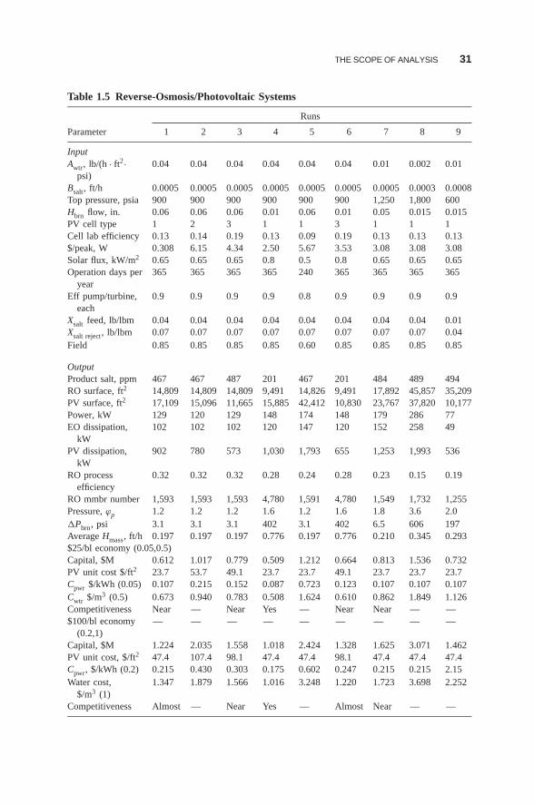
THE SCOPE OF ANALYSIS 31

Table 1.5 Reverse-Osmosis/Photovoltaic Systems

Runs

Parameter 1 2 3 4 5 6 7 8 9

InputAwtr, lb/(h · ft2·

psi)0.04 0.04 0.04 0.04 0.04 0.04 0.01 0.002 0.01

Bsalt, ft/h 0.0005 0.0005 0.0005 0.0005 0.0005 0.0005 0.0005 0.0003 0.0008Top pressure, psia 900 900 900 900 900 900 1,250 1,800 600Hbrn flow, in. 0.06 0.06 0.06 0.01 0.06 0.01 0.05 0.015 0.015PV cell type 1 2 3 1 1 3 1 1 1Cell lab efficiency 0.13 0.14 0.19 0.13 0.09 0.19 0.13 0.13 0.13$/peak, W 0.308 6.15 4.34 2.50 5.67 3.53 3.08 3.08 3.08Solar flux, kW/m2 0.65 0.65 0.65 0.8 0.5 0.8 0.65 0.65 0.65Operation days per

year365 365 365 365 240 365 365 365 365

Eff pump/turbine,each

0.9 0.9 0.9 0.9 0.8 0.9 0.9 0.9 0.9

Xsalt feed, lb/lbm 0.04 0.04 0.04 0.04 0.04 0.04 0.04 0.04 0.01Xsalt reject, lb/lbm 0.07 0.07 0.07 0.07 0.07 0.07 0.07 0.07 0.04Field 0.85 0.85 0.85 0.85 0.60 0.85 0.85 0.85 0.85

OutputProduct salt, ppm 467 467 487 201 467 201 484 489 494RO surface, ft2 14,809 14,809 14,809 9,491 14,826 9,491 17,892 45,857 35,209PV surface, ft2 17,109 15,096 11,665 15,885 42,412 10,830 23,767 37,820 10,177Power, kW 129 120 129 148 174 148 179 286 77EO dissipation,

kW102 102 102 120 147 120 152 258 49

PV dissipation,kW

902 780 573 1,030 1,793 655 1,253 1,993 536

RO processefficiency

0.32 0.32 0.32 0.28 0.24 0.28 0.23 0.15 0.19

RO mmbr number 1,593 1,593 1,593 4,780 1,591 4,780 1,549 1,732 1,255Pressure, ϕp 1.2 1.2 1.2 1.6 1.2 1.6 1.8 3.6 2.0�Pbrn, psi 3.1 3.1 3.1 402 3.1 402 6.5 606 197Average Hmass, ft/h 0.197 0.197 0.197 0.776 0.197 0.776 0.210 0.345 0.293$25/bl economy (0.05,0.5)Capital, $M 0.612 1.017 0.779 0.509 1.212 0.664 0.813 1.536 0.732PV unit cost $/ft2 23.7 53.7 49.1 23.7 23.7 49.1 23.7 23.7 23.7Cpwr $/kWh (0.05) 0.107 0.215 0.152 0.087 0.723 0.123 0.107 0.107 0.107Cwtr $/m3 (0.5) 0.673 0.940 0.783 0.508 1.624 0.610 0.862 1.849 1.126Competitiveness Near — Near Yes — Near Near — —$100/bl economy

(0.2,1)— — — — — — — — —

Capital, $M 1.224 2.035 1.558 1.018 2.424 1.328 1.625 3.071 1.462PV unit cost, $/ft2 47.4 107.4 98.1 47.4 47.4 98.1 47.4 47.4 47.4Cpwr, $/kWh (0.2) 0.215 0.430 0.303 0.175 0.602 0.247 0.215 0.215 2.15Water cost,

$/m3 (1)1.347 1.879 1.566 1.016 3.248 1.220 1.723 3.698 2.252

Competitiveness Almost — Near Yes — Almost Near — —

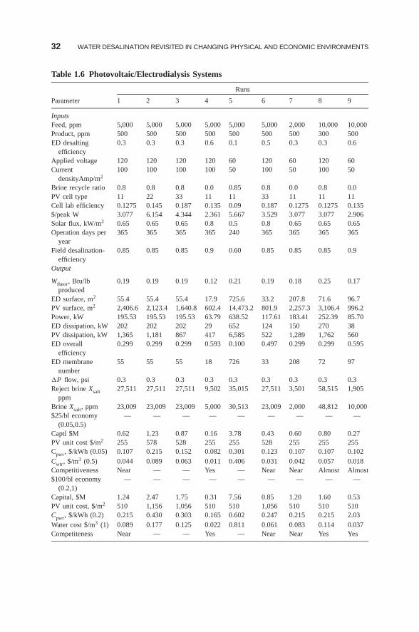
32 WATER DESALINATION REVISITED IN CHANGING PHYSICAL AND ECONOMIC ENVIRONMENTS

Table 1.6 Photovoltaic/Electrodialysis Systems

Runs

Parameter 1 2 3 4 5 6 7 8 9

InputsFeed, ppm 5,000 5,000 5,000 5,000 5,000 5,000 2,000 10,000 10,000Product, ppm 500 500 500 500 500 500 500 300 500ED desalting

efficiency0.3 0.3 0.3 0.6 0.1 0.5 0.3 0.3 0.6

Applied voltage 120 120 120 120 60 120 60 120 60Current

densityAmp/m2100 100 100 100 50 100 50 100 50

Brine recycle ratio 0.8 0.8 0.8 0.0 0.85 0.8 0.0 0.8 0.0PV cell type 11 22 33 11 11 33 11 11 11Cell lab efficiency 0.1275 0.145 0.187 0.135 0.09 0.187 0.1275 0.1275 0.135$/peak W 3.077 6.154 4.344 2.361 5.667 3.529 3.077 3.077 2.906Solar flux, kW/m2 0.65 0.65 0.65 0.8 0.5 0.8 0.65 0.65 0.65Operation days per

year365 365 365 365 240 365 365 365 365

Field desalination-efficiency

0.85 0.85 0.85 0.9 0.60 0.85 0.85 0.85 0.9

Output

Wtheor, Btu/lbproduced

0.19 0.19 0.19 0.12 0.21 0.19 0.18 0.25 0.17

ED surface, m2 55.4 55.4 55.4 17.9 725.6 33.2 207.8 71.6 96.7PV surface, m2 2,406.6 2,123.4 1,640.8 602.4 14,473.2 801.9 2,257.3 3,106.4 996.2Power, kW 195.53 195.53 195.53 63.79 638.52 117.61 183.41 252.39 85.70ED dissipation, kW 202 202 202 29 652 124 150 270 38PV dissipation, kW 1,365 1,181 867 417 6,585 522 1,289 1,762 560ED overall

efficiency0.299 0.299 0.299 0.593 0.100 0.497 0.299 0.299 0.595

ED membranenumber

55 55 55 18 726 33 208 72 97

�P flow, psi 0.3 0.3 0.3 0.3 0.3 0.3 0.3 0.3 0.3Reject brine Xsalt

ppm27,511 27,511 27,511 9,502 35,015 27,511 3,501 58,515 1,905

Brine Xsalt, ppm 23,009 23,009 23,009 5,000 30,513 23,009 2,000 48,812 10,000$25/bl economy

(0.05,0.5)— — — — — — — — —

Captl $M 0.62 1.23 0.87 0.16 3.78 0.43 0.60 0.80 0.27PV unit cost $/m2 255 578 528 255 255 528 255 255 255Cpwr, $/kWh (0.05) 0.107 0.215 0.152 0.082 0.301 0.123 0.107 0.107 0.102Cwtr, $/m3 (0.5) 0.044 0.089 0.063 0.011 0.406 0.031 0.042 0.057 0.018Competitiveness Near — — Yes — Near Near Almost Almost$100/bl economy

(0.2,1)— — — — — — — — —

Capital, $M 1.24 2.47 1.75 0.31 7.56 0.85 1.20 1.60 0.53PV unit cost, $/m2 510 1,156 1,056 510 510 1,056 510 510 510Cpwr, $/kWh (0.2) 0.215 0.430 0.303 0.165 0.602 0.247 0.215 0.215 2.03Water cost $/m3 (1) 0.089 0.177 0.125 0.022 0.811 0.061 0.083 0.114 0.037Competiteness Near — — Yes — Near Near Yes Yes

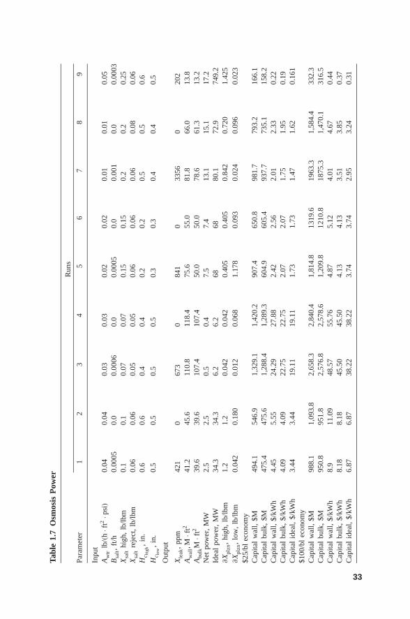
Tabl

e1.

7O

smos

isP

ower

Run

s

Para

met

er1

23

45

67

89

Inpu

tA

wtr

lb/(

h·ft

2·p

si)

0.04

0.04

0.03

0.03

0.02

0.02

0.01

0.01

0.05

Bsa

lt,

ft/h

0.00

050.

00.

0006

0.0

0.00

050.

00.

001

0.0

0.00

03X

salt

high

,lb

/lbm

0.1

0.1

0.07

0.07

0.15

0.15

0.2

0.2

0.25

Xsa

ltre

ject

,lb

/lbm

0.06

0.06

0.05

0.05

0.06

0.06

0.06

0.08

0.06

Hc h

igh,

in.

0.6

0.6

0.4

0.4

0.2

0.2

0.5

0.5

0.6

Hc l

ow,

in.

0.5

0.5

0.5

0.5

0.3

0.3

0.4

0.4

0.5

Out

put

Xle

ak,

ppm

421

067

30

841

033

560

202

Aw

all,

M·ft

241

.245

.611

0.8

118.

475

.655

.081

.866

.013

.8A

bulk

M·ft

239

.639

.610

7.4

107.

450

.050

.078

.661

.313

.2N

etpo

wer

,M

W2.

52.

50.

50.

47.

57.

413

.115

.117

.2Id

eal

pow

er,

MW

34.3

34.3

6.2

6.2

6868

80.1

72.9

749.

2∂X

plzn

,hi

gh,

lb/lb

m1.

21.

20.

042

0.04

20.

405

0.40

50.

842

0.72

01.

425

∂X

plzn

,lo

w,

lb/lb

m0.

042

0.18

00.

012

0.06

81.

178

0.09

30.

024

0.09

60.

023

$25/

blec

onom

yC

apita

lw

all,

$M49

4.1

546.

91,

329.

11,

420.

290

7.4

650.

898

1.7

793.

216

6.1

Cap

ital

bulk

,$M

475.

447

5.6

1,28

8.4

1,28

9.3

604.

960

5.4

937.

773

5.1

158.

2C

apita

lw

all,

$/kW

h4.

455.

5524

.29

27.8

82.

422.

562.

012.

330.

22C

apita

lbu

lk,

$/kW

h4.

094.

0922

.75

22.7

52.

072.

071.

751.

950.

19C

apita

lid

eal,

$/kW

h3.

443.

4419

.11

19.1

11.

731.

731.

471.

620.

161

$100

/bl

econ

omy

Cap

ital

wal

l,$M

988.

11,

093.

82,

658.

32,

840.

41,

814.

813

19.6

1963

.31,

584.

433

2.3

Cap

ital

bulk

,$M

950.

895

1.8

2,57

6.8

2,57

8.6

1,20

9.8

1210

.818

75.3

1,47

0.1

316.

5C

apita

lw

all,

$/kW

h8.

911

.09

48.5

755

.76

4.87

5.12

4.01

4.67

0.44

Cap

ital

bulk

,$/

kWh

8.18

8.18

45.5

045

.50

4.13

4.13

3.51

3.85

0.37

Cap

ital

idea

l,$/

kWh

6.87

6.87

38.2

238

.22

3.74

3.74

2.95

3.24

0.31

33

34 WATER DESALINATION REVISITED IN CHANGING PHYSICAL AND ECONOMIC ENVIRONMENTS

The results have been presented in tabular rather than graphical format becauseof the large number of decision variables. Thermodynamic decision variables areno less than 15 for any system, and the thermodynamic decisions trigger bothdesign and manufacture decisions because of the design and manufacture degreesof freedom involved. Graphs are more transparent in presenting results for cases ofone or two decision variables. The number of two and three-dimensional relationsexplodes, however, with a large number of decision variables.

1.4 THE ANALYZED SYSTEMS IN DETAIL

1.4.1 Gas Turbine/Multistage Flash Distillation Cogeneration Systems

1.4.1.1 Flow Diagram Figure 1.1 is a flow diagram showing a steam turbineboth idle and refiring active under less than design power load. Ejector steam andblowdown are allowed for. Airblade cooling for higher firing temperature is allowedfor but not employed. The system has 63 thermodynamic decision variables, 24of which can be manipulated to improve its cost objective function of higherprofitability.

1.4.1.2 Major Features of the Results• A night product raises the load factor from 0.583 to 0.865 and produces

5625 t/h desalted water <500 ppm, assuming an RO power requirement of5 kWh/t. Profitability is reduced in the absence of a night product and is raisedto 5–10 times the design steady-state value in the presence of a night product,provided all night product is salable.

• The CO2 emission is slightly reduced from 64 to 56 t/h with higher profitabilitysince burning fuel by refiring is essential to maintain the steady production ofthe MSF distiller. Auxiliary boilers and the throttling of high-pressure steamare alternatives that maintain the steady production of MSF distiller with thesame weak effect on CO2 emission.

• The cost of water remains around $1/t and the cost of power around$0.038/kWh for $25/bl economy. For $100/bl economy the costs are ∼ $3/tfor water and ∼ $0.12/kWh for power.

• The first- and second-law efficiencies are raised from their design values of0.3 and 0.355 to 0.37 and 0.405, respectively, with higher profitability.

• Automated optimization changes all the 24 manipulated decision variables.For example, the number of MSF stages is raised for its design value of 18to 28, the pinch point is reduced from 50◦F to around 10◦F, and the level ofadiabatic efficiencies of compressor, gas turbine, and steam turbine is raisedfrom 0.85 to 0.92 for higher profitability.

• The improved design points differ for each of the two economies considered,namely, $20/bl and $100/bl oil.

THE ANALYZED SYSTEMS IN DETAIL 35

• The fuel penalty of actual control compared to ideal control (the designefficiency remains constant at all load fractions) for the reference system is26 MW with no night product. This corresponds to $260/h for $20/barreleconomy and to $1042/h for $100/bl economy. The penalty for higherprofitability is only about 7 MW with a night product of desalted water.This corresponds to $70/h for a $25/bl economy and to $280/h for $100/bleconomy

1.4.2 The Simple Combined Cycle Systems

1.4.2.1 Flow Diagram Air-cooling (see Fig. 1.2) of blades is allowed for butnot employed since the firing temperature is only up to 1600◦F. The steam turbineexpands steam to condensing temperature of 100◦F. The power to be delivered aftersystem needs have been satisfied is set to 100 MW. The number of thermodynamicdecision variables is 34, 18 of which manipulated to lower production cost.

1.4.2.2 Major Features of the Results• A night product raises the load factor from 0.583 to 0.865 and produces

5625 t/h desalted water <500 ppm during installation of a night RO desalterof currently attainable power requirement of 5 kWh/t and produces 0.36 t/hH2 and 2.88 t/h O2 during installation of a night water electrolyzer of powerrequirement 78.25 MWh/t H2, which represents �Gf of the water contentdivided by an efficiency factor of 0.42 for a direct-current intensity of 1 A/cm2.Profitability becomes a loss in the absence of night products and is raised to5–10 times the design steady-state value in the presence of night products,provided all night products are salable.

• The CO2 emission design value is 45 t/h (compared to 64 t/h of the GT/MSFcase). The emission is reduced to 40 and 36 t/h with improved lower produc-tion cost.

• The cost of power is ∼ $0.035/kWh for 25$/barral economy and ∼ $0.12/kWhin $100/bl economy.

• The first- and second-law efficiencies are raised from their design valuesof 0.4 and 0.46 to 0.43 and 0.465, respectively, for lower productioncost.

• The fuel penalty of actual control compared to ideal control is 19.5 MWwith no night product. This corresponds to $195/h for $25/bl economy andto $781/h for a $100/bl economy. The penalty for lower production cost isonly ∼5.5 MW, with a night product of desalted water or of H2 and O2.This corresponds to $59/h for a $25/bl economy and to $220/h for $100/bleconomy.

• The cost of night product of water is a $0.24/t, and that of H2 and O2 is $228/tfor a $25/bl economy. For a $100/bl economy, the corresponding costs are$0.74/t and $889/t.

36 WATER DESALINATION REVISITED IN CHANGING PHYSICAL AND ECONOMIC ENVIRONMENTS

1.4.3 Vapor Compression Systems Driven by the Figure 1.2 SimpleCombined Cycle

1.4.3.1 Flow Diagrams Figure 1.3 shows a vapor compression (VC) distillerwith 16 thermodynamic decision variables, three of which are manipulated to lowerproduction cost. The operating temperature is maintained at 160◦F.

Figure 1.4 shows its version of Figure 1.3 for zero liquid discharge (ZLD) with19 decision variables, none of which are manipulated for lower production cost.Compressor efficiency is set at 85%, with a of pressure ratio of 2.73 and a suctionpressure of 0.7 psia. This low suction pressure calls for more than 10 compressorsof reasonable inlet area operating in parallel.

Both VC versions are driven by the simple combined cycle shown in Figure 1.2,with 34 decision variables, 18 of which are manipulated to lower productioncost.

1.4.3.2 Major Features of the Results• No night product is introduced because the production is at steady state, pro-

ducing 10 migd water by VC desalter.

• The reference design of the VC distiller has a capital cost of $39M for com-pressor and heat exchange surfaces and requires 44 MW power. The drivingsimple combined cycle (SCC) requires, in turn, 109 MW fuel. For a $25/bleconomy, the cost of water is $1.1/t. The cost of power is as deliveredby the combined cycle $0.0364/kWh. For a $100/bl economy, the cost ofwater is $3.36/t and the cost of power as delivered by the combined cycle is$0.1225/kWh.

• The improved design by lower production cost has a capital cost of $210Mand requires 17.5 MW power. The driving SCC requires, in turn, 40 MW fuel.For a $25/bl economy, the cost of water is $1.1/t and the cost of power asdelivered by the combined cycle is $0.035/kWh. For a $100/bl economy, thecost of water is $2.44/t and the cost of power as delivered by the combinedcycle is $0.115/kWh.

• The concept of zero liquid discharge is considered using single-stage VC.The result, so far, has not been cost-effective. Power requirement is almostdoubled (77 MW), and so is CO2 emission (35 t/h). The unit cost of wateralmost tripled. However, the high pressure of the RO case is avoided butlarge parallel compressors operating under vacuum are needed. Section 1.A.4explains the large power requirement via the theoretical work of separationextended to zero liquid discharge.

1.4.4 Reverse Osmosis Desalination Systems Driven by the Figure 1.2Simple Combined Cycle

1.4.4.1 Flow Diagrams Figure 1.5 shows conventional single- (a) and two-stage (b) reverse-osmosis desalination systems. The two-stage system is only astandby system in case product water at concentrations of <500 ppm cannot be

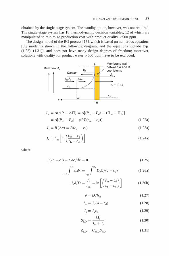
THE ANALYZED SYSTEMS IN DETAIL 37

obtained by the single-stage system. The standby option, however, was not required.The single-stage system has 18 thermodynamic decision variables, 12 of which aremanipulated to minimize production cost with product quality <500 ppm.

The design model of the RO process [15], which is based on numerous equations[the model is shown in the following diagram, and the equations include Eqs.(1.22)–(1.31)], and does not have many design degrees of freedom; moreover,solutions with quality for product water >500 ppm have to be excluded:

0

Ddc/dx

cbJv cJv

Js = Jvcd

cd

cb

cm

xδ

Jw

Bulk flow Ju

Membrane wallbetween A and Bcoefficients

Jw = A(�P − ��) = A[(Pm − Pd) − (�m − �d)]

= A[(Pm − Pd) − ϕRT (cm − cd)] (1.22a)

Js = B(�c) = B(cm − cd) (1.23a)

Jv = hm

[ln

(cm − cd

cb − cd

)](1.24a)

where

Jv(c − cd) − Ddc/dx = 0 (1.25)

x=0

∫ δ

Jvdx =cm

∫ cb

Ddc/(c − cd) (1.26a)

Jvδ/D = Jv

hm= ln

[(cm − cd

cb − cd

)](1.26b)

δ = D/hm (1.27)

Jw = Jv(ρ − cd) (1.28)

Js = Jvcd (1.29)

SRO = Md

Jw + Js(1.30)

ZRO = CaROSRO (1.31)

38 WATER DESALINATION REVISITED IN CHANGING PHYSICAL AND ECONOMIC ENVIRONMENTS

where CaRO is the membrane cost per unit membrane surface area. A multiplier>1 accommodates care of the balance of plants (default 1.5).

Equations (1.22a)–(1.24a), (1.28), and (1.29) are five equations in five unknownsJw, Js, Jv, cm and cd. The number of equations and unknowns can be reduced to 3by substituting Equations (1.28) and (1.29) in Equations (1.22a)–(1.24a), and theequations and the unknowns may be reduced to 3:

Jw = A[(Pm − Pd) − ϕRT (cm − cd)] (1.22b)

= B(cm − cd)(ρ − cd)

cd(1.23b)

= hm(ρ − cd)

[ln

(cm − cd)

cb − cd

)](1.24b)

The unknowns are Jw, cm, and cd.The following equations are needed to compute pressure losses and mass

transfer coefficient hm and hence concentration boundary-layer thickness d .The equations are based on dimensional analysis. Note that the assumption ofsingle-thickness boundary layer is often used in the analysis of RO membranes.Baker [16, p. 176] uses δ = 20 μm. This assumption is relaxed by dimensional-analysis-based equations, where the thickness responds to geometry changes offlow conduit.

f = 16/NRE for fully developed laminar flow (1.32)

= 0.078NRE−0.25 for fully developed turbulent flow, NRE < 30, 000 (1.33)

NSH = 1.85

(NPE

NV

)1/3

to asymptotic value of NSHNPE = 48 (1.34)

for laminar flow between plates(narrow passages)

= 1.62

(NPE

NV

)1/3

to asymptotic value of NSHNPE = 16 (1.35)

for laminar in tubes, NRe < 1000

= 0.04N 0.75RE NSC

0.33 (1.36)

for fully developed turbulent flow, NRE > 10, 000

NRE = Reynolds number = Udμ

ρ(1.37)

NPE = Peclet number = Vd

D(1.38)

THE ANALYZED SYSTEMS IN DETAIL 39

NSH = Sherwood number = hmd

D(1.39)

NSC = Schmidt number = μ/ρ

D(1.40)

Nv = permeated/flow velocity geometry = Jvl

Ju/d(1.41)

Jv = velocity normal to flow(x direction)

Ju = velocity in flow direction

l = length in brine flow direction

d = equivalent diameter of the brine flow area (hydraulic diameter)

d = 4WHn1/2/(W + H )/n2 (1.42)

n1 = blockage factor of brine flow area

n2 = wetted perimeter increase factor

The factors n1 and n2 depend on the thickness and the shape of feed spacers.The factors produce an equivalent reduced height He of an empty conduit. Thevalues assigned to n1 and n2 in this model are 0.25 and 2.0, respectively. Anempty conduit has n1 = n2 = 1.

The diffusion coefficient computed by Wilke–Chang equation [17, Reid p. 598]= 3.55 · 10−6 cm2/s. The diffusion coefficient quoted from Baker [16, p. 176]= 10 · 10−6 cm2/s, is used in this model. Density ρ and viscosity μ are computedby transport properties routine of reference [14].

A membrane relation that guarantees an allowable product salt content (e.g.<500 ppm) may be derived by introducing a membrane dimensionless numberNm as follows. First, the wall osmosis pressure difference (�m − �d) may bewritten in terms of wall and product salt concentrations (mass or mole per unitvolume):

(�m − �d) = ϕRT (cm − cd) (1.43)

where ϕ = 1 for ideal solution and > 1 to accommodate deviations from idealsolution. In this study, ideal solution is assumed.

Applied pressure (Pm − Pd) may be written in a similar way by introducing ϕP:

(Pm − Pd) = ϕPRT (cm − cd) (1.44)

Jw

Js= A(ϕP − ϕ)R

T

B= NM (1.45)

Equation (1.45) is realized in this model development and is believed to be impor-tant in RO membrane design. It presents the combined influence of membrane

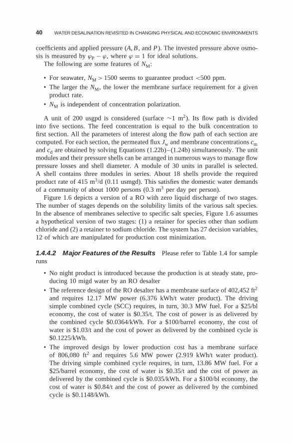
40 WATER DESALINATION REVISITED IN CHANGING PHYSICAL AND ECONOMIC ENVIRONMENTS

coefficients and applied pressure (A, B , and P ). The invested pressure above osmo-sis is measured by ϕP − ϕ, where ϕ = 1 for ideal solutions.

The following are some features of NM:

• For seawater, NM > 1500 seems to guarantee product <500 ppm.

• The larger the NM, the lower the membrane surface requirement for a givenproduct rate.

• NM is independent of concentration polarization.

A unit of 200 usgpd is considered (surface ∼1 m2). Its flow path is dividedinto five sections. The feed concentration is equal to the bulk concentration tofirst section. All the parameters of interest along the flow path of each section arecomputed. For each section, the permeated flux Jw and membrane concentrations cmand cd are obtained by solving Equations (1.22b)–(1.24b) simultaneously. The unitmodules and their pressure shells can be arranged in numerous ways to manage flowpressure losses and shell diameter. A module of 30 units in parallel is selected.A shell contains three modules in series. About 18 shells provide the requiredproduct rate of 415 m3/d (0.11 usmgd). This satisfies the domestic water demandsof a community of about 1000 persons (0.3 m3 per day per person).

Figure 1.6 depicts a version of a RO with zero liquid discharge of two stages.The number of stages depends on the solubility limits of the various salt species.In the absence of membranes selective to specific salt species, Figure 1.6 assumesa hypothetical version of two stages: (1) a retainer for species other than sodiumchloride and (2) a retainer to sodium chloride. The system has 27 decision variables,12 of which are manipulated for production cost minimization.

1.4.4.2 Major Features of the Results Please refer to Table 1.4 for sampleruns

• No night product is introduced because the production is at steady state, pro-ducing 10 migd water by an RO desalter

• The reference design of the RO desalter has a membrane surface of 402,452 ft2

and requires 12.17 MW power (6.376 kWh/t water product). The drivingsimple combined cycle (SCC) requires, in turn, 30.3 MW fuel. For a $25/bleconomy, the cost of water is $0.35/t. The cost of power is as delivered bythe combined cycle $0.0364/kWh. For a $100/barrel economy, the cost ofwater is $1.03/t and the cost of power as delivered by the combined cycle is$0.1225/kWh.

• The improved design by lower production cost has a membrane surfaceof 806,080 ft2 and requires 5.6 MW power (2.919 kWh/t water product).The driving simple combined cycle requires, in turn, 13.86 MW fuel. For a$25/barrel economy, the cost of water is $0.35/t and the cost of power asdelivered by the combined cycle is $0.035/kWh. For a $100/bl economy, thecost of water is $0.84/t and the cost of power as delivered by the combinedcycle is $0.1148/kWh.

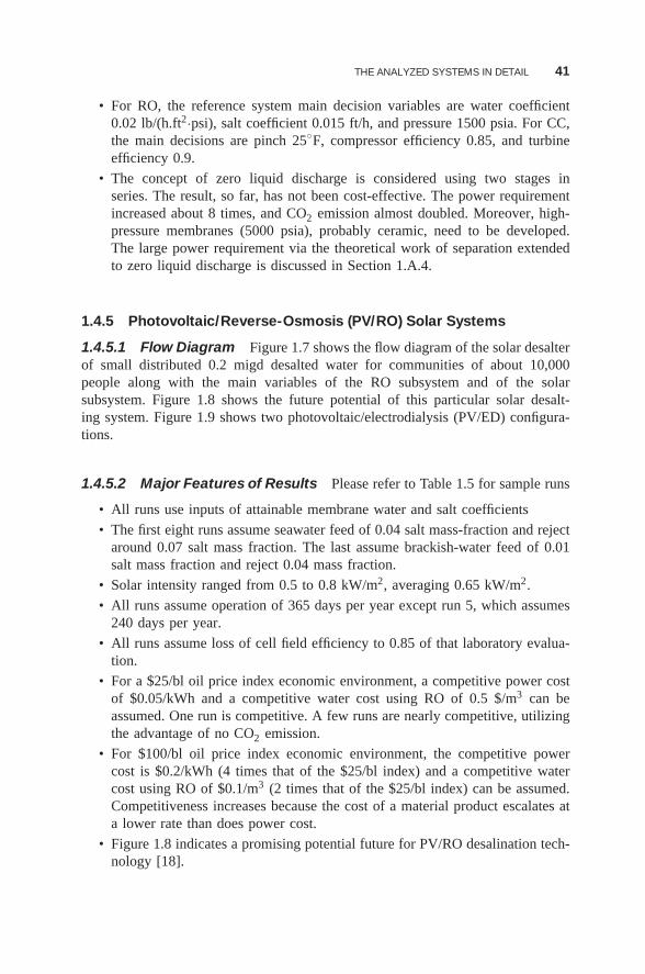
THE ANALYZED SYSTEMS IN DETAIL 41

• For RO, the reference system main decision variables are water coefficient0.02 lb/(h.ft2·psi), salt coefficient 0.015 ft/h, and pressure 1500 psia. For CC,the main decisions are pinch 25◦F, compressor efficiency 0.85, and turbineefficiency 0.9.

• The concept of zero liquid discharge is considered using two stages inseries. The result, so far, has not been cost-effective. The power requirementincreased about 8 times, and CO2 emission almost doubled. Moreover, high-pressure membranes (5000 psia), probably ceramic, need to be developed.The large power requirement via the theoretical work of separation extendedto zero liquid discharge is discussed in Section 1.A.4.

1.4.5 Photovoltaic/Reverse-Osmosis (PV/RO) Solar Systems

1.4.5.1 Flow Diagram Figure 1.7 shows the flow diagram of the solar desalterof small distributed 0.2 migd desalted water for communities of about 10,000people along with the main variables of the RO subsystem and of the solarsubsystem. Figure 1.8 shows the future potential of this particular solar desalt-ing system. Figure 1.9 shows two photovoltaic/electrodialysis (PV/ED) configura-tions.

1.4.5.2 Major Features of Results Please refer to Table 1.5 for sample runs

• All runs use inputs of attainable membrane water and salt coefficients

• The first eight runs assume seawater feed of 0.04 salt mass-fraction and rejectaround 0.07 salt mass fraction. The last assume brackish-water feed of 0.01salt mass fraction and reject 0.04 mass fraction.

• Solar intensity ranged from 0.5 to 0.8 kW/m2, averaging 0.65 kW/m2.

• All runs assume operation of 365 days per year except run 5, which assumes240 days per year.

• All runs assume loss of cell field efficiency to 0.85 of that laboratory evalua-tion.

• For a $25/bl oil price index economic environment, a competitive power costof $0.05/kWh and a competitive water cost using RO of 0.5 $/m3 can beassumed. One run is competitive. A few runs are nearly competitive, utilizingthe advantage of no CO2 emission.

• For $100/bl oil price index economic environment, the competitive powercost is $0.2/kWh (4 times that of the $25/bl index) and a competitive watercost using RO of $0.1/m3 (2 times that of the $25/bl index) can be assumed.Competitiveness increases because the cost of a material product escalates ata lower rate than does power cost.

• Figure 1.8 indicates a promising potential future for PV/RO desalination tech-nology [18].

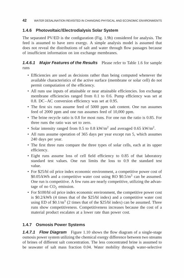
42 WATER DESALINATION REVISITED IN CHANGING PHYSICAL AND ECONOMIC ENVIRONMENTS

1.4.6 Photovoltaic/Electrodialysis Solar System

The separated PV/ED is the configuration (Fig. 1.9b) considered for analysis. Thefeed is assumed to have zero exergy. A simple analysis model is assumed thatdoes not reveal the distributions of salt and water through flow passages becauseof insufficient information on ion exchange membranes.

1.4.6.1 Major Features of the Results Please refer to Table 1.6 for sampleruns

• Efficiencies are used as decisions rather than being computed whenever theavailable characteristics of the active surface (membrane or solar cell) do notpermit computiation of the efficiency.

• All runs use inputs of attainable or near attainable efficiencies. Ion exchangemembrane efficiencies ranged from 0.1 to 0.6. Pump efficiency was set at0.8. DC–AC conversion efficiency was set at 0.95.

• The first six runs assume feed of 5000 ppm salt content. One run assumesfeed of 2000 ppm and one run assumes feed of 10,000 ppm.

• The brine recycle ratio is 0.8 for most runs. For one run the ratio is 0.85. Forthree runs the ratio was set to zero.

• Solar intensity ranged from 0.5 to 0.8 kW/m2 and averaged 0.65 kW/m2.

• All runs assume operation of 365 days per year except run 5, which assumes240 days per year.

• The first three runs compare the three types of solar cells, each at its upperefficiency.

• Eight runs assume loss of cell field efficiency to 0.85 of that laboratorystandard test values. One run limits the loss to 0.9 the standard testvalue.

• For $25/bl oil price index economic environment, a competitive power cost of$0.05/kWh and a competitive water cost using RO $0.5/m3 can be assumed.One run is competitive. A few runs are nearly competitive, utilizing the advan-tage of no CO2 emission.

• For $100/bl oil price index economic environment, the competitive power costis $0.2/kWh (4 times that of the $25/bl index) and a competitive water costusing ED of $0.1/m3 (2 times that of the $25/bl index) can be assumed. Threeruns show competitiveness. Competitiveness increases because the cost of amaterial product escalates at a lower rate than power cost.

1.4.7 Osmosis Power Systems

1.4.7.1 Flow Diagram Figure 1.10 shows the flow diagram of a single-stageosmosis power system utilizing the chemical exergy difference between two streamsof brines of different salt concentration. The less concentrated brine is assumed tobe seawater of salt mass fraction 0.04. Water mobility through water-selective

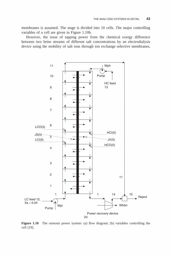
THE ANALYZED SYSTEMS IN DETAIL 43

membranes is assumed. The stage is divided into 10 cells. The major controllingvariables of a cell are given in Figure 1.10b.

However, the issue of tapping power from the chemical exergy differencebetween two brine streams of different salt concentrations by an electrodialysisdevice using the mobility of salt ions through ion exchange selective membranes,

Wph

Wpl

11

15

Pump

Power recovery device

JV(5)

JS(5)

11

10

9

8

7

6

5

4

3

2

1

HCI(5)

HCO(5)

LCI(5)

LCO(5)

LC feed 12,Xs = 0.04

HC feed 13

Reject

Pump

1411

Wtrbn

(a)

Figure 1.10 The osmosis power system: (a) flow diagram; (b) variables controlling thecell [19].

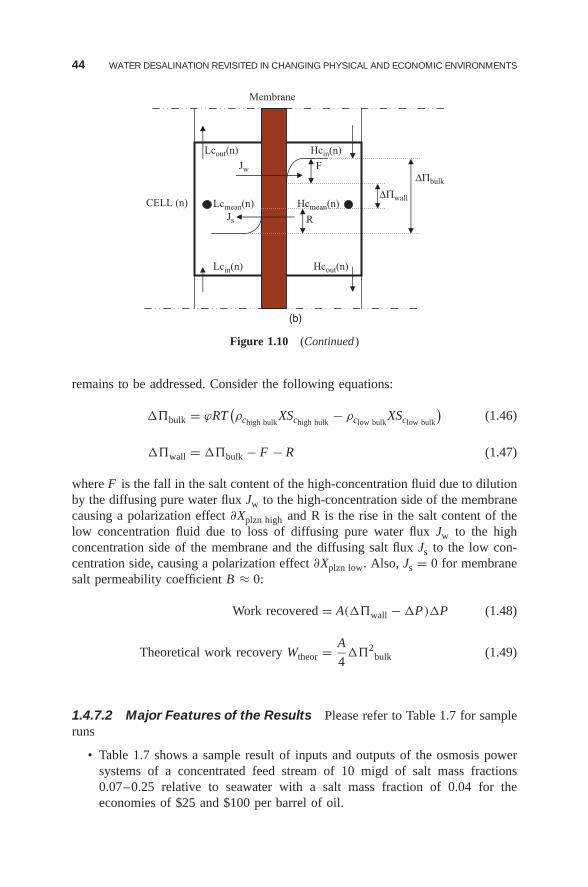
44 WATER DESALINATION REVISITED IN CHANGING PHYSICAL AND ECONOMIC ENVIRONMENTS

ΔΠbulk

ΔΠwall

Jw F

Hcout(n)

Lcout(n) Hcin(n)

Lcmean(n) Hcmean(n)

Js R

Lcin(n)

CELL (n)

Membrane

(b)

Figure 1.10 (Continued )

remains to be addressed. Consider the following equations:

��bulk = ϕRT(ρchigh bulk

XSchigh bulk− ρclow bulk

XSclow bulk

)(1.46)

��wall = ��bulk − F − R (1.47)

where F is the fall in the salt content of the high-concentration fluid due to dilutionby the diffusing pure water flux Jw to the high-concentration side of the membranecausing a polarization effect ∂Xplzn high and R is the rise in the salt content of thelow concentration fluid due to loss of diffusing pure water flux Jw to the highconcentration side of the membrane and the diffusing salt flux Js to the low con-centration side, causing a polarization effect ∂Xplzn low. Also, Js = 0 for membranesalt permeability coefficient B ≈ 0:

Work recovered = A(��wall − �P)�P (1.48)

Theoretical work recovery Wtheor = A

4��2

bulk (1.49)

1.4.7.2 Major Features of the Results Please refer to Table 1.7 for sampleruns

• Table 1.7 shows a sample result of inputs and outputs of the osmosis powersystems of a concentrated feed stream of 10 migd of salt mass fractions0.07–0.25 relative to seawater with a salt mass fraction of 0.04 for theeconomies of $25 and $100 per barrel of oil.

THE ANALYZED SYSTEMS IN DETAIL 45

• Power from conventional salt content of rejected brine (0.06–0.08 lbsalt/lbmix)due to concentration difference is not cost-effective. A small amount of power< 0.5 MW is gained by large membrane surface 110M · ft2. For brine with asalt mass fraction of 0.25, a power as high as 20 MW is gained by a membranesurface around 12 M ft2. Only for a brine of salt content 0.1 and higher doespower recovery begin to make sense.

• For a $25/bl (oil price index) economy and brine of salt mass fraction <0.1,power cost is as high as $25/kWh. The power cost for a correspondingideal process is $19/kWh. For brine of salt mass fraction 0.25, power cost isreduced to $0.2–0.4/kWh. The power cost for a corresponding ideal processis $0.16/kWh. For the $100/bl, economy, the respective costs are doubled.

• The salt mass fraction of brine from oilwells can be as high as 0.25. Powergeneration by this brine, when combined with seawater via membranes, canbe cost-effective in some situations.

1.4.8 Future Competitiveness of Combined Desalination Systems

1.4.8.1 Prediction Criteria Efficiency, dumped waste and product cost arethree major criteria that identify the most fit desalination system in the future.Overall system efficiency, CO2 emission per unit product, and cost/unit productare considered for the systems analyzed. Dumped brine is assumed to be toleratedbecause zero liquid discharge is still far from being cost-effective.

1.4.8.2 Predicted Competitiveness GT/MSF systems show that the case ofvariable power demand cogeneration counteracts most of the advantage of cogen-eration. This widely used cogeneration is likely to loose attractiveness in the future.The advantage is, however, maintained for base power load cogeneration.

SCC systems for power generation show that power-driven night products of lowstorage cost improves the plant load factor and raises its profitability provided theproducts are in short supply. The management of power generation by organizednight products may gain competitive advantage in the future.

The CC/RO desalting systems show that the attractiveness of power drivendesalting systems is likely to surpass that of distillation because of higher effi-ciency, lower emissions and lower product cost. The CC/VC desalting systemscome second to CC/RO. The lower operation pressure and the higher biofoulingresistance are advantages, but the handling of large specific volumes is a disadvan-tage. The development of strong light material for high-speed low-pressure-ratiocompressors, or the development of scale-free VC operation at atmospheric pres-sure, reduce the disadvantage as well as the gap between the product cost by ROand VC. If the disadvantage is reduced, the power-driven VC will gain also achievefuture promise for zero-liquid-discharge (ZLD) desalination.

The PV/RO system has zero CO2 emission and zero fossil fuel consumption butdoes not avoid dumping of concentrated brine in the physical environment. Theirfuture attractiveness is on the rise. The PV/ED system comes second to PV/RO ifit undergoes sufficient development.

46 WATER DESALINATION REVISITED IN CHANGING PHYSICAL AND ECONOMIC ENVIRONMENTS

The osmosis system for power production is only a possibility, not a reality,and requires the availability of brine near saturation to combine with seawaterto obtain power at acceptable cost. If developed, it can be useful for eliminatingproduct water of oilfields located near a sea.

References listed in Section 1.F.9 at the end of this chapter are additional usefulreadings for the preceding Section 1.4.

1.5 RECOMMENDED RESEARCH DIRECTIONS

1.5.1 Avoiding CO2 Emissions

• Desalination systems driven by renewable energy sources, particularly solar,are recommended if CO2 emission is to be avoided.

• Competitiveness requires high-efficiency desalting systems and high-efficiencysolar conversion systems. RO is in the lead for high efficiency, particularly forseawater. ED can be in the lead for lower salt content sources. Photovoltaicdesalination is in the lead for higher-efficiency conversion to power.

• Competitiveness is increased by:◦ RO of higher water and lower salt permeability and lower cost per unit

surface◦ ED of higher current density and lower electric resistance and lower cost

per unit surface◦ PV solar cells of higher standard test efficiency and higher field efficiency

and lower cost per unit surface

1.5.2 Reducing CO2 Emissions

• If fossil fuels have to be used, the solutions to lowering CO2 emissions isto develop higher efficiency energy conversion devices and/or produce moreproducts for the same emissions.

• Competitiveness is increased by◦ Cogeneration of power and desalted water by base-load power plants◦ Producing night low-storage-cost products to improve the load factors of

power plants and of variable-load (non-base-load) cogeneration plants.

1.5.3 Desalination of Zero Liquid Discharge

• Adequate understanding of the feed saturation limits, their sequence, theirdynamics of salt release and the separation of their solids are essential for theidea of zero liquid discharge.

• Membrane desalting is inherently high efficiency and cost-effective due to itsavoidance of water phase change.◦ Membranes should be designed to discriminate between salt species with

respect to their solubility limits. Ideally two types are needed; one membraneretains all species except sodium chloride, and the other one retains sodiumchloride and stands pressures as high as 5000 psia.

THE SOFTWARE PROGRAMS DEVELOPED BY THE AUTHOR FOR SYSTEM ANALYSIS 47

◦ A doping method for longer supersaturation time is needed to avoid theclogging of membrane passages.

• Vapor compression desalting pays an energy penalty for the presence of phasechange but has the advantages of low-pressure operation, high biofouling resis-tance, and less severe clogging problems. These advantages are also desirablefor zero liquid discharge◦ The vapor compressor should be made of a strong lightweight composite to

run efficiently at the desired high speed with lower stresses.◦ Vapor compression intake at atmospheric pressure helps further increase the

compressor efficiency and reduce its cost if scaling can be avoided.

1.6 CONCLUSIONS

Solar desalination of conventional concentration ratios has a high potential toreplace fossil fuel and avoids its CO2 emission for the production of desaltedwater. Supporting research to improve photovoltaic conversion efficiency and thedriven desalting efficiency is worthwhile. Reverse osmosis and electrodialysis arein the lead for higher desalting efficiency.

Zero liquid discharge desalination to avoid environmental damage due to dump-ing of rejected brine is far from being cost effective. Further research is needed.

Reverse osmosis driven by a simple combined cycle to produce water pro-duces much lower CO2 emission than conventional power distillation cogenerationsystems. RO driven by high-firing cooled-blade combined cycle further reducesCO2 emission.

Power plants and cogeneration plants that burn fossil fuel and operate undervariable power demand can benefit from night products of low storage cost inshort supply. Night products improve the plant load factor, produce more productsfor the same CO2 emission and raise profitability.

Increasing the efficiencies of conventional energy conversion devices and reduc-ing their costs have their limits in meeting the challenge of rising fuel prices andrising CO2 emission. New processes using new materials and new devices need tobe discovered.

1.7 THE SOFTWARE PROGRAMS DEVELOPED BY THE AUTHOR FORSYSTEM ANALYSIS

(The software discussed may be downloaded at http://booksupport.wiley.com).

1.7.1 Four Programs Developed and Their Entries

• DesRvst : handles the systems of the first six configurations. These are thesystems of: GT/MSF, SCC, VC/SCC, VCZLD, RO/SCC, and ROZLD.Each system has its own results of states, processes and costs displayable

48 WATER DESALINATION REVISITED IN CHANGING PHYSICAL AND ECONOMIC ENVIRONMENTS

or printable. An overall energy balance and exergy balance verifies theconsistency of the results. The program has the following entries:◦ GT/MSF cogeneration systems◦ Simple combined cycle systems with night RO desalter◦ Simple combined cycle systems with night electrolyzer◦ RO rejecting brine driven by simple combined cycle◦ RO rejecting salt driven by simple combined cycle◦ VC rejecting brine driven by simple combined cycle◦ VC rejecting salt driven by simple combined cycle◦ Change economic environment (default $25/bl)◦ Change power demand profile◦ Change units IP/SI (default IP)◦ Change zero exergy state (default sea)

• SOLRO : handles PV/RO systems and has the following entries:◦ Design solar-panel-driven RO system◦ Run sample of up to 10 systems◦ Display all results◦ Print all results◦ Print selected results◦ Change units IP/SI (default IP)◦ Change zero exergy state (default sea)◦ Change economic environment (default $25/bl)◦ Review software description◦ Terminate

• SOLED handles PV/ED systems and has the following entries:◦ Design solar-panels-driven ED system◦ Run sample of up to 10 systems◦ Display all results◦ Print all results◦ Print selected results◦ Change units IP/SI (default IP)◦ Change zero exergy state (default sea)◦ Change economic environment (default $25/bl)◦ Review software description◦ Terminate

• Osmosis handles osmosis power systems and has the following entries:◦ Compute one-stage osmosis given hs and dP /P

THE SOFTWARE PROGRAMS DEVELOPED BY THE AUTHOR FOR SYSTEM ANALYSIS 49

◦ Design one-stage osmosis given flow passages◦ Display all results◦ Print all results◦ Print selected results◦ Run sample of 10 systems given hs and dP /P◦ Print sample runs◦ Change Units IP/SI (default IP)◦ Change zero exergy state (default sea)◦ Change economic environment (default $25/bl)◦ Review software description◦ Terminate

1.7.2 Major Ingredients of Each Program

These ingredients are as follows:

• System description in terms of working fluids, devices, and thermodynamicdecision variables

• A routine for changing decision variables manually

• Computational routine in communication with fluid thermodynamic and trans-port properties and with the connectivity of devices to compute a solution pera selected reference unit mass. Connectivity may be explicit (handling severalconfigurations) or embedded in the computational routine (handling one con-figuration at a time). The speed of computation depends on system connectiv-ity, system decision variables, and the complexity of the controlling equations.

• A routine to compute parameters of interest, once a solution is obtained, suchas heat, power and mass rates; efficiencies; exergy destructions; costs andobjective function

• For the systems shown in Figures 1.1–1.3, an optimization routine that auto-mates the optimization of the system

1.7.3 The Software

The software developed for system analysis contains the following properties:

• Installation of the software in the user’s computer is automatic.

• The software contains:◦ The chapter explained in slides◦ Executable versions of the four programs◦ The source code of their master programs◦ Sample source codes of property and process programs

50 WATER DESALINATION REVISITED IN CHANGING PHYSICAL AND ECONOMIC ENVIRONMENTS

APPENDIX

Some Useful Equations and Facts for Water Desalination Modeling as

Employed in this Chapter [14].

1.A.1 Brief Description of the Thermodynamic Model of a System andthe Design Models of Its Main Components

1.A.1.1 Thermodynamic Model The model has a database of fluid prop-erties and elementary processes that are the building blocks of a fair number ofpower generation and cogeneration systems. The fluid property database containsthe equations essential for computation of the thermodynamic and transport prop-erties of H2O, NH3, R12, and NH3/H2O mixtures, seven ideal gases (O2, N2, H2O,CO2, SO2, CO and H2) and their combination which can cover air, gas mixtures,combustion gases dry or wet; and seven liquids (lubricating oil, ethylene glycol,glycerin, kerosene, sodium, bismuth, mercury, and seawater/brines). RefrigerantsR142a and R153b were also included. The process database contains 22 elemen-tary processes that allow the description of a large number of systems. The mainelementary processes handle expansion, compression, heat exchange, mixing, com-bustion, and throttling. Few processes are simple combinations of the elementaryprocesses, such as a multistage process. Few are purely computational, performingtasks such as splitting, merging, and tearing. The performance of a main elementaryprocess is described by its overall efficiency and loading parameters. More thanone set of the essential input parameters is allowed by the thermodynamic modelto enhance system computation with the fewest iteration loops.

The model is also used to express the exergy destruction of a device in terms ofthe device efficiency and loading parameters. To compute the exponents {ne} of adevice that correlates its exergy destruction D in terms of its efficiency and loadingparameters, the process model of the device is run with different input variablescovering the range of interest to its system. The computed exergy destruction D islisted versus its correlating parameters. A curve-fitting procedure gives the valueof {ne} applicable over the range of variation considered.

1.A.1.2 Sample Design Models The purpose of the following design modelsis to provide a rational basis for the cost of their devices. For this purpose all designmodels target the evaluation of a dominating flow passage surface for which a unitcost gives a fair prediction of the estimated device cost. The design models representsome of the current design practices and not necessarily the best ones. They alsoneed to be updated to accommodate changes in design practices.

1.A.1.2.1 The Axial Air Compressor The basic features are axial, two dimen-sional analysis at the mean radius, subsonic, 50% reaction, diffusion factor <0.45,and ideal gas properties. Blade geometry is kept constant. All stages except thefinal one experience the same temperature rise. Tip blade speed, axial velocity,root/tip radius ratio, and work factors are kept constant at 1150 ft/s−1 (250 m/s−1),500 ft/s−1 (150 m/s−1), 0.5, and. 0.98–0.83 (0.83 after the third stage), respectively.

APPENDIX 51

A polytropic efficiency is assumed, velocity triangles computed, and the stageefficiency is evaluated from cascade tests corresponding to the blade geometry.Computations are iterated until polytropic and stage efficiencies are matched. Massrate, pressure ratio, and temperature rise per stage are varied, and the number ofstages, total surface of fixed and moving blades, adiabatic efficiency, speed, andrecommended solidity are computed. An arbitrary value of solidity can also beentered as input. The total surface of the moving and fixed blades is correlated interms of air mass flow rate, pressure ratio, and efficiency ratio η/(1 − η). Ambi-ent conditions are assumed for air at compressor inlet. A version of the modelaccommodates low-pressure ratio axial and radial steam compressors .

1.A.1.2.2 The Gas Turbine The basic features are axial, uncooled blades,two-dimensional analysis at mean radius, subsonic, 50% reaction, and ideal gasproperties. Blade geometry is kept constant. Loading and flow coefficients ψ ,φ,mean blade speed, and inlet temperature are kept constant at 1.4, 0.8, 1115 ft/s(240 m/s) and 1600◦F (870◦C) respectively. The inlet temperature implies uncooledexpansion. The first two values seem to minimize the needed total surface ofblades. Stage efficiencies of nozzle and rotor blades are assumed, velocity trianglesare computed, and stage and tip clearance losses are evaluated from cascade testscorresponding to the blade geometry. Computations are iterated until the assumedefficiencies and the losses are matched. Mass rate, pressure ratio, and speed arevaried, and the number of stages, total surface of nozzle and rotor blades, adiabaticefficiency, and recommended solidity are computed. An arbitrary value of soliditycan be entered as input. The model does not guarantee that the speed matchesthat of the compressor. The total blade surface of the fixed and moving bladesis correlated in terms of gas flow rate, expansion ratio, and efficiency parameterη/(1 − η). Gas pressure at exit is assumed to be ambient.

1.A.1.2.3 The Steam Turbine The steam turbine is similar to the gas turbineexcept for a few differences. Actual steam properties were used to compute thespecific heat and the isentropic index instead of the constant values assumed in thecase of air and combustion gases. Inlet temperature and pressure and exit pressureinstead of the pressure ratio became inputs. Exit pressure was changed to cover bothcondensing and backpressure turbines. In some cases the blade heights were tooshort and high rotational speeds were entered to reduce mean diameter and increaseblade height. The total surface of blades did not change with the change in speed.The total surface of the blades is correlated in terms of steam mass rate, (T /P ) atinlet, exit pressure, and efficiency ratio η/(1 − η). Impulse stages are not included.

1.A.1.2.4 Centrifugal Pumps The basic features are centrifugal, axial flow atinlet and radial flow at exit, with velocity head recovery. Loading (head) and flowcoefficients �, , number of impeller blades, root/eye radius ratio, velocity exitingcasing, specific volume, and maximum head per stage are kept constant at 1.4, 0.8,7, 0.4, 6 ft/s (1.8 m/s), 0.016 cu ft/lb (0.001 m3/kg), and 500 ft (150 m), respec-tively. Velocity triangles and flow passages are computed given specific speed.

52 WATER DESALINATION REVISITED IN CHANGING PHYSICAL AND ECONOMIC ENVIRONMENTS

Mass flow rate, head and specific speed are varied. Speed, surface of impeller,diffuser surface, and efficiency are computed. Specific speed is changed such thatsurface is minimized. One costing equation did not fit all cases. One equation wasused for low flow rates and high-pressure heads (feed pumps) and one for largeflow rates and low-pressure heads (circulating pumps). Extending flow rates to >

500 lb/s need to be implemented. Impeller surface is correlated in terms mass rate,pressure head, and efficiency ratio η/(1 − η).

1.A.1.2.5 Gas Turbine Combustor The basic features are annular tube andburning natural gas. Inlet and exit temperatures, air/fuel mass ratio, and number ofcans are kept constant at 1600◦F (870◦C), 500◦F (260◦C), at values of 75, and 7,respectively. Air mass rate, pressure, and pressure loss are varied and the combustorsurface computed. (60 m/s). The maximum velocity was set at 200 ft/s. Combustionintensity varied at ∼80 kW (ft3· atm)−1 (2000 kW (m3· atm)−1). The combustorsurface is correlated in terms air mass rate, inlet pressure, and pressure loss.

1.A.1.2.6 Heat Exchangers The basic features are forced convection heatexchange, single- and two-phase fluids, and three generic types of exchangers(double-tube, fin-plate, and shell-and-tube). For the shell-and-tube type, flow maybe counter or crosscounter, tubes may be plain or finned on the outside, and shellmay be cylindrical or duct-type. In two-phase procedures, more than one equationis used for film coefficients and friction factor multipliers. Pressure losses werebased on the worst-case multiplier. The plate-fin type consists of layers of plateswith straight parallel fins on each side of each plate. The fins on one side are per-pendicular to those of the other side. Two sets of layers may be connected in seriesto allow for mixing. A surface geometry is selected. For shell and tube geome-try, tube length, diameter, and pitches, and shell diameter or width and depth areentered. For the plate-fin geometry, the number of plates, fins per inch on eitherside, and their heights and thickness are entered. Two groups of boundary param-eters can be entered: mass rates and temperature and pressures at all inlets andexits or mass rates and inlet pressures and temperatures and effectiveness. Withboth entries, film coefficients of heat transfer and pressure drops are computed.The heat exchange surface is computed in either of two ways: surface by geometryor surface = Q/U �T . With the first entry computations are iterated until the twoareas are matched and the two pressure drops are accommodated. With the secondone, only the surface iteration is needed. The pressure drops are output parame-ters. The iterations are both manual and automated to minimize the heat exchangesurface. This program, evolved in parallel with the thermodynamic model.

The superheater, the boiler, and the economizer of the heat recovery steam gen-erator assumed duct- type shell and tubes with outside circular fins. Fin geometryon the outside of the steam generator tubes and fouling factors in heat exchangeare kept constant. The brine heater and the flash stages are assumed to have plaintubes. The brine heater is assumed to have a cylindrical shell. The flash stages areassumed to have a duct-type shell. A constant temperature drop is assumed for allthe stages and a chamber at a temperature of 150◦F (65◦C) is assumed to represent

APPENDIX 53

all the stages. A heat transfer temperature difference correction is introduced forthe rejection stages. Two types of air preheater are considered: shell-and tube withcircular fins on the outside or a plate-fin type. For the evaporator/condenser a ver-tical shell-and-tube type with plain tubes is assumed. The heating steam condensesin the tubes, and the liquid is sprayed on the outside at a rate 10 times the vaporizedliquid. In all the exchangers fouling factors are kept constant. Inlet parameters arevaried. The temperature profile is first computed and checked for crossings andpinch point. Rate of heat exchange, effective temperature difference of heat trans-fer, and heat exchange surface are computed among other detailed heat transferoutputs. Pressure drops, if outputs, are computed. Given the inlet pressure temper-ature and mass rate for the two fluids, all heat exchange surfaces are correlated interms the rate of heat exchange, a temperature difference (terminal or logarithmicmean) and hot and cold side pressure losses. In a flash stage, any temperature dropinduced by flashing is used instead of a pressure loss. The effect of pressure andtemperature levels is accounted for in the unit cost (severity of operation).

1.A.1.2.7 Radiant Heat Exchange in Boiler A simple model is assumed.The basic features are square vertical duct type, forming water walls combinedwith reflectors and backed with insulation. The water boils in the tubes, and thevapor formed is separated in an upper drum. The total radiation exchange betweenthe entire gas volume and the walls is based on the mean beam length. Theabsorption bands of H2O and CO2 of the hot gases are factored in. The effectof temperature variation along the duct is accounted for by dividing the gas pathinto five sections, each with a uniform temperature. The gas is assumed to enterat the adiabatic flame temperature. The effect of convective film coefficients andwall resistance is included. The height of the duct and its width were observedto control both the gas-side and the steam-side pressure losses, beside the heatexchange surface. The gas-side pressure loss was not significant because of thesignificant change in gas temperature and the associated lowering of gas veloci-ties. The tube-side pressure drop progressively increased as the height is increasedrelative to the width with negligible effect on the heat transfer coefficient. Theheat exchange is expressed by an overall heat transfer coefficient ranging from 30to 50 Btu (h · ft2 · F)−1 [0.170–0.284 kW (m2· K)−1], while convection-inducedheat exchange was lower by only one order of magnitude. The surface of thewall tubes is correlated in terms of the rate of heat transfer and the conventionallogarithmic mean temperature difference. An equivalent temperature driving force�Tr = (Tgas/Tflame)

4 − (Tsteam/Tflame)4 was used in earlier applications with a dif-

ferent correlation (A = 0.39Q�T−2r ).

1.A.1.2.8 Curve-Fitting Costing Equations and Exergy Destruction Variousmathematical procedures are available for curve fitting by minimizing the deviationsaround a fit. The number of the surfaces A or exergy destructions D generatedshould be much larger than the correlating parameters, which usually vary from 2to 4. One simple procedure is to use sets of number equal to the number of thecorrelating parameters plus one, to obtain the coefficient k and exponents {n}. The

54 WATER DESALINATION REVISITED IN CHANGING PHYSICAL AND ECONOMIC ENVIRONMENTS

ratios of the computed A generated by a set to the corresponding one generated bythe design model are computed. The process is repeated with different sets until aset is found where the ratios deviate the least from one. The same rule of thumbapplies to D . The correlating parameters of the costing equations and their rangeof applicability are given in Section 1.A.2.

Deviations in curve fitting were within ±10%, and in very few cases of a widerange of applicability deviations of ±20% were found. It is important to note thatimproved correlations depend on improving the quality of models and reducingtheir range of applicability.

References listed in Section 1.F.10 at the end of this chapter are additional usefulreadings for the preceding Section 1.A.1.

1.A.2 The Capital and Fuel Costing Equations of some commonDevices (Tables 1.A.1 and 1.A.2)

For illustration, let the device be a forced-convection heat exchanger. It is assumedto be the superheater, component 7 of the heat recovery steam generator of thesimple combined cycle of Figure 2. A duct shell-and-finned tube type is assumed.The fins are assumed circular on the outside that is, on the gas side. The designmodel of heat exchangers described in Secion 1.A.2 is used.

The boundary parameters P , T , {x}, M at inlets and exits of the exchanger asembedded in the system at a design point for the system are used. The exchangerphysical surface and its geometry are defined by length, diameter, spacing, number,material, material thickness and fin geometry of the tubes. These parameters areusually more than sufficient to allow for adjustment to match the computed surfaceand pressure drops by film coefficients and friction factors for the given heat loadand its temperature profile. Any extra design degrees of freedom are used to min-imize the surface and/or to satisfy reliable design practices. The design process isthus a matching/minimizing process.

The minimized surface as a function of performance is generated by repeatingthis design process for different boundary parameters within a range relevant to theoptimization of the system. A specific geometry of minimized surface is obtainedfor each set of boundary parameters. The surface is then expressed by an appro-priate set of performance parameters such as heat loads, mass rates, heat exchangetemperature differences, effectiveness, and pressure losses. In this example, thesurface of the fins and tubes is expressed in terms of the heat load, the logarithmicmean temperature difference and pressure losses on the shell side and on the tubeside. The following form is used:

A = kQn1�Tmn2�Pn3

t �Psn4 (1.A.1)

where A is converted to a costing equation by

Z = caA (1.A.2)

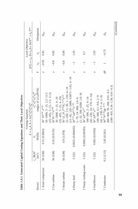
Tabl

e1.

A.1

Gen

erat

edC

apit

alC

osti

ngE

quat

ions

and

The

irL

ocal

Obj

ecti

ves

Cos

ting

Equ

atio

nL

ocal

Obj

ectiv

eZ

=c a

AA

=kx

n1 1xn2 2

xn3 3xn4 4

J(Y

)=

c dD

+czZ=

KeY

ne+

k zY

nz

c a$k

/ft2

k,

xn

11

xn

22

xn

33

xn

44

Dev

ice

/(m

2)

IP/(

SI)

rang

esof

{x},(

IP/S

I)Y

n en z

Dis

sipa

tion

1A

xial

com

pres

sor

50(5

38)

0.15

(0.0

063)

M1

Pr0.

45e0.

45e

−0.9

50.

45D

PT50

–10

00,

5–

15,

2.3

–11

.5(2

5–

455,

5–

15,

2.3,

11.5

)2

Gas

turb

ine

50(5

38)

0.32

(0.0

135)

M1Pr

−0.5

e0.85

e−0

.80.

85D

PT50

–10

00,

5–

15,

4–

19(2

5–

455,

5–

15,

4–

19)

3St

eam

turb

ine

50(5

38)

0.9

(1.9

78)

M1(T

i/P

i)0.

05P

−0.7

5e

e0.9

e−0

.80.

90D

PT25

–10

0,1.

5–

30,

1–

150,

4–

19(1

1–

45,

120

–24

00,

0.00

71–

1.03

,4

–19

4Pu

mp

feed

3(3

2)0.

0025

(0.0

0043

5)M

0.55

�P

0.55

e1.05

e−1

1.05

DPT

5–

70,

14–

900,

1.8

–9

(2–

32,

100

–62

00,

1.8

–9)

5Pu

mp

cool

ing-

wat

er3

(32)

0.00

63(0

.001

83)

M1�

P0.

1e0.

7e

−10.

7D

PT10

0–

500,

2–

25,

4–

14(4

5–

230,

14–

170,

4–

14)

6Fa

n/bl

ower

3(3

2)0.

063

(0.0

183)

M1�

P0.

1e0.

7e

−11.

05D

PT10

0–

500,

0.1

–0.

6,2

–9

(45

=23

0,0.

7–

4,2

–9)

7C

ombu

stor

0.2

(2.1

5)5.

85(0

.261

)M

0.5P

0.24

dp−0

.75

dP1

−0.7

5D

P40

0–

900,

50–

200,

0.01

–0.

3(1

80–

410,

0.34

–1.

38,

0.01

–0.

3)

(Con

tinu

ed)

55

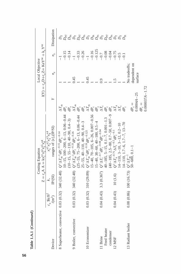
Tabl

e1.

A.1

(Con

tinue

d)

Cos

ting

Equ

atio

nL

ocal

Obj

ectiv

eZ

=c a

AA

=kx

n1 1xn2 2

xn3 3xn4 4

J(Y

)=

c dD

+czZ=

KeY

ne+

k zY

nz

c a$k

/ft2

k,

xn

11

xn

22

xn

33

xn

44

Dev

ice

/(m

2)

IP/(

SI)

rang

esof

{x},(

IP/S

I)Y

n en z

Dis

sipa

tion

8Su

perh

eate

r,co

nvec

tive

0.03

(0.3

2)34

0(3

2.48

)Q

1�

T−1 m

dP−0

.15

tdP

−0.1

4s

�T

m1

−1D

T10

–15

,10

0–

200,

6–

13,

0.06

–0.

44dP

t1

−0.1

5D

PT(1

0–

15,

55–

110,

40–

90,

0.4

–3)

dPs

1−0

.14

DPs

9B

oile

r,co

nvec

tive

0.03

(0.3

2)34

0(3

2.48

)Q

1�

T−1 m

dP−0

.33

tdP

−0.2

6s

�T

m0.

45−1

DT

(25

–55

,75

–20

0,6

–13

,0.

06–

0.44

dPt

1−0

.33

DPT

25–

55,

40–

110,

40–

90,

0.4

–3

dPs

1−0

.26

DPs

10E

cono

miz

er0.

03(0

.32)

310

(29.

89)

Q1�

T−1 m

dP−0

.16

tdP

−0.1

25s

�T

m0.

45−1

DT

15–

40,

70–

105,

6–

26,

0.00

7–

0.56

dPt

1−0

.16

DPt

15–

40,

38–

60,

40–

180,

0.5

–4

dPs

1−0

.125

DPs

11B

rine

0.04

(0.4

3)3.

3(0

.367

)Q

1�

T−0

.7t

dP−0

.08

tdP

−0.0

4s

�T

t0.

9−0

.7D

TFe

edhe

ater

40–

185,

5–

15,

0.1

–7,

0.00

1–

1.3

dPt

1−0

.08

DPT

cond

ense

r(4

0–

185,

2.5

–80

,0.

7–

50,

0.00

7–

9dP

s1

−0.0

4D

Ps12

MSF

0.04

(0.4

3)10

(1.6

)Q

1�

T−0

.75

n�

T−0

.5t

dP−0

.1t

�T

n1.

5−0

.75

DT

14–

110,

3–

10,

3–

12,

0.2

–10

�T

t1

−0.5

DT

14–

110,

1.7

–6,

1.7

–7,

13–

70dP

t1

−0.1

DPt

13R

adia

ntbo

iler

0.08

(0.8

6)10

0(1

6.73

)Q

1�

T−1 m

No

trad

eoff

s;de

pend

ent

onsu

rfac

e

50–

600,

0.1

–1

dPt=

0.00

04A−2

5dP

t=

0.00

0037

A−1

.72

56

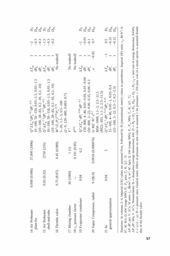
14A

irPr

ehea

ter

0.00

8(0

.086

)37

,000

(349

6)Q

1�

T−2 m

dP−0

.3h

dP−0

.3c

�T

m1

−2D

Tpl

ate-

fin10

–10

0,50

–15

0,0.

03–

1.5,

0.03

–1.

5dP

h1

−0.3

DPh

(10

–10

0,28

–83

,0.

2–

10,

0.2

–10

)dP

c1

−0.3

DPc

15A

irPr

ehea

ter

0.03

(0.3

2)27

50(2

35)

Q1�

T−1

.5m

dP−0

.3t

dP−0

.2s

�T

m1

−1.5

DT

shel

l-an

d-tu

be10

–10

0,50

–15

0,0.

03–

1.5,

0.03

–1.

5dP

t1

−0.3

DPh

(10

–10

0,28

–83

,0.

2–

10,

0.2

–10

)dP

s1

−0.2

DPc

16T

hrot

tleva

lve

0.75

(8.0

7)0.

45(0

.989

)M

1(T

i/P

i)0.

05P

−0.7

5e

No

trad

eoff

5–

20,

1.5

–5,

0.5

–10

0(2

–9,

120

–40

0,0.

003

–0.

7)17

Mix

ing

cham

ber

30(1

060)

1(1

)V

1N

otr

adeo

ff

18c a

pres

sure

fact

or—

0.19

1(0

.85)

P0.

3N

otr

adeo

ff

19E

vapo

rate

rco

nden

ser

0.04

6.2

Q1�

T−1

.m

dP−0

.01

tdP

−0.1

�T

m1

−1D

T15

0–

800,

4–

40,

0.01

–0.

05,

0.01

–0.

04dP

t1

−0.0

1D

Ph(5

0–

800,

2–

22,

0.06

–0.

35,

0.06

–0.

3dP

s1

−0.1

DPc

20V

apor

Com

pres

sor,

radi

al9

(96.

9)0.

0018

(0.0

0007

6)(v

M)1

Pr1

e0.7

e−0

.95

0.7

DPT

M50

–10

00,

1.1

–2,

2.3

–11

.5(M

22–

455,

1.1

–2,

2.3

–11

.5)

21hx

0.04

5Q

1�

T−1

.m

dP−0

.15

tdP

−0.1

5s

�T

m−1

0.5

DT

gene

ral

appr

oxim

atio

n15

–10

0,4

–40

,0.

05–

1,0.

03–

0.4

dPt

1−0

.15

DPh

(15

–10

0,2

–22

,0.

3–

7,0.

2–

2.3)

dPs

1−0

.15

DPc

Not

atio

ns:

Inco

lum

ns2

–4,

Impe

rial

(UK

)va

lues

are

pres

ente

dFi

rst,

Follo

wed

bySI

(int

emat

iona

l;m

etri

c)va

lues

inpa

rent

hese

s.Im

peri

al(I

P)un

its:

c a,

$k/f

t2;

A,

ft2;

M,

lb/s

;Q

,kW

(ran

geM

W);

Pi,

Pe,

psia

;T

i,R

;�

T,

◦ F;�

P,d

P,

psi;

V,

ft3/s

.SI

units

:c a

,$k

/m2;

A,

m2;

M,

kg/s

;Q

,kW

(ran

geM

W);

Pi,

Pe,

MPa

;T

i,K

;�

T,

◦ C;

�P

,dP

,kPa

;V

,m3/s

.N

omen

clat

ure:

D=

diss

ipat

ion

(exe

rgy

dest

ruct

ion)

,kW

;D

=D

P+

DT

+D

C,D

PT=

DP

+D

T;

c d=

unit

cost

ofex

ergy

dest

ruct

ion,

$/kW

h,e

=η/(1

−η);

Pr=

pres

sure

ratio

.G

ener

alno

tes:

Eff

ect

ofpr

essu

reon

unit

cost

sis

assu

med

1fo

rpr

essu

res

<25

0ps

ia;

cost

ofa

stea

mej

ecto

ris

assu

med

doub

leth

atof

the

thro

ttle

valv

e.

57

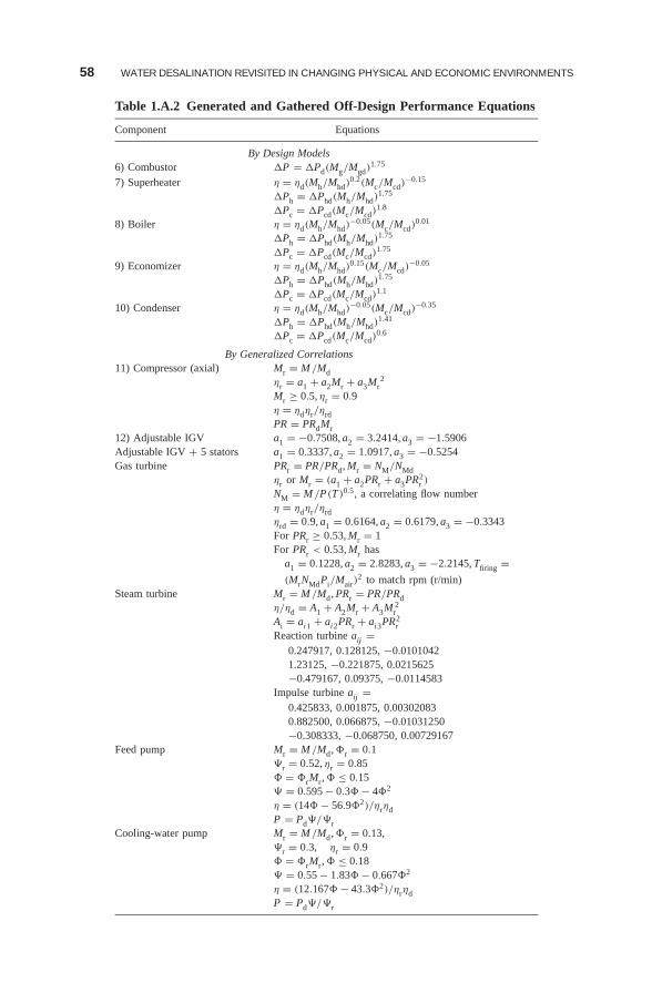
58 WATER DESALINATION REVISITED IN CHANGING PHYSICAL AND ECONOMIC ENVIRONMENTS

Table 1.A.2 Generated and Gathered Off-Design Performance Equations

Component Equations

By Design Models6) Combustor �P = �Pd(Mg/Mgd)

1.75

7) Superheater η = ηd(Mh/Mhd)0.2(Mc/Mcd)

−0.15

�Ph = �Phd(Mh/Mhd)1.75

�Pc = �Pcd(Mc/Mcd)1.8

8) Boiler η = ηd(Mh/Mhd)−0.05(Mc/Mcd)

0.01

�Ph = �Phd(Mh/Mhd)1.75

�Pc = �Pcd(Mc/Mcd)1.75

9) Economizer η = ηd(Mh/Mhd)0.15(Mc/Mcd)

−0.05

�Ph = �Phd(Mh/Mhd)1.75

�Pc = �Pcd(Mc/Mcd)1.1

10) Condenser η = ηd(Mh/Mhd)−0.05(Mc/Mcd)

−0.35

�Ph = �Phd(Mh/Mhd)1.41

�Pc = �Pcd(Mc/Mcd)0.6

By Generalized Correlations11) Compressor (axial) Mr = M /Md

ηr = a1 + a2Mr + a3Mr2

Mr ≥ 0.5, ηr = 0.9η = ηdηr/ηrdPR = PRdMr

12) Adjustable IGV a1 = −0.7508, a2 = 3.2414, a3 = −1.5906Adjustable IGV + 5 stators a1 = 0.3337, a2 = 1.0917, a3 = −0.5254Gas turbine PRr = PR/PRd, Mr = NM/NMd

ηr or Mr = (a1 + a2PRr + a3PR2r )

NM = M /P(T )0.5, a correlating flow numberη = ηdηr/ηrdηrd = 0.9, a1 = 0.6164, a2 = 0.6179, a3 = −0.3343For PRr ≥ 0.53, Mr = 1For PRr < 0.53, Mr has

a1 = 0.1228, a2 = 2.8283, a3 = −2.2145, Tfiring =(MrNMdPi/Mair)

2 to match rpm (r/min)Steam turbine Mr = M /Md, PRr = PR/PRd

η/ηd = A1 + A2Mr + A3M 2r

Ai = ai1 + ai2PRr + ai3PR2r

Reaction turbine aij =0.247917, 0.128125, −0.01010421.23125, −0.221875, 0.0215625−0.479167, 0.09375, −0.0114583

Impulse turbine aij =0.425833, 0.001875, 0.003020830.882500, 0.066875, −0.01031250−0.308333, −0.068750, 0.00729167

Feed pump Mr = M /Md, r = 0.1�r = 0.52, ηr = 0.85 = rMr, ≤ 0.15� = 0.595 − 0.3 − 4 2

η = (14 − 56.9 2)/ηrηdP = Pd�/�r

Cooling-water pump Mr = M /Md, r = 0.13,�r = 0.3, ηr = 0.9 = rMr, ≤ 0.18� = 0.55 − 1.83 − 0.667 2

η = (12.167 − 43.3 2)/ηrηdP = Pd�/�r

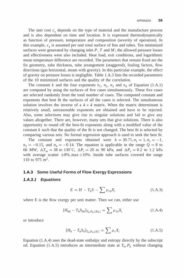
APPENDIX 59

The unit cost ca depends on the type of material and the manufacture processand is also dependent on time and location. It is expressed thermodynamicallyas function of pressure, temperature and composition (severity of operation). Inthis example, ca is assumed per unit total surface of fins and tubes. Ten minimizedsurfaces were generated by changing inlet P , T and M ; the allowed pressure lossesand effectiveness were also included. Heat load, exit conditions, and logarithmicmean temperature difference are recorded. The parameters that remain fixed are thefin geometry, tube thickness, tube arrangement (staggered), fouling factors, flowdirections (gas horizontal, steam with gravity). In this particular example, the effectof gravity on pressure losses is negligible. Table 1.A.3 lists the recorded parametersof the 10 minimized surfaces and the quality of the correlation.

The constant k and the four exponents n1, n2, n3 and n4 of Equation (1.A.1)are computed by using the surfaces of five cases simultaneously. These five casesare selected randomly from the total number of cases. The computed constant andexponents that best fit the surfaces of all the cases is selected. The simultaneoussolution involves the inverse of a 4 × 4 matrix. When the matrix determinant isrelatively small, unreasonable exponents are obtained and have to be rejected.Also, some selections may give rise to singular solutions and fail to give anyvalues altogether. There are, however, many sets that give solutions. There is alsoopportunity to round off the best-fit exponents along with a modified value of theconstant k such that the quality of the fit is not changed. The best fit is selected bycomparing various sets. No formal regression approach is used to seek the best fit.

The constant and exponents obtained were k = 30.71, n1 = 1, n2 = −1,n3 = −0.15, and n4 = −0.14. The equation is applicable in the range Q = 8 to66 MW, �Tm = 38 to 130◦C, �Pt = 20 to 90 kPa, and �Ps = 0.2 to 1.2 kPawith average scatter ±8%, max +10%. Inside tube surfaces covered the range110 to 975 m2.

1.A.3 Some Useful Forms of Flow Exergy Expressions

1.A.3.1 Equations

E = H − T0S −∑

μi0Xi (1.A.3)

where E is the flow exergy per unit matter. Then we can, either use

[H0d − T0S0d]T0,P0,{Xi0} =∑

μi0Xi (1.A.4)

or introduce

[H0 − T0S0]T0,P0,{Xi } =∑

μi Xi (1.A.5)

Equation (1.A.4) uses the dead-state enthalpy and entropy directly by the subscriptod. Equation (1.A.5) introduces an intermediate state at T0, P0 without changing

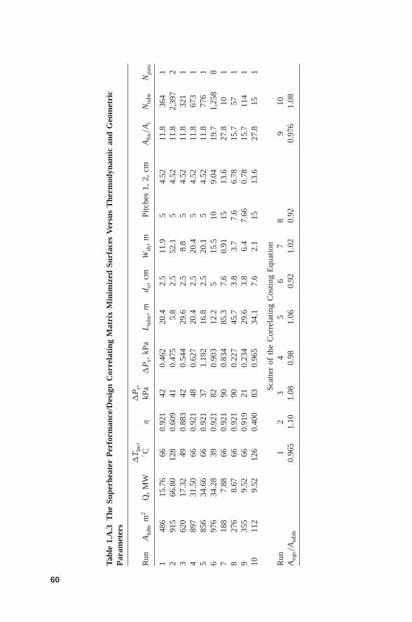
Tabl

e1.

A.3

The

Supe

rhea

ter

Per

form

ance

/Des

ign

Cor

rela

ting

Mat

rix

Min

imiz

edSu

rfac

esV

ersu

sT

herm

odyn

amic

and

Geo

met

ric

Par

amet

ers

�T

lm,

�P

t,R

unA

tube

m2

Q,

MW

◦ Cη

kPa

�P

s,kP

aL

tube

,m

d o,

cmW

sh,

mPi

tche

s1,

2,cm

Afin

/A

iN

tube

Npa

ss

148

615

.76

660.

921

420.

462

20.4

2.5

11.9

54.

5211

.836

41

291

566

.80

128

0.60

941

0.47

55.

82.

552

.15

4.52

11.8

2,39

72

362

017

.32

490.

883

420.

544

29.6

2.5

8.8

54.

5211

.832

11

489

731

.50

660.

921

480.

627

20.4

2.5

20.4

54.

5211

.867

31

585

634

.66

660.

921

371.

192

16.8

2.5

20.1

54.

5211

.877

61

697

634

.28

390.

921

820.

903

12.2

515

.510

9.04

19.7

1,25

88

718

87.

8866

0.92

190

0.83

485

.37.

60.

9115

13.6

27.8

101

827

68.

6766

0.92

190

0.22

745

.73.

83.

77.

66.

7815

.757

19

355

9.52

660.

919

210.

234

29.6

3.8

6.4

7.66

0.78

15.7

114

110

112

9.52

126

0.40

083

0.96

534

.17.

62.

115

13.6

27.8

151

Scat

ter

ofth

eC

orre

latin

gC

ostin

gE

quat

ion

Run

12

34

56

78

910

Aeq

n/A

tabl

e0.

965

1.10

1.08

0.98

1.06

0.92

1.02

0.92

0.97

61.

08

60

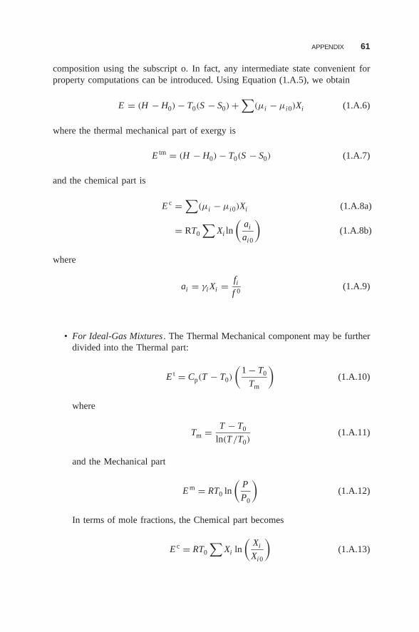
APPENDIX 61

composition using the subscript o. In fact, any intermediate state convenient forproperty computations can be introduced. Using Equation (1.A.5), we obtain

E = (H − H0) − T0(S − S0) +∑

(μi − μi0)Xi (1.A.6)

where the thermal mechanical part of exergy is

E tm = (H − H0) − T0(S − S0) (1.A.7)

and the chemical part is

E c =∑

(μi − μi0)Xi (1.A.8a)

= RT0

∑Xi ln

(ai

ai0

)(1.A.8b)

where

ai = γi Xi = fif 0

(1.A.9)

• For Ideal-Gas Mixtures . The Thermal Mechanical component may be furtherdivided into the Thermal part:

E t = Cp(T − T0)

(1 − T0

Tm

)(1.A.10)

where

Tm = T − T0

ln(T/T0)(1.A.11)

and the Mechanical part

Em = RT0 ln

(P

P0

)(1.A.12)

In terms of mole fractions, the Chemical part becomes

E c = RT0

∑Xi ln

(Xi

Xi0

)(1.A.13)

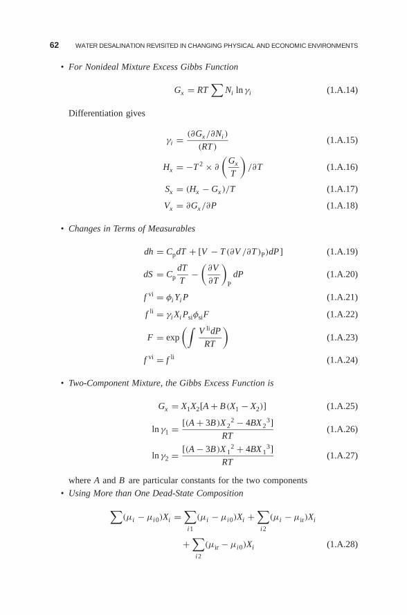
62 WATER DESALINATION REVISITED IN CHANGING PHYSICAL AND ECONOMIC ENVIRONMENTS

• For Nonideal Mixture Excess Gibbs Function

Gx = RT∑

Ni ln γi (1.A.14)

Differentiation gives

γi = (∂Gx/∂Ni )

(RT )(1.A.15)

Hx = −T 2 × ∂

(Gx

T

)/∂T (1.A.16)

Sx = (Hx − Gx )/T (1.A.17)

Vx = ∂Gx/∂P (1.A.18)

• Changes in Terms of Measurables

dh = CpdT + [V − T (∂V /∂T )P)dP ] (1.A.19)

dS = CpdT

T−

(∂V

∂T

)P

dP (1.A.20)

f vi = φi Yi P (1.A.21)

f li = γi Xi PsiφsiF (1.A.22)

F = exp

(∫V lidP

RT

)(1.A.23)

f vi = f li (1.A.24)

• Two-Component Mixture, the Gibbs Excess Function is

Gx = X1X2[A + B(X1 − X2)] (1.A.25)

ln γ1 = [(A + 3B)X 22 − 4BX 2

3]

RT(1.A.26)

ln γ2 = [(A − 3B)X 12 + 4BX 1

3]

RT(1.A.27)

where A and B are particular constants for the two components

• Using More than One Dead-State Composition

∑(μi − μi0)Xi =

∑i1

(μi − μi0)Xi +∑i2

(μi − μir)Xi

+∑i2

(μir − μi0)Xi (1.A.28)

APPENDIX 63

Another dead state, denoted here with the subscript ir (e.g., sea), is assumedfor species (e.g., salts) having traces in the usually assumed dead state denotedhere with the subscript io (e.g., air) but is relatively abundant in ir. The lastterm is a constant of no interest in exergy change beyond the dead state ir.

• Introducing Known Intermediate Chemical Changes

�GR =∑

R

(μi − μi0)XiR −∑

P

(μi − μi0)XiP (1.A.29)

Let μj be a reactant (e.g., a hydrocarbon fuel) of minute equilibrium molefraction in the assumed dead state (e.g., air); then μj0 is determined by

(μj − μj0)Xj = �GR +∑

P

(μi − μi0)XiP −∑

R

(μi − μi0)XiR,i �=j (1.A.30)

1.A.3.2 Balances1.A.3.2.1 Exergy Balance∑

in

Eb =∑out

Eb +∑

D (1.A.31)

where

D = exergy destruction (1.A.32)

Eb = E q + Ew + E f (1.A.33)

E q = Q(1 − T0/Tb) (1.A.34)

Ew = Ws (1.A.35)

E f = ME

1.A.3.2.2 Entropy Balance∑out

Sb −∑

in

Sb = S cr (1.A.36)

where

Sb = S m + S q (1.A.37)

S q = Q/Tb (1.A.38)

S m = MS (1.A.39)

D = T0S cr (1.A.40)

64 WATER DESALINATION REVISITED IN CHANGING PHYSICAL AND ECONOMIC ENVIRONMENTS

1.A.3.2.3 A Note on the Dead State Environment An absolute dead stateof zero exergy does not exist, but a reference one can be set. Arbitrary ref-erence states have long been used. In thermodynamic properties zero enthalpyand entropy differ for different working fluids. In chemical reactions, elementsare selected as reference to compute the energy and free energy of formation ofcompounds.

A reference dead state for zero exergy is defined by a pressure P0, a temperatureT0 and a set of chemical species of composition {Xio} suitable for analyzing theutilization of energy in a particular situation. The composition {Xi0} is preferredto resemble a natural state in which the chemical species of interest are not tracesin order to establish chemical exergies. Atmospheric air is an appropriate deadstate to use for work with a number of gases, including combustion products,although the pure species may be used as reference. Seawater is appropriate forwork with desalination. Bauxite is appropriate when dealing with the purificationof aluminum. More than one dead state may be assigned as shown by equation(26), so long the potential work between the two dead states is not of immediateinterest.

A selected dead state implies a large environment of constant values for P0,T0 and {Xi0}. In most natural environments, P0 and {Xi0} remain more or lessconstant but T0 may exhibit daily and seasonal variations. When the change hassignificant effect on the value of exergy, exergy analysis is repeated as function oftime periods of different dead state temperatures.

1.A.4 Theoretical Separation Work Extended to Zero Liquid Discharge

Theoretical work of separation may shed light on the thermodynamics and partly onthe economics of zero liquid discharge. Conventional desalination approximatelydoubles the dissolved salt concentration of the feed. In other words, conventionaldesalination produces half of the feed as does desalted water product. Zero liquiddischarge produces all the water in the feed as desalted water product. A theoreticalwork about double that of conventional desalination would hence be encouragingto the idea of zero liquid discharge.

The thermodynamic computations here assume sodium chloride as the idealsolution. Deviations from ideal solution are expected as concentration increasesand the theoretical work is expected to be even higher.

Assuming an ideal NaCl solution, let X = mass fraction and x = mole fraction,T = 80◦F. We can then calculate the theoretical power at infinite feed per unitproduct as follows:

wmin =(

∂G

∂Mw

)feed=∞

= RTln

(1

xw

)(1.A.41a)

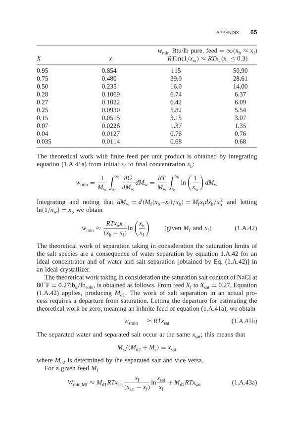
APPENDIX 65

wmin Btu/lb pure, feed = ∞(xb ≈ xf)

X x RT ln(1/xw) ≈ RTxs(xs ≤ 0.3)

0.95 0.854 115 50.900.75 0.480 39.0 28.610.50 0.235 16.0 14.000.28 0.1069 6.74 6.370.27 0.1022 6.42 6.090.25 0.0930 5.82 5.540.15 0.0515 3.15 3.070.07 0.0226 1.37 1.350.04 0.0127 0.76 0.760.035 0.0114 0.68 0.68

The theoretical work with finite feed per unit product is obtained by integratingequation (1.A.41a) from initial xf to final concentration xb:

wmin = 1

Mw

∫ xb

xf

∂G

∂MwdMw = RT

Mw

∫ xb

xf

ln

(1

xw

)dMw

Integrating and noting that dMw = d(Mf(xb−xf)/xb) = Mfxfdxb/x2b and letting

ln(1/xw) = xb we obtain

wmin ≈ RTxbxf

(xb − xf)ln

(xb

xf

)(given Mf and xf) (1.A.42)

The theoretical work of separation taking in consideration the saturation limits ofthe salt species are a consequence of water separation by equation 1.A.42 for anideal concentrator and of water and salt separation [obtained by Eq. (1.A.42)] inan ideal crystallizer.

The theoretical work taking in consideration the saturation salt content of NaCl at80◦F = 0.27lbs/lbsoln, is obtained as follows. From feed Xf to Xsat = 0.27, Equation(1.A.42) applies, producing Md1. The work of salt separation in an actual pro-cess requires a departure from saturation. Letting the departure for estimating thetheoretical work be zero, meaning an infinite feed of equation (1.A.41a), we obtain

wsmin ≈ RTxsat (1.A.41b)

The separated water and separated salt occur at the same xsat; this means that

Ms/(Md2 + Ms) = xsat

where Md2 is determined by the separated salt and vice versa.For a given feed Mf

Wmin,Mf ≈ Md1RTxsatxf

(xsat − xf)ln

xsat

xf+ Md2RTxsat (1.A.43a)

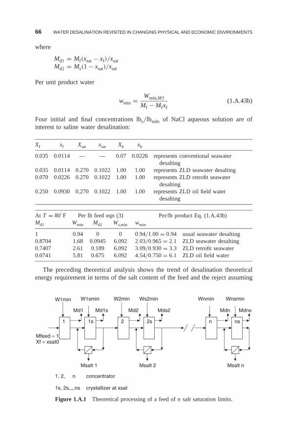
66 WATER DESALINATION REVISITED IN CHANGING PHYSICAL AND ECONOMIC ENVIRONMENTS

where

Md1 = Mf(xsat − xf)/xsatMd2 = Ms(1 − xsat)/xsat

Per unit product water

wmin = Wmin,M f

Mf − Mfxf(1.A.43b)

Four initial and final concentrations lbs/lbsoln of NaCl aqueous solution are ofinterest to saline water desalination:

Xf xf Xsat xsat Xb xb

0.035 0.0114 — — 0.07 0.0226 represents conventional seawaterdesalting

0.035 0.0114 0.270 0.1022 1.00 1.00 represents ZLD seawater desalting0.070 0.0226 0.270 0.1022 1.00 1.00 represents ZLD retrofit seawater

desalting0.250 0.0930 0.270 0.1022 1.00 1.00 represents ZLD oil field water

desalting

At T = 80◦F Per lb feed eqn (3) Per/lb product Eq. (1.A.43b)Md1 Wmin Md2 Ws,min wmin

1 0.94 0 0 0.94/1.00 = 0.94 usual seawater desalting0.8704 1.68 0.0945 6.092 2.03/0.965 = 2.1 ZLD seawater desalting0.7407 2.61 0.189 6.092 3.09/0.930 = 3.3 ZLD retrofit seawater0.0741 5.81 0.675 6.092 4.54/0.750 = 6.1 ZLD oil field water

The preceding theoretical analysis shows the trend of desalination theoreticalenergy requirement in terms of the salt content of the feed and the reject assuming

Msalt n Msalt 1

Mfeed = 1Xf = xsat0

MdnMd1sMd1

1 1s 2 2s n ns

Msalt 2

Md2 Mds2 Mdns

1, 2, n concentrator

1s, 2s,,,,ns crystallizer at xsat

W1smin Wnsmin Wnmin Ws2min W2min W1min

Figure 1.A.1 Theoretical processing of a feed of n salt saturation limits.

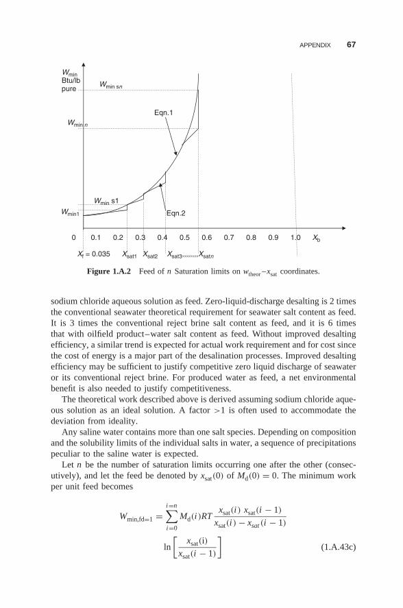
APPENDIX 67

Wmin1

Wmin n

Wmin s1

Eqn.2

Eqn.1

WminBtu/lbpure

0 0.1 0.2 0.3 0.4 0.5 0.6 0.7 0.8 0.9 1.0 Xb

Xf = 0.035 Xsat1 Xsat2 Xsat3,,,,,,,,Xsatn

Wmin sn

Figure 1.A.2 Feed of n Saturation limits on wtheor –xsat coordinates.

sodium chloride aqueous solution as feed. Zero-liquid-discharge desalting is 2 timesthe conventional seawater theoretical requirement for seawater salt content as feed.It is 3 times the conventional reject brine salt content as feed, and it is 6 timesthat with oilfield product–water salt content as feed. Without improved desaltingefficiency, a similar trend is expected for actual work requirement and for cost sincethe cost of energy is a major part of the desalination processes. Improved desaltingefficiency may be sufficient to justify competitive zero liquid discharge of seawateror its conventional reject brine. For produced water as feed, a net environmentalbenefit is also needed to justify competitiveness.

The theoretical work described above is derived assuming sodium chloride aque-ous solution as an ideal solution. A factor >1 is often used to accommodate thedeviation from ideality.

Any saline water contains more than one salt species. Depending on compositionand the solubility limits of the individual salts in water, a sequence of precipitationspeculiar to the saline water is expected.

Let n be the number of saturation limits occurring one after the other (consec-utively), and let the feed be denoted by xsat(0) of Md(0) = 0. The minimum workper unit feed becomes

Wmin,fd=1 =i=n∑i=0

Md(i )RTxsat(i ) xsat(i − 1)

xsat(i ) − xsat (i − 1)

ln

[xsat(i)

xsat(i − 1)

](1.A.43c)

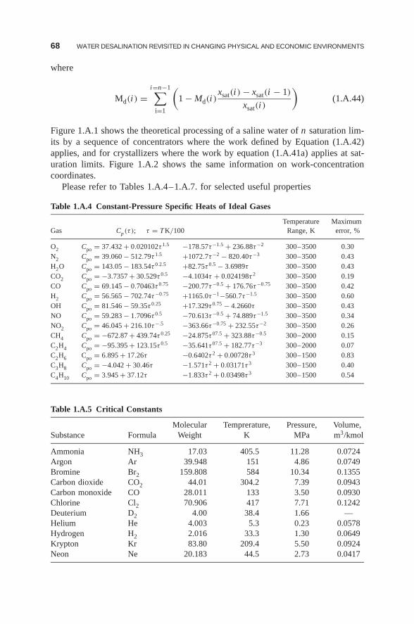
68 WATER DESALINATION REVISITED IN CHANGING PHYSICAL AND ECONOMIC ENVIRONMENTS

where

Md(i ) =i=n−1∑

i=1

(1 − Md(i )

xsat(i ) − xsat(i − 1)

xsat(i )

)(1.A.44)

Figure 1.A.1 shows the theoretical processing of a saline water of n saturation lim-its by a sequence of concentrators where the work defined by Equation (1.A.42)applies, and for crystallizers where the work by equation (1.A.41a) applies at sat-uration limits. Figure 1.A.2 shows the same information on work-concentrationcoordinates.

Please refer to Tables 1.A.4–1.A.7. for selected useful properties

Table 1.A.4 Constant-Pressure Specific Heats of Ideal Gases

Temperature MaximumGas Cp(τ ); τ = TK/100 Range, K error, %

O2 Cpo = 37.432 + 0.020102τ 1.5 −178.57τ−1.5 + 236.88τ−2 300–3500 0.30N2 Cpo = 39.060 − 512.79τ 1.5 +1072.7τ−2 − 820.40τ−3 300–3500 0.43H2O Cpo = 143.05 − 183.54τ 0.2.5 +82.75τ 0.5 − 3.6989τ 300–3500 0.43CO2 Cpo = −3.7357 + 30.529τ 0.5 −4.1034τ + 0.024198τ 2 300–3500 0.19CO Cpo = 69.145 − 0.70463τ 0.75 −200.77τ−0.5 + 176.76τ−0.75 300–3500 0.42H2 Cpo = 56.565 − 702.74τ−0.75 +1165.0τ−1−560.7τ−1.5 300–3500 0.60OH Cpo = 81.546 − 59.35τ 0.25 +17.329τ 0.75 − 4.2660τ 300–3500 0.43NO Cpo = 59.283 − 1.7096τ 0.5 −70.613τ−0.5 + 74.889τ−1.5 300–3500 0.34NO2 Cpo = 46.045 + 216.10τ−.5 −363.66τ−0.75 + 232.55τ−2 300–3500 0.26CH4 Cpo = −672.87 + 439.74τ 0.25 −24.875τ 07.5 + 323.88τ−0.5 300–2000 0.15C2H4 Cpo = −95.395 + 123.15τ 0.5 −35.641τ 07.5 + 182.77τ−3 300–2000 0.07C2H6 Cpo = 6.895 + 17.26τ −0.6402τ 2 + 0.00728τ 3 300–1500 0.83C3H8 Cpo = −4.042 + 30.46τ −1.571τ 2 + 0.03171τ 3 300–1500 0.40C4H10 Cpo = 3.945 + 37.12τ −1.833τ 2 + 0.03498τ 3 300–1500 0.54

Table 1.A.5 Critical Constants

Molecular Temprerature, Pressure, Volume,Substance Formula Weight K MPa m3/kmol

Ammonia NH3 17.03 405.5 11.28 0.0724Argon Ar 39.948 151 4.86 0.0749Bromine Br2 159.808 584 10.34 0.1355Carbon dioxide CO2 44.01 304.2 7.39 0.0943Carbon monoxide CO 28.011 133 3.50 0.0930Chlorine Cl2 70.906 417 7.71 0.1242Deuterium D2 4.00 38.4 1.66 —Helium He 4.003 5.3 0.23 0.0578Hydrogen H2 2.016 33.3 1.30 0.0649Krypton Kr 83.80 209.4 5.50 0.0924Neon Ne 20.183 44.5 2.73 0.0417

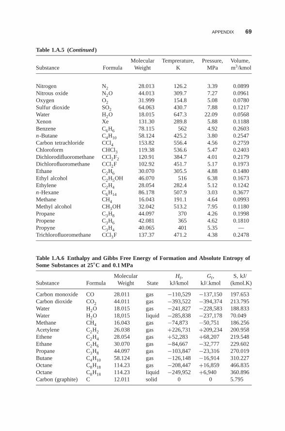
APPENDIX 69

Table 1.A.5 (Continued )

Molecular Temprerature, Pressure, Volume,Substance Formula Weight K MPa m3/kmol

Nitrogen N2 28.013 126.2 3.39 0.0899Nitrous oxide N2O 44.013 309.7 7.27 0.0961Oxygen O2 31.999 154.8 5.08 0.0780Sulfur dioxide SO2 64.063 430.7 7.88 0.1217Water H2O 18.015 647.3 22.09 0.0568Xenon Xe 131.30 289.8 5.88 0.1188Benzene C6H6 78.115 562 4.92 0.2603n-Butane C4H10 58.124 425.2 3.80 0.2547Carbon tetrachloride CCl4 153.82 556.4 4.56 0.2759Chloroform CHCl3 119.38 536.6 5.47 0.2403Dichlorodifluoromethane CCl2F2 120.91 384.7 4.01 0.2179Dichlorofluoromethane CCl2F 102.92 451.7 5.17 0.1973Ethane C2H6 30.070 305.5 4.88 0.1480Ethyl alcohol C2H5OH 46.070 516 6.38 0.1673Ethylene C2H4 28.054 282.4 5.12 0.1242n-Hexane C6H14 86.178 507.9 3.03 0.3677Methane CH4 16.043 191.1 4.64 0.0993Methyl alcohol CH3OH 32.042 513.2 7.95 0.1180Propane C3H8 44.097 370 4.26 0.1998Propene C3H6 42.081 365 4.62 0.1810Propyne C3H4 40.065 401 5.35 —Trichlorofluoromethane CCl3F 137.37 471.2 4.38 0.2478

Table 1.A.6 Enthalpy and Gibbs Free Energy of Formation and Absolute Entropy ofSome Substances at 25◦C and 0.1 MPa

Molecular Hf, Gf, S, kJ/Substance Formula Weight State kJ/kmol kJ/.kmol (kmol.K)

Carbon monoxide CO 28.011 gas −110,529 −137,150 197.653Carbon dioxide CO2 44.011 gas −393,522 −394,374 213.795Water H2O 18.015 gas −241,827 −228,583 188.833Water H2O 18,015 liquid −285,838 −237,178 70.049Methane CH4 16.043 gas −74,873 −50,751 186.256Acetylene C2H2 26.038 gas +226,731 +209,234 200.958Ethene C2H4 28.054 gas +52,283 +68,207 219.548Ethane C2H6 30.070 gas −84,667 −32,777 229.602Propane C3H8 44.097 gas −103,847 −23,316 270.019Butane C4H10 58.124 gas −126,148 −16,914 310.227Octane C8H18 114.23 gas −208,447 +16,859 466.835Octane C8H18 114.23 liquid −249,952 +6,940 360.896Carbon (graphite) C 12.011 solid 0 0 5.795

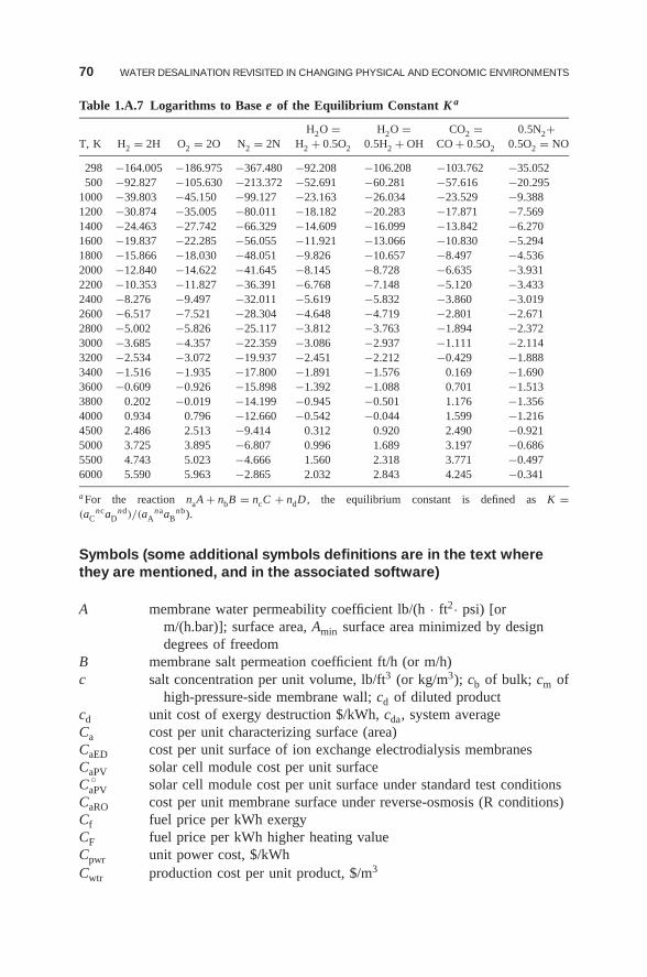
70 WATER DESALINATION REVISITED IN CHANGING PHYSICAL AND ECONOMIC ENVIRONMENTS

Table 1.A.7 Logarithms to Base e of the Equilibrium Constant K a

H2O = H2O = CO2 = 0.5N2+T, K H2 = 2H O2 = 2O N2 = 2N H2 + 0.5O2 0.5H2 + OH CO + 0.5O2 0.5O2 = NO

298 −164.005 −186.975 −367.480 −92.208 −106.208 −103.762 −35.052500 −92.827 −105.630 −213.372 −52.691 −60.281 −57.616 −20.295

1000 −39.803 −45.150 −99.127 −23.163 −26.034 −23.529 −9.3881200 −30.874 −35.005 −80.011 −18.182 −20.283 −17.871 −7.5691400 −24.463 −27.742 −66.329 −14.609 −16.099 −13.842 −6.2701600 −19.837 −22.285 −56.055 −11.921 −13.066 −10.830 −5.2941800 −15.866 −18.030 −48.051 −9.826 −10.657 −8.497 −4.5362000 −12.840 −14.622 −41.645 −8.145 −8.728 −6.635 −3.9312200 −10.353 −11.827 −36.391 −6.768 −7.148 −5.120 −3.4332400 −8.276 −9.497 −32.011 −5.619 −5.832 −3.860 −3.0192600 −6.517 −7.521 −28.304 −4.648 −4.719 −2.801 −2.6712800 −5.002 −5.826 −25.117 −3.812 −3.763 −1.894 −2.3723000 −3.685 −4.357 −22.359 −3.086 −2.937 −1.111 −2.1143200 −2.534 −3.072 −19.937 −2.451 −2.212 −0.429 −1.8883400 −1.516 −1.935 −17.800 −1.891 −1.576 0.169 −1.6903600 −0.609 −0.926 −15.898 −1.392 −1.088 0.701 −1.5133800 0.202 −0.019 −14.199 −0.945 −0.501 1.176 −1.3564000 0.934 0.796 −12.660 −0.542 −0.044 1.599 −1.2164500 2.486 2.513 −9.414 0.312 0.920 2.490 −0.9215000 3.725 3.895 −6.807 0.996 1.689 3.197 −0.6865500 4.743 5.023 −4.666 1.560 2.318 3.771 −0.4976000 5.590 5.963 −2.865 2.032 2.843 4.245 −0.341

aFor the reaction naA + nbB = ncC + ndD , the equilibrium constant is defined as K =(aC

ncaDnd)/(aA

naaBnb).

Symbols (some additional symbols definitions are in the text wherethey are mentioned, and in the associated software)

A membrane water permeability coefficient lb/(h · ft2· psi) [orm/(h.bar)]; surface area, Amin surface area minimized by designdegrees of freedom

B membrane salt permeation coefficient ft/h (or m/h)c salt concentration per unit volume, lb/ft3 (or kg/m3); cb of bulk; cm of

high-pressure-side membrane wall; cd of diluted productcd unit cost of exergy destruction $/kWh, cda, system averageCa cost per unit characterizing surface (area)CaED cost per unit surface of ion exchange electrodialysis membranesCaPV solar cell module cost per unit surfaceC ◦

aPV solar cell module cost per unit surface under standard test conditionsCaRO cost per unit membrane surface under reverse-osmosis (R conditions)Cf fuel price per kWh exergyCF fuel price per kWh higher heating valueCpwr unit power cost, $/kWhCwtr production cost per unit product, $/m3

APPENDIX 71

Cz capital recovery rate $/$·y: CzM for membranes, CzRO for remainingRO devices, CzPV for solar cells

Cap capital cost, Cap+, added capitald Diameter or equivalent diameter, ftD diffusion coefficient, m2/s; dissipation, kW (exergy destruction rate)D th10 temperature difference in the condenser, FE exergy; E s, of system; E f, of flowf friction factorF fuel; Fpenalty for fuel penalty, Fidealc for fuel of ideal control, Npfuel

for fuel of night product, Frefired for fuel of refiringFms PV cost multiplier accounting for added cost from module to systemhm RO mass transfer coefficient, ft/h (or m/h)hhv fuel higher heating valueH enthalpy; height of flow passage, in. (or mm); Hb, of RO membrane

feed side; Hd, of its product low-pressure, side; Hhc, Hlc, osmosishigh- and low-concentration sides, respectively

J objective function, $/h; mass flux, lb/(h·ft2) [or kg/(h · m2)] Jw, ofpure water; Js of salt; Jv, volume flux, ft/h (or m/h)

LF power load factormgd million gallons per day; migpd, Imperial; usmgd, AmericanMd PV/RO water product rate usmgd (m3/d)N dimensionless number; NV, velocity/geometry number; NM, a

membrane number [Eq. 4.24]OP variable-load operation, OPpen, operation cost penaltyP Applied pressure, psia (or bar); P0, dead-state pressurePw Power, kW; Pload, power required; Pdlvrd, power deliveredppm RO product water salt content, parts per million; ED feed parts per

millionPzn RO concentration polarization ratio xsm/xsb (salt at membrane

wall/bulk)R universal gas constant; resources, Rmanuf, manufacturing resources of a

device, Roperate operating resources of a deviceReff Ratio of PV expected solar cell field efficiency to standard test

conditions top cell efficiency η/η◦

Rsol the ratio of design solar intensity to the standard test intensity sol/sol◦

S entropySPV solar cell surface, m2; S ◦

PV, of standard test conditionsSRO RO membrane surface, m2

Sol design solar intensity, kW/m2; Sol◦: of standard test conditions(1kW/m2 = 1 sun)

T temperature; To dead-state temperatureV device decision variables, Vefficiency, thermodynamic; Vdesign design

Vmanufacture manufactureX dependent variable, Xduty, for a device

72 WATER DESALINATION REVISITED IN CHANGING PHYSICAL AND ECONOMIC ENVIRONMENTS

xs Salt mass fraction; xsf, of feed, xsj, of reject brine; xsm, at membranewall; xsb, of bulk flow; xsd, of product water

Z capital cost, $; ZRO, for RO subsystem; ZPV, for PV module; ZPVS forsolar subsystem; ZVC, for VC subsystem; ZED, for electrodialysissubsystem; ZGT, for gas turbine subsystem; ZMSF, multistage flashdistillation subsystem

Z capital cost rateδ concentration boundary-layer thickness, μm (10−6m)�Ph pressure loss, psi (or kPa), high-pressure side of RO membraneφ departure from ideal solution; 1 for ideal solution; φP, of RO applied

pressureη efficiency; ηRO, of separation process; ηPV, of solar-to-power

conversion; ηoPV, of standard test conditions; ηpmp, adiabatic

efficiency of pressurizing pump; ηtrb, adiabatic efficiency of workrecovery turbine or device

ρ densityμ viscosity; chemical potential; μc0, chemical potential of species at

dead state P0 and T0

Abbreviations

ED electrodialysis desalterEL water electrolysis systemGT/MSF gas turbine/multistage flash distillation cogeneration systemPV photovoltaic (solar cells)RO reverse-osmosis desalterSCC simple combined cycleVC vapor compression (distiller)ZLD zero liquid discharge

SELECTED REFERENCES FOR SECTION 1.1–1.3

1. Tribus M, Evans R, The Thermoeconomics of Sea Water Conversion , UCLA Report62–63, Aug. 1962.

2. El-Sayed Y, Evans R, Thermoeconomics and the design of heat systems, J. Eng. Power27–35 (Jan. 1970).

3. El-Sayed Y, Aplenc A, Application of the thermoeconomic approach to the analysisand optimization of a vapor-compression desalting system, J. Eng. Power 17–26 (Jan.1970).

4. Gaggioli R, ed., Thermodynamics: Second Law Analysis , ACS Symp. Series 122, Amer-ican Chemical Society , 1980.

5. Gaggioli R, ed., Efficiency and Costing , ACS Symp. Series 235, 1983.

6. El-Sayed Y, A second-law-based optimization, Parts 1 and 2, J. Eng. Gas Turb. Power118:693–703 (Oct. 1996).

FURTHER READING 73

7. Torres C, Serra L, Valero A, Lozano M, The productive structure and thermoeconomictheories of system optimization, Proc. ASME Adv. Energy Syst. Div . 36:429–436 (Nov.1996).

8. Lazaretto A, Tsatsaronis G, On the quest for objective equations in exergy costing, Proc.ASME . 37:197–210 (1997).

9. Linhoff B, The use of pinch analysis to knock down capital costs and emissions, Chem.Eng. Progress , 32–57 (Aug. 1994).

10. Sciubba E, Melli R, Artificial Intelligence in Thermal Systems Design , Nova ScientificPublishers, 1998.

11. Dimopoulos GG, Christos A, Frangopoulos CA, Optimization of energy systems basedon evolutionary and social metaphors, Energy 33:171–179 (2008).

12. Bouvy C, Lucas K, Multicriterial optimization of communal energy supply concepts,Proc. 19th Int. ECOS Conf ., Greece, 2006, Vol. 1, pp. 543–551.

13. Gibbs JW, (1978), On the Equilibrium of Heterogeneous Substances, The CollectedWork , Yale Univ. Press, 1978, (orig. publ. 1928, Vol. 1, p. 77).

14. El-Sayed Y, The Thermoeconomics of Energy Conversions , Elsevier (UK), 2003.

15. El-Sayed YM, The rising potential of competitive solar desalination, Desalination216:314–324 (2007).

16. Baker RW, Membrane Technology and Applications . Wiley, Hoboken, NJ, 2004.

17. Reid R, Pruasnitz J, Poling B, The Properties of Gases and Liquids , 4th ed., McGraw-Hill, 1989.

18. Green MA, Third Generation of Photovoltaics, Advanced Solar Energy ConversionSpringer-Verlag, 2003.

19. Mulder M, Basic Principles of Membrane Technology , Kluwer Academic, 2003.

20. Sehra A, Bettner J, Cohen A, Design of a high performance axial compressor for utilitygas turbines, J. Turbomach . 114(2):277–286 (1992).

21. Cohen H, Rogers G, Saravenamuttoo H, Gas Turbine Theory , 3rd ed., Wiley,1987.

22. Hegetschweiler H, Bartlet R, Predicting performance of large steam turbine-generatorunits, Trans. Am. Soc. Mech. Eng. ASME. 79:1085–1114 (1957).

23. Sabersky R, Acosta A, Hauptmann E, Fluid Flow, a First Course in Fluid Mechanics ,3rd ed., Macmillan, 1989.

FURTHER READING

1.F.1 International Symposia on Energy Analysis

Pleskov YV, Solar Energy Conversion: A Photoelectrochemical Approach , Springer-Verlag,1992.

Luque A, Hegedus S, ed., Handbook of Photovoltaic Science and Engineering , Wiley, Hobo-ken, NJ, 2003.

Moran M, Sciubba E, eds., Proc. 4th Int. Symp. Second Law Analysis of Thermal Systems ,Rome, May 25–29, 1987.

Cai, Ruixian, Moran M, eds., Proc. Int. Symp. Thermodynamic Analysis and Improvement ofEnergy Systems , (TAIES’89), Beijing, June 5–8, 1989.

74 WATER DESALINATION REVISITED IN CHANGING PHYSICAL AND ECONOMIC ENVIRONMENTS

Stecco S, Moran M, eds., Proc. Florence World Energy Research Symp. (FLOWERS’90),Florence, Italy, May 28–June 1, 1990.

Proc. Int. Conf. Analysis of Thermal and Energy Systems (Athens’91), Athens, 1991.

Valero A, Tsatsaronis G, editors: Proc. Int. Symp. Efficiency, Costs, Optimization, and Sim-ulation of Energy Systems (ECOS’92), Zaragoza, Spain, June 15–18, 1992.

Proc. Int. Symp. Energy Systems and Ecology (Ensec’93), Krakow, Poland, July 5–9, 1994.

Proc. Florence World Energy Research Symp. (FLOWERS’94), Florence, July 6–8, 1994.

Proc. Int. Symp. Efficiency, Costs, Optimization, Simulation and Environmental Impact ofEnergy Systems (ECOS’95), Istanbul, July 9–14, 1995.

Proc. Int. Symp. Efficiency, Costs, Optimization, Simulation and Environmental Impact ofEnergy Systems (ECOS’96), Stockholm, June 25–27, 1996.

Proc. Int. Symp. Thermodynamic Analysis and Improvement of Energy Systems , (TAIES’97),Beijing, June 10–13, 1997.

Proc. Int. Symp. Efficiency, Costs, Optimization, Simulation and Environmental Aspects ofEnergy Systems and Processes (ECOS’98), Nancy, France, July 8–10, 1998.

Proc. Int. Symp. Efficiency, Costs, Optimization, Simulation and Environmental Aspects ofEnergy Systems (ECOS’99), Tokyo, June 8–10, 1999.

Proc. Int. Symp. Efficiency, Costs, Optimization, and Simulation of Energy Systems(ECOS’00), Univ. Twente, The Netherlands, July 5–7 2000.

Proc. Int. Symp. Efficiency, Costs, Optimization, Simulation and Environmental Impact ofEnergy Systems (ECOS’01), Istanbul, July 4–6, 2001.

Proc. Int. Symp. Efficiency, Costs, Optimization, and Simulation of Energy Systems(ECOS’02), Berlin, July 3–5, 2002.

Proc. Int. Symp. Efficiency, Costs, Optimization, and Simulation of Energy Systems(ECOS’03), Denmark, June 30–July 2, 2003.

Proc. 17th Int. Conf. Efficiency, Cost, Optimization, Simulation and Environmental Impactof Energy and Process Systems (ECOS’2004), Guanajauto, Mexico, July 7–9, 2004.

Proc. 18th Int. Conf. Efficiency, Cost, Optimization, Simulation and Environmental Impactof Energy Systems (ECOS’2005), Trondheim, Norway, June 20–22, 2005.

Proc. 19th Int. Conf. Efficiency, Cost, Optimization, Simulation and Environmental Impactof Energy Systems (ECOS’2006), Aghia Pelagia, Crete, Greece, July 12–14, 2006.

Proc. 20th Int. Conf. Efficiency, Cost, Optimization, Simulation and Environmental Impactof Energy Systems (ECOS’2008), Krakow Gliwicw, Poland, June 24–27, 2008.

The 22nd International Conference on Efficiency, Cost, Optimization, Simulation and Envi-ronmental Impact of Energy Systems (ECOS’2009) held in Foz do Iguacu, Brazil, 31August -- 3 September 2009.

The 23rd International Conference on Efficiency, Cost, Optimization, Simulation and Envi-ronmental Impact of Energy Systems (ECOS’2010) held in Lausanne, Switzerland, 14-17June 2010.

The 24th International Conference on Efficiency, Cost, Optimization, Simulation and Envi-ronmental Impact of Energy Systems (ECOS’2011) held in Novi Sad, Serbia, 4-7 July2011.

FURTHER READING 75

1.F.2 Selected International Symposia on Desalination

Proc. IDA World Congress Desalination and Water Sciences , Abu Dhabi, UAE, Nov. 18–24,1995.

Proc. IDA World Congress Desalination and Water Reuse, Madrid, Oct. 6–9, 1997.

Proc. European Conf. Desalination and the Environment , Las Palmas, Gran Canaria, 1999.

Proc. The Int. Conf. Seawater Desalination Technologies on the Threshold of the New Mil-lennium , Kuwait, Nov. 4–7, 2000.

Proc. IDA Int. Conference Desalination , Singapore, March 21–22, 2001.

Proc. IDA World Congress Desalination and Water Reuse, Bahrain, March 8–13, 2002.

Proc. IDA World Congress Desalination, and Water Reuse, Paradise Island, Bahamas, Sept.28–Oct. 3, 2003.

Proc. Int. Conf. Water Security for Future Generations ,, Changchun, Jilin Province, China,July 26–31, 2004.

Proc. IDA World Congress Desalination and Water Reuse, Singapore, Sept. 11–16, 2005.

Proc. ADST 2006 Int. Conf. Desalination Technologies and Water Reuse, Alexandria, Egypt,May 6–8, 2006.

Proc. AMTA Membrane Technologies Conf ., Las Vegas, NV (USA), July 23–26, 2007.

Proc. IDA World Congress Desalination and Water Reuse, Maspalomas, Gran Canaria, Spain,Oct. 21–26, 2007.

IDA World Congress on Desalination and water Reuse, Dubai, November 7-12, 2009.

IDA World Congress on Desalination and water Reuse, Perth, Australia, September 4-9,2011.

1.F.3 Books on Thermodynamics

Gaggioli RA, ed., Thermodynamics: Second Law Analysis , ACS Symp. Series Vol. 122,American Chemical Society, 1980.

Moran MJ, Availability Analysis, A Guide to Efficient Energy Use, Prentice Hall, 1982.

Kotas TJ, The Exergy Method of Thermal Plant Analysis , Butterworth, 1984.

Reid R, Pruasnitz J, Poling B, The Properties of Gases and Liquids , 4th ed., McGraw-Hill,1989.

Szargut J, Morris D, Steward F, Exergy Analysis of Thermal, Chemical and MetallurgicalProcesses , Hemisphere Publishing, 1985.

Van Wylen GJ, Sonntag RE, Fundamentals of Classical Thermodynamics , Wiley 1996.

1.F.4 Books on Optimization and Equation Solvers

Wilde DJ, Beightler CS, Foundations of Optimization , Prentice-Hall, 1967.

Intriligator M, Mathematical Optimization and Economic Theory , Prentice-Hall, 1971.

Wismer D, Chattergy R, Introduction to Nonlinear Optimization, a Problem SolvingApproach , North-Holland Series in System Science and Engineering, 1978.

Chapra S, Canale R, Numerical Methods for Engineers , 2nd ed., McGraw-Hill, 1988.

76 WATER DESALINATION REVISITED IN CHANGING PHYSICAL AND ECONOMIC ENVIRONMENTS

1.F.5 Books on Design of Energy Conversion Devices

Hottel H, Sarofim A, Radiative Transfer , McGraw-Hill, 1967.

Siegel R, Howell J, Thermal Radiation Heat Transfer , 2nd ed., Hemisphere Publishing,1981.

Rohsenow W, Hartnett J, Ganic E, Handbook of Heat Transfer Applications , 2nd ed.,McGraw Hill Book Company.

Cohen H, Rogers G, Saravenamuttoo H, Gas Turbine Theory , 3rd ed., Wiley, 1987.

Sabersky R, Acosta A, Hauptmann E, Fluid Flow, a First Course in Fluid Mechanics , 3rded., Macmillan, 1989.

1.F.6 Books on Optimal Design

Edgerton R, Available Energy and Environmental Economics , Lexington Books.

Gaggioli R, ed., Efficiency and Costing , ACS Symp. Series Vol. 235, American ChemicalSociety, 1983.

Papalambros PY, Wilde DJ, Principles of Optimal Design, Modeling and Computation , Cam-bridge Univ. Press, 1988.

Edger TF, Himmelblau DM, Optimization of Chemical Processes , McGraw-Hill, 1988.

Bejan A, Tsatsaronis G, Moran M, Thermal Design and Optimization , Wiley, 1996.

El-Sayed YM, The Thermoeconomics of Energy Conversions , Elsevier, 2003.

1.F.7 Books on Emerging Technologies (Fuel/Solar Cells andSelective Membranes)

Kordesch K, Simader G, Fuel Cells and Their Applications , VCH, 1996.

Minh NQ, Takahashi T, Science and Technology of Ceramic Fuel Cells , Elsevier, 1995.

Appleby AJ, ed., Fuel Cells: Trends in Research and Applications , Hemisphere Publishing,1987.

Mazer JA, Solar Cells: An Introduction to Crystalline Photovoltaic Technology , KluwerAcademic, 1997.

Pleskov YV, Solar Energy Conversion: A Photoelectrochemical Approach , Springer-Verlag,1990.

Mulder M, Basic Principles of Membrane Technology , 2nd ed., Kluwer Academic 1996.

Baker RW, Membrane Technology and Applications , Wiley, 2004.

Luque A, Hegedus S, eds., Handbook of Photovoltaic Science and Engineering , Hegedus,editors, Wiley, 2003.

Green MA, Third Generation Photovoltaics, Advanced Solar Energy Conversion , Springer,2003.

1.F.8 General Additional Reading for Section 1.2

Bejan A, Tsatsaronis G, Moran M, Thermal Design and Optimization , Wiley, 1996.

Chapra SC, Canale RP, Numerical Methods for Engineers , McGraw-Hill, 1988.

DeGarmo E, Sullivan W, Bontadelli J, Engineering Economy, 9th ed., Macmillan, 1992.

FURTHER READING 77

Dunbar WR, Lior N, Gaggioli R, Combining fuel cells with fuel-fired power plants forimproved exergy efficiency, Energy 16:(10)1259–1274 (1991).

Dunbar WR, Lior N, Gaggioli R, The component equations of energy and exergy, ASME J.Energy Resources Technol . 114:75–83 (1992).

Dunbar WR, Lior N, Gaggioli R, The effect of the fuel-cell unit size on the efficiencyof a fuel-cell-topped Rankine Cycle, ASME J. Energy Resources Technol . 115:105–107(1993).

Dunbar WR, Lior N, Sources of combustion irreversibility, Comb. Sci. Technol . 103:41–6(1994).

Edger TF, Himmelblau DM, Optimization of Chemical Processes , McGraw-Hill, 1988.

Edgerton R, Available Energy and Environmental Economics , Lexington Books, 1982.

Evans RB, A Proof that Essergy is the Only Consistent Measure of Potential Work , PhDthesis, Thayer School of Engineering, Dartmouth College, Hanover, NH, 1969.

Incropera F, DeWitt D, Fundamentals of Heat and Mass Transfer, 3rd ed., Wiley, 1990.

Keenan JH, Thermodynamics , Wiley, 1941.

Kotas TJ, The Exergy Method of Thermal Plant Analysis , Butterworth, 1984.

Lior N, Sarmiento-Darkin W, Al-Sharqawi HS, The exergy fields in transport processes:Their calculation and use, Energy 31:553–578 (2006).

Means RS, Mechanical, Building, and Electrical Cost Data , Construction Publishers andConsultants, Kingston, MA, 1998.

Modern Cost Engineering: Methods and Data , compiled by Chemical Engineering ,McGraw-Hill, 1979.

Moran MJ, Availability Analysis, A Guide to Efficient Energy Use, Prentice-Hall, 1982.

Papalambros PY, Wilde DJ, Principles of Optimal Design, Modeling and Computation , Cam-bridge Univ. Press, 1988.

Rant Z, Exergie, ein neues wort fur technische arbeitsfahigkeit, Forsch. Ing. Wissen .22(1):25–32 (1956).

Szargut J, Morris D, Steward F, Exergy Analysis of Thermal, Chemical and MetallurgicalProcesses , Hemisphere Publishing, 1985.

Van Wylen RE, Sonntag GJ, Fundamentals of Classical Thermodynamics , Wiley, 1996.

Wilde DJ, Beightler CS, Foundations of Optimization , Prentice-Hall 1967.

1.F.9 General Additional Reading for Section 1.4

Archer Enterprises, Report on the Commercial Electrolytic Production of Hydrogen , Geneva,NY.

Darwish MA, Al-Najem NM, Lior N, Towards sustainable seawater desalting in the Gulfarea, Desalination Vol. 235, 5887, (2009).

Echeverria A, Desalination plant in Tenerife, San Loranzo Valley, Proc. IDA World CongressDesalination and Water Reuse, Madrid, Oct. 6–9, 1997, Vol. II, pp. 675–694.

El-Nashar AM, Validating the simulation program “Soldes” with actual performance datafrom an operating solar desalination plant, Proc. IDA World Congress Desalination andWater Reuse, Madrid, Oct. 6–9, 1997, Vol. 1, pp. 107–142.

El-Sayed YM, Desirable enforcements to optimal system design, Proc. 19th Int. Conf.Efficiency, Cost, Optimization, Simulation and Environmental Impact of Energy Systems(ECOS’06), Aghia Pelagia, Crete, Greece, July 12–14, 2006, Vol. 1, pp. 483–492.

78 WATER DESALINATION REVISITED IN CHANGING PHYSICAL AND ECONOMIC ENVIRONMENTS

Maloney K, Dopp R, Highly Efficient Hydrogen Generation via Water Electrolysis UsingNanometal Electrodes , Energy Research Laboratory, QuantumSphere Inc., Santa Ana,CA.

Torres del Corral M, (del) Pino, MP, Lodos MG, Rodrigous M, Physico-chemical andelectrodialysis reversal treatment to reclaim wastewater from a sewage treatment plant,Proce. IDA World Congress Desalination and Water Reuse, Madrid, Oct. 6–9, 1997, Vol.II, pp. 695–711.

Van Wylen RE, Sonntag GJ, Fundamentals of Classical Thermodynamics , Wiley, 1996.

Yongqing Wang, Noam Lior, Fuel allocation in a combined steam-injected gas turbine andthermal seawater desalination system, Desalination Vol. 214, 306326, (2007).

1.F.10 Literature on Design Models

El-Sayed Y, On the feasibility of large vapor compression distillation units, Desalination107:13–27, (1996).

El-Sayed Y, On the development of large vapor compression distillation units, Proc. Int.Desalination Assoc. Desalination Seminar , Cairo, Sept. 6–8, 1997.

El-Sayed Y, Gaggioli R, The integration of synthesis and optimization for conceptual designsof energy systems, J. Energy Resources Technol . 110:109–113 (1988).

Hoyt H, Sarofim A, Radiative Transfer , McGraw-Hill, 1967.

Rohsenow W, Hartnett J, Ganic E, Handbook of Heat Transfer Applications , 2nd ed.,McGraw-Hill, (1985).

Siegel R, and Howell J, Thermal Radiation Heat Transfer , 2nd ed., Hemisphere Publishing,1981.

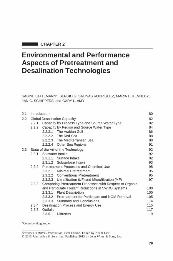
CHAPTER 2

Environmental and PerformanceAspects of Pretreatment andDesalination Technologies

SABINE LATTEMANN∗, SERGIO G. SALINAS RODRIGUEZ, MARIA D. KENNEDY,JAN C. SCHIPPERS, and GARY L. AMY

2.1 Introduction 802.2 Global Desalination Capacity 82

2.2.1 Capacity by Process Type and Source Water Type 822.2.2 Capacity by Region and Source Water Type 84

2.2.2.1 The Arabian Gulf 862.2.2.2 The Red Sea 882.2.2.3 The Mediterranean Sea 882.2.2.4 Other Sea Regions 91

2.3 State of the Art of the Technology 922.3.1 Seawater Intake 92

2.3.1.1 Surface Intake 922.3.1.2 Subsurface Intake 93

2.3.2 Pretreatment Processes and Chemical Use 952.3.2.1 Minimal Pretreatment 952.3.2.2 Conventional Pretreatment 952.3.2.3 Ultrafiltration (UF) and Microfiltration (MF) 97

2.3.3 Comparing Pretreatment Processes with Respect to Organicand Particulate Foulant Reductions in SWRO Systems 1002.3.3.1 Plant Description 1002.3.3.2 Pretreatment for Particulate and NOM Removal 1052.3.3.3 Summary and Conclusions 114

2.3.4 Desalination Process and Energy Use 1152.3.5 Outfalls 117

2.3.5.1 Diffusers 119

∗Corresponding author

Advances in Water Desalination, First Edition. Edited by Noam Lior.© 2013 John Wiley & Sons, Inc. Published 2013 by John Wiley & Sons, Inc.

79

80 ENVIRONMENTAL AND PERFORMANCE ASPECTS

2.3.5.2 Subsurface Discharge 1192.3.5.3 Codischarge with Cooling Water 1212.3.5.4 Codischarge with Waste Water 121

2.4 Potential Environmental Impacts 1222.4.1 Impingement and Entrainment 1222.4.2 Concentrate and Chemical Discharges 124

2.4.2.1 Potential Impacts of Increased Salinity 1252.4.2.2 Pretreatment and Cleaning Chemicals 131

2.4.3 Greenhouse Gases and Air Quality Pollutants 1342.4.3.1 Energy Demand in Perspective 1352.4.3.2 Greenhouse Gas Emissions 1362.4.3.3 Other Air Pollutants 139

2.5 Seawater Desalination as a Green Technology 1412.5.1 Best Available Techniques (BAT) 1432.5.2 Environmental Impact Assessment 145

2.5.2.1 Environmental Monitoring 1482.6 Multicriteria Analysis (MCA) of Intake and Pretreatment Alternatives for

SWRO 1502.6.1 Methodology 1522.6.2 Data Input 155

2.6.2.1 Alternatives 1552.6.2.2 Criteria 1572.6.2.3 Scores 1582.6.2.4 Graphical Evaluation 1642.6.2.5 Weights 167

2.6.3 Ranking Results 1702.6.3.1 Sensitivity Analysis 1702.6.3.2 Revised Scenarios 171

2.6.4 Summary and Conclusions 181References 185

2.1 INTRODUCTION

Seawater desalination is a rapidly growing coastal industry. The combined pro-duction capacity of all seawater desalination plants worldwide has increased by30% over the last few years: from 28 million cubic meters per day (Mm3/d)in 2007—which is the equivalent of the average discharge of the River Seinein Paris—to more than 40.4 Mm3/d in 2009. For the ‘pioneering’ countries inthe Middle East, which have been depending on desalinated water for decades,the driving factors for desalination were scarce freshwater resources coupled withabundant oil resources to engage in energy-intensive and costly thermal desalina-tion projects. For the newly emerging desalination markets, the preferred process isseawater reverse osmosis (SWRO), and the driving factors are more diverse, includ-ing demographic growth, economic development, urbanization, droughts, climate

INTRODUCTION 81

change, and declining conventional water resources in terms of quality and quantitycaused by overuse, pollution, or salinization of surface and groundwaters. As theeffort and cost to supply water from conventional sources has been rising in manyparts of the world and the costs of seawater desalination have been declining overthe years, desalination has also become economically more competitive.

While market analysts agree that seawater desalination capacities will continueto grow rapidly in the future, the controversial debate on the extent to which thisdevelopment may affect the environment continues. Seawater desalination is anenergy-intensive process, consumes considerable amounts of resources in the formof chemicals and materials, and may have negative effects on the marine environ-ment due to the discharges of concentrate waste waters and residual chemicals intothe sea. The growing number of desalination plants worldwide and the increasingsize of single facilities emphasises the need for greener desalination technologiesand more sustainable desalination projects.

Two complementing approaches are the development and implementation of bestavailable technology (BAT) standards and best practice guidelines for environmen-tal impact assessment (EIA) studies. While BAT is a technology-based approach,which favors state-of-the-art technologies that reduce resource consumption andwaste emissions, EIA aims at minimizing impacts at a site- and project-specificlevel through environmental monitoring, evaluation of impacts, and mitigationwhere necessary.

This chapter attempts to determine whether the present desalination technologiescan be considered as green and sustainable solutions, as recently claimed for someprojects. To follow up on the issue the present state of the art in terms of desalinationcapacities and desalination technologies will be discussed. Section 2.2 provides anoverview of the worldwide desalination capacity and discusses regional trends.The figures show that desalination is developing into a coast-based industry, whichmay have harmful effects on the environment if not well-designed and managed.The effects on the environment will generally depend on the location and sizeof a desalination project and the technology used. Section 2.3 briefly outlinesthe state of the art of SWRO processes with particular focus on the differentintake, pretreatment, and outfall designs. Our intention is not to reproduce textbookmaterials but to highlight chemical and energy use aspects and to evaluate differentintake and pretreatment systems in terms of their operational performance andenvironmental footprint. While the chemical use of a desalination plant dependsmainly on the pretreatment system and hence on feedwater quality, the actualdesalination process accounts for most of the energy use of a desalination plant.

Section 2.4 summarizes the key environmental concerns of desalination plants.These are the impingement and entrainment of organisms caused by the intakes,the impacts on the marine environment caused by the discharge of concentrate andchemical residues, and energy consumption that causes emissions of greenhousegases and air pollutants. Section 2.5 attempts to determine whether desalination canbe considered a green technology and evaluates approaches for impact mitigation.A concept for BAT for seawater desalination technologies will be proposed, incombination with a methodological approach for the EIA of desalination projects.

82 ENVIRONMENTAL AND PERFORMANCE ASPECTS

The scope of EIA studies is outlined, including environmental monitoring, toxicity,and hydrodynamic modeling studies. In Section 2.6, the usefulness of multicriteriaanalysis (MCA) as a decision support tool for EIAs is explored and used to comparedifferent intake and pretreatment options for seawater reverse osmosis plants.

2.2 GLOBAL DESALINATION CAPACITY

The use of desalination has increased in many parts of the world. According to theInternational Desalination Association’s (IDA) worldwide desalting plant inventory,the production capacity of all desalination plants worldwide increased from about∼44.1 Mm3/d in 2007 to ∼62.5 Mm3/d in 2010, which represents a 40% increase.The values include facilities that treat brine [defined as water containing >50, 000ppm total dissolved solids (TDS)], seawater (20,000–50,000 ppm), brackish water(3000–20,000 ppm), river water (500–3000 ppm), pure water (<500 ppm), orwaste water; these data have been obtained either during construction, online, orpresumed online [1,2].

Much of the growth of the desalination market takes place in the seawater sector,although waste water desalination and brackish water desalination will presumablybecome more important in the future. In some regions, such as California and Israel,waste water desalination even preceded the implementation of seawater desalina-tion projects. At present (i.e., 2010), 5% of the total capacity of 62.5 Mm3/d isproduced from waste water (Fig. 2.1, top left); 17% of the present capacity isproduced from brackish water sources, mainly brackish groundwater. A limitednumber of plants are being located in estuarine sites, such as the Thames Gate-way desalination plant in East London with a capacity of 150,000 m3/d. The plantwithdraws brackish water with a maximum salt content of 11,000 mg/L duringlow tide and therefore requires only about half the energy (1.7 kWh/m3) of SWROplants. However, the tidal and seasonal variability of the raw water with regardto dissolved and particulate organic matter requires a complex pretreatment con-sisting of coagulation, flocculation, clarification, media filtration, and ultrafiltration[3,4]. The lower energy demand is a main benefit of estuarine sites; however, thepretreatment challenge may be the reason why only a limited number of projectshave been implemented to date.

At present, ∼65% of the capacity is produced from seawater. Seawater is hencethe predominant source water for desalination and accounts for a worldwide waterproduction of 40.4 Mm3/d − a value that is comparable to the average dischargeof the Seine River (43.2 Mm3/d or 500 m3/s) before disemboguing into the EnglishChannel.

2.2.1 Capacity by Process Type and Source Water Type

For all source water types reverse osmosis (RO) is the prevalent desalination pro-cess. It accounts for more than 60% (38.7 Mm3/d) of the global capacity (Fig. 2.1,top right); 33% or 20.9 Mm3/d of the global capacity is produced by distillation

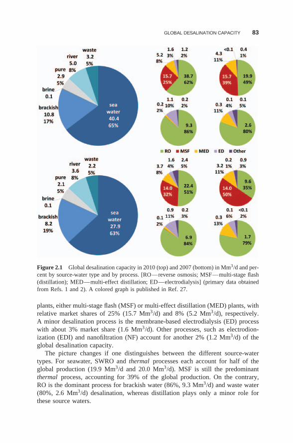
GLOBAL DESALINATION CAPACITY 83

Figure 2.1 Global desalination capacity in 2010 (top) and 2007 (bottom) in Mm3/d and per-cent by source-water type and by process. [RO—reverse osmosis; MSF—multi-stage flash(distillation); MED—multi-effect distillation; ED—electrodialysis] (primary data obtainedfrom Refs. 1 and 2). A colored graph is published in Ref. 27.

plants, either multi-stage flash (MSF) or multi-effect distillation (MED) plants, withrelative market shares of 25% (15.7 Mm3/d) and 8% (5.2 Mm3/d), respectively.A minor desalination process is the membrane-based electrodialysis (ED) processwith about 3% market share (1.6 Mm3/d). Other processes, such as electrodion-ization (EDI) and nanofiltration (NF) account for another 2% (1.2 Mm3/d) of theglobal desalination capacity.

The picture changes if one distinguishes between the different source-watertypes. For seawater, SWRO and thermal processes each account for half of theglobal production (19.9 Mm3/d and 20.0 Mm3/d). MSF is still the predominantthermal process, accounting for 39% of the global production. On the contrary,RO is the dominant process for brackish water (86%, 9.3 Mm3/d) and waste water(80%, 2.6 Mm3/d) desalination, whereas distillation plays only a minor role forthese source waters.

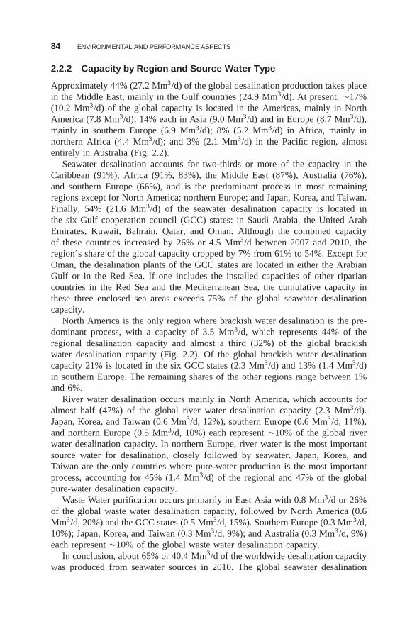
84 ENVIRONMENTAL AND PERFORMANCE ASPECTS

2.2.2 Capacity by Region and Source Water Type

Approximately 44% (27.2 Mm3/d) of the global desalination production takes placein the Middle East, mainly in the Gulf countries (24.9 Mm3/d). At present, ∼17%(10.2 Mm3/d) of the global capacity is located in the Americas, mainly in NorthAmerica (7.8 Mm3/d); 14% each in Asia (9.0 Mm3/d) and in Europe (8.7 Mm3/d),mainly in southern Europe (6.9 Mm3/d); 8% (5.2 Mm3/d) in Africa, mainly innorthern Africa (4.4 Mm3/d); and 3% (2.1 Mm3/d) in the Pacific region, almostentirely in Australia (Fig. 2.2).

Seawater desalination accounts for two-thirds or more of the capacity in theCaribbean (91%), Africa (91%, 83%), the Middle East (87%), Australia (76%),and southern Europe (66%), and is the predominant process in most remainingregions except for North America; northern Europe; and Japan, Korea, and Taiwan.Finally, 54% (21.6 Mm3/d) of the seawater desalination capacity is located inthe six Gulf cooperation council (GCC) states: in Saudi Arabia, the United ArabEmirates, Kuwait, Bahrain, Qatar, and Oman. Although the combined capacityof these countries increased by 26% or 4.5 Mm3/d between 2007 and 2010, theregion’s share of the global capacity dropped by 7% from 61% to 54%. Except forOman, the desalination plants of the GCC states are located in either the ArabianGulf or in the Red Sea. If one includes the installed capacities of other ripariancountries in the Red Sea and the Mediterranean Sea, the cumulative capacity inthese three enclosed sea areas exceeds 75% of the global seawater desalinationcapacity.

North America is the only region where brackish water desalination is the pre-dominant process, with a capacity of 3.5 Mm3/d, which represents 44% of theregional desalination capacity and almost a third (32%) of the global brackishwater desalination capacity (Fig. 2.2). Of the global brackish water desalinationcapacity 21% is located in the six GCC states (2.3 Mm3/d) and 13% (1.4 Mm3/d)in southern Europe. The remaining shares of the other regions range between 1%and 6%.

River water desalination occurs mainly in North America, which accounts foralmost half (47%) of the global river water desalination capacity (2.3 Mm3/d).Japan, Korea, and Taiwan (0.6 Mm3/d, 12%), southern Europe (0.6 Mm3/d, 11%),and northern Europe (0.5 Mm3/d, 10%) each represent ∼10% of the global riverwater desalination capacity. In northern Europe, river water is the most importantsource water for desalination, closely followed by seawater. Japan, Korea, andTaiwan are the only countries where pure-water production is the most importantprocess, accounting for 45% (1.4 Mm3/d) of the regional and 47% of the globalpure-water desalination capacity.

Waste Water purification occurs primarily in East Asia with 0.8 Mm3/d or 26%of the global waste water desalination capacity, followed by North America (0.6Mm3/d, 20%) and the GCC states (0.5 Mm3/d, 15%). Southern Europe (0.3 Mm3/d,10%); Japan, Korea, and Taiwan (0.3 Mm3/d, 9%); and Australia (0.3 Mm3/d, 9%)each represent ∼10% of the global waste water desalination capacity.

In conclusion, about 65% or 40.4 Mm3/d of the worldwide desalination capacitywas produced from seawater sources in 2010. The global seawater desalination

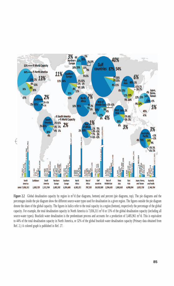
Figure 2.2 Global desalination capacity by region in m3/d (bar diagrams, bottom) and percent (pie diagrams, top). The pie diagrams and thepercentages inside the pie diagram show the different source-water types used for desalination in a given region. The figures outside the pie diagramdenote the share of the global capacity. The figures in italics refer to the total capacity in a region (bottom), respectively the percentage of the globalcapacity. For example, the total desalination capacity in North America is 7,836,311 m3/d or 13% of the global desalination capacity (including allsource-water types). Brackish water desalination is the predominant process and accounts for a production of 3,485,961 m3/d. This is equivalentto 44% of the total desalination capacity in North America, or 32% of the global brackish water desalination capacity (Primary data obtained fromRef. 2.) A colored graph is published in Ref. 27.

85

85

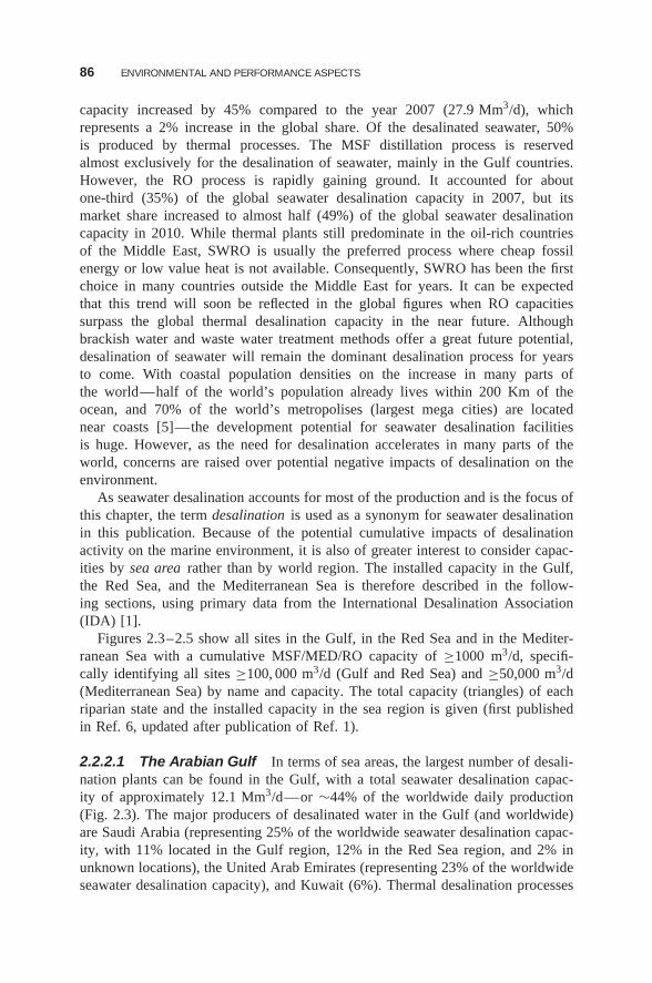
86 ENVIRONMENTAL AND PERFORMANCE ASPECTS

capacity increased by 45% compared to the year 2007 (27.9 Mm3/d), whichrepresents a 2% increase in the global share. Of the desalinated seawater, 50%is produced by thermal processes. The MSF distillation process is reservedalmost exclusively for the desalination of seawater, mainly in the Gulf countries.However, the RO process is rapidly gaining ground. It accounted for aboutone-third (35%) of the global seawater desalination capacity in 2007, but itsmarket share increased to almost half (49%) of the global seawater desalinationcapacity in 2010. While thermal plants still predominate in the oil-rich countriesof the Middle East, SWRO is usually the preferred process where cheap fossilenergy or low value heat is not available. Consequently, SWRO has been the firstchoice in many countries outside the Middle East for years. It can be expectedthat this trend will soon be reflected in the global figures when RO capacitiessurpass the global thermal desalination capacity in the near future. Althoughbrackish water and waste water treatment methods offer a great future potential,desalination of seawater will remain the dominant desalination process for yearsto come. With coastal population densities on the increase in many parts ofthe world—half of the world’s population already lives within 200 Km of theocean, and 70% of the world’s metropolises (largest mega cities) are locatednear coasts [5]—the development potential for seawater desalination facilitiesis huge. However, as the need for desalination accelerates in many parts of theworld, concerns are raised over potential negative impacts of desalination on theenvironment.

As seawater desalination accounts for most of the production and is the focus ofthis chapter, the term desalination is used as a synonym for seawater desalinationin this publication. Because of the potential cumulative impacts of desalinationactivity on the marine environment, it is also of greater interest to consider capac-ities by sea area rather than by world region. The installed capacity in the Gulf,the Red Sea, and the Mediterranean Sea is therefore described in the follow-ing sections, using primary data from the International Desalination Association(IDA) [1].

Figures 2.3–2.5 show all sites in the Gulf, in the Red Sea and in the Mediter-ranean Sea with a cumulative MSF/MED/RO capacity of ≥1000 m3/d, specifi-cally identifying all sites ≥100, 000 m3/d (Gulf and Red Sea) and ≥50,000 m3/d(Mediterranean Sea) by name and capacity. The total capacity (triangles) of eachriparian state and the installed capacity in the sea region is given (first publishedin Ref. 6, updated after publication of Ref. 1).

2.2.2.1 The Arabian Gulf In terms of sea areas, the largest number of desali-nation plants can be found in the Gulf, with a total seawater desalination capac-ity of approximately 12.1 Mm3/d—or ∼44% of the worldwide daily production(Fig. 2.3). The major producers of desalinated water in the Gulf (and worldwide)are Saudi Arabia (representing 25% of the worldwide seawater desalination capac-ity, with 11% located in the Gulf region, 12% in the Red Sea region, and 2% inunknown locations), the United Arab Emirates (representing 23% of the worldwideseawater desalination capacity), and Kuwait (6%). Thermal desalination processes

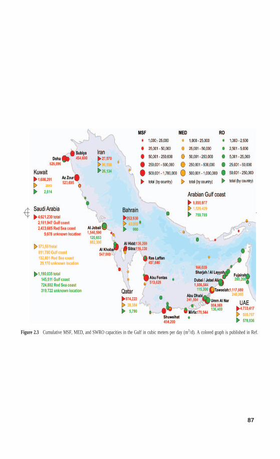
87

Figure 2.3 Cumulative MSF, MED, and SWRO capacities in the Gulf in cubic meters per day (m3/d). A colored graph is published in Ref.

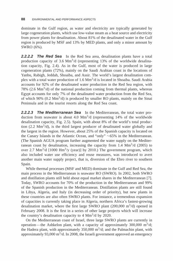
88 ENVIRONMENTAL AND PERFORMANCE ASPECTS

dominate in the Gulf region, as water and electricity are typically generated bylarge cogeneration plants, which use low-value steam as a heat source and electricityfrom power plants for desalination. About 81% of the desalinated water in the Gulfregion is produced by MSF and 13% by MED plants, and only a minor amount bySWRO (6%).

2.2.2.2 The Red Sea In the Red Sea area, desalination plants have a totalproduction capacity of 3.6 Mm3/d (representing 13% of the worldwide desalina-tion capacity, Fig. 2.4). As in the Gulf, most of the water is produced in largecogeneration plants (72%), mainly on the Saudi Arabian coast in the locations ofYanbu, Rabigh, Jeddah, Shoaiba, and Assir. The world’s largest desalination com-plex with a total water production of 1.6 Mm3/d is located in Shoaiba. Saudi Arabiaaccounts for 92% of the desalinated water production in the Red Sea region, with78% (2.6 Mm3/d) of the national production coming from thermal plants, whereasEgypt accounts for only 7% of the desalinated water production from the Red Sea,of which 90% (0.2 Mm3/d) is produced by smaller RO plants, mainly on the SinaiPeninsula and in the tourist resorts along the Red Sea coast.

2.2.2.3 The Mediterranean Sea In the Mediterranean, the total water pro-duction from seawater is about 4.0 Mm3/d (representing 14% of the worldwidedesalination capacity, Fig. 2.5). Spain, with about 8% of the world’s total produc-tion (2.2 Mm3/d), is the third largest producer of desalinated water globally andthe largest in the region. However, about 25% of the Spanish capacity is located onthe Canary Islands in the Atlantic Ocean, and “only” ∼65% in the Mediterranean.(The Spanish AGUA program further augmented the water supply on the Mediter-ranean coast by desalination, increasing the capacity from 1.4 Mm3/d (2005) toover 2.7 Mm3/d [1000 Hm3/y (year)] by 2010.) The government program, whichalso included water use efficiency and reuse measures, was introduced to avertanother main water supply project, that is, diversion of the Ebro river to southernSpain.

While thermal processes (MSF and MED) dominate in the Gulf and Red Sea, themain process in the Mediterranean is seawater RO (SWRO). In 2002, both SWROand distillation plants still held about equal market shares in the Mediterranean [7].Today, SWRO accounts for 70% of the production in the Mediterranean and 99%of the Spanish production in the Mediterranean. Distillation plants are still foundin Libya, Algeria, and Italy (in decreasing order of priority), but new plants inthese countries are also often SWRO plants. For instance, a tremendous expansionof capacities is currently taking place in Algeria, northern Africa’s fastest-growingdesalination market, where the first large SWRO plant (200,000 m3/d) opened inFebruary 2008. It is the first in a series of other large projects which will increasethe country’s desalination capacity to 4 Mm3/d by 2020.

On the Mediterranean coast of Israel, three large SWRO plants are currently inoperation—the Ashkelon plant, with a capacity of approximately 300,000 m3/d;the Hadera plant, with approximately 350,000 m3/d; and the Palmachin plant, withapproximately 93,000 m3/d. In 2008, the Israeli government approved an emergency

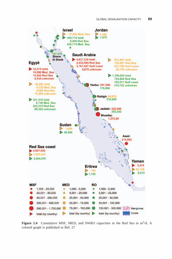
GLOBAL DESALINATION CAPACITY 89

Figure 2.4 Cumulative MSF, MED, and SWRO capacities in the Red Sea in m3/d. Acolored graph is published in Ref. 27

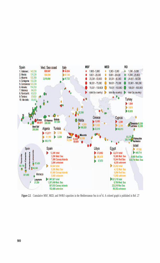
90

Figure 2.5 Cumulative MSF, MED, and SWRO capacities in the Mediterranean Sea in m3/d. A colored graph is published in Ref. 27

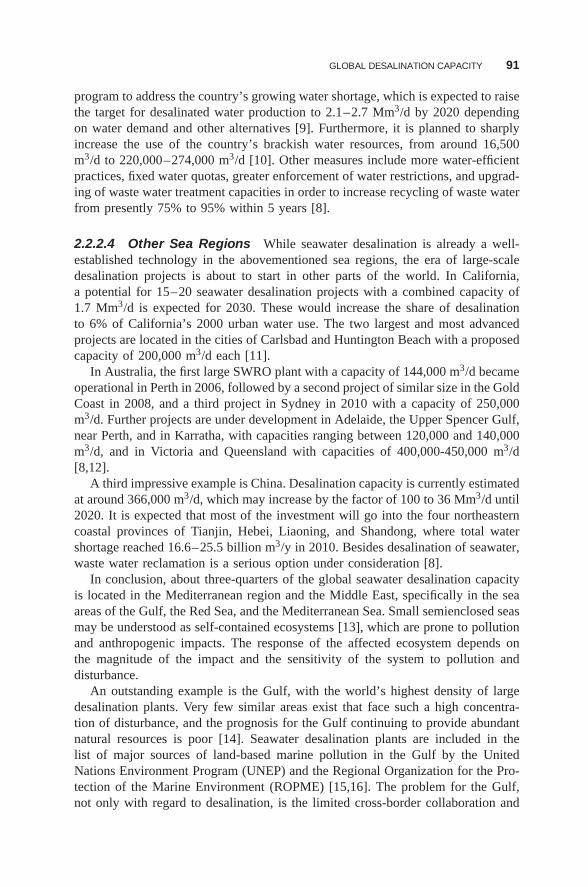
GLOBAL DESALINATION CAPACITY 91

program to address the country’s growing water shortage, which is expected to raisethe target for desalinated water production to 2.1–2.7 Mm3/d by 2020 dependingon water demand and other alternatives [9]. Furthermore, it is planned to sharplyincrease the use of the country’s brackish water resources, from around 16,500m3/d to 220,000–274,000 m3/d [10]. Other measures include more water-efficientpractices, fixed water quotas, greater enforcement of water restrictions, and upgrad-ing of waste water treatment capacities in order to increase recycling of waste waterfrom presently 75% to 95% within 5 years [8].

2.2.2.4 Other Sea Regions While seawater desalination is already a well-established technology in the abovementioned sea regions, the era of large-scaledesalination projects is about to start in other parts of the world. In California,a potential for 15–20 seawater desalination projects with a combined capacity of1.7 Mm3/d is expected for 2030. These would increase the share of desalinationto 6% of California’s 2000 urban water use. The two largest and most advancedprojects are located in the cities of Carlsbad and Huntington Beach with a proposedcapacity of 200,000 m3/d each [11].

In Australia, the first large SWRO plant with a capacity of 144,000 m3/d becameoperational in Perth in 2006, followed by a second project of similar size in the GoldCoast in 2008, and a third project in Sydney in 2010 with a capacity of 250,000m3/d. Further projects are under development in Adelaide, the Upper Spencer Gulf,near Perth, and in Karratha, with capacities ranging between 120,000 and 140,000m3/d, and in Victoria and Queensland with capacities of 400,000-450,000 m3/d[8,12].

A third impressive example is China. Desalination capacity is currently estimatedat around 366,000 m3/d, which may increase by the factor of 100 to 36 Mm3/d until2020. It is expected that most of the investment will go into the four northeasterncoastal provinces of Tianjin, Hebei, Liaoning, and Shandong, where total watershortage reached 16.6–25.5 billion m3/y in 2010. Besides desalination of seawater,waste water reclamation is a serious option under consideration [8].

In conclusion, about three-quarters of the global seawater desalination capacityis located in the Mediterranean region and the Middle East, specifically in the seaareas of the Gulf, the Red Sea, and the Mediterranean Sea. Small semienclosed seasmay be understood as self-contained ecosystems [13], which are prone to pollutionand anthropogenic impacts. The response of the affected ecosystem depends onthe magnitude of the impact and the sensitivity of the system to pollution anddisturbance.

An outstanding example is the Gulf, with the world’s highest density of largedesalination plants. Very few similar areas exist that face such a high concentra-tion of disturbance, and the prognosis for the Gulf continuing to provide abundantnatural resources is poor [14]. Seawater desalination plants are included in thelist of major sources of land-based marine pollution in the Gulf by the UnitedNations Environment Program (UNEP) and the Regional Organization for the Pro-tection of the Marine Environment (ROPME) [15,16]. The problem for the Gulf,not only with regard to desalination, is the limited cross-border collaboration and

92 ENVIRONMENTAL AND PERFORMANCE ASPECTS

even domestic collaboration among government agencies. Even where each projectreceives environmental assessment or attention, each is treated more or less in iso-lation, rarely in combination. However, the accumulative effects of an increasingnumber of projects in such a small, biologically interacting sea such as the Gulfexacerbates the overall deterioration [14].

On the contrary, desalination plants in Australia and California are unlikely toproduce measurable effects on the Pacific Oceans; however, local coastal habitatsmay be affected by the discharges, either by individual projects or cumulatively byseveral projects along a coastline.

2.3 STATE OF THE ART OF THE TECHNOLOGY

All desalination processes have been extensively described in the literature [e.g.,17–20]. The intention of this chapter is not to reproduce these textbook materi-als but to describe the different desalination processes with regard to the use ofresources, environmental considerations, and performance. While the design of theintake, pretreatment, desalination process, and outfall largely determine the impactson the marine environment, energy demand and air quality impacts depend mainlyon the process type.

2.3.1 Seawater Intake

Seawater desalination plants can receive feedwater through either a surface waterintake or a subsurface intake embedded in the seafloor or beach sediments. Surfaceintakes include the nearshore intakes of most distillation plants, which are oftenlocated directly at the shoreline, and the submerged intakes that are more commonfor large SWRO projects and are typically located further offshore and in greaterwater depths.

For SWRO plants, different types of subsurface intakes with either verticalor horizontal collectors have also been used successfully [19,21–25] [Fig. 2.6].Vertical wells and horizontal radial wells are both embedded in the permeableonshore sediments, whereas horizontal drains are drilled horizontally from a centralpoint on land into the offshore sediments. Where the natural sediments are notsufficiently permeable, onshore or offshore infiltration galleries can be constructedby replacing the natural sediments by a more permeable medium into which theperforated pipes are embedded.

2.3.1.1 Surface Intake Surface intakes are usually equipped with a combi-nation of screens to reduce the amount of debris and the number of organismsthat are absorbed by the plant with the feedwater. Most advances in screen designstem from the power industry. State-of-the-art intake systems [19] can effectivelyreduce the impingement of aquatic organisms against screens and the entrainmentof organisms into the plant. Passive screens with a large surface area and no mov-ing parts are commonly used for large SWRO plants. The screens are operated

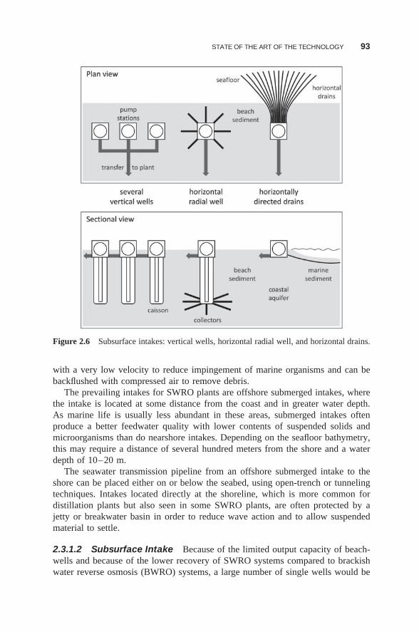
STATE OF THE ART OF THE TECHNOLOGY 93

Figure 2.6 Subsurface intakes: vertical wells, horizontal radial well, and horizontal drains.

with a very low velocity to reduce impingement of marine organisms and can bebackflushed with compressed air to remove debris.

The prevailing intakes for SWRO plants are offshore submerged intakes, wherethe intake is located at some distance from the coast and in greater water depth.As marine life is usually less abundant in these areas, submerged intakes oftenproduce a better feedwater quality with lower contents of suspended solids andmicroorganisms than do nearshore intakes. Depending on the seafloor bathymetry,this may require a distance of several hundred meters from the shore and a waterdepth of 10–20 m.

The seawater transmission pipeline from an offshore submerged intake to theshore can be placed either on or below the seabed, using open-trench or tunnelingtechniques. Intakes located directly at the shoreline, which is more common fordistillation plants but also seen in some SWRO plants, are often protected by ajetty or breakwater basin in order to reduce wave action and to allow suspendedmaterial to settle.

2.3.1.2 Subsurface Intake Because of the limited output capacity of beach-wells and because of the lower recovery of SWRO systems compared to brackishwater reverse osmosis (BWRO) systems, a large number of single wells would be

94 ENVIRONMENTAL AND PERFORMANCE ASPECTS

required for a large SWRO plant, which is difficult to realize [18]. Beachwells aretherefore usually considered only for small SWRO plants with capacities ≤20,000m3/d. A feasible alternative to open intakes for large seawater desalination plants arehorizontal drains, such as the Neodren system, which is installed from an onshoresite by horizontal directional drilling into the seafloor sediments. Sufficient flowrates can be realized for all plant sizes depending on the number of drains installed.The technology is, for example, used in the San Pedro del Pinatar plant in Spain,with a capacity of 65,000 m3/d [26; Table 4 in Ref. 27], and was also consideredin the planning studies for the Barcelona plant (200,000 m3/d) [28] and other largeplants in Algeria with capacities of ≤500,000 m3/d [Table 5 in Ref. 27; 29] butnot selected in the final design. For a 200,000-m3/d plant, a maximum batch of 25drains would be required, spaced at a distance of 2–3 m onshore (50–75 m total)and spreading out 300 m offshore in a fanlike arrangement.

In Long Beach, California, an ocean floor demonstration system is currentlybeing tested which combines offshore infiltration galleries for the intake and adischarge gallery for the outfall (see also Section 2.3.5.2). Both consist of perforatedlaterals placed under the ocean floor to collect or to discharge the water. Theinfiltration rates are 2 and 4 L/m2 per minute, and the discharge rates are 5.3–6.9L/m2 per minute. The intake in combination with 100 μM and 5 μM cartridgefilters were found to achieve sufficient DOC and turbidity removal to be used asfeedwater to a SWRO plant. The performance was comparable to effluent producedby a microfiltration system [24].

As subsurface intakes use natural sediments for prefiltration, they can bedescribed as a ‘natural treatment system’ or ‘biofilter’. Favorable conditionsfor subsurface intakes are geologic formations with a high transmissivity and acertain sediment thickness, whereas unfavorable conditions include sedimentswith high volumes of mud and a low degree of ‘flushing’ [30]. Biofilters oftenproduce a better feedwater quality than open intakes as the water is typicallycharacterized by lower and less variable amounts of organic carbon, suspendedsolids, nutrients, and microorganisms, and hence by a lower fouling potential[21]. This considerably reduces the pretreatment requirements in the ‘engineeredpretreatment system’ following the biofilter. Further pretreatment is usually limitedto acid and/or antiscalant addition followed by cartridge filtration. Extensive fieldexperience shows that SWRO systems treating wellwater, with cartridge filtrationas the only filtration step, can be operateded successfully over the years [18].

Shallow beachwells sometimes contain significant amounts of suspended parti-cles [18]. Moreover, water from beachwells is often anaerobic or anoxic and maycontain hydrogen sulfide, as well as iron(II) and manganese(II) depending on thegeology. Aeration may lead to the precipitation of ferric hydroxide, which causesturbidity, and the formation of manganese dioxide deposits on the membranes overtime. In some SWRO plants operating on wellwater, iron(II) and manganese(II)were initially absent but increased over time, e.g., in Malta. This appearance ofinsoluble salts in the feedwater is a risk of beachwell intakes, which may neces-sitate the installation of granular media filters in case feedwater conditions shoulddeteriorate over the lifetime of the project. Moreover, the water composition of

STATE OF THE ART OF THE TECHNOLOGY 95

wellwater with regard to sparingly soluble salts (barium and strontium sulfatesand silicates) may differ substantially from that of surface seawater, which maynecessitate the use of an antiscalant.

2.3.2 Pretreatment Processes and Chemical Use

The main operational concerns and reasons for pretreatment in SWRO plants(Fig. 2.7) are particulate fouling by suspended particles, biofouling by microor-ganisms, organic fouling by dissolved organic matter, scaling by sparingly solubleinorganic compounds, and oxidation and halogenation by residual chlorine. Thetype and amount of pretreatment depends on the intake water quality. An overviewon the main pretreatment alternatives for SWRO plants is given in the followingsubsections.

2.3.2.1 Minimal Pretreatment As subsurface intakes such as beachwellsand offshore horizontal drains are biofilters that can reduce both organic andbiofouling on the SWRO membranes, the following engineered pretreatment sys-tem is often minimal. The conventional steps of chlorination–dechlorination andcoagulation–flocculation are seldom required, and systems are operated with asingle filter only, using selective pretreatment against scaling where required anddepending on the feedwater composition [Tables 3 and 4 in Ref. 27]. In San Pedrodel Pinatar (Spain), for example, two “twin plants” with a capacity of 65,000 m3/dare being operated. One plant is equipped with an open intake followed by a two-stage dual media filter and uses about 4 mg/L of coagulant (FeCl3), whereas theother uses a subsurface intake followed by a sand filter and operates without coag-ulant. Both plants use about 1 mg/L of antiscalant and no chlorine [31]. A smallerbeachwell plant in Javea, Spain (26,000 m3/d) operates without any pretreatmentchemicals and requires acid and caustic cleaning of the membranes only about oncea year [32].

2.3.2.2 Conventional Pretreatment As surface intakes must accommodatemore variable water quality due to seasonal weather conditions and algae blooms,pretreatment is generally more complex and extensive than for subsurface intakes.The conventional pretreatment for SWRO plants with surface intakes includesshock chlorination to control marine growth in the intake system, followed bycoagulation–flocculation and filtration to remove suspended solids and colloids,and dechlorination prior to the RO units. Sometimes additional screening, sedi-mentation or flotation is included as an initial pretreatment step (Fig. 2.7).

Chlorine is usually added intermittently to the feedwater in doses of ≤10 mg/Lto control biogrowth on the intake screens, inside the intake pipe, and in the pre-treatment line, with one to three dosing points along that line. Chlorination canbe carried out daily, weekly, or biweekly, depending on the site. Some plants alsooperate more successfully without chlorination, which breaks natural organic matterinto biodegradable compounds that may increase biofouling in SWRO elements.The water is dechlorinated ahead of the SWRO units with a reducing agent, sodiumbisulfite (SBS), usually in a dosage of 3 times the residual chlorine concentration

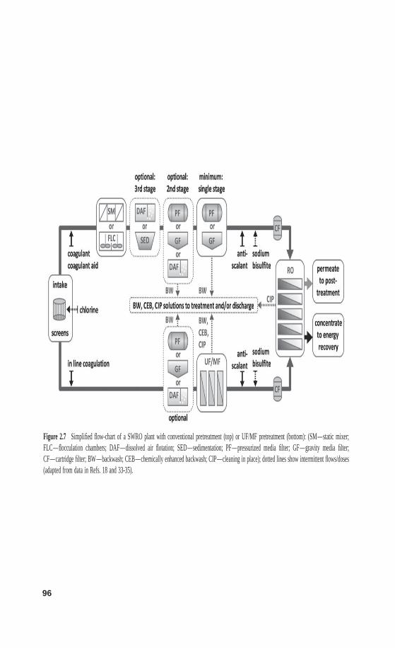
96

Figure 2.7 Simplified flow-chart of a SWRO plant with conventional pretreatment (top) or UF/MF pretreatment (bottom): (SM—static mixer;FLC—flocculation chambers; DAF—dissolved air flotation; SED—sedimentation; PF—pressurized media filter; GF—gravity media filter;CF—cartridge filter; BW—backwash; CEB—chemically enhanced backwash; CIP—cleaning in place); dotted lines show intermittent flows/doses(adapted from data in Refs. 18 and 33-35).

STATE OF THE ART OF THE TECHNOLOGY 97

to remove any residual oxidants from the RO feedwater, which might damage themembranes [Table 2 in Ref. 27].

Coagulation–flocculation is a combined process. Coagulation is the destabiliza-tion of the particle surface charge of small and colloid particles, which is followedby flocculation , i.e., the formation of larger flocs. The dosing of primary coagulants,typically ferric chloride (FeCl3) or ferrous sulfate (FeSO4), depends on the feed-water quality and ranges between 0.2 and 20 mg/L [Table 5 in Ref. 27]. Dosesof 1–6 mg/L are assumed to be the rule and 20 mg/L the exception. The resul-tant formation of metal hydroxides is very rapid, but effective coagulation requiresintensive mixing to bring the hydroxides in contact with the colloid particles. Thisis achieved downstream of the injection point by static mixers or flocculationchambers that induce more gentle mixing. The process can be further enhanced bythe addition of a coagulant aid, which is typically a longchain organic polymer.Cationic polymers can also be used as primary coagulants [18].

Filtration is either performed in pressurized vessels or gravity concrete cham-bers. The filters contain a single or dual medium, usually anthracite and sand, arearranged in a single- or two-stage configuration, and are backwashed with eitherfiltrate or concentrate. The backwash water is discharged into the sea or dewateredand the sludge transported to a landfill. The backwash frequency and the amountsof sludge produced depend on the amount of suspended solids in the feedwater andthe required coagulant dose. Two-stage dual-medium filtration is usually effectivein producing a consistent feed quality, even under fluctuating water conditions [36].Sedimentation or dissolved air flotation (DAF) can precede single- or dual-stagefiltration in locations with treatment-recalcitrant feedwater [33]. In the Gulf, somenew SWRO plants have incorporated DAF followed by UF or media filters todeal with extended periods of red tides [37]. In many SWRO plants, a single-stagepressurized or gravity filter was found to be sufficient [Table 5 in Ref. 27].

Scaling by inorganic salts, metal oxides, and hydroxides does not present aproblem with the majority of seawater feeds as a result of the relatively low recov-ery rate (≤50%) of SWRO plants, the high ionic strength of seawater, and thelow concentration of bicarbonate ions in seawater [36]. Nevertheless, most SWROplants use 1–2 mg/L of antiscalants or 20–50 mg/L of acid to avoid the risk ofscale formation on the RO membranes. Some plants also operate without any anti-scalant, e.g., on the Cayman Islands or in the Mediterranean. Laboratory studiessuggest that calcium carbonate scaling—the main scalant in SWRO—should notoccur since the induction time of calcium carbonate is considerably longer thanthe residence time of the water in the membranes [38]. This result raises questionsabout the current practice of antiscalant use in SWRO, which should be furtherevaluated by pilot studies and in full-scale SWRO plants. If a second stage is nec-essary for boron removal, which requires that the pH be raised to ∼10, antiscalantsare needed to prevent the formation of magnesium hydroxide [Mg(OH)2]. SWROplants with a single stage often use acid only, while plants with a second RO stageoften use polymer antiscalant to maintain a higher pH for boron removal.

2.3.2.3 Ultrafiltration (UF) and Microfiltration (MF) An emerging alterna-tive to conventional pretreatment in SWRO is UF/MF pretreatment. The number

98 ENVIRONMENTAL AND PERFORMANCE ASPECTS

of full-scale SWRO plants equipped with UF/MF pretreatment, however, is stillfairly low compared to the many pilot studies that have demonstrated a good per-formance of UF/MF in SWRO, and the manifold benefits that have been cited inthe literature.

One proclaimed benefit is the consistently high feedwater quality that is producedregardless of source-water fluctuations, which generally results in a reduced foulingpotential of the SWRO membranes, a lower cleaning frequency, and hence a lowerchemical use, as well as a longer membrane life and therefore savings in materialand energy use. Moreover, a better feed quality offers the potential to operateat a higher flux, so that the total membrane surface area can be reduced. Thepretreatment system would be smaller, too, because less feedwater needs to betreated. It is therefore estimated that UF/MF pretreatment can save about one-third in plant area size [18] and about one-third in the membrane replacementrate [39]. Despite these benefits, however, conventional pretreatment is still oftenchosen over UF/MF for new SWRO projects. One possible reason could be thestill limited performance data of full-scale UF/MF-SWRO plants [40].

UF/MF was once considered as a possibly “chemical-free” alternative to con-ventional pretreatment that may eliminate the need for coagulant dosing with goodfeedwater quality [41] and the need for a continuous presence of free chlorine[36,42]. However, the use of a disinfectant, either continuously or intermittently,and the use of inline coagulation, which is the dosing of a coagulant without asedimentation or filtration step, seem to be common practice in many UF/MF sys-tems in order to improve the process performance and filtrate quality. Moreover,UF/MF membranes usually require intermittent chemically enhanced backwashing(CEB) and cleaning in place (CIP).

Performance data on more than 40 UF/MF-SWRO systems could be obtainedfrom the more recent literature (years 2000–2009). Of these, only 16 providedinformation on full-scale operational plants [Table 6 in Ref. 27], the remainingwere pilot systems [Table 7 in Ref. 27]. Examining the available literature led to thefollowing conclusions concerning chemical use in UF/MF pretreatment for SWRO.

The majority of UF/MF-SWRO systems showed a reliable and often supe-rior performance to conventional pretreatment systems in terms of turbidity andmicroorganisms removal. The favorable performance, however, must partly beattributed to the use of chemicals similar in type and dosage to chemical usein conventional pretreatment. However, some UF/MF systems performed less wellcompared to conventional pretreatment in terms of dissolved organics removal.MF/UF pretreatment may therefore not always be an adequate solution for the pre-vention of organic fouling [43], unless coagulation prior to UF/MF is used, whichcan improve the adsorption and removal of organics as fine particulates. Coagulantsmay not be needed in every UF/MF system. The need and the optimum dosageshould be established by pilot testing [39], as overdosing may also result in opera-tional problems of the UF/MF membranes [44] and of the SWRO membranes [45],as well as in unnecessary costs and environmental impacts.

The reported coagulant levels in this review ranged between 0.2 and 10 mg/L inUF/MF pilot plants and between 0.3 and 10 mg/L in UF/MF full-scale plants, with

STATE OF THE ART OF THE TECHNOLOGY 99

values of 0.2–2 mg/L assumed to be the norm and 10 mg/L the exception [Tables6 and 7 in Ref. 27]. This compares to ranges of 0.2–20 mg/L in conventionalpretreatment, where ranges of 1–6 mg/L are assumed to be the norm and 20 mg/Lthe exception [Table 5 in Ref. 27].

Chlorination levels in several UF/MF systems ranged between 0.3 and 2 mg/L,which is similar to conventional pretreatment where low-level continuous chlori-nation of 1–2 mg/L is applied. However, many conventional SWRO plants nowuse intermittent chlorination. For example, an intermittent dose of 10 mg/L forone hour per day equals a continuous dosage of “only” 0.4 mg/L. As chlorinationintervals in conventional pretreatment are often even longer, e.g., once per week,chlorine use may be even lower. Many UF/MF systems additionally employ CEBswith considerable chlorine doses, which may compare to an additional chlorinelevel of 0.5–2 mg/L if the chemicals were used continuously. For instance, a UF-SWRO plant in Asia reported feedwater chlorination in a dosage of 1 mg/L andchlorination of every backwash once every hour in a dosage of 15 mg/L [40].

In conclusion, the reported chemical use in UF/MF pretreatment does not seemto live up to the expectations that were initially placed into the technology ofbeing a chemical-free process. However, total chemical use in UF/MF is in somecases claimed to be significantly lower or minimal compared to conventionallevels [40,41,46]. Pearce [39] assumes that UF/MF systems can be operated at acoagulant dose concentration of 43% of conventional pretreatment (i.e., 0.3 mg/Linstead of 0.7 mg/L as Fe) and that chlorine use can be reduced to intermittentchlorine cleaning. Indeed, a lower consumption of chemicals in UF/MF seems tobe feasible.

For example, a lifecycle analysis and aspects of operability led to the selec-tion of a UF system over a classic two-stage filtration system for a desalinationproject south of Perth with a capacity of 140,000 m3/d, which will presumablyoperate without coagulation [47]. Our literature review indicates that coagulantuse seems to be lower in UF/MF pretreatment than in conventional pretreatment,whereas chlorine use appears to be higher in some UF/MF-SWRO plants, dueto a combination of continuous chlorination and intermittent shock chlorinationduring CEB and CIP. Some UF/MF systems were found to be liable to bio-fouling without continuous or intermittent chlorination of the UF feed, CEB orCIP [48,49].

The overall chemical use of an UF/MF SWRO system depends on the filtrationtime and the backwashing, CEB, and CIP intervals. One option to postpone back-washing and CEB might be additional pretreatment prior to membrane filtration,such as a beachwell or a sand filter. Other options are to lower the flux, whichwill increase the total membrane area to be installed [50], or to operate withoutcoagulant pretreatment but more frequent cleaning [39]. A well-designed systemoperated on good feedwater quality may thus, indeed, reduce chemical use. How-ever, an integrated membrane system does not seem to be superior to conventionalpretreatment in terms of chemical use when inline coagulation, chlorination andfrequent CEB is employed. In that case, the only remaining benefit may stem fromthe reduced cleaning frequency (CIP intervals) of the SWRO membranes due to

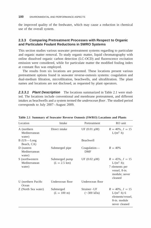
100 ENVIRONMENTAL AND PERFORMANCE ASPECTS

the improved quality of the feedwater, which may cause a reduction in chemicaluse of the overall system.

2.3.3 Comparing Pretreatment Processes with Respect to Organicand Particulate Foulant Reductions in SWRO Systems

This section studies various seawater pretreatment systems regarding to particulateand organic matter removal. To study organic matter, liquid chromatography withonline dissolved organic carbon detection (LC-OCD) and fluorescence excitationemission were considered, while for particulate matter the modified fouling indexat constant flux was employed.

The results from six locations are presented. These locations present variouspretreatment options found in seawater reverse-osmosis systems: coagulation anddual-medium filtration, microfiltration, beachwells, and ultrafiltration. The plantnames and locations are not disclosed, as requested by plant operators.

2.3.3.1 Plant Description The locations summarized in Table 2.1 were stud-ied. The locations include conventional and membrane pretreatment, and differentintakes as beachwells and a system termed the underocean floor . The studied periodcorresponds to July 2007–August 2009.

Table 2.1 Summary of Seawater Reverse Osmosis (SWRO) Locations and Plants

Location Intake Pretreatment RO unit

A (northernMediterraneanwater)

Direct intake UF (0.01 μM) R = 40%, J = 15L/(m2· h)

B (US—LongBeach, CA)

Beachwell

D (easternMediterraneanwater)

Submerged pipe Coagulation—DMF

R = 40%

S (northwesternMediterraneanwater)

Submerged pump(L = 2.5 km)

UF (0.02 μM) R = 45%, J = 15L/(m2· h);

7 elements pervessel, 8-in.module; nevercleaned

U (northern PacificOcean

Underocean floor Underocean floor

Z (North Sea water) Submerged(L = 100 m)

Strainer–UF(∼300 kDa)

R = 40%, J = 15L/(m2· h) 6elements/vessel,8-in. modulenever cleaned

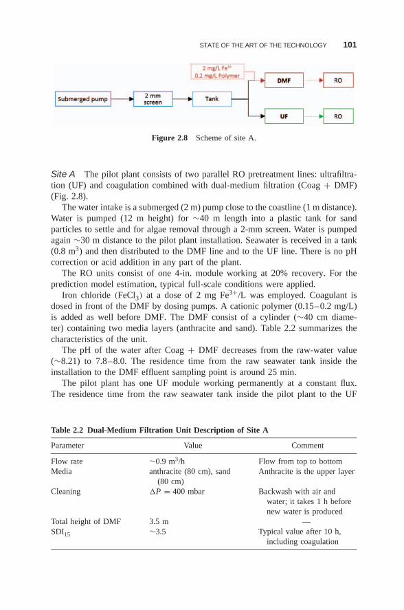
STATE OF THE ART OF THE TECHNOLOGY 101

Figure 2.8 Scheme of site A.

Site A The pilot plant consists of two parallel RO pretreatment lines: ultrafiltra-tion (UF) and coagulation combined with dual-medium filtration (Coag + DMF)(Fig. 2.8).

The water intake is a submerged (2 m) pump close to the coastline (1 m distance).Water is pumped (12 m height) for ∼40 m length into a plastic tank for sandparticles to settle and for algae removal through a 2-mm screen. Water is pumpedagain ∼30 m distance to the pilot plant installation. Seawater is received in a tank(0.8 m3) and then distributed to the DMF line and to the UF line. There is no pHcorrection or acid addition in any part of the plant.

The RO units consist of one 4-in. module working at 20% recovery. For theprediction model estimation, typical full-scale conditions were applied.

Iron chloride (FeCl3) at a dose of 2 mg Fe3+/L was employed. Coagulant isdosed in front of the DMF by dosing pumps. A cationic polymer (0.15–0.2 mg/L)is added as well before DMF. The DMF consist of a cylinder (∼40 cm diame-ter) containing two media layers (anthracite and sand). Table 2.2 summarizes thecharacteristics of the unit.

The pH of the water after Coag + DMF decreases from the raw-water value(∼8.21) to 7.8–8.0. The residence time from the raw seawater tank inside theinstallation to the DMF effluent sampling point is around 25 min.

The pilot plant has one UF module working permanently at a constant flux.The residence time from the raw seawater tank inside the pilot plant to the UF

Table 2.2 Dual-Medium Filtration Unit Description of Site A

Parameter Value Comment

Flow rate ∼0.9 m3/h Flow from top to bottomMedia anthracite (80 cm), sand

(80 cm)Anthracite is the upper layer

Cleaning �P = 400 mbar Backwash with air andwater; it takes 1 h beforenew water is produced

Total height of DMF 3.5 m —SDI15 ∼3.5 Typical value after 10 h,

including coagulation

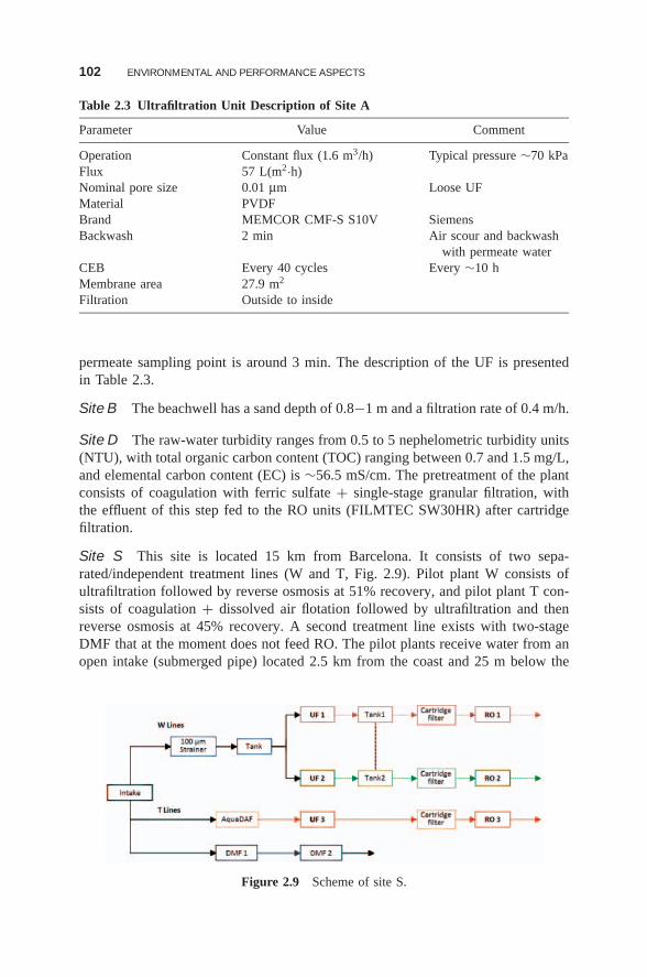
102 ENVIRONMENTAL AND PERFORMANCE ASPECTS

Table 2.3 Ultrafiltration Unit Description of Site A

Parameter Value Comment

Operation Constant flux (1.6 m3/h) Typical pressure ∼70 kPaFlux 57 L(m2·h)Nominal pore size 0.01 μm Loose UFMaterial PVDFBrand MEMCOR CMF-S S10V SiemensBackwash 2 min Air scour and backwash

with permeate waterCEB Every 40 cycles Every ∼10 hMembrane area 27.9 m2

Filtration Outside to inside

permeate sampling point is around 3 min. The description of the UF is presentedin Table 2.3.

Site B The beachwell has a sand depth of 0.8−1 m and a filtration rate of 0.4 m/h.

Site D The raw-water turbidity ranges from 0.5 to 5 nephelometric turbidity units(NTU), with total organic carbon content (TOC) ranging between 0.7 and 1.5 mg/L,and elemental carbon content (EC) is ∼56.5 mS/cm. The pretreatment of the plantconsists of coagulation with ferric sulfate + single-stage granular filtration, withthe effluent of this step fed to the RO units (FILMTEC SW30HR) after cartridgefiltration.

Site S This site is located 15 km from Barcelona. It consists of two sepa-rated/independent treatment lines (W and T, Fig. 2.9). Pilot plant W consists ofultrafiltration followed by reverse osmosis at 51% recovery, and pilot plant T con-sists of coagulation + dissolved air flotation followed by ultrafiltration and thenreverse osmosis at 45% recovery. A second treatment line exists with two-stageDMF that at the moment does not feed RO. The pilot plants receive water from anopen intake (submerged pipe) located 2.5 km from the coast and 25 m below the

Figure 2.9 Scheme of site S.

STATE OF THE ART OF THE TECHNOLOGY 103

water surface. The pipe is cleaned by chlorination (frequency not disclosed). Theaverage suspended solids of the raw water was about 3.5 mg/L, with an averagesilt density index (SDI) value of 5.

The two site S lines are described as follows:

W Lines . Before the raw water is being fed to the UF, it passes through a100 μm-strainer. The ultrafiltration units (UF1 and UF2) operate at constantflux at ∼60 L/(m2·h). Backwash is applied at double the operation flow withair scour every 30 min, consisting of 10 s air scour, 15 s backwash with UFpermeate, and 45 s forward flush with raw water (Table 2.4).

The RO systems consist of two units working in parallel (RO1 and RO2). Eachunit has six 4-in. SW30-4040HR elements and operate at 52% recovery. TheRO2 unit has a hybrid configuration (high-rejection modules in the frontof the pressure vessel and high-production modules at the end), while RO1has a standard configuration. Both RO units operate at constant pressure(70 bar). Bisulfite and antiscalant are added in front of the RO (Permatreat,phosphonated). Since the start of operation of the plant (April 2009), the ROmembranes were never cleaned. The RO production capacity is ∼0.76 m3/h.

T Lines . The AquaDAF unit was not necessary during the testing period, dueto good raw seawater quality. The UF3 modules are Zenon membranes thatoperate in a submerged mode (Table 2.5). There are two dual-medium filters(DMFs) that operate in series. In DMF1 there are two layers of sand andpumice and in DMF2 sand and anthracite. DMF1 was not in operation duringthe testing period because the raw seawater quality was good. Coagulationis used in combination with DMF. During the testing period the dose was1.5 mg/L FeCl3. The RO3 unit is one pressure vessel containing seven 8-in.elements. The RO operates at 45% recovery.

Site U This system (see Fig. 2.10) is based on the design criteria associatedwith slow sand filtration systems. The century-old slow sand filtration concept hasbeen utilized around the world and now offers the opportunity to be applied in

Table 2.4 UF1/UF2 Unit Description of Site S

Parameter Value Comment

Operation Constant flux (1.9 m3/h) Typical pressure 0.7 barFlux ∼58 L/(m2·h) —Nominal pore size 0.03 μm —Material PVDF —Brand SFP2660 OM Excell—DowBackwash 1.25 min With air scour, permeate waterCEB Every 24 h ∼48 cyclesMembrane area 33 m2 —Filtration Outside to inside —

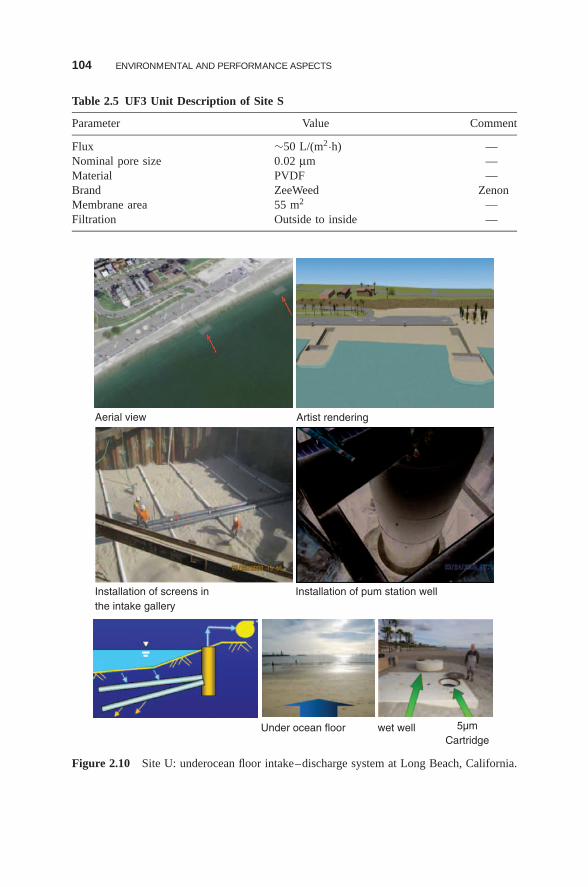
104 ENVIRONMENTAL AND PERFORMANCE ASPECTS

Table 2.5 UF3 Unit Description of Site S

Parameter Value Comment

Flux ∼50 L/(m2·h) —Nominal pore size 0.02 μm —Material PVDF —Brand ZeeWeed ZenonMembrane area 55 m2 —Filtration Outside to inside —

Aerial view

Installation of screens in the intake gallery

Installation of pum station well

Under ocean floor wet well 5µmCartridge

Artist rendering

Figure 2.10 Site U: underocean floor intake–discharge system at Long Beach, California.

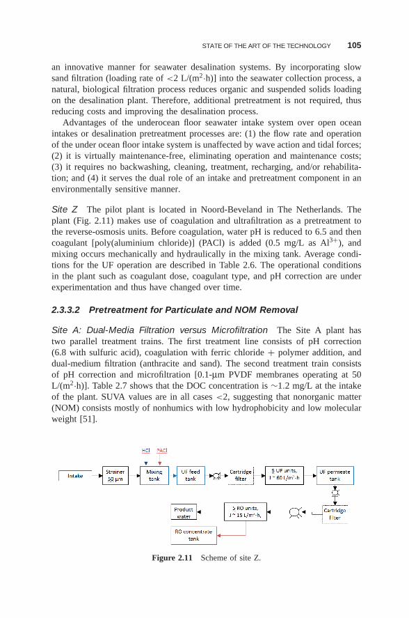
STATE OF THE ART OF THE TECHNOLOGY 105

an innovative manner for seawater desalination systems. By incorporating slowsand filtration (loading rate of <2 L/(m2·h)] into the seawater collection process, anatural, biological filtration process reduces organic and suspended solids loadingon the desalination plant. Therefore, additional pretreatment is not required, thusreducing costs and improving the desalination process.

Advantages of the underocean floor seawater intake system over open oceanintakes or desalination pretreatment processes are: (1) the flow rate and operationof the under ocean floor intake system is unaffected by wave action and tidal forces;(2) it is virtually maintenance-free, eliminating operation and maintenance costs;(3) it requires no backwashing, cleaning, treatment, recharging, and/or rehabilita-tion; and (4) it serves the dual role of an intake and pretreatment component in anenvironmentally sensitive manner.

Site Z The pilot plant is located in Noord-Beveland in The Netherlands. Theplant (Fig. 2.11) makes use of coagulation and ultrafiltration as a pretreatment tothe reverse-osmosis units. Before coagulation, water pH is reduced to 6.5 and thencoagulant [poly(aluminium chloride)] (PACl) is added (0.5 mg/L as Al3+), andmixing occurs mechanically and hydraulically in the mixing tank. Average condi-tions for the UF operation are described in Table 2.6. The operational conditionsin the plant such as coagulant dose, coagulant type, and pH correction are underexperimentation and thus have changed over time.

2.3.3.2 Pretreatment for Particulate and NOM Removal

Site A: Dual-Media Filtration versus Microfiltration The Site A plant hastwo parallel treatment trains. The first treatment line consists of pH correction(6.8 with sulfuric acid), coagulation with ferric chloride + polymer addition, anddual-medium filtration (anthracite and sand). The second treatment train consistsof pH correction and microfiltration [0.1-μm PVDF membranes operating at 50L/(m2·h)]. Table 2.7 shows that the DOC concentration is ∼1.2 mg/L at the intakeof the plant. SUVA values are in all cases <2, suggesting that nonorganic matter(NOM) consists mostly of nonhumics with low hydrophobicity and low molecularweight [51].

Figure 2.11 Scheme of site Z.

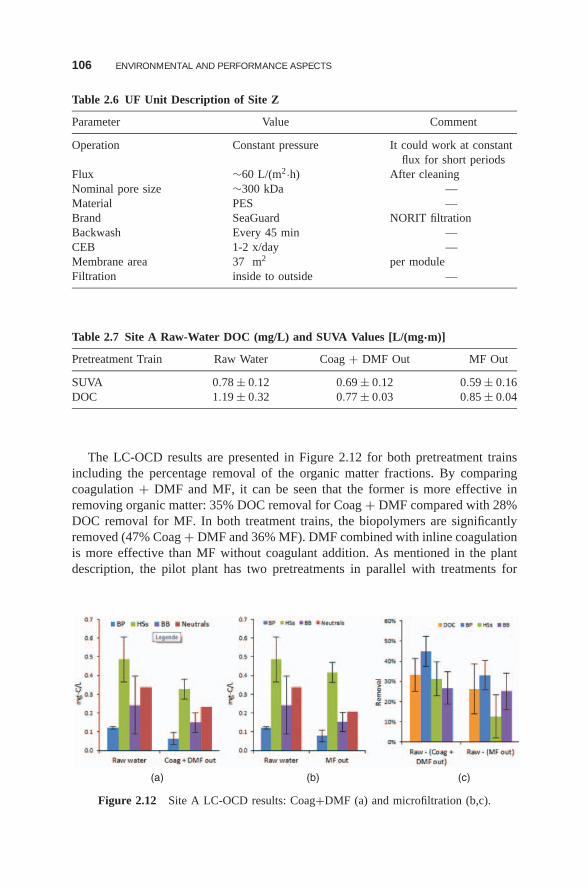
106 ENVIRONMENTAL AND PERFORMANCE ASPECTS

Table 2.6 UF Unit Description of Site Z

Parameter Value Comment

Operation Constant pressure It could work at constantflux for short periods

Flux ∼60 L/(m2·h) After cleaningNominal pore size ∼300 kDa —Material PES —Brand SeaGuard NORIT filtrationBackwash Every 45 min —CEB 1-2 x/day —Membrane area 37 m2 per moduleFiltration inside to outside —

Table 2.7 Site A Raw-Water DOC (mg/L) and SUVA Values [L/(mg·m)]

Pretreatment Train Raw Water Coag + DMF Out MF Out

SUVA 0.78 ± 0.12 0.69 ± 0.12 0.59 ± 0.16DOC 1.19 ± 0.32 0.77 ± 0.03 0.85 ± 0.04

The LC-OCD results are presented in Figure 2.12 for both pretreatment trainsincluding the percentage removal of the organic matter fractions. By comparingcoagulation + DMF and MF, it can be seen that the former is more effective inremoving organic matter: 35% DOC removal for Coag + DMF compared with 28%DOC removal for MF. In both treatment trains, the biopolymers are significantlyremoved (47% Coag + DMF and 36% MF). DMF combined with inline coagulationis more effective than MF without coagulant addition. As mentioned in the plantdescription, the pilot plant has two pretreatments in parallel with treatments for

(a) (b) (c)

Figure 2.12 Site A LC-OCD results: Coag+DMF (a) and microfiltration (b,c).

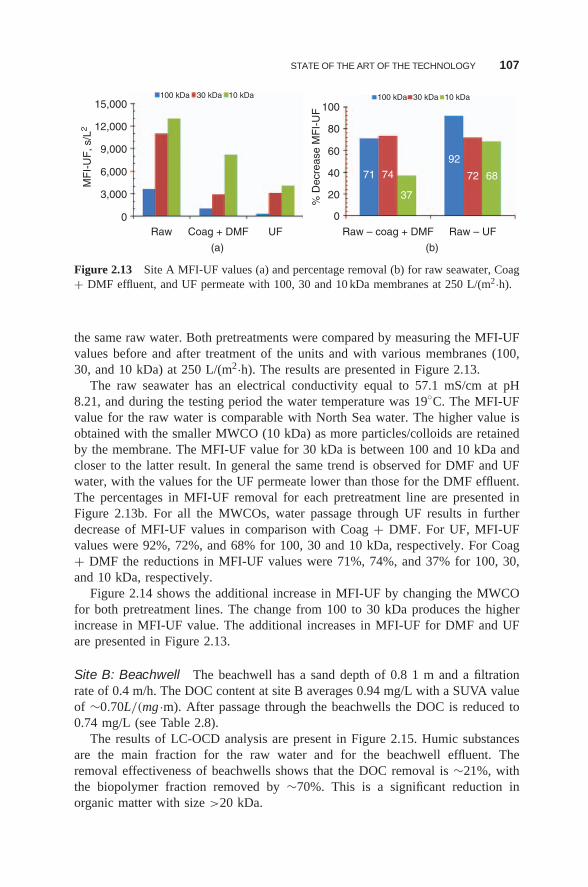
STATE OF THE ART OF THE TECHNOLOGY 107

15,000

12,000

9,000

6,000

MF

I-U

F, s

/L2

3,000

0

20

71 74

37

92

72 68

Raw – coag + DMF Raw – UF

40

60

% D

ecre

ase

MF

I-U

F

80

100

0Raw Coag + DMF

100 kDa 30 kDa 10 kDa 100 kDa 30 kDa 10 kDa

UF

(a) (b)

Figure 2.13 Site A MFI-UF values (a) and percentage removal (b) for raw seawater, Coag+ DMF effluent, and UF permeate with 100, 30 and 10 kDa membranes at 250 L/(m2·h).

the same raw water. Both pretreatments were compared by measuring the MFI-UFvalues before and after treatment of the units and with various membranes (100,30, and 10 kDa) at 250 L/(m2·h). The results are presented in Figure 2.13.

The raw seawater has an electrical conductivity equal to 57.1 mS/cm at pH8.21, and during the testing period the water temperature was 19◦C. The MFI-UFvalue for the raw water is comparable with North Sea water. The higher value isobtained with the smaller MWCO (10 kDa) as more particles/colloids are retainedby the membrane. The MFI-UF value for 30 kDa is between 100 and 10 kDa andcloser to the latter result. In general the same trend is observed for DMF and UFwater, with the values for the UF permeate lower than those for the DMF effluent.The percentages in MFI-UF removal for each pretreatment line are presented inFigure 2.13b. For all the MWCOs, water passage through UF results in furtherdecrease of MFI-UF values in comparison with Coag + DMF. For UF, MFI-UFvalues were 92%, 72%, and 68% for 100, 30 and 10 kDa, respectively. For Coag+ DMF the reductions in MFI-UF values were 71%, 74%, and 37% for 100, 30,and 10 kDa, respectively.

Figure 2.14 shows the additional increase in MFI-UF by changing the MWCOfor both pretreatment lines. The change from 100 to 30 kDa produces the higherincrease in MFI-UF value. The additional increases in MFI-UF for DMF and UFare presented in Figure 2.13.

Site B: Beachwell The beachwell has a sand depth of 0.8 1 m and a filtrationrate of 0.4 m/h. The DOC content at site B averages 0.94 mg/L with a SUVA valueof ∼0.70L/(mg ·m). After passage through the beachwells the DOC is reduced to0.74 mg/L (see Table 2.8).

The results of LC-OCD analysis are present in Figure 2.15. Humic substancesare the main fraction for the raw water and for the beachwell effluent. Theremoval effectiveness of beachwells shows that the DOC removal is ∼21%, withthe biopolymer fraction removed by ∼70%. This is a significant reduction inorganic matter with size >20 kDa.

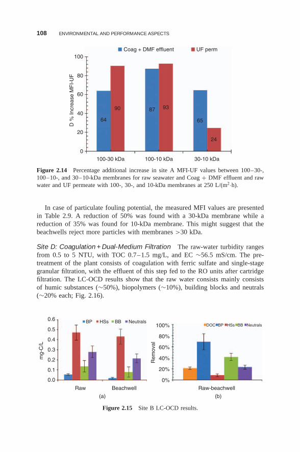
108 ENVIRONMENTAL AND PERFORMANCE ASPECTS

100

80

60

40

D %

Incr

ease

MF

I-U

F

20

0100-30 kDa 100-10 kDa 30-10 kDa

64

90

Coag + DMF effluent UF perm

87 93

65

24

Figure 2.14 Percentage additional increase in site A MFI-UF values between 100–30-,100–10-, and 30–10-kDa membranes for raw seawater and Coag + DMF effluent and rawwater and UF permeate with 100-, 30-, and 10-kDa membranes at 250 L/(m2·h).

In case of particulate fouling potential, the measured MFI values are presentedin Table 2.9. A reduction of 50% was found with a 30-kDa membrane while areduction of 35% was found for 10-kDa membrane. This might suggest that thebeachwells reject more particles with membranes >30 kDa.

Site D: Coagulation + Dual-Medium Filtration The raw-water turbidity rangesfrom 0.5 to 5 NTU, with TOC 0.7–1.5 mg/L, and EC ∼56.5 mS/cm. The pre-treatment of the plant consists of coagulation with ferric sulfate and single-stagegranular filtration, with the effluent of this step fed to the RO units after cartridgefiltration. The LC-OCD results show that the raw water consists mainly consistsof humic substances (∼50%), biopolymers (∼10%), building blocks and neutrals(∼20% each; Fig. 2.16).

0.6 BP HSs BB Neutrals100%

80%

60%

40%

Rem

oval

20%

0%

Raw-beachwell

BPDOC HSs BB Neutrals0.5

0.4

0.3

mg-

C/L

0.2

0.1

0.0

Raw Beachwell

(a) (b)

Figure 2.15 Site B LC-OCD results.

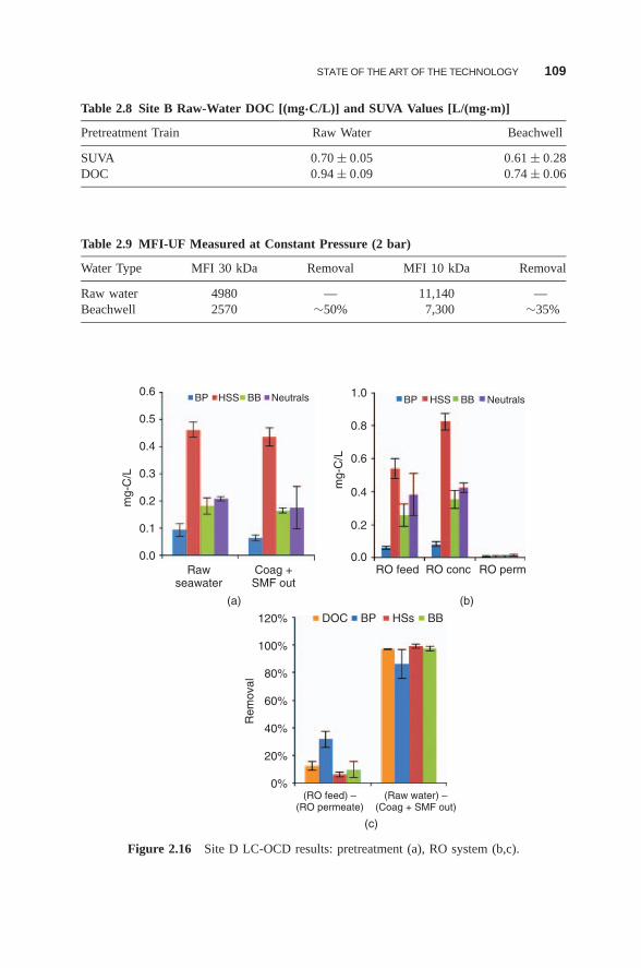
STATE OF THE ART OF THE TECHNOLOGY 109

Table 2.8 Site B Raw-Water DOC [(mg·C/L)] and SUVA Values [L/(mg·m)]

Pretreatment Train Raw Water Beachwell

SUVA 0.70 ± 0.05 0.61 ± 0.28DOC 0.94 ± 0.09 0.74 ± 0.06

Table 2.9 MFI-UF Measured at Constant Pressure (2 bar)

Water Type MFI 30 kDa Removal MFI 10 kDa Removal

Raw water 4980 — 11,140 —Beachwell 2570 ∼50% 7,300 ∼35%

0.6 BP HSS BB Neutrals

DOC BP HSs BB

0.5

0.4

0.3

mg-

C/L

0.2

0.1

0.0Raw

seawaterCoag +SMF out

0.0RO feed RO conc RO perm

0%

20%

40%

60%

80%

Rem

oval

100%

120%

(Raw water) –(Coag + SMF out)

(RO feed) –(RO permeate)

0.2

0.4

0.6

mg-

C/L

0.8

1.0BP HSS BB Neutrals

(a) (b)

(c)

Figure 2.16 Site D LC-OCD results: pretreatment (a), RO system (b,c).

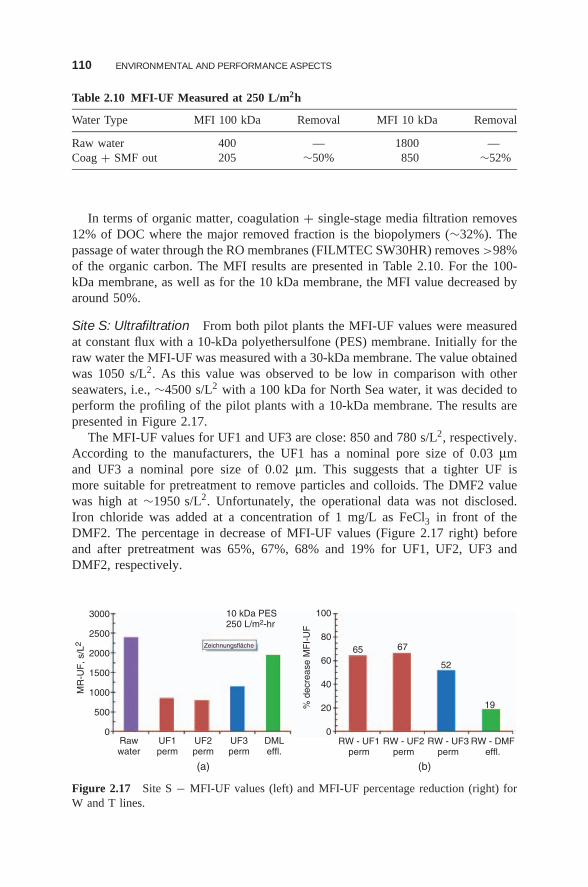
110 ENVIRONMENTAL AND PERFORMANCE ASPECTS

Table 2.10 MFI-UF Measured at 250 L/m2h

Water Type MFI 100 kDa Removal MFI 10 kDa Removal

Raw water 400 — 1800 —Coag + SMF out 205 ∼50% 850 ∼52%

In terms of organic matter, coagulation + single-stage media filtration removes12% of DOC where the major removed fraction is the biopolymers (∼32%). Thepassage of water through the RO membranes (FILMTEC SW30HR) removes >98%of the organic carbon. The MFI results are presented in Table 2.10. For the 100-kDa membrane, as well as for the 10 kDa membrane, the MFI value decreased byaround 50%.

Site S: Ultrafiltration From both pilot plants the MFI-UF values were measuredat constant flux with a 10-kDa polyethersulfone (PES) membrane. Initially for theraw water the MFI-UF was measured with a 30-kDa membrane. The value obtainedwas 1050 s/L2. As this value was observed to be low in comparison with otherseawaters, i.e., ∼4500 s/L2 with a 100 kDa for North Sea water, it was decided toperform the profiling of the pilot plants with a 10-kDa membrane. The results arepresented in Figure 2.17.

The MFI-UF values for UF1 and UF3 are close: 850 and 780 s/L2, respectively.According to the manufacturers, the UF1 has a nominal pore size of 0.03 μmand UF3 a nominal pore size of 0.02 μm. This suggests that a tighter UF ismore suitable for pretreatment to remove particles and colloids. The DMF2 valuewas high at ∼1950 s/L2. Unfortunately, the operational data was not disclosed.Iron chloride was added at a concentration of 1 mg/L as FeCl3 in front of theDMF2. The percentage in decrease of MFI-UF values (Figure 2.17 right) beforeand after pretreatment was 65%, 67%, 68% and 19% for UF1, UF2, UF3 andDMF2, respectively.

0 0

20

40

6065 67

52

19

80

100

MR

-UF

, s/L

2

% d

ecre

ase

MF

I-U

F

Rawwater

UF1perm

RW - UF1perm

RW - UF2perm

RW - UF3perm

RW - DMFeffl.

UF2perm

(a) (b)

UF3perm

DMLeffl.

500

1000

1500

2000

2500

3000

Zeichnungsfläche

10 kDa PES250 L/m2-hr

Figure 2.17 Site S − MFI-UF values (left) and MFI-UF percentage reduction (right) forW and T lines.

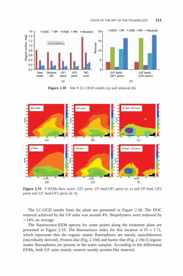
STATE OF THE ART OF THE TECHNOLOGY 111

Zeichnungsfläche

0.0 0

5

10

15

20

Org

anic

car

bon,

mg/

L

Rem

oval

0.2

0.4

0.6

0.8

1.0

1.2

1.4

1.6 DOC

Rawwater

UF1perm

UF2perm

ROconc

(UF feed) -(UF1 perm)

(UF feed) -(UF2 perm)

Strainereffl.

RP HSS

(a) (b)

RR Neutrals DOC RP HSS RR Neutrals

Figure 2.18 Site S LC-OCD results (a) and removal (b).

(a) (b) (c)

(d) (e) (f)

Figure 2.19 F-EEMs Raw water, UF1 perm, UF feed-UF1 perm (a–c) and UF feed, UF2perm and UF feed-UF2 perm (d–f).

The LC-OCD results from the plant are presented in Figure 2.18. The DOCremoval achieved by the UF units was around 4%. Biopolymers were removed by∼14% on average.

The fluorescence-EEM spectra for some points along the treatment plant arepresented in Figure 2.19. The fluorescence index for this location is FI = 1.71,which represents that the organic matter fluorophores are mainly autochthonous(microbially derived). Protein-like (Fig. 2.19d) and humic-like (Fig. 2.19e,f) organicmatter fluorophores are present in the water samples. According to the differentialEEMs, both UF units mainly remove mainly protein-like material.

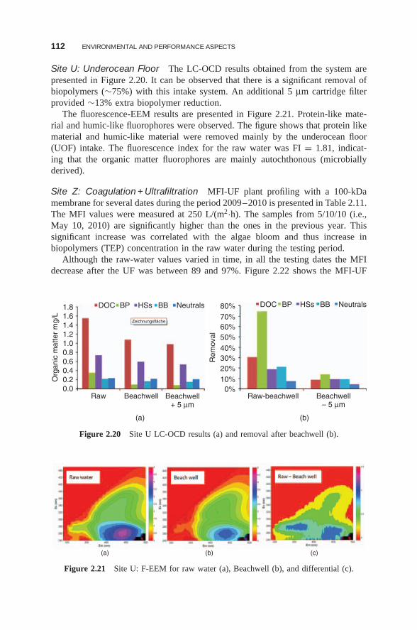
112 ENVIRONMENTAL AND PERFORMANCE ASPECTS

Site U: Underocean Floor The LC-OCD results obtained from the system arepresented in Figure 2.20. It can be observed that there is a significant removal ofbiopolymers (∼75%) with this intake system. An additional 5 μm cartridge filterprovided ∼13% extra biopolymer reduction.

The fluorescence-EEM results are presented in Figure 2.21. Protein-like mate-rial and humic-like fluorophores were observed. The figure shows that protein likematerial and humic-like material were removed mainly by the underocean floor(UOF) intake. The fluorescence index for the raw water was FI = 1.81, indicat-ing that the organic matter fluorophores are mainly autochthonous (microbiallyderived).

Site Z: Coagulation + Ultrafiltration MFI-UF plant profiling with a 100-kDamembrane for several dates during the period 2009–2010 is presented in Table 2.11.The MFI values were measured at 250 L/(m2·h). The samples from 5/10/10 (i.e.,May 10, 2010) are significantly higher than the ones in the previous year. Thissignificant increase was correlated with the algae bloom and thus increase inbiopolymers (TEP) concentration in the raw water during the testing period.

Although the raw-water values varied in time, in all the testing dates the MFIdecrease after the UF was between 89 and 97%. Figure 2.22 shows the MFI-UF

1.8 DOC BP HSs

(a) (b)

BB Neutrals

Zeichnungsfläche1.61.41.21.00.80.60.4

Org

anic

mat

ter

mg/

L

0.20.0

Raw Beachwell Beachwell+ 5 μm

DOC BP HSs BB Neutrals

Rem

oval

0%10%20%30%40%50%60%70%80%

Raw-beachwell Beachwell– 5 μm

Figure 2.20 Site U LC-OCD results (a) and removal after beachwell (b).

(a) (b) (c)

Figure 2.21 Site U: F-EEM for raw water (a), Beachwell (b), and differential (c).

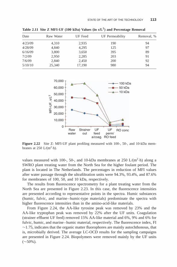
STATE OF THE ART OF THE TECHNOLOGY 113

Table 2.11 Site Z MFI-UF (100 kDa) Values (in s/L2) and Percentage Removal

Date Raw Water UF Feed UF Permeability Removal, %

4/23/09 4,310 2,935 190 944/28/09 4,840 4,295 125 976/16/09 3,800 3,650 395 897/2/09 2,950 2,285 203 917/6/09 2,840 2,450 200 925/10/10 25,340 17,190 980 94

70,000

60,000

50,000

40,000

MF

I-U

F, s

/L2

30,000

20,000

10,000

0Rawwater

Strainerout

UFfeed

a/coag.

UFperm/

RO feed

RO conc

100 kDa50 kDa10 kDa

Figure 2.22 Site Z: MFI-UF plant profiling measured with 100-, 50-, and 10-kDa mem-branes at 250 L/(m2·h).

values measured with 100-, 50-, and 10-kDa membranes at 250 L/(m2·h) along aSWRO plant treating water from the North Sea for the higher foulant period. Theplant is located in The Netherlands. The percentages in reduction of MFI valuesafter water passage through the ultrafiltration units were 94.3%, 93.4%, and 87.6%for membranes of 100, 50, and 10 kDa, respectively.

The results from fluorescence spectrometry for a plant treating water from theNorth Sea are presented in Figure 2.23. In this case, the fluorescence intensitiesare presented according to representative points in the spectra. Humic substances(humic, fulvic, and marine–humic-type materials) predominate the spectra withhigher fluorescence intensities than in the amino-acid-like materials.

From Figure 2.24, the AA-like tyrosine peak was removed by 23% and theAA-like tryptophan peak was removed by 22% after the UF units. Coagulation(strainer effluent UF feed) removed 15% AA-like material and 6%, 9% and 6% forfulvic, humic, and marine–humic material, respectively. The fluorescence index, FI∼1.75, indicates that the organic matter fluorophores are mainly autochthonous, thatis, microbially derived. The average LC-OCD results for the sampling campaignsare presented in Figure 2.24. Biopolymers were removed mainly by the UF units(∼50%).

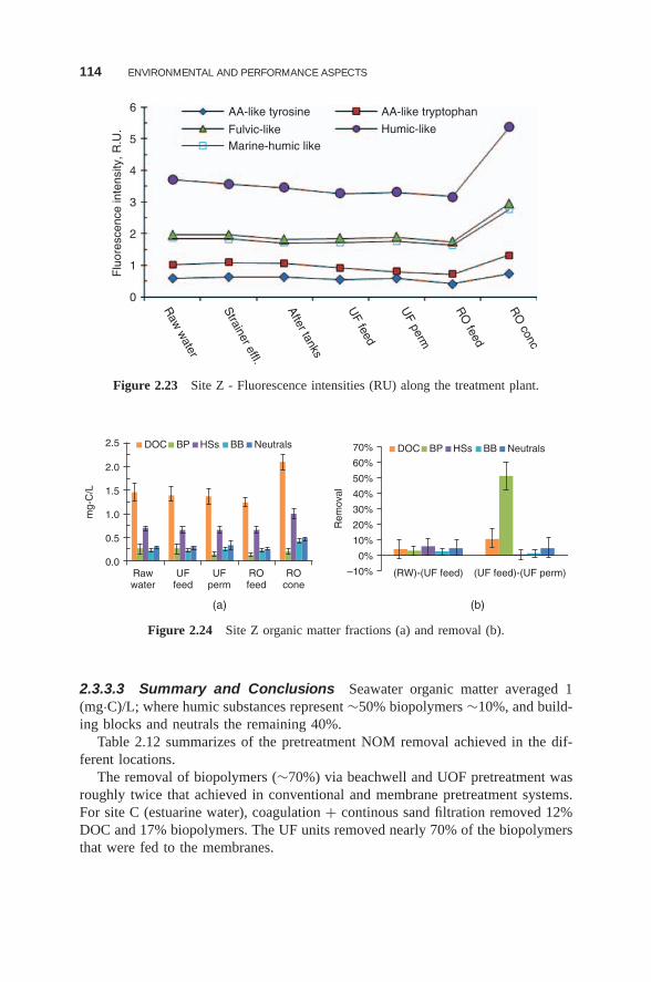
114 ENVIRONMENTAL AND PERFORMANCE ASPECTS

Raw

water

Strainer effl.

After tanks

UF feed

UF perm

RO

feed

RO

concAA-like tyrosine AA-like tryptophan

Humic-likeFulvic-likeMarine-humic like

0

1

2

3

4

Flu

ores

cenc

e in

tens

ity, R

.U.

5

6

Figure 2.23 Site Z - Fluorescence intensities (RU) along the treatment plant.

0.0Rawwater

UFfeed

UFperm

ROfeed

ROcone

mg-

C/L

Rem

oval

0.5

1.0

1.5

2.0

2.5 DOC BP HSs BB Neutrals

(RW)-(UF feed) (UF feed)-(UF perm)–10%

0%

10%

20%

30%

40%

50%

60%

70% DOC BP HSs BB Neutrals

(a) (b)

Figure 2.24 Site Z organic matter fractions (a) and removal (b).

2.3.3.3 Summary and Conclusions Seawater organic matter averaged 1(mg·C)/L; where humic substances represent ∼50% biopolymers ∼10%, and build-ing blocks and neutrals the remaining 40%.

Table 2.12 summarizes of the pretreatment NOM removal achieved in the dif-ferent locations.

The removal of biopolymers (∼70%) via beachwell and UOF pretreatment wasroughly twice that achieved in conventional and membrane pretreatment systems.For site C (estuarine water), coagulation + continous sand filtration removed 12%DOC and 17% biopolymers. The UF units removed nearly 70% of the biopolymersthat were fed to the membranes.

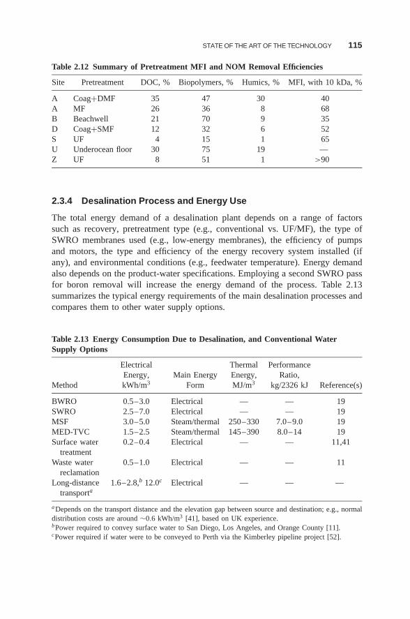
STATE OF THE ART OF THE TECHNOLOGY 115

Table 2.12 Summary of Pretreatment MFI and NOM Removal Efficiencies

Site Pretreatment DOC, % Biopolymers, % Humics, % MFI, with 10 kDa, %

A Coag+DMF 35 47 30 40A MF 26 36 8 68B Beachwell 21 70 9 35D Coag+SMF 12 32 6 52S UF 4 15 1 65U Underocean floor 30 75 19 —Z UF 8 51 1 >90

2.3.4 Desalination Process and Energy Use

The total energy demand of a desalination plant depends on a range of factorssuch as recovery, pretreatment type (e.g., conventional vs. UF/MF), the type ofSWRO membranes used (e.g., low-energy membranes), the efficiency of pumpsand motors, the type and efficiency of the energy recovery system installed (ifany), and environmental conditions (e.g., feedwater temperature). Energy demandalso depends on the product-water specifications. Employing a second SWRO passfor boron removal will increase the energy demand of the process. Table 2.13summarizes the typical energy requirements of the main desalination processes andcompares them to other water supply options.

Table 2.13 Energy Consumption Due to Desalination, and Conventional WaterSupply Options

Electrical Thermal PerformanceEnergy, Main Energy Energy, Ratio,

Method kWh/m3 Form MJ/m3 kg/2326 kJ Reference(s)

BWRO 0.5–3.0 Electrical — — 19SWRO 2.5–7.0 Electrical — — 19MSF 3.0–5.0 Steam/thermal 250–330 7.0–9.0 19MED-TVC 1.5–2.5 Steam/thermal 145–390 8.0–14 19Surface water

treatment0.2–0.4 Electrical — — 11,41

Waste waterreclamation

0.5–1.0 Electrical — — 11

Long-distancetransporta

1.6–2.8,b 12.0c Electrical — — —

a Depends on the transport distance and the elevation gap between source and destination; e.g., normaldistribution costs are around ∼0.6 kWh/m3 [41], based on UK experience.b Power required to convey surface water to San Diego, Los Angeles, and Orange County [11].cPower required if water were to be conveyed to Perth via the Kimberley pipeline project [52].

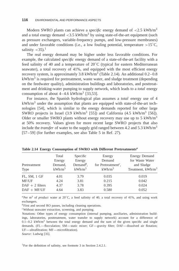
116 ENVIRONMENTAL AND PERFORMANCE ASPECTS

Modern SWRO plants can achieve a specific energy demand of <2.5 kWh/m3

and a total energy demand <3.5 kWh/m3 by using state-of-the-art equipment (suchas pressure exchangers, variable-frequency pumps, and low-pressure membranes)and under favorable conditions (i.e., a low fouling potential, temperature >15◦C,salinity <35).1

The real energy demand may be higher under less favorable conditions. Forexample, the calculated specific energy demand of a state-of-the-art facility with afeed salinity of 40 and a temperature of 20◦C (typical for eastern Mediterraneanseawater), a total recovery of 41%, and equipped with the most efficient energyrecovery system, is approximately 3.8 kWh/m3 (Table 2.14). An additional 0.2–0.8kWh/m3 is required for pretreatment, waste water, and sludge treatment (dependingon the feedwater quality), administration buildings and laboratories, and posttreat-ment and drinking-water pumping to supply network, which leads to a total energyconsumption of about 4–4.6 kWh/m3 [33,53].

For instance, the Spanish hydrological plan assumes a total energy use of 4kWh/m3 under the assumption that plants are equipped with state-of-the-art tech-nologies [54], which is similar to the energy demands reported for other largeSWRO projects in Israel (3.9 kWh/m3 [55]) and California (4.5 kWh/m3 [56]).Older or smaller SWRO plants without energy recovery may use up to 5 kWh/m3

at 50% recovery. Values given for more recent large SWRO projects that alsoinclude the transfer of water to the supply grid ranged between 4.2 and 5.3 kWh/m3

[57–59] (for further examples, see also Table 5 in Ref. 27).

Table 2.14 Energy Consumption of SWRO with Different Pretreatmentsa

Total Specific Energy Energy DemandEnergy Energy Demand for Waste Water

Pretreatment Demand, Demandb, for Pretreatmentc, and SludgeType kWh/m3 kWh/m3 kWh/m3 Treatment, kWh/m3

FL, SM, 1 GF 4.01 3.79 0.035 0.019MF/UF 4.24 3.81 0.215 0.042DAF + 2 filters 4.37 3.78 0.395 0.024DAF + MF/UF 4.64 3.83 0.580 0.052

a Per m3 of product water at 20◦C, a feed salinity of 40, a total recovery of 41%, and using workexchangers.b First and second RO passes, including cleaning operations.cWithout seawater extraction, screening, and pumping.Notations: Other types of energy consumption (internal pumping, auxiliaries, administration build-ings, laboratories, posttreatment, water transfer to supply network) account for a difference of0.1–0.2 kWh/m3 between the total energy demand and the sum of the given specific and singledemands. (FL—flocculation; SM—static mixer; GF—gravity filter; DAF—dissolved air flotation;UF—ultrafiltration; MF—microfiltration).Source: Ludwig [35].

1For the definition of salinity, see footnote 3 in Section 2.4.2.1.

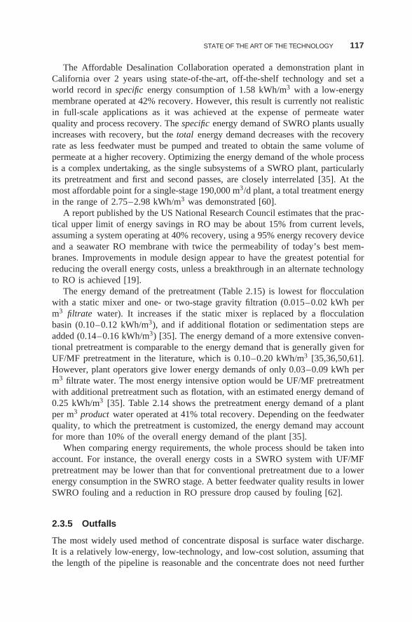
STATE OF THE ART OF THE TECHNOLOGY 117

The Affordable Desalination Collaboration operated a demonstration plant inCalifornia over 2 years using state-of-the-art, off-the-shelf technology and set aworld record in specific energy consumption of 1.58 kWh/m3 with a low-energymembrane operated at 42% recovery. However, this result is currently not realisticin full-scale applications as it was achieved at the expense of permeate waterquality and process recovery. The specific energy demand of SWRO plants usuallyincreases with recovery, but the total energy demand decreases with the recoveryrate as less feedwater must be pumped and treated to obtain the same volume ofpermeate at a higher recovery. Optimizing the energy demand of the whole processis a complex undertaking, as the single subsystems of a SWRO plant, particularlyits pretreatment and first and second passes, are closely interrelated [35]. At themost affordable point for a single-stage 190,000 m3/d plant, a total treatment energyin the range of 2.75–2.98 kWh/m3 was demonstrated [60].

A report published by the US National Research Council estimates that the prac-tical upper limit of energy savings in RO may be about 15% from current levels,assuming a system operating at 40% recovery, using a 95% energy recovery deviceand a seawater RO membrane with twice the permeability of today’s best mem-branes. Improvements in module design appear to have the greatest potential forreducing the overall energy costs, unless a breakthrough in an alternate technologyto RO is achieved [19].

The energy demand of the pretreatment (Table 2.15) is lowest for flocculationwith a static mixer and one- or two-stage gravity filtration (0.015–0.02 kWh perm3 filtrate water). It increases if the static mixer is replaced by a flocculationbasin (0.10–0.12 kWh/m3), and if additional flotation or sedimentation steps areadded (0.14–0.16 kWh/m3) [35]. The energy demand of a more extensive conven-tional pretreatment is comparable to the energy demand that is generally given forUF/MF pretreatment in the literature, which is 0.10–0.20 kWh/m3 [35,36,50,61].However, plant operators give lower energy demands of only 0.03–0.09 kWh perm3 filtrate water. The most energy intensive option would be UF/MF pretreatmentwith additional pretreatment such as flotation, with an estimated energy demand of0.25 kWh/m3 [35]. Table 2.14 shows the pretreatment energy demand of a plantper m3 product water operated at 41% total recovery. Depending on the feedwaterquality, to which the pretreatment is customized, the energy demand may accountfor more than 10% of the overall energy demand of the plant [35].

When comparing energy requirements, the whole process should be taken intoaccount. For instance, the overall energy costs in a SWRO system with UF/MFpretreatment may be lower than that for conventional pretreatment due to a lowerenergy consumption in the SWRO stage. A better feedwater quality results in lowerSWRO fouling and a reduction in RO pressure drop caused by fouling [62].

2.3.5 Outfalls

The most widely used method of concentrate disposal is surface water discharge.It is a relatively low-energy, low-technology, and low-cost solution, assuming thatthe length of the pipeline is reasonable and the concentrate does not need further

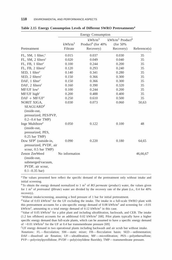
118 ENVIRONMENTAL AND PERFORMANCE ASPECTS

Table 2.15 Energy Consumption Levels of Different SWRO Pretreatmentsa

Energy Consumption

kWh/m3 kWh/m3 Productb

kWh/m3 Productb (for 40% (for 50%Pretreatment Filtrate Recovery) Recovery) Reference(s)

FL, SM, 1 filter,c 0.015 0.037 0.030 35FL, SM, 2 filtersc 0.020 0.049 0.040 35FL, FB, 1 filterc 0.100 0.244 0.200 35FL, FB, 2 filtersc 0.120 0.293 0.240 35SED, 1 filterc 0.140 0.341 0.280 35SED, 2 filtersc 0.150 0.366 0.300 35DAF, 1 filterc 0.150 0.366 0.300 35DAF, 2 filtersc 0.160 0.390 0.320 35MF/UF lowc 0.100 0.244 0.200 35MF/UF highc 0.200 0.488 0.400 35DAF + MF/UFc 0.250 0.610 0.500 35NORIT XIGA,

SEAGUARDd

(inside-out,pressurized, PES/PVP,0.2–0.4 bar TMP)

0.030 0.073 0.060 50,63

Inge Multiboree

(inside-out,pressurized, PES,0.25 bar TMP)

0.050 0.122 0.100 48

Dow SFPf (outside-in,pressurized, PVDF, airscour, 0.5 bar TMP)

0.090 0.220 0.180 64,65

Zenon ZeeWeed(inside-out,submerged/vacuum,PVDF, air scour,0.1–0.35 bar)

No information 46,66,67

a The values presented here reflect the specific demand of the pretreatment only without intake andinitial screening.b To obtain the energy demand normalized to 1 m3 of RO permeate (product) water, the values givenfor 1 m3 of pretreated (filtrate) water are divided by the recovery rate of the plant (i.e., 0.4 for 40%recovery).cWithout intake/screening, assuming a feed pressure of 1 bar for initial pretreatment.d Value of 0.03 kWh/m3 for the UF excluding the intake. The intake in a full-scale SWRO plant withthis pretreatment accounts for a site-specific energy demand of 0.08 kWh/m3 and screening for <0.01kWh/m3, amounting to a total energy demand of 0.12 kWh/m3 in this case.eValue of 0.05 kWh/m3 for a pilot plant and including ultrafiltration, backwash, and CEB. The intake(1.2 km offshore) accounts for an additional 0.02 kWh/m3 [68]. Pilot plants typically have a higherspecific energy demand than full-scale plants, which can be assumed to have a specific energy demandof ∼0.01 kWh/m3 for the UF at 0.4 bar transmembrane pressure [69].f UF energy demand in two operational plants including backwash and air scrub but without intake.Notations: FL—flocculation; SM—static mixer; FB—flocculation basin; SED—sedimentation;DAF—dissolved air flotation; UF—ultrafiltration; MF—microfiltration; PES—polyethersulfone;PVP—polyvinylpyrollidone; PVDF—poly(vinylidene fluoride); TMP—transmembrane pressure.

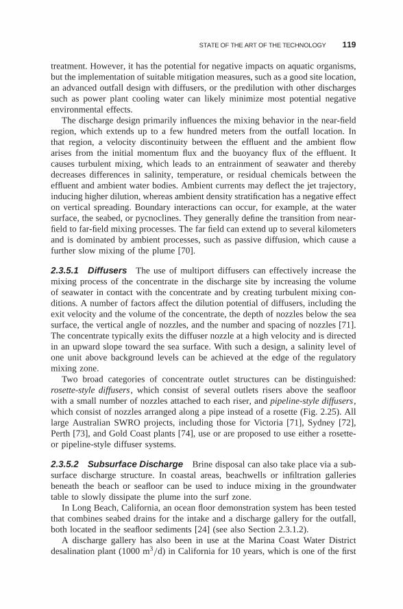
STATE OF THE ART OF THE TECHNOLOGY 119

treatment. However, it has the potential for negative impacts on aquatic organisms,but the implementation of suitable mitigation measures, such as a good site location,an advanced outfall design with diffusers, or the predilution with other dischargessuch as power plant cooling water can likely minimize most potential negativeenvironmental effects.

The discharge design primarily influences the mixing behavior in the near-fieldregion, which extends up to a few hundred meters from the outfall location. Inthat region, a velocity discontinuity between the effluent and the ambient flowarises from the initial momentum flux and the buoyancy flux of the effluent. Itcauses turbulent mixing, which leads to an entrainment of seawater and therebydecreases differences in salinity, temperature, or residual chemicals between theeffluent and ambient water bodies. Ambient currents may deflect the jet trajectory,inducing higher dilution, whereas ambient density stratification has a negative effecton vertical spreading. Boundary interactions can occur, for example, at the watersurface, the seabed, or pycnoclines. They generally define the transition from near-field to far-field mixing processes. The far field can extend up to several kilometersand is dominated by ambient processes, such as passive diffusion, which cause afurther slow mixing of the plume [70].

2.3.5.1 Diffusers The use of multiport diffusers can effectively increase themixing process of the concentrate in the discharge site by increasing the volumeof seawater in contact with the concentrate and by creating turbulent mixing con-ditions. A number of factors affect the dilution potential of diffusers, including theexit velocity and the volume of the concentrate, the depth of nozzles below the seasurface, the vertical angle of nozzles, and the number and spacing of nozzles [71].The concentrate typically exits the diffuser nozzle at a high velocity and is directedin an upward slope toward the sea surface. With such a design, a salinity level ofone unit above background levels can be achieved at the edge of the regulatorymixing zone.

Two broad categories of concentrate outlet structures can be distinguished:rosette-style diffusers , which consist of several outlets risers above the seafloorwith a small number of nozzles attached to each riser, and pipeline-style diffusers ,which consist of nozzles arranged along a pipe instead of a rosette (Fig. 2.25). Alllarge Australian SWRO projects, including those for Victoria [71], Sydney [72],Perth [73], and Gold Coast plants [74], use or are proposed to use either a rosette-or pipeline-style diffuser systems.

2.3.5.2 Subsurface Discharge Brine disposal can also take place via a sub-surface discharge structure. In coastal areas, beachwells or infiltration galleriesbeneath the beach or seafloor can be used to induce mixing in the groundwatertable to slowly dissipate the plume into the surf zone.

In Long Beach, California, an ocean floor demonstration system has been testedthat combines seabed drains for the intake and a discharge gallery for the outfall,both located in the seafloor sediments [24] (see also Section 2.3.1.2).

A discharge gallery has also been in use at the Marina Coast Water Districtdesalination plant (1000 m3/d) in California for 10 years, which is one of the first

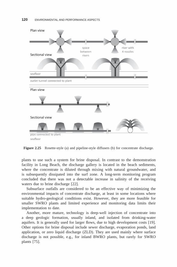
120 ENVIRONMENTAL AND PERFORMANCE ASPECTS

Figure 2.25 Rosette-style (a) and pipeline-style diffusers (b) for concentrate discharge.

plants to use such a system for brine disposal. In contrast to the demonstrationfacility in Long Beach, the discharge gallery is located in the beach sediments,where the concentrate is diluted through mixing with natural groundwater, andis subsequently dissipated into the surf zone. A long-term monitoring programconcluded that there was not a detectable increase in salinity of the receivingwaters due to brine discharge [22].

Subsurface outfalls are considered to be an effective way of minimizing theenvironmental impacts of concentrate discharge, at least in some locations wheresuitable hydro-geological conditions exist. However, they are more feasible forsmaller SWRO plants and limited experience and monitoring data limits theirimplementation to date.

Another, more mature, technology is deep-well injection of concentrate intoa deep geologic formation, usually inland, and isolated from drinking-wateraquifers. It is generally used for larger flows, due to high development costs [19].Other options for brine disposal include sewer discharge, evaporation ponds, landapplication, or zero liquid discharge (ZLD). They are used mainly where surfacedischarge is not possible, e.g., for inland BWRO plants, but rarely for SWROplants [75].

STATE OF THE ART OF THE TECHNOLOGY 121

2.3.5.3 Codischarge with Cooling Water Co-location of MSF/MED dis-tillation plants with power plants is common practice, and some large SWROplants either have been or have been proposed to be co-located with power plants.Examples include the Carlsbad and Huntington Beach SWRO plants in southernCalifornia [56,76], the Tampa Bay SWRO plant in Florida [77], and the Ashkelonand Hadera SWRO plants in Israel [78,79]. The main environmental benefits ofco-locating SWRO plants to power plants are [80]:

• The existing intake and outfall structures are utilized, reducing constructionimpacts.

• The impacts of land use and landscaping are reduced, as the facility is con-structed in an industrial area, and does not require additional power transmis-sion lines.

• If the intake water is taken from the cooling water discharge conduits ofthe power plant, the required energy demand of the SWRO process can bereduced by 5–8% because of a higher membrane permeability at higher watertemperature (mostly relevant for ambient seawater temperatures <20◦C).2

• If cooling water is reused as feedwater to the desalination process, the totalamount of feedwater intake is reduced, limiting the impingement and entrain-ment effects to the level found at the existing power plant.

• The concentrate can be blended with the cooling water before discharge, whichsignificantly reduces the salinity of the concentrate before disposal.

2.3.5.4 Codischarge with Waste Water Another option for codischargeexists with waste water treatment plant effluents, as proposed for two small SWROplants in California (Santa Barbara and Santa Cruz [22,81]) and Europe’s largestSWRO plant in Barcelona [28]. The main advantage is that the salinity of the con-centrate is very effectively diluted. A dilution ratio of 1:1 is sufficient to reduce thesalinity of the concentrate to ambient seawater salinity levels, as the SWRO con-centrate usually has twice the ambient salinity. However, there are several issuesassociated with the practice of blending SWRO concentrate with waste water treat-ment plant effluents, and the discharge through an existing waste water treatmentplant outfall has found a limited application to date.

One consideration is the potential for whole effluent toxicity of the blendeddischarge that may result from an ion imbalance of the blend of the two wastestreams [75]. As waste water effluent has a freshwater origin with a different ratioof key ions than does seawater, the ion imbalance may be responsible for theobserved toxic effects [82]. Furthermore, residual contaminants in the waste watermay have negative effects on marine life. However, both effects are attributed to thewaste water and not to the concentrate from the desalination process. Consequently,they may occur wherever waste water treatment plant effluents are discharged intothe sea.

2As higher feed temperature results in a higher degree of salt passage, it may also result in higherenergy consumption if a second RO stage has to be implemented [18].

122 ENVIRONMENTAL AND PERFORMANCE ASPECTS

Another consideration is that waste water may be considered as a resource,which should not be wasted to the ocean in water-scarce areas, as recycling isusually preferable to disposal in the concept of waste management. It must also bedetermined whether a new desalination project is necessary or could be reducedin size if the existing waste water sources were reused to full potential instead ofbeing discharged into the ocean. Another argument for waste water reuse usingdesalination technologies is the elimination of a waste product. Effluents from con-ventional waste water treatment plants still contain diverse contaminants, includingnutrients, metals, or micropollutants such as pharmaceutical and personal-care prod-ucts, which are burdensome for many rivers, estuaries, and coastal seas. Purifyingand reusing waste water not only produces a new water supply but also eliminateswaste water discharge if the remaining waste stream from the process is treatedusing ZLD technologies and disposed of appropriately.

Water reuse is practiced in many parts of the world, but the use of desalinationtechnologies in water reuse has been limited so far (see Section 2.2). The world’slargest facility treating waste water with an output capacity of 310,000 m3/d islocated in Sulaybia, Kuwait. It uses UF followed by RO to treat secondary effluentwaste water. The energy demand for waste water desalination is lower than thatfor SWRO because of the considerably lower salt content of the water, which isanother environmental benefit. An expansion of waste water desalination is there-fore expected in the future. A second advantage is that most of the water is alreadyavailable where it is most needed, i.e., near urban areas, avoiding long transportdistances. The purified water can be used for industrial purposes, landscaping activ-ities in urban areas, or aquifer recharge. From a technical logistic perspective, theproduct can even comply with WHO drinking-water standards [82,83], but directpotable reuse, such as that as practiced in Windhoek, Namibia, has found a verylimited application to date.

2.4 POTENTIAL ENVIRONMENTAL IMPACTS

The main environmental concerns of new desalination projects usually revolvearound a few key issues (Fig. 2.26). This section briefly describes three key con-cerns (for a detailed analysis, see Ref. 27): impingement/entrainment caused byintakes, marine pollution caused by concentrate and chemical discharges, and emis-sions of greenhouse gases and air pollutants due to energy use.

2.4.1 Impingement and Entrainment

Open seawater intakes usually result in the loss of eggs and larvae of fish and inver-tebrate species, spores from algae and seagrasses, phytoplankton and zooplankton,as well as smaller marine organisms that are drawn into the plant with the seawater(entrainment). As a result of the pretreatment in SWRO plants, which involveschlorination at the intakes to control marine growth and the removal of suspendedsolids, it must be assumed that the survival rate of plankton and smaller organismsinside the plant is minimal.

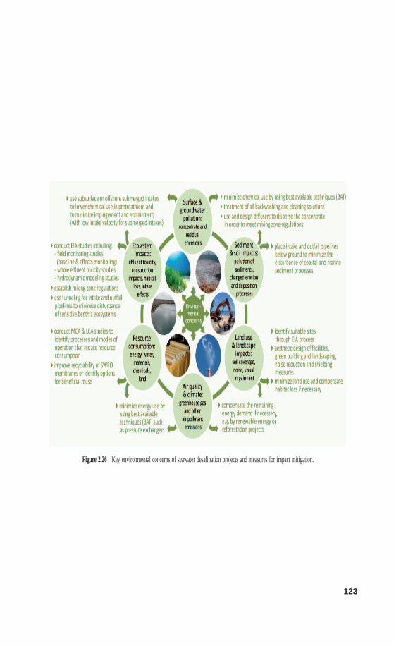
123

Figure 2.26 Key environmental concerns of seawater desalination projects and measures for impact mitigation.

124 ENVIRONMENTAL AND PERFORMANCE ASPECTS

Entrainment causes the loss of a large number of plankton organisms. The issue,however, is whether this represents a significant, additional source of mortality forthe affected species, which negatively affects the ability of the species to sustaintheir populations, and that may affect the productivity of coastal ecosystems. Thesesecondary ecosystem effects are difficult to quantify [22]. Plankton organisms aregenerally prevalent in coastal surface waters and have rapid reproductive cycles.Fish and invertebrate species produce large numbers of eggs and larvae to com-pensate for a high natural mortality rate as part of their reproduction strategy. Themortality caused by entrainment in a single facility therefore seems unlikely to havea substantial negative effect on population and ecosystem dynamics. The situationis different when endangered species, species of commercial interest, or marine pro-tected areas are potentially affected by the intakes, and when cumulative sourcesof mortality (i.e., harmful conditions resulting from the proximity of other poweror desalination plants) exist. While it is relatively straightforward to estimate thelevels of entrainment for a single desalination project, it is difficult to evaluate theindirect impacts on the ecosystem, especially in places where cumulative sourcesof mortality are involved.

Furthermore, open intakes may result in the loss of larger marine organisms atthe intake screens (impingement), if the intakes are not well designed. Impingementmortality can be caused by suffocation, starvation, or exhaustion of these organismswhen they are pinned up against the intake screens or from the physical force ofjets of water used to clear screens of debris (see Ref. 22, after Ref. 84). Similarto entrainment effects, the cumulative ecosystem effects are difficult to estimate. Ifthe intake velocity of the feedwater were reduced to velocities of ∼0.1 m/s, whichis comparable to background currents in the oceans, mobile organisms would beable to swim away from the intake area.

The California Coastal Commission concluded in 2004 that “the most significantpotential direct adverse environmental impact of seawater desalination is likely tobe on marine organisms: This impact is due primarily to the effects of the seawaterintake and discharge on nearby marine life; however, these effects can be avoidedor minimized through proper facility design, siting, and operation.”

The US Clean Water Act, Section 316(b), requires that “the location, design, con-struction and capacity of cooling water intake structures reflect the best technologyavailable for minimizing adverse environmental impact.” The same standards mayapply for seawater desalination plants in the future, although their intake volumesare smaller.

2.4.2 Concentrate and Chemical Discharges

Specific to all desalination processes is the discharge of a concentrate. This rejectstream contains mainly the natural constituents of the intake seawater in a concen-trated form. In addition, it may contain residual chemicals from pretreatment andcleaning operations and their reaction and degradation products. When evaluating

POTENTIAL ENVIRONMENTAL IMPACTS 125

the potential impacts of the concentrate and chemical discharges, one has to distin-guish between the salt, which is a natural component, and the chemical additives.The discharge of potential pollutants depends mainly on the desalination processand the design of the facility with regard to pretreatment and existing backwashwater treatment facilities.

2.4.2.1 Potential Impacts of Increased Salinity The salinity of the con-centrate usually depends on the plant recovery rate. SWRO plants typically havea recovery rate of 40–45%, with an upper operational limit of 50% to control therisk of scaling. The concentrate may therefore have up to twice the salinity as theambient seawater, and its discharge back into the sea causes elevated salinity levelsin the mixing zone. The salinity increase can be mitigated by predilution with otherwaste streams such as cooling water from coastal power plants, or dissipation bya multiport diffuser, in combination with strong wave action and currents in thedischarge site to effectively dissipate the salinity load (see Section 2.3.5).

Because of its high salt content, the RO concentrate has a higher density thanambient seawater. For example, a SWRO plant with a feedwater salinity3 of 35 andoperating at 50% recovery would produce a concentrate with a salinity of 70. At20◦C, the density4 of the concentrate is 1051 kg/m3, which is heavier (negativelybuoyant) compared to an ambient density of 1025 kg/m3. The plume would sink tothe seafloor (unless adequately dissipated), forming a water mass of elevated salinitythat spreads over the seafloor in the vicinity of the outfall pipe and that will possiblyalso diffuse into the sediment pore water. It is important to prevent such bottom-clinging plumes as they could potentially harm any sensitive benthic ecosystems.

It has been shown through several toxicity studies that locally elevated salin-ity levels caused by desalination plant discharges can be potentially harmful tomarine organisms. In general, toxicity will depend on the sensitivity of a speciesto increased salt levels, its lifecycle stage, the exposure time, and the natural salin-ity variations of the habitat to which the species is adapted. For instance, salinitytolerance studies of the seagrass Posidonia oceanica in the western Mediterraneanshowed that a salinity of 43 may reduce growth rates by 50% and that a salinity of45 may result in 50% mortality within 15 days [86]. These values compare to ambi-ent salinity levels of 37–38 in the western Mediterranean. In contrast, two relatedseagrass species from western Australia, P. australis and P. amphibolis , seem tobe adapted to naturally higher salinity levels, as densest covers are observed ata salinity of 40–50 (see Ref. 73, after Ref. 87). This indicates that even specieswithin the same genera can have very different salinity tolerances, depending ontheir natural habitat salinity.

3The UNESCO definition of practical salinity units (psu) is used, which is the conductivity ratio ofa seawater sample to a standard KCl solution and hence a dimensionless value. As salinity reflectsthe amount of total dissolved solids (TDS) in ocean water, it was traditionally expressed as parts perthousand (ppt). A salinity of 35 ppt equals 35 g of salt per 1000 g of seawater, or 35,000 ppm (mg/L),or in approximation 35 (psu).4Density is a function of salinity and temperature (and pressure in greater water depths) and is typicallycalculated by software tools that implement the equation of state for seawater [e.g., 85].

126 ENVIRONMENTAL AND PERFORMANCE ASPECTS

Some macrofauna taxa such as echinoderms (e.g., sea urchins, starfish) areassumed to be generally more sensitive to salinity variations than other species,and young lifecycle stages of organisms, such as sea urchin embryos, are generallyconsidered to be more sensitive than adults. Most marine organisms can adapt tominor deviations in salinity and might recover from extreme, short-term exposureto increased salinities. For example, P. oceanica seagrass that survived in a salin-ity of 43 over 15 days were able to recover when returned to normal conditions[86]. However, only a few species will be tolerant of high salt concentrations overprolonged periods of time, as caused by the continuous discharge of desalinationconcentrates.

Salt concentrations that continuously and significantly exceed the ambient levelsto which the native species are adapted may result in osmotic stress. This willdrive mobile animals away from the discharge site and can cause a die-off ofthe sessile fauna and flora. For example, salinity increases near the outfall of theDhekelia SWRO plant in Cyprus were reported to be responsible for a decline ofmacroalgae forests, and echinoderm species were observed to have vanished fromthe discharge site [88]. Observations on the distribution of marine species fromnaturally hypersaline environments in the Arabian Gulf indicate that a salinity above45 altered the benthic community considerably [89], which stresses the importanceof salinity as a controlling factor. The Gulf is impoverished at the species level,mostly because of its harsh environmental conditions, and low species richness wasfound for most major benthic groups such as echinoderms and corals [14].

The concentration of salts, rather than the salt itself, and the exposure time priorto the discharge is the problem. Discharge into the sea is therefore an adequatemeans of concentrate disposal if dilution to ambient levels is achieved within avery short distance from the outfall and if sensitive ecosystems are not impactedby the dispersing plume.

An adequate approach to minimize the impacts of the concentrate is to establisha restricted mixing zone around the outfall in which dilution to a level close toambient is achieved by a combination of artificial intervention (installation of mul-tiport diffusers) and natural processes (strong currents). Mixing zone regulationscombine parameters that define the spatial extent of the allowable mixing zone witha water quality standard for salinity and other pollutants that apply at the edge ofthis mixing zone. The following standards for salinity have been established fordifferent SWRO projects in different parts of the world.

• The license for the Perth SWRO plant limits salinity to within 1.2 units ofambient levels within 50 m and within 0.8 units within 1000 m from thedischarge point. This requires a dilution factor of 45–1 at a distance of 50 min all directions of the diffuser. After 2 years of operation, the actually achieveddilution factors ranged from 50–1 to 120–1. Whole effluent toxicity (WET)tests were performed with five native species at commissioning and after 12months of operation, showing that the required dilution factor to achieve a99% species protection level is about 15–1, i.e., that 99% of the species inthe marine ecosystem will be protected at this dilution level [90].

POTENTIAL ENVIRONMENTAL IMPACTS 127

• For the Sydney SWRO project, WET tests were performed using effluentsfrom a pilot plant and five indicator species. A dilution factor of 30–1 atthe edge of the near field was calculated in order to achieve salinity levelswithin natural variation levels of 1 unit above ambient, and to achieve thedesired species protection level of 95%. The studies showed that salinity wasthe key source of toxicity of the whole effluent [91]. Baseline studies havebeen conducted for a comprehensive field monitoring program to verify theresults after startup [92].

• For the Gold Coast desalination plant, field measurements during startup con-firmed an effective dilution factor of 60–1 at the edge of the near-field mixingzone in 60 m distance from the diffuser with no discernible difference toambient salinity at that point. A minimum dilution ratio of 47–1 had beenpredicted by the hydrodynamic models. WET tests using effluent from thefull-scale plant were performed on six marine species from more than threetrophic levels representative of the local ecosystem. The results imply that aminimum dilution factor of 9–1, corresponding to a salinity of 37.6 or anincrease of 2.3 units above ambient, should be achieved at the edge of themixing zone to obtain a 95% species protection level [93].

• The most extensive WET testing was carried out for the Olympic Dam SWROproject. On the basis of WET tests with 15 species from four trophic lev-els, it was calculated that a dilution of 45–1 should protect 99% of themarine species in the area, corresponding to a salinity increase of 0.7 unitsabove ambient. The hydrodynamic modeling studies predicted that this dilu-tion would be achieved within 300 m from the outfall in 90% of all times. In100 m distance from the outfall, the minimum dilution would be 8–1, corre-sponding to a maximum salinity increase of 3.7 units or 9% above ambient.The maximum extent of the 45–1 dilution contour would be ≤1.1 km for 99%of the time. A dilution of 85–1 or a salinity increase of 0.4 unit above ambi-ent, which ensures 100% species protection at all times, would be achievedwithin 3.9 km of the outfall [94].

• On the basis of extensive field and laboratory studies of the seagrass Posidoniaoceanica in Spain, it has been recommended that discharges of desalinationconcentrate nearby Posidonia meadows be avoided or that the discharge salin-ity be diluted to ensure that it neither exceeds a value of 38.5 in any point ofthe meadow for >25% of the observations (on an annual basis) or a value of40 in ≤5% of the observations. These values compare to ambient salinities inthe western Mediterranean of 37–38 [95].

• For the proposed Carlsbad SWRO project in California, long-term salinitytolerance and toxicity tests were carried out. In this study, 18 marine specieswere held in a tank containing a blend of concentrate and power plant coolingwater at a salinity of 36 (expected to occur in the mixing zone in 95% ofthe time, compared to an ambient salinity of 33.5). All organisms remainedhealthy and showed normal activity and feeding behavior during the 5-monthtest. Three indicator species were also exposed to salinities of 37–40 over anextended period of time with 100% survival and normal behavior at the end

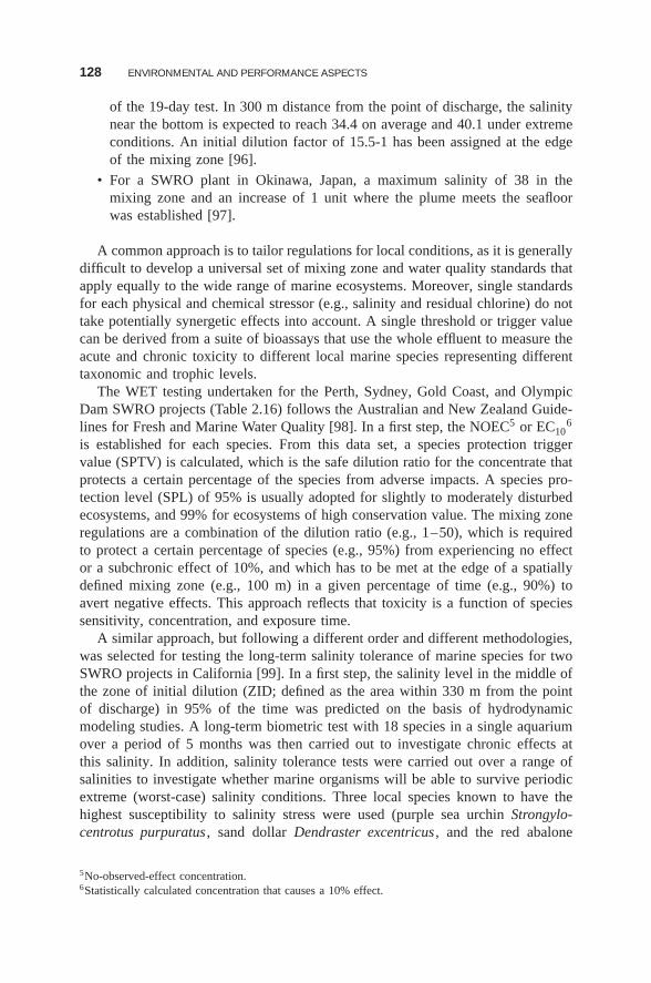
128 ENVIRONMENTAL AND PERFORMANCE ASPECTS

of the 19-day test. In 300 m distance from the point of discharge, the salinitynear the bottom is expected to reach 34.4 on average and 40.1 under extremeconditions. An initial dilution factor of 15.5-1 has been assigned at the edgeof the mixing zone [96].

• For a SWRO plant in Okinawa, Japan, a maximum salinity of 38 in themixing zone and an increase of 1 unit where the plume meets the seafloorwas established [97].

A common approach is to tailor regulations for local conditions, as it is generallydifficult to develop a universal set of mixing zone and water quality standards thatapply equally to the wide range of marine ecosystems. Moreover, single standardsfor each physical and chemical stressor (e.g., salinity and residual chlorine) do nottake potentially synergetic effects into account. A single threshold or trigger valuecan be derived from a suite of bioassays that use the whole effluent to measure theacute and chronic toxicity to different local marine species representing differenttaxonomic and trophic levels.

The WET testing undertaken for the Perth, Sydney, Gold Coast, and OlympicDam SWRO projects (Table 2.16) follows the Australian and New Zealand Guide-lines for Fresh and Marine Water Quality [98]. In a first step, the NOEC5 or EC10

6

is established for each species. From this data set, a species protection triggervalue (SPTV) is calculated, which is the safe dilution ratio for the concentrate thatprotects a certain percentage of the species from adverse impacts. A species pro-tection level (SPL) of 95% is usually adopted for slightly to moderately disturbedecosystems, and 99% for ecosystems of high conservation value. The mixing zoneregulations are a combination of the dilution ratio (e.g., 1–50), which is requiredto protect a certain percentage of species (e.g., 95%) from experiencing no effector a subchronic effect of 10%, and which has to be met at the edge of a spatiallydefined mixing zone (e.g., 100 m) in a given percentage of time (e.g., 90%) toavert negative effects. This approach reflects that toxicity is a function of speciessensitivity, concentration, and exposure time.

A similar approach, but following a different order and different methodologies,was selected for testing the long-term salinity tolerance of marine species for twoSWRO projects in California [99]. In a first step, the salinity level in the middle ofthe zone of initial dilution (ZID; defined as the area within 330 m from the pointof discharge) in 95% of the time was predicted on the basis of hydrodynamicmodeling studies. A long-term biometric test with 18 species in a single aquariumover a period of 5 months was then carried out to investigate chronic effects atthis salinity. In addition, salinity tolerance tests were carried out over a range ofsalinities to investigate whether marine organisms will be able to survive periodicextreme (worst-case) salinity conditions. Three local species known to have thehighest susceptibility to salinity stress were used (purple sea urchin Strongylo-centrotus purpuratus , sand dollar Dendraster excentricus , and the red abalone

5No-observed-effect concentration.6Statistically calculated concentration that causes a 10% effect.

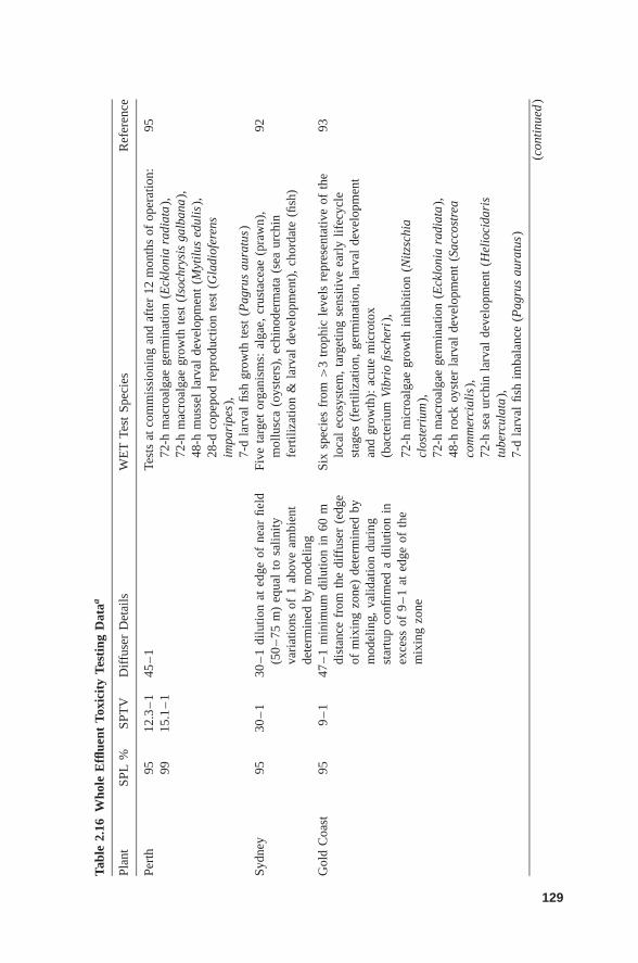
Tabl

e2.

16W

hole

Effl

uent

Toxi

city

Test

ing

Dat

aa

Plan

tSP

L%

SPT

VD

iffu

ser

Det

ails

WE

TTe

stSp

ecie

sR

efer

ence

Pert

h95

12.3

–1

45–

1Te

sts

atco

mm

issi

onin

gan

daf

ter

12m

onth

sof

oper

atio

n:95

9915

.1–

172

-hm

acro

alga

ege

rmin

atio

n(E

cklo

nia

radi

ata

),72

-hm

acro

alga

egr

owth

test

(Iso

chry

sis

galb

ana

),48

-hm

usse

lla

rval

deve

lopm

ent

(Myt

ilus

edul

is),

28-d

cope

pod

repr

oduc

tion

test

(Gla

diof

eren

sim

pari

pes)

,7-

dla

rval

fish

grow

thte

st(P

agru

sau

ratu

s)Sy

dney

9530

–1

30–

1di

lutio

nat

edge

ofne

arfie

ld(5

0–

75m

)eq

ual

tosa

linity

vari

atio

nsof

1ab

ove

ambi

ent

dete

rmin

edby

mod

elin

g

Five

targ

etor

gani

sms:

alga

e,cr

usta

ceae

(pra

wn)

,m

ollu

sca

(oys

ters

),ec

hino

derm

ata

(sea

urch

infe

rtili

zatio

n&

larv

alde

velo

pmen

t),

chor

date

(fish

)

92

Gol

dC

oast

959

–1

47–

1m

inim

umdi

lutio

nin

60m

dist

ance

from

the

diff

user

(edg

eof

mix

ing

zone

)de

term

ined

bym

odel

ing,

valid

atio

ndu

ring

star

tup

confi

rmed

adi

lutio

nin

exce

ssof

9–

1at

edge

ofth

em

ixin

gzo

ne

Six

spec

ies

from

>3

trop

hic

leve

lsre

pres

enta

tive

ofth

elo

cal

ecos

yste

m,

targ

etin

gse

nsiti

veea

rly

lifec

ycle

stag

es(f

ertil

izat

ion,

germ

inat

ion,

larv

alde

velo

pmen

tan

dgr

owth

):ac

ute

mic

roto

x(b

acte

rium

Vibr

iofis

cher

i),

93

72-h

mic

roal

gae

grow

thin

hibi

tion

(Nit

zsch

iacl

oste

rium

),72

-hm

acro

alga

ege

rmin

atio

n(E

cklo

nia

radi

ata

),48

-hro

ckoy

ster

larv

alde

velo

pmen

t(S

acco

stre

aco

mm

erci

alis

),72

-hse

aur

chin

larv

alde

velo

pmen

t(H

elio

cida

ris

tube

rcul

ata

),7-

dla

rval

fish

imba

lanc

e(P

agru

sau

ratu

s)

(con

tinu

ed)

129

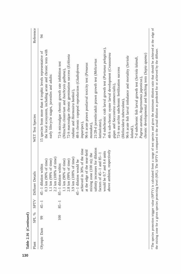
Tabl

e2.

16(C

ontin

ued

)

Plan

tSP

L%

SPT

VD

iffu

ser

Det

ails

WE

TTe

stSp

ecie

sR

efer

ence

Oly

mpi

cD

am99

45–

145

–1

dilu

tion

with

in0.

3km

(90%

oftim

e)1.

1km

(99%

oftim

e)2.

2km

(100

%of

time)

15sp

ecie

sfr

omm

ore

than

4tr

ophi

cle

vels

repr

esen

tativ

eof

the

loca

lec

osys

tem

,in

clud

ing

acut

ean

dch

roni

cte

sts

with

earl

ylif

ecyc

lest

ages

,ju

veni

les

and

adul

ts:

94

100

85–

185

–1

dilu

tion

with

in:

1.1

km(9

0%of

time)

2.8

km(9

9%of

time)

3.9

km(1

00%

oftim

e)45

–1

dilu

tion

wou

ldbe

achi

eved

in30

%of

the

time

atth

eed

geof

the

near

-fiel

dm

ixin

gzo

ne(1

00m

);th

esa

linity

incr

ease

sfo

rdi

lutio

nfa

ctor

sof

45–

1an

d85

–1

wou

ldbe

0.7

and

0.4

units

abov

eam

bien

t,re

spec

tivel

y

72-h

mic

roal

gae

chro

nic

grow

thra

tein

hibi

tion

test

(Nit

zsch

iacl

oste

rium

and

Isoc

hrys

isga

lban

a),

72-h

mac

roal

gae

chro

nic

germ

inat

ion

succ

ess

(Eck

loni

ara

diat

aan

dH

orm

osir

aba

nksi

i),

48-h

chro

nic

cope

pod

repr

oduc

tion

(Gla

diof

eren

sim

pari

pes)

,96

-hac

ute

praw

npo

stla

rval

toxi

city

test

(Pen

aeus

mon

odon

),21

/28-

dju

veni

le/a

dult

praw

ngr

owth

test

(Mel

icer

tus

lati

sulc

atus

),7-

dsu

bchr

onic

crab

larv

algr

owth

test

(Por

tunu

spe

lagi

cus)

,48

-hsu

b-ch

roni

coy

ster

larv

alde

velo

pmen

t(C

rass

ostr

eagi

gas

and

Sacc

ostr

eaco

mm

erci

alis

),72

-hse

aur

chin

subc

hron

icfe

rtili

zatio

nsu

cces

s(H

elio

cida

ris

tube

rcul

ata

),96

-hac

ute

fish

larv

alim

bala

nce

and

mor

talit

y(S

erio

lala

land

i),

7-d

subc

hron

icfis

hla

rval

grow

thte

st(S

erio

lala

land

i,P

agru

sau

ratu

s,A

rgyr

osom

usja

poni

cus)

,ch

roni

cde

velo

pmen

tal

and

hatc

hing

test

s(S

epia

apam

a)

aT

hesp

ecie

spr

otec

tion

trig

ger

valu

e(S

PTV

)is

calc

ulat

edfr

oma

rang

eof

test

spec

ies

and

give

sth

em

inim

umdi

lutio

nra

tioth

atsh

ould

beac

hiev

edat

the

edge

ofth

em

ixin

gzo

nefo

ra

give

nsp

ecie

spr

otec

ting

leve

l(S

PL).

The

SPT

Vis

com

pare

dto

the

actu

aldi

lutio

nas

pred

icte

dfo

ror

achi

eved

byth

edi

ffus

er.

130

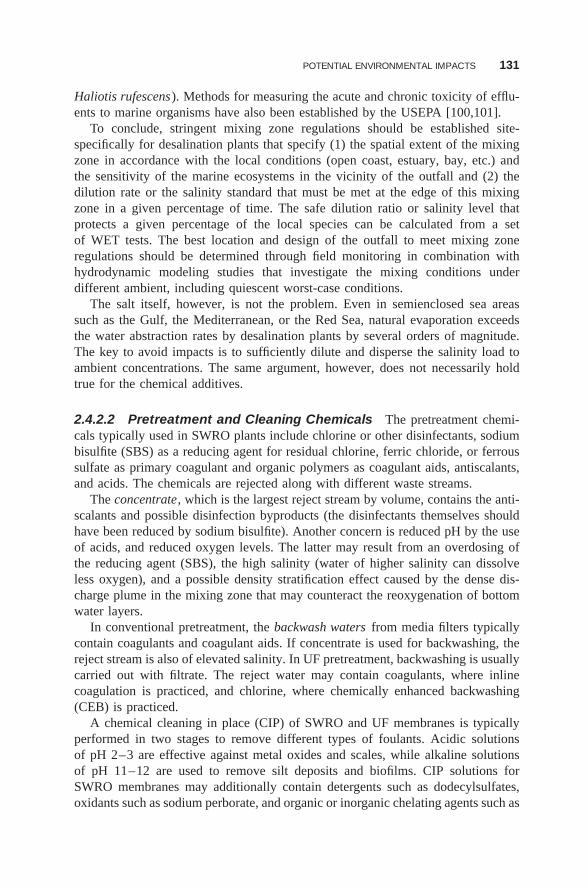
POTENTIAL ENVIRONMENTAL IMPACTS 131

Haliotis rufescens). Methods for measuring the acute and chronic toxicity of efflu-ents to marine organisms have also been established by the USEPA [100,101].

To conclude, stringent mixing zone regulations should be established site-specifically for desalination plants that specify (1) the spatial extent of the mixingzone in accordance with the local conditions (open coast, estuary, bay, etc.) andthe sensitivity of the marine ecosystems in the vicinity of the outfall and (2) thedilution rate or the salinity standard that must be met at the edge of this mixingzone in a given percentage of time. The safe dilution ratio or salinity level thatprotects a given percentage of the local species can be calculated from a setof WET tests. The best location and design of the outfall to meet mixing zoneregulations should be determined through field monitoring in combination withhydrodynamic modeling studies that investigate the mixing conditions underdifferent ambient, including quiescent worst-case conditions.

The salt itself, however, is not the problem. Even in semienclosed sea areassuch as the Gulf, the Mediterranean, or the Red Sea, natural evaporation exceedsthe water abstraction rates by desalination plants by several orders of magnitude.The key to avoid impacts is to sufficiently dilute and disperse the salinity load toambient concentrations. The same argument, however, does not necessarily holdtrue for the chemical additives.

2.4.2.2 Pretreatment and Cleaning Chemicals The pretreatment chemi-cals typically used in SWRO plants include chlorine or other disinfectants, sodiumbisulfite (SBS) as a reducing agent for residual chlorine, ferric chloride, or ferroussulfate as primary coagulant and organic polymers as coagulant aids, antiscalants,and acids. The chemicals are rejected along with different waste streams.

The concentrate, which is the largest reject stream by volume, contains the anti-scalants and possible disinfection byproducts (the disinfectants themselves shouldhave been reduced by sodium bisulfite). Another concern is reduced pH by the useof acids, and reduced oxygen levels. The latter may result from an overdosing ofthe reducing agent (SBS), the high salinity (water of higher salinity can dissolveless oxygen), and a possible density stratification effect caused by the dense dis-charge plume in the mixing zone that may counteract the reoxygenation of bottomwater layers.

In conventional pretreatment, the backwash waters from media filters typicallycontain coagulants and coagulant aids. If concentrate is used for backwashing, thereject stream is also of elevated salinity. In UF pretreatment, backwashing is usuallycarried out with filtrate. The reject water may contain coagulants, where inlinecoagulation is practiced, and chlorine, where chemically enhanced backwashing(CEB) is practiced.

A chemical cleaning in place (CIP) of SWRO and UF membranes is typicallyperformed in two stages to remove different types of foulants. Acidic solutionsof pH 2–3 are effective against metal oxides and scales, while alkaline solutionsof pH 11–12 are used to remove silt deposits and biofilms. CIP solutions forSWRO membranes may additionally contain detergents such as dodecylsulfates,oxidants such as sodium perborate, and organic or inorganic chelating agents such as

132 ENVIRONMENTAL AND PERFORMANCE ASPECTS

EDTA and tripolyphosphates. After cleaning, or prior to storage, SWRO membranesare typically disinfected. CIP of UF membranes often involves acidic or causticsolutions containing chlorine only.

Contrary to the concentrate, impact mitigation for pretreatment and cleaningchemicals should emphasize avoidance and minimization of chemical use throughthe implementation of best available techniques (BAT) rather than discharge anddilution of wastes into the sea. The concept of BAT typically involves a hierarchyof actions, which favors avoidance of wastes over treatment and disposal.

For SWRO projects, the identification of a site- and project-specific BAT solutionshould have the objective to lower the overall chemical use by:

• Reducing the occurrence of fouling through selection of an adequate intakedesign, thus minimizing cleaning and pretreatment requirements.

• Substitution of harmful substances with less harmful substances.

• Optimizing the application and dosage of pretreatment chemicals, where nec-essary, on the basis of pilot testing and/or monitoring of the feedwater quality.

• Treatment of waste streams before discharge into the sea, or disposal into thesewer.

The last point explicitly applies to all reject streams produced by intermittent fil-ter backwashing and membrane cleaning operations. Untreated discharge of thesewastes into the sea cannot be considered BAT, as collection and treatment are tech-nically feasible and have been practiced on an industrial scale in several small andlarge SWRO projects. In essence, a BAT solution should give preference to no orlow chemical use, respectively, no or low waste discharge designs.

If it were possible to choose freely between the different process options, leavingout technical, economical, and other site-specific environmental limitations andtaking only environmental benefits into account, the most preferred design wouldbe a SWRO plant with a subsurface intake and enhanced multiport diffuser designin a suitable oceanic site. A subsurface intake completely avoids impingement andentrainment of marine organisms and, as a biofiltration process, potentially canprovide a consistently high feedwater quality with advantages for pretreatment,cleaning, and membrane life, hence reducing chemical consumption in variousways:

• As beachwells are biofilters that can reduce both organic and biofouling,further pretreatment after a beachwell is often minimal (the conventionalsteps of chlorination–dechlorination and coagulation–flocculation are seldomrequired). Moreover, energy use, land use, and landscape impacts are typicallylower than for SWRO plants with an open intake followed by a conventionalor UF pretreatment.

• As cleaning intervals often increase because of the lower fouling potential,chemical use for cleaning is reduced and less cleaning wastes are generated,which would otherwise require treatment onsite or in a municipal waste watertreatment plant.

POTENTIAL ENVIRONMENTAL IMPACTS 133

• Lower fouling potential and less frequent cleaning increases the membranelifetime, thus reducing material and energy use in the manufacturing process.

The only pretreatment for a subsurface intake is often scale control. However,SWRO plants have been reported to work well without antiscalant additives and theneed for antiscalants has to be questioned, because of more recent laboratory resultsindicating that scaling may rarely occur in SWRO systems [38]. More evidenceis needed from laboratory studies, pilot testing, and operational plants. Until then,the two precautionary approaches to reducing the risk of scaling would be to(1) lower the recovery and thereby achieve completely chemical-free operationwith a subsurface intake or (2) use antiscalants, preferably acid, to control calciumcarbonate scaling in SWRO.

A low recovery rate increases the feedwater requirements of the plant, but sincethe water is taken from a subsurface intake, neither impingement, entrainment, norincreased use of other pretreatment chemicals is a concern. However, the specificenergy demand of the desalination process and the energy needed for pumpingincreases with decreasing recovery. In essence, a tradeoff between chemical use onthe one hand and a chemical-free but more energetically intensive process on theother hand must be made. If a need for antiscalants has been established throughpilot testing, readily biodegradable, phosphor-free polymers or acid should gener-ally be preferred. Acid has the advantage that surplus acidity is quickly neutralizedby mixing with surrounding seawater, whereas antiscalants require some time untildegradation is complete. If the recovery is reduced, the increase in energy demandcan be compensated by climate change mitigation measures. Another benefit of alower recovery is that the salinity of the concentrate is lower, and hence dilutionto ambient levels can be more easily achieved.

The main concerns of subsurface intakes are the construction-related impacts,such as disturbance of soils and sediments, dispersing sediment plumes that increaseturbidity and may affect water quality, habitat destruction, or the disturbance ofsensitive wildlife, and possible adverse effects on groundwater processes and flows.As a BAT approach, trenchless techniques and best environmental practice, such astiming of construction activities, should be implemented to minimize the adverseeffects on the coastal ecosystem. The hydrological conditions of the intake areashould furthermore be investigated in order to avoid adverse changes in ground-water flows and conditions.

An acceptable alternative where a subsurface intake is not possible because oftechnical, geologic, or environmental constraints is a submerged intake in deeperwater and in an offshore location fitted with a passive screen (large surface areawith low flow velocities), velocity caps, and a combination of screens. Offshoresubmerged intakes can reduce chemical requirements by providing better feedwa-ter quality than nearshore or surface intakes. Also, they reduce entrainment ofplanktonic organisms, which are usually less abundant in deeper water layers; andlow intake flows, screens, and velocity caps help to reduce impingement of largerorganisms. Nevertheless, chlorine use to control biofouling and coagulant use toremove solids and dissolved organics may be required. BAT would be low-levelor pulse chlorination, and treatment of the filter backwash waters.

134 ENVIRONMENTAL AND PERFORMANCE ASPECTS

For seawater applications, there is also a growing interest in the applicationof chlorine dioxide, which is, for example, used in the Tampa Bay SWRO plantin Florida, followed by sodium bisulfite to remove residual oxidants ahead of theRO membranes [19,77]. Chlorine dioxide is—like chlorine—a powerful oxidant,but requires a shorter contact time and dosage. Unlike chlorine, however, it doesnot readily react with bromides to form bromine, with ammonia to form chlo-ramines, and does not favor addition and substitution reactions that would producechlorination-by-products such as halomethanes. A low impact is also predicted bythe intermittent discharge of chlorine dioxide into marine waters that undergo rapidmixing on the basis of toxicity tests with species from three trophic levels. Effectswere only observed at high chlorine dioxide doses of ≥25 mg/L. The study foundchlorine dioxide to be markedly less toxic, with NOEC concentrations 1000 timeshigher than for total residual chlorine [102]. However, more studies are neededbefore a final conclusion can be drawn.

Co-location near a power plant with an once-through cooling (OTC) system,preferably with an offshore submerged intake, also provides certain environmentalbenefits over a stand-alone intake [80], but OTC systems are not considered BATin some locations, especially in restricted water bodies, but also in open coastlocations in California, mainly because of impingement and entrainment effects.

Also, UF with a low chemical approach may be a suitable alternative to con-ventional pretreatment for open intakes. UF pretreatment is still a relatively youngtechnology. The potential for future improvements is therefore high, and knowl-edge can be gleaned from past shortfalls of conventional pretreatment systems; thatis, chemical use needs to be minimized and backwash waters and spent cleaningsolutions should be collected and treated rather than discharged. To increase theperformance and acceptance of UF, most membrane suppliers and researchers havefocused on operational and economic aspects in the past. It is clear that UF will notachieve a real breakthrough over conventional pretreatment if it does not performequally well or better in terms of water quality. In case of similar performance,however, environmentally friendly designs may tip the balance in favor of UF. Thismay particularly be an advantage in emerging markets such as Australia, where UFpretreatment has been selected for two large SWRO projects.

2.4.3 Greenhouse Gases and Air Quality Pollutants

Emissions of greenhouse gases and air quality pollutants of SWRO projects areassociated primarily with the use of electricity during plant operation.7 Electricalenergy can either be produced on site by a co-location power plant or purchased

7Energy is also used during the manufacturing and transportation of materials and the construction ofproject infrastructure. However, plant operation accounts for most of the energy use over the lifetimeof a project. Lifecycle analyses of desalination processes found that material use and disposal has a lowimportance (10%) compared to plant operation (90%), due to the high energy demand of operation, irre-spective of the desalination process used [103–105]. Assessments of the Sydney and Melbourne SWROprojects arrived at similar conclusions, i.e., greenhouse gas emissions associated with the materials andconstruction stages represented <5% of the total project-related emissions [71;72].

POTENTIAL ENVIRONMENTAL IMPACTS 135

from the electricity grid. The total energy demand of a SWRO facility comprisesthe energy needed to drive the desalination process, and energy for pumping andpretreatment, for heating and air conditioning, for lighting and office supplies. Thespecific energy demand refers to the energy demand of the desalination processonly. Modern SWRO plants can achieve a specific energy demand of <2.5 kWh/m3

and a total energy demand <3.5 kWh/m3 by using state-of-the-art equipment (seeSection 2.3.4)

2.4.3.1 Energy Demand in Perspective As the treatment and distributionof water by conventional means also require energy, the relative increase in energydemand should be considered besides the total demand of the process. The elec-trical energy demand of treating local surface water is typically between 0.2 and0.4 kWh/m3, compared to a specific energy demand of modern SWRO plantsof 3 kWh/m3 (Table 2.13), resulting in the best case in a relative increase of2.6–2.8 kWh/m3 for seawater desalination. In locations where the water is trans-ported over long distances, the relative increase of a local desalination plant maybe much smaller.

In California , for instance, water is transferred in between water basins byan energy-intensive statewide conveyance system. The total water-related energyuse in California represented one-fifth of the total energy use (viz., 48,012 GWh)in the state in 2001 [106]. If additional desalination projects with a capacity of1.3–1.7 Mm3/d were to be implemented by 2030 with an average energy use of3 kWh/m3, the water-related energy use might further increase by 3–4% over the2001 levels [11,107]. Taking likely future energy savings in SWRO technologyinto account, which are estimated to be limited to 15% [19], the increase will be2.5–3% for an average energy demand of 2.5 kWh/m3.

Presently, the electricity needed to deliver water to San Diego County is2.8 kWh/m3 [108], and 3–3.2 kWh/m3 if one assumes that the water still has toundergo treatment. San Diego County is the farthest point of delivery in the aque-duct systems [107] and 90% of the county’s water supplies are imported [11]. TheCity of Carlsbad in San Diego County is planning to switch its entire water supplyfrom imported water to desalinated seawater, with a 200,000 m3/d SWRO projectunder development. The plant’s electricity demand with present state-of-the-arttechnology is expected to be about 3.6 kWh/m3 [108], which is 0.4–0.6 kWh/m3

higher than for the imported water. Seawater desalination, in this case, is still themost energy intensive water supply, but the dependence on external resources,which have become increasingly limited, made desalination an attractive option,and it may well become competitive in terms of energy demand in the future.

In Perth , Western Australia, the energy demand for transporting water by apipeline from the Kimberley river system in the north would have an estimatedenergy demand of 12 kWh/m3 [52], compared to an electricity demand of the PerthSWRO plant between 3.3 and 3.5 kWh/m3 for the whole plant [109], resulting ina metropolitan bulk water energy demand of 0.5 kWh/m3 [52].

To conclude, desalination can be a significant energy consumer in some partsof the world that depend heavily on desalinated water. For example, desalination

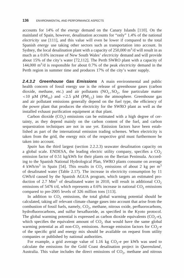
136 ENVIRONMENTAL AND PERFORMANCE ASPECTS

accounts for 14% of the energy demand on the Canary Islands [110]. On themainland of Spain, however, desalination accounts for “only” 1.4% of the nationalelectricity use [111], and this value will even be lower if compared to the totalSpanish energy use taking other sectors such as transportation into account. InSydney, the local desalination plant with a capacity of 250,000 m3/d will result in asmuch as a 0.6% increase of New South Wales’ electricity demand and will provideabout 15% of the city’s water [72,112]. The Perth SWRO plant with a capacity of144,000 m3/d is responsible for about 0.7% of the peak electricity demand in thePerth region in summer time and produces 17% of the city’s water supply.

2.4.3.2 Greenhouse Gas Emissions A main environmental and publichealth concern of fossil energy use is the release of greenhouse gases (carbondioxide, methane, etc.) and air pollutants (NOx , SO2, fine particulate matter<10 μM (PM10) and <2.5 μM (PM2.5) into the atmosphere. Greenhouse gasand air pollutant emissions generally depend on the fuel type, the efficiency ofthe power plant that produces the electricity for the SWRO plant as well as theinstalled exhaust purification equipment at that plant.

Carbon dioxide (CO2) emissions can be estimated with a high degree of cer-tainty, as they depend mainly on the carbon content of the fuel, and carbonsequestration techniques are not in use yet. Emission factors have been estab-lished as part of the international emission trading schemes. When electricity istaken from the grid, the energy mix of the respective grid must furthermore betaken into account.

Spain has the third largest (section 2.2.2.3) seawater desalination capacity ona global scale. ENDESA, the leading electric utility company, specifies a CO2emission factor of 0.51 kg/kWh for their plants on the Iberian Peninsula. Accord-ing to the Spanish National Hydrological Plan, SWRO plants consume on average4 kWh/m3 in Spain [54]. This results in CO2 emissions of about 2 kg per m3

of desalinated water (Table 2.17). The increase in electricity consumption by 11GWh/d caused by the Spanish AGUA program, which targets an estimated pro-duction of 2.7 Mm3 of desalinated water in 2010, will result in additional CO2emissions of 5476 t/d, which represents a 0.6% increase in national CO2 emissionscompared to pre-2005 levels of 326 million tons [113].

In addition to CO2 emissions, the total global warming potential should becalculated, taking all relevant climate change gases into account that arise from thecombustion of fossil fuels, namely, CO2, methane, nitrous oxide, perfluorocarbons,hydrofluorocarbons, and sulfur hexafluoride, as specified in the Kyoto protocol.The global warming potential is expressed as carbon dioxide equivalents (CO2-e),which specifies the equivalent amount of CO2 that would have the same globalwarming potential as all non-CO2 emissions. Average emission factors for CO2-eof the specific grid and energy mix should be available on request from utilitycompanies or published by national authorities.

For example, a grid average value of 1.16 kg CO2-e per kWh was used tocalculate the emissions for the Gold Coast desalination project in Queensland ,Australia. This value includes the direct emissions of CO2, methane and nitrous

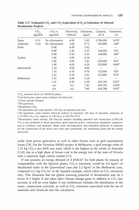
POTENTIAL ENVIRONMENTAL IMPACTS 137

Table 2.17 Estimated CO2 and CO2-Equivalent (CO2-e) Emissions of SelectedDesalination Projects

CO2, CO2-e, Electricity, Emissions, Capacity, Emissions,kg/kWh kg/kWh kWh/m3 kg/m3 m3/d t/d

Spain 0.51 No information 4.00 2.03 2,700,000 5476a

Ashkelon 0.20 No information 3.60 0.73 330,000 240b

Perth 0.98 4.00 3.92 — —0.98 2.30 2.25 144,000 325c

0.98 3.50 3.43 144,000 494d

Sydney 1.06 4.00 4.24 — —1.06 3.60 3.82 250,000 954e

1.06 4.00 4.24 250,000 1060d

Queensland 1.16 4.00 4.64 — —1.16 4.10 4.76 125,000 595e

1.16 4.70 5.43 125,000 679f

Melbourne 1.31 4.00 5.24 — —1.31 4.20 5.50 434,783 2392e

n/a n/a 7.45 434,783 3239g

n/a n/a 7.80 434,788 3391h

a CO2 emission factor for ENDESA plants.b Gas-fired power plant onsite (without fuel lifecycle).cLowest specific demand.d All operations.eDesalination only.f All operations and water transfer, 345 days of operation per year.g All operations, water transfer, lifecycle analysis of operation, 345 days of operation, emissions of1,117,950 CO2-e t/y, capacity of 150 GL/y or 434,783 m3/d.h Desalination, water transfer, full lifecycle analysis including operation and construction (1,403,140CO2-e tons attributed to diesel generators, grid-connected power, construction equipment, transporta-tion of workforce and materials, offsite waste decomposition, and embodied emissions of materialsfor the construction of the power and water grid connections, the desalination plant and the marinestructures).

oxide from power generation as well as other factors such as grid transmissionlosses [74]. For the Victorian SWRO project in Melbourne, a grid average value of1.31 kg CO2-e per kWh was used, which is the highest in the whole of Australia[114], due to a high share of brown coal in the energy mix of the state of Victoriawith a relatively high carbon content [71].

If one assumes an energy demand of 4 kWh/m3 for both plants for reasons ofcomparability with the Spanish plants, CO2-e emissions would be 4.6 kg/m3 ofdesalinated water in the Queensland case and 5.2 kg/m3 in the Melbourne case,compared to 2 kg CO2/m3 in the Spanish example, which refers to CO2 emissionsonly. This illustrates that the global warming potential of desalination may be afactor of 2 higher if one takes other climate change gases in addition to CO2 intoaccount. It will be even higher if one furthermore includes the distribution of thewater, construction activities, as well as CO2 emissions associated with the use ofmaterials and chemicals into the calculation.

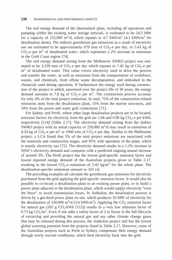
138 ENVIRONMENTAL AND PERFORMANCE ASPECTS

The real energy demand of the Queensland plant, including all operations andpumping within the existing water storage network, is estimated to be 24.5 MWfor a capacity of 125,000 m3/d, which equates to 4.7 kWh/m3 (4.1 kWh/m3 fordesalination alone). The indirect greenhouse gas emissions as a result of electricityuse are estimated to be approximately 679 tons of CO2-e per day, or 5.43 kg ofCO2-e per m3 of desalinated water, which represents a 2% increase in emissionsin the Gold Coast region [74].

The real energy demand arising from the Melbourne SWRO project was esti-mated to be 3,239 tons of CO2-e per day which equates to 7.45 kg of CO2-e perm3 of desalinated water. This value covers electricity used to drive the processand transfer the water, as well as emissions from the transportation of workforce,wastes, and chemicals, from offsite waste decomposition, and embodied in thechemicals used during operation. If furthermore the energy used during construc-tion of the project is added, amortized over the project life of 30 years, the energydemand amounts to 7.8 kg of CO2-e per m3. The construction process accountsfor only 4% of the total project emissions. In total, 75% of the construction-relatedemissions stem from the desalination plant, 15% from the marine structures, and10% from the power and water grid connections [71].

For Sydney and Perth , where other large desalination projects are to be located,emission factors for electricity from the grid are 1.06 and 0.98 kg CO2-e per kWh,respectively [114] (Table 2.17). The electricity demand arising from the SydneySWRO project with an initial capacity of 250,000 m3/d may result in emissions of4.24 kg of CO2-e per m3 or 1060 tons of CO2-e per day. Similar to the Melbourneproject, a LCA found that 5% of the total project emissions are associated withthe materials and construction stages, and 95% with operation of the plant, whichis mainly electricity use [72]. The electricity demand results in a 1.2% increase inNSW’s electricity demand and compares with a predicted ongoing annual increaseof around 3%. The Perth project has the lowest grid-specific emission factor andlowest reported energy demand of the Australian projects given in Table 2.17,resulting in the lowest CO2-e emissions of 3.43 kg/m3 for the whole plant. Thedesalination-specific emissions amount to 325 t/d.

The preceding examples all calculate the greenhouse gas emissions for electricitypurchased from the grid applying the grid-specific emission factor. It would also bepossible to co-locate a desalination plant to an existing power plant, or to build apower plant adjacent to the desalination plant, which would supply electricity “overthe fence” to avoid transmission losses. In Ashkelon, the desalination process isdriven by a gas-fired power plant on site, which produces 50 MW of electricity forthe desalination of 330,000 m3/d (3.6 kWh/m3). Applying the CO2 emission factorfor natural gas (202 g CO2/kWh [115]) results in a very low emission factor of0.73 kg CO2/m3. Even if one adds a safety factor of 2 to factor in the full lifecycleof extracting and providing the natural gas and any other climate change gasesthat may be released during this process, the Ashkelon project still has the lowestglobal warming potential from the projects listed in Table 2.17. However, some ofthe Australian projects such as Perth or Sydney compensate their energy demandthrough newly erected windfarms, which feed electricity back into the grid.

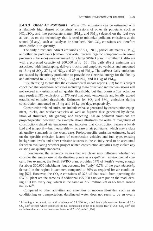
POTENTIAL ENVIRONMENTAL IMPACTS 139

2.4.3.3 Other Air Pollutants While CO2 emissions can be estimated witha relatively high degree of certainty, emissions of other air pollutants such asNOx , SO2, and fine particulate matter (PM10 and PM2.5) depend on the fuel typeas well as on the technology that is used to minimize pollutant emissions at thesource (if any), such as catalysts or scrubbers. Non-CO2 emissions are thereforemore difficult to quantify.

The daily direct and indirect emissions of SOx , NOx , particulate matter (PM10),and other air pollutants (carbon monoxide, reactive organic compound—an ozoneprecursor substance) were estimated for a large SWRO plant in southern Californiawith a projected capacity of 200,000 m3/d [56]. The daily direct emissions areassociated with landscaping, delivery trucks, and employee vehicles and amountedto 15 kg of SOx , 27 kg of NOx , and 29 kg of PM10. The indirect daily emissionsare caused by electricity production to provide the electrical energy for the facilityand amounted to <0.1 kg of SOx , 3 kg of NOx and 0.1 kg of PM10.

It is interesting to note that the environmental impact report (EIR) for this projectconcluded that operation activities including these direct and indirect emissions willnot exceed any established air quality thresholds, but that construction activitiesmay result in NOx -emissions of 176 kg/d that could temporarily and locally exceedestablished emission thresholds. Estimates for SOx and PM10 emissions duringconstruction amounted to 15 kg and 14 kg per day, respectively.

Construction-related emissions include exhaust generated by construction equip-ment, trucks, and worker vehicles as well as fugitive dust generated by demo-lition of structures, site grading, and trenching. All air pollutant emissions areproject-specific; however, the example above illustrates the order of magnitude ofconstruction-related air emissions and indicates that construction causes a local-ized and temporal—but measurable—increase in air pollutants, which may violateair quality standards in the worst case. Project-specific emission estimates, basedon the specific emission factors of construction vehicles and fuel type, existingbackground levels and other emission sources in the vicinity need to be accountedfor when evaluating whether project-related construction activities may violate anyexisting air quality standards.

In conclusion, the reference values that we chose may influence whether weconsider the energy use of desalination plants as a significant environmental con-cern. For example, the Perth SWRO plant provides 17% of Perth’s water, enoughfor about 300,000 inhabitants, but accounts for “only” 0.7% of the peak electricitydemand in the region in summer, compared to 30% as required for air condition-ing [52]. However, the CO2-e emissions of 325 t/d that result from operating theSWRO plant are the same as if additional 195,000 cars were put on the road, driv-ing 13.3 km every day, which is the same as 2.59 million km or 65 times aroundthe globe8.

Compared to other activities and amenities of modern lifestyles, such as airconditioning or transportation, desalinated water does not seem to be an overly

8Assuming an economic car with a mileage of 5 L/100 km; a full fuel cycle emission factor of 2.5 tCO2-e/m3 of fuel, which comprises the fuel combustion at the point source (car) of 2.3 t CO2-e/m3 andan indirect/fuel extraction emission factor of 0.2 t CO2-e/m3 [114].

140 ENVIRONMENTAL AND PERFORMANCE ASPECTS

energy-expensive product. However, it is far more energy-intensive than the treat-ment and distribution of local ground- and surface-water sources by conventionalprocesses, and is often still more energy-intensive than the import of water overlong distances. The energy use of desalination is therefore a matter of controversialpublic debate. However, simply understating the problem by comparing the energydemand of desalination to even more energy-intensive forms of use is not instru-mental in the discussion, nor is it to belabor the point if it is clear that conventionalwater supplies cannot meet the demand.

The wider implications in the debates about new desalination projects are usuallythe extent to which consumers need and value the additional water provided by theproject. Desalination plants are normally not built because people lack water fordrinking and sanitation, but to provide additional water as an amenity of modernlifestyles, which may include swimming pools and irrigation in home gardens. Asecond question is how much impact are consumers willing to accept in return forthese amenities, and how much costs would they except on top of the costs ofproducing desalinated water to make the process more sustainable. The price tagincludes not only energy use but also other environmental impacts. As the problemincreases in complexity, double moral standards may be applied in the discussion.The sustainability of desalination projects is often questioned on the grounds ofhigh energy use and potential marine impacts—under the tacit assumption that thestatus quo of the existing water supply or other alternatives are more sustainable,which is not necessarily the case.

Desalination is without question an energy-intensive option, but the status quois that energy is often wasted in other sectors of use, e.g., by old and inefficientelectrical appliances in households. For examples, it is estimated that the totalsaving potential of more energy-efficient household appliances in Germany is about29% per household [116], without compromising comfort or living standards. It canbe assumed that similar values apply for other industrial and developing nations.Energy saving in households could possibly make up for the additional energydemand of providing desalinated water to households [27].

The status quo of existing water supplies, which may involve the depletionof groundwater resources, or the damming, regulation or diversion of rivers, mayalso prove unsustainable. According to the World Commission on Dams, a con-siderable portion of the world’s large dams is falling short of their physical andeconomic targets; that is, they deliver less water and electricity than promisedwhile significantly overrunning costs, besides having extensive impacts on aquaticecosystems, which, in many cases, have led to irreversible loss of species andecosystems [117].

In the end, it depends on the perception and definition of significance andon local circumstances whether a community or individual considers energy useof desalination as a significant factor. In many parts of the world, energy useis generally recognized as a significant issue. This is reflected in policy initia-tives and stricter standards in many countries to reduce energy consumption andincrease energy use efficiency in all sectors. On the project level, the concept ofenvironmental impact assessment stipulates that for all significant impacts of a

SEAWATER DESALINATION AS A GREEN TECHNOLOGY 141

new development project, impact mitigation measures have to be identified andimplemented, involving a hierarchy of measures from prevention to minimizationand compensation.

If energy use of desalination projects is considered a significant impact, thenthe logical consequence must be to reduce the energy demand as far as possible,and to compensate the remaining energy use. For example, CO2 emissions are acentral issue in all large Australian SWRO projects (e.g., Perth, Sydney, Melbourne,[59,72,73]), and project proponents are encouraged to provide for the use of energyfrom renewable sources, planting of plantations, or rehabilitation of vegetation tooffset these emissions [73]. The electricity demand for two SWRO plants in Perthand the Sydney project, for instance, is compensated by newly erected windfarms,which compensate for the electricity taken from the grid [112,118,119].

2.5 SEAWATER DESALINATION AS A GREEN TECHNOLOGY

Earth Day 2009 on April 22 marked the beginning of a new campaign called thegreen generation , which seeks to foster the development of green technologiesand solutions to urgent global issues such as climate change or the world watercrisis [120]. Energy, water, and climate change are inseparable global problems.On one hand, energy is needed to deliver water, and water is needed to generateenergy [121]. On the other hand, extensive energy consumption in all sectors ofuse has caused an increase in atmospheric greenhouse gases to 37% above thepreindustrialization level, and research indicates stronger than expected forcing ofclimate change, which also affects the global water cycle. For instance, the easternand southwestern parts of Australia have experienced substantial rainfall declinessince 1950, which is assumed to be partly due to anthropogenic climate change, andmodels predict up to 20% more drought-months over most of Australia by 2030[122]. The continent has recently been experiencing one of the harshest droughts inits history and turns to desalination in order to alleviate problems of water scarcityin most major cities.

Seawater desalination is a technology that can mitigate the problems of watershortage, and analysts agree that capacities will continue to grow rapidly in thecoming years [123,124] (see also Section 2.2). However, the issue is whetherdesalination is also a green and sustainable solution. A critical examination andappraisal of the energy and chemical consumption and key environmental impactsof SWRO has been carried out in previous sections (Sections 2.3 and 2.4 and inRef. 27) and shall only be briefly exemplified here.

To date, the world’s largest operating SWRO plant produces 330,000 m3/d,which is the equivalent of 132 olympic-size swimming pools. About the sameamount of water is discharged as concentrate into the sea. The plant consists of27,000 membrane elements with a total active surface area of about 99 ha (hectares)(or 200 football fields), which need to be replaced every 3–7 years. The energydemand attributed to the use of materials during construction and operation, how-ever, is small (in the range of 5%) compared to the energy needed to operate

142 ENVIRONMENTAL AND PERFORMANCE ASPECTS

the desalination plant over its lifetime. The energy demand of SWRO is about3.5 kWh/m3 using state-of-the-art equipment (Section 2.3.4), which is the equiva-lent of a moderately efficient laundry dryer, or about 330,000 laundry dryer loadsevery day in this example. Besides materials and energy, all desalination plantsuse chemicals. Their residues are discharged into the sea along with the concen-trate (Section 2.4.2) and may amount to thousands of tons per day in some seaareas [27,125]. The discharges, and the intakes (Section 2.3.1), which may causeimpingement and entrainment, are the main reasons why marine protection groupssuch as the Surfrider Foundation in California or the Clean Ocean Foundation inAustralia campaign against proposed desalination projects. The other main publicconcern is pollution of the atmosphere (Section 2.4.3). For example, more than75% of the formal submissions received in response to the environmental assess-ment of the proposed Sydney SWRO project expressed concerns about energy useand greenhouse gases [126].

A 2008 review in Nature described desalination as a water treatment technologythat is often “chemically, energetically and operationally intensive, focused on largesystems, and thus requiring considerable infusion of capital, engineering expertiseand infrastructure.” The costs as well as the environmental concerns are still animpediment to the widespread use of desalination technologies today [127]. Yetsome project developers have more recently made headlines with buzzwords suchas “green” [108,128] or “sustainability” [112,118]. The seemingly contradictorystatements are indicative of the current debate on the extent to which SWRO plantswill actually affect the environment. As desalination capacities continue to grow,it remains even more necessary to gain an objective understanding of the energyand chemical use and the environmental impacts of desalination technologies.

The objective of this publication is therefore to investigate whether present state-of-the art desalination technologies can be considered as green and sustainable solu-tions. “Green” or “clean” or “environmental” technology are all synonyms for theapplication of environmental science and technology to conserve the natural envi-ronment and its resources and to curb the negative impacts of human involvement.Sustainable development is the core of green technologies [129]. Consequently,“green desalination” should refer to desalination technologies that conserve thenatural environment and its resources. This can be achieved by implementing tech-nology standards in order to limit waste emissions and resource consumption, i.e.,standards for best available techniques (BAT). Furthermore, if “green desalination”means the application of environmental science to curb the negative impacts ofhuman involvement, this can be interpreted as a need for investigating, evaluat-ing, and minimizing environmental impacts of each project individually, i.e., byconducting environmental impact assessment (EIA) and monitoring studies.

Both approaches, BAT and EIA, legitimately coexist because the first is atechnology-based approach that refers to industry categories, whereas the otheris applied at the project level in order to identify the best environmental optionwith regard to process design and project site from a set of alternatives. BATstandards can provide guidance in the selection of individual solutions, especiallywith regard to process design. The United Nations Environment Program released

SEAWATER DESALINATION AS A GREEN TECHNOLOGY 143

an EIA guidance manual for desalination projects in 2008 [111]. A comparablereference on BAT for desalination, which describes a standard for state-of-the-artdesalination technologies that indicate the practical suitability for limiting resourceconsumption and waste products, is lacking so far.

2.5.1 Best Available Techniques (BAT)

The concept of best available techniques (BAT) has been established by differentlegislative systems, e.g., in Europe and the United States, and has been applied tosimilar industries and applications, such as power plants and seawater coolingwater systems. In Europe and neighboring seas, the concept of BAT is intro-duced by the EC Directive on Integrated Pollution Prevention and Control (IPPC),the Conventions for the Protection of the Marine Environment of the North-EastAtlantic (OSPAR) and of the Baltic Sea Area (HELCOM), and the Protocol for theProtection against Pollution from Land-Based Sources of the Mediterranean ActionPlan (LBS protocol).

The IPPC directive imposes a requirement for certain industries with a highpollution potential to obtain a permit, which is issued if certain environmentalconditions are met, such as the use of BAT. This applies to industries listed in AnnexI of the directive, such as energy industries, but not water treatment installations.A reference document on BAT in industrial cooling systems has been providedunder the IPPC directive [130], which could serve as a guideline for designingdesalination plants.

The marine conventions, in contrast, clearly indicate the need for a BAT conceptfor seawater desalination technologies in European and neighboring sea areas. Forexample, the Mediterranean LBS protocol requires contracting parties to take BATinto account when adopting action plans, programmes and measures. In 2005, thecountries of the Mediterranean Action Plan adopted the concept that desalinationplants are “industrial facilities,” which means that they need to be regulated andassessed through EIAs [131]. In addition, BAT standards for desalination plantsshould be developed and implemented through the Mediterranean Action Plan. Insome countries, general BAT regulations exist already. In Israel, for example, aprerequisite for discharge into the sea is the use of BAT, which prohibits dis-charge directly at the coast with the exception of cooling water outfalls of powerplants. Marine outfalls therefore have to be deep offshore outfalls, and the entirelength of the pipeline has to be buried using BAT during construction to mini-mize damage to the coastal area [132]. While the first large SWRO plant in Israel(Ashkelon) is co-located to a power plant and therefore discharges directly at thecoastline, tender documents for new projects set a request for an outfall to a depth of20 m [133].

According to the IPPC directive and the marine conventions, BAT is defined asstate-of-the-art processes, facilities, or methods of operation that indicate the prac-tical suitability for limiting discharges, emissions and waste, and for reducing theimpact on the environment as a whole. The term technique includes both the tech-nology used and the way in which the installation is designed, built, maintained,

144 ENVIRONMENTAL AND PERFORMANCE ASPECTS

operated, and dismantled. The techniques that are considered BAT should be eco-nomically and technically feasible, should be used or should have been tried outon an industrial scale, and should account for technological advances in scientificknowledge. Special consideration in the development of BAT is typically given tothe consumption of raw materials, water, energy, less hazardous substances, andthe possibility for recovery and recycling of any resources used or wastes gener-ated. Applying the IPPC principle to an industry through implementation of BATimplies the need to take preventive measures when there is substantial evidence tosuspect that an activity may cause harm to the environment even if there is no abso-lute proof (prevention principle), and to reduce the emissions into the atmosphere,water, and soil, as well as waste generation (control principle).

In the United States, BAT terminology is used in the Clean Air Act and CleanWater Act (CWA). Under the CWA, the Environmental Protection Agency (EPA)issues national standards for facilities discharging directly to surface waters. Theseso-called effluent guidelines apply to categories of dischargers and are technology-based, and not on the impacts on the receiving waters. The intent of technology-based standards is to establish a basic national standard for all facilities withina category using BAT, which becomes the minimum regulatory requirement inpermits that are implemented through the National Pollutant Discharge EliminationSystem (NPDES) permit program [134].

Similar to the European IPPC directive, guidelines have been established fordifferent industrial categories including power plants but not water treatment instal-lations. CWA and NPDES regulations authorize the use of “best professionaljudgment” to derive technology-based effluent limitations on a case-by-case basiswhere standards are absent. Best professional judgment was for example used toderive the NPDES permit for the Carlsbad SWRO plant in southern California [96].The EPA has now initiated a new rulemaking on drinking water treatment effluentguidelines to address the direct discharge of drinking water treatment residuals tosurface water, such as suspended solids, aluminum or iron salts, organic matter,polymers, desalination concentrates , or other residuals [134]. Section 316(b) ofthe CWA furthermore requires that the location, design, construction, and capacityof cooling water intake structures reflect the BAT for minimizing adverse environ-mental impact, that is the impingement and entrainment of fish and other aquaticorganisms. The regulations on cooling water intakes could serve as a basis forregulating seawater desalination plant intakes as well.

In order to develop BAT standards for SWRO plants, the main components ofdesalination plants (i.e., the intake, pretreatment, desalination process, cleaning, andconcentrate disposal system) need to be compared with regard to environmental cri-teria such as energy, material and chemical use, and resulting emissions and likelyenvironmental impacts. The identified BAT solution can be used as a referencein the determination of individual BAT solutions on a case-by-case basis, takingsite- and project-specific considerations into account. It should be noted here thatthe environmental impacts of a desalination plant will depend on the technologyand mode of operation on one hand, and the environmental characteristics of theproject site on the other hand. A commonly used tool for comparing alternative

SEAWATER DESALINATION AS A GREEN TECHNOLOGY 145

technologies is the lifecycle assessment (LCA). A novel approach has been used insection 2.6., using multicriteria analysis (MCA) to compare different pretreatmentalternatives for SWRO plants.

2.5.2 Environmental Impact Assessment

By definition, the primary goals of an EIA are to provide information on theenvironmental consequences of a project for decision-making, and to promoteenvironmentally sound and sustainable development through the identification ofappropriate alternatives and mitigation measures. EIAs are seldom limited to envi-ronmental aspects, but where appropriate also address public health and socioeco-nomic concerns. Public participation is therefore an integral element of EIAs inmany legislative systems. As a result, EIAs are often complex multistage, multi-disciplinary, and multiparticipatory processes.

To deal with this complexity and facilitate the implementation of EIAs fordesalination projects on a wider scale, a 10-step process has been proposed byUNEP/ROWA, as shown in Figures 2.27 and 2.28 [111]. The initial EIA phaseincludes the steps of screening and scoping of the project, in which a decisionis taken on whether an EIA is required for a particular project, and in which thescope, contents, and methodologies of the EIA and expert studies are specifiedin the terms of reference (ToR). A reference list for preparing the ToR has beenprovided in Reference 111, which may also serve as a blueprint for preparing theEIA report. During the main EIA phase, a detailed description of the preferredproject configuration including site and process alternatives is provided, and otherstatutory permits applicable to the project are identified and obtained. The scientificstudies and analyses are conducted during this phase, including baseline studies,the prediction and evaluation of impacts, and the identification of alternatives andimpact mitigation measures. The final EIA phase involves decision-making and areview of the EIA process. An environmental management plan is often establishedat this stage, which specifies the monitoring requirements during the installationand operation of the plant.

In principle, EIAs for large desalination projects will not differ in terms ofcomplexity and level of detail from those of other water supply infrastructureprojects. Depending on the proposed project, it is generally the responsibility ofthe competent authorities to individually define the need, scope, and complexityrequirements of each EIA study. When dealing with a larger number of desali-nation proposals, a collaborative effort between the main government agenciesand participatory groups should be initiated to elaborate a national EIA guide-line for desalination projects. It would facilitate the EIA process by establishingequal standards for the environmental studies to be undertaken and the infor-mation to be submitted as part of the EIA for each individual project in thefuture. Moreover, as a number of agencies usually have permitting authority overthe project, a lead agency should be nominated to coordinate the process byinvolving other agencies and by informing the project proponent about permittingrequirements.

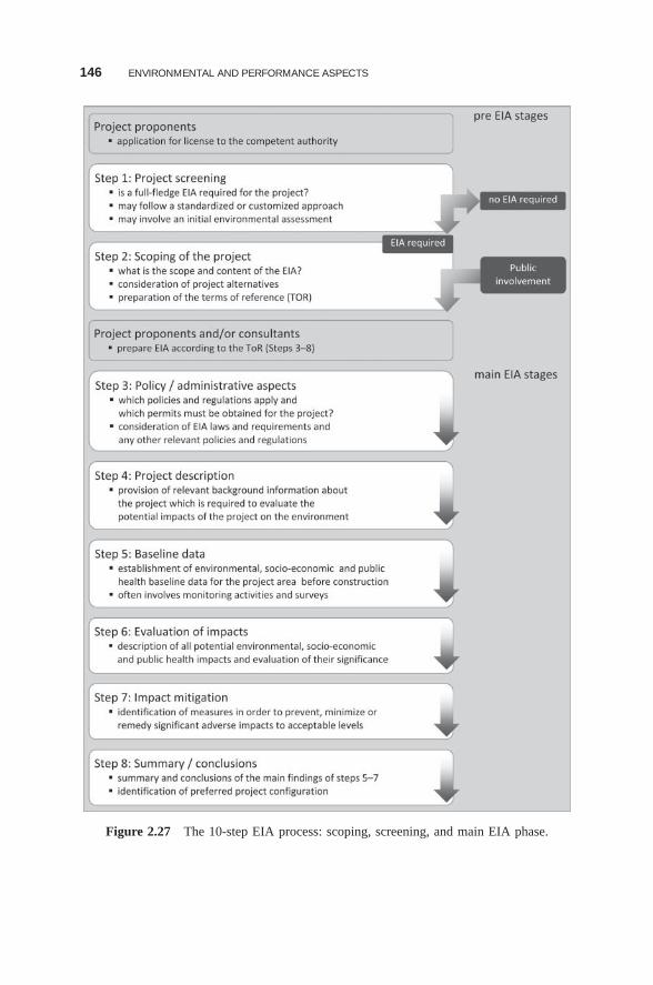
146 ENVIRONMENTAL AND PERFORMANCE ASPECTS

Figure 2.27 The 10-step EIA process: scoping, screening, and main EIA phase.

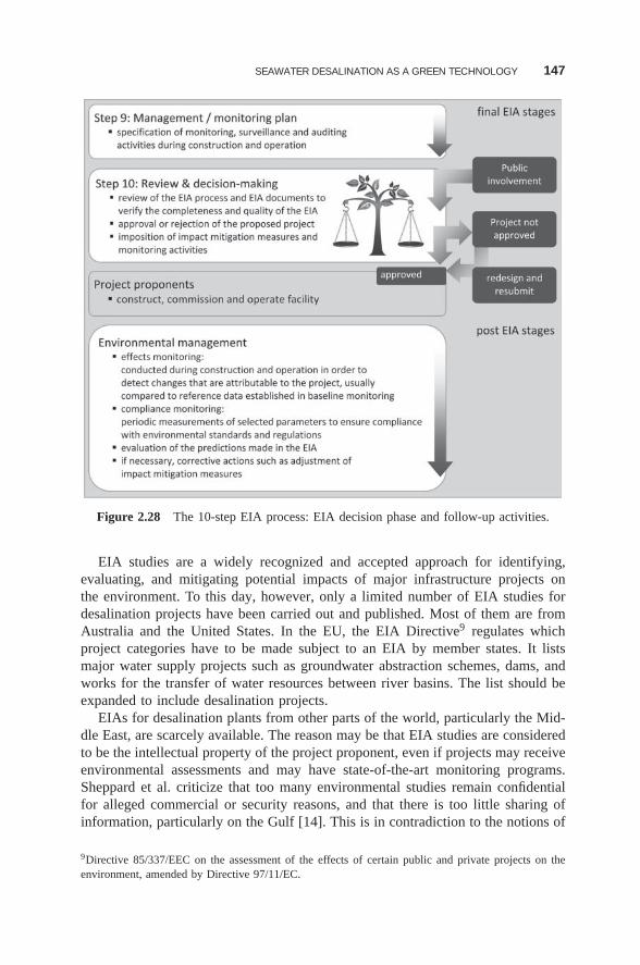
SEAWATER DESALINATION AS A GREEN TECHNOLOGY 147

Figure 2.28 The 10-step EIA process: EIA decision phase and follow-up activities.

EIA studies are a widely recognized and accepted approach for identifying,evaluating, and mitigating potential impacts of major infrastructure projects onthe environment. To this day, however, only a limited number of EIA studies fordesalination projects have been carried out and published. Most of them are fromAustralia and the United States. In the EU, the EIA Directive9 regulates whichproject categories have to be made subject to an EIA by member states. It listsmajor water supply projects such as groundwater abstraction schemes, dams, andworks for the transfer of water resources between river basins. The list should beexpanded to include desalination projects.

EIAs for desalination plants from other parts of the world, particularly the Mid-dle East, are scarcely available. The reason may be that EIA studies are consideredto be the intellectual property of the project proponent, even if projects may receiveenvironmental assessments and may have state-of-the-art monitoring programs.Sheppard et al. criticize that too many environmental studies remain confidentialfor alleged commercial or security reasons, and that there is too little sharing ofinformation, particularly on the Gulf [14]. This is in contradiction to the notions of

9Directive 85/337/EEC on the assessment of the effects of certain public and private projects on theenvironment, amended by Directive 97/11/EC.

148 ENVIRONMENTAL AND PERFORMANCE ASPECTS

transparency and public participation, and EIAs should generally be made availableto a wider public audience, especially if the studies are conducted for municipalwater supply projects.

Often, EIA investigations are carried out under immense time constraints. Forinstance, only 4 months were given for an EIA study for a large SWRO plantin Algeria [135]. This shows that environmental concerns can be of secondaryimportance when a ready supply of freshwater is urgently needed. The opposite isalso true; comprehensive and time-consuming environmental studies and concernshave been the major hurdle in the permitting process of new projects in California.The first large SWRO project in California took more than 10 years to receive allnecessary permits. In Spain, the government has announced plans to speed up theEIA process from the current average of 770 days for infrastructure projects tono more than 6 months. The reform could benefit vital water projects; however,doubts were raised from within the European Commission that it would be possibleto condense the whole EIA procedure including public consultation into a six monthperiod [136].

In 2004, Manuel Schiffler from The World Bank stated that an “internationallyagreed environmental assessment methodology for desalination plants does notexist so far and its development would be desirable” [137]. The UNEP guidancedocument partially fills this gap. It offers guidance for designers of desalinationprojects, consultants, regulators, and decisionmakers on the methodology, scope,and contents of EIA studies and specifically for desalination projects. Still missing,however, are long-term monitoring studies that improve the basic understandingof the actual environmental impacts of desalination plants. Although an increasingnumber of EIA studies is being published, these are based mainly on conceptualmodels and laboratory experimental methods, including hydrodynamic modeling ofthe discharges and effluent toxicity testing, carried out before project startup. Theresults need to be verified for the majority of these projects in effects monitoringstudies during plant operation .

2.5.2.1 Environmental Monitoring As EIA studies make predictions aboutthe expected impacts of a desalination project on the environment, it is nec-essary to validate the accuracy of these predictions against observations duringproject implementation and operation. In 2008, the US National Research Coun-cil of the National Academies attested a surprising paucity of useful experimentaldata , either from laboratory tests or from field monitoring in 2008 [19]. Largeprojects and accompanying monitoring programs are only now being implemented.The longest effects monitoring programs for a few SWRO projects worldwidehave accumulated only 2–3 years of cohesive monitoring data. Although thismay allow for some conclusions regarding those particular projects, it is too earlyto use these results as conclusive evidence concerning the long-term impacts ofdesalination plants, or concerning the cumulative impacts of several desalinationplants in a given sea area. A review of existing monitoring studies [111] revealedthat most other monitoring studies for desalination projects were either limited in

SEAWATER DESALINATION AS A GREEN TECHNOLOGY 149

scope—addressing only one aspect such as salinity, short-term—without a con-tinuous baseline and effects monitoring, and localized—without adequate spatialreplication.

The importance of operational monitoring cannot be overemphasized, whichis also illustrated by the following case study. Ambrose et al. [138] comparedthe actual impacts of the cooling water discharges from a nuclear power plant insouthern California, established by a 15-year monitoring program, to predictionsmade in the EIA which had been generated in three different ways. The compari-son showed that (1) almost all of the testimonies of scientists before the permittingagency, which were based on professional judgment with little scientific analyzes,were wrong; (2) the accuracy of the final environmental statement, based on stan-dard assessment methods at that time, was mixed but generally not too high; and(3) the predictions of the marine review committee, based on a comprehensivebaseline study over several years, were the most accurate but also showed inaccu-racies. Although a clear correlation between effort and accuracy of the predictionsseems to exist, the lesson here is that EIAs cannot predict with complete con-fidence what will happen in the environment, even if considerable resources arededicated to monitoring [138]. EIAs, like other observational studies, are likely tobe “messy” even after a conscientious effort to apply the appropriate techniquesand mathematical statistics [139]. The impacts predicted in EIAs are not alwaysthe actual impacts, although they become the de facto impacts if there is a lack offollow-up studies [138].

The core of the problem is to design a monitoring program that provides suf-ficient statistical power to be able to distinguish the effects of the desalinationproject from natural processes. For this reason, sufficient spatiotemporal replica-tion is needed in field monitoring studies. Field monitoring for desalination projectsshould include the project (impact) site and several control sites that adequatelyrepresent the habitats of the impact site. To capture the temporal variance at thesesites, paired sampling should be carried out at several times before, during, andafter project implementation (BACIPS approach). Baseline monitoring for majordevelopment projects is usually carried out over a 2-year period before projectstartup and effects monitoring for 2–3 years during commissioning and operation.A holistic monitoring framework for desalination projects should furthermore inte-grate field monitoring with hydrodynamic modeling and bioassay studies, preferablyusing whole effluent toxicity (WET) tests. These concepts have for example beenimplemented in the monitoring programmes for the Sydney and Gold Coast SWROprojects.

Regulatory agencies may still be reluctant to require rigorous operational mon-itoring studies, and project developers are understandably opposed to funding it[138]. However, there is an increasing tendency to regulate new developmentsworldwide under the requirement that predictions will be tested by measuring thereal impacts by scientific means, and by imposing project modifications if impactsare found to differ from those predicted. Adequate monitoring could therefore alsobe understood as “insurance” against unwarranted claims [140]. In this context, itis also noteworthy that both effects monitoring and compliance monitoring only

150 ENVIRONMENTAL AND PERFORMANCE ASPECTS

allow for reactive impact management. It should therefore be in the interest of allparties (and of the environment) that management responses are established in caseunexpected or more severe impacts are detected during effects monitoring, or incase trigger values are exceeded during compliance monitoring.

Effects monitoring also serves to produce much relevant fundamental research,which is of particular value to industries that are not involved in one-off devel-opments [141]. The desalination industry can thus learn from each experience tominimize impacts for the next development. As mentioned above, comprehen-sive environmental monitoring programs are underway for several large AustralianSWRO projects, which will provide valuable results in the near future. An overviewon how to design an environmental monitoring framework for desalination plantsis given by Lattemann [27].

2.6 MULTICRITERIA ANALYSIS (MCA) OF INTAKE ANDPRETREATMENT ALTERNATIVES FOR SWRO

Environmental impact studies are part of the permitting process of large infrastruc-ture projects, including new desalination projects. As such, they are often complexmultistage, multidisciplinary, and multiparticipatory processes, in which differentsite and process alternatives and a wide range of environmental impacts are beingconsidered. A vast body of quantitative data and qualitative information is thuscompiled, which results in lengthy reports with numerous appendices, and exten-sive evaluation tables, which are usually unsuitable for direct evaluation [142].For example, the recently completed EIA of the Victorian desalination project inAustralia covered 1600 pages, and the volumes stack nearly 1.5 m high. Moreover,different government agencies, stakeholders, and the wider public usually partici-pate in the permitting process of a new desalination project. It is therefore necessaryto communicate the results of the EIA to the decisionmakers, and conflicting ref-erences about the project need to be balanced in decision-making. This requiresa structured and transparent approach. As a single and objectively best solutionrarely not exists, the process of environmental decision-making has been describedas a conflict analysis characterized by environmental, social, economic, and polit-ical value judgments, which is essentially a search for an acceptable compromisesolution [143].

The increasing volume of complex and controversial information generated byEIAs and the limited capacities of individuals to integrate and process this informa-tion emphasizes the need for a formalized decision support tool, which aggregatesthe information in a transparent and consistent way. One such tool is multicriteriaanalysis (MCA), which can facilitate the EIA in different ways and in differentstages (Table 2.18). In contrast to traditional evaluation tools such as cost-benefitanalysis (CBA) often used in economics, or lifecycle analyses (LCA) used to quan-tify the resource consumption of a product, MCA allows for a comparison ofalternatives by using nonmonetary and nonquantitative criteria. Such qualitativecriteria are often more applicable in environmental contexts, and thus in EIAs.

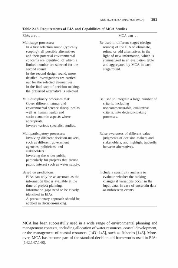
MULTICRITERIA ANALYSIS (MCA) 151

Table 2.18 Requirements of EIA and Capabilities of MCA Studies

EIAs are . . . MCA can . . .

Multistage processes:In a first selection round (typicallyscoping), all possible alternativesand their potential environmentalconcerns are identified, of which alimited number are selected for thesecond round.In the second design round, moredetailed investigations are carriedout for the selected alternatives.In the final step of decision-making,the preferred alternative is selected.

Be used in different stages (designrounds) of the EIA to eliminate,refine, or add alternatives in thelight of new information, which issummarized in an evaluation tableand aggregated by MCA in eachstage/round.

Multidisciplinary processes that:Cover different natural andenvironmental science disciplines aswell as human health andsocio-economic aspects whereappropriate.Involve various specialist studies.

Be used to integrate a large number ofcriteria, includingnoncommensurable, qualitativecriteria, into decision-makingprocesses.

Multiparticipatory processes:Involving different decision-makers,such as different governmentagencies, politicians, andstakeholders.Involving the wider public,particularly for projects that arousepublic interest such as water supply.

Raise awareness of different valuejudgments of decision-makers andstakeholders, and highlight tradeoffsbetween alternatives.

Based on predictions:EIAs can only be as accurate as theinformation that is available at thetime of project planning.Information gaps need to be clearlyidentified in EIAs.A precautionary approach should beapplied in decision-making.

Include a sensitivity analysis toevaluate whether the rankingchanges if variations occur in theinput data, in case of uncertain dataor unforeseen events.

MCA has been successfully used in a wide range of environmental planning andmanagement contexts, including allocation of water resources, coastal development,or the management of coastal resources [143–145], such as fisheries [146]. More-over, MCA has become part of the standard decision aid frameworks used in EIAs[142,147,148].

152 ENVIRONMENTAL AND PERFORMANCE ASPECTS

This section explores the usefulness of MCA as a decisions support tool for newdesalination projects. MCA has been used before in other studies, e.g., to facilitatesite selection for one large desalination plant in Australia and for two small plantsin South Africa [149–151]. However, the present evaluation focuses on a compar-ison of technologies instead of different sites for a specific project. SWRO is thepreferred process for most new desalination projects. The most important consid-eration in a SWRO system is the intake and pretreatment (Section 2.3) because agood and reliable water quality must be obtained with a low fouling potential to theSWRO membranes. The design of the outfall is another important consideration interms of environmental impacts. However, concentrate disposal is more straight-forward, i.e., it basically requires an effective diffuser in a suitable oceanographicsite, and the alternatives are therefore rather limited. It was therefore decided toapply the MCA to the main intake and pretreatment options for SWRO plants. Theinformation needed for this approach was obtained from literature sources and, toa limited extent, directly from plant operators. An overview on the methodologyis given in Section 2.6.1, the input data are described in Section 2.6.2, and resultsand conclusions are presented in Sections 2.6.3 and 2.6.4.

2.6.1 Methodology

An MCA typically involves two phases (Fig. 2.29). In the first phase, the decisionproblem is defined, input data is generated, and the alternatives can be rankedaccording to the input data by means of a graphical evaluation. In the secondphase, the alternatives are ranked using MCA, which involves the selection of anMCA model and standardization functions, applying weights to the criteria thatreflect value judgments, and a sensitivity analysis of the ranking.

A prerequisite to MCA is problem definition. This consists in the establish-ment of an overarching, primary objective that clearly states what the decisionseeks to achieve, and the identification of a complete set of alternatives . Thedecision-making objective has to be translated into a number of operational cri-teria . Structuring the criteria is an important prerequisite of MCA and results inthe establishment of an objective tree. The final set of criteria should be complete,nonredundant, operational, and minimal (see Ref. 143, after Ref. 152). Althoughup to 100 criteria have been reported for complex infrastructure projects, a moremanageable range would be 6–20, which is sufficient for well-founded decision-making in many cases [142]. The important point is to identify those criteria thatare truly relevant to decision-making and to avoid redundancy.

The performance of every alternative against all criteria is measured by scores .The data are gathered in an effects table, which is an intermediate product that canbe graphically evaluated without attaching weights to the criteria. This requires thatthe incompatible units of measurement of the various criteria be transformed intoa compatible form of measurement, which is achieved by applying a suitable stan-dardization function for each criterion. For example, scores can can be measuredon quantitative scales (e.g., costs in euros or energy use in kWh), on qualitativescales (ranking on an ordinal scale from highest impact to lowest impact), or on

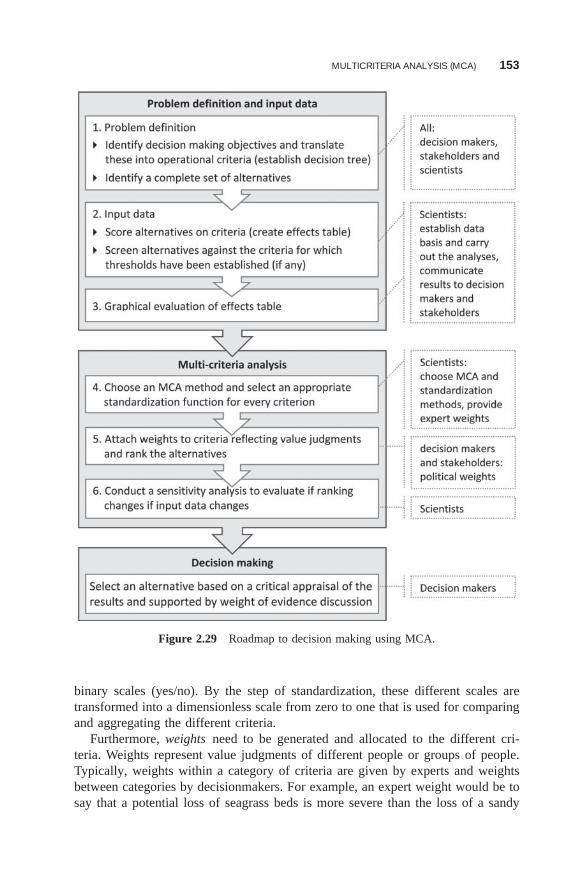
MULTICRITERIA ANALYSIS (MCA) 153

Figure 2.29 Roadmap to decision making using MCA.

binary scales (yes/no). By the step of standardization, these different scales aretransformed into a dimensionless scale from zero to one that is used for comparingand aggregating the different criteria.

Furthermore, weights need to be generated and allocated to the different cri-teria. Weights represent value judgments of different people or groups of people.Typically, weights within a category of criteria are given by experts and weightsbetween categories by decisionmakers. For example, an expert weight would be tosay that a potential loss of seagrass beds is more severe than the loss of a sandy

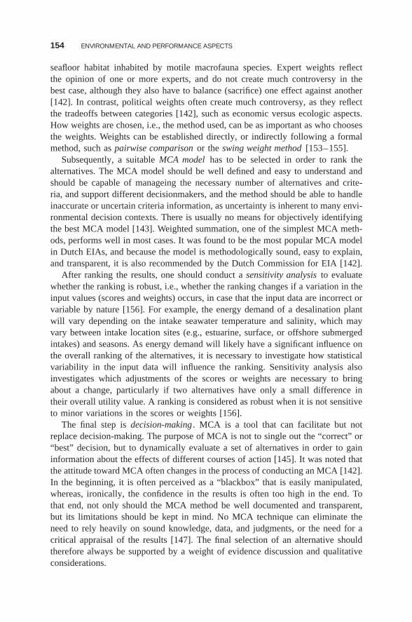
154 ENVIRONMENTAL AND PERFORMANCE ASPECTS

seafloor habitat inhabited by motile macrofauna species. Expert weights reflectthe opinion of one or more experts, and do not create much controversy in thebest case, although they also have to balance (sacrifice) one effect against another[142]. In contrast, political weights often create much controversy, as they reflectthe tradeoffs between categories [142], such as economic versus ecologic aspects.How weights are chosen, i.e., the method used, can be as important as who choosesthe weights. Weights can be established directly, or indirectly following a formalmethod, such as pairwise comparison or the swing weight method [153–155].

Subsequently, a suitable MCA model has to be selected in order to rank thealternatives. The MCA model should be well defined and easy to understand andshould be capable of manageing the necessary number of alternatives and crite-ria, and support different decisionmakers, and the method should be able to handleinaccurate or uncertain criteria information, as uncertainty is inherent to many envi-ronmental decision contexts. There is usually no means for objectively identifyingthe best MCA model [143]. Weighted summation, one of the simplest MCA meth-ods, performs well in most cases. It was found to be the most popular MCA modelin Dutch EIAs, and because the model is methodologically sound, easy to explain,and transparent, it is also recommended by the Dutch Commission for EIA [142].

After ranking the results, one should conduct a sensitivity analysis to evaluatewhether the ranking is robust, i.e., whether the ranking changes if a variation in theinput values (scores and weights) occurs, in case that the input data are incorrect orvariable by nature [156]. For example, the energy demand of a desalination plantwill vary depending on the intake seawater temperature and salinity, which mayvary between intake location sites (e.g., estuarine, surface, or offshore submergedintakes) and seasons. As energy demand will likely have a significant influence onthe overall ranking of the alternatives, it is necessary to investigate how statisticalvariability in the input data will influence the ranking. Sensitivity analysis alsoinvestigates which adjustments of the scores or weights are necessary to bringabout a change, particularly if two alternatives have only a small difference intheir overall utility value. A ranking is considered as robust when it is not sensitiveto minor variations in the scores or weights [156].

The final step is decision-making . MCA is a tool that can facilitate but notreplace decision-making. The purpose of MCA is not to single out the “correct” or“best” decision, but to dynamically evaluate a set of alternatives in order to gaininformation about the effects of different courses of action [145]. It was noted thatthe attitude toward MCA often changes in the process of conducting an MCA [142].In the beginning, it is often perceived as a “blackbox” that is easily manipulated,whereas, ironically, the confidence in the results is often too high in the end. Tothat end, not only should the MCA method be well documented and transparent,but its limitations should be kept in mind. No MCA technique can eliminate theneed to rely heavily on sound knowledge, data, and judgments, or the need for acritical appraisal of the results [147]. The final selection of an alternative shouldtherefore always be supported by a weight of evidence discussion and qualitativeconsiderations.

MULTICRITERIA ANALYSIS (MCA) 155

2.6.2 Data Input

The objective of this study is to compare different intake and pretreatment systemsfor SWRO using MCA. SWRO intake and pretreatment systems are usually opti-mized to control fouling by bacteria, organic compounds, suspended and colloidalmatter, and scaling inside the plant. Depending on local circumstances, solutionsrange from minimalist to operationally intensive; the latter consume considerableamounts of natural resources, including chemicals, materials, energy, land, andwater. The overall environmental footprint of a desalination process can thereforebe minimized by selecting the best pretreatment option in a given site. The method-ology follows the MCA approach described in Section 2.6.1 and Figure 2.29, usingthe software tool DEFINITE 3.1 [154], which facilitates ranking and comparing afinite set of alternatives [153].

2.6.2.1 Alternatives The alternatives considered, as shown in Figure 2.30included natural subsurface systems, i.e., beachwells (see Sections 2.3.1.2 and2.3.2.1), and engineered pretreatment systems, distinguishing between conventionalpretreatment (Section 2.3.2.2) and membrane pretreatment (Section 2.3.2.3).

It was assumed that the intake and pretreatment systems pretreat between 40,400and 42,000 m3 of seawater per day, depending on the water losses in the pretreat-ment system for backwashing (from 1% to 5%), and provide 40,000 m3 of feedwaterfor a single-pass SWRO plant operated at 50% recovery and with a capacity of20,000 m3/d (Fig. 2.32). A nominal plant capacity of 20,000 m3/d was selectedbecause beachwells have a limited intake capacity and are therefore mostly usedfor smaller SWRO plants. Similarly, UF/MF pretreatment has so far mostly beenapplied to smaller SWRO plants, with the largest operational UF-SWRO planthaving a capacity of 50,000 m3/d [Table 6 in Ref. 27]. Most large SWRO plantsstill use a conventional pretreatment with one granular media filtration stage. Someplants have two media filtration stages, and a few plants have a third pretreatment

Figure 2.30 Pretreatment system alternatives considered in the MCA.

156 ENVIRONMENTAL AND PERFORMANCE ASPECTS

stage in addition to two stage media filtration (Section 2.3.2.2). The conventionalpretreatment design considered in this study also consists of one stage, similar tomost SWRO plants. As no large SWRO plant uses a beachwell intake or UF pre-treatment to date, caution must be used when extrapolating the results of this studyto large SWRO projects with capacities of ≥100, 000 m3/d.

Neodren subseabed drains, which are a special configuration of natural sub-surface systems, could provide sufficient flow rates for large facilities, dependingon the number of drains installed (Section 2.3.1.2). Although the technology isused in a few SWRO plants and has been described as technologically sound andvery environmentally friendly [157], it was decided to exclude it from the list ofalternatives because of limited data availability.

We assumed that the beachwell intake is followed by an additional sand filter.Conventional pretreatment is assumed to consist of coagulation–flocculation fol-lowed by a single-stage pressurized DMF. Because cylindrical pressure vessels arelimited in diameter to about 3 m, they are commonly used in smaller SWRO plants[18]. However, several large new plants in Algeria, Southern Europe and Australia[Table 5 in Ref. 27] also reported single- or dual-stage pressure filters. Single-stagegravity filters still seem to be more common in large SWRO plants though, mainlybecause they enable larger filtration areas, require less energy, and are thereforecheaper [18].

Two alternatives for conventional pretreatment were considered in the MCA:without treatment (conventional treatment I) and with treatment of backwash watersand spent cleaning solutions (conventional treatment II). Treatment will likely resultin a higher land use, energy use, and cost, but lower marine environmental impact.Data on the costs and land use of a sludge and waste water treatment facility couldnot be obtained from the literature. To be accurate, one would also have to includethe land use impacts for the sludge landfill, which depends on the sludge quantitiesand the disposal site, and the cost of operation and transportation [158]. Smallsludge amounts may be dewatered in a simple and relatively inexpensive dryingbed onsite. A worst-case scenario would require a clarifier/thickener followed by asludge dewatering system, using a belt press or centrifuge, in a separate building.The energy use of sludge treatment can be estimated to range between 6% and 54%of the pretreatment energy costs [35] (Table 2.14). Because of the complexity andhighly site-specific nature of land use, energy use, and costs, a general increase of10% was assumed for the alternative conventional II in all three criteria.

For UF/MF pretreatment, it was assumed that the backwash and CEB wastes aredischarged into the sea, as no UF-SWRO plant in the literature reported treatment.This standard practice has also been confirmed by a UF membrane supplier. More-over, the use of a disinfectant, either continuously or intermittently, and the use ofinline coagulation, is assumed to be common practice in pilot and full-scale UFplants to improve the process performance and filtrate quality of the pretreatment(see Section 2.3.2.3).

The study was limited to single-pass RO, as the need of a second RO passdepends on the product-water specifications. As pretreatment solutions are usuallysite-specific, the number of possible alternatives is theoretically infinite. To be

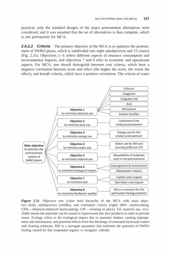
MULTICRITERIA ANALYSIS (MCA) 157

practical, only the standard designs of the major pretreatment alternatives wereconsidered, and it was assumed that the set of alternatives is thus complete, whichis one prerequisite for MCA.

2.6.2.2 Criteria The primary objective of the MCA is to optimize the pretreat-ment of SWRO plants, which is subdivided into eight subobjectives and 15 criteria(Fig. 2.31). Objectives 1–6 reflect different aspects of resource consumption andenvironmental impacts, and objectives 7 and 8 refer to economic and operationalaspects. For MCA, one should distinguish between cost criteria, which have anegative correlation between score and effect (the higher the score, the worse theeffect), and benefit criteria, which have a positive correlation. The criteria of water

Figure 2.31 Objective tree (value tree) hierarchy of the MCA with main objec-tive (left), subobjectives (middle), and evaluation criteria (right) (BW—backwashing,CEB—chemical-enhanced backwashing; CIP—cleaning in place). For material use, recy-clable means the materials can be reused or reprocessed into new products in order to preventwaste. Ecology refers to the ecological impact due to seawater intakes, causing impinge-ment and entrainment, and potential effects from the discharge of untreated backwash watersand cleaning solutions. SDI is a surrogate parameter that estimates the potential of SWROfouling caused by fine suspended organic or inorganic colloids.

158 ENVIRONMENTAL AND PERFORMANCE ASPECTS

quality and material recyclability were defined as benefits, while the remainingcriteria were all costs. Furthermore, the measurement scales of the criteria haveto be specified. Chemicals, land, energy, and water use as well as costs are ratioscales; i.e., the importance of a criterion is proportional to its value; for instance, atwofold higher energy demand is 2 times as bad (or two times as good for benefits).Ecological impact, material recyclability, and SDI are binary scales, which onlyindicate whether an effect is fulfilled (yes) or not fulfilled (no). A “yes” means abenefit in the case of material recyclability and SDI, and a cost in case of ecologicimpact.

2.6.2.3 Scores The four alternatives were scored on all 15 criteria, which canbe categorized into quantitative and qualitative criteria. In a first step, a databasewas established for all quantitative criteria through a literature review of operationaland pilot plant data and by personal communications with plant operators [Tables3–7 in Ref. 27]. In a second step, a value was selected which is considered to berepresentative of the standard design of an alternative (Table 2.19). It should bementioned that the compiled baseline data were quite variable, and that a single“true” value, which represents all operating conditions and feedwater qualities, doesnot exist. The selected values should therefore be understood as one scenario thatcan be refined and revised in the light of new or better data. To accommodate datavariability in the input data, a sensitivity analysis was carried out (Section 2.6.3.1)and two revised scenarios were considered (Section 2.6.3.2).

The MCA scores (Table 2.19) were calculated using the reference value, assum-ing a reference plant size with a capacity of 20,000 m3/d, and factoring in therespective flows and dosing points given in Figure 2.32. For example, the dos-ing concentration of 1 mg/L of chlorine is multiplied by the intake volumes of41,200 m3/d and 42,000 m3/d, which results in a daily load of 41 and 42 kg/d forconventional and UF pretreatment.

The only qualitative criteria are water quality (SDI), ecological impact, andrecyclability of materials. For SDI, a value of 3 is selected assuming that allpretreatment alternatives are running in good condition. An SDI range of 2–4is typically required by membrane manufacturers for conventional pretreatment.UF/MF has a reported SDI range of 0.8–2.2 [46,62,159,161–163], and beachwellshave reported values of 0.4–2.8 [Tables 3-7 in Ref. 27,31,160]. Concerning ecolog-ical impact, it is assumed that the open intakes of UF and conventional pretreatmentsystems have the potential to cause the impingement and entrainment of marineorganisms (“yes”), which is not the case for beachwell intakes (“no”). The othercriterion refers to the potential impact resulting from the discharge of untreatedbackwash waters from filters and UF/MF membranes and cleaning solutions in allthree pretreatment systems (“yes”). The alternative conventional II assumes that thebackwash waters are treated and that the sludge is deposited on land (“no” impact).For material use, only the UF/MF system was given a score of “no” assuming thatthe UF/MF membranes are currently not recycled, while it is being assumed thatthe filter media are recycled or have a beneficial reuse (“yes”).

A linear interval standardization function was used in this study, both for graph-ical evaluation and for the following MCA, to transform the different units of

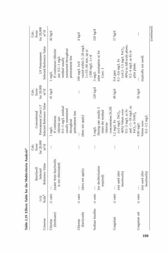
Tabl

e2.

19E

ffec

tsTa

ble

for

the

Mul

ticr

iter

iaA

naly

sisa C

alc.

Cal

c.C

alc.

Bea

chw

ell

Scor

eC

onve

ntio

nal

Scor

eSc

ore

�/⊕

Sele

cted

for

20,0

00Pr

etre

atm

ent

(Con

v.)

Icfo

r20

,000

UF

Pret

reat

men

tfo

r20

,000

Cri

teri

onSc

aleb

Ref

eren

ceV

alue

m3/d

Sele

cted

Ref

eren

ceV

alue

m3/d

Sele

cted

Ref

eren

ceV

alue

m3/d

Chl

orin

e(f

eedw

ater

)�

ratio

— (wat

erfr

ombe

achw

ells

isno

tch

lori

nate

d)

—1

mg/

LIf

cont

inuo

usch

lori

neus

e:0.

5–

1m

g/L

resi

dual

usua

llym

aint

aine

dth

roug

hout

pret

reat

men

tlin

e

41kg

/d1

mg/

LIf

cont

inuo

usch

lori

neus

e:0.

5–

1m

g/L

resi

dual

usua

llym

aint

aine

dth

roug

hout

pret

reat

men

tlin

e

42kg

/d

Chl

orin

e(b

ackw

ash)

�ra

tio— (d

oes

not

appl

y)—

— (doe

sno

tap

ply)

—10

0m

g/L

1x/d

vari

edw

ithin

5–

20m

g/L

1×/1

5–

60m

in,

upto

≤500

mg/

L1×

/d

4kg

/d

Sodi

umbi

sulfi

te�

ratio

— (no

dech

lori

natio

nre

quir

ed)

—3

mg/

LD

osin

gra

teus

ually

3tim

esth

ere

sidu

alch

lori

neco

ncen

trat

ion

[6,1

8]

120

kg/d

3m

g/L

sam

eas

sum

ptio

nas

for

Con

v.I

120

kg/d

Coa

gula

nt�

ratio

— (not

used

afte

rbe

achw

ells

)

—1.

2m

g/L

Fe(≡

3m

g/L

FeC

l 3,

40%

)V

alue

sw

ere

0.5

–3

mg/

Las

Fean

d<

1–

18m

g/L

asFe

Cl 3

orFe

SO4

49kg

/d0.

4pp

m0.

1–

0.6

mg/

LFe

(≡0.

3–

1.5

mg/

LFe

Cl 3

,40

%)

infu

ll-sc

ale

plan

ts,

0.2

–4

mg/

Las

Fein

pilo

tpl

ants

17kg

/d

Coa

gula

ntai

d�

ratio

— (not

used

afte

rbe

achw

ells

)

—0.

85m

g/L

Val

ues

wer

e0.

2–

1.5

mg/

L

35kg

/d— (typ

ical

lyno

tus

ed)

—

(con

tinu

ed)

159

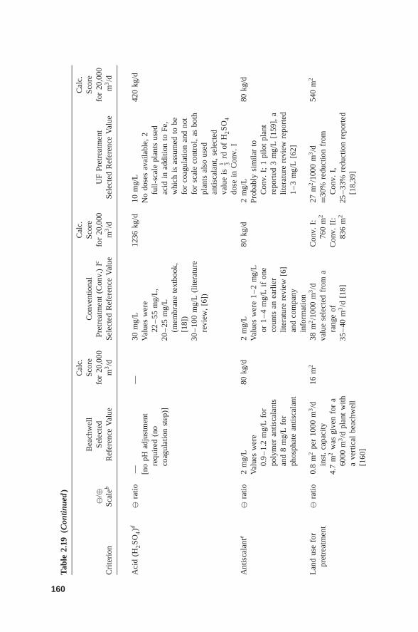
Tabl

e2.

19(C

ontin

ued

)

Cal

c.C

alc.

Cal

c.B

each

wel

lSc

ore

Con

vent

iona

lSc

ore

Scor

e�/

⊕Se

lect

edfo

r20

,000

Pret

reat

men

t(C

onv.

)Ic

for

20,0

00U

FPr

etre

atm

ent

for

20,0

00C

rite

rion

Scal

ebR

efer

ence

Val

uem

3/d

Sele

cted

Ref

eren

ceV

alue

m3/d

Sele

cted

Ref

eren

ceV

alue

m3/d

Aci

d(H

2SO

4)d

�ra

tio— [n

opH

adju

stm

ent

requ

ired

(no

coag

ulat

ion

step

)]

—30

mg/

LV

alue

sw

ere

22–

55m

g/L

,20

–25

mg/

L(m

embr

ane

text

book

,[1

8])

30–

100

mg/

L(l

itera

ture

revi

ew,

[6])

1236

kg/d

10m

g/L

No

dose

sav

aila

ble,

2fu

ll-sc

ale

plan

tsus

edac

idin

addi

tion

toFe

,w

hich

isas

sum

edto

befo

rco

agul

atio

nan

dno

tfo

rsc

ale

cont

rol,

asbo

thpl

ants

also

used

antis

cala

nt,

sele

cted

valu

eis

1 3rd

ofH

2SO

4do

sein

Con

v.I

420

kg/d

Ant

isca

lant

e�

ratio

2m

g/L

Val

ues

wer

e0.

9–

1.2

mg/

Lfo

rpo

lym

eran

tisca

lant

san

d8

mg/

Lfo

rph

osph

ate

antis

cala

nt

80kg

/d2

mg/

LV

alue

sw

ere

1–

2m

g/L

or1

–4

mg/

Lif

one

coun

tsan

earl

ier

liter

atur

ere

view

[6]

and

com

pany

info

rmat

ion

80kg

/d2

mg/

LPr

obab

lysi

mila

rto

Con

v.I;

1pi

lot

plan

tre

port

ed3

mg/

L[1

59],

alit

erat

ure

revi

ewre

port

ed1

–3

mg/

L[6

2]

80kg

/d

Lan

dus

efo

rpr

etre

atm

ent

�ra

tio0.

8m

2pe

r10

00m

3/d

inst

.ca

paci

ty4.

7m

2w

asgi

ven

for

a60

00m

3/d

plan

tw

itha

vert

ical

beac

hwel

l[1

60]

16m

238

m2/1

000

m3/d

valu

ese

lect

edfr

oma

rang

eof

35–

40m

3/d

[18]

Con

v.I:

760

m2

Con

v.II

:83

6m

2

27m

2/1

000

m3/d

≡30%

redu

ctio

nfr

omC

onv.

I,25

–33

%re

duct

ion

repo

rted

[18,

39]

540

m2

160

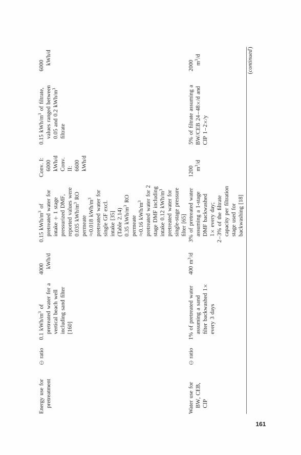
Ene

rgy

use

for

pret

reat

men

t�

ratio

0.1

kWh/

m3

ofpr

etre

ated

wat

erfo

ra

vert

ical

beac

hw

ell

incl

udin

gsa

ndfil

ter

[160

]

4000 kW

h/d

0.15

kWh/

m3

ofpr

etre

ated

wat

erfo

rin

take

+1

stag

epr

essu

rize

dD

MF,

repo

rted

valu

esw

ere

0.03

5kW

h/m

3R

Ope

rmea

te≈0

.018

kWh/

m3

pret

reat

edw

ater

for

sing

leG

Fex

cl.

inta

ke[3

5](T

able

2.14

)0.

35kW

h/m

3R

Ope

rmea

te≈0

.16

kWh/

m3

pret

reat

edw

ater

for

2st

age

DM

Fin

clud

ing

inta

ke0.

12kW

h/m

3

pret

reat

edw

ater

for

sing

le-s

tage

pres

sure

filte

r[6

5]

Con

v.I:

6000

kWh/

dC

onv.

II:

6600

kWh/

d

0.15

kWh/

m3

offil

trat

e,va

lues

rang

edbe

twee

n0.

05an

d0.

2kW

h/m

3

filtr

ate

6000 kW

h/d

Wat

erus

efo

rB

W,

CE

B,

CIP

�ra

tio1%

ofpr

etre

ated

wat

eras

sum

ing

asa

ndfil

ter

back

was

hed

1×ev

ery

3da

ys

400

m3/d

3%of

pret

reat

edw

ater

assu

min

ga

1-st

age

DM

Fba

ckw

ashe

d1×

ever

yda

y;2

–3%

ofth

efil

trat

eca

paci

type

rfil

trat

ion

stag

eus

edfo

rba

ckw

ashi

ng[1

8]

1200 m

3/d

5%of

filtr

ate

assu

min

ga

BW

/CE

B24

–48

×/d

and

CIP

1–

2×/y

2000 m

3/d

(con

tinu

ed)

161

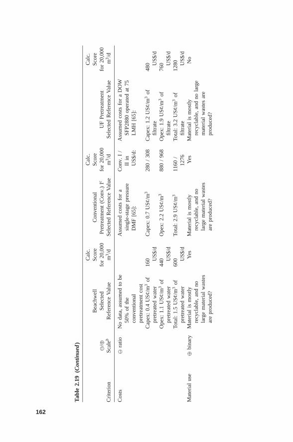
Tabl

e2.

19(C

ontin

ued

)

Cal

c.C

alc.

Cal

c.B

each

wel

lSc

ore

Con

vent

iona

lSc

ore

Scor

e�/

⊕Se

lect

edfo

r20

,000

Pret

reat

men

t(C

onv.

)Ic

for

20,0

00U

FPr

etre

atm

ent

for

20,0

00C

rite

rion

Scal

ebR

efer

ence

Val

uem

3/d

Sele

cted

Ref

eren

ceV

alue

m3/d

Sele

cted

Ref

eren

ceV

alue

m3/d

Cos

ts�

ratio

No

data

,as

sum

edto

be50

%of

the

conv

entio

nal

pret

reat

men

tco

st

Ass

umed

cost

sfo

ra

sing

le-s

tage

pres

sure

DM

F[6

5]:

Con

v.I

/II

inU

S$/d

:

Ass

umed

cost

sfo

ra

DO

WSF

P288

0op

erat

edat

75L

MH

[65]

:

Cap

ex:

0.4

US¢

/m3

ofpr

etre

ated

wat

er16

0 US$

/dC

apex

:0.

7U

S¢/m

328

0/

308

Cap

ex:

1.2

US¢

/m3

offil

trat

e48

0 US$

/dO

pex:

1.1

US¢

/m3

ofpr

etre

ated

wat

er44

0 US$

/dO

pex:

2.2

US¢

/m3

880

/96

8O

pex:

1.9

US¢

/m3

offil

trat

e76

0 US$

/dTo

tal:

1.5

US¢

/m3

ofpr

etre

ated

wat

er60

0 US$

/dTo

tal:

2.9

US¢

/m3

1160

/12

76To

tal:

3.2

US¢

/m3

offil

trat

e12

80 US$

/dM

ater

ial

use

⊕bi

nary

Mat

eria

lis

mos

tlyre

cycl

able

,an

dno

larg

em

ater

ial

was

tes

are

prod

uced

?

Yes

Mat

eria

lis

mos

tlyre

cycl

able

,an

dno

larg

em

ater

ial

was

tes

are

prod

uced

?

Yes

Mat

eria

lis

mos

tlyre

cycl

able

,an

dno

larg

em

ater

ial

was

tes

are

prod

uced

?

No

162

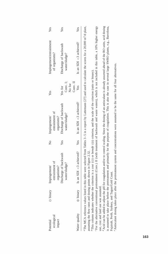
Pote

ntia

lec

olog

ical

impa

ct

�bi

nary

Impi

ngem

ent/

entr

ainm

ent

ofor

gani

sms?

No

Impi

ngem

ent/

entr

ainm

ent

ofor

gani

sms?

Yes

Impi

ngem

ent/e

ntra

inm

ent

ofor

gani

sms?

Yes

Dis

char

geof

back

was

hw

ater

/slu

dge?

Yes

Dis

char

geof

back

was

hw

ater

/slu

dge?

Yes

for

Con

v.I;

No

for

Con

v.II

Dis

char

geof

back

was

hw

ater

/slu

dge?

Yes

Wat

erqu

ality

⊕bi

nary

Isan

SDI<

3ac

hiev

ed?

Yes

Isan

SDI<

3ac

hiev

ed?

Yes

Isan

SDI

<3

achi

eved

?Y

es

aT

heM

CA

refe

renc

eva

lues

liste

din

this

tabl

ew

ere

sele

cted

from

Tabl

es3

–5

ina

repo

rtby

Lat

tem

ann

[27]

and

used

toca

lcul

ate

the

scor

esfo

ra

20,0

00m

3/d

plan

t,as

sum

ing

the

flow

rate

san

ddo

sing

poin

tssh

own

inFi

gure

2.32

.bT

his

colu

mn

indi

cate

sw

heth

erth

ecr

iteri

onis

aco

st(�

)or

bene

fit(⊕

)cr

iteri

on,

and

the

scal

eof

the

crite

rion

(rat

ioor

bina

ry).

cFo

rth

eal

tern

ativ

eco

nven

tiona

lpr

etre

atm

ent

(Con

v.)

II(w

ithtr

eatm

ent

ofba

ckw

ash

and

was

tew

ater

s),

whi

chis

not

incl

uded

inth

ista

ble,

a10

%hi

gher

ener

gyus

e,co

stan

dla

ndus

ew

asas

sum

ed.

dA

cid

can

bead

ded

toad

just

the

pHfo

rco

agul

atio

nan

d/or

toco

ntro

lsca

ling.

Sinc

eth

edo

sing

ofan

antis

cala

ntis

alre

ady

assu

med

ahea

dof

the

RO

units

,aci

ddo

sing

isas

sum

edto

take

plac

ebe

fore

the

pret

reat

men

tan

dpr

imar

ilyfo

rth

epu

rpos

eof

coag

ulat

ion.

Thi

sis

also

the

case

inse

vera

lla

rge

SWR

Opl

ants

,e.

g.,

Bar

celo

na,

Fuja

irah

,Pe

rth,

Sydn

ey,

and

Tug

un/G

old

Coa

st.

eA

ntis

cala

ntdo

sing

take

spl

ace

afte

rth

epr

etre

atm

ent

syst

eman

dco

ncen

trat

ions

wer

eas

sum

edto

beth

esa

me

for

all

four

alte

rnat

ives

.

163

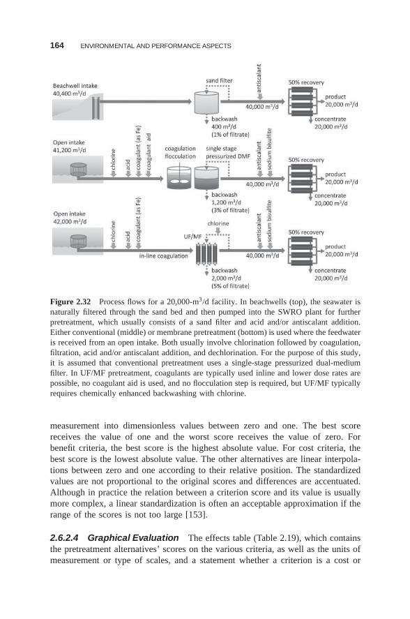
164 ENVIRONMENTAL AND PERFORMANCE ASPECTS

Figure 2.32 Process flows for a 20,000-m3/d facility. In beachwells (top), the seawater isnaturally filtered through the sand bed and then pumped into the SWRO plant for furtherpretreatment, which usually consists of a sand filter and acid and/or antiscalant addition.Either conventional (middle) or membrane pretreatment (bottom) is used where the feedwateris received from an open intake. Both usually involve chlorination followed by coagulation,filtration, acid and/or antiscalant addition, and dechlorination. For the purpose of this study,it is assumed that conventional pretreatment uses a single-stage pressurized dual-mediumfilter. In UF/MF pretreatment, coagulants are typically used inline and lower dose rates arepossible, no coagulant aid is used, and no flocculation step is required, but UF/MF typicallyrequires chemically enhanced backwashing with chlorine.

measurement into dimensionless values between zero and one. The best scorereceives the value of one and the worst score receives the value of zero. Forbenefit criteria, the best score is the highest absolute value. For cost criteria, thebest score is the lowest absolute value. The other alternatives are linear interpola-tions between zero and one according to their relative position. The standardizedvalues are not proportional to the original scores and differences are accentuated.Although in practice the relation between a criterion score and its value is usuallymore complex, a linear standardization is often an acceptable approximation if therange of the scores is not too large [153].

2.6.2.4 Graphical Evaluation The effects table (Table 2.19), which containsthe pretreatment alternatives’ scores on the various criteria, as well as the units ofmeasurement or type of scales, and a statement whether a criterion is a cost or

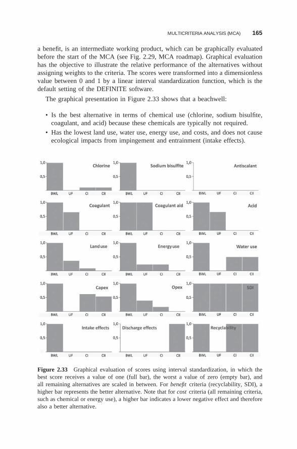
MULTICRITERIA ANALYSIS (MCA) 165

a benefit, is an intermediate working product, which can be graphically evaluatedbefore the start of the MCA (see Fig. 2.29, MCA roadmap). Graphical evaluationhas the objective to illustrate the relative performance of the alternatives withoutassigning weights to the criteria. The scores were transformed into a dimensionlessvalue between 0 and 1 by a linear interval standardization function, which is thedefault setting of the DEFINITE software.

The graphical presentation in Figure 2.33 shows that a beachwell:

• Is the best alternative in terms of chemical use (chlorine, sodium bisulfite,coagulant, and acid) because these chemicals are typically not required.

• Has the lowest land use, water use, energy use, and costs, and does not causeecological impacts from impingement and entrainment (intake effects).

Figure 2.33 Graphical evaluation of scores using interval standardization, in which thebest score receives a value of one (full bar), the worst a value of zero (empty bar), andall remaining alternatives are scaled in between. For benefit criteria (recyclability, SDI), ahigher bar represents the better alternative. Note that for cost criteria (all remaining criteria,such as chemical or energy use), a higher bar indicates a lower negative effect and thereforealso a better alternative.

166 ENVIRONMENTAL AND PERFORMANCE ASPECTS

• Is equal to the other pretreatment alternatives in terms of antiscalant use (allare assumed to use 2 mg/L), and with regard to SDI (all assumed to achievean SDI<3).

• Is equal to UF pretreatment with regard to the use of coagulant aid (none).

• Is equal to UF and conventional pretreatment I in terms of ecological impactfrom filter backwash waters if these are assumed to be discharged into thesea.

Accordingly, UF pretreatment:

• Is the second best alternative in terms of coagulant and acid use, but worstin terms of chlorine and sodium bisulfite use similar to conventional pretreat-ments I and II.

• Is the second best in terms of land use and operating costs (opex), but worstin water use and investment cost (capex).

• Is equal to conventional pretreatment I in terms of energy use.

• Is the worst alternative in terms of recyclability of materials and ecologicalimpact, if one assumes that the intake causes impingement and entrainment,and that the backwash waters from CEB and CIP are discharged withouttreatment.

Conventional pretreatments I and II:

• Are both equal to beachwells in terms of recyclability of materials.

• Are the second best alternatives in terms of water use and investment costas well as chlorine use (or second worst in the latter case, depending on theperspective), but the worst with regard to all other chemicals, as well as landuse and operating costs.

• Are the worst alternative in terms of ecological impact (the same as UF), ifone assumes that the intake causes impingement and entrainment, and that thebackwash waters from filters are discharged without treatment.

It is noteworthy that conventional pretreatment I is equal to UF in terms ofenergy use. Conventional II is the best alternative in terms of impacts caused bywaste water discharges, because a waste water treatment step has been included inthis alternative, but at the expense of additional energy and land requirements ofthis treatment step.

It can be concluded that beachwells are dominant over all other alternativesif one excludes the criterion of discharge effects. Dominance occurs when onealternative performs at least as well as another alternative on all criteria and strictlybetter than the other on at least one criterion [164]. In the considered scenario, itis assumed that the untreated discharge of backwash waters from sand filters isthe norm for small SWRO plants. However, three out of four beachwell plants[Table 3 in Ref. 27] reported a sludge treatment and landfill [31,32], and one plant

MULTICRITERIA ANALYSIS (MCA) 167

injected its waste water into a deep well [160]. Even if the backwash is dischargedwithout treatment, sludge amounts are small because of a low solids content inthe feedwater and no coagulant use, which results in a low backwash frequency ofonce every few days [32]. It is thus safe to assume that beachwells are dominantover the other alternatives. In practice, dominance of one alternative is rare, andthe extent to which it can support real decisions is correspondingly limited [164].

2.6.2.5 Weights An advantage of MCA is that subjective references abouta project are made explicit, which increases transparency of the decision-makingprocess and allows for a systematic evaluation of different stakeholder perspec-tives. The subjective references are expressed in the form of weights, which areattached to the decision-making criteria. In order to gather different perspectives,a questionnaire was prepared and sent to four groups of participants with differentperspectives in the area of seawater desalination:

• Environmental perspective (three responses): two persons with universitybackground, one person working in an international company that developsdesalination projects.

• Operators’ perspective (four responses): three plant managers and one personworking in a water authority overseeing desalination projects, all four rep-resenting plant capacities between 50,000 and 330,000 m3/d (two from theMediterranean region, two from Australia).

• Commercial perspective (five responses): two persons from an internationalcompany, three from commercial research institutes.

• Research perspective (six responses): six professors and researchers from uni-versities with expertise in process operation and optimization.

The questionnaire was sent to an equal number of stakeholders within eachgroup, but not all questionnaires were returned. The imbalance between the groups,with three responses for the environmental perspective and six responses for theresearch perspective, results in a different reliability of the weights derived foreach group; i.e., more responses in the group of environmental experts may haveresulted in a different set of weights.

The expected-value method was used to elicit the expert weights because it iseasy to explain and use. The aim was to have a single page with questions thatwould take no more than 10 min to answer. The main group of criteria [chemical,energy, water, and land use; material recyclability; water quality (SDI); costs; andecological impact (see value tree in Fig. 2.31)] were ranked from highest to lowestimportance, based on the personal background and experience of each participant.In addition, the single chemicals within the chemicals group were ranked. It waspossible to assign the same rank for two or more criteria if these were consideredequally important. Weights within a category are often given by experts, as inthis study. However, weights between categories that require tradeoffs betweenenvironmental, social, and economic aspects should be given by politicians with amandate for decision-making.

168 ENVIRONMENTAL AND PERFORMANCE ASPECTS

The average rank was calculated for each criterion within each group, and thecriteria were sorted accordingly in decreasing order of priority from rank 1 to thelowest rank. In this study, persons with an environmental and university back-ground considered ecologic impacts as most important, followed by energy use,chemical use, and water quality as lower ranks. In contrast, persons who representthe operators’ and commercial perspectives gave the highest priority to water qual-ity (SDI) and costs, followed by energy use, chemical use, and ecology as ranks3–4. The criteria of water use, land use and material use occupied the lowest ranksin all groups.

Concerning the different chemicals, all four groups considered coagulant use(rank 1 or 2) of high priority, which indicates that it is important for process oper-ations as well as in terms of environmental impact. Chlorine was also consideredvery important from an environmental perspective (rank 1), but less important fromall other perspectives (rank 3 or 4). Antiscalant and acid are considered moder-ately important (ranks 2–4) in all groups except for the university group, whichconsiders antiscalant as most important (rank 1) and acid as least important (rank6). The criteria of coagulant aid and sodium bisulfite (SBS) ranked lowest in allgroups (ranks 3–5).

The expected-value method converts the rank order of the criteria (c1 ≥ c2 ≥ c3)into a set of quantitative weights (w1 ≥ w2 ≥ w3) by the following algorithm (seeRef. 165, after Ref. 166):

wk = 1

K

K∑i=k

1

i(2.1)

where K represents = the number of criteria. The sum of all quantitative weightsis 1. When two or more criteria are considered equally important (i.e., have tiedranks), the weight given to each criterion is the average weight for the tied ranks.For example, the responses from the university group led to the following rankingand weights: ecology (w1 = 0.340) ≥ chemicals use (w2 = 0.215) ≥ energy use= water quality (w3,4 = 0.131) ≥ costs (w5 = 0.079) ≥ land use (w6 = 0.054) ≥material use (w7 = 0.033) ≥ water use (w8 = 0.016). The higher the importance,the higher the weight of the criterion and the greater the difference between thenext smaller criterion. The expected-value method therefore emphasizes the moreimportant criteria, and gives only little weight to the less important criteria. Forexample, ecology accounts for 34% of the total weight, followed by chemical usewith 21%, whereas the two least important criteria account for less than 4% and2%.

The weights derived for the main group are first-level weights as shown inthe pie diagrams in Figure 2.34. Second-level weights were established for thesingle chemicals by expert ranking and the expected-value method for each group(see Ref. 27 for details). The first-level weights are multiplied by the second-levelweights to derive the overall weight of a criterion. The criteria capex and opex inthe main group costs were considered equally important, as were the intake anddischarge effects in the main group ecologic impact .

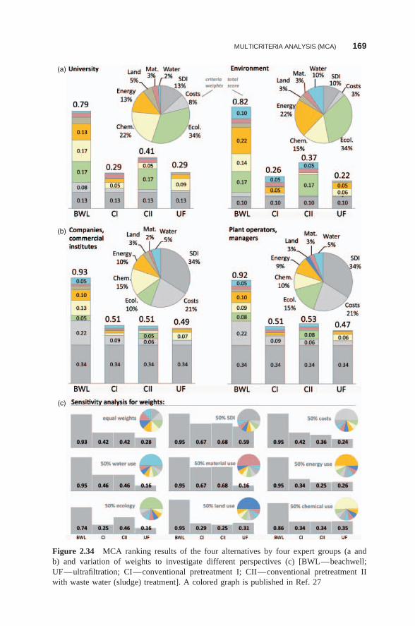
MULTICRITERIA ANALYSIS (MCA) 169

(a)

(b)

(c)

Figure 2.34 MCA ranking results of the four alternatives by four expert groups (a andb) and variation of weights to investigate different perspectives (c) [BWL—beachwell;UF—ultrafiltration; CI—conventional pretreatment I; CII—conventional pretreatment IIwith waste water (sludge) treatment]. A colored graph is published in Ref. 27

170 ENVIRONMENTAL AND PERFORMANCE ASPECTS

2.6.3 Ranking Results

The synthesis of the weights and scores into a ranking is a computational step thatdepends on the selected MCA model. Weighted summation, which was used inthis study, is a compensatory aggregation method, in which poor performance inany one criterion can be compensated for by overall good performance in the othercriteria. The overall performance of an alternative is the sum of the alternative’sscore for each criterion multiplied by the weight given to that criterion [153]:

Total score aj =N∑

i=1

wi · sij (2.2)

where A = set of alternatives with aj (j = 1, . . . , M )

C = set of criteria with ci (i = 1, . . . , N )

sij = standardized score of alternative aj for effect ciwi = weight of effect ci

The ranking results for the four groups are presented in Figure 2.34. The outcomein which beachwells are also the favored option from different perspectives was tobe expected, because the alternative was already found to be dominant by graphicalevaluation of the effects table. The analysis, however, shows that the ranking isgenerally similar in the two groups that represent plant operators and companies,and in the two groups that represent university and environmental backgrounds.Beachwells obtained the best result in the company and operators groups (totalscores of 0.93 and 0.92), followed by conventional pretreatment (0.51, 0.53) and UFpretreatment (0.49, 0.47) as ranks 2–4 with only marginal differences. Beachwellsreached a lower total score in the university and environment groups (0.79, 0.82),followed in some distance by conventional pretreatment II with sludge treatmentas the second best alternative (0.41, 0.37), followed by conventional pretreatment Iand UF with small differences in total scores as ranks 3 and 4 (0.22–0.29).

2.6.3.1 Sensitivity Analysis The sensitivity of the ranking to changes inweights and scores was investigated. First, the weights of the main criteria groupwere systematically altered. Weights were distributed equally (12.5%) between cri-teria and then successively changed to 50% for each criterion to emphasize thatperspective, while the remaining 50% were equally distributed among the remain-ing seven criteria (7% each). The subcriteria (in chemicals, costs, ecology) weregiven equal weight within their groups (Fig. 2.34c bottom). The same analysis wascarried out for the expert weights while maintaining the original weights withinthe subgroups.

In the following list, only the changes in ranks 2–4 are summarized, as theranking of beachwells is not sensitive to changes in weights. The sensitivity analysisof weights, with results shown in Figure 2.34c (bottom), shows that:

• Conventional pretreatment I and II rank second, with similar or equal scores,followed by UF as the last rank, if equal weights are allocated to the main

MULTICRITERIA ANALYSIS (MCA) 171

criteria, and if 50% is allocated to the criteria water quality (SDI), water use,or material use.

• Conventional pretreatment I is the second best alternative if 50% weight isgiven to cost or energy use, and conventional pretreatment II is the secondbest alternative if 50% weight is given to ecological impact.

• UF ranks last and only becomes second if 50% weight is allocated to thecriteria chemical and land use, or third if 50% weight is given to energyuse. However, the differences are marginal between UF and the next loweralternative in all three cases.

Then the effects of score uncertainty on the ranking was analyzed under theassumptions that the scores could be 50% or 100% higher or lower than the selectedscores listed in Table 2.19. The program calculates the probability that an alternativeranks at a certain position on the basis of the specified uncertainty values. Theprobability is calculated from 2000 repetitive outcomes, in which scores are drawnat random from the specified uncertainty limits, assuming a normal distributionfunction.

Figure 2.35 shows that beachwell has a high probability of 88–100% to rankat first position in all groups, even given a high uncertainty in the scores. In allgroups, conventional pretreatment I or II is likely to rank second. In the universityand environment groups, conventional pretreatment II is most likely (69–92%) atthe second rank. UF has a high probability of ranking at third or fourth position.

2.6.3.2 Revised Scenarios The decision problem was revised in two con-secutive scenarios, in which both the set of alternatives and the number of criteriawere changed.

Scenario 1: Comparison with Existing Plants Case studies with different intakeand pretreatment systems were used to investigate whether these produce the sameranking results as the selected reference values in the previous MCA. As the ref-erence values had been chosen independently for each criterion from a wide rangeof literature values, it is possible that the overall result gives a distorted imageof the operating conditions of existing plants. For example, chlorine use is stilloften reported as continuously in the literature, whereas it is, in fact, used intermit-tently in many plants. Moreover, beachwells are generally assumed to have a lowenergy demand in the literature; however, the reported energy demand of a Neodrenbeachwell intake was slightly higher than that of an identical plant in the same loca-tion with an open intake [31]. A third example is that many of the more recentlycommissioned conventional plants have a sludge–waste water treatment system.

The revised scenario has the objective to compare the “hypothetical textbookvalues” to real plant data. The intake and pretreatment alternatives included thetwin plants at San Pedro del Pinatar, Spain [Table 4 in Ref. 27], one of whichhas a Neodren beachwell followed by a sand filter and the other, a conventionalpretreatment with a two-stage dual-medium filter. A second conventional pretreat-ment system was included, assuming a single gravity filter as in the Tugun plant in

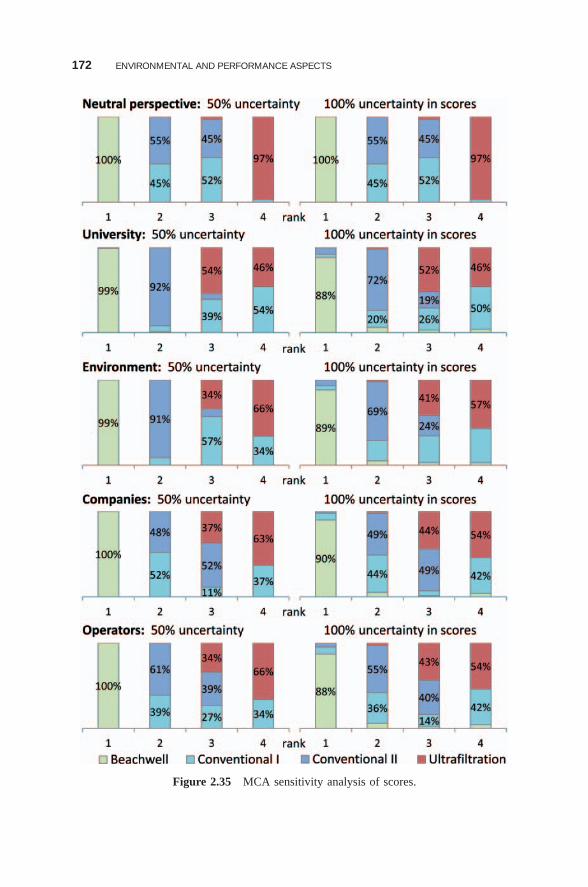
172 ENVIRONMENTAL AND PERFORMANCE ASPECTS

Figure 2.35 MCA sensitivity analysis of scores.

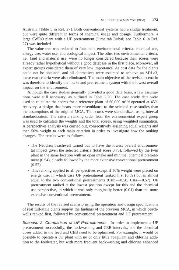
MULTICRITERIA ANALYSIS (MCA) 173

Australia [Table 5 in Ref. 27]. Both conventional systems had a sludge treatment,but were quite different in terms of chemical usage and dosage. Furthermore, alarge SWRO plant with a UF pretreatment (Jumeirah Dubai; see Table 6 in Ref.27) was included.

The value tree was reduced to four main environmental criteria: chemical use,energy use, water use, and ecological impact. The other two environmental criteria,i.e., land and material use, were no longer considered because their scores werealready rather hypothetical without a good database in the first place. Moreover, allexpert groups considered them of very low importance. As cost data for the plantscould not be obtained, and all alternatives were assumed to achieve an SDI<3,these two criteria were also eliminated. The main objective of the revised scenariowas therefore to identify the intake and pretreatment system with the lowest overallimpact on the environment.

Although the case studies generally provided a good data basis, a few assump-tions were still necessary, as outlined in Table 2.20. The case study data wereused to calculate the scores for a reference plant of 60,000 m3/d operated at 45%recovery, a design that bears more resemblance to the selected case studies thanthe assumptions of the original MCA. The scores were standardized using intervalstandardization. The criteria ranking order from the environmental expert groupwas used to calculate the weights and the total scores, using weighted summation.A perspectives analysis was carried out, consecutively assigning equal weights andthen 50% weight to each main criterion in order to investigate how the rankingchanges. The results were as follows:

• The Neodren beachwell turned out to have the lowest overall environmen-tal impact given the selected criteria (total score 0.73), followed by the twinplant in the same location with an open intake and minimal chemical pretreat-ment (0.54), closely followed by the more extensive conventional pretreatment(0.52).

• This ranking applied to all perspectives except if 50% weight were placed onenergy use, in which case UF pretreatment ranked first (0.59) but is almostequal to the two conventional pretreatments (CIIb—0.58, CIIa—0.57). UFpretreatment ranked at the lowest position except for this and the chemicaluse perspective, in which it was only marginally better (0.01) than the moreextensive conventional pretreatment.

The results of the revised scenario using the operation and design specificationsof real full-scale plants support the findings of the previous MCA, in which beach-wells ranked first, followed by conventional pretreatment and UF pretreatment.

Scenario 2: Comparison of UF Pretreatments In order to implement a UFpretreatment successfully, the backwashing and CEB intervals, and the chemicaldoses added to the feed and CEB need to be optimized. For example, it would bepossible to operate a UF plant with no or only little coagulant and chlorine addi-tion to the feedwater, but with more frequent backwashing and chlorine enhanced

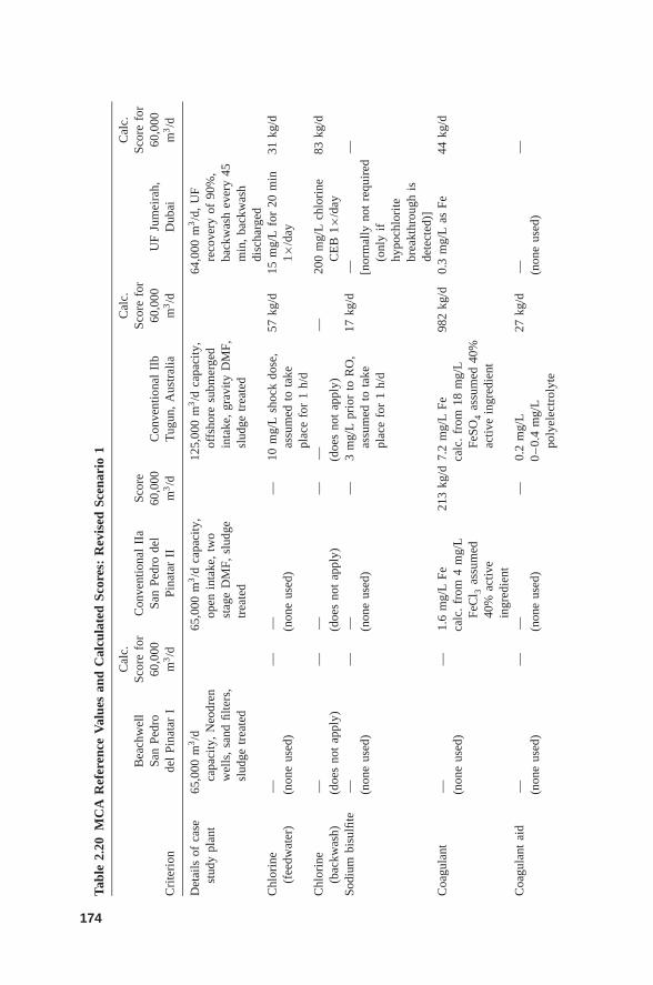
Tabl

e2.

20M

CA

Ref

eren

ceV

alue

san

dC

alcu

late

dSc

ores

:R

evis

edSc

enar

io1

Cal

c.C

alc.

Cal

c.B

each

wel

lSc

ore

for

Con

vent

iona

lII

aSc

ore

Scor

efo

rSc

ore

for

San

Pedr

o60

,000

San

Pedr

ode

l60

,000

Con

vent

iona

lII

b60

,000

UF

Jum

eira

h,60

,000

Cri

teri

onde

lPi

nata

rI

m3/d

Pina

tar

IIm

3/d

Tug

un,

Aus

tral

iam

3/d

Dub

aim

3/d

Det

ails

ofca

sest

udy

plan

t65

,000

m3/d

capa

city

,N

eodr

enw

ells

,sa

ndfil

ters

,sl

udge

trea

ted

65,0

00m

3/d

capa

city

,op

enin

take

,tw

ost

age

DM

F,sl

udge

trea

ted

125,

000

m3/d

capa

city

,of

fsho

resu

bmer

ged

inta

ke,

grav

ityD

MF,

slud

getr

eate

d

64,0

00m

3/d

,U

Fre

cove

ryof

90%

,ba

ckw

ash

ever

y45

min

,ba

ckw

ash

disc

harg

edC

hlor

ine

(fee

dwat

er)

— (non

eus

ed)

—— (n

one

used

)—

10m

g/L

shoc

kdo

se,

assu

med

tota

kepl

ace

for

1h/

d

57kg

/d15

mg/

Lfo

r20

min

1×/d

ay31

kg/d

Chl

orin

e(b

ackw

ash)

— (doe

sno

tap

ply)

—— (d

oes

not

appl

y)—

— (doe

sno

tap

ply)

—20

0m

g/L

chlo

rine

CE

B1×

/day

83kg

/d

Sodi

umbi

sulfi

te— (n

one

used

)—

— (non

eus

ed)

—3

mg/

Lpr

ior

toR

O,

assu

med

tota

kepl

ace

for

1h/

d

17kg

/d— [n

orm

ally

not

requ

ired

(onl

yif

hypo

chlo

rite

brea

kthr

ough

isde

tect

ed)]

—

Coa

gula

nt— (n

one

used

)—

1.6

mg/

LFe

calc

.fr

om4

mg/

LFe

Cl 3

assu

med

40%

activ

ein

gred

ient

213

kg/d

7.2

mg/

LFe

calc

.fr

om18

mg/

LFe

SO4

assu

med

40%

activ

ein

gred

ient

982

kg/d

0.3

mg/

Las

Fe44

kg/d

Coa

gula

ntai

d— (n

one

used

)—

— (non

eus

ed)

—0.

2m

g/L

0–

0.4

mg/

Lpo

lyel

ectr

olyt

e

27kg

/d— (n

one

used

)—

174

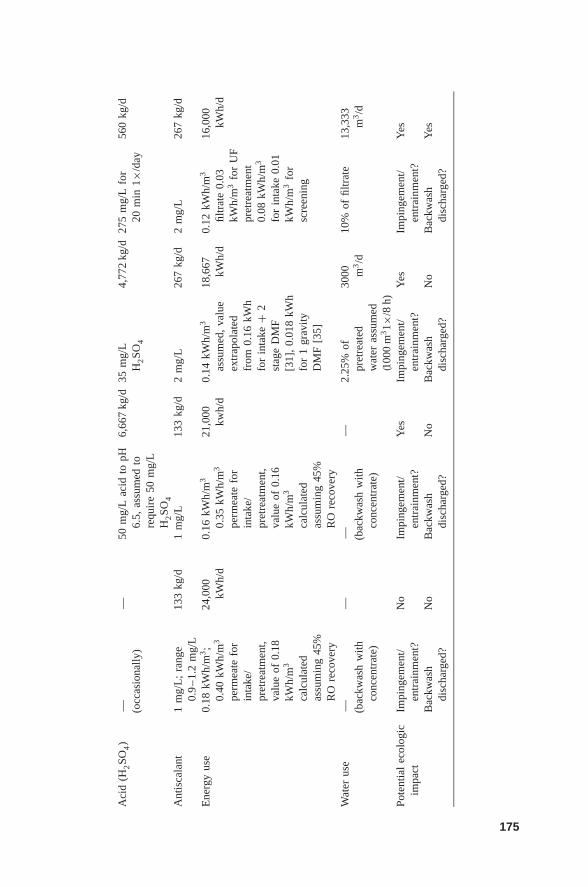
Aci

d(H

2SO

4)

— (occ

asio

nally

)—

50m

g/L

acid

topH

6.5,

assu

med

tore

quir

e50

mg/

LH

2SO

4

6,66

7kg

/d35

mg/

LH

2SO

4

4,77

2kg

/d27

5m

g/L

for

20m

in1×

/day

560

kg/d

Ant

isca

lant

1m

g/L

;ra

nge

0.9

–1.

2m

g/L

133

kg/d

1m

g/L

133

kg/d

2m

g/L

267

kg/d

2m

g/L

267

kg/d

Ene

rgy

use

0.18

kWh/

m3;

0.40

kWh/

m3

perm

eate

for

inta

ke/

pret

reat

men

t,va

lue

of0.

18kW

h/m

3

calc

ulat

edas

sum

ing

45%

RO

reco

very

24,0

00kW

h/d

0.16

kWh/

m3

0.35

kWh/

m3

perm

eate

for

inta

ke/

pret

reat

men

t,va

lue

of0.

16kW

h/m

3

calc

ulat

edas

sum

ing

45%

RO

reco

very

21,0

00kw

h/d

0.14

kWh/

m3

assu

med

,va

lue

extr

apol

ated

from

0.16

kWh

for

inta

ke+

2st

age

DM

F[3

1],

0.01

8kW

hfo

r1

grav

ityD

MF

[35]

18,6

67kW

h/d

0.12

kWh/

m3

filtr

ate

0.03

kWh/

m3

for

UF

pret

reat

men

t0.

08kW

h/m

3

for

inta

ke0.

01kW

h/m

3fo

rsc

reen

ing

16,0

00kW

h/d

Wat

erus

e— (b

ackw

ash

with

conc

entr

ate)

—— (b

ackw

ash

with

conc

entr

ate)

—2.

25%

ofpr

etre

ated

wat

eras

sum

ed(1

000

m31×

/8h)

3000 m

3/d

10%

offil

trat

e13

,333

m3/d

Pote

ntia

lec

olog

icim

pact

Impi

ngem

ent/

entr

ainm

ent?

No

Impi

ngem

ent/

entr

ainm

ent?

Yes

Impi

ngem

ent/

entr

ainm

ent?

Yes

Impi

ngem

ent/

entr

ainm

ent?

Yes

Bac

kwas

hdi

scha

rged

?N

oB

ackw

ash

disc

harg

ed?

No

Bac

kwas

hdi

scha

rged

?N

oB

ackw

ash

disc

harg

ed?

Yes

175

176 ENVIRONMENTAL AND PERFORMANCE ASPECTS

backwashing. Another factor in this optimization problem is energy use. The TMPincreases when deposits build up on the UF membranes, and backwashing is usu-ally carried out at 2–4 times the filtration flow. Both cause an increase in energydemand. Moreover, some UF manufacturers employ an air scrub, in which pressur-ized air is introduced with the backwash water. This improves the cleaning process,possibly reducing chemical but increasing energy demand.

The hypothesis was that different UF pretreatment systems optimize their chem-ical use, energy use, CEB, and backwashing intervals differently. The objective wasto compare different membrane types in terms of chemical, energy, and water use.Four different UF membranes were considered as alternatives; two are pressur-ized inside-out UF membranes (Norit, Inge), and two are pressurized outside-inmembranes (Dow, Pall). A reference value was selected, based on an inventory offull-scale plants, pilot plants, and general manufacturer information, and used tocalculate the scores. Preference was given to data from full-scale plants, if available(Table 2.22).

The value tree was further reduced from scenario 1, eliminating the criteriacoagulant aid, acid (none used), and antiscalant. Antiscalant is usually added afterthe filtration stage and does not provide meaningful information about the differentUF systems. Acid can be used in SWRO to lower the risk of scaling on the ROmembranes and is not related to the filtration step in that case. Acid can also be usedto control the pH during coagulation before the filtration step (as assumed in theprevious MCA). However, most UF pretreatment systems use inline coagulation,for which acid use is not anticipated here to reduce complexity. The ecologic impactcriterion was eliminated as all UF systems alike are assumed to operate on openintakes and to discharge their backwash waters without treatment. The remainingcriteria were chlorine, SBS, and coagulant addition to the feedwater, chlorine usein backwashing, energy, and water use.

As in scenario 1, interval standardization and weighted summation was usedto calculate the scores for a reference plant size of 60,000 m3/d (Table 2.21).A perspectives analysis of the weights was carried out assuming (1) the originalranking of the environmental group; (2) equal weights for all main criteria; and(3) 66% weight allocated to energy, chemicals, or water use. The results were asfollows:

• The inside-out UF systems (Norit, Inge) ranked at first and second positionsand the outside-in systems (Dow, Pall) at third and fourth positions in allperspectives, except when 50% weight was given to water use. In that case,Pall ranked first, followed by Inge, Dow, and Norit in final position. As PVDFin outside feed formats (Dow and Pall membranes) allows the use of air scour,which reduces water consumption for backwashing, one would have expectedDow to score better. However, the same water use (7%) has been reported forbackwashing and CIP of Dow and Inge systems (Table 2.22).

• Norit ranked first for the environmental group’s perspective and the energyuse perspective, while Inge ranked first for the equal weight and chemicalsperspectives.

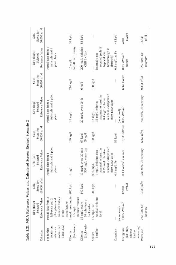
Tabl

e2.

21M

CA

Ref

eren

ceV

alue

san

dC

alcu

late

dSc

ores

:R

evis

edSc

enar

io2

UFa

(Dow

)C

alc.

UFb

(Pal

l)C

alc.

UFc

(Ing

e)C

alc.

UFd

(Nor

it)C

alc.

Sele

cted

Scor

efo

rSe

lect

edSc

ore

for

Sele

cted

Scor

efo

rSe

lect

edSc

ore

for

Cri

teri

onR

efer

ence

Val

ue60

,000

m3/d

Ref

eren

ceV

alue

60,0

00m

3/d

Ref

eren

ceV

alue

60,0

00m

3/d

Ref

eren

ceV

alue

60,0

00m

3/d

For

furt

her

deta

ilson

refe

renc

eva

lues

,se

eTa

ble

2.22

Part

ial

data

from

3fu

ll-sc

ale

and

2pi

lot

plan

tsan

dem

piri

cal

valu

esof

the

man

ufac

ture

r

Part

ial

data

from

1fu

ll-sc

ale

and

3pi

lot

plan

ts

Part

ial

data

from

1fu

ll-sc

ale

and

1pi

lot

plan

t

Part

ial

data

from

3fu

ll-sc

ale

and

4pi

lot

plan

ts

Chl

orin

e(f

eedw

ater

)2

mg/

Lre

sulti

ngin

0.5

mg/

Lch

lori

nere

sidu

al

285

kg/d

1m

g/L

140

kg/d

1.5

mg/

L21

4kg

/d15

mg/

Lfo

r20

min

1×/d

ay31

kg/d

Chl

orin

e(b

ackw

ash)

15m

g/L

ever

y60

min

(eve

ryba

ckw

ash)

140

kg/d

10m

g/L

ever

y30

min

500

mg/

Lev

ery

day

67kg

/d69

kg/d

20m

g/L

ever

y24

h6

kg/d

200

mg/

Lch

lori

neC

EB

1×/d

ay83

kg/d

Sodi

umbi

sulfi

te1.

5m

g/L

3×re

sidu

alch

lori

nele

vel

200

kg/d

0.75

mg/

L1

mg/

Lch

lori

nedo

seas

sum

edto

resu

ltin

0.25

mg/

Lch

lori

nere

sidu

al,

extr

apol

ated

from

Dow

valu

e

100

kg/d

1.2

mg/

L1.

5m

g/L

chlo

rine

assu

med

tore

sult

in0.

4m

g/L

chlo

rine

resi

dual

,ex

trap

olat

edfr

omD

owva

lue

150

kg/d

— [nor

mal

lyno

tre

quir

ed(o

nly

ifhy

poch

lori

tebr

eakt

hrou

ghis

dete

cted

)]

—

Coa

gula

nt— (n

one

used

)—

0.4

mg/

LFe

56kg

/d— (n

one

used

)—

0.3

mg/

Las

Fe44

kg/d

Ene

rgy

use

(UF

only

,w

ithou

tin

take

/sc

reen

ing)

0.09

5kW

h/m

312

,000

kWh/

d0.

1kW

h/m

3as

sum

ed13

,333

kWh/

d0.

05kW

h/m

366

67kW

h/d

0.03

kWh/

m3

filtr

ate

4000 kW

h/d

Wat

erus

e7%

;93

%U

Fre

cove

ry9,

333

m3/d

5%;

95%

UF

reco

very

6667

m3/d

7%;

93%

UF

reco

very

9,33

3m

3/d

10%

;90

%U

Fre

cove

ry13

,333

m3/d

177

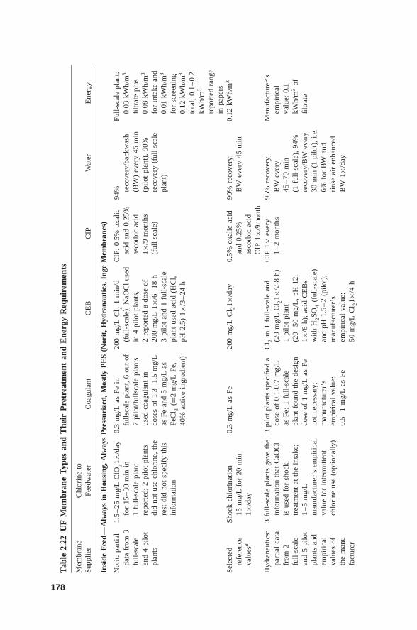
Tabl

e2.

22U

FM

embr

ane

Typ

esan

dT

heir

Pre

trea

tmen

tan

dE

nerg

yR

equi

rem

ents

Mem

bran

eC

hlor

ine

toSu

pplie

rFe

edw

ater

Coa

gula

ntC

EB

CIP

Wat

erE

nerg

y

Insi

deF

eed

—A

lway

sin

Hou

sing

,A

lway

sP

ress

uriz

ed,

Mos

tly

PE

S(N

orit

,H

ydra

naut

ics,

Inge

Mem

bran

es)

Nor

it:pa

rtia

lda

tafr

om3

full-

scal

ean

d4

pilo

tpl

ants

1.5

–25

mg/

LC

lO21×

/day

for

15–

30m

inin

1fu

ll-sc

ale

plan

tre

port

ed;

2pi

lot

plan

tsdi

dno

tus

ech

lori

ne,

the

rest

did

not

spec

ify

this

info

rmat

ion

0.3

mg/

Las

Fein

fulls

cale

plan

t,6

out

of7

pilo

t/ful

lsca

lepl

ants

used

coag

ulan

tin

dose

sof

1.3

–1.

5m

g/L

asFe

and

5m

g/L

asFe

Cl 3

(≡2

mg/

LFe

,40

%ac

tive

ingr

edie

nt)

200

mg/

LC

l 21

min

/d(f

ull-

scal

e),

NaO

Cl

used

in4

pilo

tpl

ants

,2

repo

rted

ado

seof

200

mg/

L1×

/6–

18h

3pi

lot

and

1fu

ll-sc

ale

plan

tus

edac

id(H

Cl,

pH2.

5)1×

/3–

24h

CIP

:0.

5%ox

alic

acid

and

0.25

%as

corb

icac

id1×

/9m

onth

s(f

ull-

scal

e)

94% re

cove

ry/b

ackw

ash

(BW

)ev

ery

45m

in(p

ilot

plan

t),

90%

reco

very

(ful

l-sc

ale

plan

t)

Full-

scal

epl

ant:

0.03

kWh/

m3

filtr

ate

plus

0.08

kWh/

m3

for

inta

kean

d0.

01kW

h/m

3

for

scre

enin

g0.

12kW

h/m

3

tota

l;0.

1–

0.2

kWh/

m3

repo

rted

rang

ein

pape

rsSe

lect

edre

fere

nce

valu

esa

Shoc

kch

lori

natio

n15

mg/

Lfo

r20

min

1×/d

ay

0.3

mg/

Las

Fe20

0m

g/L

Cl 2

1×/d

ay0.

5%ox

alic

acid

and

0.25

%as

corb

icac

idC

IP1×

/9m

onth

90%

reco

very

;B

Wev

ery

45m

in0.

12kW

h/m

3

Hyd

rana

utic

s:pa

rtia

lda

tafr

om2

full-

scal

ean

d5

pilo

tpl

ants

and

empi

rica

lva

lues

ofth

em

anu-

fact

urer

3fu

ll-sc

ale

plan

tsga

veth

ein

form

atio

nth

atC

aOC

lis

used

for

shoc

ktr

eatm

ent

atth

ein

take

;1

–5

mg/

Lm

anuf

actu

rer’

sem

piri

cal

valu

efo

rin

term

itten

tch

lori

neus

e(o

ptio

nally

)

3pi

lot

plan

tssp

ecifi

eda

dose

of0.

1-0.

7m

g/L

asFe

;1

full-

scal

epl

ant

foun

dth

ede

sign

dose

of1

mg/

Las

Feno

tne

cess

ary;

man

ufac

ture

r’s

empi

rica

lva

lue:

0.5

–1

mg/

Las

Fe

Cl 2

in1

full-

scal

ean

d(2

0m

g/L

Cl 2

1×/2

-8h)

1pi

lot

plan

t(2

0–

50m

g/L

,pH

12,

1×/6

h);

acid

CE

Bs

with

H2SO

4(f

ull-

scal

e)an

dpH

1.5

–2

(pilo

t);

man

ufac

ture

r’s

empi

rica

lva

lue:

50m

g/L

Cl 2

1×/4

h

CIP

1×ev

ery

1–

2m

onth

s95

%re

cove

ry;

BW

ever

y45

–70

min

(1fu

ll-sc

ale)

,94

%re

cove

ry/B

Wev

ery

30m

in(1

pilo

t),

i.e.

6%fo

rB

Wan

dri

nse

air

enha

nced

BW

1×/d

ay

Man

ufac

ture

r’s

empi

rica

lva

lue:

0.1

kWh/

m3

offil

trat

e

178

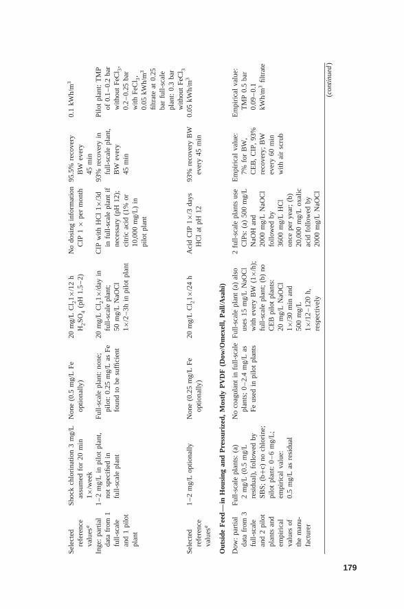
Sele

cted

refe

renc

eva

lues

a

Shoc

kch

lori

natio

n3

mg/

Las

sum

edfo

r20

min

1×/w

eek

Non

e(0

.5m

g/L

Feop

tiona

lly)

20m

g/L

Cl 2

1×/1

2h

H2SO

4(p

H1.

5–

2)N

odo

sing

info

rmat

ion

CIP

1×

per

mon

th95

.5%

reco

very

BW

ever

y45

min

0.1

kWh/

m3

Inge

:pa

rtia

lda

tafr

om1

full-

scal

ean

d1

pilo

tpl

ant

1–

2m

g/L

inpi

lot

plan

t,no

tsp

ecifi

edin

full-

scal

epl

ant

Full-

scal

epl

ant:

none

;pi

lot:

0.25

mg/

Las

Fefo

und

tobe

suffi

cien

t

20m

g/L

Cl 2

1×/d

ayin

full-

scal

epl

ant;

50m

g/L

NaO

Cl

1×/2

–3h

inpi

lot

plan

t

CIP

with

HC

l1×

/3d

infu

ll-sc

ale

plan

tif

nece

ssar

y(p

H12

);ci

tric

acid

(1%

or10

,000

mg/

L)

inpi

lot

plan

t

93%

reco

very

infu

ll-sc

ale

plan

t,B

Wev

ery

45m

in

Pilo

tpl

ant:

TM

Pof

0.1

–0.

2ba

rw

ithou

tFe

Cl 3

,0.

2–

0.25

bar

with

FeC

l 3,

0.05

kWh/

m3

filtr

ate

at0.

25ba

rfu

ll-sc

ale

plan

t:0.

3ba

rw

ithou

tFe

Cl 3

Sele

cted

refe

renc

eva

lues

a

1–

2m

g/L

optio

nally

Non

e(0

.25

mg/

LFe

optio

nally

)20

mg/

LC

l 21×

/24

hA

cid

CIP

1×/3

days

HC

lat

pH12

93%

reco

very

BW

ever

y45

min

0.05

kWh/

m3

Out

side

Fee

d—

inH

ousi

ngan

dP

ress

uriz

ed,

Mos

tly

PV

DF

(Dow

/Om

exel

l,P

all/A

sahi

)

Dow

:pa

rtia

lda

tafr

om3

full-

scal

ean

d2

pilo

tpl

ants

and

empi

rica

lva

lues

ofth

em

anu-

fact

urer

Full-

scal

epl

ants

:(a

)2

mg/

L(0

.5m

g/L

resi

dual

),fo

llow

edby

SBS;

(b+c

)no

chlo

rine

;pi

lot

plan

t:0

–6

mg/

L;

empi

rica

lva

lue:

0.5

mg/

Las

resi

dual

No

coag

ulan

tin

full-

scal

epl

ants

;0

–2.

4m

g/L

asFe

used

inpi

lot

plan

ts

Full-

scal

epl

ant

(a)

also

uses

15m

g/L

NaO

Cl

with

ever

yB

W(1

×/h)

;fu

ll-sc

ale

plan

t;(b

)no

CE

Bpi

lot

plan

ts:

20m

g/L

NaO

Cl

1×/3

0m

inan

d50

0m

g/L

1×/1

2–

120

h,re

spec

tivel

y

2fu

ll-sc

ale

plan

tsus

eC

IPs:

(a)

500

mg/

LN

aOH

and

2000

mg/

LN

aOC

lfo

llow

edby

3600

mg/

LH

Cl

once

per

year

;(b

)20

,000

mg/

Lox

alic

acid

follo

wed

by20

00m

g/L

NaO

Cl

Em

piri

cal

valu

e:7%

for

BW

,C

EB

,C

IP,

93%

reco

very

;B

Wev

ery

60m

inw

ithai

rsc

rub

Em

piri

cal

valu

e:T

MP

0.5

bar

0.09

–0.

1kW

h/m

3fil

trat

e

(con

tinu

ed)

179

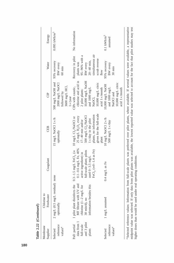
Tabl

e2.

22(C

ontin

ued

)

Mem

bran

eC

hlor

ine

toSu

pplie

rFe

edw

ater

Coa

gula

ntC

EB

CIP

Wat

erE

nerg

y

Sele

cted

refe

renc

eva

lues

a

2m

g/L

(0.5

mg/

Lre

sidu

al)

optio

nally

none

15m

g/L

NaO

Cl

1×/h

optio

nally

500

mg/

LN

aOH

and

2000

mg/

LN

aOC

lfo

llow

edby

3600

mg/

LH

Cl,

1×/y

ear

93%

reco

very

BW

ever

y60

min

0.09

5kW

h/m

3

Pall:

part

ial

data

from

1fu

ll-sc

ale

and

3pi

lot

plan

ts

1pi

lot

plan

tdi

sinf

ects

the

MF

filtr

ate

with

UV

and

chlo

rine

(1–

2m

g/L

for

30m

in/d

),no

info

rmat

ion

besi

des

this

0.3

–1.

5m

g/L

FeC

l 3(≡

0.1

–0.

6m

g/L

Fe,

40%

activ

ein

gred

ient

)in

full-

scal

epl

ant;

pilo

tsus

ed0

–3.

5m

g/L

FeC

l 3(≡

0–

1.4

asFe

)

10m

g/L

Cl 2

/NaO

Cl

or25

mg/

LH

2O

2ev

ery

17–

40m

inan

d/or

500

mg/

LC

l 2/N

aOC

l1×

/day

inth

epi

lot

plan

ts,

noin

form

atio

ngi

ven

for

the

full-

scal

epl

ant

CIP

sw

ithca

ustic

,ch

lori

nean

dac

idin

2pi

lot

plan

ts:

10,0

00m

g/L

NaO

Han

d10

00m

g/L

NaO

Cl,

10,0

00m

g/L

citr

icac

id1×

/mon

th

Rec

over

yin

pilo

tpl

ants

was

95–

96%

with

aB

Wev

ery

20–

40m

in,

sim

ulta

neou

sai

rsc

rub

reve

rse

flow

No

info

rmat

ion

Sele

cted

refe

renc

eva

lues

a

1m

g/L

assu

med

0.4

mg/

Las

Fe10

mg/

LN

aOC

l2×

/h50

0m

g/L

1×/d

ay10

,000

mg/

LN

aOH

and

1000

mg/

LN

aOC

lan

d10

,000

mg/

Lci

tric

acid

1×/m

onth

95%

reco

very

BW

ever

y30

min

0.1

kWh/

m3

assu

med

aSe

lect

edre

fere

nce

valu

es:

Info

rmat

ion

from

full-

scal

epl

ants

was

pref

erre

dov

erpi

lot

plan

ts,

whe

reav

aila

ble.

Ifse

vera

lva

lues

wer

eav

aila

ble,

are

pres

enta

tive

mid

poin

tva

lue

was

sele

cted

.If

only

data

from

pilo

tpl

ants

was

avai

labl

e,th

elo

wes

tre

port

edva

lue

was

sele

cted

toac

coun

tfo

rth

efa

ctth

atpi

lot

stud

ies

may

test

high

erdo

ses

than

wou

ldbe

used

unde

rre

alop

erat

ing

cond

ition

s.

180

MULTICRITERIA ANALYSIS (MCA) 181

• Pall ranked last for the environmental group’s perspective, the energy andchemicals perspective, while Dow ranked last when equal weights wereassigned to all criteria.

It is noteworthy that the Dow reference values are based on the full-scaleplant in Wang Tan, China (9600 m3/day UF capacity, 3120 m3/day RO capac-ity), which does not use any coagulant but high amounts of chlorine, due to bothfeed and backwash chlorination. If one assumes the Dow Magong plant in Tai-wan as baseline instead, which uses neither coagulant nor chlorine, the rankingof Dow changes to first position in the chemicals perspective and to second posi-tion behind Norit in the equal-weights perspective. A main difference between theWang Tan and Magong plants is the frequency of CIP employed for the UF mem-branes, which are given with once a year for Wang Tan and once a month forMagong [40,64].

CIP is another decisive factor in the design of an integrated membrane system,and refers to the CIP frequency of both the UF and SWRO membranes. CIP has notbeen included in the MCA because representative quantitative values are difficultto establish. The CIP intervals for UF plants generally vary between once a monthto once a year, as do the intervals for the SWRO membranes. Most typically, strongalkaline solutions up to 10,000 mg/L NaOH are used to clean the UF membranes,in combination with chlorine (2,000 mg/L NaOCl), and/or followed by acid (upto 10,000 mg/L, Table 2.22). For example, the CIP in Magong involves a 2%oxalic acid (H2C2O4) solution followed by a 0.2% sodium hypochlorite (NaOCl)solution [31]. The cleaning solutions are circulated through the UF modules inconcentrations equal to 20,000 mg/L H2C2O4 and 2000 mg/L NaOCl, which wouldbe equivalent to about 0.4 and 4 mg/L if they were to be used continuously [65].

2.6.4 Summary and Conclusions

As outlined in Section 2.1, a comparison of different intake and pretreatment sys-tems for SWRO plants was chosen as the case study for the MCA. The approachdeliberately eclipsed other desalination technologies and other aspects of designinga desalination plant in order to limit the complexity of the decision problem. Thiscan be justified because the decision between the two main technologies—reverseosmosis and distillation—is a fundamental one and usually depends on the avail-ability of a cheap energy source (therefore, it could have taken place in a prelimi-nary design round). Other design considerations, such as the number of RO stagesor posttreatment requirements, depend on the product-water specifications and arealso independent from the pretreatment.

Even though the decision problem had been narrowed down in complexity andlevel of detail, it proved difficult to establish a complete set of relevant intakeand pretreatment alternatives and operational criteria, and to gather the necessaryinput data for the MCA. On one hand, a promising alternative with a presumablylow impact on the environment (Neodren) had to be eliminated because data weremostly confidential or unavailable. On the other hand, certain criteria, such as

182 ENVIRONMENTAL AND PERFORMANCE ASPECTS

those used to measure water quality, simply proved inadequate. Although SDI hadbeen included in the main MCA, it contained no real information that allowed fora differentiation between the alternatives. For some criteria, such as land use orcosts, information was hardly available, so that values had to be estimated andextrapolated. Even for an important aspect such as energy use, which is widelydiscussed in the literature, it was difficult to establish reference values. A valueof 0.1–0.2 kWh/m3 is usually given for intake and pretreatment in general, whichneeded to be broken down into the specific demands of different media filters forconventional and membrane types for UF pretreatment.

The problems that were encountered may be attributed to the hypothetical natureof the study. Data uncertainty is an intrinsic problem of EIAs, and the same holdstrue for the MCA. In both cases, the results can only be as good as the under-lying data. In this case, the MCA had been deliberately narrowed down afterit was realized that the given data would not support a more complex decisionproblem, as would possibly be the case in a real-life scenario. The main obstaclein this study was clearly to establish a complete set of representative referencevalues for all alternatives on the various criteria. The confidence in some of thescores, despite an extensive literature search and communications with consul-tants and plant managers, is therefore limited and could be improved by moreaccurate data from operational plants. A sensitivity analysis was therefore carriedout to investigate the effects of data uncertainty on the ranking. Despite this datauncertainty, a few general conclusions can nevertheless be drawn from the MCAresults:

• Beachwells were found to be dominant over the other alternatives, that is,beachwells scored better or at least as well as the other alternatives on allcriteria. Beachwells therefore also ranked first in the MCA, irrespectiveof the weights that were attached to the criteria to represent differentperspectives.

• The MCA showed that the value judgments were generally similar in the twogroups that represented plant operators and companies on one hand, and inthe two groups that represented university and environmental backgroundson the other hand. While plant operators gave highest priority to the criteriawater quality and costs, the university and environmental groups gave highestpriority to ecological impact. Chemical and energy use varied in importancebetween ranks two to four in all groups. The most important chemical sub-stance was considered to be coagulant.

• The MCA ranking showed that conventional pretreatment II (with sludgetreatment) was the second best alternative according to the value judgmentsof the expert groups. The reference regarding conventional pretreatment I wasmore distinct in the university and environmental groups (>0.1 total scoredifference) than in the plant operators group, in which conventional II rankedsecond by a narrow margin (0.02 difference), and in the company group, inwhich both conventional pretreatments had equal reference.

MULTICRITERIA ANALYSIS (MCA) 183

• Ultrafiltration ranked at the last position in all groups, although the differenceto the next best alternative, i.e., conventional I, was small in all four groups(0–0.4 difference).

• A sensitivity analysis of weights showed that conventional pretreatment Iwould rank before conventional II if the weights of the criteria cost or energywere to be increased to 50%. This can be attributed to the assumption in thisstudy that sludge treatment causes a 10% increase in cost and energy use. UFwould rank second if the weights of the criteria chemical or land use were tobe increased to 50%.

• A sensitivity analysis of scores, assuming 50% and 100% score uncertainty,showed that beachwells had a high probability of ranking first. Either con-ventional pretreatment I or II was likely to rank second. UF pretreatmenthad a high probability of ranking on third or fourth position. In order toreverse a ranking, either discharge or intake effects had to be eliminated, orthe scores for the various aspects of resource consumption had to be reducedby ∼20–60%. A decisive criterion was energy use. If reduced by ≤11%, itbrought about a change in the ranking between the alternatives conventionalpretreatments I and II, which can again be attributed to the assumed higherenergy use for conventional pretreatment II.

The MCA ranking and sensitivity analysis support the conclusion that a beach-well is the preferred intake and pretreatment alternative for SWRO plants. Where abeachwell is not feasible, for example, due to an impermeable geologic substratumor due to size restrictions, the preferred option would most likely be a conventionalpretreatment, either with or without sludge treatment, followed by ultrafiltration.The results of the revised scenario 1, in which the specific operational conditionsof selected full-scale plants were used as baseline for the MCA instead of selectedliterature values, also support these findings. Natural intake systems (i.e., Neodren)were also the preferred choice for larger SWRO plants, followed by conventionaland UF pretreatment.

The results of the revised scenario 2, in which different UF membranes andmodes of operation were compared, showed that the successful operation of anintegrated membrane system is essentially an optimization problem, which has to besolved plant- and site-specifically, balancing energy demand, chemical use, filtrationtime, CEB and CIP intervals. Similarly to conventional pretreatment systems, whichhave diversified into various pretreatment options over the years ranging fromminimalist to an extensive three-stage design, not all UF systems are alike, letalone their modes of operation. The range of possible operation modes of UFsystems shows that a more sustainable approach with a low energy and chemicaldemand is feasible in principle, and that this approach could be altogether equal toor even better than a conventional pretreatment.

This MCA should be understood as an exercise, which can always be revisedand refined in the light of better data and new information. The results are onlyvalid for the given alternatives and criteria. The inclusion of new or modifiedalternatives and criteria may alter the ranking results. For example, the alternative

184 ENVIRONMENTAL AND PERFORMANCE ASPECTS

UF pretreatment will score better on the ecology criterion if one assumes that thebackwash water is treated instead of discharged, i.e., by modifying the presentassumptions for the alternative. Although discharge seems to be the common prac-tice of the few operational UF-SWRO plants today, future projects in Australia orCalifornia may require a treatment of the backwash. Also, UF might perform betterif better indicators for water quality were available. Pilot studies often found UFpretreatment superior to conventional pretreatment in difficult feed waters, whichmay have secondary beneficial effects on plant operations, such as lower cleaningfrequencies of SWRO membranes, lower energy demand, or lower operating costs.However, quantifying these effects in an MCA would still be highly speculative atthe moment, due to a lack of reliable indicators for both water quality and data.

Natural intake and pretreatment systems, such as beachwells or subseabed infil-tration galleries, performed best in this MCA. One recommendation for MCAs istherefore to include a criterion which considers the feasibility of a natural systemduring site selection. However, a natural intake will not be feasible for all projects,for example, because of size limitations of the beachwell, or may not be the pre-ferred alternative in all cases, for example, due to anoxic or anaerobic conditions inthe ground water. Anoxic or anaerobic feedwater from a beachwell poses the riskthat if oxygenated, iron or manganese flocs may form, which need to be retainedby a filtration step. If the solids content of the filter backwash is too high to allowfor discharge, treatment of the backwash water may be required. In that way, theadvantages of a beachwell over an open intake with conventional pretreatment orultrafiltration could be diminished.

An acceptable alternative where a subsurface intake is not possible is an openintake with conventional pretreatment, followed by an open intake with ultrafiltra-tion. However, only conventional pretreatment systems have been implemented andsuccessfully used as a pretreatment for large SWRO plants to date. Experienceswith regard to subsurface intakes, which would probably have to be horizontaldrains in the offshore sediments to provide a sufficient feed flow, and ultrafiltrationfor large SWRO projects is lacking.

The conclusion of this MCA that conventional pretreatment systems altogetheroutrank ultrafiltration is supported by a lifecycle analysis (LCA) carried out byBeery and Repke [167]. Input data for the two analyses were exchanged and dis-cussed in several meetings. While the MCA allows for an objective analysis ofthe performance of alternatives as well as subjective value judgments with regardto multiple criteria, the LCA primarily evaluates the performance with regard tochemical and energy streams over the lifecycle of a project. The researchers atTU Berlin concluded that “the gravity media filter is currently still a more sustain-able technological solution” when working with “nondifficult waters,” and call for“further optimization of UF design and operation concerning the overall processsustainability” [167].

The potential for future improvements is high, given the fact that UF pretreat-ment is still a young technology in its learning stage. In this regard, it may alsolearn from past shortfalls of conventional pretreatment systems, such as that back-wash waters and spent cleaning solutions should be collected and treated, rather

REFERENCES 185

than discharged. To increase the acceptance of UF, most membrane suppliers andresearchers have focused on operational and economic aspects so far. Accordingto the value judgment of plant operators and company representatives in this casestudy, these aspects have a higher priority than ecological aspects, energy demand,and chemical use. However, it may be shortsighted to neglect the latter becausethey are considered to be of secondary importance. Obviously, UF technology willnever achieve a real breakthrough over conventional pretreatment if it does not per-form equally well or better in terms of water quality. However, environmentallyfriendly designs may increase the acceptance and could tip the balance in favorof UF despite increased costs, especially in emerging markets such as Australia.In Australia, everything that was required has been done so far “to ensure desalworks environmentally, with price being a secondary consideration” [168].

It can be concluded that MCA is a suitable tool for assessing both the siteand process alternatives for desalination plants. As outlined in Section 2.1, theapproach has previously been used and proved useful in selecting desalinationplant sites. This study showed that MCA can also be used to compare and rankprocess alternatives, despite the limitations of a hypothetical study. It is anticipatedthat MCA will prove to be more powerful in real applications, in which uncertaintyis limited to weights and scores, and where the decision maker does not have toworry about the additional uncertainty that is inherent in a study that is basicallyhypothetical in nature.

REFERENCES

1. IDA, International Desalination Association Worldwide Desalting Plant Inventory ,No. 20, MS Excel (CD ROM), Media Analytics Ltd., Oxford, UK, 2007.

2. IDA, International Desalination Association Worldwide Desalting Plant Inventory , No.22, MS Excel spreadsheet, Media Analytics Ltd., Oxford, UK, 2010.

3. Pearce GK, The Mayor of Londons challenge to the Beckton desalination plant, Proc.IDA World Congress Desalination and Water Reuse, The Palm, Dubai, 2009.

4. Moore BJ, Malfeito BJ, Zorrilla J, An overview of the 150,000 m3/day Beckton desali-nation plant in London, Proc. IDA World Congress Desalination and Water Reuse, ThePalm, Dubai, 2009.

5. UNESCO-WWAP, Water—a Shared Responsibility, the United Nations World WaterDevelopment Report 2 , United Nations Educational, Scientific and Cultural Organiza-tion (UNESCO) and United Nations World Water Assessment Programme (WWAP)(www.unesco.org/water/wwap/wwdr/wwdr2/; last accessed 12/09/09), 2006.

6. Lattemann S, Hopner T, Seawater Desalination—Impacts of Brine and Chemical Dis-charges on the Marine Environment , Balaban Desalination Publications, L’Aquila,2003.

7. Lattemann S, Guidelines for the environmental sound management of seawaterdesalination plants in the Mediterranean region, in Seawater Desalination in theMediterranean—Assessment and Guidelines , MAP Technical Reports Series No. 139 ,UNEP/MAP/MEDPOL, Athens, 2003, p. 83.

186 ENVIRONMENTAL AND PERFORMANCE ASPECTS

8. GWI, www.desaldata.com, subscription-based internet platform incorporating the IDAdesalination plants inventory, 2008.

9. Media Analytics Ltd., Israel unveils drought-busting water strategy, Global WaterIntell ., 9(6):18 (2008).

10. Media Analytics Ltd., Israel’s brackish water challenge, Global Water Intell ., 9(7):24(2008).

11. Voutchkov N, Advances and challenges of seawater desalination in California, Proc.IDA World Congress Desalination and Water Reuse, Maspalomas, Gran Canaria, 2007.

12. Pankratz T, Melbourne desal shortlists two. (water desalination report by Media Ana-lytics Ltd.), Global Water Intell., 44(36):1 (2008).

13. Hopner T, Windelberg J, Elements of environmental impact studies on coastal desali-nation plants, Desalination 108:11–18 (1996).

14. Sheppard C, Al-Husiani M, F, Al-Jamali, F, Al-Yamani F, Baldwin R, Bishop J,Benzoni F, Dutrieux E, Dulvy N, Durvasula S, Jones D, Loughland R, Medio D,Nithyanandan M, Pillingm G, Polikarpov I, Price A, Purkis S, Riegl B, Saburova M,Samimi Namin K, Taylor O, Wilson S, Zainal K. The Gulf: A young sea in decline,Marine Pollution Bulletin 60:13–38 (2010).

15. UNEP, Overview on Land-Based Sources and Activities Affecting the Marine Environ-ment in the ROPME Sea Area , UNEP Regional Seas Reports and Studies No. 168,UNEP/GPA Coordination Office, The Netherlands, and Regional Organization for theProtection of the Marine Environment (ROPME), Kuwait, 1999.

16. Regional Organization for the Protection of the Marine Environment (ROPME), Stateof the Marine Environment Report (CD ROM), 2003.

17. Cotruvo J, Voutchkov N, Fawell J, Payment P, Cunliffe D, Lattemann S, DesalinationTechnology: Health and Environmental Impacts , CRC Press, 2010.

18. Wilf M, Awerbuch L, Bartels C, Mickley M, Pearce G, Voutchkov N, The Guidebookto Membrane Desalination Technology , Balaban Desalination Publications, L’Aquila,2007.

19. Committee on Advancing Desalination Technology, Desalination: A NationalPerspective, Water Science and Technology Board, National Research Coun-cil of the National Academies, National Academies Press, Washington, DC.(www.nap.edu/catalog/12184.html; last accessed 12/09/09), 2008.

20. Watson I, Morin O, and Henthorne L, Desalination Handbook for Planners , 3rd ed.,Report 72, US Bureau of Reclamation, Desalination and Water Purification Researchand Development Program, 2003.

21. Cartier G, Corsin P, Description of different water intakes for SWRO plants, Proc. IDAWorld Congress Desalination and Water Reuse, Maspalomas, Gran Canaria, 2007.

22. Damitz B, Furukawa D, Toal J, Desalination Feasibility Study for the Monterey BayRegion , final report prepared for the Association of Monterey Bay Area Governments(AMBAG) (www.ambag.org; last accessed 12/09/09), 2006.

23. Wang S, Leung E, Cheng R, Tseng T, Vuong D, Carlson D, Henson J, Veerapa-neni S, Ocean floor seawater intake and discharge system, Proc. IDA World CongressDesalination and Water Reuse, Maspalomas, Gran Canaria, 2007.

24. Allen J, Cheng R, Tseng T, Wattier K, Update for the pilot and demonstration-scaleresearch evaluation of under-ocean floor seawater intake and discharge, Proc. AWWAMembrane Technology Conf ., Tennesse (USA), Memphis, 2009.

REFERENCES 187

25. Poseidon Resources Corporation, Carlsbad Seawater Desalination Project, AlternativeProject Intake Source Water Collection Systems. Beach Wells, Infiltration Galleries andSeabed Filtration systems , 2004.

26. Bascompte D, Peters T, Seawater intake and pre-treatment using Neodren-technologybased on sub-seabed drains, Proc. IDA World Congress Desalination and Water Reuse,Maspalomas, Gran Canaria, 2007.

27. Lattemann S, Development of an Environmental Impact Assessment and DecisionSupport System for Seawater Desalination Plants , dissertation, CRC Press/Balkema(http://repository.tudelft.nl), 2010.

28. Sanz M, Cremer G, Beltran F, Bonnelye V, Del Campo I, Europe’s largest SWROplant takes shape, Int. Desal. Water Reuse Q . 17(4):12–18 (2008).

29. Pascaline P, Algeria Seawater Reverse Osmosis Desalination Plants: A Study of theIntake and Pre-treatment Options , Masters of Mechanical Engineering Final YearProject Report, 2007.

30. Voutchkov N, Thorough study is key to large beach-well intakes, Int. Desal. WaterReuse Q . 14(1):16–20 (2002).

31. Garcıa Molina V, personal communication, Dow Water and Process Solution, Germany,2009.

32. Visiers M, personal communication, Acciona Agua, Spain, 2008.

33. Bonnelye V, Guey L, Del Castillo J, UF/MF as RO pre-treatment: The real benefit,Proc. EDS Conf. Desalination and the Environment , Halkidiki, Greece, 2007.

34. Busch M, Chu R, Rosenberg S, Novel trends in dual media membrane systems for sea-water desalination: Minimum primary and low environmental aspect treatment scheme,Proc. IDA World Congress Desalination and Water Reuse, The Palm, Dubai, 2009.

35. Ludwig H, Energy consumption of reverse osmosis seawater desalination—possibilitiesfor its optimisation in design and operation of SWRO plants, Proc. EDS Conf.Desalination for the Environment , Baden Baden, Germany, 2009.

36. Wilf M, Schierach M, Improved performance and cost reduction of RO seawater sys-tems using UF pretreatment, Desalination 135:61–68 (2001).

37. Pankratz T, Red tide demo results are encouraging water Desalination Report by MediaAnalytics Ltd., Global Water Intell . 45(22):1 (2009).

38. Waly T, Saleh S, Kennedy M, Witkamp G, Amy G, Schippers J, Will calcium carbonatereally scale in seawater reverse osmosis? Proc. Euromed 2008 (conf.), DesalinationCooperation among Mediterranean Countries of Europe and the MENA Region, DeadSea, Jordan , 2008.

39. Pearce G, The case for UF/MF pretreatment to RO in seawater applications, Desali-nation 203:286–295 (2007).

40. Busch M, Chu R, Kolbe U, Meng Q, Li S, Integrated ultrafiltration and reverse osmosismembrane system for seawater desalination: 1000 days field experience with DOWTM

UF and FILMTECTM technology in the WangTan DaTang power plant, Proc. Euromed2008 (conf.), Desalination Cooperation among Mediterranean Countries of Europe andthe MENA Region, Dead Sea, Jordan , 2008.

41. Pearce G, Bartels C, Wilf M, Improving total water cost of desalination by membranepre-treatment, Proc. IDA World Congress Desalination and Water Reuse, Maspalomas,Gran Canaria, 2007.

188 ENVIRONMENTAL AND PERFORMANCE ASPECTS

42. Gille D, Czolkoss W, Ultrafiltration with multi-bore membranes as seawater pre-treatment, Desalination 182:301–307 (2005).

43. Katsube M, Yagi T, Nishida M, Fujiwara N, Effective chlorine injection for maintainingstable operation in seawater desalination plant, Proc. IDA World Congress Desalinationand Water Reuse, Maspalomas, Gran Canaria, 2007.

44. Knops F, te Linteli R, Long term operation experience of Seaguard UF pretreatment toSWRO in the Mediterranean region, Proc. Euromed 2008 (conf.), Desalination Coop-eration among Mediterranean Countries of Europe and the MENA region, Dead Sea,Jordan , 2008.

45. Glueckstern P, Priel M, Wilf M, Field evaluation of capillary UF technology as apretreatment for large seawater RO systems, Desalination 147:55–62 (2002).

46. Wolf P, Siverns S, Monti S, UF membranes for RO desalination pretreatment, Desali-nation 182:293–300 (2005).

47. Pankratz T, Membrane pretreatment for SWRO (Water Desalination Report by MediaAnalytics Ltd), Global Water Intell ., 45(17):2 (2009).

48. Bu-Rashid K, Czolkoss W, Pilot tests of multibore UF membrane at Addur SWROdesalination plant, Bahrain, Desalination 203:229–242 (2007).

49. Lorain O, Hersant B, Persin F, Grasmick A, Brunard N, Espenan J, Ultrafiltrationmembrane pre-treatment benefits for reverse osmosis process in seawater desalting.Quantification in terms of capital investment cost and operating cost reduction. Desali-nation 203:277–285 (2007).

50. van Hoof S, Minnery J, Mack B, Dead-end ultrafiltration as alternative pre-treatmentto reverse osmosis in seawater desalination: A case study. Desalination 139:161–168(2001).

51. Edzwald JK, Tobiason JE, Enhanced coagulation: US requirements and broader view.Water Science and Technology 40:63–70 (1999).

52. Crisp G, Seawater desalination in Australia. The Perth experience—a sustainablesolution, Proc. Conf. Water, Finance and Sustainability. New Directions for a ThirstyPlanet , London, 2008.

53. Goebel O, Uberblick uber Entsalzungsverfahren und Einbindungsmoglichkeiten furerneuerbare Energien, Clean Energy Power Fachtagung, Regenerative Meerwasser-entsalzung , ICC Berlin, 2007.

54. von Medeazza G, “Direct” and socially-induced environmental impacts of desalination.Desalination 185(1–3):57–70 (2005).

55. Tal A, Seeking sustainability: Israel’s evolving water management strategy. Science313(5790):1081–1084 (2006).

56. City of Carlsbad and Poseidon Resources, Environmental Impact Report for the Carls-bad Seawater Desalination Facility , 2005.

57. Sanz M, Stover R, Low energy consumption in the Perth seawater desalination plant,Proc. IDA World Congress Desalination and Water Reuse, Maspalomas, Gran Canaria,2007.

58. Faigon M, Koutsakos E, Van-Rooij F, Liberman B, Moxie D, Heferr D, Larnacadesalination plant 51,000 m3/day—6 years of operation, Proc. IDA World CongressDesalination and Water Reuse, Maspalomas, Gran Canaria, 2007.

59. Melbourne Water and GHD, Melbourne Augmentation Program Seawater DesalinationFeasibility Study , 2007.

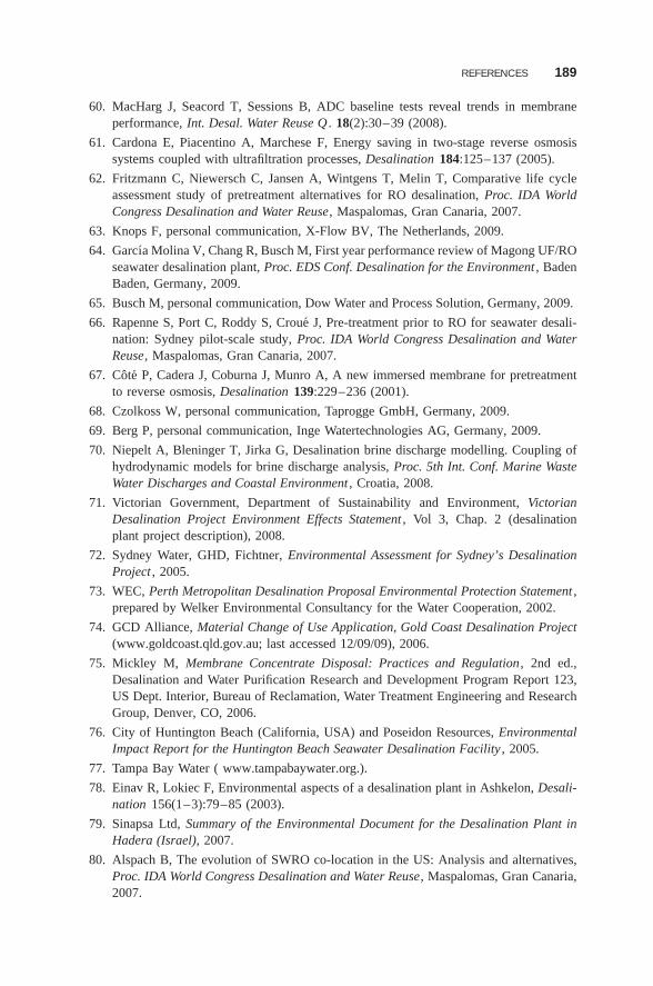
REFERENCES 189

60. MacHarg J, Seacord T, Sessions B, ADC baseline tests reveal trends in membraneperformance, Int. Desal. Water Reuse Q . 18(2):30–39 (2008).

61. Cardona E, Piacentino A, Marchese F, Energy saving in two-stage reverse osmosissystems coupled with ultrafiltration processes, Desalination 184:125–137 (2005).

62. Fritzmann C, Niewersch C, Jansen A, Wintgens T, Melin T, Comparative life cycleassessment study of pretreatment alternatives for RO desalination, Proc. IDA WorldCongress Desalination and Water Reuse, Maspalomas, Gran Canaria, 2007.

63. Knops F, personal communication, X-Flow BV, The Netherlands, 2009.

64. Garcıa Molina V, Chang R, Busch M, First year performance review of Magong UF/ROseawater desalination plant, Proc. EDS Conf. Desalination for the Environment , BadenBaden, Germany, 2009.

65. Busch M, personal communication, Dow Water and Process Solution, Germany, 2009.

66. Rapenne S, Port C, Roddy S, Croue J, Pre-treatment prior to RO for seawater desali-nation: Sydney pilot-scale study, Proc. IDA World Congress Desalination and WaterReuse, Maspalomas, Gran Canaria, 2007.

67. Cote P, Cadera J, Coburna J, Munro A, A new immersed membrane for pretreatmentto reverse osmosis, Desalination 139:229–236 (2001).

68. Czolkoss W, personal communication, Taprogge GmbH, Germany, 2009.

69. Berg P, personal communication, Inge Watertechnologies AG, Germany, 2009.

70. Niepelt A, Bleninger T, Jirka G, Desalination brine discharge modelling. Coupling ofhydrodynamic models for brine discharge analysis, Proc. 5th Int. Conf. Marine WasteWater Discharges and Coastal Environment , Croatia, 2008.

71. Victorian Government, Department of Sustainability and Environment, VictorianDesalination Project Environment Effects Statement , Vol 3, Chap. 2 (desalinationplant project description), 2008.

72. Sydney Water, GHD, Fichtner, Environmental Assessment for Sydney’s DesalinationProject , 2005.

73. WEC, Perth Metropolitan Desalination Proposal Environmental Protection Statement ,prepared by Welker Environmental Consultancy for the Water Cooperation, 2002.

74. GCD Alliance, Material Change of Use Application, Gold Coast Desalination Project(www.goldcoast.qld.gov.au; last accessed 12/09/09), 2006.

75. Mickley M, Membrane Concentrate Disposal: Practices and Regulation , 2nd ed.,Desalination and Water Purification Research and Development Program Report 123,US Dept. Interior, Bureau of Reclamation, Water Treatment Engineering and ResearchGroup, Denver, CO, 2006.

76. City of Huntington Beach (California, USA) and Poseidon Resources, EnvironmentalImpact Report for the Huntington Beach Seawater Desalination Facility , 2005.

77. Tampa Bay Water ( www.tampabaywater.org.).

78. Einav R, Lokiec F, Environmental aspects of a desalination plant in Ashkelon, Desali-nation 156(1–3):79–85 (2003).

79. Sinapsa Ltd, Summary of the Environmental Document for the Desalination Plant inHadera (Israel), 2007.

80. Alspach B, The evolution of SWRO co-location in the US: Analysis and alternatives,Proc. IDA World Congress Desalination and Water Reuse, Maspalomas, Gran Canaria,2007.

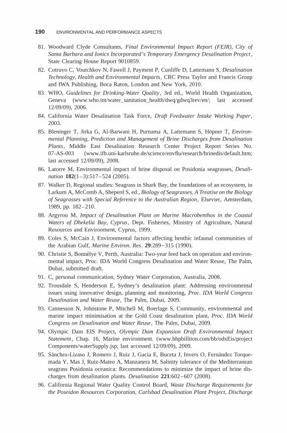
190 ENVIRONMENTAL AND PERFORMANCE ASPECTS

81. Woodward Clyde Consultants, Final Environmental Impact Report (FEIR), City ofSanta Barbara and Ionics Incorporated’s Temporary Emergency Desalination Project ,State Clearing House Report 9010859.

82. Cotruvo C, Voutchkov N, Fawell J, Payment P, Cunliffe D, Lattemann S, DesalinationTechnology, Health and Environmental Impacts , CRC Press Taylor and Francis Groupand IWA Publishing, Boca Raton, London and New York, 2010.

83. WHO, Guidelines for Drinking-Water Quality , 3rd ed., World Health Organization,Geneva (www.who.int/water_sanitation_health/dwq/gdwq3rev/en/; last accessed12/09/09), 2006.

84. California Water Desalination Task Force, Draft Feedwater Intake Working Paper ,2003.

85. Bleninger T, Jirka G, Al-Barwani H, Purnama A, Lattemann S, Hopner T, Environ-mental Planning, Prediction and Management of Brine Discharges from DesalinationPlants , Middle East Desalination Research Center Project Report Series No.07-AS-003 (www.ifh.uni-karlsruhe.de/science/envflu/research/brinedis/default.htm;last accessed 12/09/09), 2008.

86. Latorre M, Environmental impact of brine disposal on Posidonia seagrasses, Desali-nation 182(1–3):517–524 (2005).

87. Walker D, Regional studies: Seagrass in Shark Bay, the foundations of an ecosystem, inLarkum A, McComb A, Sheperd S, ed., Biology of Seagrasses. A Treatise on the Biologyof Seagrasses with Special Reference to the Australian Region , Elsevier, Amsterdam,1989, pp. 182–210.

88. Argyrou M, Impact of Desalination Plant on Marine Macrobenthos in the CoastalWaters of Dhekelia Bay, Cyprus , Dept. Fisheries, Ministry of Agriculture, NaturalResources and Environment, Cyprus, 1999.

89. Coles S, McCain J, Environmental factors affecting benthic infaunal communities ofthe Arabian Gulf, Marine Environ. Res . 29:289–315 (1990).

90. Christie S, Bonnelye V, Perth, Australia: Two-year feed back on operation and environ-mental impact, Proc. IDA World Congress Desalination and Water Reuse, The Palm,Dubai, submitted draft.

91. C, personal communication, Sydney Water Corporation, Australia, 2008.

92. Trousdale S, Henderson E, Sydney’s desalination plant: Addressing environmentalissues using innovative design, planning and monitoring, Proc. IDA World CongressDesalination and Water Reuse, The Palm, Dubai, 2009.

93. Cannesson N, Johnstone P, Mitchell M, Boerlage S, Community, environmental andmarine impact minimisation at the Gold Coast desalination plant, Proc. IDA WorldCongress on Desalination and Water Reuse, The Palm, Dubai, 2009.

94. Olympic Dam EIS Project, Olympic Dam Expansion Draft Environmental ImpactStatement , Chap. 16, Marine environment. (www.bhpbilliton.com/bb/odxEis/projectComponents/waterSupply.jsp; last accessed 12/09/09), 2009.

95. Sanchez-Lizaso J, Romero J, Ruiz J, Gacia E, Buceta J, Invers O, Fernandez Torque-mada Y, Mas J, Ruiz-Mateo A, Manzanera M, Salinity tolerance of the Mediterraneanseagrass Posidonia oceanica: Recommendations to minimize the impact of brine dis-charges from desalination plants. Desalination 221:602–607 (2008).

96. California Regional Water Quality Control Board, Waste Discharge Requirements forthe Poseidon Resources Corporation, Carlsbad Desalination Plant Project, Discharge

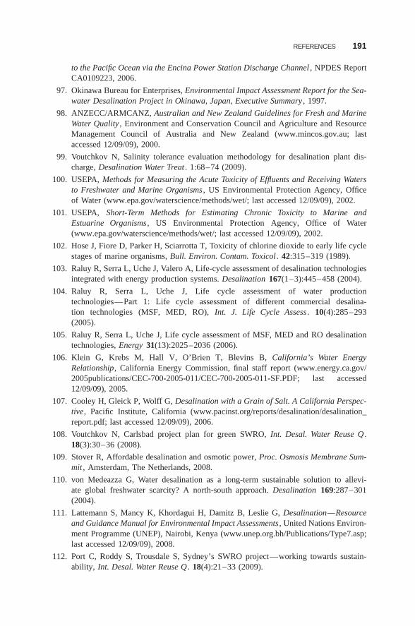
REFERENCES 191

to the Pacific Ocean via the Encina Power Station Discharge Channel , NPDES ReportCA0109223, 2006.

97. Okinawa Bureau for Enterprises, Environmental Impact Assessment Report for the Sea-water Desalination Project in Okinawa, Japan, Executive Summary , 1997.

98. ANZECC/ARMCANZ, Australian and New Zealand Guidelines for Fresh and MarineWater Quality , Environment and Conservation Council and Agriculture and ResourceManagement Council of Australia and New Zealand (www.mincos.gov.au; lastaccessed 12/09/09), 2000.

99. Voutchkov N, Salinity tolerance evaluation methodology for desalination plant dis-charge, Desalination Water Treat . 1:68–74 (2009).

100. USEPA, Methods for Measuring the Acute Toxicity of Effluents and Receiving Watersto Freshwater and Marine Organisms , US Environmental Protection Agency, Officeof Water (www.epa.gov/waterscience/methods/wet/; last accessed 12/09/09), 2002.

101. USEPA, Short-Term Methods for Estimating Chronic Toxicity to Marine andEstuarine Organisms , US Environmental Protection Agency, Office of Water(www.epa.gov/waterscience/methods/wet/; last accessed 12/09/09), 2002.

102. Hose J, Fiore D, Parker H, Sciarrotta T, Toxicity of chlorine dioxide to early life cyclestages of marine organisms, Bull. Environ. Contam. Toxicol . 42:315–319 (1989).

103. Raluy R, Serra L, Uche J, Valero A, Life-cycle assessment of desalination technologiesintegrated with energy production systems. Desalination 167(1–3):445–458 (2004).

104. Raluy R, Serra L, Uche J, Life cycle assessment of water productiontechnologies—Part 1: Life cycle assessment of different commercial desalina-tion technologies (MSF, MED, RO), Int. J. Life Cycle Assess . 10(4):285–293(2005).

105. Raluy R, Serra L, Uche J, Life cycle assessment of MSF, MED and RO desalinationtechnologies, Energy 31(13):2025–2036 (2006).

106. Klein G, Krebs M, Hall V, O’Brien T, Blevins B, California’s Water EnergyRelationship, California Energy Commission, final staff report (www.energy.ca.gov/2005publications/CEC-700-2005-011/CEC-700-2005-011-SF.PDF; last accessed12/09/09), 2005.

107. Cooley H, Gleick P, Wolff G, Desalination with a Grain of Salt. A California Perspec-tive, Pacific Institute, California (www.pacinst.org/reports/desalination/desalination_report.pdf; last accessed 12/09/09), 2006.

108. Voutchkov N, Carlsbad project plan for green SWRO, Int. Desal. Water Reuse Q .18(3):30–36 (2008).

109. Stover R, Affordable desalination and osmotic power, Proc. Osmosis Membrane Sum-mit , Amsterdam, The Netherlands, 2008.

110. von Medeazza G, Water desalination as a long-term sustainable solution to allevi-ate global freshwater scarcity? A north-south approach. Desalination 169:287–301(2004).

111. Lattemann S, Mancy K, Khordagui H, Damitz B, Leslie G, Desalination—Resourceand Guidance Manual for Environmental Impact Assessments , United Nations Environ-ment Programme (UNEP), Nairobi, Kenya (www.unep.org.bh/Publications/Type7.asp;last accessed 12/09/09), 2008.

112. Port C, Roddy S, Trousdale S, Sydney’s SWRO project—working towards sustain-ability, Int. Desal. Water Reuse Q . 18(4):21–33 (2009).

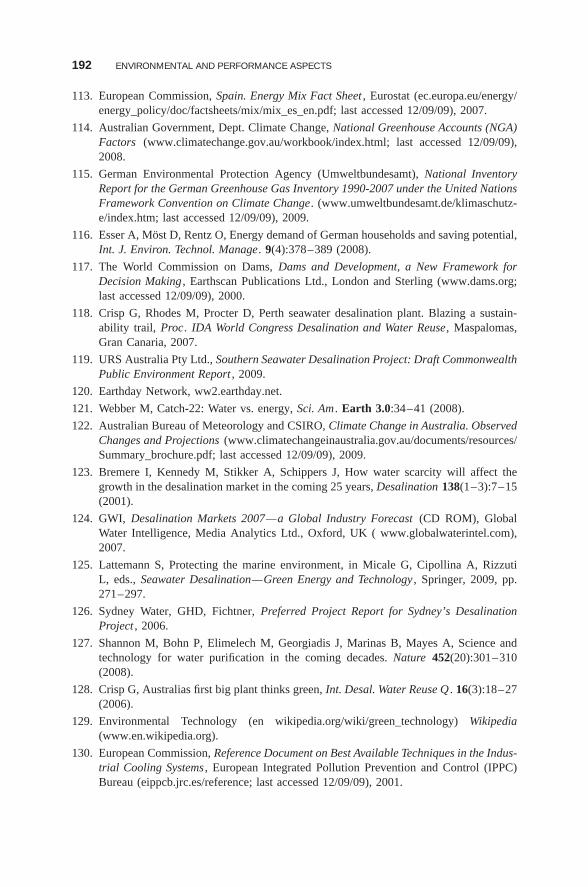
192 ENVIRONMENTAL AND PERFORMANCE ASPECTS

113. European Commission, Spain. Energy Mix Fact Sheet , Eurostat (ec.europa.eu/energy/energy_policy/doc/factsheets/mix/mix_es_en.pdf; last accessed 12/09/09), 2007.

114. Australian Government, Dept. Climate Change, National Greenhouse Accounts (NGA)Factors (www.climatechange.gov.au/workbook/index.html; last accessed 12/09/09),2008.

115. German Environmental Protection Agency (Umweltbundesamt), National InventoryReport for the German Greenhouse Gas Inventory 1990-2007 under the United NationsFramework Convention on Climate Change. (www.umweltbundesamt.de/klimaschutz-e/index.htm; last accessed 12/09/09), 2009.

116. Esser A, Most D, Rentz O, Energy demand of German households and saving potential,Int. J. Environ. Technol. Manage. 9(4):378–389 (2008).

117. The World Commission on Dams, Dams and Development, a New Framework forDecision Making , Earthscan Publications Ltd., London and Sterling (www.dams.org;last accessed 12/09/09), 2000.

118. Crisp G, Rhodes M, Procter D, Perth seawater desalination plant. Blazing a sustain-ability trail, Proc. IDA World Congress Desalination and Water Reuse, Maspalomas,Gran Canaria, 2007.

119. URS Australia Pty Ltd., Southern Seawater Desalination Project: Draft CommonwealthPublic Environment Report , 2009.

120. Earthday Network, ww2.earthday.net.

121. Webber M, Catch-22: Water vs. energy, Sci. Am . Earth 3.0:34–41 (2008).

122. Australian Bureau of Meteorology and CSIRO, Climate Change in Australia. ObservedChanges and Projections (www.climatechangeinaustralia.gov.au/documents/resources/Summary_brochure.pdf; last accessed 12/09/09), 2009.

123. Bremere I, Kennedy M, Stikker A, Schippers J, How water scarcity will affect thegrowth in the desalination market in the coming 25 years, Desalination 138(1–3):7–15(2001).

124. GWI, Desalination Markets 2007—a Global Industry Forecast (CD ROM), GlobalWater Intelligence, Media Analytics Ltd., Oxford, UK ( www.globalwaterintel.com),2007.

125. Lattemann S, Protecting the marine environment, in Micale G, Cipollina A, RizzutiL, eds., Seawater Desalination—Green Energy and Technology , Springer, 2009, pp.271–297.

126. Sydney Water, GHD, Fichtner, Preferred Project Report for Sydney’s DesalinationProject , 2006.

127. Shannon M, Bohn P, Elimelech M, Georgiadis J, Marinas B, Mayes A, Science andtechnology for water purification in the coming decades. Nature 452(20):301–310(2008).

128. Crisp G, Australias first big plant thinks green, Int. Desal. Water Reuse Q . 16(3):18–27(2006).

129. Environmental Technology (en wikipedia.org/wiki/green_technology) Wikipedia(www.en.wikipedia.org).

130. European Commission, Reference Document on Best Available Techniques in the Indus-trial Cooling Systems , European Integrated Pollution Prevention and Control (IPPC)Bureau (eippcb.jrc.es/reference; last accessed 12/09/09), 2001.

REFERENCES 193

131. Abousamra F, personal communication, MEDPOL Programme, UNEP, Greece, 2008.

132. Safrai I, Zask A, Reverse osmosis desalination plants—marine environmentalist reg-ulator point of view, Desalination 220:72–84 (2008).

133. I, Amir R, personal communication, Ministry of the Environment, Israel, 2008,2009.

134. USEPA, Effluent Limitations Guidelines and Standards , US Environmental ProtectionAgency, Office of Water (cfpub.epa.gov/npdes/techbasedpermitting/effguide.cfm; lastaccessed 12/09/09), 2009.

135. Mooij C, Hamma water desalination plant, Desalination 203(1–3):107–118(2007).

136. Media Analytics Ltd, Spain fast-tracks EIA process, Global Water Intell . 9(9):20(2008).

137. Schiffler M, Perspectives and challenges for desalination in the 21st century, Desali-nation 165(1–3):1–9 (2004).

138. Ambrose R, Schmitt R, Osenberg C, Predicted and observed environmental impacts.Can we foretell ecological change?, in Schmitt R, Osenberg C, eds., Detecting Ecolog-ical Impacts. Concepts and Applications in Coastal Habitats , Academic Press, 1996,pp. 345–369.

139. Stewart-Oaten A, Problems in the analysis of environmental monitoring data, in SchmittR, Osenberg C, eds., Detecting Ecological Impacts. Concepts and Applications inCoastal Habitats , Academic Press, 1996, pp. 109–131.

140. Underwood A, Beyond BACI: The detection of environmental impacts on populationsin the real, but variable, world, J. Exp. Marine Bio. Ecol . 161:145–178 (1992).

141. Bamber R, Environmental impact assessment: The example of marine biology and theUK power industry, Marine Pollut. Bull . 21(6): 270–274 (1990).

142. Janssen R, On the use of multi-criteria analysis in environmental impact assessmentin The Netherlands, J. Multi-Criteria Decision Anal . 10(2):101–109 (2001).

143. Lahdelma R, Salminen P, Hokkanen J, Using multicriteria methods in environmentalplanning and management, Environ. Manage. 26(6):595–605 (2000).

144. Beinat E, Multi-criteria analysis for environmental management, J. Multi-Criteria Deci-sion Anal . 10(51):51 (2001).

145. Linkov I, Satterstrom F, Kiker G, Batchelor C, Bridges T, Ferguson E, From com-parative risk assessment to multi-criteria decision analysis and adaptive management:Recent developments and applications, Environ. Int . 32(8):1072–1093 (2006).

146. Stewart T, Joubert A, Janssen R, MCDA framework for fishing rights allocation inSouth Africa, in Group Decision and Negotiation, Amsterdam , Springer, Amsterdam(online publication, DOI 10.1007/s10726-009-9159-9), 2009.

147. Kiker G, Bridges T, Varghese A, Seager T, Linkov I, Application of multi-criteriadecision analysis in environmental decision making, Integr. Environ. Assess. Manage.1(2):95–108 (2005).

148. Balasubramaniam A. Voulvoulis N, The appropriateness of multicriteria analysisin environmental decision-making problems, Environ. Technol . 26(9):951–962(2005).

149. S, personal communication, South East Queensland Desalination Company Pty Ltd.,Sure Smart Water, Australia, 2009.

194 ENVIRONMENTAL AND PERFORMANCE ASPECTS

150. Bornman T, Klages N, Ecological Pre-feasibility Study of the Establishment of a Desali-nation Plant at Knysna , Inst. Environmental and Coastal Management, Univ. PortElizabeth, South Africa, 2004.

151. Bornman T, Klages N, Ecological Pre-feasibility Study of the Establishment of a Desali-nation Plant at Plettenberg Bay , Inst. Environmental and Coastal Management, Univ.Port Elizabeth, South Africa, 2004.

152. Keeney R, Raiffa H, Decisions with Multiple Objectives: Preferences and Value Trade-offs , Cambridge Univ. Press, 1993

153. Herwijnen M, Janssen R, Software support for multicriteria decision-making, in Giup-poni C, Jakeman A, Karssenberg D, Hare M, (eds.,) Sustainable Management of WaterResources , The Fondazione eni Enrico Mattei (FEEM) Series on Economics, the Envi-ronment and Sustainable Development, Edward Elgar Publishing, 2006, pp. 131–150.

154. Janssen R, Herwijnen M, and Beinat E, DEFINITE 3.0 Case Studies andUser Manual , Inst. Environmental Studies, Vrije Uni. Amsterdam (www.ivm.vu.nl/en/projects/Departments/spatial-analysis/DEFINITE/index.asp; last accessed12/09/09), 2003.

155. Belton V, Stewart T, Multiple Criteria Decision Analysis—an Integrated Approach ,Kluwer Academic, 2002.

156. van Drunen M, Janssen R, Evaluation Methods. (Online user’s manual for DEFI-NITEprogram). Inst. Environmental Studies, Vrije Uni. Amsterdam (www.ivm.vu.nl/en/projects/Departments/spatial-analysis/DEFINITE/index.asp; last accessed 12/09/09),2009.

157. Peters T, Pinto D, and Pinto E. Improved seawater intake and pre-treatment systembased on Neodren technology, Desalination 203(1–3):134–140 (2007).

158. Pankratz T, personal communication, Water Desalination Report, USA, 2007.

159. Brehant A, Bonnelye V, Perez M, Comparison of MF/UF pretreatment with conven-tional filtration prior to RO membranes for surface seawater desalination, Desalination ,144:353–360 (2002).

160. Crowley K, personal communication, Consolidated Water Company, Cayman Islands,2009.

161. Pearce G, Talo S, Chida K, Basha A, Gulamhusein A, Pretreatment options for largescale SWRO plants: Case studies of UF trials at Kindasa, Saudi Arabia, and conven-tional pretreatment in Spain, Desalination 167:175–189 (2004).

162. Remize P, Laroche J, Leparc J, Schrotter J, A pilot scale comparison between granularmedia filtration and low pressure membrane filtration for seawater pretreatment, Proc.Euromed 2008 (conf.), Desalination Cooperation among Mediterranean Countries ofEurope and the MENA Region, Dead Sea, Jordan , 2008.

163. Vial D, Doussau G, The use of microfiltration membranes for seawater pre-treatmentprior to reverse osmosis membranes, Desalination 153:141–147 (2002).

164. Baltussen R, Niessen L, Priority setting of health interventions: The need formulti-criteria decision analysis, Cost Effect. Resource Alloc. 4(14): (2006).www.biomedcentral.com/1458-7547/4/14

165. Edwards W, Barron F, SMARTS and SMARTER: Improved simple methods for mul-tiattribute utility measurement, Organiz. Behav. Human Decision Process . 60:306–325(1994).

166. Jeffreys I, Lawrence P, Principles and methods for developing a MODSS processfor farm forestry, in Harrison S, Herbohn J, ed., Agroforestry and Farm Forestry:

REFERENCES 195

Support SA systems to assess the Viability of Whole-Farm and Regional AgroforestryEnterprises , RIRDC, Canberra (espace.library.uq.edu.au/eserv/UQ:8107/Ch_13_-_MODSS_pr.pdf; last accessed 12/09/09), 2008, pp. 166–179.

167. Beery M, Repke J, Sustainability analysis of different SWRO pre-treatment alternatives,Desal. Water Treat . 16:218–228 (2010) (in press).

168. Pankratz T, California—who or what is to blame? (Water Desalination Report byMedia Analytics Ltd.), Global Water Intel . 45(28):1–3 (2009).

This page intentionally left blank

CHAPTER 3

Economic Aspects of WaterDesalination

AMITZUR BARAK

3.1 Introduction 1993.1.1 Objectives and Scope 1993.1.2 Economics of Production in General 1993.1.3 Specific Features of Desalination 2003.1.4 Competition of Desalination with Alternative Means of Water

Supply 2013.1.5 The Roles of Economics at the Planning Stage 202

3.2 Economic Criteria 2033.3 Basic Evaluation of Desalted Water Cost 205

3.3.1 Definition of Cost 2053.3.2 Actual Cost 205

3.3.2.1 Interest and Discount Rates 2073.3.2.2 Formulas Used to Determine Actual Cost 2073.3.2.3 A Sample Cost Calculation 209

3.3.3 Practical Methods of Product Cost Evaluation 2113.3.3.1 Summation of All Cost Components 2123.3.3.2 Capital Cost 2133.3.3.3 Energy and Fuel Cost Component 2273.3.3.4 Operation and Maintenance (O&M) Cost Component 2363.3.3.5 Cost Comparison of Single-Purpose Desalination

Processes 2373.3.3.6 Socioenvironmental Costs 2393.3.3.7 Cost of Desalted Water Conveyance 240

3.4 Cost Evaluation of Complex Desalination Systems 2413.4.1 Dual-Purpose Plants 241

3.4.1.1 Common Advantages 2433.4.1.2 Common Disadvantages 2443.4.1.3 Comparison of Power Generation Systems 2453.4.1.4 Cost Calculation 248

Advances in Water Desalination, First Edition. Edited by Noam Lior.© 2013 John Wiley & Sons, Inc. Published 2013 by John Wiley & Sons, Inc.

197

198 ECONOMIC ASPECTS OF WATER DESALINATION

3.4.1.5 Discussion 2543.4.2 Hybrid Desalination Plants 256

3.4.2.1 Disadvantages 2563.4.2.2 Advantages 2563.4.2.3 Cost Calculation 257

3.4.3 Two-Quality Product Water Streams 2573.4.4 Linear Correlation Common Principle 258

3.5 Reliability of Cost Estimates 2583.5.1 Methods 2593.5.2 Levels of Accuracy 2603.5.3 Accuracy in Terms of Cost Calculation Objectives 2613.5.4 Inflation and Deflation 263

3.5.4.1 Levelized Costs in Terms of ‘‘Constant’’ Currency 2633.5.4.2 Levelized Costs in Terms of ‘‘Current’’ Money 264

3.6 Design and Optimization of Plant and Process Parameters 2653.7 Procedures and Programs 269

3.7.1 US Methods 2693.7.2 International Methods 2693.7.3 UN Methods 269

3.8 Domestic Versus Foreign Currencies 2743.9 Value of desalted water 2743.10 Prices of water and power 2753.11 Cashflow, payback period, and rate of return 2763.12 Financing 2763.13 Bids and Ownership 277

3.13.1 The Entities Involved 2773.13.2 Full and Direct Implementation of Desalted Water Production 2773.13.3 Turnkey Construction 2783.13.4 Build–Operate–Transfer (BOT) Approach 2793.13.5 Build–Own–Operate–Transfer (BOOT) Approach 2793.13.6 Build–Own–Operate (BOO) Approach 2803.13.7 Rented Plant 280

3.14 Contractual Pricing Due to Changes and Deviations from the OriginalPlan 281

3.15 National Desalination Programs 2823.16 Desalination and Hydrology 2853.17 Economics of Desalination Research and Development (Desalination

R&D) 2873.18 World Market and Future Prospects for Desalination 289Appendix 290

3.A.1 Sample Cost Calculations for Desalted Water at the Plant 2903.A.2 Optimization of the Main Process Component: An Example 297

Nomenclature 303References 307

INTRODUCTION 199

3.1 INTRODUCTION

3.1.1 Objectives and Scope

The main role of the economics of any production—in the case discussed in thischapter, desalted water—is to assist in making decisions. These decisions may bemanagerial, technical, financial, and/or administrative in nature. They may refer toa near-future small project as well as to long-term broad programs.

This assistance in decision-making, obtained by using economics, stems from areduction in the number and type of the criteria by which the production alterna-tives to be decided on are assessed. Instead of coping with many technical, physical,temporal, logistic, workforce, and many other factors, these production alternativesare measured quantitatively mainly according to the amount of monetary fundingthat is allocate to them. This monetary value serves as a common denominatorfor comparing these alternatives on a money-per-project, money-per-program, ormoney-per-unit product (where money denotes the amount of monetary fundingallocated to or spent on that project). Effective and proper comparisons are per-formed for identical times and places and for equal product quantities and qualities.

The economic criteria used as the bottom line in economic analyses are costs,prices, and values of the products; investments; percentage of local currency in theproduct cost and the investment; cashflow; payback period; and rate of return.

All these criteria, as well as related aspects, are discussed and described inthis chapter. The related aspects are financing, economy of scale, technoeconomicoptimization and scheduling. Particular attention is given to dual-purposeplants, nuclear desalination, and solar desalination. Some aspects are treatedquantitatively; others, only qualitatively. The economics of hybrid desalinationplants, energy supply alternatives, trasnport of desalted water to users, and optimalplant location are also discussed.

Specifically, economic aspects relating uniquely to desalination, rather thansimilar industrially produced materials, are described and discussed. These aspectsinclude the challenge to ensure extremely low cost per unit product, the effectof feedwater quality on the cost and the initial investment, changes in cost andinvestment with respect to the quality of the desalted water (salinity, boron con-tent, etc.), and the possible effect of hydrology–desalination integration on the costof desalted water and other aspects.

Finally, a tentative forecast of desalted water costs is presented and explained.Two examples of cost calculations are appended. One is for a single-purpose sea-

water reverse-osmosis (SWRO) desalination plant and the other, for a cogenerationplant employing electric power and desalted seawater with multieffect distillation(MED) evaporation. Another appendix discusses the principles of basic optimiza-tion of the distillation process.

3.1.2 Economics of Production in General

Desalted water is often produced by a single industrial process and in quite afew cases by a combination of several processes. As such, the economical aspects

200 ECONOMIC ASPECTS OF WATER DESALINATION

of water desalination are, in principle, identical to those of any other industriallyproduced material such as cement, sulfuric acid, or table salt (NaCl). Thus, bothas a reminder and for readers not acquainted with the details of the subject, theeconomics of the process industry are briefly presented in this section.

3.1.3 Specific Features of Desalination

However, water desalination has several unique technoeconomic features in addi-tion to those of all other industrially produced materials:

1. Large Quantities . The amounts produced, at what is considered a typical largeplant, are much larger than any other industrially produced material. [Note:Desalination processes are defined as industrial ones. A distinction existsbetween industrial production of materials and alternative means of materi-als provision (supplying), procurement, or preparation (by mining, harvesting,or treatment such as filtering or chlorination). These alternative means aresimpler, less sophisticated, and therefore less expensive than industrial pro-duction.]

2. Very Low Acceptable Price. The price of desalted water that is accept-able to the common water user is at least one order of magnitude lowerthan any other industrially produced material. Thus the cost of productionper unit mass should not exceed a few US dollars per metric ton, prefer-ably even less than US$1 per ton even for small production rates, whilefor any other industrially produced material the production cost is at leastseveral dozen US dollars per ton. Moreover, very large desalted water pro-duction rates are acceptable only for considerably less than US$1 per ton(1 ton of potable water is equal to one cubic mater, in the context discussedhere).

3. Sensitivity of Cost to Economic Environment (Particularly Energy Prices).The economics of a desalination project is strongly dependent on local factors,the prevailing market prices of electricity and water, and a series of insti-tutional factors that may influence the economic assessment of the project.Energy consumption and cost are considered crucial for desalination, partlybecause of issues mentioned here and in list item 2, above. Throughout themore recent decades, energy current prices have undergone large fluctua-tions, sometimes drastic; thus, issue of forecasting costs and determiningprices, both short- and long-term, becomes more precarious than for othermaterials.

4. National system of long term production plants . For many desalinationprojects the need for desalted water exists due to a local water shortage, thusdefining the desalination plants production and installation timing with verylittle flexibility. However, in some states and countries water shortage isforecasted for long term and wide national or regional scope. In the former

INTRODUCTION 201

type of local enterprises the economic considerations are similar to thoseof the common process industry while for a national desalination programthe economic considerations are different for various reasons which will bediscussed in section 3.15.

5. Public, Political, and Media Intensive Involvement . Since water is a commonutility commodity, the amount of public interest in the availability and qual-ity of water in general and in desalted water in particular is much greaterthan for other materials. Any difficulty—financial, managerial, technologi-cal, administrative, constructional or operational (schedule delays, accidents,etc.)—will impose additional economical penalties and create a poor imageof the project and the parties involved, of the type of desalination process,and even of the entire field of desalination. This poor image may negativelyaffect the market demand for desalination systems and desalted water (in thissense it is somewhat similar to nuclear power).

6. Need for Good, Effective, and Highly Reliable Peripheral Infrastructure.Water is almost always transported and distributed by pipelines, unlike mostother chemicals, which are transported by trains, trucks, and ships. Thus,poor infrastructure, namely, leaky or clogged pipelines and inadequatepumps, between the desalination plants and the desalted water users willsabotage the water supply. The reliability of this supply will deteriorate, thecost of transportation will increase as a result of excessive energy lossesand high maintenance expenses, and—above all—expensive high-qualitydesalted water will disappear through the leaks. All these factors—althoughexternal to the desalination system itself—will raise the actual net costof each unit (measured in m3) of desalted water used, in addition to theresulting poor image that will be attributed by the public and media to theentire branch of desalination and the impacts described above.

This aspect of the need for high quality infrastructure obviously holds for allwater sources, not only for desalination. However, the sensitivity of the public andthe water suppliers in this regard is considerably higher in the case of desaltedwater.

3.1.4 Competition of Desalination with Alternative Means of WaterSupply

The relatively high cost of desalination is one of the major reasons for the reluctanceto implement it more often. Paradoxically, broader use of desalination could havedecreased its overall cost, at least slightly. This point will be discussed further inSection 3.18. However, the cost difference between water desalination and othermethods of reducing or preventing water shortage is one of the major reasonsto reject, avoid, or at least delay desalination and turning to one or more of thefollowing alternatives:

202 ECONOMIC ASPECTS OF WATER DESALINATION

• Transporting water from distant sites

• Water reuse such as sewage reclamation

• Lowering water consumption by education and propaganda, enforcing drasticwater saving, water rationing, and/or raising water prices

• Discovering new aquifers

• Preventing water loss such as leakage or evaporation from piping and reser-voirs

• Decreasing and improving agricultural activities (e.g., reducing irrigation)

• Cloud seeding to increase or create artificial rain

Despite the tough competition from these other methods, desalination quite oftenbecomes the preferred solution because of economic considerations, and/or flex-ibility and ease of control, availability (where sufficient amounts of saline waterexist), and the possibility of improving not only the quantity but also the qualtityof the water. This may be achieved by dilution: mixing the poor-quality exist-ing water with the added desalted water, while ensuring that this water has beendesalted to a very high quality (at minimal additional cost). Such dilution yieldsan accumulative mixture of desired or at least acceptable quality, thus upgrad-ing the economic value of the water above that of the existing natural water. Forcertain sites or applications, such as where the existing natural water is of rela-tively poor quality as well as being in short supply, such upgrading may be quitemeaningful.

In certain cases desalination is performed after the site-specific relevant alterna-tives have been applied but are unable to economically satisfy the entire need forwater. This may occur if these relevant alternatives have limited, but not sufficient,potential and their resources have been fully exploited, or if the marginal waterfrom the alternative source is more expensive to obtain (or more complicated toprocess) than water that has been desalted.

Thus, the existence of potential alternatives obliges us to consider the eco-nomic aspects of these alternatives as well as the economic aspects of desalinationin our decision as to the best way to supply potable water. All the relevanteconomic criteria (described below and in Section 3.2) must be evaluated andcompared.

3.1.5 The Roles of Economics at the Planning Stage

The main role of economics of any production—in this case, desalted water—is tofacilitate the decision-making process. These decisions may be fundamental , suchas whether to solve the water shortage by desalination or take one or several ofthe above mentioned alternative solutions; technical , such as which process is bestfor the specific site in consideration; economical and financial , such as the price atwhich the water should be sold or which are the preferred sources of money for theinitial investment; managerial , such as whether to bid for desalination plants or fordesalted water; and administrative, such as whether to hire the maintenance staff

ECONOMIC CRITERIA 203

as employees or utilize the services of a contractor for periodic maintenance work.The scope and timescale of these decisions may vary from a near-future smallproject of a single plant with one unit to long-term programs involving multiplelarge plants.

The assistance in decision-making obtained by applying economic tools, stemsfrom the reduction in the number and type of the criteria by which the produc-tion alternatives, to be decided, are measured. Since the required decisions involvechoices between alternatives, comparisons of the considered alternatives have tobe accomplished (even if the decision is only between “do” and “do not”). Thecomparison process is simplified by the said economic tools as instead of deal-ing with many technical, physical, economical, temporal, workforce I still prefermanpower or personnel and other criteria while preparing these comparisons—allalternatives are measured mainly by money which serves as a common denomina-tor. More precisely, the assessment of the alternatives is done mainly by comparingeither money per unit product or money per program (consisting of one or severalprojects).

Note: an effective and proper comparison has to be based on equal terms for allthe alternative scenarios: identical times, similar sites and equal products’ quantitiesand qualities.

3.2 ECONOMIC CRITERIA

The following economic criteria are used as the basis for economic analyses:

1. Cost of Product . This is often the most important, “popular,” and usefulfactor, per unit product—in this case a metric ton of desalted water—for agiven plant or for completion of a given project on a fixed date. Product costis often considered as the sole criterion for deciding on whether to producethe needed material or to obtain it by other means.

2. Investment . This criterion is in most cases a major economical factor, whichdetermines the capital cost , which, in turn, is the largest (or second largest)product cost component. (As will be explained in detail in the followingsection, the investment is usually proportional to the capital cost.) In princi-ple, if the only impact of the investment were its contribution to the overallproduct cost, it should not be presented as a separate economic criterion.However, it has another parallel impact—on the financing problem, and istightly associated with the risk policy of the desalination plant owner as wellas with the product pricing. (Product price is another economic criterion, theseventh in this list). For example, if an evaluation of two alternatives yieldspractically the same product cost, the one with the lower investment willprobably be preferred, because of lower risk and easier financing (which isanother economic and management issue). A further possible recommenda-tion for a possible scenario may be to prefer a meaningfully lower investmenteven if the predicted product cost is slightly higher.

204 ECONOMIC ASPECTS OF WATER DESALINATION

3. Local Currency Percentage. A specific double criterion, related to the twoprevious ones, is the percentage of local currency in the product cost andin the investment. When two alternatives show practically (i.e., almost)the same product cost but the differences in local currencies are mean-ingful, the alternative with the higher percentage of local currency will bepreferred.

4. Cashflow .

5. Payback Period .

6. Rate of Return . This is usually of concern to private investors more than tolarge public authorities (such as a government) as owners. Cashflow, paybackperiod, and rate of return depend on the investment and the annual expenses.They depend also on the next criterion.

7. Price of the Product . Price differs from cost according to the profit (orsubsidy); whereas the cost constitutes the expenses for production, i.e., theproducer’s outgoing money, the price is what the customer pays back to theproducer, i.e. incoming money. The price is determined by (among otherfactors) the next economic criterion.

8. Value of the Product to the Customer . In the case of desalted water, there is anadded value, as compared with many other water resources, due to the highreliability of quantities, qualities, and availability, which are controllable toa high degree.

The considerations described in list items 1–3 above leed to criteria 4–8.Cost, price, and value are measured and expressed in the same units (currency

per product unit). They usually differ in magnitude. Under normal conditions thecost is lower than the price, which, in turn, is lower than the value to the customer.In many cases the differences between the cost, the price, and the value are quitelower than the cost. These three criteria are of interest to the customers (i.e.,desalted water consumers) as well as to the investors and plant owners involved inthe desalination systems. The other criteria are of interest mainly to the investors,plant owners, and sometimes also economists and politicians.

Criteria 7 and 8, price and product value, differ from the other criteria as theydo not result solely from the decisions made by project owners, designers, andmanagers. Rather, they result mainly from the existing economic conditions. Theyhave to be quantitatively estimated, (or determined, if objective estimation is notfeasible).

All these criteria, as well as related aspects, are discussed and described inthis chapter. (Another set of economic criteria, similar to these, is presented inSection 3.13 regarding economical evaluation of bids). The related aspects arefinancing, economy of scale, technoeconomic optimization, project scheduling, eco-nomics of hybrid desalination plants, energy supply alternatives, desalted watertransport to users, and optimal plant location.

BASIC EVALUATION OF DESALTED WATER COST 205

3.3 BASIC EVALUATION OF DESALTED WATER COST

3.3.1 Definition of Cost

The true product cost is the total expenditure needed to supply the product tothe customer per unit product. In practice, two product costs exist. One fits thedefinition fully and refers to the cost at the location and time of transition fromthe supplier to the end user and is termed delivered or gross product cost. Theother cost refers to the product leaving the plant/factory and may be termedplant or net product cost. The first includes the expenses that accrue betweenthe plant exit and the point of delivery to the customer, covering the costs of waterstorage, transportation, possible losses, and distribution. These factors have to beadded to the net cost, where the gross cost is more relevant. However, referenceto the net product cost is more often found in literature and in feasibility studiesas the “cost of desalted water.” This is so because the expenses occurring betweenthe plant exit and the point of delivery are highly site-dependent and can be ana-lyzed only on a case-by-case basis and are not process-dependent. Thus, in pricingthe desalted water for the customer, the gross product cost is the relevant onewhereas for comparing desalination methods or plants the net product cost is moreconvenient.

3.3.2 Actual Cost

The basic principle of determining the actual (real) unit product cost, net or grossC , of a given desalting plant is quite simple: C is the sum of the payments of allexpenses of the desalination plant throughout the lifetime of the plant divided by thenumber of the entire amount of desalted water units during the same period, namely,the average mix of expenditures per unit product. However, this simple costingmethod does not take the economic time factor, namely, interest, into consideration.

In order to properly introduce the time factor, the unit cost definition is slightlymodified: C is equal to the unit price of the capitalized incoming payments forall sales of the water desalted by the plant throughout its lifetime that balancesthe sum of the capitalized payments of all the expenses of the desalination plantthroughout the plant’s lifetime. Where this balance exists, the stated price equalsthe cost. This price of the water is virtual, being fixed at the cost value; thereal price is naturally higher because of the expected profit added to the cost(under normal conditions, at least). The capitalization is done by summing thediscounted values of the sales and expenses to any specified date (D). Usually thedate on which the plant commercial operation starts is taken for the discounting asfollows:

Mathematically, the balance is expressed as follows:

∑(Expense)i =

∑(Sale)j (3.1)

206 ECONOMIC ASPECTS OF WATER DESALINATION

where “Expense” is an expense payment, paid by the desalination plant, discountedto a given date as will be explained below; “Sale” is a water sale payment, receivedby the desalination plant, also discounted to the same given date; indices i and jare the serial numbers assigned to the individual payments of expenses and sales,respectively; and

∑is the summation notation.

For a sale of Wj product units [Wj for desalted water is measured in tons, m3

(=0.997 ton), acre-feet (=1233.5 m3), or kilogallons (=3.785 m3)], under paymentj at (virtual) price C per unit, the actual payment j would have been C · Wj . Thediscounted value, however, is

Salej = C · Wj · Fd j (3.2)

where Fd j is the discounting factor

Fd j = (1 + d)D−Dj (3.3)

where d is the annual discount or interest rate (see Section 3.3.2.1 next page), Dis the reference date for capitalization, and Dj is the date of payment j (the timedifference D − Dj is expressed in years).

Thus, summing the plant life income payments for product sales yields∑Salej =

∑(C · Wj (1 + d)D−Dj ) = C ·

∑Wj (1 + d)D−Dj (3.4)

and hence

C =∑

Salej∑Wj (1 + d)D−Dj

(3.5)

but since the cost-determining principle states that∑

(expense)i = ∑(Sale)j , the

last equation can also be written as

C =∑

Expensei∑Wj (1 + d)D−Dj

(3.6)

Discounting the expense payment Exi is similar to the sales payments

Expensei = Exi (1 + d)D−Di (3.7)

So the final result is

C =∑

(i )Exi (1 + d)D−Di∑

(j )Wj (1 + d)D−Dj

(3.8)

where Di is the date of payment i and the time difference D − Di is expressed inyears.

BASIC EVALUATION OF DESALTED WATER COST 207

3.3.2.1 Interest and Discount Rates The interest rate is the annual cost ofmoney required for the entire work or part of it. Similarly, the discount rate is theannual value of this money for the owner of the plant. In principle, both interestand discount rates may be quantitatively equal, especially if the total investment isfinanced by loans that have the same interest rates and a payback period identicalto the lifetime of the project. If the project is financed by loan(s) having shorter(or longer) payback periods and/or when the project is funded by several sources,with different interest rates, the discount rate d may differ from the interest rate ofthe single loan or from the mean value of interest rates of the funding (financing)sources. In such cases d is used in the preceding formula [Eq. (3.8)] to calculate thecapitalized values of the payback sums of these loans. Frequently, for feasibilityor preproject studies, there is no reference to loans, and thus the interest rate istaken equal to the discount rate, and a value identical to d is used to calculate Fdj

,Expensei , and C .

The exact value of the discount rate is often determined by the government(sometimes even arbitrarily to a certain extent) according to high-level economicand financial considerations. For example, a government that has incurred largedebts may decide on a discount rate value that is higher than the interest ratevalue, even if the total investment is financed by a single loan that does have apayback period identical to the lifetime of the project.

Usually the value of the discount rate per year is determined within the rangeof 5–10%, relative to constant currency at a given date, thus bypassing inflation.More representative annual values are 7%, 8%, or 9%. Extreme known values are4% and 12% per year. The values in most cases are round figures since they arenot calculated but determined arbitrarily, albeit within narrow range limits.

3.3.2.2 Formulas Used to Determine Actual Cost A few remarks shouldbe added regarding the last formula. [Eq. (3.8)]:

1. (Expense)i and Exi refer to

a. Payments for

(1) Equipment, including instrumentation and controls, feedwater supply,concentrate removal, desalted water posttreatment and transport tousers, in addition to the obvious main process equipment

(2) Spare parts

(3) materials for the preliminary stock [such as chemicals, oils, paints andpossibly fuels],

(4) services and labor during plant construction, planning and design,

(5) Civil engineering [buildings, storages, excavation, fencing, pavementsand roads, piping, drainage etc.],

(6) Electrical engineering [cables, transformers, contactors and switches,meters, cathodic protection etc.]

(7) Other infrastructural items, including (a) payments for rented or pur-chased land; (b) preliminary and construction management; (c) offices,

208 ECONOMIC ASPECTS OF WATER DESALINATION

documentation, communication, and transportation (vehicles used),and handling of the equipment and materials (cranes, etc.); (d) work-shop, warehouse, and laboratory; (e) preliminary insurance policies;(f) legal expenses and fees; (g) environmental surveys, permits, andlicensing; (h) employee salaries; (i) contractors, consultants, and ser-vices; (j) recruiting and training desalination equipment operators; and(k) preliminary taxes.

All these payments occur mainly before the commercial commissioningof the plant. This initial part of the expenses payments is defined as theinvestment (Inv or Capex).

b. Payments occurring after commercial commissioning of the plant, includ-ing those for(1) Salaries and fees of equipment operators, plant management and other

service staff, maintenance workers, employees, and various servicecontractors

(2) Electricity and steam(3) Materials for current use (chemicals, oils, paints, and possibly fuels)(4) Replaced items of equipment(5) Rentals, insurance, and annual taxesThese latter expenses payments (items 1b1–1b5) are collectively definedas the running cost (Rn or Opex).

c. Payments occurring during and after the decommissioning of the plant(Dec). The latter is very small relative to Inv and Rn, sometimes evennegative if the remains of the plant are sold for a good price. The dis-counted value of Dec is even lower than, almost negligible, relative to thediscounted values of Inv and Rn since it occurs at a very late stage in theplant history.

d. The following formula results from a combination of points 1a–1c above:∑(i )

Exi = Inv + Rn + Dec ≈ Inv + Rn (3.9)

e. If part or all of the financing is implemented by loans, the back pay-ments should also be considered as plant/project expenses and includedin Expense. In this case the incoming sums loaned to the project shouldbe considered as negative expenses. Both the incoming loan sums and theloan back payments should be discounted to the capitalization referencedate D (preferably the plant commissioning day).

2. Some incoming payments may be allocated for sales other than ordinarydesalted water. Typical examples are paymentsa. Used equipmentb. Buildings and/or land at the end of the plant lifec. Excess energy where the desalination plant has a built-in or self-supplied

energy systemd. Concentrated brine to salt ponds

BASIC EVALUATION OF DESALTED WATER COST 209

e. High-purity (e.g., double-distilled) water for specific applications such asfeedwater for boilers

These payments should be considered for the cost calculation as negativeexpenses rather than sales and treated as such for calculating the desaltedwater cost.

3. Introducing real and accurate values into the last formula—namely, the val-ues of all the payments (Expense)i, the water quantities Wj and the datesDi , Dj , and D —is possible only at the end of the plant life so that the accu-rate value of the product cost can be obtained only at this very late time inthe plant history.

4. Even this accurate value of C depends on one factor that is not measured orcalculated but determined rather arbitrarily—the discount rate d , discussedin Section 3.3.2.1. Thus, for given data of all the payments (Expense)i, thewater quantities Wj and the dates Di , Dj and D the desalted water cost Cis either calculated for a certain fixed value of the discount rate d , or ispresented as a one-variable function by simple tabulation of several valuesof d or is plotted in a graph for a specific range of d values.

5. When the formula for C [Eq. (3.8)] is used prior to the end of the plant’slifetime (i.e., at plant startup, before or during plant operation, or even ear-lier, before plant construction, during the bidding period, when the possibleerection of a desalting plant is only in the decision or planning stage), thisC formula serves only as an estimate —rather than a firm calculation —ofthe actual cost of the desalted water. This can be attributed to the fact thatsome or all of the other input values—including expenses (Expense)i , waterquantities Wj , and their dates Di , Dj , and D —are not known but are onlyassessed or assumed. In other words, the earlier in the plant history that thisformula [Eq. (3.8)] is applied, the lower will be the degree of accuracy.

6. In practice, using the C formula is very laborious as it requires numerouscalculations. Therefore, a shorter procedure is quite often used, even though itmay introduce additional inaccuracies. This shorter procedure, and two otheralternative methods, is discussed in Section 3.3.3. Nevertheless, the presentmethod is strongly recommended as it can be used to calculate the real costafter the plant is finally closed and decommissioned. The data obtained usingthis method can be extrapolated for comparisons with previous product costestimates and to identify any deviations of previous assumptions from theactual cost values.

3.3.2.3 A Sample Cost Calculation The per unit price of desalted water Ccan be calculated according to the last two formulas above [Eqs. (3.8) and (3.9)]as follows. Suppose that the following summarized and processed data exist in theplant’s records:

• No loans are used for financing.

• Plant life production is∑

(j )(W )j = 385 Mt (million metric tons).

210 ECONOMIC ASPECTS OF WATER DESALINATION

• Plant production life is 32 years

• Plant erection time, including design and planning, is 3.5 years.

• Discount rate d = 0.075 per year (7.5%/y).

• Total investment is Inv = $31.5M.

• Capitalized/discounted investment covering all the payments before commis-sioning: ∑

(Expense)i =∑

(i ){Exi (1 + d)D−Di } = $35.2M (3.10)

where D is the date of plant commissioning 0 ≤ D − Di ≤ 3.5.

• Running cost during plant life for an average year is = 2.65M$/y electricity+ 0.95M$/y salaries + 0.6M$/y materials + 0.7M$/y equipment + 0.3M$/ytaxes & insurance = $5.2M /year,so that Rn = $5.2M/y* 32 years = $166.4M.

• Capitalized/discounted value of running cost is∑

(Expense)i = $52.3M forpayments after commissioning.

• Decommissioning expenses are negligible.

The capitalized/discounted value of incoming payments for (virtual) water sales atcost price means:

∑Salej =

∑(C · Wj (1 + d)D−Dj )

= C ·∑

(j ){(W )j (1 + d)D−Dj } = $(120 · C )∗106 (3.11)

as∑

(j ){(W )j (1 + d)D−Dj } = 120 · 106 tons.

Thus $(120·C)*106 = $35.2M+ $52.3M = $87.5M,so that C = $87.5M/120M tons ≈ $0.73 per ton .Note: Capitalization of sum of many items

∑(i ){Exi (1 + d)D−Di } can be

expressed as being equal to: {∑(i ) Exi }(1 + d)D−Di av , where Di av is defined asthe average date of all the payments of expenses i . Similarly

∑(j )

{(W )j (1 + d)D−Dj }={∑

(j )(W )j

}(1 + d)D−Dj av (3.12)

where Dj av is defined as the average date of all the incoming payments of desaltedwater sales j .

Using the values of this sample to find these average dates yields the following:

• For the investment: D − Di av = 1.54 year; that is, Di av occurs about 1.5years before commissioning, close to the midpoint of the 3.5-year constructionperiod.

• For the running expenses: D − Di av = −16.0 years; that is, Di av occurs 16years after commissioning, at the midpoint of the 32-year production period.

BASIC EVALUATION OF DESALTED WATER COST 211

• For the water sales incoming payments: D − Dj av = −16.12 years; that is,Dj av occurs 6 weeks after Di av of the running expenses, also almost midwaythrough the production period.

• A lesson from this analysis is that approximate discounting can be easilydone by assuming that all the investment payments are made equivalently onone representative date at the midpoint of the construction period, all run-ning expenses similarly occur equivalently on one representative date midwaythrough the production period, and all the water sales incoming payments arereceived equivalently on the same representative date midway through theproduction period (or a short time later). Thus a very useful and convenientapproximate formula evolves:

C ≈ Inv(1 + d)tcon/2 + Rn(1 + d)−tprod/2

W (1 + d)−tprod/2 (3.13)

C ≈ Inv

W(1 + d)(tcon+tprod)/2 + Rn

W(3.14)

where W is the total plant water production, tcon is the construction periodin years, tprod is the production period in years, and tproj is the entire projectperiod in years.

tproj = tcon + tprod (3.15)

C ≈ Inv

W(1 + d)tproj/2 + Rn

W(3.16)

This formula, however, is not in common use. For d > 5% per year and fortprod > 20 years, the deviations from the accurate results are not negligible.

3.3.3 Practical Methods of Product Cost Evaluation

There are several ways to evaluate the cost of product:

1. Summation of all the cost components2. Using the cost practically experienced in other plants3. Various combinations of methods 1 and 2

Obviously each method has specific disadvantages due to the level of inaccuraciesand the limits of use. In principle, the most accurate evaluation is done by summingup the cost components, provided the input data are complete and accurate. Suchan evaluation process may be quite laborious and time-consuming (as indicatedabove p. 209). If a high degree of accuracy is not necessary, as explained in thefollowing paragraph, and/or if the evaluation results are needed within a short timeperiod, then one of the other evaluation methods may be used.

Product costs are evaluated for the following reasons:

1. To compare alternatives for production methods, including the “reference”alternative which is to avoid production altogether and seek other solutions;specifically, in the case of water shortage, if the cost of the desalted water

212 ECONOMIC ASPECTS OF WATER DESALINATION

is higher than that obtained using an the alternative means of water supply,then one of these alternative means must be used. Optimization of design,achieved by comparison of several different designs of the same desaltingprocess, is a special case of such comparison.

2. To prepare for financing by forecasting the cashflow using the product cost.

3. To price the product.

4. To obtain information for future projects (data extrapolation).

5. To provide an outlook on the economy of the country on the domestic,intranational level for large scale and long-term desalination (in particularfor a desalination program rather than a specific project). This objective isrelevant only for very large-scale production items such as water and energyat national scales.

In the following text the general term product refers to desalted water, althoughmany aspects discussed in the text are relevant to most industrial products.

The specific reason or objective for which the product cost is evaluated willdetermine the degree of accuracy.

3.3.3.1 Summation of All Cost Components This approximate methoddiffers from the more accurate one described in Section 3.3.2 with respect to thefollowing features:

• Calculation of the total cost by summing its three major components, describedlater Sections 3.3.3.2, 3.3.3.3 and 3.3.3.4.

• Capitalization of large sums of expenses rather than individual expenses.

• Levelization of both the expenses and the water production for the plantlifetime.

• Assumption that the annual water production and running expenses remainthe same throughout the plant’s commercial operation life.

• Assumption that no loans are needed for financing, and that the plant owner’sself-financing, estimated at “money value” by using the time factor of thediscount rate, will provide sufficient funding for the project.This is equivalent to using a loan for every expense payment prior to theplant commercial commissioning date under the conditions of: (1) interest rateequal to the discount rate and (2) equal periodical back-payments throughoutthe economical lifetime period of the plant.

• Assumption that the plant’s running expenses are paid at the same time thatequivalent sums of money are incoming from water sales—or, more accuratelybut less practically stated, that equal amounts of money are expended andcollected at the end or the midpoint of each “payment period.”

The calculation according to these principles is as follows. There are two principalproduct cost components: (1) the capital cost (Cc), which is closely associated with

BASIC EVALUATION OF DESALTED WATER COST 213

the total investment (Capex), and (2) the overall operation, maintenance, and othercurrent expenses, namely, the running cost (Opex). In the case of the desalinationplant, the latter is divided into energy cost (Ec) as a separate item, and all otheroperation and maintenance costs are designated as O&M cost (Omc).

The contribution of individual cost components to the overall cost of waterdepends on many factors, such as production capacity, type of desalination process,site characteristics, and types of energy sources. However, experience shows thatfor most seawater desalination plants1 capital cost makes up 30–50% of the totaldesalted water production cost; energy cost, 30–50%; and O&M balances, 15–25%.The cost percentage of O&M decreases as the capacity of the plant increases.

3.3.3.2 Capital Cost The capital cost (Cc) is quite often the largest componentin the cost of desalted water.

This cost component differs from the other ones because, in addition to all theactual expenses mentioned above, namely, the initial payments before commercialwater production defined above as the investment (Inv), the value of interest duringconstruction (Idc) is added by capitalization to the convenient date D of commercialcommissioning:

Itot = Inv + Idc (3.17)

where “Itot” is the total investment capitalized to date D . Thus Itot

Itot =∑

(Expense)i =∑

(i ){Exi (1 + d)D−Di } (3.18)

for payments before commissioning, where D is the date of plant commissioning.In more practical terms, Itot is often calculated not by summing all the multipli-

cationsExi (1 + d)D−Di , but by a quite accurate approximation if the construction period

tcon is shorter than 3 years:

Itot = Inv(1 + d)tcon/2 (3.19)

Thus,

Idc = Itot − Inv ≈ Inv{(1 + d)tcon/2 − 1} (3.20)

If the period tcon is ≥3 years, or if the investment payments are not evenly dis-tributed between the two halves of tcon, then tcon can be divided into two equalperiods:

Itot = Inv1(1 + d)3/4tcon + Inv2(1 + d)tcon/4 (3.21)

1Seawater desalination is more commonly practiced than is saline-water desalination, involving desaltingof brackish-water, reclaimed wastewater, marginal water, and other types of non-sea-origin water.

214 ECONOMIC ASPECTS OF WATER DESALINATION

Here Inv1 and Inv2 are, respectively, the accumulating investment payments duringthe first and second halves of the construction period tcon.

If the investment payments are far from being evenly distributed along the3–4-year construction period, tcon can be divided into annual periods:

Itot = Inv1(1 + d)0.5 + Inv2(1 + d)1.5 + Inv3(1 + d)2.5 + Inv4(1 + d)3.5 + · · ·(3.22)

Here Inv1, Inv2, Inv3, and Inv4 are, respectively, the sums of the investmentpayments during the last and the previous years of the construction period tcon.

Once Itot is known, Cc is usually calculated, per unit product, as

Cc = Itot · (CRF)

PA(3.23)

PA = W

tprod(3.24)

where: Itot is the total capitalized investment, as explained in detail above;CRF is capital recovery factor (at year end); andPA is the average annual production (in unit product). Ideally, it equalsthe nominal design capacity PNA, but in practice it may be quite lower orin rare cases even higher.

The average annual production PA is factually known only at the end of theplant life time, as are both W and tprod. At the earlier stages of a project, PA canbe only estimated. This is done by multiplying the nominal production rate PN[usually given in units per day (or per hour)] by 365 days (or 8760 h) and by theanticipated load factor

PA = 365 PN∗ LF (3.25)

where PN is the nominal production rate and LF is the load factor.The load factor LF (also referred to in the literature as capacity factor or plant

factor) is associated with the plant’s availability. It is a quantitative representationof the fact that the plant or the unit produces less than its theoretical annual potentialat full-time operation and full nominal capacity. Desalination plants—like mostprocess plants—do not operate at full design capacity along the entire year andeven less so throughout the plant lifetime. There are planned and unplanned outages,expressed quantitatively by a factor termed time-availability . Also, even duringoperation there are usually periods of time, hopefully short and few, during whichproduction is only partial because of poor equipment performance, reduced powersupply, or reduced demand for the water. The quantitative combination of partialload and planned and forced outages of the plant is known as the load factor (LF).

Optimistic LF values of are 0.9–0.93 for reverse osmosis (RO) and almost thesame for electro-dialysis (ED) and mechanical vapor compression (MVC), as these

BASIC EVALUATION OF DESALTED WATER COST 215

processes are energized by electricity, which usually has very high time availability.Multieffect distillation and multistage flash distillation (MED and MSF) processesoperating with steam and electricity have lower load factors because the steamsource time availability is often lower. LF is approximately the product of thetime availabilities of the energy sources and the desalination system LF. In case ofMED and MSF, there are at least two energy sources; heat (steam—quite often,hot water or hot gas) and mechanical work (electricity, most often; higher-pressuresteam, seldom), each having its time availability. Optimistic of the MED and MSFload factor values are 0.8–0.9.

The second factor (CRF, Capital Recovery Factor), in the formula Cc = Itot ·(CRF)/PA [Eq. (3.23)], is usually calculated (on the basis of end-of-year-recovery)by the formula used for calculating unit loan end-of-year back payments, namely

CRF = d

1 − (1 + d)−n(3.26)

where d is the annual discount or interest rate as explained previously and nrepresents years of economical lifetime of plant. It may differ from the abovementioned tprod, as will be explained later.

3.3.3.2.1 Practical Capital Recovery Factor and Other Values Assumingthat d = 7.5% per year = 0.075/y and n = 30 years, inserting these values into Eq.(3.26) yields CRF = 0.075/(1−1/1.07530) = 0.0847/y = 8.47% per year . Althoughthis expression for CRF is very commonly used, it is not accurate because it isbased on the assumption that all payments for water sales—part of which fundsthe total investment—is accepted at the end of each year. In most cases this is notcorrect. Where these payments are more frequent, namely when time periods �tbetween these payments are much shorter than a year, say, every 2 months, and thenumber of payments per year is f = 12/�t , (where �t is expressed in months),the formula for CRF becomes

CRF = f · {(1 + d)1/f − 1}/{1 − (1 + d)−n} (3.27)

This gives somewhat lower values for CRF. For the values assumed above, �t = 2months and f = 12/�t = 6 periods per year, we obtain CRF = 6·(1.0751/6 −1)/(1−1/1.07530) = 0.0822/yr = 8.22% per year rather than 8.47% per year, asgiven above.

The Specific Investment: The formula for the capital cost [Eq. (3.23)] Cc can bemodified and presented as

Cc = Itot

PA· (CRF) (3.28)

The first factor on the right side, i.e. the ratio (Itot/PA), is the actual specificinvestment , namely, the investment per unit capacity (in m3/year). The specificinvestment is a very important criterion of desalting systems and processes.

216 ECONOMIC ASPECTS OF WATER DESALINATION

This actual specific investment per factual annual production PA is ideally equaland practically rather close to ISA, the investment per unit design capacity PNA:

ISA = Itot

PNA(3.29)

which will be referred to simply as the annual specific investment . Thus, for costestimates before the end of the plant production we obtain

Cc = Itot · (CRF)

PNA= ISA · CRF = ISA · d

1 − (1 + d)−n(3.30)

Alternatively

Cc = ISA · f · {(1 + d)1/f − 1}1 − (1 + d)−n

(3.31)

where ISA is commonly expressed in US$ per annual m3 [$/(m3/year) =($ year)/m3]. However, since the actual annual load factor of a plant may fluctuate,the technical and engineering design of a desalination plant is done for a specifiednominal daily (sometimes hourly) rather than annual production rate. Thus, it ismuch more common and reasonable to express the specific investment by moneyinvested per daily capacity IS (expressed by $/(m3/day) = $d/t) rather than by ISAper annual capacity. The ratio between the values of these two definitions of IS is

IS (per daily output) = 365∗LF∗ISA(per annual output) (3.32)

Thus if, for example, ISA = $2.4/(m3/year) and LF = 92% = 0.92, then IS perdaily capacity is

IS = 365∗0.92∗2.4 = $806/(m3/day)

The actual load factor LF is obtained only at the end of the plant lifetime.Preliminary values of LF can be only estimated; deviations from this preliminaryestimated LF may occur during the plant lifetime. In view of its previous definition(per daily capacity), IS does not depend on LF, while ISA does. Hence it shouldbe presented by ISA as function of the actual LF:

ISA = IS

365LF(3.33)

Practical Values: The practical, experience-based values for existing plantsrange from ∼$2 to >$6 (US dollars) per cubic meter per annum; the lower valuesapply for very large modern plants.

For example, a 100M (=108) m3/y plant requires an investment of at least$0.2billion.

BASIC EVALUATION OF DESALTED WATER COST 217

Using these assumed values and assuming IS = $2.4/(m3/year), a numericalresult is obtained for the capital cost component:

Cc = $2.4/(m3/year)*0.0822/year = $0.197/m3 = ¢19.7 per m3 ≈ ¢20/m3.These figures refer to seawater; the values for brackish-water may be lower.More specifically, typical values of IS for efficient single-purpose plants in year

2012 are:

• $700–$1000 per unit design capacity (m3/day) for large SWRO and for verylarge low-temperature MED plants

• Higher values, $900–$1500/(m3/year), for MSF and high-temperature MED,• Lower values, $500–$1500/(m3/year), for brackish-water RO and ED (elec-

trodialysis); the latter is used only for brackish-water.• Highest values, $1000–$2000/(m3/year), for vapor compression distillation.

3.3.3.2.2 Factors influencing the Specific Investment Various factors affectthe specific investment of each process:

1. Plant capacity.2. Quality of feedwater.

a. Salinity of both seawater and brackish-waterb. For brackish-water: hardness and concentration of problematic materials

3. Required quality of product water.4. Energy supply—the lower values of specific investment given here refer to

plants with external energy supply such as electricity and steam.5. Site-specific costs of investment in the systems of feedwater supply and

product supply to users.6. Site-specific costs of energy prices, salaries, transportation, etc. paid during

plant erection.7. Land cost—the lower values given here do not include payments for the

purchased land, which are very site-specific, nor other special expenses, suchas special brackish-water feed system (deep wells) and complex concentrateremoval means. This item is not included since it is not always relevant; forsome projects the use of the land is granted free of charge or the land isleased to the plant owners or the land belongs to the plant owners.

8. The discount rate d (or the interest rate if the investment expenses arefinanced by loans) and the construction period tcon, as indicated in the for-mulas above, such as

Itot = Inv(1 + d)tcon/2 (3.34)

The effects of factors 1–4 are investigated and discussed below.

The Plant Capacity The investment increases less than proportionally with thecapacity according to the principle of the economy of scale; for example, the

218 ECONOMIC ASPECTS OF WATER DESALINATION

investment in a SWRO plant of 100 mgd (millions of gallons per day; 1milliongallons = 3785 m3) is roughly only 20–25 times as much as in a plant of 3 mgd(≈11,350 m3/day), reducing the capital cost component of m3 desalted water by30–40%.

The relationship between the investment Itot (in US dollars) in a SWRO dual-purpose plant and the nominal production rate PN (m3 per year) within the rangeof capacities given above can be demonstrated very roughly by

Itot ≈ A∗PNAm (3.35)

with A ranging between 25 and 30 and m , between 0.8 and 0.9. The values ofthe experienced-based factor A and perhaps even the power factor m have to beupdated following changes in technology and the market place. A more focusedexample for the last formula [Eq. (3.35)], relevant around year 2000 is

Itot ≈ 28∗PNA0.86 (3.36)

where the constant factor A in the economy-of-scale formula for the specific invest-ment per annual output unit is A = 28 and the power factor is m = 0.86.

This relationship stems from the convenient and popular (although approximate,simplified, and limited to a specified range of plant capacities) power law , con-necting the ratio of investments and the ratio of production rates of any two similardesalination plants as well as of other industrial products as

Itot1/Itot2 ≈ (PN1/PN2)m (3.37)

where in most cases: 0.5 < m < 0.9. (Note: More accurate and more logically the-oretical relationships exist, but they are more complex and less convenient to use).

Following the preceding definition [Eq. (3.37)] of the specific investment IS =Itot/PN, the result is

ISA(PN) ≈ A

PNA(1−m)

{≈ 28

PNA0.14

}(3.38)

for PNA in m3 per year. For PN in m3 per day, the result is

IS(PN) ≈ A1

PN(1−m)

≈ 4000

PN0.14

(3.39)

The constant factor A1 replaces A in the economy-of-scale formula for the specificinvestment per daily output.

Thus, for example, if the daily nominal production rate is 100,000 m3, theexpected specific investment is approximately 4000/(105)0.14 = 4000/100.7

= $798/(m3/day) ≈ $800/(m3/day). It should be emphasized that these latestapproximate formulas are useful in the very early phases of a project only forpreliminary cost estimates and comparisons of alternatives.

BASIC EVALUATION OF DESALTED WATER COST 219

The economy of scale leads in general to lower specific investment. Neverthe-less, at least three components of IS may increase with the plant capacity:

• The Interest during Construction (Idc/P). The reason is that the constructiontime of a larger plant is naturally longer, which obviously increases one factorof Idc/P. This cost increase may, however, be avoided if the plant is built andoperated modularly with several independent units.

• The Desalted-Water Distribution System . Usually the greater the plant capacityand the amounts of product water, the more users to whom the water isdelivered. With larger desalting plants, many users are located farther awayfrom the plant than are users of smaller more local plants. The distributionsystem size and cost increase with the average distance of delivery.

• Possible Surplus Capacity during the Initial Years of Plant Operation . Sincethe demand for water increases more or less gradually where large plantsare considered, the plant size and capacity correspond to the period of watershortage time. For example, if the predicted average demand in a certainregion increases by 20 million m3 annually, the shortage can be reversed byincrementally installing one 20Mm3/y plant each year or, say, a 50Mm3/yplant every 21/2 years or 100Mm3/y plants every 5 years. The largest plantsare least expensive per unit product having the best Itot, but might not be fullyproductive in the first 4 years, and their inferior load factor LF will increasethe capital cost Cc, despite their better specific investment, as expressed bythe following formula, which combines several of the relationships presentedabove:

Cc = ISA · f · (1 + d)1/f − 1

1 − (1 + d)−n(3.40)

= IS/365LF · f · (1 + d)1/f − 1

1 − (1 + d)−n

The following three factors, which depend negatively on plant size, limit thetendency for increasing plant capacity.

Quality of Feedwater: It is obvious that the higher the salinity of the feedwater,the higher is the effort and hence the cost to produce potable water from thisfeed. This stems from the basic need to separate more dissolved materials fromthe feedwater to obtain desalted water. This higher effort and cost are reflectedeither in energy increase or in purchase of more expensive equipment; in practicalterms, both cost components are higher under optimal design. Since the maximumconcentrate (brine) salinity is limited to about 7% or slightly higher to avoid scaledeposition, and the process design has to maintain this value, it influences thedesign with respect to two parameters:

1. The flow rate of the needed feedwater increases. For example, as the salinitycontent of ocean water is ∼3.5%, 2 tons of feedwater is needed per ton of

220 ECONOMIC ASPECTS OF WATER DESALINATION

desalted water, whereas with Red Sea water, which contains ∼4.4% salinity,almost 2.7 tons of feedwater is needed. The feedwater supply is larger by∼34%: pipes and their supporting structures, pumps and motors, controland ordinary valves, filters, chemical and physical feed pretreatment, and inevaporating processes, the vacuum system. The concentrate removal system(brine outfall) is 68% larger. In some cases the latter is only a short pipeand the added investment is marginal, but in other plants this system israther expensive because of environmental requirements. These expenses mayadd a few percent to the investment and the capital cost. In the examplementioned above, Cc may be higher by ¢1–2/m3. (Additional energy forpumping and deaerating the higher feed flow rate and additional chemicals forfeed pretreatment are part of the added running costs, to be discussed later.)In the case of inland brackish-water, the effect of larger feedwater supplyand concentrate removal systems due to higher feed salinity is even morepronounced, since the inland systems are more expensive per ton feedwaterand per ton concentrate, respectively.

2. The average salinity of a salty stream that is desalted is higher. In exampleI above (for ocean feedwater) the average process salinity is (3.5% + 7%)/2= 5.25%, whereas with the Red Sea feedwater it is (4.4% + 7%)/2 = 5.7%.The practical effect of the higher average process salinity is higher averageosmotic pressure in RO plants or higher average boiling-point elevation indistillation units. These forms of thermodynamic resistance either increasethe energy consumption, using more expensive motors and pumps for ROand larger steam lines for distillation, or require more RO membranes andlarger heat transfer area for evaporation–condensation. Another effect of thehigher mean process salinity, mainly with RO, is the higher product salinity,which often may require extra equipment and energy to correct.

In RO, the combination of parameters 1 and 2 results in larger high-pressure (main)pumps, which are quite expensive, as well as much larger pressure recovery devicessuch as water turbines. In the systems compared above for ocean versus Red Seafeedwaters, the pumps are almost 42% larger; 34%, due to higher flow rate and∼8%, to higher pressure difference. The pressure recovery device is 77% larger;68%, due to higher flow rate and ∼9%, to higher pressure difference.

Required Quality of Product Water: Similar to the salinity of high feedwater, thesalinity of product water is also indicative of the desalination effort —the lower therequired salinity, the greater the effort to ensure salt separation, in terms of energyand equipment. It is impractical to expect zero product salinity, because in thedistillation processes tiny saline droplets drift with the vapor and in membrane pro-cesses, either the salt rejection is not 100% (RO) or the salt separation is asymptotic(ED); thus it is necessary to control the migration of salt into the product stream toacceptable levels that are allowed or determined by the authorities, the customers,or international standards. Previously the acceptable salinity was 500 ppm TDS(parts per million of total dissolved solids), specifically, 0.5 g/L, since sea and

BASIC EVALUATION OF DESALTED WATER COST 221

brackish feedwaters do not contain specific problematic solutes. More recently,further restrictions have been imposed, mainly by the product users, regardingchlorides, boron, and nitrates at low levels.

The reduction in product-water salinity is quite simple and inexpensive for dis-tillation processes, employing droplet separators such as louvers or sieves; theaddition of such separators can reduce the salinity down to very few ppms. Inmembrane processes, however, 500 ppm or even 300 ppm can be attained withvery little effort, but lower values require the use of additional equipment andenergy. Quite often the 300–600-ppm product (or at least part of it) is passedthrough a secondary RO unit as the optimal way to lower the salinity meaningfullyas required. This is an expensive additional investment.

In certain situations the problematic aspect of boron should be stated whereproduct-water boron contents should be kept very low. In SWRO the boron ispoorly separated by the RO existing membranes and an additional subsystem isoften needed; This is an expensive part of the posttreatment production.

Energy Supply System–Electricity: The lower specific investment values givenabove pertain to plants with external energy supplies such as electricity and steam.However, some plants may not have these external energy sources. Also, for largeplants operated by electricity such as RO, MVC [in principle, and perhaps in thefuture also freeze-desalination (desalination obtained at freezing temperatures)] andED, even if externally supplied electricity is fully available at a reasonable price,plant self-supplied electricity, with grid connection for backup, is still preferable.This type of arrangement has several advantages:

1. Expenses per kWh are lower since only the cost is relevant, while for powerobtained from the grid (in kWh), the price is relevant. This price is muchhigher—50 to 200%—than the cost of the kWh power generated by theefficient and large grid-connected units because with the grid:a. The average generation cost of the mix of all the power units—some of

which may be old and less efficient, while other operate only at peakpower demand—is very expensive per kWh, even with efficient powerunits operating at lower load factor than a power unit dedicated to thedesalination plant. (The average load factor of the entire power generationsystem, including the efficient units, is relatively low, ∼60%, whereas theload factor of a power generation system at the desalination plant is about90%.)

b. the price of 1 kWh from the grid covers the capital cost of the grid, thegrid energy losses of 5–15%, and the grid maintenance.

c. the price of 1 kWh from the grid further includes the overhead of the utilitycompany: management, planning and design, research and administration,as well as profit.

2. The reliability of power supply is higher with two energy sources: one insitu, independent of grid failures, employee strikes, forced outage of powerplants, or excess power demand that results in reducing the power supply,with the second energy source—the grid—as backup.

222 ECONOMIC ASPECTS OF WATER DESALINATION

3. The investment in a self-generating system is relatively low since the infras-tructure for the power system is mostly shared by the desalination system,and there is another saving; cooling-water is not required, as the desalationsystem easily absorbs all the rejected heat. Moreover, the heat rejected fromthe power unit can be absorbed by the desalination process to improve itin many cases, since both heat transfer and mass transfer increase with thetemperature.

4. If the power unit of the desalination plant is generating more than neededfor the desalination, the excess electricity may be sold to the utility atsome profit (since any marginal product usually has low marginal productioncost).

On the other hand, the full-load calculated generation cost of power by thelarger and more efficient units generating many hundreds of megawatts in mostgrids—roughly 4(±20%) US¢/kWh at the power plant–is about 10–40% lowerthan that of the much smaller efficient units needed for desalination plants becauseof the economy of scale of the power units. Even for very large plants of, say,150 Mm3/year SWRO, the electric power consumption is about 60–80 MW, anorder of magnitude smaller than power units in conventional grids. However,considering the advantages of self-supplied electricity listed above, the latter optionis preferred in many cases, particularly for large desalination plants. The abovementioned advantages of self-supply versus the disadvantages, which relate mostlyto the economy of scale of the in situ generating system, balance at a certaindesalination plant with a consumption of roughly 20 MW. However, in somecases self-supplied power is preferable even for very few megawatts, whereas inother cases self-supplied power is economically justified only above 50 MW.

In those cases where this self-supplied power option is preferred, there are twodifferences with respect to the cost of desalted water as discussed above:

• For the structure of the main cost components, the term fuel cost is usedinstead of the more expensive option, energy cost . The latter item shrinks tocover the back-up grid power.

• The capital cost increases, as the total investment includes the additionalexpenditure on the installed power system. Quantitatively, this is roughly$600–$1500 per installed kWe electrical kilowatt for fossil fuel and$1000–$3000 per installed kWe for nuclear power. These values resultfrom experience and feasibility studies. The exact value of the investmentdepends on the plant capacity, site economic and physical conditions, specifictechnology, and other factors. As for solar and wind power, the investmentis even higher and very site-specific.

Typical IS values of for plants with self-supplied power per m3/day of desaltedwater capacity (as well as for dual-purpose plants with the power plant partallocated to desalination) will be, therefore, at least $880–$900 per m3/per day,as follows. With $750 per m3/day for SWRO consuming 4 kWhe per m3, plus

BASIC EVALUATION OF DESALTED WATER COST 223

$800 per installed kWe for fossil fuel (which are quite low desalination andpower investments), the sum is $750/(m3/d)+$800/kWe ∗ (4kWhe/m3)/(24 h/d)

= $883/(m3/day).This increase in investment is significant not only because of the additional

capital cost component Cc, which is more than compensated for by the decreaseresulting from the differences between the fuel cost versus the more expensiveenergy cost , but also in terms of financing.

It should be noted that even if power from the grid is used, and the desalting plantowner’s investment is low, the national or regional development of the water sectorstill bears the needed investment for the energy required for the desalination, withthe impact on financing mentioned above. This impact is sometimes problematic,sometimes marginal, and sometimes negligible.

Energy Supply System–Heat: A somewhat different situation may exist withthermal distillation plants such as MED and MSF, which usually required∼60–150 kg of low-pressure steam per ton of desalted water (in the rangeof 0.25–3 bar absolute) and 1–4 kWhe electricity (plus very few kg ofhigher-pressure steam for the vacuum system).

If these energies are supplied from external sources, the specific investment is$700–$1500/m3 per day, as given previously. However, if such external energysources are not available, low-pressure boilers have to be installed, the specificinvestment may increase by about $130–$200/(m3 per day), without backup andstill with external electricity, provided this external electricity is available, namely,with partial energy independence only. Full energy independence for MED or MSFplants may increase the specific investment by roughly $200–$300 m3/day, stillwithout backup.

This increase in specific investment by full or partial self-energy supply of MEDor MSF is the smaller part of extra cost of energy independence. The main penaltyis the high fuel cost, which is discussed in the next section with respect to theenergy cost component. Because of this penalty, MED and MSF are preferablyinstalled coupled with industrial plants that have to reject large amounts of heat,usually steam power stations and occasionally gas turbines. Such coupling resultsin an inherent reduction of the generating capacity of the power units, which issignificant in steam plants and combined cycle systems but almost negligible ingas turbines. This reduction in generating capacity can be regarded as if part ofthe investment in the power plant were dedicated to evaporative (MED or MSF)desalination.

For a virtual example, a high-temperature MED with IS = $900/m3 per day isconnected to a nuclear power unit from which it consumes 6 kWhe/m3 desaltedwater; that is, each m3 reduces the electricity generation and sales of the powerplant by 6 kWhe. The specific investment of the nuclear unit is $2400 per installednuclear kWe. The total specific investment allocated to desalination will be quitehigh: $900/m3 per day + $2400/kWe*(6 kWhe/m3)/(24 h/d) = $1500/(m3 per day).

224 ECONOMIC ASPECTS OF WATER DESALINATION

3.3.3.2.3 Direct and Indirect Capital Costs Capital costs are often dividedinto direct and indirect costs, usually during an early phase of the preliminaryevaluation of the project.

The direct costs are payments for equipment and buildings, civil and electricalengineering services, and stocks of materials, fuels, and spare parts. Indirect costsinclude

• Interest incurred during construction, assumed at 10% of the direct cost

• Provisional sums, representing 10% of the direct cost

• Contingencies and architect-engineer charges, representing 15% of the directcost

• Working capital, making up 5% of the direct cost

Another aspect of capital costs involves the definition of—in addition to the directcosts, mentioned above—three “higher-encompassing” terms, expressed in Eqs.(3.41)– (3.43):

Base cost = direct cost + indirect cost (3.41)

Indirect cost includes construction management, site services, home officeengineering and services, and field office engineering and services.

Fore cost = base cost + owner’s costs + spare parts + contingency (3.42)

This term is sometimes called overnight cost .

Total (capital) cost = fore cost + escalation

+ interest incurred during construction (3.43)

3.3.3.2.4 Infrastructure Development Cost These costs constitute a specialindirect investment component, which should be considered capable of producingbenefits by promoting the country’s overall development. It consists of many items,some of which relate to specific plants, while others relate to the entire nationaldesalination–energy program. They include the cost incurred in planning, studies,R&D activities in support of various energy and desalination alternatives, workforceteaching and training, national infrastructure development, local (state) participationpromotion, technology transfer, and regulatory and licensing costs. These costs aredifficult to evaluate per plant. Theoretically they should have been included in thespecific investment category Is as a separate, identified item; practically, this iscomplicated. However, as they represent a relatively very small part of Is, theycan be included as “miscellaneous” Is items. Some items of this component arereferred to in the following text.

3.3.3.2.5 Capital Cost Reduction For a given plant, once the site, the timing,the production rate, the quality of the desalted water, and the desalination-process

BASIC EVALUATION OF DESALTED WATER COST 225

have been determined, the capital cost component is minimized by the followingsix-step procedure (in addition to sound engineering, efficient organization, anddiligent management):

1. Determining the Daily Nominal Production Rate. Unless constrained,the plant nominal capacity should be maximized to the optimal limit ofdemand—considering not only the immediate and very near-term watershortage but also potential future needs, as long as this strategy does notsignificantly decrease the plant’s load factor or increase construction timeand distribution distances.

2. Reducing the Interest and Discount Rates . Successful negotiations to reducethese rates can result in the following:

a. The total investment Itot decreases, as well as the specific investment ISA,according to Eq. (3.19): Itot ≈ Inv(1 + d)tcon/2

b. The levelized value of the investment Itot attains lower value according toEq. (3.31): Cc = ISA · f · {(1 + d)1/f − 1}/{1 − (1 + d)−n}.

Note: Since the discount rate is very often determined by the government,a considerable reduction can be achieved because it is customary for gov-ernments to approve fairly low or even very low discount rates for “nationalprojects.” Whereas the current discount rates might be 8–10% per year,national projects are sometimes entitled to rates as low as 3%. If, for example,this value of 3% per year is assumed and compared to 7.5% while the con-struction time Tcon is 2 years and the economic plant lifetime n is 30 years,then the accumulating effect of steps 2a and 2b will be Cc = 0.0883 · Inv/PNfor 7.5% annual discount rate versus Cc = 0.0519 · Inv/PN for 3% annual dis-count rate. Lowering the interest rate might be achieved by governmental orinternational (e.g., the World Bank, UN) guarantee backing the financing oflarge desalination programs or projects. Such support reduces the risk andthus may lower the interest rate. This can sometimes also be achieved bynegotiations with the financing entities.

3. Reducing Construction Time. With diligent preparations, The constructiontime tcon can be shortened by applying the same formula as in step 2a:Itot ≈ Inv(1 + d)tcon/2 [Eq. (3.19)].

4. Bidding and Negotiations for a Purchased Plant . The strategies outlinedabove to reduce the total investment Itot by reducing the interest and dis-count rates, the construction time, and other means can be bypassed by theplant owners by bidding for a complete plant ready to begin commercialoperation often called the turnkey bid . The competition is apparently on Itot-net, which is cost to the owner and the price for the bid-winner contractor,as it includes the contractor’s profit-and-cost, namely, the contractor’s directand indirect expenses. The overall owner’s investment Itot-gross must includeanother item, the owner’s cost , which is equal to a few percentage point ofItot-net (typically 10%). In some cases the land is directly purchased or givenby the owner. This has to be added to Itot-net and the owner’s cost or included

226 ECONOMIC ASPECTS OF WATER DESALINATION

in the latter to obtain the true Itot (i.e., Itot-gross). An experienced, efficient,and diligent contractor might be motivated by the competitive bid to offerItot-net that is low enough to ensure an overall owner’s investment Itot-grossthat is better than the next-best alternative despite the gap between Itot-netand Itot-gross. The contractor can allow the low-price offer without losingmoney by lowering Inv, d , and/or tcon. Similarly, with or without bidding,reduction of the total investment or parts of it may be achieved by smartnegotiations.

5. Increasing the Frequency of Investment Recovery . Recovering the investmentseveral times a year rather than once at year end, by increasing the frequencyof payments for water, if possible monthly or bimonthly, will reduce the valueof the factor f · {(1 + d)1/f − 1} in the formulas given above.

6. Extending the Economic Plant Lifetime n . This will reduce the value of thefactor 1/{1 − (1 + d)−n} in the preceding formulas.

The contribution to Cc in steps 3 and 4 is a few percentage points each. Thecontribution of step 5 is ∼1.3% per year extension beyond n = 25 years and∼0.9% per year extension beyond n = 30 years.

3.3.3.2.6 Plant Lifetime In general, the expected lifetime of a desalinationunit2 today ranges from 20 (which is too low) to ideally 30 years after commission-ing. The factors tcon (years of construction time) and n (years of economic lifetime)used in the formula for Cc have a definite meaning for a single-unit plant or a plantthat consists of several units that are installed, commissioned, and decommissionedsimultaneously—which seems very unlikely; then the plant lifetime may be iden-tical to the unit life. However, if the units that operate in parallel are installed oneafter the other (consecutively)—which is often preferable economically—and/orif the units do not have the same lifetime each, the overall plant lifetime can bequite a few years longer than the average unit life. The cost calculations becomesomewhat more complicated and less accurate. One can calculate the capital costcomponent for each separate unit and obtain somewhat different results, but thismight be difficult with part of the investment in the infrastructure of the plantshared by all the units while the more important result is the cost of water fromthe entire plant even though the product cost from each unit is also of interest. Inthis case averaging the cost of the units and assuming some scheme of sharing thecommon infrastructure can resolve this issue.

The effect of the unit life on the water cost is moderate, in particular where thediscount rate is high. This is demonstrated in Table 3.1 for a typical plant of

• Specific investment Is = $800/(m3/day)

2So far the simplified description of the economical aspects did not really differentiate a desalinationplant from a desalination unit . This differentiation, however, is necessary for the discussion here; aplant may often consist of several units, mainly in parallel, but sometimes these units are connected inseries via the product stream or the saline-water stream.

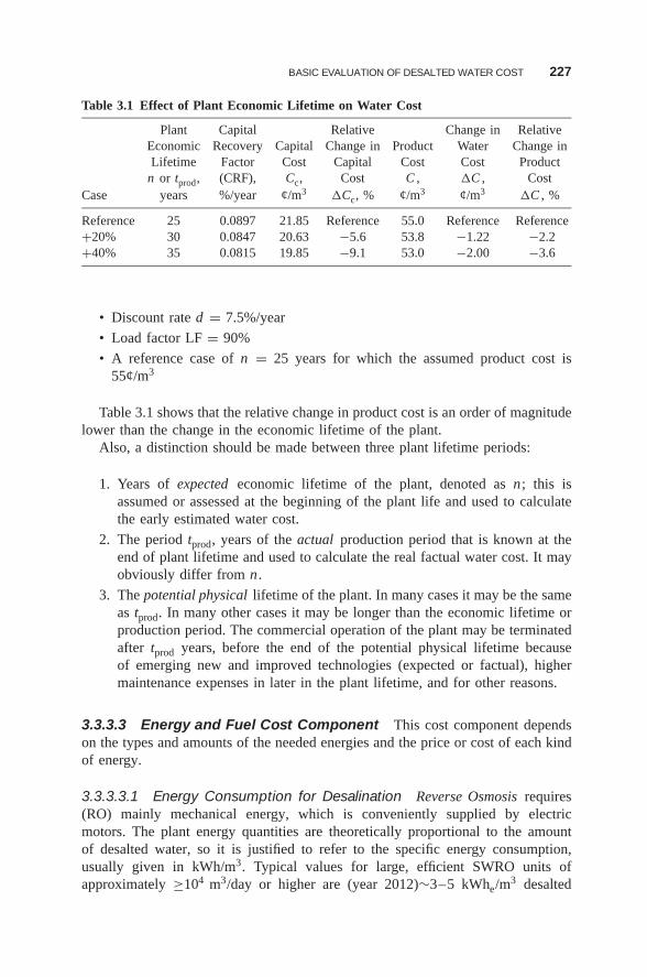
BASIC EVALUATION OF DESALTED WATER COST 227

Table 3.1 Effect of Plant Economic Lifetime on Water Cost

Plant Capital Relative Change in RelativeEconomic Recovery Capital Change in Product Water Change inLifetime Factor Cost Capital Cost Cost Productn or tprod, (CRF), Cc, Cost C , �C , Cost

Case years %/year ¢/m3 �Cc, % ¢/m3 ¢/m3 �C , %

Reference 25 0.0897 21.85 Reference 55.0 Reference Reference+20% 30 0.0847 20.63 −5.6 53.8 −1.22 −2.2+40% 35 0.0815 19.85 −9.1 53.0 −2.00 −3.6

• Discount rate d = 7.5%/year

• Load factor LF = 90%

• A reference case of n = 25 years for which the assumed product cost is55¢/m3

Table 3.1 shows that the relative change in product cost is an order of magnitudelower than the change in the economic lifetime of the plant.

Also, a distinction should be made between three plant lifetime periods:

1. Years of expected economic lifetime of the plant, denoted as n; this isassumed or assessed at the beginning of the plant life and used to calculatethe early estimated water cost.

2. The period tprod, years of the actual production period that is known at theend of plant lifetime and used to calculate the real factual water cost. It mayobviously differ from n .

3. The potential physical lifetime of the plant. In many cases it may be the sameas tprod. In many other cases it may be longer than the economic lifetime orproduction period. The commercial operation of the plant may be terminatedafter tprod years, before the end of the potential physical lifetime becauseof emerging new and improved technologies (expected or factual), highermaintenance expenses in later in the plant lifetime, and for other reasons.

3.3.3.3 Energy and Fuel Cost Component This cost component dependson the types and amounts of the needed energies and the price or cost of each kindof energy.

3.3.3.3.1 Energy Consumption for Desalination Reverse Osmosis requires(RO) mainly mechanical energy, which is conveniently supplied by electricmotors. The plant energy quantities are theoretically proportional to the amountof desalted water, so it is justified to refer to the specific energy consumption,usually given in kWh/m3. Typical values for large, efficient SWRO units ofapproximately ≥104 m3/day or higher are (year 2012)∼3–5 kWhe/m3 desalted

228 ECONOMIC ASPECTS OF WATER DESALINATION

water, not including pumping of desalted water from the plant. Much largermodern units, with capacities of ≥ 105 m3/day or so, are more sophisticatedand consume ∼2.8–4 kWhe/m3. Brackish-water consumes 1–3 kWhe/m3. Thedeviations are due to:

1. Technology versions, such as type of pressure recovery device.2. Plant size and capacity; the larger the equipment, the lower the friction flow

losses and the electric motors losses.3. Plant location and topography, which determine the pumping power required

to and from the plant.4. Salinity of feedwater; the higher the salinity, the higher are the feed needed,

the osmotic pressure, and the permeate salinity (the latter may need correctionby secondary desalination) as discussed previously. Each one of these processfeatures bears its share of energy. The difference between Atlantic and IndianOcean feedwater (3.5% and 4.5% salinity, respectively) is at least 1 kWhe/m3.

5. Required quality of product water. Reducing product salinity requires an aux-iliary system that consumes additional energy; the lower the product salinity,the higher is the additional energy.

The cost of 1 kWh depends on the source of electricity. Several possibilities exist:

• The Grid . In most countries the prices of electricity supplied to the industrialsector are significantly lower than that supplied to the domestic sector. In2004 it was 5.27¢/kWh in the United States for the industry vs. 8.97 fordomestic use, 16.15 vs. 19.13 in Italy (highest), 3.28 vs. 3.76 in Austria(lowest; subsidized??), and 9.39 vs. 11.89 in Israel. A typical energy costcomponent for power grid supply for very large units would be 3.8kWh/ton*5.5¢/kWh = 20.9¢/m3

• Load Shedding . It is possible to negotiate with the power utility on a certainreduction of the price, say, 20%, as is the case in some grids, for the option of“load shedding” under the condition of extremely high peak power demand.

• Self-supply . The possible means are diesel generators; steam turbines; gasturbines; combined cycles (of gas with steam turbines)’ after”steam turbines;and nuclear, solar, wind, tidal, (in principle; unlikely in practice) or geothermalpower. The investment in a self-generating system is relatively low since theinfrastructure for the power system is mostly shared by the desalination systemand there may be no need for cooling-water as the desalination system canabsorb all the rejected heat. The grid is used as backup, as mentioned. ThekWhe costs can range from 4.5¢ to 15¢ (US), depending mainly on the typeof fuel and its price. A typical result for very large units would be about thesame as from the grid, may be even slightly lower than 20¢/m3.

• Directly from Adjacent Power Plant . Electricity could be supplied from aneighbouring power plant or an industrial plant that has its own power system.Thus very little expenses and losses would be involved with transformationand transmission. Typical results depend on the price of purchased kWh.

BASIC EVALUATION OF DESALTED WATER COST 229

• Being Part of a Dual-Purpose Plant . This possibility is a very popular andattractive arrangement, as discussed in Section 3.4.

Mechanical vapor compression (MVC), like RO, is also energized mostly byelectricity, the sources of which are the same as mentioned above for RO. Theamounts of energy, however, are about twice those for RO, at least 6–8 kWh/m3.Because of the economy of scale, the cost of 1 kWh is somewhat lower than forRO if the power is self-supplied when compared with equal production . This isseldon relevant because of the higher energy consumption, but a reasonable marketfor MVC still exists. The specific energy of MVC also depends on technologyversions, but to a lesser extent on plant and unit capacities, site, feedwater salinity,and product quality requirements. A typical result for a very large and sophisticatedbattery of units would be 6.8 kWh/ton*5.5¢/kWh = 37.4¢/m3.

Electrodialysis (ED) is energized only by electricity, the sources of which are thesame as mentioned above for RO. The amounts of energy, however, range widelysince ED is useful mainly with brackish-water. This application requires smalleramounts of electricity per unit product, and the plant production rates are lowerthan those of large seawater desalination plants, so there is inadequate justificationfor self-supplied power. Thus, electricity is preferably purchased from the grid orfrom a nearby industrial or power plant, unless the local conditions do not allowpurchase of electricity at “acceptable prices” of below ∼10–12¢/kWh.

There is perhaps one potential advantage for self-supply of electricity to ED: thefact that ED requires mostly DC (direct current). External power sources hardly sup-ply this kind of electricity. Thus, where DC is needed while the naturally availablepower supply is AC, a conversion system is needed, but this can be expensive andconsume a few percent of the energy, due to unavoidable inefficiency. A self-supplysource can bypass these extra expenses if a DC generator or a photo-voltaic solarsystem is used. A typical result for very large units is difficult to define because ofthe variability of site-specific conditions, as the feedwater is brackish. The followingformula might be taken as somewhat typical: 2.0kWh/ton*5.5¢/kWh = 11¢/m3.

Multieffect and Multistage Flash (MED and MSF) distillation , unlike RO, ED,and MVC, require mainly thermal energy, which is convenient to supply by low-pressure or medium-pressure steam (subatmospheric or <3 bar, respectively). Alter-native heat sources are hot streams of liquids or gases. Both processes also requiresecondary mechanical energy for pumping, which is conveniently to supplied byelectricity, and tertiary energy (mechanical work, electricity, medium-pressure orhigh-pressure steam) for starting vacuum and maintaining it (i.e., with gases pump-ing from the process to the atmosphere).

The costs of these energies depend on their sources (in addition to their amountsas mentioned above).

Primary Thermal Energy The most common source for heat in a single-purposedesalination plant is a low or medium-pressure steam boiler. This source is expen-sive, relative to other alternatives. The specific investment in a fully installedmedium-pressure boiler is in the order of magnitude of a few dozen US dollars perthermal kilowatt. Assuming

230 ECONOMIC ASPECTS OF WATER DESALINATION

• $60/kWt, which is equivalent to $36,000/(t/h) of dry saturated steam at 3 barabsolute. (Since the latent heat of such steam is 516 cal/g and 1Wht = 860 cal,it follows that 516/860 = 0.6 kWht/kg steam = 600 kWht per ton of steamat 3 bar, i.e., $60/kWt*600 kWh/t steam = $36,000/(t/h) of boiler capacity.)

• A very high gain output ratio (GOR) of 12.5 m3 desalted water per ton ofsteam in an MSF plant

• A very high load factor (LF) of 89%; each ton of steam thus will produce12.5 m3/t steam*8760 h/y*0.89 = 97,500 (m3/y)/(t steam/h).

The annual CRF for a discount rate of 7.5% and 30-years boiler + plant lifetime is∼0.085, as shown in Table 3.1, so that the boiler part of the capital cost componentof the desalted water is $36,000*0.085/97,500 = $0.0314/m3 = 3 .14 ¢/m3 .

The main part of the steam cost is the fuel. Assuming low-cost coal of $50/tonhaving a lower heating value (LHV) of 6200 cal/g, with a boiler efficiency of 85%,we obtain $50/t-coal*516 Mcal/t steam/(6200 Mcal/t coal*0.85) = $4.9/t steam;thus $4.9/t-steam/12.5 m3/t-steam = $0.3916/m3 = 39 .16 ¢/m3 . Thus the capitalcost and fuel cost components of the steam contribution to the water cost add upto 3.14¢/m3 + 39.16¢/m3 = 42.3¢/m3.

With other boiler expenses such as electricity and maintenance, the heat costfor a very efficient MSF plant is at least 43 ¢/m3 .

With MED higher values of GOR are attainable, up to 20 m3 desalted water perton of steam, so the heat cost is almost proportional to the reciprocal of GOR. Inthis case, due to the economy of scale of the boiler, it is at least 27¢/m3, which issomewhat higher than the net calculation result: 43¢/m3∗12.5/20 = 26.8¢/m3.

Secondary (Pumping) and Tertiary (Lights, Services, Workshop, etc.) Mechanicaland Other Energy Forms These are effected mostly by electricity. The possiblesources and resulting costs for electricity are about the same as those above givenfor RO and for MVC. The amounts of electricity needed for MSF are 2–4 kWheper m3 desalted water and for MED, 1–3 kWhe/m3. Assuming the average valuesin the range 3kWhe/m3 for MSF and 2kWhe/m3 for MED, and taking the lowprice of electricity from the grid or from self-generation as 5.5¢/kWhe, we seethat almost 17¢/m3 and 11¢/m3 are added to the heat cost of MSF and MED,respectively.

This power cost can be reduced if the steam from the boiler to the evaporatorsis directed to expand in a steam turbine to drive a generator that will supply thesecondary and tertiary mechanical or electrical energies. This will circumvent theneed to purchase power from the grid (except as backup).

However, this strategy involves increasing the boiler size and the fuel consump-tion by 5–10% as well as installing a higher-pressure boiler, which increase thecost, plus a steam turbine and generator that are relatively expensive per unit prod-uct considering their economies of scale. The added turbine and generator increasethe system complexity, and require more labor to operate and maintain and morespare parts, oil, etc. The increased cost due to the boiler and its fuel consumptionis about 2–2.5¢/m3 for MED and 2.3–4¢/m3 for MSF. The capital cost of the

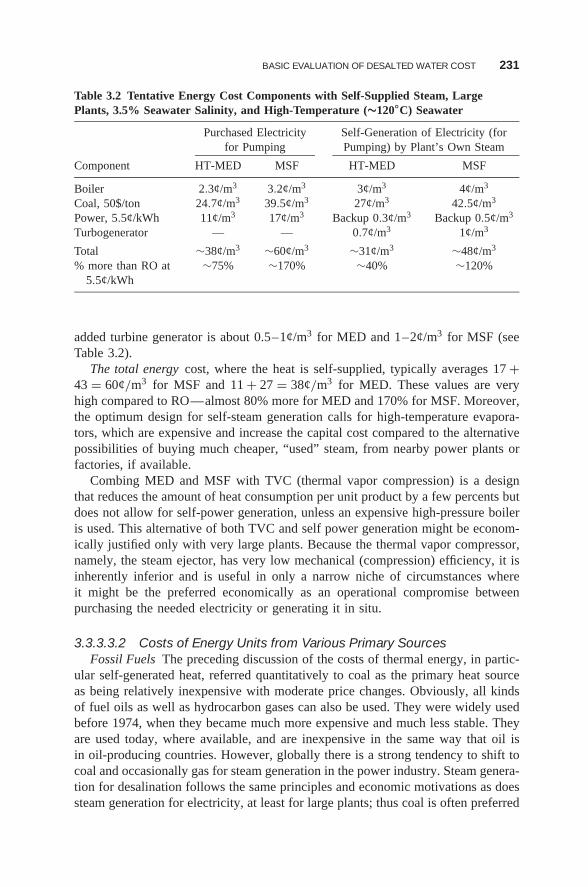
BASIC EVALUATION OF DESALTED WATER COST 231

Table 3.2 Tentative Energy Cost Components with Self-Supplied Steam, LargePlants, 3.5% Seawater Salinity, and High-Temperature (∼120◦C) Seawater

Purchased Electricity Self-Generation of Electricity (forfor Pumping Pumping) by Plant’s Own Steam

Component HT-MED MSF HT-MED MSF

Boiler 2.3¢/m3 3.2¢/m3 3¢/m3 4¢/m3

Coal, 50$/ton 24.7¢/m3 39.5¢/m3 27¢/m3 42.5¢/m3

Power, 5.5¢/kWh 11¢/m3 17¢/m3 Backup 0.3¢/m3 Backup 0.5¢/m3

Turbogenerator — — 0.7¢/m3 1¢/m3

Total ∼38¢/m3 ∼60¢/m3 ∼31¢/m3 ∼48¢/m3

% more than RO at5.5¢/kWh

∼75% ∼170% ∼40% ∼120%

added turbine generator is about 0.5–1¢/m3 for MED and 1–2¢/m3 for MSF (seeTable 3.2).

The total energy cost, where the heat is self-supplied, typically averages 17 +43 = 60¢/m3 for MSF and 11 + 27 = 38¢/m3 for MED. These values are veryhigh compared to RO—almost 80% more for MED and 170% for MSF. Moreover,the optimum design for self-steam generation calls for high-temperature evapora-tors, which are expensive and increase the capital cost compared to the alternativepossibilities of buying much cheaper, “used” steam, from nearby power plants orfactories, if available.

Combing MED and MSF with TVC (thermal vapor compression) is a designthat reduces the amount of heat consumption per unit product by a few percents butdoes not allow for self-power generation, unless an expensive high-pressure boileris used. This alternative of both TVC and self power generation might be econom-ically justified only with very large plants. Because the thermal vapor compressor,namely, the steam ejector, has very low mechanical (compression) efficiency, it isinherently inferior and is useful in only a narrow niche of circumstances whereit might be the preferred economically as an operational compromise betweenpurchasing the needed electricity or generating it in situ.

3.3.3.3.2 Costs of Energy Units from Various Primary SourcesFossil Fuels The preceding discussion of the costs of thermal energy, in partic-

ular self-generated heat, referred quantitatively to coal as the primary heat sourceas being relatively inexpensive with moderate price changes. Obviously, all kindsof fuel oils as well as hydrocarbon gases can also be used. They were widely usedbefore 1974, when they became much more expensive and much less stable. Theyare used today, where available, and are inexpensive in the same way that oil isin oil-producing countries. However, globally there is a strong tendency to shift tocoal and occasionally gas for steam generation in the power industry. Steam genera-tion for desalination follows the same principles and economic motivations as doessteam generation for electricity, at least for large plants; thus coal is often preferred

232 ECONOMIC ASPECTS OF WATER DESALINATION

as the cheapest fossil fuel. For much smaller MED and MSF single-purpose desali-nation plants, the boilers are smaller and it might sometimes be more convenientto use liquid or gaseous fossil fuels, even if they cost more than coal.

Nuclear Desalination. Several nuclear possibilities have been offered for usewith single-purpose desalination, ranging from very small units of 7–10 MWt(SAKHA-92, SES-10, NHR-10) for MED or MSF that can desalt water atrates of 3000–4000 m3/day, up to 500 MWt (AST-500), at a desalting rate of≤400,000 m3/day. Nevertheless, no single-purpose nuclear desalination plant hasbeen installed yet. One of the main reasons is the high cost. The main advantage,in principle, of nuclear energy is the lower nuclear fuel cycle cost component ascompared with fossil fuel cost—roughly 0.15–0.3¢/kWht (thermal kWh) nuclearversus 0.7–1.4 ¢/kWht from coal. The cost of fossil fuel, such as coal, includesthe cost of transportation from the pit to the plant site, thus depending on thelocation of the site and increasing with the distance. It is usually 3–5 times higherthan nuclear fuel cost per kWht.

However, this key factor in the economics of nuclear energy is partly eroded bythe much higher capital cost of nuclear energy and even more so, considerably,with evaporative desalination. MED and MSF require an additional investmentin the complex safety thermal coupling equipment that transfer the heat from thenuclear source to the MED or MSF evaporators. This coupling equipment, which isdesigned to isolate the heating stream in the nuclear system from the heated streamin the desalination system, is expensive. It also consumes electric-power directly,while indirectly lowering the thermodynamic efficiency of the plant. (directly—forpumping the circulating the heat carrier inside coupling equipment; indirectly—byreducing the useful process exergy).

The nuclear heating system for single-purpose desalination also requires

• Larger investment, which might increase financing difficulties

• More land area due to safety requirements and public acceptance aspects

• More workforce for O&M

• Higher skill of these workers, with higher salaries

• Long periods of refueling, i.e., water supply problems that are solved for extracost.

Nuclear desalination may also be performed using mechanicoelectrical energyfor RO, MVC, and ED. The fossil fuel cycle cost component per electric kWh ascompared with nuclear fuel cost is usually 2–4 times higher—about 0.5–1.0¢ pernuclear kWhe versus 1.7–3¢/kWhe from coal. The above mentioned thermal kWhfossil/nuclear ratio (3–5), is more favorable to nuclear than electrical kWh ratio(2–4), because the thermodynamic efficiency of fossil systems is higher than formost nuclear systems. On the other hand, the extra costs for specific nuclear safetyrequirements are lower where nuclear electricity rather than nuclear heat is used.

However, as mentioned above regarding evaporative desalination systems,most—and sometimes all—of this relative advantage of nuclear fuel cost is

BASIC EVALUATION OF DESALTED WATER COST 233

eroded by the higher capital cost of nuclear installations. Thus, the costs ofelectricity (at a given capacity and site) differ only a little (a fraction of a centper kWhe) regardless of whether nuclear or fossil fuel is burned to generate thiselectricity. For large-scale SWRO, this small difference in electricity cost adds upto about ±2¢/m3, sometimes in favor of fossil fuel. With the above mentionedadditional expenses for larger investment with potential financing difficulties, moreland area due to safety requirements, problematic public acceptance aspects, morelaborforce for O&M, higher skills and salaries of these workers, and long periodsof refueling, the scope of using nuclear energy for single purpose desalinationis limited for a narrow combination of site-specific conditions. On the otherhand, the scope for using nuclear energy for dual-purpose power generation withdesalination is much wider.

Solar Desalination There are three methods for using solar energy for desali-nation, which differ economically:

1. In the most popular method, using “solar stills,” the solar radiation vapor-izes the water directly at a moderate temperature slightly above ambienttemperature. This method requires very little purchased (mechanical or elec-trical) energy, for low-pressure and low-volume pumping, and can be fullyautomated at a reasonable cost, significantly reducing O&M expenditure.

2. Solar radiation can be used to generate steam or higher-temperature heat byemploying solar collectors or solar ponds at higher temperatures. This heatis transferred to MED or MSF evaporators. The expenses for secondary andtertiary energy as well as labor are the same as for self-generation of heat byfossil fuels.

3. Solar radiation can be used to generate electricity by steam or by photovoltaiccells, and this electricity can be used for RO, MVC, or ED. No secondaryand tertiary energy is purchased. In this case, the economic potential of solarpower for desalination is about the same as for ordinary power use.

All three methods suffer from high investment in equipment and large land area forcapturing the solar radiation, with impact on potential financing difficulties. Anotherproblematic feature is the load factor, which fluctuates even during the 48% =11.5 theoretical hours of solar radiation per clear average day, as it is dependenton weather and climate (clouds, fog, rains etc.), latitude, and sun position andmovement. Solar radiation methods may thus require additional investment eitherin storage of desalted water and/or energy, or in a backup energy system.

Therefore, the economic potential of solar desalination is appropriate to onlylimited combinations of site-specific conditions, such as secluded locations wherefuels are significantly more expensive, justifying the high investment.

Geothermal Desalination Like nuclear or solar energy, thermal energy sourcesrequire very little electricity but involve high investment. Geothermal desalinationmay be useful only if the following three conditions are met: (1) the thermal energy

234 ECONOMIC ASPECTS OF WATER DESALINATION

is available near sites where desalted water is needed and in sufficient quantity, (2)the cost of the geothermal heat (geothermal well, pumping, etc.) plus the system thattransmits the heat to the MED or MSF evaporators is less than that for alternativeheat sources (this may be possible if the wells are not very deep), and (3) thegeothermal well has proved reliable by operation for a sufficiently long time tojustify the investment.

Wind Energy This source supplies primary mechanical energy suitable forRO, ED, and MVC. It involves quite high investment, except if the winds arehigh-velocity and sustained, which is quite rare. Large land areas might be requiredfor installation of many wind turbine units. Occasionally such areas may be foundwhere desalted water is needed, good winds are blowing, sufficient low-costarea is available, and—if an inland site—there is enough saline water to feedthe plant.

The cheapest heat for MSF and MED can be obtained from the followingsources:

1. Low-cost “used” steam, or “waste heat” from nearby power plants or facto-ries, if available.

2. Low-cost heat from solar collectors or geothermal wells. So far these heatsources have very seldom supplied the cheapest heat where desalted water isneeded.

3. A high-pressure steam boiler that supplies energy for a large hybrid desali-nation plant that includes RO as well as MED or MSF. This is discussed ingreater detail in Section 3.4.

4. Heat produced by a desalination plant that is part of a dual-purpose plant thatuses heat to produce other products. (see Section 3.4). The most useful andfrequent product is electricity, so the discussion here focuses on dual-purposeplants that cogenerate power and water. The economic considerations of dual-purpose plants that produce other industrial products are similar to those forpower generation and of buying heat purchased from nearby factories (listitem 1 above).

3.3.3.3.3 External Heat for MSF and MED Buying low-cost used steam orwaste heat from nearby power plants or factories is economically worthwhile if theprice of the heat is below a certain value. In general, the price is determined bynegotiations. Each side may have alternatives that set the value; the desalinationplant may or may not use RO—which for high production rates ensures very lowallowable heat prices—or other heat sources, such as heat self-generation. Thepotential heat supplier may or may not use the heat to improve the economy ofthe own process and plant—for a certain cost—or sell it to a competitive heatcustomer. In some extremely rare cases the heat supplier has to dispose of excessheat and might be willing to provide the heat free of charge.

Beyond negotiations, by which the price is determined possibly subjectively,there are the objective aspects:

BASIC EVALUATION OF DESALTED WATER COST 235

1. The heat has a cost, which is complicated to calculate since it is delivered byused steam and since it depends on questionable and debated assumptions.

2. The heat has a thermodynamic value, expressed in energy units. It can betranslated into economic units by practically using the thermodynamic valuein a technical system such as power generation or heating applications suchas for industrial processes, buildings, water streams, etc. The thermodynamicvalue depends strongly on the temperature at which the heat is used. Itincreases roughly proportionally with the temperature difference above theambient temperature �Tth = Theat − Tamb. Similarly, the practical economicequivalent value is roughly proportional to the practical, smaller temperaturedifference

�Tpr = �Tth − T� (3.44)

where T� (≈10◦C) is the common economic temperature difference neededto reject heat from steam to the ambience.

This economic value of the consumed heat is slightly (∼10–40%) less than thecost of the net electricity that could have been generated by this heat. This valuedepends—sometimes in a complex way—on the amounts of the purchased heat,on the temperature at which this heat is supplied (if by superheated steam, then thepressure and temperature of the steam), and obviously on the distance between theheat source and the desalination plant. In efficient MED plants this nongeneratedelectricity is ∼4–6 kWhe/m3; for MSF it is roughly 70% higher.

Thus, for a typical optimistic example, at an efficient MED plant purchasingheat according to its technological value, which, is assumed, say, at 80% of thecost of the net nongenerated electricity, which, in turn, is assumed at 4.5¢/kWhethen, at 5kWhe nongenerated power per m3 desalted water, the cost of heat per m3

is approximately 5 kWhe/m3*4.5¢/kWhe*0.8 = 18¢/m3.As conveying the heat costs more, some profit for the heat supplier should

also be added so that well over 20¢/m3 is charged for the heat cost compo-nent. The total energy cost—considering the additional secondary and tertiarymechanical and electrical energies (1–3 kWhe/m3 for MED and 2–4 for MSF),assuming 1.5 kWhe/m3 in this example for power from the grid at 5.5¢/kWheprice—accumulates to more than 30¢/m3.

Another aspect is the time availability of the heat supply. If it is relatively low,the load factor of the desalination plant also becomes low, which increases thewater cost mainly because the capital cost rises.

3.3.3.3.4 The Effect of Discount Rate on Energy Cost This effect is quitesmall. If the electricity and the heat are procured from external sources, theirpayments occur generally at the same time as do payments for the water. A timegap of a few days is negligible. If the time gap is a few weeks, the effect is aboutd/52 = d divided by 52 weeks per year per week, i.e. with d = 8%/year and, say,3-week lag in water payments after energy purchase, the latter becomes almost0.5% more expensive.

236 ECONOMIC ASPECTS OF WATER DESALINATION

The effect is greater where the energy is self-generated. The fuel is often pur-chased a few months before use, and the effect may be an increase of a fewpercentage points.

3.3.3.4 Operation and Maintenance (O&M) Cost Component Thenumerous items covered by O&M costs can be categorized in three groups:

1. The annual variable-cost items , which are theoretically proportional to theannual amount of desalted water PA; specifically, they have constant valueper unit product. These items include chemicals for pretreatment and post-treatment; at least part of the membrane and spares replacement; and somemaintenance activities, such as filter cleaning and possibly part of the taxes.In practice, the proportionality is only approximate as a small cost reductionper unit product is expected for larger quantities of chemicals, membranes,and other materials due to the economy of scale.

2. The annual fixed-cost items , which are theoretically proportional to thedesigned production rate of the plant, i.e., the nominal capacity PN, butdo not depend on the number of annual operating hours and load factor.These include insurance and possibly another part of the taxes, part of thestaff salaries, Fee for special workers hired for intermittent short periods ofmaintenance activities, most of the periodic maintenance activities, the otherpart of membrane and spares replacement, and part of the administrativeand management activities.

3. The annual independent-cost items , which do not depend on plant size, inprinciple, at least within a wide range of plant capacities. These include theother portion of the salaries such as those of the minimum shift operators(at least nine people working without overtime pay), one plant manager orsupervisor plus minimum maintenance and administration staff, and basicoffice expenses.

The larger items covered by O&M costs are

1. Wages and Salaries . If the plant is fully automated, which applies to smallplants, this item is not expensive. Belonging partly to category 2 and partlyto category 3 (above), with large plants, this may cost between $0.5M and$2M per year.

2. Consumables, Mainly Chemicals . Belonging to category 1, this usually costs4–5¢/m3 desalted water.

3. RO or ED Membrane Replacement . Belonging partly to category 2 and partlyto category 1, this ranges within the extreme values of 2–6¢/m3. Commonvalues with large plants are 3 ± 0.5¢/m3.

4. Equipment Replacement and General Maintenance (ER&M). Belongingpartly to category 2 and partly to category 1, this is preliminarily often

BASIC EVALUATION OF DESALTED WATER COST 237

assumed to cost within the extreme range of 2% per year of the directinvestment and 3% per year of Itot, the total capitalized investment. Commonvalues with large plants are 2% per year of Itot. Assuming US$720/m3 perday and a load factor of 92%, this item is

2% per year*$720 (m3d−1)/(365 ∗ 0.92) = $0.0429/m3 ≈ 4 .3 ¢/m3.

5. Insurance. This represents 0.5–1% per year of the direct investment. Assum-ing the latter to be $500 (m3d−1), with a load factor of 92%, insurance costs:

0.75% per year∗$500/( m3d−1)/(365∗0.92) = $0.0112/m3 ≈ 1 .1 ¢/m3.

These Five items cover most of the O&M costs. In the calculation demonstratedabove, for large-scale SWRO at 108m3/year per plant, these costs total

Salaries [$2M per year/(108m3/year)] 2¢/m3

Chemicals 4¢/m3

Membrane replacement 2.5¢/m3

Equipment replacement and maintenance (ER&M) 4.3¢/m3

Insurance 1.1¢/m3

Total 14¢/m3 (approximate)

3.3.3.5 Cost Comparison of Single-Purpose Desalination ProcessesThe following comparison is obviously tentative, approximate, and virtual.It refers to the following [dispersed and normalized] economic data of year2004 for:

• 100,000 m3/day plant capacity

• Seawater of 3.5% salinity and

• Maximum product salinity of 500 ppm TDS

• 7.5% discount rate, 30-year plant lifetime, 6 payments per year (thus, annualamortization is 8.214%)

• 5.5¢/kWhe electricity cost

• With $1.5M/year salaries and wages

• Equipment replacement, general maintenance and insurance (ERMI) at 2.5%per year of Itot.

The following processes, which are at present the most popular for large-scaleseawater desalination, are compared (see also Table 3.3):

• MSF (high temperature: 120◦C Tmax brine, 125◦C Tsteam)

• HT-MED (high temperature: 120◦C Tmax brine, 125◦C Tsteam)

• LT-MED (low temperature: 70◦C Tmax brine, 125◦C Tsteam)

• SWRO

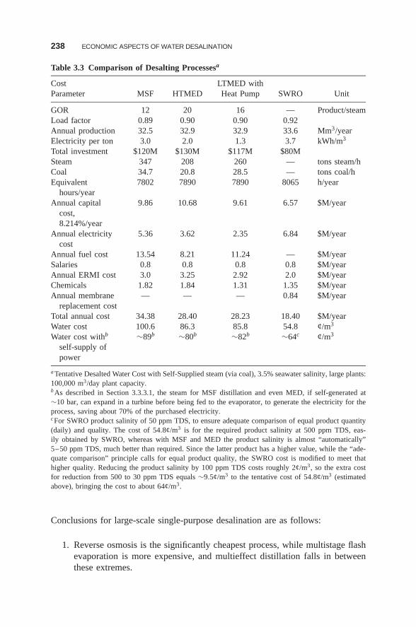
238 ECONOMIC ASPECTS OF WATER DESALINATION

Table 3.3 Comparison of Desalting Processesa

Cost LTMED withParameter MSF HTMED Heat Pump SWRO Unit

GOR 12 20 16 — Product/steamLoad factor 0.89 0.90 0.90 0.92Annual production 32.5 32.9 32.9 33.6 Mm3/yearElectricity per ton 3.0 2.0 1.3 3.7 kWh/m3

Total investment $120M $130M $117M $80MSteam 347 208 260 — tons steam/hCoal 34.7 20.8 28.5 — tons coal/hEquivalent

hours/year7802 7890 7890 8065 h/year

Annual capitalcost,8.214%/year

9.86 10.68 9.61 6.57 $M/year

Annual electricitycost

5.36 3.62 2.35 6.84 $M/year

Annual fuel cost 13.54 8.21 11.24 — $M/yearSalaries 0.8 0.8 0.8 0.8 $M/yearAnnual ERMI cost 3.0 3.25 2.92 2.0 $M/yearChemicals 1.82 1.84 1.31 1.35 $M/yearAnnual membrane

replacement cost— — — 0.84 $M/year

Total annual cost 34.38 28.40 28.23 18.40 $M/yearWater cost 100.6 86.3 85.8 54.8 ¢/m3

Water cost withb

self-supply ofpower

∼89b ∼80b ∼82b ∼64c ¢/m3

a Tentative Desalted Water Cost with Self-Supplied steam (via coal), 3.5% seawater salinity, large plants:100,000 m3/day plant capacity.bAs described in Section 3.3.3.1, the steam for MSF distillation and even MED, if self-generated at∼10 bar, can expand in a turbine before being fed to the evaporator, to generate the electricity for theprocess, saving about 70% of the purchased electricity.cFor SWRO product salinity of 50 ppm TDS, to ensure adequate comparison of equal product quantity(daily) and quality. The cost of 54.8¢/m3 is for the required product salinity at 500 ppm TDS, eas-ily obtained by SWRO, whereas with MSF and MED the product salinity is almost “automatically”5–50 ppm TDS, much better than required. Since the latter product has a higher value, while the “ade-quate comparison” principle calls for equal product quality, the SWRO cost is modified to meet thathigher quality. Reducing the product salinity by 100 ppm TDS costs roughly 2¢/m3, so the extra costfor reduction from 500 to 30 ppm TDS equals ∼9.5¢/m3 to the tentative cost of 54.8¢/m3 (estimatedabove), bringing the cost to about 64¢/m3.

Conclusions for large-scale single-purpose desalination are as follows:

1. Reverse osmosis is the significantly cheapest process, while multistage flashevaporation is more expensive, and multieffect distillation falls in betweenthese extremes.

BASIC EVALUATION OF DESALTED WATER COST 239

2. Multieffect distillation at high temperatures and low temperatures, each hav-ing relative advantages, differ negligibly in cost.

3. Despite potential complications of the equipment and O&M, self-generationof electric power significantly reduces the product cost.

3.3.3.6 Socioenvironmental Costs A major concern nowadays is toincrease the sustainability of desalination plants, preferably by accounting eco-nomically for the “externalities,” which are miscellaneous costs of environmentaland social aspects that were not considered in the past. This will include the(1) costs of improved brine discharge that does not allow for discharge ofchemicals or damaging levels of salt concentration and temperature into the sea(or wherever possible), (2) costs of reducing CO2 emissions when fossil fuels areused, or (3) cost of proliferation prevention when nuclear power is used. Thereis rapidly growing criticism of the unsustainable design of desalination plants,and it is unlikely that desalination plants will be designed in the future withoutcompensating for these problems in some way or another. Authorities such asmunicipalities, governments, and international organizations will impose stricterregulations. These costs may be for preventive purposes, thus expended prior tocommercial operation of the desalination plant, or as compensation by correctivesteps and even as fines for violating the stated regulations and expended during orafter the commercial operation.

Quantifying these costs is still problematic and to some extent premature. Theregulations are often site-specific, depending on local physical conditions and pos-sibly on the personal requirements of the executives and consultants serving withinthe local authorities. Also, in many plants the regulations are not yet at final stage.Moreover, the technical and administrative solutions to the environmental prob-lems are still in rather early phases of development. New solutions are expected toemerge, and the costs are thus expected to change.

Effluent discharge costs for seawater desalination may depend on the topographyand other local conditions of the seabed. As for brackish-water desalination, theeffluent discharge costs may depend on groundwater local conditions and geographysuch as distance from the nearest sea and transportation options.

The improved brine discharge may consist of acceptable dilution of the out-going brine returned to the sea and/or longer outfall piping. It may alternativelyor additionally consist of additional chemical treatment of the brine to deal withflocculants and iron. The detailed design of such candidate solutions may changedrastically as a result of numerous factors—physical, environmental, technical,economical, institutional, administrative, and even political (public relations, elec-toral, popularity, etc.). The cost of these candidate solutions obviously follows thedesign of each solution.

As for costs of CO2, solid particles (fly ash), NOx and SOx emissions, andnuclear proliferation prevention, where fossil fuels and nuclear power, respectivelyare used, the terms technical and administrative solutions do not refer specificallyto desalination but rather to the much broader scope of power and heat generation,thus becoming a component of the pertinent power or heat cost, automatically

240 ECONOMIC ASPECTS OF WATER DESALINATION

included in the energy price paid by the desalination facility. The cost of desaltedwater will increase equally to the costs of cement, steel, beer, sugar, and generalhousehold supplies. Although desalted water is still a small component of theoverall energy cost, it should not be ignored. Since the energy cost componentusually amounts to only 30–40% of the total water cost, the additional costs ofthese factors is—although certainly not negligible—fairly marginal. In any case,it is calculated and considered, locally, as mentioned previously, by the powergeneration sector that supplies the energy to, not by , the desalination plants.

This convenient bypassing of these energy and environment issues holds in mostcases except where the desalination plants have self-supplied power and heat. Thenthese aspects—mainly CO2, NOx and SOx emissions, which hardly represent pro-liferation prevention—become more difficult to manage, with wider scope relativeto externally energized desalination and possibly higher cost due to the negativeeconomy-of-scale effect (because energy generation for desalination is usually anorder of magnitude smaller than for common power stations). Roughly speaking,the added cost may range between a few percent and very few percent of the totalwater cost.

One cannot ignore the possibility that in some cases where desalted water iscritically essential, the environmental issues and problems may be partly offset ifthe cost of their solutions is considered too high for the users or the community.The possibility of providing desalted water of a quality higher than that of the“predesalination” status has a positive environmental impact with an equivalenteconomic value.

The social aspects are even more site-dependent than the environmental impacts.One positive socioeconomical aspect is employment in various phases of thedesalination plants—mainly construction and operation. Further long-term aspectsassociated with national and multinational desalination programs are the establish-ment of desalination research and training institutes and the emerging desalinationcourses in universities, technology institutes, etc. Another aspect is the develop-ment of the area near the plant, which is meaningful mainly for large single-purposedesalination plants (for small plants it has a negligible effect, and for dual-purposeplants it is credited to power plant as being the more dominant component of thecomplex). These social aspects do not reflect, however, on the direct cost of thedesalted water.

3.3.3.7 Cost of Desalted Water Conveyance This cost component isnot included in water production. However, it concerns the nuclear–conventionaldesalination controversy in two possible ways:

1. If the energy needed for pumping the desalted water through the distributionsystem differs in cost, due to differences between power sources

2. If the conveyance distance is longer than in the alternatives methods, due tospecific requirements imposed on nuclear plant siting.

For large amounts of desalted water, the costs of conveyance through flat andhorizontal topography range between approximately 0.1 and 0.3¢/m3 per kilometer.

COST EVALUATION OF COMPLEX DESALINATION SYSTEMS 241

Economy of scale plays a significant role in water conveyance; a double flow ratereduces the cost of transporting per unit water by roughly 7%. The cost may be anorder of magnitude higher for small amounts, for seismically problematic distances,or for meaningful elevation differences.

3.4 COST EVALUATION OF COMPLEX DESALINATION SYSTEMS

These systems include dual-purpose plants, hybrid desalination plants, and two-qualities product water streams.

3.4.1 Dual-Purpose Plants

By definition, desalination plants that are part of an industrial complex that producesother commodities may be considered as multipurpose plants. In principle, theeconomic rationale for desalting water in multi -purpose plants is to reduce the costby sharing facilities, resources, equipment, and services. In practice so far, mostlycogeneration plants have been considered for this sort of sharing. A cogenerationplant, which produces both electricity and good-quality water, is often called adual-purpose plant . The combination is logical for power plants that are situatedon coasts using large amounts of screened and filtered seawater for cooling.

The potential power-generating-components of the dual-purpose plant are asfollows:

1. Fossil fuel boiler and steam turbine.

2. Nuclear reactor and steam turbine

3. Fossil fuel gas turbine

4. Nuclear reactor and gas turbine

5. Fossil fuel combined cycle (gas turbine, boiler, and steam turbine)

6. Diesel engines

7. Geothermal heat from brines or steam and steam turbine

8. Garbage incineration and steam turbine

9. Solar collectors or ponds and steam turbine

10. Solar photovoltaic panels or cells

11. Wind turbines

All these power generation systems are suitable for the mechanically or electri-cally driven processes (RO, MVC, or ED) as obviously part of the generatedpower is diverted to the desalting sector rather than to the grid or more distantusers/customers. Generation system types 9 an 10—wind and photovoltaic—whichdo not have thermal elements, are suitable only for RO, MVC, or ED. Photovoltaicpanels or cells in particular are suitable for ED, as the primary electricity generatedby the photovoltaic system is lower-voltage DC while the basic electricity for useby the ED system is of the same type, saving costs for transformation to AC at

242 ECONOMIC ASPECTS OF WATER DESALINATION

the photovoltaic section and rectification at the ED section, thus saving investmentin equipment and unavoidable energy losses. However, wind and photovoltaic sys-tems are relatively small power sources and not very common, in particular ascandidates for dual-purpose plants, so they have a narrow potential niche in thedesalination market and only for small desalination plants.

Regarding the nine power systems that convert heat as primary energy to electricpower, they are naturally suitable for evaporative desalination by low-temperatureMED and low-temperature MSF (the latter is very rare). Most of these systems arealso suitable for high-temperature MED and MSF: fossil fuel boilers with steamor gas-turbines, nuclear reactors with steam or gas turbines, fossil fuel combinedcycle systems, garbage incineration with steam turbines. However, and solar con-centrating collectors with steam turbines; diesel engines, geothermal heat, and solarponds are suitable only for low-temperature distillation [<170◦F (77◦C)].

Diesel engines and gas turbines, both fossil fuel and nuclear, are very attractivefor distillation because they may supply low-grade heat from exhaust gases andcooling-water. This heat is not useful in single-purpose power plants. Using it fordesalination does not involve burning fuel, and the only costs are those for thenecessary heat exchange equipment; thus this type of low-grade heat is availablevirtually, free of charge. On the other hand, diesel engines and gas turbines havea narrow niche in the desalination market because

1. Diesel engines and regular fossil fuel gas turbines are considerably less com-mon than steam turbines, either fossil fuel or nuclear.

2. They do not require cooling-water and are often located inland rather thanat the seashore, and thus are not suitable for seawater desalination or forbrackish-water either, since the latter is desalted by membranes rather thanevaporation.

3. They are smaller than steam power plants, so the amount of desalting byevaporation is of narrower scope, losing the economy-of-scale advantageeven for the few plants that are located at seashore.

4. They use mostly fuel gas or fuel oil, which is often more expensive than coalper unit heat.

5. Gas turbines have lower thermodynamic efficiency than steam turbines.

6. Because of features 1–5 (above), they are not used as base-load units whenconnected to the grid, but as peak-load units with a low load factor, whichrenders the desalination costs quite high.

In principle, when one of the listed power technologies is preferred solely forpower generation in view of site-specific conditions while a need for both powerand desalted water exists, the dual-purpose plant is a good potential solution, whichmay sometimes offer significant economic advantages, as with diesel engines andgas turbines. But supplying very low-cost heat from diesel engines and gas turbineswith LT-MED, which yields very low-cost desalination, seldom justifies use of adual-purpose plant with gas turbines.

COST EVALUATION OF COMPLEX DESALINATION SYSTEMS 243

Each such power source has specific advantages and disadvantages forcombinations with desalination in addition to their common economic advan-tages over single-purpose plants. These common advantages are detailedbelow:

3.4.1.1 Common Advantages There are four basic advantages:

1. Lower Financial Investment Due to Sharing of Facilities . Seawater supplyand brine outfall, land area, site preparation, fences and roads costs are less,and some ancillary equipment such as pumps, compressors, lighting, cranes,transformers as well as administrative buildings can be used in common.For evaporative desalination there is also a large saving in boilers or steamgenerators and final condensers. Solar photovoltaic and Wind turbines shareonly part of these items.

2. Less Fuel and Energy Consumption . The total combined fuel consumptionis less, since some main components are larger in dual-purpose plants, thushaving higher efficiencies—in some cases much higher. Also, energy (inthe form of electricity, steam, or hot water) is saved in shared facilities andcommon subsystems as well as by short-distance energy transport. Wherelarge MSF and MED are installed using steam from the turbine exhaust(backpressure turbine), the turbine efficiency is somewhat higher than in aregular steam turbine (condensing turbine) because in the latter low-pressurestages the expanding steam is wet and its moisture decreases the turbineefficiency, as the moisture increases the energy losses due to higherfriction.

3. Lower Charge per Unit energy . This is a potential (not actual) advantagebecause the energy consumed by the desalination system may be rated lessthan the price at which it would have been sold to a nearby single-purposeplant. It may even be charged as low as the cost of generating this energysince it is in essence “selling to itself”; however, this possibility is notclearcut, as it might be complicated and difficult to evaluate the unit costof energy, which is generated at a dual-purpose plant sharing resources withthe water section. This difficulty can be overcome by assuming (to a reason-able extent or arbitrarily) the share of the power and the water. An extremelylow charge may be obtained if the energy is charged according to the costof the marginal amount of the energy that the desalination sector of thedual-purpose plant consumes, rather than the average cost of the generatedenergy.

4. Lower Staffing Requirement . A dual-purpose plant requires fewer staffthan the two single-purpose plants (one for power generation and the otherfor desalination) because of joint operation and maintenance of commonfacilities.

However, a dual-purpose plant also has disadvantages, compared to two single-purpose plants, as described below.

244 ECONOMIC ASPECTS OF WATER DESALINATION

3.4.1.2 Common Disadvantages These are

1. Less Overall Flexibility . The operation of a dual-purpose plant is not as flexi-ble as that of a single-purpose plant. There is economic pressure to maximizethe combined production of water and power by increasing the load factor andthus reducing the cost of both water and power. The load factor is maximizedby operation at full load for as many hours during its life time as possible.However, such design and operation may reduce the plant flexibility andcause indirect penalties; for instance, the demand for either water or powermay occasionally be low—rarely for water, which can be stored, and muchmore often for power. Where heat from gas turbines or where backpressuresteam is used to operate MED or MSF, any reduction in the power generationrate due to low demand results in less steam or hot gas to the turbine andthus from the turbine via exhaust, followed by reduced water production. Inthe reverse circumstances, when the evaporative desalination—which func-tions as a heat sink for the power generation section—operates at partialload while the power generation is fully loaded, the matching is problematic.Solutions for both situations exist, for an extra cost and risk of operationprocedures complications. Certain designs do, indeed, provide for variationin the water–electricity ratio, but at the cost of efficiency or extra investment.

Operation flexibility is inversely proportional to the degree of coupling;the higher the degree of coupling, the lower the flexibility. The degree ofcoupling isa. Maximum in the classical dual-purpose plant where backpressure steam

from the steam turbine exhaust is used to operate MED or MSF, as men-tioned above; the flexibility is lowest compared to alternative designs 1band 1c (below).

b. Slightly less where the steam for MED or MSF, comes from the cross-over point at the steam entrance to the low-pressure section of the steamturbine or from a steam extraction point between turbine stages, or if suchextracted steam drives RO pumps or MVC compressors by steam enginesor, more likely, steam turbines.

c. Much lower with RO and MVC that require electricity and get it directlyfrom the power generation section of the dual-purpose plant.

The higher the degree of coupling, the lower is the flexibility of the combinedsystem, and consequently the higher is the cost.

2. Lower Availability Factor and Load Factor . Any incident interrupting the out-put of one of the two commodities may lead to a disturbance or stoppage inthe production of the other, thus increasing the cost per unit product. It is pos-sible to improve the plant availability as a whole and reduce this cost increaseby connecting SWRO to the grid or adding devices such as bypass steam lines(in steam power units) so that steam can be directed to the evaporative desali-nation plant if the turbo-generator is out of operation. Likewise, addition of anauxiliary condenser enables the power plant to be operated if the desalinationplant is shut down. However, these devices involve extra investment.

COST EVALUATION OF COMPLEX DESALINATION SYSTEMS 245

a. As described above regarding the flexibility, power stations are operatedto meet the fluctuations in demand due to daily and seasonal variations.Load fluctuations are not favorable for plant economics, in particular fornuclear and desalination systems, which have a significant fixed cost dueto their relative high capital cost component. There are various meansto minimize the effect of these fluctuations on the load factor. One is tonominate dual-purpose plants for base-load operation. Also, depending onthe type of desalination process, the coupling of a desalination system to apower plant can improve the utilization of the latter and thereby decreasepower and water costs. On the other hand, it may impose some penaltyon the other units where all generation plants are connected to the grid.It is easy to maintain high load factors for RO systems, even if they arecoupled to a power plant that is not at base-load. In the case of poweroutage of the latter, the RO system can be energized from the grid, whichis technically easy to install as backup. (Moreover, the continuous anduniform load due to RO improves the load factor of the coupled powerplant.) Thus, the expected LF value for RO is ∼0.9–0.92.

b. A different situation takes place regarding the operation of a thermaldesalination system coupled to a power plant. As stated above, the cou-pling is definitely not flexible. The desalination plant can be operatedeconomically only when the power plant is producing electricity, as anybackup arrangement is quite expensive to install and maintain. Moreover,any negative fluctuation in power generation, which reduces the powerunit load factor, has a similar effect on the desalination plant load factor.The expected value of LF for MED or MSF is about 90–97% that of thepower system’s LF; specifically, it is ∼0.65–0.8.

3. Off-Optimum Site and Timing . The optimal location and/or commissioningdate of the desalination plant, in terms of water conveyance, distribution,and supply, may not coincide with those of the power plant, bearing anotherpenalty. As the power section is dominant in most cases, the water sectionbears the penalties.

Economic comparison of dual- and single-purpose plants involves more than abalance of their respective investment and operating costs. Indirect economic effectsmay exist, and the environment in which the plants are located should also beconsidered. It is important to note that while the economic weight of the abovementioned advantages of dual-purpose plants is fully expressed in the quantitativecost calculations, it is difficult to do so with the disadvantages , due to their narrowerscope, complex nature, and indirect role; thus, they are only partly accounted forin the cost calculation.

3.4.1.3 Comparison of Power Generation Systems The most popularcandidates for power generation are

• Fossil fuel —used in either boilers–steam-turbines combination, or in Com-bined Cycles (gas turbine–boiler–steam-turbine).

246 ECONOMIC ASPECTS OF WATER DESALINATION

• Nuclear Fuel —used in nuclear reactors in combination with either steam-turbines, or with gas-turbines.

It is therefore important to identify and weigh the basic economic differencesbetween dual-purpose plants using fossil fuel and nuclear fuel. These are describedbelow.

Nuclear Fuel is favored for the following reasons:

1. Energy Charge. Obviously the source that supplies lower-cost energy is eco-nomically favored, whether it is nuclear or fossil, according to the site condi-tions. Also, in general, the cheaper the thermal energy is, the lower is the costof the generated electricity. For generic, large-scale models, nuclear energyseems to cost less than the power or heat from fossil fuel (by ∼10–20%, butupdated data may show different values); nevertheless, fossil fuel is some-times preferred for non-cost-related reasons such as use of a smaller powergrid, negative public acceptance of nuclear energy, political reasons such asgovernmental refusal to supply nuclear technology or objections to adopt it,licensing problems (e.g., plant location in a seismically unstable area, densepopulation), or lack of appropriate infrastructure. However, fossil fuel mayoccasionally be preferred to nuclear fuel for the following economic reasons:

a. The plant in question, either existing or planned, may not be large enoughto accommodate a nuclear system to be economically competitive withfossil fuel, or the local fossil fuel prices may be low enough to havelower energy cost than nuclear.

b. Heat that is usable for MED or MSF is, indeed, quite cheap, but thecost of the power needed to produce desalted water using nuclear fuel ishigher than that using alternative energy sources (e.g., from gas turbinesvs. steam cycles, as mentioned above).

2. Maximum Production Rate. For RO or MVC there is no difference betweenfossil or nuclear dual-purpose plants with respect to maximum productionrate. However, for large-scale MED and MSF desalination, the availablenuclear reactors enable much larger desalination plants than the existinglarge fossil fuel steam boilers. This is because for large-scale plants theavailable heat sources are of fixed dimensions rather than being “tailor-made”for particular cases. With given dimensions of large fossil fuel boilers (∼2GW thermal) and nuclear reactors (∼3–4 GW thermal), the economy-of-scale principle can be applied for nuclear thermal desalination. Moreover,the amounts of usable heat for evaporative desalination from nuclear reactorsare much greater than from fossil plants since the latter lose 10–15% of theheat generated by the fuel in flue-gases and also since its thermodynamicfeatures allow for less usable heat to be exhausted to the heat sink. Thus,even with equal heat generation capacity of nuclear and fossil sources—themost common water-cooled nuclear power reactors release 60–70% moreheat, usable for MED or MSF, compared to fossil fuel steam power units.

COST EVALUATION OF COMPLEX DESALINATION SYSTEMS 247

This added heat is proportional to the production rate and further increasesthe economy-of-scale effect.

3. Load Factor and Time Availability . As nuclear power involves considerablyhigher investment than fossil power and much lower output energy cost thanfossil power, it is highly preferable economically to operate nuclear plantsconnected to the grid as base-load units with the fossil plants second in line.Thus the load factor of nuclear power plants is higher, as is the load factorof the linked desalination units. In particular, it is effective with regard toMED and MSF that have virtually no thermal back-up.

4. Bypass Line. In case of turbine generator outage, with the steam generator orboiler functioning, working with a bypass line is less expensive in the caseof evaporative desalination at a nuclear plant because of the lower initialquality of the steam; in other words, the exergy lost with single-purposeinstead of dual-purpose steam is lower under nuclear steam supply system(NSSS) thermodynamic conditions than with the use of a fossil fuel boilersystem.

5. Cost Fluctuations . Nuclear fuel operation is much less vulnerable to costfluctuations than is fossil fuel operation.

6. Geographic Location . Nuclear plant economics do not vary to any greatextent with geographic location. This factor is important for the regions withlow availability of fossil fuel. Nuclear desalination offers an additional degreeof freedom in securing local energy requirements.

7. CO2. The carbon footprint (i.e., due to CO2 emissions) is much smaller fornuclear operation, and fewer potential carbon penalties or costs are incurred.

Fossil Fuel is favored for the following reasons:

1. Safety . The requirement to ensure no radioactive penetration whatsoever fromthe nuclear section of the dual-purpose plant to the water section imposes anadditional expense on nuclear desalination. This expense is quite small withRO, where such penetration can occur only if the feedwater of the desalina-tion plant comes from the cooling-water of the power section heat rejection(steam condenser for steam turbines or gas cooler for gas turbines), andonly if there is leakage in the condenser or gas cooler. This low-probability,low-damage hazard can be eliminated at low cost by various means. How-ever, MSF and even more so MED require extensive additional investmentin the thermal coupling equipment that transfers the heat from the nuclearsource to the MED or MSF evaporators, as explained above for the potentialuse of single-purpose nuclear desalination. This high-temperature, corrosion-resistant coupling equipment, which isolates the heating stream in the nuclearsystem from the heated stream in the desalination system, is expensive notonly in terms of the large amount metal employed; it also, includes additionalinstrumentation, control and alarm equipment, and consumes pumping energyand thermodynamic exergy, thus reducing the process efficiency significantly,

248 ECONOMIC ASPECTS OF WATER DESALINATION

at least with MED. The isolation loop increases the cost of the MED evapo-rator by roughly 10–15%, the specific thermal energy by ∼5–12%, and thepumping energy by ∼10–20%.

2. Licensing . Licensing procedures are longer and require more effort andexpense.

3. Security and Proliferation Considerations . In addition to safety and licensingconsiderations, there is major concern about security and proliferation poten-tial problems with the use of nuclear energy. There is an additional cost forthe extra design efforts, security devices, special personnel training, and soon, reflected not only on the power section—which is included in the energycost component of the desalination section—but also possibly on other costcomponents of the desalination. In particular, the need for security imposes aneconomic burden for the potential single-purpose nuclear desalination plantswith relatively small nuclear reactors.

4. Conveyance Distance. Nuclear plants are located at greater distances from thepopulation centers that they serve than are fossil plants; thus transportationcosts for water delivery are higher.

5. Availability of Suitable Steam Turbines . The selection of large-scale nuclearsteam turbines, which are designed to operate under steam conditions that aredifferent from those for other steam turbines, is rather narrow. This drasti-cally limits the flexibility of adapting MED or MSF to nuclear steam supplysystems. Alternatively, appropriate turbines can be designed and developed,but the economic efforts involved are too high: roughly over $50 millionrange—and the prospective market does not seem to justify such develop-ment investment.

It is interesting to note that the first issue—energy charge—is traditionally con-sidered as the main reason to prefer nuclear over fossil fuel as the primary energysource. However, in practice, and on average, nuclear energy is preferred for desali-nation only slightly.

3.4.1.4 Cost Calculation With dual-purpose plants there is a problem of truecost calculation for each product, especially in view of the advantages and disad-vantages listed above. The total production cost of the combined two commodities(desalted water and electricity) within the boundaries of a cogeneration plant canbe obtained by evaluating the fixed and variable costs of the cogeneration plant.However, when seeking to establish a separate cost for each product, a difficultyarises due to sharing of common cost items such as seawater intake and outfallsystems, labor, land use, site development, offices, cranes, and other equipment,transportation vehicles, laboratories, and other common auxiliaries. The main diffi-culty involves placing an economic value on the energy delivered to the desalinationplant.

There are several techniques for allocating costs to the two final products of adual-purpose plant—water and electricity—or to an intermediate product such assteam delivered to the desalination plant.

COST EVALUATION OF COMPLEX DESALINATION SYSTEMS 249

3.4.1.4.1 The Power Credit Method This is the most applicable method.It is based on comparison between the dual-purpose plant studied and an imag-inary (hypothetical) reference single-purpose power plant with both plants usingidentical power generation methods and major systems (or an alternative primaryheat source). For the common cases of fossil fuels and nuclear power generation,the same maximum temperatures and pressures of steam and gases and the sameamounts of the input primary heat are attributed to both the specific dual-purposeplant and the hypothetical reference single-purpose power plant.

The annual amount of the net electric energy generated by the hypotheticalreference single-purpose plant (E ) and the total expenses, including the stabilizedcapital costs, incurred per average year (CE), are calculated first, from which thecost per salable kWh (CkWh) is derived:

CkWh = CE

E(3.45)

Then the annual amounts of both the desalted water (W ) and the lesser amount ofthe net salable power (E2) produced by the existing dual-purpose plant (let’s callthis plant A), as well as its total expenses per average year (C2), are calculated.E2 is less than E if the load factors in both cases are equal because of the energyneeded for the desalination in the dual-purpose plant. Obviously C2 is higher thanC because of the additional desalination expenses. The desalted water is thencharged by these expenses and afterwards, credited by the net salable power cost:C2 − E2

∗CkWh, to yield the net expenses attributed to the desalted water.Assuming that the cost of salable power (CkWh) is the same for plants A and

B (the hypothetical single-purpose power plant) [see Eq. (3.45)], the cost of thedesalted water can be derived as follows:

C = C2 − E2∗CkWh

W= (C2 − E2

∗CE/E )

W(3.46)

The unit price of desalted water C is obtained in $/m3 when the average annualquantities of the following parameters are given in m3, $, and kWh as appropriate:

• The desalted water W

• The levelized power expenses CE

• The net electric energy generated by plant B (the hypothetical single-purposeplant) E

• The total expenses C2

• The net salable power E2

For example, a coal power unit of 1580 MWt is commissioned to desalt300,000 m3/day using SWRO while it is capable to generate 600 MWe net salablepower as a single-purpose plant (plant B). Additional data for the dual-purposeplant (plant A) are

250 ECONOMIC ASPECTS OF WATER DESALINATION

Total investment: $950M.

Load factor for power generation: 0.86; i.e., 7534 full-capacity hours per year

Load factor for desalination: 0.91; i.e., 7972 full-capacity hours per year

Coal consumption: 220 t/h, $50/t coal = $11,000/h

O&M expenses: $54M per year

Electricity from grid: purchased at 5.53¢/kWh

Specific energy for desalted water during power generation: 3.40 kWh/m3 (3.44kWh/m3 during power outage)

Additional data for plant B are

Total investment: $730M

Load factor for power generation: 0.86 (same as for plant A)

Coal consumption: 220 t/h (same as for plant A)

O&M expenses: $25M per year

Both plants are amortized at 7.5% discount rate, with 30-year life and bimonthlypayments as given above; annual capital cost is 8.214% per year for each plant.

Calculation proceeds as follows:

1. Plant B annual expenses:

a. Amortization: 8.214%/y*$730M = $60M

b. Fuel: $11,000/h* 7534 full-capacity hours per year = $82.9M

c. O&M expenses: $25M per year

d. Total: CE = $60M+$82.9M+$25M = $168M

2. Net salable power generation: E = 600 MW*7534 h/y = 4518 GWh/y

3. Cost of kWh: CkWh = CE/E = ($168M/y/(4518 GWh/y) = 3.72¢/kWh

4. Plant A annual expenses:

a. Amortization: 8.214%/y*$950M = $78M

b. Fuel: $11,000/h* 7534 full-capacity hours per year = $82.9M

c. O&M expenses: $37M per year

d. Electricity for desalination at power outage: 365(0.91 − 0.86)d/y∗300,000m3/d∗3.44 kWh/m3 = 18.83 GWh/yr

e. Grid electricity annual cost: 18.83 GWh/y*$0.055/kWh = $1.04M

f. Total: C2 = $78M+$83M+$37M+$1M = $199M

5. Annual amount of desalted water: W = 300, 000m3/d∗(365∗0.91)d/y =99.64M m3/y

6. Electricity for desalination during power generation: Ew = (365∗0.86)d/y∗300,000 m3/d∗3.4 kWh/m3 = 32 GWh/y

7. Gross power generation: E1 = 600 MW∗7534h/y = 4518 GWh/y

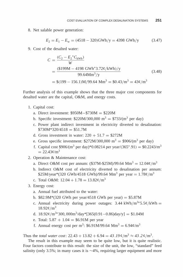
COST EVALUATION OF COMPLEX DESALINATION SYSTEMS 251

8. Net salable power generation:

E2 = E1 − Ew = (4518 − 320)GWh/y = 4398 GWh/y (3.47)

9. Cost of the desalted water:

C = (C2 − E2∗CkWh)

W

= ($199M − 4198 GWh∗3.72¢/kWh)/y

99.64Mm3/y(3.48)

= $(199 − 156.1)M/99.64 Mm3 = $0.43/m3 = 43¢/m3

Further analysis of this example shows that the three major cost components fordesalted water are the capital, O&M, and energy costs.

1. Capital cost:

a. Direct investment: $950M−$730M = $220M

b. Specific investment: $220M/300,000 m3 = $733/(m3 per day)

c. Power plant indirect investment in electricity diverted to desalination:$730M*320/4518 = $51.7M

d. Gross investment in water: 220 + 51.7 = $272M

e. Gross specific investment: $272M/300,000 m3 = $906/(m3 per day)

f. Capital cost $906/(m3 per day)*0.08214 per year/(365∗.91) = $0.2243/m3

= 22.43¢/m3

2. Operation & Maintenance cost:

a. Direct O&M cost per annum: ($37M-$25M)/99.64 Mm3 = 12.04¢/m3

b. Indirect O&M cost of electricity diverted to desalination per annum:$25M/year*(320 GWh/4518 GWh)/99.64 Mm3 per year = 1.78¢/m3

c. Total O&M: 12.04 + 1.78 = 13.82¢/m3

3. Energy cost:

a. Annual fuel attributed to the water:

b. $82.9M*(320 GWh per year/4518 GWh per year) = $5.87M

c. Annual electricity during power outages: 3.44 kWh/m3∗5.5¢/kWh =18.92¢/m3

d. 18.92¢/m3∗300, 000m3/day*[365(0.91−0.86)day/y] = $1.04M

e. Total: 5.87 + 1.04 = $6.91M per year

f. Annual energy cost per m3: $6.91M/99.64 Mm3 = 6.94¢/m3

Thus the total water cost : 22.43 + 13.82 + 6.94 = 43 .19 ¢/m3 ≈ 43 .2 ¢/m3.The result in this example may seem to be quite low, but it is quite realistic.

Four factors contribute to this result: the size of the unit, the low, “standard” feedsalinity (only 3.5%; in many cases it is ∼4%, requiring larger equipment and more

252 ECONOMIC ASPECTS OF WATER DESALINATION

energy), the mild “standard” product salinity (as high as 500 ppm TDS; in manycases it is considerably lower, requiring more equipment and energy), and the statusof being part of a dual-purpose plant.

3.4.1.4.2 Modified Power Credit Methods The power credit method benefitsthe desalted-water industry with economic advantages such as sharing the variousresources of the dual-purpose plant (plant A in the example above). Other costcalculation methods allow the cogenerated power to benefit economically (viz.,reduced cost) from the shared facilities; these methods will be presented later.However, there are two power credit method modifications that enable even lowercost results:

1. The Optimal Load Factor Cost Method . Let us assume that the load factorof plant A (above) is increased, as compared to the LF of plant B (above),enabling plant A to generate the same salable electricity if possible. This canbe done by operating more hours per year and/or by increasing the generationload to the fullest permissible and possible extent. If it is not possible togenerate and sell the same amounts of electricity from plants A and B, itmay still be possible to raise the load factor of plant B to somewhat highervalues. The possibility for both situations exists only where the optimal ornear-optimal operation of the entire grid system allows it.

2. The Marginal Water Cost Method . The difference between this costingmethod and the LF method (method 1, above) becomes obvious oncomparison between the dual- and single-purpose plants (plants A and Babove). According to the unmodified power credit method, plants A andB have identical primary heat sources, however, the marginal water costmethod assumes identical net salable power and energy as well as the sameload factor; thus E2 = E . Accordingly, the primary heat source of plant Ais larger than that for plant B, as well as the turbine, the generator, and,in the case of RO, also the heat rejection unit (steam condenser or gascooler). Consequently, lower water costs (Cwater) are derived using theeconomy-of-scale principle, with all the advantages of enlarged size andresource sharing allocated to the desalted water. This costing method hasbeen used only a few times in previous feasibility studies.

The accuracy of the power credit methods might be questionable if the requiredquantities of power and water were to lead to single- and dual-purpose plants withtwo different primary heat sources.

In principle, an opposite “symmetric” costing method can be applied by usingthe water credit method where the single-purpose plant (B) is a desalination system,rather than a power plant. This method apparently has not been used, since reductionof the desalted water cost is the crucial economic issue. Another reason may be thefact that (so far, at least) the main product of common dual-purpose plants is elec-tricity, which is more amenable to use of the water credit method—either becauseelectricity is more basic than desalted water or because it is the main product.

Various different costing methods are discussed below.

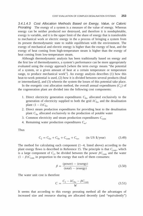
COST EVALUATION OF COMPLEX DESALINATION SYSTEMS 253

3.4.1.4.3 Cost Allocation Methods Based on Exergy, Value, or CaloricProrating The exergy of a system is a measure of the value of energy. Whereasenergy can be neither produced nor destroyed, and therefore it is nondepletable,exergy is variable, and it is the upper limit of the share of energy that is transferableto mechanical work or electric energy in the a process of bringing a system fromits present thermodynamic state to stable equilibrium with the environment. Theexergy of mechanical and electric energy is higher than the exergy of heat, and theexergy of heat coming from high-temperature steam is higher than the exergy ofheat coming from low-temperature steam.

Although thermodynamic analysis has been traditionally based on energy andthe first law of thermodynamics, a system’s performance can be more appropriatelyevaluated using the exergy approach [where the term exergy means “the potentialof a system, or a given amount of heat at a certain temperature or temperaturerange, to produce mechanical work”]. An exergy analysis describes (1) how thisheat-to-work potential is used, (2) how it is divided between several products (finalor intermediate)], and (3) wherein the system the losses of this potential take place.

In the exergetic cost allocation method, the overall annual expenditures (C2) ofthe cogeneration plant are divided into the following cost components:

1. Direct electricity generation expenditures CEe allocated exclusively to thegeneration of electricity supplied to both the grid δCEe and the desalinationplant (1 − δ)CEe

2. Direct steam production expenditures for providing heat to the desalinationplant CSe allocated exclusively to the production of potable water

3. Common electricity and steam production expenditures Ccom

4. Remaining water production expenditures Cw∗

Thus

C2 = CEe + CSe + Ccom + Cw∗ (in US $/year) (3.49)

The method for calculating each component (1–4, listed above) according to theplant exergy flows is described in Reference 15. The principle is that Ccom, whichis a large component of C2, be divided between the power βCcom and the water(1 − β)Ccom in proportion to the exergy that each of them consumes:

β = (power) − (exergy)

(total) − (exergy)(3.50)

The water unit cost is therefore

C = C2 − δCEe − βCcom

W(3.51)

It seems that according to this exergy prorating method all the advantages ofincreased size and resource sharing are allocated decently (and “equivalently”)

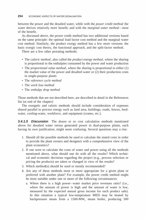
254 ECONOMIC ASPECTS OF WATER DESALINATION

between the power and the desalted water, while with the power credit method thewater derives relatively more benefit; and with the marginal water method—mostof the benefit.

As discussed above, the power credit method has two additional versions basedon the same principle: the optimal load factor cost method and the marginal watercost method. Similarly, the product exergy method has a few more versions: thebasic exergic cost theory, the functional approach, and the split-factor method.

There are a few other prorating methods:

• The caloric method , also called the product energy method , where the sharingis proportional to the enthalpies consumed by the power and water production

• The proportional value method , where the sharing is proportional to either (1)the market value of the power and desalted water or (2) their production costsin single-purpose plants

• The reference cycle method

• The work loss method

• The enthalpy drop method

Those methods that are not described here, are described in detail in the Referenceslist (at end of the chapter)

The exergetic and caloric methods should include consideration of expensesshared parallel to process energy such as land area, buildings, roads, fences, feed-water, cooling-water, workforce, and equipment (cranes, etc.).

3.4.1.5 Discussion The dozen or so cost calculation methods mentionedabove for desalted water versus generated power in dual-purpose plants, eachhaving its own justification, might seem confusing. Several questions may a rise:

1. Should all the possible methods be used to calculate the stated costs in orderto provide the plant owners and designers with a comprehensive view of theplant economics?

2. If one were to calculate the costs of water and power using all the methodsmentioned above, what should one do with all the results? Which techni-cal and economic decisions regarding the project (e.g., process selection orpricing the products) are taken or changed in view of the results?

3. Which method(s) should be used or mostly recommended?

4. Are any of these methods most or more appropriate for a given plant orpreferred with another plant? For example, the power credit method mightbe most suitable under one or more of the following circumstances:

a. Where there is a high power–water market price revenues ratio? (i.e.,where the amount of power is high and the amount of water is low,measured by the expected annual gross income for each product sale).In this situation a typical low-temperature MED may be heated bybackpressure steam from a 1500-MWt steam boiler, producing 500

COST EVALUATION OF COMPLEX DESALINATION SYSTEMS 255

MWe + 10, 000-t/h salable products. Typical prices might be 10¢/kWhand 70¢/t desalted water; the power sale might be $50,000/h, whilethe water sale might be only $7000/h; thus the main product would beelectricity, with water as the secondary product.

b. Where there is a high water : power market price revenues ratio (i.e.,where the amount of water is high and the amount of power is low,measured by the expected annual gross income for each product sale).In this situation a typical self-power-supply SWRO plant might employ a250-MWt steam boiler; producing 35 MWe + 13, 000-t/h salable products.With typical prices of 10¢/kWh and 70¢/t desalted water (the same as inexample 4a, above), the power sale might be $3500/h and the water sale$9100/h; thus the main product would be water while the electricity wouldbe a secondary byproduct.

c. Where the water : power market price revenues ratios are about the same(i.e., where the amounts of water and power, measured by the expectedannual gross income for each product sale, are close). In this scenariothere would be no secondary product.

Determining which of these scenarios is most amenable to the power credit methodis not simple. However, one should be aware of the many existing split-factormethods and their problematic applications.

In practice, the power credit method seems to be the more popular method. Thismay be explained as follows:

1. A major problem is the compound decision on (a) whether to desalt waterand, if the answer is positive, (b) which desalination technology is best forthe given project. For this twofold question, and where a dual-purpose plantis considered, it is preferable to use the energy–water splitting (split-factor)methodology that yields the low water cost. This is the power credit. Usinganother allocation method will yield more expensive water (although lower-cost power), which may, in turn, yield a negative decision—to abandon theoption of desalination by using the heat from the power plant and resort toan alternative solution: either to desalt water by, say, RO, or even providefresh-water conveyance and/or water curtailment. In such a case the powersection would be operating at a loss economically.

2. In addition, if all the desalination processes are compared on an economicbasis, the power credit method seems to be preferred; otherwise, the com-parison is considerably more complicated. The extra complication stemsfrom the need to include different energy cost comparisons in addition tothe desalted-water costs comparisons with a questionable weighing method,namely, comparing somewhat complex economic vectors rather than the sim-pler scalar values. The greater complexity of vector comes from frequentcases where the amounts of the water as well as those of the power mightdiffer for the processes being compared, leaving the economic vectors inquestion not fully defined.

256 ECONOMIC ASPECTS OF WATER DESALINATION

It seems that further work has to be done to try and find the the most suitableyet the most lucrative allocation method for each of the three possible secondary-byproduct dual-purpose arrangements: water, power, or neither, thus reducing thenumber of the relevant cost allocation methods to two: the most suitable (for thecircumstances) versus the most lucrative.

3.4.2 Hybrid Desalination Plants

A special qualitative plant design is the possible concept of a hybrid complexdesalination plant , which, by definition, consists of several desalination units ofdifferent technologies operating in parallel or connected in series. In most casestwo technologies are involved, often RO with MED or MSF. Serieal connectioncan be effected via the concentrate to feed-water, namely, where the waste streamof one unit (e.g., the RO unit) becomes the feed stream of the second unit (theMED unit), or with product going to feedwater (rarely), or with exhaust heat fromMED or MSF turned to the RO or MVC preheater.

The concept of hybrid desalination plants is mentioned frequently. Naturally ithas advantages and disadvantages as compared to single-technology plants. In thehybrid case, the disadvantages are indicated first because the idea is in principlequite negative. The philosophy of this concept is to combine the specific advantagesof each method. However, in practice this concept seldom shows any economicbenefit, except under a few rather unique circumstances.

3.4.2.1 Disadvantages1. Using Inferior Technology . The probability that the different methods are

economically equal is very low; under the same conditions one methodis slightly or considerably better than the other one. Naturally, if onedesalination method is economically superior over the other under theprevailing conditions, adding less competitive systems is economicallywrong.

2. Negative Economy of Scale. Moreover, for a given total plant capacity, asingle system is larger than any of the two or more units of the hybridplant; thus each system in the hybrid plant has a negative economy of scalecompared to a single-process plant.

3. Complications . Finally, it is easier to install, operate, control, and maintain asingle desalting technology, rather than several ones that operate in parallel,and even more so if they are connected in series.

3.4.2.2 Advantages1. Mixing Product Waters . The lower quality of low-cost product water from

the RO unit can be improved, if desired or required, either by product treat-ment within the RO plant or by mixing with very low-salinity product waterfrom the distillation unit. Sometimes the latter solution may work better, inparticular if strict boron content limit is imposed on the desalted water, whichis expensive with RO and free with distillation.

COST EVALUATION OF COMPLEX DESALINATION SYSTEMS 257

2. Insufficient Low-Cost Heat . Where very low-cost heat is available, low-temperature MED is the most economic process, but the amount of heatis not sufficient to desalt the needed quantity of water; thus the addition ofan RO system may be the best solution.

3. Correcting Power Load Fluctuations in Dual-Purpose Plants . Although MEDmay show better economic promise than RO, large power load fluctuations areexpected with the power generated by the dual-purpose plant; hence the prac-tical performance and economics of the coupled MED is damaged. Couplingadditional RO units—provided the additional desalination is needed—willimprove the power load factor as well as the relative fluctuation in watersupply and render the MED more economical.

4. Raising RO Operation Temperature. This option might be preferred if MEDis less expensive than RO—which might occur at low temperatures (whichin turn are favorable for MED but not for RO), and where the economics ofRO using the cooling-water from the MED as a higher-temperature feed isstill better than both “MED-alone” and “RO-alone” possibilities. Such casesare seldom encountered, however.

5. Late Addition of Modern Units to Older Ones . Where the economy of olderunits falls behind that of new technologies, or where their performance dete-riorates but they are still worth operating since the investment has alreadytaken place, or where a local need for more desalted water develops, a goodsolution might be to enhance production by combining additional units, oftenusing different desalting technology.

It should be noted that the disadvantages of hybrid plants are essentially generalprinciples, whereas the advantages are of a more specific nature that identify nicheswhere the hybrid plants have nevertheless positive potential. In practice, theseniches are quite wide.

3.4.2.3 Cost Calculation Where the product waters from the various compo-nents of the hybrid plant are mixed, it is easy to calculate the cost of the commonproduct, according to the procedures described above for single-purpose desaltingprocesses.

Calculating the specific cost of each product is somewhat more problematic.For the major cost components, most of the investment and energies is specific toeach unit. The questionable issue is how to allocate expenses on shared systemsand resources such as intake and outfall, labor, and some chemicals for pre- andposttreatment. Several prorating formulas can be offered—according to produc-tion, investments, market values of specific products of different qualities or othercriteria—or crediting any of the units, similarly to the costing methods used fordual-purpose plants.

3.4.3 Two-Quality Product Water Streams

Some processes may produce two streams of desalted water, each having differentqualities, such as double-distilled water in MED or MSF—the condensate resulting

258 ECONOMIC ASPECTS OF WATER DESALINATION

from flashing of the product in high-temperature effects or stages. Similarly, perme-ates may be collected from the front end and the back end of RO pressure vessels.In most of these cases it is difficult to isolate the cost of each such physicallyseparate stream; however, the main issue is their different values , which dependon their different qualities as well as on market demands, which are eventuallyexpressed in their prices .

3.4.4 Linear Correlation Common Principle

In all three complex plants discussed here—dual-purpose, hybrid, and two-quality—the arithmetic sum of the two multiplications of the average annualquantity of a product by its cost is equal to the sum of all the levelized expensesfor the year. For a dual-purpose plant, it is

W ∗C + E ∗2 CkWh = C2 (3.52)

Thus, no matter what prorating method is used for charging the desalination unitwithin the dual-purpose plant for the energy received from the power generatingsection, and/or for the shared facilities such as seawater intake, this linear correla-tion of the resulting costs of the salable power and the desalted water according toEquation (3.52) must be satisfied.

Similarly, for hybrid plants and for two-quality systems the linear correlationis

W1∗Cw1 + W2

∗Cw2 = �expenses (3.53)

where W1 and W2 are the annual water production values from each of the twosources, Cw1 and Cw2 are the costs attributed, respectively, to these water productsvia any of the allocation methods, and �expenses is the sum of all net levelizedannual expenses.

In a complex that produces more than two products (e.g., electric power, desaltedwater, salt and high-pressure steam for a nearby factory), the correlation becomesmultilinear:

∑Pk

∗Ck = �expenses (3.54)

where Pk , Ck , and k are, respectively, the amounts, the allocated costs, and thegiven serial number of the product indicated by the index k .

3.5 RELIABILITY OF COST ESTIMATES

In principle, the reliability and accuracy of product cost calculation depends on themethod of calculation, as well as its goal and its timing.

RELIABILITY OF COST ESTIMATES 259

3.5.1 Methods

As stated in Section 3.3, there are several ways to evaluate the cost of a product:

1. Summation of all the cost components . This method has been described abovein detail. The reliability has been discussed in Section 3.3 and is summarizedand elaborated on in Section 3.5.2. This method is relevant for any stageof the plant history—late as well as very early. The next method (listeditem 2, below) is relevant mainly to the preliminary stages, quite some timebefore commercial operation, while the last method (3, below) is applicableto preliminary and early stages, up to very few years of commercial operationexperience.

2. Using the cost practically experienced in other plants . Obviously these ref-erence plants should be appropriate—use the same process, be of the samenature (single-purpose or dual-purpose), yield the same product quantities andqualities, have the same feedwater, be charged according to equal discountrates, expect the same lifetime, and pay the same prices for fuels, electricity,chemicals, and workforce. This method is quite simple to apply. However,the required fitness of data may be difficult to find except where a second orthird unit is added to an existing plant, or where a plant is about to be con-structed in an environment that is similar economically to that of the referenceplant. Otherwise, if such fitness is not found or if it exists only partially, thedifferences must be identified, assessed, and modified quantitatively. Then,of course, this method is quite less simple to apply.

3. Various combinations of (methods 1 and 2 (above)). In view of the limita-tions of the above mentioned methods, several parts (or sometimes only onepart) of the cost calculation input data—either the more reliable or the morecomplicated part—can be taken from the experience of previous plants whilethe other parts are calculated as in method 1. Thus, for example, the invest-ment in the process equipment, the workers to be employed, and the amountof energy can be estimated from previous plant data while the site-specificinvestment and the operation & maintenance (minus labor) may be calcu-lated, particularly for the plant under consideration. The best combinationmight be the full implementation of method 1 while comparing each stepwith similar projects, according to method 2 as assisting guidance.

The advantages of method 1 are the lower level of inaccuracies and the wideversatility of uses. The specific disadvantages of this method compared to method2 are the effort and the time needed to apply it and the risk that certain minor costcomponents have been forgotten or gave the wrong values—erroneously assumed,calculated, or estimated. If high accuracy is not necessary, as explained in thefollowing paragraph, and/or if the evaluation results are needed within a short timeperiod, the other methods may be used.

To obtain maximum cost accuracy, the input data must be reliable, complete,and precise. Introducing real and accurate values, from the very beginning to the

260 ECONOMIC ASPECTS OF WATER DESALINATION

end of a desalination project, of all the payments and ensuring that they are madeon time, as well as ensuring that all the water quantities are supplied each monthis effective only at the end of the plant lifetime. As mentioned above, the accuratevalue of the product cost can be obtained only at this very late time in the planthistory. The abovementioned input data require accurate listing and well-preserved,accessible documentation.

3.5.2 Levels of Accuracy

Although the best evaluation in principle is done by summing up all the discountedcost components, there are many potential pitfalls to be carefully avoided to attainhigh accuracy. Fortunately, those pitfalls are of rather minor magnitude.

First, even this accurate value of the product cost depends on the discount rate,which is taken rather arbitrarily, although more or less rationally. (Hint : This valueis a round or semiround number of percents.)

Thus, for given data of all the payments, the water quantities, and the datesof incoming and outgoing payments, the desalted-water cost is either calculatedfor a certain stated value of the discount rate or is displayed as a sensitivity testas a one-variable function by simple tabulation of several values of the discountrate—often 5%, 8%, and 10% per year—or as a graph for a certain range of dvalues.

The post factum true cost is very difficult to obtain also because it shouldinclude positive and negative indirect effects such as environmental changes (e.g.,warm concentrated brine stream, long-term possible damages), employment dur-ing construction and operation, experience, and possible impact on the electricgrid.

In most cases the product cost is needed much earlier than at the end of theplant lifetime—namely, either during the period of plant operation, at plant startup,quite often before the beginning of operation, or even before plant construction:during the bidding period, when a decision is made whether or not to erect adesalting plant. Most of the input data are assumed by the person who performsthe calculation with a certain degree of subjectivity. The plant supplier tends toassume long plant lifetime, low prices for purchased electricity, high load factoreven late in the plant lifetime (ignoring the prediction that failures occur morefrequently), and obviously no equipment malfunctioning. The tendency is to ignorethe probability for emerging new competing technologies that might render theplant obsolete on one hand and on the other hand, the probability that noveltiesand improvements may be applied to the plant itself, such as better and/or cheapermembranes. Moreover, there is a tendency to adopt optimistic methodologies thatfavor desalination such as the marginal water cost method. Finally, positive andmainly negative escalation of prices of project components, such as salaries, fuels,and electricity are rarely considered and are difficult to predict quantitatively.

As the project progresses, more factual data accumulate and replace previouslyassessed or assumed input values. Thus the degree of the cost accuracy improvesduring the later stages of the plant history.

RELIABILITY OF COST ESTIMATES 261

3.5.3 Accuracy in Terms of Cost Calculation Objectives

In this respect, distinctions should be made between cost estimates intended for eco-nomic comparisons of alternatives, and cost estimates needed for cashflow studies,pricing, or future project evaluations. More specifically, there are several differentobjectives for which product costs are evaluated:

1. Comparing economically relevant alternative methods for water production,within and out of desalination, including the basic alternative to avoid desali-nation and find other solutions; for example, in the case of water shortage,if the cost of desalted water is too high, an alternative to desalination maybe preferable.

2. Optimization of design by economic comparison of several designs of thesame desalting process is a special case of such evaluation.

3. Preparing for financing by forecasting the cashflow using the product cost.

4. Pricing the product.

5. Information for future projects.

6. Outlook on the economy of the country for large-scale, long-term desalination(in particular for desalination program rather than a specific project). Thisobjective is relevant only to very large scale production items such as waterand energy at national scales.

The specific objective for which the product cost is evaluated will determine thedegrees of accuracy, detail, and caution at which this task of cost evaluation is car-ried out. Also, the timing at which the cost evaluation takes place is determined bythe specific objective. For example, if the objective is pricing, the time should bevery close to the plant commissioning, whereas for comparing alternative desalina-tion processes, the water costs of the alternative candidate processes are evaluateda few years earlier, at the time of bidding or decisions making and well before theplant design stage.

A special duality exists regarding cost estimates for comparisons. Such estimatesare prepared very often at the preliminary phase of a national program or at thetime of decision regarding installation of a plant. At such early stages, the inputdata include many values that are assumed:

• On one hand, erroneous input data can be tolerated in cases of certain neededcomparisons more than in cases of needed absolute results, since all the com-pared alternatives tend to deviate from real values to quite close degree. Forexample, if the size of a plant is the compared variable for which the costestimates are calculated, then assuming an erroneous (too low) input datapower price of 5.5¢/kWh instead of a correct price of 8¢/kWh contributesa very small cost difference (<0.5¢/m3) between the erroneous and correctcomparisons. This is because there are very small power consumption differ-ences between the compared variables or parameters. The conclusions fromthe comparisons do not change, regardless of whether the power cost estimate

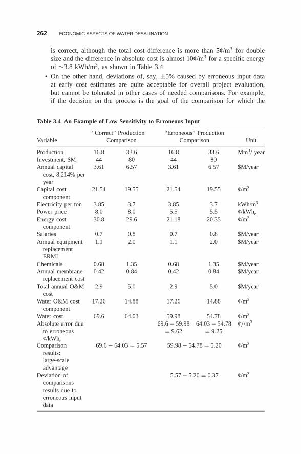
262 ECONOMIC ASPECTS OF WATER DESALINATION

is correct, although the total cost difference is more than 5¢/m3 for doublesize and the difference in absolute cost is almost 10¢/m3 for a specific energyof ∼3.8 kWh/m3, as shown in Table 3.4

• On the other hand, deviations of, say, ±5% caused by erroneous input dataat early cost estimates are quite acceptable for overall project evaluation,but cannot be tolerated in other cases of needed comparisons. For example,if the decision on the process is the goal of the comparison for which the

Table 3.4 An Example of Low Sensitivity to Erroneous Input

“Correct” Production “Erroneous” ProductionVariable Comparison Comparison Unit

Production 16.8 33.6 16.8 33.6 Mm3/ yearInvestment, $M 44 80 44 80 —Annual capital

cost, 8.214% peryear

3.61 6.57 3.61 6.57 $M/year

Capital costcomponent

21.54 19.55 21.54 19.55 ¢/m3

Electricity per ton 3.85 3.7 3.85 3.7 kWh/m3

Power price 8.0 8.0 5.5 5.5 ¢/kWheEnergy cost

component30.8 29.6 21.18 20.35 ¢/m3

Salaries 0.7 0.8 0.7 0.8 $M/yearAnnual equipment

replacementERMI

1.1 2.0 1.1 2.0 $M/year

Chemicals 0.68 1.35 0.68 1.35 $M/yearAnnual membrane

replacement cost0.42 0.84 0.42 0.84 $M/year

Total annual O&Mcost

2.9 5.0 2.9 5.0 $M/year

Water O&M costcomponent

17.26 14.88 17.26 14.88 ¢/m3

Water cost 69.6 64.03 59.98 54.78 ¢/m3

Absolute error dueto erroneous¢/kWhe

69.6 − 59.98 64.03 − 54.78 ¢//m3

= 9.62 = 9.25

Comparisonresults:large-scaleadvantage

69.6 − 64.03 = 5.57 59.98 − 54.78 = 5.20 ¢/m3

Deviation ofcomparisonsresults due toerroneous inputdata

5.57 − 5.20 = 0.37 ¢/m3

RELIABILITY OF COST ESTIMATES 263

cost estimates are calculated, then assuming the same low power price of5.5¢ instead of 8¢ per kWh for 1.3 kWh/m3 in MED contributes a verysignificant erroneous cost difference, about 6.5¢/m3, to the total true costdifference that may be only 5¢/m3 for the competing RO with a specificenergy of 3.9 kWh/m3.

Thus, each case has to be examined individually for accuracy:

Cost Estimates at Different Times . As the degree of sophistication and com-plexity increases, in particular with dual-purpose power-and-desalting plants,several economic estimates may be needed for evaluating the economics ofthese plants. Different estimations may be employed for the same project,each with a unique purpose. Two examples are listed next.

Costs at Time of Estimate. This is the most common procedure used in thewater desalination literature for reporting capital and operating costs of adesalination plant. It has value for feasibility studies, for project screening,and for evaluation of the bid. Its value is diminished in later project stages,when considering real, rather than presumed, capital and operating costs overthe plant life time.

Costs at Later Times, toward Project Completion . During the history of a desali-nation plant, cost components change inevitably, which affects the planteconomics compared to preliminary cost data and predictions. Even moreso, this occurs during the history of a large-scale desalination program of awater utility or a long-term national desalination program.

This upgrades the cost estimating procedure to the next higher levels of accuracy bythe input of more factual data regarding updated changes from the original estimatedexpenditures on equipment, energy, salaries, and chemicals. This escalation of thecost estimation, as well as any other deviations from the originally estimated orplanned production rates, and the lengths of—and expenses incurred on—anyunplanned outages, must be accounted and adjusted for. Future inflation rate thatwill be faced by the project through to its completion must be estimated. Thiscosting procedure is of particular importance when the project requires severalyears from the time of bid to startup, and/or when the procurement documentsallow for progress payments and an extra charge for inflation.

It is relevant to include inflationary effects on payment schedules when estimat-ing the future financial and pricing needs.

3.5.4 Inflation and Deflation

3.5.4.1 Levelized Costs in Terms of ‘‘Constant’’ Currency Inflation isthe weighted result of all the price changes (equipment, energy, salaries, chemicals,services, etc. not only within the desalination project but within the entire market)with the time, and thus expresses the change in terms of the purchasing power of

264 ECONOMIC ASPECTS OF WATER DESALINATION

the relevant currency; if the changes decrease, the constant currency cost (i.e., theinflation rate) is negative, this is called deflation .

Inflation and deflation complicate these estimates and contribute to fuzzy results.Using “constant” currency with a known fixed value and purchasing power at thetime of the estimate, or at any other convenient reference date, is a common methodfor bypassing this problem.

3.5.4.2 Levelized Costs in Terms of ‘‘Current’’ Money The levelizedunit cost may be determined—in addition to “constant” currency, where the costsare expressed in terms of the purchasing power of the relevant currency—interms of “current money” or as “spent money.” The constant-currency cost isreplaced by the actual increased or decreased values, usually by the rate of infla-tion or deflation of a given number of current dollars (or any other relevantcurrency).

The transition from actual expenses in current money of year j payments toconstant money (constant of the plant commissioning date D) is effected by usingthe factor (1 + d)D−Dj /�(j )(1 + infy ) instead of (1 + d)D−Dj in the formulas pre-sented in Section 3.3, where “inf” is the inflation rate and infy is the inflation rateduring year y . (� is the multiplication notation). Then y is counted from the dateof commissioning between 1 and j . If j is also counted from the date of plantcommissioning, then

D − Dj = j (3.55)

Often in literature the factor (1 + d)D−Dj /�(j )(1 + infy ) is presented as Z j

Z j = (1 + d)D−Dj /�(j )(1 + infy ) (3.56)

where

Z = 1 + d

1 + ea(3.57)

and ea is the average inflation rate during the referred period of j years:

ea = [�(j )(1 + infy )]1/j − 1 = [(1 + inf1)(1 + inf2)

(1 + inf3) · · · (1 + infy ) · · · (1 + infj )]1/j − 1 (3.58)

Regardless of which methodology is used, only the total cost of the product wateris thus determined, not the selling price.

DESIGN AND OPTIMIZATION OF PLANT AND PROCESS PARAMETERS 265

3.6 DESIGN AND OPTIMIZATION OF PLANT AND PROCESSPARAMETERS

There are two kinds of a desalination system design parameters—those that influ-ence the economics, mainly the external plant parameters, which constitute inputdata, and those that are influenced by the economics, namely, process parameters.The latter are determined in principle by economical considerations via optimiza-tion, unless the optimal value is beyond a limiting technological constraint thatreplaces the stated optimal value, and in practice also by experience and profes-sional tradition.

The first type includes in principle the quality and the production rate of thedesalted water, timing and location of the project (the latter determines the feedwa-ter properties—salinity, analysis, and temperatures—as well as other environmen-tal, geographic, and infrastructural characteristics), the type of plant—contiguous(multipurpose) or standalone (single-purpose)—and the desalination method. Theseplant parameters may constitute user requirements or input data, expressing theplant owner’s preference and possible constraints. Initially they seem to have aone-way effect on the economics. When methodically examined, however, almostall of them have mutual feedback effects to some extent with economic consid-erations. Thus, for example, the user may compromise on higher product-watersalinity (e.g., 400 ppm TDS instead of the 250 ppm initially required level) toreduce the water cost by a few percentage points.

Parameters of the second type are internal plant specifications. They includeselection of the process itself and the specific energies, the number and magnitude ofeffects or stages, and the top brine temperature—in thermal desalination plants—aswell as the membrane configuration and type, flux, recovery ratio and rejectionrate, operating temperature, and pressure in RO plants. These process parametersobviously influence the desalted-water production cost. However, the economicfeedback is very effective and should be used, with sound engineering, to determinethese parameters. This is done by the use of applicable optimization techniques.

The usual goal of optimization is to identify the parameters with which opti-mal results, in most cases lowest product cost, are obtained. The output of theoptimization is a set of qualitative choices and quantitative values according towhich a desired project is implemented. In the optimization procedure the relevantoptions are examined by weighing (to the fullest extent possible) their advantagesand disadvantages. Eventually the product cost is calculated for all the promisingcandidate options, and the best one is found by discrete comparison or by theminimum-derivative technique.

One problem with optimization is the sensitivity of the results to variationsin the input values; small changes in these data may yield large quantitative andqualitative differences with the output results. Thus, input data should be cautiouslyand accurately determined. This might be difficult as some of the input data arenot known accurately during the optimization stage of the project.

Another problem may occur in case of a dual-purpose plant. If the lowest watercost is found, through optimization, for an option (i.e., one of a few possible sets

266 ECONOMIC ASPECTS OF WATER DESALINATION

of parameters) in which the electrical energy is generated at a higher cost than withone or more other options, a method should be selected to identify the best option.This situation is seldom expected, but has been encountered in a previous studycitation reference No. 15, page 62 and may be encountered in future comparisons.

Four outstanding input parameters are the most characteristic of all desalinationprocesses and have significant economical effects: the production rate, feedwaterquality (hardness, turbidity, and total salinity), desalted-water quality (mainly totalsalinity), and the recovery ratio (their roles have been briefly described in Sections3.3.2 and 3.3.3.1):

• The production rate, namely, plant capacity, is based on the economy-of-scaleprinciple. The economic contribution of large capacities manifests itself in fouraspects. In percentage cost reduction, the first one is the labor (workforce)expense; e.g., a plant of with a production rate of 100 mgd (million gallon perday) employs roughly only 4 times as many the workers as a 3-mgd plant.Second is the investment , as discussed in detail in Section 3.3.2. The thirdaspect of product cost reduction based on economy of scale is the energy ,as the energy efficiencies of equipment items usually increase with equip-ment size. The fourth and final aspect is the potential benefit of secondaryimprovements , which also increases with plant size. This input parameter isapparently determined by the need for desalted water rather than by economicconsiderations, but for the reasons mentioned above, decisions regarding erec-tion of a larger plant or expansion of an existing one can be made within theframework of long-term desalination program.

• The feedwater quality is also discussed in detail in Section 3.3.2, explain-ing the contributions of low feed salinity to the reduction of desalinationcost. Decisions regarding this parameter cannot be based on economic con-siderations except where high-salinity feedwater can be mixed with othernonpotable water to reduce this salinity. Mixing may take place with availablelower-salinity streams such as high-hardness brackish-water, concentrate froma brackish-water desalting plant, or even treated sewage water.

• The quality of the product water is also mentioned above and determined onthe basis of health and agricultural criteria and standards. Economically, inthe 600–50 ppm range it may add roughly 2¢/m3 per 100 ppm product-watersalinity reduction. Boron removal from the SWRO permeate, ∼1.5–2 ppm,to the required level of 0.2–0.5 ppm today costs 2–10¢/m3. Although theproduct quality is an input parameter, economic consideration may lead tocompromises within a rather narrow range of salinity and boron levels.

A few notes regarding the economic aspects of the product-water quality are appro-priate here. Assigning milder restrictions and requirements for the desalted-waterquality where possible, will consequently reduce the product cost. At some desali-nation plants the required salinity of the desalted water is too low, driving the watercost up. This requirement may be too severe, since the average domestic water con-sumption rate is ∼100 m3 per year per capita, only ≤0.5–1 m3 per year per capita

DESIGN AND OPTIMIZATION OF PLANT AND PROCESS PARAMETERS 267

of which is being used for drinking. Also, the issue of whether the quality of >99%of domestic water should be as high as that of the “best” drinking water should bestudied. Furthermore, people obtain their beverage water from juices, milk, bottledmineral water, and solid food and only part from the faucet; thus, another issueto consider is whether faucet (tap) water has to be as good as the “best” drinkingwater. Finally, adding another economic criterion for water desalination—the costof a unit of salt removed as a function of, inter alia, water salinity—might help inthe optimal design of membrane desalination processes.

The three parameters listed above—production rate, feedwater salinity, anddesalted-water quality—are plant characteristics. The fourth one is a processparameter:

• A high recovery ratio, namely, the amount of desalted water per unit feed-water, decreases the feed requirement for a given plant output and hence thepretreatment equipment and chemical consumption. For single-purpose plantsof electrically driven processes (RO, ED, and MVC), a high recovery ratio alsoreduces the pumping energy, the intake, and outfall equipment size, includ-ing feed pumps. [In most dual-purpose plants the feedwater is taken fromthe cooling-water stream, so the intake and outfall systems are not affectedby the recovery ratio; similarly, in seawater MFS and MED, the amount ofseawater (feedwater plus cooling-water) does not depend significantly on therecovery ratio.] In the case of RO, a high recovery ratio also reduces themain process pumps and the pressure recovery device; smaller pumps andpressure recovery devices reduce the investment and conserve energy. Theseeconomic savings, however, bear some penalties. A higher recovery ratiomeans higher salt concentrations in the main desalination system and, in par-ticular, toward the brine outlet. Consequently, it increases the specific energyin the main desalination system as well as the probability of scaling in thebrine outlet zone of the main desalination system; and, especially in the caseof RO, it adversely affects the product-water quality. This design parameteris apparently not an input factor but should result from design optimization.However, in many cases the recovery ratio is determined by a chemical con-straint of a maximum brine salinity limit of 7–8.5% to avoid sulfate scalingin the evaporators and on the membranes. Thus, for seawater this constraintimposes an upper limit for a recovery ratio of 44–60%, depending on theseawater salinity, even if the optimization results in higher recovery ratiovalue.

Other major process parameters determined by a combination of technologicalconsiderations and economical optimization are

1. The maximum process temperature in distillation plants, which depends onseveral conditions and requirements, such as single- or dual-purpose plant,ratio of product to available heat, temperature, and price at which the heat isavailable. For example, if the amount of available low-cost heat per unit

268 ECONOMIC ASPECTS OF WATER DESALINATION

desalted water is above 60 kWht per needed ton product, this tempera-ture is about ∼70◦C. In some cases this parameter may lead, in view ofthe prevailing conditions, to an optimal arrangement where a heat pump isintroduced.

2. The average temperature drop per effect of MED —�Teff, which, in turn,determines partly (but to a large extent) the energy of the plant as well as thenumber, size, and cost of effects of the evaporator, which is the main compo-nent of the plant [when considering the maximum process temperature (seelist item 1, above) and the feedwater temperature]. Thus, the main economiccharacteristics of the process are largely determined—the specific energy andthe specific investment. This temperature drop has a significant thermody-namic meaning and depends on many variables, including prices of electricpower and heat transfer equipment, heat transfer coefficients, power genera-tion system efficiency, and load factor. This optimization step is demonstratedand discussed in detail in Section 3.A.2 (in the Appendix). Basically, it isthe best compromise between the cost of the process energy, per unit product(ton desalted water) which increases linearly with �Teff, and the cost per unitproduct of the evaporator, which decreases with �Teff.

3. The temperature increase in the brine heater of MSF— �TBH, which, in turn(similarly to MED), determines partly (but to large extent) the energy of theplant as well as the size and cost of the evaporator, which is the main com-ponent of the plant. Thus, the main economic characteristics of the processare largely determined—the specific energy and the specific investment. Thistemperature increase has a significant thermodynamic meaning and dependson many variables (similarly to MED), such as prices of electric power andheat transfer equipment, heat transfer coefficients, power generation systemefficiency, and load factor. The optimal value is the result of a compromisebetween the cost of the process energy, which increases linearly with �TBH,and the cost of the evaporator, which decreases with �TBH.

4. The number of MSF stages , which is the best compromise between the cost ofthe envelope of the stage, i.e., the vessel or partitions, which increases linearlywith the number of MSF stages, and the cost of the internal components ofthe evaporator, mainly the heat transfer surfaces and droplet separators, whichdecreases with the number of stages.

5. The pressure of RO process , which, in turn, determines the average waterflux through the membranes. This is only theoretically true for most caseswith the first RO pass, as the practical flux is lower than optimum, due tothe fouling limit and concentration polarization phenomena, but it is practicalfor the second or third pass. This pressure is the best compromise betweenthe costs of the energy and the pump, which increase with RO pressure andthe cost of the membranes, pressure vessels, and associated equipment andconstruction, which decrease with RO pressure and the flux.

PROCEDURES AND PROGRAMS 269

3.7 PROCEDURES AND PROGRAMS

To provide a common basis for comparisons and ensure a reliable cost calculationthat includes all the relevant items and factors, it has been recognized that a formalprocedure should be established for these purposes. Several procedures have beenoffered since the mid-1950s.

3.7.1 US Methods

In 1956 the US federal Office of Saline Water, Department of the Interior (OSW)published a 44-page detailed report titled A Standardized Procedure for EstimatingCosts of Saline Water Conversion [1], which refers only to thermal desalinationsince membrane processes were in the earliest stages of development. The reportis very informative as it supplies both the calculating procedure and input data onprices of energy and equipment. Almost all input numerical values are outdated,but most of the procedures, published as guidelines and cost component checklists,are still valid.

This was followed 16 years later by an OSW report that included a cost format inthe 1972 edition of the Desalting Handbook for Planners [6]. It includes a tabulationof all direct capital costs and indirect costs (interest incurred during construction,working capital, and contingency expenditure). It also includes a tabulation ofannual operating costs, including an annual cost for depreciating capital. The totalcost for production of desalted water is then worked out as the total annual costsdivided by the annual production.

3.7.2 International Methods

An adaptation of the 1972 OSW format was used in the cost updates prepared forthe US Office of Water Research and Technology (OSRT) and is recognized by theInternational Desalination Association (IDA). A software package for calculation ofcosts for seawater desalination, following this format, is now available through IDA.It is designed to calculate cost for three commercial processes—MSF, MED, andRO—for seawater desalination. The desalted-water cost does not include product-water storage, distribution, or administrative costs. The sample cost figures for RO,MED, and MSF based on the IDA seawater desalting cost program are presentedin Table 3.5. (Note: The values in this table are extremely pessimistic for presentday’s desalination. Currently, plants of this capacity can supply water at a cost∼30% less!!).

3.7.3 UN Methods

Fossil-fuel-based and nuclear methods of water desalination can be compared on aneconomic basis. The preferred source of primary energy for seawater desalinationgoes a long way in the economics of desalination system. Nuclear energy becomes

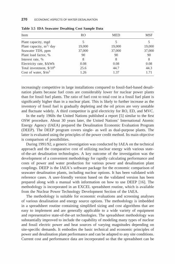
270 ECONOMIC ASPECTS OF WATER DESALINATION

Table 3.5 IDA Seawater Desalting Cost Sample Data

Item RO MED MSF

Plant capacity, mgd 5 5 5Plant capacity, m3/ day 19,000 19,000 19,000Seawater TDS, ppm 37,000 37,000 37,000Plant load factor, % 90 90 90Interest rate, % 8 8 8Electricity rate, $/kWh 0.08 0.08 0.08Total investment, $/106 25.6 44.7 44.3Cost of water, $/m3 1.26 1.37 1.71

increasingly competitive in large installations compared to fossil-fuel-based desali-nation plants because fuel costs are considerably lower for nuclear power plantsthan for fossil fuel plants. The ratio of fuel cost to total cost in a fossil fuel plant issignificantly higher than in a nuclear plant. This is likely to further increase as theinventory of fossil fuel is gradually depleting and the oil prices are very unstableand fluctuate widely. A third competitor is grid electricity for RO, ED, and MVC.

In the early 1960s the United Nations published a report [5] similar to the firstOSW procedure. About 30 years later, the United Nations’ International AtomicEnergy Agency (IAEA) prepared the Desalination Economic Evaluation Program(DEEP). The DEEP program covers single- as well as dual-purpose plants. Thelatter is evaluated using the principles of the power credit method. Its main objectiveis comparison of possibilities.

During 1991/92, a generic investigation was conducted by IAEA on the technicalapproach and the comparative cost of utilizing nuclear energy with various state-of-the-art desalination technologies. A key outcome of the investigation was thedevelopment of a convenient methodology for rapidly calculating performance andcosts of power and water production for various power and desalination plantcouplings. DEEP is the IAEA’s software package for the economic comparison ofseawater desalination plants, including nuclear options. It has been validated withreference cases. A user-friendly version based on the validated version has beenprepared along with a manual with information on how to use DEEP [16]. Themethodology is incorporated in an EXCEL spreadsheet routine, which is availablefrom the Nuclear Power Technology Development Section of the IAEA.

The methodology is suitable for economic evaluations and screening analysesof various desalination and energy source options. The methodology is imbeddedin a spreadsheet routine containing simplified sizing and cost algorithms that areeasy to implement and are generally applicable to a wide variety of equipmentand representative state-of-the-art technologies. The spreadsheet methodology wassubstantially improved to include the capability of modeling many types of nuclearand fossil electric power and heat sources of varying magnitudes depending onsite-specific demands. It embodies the basic technical and economic principles ofpower and desalination plant performance and can be adapted to any site conditions.Current cost and performance data are incorporated so that the spreadsheet can be

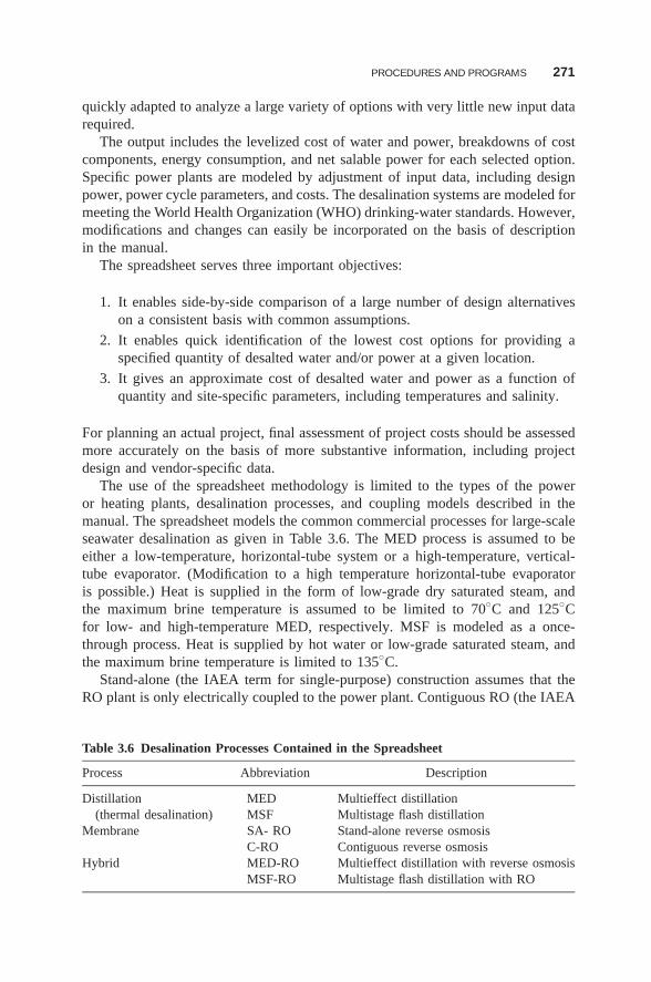
PROCEDURES AND PROGRAMS 271

quickly adapted to analyze a large variety of options with very little new input datarequired.

The output includes the levelized cost of water and power, breakdowns of costcomponents, energy consumption, and net salable power for each selected option.Specific power plants are modeled by adjustment of input data, including designpower, power cycle parameters, and costs. The desalination systems are modeled formeeting the World Health Organization (WHO) drinking-water standards. However,modifications and changes can easily be incorporated on the basis of descriptionin the manual.

The spreadsheet serves three important objectives:

1. It enables side-by-side comparison of a large number of design alternativeson a consistent basis with common assumptions.

2. It enables quick identification of the lowest cost options for providing aspecified quantity of desalted water and/or power at a given location.

3. It gives an approximate cost of desalted water and power as a function ofquantity and site-specific parameters, including temperatures and salinity.

For planning an actual project, final assessment of project costs should be assessedmore accurately on the basis of more substantive information, including projectdesign and vendor-specific data.

The use of the spreadsheet methodology is limited to the types of the poweror heating plants, desalination processes, and coupling models described in themanual. The spreadsheet models the common commercial processes for large-scaleseawater desalination as given in Table 3.6. The MED process is assumed to beeither a low-temperature, horizontal-tube system or a high-temperature, vertical-tube evaporator. (Modification to a high temperature horizontal-tube evaporatoris possible.) Heat is supplied in the form of low-grade dry saturated steam, andthe maximum brine temperature is assumed to be limited to 70◦C and 125◦Cfor low- and high-temperature MED, respectively. MSF is modeled as a once-through process. Heat is supplied by hot water or low-grade saturated steam, andthe maximum brine temperature is limited to 135◦C.

Stand-alone (the IAEA term for single-purpose) construction assumes that theRO plant is only electrically coupled to the power plant. Contiguous RO (the IAEA

Table 3.6 Desalination Processes Contained in the Spreadsheet

Process Abbreviation Description

Distillation MED Multieffect distillation(thermal desalination) MSF Multistage flash distillation

Membrane SA- RO Stand-alone reverse osmosisC-RO Contiguous reverse osmosis

Hybrid MED-RO Multieffect distillation with reverse osmosisMSF-RO Multistage flash distillation with RO

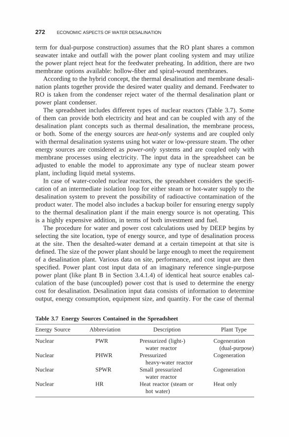
272 ECONOMIC ASPECTS OF WATER DESALINATION

term for dual-purpose construction) assumes that the RO plant shares a commonseawater intake and outfall with the power plant cooling system and may utilizethe power plant reject heat for the feedwater preheating. In addition, there are twomembrane options available: hollow-fiber and spiral-wound membranes.

According to the hybrid concept, the thermal desalination and membrane desali-nation plants together provide the desired water quality and demand. Feedwater toRO is taken from the condenser reject water of the thermal desalination plant orpower plant condenser.

The spreadsheet includes different types of nuclear reactors (Table 3.7). Someof them can provide both electricity and heat and can be coupled with any of thedesalination plant concepts such as thermal desalination, the membrane process,or both. Some of the energy sources are heat-only systems and are coupled onlywith thermal desalination systems using hot water or low-pressure steam. The otherenergy sources are considered as power-only systems and are coupled only withmembrane processes using electricity. The input data in the spreadsheet can beadjusted to enable the model to approximate any type of nuclear steam powerplant, including liquid metal systems.

In case of water-cooled nuclear reactors, the spreadsheet considers the specifi-cation of an intermediate isolation loop for either steam or hot-water supply to thedesalination system to prevent the possibility of radioactive contamination of theproduct water. The model also includes a backup boiler for ensuring energy supplyto the thermal desalination plant if the main energy source is not operating. Thisis a highly expensive addition, in terms of both investment and fuel.

The procedure for water and power cost calculations used by DEEP begins byselecting the site location, type of energy source, and type of desalination processat the site. Then the desalted-water demand at a certain timepoint at that site isdefined. The size of the power plant should be large enough to meet the requirementof a desalination plant. Various data on site, performance, and cost input are thenspecified. Power plant cost input data of an imaginary reference single-purposepower plant (like plant B in Section 3.4.1.4) of identical heat source enables cal-culation of the base (uncoupled) power cost that is used to determine the energycost for desalination. Desalination input data consists of information to determineoutput, energy consumption, equipment size, and quantity. For the case of thermal

Table 3.7 Energy Sources Contained in the Spreadsheet

Energy Source Abbreviation Description Plant Type

Nuclear PWR Pressurized (light-)water reactor

Cogeneration(dual-purpose)

Nuclear PHWR Pressurizedheavy-water reactor

Cogeneration

Nuclear SPWR Small pressurizedwater reactor

Cogeneration

Nuclear HR Heat reactor (steam orhot water)

Heat only

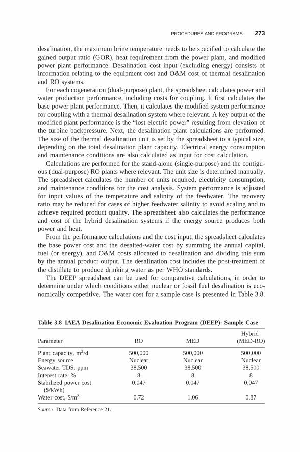
PROCEDURES AND PROGRAMS 273

desalination, the maximum brine temperature needs to be specified to calculate thegained output ratio (GOR), heat requirement from the power plant, and modifiedpower plant performance. Desalination cost input (excluding energy) consists ofinformation relating to the equipment cost and O&M cost of thermal desalinationand RO systems.

For each cogeneration (dual-purpose) plant, the spreadsheet calculates power andwater production performance, including costs for coupling. It first calculates thebase power plant performance. Then, it calculates the modified system performancefor coupling with a thermal desalination system where relevant. A key output of themodified plant performance is the “lost electric power” resulting from elevation ofthe turbine backpressure. Next, the desalination plant calculations are performed.The size of the thermal desalination unit is set by the spreadsheet to a typical size,depending on the total desalination plant capacity. Electrical energy consumptionand maintenance conditions are also calculated as input for cost calculation.

Calculations are performed for the stand-alone (single-purpose) and the contigu-ous (dual-purpose) RO plants where relevant. The unit size is determined manually.The spreadsheet calculates the number of units required, electricity consumption,and maintenance conditions for the cost analysis. System performance is adjustedfor input values of the temperature and salinity of the feedwater. The recoveryratio may be reduced for cases of higher feedwater salinity to avoid scaling and toachieve required product quality. The spreadsheet also calculates the performanceand cost of the hybrid desalination systems if the energy source produces bothpower and heat.

From the performance calculations and the cost input, the spreadsheet calculatesthe base power cost and the desalted-water cost by summing the annual capital,fuel (or energy), and O&M costs allocated to desalination and dividing this sumby the annual product output. The desalination cost includes the post-treatment ofthe distillate to produce drinking water as per WHO standards.

The DEEP spreadsheet can be used for comparative calculations, in order todetermine under which conditions either nuclear or fossil fuel desalination is eco-nomically competitive. The water cost for a sample case is presented in Table 3.8.

Table 3.8 IAEA Desalination Economic Evaluation Program (DEEP): Sample Case

HybridParameter RO MED (MED-RO)

Plant capacity, m3/d 500,000 500,000 500,000Energy source Nuclear Nuclear NuclearSeawater TDS, ppm 38,500 38,500 38,500Interest rate, % 8 8 8Stabilized power cost

($/kWh)0.047 0.047 0.047

Water cost, $/m3 0.72 1.06 0.87

Source: Data from Reference 21.

274 ECONOMIC ASPECTS OF WATER DESALINATION

3.8 DOMESTIC VERSUS FOREIGN CURRENCIES

In many countries the decision-makers may prefer to pay a little more for desaltedwater or power if the local currency percentage of the cost is higher.

In comparing the alternatives of desalination, nuclear, grid electricity, and fos-sil fuel energy supply sources for desalination, it is important to know the local(domestic)–foreign currency ratio in the product cost. This seems to be meaningfulfor developing (and possibly other) countries that are short in foreign currency. Incountries that import fossil fuel, the foreign currency component in the energy costbecomes relatively high. Therefore the nuclear option might be preferred even ifthe total product cost for this option is not lower than those of the alternatives.Also, in many cases the civil engineering and to some extent even the electricalengineering cost components in the nuclear installation are relatively higher. Thisexpense is usually local currency, giving additional motivation to prefer the nuclearoption.

Another cost component is labor (workforce): employment and training. Manycountries prefer to increase or maximize the local participation in infrastructuralprograms and projects. This may be manifested in recruiting most of the employedworkforce from local sources for power generation and for water supply becauseof (1) local currency considerations, (2) better communication, and (3) increasedemployment. Large desalination programs as well as nuclear power plants require ameaningful amount of staffing at the high professional expertise level. For desalina-tion in general and nuclear desalination in particular, the term specialized expertiserefers not only to O&M tasks but also to design and construction activities. Selec-tion of adequate staff, and preparing and training them, requires some preliminaryorganization such as establishing special academic desalination studies classeswithin the departments of chemical or mechanical engineering at some universitiesor at least courses—studies and tests—outside the academia.

3.9 VALUE OF DESALTED WATER

The value is the worth of the desalted water to the consumer. It depends on manyfactors such as water scarcity, specific applications, desalted-water quantity andsalinity, and qualities and costs of additional and alternative water sources. Thus,for example, the value of water for luxurious hotels or military bases may be quitehigh, whereas for large-scale agricultural irrigation it is usually expected to be low.

In many cases it is difficult to assess the value of the desalted water. However,it is reasonable to assume that, because of the relatively high availability andreliability of the desalted-water controlled quantity and quality, the real value ofdesalted water may be higher than that of alternative-source water, in particularwhere the latter has lower quality, such as high salinity, boron content, or hardness.

In principle, it is justified to use desalted water if the real value of such marginaldesalted water (considering the availability, quality, and quantity) is higher than

PRICES OF WATER AND POWER 275

its cost, provided, of course, that there is no better water source. The poten-tial consumer of desalted water—in many cases the national or regional waterutility or a large municipality—should consider this possibility while makingdecisions regarding payment for desalted water. Similarly, a government shouldconsider this aspect while determining its desalination policy and desalinationprogram.

3.10 PRICES OF WATER AND POWER

Price is the money paid to the supplier by the consumer. It differs from the cost ,which the supplier expended to produce the water or the energy, by the net profit.Under normal conditions the price level is between the cost and the abovementionedvalue of the product to the consumer. Thus, both the supplier and the consumerbenefit. If the consumer produces for her/himself, the price equals the cost. On theother hand, if the authorities intervene by taxing or by subsidizing (having eco-nomic, social, or political motives)—the price received by the supplier is differentfrom that paid by the consumer.

The situation may become more complex for dual-purpose plants. Even undernormal market conditions one product may be sold at a price that leaves a relativelymodest profit while the other product yields a high profit. It is also possible tohave an overall positive net profit due to a “good” price of one product, such aselectricity, even if the other—say, the desalted water—is sold for a price lowerthan its cost. In such case, the latter is practically subsidized by the former. Thismight sometimes give a misleading impression (as some people mix the notions ofcost and price) that the cost of desalination is quite low, with a risk that erroreousdecisions may follow.

One issue that concerns power price affecting desalted-water cost refers to dual-purpose plants. In the preferred power credit method, the water is charged by thecost of the differential electrical energy that would have been sold if the same powerplant were to operate on a single-purpose basis. One may question whether it isnot justified to charge the water by the price of this “unsold” amount of electricity,which is the commercial loss of the entire plant.

Quantitatively, for example, if the water consumes 4 kWh/m3 that cost 4.5¢/kWhto generate and the water cost is therefore 60¢/m3, and if the net price of electricityis, say, 5.4¢/kWh and the net price of the water is 72¢/m3 (i.e., 20% profit for each),then the plant loses [= 4 kWh/m3 ∗ (5.4 − 4.5)¢/kWh] that have to be recovered byeither increasing the price of the water or charging the water cost for the lost profit.The real profit of the water—if the price cannot be raised—is then only 8.4¢/m3

rather than 12¢/m3. Thus, the gross water cost is 72¢/m3 − 8.4¢/m3 = 63.6¢/m3,rather than 60¢/m3 given above.

Raising the price by the authorities or by the water supplier—probably withthe approval of the authorities—may serve two additional goals: (1) to reducethe demand for water and encourage saving and (2) to finance current and futuredesalination projects or research and development (R&D) activities.

276 ECONOMIC ASPECTS OF WATER DESALINATION

3.11 CASHFLOW, PAYBACK PERIOD, AND RATE OF RETURN

These three criteria are strongly interconnected. They concern mainly the investorsand the owners, but to a lesser extent they may be of interest to the water customersand to the government. Each of them constitutes a special criterion regarding thefinancial aspects of the investment:

1. Cashflow provides two-dimensional information about the financial balance andtimetable according to which investment components and other expenses—notonly fixed payments—are paid, and which payments for the products arereceived.

2. The payback period is the time difference between the date of the cashflowturning zero from previously negative and the (representative) date of the invest-ment.

3. The rate of return is the equivalent compounded interest at which the investmentis recovered, by the revenues from product sales, considering the price.

These criteria, as well as others (such as the ratio of net profit: investment) dependstrongly on product price, investment, plant load factor, and plant lifetime. Theyare significant in determining price and mainly in financing the investments.

It may be interesting to indicate that these criteria can be bypassed from the plantowners perspective, if the equipment installed in the plant, the price of which is themajor part of the plant investment, will be rented by the contractor who installed theplant to the owners or the operator. Thus, almost all the plant operator’s expenseswill be continuous and annual, linked to the sales revenues rather than a preliminarylarge investment. Such an arrangement has not yet taken place in the desalinationmarket.

It may also be interesting and important to note that when a long-term, multiplantprogram is initiated, investment may take place over a multiyear period. A singleinvestor in such a program will have to endure very long payback periods, especiallyif the production and/or generation capabilities are expanding, because the cashflowof the program in later years consists of revenues from water/power sales (incomes)on one hand and progressing investment (expenditures) on the other hand.

3.12 FINANCING

As mentioned above, the overall gross investments in large seawater desalinationplants are in the range of $1000 per unit capacity of cubic meter per day. Similarly,it is around $1000 per installed power unit capacity (kWe) for fossil fuel plantsand roughly 50–200% more for nuclear power plants.

The problems of financing nuclear desalination projects are quite similar to thosefor nuclear power.

The major issues of financing high-capacity plants are raising large capital fundsunder the optimal combination of the following conditions: low interest rate, long

BIDS AND OWNERSHIP 277

payback periods, and maximum local currency. One difficulty is the long period oftime between the investment date and the start of the payback period. Experiencein past projects proved that poor financing led to major difficulties.

As a general guideline, the financing entity gains profit, which adds to theprice (and possibly to the cost) of the water and/or power unless this entity is theconsumer or the government.

More aspects of financing are discussed in the following sections, describ-ing the contractual approaches of turnkey, build–operate–transfer (BOT)build–own–operate–transfer (BOOT), and build–own–operate (BOO) withinwhich financing is included. Another possible contractual approach is a version ofturnkey with the plant being rented, rather than sold, to the water/power supplier,as mentioned above (section 3.11).

3.13 BIDS AND OWNERSHIP

3.13.1 The Entities Involved

There are several possibilities to establish a desalination plant, possess it, andoperate it. The following legal distinct positions with this respect are

1. The water manufacture

2. The water supplier

3. The water user4. The water owner (not to be confused with the desalination plant owner)

5. The authorities

Often the authorities are also the water owners, who, in turn, grant the right of usingthe water to the users, and the permission to produce—to the water manufacturerand the license to distribute the desalted water—to the water supplier. This mutualstatus of authorities, owner, manufacturer, supplier, and user imposes certain mutualresponsibilities on each party.

In principle, the water supplier (listed item 2, above), who is responsible to thesupply of potable water, buys the water from the manufacturers (1) and sells it tothe water users (3). These positions 1–3, can be manifested either by three differententities, or by two—where the water supplier is also the water manufacturer suchas in the case of some water utilities—or, relatively seldom, even by a single entitywhere the water user is also the water manufacturer, as described in Section 3.13.2,with no need and no room for the function of a water supplier.

The initiative of establishing desalination plants can originate with either one ofthe five entities listed and described above.

3.13.2 Full and Direct Implementation of Desalted Water Production

The organization that requires desalted water or is responsible to the supply ofpotable water initiates the desalination project. This initiating organization—which

278 ECONOMIC ASPECTS OF WATER DESALINATION

may be either a private entity such as an industrial factory or a resort, or a publicentity such as the army for a military camp, municipal or state authorities for atown, or a region or an entire country—may independently decide to build, own,and operate the plant. In such cases, the cost (to these owners) of the desaltedwater is the lowest, as compared to the following alternatives, provided the ownersand their teams (plant managers, operators, and maintenance workers) carry outtheir professional tasks diligently. Thus, two principal advantages are gained: (1)from the performance aspect—maximum control of the owners on the plant andits operation is achieved, and (2) economically , the net profits to contractors in thealternative arrangements (discussed below) are saved.

Nevertheless, although the desalted-water preliminary cost under such anarrangement is the lowest, in quite a few cases the abovementioned authoritiesor organizations feel that they lack the experience or are not equipped to handleefficiently all the numerous activities needed to accomplish the supply of desaltedwater, or have other priorities and limitations. Thus, they do not want to entersuch obligation and prefer to pass considerable responsibilities to other entitiesaccording to the arrangements described below.

3.13.3 Turnkey Construction

The authorities or organizations that require the desalted water own the plant asin the abovementioned arrangement, but the entire plant construction is given tocontractors under an arrangement called a turnkey construction project . Most of thepreliminary investment is paid to the contractor, plus very roughly ∼10% of theinvestment that is expended by the plant owners on miscellaneous items such asland, possibly employing an advisory and planning architect-engineering company,legal and accounting services, supervision, selection of contractors, and recruitingand training the operation and maintenance staff. Operation and maintenance areoften carried out by the owners’ direct employees, but may also be given to specialcontractors. These turnkey construction project contractors (and possibly the O&Mcontractors) are often determined by bids for the lowest price for the plant and forthe O&M services. Other criteria, beside low cost, are also required or consideredconcerning the bid winner such as experience in similar projects, early and briefstartup or implementation, good reputation, and having proven sufficient economicresources that will enable successful accomplishment of the implementation.

The bid concept has the advantages of granting the work to the winner on thebasis of competence and impartiality as well as potentially lowering the price (andperhaps even the cost) of the work through the motivation created by competi-tion. However, bidding procedures consume time and money for both the ownersand candidate contractors, increasing the desalted water cost by a certain amount.Thus, the owner may alternatively contact contractors without bids and select themaccording to other criteria such as previous activities and acquaintance, recommen-dations, and other considerations. Avoiding bidding may save time and money butintroduces the economic risk of not acquiring the lowest price plant or services.With or without bids, using contractors may raise the water cost for the plant owneras the net profits of the contractors are added to the plant owner expenses.

BIDS AND OWNERSHIP 279

3.13.4 Build–Operate–Transfer (BOT) Approach

A less direct degree of responsibility of the entity that initiated the desalinationproject exists with the BOT option mentioned in Section 3.12. The initial financingand early O&M expenses are the direct responsibility of the company (or often aconsortium of several companies) that erect and run the plant, rather than of theorganizations that need desalted water. The latter are thus free from the risky stagesof the project. Only after sufficient time for the project to prove successful is thedesalination plant handed to or purchased by the entity that initiated the desalinationproject. Part or all of the investment is recovered by the contractor through thesale of the desalted water so that the price at which the plant is transferred to theentity that initiated the desalination project—often the government or the municipalauthorities—is the relatively small remaining part of the entire initial investment.The longer the time at which the contractor operates the plant, the lower is thepayment for transferring the plant.

The BOT option sometimes leads to the next possibility, BOOT, as detailedbelow.

3.13.5 Build–Own–Operate–Transfer (BOOT) Approach

With the build–own–operate–transfer (BOOT) approach, the responsibility forO&M and other expenses of the party who initiated the desalination project iseven less direct than that with the BOT option (described in Section 3.13.4). Thefinancing and current O&M expenses are the direct responsibility of the companiesthat erect and run the plant for a 20–30-year period, rather than those organizationsthat require desalted water, who, in turn, pay only for the water rather than forthe plant, exempting them from involvement in issues related to the project, inparticular, the financing. Only after a long period of time during which all theinvestment has already been recovered through payments for the consumed wateris the plant transferred to the entity that initiated the desalination project.

(Note: The distinction between BOT and BOOT is small and is sometimesignored. According to those who do distinguish between the two possibilities, themain difference is obviously the ownership. Whereas with BOT the plant is contin-uously owned by the initiating entity that grants the right to build and operate to thecontractor, with the land possessed by the initiating entity, with BOOT the plantand the land belong to the contractor until the transfer. Another difference may bethe length of the operation period before transferring the plant from the contractorto the initiating entity, which may be longer with the BOOT arrangement.)

In the broad sense and also in more detail, one information source refersto the BOT and BOOT option: as follows:

Build-Operate-Transfer (BOT) is a form of project financing, wherein a private entityreceives a franchise from the private or public sector to finance, design, construct, andoperate a facility for a specified period, after which ownership is transferred back tothe funding entity. During the time that the project proponent operates the facility, itis allowed to charge facility users appropriate tolls, fees, rentals, and charges stated in

280 ECONOMIC ASPECTS OF WATER DESALINATION

their contract to enable the project proponent to recover its investment, and operatingand maintenance expenses in the project. However, in some countries, the term usedis Build-Own-Operate-Transfer (BOOT).

In a BOT arrangement, the private sector designs and builds the infrastructure, financesits construction and owns, operates and maintains it over a period, often as long as20 or 30 years. This period is sometimes referred to as the “concession” period.

Traditionally, such projects provide for the infrastructure to be transferred to thegovernment at the end of the concession period. BOT is a type of project financing.The hallmarks of project financing are:

The lenders to the project look primarily at the earnings of the project as the sourcefrom which loan repayments will be made. Their credit assessment is based on theproject, not on the credit worthiness of the borrowing entity.

The security taken by the lenders is largely confined to the project assets. As such,project financing is often referred to as “limited recourse” financing because lendersare given only a limited recourse against the borrower.

Most project finance structures are complex. The risks in the project are spreadbetween the various parties; each risk is usually assumed by the party which canmost efficiently and cost-effectively control or handle it.

Once the project’s risks are identified, the likelihood of their occurrence assessed andtheir impact on the project determined, the sponsor must allocate those risks. Briefly,its options are to absorb the risk, lay off the risk with third parties, such as insurers,or allocate the risk among contractors and lenders. The sponsor will be acting, moreoften than not, on behalf of a sponsor at a time when the equity participants areunknown. Nevertheless, each of the participants in the project must be satisfied withthe risk allocation, the creditworthiness of the risk taker and the reward that flows tothe party taking the risk. In this respect, each party takes a quasi equity risk in theproject.

3.13.6 Build–Own–Operate (BOO) Approach

The entity that initiated the desalination project using the build–own–operate(BOO) approach, has the least direct responsibility for the project compared tothe previous approaches. The financing and current operation and maintenanceexpenses are under the direct responsibility of the companies that erect and run theplant along its lifetime, rather than those organizations that need desalted water.The latter, in turn, pay for the water rather than for the plant, absolving theminvolvement any potential or actual issues regarding the project. On the other hand,they pay the full price of the water—the gross cost of desalination, possibly thecoverage for risk elements of the project, and the net profit of the contractors.

3.13.7 Rented Plant

Another possible arrangement of plant ownership for the desalination project ini-tiators, not in use so far, is aimed at bypassing financing issues by holding and

CONTRACTUAL PRICING DUE TO CHANGES AND DEVIATIONS FROM THE ORIGINAL PLAN 281

operating the plant while it is being rented from those investors that finance theerection of the plant to the entity that operates the plant and sells the water. Thedesalination project initiators may operate and maintain the plant directly or hirecontractors to operate and maintain it.

3.14 CONTRACTUAL PRICING DUE TO CHANGES AND DEVIATIONSFROM THE ORIGINAL PLAN

These modifications include linkages, bonuses, penalties, compensation for “excesswater,” and high-quality product water streams. The economic changes and risks areas follows. At the stage of decision-making regarding construction of a desalinationplant (and even more so regarding a multiplant desalination plan), changes and risksare expected, even in the construction phase of the plant, which is near-future andrather short in duration. Such modifications are most likely to occur during theoperation phase, which usually extends a few years into the future and is a ratherlong period, especially where construction of several plants is planned to take placeat specified time intervals.

Special clauses regarding contractors’ and water users’ risks reduction are usu-ally included in the contracts of BOT, BOOT, and BOO arrangements. The esca-lations risk is diminished by linking the water prices through an agreeable formulato the main operation cost components, namely, energy (fuels and electricity) andsalaries and possibly the pertinent chemicals and spare parts.

Another contractor risk of the project economy calls for a compensation clauseprotecting the contractor against the possibility of refusal of water customers toaccept the desalted water—due either to an early end of the project life, emergenceof cheaper alternative water sources, or inclement wheather, to be included inthe contract. The compensation for rejecting product water covers the water costcomponents that are not proportional to the amount of the water produced: capitalcost and most of the staff salaries, but excluding energy, chemicals, and workerovertime.

On the other hand, there are risks on the side of the water customers or theauthorities who granted the contract to the plant contractor—mainly negative devi-ations from the original terms of the contract:

• Late plant commissioning (which is also relevant in turnkey contracts)• Low water production rate• High TDS contents of and/or chlorides, boron, nitrates, etc.• High energy or chemical consumption• Low time availability• Short life of main equipment components such as membranes, pumps, or heat

transfer surfaces• Short life of the entire plant or a unit

If these deviations are not too large, or if they can be reasonably corrected,they are usually compensated for by penalties paid by the contractors to the water

282 ECONOMIC ASPECTS OF WATER DESALINATION

users according to agreed-on formulas. Otherwise they can cause termination ofthe project.

Positively, the opposite deviations from the original terms of the contract mayalso occur, due to high safety factors taken in the design, high-diligence operation,excellent management, or for other good reasons. If such positive deviations aredesirable to the water users, they may be compensated by bonuses paid to thecontractors according to established formulas.

3.15 NATIONAL DESALINATION PROGRAMS

The complexity of national desalination programs is larger than that of specificprojects in the following aspects:

1. Different Decisions . Since a national desalination program usually comprisesseveral desalination plants, there is a certain flexibility regarding the size,location, and timing of each individual plant. In some cases even the detailedrequired quality of the desalted water may differ according to the locationfrom one plant to another. These principal decisions—water quantity andquality, locations, and time schedule—are strongly dependent on economicconsiderations that may drastically change the final results (whereas for localwater shortage problems the location is simply given, size is more or lessknown according to the needed amounts of water, and the timing flexibilityis usually quite narrow so that the main decisions for a local water problemdetermine which desalination process will be used and who will erect andoperate the plant).

2. Broader Scope. The scope of a national desalination programs is muchbroader than that of specific projects in the water quantities, length of timeperiod, number of involved entities (suppliers, advisors, contractors, and sub-contractors), and number of sites. Because of this broad scope, even smallcost and price differences, which might be of marginal significance in a sin-gle plant for an acute water shortage, accumulate to large amounts of moneyand become important.

3. Land Area . To enable the smooth implementation of a national or regionaldesalination program, the authorities have to allocate and reserve appropriatesites of sufficient area for all the planned desalination projects. This mightinfluence the economy both directly and indirectly: directly, by having to payfor the areas very early or compensate other entities that may have interestin the said areas, in particular sites near the sea that are more limited andhave high demand; indirectly, by causing escalation in land prices due to thechanges incurred in the demand versus supply within the real estate market.In view of large-scale desalination financing difficulties, a reasonable prelim-inary cost, cashflow and financial evaluation and planning should include, insome cases, these ground area impacts for dedicated plants or an additionalarea in dual-purpose projects.

NATIONAL DESALINATION PROGRAMS 283

4. Distribution and Conveyance of the Desalted Water . The large amounts ofdesalted water via the national program are, at least partly, delivered torelatively distant water users. This may require additional investments inpipelines and pumps and possibly also storage facilities, as well as in areasand/or passage permissions for these installations. Energy is also consumedby this water conveyance, in particular for delivery to water users locatedat elevated sites. Moreover, old pipes—either galvanized steel or concretewhich rather often suffers from leakage might need repairs or replacementby plastic pipes to avoid loss of expensive desalted water, and even more sobecause the chemistry of the desalted water may enhance the leakage. Allthese activities, associated with the desalted water outside the desalinationplants, impose an additional cost burden on the national program.

5. Energy . Similarly, another activity strongly associated with the desalted wateroutside the desalination plants is the energy generation for the national desali-nation program; the quantity becomes a factor of significant economic weight.For example, a very large local SWRO 50,000-m3/day plant that can sup-ply water to between quarter and half million people requires a ∼8–9 MWeenergy source, which can be easily supplied from the grid; but a typicalnational program that will produce 500 million m3/year needs, including dis-tribution pumping, ∼250–300 MWe, which requires a significant addition tothe nation’s power generation capacity. With a specific investment of veryroughly $1000 per installed kWe, it requires financing of ∼$0.25 billion(US) investment in addition to financing of the desalination plants and thefinancing of the pipelines and pumping equipment for the delivery.

6. Applications . Within the national program, the practical value of the desaltedwater can become higher because of the versatility of its applications, whichresult from the high degree of reliable supply, and especially from the con-trolled quality and quantity. This practical value has a reflected economicvalue as well. In addition to the obvious basic aspects of enhancing theamount of available water of desired solute concentrations, the applicationsinclude the following:

a. The possibility of diluting of the existing waters with the low-salinitydesalted water to improve the quality of the former. This applicationhas impacts on health; scale deposits in pipes, kettles, boilers, washingmachines, and other devices; and reduction of detergent consumption.Where a low-salinity mixture of desalted water and regular water is deliv-ered for domestic use, the resulting sewage, which is more salty by∼100–150 mg/liter than the incoming water, is still suitable for agri-cultural irrigation. Consequently, sometimes there is a higher potential toreuse up to 70% or even 80% of the incoming water.

b. Redemption of old water sources that have been abandoned because ofexceedingly poor quality, thus adding more water—between roughly 20%and 200% of the desalted water used for such dilution—to the nationalwater balance.

284 ECONOMIC ASPECTS OF WATER DESALINATION

c. Similar potential addition to the water balance may be achieved by dilutionof originally inappropriate brackish-water, if available. Thus, comparedto the alternative of desalting the brackish-water, the entire amount ofbrackish-water is utilized, rather than only 70–90% of it; thus the cost ofdesalting the brackish-water is avoided, as well as the difficult problemof inland concentrate removal.

7. Impacts on National Economy: Index of Living . Since the production costof desalted water is in most cases considerably higher than that of otherwaters and the prices of desalted water are obviously even higher, the largeamounts of desalted water produced in a national program may affect theindex of living. Introducing a new costly elementary commodity to the listof items that constitute the basis for calculating the index of living will raisethe level of this index when this new commodity is widely consumed, whichin many cases is eventually inevitable. This effect may, in turn, contributeto the salary increases of those employees whose wages depend on or arelinked to the index of living—possibly the majority of employees throughoutthe country. Thus, part or all the government may object to such an effectand may try to reduce it by reducing the scope and pace of the nationaldesalination program.

8. Employment . On the other hand, large-scale building and operation of desali-nation systems involves employment of many hundreds of local workers,which may somewhat motivate the government to support and encourage abroad desalination program.

9. Impacts on National Economy: Subsidies . Some water users cannot afford topay the full price of desalted water, in particular the agriculture sector. Thestate may cover the difference between the price paid to the water suppliersand the lower price paid by these water users. In the case of desalted water,this subsidy is usually quite high per cubic meter and when multiplied bylarge quantities, may consume large amounts of money. Governments arereluctant to spend this money, and may consequently try to reduce the scopeof national desalination programs.

10. Taxes . Taxing policy—the opposite of subsidies—relating to desalted wateras part of national program may differ from that related to local desalinationprojects.

11. Financing . Similarly, financing policy relating to desalted water as part of anational program may differ from that related to local desalination projects interms of both or either allocating and/or investing money and determining thediscount rate. The latter can be reduced—in favor of cost reduction—directlyby government decisions or legislation or indirectly by state guarantees toother financing entities that may decrease the discount or interest rate in viewof the reduced financial risk resulting from this state guarantee.

DESALINATION AND HYDROLOGY 285

3.16 DESALINATION AND HYDROLOGY

In many cases, in particular large desalination projects, the desalted water is one ofseveral water sources. Integration of all water sources throughout the entire watersystem is obviously necessary. The desalted water can be integrated in several wayswith the hydrology of the country, the region and/or the vicinity of an existing (ora candidate) desalination plant:

1. Parallel and Complementary . The potential amounts of water pumped fromthe available aquifers do not reach the existing or expected demand. Theresulting gap, if no other (or better) sources exist, is covered by desalination.

2. Parallel and Mixing . In addition to closing the quantitative gap describedabove (1), mixing the desalted water with the groundwater may improve thequality of the latter and in some cases of salty brackish-water may reclaiminappropriate groundwater and redeem contaminated wells.

3. Storage. In years of high rainfall the demand for potable water may decrease,while during dry seasons, which may last several years, water shortage mightdevelop even with desalination systems in place. Reducing the output of thelatter during rainy years due to the low demand might prove to be unwise ifdry spells or droughts were to develop later. An optimal strategy might be tooperate the desalination plants in full capacity (or almost full) and store theexcess water during rainy seasons. The storage can be performed directly,by infiltrating the desalted water into the ground and thus recharging theaquifers, or—perhaps even more effectively—to use all the desalted waterwhile reducing the pumping from the aquifer and allow the water table to risewith the surplus of incoming rain water seepage above the lowered pumpingrate, namely, to ensure a definite positive groundwater balance.

4. Delaying Erection of Desalination Plants . Postponing the installation ofdesalination plants by one or more years has several advantages:

a. Reducing interest fees on the investments and O&M.

b. Preventing or reducing risk of equipment deterioration.

c. Using more advanced technology, as progress develops during the periodof postponement (improved RO membranes etc.).

d. Cost reduction due to application of economy-of-scale principle as thepostponed plants need to be of larger capacity than the original or alter-native planned plants.

e. Accumulating more experience elsewhere.

f. Since many desalination plants are and will be integrated with electricpower generation, reducing the power plant capital costs or grid capitalcosts resulting from power unit operation may be achieved by postponingthe project, if the larger desalination units are commissioned simultane-ously with the power plant. (This strategy is effective particularly for

286 ECONOMIC ASPECTS OF WATER DESALINATION

nuclear desalination.) The reason is that when a large power unit is addedto the grid, there is a surplus of power supply for a few years, until thegradually increasing power demand consumes this surplus. Obviously thissurplus increases the amortization of the extended generating system. Thisamortization can be reduced by connecting a large (step function) powerconsumer, namely, the large desalination system to the power plant, oreven to the grid simultaneously with commissioning of the large powerunit or very short time later, thus reducing the power surplus.

Postponement of the installation of dual-purpose or large-scale desalination plants,in particular nuclear plants, by several years may be preferred, because of the sixadvantages mentioned above, in those cases where the need for additional poweris less crucial than the need for water, even if desalination is the best or the onlysolution for water shortage. More specifically, apparent hydrological constraintsforbid additional pumping from the aquifers. Despite such hydrological constraints,it is still possible to use groundwater provided it is done temporarily and followedby recuperation as described here.

The obvious disadvantage of water shortage can be reversed by carefully inte-grating groundwater utilization and national or regional desalination activities insuch a way that may allow project postponement while avoiding water shortage asdescribed below.

One way to postpone desalination because of actual or potential water shortageis to deplete certain aquifers to a specified limit as follows. Those aquifers thatcan withstand a few years of overpumping have to be identified, located, andutilized. Tolerance for overpumping is determined by the following hydrologicaland management conditions:

• A temporary drop of the water table of the aquifer below the minimum levelmust not cause irreversible damage to the potable groundwater. This is a purehydrological condition.

• The period of overpumping from those aquifers shall be immediately followedby a period of low-pumping, no-pumping, or even recharge of freshwater ordesalted water to accelerate recuperation. This condition is of operational innature and is related to hydrology management.

Another management condition and requirement is that larger desalination capacity(compared to the original or alternative plan) be available immediately after theoverpumping period to cover the previous original need for desalted water, replacedby the overpumping, plus the added increasing demand for freshwater during thepostponement period, plus the “overdraft” accumulated by the overpumping to berecuperated.

For example, if an aquifer is found where the water table in a 10-miles-radiuscan tolerate, for a few years, an average drop of 2 m, and assuming 30% effectivesoil porosity, the potential amount of water “loaned” from this aquifer is almost500 Mm3. This potential “overdraft” amount may, indeed, allow delay in installingdesalination systems by a few years, even if the aquifer is not fully exploited.

ECONOMICS OF DESALINATION RESEARCH AND DEVELOPMENT (DESALINATION R&D) 287

3.17 ECONOMICS OF DESALINATION RESEARCH ANDDEVELOPMENT (DESALINATION R&D)

Parallel to the vast of economic amount resources and efforts invested in desali-nation plants, another channel of activity exists in which additional funds areallocated for exploring new possibilities for desalination, investigating partly famil-iar phenomena, developing new processes, and improving existing systems andcomponents. These desalination R&D activities take place at various levels, arefinanced by several sources, and are carried out by many entities. The financingcomes from governments, desalination system manufacturers, desalination plantoperators, water and power utilities, and other sources. Relatively small amountsof money are invested by the academia.

The R&D activities are categorized in the following groups according to costof a typical activity:

• Research; specifically, investigation of phenomena. This is done by theacademia, in research institutes, and by industrial entities, namely, variousdesalination equipment manufacturers and desalination systems users.Expenses for research are relatively low per year, but may accumulate overthe years because research activities usually are long term. Expenses consistmainly of salaries, since the equipment is of small size. Funding sources forthese activities may include the government of the state where the researchtakes place, sometimes other governments under multinational cooperativeagreements, possibly other public sources, manufacturers and/or users ofdesalination equipment, and—usually only if the expenditure is relativelysmall—the institute’s own internal funds. It is important to note that asignificant part of the expenses involved are not recognized as desalted-watercost components and are not recovered by sale of the desalted water, at leastnot directly.

• Development Small-scale development at bench scale or unit operationscale—in early phase of testing concepts or formulas underlying equipmentitems or subsystems. The expenses are relatively low per year, and mostactivities are carried out during relatively short periods, such as a fewweeks of operation and very few months for preparation.

• Medium-scale development at pilot plant scale—at advanced phase of test-ing ideas of subsystems or complete systems of rather smaller size relativeto commercial units. Sometimes the tested system operates in closed-loopfashion to save part of the infrastructure. (A closed-loop desalination pilotplant is a plant at which the saline feedwater stream is artificially createdby mixing the product desalted water with the stream of the concentratedbrine, thus obviating the expenses of seawater or brackish-water intake andpretreatment and brine outfall system, and enabling the testing activity to becarried out at convenient sites, not necessarily near the sea or saline-waterwells.) The capacity is usually about one order of magnitude smaller thana small commercial plant or even smaller. The expenses may very roughly

288 ECONOMIC ASPECTS OF WATER DESALINATION

in the range of $100,000 (US) per installed pilot plant plus at least a sim-ilar amount of money for operation, analyzing the results, reporting, anddecommissioning.

• Large-scale development at demonstration plant scale—last phase of test-ing and validating semiproven ideas and concepts of complete systems ofrather full size and open loop as (or almost as large as) commercial units,often with considerably more instrumentation and windows than in com-mercial units, to enable better follow-up and detailed measurements of theprocess and equipment performance. Because of the size of the equipment,the needed infrastructure, the instrumentation, and the relatively long peri-ods of the tests, this phase is quite expensive. The expenses are relativelyhigh but take place only once in several years and hopefully are lucrativebecause the demonstration plant yields salable potable water in addition toinformation, data, know-how, and experience. Since there it is highly prob-able that a demonstration plant will be installed at the site where desaltedwater is needed, selling the desalted water may compensate for most orall of the demonstration expenses. The expenses of such large-scale R&Dmay total between a few hundred thousands and a few tens of millions USdollars. Financing these expenses comes either from desalination systemmanufacturers or other investors who want to sell plants or desalted wateror from governments of states that require desalted water or are interestedin developing a desalination industry for export of desalination plants.

• R&D priorities —in principle two possible scenarios can exist with regardto financing R&D activities. In scenario 1, the initiative for such activitiesoriginates with the financing entities who allot a certain amount of moneyfor the general purpose of advancing the technologies and offer this moneyto the technology entities, such as academia, research institutes, industry,and water and power utilities. In scenario 2, the initiative originates with thetechnology entities that want to carry out the R&D activities and request themoney from external financing entities or raise it from their own resources.

In scenario 1 the specific subjects of the activities are not defined and the overallamount of money is offered for desalination in general or for the type of activitythat the financing organization prefers, such as inland desalination, desalinationenvironmental aspects, novel processes, or new RO membranes. Occasionally, veryfew research activities actually develop, due to a lack of definite ideas or lackof enthusiasm from the R&D community to participate because they are eitherreluctant to accept some of the conditions that usually accompany the grantingof money, or otherwise too occupied. In such cases the few proposed activitiesare very likely to be fully financed. In the opposite case, where several definiteactivities in need of relatively large amounts of money compete on a limited budgetthat is less than the total requested sum, the money should be granted according topriority in which economic potential is the main consideration. Two other factorsare the expected probability of success of the R&D efforts in the subject activityand the amount of resources—money and time—requested. For example, in a

WORLD MARKET AND FUTURE PROSPECTS FOR DESALINATION 289

competition between two well defined development steps where one is improvingthe corrosion resistance of RO pumps to absolute durability versus raising thesalt rejection of SWRO membranes to 99.9%, the priority will most probably beassigned to improving membranes, (unless the needed money for finding a way toraise the membrane rejection is orders of magnitude greater than that needed forthe pump durability).

In scenario 2, where the initiative for R&D activities originates within thetechnology community, there might also be some competition between candidateactivities, but more seldom, since the financing is requested for well-defined activi-ties, normally after some self-criticism. On the other hand, and for the same reason,the lack of definite ideas or enthusiasm from the R&D community to participatehardly exists. Then the main two criteria for financing the R&D activities are thetime period for full commercial recovery of the investment in the activity (or, moreaccurately, its probabilistic equivalent) and the expected cashflow resulting fromthis activity.

3.18 WORLD MARKET AND FUTURE PROSPECTS FORDESALINATION

The global need for potable water is expected to grow quite rapidly, due to increaseof world population, the striving to improve the quality of life in developingcountries, and deterioration of the quality of part of the freshwater sources. Aconsiderable part of the additional water will come from desalination.

The demand for desalted water and desalination plants will rise and may conse-quently bring the prices up according to the market forces. Another potential motivefor future price escalation is the possibility of the authorities requiring more strictenvironmental limits from the desalination plants. A third risk is the rising energyprices.

On the other hand, there are several factors that may contribute to price reduc-tion, most of them via cost reduction:

1. The economy of scale of the desalination systems’ manufacturing enterprises.

2. The continuous development of better desalination equipment, such as (forRO) new membranes having lower price and/or improved performance(longer life, higher water flux per unit driving pressure, and/or better saltrejection) or better pumps, in particular, pressure energy recovery devices,or developing low-cost heat transfer surface elements with high-heat-transfercoefficients for MED process.

3. Improvement of desalination system manufacturing procedures and tech-niques.

4. Finding better solutions to existing operation problems, stemming from accu-mulating (and hopefully shared) experience.

5. Competition between desalination system suppliers (and operators where theplants are not operated by the owner or the desalination system supplier).

290 ECONOMIC ASPECTS OF WATER DESALINATION

6. Accumulating experience with erection, operation, and management of desali-nation plants will reduce the level of technological and managerial risk asso-ciated with desalination projects and might bring down the interest rates andlower the capital costs. The same effect may occur with market client pres-sures in view of the vitality of water to the citizens. This might be additionallyachieved by governmental or international (e.g., the World Bank, UN) guar-antee backing the financing of large desalination programs or projects. Suchbacking further reduces the financial risk and thus may lower the interest rate.

APPENDIX

3.A.1 Sample Cost Calculations for Desalted Water at the Plant

The equipment prices given below do not represent any actual information. Theyare presented only for demonstrating a typical cost calculation procedure, so thereader should not use them as proven professional data. They constitute only roughapproximations at some sites, and even at those sites they are subjected to negoti-ations and changes with time and technological and commercial developments.

Cases 1: Single-Purpose SWRO Plant of 100,000 m3/d Capacity

Parameters: PN = 100, 000 t/d = 4167 t/h; at load/plant factor of 92%, theannual production is PNA = 33.6 Mm3/year.

Main Process Design1. For given seawater salinity of 3.5%: sf = 35 kg/t.

2. Required permeate (product) salinity of 500 ppm TDS: sp = 0.5 kg/t.

3. Allowed maximum concentrate (brine) salinity of 7.0%: sb = 70 kg/t.a. The feed flow rate can consequently be calculated as the mass

balances of the water and the salt yield: PN(sb − sp)/(sb − sf) =100, 000(70 − 0.5)/(70 − 35) = 198, 570 t/d = 8274 t/h.

b. The average permeate flux is 8 gfd (US gallons per square foot perday) = 8 ∗ 1.698 = 13.58 L/m2 per hour ≈0.326 m/d ≈0.325 t/m2

per day. [1 gfd = 1.698 Liter/m2 per hour ≈1.7 mm/hour].

c. At this point the net area of the membranes, which is themain equipment component of the process, can be calculated:Membrane area = 100, 000/0.325 = 306770 m2 = 3.3 ∗ 106 ft2.

d. The number of elements, each of which has about 400 ft2 of activemembrane area per element, is approximately3.3 ∗ 106 ft2/400(ft2 per element) = 8250 elements.

e. However, according to the membrane manufacturer’s data and com-puter program, which yields the plan with the numbers of vesselsand elements, 1020 vessels with 8 elements per vessel = 8160 ele-ments, are needed. (Either the exact membrane area of the elementsis slightly larger than 400 ft2 per element, or the flux taken by thecomputer program is 1.1% higher.)

APPENDIX 291

f. Cost of installed elements: ∼$600 (US monetary units, throughout)per element including labor: 8160 ∗ 600 = $4,896,000, plus ∼2%spare membranes, result in $5M = $50 per daily ton.

g. Cost of installed pressure vessels: ∼$2500 per vessel includinglabor: 1020 ∗ 2500 = $2.05M = $21 per daily ton of desaltedwater.

h. Membrane racks and piping: ∼15% of membranes and pressurevessels: 0.15*(4.9M$+ 2.05M$) = $1.04M = $10 per daily ton ofdesalted water.

i. Power of installed high-pressure pumps (pressure is given by thecomputer program Hydranautics, the membrane manufacturer):8274 t/h/(1.03 t/m3) ∗ 64 bar/0.87/(36 bar∗m3/h) = 16.41 MW =20, 417 hp (horsepower), installed power ∼15% more −24, 000 hp.

j. Cost of installed high-pressure pumps: ∼$200/hp, includinglabor: 24,000 hp*$200 = $4.8M = $48 per daily ton of desaltedwater.

k. Power of installed high-pressure recovery device: (8274 −4167) t/h/(1.06 t/m3) ∗ 62 bar ∗ 0.87/(36 bar ∗ m3/h) =5.8 MW = 7900 hp, installed − 9000 hp.

l. Cost of installed high-pressure recovery device: ∼$200/hp, includinglabor: 9000 hp*$200 = $1.8M = $18 per daily ton of desalted water.[Note: The recent use of the modern pressure exchanger as an energyrecovery device (rather than the water turbine) reduces the size, cost,and energy consumption of high-pressure pumps by roughly 50%.The net energy and investive savings are, however, about 15% (0.4kwh/m and 0.5M$, respectively.]

m. Installed low-pressure pumps:(1) Feed: 8274 t/h/(1.03 t/m3)*5 bar/0.86 = 1.3 MW = 1770 hp.

(2) Product: 4167 t/h/(1.00 t/m3)*5 bar/0.86 = 0.67 MW = 910 hp.

Total: 1.3 + 0.67 ≈ 2.0 MW, installed −3000 hp.

n. Cost of installed low-pressure pumps: ∼$200/hp including labor:3000 hp*$200 = $0.6M = $6 per daily ton of desalted water.

o. Cost of pretreatment system: ∼$12M = $120 per daily ton ofdesalted water.

p. Cost of seawater intake system and concentrate outfall: ∼$4M =$40 per daily ton of desalted water.

q. Cost of instrumentation: ∼$1.5M = $15 per daily ton of desaltedwater.

r. Cost of control system: ∼$1.5M = $15 per daily ton of desaltedwater.

s. Cost of electrical work: ∼$4M = $40 per daily ton of desaltedwater.

292 ECONOMIC ASPECTS OF WATER DESALINATION

t. Cost of membrane cleaning system: ∼$1M = $10 per daily ton ofdesalted water.

u. Cost of other piping: ∼$2M = $20 per daily ton of desalted water.

v. Cost of buildings: ∼$4M = $40 per daily ton of desalted water.

w. Cost of civil engineering: ∼$10M = $100 per daily ton of desaltedwater.

x. Cost of product posttreatment: ∼$4M = $40 per daily ton ofdesalted water.

y. Cost of furniture, laboratory, communication equipment, computers,transportation means, cranes, and miscellaneous: ∼$3M = $30 perdaily ton of desalted water.

z. Total: $62.25M = $623/t per day.aa Cost of management, planning, and design: ∼15% of the total

(item z, above) = 0.15*62.3 = $9.4M = $94 (US)/t per day.

bb Owner’s cost: ∼10% = 0.1*(62.3+9.4) = $7.2M = $72/t perday.

cc Total, assuming 7.5%/py as interest during construction, effec-tive period of construction 2.5 annual years: 1.0752.5/2(62.3+9.4+7.2) = 1.0946 ∗ 78.9 ≈ $86.4M = $864/per day; hence thetotal percentage of interest during construction is 1.0946 − 1 =0.0946 ≈ 9.5%.

dd Energy:(1) Pumps total: 16.4 MW + 1.3 MW + 0.67 MW = 18.4 MW

mechanical work.

(2) Pressure recovery: 5.8 MW mechanical works.

(3) Net mechanical works: 18.4 − 5.8 = 12.6 MW.

(4) At 92% electrical system efficiency (motors, trans-formers, etc.), average electric power consumption:12.6/0.92 = 13.7 MWe.

(5) An additional 200 kWe, is consumed by plant outside desali-nation process for facilities such as lights, workshop, kitchen,air conditioning, offices, and showers: 13.7 MWe + 0.2 ≈14 MWe.

(6) Specific energy of the desalted water at the plant is14 MWe/4167 t/h = 3.36 kWhe/ton.

(7) Allowing ∼2% additional losses for off-optimum operation,and another 2% for gradual decrease in the efficiencies of thepumps and pressure recovery devices, the estimated specificenergy is 3.36/0.96 = 3.5 kWhe/ton

(Note: Comparing the specific investment and energy calculated herewith the values presented in Table 3.3 shows 8% higher investmentbut 5.4% lower energy. The higher investment is explained partly

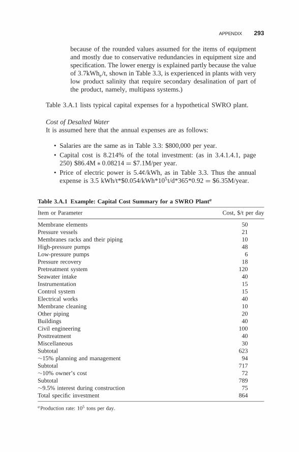
APPENDIX 293

because of the rounded values assumed for the items of equipmentand mostly due to conservative redundancies in equipment size andspecification. The lower energy is explained partly because the valueof 3.7kWhe/t, shown in Table 3.3, is experienced in plants with verylow product salinity that require secondary desalination of part ofthe product, namely, multipass systems.)

Table 3.A.1 lists typical capital expenses for a hypothetical SWRO plant.

Cost of Desalted WaterIt is assumed here that the annual expenses are as follows:

• Salaries are the same as in Table 3.3: $800,000 per year.

• Capital cost is 8.214% of the total investment: (as in 3.4.1.4.1, page250) $86.4M ∗ 0.08214 = $7.1M/per year.

• Price of electric power is 5.4¢/kWh, as in Table 3.3. Thus the annualexpense is 3.5 kWh/t*$0.054/kWh*105t/d*365*0.92 = $6.35M/year.

Table 3.A.1 Example: Capital Cost Summary for a SWRO Planta

Item or Parameter Cost, $/t per day

Membrane elements 50Pressure vessels 21Membranes racks and their piping 10High-pressure pumps 48Low-pressure pumps 6Pressure recovery 18Pretreatment system 120Seawater intake 40Instrumentation 15Control system 15Electrical works 40Membrane cleaning 10Other piping 20Buildings 40Civil engineering 100Posttreatment 40Miscellaneous 30Subtotal 623∼15% planning and management 94Subtotal 717∼10% owner’s cost 72Subtotal 789∼9.5% interest during construction 75Total specific investment 864

a Production rate: 105 tons per day.

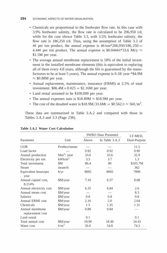
294 ECONOMIC ASPECTS OF WATER DESALINATION

• Chemicals are proportional to the feedwater flow rate. In this case with3.9% feedwater salinity, the flow rate is calculated to be 206,950 t/d,while for the case shown Table 3.3, with 3.5% feedwater salinity, theflow rate is 186,250 t/d. Thus, using the assumption of Table 3.3 of4¢ per ton product, the annual expense is 4¢/ton*206,950/186, 250 =4.44¢ per ton product. The annual expense is $0.0444/t*33.6 Mt/y ≈$1.5M per year.

• The average annual membrane replacement is 18% of the initial invest-ment in the installed membrane elements (this is equivalent to replacingall of them every 4.8 years, although the life is guaranteed by the manu-facturers to be at least 5 years). The annual expense is 0.18/ year *$4.9M≈ $0.88M per year.

• Annual replacement, maintenance, insurance (ERMI) at 2.5% of totalinvestment: $86.4M ∗ 0.025 = $2.16M per year.

• Land rental assumed to be $100,000 per year.

• The annual expenses sum is $18.89M ≈ $18.9M per year.

• The cost of the desalted water is $18.9M/33.6Mt = $0.562/t ≈ 56¢/m3.

These data are summarized in Table 3.A.2 and compared with those inTables 3.A.3 and 3.3 (Page 238).

Table 3.A.2 Water Cost Calculation

SWRO Data Presented LT-MED,Parameter Unit Above In Table 3.A.3 Dual-Purpose

GOR Product/steam — — 11.5Load factor — 0.92 0.92 0.90Annual production Mm3/ year 33.6 33.6 32.9Electricity per ton kWh/m3 3.5 3.7 1.3Total investment $M 86.4 80 $105.7MSteam steam/h — — 362Equivalent hours/per

yearh/yr 8065 8065 7890

Annual capital cost,8.214%

$M/year 7.10 6.57 8.68

Annual electricity cost $M/year 6.35 6.84 2.6Annual steam cost $M/year — — 8.3Salaries $M/year 0.8 0.8 0.8Annual ERMI cost $M/year 2.16 2.0 2.64Chemicals $M/year 1.5 1.35 1.31Annual membrane

replacement cost$M/year 0.88 0.84 —

Land rental 0.1 0.1Total annual cost $M/year 18.90 18.40 24.43Water cost ¢/m3 56.0 54.8 74.3

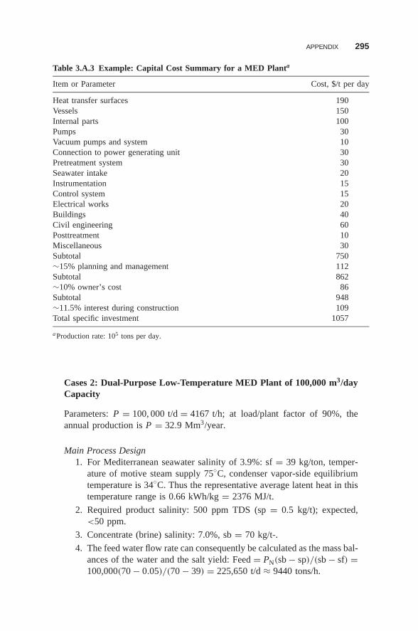
APPENDIX 295

Table 3.A.3 Example: Capital Cost Summary for a MED Planta

Item or Parameter Cost, $/t per day

Heat transfer surfaces 190Vessels 150Internal parts 100Pumps 30Vacuum pumps and system 10Connection to power generating unit 30Pretreatment system 30Seawater intake 20Instrumentation 15Control system 15Electrical works 20Buildings 40Civil engineering 60Posttreatment 10Miscellaneous 30Subtotal 750∼15% planning and management 112Subtotal 862∼10% owner’s cost 86Subtotal 948∼11.5% interest during construction 109Total specific investment 1057

a Production rate: 105 tons per day.

Cases 2: Dual-Purpose Low-Temperature MED Plant of 100,000 m3/dayCapacity

Parameters: P = 100, 000 t/d = 4167 t/h; at load/plant factor of 90%, theannual production is P = 32.9 Mm3/year.

Main Process Design1. For Mediterranean seawater salinity of 3.9%: sf = 39 kg/ton, temper-

ature of motive steam supply 75◦C, condenser vapor-side equilibriumtemperature is 34◦C. Thus the representative average latent heat in thistemperature range is 0.66 kWh/kg = 2376 MJ/t.

2. Required product salinity: 500 ppm TDS (sp = 0.5 kg/t); expected,<50 ppm.

3. Concentrate (brine) salinity: 7.0%, sb = 70 kg/t-.

4. The feed water flow rate can consequently be calculated as the mass bal-ances of the water and the salt yield: Feed = PN(sb − sp)/(sb − sf) =100,000(70 − 0.05)/(70 − 39) = 225,650 t/d ≈ 9440 tons/h.

296 ECONOMIC ASPECTS OF WATER DESALINATION

5. The average optimal heat flux is 5 kWt/m2. (See end of Section 3.A.2.)

With the average latent heat of water at the temperatures range givenabove at 0.66 kWh/kg, the mass flux is thus 5/0.66 = 7.6 kg/h/m2.

6. At this point the net heat transfer area of the evaporators, which isthe main equipment component of the process, can be calculated:Area = 4,167,000(kg/h)/(7.6 kg h−1m−2) = 550,000 m2. Because ofinefficiencies, the needed area is ∼8% larger, in addition to the con-denser area, which is ∼6% more; thus the total heat transfer area is550, 000 m2 ∗ 1.14 = 630, 000 m2.

7. Cost of installed heat transfer area (aluminum alloy): ∼$30/m2, includ-ing labor: 630,000 m2*30 = $19M = $190 per daily ton of desaltedwater.

8. Cost of installed vessels including foundations: ∼$15M including labor= $150 per daily ton of desalted water.

9. Internal items in the vessel (tube sheets, spray nozzles, partitions,droplet separators, tube supporting equipment, etc.) ∼$10M = $100per daily ton of desalted water.

10. Piping: ∼$3M = $30 per daily ton of desalted water.

11. Connection to power generating unit: ∼$3M = $30 per daily ton ofdesalted water.

12. Vacuum system: ∼$1M = $10 per daily ton of desalted water.

13. Cost of installed pumps: ∼8000 hp*$200/hp including labor: $16M =$16 per daily ton of desalted water.

14. Cost of pretreatment system: ∼$2M = $20 per daily ton of desaltedwater.

15. Cost of seawater intake system and concentrate outfall: ∼$2M = $20per daily ton of desalted water. This cost is low as the cooling-watersystem of the power plant is utilized.

16. Cost of instrumentation: ∼$1.5M = $15 per daily ton of desalted water.

17. Cost of control system: ∼$1.5M = $15 per daily ton of desalted water.

18. Cost of electrical work: ∼$3M = $30 per daily ton of desalted water.

19. Cost of buildings: ∼4M = $40 per daily ton of desalted water.

20. Cost of civil engineering: ∼$6M = $60 per daily ton of desalted water.

21. Cost of product post treatment: $1M = $10 per daily ton of desaltedwater.

22. Cost of furniture, laboratory, communication equipment, computers,transportation means, cranes and miscellaneous items: ∼$3M = $30per daily ton of desalted water.

23. Total: $75M = $750/t per day.

24. Cost of management, planning, and design: ∼15% = 0.15*75 =$11.2M = $112/t per day.

25. Owner’s cost: ∼10% = 0.1*(75 + 11.2) = $8.62M = $86t per day.

APPENDIX 297

26. Total, assuming 7.5% interest during construction, effective period ofconstruction 3 years: 1.0753/2 (75 + 11.2 + 8.6) = 1.1146*94.8≈$105.7M = $1057/t per day.

27. Energy:a. Loss of electricity generation: due to 362 ton steam/hour extraction

at 75◦C, 0.385 bar is 21 MWe generation, 19.5 MWe loss of powersales.

b. Pumps total, including vacuum: 5.5 MW mechanical work.c. At 92% electrical system efficiency (motors, transformers, etc.),

average electric power consumption: 5.5/0.92 = 6 MWe.d. An additional 100 kWe, is consumed by plant outside desalination

process for facilities such as lights, workshop, kitchen, air condi-tioning, and showers: 6 MWe + 0.1 = 6.1 MWe.

e. Specific energy of desalted water of plant: (19.5 + 6.1) MWe/

4167t/h = 25.6/4167 = 6.14 kWhe/ton.

Cost of Desalted WaterIt is assumed here that the annual expenses are as follows:

• Salaries are the same as in Table 3.3: $800,000 per year.• Capital cost is 8.214% (as in 3.4.1.4.1, page 250) of the total investment:

$105.7M*0.08214 = $8.68M/year.• Price of electric power is 5.4¢/kWh = $54/MWh, as in Table 3.3. Thus

the annual expense is 6.1MW*$54/MWh*8760 h/y*0.9 = $2.6M peryear.

• The price of steam for reduced electric power compensation isalso 54$/MWh, as in Table 3.3. Thus this annual expense is19.5MW*$54/MWh*8760 h/y*0.9 = $8.3M/year.

• Chemicals are as in Table 3.3; $1.31M/year.• Annual ERMI at 2.5% of total investment: $105.7M*0.025 =

$2.64M/year.• Land rental assumed at $100,000 per year.• Annual expenses sum: $18.89M ≈ $24.43M/year.• Cost of desalted water: Thus $24.43M/32.9M ton = $0.743/t ≈ 74.3/m3.

These data are summarized in Table 3.A.2 and compared to those in Table3.A.3.

3.A.2 Optimization of the Main Process Component: An Example

In this example, we will consider the magnitude and number effects in a low-temperature MED plant. Assume, as an example, that an effect of MED is taken.Vapor is introduced at a certain temperature and pressure to be condensed to potablewater while heat is being supplied to evaporate an equivalent amount of pure water

298 ECONOMIC ASPECTS OF WATER DESALINATION

from a stream of saline water. This heat is ejected from the said condensing vaporand is transferred to the said saline water.

The parameter to be optimized is the temperature difference that is the driv-ing force for heat transfer θ . In turn, by knowing θ , we can easily calculate theoptimal heat and mass fluxes, as well as the number of effects. With increasingθ , the heat transfer surface is reduced and the investment in the heat transfer areaand associated equipment (IHT) decreases. On the other hand, the practical usefulthermodynamic exergy consumed for heat transfer by the thermal driving force(EXR) increases:

IHT = Area∗Ca (3.A.1)

where

Area = q

U θ(3.A.2)

where q is the transferred heat (in kW), U is the heat transfer coefficient (in kWm−2 K−1), and Ca is the cost of unit area (in $/m2):

EXR = qηθ

T(3.A.3)

Here, T is the absolute temperature (in kelvins) at which a representative effectoperates (i.e., average of condensing and evaporating sides: ∼54◦C = 327 K) and η

is the efficiency involved in converting gross mechanical energy to salable electricalpower.

The economic value of IHT per year is

Carea = (CRF + ERMI) ∗ IHT (3.A.4)

where CRF = d/{1 − (1 + d)−n} is the capital recovery factor presented in Section3.3.2 (where d is the annual discount rate and n is the lifetime of the equipmentin years; for d = 7.5% per year and n = 30 years, CRF = 8.46% per year) andERMI (equipment replacement, maintenance, and insurance) is the annual fractionof plant maintenance, assumed to be 2.5% of the investment per year in the costestimates presented above.

The economic value of EXR per year is

CXRGθ = CkWh ∗ EXR ∗ 8760 ∗ τ (3.A.5)

where CkWh is the cost of kWh ($/kWh), which is not generated because of theexergy consumed by heat transfer, (8760 h per year; 365*24), and τ is the timefraction of heat transfer occurrence; thus 8760τ is the life average number of hoursof heat transfer performance per year (7884 for the assumed τ = 90%).

Optimum θ is when

∂(Carea + CXRGθ )

∂θ= 0, (3.A.6)

APPENDIX 299

namely

∂

∂θ[(CRF + ERMI) ∗ IHT + CkWh ∗ EXR ∗ 8760 ∗ τ ] = 0 (3.A.7)

Substituting these formulas for IHT and EXR, we can perform the following deriva-tives:

∂

∂θ

[(CRF + ERMI) ∗ Ca ∗ q

U θ

]+ ∂

∂θ

(CkWh ∗ qηθ

T∗ 8760 ∗ τ

)= 0 (3.A.8)

Thus

∂

∂θ

[(CRF + ERMI) ∗ Ca ∗ q

U θ

]= −(CRF + ERMI) ∗ Ca ∗ q/U /θ2 (3.A.9)

∂

∂θ

(CkWh ∗ q ∗ η ∗ θ

T∗ 8760 ∗ τ

)= CkWh ∗ q ∗ η

T∗ 8760 ∗ τ (3.A.10)

From which:

CkWh ∗ q ∗ η

T∗ 8760 ∗ τ +

{−(CRF + ERMI) ∗ Ca ∗ q

U θ2

}= 0 (3.A.11)

θ2 = (CRF ∗ Ca/U )

(CRF + ERMI) ∗ Ca/U

= (CRF + ERMI) ∗ Ca ∗ T

CkWh ∗ η ∗ U ∗ 8760 ∗ τ(3.A.12)

Optimum θ = √{(CRF + ERMI) ∗ Ca ∗ T

CkWh ∗ η ∗ U ∗ 8760 ∗ τ } (3.A.13)

The numerical sample calculation for MED is

CRF = 0.0847/year

ERMI = 0.025/year

(CRF + ERMI) = 0.0847/year + 0.025/year = 0.1097/year

Ca = {net − 30$/m2}; gross − 70$/m2

T = 54 + 273 = 327K

CkWh = 0.055$/kWh

η = 0.8

U = 3.5 kW/Km2

τ = 0.9

300 ECONOMIC ASPECTS OF WATER DESALINATION

Thus θop = √{0.1097 ∗ 70 ∗ 327/[0.055 ∗ 0.8 ∗ 3.5 ∗ 8760 ∗ 0.9]} = 1.44 K,optimum heat flux = Uθop = 3.5 ∗ 1.44 = 5.05kW/m2, and optimum water massflux = (5.05kW/m2)/0.66(kWh/kg) = 7.65 kg/(m2h).

It is interesting to note the following:

1. According to the design of the evaporators, based on the optimal heat transferdriving force θop, we obtain

Carea = CXRGθ (3.A.14)

In other words, the gross capital cost component of the desalted water dueto that part of the evaporator that is proportional to the heat transfer area isequal to the energy cost component of the desalted water due to that part ofthe energy charge for reducing the power generation by the exergy consumedfor heat transfer instead of for generating power. This equality is obtainedby substituting the expression for θop in the expression for Carea:

(CRF + ERMI) ∗ Ca ∗ q

U θop

= (CRF + ERMI) ∗ Ca ∗ q ∗ √[CkWh ∗ η ∗ U ∗ 8760 ∗ τ ]

U√

[(CRF + ERMI) ∗ Ca ∗ T ]

= q√{(CRF + ERMI) ∗ Ca ∗ CkWh ∗ η ∗ 8760 ∗ τ }√

(T ∗ U )(3.A.15)

The same result is obtained by substituting the expression for θop in theexpression for CXRGθ :

CkWh ∗ EXR ∗ 8760 ∗ τ = 8760CkWhτqηθop

T

= 8760CkWhτqη T√ (CRF + ERMI) ∗ Ca ∗ T

CkWh ∗ η ∗ U ∗ 8760 ∗ τ

= q√{(CRF + ERMI) ∗ Ca ∗ CkWh ∗ η ∗ 8760 ∗ τ

T ∗ U } (3.A.16)

The quantitative data given in this example yield CXRGθ = q√{0.11*70*

0.055*0.8*8760*0.9/327/3.5} = 1.528q in $/year = 8760CkWhτqηθop/T =8760 ∗ 0.055 ∗ 0.9 ∗ 0.8 ∗ 1.44q/327 = 1.528q . Thus

q = PA(1 + ε)λ

8760 ∗ 3600τ(3.A.17)

where PA is the annual water production, and ε is the additional fractionof the net heat transfer area needed to transfer parasitic heat (whereas thenet heat transfer area transfer the latent heat of the condensing product). In

APPENDIX 301

Section 3.A.1 ε was estimated as 14%, and λ is the average latent heat of thecondensing product, 2374Jl/g = 2.374 ∗ 106 kJ/t; 8760*3600τ is the activeheat transfer time per average year in seconds. Thus q = PA1.14 ∗ 2.374 ∗106kJ/t/(8760 ∗ 3600 ∗ 0.9) = 0.0954PA (in kW), and CXRGθ = 1.528q in$/year = 1.528*0.0954 PA = 0.1457PA. This cost component per unit prod-uct is CXRGθ /PA = $0.1457/t, and since Carea = CXRG, that part of theannual charge that depends on the thermal driving force θ totals 2*0.1457 =$0.292/m3. This sum represents ∼40% of the total water cost, estimated inSection 3.A.1 to be ∼74¢/m3.

2. The full annual charge CXRGT for the heat consumed by the MED desali-nation process is almost twice that of CXRGθ . Theoretically, it is calculatedaccording to the same thermodynamic principles as applied for CXRGθ andhas almost the same formula, with one difference—θ is replaced by theaverage temperature drop per effect of MED, �Teff:

CXRGT = 8760CkWhτqη�Teff

T= CXRGθ ∗ �Teff

θ(3.A.18)

where �Teff is essentially the sum of four components. The largest is θ . Thesecond quantitatively is BPE (the boiling-point elevation), which is propor-tional to the thermodynamic free energy needed to separate pure water fromsaline water. For the range of the low-temperature MED process feedwaterand brine salinities and temperatures, it is about ∼0.7 K; at other distillationprocesses or in high-temperature MED it can be as high as 1.2 K.The third and fourth components are pressures. One pressure value is thesum of all local and longitudinal friction pressure drops �p of the flow-ing vapors; the other is the partial pressure of noncondensable gases pncgin the vapor. Vapor pressure differences are equivalent to saturation tem-perature differences according to the thermodynamic principle known as theClausius–Clapeyron relation (for small differences):

�T = RT 2�p

p ∗ λ. (3.A.19)

The equivalent equilibrium temperature differences are (1) approximately∼0.2–0.3 K for the friction pressure drop �p of the flowing vapors and (2)<0.1 K for pncg. Thus

�Teff = θ + BPE + �p + pncg = 1.44 + 0.7 + 0.25 + 0.1 ≈ 2.5K(3.A.20)

The charge of heat per unit product can now be estimated approximately:

CXRGT = CXRGθ ∗ �Teff

θ= 0.1457 ∗ 2.5

1.44= $0.253/m3 (3.A.21)

302 ECONOMIC ASPECTS OF WATER DESALINATION

This represents ∼34% of the total water cost, estimated in Section 3.A.1 to be∼74¢/m3. The economically optimal number of effects Neff can be calculatedon the basis of the optimal known �Teff. We assume the maximum processtemperature to be 72◦C due to scaling deposits and aluminum corrosionconsiderations and the lowest condensing temperature to be 34◦C, as in steampower plants. The range between these temperatures is �Tpr = 72 − 34 =38◦C. Then

Neff = �Tpr

�Teff≈ 38

2.5≈ 15 effects (3.A.22)

[Note: The small deviation of 0.5 = �Tpr − Neff ∗ �Teff means that eitherthe heat will be supplied at 0.5 K lower temperature, or the average �Teffand θ will be higher by ∼0.03 K. (The first alternative is slightly better.)]Thus, the average production rate is PN/Neff = PN/15 t/d per effect or2.778PN effect. Since it was found above that the optimum water massflux = 7.65 kg/h per m2, the net heat transfer surface per effect is a2.77PN/7.65 = 0.363PN (in m2/effect). The gross area is about 8–10%higher, ∼0.4PN m2 per effect. In a 100,000-m3/d MED plant consistingof two units PN = 50, 000 m3/d per unit, the economically optimalheat transfer area per effect is therefore 0.4*50000 = 20, 000 m2 pereffect.

3. Modifying the evaporator design by assigning a different value for θ that isnot the optimal one will result in a very small relative increase in the watercost if the deviation θ − θop is within ± 15% of θop. The result of such changeis investment reduction and capital cost decrease with slightly higher increaseof the energy charge for θ > θop, or vice versa for θ < θop. To demonstrate,if, instead of the optimal value of θop = 1.44 K calculated above, the designvalue of the heat transfer driving force is taken as ∼15% higher, namely,θ = 1.65 K and with 14 smaller effects instead of 15 optimal ones, thenCXRGθ = 0.1457*1.65/1.44 = $0.167/t, while Carea = 0.1457*1.44/1.65 =$0.1271/t, and the off-optimum sum will be CXRGθ + Carea = 0.167 + 0.1271= $0.2941/t, compared to the optimum design sum of 2*0.1457 = $0.2914/t.The difference is 0.2941−0.2914 = $0.0027/t = 0.27¢ per ton, which is only0.36% of the total water cost.

On the other hand, at a production rate of 100M/t per year, this 0.27¢/tcost increase accumulates to over $8 million during 30 years of the plantlifetime!! (Note: The last example is a plausible strategy of “pay less nowand more later” taken by decision-makers who prefer to lower the initialinvestment and thus reduce risk and financing scope—even if the expectedhigher energy expenses will push the product cost to values a bit above theminimum.)

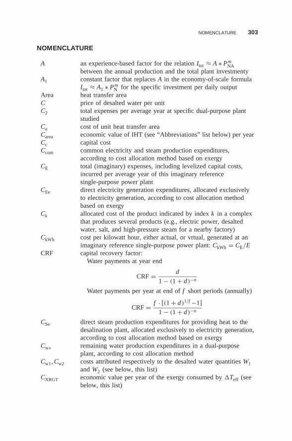
NOMENCLATURE 303

NOMENCLATURE

A an experience-based factor for the relation Itot ≈ A ∗ PmNA

between the annual production and the total plant investmentyA1 constant factor that replaces A in the economy-of-scale formula

Itot ≈ A1 ∗ PmN for the specific investment per daily output

Area heat transfer areaC price of desalted water per unitC2 total expenses per average year at specific dual-purpose plant

studiedCa cost of unit heat transfer areaCarea economic value of IHT (see “Abbreviations” list below) per yearCc capital costCcom common electricity and steam production expenditures,

according to cost allocation method based on exergyCE total (imaginary) expenses, including levelized capital costs,

incurred per average year of this imaginary referencesingle-purpose power plant

CEe direct electricity generation expenditures, allocated exclusivelyto electricity generation, according to cost allocation methodbased on exergy

Ck allocated cost of the product indicated by index k in a complexthat produces several products (e.g., electric power, desaltedwater, salt, and high-pressure steam for a nearby factory)

CkWh cost per kilowatt hour, either actual, or vrtual, generated at animaginary reference single-purpose power plant: CkWh = CE/E

CRF capital recovery factor:Water payments at year end

CRF = d

1 − (1 + d)−n

Water payments per year at end of f short periods (annually)

CRF = f · [(1 + d)1/f −1]

1 − (1 + d)−n

CSe direct steam production expenditures for providing heat to thedesalination plant, allocated exclusively to electricity generation,according to cost allocation method based on exergy

Cw∗ remaining water production expenditures in a dual-purposeplant, according to cost allocation method

Cw1, Cw2 costs attributed respectively to the desalted water quantities W1and W2 (see below, this list)

CXRGT economic value per year of the exergy consumed by �Teff (seebelow, this list)

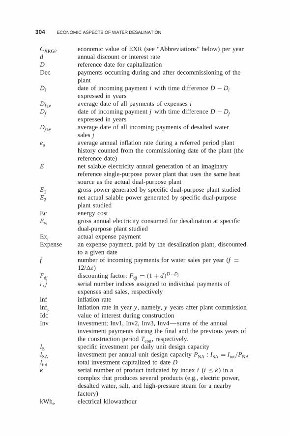
304 ECONOMIC ASPECTS OF WATER DESALINATION

CXRGθ economic value of EXR (see “Abbreviations” below) per yeard annual discount or interest rateD reference date for capitalizationDec payments occurring during and after decommissioning of the

plantDi date of incoming payment i with time difference D − Di

expressed in yearsDiav average date of all payments of expenses iDj date of incoming payment j with time difference D − Dj

expressed in yearsDjav average date of all incoming payments of desalted water

sales jea average annual inflation rate during a referred period plant

history counted from the commissioning date of the plant (thereference date)

E net salable electricity annual generation of an imaginaryreference single-purpose power plant that uses the same heatsource as the actual dual-purpose plant

E1 gross power generated by specific dual-purpose plant studiedE2 net actual salable power generated by specific dual-purpose

plant studiedEc energy costEw gross annual electricity consumed for desalination at specific

dual-purpose plant studiedExi actual expense paymentExpense an expense payment, paid by the desalination plant, discounted

to a given datef number of incoming payments for water sales per year (f =

12/�t)Fdj discounting factor: Fdj = (1 + d)D−Dj

i , j serial number indices assigned to individual payments ofexpenses and sales, respectively

inf inflation rateinfy inflation rate in year y , namely, y years after plant commissionIdc value of interest during constructionInv investment; Inv1, Inv2, Inv3, Inv4—sums of the annual

investment payments during the final and the previous years ofthe construction period Tcon, respectively.

IS specific investment per daily unit design capacityISA investment per annual unit design capacity PNA : ISA = Itot/PNAItot total investment capitalized to date Dk serial number of product indicated by index i (i ≤ k ) in a

complex that produces several products (e.g., electric power,desalted water, salt, and high-pressure steam for a nearbyfactory)

kWhe electrical kilowatthour

NOMENCLATURE 305

kWht thermal kilowatthourLF load factor; ratio between actual plant life production and

theoretical (i.e., full time at full design capacity) plant lifeproduction {PA = 365PN ∗ LF}

m economy-of-scale power factor for relation Itot ≈ A ∗ PmNA

between the annual production and the total plant investment.n years of economic lifetime of plant (may differ from tprod,

defined below, this list)Omc all other operation and maintenance costs, designated as O&M

costp absolute pressure of the vaporpncg partial pressure of noncondensable gases in vaporPA average annual production (in unit product); ideally equal to

PNAPk amount of product indicated by index k in an industrial complex

that produces several products (e.g., electric power, desaltedwater, salt, and high-pressure steam for a nearby factory)

PN nominal daily design capacity usually given in units per dayPNA nominal annual design capacityq transferred heat (in kW)Rn running cost (i.e., later part of the expenses payments)Sale a water sale payment, received by the desalination plant,

discounted to a given datesb brine salinitysf seawater salinitysp product salinitytcon construction period in yearstprod production period in yearstproj entire project period in yearsT absolute temperature [in degrees Kelvin (K)] at which a

representative effect operatesTamb ambient absolute temperatureTheat active heat temperature, specifically, the absolute temperature at

which the heatsource is used in distillation processesT� common economical temperature difference needed to reject

heat from exhaust steam to ambience or to heatsink (≈10 ±3◦C)

U heat transfer coefficient kW m−2 K−1

W plant total water productionWj product units measured in tons: cubicmeters (m3) or kilogallonsW1, W2 annual water productions from each of the two sources (hybrid

plant or two-quality plant)y ordinal number representing one year in a desalination plant

history y years after plant commission (y may have a negativevalue for years of construction and other preparations)

306 ECONOMIC ASPECTS OF WATER DESALINATION

Z annual discount factor corrected by average inflation rate,Z = (1 + d)/(1 + ea)

�p average sum of all drops in vapor pressure due to local andlongitudinal vapor friction as a result of the vapor movinginside of an average effect of a multieffect distillation plant

�t time periods, expressed in months, between water salespayments (usually very few months)

�TBH temperature increase in the brine heater of multistage flashdistillation

�Teff− average temperature drop per effect of multieffect distillation�Tpr practical, thermodynamic temperature difference, which is

roughly proportional to the practical economical equivalentvalue of the heat:

�Tpr = �Tth − T�

�Tth temperature difference above the ambient temperature:�Tth = Theat − Tamb

ε fraction of net heat transfer area needed to transfer parasitic heatη efficiency of conversion of theoretical gross mechanical energy

to electrical powerθ average heat transfer driving forceθop optimal heat transfer driving forceλ average latent heat of condensationτ average annual time fraction of heat transfer occurrence� multiplication notation� summation notation�exp expenses sum of all net levelized annual expenses of hybrid

plant or two-quality plant.

Abbreviations

AC alternating (electrical) currentBPE boiling-point elevationDEEP Desalination Economic Evaluation Program: IAEA program for

economic comparisons between power generation anddesalination plants

ED electrodialysisERMI equipment replacement, maintenance, and insurance percentage

of total investment per yearEXR practical thermodynamic exergy consumed for heat transfer by

thermal driving forcegfd gallons per square foot per day (US)GOR gained output ratioIAEA International Atomic Energy Agency

REFERENCES 307

IHT investment in heat transfer area and associated equipmentMED multiple-effect (multieffect) Distillationmgd million gallons per dayMSF Multistage flash distillationMVC mechanical vapor compressionO&M operation and maintenanceppm parts per million (g/ton or mg/kg)RO reverse osmosisSA stand-aloneSW seawaterTVC thermal vapor compressionVC vapor compressionWHO World Health Organization

REFERENCES

1. US Office of Saline Water (OSW), A Standardized Procedure for Estimating Costs ofSaline Water Conversion , US Dept. Interior, 1956.

2. MW Kellogg Company, Saline Water Conversion Engineering Data Book for the OSW,1965 (Sec. 3. 500).

3. IAEA, Costing Methods for Nuclear Desalination , Technical Report 69, Vienna, 1966.

4. IAEA, Guide to the Costing of Water from Nuclear Desalination Plants , Technical Report80, Vienna, 1967.

5. Barnea J, Costing of Desalted Water?, United Nations, early 1960s—(a report similarto the first OSW procedure [1]).

6. OSW, Desalting Handbook for Planners , 1972, a cost format, [an adaptation of whichwas used in cost updates prepared for the US Office of Water Research and Technologyand is recognized by the International Desalination Association (IDA)].

7. IAEA, Guide to the Costing of Water from Nuclear Desalination Plants , 1973 Edition,Technical Report 151, Vienna, 1973.

8. IAEA, Guidebook on the Introduction of Nuclear Power , Technical Report 217, Vienna,1982, pp. 75–94, 147–154, 235–243, 286–288, 306.

9. Awerbuch L, Rogers AN, Siebentthal CD, Battey RF, Desalination Technology—Reporton the State of the Art , Bechtel Group Inc. Job 15669 (agreement 1462), San Francisco,Feb. 1983.

10. IAEA, Expansion Planning for Electrical Generating Systems—a Guidebook , TechnicalReport 241, Vienna, 1984, pp. 151–241.

11. IAEA, Use of Nuclear Reactors for Seawater Desalination , International Atomic EnergyAgency Technical Document IAEA-TECDOC 574, Vienna, Sept. 1990.

12. IAEA, Technical and Economical Evaluation of Potable Water Production throughDesalination . . . Using Nuclear Energy and Other Means , International Atomic EnergyAgency Technical Document IAEA-TECDOC 666, Vienna, 1992.

13. IAEA, Options Identification Program for Demonstration of Nuclear Desalination ,IAEA-TECDOC 898, Vienna, 1996.

308 ECONOMIC ASPECTS OF WATER DESALINATION

14. IAEA, Potential for Nuclear Desalination as a Source of Low Cost Potable Water inNorth Africa , IAEA-TECDOC 917, Vienna, 1996.

15. IAEA, Thermodynamic and Economic Evaluation of Co-production Plants for Electricityand Potable Water , IAEA-TECDOC 942, Vienna, 1997.

16. IAEA, Methodology for the Economical Evaluation of Cogeneration/DesalinationOptions: A User’s Manual , IAEA Computer Manual Series Vol. 12, Vienna, 1997.

17. Leitner GF, Breaking the cost barrier for seawater desalination, Int. Desal. Water Reuse.8(1):14–20 1998.

18. Barak A, Economic aspects of desalination in Israel, Water Irrig . (Israeli journal, inHebrew), 380:28–32 (June 1998).

19. IAEA, Desalination Economic Evaluation Program (DEEP): User’s Manual , IAEAComputer Manual Series Vol. 14, Vienna, 2000, pp. 133–150.

20. IAEA, Examining the Economics of Seawater Desalination Using the DEEP Code,IAEA-TECDOC 1186, Vienna, 2000.

21. Barak A, Steps of planning, development, research and additional technological activitiesfor seawater desalination cost reduction, Water Irrig . 406:4–11 (Aug. 2000).

22. IAEA, Introduction of Nuclear Desalination , Technical Report 400, Vienna, 2000, pp.135–160, 188–189, 203, 221, 230–235, 240–245, 282.

23. Glueckstern P, Priel M, Potential cost reduction in large SWRO systems, Proc. 5th IWAConf. Membranes in Drinking Water and Industrial Water Production , Muelheim an derRuhr, Germany, Sept. 2002.

24. IAEA, Optimization of the Coupling of Nuclear Reactors and Desalination Systems ,IAEA-TECDOC 1444, Vienna, 2005.

25. Middle East Desalination Research Center (MEDRC), Proc. Int. Conf. DesalinationCosting , Lemesos/Limassol, Cyprus, Dec. 6–8, 2004.

26. Glueckstern P, History of desalination cost estimations, Proc. MEDRC Int. Conf. Desali-nation Costing , Lemesos/Limassol, Cyprus, 6–8, Dec. 2004, pp. 1–17, this paper cites45 references on costing of desalted water during 1966–2004.

27. Dore MHI, Forecasting the economic costs of desalination technology, Desalination172:207–214 (2005).

28. Blank JE, Tusel GF, Nisan S, The real cost of desalted water and how to reduce itfurther, Desalination 205:298–311 (2007).

29. Methnani M, The influence of fuel costs on seawater desalination options, Desalination205:332–339 (2007).

30. Reddy KV, Ghaffour N, Overview of the cost of desalinated water and costing method-ologies, Desalination 205:340–353 (2007).

31. Abdulnasser AM, Nafey AS, Fath HES, Thermoeconomics analysis of some existingdesalination processes, Desalination 205:354–373 (2007).

32. Yongqing W, Lior N, Fuel allocation in a combined steam-injected gas turbine andthermal seawater desalination system, Desalination 214:306–326 (2007).

CHAPTER 4

Advances in Hollow-FiberReverse-Osmosis MembraneModules in Seawater Desalination

ATSUO KUMANO

4.1 Introduction 3114.2 Background 3124.3 Separation Membranes and Production Methods 313

4.3.1 Separation Characteristics 3134.3.2 Membrane Structure 3144.3.3 Membrane Shape and Module Configuration 316

4.3.3.1 Flat-Sheet (Plate-and-Frame) Type 3164.3.3.2 Spiral-Wound Type 3174.3.3.3 Hollow-Fiber Type 3184.3.3.4 Tubular Type 320

4.3.4 Materials of RO Membranes 3204.3.4.1 Cellulose Derivative Material 3214.3.4.2 Polyamide Material 3224.3.4.3 Other Materials 323

4.3.5 Membrane Production Method 3234.3.5.1 Outlines of Membrane Production 3234.3.5.2 Phase Separation Method 3244.3.5.3 Stretching Method 3264.3.5.4 Interfacial Polymerization Method 326

4.4 Reverse-Osmosis Desalination Process 3284.4.1 Fouling Control 328

4.4.1.1 Biological Fouling 3294.4.1.2 Physical Fouling 329

4.4.2 Disinfection Method for Pretreatment 3304.4.2.1 Disinfection by Intermittent Chlorine Injection (ICI) 3314.4.2.2 Control by Shock Treatment 3324.4.2.3 Bacteria Content of RO Product Water 332

Advances in Water Desalination, First Edition. Edited by Noam Lior.© 2013 John Wiley & Sons, Inc. Published 2013 by John Wiley & Sons, Inc.

309

310 ADVANCES IN HOLLOW-FIBER REVERSE-OSMOSIS MEMBRANE MODULES

4.4.3 Prediction of RO Performance for Long-Term Operation 3324.4.3.1 Membrane Compaction 3324.4.3.2 Performance Change Rate of Cellulose Triacetate RO

Membrane in Case of Degradation [15] 3344.4.4 High-Recovery Process 336

4.4.4.1 Higher-Efficiency RO Single-Stage High-RecoverySystem 336

4.4.4.2 Brine Conversion Two-Stage RO Seawater DesalinationSystem 337

4.5 Development of Hollow-Fiber RO Membrane Module for SeawaterDesalination 3384.5.1 Hollow-Fiber Bundle Configuration 3384.5.2 Features of Hollow-Fiber RO Membrane Module for Seawater

Desalination 3384.5.2.1 Module Structure (Hollow-Fiber Configuration) 3384.5.2.2 Stable RO Performance 3404.5.2.3 Superior Fouling Resistance 341

4.5.3 Analytical Model of Hollow-Fiber RO Modules 3434.5.3.1 Model Formulation of Friction Concentration

Polarization (FCP) Model 3444.5.3.2 Optimum Design of Double-Element Hollow-Fiber RO

Module 3454.5.4 Development of RO Module for Higher Recovery 3464.5.5 Development of Both Open-Ended (B.O.E.) RO Module 3494.5.6 Advanced Larger RO Module 354

4.6 Actual Performance of Hollow-Fiber RO Membrane Module forSeawater Desalination 3544.6.1 Actual Global Performance 3544.6.2 Jeddah 1 RO Plant in Saudi Arabia 356

4.6.2.1 Operation Results of Phase II Plant 3594.6.2.2 Product Flow Rate and Quality 3594.6.2.3 Differential Pressure 359

4.6.3 AdDur Plant in Bahrain 3604.6.3.1 Schematic Flow Diagram of CTA Membrane Test

Unit 3614.6.3.2 Test Conditions 3624.6.3.3 RO Performance at Site Test 3624.6.3.4 Differential Pressure 363

4.6.4 Ikata Power Station in Japan 3644.6.5 Fukuoka Seawater RO Desalination Plant in Japan 364

4.7 Economics of Seawater Desalination with RO Membrane Modules 3674.8 Conclusions 370Nomenclature 372References 372

INTRODUCTION 311

4.1 INTRODUCTION

The reverse-osmosis (RO) method has become widely accepted for reliable andlong-term seawater desalination. In particular, the RO method based on the use ofhollow-fiber RO modules has earned recognition for excellent performance in high-salinity waters such as occur in the Mediterranean and the Middle East. A cellulosetriacetate (CTA) hollow-fiber RO module is recognized for providing high-qualitypermeate water and reliable performance for long-term operation in many practicalseawater applications.

Reverse-osmosis membranes were first developed from cellulose acetate (CA)and cellulose triacetate CTA. These CA and CTA membranes have been in com-mercial use for many years. The CTA membrane, in particular, is still in widespreaduse throughout the world. This global use proves that the CTA membrane is excel-lent as an RO membrane. Its performance is enhanced by a combination of highpermeability and high selectivity, due to a balance of excellent hydrophilic andhydrophobic properties. Moreover, the CTA membrane has high tolerance to oxi-dizers such as chlorine. This characteristic makes it useful as a RO membrane.The CTA membrane is the only RO membrane among many other RO membranescurrently marketed that offers this high degree of chlorine resistance. On the basisof the prediction model of performance change of RO module due to hydrolysisand oxidation by chlorination, the intermittent chlorine injection (ICI) method hasbeen developed and is effectively used with the CTA membrane to control bio-fouling growth. It also enables the stable operation of seawater desalination plants,especially in the Middle East, where there is increased biofouling potential due tohigh temperatures.

Following development of aromatic polyamide hollow-fiber RO membranes,CTA with a hollow-fiber membrane structure was developed to control biofouling.Because of its superior resistance to chlorine in comparison with polyamide hollow-fiber RO membranes, the CTA membrane is relatively impervious to contaminationby the biofouling material to which it is exposed. Furthermore, the CTA membraneis capable of significantly reducing flux per unit membrane area, because its hollow-fiber configuration provides an element in a module that has a membrane areathat is approximately 10 times larger per unit volume than that of a spiral-woundmembrane element. Therefore, with the CTA membrane, it is possible to decreasethe membrane load, which makes it more difficult for fouling to occur. These keyattributes lead to minimum chemical cleaning and long membrane life. The hollow-fiber RO module design and the optimization of flow pattern in the module arebased on an analytical model of hollow-fiber RO modules. The analytical model hasbeen presented as a friction–concentration–polarization (FCP) model, in which theconcentration polarization and the pressure drop in the fiber bore were considered.The validity of this FCP model has been verified by actual performance data onhollow-fiber modules.

A more cost-efficient and high-efficiency RO desalination module has beendeveloped that further reduces product-water cost. This is achieved by a higher

312 ADVANCES IN HOLLOW-FIBER REVERSE-OSMOSIS MEMBRANE MODULES

recovery capability due to a higher pressure-resistant membrane and module capa-bility. An innovative module has been developed by Toyobo for the next generationof improvements. This newest module can provide more than 2 times the product-water capacity compared with previous conventional modules. The success indeveloping this newest module will lead to even further reduction of product-watercosts. Toyobo seawater RO modules provide high reliability and low cost capabilityto produce freshwater. The ability to ensure low-cost, fresh drinking water by ROwith this latest innovative technology undoubtedly will lead to future statementssuch as “the 21st century is [was] an age of water” (i.e., reclamation of water as anatural resource).

4.2 BACKGROUND

The US Saline Water Act was enacted on July 3, 1952. At that time, the USOffice of Saline Water (OSW) was commissioned by the Department of the Inte-rior to develop a method for obtaining freshwater from seawater and brackish-water economically. This effort accelerated the development of reverse-osmosis(RO) membranes. The RO process was proposed as a desalination methods byDr. C. E. Reid of the University of Florida in early 1953 [1]. Workers at thatuniversity studied various commercial polymer films in 1957, and announced thedevelopment of a cellulose diacetate film with a semipermeable membrane thatprovided a salt rejection rate of ≥ 96%. However, the water permeability wasnegligible. In 1960, Loeb and Sourirajan of the University of California succeededin developing a method of manufacturing a new asymmetric membrane [2]. Themembrane had high permeability and consisted of heat-treated cellulose diacetate.These enhancements in membrane performance lead to a practical application ofthe RO membrane module [1–3].

In more recent years, seawater RO technology has been applied for desalinationin large power plant projects, increasingly replacing the older thermal distillationtechnology. In the case of single-purpose (with no excess power production) sea-water desalination plants, RO technology has displaced MSF (multistage flash)technology. Key examples in the Middle East include Jeddah phases 1 and 2[each producing 15 million gallons per day (mgpd)], Yanbu (33 mgpd), and Jubail(24 mgpd). No other technology offers lower water production costs and the otheradvantages of RO over thermal processes in single-purpose desalination plants.The advantages of RO over thermal methods include greater mitigation of theeffects of environmental pollution, wider availability of suitable site, for desalina-tion plant construction, less complex plant design, lower maintenance costs, andlower operating costs.

Since seawater RO technology was first commercialized in the mid to late 1970s,it has become the most practical and cost-effective method for water desalination.The only exceptions to the automatic selection of RO technology for desalinationare those large projects where energy costs are low (such as in the Middle East)and where both power and water needs are required. However, even in these cases,

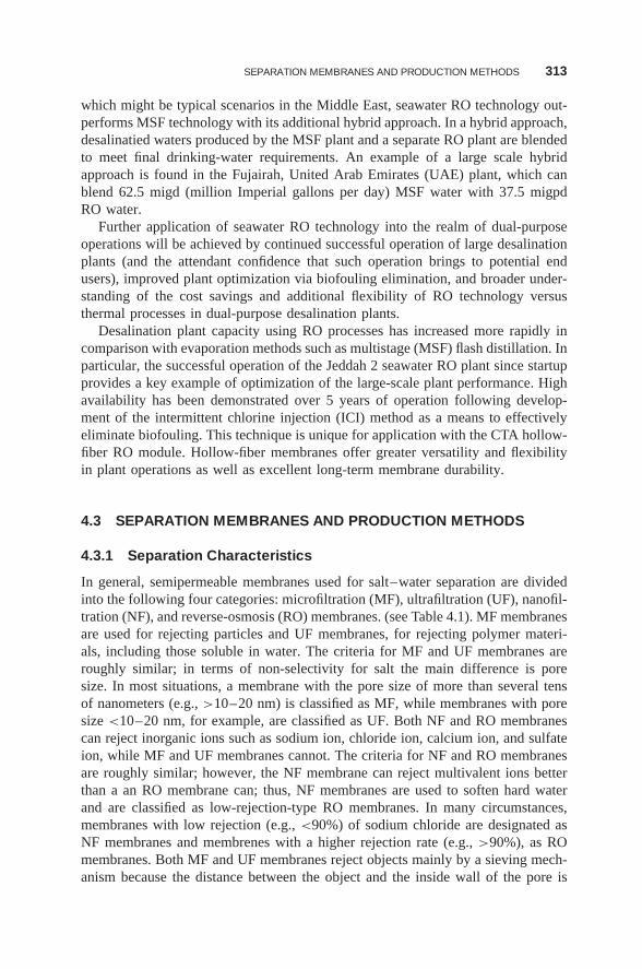
SEPARATION MEMBRANES AND PRODUCTION METHODS 313

which might be typical scenarios in the Middle East, seawater RO technology out-performs MSF technology with its additional hybrid approach. In a hybrid approach,desalinatied waters produced by the MSF plant and a separate RO plant are blendedto meet final drinking-water requirements. An example of a large scale hybridapproach is found in the Fujairah, United Arab Emirates (UAE) plant, which canblend 62.5 migd (million Imperial gallons per day) MSF water with 37.5 migpdRO water.

Further application of seawater RO technology into the realm of dual-purposeoperations will be achieved by continued successful operation of large desalinationplants (and the attendant confidence that such operation brings to potential endusers), improved plant optimization via biofouling elimination, and broader under-standing of the cost savings and additional flexibility of RO technology versusthermal processes in dual-purpose desalination plants.

Desalination plant capacity using RO processes has increased more rapidly incomparison with evaporation methods such as multistage (MSF) flash distillation. Inparticular, the successful operation of the Jeddah 2 seawater RO plant since startupprovides a key example of optimization of the large-scale plant performance. Highavailability has been demonstrated over 5 years of operation following develop-ment of the intermittent chlorine injection (ICI) method as a means to effectivelyeliminate biofouling. This technique is unique for application with the CTA hollow-fiber RO module. Hollow-fiber membranes offer greater versatility and flexibilityin plant operations as well as excellent long-term membrane durability.

4.3 SEPARATION MEMBRANES AND PRODUCTION METHODS

4.3.1 Separation Characteristics

In general, semipermeable membranes used for salt–water separation are dividedinto the following four categories: microfiltration (MF), ultrafiltration (UF), nanofil-tration (NF), and reverse-osmosis (RO) membranes. (see Table 4.1). MF membranesare used for rejecting particles and UF membranes, for rejecting polymer materi-als, including those soluble in water. The criteria for MF and UF membranes areroughly similar; in terms of non-selectivity for salt the main difference is poresize. In most situations, a membrane with the pore size of more than several tensof nanometers (e.g., >10–20 nm) is classified as MF, while membranes with poresize <10–20 nm, for example, are classified as UF. Both NF and RO membranescan reject inorganic ions such as sodium ion, chloride ion, calcium ion, and sulfateion, while MF and UF membranes cannot. The criteria for NF and RO membranesare roughly similar; however, the NF membrane can reject multivalent ions betterthan a an RO membrane can; thus, NF membranes are used to soften hard waterand are classified as low-rejection-type RO membranes. In many circumstances,membranes with low rejection (e.g., <90%) of sodium chloride are designated asNF membranes and membrenes with a higher rejection rate (e.g., >90%), as ROmembranes. Both MF and UF membranes reject objects mainly by a sieving mech-anism because the distance between the object and the inside wall of the pore is

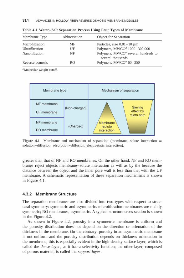
314 ADVANCES IN HOLLOW-FIBER REVERSE-OSMOSIS MEMBRANE MODULES

Table 4.1 Water–Salt Separation Process Using Four Types of Membrane

Membrane Type Abbreviation Object for Separation

Microfiltration MF Particles, size 0.01–10 μmUltrafiltration UF Polymers, MWCOa 1000–300,000Nanofiltration NF Polymers, MWCOa several hundreds to

several thousandsReverse osmosis RO Polymers, MWCOa 60–350

aMolecular weight cutoff.

Membrane type

MF membrane

UF membrane(Non-charged)

Membrane-solute

interaction

Sievingeffect by

micro pore

(Charged)NF membrane

RO membrane

Mechanism of separation

Figure 4.1 Membrane and mechanism of separation (membrane–solute interaction =solution–diffusion, adsorption–diffusion, electrostatic interaction).

greater than that of NF and RO membranes. On the other hand, NF and RO mem-branes reject objects membrane–solute interaction as will as by the because thedistance between the object and the inner pore wall is less than that with the UFmembrane. A schematic representation of these separation mechanisms is shownin Figure 4.1.

4.3.2 Membrane Structure

The separation membranes are also divided into two types with respect to struc-tural symmetry: symmetric and asymmetric. microfiltration membranes are mainlysymmetric; RO membranes, asymmetric. A typical structure cross section is shownin the Figure 4.2.

As shown in Figure 4.2, porosity in a symmetric membrane is uniform andthe porosity distribution does not depend on the direction or orientation of thethickness in the membrane. On the contrary, porosity in an asymmetric membraneis not uniform and the porosity distribution depends on thickness orientation inthe membrane; this is especially evident in the high-density surface layer, which iscalled the dense layer , as it has a selectivity function; the other layer, composedof porous material, is called the support layer .

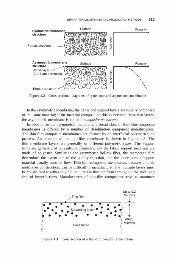
SEPARATION MEMBRANES AND PRODUCTION METHODS 315

Porosity

Porosity

Thi

ckne

ssT

hick

ness

Porous structure

Symmetric membranestructure

Dense layer(0.1–1 μm thickness)

Porous structure

Surface

SurfaceAsymmetric membranestructure

Figure 4.2 Cross sectional diagrams of symmetric and asymmetric membranes.

In the asymmetric membrane, the dense and support layers are usually composedof the same material; if the material composition differs between these two layers,the asymmetric membrane is called a composite membrane.

In addition to the asymmetric membrane, a broad class of thin-film compositemembranes is offered by a number of desalination equipment manufacturers.The thin-film composite membranes are formed by an interfacial polymerizationprocess. An example of the thin-film membrane is shown in Figure 4.3. Thethin membrane layers are generally of different polymeric types. The supportfilms are generally of polysulfone chemistry, and the fabric support materials aremade of polyester. Similar to the asymmetric hollow fiber, the membrane filmdetermines the extent and of the quality rejection, and the more porous supportmaterial usually controls flow. Thin-film composite membranes, because of theirmultilayer construction, can be difficult to manufacture. The multiple layers mustbe constructed together to yield an ultrathin film, uniform throughout the sheet andfree of imperfections. Manufacturers of thin-film composites strive to automate

Thin film

Supporting layer

Base fabric

60-75Microns

Up to 0.2Microns

Figure 4.3 Cross section of a thin-film composite membrane.

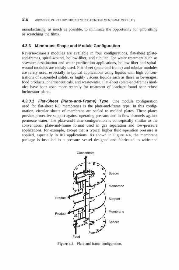
316 ADVANCES IN HOLLOW-FIBER REVERSE-OSMOSIS MEMBRANE MODULES

manufacturing, as much as possible, to minimize the opportunity for embrittlingor scratching the films.

4.3.3 Membrane Shape and Module Configuration

Reverse-osmosis modules are available in four configurations, flat-sheet (plate-and-frame), spiral-wound, hollow-fiber, and tubular. For water treatment such asseawater desalination and water purification applications, hollow-fiber and spiral-wound modules are mostly used. Flat-sheet (plate-and-frame) and tubular modulesare rarely used, especially in typical applications using liquids with high concen-trations of suspended solids, or highly viscous liquids such as those in beverages,food products, pharmaceuticals, and wastewater. Flat-sheet (plate-and-frame) mod-ules have been used more recently for treatment of leachate found near refuseincinerator plants.

4.3.3.1 Flat-Sheet (Plate-and-Frame) Type One module configurationused for flat-sheet RO membranes is the plate-and-frame type. In this config-uration, circular sheets of membrane are sealed to molded plates. These platesprovide protective support against operating pressure and in flow channels againstpermeate water. The plate-and-frame configuration is conceptually similar to theconventional plate-and-frame format used in gas separation and low-pressureapplications, for example, except that a typical higher fluid operation pressure isapplied, especially in RO applications. As shown in Figure 4.4, the membranepackage is installed in a pressure vessel designed and fabricated to withstand

Concentrate

Spacer

Spacer

Feed

Product

Product

Membrane

Membrane

Support

Figure 4.4 Plate-and-frame configuration.

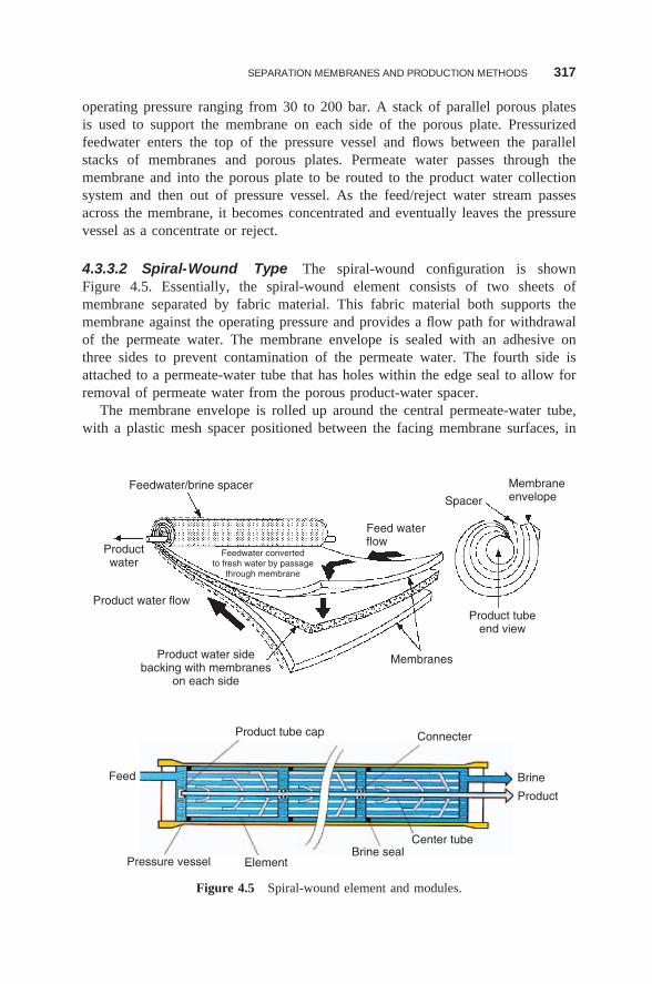
SEPARATION MEMBRANES AND PRODUCTION METHODS 317

operating pressure ranging from 30 to 200 bar. A stack of parallel porous platesis used to support the membrane on each side of the porous plate. Pressurizedfeedwater enters the top of the pressure vessel and flows between the parallelstacks of membranes and porous plates. Permeate water passes through themembrane and into the porous plate to be routed to the product water collectionsystem and then out of pressure vessel. As the feed/reject water stream passesacross the membrane, it becomes concentrated and eventually leaves the pressurevessel as a concentrate or reject.

4.3.3.2 Spiral-Wound Type The spiral-wound configuration is shownFigure 4.5. Essentially, the spiral-wound element consists of two sheets ofmembrane separated by fabric material. This fabric material both supports themembrane against the operating pressure and provides a flow path for withdrawalof the permeate water. The membrane envelope is sealed with an adhesive onthree sides to prevent contamination of the permeate water. The fourth side isattached to a permeate-water tube that has holes within the edge seal to allow forremoval of permeate water from the porous product-water spacer.

The membrane envelope is rolled up around the central permeate-water tube,with a plastic mesh spacer positioned between the facing membrane surfaces, in

ElementBrine seal

Center tube

Connecter

MembraneenvelopeSpacer

Feed waterflow

Feedwater convertedto fresh water by passage

through membrane

Feedwater/brine spacer

Productwater

Product water flow

Product water sidebacking with membranes

on each side

Product tubeend view

Membranes

Product tube cap

Pressure vessel

Feed Brine

Product

Figure 4.5 Spiral-wound element and modules.

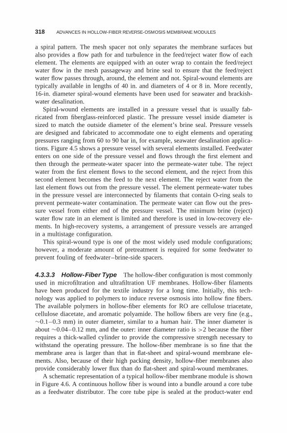
318 ADVANCES IN HOLLOW-FIBER REVERSE-OSMOSIS MEMBRANE MODULES

a spiral pattern. The mesh spacer not only separates the membrane surfaces butalso provides a flow path for and turbulence in the feed/reject water flow of eachelement. The elements are equipped with an outer wrap to contain the feed/rejectwater flow in the mesh passageway and brine seal to ensure that the feed/rejectwater flow passes through, around, the element and not. Spiral-wound elements aretypically available in lengths of 40 in. and diameters of 4 or 8 in. More recently,16-in. diameter spiral-wound elements have been used for seawater and brackish-water desalination.

Spiral-wound elements are installed in a pressure vessel that is usually fab-ricated from fiberglass-reinforced plastic. The pressure vessel inside diameter issized to match the outside diameter of the element’s brine seal. Pressure vesselsare designed and fabricated to accommodate one to eight elements and operatingpressures ranging from 60 to 90 bar in, for example, seawater desalination applica-tions. Figure 4.5 shows a pressure vessel with several elements installed. Feedwaterenters on one side of the pressure vessel and flows through the first element andthen through the permeate-water spacer into the permeate-water tube. The rejectwater from the first element flows to the second element, and the reject from thissecond element becomes the feed to the next element. The reject water from thelast element flows out from the pressure vessel. The element permeate-water tubesin the pressure vessel are interconnected by filaments that contain O-ring seals toprevent permeate-water contamination. The permeate water can flow out the pres-sure vessel from either end of the pressure vessel. The minimum brine (reject)water flow rate in an element is limited and therefore is used in low-recovery ele-ments. In high-recovery systems, a arrangement of pressure vessels are arrangedin a multistage configuration.

This spiral-wound type is one of the most widely used module configurations;however, a moderate amount of pretreatment is required for some feedwater toprevent fouling of feedwater–brine-side spacers.

4.3.3.3 Hollow-Fiber Type The hollow-fiber configuration is most commonlyused in microfiltration and ultrafiltration UF membranes. Hollow-fiber filamentshave been produced for the textile industry for a long time. Initially, this tech-nology was applied to polymers to induce reverse osmosis into hollow fine fibers.The available polymers in hollow-fiber elements for RO are cellulose triacetate,cellulose diacetate, and aromatic polyamide. The hollow fibers are very fine (e.g.,∼0.1–0.3 mm) in outer diameter, similar to a human hair. The inner diameter isabout ∼0.04–0.12 mm, and the outer: inner diameter ratio is >2 because the fiberrequires a thick-walled cylinder to provide the compressive strength necessary towithstand the operating pressure. The hollow-fiber membrane is so fine that themembrane area is larger than that in flat-sheet and spiral-wound membrane ele-ments. Also, because of their high packing density, hollow-fiber membranes alsoprovide considerably lower flux than do flat-sheet and spiral-wound membranes.

A schematic representation of a typical hollow-fiber membrane module is shownin Figure 4.6. A continuous hollow fiber is wound into a bundle around a core tubeas a feedwater distributor. The core tube pipe is sealed at the product-water end

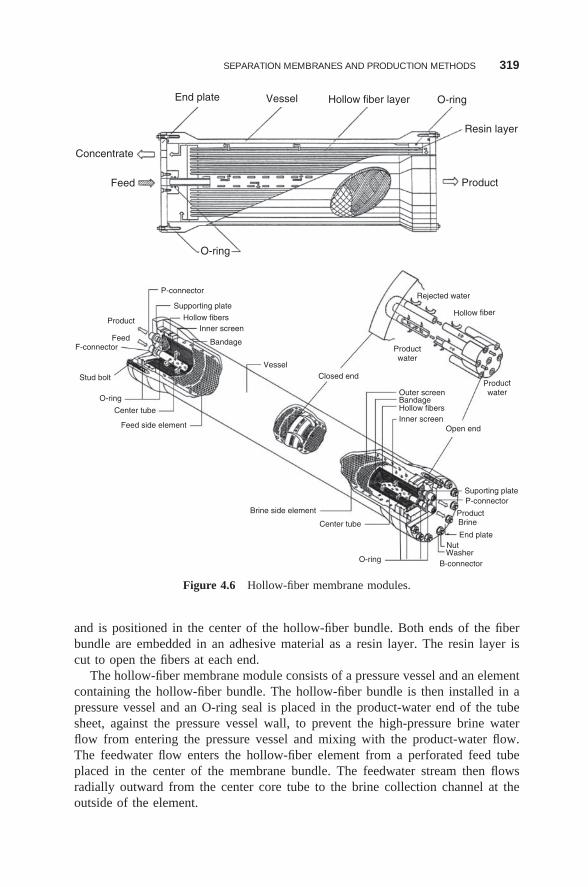
SEPARATION MEMBRANES AND PRODUCTION METHODS 319

P-connector

Supporting plate

Product

FeedF-connector

Stud bolt

O-ring

Center tube

Feed side element

Brine side element

Center tube

O-ring

Hollow fibersInner screen

Bandage

VesselClosed end

Outer screenBandageHollow fibersInner screen

Open end

Suporting plateP-connector

Product

End plateNutWasher

B-connector

Brine

Productwater

Rejected water

Hollow fiber

Productwater

End plate Vessel Hollow fiber layer O-ring

Resin layer

Product

O-ring

Feed

Concentrate

Figure 4.6 Hollow-fiber membrane modules.

and is positioned in the center of the hollow-fiber bundle. Both ends of the fiberbundle are embedded in an adhesive material as a resin layer. The resin layer iscut to open the fibers at each end.

The hollow-fiber membrane module consists of a pressure vessel and an elementcontaining the hollow-fiber bundle. The hollow-fiber bundle is then installed in apressure vessel and an O-ring seal is placed in the product-water end of the tubesheet, against the pressure vessel wall, to prevent the high-pressure brine waterflow from entering the pressure vessel and mixing with the product-water flow.The feedwater flow enters the hollow-fiber element from a perforated feed tubeplaced in the center of the membrane bundle. The feedwater stream then flowsradially outward from the center core tube to the brine collection channel at theoutside of the element.

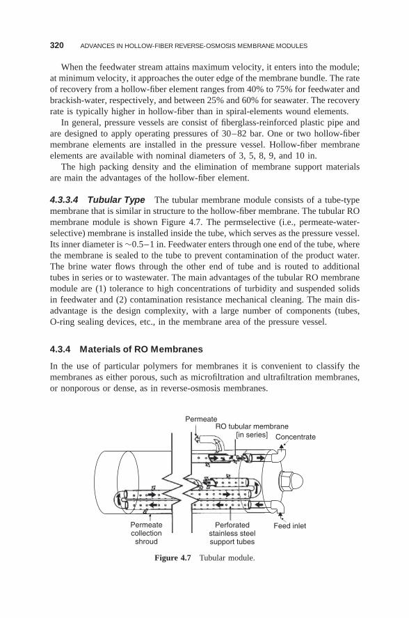
320 ADVANCES IN HOLLOW-FIBER REVERSE-OSMOSIS MEMBRANE MODULES

When the feedwater stream attains maximum velocity, it enters into the module;at minimum velocity, it approaches the outer edge of the membrane bundle. The rateof recovery from a hollow-fiber element ranges from 40% to 75% for feedwater andbrackish-water, respectively, and between 25% and 60% for seawater. The recoveryrate is typically higher in hollow-fiber than in spiral-elements wound elements.

In general, pressure vessels are consist of fiberglass-reinforced plastic pipe andare designed to apply operating pressures of 30–82 bar. One or two hollow-fibermembrane elements are installed in the pressure vessel. Hollow-fiber membraneelements are available with nominal diameters of 3, 5, 8, 9, and 10 in.

The high packing density and the elimination of membrane support materialsare main the advantages of the hollow-fiber element.

4.3.3.4 Tubular Type The tubular membrane module consists of a tube-typemembrane that is similar in structure to the hollow-fiber membrane. The tubular ROmembrane module is shown Figure 4.7. The permselective (i.e., permeate-water-selective) membrane is installed inside the tube, which serves as the pressure vessel.Its inner diameter is ∼0.5–1 in. Feedwater enters through one end of the tube, wherethe membrane is sealed to the tube to prevent contamination of the product water.The brine water flows through the other end of tube and is routed to additionaltubes in series or to wastewater. The main advantages of the tubular RO membranemodule are (1) tolerance to high concentrations of turbidity and suspended solidsin feedwater and (2) contamination resistance mechanical cleaning. The main dis-advantage is the design complexity, with a large number of components (tubes,O-ring sealing devices, etc., in the membrane area of the pressure vessel.

4.3.4 Materials of RO Membranes

In the use of particular polymers for membranes it is convenient to classify themembranes as either porous, such as microfiltration and ultrafiltration membranes,or nonporous or dense, as in reverse-osmosis membranes.

Permeatecollectionshroud

Perforatedstainless steelsupport tubes

Feed inlet

Concentrate

PermeateRO tubular membrane

[in series]

Figure 4.7 Tubular module.

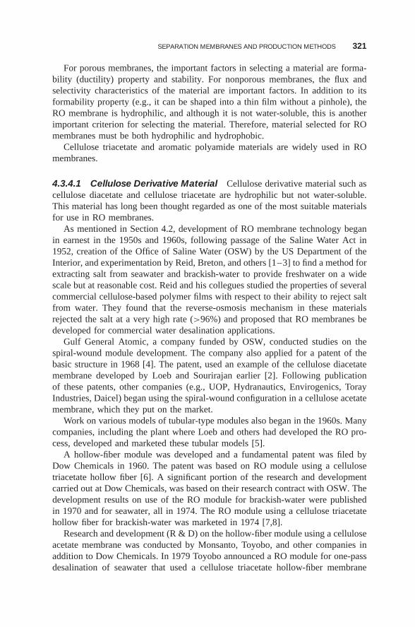
SEPARATION MEMBRANES AND PRODUCTION METHODS 321

For porous membranes, the important factors in selecting a material are forma-bility (ductility) property and stability. For nonporous membranes, the flux andselectivity characteristics of the material are important factors. In addition to itsformability property (e.g., it can be shaped into a thin film without a pinhole), theRO membrane is hydrophilic, and although it is not water-soluble, this is anotherimportant criterion for selecting the material. Therefore, material selected for ROmembranes must be both hydrophilic and hydrophobic.

Cellulose triacetate and aromatic polyamide materials are widely used in ROmembranes.

4.3.4.1 Cellulose Derivative Material Cellulose derivative material such ascellulose diacetate and cellulose triacetate are hydrophilic but not water-soluble.This material has long been thought regarded as one of the most suitable materialsfor use in RO membranes.

As mentioned in Section 4.2, development of RO membrane technology beganin earnest in the 1950s and 1960s, following passage of the Saline Water Act in1952, creation of the Office of Saline Water (OSW) by the US Department of theInterior, and experimentation by Reid, Breton, and others [1–3] to find a method forextracting salt from seawater and brackish-water to provide freshwater on a widescale but at reasonable cost. Reid and his collegues studied the properties of severalcommercial cellulose-based polymer films with respect to their ability to reject saltfrom water. They found that the reverse-osmosis mechanism in these materialsrejected the salt at a very high rate (>96%) and proposed that RO membranes bedeveloped for commercial water desalination applications.

Gulf General Atomic, a company funded by OSW, conducted studies on thespiral-wound module development. The company also applied for a patent of thebasic structure in 1968 [4]. The patent, used an example of the cellulose diacetatemembrane developed by Loeb and Sourirajan earlier [2]. Following publicationof these patents, other companies (e.g., UOP, Hydranautics, Envirogenics, TorayIndustries, Daicel) began using the spiral-wound configuration in a cellulose acetatemembrane, which they put on the market.

Work on various models of tubular-type modules also began in the 1960s. Manycompanies, including the plant where Loeb and others had developed the RO pro-cess, developed and marketed these tubular models [5].

A hollow-fiber module was developed and a fundamental patent was filed byDow Chemicals in 1960. The patent was based on RO module using a cellulosetriacetate hollow fiber [6]. A significant portion of the research and developmentcarried out at Dow Chemicals, was based on their research contract with OSW. Thedevelopment results on use of the RO module for brackish-water were publishedin 1970 and for seawater, all in 1974. The RO module using a cellulose triacetatehollow fiber for brackish-water was marketed in 1974 [7,8].

Research and development (R & D) on the hollow-fiber module using a celluloseacetate membrane was conducted by Monsanto, Toyobo, and other companies inaddition to Dow Chemicals. In 1979 Toyobo announced a RO module for one-passdesalination of seawater that used a cellulose triacetate hollow-fiber membrane

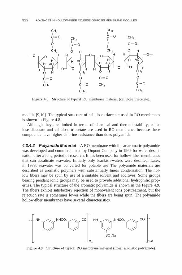
322 ADVANCES IN HOLLOW-FIBER REVERSE-OSMOSIS MEMBRANE MODULES

O

H

O

H

OO|C || O

C || O|CH3

H

AC

H

H

CH3|C|O|CH2

O

H

O

H

O|

|CH3

H

AC

H

H

CH3|

|O|CH2

O

H

OH

CH2|O|

|CH3

H

AC

OH

CH3|C|O

O

H

H

CH2|O|

|CH3

H

AC

H

CH3|

|O

HH

|

|

|

|

|

H O

|

|

|

|

||

O

O

O

|| O

C || O

C || O

C || O

C || O

Figure 4.8 Structure of typical RO membrane material (cellulose triacetate).

module [9,10]. The typical structure of cellulose triacetate used in RO membranesis shown in Figure 4.8.

Although they are limited in terms of chemical and thermal stability, cellu-lose diacetate and cellulose triacetate are used in RO membranes because thesecompounds have higher chlorine resistance than does polyamide.

4.3.4.2 Polyamide Material A RO membrane with linear aromatic polyamidewas developed and commercialized by Dupont Company in 1969 for water desali-nation after a long period of research. It has been used for hollow-fiber membranesthat can desalinate seawater. Initially only brackish-waters were desalted. Later,in 1973, seawater was converted for potable use The polyamide materials aredescribed as aromatic polymers with substantially linear condensation. The hol-low fibers may be spun by use of a suitable solvent and additives. Some groupsbearing pendant ionic groups may be used to provide additional hydrophilic prop-erties. The typical structure of the aromatic polyamide is shown in the Figure 4.9.The fibers exhibit satisfactory rejection of monovalent ions posttreatment, but therejection rate is sometimes lower while the fibers are being spun. The polyamidehollow-fiber membranes have several characteristics.

NH

n

NHCO

SO3Na

CO

1-n

NH NHCO CO

Figure 4.9 Structure of typical RO membrane material (linear aromatic polyamide).

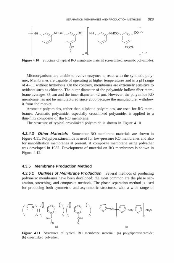
SEPARATION MEMBRANES AND PRODUCTION METHODS 323

NHCONH

CO

CO NH NHCO

COOH

CO

n 1–n

Figure 4.10 Structure of typical RO membrane material (crosslinked aromatic polyamide).

Microorganisms are unable to evolve enzymes to react with the synthetic poly-mer, Membranes are capable of operating at higher temperatures and in a pH rangeof 4–11 without hydrolysis. On the contrary, membranes are extremely sensitive tooxidants such as chlorine. The outer diameter of the polyamide hollow fiber mem-brane averages 85 μm and the inner diameter, 42 μm. However, the polyamide ROmembrane has not be manufactured since 2000 because the manufacturer withdrewit from the market.

Aromatic polyamides, rather than aliphatic polyamides, are used for RO mem-branes. Aromatic polyamide, especially crosslinked polyamide, is applied to athin-film composite of the RO membrane.

The structure of typical crosslinked polyamide is shown in Figure 4.10.

4.3.4.3 Other Materials Someother RO membrane materials are shown inFigure 4.11. Polypiperazineamide is used for low-pressure RO membranes and alsofor nanofiltration membranes at present. A composite membrane using polyetherwas developed in 1982. Development of material on RO membranes is shown inFigure 4.12.

4.3.5 Membrane Production Method

4.3.5.1 Outlines of Membrane Production Several methods of producingpolymeric membranes have been developed; the most common are the phase sep-aration, stretching, and composite methods. The phase separation method is usedfor producing both symmetric and asymmetric structures, with a wide range of

CCN N

CO

HN

O O

(a) (b)

CC

COH

O O

O

OCH2

OCH2

Onyx z

CH2OH

Figure 4.11 Structures of typical RO membrane material: (a) polypiperazineamide;(b) crosslinked polyether.

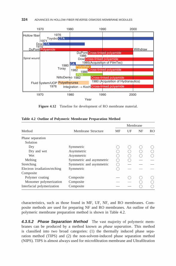
324 ADVANCES IN HOLLOW-FIBER REVERSE-OSMOSIS MEMBRANE MODULES

1970 1980 1990 2000

200019901980

Year

1970

1976

Hollow fiber 1976Toyobo CTA

CTA1971

Dow1970

DuPont WithdrawDuPont Cross-linked polyamide

1986Spiral wound Dow Cross-linked polyamide

1985(Acquisition of FilmTec)CA1980 Polyether1982 Cross-linked polyamide

1986PVA

NittoDenko 1982 Cross-linked polyamide1980 (Acquisition of Hydranautics)Fluid System/UOP Polyetherurea

Integration → Koch Cross-linked polyamide

Toray

Polyamide

Figure 4.12 Timeline for development of RO membrane material.

Table 4.2 Outline of Polymeric Membrane Preparation Method

Membrane

Method Membrane Structure MF UF NF RO

Phase separationSolution

Dry Symmetric © © © ©Dry and wet Asymmetric © © © ©Wet Asymmetric © © © ©

Melting Symmetric and asymmetric © © — —Stretching Symmetric and asymmetric © — — —Electron irradiation/etching Symmetric © — — —Composite

Polymer coating Composite — © © ©Monomer polymerization Composite — — © ©

Interfacial polymerization Composite — — © ©

characteristics, such as those found in MF, UF, NF, and RO membranes. Com-posite methods are used for preparing NF and RO membranes. An outline of thepolymeric membrane preparation method is shown in Table 4.2.

4.3.5.2 Phase Separation Method The vast majority of polymeric mem-branes can be produced by a method known as phase separation . This methodis classified into two broad categories: (1) the thermally induced phase sepa-ration method (TIPS) and (2) the non-solvent-induced phase separation method(NIPS). TIPS is almost always used for microfiltration membrane and Ultrafiltration

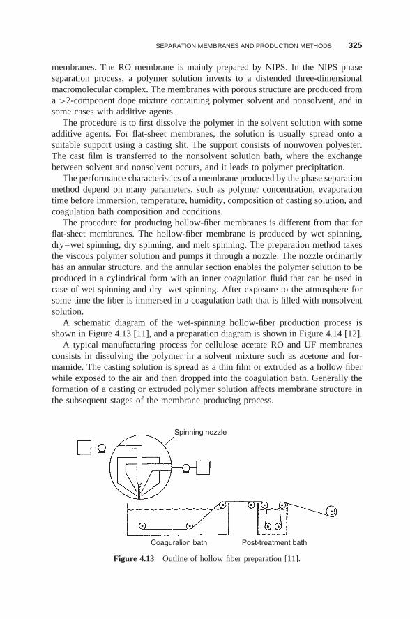
SEPARATION MEMBRANES AND PRODUCTION METHODS 325

membranes. The RO membrane is mainly prepared by NIPS. In the NIPS phaseseparation process, a polymer solution inverts to a distended three-dimensionalmacromolecular complex. The membranes with porous structure are produced froma >2-component dope mixture containing polymer solvent and nonsolvent, and insome cases with additive agents.

The procedure is to first dissolve the polymer in the solvent solution with someadditive agents. For flat-sheet membranes, the solution is usually spread onto asuitable support using a casting slit. The support consists of nonwoven polyester.The cast film is transferred to the nonsolvent solution bath, where the exchangebetween solvent and nonsolvent occurs, and it leads to polymer precipitation.

The performance characteristics of a membrane produced by the phase separationmethod depend on many parameters, such as polymer concentration, evaporationtime before immersion, temperature, humidity, composition of casting solution, andcoagulation bath composition and conditions.

The procedure for producing hollow-fiber membranes is different from that forflat-sheet membranes. The hollow-fiber membrane is produced by wet spinning,dry–wet spinning, dry spinning, and melt spinning. The preparation method takesthe viscous polymer solution and pumps it through a nozzle. The nozzle ordinarilyhas an annular structure, and the annular section enables the polymer solution to beproduced in a cylindrical form with an inner coagulation fluid that can be used incase of wet spinning and dry–wet spinning. After exposure to the atmosphere forsome time the fiber is immersed in a coagulation bath that is filled with nonsolventsolution.

A schematic diagram of the wet-spinning hollow-fiber production process isshown in Figure 4.13 [11], and a preparation diagram is shown in Figure 4.14 [12].

A typical manufacturing process for cellulose acetate RO and UF membranesconsists in dissolving the polymer in a solvent mixture such as acetone and for-mamide. The casting solution is spread as a thin film or extruded as a hollow fiberwhile exposed to the air and then dropped into the coagulation bath. Generally theformation of a casting or extruded polymer solution affects membrane structure inthe subsequent stages of the membrane producing process.

Spinning nozzle

Post-treatment bathCoaguralion bath

Figure 4.13 Outline of hollow fiber preparation [11].

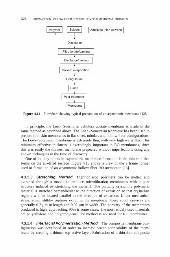
326 ADVANCES IN HOLLOW-FIBER REVERSE-OSMOSIS MEMBRANE MODULES

Additives (Non-solvent)Polymer

Discharge/casting

Membrane

Solvent

Dissolution

Filtration/defoaming

Solvent evaporation

Coagulation

Rinse

Post-treatment

Figure 4.14 Flowchart showing typical preparation of an asymmetric membrane [12].

In principle, the Loeb–Sourirajan cellulose acetate membrane is made in thesame method as described above. The Loeb–Sourirajan technique has been used toprepare thin-skin membranes in flat-sheet, tubular, and hollow-fiber configurations.The Loeb–Sourirajan membrane is extremely thin, with very high water flux. Thisminimum effective thickness is exceedingly important in RO membranes, sincethis was easily the thinnest membrane prepeared without imperfections using anyknown techniques at the time of discovery.

One of the key points in asymmetric membrane formation is the thin skin thatforms on the air-dried surface. Figure 4.15 shows a view of the a frame formatused in formation of an asymmetric hollow-fiber RO membrane [13].

4.3.5.3 Stretching Method Thermoplastic polymers can be melted andextruded through a nozzle to produce microfiltration membranes with a porestructure induced by stretching the material. The partially crystalline polymericmaterial is stretched perpendicular to the direction of extrusion so that crystallineregions will be located parallel to the direction of extrusion. Under mechanicalstress, small slitlike ruptures occur in the membrane; these small crevices aregenerally 0.2 μm in length and 0.02 μm in width. The porosity of the membranesproduced is high, approaching 90% is some cases. The most widely used materialsare polyethylene and polypropylene. The method is not used for RO membranes.

4.3.5.4 Interfacial Polymerization Method The composite membrane con-figuration was developed in order to increase water permeability of the mem-brane by creating a thinner top active layer. Fabrication of a thin-film composite

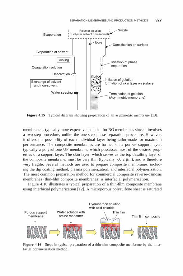
SEPARATION MEMBRANES AND PRODUCTION METHODS 327

Densification on surface

Initiation of gelationformation of skin layer on surface

Coagulation solution

Nozzle

Bore

Cooling

Evaporation

Evaporation of solvent

Initiation of phaseseparation

Polymer solution(Polymer solvent non-solvent)

Termination of gelation(Asymmetric membrane)

Water seeping

Exchange of solventand non-solvent

Desolvation

Figure 4.15 Typical diagram showing preparation of an asymmetric membrane [13].

membrane is typically more expensive than that for RO membranes since it involvesa two-step procedure, unlike the one-step phase separation procedure. However,it offers the possibility of each individual layer being tailor-made for maximumperformance. The composite membranes are formed on a porous support layer,typically a polysulfone UF membrane, which possesses most of the desired prop-erties of a support layer. The skin layer, which serves as the top desalting layer ofthe composite membrane, must be very thin (typically <0.2 μm), and is thereforevery fragile. Several methods are used to prepare composite membranes, includ-ing the dip coating method, plasma polymerization, and interfacial polymerization.The most common preparation method for commercial composite reverse-osmosismembranes (thin-film composite membranes) is interfacial polymerization.

Figure 4.16 illustrates a typical preparation of a thin-film composite membraneusing interfacial polymerization [12]. A microporous polysulfone sheet is saturated

Porous supportmembrane

Water solution withamine monomer

Hydrocarbon solutionwith acid chloride

Thin filmThin film composite

Figure 4.16 Steps in typical preparation of a thin-film composite membrane by the inter-facial polymerization method.

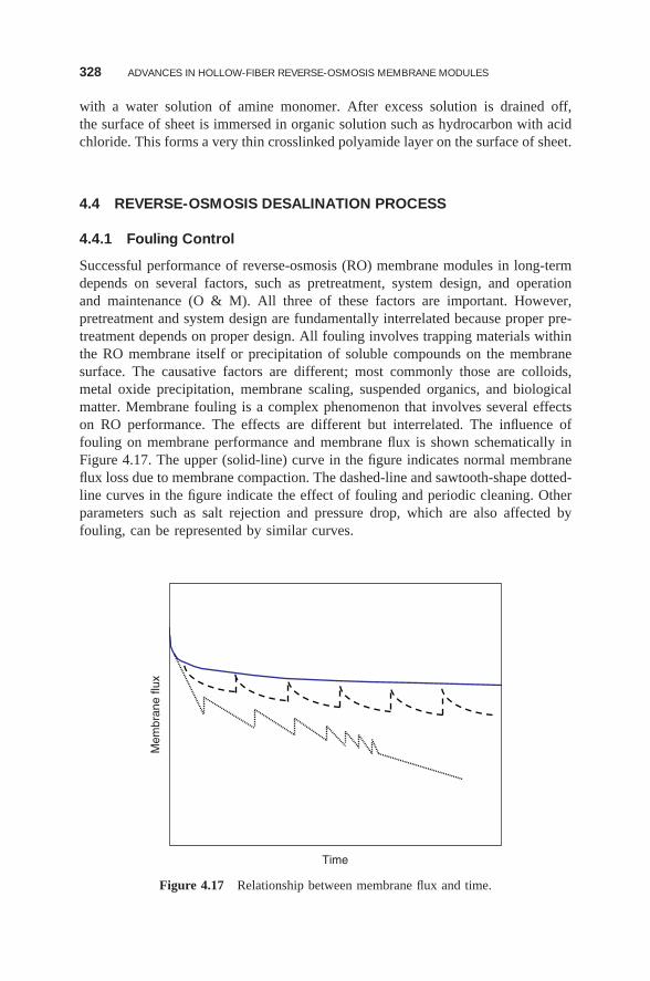
328 ADVANCES IN HOLLOW-FIBER REVERSE-OSMOSIS MEMBRANE MODULES

with a water solution of amine monomer. After excess solution is drained off,the surface of sheet is immersed in organic solution such as hydrocarbon with acidchloride. This forms a very thin crosslinked polyamide layer on the surface of sheet.

4.4 REVERSE-OSMOSIS DESALINATION PROCESS

4.4.1 Fouling Control

Successful performance of reverse-osmosis (RO) membrane modules in long-termdepends on several factors, such as pretreatment, system design, and operationand maintenance (O & M). All three of these factors are important. However,pretreatment and system design are fundamentally interrelated because proper pre-treatment depends on proper design. All fouling involves trapping materials withinthe RO membrane itself or precipitation of soluble compounds on the membranesurface. The causative factors are different; most commonly those are colloids,metal oxide precipitation, membrane scaling, suspended organics, and biologicalmatter. Membrane fouling is a complex phenomenon that involves several effectson RO performance. The effects are different but interrelated. The influence offouling on membrane performance and membrane flux is shown schematically inFigure 4.17. The upper (solid-line) curve in the figure indicates normal membraneflux loss due to membrane compaction. The dashed-line and sawtooth-shape dotted-line curves in the figure indicate the effect of fouling and periodic cleaning. Otherparameters such as salt rejection and pressure drop, which are also affected byfouling, can be represented by similar curves.

Time

Mem

bran

e flu

x

Figure 4.17 Relationship between membrane flux and time.

REVERSE-OSMOSIS DESALINATION PROCESS 329

4.4.1.1 Biological Fouling Performance of the RO module may be affectedby increased amounts of biological matter such as the growth of microorganisms,which can sometimes damage cortain types of membranes and modules. However,proper treatment for preventing growth of microorganisms is effective in preventingbiological fouling. A typical treatment is proper disinfection of the membrane. Ifthe feedwater contains sufficient nutrient source to sustain rapid growth of microor-ganisms in the module, growth of biological matter can occur. This growth can leadto the formation of biofilms on the membrane, and biofilms and their metabolitesare known to compromise module performance.

In actual operation, with rapid pressure loss in the module, biological growthis normally first indicated. This pressure loss is the pressure difference betweenthe feed side and the brine side of the module. In the hollow-fiber module, plug-ging across the fiber bundles with matter leads to increased pressure loss. In casebiological fouling occurs, biological cleaning treatment is recommended. Thereare several cleaning methods, such as acid/alkali shock treatment, sodium bisulfite(SBS) shock treatment, and chlorine injection. The acid or alkali shock treatmentrequires a large quantity of chemicals to effectively decrease the pressure loss inmodules. Meanwhile, SBS shock treatment is seldom effective in decreaseing pres-sure loss, especially after numerous operations, because SBS is an antibacterialmaterial, not a disinfection agent. In contrast, chlorination by injection of chlorineis very effective for preventing the growth of biologicalmaterial that causes foulingin RO modules.

A typical desalination plant using a polyamide RO membrane module useschlorine as a disinfectant in the pretreatment process. Because the polyamide ROmembrane module is affected by chlorine, SBS is injected to dechlorinate the feed-water before it enters the RO module. Since chlorination treatment does not destroyall the microorganisms, some of them will survive and continue to grow, result-ing in biological fouling, also called aftergrowth . However, some membranes haveno resistance to chlorine as an oxidant; for instance, chlorine cannot be used forbiological cleaning of polyamide RO membranes, which are the most commontype of RO membranes used in the world. Meanwhile, a cellulose triacetate ROmembrane does have resistance to chlorine and therefore be disinfected directly toprevent biological fouling. Monitoring biological activity is also effective in pre-venting biological fouling of RO membrane modules, especially in surface seawaterapplications.

4.4.1.2 Physical Fouling Physical fouling normally consists of fouling bymetal oxides; scaling is the most common form of fouling. Scaling is caused by theprecipitation of relatively insoluble salts (CaCO3, CaSO4, BaSO4, SrSO4, SiO2 etc.)in the module. The scaling potential of any feedwater is determined from chemicalanalyses of that feedwater, recovery of the RO system, and the solubility limits ofvarious salts. CaCO3 is usually the only salt in seawater for which pretreatment isrequired. In normal operation using commercial RO modules, recovery is 30–60%in seawater, and the solubility limits of CaCO3, BaSO4, SrSO4, and SiO2 are rarelyexceeded in this recovery.

330 ADVANCES IN HOLLOW-FIBER REVERSE-OSMOSIS MEMBRANE MODULES

The second type of fouling that can occur in RO modules is precipitation of metaloxides. This is caused by the formation of the oxides and hydroxide of iron andmanganese. For seawater containing iron, the iron will probably be present in theform of soluble ferrous bicarbonate. If the iron remains in the soluble ferrous form,the RO modules will reject it quite effectively. However, if the soluble (ferrous)iron is oxidized to the ferric state in the RO module, iron fouling will occur withthe formation of Fe(OH)3 precipitates.

4.4.2 Disinfection Method for Pretreatment

Implementation of an adequate disinfection procedure is critical for reliable oper-ation of RO modules, especially when source feedwater is obtained from surfacewater. The rationale for disinfection is to prevent growth of microorganisms inthe RO module that can adversely affect the performance (permeate water flowcapacity and salt rejection). In addition to prevention of microorganism growth,the proper disinfection procedure must also ensure that membrane damage doesnot occur because of the presence of microorganisms or the disinfectant chemicalitself. The two key factors to consider in discussing biological matter include (1)degradation of the membrane and (2) biological fouling of the membrane. Thesetwo factors are

In this section, the following described with respect to a disinfection methodused to eradicate biological fouling in cellulose triacetate RO modules that havechlorine resistance:

1. Membrane Degradation . The cellulose triacetate membrane used is com-patible with chlorine disinfectant and hence can be easily protected frombiological attack.

2. Membrane Biological Fouling . Biological matter can grow inside RO mod-ules when the feedwater contains sufficient nutrients to sustain rapid growth.In more recent years this rapid biological growth has been recognized as‘aftergrowth’, even in situations where chlorination of feedwater was initiallyemployed. This possibility is greater for polyamide membranes than celluloseacetate membranes since a dechlorination step must be performed before thetreated feedwater enters the membrane element. Elimination of chlorine inthe feedwater has been observed to allow potentially rapid aftergrowth sincethe initial chlorination step does not completely kill all microorganism. Infact, it has been speculated that the chlorination step reacts with organic mat-ter such as humic acids to render them more assimilable as food to supportmicroorganism growth in the RO modules. Ultimately this biological organ-ism growth can lead to formation of biofilms on the membranes, leading, inturn, to poor RO module performance.

In the case of cellulose triacetate membranes, compatibility with chlorine disin-fection prevents the potential rapid aftergrowth of microorganisms in the module.Generally, at plant startup the chlorine dosing amount is optimized to minimize the

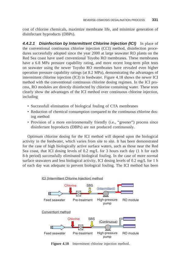
REVERSE-OSMOSIS DESALINATION PROCESS 331

cost of chlorine chemicals, maximize membrane life, and minimize generation ofdisinfectant byproducts (DBPs).

4.4.2.1 Disinfection by Intermittent Chlorine Injection (ICI) In place ofthe conventional continuous chlorine injection (CCI) method, disinfection proce-dures successfully adopted since the year 2000 at large seawater RO plants on theRed Sea coast have used conventional Toyobo RO membranes. These membraneshave a 6.8 MPa pressure capability rating, and more recent long-term pilot testson seawater using the newer Toyobo RO membranes have revealed even higheroperation pressure capability ratings (at 8.2 MPa), demonstrating the advantages ofintermittent chlorine injection (ICI) in feedwater. Figure 4.18 shows the newer ICImethod with the conventional continuous chlorine dosing regimen. In the ICI pro-cess, RO modules are directly disinfected by chlorine containing water. These testsclearly show the advantages of the ICI method over continuous chlorine injection,including

• Successfull elimination of biological fouling of CTA membranes

• Reduction of chemical consumption compared to the continuous chlorine dos-ing method

• Provision of a more environmentally friendly (i.e., “greener”) process sincedisinfectant byproducts (DBPs) are not produced continuously.

Optimum chlorine dosing for the ICI method will depend upon the biologicalactivity in the feedwater, which varies from site to site. It has been demonstratedfor the case of high biologically active surface waters, such as those near the RedSea coast, that ICI dosing levels of 0.2 mg/L for 3 hours each day (1 h for each8-h period) successfully eliminated biological fouling. In the case of more normalsurface seawaters and less biological activity, ICI dosing levels of 0.2 mg/L for 1 hof each day was adequate to prevent biological fouling. The ICI method has been

ICI (Intermittent Chlorine Injection) method

Feed seawater

Conventionl method

Pre-treatment

Pre-treatment

High-pressurepump

Chlorine SBS(Intermittent)

Chlorine SBS

RO moduleHigh-pressurepump

Feed seawater

(Continuous)

RO module

Figure 4.18 Intermittent chlorine injection method.

332 ADVANCES IN HOLLOW-FIBER REVERSE-OSMOSIS MEMBRANE MODULES

successfully demonstrated in plant operations with recovery ranges of 30–55%,and offers an opportunity to maximize plant availability by minimizing time andcost of frequent cleaning.

4.4.2.2 Control by Shock Treatment In cases where chlorination anddechlorination do not provide adequate control of microbiological foulingcondition and rapid growth of microorganisms resumes in the modules, chemicalshock treatments have been employed using sodium bisulfite (NaHSO3, SBS) andacid such as sulfuric acid.

The intermittent injection of SBS at concentrations of ∼500–1000 mg/L inthe RO modules may be effective. As mentioned above, SBS is an antibacterialmaterial, not a disinfection agent. The effectiveness of this method using SBS islimited, although SBS does not react with the membrane, such as a polyamide ROmembrane.

The acid shock treatment needs a large quantity of chemicals to effectively stabi-lize the microbiological condition. In general, microorganisms may develop higherthresholds to the effects of the chemicals after many, repeated shock treatmentsusing acids.

4.4.2.3 Bacteria Content of RO Product Water While RO membraneswill reject almost 100% of bacteria, all RO devices have mechanical seals, butit is possible for minute, trace quantities of feedwater to bypass or breach theseseals and enter the product-water stream. In addition, any broken fibers or microc-racks in spiral-wound membranes, although very small in quantity, can also permitfeedwater to enter the product-water stream. For these reasons, RO modules arenot guaranteed to produce sterile water. If sterile water is desired, ultraviolet (UV)radiation can be used. This technique is commonly used in the electronics industry.

4.4.3 Prediction of RO Performance for Long-Term Operation

4.4.3.1 Membrane Compaction Some degree of membrane compactionusually occurs during the operating period, which results in reduced permeatewater flow rate. This phenomenon is known as membrane flux decline. The effectof pressure, temperature, and time on membrane flux is expressed as a membraneflux retention coefficient (MFRC) as shown in the following equation

MFRC = Qpt

Qpt0(4.1)

where Qpt is the permeate flow rate at time t and Qp0 is the permeate flow rate atinitial time t0. Both Q values have the same operating parameters such as pressure,temperature, and water recovery. The rate of decline depends on the operatingparameters such as temperature and pressure. The greater the temperature and/orpressure, the greater the rate of decline of membrane flux.

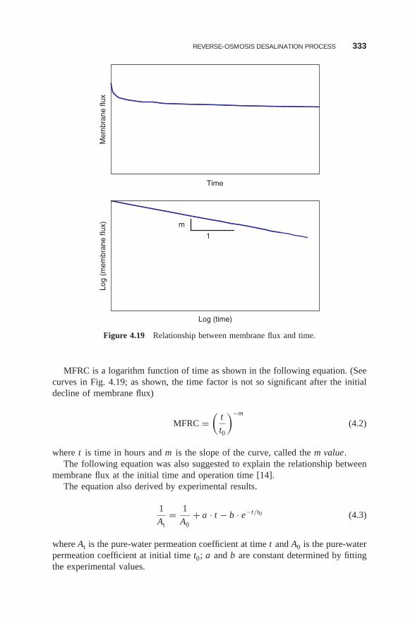
REVERSE-OSMOSIS DESALINATION PROCESS 333

Time

Mem

bran

e flu

xLo

g (m

embr

ane

flux)

Log (time)

1

m

Figure 4.19 Relationship between membrane flux and time.

MFRC is a logarithm function of time as shown in the following equation. (Seecurves in Fig. 4.19; as shown, the time factor is not so significant after the initialdecline of membrane flux)

MFRC =(

t

t0

)−m

(4.2)

where t is time in hours and m is the slope of the curve, called the m value.The following equation was also suggested to explain the relationship between

membrane flux at the initial time and operation time [14].The equation also derived by experimental results.

1

At= 1

A0+ a · t − b · e−t/t0 (4.3)

where At is the pure-water permeation coefficient at time t and A0 is the pure-waterpermeation coefficient at initial time t0; a and b are constant determined by fittingthe experimental values.

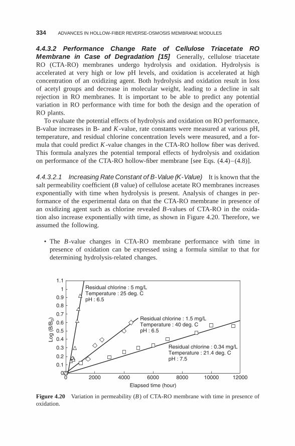
334 ADVANCES IN HOLLOW-FIBER REVERSE-OSMOSIS MEMBRANE MODULES

4.4.3.2 Performance Change Rate of Cellulose Triacetate ROMembrane in Case of Degradation [15] Generally, cellulose triacetateRO (CTA-RO) membranes undergo hydrolysis and oxidation. Hydrolysis isaccelerated at very high or low pH levels, and oxidation is accelerated at highconcentration of an oxidizing agent. Both hydrolysis and oxidation result in lossof acetyl groups and decrease in molecular weight, leading to a decline in saltrejection in RO membranes. It is important to be able to predict any potentialvariation in RO performance with time for both the design and the operation ofRO plants.

To evaluate the potential effects of hydrolysis and oxidation on RO performance,B-value increases in B- and K -value, rate constants were measured at various pH,temperature, and residual chlorine concentration levels were measured, and a for-mula that could predict K -value changes in the CTA-RO hollow fiber was derived.This formula analyzes the potential temporal effects of hydrolysis and oxidationon performance of the CTA-RO hollow-fiber membrane [see Eqs. (4.4)–(4.8)].

4.4.3.2.1 Increasing Rate Constant of B-Value (K-Value) It is known that thesalt permeability coefficient (B value) of cellulose acetate RO membranes increasesexponentially with time when hydrolysis is present. Analysis of changes in per-formance of the experimental data on that the CTA-RO membrane in presence ofan oxidizing agent such as chlorine revealed B -values of CTA-RO in the oxida-tion also increase exponentially with time, as shown in Figure 4.20. Therefore, weassumed the following.

• The B -value changes in CTA-RO membrane performance with time inpresence of oxidation can be expressed using a formula similar to that fordetermining hydrolysis-related changes.

00 2000 4000 6000

Residual chlorine : 0.34 mg/LTemperature : 21.4 deg. CpH : 7.5

Residual chlorine : 1.5 mg/LTemperature : 40 deg. CpH : 6.5

Residual chlorine : 5 mg/LTemperature : 25 deg. CpH : 6.5

Elapsed time (hour)

8000 10000 12000

0.1

0.2

0.3

0.4

0.5

Log

(B/B

0)

0.6

0.7

0.8

0.9

1

1.1

Figure 4.20 Variation in permeability (B ) of CTA-RO membrane with time in presence ofoxidation.

REVERSE-OSMOSIS DESALINATION PROCESS 335

• The B -value increasing rate constant (K value) is equal to the sum of KH andKO, where KH and KO are B -value increasing rate constants in hydrolysis andoxidation, respectively. In short, an additive applies to KH and KO.

Therefore, we defined the B -value increasing rate constant for both hydrolysis andoxidation (K value) by the formulas

logB

B0= Kt (4.4)

K = KH + KO (4.5)

where B0 = initial B value, cm/st = elapsed time, h

K = B -value increasing rate constant, h−1

KH = B -value increasing rate constant in hydrolysis, h−1

KO = B -value increasing rate constant in oxidation, h−1

4.4.3.2.2 Derivation of Prediction Formula Using the B-Value IncreasingRate Constant (K Value)

Derivation of Prediction Formula for KH (in Hydrolysis). Data on KH-valuechanges recorded on continuous operation of CTA-RO hollow-fiber moduleswere measured at various temperature and pH levels. The following formulafor predicting changes in KH values with respect to temperature and pH wasderived:

log(KH) = −6400

273.2 + Tfw+ 0.80pH + 11.0 (4.6)

where Tfw = feedwater temperature, ◦CpH = feedwater pH (−)

Derivation of Prediction Formula on KO (in Oxidation). Since KO could notbe measured directly, it was obtained as the difference between K and KH,which was calculated using Equation (4.4). The K value, that is, KH + KO,as shown before, was measured by experimental results in the presence of anoxidizing agent such as chlorine. The following prediction formula for KOwas derived by a multiregression analysis:

log(KO) = 1.072 log(CCl2 res)−1850

273.2 + Tfw+ 0.89pH − 4.246 (4.7)

where CCl2 res is the residual chlorine concentration in feedwater (in mg/L).

336 ADVANCES IN HOLLOW-FIBER REVERSE-OSMOSIS MEMBRANE MODULES

Prediction Formula for K-Value. By rearranging Equations (4.5)–(4.7), weobtain the following formula:

K = 1 × 1011 × exp

( −14, 740

273.2 + Tfw+ 1.842pH

)

+ 5.675 × 10−5(CCl2 res)1.072 × (4.8)

exp

( −4260

273.2 + Tfw+ 2.049pH

)

The calculated K values are in fair agreement with experimental values. Sincethe B -value increasing rate constants for both hydrolysis and oxidation can becalculated independently, This formula presumably applies to the predictionof performance changes with time, including the period of suspension in ROplants.

4.4.4 High-Recovery Process

Reverse-osmosis technology is becoming the key method for obtaining freshwaterfrom the sea, especially in the Middle East. Membrane manufacturers are workingto develop membranes offering higher water recovery and lower energy and instal-lation costs in order to establish world wide recognition of the RO process as themost popular method for supplying freshwater.

In a seawater RO process, the water is subjected to disinfection,coagulation–filtration, and acidification processes in the pretreatment section andforwarded as feedwater to the RO section. When the recovery fraction, the ratio ofproduct flow rate to feed flow rate, is high, the amount of feedwater required fordesired production volume is lower; hence, cost of chemicals, equipment sizing,and energy cost are for the pretreatment system significantly reduced.

For high-recovery operation, in comparison with conventional low-recoveryoperation, higher feed pressure (i.e., driving force) is required. In order to enablethe high-recovery operation, the RO module must be designed and manufacturedto withstand the higher pressure.

4.4.4.1 Higher-Efficiency RO Single-Stage High-Recovery SystemFigure 4.21 shows a higher-efficiency RO single-stage high-recovery systemat 60% recovery level in comparison to a conventional 40% recovery process.Application of the higher-pressure capability module compared to the conventionalmodule can reduce the feed seawater flow rate by ∼40% compared withthe conventional process. This higher recovery makes it possible to reducethe construction and running costs of the pretreatment process. In addition,with the lower amount of seawater that must be pressurized, energy can berecovered efficiently from the high-pressure brine by use of energy recoverydevices. Therefore, energy consumption per cubic meter of water produced wouldpresumably also be less than that in the conventional process.

This is a simple and a reliable system with a reliable track record in manyoperations, and facilitates control of the operation.

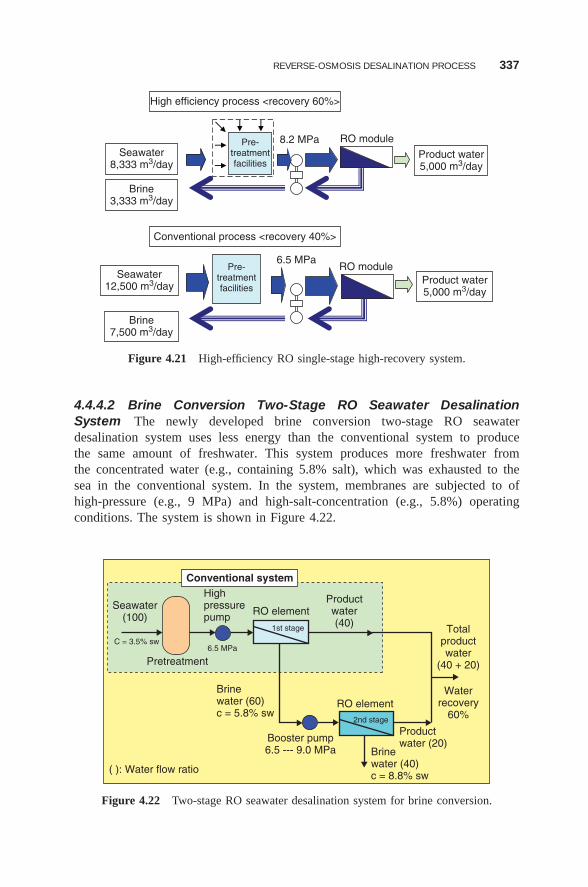
REVERSE-OSMOSIS DESALINATION PROCESS 337

Seawater8,333 m3/day

Brine3,333 m3/day

Product water5,000 m3/day

8.2 MPa RO module

RO module

Pre-treatmentfacilities

Pre-treatmentfacilities

Seawater12,500 m3/day

Brine7,500 m3/day

Product water5,000 m3/day

6.5 MPa

Conventional process <recovery 40%>

High efficiency process <recovery 60%>

Figure 4.21 High-efficiency RO single-stage high-recovery system.

4.4.4.2 Brine Conversion Two-Stage RO Seawater DesalinationSystem The newly developed brine conversion two-stage RO seawaterdesalination system uses less energy than the conventional system to producethe same amount of freshwater. This system produces more freshwater fromthe concentrated water (e.g., containing 5.8% salt), which was exhausted to thesea in the conventional system. In the system, membranes are subjected to ofhigh-pressure (e.g., 9 MPa) and high-salt-concentration (e.g., 5.8%) operatingconditions. The system is shown in Figure 4.22.

Conventional system

Seawater(100)

Pretreatment

Brinewater (60)c = 5.8% sw

Booster pump6.5 --- 9.0 MPa

( ): Water flow ratio

Highpressurepump RO element

RO element

Productwater(40) Total

productwater

(40 + 20)

Waterrecovery

60%

Productwater (20)

Brinewater (40)c = 8.8% sw

C = 3.5% sw6.5 MPa

1st stage

2nd stage

Figure 4.22 Two-stage RO seawater desalination system for brine conversion.

338 ADVANCES IN HOLLOW-FIBER REVERSE-OSMOSIS MEMBRANE MODULES

4.5 DEVELOPMENT OF HOLLOW-FIBER RO MEMBRANE MODULEFOR SEAWATER DESALINATION

4.5.1 Hollow-Fiber Bundle Configuration

Hollow-fiber membrane modules are classified into several types according tohollow-fiber bundle configuration and flow pattern. Hollow-fiber membrane mod-ules are classified broadly into cross-wound configuration type and parallel config-uration type. The parallel configuration is necessary to enable the spacer to bundlethe hollow fibers together, while the cross-wound configuration does not reguirea spacer because the hollow fibers automatically pack themselves into a bundle.Therefore, the cross-wound type is preferred for fouling resistance.

The flow patterns in the hollow fiber bundle are classified into axial and radial.In general, feedwater velocity in the module in axial flow is higher than that inradial flow. Therefore, pressure loss in the axial-flow module is higher than that inthe radial-flow module. The greater the module length is, the greater the differencebetween velocity and pressure values.

In RO module applications, feedwater is usually pressurized outside the hollow-fiber membrane and permeated water flows from outside to inside of the hollowfiber, especially in high-pressure operation such as seawater desalination appli-cations. In some RO membrane modules designed for low-pressure operation,feedwater is fed into the hollow-fiber bore. It is than pressurized inside the hol-low fiber, and permeated water flows from inside to outside of the fiber. The “bothopen-ended” (BOE) module configuration is reguired for this internally pressurizedtype module.

4.5.2 Features of Hollow-Fiber RO Membrane Module for SeawaterDesalination

The cellulose triacetate RO membrane module typically has a hollow-fiber config-uration.

4.5.2.1 Module Structure (Hollow-Fiber Configuration) Hollow-fibermodules can offer greater surface membrane area in the module than canspiral-wound modules. Because of the greater compactness of the hollow-Fiberbundle, the production rate is higher in these modules and their footprints in thesoil or sand banks near the desalination plant are smaller. Figure 4.23 showsa cellulose triacetate hollow-fiber array fixed in epoxy resin at both ends. Thisarrangement provides mechanical stability to the fiber array. The fibers at one endof the element are cut precisely so that product water can be discharged from thefibers bore.

The cellulose triacetate RO module used for seawater desalination has a double-element configuration, as shown in Figure 4.23. Because permeate water of eachelement in a pressure vessel can be obtained directly, the quality of permeatewater throughout the vessel can be measured directly, which Facilitates RO plantmaintenance [16].

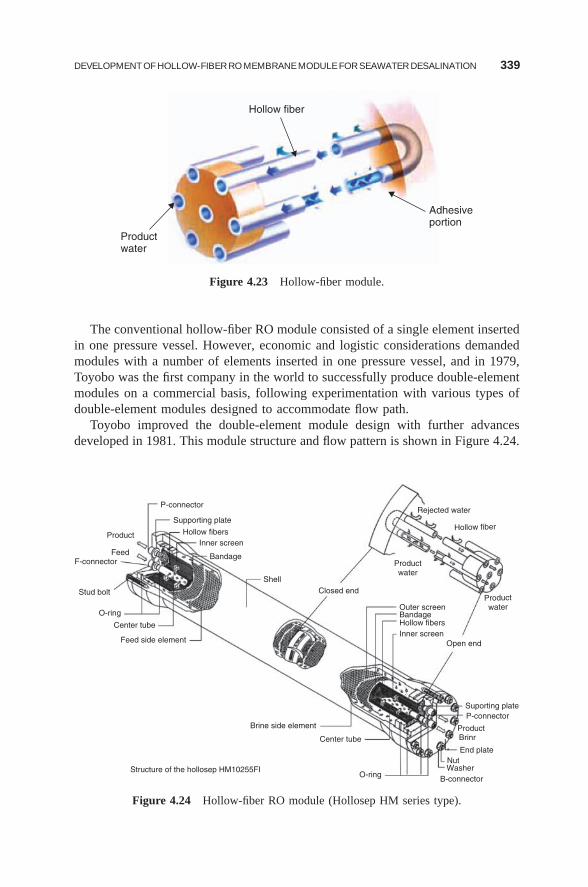
DEVELOPMENT OF HOLLOW-FIBER RO MEMBRANE MODULE FOR SEAWATER DESALINATION 339

Hollow fiber

Productwater

Adhesiveportion

Figure 4.23 Hollow-fiber module.

The conventional hollow-fiber RO module consisted of a single element insertedin one pressure vessel. However, economic and logistic considerations demandedmodules with a number of elements inserted in one pressure vessel, and in 1979,Toyobo was the first company in the world to successfully produce double-elementmodules on a commercial basis, following experimentation with various types ofdouble-element modules designed to accommodate flow path.

Toyobo improved the double-element module design with further advancesdeveloped in 1981. This module structure and flow pattern is shown in Figure 4.24.

P-connector

Supporting plate

Product

FeedF-connector

Stud bolt

O-ring

Center tube

Feed side element

Brine side element

Structure of the hollosep HM10255FI

Center tube

O-ring

Hollow fibersInner screen

Bandage

ShellClosed end

Outer screenBandageHollow fibersInner screen

Open end

Suporting plateP-connector

Product

End plateNutWasher

B-connector

Brinr

Productwater

Rejected water

Hollow fiber

Productwater

Figure 4.24 Hollow-fiber RO module (Hollosep HM series type).

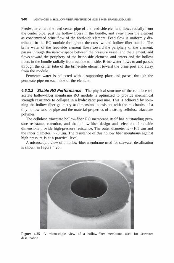
340 ADVANCES IN HOLLOW-FIBER REVERSE-OSMOSIS MEMBRANE MODULES

Feedwater enters the feed center pipe of the feed-side element, flows radially fromthe center pipe, past the hollow fibers in the bundle, and away from the elementas concentrated brine flow of the feed-side element. Feed flow is uniformly dis-tributed in the RO module throughout the cross-wound hollow-fiber bundle. Thebrine water of the feed-side element flows toward the periphery of the element,passes through the narrow space between the pressure vessel and the element, andflows toward the periphery of the brine-side element, and enters and the hollowfibers in the bundle radially from outside to inside. Brine water flows to and passesthrough the center tube of the brine-side element toward the brine port and awayfrom the module.

Permeate water is collected with a supporting plate and passes through thepermeate pipe on each side of the element.

4.5.2.2 Stable RO Performance The physical structure of the cellulose tri-acetate hollow-fiber membrane RO module is optimized to provide mechanicalstrength resistance to collapse in a hydrostatic pressure. This is achieved by spin-ning the hollow-fiber geometry at dimensions consistent with the mechanics of atiny hollow tube or pipe and the material properties of a strong cellulose triacetatepolymer.

The cellulose triacetate hollow-fiber RO membrane itself has outstanding pres-sure resistance retention, and the hollow-fiber design and selection of suitabledimensions provide high-pressure resistance. The outer diameter is ∼165 μm andthe inner diameter, ∼70 μm. The resistance of this hollow fiber membrane againsthigh pressure is at a practical level.

A microscopic view of a hollow-fiber membrane used for seawater desalinationis shown in Figure 4.25.

Figure 4.25 A microscopic view of a hollow-fiber membrane used for seawaterdesalination.

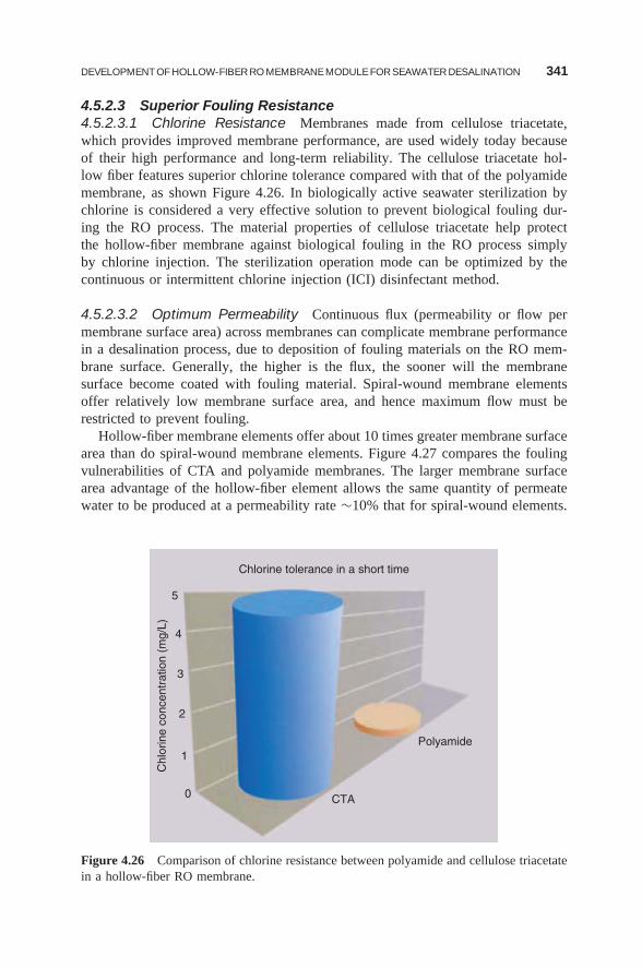
DEVELOPMENT OF HOLLOW-FIBER RO MEMBRANE MODULE FOR SEAWATER DESALINATION 341

4.5.2.3 Superior Fouling Resistance4.5.2.3.1 Chlorine Resistance Membranes made from cellulose triacetate,which provides improved membrane performance, are used widely today becauseof their high performance and long-term reliability. The cellulose triacetate hol-low fiber features superior chlorine tolerance compared with that of the polyamidemembrane, as shown Figure 4.26. In biologically active seawater sterilization bychlorine is considered a very effective solution to prevent biological fouling dur-ing the RO process. The material properties of cellulose triacetate help protectthe hollow-fiber membrane against biological fouling in the RO process simplyby chlorine injection. The sterilization operation mode can be optimized by thecontinuous or intermittent chlorine injection (ICI) disinfectant method.

4.5.2.3.2 Optimum Permeability Continuous flux (permeability or flow permembrane surface area) across membranes can complicate membrane performancein a desalination process, due to deposition of fouling materials on the RO mem-brane surface. Generally, the higher is the flux, the sooner will the membranesurface become coated with fouling material. Spiral-wound membrane elementsoffer relatively low membrane surface area, and hence maximum flow must berestricted to prevent fouling.

Hollow-fiber membrane elements offer about 10 times greater membrane surfacearea than do spiral-wound membrane elements. Figure 4.27 compares the foulingvulnerabilities of CTA and polyamide membranes. The larger membrane surfacearea advantage of the hollow-fiber element allows the same quantity of permeatewater to be produced at a permeability rate ∼10% that for spiral-wound elements.

Chlorine tolerance in a short time

Polyamide

CTA0

1

2

3

Chl

orin

e co

ncen

trat

ion

(mg/

L)

4

5

Figure 4.26 Comparison of chlorine resistance between polyamide and cellulose triacetatein a hollow-fiber RO membrane.

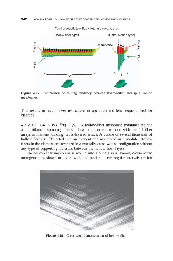
342 ADVANCES IN HOLLOW-FIBER REVERSE-OSMOSIS MEMBRANE MODULES

Fouling

Total productivity = flux x total membrane area

(Hollow fiber type)F

ouling

Membrane

(Spiral wound type)

Flux

Flux

Figure 4.27 Comparison of fouling tendency between hollow-fiber and spiral-woundmembranes.

This results in much fewer restrictions in operation and less frequent need forcleaning.

4.5.2.3.3 Cross-Winding Style A hollow-fiber membrane manufactured viaa multifilament spinning process allows element construction with parallel fiberarrays or filament winding, cross-layered arrays. A bundle of several thousands ofhollow fibers is fabricated into an element and assembled in a module. Hollowfibers in the element are arranged in a mutually cross-wound configuration withoutany type of supporting materials between the hollow-fiber layers.

The hollow-fiber membrane is wound into a bundle in a layered, cross-woundarrangement as shown in Figure 4.28, and moderate-size, regular intervals are left

Figure 4.28 Cross-wound arrangement of hollow fiber.

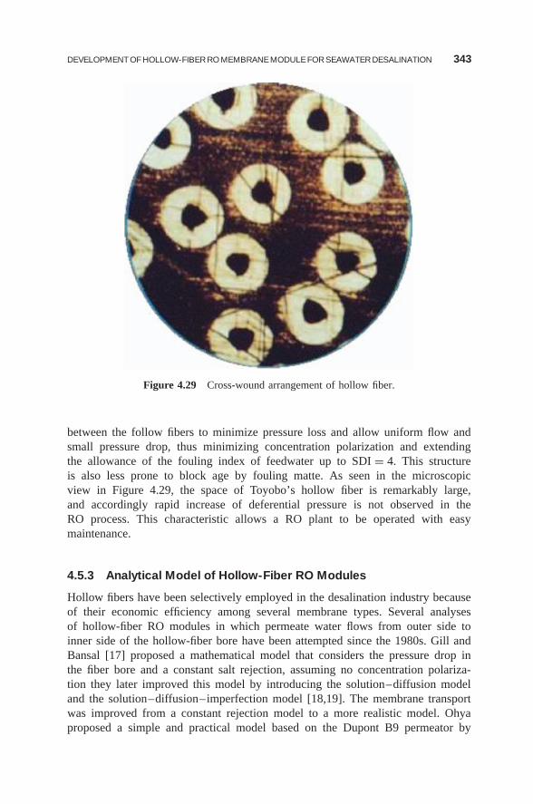
DEVELOPMENT OF HOLLOW-FIBER RO MEMBRANE MODULE FOR SEAWATER DESALINATION 343

Figure 4.29 Cross-wound arrangement of hollow fiber.

between the follow fibers to minimize pressure loss and allow uniform flow andsmall pressure drop, thus minimizing concentration polarization and extendingthe allowance of the fouling index of feedwater up to SDI = 4. This structureis also less prone to block age by fouling matte. As seen in the microscopicview in Figure 4.29, the space of Toyobo’s hollow fiber is remarkably large,and accordingly rapid increase of deferential pressure is not observed in theRO process. This characteristic allows a RO plant to be operated with easymaintenance.

4.5.3 Analytical Model of Hollow-Fiber RO Modules

Hollow fibers have been selectively employed in the desalination industry becauseof their economic efficiency among several membrane types. Several analysesof hollow-fiber RO modules in which permeate water flows from outer side toinner side of the hollow-fiber bore have been attempted since the 1980s. Gill andBansal [17] proposed a mathematical model that considers the pressure drop inthe fiber bore and a constant salt rejection, assuming no concentration polariza-tion they later improved this model by introducing the solution–diffusion modeland the solution–diffusion–imperfection model [18,19]. The membrane transportwas improved from a constant rejection model to a more realistic model. Ohyaproposed a simple and practical model based on the Dupont B9 permeator by

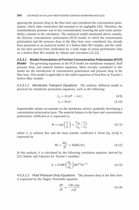
344 ADVANCES IN HOLLOW-FIBER REVERSE-OSMOSIS MEMBRANE MODULES

ignoring the pressure drop in the fiber bore and considered the concentration polar-ization, which other researchers had assumed to be negligible [20]. Therefore, thetransmembrane pressure was in fact overestimated, lowering the pure-water perme-ability constant in the calculation. The analytical model mentioned above, namely,the (friction–concentration–polarization (FCP) model, in which the concentrationpolarization and the pressure drop in the fiber bore were considered, has alreadybeen presented as an analytical model of a hollow-fiber RO module, and the valid-ity has been proved from verification by a wide range of actual performance dataon a hollow-fiber RO module by Sekino and coworkers [21,22].

4.5.3.1 Model Formulation of Friction Concentration Polarization (FCP)Model The governing equations in the FCP model are membrane transport, fluidpressure drop, and material balance equations. More recently considered in thismodel are the introduction of concentration polarization and pressure drop in thefiber bore. This model is applicable to the radial expansion of feed flow in Toyobo’shollow-fiber module.

4.5.3.1.1 Membrane Transport Equations The solution–diffusion model ispractical for membrane permeation equations, such as the following:

Jw = A(�P − �π) (4.9)

Js = B�C (4.10)

Impermeable solutes accumulate on the membrane surface, gradually developing aconcentration polarization layer. The material balance in the layer and concentrationpolarization coefficient φ is expressed as:

� = exp

(Jv

k

)= CM − CP

CB − CP(4.11)

where Jv is solution flux and the mass transfer coefficient k [from Eq. (4.4)] isexpressed by

Sh = kdO

D= Sh(Re,Sc) (4.12)

In this analysis, k is calculated by the following correlation equation, derived by[21] Sekino and Fujiwara for Toyobo’s modules:

k = 0.048

(DL

dO

)Re0.6Sc1/3 (4.13)

4.5.3.1.2 Fluid Pressure-Drop Equations The pressure drop in the fiber boreis expressed by the Hagen–Poiseuille equation:

dP

dz= 128 μQP

πd4I

(4.14)

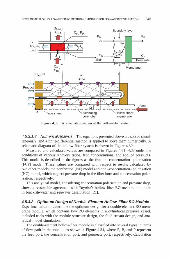
DEVELOPMENT OF HOLLOW-FIBER RO MEMBRANE MODULE FOR SEAWATER DESALINATION 345

Product

ΣSi,j Jv i,j

n

j = j

LS

z

r

Tube sheet

QB i+1,jCB i+1,j

CB i,j

QB i,j

Jv ij

ΔZ

Cpi,j Ppi,j

ΣSij Jv i,jn

j = j + 1

LA

Brine

Distributingcore tube

D

PBJV

CB

DI

D O

Bulk

Boundary layer

CM

δMembrane

DdCdx

Hollow fibbermembrane

PP

CP

Feed

Permeate

Figure 4.30 A schematic diagram of the hollow-fiber system.

4.5.3.1.3 Numerical Analysis The equations presented above are solved simul-taneously, and a finite-differential method is applied to solve them numerically. Aschematic diagram of the hollow-fiber system is shown in Figure 4.30.

Measured and calculated values are compared in Figures 4.31–4.33 under theconditions of various recovery ratios, feed concentrations, and applied pressures.This model is described in the figures as the friction–concentration–polarization(FCP) model. These values are compared with respect to results calculated bytwo other models, the nonfriction (NF) model and non–concentration–polarization(NC) model, which neglect pressure drop in the fiber bore and concentration polar-ization, respectively.

This analytical model, considering concentration polarization and pressure drop,shows a reasonable agreement with Toyobo’s hollow-fiber RO membrane modulein brackish-water and seawater desalination [21].

4.5.3.2 Optimum Design of Double-Element Hollow-Fiber RO ModuleExperimentation to determine the optimum design for a double-element RO mem-brane module, which contains two RO elements in a cylindrical pressure vessel,included trials with the module structure design, the fluid stream design, and ana-lytical model simulation.

The double-element hollow-fiber module is classified into several types in termsof flow path in the module as shown in Figure 4.34, where F, B, and P representthe feed port, the concentration port, and permeate port, respectively. Calculation

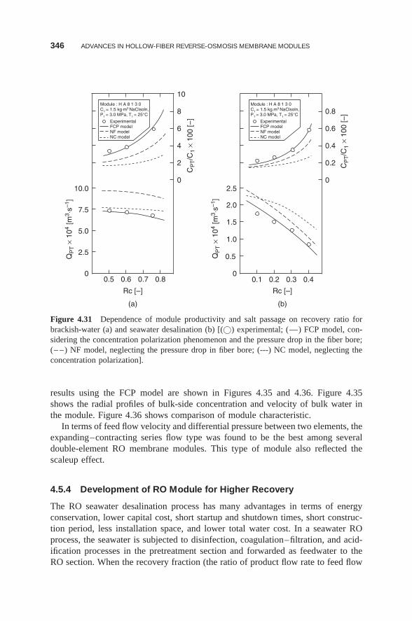
346 ADVANCES IN HOLLOW-FIBER REVERSE-OSMOSIS MEMBRANE MODULES

00.5 0.6 0.7

Rc [–]

(a)

Rc [–]

(b)

0.8

0

2

4

6

8ExperimentalFCP modelNF modelNC model

Module : H A 8 1 3 0C1 = 1.5 kg⋅m3 NaClsoln,P1 = 3.0 MPa, T1 = 25°C

10

2.5

5.0

7.5

10.0

00.1 0.2 0.3 0.4

0

0.2

0.4

0.6

0.8

0.5

1.0

1.5

2.0

2.5

QP

T ×

104

[m3 ⋅s

–1]

QP

T ×

104

[m3 ⋅s

–1]

CP

T/C

1 ×

100

[–]

CP

T/C

1 ×

100

[–]

ExperimentalFCP modelNF modelNC model

Module : H A 8 1 3 0C1 = 1.5 kg.m3 NaClsoln,P1 = 3.0 MPa, T1 = 25°C

Figure 4.31 Dependence of module productivity and salt passage on recovery ratio forbrackish-water (a) and seawater desalination (b) [(©) experimental; (—) FCP model, con-sidering the concentration polarization phenomenon and the pressure drop in the fiber bore;(– –) NF model, neglecting the pressure drop in fiber bore; (---) NC model, neglecting theconcentration polarization].

results using the FCP model are shown in Figures 4.35 and 4.36. Figure 4.35shows the radial profiles of bulk-side concentration and velocity of bulk water inthe module. Figure 4.36 shows comparison of module characteristic.

In terms of feed flow velocity and differential pressure between two elements, theexpanding–contracting series flow type was found to be the best among severaldouble-element RO membrane modules. This type of module also reflected thescaleup effect.

4.5.4 Development of RO Module for Higher Recovery

The RO seawater desalination process has many advantages in terms of energyconservation, lower capital cost, short startup and shutdown times, short construc-tion period, less installation space, and lower total water cost. In a seawater ROprocess, the seawater is subjected to disinfection, coagulation–filtration, and acid-ification processes in the pretreatment section and forwarded as feedwater to theRO section. When the recovery fraction (the ratio of product flow rate to feed flow

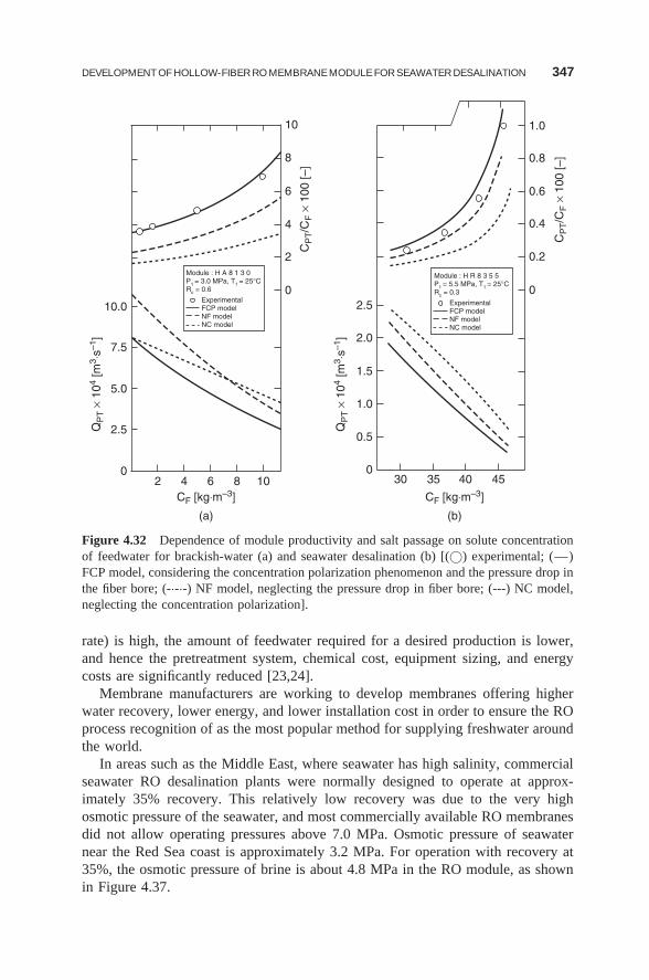
DEVELOPMENT OF HOLLOW-FIBER RO MEMBRANE MODULE FOR SEAWATER DESALINATION 347

20

2.5

5.0

7.5

10.00 0

0.2

0.4

0.6

0.8

1.0

2

4

6

8

10

4 6CF [kg⋅m–3]

(a)

CF [kg⋅m–3]

(b)

8 10 300

0.5

1.0

1.5

2.0

2.5

35 40 45

QP

T ×

104

[m3 ⋅s

–1]

QP

T ×

104

[m3 ⋅s

–1]

CP

T/C

F ×

100

[–]

CP

T/C

F ×

100

[–]

ExperimentalFCP modelNF modelNC model

Module : H A 8 1 3 0P1 = 3.0 MPa, T1 = 25°CRc = 0.6

ExperimentalFCP modelNF modelNC model

Module : H R 8 3 5 5P1 = 5.5 MPa, T1 = 25°CRc = 0.3

Figure 4.32 Dependence of module productivity and salt passage on solute concentrationof feedwater for brackish-water (a) and seawater desalination (b) [(©) experimental; (—)FCP model, considering the concentration polarization phenomenon and the pressure drop inthe fiber bore; (-·-·-) NF model, neglecting the pressure drop in fiber bore; (---) NC model,neglecting the concentration polarization].

rate) is high, the amount of feedwater required for a desired production is lower,and hence the pretreatment system, chemical cost, equipment sizing, and energycosts are significantly reduced [23,24].

Membrane manufacturers are working to develop membranes offering higherwater recovery, lower energy, and lower installation cost in order to ensure the ROprocess recognition of as the most popular method for supplying freshwater aroundthe world.

In areas such as the Middle East, where seawater has high salinity, commercialseawater RO desalination plants were normally designed to operate at approx-imately 35% recovery. This relatively low recovery was due to the very highosmotic pressure of the seawater, and most commercially available RO membranesdid not allow operating pressures above 7.0 MPa. Osmotic pressure of seawaternear the Red Sea coast is approximately 3.2 MPa. For operation with recovery at35%, the osmotic pressure of brine is about 4.8 MPa in the RO module, as shownin Figure 4.37.

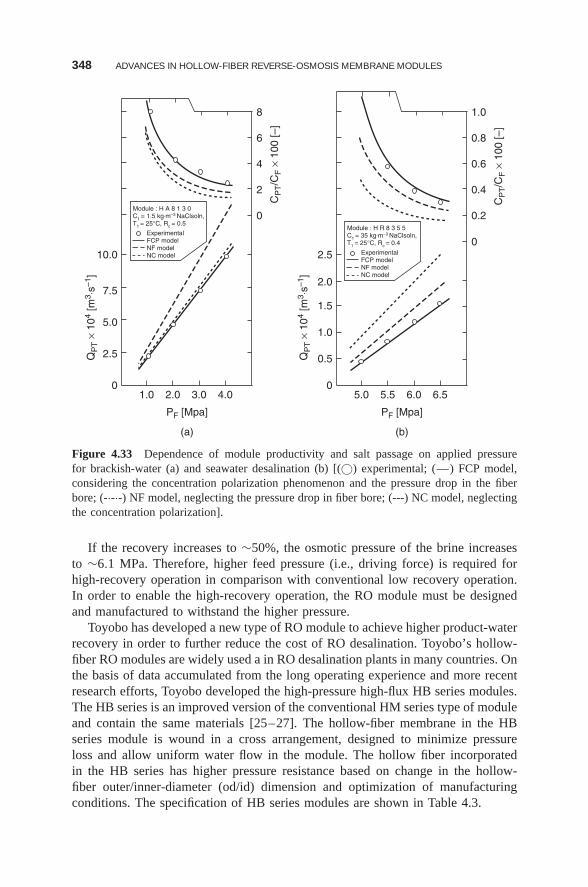
348 ADVANCES IN HOLLOW-FIBER REVERSE-OSMOSIS MEMBRANE MODULES

1.00

2.5QP

T ×

104

[m3 ⋅s

–1]

QP

T ×

104

[m3 ⋅s

–1]

CP

T/C

F ×

100

[–]

CP

T/C

F ×

100

[–]

5.0

7.5

10.0

0

2

4

6

8

2.0 3.0

PF [Mpa]

(a)

4.0 5.00

0.5

1.0

1.5

2.0

2.5

0.2

0

0.4

0.6

0.8

1.0

5.5 6.0

PF [Mpa]

(b)

6.5

ExperimentalFCP modelNF modelNC model

Module : H A 8 1 3 0C1 = 1.5 kg⋅m–3 NaClsoln,T1 = 25°C, Rc = 0.5

ExperimentalFCP modelNF modelNC model

Module : H R 8 3 5 5C1 = 35 kg⋅m–3 NaClsoln,T1 = 25°C, Rc = 0.4

Figure 4.33 Dependence of module productivity and salt passage on applied pressurefor brackish-water (a) and seawater desalination (b) [(©) experimental; (—) FCP model,considering the concentration polarization phenomenon and the pressure drop in the fiberbore; (-·-·-) NF model, neglecting the pressure drop in fiber bore; (---) NC model, neglectingthe concentration polarization].

If the recovery increases to ∼50%, the osmotic pressure of the brine increasesto ∼6.1 MPa. Therefore, higher feed pressure (i.e., driving force) is required forhigh-recovery operation in comparison with conventional low recovery operation.In order to enable the high-recovery operation, the RO module must be designedand manufactured to withstand the higher pressure.

Toyobo has developed a new type of RO module to achieve higher product-waterrecovery in order to further reduce the cost of RO desalination. Toyobo’s hollow-fiber RO modules are widely used a in RO desalination plants in many countries. Onthe basis of data accumulated from the long operating experience and more recentresearch efforts, Toyobo developed the high-pressure high-flux HB series modules.The HB series is an improved version of the conventional HM series type of moduleand contain the same materials [25–27]. The hollow-fiber membrane in the HBseries module is wound in a cross arrangement, designed to minimize pressureloss and allow uniform water flow in the module. The hollow fiber incorporatedin the HB series has higher pressure resistance based on change in the hollow-fiber outer/inner-diameter (od/id) dimension and optimization of manufacturingconditions. The specification of HB series modules are shown in Table 4.3.

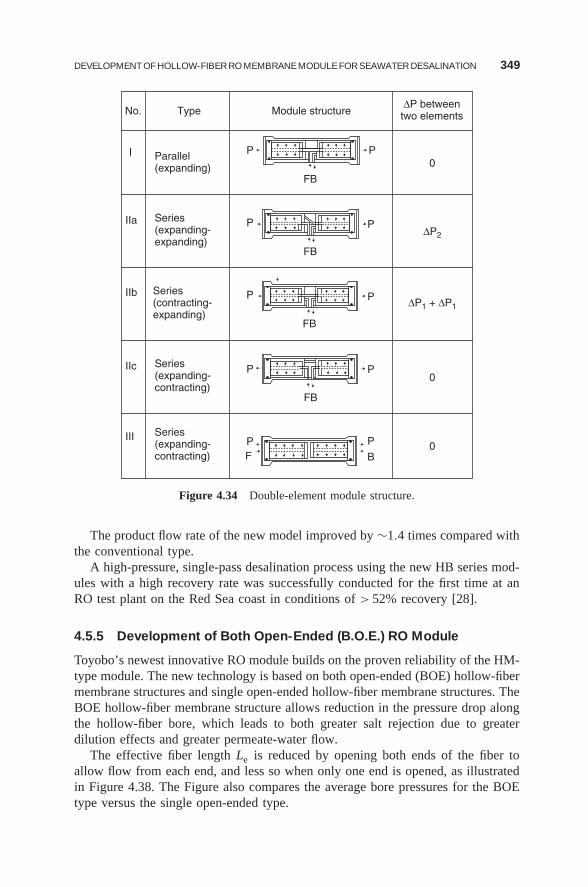
DEVELOPMENT OF HOLLOW-FIBER RO MEMBRANE MODULE FOR SEAWATER DESALINATION 349

No.

I

IIa

IIb

IIc

III

Type

Parallel(expanding)

Series(expanding-expanding)

Series(contracting-expanding)

Series(expanding-contracting)

Series(expanding-contracting)

Module structureΔP betweentwo elements

P

P

P

P

B

P

FB

FB

FB

FB

P

P

P

P

PF

0

ΔP2

ΔP1 + ΔP1

0

0

Figure 4.34 Double-element module structure.

The product flow rate of the new model improved by ∼1.4 times compared withthe conventional type.

A high-pressure, single-pass desalination process using the new HB series mod-ules with a high recovery rate was successfully conducted for the first time at anRO test plant on the Red Sea coast in conditions of > 52% recovery [28].

4.5.5 Development of Both Open-Ended (B.O.E.) RO Module

Toyobo’s newest innovative RO module builds on the proven reliability of the HM-type module. The new technology is based on both open-ended (BOE) hollow-fibermembrane structures and single open-ended hollow-fiber membrane structures. TheBOE hollow-fiber membrane structure allows reduction in the pressure drop alongthe hollow-fiber bore, which leads to both greater salt rejection due to greaterdilution effects and greater permeate-water flow.

The effective fiber length Le is reduced by opening both ends of the fiber toallow flow from each end, and less so when only one end is opened, as illustratedin Figure 4.38. The Figure also compares the average bore pressures for the BOEtype versus the single open-ended type.

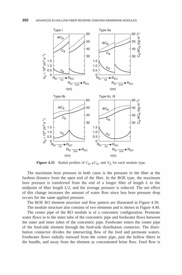
350 ADVANCES IN HOLLOW-FIBER REVERSE-OSMOSIS MEMBRANE MODULES

00.51.0

1.5

30

1stREI REO

40

50

60Type I

ΦCB

ΦCB ΦCB

ΦCB

CB

CB CB

CB

VB

VB VB

VB

2ndREI REO

00.51.0

1.530

40

50

60Type IIa

00.51.0

1.530

40

50

60Type IIb

r(m)

1stREI REO

2ndREI REO

r(m)

1stREI REO

2ndREI REO

r(m)

1stREI REO

2ndREI REO

r(m)

00.51.0

1.530

40

50

60Type IIc, III

VB ×

104

(m3 ⋅s

–1)

VB ×

104

(m3 ⋅s

–1)

CB,Φ

CB (

kg⋅m

–3)

CB,Φ

CB (

kg⋅m

–3)

Figure 4.35 Radial profiles of CB, ϕCB, and VB for each module type.

The maximum bore pressure in both cases is the pressure in the fiber at thefurthest distance from the open end of the fiber. In the BOE type, the maximumbore pressure is transferred from the end of a longer fiber of length L to themidpoint of fiber length L/2, and the average pressure is reduced. The net effectof this change increases the amount of water flow since less bore pressure dropoccurs for the same applied pressure.

The BOE RO element structure and flow pattern are illustrated in Figure 4.39.The module structure also consists of two elements and is shown in Figure 4.40.The center pipe of the RO module is of a concentric configuration. Permeate

water flows in to the inner tube of the concentric pipe and feedwater flows betweenthe outer and inner tubes of the concentric pipe. Feedwater enters the center pipeof the feed-side element through the feed-side distribution connector. The distri-bution connector divides the intersecting flow of the feed and permeate waters.Feedwater flows radially outward from the center pipe, past the hollow fibers inthe bundle, and away from the element as concentrated brine flow. Feed flow is

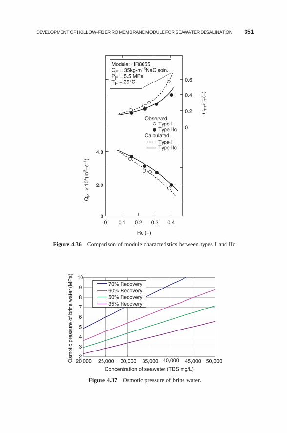
DEVELOPMENT OF HOLLOW-FIBER RO MEMBRANE MODULE FOR SEAWATER DESALINATION 351

00

2.0

4.0

QP

T ×

104 (

m3 –

s–1)

0

0.2Observed

Calculated

Type IType IIc

Type IType IIc

CP

T/C

F(–

)

0.4

0.6

0.1 0.2 0.3

Rc (–)

0.4

Module: HR8655CF = 35kg-m–3NaClsoin.PF = 5.5 MPaTF = 25°C

Figure 4.36 Comparison of module characteristics between types I and IIc.

2

3

4

5

6

7

8

9

10

50,00025,000

Concentration of seawater (TDS mg/L)

Osm

otic

pre

ssur

e of

brin

e w

ater

(M

Pa)

70% Recovery60% Recovery50% Recovery35% Recovery

20,000 30,000 35,000 40,000 45,000

Figure 4.37 Osmotic pressure of brine water.

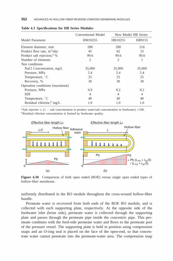
352 ADVANCES IN HOLLOW-FIBER REVERSE-OSMOSIS MEMBRANE MODULES

Table 4.3 Specifications for HB Series Modules

Conventional Model New Model HB Series

Model Parameter HM10255 HB10255 HB9155

Element diameter, mm 280 280 216Product flow rate, m3/day 45 62 15Product salt rejection,a % 99.6 99.6 99.6Number of elements 2 2 1Test conditions

NaCl Concentration, mg/L 35,000 35,000 35,000Pressure, MPa 5.4 5.4 5.4Temperature, ◦C 25 25 25Recovery, % 30 30 30

Operation conditions (maximum)Pressure, MPa 6.9 8.2 8.2SDI 4 4 4Temperature, ◦C 40 40 40Residual chlorine,b mg/L 1.0 1.0 1.0

aSalt rejecton = (1 − salt concentration in product water/salt concentration in feedwater) ×100.bResidual chlorine concentration is limited by feedwater quality.

Adhesive resin

Hollow fiber Hollow fiber

Effective fiber length LeEffective fiber length Le

0

(a)

0

PbPb

Pd

LL/2

= Pb (LTS + LE/2)/ (LTS + LE/3)

(b)

Figure 4.38 Comparison of both open ended (BOE) versus single open ended types ofhollow-fiber membrane.

uniformly distributed in the RO module throughout the cross-wound hollow-fiberbundle.

Permeate water is recovered from both ends of the BOE RO module, and iscollected with each supporting plate, respectively. At the opposite side of thefeedwater inlet (brine side), permeate water is collected through the supportingplate and passes through the permeate pipe inside the concentric pipe. This per-meate combines with the feed-side permeate water and flows to the permeate portof the pressure vessel. The supporting plate is held in position using compressionsnaps and an O-ring seal is placed on the face of the open-end, so that concen-trate water cannot penetrate into the permeate-water area. The compression snap

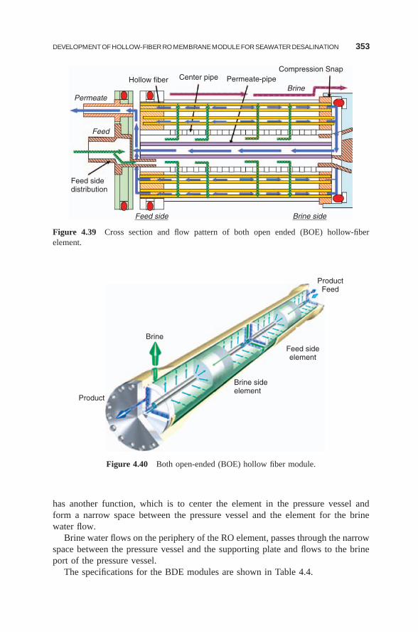
DEVELOPMENT OF HOLLOW-FIBER RO MEMBRANE MODULE FOR SEAWATER DESALINATION 353

Hollow fiber

PermeateBrine

Permeate-pipeCompression Snap

Feed

Center pipe

Feed sidedistribution

Feed side Brine side

Figure 4.39 Cross section and flow pattern of both open ended (BOE) hollow-fiberelement.

ProductFeed

Feed sideelement

Brine sideelement

Product

Brine

Figure 4.40 Both open-ended (BOE) hollow fiber module.

has another function, which is to center the element in the pressure vessel andform a narrow space between the pressure vessel and the element for the brinewater flow.

Brine water flows on the periphery of the RO element, passes through the narrowspace between the pressure vessel and the supporting plate and flows to the brineport of the pressure vessel.

The specifications for the BDE modules are shown in Table 4.4.

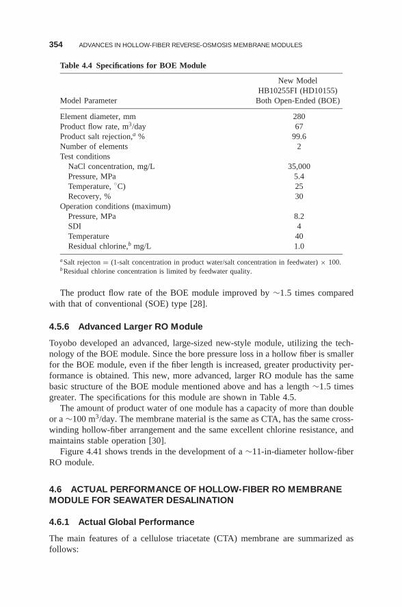
354 ADVANCES IN HOLLOW-FIBER REVERSE-OSMOSIS MEMBRANE MODULES

Table 4.4 Specifications for BOE Module

New ModelHB10255FI (HD10155)

Model Parameter Both Open-Ended (BOE)

Element diameter, mm 280Product flow rate, m3/day 67Product salt rejection,a % 99.6Number of elements 2Test conditions

NaCl concentration, mg/L 35,000Pressure, MPa 5.4Temperature, ◦C) 25Recovery, % 30

Operation conditions (maximum)Pressure, MPa 8.2SDI 4Temperature 40Residual chlorine,b mg/L 1.0

aSalt rejecton = (1-salt concentration in product water/salt concentration in feedwater) × 100.bResidual chlorine concentration is limited by feedwater quality.

The product flow rate of the BOE module improved by ∼1.5 times comparedwith that of conventional (SOE) type [28].

4.5.6 Advanced Larger RO Module

Toyobo developed an advanced, large-sized new-style module, utilizing the tech-nology of the BOE module. Since the bore pressure loss in a hollow fiber is smallerfor the BOE module, even if the fiber length is increased, greater productivity per-formance is obtained. This new, more advanced, larger RO module has the samebasic structure of the BOE module mentioned above and has a length ∼1.5 timesgreater. The specifications for this module are shown in Table 4.5.

The amount of product water of one module has a capacity of more than doubleor a ∼100 m3/day. The membrane material is the same as CTA, has the same cross-winding hollow-fiber arrangement and the same excellent chlorine resistance, andmaintains stable operation [30].

Figure 4.41 shows trends in the development of a ∼11-in-diameter hollow-fiberRO module.

4.6 ACTUAL PERFORMANCE OF HOLLOW-FIBER RO MEMBRANEMODULE FOR SEAWATER DESALINATION

4.6.1 Actual Global Performance

The main features of a cellulose triacetate (CTA) membrane are summarized asfollows:

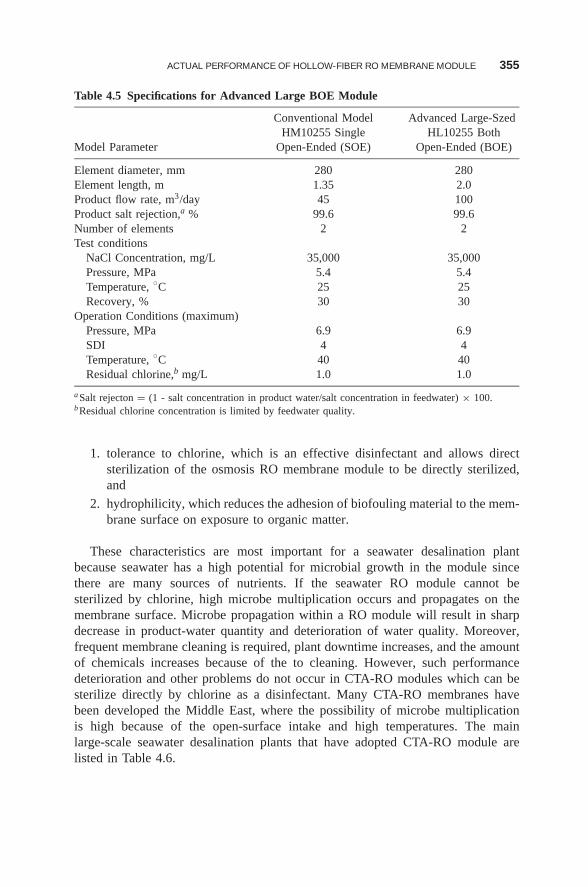
ACTUAL PERFORMANCE OF HOLLOW-FIBER RO MEMBRANE MODULE 355

Table 4.5 Specifications for Advanced Large BOE Module

Conventional Model Advanced Large-SzedHM10255 Single HL10255 Both

Model Parameter Open-Ended (SOE) Open-Ended (BOE)

Element diameter, mm 280 280Element length, m 1.35 2.0Product flow rate, m3/day 45 100Product salt rejection,a % 99.6 99.6Number of elements 2 2Test conditions

NaCl Concentration, mg/L 35,000 35,000Pressure, MPa 5.4 5.4Temperature, ◦C 25 25Recovery, % 30 30

Operation Conditions (maximum)Pressure, MPa 6.9 6.9SDI 4 4Temperature, ◦C 40 40Residual chlorine,b mg/L 1.0 1.0

aSalt rejecton = (1 - salt concentration in product water/salt concentration in feedwater) × 100.bResidual chlorine concentration is limited by feedwater quality.

1. tolerance to chlorine, which is an effective disinfectant and allows directsterilization of the osmosis RO membrane module to be directly sterilized,and

2. hydrophilicity, which reduces the adhesion of biofouling material to the mem-brane surface on exposure to organic matter.

These characteristics are most important for a seawater desalination plantbecause seawater has a high potential for microbial growth in the module sincethere are many sources of nutrients. If the seawater RO module cannot besterilized by chlorine, high microbe multiplication occurs and propagates on themembrane surface. Microbe propagation within a RO module will result in sharpdecrease in product-water quantity and deterioration of water quality. Moreover,frequent membrane cleaning is required, plant downtime increases, and the amountof chemicals increases because of the to cleaning. However, such performancedeterioration and other problems do not occur in CTA-RO modules which can besterilize directly by chlorine as a disinfectant. Many CTA-RO membranes havebeen developed the Middle East, where the possibility of microbe multiplicationis high because of the open-surface intake and high temperatures. The mainlarge-scale seawater desalination plants that have adopted CTA-RO module arelisted in Table 4.6.

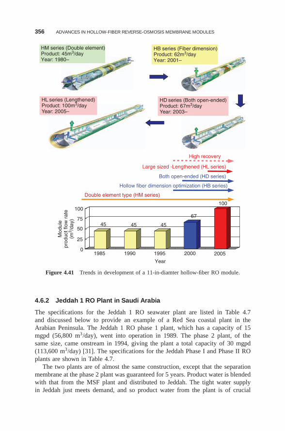
356 ADVANCES IN HOLLOW-FIBER REVERSE-OSMOSIS MEMBRANE MODULES

45 45 45

67

100

0

25

50

75

100

Mod

ule

prod

uct f

low

rat

e(m

3 /da

y)

1985 1990 1995 2000 2005

Year

Double element type (HM series)

Hollow fiber dimension optimization (HB series)

Both open-ended (HD series)

Large sized -Lengthened (HL series)

High recovery

HB series (Fiber dimension)Product: 62m3/dayYear: 2001–

HD series (Both open-ended)Product: 67m3/dayYear: 2003–

HM series (Double element)Product: 45m3/dayYear: 1980–

HL series (Lengthened)Product: 100m3/dayYear: 2005–

Figure 4.41 Trends in development of a 11-in-diamter hollow-fiber RO module.

4.6.2 Jeddah 1 RO Plant in Saudi Arabia

The specifications for the Jeddah 1 RO seawater plant are listed in Table 4.7and discussed below to provide an example of a Red Sea coastal plant in theArabian Peninsula. The Jeddah 1 RO phase 1 plant, which has a capacity of 15mgpd (56,800 m3/day), went into operation in 1989. The phase 2 plant, of thesame size, came onstream in 1994, giving the plant a total capacity of 30 mgpd(113,600 m3/day) [31]. The specifications for the Jeddah Phase I and Phase II ROplants are shown in Table 4.7.

The two plants are of almost the same construction, except that the separationmembrane at the phase 2 plant was guaranteed for 5 years. Product water is blendedwith that from the MSF plant and distributed to Jeddah. The tight water supplyin Jeddah just meets demand, and so product water from the plant is of crucial

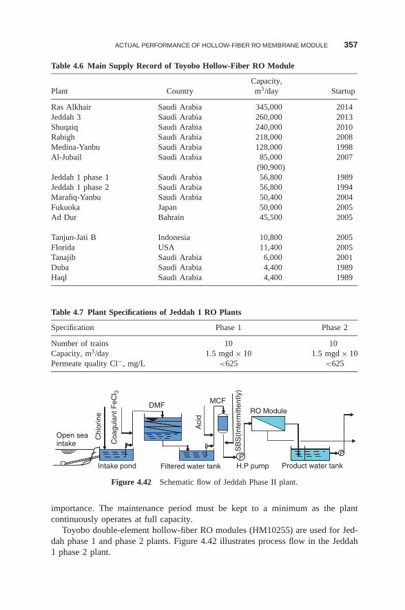
ACTUAL PERFORMANCE OF HOLLOW-FIBER RO MEMBRANE MODULE 357

Table 4.6 Main Supply Record of Toyobo Hollow-Fiber RO Module

Capacity,Plant Country m3/day Startup

Ras Alkhair Saudi Arabia 345,000 2014Jeddah 3 Saudi Arabia 260,000 2013Shuqaiq Saudi Arabia 240,000 2010Rabigh Saudi Arabia 218,000 2008Medina-Yanbu Saudi Arabia 128,000 1998Al-Jubail Saudi Arabia 85,000 2007

(90,900)Jeddah 1 phase 1 Saudi Arabia 56,800 1989Jeddah 1 phase 2 Saudi Arabia 56,800 1994Marafiq-Yanbu Saudi Arabia 50,400 2004Fukuoka Japan 50,000 2005Ad Dur Bahrain 45,500 2005

Tanjun-Jati B Indonesia 10,800 2005Florida USA 11,400 2005Tanajib Saudi Arabia 6,000 2001Duba Saudi Arabia 4,400 1989Haql Saudi Arabia 4,400 1989

Table 4.7 Plant Specifications of Jeddah 1 RO Plants

Specification Phase 1 Phase 2

Number of trains 10 10Capacity, m3/day 1.5 mgd × 10 1.5 mgd × 10Permeate quality Cl−, mg/L <625 <625

SB

S(I

nter

mitt

ently

)

P P

Filtered water tank Product water tankH.P pump

MCFRO Module

DMF

Chl

orin

e

Coa

gula

nt F

eCl 3

Aci

d

Open seaintake

Intake pond

Figure 4.42 Schematic flow of Jeddah Phase II plant.

importance. The maintenance period must be kept to a minimum as the plantcontinuously operates at full capacity.

Toyobo double-element hollow-fiber RO modules (HM10255) are used for Jed-dah phase 1 and phase 2 plants. Figure 4.42 illustrates process flow in the Jeddah1 phase 2 plant.

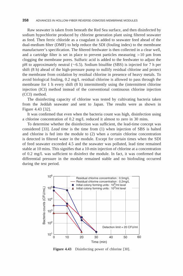
358 ADVANCES IN HOLLOW-FIBER REVERSE-OSMOSIS MEMBRANE MODULES

Raw seawater is taken from beneath the Red Sea surface, and then disinfected bysodium hypochlorite produced by chlorine generation plant using filtered seawateras feed. Then ferric chloride as a coagulant is added to seawater feed ahead of thedual-medium filter (DMF) to help reduce the SDI (fouling index) to the membranemanufacturer’s specification. The filtered feedwater is then collected in a clear well,and a cartridge filter is set in place to prevent particles measuring >10 μm fromclogging the membrane pores. Sulfuric acid is added to the feedwater to adjust thepH to approximately neutral (∼6.5). Sodium bisulfite (SBS) is injected for 7 h pershift (8 h) ahead of the high-pressure pump to nullify residual chlorine and protectthe membrane from oxidation by residual chlorine in presence of heavy metals. Toavoid biological fouling, 0.2 mg/L residual chlorine is allowed to pass through themembrane for 1 h every shift (8 h) intermittently using the (intermittent chlorineinjection (ICI) method instead of the conventional continuous chlorine injection(CCI) method.

The disinfecting capacity of chlorine was tested by cultivating bacteria takenfrom the Jeddah seawater and sent to Japan. The results were as shown inFigure 4.43 [32].

It was confirmed that even when the bacteria count was high, disinfection usinga chlorine concentration of 0.2 mg/L reduced it almost to zero in 30 mins.

To determine whether the disinfection was sufficient, the lead-time concept wasconsidered [33]. Lead time is the time from (1) when injection of SBS is haltedand chlorine is fed into the module to (2) when a certain chlorine concentrationis detected in filtered water in the module. Except for certain times when the SDIof feed seawater exceeded 4.5 and the seawater was polluted, lead time remainedstable at 10 mins. This signifies that a 10-min injection of chlorine at a concentrationof 0.2 mg/L was sufficient to disinfect the module. In fact, it was confirmed thatdifferential pressure in the module remained stable and no biofouling occurredduring the test period.

Bac

teria

coun

ts (

CF

U/m

L)

Time (min)

0 10 20 30 40 50 60

106

105

104

103

102

101

Residual chlorine concentration : 0.5mg/L Residual chlorine concentration : 0.2mg/L Initial colony forming units : 105/ml levelInitial colony forming units : 103/ml level

Detection limit = 20 CFU/ml

Figure 4.43 Disinfecting power of chlorine [30].

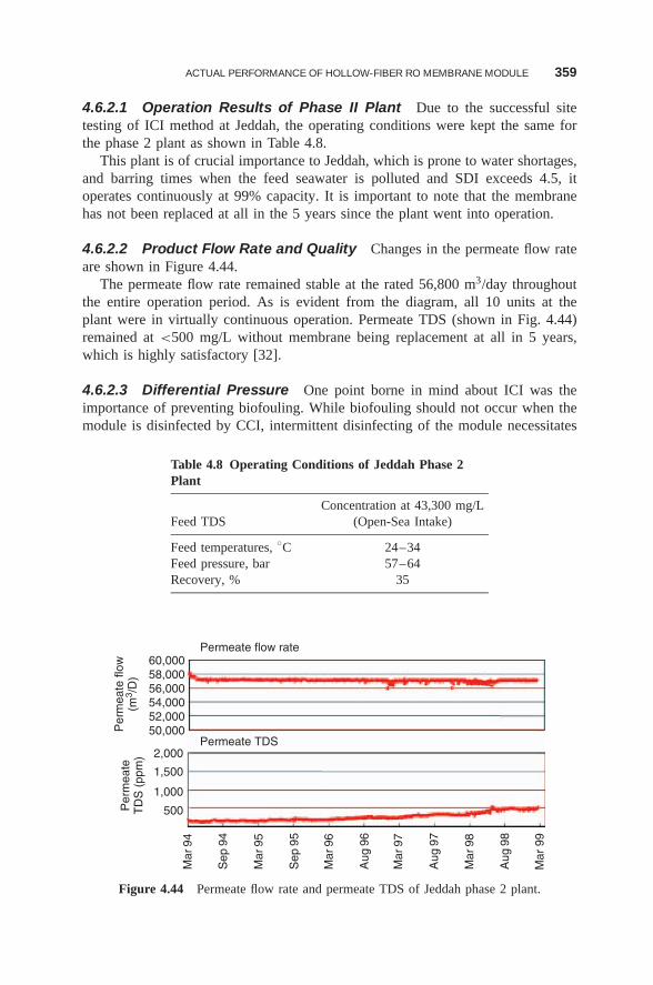
ACTUAL PERFORMANCE OF HOLLOW-FIBER RO MEMBRANE MODULE 359

4.6.2.1 Operation Results of Phase II Plant Due to the successful sitetesting of ICI method at Jeddah, the operating conditions were kept the same forthe phase 2 plant as shown in Table 4.8.

This plant is of crucial importance to Jeddah, which is prone to water shortages,and barring times when the feed seawater is polluted and SDI exceeds 4.5, itoperates continuously at 99% capacity. It is important to note that the membranehas not been replaced at all in the 5 years since the plant went into operation.

4.6.2.2 Product Flow Rate and Quality Changes in the permeate flow rateare shown in Figure 4.44.

The permeate flow rate remained stable at the rated 56,800 m3/day throughoutthe entire operation period. As is evident from the diagram, all 10 units at theplant were in virtually continuous operation. Permeate TDS (shown in Fig. 4.44)remained at <500 mg/L without membrane being replacement at all in 5 years,which is highly satisfactory [32].

4.6.2.3 Differential Pressure One point borne in mind about ICI was theimportance of preventing biofouling. While biofouling should not occur when themodule is disinfected by CCI, intermittent disinfecting of the module necessitates

Table 4.8 Operating Conditions of Jeddah Phase 2Plant

Concentration at 43,300 mg/LFeed TDS (Open-Sea Intake)

Feed temperatures, ◦C 24–34Feed pressure, bar 57–64Recovery, % 35

Permeate flow rate60,00058,000

Per

mea

te fl

ow(m

3 /D

)P

erm

eate

TD

S (

ppm

)

56,00054,00052,00050,000

2,000

1,500

1,000

500

Mar

94

Sep

94

Mar

95

Sep

95

Mar

96

Mar

97

Mar

98

Mar

99

Aug

96

Aug

97

Aug

98

Permeate TDS

Figure 4.44 Permeate flow rate and permeate TDS of Jeddah phase 2 plant.

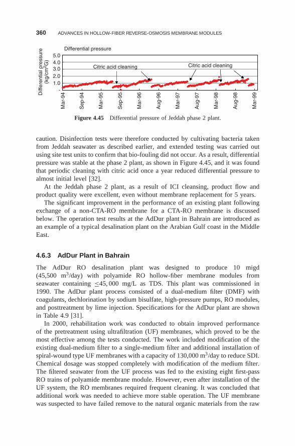
360 ADVANCES IN HOLLOW-FIBER REVERSE-OSMOSIS MEMBRANE MODULES

Differential pressure5.04.03.02.01.0

Diff

eren

tial p

ress

ure

(kg/

cm2 G

)

-

Mar

-94

Sep

-94

Mar

-95

Sep

-95

Mar

-96

Aug

-96

Mar

-97

Aug

-97

Mar

-98

Aug

-98

Mar

-99

Citric acid cleaning Citric acid cleaning

Figure 4.45 Differential pressure of Jeddah phase 2 plant.

caution. Disinfection tests were therefore conducted by cultivating bacteria takenfrom Jeddah seawater as described earlier, and extended testing was carried outusing site test units to confirm that bio-fouling did not occur. As a result, differentialpressure was stable at the phase 2 plant, as shown in Figure 4.45, and it was foundthat periodic cleaning with citric acid once a year reduced differential pressure toalmost initial level [32].

At the Jeddah phase 2 plant, as a result of ICI cleansing, product flow andproduct quality were excellent, even without membrane replacement for 5 years.

The significant improvement in the performance of an existing plant followingexchange of a non-CTA-RO membrane for a CTA-RO membrane is discussedbelow. The operation test results at the AdDur plant in Bahrain are introduced asan example of a typical desalination plant on the Arabian Gulf coast in the MiddleEast.

4.6.3 AdDur Plant in Bahrain

The AdDur RO desalination plant was designed to produce 10 migd(45,500 m3/day) with polyamide RO hollow-fiber membrane modules fromseawater containing ≤45, 000 mg/L as TDS. This plant was commissioned in1990. The AdDur plant process consisted of a dual-medium filter (DMF) withcoagulants, dechlorination by sodium bisulfate, high-pressure pumps, RO modules,and posttreatment by lime injection. Specifications for the AdDur plant are shownin Table 4.9 [31].

In 2000, rehabilitation work was conducted to obtain improved performanceof the pretreatment using ultrafiltration (UF) membranes, which proved to be themost effective among the tests conducted. The work included modification of theexisting dual-medium filter to a single-medium filter and additional installation ofspiral-wound type UF membranes with a capacity of 130,000 m3/day to reduce SDI.Chemical dosage was stopped completely with modification of the medium filter.The filtered seawater from the UF process was fed to the existing eight first-passRO trains of polyamide membrane module. However, even after installation of theUF system, the RO membranes required frequent cleaning. It was concluded thatadditional work was needed to achieve more stable operation. The UF membranewas suspected to have failed remove to the natural organic materials from the raw

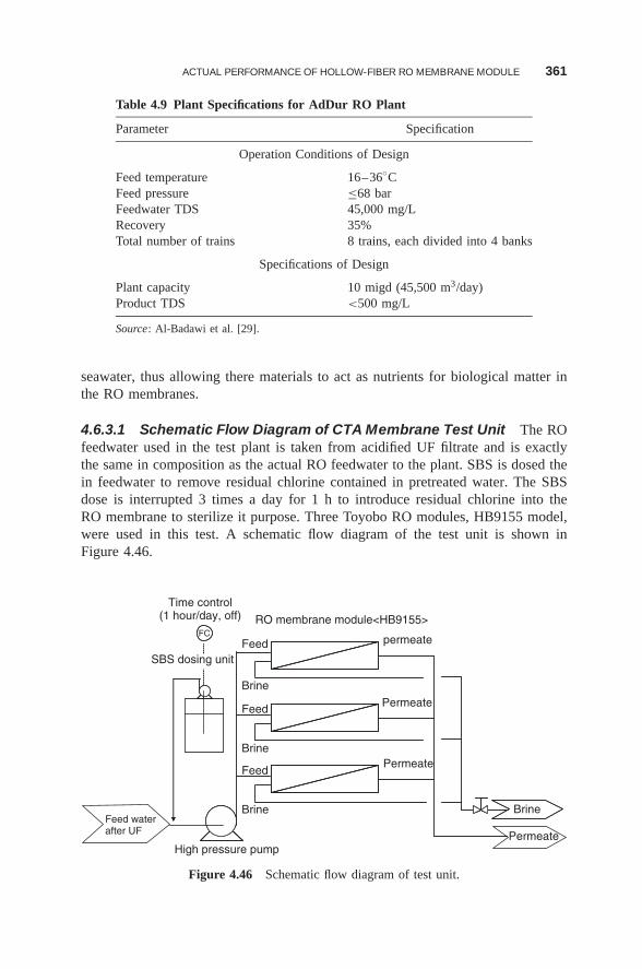
ACTUAL PERFORMANCE OF HOLLOW-FIBER RO MEMBRANE MODULE 361

Table 4.9 Plant Specifications for AdDur RO Plant

Parameter Specification

Operation Conditions of Design

Feed temperature 16–36◦CFeed pressure ≤68 barFeedwater TDS 45,000 mg/LRecovery 35%Total number of trains 8 trains, each divided into 4 banks

Specifications of Design

Plant capacity 10 migd (45,500 m3/day)Product TDS <500 mg/L

Source: Al-Badawi et al. [29].

seawater, thus allowing there materials to act as nutrients for biological matter inthe RO membranes.

4.6.3.1 Schematic Flow Diagram of CTA Membrane Test Unit The ROfeedwater used in the test plant is taken from acidified UF filtrate and is exactlythe same in composition as the actual RO feedwater to the plant. SBS is dosed thein feedwater to remove residual chlorine contained in pretreated water. The SBSdose is interrupted 3 times a day for 1 h to introduce residual chlorine into theRO membrane to sterilize it purpose. Three Toyobo RO modules, HB9155 model,were used in this test. A schematic flow diagram of the test unit is shown inFigure 4.46.

Feed waterafter UF

Feed permeate

Brine

Feed

Brine

FeedPermeate

Brine

FC

Time control(1 hour/day, off)

Permeate

Brine

RO membrane module<HB9155>

High pressure pump

Permeate

SBS dosing unit

Figure 4.46 Schematic flow diagram of test unit.

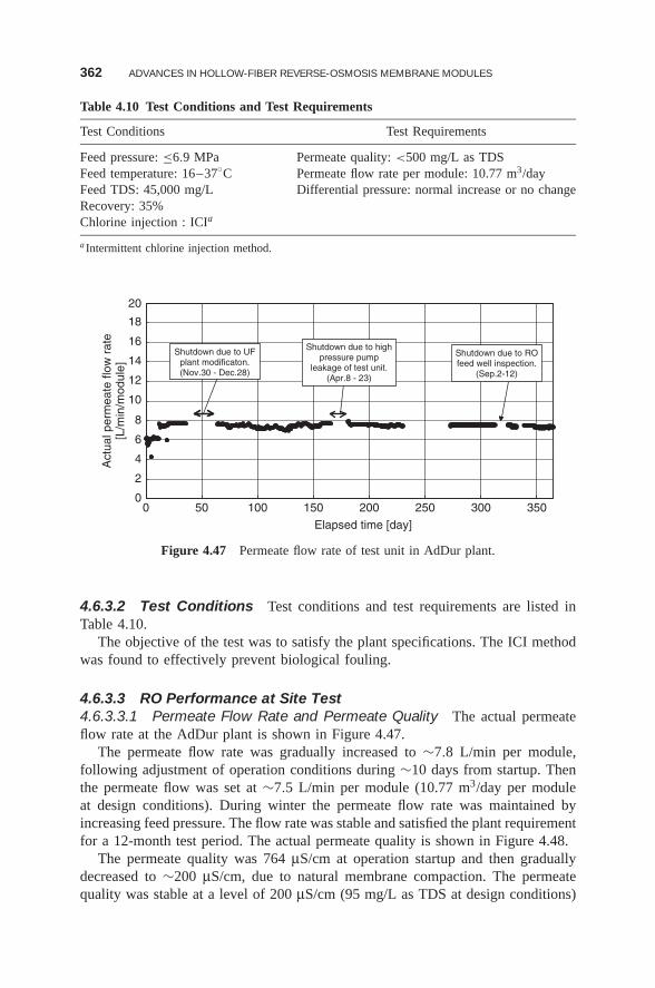
362 ADVANCES IN HOLLOW-FIBER REVERSE-OSMOSIS MEMBRANE MODULES

Table 4.10 Test Conditions and Test Requirements

Test Conditions Test Requirements

Feed pressure: ≤6.9 MPa Permeate quality: <500 mg/L as TDSFeed temperature: 16–37◦C Permeate flow rate per module: 10.77 m3/dayFeed TDS: 45,000 mg/L Differential pressure: normal increase or no changeRecovery: 35%Chlorine injection : ICIa

a Intermittent chlorine injection method.

0

2

4

6

8

10

12

14

16

18

20

0 50 100 150 200 250 300 350

Elapsed time [day]

Act

ual p

erm

eate

flow

rat

e[L

/min

/mod

ule]

Shutdown due to UFplant modificaton.(Nov.30 - Dec.28)

Shutdown due to highpressure pump

leakage of test unit.(Apr.8 - 23)

Shutdown due to ROfeed well inspection.

(Sep.2-12)

Figure 4.47 Permeate flow rate of test unit in AdDur plant.

4.6.3.2 Test Conditions Test conditions and test requirements are listed inTable 4.10.

The objective of the test was to satisfy the plant specifications. The ICI methodwas found to effectively prevent biological fouling.

4.6.3.3 RO Performance at Site Test4.6.3.3.1 Permeate Flow Rate and Permeate Quality The actual permeateflow rate at the AdDur plant is shown in Figure 4.47.

The permeate flow rate was gradually increased to ∼7.8 L/min per module,following adjustment of operation conditions during ∼10 days from startup. Thenthe permeate flow was set at ∼7.5 L/min per module (10.77 m3/day per moduleat design conditions). During winter the permeate flow rate was maintained byincreasing feed pressure. The flow rate was stable and satisfied the plant requirementfor a 12-month test period. The actual permeate quality is shown in Figure 4.48.

The permeate quality was 764 μS/cm at operation startup and then graduallydecreased to ∼200 μS/cm, due to natural membrane compaction. The permeatequality was stable at a level of 200 μS/cm (95 mg/L as TDS at design conditions)

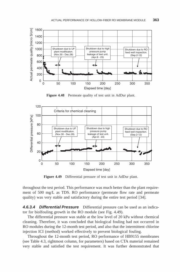
ACTUAL PERFORMANCE OF HOLLOW-FIBER RO MEMBRANE MODULE 363

0

200

400

600

800

1000

1200

1400

1600

0 50 100 150 200 250 300 350

Elapsed time [day]

Act

ual p

erm

eate

qua

lity

[mic

ro S

/cm

]

Shutdown due to ROfeed well inspection.

(Sep.2-12)

Shutdown due to UFplant modificaton.(Nov.30 - Dec.28)

Shutdown due to highpressure pump

leakage of test unit.(Apr.8 - 23)

Figure 4.48 Permeate quality of test unit in AdDur plant.

0

20

40

60

80

100

120

0 50 100 150 200 250 300 350

Elapsed time [day]

Diff

eren

tial p

ress

ure

[kP

a]

Shutdown due to UFplant modificaton.(Nov.30 - Dec.28)

Shutdown due to highpressure pump

leakage of test unit.(Apr.8 - 23)

Shutdown due to ROfeed well inspection.

(Sep.2-12)

Criteria for chemical cleaning

Figure 4.49 Differential pressure of test unit in AdDur plant.

throughout the test period. This performance was much better than the plant require-ment of 500 mg/L as TDS. RO performance (permeate flow rate and permeatequality) was very stable and satisfactory during the entire test period [34].

4.6.3.4 Differential Pressure Differential pressure can be used as an indica-tor for biolfouling growth in the RO module (see Fig. 4.49).

The differential pressure was stable at the low level of 20 kPa without chemicalcleaning. Therefore, it was concluded that biological fouling had not occurred inRO modules during the 12-month test period, and also that the intermittent chlorineinjection ICI (method) worked effectively to prevent biological fouling.

Throughout the 12-month test period, RO performance of HB9155 membranes(see Table 4.3, rightmost column, for parameters) based on CTA material remainedvery stable and satisfied the test requirement. It was further demonstrated that

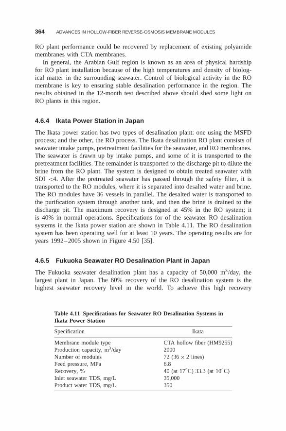
364 ADVANCES IN HOLLOW-FIBER REVERSE-OSMOSIS MEMBRANE MODULES

RO plant performance could be recovered by replacement of existing polyamidemembranes with CTA membranes.

In general, the Arabian Gulf region is known as an area of physical hardshipfor RO plant installation because of the high temperatures and density of biolog-ical matter in the surrounding seawater. Control of biological activity in the ROmembrane is key to ensuring stable desalination performance in the region. Theresults obtained in the 12-month test described above should shed some light onRO plants in this region.

4.6.4 Ikata Power Station in Japan

The Ikata power station has two types of desalination plant: one using the MSFDprocess; and the other, the RO process. The Ikata desalination RO plant consists ofseawater intake pumps, pretreatment facilities for the seawater, and RO membranes.The seawater is drawn up by intake pumps, and some of it is transported to thepretreatment facilities. The remainder is transported to the discharge pit to dilute thebrine from the RO plant. The system is designed to obtain treated seawater withSDI <4. After the pretreated seawater has passed through the safety filter, it istransported to the RO modules, where it is separated into desalted water and brine.The RO modules have 36 vessels in parallel. The desalted water is transported tothe purification system through another tank, and then the brine is drained to thedischarge pit. The maximum recovery is designed at 45% in the RO system; itis 40% in normal operations. Specifications for of the seawater RO desalinationsystems in the Ikata power station are shown in Table 4.11. The RO desalinationsystem has been operating well for at least 10 years. The operating results are foryears 1992–2005 shown in Figure 4.50 [35].

4.6.5 Fukuoka Seawater RO Desalination Plant in Japan

The Fukuoka seawater desalination plant has a capacity of 50,000 m3/day, thelargest plant in Japan. The 60% recovery of the RO desalination system is thehighest seawater recovery level in the world. To achieve this high recovery

Table 4.11 Specifications for Seawater RO Desalination Systems inIkata Power Station

Specification Ikata

Membrane module type CTA hollow fiber (HM9255)Production capacity, m3/day 2000Number of modules 72 (36 × 2 lines)Feed pressure, MPa 6.8Recovery, % 40 (at 17◦C) 33.3 (at 10◦C)Inlet seawater TDS, mg/L 35,000Product water TDS, mg/L 350

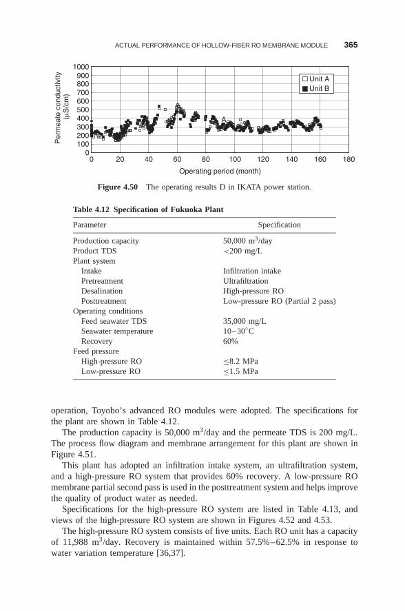
ACTUAL PERFORMANCE OF HOLLOW-FIBER RO MEMBRANE MODULE 365

0100200300400500600700800900

1000

0 20 40 60 80 100 120 140 160 180

Operating period (month)

Per

mea

te c

ondu

ctiv

ity

(μS

/cm

)

A

Unit AUnit B

Figure 4.50 The operating results D in IKATA power station.

Table 4.12 Specification of Fukuoka Plant

Parameter Specification

Production capacity 50,000 m3/dayProduct TDS <200 mg/LPlant system

Intake Infiltration intakePretreatment UltrafiltrationDesalination High-pressure ROPosttreatment Low-pressure RO (Partial 2 pass)

Operating conditionsFeed seawater TDS 35,000 mg/LSeawater temperature 10–30◦CRecovery 60%

Feed pressureHigh-pressure RO ≤8.2 MPaLow-pressure RO ≤1.5 MPa

operation, Toyobo’s advanced RO modules were adopted. The specifications forthe plant are shown in Table 4.12.

The production capacity is 50,000 m3/day and the permeate TDS is 200 mg/L.The process flow diagram and membrane arrangement for this plant are shown inFigure 4.51.

This plant has adopted an infiltration intake system, an ultrafiltration system,and a high-pressure RO system that provides 60% recovery. A low-pressure ROmembrane partial second pass is used in the posttreatment system and helps improvethe quality of product water as needed.

Specifications for the high-pressure RO system are listed in Table 4.13, andviews of the high-pressure RO system are shown in Figures 4.52 and 4.53.

The high-pressure RO system consists of five units. Each RO unit has a capacityof 11,988 m3/day. Recovery is maintained within 57.5%–62.5% in response towater variation temperature [36,37].

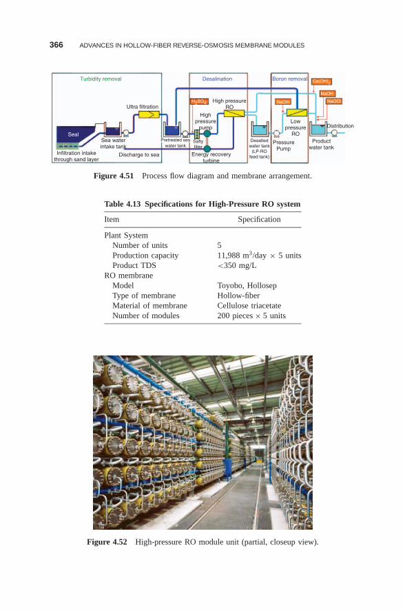
366 ADVANCES IN HOLLOW-FIBER REVERSE-OSMOSIS MEMBRANE MODULES

Turbidity removal

Ultra filtration

Desalination Boron removal

Sea waterintake tank

Discharge to sea Energy recoveryturbine

Saftyfilter

Highpressure

pump

High pressureRO

Lowpressure

RO

PressurePump

Desaltedwater tank

(LP-ROfeed tank)

Productwater tank

Distribution

H2SO4 NaOH

Ca(OH)2

NaOH

NaOCl

Infiltration intakethrough sand layer

SealPretreated sea

water tank

Figure 4.51 Process flow diagram and membrane arrangement.

Table 4.13 Specifications for High-Pressure RO system

Item Specification

Plant SystemNumber of units 5Production capacity 11,988 m3/day × 5 unitsProduct TDS <350 mg/L

RO membraneModel Toyobo, HollosepType of membrane Hollow-fiberMaterial of membrane Cellulose triacetateNumber of modules 200 pieces × 5 units

Figure 4.52 High-pressure RO module unit (partial, closeup view).

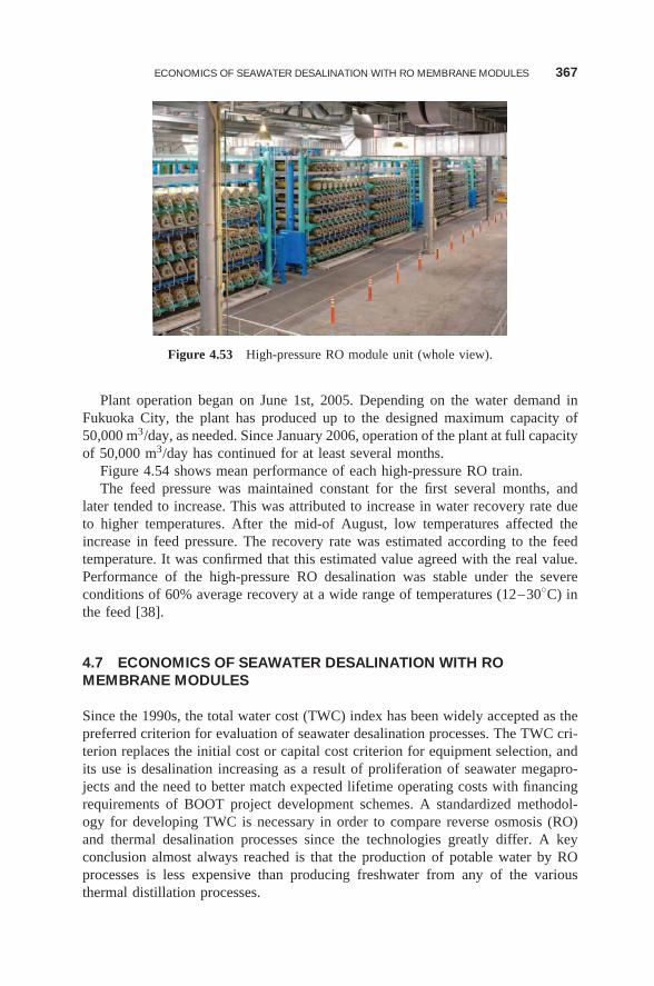
ECONOMICS OF SEAWATER DESALINATION WITH RO MEMBRANE MODULES 367

Figure 4.53 High-pressure RO module unit (whole view).

Plant operation began on June 1st, 2005. Depending on the water demand inFukuoka City, the plant has produced up to the designed maximum capacity of50,000 m3/day, as needed. Since January 2006, operation of the plant at full capacityof 50,000 m3/day has continued for at least several months.

Figure 4.54 shows mean performance of each high-pressure RO train.The feed pressure was maintained constant for the first several months, and

later tended to increase. This was attributed to increase in water recovery rate dueto higher temperatures. After the mid-of August, low temperatures affected theincrease in feed pressure. The recovery rate was estimated according to the feedtemperature. It was confirmed that this estimated value agreed with the real value.Performance of the high-pressure RO desalination was stable under the severeconditions of 60% average recovery at a wide range of temperatures (12–30◦C) inthe feed [38].

4.7 ECONOMICS OF SEAWATER DESALINATION WITH ROMEMBRANE MODULES

Since the 1990s, the total water cost (TWC) index has been widely accepted as thepreferred criterion for evaluation of seawater desalination processes. The TWC cri-terion replaces the initial cost or capital cost criterion for equipment selection, andits use is desalination increasing as a result of proliferation of seawater megapro-jects and the need to better match expected lifetime operating costs with financingrequirements of BOOT project development schemes. A standardized methodol-ogy for developing TWC is necessary in order to compare reverse osmosis (RO)and thermal desalination processes since the technologies greatly differ. A keyconclusion almost always reached is that the production of potable water by ROprocesses is less expensive than producing freshwater from any of the variousthermal distillation processes.

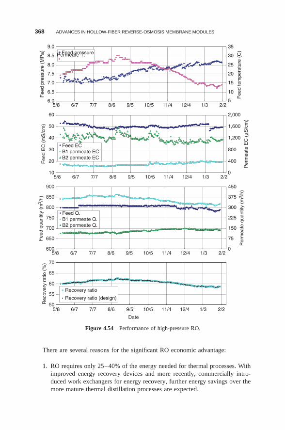
368 ADVANCES IN HOLLOW-FIBER REVERSE-OSMOSIS MEMBRANE MODULES

Date

6.0

6.5

7.0

7.5

8.0

8.5

9.0F

eed

pres

sure

(M

Pa)

5

10

15

20

25

30

35

Fee

d te

mpe

ratu

re (

C)Feed pressurePermeate T.

5/8 6/7 7/7 8/6 9/5 10/5 11/4 12/4 1/3 2/2

10

20

30

40

50

60

Fee

d E

C (

mS

/cm

)

0

400

800

1,200

1,600

2,000

Per

mea

te E

C (

μS/c

m)

Feed ECB1 permeate ECB2 permeate EC

5/8 6/7 7/7 8/6 9/5 10/5 11/4 12/4 1/3 2/2

600

650

700

750

800

850

900

Fee

d qu

antit

y (m

3 /h)

0

75

150

225

300

375

450

Per

mea

te q

uant

ity (

m3 /

h)

Feed Q.B1 permeate Q.B2 permeate Q.

5/8 6/7 7/7 8/6 9/5 10/5 11/4 12/4 1/3 2/2

50

55

60

65

70

Rec

over

y ra

tio (

%)

Recovery ratio

Recovery ratio (design)

5/8 6/7 7/7 8/6 9/5 10/5 11/4 12/4 1/3 2/2

Figure 4.54 Performance of high-pressure RO.

There are several reasons for the significant RO economic advantage:

1. RO requires only 25–40% of the energy needed for thermal processes. Withimproved energy recovery devices and more recently, commercially intro-duced work exchangers for energy recovery, further energy savings over themore mature thermal distillation processes are expected.

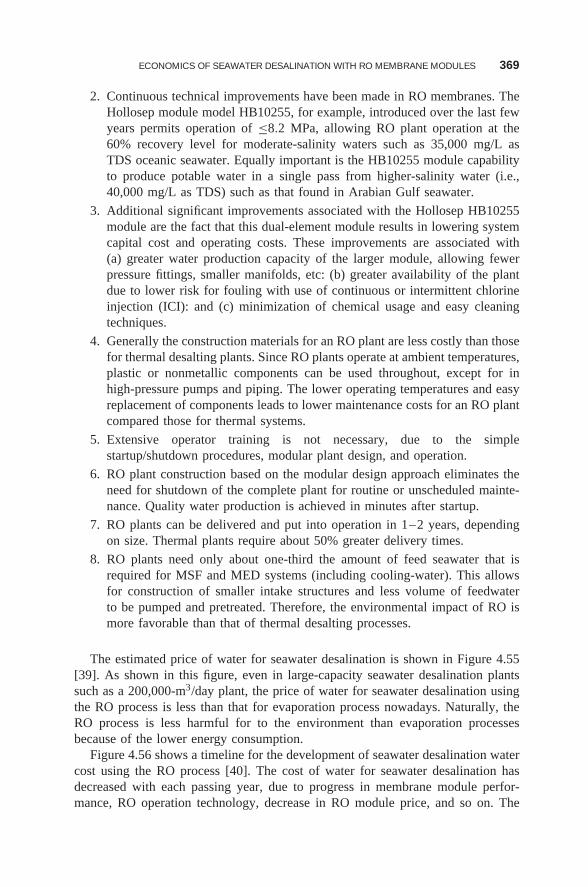
ECONOMICS OF SEAWATER DESALINATION WITH RO MEMBRANE MODULES 369

2. Continuous technical improvements have been made in RO membranes. TheHollosep module model HB10255, for example, introduced over the last fewyears permits operation of ≤8.2 MPa, allowing RO plant operation at the60% recovery level for moderate-salinity waters such as 35,000 mg/L asTDS oceanic seawater. Equally important is the HB10255 module capabilityto produce potable water in a single pass from higher-salinity water (i.e.,40,000 mg/L as TDS) such as that found in Arabian Gulf seawater.

3. Additional significant improvements associated with the Hollosep HB10255module are the fact that this dual-element module results in lowering systemcapital cost and operating costs. These improvements are associated with(a) greater water production capacity of the larger module, allowing fewerpressure fittings, smaller manifolds, etc: (b) greater availability of the plantdue to lower risk for fouling with use of continuous or intermittent chlorineinjection (ICI): and (c) minimization of chemical usage and easy cleaningtechniques.

4. Generally the construction materials for an RO plant are less costly than thosefor thermal desalting plants. Since RO plants operate at ambient temperatures,plastic or nonmetallic components can be used throughout, except for inhigh-pressure pumps and piping. The lower operating temperatures and easyreplacement of components leads to lower maintenance costs for an RO plantcompared those for thermal systems.

5. Extensive operator training is not necessary, due to the simplestartup/shutdown procedures, modular plant design, and operation.

6. RO plant construction based on the modular design approach eliminates theneed for shutdown of the complete plant for routine or unscheduled mainte-nance. Quality water production is achieved in minutes after startup.

7. RO plants can be delivered and put into operation in 1–2 years, dependingon size. Thermal plants require about 50% greater delivery times.

8. RO plants need only about one-third the amount of feed seawater that isrequired for MSF and MED systems (including cooling-water). This allowsfor construction of smaller intake structures and less volume of feedwaterto be pumped and pretreated. Therefore, the environmental impact of RO ismore favorable than that of thermal desalting processes.

The estimated price of water for seawater desalination is shown in Figure 4.55[39]. As shown in this figure, even in large-capacity seawater desalination plantssuch as a 200,000-m3/day plant, the price of water for seawater desalination usingthe RO process is less than that for evaporation process nowadays. Naturally, theRO process is less harmful for to the environment than evaporation processesbecause of the lower energy consumption.

Figure 4.56 shows a timeline for the development of seawater desalination watercost using the RO process [40]. The cost of water for seawater desalination hasdecreased with each passing year, due to progress in membrane module perfor-mance, RO operation technology, decrease in RO module price, and so on. The

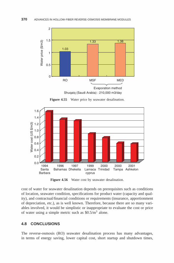
370 ADVANCES IN HOLLOW-FIBER REVERSE-OSMOSIS MEMBRANE MODULES

1.03

1.33 1.38

0

0.5

1

1.5

2

RO MSF MED

Wat

er p

rice

($/m

3)

Evaporation method

Shuqaiq (Saudi Arabia) : 210,000 m3/day

Figure 4.55 Water price by seawater desalination.

0.0

0.2

0.4

0.6

0.8

1.0

1.2

1.4

1.6

Wat

er c

ost (

US

$/m

3)

1994Santa

Barbara

1996Bahamas

1997Dhekelia

1999Larnacacyprus

2000Trinidad

2000Tampa

2001Ashkelon

Figure 4.56 Water cost by seawater desalination.

cost of water for seawater desalination depends on prerequisites such as conditionsof location, seawater condition, specifications for product water (capacity and qual-ity), and contractual/financial conditions or requirements (insurance, apportionmentof depreciation, etc.), as is well known. Therefore, because there are so many vari-ables involved, it would be simplistic or inappropriate to evaluate the cost or priceof water using a simple metric such as $0.5/m3 alone.

4.8 CONCLUSIONS

The reverse-osmosis (RO) seawater desalination process has many advantages,in terms of energy saving, lower capital cost, short startup and shutdown times,

CONCLUSIONS 371

short construction period, less installation space needed, and less total water cost.The RO process is becoming the key technology for obtaining freshwater fromthe sea, especially in the Middle East. Desalination equipment manufacturers areworking to develop membranes offering higher product-water recovery, lowerenergy consumption, and lower installation costs, in the hopes that the RO processwill be adopted worldwide as the most reliable, efficient method for supplyingfreshwater.

Reverse-osmosis membranes were first developed from cellulose acetate (CA)and cellulose triacetate (CTA). These CA and CTA membranes have been incommercial use for many years. The CTA membrane, in particular is still usedthroughout the world. This wide spread use demonstrates the superior properties ofCTA in RO membranes. As for performance, the coexistence of high permeabilityand high selectivity is enabled by an outstanding balance of hydrophilic andhydrophobic properties in the CTA RO membrane. Moreover, the CTA membraneis the only RO membrane currently marketed that offers such a high degree ofchlorine resistance. The intermittent chlorine injection (ICI) method is effectivewith the CTA membrane to control biofouling growth and allows stable opera-tion in seawater desalination plants, especially in the Middle East, where thereis very high biofouling potential due to high seawater temperatures. RO mem-branes that not are chlorine-resistant are biofouling, more susceptible to whichprevents the RO plants, from operating in stable mode because of the need for fre-quent cleaning. In those cases where CTA membranes have replaced non-chlorine-tolerant RO membranes because of the risk of biofouling, stable operation has beenattained.

Moreover, the CTA material, when used in hollow-fiber bundles, offers excellentresistance to biofouling because it is generally hydrophilic, reducing the potentialfor adhesion of organic material to the membrane surface. Also, a hollow-fiberCTA module element provides a membrane area that is ∼10 times larger perunit volume than that provided by a spiral wound membrane element, and thisproperty significantly reduces the flux per unit membrane area. Therefore, withCTA it is possible to decrease membrane load, which helps prevent biofouling, tooccur. These key attributes lead to minimal chemical cleaning and long membranelife.

At the time of writing, CTA-RO hollow-fiber membrane technology contin-ues to expand throughout the world, especially in seawater desalination appli-cations. This technology is expected to contribute significantly to the increasingglobal demand for freshwater. With high-volume commercial operation of large-scale, recently constructed desalination plants in the Middle East and North Africa[e.g., the Hamma desalination plant, Algeria, with a capacity of 200,000 m3/day(73 million m3/year)] now well underway, with plans for future plant installationsin thos areas, CTA-based hollow-fiber RO membrane technology—developed pri-marily by Toyobo Co., Ltd. of Japan—seems to be the premier method for seawaterdesalination.

372 ADVANCES IN HOLLOW-FIBER REVERSE-OSMOSIS MEMBRANE MODULES

NOMENCLATURE

Symbols

A pure-water permeability constantB solute transport constantC solute concentrationD diffusion coefficientdI inner diameter of hollow fiberdO outer diameter of hollow fiberJS solute flux through membraneJV solution flux through membraneJW water flux through membranek mass transfer coefficientP pressureQ flow rateRc recovery ratioRe Reynolds number, do Vρ/μSc Schmidt number, μ/ρDSh Sherwood number, kdO/DTFW Feedwater temperatureV fluid velocityz axial coordinate� differenceμ viscosityρ densityπ osmotic pressureφ concentration polarization

Subscripts

B bulkF feedP permeate

REFERENCES

1. Reid CE, Breton EJ, Water and ion flow across cellulosic membranes, J. Appl. Polym.Sci . 1:133 (1959).

2. Loeb S, Sourirajan S, High Flow Porous Membranes for Separating Water from SalineSolutions , US Patent 3,133,132 (1964).

REFERENCES 373

3. Breton EJ, Water and ionic flow through osmotic membranes OSWRDP Report 16, NewYork, 1957.

4. Westmoreland JC, Spirally Wrapped Reverse Osmosis Membrane Cell , US Patent3,367,504, (1968).

5. McCutchan JW, Johnson JS, Reverse osmosis at Coalinga, California, European Feder-ation of Chemical Engineering, J. Am Water Works Assoc., 62:346 (1970).

6. Mahon HI, Permeability Separatory Apparatus, Permeability Separatory Membrane Ele-ment, Method of Making the Same and Process Utilizing the Same, US Patent 3,228,876(1966).

7. Dance EL, Davis TE, Mahon HI, McLain EA, Skiens WE, Spano JO, Development ofCellulose Triacetate Hollow Fiber Reverse Osmosis Modules for Brackish-Water Desali-nation , OSWRDP Report 763, New York, 1971.

8. Ammons RD, Mahon HI, Development of a One-Pass Hollow-Fiber SeawaterDesalination Module Having a Capacity of 2500–3000 gpd , Report 924, US Officeof Saline Water Research and Development Program (OSWRDP), US GovernmentPrinting Office, Washington, DC, 1974.

9. Orofino TA, Development of Hollow Filament Technology for Reverse Osmosis Desali-nation Systems , OSWRDP Report 549, 1970.

10. Ukai T, Nimura Y, Hamada K, Matsui H, Development of one pass sea water reverseosmosis module,“HOLLOSEP”, Desalination 32:169 (1980).

11. Aptel P, Buckley CA, Categories of membrane operations, in Mallevialle J, OdendaalPE, Wiesne MR, eds., Water Treatment Membrane Processes , McGraw-Hill, Johannes-burg, 1996, p. 2.16.

12. Kumano A, Reverse osmosis membranes and the method of formation, Seikei-Kakou14(12):766 (2002).

13. Nita K, The aromatic polyamide hollow fiber reverse osmosis membrane with chlorineresistance, Plant Process , (Japan) 34(2):63 (1992).

14. Ohya H, An expression method of compaction effects on reverse osmosis membranesat high pressure operation, Desalination 26:163 (1978).

15. Kumano A, Matsui Y, Numata K, Fujiwara N, Iwahashi H, Nagai M, Performancechange formula of cellulose triacetate hollow fiber RO membranes due to oxidation andhydrolysis Desalination , 96:451 (1994).

16. Kannari T, Module performance monitoring system, Proc. IDA World Congress Desali-nation and Water Reuse, IDA, Abu Dhabi, 1995, Vol. 3, pp. 3–11.

17. Gill WN, Bansal B, Hollow fiber reverse osmosis systems analysis and design, Am. Inst.Chem Eng. (AIChE) J . 19:823 (1973).

18. Dandavati MS, Doshi MR, Gill WN, Hollow fiber reverse osmosis experiments andanalysis of radial flow systems, Chem. Eng. Sci . 30:877 (1975).

19. Kabadi VN, Doshi MR, Gill WN, Radial flow hollow fiber reverse osmosis experimentsand theory, Chem. Eng. Commun . 3:339 (1979).

20. Ohya H, Nakajima H, Takagi K, Kagawa S, Negishi Y, An analysis of reverse osmoticcharacteristics of B-9 hollow fiber module, Desalination 21:257 (1977).

21. Sekino M, Fujiwara N, Analysis of hollow- fiber reverse- osmosis module, KagakuKogaku Ronbunshu 17:1088 (1991).

374 ADVANCES IN HOLLOW-FIBER REVERSE-OSMOSIS MEMBRANE MODULES

22. Sekino M, Precise analytical model of hollow fiber reverse osmosis modules, J. Mem-brane Sci . 85:241 (1993).

23. Ohya H, Suzuki T, Nakao S, Kato S, Tsuji M, Sugi J, Proposal and technologicalbreakthrough of an integrated system for the complete usage of sea water, Bulle. Soc.Sea Water Sci . (Japan), 50(6):389 (1996).

24. Nakao S, Sea water desalination process for high recovery of fresh water by reverseosmosis, Bull. Soc. Sea Water Sci. (Japan), 50(6):406 (1996).

25. Ohnishi J, Nita K, Sekino M, Development of high permeate flow rate and high pressureresistance RO module for seawater desalination, Proc. IDA World Congress Desalinationand Water Reuse, IDA, Madrid, Oct. 6–9, 1997, pp. 479–489.

26. Sekino M, Important conditions and present state for seawater desalination RO module,Bull. Soc. Sea Water Sci . (Japan) 52(2):107 (1998).

27. Fujiwara N, Tanaka T, Kumano A, Sekino M, New economical RO desalination systemby a recovery ratio of 60%, Proc. IDA World Congress Desalination and Water Reuse,IDA, San Diego, CA (USA), Aug. 29–Sept. 3, 1999, pp. 101–109.

28. Kumano A, Fujiwara N, Nishida M, Sekino M, A single-stage RO seawater desalinationprocess at higher recovery with improved hollow fiber membrane modules, Proc. IDAWorld Congress Desalination and Water Reuse, IDA, Paradise Island, Bahamas, Sept.28–Oct. 3, 2003.

29. Kumano A, Focus on the high pressure and high recovery operation system and sin-gle stage RO module in Fukuoka plant, Bull. Soc. Sea Water Sci . (Japan) 58(3):248(2004).

30. Marui K, Kumano A, Kotera H, Fujiwara N, Tanaka T, Sekino M, Higher recovery withimproved hollow fiber membrane modules, Proc. IDA World Congress Desalination andWater Reuse, IDA, Paradise Island, Bahamas, Sept. 28–Oct. 3, 2003.

31. Al-Badawi AR, Al-Harthi SS, Imai H, Iwahashi H, Katsube M, Fujiwara N, Operationand analysis of Jeddah 1—phase 2 Plant, Proc. IDA World Congress Desalination andWater Reuse, IDA, Abu Dhabi, UAE, Nov. 18–24, 1995, Vol. 3, pp. 41–53.

32. Fujiwara N, Tanaka T, Katsube M, Farhan MA, Al-Harthi ASS, Imai H, IwahashiH, Five-year operational performance of membrane at 15 MGPD Jeddah RO phase 2plant, Proc. IDA World Congress Desalination and Water Reuse, IDA, San Diego, Aug.29–Sept. 3, 1999, pp. 89–98.

33. Nada N, Iwahashi H, Umemori F, Test result of the intermittent chlorine injectionmethod in Jeddah 1 plant, Desalination 96:283 (1994).

34. Alawadhi A, Kannari T, Katsube M, Umemori F, Fujiwara N, Elimination of bio-logical fouling in seawater desalination plant in Bahrain, Proc. IDA World CongressDesalination and Water Reuse, IDA, Singapore, Sept. 11–16, 2005).

35. Kumano A, Application of environmental reverse osmosis membrane of hollow fibers,Nuclear Viewponits 53(2): 25–28 (2007).

36. Kotera H, Kumano A, Marui K, Fujiwara N, Tanaka T, Sekino M, Advanced ROmodule in the largest seawater desalination plant in Japan, Proc. IDA World CongressDesalination and Water Reuse, IDA, Singapore, Sept. 11–16, 2005.

37. Matsumoto Y, Kajiwara T, Funayama K, Sekino M, Tanaka T, Iwahori H, 50,000 m3/dayFukuoka sea water RO desalination plant by a recovery ratio of 60%, Proc. IDA World

REFERENCES 375

Congress Desalination and Water Reuse—Water for a Better Future, IDA, Manama,Bahrain, March 8–13, 2002.

38. Hamano T, Tsuge H, Goto T, Innovations perform well in first year of operation, Desali-nation Water Reuse 16(1):31 (2006).

39. RO comes out top of fight for Shuqaiq. Global Water Intelli . 7(8):9 (Aug. 2006).

40. Henthorne L, Introduction to the desalination market and pretreatment use, Proc. Int.Desalination Assoc. RO Pretreatment Workshops 2004, Tampa, FL. and San Diego, CA,2004.

This page intentionally left blank

CHAPTER 5

Adsorption–Desalination Cycle

ANUTOSH CHAKRABORTY, KYAW THU, BIDYUT BARAN SAHA*, and KIMCHOON NG*

5.1 Introduction 3785.1.1 Water Cycle 3805.1.2 Current Desalination Technologies 380

5.1.2.1 Thermal Desalination 3815.1.2.2 Nonthermal Desalination 3845.1.2.3 Discussion 386

5.1.3 Objectives of this Chapter 3865.2 Adsorption and Desorption Phenomena 3885.3 Adsorbents Suitable for Adsorption–Desalination 390

5.3.1 Silica Gels 3905.3.2 Zeolites 3935.3.3 CaCl2-in-Silica Gel 3945.3.4 Metallorganic Frameworks 395

5.4 Fundamental Study of Adsorption–Desalination 3965.4.1 Description of Adsorption–Desalination (AD) Cycle 3975.4.2 Theoretical Insight into AD 3985.4.3 Thermodynamics of an AD Device 3985.4.4 Effects of Adsorbent Pore Size on AD 4005.4.5 Results and Discussion 4025.4.6 Summary 405

5.5 Adsorption–Desalination System Modeling 4055.5.1 Evaporator 4055.5.2 Adsorption Beds 4065.5.3 Condenser 4075.5.4 Energy Balance of AD System 4085.5.5 Simulation Results 409

5.6 Experimental Investigation of Adsorption–Desalination Plant 412

∗Corresponding authors.

Advances in Water Desalination, First Edition. Edited by Noam Lior.© 2013 John Wiley & Sons, Inc. Published 2013 by John Wiley & Sons, Inc.

377

378 ADSORPTION–DESALINATION CYCLE

5.6.1 Experiments 4125.6.2 Results and Discussion 4135.6.3 Bed Cooling Scheme 4175.6.4 Summary 419

5.7 Advanced Adsorption–Desalination Cycle 4195.7.1 Basic Concept of Advanced AD Cycle 4195.7.2 Simulation of Advanced AD Cycle 4205.7.3 AD Cycle with a Coolant Circuit between Evaporator

and Condenser 4245.7.3.1 Description of Evaporator–Condenser Heat Recovery

Circuit 4245.7.3.2 Simulation Results and Discussion 424

5.7.4 Experimental Investigation of Advanced AD Cycle 4255.7.5 Validation of Experimental and Simulation Results 4285.7.6 Summary 433

5.8 Lifecycle Analysis of AD System 4335.8.1 Factors Affecting Cost of AD Plant 4345.8.2 Total Cost of AD Plant 4345.8.3 Production Cost Comparison between AD and RO Plants 4385.8.4 Energy Sources of Desalination 440

5.9 CO2 Emission Savings 4415.10 Overall Conclusions 442

Appendix 4435.A.1 Minimum-Energy Requirement for Desalting by Gibbs

Free-Energy Approach 4435.A.2 Baseline Calculation for CO2 Emission 445

Nomenclature 446References 448

5.1 INTRODUCTION

Freshwater and energy are essential for sustaining human life on earth. The supplyof clean, potable water requires energy expenditure and unfortunately, many coun-tries of the world are deficient in energy sources, such as fossil fuel, natural gas,and coal. So, the combination of a renewable energy source, such as waste heat,wind, and solar and geothermal energy, with desalination systems holds immensepromise for improving potable-water supplies that does not produce air pollution

INTRODUCTION 379

or contribute to the global crisis of climate change. In recent years, researchersin Singapore and Japan have experimented on the adsorption cycle for desalina-tion, as it is both cost-effective and environmentally friendly and requires onlylow-temperature waste heat to operate.

The search for fresh or potable water remains a pressing concern throughoutmany regions of the world. The World Health Organization (WHO) reported thatabout 41% of the earth’s population lives in water-stressed areas, and the numberof people in the water-scarce regions may climb to 3.5 billion by the year 2025.At least one billion people do not have access to clean and potable water, andover one billion people live where water is economically scare, or places wherewater is available in rivers and aquifers, but the lack of infrastructures renders thiswater unavailable to people [1,2]. Figure 5.1 shows a projection of global waterscarcity in 2025 [3]. According to the International Water Management Institute(IWMI), water scarcity is not a factor of absolute quantity; rather, it is a relativeconcept comparing the availability of water to actual use. Ultimately, it is necessaryto limit the effects of water shortages by improving the efficiency of water use,implementing desalination technologies and policies to encourage water conserva-tion and reuse, slowing population growth, and tapping nontraditional sources offreshwater such as seawater, fog water, and atmospheric water vapor. [2,4,5]. It isessential to discuss the water cycle, as water in the form of solid, liquid, or gaseousphase moves perpetually through the water cycle of evaporation and transpiration,precipitation, and runoff usually reaching the sea.

Figure 5.1 Global water scarcity in 2025: a prediction.

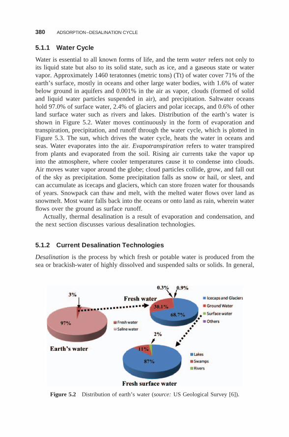
380 ADSORPTION–DESALINATION CYCLE

5.1.1 Water Cycle

Water is essential to all known forms of life, and the term water refers not only toits liquid state but also to its solid state, such as ice, and a gaseous state or watervapor. Approximately 1460 teratonnes (metric tons) (Tt) of water cover 71% of theearth’s surface, mostly in oceans and other large water bodies, with 1.6% of waterbelow ground in aquifers and 0.001% in the air as vapor, clouds (formed of solidand liquid water particles suspended in air), and precipitation. Saltwater oceanshold 97.0% of surface water, 2.4% of glaciers and polar icecaps, and 0.6% of otherland surface water such as rivers and lakes. Distribution of the earth’s water isshown in Figure 5.2. Water moves continuously in the form of evaporation andtranspiration, precipitation, and runoff through the water cycle, which is plotted inFigure 5.3. The sun, which drives the water cycle, heats the water in oceans andseas. Water evaporates into the air. Evapotranspiration refers to water transpiredfrom plants and evaporated from the soil. Rising air currents take the vapor upinto the atmosphere, where cooler temperatures cause it to condense into clouds.Air moves water vapor around the globe; cloud particles collide, grow, and fall outof the sky as precipitation. Some precipitation falls as snow or hail, or sleet, andcan accumulate as icecaps and glaciers, which can store frozen water for thousandsof years. Snowpack can thaw and melt, with the melted water flows over land assnowmelt. Most water falls back into the oceans or onto land as rain, wherein waterflows over the ground as surface runoff.

Actually, thermal desalination is a result of evaporation and condensation, andthe next section discusses various desalination technologies.

5.1.2 Current Desalination Technologies

Desalination is the process by which fresh or potable water is produced from thesea or brackish-water of highly dissolved and suspended salts or solids. In general,

Figure 5.2 Distribution of earth’s water (source: US Geological Survey [6]).

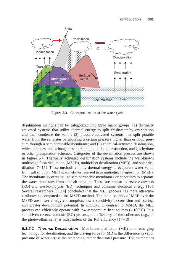
INTRODUCTION 381

Condensation

Transpiration Transpiration

Condensation

Evaporation

Precipitation

Snow

Surfacerunoff

Accumulation

Undergroundrunoff

SeaSea

Figure 5.3 Conceptualization of the water cycle.

desalination methods can be categorized into three major groups: (1) thermallyactivated systems that utilize thermal energy to split freshwater by evaporationand then condense the vapor; (2) pressure-activated systems that split potablewater from the saltwater by applying a certain pressure higher than osmotic pres-sure through a semipermeable membrane; and (3) chemical-activated desalination,which includes ion exchange desalination, liquid–liquid extraction, and gas hydrateor other precipitation schemes. Categories of the desalination process are shownin Figure 5.4. Thermally activated desalination systems include the well-knownmultistage flash distillation (MSFD), multieffect desalination (MED), and solar dis-tillation [7–15]. These methods employ thermal energy to evaporate water vaporfrom salt solution. MED is sometimes referred to as multieffect evaporation (MEE).The membrane systems utilize semipermeable membranes or nanotubes to separatethe water molecules from the salt solution. These are known as reverse-osmosis(RO) and electro-dialysis (ED) techniques and consume electrical energy [16].Several researchers [11,14] concluded that the MEE process has more attractiveattributes as compared to the MSFD method. The main benefits of MEE over theMSFD are lower energy consumption, lower sensitivity to corrosion and scaling,and greater development potential. In addition, in contrast to MSFD, the MEEprocess can efficiently operate with low-temperature heat sources (<100◦C). In asun-driven reverse-osmosis (RO) process, the efficiency of the collectors (e.g., ofthe photovoltaic cells) is independent of the RO efficiency [17–19].

5.1.2.1 Thermal Desalination Membrane distillation (MD) is an emergingtechnology for desalination, and the driving force for MD is the difference in vaporpressure of water across the membrane, rather than total pressure. The membranes

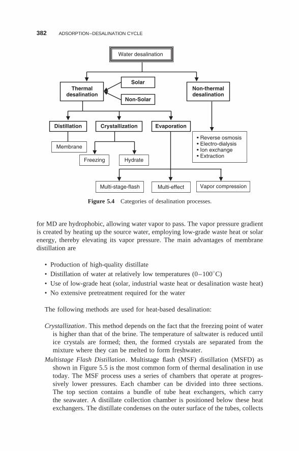
382 ADSORPTION–DESALINATION CYCLE

Water desalination

Thermaldesalination

Non-thermaldesalination

Solar

Non-Solar

Distillation Crystallization Evaporation

Membrane

• Reverse osmosis• Electro-dialysis• Ion exchange• Extraction

Freezing Hydrate

Multi-stage-flash Multi-effect Vapor compression

Figure 5.4 Categories of desalination processes.

for MD are hydrophobic, allowing water vapor to pass. The vapor pressure gradientis created by heating up the source water, employing low-grade waste heat or solarenergy, thereby elevating its vapor pressure. The main advantages of membranedistillation are

• Production of high-quality distillate

• Distillation of water at relatively low temperatures (0–100◦C)

• Use of low-grade heat (solar, industrial waste heat or desalination waste heat)

• No extensive pretreatment required for the water

The following methods are used for heat-based desalination:

Crystallization . This method depends on the fact that the freezing point of wateris higher than that of the brine. The temperature of saltwater is reduced untilice crystals are formed; then, the formed crystals are separated from themixture where they can be melted to form freshwater.

Multistage Flash Distillation . Multistage flash (MSF) distillation (MSFD) asshown in Figure 5.5 is the most common form of thermal desalination in usetoday. The MSF process uses a series of chambers that operate at progres-sively lower pressures. Each chamber can be divided into three sections.The top section contains a bundle of tube heat exchangers, which carrythe seawater. A distillate collection chamber is positioned below these heatexchangers. The distillate condenses on the outer surface of the tubes, collects

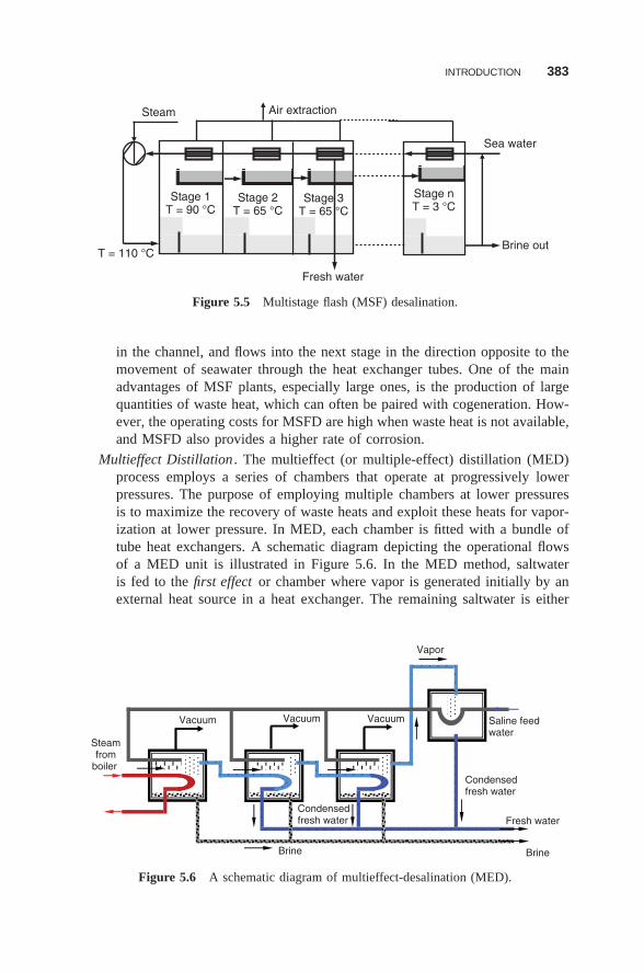
INTRODUCTION 383

Sea water

Brine out T = 110 °C

Fresh water

Steam Air extraction

Stage 1T = 90 °C

Stage 2T = 65 °C

Stage 3T = 65 °C

Stage nT = 3 °C

Figure 5.5 Multistage flash (MSF) desalination.

in the channel, and flows into the next stage in the direction opposite to themovement of seawater through the heat exchanger tubes. One of the mainadvantages of MSF plants, especially large ones, is the production of largequantities of waste heat, which can often be paired with cogeneration. How-ever, the operating costs for MSFD are high when waste heat is not available,and MSFD also provides a higher rate of corrosion.

Multieffect Distillation . The multieffect (or multiple-effect) distillation (MED)process employs a series of chambers that operate at progressively lowerpressures. The purpose of employing multiple chambers at lower pressuresis to maximize the recovery of waste heats and exploit these heats for vapor-ization at lower pressure. In MED, each chamber is fitted with a bundle oftube heat exchangers. A schematic diagram depicting the operational flowsof a MED unit is illustrated in Figure 5.6. In the MED method, saltwateris fed to the first effect or chamber where vapor is generated initially by anexternal heat source in a heat exchanger. The remaining saltwater is either

Condensedfresh water

Vapor

Saline feedwater

Vacuum Vacuum Vacuum

Steamfrom

boiler

Fresh water

Brine

Condensedfresh water

Brine

Figure 5.6 A schematic diagram of multieffect-desalination (MED).

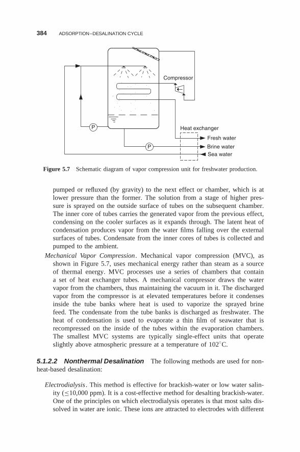
384 ADSORPTION–DESALINATION CYCLE

P

P

Heat exchanger

Compressor

Fresh water

Brine waterSea water

Figure 5.7 Schematic diagram of vapor compression unit for freshwater production.

pumped or refluxed (by gravity) to the next effect or chamber, which is atlower pressure than the former. The solution from a stage of higher pres-sure is sprayed on the outside surface of tubes on the subsequent chamber.The inner core of tubes carries the generated vapor from the previous effect,condensing on the cooler surfaces as it expands through. The latent heat ofcondensation produces vapor from the water films falling over the externalsurfaces of tubes. Condensate from the inner cores of tubes is collected andpumped to the ambient.

Mechanical Vapor Compression . Mechanical vapor compression (MVC), asshown in Figure 5.7, uses mechanical energy rather than steam as a sourceof thermal energy. MVC processes use a series of chambers that containa set of heat exchanger tubes. A mechanical compressor draws the watervapor from the chambers, thus maintaining the vacuum in it. The dischargedvapor from the compressor is at elevated temperatures before it condensesinside the tube banks where heat is used to vaporize the sprayed brinefeed. The condensate from the tube banks is discharged as freshwater. Theheat of condensation is used to evaporate a thin film of seawater that isrecompressed on the inside of the tubes within the evaporation chambers.The smallest MVC systems are typically single-effect units that operateslightly above atmospheric pressure at a temperature of 102◦C.

5.1.2.2 Nonthermal Desalination The following methods are used for non-heat-based desalination:

Electrodialysis . This method is effective for brackish-water or low water salin-ity (≤10,000 ppm). It is a cost-effective method for desalting brackish-water.One of the principles on which electrodialysis operates is that most salts dis-solved in water are ionic. These ions are attracted to electrodes with different

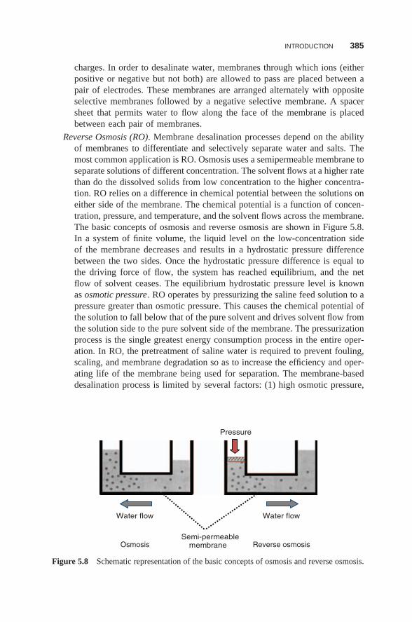
INTRODUCTION 385

charges. In order to desalinate water, membranes through which ions (eitherpositive or negative but not both) are allowed to pass are placed between apair of electrodes. These membranes are arranged alternately with oppositeselective membranes followed by a negative selective membrane. A spacersheet that permits water to flow along the face of the membrane is placedbetween each pair of membranes.

Reverse Osmosis (RO). Membrane desalination processes depend on the abilityof membranes to differentiate and selectively separate water and salts. Themost common application is RO. Osmosis uses a semipermeable membrane toseparate solutions of different concentration. The solvent flows at a higher ratethan do the dissolved solids from low concentration to the higher concentra-tion. RO relies on a difference in chemical potential between the solutions oneither side of the membrane. The chemical potential is a function of concen-tration, pressure, and temperature, and the solvent flows across the membrane.The basic concepts of osmosis and reverse osmosis are shown in Figure 5.8.In a system of finite volume, the liquid level on the low-concentration sideof the membrane decreases and results in a hydrostatic pressure differencebetween the two sides. Once the hydrostatic pressure difference is equal tothe driving force of flow, the system has reached equilibrium, and the netflow of solvent ceases. The equilibrium hydrostatic pressure level is knownas osmotic pressure. RO operates by pressurizing the saline feed solution to apressure greater than osmotic pressure. This causes the chemical potential ofthe solution to fall below that of the pure solvent and drives solvent flow fromthe solution side to the pure solvent side of the membrane. The pressurizationprocess is the single greatest energy consumption process in the entire oper-ation. In RO, the pretreatment of saline water is required to prevent fouling,scaling, and membrane degradation so as to increase the efficiency and oper-ating life of the membrane being used for separation. The membrane-baseddesalination process is limited by several factors: (1) high osmotic pressure,

Pressure

Water flow

Semi-permeablemembrane

Water flow

Osmosis Reverse osmosis

Figure 5.8 Schematic representation of the basic concepts of osmosis and reverse osmosis.

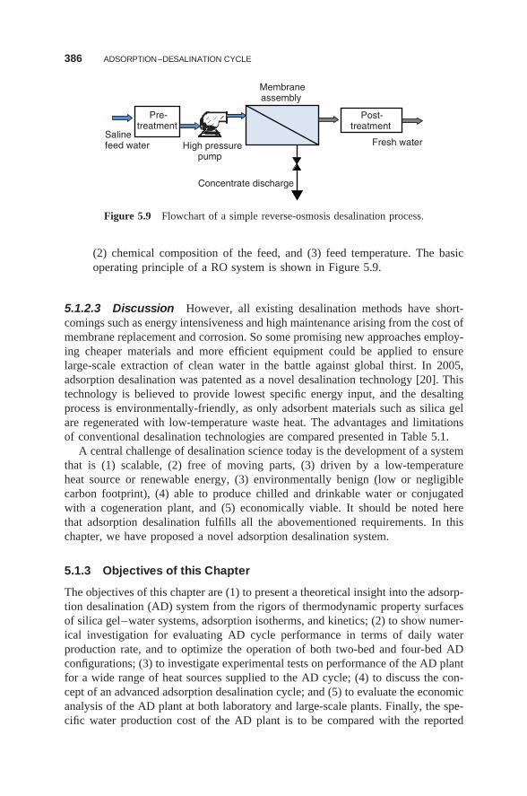
386 ADSORPTION–DESALINATION CYCLE

High pressurepump

Pre-treatment

Membraneassembly

Post-treatment

Fresh waterSalinefeed water

Concentrate discharge

Figure 5.9 Flowchart of a simple reverse-osmosis desalination process.

(2) chemical composition of the feed, and (3) feed temperature. The basicoperating principle of a RO system is shown in Figure 5.9.

5.1.2.3 Discussion However, all existing desalination methods have short-comings such as energy intensiveness and high maintenance arising from the cost ofmembrane replacement and corrosion. So some promising new approaches employ-ing cheaper materials and more efficient equipment could be applied to ensurelarge-scale extraction of clean water in the battle against global thirst. In 2005,adsorption desalination was patented as a novel desalination technology [20]. Thistechnology is believed to provide lowest specific energy input, and the desaltingprocess is environmentally-friendly, as only adsorbent materials such as silica gelare regenerated with low-temperature waste heat. The advantages and limitationsof conventional desalination technologies are compared presented in Table 5.1.

A central challenge of desalination science today is the development of a systemthat is (1) scalable, (2) free of moving parts, (3) driven by a low-temperatureheat source or renewable energy, (3) environmentally benign (low or negligiblecarbon footprint), (4) able to produce chilled and drinkable water or conjugatedwith a cogeneration plant, and (5) economically viable. It should be noted herethat adsorption desalination fulfills all the abovementioned requirements. In thischapter, we have proposed a novel adsorption desalination system.

5.1.3 Objectives of this Chapter

The objectives of this chapter are (1) to present a theoretical insight into the adsorp-tion desalination (AD) system from the rigors of thermodynamic property surfacesof silica gel–water systems, adsorption isotherms, and kinetics; (2) to show numer-ical investigation for evaluating AD cycle performance in terms of daily waterproduction rate, and to optimize the operation of both two-bed and four-bed ADconfigurations; (3) to investigate experimental tests on performance of the AD plantfor a wide range of heat sources supplied to the AD cycle; (4) to discuss the con-cept of an advanced adsorption desalination cycle; and (5) to evaluate the economicanalysis of the AD plant at both laboratory and large-scale plants. Finally, the spe-cific water production cost of the AD plant is to be compared with the reported

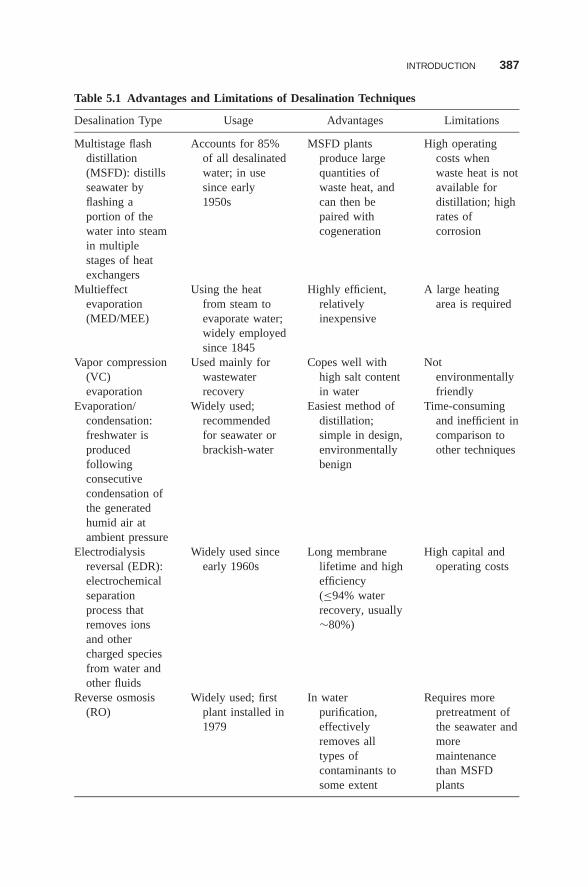
INTRODUCTION 387

Table 5.1 Advantages and Limitations of Desalination Techniques

Desalination Type Usage Advantages Limitations

Multistage flashdistillation(MSFD): distillsseawater byflashing aportion of thewater into steamin multiplestages of heatexchangers

Accounts for 85%of all desalinatedwater; in usesince early1950s

MSFD plantsproduce largequantities ofwaste heat, andcan then bepaired withcogeneration

High operatingcosts whenwaste heat is notavailable fordistillation; highrates ofcorrosion

Multieffectevaporation(MED/MEE)

Using the heatfrom steam toevaporate water;widely employedsince 1845

Highly efficient,relativelyinexpensive

A large heatingarea is required

Vapor compression(VC)evaporation

Used mainly forwastewaterrecovery

Copes well withhigh salt contentin water

Notenvironmentallyfriendly

Evaporation/condensation:freshwater isproducedfollowingconsecutivecondensation ofthe generatedhumid air atambient pressure

Widely used;recommendedfor seawater orbrackish-water

Easiest method ofdistillation;simple in design,environmentallybenign

Time-consumingand inefficient incomparison toother techniques

Electrodialysisreversal (EDR):electrochemicalseparationprocess thatremoves ionsand othercharged speciesfrom water andother fluids

Widely used sinceearly 1960s

Long membranelifetime and highefficiency(≤94% waterrecovery, usually∼80%)

High capital andoperating costs

Reverse osmosis(RO)

Widely used; firstplant installed in1979

In waterpurification,effectivelyremoves alltypes ofcontaminants tosome extent

Requires morepretreatment ofthe seawater andmoremaintenancethan MSFDplants

388 ADSORPTION–DESALINATION CYCLE

Table 5.1 (Continued )

Desalination Type Usage Advantages Limitations

Nanofiltration (NF) Emergingtechnology

Very highefficiency

High capital cost;unknownlifetime ofmembrane; nolarge-scale plantbuilt yet

Forward osmosis(FO)

Emergingtechnology

Low or nohydraulicpressures; noenergy neededfor seperation;effect separationof water fromdissolved solutes

Cannot producepure water; onlyconcentratedsolutions

Membranedistillation (MD)

Widely used Low energyconsumption;low fouling

Cooling is neededon the permeateside; sensitivityto pressure andsurface tensionof liquids lowrejection ofvolatilecompounds

cost data found in the literature. For understanding adsorption desalination, the nextsection provides the general idea of physical adsorption and desorption.

5.2 ADSORPTION AND DESORPTION PHENOMENA

Adsorption phenomena have been known to humankind for a very long time, andthey are increasingly utilized for separation, purification, gas storage, and cool-ing applications. The adsorption process occurs in a porous solid medium. Thefundamentals of adsorption distinguish the relations between physical adsorptionand chemisorption. Physical adsorption is attributed to van der Waals forces andthe electrostatic force between adsorbate molecules and the surface atoms. On theother hand, chemisorption involves the formation of a chemical bond between thesorbate molecule and the surface of the adsorbent. The heat of adsorption accom-panying adsorption can be higher than the heat of vaporization (condensation) ofthe adsorbate by as much as 30–100%. When an adsorbent is in contact with thesurrounding fluid of a certain composition (adsorbate), adsorption takes place inthe Henry region, and after a sufficiently long time, the adsorbent and the adsor-bate reach equilibrium [21], as shown in Figure 5.10. The amount of adsorbate

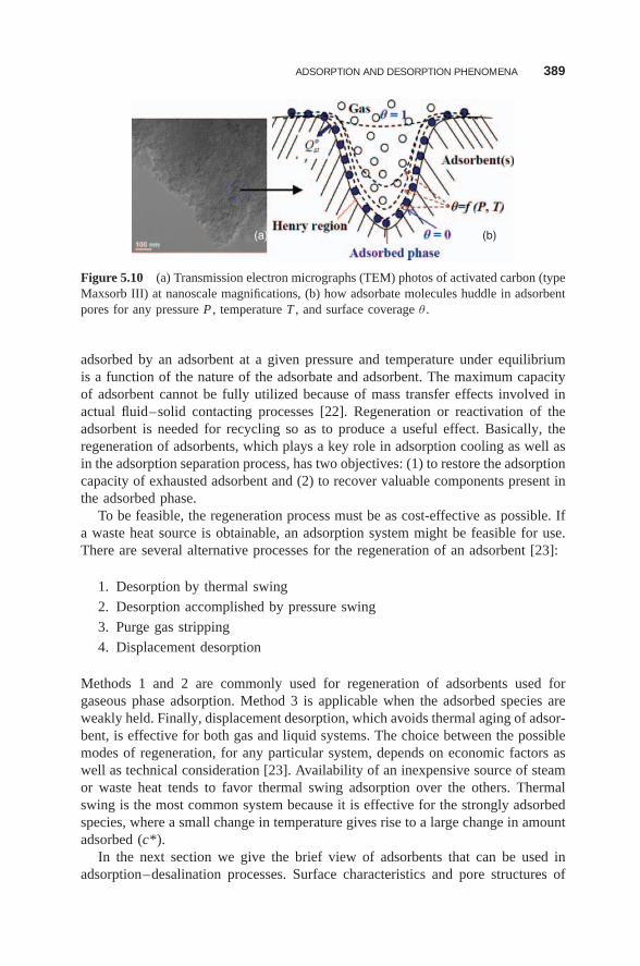
ADSORPTION AND DESORPTION PHENOMENA 389

(a) (b)

Figure 5.10 (a) Transmission electron micrographs (TEM) photos of activated carbon (typeMaxsorb III) at nanoscale magnifications, (b) how adsorbate molecules huddle in adsorbentpores for any pressure P , temperature T , and surface coverage θ .

adsorbed by an adsorbent at a given pressure and temperature under equilibriumis a function of the nature of the adsorbate and adsorbent. The maximum capacityof adsorbent cannot be fully utilized because of mass transfer effects involved inactual fluid–solid contacting processes [22]. Regeneration or reactivation of theadsorbent is needed for recycling so as to produce a useful effect. Basically, theregeneration of adsorbents, which plays a key role in adsorption cooling as well asin the adsorption separation process, has two objectives: (1) to restore the adsorptioncapacity of exhausted adsorbent and (2) to recover valuable components present inthe adsorbed phase.

To be feasible, the regeneration process must be as cost-effective as possible. Ifa waste heat source is obtainable, an adsorption system might be feasible for use.There are several alternative processes for the regeneration of an adsorbent [23]:

1. Desorption by thermal swing

2. Desorption accomplished by pressure swing

3. Purge gas stripping

4. Displacement desorption

Methods 1 and 2 are commonly used for regeneration of adsorbents used forgaseous phase adsorption. Method 3 is applicable when the adsorbed species areweakly held. Finally, displacement desorption, which avoids thermal aging of adsor-bent, is effective for both gas and liquid systems. The choice between the possiblemodes of regeneration, for any particular system, depends on economic factors aswell as technical consideration [23]. Availability of an inexpensive source of steamor waste heat tends to favor thermal swing adsorption over the others. Thermalswing is the most common system because it is effective for the strongly adsorbedspecies, where a small change in temperature gives rise to a large change in amountadsorbed (c*).

In the next section we give the brief view of adsorbents that can be used inadsorption–desalination processes. Surface characteristics and pore structures of

390 ADSORPTION–DESALINATION CYCLE

adsorbents are the main properties in determining adsorption equilibrium and therate properties that are needed for the adsorption–desalination plant design.

5.3 ADSORBENTS SUITABLE FOR ADSORPTION–DESALINATION

It is well known that the adsorbent of an adsorption process is a critical variable,and that system performance depends on how the solid adsorbents perform in bothequilibrium and kinetics. For instance, a material with high sorption capacity butslow kinetics is not a good choice as it takes adsorbate or water molecules a longa time to reach the equilibrium. On the other hand, the adsorbent material withrapid kinetics and low adsorbate capacity is also not a good choice, due to therequirements of more solid adsorbents for the system. A good adsorbent materialis one that provides good adsorptive capacity as well as good kinetics. To satisfythese two requirements, the material must have (1) reasonably high surface areaor micropore volume and (2) a relatively large pore network for the transportof molecules to the interior of solid adsorbents. To satisfy the first requirement,the porous solid should have small pore size with a reasonable porosity. Thissuggests that an adsorbent must have a combination of two pore types, ranging frommicropores (pore width <2 nm) to mesopores (pore width varying within 2–50 nmaccording to IUPAC [24]). The efficacy of the adsorption–desalination (AD) cycledepends on the sorption characteristics of adsorbent and adsorbate (hence watervapor) for the production of potable water. For desalination purposes, the adsorbentmaterial should be hydrophilic in nature with lower regeneration temperatures. Thesuitable adsorbents for desalination are described in the following subsections.

5.3.1 Silica Gels

It is well known that pure silica (SiO2) is a generally chemically inactive nonpolarmaterial. However, the surface becomes polar and hydrophilic when it contains ahydroxyl functional group (silanol group) [25]. Silica gel is prepared by coagulationof a colloidal solution of silicic acid with controlled dehydration. At higher regener-ation temperature, silica gel rejects almost all water vapor and causes hydrophobicphenomena. Because silica gel is both hydrophilic and hydrophobic, it has beenconsidered as the most suitable adsorbent for water-refrigerant-based cooling appli-cations. It should be noted here that the regeneration temperature of silica gel islow compared with other adsorbents, as shown in Table 5.2. The literature showsthat silica gel is used in most industries for water removal because of its stronghydrophilicity toward water. Some applications of silica gel are [26]: (1) waterremoval from air (dehumidification), (2) drying of nonreactive gases, (3) drying ofreactive gases, (4) adsorption of hydrogen sulfide, (5) oil vapor adsorption, and (6)adsorption of alcohols.

The properties of silica gel are analyzed using the N2 adsorption method. Theamount of gas adsorbed or desorbed from a porous surface at a predeterminedequilibrium (vapor) pressure is measured by the static volumetric method with

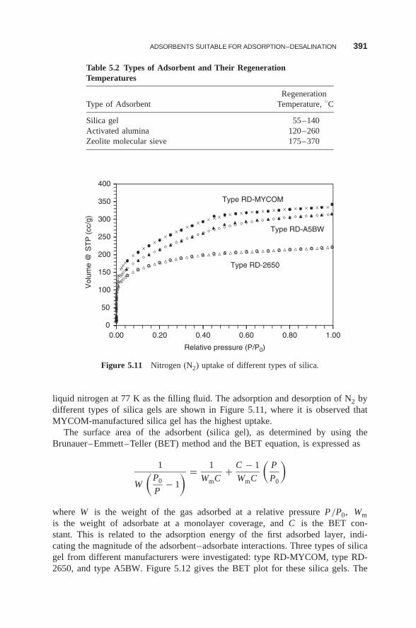
ADSORBENTS SUITABLE FOR ADSORPTION–DESALINATION 391

Table 5.2 Types of Adsorbent and Their RegenerationTemperatures

RegenerationType of Adsorbent Temperature, ◦C

Silica gel 55–140Activated alumina 120–260Zeolite molecular sieve 175–370

0

50

100

150

200

250

300

350

400

0.00 0.20 0.40 0.60 0.80 1.00

Vol

ume

@ S

TP

(cc

/g)

Relative pressure (P/P0)

Type RD-MYCOM

Type RD-A5BW

Type RD-2650

Figure 5.11 Nitrogen (N2) uptake of different types of silica.

liquid nitrogen at 77 K as the filling fluid. The adsorption and desorption of N2 bydifferent types of silica gels are shown in Figure 5.11, where it is observed thatMYCOM-manufactured silica gel has the highest uptake.

The surface area of the adsorbent (silica gel), as determined by using theBrunauer–Emmett–Teller (BET) method and the BET equation, is expressed as

1

W

(P0

P− 1

) = 1

WmC+ C − 1

WmC

(P

P0

)

where W is the weight of the gas adsorbed at a relative pressure P/P0, Wmis the weight of adsorbate at a monolayer coverage, and C is the BET con-stant. This is related to the adsorption energy of the first adsorbed layer, indi-cating the magnitude of the adsorbent–adsorbate interactions. Three types of silicagel from different manufacturers were investigated: type RD-MYCOM, type RD-2650, and type A5BW. Figure 5.12 gives the BET plot for these silica gels. The

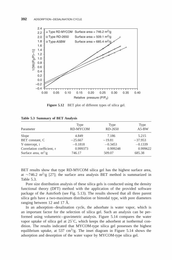
392 ADSORPTION–DESALINATION CYCLE

–0.4–0.2

0.00.20.40.60.81.01.21.41.61.82.02.22.4

1/[W

((P

0/P

)–1)

]

Relative pressure (P/P0)

0.00 0.05 0.10 0.15 0.20 0.25 0.30 0.35 0.40

Type RD-MYCOM

Type RD-2650

Type-A5BW

Surface area = 746.2 m2/g

Surface area = 509.1 m2/g

Surface area = 685.4 m2/g

Figure 5.12 BET plot of different types of silica gel.

Table 5.3 Summary of BET Analysis

Type Type TypeParameter RD-MYCOM RD-2650 A5-BW

Slope 4.849 7.186 5.215BET constant, C −25.667 −19.81 −37.953Y-intercept, i −0.1818 −0.3453 −0.1339Correlation coefficient, r 0.999373 0.999248 0.999622Surface area, m2/g 746.17 509.07 685.38

BET results show that type RD-MYCOM silica gel has the highest surface area,at ∼746.2 m2/g [27]; the surface area analysis BET method is summarized inTable 5.3.

Pore size distribution analysis of these silica gels is conducted using the densityfunctional theory (DFT) method with the application of the provided softwarepackage of the AutoSorb (see Fig. 5.13). The results showed that all three parentsilica gels have a two-maximum distribution or bimodal type, with pore diametersranging between 12 and 17 A.

In an adsorption–desalination cycle, the adsorbate is water vapor, which isan important factor for the selection of silica gel. Such an analysis can be per-formed using volumetric–gravimetric analysis. Figure 5.14 compares the watervapor uptake of silica gel at 25◦C, which keeps the adsorbent at isothermal con-dition. The results indicated that MYCOM-type silica gel possesses the highestequilibrium uptake, at 537 cm3/g. The inset diagram in Figure 5.14 shows theadsorption and desorption of the water vapor by MYCOM-type silica gel.

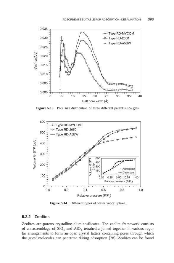
ADSORBENTS SUITABLE FOR ADSORPTION–DESALINATION 393

0.0000 5 10 15 20 25 30 35 40

0.005

0.010

0.015

0.020

0.025

0.030

0.035

dV(r

)(cc

/Å/g

)

Half pore width (Å)

Type RD-MYCOM

Type RD-2650

Type RD-A5BW

Figure 5.13 Pore size distribution of three different parent silica gels.

00.0 0.2 0.4 0.6 0.8 1.0

100

200

300

400

500

600

Vol

ume

@ S

TP

(cc

/g)

Relative pressure (P/P0)

00.00 0.25 0.50 0.75 1.00

150

300

450

600

Vol

ume

@ S

TP

(cc/

g)

Relative pressure (P/P0)

AdsorptionDesorption

Type RD-MYCOMType RD-2650

Type RD-A5BW

Figure 5.14 Different types of water vapor uptake.

5.3.2 Zeolites

Zeolites are porous crystalline aluminosilicates. The zeolite framework consistsof an assemblage of SiO4 and AlO4 tetrahedra joined together in various regu-lar arrangements to form an open crystal lattice containing pores through whichthe guest molecules can penetrate during adsorption [28]. Zeolites can be found

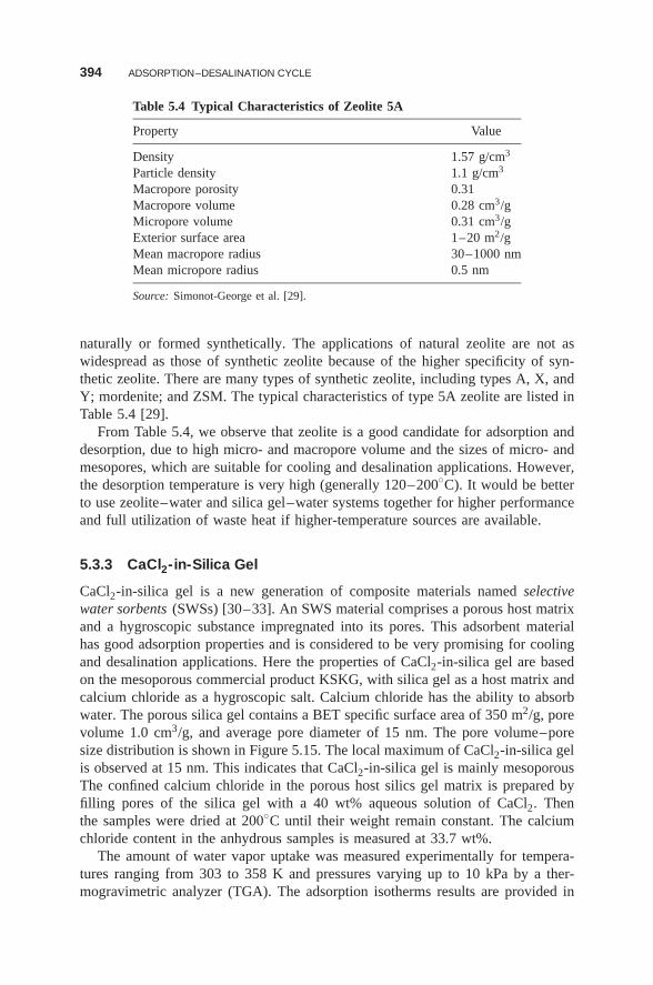
394 ADSORPTION–DESALINATION CYCLE

Table 5.4 Typical Characteristics of Zeolite 5A

Property Value

Density 1.57 g/cm3

Particle density 1.1 g/cm3

Macropore porosity 0.31Macropore volume 0.28 cm3/gMicropore volume 0.31 cm3/gExterior surface area 1–20 m2/gMean macropore radius 30–1000 nmMean micropore radius 0.5 nm

Source: Simonot-George et al. [29].

naturally or formed synthetically. The applications of natural zeolite are not aswidespread as those of synthetic zeolite because of the higher specificity of syn-thetic zeolite. There are many types of synthetic zeolite, including types A, X, andY; mordenite; and ZSM. The typical characteristics of type 5A zeolite are listed inTable 5.4 [29].

From Table 5.4, we observe that zeolite is a good candidate for adsorption anddesorption, due to high micro- and macropore volume and the sizes of micro- andmesopores, which are suitable for cooling and desalination applications. However,the desorption temperature is very high (generally 120–200◦C). It would be betterto use zeolite–water and silica gel–water systems together for higher performanceand full utilization of waste heat if higher-temperature sources are available.

5.3.3 CaCl2-in-Silica Gel

CaCl2-in-silica gel is a new generation of composite materials named selectivewater sorbents (SWSs) [30–33]. An SWS material comprises a porous host matrixand a hygroscopic substance impregnated into its pores. This adsorbent materialhas good adsorption properties and is considered to be very promising for coolingand desalination applications. Here the properties of CaCl2-in-silica gel are basedon the mesoporous commercial product KSKG, with silica gel as a host matrix andcalcium chloride as a hygroscopic salt. Calcium chloride has the ability to absorbwater. The porous silica gel contains a BET specific surface area of 350 m2/g, porevolume 1.0 cm3/g, and average pore diameter of 15 nm. The pore volume–poresize distribution is shown in Figure 5.15. The local maximum of CaCl2-in-silica gelis observed at 15 nm. This indicates that CaCl2-in-silica gel is mainly mesoporousThe confined calcium chloride in the porous host silics gel matrix is prepared byfilling pores of the silica gel with a 40 wt% aqueous solution of CaCl2. Thenthe samples were dried at 200◦C until their weight remain constant. The calciumchloride content in the anhydrous samples is measured at 33.7 wt%.

The amount of water vapor uptake was measured experimentally for tempera-tures ranging from 303 to 358 K and pressures varying up to 10 kPa by a ther-mogravimetric analyzer (TGA). The adsorption isotherms results are provided in

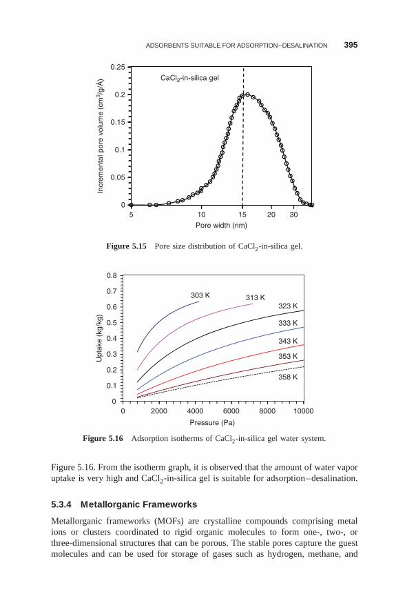
ADSORBENTS SUITABLE FOR ADSORPTION–DESALINATION 395

05 10 15

Pore width (nm)

20 30

0.05

0.1

0.15

0.2

0.25

CaCl2-in-silica gel

Incr

emen

tal p

ore

vol

ume

(cm

3 /g

/Å)

Figure 5.15 Pore size distribution of CaCl2-in-silica gel.

0

0.1

0.2

0.3

0.4

0.5

0.6

0.7

0.8

0 2000 4000 6000 8000 10000

Upt

ake

(kg/

kg)

Pressure (Pa)

303 K 313 K323 K

333 K

343 K

353 K

358 K

Figure 5.16 Adsorption isotherms of CaCl2-in-silica gel water system.

Figure 5.16. From the isotherm graph, it is observed that the amount of water vaporuptake is very high and CaCl2-in-silica gel is suitable for adsorption–desalination.

5.3.4 Metallorganic Frameworks

Metallorganic frameworks (MOFs) are crystalline compounds comprising metalions or clusters coordinated to rigid organic molecules to form one-, two-, orthree-dimensional structures that can be porous. The stable pores capture the guestmolecules and can be used for storage of gases such as hydrogen, methane, and

396 ADSORPTION–DESALINATION CYCLE

carbon dioxide. Other possible applications of MOFs are found in gas purifica-tion, gas separation, and catalysis. In more recent years, there has been significantresearch on the development of micro- and mesoporous adsorbent materials forclosed-system heat transformation applications, such as thermally driven adsorptionchillers. For adsorption–desalination application, the adsorbent material should behydrophilic; it behaves hydrophobically at relatively high temperatures (e.g., 80◦C),and the choice of the adsorbent–water working pair is determined by the amountof heat that can be extracted from the evaporator and is rejected from the condenserper adsorption cycle [34]. The heat extracted as a result of cooling load from theevaporator is proportional to (1) the amount of water vapor adsorbed and (2) theevaporation enthalpy of water vapor. Therefore, the loading spread, or the differencebetween the water vapor uptakes and offtakes over a given adsorption–desorptioncycle, provides the best criterion for selection of a suitable adsorbent. The presentadsorption chillers and desalination plants use silica gels mostly as adsorbents. Themetal metallorganic framework (MOF) is a good adsorbent for heat transformationsapplications. The amount of water vapor uptake is quite high as compared withother adsorbents such as zeolites and silica gels [35]. It should be noted here thatthe metallorganic framework is less hydrophilic than silica gel or zeolites; thus, itreleases water at lower temperature and lower partial pressure, which also indicatesthe potentiality of MOF materials for heat transformation processes or desalina-tion. The dehydratable–hydratable water-stable MOF material with a large loadingspread of 0.25 kg/kg will be the best candidate in heat transformation cycles forrefrigeration, heat pumping, and heat storage.

5.4 FUNDAMENTAL STUDY OF ADSORPTION–DESALINATION

The physical adsorption process occurs mainly within the pores of adsorbent andat the external adsorbent surface, and is determined by its adsorption isotherms,heats of adsorption, and adsorption kinetics. In a physicsorption, the adsorbedphase is held near the pores of the adsorbent by the existence of van der Waalsforces. Development of the adsorption–desalination (AD) system is based on thethermodynamic property surfaces of the silica gel–water system and the thermalcompression of water, and lies in its ability to operate with motive energy derivedfrom fairly low-temperature waste heat sources or solar energy, which indicates theadsorption process as an avenue for avoiding the use of ozone depleting substances[36–40]. The major components of the typical AD system are the evaporator, thecondenser, and two or more adsorbent beds in which the adsorbents are packed intube-fin heat exchangers. Operation of the AD cycle is the union of adsorption-triggered evaporation and the desorption-resulting condensation. This means thatthe pre-treated seawater is evaporated and adsorbed onto silica gel at low pressureand temperature. When the vapors are adsorbed on the adsorbent, the heat ofadsorption is developed, and this heat is rejected into the cooling-water circuitrunning across the adsorbent bed. This adsorption process continues until onset ofthe switching time. For the regeneration of saturated silica gels, low-temperature

FUNDAMENTAL STUDY OF ADSORPTION–DESALINATION 397

waste heat is supplied to the bed at the onset of the desorption mode. The sorptionbed is connected to the condenser, where the water vapor migrates to the cooler tubesurfaces of the condenser and the potable water is collected in the collection tank.

5.4.1 Description of Adsorption–Desalination (AD) Cycle

The adsorption–desalination (AD) cycle is a novel desalination method for produc-ing potable water from seawater or brackish-water, utilizing only low-temperaturehot water from renewable energy such as process exhaust and solar energy. The ADcycle is based on the patented cycle by Ng et al. [20] that produces both desaltedwater and cooling by using low-temperature waste heat. A typical AD plant con-sists of three major components: (1) the evaporator, (2) single or multireactor bedswhere the adsorbent is placed, and (3) the condenser. A schematic diagram of theAD cycle is given in Figure 5.17 showing the major components. The subsystemsinvolved in AD cycle are

1. Pretreatment System . Seawater is first pretreated where unwanted physicalparticles such as debris in the seawater are screened using a conventionalfilter (mesh size 20–30), and the dissolved air in the seawater is removed bydeaeration.

2. Adsorption-Initiated Evaporation System . The deaerated seawater is pumpedintermittently into the evaporator, where evaporation is achieved by watervapor uptake by the adsorbent (type RD silica gel). The evaporation processis enhanced by a spray system using full-cone type nozzles. The evaporationprocess is maintained by an external water circuit that provides the heatingcapacity to sustain the evaporation. The energy required for the evaporation is

Sea water

Pre treatmentEvaporator

Condenser

Was

te h

eat

sour

ce

Beds Fresh water

Figure 5.17 Schematic diagram of the adsorption–desalination system.

398 ADSORPTION–DESALINATION CYCLE

either supplied from the ambient or recovered internally within the condenseror adsorption process. The concentrated brine is occasionally discharged fromthe evaporator. Water vapor from the evaporator is adsorbed by the unsatu-rated silica gel, which is packed into a tube-fin heat exchanger housed insidea reactor bed. When the vapor valve is opened, a continuous vapor uptake isachieved. Owing to the exothermic nature of the adsorption process, heat isreleased during vapor uptake, and the adsorption process continues at a pre-set cycle time. In general, process cycle time is one of the input parametersfor controlling the AD process, and its time interval of operation is a directfunction of hot-water inlet temperatures.

3. Heat-Activated Desorption–Condensation System . The saturated silica gel(from adsorption of previous half-cycle) can be regenerated by introducinglow-temperature hot water (typically <85◦C); this procedure is known as thedesorption process . With the connecting vapor valves set to open position,the regenerated water vapor flows to the external surfaces of the water-cooled tubes and condenses to yield the distilled water. The condensationprocess is accompanied by rejection of the latent heat of condensation into thecooling-water passing through the condenser, and the condensate is collectedas potable water.

4. Potable-Water Collection System . The condensate inside the condenser isremoved using by a freshwater pump or a 10-m U-tube arrangement to over-come the differential pressure.

5.4.2 Theoretical Insight into AD

The AD method offers merits of scale independence since adsorption and desorp-tion are primarily surface, rather than bulk, processes. The performance of ADdepends on (1) the adsorption isotherms and kinetics of silica gel–water pair and(2) structural features such as pore width d , pore volume vp, and specific surfacearea of silica gels. The heat of adsorption is of secondary importance since it issimply rejected to the environment. The thermodynamic behavior of the AD cycleconsists of two isosters and two isobars, characterized by three temperatures: evap-orator (Tevap), condenser (Tcond), and the driving heat source (Tdes) temperatures.In this section, we have presented a thermodynamic framework, which has beenderived from the rigor of classical thermodynamics, the Boltzmann energy distri-bution function, the condensation approximation approach, and the Lennard–Jonespotential model for calculation of the energetic performances of AD in terms ofspecific water production and performance ratio for various pore sizes and volumesof silica gels. Employing the proposed formulations, we report a simulation studyhere for calculation of the maximum isosteric heats and characteristics energy forthe adsorption of water vapor on silica gels as a function of pore width.

5.4.3 Thermodynamics of an AD Device

The energy flow for each sorption component of the AD system is derivedand developed from the rigor of thermodynamic property surfaces of the silica

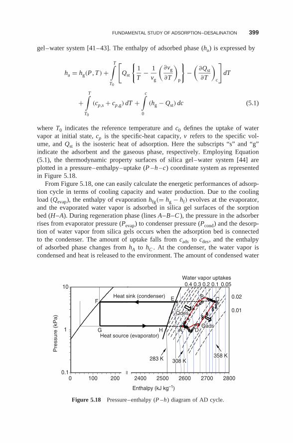
FUNDAMENTAL STUDY OF ADSORPTION–DESALINATION 399

gel–water system [41–43]. The enthalpy of adsorbed phase (ha) is expressed by

ha = hg(P , T ) +T∫

T0

[Qst

{1

T− 1

vg

(∂vg

∂T

)p

}−

(∂Qst

∂T

)c

]dT

+T∫

T0

(cp,s + cp,g) dT +c∫

0

(hg − Qst) dc (5.1)

where T0 indicates the reference temperature and c0 defines the uptake of watervapor at initial state, cp is the specific-heat capacity, v refers to the specific vol-ume, and Qst is the isosteric heat of adsorption. Here the subscripts “s” and “g”indicate the adsorbent and the gaseous phase, respectively. Employing Equation(5.1), the thermodynamic property surfaces of silica gel–water system [44] areplotted in a pressure–enthalpy–uptake (P –h –c) coordinate system as representedin Figure 5.18.

From Figure 5.18, one can easily calculate the energetic performances of adsorp-tion cycle in terms of cooling capacity and water production. Due to the coolingload (Qevap), the enthalpy of evaporation hfg(= hg − hf) evolves at the evaporator,and the evaporated water vapor is adsorbed in silica gel surfaces of the sorptionbed (H–A). During regeneration phase (lines A–B–C ), the pressure in the adsorberrises from evaporator pressure (Pevap) to condenser pressure (Pcond) and the desorp-tion of water vapor from silica gels occurs when the adsorption bed is connectedto the condenser. The amount of uptake falls from cads to cdes, and the enthalpyof adsorbed phase changes from hA to hC . At the condenser, the water vapor iscondensed and heat is released to the environment. The amount of condensed water

0.10 100 200 2400 2500 2600 2700 2800

1

10

Enthalpy (kJ kg–1)

Pre

ssure

(kP

a)

A

B C

D

0.01

0.02

0.05 0.1

EF

G H

0.20.30.4

358 K 358 K 283 K 308 K 308 K

≈

Heat source (evaporator)

Heat sink (condenser)

Water vapor uptakes

QadsQads

Qdes Qdes

Figure 5.18 Pressure–enthalpy (P –h) diagram of AD cycle.

400 ADSORPTION–DESALINATION CYCLE

is calculated by Msg(cads − cdes), where Msg is the mass of silica gel. During thatphase, the enthalpy changes from hC to hF . Finally the condensed water goes to thefreshwater tank and completes the cycle. During adsorption phase (lines C–D–A),the sorption bed is cooled and the pressure falls from Pcond to Pevap. The refriger-ant vapor is adsorbed on the adsorbents and the amount of water vapor increasesup to cads. The overall performance ratio (OPR) is given by (Qevap + Qcond)/Qdes,where Qdes is the amount of heats during regeneration periods and Qcond is the heatremoval for condensation. From Figure 5.18, we find that during the preheatingstage (A → B ), the sorption bed is isolated from the evaporator and the condenser,and the pressure is increased from evaporator pressure to a pressure dependingon cads and regeneration temperature. During desorption phase (line A–B–C ofFig. 5.18), the quantity of heat applied to the sorption bed is given by

Qdes =Treg∫

Tads

[cp,s + cads

{cp,l + Qst

(1

T− 1

vg

dvg

dT

)}]dT

+cads∫

cdes

{ha(P , T , c) − hg(T )} dc +Pcond∫

Pevap

Qst∂c

∂P

∣∣∣∣T

dP

+Tdes∫

Treg

[cp,s + cads

{cp,l + Qst

(1

T− 1

vg

dvg

dT

)}+ Qst

∂c

∂T

∣∣∣∣P

]dT (5.2)

The cooling capacity (Qevap) and the amount of condensation heat arecalculated as

Qevap =cads∫

cdes

hfg(Tevap) dc −cads∫

cdes

{hg(P , T ) − hg(T )} dc and

Qcond =cads∫

cdes

hfg(Tcond) dc +cads∫

cdes

{hg(P , T ) − hg(T )} dc

respectively.

5.4.4 Effects of Adsorbent Pore Size on AD

The experimentally measured adsorption isotherm data of silica gel–water systemsare fitted well with Dubinin–Astakhov (DA) adsorption isotherm equation. Param-eters of the D–A model are presented in Table 5.5. The D–A isotherm equation isgiven by

c = c◦ exp

[{RT ln(Ps/P

E

}n]

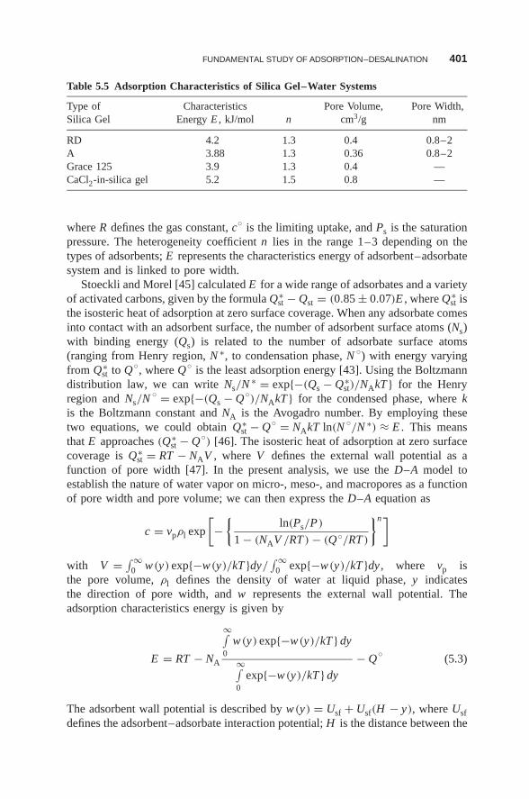
FUNDAMENTAL STUDY OF ADSORPTION–DESALINATION 401

Table 5.5 Adsorption Characteristics of Silica Gel–Water Systems

Type of Characteristics Pore Volume, Pore Width,Silica Gel Energy E , kJ/mol n cm3/g nm

RD 4.2 1.3 0.4 0.8–2A 3.88 1.3 0.36 0.8–2Grace 125 3.9 1.3 0.4 —CaCl2-in-silica gel 5.2 1.5 0.8 —

where R defines the gas constant, c◦ is the limiting uptake, and Ps is the saturationpressure. The heterogeneity coefficient n lies in the range 1–3 depending on thetypes of adsorbents; E represents the characteristics energy of adsorbent–adsorbatesystem and is linked to pore width.

Stoeckli and Morel [45] calculated E for a wide range of adsorbates and a varietyof activated carbons, given by the formula Q∗

st − Qst = (0.85 ± 0.07)E , where Q∗st is

the isosteric heat of adsorption at zero surface coverage. When any adsorbate comesinto contact with an adsorbent surface, the number of adsorbent surface atoms (Ns)with binding energy (Qs) is related to the number of adsorbate surface atoms(ranging from Henry region, N ∗, to condensation phase, N ◦) with energy varyingfrom Q∗

st to Q◦, where Q◦ is the least adsorption energy [43]. Using the Boltzmanndistribution law, we can write Ns/N ∗ = exp{−(Qs − Q∗

st)/NAkT } for the Henryregion and Ns/N ◦ = exp{−(Qs − Q◦

)/NAkT } for the condensed phase, where kis the Boltzmann constant and NA is the Avogadro number. By employing thesetwo equations, we could obtain Q∗

st − Q◦ = NAkT ln(N ◦/N ∗) ≈ E . This means

that E approaches (Q∗st − Q◦

) [46]. The isosteric heat of adsorption at zero surfacecoverage is Q∗

st = RT − NAV , where V defines the external wall potential as afunction of pore width [47]. In the present analysis, we use the D–A model toestablish the nature of water vapor on micro-, meso-, and macropores as a functionof pore width and pore volume; we can then express the D–A equation as

c = vpρl exp

[−

{ln(Ps/P)

1 − (NAV /RT ) − (Q◦/RT )

}n]

with V = ∫ ∞0 w(y) exp{−w(y)/kT }dy/

∫ ∞0 exp{−w(y)/kT }dy , where vp is

the pore volume, ρl defines the density of water at liquid phase, y indicatesthe direction of pore width, and w represents the external wall potential. Theadsorption characteristics energy is given by

E = RT − NA

∞∫0

w(y) exp{−w(y)/kT } dy

∞∫0

exp{−w(y)/kT } dy

− Q◦ (5.3)

The adsorbent wall potential is described by w(y) = Usf + Usf(H − y), where Usfdefines the adsorbent–adsorbate interaction potential; H is the distance between the

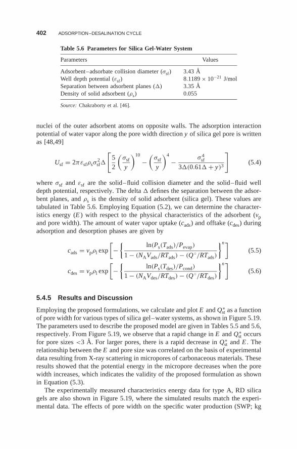
402 ADSORPTION–DESALINATION CYCLE

Table 5.6 Parameters for Silica Gel-Water System

Parameters Values

Adsorbent–adsorbate collision diameter (σsf) 3.43 AWell depth potential (εsf) 8.1189 × 10−21 J/molSeparation between adsorbent planes (�) 3.35 ADensity of solid adsorbent (ρs) 0.055

Source: Chakraborty et al. [46].

nuclei of the outer adsorbent atoms on opposite walls. The adsorption interactionpotential of water vapor along the pore width direction y of silica gel pore is writtenas [48,49]

Usf = 2πεsfρsσ2sf�

[5

2

(σsf

y

)10

−(

σsf

y

)4

− σ 4sf

3�(0.61� + y)3

](5.4)

where σsf and εsf are the solid–fluid collision diameter and the solid–fluid welldepth potential, respectively. The delta � defines the separation between the adsor-bent planes, and ρs is the density of solid adsorbent (silica gel). These values aretabulated in Table 5.6. Employing Equation (5.2), we can determine the character-istics energy (E ) with respect to the physical characteristics of the adsorbent (vpand pore width). The amount of water vapor uptake (cads) and offtake (cdes) duringadsorption and desorption phases are given by

cads = vpρl exp

[−

{ln(Ps(Tads)/Pevap)

1 − (NAVads/RTads) − (Q◦/RTads)

}n](5.5)

cdes = vpρl exp

[−

{ln(Ps(Tdes)/Pcond)

1 − (NAVdes/RTdes) − (Q◦/RTdes)

}n](5.6)

5.4.5 Results and Discussion

Employing the proposed formulations, we calculate and plot E and Q∗st as a function

of pore width for various types of silica gel–water systems, as shown in Figure 5.19.The parameters used to describe the proposed model are given in Tables 5.5 and 5.6,respectively. From Figure 5.19, we observe that a rapid change in E and Q∗

st occursfor pore sizes <3 A. For larger pores, there is a rapid decrease in Q∗

st and E . Therelationship between the E and pore size was correlated on the basis of experimentaldata resulting from X-ray scattering in micropores of carbonaceous materials. Theseresults showed that the potential energy in the micropore decreases when the porewidth increases, which indicates the validity of the proposed formulation as shownin Equation (5.3).

The experimentally measured characteristics energy data for type A, RD silicagels are also shown in Figure 5.19, where the simulated results match the experi-mental data. The effects of pore width on the specific water production (SWP; kg

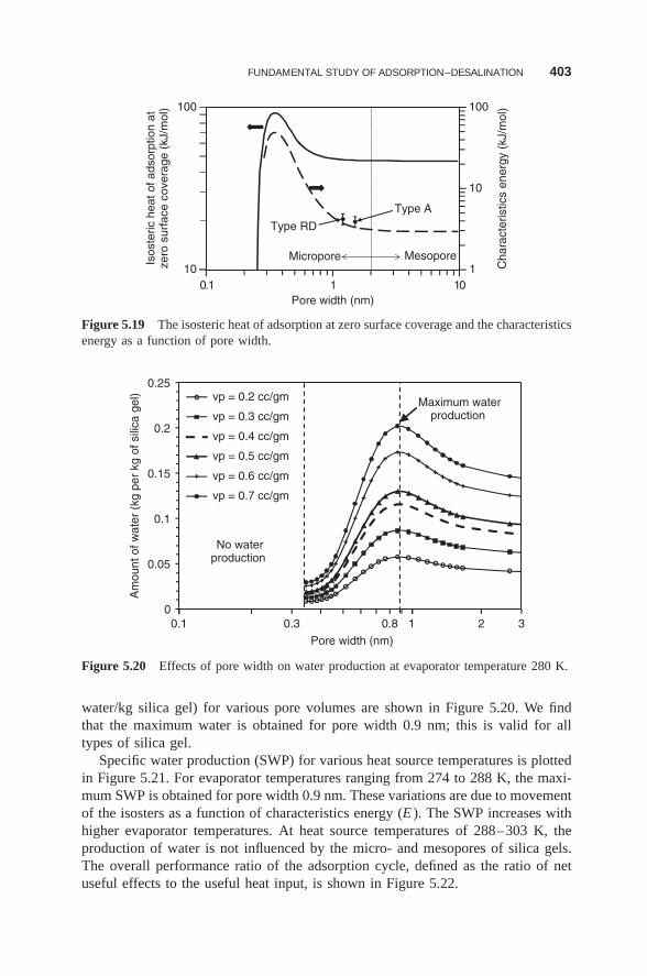
FUNDAMENTAL STUDY OF ADSORPTION–DESALINATION 403

1

10

100

10

100

0111.0

Isos

teric

hea

t of a

dsor

ptio

n at

zero

sur

face

cov

erag

e (k

J/m

ol)

Cha

ract

eris

tics

ener

gy (

kJ/m

ol)

Pore width (nm)

MesoporeMicropore

Type A

Type RD

Figure 5.19 The isosteric heat of adsorption at zero surface coverage and the characteristicsenergy as a function of pore width.

0

0.05

0.1

0.15

0.2

0.25

10.1

Am

ount

of w

ater

(kg

per

kg

of s

ilica

gel

)

Pore width (nm)

vp = 0.2 cc/gm

vp = 0.3 cc/gm

vp = 0.4 cc/gm

vp = 0.5 cc/gm

vp = 0.6 cc/gm

vp = 0.7 cc/gm

0.3 2 3

No waterproduction

Maximum waterproduction

0.8

Figure 5.20 Effects of pore width on water production at evaporator temperature 280 K.

water/kg silica gel) for various pore volumes are shown in Figure 5.20. We findthat the maximum water is obtained for pore width 0.9 nm; this is valid for alltypes of silica gel.

Specific water production (SWP) for various heat source temperatures is plottedin Figure 5.21. For evaporator temperatures ranging from 274 to 288 K, the maxi-mum SWP is obtained for pore width 0.9 nm. These variations are due to movementof the isosters as a function of characteristics energy (E ). The SWP increases withhigher evaporator temperatures. At heat source temperatures of 288–303 K, theproduction of water is not influenced by the micro- and mesopores of silica gels.The overall performance ratio of the adsorption cycle, defined as the ratio of netuseful effects to the useful heat input, is shown in Figure 5.22.

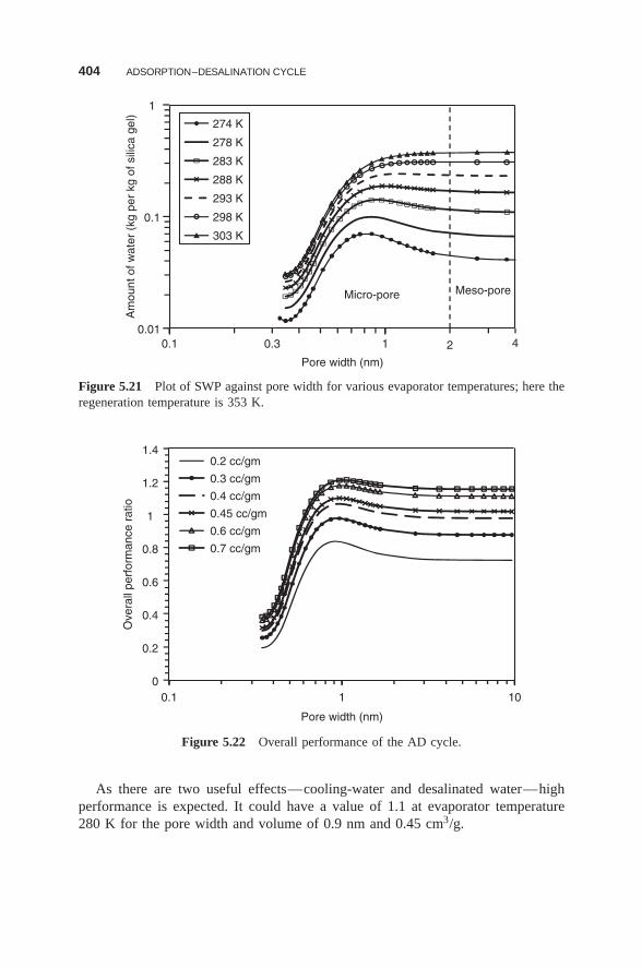
404 ADSORPTION–DESALINATION CYCLE

0.01

0.1

1

10.1

Am

ount

of w

ater

(kg

per

kg

of s

ilica

gel

)

Pore width (nm)

274 K

278 K

283 K

288 K

293 K

298 K

303 K

2 40.3

Micro-pore Meso-pore

Figure 5.21 Plot of SWP against pore width for various evaporator temperatures; here theregeneration temperature is 353 K.

0

0.2

0.4

0.6

0.8

1

1.2

1.4

1010.1

Ove

rall

perf

orm

ance

rat

io

Pore width (nm)

0.2 cc/gm

0.3 cc/gm

0.4 cc/gm

0.45 cc/gm

0.6 cc/gm

0.7 cc/gm

Figure 5.22 Overall performance of the AD cycle.

As there are two useful effects—cooling-water and desalinated water—highperformance is expected. It could have a value of 1.1 at evaporator temperature280 K for the pore width and volume of 0.9 nm and 0.45 cm3/g.

ADSORPTION–DESALINATION SYSTEM MODELING 405

5.4.6 Summary

From the present analysis, we notice that silica gels optimized with respectto pore size and volume for a given evaporating temperature can entail anincrease in overall performances in the order of 20–40%, which cannot beneglected. If the evaporator temperature varies, especially when it decreases,there is a decreasing tendency of specific water production. Another conclusionof this study is that an increase in pore volume does not entail systematicallyan improvement of performance. The best adsorption–desalination performanceis obtained from a compromise between the greatest pore volume and theoptimal pore size. From the present analysis, it is observed that there is waterproduction for pore widths varying from 0 to 0.3 nm. The best performanceof silica gel–water–based AD is obtained at pore width 0.9 nm with higherpore volume. The characteristics energy (E ) is found to be higher in microporeranges. This indicates that the adsorption and desorption rates are higher inmicropores. Adsorbent materials such as silica gel should be designed withmicropores ranging from 0.8 to 1 nm and higher micropore volume for ADapplications.

5.5 ADSORPTION–DESALINATION SYSTEM MODELING

The AD system utilizes the silica gel–water characteristics and produces drinkablewater at the condenser by the amalgamation of adsorption-triggered evaporationand desorption-resulting condensation . These phenomena are expressed mathe-matically using the mass and energy balances between major components of theadsorption chiller system [50].

5.5.1 Evaporator

For continuous water production operation, initially, sea- or brackish-water is evap-orated in the evaporator. Seawater is fed into the evaporator, and potable water isextracted from the condenser of the AD cycle, and the overall mass balance of thecycle is thus given by

dMs,evap

dt= ms,in − md,cond − mb (5.7)

where Ms,evap is the amount of seawater in the evaporator, ms,in is the rate of feedseawater, md,cond is the mass of potable water extracted from the condenser, and mbis the mass of concentrated brine rejected from the evaporator. The feed seawateris intermittently pumped into the evaporator depending on the amount and levelof seawater, while brine is discharged once the concentration in the evaporatorreaches the predetermined limit. The mass–salt balance for the evaporator of the

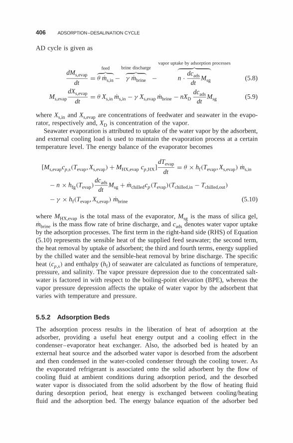
406 ADSORPTION–DESALINATION CYCLE

AD cycle is given as

dMs,evap

dt=

feed︷ ︸︸ ︷θ ms,in −

brine discharge︷ ︸︸ ︷γ mbrine −

vapor uptake by adsorption processes︷ ︸︸ ︷n · dcads

dtMsg (5.8)

Ms,evap

dXs,evap

dt= θ Xs,in ms,in − γ Xs,evap mbrine − nXD

dcads

dtMsg (5.9)

where Xs,in and Xs,evap are concentrations of feedwater and seawater in the evapo-rator, respectively and, XD is concentration of the vapor.

Seawater evaporation is attributed to uptake of the water vapor by the adsorbent,and external cooling load is used to maintain the evaporation process at a certaintemperature level. The energy balance of the evaporator becomes

[Ms,evapcp,s(Tevap, Xs,evap) + MHX,evap cp,HX]dTevap

dt= θ × hf(Tevap, Xs,evap) ms,in

− n × hfg(Tevap)dcads

dtMsg + mchilledcp(Tevap)(Tchilled,in − Tchilled,out)

− γ × hf(Tevap, Xs,evap) mbrine (5.10)

where MHX,evap is the total mass of the evaporator, Msg is the mass of silica gel,mbrine is the mass flow rate of brine discharge, and cads denotes water vapor uptakeby the adsorption processes. The first term in the right-hand side (RHS) of Equation(5.10) represents the sensible heat of the supplied feed seawater; the second term,the heat removal by uptake of adsorbent; the third and fourth terms, energy suppliedby the chilled water and the sensible-heat removal by brine discharge. The specificheat (cp,s) and enthalpy (hf) of seawater are calculated as functions of temperature,pressure, and salinity. The vapor pressure depression due to the concentrated salt-water is factored in with respect to the boiling-point elevation (BPE), whereas thevapor pressure depression affects the uptake of water vapor by the adsorbent thatvaries with temperature and pressure.

5.5.2 Adsorption Beds

The adsorption process results in the liberation of heat of adsorption at theadsorber, providing a useful heat energy output and a cooling effect in thecondenser–evaporator heat exchanger. Also, the adsorbed bed is heated by anexternal heat source and the adsorbed water vapor is desorbed from the adsorbentand then condensed in the water-cooled condenser through the cooling tower. Asthe evaporated refrigerant is associated onto the solid adsorbent by the flow ofcooling fluid at ambient conditions during adsorption period, and the desorbedwater vapor is dissociated from the solid adsorbent by the flow of heating fluidduring desorption period, heat energy is exchanged between cooling/heatingfluid and the adsorption bed. The energy balance equation of the adsorber bed

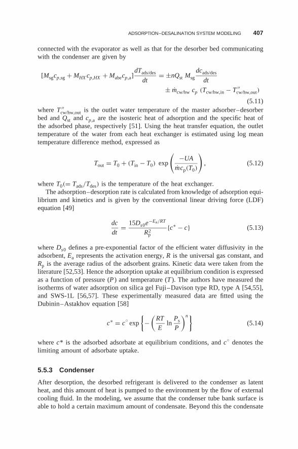
ADSORPTION–DESALINATION SYSTEM MODELING 407

connected with the evaporator as well as that for the desorber bed communicatingwith the condenser are given by

[Msgcp,sg + MHX cp,HX + Mabecp,a]dTads/des

dt= ±nQst Msg

dcads/des

dt

± mcw/hw cp (Tcw/hw,in − T ′′cw/hw,out)

(5.11)where T ′′

cw/hw,out is the outlet water temperature of the master adsorber–desorberbed and Qst and cp,a are the isosteric heat of adsorption and the specific heat ofthe adsorbed phase, respectively [51]. Using the heat transfer equation, the outlettemperature of the water from each heat exchanger is estimated using log meantemperature difference method, expressed as

Tout = T0 + (Tin − T0) exp

(−UA

mcp(T0)

), (5.12)

where T0(= Tads/Tdes) is the temperature of the heat exchanger.The adsorption–desorption rate is calculated from knowledge of adsorption equi-

librium and kinetics and is given by the conventional linear driving force (LDF)equation [49]

dc

dt= 15Ds0e−Ea/RT

R2p

{c∗ − c} (5.13)

where Ds0 defines a pre-exponential factor of the efficient water diffusivity in theadsorbent, Ea represents the activation energy, R is the universal gas constant, andRp is the average radius of the adsorbent grains. Kinetic data were taken from theliterature [52,53]. Hence the adsorption uptake at equilibrium condition is expressedas a function of pressure (P ) and temperature (T ). The authors have measured theisotherms of water adsorption on silica gel Fuji–Davison type RD, type A [54,55],and SWS-1L [56,57]. These experimentally measured data are fitted using theDubinin–Astakhov equation [58]

c∗ = c◦ exp

{−

(RT

Eln

Ps

P

)n}(5.14)

where c* is the adsorbed adsorbate at equilibrium conditions, and c◦ denotes thelimiting amount of adsorbate uptake.

5.5.3 Condenser

After desorption, the desorbed refrigerant is delivered to the condenser as latentheat, and this amount of heat is pumped to the environment by the flow of externalcooling fluid. In the modeling, we assume that the condenser tube bank surface isable to hold a certain maximum amount of condensate. Beyond this the condensate

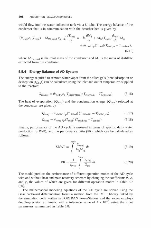
408 ADSORPTION–DESALINATION CYCLE

would flow into the water collection tank via a U-tube. The energy balance of thecondenser that is in communication with the desorber bed is given by

[Mcondcp(Tcond) + MHX ,cond cp,HX]dTcond

dt= −hf

dMd

dt+ nhfg(Tcond)

dcdes

dtMsg

+ mcond cp(Tcond)(Tcond,in − Tcond,out),

(5.15)

where MHX,cond is the total mass of the condenser and Md is the mass of distillateextracted from the condenser.

5.5.4 Energy Balance of AD System

The energy required to remove water vapor from the silica gels [here adsorption ordesorption (Qdes)] can be calculated using the inlet and outlet temperatures suppliedto the reactors:

Qads/des = mcw/hwcp(TMads/Mdes) (Tcw/hw,in − T ′′cw/hw,out) (5.16)

The heat of evaporation (Qevap) and the condensation energy (Qcond) rejected atthe condenser are given by

Qevap = mchilled cp(Tchilled) (Tchilled,in − Tchilled,out) (5.17)

Qcond = mcond cp(Tcond) (Tcond,out − Tcond,in) (5.18)

Finally, performance of the AD cycle is assessed in terms of specific daily waterproduction (SDWP), and the performance ratio (PR), which can be calculated asfollows:

SDWP =tcycle∫0

Qcond

hfgMsgdt (5.19)

PR = 1

tcycle

tcycle∫0

mdhfg

Qdesdt (5.20)

The model predicts the performance of different operation modes of the AD cyclewith and without heat and mass recovery schemes by changing the coefficients θ , ε,and γ , the values of which are given for different operation modes in Table 5.7[50].

The mathematical modeling equations of the AD cycle are solved using theGear backward differentiation formula method from the IMSL library linked bythe simulation code written in FORTRAN PowerStation, and the solver employsdouble-precision arithmetic with a tolerance value of 1 × 10−6 using the inputparameters summarized in Table 5.8.

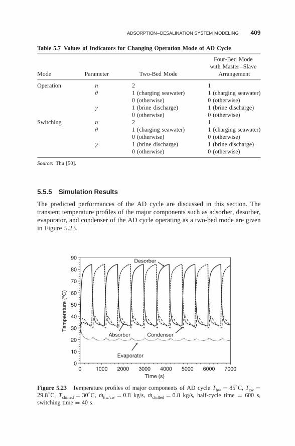
ADSORPTION–DESALINATION SYSTEM MODELING 409

Table 5.7 Values of Indicators for Changing Operation Mode of AD Cycle

Four-Bed Modewith Master–Slave

Mode Parameter Two-Bed Mode Arrangement

Operation n 2 1θ 1 (charging seawater) 1 (charging seawater)

0 (otherwise) 0 (otherwise)γ 1 (brine discharge) 1 (brine discharge)

0 (otherwise) 0 (otherwise)Switching n 2 1

θ 1 (charging seawater) 1 (charging seawater)0 (otherwise) 0 (otherwise)

γ 1 (brine discharge) 1 (brine discharge)0 (otherwise) 0 (otherwise)

Source: Thu [50].

5.5.5 Simulation Results

The predicted performances of the AD cycle are discussed in this section. Thetransient temperature profiles of the major components such as adsorber, desorber,evaporator, and condenser of the AD cycle operating as a two-bed mode are givenin Figure 5.23.

00

10

Tem

pera

ture

(°C

)

20

30

40

50

60

70

80

90

1000 2000 3000 4000TIme (s)

Evaporator

Condenser

Desorber

Absorber

5000 6000 7000

Figure 5.23 Temperature profiles of major components of AD cycle Thw = 85◦C, Tcw =29.8◦C, Tchilled = 30◦C, mhw/cw = 0.8 kg/s, mchilled = 0.8 kg/s, half-cycle time = 600 s,switching time = 40 s.

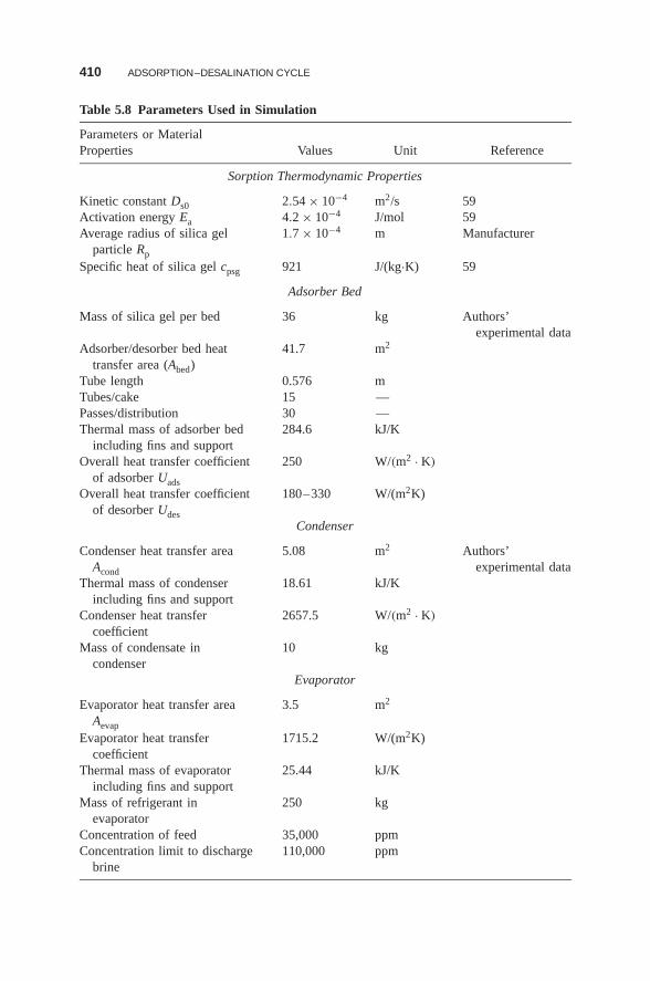
410 ADSORPTION–DESALINATION CYCLE

Table 5.8 Parameters Used in Simulation

Parameters or MaterialProperties Values Unit Reference

Sorption Thermodynamic Properties

Kinetic constant Ds0 2.54 × 10−4 m2/s 59Activation energy Ea 4.2 × 10−4 J/mol 59Average radius of silica gel

particle Rp

1.7 × 10−4 m Manufacturer

Specific heat of silica gel cpsg 921 J/(kg·K) 59

Adsorber Bed

Mass of silica gel per bed 36 kg Authors’experimental data

Adsorber/desorber bed heattransfer area (Abed)

41.7 m2

Tube length 0.576 mTubes/cake 15 —Passes/distribution 30 —Thermal mass of adsorber bed

including fins and support284.6 kJ/K

Overall heat transfer coefficientof adsorber Uads

250 W/(m2 · K)

Overall heat transfer coefficientof desorber Udes

180–330 W/(m2K)

Condenser

Condenser heat transfer areaAcond

5.08 m2 Authors’experimental data

Thermal mass of condenserincluding fins and support

18.61 kJ/K

Condenser heat transfercoefficient

2657.5 W/(m2 · K)

Mass of condensate incondenser

10 kg

Evaporator

Evaporator heat transfer areaAevap

3.5 m2

Evaporator heat transfercoefficient

1715.2 W/(m2K)

Thermal mass of evaporatorincluding fins and support

25.44 kJ/K

Mass of refrigerant inevaporator

250 kg

Concentration of feed 35,000 ppmConcentration limit to discharge

brine110,000 ppm

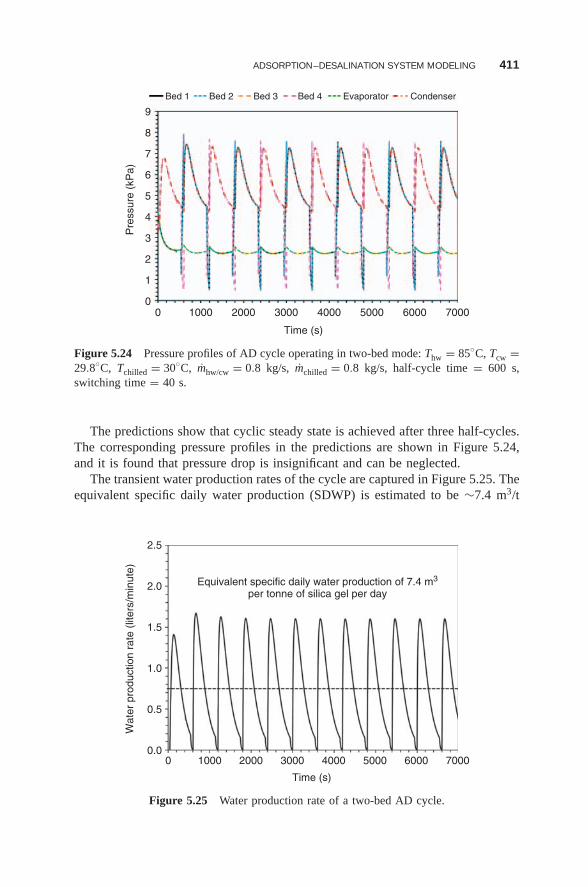
ADSORPTION–DESALINATION SYSTEM MODELING 411

00

1

2

3

4

Pre

ssur

e (k

Pa)

5

6

7

8

9

1000 2000 3000 4000

Time (s)

Bed 1 Bed 2 Bed 3 Bed 4 Evaporator Condenser

5000 6000 7000

Figure 5.24 Pressure profiles of AD cycle operating in two-bed mode: Thw = 85◦C, Tcw =29.8◦C, Tchilled = 30◦C, mhw/cw = 0.8 kg/s, mchilled = 0.8 kg/s, half-cycle time = 600 s,switching time = 40 s.

The predictions show that cyclic steady state is achieved after three half-cycles.The corresponding pressure profiles in the predictions are shown in Figure 5.24,and it is found that pressure drop is insignificant and can be neglected.

The transient water production rates of the cycle are captured in Figure 5.25. Theequivalent specific daily water production (SDWP) is estimated to be ∼7.4 m3/t

00.0

0.5

1.0

Wat

er p

rodu

ctio

n ra

te (

liter

s/m

inut

e)

1.5

2.0

2.5

Equivalent specific daily water production of 7.4 m3

per tonne of silica gel per day

1000 2000 3000 4000

Time (s)

5000 6000 7000

Figure 5.25 Water production rate of a two-bed AD cycle.

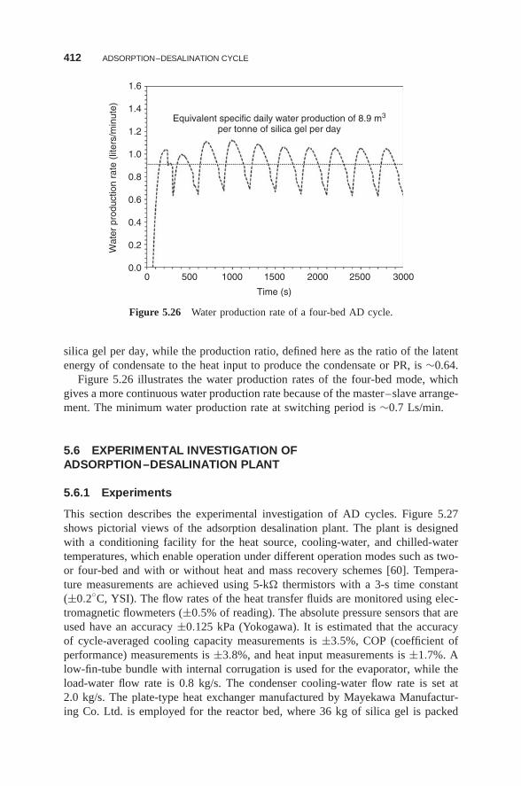
412 ADSORPTION–DESALINATION CYCLE

00.0

0.2

0.4

Wat

er p

rodu

ctio

n ra

te (

liter

s/m

inut

e)

0.6

0.8

1.0

1.2

1.4

1.6

Equivalent specific daily water production of 8.9 m3

per tonne of silica gel per day

500 1000 1500 2000

Time (s)

2500 3000

Figure 5.26 Water production rate of a four-bed AD cycle.

silica gel per day, while the production ratio, defined here as the ratio of the latentenergy of condensate to the heat input to produce the condensate or PR, is ∼0.64.

Figure 5.26 illustrates the water production rates of the four-bed mode, whichgives a more continuous water production rate because of the master–slave arrange-ment. The minimum water production rate at switching period is ∼0.7 Ls/min.

5.6 EXPERIMENTAL INVESTIGATION OFADSORPTION–DESALINATION PLANT

5.6.1 Experiments

This section describes the experimental investigation of AD cycles. Figure 5.27shows pictorial views of the adsorption desalination plant. The plant is designedwith a conditioning facility for the heat source, cooling-water, and chilled-watertemperatures, which enable operation under different operation modes such as two-or four-bed and with or without heat and mass recovery schemes [60]. Tempera-ture measurements are achieved using 5-k thermistors with a 3-s time constant(±0.2◦C, YSI). The flow rates of the heat transfer fluids are monitored using elec-tromagnetic flowmeters (±0.5% of reading). The absolute pressure sensors that areused have an accuracy ±0.125 kPa (Yokogawa). It is estimated that the accuracyof cycle-averaged cooling capacity measurements is ±3.5%, COP (coefficient ofperformance) measurements is ±3.8%, and heat input measurements is ±1.7%. Alow-fin-tube bundle with internal corrugation is used for the evaporator, while theload-water flow rate is 0.8 kg/s. The condenser cooling-water flow rate is set at2.0 kg/s. The plate-type heat exchanger manufactured by Mayekawa Manufactur-ing Co. Ltd. is employed for the reactor bed, where 36 kg of silica gel is packed

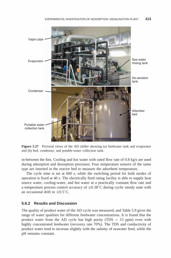
EXPERIMENTAL INVESTIGATION OF ADSORPTION–DESALINATION PLANT 413

(a)

Vapor pipe

Sea watermixing tank

De-aerationtank

Adsorberbed

Evaporator

Condenser

Portable watercollection tank

(b)

Figure 5.27 Pictorial views of the AD chiller showing (a) feedwater tank and evaporatorand (b) bed, condenser, and potable-water collection tank.

in-between the fins. Cooling and hot water with rated flow rate of 0.8 kg/s are usedduring adsorption and desorption processes. Four temperature sensors of the sametype are inserted in the reactor bed to measure the adsorbent temperature.

The cycle time is set at 600 s, while the switching period for both modes ofoperation is fixed at 40 s. The electrically fired rating facility is able to supply heatsource water, cooling-water, and hot water at a practically constant flow rate anda temperature process control accuracy of ±0.38◦C during cyclic steady state withan occasional drift to ±0.5◦C.

5.6.2 Results and Discussion

The quality of product water of the AD cycle was measured, and Table 5.9 gives therange of water qualities for different feedwater concentrations. It is found that theproduct water from the AD cycle has high purity (TDS < 15 ppm) even withhighly concentrated feedwater (recovery rate 70%). The TDS and conductivity ofproduct water tend to increase slightly with the salinity of seawater feed, while thepH remains constant.

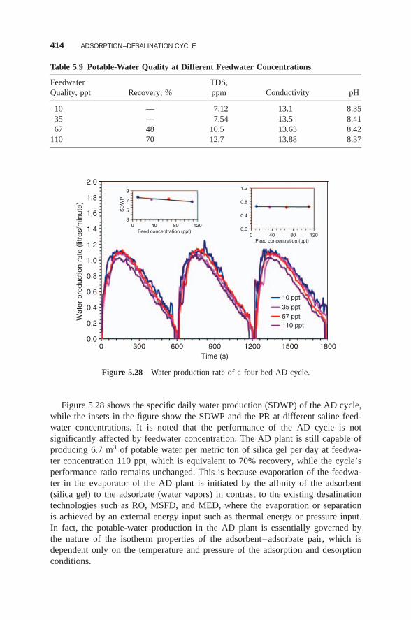
414 ADSORPTION–DESALINATION CYCLE

Table 5.9 Potable-Water Quality at Different Feedwater Concentrations

Feedwater TDS,Quality, ppt Recovery, % ppm Conductivity pH

10 — 7.12 13.1 8.3535 — 7.54 13.5 8.4167 48 10.5 13.63 8.42

110 70 12.7 13.88 8.37

0.00 300 600 900

Time (s)1200 1500 1800

0.2

0.4

Wat

er p

rodu

ctio

n ra

te (

litre

s/m

inut

e)

0.6

0.8

1.0

1.2

1.4

1.6

1.8

2.0

3

0.0

0.4

0.8

1.2

SD

WP

0 40 80Feed concentration (ppt)

120

0

10 ppt35 ppt57 ppt110 ppt

40 80Feed concentration (ppt)

120

5

7

9

Figure 5.28 Water production rate of a four-bed AD cycle.

Figure 5.28 shows the specific daily water production (SDWP) of the AD cycle,while the insets in the figure show the SDWP and the PR at different saline feed-water concentrations. It is noted that the performance of the AD cycle is notsignificantly affected by feedwater concentration. The AD plant is still capable ofproducing 6.7 m3 of potable water per metric ton of silica gel per day at feedwa-ter concentration 110 ppt, which is equivalent to 70% recovery, while the cycle’sperformance ratio remains unchanged. This is because evaporation of the feedwa-ter in the evaporator of the AD plant is initiated by the affinity of the adsorbent(silica gel) to the adsorbate (water vapors) in contrast to the existing desalinationtechnologies such as RO, MSFD, and MED, where the evaporation or separationis achieved by an external energy input such as thermal energy or pressure input.In fact, the potable-water production in the AD plant is essentially governed bythe nature of the isotherm properties of the adsorbent–adsorbate pair, which isdependent only on the temperature and pressure of the adsorption and desorptionconditions.

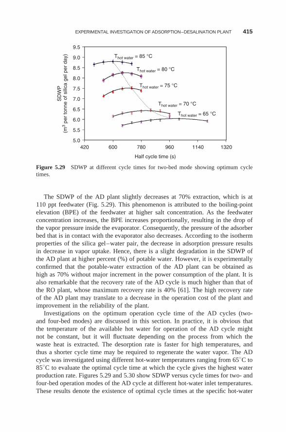
EXPERIMENTAL INVESTIGATION OF ADSORPTION–DESALINATION PLANT 415

Thot water = 85 °C

Thot water = 80 °C

Thot water = 75 °C

Thot water = 70 °C

Thot water = 65 °C

5.0420 600 780 960 1140 1320

5.5

6.0

6.5

7.0

7.5

8.0

8.5

9.0

9.5

SD

WP

(m3

per

tonn

e of

sili

ca g

el p

er d

ay)

Half cycle time (s)

Figure 5.29 SDWP at different cycle times for two-bed mode showing optimum cycletimes.

The SDWP of the AD plant slightly decreases at 70% extraction, which is at110 ppt feedwater (Fig. 5.29). This phenomenon is attributed to the boiling-pointelevation (BPE) of the feedwater at higher salt concentration. As the feedwaterconcentration increases, the BPE increases proportionally, resulting in the drop ofthe vapor pressure inside the evaporator. Consequently, the pressure of the adsorberbed that is in contact with the evaporator also decreases. According to the isothermproperties of the silica gel–water pair, the decrease in adsorption pressure resultsin decrease in vapor uptake. Hence, there is a slight degradation in the SDWP ofthe AD plant at higher percent (%) of potable water. However, it is experimentallyconfirmed that the potable-water extraction of the AD plant can be obtained ashigh as 70% without major increment in the power consumption of the plant. It isalso remarkable that the recovery rate of the AD cycle is much higher than that ofthe RO plant, whose maximum recovery rate is 40% [61]. The high recovery rateof the AD plant may translate to a decrease in the operation cost of the plant andimprovement in the reliability of the plant.

Investigations on the optimum operation cycle time of the AD cycles (two-and four-bed modes) are discussed in this section. In practice, it is obvious thatthe temperature of the available hot water for operation of the AD cycle mightnot be constant, but it will fluctuate depending on the process from which thewaste heat is extracted. The desorption rate is faster for high temperatures, andthus a shorter cycle time may be required to regenerate the water vapor. The ADcycle was investigated using different hot-water temperatures ranging from 65◦C to85◦C to evaluate the optimal cycle time at which the cycle gives the highest waterproduction rate. Figures 5.29 and 5.30 show SDWP versus cycle times for two- andfour-bed operation modes of the AD cycle at different hot-water inlet temperatures.These results denote the existence of optimal cycle times at the specific hot-water

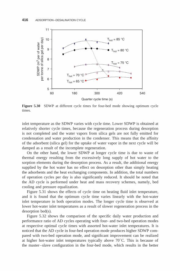
416 ADSORPTION–DESALINATION CYCLE

560 180 300 420 540

6

7

8

9

10

11

SD

WP

(m

3 pe

r of

wat

erpe

r to

nne

of s

ilica

gel

per

day

)

Quarter cycle time (s)

Thot = 85 °C

Thot = 80 °C

Thot = 75 °C

Thot = 70 °C

Thot = 65 °C

Figure 5.30 SDWP at different cycle times for four-bed mode showing optimum cycletimes.

inlet temperature as the SDWP varies with cycle time. Lower SDWP is obtained atrelatively shorter cycle times, because the regeneration process during desorptionis not completed and the water vapors from silica gels are not fully emitted forcondensation and water production in the condenser. This means that the affinityof the adsorbent (silica gel) for the uptake of water vapor in the next cycle will bedamped as a result of the incomplete regeneration.

On the other hand, the lower SDWP at longer cycle time is due to waste ofthermal energy resulting from the excessively long supply of hot water to thesorption elements during the desorption process. As a result, the additional energysupplied by the hot water has no effect on desorption other than simply heatingthe adsorbents and the heat exchanging components. In addition, the total numbersof operation cycles per day is also significantly reduced. It should be noted thatthe AD cycle is performed under heat and mass recovery schemes, namely, bedcooling and pressure equalization.

Figure 5.31 shows the effects of cycle time on heating fluid inlet temperature,and it is found that the optimum cycle time varies linearly with the hot-waterinlet temperature in both operation modes. The longer cycle time is observed atlower hot-water inlet temperatures as a result of slower regeneration process in thedesorption bed(s).

Figure 5.32 shows the comparison of the specific daily water production andperformance ratio of AD cycles operating with four- and two-bed operation modesat respective optimal cycle times with assorted hot-water inlet temperatures. It isnoticed that the AD cycle in four-bed operation mode produces higher SDWP com-pared with two-bed operation mode, and significant improvement can be realizedat higher hot-water inlet temperatures typically above 70◦C. This is because ofthe master–slave configuration in the four-bed mode, which results in the better

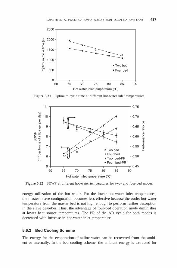
EXPERIMENTAL INVESTIGATION OF ADSORPTION–DESALINATION PLANT 417

060 65 70 75 80 85 90

500

1000

1500

2000

2500

Opt

imum

cyc

le ti

me

(s)

Hot water inlet temperature (°C)

Two bed

Four bed

Figure 5.31 Optimum cycle time at different hot-water inlet temperatures.

0.45

0.50

0.55

0.60

0.65

0.70

0.75

560 65 70 75 80 85 90

6

7

8

9

10

11

Per

form

ance

rat

io (

-)

SD

WP

(m3

per

tonn

e o

f sili

ca g

el p

er d

ay)

Hot water inlet temperature (°C)

Two bed Four bed Two bed-PRFour bed-PR

Figure 5.32 SDWP at different hot-water temperatures for two- and four-bed modes.

energy utilization of the hot water. For the lower hot-water inlet temperatures,the master–slave configuration becomes less effective because the outlet hot-watertemperature from the master bed is not high enough to perform further desorptionin the slave desorber. Thus, the advantage of four-bed operation mode diminishesat lower heat source temperatures. The PR of the AD cycle for both modes isdecreased with increase in hot-water inlet temperature.

5.6.3 Bed Cooling Scheme

The energy for the evaporation of saline water can be recovered from the ambi-ent or internally. In the bed cooling scheme, the ambient energy is extracted for

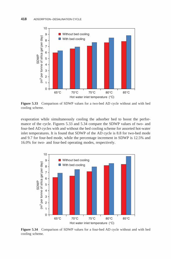
418 ADSORPTION–DESALINATION CYCLE

065°C 70°C 75°C 80°C 85°C

1

2

3

4

5

6

7

8

9

10

SD

WP

(m3

per

tonn

e of

sili

ca g

el p

er d

ay)

Hot water inlet temperature (°C)

Without bed cooling

With bed cooling

Figure 5.33 Comparison of SDWP values for a two-bed AD cycle without and with bedcooling scheme.

evaporation while simultaneously cooling the adsorber bed to boost the perfor-mance of the cycle. Figures 5.33 and 5.34 compare the SDWP values of two- andfour-bed AD cycles with and without the bed cooling scheme for assorted hot-waterinlet temperatures. It is found that SDWP of the AD cycle is 8.8 for two-bed modeand 9.7 for four-bed mode, while the percentage increment in SDWP is 12.5% and16.0% for two- and four-bed operating modes, respectively.

065°C 70°C 75°C 80°C 85°C

1

2

3

4

5

6

7

8

9

10

SD

WP

(m3

per

tonn

e of

sili

ca g

el p

er d

ay)

Hot water inlet temperature (°C)

Without bed cooling

With bed cooling

Figure 5.34 Comparison of SDWP values for a four-bed AD cycle without and with bedcooling scheme.

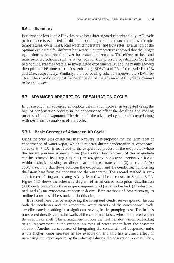
ADVANCED ADSORPTION–DESALINATION CYCLE 419

5.6.4 Summary

Performance levels of AD cycles have been investigated experimentally. AD cycleperformance is evaluated for different operating conditions such as hot-water inlettemperatures, cycle times, load water temperature, and flow rates. Evaluation of theoptimal cycle time for different hot-water inlet temperatures showed that the longercycle time is required for lower hot-water temperatures. The effects of heat andmass recovery schemes such as water recirculation, pressure equalization (PE), andbed cooling schemes were also investigated experimentally, and the results showedthe optimum PE time to be 10 s, enhancing SDWP and PR of the cycle by 12%and 21%, respectively. Similarly, the bed cooling scheme improves the SDWP by16%. The specific unit cost for desalination of the advanced AD cycle is deemedto be the lowest.

5.7 ADVANCED ADSORPTION–DESALINATION CYCLE

In this section, an advanced adsorption desalination cycle is investigated using theheat of condensation process in the condenser to effect the desalting and coolingprocesses in the evaporator. The details of the advanced cycle are discussed alongwith performance analyses of the cycle.

5.7.1 Basic Concept of Advanced AD Cycle

Using the principles of internal heat recovery, it is proposed that the latent heat ofcondensation of water vapor, which is rejected during condensation at vapor pres-sures of 5–7 kPa, is recovered to the evaporative process of the evaporator wherethe system pressure is much lower (2–3 kPa). Heat recovery of this magnitudecan be achieved by using either (1) an integrated condenser–evaporator layoutwithin a single housing for direct heat and mass transfer or (2) a recirculatingcoolant medium that flows between the evaporator and the condenser, transferringthe latent heat from the condenser to the evaporator. The second method is suit-able for retrofitting an existing AD cycle and will be discussed in Section 5.7.3.Figure 5.35 shows the schematic diagram of an advanced adsorption–desalination(AD) cycle comprising three major components: (1) an adsorber bed, (2) a desorberbed, and (3) an evaporator–condenser device. Both methods of heat recovery, asoutlined above, will be simulated in this chapter.

It is noted here that by employing the integrated condenser–evaporator layout,both the condenser and the evaporator water circuits of the conventional cycleare eliminated, resulting in a significant saving in the pumping cost. The heat istransferred directly across the walls of the condenser tubes, which are placed withinthe evaporator shell. This arrangement reduces the heat transfer resistance, leadingto an improvement in the evaporation rates of water vapor from the seawatersolution. Another consequence of integrating the condenser and evaporator unitsis the higher vapor pressure in the evaporator, and this has a direct effect ofincreasing the vapor uptake by the silica gel during the adsorption process. Thus,

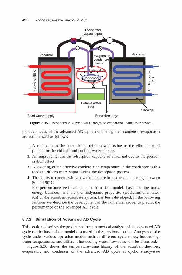
420 ADSORPTION–DESALINATION CYCLE

Desorber Adsorber

Potable watertank

Hot

wat

er 8

5°C

Evaporator-condenserdevice

Feed water supply Brine discharge

Evaporatorvapour pipes

Silica gel

Coo

ling

wat

er30

°C

Evaporator

Condensor

Figure 5.35 Advanced AD cycle with integrated evaporator–condenser device.

the advantages of the advanced AD cycle (with integrated condenser-evaporator)are summarized as follows:

1. A reduction in the parasitic electrical power owing to the elimination ofpumps for the chilled- and cooling-water circuits

2. An improvement in the adsorption capacity of silica gel due to the pressur-ization effect

3. A lowering of the effective condensation temperature in the condenser as thistends to desorb more vapor during the desorption process

4. The ability to operate with a low temperature heat source in the range between50 and 90◦C.For performance verification, a mathematical model, based on the mass,energy balances, and the thermodynamic properties (isotherms and kinet-ics) of the adsorbent/adsorbate system, has been developed. In the followingsections we describe the development of the numerical model to predict theperformance of the advanced AD cycle.

5.7.2 Simulation of Advanced AD Cycle

This section describes the predictions from numerical analysis of the advanced ADcycle on the basis of the model discussed in the previous section. Analyses of thecycle under various operation modes such as different cycle times, hot/cooling-water temperatures, and different hot/cooling-water flow rates will be discussed.

Figure 5.36 shows the temperature–time history of the adsorber, desorber,evaporator, and condenser of the advanced AD cycle at cyclic steady-state

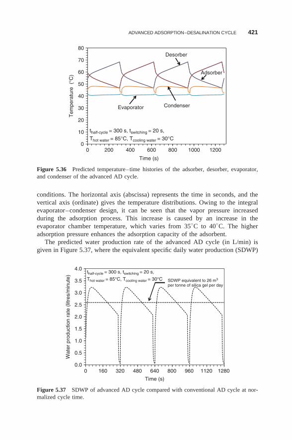
ADVANCED ADSORPTION–DESALINATION CYCLE 421

0

10

20

30

40

50

60

70

80

0 200 400 600 800 1000 1200

Tem

pera

ture

(°C

)

Time (s)

Evaporator

Desorber

Adsorber

Condenser

thalf-cycle = 300 s, tswitching = 20 s,

Thot water = 85°C, Tcooling water = 30°C

Figure 5.36 Predicted temperature–time histories of the adsorber, desorber, evaporator,and condenser of the advanced AD cycle.

conditions. The horizontal axis (abscissa) represents the time in seconds, and thevertical axis (ordinate) gives the temperature distributions. Owing to the integralevaporator–condenser design, it can be seen that the vapor pressure increasedduring the adsorption process. This increase is caused by an increase in theevaporator chamber temperature, which varies from 35◦C to 40◦C. The higheradsorption pressure enhances the adsorption capacity of the adsorbent.

The predicted water production rate of the advanced AD cycle (in L/min) isgiven in Figure 5.37, where the equivalent specific daily water production (SDWP)

00.0

0.5

1.0

1.5

2.0

2.5

3.0

3.5

4.0

160 320 480 640

Time (s)

SDWP equivalent to 26 m3

per tonne of silica gel per day

Wat

er p

rodu

ctio

n ra

te (

litre

s/m

inut

e)

800 960 1120 1280

thalf-cycle = 300 s, tswitching = 20 s,

Thot water = 85°C, Tcooling water = 30°C

Figure 5.37 SDWP of advanced AD cycle compared with conventional AD cycle at nor-malized cycle time.

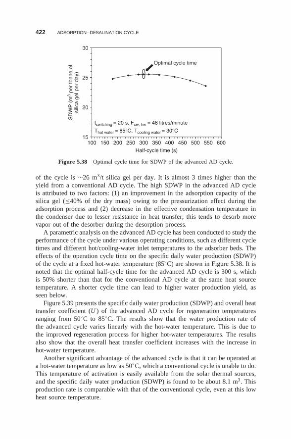
422 ADSORPTION–DESALINATION CYCLE

15100 150 200 250 300 350 400 450 500 550 600

20

25

30

SD

WP

(m

3 pe

r to

nne

ofsi

lica

gel p

er d

ay)

Half-cycle time (s)

tswitching = 20 s, Fcw, hw = 48 litres/minute

Thot water = 85°C, Tcooling water = 30°C

Optimal cycle time

Figure 5.38 Optimal cycle time for SDWP of the advanced AD cycle.

of the cycle is ∼26 m3/t silica gel per day. It is almost 3 times higher than theyield from a conventional AD cycle. The high SDWP in the advanced AD cycleis attributed to two factors: (1) an improvement in the adsorption capacity of thesilica gel (≤40% of the dry mass) owing to the pressurization effect during theadsorption process and (2) decrease in the effective condensation temperature inthe condenser due to lesser resistance in heat transfer; this tends to desorb morevapor out of the desorber during the desorption process.

A parametric analysis on the advanced AD cycle has been conducted to study theperformance of the cycle under various operating conditions, such as different cycletimes and different hot/cooling-water inlet temperatures to the adsorber beds. Theeffects of the operation cycle time on the specific daily water production (SDWP)of the cycle at a fixed hot-water temperature (85◦C) are shown in Figure 5.38. It isnoted that the optimal half-cycle time for the advanced AD cycle is 300 s, whichis 50% shorter than that for the conventional AD cycle at the same heat sourcetemperature. A shorter cycle time can lead to higher water production yield, asseen below.

Figure 5.39 presents the specific daily water production (SDWP) and overall heattransfer coefficient (U ) of the advanced AD cycle for regeneration temperaturesranging from 50◦C to 85◦C. The results show that the water production rate ofthe advanced cycle varies linearly with the hot-water temperature. This is due tothe improved regeneration process for higher hot-water temperatures. The resultsalso show that the overall heat transfer coefficient increases with the increase inhot-water temperature.

Another significant advantage of the advanced cycle is that it can be operated ata hot-water temperature as low as 50◦C, which a conventional cycle is unable to do.This temperature of activation is easily available from the solar thermal sources,and the specific daily water production (SDWP) is found to be about 8.1 m3. Thisproduction rate is comparable with that of the conventional cycle, even at this lowheat source temperature.

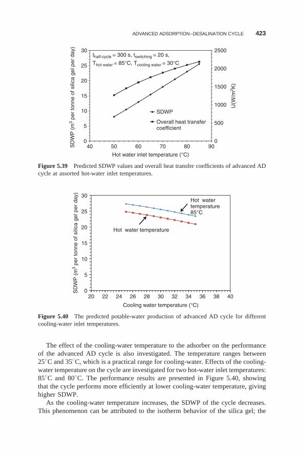
ADVANCED ADSORPTION–DESALINATION CYCLE 423

0

500

1000

1500

2000

2500

0

5

10

15

20

25

30

40 50 60 70 80 90

U(W

/m2 K

)

SD

WP

(m

3 pe

r to

nne

of s

ilica

gel

per

day

)

Hot water inlet temperature (°C)

SDWP

Overall heat transfercoefficient

thalf-cycle = 300 s, tswitching = 20 s,

Thot water = 85°C, Tcooling water = 30°C

Figure 5.39 Predicted SDWP values and overall heat transfer coefficients of advanced ADcycle at assorted hot-water inlet temperatures.

0

5

10

15

20

25

30

20 22 24 26 28 30 32 34 36 38 40

SD

WP

(m

3 pe

r to

nne

of s

ilica

gel

per

day

)

Cooling water temperature (°C)

Hot water temperature

Hot watertemperature85°C

Figure 5.40 The predicted potable-water production of advanced AD cycle for differentcooling-water inlet temperatures.

The effect of the cooling-water temperature to the adsorber on the performanceof the advanced AD cycle is also investigated. The temperature ranges between25◦C and 35◦C, which is a practical range for cooling-water. Effects of the cooling-water temperature on the cycle are investigated for two hot-water inlet temperatures:85◦C and 80◦C. The performance results are presented in Figure 5.40, showingthat the cycle performs more efficiently at lower cooling-water temperature, givinghigher SDWP.

As the cooling-water temperature increases, the SDWP of the cycle decreases.This phenomenon can be attributed to the isotherm behavior of the silica gel; the

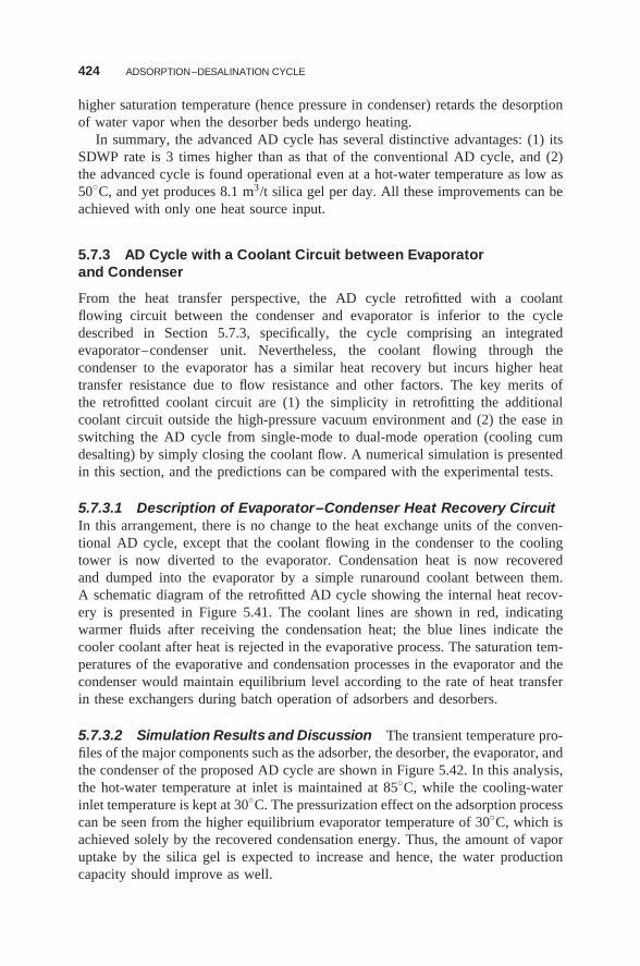
424 ADSORPTION–DESALINATION CYCLE

higher saturation temperature (hence pressure in condenser) retards the desorptionof water vapor when the desorber beds undergo heating.

In summary, the advanced AD cycle has several distinctive advantages: (1) itsSDWP rate is 3 times higher than as that of the conventional AD cycle, and (2)the advanced cycle is found operational even at a hot-water temperature as low as50◦C, and yet produces 8.1 m3/t silica gel per day. All these improvements can beachieved with only one heat source input.

5.7.3 AD Cycle with a Coolant Circuit between Evaporatorand Condenser

From the heat transfer perspective, the AD cycle retrofitted with a coolantflowing circuit between the condenser and evaporator is inferior to the cycledescribed in Section 5.7.3, specifically, the cycle comprising an integratedevaporator–condenser unit. Nevertheless, the coolant flowing through thecondenser to the evaporator has a similar heat recovery but incurs higher heattransfer resistance due to flow resistance and other factors. The key merits ofthe retrofitted coolant circuit are (1) the simplicity in retrofitting the additionalcoolant circuit outside the high-pressure vacuum environment and (2) the ease inswitching the AD cycle from single-mode to dual-mode operation (cooling cumdesalting) by simply closing the coolant flow. A numerical simulation is presentedin this section, and the predictions can be compared with the experimental tests.

5.7.3.1 Description of Evaporator–Condenser Heat Recovery CircuitIn this arrangement, there is no change to the heat exchange units of the conven-tional AD cycle, except that the coolant flowing in the condenser to the coolingtower is now diverted to the evaporator. Condensation heat is now recoveredand dumped into the evaporator by a simple runaround coolant between them.A schematic diagram of the retrofitted AD cycle showing the internal heat recov-ery is presented in Figure 5.41. The coolant lines are shown in red, indicatingwarmer fluids after receiving the condensation heat; the blue lines indicate thecooler coolant after heat is rejected in the evaporative process. The saturation tem-peratures of the evaporative and condensation processes in the evaporator and thecondenser would maintain equilibrium level according to the rate of heat transferin these exchangers during batch operation of adsorbers and desorbers.

5.7.3.2 Simulation Results and Discussion The transient temperature pro-files of the major components such as the adsorber, the desorber, the evaporator, andthe condenser of the proposed AD cycle are shown in Figure 5.42. In this analysis,the hot-water temperature at inlet is maintained at 85◦C, while the cooling-waterinlet temperature is kept at 30◦C. The pressurization effect on the adsorption processcan be seen from the higher equilibrium evaporator temperature of 30◦C, which isachieved solely by the recovered condensation energy. Thus, the amount of vaporuptake by the silica gel is expected to increase and hence, the water productioncapacity should improve as well.

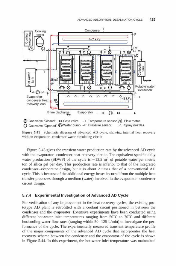
ADVANCED ADSORPTION–DESALINATION CYCLE 425

FM

Potable waterextraction

Evaporator-condenser heatrecovery loop

Brine discharge

Col

lect

ion

tank

Hot

wat

erta

nk

Condenser

Evaporator

T TT T

T T T T

T

TP

P P PP

FMT

TP

Coo

ling

wat

er ta

nk

SE I SE II SE IV

T

Coolingtower

1–3 kPa

Gas valve “Closed”

Gas valve “Opened”

Gate valve Water pump

–T Temperature sensor –P Pressure sensor

FM Flow meter Spray nozzles

T

4–7 kPa

T

T

T

SE III Silicagel Silicagel

Figure 5.41 Schematic diagram of advanced AD cycle, showing internal heat recoverywith an evaporator–condenser water circulating circuit.

Figure 5.43 gives the transient water production rate by the advanced AD cyclewith the evaporator–condenser heat recovery circuit. The equivalent specific dailywater production (SDWP) of the cycle is ∼13.5 m3 of potable water per metricton of silica gel per day. This production rate is inferior to that of the integratedcondenser–evaporator design, but it is about 2 times that of a conventional ADcycle. This is because of the additional energy losses incurred from the multiple heattransfer processes through a medium (water) involved in the evaporator–condensercircuit design.

5.7.4 Experimental Investigation of Advanced AD Cycle

For verification of any improvement in the heat recovery cycles, the existing pro-totype AD plant is retrofitted with a coolant circuit positioned in between thecondenser and the evaporator. Extensive experiments have been conducted usingdifferent hot-water inlet temperatures ranging from 50◦C to 70◦C and differenthot/cooling-water flow rates (ranging within 50–125 L/min) to investigate the per-formance of the cycle. The experimentally measured transient temperature profileof the major components of the advanced AD cycle that incorporates the heatrecovery scheme between the condenser and the evaporator of the cycle is shownin Figure 5.44. In this experiment, the hot-water inlet temperature was maintained

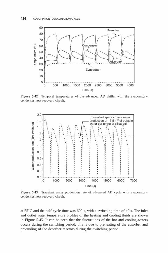
426 ADSORPTION–DESALINATION CYCLE

00

10

20

30

40

50

60

70

80

90

500 1000 1500 2000

Evaporator

Desorber

Adsorber

Time (s)

Tem

pera

ture

(°C

)

2500 3000 3500 4000

Condenser

Figure 5.42 Temporal temperatures of the advanced AD chiller with the evaporator–condenser heat recovery circuit.

0 1000 2000 3000 4000 5000 6000 70000.0

0.2Wat

er p

rodu

ctio

n ra

te (

litre

s/m

inut

e)

0.4

0.6

0.8

1.0

1.2

1.4

1.6

1.8

2.0

Time (s)

Equivalent specific daily waterproduction of 13.5 m3 of potablewater per tonne of silica gel

Figure 5.43 Transient water production rate of advanced AD cycle with evaporator–condenser heat recovery circuit.

at 55◦C and the half-cycle time was 600 s, with a switching time of 40 s. The inletand outlet water temperature profiles of the heating and cooling fluids are shownin Figure 5.45. It can be seen that the fluctuations of the hot and cooling-watersoccurs during the switching period; this is due to preheating of the adsorber andprecooling of the desorber reactors during the switching period.

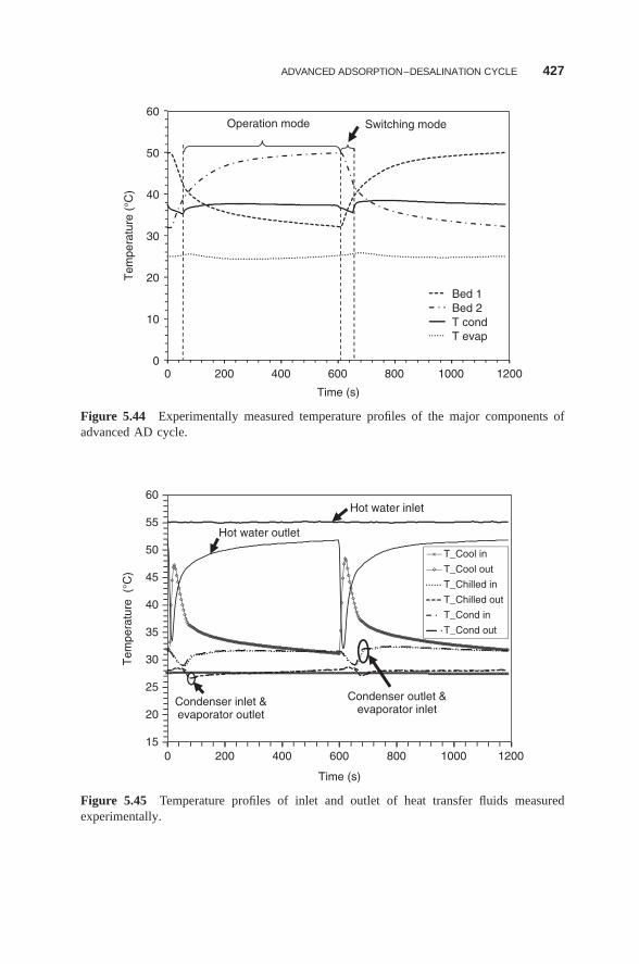
ADVANCED ADSORPTION–DESALINATION CYCLE 427

0

10

20

30

40

50

60

0 200 400 600 800 1000 1200

Tem

pera

ture

(°C

)

Time (s)

Bed 1Bed 2T condT evap

Operation mode Switching mode

Figure 5.44 Experimentally measured temperature profiles of the major components ofadvanced AD cycle.

15

20

25

30

35

40

45

50

55

60

0 200 400 600 800 1000 1200

Tem

pera

ture

(°C

)

Time (s)

T_Cool in

T_Cool out T_Chilled in T_Chilled out T_Cond in T_Cond out

Hot water inlet

Hot water outlet

Condenser outlet &evaporator inlet

Condenser inlet &evaporator outlet

Figure 5.45 Temperature profiles of inlet and outlet of heat transfer fluids measuredexperimentally.

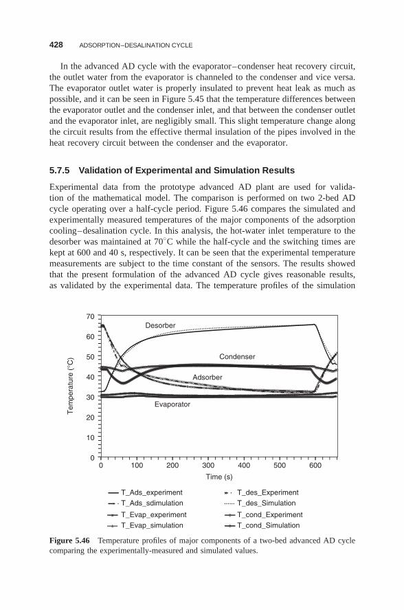
428 ADSORPTION–DESALINATION CYCLE

In the advanced AD cycle with the evaporator–condenser heat recovery circuit,the outlet water from the evaporator is channeled to the condenser and vice versa.The evaporator outlet water is properly insulated to prevent heat leak as much aspossible, and it can be seen in Figure 5.45 that the temperature differences betweenthe evaporator outlet and the condenser inlet, and that between the condenser outletand the evaporator inlet, are negligibly small. This slight temperature change alongthe circuit results from the effective thermal insulation of the pipes involved in theheat recovery circuit between the condenser and the evaporator.

5.7.5 Validation of Experimental and Simulation Results

Experimental data from the prototype advanced AD plant are used for valida-tion of the mathematical model. The comparison is performed on two 2-bed ADcycle operating over a half-cycle period. Figure 5.46 compares the simulated andexperimentally measured temperatures of the major components of the adsorptioncooling–desalination cycle. In this analysis, the hot-water inlet temperature to thedesorber was maintained at 70◦C while the half-cycle and the switching times arekept at 600 and 40 s, respectively. It can be seen that the experimental temperaturemeasurements are subject to the time constant of the sensors. The results showedthat the present formulation of the advanced AD cycle gives reasonable results,as validated by the experimental data. The temperature profiles of the simulation

0

10

20

30

40

50

60

70

0 100 200 300 400 500 600

Tem

pera

ture

(°C

)

Time (s)

T_Ads_experiment T_des_Experiment

T_Evap_experiment T_cond_Experiment

T_Ads_sdimulation T_des_Simulation

T_Evap_simulation T_cond_Simulation

Desorber

Adsorber

Condenser

Evaporator

Figure 5.46 Temperature profiles of major components of a two-bed advanced AD cyclecomparing the experimentally-measured and simulated values.

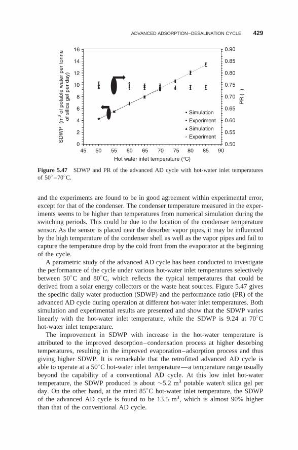
ADVANCED ADSORPTION–DESALINATION CYCLE 429

0.50

0.55

0.60

0.65

0.70

0.75

0.80

0.85

0.90

045 50 55 60 65 70 75 80 85 90

2

4

6

8

10

12

14

16

PR

(–)

SD

WP

(m

3 of

pot

able

wat

er p

er to

nne

of s

ilica

gel

per

day

)

Hot water inlet temperature (°C)

Simulation

Experiment

Simulation

Experiment

Figure 5.47 SDWP and PR of the advanced AD cycle with hot-water inlet temperaturesof 50◦ –70◦C.

and the experiments are found to be in good agreement within experimental error,except for that of the condenser. The condenser temperature measured in the exper-iments seems to be higher than temperatures from numerical simulation during theswitching periods. This could be due to the location of the condenser temperaturesensor. As the sensor is placed near the desorber vapor pipes, it may be influencedby the high temperature of the condenser shell as well as the vapor pipes and fail tocapture the temperature drop by the cold front from the evaporator at the beginningof the cycle.

A parametric study of the advanced AD cycle has been conducted to investigatethe performance of the cycle under various hot-water inlet temperatures selectivelybetween 50◦C and 80◦C, which reflects the typical temperatures that could bederived from a solar energy collectors or the waste heat sources. Figure 5.47 givesthe specific daily water production (SDWP) and the performance ratio (PR) of theadvanced AD cycle during operation at different hot-water inlet temperatures. Bothsimulation and experimental results are presented and show that the SDWP varieslinearly with the hot-water inlet temperature, while the SDWP is 9.24 at 70◦Chot-water inlet temperature.

The improvement in SDWP with increase in the hot-water temperature isattributed to the improved desorption–condensation process at higher desorbingtemperatures, resulting in the improved evaporation–adsorption process and thusgiving higher SDWP. It is remarkable that the retrofitted advanced AD cycle isable to operate at a 50◦C hot-water inlet temperature—a temperature range usuallybeyond the capability of a conventional AD cycle. At this low inlet hot-watertemperature, the SDWP produced is about ∼5.2 m3 potable water/t silica gel perday. On the other hand, at the rated 85◦C hot-water inlet temperature, the SDWPof the advanced AD cycle is found to be 13.5 m3, which is almost 90% higherthan that of the conventional AD cycle.

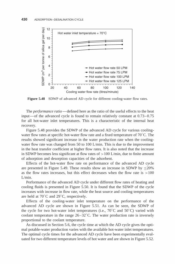
430 ADSORPTION–DESALINATION CYCLE

0

2

4

6

8

10

12

20 40 60 80 100 120 140

SD

WP

(m

3 pe

r to

nne

of s

ilica

gel

per

day

)

Cooling water flow rate (litres/minute)

Hot water flow rate 50 LPMHot water flow rate 75 LPMHot water flow rate 100 LPMHot water flow rate 125 LPM

Hot water inlet temperature = 70°C

Figure 5.48 SDWP of advanced AD cycle for different cooling-water flow rates.

The performance ratio —defined here as the ratio of the useful effects to the heatinput—of the advanced cycle is found to remain relatively constant at 0.73–0.75for all hot-water inlet temperatures. This is a characteristic of the internal heatrecovery.

Figure 5.48 provides the SDWP of the advanced AD cycle for various cooling-water flow rates at specific hot-water flow rate and a fixed temperature of 70◦C. Theresults showed significant increase in the water production rate when the cooling-water flow rate was changed from 50 to 100 L/min. This is due to the improvementin the heat transfer coefficient at higher flow rates. It is also noted that the increasein SDWP becomes less significant at flow rates of >100 L/min, due to finite amountof adsorption and desorption capacities of the adsorbent.

Effects of the hot-water flow rate on performance of the advanced AD cycleare presented in Figure 5.49. These results show an increase in SDWP by ≤20%as the flow rates increases, but this effect decreases when the flow rate is >100L/min.

Performance of the advanced AD cycle under different flow rates of heating andcooling fluids is presented in Figure 5.50. It is found that the SDWP of the cycleincreases with increase in flow rate, while the heat source and cooling temperaturesare held at 70◦C and 29◦C, respectively.

Effects of the cooling-water inlet temperature on the performance of theadvanced AD cycle are shown in Figure 5.51. As can be seen, the SDWP ofthe cycle for two hot-water inlet temperatures (i.e., 70◦C and 50◦C) varied withcoolant temperature in the range 26–32◦C. The water production rate is inverselyproportional to the coolant temperature.

As discussed in Section 5.6, the cycle time at which the AD cycle gives the opti-mal potable-water production varies with the available hot-water inlet temperatures.The optimal cycle times for the advanced AD cycle have been experimentally eval-uated for two different temperature levels of hot water and are shown in Figure 5.52.

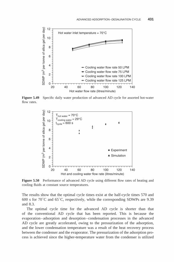
ADVANCED ADSORPTION–DESALINATION CYCLE 431

0

2

4

6

8

10

12

20 40 60 80 100 120 140

SD

WP

(m

3 pe

r to

nne

of s

ilica

gel

per

day

)

Hot water flow rate (litres/minute)

Cooling water flow rate 50 LPMCooling water flow rate 75 LPMCooling water flow rate 100 LPMCooling water flow rate 125 LPM

Hot water inlet temperature = 70°C

Figure 5.49 Specific daily water production of advanced AD cycle for assorted hot-waterflow rates.

0

2

4

6

8

10

12

20 40 60 80 100 120 140

SD

WP

(m

3 pe

r to

nne

of s

ilica

gel

per

day

)

Hot and cooling water flow rate (litres/minute)

Experiment

Simulation

Thot water = 70°CTcooling water = 29°Ctcycle = 600 s

Figure 5.50 Performance of advanced AD cycle using different flow rates of heating andcooling fluids at constant source temperatures.

The results show that the optimal cycle times exist at the half-cycle times 570 and600 s for 70◦C and 65◦C, respectively, while the corresponding SDWPs are 9.39and 8.3.

The optimal cycle time for the advanced AD cycle is shorter than thatof the conventional AD cycle that has been reported. This is because theevaporation–adsorption and desorption–condensation processes in the advancedAD cycle are greatly accelerated, owing to the pressurization of the adsorption,and the lower condensation temperature was a result of the heat recovery processbetween the condenser and the evaporator. The pressurization of the adsorption pro-cess is achieved since the higher-temperature water from the condenser is utilized

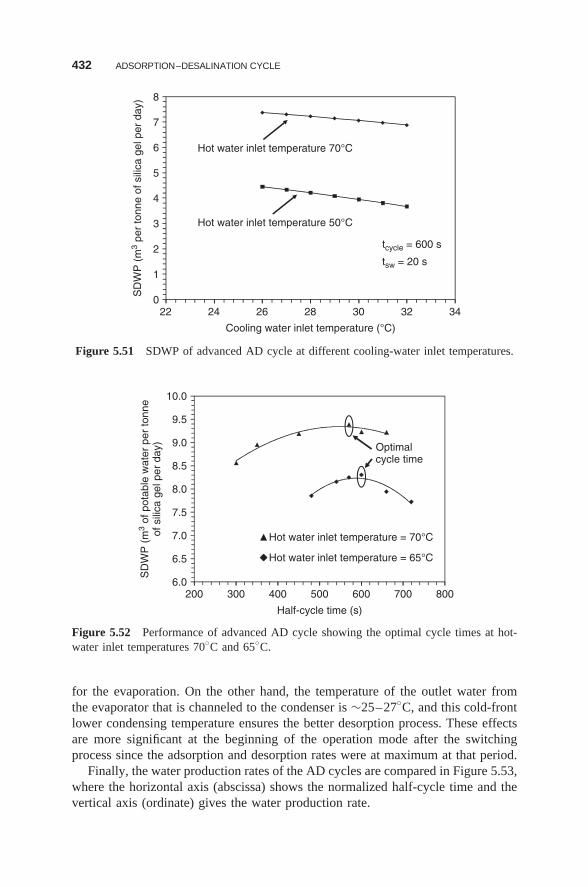
432 ADSORPTION–DESALINATION CYCLE

0

1

2

3

4

5

6

7

8

22 24 26 28 30 32 34

SD

WP

(m

3 pe

r to

nne

of s

ilica

gel

per

day

)

Cooling water inlet temperature (°C)

Hot water inlet temperature 70°C

Hot water inlet temperature 50°C

tcycle = 600 s

tsw = 20 s

Figure 5.51 SDWP of advanced AD cycle at different cooling-water inlet temperatures.

6.0

6.5

7.0

7.5

8.0

8.5

9.0

9.5

10.0

200 300 400 500 600 700 800

SD

WP

(m

3 of

pot

able

wat

er p

er to

nne

of s

ilica

gel

per

day

)

Half-cycle time (s)

Hot water inlet temperature = 70°C

Hot water inlet temperature = 65°C

Optimalcycle time

Figure 5.52 Performance of advanced AD cycle showing the optimal cycle times at hot-water inlet temperatures 70◦C and 65◦C.

for the evaporation. On the other hand, the temperature of the outlet water fromthe evaporator that is channeled to the condenser is ∼25–27◦C, and this cold-frontlower condensing temperature ensures the better desorption process. These effectsare more significant at the beginning of the operation mode after the switchingprocess since the adsorption and desorption rates were at maximum at that period.

Finally, the water production rates of the AD cycles are compared in Figure 5.53,where the horizontal axis (abscissa) shows the normalized half-cycle time and thevertical axis (ordinate) gives the water production rate.

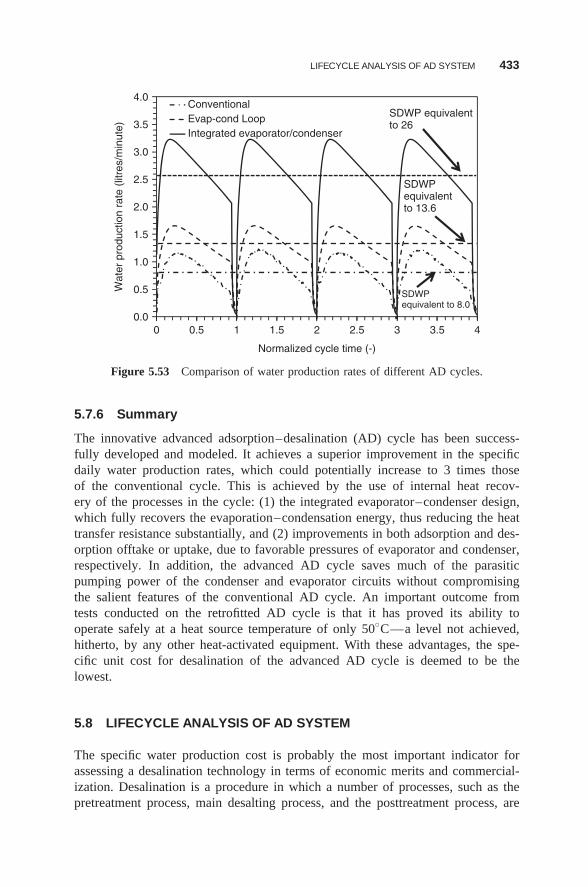
LIFECYCLE ANALYSIS OF AD SYSTEM 433

0.0

0.5

1.0

1.5

2.0

2.5

3.0

3.5

4.0

0 0.5 1 1.5 2 2.5 3 3.5 4

Wat

er p

rodu

ctio

n ra

te (

litre

s/m

inut

e)

Normalized cycle time (-)

ConventionalEvap-cond LoopIntegrated evaporator/condenser

SDWP equivalentto 26

SDWPequivalentto 13.6

SDWPequivalent to 8.0

Figure 5.53 Comparison of water production rates of different AD cycles.

5.7.6 Summary

The innovative advanced adsorption–desalination (AD) cycle has been success-fully developed and modeled. It achieves a superior improvement in the specificdaily water production rates, which could potentially increase to 3 times thoseof the conventional cycle. This is achieved by the use of internal heat recov-ery of the processes in the cycle: (1) the integrated evaporator–condenser design,which fully recovers the evaporation–condensation energy, thus reducing the heattransfer resistance substantially, and (2) improvements in both adsorption and des-orption offtake or uptake, due to favorable pressures of evaporator and condenser,respectively. In addition, the advanced AD cycle saves much of the parasiticpumping power of the condenser and evaporator circuits without compromisingthe salient features of the conventional AD cycle. An important outcome fromtests conducted on the retrofitted AD cycle is that it has proved its ability tooperate safely at a heat source temperature of only 50◦C—a level not achieved,hitherto, by any other heat-activated equipment. With these advantages, the spe-cific unit cost for desalination of the advanced AD cycle is deemed to be thelowest.

5.8 LIFECYCLE ANALYSIS OF AD SYSTEM

The specific water production cost is probably the most important indicator forassessing a desalination technology in terms of economic merits and commercial-ization. Desalination is a procedure in which a number of processes, such as thepretreatment process, main desalting process, and the posttreatment process, are

434 ADSORPTION–DESALINATION CYCLE

included to produce potable water. All these processes require significant input ofenergy and chemicals, and thus the related cost must be considered in the costanalysis. A lifecycle analysis is adopted as a platform for the evaluation of unitproduction cost of potable water from desalination. This method enables estimationof the unit cost over a specific lifespan of the plant considering both capital andoperational costs with inflation and interest rates [62,63]. Several factors influencethe desalting cost and an overview of the factors affecting the desalination costs ispresented below.

5.8.1 Factors Affecting Cost of AD Plant

Cost factors considered for selection of a desalination technology are generic tomost desalination plants, but some of them are more site-specific, weighing in onfactors such as location of the plant and access for feedwater and brine discharge.However, it is possible to categorize most common factors that are subject to mostdesalting plants. The general factors contributing to the unit cost calculation ofdesalination plants are listed in Table 5.10. The less apparent or indirect factors,such as the plant load factor, availability of skilled labor, storage and distribution offreshwater, and plant capacity and location, could also affect the unit cost, althoughto a lesser extent. For these indirect factors, a simple cost estimation methodologyhas been applied, and in the following section we describe these parameters indetail.

5.8.2 Total Cost of AD Plant

The total costs of a desalination plant comprise the capital, operational, and replace-ment costs of key components such as heat exchangers and membranes. Dependingon the desalination methodology and the water production capacity, the plant life-time could affect the annualized capital cost via the amortization period (n) andthe interest rate (i ) through a capital recovery factor (CRF), namely, the productbetween the initial investment and the CRF [64]. The operational cost comprisescontributions from fuel and electricity rates, maintenance and replacement, pump-ing requirements, and chemical treatment of feedwater and output water. In reality,all operational costs can be subjected to the inflation effect or rates (j ), arising fromprimary fuel, electricity price fluctuations, and other factors. Such increases overa period of time in the future could be incorporated using the inflation-weightedfactor, IWF = (CFR(i , n))/(CRF(i i , n)). A lifecycle approach is adopted here forcalculation of the unit cost of desalination, i.e.,

A($/m3) =(

m∑k=1

Ccapital(CRF(i , n))k

)+

( p∑l=1

Coperational

((CRF(i , n))

CRF(i i , n)

)l

)

(5.21)where A is the unit cost of desalination on a volumetric basis, m is the numberof items of capital investment, and p is the number of items related to opera-tional cost. With Equation (5.21), the unit production cost of AD plants of varying

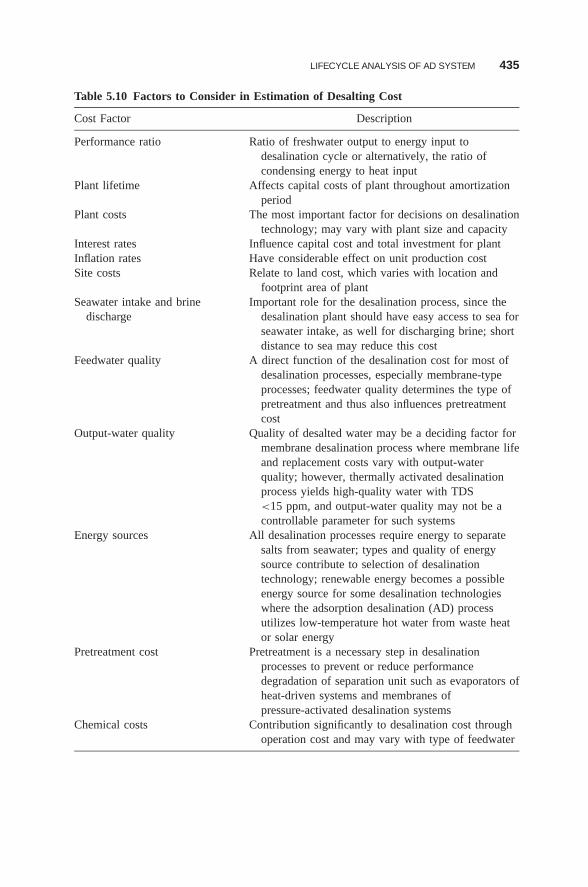
LIFECYCLE ANALYSIS OF AD SYSTEM 435

Table 5.10 Factors to Consider in Estimation of Desalting Cost

Cost Factor Description

Performance ratio Ratio of freshwater output to energy input todesalination cycle or alternatively, the ratio ofcondensing energy to heat input

Plant lifetime Affects capital costs of plant throughout amortizationperiod

Plant costs The most important factor for decisions on desalinationtechnology; may vary with plant size and capacity

Interest rates Influence capital cost and total investment for plantInflation rates Have considerable effect on unit production costSite costs Relate to land cost, which varies with location and

footprint area of plantSeawater intake and brine

dischargeImportant role for the desalination process, since the

desalination plant should have easy access to sea forseawater intake, as well for discharging brine; shortdistance to sea may reduce this cost

Feedwater quality A direct function of the desalination cost for most ofdesalination processes, especially membrane-typeprocesses; feedwater quality determines the type ofpretreatment and thus also influences pretreatmentcost

Output-water quality Quality of desalted water may be a deciding factor formembrane desalination process where membrane lifeand replacement costs vary with output-waterquality; however, thermally activated desalinationprocess yields high-quality water with TDS<15 ppm, and output-water quality may not be acontrollable parameter for such systems

Energy sources All desalination processes require energy to separatesalts from seawater; types and quality of energysource contribute to selection of desalinationtechnology; renewable energy becomes a possibleenergy source for some desalination technologieswhere the adsorption desalination (AD) processutilizes low-temperature hot water from waste heator solar energy

Pretreatment cost Pretreatment is a necessary step in desalinationprocesses to prevent or reduce performancedegradation of separation unit such as evaporators ofheat-driven systems and membranes ofpressure-activated desalination systems

Chemical costs Contribution significantly to desalination cost throughoperation cost and may vary with type of feedwater

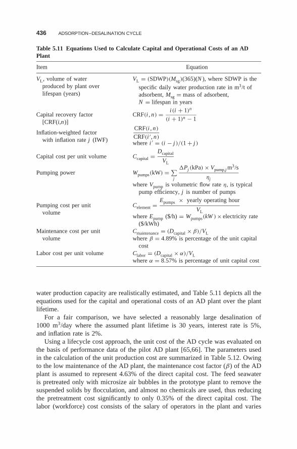
436 ADSORPTION–DESALINATION CYCLE

Table 5.11 Equations Used to Calculate Capital and Operational Costs of an ADPlant

Item Equation

VL, volume of waterproduced by plant overlifespan (years)

VL = (SDWP)(Msg)(365)(N ), where SDWP is the

specific daily water production rate in m3/t ofadsorbent, Msg = mass of adsorbent,N = lifespan in years

Capital recovery factor[CRF(i,n)]

CRF(i , n) = i (i + 1)n

(i + 1)n − 1

Inflation-weighted factorwith inflation rate j (IWF)

CRF(i , n)

CRF(i ′, n)where i ′ = (i − j )/(1 + j )

Capital cost per unit volume Ccapital = Dcapital

VL

Pumping power Wpumps(kW) = ∑j

�Pj (kPa) × Vpump,j m3/s

ηjwhere Vpump is volumetric flow rate η, is typical

pump efficiency, j is number of pumps

Pumping cost per unitvolume

Celement = Epumps × yearly operating hour

VLwhere Epump ($/h) = Wpumps(kW )× electricity rate

($/kWh)Maintenance cost per unit

volumeCmaintenance = (Dcapital × β)/VLwhere β = 4.89% is percentage of the unit capital

costLabor cost per unit volume Clabor = (Dcapital × α)/VL

where α = 8.57% is percentage of unit capital cost

water production capacity are realistically estimated, and Table 5.11 depicts all theequations used for the capital and operational costs of an AD plant over the plantlifetime.

For a fair comparison, we have selected a reasonably large desalination of1000 m3/day where the assumed plant lifetime is 30 years, interest rate is 5%,and inflation rate is 2%.

Using a lifecycle cost approach, the unit cost of the AD cycle was evaluated onthe basis of performance data of the pilot AD plant [65,66]. The parameters usedin the calculation of the unit production cost are summarized in Table 5.12. Owingto the low maintenance of the AD plant, the maintenance cost factor (β) of the ADplant is assumed to represent 4.63% of the direct capital cost. The feed seawateris pretreated only with microsize air bubbles in the prototype plant to remove thesuspended solids by flocculation, and almost no chemicals are used, thus reducingthe pretreatment cost significantly to only 0.35% of the direct capital cost. Thelabor (workforce) cost consists of the salary of operators in the plant and varies

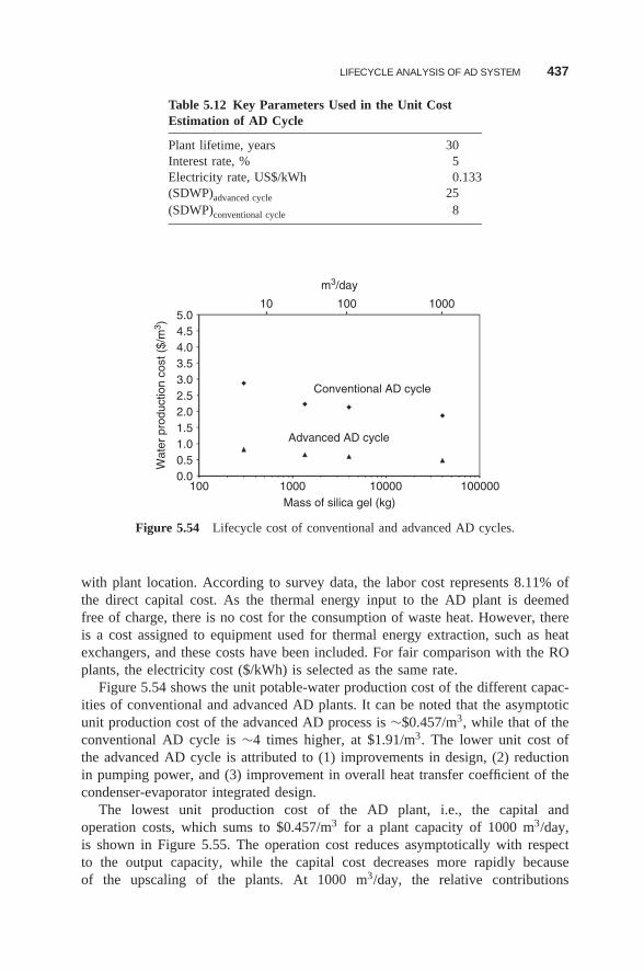
LIFECYCLE ANALYSIS OF AD SYSTEM 437

Table 5.12 Key Parameters Used in the Unit CostEstimation of AD Cycle

Plant lifetime, years 30Interest rate, % 5Electricity rate, US$/kWh 0.133(SDWP)advanced cycle 25(SDWP)conventional cycle 8

0.00.51.01.52.02.53.03.54.04.55.0

100 1000 10000 100000

Wat

er p

rodu

ctio

n co

st (

$/m

3 )

Mass of silica gel (kg)

m3/day

10 100 1000

Advanced AD cycle

Conventional AD cycle

Figure 5.54 Lifecycle cost of conventional and advanced AD cycles.

with plant location. According to survey data, the labor cost represents 8.11% ofthe direct capital cost. As the thermal energy input to the AD plant is deemedfree of charge, there is no cost for the consumption of waste heat. However, thereis a cost assigned to equipment used for thermal energy extraction, such as heatexchangers, and these costs have been included. For fair comparison with the ROplants, the electricity cost ($/kWh) is selected as the same rate.

Figure 5.54 shows the unit potable-water production cost of the different capac-ities of conventional and advanced AD plants. It can be noted that the asymptoticunit production cost of the advanced AD process is ∼$0.457/m3, while that of theconventional AD cycle is ∼4 times higher, at $1.91/m3. The lower unit cost ofthe advanced AD cycle is attributed to (1) improvements in design, (2) reductionin pumping power, and (3) improvement in overall heat transfer coefficient of thecondenser-evaporator integrated design.

The lowest unit production cost of the AD plant, i.e., the capital andoperation costs, which sums to $0.457/m3 for a plant capacity of 1000 m3/day,is shown in Figure 5.55. The operation cost reduces asymptotically with respectto the output capacity, while the capital cost decreases more rapidly becauseof the upscaling of the plants. At 1000 m3/day, the relative contributions

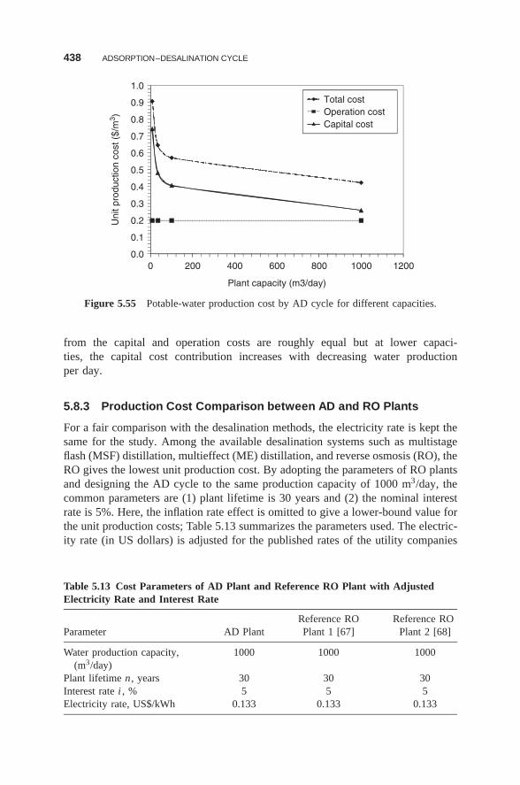
438 ADSORPTION–DESALINATION CYCLE

0.0

0.1

0.2

0.3

0.4

0.5

0.6

0.7

0.8

0.9

1.0

0 200 400 600 800 1000 1200

Uni

t pro

duct

ion

cost

($/

m3 )

Plant capacity (m3/day)

Total costOperation costCapital cost

Figure 5.55 Potable-water production cost by AD cycle for different capacities.

from the capital and operation costs are roughly equal but at lower capaci-ties, the capital cost contribution increases with decreasing water productionper day.

5.8.3 Production Cost Comparison between AD and RO Plants

For a fair comparison with the desalination methods, the electricity rate is kept thesame for the study. Among the available desalination systems such as multistageflash (MSF) distillation, multieffect (ME) distillation, and reverse osmosis (RO), theRO gives the lowest unit production cost. By adopting the parameters of RO plantsand designing the AD cycle to the same production capacity of 1000 m3/day, thecommon parameters are (1) plant lifetime is 30 years and (2) the nominal interestrate is 5%. Here, the inflation rate effect is omitted to give a lower-bound value forthe unit production costs; Table 5.13 summarizes the parameters used. The electric-ity rate (in US dollars) is adjusted for the published rates of the utility companies

Table 5.13 Cost Parameters of AD Plant and Reference RO Plant with AdjustedElectricity Rate and Interest Rate

Reference RO Reference ROParameter AD Plant Plant 1 [67] Plant 2 [68]

Water production capacity,(m3/day)

1000 1000 1000

Plant lifetime n , years 30 30 30Interest rate i , % 5 5 5Electricity rate, US$/kWh 0.133 0.133 0.133

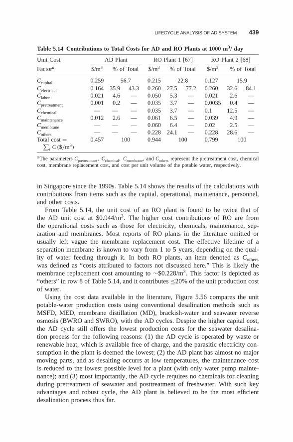
LIFECYCLE ANALYSIS OF AD SYSTEM 439

Table 5.14 Contributions to Total Costs for AD and RO Plants at 1000 m3/ day

Unit Cost AD Plant RO Plant 1 [67] RO Plant 2 [68]

Factora $/m3 % of Total $/m3 % of Total $/m3 % of Total

Ccapital 0.259 56.7 0.215 22.8 0.127 15.9Celectrical 0.164 35.9 43.3 0.260 27.5 77.2 0.260 32.6 84.1Clabor 0.021 4.6 — 0.050 5.3 — 0.021 2.6 —Cpretreatment 0.001 0.2 — 0.035 3.7 — 0.0035 0.4 —Cchemical — — — 0.035 3.7 — 0.1 12.5 —Cmaintenance 0.012 2.6 — 0.061 6.5 — 0.039 4.9 —Cmembrane — — — 0.060 6.4 — 0.02 2.5 —Cothers — — — 0.228 24.1 — 0.228 28.6 —Total cost =∑

i C ($/m3)

0.457 100 0.944 100 0.799 100

aThe parameters Cpretreatment, Cchemical, Cmembrane, and Cothers represent the pretreatment cost, chemicalcost, membrane replacement cost, and cost per unit volume of the potable water, respectively.

in Singapore since the 1990s. Table 5.14 shows the results of the calculations withcontributions from items such as the capital, operational, maintenance, personnel,and other costs.

From Table 5.14, the unit cost of an RO plant is found to be twice that ofthe AD unit cost at $0.944/m3. The higher cost contributions of RO are fromthe operational costs such as those for electricity, chemicals, maintenance, sep-aration and membranes. Most reports of RO plants in the literature omitted orusually left vague the membrane replacement cost. The effective lifetime of aseparation membrane is known to vary from 1 to 5 years, depending on the qual-ity of water feeding through it. In both RO plants, an item denoted as Cotherswas defined as “costs attributed to factors not discussed here.” This is likely themembrane replacement cost amounting to ∼$0.228/m3. This factor is depicted as“others” in row 8 of Table 5.14, and it contributes ≤20% of the unit production costof water.

Using the cost data available in the literature, Figure 5.56 compares the unitpotable-water production costs using conventional desalination methods such asMSFD, MED, membrane distillation (MD), brackish-water and seawater reverseosmosis (BWRO and SWRO), with the AD cycles. Despite the higher capital cost,the AD cycle still offers the lowest production costs for the seawater desalina-tion process for the following reasons: (1) the AD cycle is operated by waste orrenewable heat, which is available free of charge, and the parasitic electricity con-sumption in the plant is deemed the lowest; (2) the AD plant has almost no majormoving parts, and as desalting occurrs at low temperatures, the maintenance costis reduced to the lowest possible level for a plant (with only water pump mainte-nance); and (3) most importantly, the AD cycle requires no chemicals for cleaningduring pretreatment of seawater and posttreatment of freshwater. With such keyadvantages and robust cycle, the AD plant is believed to be the most efficientdesalination process thus far.

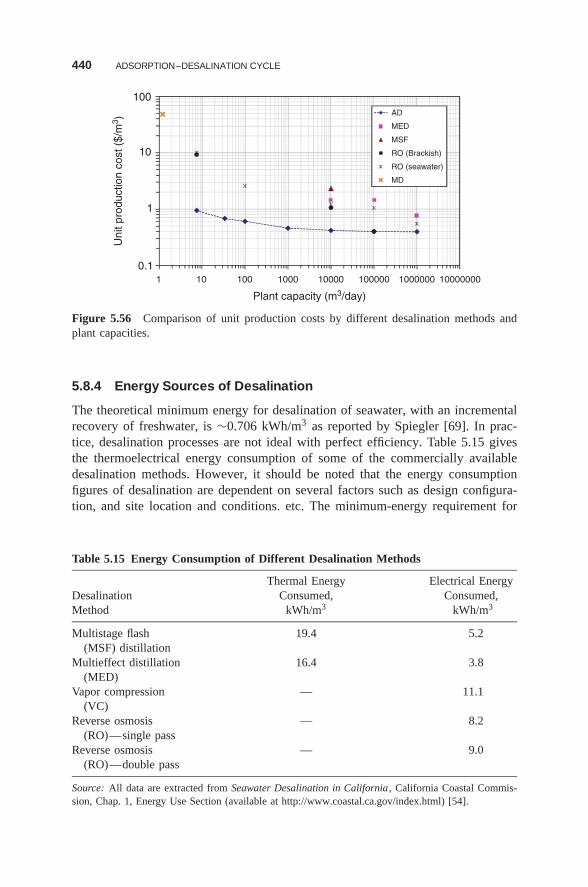
440 ADSORPTION–DESALINATION CYCLE

0.1

1

10

100

1 10 100 1000 10000 100000 1000000 10000000

Uni

t pro

duct

ion

cost

($/

m3 )

Plant capacity (m3/day)

AD

MED

MSF

RO (Brackish)

RO (seawater)

MD

Figure 5.56 Comparison of unit production costs by different desalination methods andplant capacities.

5.8.4 Energy Sources of Desalination

The theoretical minimum energy for desalination of seawater, with an incrementalrecovery of freshwater, is ∼0.706 kWh/m3 as reported by Spiegler [69]. In prac-tice, desalination processes are not ideal with perfect efficiency. Table 5.15 givesthe thermoelectrical energy consumption of some of the commercially availabledesalination methods. However, it should be noted that the energy consumptionfigures of desalination are dependent on several factors such as design configura-tion, and site location and conditions. etc. The minimum-energy requirement for

Table 5.15 Energy Consumption of Different Desalination Methods

Thermal Energy Electrical EnergyDesalination Consumed, Consumed,Method kWh/m3 kWh/m3

Multistage flash(MSF) distillation

19.4 5.2

Multieffect distillation(MED)

16.4 3.8

Vapor compression(VC)

— 11.1

Reverse osmosis(RO)—single pass

— 8.2

Reverse osmosis(RO)—double pass

— 9.0

Source: All data are extracted from Seawater Desalination in California , California Coastal Commis-sion, Chap. 1, Energy Use Section (available at http://www.coastal.ca.gov/index.html) [54].

CO2 EMISSION SAVINGS 441

desalting using the Gibbs free-energy approach is discussed in Section 5.A.1 of theAppendix.

It is reasonable to state that the MSFD process consumes the most energy,despite its relative maturity (≥50 years). It is followed by MED (or hybrid MED)systems and then vapor compression systems. The energy consumption of MSFdistillation, by far the most widely used thermal process, is still at least 20–30times the theoretical minimum. RO is a newer technology (30 years) that, withmore recent improvements in energy recovery, is remarkably efficient, consumingonly 3–10 times the theoretical minimum. It is important to consider, however,that RO consumes energy in the form of electricity. On the other hand, MSFD usesheat (or fuel) more directly. The conversion of thermal energy to electrical energyis only ∼35% efficient. Therefore, in terms of fuel, RO consumes 9–30 times thetheoretical energy requirement.

Overall, it is reasonable to conclude that today’s desalination costs are ∼$5/m3

and the energy consumption is at least 5 times that of the theoretical thermody-namic limit. It has been found that the adsorption–desalination process mitigatesshortcomings such as high maintenance cost and high energy consumption that thecurrent desalination technologies are facing. Adsorption–desalination is a noveldesalination technology that has the potential of becoming the most energy-efficientmethod for production of potable water typically less than the benchmark energyconsumption of 1.5 kWh/m3.

5.9 CO2 EMISSION SAVINGS

A CO2 emission study was conducted that included a direct comparison to theexisting desalination methods with respect to the thermoelectrical energy consumed.If the AD cycle is utilized for freshwater production, some CO2 emission can beavoided because the AD cycle consumes only low-temperature heat source, thus,reducing global warming directly. The environmentally friendly aspect of the ADplant is demonstrated by comparing the amounts of CO2 emission. A baselinecalculation for CO2 emission is shown in Section 5.A.2.

Assuming an emission rate of CO2 at 64.2 t/TJ (terajoule) for natural gas (usedas a primary fuel), and from the thermal and electricity consumption rates ofTable 5.16, the corresponding CO2 emission of the desalination processes of MSFD,MED, and RO plants can be computed. Detailed calculations of CO2 emission areoutlined in Section 5.A.2. The baseline emissions for thermaoelectrical energy con-sumption for the conventional desalination methods are compared to the emissionobtained by the AD plant, as shown in Table 5.16, where the last (rightmost)column indicates the CO2 savings.

The thermoeconomic viability of the adsorption–desalination (AD) process hasbeen presented using a lifecycle approach. The specific-energy cost of AD plantis found to be 1.38 kWh/m3, which is twice that of the thermodynamic limit: thelowest energy usage ever reported for a desalination method. At ≥1000 m3/day, thetotal lifecycle cost asymptotic to a unit production cost of $0.457/m3 as compared

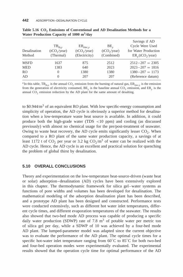
442 ADSORPTION–DESALINATION CYCLE

Table 5.16 CO2 Emissions of Conventional and AD Desalination Methods for aWater Production Capacity of 1000 m3/day

Savings if ADTBth,y EBelec,y BEy Cycle Were Used

Desalination (tCO2/year) (tCO2/year) (tCO2/year) for Water ProductionMethod (Thermal) (Electricity) (Combined) ERy (tCO2/year)

MSFD 1637 875 2512 2512−207 = 2305MED 1383 640 2023 2023−207 = 1816RO 0 1380 1380 1380−207 = 1173AD 0 207 207 (Reference datum)

a In this table, TBth,y is the annual CO2 emission from the burning of natural gas, EBelec,y is the emissionfrom the generation of electricity consumed, BEy is the baseline annual CO2 emission, and ERy is theannual CO2 emission reduction by the AD plant for the same amount of desalting.

to $0.944/m3 of an equivalent RO plant. With low specific-energy consumption andsimplicity of operation, the AD cycle is obviously a superior method for desalina-tion when a low-temperature waste heat source is available. In addition, it couldproduce both the high-grade water (TDS <10 ppm) and cooling (as discussedpreviously) with almost no chemical usage for the pre/post-treatment of seawater.Owing to waste heat recovery, the AD cycle emits significantly lesser CO2. Whencompared to a RO plant of the same water production capacity, a savings of atleast 1172 t of CO2 per year or 3.2 kg CO2/m3 of water can be realized with theAD cycle. Hence, the AD cycle is an excellent and practical solution for quenchingthe problem of global thirst by desalination.

5.10 OVERALL CONCLUSIONS

Theory and experimentation on the low-temperature heat-source-driven (waste heator solar) adsorption–desalination (AD) cycles have been extensively exploredin this chapter. The thermodynamic framework for silica gel–water systems asfunctions of pore widths and volumes has been developed for desalination. Themathematical modeling of the adsorption desalination plant has been described,and a prototype AD plant has been designed and constructed. Performance testswere conducted extensively, such as different hot water inlet temperatures, differ-ent cycle times, and different evaporation temperatures of the seawater. The resultsalso showed that two-bed mode AD process was capable of producing a specificdaily water production (SDWP) rate of 7.8 m3 of potable water per metric tonof silica gel per day, while a SDWP of 10 was achieved by a four-bed modeAD plant. The lumped-parameter model was adapted since the current objectivewas to evaluate the performance of the AD plant. The optimal cycle times for aspecific hot-water inlet temperature ranging from 60◦C to 85◦C for both two-bedand four-bed operation modes were experimentally evaluated. The experimentalresults showed that the operation cycle time for optimal performance of the AD

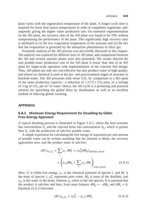
APPENDIX 443

plant varies with the regeneration temperature of the plant. A longer cycle time isrequired for lower heat source temperatures in order to completely regenerate, sub-sequently giving the higher water production rate. On extensive experimentationon the AD plant, the recovery ratio of the AD plant was found to be 70% withoutcompromising the performance of the plant. This significantly high recovery ratiois attributed to (1) the low evaporation temperature of the seawater and (2) the factthat the evaporation is governed by the adsoprtion phenomenon of silica gel.

Economic analysis of the AD process was also briefly discussed in this chapter.The analysis was explored for different sizes of AD plant, and comparisons betweenthe AD and reverse osmosis plants were also presented. The results showed theunit potable-water production cost of the AD plant is lower than that of an ROplant for larger-scale operation with implementation of the concrete bed design.Thus, AD plants not only are cost-effective but also produce water of high quality,and almost no chemical is used at the pre- and post-treatment stages of seawater orbrackish-water. The AD processes emit lesser CO2 by comparison to a RO plantof the same production capacity:- a reduction of ≥1172 t CO2/year, or a savingsof 3 kg of CO2 per m3 of water. Hence, the AD cycle is a promising and practicalsolution for quenching the global thirst by desalination as well as an excellentmethod of reducing global warming.

APPENDIX

5.A.1 Minimum-Energy Requirement for Desalting by GibbsFree-Energy Approach

A typical desalting process is illustrated in Figure 5.A.1, where the feed seawaterhas concentration Xs and the rejected brine has concentration Xb, which is greaterthan Xs with the production of salt-free potable water.

A simple expression for calculating the free energy of separation per unit amountof potable water can be written assuming that the solution is dilute, the recoveryapproaches zero, and the product water is salt-free:

(dG)P0,T0=

∑i

μi dMi = (μ0wdMd)distillate stream

+(

μwdMb +∑

s

μs dMs

)brine stream

(5.A.1)

Here, G is Gibbs free energy, μi is the chemical potential of species i , and Mi isthe mass of species i ; μ0

w represents pure water, Md is mass of the distillate, andμw is the water in the brine, whereas μs refers to the salt species. It is assumed thatthe product is salt-free and thus, from mass balance dMd = −dMb and dMs = 0,Equation (5.A.1) becomes

(dG)P0,T0= (μ0

w − μw) dMd (5.A.2)

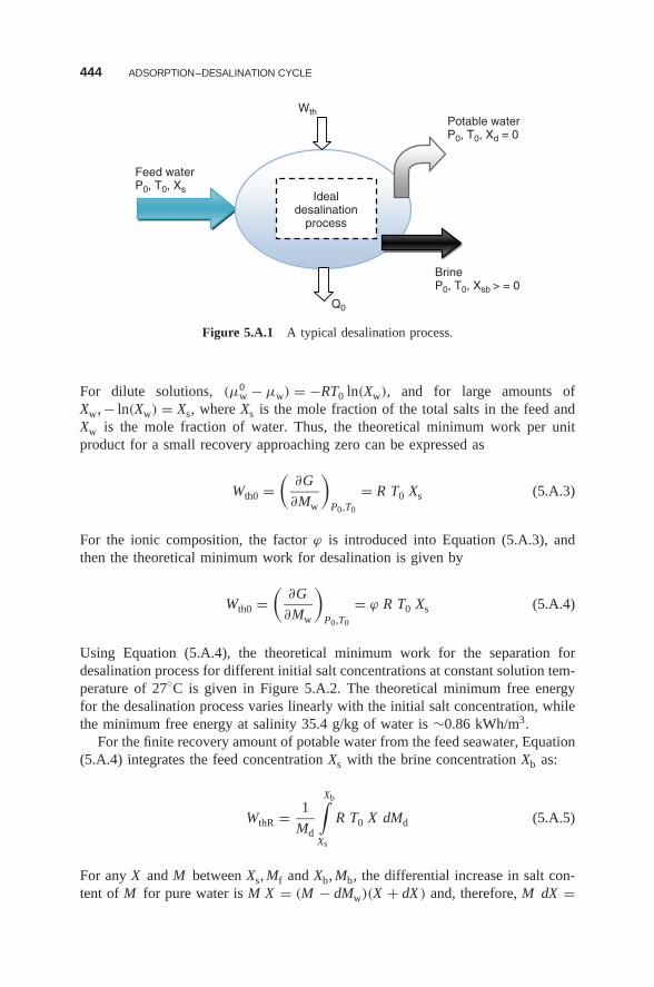
444 ADSORPTION–DESALINATION CYCLE

Q0

Feed waterP0, T0, Xs

Potable waterP0, T0, Xd = 0

BrineP0, T0, Xsb > = 0

Wth

Idealdesalination

process

Figure 5.A.1 A typical desalination process.

For dilute solutions, (μ0w − μw) = −RT0 ln(Xw), and for large amounts of

Xw, − ln(Xw) = Xs, where Xs is the mole fraction of the total salts in the feed andXw is the mole fraction of water. Thus, the theoretical minimum work per unitproduct for a small recovery approaching zero can be expressed as

Wth0 =(

∂G

∂Mw

)P0,T0

= R T0 Xs (5.A.3)

For the ionic composition, the factor ϕ is introduced into Equation (5.A.3), andthen the theoretical minimum work for desalination is given by

Wth0 =(

∂G

∂Mw

)P0,T0

= ϕ R T0 Xs (5.A.4)

Using Equation (5.A.4), the theoretical minimum work for the separation fordesalination process for different initial salt concentrations at constant solution tem-perature of 27◦C is given in Figure 5.A.2. The theoretical minimum free energyfor the desalination process varies linearly with the initial salt concentration, whilethe minimum free energy at salinity 35.4 g/kg of water is ∼0.86 kWh/m3.

For the finite recovery amount of potable water from the feed seawater, Equation(5.A.4) integrates the feed concentration Xs with the brine concentration Xb as:

WthR = 1

Md

Xb∫Xs

R T0 X dMd (5.A.5)

For any X and M between Xs, Mf and Xb, Mb, the differential increase in salt con-tent of M for pure water is M X = (M − dMw)(X + dX ) and, therefore, M dX =

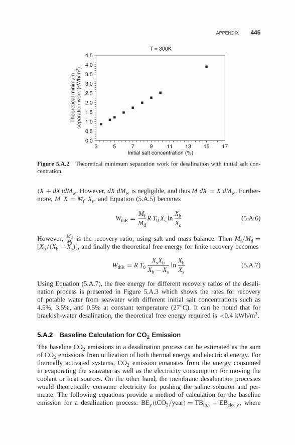
APPENDIX 445

0.0

0.5

1.0

1.5

2.0

2.5

3.0

3.5

4.0

4.5

3 5 7 9 11 13 15 17

The

oret

ical

min

imum

sepa

ratio

n w

ork

(kW

h/m

3 )

Initial salt concentration (%)

T = 300K

Figure 5.A.2 Theoretical minimum separation work for desalination with initial salt con-centration.

(X + dX )dMw. However, dX dMw is negligible, and thus M dX = X dMw. Further-more, M X = Mf Xs, and Equation (5.A.5) becomes

WthR = Mf

MdR T0 Xs ln

Xb

Xs(5.A.6)

However, MdMf

is the recovery ratio, using salt and mass balance. Then Mf/Md =[Xb/(Xb − Xs)], and finally the theoretical free energy for finite recovery becomes

WthR = R T0XsXb

Xb − Xsln

Xb

Xs(5.A.7)

Using Equation (5.A.7), the free energy for different recovery ratios of the desali-nation process is presented in Figure 5.A.3 which shows the rates for recoveryof potable water from seawater with different initial salt concentrations such as4.5%, 3.5%, and 0.5% at constant temperature (27◦C). It can be noted that forbrackish-water desalination, the theoretical free energy required is <0.4 kWh/m3.

5.A.2 Baseline Calculation for CO2 Emission

The baseline CO2 emissions in a desalination process can be estimated as the sumof CO2 emissions from utilization of both thermal energy and electrical energy. Forthermally activated systems, CO2 emission emanates from the energy consumedin evaporating the seawater as well as the electricity consumption for moving thecoolant or heat sources. On the other hand, the membrane desalination processeswould theoretically consume electricity for pushing the saline solution and per-meate. The following equations provide a method of calculation for the baselineemission for a desalination process: BEy (tCO2/year) = TBth,y + EBelec,y , where

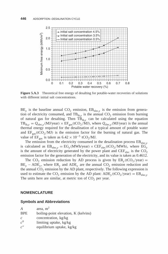
446 ADSORPTION–DESALINATION CYCLE

0.0

0.5

1.0

1.5

2.0

2.5

0 0.1 0.2 0.3 0.4 0.5 0.6 0.7 0.8

Min

imum

free

ene

rgy

(kW

h/m

3 )

Potable water recovery (%)

initial salt concentration 4.5%Initial salt concentration 3.5%Initial salt concentration 0.5%

Figure 5.A.3 Theoretical free energy of desalting for potable-water recoveries of solutionswith different initial salt concentrations.

BEy is the baseline annual CO2 emission, EBelec,y is the emission from genera-tion of electricity consumed, and TBth,y is the annual CO2 emission from burningof natural gas for desalting. Then TBth,y can be calculated using the equationTBth,y = Qelec,y (MJ/year) × EFgas(tCO2/MJ), where Qelec,y (MJ/year) is the annualthermal energy required for the desalination of a typical amount of potable waterand EFgas(tCO2/MJ) is the emission factor for the burning of natural gas. Thevalue of EFgas is taken as 6.42 × 10−5 tCO2/MJ.

The emission from the electricity consumed in the desalination process EBelec,yis calculated as EBelec,y = EGy (MWh/year) × CEFelec(tCO2/MWh), where EGyis the amount of electricity generated by the power plant and CEFelec is the CO2emission factor for the generation of the electricity, and its value is taken as 0.4612.

The CO2 emission reduction by AD process is given by ERy (tCO2/year) =BEy − ADEy , where ERy and ADEy are the annual CO2 emission reduction andthe annual CO2 emission by the AD plant, respectively. The following expression isused to estimate the CO2 emission by the AD plant: ADEy (tCO2/year) = EBelec,yThe units here are similar, at metric ton of CO2 per year.

NOMENCLATURE

Symbols and Abbreviations

A area, m2

BPE boiling-point elevation, K (kelvins)c concentration, kg/kgc0 limiting uptake, kg/kgc∗ equilibrium uptake, kg/kg

NOMENCLATURE 447

COP coefficient of performancecp specific-heat capacity, J kg−1 K−1

Dso a kinetic constant for silica gel–water system, m2 s−1

Ea activation energy of surface diffusion, kJ/molhfg latent heat, kJ/kgk thermal conductivity, W m−1 K−1

K0 preexponential coefficient, k/PaL length, mm mass, kgm mass flow rate, kg/sn number of bedsN ∗ number of adsorbent surface atoms in Henry regionN 0 number of adsorbent surface atoms in condensing phaseNs number of adsorbent surface atomsOPR overall performance ratioP pressure, PaP0 reference pressure, PaPR performance ratio,q fraction of refrigerant adsorbed by adsorbent, kg/kgQ total heat or energy, W or JQst isosteric heat of adsorption, kJ/kgQ∗

st isosteric heat of adsorption at zero surface coverage, kJ/molQ0 least adsorption energy, kJ/molR universal gas constant, J kg−1 K−1

Rp average radius of silica gel, mSDWP specific daily water production, m3/t·day (where t = metric ton)T temperature, Kt time/(t/thcycle), sT0 reference temperature, KU overall heat transfer coefficient, W m−2 K−1

u internal energy per unit mass, J kg−1 K−1

v specific volume, m3/kgvp pore volume, cm3/g

γ , δ, theta flags governing mode of operationλ thermal conductivity, W m−1 K−1

ρ effective density, kg/m3

τ number of cycles per day

Subscripts

a adsorbateads adsorbent; adsorptionch chilled water

448 ADSORPTION–DESALINATION CYCLE

cond condensercw cooling-waterd distillateevap evaporatorg gaseous phasehw hot waterHX heat exchangerin inletMads master adsorptionMdes master desorptionout outletreg regenerations salt, adsorbent, or saturationSads slave adsorberSdes slave desorbersg silica gelw pure water

REFERENCES

1. WHO, Guidelines for Drinking-Water Quality , Vol. 1, Recommendation , World HealthOrganization, 2008, p. 218.

2. Shiklomanov IA, An introduction to global fresh water issues, in Gleick PH, ed., Waterin Crisis: A Guide to the World’s Fresh Water Resources , Oxford Univ. Press, NewYork, 1993. pp. 4– 5.

3. National Intelligence Council, Water scarcity map adapted from the original map andresearch published by the International Water Management Institute (IWMI) (AnnualReport 2007–2008, p. 11), in Global Trends 2025: A Transformed World , GovernmentPrinting Office, Washington, DC, Nov. 2008, p. 55.

4. See http://atlas.nrcan.gc.ca/site/english/maps/freshwater/1 7.

5. Anonymous, A thirsty world, UNESCO Courier p. 21 (Sept. 2001).

6. Wagner L, Water Desalination: Tap in to Liquid Gold , Research Report, 2007.

7. US Dept. of Energy, Desalination and Water Purification Technology Roadmap Report ,2003.

8. Darwish MA, Al-Najem NM, Energy consumption by multi-stage flash and reverseosmosis desalters, Appl. Thermal Eng ., 20:399 (2000).

9. Fiorinia P, Sciubbaa E, Sommarivab C, A new formulation for the non-equilibriumallowance in MSF processes, Desalination 136:177–188 (2001).

10. Aly NH, El-Fiqi AK, Thermal performance of seawater desalination systems, Desali-nation , 158:127–142 (2003).

11. A1-Shammiri M, Safar M, Multi-effect distillation plants: State of the art, Desalination ,126:45–59 (1999).

12. Rahman H, Hawlader MNA, Malek A, An experiment with a single-effect submergedvertical tube evaporator in multi-effect desalination, Desalination 156:91–100 (2003).

REFERENCES 449

13. El-Dessouky HT, Ettouney HM, Multiple-effect evaporation desalination systems: Ther-mal analysis, Desalination 125:259–276 (1999).

14. El-Dessouky HT, Ettouneya HM, Mandani F, Performance of parallel feed multipleeffect evaporation system for seawater desalination, Appl. Thermal Eng ., 20:1679–1706(2000).

15. E1-Nashar AM, Qamhiyeh AM, Simulation of the steady-state operation of a multi-effectstack seawater distillation plant, Desalination , 101:231–243 (1995).

16. Van der Bruggen B, Vandecasteele C, Distillation vs. membrane filtration: Overview ofprocess evolutions in seawater desalination, Desalination 143:207–218 (2002).

17. Kershman SA, Rheinlander J, Gabler H, Seawater reverse osmosis powered by reneaw-able energy sources—hybrid wind/photovoltaic power/grid power supply for small-scaledesalination in Libya, Desalination , 153:17–23 (2002).

18. Ahmad GE, Schmid J, Feasibility study of brackish-water desalination in Egyptiandeserts and rural regions using PV systems, Energy Convers. Manage. 43:2641–2649(2002).

19. Tzen E, Theofilloyianakos D, Sigalas M, Karamanis K, Design and development of ahybrid autonomous system for seawater desalination Desalination 166:267–274 (2004).

20. Ng KC, Wang XL, Gao LZ, Chakraborty A, Saha BB, Koyama S, Apparatus and Methodfor Desalination , SG Patent Application 200503029-1 (2005) and WO Patent 121414A1(2006).

21. Dabrowski A, Adsorption—from theory to practice, Adv. Colloid Interface Sci .93:135–224 (2001).

22. Chakraborty A, Thermoelectric Cooling Devices: Thermodynamic Modelling and TheirApplications in Adsorption Cooling Cycle, PhD thesis, National Univ. Singapore, Nov.2005.

23. IUPAC, Reporting physisorption data for gas/solid systems, Pure Appl. Chem . 57(4):603–619 (1985).

24. Sukuki M, Adsorption Engineering , Kodansha Ltd., Tokyo and Elsevier Science Pub-lishers B. V., Amsterdam, 1990.

25. Ruthven DM, Principles of Adsorption and Adsorption Processes , Wiley, New York,1984.

26. Do DD, Adsorptrion Analysis: Equilibrium and Kinetics , Series on Chemical Engineer-ing, Vol. 2, Imperial College Press, 1998.

27. Authors’ unpublished data on silica gel characteristics, 2011.

28. Cortes FB, Chejne F, Carrasco-Marın F, Moreno-Castilla C, Perez-Cadenas AF, Wateradsorption on zeolite 13X: Comparison of the two methods based on mass spectrometryand thermogravimetry, Adsorption 16:141–146 (2010).

29. Simonot-Grange MH, Elm’Chaouri A, Weber G, Dufresne P, Raatz F, Joly J-F, Charac-terization of the dealumination effect into H faujasites by adsorption: Part 1. The watermolecule as a structural aluminum ion selective probe, Zeolites 12:155–159 (1992).

30. Aristov YI, Tokarev MM, Freni A, Glaznev IS, Restuccia G, Kinetics of water adsorptionon silica Fuji Davison RD, Micropor. Mesopor. Mater . 96:65–71 (2006).

31. Gordeeva LG, Tokarev NLM, Parmon VN, Aristov YmL, Selective water sorbents formultiple application. 6. Freshwater production from the atmosphere, React. Kinet. Catal.Lett . 65(1):153–159 (1998).

450 ADSORPTION–DESALINATION CYCLE

32. Restuccia G, Cacciola G, Performances of adsorption systems for ambient heating andair conditioning, Int. J. Refrig . 22:18–26 (1999).

33. Gavrilov KB, Okunev AG, Aristov YuI, Monolayer physical adsorption in narrow pores.Apparent surface dimension, React. Kinet. Catal. Lett . 58(1):39–48 (1996).

34. Alefeld G, Bauer HC, Maier-Laxhuber P, Rothmeyer M, A zeolite heat pump, heattransformer and heat accumulator, Proc. Int. Conf. Energy Storage, Brighton, UK, 1981.

35. Henninger SK, Habib HA, Janiak C, MOFs as adsorbents for low temperature heatingand cooling applications, J. Am. Chem. Soc. 131:2776–2777 (2009).

36. Wang X, Ng KC, Experimental investigation of an adsorption desalination plant usinglow-temperature waste heat, Appl. Thermal Eng . 25(17–18):2780–2789 (2005).

37. Zejli D, Benchrifa R, Bennouna A, Bouhelal OK, A solar adsorption desalination device:First simulation results, Desalination 168(1–3):127–135 (2004).

38. Wang X, Chakarborty A, Ng KC, Saha BB, How heat and mass recovery strategiesimpact the performance of adsorption desalination plant: Theory and experiments, HeatTransfer Eng . 28(2):147–153 (2007).

39. Ng KC, Saha BB, Chakraborty A, Koyama S, Adsorption desalination quenches globalthirst, Heat Transfer Eng . 29(10):845–848 (2008).

40. Thu K, Ng KC, Saha BB, Chakraborty A, Koyama S, Operational strategy of adsorptiondesalination systems, Int. J. Heat Mass Transfer 52(7–8):1811–1816 (2009).

41. Thu K, Saha BB, Chakraborty A, Chun WG, Ng KC, Study on an advanced adsorptiondesalination cycle with evaporator-condenser heat recovery circuit, Int. J. Heat MassTransfer 54(1–3):43–51 (2011).

42. Chakraborty A, Saha BB, Ng KC, Koyama S, Srinivasan K, Theoretical insight of physi-cal adsorption for a single-component adsorbent + adsorbate system: I. Thermodynamicproperty surfaces, Langmuir 25:2204–2211 (2009).

43. Chakraborty A, Saha BB, Ng KC, Koyama S, Srinivasan K, Theoretical insight ofphysical adsorption for a single component adsorbent + adsorbate system: II. The Henryregion, Langmuir 25(13):7359–7367 (2009).

44. Chakraborty A, Saha BB, Koyama S, Ng KC, Srinivasan K, Adsorption thermodynamicsof silica gel-water systems, J. Chem. Eng. Data 54(2):448–452 (2009).

45. Mcenaney B, Estimation of the dimensions of micropores in activated carbons usingthe Dubinin-Raduskevich equation, Carbon, 25:69–75 (1987).

46. Chakraborty A, Leong KC, Thu K, Saha BB, and Ng KC, Theoretical insight of adsorp-tion cooling, Applied Physics Letters Vol. 98, No. 22. art no. 221910 (2011).

47. Steele WA, The interaction of gases with solid surface, The International Encyclopediaof Physical Chemistry and Chemical Physics , Vol. 3, Pergamon Press, Oxford, 1974.

48. Schindler JB, Levan MD, The theoretical maximum isosteric heat of adsorption in theHenry’s law region for slit-shaped carbon nanopores, Carbon 46:644–648 (2008).

49. Ravikovitch PI, Vishnyakov A, and Neimark AV, Density functional theories and molec-ular simulations of adsorption and phase transitions in nanopores, Physical review E ,64: art no. 011602, (2001).

50. Thu K, Adsorption Desalination: Theory and Experiments , PhD thesis, National Univ.Singapore, 2010.

51. Chakraborty A, Saha BB, Koyama S, Ng KC, Specific heat capacity of a single com-ponent adsorbent-adsorbate system, Applied Physics Letters 90(17): art. no. 171902,(2007).

REFERENCES 451

52. Tien C, Adsorption Calculation and Modeling , Butterworh-Heinemann Series in Chem-ical Engineering, Boston, 1994.

53. Saha BB, Kashiwagi T, Experimental investigation of an advanced adsorptiosn refriger-ation cycle, ASHRAE (Am. Soc. Heating, Refrigerating, and Air-Conditioning) Trans .103(2):50–58 (1997).

54. Boelman EC, Saha, BB, Kashiwagi T. Experimental investigation of a silica gel–wateradsorption refrigeration cycle—the influence of operating conditions on cooling outputand COP, ASHRAE Trans . 101(2):358–366 (1995).

55. Chua HT, Ng KC, Chakraborty A, Oo NM, Othman MA, Adsorption characteristics ofsilica gel + water systems, J. Chem. Eng. Data 47(5):1177–1181 (2002).

56. Aristov YI, Tokarev MM, Cacciola G, Restuccia G, Selective water sorbents for multipleapplications: 1. CaCl2 confined in mesopores of the silica gel: Sorption properties, React.Kinet. Catal. Lett . 59(2):325–334 (1996).

57. Tokarev MM, Okunev BN, Safonov MS, Kheifets LI, Aristov YI, Approximationequations for describing the sorption equilibrium between water vapor and a SWS-1Lcomposite sorbent, Russ. J. Phys. Chem . 79(9):1490–1493 (2005).

58. Saha BB, Chakraborty A, Koyama S, Aristov YI, A new generation coolingdevice employing CaCl2-in-silica gel-water system, Int. J. Heat Mass Transfer52(1–2):516–524 (2011).

59. Chihara K, Suzuki M, Air drying by pressure swing adsorption, J. Chem. Eng . (Japan)16:293–298 (1983).

60. Ng KC, Thu K, Saha BB, Chakraborty A, Study on a waste heat-driven adsorptioncooling cum desalination cycle, International Journal of Refrigeration Vol. 35, No. 3,pp. 685–693, (2011).

61. Spiegler KS, El-Sayed YM, A Desalination Primer Balaban Desalination Publications,Santa Maria Imbaro, Italy, 1994.

62. Ng KC, Thu K, Chakraborty A, Saha BB, Chun WG, Solar-assisted dual-effect adsorp-tion cycle for the production of cooling effect and potable water, Int. J. Low-CarbonTechnol . 4(2):61–67 (2009).

63. Thu K, Chakraborty A, Saha BB, Chun WG, Ng KC, Life-cycle cost analysis of adsorp-tion cycles for desalination, Desal. Water Treat . 20(1–3):1–10 (2010).

64. Atikol U, Aybar HS, Estimation of water production cost in the feasibility analysis ofRO systems, Desalination 184(1–3):253–258 (2005).

65. Ng KC, Thu K, Yanagi H, Saha BB, Chakraborty A, Tawfiq Y, Al-Tawfiq YG, Apparatusand Method for Improved Desalination , PCT/SG2009/000223, 2008.

66. Saha BB, Ng KC, Chakraborty A, Thu K, Desalination System and Method ,PCT/IB2010/001757, publication date Jan. 27, 2011.

67. Atikol U, Aybar HS, Estimation of water production cost in the feasibility analysis ofRO systems, Desalination 184:253–258 (2005).

68. Fiorenza G, Sharma VK, Braccio G. Techno-economic evaluation of a solar poweredwater desalination plan, Energy Convers. Manage. 44:2217–2240 (2003).

69. Spiegler KS, El-Sayed YM, The energetics of desalination processes, Desalination134:109–128 (2001).

70. California Coastal Commission, Energy use, Chap. 1 in Seawater Desalination in Cali-fornia , (available at http://www.coastal.ca.gov/index.html; accessed 1/15/07).

This page intentionally left blank

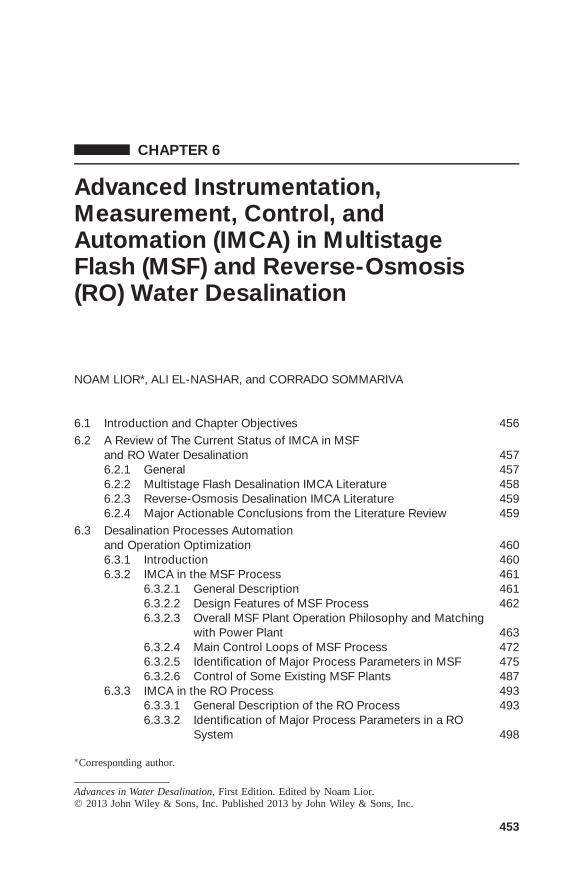
CHAPTER 6

Advanced Instrumentation,Measurement, Control, andAutomation (IMCA) in MultistageFlash (MSF) and Reverse-Osmosis(RO) Water Desalination

NOAM LIOR*, ALI EL-NASHAR, and CORRADO SOMMARIVA

6.1 Introduction and Chapter Objectives 4566.2 A Review of The Current Status of IMCA in MSF

and RO Water Desalination 4576.2.1 General 4576.2.2 Multistage Flash Desalination IMCA Literature 4586.2.3 Reverse-Osmosis Desalination IMCA Literature 4596.2.4 Major Actionable Conclusions from the Literature Review 459

6.3 Desalination Processes Automationand Operation Optimization 4606.3.1 Introduction 4606.3.2 IMCA in the MSF Process 461

6.3.2.1 General Description 4616.3.2.2 Design Features of MSF Process 4626.3.2.3 Overall MSF Plant Operation Philosophy and Matching

with Power Plant 4636.3.2.4 Main Control Loops of MSF Process 4726.3.2.5 Identification of Major Process Parameters in MSF 4756.3.2.6 Control of Some Existing MSF Plants 487

6.3.3 IMCA in the RO Process 4936.3.3.1 General Description of the RO Process 4936.3.3.2 Identification of Major Process Parameters in a RO

System 498

∗Corresponding author.

Advances in Water Desalination, First Edition. Edited by Noam Lior.© 2013 John Wiley & Sons, Inc. Published 2013 by John Wiley & Sons, Inc.

453

454 ADVANCED INSTRUMENTATION, MEASUREMENT, CONTROL, AND AUTOMATION

6.3.3.3 RO Automation System 4996.3.3.4 The Major RO Process Parameters and Their Control 5006.3.3.5 Comparison of Specific Requirements of Control

Systems in Brackish and Seawater RO Plants 5036.3.3.6 Control of Some Existing RO Plants 505

6.3.4 Conclusions and Recommendations on Current and PotentiallyFuture Desalination Process Automation Methods 516

6.4 Current and Potentially Future Process Automation Methods for RO andMSF Desalination Processes 5176.4.1 Current Status and Projected Development of MSF Process

Automation 5176.4.1.1 Some Promising Future Control and Automation

Options 5176.4.1.2 Future Automation Improvements 518

6.4.2 Status and Projected Development of RO Process Automation 5256.4.3 Prospects for Advanced Control Methods in MSF and RO

Desalination Plants 5276.4.3.1 Introduction 5276.4.3.2 Prospects for Dynamic Matrix Control Method 5296.4.3.3 Prospects for Nonlinear Model Predictive Control

(NMPC) Method 5296.4.3.4 Prospects for Constrained Model Predictive Control

(CMPC) Method 5306.4.3.5 Prospects for Use of Neural Networks in MSF Plants 5316.4.3.6 Intelligent Control Approaches 5316.4.3.7 Prospects for Online Optimization 533

6.4.4 Conclusions and Recommendations on Potential of Future IMCASystems 535

6.5 Calculation of Impact of Automation on Product Water Cost 5366.5.1 Introduction 5366.5.2 Rigorous and Detailed Estimation of Economic Benefits

from Advanced Process Control 5406.5.2.1 General Approach 5406.5.2.2 Savings Due to Reduction in Variance of Controlled

Variables 5416.5.2.3 Savings Due to Running at Optimum Condition 543

6.5.3 Process Control Structure 5436.5.3.1 Architecture of Automatic Setpoint Control System 5436.5.3.2 Main Components of Setpoint Optimization System 5446.5.3.3 Reconciliation of Measurements 5456.5.3.4 Identification of Model Parameters 5456.5.3.5 Optimization and Sensitivity Analysis 5466.5.3.6 Mathematical Simulation Model 546

6.5.4 MSF Cost-Benefit Ratio of New IMCA Systems 5476.5.4.1 General Comments 5476.5.4.2 Modeling and Simulating the Performance of the MSF

Process 5476.5.4.3 Optimization of Operation of the MSF Process 557

ADVANCED INSTRUMENTATION, MEASUREMENT, CONTROL, AND AUTOMATION 455

6.5.4.4 An Additional Way to Improve: Change of IMCAPhilosophy 562

6.5.5 RO Cost–Benefit Ratio of New IMCA Systems 5656.5.5.1 RO Process 5656.5.5.2 Model of an RO Process 5666.5.5.3 Optimization of RO Process Operation 5696.5.5.4 Promising RO Automation Methods and Their Potential

Cost–Benefit Ratios 5756.5.6 Conclusions 579

6.6 IMCA Systems Recommended for RO and MSF Desalination Plants 5806.6.1 Introduction 5806.6.2 Model Predictive Advanced Controller (MPC) a Recommended

Advanced Controller 5806.6.2.1 Rationale for Selecting MPC Controllers 5806.6.2.2 Brief Introduction to MPC 5816.6.2.3 APC Selection Considerations 5836.6.2.4 System Configuration of a Typical MPC 5846.6.2.5 Advanced Identification and Analysis (AIDA) 5846.6.2.6 MPC Controller 5866.6.2.7 Cost Estimation for Advanced Controller 5876.6.2.8 Distributed Control System (DCS) Configuration 5886.6.2.9 Hardware Components 5896.6.2.10 Software Components 5896.6.2.11 DCS Configuration Definition 5906.6.2.12 Cost Estimate 5916.6.2.13 Added Cost of Water Due to DCS Installation 5956.6.2.14 Benefit Due to DCS Installation 5976.6.2.15 Results and Discussion 5986.6.2.16 Conclusions and Recommendations 600

6.6.3 Recommendations for the Most Suitable Automation Systems:MSF Plants 601

6.6.4 RO: Suitable and Recommended IMCA System 6016.6.4.1 Control System Architecture 6016.6.4.2 Control Room 6036.6.4.3 Intake Control Loop 6046.6.4.4 Pretreatment Control Loop 6046.6.4.5 Main RO Control Loop 6046.6.4.6 RO Train Control Loops 6046.6.4.7 Motor Control Center 6046.6.4.8 Electrical Circuits and VFD 6046.6.4.9 Permeate Posttreatment and Storage 6056.6.4.10 Wastewater Neutralization and Discharge 6056.6.4.11 Operator–Computer Interface (HMI), Alarms 605

6.7 Modeling and Analysis Recommendations for MSF and RO Plants 6056.7.1 Modeling Requirements 6056.7.2 Steady-State or Dynamic Modeling 606

6.7.2.1 Steady-State Modeling 6066.7.2.2 Dynamic Modeling 608

456 ADVANCED INSTRUMENTATION, MEASUREMENT, CONTROL, AND AUTOMATION

6.7.3 Mathematical Modeling: Description and needs in DesalinationIMCA 6126.7.3.1 The Modeling in General 6126.7.3.2 State Variables and State Equations 6136.7.3.3 Conservation Equations 6136.7.3.4 Additional (Algebraic) Equations 615

6.7.4 Modeling Requirements in RO Desalination 6176.7.4.1 Modeling of RO Process 6176.7.4.2 Power Requirement Modeling of RO Process 6266.7.4.3 Practical Approach to RO System Performance

Optimization 6276.7.5 Mathematical Formulation of the Dynamic Modeling Problem 628

6.7.5.1 Model Equations 6286.7.5.2 Solution for the Dynamic Simulation Model 6306.7.5.3 Solution Algorithm 630

6.7.6 Summary of Modeling Needs for the Future 6326.8 Conclusions and Recommendations 632Acknowledgment 635Nomenclature 636References 642Further Reading 647

6.F.1 Literature on MFSD-Related IMCA 6476.F.2 Literature on RO-Related IMCA 6516.F.3 Literature on IMCA References Related to Desalination in

General (Mostly Excluding MSF and RO) 6526.F.4 Literature on Some General Controls 656

6.1 INTRODUCTION AND CHAPTER OBJECTIVES

A paramount goal in the proper design and operation of any desalination plantis the reduction of its investment and operating costs to minimize the cost of thefreshwater produced. Important methods for cost reduction include the minimiza-tion, per unit desalted product water, of the costs of the (1) capital investment,(2) energy, (3) chemical additives consumed by the plant, (4) labor (amount andskill level), and (5) plant environmental impact. Another goal, related but alsoindependent, is to maximize production, and to that end increase reliability anddecrease downtime. One potential tool for these optimization tasks is the use ofadequate and economical control strategies that can stabilize the operation of theplant at high-efficiency operating points while effectively handling the differentconstraints on the process variables. Better instrumentation, measurement, control,and automation (IMCA), indeed, are important for meeting these optimizationobjectives. This chapter focuses on the status and improvement needs for MSF andRO (the predominant seawater desalting processes in the world) plant automation

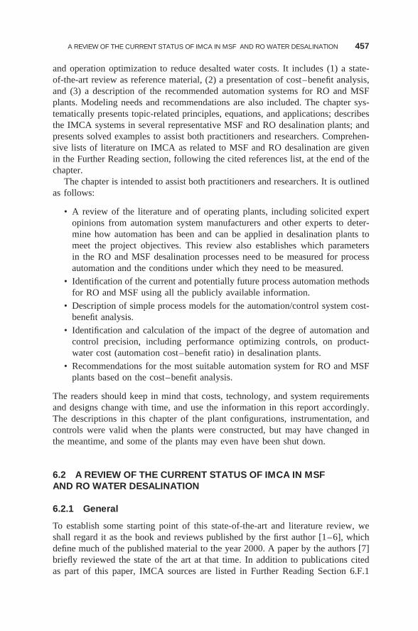
A REVIEW OF THE CURRENT STATUS OF IMCA IN MSF AND RO WATER DESALINATION 457

and operation optimization to reduce desalted water costs. It includes (1) a state-of-the-art review as reference material, (2) a presentation of cost–benefit analysis,and (3) a description of the recommended automation systems for RO and MSFplants. Modeling needs and recommendations are also included. The chapter sys-tematically presents topic-related principles, equations, and applications; describesthe IMCA systems in several representative MSF and RO desalination plants; andpresents solved examples to assist both practitioners and researchers. Comprehen-sive lists of literature on IMCA as related to MSF and RO desalination are givenin the Further Reading section, following the cited references list, at the end of thechapter.

The chapter is intended to assist both practitioners and researchers. It is outlinedas follows:

• A review of the literature and of operating plants, including solicited expertopinions from automation system manufacturers and other experts to deter-mine how automation has been and can be applied in desalination plants tomeet the project objectives. This review also establishes which parametersin the RO and MSF desalination processes need to be measured for processautomation and the conditions under which they need to be measured.

• Identification of the current and potentially future process automation methodsfor RO and MSF using all the publicly available information.

• Description of simple process models for the automation/control system cost-benefit analysis.

• Identification and calculation of the impact of the degree of automation andcontrol precision, including performance optimizing controls, on product-water cost (automation cost–benefit ratio) in desalination plants.

• Recommendations for the most suitable automation system for RO and MSFplants based on the cost–benefit analysis.

The readers should keep in mind that costs, technology, and system requirementsand designs change with time, and use the information in this report accordingly.The descriptions in this chapter of the plant configurations, instrumentation, andcontrols were valid when the plants were constructed, but may have changed inthe meantime, and some of the plants may even have been shut down.

6.2 A REVIEW OF THE CURRENT STATUS OF IMCA IN MSFAND RO WATER DESALINATION

6.2.1 General

To establish some starting point of this state-of-the-art and literature review, weshall regard it as the book and reviews published by the first author [1–6], whichdefine much of the published material to the year 2000. A paper by the authors [7]briefly reviewed the state of the art at that time. In addition to publications citedas part of this paper, IMCA sources are listed in Further Reading Section 6.F.1

458 ADVANCED INSTRUMENTATION, MEASUREMENT, CONTROL, AND AUTOMATION

for MSF; in Section 6.F.2, for RO; in Section 6.F.3 for general desalination andrelated topics; and in Section 6.F.4 for general control theory.

A dynamic source of information is the Encyclopedia of Desalination and WaterResources (DESWARE), published in 2001, which has a fairly large chapter onprocess instrumentation, control, and automation. It contains brief general reviewson control theory and components, but not specific to desalination, in the articles byBunzemeier and Krause [8], Bunzemeier and Litz [9], and two articles by Muroniand Borsani [10,11].

A brief review of the theory of fault diagnosis, a systematic method for determin-ing (after detection of a fault) unacceptable deviation of a measured or calculatedparameter in chemical processes, is given by Tarifa and Scenna [12].

6.2.2 Multistage Flash Desalination IMCA Literature

DESWARE contains a section on plant availability analysis of MSF distillation [13],using fault-tree logic, and contains methodology and examples and evaluations ofsome MSF plants in the UAE based on a somewhat small and old set of data. Itconcludes that availability is reasonably high (∼80%), with pumps typically havingthe highest failure rate, followed by valves. Hence, it recommends consideration ofthe once-through rather than the commonly used recirculation MSF plant design,the use of variable-speed pumps (without flow control valves), and hydrostaticprotection from boiling of the brine in the brine heater (which causes scaling)instead of a �p control valve. In summary, it states: “Considering future MSFplants, the central message of this work for improved design and operation is tosimplify the design substantially. This shows a much higher potential than anysophisticated modeling control and simulation effort.” This conclusion is identicalto ours. We note, however, that current operational experience shows that both MSFand MED plants operating in the Gulf have an availability in excess of 99.5% andhave operated continuously without interruption for more than 5 years betweenacid cleanings, and the specific suggestion to implement once-through plants maynot offer the advantage perceived from much older experiences.

A paper on brine flow hydraulics in MSF plants, [14] is useful for modelingimprovement, and another expounds the need for multivariable control in MSFdesalination plants [15].

Tarifa and Scenna [12] briefly review the theory of fault diagnosis using artificialintelligence, as applied to MSF plants. They followed this work up to apply the faultdiagnostic system to an MSF plant, and met with some, albeit insufficient, success.In another paper Tarifa and Nicolas [16] used neural networks for developing themodel, and stated that the training method they developed makes the system simpleryet more accurate than previous ones. More work remains to link this model witha qualitative one to generate appropriate explanations for each diagnostic.

Another article in DESWARE is on control of cogeneration power plants forMSF desalination [17]. Since combined cycles using gas turbines with bottomingsteam turbines are being aggressively and successfully developed and used forraising the energy efficiency (now approaching 60%) and reducing emissions in

A REVIEW OF THE CURRENT STATUS OF IMCA IN MSF AND RO WATER DESALINATION 459

power generation applications, this article discusses control schemes and strategiesfor some of these cycles in conjunction with MSF plants.

A brief review of hybrid modeling and control techniques with examples forthe control of an MSF brine heater and of the TBT, as well as level control of thepretreatment stage in an RO plant, are contained in a publication by Gambier andBadreddin [18].

The application of neural network process simulation to a large-scale commercialMSF desalination plant (22,270 m3/d, Az-Zour, Kuwait) and a RO desalinationplant (56,800 m3/d, Jeddah, Saudi Arabia) was compared with that obtained fromprocess models developed by the combination of the ASPEN PLUS and SPEEDUPcommercial systems. The approach to neural network modeling is described in somedetail with recommendations for the best approach. Neural networks are stated tohave been effective for performance modeling but seem to have produced largererrors than model-based process simulation.

Nonlinear model predictive control (NLMPC) was analyzed as a control strategyfor MSF desalination plants [19], and was found to offer good control performanceand substantial energy savings. At the same time, it was found in comparisonwith conventional proportional integral (PI) control that its tuning was difficult andcomputation long. A thorough search of desalination-related IMCA patents was notpart of this study, although but a number of patents were issued on these topics.Krause [20] describes a new method for controlling MSF.

6.2.3 Reverse-Osmosis Desalination IMCA Literature

It was realized very early that careful plant supervision and maintenance, assistedin a major way by real-time computer-aided automatic controls, are of vitalimportance for the economical and reliable operation of RO desalination plants[21–23]. The early publications have described system design and methodology,but not field testing.

Conventional automatic control of RO uses the PI control strategy [proportionalintegral; the derivative mode is often disabled because of large signal–noise ratio(SNR) in the process]. In an attempt to examine the application of advanced con-trol and optimization to RO processes [24,25], constrained model predictive control(CMPC) was applied to laboratory-scale systems. While only some of the relevantparameters were controlled, the application of CMPC was found to increase theplant output by up to 13.6% and slightly improve the product quality, as comparedwith the PI system. An important aspect of this improvement is that CMPC allowsfor some knowledge-based corrections. Further investigations of applying neuralnetworks and fuzzy logic to desalination plant control were made but very super-ficially [26], and similarly to all the other proposals and studies for the applicationof advanced control systems to water desalination conducted in the past, none haveincluded a cost–benefit analysis.

6.2.4 Major Actionable Conclusions from the Literature Review

One of the most critical issues for maintaining low product cost is the achievementof high plant availability, and to this end the following measures could be beneficial:

460 ADVANCED INSTRUMENTATION, MEASUREMENT, CONTROL, AND AUTOMATION

• Using fault-tree analysis in some form, identify the most vulnerable compo-nents, attempt to replace them by an improved design, and monitor them morecarefully.

• Simplifying the design wherever possible.

Model-based predictive control seems to have the potential for improving controlof both MSF and RO plants, but needs to be examined and tested in the field.

Artificial intelligence, neural networks, and fuzzy logic have been studied fur-ther for desalination plants, but haven’t been proven (perhaps not yet) as viableapproaches.

6.3 DESALINATION PROCESSES AUTOMATIONAND OPERATION OPTIMIZATION

6.3.1 Introduction

Currently (as of early 2012), the majority of operating MSF and RO plants arecontrolled by simple proportional integral derivative (PID)-type controllers (a glos-sary of abbreviations and instrumentation, measurement, control, and automationterms is given in the Nomenclature section at the end of this chapter (beforethe References list). The use of simple PID controllers, which can maintain thestable operation of the plant, certainly overlooks the complex interactions thatmay exist within the plant. Both MSF and RO plants are nonlinear multivariablesystems, and an in-depth investigation of the different interactions between theinputs and outputs of the plant is necessary to optimize the selection of the controlstructure.

The use of advanced model-based control schemes such as dynamic matrixcontrol (DMC), and nonlinear model predictive control (NLMPC) can have thepotential of providing better control of the plant, but their cost and added complexitymust be justified by the cost–benefit ratio resulting from any improvements it mayproduce.

Both MSF and RO plants are particularly suited for constraint-accommodatingcontrol strategies for a number of reasons; for instance, limits on temperature in thebrine heater (in MSF plants) and feedwater (in RO plants) must be observed, basedon the scale control method used. These constraints can be easily incorporatedwithin the framework of an advanced control strategy that can accommodate, ormake adjustments for, such constraints.

While the most important goal in the past was to achieve the highest pos-sible availability of plants, today, optimization of plant, performance becomesincreasingly important. For that purpose, it is no longer sufficient to operate plantsaccording to the operation manuals of the process manufacturer or to follow theexperience of the operators. It now becomes necessary to use supplementary cal-culations to determine the optimal setpoints of the individual control loops basedon a rigorous process model, which allows for improvement of efficiency under allmodes of operation.

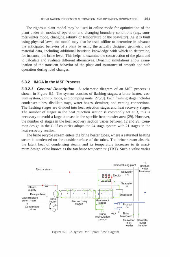
DESALINATION PROCESSES AUTOMATION AND OPERATION OPTIMIZATION 461

The rigorous plant model may be used in online mode for optimization of theplant under all modes of operation and changing boundary conditions (e.g., sum-mer/winter mode, changing salinity or temperature of the seawater). As it is builtusing physical laws, the model may also be used offline to determine in advancethe anticipated behavior of a plant by using the actually designed geometric andmaterial data, including additional heuristic knowledge with which to determine,for instance, the brine level. This helps to examine the construction of the plant andto calculate and evaluate different alternatives. Dynamic simulations allow exam-ination of the transient behavior of the plant and assurance of smooth and safeoperation during load changes.

6.3.2 IMCA in the MSF Process

6.3.2.1 General Description A schematic diagram of an MSF process isshown in Figure 6.1. The system consists of flashing stages, a brine heater, vac-uum system, control loops, and pumping units [27,28]. Each flashing stage includescondenser tubes, distillate trays, water boxes, demister, and venting connections.The flashing stages are divided into heat rejection stages and heat recovery stages.The number of stages in the heat rejection section is commonly set at 3, this isnecessary to avoid a large increase in the specific heat transfer area [29]. However,the number of stages in the heat recovery section varies between 12 and 29. Com-mon design in the Gulf countries adopts the 24-stage system with 21 stages in theheat recovery section.

The brine recycle stream enters the brine heater tubes, where a saturated heatingsteam is condensed on the outside surface of the tubes. The brine stream absorbsthe latent heat of condensing steam, and its temperature increases to its maxi-mum design value known as the top brine temperature (TBT). Such a value varies

Ejector steam

Steamsupply

Condensatereturn

Brineheater Heat recovery

stagesHeat reject

stages

Brinerecirculation

pumps

Brineblowdown

Productout

Deaerator

Seawaterin

Seawaterout

Remineralising plantTo

productwater

treatment

Ejector

Seawaterinlet

header

Seawateroutlet

header

Low pressuresteam main

Desuperheat

Figure 6.1 A typical MSF plant flow diagram.

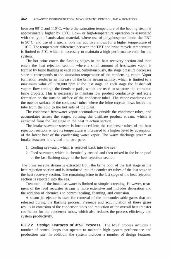
462 ADVANCED INSTRUMENTATION, MEASUREMENT, CONTROL, AND AUTOMATION

between 90◦C and 110◦C, where the saturation temperature of the heating steam isapproximately higher by 10◦C. Low- or high-temperature operation is associatedwith the type of antiscalant material, where use of polyphosphate limits the TBTto 90◦C, and use of a special polymer additive allows for a higher temperature of110◦C. The temperature difference between the TBT and brine recycle temperatureis limited to 5◦C, which is necessary to maintain a high-performance ratio for thesystem.

The hot brine enters the flashing stages in the heat recovery section and thenenters the heat rejection section, where a small amount of freshwater vapor isformed by brine flashing in each stage. Simultaneously, the stage pressure decreasessince it corresponds to the saturation temperature of the condensing vapor. Vaporformation results in an increase of the brine stream salinity, which is limited to amaximum value of ∼70,000 ppm at the last stage. In each stage the flashed-offvapors flow through the demister pads, which are used to separate the entrainedbrine droplets. This is necessary to maintain low product conductivity and scaleformation on the outside surface of the condenser tubes. The vapor condenses onthe outside surface of the condenser tubes where the brine recycle flows inside thetube from the cold to the hot side of the plant.

The condensed freshwater vapor accumulates outside the condenser tubes, andaccumulates across the stages, forming the distillate product stream, which isextracted from the last stage in the heat rejection section.

The intake seawater stream is introduced into the condenser tubes of the heatrejection section, where its temperature is increased to a higher level by absorptionof the latent heat of the condensing water vapor. The warm discharge stream ofintake seawater is divided into two parts:

1. Cooling seawater, which is rejected back into the sea

2. Feed seawater, which is chemically treated and then mixed in the brine poolof the last flashing stage in the heat rejection section

The brine recycle stream is extracted from the brine pool of the last stage in theheat rejection section and is introduced into the condenser tubes of the last stage inthe heat recovery section. The remaining brine in the last stage of the heat rejectionsection is rejected into the sea.

Treatment of the intake seawater is limited to simple screening. However, treat-ment of the feed seawater stream is more extensive and includes deaeration andthe addition of chemicals to control scaling, foaming, and corrosion.

A steam jet ejector is used for removal of the noncondensable gases that arereleased during the flashing process. Presence and accumulation of these gasesresults in corrosion of the condenser tubes and reduction of the overall heat transfercoefficient for the condenser tubes, which also reduces the process efficiency andsystem productivity.

6.3.2.2 Design Features of MSF Process The MSF process includes anumber of control loops that operate to maintain high system performance andproduction rate. In addition, the system includes a number of design features,

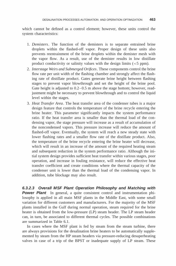
DESALINATION PROCESSES AUTOMATION AND OPERATION OPTIMIZATION 463

which cannot be defined as a control element; however, these units control thesystem characteristics:

1. Demisters . The function of the demisters is to separate entrained brinedroplets within the flashed-off vapor. Proper design of these units alsoprevents reentrainment of the brine droplets within the demister mesh withthe vapor flow. As a result, use of the demister results in low distillateproduct conductivity or salinity values with the design limits (<5 ppm).

2. Interstage Weirs and Submerged Orifices . These components control the brineflow rate per unit width of the flashing chamber and strongly affect the flash-ing rate of distillate product. Gates generate brine height between flashingstages to prevent vapor blowthrough and set the height of the brine pool.Gate height is adjusted to 0.2–0.5 m above the stage bottom; however, read-justment might be necessary to prevent blowthrough and to control the liquidlevel within the stages.

3. Heat Transfer Area . The heat transfer area of the condenser tubes is a majordesign feature that controls the temperature of the brine recycle entering thebrine heater. This parameter significantly impacts the system performanceratio. If the heat transfer area is smaller than the thermal load of the con-densing vapor, the stage pressure will increase as a result of accumulation ofthe noncondensed vapors. This pressure increase will reduce the amount offlashed-off vapor. Eventually, the system will reach a new steady state withlower flashing rates and a smaller flow rate of the distillate product. Also,the temperature of the brine recycle entering the brine heater will decrease,which will result in an increase of the amount of the required heating steamand subsequent reduction in the system performance ratio. Although the ini-tial system design provides sufficient heat transfer within various stages, pooroperation, and increase in fouling resistance, will reduce the effective heattransfer coefficient and create conditions where the thermal capacity of thecondenser unit is lower than the thermal load of the condensing vapor. Inaddition, tube blockage may also result.

6.3.2.3 Overall MSF Plant Operation Philosophy and Matching withPower Plant In general, a quite consistent control and instrumentation phi-losophy is applied in all main MSF plants in the Middle East, with some smallvariation for different customers and manufacturers. For the majority of the MSFplants installed in the Gulf during normal operation, steam required for the brineheater is obtained from the low-pressure (LP) steam header. The LP steam headercan, in turn, be associated to different thermal cycles. The possible combinationsare summarized in Table 6.1.

In cases where the MSF plant is fed by steam from the steam turbine, thereare always provisions for the desalination brine heaters to be automatically supple-mented by steam from the HP steam headers via pressure-reducing desuperheatingvalves in case of a trip of the BPST or inadequate supply of LP steam. These

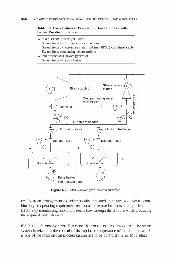
464 ADVANCED INSTRUMENTATION, MEASUREMENT, CONTROL, AND AUTOMATION

Table 6.1 Classification of Process Interfaces for ThermallyDriven Desalination Plants

With associated power generatorSteam from heat recovery steam generationSteam from backpressure steam turbine (BPST) combined cycleSteam from condensing steam turbine

Without associated power generatorSteam from auxiliary boiler

Steam turbine

Demister

MP steam headerPC

A

PCIC

TBT control valve TBT control valve

Desuperheater Desuperheater

Desuperheater

Brine heater Brine heater

Brine heater

Steam reducingstation

Desuperheating waterfrom BFWP

p p

Condensate pump

Figure 6.2 MSF–power yard process interface.

results in an arrangement as schematically indicated in Figure 6.2. Actual com-bined cycle operating requirement tend to achieve maximal power output from theBPST’s by maintaining maximum steam flow through the BPST’s while producingthe required water demand.

6.3.2.3.1 Steam System: Top Brine Temperature Control Loop The steamsystem is related to the control of the top brine temperature of the distiller, whichis one of the most critical process parameters to be controlled in an MSF plant.

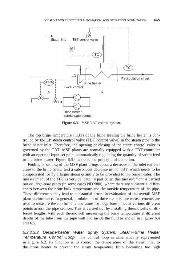
DESALINATION PROCESSES AUTOMATION AND OPERATION OPTIMIZATION 465

TBT control valve

Level control

Brine heatercondensate pumps

Brine heater

Recirculation circuitLC

Steam line

TC

TC

AIRA

Figure 6.3 MSF TBT control system.

The top brine temperature (TBT) of the brine leaving the brine heater is con-trolled by the LP steam control valve (TBT control valve) in the steam pipe to thebrine heater inlet. Therefore, the opening or closing of the steam control valve isgoverned by the TBT. MSF plants are normally equipped with a TBT controllerwith an operator input set point automatically regulating the quantity of steam feedto the brine heater. Figure 6.3 illustrates the principle of operation.

Fouling or scaling of the MSF plant brings about a decrease in the inlet temper-ature to the brine heater and a subsequent decrease in the TBT, which needs to becompensated for by a larger steam quantity to be provided to the brine heater. Themeasurement of the TBT is very delicate. In particular, this measurement is carriedout on large-bore pipes (in some cases ND2000), where there are substantial differ-ences between the brine bulk temperature and the outside temperature of the pipe.These differences may lead to substantial errors in evaluation of the overall MSFplant performance. In general, a minimum of three temperature measurements areused to measure the top brine temperature for large-bore pipes at various differentpoints across the pipe section. This is carried out by installing thermowells of dif-ferent lengths, with each thermowell measuring the brine temperature at differentdepths of the tube from the pipe wall and inside the fluid as shown in Figures 6.4and 6.5.

6.3.2.3.2 Desuperheater Water Spray System: Steam–Brine HeaterTemperature Control Loop The control loop is schematically representedin Figure 6.2. Its function is to control the temperature of the steam inlet tothe brine heater to prevent the steam temperature from becoming too high

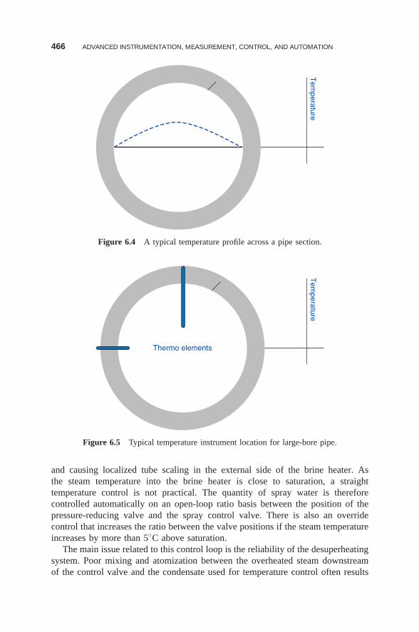
466 ADVANCED INSTRUMENTATION, MEASUREMENT, CONTROL, AND AUTOMATION

Tem

perature

Figure 6.4 A typical temperature profile across a pipe section.

Tem

perature

Thermo elements

Figure 6.5 Typical temperature instrument location for large-bore pipe.

and causing localized tube scaling in the external side of the brine heater. Asthe steam temperature into the brine heater is close to saturation, a straighttemperature control is not practical. The quantity of spray water is thereforecontrolled automatically on an open-loop ratio basis between the position of thepressure-reducing valve and the spray control valve. There is also an overridecontrol that increases the ratio between the valve positions if the steam temperatureincreases by more than 5◦C above saturation.

The main issue related to this control loop is the reliability of the desuperheatingsystem. Poor mixing and atomization between the overheated steam downstreamof the control valve and the condensate used for temperature control often results

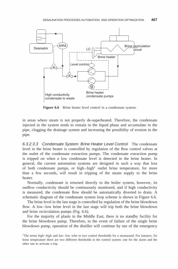
DESALINATION PROCESSES AUTOMATION AND OPERATION OPTIMIZATION 467

Level control

Deareator

Brine heatercondensate pumpsHigh conductivity

condensate to waste

Brine heater

LCAIRA

M

Brine recirculationcircuit

Figure 6.6 Brine heater level control in a condensate system.

in areas where steam is not properly de-superheated. Therefore, the condensateinjected in the system tends to remain in the liquid phase and accumulate in thepipe, clogging the drainage system and increasing the possibility of erosion in thepipe.

6.3.2.3.3 Condensate System: Brine Heater Level Control The condensatelevel in the brine heater is controlled by regulation of the flow control valves atthe outlet of the condensate extraction pumps. The condensate extraction pumpis tripped on when a low condensate level is detected in the brine heater. Ingeneral, the current automation systems are designed in such a way that lossof both condensate pumps, or high–high1 outlet brine temperature, for morethan a few seconds, will result in tripping of the steam supply to the brineheater.

Normally, condensate is returned directly to the boiler system, however, itsoutflow conductivity should be continuously monitored, and if high conductivityis measured, the condensate flow should be automatically diverted to drain. Aschematic diagram of the condensate system loop scheme is shown in Figure 6.6.

The brine level in the last stage is controlled by regulation of the brine blowdownflow. A low–low brine level in the last stage will trip both the brine blowdownand brine recirculation pumps (Fig. 6.6).

For the majority of plants in the Middle East, there is no standby facility forthe brine blowdown pump. Therefore, in the event of failure of the single brineblowdown pump, operation of the distiller will continue by use of the emergency

1The terms high–high and low–low refer to two control thresholds for a measurand. For instance, forbrine temperature there are two different thresholds in the control system: one for the alarm and theother one to activate a trip.

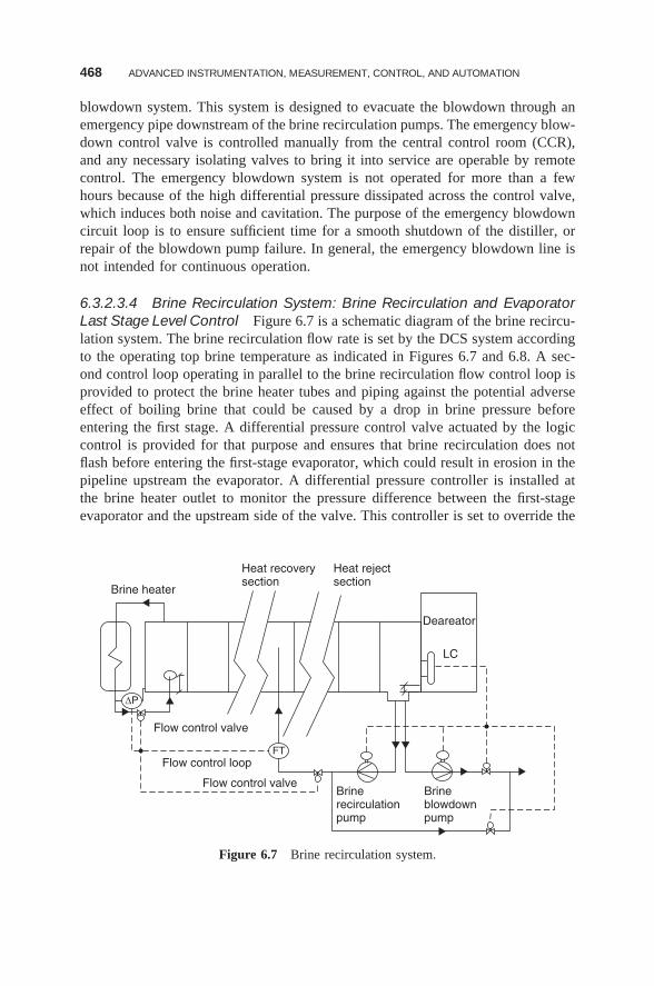
468 ADVANCED INSTRUMENTATION, MEASUREMENT, CONTROL, AND AUTOMATION

blowdown system. This system is designed to evacuate the blowdown through anemergency pipe downstream of the brine recirculation pumps. The emergency blow-down control valve is controlled manually from the central control room (CCR),and any necessary isolating valves to bring it into service are operable by remotecontrol. The emergency blowdown system is not operated for more than a fewhours because of the high differential pressure dissipated across the control valve,which induces both noise and cavitation. The purpose of the emergency blowdowncircuit loop is to ensure sufficient time for a smooth shutdown of the distiller, orrepair of the blowdown pump failure. In general, the emergency blowdown line isnot intended for continuous operation.

6.3.2.3.4 Brine Recirculation System: Brine Recirculation and EvaporatorLast Stage Level Control Figure 6.7 is a schematic diagram of the brine recircu-lation system. The brine recirculation flow rate is set by the DCS system accordingto the operating top brine temperature as indicated in Figures 6.7 and 6.8. A sec-ond control loop operating in parallel to the brine recirculation flow control loop isprovided to protect the brine heater tubes and piping against the potential adverseeffect of boiling brine that could be caused by a drop in brine pressure beforeentering the first stage. A differential pressure control valve actuated by the logiccontrol is provided for that purpose and ensures that brine recirculation does notflash before entering the first-stage evaporator, which could result in erosion in thepipeline upstream the evaporator. A differential pressure controller is installed atthe brine heater outlet to monitor the pressure difference between the first-stageevaporator and the upstream side of the valve. This controller is set to override the

Brine heater

Flow control valve

Flow control loop

Flow control valveBrinerecirculationpump

Brineblowdownpump

Heat recoverysection

Heat rejectsection

Deareator

LC

ΔP

FT

Figure 6.7 Brine recirculation system.

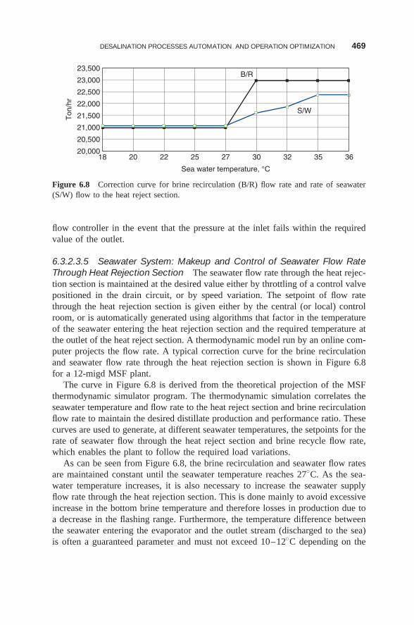
DESALINATION PROCESSES AUTOMATION AND OPERATION OPTIMIZATION 469

Ton

/hr

23,500

23,000

22,500

22,000

21,500

21,000

20,500

20,00018 20 22 25 27

B/R

S/W

Sea water temperature, °C

30 32 35 36

Figure 6.8 Correction curve for brine recirculation (B/R) flow rate and rate of seawater(S/W) flow to the heat reject section.

flow controller in the event that the pressure at the inlet fails within the requiredvalue of the outlet.

6.3.2.3.5 Seawater System: Makeup and Control of Seawater Flow RateThrough Heat Rejection Section The seawater flow rate through the heat rejec-tion section is maintained at the desired value either by throttling of a control valvepositioned in the drain circuit, or by speed variation. The setpoint of flow ratethrough the heat rejection section is given either by the central (or local) controlroom, or is automatically generated using algorithms that factor in the temperatureof the seawater entering the heat rejection section and the required temperature atthe outlet of the heat reject section. A thermodynamic model run by an online com-puter projects the flow rate. A typical correction curve for the brine recirculationand seawater flow rate through the heat rejection section is shown in Figure 6.8for a 12-migd MSF plant.

The curve in Figure 6.8 is derived from the theoretical projection of the MSFthermodynamic simulator program. The thermodynamic simulation correlates theseawater temperature and flow rate to the heat reject section and brine recirculationflow rate to maintain the desired distillate production and performance ratio. Thesecurves are used to generate, at different seawater temperatures, the setpoints for therate of seawater flow through the heat reject section and brine recycle flow rate,which enables the plant to follow the required load variations.

As can be seen from Figure 6.8, the brine recirculation and seawater flow ratesare maintained constant until the seawater temperature reaches 27◦C. As the sea-water temperature increases, it is also necessary to increase the seawater supplyflow rate through the heat rejection section. This is done mainly to avoid excessiveincrease in the bottom brine temperature and therefore losses in production due toa decrease in the flashing range. Furthermore, the temperature difference betweenthe seawater entering the evaporator and the outlet stream (discharged to the sea)is often a guaranteed parameter and must not exceed 10–12◦C depending on the

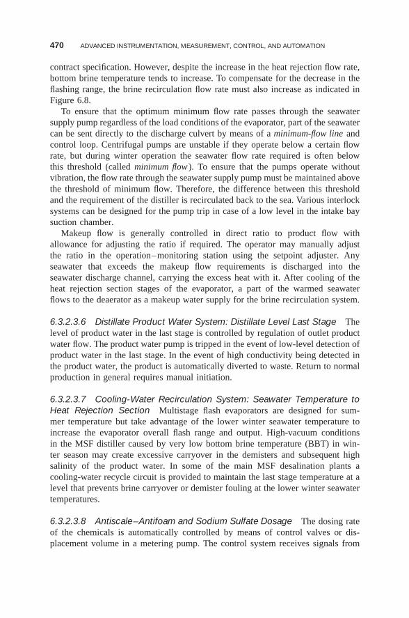
470 ADVANCED INSTRUMENTATION, MEASUREMENT, CONTROL, AND AUTOMATION

contract specification. However, despite the increase in the heat rejection flow rate,bottom brine temperature tends to increase. To compensate for the decrease in theflashing range, the brine recirculation flow rate must also increase as indicated inFigure 6.8.

To ensure that the optimum minimum flow rate passes through the seawatersupply pump regardless of the load conditions of the evaporator, part of the seawatercan be sent directly to the discharge culvert by means of a minimum-flow line andcontrol loop. Centrifugal pumps are unstable if they operate below a certain flowrate, but during winter operation the seawater flow rate required is often belowthis threshold (called minimum flow ). To ensure that the pumps operate withoutvibration, the flow rate through the seawater supply pump must be maintained abovethe threshold of minimum flow. Therefore, the difference between this thresholdand the requirement of the distiller is recirculated back to the sea. Various interlocksystems can be designed for the pump trip in case of a low level in the intake baysuction chamber.

Makeup flow is generally controlled in direct ratio to product flow withallowance for adjusting the ratio if required. The operator may manually adjustthe ratio in the operation–monitoring station using the setpoint adjuster. Anyseawater that exceeds the makeup flow requirements is discharged into theseawater discharge channel, carrying the excess heat with it. After cooling of theheat rejection section stages of the evaporator, a part of the warmed seawaterflows to the deaerator as a makeup water supply for the brine recirculation system.

6.3.2.3.6 Distillate Product Water System: Distillate Level Last Stage Thelevel of product water in the last stage is controlled by regulation of outlet productwater flow. The product water pump is tripped in the event of low-level detection ofproduct water in the last stage. In the event of high conductivity being detected inthe product water, the product is automatically diverted to waste. Return to normalproduction in general requires manual initiation.

6.3.2.3.7 Cooling-Water Recirculation System: Seawater Temperature toHeat Rejection Section Multistage flash evaporators are designed for sum-mer temperature but take advantage of the lower winter seawater temperature toincrease the evaporator overall flash range and output. High-vacuum conditionsin the MSF distiller caused by very low bottom brine temperature (BBT) in win-ter season may create excessive carryover in the demisters and subsequent highsalinity of the product water. In some of the main MSF desalination plants acooling-water recycle circuit is provided to maintain the last stage temperature at alevel that prevents brine carryover or demister fouling at the lower winter seawatertemperatures.

6.3.2.3.8 Antiscale–Antifoam and Sodium Sulfate Dosage The dosing rateof the chemicals is automatically controlled by means of control valves or dis-placement volume in a metering pump. The control system receives signals from

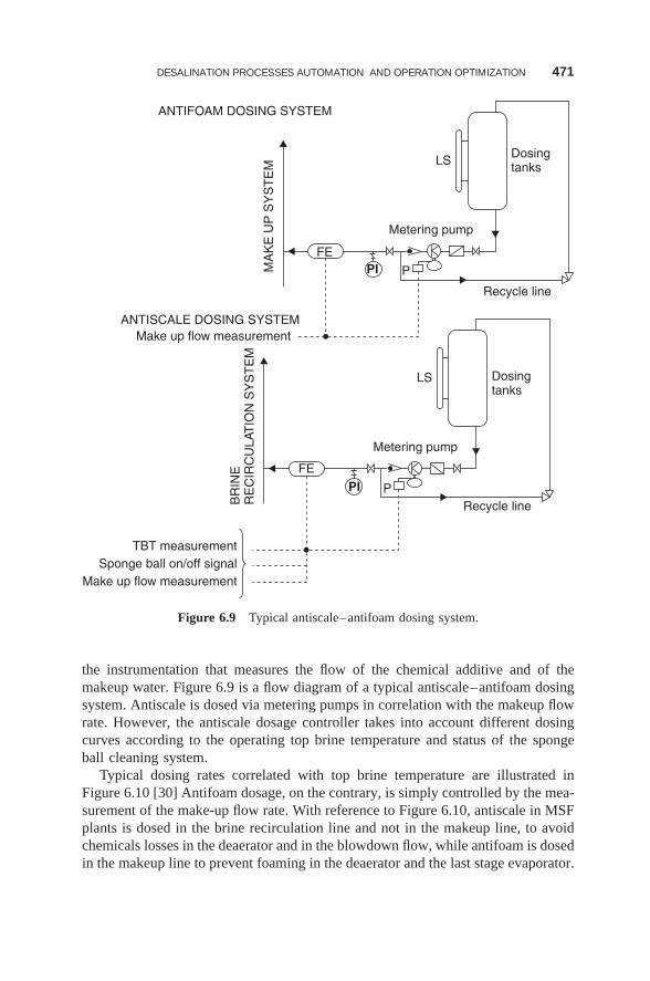
DESALINATION PROCESSES AUTOMATION AND OPERATION OPTIMIZATION 471

ANTIFOAM DOSING SYSTEM

ANTISCALE DOSING SYSTEMMake up flow measurement

LS

LS

FE

FE

P

P

PI

PI

Metering pump

Metering pump

Dosingtanks

Dosingtanks

Recycle line

Recycle line

TBT measurementSponge ball on/off signal

Make up flow measurement

MA

KE

UP

SY

ST

EM

BR

INE

RE

CIR

CU

LAT

ION

SY

ST

EM

Figure 6.9 Typical antiscale–antifoam dosing system.

the instrumentation that measures the flow of the chemical additive and of themakeup water. Figure 6.9 is a flow diagram of a typical antiscale–antifoam dosingsystem. Antiscale is dosed via metering pumps in correlation with the makeup flowrate. However, the antiscale dosage controller takes into account different dosingcurves according to the operating top brine temperature and status of the spongeball cleaning system.

Typical dosing rates correlated with top brine temperature are illustrated inFigure 6.10 [30] Antifoam dosage, on the contrary, is simply controlled by the mea-surement of the make-up flow rate. With reference to Figure 6.10, antiscale in MSFplants is dosed in the brine recirculation line and not in the makeup line, to avoidchemicals losses in the deaerator and in the blowdown flow, while antifoam is dosedin the makeup line to prevent foaming in the deaerator and the last stage evaporator.

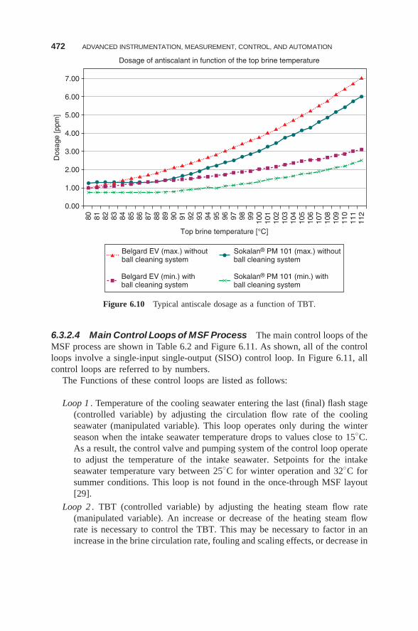
472 ADVANCED INSTRUMENTATION, MEASUREMENT, CONTROL, AND AUTOMATION

7.00

Dos

age

[ppm

]Dosage of antiscalant in function of the top brine temperature

6.00

5.00

4.00

3.00

2.00

1.00

0.00

80 81 82 83 84 85 86 87 88 89 90 91 92 93 94 95

Top brine temperature [°C]96 97 98 99 10

010

110

210

310

410

510

610

710

810

911

011

111

2

Belgard EV (max.) withoutball cleaning system

Belgard EV (min.) withball cleaning system

Sokalan® PM 101 (max.) withoutball cleaning system

Sokalan® PM 101 (min.) withball cleaning system

Figure 6.10 Typical antiscale dosage as a function of TBT.

6.3.2.4 Main Control Loops of MSF Process The main control loops of theMSF process are shown in Table 6.2 and Figure 6.11. As shown, all of the controlloops involve a single-input single-output (SISO) control loop. In Figure 6.11, allcontrol loops are referred to by numbers.

The Functions of these control loops are listed as follows:

Loop 1 . Temperature of the cooling seawater entering the last (final) flash stage(controlled variable) by adjusting the circulation flow rate of the coolingseawater (manipulated variable). This loop operates only during the winterseason when the intake seawater temperature drops to values close to 15◦C.As a result, the control valve and pumping system of the control loop operateto adjust the temperature of the intake seawater. Setpoints for the intakeseawater temperature vary between 25◦C for winter operation and 32◦C forsummer conditions. This loop is not found in the once-through MSF layout[29].

Loop 2 . TBT (controlled variable) by adjusting the heating steam flow rate(manipulated variable). An increase or decrease of the heating steam flowrate is necessary to control the TBT. This may be necessary to factor in anincrease in the brine circulation rate, fouling and scaling effects, or decrease in

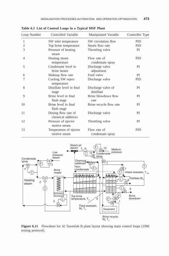
DESALINATION PROCESSES AUTOMATION AND OPERATION OPTIMIZATION 473

Table 6.2 List of Control Loops in a Typical MSF Plant

Loop Number Controlled Variable Manipulated Variable Controller Type

1 SW inlet temperature SW circulation flow PID2 Top brine temperature Steam flow rate PID3 Pressure of heating

steamThrottling valve PI

4 Heating steamtemperature

Flow rate ofcondensate spray

PID

5 Condensate level inbrine heater

Discharge valveadjustment

PI

6 Makeup flow rate Feed valve PI7 Cooling SW reject

temperatureDischarge valve PID

8 Distillate level in finalstage

Discharge valve ofdistillate

PI

9 Brine level in finalflash stage

Brine blowdown flowrate

PI

10 Brine level in finalflash stage

Brine recycle flow rate PI

11 Dosing flow rate ofchemical additives

Discharge valve PI

12 Pressure of ejectormotive steam

Throttling valve PI

13 Temperature of ejectormotive steam

Flow rate ofcondensate spray

PID

Condensatespray

Lowpressuresteam

ChemicaladditivesNon-condensate

Condensatespray

Mediumpressure

12

13

11 7

1

8

9

16

5

2

4

3

Brineblowdown

Brine recycle,Mf, Tn

Feed seawater,Mf, Tn

Top brinetemperature, To

Deaerator

Distillate Md

Steam jetejector Tc, Pc

Brineheater

Heatingsteam

T

F

T

L

L

F

T

F

F

T

L

F

T Intake seawater, T cw

Figure 6.11 Flowsheet for Al Taweelah B plant layout showing main control loops (1996testing protocol).

474 ADVANCED INSTRUMENTATION, MEASUREMENT, CONTROL, AND AUTOMATION

the temperature of the brine circulation. The setpoint for the TBT depends onthe type of antiscalant used in the plant where 90◦C is suitable for a polyphos-phate type and the temperature range 100–110◦C is used for polymer-typeadditives.

Loop 3 . Pressure of the heating steam (controlled variable) and adjustment of thethrottling valve (manipulated variable). Commonly, the low pressure steamhas a pressure of 4–7 bar, and it is necessary to reduce the pressure to avalue of ∼2 bar, where it becomes superheated with a temperature close to170◦C.

Loop 4 . Temperature of the heating steam (controlled variable) by adjusting theflow rate of the condensate spray (manipulated variable). This loop changesthe steam quality from superheated to saturated, where its temperature dropsfrom 170◦C to 100–110◦C. The steam temperature is controlled to be higherthan the TBT by 5–10◦C. This is necessary to prevent the formation ofhotspots and scale formation.

Loop 5 . Condensate level in the brine heater (controlled variable) and open-ing of the distillate discharge valve (manipulated variable). It is necessary tomaintain a sufficient static head above the condensate pump to prevent con-densate flashing within the discharge line or the pumping unit, which wouldresult in violent vibrations, loosening of various connections, and severeerosion.

Loop 6 . The flow rate of the makeup seawater entering the last stage (controlledvariable) by adjusting the valve opening on the feedline (manipulated vari-able). The set-point for this control is adjusted according to the flow rate ratioof distillate and brine blowdown. This control loop maintains a constant con-version ratio (defined as the ratio between distillate and make-up flow rates),which is necessary to keep the salinity of the brine blowdown from the laststage at a design constant value of ∼70,000 ppm. In the Gulf, the intakeseawater salinity varies between 42,000–48,000 ppm and accordingly, theconversion ratio varies between 0.4 and 0.314. This sets the controller ratio(ratio of distillate and blowdown) at 0.46–0.67, measured as kg distillate per1 kg brine blowdown.

Loop 7 . Temperature of the reject flow rate of the cooling seawater (con-trolled variable) by adjusting the opening of the discharge valve (manipulatedvariable). The set-point of the controller is made in reference to the tem-perature of the last flash stage. For a constant plant capacity, an increasein the final-stage temperature results in a reduction in the flashing rangeand a consequent decrease in performance ratio. The final-stage tempera-ture is normally set at ∼40◦C for summer operation and 32◦C for winteroperation.

Loop 8 . Distillate level in the last stage (controlled variable) by adjusting thedistillate product flow rate (manipulated variable). This control loop has a

DESALINATION PROCESSES AUTOMATION AND OPERATION OPTIMIZATION 475

function similar to that of the level controller of the heating steam condensatewhere a decrease of the distillate product static head would cause operationalproblems in the associated pumping unit.

Loop 9 . Brine level in the last flash stage (controlled variable) by adjusting thebrine blowdown flow rate (manipulated variable). This is one of the mostimportant control loops in the MSF plant since the level in the last stageaffects the levels in the previous stages. Simultaneously, the flashing effi-ciency is affected in various stages as well as the amount of distillate product.The increase of brine level reduces the flashing rates as well as the amount ofdistillate product; consequently, the amount of heat released on condensationof the distillate vapor becomes lower. Eventually, the temperature of thebrine recycle stream entering the brine heater decreases, which results in anincrease of the amount of heating steam and reduction in the system perfor-mance ratio. However, reduction of the brine level may result in blowthroughof the flashed-off vapors across the stages, thus resulting in a reductionof the effective number of stages and a decrease in plant performanceratio.

Loop 10 . Brine level in the last flash stage (controlled variable) by adjustingthe brine recycle flow rate (manipulated variable). Function and effectson system performance for thus control loop are similar to those ofloop 9.

Loop 11 . Dosing flow rate of the chemical additives (controlled variable)by adjusting the opening of the discharge valve of the chemical additive(manipulated variable). Variations in the brine circulation flow ratenecessitate adjustment of the dosing rate of the chemical additives. Suchvariations are caused by adjustments in the flow rate of the brine circulationstream, which might be necessary to adjust the brine level in the last flashingstage.

Loop 12 . Pressure of the ejector motive steam (controlled variable) and the open-ing of the throttling valve (manipulated variable). Commonly, the medium-pressure steam has a pressure of 16 bar and it is necessary to reduce its valueto 7 bar.

Loop 13 . Temperature of the ejector motive steam (controlled variable) byadjusting the flow rate of the condensate spray (manipulated variable). Thisloop reduces the ejector motive steam temperature from ∼201◦C to 165◦Cby spraying with steam condensate.

6.3.2.5 Identification of Major Process Parameters in MSF6.3.2.5.1 Introduction In this section we will attempt to identify the majorprocess parameters, which need to be measured for process automation of the MSFprocess. Table 6.3 represents the state of the art in a typical modern installation,typically an MSF crossflow plant with flow recirculation, where instrumentation

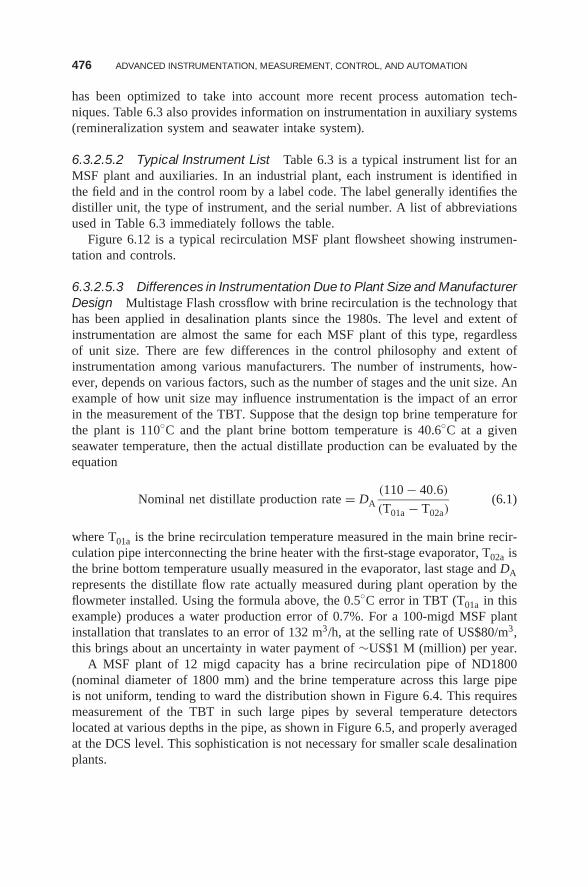
476 ADVANCED INSTRUMENTATION, MEASUREMENT, CONTROL, AND AUTOMATION

has been optimized to take into account more recent process automation tech-niques. Table 6.3 also provides information on instrumentation in auxiliary systems(remineralization system and seawater intake system).

6.3.2.5.2 Typical Instrument List Table 6.3 is a typical instrument list for anMSF plant and auxiliaries. In an industrial plant, each instrument is identified inthe field and in the control room by a label code. The label generally identifies thedistiller unit, the type of instrument, and the serial number. A list of abbreviationsused in Table 6.3 immediately follows the table.

Figure 6.12 is a typical recirculation MSF plant flowsheet showing instrumen-tation and controls.

6.3.2.5.3 Differences in Instrumentation Due to Plant Size and ManufacturerDesign Multistage Flash crossflow with brine recirculation is the technology thathas been applied in desalination plants since the 1980s. The level and extent ofinstrumentation are almost the same for each MSF plant of this type, regardlessof unit size. There are few differences in the control philosophy and extent ofinstrumentation among various manufacturers. The number of instruments, how-ever, depends on various factors, such as the number of stages and the unit size. Anexample of how unit size may influence instrumentation is the impact of an errorin the measurement of the TBT. Suppose that the design top brine temperature forthe plant is 110◦C and the plant brine bottom temperature is 40.6◦C at a givenseawater temperature, then the actual distillate production can be evaluated by theequation

Nominal net distillate production rate = DA(110 − 40.6)

(T01a − T02a)(6.1)

where T01a is the brine recirculation temperature measured in the main brine recir-culation pipe interconnecting the brine heater with the first-stage evaporator, T02a isthe brine bottom temperature usually measured in the evaporator, last stage and DArepresents the distillate flow rate actually measured during plant operation by theflowmeter installed. Using the formula above, the 0.5◦C error in TBT (T01a in thisexample) produces a water production error of 0.7%. For a 100-migd MSF plantinstallation that translates to an error of 132 m3/h, at the selling rate of US$80/m3,this brings about an uncertainty in water payment of ∼US$1 M (million) per year.

A MSF plant of 12 migd capacity has a brine recirculation pipe of ND1800(nominal diameter of 1800 mm) and the brine temperature across this large pipeis not uniform, tending to ward the distribution shown in Figure 6.4. This requiresmeasurement of the TBT in such large pipes by several temperature detectorslocated at various depths in the pipe, as shown in Figure 6.5, and properly averagedat the DCS level. This sophistication is not necessary for smaller scale desalinationplants.

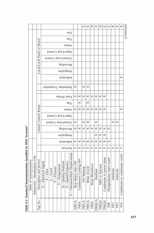
Tabl

e6.

3St

anda

rdIn

stru

men

tati

onIn

stal

led

inM

SFSy

stem

sa

Tabl

eof

Inst

rum

enta

tion

Subs

ectio

n:

Des

alin

atio

nU

nit

Tag

No.

Des

crip

tion

and

Serv

ice

Cen

tral

Con

trol

Roo

mL

ocal

/Loc

alPa

nel

orB

oard

E—

Ele

ctri

cal

Sign

al

Services

Indication

Integration

Recording

Closed-loopControl

Open-LoopControl

Alarm

Trip

FaultPrinter

RedundantTransmitter

Indication

Integration

Recording

Closed-LoopControl

Open-LoopControl

Alarm

Trip

Test

F—

Flow

L—

Lev

elP

—Pr

essu

reT

—Te

mpe

ratu

reQ

—Q

ualit

y/A

naly

sis

S—

Spee

d/Fr

eque

ncy

Y—

Vib

ratio

n/Sh

aft

Dis

plac

emen

tFI

RC

AH

eat

Rej

ect

inle

tSW

FX

XX

XX

XFI

RA

Con

dens

ers

Coo

ling

SWF

XX

XX

XFI

RC

ASW

Mak

eup

FX

XX

XX

XE

FIR

CA

Bri

nere

cycl

eF

XX

XX

XX

XE

FIR

AB

rine

Blo

wdo

wn

FX

XX

XD

FIR

QC

AD

istil

late

FX

XX

XX

XE

FIR

QA

MPS

toE

ject

ors

FX

XX

XX

DFI

RQ

AC

onde

nsat

eto

pow

erpl

ant

FX

XX

XX

EFI

RD

esup

erhe

ater

inje

ctw

ater

FX

XE

FFC

Ant

ifoa

mF

XR

FFC

Ant

isca

leF

XE

FIA

Con

dens

ate

toco

nden

sate

cool

erF

XX

R(c

onti

nued

)

477

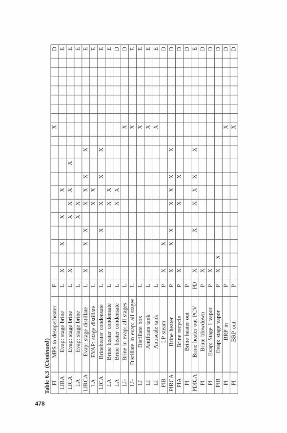
Tabl

e6.

3(C

ontin

ued

)FI

MPS

tode

supe

rhea

ter

FX

DL

IRA

Eva

p:st

age

brin

eL

XX

XX

EL

ICA

Eva

p:st

age

brin

eL

XX

XX

XE

LA

Eva

p:st

age

brin

eL

XX

EL

IRC

AE

vap:

stag

edi

still

ate

LX

XX

XX

XX

EL

AE

VA

P:st

age

dist

illat

eL

XX

EL

ICA

Bri

nehe

ater

cond

ensa

teL

XX

XX

XE

LA

Bri

nehe

ater

cond

ensa

teL

XX

EL

AB

rine

heat

erco

nden

sate

LX

XD

LI-

Bri

nein

evap

:al

lst

ages

LX

DL

I-D

istil

late

inev

ap:

all

stag

esL

XE

LI

Dis

tilla

tebo

xL

XE

LI

Ant

ifoa

mta

nkL

XE

LI

Ant

isca

leta

nkL

XE

PIR

LP

stea

mP

XX

DPI

RC

AB

rine

heat

erP

XX

XX

XX

XD

PIA

Bri

nere

cycl

eP

XX

XD

PIB

rine

heat

erou

tP

DPD

ICA

Bri

nehe

ater

out

PCV

PDX

XX

XX

XE

PIB

rine

blow

dow

nP

XD

PIE

vap:

Stag

e1

vapo

rP

XD

PIR

Eva

p:st

age

vapo

rP

XX

DPI

BR

Pin

PX

DPI

BR

Pou

tP

XD

478

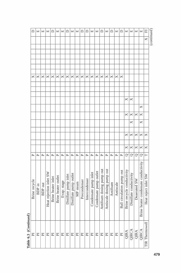
Tabl

e6.

3(C

ontin

ued

)PI

Bri

nere

cycl

eP

XD

PIB

DP

inP

XE

PIB

DP

out

PX

EPI

Hea

tre

ject

ion

inle

tSW

PX

EPI

Bri

nehe

ater

inle

tP

XD

PIB

rine

heat

erou

tlet

PX

EPI

Eva

p:st

age

PX

EPI

Dis

tilla

tepu

mp

inle

tP

XD

PID

istil

late

pum

pou

tlet

PX

EPI

MP

stea

mP

XE

PIPr

econ

dens

erP

XD

PIIn

terc

onde

nser

PX

DPI

Con

dens

ate

pum

pin

let

PX

EPI

Con

dens

ate

pum

pou

tlet

PX

EPI

Ant

ifoa

mdo

sing

pum

pou

tP

XD

PIA

ntis

cale

dosi

ngpu

mp

out

PX

EPI

Ant

ifoa

mP

XD

PIA

ntis

cale

PX

EPI

Bal

lci

rcul

atio

npu

mp

out

PX

DQ

IRA

Bri

nere

cycl

eco

nduc

tivity

QX

XX

XE

QIR

CA

Dis

tilla

teco

nduc

tivity

QX

XX

XX

EQ

IRA

Dea

erat

edSW

QX

XX

EQ

IRC

AB

rine

heat

erco

nden

sate

cond

uctiv

ityQ

XX

XX

XE

TIR

The

rmow

ell

Hea

tre

ject

inle

tSW

TX

XX

FI(c

onti

nued

)

479

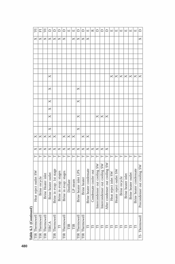
Tabl

e6.

3(C

ontin

ued

)T

IRT

herm

owel

lH

eat

reje

ctou

tlet

SWT

XX

X′ F

IT

IRT

herm

owel

lB

rine

recy

cle

TX

XX

FIT

IRT

herm

owel

lB

rine

Hea

ter

inle

tT

XX

X′ F

IT

IRC

AB

rine

heat

erou

tlet

TX

XX

XX

XX

XX

DT

IRT

herm

owel

lB

rine

inev

ap:

1st

stag

eT

XX

XD

TI

Bri

nein

evap

:st

ages

TX

XD

TIR

The

rmow

ell

Bri

nein

evap

:st

ages

TX

XX

DT

IRD

istil

late

TX

XE

TIR

LP

stea

mT

XX

XE

TIR

The

rmow

ell

Bri

nehe

ater

inle

tL

PST

XX

XX

XX

DT

IRT

herm

owel

lB

rine

heat

erT

XX

XD

TI

Bri

nehe

ater

cond

ensa

teT

XX

XE

TI

Con

dens

ate

cool

erou

tT

XR

TI

Inte

rcon

dens

erou

tco

olin

gSW

TX

XD

TI

Inte

rcon

dens

erou

tco

olin

gSW

TX

XD

TI

Aft

erco

nden

ser

out

cool

ing

SWT

XX

DT

IH

eat

reje

ctin

let

SWT

XE

TI

Hea

ter

reje

ctou

tlet

SWT

XE

TI

Bri

nere

cycl

eT

XE

TI

Bri

nehe

ater

inle

tT

XE

TI

Bri

nehe

ater

outle

tT

XE

TI

Bri

nehe

ater

cond

ensa

teT

XE

TI-

The

rmow

ell

Prec

onde

nser

out

cool

ing

SWT

XX

D

480

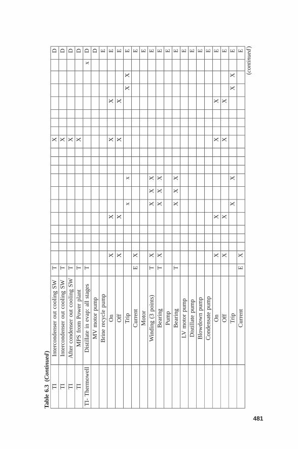
Tabl

e6.

3(C

ontin

ued

)T

IIn

terc

onde

nser

out

cool

ing

SWT

XD

TI

Inte

rcon

dens

erou

tco

olin

gSW

TX

DT

IA

fter

cond

ense

rou

tco

olin

gSW

TX

DT

IM

PSfr

omPo

wer

plan

tT

XD

TI-

The

rmow

ell

Dis

tilla

tein

evap

:al

lst

ages

Tx

DM

Vm

otor

pum

pD

Bri

nere

cycl

epu

mp

EO

nX

XX

XE

Off

XX

XX

ET

rip

xx

XX

EC

urre

ntE

XE

Mot

orE

Win

ding

(3po

ints

)T

XX

XX

EB

eari

ngT

XX

XX

EPu

mp

EB

eari

ngT

XX

XE

LVm

otor

pum

pE

Dis

tilla

tepu

mp

EB

low

dow

npu

mp

EC

onde

nsat

epu

mp

EO

nX

XX

XE

Off

XX

XX

ET

rip

XX

XX

EC

urre

ntE

XE

(con

tinu

ed)

481

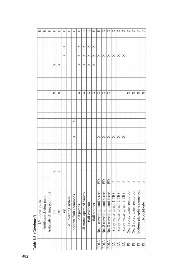
Tabl

e6.

3(C

ontin

ued

)LV

mot

orpu

mp

EA

ntif

oam

dosi

ngpu

mp

EA

ntis

cale

dosi

ngpu

mp

out

EO

nX

XX

EO

ffX

XX

ET

rip

XX

EB

all

clea

ning

syst

emE

Syst

emfa

ult

(com

mon

)X

XE

All

pum

psX

XX

XE

All

mot

orop

erat

edva

lves

XX

XX

DB

all

colle

ctor

XX

XX

DB

all

stra

iner

XX

XX

EPD

IAN

o.1

trav

ellin

gba

ndsc

reen

PDX

XX

EPD

IAN

o.2

trav

ellin

gba

ndsc

reen

PDX

XX

DPD

IAN

o.3

trav

ellin

gba

ndsc

reen

PDX

XX

DPA

Spra

yw

ater

tono

.1

TB

SP

XX

DPA

Spra

yw

ater

tono

.2

TB

SP

XX

DPA

Spra

yw

ater

tono

.3

TB

SP

XX

DPI

No.

1sp

ray

wat

erpu

mp

out

PX

DPI

No.

2sp

ray

wat

erpu

mp

out

PX

DPI

Sodi

umph

osph

ate

pum

pou

tP

XD

PIH

ypoc

hlor

iteP

XD

482

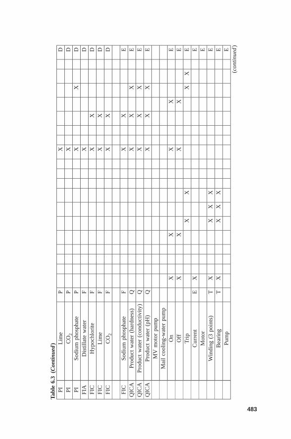
Tabl

e6.

3(C

ontin

ued

)PI

Lim

eP

XD

PIC

O2

PX

DPI

Sodi

umph

osph

ate

PX

XD

FIA

Dis

tilla

tew

ater

FX

DFI

CH

ypoc

hlor

iteF

XX

DFI

CL

ime

FX

XD

FIC

CO

2F

XX

D

FIC

Sodi

umph

osph

ate

FX

XE

QIC

APr

oduc

tw

ater

(har

dnes

s)Q

XX

XE

QIC

APr

oduc

tw

ater

(con

duct

ivity

)Q

XX

XE

QIC

APr

oduc

tw

ater

(pH

)Q

XX

XE

MV

mot

orpu

mp

Mai

lco

olin

g-w

ater

pum

pO

nX

XX

XE

Off

XX

XX

ET

rip

XX

XX

EC

urre

ntE

XE

Mot

orE

Win

ding

(3po

ints

)T

XX

XX

EB

eari

ngT

XX

XX

EPu

mp

E(c

onti

nued

)

483

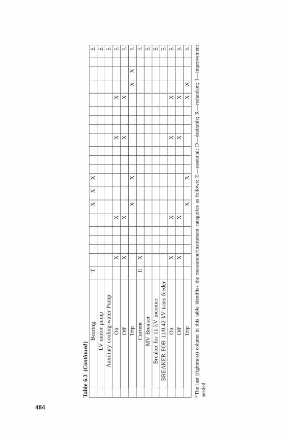
Tabl

e6.

3(C

ontin

ued

) Bea

ring

TX

XX

ELV

mot

orpu

mp

EA

uxili

ary

cool

ing-

wat

erPu

mp

EO

nX

XX

XE

Off

XX

XX

ET

rip

XX

XX

EC

urre

ntE

XE

MV

Bre

aker

EB

reak

erfo

r11

-kV

inco

mer

EB

RE

AK

ER

FOR

11/0

.42-

kVtr

ans

feed

erE

On

XX

XX

EO

ffX

XX

XE

Tri

pX

XX

XE

aT

hela

st(r

ight

mos

t)co

lum

nin

this

tabl

eid

entifi

esth

em

easu

rand

/inst

rum

ent

cate

gori

esas

follo

ws:

E—

esse

ntia

l;D

—de

sira

ble;

R—

redu

ndan

t;I—

impr

ovem

ent

need

ed.

484

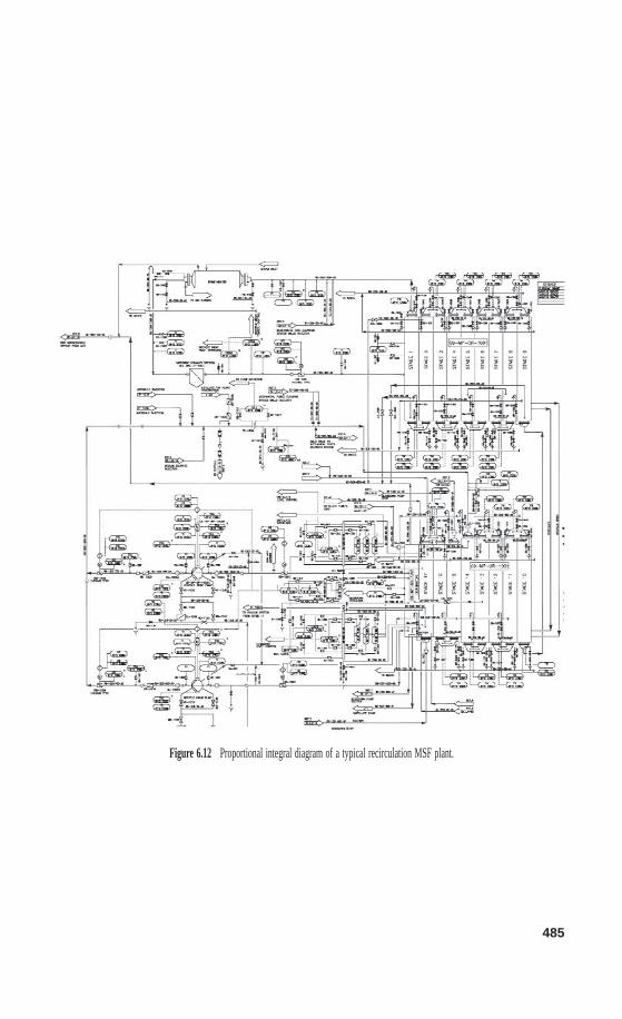
485

Figure 6.12 Proportional integral diagram of a typical recirculation MSF plant.

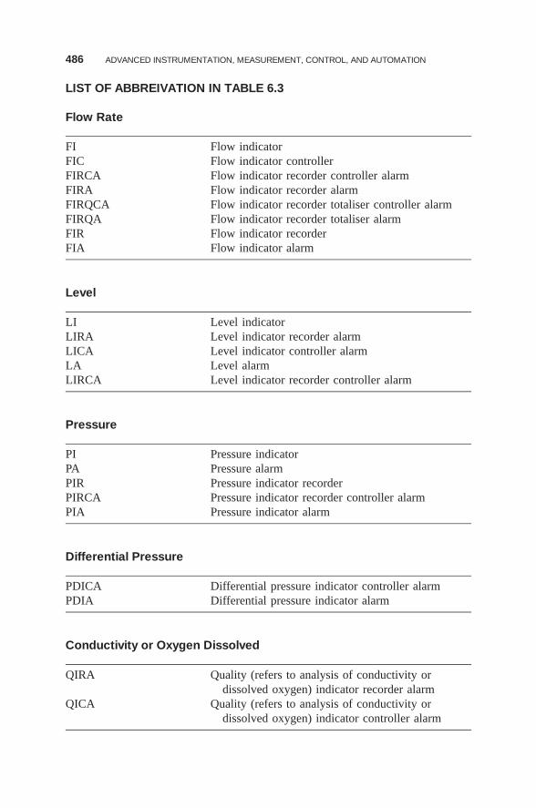
486 ADVANCED INSTRUMENTATION, MEASUREMENT, CONTROL, AND AUTOMATION

LIST OF ABBREIVATION IN TABLE 6.3

Flow Rate

FI Flow indicatorFIC Flow indicator controllerFIRCA Flow indicator recorder controller alarmFIRA Flow indicator recorder alarmFIRQCA Flow indicator recorder totaliser controller alarmFIRQA Flow indicator recorder totaliser alarmFIR Flow indicator recorderFIA Flow indicator alarm

Level

LI Level indicatorLIRA Level indicator recorder alarmLICA Level indicator controller alarmLA Level alarmLIRCA Level indicator recorder controller alarm

Pressure

PI Pressure indicatorPA Pressure alarmPIR Pressure indicator recorderPIRCA Pressure indicator recorder controller alarmPIA Pressure indicator alarm

Differential Pressure

PDICA Differential pressure indicator controller alarmPDIA Differential pressure indicator alarm

Conductivity or Oxygen Dissolved

QIRA Quality (refers to analysis of conductivity ordissolved oxygen) indicator recorder alarm

QICA Quality (refers to analysis of conductivity ordissolved oxygen) indicator controller alarm

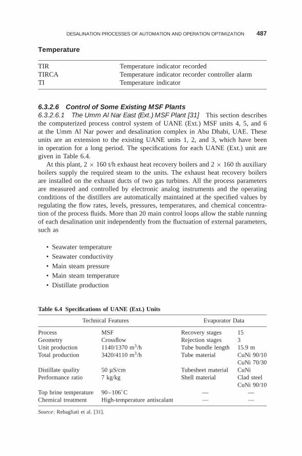
DESALINATION PROCESSES OF AUTOMATION AND OPERATION OPTIMIZATION 487

Temperature

TIR Temperature indicator recordedTIRCA Temperature indicator recorder controller alarmTI Temperature indicator

6.3.2.6 Control of Some Existing MSF Plants6.3.2.6.1 The Umm Al Nar East (Ext.) MSF Plant [31] This section describesthe computerized process control system of UANE (Ext.) MSF units 4, 5, and 6at the Umm Al Nar power and desalination complex in Abu Dhabi, UAE. Theseunits are an extension to the existing UANE units 1, 2, and 3, which have beenin operation for a long period. The specifications for each UANE (Ext.) unit aregiven in Table 6.4.

At this plant, 2 × 160 t/h exhaust heat recovery boilers and 2 × 160 th auxiliaryboilers supply the required steam to the units. The exhaust heat recovery boilersare installed on the exhaust ducts of two gas turbines. All the process parametersare measured and controlled by electronic analog instruments and the operatingconditions of the distillers are automatically maintained at the specified values byregulating the flow rates, levels, pressures, temperatures, and chemical concentra-tion of the process fluids. More than 20 main control loops allow the stable runningof each desalination unit independently from the fluctuation of external parameters,such as

• Seawater temperature

• Seawater conductivity

• Main steam pressure

• Main steam temperature

• Distillate production

Table 6.4 Specifications of UANE (Ext.) Units

Technical Features Evaporator Data

Process MSF Recovery stages 15Geometry Crossflow Rejection stages 3Unit production 1140/1370 m3/h Tube bundle length 15.9 mTotal production 3420/4110 m3/h Tube material CuNi 90/10

CuNi 70/30Distillate quality 50 μS/cm Tubesheet material CuNiPerformance ratio 7 kg/kg Shell material Clad steel

CuNi 90/10Top brine temperature 90–106◦C — —Chemical treatment High-temperature antiscalant — —

Source: Rebagliati et al. [31].

488 ADVANCED INSTRUMENTATION, MEASUREMENT, CONTROL, AND AUTOMATION

The process control system (PCS) provides supervision and control of the threeMSF desalination units: recovery and auxiliary boilers and gas turbines. It consistsof two VAX 11/750 computers operating in backup. The architecture of the PCSis shown in Figure 6.13.

The PCS is capable of performing the following functions:

• Data acquisition and validation

• Data transmission to main plant supervisor

• Supervisory control

• Event recording

• Data and event logging

• Failure analysis

• Maintenance logs

• Graphic displays of plant systems

The supervisory control function allows the processing of plant data either onlineor offline. The online supervisory program performs a running plant parameterestimation of the current values of different plant parameters (e.g., fouling factors,nonequilibrium allowance, �T across demister) using the current validated data.The mathematical simulation program is then activated, and the setpoints of allcontrolled variable are calculated for the optimal plant running condition.

The PCS allows several operational tasks to be carried out:

• Automatic distillate production change

• Automatic constant distillate production

• Plant trip analysis

The load variation is carried out automatically by changing the setpoints of the topbrine temperature and brine circulation flow (recovery section), seawater flow andseawater inlet temperature (rejection section), antiscalant dosing rate, and brineheater inlet steam temperature. The first two variables are responsible for pro-duction, and performance ratio, seawater temperature, and flow are controlled tomaintain correctly operated heat rejection sections, while the last two variables areadjusted to prevent tube fouling. When the PCS receives a request for load change,it checks for compatibility with the following constraints:

• Compatibility of type of antiscalant in use with the maximum TBT requestedby the load variation

• Available steam flow rate compatible with the maximum steam flow raterequested by the new load

• Assurance that the constraints of the brine level in the stages are within allow-able limits.

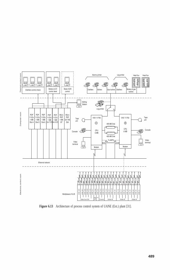
489

Distillers control check Boilers & GTcontrol desk

Boiler SCRcontrol

PDP11/23+1 MBDist 4

PDP11/23+1 MBDist 5

PDP11/23+1 MBDist 6

MicroPDP

521 KBEdit

PDP11/23+1 MB

Boil TCR

PDP11/23+1 MB

Boil SCR

MicroPDP1 MBGT

Alarms printer

UN

E #

22

UN

E #

21

UN

E #

20

UN

E #

19

UN

E #

18

UN

E #

17

UN

E #

16

UN

E #

15

UN

E #

14

UN

E #

13

UN

E #

12

UN

E #

11

UN

E #

10

UN

E #

9

UN

E #

8

UN

E #

7

UN

E #

6

UN

E #

5

UN

E #

4

UN

E #

3

UN

E #

2

UN

E #

1

Boilers Aux & EhrTempLCR

GT

Common Distiller #6 Distiller #5 Distiller #4

ModemModem

BA

VAX 11/750 VAX 11/750

CPU6 MBCPU

6 MB

Tape unit

Console

Videoterminal

Videoterminal

Console

Tapeunit

To MIPS

495 MB Disk

495 MB Disk

Log printer

Distillers Boilers Gas turbine Distillers Boilers & gasturbine

Heat flux Heat flux

Log printer

EditingStation

Therm

al contr

ol ro

om

Com

pute

r ro

om

Ele

ctr

onic

contr

ol ro

om

Multiplexers H & B

Ethernet network

Figure 6.13 Architecture of process control system of UANE (Ext.) plant [31].

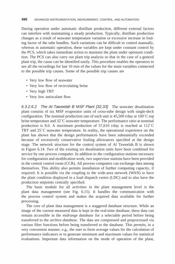
490 ADVANCED INSTRUMENTATION, MEASUREMENT, CONTROL, AND AUTOMATION

During operation under automatic distillate production, different external factorscan interfere with maintaining a steady production. Typically, distillate productionchanges as a result of seawater temperature variation or excessive increase in foul-ing factor of the tube bundles. Such variations can be difficult to control manually,whereas in automatic operation, these variables are kept under constant control bythe PCS, which takes immediate action to maintain the plant under optimum condi-tion. The PCS can also carry out plant trip analysis so that in the case of a generalplant trip, the cause can be identified easily. This procedure enables the operators tosee all the recordings for last 10 min of the values for the main variables connectedto the possible trip causes. Some of the possible trip causes are

• Very low flow of seawater

• Very low flow of recirculating brine

• Very high TBT

• Very low antiscalant flow

6.3.2.6.2 The Al-Taweelah B MSF Plant [32,33] The seawater desalinationplant consists of six MSF evaporator units of cross-tube design with single-deckconfiguration. The nominal production rate of each unit is 45,500 t/day at 100◦C topbrine temperature and 32◦C seawater temperature. The performance ratio at nominalproduction is 8.0. A maximum production of 57,610 t/day is reached at 112◦CTBT and 25◦C seawater temperature. In reality, the operational experience on theplant has shown that the design performances have been substantially exceededbecause of excessively conservative fouling allowances specified at the designstage. The network structure for the control system of Al Taweelah B is shownin Figure 6.14. Two of the existing six desalination units have been combined forservice by one process computer. In addition to the configuration stations necessaryfor configuration and modification work, two supervisor stations have been providedin the central control room (CCR). All process computers can exchange data amongthemselves. This ability also permits installation of further computing capacity, ifrequired. It is possible via the coupling to the wide-area network (WAN) to havethe plant condition displayed in a load dispatch centre (LDC) and to also have theproduction setpoints centrally specified.

The basic module for all activities in the plant management level is theplant data management (see Fig. 6.15). It handles the communication withthe process control system and makes the acquired data available for furtherprocessing.

The core of plant data management is a staggered database structure. While animage of the current measured data is kept in the real-time database, these data canremain accessible in the midrange database for a selectable period before beingtransferred to the archive database. The data are compressed and preprocessed viavarious filter functions before being transferred to the database. This permits, in avery convenient manner, e.g., the user to form average values for the calculation ofperformance indicators or to generate minimum and maximum values for statisticalevaluations. Important data information on the mode of operation of the plant,

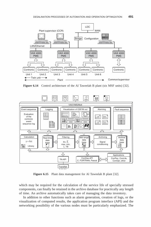
DESALINATION PROCESSES OF AUTOMATION AND OPERATION OPTIMIZATION 491

Plant supervisor (CCR)

LDC

WAN

ConfigurationBridge

LAN/Ethernet

Unit 1 Unit 2 Unit 3 Unit 4 Unit 5 Unit 6

Common/supervisorTwin unit

Plant

Contronic Contronic Contronic Contronic Contronic Contronic Contronic

VAX 4000PMS

VAX 4000PMS

VAX 4000PMS

VAX 4000PMS

Figure 6.14 Control architecture of the Al Taweelah B plant (six MSF units) [32].

LANxyColor BW

MD

Event sequence

Evaluationof the

contronicevent

sequence log

Visualization of OSF/M out

VAX/VMS/Molt

Alarming Fault sequence

Archivedatabase

ArchivingMid rangedatabase

FilteringReal-timedatabase

TN-API

TransNet

ConDas-APIC. FORTRAN, Pascal

Applications

ConPec, ConLife,ConOpt, other

Calculation

y = f(x)

Library

Signalconditioning

Logging

Xn, X,max, min,Σ, TB AD

xxxxxxx

x

x

x

xxxxxxxx

xxxx

xxxxxxx

xxxx

Figure 6.15 Plant data management for Al Taweelah B plant [32].

which may be required for the calculation of the service life of specially stressedcomponents, can finally be retained in the archive database for practically any lengthof time. An archive automatically takes care of managing the data inventory.

In addition to other functions such as alarm generation, creation of logs, or thevisualization of computed results, the application program interface (API) and thenetworking possibility of the various nodes must be particularly emphasized. The

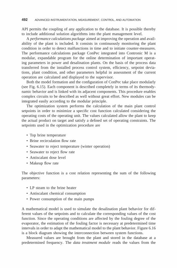
492 ADVANCED INSTRUMENTATION, MEASUREMENT, CONTROL, AND AUTOMATION

API permits the coupling of any application to the database. It is possible therebyto include additional solution algorithms into the plant management level.

A performance calculations package aimed at improving the operation and avail-ability of the plant is included. It consists in continuously monitoring the plantcondition in order to detect malfunctions in time and to initiate counter-measures.The performance calculations package ConPec integrated into Contronic M is amodular, expandable program for the online determination of important operat-ing parameters in power and desalination plants. On the basis of the process datatransferred from the installed process control system, efficiency, setpoint devia-tions, plant condition, and other parameters helpful in assessment of the currentoperation are calculated and displayed to the supervisor.

Both the model formation and the configuration of ConPec take place modularly(see Fig. 6.15). Each component is described completely in terms of its thermody-namic behavior and is linked with its adjacent components. This procedure enablescomplex circuits to be described as well without great effort. New modules can beintegrated easily according to the modular principle.

The optimization system performs the calculation of the main plant controlsetpoints in order to minimize a specific cost function calculated considering theoperating costs of the operating unit. The values calculated allow the plant to keepthe actual product on target and satisfy a defined set of operating constraints. Thesetpoints used in the optimization procedure are

• Top brine temperature

• Brine recirculation flow rate

• Seawater to reject temperature (winter operation)

• Seawater to reject flow rate

• Antiscalant dose level

• Makeup flow rate

The objective function is a cost relation representing the sum of the followingparameters:

• LP steam to the brine heater

• Antiscalant chemical consumption

• Power consumption of the main pumps

A mathematical model is used to simulate the desalination plant behavior for dif-ferent values of the setpoints and to calculate the corresponding values of the costfunction. Since the operating conditions are affected by the fouling degree of theevaporator, the estimation of the fouling factor is necessary at predetermined timeintervals in order to adapt the mathematical model to the plant behavior. Figure 6.16is a block diagram showing the interconnection between system functions.

Measured values are brought from the plant and stored in the database at apredetermined frequency. The data treatment module reads the values from the

DESALINATION PROCESSES OF AUTOMATION AND OPERATION OPTIMIZATION 493

Input fromdata base

Output to database

Data treatment

Parameterestimation

Mathematicalmodel

Optimizationsystem

r m

fk

k

s

p

t

fm

f+

–

Legend:m measured valuesf best estimates of measurementsfm true values from modelk model parametersp optimization parameters (trial values for set-points)r operator requestt targetss set-points

Figure 6.16 Block diagram showing the interconnection between system functions [32].

database and carries out validation checks in order to feed the optimization systemwith reliable values. These values are stored in the database for archiving andvisualization.

Some of the reliable values are used to check the mathematical model in order toaccount for variations in the external parameters (fouling factors). The parametersestimation module evaluates the model parameters that allow the mathematicalmodel to fit the real plant behavior. The updated model parameters are stored forarchiving and visualization.

The mathematical model is used to simulate the plant operating conditions tak-ing place for a predetermined set of input values. It is a steady-state model. Theoptimization module calculates the best set of control parameters that allow theplant to maintain the required distillate production. It uses the mathematical modelto simulate various conditions in the operating range starting from the actual oper-ating point. The calculated setpoints are stored in the database for downloading.The optimization module also operates in steady-state mode.

6.3.3 IMCA in the RO Process

6.3.3.1 General Description of the RO Process A schematic flowsheet ofthe membrane section of a typical seawater RO plant is shown in Figure 6.17a. Rawseawater is pumped from seawater intake to the pretreatment unit. At the intake,a disinfection of seawater can be conducted using chlorination in an intermittentmode, if necessary. Prior to media filters, seawater pH is adjusted to improvecoagulation. As a coagulant, ferric salts are frequently used. In some seawater sys-tems flocculation follows coagulation step. During flocculation, this lasts ∼10 min,and size of flock particles increases, improving efficiency of removal of colloidalparticles in the subsequent filtration step.

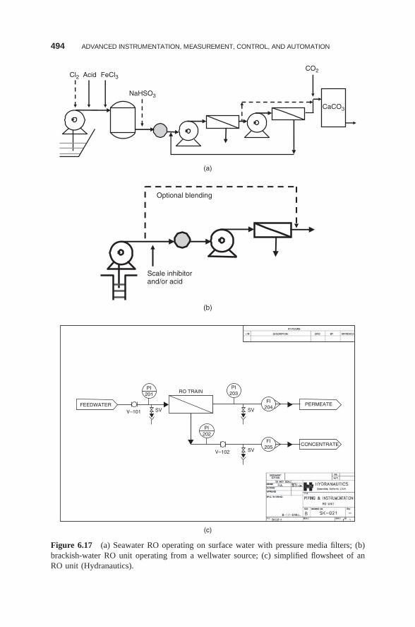
494 ADVANCED INSTRUMENTATION, MEASUREMENT, CONTROL, AND AUTOMATION

(a)

(c)

Acid FeCl3

CaCO3

CO2Cl2

NaHSO3

(b)

Scale inhibitorand/or acid

Optional blending

FEEDWATERV–101

V–102

SV SV

SV

PI201

PI203

PERMEATE

CONCENTRATE

PI202

FI204

FI205

RO TRAIN

Figure 6.17 (a) Seawater RO operating on surface water with pressure media filters; (b)brackish-water RO unit operating from a wellwater source; (c) simplified flowsheet of anRO unit (Hydranautics).

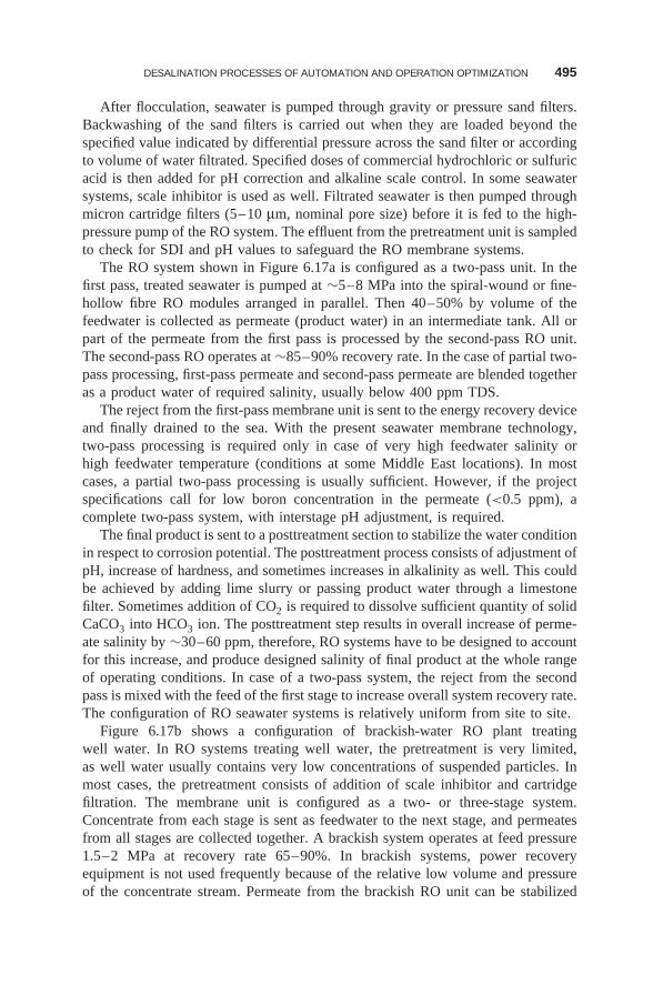
DESALINATION PROCESSES OF AUTOMATION AND OPERATION OPTIMIZATION 495

After flocculation, seawater is pumped through gravity or pressure sand filters.Backwashing of the sand filters is carried out when they are loaded beyond thespecified value indicated by differential pressure across the sand filter or accordingto volume of water filtrated. Specified doses of commercial hydrochloric or sulfuricacid is then added for pH correction and alkaline scale control. In some seawatersystems, scale inhibitor is used as well. Filtrated seawater is then pumped throughmicron cartridge filters (5–10 μm, nominal pore size) before it is fed to the high-pressure pump of the RO system. The effluent from the pretreatment unit is sampledto check for SDI and pH values to safeguard the RO membrane systems.

The RO system shown in Figure 6.17a is configured as a two-pass unit. In thefirst pass, treated seawater is pumped at ∼5–8 MPa into the spiral-wound or fine-hollow fibre RO modules arranged in parallel. Then 40–50% by volume of thefeedwater is collected as permeate (product water) in an intermediate tank. All orpart of the permeate from the first pass is processed by the second-pass RO unit.The second-pass RO operates at ∼85–90% recovery rate. In the case of partial two-pass processing, first-pass permeate and second-pass permeate are blended togetheras a product water of required salinity, usually below 400 ppm TDS.

The reject from the first-pass membrane unit is sent to the energy recovery deviceand finally drained to the sea. With the present seawater membrane technology,two-pass processing is required only in case of very high feedwater salinity orhigh feedwater temperature (conditions at some Middle East locations). In mostcases, a partial two-pass processing is usually sufficient. However, if the projectspecifications call for low boron concentration in the permeate (<0.5 ppm), acomplete two-pass system, with interstage pH adjustment, is required.

The final product is sent to a posttreatment section to stabilize the water conditionin respect to corrosion potential. The posttreatment process consists of adjustment ofpH, increase of hardness, and sometimes increases in alkalinity as well. This couldbe achieved by adding lime slurry or passing product water through a limestonefilter. Sometimes addition of CO2 is required to dissolve sufficient quantity of solidCaCO3 into HCO3 ion. The posttreatment step results in overall increase of perme-ate salinity by ∼30–60 ppm, therefore, RO systems have to be designed to accountfor this increase, and produce designed salinity of final product at the whole rangeof operating conditions. In case of a two-pass system, the reject from the secondpass is mixed with the feed of the first stage to increase overall system recovery rate.The configuration of RO seawater systems is relatively uniform from site to site.

Figure 6.17b shows a configuration of brackish-water RO plant treatingwell water. In RO systems treating well water, the pretreatment is very limited,as well water usually contains very low concentrations of suspended particles. Inmost cases, the pretreatment consists of addition of scale inhibitor and cartridgefiltration. The membrane unit is configured as a two- or three-stage system.Concentrate from each stage is sent as feedwater to the next stage, and permeatesfrom all stages are collected together. A brackish system operates at feed pressure1.5–2 MPa at recovery rate 65–90%. In brackish systems, power recoveryequipment is not used frequently because of the relative low volume and pressureof the concentrate stream. Permeate from the brackish RO unit can be stabilized

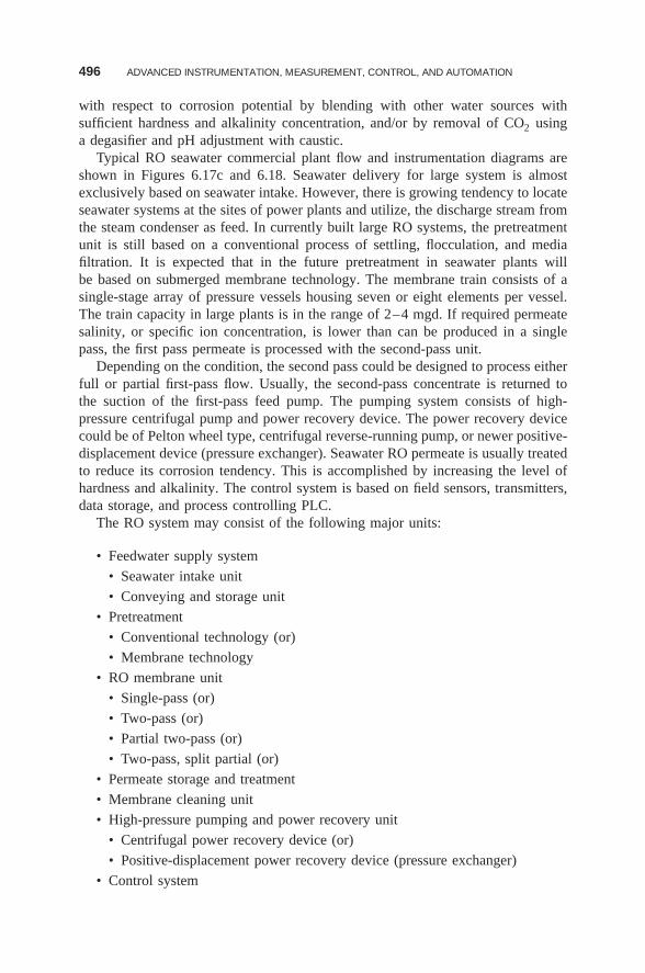
496 ADVANCED INSTRUMENTATION, MEASUREMENT, CONTROL, AND AUTOMATION

with respect to corrosion potential by blending with other water sources withsufficient hardness and alkalinity concentration, and/or by removal of CO2 usinga degasifier and pH adjustment with caustic.

Typical RO seawater commercial plant flow and instrumentation diagrams areshown in Figures 6.17c and 6.18. Seawater delivery for large system is almostexclusively based on seawater intake. However, there is growing tendency to locateseawater systems at the sites of power plants and utilize, the discharge stream fromthe steam condenser as feed. In currently built large RO systems, the pretreatmentunit is still based on a conventional process of settling, flocculation, and mediafiltration. It is expected that in the future pretreatment in seawater plants willbe based on submerged membrane technology. The membrane train consists of asingle-stage array of pressure vessels housing seven or eight elements per vessel.The train capacity in large plants is in the range of 2–4 mgd. If required permeatesalinity, or specific ion concentration, is lower than can be produced in a singlepass, the first pass permeate is processed with the second-pass unit.

Depending on the condition, the second pass could be designed to process eitherfull or partial first-pass flow. Usually, the second-pass concentrate is returned tothe suction of the first-pass feed pump. The pumping system consists of high-pressure centrifugal pump and power recovery device. The power recovery devicecould be of Pelton wheel type, centrifugal reverse-running pump, or newer positive-displacement device (pressure exchanger). Seawater RO permeate is usually treatedto reduce its corrosion tendency. This is accomplished by increasing the level ofhardness and alkalinity. The control system is based on field sensors, transmitters,data storage, and process controlling PLC.

The RO system may consist of the following major units:

• Feedwater supply system

• Seawater intake unit

• Conveying and storage unit

• Pretreatment

• Conventional technology (or)

• Membrane technology

• RO membrane unit

• Single-pass (or)

• Two-pass (or)

• Partial two-pass (or)

• Two-pass, split partial (or)

• Permeate storage and treatment

• Membrane cleaning unit

• High-pressure pumping and power recovery unit

• Centrifugal power recovery device (or)

• Positive-displacement power recovery device (pressure exchanger)

• Control system

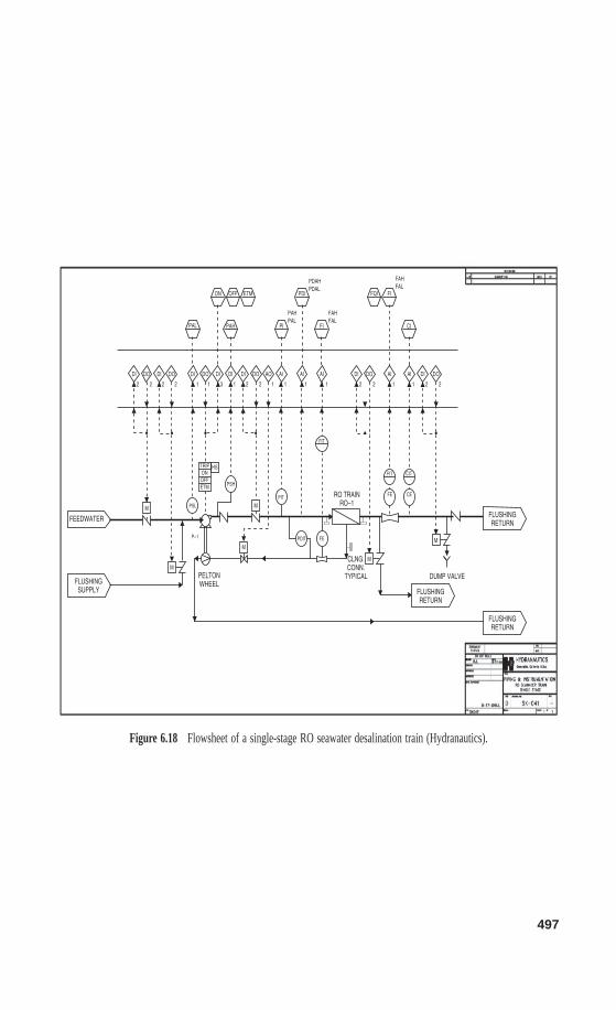
497

FEEDWATER

FLUSHINGSUPPLY FLUSHING

RETURN

DUMP VALVEPELTONWHEEL

RO TRAINRO–1

FLUSHINGRETURN

FLUSHINGRETURN

DI

2 2 2 2 1 1 3 1 2 2 1 1 1 1 2 2 211 2

DO DI DI DI DIDO DO DI DOAO AI AI AI DI DOAIDI DO

PAL PAH PI FI CI

ON OFF ETM PDI

PDAHPDAL

PAHPAL

FAHFAL

FAHFAL

FIFQI

AI

M

M

M

M

M

PSL

P–1

TRIPONOFFETM

HS

M

PSH

PIT

PDIT FE

FIT

FIT CIT

CEFE

CLNG.CONN.

TYPICAL

Figure 6.18 Flowsheet of a single-stage RO seawater desalination train (Hydranautics).

498 ADVANCED INSTRUMENTATION, MEASUREMENT, CONTROL, AND AUTOMATION

6.3.3.2 Identification of Major Process Parameters in a RO SystemThe process parameters are monitored to control performance of the plant to main-tain operating parameters within the design range and to protect the integrity ofthe equipment. The following process parameters are monitored in RO plants:

• Raw-water conductivity

• Raw-water temperature

• Raw-water flow

• Raw-water pump suction and discharged pressure

• Raw-water turbidity

• Dosing rates of pretreatment chemicals

• Raw-water free (combined) chlorine

• Media filters head loss

• Filter effluent turbidity

• Filter effluent particle count

• Filter effluent SDI (MFI)

• Cartridge filter pressure drop

• High-pressure pump suction and discharged pressure

• Feedwater pressure

• Feedwater pH

• Feedwater free (combined) chlorine

• RO permeate flow

• RO permeate pressure

• RO permeate conductivity

• RO permeate temperature

• RO permeate pH

• RO concentrate flow

• RO concentrate pressure

• Dosing rate of posttreatment chemicals

• Product-water turbidity

• Product-water free (combined) chlorine

• RO permeate storage tank level

The monitoring activity conducted to protect plant equipment includes monitoringoperating parameters of major equipment. These include setting alarms and shutoffswitches to indicate off-limit conditions of the following parameters:

Levels in water storage tanks

Levels in chemical storage tanks

Flow of treatment chemicals

Water temperature

DESALINATION PROCESSES OF AUTOMATION AND OPERATION OPTIMIZATION 499

Water pH

Water turbidity

Free (combined) chlorine concentration

Pressure drop in cartridge filters

Pump suction pressure

Pump discharged pressure

Feed pressure

Permeate pH

Permeate conductivity

Permeate temperature

Permeate pressure

Concentrate flow

Concentrate pressure

Pressure drop in RO system

Temperature of electric motors

6.3.3.3 RO Automation System6.3.3.3.1 Introduction Control of operation of the RO system can be accom-plished with a very small amount of instrumentation. Figure 6.17c depicts a simpli-fied process–instrumentation diagram showing only pressure sensors on the feed,concentrate, and permeate lines and flow sensors on permeate and concentratestreams. Such instrumentation would be sufficient to determine the capacity of theunit and to calculate permeate recovery ratio. In an extremely simplistic approach,the system could be operated and controlled even with instrumentation that is morelimited. The only instrument required online would be a pressure gauge on the high-pressure pump discharge. Readings of discharge pressure and pressure–versus flowdiagram of the pump would be sufficient to determine feed flow to the RO block.Then the permeate recovery rate (R) can be determine by measuring salinity (con-ductivities) of the feed, permeate and the concentrate streams, according to thefollowing equation

R = Cf − Cp

Cc − Cp(6.2)

where Cf = feed salinityCP = permeate salinityCc = concentrate salinity

Equation 6.2 is derived based on conservation of flow and concentration in the ROunit. Information of feed flow and recovery ratio enables calculation of permeateflow. The above approach is sometimes practiced in RO systems at the early stagesof operation if the instrumentation–control system is fully functional. This methodis also used to reconfirm readings of the flowmeters in the system.

500 ADVANCED INSTRUMENTATION, MEASUREMENT, CONTROL, AND AUTOMATION

In commercial units, the monitoring and control system is based on a largenumber of local gauges, sensors, and transmitters as shown in Figure 6.18.

6.3.3.3.2 Current Status of RO Process Control Process control andmonitoring in commercial RO desalination systems utilizes an almost exclusivelycomputer-based supervisory control and data acquisition (SCADA) system. TheSCADA configuration includes central computer providing videodisplay, datastorage, and reports is connected through a data highway with a distributed networkof process monitoring and controlling microprocessors. The local microprocessorsevaluate process parameters of designated system unit and control its operationwithin determined limits. Process control is achieved by evaluating the output ofsensors installed in the plant and controlling operation of pumps and valves.

The current control system provides the following functions:

1. Protects the system from operating at conditions that may result in equip-ment damage. For example, equipment operation is started in a predeterminedsequence. Pumps are protected from operation if the suction pressure is inad-equate. At extreme pH or temperature feedwater is diverted to drain.

2. Maintains equipment operation within the design process limits. For example,operation is controlled to maintain design limits of feed temperature, pressure,flow and other parameters.

3. Maintains production of the design quantity and quality of product water.For example, feed pressure is adjusted to produce design output capacity.Permeate is diverted to drain if design quality is not met. Dosing pumps arecontrolled to maintain designed pH and hardness of the product water.

4. Stores operating data, generates reports, visual and hardcopy, from unit oper-ation. For example, historical results and performance trends reports aregenerated. Membrane performance results are normalized. Operating costdata are calculated.

At present the application of process automation does not provide direct optimiza-tion of system performance to achieve the optimum product quality or minimumwater cost. The only direct cost reduction measure applied currently is sequenc-ing of operation desalting units according to predetermined cost parameters, forexample, system capacity utilization according to variable power cost or priorityof unit operations according to prior determined operating cost of individual units(unit required highest operating pressure will be activated last). The abovemen-tioned cost reduction measures are applied on the basis of the offline operator’sevaluation of the prevailing economic conditions.

6.3.3.4 The Major RO Process Parameters and Their Control Accord-ing to the points mentioned above, the performance of RO membranes is affectedby the following parameters:

• System recovery rate

• Design permeate flux

DESALINATION PROCESSES OF AUTOMATION AND OPERATION OPTIMIZATION 501

• Feed salinity

• Feed temperature

• Membrane surface condition

Effects of the individual process parameters on permeate salinity (salt passage) andfeed pressure (water permeability) are listed in Table 6.5. However, in practice, thepossibility of changing these parameters to optimize performance of an existingsystem is constrained by the system configuration and design.

6.3.3.4.1 Recovery Rate RO systems are designed to operate in the narrowrange of two basic operating parameters: recovery rate and permeate flux.

In the majority of commercial systems, the pumping and pretreatment equip-ment available determines the maximum rate of feed flow. Therefore, for constantfeed flow, reduction of recovery rate will result in lower permeate flow. Increasein recovery rate is possible as far as the pretreatment system is concerned. Atconditions of constant feed water temperature, recovery increase requires higherfeed pressure to maintain the same permeate output. Therefore, the motor of thehigh-pressure pump or booster pump has to be equipped with a variable-frequencydrive (VFD) to enable increase of feed pressure. In the case of increase in feed-water temperature below 25◦C, it would be possible to increase recovery rate inparallel to increase of membrane permeability. Depending on feedwater salinity,at temperatures above 25◦C, usually the effects of the osmotic pressure increaseare similar to or higher than those due to increase in water permeability withtemperature.

In an existing system, the recovery rate may be adjusted by

1. Changing throttling position of the valve on the concentrate line

2. Changing the rpm of the pump’s electric motor using VFD and, in parallel,adjusting throttling position of the concentrate valve

3. Allowing changes in feedwater temperature

Table 6.5 Effect of Process Parameters on Permeate Salinity and Feed Pressure

Parameter Value Permeate Salinity Feed PressureParameter Change Value Change Value Change

Feed salinity Increase Increase IncreaseDecrease Decrease Decrease

Recovery rate Increase Increase IncreaseDecrease Decrease Decrease

Feedwater temperature Increase Increase DecreaseDecrease Decrease Increase

Permeate flux rate Increase Decrease IncreaseDecrease Increase Decrease

Membrane age Increase Increase Increase

502 ADVANCED INSTRUMENTATION, MEASUREMENT, CONTROL, AND AUTOMATION

6.3.3.4.2 Permeate Flux The permeate flux rate is determined by the net driv-ing pressure, which is the function of the difference between applied feed pressureand osmotic pressure. An increase of flux rate would require operation at higherrecovery rate, which would require an additional increase of feed pressure. Anotheroption that would result in higher flux rate is reduction of membrane area in oper-ation. Changing membrane area in operation is not a very practical approach incommercial systems, except for systems with extreme fluctuation of feed salinity.

In an existing system the permeate flux rate can be changed by

1. Adjusting feed pressure by changing rpm of pump’s electric motor usingVFD and by adjusting, in parallel, the throttling position of the concentratevalve

2. Allowing changes of feed water temperature

6.3.3.4.3 Feedwater Temperature Fluctuation of feedwater temperature isusually a result of the natural weather pattern. If the RO system is located adjacentto the sea, seawater at elevated temperature is available that can be used to increasethe feedwater temperature. Fluctuation of feedwater temperature can be utilized tosome extent to reduce power requirements by adjusting feed pressure and recoveryrate. For example, increased feedwater temperature could allow decrease in thefeed pressure or increase in recovery rate while maintaining the feed pressureconstant—this is possible only if the permeate salinity at elevated temperature isstill within design limits.

Fluctuations of feedwater temperature are natural phenomena. On sites wherehot feedwater is available, some control of feedwater temperature may be managedby blending water from hot and cold sources.

6.3.3.4.4 Feedwater Salinity At a majority of seawater sites, feed salinity fluc-tuates within a narrow range not exceeding 5–10%. RO systems are designed toprovide rated output at maximum feed salinity. During periods of lower salinity, thesystem can operate at higher recovery rate or lower feed pressure. At some loca-tions, very wide salinity fluctuations are experienced, mainly because of rainwaterinflux. These conditions are addressed during the design stage to provide suffi-cient flexibility of pumping–power recovery equipment. In extreme cases hybridmembrane systems are considered, on which some limited pilot work has beenconducted.

Control of feed water salinity can be executed to some extent in brackish sys-tems receiving feedwater from multiple wells. In seawater systems, fluctuations offeedwater salinity are mainly a weather related phenomenon.

6.3.3.4.5 Water and Salt Transport Changes Related to Membrane Ageand Fouling Increased membrane age almost universally results in higher saltpassage and lower water permeability (need for higher feed pressure). A parallelprocess of membrane fouling has a very similar effect on membrane performance.The effect of compaction is not reversible. The effect of fouling can be reversed

DESALINATION PROCESSES OF AUTOMATION AND OPERATION OPTIMIZATION 503

to some extent by membrane cleaning. This provides another dimension to theoptimization process. For example, ability of increasing recovery rate is restrictedto a narrower range with older membranes than with newer ones, due to increasedsalt passage.

6.3.3.4.6 High-Pressure Pumping Equipment and Energy Recovery UnitsCurrently, large commercial plants utilize, almost universally, centrifugal pumpsfor pumping feedwater to the membrane elements. In seawater systems, the newerpumping configuration consists of pressure centers. In this configuration, a smallnumber of high-capacity high-pressure pumps are connected to a common feedmanifold, connected to number of RO trains. In the same manner, the concentratemanifolds from all trains are connected together to the energy recovery devices. Useof high-capacity pumps provides higher pump efficiency than would be availablein the conventional configuration, i.e., a smaller pump and energy recovery devicededicated to a single train. Because of the very high efficiency of large-capacitypumps and new energy recovery devices (pressure exchangers), there is a verysmall energy penalty when some RO trains are offline due to maintenance workand when the RO system operates at lower recovery rate [34].

In brackish-water RO units, the energy recovery devices, which are gaining pop-ularity, are turbochargers. A turbocharger consists of two pump impellers, directlyconnected on a common axis. The two impellers have blades configured in oppositedirections. Therefore, the impeller that receives the concentrate stream acts as adriver for the second impeller that provides boost to the feedwater. Turbochargersare usually used to increase interstage pressure in two-stage brackish units. Pres-sure boost provided by turbocharger is proportional to the flow and pressure ofthe concentrate stream. Turbochargers are very compact and relatively inexpensivedevices. Operation of turbocharger does not require any specific control equipmentor operators intervention to adjust its operation, after the initial setting. Usually theturbocharger device is equipped with valves that enable redirect concentrate flowin order to bypass turbocharger partially or completely. This arrangement enablesregulation of pressure boost provided by turbocharger, if required.

6.3.3.5 Comparison of Specific Requirements of Control Systems inBrackish and Seawater RO Plants Desalination processes in seawater andbrackish-water (or nanofiltration) plants are very similar in most cases. The signif-icant differences are related to feed salinity, operating pressure, recovery rate, andsystem configuration. Feed salinity and feed temperature in brackish and nanofil-tration systems that mostly process wellwater are relatively constant. Stability offeed salinity and temperature results of operation at a narrow range of feed pres-sure. Feed pressure in nanofiltration systems is below 0.7 MPa and in brackishsystems; in the range of 1.0–2.0 MPa. The tendency in nanofiltration and brackishsystems is to maximize recovery rate, due to limited availability of feedwater anddifficulty with disposal of the concentrate. Therefore, nanofiltration and brackishsystems operate at conditions of oversaturation of the sparingly soluble salts inthe concentrate stream. To maintain sparingly soluble salts in solution, acid and/or

504 ADVANCED INSTRUMENTATION, MEASUREMENT, CONTROL, AND AUTOMATION

scale inhibitor is added to the feed stream. The control system plays an importantrole in assuring uninterrupted flow of acid and/or scale inhibitor. Acid addition isusually controlled through measurement of pH and flow rate of relevant streams(usually permeate and concentrate). Controlling addition of scale inhibitor is moredifficult as direct measurements of concentration of scale inhibitor in feed or con-centrate is not available. A range of indirect measurement approaches are used.One technique, which is close to direct measurement, is use of scale inhibitor thatcontains fluorescent marker additive and applying light sensor to measure markerconcentration. The other method of control relays on measurement of quantity ofscale inhibitor removed over time from the storage container. In case that scaleinhibitor flow is interrupted, membrane system has to stop operation, otherwiseirreversible scaling of membrane element could result.

Brackish and nanofitration systems have a multistage configuration. The numberof desalination stages (concentrate staging) is usually two for brackish-water unitsand up to three for nanofiltration units. It is common in large nanofiltration plantsto have a separate third-stage unit that processes combined concentrate from morethan one first- or second-stage units. These third-stage units have a dedicated pumpand require a separate control system. Potential for optimization of operation ofnanofiltration or brackish systems is limited to adjusting permeate output accordingto fluctuation of potable water demand. Large systems are composed of a numberof wells and RO units. The operation schedule will be based on the predeterminedsequence of adjusting operation of water sources and RO units according to demand.Better quality water sources and lower energy consuming unit would be used asa base load and less efficient unit would be put online later to satisfy increasingdemand. This operation schedule would be adjusted periodically according to theunit’s performance evaluation, conducted offline.

Seawater systems operate at feed pressures of 5.5–7.5 MPa. Feed pressure in aseawater RO unit could vary over a wide range. With few exceptions, seawater issubject to moderate salinity fluctuations and relatively wide fluctuations of feedwa-ter temperature. The normal fluctuation of seawater salinity is in the range of ∼5%.This corresponds to a salinity change of ∼2000 ppm TDS, which is equivalent toaverage osmotic pressure change of ∼0.2 MPa. Feed pressure would have to changeroughly by the same amount to compensate for a decrease of net driving pressure.In some locations, seawater salinity is affected by rivers discharge or low-salinityrunoff during rainy seasons. Then the salinity fluctuation could be quite significant,sometimes in the range of 50%. Fluctuations of seawater temperatures are quitecommon (with some exceptions for locations close to the equator). Current trendof locating seawater RO plant at the site of electric power plants and utilizingcondenser discharge as a RO feed, increases even more the potential range of feed-water temperatures. If one compares winter conditions of a power plant operatingat low capacity and summer conditions of high-capacity power plant operation, thetemperature difference could reach up to 20◦C. This difference alone could changethe specific water permeability of RO membranes by 40–60%. In addition, thereis the effect of membrane compaction and fouling that could result in additionalpermeability changes of up to 20%. The other parameter that can affect system

DESALINATION PROCESSES OF AUTOMATION AND OPERATION OPTIMIZATION 505

operation is salt passage. Salt passage is affected by temperature (see previoussection for more detailed discussion) and condition of membrane surface. Highersalt passage may require increased operation of second-pass RO.

6.3.3.6 Control of Some Existing RO Plants6.3.3.6.1 A Fully Automated 5000-gpd Seawater RO Test Unitin Kuwait [35]

Description of Plant Figure 6.19 shows a schematic diagram of the process flowand instrumentation of the fully automated RO plant. A beachwell seawater intakewas utilized for seawater feed for the RO plant. The feedline from the beachwellwas connected to a 110-mm inlet feedline from the RO unit with one secondary linefor silt density index (SDI) measurements. The feed flow rate was set at 12 m3/h ata pressure of 0.4 MPa. A 1000 liter intermediate tank was connected after the twocartridge filters. The tank was equipped with three level controls to ensure that thehigh pressure pump never ran dry and that constant water pressure was maintainedon the feed line to the RO membrane. A 2000-L cleaning/flushing tank was usedas a product tank and for the preparation of cleaning solutions, for the cleaningcycle, and for flushing of the RO membrane after stoppage and cleaning.

A 5000-gpd RO test unit, consisting of a high-pressure pump, a pulsationdamper, and a high-pressure vessel, was used to complete the RO plant. The max-imum capacity of the piston pump is 134 L/min running at 800 rpm at a pressureof 9.0 MPa. The diameter of the pump’s pistons is 42 mm, and the pump hasa maximum operating temperature of 60◦C. The driving motor is a three-phase,star-delta, asynchronous type with a maximum power consumption of 23.8 kW.The motor is equipped with an overcurrent relay thermistor and fuse protection.The safety pulsation damper range is 4.0–11.0 MPa; the set point of the damperwas set at 6.5 MPa to ensure protection of the membrane. An intermediate tankand a product tank were connected to the feed- and product lines, respectively.

Description of Control System A Siemens SU-115U PLC with relays, contactors,and supply voltage was installed on a frame located in the upper-floor control room(see Fig. 6.20). A cable tray was installed to carry all cables and wires to the R&Droom where the unit was located. A three-phase 415-V AC supply voltage anda 24-V DC control voltage were connected from the low-tension cubicles to thePLC frame bus. The membrane used was the Fluid Systems spiral-wound, model2822SS. The critical parameters that were identified for control purposes as follows:

Feed Flow Rate. The feed flow rate was set at 13 m3/h through the intermediatetank. This flow rate ensured that the feed line and up to the intermediatetank was full at all times and that there was enough flow to the side streamfeeding the automatic SDI unit. This was ensured by the proper setting ofthe minimum flow limit of the flow sensor controller.

Feed Temperature. One advantage of the beachwell intake is the steadiness ofthe feedwater temperature variations throughout the year (25–30◦C). Theoperating temperature range was set to be within the allowable temperature

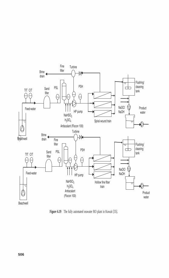
506

NaHSO3H2SO4

Antiscalant (Flocon 100)

NaOClNaOH

Feed-water

Sandfilter

Finefilter

HP pump

Spiral wound train

Flushing/cleaningtank

CITTITPSHPSL

Hollow fine fibertrain

Beachwell

Feed-water

CITTIT

Beachwell

Sandfilter

Finefilter

HP pump

PSHPSL

Flushing/cleaningtank

Productwater

Productwater

NaHSO3H2SO4

Antiscalant(Flocon 100)

Turbine

Turbine

Brinedrain

Brinedrain

NaOClNaOH

Figure 6.19 The fully automated seawater RO plant in Kuwait [35].

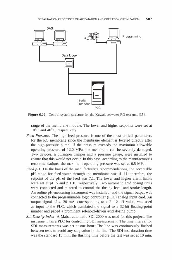
DESALINATION PROCESSES OF AUTOMATION AND OPERATION OPTIMIZATION 507

DAS

Data logger

PLC

Programming

Serialinterface

Figure 6.20 Control system structure for the Kuwait seawater RO test unit [35].

range of the membrane module. The lower and higher setpoints were set at10◦C and 40◦C, respectively.

Feed Pressure. The high feed pressure is one of the most critical parametersfor the RO membrane since the membrane element is located directly afterthe high-pressure pump. If the pressure exceeds the maximum allowableoperating pressure of 12.0 MPa, the membrane can be severely damaged.Two devices, a pulsation damper and a pressure gauge, were installed toensure that this would not occur. In this case, according to the manufacturer’srecommendations, the maximum operating pressure was set at 6.5 MPa.

Feed pH . On the basis of the manufacturer’s recommendations, the acceptablepH range for feed-water through the membrane was 4–11; therefore, thesetpoint of the pH of the feed was 7.1. The lower and higher alarm limitswere set at pH 5 and pH 10, respectively. Two automatic acid dosing unitswere connected and metered to control the dosing level and stroke length.An online pH-measuring instrument was installed, and the signal output wasconnected to the programmable logic controller (PLC) analog input card. Anoutput signal of 4–20 mA, corresponding to a 2–12 pH value, was usedas input to the PLC, which translated the signal to a 32-bit floating-pointnumber and paced a prominent solenoid-driven acid dosing pump.

Silt Density Index . A Mabat automatic SDI 2000 was used for this project. Theinstrument has a PLC for controlling SDI measurement. The time interval forSDI measurements was set at one hour. The line was continuously flushedbetween tests to avoid any stagnation in the line. The SDI test duration timewas the standard 15 min; the flushing time before the test was set at 10 min.

508 ADVANCED INSTRUMENTATION, MEASUREMENT, CONTROL, AND AUTOMATION

The values of the automatic SDI unit were cross-checked randomly withmanual SDI measurements on the same line. The automatic SDI unit showedconsistency with the manual sampling.

Chlorine Concentration . A chlorine measuring instrument (0–2 ppm) wasinstalled and connected to the analogue input of the PLC. The manufacturerrecommends that no chlorine pass through the membrane; therefore, the setpoint for the high Cl2 level was set at zero. An automatic dosing pump wasconnected for the dosing of a deoxidizing agent, i.e. sodium bisulphite.

Cartridge Filter Differential Pressure. Two alternate 5-μm cartridge filters units,each with a capacity of 15 m3/h, were installed in the feedline in front of theintermediate tank. Before installation, a test was conducted using the samebeachwell feedwater to determine the size and number of filter elementsrequired. Tests showed that a considerable drop in the flow rate (<8 m3/h)resulted when the differential pressure across the cartridge filters reached0.1 MPa. Therefore, the limit for the high differential pressure of the filterswas set at 0.09 MPa.

Membrane Differential Pressure. A high differential pressure across the mem-brane is caused by salt deposits or fouling of the membrane on the feedside. On the basis of the manufacturer’s recommendations, the setpoint forthe membrane differential pressure was set at 0.5 MPa, at which point thesystem diverted the flow and an alarm was activated. The frequency of filterchanges was 3–4 days.

High Product Conductivity and/or Low Product Flow . When either of the param-eters’ setpoints was reached, flow diversion and alarm signals were activated.In addition, a signal for membrane cleaning was activated. Cleaning normallyresulted in a reduction in product conductivity to 800 μs/cm−1, an increasein product flow to 1.2 m3/h, and a drop in feed pressure to 4.3 MPa.

Low Chemicals Level . When the levels of both acid tanks or the level inthe sodium tribisulfate tank was low, flow was diverted and an alarm wasactivated. When the operator refilled the tanks, the system restarted the unitautomatically.

6.3.3.6.2 Larnaca 54,000 m3/day Seawater RO Plant [36,37]Description of Plant This plant, which has a state-of-the-art controls and

monitoring system and is designed to treat seawater of salinity in the range of38,000–40,000 mg/L with a minimum of operator interface.

Pretreatment consists in addition of sulfuric acid for pH adjustment prior tocoagulation–flocculation, followed by gravity media filters. Media filter effluentflows into clear well. From a clear well, seawater is pumped using booster pumpsthrough cartridge filters. The booster pump motors are equipped with variable-frequency drive converters (VFCs). Use of VFCs enable adjustment of suctionpressure to the high-pressure feed pump, which enables convenient adjustment offeed pressure to the RO membranes. Use of VFC on a smaller motor of the boosterpump, rather than on the large motor of the high-pressure pump, reduces the cost of

DESALINATION PROCESSES OF AUTOMATION AND OPERATION OPTIMIZATION 509

VFC and results in a small reduction in the electric efficiency. The cartridge filtershave 20 μm porosity nominal rating and are of vertical configuration. Scale inhibitoris added to seawater upstream of the cartridge to protect against potential scale for-mation in the RO concentrate. From the cartridge filters, seawater feed is distributedto six high-pressure pumps operating in parallel. The pumps are of horizontal con-figuration, multistage, split case. Each pump is driven by an electric motor and anenergy recovery turbine connected on the same axis. The energy recovery turbinesare of the Pelton wheel type. Each pumping station is dedicated to operation of a sin-gle RO train. Train design capacity is 9000 m3/day each. RO trains operate at 50%recovery rate. The seawater trains are configured as single-stage, with 120 pres-sure vessels per train. Each pressure vessel contains eight spiral-wound seawaterelements, manufactured by Hydranautics. Permeate quality specifications includelimit on boron concentration to be below 1 ppm. For this reason, the RO plant isconfigured as a partial two-pass system. Depending on concentration of boron inthe feedwater and feedwater temperature, up to 15% of the first pass permeate canbe processed by the second-pass RO units. The second-pass units are equipped withbrackish membranes, configured in a 8–4 array configuration, eight elements pervessel. In order to improve boron rejection of the brackish membranes, the pH offeedwater to the second pass is increased to about 10 by addition of sodium hydrox-ide. Permeate from the second-pass RO units and unprocessed permeate from thefirst-pass RO are blended together and sent to the posttreatment system. In theposttreatment system, hardness and pH of the combined permeate are increasedby passing permeate through a limestone filter with the addition of NaOH, ifnecessary.

Description of Control System The control system, at Larnaca, shown inFigure 6.21a, is of distributed configuration, divided into eight functional modulescontrolled through a central programmable logic controller (PLC):

1. Raw-water supply system

2. Pretreatment system

3. Feedwater transfer pumps

4. First-pass high-pressure pumps and seawater RO trains

5. Second-pass high-pressure pumps and brackish RO trains

6. Posttreatment system

7. Product delivery system

8. Auxiliaries (cleaning system, chemicals delivery, etc.)

Such a distributed control system is usually more expensive in terms of hardwarecost and maintenance than the central system, but this control system configurationprovides better flexibility and higher process availability.

The unique conditions of the electric tariff schedule in Cyprus provided strongincentives to reduce power consumption during the peak demand hours. To benefitfrom lower electric rates, the Larnaca plant has to reduce power consumption for 3 hduring the peak electricity demand period. To accommodate this requirement, three

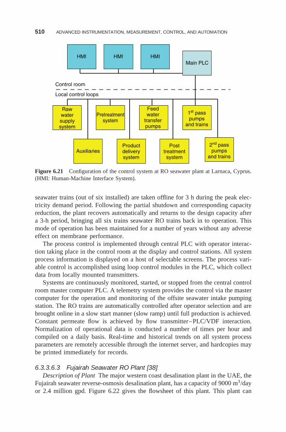
510 ADVANCED INSTRUMENTATION, MEASUREMENT, CONTROL, AND AUTOMATION

Main PLC

Rawwatersupplysystem

Pretreatmentsystem

Feedwater

transferpumps

1st passpumps

and trains

2nd passpumps

and trains

Posttreatmentsystem

Productdeliverysystem

Auxiliaries

HMI HMI HMI

Control room

Local control loops

Figure 6.21 Configuration of the control system at RO seawater plant at Larnaca, Cyprus.(HMI: Human-Machine Interface System).

seawater trains (out of six installed) are taken offline for 3 h during the peak elec-tricity demand period. Following the partial shutdown and corresponding capacityreduction, the plant recovers automatically and returns to the design capacity aftera 3-h period, bringing all six trains seawater RO trains back in to operation. Thismode of operation has been maintained for a number of years without any adverseeffect on membrane performance.

The process control is implemented through central PLC with operator interac-tion taking place in the control room at the display and control stations. All systemprocess information is displayed on a host of selectable screens. The process vari-able control is accomplished using loop control modules in the PLC, which collectdata from locally mounted transmitters.

Systems are continuously monitored, started, or stopped from the central controlroom master computer PLC. A telemetry system provides the control via the mastercomputer for the operation and monitoring of the offsite seawater intake pumpingstation. The RO trains are automatically controlled after operator selection and arebrought online in a slow start manner (slow ramp) until full production is achieved.Constant permeate flow is achieved by flow transmitter–PLC/VDF interaction.Normalization of operational data is conducted a number of times per hour andcompiled on a daily basis. Real-time and historical trends on all system processparameters are remotely accessible through the internet server, and hardcopies maybe printed immediately for records.

6.3.3.6.3 Fujairah Seawater RO Plant [38]Description of Plant The major western coast desalination plant in the UAE, the

Fujairah seawater reverse-osmosis desalination plant, has a capacity of 9000 m3/dayor 2.4 million gpd. Figure 6.22 gives the flowsheet of this plant. This plant can

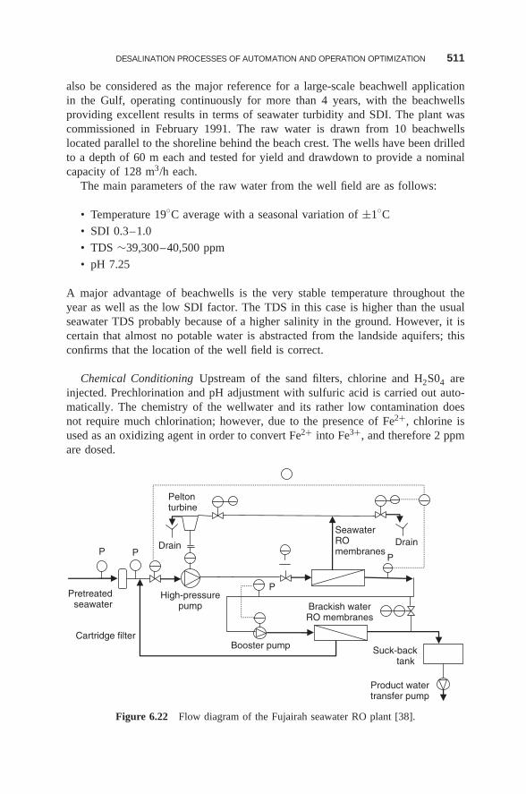
DESALINATION PROCESSES OF AUTOMATION AND OPERATION OPTIMIZATION 511

also be considered as the major reference for a large-scale beachwell applicationin the Gulf, operating continuously for more than 4 years, with the beachwellsproviding excellent results in terms of seawater turbidity and SDI. The plant wascommissioned in February 1991. The raw water is drawn from 10 beachwellslocated parallel to the shoreline behind the beach crest. The wells have been drilledto a depth of 60 m each and tested for yield and drawdown to provide a nominalcapacity of 128 m3/h each.

The main parameters of the raw water from the well field are as follows:

• Temperature 19◦C average with a seasonal variation of ±1◦C

• SDI 0.3–1.0

• TDS ∼39,300–40,500 ppm

• pH 7.25

A major advantage of beachwells is the very stable temperature throughout theyear as well as the low SDI factor. The TDS in this case is higher than the usualseawater TDS probably because of a higher salinity in the ground. However, it iscertain that almost no potable water is abstracted from the landside aquifers; thisconfirms that the location of the well field is correct.

Chemical Conditioning Upstream of the sand filters, chlorine and H2S04 areinjected. Prechlorination and pH adjustment with sulfuric acid is carried out auto-matically. The chemistry of the wellwater and its rather low contamination doesnot require much chlorination; however, due to the presence of Fe2+, chlorine isused as an oxidizing agent in order to convert Fe2+ into Fe3+, and therefore 2 ppmare dosed.

SeawaterROmembranes

Peltonturbine

Brackish waterRO membranes

High-pressurepump

Pretreatedseawater

Cartridge filter

Suck-backtank

Product watertransfer pump

Drain Drain

Booster pump

P P P

P

Figure 6.22 Flow diagram of the Fujairah seawater RO plant [38].

512 ADVANCED INSTRUMENTATION, MEASUREMENT, CONTROL, AND AUTOMATION

Acid is dosed at 15–20 ppm to maintain a feed pH in the range 6.9–7.0.Upstream of the cartridge filters, sodium bisulfite NaHS03 (7–8 ppm) is injectedto eliminate the residual chlorine (∼1.2 ppm) and to protect the membranes. Down-stream of the cartridge filters, the redox (reduction–oxidation) potential is measuredin the RO feedwater. If insufficient NaHS03 is present in the RO feedwater, theRO units are shut down automatically and the water is dumped back in to the seavia the dump valve.

The dump valve is also used for startup of the plant whereby the RO feedwaterwill be dumped automatically regardless of the water quality for 15 min beforeany RO stream can be started in order to ensure that the pretreatment and chemicaldosing has been strictly established.

The Sand Filter Station This consists of nine pressure sand filters of 3.5 mdiameter each, internally hard-rubber-lined with an incorporated nozzle floor. Thesand filters are backwashed automatically in sequence with air scouring and waterfollowed by an infiltration period. The filter medium composed of sand of differentgrain sizes (coarse and fine sand) as well as anthracite to enhance the filtrationeffect, eliminating suspended iron. The water out of the sand filtration station is ledto an intermediate filtered-water tank providing storage capacity for the backwashwater for the sand filters and surge capacity for the filtered water transfer pumps,which transfer the water through the cartridge, filters to the RO trains.

Desalination Membranes Three module racks are used, each RO streamequipped with 48 pressure vessels. Each pressure vessel can hold six spiral woundmembranes. The maximum number of membranes that can be installed per trainis 288.

The permeate is transferred to the surge suckback tank acting as an intermediatetank for the product-water transfer pumps and further to a 5000-m3 product storagetank outside the main building. A postchlorination and a pH adjustment with sodiumhydroxide is carried out automatically in front of the product-water tank.

At every shutdown of each RO train, the flushing pumps fed from the surgesuckback tank start automatically replacing the brine solution within the system bylow-salinity water, thus avoiding scaling and corrosion by long-term exposure tohigh-salinity brine.

Description of Control System Programmable logic controllers control theparameters and devices that are automated. They allow the control of all processeswithin the plant, as well as providing data to external systems via analog signalsor serial strings. The controls of the individual plant sections are individuallycarried out by sub-PLC stations, which are all linked together by a digital bussystem. The overall control is made by the master station, which communicateswith the VDU system and the protocol system. A human–machine interface(HMI) system is used to indicate and record data gathered by the PLC.

Two levels of control are carried out by the PLCs:

DESALINATION PROCESSES OF AUTOMATION AND OPERATION OPTIMIZATION 513

Level 1 —involves sequencing operations such as manipulating valves or start-ing/stopping pumps, instrument verification, data acquisition, online mainte-nance, and fail-safe shutdown procedures

Level 2 —control parameters such as flow, pressure, temperature, and pH

The PLC can be connected via a digital communication link to an HMI computer.This computer may be programmed with graphical–equipment/process screens toenable the operator to view the system from a primary location and adjust thesetpoint values of the control valves.

The process parameters and status indications are displayed on a backup processand power mimic. The automatic operation of the plant is accomplished using aprocess visualization system (VDU) with videoscreen, terminal, and mouse. Aseparate printer prints all incoming faults and system alarms for the record.

All process data are also stored in the system for 36 h in the form of graphs. Theplant monitoring system (of the redox type) has a duplicate system for backup witha self-check function to identify sensor faults and any deviation from calibration.

The control system also provides alarm conditions for

• Pressure at high-pressure pump inlet

• Pressure at high-pressure pump discharge

• Pressure at membrane inlet

• Product (permeate) water pressure

• Reject output pressure

Pressure switches and transmitters monitor these pressures. To ensure long-termsafe plant operation, pressure switches shut down the high-pressure pumps duringlow inlet pressure and high discharge pressure conditions. A relief valve in the pro-duct water line protects membrane elements from damage due to any backpressuredownstream. Feedwater parameters (e.g., high pH, free chlorine, high temperature)that could adversely affect membrane longevity are indicated by an alarm condition.Automatic on/off valves are provided to divert the feed or the permeate stream todrain when stream quality is not within the safe range. For example, a much higherthan design product-water conductivity is an indication of membrane scaling, abreakdown in membrane integrity, or membrane damage. Hence, a “low membranerejection” alarm is provided.

6.3.3.6.4 Sabha Brackish-Water RO Plant [21]Description of Plant This plant was located 3 km north of the town of Eilat,

Israel and desalts brackish-water having a salinity of 4600–6000 ppm TDS andsupplies potable water to the town of Eilat. Plant capacity started with 700 m3/dayin 1978 using a single RO unit to 13,000 m3/day in 1984 using four RO units. Theplant is fed from an array of 11 wells, which differed from each other in flow rateand salinity. As shown in Figure 6.23, the plant consists of four RO units, eachunit consisting of two stages of RO vessels connected such that the brine dischargefrom the first stage is used as the feed to the second stage (brine staging). The

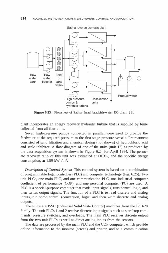
514 ADVANCED INSTRUMENTATION, MEASUREMENT, CONTROL, AND AUTOMATION

Rawwaterbank

Rawwater

booster

Bankof

sandfilters

High pressurepumps &hydraulic turbine

Sabha reverse osmosis plant

Desalinationunits

Product water

Figure 6.23 Flowsheet of Sabha, Israel brackish-water RO plant [21].

plant incorporates an energy recovery hydraulic turbine that is supplied by brinecollected from all four units.

Seven high-pressure pumps connected in parallel were used to provide thefeedwater at the required pressure to the first-stage pressure vessels. Pretreatmentconsisted of sand filtration and chemical dosing (not shown) of hydrochloric acidand scale inhibitor. A flow diagram of one of the units (unit 12) as produced bythe data acquisition system is shown in Figure 6.24 for April 1984. The perme-ate recovery ratio of this unit was estimated at 60.3%, and the specific energyconsumption, at 1.59 kWh/m3.

Description of Control System This control system is based on a combinationof programmable logic controller (PLC) and computer technology (Fig. 6.25). Twounit PLCs, one main PLC, and one communication PLC, one industrial computercoefficient of performance (COP), and one personal computer (PC) are used. APLC is a special-purpose computer that reads input signals, runs control logic, andthen writes output signals. The function of a PLC is to read discrete and analoginputs, run some control (conversion) logic, and then write discrete and analogoutputs.

The PLCs are ISSC (Industrial Solid State Control) machines from the IPC620family. The unit PLCs 1 and 2 receive discrete input signals such as start/stop com-mands, pressure switches, and overloads. The main PLC receives discrete outputfrom the two unit PLCs as well as direct analog inputs from the sensors.

The data are processed by the main PLC and the COP computer, which provideonline information to the monitor (screen) and printer, and to a communication

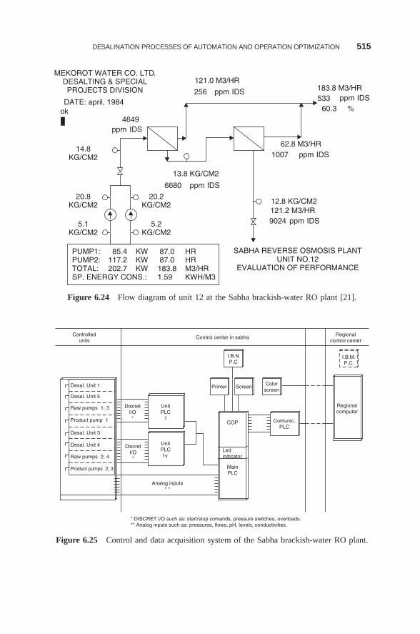
DESALINATION PROCESSES OF AUTOMATION AND OPERATION OPTIMIZATION 515

MEKOROT WATER CO. LTD.DESALTING & SPECIAL

PROJECTS DIVISION

DATE: april, 1984ok

4649

13.8 KG/CM2

62.8 M3/HR

60.3 %

183.8 M3/HR533

121.0 M3/HR

256

12.8 KG/CM2

SABHA REVERSE OSMOSIS PLANTUNIT NO.12

EVALUATION OF PERFORMANCE

121.2 M3/HR9024

1007

6680

14.8KG/CM2

20.8KG/CM2

5.1KG/CM2

PUMP1: 85.4 KW 87.0 HRPUMP2: 117.2 KW 87.0 HRTOTAL: 202.7 KW 183.8 M3/HRSP. ENERGY CONS.: 1.59 KWH/M3

5.2KG/CM2

20.2KG/CM2

ppm

ppm

IDS

IDS

ppm IDS

ppm IDSppm IDS

ppm IDS

Figure 6.24 Flow diagram of unit 12 at the Sabha brackish-water RO plant [21].

DiscretI/O*

Desal. Unit 1

Desal. Unit 5

Desal. Unit 3

Desal. Unit 4

Raw pumps 1; 3

Raw pumps 2; 4

Product pump 1

Product pumps 2; 3

UnitPLC

1

UnitPLC1v

MainPLC

Ledindicator

COP Comunic.PLC

Regionalcomputer

Colorscreen

ScreenPrinter

I.B.NP.C

I.B.M.P.C.

Regionalcontrol center

Control center in sabhaControlledunits

DiscretI/O*

Analog inputs* *

* DISCRET I/O such as: start/stop comands, pressure switches, overloads.** Analog inputs such as: pressures, flows, pH, levels, conductivities.

Figure 6.25 Control and data acquisition system of the Sabha brackish-water RO plant.

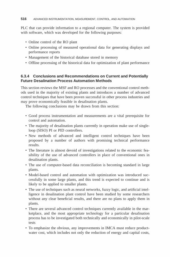
516 ADVANCED INSTRUMENTATION, MEASUREMENT, CONTROL, AND AUTOMATION

PLC that can provide information to a regional computer. The system is providedwith software, which was developed for the following purposes:

• Online control of the RO plant

• Online processing of measured operational data for generating displays andperformance reports

• Management of the historical database stored in memory

• Offline processing of the historical data for optimization of plant performance

6.3.4 Conclusions and Recommendations on Current and PotentiallyFuture Desalination Process Automation Methods

This section reviews the MSF and RO processes and the conventional control meth-ods used in the majority of existing plants and introduces a number of advancedcontrol techniques that have been proven successful in other process industries andmay prove economically feasible in desalination plants.

The following conclusions may be drawn from this section:

• Good process instrumentation and measurements are a vital prerequisite forcontrol and automation.

• The majority of desalination plants currently in operation make use of single-loop (SISO) PI or PID controllers.

• New methods of advanced and intelligent control techniques have beenproposed by a number of authors with promising technical performanceresults.

• The literature is almost devoid of investigations related to the economic fea-sibility of the use of advanced controllers in place of conventional ones indesalination plants.

• The use of computer-based data reconciliation is becoming standard in largeplants.

• Model-based control and automation with optimization was introduced suc-cessfully in some large plants, and this trend is expected to continue and islikely to be applied to smaller plants.

• The use of techniques such as neural networks, fuzzy logic, and artificial intel-ligence in desalination plant control have been studied by some researcherswithout any clear beneficial results, and there are no plans to apply them inplants.

• There are several advanced control techniques currently available in the mar-ketplace, and the most appropriate technology for a particular desalinationprocess has to be investigated both technically and economically in pilot-scaletests

• To emphasize the obvious, any improvements in IMCA must reduce product-water cost, which includes not only the reduction of energy and capital costs,

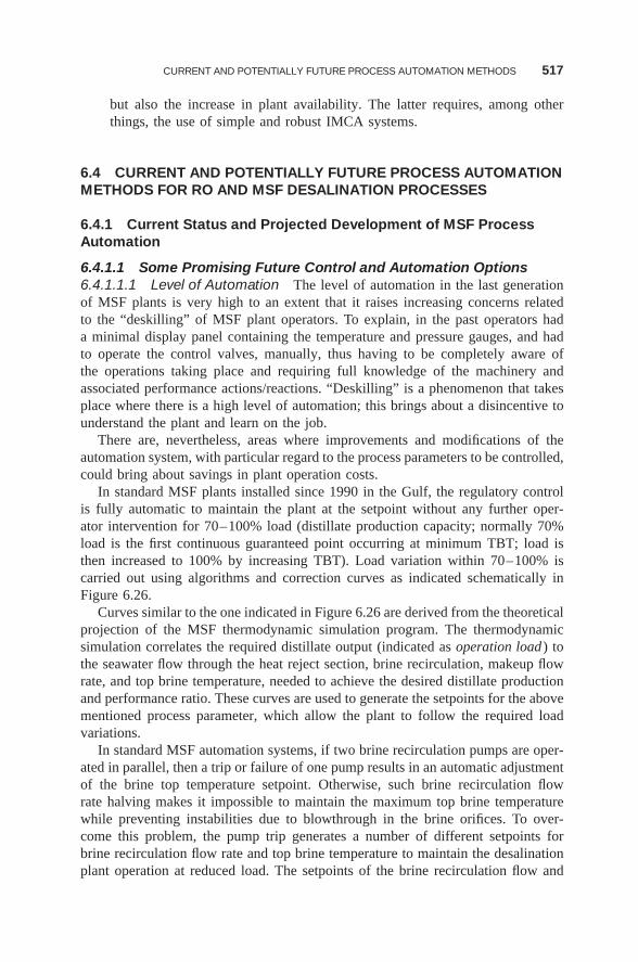
CURRENT AND POTENTIALLY FUTURE PROCESS AUTOMATION METHODS 517

but also the increase in plant availability. The latter requires, among otherthings, the use of simple and robust IMCA systems.

6.4 CURRENT AND POTENTIALLY FUTURE PROCESS AUTOMATIONMETHODS FOR RO AND MSF DESALINATION PROCESSES

6.4.1 Current Status and Projected Development of MSF ProcessAutomation

6.4.1.1 Some Promising Future Control and Automation Options6.4.1.1.1 Level of Automation The level of automation in the last generationof MSF plants is very high to an extent that it raises increasing concerns relatedto the “deskilling” of MSF plant operators. To explain, in the past operators hada minimal display panel containing the temperature and pressure gauges, and hadto operate the control valves, manually, thus having to be completely aware ofthe operations taking place and requiring full knowledge of the machinery andassociated performance actions/reactions. “Deskilling” is a phenomenon that takesplace where there is a high level of automation; this brings about a disincentive tounderstand the plant and learn on the job.

There are, nevertheless, areas where improvements and modifications of theautomation system, with particular regard to the process parameters to be controlled,could bring about savings in plant operation costs.

In standard MSF plants installed since 1990 in the Gulf, the regulatory controlis fully automatic to maintain the plant at the setpoint without any further oper-ator intervention for 70–100% load (distillate production capacity; normally 70%load is the first continuous guaranteed point occurring at minimum TBT; load isthen increased to 100% by increasing TBT). Load variation within 70–100% iscarried out using algorithms and correction curves as indicated schematically inFigure 6.26.

Curves similar to the one indicated in Figure 6.26 are derived from the theoreticalprojection of the MSF thermodynamic simulation program. The thermodynamicsimulation correlates the required distillate output (indicated as operation load ) tothe seawater flow through the heat reject section, brine recirculation, makeup flowrate, and top brine temperature, needed to achieve the desired distillate productionand performance ratio. These curves are used to generate the setpoints for the abovementioned process parameter, which allow the plant to follow the required loadvariations.

In standard MSF automation systems, if two brine recirculation pumps are oper-ated in parallel, then a trip or failure of one pump results in an automatic adjustmentof the brine top temperature setpoint. Otherwise, such brine recirculation flowrate halving makes it impossible to maintain the maximum top brine temperaturewhile preventing instabilities due to blowthrough in the brine orifices. To over-come this problem, the pump trip generates a number of different setpoints forbrine recirculation flow rate and top brine temperature to maintain the desalinationplant operation at reduced load. The setpoints of the brine recirculation flow and

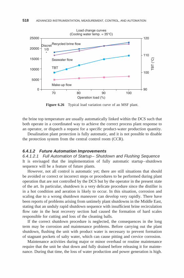
518 ADVANCED INSTRUMENTATION, MEASUREMENT, CONTROL, AND AUTOMATION

Discret1/0*

25000

Recycled brine flow

Seawater flow

TBT

Make-up flow

20000

15000

10000

5000

70 80Operation load (%)

Load change curves(Cooling water temp. = 35°C)

90 10090

100

TB

T (

°C)

110

120

0

Figure 6.26 Typical load variation curve of an MSF plant.

the brine top temperature are usually automatically linked within the DCS such thatboth operate in a coordinated way to achieve the correct process plant response toan operator, or dispatch a request for a specific product-water production quantity.

Desalination plant protection is fully automatic, and it is not possible to disablethe protection system from the central control room (CCR).

6.4.1.2 Future Automation Improvements6.4.1.2.1 Full Automation of Startup– Shutdown and Flushing SequenceIt is envisaged that the implementation of fully automatic startup–shutdownsequence will be a feature of future plants.

However, not all control is automatic yet; there are still situations that shouldbe avoided or correct or incorrect steps or procedures to be performed during plantoperation that are not controlled by the DCS but by the operator in the present stateof the art. In particular, shutdown is a very delicate procedure since the distiller isin a hot condition and aeration is likely to occur. In this situation, corrosion andscaling due to a wrong shutdown maneuver can develop very rapidly. There havebeen reports of problems arising from untimely plant shutdowns in the Middle East,stating that an unduly rapid shutdown sequence with insufficient brine recirculationflow rate in the heat recovery section had caused the formation of hard scalesresponsible for cutting and loss of the cleaning balls.

If the correct shutdown procedure is neglected, the consequences in the longterm may be corrosion and maintenance problems. Before carrying out the plantshutdown, flushing the unit with product water is necessary to prevent formationof stagnant pockets of salty water, which can cause pitting and crevice corrosion.

Maintenance activities during major or minor overhaul or routine maintenancerequire that the unit be shut down and fully drained before releasing it for mainte-nance. During that time, the loss of water production and power generation is high.

CURRENT AND POTENTIALLY FUTURE PROCESS AUTOMATION METHODS 519

In addition, units are not fully dry or protected from corrosion during the flushingtime. The following steps are recommended for future systems:

• Modify existing manual procedures so as to reduce shutdown, flushing, anddryout time

• Investigate possibilities to implement an automatic procedure to reduce thedown time

• Protect the unit from corrosion during flushing time

It is difficult to provide an economic evaluation of the financial advantages aris-ing from the implementation of these procedures; we can, however, in general,highlight the fact that in IWPP (International Water and Power Project) loss inwater production involves a loss in water revenues. For example, reduction of thedowntime by 3 h per year in a 100 MIGD plant at the current cost of water (US$0.8/m3) would allow a saving of US$ 45,000 per year in terms of water revenues.This implies that even this small reduction in downtime would pay back for theDCS modifications in just a few years.

6.4.1.2.2 Modification in Top Brine Temperature Control Scheme Thearrangement shown in Figure 6.27 is proposed as a TBT control pattern alternativeto the classical system which has been described in Figure 6.26. While allowingfull temperature control of the desalination plant, this classical system has thedisadvantage of incurring several heat and pressure losses due to control valvethrottling.

The arrangement as indicated in Figure 6.27 shows direct control of top brinetemperature both on HP (MP)-LP steam reducing station and/or steam turbineextraction, thus avoiding further throttling of steam in the TBT control valve asdone in the currently used scheme (Fig. 6.26). The modified scheme has beenimplemented so far in only a few installations with steam reducing stations.

The main disadvantage of this control scheme is the uncertainty of energy inputwhen steam that is extracted from the steam turbine is in wet condition. In partic-ular, it is impossible to ascertain the degree of wetness of the steam and thereforeprecisely measure the enthalpy of the steam entering the desalination plant in thisconfiguration.

The requirement of a total energy control at the brine heater inlet becomesredundant once the MSF performance ratio has been performance-tested. In general,the design of the steam generation plant allows sufficient flexibility to operatethe plant with superheated steam during the performance test of the plant, foracceptance purposes. The actual value of the performance ratio during operationcan be considered relatively unimportant.

It is actually more important to control the fouling trend and the variation overthe time of the energy input, rather than ensure a precise absolute value. In thisrespect, implementation of control software matching the expansion curve of thesteam turbine with the steam energy input to the brine heater can be considered. The

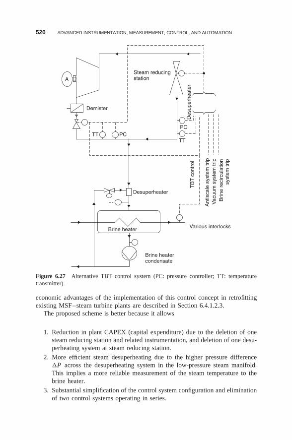
520 ADVANCED INSTRUMENTATION, MEASUREMENT, CONTROL, AND AUTOMATION

Desuperheater

Demister

ASteam reducingstation

Des

uper

heat

erT

BT

con

trol

Ant

isca

le s

yste

m tr

ipV

acuu

m s

yste

m tr

ipB

rine

reci

rcul

atio

nsy

stem

trip

PCPC

TTTT

Brine heater

Brine heatercondensate

Various interlocks

Figure 6.27 Alternative TBT control system (PC: pressure controller; TT: temperaturetransmitter).

economic advantages of the implementation of this control concept in retrofittingexisting MSF–steam turbine plants are described in Section 6.4.1.2.3.

The proposed scheme is better because it allows

1. Reduction in plant CAPEX (capital expenditure) due to the deletion of onesteam reducing station and related instrumentation, and deletion of one desu-perheating system at steam reducing station.

2. More efficient steam desuperheating due to the higher pressure difference�P across the desuperheating system in the low-pressure steam manifold.This implies a more reliable measurement of the steam temperature to thebrine heater.

3. Substantial simplification of the control system configuration and eliminationof two control systems operating in series.

CURRENT AND POTENTIALLY FUTURE PROCESS AUTOMATION METHODS 521

4. Reduction of pressure losses in the steam line to brine heater. This featureallows in lower steam extraction pressure from the steam turbine with ahigher power output rendered at turbine shaft.

6.4.1.2.3 Automation in Control of Fouling AspectsIntroduction to Automation of Fouling Control. Experimental results on existing

MSF desalination plants have demonstrated that the actual antiscale dosing rate canbe up to 10% lower than the dosing rate recommended by the manufacturer forthe same operating conditions [39]. These results can yield a substantial saving inplant O&M cost if fouling and scaling in the MSF desalination plant are kept undercontrol.

Automation can provide a useful means of keeping scaling under control withoptimized chemical dosing. The parameter to be controlled in this respect is thefouling rate.

Technical Background on Fouling in Existing MSF plants. In the operating con-ditions found in MSF plants today, the fouling rate increases quite rapidly duringthe first 2 months of operation (from startup).

Curve E in Figure 6.28 shows a typical trend of performance ratio declinein MSF plants due to increasing fouling of the evaporator. As can also beseen, the present operational procedures using a sponge ball cleaning system incontinuous operation and antiscale dosing after 2 months of operation maintainsa stable performance ratio, and no or little performance decline is experiencedafter the initial stabilization period. After this period, the fouling factor tends tobecome stable and no substantial variation in MSF plant performance ratio isobserved.

As indicated in Figure 6.29, the fouling rate becomes constant after6000–7000 h of operation. In general, there are safety margins in the assumptionsof the fouling factor, whose effect is described in Figure 6.29. Feedback datafrom operating plants show that the actual fouling factors develop from a valueof ∼0.06 m2 C−1 kW−1 to reach an asymptotic value of ∼0.09 m2 C−1 kW−1,while the fouling factors assumed in the design are more conservative, rangingfrom 0.106 to 0.152 m2 C−1 kW−1. The situation is summarized in Figure 6.29,where the upper curve represents the EPC contractor contractual obligation,while the lower curve represents the real plant expectation during test results.The difference between the curves reflects the fact that the interval betweentwo successive acid cleanings is generally greater than the stated value (usually17,000 h).

In existing plants, this margin may be converted into operational cost savings bydecreasing the antiscale dosage to an optimum level, and by controlling the foulingrate of the evaporator by fine-tuning the sponge ball cleaning system variables asindicated below.

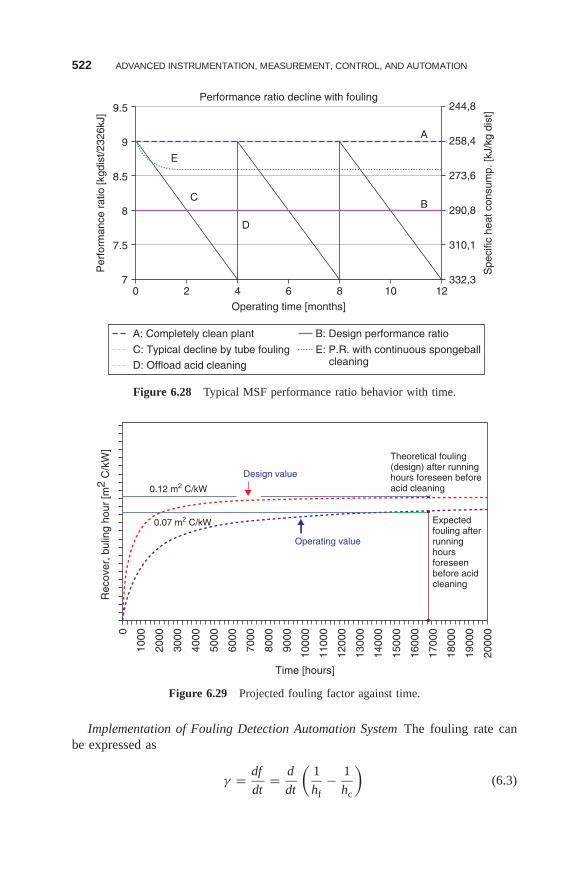
522 ADVANCED INSTRUMENTATION, MEASUREMENT, CONTROL, AND AUTOMATION

9.5

E

C

D

A

B

9

8.5

8

7.5

70 2 4 6

Operating time [months]

Performance ratio decline with fouling

8 10 12

244,8

258,4

273,6

Spe

cific

hea

t con

sum

p. [k

J/kg

dis

t]

Per

form

ance

rat

io [k

gdis

t/232

6kJ]

290,8

310,1

332,3

B: Design performance ratio

E: P.R. with continuous spongeball cleaning

A: Completely clean plant

C: Typical decline by tube fouling

D: Offload acid cleaning

Figure 6.28 Typical MSF performance ratio behavior with time.

0

1000

0.12 m2 C/kW

0.07 m2 C/kW

Design value

Operating value

Theoretical fouling(design) after runninghours foreseen beforeacid cleaning

Expectedfouling afterrunninghoursforeseenbefore acidcleaning

2000

3000

4000

5000

6000

7000

8000

9000

1000

0

Time [hours]

Rec

over

, bul

ing

hour

[m2

C/k

W]

1100

0

1200

0

1300

0

1400

0

1500

0

1600

0

1700

0

1800

0

1900

0

2000

0

Figure 6.29 Projected fouling factor against time.

Implementation of Fouling Detection Automation System The fouling rate canbe expressed as

γ = df

dt= d

dt

(1

hf− 1

hc

)(6.3)

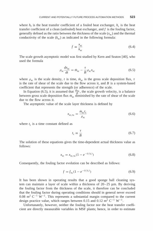
CURRENT AND POTENTIALLY FUTURE PROCESS AUTOMATION METHODS 523

where hf is the heat transfer coefficient of a fouled heat exchanger, hc is the heattransfer coefficient of a clean (unfouled) heat exchanger, and f is the fouling factor,generally defined as the ratio between the thickness of the scale (xsc) and the thermalconductivity of the scale (ksc) as indicated in the following formula:

f ≡ xsc

ksc(6.4)

The scale growth asymptotic model was first studied by Kern and Seaton [40], whoused the formula

ρscdxsc

dt= msc − τ

Bρscxsc (6.5)

where ρsc is the scale density, t is time, msc is the gross scale deposition flux, τ

is the rate of shear of the scale due to the flow across it, and B is a system-basedcoefficient that represents the strength (or adherence) of the scale.

In Equation (6.5), it is assumed that dxscdt , the scale growth velocity, is a balance

between gross scale deposition flux msc diminished by the rate of shear of the scaledue to the flow across it.

The asymptotic value of the scale layer thickness is defined by

xsc,∞ = msctcρsc

(6.6)

where tc is a time constant defined as

tc ≡ τ

B(6.7)

The solution of these equations gives the time-dependent actual thickness value asfollows:

xsc = xsc,∞(1 − e−(t/tc)) (6.8)

Consequently, the fouling factor evolution can be described as follows:

f = f∞(1 − e−(t/tc)) (6.9)

It has been shown in operating results that a good sponge ball cleaning sys-tem can maintain a layer of scale within a thickness of 20–25 μm. By derivingthe fouling factor from the thickness of the scale, it therefore can be concludedthat the fouling factor during operating conditions should in general never exceed0.08 m2 C−1 W−1. This represents a substantial margin compared to the currentdesign practice value, which ranges between 0.15 and 0.12 m2 C−1 W−1.

Unfortunately, however, neither the fouling factor nor the heat transfer coeffi-cient are directly measurable variables in MSF plants; hence, in order to estimate

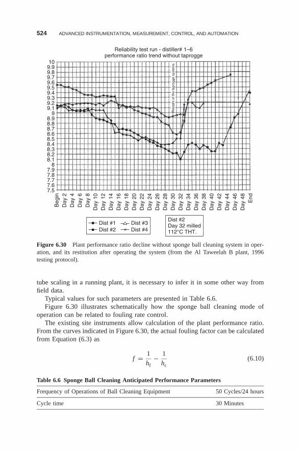
524 ADVANCED INSTRUMENTATION, MEASUREMENT, CONTROL, AND AUTOMATION

Res

taht

of t

he ta

prog

ge s

yste

ms

Reliability test run - distiller# 1–6performance ratio trend without taprogge

109.99.89.79.69.59.49.39.29.1

98.98.88.78.68.58.48.38.28.1

7.97.87.77.67.5

Beg

inD

ay 2

Day

4D

ay 6

Day

8D

ay 1

0D

ay 1

2D

ay 1

4D

ay 1

6D

ay 1

8D

ay 2

0D

ay 2

2D

ay 2

4D

ay 2

6D

ay 2

8D

ay 3

0D

ay 3

2D

ay 3

4D

ay 3

6D

ay 3

8D

ay 4

0D

ay 4

2D

ay 4

4D

ay 4

6D

ay 4

8E

nd

8

Dist #1Dist #2

Dist #3Dist #4

Dist #2Day 32 milled112°C THT.

Figure 6.30 Plant performance ratio decline without sponge ball cleaning system in oper-ation, and its restitution after operating the system (from the Al Taweelah B plant, 1996testing protocol).

tube scaling in a running plant, it is necessary to infer it in some other way fromfield data.

Typical values for such parameters are presented in Table 6.6.Figure 6.30 illustrates schematically how the sponge ball cleaning mode of

operation can be related to fouling rate control.The existing site instruments allow calculation of the plant performance ratio.

From the curves indicated in Figure 6.30, the actual fouling factor can be calculatedfrom Equation (6.3) as

f = 1

hf− 1

hc(6.10)

Table 6.6 Sponge Ball Cleaning Anticipated Performance Parameters

Frequency of Operations of Ball Cleaning Equipment 50 Cycles/24 hours

Cycle time 30 Minutes

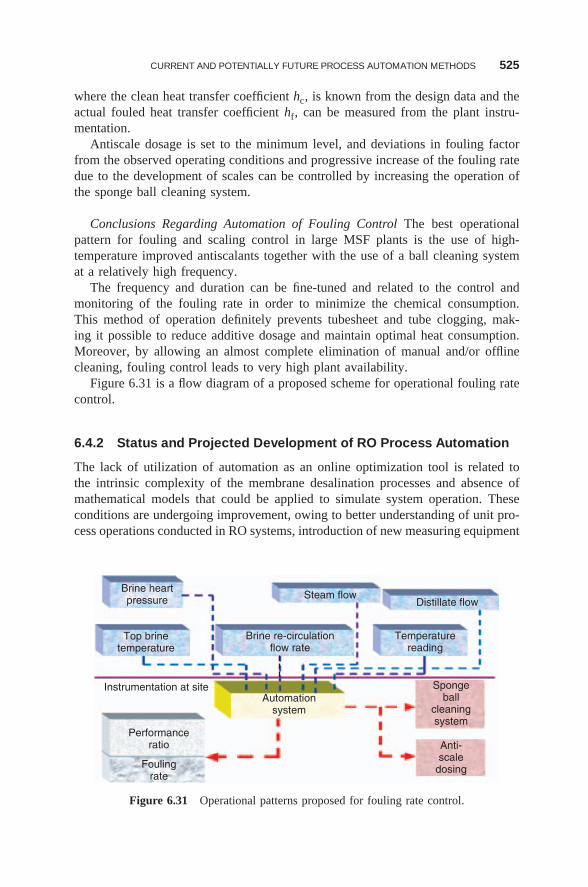
CURRENT AND POTENTIALLY FUTURE PROCESS AUTOMATION METHODS 525

where the clean heat transfer coefficient hc, is known from the design data and theactual fouled heat transfer coefficient hf, can be measured from the plant instru-mentation.

Antiscale dosage is set to the minimum level, and deviations in fouling factorfrom the observed operating conditions and progressive increase of the fouling ratedue to the development of scales can be controlled by increasing the operation ofthe sponge ball cleaning system.

Conclusions Regarding Automation of Fouling Control The best operationalpattern for fouling and scaling control in large MSF plants is the use of high-temperature improved antiscalants together with the use of a ball cleaning systemat a relatively high frequency.

The frequency and duration can be fine-tuned and related to the control andmonitoring of the fouling rate in order to minimize the chemical consumption.This method of operation definitely prevents tubesheet and tube clogging, mak-ing it possible to reduce additive dosage and maintain optimal heat consumption.Moreover, by allowing an almost complete elimination of manual and/or offlinecleaning, fouling control leads to very high plant availability.

Figure 6.31 is a flow diagram of a proposed scheme for operational fouling ratecontrol.

6.4.2 Status and Projected Development of RO Process Automation

The lack of utilization of automation as an online optimization tool is related tothe intrinsic complexity of the membrane desalination processes and absence ofmathematical models that could be applied to simulate system operation. Theseconditions are undergoing improvement, owing to better understanding of unit pro-cess operations conducted in RO systems, introduction of new measuring equipment

Steam flowDistillate flow

Temperaturereading

Brine re-circulationflow rate

Performanceratio

Instrumentation at site Spongeball

cleaningsystem

Anti-scale

dosingFoulingrate

Automationsystem

Brine heartpressure

Top brinetemperature

Figure 6.31 Operational patterns proposed for fouling rate control.

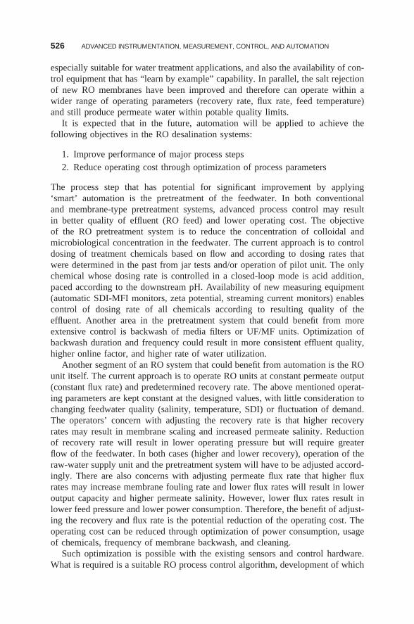
526 ADVANCED INSTRUMENTATION, MEASUREMENT, CONTROL, AND AUTOMATION

especially suitable for water treatment applications, and also the availability of con-trol equipment that has “learn by example” capability. In parallel, the salt rejectionof new RO membranes have been improved and therefore can operate within awider range of operating parameters (recovery rate, flux rate, feed temperature)and still produce permeate water within potable quality limits.

It is expected that in the future, automation will be applied to achieve thefollowing objectives in the RO desalination systems:

1. Improve performance of major process steps2. Reduce operating cost through optimization of process parameters

The process step that has potential for significant improvement by applying‘smart’ automation is the pretreatment of the feedwater. In both conventionaland membrane-type pretreatment systems, advanced process control may resultin better quality of effluent (RO feed) and lower operating cost. The objectiveof the RO pretreatment system is to reduce the concentration of colloidal andmicrobiological concentration in the feedwater. The current approach is to controldosing of treatment chemicals based on flow and according to dosing rates thatwere determined in the past from jar tests and/or operation of pilot unit. The onlychemical whose dosing rate is controlled in a closed-loop mode is acid addition,paced according to the downstream pH. Availability of new measuring equipment(automatic SDI-MFI monitors, zeta potential, streaming current monitors) enablescontrol of dosing rate of all chemicals according to resulting quality of theeffluent. Another area in the pretreatment system that could benefit from moreextensive control is backwash of media filters or UF/MF units. Optimization ofbackwash duration and frequency could result in more consistent effluent quality,higher online factor, and higher rate of water utilization.

Another segment of an RO system that could benefit from automation is the ROunit itself. The current approach is to operate RO units at constant permeate output(constant flux rate) and predetermined recovery rate. The above mentioned operat-ing parameters are kept constant at the designed values, with little consideration tochanging feedwater quality (salinity, temperature, SDI) or fluctuation of demand.The operators’ concern with adjusting the recovery rate is that higher recoveryrates may result in membrane scaling and increased permeate salinity. Reductionof recovery rate will result in lower operating pressure but will require greaterflow of the feedwater. In both cases (higher and lower recovery), operation of theraw-water supply unit and the pretreatment system will have to be adjusted accord-ingly. There are also concerns with adjusting permeate flux rate that higher fluxrates may increase membrane fouling rate and lower flux rates will result in loweroutput capacity and higher permeate salinity. However, lower flux rates result inlower feed pressure and lower power consumption. Therefore, the benefit of adjust-ing the recovery and flux rate is the potential reduction of the operating cost. Theoperating cost can be reduced through optimization of power consumption, usageof chemicals, frequency of membrane backwash, and cleaning.

Such optimization is possible with the existing sensors and control hardware.What is required is a suitable RO process control algorithm, development of which

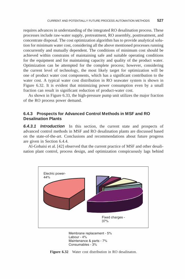
CURRENT AND POTENTIALLY FUTURE PROCESS AUTOMATION METHODS 527

requires advances in understanding of the integrated RO desalination process. Theseprocesses include raw-water supply, pretreatment, RO assembly, posttreatment, andconcentrate disposal. The cost optimization algorithm has to provide analytical solu-tion for minimum water cost, considering all the above mentioned processes runningconcurrently and mutually dependent. The conditions of minimum cost should beachieved within constrains of maintaining safe and suitable operating conditionsfor the equipment and for maintaining capacity and quality of the product water.Optimization can be attempted for the complete process; however, consideringthe current level of technology, the most likely target for optimization will beone of product water cost components, which has a significant contribution to thewater cost. A typical water cost distribution in RO seawater system is shown inFigure 6.32. It is evident that minimizing power consumption even by a smallfraction can result in significant reduction of product-water cost.

As shown in Figure 6.33, the high-pressure pump unit utilizes the major fractionof the RO process power demand.

6.4.3 Prospects for Advanced Control Methods in MSF and RODesalination Plants

6.4.3.1 Introduction In this section, the current state and prospects ofadvanced control methods in MSF and RO desalination plants are discussed basedon the state-of-the-art. Conclusions and recommendations about future progressare given in Section 6.4.4.

Al-Gobaisi et al. [42] observed that the current practice of MSF and other desali-nation plant control, process design, and optimization conspicuously lags behind

Electric power-44%

Fixed charges -37%

Membrane replacement - 5%Labour - 4%Maintenance & parts - 7%Consumables - 3%

Figure 6.32 Water cost distribution in RO desalinaton.

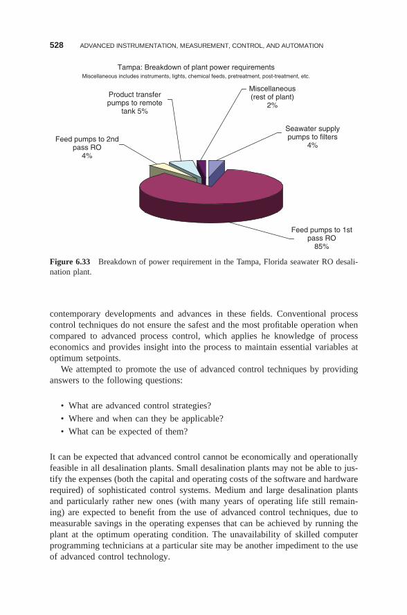
528 ADVANCED INSTRUMENTATION, MEASUREMENT, CONTROL, AND AUTOMATION

Tampa: Breakdown of plant power requirementsMiscellaneous includes instruments, lights, chemical feeds, pretreatment, post-treatment, etc.

Seawater supplypumps to filters

4%

Miscellaneous(rest of plant)

2%

Feed pumps to 1stpass RO

85%

Feed pumps to 2ndpass RO

4%

Product transferpumps to remote

tank 5%

Figure 6.33 Breakdown of power requirement in the Tampa, Florida seawater RO desali-nation plant.

contemporary developments and advances in these fields. Conventional processcontrol techniques do not ensure the safest and the most profitable operation whencompared to advanced process control, which applies he knowledge of processeconomics and provides insight into the process to maintain essential variables atoptimum setpoints.

We attempted to promote the use of advanced control techniques by providinganswers to the following questions:

• What are advanced control strategies?

• Where and when can they be applicable?

• What can be expected of them?

It can be expected that advanced control cannot be economically and operationallyfeasible in all desalination plants. Small desalination plants may not be able to jus-tify the expenses (both the capital and operating costs of the software and hardwarerequired) of sophisticated control systems. Medium and large desalination plantsand particularly rather new ones (with many years of operating life still remain-ing) are expected to benefit from the use of advanced control techniques, due tomeasurable savings in the operating expenses that can be achieved by running theplant at the optimum operating condition. The unavailability of skilled computerprogramming technicians at a particular site may be another impediment to the useof advanced control technology.

CURRENT AND POTENTIALLY FUTURE PROCESS AUTOMATION METHODS 529

The main goal in using advanced control in desalination plants is to produce aproduct (potable water) that has a minimum cost all the time and during all phasesof operation of the plant (full-load or part-load operation or during transient oper-ation). This has to be achieved taking into consideration the normal performancedeterioration of the different plants components such as fouling.

6.4.3.2 Prospects for Dynamic Matrix Control Method Computersimulations were performed by Robertson et al. [42] using the dynamic matrixcontrol (DMC) algorithm for the control of an RO desalination plant, and comparedthe performance of the DMC controller with that of a conventional PI controller. Itwas found that with the selection of proper tuning constants, the DMC controllerallows for substantial improvement over the PI control, based on the integralsquare error (ISE) performance criteria. For the same magnitude setpoint changein product flow rate, the ISE results for the flow rate were comparable between thetwo controllers; however, the ISE results for conductivity were substantially betterusing DMC control (for PI controller, ISE = 1688.92 and for DMC controller,ISE ≤ 1.0).

6.4.3.3 Prospects for Nonlinear Model Predictive Control (NMPC)Method Aly et al. [19] investigated the use of the nonlinear predictive con-trol (NMPC) method as an advanced control strategy for the control of multistageflash desalination plants and compared the performance of the NMPC controllerwith a PI controller. For this purpose, a comprehensive nonlinear dynamic modelwas developed for the MSF plant and was validated with actual plant data (KhobarII, Saudi Arabia, with a capacity of 1184 t/h). A control structure for the plantwas then developed from which two control objectives were selected. One controlobjective is to maximize the distillate product, and the other is to maximize theperformance ratio while maintaining the manipulated variables in both cases undertight constraints.

The controlled variables are the top brine temperature (TBT) and the distillateproduction (Md) and the manipulated variables are the recirculation flow rate (Mr),and the steam flow rate to the brine heater (Ms). The NLMPC algorithm wastested for a setpoint change of 4◦C in the TBT and a step change of 1.8 t/min inMd. For the first control objective (maximization of distillate flow), the controllersucceeded in increasing Md by 10% by increasing Ms by 12.5% and increasingMr by 8.2%. For the second control objective (to maximize performance ratio),the controller was able to increase the performance ratio from its initial value by2.8% (from 3.21 to 3.30) by reducing Mr by 8.5% (from 217.4 to 198.8 t/min)and reducing Ms by 2.8%, which translates to 35,250 tons of steam saved peryear [19].

The NMPC model was tested for the rejection of plant internal disturbances byinserting changes in the heat transfer coefficient and the boiling point rise. Thesechanges represent a realistic case in plant operation. The aim was to see whetherthe controller utilizing a simplified model can still maintain the performance ratioof the plant in light of these internal disturbances. Despite the large propagated

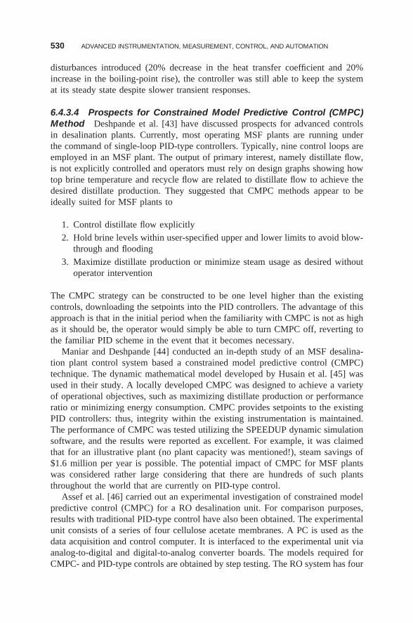
530 ADVANCED INSTRUMENTATION, MEASUREMENT, CONTROL, AND AUTOMATION

disturbances introduced (20% decrease in the heat transfer coefficient and 20%increase in the boiling-point rise), the controller was still able to keep the systemat its steady state despite slower transient responses.

6.4.3.4 Prospects for Constrained Model Predictive Control (CMPC)Method Deshpande et al. [43] have discussed prospects for advanced controlsin desalination plants. Currently, most operating MSF plants are running underthe command of single-loop PID-type controllers. Typically, nine control loops areemployed in an MSF plant. The output of primary interest, namely distillate flow,is not explicitly controlled and operators must rely on design graphs showing howtop brine temperature and recycle flow are related to distillate flow to achieve thedesired distillate production. They suggested that CMPC methods appear to beideally suited for MSF plants to

1. Control distillate flow explicitly

2. Hold brine levels within user-specified upper and lower limits to avoid blow-through and flooding

3. Maximize distillate production or minimize steam usage as desired withoutoperator intervention

The CMPC strategy can be constructed to be one level higher than the existingcontrols, downloading the setpoints into the PID controllers. The advantage of thisapproach is that in the initial period when the familiarity with CMPC is not as highas it should be, the operator would simply be able to turn CMPC off, reverting tothe familiar PID scheme in the event that it becomes necessary.

Maniar and Deshpande [44] conducted an in-depth study of an MSF desalina-tion plant control system based a constrained model predictive control (CMPC)technique. The dynamic mathematical model developed by Husain et al. [45] wasused in their study. A locally developed CMPC was designed to achieve a varietyof operational objectives, such as maximizing distillate production or performanceratio or minimizing energy consumption. CMPC provides setpoints to the existingPID controllers: thus, integrity within the existing instrumentation is maintained.The performance of CMPC was tested utilizing the SPEEDUP dynamic simulationsoftware, and the results were reported as excellent. For example, it was claimedthat for an illustrative plant (no plant capacity was mentioned!), steam savings of$1.6 million per year is possible. The potential impact of CMPC for MSF plantswas considered rather large considering that there are hundreds of such plantsthroughout the world that are currently on PID-type control.

Assef et al. [46] carried out an experimental investigation of constrained modelpredictive control (CMPC) for a RO desalination unit. For comparison purposes,results with traditional PID-type control have also been obtained. The experimentalunit consists of a series of four cellulose acetate membranes. A PC is used as thedata acquisition and control computer. It is interfaced to the experimental unit viaanalog-to-digital and digital-to-analog converter boards. The models required forCMPC- and PID-type controls are obtained by step testing. The RO system has four

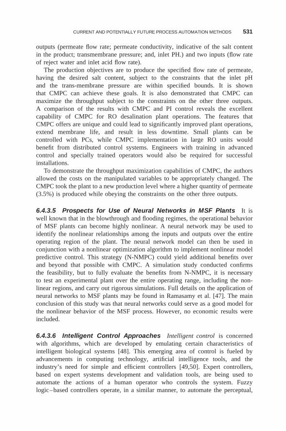
CURRENT AND POTENTIALLY FUTURE PROCESS AUTOMATION METHODS 531

outputs (permeate flow rate; permeate conductivity, indicative of the salt contentin the product; transmembrane pressure; and, inlet PH.) and two inputs (flow rateof reject water and inlet acid flow rate).

The production objectives are to produce the specified flow rate of permeate,having the desired salt content, subject to the constraints that the inlet pHand the trans-membrane pressure are within specified bounds. It is shownthat CMPC can achieve these goals. It is also demonstrated that CMPC canmaximize the throughput subject to the constraints on the other three outputs.A comparison of the results with CMPC and PI control reveals the excellentcapability of CMPC for RO desalination plant operations. The features thatCMPC offers are unique and could lead to significantly improved plant operations,extend membrane life, and result in less downtime. Small plants can becontrolled with PCs, while CMPC implementation in large RO units wouldbenefit from distributed control systems. Engineers with training in advancedcontrol and specially trained operators would also be required for successfulinstallations.

To demonstrate the throughput maximization capabilities of CMPC, the authorsallowed the costs on the manipulated variables to be appropriately changed. TheCMPC took the plant to a new production level where a higher quantity of permeate(3.5%) is produced while obeying the constraints on the other three outputs.

6.4.3.5 Prospects for Use of Neural Networks in MSF Plants It iswell known that in the blowthrough and flooding regimes, the operational behaviorof MSF plants can become highly nonlinear. A neural network may be used toidentify the nonlinear relationships among the inputs and outputs over the entireoperating region of the plant. The neural network model can then be used inconjunction with a nonlinear optimization algorithm to implement nonlinear modelpredictive control. This strategy (N-NMPC) could yield additional benefits overand beyond that possible with CMPC. A simulation study conducted confirmsthe feasibility, but to fully evaluate the benefits from N-NMPC, it is necessaryto test an experimental plant over the entire operating range, including the non-linear regions, and carry out rigorous simulations. Full details on the application ofneural networks to MSF plants may be found in Ramasamy et al. [47]. The mainconclusion of this study was that neural networks could serve as a good model forthe nonlinear behavior of the MSF process. However, no economic results wereincluded.

6.4.3.6 Intelligent Control Approaches Intelligent control is concernedwith algorithms, which are developed by emulating certain characteristics ofintelligent biological systems [48]. This emerging area of control is fueled byadvancements in computing technology, artificial intelligence tools, and theindustry’s need for simple and efficient controllers [49,50]. Expert controllers,based on expert systems development and validation tools, are being used toautomate the actions of a human operator who controls the system. Fuzzylogic–based controllers operate, in a similar manner, to automate the perceptual,

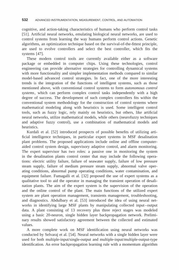
532 ADVANCED INSTRUMENTATION, MEASUREMENT, CONTROL, AND AUTOMATION

cognitive, and action-taking characteristics of humans who perform control tasks[51]. Artificial neural networks, emulating biological neural networks, are used tocontrol systems from learning the way humans perform control actions. Geneticalgorithms, an optimization technique based on the survival-of-the-fittest principle,are used to evolve controllers and select the best controller, which fits thesystems [47].

These modern control tools are currently available either as a softwarepackage or embedded in computer chips. Using these technologies, controlengineering can provide alternative strategies for controlling dynamical systemswith more functionality and simpler implementation methods compared to similarmodel-based advanced control strategies. In fact, one of the more interestingtrends is the integration of the functions of intelligent systems, such as thosementioned above, with conventional control systems to form autonomous controlsystems , which can perform complex control tasks independently with a highdegree of success. The development of such complex controllers fits within theconventional system methodology for the construction of control systems wheremathematical modeling along with heuristics is used. Some intelligent controltools, such as fuzzy logic, rely mainly on heuristics, but others, like artificialneural networks, utilize mathematical models, while others (neurofuzzy techniquesand adaptive fuzzy control), use a combination of mathematical models andheuristics.

Kurdali et al. [52] introduced prospects of possible benefits of utilizing arti-ficial intelligence techniques, in particular expert systems in MSF desalinationplant problems. The proposed applications include online and offline computer-aided control system design, supervisory adaptive control, and alarm monitoring.The expert supervisor has two roles: a passive one in monitoring the systemin the desalination plants control center that may include the following opera-tions: electric utility failure, failure of seawater supply, failure of low pressuresteam supply, failure of medium pressure steam supply, abnormal valve oper-ating conditions, abnormal pump operating conditions, water contamination, andequipment failure. Fumagalli et al. [32] proposed the use of expert systems as aqualitative tool to aid the operator in managing the transient operation of desali-nation plants. The aim of the expert system is the supervision of the operationand the online control of the plant. The main functions of the utilized expertsystem are plant operation management, transients management, troubleshooting,and diagnostics. Abdulbary et al. [53] introduced the idea of using neural net-works in identifying large MSF plants by manipulating collected input–outputdata. A plant consisting of 13 recovery plus three reject stages was modeledusing a basic 20-neuron, single hidden layer backpropagation network. Prelimi-nary results showed satisfactory agreement between the collected and estimatedvalues.

A more complete work on MSF identification using neural networks wasconducted by Selvaraj et al. [54]. Neural networks with a single hidden layer wereused for both multiple-input/single-output and multiple-input/multiple-output-typeidentification. An error backpropagation learning rule with a momentum algorithm

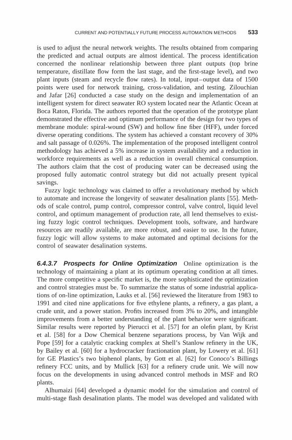
CURRENT AND POTENTIALLY FUTURE PROCESS AUTOMATION METHODS 533

is used to adjust the neural network weights. The results obtained from comparingthe predicted and actual outputs are almost identical. The process identificationconcerned the nonlinear relationship between three plant outputs (top brinetemperature, distillate flow form the last stage, and the first-stage level), and twoplant inputs (steam and recycle flow rates). In total, input–output data of 1500points were used for network training, cross-validation, and testing. Zilouchianand Jafar [26] conducted a case study on the design and implementation of anintelligent system for direct seawater RO system located near the Atlantic Ocean atBoca Raton, Florida. The authors reported that the operation of the prototype plantdemonstrated the effective and optimum performance of the design for two types ofmembrane module: spiral-wound (SW) and hollow fine fiber (HFF), under forceddiverse operating conditions. The system has achieved a constant recovery of 30%and salt passage of 0.026%. The implementation of the proposed intelligent controlmethodology has achieved a 5% increase in system availability and a reduction inworkforce requirements as well as a reduction in overall chemical consumption.The authors claim that the cost of producing water can be decreased using theproposed fully automatic control strategy but did not actually present typicalsavings.

Fuzzy logic technology was claimed to offer a revolutionary method by whichto automate and increase the longevity of seawater desalination plants [55]. Meth-ods of scale control, pump control, compressor control, valve control, liquid levelcontrol, and optimum management of production rate, all lend themselves to exist-ing fuzzy logic control techniques. Development tools, software, and hardwareresources are readily available, are more robust, and easier to use. In the future,fuzzy logic will allow systems to make automated and optimal decisions for thecontrol of seawater desalination systems.

6.4.3.7 Prospects for Online Optimization Online optimization is thetechnology of maintaining a plant at its optimum operating condition at all times.The more competitive a specific market is, the more sophisticated the optimizationand control strategies must be. To summarize the status of some industrial applica-tions of on-line optimization, Lauks et al. [56] reviewed the literature from 1983 to1991 and cited nine applications for five ethylene plants, a refinery, a gas plant, acrude unit, and a power station. Profits increased from 3% to 20%, and intangibleimprovements from a better understanding of the plant behavior were significant.Similar results were reported by Pierucci et al. [57] for an olefin plant, by Kristet al. [58] for a Dow Chemical benzene separations process, by Van Wijk andPope [59] for a catalytic cracking complex at Shell’s Stanlow refinery in the UK,by Bailey et al. [60] for a hydrocracker fractionation plant, by Lowery et al. [61]for GE Plastics’s two biphenol plants, by Gott et al. [62] for Conoco’s Billingsrefinery FCC units, and by Mullick [63] for a refinery crude unit. We will nowfocus on the developments in using advanced control methods in MSF and ROplants.

Alhumaizi [64] developed a dynamic model for the simulation and control ofmulti-stage flash desalination plants. The model was developed and validated with

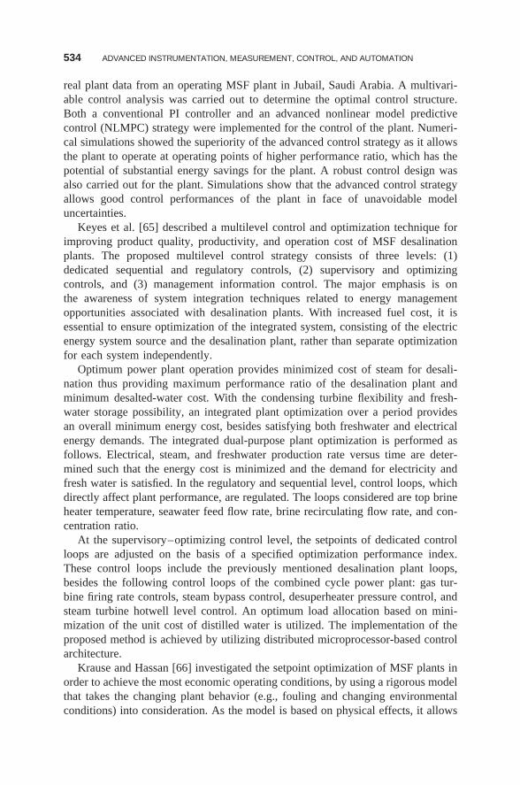
534 ADVANCED INSTRUMENTATION, MEASUREMENT, CONTROL, AND AUTOMATION

real plant data from an operating MSF plant in Jubail, Saudi Arabia. A multivari-able control analysis was carried out to determine the optimal control structure.Both a conventional PI controller and an advanced nonlinear model predictivecontrol (NLMPC) strategy were implemented for the control of the plant. Numeri-cal simulations showed the superiority of the advanced control strategy as it allowsthe plant to operate at operating points of higher performance ratio, which has thepotential of substantial energy savings for the plant. A robust control design wasalso carried out for the plant. Simulations show that the advanced control strategyallows good control performances of the plant in face of unavoidable modeluncertainties.

Keyes et al. [65] described a multilevel control and optimization technique forimproving product quality, productivity, and operation cost of MSF desalinationplants. The proposed multilevel control strategy consists of three levels: (1)dedicated sequential and regulatory controls, (2) supervisory and optimizingcontrols, and (3) management information control. The major emphasis is onthe awareness of system integration techniques related to energy managementopportunities associated with desalination plants. With increased fuel cost, it isessential to ensure optimization of the integrated system, consisting of the electricenergy system source and the desalination plant, rather than separate optimizationfor each system independently.

Optimum power plant operation provides minimized cost of steam for desali-nation thus providing maximum performance ratio of the desalination plant andminimum desalted-water cost. With the condensing turbine flexibility and fresh-water storage possibility, an integrated plant optimization over a period providesan overall minimum energy cost, besides satisfying both freshwater and electricalenergy demands. The integrated dual-purpose plant optimization is performed asfollows. Electrical, steam, and freshwater production rate versus time are deter-mined such that the energy cost is minimized and the demand for electricity andfresh water is satisfied. In the regulatory and sequential level, control loops, whichdirectly affect plant performance, are regulated. The loops considered are top brineheater temperature, seawater feed flow rate, brine recirculating flow rate, and con-centration ratio.

At the supervisory–optimizing control level, the setpoints of dedicated controlloops are adjusted on the basis of a specified optimization performance index.These control loops include the previously mentioned desalination plant loops,besides the following control loops of the combined cycle power plant: gas tur-bine firing rate controls, steam bypass control, desuperheater pressure control, andsteam turbine hotwell level control. An optimum load allocation based on mini-mization of the unit cost of distilled water is utilized. The implementation of theproposed method is achieved by utilizing distributed microprocessor-based controlarchitecture.

Krause and Hassan [66] investigated the setpoint optimization of MSF plants inorder to achieve the most economic operating conditions, by using a rigorous modelthat takes the changing plant behavior (e.g., fouling and changing environmentalconditions) into consideration. As the model is based on physical effects, it allows

CURRENT AND POTENTIALLY FUTURE PROCESS AUTOMATION METHODS 535

the determination of the plant behavior from the physical and geometrical data ofthe plant, thus permitting it to modify and optimize the plant layout during theplanning phase. Consultants and manufacturers will use the optimization strategybased on rigorous models online either during operation or offline during the plan-ning phase. During operation, the geometric data of the plant remain constant, butthe environmental conditions will change. These, together with the restrictions thatare imposed on the process (maximum temperatures, chemical dosing, restrictedsteam production, etc.), are also taken into account by the model, and the optimalsetpoints are calculated accordingly. In order to follow up the real plant behav-ior, it is necessary to determine the changes imposed by, for example, fouling.This is achieved by calculating the changed heat transfer coefficients. Anothermodule accommodates of the measurement errors and tries to minimize theireffects.

It was shown how the above-described tasks are implemented in the distributedcontrol systems manufactured by Hartmann & Braun and which tools are avail-able for consultants and manufacturers to support their evaluation work during theplanning phase.

6.4.4 Conclusions and Recommendations on Potential of FutureIMCA Systems

Conclusions and guidelines are as follows:

1. The level of automation in the last generation of MSF plants is very high tothe extent that it brings up increasing concerns related to the deskilling ofMSF plant operators.

2. Full automation of the startup–shutdown sequence is desirable but has so farbeen implemented in only one plant.

3. Modification in the control schemes that affect reductions in exergy (or justpressure) losses in the plant should to be explored, and an example of sucha proposed scheme to control the top brine temperature in MSF plants wasgiven.

4. Automation to control fouling is an important proposed approach.5. The process step that has potential for significant improvement by applying

smart automation is the pretreatment of the feed water, especially in RO.6. In RO, implementation of automation of the recovery and flux rate combi-

nation, instead of the conventional method of maintaining constant flux, isrecommended for potential reduction of the operating cost.

7. From the various advanced control methods considered, the use of constrainedmodel predictive controllers (CMPCs) appears to be promising for implemen-tation.

8. Automation as online optimization is highly desirable, but adequatemathematical dynamical models of the process are as yet unavailable toimplement it.

536 ADVANCED INSTRUMENTATION, MEASUREMENT, CONTROL, AND AUTOMATION

6.5 CALCULATION OF IMPACT OF AUTOMATION ON PRODUCTWATER COST

6.5.1 Introduction

Automation is intended to simplify plant operation and optimize its performance,while maintaining safety. Performance optimization includes the minimization ofoperating expenses (energy, chemicals, labor, etc.) and maximization of availabil-ity. The general issue of instrumentation, measurements, control, and automation(IMCA) has three major impacts on produced water cost:

1. The sophistication level of automation that should be implemented to increasecontrol accuracy and optimize plant performance

2. Some areas in which the IMCA philosophy should be changed

3. Process aspects that have not been automated yet but probably should be

It is obvious that automation is, from a fundamental viewpoint, not a vital com-ponent of a desalination plant since the plant can produce water even with purelymanual control, so consequently any level of automation, or generally IMCA, mustthus be economically justified. That justification must also include the consider-ation of IMCA system reliability, which would manifest itself in any changes inplant availability that may take place when the intended IMCA system would beimplemented.

As opposed to the enormous amount of published information on control systemsand their advancement, those on cost–benefit analysis of their implementation arevery few in general [67,68], and, except for a paper by the authors [69], nearlynonexistent for desalination plants in particular. Some introductory comments onthe subject including citations to available papers are therefore presented below.

A systematic approach to the problem was proposed by Martin et al. [70],presenting seven industrial sample cases. The first step in such a cost–benefitanalysis is to identify the process variables, which affect the process parameters thatcarry the highest potential economic benefit [71], and that can, in fact, be changedin the desired direction by the application of improved controls. For example, indistillation desalination processes, raising the top brine temperature will reducethe specific-energy consumption, but should not be done because of scaling thattakes place at the higher temperatures. Nevertheless, the constraints that might limitbenefits must be carefully challenged before their acceptance. The base-case systemand operation, existing before the IMCA system improvements are made, must alsobe clearly defined, based on existing data. It is important at this point to note thatthe conventional control scheme was to just aim at keeping a variable close to atarget value, yet a more rewarding scheme is to keep the variables within certainlimits that accomplish a desired final objective, such as, maximizing throughput,quality, or profit, under varying operating and economic circumstances.

The next step is to establish the relationship between the variation of this param-eter and the resulting economic benefit. The latter is the product of this variation

CALCULATION OF IMPACT OF AUTOMATION ON PRODUCT WATER COST 537

and its economic sensitivity factor. This is then repeated for each control function,taking care not to ignore possible parameter interactions.

The significant parameters and their relation to the process performance can bedetermined by proper mathematical modeling of the process, or when the modelingis insufficiently accurate, or absent altogether, by examining the actual operatingdata over a long enough period. Because of the inherent fluctuations of the data,statistical methods should be used to extract the information that is significant[70,72]. For some simple steady-state systems, Contreras-Dordelly and Martin [73]have developed a method for selecting the control system yielding the higheststeady-state operation profit from among candidate multiloop designs, taking intoaccount disturbances and model mismatch.

Historical operating data of a plant are akin to a gold mine, which can be minedfor information useful for improving plant performance and safety. If examinedand correlated carefully to show trends of the significant performance parameters,such as production rate, quality of product, energy and chemical consumption,and fouling, as a function of the process variables, they could teach us aboutthe influences of process variables that perhaps could not have been predictedby intuition or even modeling. Analyzing the data can lead to conclusions aboutthe need for additional or different instrumentation, for different control methods,or changes in the process. In some examples from various process plants, it wasshown [74] that such analysis has had an excellent cost–benefit ratio, where inone example it resulted in savings of $35,000 per month at the one-time expenseof only $21,000 for the addition of certain instruments and control procedures.Since larger plants use computers anyway, all the relevant data can be stored forstatistical analysis and correlation. Such programs are relatively easy to implementand run automatically at desired periods.

Theoretical predictions of utility of IMCA schemes must eventually be put to thetest in an operating plant. The test should assess the system functionality, as wellas its economic promise. The latter is especially difficult in view of fluctuationsand changes in operation inherent with any real plant and control scheme, whichmay be larger than the examined sought outcome, but good statistical analysis isable to extract the desired information, as shown in the literature [67,70,75–77],presenting an approach that attempts to permit the calculation of the important issueof simultaneous impact of process dynamics, model uncertainty, and controllercomplexity on the process economics. A benchmarking questionnaire, including asimple statistical tool for evaluation of benefits, sent to plant owners/operators todetermine whether the plant has good potential for benefits from improved processcontrol (“Should I invest in improved process control”?) was developed and testedby Lant and Steffens [78].

The above-described analysis of cost–benefit ratios of IMCA systems consideronly the direct economic gains resulting from operating closer to the optimal pointthat gives the desired product yield and quality. It is important to note, however, thatoperating with tighter tolerances near the optimal point, for example, by reducingfluctuations near the setpoint and/or moving the setpoint closer to the specifications,while often considered unnecessary trouble, may have benefits that even exceed

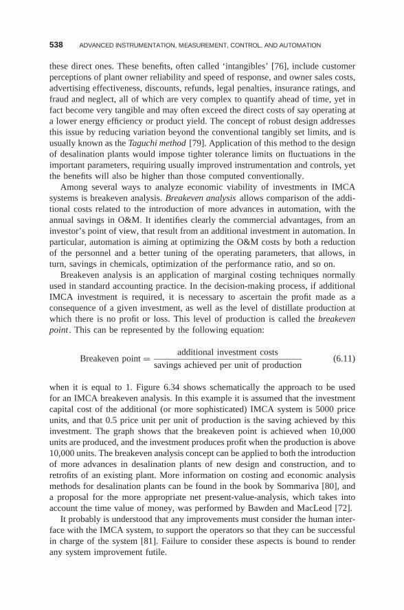
538 ADVANCED INSTRUMENTATION, MEASUREMENT, CONTROL, AND AUTOMATION

these direct ones. These benefits, often called ‘intangibles’ [76], include customerperceptions of plant owner reliability and speed of response, and owner sales costs,advertising effectiveness, discounts, refunds, legal penalties, insurance ratings, andfraud and neglect, all of which are very complex to quantify ahead of time, yet infact become very tangible and may often exceed the direct costs of say operating ata lower energy efficiency or product yield. The concept of robust design addressesthis issue by reducing variation beyond the conventional tangibly set limits, and isusually known as the Taguchi method [79]. Application of this method to the designof desalination plants would impose tighter tolerance limits on fluctuations in theimportant parameters, requiring usually improved instrumentation and controls, yetthe benefits will also be higher than those computed conventionally.

Among several ways to analyze economic viability of investments in IMCAsystems is breakeven analysis. Breakeven analysis allows comparison of the addi-tional costs related to the introduction of more advances in automation, with theannual savings in O&M. It identifies clearly the commercial advantages, from aninvestor’s point of view, that result from an additional investment in automation. Inparticular, automation is aiming at optimizing the O&M costs by both a reductionof the personnel and a better tuning of the operating parameters, that allows, inturn, savings in chemicals, optimization of the performance ratio, and so on.

Breakeven analysis is an application of marginal costing techniques normallyused in standard accounting practice. In the decision-making process, if additionalIMCA investment is required, it is necessary to ascertain the profit made as aconsequence of a given investment, as well as the level of distillate production atwhich there is no profit or loss. This level of production is called the breakevenpoint . This can be represented by the following equation:

Breakeven point = additional investment costs

savings achieved per unit of production(6.11)

when it is equal to 1. Figure 6.34 shows schematically the approach to be usedfor an IMCA breakeven analysis. In this example it is assumed that the investmentcapital cost of the additional (or more sophisticated) IMCA system is 5000 priceunits, and that 0.5 price unit per unit of production is the saving achieved by thisinvestment. The graph shows that the breakeven point is achieved when 10,000units are produced, and the investment produces profit when the production is above10,000 units. The breakeven analysis concept can be applied to both the introductionof more advances in desalination plants of new design and construction, and toretrofits of an existing plant. More information on costing and economic analysismethods for desalination plants can be found in the book by Sommariva [80], anda proposal for the more appropriate net present-value-analysis, which takes intoaccount the time value of money, was performed by Bawden and MacLeod [72].

It probably is understood that any improvements must consider the human inter-face with the IMCA system, to support the operators so that they can be successfulin charge of the system [81]. Failure to consider these aspects is bound to renderany system improvement futile.

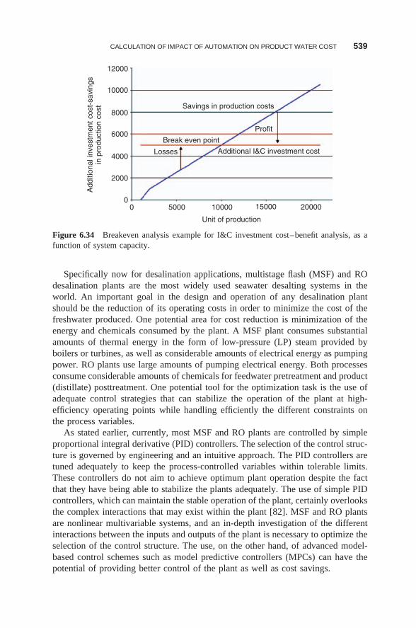
CALCULATION OF IMPACT OF AUTOMATION ON PRODUCT WATER COST 539

00

2000

4000Losses

Break even point

Additional I&C investment cost

Profit

Savings in production costs

6000

8000

10000

12000

5000 10000

Unit of production

Add

ition

al in

vest

men

t cos

t-sa

ving

sin

pro

duct

ion

cost

15000 20000

Figure 6.34 Breakeven analysis example for I&C investment cost–benefit analysis, as afunction of system capacity.

Specifically now for desalination applications, multistage flash (MSF) and ROdesalination plants are the most widely used seawater desalting systems in theworld. An important goal in the design and operation of any desalination plantshould be the reduction of its operating costs in order to minimize the cost of thefreshwater produced. One potential area for cost reduction is minimization of theenergy and chemicals consumed by the plant. A MSF plant consumes substantialamounts of thermal energy in the form of low-pressure (LP) steam provided byboilers or turbines, as well as considerable amounts of electrical energy as pumpingpower. RO plants use large amounts of pumping electrical energy. Both processesconsume considerable amounts of chemicals for feedwater pretreatment and product(distillate) posttreatment. One potential tool for the optimization task is the use ofadequate control strategies that can stabilize the operation of the plant at high-efficiency operating points while handling efficiently the different constraints onthe process variables.

As stated earlier, currently, most MSF and RO plants are controlled by simpleproportional integral derivative (PID) controllers. The selection of the control struc-ture is governed by engineering and an intuitive approach. The PID controllers aretuned adequately to keep the process-controlled variables within tolerable limits.These controllers do not aim to achieve optimum plant operation despite the factthat they have being able to stabilize the plants adequately. The use of simple PIDcontrollers, which can maintain the stable operation of the plant, certainly overlooksthe complex interactions that may exist within the plant [82]. MSF and RO plantsare nonlinear multivariable systems, and an in-depth investigation of the differentinteractions between the inputs and outputs of the plant is necessary to optimize theselection of the control structure. The use, on the other hand, of advanced model-based control schemes such as model predictive controllers (MPCs) can have thepotential of providing better control of the plant as well as cost savings.

540 ADVANCED INSTRUMENTATION, MEASUREMENT, CONTROL, AND AUTOMATION

An advanced process control project in the desalination industry (MSF and ROprocesses) typically includes the installation of microprocessor-based distributedcontrol system instrumentation, a supervisory computer, and implementation ofsophisticated advanced control software for process control and optimization. Inan oil refinery or petrochemical plant, such a project would cost somewhere inthe range $1,000,000–$5,000,000 in 1991 dollars [70]. An economic justifica-tion is therefore essential for the approval of such a project, which is the IMCAcost–benefit ratio introduced at the beginning of this section.

The current study includes the first and predominant step in an economic fea-sibility of using advanced control to retrofit existing conventional PID controllers.The aim of this study is to evaluate the potential savings in the major operatingcomponents, namely, electrical energy, heating steam and chemical additives. Obvi-ously, the operating cost involves other components such as administration, spareparts, operating and maintenance personnel, and insurance. These components arenot included in the present study and should be included in a larger investigation.

All of the economics-related results shown in this chapter are based on costs ofmaterials, energy, equipment, labor, etc., that existed at the time the studies wereconducted, and some well before the date of publication of this chapter. Since thesecosts vary with time, sometimes significantly, readers of this chapter who wish toconduct economic analyses would naturally have to update the costs. The emphasisin our analysis is on methodology, not on actual value magnitudes, which are time-and case-dependent.

6.5.2 Rigorous and Detailed Estimation of Economic Benefitsfrom Advanced Process Control

6.5.2.1 General Approach Advanced process control is a service available toplant operators, helping them improve the performance of the process. The primaryobjective of an advanced control system is to maximize profits by operating theprocess at its optimum point while satisfying criteria such as safety, environmentalregulations, product specifications, and operational constraints. Advanced processcontrol, therefore, aims to deliver higher plant performance than conventional con-trol. Most desalination processes must follow a given target during operation andthey have to follow this target as closely as possible despite the continued presenceof disturbances. These targets are seen as the optimal values of the controlled vari-ables. Every deviation from the optimal values on either side results in some kindof economic loss or cost penalty. The variance of the variable in question has tobe reduced. Performance is related to the magnitude of the variations of a certainvariable or property around the target. The more we can reduce the variance, thesmaller is the cost penalty. It is important to note that performance optimizationalso includes the management of transient conditions and load changes as well asstartup sequences to maintain and increase plant life time and reduce corrosion.

Estimating the quantitative economic benefit from advanced process controlbegins by determining the base operation. This operation is characterized by pro-cess data that are collected during a period of typical closed-loop operation with

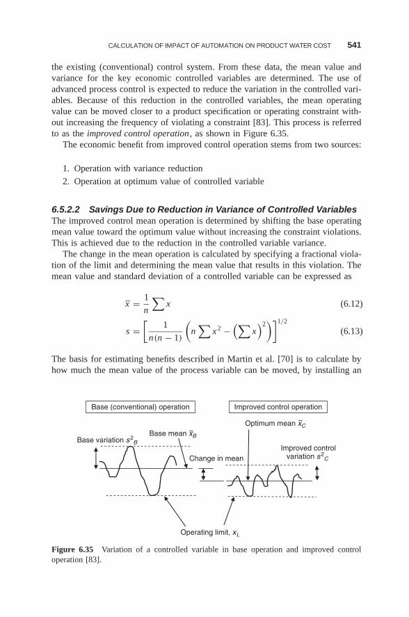
CALCULATION OF IMPACT OF AUTOMATION ON PRODUCT WATER COST 541

the existing (conventional) control system. From these data, the mean value andvariance for the key economic controlled variables are determined. The use ofadvanced process control is expected to reduce the variation in the controlled vari-ables. Because of this reduction in the controlled variables, the mean operatingvalue can be moved closer to a product specification or operating constraint with-out increasing the frequency of violating a constraint [83]. This process is referredto as the improved control operation , as shown in Figure 6.35.

The economic benefit from improved control operation stems from two sources:

1. Operation with variance reduction

2. Operation at optimum value of controlled variable

6.5.2.2 Savings Due to Reduction in Variance of Controlled VariablesThe improved control mean operation is determined by shifting the base operatingmean value toward the optimum value without increasing the constraint violations.This is achieved due to the reduction in the controlled variable variance.

The change in the mean operation is calculated by specifying a fractional viola-tion of the limit and determining the mean value that results in this violation. Themean value and standard deviation of a controlled variable can be expressed as

x = 1

n

∑x (6.12)

s =[

1

n(n − 1)

(n

∑x2 −

(∑x)2

)]1/2

(6.13)

The basis for estimating benefits described in Martin et al. [70] is to calculate byhow much the mean value of the process variable can be moved, by installing an

Optimum mean xC

Base variation s2B

Improved controlvariation s2

C

Operating limit, xL

Base (conventional) operation Improved control operation

Change in mean

Base mean xB

Figure 6.35 Variation of a controlled variable in base operation and improved controloperation [83].

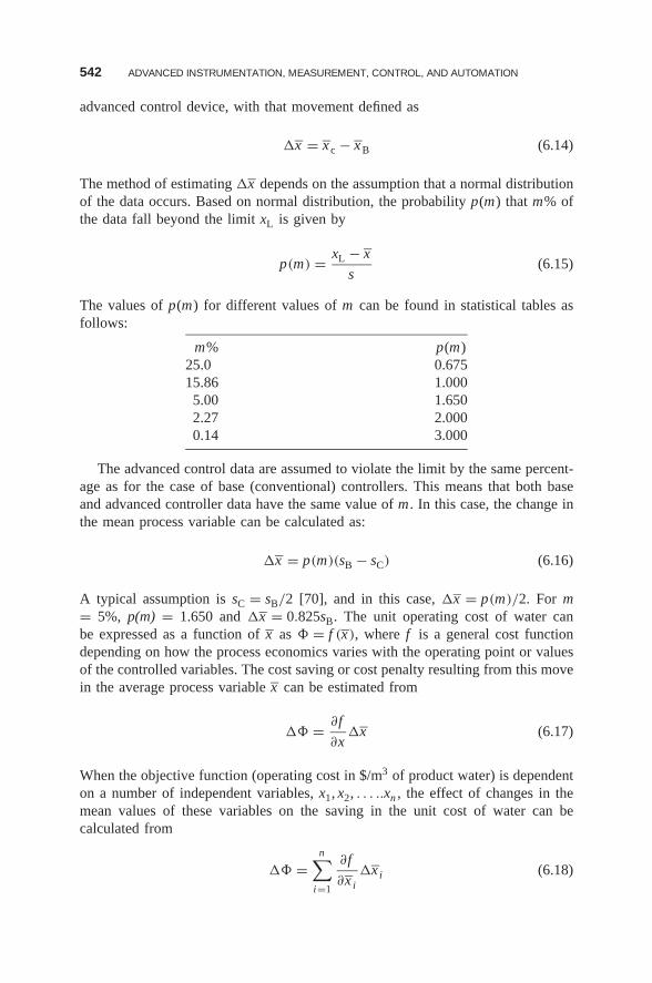
542 ADVANCED INSTRUMENTATION, MEASUREMENT, CONTROL, AND AUTOMATION

advanced control device, with that movement defined as

�x = x c − xB (6.14)

The method of estimating �x depends on the assumption that a normal distributionof the data occurs. Based on normal distribution, the probability p(m) that m% ofthe data fall beyond the limit xL is given by

p(m) = xL − x

s(6.15)

The values of p(m) for different values of m can be found in statistical tables asfollows:

m% p(m)25.0 0.67515.86 1.0005.00 1.6502.27 2.0000.14 3.000

The advanced control data are assumed to violate the limit by the same percent-age as for the case of base (conventional) controllers. This means that both baseand advanced controller data have the same value of m . In this case, the change inthe mean process variable can be calculated as:

�x = p(m)(sB − sC) (6.16)

A typical assumption is sC = sB/2 [70], and in this case, �x = p(m)/2. For m= 5%, p(m) = 1.650 and �x = 0.825sB. The unit operating cost of water canbe expressed as a function of x as � = f (x), where f is a general cost functiondepending on how the process economics varies with the operating point or valuesof the controlled variables. The cost saving or cost penalty resulting from this movein the average process variable x can be estimated from

�� = ∂f

∂x�x (6.17)

When the objective function (operating cost in $/m3 of product water) is dependenton a number of independent variables, x1, x2, . . . ..xn , the effect of changes in themean values of these variables on the saving in the unit cost of water can becalculated from

�� =n∑

i=1

∂f

∂x i�x i (6.18)

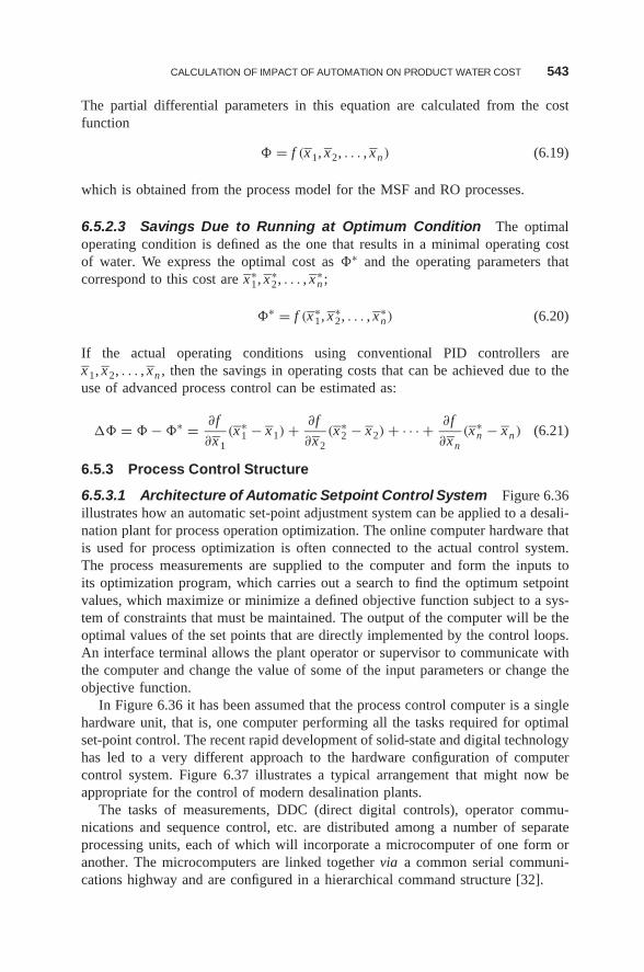
CALCULATION OF IMPACT OF AUTOMATION ON PRODUCT WATER COST 543

The partial differential parameters in this equation are calculated from the costfunction

� = f (x1, x2, . . . , xn) (6.19)

which is obtained from the process model for the MSF and RO processes.

6.5.2.3 Savings Due to Running at Optimum Condition The optimaloperating condition is defined as the one that results in a minimal operating costof water. We express the optimal cost as �∗ and the operating parameters thatcorrespond to this cost are x∗

1, x∗2, . . . , x∗

n ;

�∗ = f (x∗1, x∗

2, . . . , x∗n) (6.20)

If the actual operating conditions using conventional PID controllers arex1, x2, . . . , xn , then the savings in operating costs that can be achieved due to theuse of advanced process control can be estimated as:

�� = � − �∗ = ∂f

∂x1(x∗

1 − x1) + ∂f

∂x2(x∗

2 − x2) + · · · + ∂f

∂xn(x∗

n − xn) (6.21)

6.5.3 Process Control Structure

6.5.3.1 Architecture of Automatic Setpoint Control System Figure 6.36illustrates how an automatic set-point adjustment system can be applied to a desali-nation plant for process operation optimization. The online computer hardware thatis used for process optimization is often connected to the actual control system.The process measurements are supplied to the computer and form the inputs toits optimization program, which carries out a search to find the optimum setpointvalues, which maximize or minimize a defined objective function subject to a sys-tem of constraints that must be maintained. The output of the computer will be theoptimal values of the set points that are directly implemented by the control loops.An interface terminal allows the plant operator or supervisor to communicate withthe computer and change the value of some of the input parameters or change theobjective function.

In Figure 6.36 it has been assumed that the process control computer is a singlehardware unit, that is, one computer performing all the tasks required for optimalset-point control. The recent rapid development of solid-state and digital technologyhas led to a very different approach to the hardware configuration of computercontrol system. Figure 6.37 illustrates a typical arrangement that might now beappropriate for the control of modern desalination plants.

The tasks of measurements, DDC (direct digital controls), operator commu-nications and sequence control, etc. are distributed among a number of separateprocessing units, each of which will incorporate a microcomputer of one form oranother. The microcomputers are linked together via a common serial communi-cations highway and are configured in a hierarchical command structure [32].

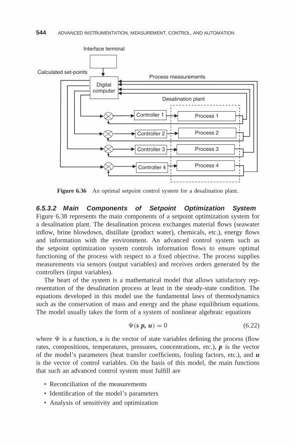
544 ADVANCED INSTRUMENTATION, MEASUREMENT, CONTROL, AND AUTOMATION

Interface terminal

Digitalcomputer

Process 1

Process 2

Process 3

Process 4

Controller 1

Controller 2

Controller 3

Calculated set-points

Desalination plant

Process measurements

Controller 4

Figure 6.36 An optimal setpoint control system for a desalination plant.

6.5.3.2 Main Components of Setpoint Optimization SystemFigure 6.38 represents the main components of a setpoint optimization system fora desalination plant. The desalination process exchanges material flows (seawaterinflow, brine blowdown, distillate (product water), chemicals, etc.), energy flowsand information with the environment. An advanced control system such asthe setpoint optimization system controls information flows to ensure optimalfunctioning of the process with respect to a fixed objective. The process suppliesmeasurements via sensors (output variables) and receives orders generated by thecontrollers (input variables).

The heart of the system is a mathematical model that allows satisfactory rep-resentation of the desalination process at least in the steady-state condition. Theequations developed in this model use the fundamental laws of thermodynamicssuch as the conservation of mass and energy and the phase equilibrium equations.The model usually takes the form of a system of nonlinear algebraic equations

�(s p, u) = 0 (6.22)

where � is a function, s is the vector of state variables defining the process (flowrates, compositions, temperatures, pressures, concentrations, etc.), p is the vectorof the model’s parameters (heat transfer coefficients, fouling factors, etc.), and uis the vector of control variables. On the basis of this model, the main functionsthat such an advanced control system must fulfill are

• Reconciliation of the measurements

• Identification of the model’s parameters

• Analysis of sensitivity and optimization

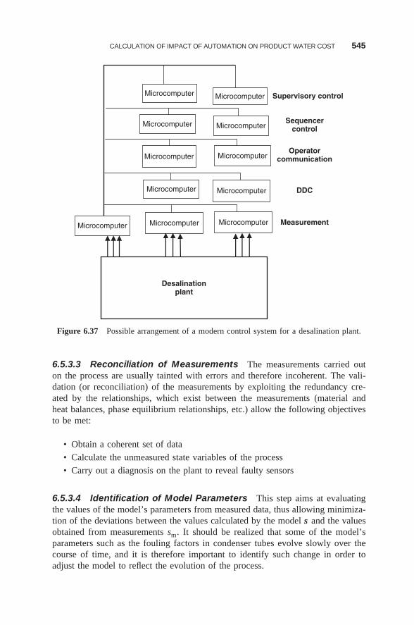
CALCULATION OF IMPACT OF AUTOMATION ON PRODUCT WATER COST 545

Microcomputer Microcomputer

Microcomputer Microcomputer

Microcomputer Microcomputer

Microcomputer Microcomputer

Microcomputer MicrocomputerMicrocomputer

Desalinationplant

Measurement

DDC

Operatorcommunication

Sequencercontrol

Supervisory control

Figure 6.37 Possible arrangement of a modern control system for a desalination plant.

6.5.3.3 Reconciliation of Measurements The measurements carried outon the process are usually tainted with errors and therefore incoherent. The vali-dation (or reconciliation) of the measurements by exploiting the redundancy cre-ated by the relationships, which exist between the measurements (material andheat balances, phase equilibrium relationships, etc.) allow the following objectivesto be met:

• Obtain a coherent set of data

• Calculate the unmeasured state variables of the process

• Carry out a diagnosis on the plant to reveal faulty sensors

6.5.3.4 Identification of Model Parameters This step aims at evaluatingthe values of the model’s parameters from measured data, thus allowing minimiza-tion of the deviations between the values calculated by the model s and the valuesobtained from measurements sm. It should be realized that some of the model’sparameters such as the fouling factors in condenser tubes evolve slowly over thecourse of time, and it is therefore important to identify such change in order toadjust the model to reflect the evolution of the process.

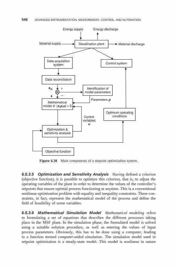
546 ADVANCED INSTRUMENTATION, MEASUREMENT, CONTROL, AND AUTOMATION

Desalination plant

Data acquisitionsystem

Mathematicalmodel Y (s,p,u) = 0

Optimization &sensitivity analysis

Objective function

Optimum operatingconditions

Identification ofmodel parameters

Control system

Data reconciliation

Material supply

Energy supply Energy discharge

Material discharge

Parameters p

Controlvariables

u

s

sm +

–

Figure 6.38 Main components of a setpoint optimization system.

6.5.3.5 Optimization and Sensitivity Analysis Having defined a criterion(objective function), it is possible to optimize this criterion, that is, to adjust theoperating variables of the plant in order to determine the values of the controller’ssetpoints that ensure optimal process functioning at anytime. This is a conventionalnonlinear optimization problem with equality and inequality constraints. These con-straints, in fact, represent the mathematical model of the process and define thefield of feasibility of some variables.

6.5.3.6 Mathematical Simulation Model Mathematical modeling refersto formulating a set of equations that describes the different processes takingplace in the MSF plant. In the simulation phase, the formulated model is solvedusing a suitable solution procedure, as well as entering the values of inputprocess parameters. Obviously, this has to be done using a computer, leadingto a function termed computer-aided simulation . The simulation model used insetpoint optimization is a steady-state model. This model is nonlinear in nature

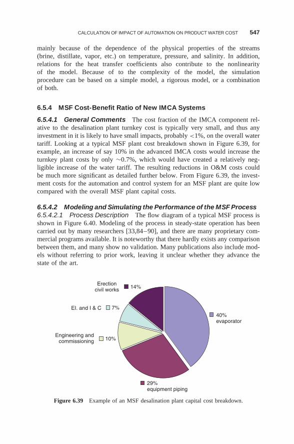
CALCULATION OF IMPACT OF AUTOMATION ON PRODUCT WATER COST 547

mainly because of the dependence of the physical properties of the streams(brine, distillate, vapor, etc.) on temperature, pressure, and salinity. In addition,relations for the heat transfer coefficients also contribute to the nonlinearityof the model. Because of to the complexity of the model, the simulationprocedure can be based on a simple model, a rigorous model, or a combinationof both.

6.5.4 MSF Cost-Benefit Ratio of New IMCA Systems

6.5.4.1 General Comments The cost fraction of the IMCA component rel-ative to the desalination plant turnkey cost is typically very small, and thus anyinvestment in it is likely to have small impacts, probably <1%, on the overall watertariff. Looking at a typical MSF plant cost breakdown shown in Figure 6.39, forexample, an increase of say 10% in the advanced IMCA costs would increase theturnkey plant costs by only ∼0.7%, which would have created a relatively neg-ligible increase of the water tariff. The resulting reductions in O&M costs couldbe much more significant as detailed further below. From Figure 6.39, the invest-ment costs for the automation and control system for an MSF plant are quite lowcompared with the overall MSF plant capital costs.

6.5.4.2 Modeling and Simulating the Performance of the MSF Process6.5.4.2.1 Process Description The flow diagram of a typical MSF process isshown in Figure 6.40. Modeling of the process in steady-state operation has beencarried out by many researchers [33,84–90], and there are many proprietary com-mercial programs available. It is noteworthy that there hardly exists any comparisonbetween them, and many show no validation. Many publications also include mod-els without referring to prior work, leaving it unclear whether they advance thestate of the art.

40%evaporator

29%equipment piping

Engineering andcommissioning

EI. and I & C

Erectioncivil works

10%

7%

14%

Figure 6.39 Example of an MSF desalination plant capital cost breakdown.

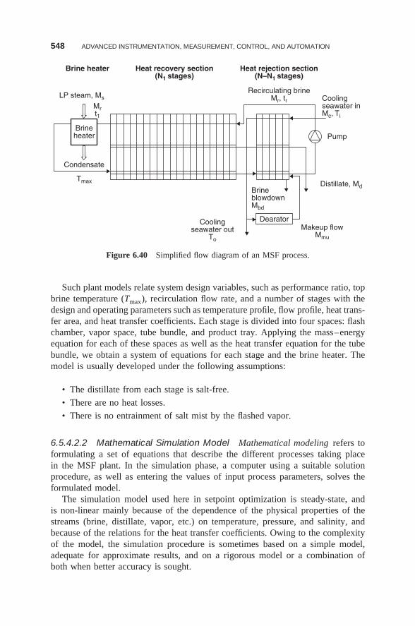
548 ADVANCED INSTRUMENTATION, MEASUREMENT, CONTROL, AND AUTOMATION

Brineheater

Brine heater Heat rejection section(N–N1 stages)

Recirculating brineMr, tr

Heat recovery section(N1 stages)

Condensate

Tmax

LP steam, Ms

Mrt1

Distillate, Md

Dearator

Pump

Coolingseawater out

To

Coolingseawater inMc, Ti

BrineblowdownMbd

Makeup flowMmu

Figure 6.40 Simplified flow diagram of an MSF process.

Such plant models relate system design variables, such as performance ratio, topbrine temperature (Tmax), recirculation flow rate, and a number of stages with thedesign and operating parameters such as temperature profile, flow profile, heat trans-fer area, and heat transfer coefficients. Each stage is divided into four spaces: flashchamber, vapor space, tube bundle, and product tray. Applying the mass–energyequation for each of these spaces as well as the heat transfer equation for the tubebundle, we obtain a system of equations for each stage and the brine heater. Themodel is usually developed under the following assumptions:

• The distillate from each stage is salt-free.

• There are no heat losses.

• There is no entrainment of salt mist by the flashed vapor.

6.5.4.2.2 Mathematical Simulation Model Mathematical modeling refers toformulating a set of equations that describe the different processes taking placein the MSF plant. In the simulation phase, a computer using a suitable solutionprocedure, as well as entering the values of input process parameters, solves theformulated model.

The simulation model used here in setpoint optimization is steady-state, andis non-linear mainly because of the dependence of the physical properties of thestreams (brine, distillate, vapor, etc.) on temperature, pressure, and salinity, andbecause of the relations for the heat transfer coefficients. Owing to the complexityof the model, the simulation procedure is sometimes based on a simple model,adequate for approximate results, and on a rigorous model or a combination ofboth when better accuracy is sought.

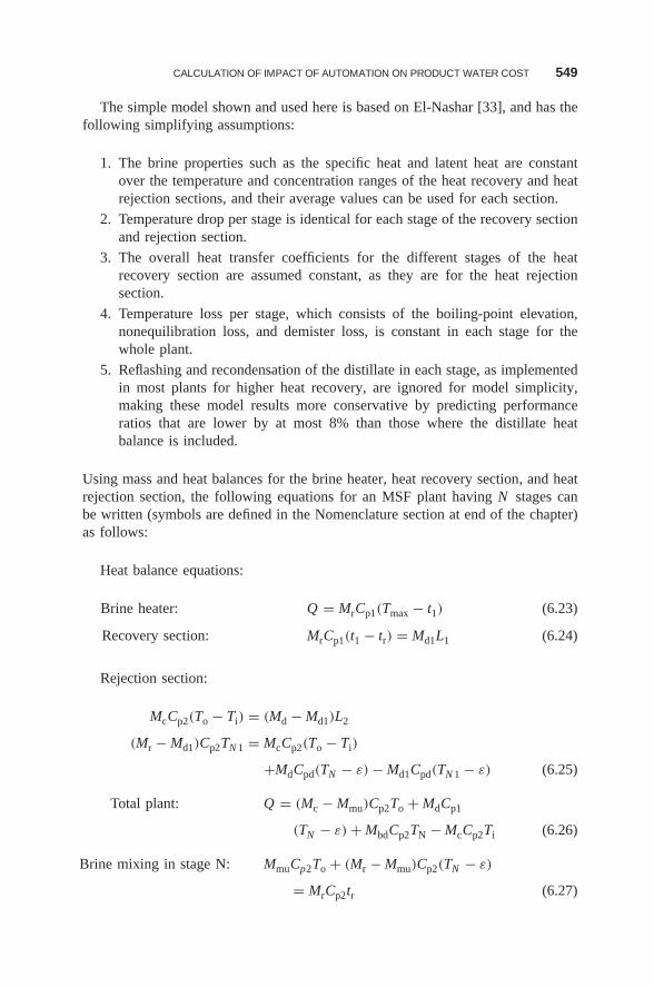
CALCULATION OF IMPACT OF AUTOMATION ON PRODUCT WATER COST 549

The simple model shown and used here is based on El-Nashar [33], and has thefollowing simplifying assumptions:

1. The brine properties such as the specific heat and latent heat are constantover the temperature and concentration ranges of the heat recovery and heatrejection sections, and their average values can be used for each section.

2. Temperature drop per stage is identical for each stage of the recovery sectionand rejection section.

3. The overall heat transfer coefficients for the different stages of the heatrecovery section are assumed constant, as they are for the heat rejectionsection.

4. Temperature loss per stage, which consists of the boiling-point elevation,nonequilibration loss, and demister loss, is constant in each stage for thewhole plant.

5. Reflashing and recondensation of the distillate in each stage, as implementedin most plants for higher heat recovery, are ignored for model simplicity,making these model results more conservative by predicting performanceratios that are lower by at most 8% than those where the distillate heatbalance is included.

Using mass and heat balances for the brine heater, heat recovery section, and heatrejection section, the following equations for an MSF plant having N stages canbe written (symbols are defined in the Nomenclature section at end of the chapter)as follows:

Heat balance equations:

Brine heater: Q = MrCp1(Tmax − t1) (6.23)

Recovery section: MrCp1(t1 − tr) = Md1L1 (6.24)

Rejection section:

McCp2(To − Ti) = (Md − Md1)L2

(Mr − Md1)Cp2TN 1 = McCp2(To − Ti)

+MdCpd(TN − ε) − Md1Cpd(TN 1 − ε) (6.25)

Total plant: Q = (Mc − Mmu)Cp2To + MdCp1

(TN − ε) + MbdCp2TN − McCp2Ti (6.26)

Brine mixing in stage N: MmuCp2To + (Mr − Mmu)Cp2(TN − ε)

= MrCp2tr (6.27)

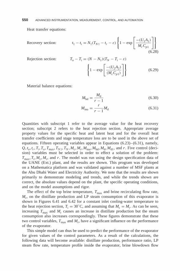
550 ADVANCED INSTRUMENTATION, MEASUREMENT, CONTROL, AND AUTOMATION

Heat transfer equations:

Recovery section: t1 − tr = N1(TN 1 − tr − ε)

{1 − exp

[−(U1A1)

MrCp1

]}

(6.28)

Rejection section: To − Ti = (N − N1)(TN − Ti − ε){1 − exp

[−(U2A2)

(McCp1)

]}(6.29)

Material balance equations:

Mbd = Md

r − 1(6.30)

Mmu = r

r − 1Md (6.31)

Quantities with subscript 1 refer to the average value for the heat recoverysection; subscript 2 refers to the heat rejection section. Appropriate averageproperty values for the specific heat and latent heat and for the overall heattransfer coefficients and stage temperature loss are to be used in the above set ofequations. Fifteen operating variables appear in Equations (6.23)–(6.31), namely,Q , to, tr , Ti, To, Tmax, TN 1, TN , Mc, Mr, Mmu, Mbd, Md, Md1, and r . Five control (deci-sion) variables must be selected in order to effect a solution of the problem:Tmax, Ti, Mc, Mr, and r . The model was run using the design specification data ofthe UANE (Ext.) plant, and the results are shown. This program was developedon a Mathematica platform and was validated against a number of MSF plants atthe Abu Dhabi Water and Electricity Authority. We note that the results are shownprimarily to demonstrate modeling and trends, and while the trends shown arecorrect, the absolute values depend on the plant, the specific operating conditions,and on the model assumptions and rigor.

The effect of the top brine temperature, Tmax and brine recirculating flow rate,Mr, on the distillate production and LP steam consumption of this evaporator isshown in Figures 6.41 and 6.42 for a constant inlet cooling-water temperature tothe heat rejection section, Ti = 30◦C, and assuming that Mc = Mr. As can be seen,increasing Tmax and Mr causes an increase in distillate production but the steamconsumption also increases correspondingly. These figures demonstrate that thesetwo control variables, Tmax and Mr, have a significant influence on the performanceof the evaporator.

This simple model can thus be used to predict the performance of the evaporatorfor given values of the control parameters. As a result of the calculations, thefollowing data will become available: distillate production, performance ratio, LPsteam flow rate, temperature profile inside the evaporator, brine blowdown flow

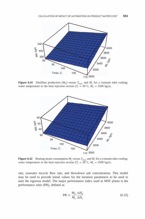
CALCULATION OF IMPACT OF AUTOMATION ON PRODUCT WATER COST 551

4000

3800

3600

3400

3200

3000110

105

100

Tmax, C

Md,

kg/

s

Mr,

kg/s

95

90300

400

500

Figure 6.41 Distillate production (Md) versus Tmax and Mr for a constant inlet cooling-water temperature to the heat rejection section (Ti = 30◦C, Mc = 3500 kg/s).

4000

3800

3600

3400

3200

3000110

105

100

Tmax, C

Md,

kg/

s

Mr,

kg/s

95

90

40

50

60

Figure 6.42 Heating steam consumption Ms versus Tmax and Mr for a constant inlet cooling-water temperature to the heat rejection section (Ti = 30◦C, Mc = 3500 kg/s).

rate, seawater recycle flow rate, and blowdown salt concentration. This modelmay be used to provide initial values for the iteration parameters to be used tostart the rigorous model. The major performance index used in MSF plants is theperformance ratio (PR), defined as

PR ≡ Md �Hd

Ms �Hs(6.32)

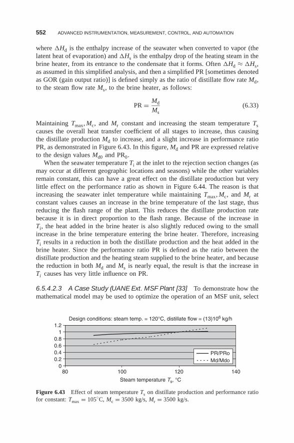
552 ADVANCED INSTRUMENTATION, MEASUREMENT, CONTROL, AND AUTOMATION

where �Hd is the enthalpy increase of the seawater when converted to vapor (thelatent heat of evaporation) and �Hs is the enthalpy drop of the heating steam in thebrine heater, from its entrance to the condensate that it forms. Often �Hd ≈ �Hs,as assumed in this simplified analysis, and then a simplified PR [sometimes denotedas GOR (gain output ratio)] is defined simply as the ratio of distillate flow rate Md,to the steam flow rate Ms, to the brine heater, as follows:

PR = Md

Ms(6.33)

Maintaining Tmax, Mc, and Mr constant and increasing the steam temperature Tscauses the overall heat transfer coefficient of all stages to increase, thus causingthe distillate production Md to increase, and a slight increase in performance ratioPR, as demonstrated in Figure 6.43. In this figure, Md and PR are expressed relativeto the design values Md0 and PR0.

When the seawater temperature Ti at the inlet to the rejection section changes (asmay occur at different geographic locations and seasons) while the other variablesremain constant, this can have a great effect on the distillate production but verylittle effect on the performance ratio as shown in Figure 6.44. The reason is thatincreasing the seawater inlet temperature while maintaining Tmax, Mc, and Mr atconstant values causes an increase in the brine temperature of the last stage, thusreducing the flash range of the plant. This reduces the distillate production ratebecause it is in direct proportion to the flash range. Because of the increase inTi, the heat added in the brine heater is also slightly reduced owing to the smallincrease in the brine temperature entering the brine heater. Therefore, increasingTi results in a reduction in both the distillate production and the heat added in thebrine heater. Since the performance ratio PR is defined as the ratio between thedistillate production and the heating steam supplied to the brine heater, and becausethe reduction in both Md and Ms is nearly equal, the result is that the increase inTi causes has very little influence on PR.

6.5.4.2.3 A Case Study (UANE Ext. MSF Plant [33] To demonstrate how themathematical model may be used to optimize the operation of an MSF unit, select

Design conditions: steam temp. = 120°C, distillate flow = (13)106 kg/h

00.20.40.60.8

11.2

80 100 120 140

Steam temperature Ts, °C

PR/PRoMd/Mdo

Figure 6.43 Effect of steam temperature Ts on distillate production and performance ratiofor constant: Tmax = 105◦C, Mc = 3500 kg/s, Mr = 3500 kg/s.

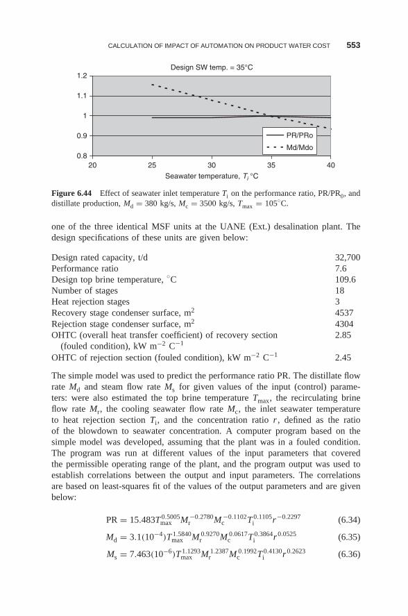
CALCULATION OF IMPACT OF AUTOMATION ON PRODUCT WATER COST 553

Design SW temp. = 35°C

0.8

0.9

1

1.1

1.2

20 25 30 35 40

Seawater temperature, Ti °C

PR/PRo

Md/Mdo

Figure 6.44 Effect of seawater inlet temperature Ti on the performance ratio, PR/PR0, anddistillate production, Md = 380 kg/s, Mc = 3500 kg/s, Tmax = 105◦C.

one of the three identical MSF units at the UANE (Ext.) desalination plant. Thedesign specifications of these units are given below:

Design rated capacity, t/d 32,700Performance ratio 7.6Design top brine temperature, ◦C 109.6Number of stages 18Heat rejection stages 3Recovery stage condenser surface, m2 4537Rejection stage condenser surface, m2 4304OHTC (overall heat transfer coefficient) of recovery section

(fouled condition), kW m−2 C−12.85

OHTC of rejection section (fouled condition), kW m−2 C−1 2.45

The simple model was used to predict the performance ratio PR. The distillate flowrate Md and steam flow rate Ms for given values of the input (control) parame-ters: were also estimated the top brine temperature Tmax, the recirculating brineflow rate Mr, the cooling seawater flow rate Mc, the inlet seawater temperatureto heat rejection section Ti, and the concentration ratio r , defined as the ratioof the blowdown to seawater concentration. A computer program based on thesimple model was developed, assuming that the plant was in a fouled condition.The program was run at different values of the input parameters that coveredthe permissible operating range of the plant, and the program output was used toestablish correlations between the output and input parameters. The correlationsare based on least-squares fit of the values of the output parameters and are givenbelow:

PR = 15.483T 0.5005max M −0.2780

r M −0.1102c T 0.1105

i r−0.2297 (6.34)

Md = 3.1(10−4)T 1.5840max M 0.9270

r M 0.0617c T 0.3864

i r0.0525 (6.35)

Ms = 7.463(10−6)T 1.1293max M 1.2387

r M 0.1992c T 0.4130

i r0.2623 (6.36)

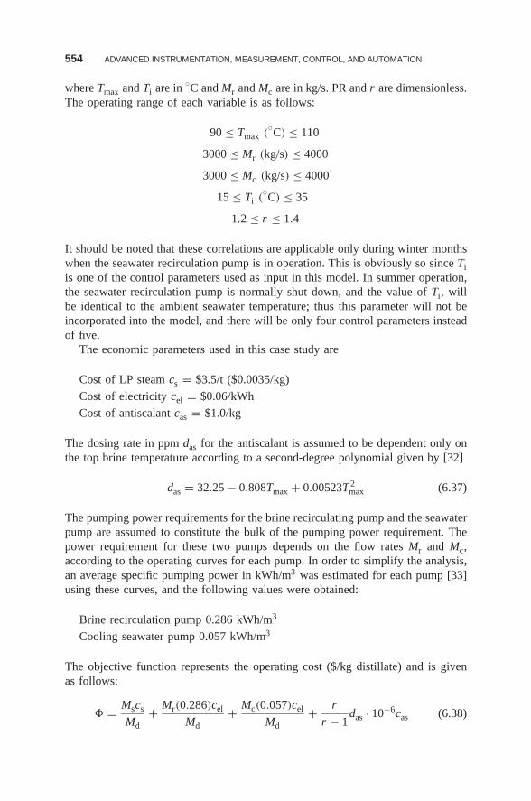
554 ADVANCED INSTRUMENTATION, MEASUREMENT, CONTROL, AND AUTOMATION

where Tmax and Ti are in ◦C and Mr and Mc are in kg/s. PR and r are dimensionless.The operating range of each variable is as follows:

90 ≤ Tmax (◦C) ≤ 110

3000 ≤ Mr (kg/s) ≤ 4000

3000 ≤ Mc (kg/s) ≤ 4000

15 ≤ Ti (◦C) ≤ 35

1.2 ≤ r ≤ 1.4

It should be noted that these correlations are applicable only during winter monthswhen the seawater recirculation pump is in operation. This is obviously so since Tiis one of the control parameters used as input in this model. In summer operation,the seawater recirculation pump is normally shut down, and the value of Ti, willbe identical to the ambient seawater temperature; thus this parameter will not beincorporated into the model, and there will be only four control parameters insteadof five.

The economic parameters used in this case study are

Cost of LP steam cs = $3.5/t ($0.0035/kg)

Cost of electricity cel = $0.06/kWh

Cost of antiscalant cas = $1.0/kg

The dosing rate in ppm das for the antiscalant is assumed to be dependent only onthe top brine temperature according to a second-degree polynomial given by [32]

das = 32.25 − 0.808Tmax + 0.00523T 2max (6.37)

The pumping power requirements for the brine recirculating pump and the seawaterpump are assumed to constitute the bulk of the pumping power requirement. Thepower requirement for these two pumps depends on the flow rates Mr and Mc,according to the operating curves for each pump. In order to simplify the analysis,an average specific pumping power in kWh/m3 was estimated for each pump [33]using these curves, and the following values were obtained:

Brine recirculation pump 0.286 kWh/m3

Cooling seawater pump 0.057 kWh/m3

The objective function represents the operating cost ($/kg distillate) and is givenas follows:

� = Mscs

Md+ Mr(0.286)cel

Md+ Mc(0.057)cel

Md+ r

r − 1das · 10−6cas (6.38)

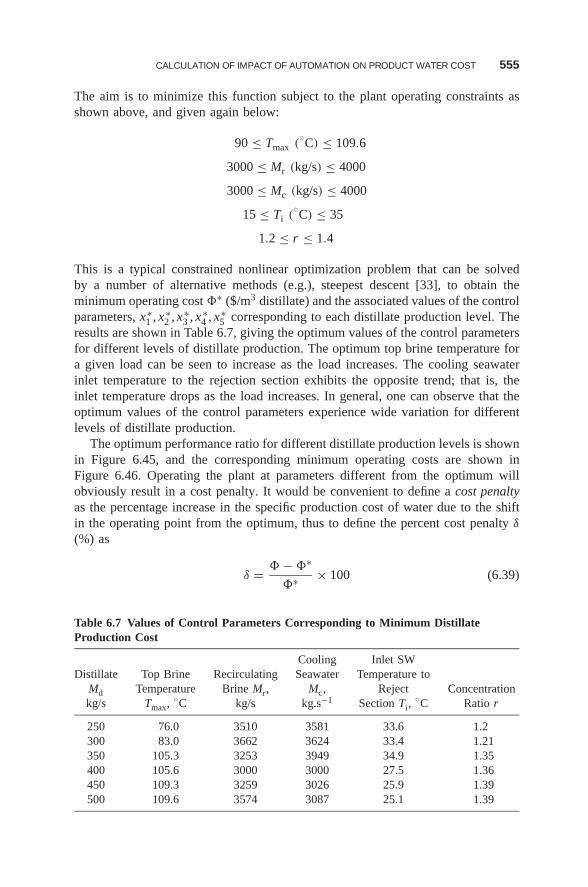
CALCULATION OF IMPACT OF AUTOMATION ON PRODUCT WATER COST 555

The aim is to minimize this function subject to the plant operating constraints asshown above, and given again below:

90 ≤ Tmax (◦C) ≤ 109.6

3000 ≤ Mr (kg/s) ≤ 4000

3000 ≤ Mc (kg/s) ≤ 4000

15 ≤ Ti (◦C) ≤ 35

1.2 ≤ r ≤ 1.4

This is a typical constrained nonlinear optimization problem that can be solvedby a number of alternative methods (e.g.), steepest descent [33], to obtain theminimum operating cost �∗ ($/m3 distillate) and the associated values of the controlparameters, x∗

1 , x∗2 , x∗

3 , x∗4 , x∗

5 corresponding to each distillate production level. Theresults are shown in Table 6.7, giving the optimum values of the control parametersfor different levels of distillate production. The optimum top brine temperature fora given load can be seen to increase as the load increases. The cooling seawaterinlet temperature to the rejection section exhibits the opposite trend; that is, theinlet temperature drops as the load increases. In general, one can observe that theoptimum values of the control parameters experience wide variation for differentlevels of distillate production.

The optimum performance ratio for different distillate production levels is shownin Figure 6.45, and the corresponding minimum operating costs are shown inFigure 6.46. Operating the plant at parameters different from the optimum willobviously result in a cost penalty. It would be convenient to define a cost penaltyas the percentage increase in the specific production cost of water due to the shiftin the operating point from the optimum, thus to define the percent cost penalty δ

(%) as

δ = � − �∗

�∗ × 100 (6.39)

Table 6.7 Values of Control Parameters Corresponding to Minimum DistillateProduction Cost

Cooling Inlet SWDistillate Top Brine Recirculating Seawater Temperature to

Md Temperature Brine Mr, Mc, Reject Concentrationkg/s Tmax, ◦C kg/s kg.s−1 Section Ti,

◦C Ratio r

250 76.0 3510 3581 33.6 1.2300 83.0 3662 3624 33.4 1.21350 105.3 3253 3949 34.9 1.35400 105.6 3000 3000 27.5 1.36450 109.3 3259 3026 25.9 1.39500 109.6 3574 3087 25.1 1.39

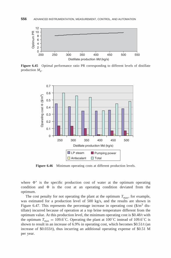
556 ADVANCED INSTRUMENTATION, MEASUREMENT, CONTROL, AND AUTOMATION

02468

1012

200 250 300 350 400 450 500 550

Distillate production Md (kg/s)

Opt

imum

PR

Figure 6.45 Optimal performance ratio PR corresponding to different levels of distillateproduction Md.

0

0.1

0.2

0.3

0.4

0.5

0.6

0.7

250 300 350 400 450 500

Distillate production Md (kg/s)

Op

era

ting

cos

t Φ (

$/m

3)

LP steam Pumping power

Antiscalant Total

Figure 6.46 Minimum operating costs at different production levels.

where �∗ is the specific production cost of water at the optimum operatingcondition and � is the cost at an operating condition deviated from theoptimum.

The cost penalty for not operating the plant at the optimum Tmax, for example,was estimated for a production level of 500 kg/s, and the results are shown inFigure 6.47. This represents the percentage increase in operating cost ($/m3 dis-tillate) incurred because of operation at a top brine temperature different from theoptimum value. At this production level, the minimum operating cost is $0.48/t withthe optimum Tmax = 109.6◦C. Operating the plant at 100◦C instead of 109.6◦C isshown to result in an increase of 6.9% in operating cost, which becomes $0.51/t (anincrease of $0.033/t), thus incurring an additional operating expense of $0.51 Mper year.

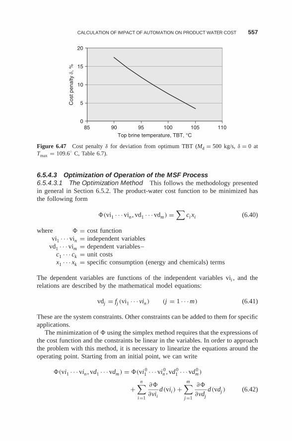
CALCULATION OF IMPACT OF AUTOMATION ON PRODUCT WATER COST 557

0

5

10

15

20

85 90 95 100 105 110

Top brine temperature, TBT, °C

Cos

t pen

alty

δ, %

Figure 6.47 Cost penalty δ for deviation from optimum TBT (Md = 500 kg/s, δ = 0 atTmax = 109.6◦ C, Table 6.7).

6.5.4.3 Optimization of Operation of the MSF Process6.5.4.3.1 The Optimization Method This follows the methodology presentedin general in Section 6.5.2. The product-water cost function to be minimized hasthe following form

�(vi1 · · · vin , vd1 · · · vdm) =∑

ci xi (6.40)

where � = cost functionvi1 · · · vin = independent variables

vd1 · · · vim = dependent variables–c1 · · · ck = unit costsx1 · · · xk = specific consumption (energy and chemicals) terms

The dependent variables are functions of the independent variables vii , and therelations are described by the mathematical model equations:

vdj = fj (vi1 · · · vin) (j = 1 · · · m) (6.41)

These are the system constraints. Other constraints can be added to them for specificapplications.

The minimization of � using the simplex method requires that the expressions ofthe cost function and the constraints be linear in the variables. In order to approachthe problem with this method, it is necessary to linearize the equations around theoperating point. Starting from an initial point, we can write

�(vi1 · · · vin , vd1 · · · vdm) = �(vi 01 · · · vi 0

n , vd01 · · · vd0

m)

+n∑

i=1

∂�

∂viid(vii ) +

m∑j=1

∂�

∂vdjd(vdj ) (6.42)

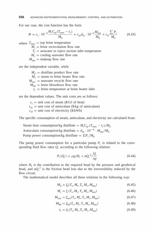
558 ADVANCED INSTRUMENTATION, MEASUREMENT, CONTROL, AND AUTOMATION

For our case, the cost function has the form

� = cs · 10−6MrCpr(Tmax − t1)

Md+ casdas · 10−6 Mmu

Md+ cel

∑Pi

Md(6.43)

where Tmax = top brine temperatureMr = brine recirculation flow rateTi = seawater to reject section inlet temperature

Mc = cooling seawater flow rateMmu = makeup flow rate

are the independent variable, while

Md = distillate product flow rateMs = steam to brine heater flow rate

Mswr = seawater recycle flow rateMbd = brine blowdown flow rate

t1 = brine temperature at brine heater inlet

are the dependent values. The unit costs are as follows:

cs = unit cost of steam ($/GJ of heat)cas = unit cost of antiscalant ($/kg of antiscalant)cel = unit cost of electricity ($/kWh)

The specific consumption of steam, antiscalant, and electricity are calculated from:

Steam heat consumption/kg distillate = MrCpr (Tmax − t1)/Md

Antiscalant consumption/kg distillate = das · 10 −6 · Mmu/Md

Pump power consumption/kg distillate = �Pi/Md

The pump power consumption for a particular pump Pi is related to the corre-sponding fluid flow rates Qi according to the following relation:

Pi (Qi ) = ρg(Hf + aQi2)

Qi

ηp(6.44)

where Hf is the contribution to the required head by the pressure and geodeticalhead, and aQi

2 is the friction head loss due to the irreversibility induced by theflow circuit.

The mathematical model describes all these relations in the following way:

Md = fd(Ts, Mr, Ti, Mc, Mmu) (6.45)

Mc = fc(Ts, Mr, Ti, Mc, Mmu) (6.46)

Mswr = fswr(Ts, Mr, Ti, Mc, Mmu) (6.47)

Mbd = fbd(Ts, Mr, Ti, Mc, Mmu) (6.48)

t1 = fT(Ts, Mr, Ti, Mc, Mmu) (6.49)

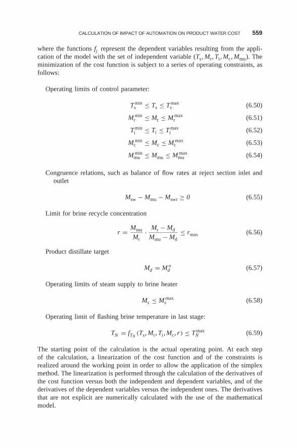
CALCULATION OF IMPACT OF AUTOMATION ON PRODUCT WATER COST 559

where the functions fj represent the dependent variables resulting from the appli-cation of the model with the set of independent variable (Ts, Mr, Ti, Mc, Mmu). Theminimization of the cost function is subject to a series of operating constraints, asfollows:

Operating limits of control parameter:

T mins ≤ Ts ≤ T max

s (6.50)

M minr ≤ Mr ≤ M max

r (6.51)

T mini ≤ Ti ≤ T max

i (6.52)

M minc ≤ Mc ≤ M max

c (6.53)

M minmu ≤ Mmu ≤ M max

mu (6.54)

Congruence relations, such as balance of flow rates at reject section inlet andoutlet

Msw − Mmu − Mswr ≥ 0 (6.55)

Limit for brine recycle concentration

r = Mmu

Mr· Mr − Md

Mmu − Md≤ rmax (6.56)

Product distillate target

Md = M od (6.57)

Operating limits of steam supply to brine heater

Ms ≤ M maxs (6.58)

Operating limit of flashing brine temperature in last stage:

TN = fTN(Ts, Mr, Ti, Mc, r) ≤ T max

N (6.59)

The starting point of the calculation is the actual operating point. At each stepof the calculation, a linearization of the cost function and of the constraints isrealized around the working point in order to allow the application of the simplexmethod. The linearization is performed through the calculation of the derivatives ofthe cost function versus both the independent and dependent variables, and of thederivatives of the dependent variables versus the independent ones. The derivativesthat are not explicit are numerically calculated with the use of the mathematicalmodel.

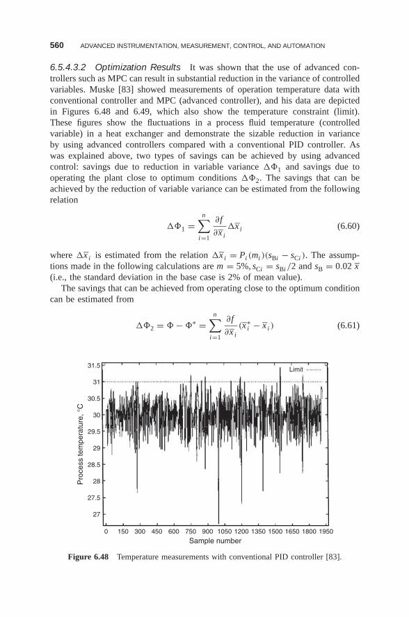
560 ADVANCED INSTRUMENTATION, MEASUREMENT, CONTROL, AND AUTOMATION

6.5.4.3.2 Optimization Results It was shown that the use of advanced con-trollers such as MPC can result in substantial reduction in the variance of controlledvariables. Muske [83] showed measurements of operation temperature data withconventional controller and MPC (advanced controller), and his data are depictedin Figures 6.48 and 6.49, which also show the temperature constraint (limit).These figures show the fluctuations in a process fluid temperature (controlledvariable) in a heat exchanger and demonstrate the sizable reduction in varianceby using advanced controllers compared with a conventional PID controller. Aswas explained above, two types of savings can be achieved by using advancedcontrol: savings due to reduction in variable variance ��1 and savings due tooperating the plant close to optimum conditions ��2. The savings that can beachieved by the reduction of variable variance can be estimated from the followingrelation

��1 =n∑

i=1

∂f

∂x i�x i (6.60)

where �x i is estimated from the relation �x i = Pi (mi )(sBi − sCi ). The assump-tions made in the following calculations are m = 5%, sCi = sBi/2 and sB = 0.02 x(i.e., the standard deviation in the base case is 2% of mean value).

The savings that can be achieved from operating close to the optimum conditioncan be estimated from

��2 = � − �∗ =n∑

i=1

∂f

∂x i(x∗

i − x i ) (6.61)

31.5Limit

30.5

29.5

29

28.5

28

27.5

27

0 150 300 450 600 750 900

Sample number1050 1200 1350 1500 1650 1800 1950

30

31

Pro

cess

tem

pera

ture

, °C

Figure 6.48 Temperature measurements with conventional PID controller [83].

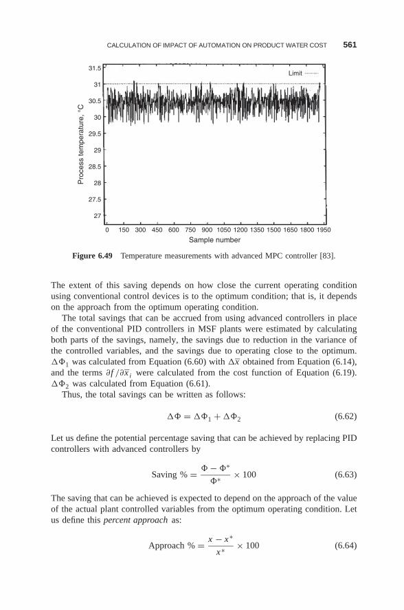
CALCULATION OF IMPACT OF AUTOMATION ON PRODUCT WATER COST 561

31.5Limit

30.5

29.5

29

28.5

Pro

cess

tem

pera

ture

, °C

28

27.5

27

0 150 300 450 600 750 900

Sample number1050 1200 1350 1500 1650 1800 1950

30

31

Figure 6.49 Temperature measurements with advanced MPC controller [83].

The extent of this saving depends on how close the current operating conditionusing conventional control devices is to the optimum condition; that is, it dependson the approach from the optimum operating condition.

The total savings that can be accrued from using advanced controllers in placeof the conventional PID controllers in MSF plants were estimated by calculatingboth parts of the savings, namely, the savings due to reduction in the variance ofthe controlled variables, and the savings due to operating close to the optimum.��1 was calculated from Equation (6.60) with �x obtained from Equation (6.14),and the terms ∂f /∂x i were calculated from the cost function of Equation (6.19).��2 was calculated from Equation (6.61).

Thus, the total savings can be written as follows:

�� = ��1 + ��2 (6.62)

Let us define the potential percentage saving that can be achieved by replacing PIDcontrollers with advanced controllers by

Saving % = � − �∗

�∗ × 100 (6.63)

The saving that can be achieved is expected to depend on the approach of the valueof the actual plant controlled variables from the optimum operating condition. Letus define this percent approach as:

Approach % = x − x∗

x∗ × 100 (6.64)

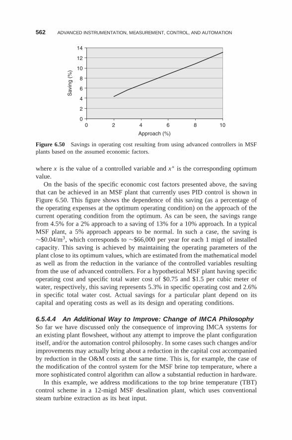
562 ADVANCED INSTRUMENTATION, MEASUREMENT, CONTROL, AND AUTOMATION

0

2

4

6

8

10

12

14

0 2 4 6 8 10

Approach (%)

Sav

ing

(%)

Figure 6.50 Savings in operating cost resulting from using advanced controllers in MSFplants based on the assumed economic factors.

where x is the value of a controlled variable and x∗ is the corresponding optimumvalue.

On the basis of the specific economic cost factors presented above, the savingthat can be achieved in an MSF plant that currently uses PID control is shown inFigure 6.50. This figure shows the dependence of this saving (as a percentage ofthe operating expenses at the optimum operating condition) on the approach of thecurrent operating condition from the optimum. As can be seen, the savings rangefrom 4.5% for a 2% approach to a saving of 13% for a 10% approach. In a typicalMSF plant, a 5% approach appears to be normal. In such a case, the saving is∼$0.04/m3, which corresponds to ∼$66,000 per year for each 1 migd of installedcapacity. This saving is achieved by maintaining the operating parameters of theplant close to its optimum values, which are estimated from the mathematical modelas well as from the reduction in the variance of the controlled variables resultingfrom the use of advanced controllers. For a hypothetical MSF plant having specificoperating cost and specific total water cost of $0.75 and $1.5 per cubic meter ofwater, respectively, this saving represents 5.3% in specific operating cost and 2.6%in specific total water cost. Actual savings for a particular plant depend on itscapital and operating costs as well as its design and operating conditions.

6.5.4.4 An Additional Way to Improve: Change of IMCA PhilosophySo far we have discussed only the consequence of improving IMCA systems foran existing plant flowsheet, without any attempt to improve the plant configurationitself, and/or the automation control philosophy. In some cases such changes and/orimprovements may actually bring about a reduction in the capital cost accompaniedby reduction in the O&M costs at the same time. This is, for example, the case ofthe modification of the control system for the MSF brine top temperature, where amore sophisticated control algorithm can allow a substantial reduction in hardware.

In this example, we address modifications to the top brine temperature (TBT)control scheme in a 12-migd MSF desalination plant, which uses conventionalsteam turbine extraction as its heat input.

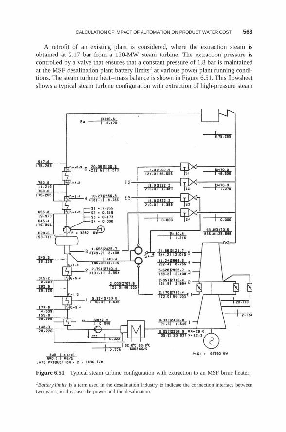
CALCULATION OF IMPACT OF AUTOMATION ON PRODUCT WATER COST 563

A retrofit of an existing plant is considered, where the extraction steam isobtained at 2.17 bar from a 120-MW steam turbine. The extraction pressure iscontrolled by a valve that ensures that a constant pressure of 1.8 bar is maintainedat the MSF desalination plant battery limits2 at various power plant running condi-tions. The steam turbine heat–mass balance is shown in Figure 6.51. This flowsheetshows a typical steam turbine configuration with extraction of high-pressure steam

Figure 6.51 Typical steam turbine configuration with extraction to an MSF brine heater.

2Battery limits is a term used in the desalination industry to indicate the connection interface betweentwo yards, in this case the power and the desalination.

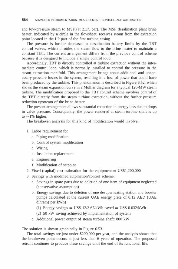
564 ADVANCED INSTRUMENTATION, MEASUREMENT, CONTROL, AND AUTOMATION

and low-pressure steam to MSF (at 2.17. bar). The MSF desalination plant brineheater, indicated by a circle in the flowsheet, receives steam from the extractionpoint located in the LP part of the first turbine casing.

The pressure is further decreased at desalination battery limits by the TBTcontrol valves, which throttles the steam flow to the brine heater to maintain aconstant TBT. The current arrangement differs from the previous control schemebecause it is designed to include a single control loop.

Accordingly, TBT is directly controlled at turbine extraction without the inter-mediate control loop, which is normally installed to control the pressure in thesteam extraction manifold. This arrangement brings about additional and unnec-essary pressure losses in the system, resulting in a loss of power that could havebeen produced by the turbine. This phenomenon is described in Figure 6.52, whichshows the steam expansion curve in a Mollier diagram for a typical 120-MW steamturbine. The modification proposed to the TBT control scheme involves control ofthe TBT directly from the steam turbine extraction, without the further pressurereduction upstream of the brine heater.

The present arrangement allows substantial reduction in energy loss due to dropsin valve pressure. Consequently, the power rendered at steam turbine shaft is upto ∼1% higher.

The breakeven analysis for this kind of modification would involve:

1. Labor requirement for

a. Piping modification

b. Control system modification

c. Wiring

d. Insulation replacement

e. Engineering

f. Modification of setpoint

2. Fixed (capital) cost estimation for the equipment = US$1,200,000

3. Savings with modified automation/control scheme:

a. Savings in spare parts due to deletion of one item of equipment neglected(conservative assumption)

b. Energy savings due to deletion of one desuperheating station and boosterpumps calculated at the current UAE energy price of 0.12 AED (UAEdihram) per kWh)

(1) Energy savings = US$ 12/3.67/kWh saved = US$ 0.032/kWh

(2) 50 kW saving achieved by implementation of system

c. Additional power output of steam turbine shaft: 800 kW

The solution is shown graphically in Figure 6.53.The total savings are just under $200,000 per year, and the analysis shows that

the breakeven point occurs at just less than 6 years of operation. The proposedretrofit continues to produce these savings until the end of its functional life.

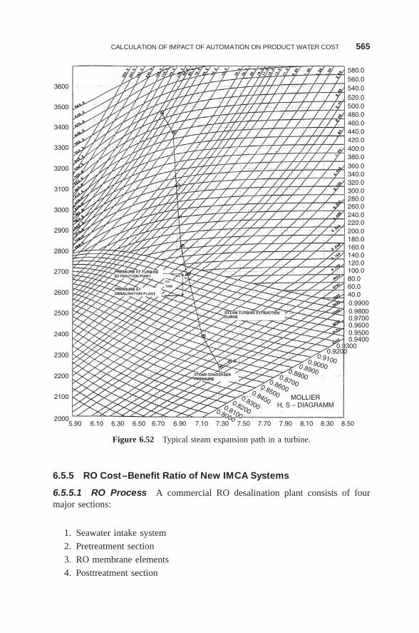
CALCULATION OF IMPACT OF AUTOMATION ON PRODUCT WATER COST 565

20005.90 6.10 6.30 6.50 6.70 6.90 7.10 7.30 7.50 7.70 7.90 8.10 8.30

580.0560.0540.0520.0500.0480.0460.0440.0420.0400.0380.0360.0340.0320.0300.0280.0260.0240.0220.0200.0180.0160.0140.0120.0100.080.060.040.00.99000.98000.97000.96000.95000.9400

0.93000.93000.9200

0.91000.90000.89000.88000.87000.84000.83000.82000.8100

0.8000

0.81000.8000

8.50

2100

2200

2300

2400

2500

2600

2700

2800

2900

3000

3100

3200

3300

3400

3500

3600

0.86000.8500 MOLLIERH, S – DIAGRAMM

Figure 6.52 Typical steam expansion path in a turbine.

6.5.5 RO Cost–Benefit Ratio of New IMCA Systems

6.5.5.1 RO Process A commercial RO desalination plant consists of fourmajor sections:

1. Seawater intake system

2. Pretreatment section

3. RO membrane elements

4. Posttreatment section

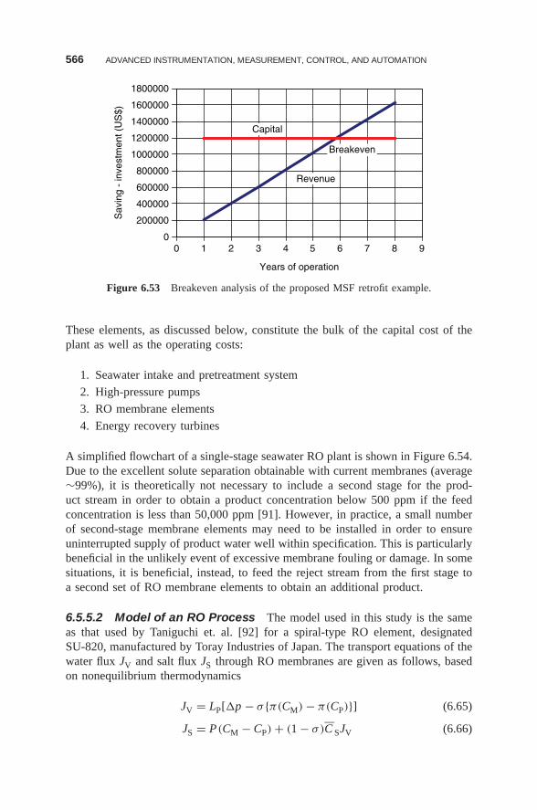
566 ADVANCED INSTRUMENTATION, MEASUREMENT, CONTROL, AND AUTOMATION

0

200000

400000

600000

800000

1000000

1200000

1400000

1600000

1800000

0 1 2 3 4 5 6 7 8 9

Years of operation

Sav

ing

- in

vest

men

t (U

S$)

Capital

Breakeven

Revenue

Figure 6.53 Breakeven analysis of the proposed MSF retrofit example.

These elements, as discussed below, constitute the bulk of the capital cost of theplant as well as the operating costs:

1. Seawater intake and pretreatment system

2. High-pressure pumps

3. RO membrane elements

4. Energy recovery turbines

A simplified flowchart of a single-stage seawater RO plant is shown in Figure 6.54.Due to the excellent solute separation obtainable with current membranes (average∼99%), it is theoretically not necessary to include a second stage for the prod-uct stream in order to obtain a product concentration below 500 ppm if the feedconcentration is less than 50,000 ppm [91]. However, in practice, a small numberof second-stage membrane elements may need to be installed in order to ensureuninterrupted supply of product water well within specification. This is particularlybeneficial in the unlikely event of excessive membrane fouling or damage. In somesituations, it is beneficial, instead, to feed the reject stream from the first stage toa second set of RO membrane elements to obtain an additional product.

6.5.5.2 Model of an RO Process The model used in this study is the sameas that used by Taniguchi et. al. [92] for a spiral-type RO element, designatedSU-820, manufactured by Toray Industries of Japan. The transport equations of thewater flux JV and salt flux JS through RO membranes are given as follows, basedon nonequilibrium thermodynamics

JV = LP[�p − σ {π(CM) − π(CP)}] (6.65)

JS = P(CM − CP) + (1 − σ)C SJV (6.66)

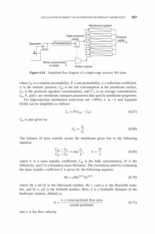
CALCULATION OF IMPACT OF AUTOMATION ON PRODUCT WATER COST 567

Productwater

Membrane system

High-pressurepump

Pretreatment

Brine concentrateto drain Pelton turbine

Seawater

Figure 6.54 Simplified flow diagram of a single-stage seawater RO plant.

where LP is a solution permeability, P a salt permeability, σ a reflection coefficient,π is the osmotic pressure, CM is the salt concentration at the membrane surface,CP is the permeate (product concentration), and C S is an average concentration;LP, P , and σ are membrane transport parameters that specify membrane properties.

For high-rejection membranes (rejections are >99%), σ is ∼1 and Equation(6.66) can be simplified as follows:

JS = P(CM − CP) (6.67)

CP is also given by

CP = JS

JV(6.68)

The balance of mass transfer across the membrane gives rise to the followingequation

CM − CP

CB − CP= exp

JV

k, k = D

δ(6.69)

where k is a mass transfer coefficient, CB is the bulk concentration, D is thediffusivity, and δ is a boundary-layer thickness. The correlation used for evaluatingthe mass transfer coefficient k is given by the following equation

Sh = aRe0.875Sc0.25 (6.70)

where Sh = kd/D is the Sherwood number, Re = ρud/η is the Reynolds num-ber, and Sc = ηD is the Schmidt number. Here, d is a hydraulic diameter of thefeedwater channel, defined as

d = 4 × cross-sectional flow area

wetted perimeter(6.71)

and u is the flow velocity.

568 ADVANCED INSTRUMENTATION, MEASUREMENT, CONTROL, AND AUTOMATION

A membrane element is divided into N sections along the feed flow direction.Mass balance equations at each section (�h = h/N ) are given as

�QPi = JVi�h (6.72)

CPi = JSi

JVi= PCMi

JVi + P(6.73)

QPo =N∑

i=1

�QPi =N∑

i=1

JVi�hW (6.74)

CPo =

N∑i=1

CPi�QPi

QPo=

∑(PCMi/JVi + P)JVi�hW

QPo(6.75)

where subscript i is the i th section, subscript “o” refers to the outlet of the mem-brane, W is the width of the membrane, and Q is the volume flow rate.

The properties of seawater are calculated from the correlations used by Taniguchiet al. [92]. For the osmotic pressure (Pa), density (kg/m3), viscosity (Pa·s), anddiffusivity (m2/s), the correlations are

π(c, T ) = (0.6955 + 0.0025T ) × 108 c

ρ(6.76)

where C is the salt concentration in kg/m3 and T is the temperature in ◦C.

For the density of seawater:

ρ = 498.4m +√

248400m2 + 752.4mC (6.77)

where

m = 1.0069 − 2.757 × 10−4T (6.78)

For the viscosity of seawater:

η = 1.234 × 10−6 exp

(0.00212C + 1965

273.15 + T

)(6.79)

For the diffusivity:

D = 6.725 × 10−6 exp

(0.1546 × 10−3C − 2513

273.15 + T

)(6.80)

CALCULATION OF IMPACT OF AUTOMATION ON PRODUCT WATER COST 569

A computer program was developed to estimate the properties of the RO membraneelements at different operating conditions. The program was written using Math-ematica software. Using a very similar analysis, Taniguchi et al. [92] comparedtheir results with those of actual experimental results obtained from the Ehime testplant in Japan under different operating conditions, and the agreement between hissimulation program and the test results was excellent.

With the membrane parameters LP and P given and seawater conditions (sea-water concentration Cf and seawater temperature Tf) known and the operatingcondition (feed pressure Pf) fixed, the program estimates the fluxes of salt andwater for each section of membrane and evaluates the product concentration Cpand product recovery Rc.

A membrane made of crosslinked fully aromatic polyamide material identical tothe material used by Toray Industries of Japan is assumed [92]. For this material,the membrane parameters at the standard operating conditions (25◦C temperatureand 6.5 MPa pressure) are

LP = (2.52)10−12 m3m−2(Pa · s)−1 and P = (12.1)10−9 m/s

The membrane element used is of the spiral-wound type having the dimensions:W = 1 m and h = 6 m, d = 2 mm. The inlet Reynolds number is Re = 100.Several program runs were made at different feed pressures, feed concentrations,and feed temperatures, and the results are shown as three-dimensional graphs inFigures 6.55 and 6.56. As demonstrated in these figures, the product concentra-tion is quite sensitive to both temperature and concentration of the feedwater;increasing either of them results in a substantial increase in Cp. The feed pressure,however, has the opposite effect; increasing the feed pressure decreases the productconcentration.

The effects of Tf, Cf, and Pf on recovery R [defined as the ratio between perme-ate (product) water flow rate and feedwater flow rate] of the RO membrane elementis demonstrated in the three-dimensional graphs of Figures 6.57 and 6.58. It canbe seen that the increase in feedwater temperature for a given value of feed con-centration causes an increase in water recovery. This increase is more pronouncedat the high feed concentration than at the low feed concentration. It can also beseen that the recovery levels are higher for lower feed concentration than for higherconcentration. The effect of the feed pressure is such that increasing the pressureresults in an increase in the recovery. Such an increase is more appreciable at lowerfeed concentrations than at higher ones.

6.5.5.3 Optimization of RO Process Operation In the same way as for theMSF process (Section 6.5.4), the cost function to be minimized has the followingform

�(vi1 · · · vin , vd1 · · · vdm) =k∑

i=1

ci · xi (6.81)

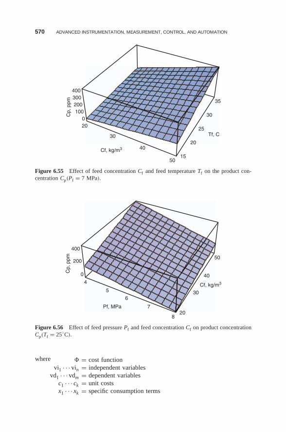
570 ADVANCED INSTRUMENTATION, MEASUREMENT, CONTROL, AND AUTOMATION

020

30

Cf, kg/m3

Tf, C

40

5015

20

25

30

35

100

Cp,

ppm 200

300400

Figure 6.55 Effect of feed concentration Cf and feed temperature Tf on the product con-centration Cp(Pf = 7 MPa).

0

4

5

6

Pf, MPa

Cf, kg/m3

7

820

30

40

50

Cp,

ppm 200

400

Figure 6.56 Effect of feed pressure Pf and feed concentration Cf on product concentrationCp(Tf = 25◦C).

where � = cost functionvi1 · · · vin = independent variables

vd1 · · · vdm = dependent variablesc1 · · · ck = unit costsx1 · · · xk = specific consumption terms

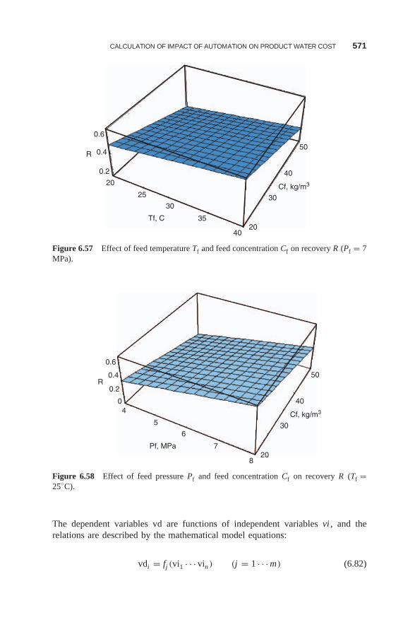
CALCULATION OF IMPACT OF AUTOMATION ON PRODUCT WATER COST 571

0.2

20

25

30

Tf, C

Cf, kg/m3

35

4020

30

40

500.4

0.6

R

Figure 6.57 Effect of feed temperature Tf and feed concentration Cf on recovery R (Pf = 7MPa).

0.2

04

5

6

Pf, MPa

Cf, kg/m3

7

820

30

40

500.4

0.6

R

Figure 6.58 Effect of feed pressure Pf and feed concentration Cf on recovery R (Tf =25◦C).

The dependent variables vd are functions of independent variables vi , and therelations are described by the mathematical model equations:

vdi = fj (vi1 · · · vin) (j = 1 · · · m) (6.82)

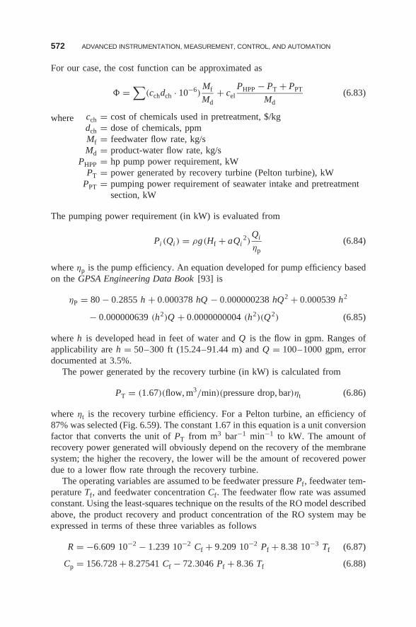
572 ADVANCED INSTRUMENTATION, MEASUREMENT, CONTROL, AND AUTOMATION

For our case, the cost function can be approximated as

� =∑

(cchdch · 10−6)Mf

Md+ cel

PHPP − PT + PPT

Md(6.83)

where cch = cost of chemicals used in pretreatment, $/kgdch = dose of chemicals, ppmMf = feedwater flow rate, kg/sMd = product-water flow rate, kg/s

PHPP = hp pump power requirement, kWPT = power generated by recovery turbine (Pelton turbine), kW

PPT = pumping power requirement of seawater intake and pretreatmentsection, kW

The pumping power requirement (in kW) is evaluated from

Pi (Qi ) = ρg(Hf + aQi2)

Qi

ηp(6.84)

where ηp is the pump efficiency. An equation developed for pump efficiency basedon the GPSA Engineering Data Book [93] is

ηP = 80 − 0.2855 h + 0.000378 hQ − 0.000000238 hQ2 + 0.000539 h2

− 0.000000639 (h2)Q + 0.0000000004 (h2)(Q2) (6.85)

where h is developed head in feet of water and Q is the flow in gpm. Ranges ofapplicability are h = 50–300 ft (15.24–91.44 m) and Q = 100–1000 gpm, errordocumented at 3.5%.

The power generated by the recovery turbine (in kW) is calculated from

PT = (1.67)(flow, m3/min)(pressure drop, bar)ηt (6.86)

where ηt is the recovery turbine efficiency. For a Pelton turbine, an efficiency of87% was selected (Fig. 6.59). The constant 1.67 in this equation is a unit conversionfactor that converts the unit of PT from m3 bar−1 min−1 to kW. The amount ofrecovery power generated will obviously depend on the recovery of the membranesystem; the higher the recovery, the lower will be the amount of recovered powerdue to a lower flow rate through the recovery turbine.

The operating variables are assumed to be feedwater pressure Pf, feedwater tem-perature Tf, and feedwater concentration Cf. The feedwater flow rate was assumedconstant. Using the least-squares technique on the results of the RO model describedabove, the product recovery and product concentration of the RO system may beexpressed in terms of these three variables as follows

R = −6.609 10−2 − 1.239 10−2 Cf + 9.209 10−2 Pf + 8.38 10−3 Tf (6.87)

Cp = 156.728 + 8.27541 Cf − 72.3046 Pf + 8.36 Tf (6.88)

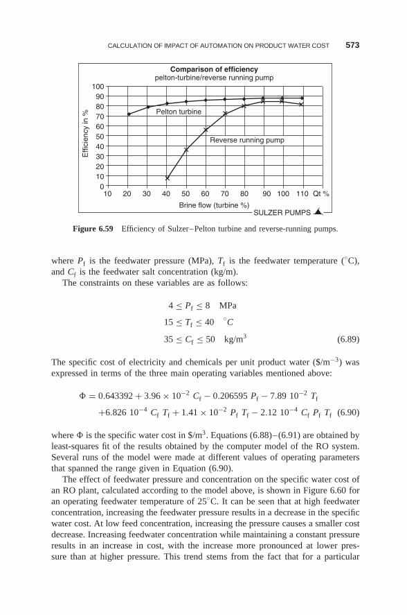
CALCULATION OF IMPACT OF AUTOMATION ON PRODUCT WATER COST 573

100

102030405060708090

100

Comparison of efficiencypelton-turbine/reverse running pump

20 30 40 50 60

Brine flow (turbine %)

Effi

cien

cy in

%

70 80 90 100

SULZER PUMPS

110 Qt %

Reverse running pump

Pelton turbine

Figure 6.59 Efficiency of Sulzer–Pelton turbine and reverse-running pumps.

where Pf is the feedwater pressure (MPa), Tf is the feedwater temperature (◦C),and Cf is the feedwater salt concentration (kg/m).

The constraints on these variables are as follows:

4 ≤ Pf ≤ 8 MPa

15 ≤ Tf ≤ 40 ◦C

35 ≤ Cf ≤ 50 kg/m3 (6.89)

The specific cost of electricity and chemicals per unit product water ($/m−3) wasexpressed in terms of the three main operating variables mentioned above:

� = 0.643392 + 3.96 × 10−2 Cf − 0.206595 Pf − 7.89 10−2 Tf

+6.826 10−4 Cf Tf + 1.41 × 10−2 Pf Tf − 2.12 10−4 Cf Pf Tf (6.90)

where � is the specific water cost in $/m3. Equations (6.88)–(6.91) are obtained byleast-squares fit of the results obtained by the computer model of the RO system.Several runs of the model were made at different values of operating parametersthat spanned the range given in Equation (6.90).

The effect of feedwater pressure and concentration on the specific water cost ofan RO plant, calculated according to the model above, is shown in Figure 6.60 foran operating feedwater temperature of 25◦C. It can be seen that at high feedwaterconcentration, increasing the feedwater pressure results in a decrease in the specificwater cost. At low feed concentration, increasing the pressure causes a smaller costdecrease. Increasing feedwater concentration while maintaining a constant pressureresults in an increase in cost, with the increase more pronounced at lower pres-sure than at higher pressure. This trend stems from the fact that for a particular

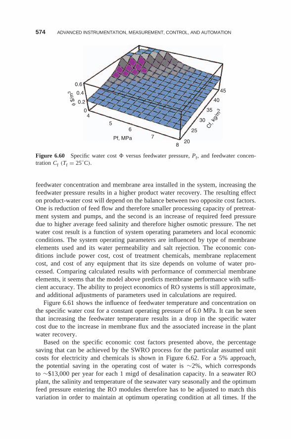
574 ADVANCED INSTRUMENTATION, MEASUREMENT, CONTROL, AND AUTOMATION

0.2

04

56

Pf, MPa

Cf,

kg/m

3

7

820

25

35

30

45

400.4

0.6

φ $/

m3

Figure 6.60 Specific water cost � versus feedwater pressure, Pf, and feedwater concen-tration Cf (Tf = 25◦C).

feedwater concentration and membrane area installed in the system, increasing thefeedwater pressure results in a higher product water recovery. The resulting effecton product-water cost will depend on the balance between two opposite cost factors.One is reduction of feed flow and therefore smaller processing capacity of pretreat-ment system and pumps, and the second is an increase of required feed pressuredue to higher average feed salinity and therefore higher osmotic pressure. The netwater cost result is a function of system operating parameters and local economicconditions. The system operating parameters are influenced by type of membraneelements used and its water permeability and salt rejection. The economic con-ditions include power cost, cost of treatment chemicals, membrane replacementcost, and cost of any equipment that its size depends on volume of water pro-cessed. Comparing calculated results with performance of commercial membraneelements, it seems that the model above predicts membrane performance with suffi-cient accuracy. The ability to project economics of RO systems is still approximate,and additional adjustments of parameters used in calculations are required.

Figure 6.61 shows the influence of feedwater temperature and concentration onthe specific water cost for a constant operating pressure of 6.0 MPa. It can be seenthat increasing the feedwater temperature results in a drop in the specific watercost due to the increase in membrane flux and the associated increase in the plantwater recovery.

Based on the specific economic cost factors presented above, the percentagesaving that can be achieved by the SWRO process for the particular assumed unitcosts for electricity and chemicals is shown in Figure 6.62. For a 5% approach,the potential saving in the operating cost of water is ∼2%, which correspondsto ∼$13,000 per year for each 1 migd of desalination capacity. In a seawater ROplant, the salinity and temperature of the seawater vary seasonally and the optimumfeed pressure entering the RO modules therefore has to be adjusted to match thisvariation in order to maintain at optimum operating condition at all times. If the

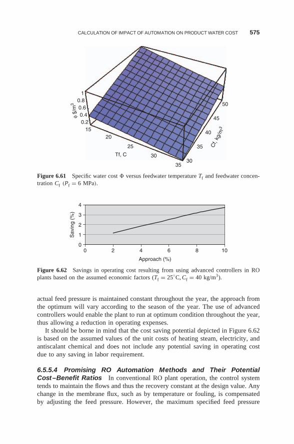
CALCULATION OF IMPACT OF AUTOMATION ON PRODUCT WATER COST 575

0.215

20

25

Tf, C

Cf,

kg/m

3

30

3530

35

40

45

50

0.40.60.8

1

φ $/

m3

Figure 6.61 Specific water cost � versus feedwater temperature Tf and feedwater concen-tration Cf (Pf = 6 MPa).

0

1

2

3

4

0 2 4 6 8 10

Approach (%)

Sav

ing

(%)

Figure 6.62 Savings in operating cost resulting from using advanced controllers in ROplants based on the assumed economic factors (Tf = 25◦C, Cf = 40 kg/m3).

actual feed pressure is maintained constant throughout the year, the approach fromthe optimum will vary according to the season of the year. The use of advancedcontrollers would enable the plant to run at optimum condition throughout the year,thus allowing a reduction in operating expenses.

It should be borne in mind that the cost saving potential depicted in Figure 6.62is based on the assumed values of the unit costs of heating steam, electricity, andantiscalant chemical and does not include any potential saving in operating costdue to any saving in labor requirement.

6.5.5.4 Promising RO Automation Methods and Their PotentialCost–Benefit Ratios In conventional RO plant operation, the control systemtends to maintain the flows and thus the recovery constant at the design value. Anychange in the membrane flux, such as by temperature or fouling, is compensatedby adjusting the feed pressure. However, the maximum specified feed pressure

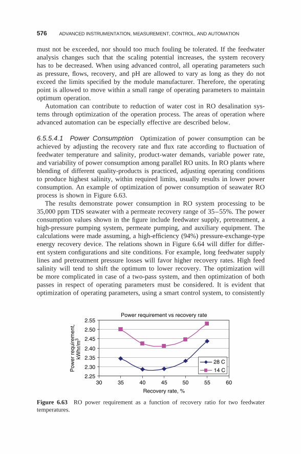
576 ADVANCED INSTRUMENTATION, MEASUREMENT, CONTROL, AND AUTOMATION

must not be exceeded, nor should too much fouling be tolerated. If the feedwateranalysis changes such that the scaling potential increases, the system recoveryhas to be decreased. When using advanced control, all operating parameters suchas pressure, flows, recovery, and pH are allowed to vary as long as they do notexceed the limits specified by the module manufacturer. Therefore, the operatingpoint is allowed to move within a small range of operating parameters to maintainoptimum operation.

Automation can contribute to reduction of water cost in RO desalination sys-tems through optimization of the operation process. The areas of operation whereadvanced automation can be especially effective are described below.

6.5.5.4.1 Power Consumption Optimization of power consumption can beachieved by adjusting the recovery rate and flux rate according to fluctuation offeedwater temperature and salinity, product-water demands, variable power rate,and variability of power consumption among parallel RO units. In RO plants whereblending of different quality-products is practiced, adjusting operating conditionsto produce highest salinity, within required limits, usually results in lower powerconsumption. An example of optimization of power consumption of seawater ROprocess is shown in Figure 6.63.

The results demonstrate power consumption in RO system processing to be35,000 ppm TDS seawater with a permeate recovery range of 35–55%. The powerconsumption values shown in the figure include feedwater supply, pretreatment, ahigh-pressure pumping system, permeate pumping, and auxiliary equipment. Thecalculations were made assuming, a high-efficiency (94%) pressure-exchange-typeenergy recovery device. The relations shown in Figure 6.64 will differ for differ-ent system configurations and site conditions. For example, long feedwater supplylines and pretreatment pressure losses will favor higher recovery rates. High feedsalinity will tend to shift the optimum to lower recovery. The optimization willbe more complicated in case of a two-pass system, and then optimization of bothpasses in respect of operating parameters must be considered. It is evident thatoptimization of operating parameters, using a smart control system, to consistently

Power requirement vs recovery rate

2.25

2.30

2.35

2.40

2.45

2.50

2.55

30 35 40 45 50 55 60

Recovery rate, %

Pow

er r

equi

rem

ent,

kWhr

/m3

28 C

14 C

Figure 6.63 RO power requirement as a function of recovery ratio for two feedwatertemperatures.

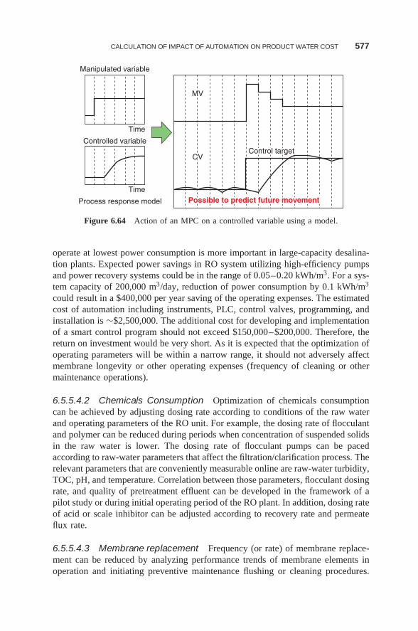
CALCULATION OF IMPACT OF AUTOMATION ON PRODUCT WATER COST 577

Manipulated variable

Controlled variable

Process response model

Time

MV

CV

MV

CVControl targetControl target

Possible to predict future movementPossible to predict future movementTime

Figure 6.64 Action of an MPC on a controlled variable using a model.

operate at lowest power consumption is more important in large-capacity desalina-tion plants. Expected power savings in RO system utilizing high-efficiency pumpsand power recovery systems could be in the range of 0.05–0.20 kWh/m3. For a sys-tem capacity of 200,000 m3/day, reduction of power consumption by 0.1 kWh/m3

could result in a $400,000 per year saving of the operating expenses. The estimatedcost of automation including instruments, PLC, control valves, programming, andinstallation is ∼$2,500,000. The additional cost for developing and implementationof a smart control program should not exceed $150,000–$200,000. Therefore, thereturn on investment would be very short. As it is expected that the optimization ofoperating parameters will be within a narrow range, it should not adversely affectmembrane longevity or other operating expenses (frequency of cleaning or othermaintenance operations).

6.5.5.4.2 Chemicals Consumption Optimization of chemicals consumptioncan be achieved by adjusting dosing rate according to conditions of the raw waterand operating parameters of the RO unit. For example, the dosing rate of flocculantand polymer can be reduced during periods when concentration of suspended solidsin the raw water is lower. The dosing rate of flocculant pumps can be pacedaccording to raw-water parameters that affect the filtration/clarification process. Therelevant parameters that are conveniently measurable online are raw-water turbidity,TOC, pH, and temperature. Correlation between those parameters, flocculant dosingrate, and quality of pretreatment effluent can be developed in the framework of apilot study or during initial operating period of the RO plant. In addition, dosing rateof acid or scale inhibitor can be adjusted according to recovery rate and permeateflux rate.

6.5.5.4.3 Membrane replacement Frequency (or rate) of membrane replace-ment can be reduced by analyzing performance trends of membrane elements inoperation and initiating preventive maintenance flushing or cleaning procedures.

578 ADVANCED INSTRUMENTATION, MEASUREMENT, CONTROL, AND AUTOMATION

Indirectly, automation can reduce the membrane replacement rate by helping tomaintain more consistent feedwater quality and therefore ensure consistent mem-brane performance.

In this area of application, the computerized automatic control system is usedto store operating data, calculate performance trends, and calculate projected per-formance at various operating conditions and ranges of performance of membraneelements. The current approach to correction of system performance through mem-brane replacement includes replacement of old elements with a new one in awhole train or stage. The replaced elements are being individually tested. Poorlyperformed elements are being discarded; the better ones are stored for futurereplacement. Utilization of a computerized system to calculate system performance,based on performance of elements in the system and utilization of the old elementsin the inventory, can result in reduced use of new elements for replacement whilemaintaining required plant performance.

6.5.5.4.4 Labor and Maintenance Labor requirements can be reduced byautomation. Currently, even some large RO systems, are remotely controlled. How-ever, extent of labor reduction due to automation strongly depends on local regu-lations. At some locations, local regulations require the presence of operators evenin fully automated plants.

The water cost in a typical large (∼200,000 m3/day) seawater RO system is∼$0.70/m3. The contributions to the water cost are as follows:

Product-Water Cost Component Cost, $/m3

Capital cost, including land fee (25 years at 6.0% interest) 0.320Electric power ($0.060 kWhr1) 0.210RO membrane replacement (5 years membrane life) 0.035Membrane replacement (7 years membrane life) 0.030Chemicals 0.025Maintenance and spare parts 0.036Labor 0.030

Total cost 0.686

The cost contribution parameters that potentially could be optimized by moreadvanced automations are electric power, RO membrane replacement, chemicals,and possibly maintenance (frequency of membrane cleaning). The total contributionof these components in the example above is $0.336. Assuming that it would bepossible to reduce contribution of these components by 10%, this would result in a200,000-m3/day capacity system and a water cost saving of ∼$61 M over a periodof 25 years of plant operation. By comparison, the total budgetary cost of such aproject is in the range of $200M. Comparing this to potential reduction of oper-ating cost due to better automation provides justification for a more sophisticatedautomation equipment to be implemented.

CALCULATION OF IMPACT OF AUTOMATION ON PRODUCT WATER COST 579

6.5.6 Conclusions

The following major conclusions of this section are:

• A basic premise of this study is that any level of automation or IMCA ingeneral must be economically justified, and consideration of IMCA systemreliability must also be included.

• As opposed to the enormous amount of published information on controlsystems and their advancement, those on cost–benefit analysis of their imple-mentation are very few in general, and nearly nonexistent for desalinationplants in particular.

• A critical review of the status of cost–benefit analysis of IMCA systemswith emphasis on their use in MSF and RO desalination, was performed andpresented.

• An explicit methodology for such analysis was developed and presented.

• To implement this methodology, simplified models for predicting the perfor-mance of MSF and RO plants were developed and successfully implemented.

• Specific examples of IMCA system cost–benefit ratios for large RO and MSFplants were calculated.

• Suggestions were made for some promising ways where automation could beimplemented in MSF and RO plant design and operation to reduce productwater cost.

• Proper saving and analysis of historical plant data can lead to product costreduction in ways not always possible to discover by conventional modeling.

• The use of advanced controllers in MSF and RO plants may result in economicsaving in the operating expenses [steam consumption (MSF), electrical energyconsumption (MSF and RO), and chemical consumption (MSF and RO)].

• In the examples analyzed, based on unit cost assumptions, the following valueswere estimated: steam cost = $3.5/t, electricity cost = $0.06 kWh, averagecost of chemicals $1.0/kg−1, direct savings of $66,000 per year (MSF) and$13,000 per year (RO). These values can be achieved for each migd of plantinstalled capacity if the advanced IMCA system results in a deviation fromoptimum that is at most 5%. The real savings depend on the actual operationstrategy of the existing plant as well as the extent of seasonal variation inseawater temperature and salinity in plant site.

• The economic feasibility of replacing conventional PID controllers withadvanced controllers depends on the results of a cost–benefit analysis to becarried out on the particular plant under consideration. This analysis shouldtake into consideration both the operating condition of the plant as well asthe purchase and installation costs of the controller hardware and software.

• The direct cost–benefit ratio for large plants (say, 200,000 m3/day) is esti-mated to be ∼30 for MSF and ∼23 for RO processes, indicating that advancedIMCA systems have a very desirable financial outcome. That ratio becomeseven higher when the indirect benefits are added.

580 ADVANCED INSTRUMENTATION, MEASUREMENT, CONTROL, AND AUTOMATION

• It is well recognized in process IMCA system design and implementationthat there are many intangible benefits to IMCA system improvement thatmay actually exceed those simply calculated from the resulting higher productoutput and quality; more attention to such robust design is thus recommended.

6.6 IMCA SYSTEMS RECOMMENDED FOR RO AND MSFDESALINATION PLANTS

6.6.1 Introduction

Based on the critical review, analysis of the information and the cost–benefitanalysis described in Section 6.5, we make in the following several general recom-mendations for IMCA for RO and MSF plants. We note, however, that concreterecommendations for specific plants can be made only after the plants have beenanalyzed individually with respect ot the prevailing technology, prices, and plantuse at that time. The report provides adequate guidance for performing such anal-yses.

Because of concern for producing water at the lowest possible cost, it is becom-ing increasingly important to operate the desalination plants as close as possible tothe optimum at all times.

In many application areas of automation, such as power stations, chemical,steel, and pulp-and-paper industries, modern control schemes were implementedtogether with new microprocessor-based I&C equipment, this development is ina very early stage for desalination plants. Modern control modules, however, willhave a measurable effect on the economy of desalination plants.

As stated, most desalination plants currently in operation use simple conven-tional PID controllers. The use of simple PID controllers, which can maintain thestable operation of the plant, certainly overlooks the complex interactions that mayexist within the plant. MSF and SWRO plants are nonlinear multivariable sys-tems, and an in-depth investigation of the different interactions between inputs andoutputs of the plant is necessary to optimize the selection of the control structure.

In this section, we identify the desirability or prospects of advanced control sys-tems for desalination plants of different capacities by investigating their economicfeasibility through a cost–benefit analysis of replacing existing PID controllerswith advanced ones to existing desalination plant under operation.

6.6.2 Model Predictive Advanced Controller (MPC) a RecommendedAdvanced Controller

6.6.2.1 Rationale for Selecting MPC Controllers Because of the interac-tive nature of MSF and SWRO process variables where a change in one affectsmore than one related variable, it would be ideal to have a controller that is ableto combine the operation of a number of single-loop controllers. At the same time,this controller should be able to choose, intelligently, a comfortable selective group

IMCA SYSTEMS RECOMMENDED FOR RO AND MSF DESALINATION PLANTS 581

of those variables whose manipulation will drive the object variable(s) to its (their)optimum targets.

Interaction among process variables is a very common situation encountered inmany process plants. Often the selection of variables to be driven to their limits andextent of their manipulation is left to the subjective judgment consequent of expe-rience of the operator-in-charge. The selection is essentially a tradeoff betweenvariables to be driven to their limits. This is largely due to the complexity ofinteractions among variables. This judgment, while not wrong from a process oroperational viewpoint, may not be in line with the company’s objectives or mar-ket demands. Every operator recognizes the interaction among process variables.However, it is the impracticality of negotiating these variables to maintain an opti-mum condition at all times that forces operators to maintain the variables at a“comfortable” location, away from their constraints. A direct result of this is thatthe operation is never at its optimum point. This is where multivariable controllersbecomes useful.

6.6.2.2 Brief Introduction to MPC To drive a process to its operating target,we have to know how the process or plant will respond to each step change. Abehavioral pattern of the process is therefore necessary to predict “process status”for each change. This pattern is represented by a set of mathematical equations andis known as the process model . Using this model, the controller makes a decisionin real time, the extent of move required for a manipulated variable that will movethe process as close as possible to a reference trajectory. This is done at eachcontrol step and for the entire horizon. It is this predictive nature of the controllerthat enables it to handle constraints, and feedforward and allows us to incorporateabilities to handle noise etc.

Model predictive control algorithms are algorithms that compute a sequence ofmanipulated variable adjustments to optimize future behavior of a plant. They usea model to evaluate how control strategies will affect the future behavior. Theycan deal with explicit constraints. After finding a good strategy, MPC pursues astrategy for one control step and then reevaluates its strategy based on the plant’sresponse.

Simultaneously, MPC copes with amplitude constraints on inputs, outputs, andstates. It is in effect a controller having a process response model inside, whichenables it to predict the optimum manipulating output to elicit the desired processresponse. With this information, the controller drives a manipulated variable intosteps that will ultimately drive a controlled variable to its target. All the while, itchecks for constraints, both on manipulated and controlled variables, and any othersthat the operator may choose to define and specify. Figure 6.64 shows how a modelpredictive controller is able to drive a controlled variable to its target by using aprocess model. A model predictive controller is also able to handle processes withlong dead time, or inverse or integral response. A feedback mechanism enablesthe controller to constantly update its prediction model (Figure 6.65). It is typicallysuited to processes where large interactions among controlled and manipulated vari-ables are witnessed. Figure 6.66 shows how an MPC moves a manipulated variable

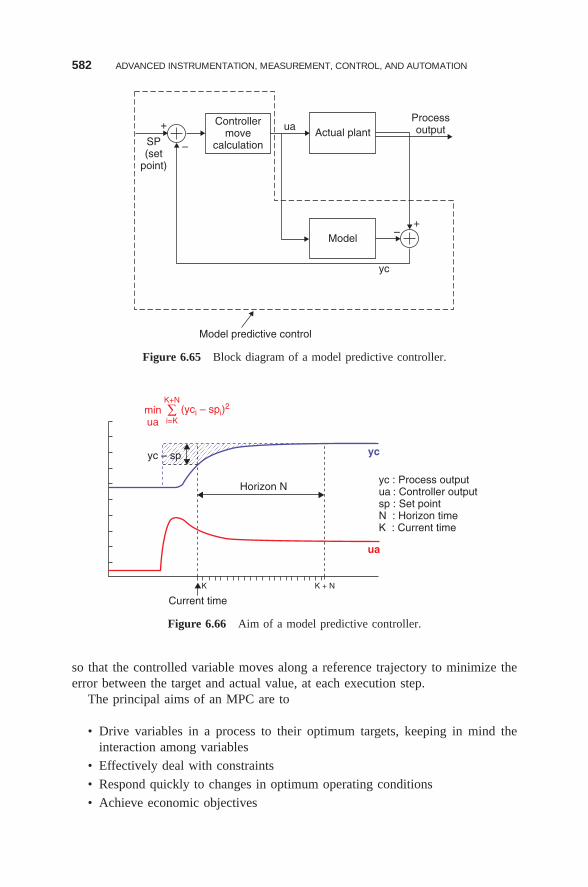
582 ADVANCED INSTRUMENTATION, MEASUREMENT, CONTROL, AND AUTOMATION

Controllermove

calculationActual plant

ua

Model

yc

Model predictive control

Processoutput

SP(set

point)

+

–

+–

Figure 6.65 Block diagram of a model predictive controller.

Horizon N

minua

K+N

i=K∑

K

Current time

K + N

yc – sp

(yci – spi)2

yc

ua

yc : Process outputua : Controller output sp : Set pointN : Horizon timeK : Current time

Figure 6.66 Aim of a model predictive controller.

so that the controlled variable moves along a reference trajectory to minimize theerror between the target and actual value, at each execution step.

The principal aims of an MPC are to

• Drive variables in a process to their optimum targets, keeping in mind theinteraction among variables

• Effectively deal with constraints

• Respond quickly to changes in optimum operating conditions

• Achieve economic objectives

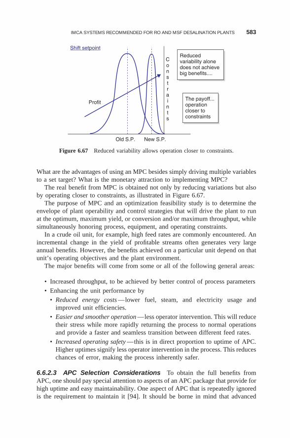
IMCA SYSTEMS RECOMMENDED FOR RO AND MSF DESALINATION PLANTS 583

Reducedvariability alonedoes not achievebig benefits....

The payoff...operationcloser toconstraints

Old S.P. New S.P.

Profit

Shift setpoint

Constraints

Figure 6.67 Reduced variability allows operation closer to constraints.

What are the advantages of using an MPC besides simply driving multiple variablesto a set target? What is the monetary attraction to implementing MPC?

The real benefit from MPC is obtained not only by reducing variations but alsoby operating closer to constraints, as illustrated in Figure 6.67.

The purpose of MPC and an optimization feasibility study is to determine theenvelope of plant operability and control strategies that will drive the plant to runat the optimum, maximum yield, or conversion and/or maximum throughput, whilesimultaneously honoring process, equipment, and operating constraints.

In a crude oil unit, for example, high feed rates are commonly encountered. Anincremental change in the yield of profitable streams often generates very largeannual benefits. However, the benefits achieved on a particular unit depend on thatunit’s operating objectives and the plant environment.

The major benefits will come from some or all of the following general areas:

• Increased throughput, to be achieved by better control of process parameters

• Enhancing the unit performance by

• Reduced energy costs —lower fuel, steam, and electricity usage andimproved unit efficiencies.

• Easier and smoother operation —less operator intervention. This will reducetheir stress while more rapidly returning the process to normal operationsand provide a faster and seamless transition between different feed rates.

• Increased operating safety —this is in direct proportion to uptime of APC.Higher uptimes signify less operator intervention in the process. This reduceschances of error, making the process inherently safer.

6.6.2.3 APC Selection Considerations To obtain the full benefits fromAPC, one should pay special attention to aspects of an APC package that provide forhigh uptime and easy maintainability. One aspect of APC that is repeatedly ignoredis the requirement to maintain it [94]. It should be borne in mind that advanced

584 ADVANCED INSTRUMENTATION, MEASUREMENT, CONTROL, AND AUTOMATION

controllers, once they are designed and implemented, also need to be maintained,just like any other piece of equipment such as a pump or compressor [94]. Howeasy a controller is to handle, maintain, or alter is determined by important factorssuch as

• Robustness

• How easily a controller adapts itself to changing process conditions, which isdirectly influences extent of intervention required

• How easily it can be maintained, or the model updated, or returned

• How easily it can be remodelled, if necessary, for gross excursions in processconditions from what it is designed for

• How one validates a model developed

• The peripherals that are required

• How easily it can be integrated with existing equipment

6.6.2.4 System Configuration of a Typical MPC The principal compo-nents of an overall integrated system (Fig. 6.68) will be

• One PC running on MS Windows for model building

• One PC running on MS Windows that will act as a control station

The difference in system configuration will be due to the operating systemof the existing DCS, the communication network that is used by DCS, and thecorresponding communication protocol that needs to be established between DCSand the control station (see Fig. 6.68) [94].

To solve this problem, the control package usually provides an interface that iscompliant with an OPC (OLE for process control systems) standard interface. OPCis a server running on Windows, which can be connected to a variety of processcontrol systems and provides an OPC client with process data via an OPC interface.The OPC client can acquire and define process data to and from process controland the control station. While the control station is connected to an Ethernet bus,OPC is connected to both Ethernet via Ethernet card and to the control bus.

6.6.2.5 Advanced Identification and Analysis (AIDA) The first and fore-most task in designing a controller is to develop a model. An AIDA Model is thebehavioral representation of a process. It represents process behavior to specificprocess inputs. AIDA establishes, mathematically, the relationship between input(manipulated) and output (controlled) variables. This is crucial in defining the scopeof the control algorithm. It should represent adequately all aspects of system behav-ior. It should also be robust with sufficient flexibility to face uncertainties in theprocess.

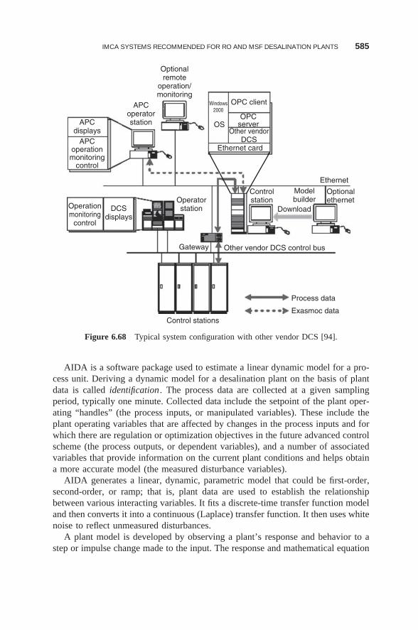
IMCA SYSTEMS RECOMMENDED FOR RO AND MSF DESALINATION PLANTS 585

APCdisplays

APCoperatorstation

Optionalremote

operation/monitoring

Windows2000

OS

OPC client

OPCserver

Other vendorDCS

Ethernet card

Operatorstation

Other vendor DCS control bus

Process data

Exasmoc data

Controlstation

Control stations

Modelbuilder

Ethernet

Optionalethernet

Download

Gateway

APCoperationmonitoring

control

Operationmonitoring

control

DCSdisplays

Figure 6.68 Typical system configuration with other vendor DCS [94].

AIDA is a software package used to estimate a linear dynamic model for a pro-cess unit. Deriving a dynamic model for a desalination plant on the basis of plantdata is called identification . The process data are collected at a given samplingperiod, typically one minute. Collected data include the setpoint of the plant oper-ating “handles” (the process inputs, or manipulated variables). These include theplant operating variables that are affected by changes in the process inputs and forwhich there are regulation or optimization objectives in the future advanced controlscheme (the process outputs, or dependent variables), and a number of associatedvariables that provide information on the current plant conditions and helps obtaina more accurate model (the measured disturbance variables).

AIDA generates a linear, dynamic, parametric model that could be first-order,second-order, or ramp; that is, plant data are used to establish the relationshipbetween various interacting variables. It fits a discrete-time transfer function modeland then converts it into a continuous (Laplace) transfer function. It then uses whitenoise to reflect unmeasured disturbances.

A plant model is developed by observing a plant’s response and behavior to astep or impulse change made to the input. The response and mathematical equation

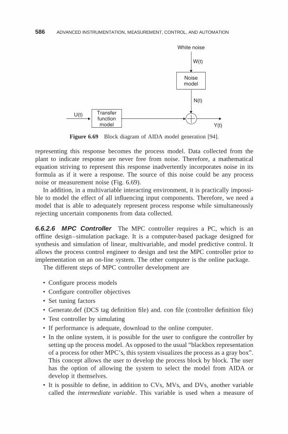
586 ADVANCED INSTRUMENTATION, MEASUREMENT, CONTROL, AND AUTOMATION

White noise

Noisemodel

Transferfunctionmodel

U(t)

N(t)

Y(t)

W(t)

Figure 6.69 Block diagram of AIDA model generation [94].

representing this response becomes the process model. Data collected from theplant to indicate response are never free from noise. Therefore, a mathematicalequation striving to represent this response inadvertently incorporates noise in itsformula as if it were a response. The source of this noise could be any processnoise or measurement noise (Fig. 6.69).

In addition, in a multivariable interacting environment, it is practically impossi-ble to model the effect of all influencing input components. Therefore, we need amodel that is able to adequately represent process response while simultaneouslyrejecting uncertain components from data collected.

6.6.2.6 MPC Controller The MPC controller requires a PC, which is anoffline design–simulation package. It is a computer-based package designed forsynthesis and simulation of linear, multivariable, and model predictive control. Itallows the process control engineer to design and test the MPC controller prior toimplementation on an on-line system. The other computer is the online package.

The different steps of MPC controller development are

• Configure process models

• Configure controller objectives

• Set tuning factors

• Generate.def (DCS tag definition file) and. con file (controller definition file)

• Test controller by simulating

• If performance is adequate, download to the online computer.

• In the online system, it is possible for the user to configure the controller bysetting up the process model. As opposed to the usual “blackbox representationof a process for other MPC’s, this system visualizes the process as a gray box”.This concept allows the user to develop the process block by block. The userhas the option of allowing the system to select the model from AIDA ordevelop it themselves.

• It is possible to define, in addition to CVs, MVs, and DVs, another variablecalled the intermediate variable. This variable is used when a measure of

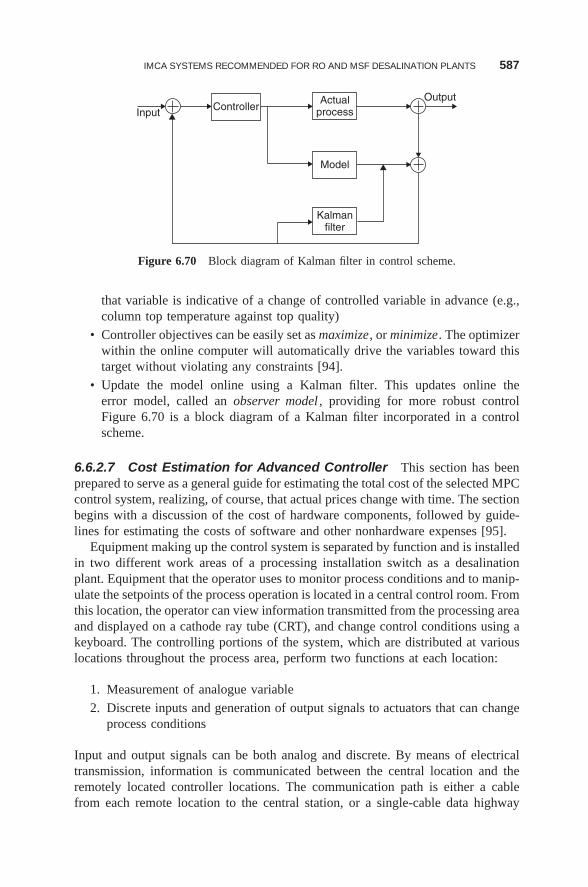
IMCA SYSTEMS RECOMMENDED FOR RO AND MSF DESALINATION PLANTS 587

Input ControllerActual

processOutput

Model

Kalmanfilter

Figure 6.70 Block diagram of Kalman filter in control scheme.

that variable is indicative of a change of controlled variable in advance (e.g.,column top temperature against top quality)

• Controller objectives can be easily set as maximize, or minimize. The optimizerwithin the online computer will automatically drive the variables toward thistarget without violating any constraints [94].

• Update the model online using a Kalman filter. This updates online theerror model, called an observer model , providing for more robust controlFigure 6.70 is a block diagram of a Kalman filter incorporated in a controlscheme.

6.6.2.7 Cost Estimation for Advanced Controller This section has beenprepared to serve as a general guide for estimating the total cost of the selected MPCcontrol system, realizing, of course, that actual prices change with time. The sectionbegins with a discussion of the cost of hardware components, followed by guide-lines for estimating the costs of software and other nonhardware expenses [95].

Equipment making up the control system is separated by function and is installedin two different work areas of a processing installation switch as a desalinationplant. Equipment that the operator uses to monitor process conditions and to manip-ulate the setpoints of the process operation is located in a central control room. Fromthis location, the operator can view information transmitted from the processing areaand displayed on a cathode ray tube (CRT), and change control conditions using akeyboard. The controlling portions of the system, which are distributed at variouslocations throughout the process area, perform two functions at each location:

1. Measurement of analogue variable

2. Discrete inputs and generation of output signals to actuators that can changeprocess conditions

Input and output signals can be both analog and discrete. By means of electricaltransmission, information is communicated between the central location and theremotely located controller locations. The communication path is either a cablefrom each remote location to the central station, or a single-cable data highway

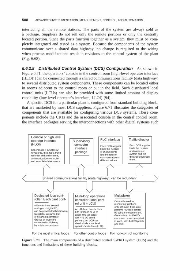
588 ADVANCED INSTRUMENTATION, MEASUREMENT, CONTROL, AND AUTOMATION

interfacing all the remote stations. The parts of the system are always sold asa package. Suppliers do not sell only the remote portions or only the centrallylocated portion. Since the parts function together as a system, they must be com-pletely integrated and tested as a system. Because the components of the systemcommunicate over a shared data highway, no change is required to the wiringwhen process modifications result in revisions to the control system of the plant(Fig. 6.68).

6.6.2.8 Distributed Control System (DCS) Configuration As shown inFigure 6.71, the operators’ console in the control room [high-level operator interface(HLOI)] can be connected through a shared communications facility (data highway)to several distributed system components. These components can be located eitherin rooms adjacent to the control room or out in the field. Such distributed localcontrol units (LCUs) can also be provided with some limited amount of displaycapability (low-level operator’s interface, LLOI) [94].

A specific DCS for a particular plant is configured from standard building blocksthat are marketed by most DCS suppliers. Figure 6.71 illustrates the categories ofcomponents that are available for configuring various DCS systems. These com-ponents include the CRTs and the associated console in the central control room,the interface packages serving the interconnections with other digital systems such

Console or high leveloperator interface(HLOI)

Supervisorycomputerinterfacepackage

Shared communications facility (data highway), can be redundant.

For the most critical loops For other control loops For non-control monitoring

Multi-loop operationscontroller (local cont-rol unit = LCU)

Multiplexer

PLC interface Traffic director

Each DCS supplierlimits the numberof DI/DO pointsand the rates ofcommunication todifferent values.

Each DCS supplierlimits the numberof devices persystem and thedistances betweenthem.

Can include 2–5 CRTs w/keyboards, disc, tape, trendrecorder and printer units,communications controllerand associated electronics.

Dedicated loop cont-roller: Each card cont-

roller can have severalanalog and digital I/O,can be provided with hardwarefaceplate, similar to thatof an analog controller.Groups of these areconnected to highwayby a data concentrator.

An LCU can handle from8 to 32 loops or up toabout 100 I/O cardswith 4–6 I/O pointsper card. An LCU canalso include a low leveloperator’s interface (LLOI)

Generally used formonitoring functionsonly although it can alsoperform PID loop controlby using the main consol.Generally up to 100 I/Ocards can be accomodatedin each, with 4–8 I/O pointsper card.

Figure 6.71 The main components of a distributed control SWRO system (DCS) and thefunctions and limitations of these building blocks.

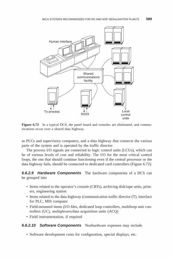
IMCA SYSTEMS RECOMMENDED FOR RO AND MSF DESALINATION PLANTS 589

Sharedcommunications

facility

Localcontrolunits

To processXXXX

Human interface

Figure 6.72 In a typical DCS, the panel board and consoles are eliminated, and commu-nications occur over a shared data highway.

as PLCs and supervisory computers, and a data highway that connects the variousparts of the system and is operated by the traffic director.

The process I/O signals are connected to logic control units (LCUs), which canbe of various levels of cost and reliability. The I/O for the most critical controlloops, the one that should continue functioning even if the central processor or thedata highway fails, should be connected to dedicated card controllers (Figure 6.72).

6.6.2.9 Hardware Components The hardware components of a DCS canbe grouped into

• Items related to the operator’s console (CRTs), archiving disk/tape units, print-ers, engineering station

• Items related to the data highway (communication traffic director (T), interfacefor PLC, MIS computer

• Field-mounted items (I/O files, dedicated loop controllers, multiloop unit con-trollers (UC), multiplexers/data acquisition units (ACQ)

• Field instrumentation, if required

6.6.2.10 Software Components Nonhardware expenses may include

• Software development costs for configuration, special displays, etc.

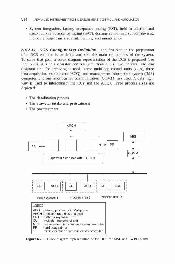
590 ADVANCED INSTRUMENTATION, MEASUREMENT, CONTROL, AND AUTOMATION

• System integration, factory acceptance testing (FAT), field installation andcheckout, site acceptance testing (SAT), documentation, and support devices,including project management, training, and maintenance

6.6.2.11 DCS Configuration Definition The first step in the preparationof a DCS estimate is to define and size the main components of the system.To serve that goal, a block diagram representation of the DCS is prepared (seeFig. 6.73). A single operator console with three CRTs, two printers, and onedisk/tape unit for archiving is used. Three multiloop control units (CUs), threedata acquisition multiplexers (ACQ), one management information system (IMS)computer, and one interface for communication (COMM) are used. A data high-way is used to interconnect the CUs and the ACQs. Three process areas aredepicted:

• The desalination process

• The seawater intake and pretreatment

• The posttreatment

PRPR

ARCH

MIS

COMM

CU ACQ CU ACQ CU ACQ

Process area 1 Process area 2 Process area 3

Operator’s console with 3 CRT’s

Legend

ACQ data acquisition unit, MultiplexerARCH archiving unit, disk and tapeCRT cathode ray tubeCU multiple-loop control unitMIS management information system computerPR hard copy printerT traffic director or communication controller

Figure 6.73 Block diagram representation of the DCS for MSF and SWRO plants.

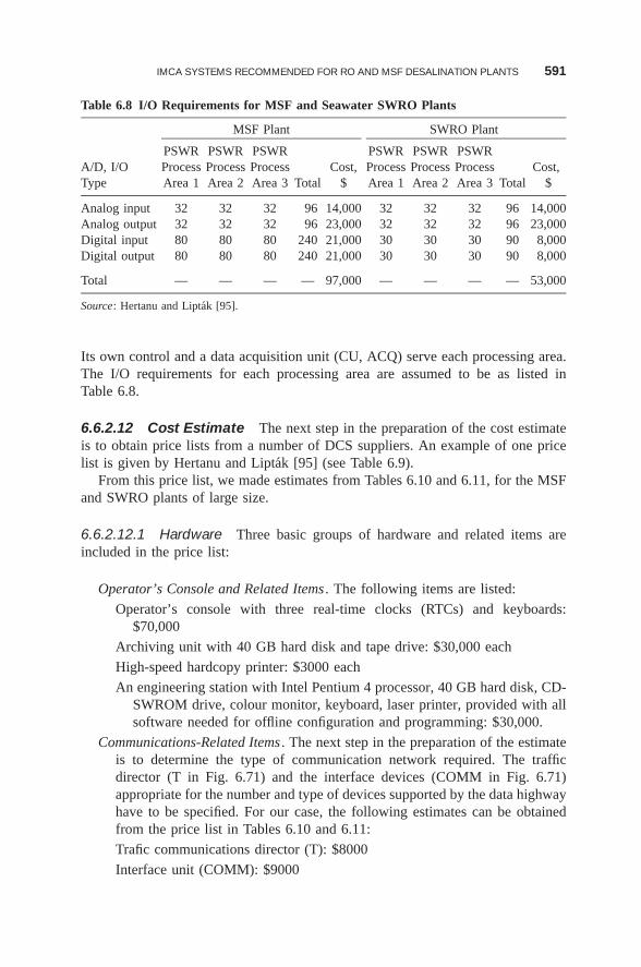
IMCA SYSTEMS RECOMMENDED FOR RO AND MSF DESALINATION PLANTS 591

Table 6.8 I/O Requirements for MSF and Seawater SWRO Plants

MSF Plant SWRO Plant

PSWR PSWR PSWR PSWR PSWR PSWRA/D, I/O Process Process Process Cost, Process Process Process Cost,Type Area 1 Area 2 Area 3 Total $ Area 1 Area 2 Area 3 Total $

Analog input 32 32 32 96 14,000 32 32 32 96 14,000Analog output 32 32 32 96 23,000 32 32 32 96 23,000Digital input 80 80 80 240 21,000 30 30 30 90 8,000Digital output 80 80 80 240 21,000 30 30 30 90 8,000

Total — — — — 97,000 — — — — 53,000

Source: Hertanu and Liptak [95].

Its own control and a data acquisition unit (CU, ACQ) serve each processing area.The I/O requirements for each processing area are assumed to be as listed inTable 6.8.

6.6.2.12 Cost Estimate The next step in the preparation of the cost estimateis to obtain price lists from a number of DCS suppliers. An example of one pricelist is given by Hertanu and Liptak [95] (see Table 6.9).

From this price list, we made estimates from Tables 6.10 and 6.11, for the MSFand SWRO plants of large size.

6.6.2.12.1 Hardware Three basic groups of hardware and related items areincluded in the price list:

Operator’s Console and Related Items . The following items are listed:

Operator’s console with three real-time clocks (RTCs) and keyboards:$70,000

Archiving unit with 40 GB hard disk and tape drive: $30,000 each

High-speed hardcopy printer: $3000 each

An engineering station with Intel Pentium 4 processor, 40 GB hard disk, CD-SWROM drive, colour monitor, keyboard, laser printer, provided with allsoftware needed for offline configuration and programming: $30,000.

Communications-Related Items . The next step in the preparation of the estimateis to determine the type of communication network required. The trafficdirector (T in Fig. 6.71) and the interface devices (COMM in Fig. 6.71)appropriate for the number and type of devices supported by the data highwayhave to be specified. For our case, the following estimates can be obtainedfrom the price list in Tables 6.10 and 6.11:

Trafic communications director (T): $8000

Interface unit (COMM): $9000

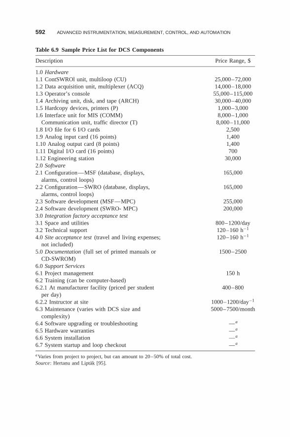
592 ADVANCED INSTRUMENTATION, MEASUREMENT, CONTROL, AND AUTOMATION

Table 6.9 Sample Price List for DCS Components

Description Price Range, $

1.0 Hardware1.1 ContSWROl unit, multiloop (CU) 25,000–72,0001.2 Data acquisition unit, multiplexer (ACQ) 14,000–18,0001.3 Operator’s console 55,000–115,0001.4 Archiving unit, disk, and tape (ARCH) 30,000–40,0001.5 Hardcopy devices, printers (P) 1,000–3,0001.6 Interface unit for MIS (COMM) 8,000–1,000

Communication unit, traffic director (T) 8,000–11,0001.8 I/O file for 6 I/O cards 2,5001.9 Analog input card (16 points) 1,4001.10 Analog output card (8 points) 1,4001.11 Digital I/O card (16 points) 7001.12 Engineering station 30,0002.0 Software2.1 Configuration—MSF (database, displays,

alarms, control loops)165,000

2.2 Configuration—SWRO (database, displays,alarms, control loops)

165,000

2.3 Software development (MSF—MPC) 255,0002.4 Software development (SWRO- MPC) 200,0003.0 Integration factory acceptance test3.1 Space and utilities 800–1200/day3.2 Technical support 120–160 h−1

4.0 Site acceptance test (travel and living expenses;not included)

120–160 h−1

5.0 Documentation (full set of printed manuals orCD-SWROM)

1500–2500

6.0 Support Services6.1 Project management 150 h6.2 Training (can be computer-based)6.2.1 At manufacturer facility (priced per student

per day)400–800

6.2.2 Instructor at site 1000–1200/day−1

6.3 Maintenance (varies with DCS size andcomplexity)

5000–7500/month

6.4 Software upgrading or troubleshooting —a

6.5 Hardware warranties —a

6.6 System installation —a

6.7 System startup and loop checkout —a

aVaries from project to project, but can amount to 20–50% of total cost.Source: Hertanu and Liptak [95].

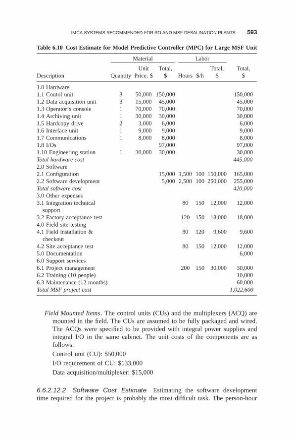
IMCA SYSTEMS RECOMMENDED FOR RO AND MSF DESALINATION PLANTS 593

Table 6.10 Cost Estimate for Model Predictive Controller (MPC) for Large MSF Unit

Material Labor

Unit Total, Total, Total,Description Quantity Price, $ $ Hours $/h $ $

1.0 Hardware1.1 Contol unit 3 50,000 150,000 150,0001.2 Data acquisition unit 3 15,000 45,000 45,0001.3 Operator’s console 1 70,000 70,000 70,0001.4 Archiving unit 1 30,000 30,000 30,0001.5 Hardcopy drive 2 3,000 6,000 6,0001.6 Interface unit 1 9,000 9,000 9,0001.7 Communications 1 8,000 8,000 8,0001.8 I/Os 97,000 97,0001.10 Engineering station 1 30,000 30,000 30,000Total hardware cost 445,0002.0 Software2.1 Configuration 15,000 1,500 100 150,000 165,0002.2 Software development 5,000 2,500 100 250,000 255,000Total software cost 420,0003.0 Other expenses3.1 Integration technical

support80 150 12,000 12,000

3.2 Factory acceptance test 120 150 18,000 18,0004.0 Field site testing4.1 Field installation &

checkout80 120 9,600 9,600

4.2 Site acceptance test 80 150 12,000 12,0005.0 Documentation 6,0006.0 Support services6.1 Project management 200 150 30,000 30,0006.2 Training (10 people) 10,0006.3 Maintenance (12 months) 60,000Total MSF project cost 1,022,600

Field Mounted Items . The control units (CUs) and the multiplexers (ACQ) aremounted in the field. The CUs are assumed to be fully packaged and wired.The ACQs were specified to be provided with integral power supplies andintegral I/O in the same cabinet. The unit costs of the components are asfollows:

Control unit (CU): $50,000

I/O requirement of CU: $133,000

Data acquisition/multiplexer: $15,000

6.6.2.12.2 Software Cost Estimate Estimating the software developmenttime required for the project is probably the most difficult task. The person-hour

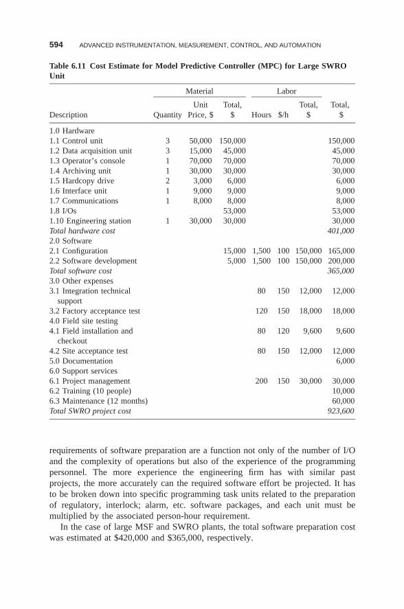
594 ADVANCED INSTRUMENTATION, MEASUREMENT, CONTROL, AND AUTOMATION

Table 6.11 Cost Estimate for Model Predictive Controller (MPC) for Large SWROUnit

Material Labor

Unit Total, Total, Total,Description Quantity Price, $ $ Hours $/h $ $

1.0 Hardware1.1 Control unit 3 50,000 150,000 150,0001.2 Data acquisition unit 3 15,000 45,000 45,0001.3 Operator’s console 1 70,000 70,000 70,0001.4 Archiving unit 1 30,000 30,000 30,0001.5 Hardcopy drive 2 3,000 6,000 6,0001.6 Interface unit 1 9,000 9,000 9,0001.7 Communications 1 8,000 8,000 8,0001.8 I/Os 53,000 53,0001.10 Engineering station 1 30,000 30,000 30,000Total hardware cost 401,0002.0 Software2.1 Configuration 15,000 1,500 100 150,000 165,0002.2 Software development 5,000 1,500 100 150,000 200,000Total software cost 365,0003.0 Other expenses3.1 Integration technical

support80 150 12,000 12,000

3.2 Factory acceptance test 120 150 18,000 18,0004.0 Field site testing4.1 Field installation and

checkout80 120 9,600 9,600

4.2 Site acceptance test 80 150 12,000 12,0005.0 Documentation 6,0006.0 Support services6.1 Project management 200 150 30,000 30,0006.2 Training (10 people) 10,0006.3 Maintenance (12 months) 60,000Total SWRO project cost 923,600

requirements of software preparation are a function not only of the number of I/Oand the complexity of operations but also of the experience of the programmingpersonnel. The more experience the engineering firm has with similar pastprojects, the more accurately can the required software effort be projected. It hasto be broken down into specific programming task units related to the preparationof regulatory, interlock; alarm, etc. software packages, and each unit must bemultiplied by the associated person-hour requirement.

In the case of large MSF and SWRO plants, the total software preparation costwas estimated at $420,000 and $365,000, respectively.

IMCA SYSTEMS RECOMMENDED FOR RO AND MSF DESALINATION PLANTS 595

6.6.2.12.3 Other Expenses After the hardware components of the DCS havebeen procured, the system must be integrated and made operational before it can beused. The location, space, utility, and labor requirements of the integration effortvary with project size and complexity. The cost of integration is usually estimatedbased on a specific integration plan, listing all the tasks that are to be performedduring the integration process. For our case, it was estimated that this task wouldcost $12,000 for the MSF and SWRO cases.

The factory acceptance test (FAT) seldom represents an additional cost for theproject, as the same engineering firm, which prepared the software, performs itand the person-hours are charged against the software preparation budget. The FATtests should be started by testing the integrity of the hardware components and theirconnection paths. This is followed by loading both the standard and applicationsoftware packages and verifying the functional operation using the applicationprograms and their database. Field checkout and installation costs for this projectwere estimated based on providing supervision only at $9600 and consisted ofsupervising the receiving, unpacking, installing, wiring, and powerup of the DCScomponents. The material costs for cables, wires, and mounting hardware wereincluded in the DCS hardware estimate.

The site acceptance test (SAT) follows installation and precedes the actual plantstartup. During SAT, all required DCS functions are verified. The cost of this taskwas estimated in Tables 6.10 and 6.11 as $12,000.

The estimate also includes $6000 for documentation. The project documentationshould include manufacturer’s cataloges and manuals for the relevant hardware,software, installation, site preparation, and maintenance guidance. It also includesall engineering drawings, validation documents, and test plans, procedures, andresults that were specifically prepared for the project.

The total cost estimate in Tables 6.10 and 6.11 also includes $31,200 for projectmanagement, $6000 for training operators, and $60,000 for the first year of main-tenance.

The additional cost of water due to the estimated capital and operating expensesof a newly installed DCS system on an existing desalination plant depends on theremaining lifetime of the plant, the capacity of the plant, and the technology used(whether MSF or SWRO). Using the data in the tables above, the additional costof water can be estimated as shown in the following section.

6.6.2.13 Added Cost of Water Due to DCS Installation Installing anadvanced controller is associated with capital and operating expenses as shown inTable 6.12. This results in an added cost to the original water cost. The capac-ities of the small, medium, and large MSF and SWRO plants are defined inTable 6.13.

The amount of added cost depends on a number of factors:

• The remaining lifetime of the desalination plant

• The actual cost of the DCS system equipment and installation

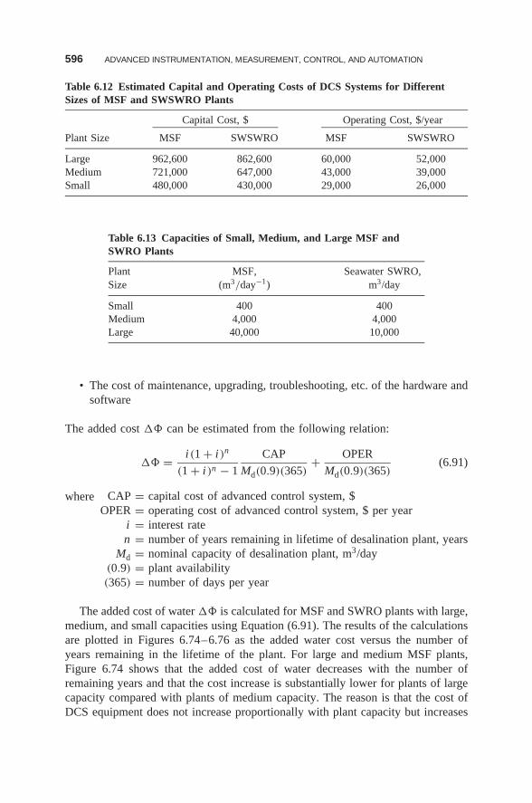
596 ADVANCED INSTRUMENTATION, MEASUREMENT, CONTROL, AND AUTOMATION

Table 6.12 Estimated Capital and Operating Costs of DCS Systems for DifferentSizes of MSF and SWSWRO Plants

Capital Cost, $ Operating Cost, $/year

Plant Size MSF SWSWRO MSF SWSWRO

Large 962,600 862,600 60,000 52,000Medium 721,000 647,000 43,000 39,000Small 480,000 430,000 29,000 26,000

Table 6.13 Capacities of Small, Medium, and Large MSF andSWRO Plants

Plant MSF, Seawater SWRO,Size (m3/day−1) m3/day

Small 400 400Medium 4,000 4,000Large 40,000 10,000

• The cost of maintenance, upgrading, troubleshooting, etc. of the hardware andsoftware

The added cost �� can be estimated from the following relation:

�� = i (1 + i )n

(1 + i )n − 1

CAP

Md(0.9)(365)+ OPER

Md(0.9)(365)(6.91)

where CAP = capital cost of advanced control system, $OPER = operating cost of advanced control system, $ per year

i = interest raten = number of years remaining in lifetime of desalination plant, years

Md = nominal capacity of desalination plant, m3/day(0.9) = plant availability(365) = number of days per year

The added cost of water �� is calculated for MSF and SWRO plants with large,medium, and small capacities using Equation (6.91). The results of the calculationsare plotted in Figures 6.74–6.76 as the added water cost versus the number ofyears remaining in the lifetime of the plant. For large and medium MSF plants,Figure 6.74 shows that the added cost of water decreases with the number ofremaining years and that the cost increase is substantially lower for plants of largecapacity compared with plants of medium capacity. The reason is that the cost ofDCS equipment does not increase proportionally with plant capacity but increases

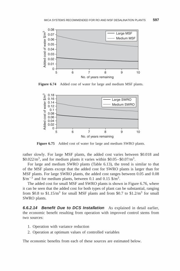
IMCA SYSTEMS RECOMMENDED FOR RO AND MSF DESALINATION PLANTS 597

0

0.01

0.02

0.03

0.04

0.05

0.06

0.07

0.08

5 6 7 8 9 10No. of years remaining

Add

ed c

ost o

f wat

er $

/m3

Large MSF

Medium MSF

Figure 6.74 Added cost of water for large and medium MSF plants.

0

0.040.02

0.060.080.1

0.120.140.160.18

5 6 7 8 9 10No. of years remaining

Add

ed c

ost o

f wat

er $

/m3

Large SWRO

Medium SWRO

Figure 6.75 Added cost of water for large and medium SWRO plants.

rather slowly. For large MSF plants, the added cost varies between $0.018 and$0.022/m3, and for medium plants it varies within $0.05–$0.07/m3.

For large and medium SWRO plants (Table 6.13), the trend is similar to thatof the MSF plants except that the added cost for SWRO plants is larger than forMSF plants. For large SWRO plants, the added cost ranges between 0.05 and 0.08$/m−3 and for medium plants, between 0.1 and 0.15 $/m3.

The added cost for small MSF and SWRO plants is shown in Figure 6.76, whereit can be seen that the added cost for both types of plant can be substantial, rangingfrom $0.8 to $1.15/m3 for small MSF plants and from $0.7 to $1.2/m3 for smallSWRO plants.

6.6.2.14 Benefit Due to DCS Installation As explained in detail earlier,the economic benefit resulting from operation with improved control stems fromtwo sources:

1. Operation with variance reduction

2. Operation at optimum values of controlled variables

The economic benefits from each of these sources are estimated below.

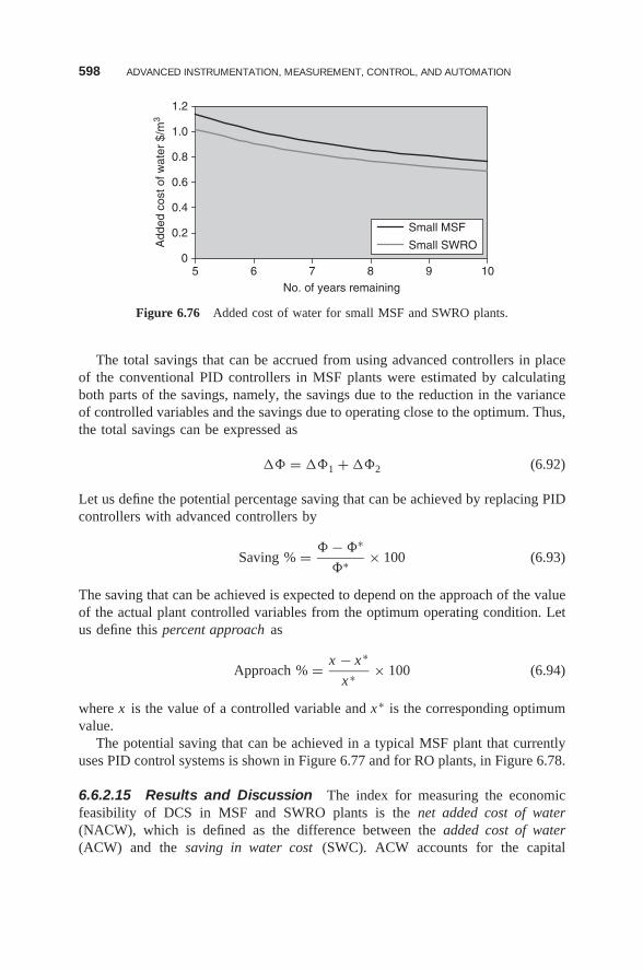
598 ADVANCED INSTRUMENTATION, MEASUREMENT, CONTROL, AND AUTOMATION

0

0.2

0.4

0.6

0.8

1.0

1.2

5 6 7 8 9 10No. of years remaining

Add

ed c

ost o

f wat

er $

/m3

Small MSF

Small SWRO

Figure 6.76 Added cost of water for small MSF and SWRO plants.

The total savings that can be accrued from using advanced controllers in placeof the conventional PID controllers in MSF plants were estimated by calculatingboth parts of the savings, namely, the savings due to the reduction in the varianceof controlled variables and the savings due to operating close to the optimum. Thus,the total savings can be expressed as

�� = ��1 + ��2 (6.92)

Let us define the potential percentage saving that can be achieved by replacing PIDcontrollers with advanced controllers by

Saving % = � − �∗

�∗ × 100 (6.93)

The saving that can be achieved is expected to depend on the approach of the valueof the actual plant controlled variables from the optimum operating condition. Letus define this percent approach as

Approach % = x − x∗

x∗ × 100 (6.94)

where x is the value of a controlled variable and x∗ is the corresponding optimumvalue.

The potential saving that can be achieved in a typical MSF plant that currentlyuses PID control systems is shown in Figure 6.77 and for RO plants, in Figure 6.78.

6.6.2.15 Results and Discussion The index for measuring the economicfeasibility of DCS in MSF and SWRO plants is the net added cost of water(NACW), which is defined as the difference between the added cost of water(ACW) and the saving in water cost (SWC). ACW accounts for the capital

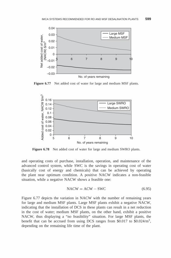
IMCA SYSTEMS RECOMMENDED FOR RO AND MSF DESALINATION PLANTS 599

–0.03

–0.02

–0.01

0

0.01

0.02

0.03

0.04

5 6 7 8 9 10

No. of years remaining

Net

add

ed c

ost o

f wat

er,

(NA

CW

) $/

m3

Large MSFMedium MSF

Figure 6.77 Net added cost of water for large and medium MSF plants.

00.020.040.060.08

0.10.120.140.16

5 6 7 8 9 10No. of years remaining

Add

ed c

ost o

f wat

er, N

AC

W $

/m3

Large SWRO

Medium SWRO

Figure 6.78 Net added cost of water for large and medium SWRO plants.

and operating costs of purchase, installation, operation, and maintenance of theadvanced control system, while SWC is the savings in operating cost of water(basically cost of energy and chemicals) that can be achieved by operatingthe plant near optimum condition. A positive NACW indicates a non-feasiblesituation, while a negative NACW shows a feasible one:

NACW = ACW − SWC (6.95)

Figure 6.77 depicts the variation in NACW with the number of remaining yearsfor large and medium MSF plants. Large MSF plants exhibit a negative NACW,indicating that the installation of DCS in these plants can result in a net reductionin the cost of water; medium MSF plants, on the other hand, exhibit a positiveNACW, thus displaying a “no feasibility” situation. For large MSF plants, thebenefit that can be accrued from using DCS ranges from $0.017 to $0.024/m3,depending on the remaining life time of the plant.

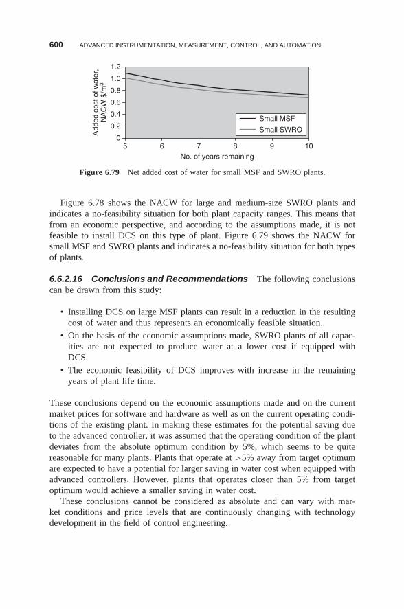
600 ADVANCED INSTRUMENTATION, MEASUREMENT, CONTROL, AND AUTOMATION

0

0.2

0.4

0.6

0.8

1.0

1.2

5 6 7 8 9 10No. of years remaining

Add

ed c

ost o

f wat

er,

NA

CW

$/m

3

Small MSF

Small SWRO

Figure 6.79 Net added cost of water for small MSF and SWRO plants.

Figure 6.78 shows the NACW for large and medium-size SWRO plants andindicates a no-feasibility situation for both plant capacity ranges. This means thatfrom an economic perspective, and according to the assumptions made, it is notfeasible to install DCS on this type of plant. Figure 6.79 shows the NACW forsmall MSF and SWRO plants and indicates a no-feasibility situation for both typesof plants.

6.6.2.16 Conclusions and Recommendations The following conclusionscan be drawn from this study:

• Installing DCS on large MSF plants can result in a reduction in the resultingcost of water and thus represents an economically feasible situation.

• On the basis of the economic assumptions made, SWRO plants of all capac-ities are not expected to produce water at a lower cost if equipped withDCS.

• The economic feasibility of DCS improves with increase in the remainingyears of plant life time.

These conclusions depend on the economic assumptions made and on the currentmarket prices for software and hardware as well as on the current operating condi-tions of the existing plant. In making these estimates for the potential saving dueto the advanced controller, it was assumed that the operating condition of the plantdeviates from the absolute optimum condition by 5%, which seems to be quitereasonable for many plants. Plants that operate at >5% away from target optimumare expected to have a potential for larger saving in water cost when equipped withadvanced controllers. However, plants that operates closer than 5% from targetoptimum would achieve a smaller saving in water cost.

These conclusions cannot be considered as absolute and can vary with mar-ket conditions and price levels that are continuously changing with technologydevelopment in the field of control engineering.

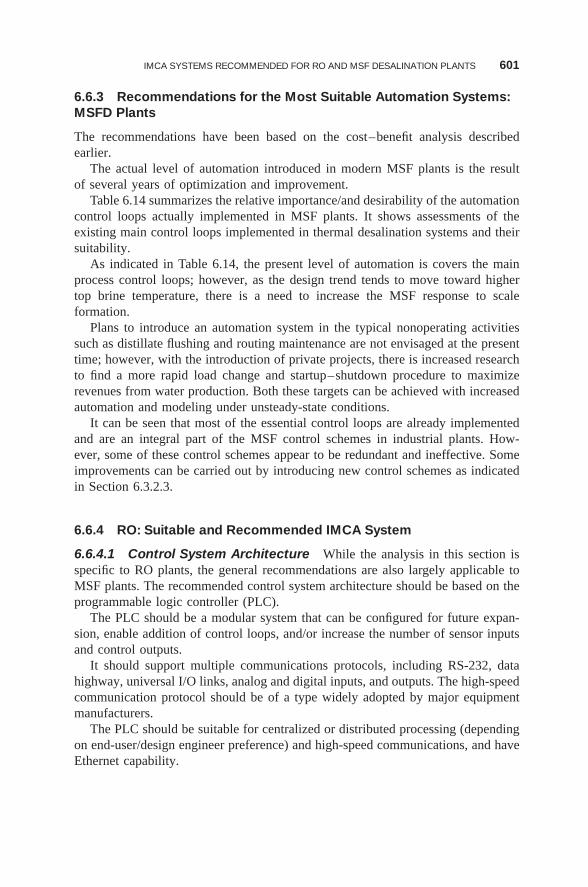
IMCA SYSTEMS RECOMMENDED FOR RO AND MSF DESALINATION PLANTS 601

6.6.3 Recommendations for the Most Suitable Automation Systems:MSFD Plants

The recommendations have been based on the cost–benefit analysis describedearlier.

The actual level of automation introduced in modern MSF plants is the resultof several years of optimization and improvement.

Table 6.14 summarizes the relative importance/and desirability of the automationcontrol loops actually implemented in MSF plants. It shows assessments of theexisting main control loops implemented in thermal desalination systems and theirsuitability.

As indicated in Table 6.14, the present level of automation is covers the mainprocess control loops; however, as the design trend tends to move toward highertop brine temperature, there is a need to increase the MSF response to scaleformation.

Plans to introduce an automation system in the typical nonoperating activitiessuch as distillate flushing and routing maintenance are not envisaged at the presenttime; however, with the introduction of private projects, there is increased researchto find a more rapid load change and startup–shutdown procedure to maximizerevenues from water production. Both these targets can be achieved with increasedautomation and modeling under unsteady-state conditions.

It can be seen that most of the essential control loops are already implementedand are an integral part of the MSF control schemes in industrial plants. How-ever, some of these control schemes appear to be redundant and ineffective. Someimprovements can be carried out by introducing new control schemes as indicatedin Section 6.3.2.3.

6.6.4 RO: Suitable and Recommended IMCA System

6.6.4.1 Control System Architecture While the analysis in this section isspecific to RO plants, the general recommendations are also largely applicable toMSF plants. The recommended control system architecture should be based on theprogrammable logic controller (PLC).

The PLC should be a modular system that can be configured for future expan-sion, enable addition of control loops, and/or increase the number of sensor inputsand control outputs.

It should support multiple communications protocols, including RS-232, datahighway, universal I/O links, analog and digital inputs, and outputs. The high-speedcommunication protocol should be of a type widely adopted by major equipmentmanufacturers.

The PLC should be suitable for centralized or distributed processing (dependingon end-user/design engineer preference) and high-speed communications, and haveEthernet capability.

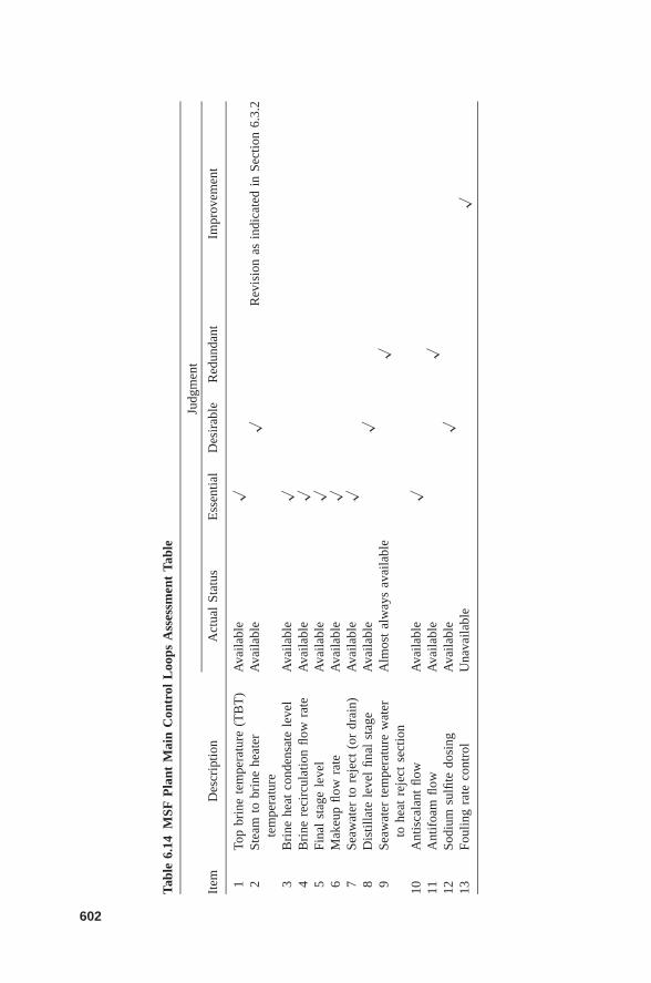
Tabl

e6.

14M

SFP

lant

Mai

nC

ontr

olL

oops

Ass

essm

ent

Tabl

e

Judg

men

t

Item

Des

crip

tion

Act

ual

Stat

usE

ssen

tial

Des

irab

leR

edun

dant

Impr

ovem

ent

1To

pbr

ine

tem

pera

ture

(TB

T)

Ava

ilabl

e√

2St

eam

tobr

ine

heat

erte

mpe

ratu

reA

vaila

ble

√R

evis

ion

asin

dica

ted

inSe

ctio

n6.

3.2

3B

rine

heat

cond

ensa

tele

vel

Ava

ilabl

e√

4B

rine

reci

rcul

atio

nflo

wra

teA

vaila

ble

√5

Fina

lst

age

leve

lA

vaila

ble

√6

Mak

eup

flow

rate

Ava

ilabl

e√

7Se

awat

erto

reje

ct(o

rdr

ain)

Ava

ilabl

e√

8D

istil

late

leve

lfin

alst

age

Ava

ilabl

e√

9Se

awat

erte

mpe

ratu

rew

ater

tohe

atre

ject

sect

ion

Alm

ost

alw

ays

avai

labl

e√

10A

ntis

cala

ntflo

wA

vaila

ble

√11

Ant

ifoa

mflo

wA

vaila

ble

√12

Sodi

umsu

lfite

dosi

ngA

vaila

ble

√13

Foul

ing

rate

cont

rol

Una

vaila

ble

√

602

IMCA SYSTEMS RECOMMENDED FOR RO AND MSF DESALINATION PLANTS 603

The main PLC should be configured for operation without interference fromharsh environmental or industrial conditions such as electric noise, fluctuationof ambient temperature, and vibrations. At present, noise-free communication isachieved mainly by connecting different system segments through fiberoptic lines.

Sufficient redundancy should be provided to ensure continuous operation whilemaintenance is conducted on part of the control system (independent operation ofcontrol modules).

Operation of the control system should be supported by an uninterrupted powersupply (UPS). The UPS should provide sufficient power capacity to maintain thecontrol system operational during the time lapse between the time of failure ofmain power supply and the time that emergency power generator is online andoperational. The control system should be divided into a functional sections (controlloops) according to logic of plant operation and functions performed by individualsections of the plant.

In the following discussion, it is assumed that some of the control loops arecontrolled by a separate PLC, which communicates with the main PLC througha dedicated Ethernet network (distributed control configuration). However, it ispossible that separate software modules that reside on the main PLC (centralizedcontrol configuration) could manage all individual control loops. The selection ofhardware or software specific for distributed control loops will be dictated by con-sideration of cost, logistics, and reliability. If the main PLC is capable of handlingall inputs and outputs and all system components are located on a single site, thenmost likely a software solution of managing and control of connected subsystemswill be preferred.

The local control loops will include sensors, activators, control logic software,and setpoints and will provide output to the local or central PLC.

6.6.4.2 Control Room The control room will include a number of work-stations, connected through a dedicated Ethernet network, that provide a displayof operating parameters and enable process control. The workstation should beinterchangeable and configured to provide five levels of accessibility according toauthorization level of operator:

Level 1 —anyone; view any display screen except for setpoint values

Level 2 —operator level; view any display screen except for setpoint values;ability to stop any equipment, print reports, and enter data

Level 3 —plant engineer level; access to all operator functions and ability tomodify setpoints and all process parameters

Level 4 —plant supervisor level; access to all functions of plant engineer andability to add/delete users, change access level, and change password

Level 5 —PLC program developer; unrestricted access and modificationauthority

In addition, the control room should include a server with an industrial databasefor plant data management. The database will provide information for evaluation of

604 ADVANCED INSTRUMENTATION, MEASUREMENT, CONTROL, AND AUTOMATION

system performance and conducting calculations for performance projections andoptimization. The server should have the ability to record information on externalmedia (CD or other mass data storage). Printers are also located in the controlroom.

6.6.4.3 Intake Control Loop The equipment for the intake control loopincludes

• PLC with required power supply and adapters

• Enclosures for instrumentation and sensor input

• Communication modem for connection to RO control loop

6.6.4.4 Pretreatment Control Loop Equipment for the pretreatment controlloop includes

• PLC with required power supply and adapters

• Enclosures for instrumentation and sensor input

• Communication modem for connection to RO control loop

6.6.4.5 Main RO Control Loop Equipment for the pretreatment control loopincludes

• PLC with required power supply and adapters

• Enclosures for instrumentation and sensor input

• Communication modem for connection to intake and pretreatment controlloops

6.6.4.6 RO Train Control Loops Equipment for the RO train control loopsincludes

• Enclosures for sensors and instrumentations input and local control

• Remote nodes with required power supplies and adapters

• Analog input–output modules

6.6.4.7 Motor Control Center• Enclosures for sensors and instrumentation input and local control

• Remote nodes with required power supplies and adapters

• Analog input and output modules

6.6.4.8 Electrical Circuits and VFD• Enclosure for sensors and instrumentations input and local control

• Remote nodes with required power supplies and adapters

• Analog input and output modules

MODELING AND ANALYSIS RECOMMENDATIONS FOR MSF AND RO PLANTS 605

6.6.4.9 Permeate Posttreatment and Storage• Enclosures for sensors and instrumentation input and local control

• Remote nodes with required power supplies and adapters

• Analog input–output modules

6.6.4.10 Wastewater Neutralization and Discharge• Enclosure for sensors and instrumentations input and local control

• Remote node with required power supplier and adapters

• Analog input–output modules

6.6.4.11 Operator–Computer Interface (HMI), Alarms They will bemanaged through integrated software that provides capability of managementof plant operation, display process parameters, process control, data logging,and data management. The integrated software will manage plant operation bymaintaining operating parameters within limits included in the setup parameterdatabase. According to plant conditions or process parameters, alarms could beinitiated. Alarms are initiated according to the following conditions:

1. Failure of equipment to operate (motors, valves, etc.)

2. Operating parameters outside limits (temperature, pH, pressure, etc.)

Software will initiate equipment shutdown if operating conditions are in a rangethat could result in equipment damage (high free chlorine, low suction pressure,etc.).

Both alarms and shutdown procedure will start after some delay, length of whichwill be defined during the detail design process.

Some of the alarms will be designed to clear when conditions change; othersmay require acknowledgment of operator or plant supervisor.

6.7 MODELING AND ANALYSIS RECOMMENDATIONS FOR MSF ANDRO PLANTS

6.7.1 Modeling Requirements

It is obvious that at least for the larger plants, future automation systems will bebased on line optimization where the measuring instruments, the control system,and the computer model of the process will interact in real time for the optimumperformance of the plant. This requires the establishment of models that describethe process properly under both steady-state and transient conditions. Transient“dynamic” modeling of both RO and MSF plants is still in its infancy (repre-sentative state-of-the art references are shown in the listed in the Further Readingsection below). This is especially true for MSF plants, where the flashing brine flowis still not adequately modeled. In our earlier studies that we cite in this chapter,

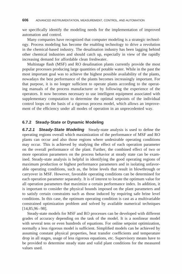
606 ADVANCED INSTRUMENTATION, MEASUREMENT, CONTROL, AND AUTOMATION

we specifically identify the modeling needs for the implementation of improvedautomation and control.

Many companies have recognized that computer modeling is a strategic technol-ogy. Process modeling has become the enabling technology to drive a revolutionin the chemical-based industry. The desalination industry has been lagging behindother chemical industries and should catch up, especially in view of the rapidlyincreasing demand for affordable clean freshwater.

Multistage flash (MSF) and RO desalination plants currently provide the mostpopular processes producing large quantities of potable water. While in the past themost important goal was to achieve the highest possible availability of the plants,nowadays the best performance of the plants becomes increasingly important. Forthat purpose, it is no longer sufficient to operate plants according to the operat-ing manuals of the process manufacturer or by following the experience of theoperators. It now becomes necessary to use intelligent equipment associated withsupplementary computation to determine the optimal setpoints of the individualcontrol loops on the basis of a rigorous process model, which allows an improve-ment of the efficiency under all modes of operation in an unprecedented way.

6.7.2 Steady-State or Dynamic Modeling

6.7.2.1 Steady-State Modeling Steady-state analysis is used to define theoperating regions overall which maximization of the performance of MSF and ROplants can occur and also those regions where undesirable operating conditionsmay occur. This is achieved by studying the effect of each operation parameteron the overall performance of the plant. Further, the combined effect of two ormore operation parameters on the process behavior at steady state can be exam-ined. Steady-state analysis is helpful in identifying the good operating regions ofmaximum production or highest performance parameters and in isolating unfavor-able operating conditions, such as, the brine levels that result in blowthrough orcarryover in MSF. However, favorable operating conditions can be determined foreach operation parameter separately. It is of interest to locate the optimum value forall operation parameters that maximize a certain performance index. In addition, itis important to consider the physical bounds imposed on the plant parameters andto satisfy certain constraints such as those induced by requiring safe brine levelconditions. In this case, the optimum operating condition is cast as a multivariableconstrained optimization problem and solved by available numerical techniques[14,85,96–98].

Steady-state models for MSF and RO processes can be developed with differentgrades of accuracy depending on the task of the model. It is a nonlinear modelwith several tens or even hundreds of equations. For online setpoint optimization,normally a less rigorous model is sufficient. Simplified models can be achieved byassuming constant physical properties, heat transfer coefficients and temperaturedrop in all stages, usage of less rigorous equations, etc. Supervisory means have tobe provided to determine steady state and valid plant conditions for the measuredvalues used.

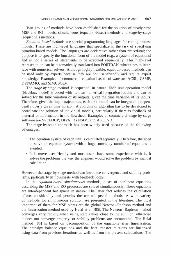
MODELING AND ANALYSIS RECOMMENDATIONS FOR MSF AND RO PLANTS 607

Two groups of methods have been established for the solution of steady-stateMSF and RO models: simultaneous (equation-based) methods and stage-by-stage(sequential) methods.

Equation-based methods use special programming languages for coding processmodels. These are high-level languages that specialize in the task of specifyingequation-based models. The languages are declarative rather than procedural; thepurpose is to specify the functional form of the model (e.g., a system of equations)and is not a series of statements to be executed sequentially. This high-levelrepresentation can be automatically translated into FORTRAN subroutines to inter-face with numerical solvers. Although highly flexible, equation-based methods canbe used only by experts because they are not user-friendly and require expertknowledge. Examples of commercial equation-based software are ACSL, CSMP,DYNAMO, and SIMUSOLV.

The stage-by-stage method is sequential in nature. Each unit operation model(blackbox model) is coded with its own numerical integration routine and can besolved for the time variation of its outputs, given the time variation of its inputs.Therefore, given the input trajectories, each unit model can be integrated indepen-dently over a given time horizon. A coordinator algorithm has to be developed tocoordinate the solution of individual models, particularly if there is feedback ofmaterial or information in the flowsheet. Examples of commercial stage-by-stagesoftware are SPEEDUP, DIVA, DYNSIM, and ASCEND.

The stage-by-stage approach has been widely used because of the followingadvantages:

• The equation system of each unit is calculated separately. Therefore, the needto solve an equation system with a huge, unwieldy number of equations isavoided.

• It is move user-friendly and most users have some experience with it. Itsolves the problems the way the engineer would solve the problem by manualcalculation.

However, the stage-by-stage method can introduce convergence and stability prob-lems, particularly in flowsheets with feedback loops.

In the equation-based simultaneous methods, a set of nonlinear equationsdescribing the MSF and RO processes are solved simultaneously. These equationsare interdependent but sparse in nature. The latter fact reduces the calculationefforts considerably and permits the use of special methods. A wide varietyof methods for simultaneous solution are presented in the literature. The mostimportant of them for MSF plants are the global Newton–Raphson method andthe linearization method used by Helal et al. [85]. The Newton–Raphson methodconverges very rapidly when using start values close to the solution, otherwiseit does not converge properly, or stability problems are encountered. The Helalmethod [85] is based on decomposition of the equations after linearization.The enthalpy balance equations and the heat transfer relations are linearizedusing data from previous iterations as well as from the present calculations. The

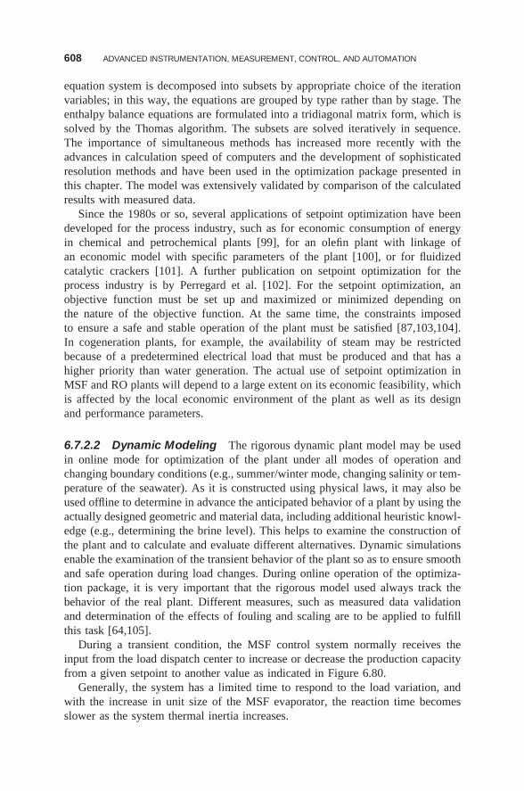
608 ADVANCED INSTRUMENTATION, MEASUREMENT, CONTROL, AND AUTOMATION

equation system is decomposed into subsets by appropriate choice of the iterationvariables; in this way, the equations are grouped by type rather than by stage. Theenthalpy balance equations are formulated into a tridiagonal matrix form, which issolved by the Thomas algorithm. The subsets are solved iteratively in sequence.The importance of simultaneous methods has increased more recently with theadvances in calculation speed of computers and the development of sophisticatedresolution methods and have been used in the optimization package presented inthis chapter. The model was extensively validated by comparison of the calculatedresults with measured data.

Since the 1980s or so, several applications of setpoint optimization have beendeveloped for the process industry, such as for economic consumption of energyin chemical and petrochemical plants [99], for an olefin plant with linkage ofan economic model with specific parameters of the plant [100], or for fluidizedcatalytic crackers [101]. A further publication on setpoint optimization for theprocess industry is by Perregard et al. [102]. For the setpoint optimization, anobjective function must be set up and maximized or minimized depending onthe nature of the objective function. At the same time, the constraints imposedto ensure a safe and stable operation of the plant must be satisfied [87,103,104].In cogeneration plants, for example, the availability of steam may be restrictedbecause of a predetermined electrical load that must be produced and that has ahigher priority than water generation. The actual use of setpoint optimization inMSF and RO plants will depend to a large extent on its economic feasibility, whichis affected by the local economic environment of the plant as well as its designand performance parameters.

6.7.2.2 Dynamic Modeling The rigorous dynamic plant model may be usedin online mode for optimization of the plant under all modes of operation andchanging boundary conditions (e.g., summer/winter mode, changing salinity or tem-perature of the seawater). As it is constructed using physical laws, it may also beused offline to determine in advance the anticipated behavior of a plant by using theactually designed geometric and material data, including additional heuristic knowl-edge (e.g., determining the brine level). This helps to examine the construction ofthe plant and to calculate and evaluate different alternatives. Dynamic simulationsenable the examination of the transient behavior of the plant so as to ensure smoothand safe operation during load changes. During online operation of the optimiza-tion package, it is very important that the rigorous model used always track thebehavior of the real plant. Different measures, such as measured data validationand determination of the effects of fouling and scaling are to be applied to fulfillthis task [64,105].

During a transient condition, the MSF control system normally receives theinput from the load dispatch center to increase or decrease the production capacityfrom a given setpoint to another value as indicated in Figure 6.80.

Generally, the system has a limited time to respond to the load variation, andwith the increase in unit size of the MSF evaporator, the reaction time becomesslower as the system thermal inertia increases.

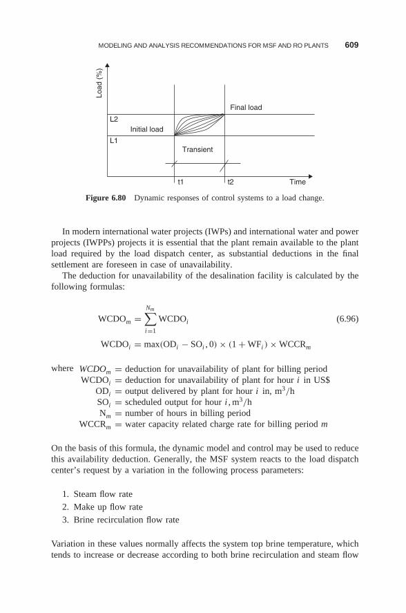
MODELING AND ANALYSIS RECOMMENDATIONS FOR MSF AND RO PLANTS 609

L1

t1 t2 Time

L2Initial load

Load

(%

)

Transient

Final load

Figure 6.80 Dynamic responses of control systems to a load change.

In modern international water projects (IWPs) and international water and powerprojects (IWPPs) projects it is essential that the plant remain available to the plantload required by the load dispatch center, as substantial deductions in the finalsettlement are foreseen in case of unavailability.

The deduction for unavailability of the desalination facility is calculated by thefollowing formulas:

WCDOm =Nm∑i=1

WCDOi (6.96)

WCDOi = max(ODi − SOi , 0) × (1 + WFi ) × WCCRm

where WCDOm = deduction for unavailability of plant for billing periodWCDOi = deduction for unavailability of plant for hour i in US$

ODi = output delivered by plant for hour i in, m3/hSOi = scheduled output for hour i , m3/hNm = number of hours in billing period

WCCRm = water capacity related charge rate for billing period m

On the basis of this formula, the dynamic model and control may be used to reducethis availability deduction. Generally, the MSF system reacts to the load dispatchcenter’s request by a variation in the following process parameters:

1. Steam flow rate

2. Make up flow rate

3. Brine recirculation flow rate

Variation in these values normally affects the system top brine temperature, whichtends to increase or decrease according to both brine recirculation and steam flow

610 ADVANCED INSTRUMENTATION, MEASUREMENT, CONTROL, AND AUTOMATION

rate. The distillate flow rate during transient conditions can be expressed as

md(t) = ϕ(t) (6.97)

md(t) = ψ[mbr(t), mst(t), mmu(t)] (6.98)

where t = timemd(t) = distillate flow ratembr(t) = brine recirculation flow ratemst(t) = makeup flow rate

mmu(t) = steam flow rate

The basic relationship governing the heat transfer and distillate production in thedesalination brine heater section is the definition of performance ratio as indicatedin equation (100) below:

η(t) = md(t)

mst(t)

�Href

�Hbh(6.99)

where η(t) = performance ratio�Href = reference enthalpy (normally 2,326 kJ/kg)�Hbh = difference between the steam and condensate enthalpies in the

brine heater

These sets of relationships may be simplified through the introduction of thedistillate production recirculation ratio parameter λ, defined as

λ ≡ md

mbr(6.100)

where λ can be expressed using Silver’s simplified equation as

λ = 1(1 − e−[(Cv�T )/�Hbh]

)ns (6.101)

where �T = flashing range of the evaporator (difference between highest andlowest brine temperatures)

ns = number of MSF stagesCv = brine specific heat

Ideally, the transient conditions should be managed in such a way that the plantperformance ratio remains constant (at, say, value K ) until the new steady state

η(t) = K (6.102)

MODELING AND ANALYSIS RECOMMENDATIONS FOR MSF AND RO PLANTS 611

is obtained. Thus

d [η(t)]

dt= d

dt

[md(t)

mst(t)

�Href

�Hbh

]= 0 (6.103)

Improved thermodynamic performance of the plant can also be sought by minimiz-ing entropy production. Entropy changes in the heat transfer process in the brineheater can be expressed as

�Ss = �Sbh + �Hbh

T(6.104)

where �Hbh and �Sbh represent the enthalpy drop and entropy rise of the steam inthe brine heater, and �Ss is the total entropy production. By combining Equations(6.10) and (6.106), we obtained the following equation:

�Ss = �Sbh + md

ms

�Href

ηT(6.105)

To achieve an efficient process, the overall entropy production �Ss must be mini-mized, and therefore the operating conditions that satisfy Equation (6.106) shouldbe selected for that purpose:

d�Ss

dt= 0 (6.106)

The power cycle simulation model for the MSF desalination plant can be usedto find the optimal settings for the abovementioned controllable parameters insideeach MSF. The simulation and monitoring of the MSF desalination allows theoperator to find deviations from the designed operation and to define optimizedsetpoints for operation of the MSF desalination. It will be possible to analyze

• The behavior of the process

• The production costs

• Steam costs

• Electrical costs

Further optimization can be related to optimization of the antiscaling costs. In fact,the antiscale dosing rate depends on the top brine temperature and the feedwaterflow according to the MSF evaporator antiscale dosing schedule. Its influence onthe transient costs is calculated on the basis of this function with a given price perquantity. The following inputs are used for the model:

• Top brine temperature

• Pressure of LP steam to brine heater

• Temperature of LP steam to brine heater

612 ADVANCED INSTRUMENTATION, MEASUREMENT, CONTROL, AND AUTOMATION

• Flow of LP steam to brine heater

• Brine recirculation flow rate

• Makeup flow rate

• Distillate flow rate setpoint at time 1

• Distillate flow rate setpoint at time 2

6.7.3 Mathematical Modeling: Description and needs in DesalinationIMCA

6.7.3.1 The Modeling in General To analyze the behavior of desalinationprocesses and to answer some of the questions raised regarding its control, we needa mathematical representation of the physical phenomena taking place in it. Such amathematical representation constitutes the model of the system, while the activitiesleading to the construction of the “model” will be referred to “as modeling.”

Modeling the MSF and RO desalination processes is a very synthetic activity,requiring the use of all the basic principles of thermal/fluid engineering science,such as thermodynamics, heat transfer, fluid mechanics, and transport phenomena.For the design of controllers for MSF and RO processes, modeling is a very crit-ical step. It should be approached with care and thoughtfulness. The goal is todevelop a control system that will guarantee that the operational objectives of theprocess are satisfied in the presence of ever-changing disturbances. Then, why dowe need to develop an accurate mathematical description (model) for the MSF andRO processes that we want to control? Often, the physical equipment we want tocontrol has not been constructed. Consequently, we cannot experiment to determinehow the process reacts to various inputs and therefore cannot design the appro-priate control system. Nevertheless, even if the process equipment is available forexperimentation, the procedure is usually very costly. Therefore, we need a sim-ple description of how the process reacts to various inputs, and this is what themathematical models can provide to the control engineer.

In general, processes can be represented by dynamic as well as steady-statemodels. The former are based on differential equations and/or state machines, andthey are required for solving problems in the transient phase, process interactions,troubleshooting, etc. However, they are necessary to implement advanced control,supervision, fault detection, and recovery strategies and dependable systems. Asteady-state model consists of algebraic equations, and it is a useful tool at thedesign stage, helping in the appropriate dimensioning of the plant, optimizationaspects, and calculation of the set points. They may also be used to determinefixed parameters and to validate dynamical models. However, they are not usefulfor control design and analysis purposes. The modeling process is usually integratedwith other types of engineering analysis, such as steady-state and dynamic processsimulation and online optimization. Dynamic modeling is normally needed forcontrol system design, while steady-state models are sufficient for optimization. Thefocus on dynamic modeling is on determining first-principle-based mathematicalmodels with emphasis on lumped-parameter (one-dimensional) systems with theaim of predicting the evolution of the system behavior with respect to time. In

MODELING AND ANALYSIS RECOMMENDATIONS FOR MSF AND RO PLANTS 613

terms of control, for a mathematical model to be useful it has to represent thedynamic behavior of the system inside its operation range. This means that thedominant time constants and the gains of both plant and model must match withadequate precision.

It should be noted that mathematical modeling of a process is only an abstrac-tion of the true system behavior. The model should mimic the system’s behaviorwith sufficient accuracy and should be verified against system behavior wheneverpossible. There are many models for a single system, each representing a differentlevel of abstraction, and the key task is to select the appropriate level of abstraction.

6.7.3.2 State Variables and State Equations To characterize a desalina-tion process (or generally any system) and its behavior, we need

• A set of fundamental dependent quantities whose values will describe thenatural state of the system

• A set of equations including the variables presented above that will describehow the natural state of the system changes with time

For desalination plants, the processes of interest have four fundamental quantities:mass, species, energy, and momentum. Quite often, the fundamental dependentvariables cannot be measured directly and conveniently. In such cases, we selectother variables that can be measured conveniently, and when grouped appropri-ately, they determine the value of the fundamental variables. Thus, mass, energy,and momentum can be characterized by variables such as density, concentration,temperature, pressure, and flow rate. These characterizing variables are called statevariables and their values, the state of a processing system.

The equations that relate the state variables (dependent variables) to the variousindependent variables are derived from application of the conservation principleson the fundamental quantities and are called state equations .

6.7.3.3 Conservation Equations The principle of conservation of a quantityS states that

Accumulation of Swithin systemTime period

= flow of S in system

time period− flow of S out of system

time period

+ amount of S generated within system

time period

− amount of S consumed within system

time period(6.107)

The quantity S can be any of the following fundamental quantities:

• Total mass

• Mass of individual species

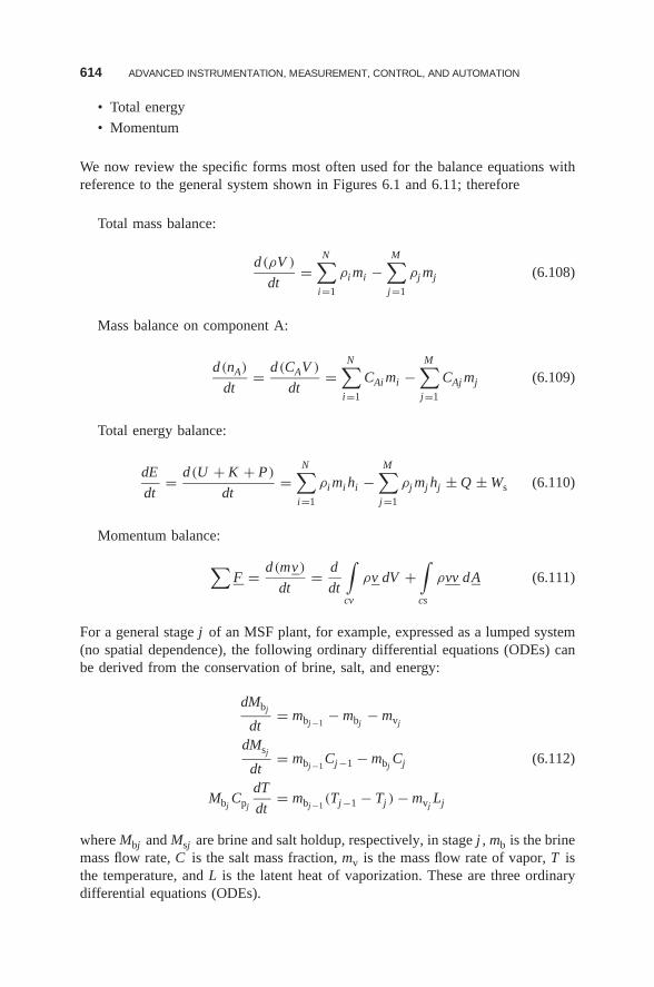
614 ADVANCED INSTRUMENTATION, MEASUREMENT, CONTROL, AND AUTOMATION

• Total energy

• Momentum

We now review the specific forms most often used for the balance equations withreference to the general system shown in Figures 6.1 and 6.11; therefore

Total mass balance:

d(ρV )

dt=

N∑i=1

ρi mi −M∑

j=1

ρj mj (6.108)

Mass balance on component A:

d(nA)

dt= d(CAV )

dt=

N∑i=1

CAi mi −M∑

j=1

CAj mj (6.109)

Total energy balance:

dE

dt= d(U + K + P)

dt=

N∑i=1

ρi mi hi −M∑

j=1

ρj mj hj ± Q ± Ws (6.110)

Momentum balance:

∑F = d(mv)

dt= d

dt

∫cv

ρv dV +∫cs

ρvv dA (6.111)

For a general stage j of an MSF plant, for example, expressed as a lumped system(no spatial dependence), the following ordinary differential equations (ODEs) canbe derived from the conservation of brine, salt, and energy:

dMbj

dt= mbj−1

− mbj− mvj

dMsj

dt= mbj−1

Cj−1 − mbjCj (6.112)

MbjCpj

dT

dt= mbj−1

(Tj−1 − Tj ) − mvjLj

where Mbj and Msj are brine and salt holdup, respectively, in stage j , mb is the brinemass flow rate, C is the salt mass fraction, mv is the mass flow rate of vapor, T isthe temperature, and L is the latent heat of vaporization. These are three ordinarydifferential equations (ODEs).

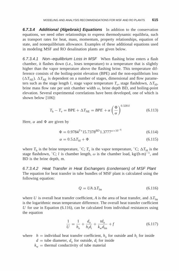
MODELING AND ANALYSIS RECOMMENDATIONS FOR MSF AND RO PLANTS 615

6.7.3.4 Additional (Algebraic) Equations In addition to the conservationequations, we need other relationships to express thermodynamic equilibria, suchas transport rates for heat, mass, momentum, property relationships, equation ofstate, and nonequilibrium allowance. Examples of these additional equations usedin modeling MSF and RO desalination plants are given below.

6.7.3.4.1 Non–equilibrium Loss in MSF When flashing brine enters a flashchamber, it flashes down (i.e., loses temperature) to a temperature that is slightlyhigher than the vapor temperature above the flashing brine. This temperature dif-ference consists of the boiling-point elevation (BPE) and the non-equilibrium loss(�TNE). �TNE is dependent on a number of stages, dimensional and flow parame-ters such as the stage length l , stage vapor temperature Tv, stage flashdown, �Tfd,brine mass flow rate per unit chamber width ω, brine depth BD, and boiling-pointelevation. Several experimental correlations have been developed, one of which isshown below [106]:

Tb − Tv = BPE + �TNE = BPE + α

(�

α

)0.3281l

(6.113)

Here, α and � are given by

� = 0.9784Tv15.7378BD 1.3777ω×10−6(6.114)

α = 0.5�Tfd + � (6.115)

where Tb is the brine temperature, ◦C; Tv is the vapor temperature, ◦C; �Tfd is thestage flashdown, ◦C; l is chamber length, ω is the chamber load, kg/(h·m)−1, andBD is the brine depth, m.

6.7.3.4.2 Heat Transfer in Heat Exchangers (condensers) of MSF PlantThe equation for heat transfer in tube bundles of MSF plant is calculated using thefollowing equation:

Q = UA �Tlm (6.116)

where U is overall heat transfer coefficient, A is the area of heat transfer, and �Tlmis the logarithmic mean temperature difference. The overall heat transfer coefficientU for use in Equation (6.116), can be calculated from individual resistances usingthe equation

1

U= 1

ho+ do

hidi+ tdo

kwdlm+ f (6.117)

where h = individual heat transfer coefficient, ho for outside and hi for insided = tube diameter, do for outside, di for inside

kw = thermal conductivity of tube material

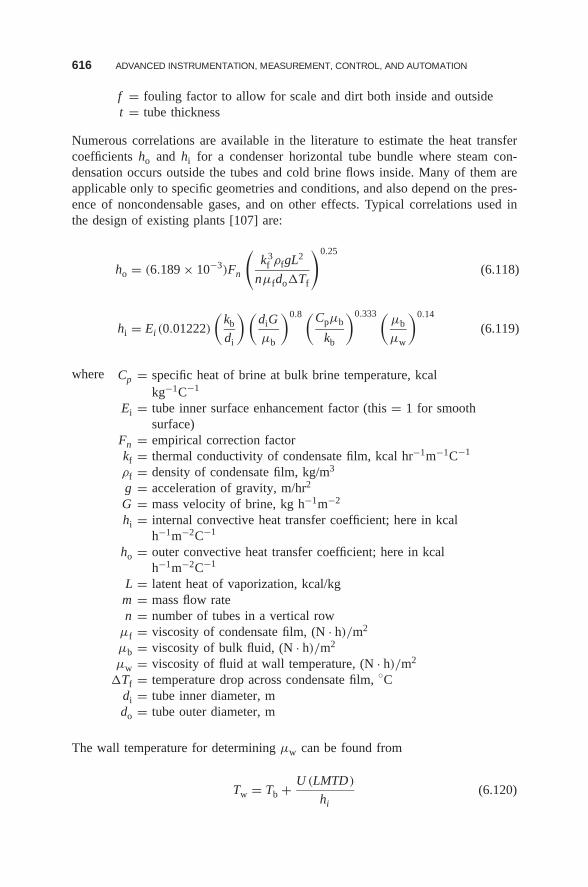
616 ADVANCED INSTRUMENTATION, MEASUREMENT, CONTROL, AND AUTOMATION

f = fouling factor to allow for scale and dirt both inside and outsidet = tube thickness

Numerous correlations are available in the literature to estimate the heat transfercoefficients ho and hi for a condenser horizontal tube bundle where steam con-densation occurs outside the tubes and cold brine flows inside. Many of them areapplicable only to specific geometries and conditions, and also depend on the pres-ence of noncondensable gases, and on other effects. Typical correlations used inthe design of existing plants [107] are:

ho = (6.189 × 10−3)Fn

(k3

f ρfgL2

nμfdo�Tf

)0.25

(6.118)

hi = Ei (0.01222)

(kb

di

) (diG

μb

)0.8 (Cpμb

kb

)0.333 (μb

μw

)0.14

(6.119)

where Cp = specific heat of brine at bulk brine temperature, kcalkg−1C−1

Ei = tube inner surface enhancement factor (this = 1 for smoothsurface)

Fn = empirical correction factorkf = thermal conductivity of condensate film, kcal hr−1m−1C−1

ρf = density of condensate film, kg/m3

g = acceleration of gravity, m/hr2

G = mass velocity of brine, kg h−1m−2

hi = internal convective heat transfer coefficient; here in kcalh−1m−2C−1

ho = outer convective heat transfer coefficient; here in kcalh−1m−2C−1

L = latent heat of vaporization, kcal/kgm = mass flow raten = number of tubes in a vertical row

μf = viscosity of condensate film, (N · h)/m2

μb = viscosity of bulk fluid, (N · h)/m2

μw = viscosity of fluid at wall temperature, (N · h)/m2

�Tf = temperature drop across condensate film, ◦Cdi = tube inner diameter, mdo = tube outer diameter, m

The wall temperature for determining μw can be found from

Tw = Tb + U (LMTD)

hi(6.120)

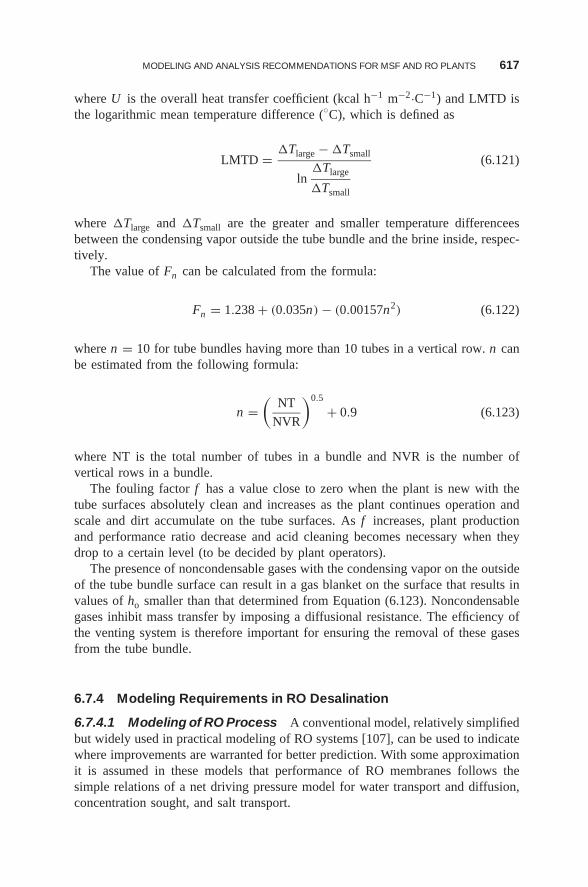
MODELING AND ANALYSIS RECOMMENDATIONS FOR MSF AND RO PLANTS 617

where U is the overall heat transfer coefficient (kcal h−1 m−2·C−1) and LMTD isthe logarithmic mean temperature difference (◦C), which is defined as

LMTD = �Tlarge − �Tsmall

ln�Tlarge

�Tsmall

(6.121)

where �Tlarge and �Tsmall are the greater and smaller temperature differenceesbetween the condensing vapor outside the tube bundle and the brine inside, respec-tively.

The value of Fn can be calculated from the formula:

Fn = 1.238 + (0.035n) − (0.00157n2) (6.122)

where n = 10 for tube bundles having more than 10 tubes in a vertical row. n canbe estimated from the following formula:

n =(

NT

NVR

)0.5

+ 0.9 (6.123)

where NT is the total number of tubes in a bundle and NVR is the number ofvertical rows in a bundle.

The fouling factor f has a value close to zero when the plant is new with thetube surfaces absolutely clean and increases as the plant continues operation andscale and dirt accumulate on the tube surfaces. As f increases, plant productionand performance ratio decrease and acid cleaning becomes necessary when theydrop to a certain level (to be decided by plant operators).

The presence of noncondensable gases with the condensing vapor on the outsideof the tube bundle surface can result in a gas blanket on the surface that results invalues of ho smaller than that determined from Equation (6.123). Noncondensablegases inhibit mass transfer by imposing a diffusional resistance. The efficiency ofthe venting system is therefore important for ensuring the removal of these gasesfrom the tube bundle.

6.7.4 Modeling Requirements in RO Desalination

6.7.4.1 Modeling of RO Process A conventional model, relatively simplifiedbut widely used in practical modeling of RO systems [107], can be used to indicatewhere improvements are warranted for better prediction. With some approximationit is assumed in these models that performance of RO membranes follows thesimple relations of a net driving pressure model for water transport and diffusion,concentration sought, and salt transport.

618 ADVANCED INSTRUMENTATION, MEASUREMENT, CONTROL, AND AUTOMATION

6.7.4.1.1 Osmotic Process Osmosis is a natural process involving fluid flowacross a semipermeable membrane barrier. It is selective in the sense that the solventpasses through the membrane at a higher rate than the passage of dissolved solids.The difference of passage rate results in solvent–solids separation. The direction ofsolvent flow is determined by its chemical potential, which is a function of pressure,temperature, and concentration of dissolved solids. Pure water in contact with bothsides of an ideal semipermeable membrane at equal pressure and temperature hasno net flow across the membrane because the chemical potential is equal on bothsides. If a soluble salt is added to water on one side of the membrane, the chemicalpotential of this salt solution is reduced. Osmotic flow from the pure-water sideacross the membrane to the salt solution side will occur until the equilibrium ofchemical potential is restored. Equilibrium occurs when the hydrostatic pressuredifferential resulting from the volume changes on both sides is equal to the osmoticpressure. This is a solution property independent of the membrane. Application ofan external pressure to the salt solution side, which is equal to the osmotic pressure,will also cause equilibrium. Additional pressure will raise the chemical potentialof the water in the salt solution and cause a solvent flow to the pure-water side,because it now has a lower chemical potential. This phenomenon is called reverseosmosis . The osmotic pressure Posm of a solution can be approximated indirectlyby measuring the concentration of dissolved salts in solution

Posm = RT∑

i

mi (6.124)

where Posm = osmotic pressure (bar), R is the universal gas constant (0.082 l atmmol−1 K−1), T is the temperature (K), and �mi is the sum of molar concentration ofall constituents in a solution. An approximation for Posm can be made by assumingthat 1000 ppm concentration of total dissolved solids (TDS) equals ∼0.77 bar(11 psi) of osmotic pressure. For example, in a RO unit, operating at 75% recoveryrate, feed salinity is 3000 ppm TDS and concentrate salinity is ∼11,500 ppmTDS. Accordingly, the osmotic pressure of the feed is 2.3 bar (33 psi) and ofthe concentrate, it is 8.7 bar (126 psi). Equation (6.124) only holds for dilute saltsolutions and temperatures close to 25◦C. Under significantly different conditions amore rigorous calculation, which takes into consideration ion activities rather thanconcentrations, has to be applied.

6.7.4.1.2 Permeate Recovery Rate (Conversion) Permeate recovery is oneof more important parameters in the design and operation of RO systems. Recoveryor conversion rate of feedwater to product (permeate) is defined (in %) by

R ≡ mp

mf100 (6.125)

R ≡ mp

mp + mc100 (6.126)

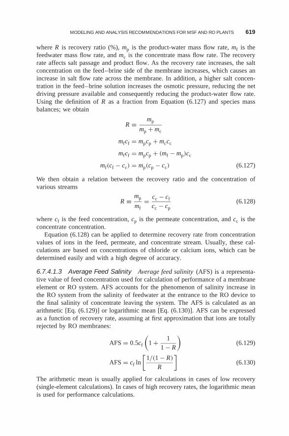
MODELING AND ANALYSIS RECOMMENDATIONS FOR MSF AND RO PLANTS 619

where R is recovery ratio (%), mp is the product-water mass flow rate, mf is thefeedwater mass flow rate, and mc is the concentrate mass flow rate. The recoveryrate affects salt passage and product flow. As the recovery rate increases, the saltconcentration on the feed–brine side of the membrane increases, which causes anincrease in salt flow rate across the membrane. In addition, a higher salt concen-tration in the feed–brine solution increases the osmotic pressure, reducing the netdriving pressure available and consequently reducing the product-water flow rate.Using the definition of R as a fraction from Equation (6.127) and species massbalances; we obtain

R ≡ mp

mp + mc

mfcf = mpcp + mccc

mfcf = mpcp + (mf − mp)cc

mf(cf − cc) = mp(cp − cc) (6.127)

We then obtain a relation between the recovery ratio and the concentration ofvarious streams

R ≡ mp

mf= cc − cf

cc − cp(6.128)

where cf is the feed concentration, cp is the permeate concentration, and cc is theconcentrate concentration.

Equation (6.128) can be applied to determine recovery rate from concentrationvalues of ions in the feed, permeate, and concentrate stream. Usually, these cal-culations are based on concentrations of chloride or calcium ions, which can bedetermined easily and with a high degree of accuracy.

6.7.4.1.3 Average Feed Salinity Average feed salinity (AFS) is a representa-tive value of feed concentration used for calculation of performance of a membraneelement or RO system. AFS accounts for the phenomenon of salinity increase inthe RO system from the salinity of feedwater at the entrance to the RO device tothe final salinity of concentrate leaving the system. The AFS is calculated as anarithmetic [Eq. (6.129)] or logarithmic mean [Eq. (6.130)]. AFS can be expressedas a function of recovery rate, assuming at first approximation that ions are totallyrejected by RO membranes:

AFS = 0.5cf

(1 + 1

1 − R

)(6.129)

AFS = cf ln

[1/(1 − R)

R

](6.130)

The arithmetic mean is usually applied for calculations in cases of low recovery(single-element calculations). In cases of high recovery rates, the logarithmic meanis used for performance calculations.

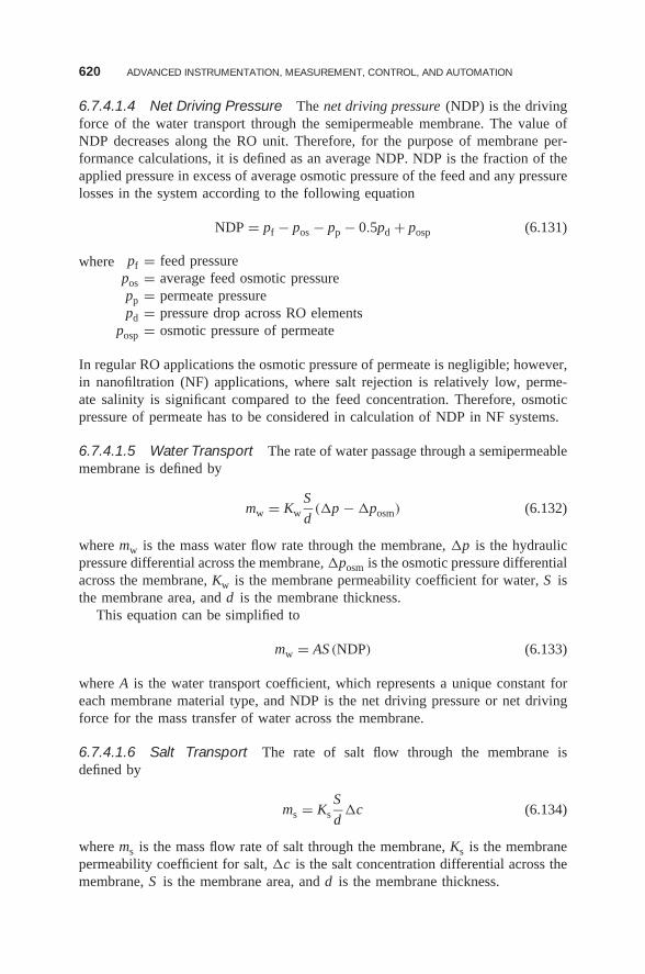
620 ADVANCED INSTRUMENTATION, MEASUREMENT, CONTROL, AND AUTOMATION

6.7.4.1.4 Net Driving Pressure The net driving pressure (NDP) is the drivingforce of the water transport through the semipermeable membrane. The value ofNDP decreases along the RO unit. Therefore, for the purpose of membrane per-formance calculations, it is defined as an average NDP. NDP is the fraction of theapplied pressure in excess of average osmotic pressure of the feed and any pressurelosses in the system according to the following equation

NDP = pf − pos − pp − 0.5pd + posp (6.131)

where pf = feed pressurepos = average feed osmotic pressurepp = permeate pressurepd = pressure drop across RO elements

posp = osmotic pressure of permeate

In regular RO applications the osmotic pressure of permeate is negligible; however,in nanofiltration (NF) applications, where salt rejection is relatively low, perme-ate salinity is significant compared to the feed concentration. Therefore, osmoticpressure of permeate has to be considered in calculation of NDP in NF systems.

6.7.4.1.5 Water Transport The rate of water passage through a semipermeablemembrane is defined by

mw = KwS

d(�p − �posm) (6.132)

where mw is the mass water flow rate through the membrane, �p is the hydraulicpressure differential across the membrane, �posm is the osmotic pressure differentialacross the membrane, Kw is the membrane permeability coefficient for water, S isthe membrane area, and d is the membrane thickness.

This equation can be simplified to

mw = AS (NDP) (6.133)

where A is the water transport coefficient, which represents a unique constant foreach membrane material type, and NDP is the net driving pressure or net drivingforce for the mass transfer of water across the membrane.

6.7.4.1.6 Salt Transport The rate of salt flow through the membrane isdefined by

ms = KsS

d�c (6.134)

where ms is the mass flow rate of salt through the membrane, Ks is the membranepermeability coefficient for salt, �c is the salt concentration differential across themembrane, S is the membrane area, and d is the membrane thickness.

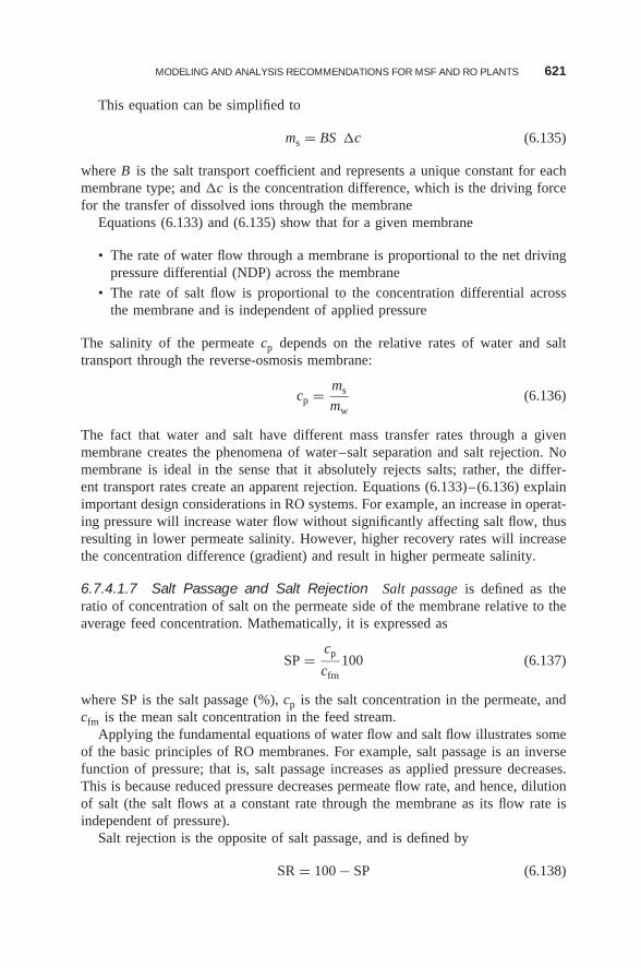
MODELING AND ANALYSIS RECOMMENDATIONS FOR MSF AND RO PLANTS 621

This equation can be simplified to

ms = BS �c (6.135)

where B is the salt transport coefficient and represents a unique constant for eachmembrane type; and �c is the concentration difference, which is the driving forcefor the transfer of dissolved ions through the membrane

Equations (6.133) and (6.135) show that for a given membrane

• The rate of water flow through a membrane is proportional to the net drivingpressure differential (NDP) across the membrane

• The rate of salt flow is proportional to the concentration differential acrossthe membrane and is independent of applied pressure

The salinity of the permeate cp depends on the relative rates of water and salttransport through the reverse-osmosis membrane:

cp = ms

mw(6.136)

The fact that water and salt have different mass transfer rates through a givenmembrane creates the phenomena of water–salt separation and salt rejection. Nomembrane is ideal in the sense that it absolutely rejects salts; rather, the differ-ent transport rates create an apparent rejection. Equations (6.133)–(6.136) explainimportant design considerations in RO systems. For example, an increase in operat-ing pressure will increase water flow without significantly affecting salt flow, thusresulting in lower permeate salinity. However, higher recovery rates will increasethe concentration difference (gradient) and result in higher permeate salinity.

6.7.4.1.7 Salt Passage and Salt Rejection Salt passage is defined as theratio of concentration of salt on the permeate side of the membrane relative to theaverage feed concentration. Mathematically, it is expressed as

SP = cp

cfm100 (6.137)

where SP is the salt passage (%), cp is the salt concentration in the permeate, andcfm is the mean salt concentration in the feed stream.

Applying the fundamental equations of water flow and salt flow illustrates someof the basic principles of RO membranes. For example, salt passage is an inversefunction of pressure; that is, salt passage increases as applied pressure decreases.This is because reduced pressure decreases permeate flow rate, and hence, dilutionof salt (the salt flows at a constant rate through the membrane as its flow rate isindependent of pressure).

Salt rejection is the opposite of salt passage, and is defined by

SR = 100 − SP (6.138)

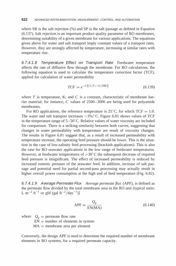
622 ADVANCED INSTRUMENTATION, MEASUREMENT, CONTROL, AND AUTOMATION

where SR is the salt rejection (%) and SP is the salt passage as defined in Equation(6.137). Salt rejection is an important product quality parameter of RO membranes,determining suitability of a given membrane for various applications. The equationsgiven above for water and salt transport imply constant values of a transport rates.However, they are strongly affected by temperature, increasing at similar rates withtemperature rise.

6.7.4.1.8 Temperature Effect on Transport Rate Feedwater temperatureaffects the rate of diffusive flow through the membrane. For RO calculations, thefollowing equation is used to calculate the temperature correction factor (TCF),applied for calculation of water permeability

TCF = e−C [(1/T )−(1/298)] (6.139)

where T is temperature, K; and C is a constant, characteristic of membrane bar-rier material; for instance, C values of 2500–3000 are being used for polyamidemembranes.

For RO applications, the reference temperature is 25◦C, for which TCF = 1.0.The water and salt transport increases ∼3%/◦C. Figure 6.81 shows values of TCFin the temperature range of 5–50◦C. Relative values of water viscosity are includedfor comparison. There is a striking similarity between both curves, suggesting thatchanges in water permeability with temperature are result of viscosity changes.The results in Figure 6.81 suggest that, as a result of increased permeability withtemperature increase, the operating feed pressure should be lower. This is the situa-tion in the case of low-salinity feed processing (brackish applications). This is alsothe case for RO seawater applications in the low range of feedwater temperatures.However, at feedwater temperatures of >30◦C the subsequent decrease of requiredfeed pressure is insignificant. The effect of increased permeability is reduced byincreased osmotic pressure of the seawater feed. In addition, increase of salt pas-sage and potential need for partial second-pass processing may actually result inhigher overall power consumption at the high end of feed temperature (Fig. 6.82).

6.7.4.1.9 Average Permeate Flux Average permeate flux (APF), is defined asthe permeate flow divided by the total membrane area in the RO unit [typical units:L m−2 h−1 or gfd (gal ft−2/day−1)]

APF ≡ Qp

EN(MA)(6.140)

where Qp = permeate flow rateEN = number of elements in system

MA = membrane area per element

Conversely, the design APF is used to determine the required number of membraneelements in RO systems, for a required permeate capacity.

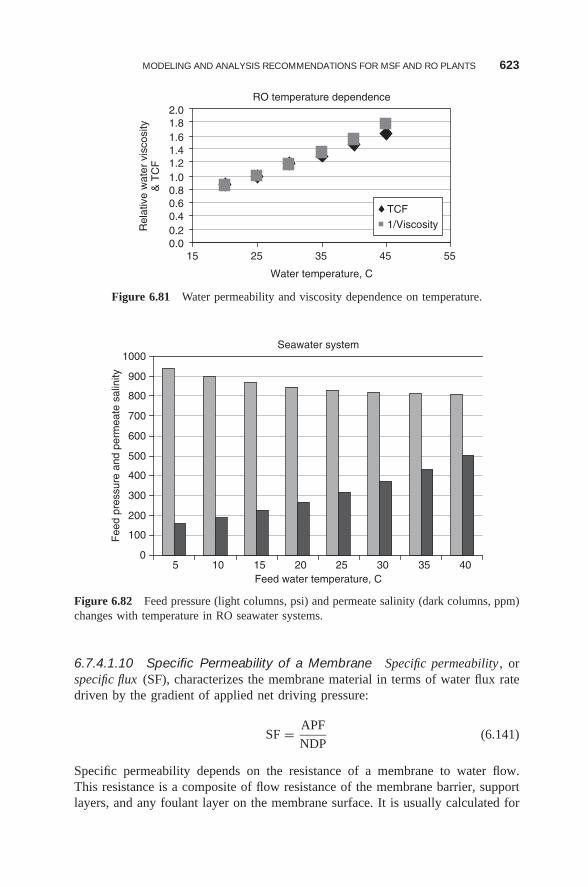
MODELING AND ANALYSIS RECOMMENDATIONS FOR MSF AND RO PLANTS 623

RO temperature dependence

0.00.20.40.60.81.01.21.41.61.82.0

15 25 35 45 55

Water temperature, C

Rel

ativ

e w

ater

vis

cosi

ty&

TC

F

TCF1/Viscosity

Figure 6.81 Water permeability and viscosity dependence on temperature.

Seawater system

0

100

200

300

400

500

600

700

800

900

1000

5 10 15 20 25 30 35 40Feed water temperature, C

Fee

d pr

essu

re a

nd p

erm

eate

sal

inity

Figure 6.82 Feed pressure (light columns, psi) and permeate salinity (dark columns, ppm)changes with temperature in RO seawater systems.

6.7.4.1.10 Specific Permeability of a Membrane Specific permeability , orspecific flux (SF), characterizes the membrane material in terms of water flux ratedriven by the gradient of applied net driving pressure:

SF = APF

NDP(6.141)

Specific permeability depends on the resistance of a membrane to water flow.This resistance is a composite of flow resistance of the membrane barrier, supportlayers, and any foulant layer on the membrane surface. It is usually calculated for

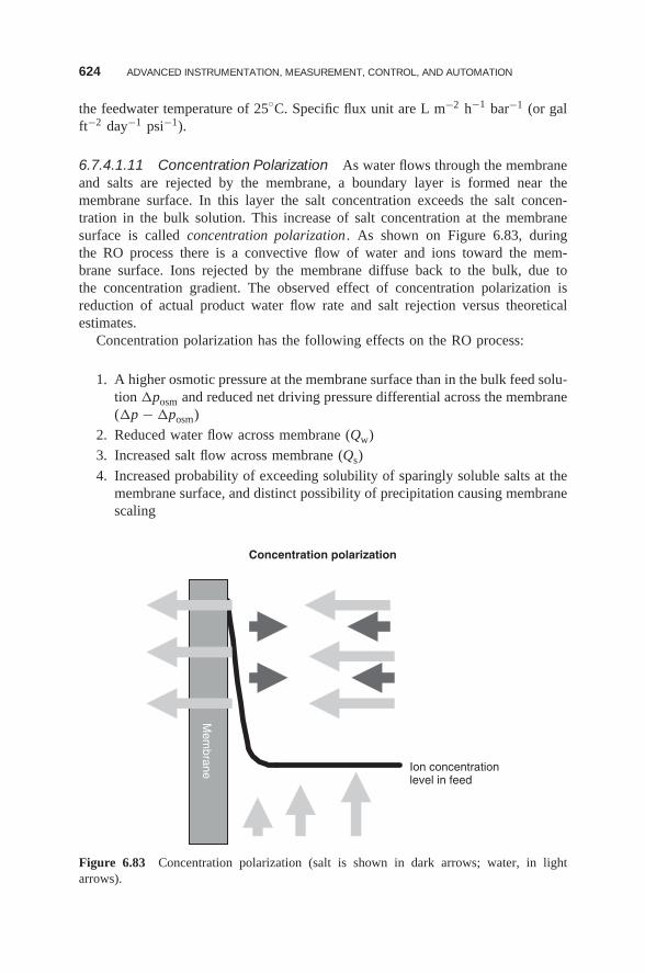
624 ADVANCED INSTRUMENTATION, MEASUREMENT, CONTROL, AND AUTOMATION

the feedwater temperature of 25◦C. Specific flux unit are L m−2 h−1 bar−1 (or galft−2 day−1 psi−1).

6.7.4.1.11 Concentration Polarization As water flows through the membraneand salts are rejected by the membrane, a boundary layer is formed near themembrane surface. In this layer the salt concentration exceeds the salt concen-tration in the bulk solution. This increase of salt concentration at the membranesurface is called concentration polarization . As shown on Figure 6.83, duringthe RO process there is a convective flow of water and ions toward the mem-brane surface. Ions rejected by the membrane diffuse back to the bulk, due tothe concentration gradient. The observed effect of concentration polarization isreduction of actual product water flow rate and salt rejection versus theoreticalestimates.

Concentration polarization has the following effects on the RO process:

1. A higher osmotic pressure at the membrane surface than in the bulk feed solu-tion �posm and reduced net driving pressure differential across the membrane(�p − �posm)

2. Reduced water flow across membrane (Qw)

3. Increased salt flow across membrane (Qs)

4. Increased probability of exceeding solubility of sparingly soluble salts at themembrane surface, and distinct possibility of precipitation causing membranescaling

Ion concentrationlevel in feed

Concentration polarization

Mem

brane

Figure 6.83 Concentration polarization (salt is shown in dark arrows; water, in lightarrows).

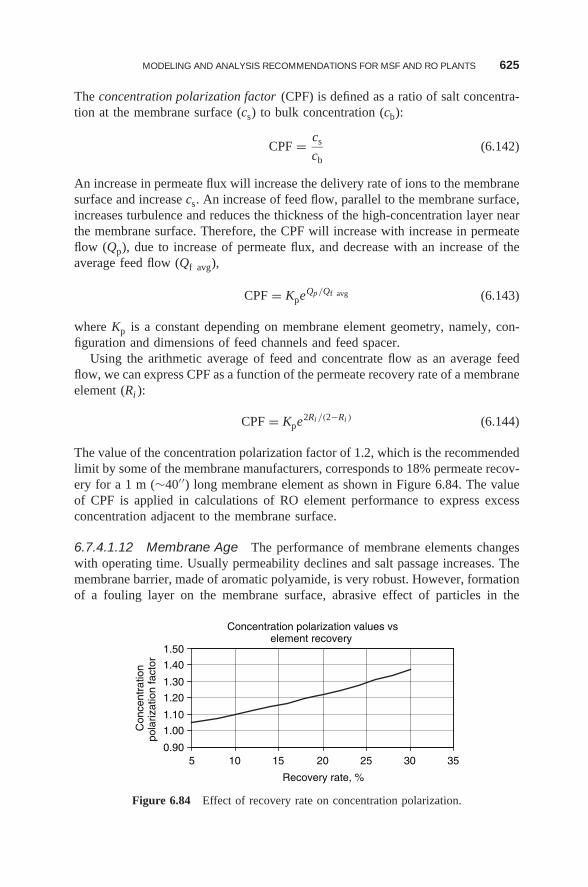
MODELING AND ANALYSIS RECOMMENDATIONS FOR MSF AND RO PLANTS 625

The concentration polarization factor (CPF) is defined as a ratio of salt concentra-tion at the membrane surface (cs) to bulk concentration (cb):

CPF = cs

cb(6.142)

An increase in permeate flux will increase the delivery rate of ions to the membranesurface and increase cs. An increase of feed flow, parallel to the membrane surface,increases turbulence and reduces the thickness of the high-concentration layer nearthe membrane surface. Therefore, the CPF will increase with increase in permeateflow (Qp), due to increase of permeate flux, and decrease with an increase of theaverage feed flow (Qf avg),

CPF = KpeQp/Qf avg (6.143)

where Kp is a constant depending on membrane element geometry, namely, con-figuration and dimensions of feed channels and feed spacer.

Using the arithmetic average of feed and concentrate flow as an average feedflow, we can express CPF as a function of the permeate recovery rate of a membraneelement (Ri ):

CPF = Kpe2Ri /(2−Ri ) (6.144)

The value of the concentration polarization factor of 1.2, which is the recommendedlimit by some of the membrane manufacturers, corresponds to 18% permeate recov-ery for a 1 m (∼40′′) long membrane element as shown in Figure 6.84. The valueof CPF is applied in calculations of RO element performance to express excessconcentration adjacent to the membrane surface.

6.7.4.1.12 Membrane Age The performance of membrane elements changeswith operating time. Usually permeability declines and salt passage increases. Themembrane barrier, made of aromatic polyamide, is very robust. However, formationof a fouling layer on the membrane surface, abrasive effect of particles in the

Concentration polarization values vselement recovery

0.90

1.00

1.10

1.20

1.30

1.40

1.50

5 10 15 20 25 30 35

Recovery rate, %

Con

cent

ratio

npo

lariz

atio

n fa

ctor

Figure 6.84 Effect of recovery rate on concentration polarization.

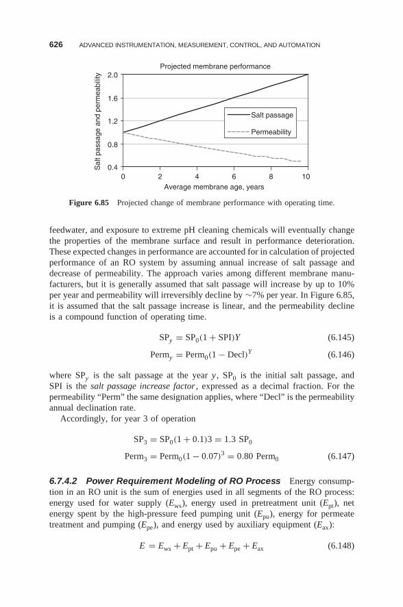
626 ADVANCED INSTRUMENTATION, MEASUREMENT, CONTROL, AND AUTOMATION

Projected membrane performance

0.4

0.8

1.2

1.6

2.0

0 2 4 6 8 10Average membrane age, years

Sal

t pas

sage

and

per

mea

bilit

y

Salt passage

Permeability

Figure 6.85 Projected change of membrane performance with operating time.

feedwater, and exposure to extreme pH cleaning chemicals will eventually changethe properties of the membrane surface and result in performance deterioration.These expected changes in performance are accounted for in calculation of projectedperformance of an RO system by assuming annual increase of salt passage anddecrease of permeability. The approach varies among different membrane manu-facturers, but it is generally assumed that salt passage will increase by up to 10%per year and permeability will irreversibly decline by ∼7% per year. In Figure 6.85,it is assumed that the salt passage increase is linear, and the permeability declineis a compound function of operating time.

SPy = SP0(1 + SPI)Y (6.145)

Permy = Perm0(1 − Decl)Y (6.146)

where SPy is the salt passage at the year y , SP0 is the initial salt passage, andSPI is the salt passage increase factor , expressed as a decimal fraction. For thepermeability “Perm” the same designation applies, where “Decl” is the permeabilityannual declination rate.

Accordingly, for year 3 of operation

SP3 = SP0(1 + 0.1)3 = 1.3 SP0

Perm3 = Perm0(1 − 0.07)3 = 0.80 Perm0 (6.147)

6.7.4.2 Power Requirement Modeling of RO Process Energy consump-tion in an RO unit is the sum of energies used in all segments of the RO process:energy used for water supply (Ews), energy used in pretreatment unit (Ept), netenergy spent by the high-pressure feed pumping unit (Epu), energy for permeatetreatment and pumping (Epe), and energy used by auxiliary equipment (Eax):

E = Ews + Ept + Epu + Epe + Eax (6.148)

MODELING AND ANALYSIS RECOMMENDATIONS FOR MSF AND RO PLANTS 627

In a RO plant, except for a small quantity of energy that is used for lighting and tooperate the control system, the rest is used to power the water pumping equipment.Energy of pumping (Ep) is a direct function of flow rate (Qf), head differential(�pf) developed by the pump, and specific gravity (ρ) of the fluid being pumped.Energy usage for the pumping is inversely affected by hydraulic efficiency of thepump (ηp) and transformation efficiency of the electric motor (ηm):

Ep = kQf�pfρ

ηpηm(6.149)

where k is a unit conversion factor.The energy recovered (Er) in the energy recovery device is a function of concen-

trate flow rate (Qc), head differential (�pc) between inlet and outlet of the energyrecovery device and its efficiency (ηt), and of the specific gravity of the concentratestream (ρ). It is expressed as

Er = kρQc�pcηt (6.150)

Accordingly, the pumping energy is

Epu = Ep − Er (6.151)

and Equation (6.148) can be modified as follows:

E = Ews + Ept + Epe + Eax + Ep − Er (6.152)

6.7.4.3 Practical Approach to RO System Performance OptimizationIt is intuitively obvious what the ideal result of process optimization would be: a setof operating parameters that would result in operating conditions of lowest powerconsumption and/or lowest consumption of pretreatment chemicals. This is underconditions of producing permeate salinity within the design limits. Due to a largenumber of major process parameters that are interrelated, it is not very likely thata simple analytical model can be developed that could be universally applied tocommercial membrane systems. Conditions of the RO system, including intrinsicproperties of RO membranes, are not stationary. They change with time, fluctuatingwithin the range of parameters discussed above. Still there are calculations algo-rithms, based on the NDP model and equations listed above, that enable calculationsof RO membrane performance on the basis of element performance at referenceconditions. The calculations are conducted using state-of-the-art computers in aniterative mode, providing results that are close to actual field performance.

The calculated performances are close to results seen in field operation forconditions of new membranes. There is no analytical model that could be used topredict, with sufficient accuracy, performance of membrane systems as a functionof time and possible membrane performance deterioration. The assumptions madeduring plant design stage are based on a collective industrial experience with given

628 ADVANCED INSTRUMENTATION, MEASUREMENT, CONTROL, AND AUTOMATION

membrane type and water source. As expected in such situations, a good design isconsidered one with sufficient safety margins. Such design ensures that the plantwill provide the required performance, but it is not a design that results in optimumefficiency of operation. Therefore, a simplified practical approach would be to adoptthe algorithms of commercial computer programs for process optimization. In a firststep, performance of the RO system will be used to calculate current membraneperformance to establish a reference point for calculations. This reference pointwill provide an average performance of elements in the RO system that is adjustedfor fouling and compaction. Such performance of an average element will be usedto project system performance in the range of operating parameters that can becontrolled. The result will be a matrix of discrete values of feed pressures andpermeate salinity. Then, on this matrix, limits of designed permeate salinity andcapacity of pumping equipment (water flow and head) will be imposed. For valuesthat are allowable in terms of these limits, the operating cost will be calculatedon the basis of the operating parameters. The net results will be a set of operatingparameters that would result in a minimum operating cost. With the state-of -the-art computers, the calculation process will be very fast and operation of the plantcould be adjusted instantaneously in response to change of process parameters. Sucha control system requires the continuous intervention of the system operator, whowould adjust parameters of membrane elements, stored in the database, according toconditions of the membrane elements. These can be derived from plant performancerecords and calculated using normalization programs. All the components of sucha system, including algorithms of calculations programs, are currently available.What is required is a demonstration in a small- to medium-scale RO system toprove functionality and benefits of such approach.

A more correct way of controlling performance of RO systems would bethrough the utilization of dynamic models. These could be developed based onartificial neural networks and fuzzy logic control. This technology, used to someextent in the electronics industry, is being proposed as a control approach in thedesalination industry.

6.7.5 Mathematical Formulation of the Dynamic Modeling Problem

Because of the importance of applying dynamic modeling to desalination processes,we offer a brief introduction to the approach here.

6.7.5.1 Model Equations The dynamic model equations for the MSF and ROprocesses normally give rise to a set of equations that consist of a group of first-order differential equations with time as an independent parameter, and anothergroup of algebraic equations. This set of equations, called differential algebraicequations (DAE), has the form

f (x , x , y , u , t) = 0

g(x , y , u , t) = 0 (6.153)

u = u(t)

MODELING AND ANALYSIS RECOMMENDATIONS FOR MSF AND RO PLANTS 629

The group of equations f contains the differential equations, and the group gcontains the algebraic equations. In these equations x is the vector of state variables,y is the vector of output variables, u is the vector of input (manipulating) variables,and t is the time. Since u is a known function of time, it can be substituted in theequations f , g , and the model equations can be simplified to the form

f (x , x , y , t) = 0

g(x , y , t) = 0 (6.154)

Therefore, if we have n differential variables x , m algebraic variables y , and linput (given) variables u , we have a total of (n + m) unknown variables.

The following form of the differential group of equations is more appropriatefor MSF and RO desalination processes since all differential equations can be castin this form:

x = f (x , y , t) (6.155)

To reduce this form to the fully determined ordinary first-order differential equation(ODE) system x = f (x , t), it is necessary to cast the group of algebraic equationsin the following form:

y1 = g1(x)

y2 = g2(x , y1)

. . . (6.156)

. . .

ym = gm(x , y1, y2, . . . , ym−1)

Each algebraic variable y1, y2, . . . can be calculated explicitly given x and anypreviously calculated yi ; that is, the algebraic variables can be eliminated by directsubstitution of the algebraic equations into the ordinary differential equations. Notethat most of the models do not conform directly to this formulation without someform of manipulation (in general, differentiation [108]. Substituting the y vectorinto the vector function f , we obtain the fully determined form:

x = f (x , t) (6.157)

This is the most natural form in which to derive the component models. Directintegration of this set of ODE’s ensures that the algebraic equations are satisfiedin each time step, hence the algebraic variables will remain consistent with thedifferential variables, [108].

A very simple example of the above-described procedure follows. Assume thatthe system of equations is composed of ODEs and the algebraic equation shownbelow:

x1 = 2x1 + x2 + x3 (6.158)

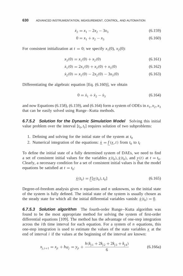
630 ADVANCED INSTRUMENTATION, MEASUREMENT, CONTROL, AND AUTOMATION

x2 = x1 − 2x2 − 3x3 (6.159)

0 = x1 + x2 − x3 (6.160)

For consistent initialization at t = 0; we specify x1(0), x2(0):

x3(0) = x1(0) + x2(0) (6.161)

x1(0) = 2x1(0) + x2(0) + x3(0) (6.162)

x2(0) = x1(0) − 2x2(0) − 3x3(0) (6.163)

Differentiating the algebraic equation [Eq. (6.160)], we obtain

0 = x1 + x2 − x3 (6.164)

and now Equations (6.158), (6.159), and (6.164) form a system of ODEs in x1, x2, x3that can be easily solved using Runge–Kutta methods.

6.7.5.2 Solution for the Dynamic Simulation Model Solving this initialvalue problem over the interval [t0, tf] requires solution of two subproblems:

1. Defining and solving for the initial state of the system at t02. Numerical integration of the equations: x = f (x , t) from t0 to tf

To define the initial state of a fully determined system of DAEs, we need to finda set of consistent initial values for the variables x(t0), x(t0), and y(t) at t = t0.Clearly, a necessary condition for a set of consistent initial values is that the modelequations be satisfied at t = t0:

x(t0) = f [x(t0), t0] (6.165)

Degree-of-freedom analysis gives n equations and n unknowns, so the initial stateof the system is fully defined. The initial state of the system is usually chosen asthe steady state for which all the initial differential variables vanish: x(t0) = 0.

6.7.5.3 Solution algorithm The fourth-order Runge–Kutta algorithm wasfound to be the most appropriate method for solving the system of first-orderdifferential equations [109]. The method has the advantage of one-step integrationacross the i th time interval for each equation. For a system of n equations, thisone-step integration is used to estimate the values of the state variables x at theend of interval i if the values at the beginning of the interval are known:

xj ,i+1 = xji + hϕj = yji + h(kj1 + 2kj2 + 2kj3 + kj4)

6(6.166a)

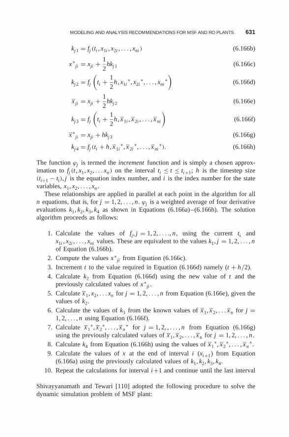
MODELING AND ANALYSIS RECOMMENDATIONS FOR MSF AND RO PLANTS 631

kj1 = fj (ti , x1i , x2i , . . . , xni ) (6.166b)

x∗ji = xji + 1

2hkj1 (6.166c)

kj2 = fj

(ti + 1

2h , x1i

∗, x2i∗, . . . , xni

∗)

(6.166d)

x ji = xji + 1

2hkj2 (6.166e)

kj3 = fj

(ti + 1

2h , x1i , x2i , . . . , xni

)(6.166f)

x∗ji = xji + hkj3 (6.166g)

kj4 = fj (ti + h , x1i∗, x2i

∗, . . . , xni∗). (6.166h)

The function ϕj is termed the increment function and is simply a chosen approx-imation to fj (t , x1, x2, . . . xn) on the interval ti ≤ t ≤ ti+1; h is the timestep size(ti+1 − ti), j is the equation index number, and i is the index number for the statevariables, x1, x2, . . . , xn .

These relationships are applied in parallel at each point in the algorithm for alln equations, that is, for j = 1, 2, . . . , n . ϕj is a weighted average of four derivativeevaluations k1, k2, k3, k4 as shown in Equations (6.166a)–(6.166h). The solutionalgorithm proceeds as follows:

1. Calculate the values of fj, j = 1, 2, . . . ., n , using the current ti andx1i , x2i , . . . , xni values. These are equivalent to the values k1, j = 1, 2, . . . , nof Equation (6.166b).

2. Compute the values x∗ji from Equation (6.166c).

3. Increment t to the value required in Equation (6.166d) namely (t + h/2).

4. Calculate k2 from Equation (6.166d) using the new value of t and thepreviously calculated values of x∗

ji .

5. Calculate x1, x2, . . . xn for j = 1, 2, . . . , n from Equation (6.166e), given thevalues of k2.

6. Calculate the values of k3 from the known values of x1, x2, . . . xn for j =1, 2, . . . , n using Equation (6.166f).

7. Calculate x1∗, x2

∗, . . . , xn∗ for j = 1, 2, , . . . , n from Equation (6.166g)

using the previously calculated values of x1, x2, . . . , xn for j = 1, 2, . . . , n .

8. Calculate k4 from Equation (6.166h) using the values of x1∗, x2

∗, . . . , xn∗.

9. Calculate the values of x at the end of interval i (xi+1) from Equation(6.166a) using the previously calculated values of k1, k2, k3, k4.

10. Repeat the calculations for interval i+1 and continue until the last interval

Shivayyanamath and Tewari [110] adopted the following procedure to solve thedynamic simulation problem of MSF plant:

632 ADVANCED INSTRUMENTATION, MEASUREMENT, CONTROL, AND AUTOMATION

1. Assign the initial values for all the differential variables.

2. Choose proper timestep size.

3. Calculate the brine heater outlet temperature by solving the energy and heattransfer equations for the brine heater.

4. Calculate the flashing brine temperature using the energy equation applied tothe flashing brine.

5. Calculate the stagewise recirculating brine temperatures and tube wall tem-peratures using the energy equation applied to the recirculating brine andtube material of the condenser tube bundles in each stage.

6. Calculate the flashing brine flow rate in each stage using a mass balance onthe flashing brine in each stage.

7. Calculate the salinity of flashing brine leaving each stage using using a saltmass balance in each stage.

The predicted values are used to estimate the variables for the next periodusing the Runge–Kutta method. Calculations are continued until the steady stateis reached or until the end of the specified period.

6.7.6 Summary of Modeling Needs for the Future

It appears that the current modeling capabilities and experience are in generalsufficient for integration with advanced control systems for MSF and RO plants,and the main improvement recommended at this time is to implement them morewidely and economically, especially for larger plants, where appropriate. At thesame time, two major targets of improvement should be sought for even moreeffective implementation and use of IMCA systems that would reduce watercosts:

1. Better physical/chemical modeling of the basic fluid dynamics and transportprocesses in MSF and RO plants that would reduce the predictive errorunder the varying conditions and compositions in the plant, especially undertransient conditions.

2. More rapid computational algorithms, enabling models to produce resultscloser to the real process time.

6.8 CONCLUSIONS AND RECOMMENDATIONS

• Good process instrumentation and measurements are a vital prerequisite forcontrol and automation.

• The majority of desalination plants currently in operation make use of single-loop (SISO) PI or PID controllers.

• New methods of advanced and intelligent control techniques have been pro-posed by a number of authors with promising technical performance results:

CONCLUSIONS AND RECOMMENDATIONS 633

• Model-based predictive control seems to have the potential for improvingcontrol of both MSF and RO plants, but needs to be examined and testedin the field.

• Artificial intelligence, neural networks, and fuzzy logic have been stud-ied further for desalination plants, but have not been proven as viableapproaches.

• One of the most critical issues for maintaining low product cost is the achieve-ment of high plant availability, and to this end:• Using fault-tree analysis in some form (after component reliability statistics

such as failure and repair rates were collected), identify the most vulnerablecomponents, attempt to replace them by an improved design, and monitorthem more carefully.

• Simplify the design wherever possible.

• A basic premise of this study is that any level of automation or IMCA ingeneral must be economically justified, to also include consideration of IMCAsystem reliability.

• As opposed to the enormous amount of published information on controlsystems and their advancement, those on cost–benefit analysis of their imple-mentation are very few in general, and nearly nonexistent for desalinationplants in particular.

• The literature is almost devoid of investigations related to the economic fea-sibility of the use of advanced controllers in lieu of conventional ones indesalination plants.

• The use of computer-based data reconciliation is becoming standard in largeplants.

• Model-based control and automation with optimization was introduced suc-cessfully in some large plants, and this trend is expected to continue and islikely to be applied to smaller plants as well.

• The use of techniques such as neural networks, fuzzy logic, and artificial intel-ligence in desalination plant control have been studied by some researchers,without any clear beneficial results, and there are no plans known to us toapply them in plants.

• There are several advanced control techniques currently available in the mar-ketplace, and the most appropriate technology for a particular desalinationprocess has to be investigated both technically and economically in pilot-scaletests.

• To emphasize the obvious, any improvements in IMCA must reduce product-water cost, which includes not only a reduction in energy and capital costs butalso an increase of plant availability. The latter requires, among other things,the use of simple and robust IMCA systems.

• The level of automation in the previous generation of MSF plants is very high,to the extent that it brings up increasing concerns related to the deskilling of

634 ADVANCED INSTRUMENTATION, MEASUREMENT, CONTROL, AND AUTOMATION

MSF plant operators. Training simulators could prove very useful in improvingthe skill level of plant operators.

• Full automation of the startup–shutdown sequence is desirable but has thusfar been implemented in only one plant.

• Modification of the control schemes that affect reductions in exergy (or simplypressure) losses in the plant need to be explored, and an example of such aproposed scheme to control the top brine temperature in MSF plants waspresented.

• Automation to control fouling is an important proposed approach.

• The process step that has potential for significant improvement by applying“smart” automation is the pretreatment of the feedwater, especially in RO.

• In RO, automation of the recovery–flux rate combination, instead of theconventional method of maintaining constant flux, is proposed for potentialreduction of operating cost.

• From the various advanced control methods considered, the use of constrainedmodel predictive controllers (CMPCs) appears to be promising for implemen-tation.

• Automation as online optimization is highly desirable, but adequate mathe-matical dynamical models of the process are not yet available to implementit.

• A critical review of the status of cost–benefit analysis of IMCA systems,with emphasis on their use in MSF and RO desalination, was performed andpresented.

• An explicit methodology for such analysis was developed and presented.

• To implement this methodology, simplified models for predicting theperformance of MSF and RO plants were developed and successfullyimplemented.

• Specific examples of IMCA system cost–benefit ratios for large RO and MSFplants were calculated.

• Some promising ways in which automation could be implemented to improveMSF and RO plant design and operation to reduce product-water cost weresuggested.

• Proper saving and analysis of historical plant data can lead to product costreduction in ways not always obviour with conventional modeling.

• The use of advanced controllers in MSF and RO plants can result in eco-nomic saving in the operating expenses [steam consumption (MSF), electricalenergy consumption (MSF and RO), and chemical consumption (MSF andRO)].

• In the examples analyzed, on the basis of unit cost assumptions (steam cost= $3.5/t, electricity cost = $0.06/kWh, average cost of chemicals $1.0./kg),it was concluded that direct savings of $66,000 per year (MSF) and $13,000per year (RO) can be achieved for each migd of plant installed capacity ifthe advanced IMCA system ensures a departure from optimum that is at most

ACKNOWLEDGMENT 635

5%. The real savings depend on the actual operation strategy of the existingplant as well as the extent of seasonal variation in seawater temperature andsalinity in the plant site.

• The economic feasibility of replacing conventional PID controllers withadvanced ones depends on the results of a cost–benefit analysis to be carriedout on the particular plant under consideration. This analysis should factor inthe operating condition of the plant as well as the purchase and installationcosts of the controller’s hardware and software.

• The direct benefit–cost ratio for large plants (say, 200,000 m3/day) is esti-mated to be ∼30 for MSF and 23 for RO processes, indicating that advancedIMCA systems have a very desirable financial outcome. That ratio becomeseven higher when the indirect benefits are added.

• It is well recognized in process IMCA system design and implementationthat there are many intangible benefits to IMCA system improvement thatmay actually exceed those simply calculated from the resulting higherproduct output and quality; more attention to such “robust design” is thusrecommended

• Design life of the automation system is much shorter than that of the desali-nation plant, and better ways to match the automation system with the overallplant lifetime should be found.

• Automatic control procedures and systems should be developed for optimizingthe operation of hybrid desalination plants.

• It appears that the current modeling capabilities and experience are qualita-tively sufficient for integration with advanced control systems for MSF andRO plants, and the immediate improvement recommended at this time is toimplement them more widely and economically, especially for larger plants,where appropriate.

• At the same time two major targets of improvement should be sought for evenmore effective implementation and use of IMCA systems that would reducewater costs:• Better physical/chemical modeling of the basic fluid dynamics and transport

processes in MSF and RO plants that would reduce the predictive errorunder the varying conditions and compositions in the plant, especially undertransient conditions

• Faster computational algorithms that enable the models to produce resultscloser to the real process time

ACKNOWLEDGMENT

The authors are grateful to the Middle East Desalination Research Center for par-tial support of this study. Dr. Mark Wilf has made major contributions to thiswork, writing most of Sections 6.3.3, 6.4.2, 6.5.5.4 and 6.7.4 and participating inconclusions and recommendations of most sections and in Section 6.8.

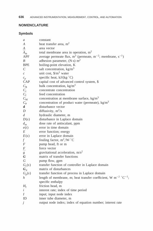
636 ADVANCED INSTRUMENTATION, MEASUREMENT, CONTROL, AND AUTOMATION

NOMENCLATURE

Symbols

a constantA heat transfer area, m2

A area vectorAm total membrane area in operation, m2

APF average permeate flux, m3 (permeate, m−2; membrane, s−1)B adhesion parameter, (N·s) m2

BPE boiling-point elevation, KC salt concentration, kg/m3

c unit cost, $/m3 watercp specific heat, kJ/(kg·◦C)CAP capital cost of advanced control system, $CB bulk concentration, kg/m3

Cc concentrate concentrationCf feed concentrationCM concentration at membrane surface, kg/m3

CP concentration of product water (permeate), kg/m3

d disturbance vectorD diffusivity, m2/sd hydraulic diameter, mD(s) disturbance in Laplace domaindas dose rate of antiscalant, ppme(t) error in time domainE error function; energyE (s) error in Laplace domainf fouling factor, m2/W·◦CF pump head, ft or mF force vectorg gravitational acceleration, m/s2

G matrix of transfer functionsG pump flow, gpmGc(s) transfer function of controller in Laplace domainGd matrix of disturbancesGp(s) transfer function of process in Laplace domainh length of membrane, m; heat transfer coefficient, W m−2 ◦C−1;

specific enthalpyHf friction head, mi interest rate; index of time periodI input; input node indexID inner tube diameter, mj output node index; index of equation number; interest rate

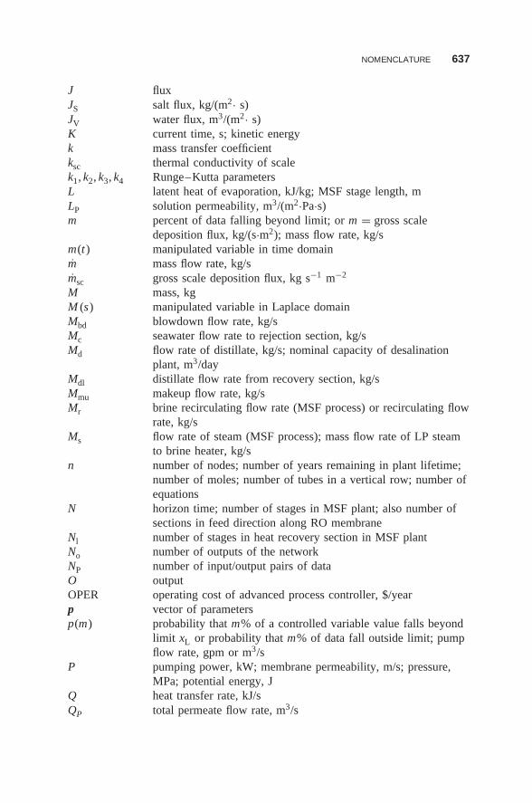
NOMENCLATURE 637

J fluxJS salt flux, kg/(m2· s)JV water flux, m3/(m2· s)K current time, s; kinetic energyk mass transfer coefficientksc thermal conductivity of scalek1, k2, k3, k4 Runge–Kutta parametersL latent heat of evaporation, kJ/kg; MSF stage length, mLP solution permeability, m3/(m2·Pa·s)m percent of data falling beyond limit; or m = gross scale

deposition flux, kg/(s·m2); mass flow rate, kg/sm(t) manipulated variable in time domainm mass flow rate, kg/smsc gross scale deposition flux, kg s−1 m−2

M mass, kgM (s) manipulated variable in Laplace domainMbd blowdown flow rate, kg/sMc seawater flow rate to rejection section, kg/sMd flow rate of distillate, kg/s; nominal capacity of desalination

plant, m3/dayMdl distillate flow rate from recovery section, kg/sMmu makeup flow rate, kg/sMr brine recirculating flow rate (MSF process) or recirculating flow

rate, kg/sMs flow rate of steam (MSF process); mass flow rate of LP steam

to brine heater, kg/sn number of nodes; number of years remaining in plant lifetime;

number of moles; number of tubes in a vertical row; number ofequations

N horizon time; number of stages in MSF plant; also number ofsections in feed direction along RO membrane

Nl number of stages in heat recovery section in MSF plantNo number of outputs of the networkNP number of input/output pairs of dataO outputOPER operating cost of advanced process controller, $/yearp vector of parametersp(m) probability that m% of a controlled variable value falls beyond

limit xL or probability that m% of data fall outside limit; pumpflow rate, gpm or m3/s

P pumping power, kW; membrane permeability, m/s; pressure,MPa; potential energy, J

Q heat transfer rate, kJ/sQP total permeate flow rate, m3/s

638 ADVANCED INSTRUMENTATION, MEASUREMENT, CONTROL, AND AUTOMATION

r concentration ratior(t) setpoint in time domainR RO plant recovery ratio; membrane rejectionR(s) setpoint in Laplace domainRe Reynolds numbers Laplace transform variable; standard deviation; standard

deviation of a controlled variables vector of state variableSc Schmidt number, dimensionlessSh Sherwood number, dimensionlesssp setpointt time, sT temperature,◦Ct1 brine inlet temperature to brine heater,◦CTi seawater inlet temperature to heat rejection section,◦Cti temperature of recirculating brine or cooling seawater,◦CTmax top brine temperature,◦CTN flashing brine temperature in the last stage,◦CTN 1 flashing brine temperature out of heat recovery section,◦CTo outlet temperature from heat rejection section,◦Ctr temperature of recirculating brine entering last recovery stage,◦Cu vector of manipulated variablesu vector of independent parametersu velocity, m/sU overall heat transfer coefficient, kW/(m2·◦C); internal energy, JU (t) input signal to controllerua controller outputvc calculated variablevd dependent variablevi independent variableV volume, m3

w weighting factorW width of membrane, m; work, JW (t) white noisex controlled variable, also, specific consumption termsx vector of state variablesx mean value of a controlled variablexB mean value of a controlled variable with conventional controllerxC mean value of a controlled variable with advanced controllerxL limit value of a controlled variablex sc scale layer thickness, mxsc,∞ asymptotic scale layer thickness, my vector of measured datayc process output

NOMENCLATURE 639

Y (s) output (controlled variable) in Laplace domainy(t) output (controlled variable) in time domain

β bias neuron weightγ fouling rate, m2 W−1 ◦C−1 s−1

δ boundary-layer thickness, m�c total saving in water cost achievable by using advanced

controllers, $/m3

�h length of a membrane section, m�P pressure difference, bar�QPi permeate volume flow at ith section, m3/s�x amount that mean value is shifted on installation of advanced

controllers; change in mean value of process variable�� added cost of water, $/m3

��1 saving due to reduction in variance of controlled variable��2 saving due to operation close to optimum value of controlled

variableε stage temperature loss, (BPE+nonequilibrium loss + demister

loss),◦Cζ damping ratioη efficiency; also viscosity, kg/(m·s)κsc scale thermal conductivity, kW m−2 ◦C−1

μ dynamic viscosityπ osmotic pressure, Paρ density, kg/m3

σ membrane reflection coefficientτ time constant, sτf flowing shear stress, N/m2

� cost of water, $/m3

�∗ cost of water at optimum operating point, $/m3

ωn natural angular frequency, s−1 (reciprocal seconds)

Subscripts

1 recovery section2 rejection sectionas antiscalantb brinebd blowdownB base (conventional)c clean conditionC advanced (improved) controllerch chemicalsd distillate (product)

640 ADVANCED INSTRUMENTATION, MEASUREMENT, CONTROL, AND AUTOMATION

el electricityf feed; or refers to fouling; filmfo fouled conditionHPP high-pressure pumpi stage number or indexj indexL limitm membranemu makeupo cooling-water outp productp(m) probability that m% of data fall outside limitP pumpPT pretreatments steamsc scaleswr seawater recycleT turbinev vaporw wall∞ infinity

Superscripts

− average* optimum condition

Abbreviations

ACW added cost of water, $/m3

ANN artificial neural networkAPC advanced process control(ler)API application program interfaceBPST backpressure steam turbineCAPEX capital expense (cost)CCR central control roomCOMM communicationCRT cathode ray tubeCU control unitCV controlled variableDCS distributed control systemDMC dynamic matrix control

NOMENCLATURE 641

DV disturbance variableFAT factory acceptance testingHFF hollow fine fiberHLOI high-level operating interfaceHP high pressureIMCA instrumentation, measurement, control and automationISE integral square errorLAN local-area networkLCU local control unitLDC load dispatch centerLLOI low-level operating interfaceLP low pressureMIMO multi-input multi-outputMP medium pressureMPC model predictive control; model predictive

controllerMSF multistage flashMSFD multistage flash desalinationMV manipulated variableNACW net added cost of water, $/m3

NB negative bigNeg negativeNLP nonlinear programmingNM negative mediumNMPC nonlinear model predictive controlN-NMPC neural nonlinear model predictive controlO&M operation and maintenanceOLE object linking and embeddingOPEX operating expensePI proportional integralPID proportional integral derivativePLC programmable logic(al) controllerPR performance ratioRO reverse osmosisSAT site acceptance testingSCADA system control and data acquisitionSDI silt density indexSISO single-input single-outputSW spiral woundSWRO seawater reverse osmosisTBT top brine temperature in MSF processTDS total dissolved solidsWAN wide-area network

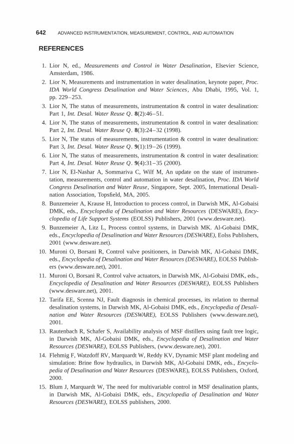
642 ADVANCED INSTRUMENTATION, MEASUREMENT, CONTROL, AND AUTOMATION

REFERENCES

1. Lior N, ed., Measurements and Control in Water Desalination , Elsevier Science,Amsterdam, 1986.

2. Lior N, Measurements and instrumentation in water desalination, keynote paper, Proc.IDA World Congress Desalination and Water Sciences , Abu Dhabi, 1995, Vol. 1,pp. 229–253.

3. Lior N, The status of measurements, instrumentation & control in water desalination:Part 1, Int. Desal. Water Reuse Q . 8(2):46–51.

4. Lior N, The status of measurements, instrumentation & control in water desalination:Part 2, Int. Desal. Water Reuse Q . 8(3):24–32 (1998).

5. Lior N, The status of measurements, instrumentation & control in water desalination:Part 3, Int. Desal. Water Reuse Q . 9(1):19–26 (1999).

6. Lior N, The status of measurements, instrumentation & control in water desalination:Part 4, Int. Desal. Water Reuse Q . 9(4):31–35 (2000).

7. Lior N, El-Nashar A, Sommariva C, Wilf M, An update on the state of instrumen-tation, measurements, control and automation in water desalination, Proc. IDA WorldCongress Desalination and Water Reuse, Singapore, Sept. 2005, International Desali-nation Association, Topsfield, MA, 2005.

8. Bunzemeier A, Krause H, Introduction to process control, in Darwish MK, Al-GobaisiDMK, eds., Encyclopedia of Desalination and Water Resources (DESWARE), Ency-clopedia of Life Support Systems (EOLSS) Publishers, 2001 (www.desware.net).

9. Bunzemeier A, Litz L, Process control systems, in Darwish MK. Al-Gobaisi DMK,eds., Encyclopedia of Desalination and Water Resources (DESWARE), Eolss Publishers,2001 (www.desware.net).

10. Muroni O, Borsani R, Control valve positioners, in Darwish MK, Al-Gobaisi DMK,eds., Encyclopedia of Desalination and Water Resources (DESWARE), EOLSS Publish-ers (www.desware.net), 2001.

11. Muroni O, Borsani R, Control valve actuators, in Darwish MK, Al-Gobaisi DMK, eds.,Encyclopedia of Desalination and Water Resources (DESWARE), EOLSS Publishers(www.desware.net), 2001.

12. Tarifa EE, Scenna NJ, Fault diagnosis in chemical processes, its relation to thermaldesalination systems, in Darwish MK, Al-Gobaisi DMK, eds., Encyclopedia of Desali-nation and Water Resources (DESWARE), EOLSS Publishers (www.desware.net),2001.

13. Rautenbach R, Schafer S, Availability analysis of MSF distillers using fault tree logic,in Darwish MK, Al-Gobaisi DMK, eds., Encyclopedia of Desalination and WaterResources (DESWARE), EOLSS Publishers, (www.desware.net), 2001.

14. Flehmig F, Watzdoff RV, Marquardt W, Reddy KV, Dynamic MSF plant modeling andsimulation: Brine flow hydraulics, in Darwish MK, Al-Gobaisi DMK, eds., Encyclo-pedia of Desalination and Water Resources (DESWARE), EOLSS Publishers, Oxford,2000.

15. Blum J, Marquardt W, The need for multivariable control in MSF desalination plants,in Darwish MK, Al-Gobaisi DMK, eds., Encyclopedia of Desalination and WaterResources (DESWARE), EOLSS publishers, 2000.

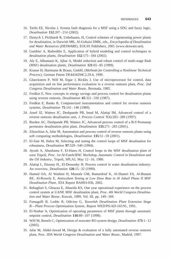
REFERENCES 643

16. Tarifa EE, Nicolas J, Scenna fault diagnosis for a MSF using a SDG and fuzzy logic,Desalination 152:207–214 (2002).

17. Dastych J, Pickhardt R, Unbehauen, H, Control schemes of cogenerating power plantsfor desalination, in Darwish MK, Al-Gobaisi DMK, eds., Encyclopedia of Desalinationand Water Resources (DESWARE), EOLSS Publishers, 2001 (www.desware.net).

18. Gambier A, Badreddin E, Application of hybrid modeling and control techniques todesalination plants, Desalination 152:175–184 (2002).

19. Aly E, Alhumaizi K, Ajbar A, Model reduction and robust control of multi-stage flash(MSF) desalination plants, Desalination 121:65–85 (1999).

20. Krause H, Hartmann & Braun, GmbH, (Methods for Controlling a Nonlinear TechnicalProcess), German Patent DE4434294C2,29.4, 1999.

21. Glueckstern P, Wilf M, Etgar J, Ricklis J, Use of microprocessor for control, dataacquisition and on line performance evaluation in a reverse osmosis plant, Proc. 2ndCongress Desalination and Water Reuse, Bermuda, 1985.

22. Fredkin E, New concepts in energy savings and process control for desalination plantsusing reverse osmosis, Desalination 65:321–330 (1987).

23. Fredkin E, Banks R, Computerized instrumentation and control for reverse osmosissystems, Desalination 75:141–148 (1989).

24. Assef JZ, Watters JC, Deshpande PB, Imad M, Alatiqi IM, Advanced control of areverse osmosis desalination unit, J. Process Control 7(4):283–289 (1997).

25. Burden AC, Deshpande PB, Watters JC, Advanced process control of a B-9 Permaseppermeator desalination pilot plant, Desalination 133:271–283 (2001).

26. Zilouchian A, Jafar M, Automation and process control of reverse osmosis plants usingsoft computing methodologies, Desalination 135:51–59 (2001).

27. El-Saie M, Hafez M, Selecting and tuning the control loops of MSF desalination forrobustness, Desalination 97:529–540 (1994).

28. Ayoub A, Abushama F, El-Hares H, Control loops in the MSF desalination plant ofwest Tripoli, Proc. 1st Al-Fateh/IFAC Workshop, Automatic Control in Desalintion andthe Oil Industry , Tripoli, SPLAJ, May 12–16, 1980.

29. Alatiqi I., Ettouny H., El-Dessouky H. Process control in water desalination industry:An overview, Desalination 126:15–32 (1999).

30. Hamed OA, Al Washmi H, Mustafa GM, Bamardouf K, Al-Shamri FA, Al-BunainRE, Al-Rowely E, Antiscalant Testing at Low Dose Rate in Al Jubail Phase II MSFDesalination Plant , IDA Report BAH03-036, 2002.

31. Rebagliati S, Ghiazza E, Abueida KS, One year operational experience on the processcontrol system at UANE MSF desalination plant, Proc. 4th World Congress Desalina-tion and Water Reuse, Kuwait, 1989, Vol. III, pp. 149–169.

32. Fumagalli B, Loddo R, Odicino G, Taweelah Desalination Plant Extension StageB—Plant Process Optimization System , Report WED/PS/AD-165/91, 1991.

33. El-Nashar A, Optimization of operating parameters of MSF plants through automaticsetpoint control, Desalination 116:89–107 (1998).

34. Wilf M, Bartels C, Optimization of seawater RO system design, Desalination 173:1–12(2005).

35. Jafar M, Abdel-Jawad M, Design & evaluation of a fully automated reverse osmosisplant, Proc. IDA World Congress Desalination and Water Reuse, Madrid, 1997.

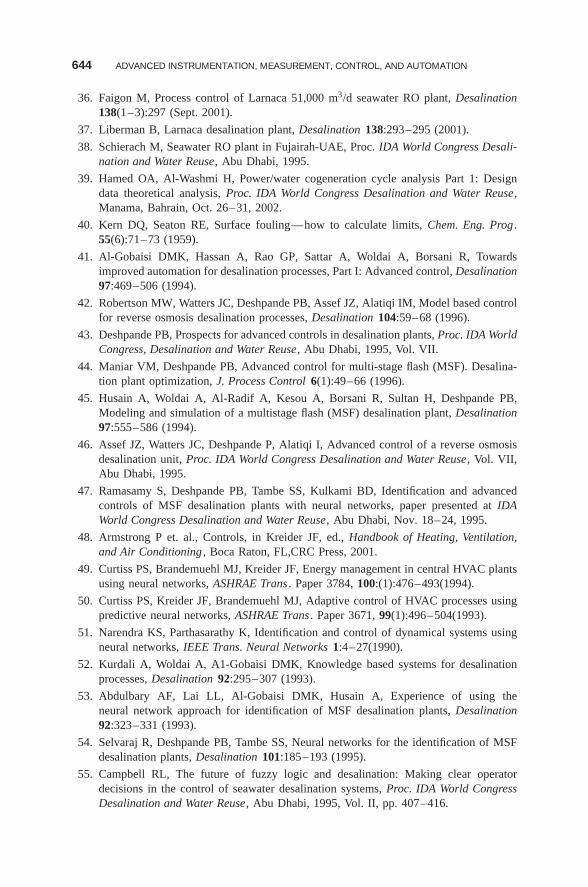
644 ADVANCED INSTRUMENTATION, MEASUREMENT, CONTROL, AND AUTOMATION

36. Faigon M, Process control of Larnaca 51,000 m3/d seawater RO plant, Desalination138(1–3):297 (Sept. 2001).

37. Liberman B, Larnaca desalination plant, Desalination 138:293–295 (2001).

38. Schierach M, Seawater RO plant in Fujairah-UAE, Proc. IDA World Congress Desali-nation and Water Reuse, Abu Dhabi, 1995.

39. Hamed OA, Al-Washmi H, Power/water cogeneration cycle analysis Part 1: Designdata theoretical analysis, Proc. IDA World Congress Desalination and Water Reuse,Manama, Bahrain, Oct. 26–31, 2002.

40. Kern DQ, Seaton RE, Surface fouling—how to calculate limits, Chem. Eng. Prog .55(6):71–73 (1959).

41. Al-Gobaisi DMK, Hassan A, Rao GP, Sattar A, Woldai A, Borsani R, Towardsimproved automation for desalination processes, Part I: Advanced control, Desalination97:469–506 (1994).

42. Robertson MW, Watters JC, Deshpande PB, Assef JZ, Alatiqi IM, Model based controlfor reverse osmosis desalination processes, Desalination 104:59–68 (1996).

43. Deshpande PB, Prospects for advanced controls in desalination plants, Proc. IDA WorldCongress, Desalination and Water Reuse, Abu Dhabi, 1995, Vol. VII.

44. Maniar VM, Deshpande PB, Advanced control for multi-stage flash (MSF). Desalina-tion plant optimization, J. Process Control 6(1):49–66 (1996).

45. Husain A, Woldai A, Al-Radif A, Kesou A, Borsani R, Sultan H, Deshpande PB,Modeling and simulation of a multistage flash (MSF) desalination plant, Desalination97:555–586 (1994).

46. Assef JZ, Watters JC, Deshpande P, Alatiqi I, Advanced control of a reverse osmosisdesalination unit, Proc. IDA World Congress Desalination and Water Reuse, Vol. VII,Abu Dhabi, 1995.

47. Ramasamy S, Deshpande PB, Tambe SS, Kulkami BD, Identification and advancedcontrols of MSF desalination plants with neural networks, paper presented at IDAWorld Congress Desalination and Water Reuse, Abu Dhabi, Nov. 18–24, 1995.

48. Armstrong P et. al., Controls, in Kreider JF, ed., Handbook of Heating, Ventilation,and Air Conditioning , Boca Raton, FL,CRC Press, 2001.

49. Curtiss PS, Brandemuehl MJ, Kreider JF, Energy management in central HVAC plantsusing neural networks, ASHRAE Trans . Paper 3784, 100:(1):476–493(1994).

50. Curtiss PS, Kreider JF, Brandemuehl MJ, Adaptive control of HVAC processes usingpredictive neural networks, ASHRAE Trans . Paper 3671, 99(1):496–504(1993).

51. Narendra KS, Parthasarathy K, Identification and control of dynamical systems usingneural networks, IEEE Trans. Neural Networks 1:4–27(1990).

52. Kurdali A, Woldai A, A1-Gobaisi DMK, Knowledge based systems for desalinationprocesses, Desalination 92:295–307 (1993).

53. Abdulbary AF, Lai LL, Al-Gobaisi DMK, Husain A, Experience of using theneural network approach for identification of MSF desalination plants, Desalination92:323–331 (1993).

54. Selvaraj R, Deshpande PB, Tambe SS, Neural networks for the identification of MSFdesalination plants, Desalination 101:185–193 (1995).

55. Campbell RL, The future of fuzzy logic and desalination: Making clear operatordecisions in the control of seawater desalination systems, Proc. IDA World CongressDesalination and Water Reuse, Abu Dhabi, 1995, Vol. II, pp. 407–416.

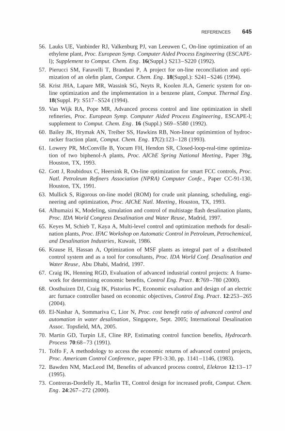
REFERENCES 645

56. Lauks UE, Vanbinder RJ, Valkenburg PJ, van Leeuwen C, On-line optimization of anethylene plant, Proc. European Symp. Computer Aided Process Engineering (ESCAPE-l); Supplement to Comput. Chem. Eng . 16(Suppl.) S213–S220 (1992).

57. Pierucci SM, Faravelli T, Brandani P, A project for on-line reconciliation and opti-mization of an olefin plant, Comput. Chem. Eng . 18(Suppl.): S241–S246 (1994).

58. Krist JHA, Lapare MR, Wassink SG, Neyts R, Koolen JLA, Generic system for on-line optimization and the implementation in a benzene plant, Comput. Thermal Eng .18(Suppl. P): S517–S524 (1994).

59. Van Wijk RA, Pope MR, Advanced process control and line optimization in shellrefineries, Proc. European Symp. Computer Aided Process Engineering , ESCAPE-l;supplement to Comput. Chem. Eng . 16 (Suppl.) S69–S580 (1992).

60. Bailey JK, Hrymak AN, Treiber SS, Hawkins RB, Non-linear optimimtion of hydroc-racker fraction plant, Comput. Chem. Eng . 17(2):123–128 (1993).

61. Lowery PR, McConville B, Yocum FH, Hendon SR, Closed-loop-real-time optimiza-tion of two biphenol-A plants, Proc. AIChE Spring National Meeting , Paper 39g,Houston, TX, 1993.

62. Gott J, Roubidoux C, Heersink R, On-line optimization for smart FCC controls, Proc.Natl. Petroleum Refiners Association (NPRA) Computer Confe., Paper CC-91-130,Houston, TX, 1991.

63. Mullick S, Rigorous on-line model (ROM) for crude unit planning, scheduling, engi-neering and optimization, Proc. AIChE Natl. Meeting , Houston, TX, 1993.

64. Alhumaizi K, Modeling, simulation and control of multistage flash desalination plants,Proc. IDA World Congress Desalination and Water Reuse, Madrid, 1997.

65. Keyes M, Schieb T, Kaya A, Multi-level control and optimization methods for desali-nation plants, Proc. IFAC Workshop on Automatic Control in Petroleum, Petrochemical,and Desalination Industries , Kuwait, 1986.

66. Krause H, Hassan A, Optimization of MSF plants as integral part of a distributedcontrol system and as a tool for consultants, Proc. IDA World Conf. Desalination andWater Reuse, Abu Dhabi, Madrid, 1997.

67. Craig IK, Henning RGD, Evaluation of advanced industrial control projects: A frame-work for determining economic benefits, Control Eng. Pract . 8:769–780 (2000).

68. Oosthuizen DJ, Craig IK, Pistorius PC, Economic evaluation and design of an electricarc furnace controller based on economic objectives, Control Eng. Pract . 12:253–265(2004).

69. El-Nashar A, Sommariva C, Lior N, Proc. cost benefit ratio of advanced control andautomation in water desalination , Singapore, Sept. 2005; International DesalinationAssoc. Topsfield, MA, 2005.

70. Martin GD, Turpin LE, Cline RP, Estimating control function benefits, Hydrocarb.Process 70:68–73 (1991).

71. Tolfo F, A methodology to access the economic returns of advanced control projects,Proc. Americam Control Conference, paper FP1-3:30, pp. 1141–1146, (1983).

72. Bawden NM, MacLeod IM, Benefits of advanced process control, Elektron 12:13–17(1995).

73. Contreras-Dordelly JL, Marlin TE, Control design for increased profit, Comput. Chem.Eng . 24:267–272 (2000).

646 ADVANCED INSTRUMENTATION, MEASUREMENT, CONTROL, AND AUTOMATION

74. Stanton BD, Using historical data to justify controls, Hydrocarb. Process 69:57–60(1990).

75. Bozenhardt H, Dybeck M, Estimating savings from upgrading process control, Chem.Eng . 93(3):99–102 (1986).

76. Latour PR, Quantify quality control’s intangible benefits, Hydrocarb. Process71:61–68 (1992).

77. Lear JB, Barton GW, Perkins JD, Interaction between process design and process con-trol: The impact of disturbances and uncertainty on estimates of achievable economicperformance, J. Process Control 5(1):49–62 (1995).

78. Lant P, Steffens M, Benchmarking for process control: Should I invest in improvedprocess control? Water Sci. Technol . 37(12):49–54 (1998).

79. The American Supplier Institute (trademark owner of Taguchi Methods)(http://www.amsup.com/).

80. Sommariva C, Desalination Management and Economics , Surrey, UK, 2004.

81. Martin T, (18–23 July). Considering social effects in control system design: A sum-mary, Proc. 12th World Congress International Federation of Automatic Control ; Syd-ney, Australia, July 18–23, 1993, Vol. 7, pp. 325–330.

82. Ali E, Understanding the operation of industrial MSF plants, Part I: Stability and steadystate analysis, Desalination 143:53–72 (2002).

83. Muske K, Estimating the economic benefits from improved control, Industr. Eng.Chem. Res . 42:4535–4544 (2003).

84. Aly N, El-Fiqi A, Thermal performance of seawater desalination plants, Desalination158:127–142 (2003).

85. Helal AM, Medani MS, Soliman MA, Flower JR, A tridiagonal matrix model formultistage flash desalination plants, Comput. Chem. Eng . 10(4):327–342 (1986).

86. Mazzotti M, Rosso M, Beltramini A, Morbidelli M, Dynamic modeling of multistageflash desalination plants, Desalination 127:207–218 (2000).

87. Husain A, Hassan A, Al-Gobaisi DMK, Al-Radif A, Woldai A, Sommariva C, Mod-eling, simulation, optimization and control of multistage flashing (MSF) desalinationplants, Part I: Modeling and simulation, Desalination 92:21–41 (1993).

88. Rosso M, Beltramini A, Mazzotti M, Morbidelli M, Modeling multistage flash desali-nation plants, Desalination 108:365–374 (1996).

89. Bourouis M, Pibouleau L, Floquet P, Domenech S, Al-Gobaisi DMK, Simulation anddata validation in multistage flash desalination plants, Desalination 115:1–14 (1998).

90. El-Dessouky HT, Ettouney HM, Fundamentals of Salt Water Desalination , Elsevier,Amsterdam, 2002.

91. Malek A, Hawlader MNA, Ho JC, Design and economics of RO seawater desalination,Desalination 105:245–261 (1996).

92. Taniguchi M, Kurihara M, Kimura S, Behavior of a reverse osmosis plant adoptinga brine conversion two-stage process and its computer simulation, J. Membrane Sci .183:249–257 (2001).

93. Gas Processors Assoc., GPSA data book , 12th ed., Tulsa, OK (USA), 2004.

94. Yokogawa Electric Corp., Advanced Process Control Solutions—Exasmoc, ReportTI36J06D10-01E, Oct. 2001.

95. Hertanu H, Liptak B, DCS-cost estimating, in Liptak BG, ed., Instrument Engineers’Handbook , 3rd ed., Vol. 2, Process Control , Chilton Book Co., Radnor, PA, 1995.

FURTHER READING 647

96. Glueck AR, Bradshaw RW, A mathematical model for a multistage flash dis-tillation plant, Proc. 3rd Int. Symp. Fresh Water from the Sea , 1970, Vol. 1, pp.95–108.

97. Delene JG, Ball SJ, A digital computer code for simulating large MSF EvaporatorDesalting Plant Dynamics , Oak Ridge National Laboratory Report ORNL-TM-2933,1971.

98. Ettouney HM, E1-Dessouky H, A simulator for thermal desalination processes, Desali-nation 125:277–291 (2001).

99. Poje JB, Smart AM, On-line energy optimization in a chemical complex, Chem. Eng.Progr . 39–41 (May 1988).

100. Prichard PC, Computer control of an olefin plant using an on-line optimisor , Inst.Chem. Eng. Symp. Series, 1988, Vol. 100, pp. 277–283.

101. Moro LFL, Odloak D, Constrained multivariable control of fluid catalytic crackingconverters, J. Process Control 5(1):29–39 (1995).

102. Perregard J, Genovese F, Gani R, Efficient integration of simulation and optimizationfor study of complex chemical processes, Proc. Computer-Oriented Process Engineer-ing (COPE-91), Barcelona, Oct. 14–16, 1991, pp. 139–144.

103. Rimawi MA, Ettouney HM, Aly GS, Transient model of multistage flash desalination,Desalination 74:327–338 (1989).

104. Reddy KV, Husain A, Woldai A, Dynamic modeling of the MSF desalination pro-cess, Proc. IDA and WRPC World Congress on Desalination and Water Treatment ,Al-Gobaisi DMK, ed., Abu Dhabi, 1995, pp. 227–242.

105. Thomas PJ, Bhattacharyya S, Patra A, Rao GP, Steady state and dynamic simulation ofmultistage ash desalination plants: A case study, Comput. Chem. Eng . 22:1515–1529(1998).

106. Lior N, Formulas for calculating the approach to equilibrium in open channel flashevaporators for saline water, Desalination 60:223 (1986).

107. Morin OJ, Hempstead TD, for DSS Engineers, Inc., 27,486 m3/d MSF DesalinationPlant—Design Verification , Vol. 1, report submitted to Government of Abu DhabiWater & Electricity Dept., 1984.

108. Barton Paul I, Dynamic Simulation , Sec. 109. II, Special Summer Program, MIT,Cambridge, MA, Aug. 1–10, 1994.

109. Carnahan B, Luther HA, Wilkes JO, Applied Numerical Methods , Wiley, New York,1969.

110. Shivayyanamath S, Tewari PK, Simulation of startup characteristics of multi-stagedesalination plants, Desalination 155:277–286 (2003).

FURTHER READING

6.F.1 Literature on MFSD-Related IMCA

Aly E, Ajbar A, Alhumaizi K, Robust control of industrial multi-stage desalination plants,Desalination 114:289–302 (1997).

Wangnick K, IDA Worldwide Desalting Plants Inventory , Wangnick Consulting for Interna-tional Desalination Assoc., 2004.

648 ADVANCED INSTRUMENTATION, MEASUREMENT, CONTROL, AND AUTOMATION

Kirstaedter K, Measurement, modeling, identification and optimized controller-parametersettings of MSF-desalination units, Proc. IDA World Congress Desalination and WaterReuse, Abu Dhabi, 1995.

Akbarzadeh-T, M-R, Kumbla KK, Jamshidi M, Al-Gobaisi DMK, Evolutionary PID fuzzycontrol of MSF desalination processes, Proc. IDA World Congress Desalination and WaterReuse, Madrid, Oct. 6-9, 1997, Vol. III, pp. 35–45.

Al-Aamry N, Saudi Arabia shutdown and flushing procedure modification for MSF units,Proc. IDA World Congress Desalination and Water Reuse, Bahrain 2002, pp. 78–79.

Alatiqi I, Ettouney H, El-Dessouki H, Al-Hajri K, Measurement of dynamic behavior of amultistage flash water desalination system, Desalination 160:233–251 (2004).

Al-Gobaisi DMK, Barakzai AS, EI-Nashar AM, An overview of modem control strategiesfor optimizing thermal desalination plants, Desalination 84:3–43 (1991).

Alhumaizi K, Modeling, simulation and control of multistage flash desalination plants, Proc.IDA World Congress Desalination and Water Reuse, Madrid, 1997, Vol. III, pp. 111–129.

Ali E, Alhumaizi K, Ajbar A, Model reduction and robust control of multi-stage flash (MSF)desalination plants, Desalination 121:65–85. (1999).

Aly E, Ajbar A, Alhumaizi K, Robust control of industrial multi-stage desalination plants,Desalination 114:289–302 (1997).

Ayoub A, Abushama F, El-Hares H, Control loops in the MSF desalination plant of WestTripoli, Proc. 1st Al-Fateh/IFAC Workshop, Automatic Control in Desalintion and the OilIndustry , Tripoli, SPLAJ, May 12–16, 1980.

Barba D, Luizzo G, Tagliferri G, Mathematical model for multiflash desalting plant control,Proc. 4th Int. Symp. Fresh Water from the Sea , 1973, pp. 153–168.

Borsani R, Barone A, Four years operation of the largest single train MSF desalination plant,Proc. IDA World Congress Desalination and Water Reuse, San Diego, CA, 1999.

Borsani R, Claps B, First Year Operation of the Largest MSF Units at Jebel Ali K2 Site IDABAH03-026, 2002.

Bourouis M, Pibouleau L, Floquet P, Domenech S, Al-Gobaisi DMK, Data reconciliation andgross error detection in multistage flash desalination plants, Proc. IDA World CongressDesalination and Water Reuse, Madrid, Oct. 6–9, 1997, Vol. III, pp. 167–180.

Bunzemeier A. A new control concept for an improved level control in MSF desalinationplants, Desalination 114:13–22, (1997).

Burns and Roe, Inc., Universal Design—Report and User’s Manual on Design of 2.5 MillionGallon per Day Universal Desalting Plant , Vols. I–V (especially Vol. V), US Dept.Interior, OSW Contract 14-01-0001-955, Washington, DC, 1969.

Chidambaram M, Al-Gobaisi DMK, Controller tuning for a MSF desalination plant, Proc.IDA World Congress Desalination and Water Reuse, Abu Dhabi, Nov. 18–24, 1995, Vol.III, pp. 263–278.

Dastych J, Pickhardt PC, Unbehauen H, Control schemes of cogenerating power plantsfor desalination, in Darwish MK, Al-Gobaisi DMK, eds., Encyclopedia of Desalinationand Water Resources (DESWARE), EOLSS Publishers (178H178H, www.desware.net),2001.

Drake FA, Measurements and control in flash evaporation plants, in Lior N, ed., Mea-surements and Control in Water Desalination , Elsevier, Amsterdam, 1986, Sec. 21, pp.241–262.

FURTHER READING 649

El-Hares H, Control loops in MSF desalination plants, Proc. 7th Symp. on Fresh Water fromthe Sea , 1980, Vol. 2, pp. 417–432.

El-Nashar AM, Optimization of operating parameters of MSF plants through automaticsetpoint control, Desalination 116:89–107 (1998).

El-Saie Ali AH, Ramadan AH, Gomaa SS. Multi stage flash desalination process controlsystem, Proc. 1st Al-Fateh/IFAC Workshop, Automatic Control in Desalination and theOil Industry , Tripoli, SPLAJ, May 12–16, 1980.

Fertig M, Modeling and Control of a Brine Heater on the Basis of Hybrid Systems , diplomathesis, Automation Laboratory, Univ. Mannheim (Germany), 2001.

Flehmig F, Watzdoff RV, Marquardt W, Reddy KV, Dynamic MSF plant modeling andsimulation: Brine flow hydraulics, in Al-Gobaisi, DMK, ed., Encyclopedia of Desalinationand Water Resources (DESWARE), ELOSS publishers, 2000.

Fortuna L, Graziani S, Manganaro G, Muscato G, The CNN’s as innovative computingparadigm for modeling, Proc. of IDA World Congress Desalination and Water Sciences ,Abu Dhabi, Nov. 18–24, 1995, Vol. IV, pp. 399–409.

Fumagalli B, Loddo R, Odicino G, Taweelah Desalination Plant Extension-Plant ProcessOptimization System , MEI/TIM/AUT/ BF, WED Report WED/PS/AD-16/91, 1991.

Gambier A, Fabricius SMO, Badreddin E, Simulation using block-oriented and object-oriented software for desalination plants, Proc. Asian Control Conf ., Singapore, 2002, pp.1991–1996; Proc. 13th IASTED International Conf., Modeling Identification and Control ,Anaheim, CA, 1994, pp. 256–259 (paper presented at both confs.)

Gambier A, Fabricius SMO, Badreddin E, Simulation using block-oriented and object-oriented software for desalination plants. Proc. Asian Control Conf ., Singapore, 2002,pp. 1991–1996.

Gambier A, Fertig M, Badreddin E, Hybrid modeling for supervisory control purposesfor the brine heater of a multi-stage flash desalination plant. Proc. Am. Control Conf .,Anchorage, 2002, pp. 5060–5065.

Ghiazza E, Fumagalli B, Odicino G, Drops: The first data reconciliation and optimizationsystem for MSF distillers has been installed and Al-Taweelah B, First feedback data andresults after some months of operation on the world’s largest desalination plant, Proc.IDA World Congress Desalination and Water Reuse, Madrid, Oct. 6–9, 1997, Vol. III79–90.

Hamed, Osman A, Al Washmi H, Mustafa GM, Bamardouf K, Al-Shamri FA, Al-BunainE, Rashid E, Al-Rowely E, Antiscalant Testing at Low Dose Rate in Al Jubail Phase IIMSF Desalination Plant , IDA BAH03—036, 2002.

Hornburg CD, Watson BM, Operational optimization of MSFsystems, Desalination92:333–351 (1993).

Husain A, Woldai A, Al-Radif A, Kesou A, Borsani R, Sultan H, Deshpandey PB,. Modelingand simulation of a multistage flash (MSF) desalination plant, Desalination 97:555–586(1994).

Ismail A, Oct. 6–9, (1997). Fuzzy model reference learning control of multi-stage flashdesalination plants, Proc. IDA World Congress Desalination and Water Reuse, Madrid,Oct. 6–9, 1997, Vol. III, pp. 3–18.

Ismail A, Control of multi stage flash (MSF) desalination plants; a survey, Proc. IDACongress Desalination and Water Reuse, Madrid, 1997, Vol. II, pp. 1–38.

Ismail A. Control of multi-stage flash desalination plants, a survey, Desalination116:145–156 (1998).

650 ADVANCED INSTRUMENTATION, MEASUREMENT, CONTROL, AND AUTOMATION

Jernqvist A, Jernqvist M, Aly G, Simulation of thermal desalination processes, Desalination134:187–193, (2001).

Kirstaedter K, Measurement modeling, identification and optimised controller-parametersettings of MSF-desalination units, Proc. IDA World Congress Desalination and WaterReuse, Abu Dhabi, Nov. 18–24, 1995, Vol. VII, pp. 52–81.

Krause H, Hartmann & Braun GmbH, (Methods for controlling a nonlinear technical pro-cess), German Patent DE4434294C2,29.4, 1999.

Krause H, Hassan A, Training simulators for MSF plants, Proc. IDA World Congress Desali-nation and Water Reuse, Abu Dhabi, Nov. 18–24, 1995, Vol. IV, pp. 185–201.

Kurdali A, Woldai A, A1- Gobaisi DMK, Knowledge based systems for desalination pro-cesses, Desalination 92:295–307 (1993).

Maniar VM, Deshpande PB, Advanced control for multi-stage flash (MSF) desalination plantoptimization, J. Proc. Control 6(1):49–66 (1996).

Mazzotti M, Rosso M, Beltramini A, Morbidelli M, Dynamic modeling of multistage flashdesalination plants, Desalination 127:207–218 (2000).

Omar AM, Simulation of MSF desalination plants, Desalination 45:65–76 (1983).

Parenti SB, Masarani A, Industrial application of real time neural networks in multistagedesalination plant, Proc. IDA World Congress, Desalination and Water Reuse, Abu Dhabi,1995, Vol. II, pp. 457–467.

Ramaswamy S, Deshpande PB, Tambe SS, Kulkami BD,. Identification and advancedcontrols of MSF desalination plants with neural networks, Proc. IDA World CongressDesalination and Water Reuse, Abu Dhabi, Nov. 18–24, 1995.

Rautenbach R, Schafer S, Availability analysis of MSF distillers using fault tree logic, inDarwish MK, Al-Gobaisi DMK, eds., Encyclopedia of Desalination and Water Resources(DESWARE), EOLSS Publishers (179H179H www.desware.net), 2001.

Reddy BC, Chidambaram M, Al-Gobaisi DMK, Design of centralized controllers for a MSFplant, Desalination 113:27–38, (1997).

Reddy KV, Husain A, Woldai A, Al-Gobaisi DMK, Dynamic modeling of the MSF desali-nation process, Proc. IDA World Congress Desalination and Water Reuse, Abu Dhabi,Nov. 18–24, 1995, Vol. IV, pp. 227–242.

Rosso M, Beltramini A, Mazzotti M, Morbidelli M, Modeling multistage flash desalinationplants, Desalination 108:365–374, (1996).

Rost M,. Design and Simulation of Adaptive Multivariable Control for the model of MSFPlant, graduation thesis (in German), Univ. Dresden, Germany, 1995.

Shivayyanamath S, Tewari PK Simulation of startup characteristics of multi-stage desalina-tion plants, Desalination 155:277–286 (2003).

Sommariva C, A new milestone: The 72 MIGD multi stage flash distillation plant at AlTaweelah, Abu Dhabi U.A.E, Proc. Int. Desalination and Water Re-use Conf ., quarterlyMay/June 1996, pp. 30–36.

Tarifa EE, Scenna NJ, A dynamic simulator for MSF plants, Desalination , 138:349–364(2001).

Tarifa EE, Nicolas J, Scenna fault diagnosis for a MSF using a SDG and fuzzy logic,Desalination 152:207–214 (2002).

Tarifa EE, Demetrio, H, Samuel F, Sergio L, Martinez AF, Nunez NJ, Scenna fault diagnosisfor a MSF using neural networks, Desalination 152:215–222 (2002).

FURTHER READING 651

Uche J, Serra L, Valero A, Correas L, On-line thermoeconomic diagnosis of a dual purposepower and desalination plant, Proc. IDA World Congress on Desalination and WaterReuse, March 8–13, 2002, pp. 78–79.

Woldai A, Al-Gobaisi DMK, Dunn RW, Kurdali A, Rao GP, An adaptive scheme with anoptimally tuned PID controller for a large MSF desalination plant, Control. Eng. Pract .4(5):721–734 (1996).

Woldai A, A1-Gobaisi DMK, Dunn RW, Kurdali A, Rao GP, Simulation aided design anddevelopment of an adaptive scheme with optimally tuned PID controller for a largemultistage flash seawater desalination plant. Proc. 5th IFAC Symp. Adaptive Systems inControl and Signal Processing , Parts I–III, Budapest, 1995, pp. 95–112.

Zhang H, Wang S, Studies on the dynamic behavior of MSF systems, Proc. IDA and WRPCWorld Congress Desalination and Water Reuse, Madrid, 1997, Vol. 3, pp. 103–109.

6.F.2 Literature on RO-Related IMCA

Assef JZ, Watters JC, Deshpande PB, Imad M, Alatiqi IM Advanced control of a reverseosmosis desalination unit, J. Process Control 7(4):283–289 (1997).

Bartman AR, Zhu A, Christofides PD, Cohen Y, Minimizing energy consumption in reverseosmosis membrane desalination using optimization-based control, Proc. Am. ControlConf ., Baltimore, June 30–July 2, 2010, paper ThB14.6 2010, pp. 3629–3635.

Bou-Hamad S, Abdel-Jawad M, Al-Tabtabaei M, Al-Shammari S, Comparative performanceanalysis of two seawater reverse osmosis plants: Twin hollow fine fibre and spiral woundmembranes, Desalination 120:95–106 (1998).

Burden AC, Deshpande PB, Watters JC, Advanced process control of a B-9 Permaseppermeator desalination pilot plant, Desalination 133:271–283 (2001).

Caldwell Membrane pre-treatment and operation monitoring and control, Proc. UltrapureWater Expo, Orlando, FL, April 2002.

Fredkin E, New concepts in energy savings and process control for desalination plants usingreverse osmosis, Desalination 65:321–330 (1987).

Fredkin E, Banks R, Computerized instrumentation and control for reverse osmosis systems,Desalination 75:141–148 (1989).

Glueckstern P, Wilf M, Etgar J, Ricklis J, Use of microprocessor for control, data acquisitionand on line performance evaluation in a reverse osmosis plant, Proc. 2nd CongressDesalination and Water Reuse, Bermuda, 1985.

Goswami G, Srivastava VK, Hanra MS, Misra BM, Sadhukhan HK, Design of a 1800m3/day two stage RO plant for drinking water supply in water scarce area, Proc. IDAWorld Congress, Desalination and Water Reuse, Abu Dhabi, 1995.

Jafar MM, Abdel-Jawad M, Design, implementation, and evaluation of a fully automatedreverse osmosis plant, Proc. IDA World Congress Desalination and Water Reuse, Madrid,Oct. 6–9, 1997, Vol. III, pp. 189–217.

Kadaj R, McMillan D, Losch J, The 4 MGD RO plant in Marco Island, Florida, Desalination102:25–26 (1995).

Malik A, Hawlader MNA, Ho JC, Design and economics of RO seawater desalination,Desalination 105:245–261 (1996).

Matsuda M, Kamizawa C, Precise measurement of membrane constants of cellulose acetatemembranes by direct osmosis tests, Desalination 49:367–378 (1984).

652 ADVANCED INSTRUMENTATION, MEASUREMENT, CONTROL, AND AUTOMATION

Mindler AB, Epstein AC, Measurements and control in reverse osmosis desalination, in LiorN, ed., Measurements and Control in Water Desalination , Elsevier, Amsterdam, 1986,Sec. 2.6, pp. 343–379.

Palacin LG, Tadeo F, Elfil H, de Prada C, Salazar J, New dynamic library of reverse osmosisplants with fault simulation, Desal. Water Treat . 25:127–132 (2011).

Poullikkas A, Optimization algorithm for reverse osmosis desalination economics, Desali-nation 133:75–81 (2001).

Robertson MW, Watters JB, Deshpande PB, Assef JZ, Alatiqi IM, Model base control forreverse osmosis desalination processes, Desalination 104:59–68 (1996).

Schierach M, Seawater RO plant in Fujairah-UAE, Proc. IDA World Congress Desalinationand Water Reuse, Abu Dhabi, 1995.

Senthilmurugan S, Ahluwalia A, Gupta SK, Modelling of a spiral-wound module and estima-tion of model parameters using numerical techniques, Desalination 173:269–286 (2005).

Singh R, Tembrock J, Effectively control reverse osmosis systems, Chem. Eng. Prog . 95: 9(Sept. 1999).

Starov VM, Smart J, Lloyd DR Performance optimization of hollow fibre reverse osmosismembranes, Part I. Development of theory,. Membrane Sci . 103:257–270 (1995).

Taniguchi M, Kurihara M, Kimura S, Behaviour of a reverse osmosis plant adopting abrine conversion two-stage process and its computer simulation, J. Membrane Sci .183:249–257 (2011).

Tanny S, Ricklis WM, An automated modified fouling index device for monitoring andcontrolling pretreatment process, Proc. Symp. Progress of Reverse Osmosis Desalination ,Ashkelon, Israel, 1983.

Zilouchian A, Mutaz J, Automation and process control of reverse osmosis plants using softcomputing methodologies, Desalination 135:51–59 (2001).

6.F.3 Literature on IMCA References Related to Desalination inGeneral (Mostly Excluding MSF and RO)

Abdulbary AF, Lai LL, Reddy KV, Al-Gobaisi DMK, Artificial neural networks as efficienttools of simulation, Proc. IDA World Congress Desalination and Water Reuse, Abu Dhabi,Nov. 18–24, 1995, Vol, IV, pp. 361–374..

Abdul-Majid S, Applications of neutron back-diffusion technique for wall thickness and scalemeasurements at desalination or chemical plants, Desalination 94:101–107 (1993).

Albuquerque JS, Biegler LT, Data reconciliation and gross-error detection for dynamic sys-tems, AIChE J . 42:2841–2856 (1996).

Ackers P, White WR, Perkins JA, Harrison AJM, Weirs and Flumes for Flow Measurement ,Wiley, New York, 1978.

AIChE, Testing Procedure for Evaporators , American Institute of Chemical Engineers, NewYork, 1961.

Al-Shayji K, Liu YA, Neural networks for predictive modeling and optimization of large-scale commercial water desalination plants, Proc. IDA World Congress Desalination andWater Reuse, Madrid, Oct. 6–9, 1997 Vol. III, pp. 35–45.

Al-Sum EA, Satter A, Aziz MA, Automation of water treatment plants and its applicationin the power and desalination plants, Proc. Arabian Gulf Regulation Water DesalinationSymp. (DESAL’92), Al Ain, UAE, 1992.

FURTHER READING 653

Altmann T, DPMS—desalination plant management system, Proc. IDA World CongressDesalination and Water Resuse, Abu Dhabi, 1995, Vol. V, pp. 43–50.

Aly NH, Marwan MA, Dynamic response of multi-effect evaporators, Desalination114:189–196 (1997).

APHA, Standard Methods for the Examination of Water and Wastewater, Proc. 15th Am.Public Health Assoc. Conf ., Washington, DC, 1981.

ASME, Plant Performance, PT 46, American Society of Mechanical Engineers, NY, 1996.

ASME, Fluid Meters—Their Theory and Application , American Society of Mechanical Engi-neers, New York, 1971.

Atherton Derek P, Plant models for controller design, Proc. IDA Congress Desalination andWater Reuse, Abu Dhabi, 1995, Vol. I, 175–194 pp. 175–194.

Bailey JK, Hrymak AN, Treiber SS, Hawkins RB, Non-linear optimization of hydrocrackerfraction plant, Comput. Chem. Eng . 17(2):123–128 (1993).

Bunzemeier A, A new approach to the modulating control of processes without self-regulation—the SPI(D) controller, Proc. IDA Congress Desalination and Water Reuse,Madrid, 1997, Vol. III, pp. 61–77.

Cadet C, Beteau JF, Carlos Hernandes S, Multicriteria control strategy for cost/quality com-promiso in wastewater treatment plants, Control Eng. Pract . 12:335–347 (2004).

Campbell RL, The future of fuzzy logic and desalination: Making clear operator decisionsin the control of seawater desalination systems, Proc. IDA World Congress Desalinationand Water Reuse, Abu Dhabi, Nov. 18–24, 1995, Vol. II, pp. 407–415.

Craig IK, Henning RGD, Evaluation of advanced industrial control projects: A frameworkfor determining economic benefits, Control Eng. Pract . 8:769–780 (2000).

Deshpande PB, Prospects for advanced controls in desalination plants, Proc. IDA WorldCongress Desalination and Water Reuse, Abu Dhabi, Nov. 18–24, 1995, Vol. VII, pp.189–203.

Effelsberg H, Hirschfeld D, Sampling and analysis in seawater desalination in Heitmann,H-G, ed., Saline Water Processing , VCH, Weinheim, Germany, 1990, pp. 17–24.

Forbes JF, Marlin TE, Design cost: A systematic approach to technology selection formodel-based real-time optimization systems, Energy 717–734 (1996).

Gambier A, Wolf, M, Miksch T, Wellenreuther A, Badreddin E, Optimal systems engineeringand control co-design for water and energy production: A European project, Desali. WaterTreat. 10:192–199 (2009).

Hahn WJ, Measurements and control in freeze-desalination plants, in Lior N, ed, Mea-surements and Control in Water Desalination , Elsevier, Amsterdam 1986, Sec. 2.5, pp.321–341.

Halversen IJ, Skogestad S, Optimal operation of Petlyuk distillation: Steady state behavior,J. Process Control 9:407–424 (1999).

Hewitt GF, Lovegrove PC, Experimental Methods for Two-Phase Flow Studies , Report EPRINP-118, Electric Power Research Inst. Palo Alto, CA. 1975.

Hovd M, Michaelsen R, Montin T, Model predictive control of a crude oil distillationcolumn, Comput. Chem. Eng . 21 (Suppl.): S893–S897 (1997).

Howe ED, Measurements and control in solar distillation plants, in Lior N, ed., Measurementsand control in Water Desalination , Elsevier, Amsterdam, 1986, Sec. 2.4 pp. 307–320.

654 ADVANCED INSTRUMENTATION, MEASUREMENT, CONTROL, AND AUTOMATION

Jamieson DT, Experimental methods for the determination of the properties of seawater,in Lior N, ed., Measurements and Control in Water Desalination , Elsevier, Amsterdam,1986, Sec. 1.6, pp. 219–240.

Jones DA, Principles and Prevention of Corrosion , 2nd ed., Prentice-Hall, Englewood Cliffs,NJ, 1996.

Lauks UE, Vanbinder RJ, Valkenburg PJ, van Leeuwen C, Online Optimization of an ethyleneplant, Proc. European Symp. Computer Aided Process Engineering, ESCAPE-l; Supple-ment to Comput. Chem. Eng . 16 (Supp.): S213–S220 (1992).

Lausterer GK, Aiwanger G, Improving the economics of desalination plants by advancedcontrol methods, Proc. IDA World Congress , Abu Dhabi, Vol. III:279–296.

Lear JB, Barton GW, Perkins JD, Interaction between process design and process con-trol: The impact of disturbances and uncertainty on estimates of achievable economicperformance, J. Process Control 5(1):49–62 (1995).

Leitz FB, Measurements and control in electrodialysis, in Lior N, ed., Measurements andControl in Water Desalination , Elsevier, Amsterdam, 1986, Sec. 2.7, pp. 383–401.

Lior N, Instrumentation principles for performance measurement of solar heating systems,Energy 4:561–573 (1979).

Lior N, Measurements and Control in Water Desalination , Elsevier, Amsterdam, 1986 (thisbook is out of print at the publishers, but a few remaining copies are available forpurchase from the author).

Lior N, Measurements and instrumentation in water desalination, keynote paper, Proc. IDAWorld Congress Desalination and Water Reuse, Abu Dhabi, 1995, Vol. I, pp. 229–253.

Lior N, Measurement of small temperature and pressure differences, in Lior N, ed., Mea-surements and Control in Water Desalination , Elsevier, Amsterdam, 1986, Sec. 1.2, pp.19–60.

Lior N, The status of measurements, instrumentation & control in water desalination: Part1, Int. Desal. Water Reuse Q . 8(2):46–51 (1998).

Lior N, The status of measurements, instrumentation & control in water desalination: Part2, Int. Desal. Water Reuse Q . 8(3):24–32 (1998).

Lior N, The status of measurements, instrumentation & control in water desalination: Part3, Int. Desal. Water Reuse Q . 9(1):19–26 (1999).

Lior N, The status of measurements, instrumentation & control in water desalination: Part4, Int. Desal. Water Reuse Q . 9(4):31–35 (2000).

Lowery PR, McConville B, Yocum FH, Hendon SR, Closed-loop-real-time optimizationof two biphenol-A plants, Proc. AIChE Spring 1993 Natl. Meeting , paper 39g, 1993,Houston, TX.

Lu J, Challenging control problems and emerging technologies in enterprise optimization,Control Eng. Pract . 11:847–858 (2003).

MacDonald RJ, Data reconciliation and parameter estimation in plant performance analysis,AIChE J. 34:1–8 (1988).

Martin GD, Turpin LE, Cline RP, Estimating control function benefits, Hydrocar. Pro-cess .:–(June 1991).

Marquardt K, Continuous measuring of colloidal substances in the treatment of fresh waterand wastewater, in Heitmann HG, ed., Saline Water Processing, VCH, Weinheim, Ger-many, 1990, pp. 25–36.

FURTHER READING 655

Marquardt K, Greiner G, Colloidal index. Determining the colloidal index (fouling index; siltdensity index) of various types of water, in Heitmann HG, ed., Saline Water Processing,VCH, Weinheim, Germany, 1990, pp. 37–43.

McGarvey FX, Fisher SA. Measurements and control in ion exchange installations, in LiorN, ed. Measurements and Control in Water Desalination , Elsevier, Amsterdam, 1986,Sec. 2.8, pp. 404–424.

McIlhenny WF, Measurements and control of feed water and product water composition,in Measurements and Control in Water Desalination , Elsevier, Amsterdam, 1986, Sec.2.10, pp. 445–460.

Moore FE, Today’s status of pH measurement and control in desalination plants, Desalination39:23–31 (1981).

Moro LFL, Odloak D, Constrained multivariable control of fluid catalytic cracking convert-ers, J. Process Control 5(1):29–39 (1995).

Mullick S, Rigorous on-line model (ROM) for crude unit planning, scheduling, engineeringand optimization, Proc. AIChE Natl. Meeting , Houston, TX, 1993.

Muske K, Estimating the economic benefits from improved control, Industr. Eng. Chem.Res . 42:4535–4544. (2003).

Nath R, Alzein Z, On-line dynamic optimization of olefins plants, Comput. Chem. Eng .24:533–538 (2000).

Oak Ridge National Laboratory (ORNL), Instrumentation Guide for Seawater DistillationPlants , Report OWRT/S-76/28, NTIS Publication PB-252–693, Office of Water Researchand Technology, US Dept. Interior, Washington, DC, 1972.

Oosthuizen DJ, Craig IK, Pistorius PC, Economic evaluation and design of an electricarc furnace controller based on economic objectives, Control Eng. Pract. 12:253–265,(2004).

Pierucci SM, Faravelli T, Brandani P, A project for on-line reconciliation and optimizationof an olefin plant, Comput. Chem. Eng . 18(Suppl.): S241–S246 (1994).

Pusch W, Measurement techniques of transport through membranes, in Lior N, ed., Mea-surements and Control in Water Desalination , Elsevier, Amsterdam, 1986, Sec. 1.4, pp.105–198.

Quinn MF, Lo J-M, Electromagnetic flow meter errors caused by incorrect installationprocedures, Proc. IDA World Congress Desalination and Water Reuse, Madrid, Oct. 6–9,1997, Vol. III, pp. 241–248.

Raymond C, Titli A, Boverie S, About the fuzzy control of complex systems, Proc. IDAWorld Congress Desalination and Water Reuse, Abu Dhabi, 1995, Vol. II, pp. 429–438.

Reddy GP, Husain A, Al-Gobaisi DMK, Modeling and optimization of multi-effect hori-zontal tube falling film evaporators, Proc. IDA World Congress Desalination and WaterReuse, Madrid, Oct. 6–9, 1997, Vol. III, pp. 131–149.

Riley JP, Skirrow G, Chemical Oceanography , 2nd ed., Academic Press, New York, 1975.

Schreiber CF, Measurements and control related to corrosion and scale in water desalinationinstallations, in Lior N, ed.,. Measurements and Control in Water Desalination , Elsevier,Amsterdam, 1986, See. 2.9, pp. 425–444.

Shinskey FG, pH and pIon Control in Process and Waste Streams , Wiley, New York, 1973.

Simon GP, Calmon C, Experimental methods for the determination of non-transport prop-erties of membranes, in Lior N, ed., Measurements and Control in Water desalination ,Elsevier, Amsterdam, 1986, Sec. 13, pp. 61–103.

656 ADVANCED INSTRUMENTATION, MEASUREMENT, CONTROL, AND AUTOMATION

Standiford FS, Control in multiple effect evaporator plants, in Lior N, ed., Measurementsand Control in Water Desalination , 1986, Elsevier, Amsterdam, 2.2, pp. 263–292.

Standiford FS, Control in vapor compression evaporators, in Lior N, ed., (1986). Mea-surements and Control in Water Desalination , Elsevier, Amsterdam, 1986, Sec. 2.3, pp.293–305.

Unbehauen H, Supervisory control systems and problems for imbedding advanced controlstrategies, Proc. IDA World Congress, Desalination and Water Reuse, Abu Dhabi, 1995,Vol. I, pp. 105–116.

Vanderbroucke EJ, SCADA System design: Meeting the owner requirements, Proc. Com-puter Conf. Productivity through Innovation , Am. Water Works Assoc., 1966.

van der Leeden F, Troise FL, Todd DK, The Water Encyclopedia , 2nd ed., Lewis Publishers,Chelsea, MI, 1990.

VDI, Bestimmung der mittleren temperatur in stromenden flussigkeiten, VDI/VDE 2640Blatt 4, in VDI/VDE-Handbuch Mess- und Regelungstechnik , VDI-Verlag GmbH, Dus-seldorf, Oct. 1983.

Wangnick K, How incorrectly determined physical and constructional properties in theseawater and brine regimes influence the design and size of an MSF desalinationplant—stimulus for further thought, Proc. IDA World Congress Desalination and WaterReuse, Abu Dhabi, Nov. 18–24, 1995 Vol. II, pp. 201–218.

WHO, International Standards for Drinking Water , World Health Organization, Geneva,1971.

Wilson JR, (1960). Demineralization by Electrodialysis , Butterworths, London, 1960.

Zahedi G, Saba S, al-Otaibi M, Mohd-Yusof K, Troubleshooting of crude oil desalinationplant using fuzzy expert system, Desalination 266:162–170. (2011).

Zhang Z, Pike RW, Hertwig TA, An approach to on-line optimization of chemical plants,Comput. Chem. Eng . 19, (Suppl.): S305–S310 (1995).

6.F.4 Literature on Some General Controls

Allgower F, Badgwell TA, Qin JS, Rawlings JB, Wright SJ, Nonlinear predictive controland moving horizon estimation—an introductory overview, in Frank PM, ed., Advancesin Control, Highlights of ECC’99 , Springer, 1999, pp. 391–449.

Amin M, Womack BF, Masada GY, (1985). Application of the Multi-Input Multi-OutputOne-Step-Ahead Adaptive Controller to a Power Plant Boiler. Paper presented at Pro-ceedings of the 1985 American Control Conference Boston Marriott Hotel, Copley Place,Boston, MA., June 19–21, 1985, (pp. 620–625).

Armstrong P et. al. Controls, Handbook of Heating, Ventilation, and Air in Kreider JF, ed.,Conditioning CRC Press, Boca Raton, FL, 2001.

Astrom KJ, Hagglund T, Automatic Tuning of PID Controllers , ISA, Research Triangle Park,NC (USA), 1998.

Barney GC, Florez J, Proc. IFAC Symp. Identification and System Parameter Estimation ,York, UK, 1985.

Beale R, Jackson T, Neural Computing: An Introduction , Adam Hilger, Bristol, UK,1990.

FURTHER READING 657

Bhat NV, McAvoy TJ, Use of neural nets for dynamic modeling and control of chemicalprocess systems, Comput. Chem. Eng. 14:573–582, (1990).

Box GEP, Jenkins GM, Time Series Analysis , revised ed. Holden Day, Oakland, CA, 1976.

Chen H., Allgower F, Nonlinear Model Predictive Control Schemes with guaranteed sta-bility, in Berber R, Kravaris C, eds., Nonlinear Model Based Process Control , KluwerAcademic, Dondrecht, 1998, pp. 465–494.

Curtiss PS, Kreider JF, Brandemuehl MJ, Adaptive control of HVAC processes using pre-dictive neural networks, ASHRAE Trans . 99(Pt. 1): –(1993).

Curtiss PS, Brandemuehl MJ, Kreider JF, Energy management in central HVAC plants usingneural networks, ASHRAE Trans . 100, (Pt. 1): –(1993).

Goldberg, DE, Genetic Algorithms in Search, Optimization, and Machine Learning , Addison-Wesley, 1989.

Graettinger TJ, Bhat NV, Heckendorn K, Buck JS, Model predictive Control Using Neuralnetworks, Proc. AIChE Spring Natl. Meeting , Paper 100b, 1994.

Gupta M, Sinha N, eds., Intelligent Control, Theory and Practice, IEEE Press, Piscataway,NJ, 1995.

Harold D, Process controller tuning guidelines, Control Eng . v. 46, no. 8 pg 22 (Aug. 1999).

Harris CJ, Moore CG, Brown M, Intelligent Control—Aspects of Fuzzy Logic and NeuralNets , World Scientific, Singapore, 1992.

Hegglid GJ, J. Model. Ident. Control 4:43–61(1983).

Huang YL, Lou HH, Gong JP, Edgar TF, Fuzzy model predictive control, IEEE Trans. FuzzySyst . 8:665–677, (2000).

Hunt KJ, Sbarbaro D, Zbikowski R, Gawthrop, PJ, Neural networks for control systems—asurvey, Automatica 28:1083–1112 (1992).

Jantzen J, Design of Fuzzy Controllers , Technical report 98-E 864 (design), Technic,al Univ.Denmark, Dept. Automation, Lyngby, Denmark, 1998.

Kreider JF, Curtiss PS, Sheridan TB, Huang SH, Nelson RM, Mechanical systems control,in Kreith ed., The CRC Handbook of Mechanical Engineering , CRC Press, Boca Raton,FL, 1997, pp. 6-1–6-57.

Luyben WL, Process Modeling, Simulation and Control for Chemical Engineers , McGraw-Hill, New York, 1990.

Mah RSH, Chemical Process Structures and Information Flows , Butterworths, Stoneham,MA, 1990.

Ochiai, Calculating process control parameters from steady state operating data, InstrumentSociety of America Trans . 36(4):313–320 (1998).

Passino K., Yurkovich S, Fuzzy Control: Theory and Applications , Addison-Wesley, 1997.

Pollard JF, Broussard MR, Garrison DB, San KY, Process identification using neural net-works, Comput. Chem. Eng. 16:253–270 (1992).

Psichogios DC, Ungar LH, Direct and indirect model based control using artificial neuralnetworks, Industr. Eng. Chem. Res. 30:2564–2573 (1991).

Riggs JB, Chemical Process Control , Ferret Publishing, Lubbock, TX, (1999).

Smith CA, Corripio AB, Principles and Practice of Automatic Process Control , Wiley, NewYork, 1985.

658 ADVANCED INSTRUMENTATION, MEASUREMENT, CONTROL, AND AUTOMATION

Tanttu JT, Lieslehto J, A comparative study of some multivariable PI controller tuningmethods, in Devanathan R, ed, Intelligent Tuning and Adaptive Control , Pergamon Press,New York, 1991.

Wang L-X, Adaptive Fuzzy Systems and Control: Design and Stability Analysis , Prentice-Hall, Englewood Cliffs, NJ, 1994.

Zanin AC, Tvrzska de Gouvea M, Odloak D, Integrating real-time optimization into themodel predictive controller of the FCC system, Control Eng. Pract. 10:819–831 (2002).

INDEX

Absolute entropy, zero liquid discharge,theoretical separation, 69–70

Accuracy levels, cost analysis reliability, 260–63Actual costs, economics of desalination, 205–11

formulas for determination, 207–9interest and discount rates, 207sample calculation, 209–11

Actual production periods, plant lifetimecalculations, 227

Actual specific investment, capital costs ofdesalination, 215–23

Added cost of water (ACW), cost-benefitanalysis, 598–600

AdDur desalination plant (Bahrain), performanceevaluation, 360–64

Adiabatic analysis, thermodynamics, 6–7Adjacent power systems:

dual-purpose systems, 243energy consumption costs using, 228–31external heat from, 234–35multistage flash desalination operation with,

463–72Administrative issues:

economics of desalination and, 202–3socioenvironmental mitigation, 239–40

Adsorbent-adsorbate interaction potential, wateradsorption-desalination systems, 401–2

Adsorbent materials, wateradsorption-desalination cycle:

metallorganic frameworks, 395–96selective water sorbents, 394–95zeolites, 393–94

Adsorbents, water adsorption-desalination cycle,390–96

silica gels, 390–93Adsorption beds, water adsorption-desalination

systems, 406–7Adsorption-desalination cycle:

advanced cycle, 419–33basic concepts, 419–20

Advances in Water Desalination, First Edition. Edited by Noam Lior.© 2013 John Wiley & Sons, Inc. Published 2013 by John Wiley & Sons, Inc.

evaporator-condenser coolant circuit,424–25

experimental research, 425–33simulation, 420–24

basic principles, 388–90, 396–405experimental research, 412–19minimum-energy requirement, Gibbs free

energy desalting, 443–45system modeling, 405–12

Advanced control methods, MSF/ROdesalination, 527–35

constrained model predictive control, 530–31dynamic matrix control, 529economic benefits, 540–43intelligent control approaches, 532–33nonlinear model predictive control method,

529–30online optimization, 533–35

Advanced cycle systems, wateradsorption-desalination cycle, 419–33

coolant evaporator-condenser circuit, 424–25cycle simulation, 420–24performance evaluation, 425–33predicted water production rate, 421–24specific daily water production, 421–24temperature-time history, 420–24

Advanced identification and analysis (AIDA),model predictive controllers, 584–86

Advanced predictive controller (APC):cost estimation, 587–88

Aftergrowth, hollow-fiber RO desalination,membrane fouling, 330–31

Air quality pollutants, desalination,environmental impact, 134–41

Algebraic equations, mathematical modeling,IMCA desalination, 615–17

Al-Taweelah B MSF plant, control system in,490–93

Alternatives identification, multicriteria analysis,152–54

659

660 INDEX

Alternative water supplies, economics ofdesalination and competition from, 201–2

Aluminosilicates, zeolite adsorbents, 393–94Analytical modeling, hollow-fiber reverse

osmosis modules, 343–46Annual specific investment, capital costs of

desalination, 216–23Antiscale-antifoam chemicals, multistage flash

desalination, 470–72Artificial intelligence, global energy

methodologies, 5ASPEN PLUS commercial system,

instrumentation, measurement, control, andautomation systems, 459

Asymmetric membrane structure, hollow-fiberRO desalination, 314–16, 326–28

Australia:desalination capacity, 91–92environmental impact of desalination, 135–41green technologies, seawater desalination,

141–43Automatic setpoint control system:

architecture of, 543–44components, 544–45mathematical simulation, 546–47measurement reconciliation, 545model parameters, 545–46optimization and sensitivity analysis, 546

Automation optimization:current and future processes, conclusions and

recommendations, 516–17desalination processes, overview, 460–85multistage flash desalination:

current and future processes, 517–25recommendations, 601–2

product water costs, 536–40reverse osmosis desalination, 499–500

cost-benefit analysis, 575–80current and future projects, 525–27

Autonomous control systems, advanced controltechniques, MSDF/RO desalination systems,532

Availability factor, dual-purpose systems,244–45

Average feed salinity (AFS), reverse osmosisdesalination systems, 619

Average permeate flux (APF), reverse osmosisdesalination systems, 622–23

Average temperature drop per effect of MED,plant design and optimization, 268

Axial air compressor, thermodynamic designmodels, 50–51

Axial/radial steam compressors, thermodynamicdesign models, 51

Backwash waters:environmental impact, 131–34multicriteria analysis, SWRO intake and

pretreatment technology, 156–57UF pretreatment comparisons, 173, 176–81

Bacteria content, hollow-fiber reverse osmosismodules, product water contamination, 332

Bahrain, AdDur desalination plant, performanceevaluation, 360–64

Balances, flow exergy, 63Beachwell intake systems:

environmental impact assessment, 132–34multicriteria analysis, SWRO intake and

pretreatment technology, 155–57existing plant comparisons, 171–73future research issues, 181–85graphical evaluation, 165–67results ranking, 167–81

seawater intake technology, 94–95seawater reverse osmosis desalination plants,

particulate and NOM removal, 107–15SWRO control systems, 510–13

Bed cooling system, adsorption-desalinationsystems, 417–18

Benefits criteria, multicriteria analysis, SWROintake and pretreatment technology,157–58, 166–67

Best available technology (BAT):environmental impact assessment, 132–34green desalination technology, 142–45seawater desalination, 81–82

Bidding process, desalination economics, 277–81build-operate-transfer approach, 279build-own-operate approach, 280build-own-operate-transfer approach, 279–80legal entities, 277plant purchases, 225production implementation, 277–78rented plants, 280–81turnkey construction, 278

Biofiltration systems, seawater intake technology,94–95

Biological fouling, hollow-fiber RO desalination,reverse-osmosis membrane modules,329–32

Biopolymer removal, seawater reverse osmosisdesalination plants, 112–15

Boiling-point elevation (BPE):adsorption-desalination cycle:

adsorption-triggered evaporation, 406specific daily water production, 415–17

nonequilibrium loss, multistage flash systems,615

INDEX 661

Both open-ended (B.O.E.) module, hollow-fiberreverse osmosis systems, 349–54

Bottom brine temperature (BBT), multistageflash desalination, 470

Brackish-water desalination:cost analysis, AD cycle production cost

comparisons, 439–40deep-well injection systems, 120–22energy consumption costs, 227–31existing plant control systems, 513–16global capacity, 82–92regional capacity, 84–92reverse osmosis control systems, 503–5

Brackish-water reverse osmosis (BWRO)systems, seawater intake technology, 92–95

Breakeven analysis, cost-benefit analysis ofautomation, 538–40

Brine conversion two-stage reverse osmosisseawater desalination system, high recoverysystem, 337

Brine discharge:adsorption-desalination cycle, 398

adsorption-triggered evaporation, 405–6socioenvironmental costs, 239–40

Brine heater level controls, multistage flashdesalination, 467–68

Brine pressure, hollow-fiber reverse osmosissystem, 347, 351–52

Brine recycle stream, multistage flashdesalination, 461–62

recirculation control loop, 468–69Brunauer-Emmett-Teller (BET) method and

equation, silica gel adsorbents, 391–93Build-operate-transfer (BOT) approach,

desalination economics, 279–80Build-own-operate (BOO) approach, desalination

economics, 280Build-own-operate-transfer (BOOT) approach:

desalination economics, 279–80economics of, 367–70

Bundle configuration, hollow-fiberreverse-osmosis membrane modules,seawater desalination, 338

B value. See Salt permeability coefficient (Bvalue)

Bypass steam lines, dual-purpose systems:disadvantages, 244–45power generation and, 247–48

Calcium chloride-silica gels. See Selective watersorbents (SWS)

California:desalination capacity in, 91environmental impact of desalination, energy

demand and, 135

Caloric prorating, economics of desalination, costallocation methods, 253–54

Capacity factor, economics of desalination,214–23

Capital costs:economics of desalination, 213–27

direct/indirect costs, 224energy supply, 221–24feedwater quality, 219–21plant capacity, 217–19plant lifetime, 226–27practical capital recovery factor,

216–17reductions, 224–27specific investment values, 213–23

equations, heat exchange devices,54–59

investment criteria and, 203MSDF cost-benefit analysis, 547–48nuclear desalination, 232–34product cost evaluation, 212–13

Capitalized/discounted value, economics ofdesalination, actual costs, 210

Capital recovery factor (CRF):adsorption-desalination cycle plant costs,

434–38economics of desalination, 215–23investment recovery, 226main process component optimization,

298–302thermal desalination, energy consumption

costs, 230Carbon dioxide emissions:

adsorption-desalination systems, 441–42baseline calculations, 445–46

avoidance of, 46dual-purpose systems, power generation and,

247–48environmental impact of desalination, 134,

136–41fossil-fuel-driven desalination, 15gas turbine/multistage flash distillation

(GST/MSFD) cogeneration system,34–35

reduction of, 46simple combined cycle (SCC) desalination

system, 35socioenvironmental costs, 239–40

Cartridge filter differential pressure, seawaterreverse osmosis desalination, existing plantcontrol systems, 508

Cashflow issues:cost calculation accuracy and, 261–63economics of desalination and, 204, 276

662 INDEX

Cellulose acetate (CA), hollow-fiber reverseosmosis modules, 311–13

future trends, 371membrane production, 325–26

Cellulose triacetate (CTA), hollow-fiber reverseosmosis modules:

AdDur desalination plant (Bahrain), 361–64chlorine resistance, 341–43derivative materials, 321–22future trends, 371global performance evaluation, 354–56membrane degradation and performance

change, 334–36overview, 311–13pretreatment disinfection, 330–32seawater desalination, 338–40

Centrifugal pumps, thermodynamic designmodels, 51–52

Chemical consumption:operation and maintenance costs, 236–37reverse osmosis desalination systems,

cost-benefit analysis, 577Chemical discharges:

environmental impact, desalination technology,124–34

multicriteria analysis, SWRO intake andpretreatment technology, UF pretreatmentcomparisons, 177–81

seawater reverse osmosis desalination, existingplant control systems, 508, 511–13

Chemically enhanced backwashing (CEB):multicriteria analysis, SWRO intake and

pretreatment technology, UF pretreatmentcomparisons, 173, 176–81

seawater reverse osmosis desalination,ultrafiltration/microfiltration, 99–100

China, desalination capacity, 91–92Chlorination. See also Intermittent chlorine

injection (ICI)hollow-fiber RO desalination, CTA resistance,

341–43, 355–56seawater reverse osmosis desalination:

existing plant control systems, 508pretreatment process, 95–98

Chlorine dioxide, pretreatment and cleaningchemicals, 134

Clausius-Clapeyron relation, main processcomponent optimization, 301–2

Cleaning in place (CIP) systems:environmental impact, 131–34multicriteria analysis, SWRO intake and

pretreatment technology, UF pretreatmentcomparisons, 177–81

seawater reverse osmosis desalination,ultrafiltration/microfiltration, 99–100

Clean Water Act (CWA) (U.S.), greendesalination technology guidelines, 144–45

Closed-loop desalination plant, research anddevelopment, 287–89

Coagulation-flocculation, seawater reverseosmosis desalination:

multicriteria analysis, 156–57pretreatment process, 97–98

Coagulation-ultrafiltration, seawater reverseosmosis desalination, particulate and NOMremoval, 112–15

Coagulation with dual-medium filtration (Coag +DMF), seawater reverse osmosisdesalination plant design, 101–5

energy consumption, 117–22particulate and NOM removal, 108–15

Codischarge systems, desalination technology:cooling water codischarge, 121wastewater codischarge, 121–22

Coefficient of performance (COP),brackish-water desalination, 514–16

Cogeneration power plants, instrumentation,measurement, control, and automation for,458–59

Commercial perspective, multicriteria analysis,SWRO intake and pretreatment technology,168–69

Competitive predictions:alternative water supplies and desalination

economics, 201–2combined desalination systems, 45–46

Complex desalination systems, cost evaluation,241–58

Component summary:cost analysis of desalination, 212–13, 259main process component optimization,

example, 297–302Composite membrane structure, hollow-fiber RO

desalination, 315–16Computer-aided simulation, setpoint control

system optimization, 546–47Concentrated brine systems:

configuration, 16–17, 22fossil-fuel-driven desalination, 15

Concentrate discharges:environmental impact, desalination technology,

124–34pretreatment and cleaning chemicals, 131–34

Concentration polarization, reverse osmosisdesalination, 624–25

Condenser components:multistage flash desalination, 462

INDEX 663

brine heater level control, 467–68heat transfer, 615–17

water adsorption-desalination systems, 407–8Condenser-evaporator heat exchanger, water

adsorption-desalination systems, adsorptionbeds, 406–7

ConPec software, multistage flash desalinationplants, sample control system, 492–93

Conservation equations, mathematical modeling,IMCA desalination, 613–14

Constant-pressure specific heats, zero liquiddischarge, theoretical separation, 67–70

Constrained model predictive control (CMPC):advanced control techniques, MSDF/RO

desalination systems, 530–31reverse osmosis desalination, instrumentation,

measurement, control, and automationsystems, 459

Construction time reduction, capital costs and,225

Consumables, operation and maintenance costs,236–37

Continuous chlorine injection (CCI), hollow-fiberreverse osmosis modules, 331–32,358–60

Contractual pricing issues, 281–82Control systems:

advanced control techniques, MSDF/ROdesalination systems, 527–35

economic benefits, 540–43multistage flash desalination:

antiscale-antifoam and sodium sulfatedosage, 470–72

brine heater level controls, 467–68brine recirculation system, 468–69cooling-water recirculation system,

470distillate product water system, 470existing plant control systems, 487–93main control loops, 472–75, 603–5seawater flow rate through heat rejection

control, 469–70steam-brine heater temperature control,

465–67top brine temperature, 464–65

optimization, 460–61process control structure, automation of,

543–47reverse osmosis desalination:

architecture, 600, 602–5brackish and seawater RO plants,

503–5existing plant control systems, 505–16process control systems, 500–503

Conventional pretreatment technology:multicriteria analysis, SWRO intake and

pretreatment technology, 156–57,165–81

future research issues, 183–85seawater reverse osmosis desalination, 95–98sensitivity analysis, 170–71

Convergence, system optimization, 13Conversion ratios, multistage flash desalination,

control loops, 474–75Conveyance systems, desalted water:

costs of, 240–41dual-purpose systems, 248national desalination systems, 283

Coolant evaporator-condenser circuit, advancedAD cycle systems, 424–26

Cooling load, water adsorption-desalinationsystem, 399–400

Cooling water codischarge systems, desalinationtechnology, 121

Cooling water effects, adsorption-desorptionmechanics, 404

Cooling-water temperature:adsorption-desalination systems, advanced AD

cycle systems, 423–24multistage flash desalination, seawater

temperature to heat rejection,recirculation system, 470

Cost allocation methods, dual-purpose systemcost analysis, 253–54

Cost-benefit analysis :adsorption-desalination cycle plants, 434–38automation, product water costs, 536–40cost reduction strategies, 456–57curve-fitting costing equations and exergy

destruction, 53–54device-by-device optimization, 11–13distributed control system configuration,

597–98dual-purpose systems, 248–54economics of desalination, 205–41

actual costs, 205–11formulas for determination, 207–9interest and discount rates, 207sample calculation, 209–11

analysis procedures and programs, samplecalculations, 290–97

capital costs, 213–27direct/indirect costs, 224energy supply, 221–24feedwater quality, 219–21plant capacity, 217–19plant lifetime, 226–27practical capital recovery factor, 216–17

664 INDEX

Cost-benefit analysis (Continued)reductions, 224–27specific investment values, 215–23

complex desalination systems, 241–58dual-purpose plants, 241–56

component summary, 212–13definitions, 205desalted water conveyance costs, 240–41dual-purpose plants:

advantages, 243calculation methodologies, 248–56,

295–98components, 241–43disadvantages, 244–45energy costs, 229exergy, value, or prorating cost

allocations, 253–54marginal water cost method, 252optimal load factor cost method, 252power credit method, 246–52power generation systems, 245–48

energy and fuel costs, 227–35adjacent power plant electricity, 228–29discount rates, 235–36dual-purpose power plants, 229energy consumption for desalination,

227–31energy source costs, 231external heat for MSF/MED, 234–35fossil fuels, 231–32geothermal desalination, 233–34grid prices, 228load shedding, 228mechanical vapor compression, 229MED/MSF distillation, 229nuclear desalination, 232–33primary energy unit costs, 231–34secondary, tertiary and mechanical

energy, 230–31self-supply, 228solar desalination, 233thermal energy, 229–30wind energy, 234

hybrid desalination plants, 256–57infrastructure development, 224linear correlation common principle, 258operation and maintenance costs, 236–37procedures and programs analysis, 269–73

international methods, 269UN methods, 269–73U.S. methods, 269

product cost evaluation methodology,211–27

reliability, 258–64

accuracy levels, 260–63inflation and deflation, 263–64methodology, 259–60

single-purpose desalination processes,237–39, 290–95

socioenvironmental costs, 239–40two-quality product water systems, 257–58

heat exchange device, 54–59hybrid desalination plants, 257model predictive controllers, 587–88

hardware/software estimations, 591–94multicriteria analysis, SWRO intake and

pretreatment technology, 157–58,166–67

multistage flash desalination, 547–65IMCA philosophy, 562–65performance modeling and simulation,

547–57process optimization, 557–62

reverse osmosis desalination, 527–28, 565–80thermodynamics, 8–10

Critical constants, zero liquid discharge,theoretical separation, 68–70

Crosslinked polyethers, hollow-fiber ROdesalination membranes, 323

Crossover points, dual-purpose systems, 244–45Cross-winding process, hollow-fiber reverse

osmosis modules, seawater desalination,342–43

Crystallization, thermal desalination, 382–84Currency issues:

domestic vs. foreign currencies, 274economics of desalination and:

“constant” currency and cost analysis,263–64

percentage of local currency, 204Current money, cost analysis and, 264“Current” money criteria:

cost analysis, 264Curve-fitting costing equations, exergy

destruction, 53–54Customer preferences, economics of desalination,

204

Daily nominal production rate, capital costs and,225

Data input:multicriteria analysis, SWRO intake and

pretreatment technology, 155–69multistage flash desalination plants, sample

control system, 492–93reliable cost analysis, 259–63

Dead-state enthalpy/entropy, flow exergyequations, 59–63

multiple compositions, 62–63

INDEX 665

reference state, 64Decision-making models:

multicriteria analysis, SWRO intake andpretreatment technology, 152–54,171–81

national desalination systems, 282Deep-well injection systems, desalination

technology, 120–22DEFINITE software system, multicriteria

analysis, SWRO intake and pretreatmenttechnology, 155, 165

Deflation, cost analysis of desalination, 263–64Demisters, multistage flash desalination systems,

463Dense membrane layers, hollow-fiber RO

desalination, 314–16Density functional theory (DFT), silica gel

adsorbents, 392–93Desalination:

comparison of techniques, 387–88current technology for, 92–115, 380–86global environmental concerns, 4–5past and present, 3–4physical and economic environments, 14–15systems configuration, 15–34

Desalination Economic Evaluation Program(DEEP), 270–73

Desalted-water distribution system, capital costsof desalination, 219–23

Desorber bed, condenser communication, 407–8Desorption process:

desalination technology, 388–90heat-activated desorption-condensation system,

398Desorption-resulting condensation, 405DesRvst software program, 47–48Desuperheating system, multistage flash

desalination, steam-brine heater temperaturecontrol loop, 465–67

Device-by-device optimization,thermoeconomics, 11–12

Device objective function, thermodynamicvariables, 10

Differential algebraic equation, dynamicmodeling, 628–32

Differential pressure:hollow-fiber reverse osmosis modules,

performance evaluation, 359–60, 363–64multistage flash desalination, brine

recirculation control loop, 468–69Diffusion pure water flux, osmosis power

desalination systems, 44–45Diffusion salt flux, osmosis power desalination

systems, 44–45

Diffusion system, desalination technology, 119Dilution factor, salinity levels and, 127–31Direct capital costs, economics of desalination,

224Discharge design:

salinity levels, 126–31seawater reverse osmosis desalination plants,

energy consumption, 119–22Discount rates:

capital cost reduction, 225economics of desalination:

actual costs, 208calculation, 207energy costs, 235–36

Disinfectant byproducts (DPBS), hollow-fiberreverse osmosis modules, disinfection and,331–32

Disinfection methods, hollow-fiber ROdesalination, 330–32

Dissolved organic carbon, seawater reverseosmosis desalination plants, particulate andNOM removal, 106–7

Distillate product water system, multistage flashdesalination, 470

Distillation desalination systems:dual-purpose systems, 242–43multicriteria analysis, 181–85product water quality, 221–23

Distributed control system (DCS) configuration:cost-benefit analysis, 597–98model predictive controllers, 588–89water costs, 595–97

Distribution technology, national desalinationsystems, 283

Dominating flow passage surface,thermodynamic design models, 50–54

Double-distilled water streams, production of,257–58

Double-element module design, hollow-fiberreverse osmosis modules, 339–40

design optimization, 345–46, 349–51Dry spinning, hollow-fiber reverse-osmosis

membrane production, 325–26Dry-wet spinning, hollow-fiber reverse-osmosis

membrane production, 325–26Dual-medium filtration (DMF), seawater reverse

osmosis desalination plant design, 101–5particulate and NOM removal, 105–7

Dual-purpose desalination plants :cost evaluation, 241–56

advantages, 243calculation methodologies, 248–56, 295–98components, 241–43disadvantages, 244–45

666 INDEX

Dual-purpose desalination plants (Continued)energy costs, 229exergy, value, or prorating cost allocations,

253–54marginal water cost method, 252optimal load factor cost method, 252power credit method, 246–52power generation systems, 245–48

design and optimization, 265–68energy consumption costs using, 229–31,

243hollow-fiber reverse osmosis methods, 313nuclear fuel costs, 233–34

Dubinin-Astakhov DA adsorption isothermequation:

pore size effects, adsorption-desorption,400–402

water adsorption-desalination systems,adsorption beds, 407

Ductility, hollow-fiber RO desalinationmembranes, 321–23

Dumped waste costs, combined desalinationsystems, 45

Dupont B9 permeator, hollow-fiber reverseosmosis modules, 343–46

Dynamic matrix control (DMC):advanced control techniques, MSDF/RO

desalination systems, 529instrumentation, measurement, control, and

automation systems, 460–61Dynamic modeling:

mathematical formulation, 628–32MSF and RO plants, 605–11

Echinoderms, salinity levels and, 126Economic equivalent value, MED/MSFD

systems, 235Economics of desalination:

advanced process control, benefits of, 540–43alternative water supply competition, 201–2automation impact on, 536–40basic criteria, 203–4bids and ownership issues, 277–81

build-operate-transfer approach, 279build-own-operate approach, 280build-own-operate-transfer approach,

279–80legal entities, 277production implementation, 277–78rented plants, 280–81turnkey construction, 278

cashflow, 204, 276contractual pricing changes, 281–82cost evaluation, 205–41

actual costs, 205–11

formulas for determination, 207–9interest and discount rates, 207sample calculation, 209–11

analysis procedures and programs, samplecalculations, 290–97

capital costs, 213–27direct/indirect costs, 224energy supply, 221–24feedwater quality, 219–21plant capacity, 217–19plant lifetime, 226–27practical capital recovery factor, 216–17reductions, 224–27specific investment values, 215–23

complex desalination systems, 241–58dual-purpose plants, 241–56

component summary, 212–13definitions, 205desalted water conveyance costs, 240–41dual-purpose plants:

advantages, 243calculation methodologies, 248–56,

295–98components, 241–43disadvantages, 244–45energy costs, 229exergy, value, or prorating cost

allocations, 253–54marginal water cost method, 252optimal load factor cost method, 252power credit method, 246–52power generation systems, 245–48

energy and fuel costs, 227–35adjacent power plant electricity, 228–29discount rates, 235–36dual-purpose power plants, 229energy consumption for desalination,

227–31external heat for MSF/MED, 234–35fossil fuels, 231–32geothermal desalination, 233–34grid prices, 228load shedding, 228mechanical vapor compression, 229MED/MSF distillation, 229nuclear desalination, 232–33primary energy unit costs, 231–34secondary, tertiary and mechanical

energy, 230–31self-supply, 228solar desalination, 233thermal energy, 229–30wind energy, 234

hybrid desalination plants, 256–57

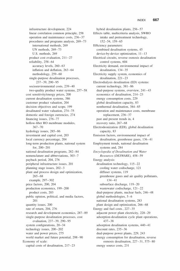
INDEX 667

infrastructure development, 224linear correlation common principle, 258operation and maintenance costs, 236–37procedures and programs analysis, 269–73

international methods, 269UN methods, 269–73U.S. methods, 269

product cost evaluation, 211–27reliability, 258–64

accuracy levels, 260–63inflation and deflation, 263–64methodology, 259–60

single-purpose desalination processes,237–39, 290–95

socioenvironmental costs, 239–40two-quality product water systems, 257–58

cost sensitivity/energy prices, 200current desalination systems, 386customer product valuation, 204decision objectives and scope, 199desalinated water valuation, 274–75domestic and foreign currencies, 274financing issues, 276–77hollow-fiber RO membrane modules,

367–70hydrology issues, 285–86investment and capital cost, 203local currency percentage, 204long-term production plants, national system

for, 200–201national desalination programs, 282–84nomenclature and abbreviations, 303–7payback period, 204, 276peripheral infrastructure issues, 201planning stage issues, 202–3plant and process design and optimization,

265–68example, 297–302

price factors, 200, 204production economics, 199–200

product costs, 203public opinion, political, and media factors,

201quantity issues, 200rate of return, 204, 276research and development economics, 287–89single-purpose desalination processes, cost

evaluation, 237–39, 290–95system configurations, 20–34technology issues, 200–202water and power prices, 275world market and future potential, 298–90

Economy of scale:capital costs of desalination, 217–23

hybrid desalination plants, 256–57Effects table, multicriteria analysis, SWRO

intake and pretreatment technology,152–54, 159–65

Efficiency parameters:combined desalination systems, 45device-by-device optimization, 11–13

Electrical circuits, reverse osmosis desalinationcontrol systems, 604

Electricity demand, environmental impact ofdesalination, 134–35

Electricity supply system, economics ofdesalination, 221–23

Electrodialysis desalination (ED) systems:current technology, 381–86dual-purpose systems, overview, 241–43economics of desalination, 214–23energy consumption costs, 229global desalination capacity, 83nonthermal desalination, 384–85operation and maintenance costs, membrane

replacement, 236–37past and present trends in, 4recovery ratio, 267–68

Electrodeonization (EDI), global desalinationcapacity, 83

Emission factors, environmental impact ofdesalination, greenhouse gases, 136–41

Employment trends, national desalinationsystems and, 284

Encyclopedia of Desalination and WaterResources (DESWARE), 458–59

Energy analysis:desalination technology, 115–22

cooling water codischarge, 121diffuser systems, 119greenhouse gases and air quality pollutants,

134–41subsurface discharge, 119–20wastewater codischarge, 121–22

dual-purpose plants, nuclear fuels, 246–48global methodologies, 5–6national desalination systems, 283plant design and optimization, 266–68

Energy and fuel costs , 227–35adjacent power plant electricity, 228–29adsorption-desalination cycle plant operations,

437–38adsorption desalination systems, 440–41discount rates, 235–36dual-purpose power plants, 229, 243energy consumption for desalination, reverse

osmosis desalination, 227–31, 575–80energy source costs, 231

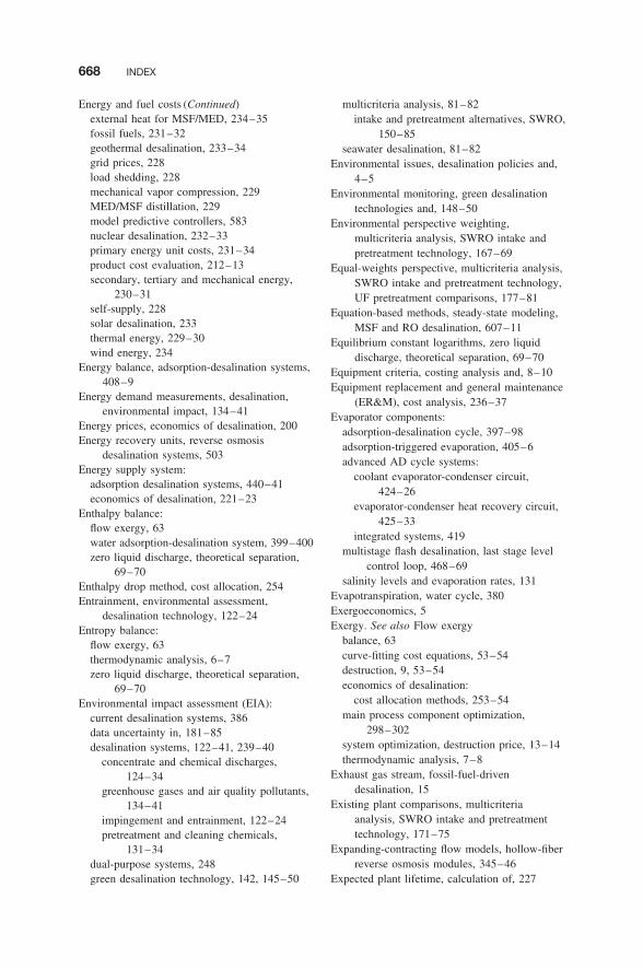
668 INDEX

Energy and fuel costs (Continued)external heat for MSF/MED, 234–35fossil fuels, 231–32geothermal desalination, 233–34grid prices, 228load shedding, 228mechanical vapor compression, 229MED/MSF distillation, 229model predictive controllers, 583nuclear desalination, 232–33primary energy unit costs, 231–34product cost evaluation, 212–13secondary, tertiary and mechanical energy,

230–31self-supply, 228solar desalination, 233thermal energy, 229–30wind energy, 234

Energy balance, adsorption-desalination systems,408–9

Energy demand measurements, desalination,environmental impact, 134–41

Energy prices, economics of desalination, 200Energy recovery units, reverse osmosis

desalination systems, 503Energy supply system:

adsorption desalination systems, 440–41economics of desalination, 221–23

Enthalpy balance:flow exergy, 63water adsorption-desalination system, 399–400zero liquid discharge, theoretical separation,

69–70Enthalpy drop method, cost allocation, 254Entrainment, environmental assessment,

desalination technology, 122–24Entropy balance:

flow exergy, 63thermodynamic analysis, 6–7zero liquid discharge, theoretical separation,

69–70Environmental impact assessment (EIA):

current desalination systems, 386data uncertainty in, 181–85desalination systems, 122–41, 239–40

concentrate and chemical discharges,124–34

greenhouse gases and air quality pollutants,134–41

impingement and entrainment, 122–24pretreatment and cleaning chemicals,

131–34dual-purpose systems, 248green desalination technology, 142, 145–50

multicriteria analysis, 81–82intake and pretreatment alternatives, SWRO,

150–85seawater desalination, 81–82

Environmental issues, desalination policies and,4–5

Environmental monitoring, green desalinationtechnologies and, 148–50

Environmental perspective weighting,multicriteria analysis, SWRO intake andpretreatment technology, 167–69

Equal-weights perspective, multicriteria analysis,SWRO intake and pretreatment technology,UF pretreatment comparisons, 177–81

Equation-based methods, steady-state modeling,MSF and RO desalination, 607–11

Equilibrium constant logarithms, zero liquiddischarge, theoretical separation, 69–70

Equipment criteria, costing analysis and, 8–10Equipment replacement and general maintenance

(ER&M), cost analysis, 236–37Evaporator components:

adsorption-desalination cycle, 397–98adsorption-triggered evaporation, 405–6advanced AD cycle systems:

coolant evaporator-condenser circuit,424–26

evaporator-condenser heat recovery circuit,425–33

integrated systems, 419multistage flash desalination, last stage level

control loop, 468–69salinity levels and evaporation rates, 131

Evapotranspiration, water cycle, 380Exergoeconomics, 5Exergy. See also Flow exergy

balance, 63curve-fitting cost equations, 53–54destruction, 9, 53–54economics of desalination:

cost allocation methods, 253–54main process component optimization,

298–302system optimization, destruction price, 13–14thermodynamic analysis, 7–8

Exhaust gas stream, fossil-fuel-drivendesalination, 15

Existing plant comparisons, multicriteriaanalysis, SWRO intake and pretreatmenttechnology, 171–75

Expanding-contracting flow models, hollow-fiberreverse osmosis modules, 345–46

Expected plant lifetime, calculation of, 227

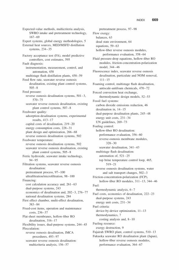
INDEX 669

Expected-value methods, multicriteria analysis,SWRO intake and pretreatment technology,167–69

Expert systems, global energy methodologies, 5External heat sources, MED/MSFD distillation

systems, 234–35

Factory acceptance test (FA), model predictivecontrollers, cost estimates, 595

Fault diagnosis:instrumentation, measurement, control, and

automation, 458multistage flash distillation plants, 458–59

Feed flow rate, seawater reverse osmosisdesalination, existing plant control systems,505–8

Feed pressure:reverse osmosis desalination systems, 501–3,

570–75seawater reverse osmosis desalination, existing

plant control systems, 507–8Feedwater quality:

adsorption-desalination systems, experimentalresults, 413–17

capital costs of desalination, 219–20energy consumption costs, 228–31plant design and optimization, 266–68reverse osmosis desalination systems, 502

Feedwater temperature:reverse osmosis desalination systems, 502seawater reverse osmosis desalination, existing

plant control systems, 505–8Ferric hydroxide, seawater intake technology,

94–95Filtration systems, seawater reverse osmosis

desalination:pretreatment process, 97–100ultrafiltration/microfiltration, 98–100

Financing:cost calculation accuracy and, 261–63dual-purpose systems, 243economics of desalination and, 202–3, 276–77national desalination systems, 284

First effect chamber, multi-effect desalination,383–84

Fixed-cost items, operation and maintenancecosts, 236–37

Flat-sheet membranes, hollow-fiber ROdesalination, 316–17

Flexibility issues, dual-purpose systems, 244–45Flocculation:

reverse osmosis desalination, IMCAprocedures, 493–97

seawater reverse osmosis desalination:multicriteria analysis, 156–57

pretreatment process, 97–98Flow exergy:

balances, 63dead state environment, 64equations, 59–63hollow-fiber reverse osmosis modules,

performance evaluation, 358–64Fluid pressure-drop equations, hollow-fiber RO

modules, friction-concentration-polarizationmodel, 344–46

Fluorescence index, seawater reverse osmosisdesalination, particulate and NOM removal,111–15

Foaming control, multistage flash desalination,antiscale-antifoam chemicals, 470–72

Forced convection heat exchange,thermodynamic design models, 52–53

Fossil fuel systems:carbon dioxide emissions reduction, 46desalination in, 14–15dual-purpose desalination plants, 245–48energy unit costs, 231–34UN guidelines, 269–73

Fouling control:hollow-fiber RO desalination:

performance evaluation, 356–60reverse-osmosis membrane modules,

328–30seawater desalination, 341–43

multistage flash desalination:automation of, 521–25top brine temperature control loop, 465,

519–21reverse osmosis desalination systems, water

and salt transport changes, 502–3Friction-concentration-polarization (FCP),

hollow-fiber RO modules, 311–13, 344–46Fuel:

thermodynamic analysis, 6–7Fuel costs, economics of desalination, 222–23

dual-purpose systems, 243energy unit costs, 231–34

Fuel criteria:device-by-device optimization, 11–13thermodynamics, 7

costing analysis and, 8–10Fueling resource:

exergy destruction, 9Fujairah SWRO plant, control systems, 510–13Fukuoka seawater RO desalination plant (Japan),

hollow-fiber reverse osmosis modules,performance evaluation, 364–67

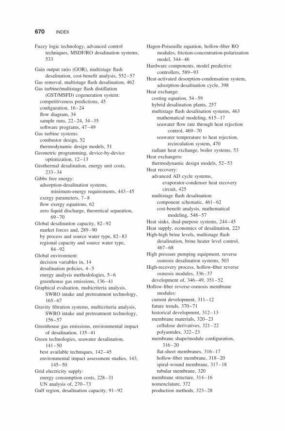
670 INDEX

Fuzzy logic technology, advanced controltechniques, MSDF/RO desalination systems,533

Gain output ratio (GOR), multistage flashdesalination, cost-benefit analysis, 552–57

Gas removal, multistage flash desalination, 462Gas turbine/multistage flash distillation

(GST/MSFD) cogeneration system:competitiveness predictions, 45configuration, 16–24flow diagram, 34sample runs, 22–24, 34–35software programs, 47–49

Gas turbine systems:combustor design, 52thermodynamic design models, 51

Geometric programming, device-by-deviceoptimization, 12–13

Geothermal desalination, energy unit costs,233–34

Gibbs free energy:adsorption-desalination systems,

minimum-energy requirements, 443–45exergy parameters, 7–8flow exergy equations, 62zero liquid discharge, theoretical separation,

69–70Global desalination capacity, 82–92

market forces and, 289–90by process and source water type, 82–83regional capacity and source water type,

84–92Global environment:

decision variables in, 14desalination policies, 4–5energy analysis methodologies, 5–6greenhouse gas emissions, 136–41

Graphical evaluation, multicriteria analysis,SWRO intake and pretreatment technology,165–67

Gravity filtration systems, multicriteria analysis,SWRO intake and pretreatment technology,156–57

Greenhouse gas emissions, environmental impactof desalination, 135–41

Green technologies, seawater desalination,141–50

best available techniques, 142–45environmental impact assessment studies, 143,

145–50Grid electricity supply:

energy consumption costs, 228–31UN analysis of, 270–73

Gulf region, desalination capacity, 91–92

Hagen-Poiseuille equation, hollow-fiber ROmodules, friction-concentration-polarizationmodel, 344–46

Hardware components, model predictivecontrollers, 589–93

Heat-activated desorption-condensation system,adsorption-desalination cycle, 398

Heat exchange:costing equation, 54–59hybrid desalination plants, 257multistage flash desalination systems, 463

mathematical modeling, 615–17seawater flow rate through heat rejection

control, 469–70seawater temperature to heat rejection,

recirculation system, 470radiant heat exchange, boiler systems, 53

Heat exchangers:thermodynamic design models, 52–53

Heat recovery:advanced AD cycle systems,

evaporator-condenser heat recoverycircuit, 425

multistage flash desalination:component schematic, 461–62cost-benefit analysis, mathematical

modeling, 548–57Heat sinks, dual-purpose systems, 244–45Heat supply, economics of desalination, 223High-high brine levels, multistage flash

desalination, brine heater level control,467–68

High pressure pumping equipment, reverseosmosis desalination systems, 503

High-recovery process, hollow-fiber reverseosmosis modules, 336–37

development of, 346–49, 351–52Hollow-fiber reverse-osmosis membrane

modules:current development, 311–12future trends, 370–71historical development, 312–13membrane materials, 320–23

cellulose derivatives, 321–22polyamides, 322–23

membrane shape/module configuration,316–20

flat-sheet membranes, 316–17hollow-fiber membrane, 318–20spiral-wound membrane, 317–18tubular membrane, 320

membrane structure, 314–16nomenclature, 372production methods, 323–28

INDEX 671

interfacial polymerization, 326–28phase separation, 324–26stretching, 326timeline, 324

reverse-osmosis desalination, 328–37fouling control, 328–30high-recovery process, 336–37performance prediction, 332–36pretreatment disinfection, 330–32

seawater desalination, 338–67actual performance, 354–67

AdDur plant, Bahrain, 360–64global performance, 354–56Ikata power station, Japan, 364Jeddah 1 RO plant, Saudi Arabia, 356–60

advanced large-sized reverse osmosismodule, 354

analytical module modeling, 343–44both open-ended reverse osmosis module,

349–54double-element hollow-fiber module design,

345–49economics, 367–70fouling resistance, 341–43friction concentration polarization, 344–45Fukuoka plant, Japan, 364–67higher recovery optimization, 346–49hollow-fiber bundle configuration, 338module structure, 338–40performance stability, 340

separation characteristics, 313–14Horizontal intake systems, seawater intake

technology, 92–95Hybrid desalination plants:

cost evaluation, 256–57hollow-fiber reverse osmosis methods, 312–13instrumentation, measurement, control, and

automation for, 459Hydrology, desalination and, 285–86Hydrolysis, hollow-fiber RO desalination,

cellulose triacetate change rate, 334–36Hydrophilicity:

adsorbent materials, 390–93hollow-fiber RO desalination, global

performance, 355–56Hydrophobicity, adsorbent materials, 390–93

Ideal-gas mixture:flow exergy equations, 61zero liquid discharge, theoretical separation,

constant-pressure specific heats, 67–70Identification data, model predictive controllers,

advanced identification and analysis,585–86

Ikata power station (Japan), hollow-fiber reverseosmosis modules, performance evaluation,364

Impingement, environmental assessment,desalination technology, 122–24

Improved control operation, economic benefitsof, 541–43

Increment function, dynamic modeling, 631–32Independent-cost items, operation and

maintenance costs, 236–37Index of living, national desalination systems,

284Indirect capital costs, economics of desalination,

224Industrial production, economics of desalination,

200Inflation:

adsorption-desalination cycle plant costs,capital recovery factor vs.inflation-weighted factor, 434–38

cost analysis of desalination, 263–64Infrastructure, economics of desalination and:

development costs, 224reliability, 201

Input data, multicriteria analysis, SWRO intakeand pretreatment technology, 152–54

Inside-out systems, multicriteria analysis, SWROintake and pretreatment technology, UFpretreatment comparisons, 177–81

Instrumentation, measurement, control, andautomation (IMCA) :

abbreviations, 640–41advanced control methods, MSF/RO

desalination, 527–35constrained model predictive control,

530–31dynamic matrix control, 529intelligent control approaches, 532–33nonlinear model predictive control method,

529–30online optimization, 533–35

automation and operation optimization,460–517

current and projected projects, 517–25fouling control, 521–25startup-shutdown-flushing automation,

518–19top brine temperature modification and

control, 519–21current and future automated processing,

516–17current status, 457–58literature review, 459–60modeling and analysis, 605–32

672 INDEX

Instrumentation, measurement, control, andautomation (IMCA) (Continued)

basic requirements, 605–6dynamic modeling, 608–12, 628–32mathematical modeling, 612–17reverse osmosis desalination, 617–28steady-state modeling, 606–8

multistage flash desalination:antiscale-antifoam and sodium sulfate

dosage, 470–72brine recirculation system, 468–69condensate system, 467–68control loops, 472–75cooling-water recirculation system, 470cost-benefit ratio, 547–65design criteria, 462–63desuperheater water spray system, 465–67distillate product water system, 470existing plants, 487–93general characteristics, 461–62instrumentation list, 476–87modeling and analysis, 605–32operation and power plant criteria, 463–72overview, 458–59process parameters, 475–84proportional integral diagram, 485seawater system, 469–70steam system characteristics, 464–65system recommendations, 601

nomenclature, 636–40overview, 456–57product water costs, automation impact on,

536–40advanced process control, economic impact,

540–43multistage flash distillation, cost-benefit

ratio, 547–65process control structure, 543–47reverse-osmosis cost-benefit ratio, 565–78

reverse-osmosis desalination, 459automation systems, 499–500brackish vs. seawater control systems,

503–4control parameters, 500–516

feedwater salinity, 502feedwater temperature, 502high-pressure pumping equipment, 503permeate flux, 502recovery rate, 501water and salt transport, membrane age

and fouling, 502–3cost-benefit ratio, 565–78current and projected automation of, 525–27existing control systems, 504–16

modeling and analysis, 605–6, 617–28overview, 493–99system recommendations, 601–5

system recommendations, 580–605model predictive advanced controller,

580–600multistage flash distillation plants, 601reverse-osmosis systems, 601–5

Insurance costs, desalination systems, 237Intake systems

impingement and entrainment, 122–24multicriteria analysis, 150–85

data input, 155–69existing plant comparisons, 171–73future research issues, 181–85methodology, 152–54results evaluation, 170–81sensitivity analysis, 170–71study requirements and capabilities, 152ultrafiltration pretreatment comparisons,

173, 176–81multistage flash desalination, 462reverse osmosis desalination, 604seawater reverse osmosis desalination plant

design, 100–105subsurface intake systems, 93–95surface intake systems, 92–93

Intangible benefits, cost-benefit analysis ofautomation, 537–40

Integrated condenser-evaporator, advanced ADcycle systems, 419–33

Integrated Pollution Prevention and Control(IPPC), EC Directive for, green desalinationtechnology guidelines, 143–45

Intelligent control, advanced control techniques,MSDF/RO desalination systems, 532

Interest during construction (IDC), economics ofdesalination, 213–23

Interest rates:capital cost reduction, 225economics of desalination, 207

Interfacial polymerization, hollow-fiber ROdesalination membrane production, 326–28

Intermediate variables, model predictivecontrollers, 586–87

Intermittent chlorine injection (ICI):economics of, 369–70hollow-fiber reverse osmosis modules, 311–13

disinfection, 331–32performance evaluation, 358–60

International Atomic Energy Agency (IAEA),desalination guidelines, 270–73

International Desalination Association (IDA):cost sample data, 269–70

INDEX 673

desalination plant inventory, 82International power and water projects (IWPPs),

dynamic modeling, 609–11International procedures, desalination systems,

269International water projects, dynamic modeling,

609–11Interstage weirs and submerged orifices,

multistage flash desalination systems, 463Investment criteria:

economics of desalination, 203actual cost calculations, 207–8capital costs, 213–23

frequency of recovery, 226plant design and optimization, 266–68

Investment payments:capital cost evaluation, 213–14

Isosteric heat of adsorption, wateradsorption-desalination systems, 402–4

Japanese desalination plants, Ikata power station,hollow-fiber reverse osmosis modules,performance evaluation, 364

Jeddah 1 reverse osmosis desalination plant,performance evaluation, 356–60

Kelvin optimality equation, device-by-deviceoptimization, 13

Known intermediate chemical changes, flowexergy equations, 63

Kuwait, seawater reverse osmosis desalinationsystem in, 505–8

K -value. See Salt permeability coefficient (Bvalue)

Labor requirements:dual-purpose systems, 243economics of desalination, 274national desalination systems and employment

trends, 284plant design and optimization, 266–68reverse osmosis desalination, cost-benefit

analysis, 578–80Lanarca 54,000 m3/day SWRO plant, 508–10Land area, national desalination systems, 282Land-Based Sources of the Mediterranean Action

Plan (LBS), green desalination technologyguidelines, 143–45

Large-scale seawater desalination:cost comparisons, 237–39research and development, 288–89

Lead time, hollow-fiber reverse osmosismodules, performance evaluation, 358–60

Licensing procedures, dual-purpose systems, 248Life cycle analysis:

green desalination technology guidelines, 145

water adsorption-desalination cycle, 433–41cost recovery factors, 434–38energy sources, 440–41product cost comparison, RO plants,

438–40Linear correlation common principle, cost

analysis of desalination, 258Linear driving force (LDF) equation, water

adsorption-desalination systems, adsorptionbeds, 407

Linear interval standardization function,multicriteria analysis, SWRO intake andpretreatment technology, 165–67

UF pretreatment comparisons, 177–81Liquid chromatography with organic carbon

detection (LC-OCD):pretreatment technology:

particulate and NOM removal, 105–15plant design, 100–105

Literature review, instrumentation, measurement,control, and automation systems, 457–60

Load factor (LF):dual-purpose systems, 244–45

power generation and, 247–48economics of desalination, 214–23thermal desalination, 229–30

Load shedding, energy consumption costs,228–31

Loeb-Sourirajan cellulose acetate membrane,hollow-fiber reverse osmosis modules, 326

Low-low brine levels, multistage flashdesalination, brine heater level control,467–68

Low-pressure (LP) steam header, multistage flashdesalination operations, 463–72

Low-temperature heat source, currentdesalination systems, 386

Managerial issues, economics of desalinationand, 202–3

Manganese dioxide deposits, seawater intaketechnology, 94–95

Manufacturing resources:thermodynamic variables, 9–10thermoeconomic analysis, 8–9

Marginal water cost method, dual-purposesystem cost analysis, 252–54

Market potential, global desalination capacity,289–90

Mass-salt balance, adsorption-triggeredevaporation, 405–6

Mathematical modeling :desalination IMCA methods, 611–17dynamic simulation, 628–32future trends, 632

674 INDEX

Mathematical modeling (Continued)multistage flash desalination, cost-benefit

analysis, 548–57setpoint control system optimization, 546–47

Maximum process temperature, plant design andoptimization, 267–68

Maximum production rate, dual-purpose systems,power generation systems, 246–48

Measurement scales:multicriteria analysis, SWRO intake and

pretreatment technology, 157–58setpoint control system, reconciliation of, 545

Mechanical energy sources, energy consumptioncosts, 230–31

Mechanical vapor compression (MVC):dual-purpose systems:

disadvantages, 244–45maximum production rate, 246–48overview, 241–43

economics of desalination, 214–23energy consumption costs, 2290231recovery ratio, 267–68thermal desalination, 384

Media coverage issues, economics ofdesalination and, 201

Mediterranean Sea:desalination capacity in, 88, 90–91green desalination technology guidelines,

144–45reverse osmosis methods in, 311–13

Melt spinning, hollow-fiber reverse-osmosismembrane production, 325–26

Membrane degradation:hollow-fiber RO desalination:

cellulose triacetate change rate, 334–36membrane compaction, 332–33pretreatment disinfection and, 330

reverse osmosis desalination, cost-benefitanalysis, 577–80

membrane age, 625–26Membrane differential pressure, seawater reverse

osmosis desalination, existing plant controlsystems, 508

Membrane flux decline/membrane flux retentioncoefficient (MFRC), hollow-fiber ROdesalination, 332–33

Membrane materials:cost analysis:

AD cycle production cost comparisons,439–40

reverse osmosis desalination systems,577–80

hollow-fiber RO desalination, 320–23cellulose derivatives, 321–22

polyamides, 322–23production methods, 323–28

interfacial polymerization, 326–28phase separation, 324–26stretching, 326timeline, 324

shape and configuration, 316–20hollow-fiber membrane, 318–20spiral-wound membrane, 317–18tubular membrane, 320

structural properties, 314–16product water quality, 221–23reverse osmosis desalination systems:

existing plant control systems, 512–13permeability, 623–24water and salt transport changes, 502–3

thermal desalination, 381–84Membrane transport equations, hollow-fiber RO

modules, friction-concentration-polarizationmodel, 344–46

Metallorganic frameworks (MOFs), adsorbentmaterials, 395–96

Metal oxides, hollow-fiber RO desalination,membrane fouling, 329–30

MFI values. See alsoUltrafiltration/microfiltration (UF/MF)

seawater reverse osmosis desalination,particulate and NOM removal, 107–15

Microfiltration membranes. See alsoUltrafiltration/microfiltration (UF/MF)

hollow-fiber reverse-osmosis desalination:shape/configuration, 318–20thermally-induced phase separation

production, 324–26hollow-fiber RO desalination, 313–16

Microorganism removal, seawater reverseosmosis desalination,ultrafiltration/microfiltration, 99–100

Micropore volume, adsorbent materials, 390Middle East desalination systems:

hollow-fiber reverse osmosis methods, 311–14high recovery rate models, 346–49, 351–52

multistage flash desalination, existing plantcontrol systems, 487–93

reverse osmosis systems, 505–16Minimal pretreatment technology, seawater

reverse osmosis desalination, 95Minimized unit surface cost:

heat exchangers, 54–59thermodynamic variables, 10

Minimum distillate production costs, multistageflash desalination, cost-benefit analysis,554–57

INDEX 675

Minimum energy requirements,adsorption-desalination systems, Gibbs freeenergy calculations, 443–45

Minimum-flow line, multistage flashdesalination, seawater flow rate throughheat rejection control, 470

Mixing zone regulations:desalination and, 285–86salinity levels and, 126

Model predictive controllers (MPCs):advanced identification and analysis (AIDA),

584–86automation cost-benefit analysis, 539–40basic principles, 581–83cost estimations, 587–88distributed control system configuration,

588–89hardware components, 589–94multistage flash desalination operation,

cost-benefit analysis, 560–62selection criteria, 580–600software components, 589–94system configuration, 584

Money value, product cost evaluation, 212–13Multicriteria analysis (MCA):

environmental impact assessment, 81–82green desalination technology guidelines, 145intake and pretreatment alternatives, SWRO,

150–85data input, 155–69existing plant comparisons, 171–75future research issues, 181–85methodology, 152–54results evaluation, 170–81sensitivity analysis, 170–71study requirements and capabilities, 151ultrafiltration pretreatment comparisons,

173, 176, 178–81Multi-effect desalination (MED):

adsorption desalination systems, energy costcomparisons, 441

average temperature drop per effect, 268capital costs, 215–23cooling water codischarge systems, 121current technology, 381–86double-distilled water streams, 257–58dual-purpose systems:

disadvantages, 244–45low-temperature systems, 242–43power generation systems, 246–48

economics of desalination:AD cycle production cost comparisons,

438–40energy consumption costs, 229–31

energy supply, 223sample cost calculations, 295–97

external heat sources, 234–35global desalination capacity, 82–83hybrid desalination plants, 256–57main process component optimization,

297–302nuclear fuel costs, 232–34recovery ratio, 267–68regional capacity, 88–92single-stage systems, cost comparisons,

238–39thermal desalination, 383–84wind energy unit costs, 234

Multiport diffusers, desalination technology,119–20

Multistage flash desalination (MSFD) :adsorption desalination systems, energy cost

comparisons, 441advanced control methods:

constrained model predictive control,530–31

dynamic matrix control, 529intelligent control approaches, 532–33nonlinear model predictive control method,

529–30online optimization, 533–35

automation cost-benefit analysis, 538–40brine heater, temperature increase, 268capital costs, 215–23components schematic, 461–62cooling water codischarge systems, 121cost-benefit analysis, 547–65

IMCA philosophy, 562–65performance modeling and simulation,

547–57process optimization, 557–62

current technology, 381–86double-distilled water streams, 257–58dual-purpose systems:

disadvantages, 244–45low-temperature systems, 242–43power generation systems, 246–48

dynamic modeling, 605–11economics of desalination:

AD cycle production cost comparisons,438–40

energy consumption costs, 229–31energy supply, 223

external heat sources, 234–35gas turbine/multistage flash distillation

(GST/MSFD) cogeneration system,34–35

global desalination capacity, 82–83

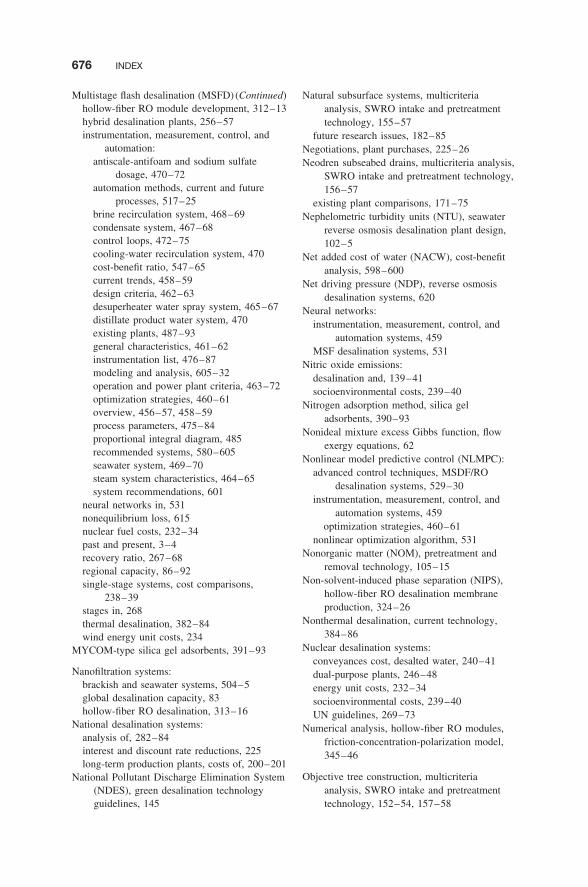
676 INDEX

Multistage flash desalination (MSFD) (Continued)hollow-fiber RO module development, 312–13hybrid desalination plants, 256–57instrumentation, measurement, control, and

automation:antiscale-antifoam and sodium sulfate

dosage, 470–72automation methods, current and future

processes, 517–25brine recirculation system, 468–69condensate system, 467–68control loops, 472–75cooling-water recirculation system, 470cost-benefit ratio, 547–65current trends, 458–59design criteria, 462–63desuperheater water spray system, 465–67distillate product water system, 470existing plants, 487–93general characteristics, 461–62instrumentation list, 476–87modeling and analysis, 605–32operation and power plant criteria, 463–72optimization strategies, 460–61overview, 456–57, 458–59process parameters, 475–84proportional integral diagram, 485recommended systems, 580–605seawater system, 469–70steam system characteristics, 464–65system recommendations, 601

neural networks in, 531nonequilibrium loss, 615nuclear fuel costs, 232–34past and present, 3–4recovery ratio, 267–68regional capacity, 86–92single-stage systems, cost comparisons,

238–39stages in, 268thermal desalination, 382–84wind energy unit costs, 234

MYCOM-type silica gel adsorbents, 391–93

Nanofiltration systems:brackish and seawater systems, 504–5global desalination capacity, 83hollow-fiber RO desalination, 313–16

National desalination systems:analysis of, 282–84interest and discount rate reductions, 225long-term production plants, costs of, 200–201

National Pollutant Discharge Elimination System(NDES), green desalination technologyguidelines, 145

Natural subsurface systems, multicriteriaanalysis, SWRO intake and pretreatmenttechnology, 155–57

future research issues, 182–85Negotiations, plant purchases, 225–26Neodren subseabed drains, multicriteria analysis,

SWRO intake and pretreatment technology,156–57

existing plant comparisons, 171–75Nephelometric turbidity units (NTU), seawater

reverse osmosis desalination plant design,102–5

Net added cost of water (NACW), cost-benefitanalysis, 598–600

Net driving pressure (NDP), reverse osmosisdesalination systems, 620

Neural networks:instrumentation, measurement, control, and

automation systems, 459MSF desalination systems, 531

Nitric oxide emissions:desalination and, 139–41socioenvironmental costs, 239–40

Nitrogen adsorption method, silica geladsorbents, 390–93

Nonideal mixture excess Gibbs function, flowexergy equations, 62

Nonlinear model predictive control (NLMPC):advanced control techniques, MSDF/RO

desalination systems, 529–30instrumentation, measurement, control, and

automation systems, 459optimization strategies, 460–61

nonlinear optimization algorithm, 531Nonorganic matter (NOM), pretreatment and

removal technology, 105–15Non-solvent-induced phase separation (NIPS),

hollow-fiber RO desalination membraneproduction, 324–26

Nonthermal desalination, current technology,384–86

Nuclear desalination systems:conveyances cost, desalted water, 240–41dual-purpose plants, 246–48energy unit costs, 232–34socioenvironmental costs, 239–40UN guidelines, 269–73

Numerical analysis, hollow-fiber RO modules,friction-concentration-polarization model,345–46

Objective tree construction, multicriteriaanalysis, SWRO intake and pretreatmenttechnology, 152–54, 157–58

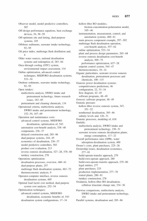
INDEX 677

Observer model, model predictive controllers,587

Off-design performance equations, heat exchangedevices, 54, 58–59

Off-optimum site and timing, dual-purposesystems, 245

Offshore sediments, seawater intake technology,92–95

Oil price index, multistage flash distillation and,4

Older water sources, national desalinationsystems and redemption of, 283–84

Once-through cooling (OTC) system,environmental impact assessment, 134

Online optimization, advanced controltechniques, MSDF/RO desalination systems,533–34

Onshore sediments, seawater intake technology,92–95

Open intakes:multicriteria analysis, SWRO intake and

pretreatment technology, future researchissues, 183–85

pretreatment and cleaning chemicals, 134Operational criteria, multicriteria analysis,

SWRO intake and pretreatment technology,152–54, 167–69

Operation and maintenance costs:advanced control systems, MSDF/RO

desalination, optimization of, 543automation cost-benefit analysis, 538–40components, 236–37delayed construction and, 285–86dual-purpose systems, 244–45economics of desalination, 236–37model predictive controllers, 583product cost evaluation, 213reverse osmosis desalination, 527–28, 578–80turnkey construction, 278

Operations optimization:desalination processes, overview, 460–61dual-purpose plants, 257multistage flash desalination systems, 463–72thermoeconomic analysis, 9

Operator-computer interface, reverse osmosisdesalination systems, 605

Optimal load factor cost method, dual-purposesystem cost analysis, 252–54

Optimization techniques:advanced control systems, MSDF/RO

desalination, economic benefits of, 543desalination system configurations, 17–34

hollow-fiber RO modules,friction-concentration-polarization model,345–46

instrumentation, measurement, control, andautomation systems, 460–61

main process component example, 297–302multistage flash desalination operation,

cost-benefit analysis, 557–62online optimization, 533–34plant and process design parameters, 265–68reverse osmosis desalination cost-benefit

analysis, 569–75performance optimization, 627–28

setpoint control system, 544–47thermoeconomics, 10–14

Organic particulates, seawater reverse osmosisdesalination, pretreatment processes andchemicals, 100–115

Osmosis power desalination systems:competitiveness predictions, 46configuration, 22, 33–34flow diagram, 42–45software programs, 48–49

Osmosis software program, 48–49Osmotic pressure:

hollow-fiber reverse osmosis system, 347,351–52

nonthermal desalination, 385–86salinity levels and, 126–31

Osmotic processes, modeling of, 618Outfalls:

multicriteria analysis, SWRO intake andpretreatment technology, 150–51

seawater reverse osmosis desalination plants,energy consumption, 117–22

Overall performance ratio (OPR), wateradsorption-desalination system, 400

Owner’s costs, plant purchases, 225–26Ownership issues, desalination economics,

277–81build-operate-transfer approach, 279build-own-operate approach, 280build-own-operate-transfer approach, 279–80legal entities, 277plant purchases, 225production implementation, 277–78rented plants, 280–81turnkey construction, 278

Oxidation, hollow-fiber RO desalination,cellulose triacetate change rate, 334–36

Pairwise comparisons, multicriteria analysis,SWRO intake and pretreatment technology,154

Parallel systems, desalination and, 285–86

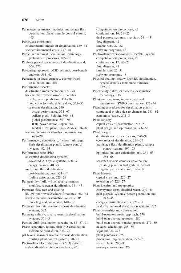
678 INDEX

Parameters estimation modules, multistage flashdesalination plants, sample control system,493

Particulate emissions:environmental impact of desalination, 139–41socioenvironmental costs, 239–40

Particulate removal, desalination technology,pretreatment processes, 105–15

Payback period, economics of desalination and,204, 276

Percentage approach, MSD systems, cost-benefitanalysis, 561–62

Percentage of local currency, economics ofdesalination and, 204

Performance aspects:desalination implementation, 277–78hollow-fiber reverse osmosis modules:

performance prediction, 332–36prediction formula, B/K values, 335–36seawater desalination, 340

actual performance, 354–67AdDur plant, Bahrain, 360–64global performance, 354–56Ikata power station, Japan, 364Jeddah 1 RO plant, Saudi Arabia, 356–60

reverse osmosis desalination, optimization,627–28

Performance calculations software, multistageflash desalination plants, sample controlsystem, 492–93

Performance ratio (PR):adsorption-desalination systems:

advanced AD cycle systems, 430–33energy balance, 408–9

multistage flash desalination:cost-benefit analysis, 551–57fouling automation, 523–25

Permeability, hollow-fiber reverse osmosismodules, seawater desalination, 341–43

Permeate flow rate and quality:hollow-fiber reverse osmosis modules, 362–64reverse osmosis desalination systems, 605

modeling and conversion, 618–19Permeate flux rate, reverse osmosis desalination

systems, 502Permeate salinity, reverse osmosis desalination

systems, 501–3Persian Gulf, desalination capacity in, 86–87, 91Phase separation, hollow-fiber RO desalination

membrane production, 324–26pH levels, seawater reverse osmosis desalination,

existing plant control systems, 507–8Photovoltaic/electrodialysis (PV/ED) system:

carbon dioxide emission avoidance, 46

competitiveness predictions, 45configuration, 16, 21–22dual-purpose systems, overview, 241–43flow diagram, 42sample runs, 22, 32software programs, 48

Photovoltaic/reverse-osmosis (PV/RO) system:competitiveness predictions, 45configuration, 17, 20–21flow diagram, 41sample runs, 22, 31software programs, 48

Physical fouling, hollow-fiber RO desalination,reverse-osmosis membrane modules,329–30

Pipeline-style diffuser systems, desalinationtechnology, 119

Plankton organisms, impingement andentrainment, SWRO desalination, 122–24

Planning procedures for desalination plants:contractual pricing due to changes in, 281–82economics issues, 202–3

Plant capacity:capital costs of desalination, 217–23plant design and optimization, 266–68

Plant design:desalination cost calculations, 290–97economics of desalination, 214–23multistage flash desalination plants, sample

control system, 490–93optimization, cost calculation and, 261–63,

265–68seawater reverse osmosis desalination:

existing plant control systems, 505–8organic particulates and, 100–105

Plant lifetime:capital costs and, 226–27extension of, 226–27

Plant location and topography:conveyance costs, desalted water, 240–41dual-purpose systems, power generation and,

247–48energy consumption costs, 228–31land area, national desalination systems, 282

Plant ownership and construction:build-operate-transfer approach, 279build-own-operate approach, 280build-own-operate-transfer approach, 279–80delayed scheduling, 285–86legal entities, 277plant purchases, 225production implementation, 277–78rented plants, 280–81turnkey construction, 278

INDEX 679

Political issues, economics of desalination and,201

Polyamides, hollow-fiber RO desalination,322–23, 328

Polypiperazineamide membranes, hollow-fiberRO module desalination, 323

Polysulfone membranes, hollow-fiber ROdesalination, 315–16, 327–28

Pore network, adsorbent materials, 390Pore size distribution:

adsorption-desorption mechanics, 400–404water adsorption-desalination system:

selective water sorbents, 394–95silica gel adsorbents, 390–93

Porosity of membranes:adsorbent materials, 390hollow-fiber RO desalination, 314–16, 320–23

Posidonia spp., salinity levels and, 125–31Potable-water collection system:

adsorption-desalination cycle, 398adsorption-desalination systems, quality

analysis, 413–17advanced AD cycle systems, 422–24

Potential physical plant lifetime, calculation of,227

Power credit method, dual-purpose system costanalysis, 249–54

Power generation systems, dual-purposedesalination plants, 245–48

Power law, capital costs of desalination, 218–23Power load fluctuations, dual-purpose plants, 257Power pricing, desalination economics and, 275Power requirement modeling, reverse osmosis

desalination, 626–27Practical salinity units (PSUs), salinity

measurements, 125–31Prediction criteria, combined desalination

systems, 45Pressure equalization (PE),

adsorption-desalination systems, 418Pressure filtration systems, multicriteria analysis,

SWRO intake and pretreatment technology,156–57

Pressure profiles, adsorption-desalinationsystems, simulation results, 411–12

Pretreatment processes and chemicals:adsorption-desalination cycle, 397desalination technology, 95–100

conventional pretreatment, 95–98energy consumption and, 117–22minimal pretreatment, 95organic particulate foulants, 100–115particulate and NOM removal, 105–15ultrafiltration/microfiltration, 98–100

environmental impact, 131–34hollow-fiber RO desalination, disinfection

procedures, 330–32multicriteria analysis (MCA), 150–85

data input, 155–69existing plant comparisons, 171–75future research issues, 181–85methodology, 152–54results evaluation, 169–81sensitivity analysis, 170–71study requirements and capabilities, 151ultrafiltration pretreatment comparisons,

173, 176–81reverse osmosis desalination, 604

automation projects, 526–27Pricing issues:

contractual pricing, 281–82economics of desalination:

electricity supply system, 221–23product price, 204very low acceptable price, 200

national desalination systems, subsidies for,284

seawater desalination, 369–70two-quality water streams, 258water and power pricing, 275

Primary energy sources:cost evaluation, 231–34

Primary thermal energy, energy consumptioncosts, 229–31

Problem definition, multicriteria analysis, SWROintake and pretreatment technology, 152–54

Process modeling, model predictive controllers,581–83

Process parameters:control structure automation of, 543–47design and optimization, 265–68economics of desalination, 269–73

international methods, 269UN methods, 269–73U.S. methods, 269

global desalination capacity, 82–83multistage flash desalination, 475–84

existing plant control systems, 487–93instrumentation list and flow sheet, 476–87plant size and manufacture design, 476process control system schematic, 488–90

optimization, 297–302reverse osmosis desalination, 498–99

control systems, 500–503cost-benefit analysis, 565–66

thermally driven desalination plants, processinterfaces, 463–72

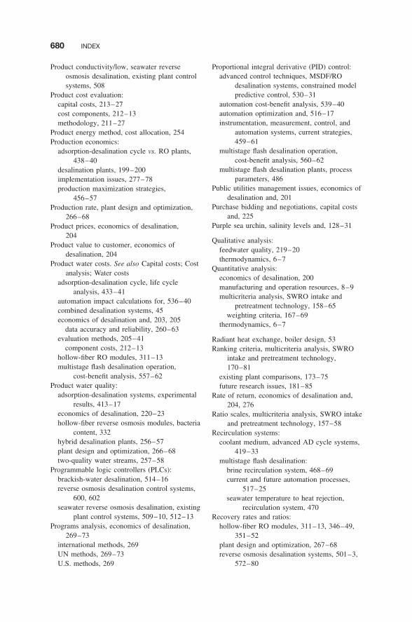
680 INDEX

Product conductivity/low, seawater reverseosmosis desalination, existing plant controlsystems, 508

Product cost evaluation:capital costs, 213–27cost components, 212–13methodology, 211–27

Product energy method, cost allocation, 254Production economics:

adsorption-desalination cycle vs. RO plants,438–40

desalination plants, 199–200implementation issues, 277–78production maximization strategies,

456–57Production rate, plant design and optimization,

266–68Product prices, economics of desalination,

204Product value to customer, economics of

desalination, 204Product water costs. See also Capital costs; Cost

analysis; Water costsadsorption-desalination cycle, life cycle

analysis, 433–41automation impact calculations for, 536–40combined desalination systems, 45economics of desalination and, 203, 205

data accuracy and reliability, 260–63evaluation methods, 205–41

component costs, 212–13hollow-fiber RO modules, 311–13multistage flash desalination operation,

cost-benefit analysis, 557–62Product water quality:

adsorption-desalination systems, experimentalresults, 413–17

economics of desalination, 220–23hollow-fiber reverse osmosis modules, bacteria

content, 332hybrid desalination plants, 256–57plant design and optimization, 266–68two-quality water streams, 257–58

Programmable logic controllers (PLCs):brackish-water desalination, 514–16reverse osmosis desalination control systems,

600, 602seawater reverse osmosis desalination, existing

plant control systems, 509–10, 512–13Programs analysis, economics of desalination,

269–73international methods, 269UN methods, 269–73U.S. methods, 269

Proportional integral derivative (PID) control:advanced control techniques, MSDF/RO

desalination systems, constrained modelpredictive control, 530–31

automation cost-benefit analysis, 539–40automation optimization and, 516–17instrumentation, measurement, control, and

automation systems, current strategies,459–61

multistage flash desalination operation,cost-benefit analysis, 560–62

multistage flash desalination plants, processparameters, 486

Public utilities management issues, economics ofdesalination and, 201

Purchase bidding and negotiations, capital costsand, 225

Purple sea urchin, salinity levels and, 128–31

Qualitative analysis:feedwater quality, 219–20thermodynamics, 6–7

Quantitative analysis:economics of desalination, 200manufacturing and operation resources, 8–9multicriteria analysis, SWRO intake and

pretreatment technology, 158–65weighting criteria, 167–69

thermodynamics, 6–7

Radiant heat exchange, boiler design, 53Ranking criteria, multicriteria analysis, SWRO

intake and pretreatment technology,170–81

existing plant comparisons, 173–75future research issues, 181–85

Rate of return, economics of desalination and,204, 276

Ratio scales, multicriteria analysis, SWRO intakeand pretreatment technology, 157–58

Recirculation systems:coolant medium, advanced AD cycle systems,

419–33multistage flash desalination:

brine recirculation system, 468–69current and future automation processes,

517–25seawater temperature to heat rejection,

recirculation system, 470Recovery rates and ratios:

hollow-fiber RO modules, 311–13, 346–49,351–52

plant design and optimization, 267–68reverse osmosis desalination systems, 501–3,

572–80

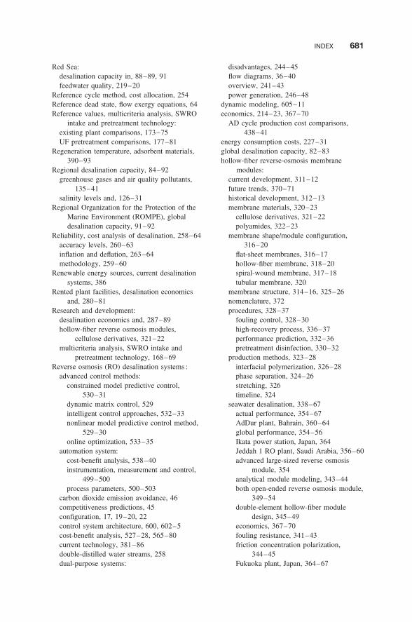
INDEX 681

Red Sea:desalination capacity in, 88–89, 91feedwater quality, 219–20

Reference cycle method, cost allocation, 254Reference dead state, flow exergy equations, 64Reference values, multicriteria analysis, SWRO

intake and pretreatment technology:existing plant comparisons, 173–75UF pretreatment comparisons, 177–81

Regeneration temperature, adsorbent materials,390–93

Regional desalination capacity, 84–92greenhouse gases and air quality pollutants,

135–41salinity levels and, 126–31

Regional Organization for the Protection of theMarine Environment (ROMPE), globaldesalination capacity, 91–92

Reliability, cost analysis of desalination, 258–64accuracy levels, 260–63inflation and deflation, 263–64methodology, 259–60

Renewable energy sources, current desalinationsystems, 386

Rented plant facilities, desalination economicsand, 280–81

Research and development:desalination economics and, 287–89hollow-fiber reverse osmosis modules,

cellulose derivatives, 321–22multicriteria analysis, SWRO intake and

pretreatment technology, 168–69Reverse osmosis (RO) desalination systems :

advanced control methods:constrained model predictive control,

530–31dynamic matrix control, 529intelligent control approaches, 532–33nonlinear model predictive control method,

529–30online optimization, 533–35

automation system:cost-benefit analysis, 538–40instrumentation, measurement and control,

499–500process parameters, 500–503

carbon dioxide emission avoidance, 46competitiveness predictions, 45configuration, 17, 19–20, 22control system architecture, 600, 602–5cost-benefit analysis, 527–28, 565–80current technology, 381–86double-distilled water streams, 258dual-purpose systems:

disadvantages, 244–45flow diagrams, 36–40overview, 241–43power generation, 246–48

dynamic modeling, 605–11economics, 214–23, 367–70

AD cycle production cost comparisons,438–41

energy consumption costs, 227–31global desalination capacity, 82–83hollow-fiber reverse-osmosis membrane

modules:current development, 311–12future trends, 370–71historical development, 312–13membrane materials, 320–23

cellulose derivatives, 321–22polyamides, 322–23

membrane shape/module configuration,316–20

flat-sheet membranes, 316–17hollow-fiber membrane, 318–20spiral-wound membrane, 317–18tubular membrane, 320

membrane structure, 314–16, 325–26nomenclature, 372procedures, 328–37

fouling control, 328–30high-recovery process, 336–37performance prediction, 332–36pretreatment disinfection, 330–32

production methods, 323–28interfacial polymerization, 326–28phase separation, 324–26stretching, 326timeline, 324

seawater desalination, 338–67actual performance, 354–67AdDur plant, Bahrain, 360–64global performance, 354–56Ikata power station, Japan, 364Jeddah 1 RO plant, Saudi Arabia, 356–60advanced large-sized reverse osmosis

module, 354analytical module modeling, 343–44both open-ended reverse osmosis module,

349–54double-element hollow-fiber module

design, 345–49economics, 367–70fouling resistance, 341–43friction concentration polarization,

344–45Fukuoka plant, Japan, 364–67

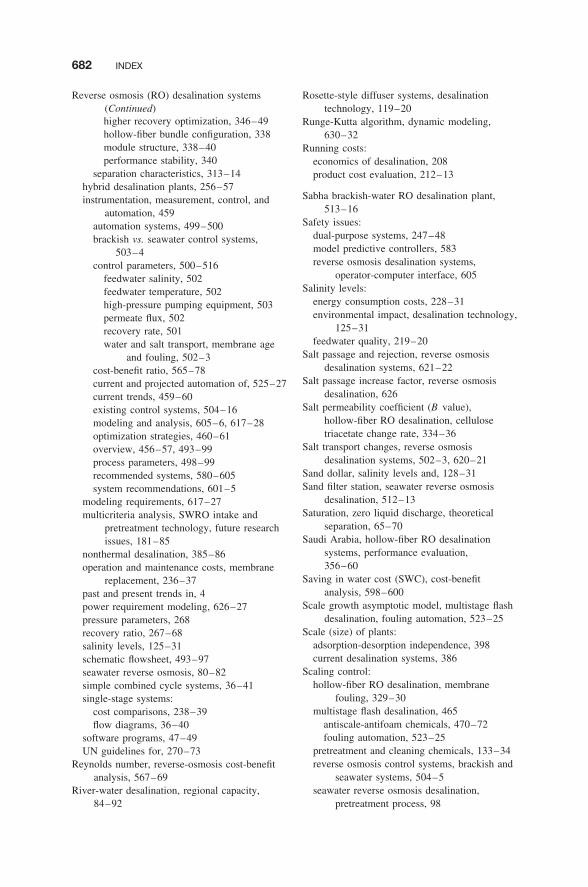
682 INDEX

Reverse osmosis (RO) desalination systems(Continued)higher recovery optimization, 346–49hollow-fiber bundle configuration, 338module structure, 338–40performance stability, 340

separation characteristics, 313–14hybrid desalination plants, 256–57instrumentation, measurement, control, and

automation, 459automation systems, 499–500brackish vs. seawater control systems,

503–4control parameters, 500–516

feedwater salinity, 502feedwater temperature, 502high-pressure pumping equipment, 503permeate flux, 502recovery rate, 501water and salt transport, membrane age

and fouling, 502–3cost-benefit ratio, 565–78current and projected automation of, 525–27current trends, 459–60existing control systems, 504–16modeling and analysis, 605–6, 617–28optimization strategies, 460–61overview, 456–57, 493–99process parameters, 498–99recommended systems, 580–605system recommendations, 601–5

modeling requirements, 617–27multicriteria analysis, SWRO intake and

pretreatment technology, future researchissues, 181–85

nonthermal desalination, 385–86operation and maintenance costs, membrane

replacement, 236–37past and present trends in, 4power requirement modeling, 626–27pressure parameters, 268recovery ratio, 267–68salinity levels, 125–31schematic flowsheet, 493–97seawater reverse osmosis, 80–82simple combined cycle systems, 36–41single-stage systems:

cost comparisons, 238–39flow diagrams, 36–40

software programs, 47–49UN guidelines for, 270–73

Reynolds number, reverse-osmosis cost-benefitanalysis, 567–69

River-water desalination, regional capacity,84–92

Rosette-style diffuser systems, desalinationtechnology, 119–20

Runge-Kutta algorithm, dynamic modeling,630–32

Running costs:economics of desalination, 208product cost evaluation, 212–13

Sabha brackish-water RO desalination plant,513–16

Safety issues:dual-purpose systems, 247–48model predictive controllers, 583reverse osmosis desalination systems,

operator-computer interface, 605Salinity levels:

energy consumption costs, 228–31environmental impact, desalination technology,

125–31feedwater quality, 219–20

Salt passage and rejection, reverse osmosisdesalination systems, 621–22

Salt passage increase factor, reverse osmosisdesalination, 626

Salt permeability coefficient (B value),hollow-fiber RO desalination, cellulosetriacetate change rate, 334–36

Salt transport changes, reverse osmosisdesalination systems, 502–3, 620–21

Sand dollar, salinity levels and, 128–31Sand filter station, seawater reverse osmosis

desalination, 512–13Saturation, zero liquid discharge, theoretical

separation, 65–70Saudi Arabia, hollow-fiber RO desalination

systems, performance evaluation,356–60

Saving in water cost (SWC), cost-benefitanalysis, 598–600

Scale growth asymptotic model, multistage flashdesalination, fouling automation, 523–25

Scale (size) of plants:adsorption-desorption independence, 398current desalination systems, 386

Scaling control:hollow-fiber RO desalination, membrane

fouling, 329–30multistage flash desalination, 465

antiscale-antifoam chemicals, 470–72fouling automation, 523–25

pretreatment and cleaning chemicals, 133–34reverse osmosis control systems, brackish and

seawater systems, 504–5seawater reverse osmosis desalination,

pretreatment process, 98

INDEX 683

Schmidt number, reverse-osmosis cost-benefitanalysis, 567–69

Scoring criteria:multicriteria analysis, SWRO intake and

pretreatment technology, 158–65sensitivity analysis, 171–72

Sea area distribution, regional desalinationcapacity, 86–92

Seawater desalination:adsorption-triggered evaporation, 405–6capital costs, 213–23global capacity, 82–92green technologies, 141–50

best available techniques, 142–45environmental impact assessment studies,

143, 145–50hollow-fiber reverse-osmosis membrane

modules, 338–67actual performance, 354–67

AdDur plant, Bahrain, 360–64global performance, 354–56Ikata power station, Japan, 364Jeddah 1 RO plant, Saudi Arabia, 356–60

advanced large-sized reverse osmosismodule, 354

analytical module modeling, 343–44both open-ended reverse osmosis module,

349–54bundle configuration, 338development of, 312–13double-element hollow-fiber module design,

345–49economics, 367–70fouling resistance, 341–43friction concentration polarization, 344–45Fukuoka plant, Japan, 364–67higher recovery optimization, 346–49high-recovery process, 336–37module structure, 338–40performance stability, 340

industrial growth, 80–82multistage flash desalination, flow rate through

heat rejection control, 469–70regional capacity, 84–92

Seawater intake technology, 92–95Seawater reverse osmosis (SWRO) desalination:

capital costs, 217–23AD cycle production cost comparisons,

439–40sample calculations, 290–95

control systems, 503–16cooling water codischarge systems, 121cost-benefit analysis, 565–80dual-purpose systems, disadvantages, 244–45

energy consumption, 115–22energy consumption costs, 227–31energy unit costs, 232–34environmental impact assessments, 125–31,

148–50Fukuoka seawater RO desalination plant

(Japan), 364–67global desalination capacity, 83greenhouse gases and air quality pollutants,

134–41green technologies, 141–50

best available techniques, 142–45environmental impact assessment studies,

143, 145–50historical development of, 80–82impingement and entrainment, 122–24locations and plants, summary of, 97multicriteria analysis (MCA), 150–85

data input, 155–69existing plant comparisons, 171–75future research issues, 181–85methodology, 152–54results evaluation, 170–81sensitivity analysis, 170–71study requirements and capabilities, 151ultrafiltration pretreatment comparisons,

173, 176–81operational environmental monitoring, 148–50operational plants, 99pilot systems, 99plant properties, organic particulates and,

100–105pretreatment processes and chemicals, 95–115

conventional pretreatment, 95–98minimal pretreatment, 95organic particulate foulants, 100–115particulate and NOM removal, 105–15plant design, 100–105ultrafiltration/microfiltration, 98–100

process flowchart, 493–97regional capacity, 86–92regional salinity levels, 126–31salinity levels, 125–31sample cost calculations, 290–95seawater intake technology, 92–95

subsurface intake systems, 93–95surface intake systems, 92–93

wastewater codischarge systems, 121–22water cost calculations, 294–95

Secondary energy forms, energy consumptioncosts, 230–31

Secondary improvements, plant design andoptimization, 266–68

Security issues, dual-purpose systems, 248

684 INDEX

Selective water sorbents (SWS), composition andfunction, 394–95

Self-generated energy systems:desalination in, 14–15energy consumption costs, 228–31

Sensitivity analysis:economics of desalination, 200multicriteria analysis, SWRO intake and

pretreatment technology, 154future research issues, 181–85results ranking, 170–72

setpoint control system optimization, 546–47Separation membrane characteristics:

hollow-fiber RO desalination, 313–14zero liquid discharge, 64–70

Setpoint control system:architecture of, 543–44components, 544–45mathematical simulation, 546–47measurement reconciliation, 545model parameters, 545–46optimization and sensitivity analysis, 546

Sherwood, reverse osmosis cost-benefit analysis,565–69

Shock treatment, hollow-fiber reverse osmosismodules, disinfection and, 332

Signal-to-noise ratio (SNR), reverse osmosisdesalination, instrumentation, measurement,control, and automation systems, 459–60

Silica gels, adsorbent materials, 390–93, 401–2calcium chloride-in-silica gel, 394–95

Silt density index (SDI):hollow-fiber reverse osmosis modules,

performance evaluation, 358–60multicriteria analysis, SWRO intake and

pretreatment technology, 158, 164–65,167–69

seawater reverse osmosis desalination, existingplant control systems, 505–8

seawater reverse osmosis desalination plantdesign, 103–5

Simple combined cycle (SCC) desalinationsystem:

competitiveness predictions, 45configuration, 16–17, 22flow diagram, 35reverse osmosis desalination, 36–41sample runs, 22, 25, 27–30, 35software programs, 47–49vapor compression systems, 36

Simulation results:adsorption-desalination systems, 409–12MSDF cost-benefit analysis, 547–57

Single-input single-output (SISO) control loops:

automation optimization and, 516–17multistage flash desalination, 472–75

Single-purpose desalination:cost comparisons, 237–39

sample comparison, 290–95hollow-fiber RO module development, 312–13nuclear fuel costs, 233–34recovery ratio, 267–68

Single-stage high recovery system:hollow-fiber RO modules, 336–37reverse-osmosis desalination, IMCA

procedures, 493–97Site acceptance test, model predictive controllers,

cost estimates, 595Slow sand filtration systems, plant design and,

103–5Socioenvironmental costs, desalination systems,

239–40Sodium bisulfite (SBS):

environmental impact, 131–34hollow-fiber reverse osmosis modules:

disinfection, 332performance evaluation, 360–64

seawater reverse osmosis desalination,pretreatment process, 95–98

Sodium sulfate dosage, multistage flashdesalination, 470–72

Software programs:desalination system analysis, 47–49model predictive controllers, 589–94

Solar desalination, energy unit costs, 233Solar systems. See also

Photovoltaic/electrodialysis system;Photovoltaic/reverse-osmosis systems

SOLED software program, 48Solid-fluid collision, adsorbent materials, 402SOLRO software program, 48Source water categories:

global desalination capacity, 82–83regional desalination capacity, 84–92

Spain:desalination and greenhouse gas emissions,

136environmental impact assessments of

desalination in, 148–50Species protection level (SPL), salinity levels

and, 128–31Species protection trigger value (SPTV), salinity

levels and, 128–31Specific daily water production (SDWP),

adsorption-desalination systems:adsorption-desorption mechanics, 403–4advanced AD cycle systems, 419–33bed cooling system, 417–18

INDEX 685

energy balance, 408–9performance ratios, 414–17transient water production rates, 411–12

Specific energy demand, seawater reverseosmosis desalination, 116–22

Specific investment, capital costs of desalination,215–23

Specific permeability/flux, reverse osmosisdesalination systems, 623–24

SPEEDUP commercial system, instrumentation,measurement, control, and automationsystems, 459

Spent cleaning solutions, multicriteria analysis,SWRO intake and pretreatment technology,156–57

Spiral-wound membranes, hollow-fiberreverse-osmosis desalination, 317–18

Sponge ball cleaning systems, multistage flashdesalination, fouling automation, 524–25

Stage-by-stage methods, steady-state modeling,MSF and RO desalination, 607–11

Standardization function, multicriteria analysis,SWRO intake and pretreatment technology,152–54

Startup-shutdown-flushing sequence, multistageflash desalination, current and futureautomation processes, 518–19

State variables and equations, mathematicalmodeling, IMCA desalination, 613

Steady-state modeling, MSF and ROdesalination, 606–11

Steam-brine heater temperature control loop,multistage flash desalination, 465–67

modification of, 519–21Steam turbine:

dual-purpose systems, 248multistage flash desalination operations,

463–72thermodynamic design models, 51

Storage issues, desalination and, 285–86Stretched membrane production, hollow-fiber RO

desalination, 326Subsidies, national desalination systems, 284Subsurface discharge, desalination technology,

93–95, 119–20Subsurface intake systems:

desalination technology, 93–95pretreatment and cleaning chemicals, 132–34

Sulfur dioxide emissions:desalination and, 139–41socioenvironmental costs, 239–40

Superheater water spray system, multistage flashdesalination, 465–67

Supervisory control and data acquisition(SCADA) system, reverse osmosisdesalination, 500

Support membrane layers, hollow-fiber ROdesalination, 314–16

Surface water discharge, desalination technology,119–22

Surplus capacity, capital costs of desalination,219–23

Swing weight method, multicriteria analysis,SWRO intake and pretreatment technology,154

Symmetric membrane structure, hollow-fiber ROdesalination, 314–16

System configuration, desalinationmethodologies, 15–34

System optimization:convergence mechanisms, 13exergy destruction price, 13–14

Taniguchi cost-benefit analysis of automation,538–40

reverse-osmosis cost-benefit analysis, 566–69Tapping power, osmosis power desalination

systems, 43–45Taxing policies, national desalination systems,

284Technology for desalination:

energy use, 115–22hybrid desalination plants, 256–57outfalls, 117–22pretreatment processes and chemicals,

95–100conventional pretreatment, 95–98minimal pretreatment, 95ultrafiltration/microfiltration, 98–100

seawater intake, 92–95subsurface intake, 93–95surface intake, 92–93

socioenvironmental mitigation, 239–40Temperature effects:

adsorption-desalination systems:AD cycle profiles, 409–12advanced AD cycle systems, 420–24energy balance, 408–9

multistage flash desalination, seawatertemperature to heat rejection,recirculation system, 470

plant design and optimization, 268reverse osmosis desalination systems, 622seawater reverse osmosis desalination, existing

plant control systems, 505–8water adsorption-desalination system, 398–400

Tertiary energy forms, energy consumption costs,230–31

686 INDEX

Thermal desalination:current technology, 381–84energy consumption costs, 229–31global desalination capacity, 83

Thermally induced phase separation (TIPS),hollow-fiber RO desalination membraneproduction, 324–26

Thermodynamics:costing methodologies, 8–10

thermodynamic value, 235desalination systems, system and design

models, 50–54exergy function, 7–8main process component optimization,

298–302quantitative vs. qualitative methodologies, 6–7water adsorption-desalination system, 398–400zero liquid discharge, theoretical separation,

64–70Thermoeconomics:

analytical principles, 6–14costing analysis and, 8–10global decision variables, 14global energy methodologies, 5optimization enhancement, 10–14thermodynamic analysis, 6–8

Thin-film membranes, hollow-fiber ROdesalination, 315–16, 326–28

Time/availability factor:dual-purpose systems, power generation and,

247–48economics of desalination, 214–23

Time-temperature histories,adsorption-desalination systems, advancedAD cycle systems, 420–24

Top brine temperature (TBT):advanced control techniques, MSDF/RO

desalination systems, nonlinear modelpredictive control, 529–30

multistage flash desalination, 461–62antiscale-antifoam dosage, 470–72control loop, 464–65, 472–75cost-benefit analysis, 548–57current and future automation processes,

517–25IMCA philosophy, 562–65modification of control system, 519–21

Total dissolved solids (TDSs):adsorption-desalination systems, product water

quality, 413–17reverse osmosis desalination systems,

modeling and conversion, 618–19Total energy costs, calculation of, 231

Total energy demand, seawater reverse osmosisdesalination, 117–22

Total water cost (TWC) index:dual-purpose system cost analysis, 251–54hollow-fiber RO membrane modules, 367–70

Toxicity studies:salinity levels, 125–31whole-effluent toxicity, 121–22

Toyobo hollow-fiber RO modules:advanced large-sized module, 354–56both open-ended (B.O.E.) module, 349–54development of, 313double-element module design, 339–40high recovery rate models, 348–49performance evaluation, 356–60, 361–64

Transient water production rates,adsorption-desalination systems:

evaporator-condenser heat recovery circuit,426–33

specific daily water production, 411–12Tubular membranes, hollow-fiber

reverse-osmosis desalination, 320Turbidity, seawater reverse osmosis desalination,

ultrafiltration/microfiltration, 99–100Turbochargers, reverse osmosis desalination

systems, 503Turnkey bidding:

plant construction, 278plant purchases, 225–26

Two-component mixtures, flow exergy equations,62

Ultrafiltration/microfiltration (UF/MF):dual-medium filtration vs., 105–7environmental impact assessment, 133–34hollow-fiber reverse-osmosis desalination:

AdDur desalination plant (Bahrain), 360–64interfacial polymerization, 327–28shape/configuration, 318–20thermally-induced phase separation

production, 324–26hollow-fiber RO desalination, 313–16multicriteria analysis, SWRO intake and

pretreatment technology, 157existing plant comparisons, 171–73future research issues, 181–85pretreatment comparisons, 173, 176–81results ranking, 167–82

seawater reverse osmosis desalination, 97–100particulate and NOM removal, 105–15plant design, 101–5

Umm Al Nar East power station, multistage flashdesalination control system, 487–90

Underocean floor:particulate and NOM removal, 112

INDEX 687

seawater reverse osmosis desalination plantdesign, 100–105

Uninterrupted power supply (UPS), reverseosmosis desalination, 603

Unit costs:adsorption-desalination cycle plant operations,

436–38“constant” currency and cost analysis, 264dual-purpose systems, 243energy units, 231–34heat exchange devices, 59hybrid desalination plants, 257unit lifetime and, 226–27

United Nations, desalination guidelines, 269–70United Nations Environment Program (UNEP):

environmental impact assessments, 146–50global desalination capacity, 91–92green desalination technology guidelines,

145–50United States:

desalination procedures and programs, 269green desalination technology guidelines,

144–45hollow-fiber RO module development, 312–13

cellulose derivatives development, 321–22

Value of energy, economics of desalination:cost allocation methods, 253–54desalted water values, 274–75

Value tree construction, multicriteria analysis,SWRO intake and pretreatment technology:

existing plant comparisons, 171–73future research issues, 181–85UF pretreatment comparisons, 173, 176–81

Vapor compression (VC) system:competitiveness predictions, 45configuration, 16, 18energy penalties, 47simple combined cycle systems, 36

Variable-cost items, operation and maintenancecosts, 236

Variable-frequency drive (VFD):reverse osmosis desalination systems, 501

control systems, 604seawater reverse osmosis desalination, existing

plant control systems, 508–10Variance reduction, advanced control systems,

MSDF/RO desalination, 541–43Vertical intake systems, seawater intake

technology, 92–95

Wages and salaries, operation and maintenancecosts, 236

Wall osmosis pressure differences, reverseosmosis desalination system, 39–41

Wastewater desalination:codischarge systems, 121–22global capacity, 82–92regional capacity, 84–92reverse osmosis desalination systems, 605

Water adsorption-desalination cycle :adsorbent materials, 390–96

metallorganic frameworks, 395–96selective water sorbents, 394–95silica gels, 390–93zeolites, 393–94

adsorption beds, 406–7adsorption-desorption phenomena, 388–90advanced cycle systems, 419–33

coolant evaporator-condenser circuit,424–25

cycle simulation, 420–24performance evaluation, 425–33predicted water production rate, 421–24specific daily water production, 421–24temperature-time history, 420–24

basic principles, 378–80bed cooling system, 417–19carbon dioxide emission savings, 441–42

baseline calculations, 445–46condenser systems, 407–8current technologies, 380–86

advantages and limitations, 386–88nonthermal desalination, 384–86thermal desalination, 381–84

cycle time optimization, 416–17hot water temperature effects, 416–17

energy balance, 408–9evaporator modeling, 405–6experimental research, 412–19feedwater boiling-point elevation, 415–17Gibbs free energy approach, minimum energy

requirements, 443–45integrated condenser-evaporator layout,

419–33life cycle analysis, 433–41

cost recovery factors, 434–38energy sources, 440–41product cost comparison, RO plants,

438–40nomenclature, 446–48performance evaluation, 404–19, 442–43plant components, 412–14potable-water quality, 413–17recirculating coolant medium, 419–33simulation parameters and results, 409–12specific daily water production:

advanced cycle systems, 421–24experimental results, 414–19

688 INDEX

Water adsorption-desalination cycle (Continued)system components, 396–405

evaporation process, 397–98heat-activated desorption-condensation,

398isosteric heat of adsorption, 402–3pore size effects, 400–403potable-water collection system, 398pressure-enthalpy diagram, 399–400pretreatment system, 397scale independence, 398specific water production, 403–4thermodynamics, 398–400

two-bed and four-bed cycle times, 415–17Water costs. See also Product water costs

desalination economics and, 275distributed control system configuration,

595–97Water cycle, basic principles, 380Water quality criteria:

energy consumption costs, 228–31multicriteria analysis, SWRO intake and

pretreatment technology, 164–65Water reuse:

green technologies, desalination, 142–50wastewater codischarge systems, 122

Water supply, global scarcity projections,378–79

Water transport changes, reverse osmosisdesalination systems, 502–3, 620

Water vapor uptake:pore size distribution, 402selective water sorbents, 394–95silica gel adsorbents, 392–93

Weighted summation, multicriteria analysis,SWRO intake and pretreatment technology,170–81

Weights:multicriteria analysis:

SWRO intake and pretreatment technology,154, 167–69

sensitivity analysis, 170–71Wet spinning, hollow-fiber reverse-osmosis

membrane production, 325–26Whole-effluent toxicity (WET):

environmental monitoring, 150salinity levels, 126–31wastewater codischarge systems, 121–22

Wilke-Chang equation, reverse osmosisdesalination system, 39–41

Wind energy, desalination costs, 234Workforce issues. See Labor requirementsWork loss method, cost allocation, 254

Zeolite adsorbents, 393–94Zero liquid discharge (ZLD):

competitiveness predictions, 45deep-well injection systems, 120–22desalination system configurations, 16–22,

46–47reverse osmosis desalination systems, 40–42simple combined cycle systems, 36theoretical separation work, 64–70wastewater codischarge systems, 122

Zone of initial dilution (ZID), salinity levels and,128–31

Zooplankton, impingement and entrainment,SWRO desalination, 122–24