additions to astronomy-op 2017 - openstax cnx

Additions to Astronomy-OP 2017

Collection edited by: Jack StratonContent authors: Jack Straton and OpenStax AstronomyOnline: <https://legacy.cnx.org/content/col12135/1.4>This selection and arrangement of content as a collection is copyrighted by Jack Straton.Creative Commons Attribution License 4.0 http://creativecommons.org/licenses/by/4.0/Collection structure revised: 2017/04/04PDF Generated: 2017/04/04 12:07:52For copyright and attribution information for the modules contained in this collection, see the "Attributions"section at the end of the collection.

1

www.princexml.com

Prince - Non-commercial License

This document was created with Prince, a great way of getting web content onto paper.

https://legacy.cnx.org/content/col12135/1.4

http://creativecommons.org/licenses/by/4.0/

2

This OpenStax book is available for free at https://legacy.cnx.org/content/col12135/1.4

TABLE OF CONTENTS

1 Derived copy of Using Spectra to Measure Stellar Radius,Composition, and Motion

5

1.1 Learning Objectives 51.2 Clues to the Size of a Star 51.3 Abundances of the Elements 61.4 Radial Velocity 71.5 Proper Motion 81.6 Rotation 101.7 Key Concepts and Summary 131.8 For Further Exploration 131.9 Collaborative Group Activities 141.10 Review Questions 151.11 Thought Questions 161.12 Figuring for Yourself 18

2 Derived copy of The Brightness of Stars 21

2.1 Learning Objectives 212.2 Luminosity 212.3 Apparent Brightness 212.4 The Magnitude Scale 222.5 Other Units of Brightness 262.6 Key Concepts and Summary 27

3 addition to p 678 new figs 29

3.1 The Cosmological Distance Ladder 30

4 Derived copy of A Conclusion and a Beginning with addedexercises

37

4.1 For Further Exploration 38

Index 41

1.1 LEARNING OBJECTIVES

By the end of this section, you will be able to:

• Understand how astronomers can learn about a star’s radius and composition by studying its spectrum

• Explain how astronomers can measure the motion and rotation of a star using the Doppler effect

• Describe the proper motion of a star and how it relates to a star’s space velocity

Analyzing the spectrum of a star can teach us all kinds of things in addition to its temperature. We can measureits detailed chemical composition as well as the pressure in its atmosphere. From the pressure, we get cluesabout its size. We can also measure its motion toward or away from us and estimate its rotation.

1.2 CLUES TO THE SIZE OF A STAR

As we shall see in The Stars: A Celestial Census (https://legacy.cnx.org/content/m59897/latest/) , starscome in a wide variety of sizes. At some periods in their lives, stars can expand to enormous dimensions. Starsof such exaggerated size are called giants. Luckily for the astronomer, stellar spectra can be used to distinguishgiants from run-of-the-mill stars (such as our Sun).

Suppose you want to determine whether a star is a giant. A giant star has a large, extended photosphere.Because it is so large, a giant star’s atoms are spread over a great volume, which means that the density ofparticles in the star’s photosphere is low. As a result, the pressure in a giant star’s photosphere is also low.This low pressure affects the spectrum in two ways. First, a star with a lower-pressure photosphere showsnarrower spectral lines than a star of the same temperature with a higher-pressure photosphere (Figure 1.1).The difference is large enough that careful study of spectra can tell which of two stars at the same temperaturehas a higher pressure (and is thus more compressed) and which has a lower pressure (and thus must beextended). This effect is due to collisions between particles in the star’s photosphere—more collisions lead tobroader spectral lines. Collisions will, of course, be more frequent in a higher-density environment. Think aboutit like traffic—collisions are much more likely during rush hour, when the density of cars is high.

Second, more atoms are ionized in a giant star than in a star like the Sun with the same temperature. Theionization of atoms in a star’s outer layers is caused mainly by photons, and the amount of energy carriedby photons is determined by temperature. But how long atoms stay ionized depends in part on pressure.Compared with what happens in the Sun (with its relatively dense photosphere), ionized atoms in a giant star’sphotosphere are less likely to pass close enough to electrons to interact and combine with one or more of them,thereby becoming neutral again. Ionized atoms, as we discussed earlier, have different spectra from atoms thatare neutral.

1DERIVED COPY OF USING SPECTRA TO MEASURE STELLAR RADIUS,COMPOSITION, AND MOTION

Chapter 1 Derived copy of Using Spectra to Measure Stellar Radius, Composition, and Motion* 5

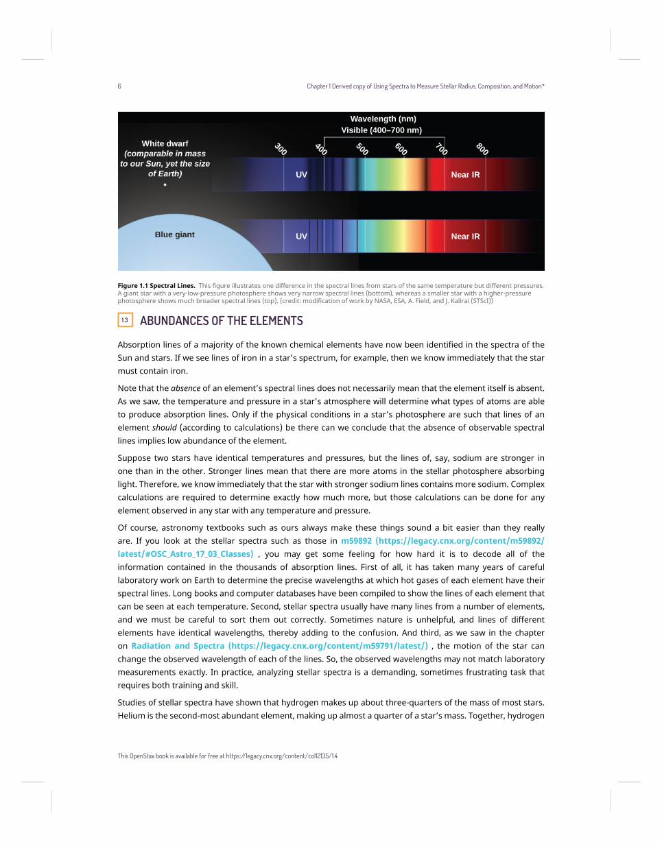
https://legacy.cnx.org/content/m59897/latest/

Figure 1.1 Spectral Lines. This figure illustrates one difference in the spectral lines from stars of the same temperature but different pressures.A giant star with a very-low-pressure photosphere shows very narrow spectral lines (bottom), whereas a smaller star with a higher-pressurephotosphere shows much broader spectral lines (top). (credit: modification of work by NASA, ESA, A. Field, and J. Kalirai (STScI))

1.3 ABUNDANCES OF THE ELEMENTS

Absorption lines of a majority of the known chemical elements have now been identified in the spectra of theSun and stars. If we see lines of iron in a star’s spectrum, for example, then we know immediately that the starmust contain iron.

Note that the absence of an element’s spectral lines does not necessarily mean that the element itself is absent.As we saw, the temperature and pressure in a star’s atmosphere will determine what types of atoms are ableto produce absorption lines. Only if the physical conditions in a star’s photosphere are such that lines of anelement should (according to calculations) be there can we conclude that the absence of observable spectrallines implies low abundance of the element.

Suppose two stars have identical temperatures and pressures, but the lines of, say, sodium are stronger inone than in the other. Stronger lines mean that there are more atoms in the stellar photosphere absorbinglight. Therefore, we know immediately that the star with stronger sodium lines contains more sodium. Complexcalculations are required to determine exactly how much more, but those calculations can be done for anyelement observed in any star with any temperature and pressure.

Of course, astronomy textbooks such as ours always make these things sound a bit easier than they reallyare. If you look at the stellar spectra such as those in m59892 (https://legacy.cnx.org/content/m59892/latest/#OSC_Astro_17_03_Classes) , you may get some feeling for how hard it is to decode all of theinformation contained in the thousands of absorption lines. First of all, it has taken many years of carefullaboratory work on Earth to determine the precise wavelengths at which hot gases of each element have theirspectral lines. Long books and computer databases have been compiled to show the lines of each element thatcan be seen at each temperature. Second, stellar spectra usually have many lines from a number of elements,and we must be careful to sort them out correctly. Sometimes nature is unhelpful, and lines of differentelements have identical wavelengths, thereby adding to the confusion. And third, as we saw in the chapteron Radiation and Spectra (https://legacy.cnx.org/content/m59791/latest/) , the motion of the star canchange the observed wavelength of each of the lines. So, the observed wavelengths may not match laboratorymeasurements exactly. In practice, analyzing stellar spectra is a demanding, sometimes frustrating task thatrequires both training and skill.

Studies of stellar spectra have shown that hydrogen makes up about three-quarters of the mass of most stars.Helium is the second-most abundant element, making up almost a quarter of a star’s mass. Together, hydrogen

6 Chapter 1 Derived copy of Using Spectra to Measure Stellar Radius, Composition, and Motion*


https://legacy.cnx.org/content/m59892/latest/#OSC_Astro_17_03_Classes

https://legacy.cnx.org/content/m59892/latest/#OSC_Astro_17_03_Classes


and helium make up from 96 to 99% of the mass; in some stars, they amount to more than 99.9%. Among the4% or less of “heavy elements,” oxygen, carbon, neon, iron, nitrogen, silicon, magnesium, and sulfur are amongthe most abundant. Generally, but not invariably, the elements of lower atomic weight are more abundant thanthose of higher atomic weight.

Take a careful look at the list of elements in the preceding paragraph. Two of the most abundant are hydrogenand oxygen (which make up water); add carbon and nitrogen and you are starting to write the prescription forthe chemistry of an astronomy student. We are made of elements that are common in the universe—just mixedtogether in a far more sophisticated form (and a much cooler environment) than in a star.

As we mentioned in The Spectra of Stars (and Brown Dwarfs) (https://legacy.cnx.org/content/m59892/latest/) section, astronomers use the term “metals” to refer to all elements heavier than hydrogen and helium.The fraction of a star’s mass that is composed of these elements is referred to as the star’s metallicity. Themetallicity of the Sun, for example, is 0.02, since 2% of the Sun’s mass is made of elements heavier than helium.

Appendix K (https://legacy.cnx.org/content/m60004/latest/) lists how common each element is in theuniverse (compared to hydrogen); these estimates are based primarily on investigation of the Sun, which is atypical star. Some very rare elements, however, have not been detected in the Sun. Estimates of the amountsof these elements in the universe are based on laboratory measurements of their abundance in primitivemeteorites, which are considered representative of unaltered material condensed from the solar nebula (seethe Cosmic Samples and the Origin of the Solar System (https://legacy.cnx.org/content/m59870/latest/)chapter).

1.4 RADIAL VELOCITY

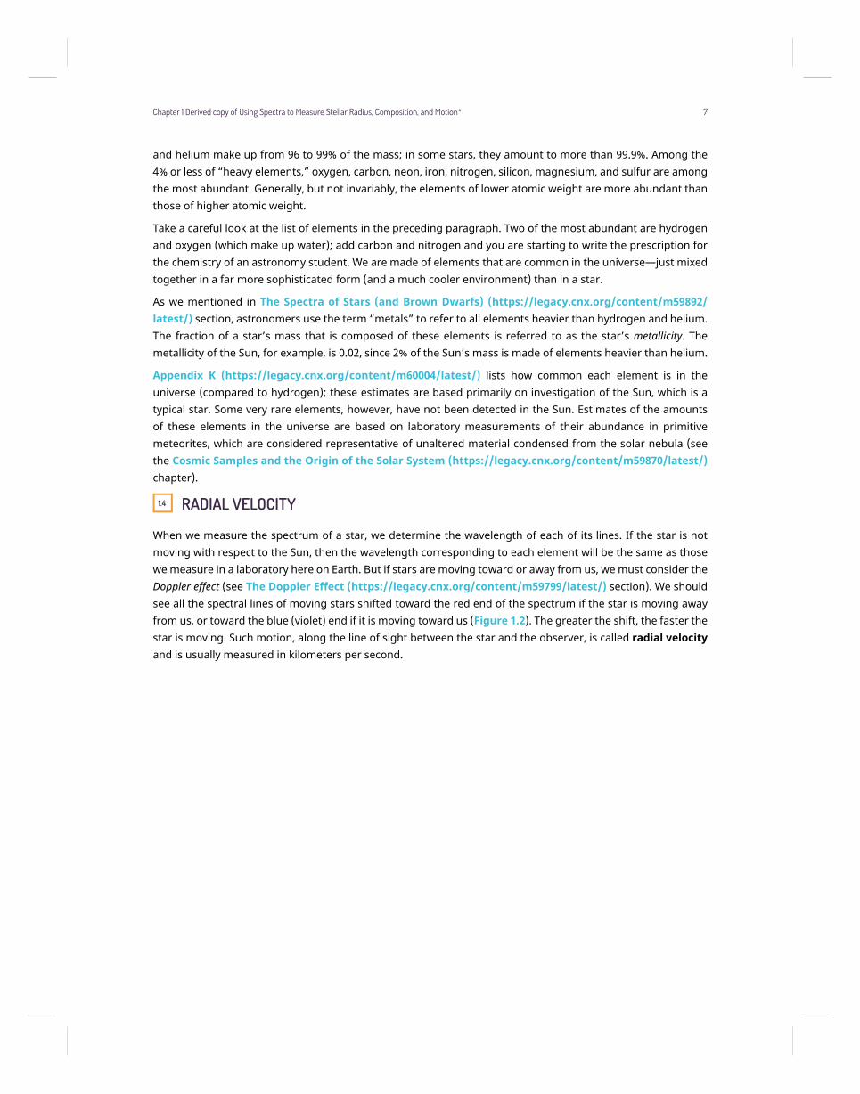
When we measure the spectrum of a star, we determine the wavelength of each of its lines. If the star is notmoving with respect to the Sun, then the wavelength corresponding to each element will be the same as thosewe measure in a laboratory here on Earth. But if stars are moving toward or away from us, we must consider theDoppler effect (see The Doppler Effect (https://legacy.cnx.org/content/m59799/latest/) section). We shouldsee all the spectral lines of moving stars shifted toward the red end of the spectrum if the star is moving awayfrom us, or toward the blue (violet) end if it is moving toward us (Figure 1.2). The greater the shift, the faster thestar is moving. Such motion, along the line of sight between the star and the observer, is called radial velocityand is usually measured in kilometers per second.







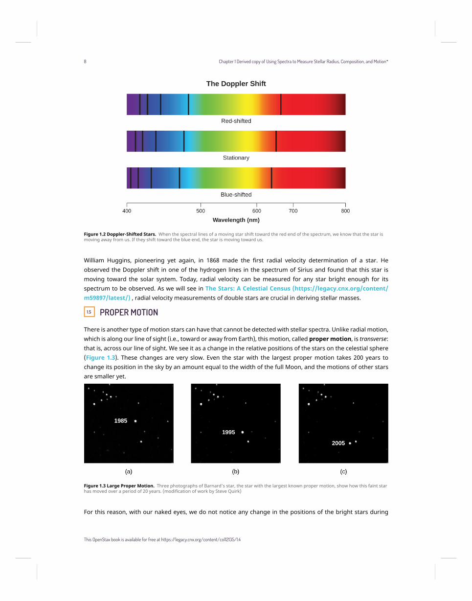
Figure 1.2 Doppler-Shifted Stars. When the spectral lines of a moving star shift toward the red end of the spectrum, we know that the star ismoving away from us. If they shift toward the blue end, the star is moving toward us.

William Huggins, pioneering yet again, in 1868 made the first radial velocity determination of a star. Heobserved the Doppler shift in one of the hydrogen lines in the spectrum of Sirius and found that this star ismoving toward the solar system. Today, radial velocity can be measured for any star bright enough for itsspectrum to be observed. As we will see in The Stars: A Celestial Census (https://legacy.cnx.org/content/m59897/latest/) , radial velocity measurements of double stars are crucial in deriving stellar masses.

1.5 PROPER MOTION

There is another type of motion stars can have that cannot be detected with stellar spectra. Unlike radial motion,which is along our line of sight (i.e., toward or away from Earth), this motion, called proper motion, is transverse:that is, across our line of sight. We see it as a change in the relative positions of the stars on the celestial sphere(Figure 1.3). These changes are very slow. Even the star with the largest proper motion takes 200 years tochange its position in the sky by an amount equal to the width of the full Moon, and the motions of other starsare smaller yet.

Figure 1.3 Large Proper Motion. Three photographs of Barnard’s star, the star with the largest known proper motion, show how this faint starhas moved over a period of 20 years. (modification of work by Steve Quirk)

For this reason, with our naked eyes, we do not notice any change in the positions of the bright stars during





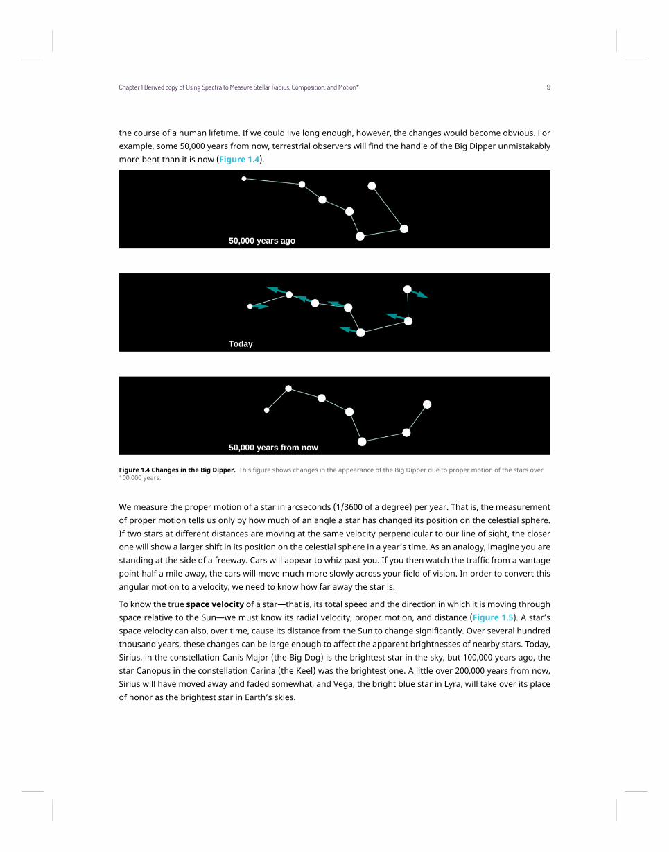
the course of a human lifetime. If we could live long enough, however, the changes would become obvious. Forexample, some 50,000 years from now, terrestrial observers will find the handle of the Big Dipper unmistakablymore bent than it is now (Figure 1.4).

Figure 1.4 Changes in the Big Dipper. This figure shows changes in the appearance of the Big Dipper due to proper motion of the stars over100,000 years.

We measure the proper motion of a star in arcseconds (1/3600 of a degree) per year. That is, the measurementof proper motion tells us only by how much of an angle a star has changed its position on the celestial sphere.If two stars at different distances are moving at the same velocity perpendicular to our line of sight, the closerone will show a larger shift in its position on the celestial sphere in a year’s time. As an analogy, imagine you arestanding at the side of a freeway. Cars will appear to whiz past you. If you then watch the traffic from a vantagepoint half a mile away, the cars will move much more slowly across your field of vision. In order to convert thisangular motion to a velocity, we need to know how far away the star is.

To know the true space velocity of a star—that is, its total speed and the direction in which it is moving throughspace relative to the Sun—we must know its radial velocity, proper motion, and distance (Figure 1.5). A star’sspace velocity can also, over time, cause its distance from the Sun to change significantly. Over several hundredthousand years, these changes can be large enough to affect the apparent brightnesses of nearby stars. Today,Sirius, in the constellation Canis Major (the Big Dog) is the brightest star in the sky, but 100,000 years ago, thestar Canopus in the constellation Carina (the Keel) was the brightest one. A little over 200,000 years from now,Sirius will have moved away and faded somewhat, and Vega, the bright blue star in Lyra, will take over its placeof honor as the brightest star in Earth’s skies.


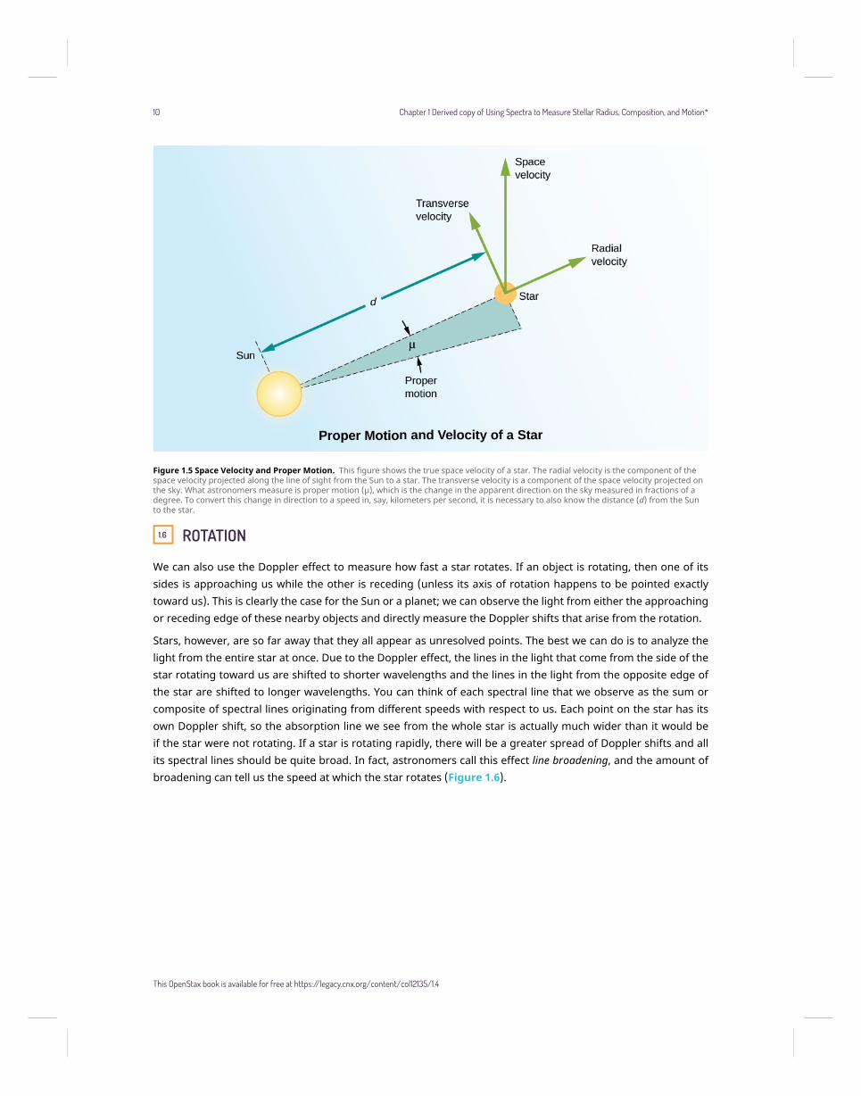
Figure 1.5 Space Velocity and Proper Motion. This figure shows the true space velocity of a star. The radial velocity is the component of thespace velocity projected along the line of sight from the Sun to a star. The transverse velocity is a component of the space velocity projected onthe sky. What astronomers measure is proper motion (μ), which is the change in the apparent direction on the sky measured in fractions of adegree. To convert this change in direction to a speed in, say, kilometers per second, it is necessary to also know the distance (d) from the Sunto the star.

1.6 ROTATION

We can also use the Doppler effect to measure how fast a star rotates. If an object is rotating, then one of itssides is approaching us while the other is receding (unless its axis of rotation happens to be pointed exactlytoward us). This is clearly the case for the Sun or a planet; we can observe the light from either the approachingor receding edge of these nearby objects and directly measure the Doppler shifts that arise from the rotation.

Stars, however, are so far away that they all appear as unresolved points. The best we can do is to analyze thelight from the entire star at once. Due to the Doppler effect, the lines in the light that come from the side of thestar rotating toward us are shifted to shorter wavelengths and the lines in the light from the opposite edge ofthe star are shifted to longer wavelengths. You can think of each spectral line that we observe as the sum orcomposite of spectral lines originating from different speeds with respect to us. Each point on the star has itsown Doppler shift, so the absorption line we see from the whole star is actually much wider than it would beif the star were not rotating. If a star is rotating rapidly, there will be a greater spread of Doppler shifts and allits spectral lines should be quite broad. In fact, astronomers call this effect line broadening, and the amount ofbroadening can tell us the speed at which the star rotates (Figure 1.6).



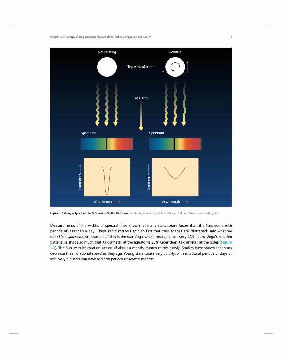
Figure 1.6 Using a Spectrum to Determine Stellar Rotation. A rotating star will show broader spectral lines than a nonrotating star.

Measurements of the widths of spectral lines show that many stars rotate faster than the Sun, some withperiods of less than a day! These rapid rotators spin so fast that their shapes are “flattened” into what wecall oblate spheroids. An example of this is the star Vega, which rotates once every 12.5 hours. Vega’s rotationflattens its shape so much that its diameter at the equator is 23% wider than its diameter at the poles (Figure1.7). The Sun, with its rotation period of about a month, rotates rather slowly. Studies have shown that starsdecrease their rotational speed as they age. Young stars rotate very quickly, with rotational periods of days orless. Very old stars can have rotation periods of several months.


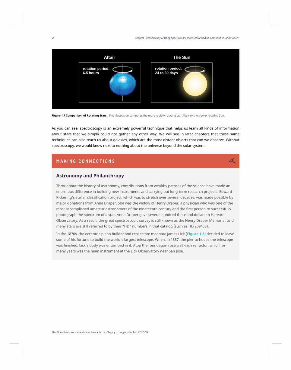
Figure 1.7 Comparison of Rotating Stars. This illustration compares the more rapidly rotating star Altair to the slower rotating Sun.

As you can see, spectroscopy is an extremely powerful technique that helps us learn all kinds of informationabout stars that we simply could not gather any other way. We will see in later chapters that these sametechniques can also teach us about galaxies, which are the most distant objects that can we observe. Withoutspectroscopy, we would know next to nothing about the universe beyond the solar system.

M A K I N G C O N N E C T I O N S

Astronomy and Philanthropy

Throughout the history of astronomy, contributions from wealthy patrons of the science have made anenormous difference in building new instruments and carrying out long-term research projects. EdwardPickering’s stellar classification project, which was to stretch over several decades, was made possible bymajor donations from Anna Draper. She was the widow of Henry Draper, a physician who was one of themost accomplished amateur astronomers of the nineteenth century and the first person to successfullyphotograph the spectrum of a star. Anna Draper gave several hundred thousand dollars to HarvardObservatory. As a result, the great spectroscopic survey is still known as the Henry Draper Memorial, andmany stars are still referred to by their “HD” numbers in that catalog (such as HD 209458).

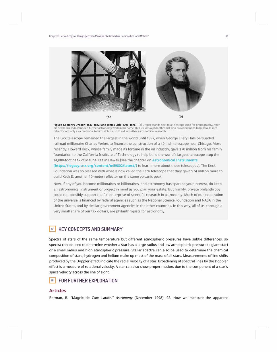
In the 1870s, the eccentric piano builder and real estate magnate James Lick (Figure 1.8) decided to leavesome of his fortune to build the world’s largest telescope. When, in 1887, the pier to house the telescopewas finished, Lick’s body was entombed in it. Atop the foundation rose a 36-inch refractor, which formany years was the main instrument at the Lick Observatory near San Jose.



1.7 KEY CONCEPTS AND SUMMARY

Spectra of stars of the same temperature but different atmospheric pressures have subtle differences, sospectra can be used to determine whether a star has a large radius and low atmospheric pressure (a giant star)or a small radius and high atmospheric pressure. Stellar spectra can also be used to determine the chemicalcomposition of stars; hydrogen and helium make up most of the mass of all stars. Measurements of line shiftsproduced by the Doppler effect indicate the radial velocity of a star. Broadening of spectral lines by the Dopplereffect is a measure of rotational velocity. A star can also show proper motion, due to the component of a star’sspace velocity across the line of sight.

1.8 FOR FURTHER EXPLORATION

ArticlesBerman, B. “Magnitude Cum Laude.” Astronomy (December 1998): 92. How we measure the apparent

Figure 1.8 Henry Draper (1837–1882) and James Lick (1796–1876). (a) Draper stands next to a telescope used for photography. Afterhis death, his widow funded further astronomy work in his name. (b) Lick was a philanthropist who provided funds to build a 36-inchrefractor not only as a memorial to himself but also to aid in further astronomical research.

The Lick telescope remained the largest in the world until 1897, when George Ellery Hale persuadedrailroad millionaire Charles Yerkes to finance the construction of a 40-inch telescope near Chicago. Morerecently, Howard Keck, whose family made its fortune in the oil industry, gave $70 million from his familyfoundation to the California Institute of Technology to help build the world’s largest telescope atop the14,000-foot peak of Mauna Kea in Hawaii (see the chapter on Astronomical Instruments(https://legacy.cnx.org/content/m59802/latest/) to learn more about these telescopes). The KeckFoundation was so pleased with what is now called the Keck telescope that they gave $74 million more tobuild Keck II, another 10-meter reflector on the same volcanic peak.

Now, if any of you become millionaires or billionaires, and astronomy has sparked your interest, do keepan astronomical instrument or project in mind as you plan your estate. But frankly, private philanthropycould not possibly support the full enterprise of scientific research in astronomy. Much of our explorationof the universe is financed by federal agencies such as the National Science Foundation and NASA in theUnited States, and by similar government agencies in the other countries. In this way, all of us, through avery small share of our tax dollars, are philanthropists for astronomy.




brightnesses of stars is discussed.

Dvorak, J. “The Women Who Created Modern Astronomy [including Annie Cannon].” Sky & Telescope (August2013): 28.

Hearnshaw, J. “Origins of the Stellar Magnitude Scale.” Sky & Telescope (November 1992): 494. A good history ofhow we have come to have this cumbersome system is discussed.

Hirshfeld, A. “The Absolute Magnitude of Stars.” Sky & Telescope (September 1994): 35.

Kaler, J. “Stars in the Cellar: Classes Lost and Found.” Sky & Telescope (September 2000): 39. An introduction isprovided for spectral types and the new classes L and T.

Kaler, J. “Origins of the Spectral Sequence.” Sky & Telescope (February 1986): 129.

Skrutskie, M. “2MASS: Unveiling the Infrared Universe.” Sky & Telescope (July 2001): 34. This article focuses on anall-sky survey at 2 microns.

Sneden, C. “Reading the Colors of the Stars.” Astronomy (April 1989): 36. This article includes a discussion ofwhat we learn from spectroscopy.

Steffey, P. “The Truth about Star Colors.” Sky & Telescope (September 1992): 266. The color index and how theeye and film “see” colors are discussed.

Tomkins, J. “Once and Future Celestial Kings.” Sky & Telescope (April 1989): 59. Calculating the motion of starsand determining which stars were, are, and will be brightest in the sky are discussed.

WebsitesDiscovery of Brown Dwarfs: http://w.astro.berkeley.edu/~basri/bdwarfs/SciAm-book.pdf.

Listing of Nearby Brown Dwarfs: http://www.solstation.com/stars/pc10bd.htm.

Spectral Types of Stars: http://www.skyandtelescope.com/astronomy-equipment/the-spectral-types-of-stars/.

Stellar Velocities https://www.e-education.psu.edu/astro801/content/l4_p7.html.

Unheard Voices! The Contributions of Women to Astronomy: A Resource Guide:http://multiverse.ssl.berkeley.edu/women and http://www.astrosociety.org/education/astronomy-resource-guides/women-in-astronomy-an-introductory-resource-guide/.

VideosWhen You Are Just Too Small to be a Star: https://www.youtube.com/watch?v=zXCDsb4n4KU. 2013 Public Talkon Brown Dwarfs and Planets by Dr. Gibor Basri of the University of California–Berkeley (1:32:52).

1.9 COLLABORATIVE GROUP ACTIVITIES

A. The Voyagers in Astronomy feature on Annie Cannon: Classifier of the Stars (https://legacy.cnx.org/content/m59892/latest/#fs-id1170326186380) discusses some of the difficulties women who wantedto do astronomy faced in the first half of the twentieth century. What does your group think about thesituation for women today? Do men and women have an equal chance to become scientists? Discusswith your group whether, in your experience, boys and girls were equally encouraged to do science andmath where you went to school.

B. In the section on magnitudes in The Brightness of Stars (https://legacy.cnx.org/content/m59890/latest/) , we discussed how this old system of classifying how bright different stars appear to the eyefirst developed. Your authors complained about the fact that this old system still has to be taught toevery generation of new students. Can your group think of any other traditional systems of doing things



https://legacy.cnx.org/content/m59892/latest/#fs-id1170326186380




in science and measurement where tradition rules even though common sense says a better systemcould certainly be found. Explain. (Hint: Try Daylight Savings Time, or metric versus English units.)

C. Suppose you could observe a star that has only one spectral line. Could you tell what element thatspectral line comes from? Make a list of reasons with your group about why you answered yes or no.

D. A wealthy alumnus of your college decides to give $50 million to the astronomy department to build aworld-class observatory for learning more about the characteristics of stars. Have your group discusswhat kind of equipment they would put in the observatory. Where should this observatory be located?Justify your answers. (You may want to refer back to the Astronomical Instruments(https://legacy.cnx.org/content/m59802/latest/) chapter and to revisit this question as you learnmore about the stars and equipment for observing them in future chapters.)

E. For some astronomers, introducing a new spectral type for the stars (like the types L, T, and Y discussedin the text) is similar to introducing a new area code for telephone calls. No one likes to disrupt the oldsystem, but sometimes it is simply necessary. Have your group make a list of steps an astronomer wouldhave to go through to persuade colleagues that a new spectral class is needed.

1.10 REVIEW QUESTIONS

Exercise 1.1

What two factors determine how bright a star appears to be in the sky?

Exercise 1.2

Explain why color is a measure of a star’s temperature.

Exercise 1.3

What is the main reason that the spectra of all stars are not identical? Explain.

Exercise 1.4

What elements are stars mostly made of? How do we know this?

Exercise 1.5

What did Annie Cannon contribute to the understanding of stellar spectra?

Exercise 1.6

Name five characteristics of a star that can be determined by measuring its spectrum. Explain how you woulduse a spectrum to determine these characteristics.

Exercise 1.7

How do objects of spectral types L, T, and Y differ from those of the other spectral types?

Exercise 1.8

Do stars that look brighter in the sky have larger or smaller magnitudes than fainter stars?

Exercise 1.9

The star Antares has an apparent magnitude of 1.0, whereas the star Procyon has an apparent magnitude of0.4. Which star appears brighter in the sky?

Exercise 1.10

Based on their colors, which of the following stars is hottest? Which is coolest? Archenar (blue), Betelgeuse(red), Capella (yellow).




Exercise 1.11

Order the seven basic spectral types from hottest to coldest.

Exercise 1.12

What is the defining difference between a brown dwarf and a true star?

1.11 THOUGHT QUESTIONS

Exercise 1.13

If the star Sirius emits 23 times more energy than the Sun, why does the Sun appear brighter in the sky?

Exercise 1.14

How would two stars of equal luminosity—one blue and the other red—appear in an image taken through afilter that passes mainly blue light? How would their appearance change in an image taken through a filter thattransmits mainly red light?

Exercise 1.15

m59892 (https://legacy.cnx.org/content/m59892/latest/#fs-id1170326111681) lists the temperature rangesthat correspond to the different spectral types. What part of the star do these temperatures refer to? Why?

Exercise 1.16

Suppose you are given the task of measuring the colors of the brightest stars, listed in Appendix J(https://legacy.cnx.org/content/m60003/latest/) , through three filters: the first transmits blue light, thesecond transmits yellow light, and the third transmits red light. If you observe the star Vega, it will appearequally bright through each of the three filters. Which stars will appear brighter through the blue filter thanthrough the red filter? Which stars will appear brighter through the red filter? Which star is likely to have colorsmost nearly like those of Vega?

Exercise 1.17

Star X has lines of ionized helium in its spectrum, and star Y has bands of titanium oxide. Which is hotter?Why? The spectrum of star Z shows lines of ionized helium and also molecular bands of titanium oxide. What isstrange about this spectrum? Can you suggest an explanation?

Exercise 1.18

The spectrum of the Sun has hundreds of strong lines of nonionized iron but only a few, very weak lines ofhelium. A star of spectral type B has very strong lines of helium but very weak iron lines. Do these differencesmean that the Sun contains more iron and less helium than the B star? Explain.

Exercise 1.19

What are the approximate spectral classes of stars with the following characteristics?

A. Balmer lines of hydrogen are very strong; some lines of ionized metals are present.

B. The strongest lines are those of ionized helium.

C. Lines of ionized calcium are the strongest in the spectrum; hydrogen lines show only moderate strength;lines of neutral and metals are present.

D. The strongest lines are those of neutral metals and bands of titanium oxide.

Exercise 1.20

Look at the chemical elements in Appendix K (https://legacy.cnx.org/content/m60004/latest/) . Can you







identify any relationship between the abundance of an element and its atomic weight? Are there any obviousexceptions to this relationship?

Exercise 1.21

Appendix I (https://legacy.cnx.org/content/m60002/latest/) lists some of the nearest stars. Are most ofthese stars hotter or cooler than the Sun? Do any of them emit more energy than the Sun? If so, which ones?

Exercise 1.22

Appendix J (https://legacy.cnx.org/content/m60003/latest/) lists the stars that appear brightest in our sky.Are most of these hotter or cooler than the Sun? Can you suggest a reason for the difference between thisanswer and the answer to the previous question? (Hint: Look at the luminosities.) Is there any tendency for acorrelation between temperature and luminosity? Are there exceptions to the correlation?

Exercise 1.23

What star appears the brightest in the sky (other than the Sun)? The second brightest? What color isBetelgeuse? Use Appendix J (https://legacy.cnx.org/content/m60003/latest/) to find the answers.

Exercise 1.24

Suppose hominids one million years ago had left behind maps of the night sky. Would these maps representaccurately the sky that we see today? Why or why not?

Exercise 1.25

Why can only a lower limit to the rate of stellar rotation be determined from line broadening rather than theactual rotation rate? (Refer to Figure 1.6.)

Exercise 1.26

Why do you think astronomers have suggested three different spectral types (L, T, and Y) for the brown dwarfsinstead of M? Why was one not enough?

Exercise 1.27

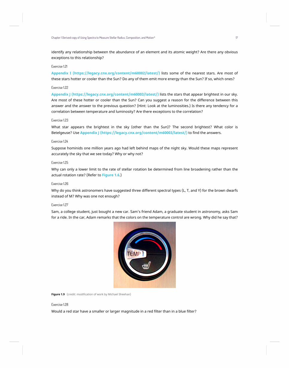
Sam, a college student, just bought a new car. Sam’s friend Adam, a graduate student in astronomy, asks Samfor a ride. In the car, Adam remarks that the colors on the temperature control are wrong. Why did he say that?

Figure 1.9 (credit: modification of work by Michael Sheehan)

Exercise 1.28

Would a red star have a smaller or larger magnitude in a red filter than in a blue filter?





Exercise 1.29

Two stars have proper motions of one arcsecond per year. Star A is 20 light-years from Earth, and Star B is 10light-years away from Earth. Which one has the faster velocity in space?

Exercise 1.30

Suppose there are three stars in space, each moving at 100 km/s. Star A is moving across (i.e., perpendicular to)our line of sight, Star B is moving directly away from Earth, and Star C is moving away from Earth, but at a 30°angle to the line of sight. From which star will you observe the greatest Doppler shift? From which star will youobserve the smallest Doppler shift?

Exercise 1.31

What would you say to a friend who made this statement, “The visible-light spectrum of the Sun shows weakhydrogen lines and strong calcium lines. The Sun must therefore contain more calcium than hydrogen.”?

1.12 FIGURING FOR YOURSELF

Exercise 1.32

In Appendix J (https://legacy.cnx.org/content/m60003/latest/) , how much more luminous is the mostluminous of the stars than the least luminous?

For Exercise 1.33 through Exercise 1.38, use the equations relating magnitude and apparent brightness givenin the section on the magnitude scale in The Brightness of Stars (https://legacy.cnx.org/content/m59890/latest/) and m59890 (https://legacy.cnx.org/content/m59890/latest/#fs-id1170326254336) .

Exercise 1.33

Verify that if two stars have a difference of five magnitudes, this corresponds to a factor of 100 in the ratio ⎛⎝b2b1

⎞⎠;

that 2.5 magnitudes corresponds to a factor of 10; and that 0.75 magnitudes corresponds to a factor of 2.

Exercise 1.34

As seen from Earth, the Sun has an apparent magnitude of about −26.7. What is the apparent magnitude of theSun as seen from Saturn, about 10 AU away? (Remember that one AU is the distance from Earth to the Sun andthat the brightness decreases as the inverse square of the distance.) Would the Sun still be the brightest star inthe sky?

Exercise 1.35

An astronomer is investigating a faint star that has recently been discovered in very sensitive surveys of the sky.The star has a magnitude of 16. How much less bright is it than Antares, a star with magnitude roughly equal to1?

Exercise 1.36

The center of a faint but active galaxy has magnitude 26. How much less bright does it look than the veryfaintest star that our eyes can see, roughly magnitude 6?

Exercise 1.37

You have enough information from this chapter to estimate the distance to Alpha Centauri, the second neareststar, which has an apparent magnitude of 0. Since it is a G2 star, like the Sun, assume it has the same luminosityas the Sun and the difference in magnitudes is a result only of the difference in distance. Estimate how faraway Alpha Centauri is. Describe the necessary steps in words and then do the calculation. (As we will learn







in the Celestial Distances (https://legacy.cnx.org/content/m59902/latest/) chapter, this method—namely,assuming that stars with identical spectral types emit the same amount of energy—is actually used to estimatedistances to stars.) If you assume the distance to the Sun is in AU, your answer will come out in AU.

Exercise 1.38

Do the previous problem again, this time using the information that the Sun is 150,000,000 km away. You will geta very large number of km as your answer. To get a better feeling for how the distances compare, try calculatingthe time it takes light at a speed of 299,338 km/s to travel from the Sun to Earth and from Alpha Centauri toEarth. For Alpha Centauri, figure out how long the trip will take in years as well as in seconds.

Exercise 1.39

Star A and Star B have different apparent brightnesses but identical luminosities. If Star A is 20 light-years awayfrom Earth and Star B is 40 light-years away from Earth, which star appears brighter and by what factor?

Exercise 1.40

Star A and Star B have different apparent brightnesses but identical luminosities. Star A is 10 light-years awayfrom Earth and appears 36 times brighter than Star B. How far away is Star B?

Exercise 1.41

The star Sirius A has an apparent magnitude of −1.5. Sirius A has a dim companion, Sirius B, which is 10,000times less bright than Sirius A. What is the apparent magnitude of Sirius B? Can Sirius B be seen with the nakedeye?

Exercise 1.42

Our Sun, a type G star, has a surface temperature of 5800 K. We know, therefore, that it is cooler than a typeO star and hotter than a type M star. Given what you learned about the temperature ranges of these types ofstars, how many times hotter than our Sun is the hottest type O star? How many times cooler than our Sun isthe coolest type M star?

Exercise 1.43

The star Sirius A is about 9 light years away from the Sun. If a space ship travels there at v = 0.6 c, how manyEarth years does the one-way trip take? How many years pass for the people on the space ship on the one-waytrip?



2.1 LEARNING OBJECTIVES

By the end of this section, you will be able to:

• Explain the difference between luminosity and apparent brightness

• Understand how astronomers specify brightness with magnitudes

2.2 LUMINOSITY

Perhaps the most important characteristic of a star is its luminosity—the total amount of energy at allwavelengths that it emits per second. Earlier, we saw that the Sun puts out a tremendous amount of energyevery second. (And there are stars far more luminous than the Sun out there.) To make the comparison amongstars easy, astronomers express the luminosity of other stars in terms of the Sun’s luminosity. For example, theluminosity of Sirius is about 25 times that of the Sun. We use the symbol LSun to denote the Sun’s luminosity;hence, that of Sirius can be written as 25 LSun. In a later chapter, we will see that if we can measure how muchenergy a star emits and we also know its mass, then we can calculate how long it can continue to shine beforeit exhausts its nuclear energy and begins to die.

2.3 APPARENT BRIGHTNESS

Astronomers are careful to distinguish between the luminosity of the star (the total energy output) and theamount of energy that happens to reach our eyes or a telescope on Earth. Stars are democratic in how theyproduce radiation; they emit the same amount of energy in every direction in space. Consequently, only aminuscule fraction of the energy given off by a star actually reaches an observer on Earth. We call the amountof a star’s energy that reaches a given area (say, one square meter) each second here on Earth its apparentbrightness. If you look at the night sky, you see a wide range of apparent brightnesses among the stars. Moststars, in fact, are so dim that you need a telescope to detect them.

If all stars were the same luminosity—if they were like standard bulbs with the same light output—we could usethe difference in their apparent brightnesses to tell us something we very much want to know: how far awaythey are. Imagine you are in a big concert hall or ballroom that is dark except for a few dozen 25-watt bulbsplaced in fixtures around the walls. Since they are all 25-watt bulbs, their luminosity (energy output) is the same.But from where you are standing in one corner, they do not have the same apparent brightness. Those close toyou appear brighter (more of their light reaches your eye), whereas those far away appear dimmer (their lighthas spread out more before reaching you). In this way, you can tell which bulbs are closest to you. In the sameway, if all the stars had the same luminosity, we could immediately infer that the brightest-appearing stars wereclose by and the dimmest-appearing ones were far away.

To pin down this idea more precisely, recall from the Radiation and Spectra (https://legacy.cnx.org/content/m59791/latest/) chapter that we know exactly how light fades with increasing distance. The energy we receiveis inversely proportional to the square of the distance. If, for example, we have two stars of the same luminosityand one is twice as far away as the other, it will look four times dimmer than the closer one. If it is three timesfarther away, it will look nine (three squared) times dimmer, and so forth.

Alas, the stars do not all have the same luminosity. (Actually, we are pretty glad about that because having manydifferent types of stars makes the universe a much more interesting place.) But this means that if a star looksdim in the sky, we cannot tell whether it appears dim because it has a low luminosity but is relatively nearby,or because it has a high luminosity but is very far away. To measure the luminosities of stars, we must firstcompensate for the dimming effects of distance on light, and to do that, we must know how far away they are.Distance is among the most difficult of all astronomical measurements. We will return to how it is determined

2

DERIVED COPY OF THE BRIGHTNESS OF STARS

Chapter 2 Derived copy of The Brightness of Stars* 21



after we have learned more about the stars. For now, we will describe how astronomers specify the apparentbrightness of stars.

2.4 THE MAGNITUDE SCALE

The process of measuring the apparent brightness of stars is called photometry (from the Greek photo meaning“light” and –metry meaning “to measure”). As we saw Observing the Sky: The Birth of Astronomy(https://legacy.cnx.org/content/m59769/latest/) , astronomical photometry began with Hipparchus. Around150 B.C.E., he erected an observatory on the island of Rhodes in the Mediterranean. There he prepared a catalogof nearly 1000 stars that included not only their positions but also estimates of their apparent brightnesses.

Hipparchus did not have a telescope or any instrument that could measure apparent brightness accurately, sohe simply made estimates with his eyes. He sorted the stars into six brightness categories, each of which hecalled a magnitude. He referred to the brightest stars in his catalog as first-magnitudes stars, whereas thoseso faint he could barely see them were sixth-magnitude stars. During the nineteenth century, astronomersattempted to make the scale more precise by establishing exactly how much the apparent brightness of a sixth-magnitude star differs from that of a first-magnitude star. Measurements showed that we receive about 100times more light from a first-magnitude star than from a sixth-magnitude star. Based on this measurement,astronomers then defined an accurate magnitude system in which a difference of five magnitudes correspondsexactly to a brightness ratio of 100:1. In addition, the magnitudes of stars are decimalized; for example, a starisn’t just a “second-magnitude star,” it has a magnitude of 2.0 (or 2.1, 2.3, and so forth). So what number is itthat, when multiplied together five times, gives you this factor of 100? Play on your calculator and see if youcan get it. The answer turns out to be about 2.5, which is the fifth root of 100. This means that a magnitude 1.0star and a magnitude 2.0 star differ in brightness by a factor of about 2.5. Likewise, we receive about 2.5 timesas much light from a magnitude 2.0 star as from a magnitude 3.0 star. What about the difference between amagnitude 1.0 star and a magnitude 3.0 star? Since the difference is 2.5 times for each “step” of magnitude, thetotal difference in brightness is 2.5 × 2.5 = 6.25 times.

Here are a few rules of thumb that might help those new to this system. If two stars differ by 0.75 magnitudes,they differ by a factor of about 2 in brightness. If they are 2.5 magnitudes apart, they differ in brightness by afactor of 10, and a 4-magnitude difference corresponds to a difference in brightness of a factor of 40.You mightbe saying to yourself at this point, “Why do astronomers continue to use this complicated system from morethan 2000 years ago?” That’s an excellent question and, as we shall discuss, astronomers today can use otherways of expressing how bright a star looks. But because this system is still used in many books, star charts, andcomputer apps, we felt we had to introduce students to it (even though we were very tempted to leave it out.)

The brightest stars, those that were traditionally referred to as first-magnitude stars, actually turned out (whenmeasured accurately) not to be identical in brightness. For example, the brightest star in the sky, Sirius, sendsus about 10 times as much light as the average first-magnitude star. On the modern magnitude scale, Sirius, thestar with the brightest apparent magnitude, has been assigned a magnitude of −1.5. Other objects in the skycan appear even brighter. Venus at its brightest is of magnitude −4.4, while the Sun has a magnitude of −26.8.Figure 2.1 shows the range of observed magnitudes from the brightest to the faintest, along with the actualmagnitudes of several well-known objects. The important fact to remember when using magnitude is that thesystem goes backward: the larger the magnitude, the fainter the object you are observing.

22 Chapter 2 Derived copy of The Brightness of Stars*




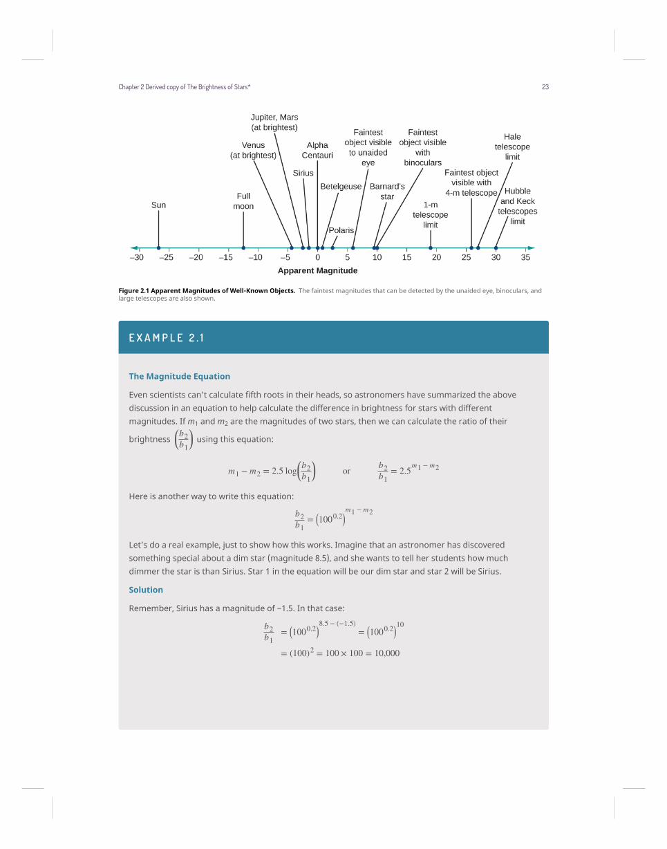
Figure 2.1 Apparent Magnitudes of Well-Known Objects. The faintest magnitudes that can be detected by the unaided eye, binoculars, andlarge telescopes are also shown.

E X A M P L E 2 . 1

The Magnitude Equation

Even scientists can’t calculate fifth roots in their heads, so astronomers have summarized the abovediscussion in an equation to help calculate the difference in brightness for stars with differentmagnitudes. If m1 and m2 are the magnitudes of two stars, then we can calculate the ratio of their

brightness ⎛⎝b2b1

⎞⎠ using this equation:

m1 − m2 = 2.5 log⎛⎝b2b1

⎞⎠ or b2

b1= 2.5

m1 − m2

Here is another way to write this equation:

b2b1

= ⎛⎝1000.2⎞⎠m1 − m2

Let’s do a real example, just to show how this works. Imagine that an astronomer has discoveredsomething special about a dim star (magnitude 8.5), and she wants to tell her students how muchdimmer the star is than Sirius. Star 1 in the equation will be our dim star and star 2 will be Sirius.

Solution

Remember, Sirius has a magnitude of −1.5. In that case:

b2b1

= ⎛⎝1000.2⎞⎠8.5 − (−1.5)

= ⎛⎝1000.2⎞⎠10

= (100)2 = 100 × 100 = 10,000


.

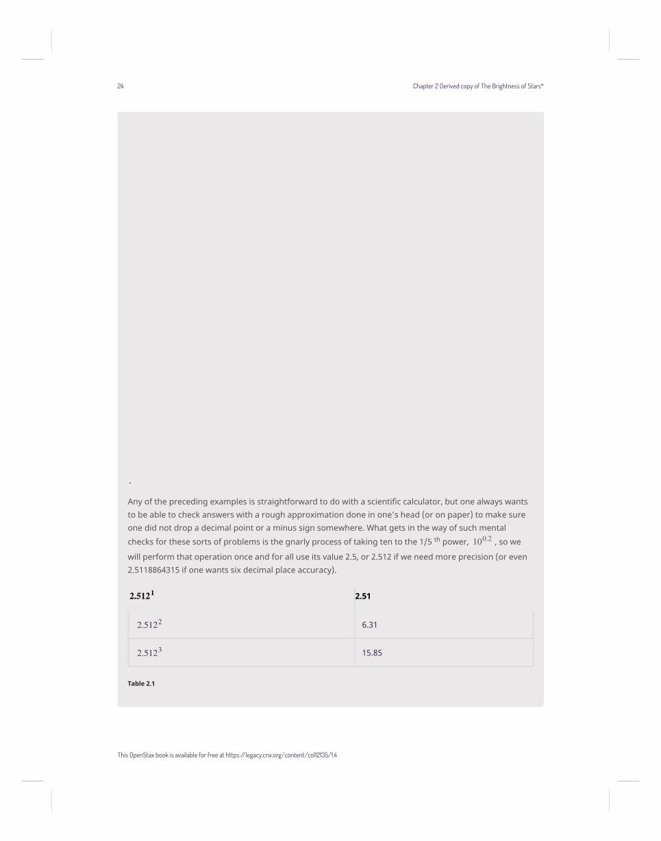
Any of the preceding examples is straightforward to do with a scientific calculator, but one always wantsto be able to check answers with a rough approximation done in one’s head (or on paper) to make sureone did not drop a decimal point or a minus sign somewhere. What gets in the way of such mental

checks for these sorts of problems is the gnarly process of taking ten to the 1/5 th power, 100.2 , so we

will perform that operation once and for all use its value 2.5, or 2.512 if we need more precision (or even2.5118864315 if one wants six decimal place accuracy).

2.5121 2.51

2.5122 6.31

2.5123 15.85

Table 2.1



2.5121 2.51

2.5124 39.81

2.5125 100

2.5126 251

2.5127 631

2.5128 1585

2.5129 3981

2.51210 10000

Table 2.1

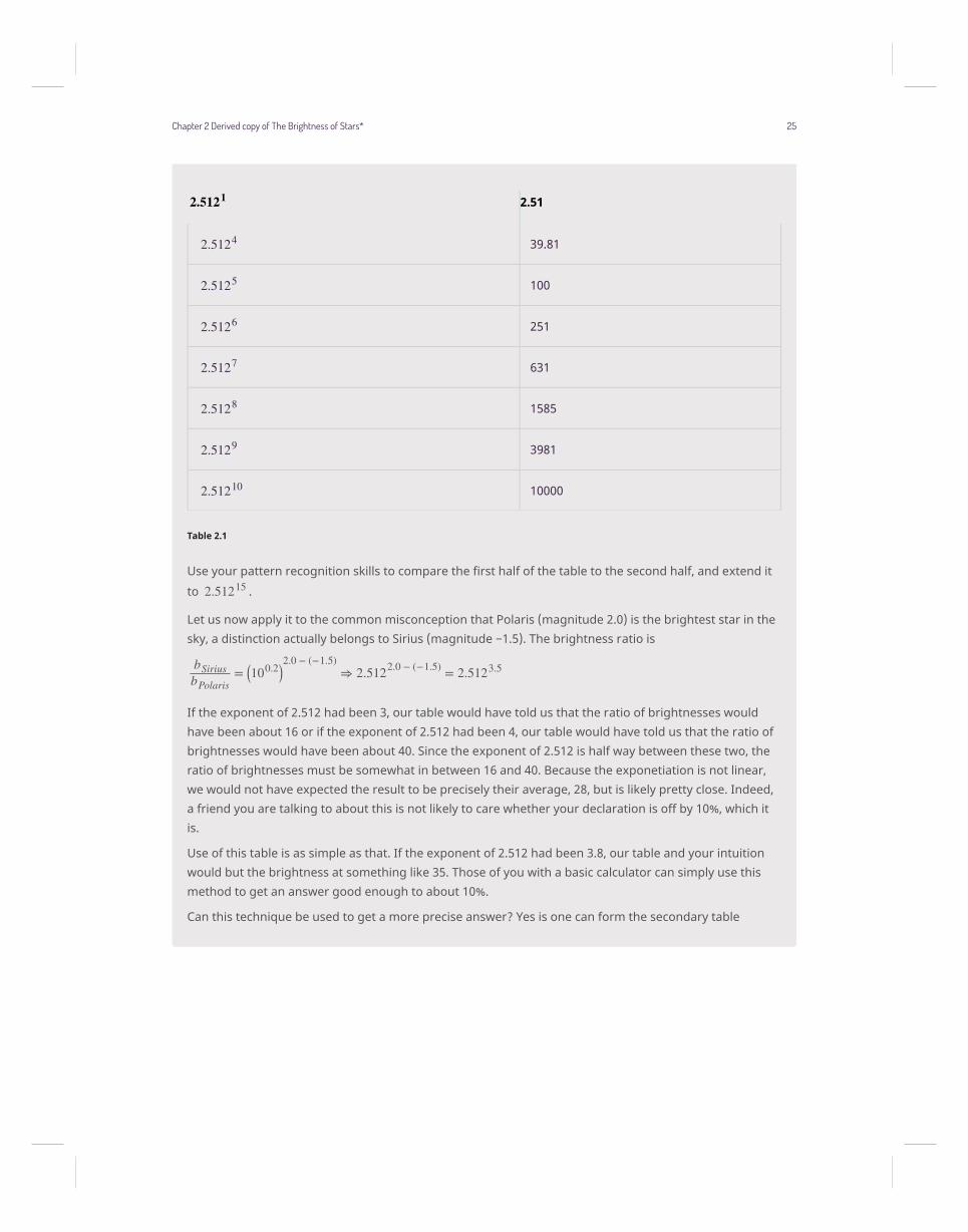
Use your pattern recognition skills to compare the first half of the table to the second half, and extend it

to 2.51215 .

Let us now apply it to the common misconception that Polaris (magnitude 2.0) is the brightest star in thesky, a distinction actually belongs to Sirius (magnitude −1.5). The brightness ratio is

bSiriusbPolaris

= ⎛⎝100.2⎞⎠2.0 − (−1.5)

⇒ 2.5122.0 − (−1.5) = 2.5123.5

If the exponent of 2.512 had been 3, our table would have told us that the ratio of brightnesses wouldhave been about 16 or if the exponent of 2.512 had been 4, our table would have told us that the ratio ofbrightnesses would have been about 40. Since the exponent of 2.512 is half way between these two, theratio of brightnesses must be somewhat in between 16 and 40. Because the exponetiation is not linear,we would not have expected the result to be precisely their average, 28, but is likely pretty close. Indeed,a friend you are talking to about this is not likely to care whether your declaration is off by 10%, which itis.

Use of this table is as simple as that. If the exponent of 2.512 had been 3.8, our table and your intuitionwould but the brightness at something like 35. Those of you with a basic calculator can simply use thismethod to get an answer good enough to about 10%.

Can this technique be used to get a more precise answer? Yes is one can form the secondary table


2.5 OTHER UNITS OF BRIGHTNESS

Although the magnitude scale is still used for visual astronomy, it is not used at all in newer branches of thefield. In radio astronomy, for example, no equivalent of the magnitude system has been defined. Rather, radioastronomers measure the amount of energy being collected each second by each square meter of a radio

2.5120.1 1.1

2.5120.2 1.2

2.5120.3 1.32

2.5120.4 1.45

2.5120.5 1.58

2.5120.6 1.74

2.5120.7 1.91

2.5120.8 2.09

2.5120.9 2.29

Table 2.2

and use the relation for exponents that xa + b = xaxb to givebSiriusbPolaris

= 2.5123.5 = 2.5123 ´2.5120.5 = 15.85´1.58 = 25 ,

the correct answer.

(2.1)15.85×1.58

Answer:

bSiriusbPolaris

= ⎛⎝1000.2⎞⎠2.0 − (−1.5)

= ⎛⎝1000.2⎞⎠3.5

= 1000.7 = 25

(Hint: If you only have a basic calculator, you may wonder how to take 100 to the 0.7th power. But this issomething you can ask Google to do. Google now accepts mathematical questions and will answer them.So try it for yourself. Ask Google, “What is 100 to the 0.7th power?”)

Our calculation shows that Sirius’ apparent brightness is 25 times greater than Polaris’ apparentbrightness.



telescope and express the brightness of each source in terms of, for example, watts per square meter.

Similarly, most researchers in the fields of infrared, X-ray, and gamma-ray astronomy use energy per area persecond rather than magnitudes to express the results of their measurements. Nevertheless, astronomers inall fields are careful to distinguish between the luminosity of the source (even when that luminosity is all in X-rays) and the amount of energy that happens to reach us on Earth. After all, the luminosity is a really importantcharacteristic that tells us a lot about the object in question, whereas the energy that reaches Earth is anaccident of cosmic geography.

To make the comparison among stars easy, in this text, we avoid the use of magnitudes as much as possibleand will express the luminosity of other stars in terms of the Sun’s luminosity. For example, the luminosity ofSirius is 25 times that of the Sun. We use the symbol LSun to denote the Sun’s luminosity; hence, that of Siriuscan be written as 25 LSun.

2.6 KEY CONCEPTS AND SUMMARY

The total energy emitted per second by a star is called its luminosity. How bright a star looks from theperspective of Earth is its apparent brightness. The apparent brightness of a star depends on both its luminosityand its distance from Earth. Thus, the determination of apparent brightness and measurement of the distanceto a star provide enough information to calculate its luminosity. The apparent brightnesses of stars are oftenexpressed in terms of magnitudes, which is an old system based on how human vision interprets relative lightintensity.


3

ADDITION TO P 678 NEW FIGS

Chapter 3 addition to p 678 new figs* 29

3.1 THE COSMOLOGICAL DISTANCE LADDER

Let us actually find the distance to a star using the parallax technique. The bright Southern star Beta Doraduswas observed by the Fine Guidance Sensor on the Hubble Space Telescope

[1]to have a parallax of 0.00314

±0.000016 arc seconds, so its distance is

D (pc) = 1/parallax (s) = 1/(0.00314 ±0.000059 s) = 318±15 pc.

If we want to understand the why of stars as well as the what, we must add to its catalogue of extrinsicproperties like distance, position in the sky, spectral type, and apparent brightness (b), that as seen at Earth. Thefirst step in investigating a star’s intrinsic properties is to define its absolute brightness or luminosity (L), definedas how bright it would be if it were precisely 10 pc away.

As seen in Figure 5.5, brightness falls off with the square of the distance, so the ratio of the luminosity at 10 pc,L@10pc, to the apparent brightness, b, we see at its true distance will give the ratios of the squares of the star’strue distance divided by 10 pc:

[2]

L@10pcb = D2

⎛⎝10pc⎞⎠2

.

In Example 17 we presented a relationship between the ratio of brightnesses of two different stars and theirapparent magnitudes . (The difference of the latter is proportional to the logarithm of the former.) We can usethis same relation for the ratio for absolute luminosity (L) to the apparent brightness (b) of a single star in for theparallel quantities called the absolute magnitude (M)and apparent magnitude (m). That is

m − M = 2.5log⎛⎝Lb⎞⎠

If we know the distance from its parallax, we can use distance ratio above in this expression to give the intrinsic,absolute magnitude (M) of any star:

M = m − 2.5log⎛⎝Lb⎞⎠ = m − 2.5log

⎛⎝⎜⎛⎝ D10pc⎞⎠2⎞⎠⎟ = m − 5log⎛⎝ D

10pc⎞⎠ ,

where we have used the property of logarithms that log(a p) = plog(a) to simplify the expression.

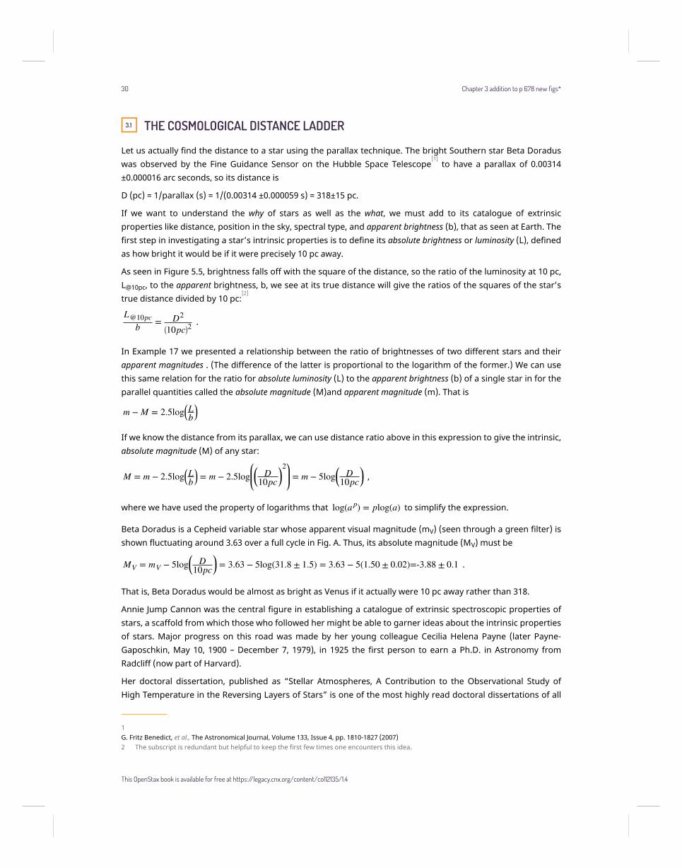
Beta Doradus is a Cepheid variable star whose apparent visual magnitude (mV) (seen through a green filter) isshown fluctuating around 3.63 over a full cycle in Fig. A. Thus, its absolute magnitude (MV) must be

MV = mV − 5log⎛⎝ D10pc⎞⎠ = 3.63 − 5log(31.8 ± 1.5) = 3.63 − 5(1.50 ± 0.02)=-3.88 ± 0.1 .

That is, Beta Doradus would be almost as bright as Venus if it actually were 10 pc away rather than 318.

Annie Jump Cannon was the central figure in establishing a catalogue of extrinsic spectroscopic properties ofstars, a scaffold from which those who followed her might be able to garner ideas about the intrinsic propertiesof stars. Major progress on this road was made by her young colleague Cecilia Helena Payne (later Payne-Gaposchkin, May 10, 1900 – December 7, 1979), in 1925 the first person to earn a Ph.D. in Astronomy fromRadcliff (now part of Harvard).

Her doctoral dissertation, published as “Stellar Atmospheres, A Contribution to the Observational Study ofHigh Temperature in the Reversing Layers of Stars” is one of the most highly read doctoral dissertations of all

1G. Fritz Benedict, et al., The Astronomical Journal, Volume 133, Issue 4, pp. 1810-1827 (2007)2 The subscript is redundant but helpful to keep the first few times one encounters this idea.

30 Chapter 3 addition to p 678 new figs*


time. Building on the ionization theory developed by Indian physicist Megh Nad Saha, she was able to showthat Cannon’s classification system was a measure of stars’ temperatures. She also upended the conventionalwisdom that stars’ compositions were roughly in proportion to the abundances on Earth by showing that starscontained roughly a million times more hydrogen than elements heavier than helium, a group of elementscollectively referred to as “metals” by astronomers, though of course containing other sorts of heavy elements.

Modern determinations of the absolute magnitude correct for variations in a star’s proportion of suchelements, called its “metallicity.” They also correct for other intrinsic effects like a Cepheid’s evolutionary stageas it passes through what is called the instability strip color of the HR diagram, and extrinsic effects of likeinterstellar dust that reddens and dims the light from a star. All of these effects alter mV and hence the valuewe calculate for MV. With such considerations, David G. Turner

[3]places the absolute visual magnitude of Beta

Doradus at

MV = -3.91 ± 0.11 .

Once one has calibrated many stars in Cannon’s classification scheme through this means, Cepheid or not, onemay reverse the process and find a star’s distance from its absolute magnitude by using the other relation inExample 17,

L@10pcb = ⎛⎝1000.2⎞⎠

m − M= 2.512m − M .

This slips nicely into our distance relation to give

D = 10pcL@10pc

b = 10pc ⎛⎝1000.2⎞⎠m − M

= 10pc 2.512m − M = 10pc ∗ 1.585m − M

This is a helpful new rung on a distance ladder for finding distances to stars too far away for parallaxmeasurements and is called spectroscopic parallax, that may be applied much further out until it become thestars become too faint to identify their spectral type.

Figure 3.1 Fig. A. Magnitudes from the fine error sensor, w(FES). Solid curves are light curves through a Visual (green) filter.[4]

Cepheid Variable stars continue play a central role in cosmology, including questions such as the age of theuniverse. This is due to the work of another of Annie Jump Cannon’s colleagues, Henrietta Leavitt (see Figure19.10).

[5]It is not often that nonscientists can catch a glimpse of the creative process of scientific advancement,

3 David G. Turner, Astrophysics and Space Science, Volume 326, Issue 2, pp 219–231, 2010.4 Edward G. Schmidt and Sidney B. Parsons, The Astrophysical Journal Supplement Series, 48:185-198, 1982. Henrietta S. Leavitt, Annals ofHarvard College Observatory 60, 87 (1908); Henrietta Leavitt and Edward C. Pickering, Harvard College Observatory Circular 173 1-3 (1912).5 Henrietta S. Leavitt, Annals of Harvard College Observatory 60, 87 (1908); Henrietta Leavitt and Edward C. Pickering, Harvard CollegeObservatory Circular 173 1-3 (1912)


much less the explication of a natural law as fundamental as then one named for the more famous astronomer,Edwin Hubble, who build upon her work. The following extract is a description of what is coming to be calledThe Leavitt Law

[6]in her own words at the time of its discovery:

In H.A. 60, No. 4, attention was called to the fact that the brighter variables [2] have the longer periods, but atthat time it was felt that the number was too small to warrant the drawing of general conclusions. The periodsof 8 additional variables which have been determined since that time, however, conform to the same law.

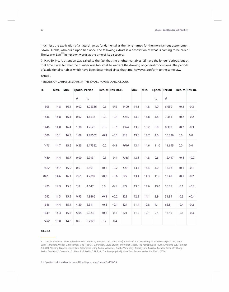
TABLE I.

PERIODS OF VARIABLE STARS IN THE SMALL MAGELLANIC CLOUD.

H. Max. Min. Epoch. Period Res. M. Res. m.H. Max. Min. Epoch. Period Res. M. Res. m.

d, d, d, d,

1505 14.8 16.1 0.02 1.25336 -0.6 -0.5 1400 14.1 14.8 4.0 6.650 +0.2 -0.3

1436 14.8 16.4 0.02 1.6637 -0.3 +0.1 1355 14.0 14.8 4.8 7.483 +0.2 -0.2

1446 14.8 16.4 1.38 1.7620 -0.3 +0.1 1374 13.9 15.2 6.0 8.397 +0.2 -0.3

1506 15.1 16.3 1.08 1.87502 +0.1 +0.1 818 13.6 14.7 4.0 10.336 0.0 0.0

1413 14.7 15.6 0.35 2.17352 -0.2 -0.5 1610 13.4 14.6 11.0 11.645 0.0 0.0

1460 14.4 15.7 0.00 2.913 -0.3 -0.1 1365 13.8 14.8 9.6 12.417 +0.4 +0.2

1422 14.7 15.9 0.6 3.501 +0.2 +0.2 1351 13.4 14.4 4.0 13.08 +0.1 -0.1

842 14.6 16.1 2.61 4.2897 +0.3 +0.6 827 13.4 14.3 11.6 13.47 +0.1 -0.2

1425 14.3 15.3 2.8 4.547 0.0 -0.1 822 13.0 14.6 13.0 16.75 -0.1 +0.3

1742 14.3 15.5 0.95 4.9866 +0.1 +0.2 823 12.2 14.1 2.9 31.94 -0.3 +0.4

1646 14.4 15.4 4.30 5.311 +0.3 +0.1 824 11.4 12.8 4. 65.8 -0.4 -0.2

1649 14.3 15.2 5.05 5.323 +0.2 -0.1 821 11.2 12.1 97. 127.0 -0.1 -0.4

1492 13.8 14.8 0.6 6.2926 -0.2 -0.4

Table 3.1

6 See for instance, “The Cepheid Period-Luminosity Relation (The Leavitt Law) at Mid-Infrared Wavelengths. II. Second-Epoch LMC Data,”Barry F. Madore, Wendy L. Freedman, Jane Rigby, S. E. Persson, Laura Sturch, and Violet Mager, The Astrophysical Journal, Volume 695, Number2 (2009); “Vetting Galactic Leavitt Law Calibrators Using Radial Velocities: On the Variability, Binarity, and Possible Parallax Error of 19 Long-Period Cepheids,” Casertano, S. Riess, A. G. Melis, C. Holl, B., The Astrophysical journal Supplement series, Vol.226(2) (2016).



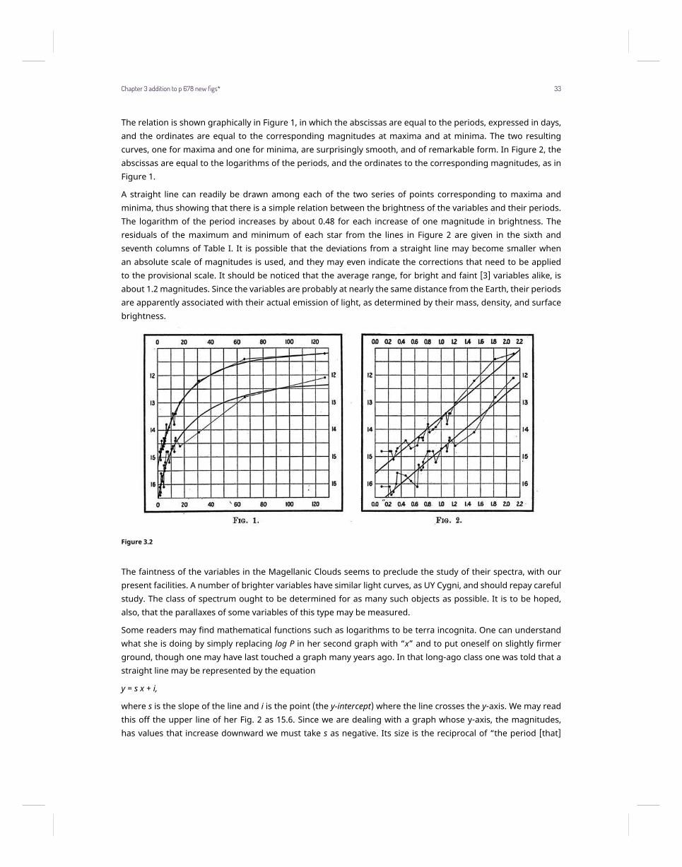
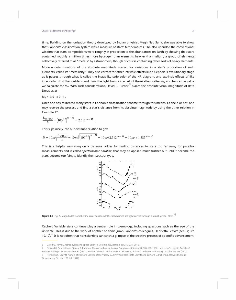
The relation is shown graphically in Figure 1, in which the abscissas are equal to the periods, expressed in days,and the ordinates are equal to the corresponding magnitudes at maxima and at minima. The two resultingcurves, one for maxima and one for minima, are surprisingly smooth, and of remarkable form. In Figure 2, theabscissas are equal to the logarithms of the periods, and the ordinates to the corresponding magnitudes, as inFigure 1.

A straight line can readily be drawn among each of the two series of points corresponding to maxima andminima, thus showing that there is a simple relation between the brightness of the variables and their periods.The logarithm of the period increases by about 0.48 for each increase of one magnitude in brightness. Theresiduals of the maximum and minimum of each star from the lines in Figure 2 are given in the sixth andseventh columns of Table I. It is possible that the deviations from a straight line may become smaller whenan absolute scale of magnitudes is used, and they may even indicate the corrections that need to be appliedto the provisional scale. It should be noticed that the average range, for bright and faint [3] variables alike, isabout 1.2 magnitudes. Since the variables are probably at nearly the same distance from the Earth, their periodsare apparently associated with their actual emission of light, as determined by their mass, density, and surfacebrightness.

Figure 3.2

The faintness of the variables in the Magellanic Clouds seems to preclude the study of their spectra, with ourpresent facilities. A number of brighter variables have similar light curves, as UY Cygni, and should repay carefulstudy. The class of spectrum ought to be determined for as many such objects as possible. It is to be hoped,also, that the parallaxes of some variables of this type may be measured.

Some readers may find mathematical functions such as logarithms to be terra incognita. One can understandwhat she is doing by simply replacing log P in her second graph with “x” and to put oneself on slightly firmerground, though one may have last touched a graph many years ago. In that long-ago class one was told that astraight line may be represented by the equation

y = s x + i,

where s is the slope of the line and i is the point (the y-intercept) where the line crosses the y-axis. We may readthis off the upper line of her Fig. 2 as 15.6. Since we are dealing with a graph whose y-axis, the magnitudes,has values that increase downward we must take s as negative. Its size is the reciprocal of “the period [that]


increases by about 0.48 for each increase of one magnitude in brightness.” Thus setting y = mmax we makeexplicit one version of Leavitt’s Law that is laid out in English in her paper and applied to maximum brightness:

m max = -2.1 x + 15.6 .

Let us see that we have the correct form for this by applying it at a particular point, say x = 0.8:

m max = -2.1 x + 15.6 = -2.1 ≥ 0.8 + 15.6 =13.92 ,

which looks about right if one moves upward from 0.8 on the horizontal axis of her Fig. 2 to the upper line andthen moves leftward to the vertical axis, crossing at about 13.9.

A modern replacement of the data Leavitt relied upon[7]

gives a slope somewhat steeper, with a slightly differentpoint where the line crosses the y axis. Thus, the Leavitt Law for apparent magnitudes becomes

mV =(-2.734± 0.031) log(P) + (15.040 ± 0.034+2.734± 0.031)

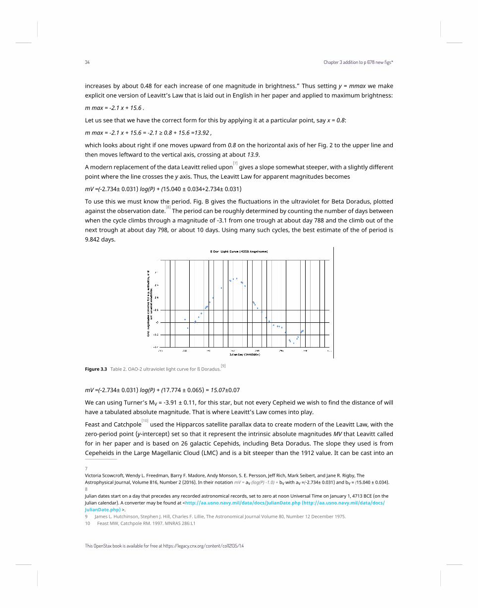
To use this we must know the period. Fig. B gives the fluctuations in the ultraviolet for Beta Doradus, plottedagainst the observation date.

[8]The period can be roughly determined by counting the number of days between

when the cycle climbs through a magnitude of -3.1 from one trough at about day 788 and the climb out of thenext trough at about day 798, or about 10 days. Using many such cycles, the best estimate of the of period is9.842 days.

Figure 3.3 Table 2. OAO-2 ultraviolet light curve for ß Doradus.[9]

mV =(-2.734± 0.031) log(P) + (17.774 ± 0.065) = 15.07±0.07

We can using Turner’s MV = -3.91 ± 0.11, for this star, but not every Cepheid we wish to find the distance of willhave a tabulated absolute magnitude. That is where Leavitt’s Law comes into play.

Feast and Catchpole[10]

used the Hipparcos satellite parallax data to create modern of the Leavitt Law, with thezero-period point (y-intercept) set so that it represent the intrinsic absolute magnitudes MV that Leavitt calledfor in her paper and is based on 26 galactic Cepehids, including Beta Doradus. The slope they used is fromCepeheids in the Large Magellanic Cloud (LMC) and is a bit steeper than the 1912 value. It can be cast into an

7Victoria Scowcroft, Wendy L. Freedman, Barry F. Madore, Andy Monson, S. E. Persson, Jeff Rich, Mark Seibert, and Jane R. Rigby, TheAstrophysical Journal, Volume 816, Number 2 (2016). In their notation mV = aV (log(P) -1.0) + bV with aV =(-2.734± 0.031) and bV = (15.040 ± 0.034).8Julian dates start on a day that precedes any recorded astronomical records, set to zero at noon Universal Time on January 1, 4713 BCE (on theJulian calendar). A converter may be found at <http://aa.usno.navy.mil/data/docs/JulianDate.php (http://aa.usno.navy.mil/data/docs/JulianDate.php) >.9 James L. Hutchinson, Stephen J. Hill, Charles F. Lillie, The Astronomical Journal Volume 80, Number 12 December 1975.10 Feast MW, Catchpole RM. 1997. MNRAS 286:L1



http://aa.usno.navy.mil/data/docs/JulianDate.php

http://aa.usno.navy.mil/data/docs/JulianDate.php

equation as above,

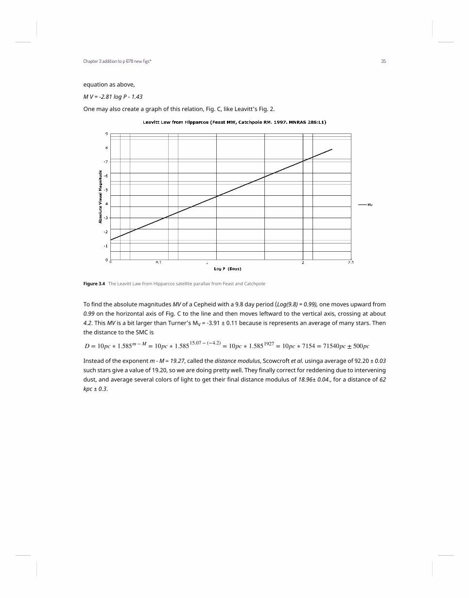
M V = -2.81 log P - 1.43

One may also create a graph of this relation, Fig. C, like Leavitt’s Fig. 2.

Figure 3.4 The Leavitt Law from Hipparcos satellite parallax from Feast and Catchpole.

To find the absolute magnitudes MV of a Cepheid with a 9.8 day period (Log(9.8) = 0.99), one moves upward from0.99 on the horizontal axis of Fig. C to the line and then moves leftward to the vertical axis, crossing at about4.2. This MV is a bit larger than Turner’s MV = -3.91 ± 0.11 because is represents an average of many stars. Thenthe distance to the SMC is

D = 10pc ∗ 1.585m − M = 10pc ∗ 1.58515.07 − (−4.2) = 10pc ∗ 1.5851927 = 10pc ∗ 7154 = 71540pc ± 500pc

Instead of the exponent m - M = 19.27, called the distance modulus, Scowcroft et al. usinga average of 92.20 ± 0.03such stars give a value of 19.20, so we are doing pretty well. They finally correct for reddening due to interveningdust, and average several colors of light to get their final distance modulus of 18.96± 0.04., for a distance of 62kpc ± 0.3.


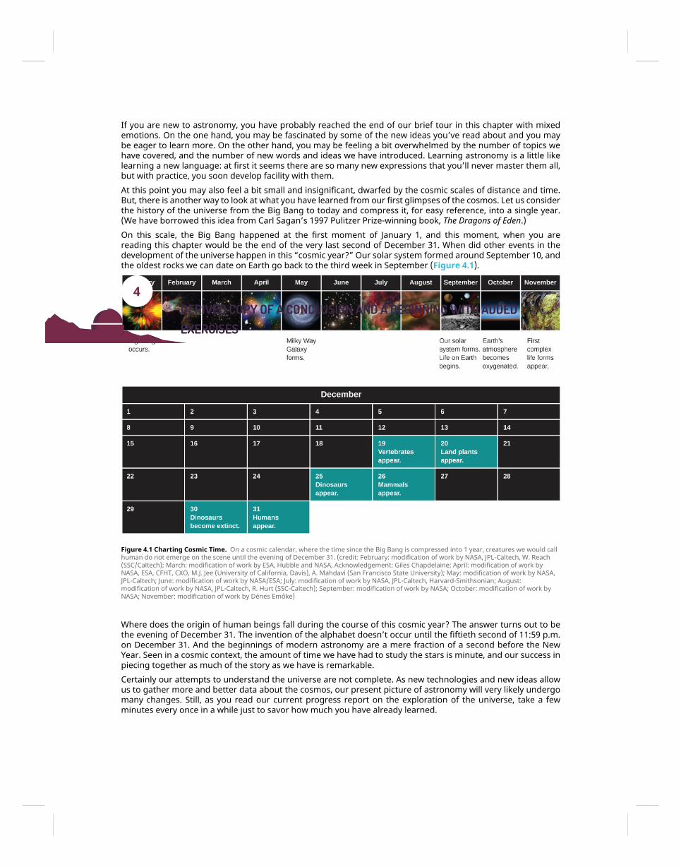
If you are new to astronomy, you have probably reached the end of our brief tour in this chapter with mixedemotions. On the one hand, you may be fascinated by some of the new ideas you’ve read about and you maybe eager to learn more. On the other hand, you may be feeling a bit overwhelmed by the number of topics wehave covered, and the number of new words and ideas we have introduced. Learning astronomy is a little likelearning a new language: at first it seems there are so many new expressions that you’ll never master them all,but with practice, you soon develop facility with them.At this point you may also feel a bit small and insignificant, dwarfed by the cosmic scales of distance and time.But, there is another way to look at what you have learned from our first glimpses of the cosmos. Let us considerthe history of the universe from the Big Bang to today and compress it, for easy reference, into a single year.(We have borrowed this idea from Carl Sagan’s 1997 Pulitzer Prize-winning book, The Dragons of Eden.)On this scale, the Big Bang happened at the first moment of January 1, and this moment, when you arereading this chapter would be the end of the very last second of December 31. When did other events in thedevelopment of the universe happen in this “cosmic year?” Our solar system formed around September 10, andthe oldest rocks we can date on Earth go back to the third week in September (Figure 4.1).

Figure 4.1 Charting Cosmic Time. On a cosmic calendar, where the time since the Big Bang is compressed into 1 year, creatures we would callhuman do not emerge on the scene until the evening of December 31. (credit: February: modification of work by NASA, JPL-Caltech, W. Reach(SSC/Caltech); March: modification of work by ESA, Hubble and NASA, Acknowledgement: Giles Chapdelaine; April: modification of work byNASA, ESA, CFHT, CXO, M.J. Jee (University of California, Davis), A. Mahdavi (San Francisco State University); May: modification of work by NASA,JPL-Caltech; June: modification of work by NASA/ESA; July: modification of work by NASA, JPL-Caltech, Harvard-Smithsonian; August:modification of work by NASA, JPL-Caltech, R. Hurt (SSC-Caltech); September: modification of work by NASA; October: modification of work byNASA; November: modification of work by Dénes Emőke)

Where does the origin of human beings fall during the course of this cosmic year? The answer turns out to bethe evening of December 31. The invention of the alphabet doesn’t occur until the fiftieth second of 11:59 p.m.on December 31. And the beginnings of modern astronomy are a mere fraction of a second before the NewYear. Seen in a cosmic context, the amount of time we have had to study the stars is minute, and our success inpiecing together as much of the story as we have is remarkable.Certainly our attempts to understand the universe are not complete. As new technologies and new ideas allowus to gather more and better data about the cosmos, our present picture of astronomy will very likely undergomany changes. Still, as you read our current progress report on the exploration of the universe, take a fewminutes every once in a while just to savor how much you have already learned.

4DERIVED COPY OF A CONCLUSION AND A BEGINNING WITH ADDEDEXERCISES

Chapter 4 Derived copy of A Conclusion and a Beginning with added exercises* 37

4.1 FOR FURTHER EXPLORATION

BooksMiller, Ron, and William Hartmann. The Grand Tour: A Traveler’s Guide to the Solar System. 3rd ed. Workman, 2005.This volume for beginners is a colorfully illustrated voyage among the planets.

Sagan, Carl. Cosmos. Ballantine, 2013 [1980]. This tome presents a classic overview of astronomy by anastronomer who had a true gift for explaining things clearly. (You can also check out Sagan’s television seriesCosmos: A Personal Voyage and Neil DeGrasse Tyson’s current series Cosmos: A Spacetime Odyssey.)

Tyson, Neil DeGrasse, and Don Goldsmith. Origins: Fourteen Billion Years of Cosmic Evolution. Norton, 2004. This

38 Chapter 4 Derived copy of A Conclusion and a Beginning with added exercises*


book provides a guided tour through the beginnings of the universe, galaxies, stars, planets, and life.

WebsitesIf you enjoyed the beautiful images in this chapter (and there are many more fabulous photos to come in otherchapters), you may want to know where you can obtain and download such pictures for your own enjoyment.(Many astronomy images are from government-supported instruments or projects, paid for by tax dollars, andtherefore are free of copyright laws.) Here are three resources we especially like:

• Astronomy Picture of the Day: apod.nasa.gov/apod/astropix.html. Two space scientists scour theInternet and select one beautiful astronomy image to feature each day. Their archives range widely,from images of planets and nebulae to rockets and space instruments; they also have many photos ofthe night sky. The search function (see the menu on the bottom of the page) works quite well for findingsomething specific among the many years’ worth of daily images.

• Hubble Space Telescope Images: www.hubblesite.org/newscenter/archive/browse/images. Starting atthis page, you can select from among hundreds of Hubble pictures by subject or by date. Note thatmany of the images have supporting pictures with them, such as diagrams, animations, or comparisons.Excellent captions and background information are provided. Other ways to approach these imagesare through the more public-oriented Hubble Gallery (www.hubblesite.org/gallery) and the Europeanhomepage (www.spacetelescope.org/images).

• National Aeronautics and Space Administration’s (NASA’s) Planetary Photojournal:photojournal.jpl.nasa.gov. This site features thousands of images from planetary exploration, withcaptions of varied length. You can select images by world, feature name, date, or catalog number, anddownload images in a number of popular formats. However, only NASA mission images are included.Note the Photojournal Search option on the menu at the top of the homepage to access ways to searchtheir archives.

VideosCosmic Voyage: www.youtube.com/watch?v=qxXf7AJZ73A. This video presents a portion of Cosmic Voyage,narrated by Morgan Freeman (8:34).

Powers of Ten: www.youtube.com/watch?v=0fKBhvDjuy0. This classic short video is a much earlier version ofPowers of Ten, narrated by Philip Morrison (9:00).

The Known Universe: www.youtube.com/watch?v=17jymDn0W6U. This video tour from the American Museumof Natural History has realistic animation, music, and captions (6:30).

Wanderers: apod.nasa.gov/apod/ap141208.html. This video provides a tour of the solar system, with narrativeby Carl Sagan, imagining other worlds with dramatically realistic paintings (3:50).

EXERCISES1. (a) If it takes light about 8 minutes to travel from the Sun to Earth, how long does it take light to reach Earthfrom Neptune, which is 30 times as far from us? (b) What does this mean for a two-way conversation betweenEarth and a spacecraft orbiting Neptune using radio waves?

2. Since most of the math you need for this class consists of ratios, you may find that you already have aplatform from which to venture forth by making a list of five different proportionalities (ratios) from your dailylife.

3. (a) Write the following numbers in scientific notation (see Appendix C if you are unfamiliar with this notation):100; 0.011; 101; 1,000,000,000,000,000; 6378; and 0.000654. (b) Write the following numbers in “normal"

Chapter 4 Derived copy of A Conclusion and a Beginning with added exercises* 39

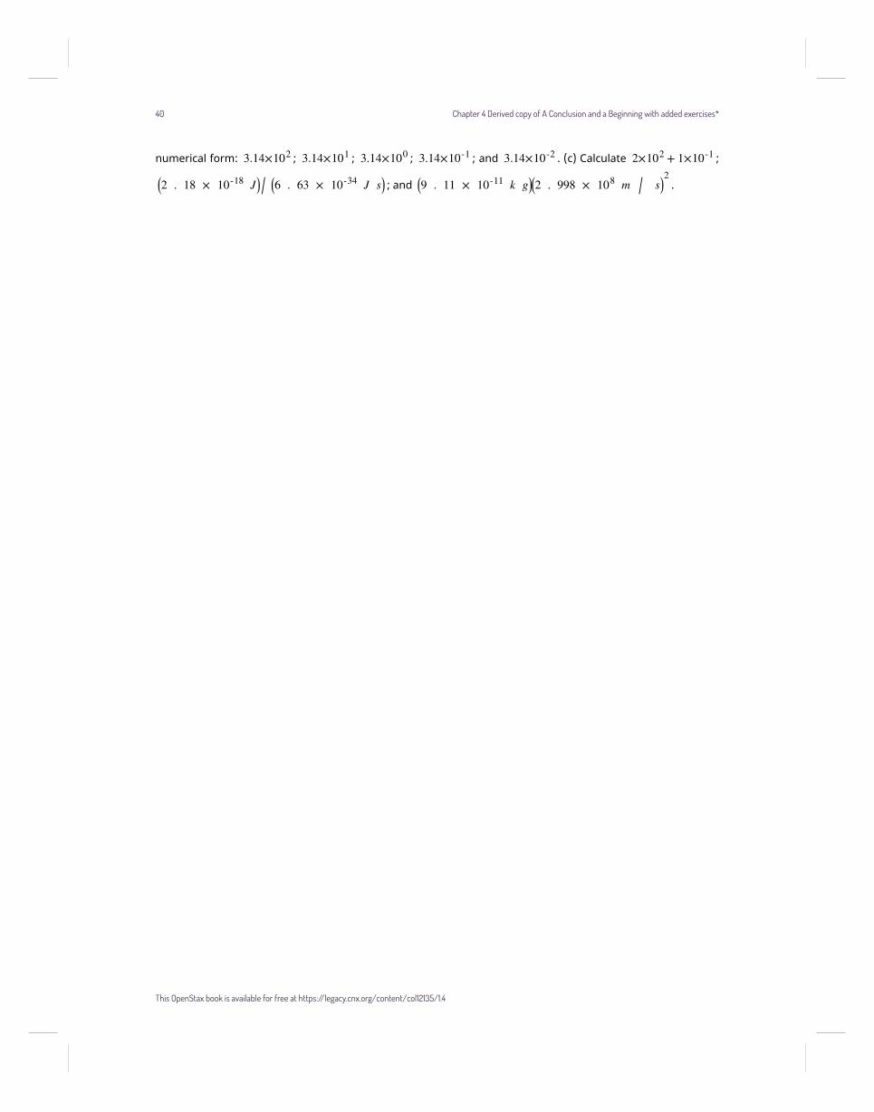
numerical form: 3.14×102 ; 3.14×101 ; 3.14×100 ; 3.14×10-1 ; and 3.14×10-2 . (c) Calculate 2×102 + 1×10-1 ;

⎛⎝2 . 18 × 10-18 J⎞⎠ / ⎛⎝6 . 63 × 10-34 J s⎞⎠ ; and ⎛⎝9 . 11 × 10-11 k g⎞⎠

⎛⎝2 . 998 × 108 m / s⎞⎠

2.

40 Chapter 4 Derived copy of A Conclusion and a Beginning with added exercises*


INDEX

Aapparent brightness, 21

DDoppler, 0Draper, 12

Ggiants, 5

HHale, 13Hipparchus, 22Huggins, 8

KKeck, 13

LLick, 12luminosity, 21

Mmagnitude, 22, 23

Pproper motion, 8

Rradial velocity, 7

SSirius, 8, 9, 21, 22, 23space velocity, 9

VVega, 9, 11Venus, 22

YYerkes, 13

Index 41

42 Index


ATTRIBUTIONSCollection: Additions to Astronomy-OP 2017Edited by: Jack StratonURL: https://legacy.cnx.org/content/col12135/1.4/Copyright: Jack StratonLicense: http://creativecommons.org/licenses/by/4.0/

Module: Derived copy of Using Spectra to Measure Stellar Radius, Composition, and MotionBy: Jack StratonURL: https://legacy.cnx.org/content/m63818/1.1/Copyright: Jack StratonLicense: http://creativecommons.org/licenses/by/4.0/Based on: Using Spectra to Measure Stellar Radius, Composition, and Motion <http://legacy.cnx.org/content/m59896/1.4> by OpenStax Astronomy.

Module: Derived copy of The Brightness of StarsBy: Jack StratonURL: https://legacy.cnx.org/content/m63821/1.2/Copyright: Jack StratonLicense: http://creativecommons.org/licenses/by/4.0/Based on: The Brightness of Stars <http://legacy.cnx.org/content/m59890/1.3> by OpenStax Astronomy.

Module: addition to p 678 new figsBy: Jack StratonURL: https://legacy.cnx.org/content/m63832/1.2/Copyright: Jack StratonLicense: http://creativecommons.org/licenses/by/4.0/

Module: Derived copy of A Conclusion and a Beginning with added exercisesBy: Jack StratonURL: https://legacy.cnx.org/content/m63566/1.2/Copyright: Jack StratonLicense: http://creativecommons.org/licenses/by/4.0/Based on: A Conclusion and a Beginning <http://legacy.cnx.org/content/m59762/1.4> by OpenStaxAstronomy.

Index 43

https://legacy.cnx.org/content/col12135/1.4/


https://legacy.cnx.org/content/m63818/1.1/


http://legacy.cnx.org/content/m59896/1.4










44 Index


ABOUT CONNEXIONSSince 1999, Connexions has been pioneering a global system where anyone can create course materials andmake them fully accessible and easily reusable free of charge. We are a Web-based authoring, teaching andlearning environment open to anyone interested in education, including students, teachers, professors andlifelong learners. We connect ideas and facilitate educational communities. Connexions's modular, interactivecourses are in use worldwide by universities, community colleges, K-12 schools, distance learners, and lifelonglearners. Connexions materials are in many languages, including English, Spanish, Chinese, Japanese, Italian,Vietnamese, French, Portuguese, and Thai.

Index 45

additions to astronomy-op 2017 - openstax cnx

Documents