Adaptive Shared-State Sampling

Frederic RaspallDepartment of Telematics

Technical University of Catalonia (UPC)fredi@entel.upc.edu

Sebastia SallentDepartment of Telematics

Technical University of Catalonia (UPC)sallent@entel.upc.edu

ABSTRACTWe present two algorithms to the problem of identifyingand measuring heavy-hitters. Our schemes report, with highprobability, those flows that exceed a prescribed share of thetraffic observed so far; along with an estimate of their sizes.One of the biggest advantages of our schemes is that theyentirely rely on sampling. This makes them flexible andlightweight, permits implementing them in cheap DRAMand scale to very high speeds. Despite sampling, our al-gorithms can provide very accurate results and offer per-formance guarantees independent of the traffic mix. Mostremarkably, the schemes are shown to require memory thatis constant regardless of the volume and composition of thetraffic observed. Thus, besides computationally light, cost-effective and flexible, they are scalable and robust againstmalicious traffic patterns. We provide theoretical and em-pirical results on their performance; the latter, with softwareimplementations and real traffic traces.

Categories and Subject DescriptorsC.2.3 [Computer-Communication Networks]: NetworkOperations—Network monitoring

General TermsAlgorithms, Design, Measurement, Theory

KeywordsHeavy-hitters, Frequent Items, Sampling, Scalability

1. INTRODUCTIONIdentifying frequent items is one of the problems that have

most extensively been studied in the past, attracting theattention of researchers in distinct disciplines such as net-working or data mining. One of the contexts where find-ing frequent items is of most use is traffic monitoring. Dis-covering which flows are responsible for the bulk of traffic

Permission to make digital or hard copies of all or part of this work forpersonal or classroom use is granted without fee provided that copies arenot made or distributed for profit or commercial advantage and that copiesbear this notice and the full citation on the first page. To copy otherwise, torepublish, to post on servers or to redistribute to lists, requires prior specificpermission and/or a fee.IMC’08, October 20–22, 2008, Vouliagmeni, Greece.Copyright 2008 ACM 978-1-60558-334-1/08/10 ...$5.00.

(the so-called heavy-hitters or elephants) is useful for net-work administrators, who need to have a good understand-ing of the traffic flowing through their networks. Identifyingand measuring such flows is helpful for traffic engineering(e.g. load balancing or finding traffic matrices), warning ofheavy users, revealing traffic trends or identifying denial-of-service attacks. Finding frequent patterns also permitsthe discovery of worm or virus signatures [15]. Besides sup-plying valuable information for several network managementapplications, focusing on the largest flows alleviates the scal-ability issue of keeping state for a huge number of flows [7].

While there exist many approaches that identify and ac-curately measure large flows using small memory footprints,most techniques need to inspect each packet present, per-form memory accesses on a per-packet basis (e.g. updat-ing sketches) or frequently carry out “housekeeping” tasks tokeep their memory usage low; intensive computations thatcan hinder their useability as the speed of links improve.

In this paper, we present two algorithms to the problemof finding heavy hitters that have two appealing features.First, despite relying on sampling, they succeed in iden-tifying heavy hitters with high probability and accuratelymeasuring their size. Thus, they perform as well as schemesneeding to process each packet, while retaining all the ad-vantages of sampling in terms of flexibility and lightness.Second, both require memory that is constant regardless ofthe amount of traffic under observation or its properties.Thus, the schemes scale well in both space and speed.

The organization of this paper is as follows. Section 2discusses related and prior work on which our algorithmsbuild. In section 3, we present our algorithms and studytheir performance from a theoretical standpoint, focusingon the identification guarantees these offer and their mem-ory requirements. Section 4 discusses the accuracy of ourschemes. Section 5 presents experimental results obtainedwith software implementations of the algorithms and realtraffic traces. Section 6 concludes the paper.

2. BACKGROUND

2.1 Related workIn the context of databases, [16] proposes algorithms that

use uniform random sampling for the discovery of associa-tion rules which, compared to prior work, require a singlepass over the data. [5] proposes algorithms that identifyhot items in databases also in a single pass but allowing fordeletions. [10] proposes a “Simple”algorithm to identify fre-quent items. In a single pass, their algorithm produces an

271

approximate superset of the set of frequent items. A secondpass allows their algorithm to report the exact set of frequentitems and their frequencies. [11] proposes two algorithms,Sticky Sampling (S2) and Lossy Counting (LC), for com-puting frequency counts exceeding user-specified thresholds.Besides identifying, these produce estimates of the frequencyof items in a single pass. [6] recently proposed ProbabilisticLossy Counting (PLC) which reduces the memory needs ofLC at the cost of providing probabilistic instead of deter-ministic guarantees on its accuracy. [9], [8] and [2] proposealgorithms obeying the sliding-window paradigm. Concep-tually, these weigh recent items (those in the window) and al-low identifying emerging trends. The first algorithms to theproblem proposed in the networking context were Sample-and-Hold (S&H) and Multistage Filters (MF) in [7]. Theidea behind these is that, since the number of large flows isbounded, if these can be identified, small but fast memoriescan be used to individually track them by keeping a dedicatedentry in the so-called flow memory. By limiting the numberof flows that get detected, a small amount of SRAM can beused to implement the flow memory, which allows for per-packet updates and, thus, accurately measuring their size. Inboth, flows are ”challenged” to instantiate entries in the flowmemory. In S&H, flows have to be sampled once to get de-tected. In MF, flows need to raise several counters beyonda threshold to occupy an entry. [14] proposes Shared-StateSampling (S3), that generalizes S&H and MF. Our algo-rithms are based on S3, as we discuss in section 2.2. [3]presents several approaches based on the Count-Min Sketch[4] and Misra Gries that skip over some items to reduce thecost of updating the sketch. Instead of performing updatesevery Nth item (as done by sampling methods), their ap-proach alternates between two phases where updates occuronly in one of them. Switching between the two phases isdone depending on the current value of the norm of skippedand sketched items. Our approach is similar to theirs in howdata is sketched and in that some items are skipped.

2.2 Shared-State Sampling (S3)Our algorithms are best understood in terms of a prior

scheme, Shared-State Sampling (S3) in [14], which we sum-marize next. S3 is similar to S&H and MF in that it chal-lenges flows to gain an entry in the flow memory. Oncethis happens, flows are considered detected and their sizeexactly measured by updating the corresponding entry forevery subsequent packet from the flow. S3 samples trafficbytes with some probability p and requires flows be sampledsome number of times d (the sample threshold) to occupyan entry. The “principle” on which it relies is that, if thesampling probability is set as p = d

Vcut, then flows larger

than Vcut are likely to be detected while it is unlikely thatflows below do. This is because, by setting p = d

Vcut, the

expected number of times that a flow sending v bytes getssampled is E[Nv ] = vp = v

Vcutd. Thus, if v > Vcut, a flow is

likely to be sampled more than d times; and fewer otherwise.Further, the selectivity of the detection curve improves byraising d, as fig. 1 shows. Intuitively, if p = d

Vcut, then the

expected number of bytes that pass from a flow before itgets detected, d

p= Vcut, is constant regardless of d. Thus,

by rasing p (and d) more samples are taken and the uncer-tainty about the size of a flow diminishes, for the same Vcut.Note that d plays, thus, a dual role: that of a threshold andthat of an oversampling factor. We call Vcut the cutoff size.

0

0.1

0.2

0.3

0.4

0.5

0.6

0.7

0.8

0.9

1

0 25000 50000 75000 100000 125000 150000 175000

Det

ectio

n pr

obab

ility

flow size (v)

Vcut

d=1d=3d=5

d=10d=100d=500

d=1000

Figure 1: Detection probability as a function of flow size

if p = dVcut

, for increasing values of d and Vcut = 105.

The behavior above corresponds to the case where thenumber of times that flows get sampled can be exactly counted.To avoid keeping a counter per flow, S3 approximately countsflows’ samples in m stages, each with b counters. Whenevera sample is taken, m independent hash functions are appliedon the flow ID and the results, h1, ..hm, used to update oneof the b counters at each stage. This way, samples from aflow update the same stage counters and a flow gets detectedif one of its samples finds all its stage counters at d−1. Thisidea (borrowed from MF) gets around the issue of keeping acounter for each flow but permits that several flows raise thesame counter. This interference effect increases the chancesthat flows smaller than Vcut get detected, as the algorithmcan be misled to think that such flows have been sampledmore times than they really were. Specifically, if c1, ..cm arethe amounts by which the counters hit by a flow get raisedby other flows and cmin = min(c1, ..cm), then the flow needsonly be sampled (d − cmin) times to be detected, becausesuch number of samples suffices to make all counters reach(d − 1) and for one sample to find them at that value. Al-though the interference can cause stage counters “saturate”,there is a minimum number of stage counters with which theselectivity of the approach is not hindered by the effect ofinterference, regardless of how the traffic is composed [13].

S3 has the advantage over MF that, since it needs only up-date stages per sample, these can be implemented in DRAM.In practice, this permits supporting enough counters for theinterference to be small. Our algorithms build on a vari-ant of S3, that we call Sample-and-Hash (SHa) and reportin [13]. SHa proceeds like S3 except that it only updatesentries per sampled packet. The idea is depicted in fig. 2.

Figure 2: Sample-and-Hash (SHa)

In SHa, each traffic byte is sampled with some probabilityp. If a packet is sampled, its FID is determined and the flow

272

memory consulted. If the packet belongs to a flow alreadyin the flow memory, its entry is updated. If it does not, mhash functions are applied on the FID to select one counterat each stage. If all the selected counters are at d − 1, theflow enters the flow memory. Otherwise, the stage countersare raised by using conservative update1 (CU) in [7].

Every entry contains a flow ID and a sample count Ne

used to estimate the size of a flow. When a flow is detected,its sample count is set to Ne = d, as this is the number ofsamples that, presumably, have been taken from the flowso far. In this regard, if a flow is sampled Nv times andsome (d − cmin) samples sufficed to detect it, we have thatNv = (d− cmin) + Npost, with Npost the number of samplestaken from the flow “post” detection. Thus, by initializingNe = d, we have that Ne = Nv + cmin. That is, the samplecount for a flow is never smaller than the number of times itis sampled. Apart from helping small flows pass, interferenceaffects the accuracy of SHa.

While updating entries on a per-sample basis comes to thedetriment of accuracy, SHa offers the same detection guar-antees as S3 and fairly accurate traffic estimates [13]. Theadvantage is that performing entry updates only per sampleallows SHa to: 1) evade the bottleneck of inspecting andexecuting memory lookups for every packet 2) implementthe flow memory in DRAM (instead of SRAM/CAM) and3) fully control the overhead of the algorithm with the sam-pling rate, as no action is performed for unsampled packets.Thus, SHa can scale to much higher speeds, where inspecting(or executing lookups for) each packet may not be feasible.

2.3 Motivation behind our algorithmsS3 and SHa report, with high probability, those flows

above a certain threshold that is constant irrespective of howmuch traffic is actually sent during some measurement inter-val. The algorithms in the present paper aim at identifying,more than those flows above some threshold T (say, 1MB),those whose share exceeds a prescribed fraction z of the traf-fic actually observed (such as 1%), either in a measurementinterval or whenever a network administrator queried thealgorithm. We call z the target share. An ideal algorithmwould report the (FID, size) pairs of only large flows. Realalgorithms may fail in several ways: failing to report flowsabove z (false negatives), adding flows with share below zto the report (false positives) and incorrectly determiningtheir size. The performance of an algorithm depends on theextent to which it incurs any of the errors above and its costin terms of memory and processing. In this regard, the min-imum amount of memory required by an algorithm is 1/zentries or (FID, size) pairs.

In what follows, v denotes the size of a flow in bytes. Ct

stands for the total amount of traffic observed so far. Theshare of a flow is defined as zf = v

Ct. Note that v and zf

vary in time, although our notation omits this for clarity.

3. ADAPTIVE SHARED-STATE SAMPLINGOur algorithms can be understood as means to enforce

that the flows reported by SHa always correspond to thoseexceeding a prescribed share z of the traffic observed so far,

1Conservative update minimizes the pace at which shared counters

grow in MF, with the guarantee that flow sizes will not be under-counted. It consists in not raising the counters beyond the value thatthe smallest of them would have after the update.

Ct. All of them follow the structure depicted in fig. 2. Thesesample traffic bytes with some probability p, require flowsbe sampled a certain number of times to be detected and ap-proximately count samples in m stages of size b, where coun-ters are selected applying hash functions on packet FIDs.Once flows get detected, their samples update entries andnot stage counters.

Ideally, we would like to achieve a behavior as that in fig.1 except that, instead of some cutoff size, we would like tohave some cutoff share. Thus, in terms of SHa, the problemwe address is, essentially, how to make Vcut correspond to afraction z of Ct, which is not known in advance.

Let us sketch this with an example. For Vcut to equalzCt, the sample threshold and sampling probability shouldbe such that d

p= zCt. Suppose we fixed p to some value. We

could meet our goal by setting d = dr = zpCt. We call dr theright threshold. The problem is that Ct is unknown, as wemay query the algorithm at any point in time or because theamount of traffic that shall arrive during some measurementinterval (e.g. one hour, a day or a month) is not knownbeforehand. A first approach that suggests itself is tryingto predict Ct and setting d accordingly. However, this isnot suitable for the following. Suppose we set d = dg =zpCg, with Cg our guess of Ct. If we “overestimate” Ct, thethreshold used will be higher than the right, so will the cutoffsize. We say we “overthreshold”. Intuitively, we may onlydetect flows above some share z′ > z. Thus, flows with sharezf ∈ (z, z′) may be missed. By underestimating Ct, thethreshold will be smaller than dr, causing flows with sharebelow some z′ < z be detected. We say we“underthreshold”.We find it useful to represent the problem as follows.

Once z is chosen and p set, the sample threshold we shoulduse (dr) is a linear function of Ct; specifically, a straight linecrossing the origin with slope zp, as depicted in fig. 3.

Figure 3: Setting d by predicting Ct.

If Cg �= Ct, then the cutoff share after observing Ct bytesdiffers from z since, if d �= zpCt, then the threshold intersectsa line with a slope different from zp. Since the coordinatesof this intersection are (Ct, zpCg), the slope of such line is

ϕ =zpCg

Ct. Since, once p is set, such slope determines the

cutoff share, the resulting cutoff share is z′ = zCg

Ct. Thus,

if Cg > Ct (as in the figure), we have that z′ > z; theinequality being reversed otherwise. If we write Cg = Ct +εc, with εc the error in our prediction, we have that z′ =z(1+ εc

Ct). Thus, | z′−z

z| = | εc

Ct|, meaning that the cutoff share

can differ from the desired in the same proportion that ourprediction from the actual traffic present. That is, a 10%error guessing Ct would yield a 10% deviation of the cutoffshare with respect to the target one. While predicting theamount of traffic crossing a link in a certain period of time

273

may be possible to some extent, this approach is definitelynot suitable to support queries at any time.

3.1 “Slide-and-Chop” (S&C)Besides the unsuitability of setting the threshold by guess-

ing Ct, the previous discussion reveals that overthresholdinghas a distinct effect from underthresholding. The former cancause false negatives. The latter, false positives. While falsenegatives are irreversible, false positives may be tolerable ifwe can determine, among the flows detected, which reallyexceeded a share z of the traffic present. This motivates ourfirst algorithm, Slide-and-Chop (S&C).

Base idea: In SHa, sample traffic bytes with some prob-ability p and set the sample threshold to d = zpΔc. EveryΔc traffic bytes, raise the sample threshold by Δd = zpΔc.If a sample finds all counters at d−1, the corresponding flowis detected and its entry sample count Ne set to the currentthreshold. Before raising d at each stretch, flush all entrieswhose sample count is below the current sample threshold.If queried, report, among the flows detected, those whoseNe ≥ zpCt. Fig. 4 illustrates the process.

Figure 4: Evolution of d in Slide-and-Chop.

3.1.1 Preliminary observations and analysisCompared to the “predictive” approach, S&C can be un-

derstood as, to avoid overthresholding, drawing a very con-servative guess of Ct; some Δc such that, with high prob-ability, Ct � Δc. Think of the starting points of eachstretch as deadlines that are reached as traffic is observed.These occur at Ci = iΔc, where the threshold visits thevalues di = zpCi = zpiΔc = iΔd. Each time a deadline isreached, the sample threshold used coincides to the right forthe amount of traffic observed so far and is, then, raised tothe right in case the next deadline is attained.

Let us see what happens. Suppose that a flow has sentv bytes up to the kth deadline, which is just reached (i.e.Ct = Ck = kΔc). At Ck, the share of this flow is zf = v

kΔc.

For the flow to get detected, it must have been sampleda number of times higher than the current or prior thresh-olds (for simplicity, disregard the effect of interference). Theexpected number of times such a flow may be sampled isE[Nv ] = vp = (zfkΔc)p. Since dk = zpkΔc, this is E[Nv] =(

zf

z)dk. Thus, if zf > z, such flow will be sampled, on the

average, more times than the highest of the thresholds, dk.Consequently, by the S3/SHa “principle”, it will be detectedwith high probability. Note that our flow may have not ex-ceeded prior thresholds, as its share may have been lower.Yet, if its current share exceeds z, it will be detected with“high probability”. If zf < z, then E[Nv ] < dk. Thus, withhigh probability, Nv < dk. However, before Ck is reached,

the sample threshold has been lower than dk for some time.Thus, such flow could have exceeded prior thresholds andbe in the flow memory, either because its share exceeded zby that time or because it hit counters made large by otherflows. In this regard, note that if we had known that dead-line Ck were to be reached, we could have set the samplethreshold to dk = zpCk from the beginning. This is themotivation for flushing: if, at Ck, we delete all entries withsample counts below dk, we will not miss flows that wouldhave exceeded dk had the threshold been that high from thebeginning. However, getting rid of entries with low samplecounts poses the following problem. Once a flow gets de-tected in SHa, its samples stop raising counters and update,instead, some entry sample count, Ne. If we flush the entryfor a flow whose share happens to exceed z later on, suchflow may be missed, as subsequent samples from the flowmay find stage counters at values that are lower than if ithad not visited the flow memory: samples taken when theflow “lived” in an entry will go uncounted.

3.1.2 Flushing entries while preserving detectionThere are several ways to get around the undercount prob-

lem above. The simplest is to let flows raise stage counters,even if detected. This way, stage counters would never besmaller than the number of times that the flows raising themwere sampled. This requires updating the flow memory andthe stages per sample. While feasible, this unnecessarily in-flates stage counters. Consider, instead, “returning” back tothe stages the samples counted when the flow occupied anentry. This would leave the stage counters as if the flow hadnever been detected and requires updating the stages onlywhen flushing. Further, the idea of conservative update (CU)could be applied, by not raising the counters beyond thevalue that the smallest of them would have after increasingit with the returned samples. There is a better scheme thatwe call conservative flush (CF). Instead of returning sam-ples, set the stage counters to the maximum of their currentvalue and the sample count of the flushed entry, Ne. Thisnever undercounts samples from any of the flows using theaffected counters2.

Lemma 1. By applying CU (on stage counter updates)and CF (when flushing), stage counters cannot reach thecurrent sample threshold d.

Proof. With CU, a sample could only make a counterreach d if the smallest of the counters it hit were d − 1.But, in that case, the sample would occupy an entry andnot raise the counters. Suppose an entry were to be flushedwith threshold d. With CF, the only way for the entry toraise counters beyond d−1 would be having a sample count≥ d. However, such an entry would never be flushed.

Lemma 2. The probability that, in S&C, a flow remainsafter flushing with threshold df is no smaller than the proba-bility that the flow got detected had the threshold always beendf and there were no interference.2

For instance, suppose that a flow were detected when d = 10, whichit exceeded on its own. Imagine that its entry were updated with 11samples and that the threshold became d = 40 later on. Since Ne =21, the flow would be flushed. Assume that the four stage countersit hit were raised to {15, 18, 22, 27} by other flows. If no sampleswere returned, there could be an undercount of 21−15 = 6 (althoughnew “interfering” samples could compensate this). If the 11 sampleswere simply “returned”, stage counters would become {26, 29, 33, 38}.Returning these with CU, {26, 26, 26, 27}. Using CF, {21, 21, 22, 27}.

274

Proof. Entries occupied when d = df cannot be flushedsince, in these, Ne ≥ df . Only flows detected at a lowerthreshold can be flushed. Consider a flow detected whendj < df and let Nv be the number of times it has beensampled when flushing occurs. Since its sample count isnever smaller than Nv, if the entry is flushed, it means thatthe flow were sampled fewer than df times, in which case theflow would have not been detected had the threshold beendf and there were no interference. Formally, since Ne ≥ Nv ,Ne < df ⇒ Nv < df . Thus, P (Ne < df ) ≤ P (Nv < df ).

Lemma 2 does not imply that large flows cannot be flushed.It says that, by flushing entries, the probability that we missa large flow is no larger than if the right threshold had beenused and it got no help from other flows to pass. Sincethe probability that such a flow got detected is high, thismeans that flushing is safe in that large flows are unlikelyto abandon the flow memory.

3.1.3 Detection probability for large flowsLet us now see the probability that S&C reports, when

queried, flows with share above z. At each deadline, the sam-ple threshold is no larger than the right. However, within astretch, the threshold is higher than dr. What would hap-pen if we queried the algorithm in the middle of a stretch?Note that, whenever S&C is queried, the amount of trafficobserved Ct is not anymore unknown and that we can al-ways write Ct = nΔc + r, with n = � Ct

Δc the number of

stretches completed and r ∈ [0, Δc).

Lemma 3. In S&C, the probability that, at a deadline,a flow with share z + ε goes undetected is, for any ε > 0,

smaller than`(1 + ε

z)e−

εz

´zpCt . If queried anytime, theprobability that such a flow is not reported is smaller than

e(z+ε)p(Δc−r)`(1 + ε

z)e−

εz

´zpΔc(n+1).

Proof. Let Ct = Cn = nΔc be the traffic seen so farand Nv the number of samples taken from a flow of sizev = (z + ε)Cn. A flow is missed if it does not enter the flowmemory or if its sample count is below dn. As of lemma 2,the probability that the flow gets detected is no smaller thanP (Nv ≥ dn). Thus, the flow can be missed with probabilityP (Nv < dn) at the most. Since each of the flow bytes issampled with probability p, we have that μ = E[Nv] =(z + ε)Cnp. Since dn = zpCn, this is μ = z+ε

zdn. Equating

(1−δ)μ = dn, we can write P (Nv < dn) as P (Nv < (1−δ)μ),with (1−δ) = z

z+ε. Since Nv is a binomial r.v., the following

Chernoff bound holds P (Nv < (1 − δ)μ) = ( e−δ

(1−δ)1−δ )μ,

which gives ((1 + εz)e

−εz )dn for our values of μ and 1 − δ.

Since the Chernoff bound above is valid ∀δ ∈ (0, 1] and δ =ε

z+ε, the above holds for any ε > 0. The proof for case

where the algorithm is queried in the middle of a stretch(e.g. within the (n+1)th) is identical and proceeds by takingCt = nΔc + r and dn+1 = (n + 1)zpΔc.

Since (1 + x)e−x < 1 ∀x �= 0, lemma 3 says that, ateach deadline, the probability that a flow slightly above zis missed exponentially decreases in Ct = nΔc. Thus, astime goes by, large flows are reported with higher proba-bility. At any other instant, the probability that S&C failsto report one such flow is higher. However, such probabil-ity also decreases exponentially in the number of stretcheselapsed. One explanation for this is that the difference be-tween the right threshold, d = zp(nΔc+r), and the one used,

dn+1 = zp(n + 1)Δc, becomes, after several stretches, very

small relative to the right:dn+1−d

d< zp(Δc−r)

zpnΔc= 1

n

`1− r

Δc

´.

Let us now compare S&C with the approach predictingCt. Suppose that S&C stopped after observing Ct bytes,where d = (n + 1)Δd (see fig.4). Consider the point labeledas x. The coordinates of x are (Ct, (n + 1)Δd). Thus, theslope of a line joining x with the origin is given by

ϕ =(n + 1)Δd

Ct=

1

Ct

“� Ct

Δc + 1

”zpΔc ≤ zp

“1 +

Δc

Ct

”.

Consequently, the resulting cutoff share is z′ ≤ z(1 + ΔcCt

).

Since ΔcCt

≤ 1n, we have that z ≤ z′ ≤ z(1 + 1

n), meaning

that z′ → z as stretches pass by. Although S&C locallyoverthresholds within each stretch, if Δc is “small”, then thecutoff share it attains will be very close to the desired.

3.1.4 Bounds for the number of flows detectedIn this section, we derive upper bounds for the number

of flows that get detected by S&C. We first derive a boundfor the case where a single right threshold were used. Whilewe provide a similar bound for S3/SHa in [13], the followingbuilds on a new interpretation that will allow us to simplifythe analysis and discussion of S&C and the advantages itoffers compared to the case of using a single threshold.

Theorem 1. If d ≥ z(m+1), the expected number of flowsthat can be detected using a single threshold d = zpC is,regardless of the traffic mix and amount of traffic C, bounded

above by φ(d) = 1z(1+ (d−1)

(bz)mη

(m+1)); η = em/(d−1)eez(m+1)2/d.

Proof. Let No be the number of entries occupied andR the number of samples taken from the total traffic C.Think of each sample as an attempt to occupy an entryand of flows as colors. Imagine an attacker purposely col-oring the samples so that E[No] is maximum and think ofR as his budget. Every sample either increments a stagecounter or occupies an entry. If a sample succeeds, it incre-ments No. If it fails, it doesn’t raise No, but it increases theprobability that subsequent samples succeed. After k sam-ples fail, the success probability Ps is, at most, ( k

(d−1)b)m.

Consider first the interference-free case (where two distinctcolors could never hit the same counters). The best strat-egy would entail equally coloring the first d samples: thefirst d−1 would raise stage counters; the dth would succeed.After this, he would need to choose a new color: otherwise,the next sample would update the entry, without raising No

nor Ps. Thus, he would paint d samples with a new andsame color. Proceeding this way, he would spend d sam-ples per success for, at most, �R/d ≤ R/d entries occu-pied. Since E[R] = Cp and d = zpC, this would mean thatE[No] ≤ E[R]/d = 1/z.

If flows interfere, the attacker must also choose a newcolor anytime a sample succeeds. Further, he must colorthe first d samples the same. However, from then on, send-ing d equally-colored samples is not optimal since this doesnot exploit the fact that the first of these could “luckily”hit counters previously set to d − 1. Such “lucky hits” arebeneficial since raise No by one, at the cost of only one sam-ple. Indeed, for each of such hits, the attacker saves d − 1samples compared to the case where he had to raise countersfrom 0. The best strategy is to send one sample with a newcolor and, if it succeeds, keep on probing with new colorsuntil one fails. When this happens, he can succeed once by

275

sending d − 1 samples with the color of the failing sample.However, at some point, it may be more convenient, aftera failure, to probe with distinct colors (instead of equallycoloring the subsequent d− 1 ones). This occurs when Ps isso high that the expected number of successes using distinctcolors for the d−1 samples, (d−1)Ps, exceeds 1, the numberof successes if samples are equally colored (see [13]).

Now, imagine that, for each lucky hit, we rewarded theattacker with d−1 extra samples but forced him to raise someimaginary counter from 0 to d, to occupy an entry. Clearly,he would occupy exactly the same number of entries. Thus,we can think of the attacker as having some larger effectivebudget Re = R+W (R, b, m) but needing to spend d samplesto occupy each entry, where W represents his overall reward.Note that R is random (due to sampling) so is W (whichdepends on how lucky he is). Subject to R = r, his expectedeffective budget re = E[Re|R = r] is no larger than

r + (d − 1)rX

i=1

“ i − 1

b(d − 1)

”m

= r +(d − 1)

bm(d − 1)m

rXi=1

(i − 1)m

because this corresponds to the case where all his sampleswere rewarded with the highest probability, assuming, foreach, that all prior samples failed and raised counters inthe most convenient way; even if they didn’t. Given thatPr

i=1(i − 1)m ≤ R r+11 (x − 1)m = rm+1

m+1and that the attacker

must use d effective samples per entry,

E[No|R = r] ≤ �re

d ≤ re

d≤ r

d+

1

d

(d − 1)

bm(d − 1)m

rm+1

m + 1.

Thus, unconditioning from R,

E[No] ≤ E[R]

d+

1

d

(d − 1)

bm(d − 1)m

E[Rm+1]

m + 1. (1)

As we show in [13], if (m + 1) ≤ d/z, then E[Rm+1] can be

bounded above as E[Rm+1] ≤ `dz

´m+1e(m+1)2ez/d. Plugging

this and E[R] = dz

in (1), it follows that

E[No] ≤ 1

z

“1 +

d − 1

(bz)m(m + 1)

“1 +

1

d − 1

”m

e(m+1)2ez

d

”.

Since (1 + 1d−1

)m ≤ em

d−1 , this is E[No] ≤ 1z

`1 + d−1

(bz)mη

m+1

´with η = em/(d−1)eez(m+1)2/d. This bound does not dependon the traffic mix since the attacker can color samples atwill, using an arbitrary number of colors (flows). Finally,notice that η becomes ≈ 1 for large d.

This theorem has several implications that will allow usto understand the advantages of our schemes. Recall thatthe theoretical minimum number of entries required by analgorithm is 1/z. Theorem 1 says that if the term d

(bz)m is

small, then the number of flows that get detected will onlyexceed 1/z in a small factor. This can be accomplished bysupporting several stages of size b > 1

z. Intuitively, keep-

ing enough stage counters, the effect of interference is small;thus, flows get little help to pass. Now, subject to a cer-tain total number of counters M = bm, the term (bz)m canbe written as (Mz

m)m which, as a function of m, renders a

maximum if m = Mze

or if b = ez. As we show in [13], this

corresponds to a fairly optimal arrangement. By supportingstages of size b = e

z, the term (bz)m yields em and bound

φ(d) becomes φopt(d) = 1z(1+ d−1

emη′

m+1). Thus, if m ≈ log(d)

of such stages are supported, then the number of flows de-tected is granted to exceed 1/z only by a small factor, re-gardless how the traffic is composed or how high d is set.This permits approaches like S3 or SHa use constant mem-ory regardless of the volume of traffic, by keeping the valueof d constant. Intuitively, since d = zpCt, the total numberof stage counters required is M = e

zlog(zpCt), which can be

kept constant if, for each tenfold increase in Ct, we diminishthe sampling probability tenfold. This is the approach dis-cussed in [13], targeting flows above some constant size. Theobservation is that, at a constant sampling probability, thememory requirements of a scheme using a single thresholdincrease logarithmically with the total traffic observed Ct.

Let us see the number of entries that can remain in S&C,where the threshold varies and entries can be flushed.

Theorem 2. In S&C, the expected number of entries thatcan remain after any number of flushes is bounded above byφ(Δd), where Δd = zpΔc. The peak number of entries oc-cupied is, on the average, no larger than 2φ(Δd). This holdsregardless of the amount of traffic or its composition.

Proof. Consider an attacker willing to maximize the num-ber of entries that remain after n stretches, Nr,n. Let Ri

be the number of samples taken at each stretch, i = 1..n.Note that E[Ri] = Δcp = Δd

z. Such samples “face” distinct

thresholds, di = zpCi. Seeing what the best strategy wouldbe is much harder, because it does not suffice to occupy en-tries; the attacker must also strengthen them for these toremain. Each sample can either raise stage counters, occupyan entry or strengthen it. Let Ne be the sample count of anentry and let us first discuss how the attacker could proceed.

At C1, no entry can be flushed, because entries occupiedin (0, C1) get their Ne set to d1. In general, entries canonly be flushed with thresholds higher than that exceededon their creation: an entry occupied before Ck can only beflushed in (Ck+1, Cn). Further, for an entry occupied in theith stretch to remain at Cn, it should be strengthened withat least (n − i)Δd samples. In (0, C1) he could occupy, onaverage, at most φ(Δd) entries, as this is the case with onethreshold, for d = Δd and C = Δc. He could also occupyfewer entries but make them stronger or no entry at all anduse the R1 samples to raise counters. In (C1, C2) he couldoccupy new entries, strengthen previously created ones orboth. If, beyond C1, he used his remaining budget R≥2 =Pn

i=2 Ri to strengthen prior entries, he would manage to

keep onlyE[R≥2]

(n−1)Δd= (n−1)Δd/z

(n−1)Δd= 1

zalive. Alternatively, he

could let all prior entries stale and try to occupy new ones.Later on, he could feed some, occupy new or let other starve.

Now, no matter what the attacker does, stage counters atCi are, at most, at di − 1; even if samples get back to thestages because of flushing entries. Assume that, at eachdeadline, all counters were raised up to the threshold in useright before, di−1. This can only help the attacker. Further,this is as if the threshold were kept constant and all counterscleared. Thus, the attacker sees the system as if he startedanew. Except for the entries he occupied, anything he didbefore does not count. Let us think in terms of his effectivebudget. Re is maximum if he always tries to instantiateentries at each stretch: if he strengthened entries, Re wouldbe smaller, since such samples never get rewarded; if entrieswere flushed, the samples used to create them would losetheir reward since, after flushing, stages are, in the worstcase, as if the flushed flow had not been detected. Indeed,

276

by raising counters to di − 1, not only the reward but thesamples themselves would be “lost”. Since at Ci countersare at di − 1, he must raise them by Δd to occupy entries,and the reward per sample is Δd. Thus, subject to Ri = ri,his expected effective budget per-stretch is at most re,i =

ri+Δd−1

bm(Δd−1)m

rm+1im+1

, for an overall expected effective budget

of E[Re] =Pn

i=1 E[Re,i] = n(Δdz

+ Δd(Δd−1)

(bz)m(m+1)η′). Since,

to make an entry remain, he needs nΔd effective samples,

E[Nr,n] ≤ E[Re]

nΔd=

1

z

“1 +

(Δd − 1)

(bz)m

η′

m + 1

”= φ(Δd)

where η′ is the value of η in theorem 1 for d = Δd. Note thatthis bound does not depend on n and that it holds regardlessof the traffic mix, for the same reasons that the bound intheorem 1. Now, assume that k stretches have passed. Theexpected number of entries at the beginning of Ck is φ(Δd).In the new stretch, he could occupy φ(Δd) new entries atthe most. Thus, right before Ck+1, 2φ(Δd) entries could beoccupied, only half of which would remain on average. Asthis holds for any k, at most 2φ(Δd) entries can be alive.

Theorem 2 says that, by supporting enough stage coun-ters: first, the peak number of entries that may be occu-pied in S&C is bounded above, on the average, by ≈ 2

z;

second, that only ≈ 1/z entries shall remain occupied af-ter flushing. Specifically, note that if b = ke

zcounters per

stage are kept (for some k ≥ 1), then the bound becomes

φ(Δd) = 1z(1 + Δd

(k)memη′

m+1). Thus, if m ≈ log(Δd) =

log(zpΔc) stages of this size are supported, the number offlows that remain is, on the average, guaranteed not to be

larger than 1z

`1 +

`1k

´log(zpΔc) η′log(pzΔc)+1

´, which can be

made very close to 1/z by slightly inflating the stages be-

yond ez. In particular, if k = e (b = e2

z), this bound is

1z(1 + 1

zpΔc

η′log(zpΔc)+1

), which quickly approaches 1z

in Δc.

Thus, supporting m = log(zpΔc) stages of size e2

zand a

flow memory to fit slightly more than 2z

entries guaranteesthat the algorithm succeeds in flushing enough entries andthat flows find an entry available when detected. The im-portant observation is that, once we fix p, z and Δc, theoverall amount of memory (stage counters plus entries) re-quired by S&C is constant regardless of the amount of trafficobserved and its composition. Thus, S&C improves over thecase where a single “right” threshold were used, which re-quires m increase logarithmically with Ct, if p is fixed.

3.1.5 The dynamic “convergence” of S&CLemma 3 says that the probability that, in S&C, flows

with share above z evade detection exponentially decreasesin Ct. As for theorem 2, the expected number of flows thatremain after flushing (and that get reported) is constant.The fact that all large flows tend to be detected and that,no matter the number of flows, the expected number of flowsreported is constant, suggest that, in reality, the set of flowsidentified as“large”by S&C converges to the true set of largeflows3.

3In [13] we report a distinct form of convergence for the static case

(i.e. S3/SHa). We show that, by repeatedly processing the sametraffic at increasing values of d in distinct realizations, the set of flowsdetected progressively approaches the set of large flows. S&C achievesthe same effect within a single realization and without knowing Ct.We call the former static convergence; the later, dynamic.

To illustrate this, fig. 5 shows the evolution of the num-ber of entries used by S&C when targeting z = 0.1% in a10GB trace, for three stretch sizes (expressed in terms ofn = Ct/Δc). The flat line at 113 corresponds to the numberof flows with share 0.1% or above at Ct = 10GB. As can beseen, the number of entries occupied approaches the numberof large flows, regardless of Δc. Notice also that, at the endof the first stretch (C = 2 107, for n = 500), no entry getsflushed and raising the threshold only decreases the pace atwhich new entries get occupied. Finally, note that stretchesare of constant size although the logscale on the x axis makesthese appear of variable size. In this connection, note thatthe range [0, 109] corresponds to one tenth of the total.

0

50

100

150

200

250

300

350

400

450

1e+06 1e+07 1e+08 1e+09 1e+10traffic observed (bytes)

Entries used by S&C for trace OC48-03 (10GB, z=0.1%)

113

True number ofLARGE flows(exactly foundevery 10MB)

n=10, Δc=1GByten=100, Δc=100MByten=500, Δc=20MByte

Figure 5: Entries used by S&C in a 10GB trace for

z = 0.1% and distinct Δc, when p = 10−4, m = 4 and b = ez.

Note the simplicity of S&C. The algorithm just samplestraffic and updates either entries or stage counters. EveryΔc bytes, it just “pushes some flows back to the stages”. No-tice also its ease of configuration. By keeping m = log(zpΔc)stages of size b = ke

z(for some k ≥ 1), only two parameters

need to be set, p and Δc, besides the target share z. Con-cerning the choice of p and Δc, consider the following.

For small values of p, the probability of sampling a packetof size s is ≈ sp. Thus, on one hand, we can set p to somevalue compatible with the speed of the memories used or acertain CPU usage. On the other hand, in a link of capac-ity Cl, flushing would occur no more frequently than everyΔc/Cl seconds. Therefore, with p we can govern the rate atwhich samples are acquired and, with Δc, the rate at whichthe flow memory needs to be inspected. This permits tradingmemory for CPU effort (to process samples or to flush en-tries) in several ways. For instance, if m = log(zpΔc), thendiminishing the flushing rate comes only at a logarithmic in-crease in the number of stages; which we can compensated,for instance, by diminishing p.

Regarding the choice of Δc, note that, for S&C to “effec-tively act” at each stretch, it must be that Δd = zpΔc ≥ 1.Raising d by Δd < 1 at each stretch will have no effect untila number of stretches pass such that d jumps in one unit:for instance, if Δc is such that Δd = 0.2, then S&C willactually perform as if stretches were 5Δc large.

3.1.6 Further observations about S&CIntuitively, S&C raises the sample threshold conservatively

as traffic gets observed, pruning, at regular intervals, thoseflows that should not have been detected had the samplethreshold been the current. More than self-correcting, S&C

277

is divide and conquer by nature in the following sense, ascompared to the case of using a single right threshold. In thelatter case, flows “cooperatively sum” their samples to makecounters reach the threshold; detected flows being given aninitial sample count as high as the threshold. By using lowerthresholds, S&C makes it easier for flows to occupy entries.However, these are given a smaller initial strength. Further,from then on, samples from those flows do not sum anymore;these are counted in “parallel”. Small flows detected becauseof this must strengthen their entries on their own to survive.If they don’t, conservative flushing penalizes the joint effortof flows to raise stage counters. To remain, such flows shouldrepeatedly exceed increasing thresholds, say, with the aid oflarger flows. Yet, these are likely to stay in the flow memory,without raising stage counters anymore.

At each deadline, the threshold in S&C satisfies di = zpCi

or dip

= zCi. The latter corresponds to the cutoff size of the

detection curve when Ci is reached (without interference).Right after, the threshold is raised to di+1. Since under-thresholding and flushing leave the flow memory as if thethreshold had been di+1, the detection curve at Ci+1 is ap-proximately that had the threshold been di+1; i.e. much like

if the cutoff size had beendi+1

p= z(Ci + Δc). Thus, S&C

has much of a stochastic sliding window behavior: every Δc

bytes, the detection curve “slides” rightwards by Δv = zΔc.Fig. 6 shows the effect. The dark curves correspond to set-ting p = 10−4 (and no interference); the dashed ones, top = 10−3. Note that the higher the sampling probability, themore selective the curve is. In those cases, the lower theuncertainty is and the faster that the threshold increases.

0

0.2

0.4

0.6

0.8

1

100000 200000 300000 400000 500000 600000 700000 800000

Det

ectio

n pr

obab

ility

flow size (v)

p=10-3

p=10-4

Δv=zΔc=Δd/p

Figure 6: Sliding effect of the detection curve in S&C.

3.2 “Pelican” S&CAlgorithms targeting heavy-hitters should be dimensioned

to fit, at least, 1/z entries, unless some assumption is madeabout the composition of the traffic. In practice, however,the number of large flows shall rarely be 1/z. Our nextalgorithm, Pelican, exploits the interference concealing effectof CF and that, when in the flow memory, flows’ samples areunambiguously counted. It does so by “swallowing” as manyflows as possible, using entries that would, otherwise, not beoccupied.

Base idea: As in S&C, set some sampling probabilityp and sample threshold d0 = zpΔc. After observing Δc

bytes, do not raise the threshold. Instead, wait until someconfigurable number of entries toc (target occupation) be inuse. When this happens, raise the threshold to dF = zpCt

and flush flows with Ne < dF using CF. If queried, reportthose flows whose Ne ≥ zpCt. Fig. 7 illustrates the idea.

Figure 7: Evolution of d in Pelican.

3.2.1 Analysis and observationsThe intuitive idea behind Pelican is the following. By

sampling with probability p and setting d = d0, the expectednumber of flows detected after observing C0 = d0

zpbytes is,

by virtue of theorem 1, no larger than φ(d0). Thus, if we settoc larger than this value, then some entries will be emptywhen C0 is reached. Instead of raising the threshold, Pelicanwaits until toc entries are occupied.

Theorem 3. If toc > 1z, then the expected number of en-

tries that remain in Pelican after flushing is no larger than1/z, regardless of the amount of traffic and its composition,number of stages and their size.

Proof. Consider an attacker willing to maximize the num-ber of entries that remain after a flush event, Ni. Unless heoccupies toc entries, no flush will occur. Assume that, ini-tially, d0 = 1, so that one sample suffices to occupy an entry.His samples can either occupy or strengthen entries. He candecide when flush will occur by, after occupying toc − 1 en-tries, coloring a sample with a new tone. By reusing colors,he can decide how much to strengthen the entries, until hestops. Yet, the more he strengthens entries, the more trafficpasses and the higher the flushing threshold dF gets: eachsample he uses comes after observing xk bytes, which raisesdF by zpxk; where xk is a geometric(p) r.v. Suppose hestopped after C1 bytes, where he took R1 samples. Notethat C1 (and dF = zpC1) are random, as he always “stops”after coloring a sample and that R1 ≥ toc. However, we havethat E[R1|C1] = C1p, because, if R1 samples are taken, theexpected volume observed is, no matter when he stops, 1/pbytes per sample. With the R1 samples, he must occupy toc

entries and, possibly, strengthen some. However, at most≤ R1

d1can remain. Thus, E[N1|C1] ≤ C1p

zpC1= 1

z, meaning

that, on the average, E[N1] ≤ 1z

(for the time being, as-

sume that toc is such that P (R1d1

> toc) ≈ 0). Flushing some

toc − N1 entries causes stage counters grow. From then on,he needs to exceed dF to detect new flows. However, stagecounters are at dF − 1, at the most. Suppose we raised allof them up to that value. This can only help him: one sam-ple will allow him to gain an entry with a sample count ofdF , raising dF only by zpxk, instead of zp

PdFk=1 xk. Any-

time he stops again will be after observing some ΔC bytesbeyond C1, where he will have occupied toc − N1 entries,initialized at dF . Let ΔR be the number of samples he maytake from ΔC . Clearly, E[ΔR] = ΔCp. Now, to remain, thenewly occupied entries need their sample counts be raisedby zpΔC , since the flushing threshold will be dF + zpΔC .Thus, of those entries, he can only keep ΔR

zpΔCalive, which

is 1/z on the average; provided that more than 1/z of such

278

entries had been occupied. How about the N1 entries thatsurvived at C1? More than as his budget, think of R1 as hisavailable energy right before C1. After flushing, his energyis the sum of the sample counts of the entries that survived,which is no larger than R1. He could only keep an energyof R1 if no entry were flushed. Since, after C1, he requiresone sample to occupy an entry (in the worst case), he can’tdo better than in case, right after C1, he were given all theR1 samples back. Yet, in this case, he could keep R1+ΔR

zp(C1+ΔC)

entries at C1 +ΔC at the most, which is 1/z on the average.In other words, the “energy” he may gain in a stretch of anysize C suffices to keep, on average, 1/z counters at zpC atthe most; flushes in between only diminishing this energy.If d0 > 1, some of its samples could be “rewarded” (as inS&C). However, by the same argument, he could only keep1/z entries alive on the average.

Notice the flushing effectivity of Pelican, despite the ex-treme assumptions of our analysis. Theorem 3 says that, onthe average, no more than 1/z entries can remain, even ifwe wrongly dimension the stages. How large should toc be?

Theorem 4. For any α > 1, the probability that morethan α/z entries remain occupied in Pelican after flushingis no larger than e−Ctp( e

α)α, regardless of the number of

stages, their size or the composition of the traffic observed.

Proof. As for theorem 3, the number of entries that canremain occupied in Pelican after flushing is, at any time,largest if no flush has occurred. Let Rc and Nc be the num-ber of samples and remaining entries (respectively) after ob-serving C bytes; where dF = zpC. For any C, k or moreentries can remain only if Rc ≥ kdF . Thus, if we let k = α

z,

P“Nc >

α

z

”≤ P

“Rc >

α

zdF

”= P

“Rc > αCp

”. (2)

Letting (1 + δ) = α and considering that E[Rc] = Cp, (2) isP (Rc > (1 + δ)E[Rc]). Using the classic form of Chernoff’sbound, we have that P (Nc > α

z) < e−Cp( e

α)α, ∀α > 1.

Theorem 3 says that, on the average, 1/z flows may remainin the flow memory after a flush episode in Pelican. Theorem4 goes a step further and asserts that, while the numberof entries that may remain occupied could exceed 1/z atinitial stages, the probability that more than 1/z entriessurvive after flushing becomes negligible as sufficient trafficis observed. This means that if we set toc slightly above1/z, we can be almost sure that the algorithm will not be“stuck” endlessly occupying and flushing entries. This isparticularly true considering that, by keeping several stagesof size ≈ 1/z, our attacker would spend many samples toraise stage counters.

As of the above, note that Pelican requires constant mem-ory, regardless of the total amount of traffic or its composi-tion. Fig. 8 shows the number of entries used by Pelican forthe same trace that fig. 5, for different values of toc. Notehow the algorithm succeeds in flushing many entries, evenfor small target occupations such as toc = 0.2/z.

3.2.2 Pelican vs. S&CWhy is Pelican more effective than S&C at flushing? In

S&C, entries are given an initial strength equal to the thresh-old used to flush entries at the end of a stretch. Thus, en-tries occupied in a stretch cannot be flushed at the end ofit. Because of interference, the strength given by S&C to

0

100

200

300

400

500

600

700

800

900

1000

1e+06 1e+07 1e+08 1e+09 1e+10traffic observed (bytes)

Entries used by Pelican for trace OC48-03 (10GB, z=0.1%)

113

large

toc=1.0/ztoc=0.5/ztoc=0.2/z

Figure 8: Entries used by Pelican for z = 0.1% for several

toc when p = 10−4, using m = 4 stages of size b = ez.

flows when these occupy entries can be larger than the “en-ergy” they spent to occupy them (recall the “reward” in the-orem 2). On the contrary, Pelican initializes entries witha threshold smaller than the used to flush; it gives entriesless energy than that required to remain. Even if samplesget “rewarded”, the energy “produced” is lost if an entry isflushed.

A second difference is that, in Pelican, the sample thresh-old is never larger than the right, except, maybe, whenCt < C0, depending on how high d0 is set. Thus, anytimewe query the algorithm, the probability that large flows getreported is, at least, that had the threshold been the rightand there were no interference. Thus, a flow with sharez + ε is not reported with probability ((1 + ε

z)e−

εz )zpCt at

the most; as of lemma 3. Now, the fact that large flows tendto be detected and that the worst-case expected number offlows that survive after flushing is constant, suggest that,although the set of flows living in the flow memory does not“converge” to the set of large flows, the set of flows thatremain after successive flushes does.

Another difference is that Pelican “self-clocked”: the moreit takes it to fill the flow memory, the less often it flushes;the less it takes (as could be the case in the onset of cer-tain DoS attacks) the more aggressive it gets. Compared toS&C, its detection curve slides at a pace that depends onhow fast entries get occupied. Finally, note that if we couldexactly count the number of samples taken from each flow,both algorithms would equally perform; the only differencebeing their “dynamics” and that S&C could exhibit a slightlyhigher false negative ratio, if queried within a stretch.

3.2.3 Conservatively flushing entries in practiceFlushing an entry can be done by switching a bit from

1 (occupied) to 0 (free). However, to flush, our algorithms(and other in the literature) need to traverse the set of en-tries to check their sample counts. Further, CF requires up-dating the m counters where the flow hashes to. This mayinvolve computing m hash functions on the flow ID and ac-cessing the counters. Setting the sampling rate sufficientlylow, this is feasible even if implementing the stages and theflow memory in DRAM. Further, consider the following.

Computing the m hash functions per flushed entry canbe avoided if, when an entry is occupied, the hash resultshi ∈ [1, b] (computed anyway) are stored. This requires≈ m log2(b) additional bits per entry. While this increases

279

the memory requirements, the overall memory required isstill constant. Proceeding this way, the cost to flush anentry is smaller than that to update the stages for a sample.Indeed, the “amortized” effort diminishes, as all the samplesthat updated the flushed entry raise the counters in a singleshot. Still, one might argue that flushing a large numberof entries could be a problem as CF could “contend” withincoming samples to update, say, some memory bank wherethe stages were implemented. This is particularly true forPelican as it may have to flush a large number of entries(around 800 in fig. 8). Further, flushing many entries isagainst the philosophy of reusing them as much as possible.

The observation is that, in Pelican, entries can be flushedanytime: so long the right threshold is used, d = zpCt, thedetection probability will be preserved; as of our energeticargument, deferring the flush of an entry will not hinder theflushing effectiveness of the approach at a later stage. Thispermits scheduling the clearance of entries in a number ofways. For instance, an implementation could flush as manyentries as possible within some allotted time, or no morethan some number of entries E or, every s seconds, “traverse”the flow memory for some time and go on some time later.

To keep the flow memory as full as possible, we proposethe following. Whenever toc is reached, instead of flushingthe entries whose Ne is below dF = zpCt, flush only thosewhere Ne < d′

F = dF hy , for hy ≤ 1. We call hy the hys-teresis factor, as undetected flows need to reach d to occupyentries while it suffices that detected flows reach dhy to stay.

Lemma 4. For a given hy factor, the expected numberof entries that remain in Pelican after flushing is alwaysbounded above by 1

z1

hy.

Proof. Flushing with d′F = dF hy is much like if we tar-

geted z′ = zhy, since z′pCt = zpCthy; except that flowsneed to still exceed dF (instead of d′

F ) to be detected. Us-ing the argument of theorem 3 and considering that the at-tacker must use more samples than if he had to exceed d′

F ,

E[Nr] ≤ E[R]hydF

= 1zhy

.

Fig. 9 shows the effect of hysteresis for distinct hy whentoc = 1

z, m = 4 and b = e

z. Note how, more than 1/zhy , the

number of entries that remain is, roughly, a factor 1/hy ofthe number of flows surviving if hy = 1.

0

200

400

600

800

1000

1e+06 1e+07 1e+08 1e+09 1e+10traffic observed (bytes)

Entries used by Pelican for trace OC48-03 (10GB, z=0.1%)

113 (large at Ct=10GB)

toc=1/z

S&C

hy=1.0hy=0.75hy=0.50hy=0.4hy=0.25

Figure 9: Effect of hysteresis in Pelican for several hy.

Finally, note that hysteresis is not “unsafe” because, any-time we wish, we can always flush with dF = zpCt that nomore than 1/z entries will survive on the average.

4. ACCURACY OF OUR ALGORITHMSIn S&C and Pelican, flow sizes can be estimated from their

entry sample counts as in SHa. By sampling every byte withprobability p, the number of samples taken from a flow of sizev bytes is a binomial(v, p) r.v. with expectation E[Nv] = vp.Thus, Nv

pprovides an unbiased estimate of v. However, as

discussed in section 2, the sample count of each entry isNe = Nv + cmin, with cmin the smallest amount by whichthe m counters corresponding to a flow have been raised byother flows when detection occurs. Thus, by estimating flowsizes on the basis of Ne, we have that v̂ = Nv+cmin

p, which

translates into a mean square error (MSE) given by

E[(v − v̂)2] =v(1 − p)

p+

E[c2min]

p2.

Therefore, the relative error for a flow of size v (defined

as√

MSE/v ) is ε =

r1−pvp +

E[c2min

]

(vp)2. Thus, after observing

Ct bytes, the error for a flow with share z is

ε =

s1 − p

zpCt+

E[c2min]

(zpCt)2. (3)

This error has to components. The first summand in thesquare root is due to sampling; the second, due to the in-terference. In this connection, note that if flows did not

interfere, the error would beq

1−pzpCt

, which decreases in Ct.

Regarding the effect of interference, note that if we letzpCt = d, then (3) corresponds to the relative error in casea single right threshold had been used. The point is that, inour adaptive schemes, the effect of interference can be muchlower compared to this case. This is because: first, flowsenter the flow memory earlier. Thus, more of their sam-ples get exactly counted; second, because the interferenceconcealing effect of CF. While it is difficult to quantify howmuch interference is reduced, some observations follow.

Whenever a flow is detected, the stage counters it seesare, at most, at d − 1, with d the current sample thresh-old. Thus, cmin is d − 1 at the most. Therefore, we canwrite E[c2

min] < dE[cmin]. Take the case of a flow de-tected by S&C in the ith stretch, where di = iΔd. Theoverall expected number of samples taken when detectionoccurred would be iΔcp = iΔd

z. Thus, assuming that the

hash functions uniformly spread flows along each stage, onthe average, the stage counters where a flow hit would bepolluted with E[cmin] ≤ iΔd

zb samples from other flows at the

most. Therefore, E[c2min] <

(iΔd)2

zb . If such flow remainedup to stretch n = i + ne, we would have that zpCt = nΔd

and the relative error incurred estimating its size would ber1−pzpCt

+ i2i2+n2

e

1bz .

Hence, if flows experience enough activity to stay in theflow memory, the relative error estimating their size tendsto 0 as more traffic gets observed. The same effect occursin Pelican, especially if hysteresis is used, as this helps flowsremain in the flow memory.

5. EXPERIMENTAL RESULTSIn this section, we present some experimental results ob-

tained with software implementations of our algorithms andpublicly available real-traffic traces [12][1]. Table 1 showssome features of the 10GB traces we present results for.

Fig. 10 shows the number of entries occupied by S&C in

280

TRACE number packets large, z = 0.1%of flows (million) (at Ct = 10GB)

Sandiego 242,233 15.3 149Cesca 519,921 16.52 102IPLS 136,672 10.07 108NZIX-II 311,963 34.07 82NCAR 725,080 20.31 87UNC 211,044 53.03 94OC48-02 310,848 17.48 65OC48-03 372,588 14.56 113

Table 1: Some features of the traces used.

several traces when targeting z = 0.1%, for distinct Δc,expressed in terms of n = Ct/Δc, where Ct = 10GB. Fourstages of size b = e

zwere supported and p was 10−4. This is

sampling one in 250 40-byte packets on the average.

0

50

100

150

200

250

300

350

400

1e+06 1e+07 1e+08 1e+09 1e+10traffic observed (bytes)

Entries used by S&C for trace Sandiego

n=1000

n=100

n=10n=2

n=1

149

0

50

100

150

200

250

300

350

400

450

1e+06 1e+07 1e+08 1e+09 1e+10traffic observed (bytes)

Entries used by S&C for trace NZIX

82

0

100

200

300

400

500

600

700

1e+06 1e+07 1e+08 1e+09 1e+10traffic observed (bytes)

Entries used by S&C for trace Cesca

102

0

20

40

60

80

100

120

140

1e+06 1e+07 1e+08 1e+09 1e+10traffic observed (bytes)

Entries used by S&C for trace NCAR

87

Figure 10: Entries occupied by S&C when targeting

z = 0.1%, p = 10−4, m = 4 and b = ez; for several Δc.

The case labeled as n = 1 corresponds to using a sin-gle right threshold as high as d = zpCt = 1000. Casesn = 1000, 100, 10, 2 correspond to stretch sizes (Δc) suchthat the threshold is raised by Δd = 1, 10, 100, 500, respec-tively. These plots well illustrate the idea behind S&C: thealgorithm starts with a very small threshold and progres-sively raises it every Δc bytes, eliminating the flows that fallbehind it. The smaller the Δc, the smaller the initial thresh-olds and the earlier the flows enter the flow memory. Notehow the number of entries occupied never reaches 2

z= 2000.

Further, the number of flows that remain after adapting dis not only below 1/z but also converges to the number offlows exceeding z at Ct = 10GB (shown by flat lines).

Fig. 11 shows the results with Pelican for four traces andthe same configurations. The results correspond to settingd0 = 1, toc = 1000 and hy = 1, 0.8, 0.6. Note how the num-ber of entries that remain after flushing without hysteresis isequal to that with S&C. A similar behavior was observed fordistinct z, as can be seen in fig. 12, which shows the numberof entries occupied when z = 0.5%, 0.1%, 0.05% and 0.01%in S&C and Pelican, using 4 stages of size e

z.

0

200

400

600

800

1000

1e+06 1e+07 1e+08 1e+09 1e+10traffic observed (bytes)

Entries used by Pelican for trace Sandiego

S&C n=1

toc=1000

149

0

200

400

600

800

1000

1e+06 1e+07 1e+08 1e+09 1e+10traffic observed (bytes)

Entries used by Pelican for trace NZIX

82

0

200

400

600

800

1000

1e+06 1e+07 1e+08 1e+09 1e+10traffic observed (bytes)

Entries used by Pelican for trace UNC

94

0

200

400

600

800

1000

1e+06 1e+07 1e+08 1e+09 1e+10traffic observed (bytes)

Entries used by Pelican for trace NCAR

87

Figure 11: Entries used by Pelican when targeting z =

0.1% and toc = 1/z, for several values of hy.

1

10

100

1000

10000

100000 1e+06 1e+07 1e+08 1e+09 1e+10traffic observed (bytes)

Entries used for trace NZIX

4 (0.5%)

82 (0.1%)

1461 (0.01%)

241 (0.05%)

1

10

100

1000

10000

100000 1e+06 1e+07 1e+08 1e+09 1e+10traffic observed (bytes)

Entries used for trace Sandiego

21

149

294

979

Figure 12: Entries used when targeting distinct z.

Fig. 13 shows the results with S&C for z = 0.1% as afunction of p; for the traces in table 1. We plot the numberof false positives, false negatives, relative error and % ofpackets inspected by the algorithm. The results correspondto querying at Ct = 10GB, setting Δc = 1GB, and using4 stages of size b = e

z. p ranged from 10−6 to 10−2. This

is, on the average, sampling one in 25, 000 40-byte packets(p = 10−6) up to 1 every to 2.5 (p = 10−2). The metricsshown correspond to the average in 40 trials.

Note how, as the sampling probability increases, the num-ber of false positives diminishes, so does the number of falsenegatives. As S3 and SHa (for fixed thresholds), S&C ap-proximates, if well dimensioned, an ideal algorithm as thesampling probability increases. The rightmost plot showsthe average number of packets inspected by the algorithm.As can be seen, even processing a very small fraction ofthe traffic, S&C well identifies the largest flows, incurringa very small number of false positives (relative to the num-ber of flows (see table 1) and a small relative error. In thisregard, the line labeled “theoretical” corresponds to (3) fora flow with share z and without the term E[c2

min]/(zpCt)2.

The results with Pelican were almost identical. The reasonfor this is that keeping four stages of size b = e

zsuffices in

281

0

5

10

15

20

25

30

35

40

45

1e-06 1e-05 1e-04 0.001 0.01sampling probability p

False POSITIVES (10GB, z=0.1%)

CescaSandiego

NZIX-IIIPLS

OC48-03OC48-02

NCARUNC

0

2

4

6

8

10

12

14

16

18

1e-06 1e-05 1e-04 0.001 0.01sampling probability p

False NEGATIVES (10GB, z=0.1%)

CescaSandiego

NZIX-IIIPLS

OC48-03OC48-02

NCARUNC

0.1

1

10

100

1e-06 1e-05 1e-04 0.001 0.01sampling probability p

Relative ERROR (%)(10GB, z=0.1%)

theoreticalCesca

SandiegoNZIX-II

IPLSOC48-03OC48-02

NCARUNC

0.01

0.1

1

10

100

1e-06 1e-05 1e-04 0.001 0.01sampling probability p

% of packets inspected

CescaSandiego

NZIX-IIIPLS

OC48-03OC48-02

NCARUNC

Figure 13: The results with S&C at Ct = 10GB when targeting z = 0.1% for different traces, as a function of p.

0.1

1

10

100

2e+09 4e+09 6e+09 8e+09 1e+10Ct (bytes)

False POSITIVES, (m=4 b=e/z)

p=10-5

p=10-4

p=10-3

0.1

1

10

100

2e+09 4e+09 6e+09 8e+09 1e+10Ct (bytes)

False NEGATIVES, (m=4 b=e/z)

p=10-5

p=10-4

p=10-3

0.1

1

10

100

2e+09 4e+09 6e+09 8e+09 1e+10Ct (bytes)

% relative ERROR, (m=4 b=e/z)

100/√zpCtp=10-5

p=10-4

p=10-3

p=10-2

Figure 14: Performance of S&C querying every 100MB in trace Cesca when z = 0.1% and Δc = 100MB, for several p.

both schemes to almost eliminate the effect of interference,in which case both algorithms equally perform. Thus, we willnot show such results. Another observation was that hys-teresis did not noticeably improve the accuracy of Pelican.We believe that this is because the traces we used were notsufficiently large. Still, even if it did not improve the accu-racy of the approach, hysteresis reduces the number of stagecounter updates caused by CF.

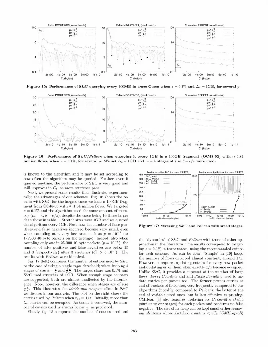
The previous results correspond to querying the algorithmsat Ct = 10GB. Fig. 14 plots the results with S&C for traceCesca when setting Δc = 100MB and querying the algo-rithm exactly every 100MB; i.e. each time the thresholdis adapted, when d coincides to the right threshold. 100adaptations/queries occur before Ct = 10GB. We targetedz = 0.1% and m = 4 stages of size e/z were supported. Eachcurve corresponds to using a different sampling probabilityp and, each dot, to the average in 80 realizations. Note thelogscale on the y axis. As can be seen, the number of falsepositives and false negatives decrease in Ct, even when sam-pling with a small probability such as 10−5: the more trafficis observed, the higher the threshold gets; further, the higherthe sampling probability, the faster the threshold raises andthe higher it becomes. The rightmost plot shows the averagerelative error for those flows exceeding z that get reported.Note how the error decreases as 1/

√zpCt (in %), except for

some “ripple” that appears when the sampling probability ishigh. This is the effect of interference; in our analysis, theterm E[c2

min] in (3). The reason why it appears is becausewe increased the sampling rate but kept the number of stagecounters the same. As of our analysis, we should have in-creased the number of stages as m = log(zpΔc). Despitethis fact, note how the number of false positives and falsenegatives decreased.

To illustrate the effect of Δc, fig. 15 shows the results for

S&C for the same setups except that we set Δc = 1GB (tentimes larger). Since Δc = 1GB, d was only adapted 10 timesand the algorithm were queried 10 times per stretch.

Note how, when Ct < 109 (i.e. in the first 1GB stretch),the algorithm produces almost no false positive but it fails toreport many large flows. This is because, setting Δc = 1GB,the initial sample threshold is very high. Further, the higherthe sampling rate, the higher the initial value that d takesand the fewer the flows (large or small) that pass. However,beyond the first 1GB, the number of false positives is almostidentical to the case where Δc = 100MB in fig. 14. Further,the number of false negatives greatly decreases when the firststretch ends. Notice how the curves exhibit local“peaks”andsuddenly decrease to much smaller values, every 1GB. Thisis, clearly, the effect of (locally) overthresholding: the peakscorrespond to queries performed within the stretch (wherethe sample threshold is higher than the right) and, the mini-mums, to queries executed when d = zpCt. The observationis that, at such points, S&C performed identically to thecase where Δc = 100MB: the black circles in fig. 15 (cen-ter) correspond to the number of false negatives for the caseΔc = 100MB and p = 10−3. Another observation is thatthis effect is most visible for large sampling rates. This isbecause, for such values of p, the threshold increases fasterand the “gap” due to overthresholding is larger.

Concerning the relative error, note that, beyond the firststretch, it coincides to that when Δc = 100MB. The reasonwhy it is smaller when Ct < 109 if Δc = 1GB is becauseit corresponds to the error for a few very large flows thatwere detected despite overthresholding. Pelican producedidentical results to the case where Δc = 100MB, no mat-ter when we queried it. This illustrates the advantages ofPelican and the limitations of S&C. We note, however, thatthis drawback of S&C may not be an issue in practice as Δc

282

0.1

1

10

100

2e+09 4e+09 6e+09 8e+09 1e+10Ct (bytes)

False POSITIVES, (m=4 b=e/z)

Δc p=10-5

p=10-4

p=10-3

0.1

1

10

100

2e+09 4e+09 6e+09 8e+09 1e+10Ct (bytes)

False NEGATIVES, (m=4 b=e/z)

Δc

p=10-5

p=10-4

p=10-3

0.1

1

10

100

2e+09 4e+09 6e+09 8e+09 1e+10Ct (bytes)

% relative ERROR, (m=4 b=e/z)

Δc

p=10-5

p=10-4

p=10-3

p=10-2

Figure 15: Performance of S&C querying every 100MB in trace Cesca when z = 0.1% and Δc = 1GB, for several p.

0

5

10

15

20

25

30

2e+10 4e+10 6e+10 8e+10 1e+11Ct (bytes)

False POSITIVES, (m=4 b=e/z)

p=10-6

p=10-5

p=10-4

p=10-3

0

5

10

15

20

2e+10 4e+10 6e+10 8e+10 1e+11Ct (bytes)

False NEGATIVES, (m=4 b=e/z)

p=10-6

p=10-5

p=10-4

p=10-3

0.1

1

10

100

2e+10 4e+10 6e+10 8e+10 1e+11Ct (bytes)

% relative ERROR, (m=4 b=e/z)

p=10-6

p=10-5

p=10-4

p=10-3

Figure 16: Performance of S&C/Pelican when querying it every 1GB in a 100GB fragment (OC48-02) with ≈ 1.84

million flows, when z = 0.1%, for several p. We set Δc = 1GB and m = 4 stages of size b = e/z were used.

is known to the algorithm and it may be set according tohow often the algorithm may be queried. Further, even ifqueried anytime, the performance of S&C is very good andstill improves in Ct; as more stretches pass.

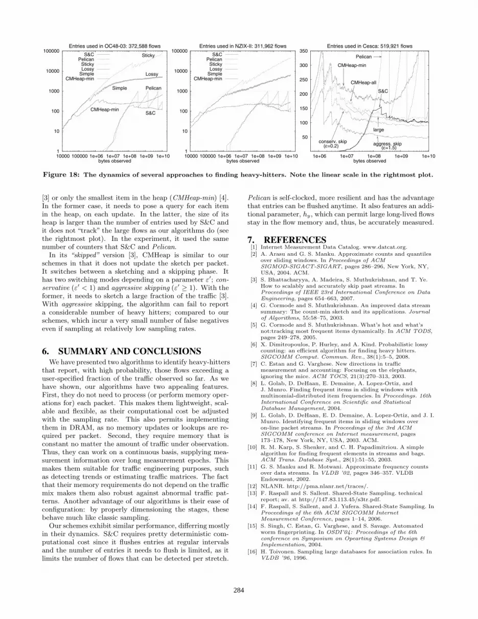
Next, we present some results that illustrate, experimen-tally, the advantages of our schemes. Fig. 16 shows the re-sults with S&C for the largest trace we had; a 100GB frag-ment from OC48-03 with ≈ 1.84 million flows. We targetedz = 0.1% and the algorithm used the same amount of mem-ory (m = 4, b = e/z), despite the trace being 10 times largerthan those in table 1. Stretch sizes were 1GB and we queriedthe algorithm every 1GB. Note how the number of false pos-itives and false negatives incurred become very small, evenwhen sampling at a very low rate, such as p = 10−5 (or1/2500 40-byte packets on the average). Indeed, also whensampling only one in 25.000 40-byte packets (p = 10−6), thenumber of false positives and false negatives are below 15and 8 (respectively) after 3 stretches (Ct > 3 1010). Theresults with Pelican were identical.

Fig. 17 (left) compares the number of entries used by S&Cto the case of using a single right threshold; when keeping 4stages of size b = e

zand 1

8ez. The target share was 0.1% and

S&C used stretches of 1GB. When enough stage countersare supported, both are almost unaffected by the interfer-ence. Note, however, the difference when stages are of size18

ez. This illustrates the divide-and-conquer effect in S&C

we discuss in our analysis. The plot on the right shows theentries used by Pelican when toc = 1/z. Initially, more thantoc entries can be occupied. As traffic is observed, the num-ber of entries used is always below 1

z, as predicted.

Finally, fig. 18 compares the number of entries used and

0

50

100

150

200

250

300

350

400

450

1e+08 1e+09 1e+10traffic observed (bytes)

Entries used by S&C for trace CESCA

S&C, b=e/zS&C, b=e/8zn=1 b=e/zn=1 b=e/8z

10

100

1000

1e+06 1e+07 1e+08 1e+09 1e+10traffic observed (bytes)

Entries used by Pelican for trace CESCA

Pelican b=e/8zn=1 b=e/zn=1 b=e/8z

Figure 17: Stressing S&C and Pelican with small stages.

the “dynamics” of S&C and Pelican with those of other ap-proaches in the literature. The results correspond to target-ing z = 0.1% in three traces, using the recommended setupsfor each scheme. As can be seen, “Simple” in [10] keepsthe number of flows detected almost constant, around 1/z.However, it requires updating entries for every new packetand updating all of them when exactly 1/z become occupied.Unlike S&C, it provides a superset of the number of largeflows. Lossy Counting and and Sticky Sampling need to up-date entries per packet too. The former prunes entries atend of buckets of fixed size, very frequently compared to ouralgorithms (notably, compared to Pelican); the latter at theend of variable-sized ones, but is less effective at pruning.CMHeap [4] also requires updating its Count-Min sketch(similar to our stages) for each packet and produces no falsenegative. The size of its heap can be kept small either remov-ing all items whose sketched count is < zCt (CMHeap-all)

283

1

10

100

1000

10000

100000

10000 100000 1e+06 1e+07 1e+08 1e+09 1e+10bytes observed

Entries used in OC48-03: 372,588 flows

Sticky

Lossy

Simple

CMHeap-min

Pelican

S&C

S&CPelican

StickyLossy

SimpleCMHeap-min

1

10

100

1000

10000

100000

10000 100000 1e+06 1e+07 1e+08 1e+09 1e+10bytes observed

Entries used in NZIX-II: 311,962 flows

S&CPelican

StickyLossy

SimpleCMHeap-min

50

100

150

200

250

300

350

1e+06 1e+07 1e+08 1e+09 1e+10bytes observed

Entries used in Cesca: 519,921 flows

CMHeap-min

CMHeap-all

aggress. skip(ε=1.5)

conserv. skip(ε=0.2)

Pelican

S&C

large

Figure 18: The dynamics of several approaches to finding heavy-hitters. Note the linear scale in the rightmost plot.

[3] or only the smallest item in the heap (CMHeap-min) [4].In the former case, it needs to pose a query for each itemin the heap, on each update. In the latter, the size of itsheap is larger than the number of entries used by S&C andit does not “track” the large flows as our algorithms do (seethe rightmost plot). In the experiment, it used the samenumber of counters that S&C and Pelican.

In its “skipped” version [3], CMHeap is similar to ourschemes in that it does not update the sketch per packet.It switches between a sketching and a skipping phase. Ithas two switching modes depending on a parameter ε′; con-servative (ε′ < 1) and aggressive skipping (ε′ ≥ 1). With theformer, it needs to sketch a large fraction of the traffic [3].With aggressive skipping, the algorithm can fail to reporta considerable number of heavy hitters; compared to ourschemes, which incur a very small number of false negativeseven if sampling at relatively low sampling rates.

6. SUMMARY AND CONCLUSIONSWe have presented two algorithms to identify heavy-hitters

that report, with high probability, those flows exceeding auser-specified fraction of the traffic observed so far. As wehave shown, our algorithms have two appealing features.First, they do not need to process (or perform memory oper-ations for) each packet. This makes them lightweight, scal-able and flexible, as their computational cost be adjustedwith the sampling rate. This also permits implementingthem in DRAM, as no memory updates or lookups are re-quired per packet. Second, they require memory that isconstant no matter the amount of traffic under observation.Thus, they can work on a continuous basis, supplying mea-surement information over long measurement epochs. Thismakes them suitable for traffic engineering purposes, suchas detecting trends or estimating traffic matrices. The factthat their memory requirements do not depend on the trafficmix makes them also robust against abnormal traffic pat-terns. Another advantage of our algorithms is their ease ofconfiguration: by properly dimensioning the stages, thesebehave much like classic sampling.

Our schemes exhibit similar performance, differring mostlyin their dynamics. S&C requires pretty deterministic com-putational cost since it flushes entries at regular intervalsand the number of entries it needs to flush is limited, as itlimits the number of flows that can be detected per stretch.

Pelican is self-clocked, more resilient and has the advantagethat entries can be flushed anytime. It also features an addi-tional parameter, hy , which can permit large long-lived flowsstay in the flow memory and, thus, be accurately measured.

7. REFERENCES[1] Internet Measurement Data Catalog. www.datcat.org.

[2] A. Arasu and G. S. Manku. Approximate counts and quantilesover sliding windows. In Proceedings of ACMSIGMOD-SIGACT-SIGART, pages 286–296, New York, NY,USA, 2004. ACM.

[3] S. Bhattacharyya, A. Madeira, S. Muthukrishnan, and T. Ye.How to scalably and accurately skip past streams. InProceedings of IEEE 23rd International Conference on DataEngineering, pages 654–663, 2007.

[4] G. Cormode and S. Muthukrishnan. An improved data streamsummary: The count-min sketch and its applications. Journalof Algorithms, 55:58–75, 2003.

[5] G. Cormode and S. Muthukrishnan. What’s hot and what’snot:tracking most frequent items dynamically. In ACM TODS,pages 249–278, 2005.

[6] X. Dimitropoulos, P. Hurley, and A. Kind. Probabilistic lossycounting: an efficient algorithm for finding heavy hitters.SIGCOMM Comput. Commun. Rev., 38(1):5–5, 2008.

[7] C. Estan and G. Varghese. New directions in trafficmeasurement and accounting: Focusing on the elephants,ignoring the mice. ACM TOCS, 21(3):270–313, 2003.

[8] L. Golab, D. DeHaan, E. Demaine, A. Lopez-Ortiz, andJ. Munro. Finding frequent items in sliding windows withmultinomial-distributed item frequencies. In Proceedings. 16thInternational Conference on Scientific and StatisticalDatabase Management, 2004.

[9] L. Golab, D. DeHaan, E. D. Demaine, A. Lopez-Ortiz, and J. I.Munro. Identifying frequent items in sliding windows overon-line packet streams. In Proceedings of the 3rd ACMSIGCOMM conference on Internet measurement, pages173–178, New York, NY, USA, 2003. ACM.

[10] R. M. Karp, S. Shenker, and C. H. Papadimitriou. A simplealgorithm for finding frequent elements in streams and bags.ACM Trans. Database Syst., 28(1):51–55, 2003.

[11] G. S. Manku and R. Motwani. Approximate frequency countsover data streams. In VLDB ’02, pages 346–357. VLDBEndowment, 2002.

[12] NLANR. http://pma.nlanr.net/traces/.

[13] F. Raspall and S. Sallent. Shared-State Sampling. technicalreport; av. at http://147.83.113.45/s3tr.pdf.

[14] F. Raspall, S. Sallent, and J. Yufera. Shared-State Sampling. InProceedings of the 6th ACM SIGCOMM InternetMeasurement Conference, pages 1–14, 2006.

[15] S. Singh, C. Estan, G. Varghese, and S. Savage. Automatedworm fingerprinting. In OSDI’04: Proceedings of the 6thconference on Symposium on Opearting Systems Design &Implementation, 2004.

[16] H. Toivonen. Sampling large databases for association rules. InVLDB ’96, 1996.

284