a waste supply-use analysis of australian waste flows
TRANSCRIPT
Journal of Economic Structures (2014) 3:5DOI 10.1186/s40008-014-0005-0
R E S E A R C H A RT I C L E Open Access
A Waste Supply-Use Analysis of Australian WasteFlows
Christian John Reynolds · Julia Piantadosi ·John Boland
Received: 18 March 2014 / Revised: 28 August 2014 / Accepted: 19 October 2014 /
© 2014 Reynolds et al.; licensee Springer. This is an Open Access article distributed under the terms ofthe Creative Commons Attribution License (http://creativecommons.org/licenses/by/4.0), which permitsunrestricted use, distribution, and reproduction in any medium, provided the original work is properlycredited.
Abstract In this paper we apply the Lenzen and Reynolds (2014) Waste SupplyUse Table extension of Nakamura and Kondo’s (2002a) Waste Input–Output (WIO)framework to the 2008 Australian economy. This is the first application of any WIO-style method to Australia as a nation. We find that the Services sector has the largestdirect and indirect waste generation for an intermediate sector. This is followed bythe Forestry sector, for direct waste generation, and the Transport sector for directand indirect waste generation effects.
In terms of waste treatment methods, landfill generates the smallest direct andindirect waste tonnages, but it also provides the least amount of economic activity pertonne treated, producing $US2.53 in total of economic production per tonne treated.
Keywords Food waste · Commercial and industrial waste · Municipal solid waste ·Australia input–output
JEL Classification Q53 · Q56 · Q57
1 Introduction
Waste Input–Output (WIO) analysis can provide much needed information regard-ing the economic impact of waste generated by sectors of the economy. A WIO (or
Electronic supplementary material The online version of this article(doi:10.1186/s40008-014-0005-0) contains supplementary material.
C.J. Reynolds (B) · J. Piantadosi · J. BolandCentre for Industrial and Applied Mathematics and the Barbara Hardy Institute, University of SouthAustralia, Mawson Lakes Boulevard, Mawson Lakes, SA 5095, Australiae-mail: [email protected]
C.J. ReynoldsIntegrated Sustainability Analysis, University of Sydney, Sydney, Australia
Page 2 of 16 C.J. Reynolds et al.
Waste Supply Use Table (WSUT)) analysis provides the means to devise interven-tions and policy with a sectoral focus (Nakamura and Kondo 2002a; Kagawa 2005;Kagawa et al. 2007; Tsukui 2007; Lin 2009; Tsukui and Nakamura 2010; Matsubaeet al. 2011; Tsukui et al. 2011, 2012). Yet there has never been a WIO of Australiaconstructed, primarily because the level of waste data required for a WIO have beentoo high (though previously there has been some attempted IO analysis of waste inAustralia (Reynolds and Boland 2011, 2013a, 2013b; Reynolds et al. 2011). How-ever, thanks to the high resolution waste data set of Australia discussed in Lenzenand Reynolds (2014), WIO analysis for Australia is now a reality.
In this paper we apply Lenzen and Reynolds (2014) extension of Nakamura andKondo’s WIO framework, first published in English as (Nakamura 1999), and later(Nakamura and Kondo 2002a, 2002b, 2002c, 2006, 2008, 2009; Nakamura et al.2007; Nakamura 2010) to the Australian economy. It is worth noting again that thisis the first application of any WIO-style method to Australia as a nation.
In Sect. 2 we discuss the methodology, data sources and procedures followed tocreate an Australian WSUT. In Sect. 3 we present the results of a practical applicationof the WSUT methodology to Australia, and discuss these results in Sect. 4. Section 5provides concluding remarks. In Appendix A (Additional files 1–3) we list the directand indirect waste multipliers for 343 intermediate sectors and ten waste treatmentsectors in the Australian economy as of 2008, as well as the disaggregated tonnagesof industrial solid waste (ISW) and municipal solid waste (MSW). In Appendix B(Additional file 4) we provide analysis of the largest direct and indirect waste mul-tipliers for 14 waste types. In Appendix C (Additional file 5) we provide unalteredversions of the aggregated seven sector Coefficients and Leontief matrices (Tables 2and 3) for comparison, and a concordance matrix between the 7 and 343 sector ver-sions of the WSUT. For completeness we also include the simplified Transactionsmatrix and the Gross output vector used for calculations.
2 Methodology
2.1 WSUT Notation
In this paper we will use the notation described in Lenzen and Reynolds (2014). TheWSUT in balanced form is written as
⎛⎝
T11 T12 00 0 W23
W31 W32 0
⎞⎠
⎛⎝
111213
⎞⎠ +
⎛⎝
f0
WF
⎞⎠1F =
⎛⎝
x1x2x3
⎞⎠ (1)
where T11 ∈ RN1×N1 represents an intermediate demand matrix for N1 goods andservice-producing sectors, f ∈ R
N1×NF a final demand matrix for NF final de-mand categories, and x1 ∈ R
N1×1 a gross output vector for N1 goods and service-producing sectors, respectively. Waste generation is categorised per intermediate sec-tor as W31 ∈ R
N3×N1 , and final demand as WF ∈ RN3×NF , distinguishing N3 waste
types in the economy. The monetary inputs T12 ∈ RN1×N2 into N2 waste treatment
Journal of Economic Structures (2014) 3:5 Page 3 of 16
sectors (applying N2 treatment methods) are distinguished from the monetary in-puts T11 into other intermediate sectors. The waste produced by N2 waste treatmentsectors is represented by W32 ∈ R
N3×N2 represent and the waste treated by the N2
waste treatment methods is contained in W23 ∈ RN2×N3 . The vectors x3 ∈R
N3×1 andx2 ∈ R
N2×1 are the total output of N3 waste types and N2 waste treatment methodsfor the economy, respectively. 11, 12, 13, and 1F are column vectors of ones withappropriate dimensions.
We can express Eq. (1) in coefficient form, given by
⎛⎝
A11 A12 00 0 S23
G31 G32 0
⎞⎠
⎛⎝
x1x2x3
⎞⎠ +
⎛⎝
f0
WF
⎞⎠1F =
⎛⎝
x1x2x3
⎞⎠ (2)
where we define input coefficients matrices A11 = T11x̂−11 ($/$), A12 = T12x̂−1
2 ($/t),G31 = W31x̂−1
1 (t/$), and G32 = W32x̂−12 (t/t), where the “hat” over a vector x de-
notes a diagonal matrix with the elements of the vector along the main diagonal.For instance, if x = [ x1
x2
]then x̂ = [ x1 0
0 x2
]. The matrix S23 ∈ RN2×N3 is an N2 × N3
version of Nakamura and Kondo’s (2009) allocation matrix (Nakamura and Kondo2002a). The elements of S23(i, j) refer to the share of waste type j that is treated bytreatment method i, and are normalised according to
∑j S23(i, j) = 1.
The Leontief inverse of the WSUT is finally formulated as follows:
⎛⎝
x1x2x3
⎞⎠ =
⎛⎝
I − A11 −A12 00 I −S23
−G31 −G32 I
⎞⎠
−1 ⎛⎝
f0
WF
⎞⎠1F . (3)
2.2 Data Sources and Processing
In Lenzen and Reynolds (2014) a national Australian WSUT for 2008 was providedas a technical example. We now further describe the data sources, processing andcompilation methods used to create this WSUT.
The Australian IO table was sourced from the Eora database in US dollars (Lenzenet al. 2011, 2012a, 2012b, 2013), to provide the WSUT block T11, distinguishingN1 = 343 industry sectors. Waste data were estimated (as discussed in Lenzen andReynolds 2014 and Reynolds 2013), with only formal disposal accounted for. Thiswaste estimation methodology is discussed in abridged form below.
The Australian waste treatment sector is quite small employing ∼3,300 persons,(0.3% of total Australian labour) and generating 9 billion AU$ gross output in 2009–2010. This can be explained by the majority of waste being sent to landfill, withmuch of the recycled/recovered material being sent overseas for reprocessing (Aus-tralian Bureau of Statistics 2013a). In addition to being small in size, the Australianwaste (and recycling) treatment sector is not well documented, thus to create thisWSUT we disaggregated the recycling parts from Eora sector #344 ‘Sanitary andgarbage disposal’ into the block T12, yielding N2 = 10 separate treatment sectors, us-ing data/sector labels on recycling from Department of Sustainability, Environment,
Page 4 of 16 C.J. Reynolds et al.
Water, Population and Communities (DSEWPaC) (DSEWPaC 2012) and Hyder Con-sulting (Hyder Consulting 2012).1 Waste data for WSUT block W31, distinguishingMunicipal Solid Waste (MSW), Commercial and Industrial (C&I), and Constructionand Demolition (C&D) origins were sourced from the Australian Bureau of Statistics(Australian Bureau of Statistics 2008, 2009, 2010, 2011, 2013b), as well as HyderConsulting (Hyder Consulting 2012), DSEWPaC (Department of Sustainability, En-vironment, Water, Population and Communities 2012; Environment Protection andHeritage Council and the Department of Environment, Water, Heritage and the Arts2010), and Inside Waste (WCS Market Intelligence 2008; Waste Management & En-vironment Media Pty Ltd 2011). Data on recycling (WSUT block W32) were sourcedfrom DSEWPaC (DSEWPaC 2012) and Hyder Consulting (Hyder Consulting 2012).WF was estimated using MSW data (2008, 2012). This step is an assumption for sim-plicity, as MSW is produced by households and households are the major contributorto final demand. Finally, S23 and W23 were populated using data from Wright Cor-porate Strategy Pty Ltd and Rawtec Pty Ltd (Wright Corporate Strategy Pty Ltd andRawtec Pty Ltd 2010) and Hyder Consulting (Hyder Consulting 2012). In our ex-ample we distinguish N3 = 14 waste types.2 Where data were aggregated across theN1 = 344 industry sectors, we applied a prorating procedure using sectoral economicoutput (x, gross output) as a proxy (see Lenzen et al. 2012a, 2012b for more details).
To disaggregate the waste generation and treatment data for W31 we utilised abinary concordance matrix that uniquely allocates C&I and C&D waste streamsto the 344 sectors of the Eora database’s Australian IOT. C&D waste produc-ing sectors were understood to be numbered 68, 170, 218, 232, 243–249, 253–255, and 257. Fourteen waste types (Organics (Food, Green); Timber; TextilesAnd Clothing; Paper, Printing, And Cardboard; Plastics; Rubber; Glass; PlasterBoard; Cement And Construction; Metals (Ferrous, Non-Ferrous); Electronic Waste;and Other), were mapped across the intermediate sectors using the average fromthree proxy vectors: total sectoral gross output per sector, employment per sector,and the amount of inputs of production per intermediate sector (Reynolds 2013;Lenzen and Reynolds 2014). This method assumes that each sector produces wasterelative to its economic size and employment capacity: i.e. we distributed the totalamount of waste among the waste treatment methods with the larger the economicsize and employment level, the greater the volume of waste was assumed to have beentreated. No assumptions were made regarding the relative technological efficiency ofwaste generation between sectors.
The composition of waste generated by each sector is assumed to be unique, andso was estimated by applying industry → product → waste concordance matricesto normalised versions of the matrices A11 (the direct inputs between the interme-diate sectors of the economy), and A12 (the direct inputs between the intermediatesector of the economy, and the waste treatment sectors). These concorded A matrices
1Landfill (Lf), and recycling of glass (Gl R), paper and cardboard (Ppr R), plastics (Pla R), metals (Me), or-ganics treatment and commercial composting (Or C), construction & demolition (Cn R), e-waste (EW R),leather and textiles (Le R), and tires and other rubber (Ru R).2Food waste (Food), green waste (Gdn), timber (Tim), textiles and clothing (Txt), paper, printing andcardboard (Ppr), plastics (Pla), rubber (Ru), glass (Gl), plaster board (Pb), cement and construction (Cn),ferrous metals (M F), non-ferrous metal (MNF), electronic waste (EW), and other (Oth).
Journal of Economic Structures (2014) 3:5 Page 5 of 16
were multiplied by total waste produced per sector to replicate the phenomenon ofeach product/industry having different waste types associated with its consumptionand production. For example, the sectors of Forestry (sector number 35), Softwoods(36), and Hardwoods (37) are all sectors associated with Timber products, which isin turn associated with Timber waste. Each sector that has a part of its direct require-ments (coefficient multiplier) attributed to Forestry (35), Softwoods (36), etc. will beassumed to produce a proportional amount of timber waste relative to the amount oftimber products used in its production processes. For full discussion of this method-ology please refer to Reynolds (2013).
To summarise, the resulting Australian WSUT model has N1 = 343, N2 = 10, andN3 = 14. Note that N1 has one sector less than the equivalent Eora table, as this sectorhas been disaggregated to become N2.
3 Results
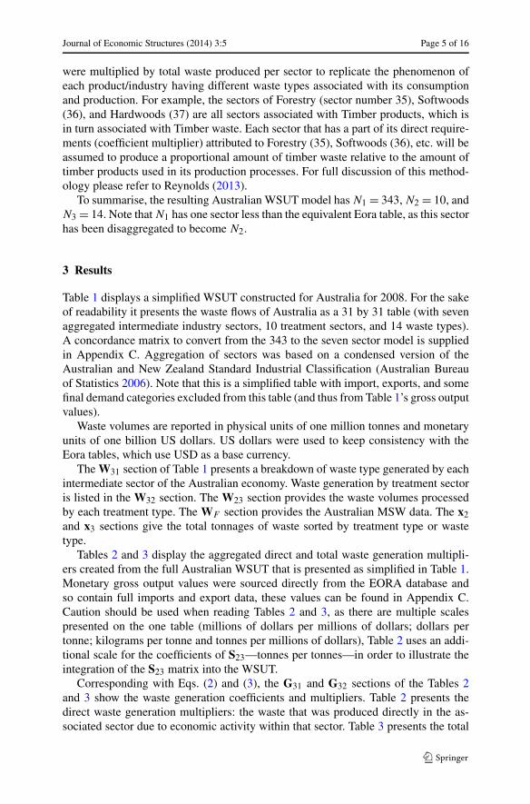
Table 1 displays a simplified WSUT constructed for Australia for 2008. For the sakeof readability it presents the waste flows of Australia as a 31 by 31 table (with sevenaggregated intermediate industry sectors, 10 treatment sectors, and 14 waste types).A concordance matrix to convert from the 343 to the seven sector model is suppliedin Appendix C. Aggregation of sectors was based on a condensed version of theAustralian and New Zealand Standard Industrial Classification (Australian Bureauof Statistics 2006). Note that this is a simplified table with import, exports, and somefinal demand categories excluded from this table (and thus from Table 1’s gross outputvalues).
Waste volumes are reported in physical units of one million tonnes and monetaryunits of one billion US dollars. US dollars were used to keep consistency with theEora tables, which use USD as a base currency.
The W31 section of Table 1 presents a breakdown of waste type generated by eachintermediate sector of the Australian economy. Waste generation by treatment sectoris listed in the W32 section. The W23 section provides the waste volumes processedby each treatment type. The WF section provides the Australian MSW data. The x2and x3 sections give the total tonnages of waste sorted by treatment type or wastetype.
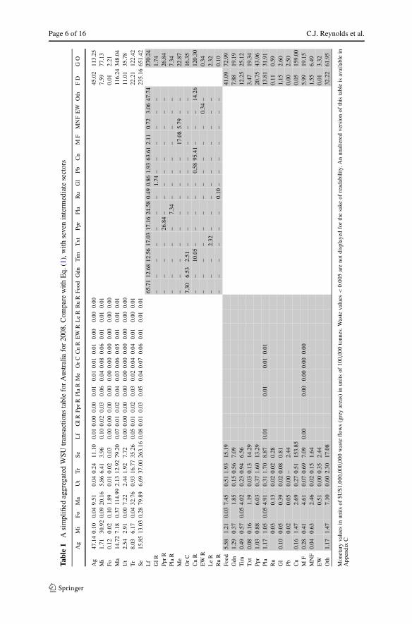
Tables 2 and 3 display the aggregated direct and total waste generation multipli-ers created from the full Australian WSUT that is presented as simplified in Table 1.Monetary gross output values were sourced directly from the EORA database andso contain full imports and export data, these values can be found in Appendix C.Caution should be used when reading Tables 2 and 3, as there are multiple scalespresented on the one table (millions of dollars per millions of dollars; dollars pertonne; kilograms per tonne and tonnes per millions of dollars), Table 2 uses an addi-tional scale for the coefficients of S23—tonnes per tonnes—in order to illustrate theintegration of the S23 matrix into the WSUT.
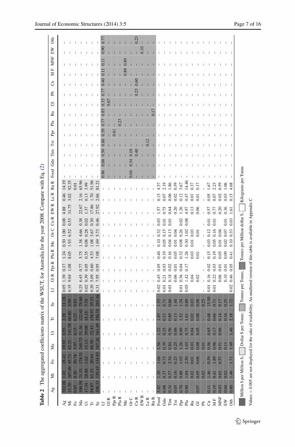
Corresponding with Eqs. (2) and (3), the G31 and G32 sections of the Tables 2and 3 show the waste generation coefficients and multipliers. Table 2 presents thedirect waste generation multipliers: the waste that was produced directly in the as-sociated sector due to economic activity within that sector. Table 3 presents the total
Page 6 of 16 C.J. Reynolds et al.
Tabl
e1
Asi
mpl
ified
aggr
egat
edW
SUtr
ansa
ctio
nsta
ble
for
Aus
tral
iafo
r20
08.C
ompa
rew
ithE
q.(1
),w
ithse
ven
inte
rmed
iate
sect
ors
Ag
Mi
FoM
aU
tT
rSe
Lf
GlR
Ppr
RPl
aR
Me
Or
CC
nR
EW
RL
eR
Ru
RFo
odG
dnT
imT
xtPp
rPl
aR
uG
lPb
Cn
MF
MN
FE
WO
thF
DG
O
Ag
47.1
40.
100.
049.
510.
040.
2411
.10
0.01
0.00
0.00
0.01
0.01
0.01
0.01
0.00
0.00
0.00
45.0
211
3.25
Mi
1.71
30.9
20.
0920
.16
5.86
6.41
3.96
0.10
0.02
0.03
0.06
0.04
0.08
0.06
0.01
0.01
0.01
7.59
77.1
3Fo
0.12
0.02
0.10
1.89
0.01
0.02
0.03
0.00
0.00
0.00
0.00
0.00
0.00
0.00
0.00
0.00
0.00
0.01
2.21
Ma
14.7
27.
180.
3711
4.99
2.13
12.9
279
.20
0.07
0.01
0.02
0.04
0.03
0.06
0.05
0.01
0.01
0.01
116.
2434
8.04
Ut
2.54
2.91
0.00
7.22
2.44
1.92
7.72
0.00
0.00
0.00
0.00
0.00
0.00
0.00
0.00
0.00
0.00
11.0
135
.78
Tr
8.03
6.17
0.04
32.7
60.
9316
.77
35.2
60.
050.
010.
020.
030.
020.
040.
040.
010.
000.
0122
.21
122.
42Se
15.8
513
.03
0.28
79.8
96.
6937
.00
263.
160.
080.
010.
030.
050.
040.
070.
060.
010.
010.
0123
5.16
651.
42L
f65
.71
12.6
812
.56
17.0
317
.16
24.5
80.
490.
861.
9363
.61
2.11
0.72
3.06
47.7
427
0.24
GlR
––
––
––
–1.
74–
––
––
–1.
74Pp
rR
––
––
26.8
4–
––
––
––
––
26.8
4Pl
aR
––
––
–7.
34–
––
––
––
–7.
34M
e–
––
––
––
––
–17
.08
5.79
––
22.8
7O
rC
7.30
6.53
2.51
––
––
––
––
––
–16
.35
Cn
R–
–10
.05
––
––
–0.
5895
.41
––
–14
.26
120.
30E
WR
––
––
––
––
––
––
0.34
–0.
34L
eR
––
–2.
32–
––
––
––
––
–2.
32R
uR
––
––
––
0.10
––
––
––
–0.
10Fo
od5.
581.
210.
037.
450.
511.
9315
.19
41.0
972
.99
Gdn
1.29
0.37
1.85
0.15
0.56
7.09
7.88
19.1
9T
im0.
490.
570.
054.
020.
230.
946.
5612
.25
25.1
2T
xt0.
080.
161.
190.
030.
1314
.29
3.47
19.3
4Pp
r1.
030.
886.
030.
371.
6013
.29
20.7
543
.96
Pla
1.17
1.05
0.05
4.91
0.31
1.70
8.87
0.01
0.01
0.01
0.01
13.8
131
.91
Ru
0.03
0.13
0.02
0.02
0.28
0.11
0.59
Gl
0.10
0.05
0.39
0.02
0.08
0.81
1.15
2.60
Pb0.
020.
050.
00–
2.44
0.00
2.50
Cn
0.16
1.47
2.69
0.27
0.51
153.
850.
0515
9.00
MF
0.28
0.41
4.61
0.07
0.69
7.09
0.00
0.00
0.00
0.00
0.00
5.99
19.1
5M
NF
0.04
0.63
2.46
0.02
0.15
1.64
1.55
6.49
EW
0.51
0.00
0.35
2.44
0.01
3.32
Oth
1.17
1.47
7.10
0.60
2.30
17.0
832
.22
61.9
5
Mon
etar
yva
lues
inun
itsof
$US1
,000
,000
,000
was
teflo
ws
(gre
yar
eas)
inun
itsof
100,
000
tonn
es.W
aste
valu
es<
0.00
5ar
eno
tdis
play
edfo
rth
esa
keof
read
abili
ty.A
nun
alte
red
vers
ion
ofth
ista
ble
isav
aila
ble
inA
ppen
dix
C
Journal of Economic Structures (2014) 3:5 Page 7 of 16
Tabl
e2
The
aggr
egat
edco
effic
ient
sm
atri
xof
the
WSU
T,fo
rA
ustr
alia
for
the
year
2008
.Com
pare
with
Eq.
(2)
Ag
Mi
FoM
aU
tT
rSe
Lf
GlR
Ppr
RPl
aR
Me
Or
CC
nR
EW
RL
eR
Ru
RFo
odG
dnT
imT
xtPp
rPl
aR
uG
lPb
Cn
MF
MN
FE
WO
th
Ag
322.
081.
0218
.42
19.9
20.
932.
2811
.18
0.05
1.39
0.17
1.24
0.30
1.00
0.08
4.88
0.46
14.1
9–
––
––
––
––
––
––
–M
i11
.70
307.
0945
.73
42.2
114
1.58
60.8
03.
990.
359.
041.
088.
051.
936.
520.
5331
.75
3.02
92.3
5–
––
––
––
––
––
––
–Fo
0.85
0.20
50.7
63.
970.
150.
220.
030.
01–
––
––
––
––
––
––
–M
a10
0.59
71.3
317
8.51
240.
7551
.36
122.
4379
.80
0.25
6.45
0.77
5.75
1.38
4.66
0.38
22.6
72.
1665
.96
––
––
––
––
––
––
––
Ut
17.3
428
.88
1.62
15.1
359
.00
18.1
57.
780.
020.
390.
050.
350.
080.
280.
021.
370.
133.
99–
––
––
––
––
––
––
–T
r54
.87
61.3
320
.44
68.5
922
.43
158.
9735
.53
0.20
5.09
0.60
4.53
1.08
3.67
0.30
17.8
61.
7051
.96
––
––
––
––
––
––
––
Se10
8.33
129.
4313
4.83
167.
2616
1.49
350.
7426
5.16
0.31
7.95
0.95
7.08
1.69
5.73
0.46
27.9
22.
6681
.21
––
––
––
––
––
––
––
Lf
––
––
––
––
––
––
––
––
–0.
960.
660.
500.
880.
390.
770.
830.
330.
770.
400.
110.
110.
900.
77G
lR–
––
––
––
––
––
––
––
––
––
––
––
–0.
67–
––
––
–Pp
rR
––
––
––
––
––
––
––
––
––
––
–0.
61–
––
––
––
––
Pla
R–
––
––
––
––
––
––
––
––
––
––
–0.
23–
––
––
––
–M
e–
––
––
––
––
––
––
––
––
––
––
––
––
––
0.89
0.89
––
Or
C–
––
––
––
––
––
––
––
––
0.04
0.34
0.10
––
––
––
––
––
–C
nR
––
––
––
––
––
––
––
––
––
–0.
40–
––
––
0.23
0.60
––
–0.
23E
WR
––
––
––
––
––
––
––
––
––
––
––
––
––
––
–0.
10–
Le
R–
––
––
––
––
––
––
––
––
––
–0.
12–
––
––
––
––
–R
uR
––
––
––
––
––
––
––
––
––
––
––
–0.
17–
––
––
––
Food
3.82
1.20
1.66
1.56
1.22
1.83
1.53
0.02
0.45
0.05
0.40
0.10
0.32
0.03
1.57
0.15
4.57
––
––
––
––
––
––
––
Gdn
0.88
0.37
0.73
0.39
0.35
0.53
0.71
0.01
0.21
0.03
0.19
0.05
0.15
0.01
0.75
0.07
2.19
––
––
––
––
––
––
––
Tim
0.34
0.57
2.54
0.84
0.56
0.89
0.66
0.01
0.18
0.02
0.16
0.04
0.13
0.01
0.64
0.06
1.86
––
––
––
––
––
––
––
Txt
0.05
0.16
0.23
0.25
0.06
0.13
1.44
0.06
0.01
0.05
0.01
0.04
0.20
0.02
0.59
––
––
––
––
––
––
––
Ppr
0.70
0.88
1.03
1.26
0.89
1.52
1.34
0.01
0.36
0.04
0.32
0.08
0.26
0.02
1.26
0.12
3.67
––
––
––
––
––
––
––
Pla
0.80
1.04
2.50
1.03
0.75
1.61
0.89
0.05
1.42
0.17
1.26
0.30
1.02
0.08
4.97
0.47
14.4
6–
––
––
––
––
––
––
–R
u0.
020.
010.
030.
040.
020.
030.
040.
030.
010.
030.
130.
010.
37–
––
––
––
––
––
––
–G
l0.
070.
050.
060.
080.
050.
080.
080.
020.
010.
010.
060.
010.
17–
––
––
––
––
––
––
–Pb
0.02
–0.
01–
0.25
––
––
––
––
––
––
––
––
––
––
––
––
Cn
0.11
1.46
0.59
0.56
0.65
0.48
15.5
00.
010.
160.
020.
150.
030.
120.
010.
570.
051.
67–
––
––
––
––
––
––
–M
F0.
190.
411.
890.
960.
170.
660.
710.
010.
220.
030.
190.
050.
160.
010.
770.
072.
23–
––
––
––
––
––
––
–M
NF
0.03
0.62
0.57
0.51
0.06
0.14
0.17
0.06
0.01
0.05
0.01
0.04
0.20
0.02
0.59
––
––
––
––
––
––
––
EW
0.04
0.02
0.11
0.34
0.25
0.10
0.01
0.09
0.02
0.07
0.01
0.36
0.03
1.06
––
––
––
––
––
––
––
Oth
0.80
1.46
1.71
1.49
1.46
2.18
1.72
0.02
0.46
0.05
0.41
0.10
0.33
0.03
1.61
0.15
4.68
––
––
––
––
––
––
––
Mill
ion
$pe
rM
illio
n$;
Dol
lar
$pe
rTo
nne;
Tonn
espe
rTo
nne;
Tonn
espe
rM
illio
ndo
llar
$;K
ilogr
ams
per
Tonn
e
Val
ues<
0.00
5ar
eno
tdis
play
edfo
rth
esa
keof
read
abili
ty.A
nun
alte
red
vers
ion
ofth
ista
ble
isav
aila
ble
inA
ppen
dix
C
Page 8 of 16 C.J. Reynolds et al.
Tabl
e3
Agg
rega
ted
tota
lwas
tege
nera
tion
mul
tiplie
rsof
the
WSU
T,fo
rA
ustr
alia
for
the
year
2008
.Com
pare
with
Eq.
(3)
Ag
Mi
FoM
aU
tT
rSe
Lf
GlR
Ppr
RPl
aR
Me
Or
CC
nR
EW
RL
eR
Ru
RFo
odG
dnT
imT
xtPp
rPl
aR
uG
lPb
Cn
MF
MN
FE
WO
th
Ag
1,48
9.83
15.5
543
.73
49.2
312
.19
24.9
729
.52
0.11
2.90
0.34
2.58
0.62
2.09
0.17
10.1
70.
9729
.58
0.20
0.78
0.33
0.21
0.25
0.68
5.12
1.98
0.12
0.15
0.56
0.56
1.12
0.12
Mi
64.5
81,
482.
9510
1.35
109.
1823
7.93
141.
4830
.69
0.59
15.2
71.
8213
.60
3.25
11.0
10.
8953
.62
5.10
155.
971.
044.
131.
751.
131.
343.
5827
.00
10.4
20.
660.
772.
962.
965.
890.
66Fo
2.51
1.26
1,05
4.86
5.99
0.87
1.61
0.82
0.07
0.01
0.06
0.01
0.05
0.24
0.02
0.71
0.02
0.01
0.01
0.01
0.02
0.12
0.05
0.01
0.01
0.03
Ma
268.
3721
0.29
311.
371,
405.
7514
5.77
296.
6617
4.19
0.55
14.3
11.
7012
.74
3.05
10.3
20.
8350
.25
4.78
146.
190.
973.
871.
641.
061.
253.
3625
.31
9.77
0.62
0.72
2.78
2.78
5.52
0.62
Ut
39.5
255
.23
14.9
333
.18
1,07
6.89
39.6
517
.86
0.06
1.53
0.18
1.37
0.33
1.11
0.09
5.39
0.51
15.6
70.
100.
420.
180.
110.
130.
362.
711.
050.
070.
080.
300.
300.
590.
07T
r14
0.65
144.
5875
.75
144.
9673
.65
1,25
6.27
80.4
60.
379.
501.
138.
462.
036.
850.
5533
.37
3.18
97.0
80.
652.
571.
090.
700.
832.
2316
.81
6.49
0.41
0.48
1.84
1.84
3.67
0.41
Se36
8.67
393.
0332
8.52
424.
3634
9.07
705.
151,
453.
090.
8522
.09
2.63
19.6
74.
7115
.94
1.29
77.5
97.
3922
5.71
1.50
5.98
2.53
1.64
1.93
5.18
39.0
815
.08
0.95
1.11
4.29
4.29
8.53
0.95
Lf
16.6
914
.69
15.3
714
.98
11.4
420
.18
20.5
41,
000.
307.
750.
926.
901.
655.
590.
4527
.23
2.59
79.2
295
7.53
662.
1050
0.89
880.
5739
0.68
771.
8284
3.71
335.
2977
0.33
400.
3911
1.50
111.
5090
2.99
770.
33G
lR0.
120.
090.
090.
120.
080.
130.
101,
000.
040.
010.
040.
010.
030.
150.
010.
440.
010.
010.
0867
0.03
0.01
0.01
0.02
Ppr
R1.
341.
451.
331.
671.
192.
081.
440.
030.
701,
000.
080.
620.
150.
510.
042.
460.
237.
160.
050.
190.
080.
0561
0.06
0.16
1.24
0.48
0.03
0.04
0.14
0.14
0.27
0.03
Pla
R0.
490.
550.
810.
520.
380.
730.
390.
020.
490.
061,
000.
430.
100.
350.
031.
700.
164.
960.
030.
130.
060.
040.
0423
0.11
0.86
0.33
0.02
0.02
0.09
0.09
0.19
0.02
Me
1.10
2.07
3.13
2.42
0.96
1.99
1.46
0.03
0.83
0.10
0.74
1,00
0.18
0.60
0.05
2.90
0.28
8.43
0.06
0.22
0.09
0.06
0.07
0.19
1.46
0.56
0.04
0.04
890.
1689
0.16
0.32
0.04
Or
C1.
030.
630.
890.
670.
510.
840.
650.
010.
320.
040.
290.
071,
000.
230.
021.
130.
113.
2843
.02
340.
0910
0.04
0.02
0.03
0.08
0.57
0.22
0.01
0.02
0.06
0.06
0.12
0.01
Cn
R4.
846.
525.
736.
075.
109.
0614
.90
0.12
2.99
0.36
2.66
0.64
2.16
1,00
0.17
10.5
11.
0030
.56
0.20
0.81
400.
340.
220.
260.
705.
292.
0423
0.13
600.
150.
580.
581.
1523
0.13
EW
R0.
020.
020.
010.
030.
010.
060.
040.
020.
020.
021,
000.
070.
010.
210.
010.
040.
0110
0.01
Le
R0.
090.
110.
100.
120.
080.
150.
260.
050.
010.
050.
010.
040.
191,
000.
020.
550.
010.
0112
0.01
0.10
0.04
0.01
0.01
0.02
Ru
R0.
010.
010.
010.
010.
010.
010.
010.
010.
010.
031,
000.
0917
0.02
0.01
Food
7.06
3.10
3.18
3.48
2.54
4.16
2.82
0.06
1.50
0.18
1.33
0.32
1.08
0.09
5.26
0.50
15.2
91,
000.
100.
410.
170.
110.
130.
352.
651.
020.
060.
080.
290.
290.
580.
06G
dn1.
791.
031.
251.
020.
831.
371.
190.
020.
570.
070.
500.
120.
410.
031.
990.
195.
780.
041,
000.
150.
060.
040.
050.
131.
000.
390.
020.
030.
110.
110.
220.
02T
im1.
161.
453.
311.
711.
171.
951.
220.
020.
640.
080.
570.
140.
460.
042.
250.
216.
550.
040.
171,
000.
070.
050.
060.
151.
130.
440.
030.
030.
120.
120.
250.
03T
xt0.
710.
880.
821.
000.
661.
272.
150.
020.
450.
050.
400.
100.
330.
031.
580.
154.
610.
030.
120.
051,
000.
030.
040.
110.
800.
310.
020.
020.
090.
090.
170.
02Pp
r2.
192.
382.
172.
731.
953.
402.
350.
041.
150.
141.
020.
240.
830.
074.
030.
3811
.74
0.08
0.31
0.13
0.09
1,00
0.10
0.27
2.03
0.78
0.05
0.06
0.22
0.22
0.44
0.05
Pla
2.13
2.41
3.53
2.25
1.65
3.16
1.68
0.08
2.11
0.25
1.88
0.45
1.52
0.12
7.41
0.71
21.5
60.
140.
570.
240.
160.
181,
000.
493.
731.
440.
090.
110.
410.
410.
810.
09R
u0.
030.
060.
030.
060.
060.
060.
050.
050.
010.
050.
010.
040.
190.
020.
540.
010.
010.
011,
000.
090.
040.
010.
010.
02G
l0.
170.
140.
140.
170.
110.
190.
140.
060.
010.
060.
010.
050.
230.
020.
660.
020.
010.
010.
020.
111,
000.
040.
010.
010.
02Pb
0.09
0.12
0.09
0.12
0.09
0.18
0.36
0.06
0.01
0.05
0.01
0.04
0.20
0.02
0.60
0.02
0.01
0.01
0.01
0.10
0.04
100,
00.2
50.
010.
010.
02C
n6.
228.
486.
097.
636.
5711
.94
22.7
20.
153.
950.
473.
520.
842.
850.
2313
.87
1.32
40.3
60.
271.
070.
450.
290.
350.
936.
992.
700.
171,
000.
200.
770.
771.
520.
17M
F0.
941.
202.
631.
830.
721.
691.
280.
020.
650.
080.
580.
140.
470.
042.
280.
226.
620.
040.
180.
070.
050.
060.
151.
150.
440.
030.
031,
000.
130.
130.
250.
03M
NF
0.30
1.12
0.89
0.89
0.36
0.54
0.36
0.01
0.28
0.03
0.25
0.06
0.20
0.02
0.98
0.09
2.86
0.02
0.08
0.03
0.02
0.02
0.07
0.49
0.19
0.01
0.01
0.05
1,00
0.05
0.11
0.01
EW
0.23
0.20
0.15
0.31
0.13
0.63
0.40
0.01
0.21
0.02
0.19
0.04
0.15
0.01
0.73
0.07
2.14
0.01
0.06
0.02
0.02
0.02
0.05
0.37
0.14
0.01
0.01
0.04
0.04
1,00
0.08
0.01
Oth
2.69
3.56
3.20
3.40
2.91
4.68
3.03
0.06
1.53
0.18
1.36
0.33
1.10
0.09
5.37
0.51
15.6
10.
100.
410.
180.
110.
130.
362.
701.
040.
070.
080.
300.
300.
591,
000.
07
Val
ues<
5ar
eno
tdis
play
edfo
rth
esa
keof
read
abili
ty.A
nun
alte
red
vers
ion
ofth
ista
ble
isav
aila
ble
inA
ppen
dix
C
Journal of Economic Structures (2014) 3:5 Page 9 of 16
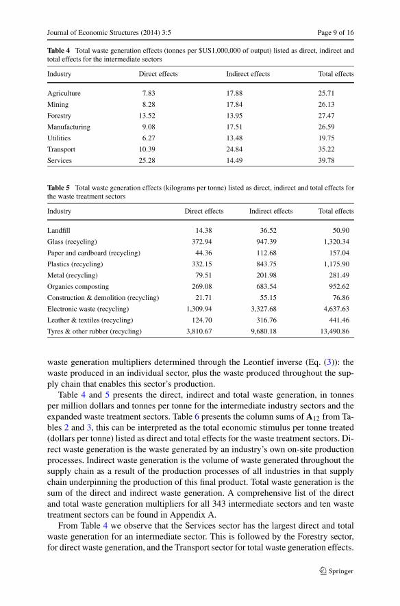
Table 4 Total waste generation effects (tonnes per $US1,000,000 of output) listed as direct, indirect andtotal effects for the intermediate sectors
Industry Direct effects Indirect effects Total effects
Agriculture 7.83 17.88 25.71
Mining 8.28 17.84 26.13
Forestry 13.52 13.95 27.47
Manufacturing 9.08 17.51 26.59
Utilities 6.27 13.48 19.75
Transport 10.39 24.84 35.22
Services 25.28 14.49 39.78
Table 5 Total waste generation effects (kilograms per tonne) listed as direct, indirect and total effects forthe waste treatment sectors
Industry Direct effects Indirect effects Total effects
Landfill 14.38 36.52 50.90
Glass (recycling) 372.94 947.39 1,320.34
Paper and cardboard (recycling) 44.36 112.68 157.04
Plastics (recycling) 332.15 843.75 1,175.90
Metal (recycling) 79.51 201.98 281.49
Organics composting 269.08 683.54 952.62
Construction & demolition (recycling) 21.71 55.15 76.86
Electronic waste (recycling) 1,309.94 3,327.68 4,637.63
Leather & textiles (recycling) 124.70 316.76 441.46
Tyres & other rubber (recycling) 3,810.67 9,680.18 13,490.86
waste generation multipliers determined through the Leontief inverse (Eq. (3)): thewaste produced in an individual sector, plus the waste produced throughout the sup-ply chain that enables this sector’s production.
Table 4 and 5 presents the direct, indirect and total waste generation, in tonnesper million dollars and tonnes per tonne for the intermediate industry sectors and theexpanded waste treatment sectors. Table 6 presents the column sums of A12 from Ta-bles 2 and 3, this can be interpreted as the total economic stimulus per tonne treated(dollars per tonne) listed as direct and total effects for the waste treatment sectors. Di-rect waste generation is the waste generated by an industry’s own on-site productionprocesses. Indirect waste generation is the volume of waste generated throughout thesupply chain as a result of the production processes of all industries in that supplychain underpinning the production of this final product. Total waste generation is thesum of the direct and indirect waste generation. A comprehensive list of the directand total waste generation multipliers for all 343 intermediate sectors and ten wastetreatment sectors can be found in Appendix A.
From Table 4 we observe that the Services sector has the largest direct and totalwaste generation for an intermediate sector. This is followed by the Forestry sector,for direct waste generation, and the Transport sector for total waste generation effects.
Page 10 of 16 C.J. Reynolds et al.
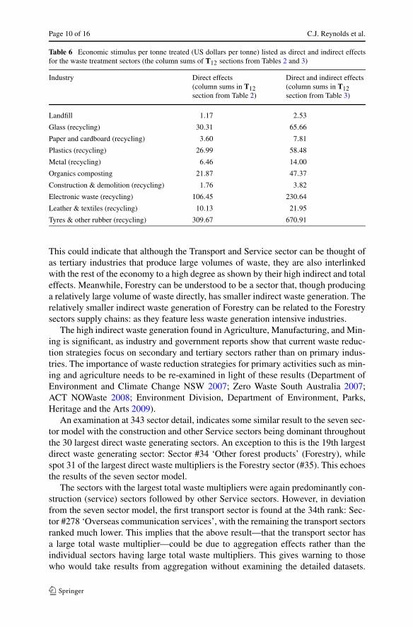
Table 6 Economic stimulus per tonne treated (US dollars per tonne) listed as direct and indirect effectsfor the waste treatment sectors (the column sums of T12 sections from Tables 2 and 3)
Industry Direct effects(column sums in T12section from Table 2)
Direct and indirect effects(column sums in T12section from Table 3)
Landfill 1.17 2.53
Glass (recycling) 30.31 65.66
Paper and cardboard (recycling) 3.60 7.81
Plastics (recycling) 26.99 58.48
Metal (recycling) 6.46 14.00
Organics composting 21.87 47.37
Construction & demolition (recycling) 1.76 3.82
Electronic waste (recycling) 106.45 230.64
Leather & textiles (recycling) 10.13 21.95
Tyres & other rubber (recycling) 309.67 670.91
This could indicate that although the Transport and Service sector can be thought ofas tertiary industries that produce large volumes of waste, they are also interlinkedwith the rest of the economy to a high degree as shown by their high indirect and totaleffects. Meanwhile, Forestry can be understood to be a sector that, though producinga relatively large volume of waste directly, has smaller indirect waste generation. Therelatively smaller indirect waste generation of Forestry can be related to the Forestrysectors supply chains: as they feature less waste generation intensive industries.
The high indirect waste generation found in Agriculture, Manufacturing, and Min-ing is significant, as industry and government reports show that current waste reduc-tion strategies focus on secondary and tertiary sectors rather than on primary indus-tries. The importance of waste reduction strategies for primary activities such as min-ing and agriculture needs to be re-examined in light of these results (Department ofEnvironment and Climate Change NSW 2007; Zero Waste South Australia 2007;ACT NOWaste 2008; Environment Division, Department of Environment, Parks,Heritage and the Arts 2009).
An examination at 343 sector detail, indicates some similar result to the seven sec-tor model with the construction and other Service sectors being dominant throughoutthe 30 largest direct waste generating sectors. An exception to this is the 19th largestdirect waste generating sector: Sector #34 ‘Other forest products’ (Forestry), whilespot 31 of the largest direct waste multipliers is the Forestry sector (#35). This echoesthe results of the seven sector model.
The sectors with the largest total waste multipliers were again predominantly con-struction (service) sectors followed by other Service sectors. However, in deviationfrom the seven sector model, the first transport sector is found at the 34th rank: Sec-tor #278 ‘Overseas communication services’, with the remaining the transport sectorsranked much lower. This implies that the above result—that the transport sector hasa large total waste multiplier—could be due to aggregation effects rather than theindividual sectors having large total waste multipliers. This gives warning to thosewho would take results from aggregation without examining the detailed datasets.
Journal of Economic Structures (2014) 3:5 Page 11 of 16
Please refer to Appendices A and B for data and detailed analysis of the 343 wastegenerating sectors.
3.1 Treatment Analysis
The S23 section of Table 2 indicates landfill (Lf) as the dominant treatment method interms of tonnes treated. The results in Table 5 indicate that landfill generates smallerdirect and total waste tonnages when compared to the various recycling treatments.Electronic waste, Tyres and other rubber, and Glass recycling are the three most ‘in-efficient’ waste treatment sectors in terms of both direct and total waste generationeffects; as in treating a tonne of waste they produce the largest volume of wasteproducts. Notably the volume of total waste generated is larger than the volume ofwaste originally treated (Rubber 13:1, Electronic waste 4:1, Glass 1.3:1). However,the composition of this ‘new’ waste is mixed rather than singular. Technically, re-cycling via these inefficient methods could be understood to be transforming (at amacroeconomic level) a single type of waste into greater tonnages of other types ofwaste rather than actual ‘treatment’.
In current Australian circumstance (i.e. overall reliance on landfill as a treatmentmethod), this finding also implies that as greater volumes of these wastes are ‘in-efficiently’ recycled, a greater volume of waste overall will be sent to landfill. Thissituation will begin to change if these treatment methods become more efficient, andover 50% of Australia’s waste is recycled.
This result shows that the technologically and labour intensive treatment methodsproduce a greater volume of waste per tonne treated than the less technologicallycomplex and labour intensive treatment method of landfill. This finding confirmswhat was already intuitively suspected: the activity of burying waste in the ground in-herently produces less waste per tonne than recycling the waste (via relatively labourand monetarily intensive methods). However, it is worth being reminded that oncelandfilled, the waste material can then no longer be used as an input of production.
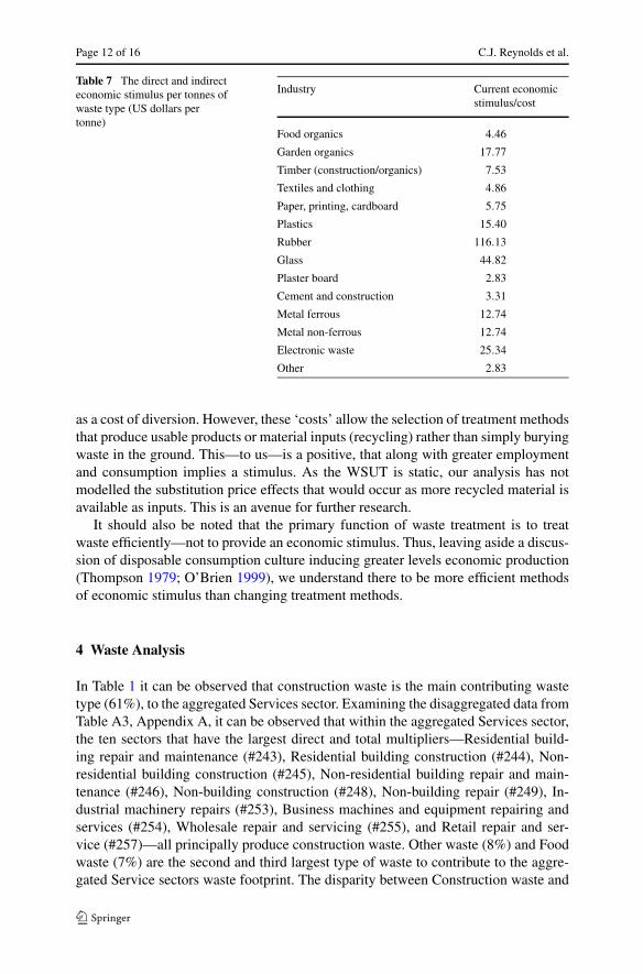
Landfill provides the least amount of economic activity per tonne treated. As indi-cated in Table 6, for every tonne of waste disposed of via landfill stimulates $US1.17direct, or $US2.53 in total of economic activity. This is low compared to the moretechnologically and labour intensive treatment methods such as rubber recycling($US310 in direct effects, and $US671 in direct and indirect effects of economic pro-duction per tonne treated), or electronic waste recycling ($US106 for direct effects,and $US230 in direct and indirect effects of economic production per tonne treated).However, at present, with landfill the dominant treatment method, each tonne of rub-ber or electronic waste treated produces economic production worth only $US116 or$US25 (Table 7). This result indicates that recycling provides a larger economic pro-duction than landfill per tonne of waste treated, and that there is room to improve theeconomic stimulus associated with waste treatment by diverting waste from landfillto recycling.
We have used the term ‘economic stimulus’ to indicate the amount of money asso-ciated with an additional tonne of waste being treated in each manner. This monetaryvalue could likewise be understood to be related to labour, monetary and materialflows). This means that each per tonne economic stimulus could likewise be described
Page 12 of 16 C.J. Reynolds et al.
Table 7 The direct and indirecteconomic stimulus per tonnes ofwaste type (US dollars pertonne)
Industry Current economicstimulus/cost
Food organics 4.46
Garden organics 17.77
Timber (construction/organics) 7.53
Textiles and clothing 4.86
Paper, printing, cardboard 5.75
Plastics 15.40
Rubber 116.13
Glass 44.82
Plaster board 2.83
Cement and construction 3.31
Metal ferrous 12.74
Metal non-ferrous 12.74
Electronic waste 25.34
Other 2.83
as a cost of diversion. However, these ‘costs’ allow the selection of treatment methodsthat produce usable products or material inputs (recycling) rather than simply buryingwaste in the ground. This—to us—is a positive, that along with greater employmentand consumption implies a stimulus. As the WSUT is static, our analysis has notmodelled the substitution price effects that would occur as more recycled material isavailable as inputs. This is an avenue for further research.
It should also be noted that the primary function of waste treatment is to treatwaste efficiently—not to provide an economic stimulus. Thus, leaving aside a discus-sion of disposable consumption culture inducing greater levels economic production(Thompson 1979; O’Brien 1999), we understand there to be more efficient methodsof economic stimulus than changing treatment methods.
4 Waste Analysis
In Table 1 it can be observed that construction waste is the main contributing wastetype (61%), to the aggregated Services sector. Examining the disaggregated data fromTable A3, Appendix A, it can be observed that within the aggregated Services sector,the ten sectors that have the largest direct and total multipliers—Residential build-ing repair and maintenance (#243), Residential building construction (#244), Non-residential building construction (#245), Non-residential building repair and main-tenance (#246), Non-building construction (#248), Non-building repair (#249), In-dustrial machinery repairs (#253), Business machines and equipment repairing andservices (#254), Wholesale repair and servicing (#255), and Retail repair and ser-vice (#257)—all principally produce construction waste. Other waste (8%) and Foodwaste (7%) are the second and third largest type of waste to contribute to the aggre-gated Service sectors waste footprint. The disparity between Construction waste and
Journal of Economic Structures (2014) 3:5 Page 13 of 16
all other waste types within the aggregated service sector is due to the C&D wastestream (which is exclusively these sectors) consisting of primarily construction-basedwaste.
Primary industries have a more varied waste composition, even though organic andconstruction wastes are again the prevalent waste types in the aggregated Mining andAgricultural sectors. Surprising results include Phosphate rock (#72), having a highdirect and total organic waste component; and Eggs (#14), having a large indirectconstruction waste footprint due to its inputs (and thus waste) from the Non-buildingconstruction (#248) sector.
For many of the results the sectors with the largest direct and total waste mul-tipliers are sector Phosphate Rock (#72) and sector Natural Rubber (#28). This isbecause both these sectors have very large multipliers—in many cases three timeslarger than the other largest sectors in that waste category. The reason for PhosphateRock and Natural Rubber having large multipliers is that they are the two smallestwaste generating sectors of the Australian economy for 2008, and so produce a verysmall amount of waste. They are also small economic sectors and so relative to theireconomic activity they produce a very large amount of waste. This illustrates that justbecause a sector has a high multiplier it does not equate to the importance of thatsector in terms of economic influence or that it currently produces a high tonnage ofwaste.
In Appendix B we discuss the largest direct and total waste multipliers for each ofthe 14 waste types. Please refer to Appendix A for a full list of all sectors and wastetypes direct and total multipliers.
5 Conclusion
In this paper we have applied the WSUT method proposed by Lenzen and Reynolds(2014) to the Australian economy. To our knowledge this is the first application ofthe waste IO methodology to Australia—a very exciting outcome. The resulting 2008model is the highest resolution estimate ever created for Australian waste data. Its 343intermediate sectors, ten treatment sectors and 14 waste types provide a superior un-derstanding of contemporary Australian waste issues when compared to the standardMSW, C&I and C&D classification systems found in government reports.
The results section discussed the general situation of waste generation and recy-cling in Australia, presenting an aggregated seven intermediate sector and ten treat-ment sector model. We then provided a detailed breakdown of direct and total wastegeneration multipliers, listing the ten largest of the 343 intermediate sectors for all 14waste types.
The aggregated analysis affirms the current Australian industry and governmentunderstanding of the Australian waste production with the Service (notably construc-tion) industry having the largest direct and total waste generation multipliers. TheWSUT also reveals the surprising result of the high indirect waste generation ratesfound in Agriculture, Manufacturing, Transport, and Mining sectors, illustrating thelinkages between these sectors and the rest of the economy. Furthermore the resultsillustrate the dominant role of construction waste (and the C&D waste stream) in the
Page 14 of 16 C.J. Reynolds et al.
Australian economy, showing that many sectors contribute indirectly to the construc-tion footprint of Australia. Organic waste—specifically food waste—also featuresheavily throughout the supply chain. These findings indicate that a change of focusmay be required in waste prevention strategy, as currently C&D waste receives littlepublic attention. The Australian WSUT framework also displays that, per tonne ofwaste treated, recycling stimulates greater economic activity than landfill. However,landfill operations generate less waste per tonne of waste treated than other wastetreatments methods. Though, this volume of waste is small compared to the totalamount of waste generated in the economy. This finding should encourage furtherdiversion from landfill.
Competing Interests
The authors declare that they have no competing interests.
Authors’ Contributions
All authors contributed equally to the writing of this paper. All authors read and approved the finalmanuscript.
Acknowledgements Many thanks to Shigemi Kagawa, and the two anonymous reviewers for their con-structive comments and suggestions. Thanks also to the team at Integrated Sustainability Analysis, Uni-versity of Sydney for their advice over the writing of this paper. This paper is based on research fundedunder the ARC Linkage Project ‘Zeroing in on Food Waste: Measuring, understanding and reducing foodwaste’ (LP0990554) by the Australian Research Council and industry partners Zero Waste South Australiaand the Local Government Association of South Australia.
References
ACT NOWaste (2008) ACT NOWaste strategy & targets: review & assessment of options. Wright Corpo-rate Strategy
Australian Bureau of Statistics (2006) Australian and New Zealand standard industrial classification(ANZSIC) 2006. Australian Bureau of Statistics, Canberra.
Australian Bureau of Statistics (2008) Electricity, gas, water and waste services, Australia. AustralianBureau of Statistics, Canberra
Australian Bureau of Statistics (2009) Environmental issues: waste management and transport use. Aus-tralian Bureau of Statistics, Canberra
Australian Bureau of Statistics (2010) Waste generation by state. In: Australia’s environment: issues andtrends. Australian Bureau of Statistics, Canberra
Australian Bureau of Statistics (2011) Waste management services, Australia, 2009–10. Australian Bureauof Statistics, Canberra
Australian Bureau of Statistics (2013a) Waste account, Australia, experimental estimates (WAAEE) 2013.Australian Bureau of Statistics, Canberra
Australian Bureau of Statistics (2013b) Australian commodities. National and state 2011–12. AustralianBureau of Statistics, Canberra
Department of Environment and Climate Change NSW (2007) NSW waste avoidance and resource recov-ery strategy 2007
Department of Sustainability, Environment, Water, Population and Communities (2012) Waste and recy-cling in Australia 2011: incorporating a revised method for compiling waste and recycling data. Finalreport
Journal of Economic Structures (2014) 3:5 Page 15 of 16
DSEWPaC (2012) The Australian recycling sector. Department of Sustainability, Environment, Water,Population and Communities, Canberra
Environment Division, Department of Environment, Parks, Heritage and the Arts (2009) The Tasmanianwaste and resource management strategy
Environment Protection and Heritage Council and the Department of Environment, Water, Heritage andthe Arts (2010) National waste report
Hyder Consulting (2012) Waste and recycling in Australia 2011: incorporating a revised method for com-piling waste and recycling data. Department of Sustainability, Environment, Water, Population andCommunities, Canberra
Kagawa S (2005) Inter-industry analysis, consumption structure, and the household waste productionstructure. Econ Syst Res 17(4):409–423
Kagawa S, Nakamura S, Inamura H, Yamada M (2007) Measuring spatial repercussion effects of regionalwaste management. Resour Conserv Recycl 51(1):141–174
Lenzen M, Reynolds C (2014) A supply-use approach to waste input–output analysis. J Ind Ecol18(2):212–226
Lenzen M, Geschke A, Kanemoto K, Moran D (2011) Eora: a global multi-region input–output database.http://www.globalcarbonfootprint.com
Lenzen M, Kanemoto K, Moran D, Geschke A (2012a) Mapping the structure of the world economy.Environ Sci Technol 46(15):8374–8381
Lenzen M, Kanemoto K, Moran D, Geschke A (2012b) Supporting information for “Mapping the structureof the world economy”. Environ Sci Technol
Lenzen M, Moran D, Kanemoto K, Geschke A (2013) Building Eora: a global multi-region input–outputdatabase at high country and sector resolution. Econ Syst Res 25(1):20–49
Lin C (2009) Hybrid input–output analysis of wastewater treatment and environmental impacts: a casestudy for the Tokyo Metropolis. Ecol Econ 68(7):2096–2105
Matsubae K, Nakajima K, Nakamura S, Nagasaka T (2011) Impacts on CO2 of the recovery of secondaryferrous materials from alternative ELV treatment methods: a waste input–output analysis. ISIJ Int51:151–157
Nakamura S (1999) Input–output analysis of waste cycles. In: Proceedings of the EcoDesign ’99: firstinternational symposium on environmentally conscious design and inverse manufacturing, 1999
Nakamura S (2010) Waste input–output (WIO) table for Japan 2000, version 0.06b. http://www.f.waseda.jp/nakashin/WIO.html
Nakamura S, Kondo Y (2002a) Input–output analysis of waste management. J Ind Ecol 6(1):39–63Nakamura S, Kondo Y (2002b) Recycling, landfill consumption, and CO2 emission: analysis by waste
input–output model. J Mater Cycles Waste Manag 4(1):2–11Nakamura S, Kondo Y (2002c) Waste input–output model: concepts, data, and application. KEO discus-
sion paper G-153: inter-disciplinary studies for sustainable development in Asian countries, KeioUniversity
Nakamura S, Kondo Y (2006) A waste input–output life cycle cost analysis of the recycling of end-of-lifeelectrical home appliances. Ecol Econ 57(3):494–506
Nakamura S, Kondo Y (2008) Waste input–output analysis, LCA and LCC. In: Suh S (ed) Handbook oninput–output economics in industrial ecology Springer, New York, pp 561–572
Nakamura S, Kondo Y (2009) Waste input–output analysis: concepts and application to industrial ecology.Springer, New York
Nakamura S, Nakajima K, Kondo Y, Nagasaka T (2007) The waste input–output approach to materialsflow analysis. J Ind Ecol 11(4):50–63
O’Brien M (1999) Rubbish values: reflections on the political economy of waste. Sci Cult 8(3):269–295Reynolds CJ (2013) Quantification of Australian food wastage with input–output analysis. Doctor of
philosophy (applied mathematics), University of South Australia. http://arrow.unisa.edu.au:8081/1959.8/157480
Reynolds CJ, Boland J (2011) Extending the waste input–output model to behavioural change: the case ofmunicipal food waste in South Australia. In: 19th international input–output conference, Alexandria,VA, USA
Reynolds CJ, Boland J (2013a) Waste flows in multi-regional input–output models. In: Murray J, LenzenM (eds) The sustainability practitioner’s guide to multi-regional input–output analysis. CommonGround Publishing LLC, Champaign
Reynolds CJ, Boland J (2013b) Waste not, want not? The economics of waste and the good of charity in aWIO framework. In: 21st IIOA conference, Kitakyushu, Japan
Page 16 of 16 C.J. Reynolds et al.
Reynolds CJ, Boland J, Thompson K, Dawson D (2011) An introduction to the waste input–output model:a methodology to evaluate sustainable behaviour around (food) waste. In: Roetman PE, Daniels CB(eds) Creating sustainable communities in a changing world. Crawford House Publishing, Adelaide
Thompson M (1979) Rubbish theory: the creation and destruction of value. Oxford University Press, Ox-ford
Tsukui M (2007) Analysis of structure of waste emission in Tokyo by interregional waste input–outputtable. In: 11th international waste management and landfill symposium, Sardinia
Tsukui M, Nakamura K (2010) The impact and effects of modal shift of waste transportation by IR-WIO(interregional waste input–output) analysis. In: 18th international input–output conference, Sydney,Australia
Tsukui M, Ichikawa T, Kagawa S, Kondo Y, Kagatsume M (2011) A regional WIO analysis of the effect ofnon-residents’ consumption: a comparison between Tokyo and Kyoto. In: 19th international input–output conference, Alexandria, VA, USA
Tsukui M, Hasegawa R, Kagawa S, Kondo Y (2012) Construction of a multi-regional waste input–outputtable. In: 20th international input–output conference, Bratislava, Slovakia
Waste Management & Environment Media Pty Ltd (2011) Inside waste industry report 2011–12.Gladesville, NSW
WCS Market Intelligence (2008) The blue book: Australian waste industry, 2007/08 industry and marketreport
Wright Corporate Strategy Pty Ltd and Rawtec Pty Ltd (2010) A study of Australia’s current and future e-waste recycling infrastructure capacity and needs. Department of Sustainability, Environment, Water,Population and Communities, Canberra
Zero Waste South Australia (2007) South Australia’s waste strategy 2005–2010: benefit cost assessment,volume 1: summary report