INTERNATIONAL JOURNAL FOR NUMERICAL METHODS IN FLUIDS, VOL. 2 1, 64 1-65 1 (1 995)

A VARIABLE BOUNDARY MODEL OF STORM SURGE FLOODING IN GENERALIZED CURVILINEAR GRIDS

FENGYAN SHI AND WENXIN SUN Physical Oceanography Institute, Ocean University of Qingdao, Shandong 266003. People b Republic of China

SUMMARY In this paper, generalized 2D shallow sea dynamic equations in movable curvilinear co-ordinates are derived. Through a differential co-ordinate transformation a self-adaptive grid is proposed to treat a continuously deforming lateral boundary and a kinematical boundary condition is adopted. The self-adaptive grid method (SAM) is used to simulate numerically the storm surge flooding in the Bohai Sea on 23 April 1969, which was one of the largest storm surge inundations in China.

KEY WORDS: variable boundary model; storm surge flooding; self-adaptive grid; generalized shallow sea dynamic equations in curvilinear co-ordinates

INTRODUCTION

It is well known that in some fluid dynamic problems the water boundary usually varies with time owing to the fluctuation of the free surface and the movement of lateral boundaries. Strictly speaking, the particles at a variable boundary should satisfy a kinematical boundary condition, i.e. without a source or a sink at the boundary the particles will always move in the tangential plane of the boundary. It is impossible to adopt this condition in a finite difference scheme with fixed grid points, because the moving boundary points are not generally at the grid points. The 'wet or dry point' method (WDM),',* which allows the advancing water front to move discontinuously from one grid point to another according to a prescribed criterion, are not so effective in computations with large water intrusions such as a storm surge inundation, because a vertical wall boundary condition, i.e. the normal velocity is zero, is adopted. A co-ordinate transformation method was proved convenient for the handling of the kinematical boundary condition by Johns: who employed perfectly this condition in transformed co- ordinates by introducing an algebraic co-ordinate transformation with a time term. However, the use of his method is limited to a simple transformation in a single direction, which can only deal with some partial movements of coastlines and from which a numerical instability will arise because of the excessive shearing of coastlines. To solve this problem, a similar co-ordinate transformation based on the equations in polar co-ordinates was conducted by Shi and Sun4 to improve the numerical stability and enlarge the calculated area with a variable boundary, though such a method is still restricted to the computation of some simple area. It is the purpose of the present paper to give generalized shallow sea dynamic equations suitable for dealing with all kinds of co-ordinate transformations, including those of Johns3 and Shi and A self-adaptive grid system obtained from a differential co-ordinate transformation with a time term is introduced to represent a variable analysis area extending and contracting in response to the continuous movement of lateral boundaries. The method is finally used to simulate the storm surge flooding in the Bohai Sea on 23 April 1969 and the result is in good agreement with actual observations.

CCC 0271-2091/95/080641-11 0 1995 by John Wiley & Sons, Ltd.

Received September 1994 Revised February 1995

642 F. Y. SHI AND W. X. SUN

GENERALIZED 2D SHALLOW SEA DYNAMIC EQUATIONS IN MOVABLE

The sphericity of the earth’s surface is ignored and a system of rectangular Cartesian co-ordinates is used. The depth-averaged components of velocity, u and v, then satisfy

CURVILINEAR CO-ORDINATES

aH aHu aHv -+-+-=o, at ax ay

au au au ac 1 - + U- + V - -fi, = - g - + -[t, - kpu(u2 + V 2 ) ” 2 ] , at ax ay ax ~p

a v a v a v ac 1 - + U - + V - + ~ U = -g-+-[t,- kpv(u2+V2)”2]. at ax ay ay HP (3)

In equations (1H3), f denotes the Coriolis parameter; the pressure is taken as hydrostatic and the effects of astronomical tide-generating forces and barometric forcings are omitted, c denotes the surface elevation and h the depth from the undisturbed sea level to the sea-floor; H = h + c; (tar, tay) represents the applied surface wind stress and the bottom stress is parameterized in terms of a quadratic law; p denotes the water density and the friction coefficient k is taken to be 2.6 x

A co-ordinate transformation is introduced in the general form

r = a x , y , 4, q = q(x, y , 0, t = t ,

where (c, q, t) are new independent variables in the transformed image space. The coastal boundaries rl, r2, r3 and r4 in the physical plane thus becomes n,, II,, 113 and n4 respectively in the image plane as shown in Figure 1.

The contravariant components of the velocity vector in curvilinear co-ordinates can be written as

where J=xry,-xgvc Equations (4) and ( 5 ) are based on the relations

G =YqlJ, t y = -xq/J, rlx = -Yt/J, rly = X d J . (6)

Figure 1. (a) Physical plane and (b) transformed image plane

MODEL OF STORM SURGE FLOODING 643

Now a t /& and aq+/at in (4) and (5) are replaced by

Then the descriptions of (4) and (5) in the image space (5 , q+, z) can be written as

Jv = -(g - v)xt + ($ - u)..

By using (7) and (8), equations ( 1 x 3 ) may be transformed into aJH aJHU UHV --+--- + - - - = O , at a t av (9)

where

6 = HJu, V = HJv.

Equations (9x11) are generalized equations applicable to any kind of curvilinear co-ordinates, because they are not dependent on any specific transformation. In the case of Johns: for instance, equations ( 9 x 1 1) become the equations deduced by him with J = b2-bl. Equations (9H11) are also applicable to the polar co-ordinate transformation of Shi and Sun.4

THE KINEMATICAL BOUNDARY CONDITION

The model of the present paper differs fiom the WDM model in its reasonable adoption of the kinematical boundary condition. Sun' proposed a generalized kinematical boundary condition, the analysis of which was further made by him in the same paper. Theoretically speaking, the kinematical condition, which is non-linear, can be used to represent strictly a dynamic process. In the vertical side- wall condition, i.e. u, = 0, on the other hand, the non-linear effects, which are important for variable boundary problems, are omitted. In addition, the rough approximation that a moving boundary is treated as a discontinuous movement instead of a continuous one may lead to a misrepresentation of the current distribution. The calculation error is conspicuous in the case of a mildly sloping coastal area.

The coastline in the physical plane remains a curve H(xb, yb, t)=O. The kinematical boundary condition is that the normal velocity of particles at the coastal boundary equals the normal velocity of the coastline itself, i.e.

6

644 F. Y. SHI AND W. X. SUN

Equation (1 3) can be written in the image plane as

because aH/@ = 0 at HI, 112, equation (13) can be written by means of (6) as

(g - v)xq - (2 - ")Yq = 01

because aH/a( = 0 at 113, 114, equation (13) can be written as

(2 - v)x t - - U)Yt = 0.

Comparing (14) and (1 5) with (7) and (8) respectively yields the kinematical boundary condition in the image plane as

U = O at n,, n2, (16)

V = O at n3, l l 4 . (17) The kinematical condition (13) can be easily satisfied by taking U= 0 at II,, 112 and V= 0 at I I 3 , H4.

A further requirement is that the depth of the water should be zero at the coastline, which leads to aH aHdrb aHdyb - + -- + -- = 0. at ax dt ay dt

Using (13) yields the final equation aH aH aH -+u-+v- = 0 at ax ay

or, equivalently, dH - = 0. dt

Equation (18) is the representation of the generalized non-liner kinematical condition given by Sun.' Because U=O, aH/* = 0 at HI, II, or V=O, aH/at = 0 at Il,, 114, equation (18) can be written in the image plane as

or, equivalently,

Equation (19) is the curve equation of the coastline.

NUMERICAL GENERATION OF THE SELF-ADAPTIVE GRID

In terms of numerical stability and accuracy it is important to generate a smooth and orthogonal grid point system. Brackbill and Saltrman7 proposed a numerical generation method optimizing simultaneously grid smoothness, orthogonality and variation in cell volumes. The main idea is that minimizing the functions by which the three properties are measured results in a set of Euler equations which are satisfied by the co-ordinate values of grid points.

MODEL OF STORM SURGE FLOODING 645

The smoothness of the grid is measured by the function

1, = J K V O ~ + ( v ~ ) ~ I ~ s z , R

the orthogonality of the grid by

I,, = 1 (VlVq)2J3dsz R

and the weighted volume variation by

z v = J wm, R

where W= W(x, y) is a given function which can control the density of the grid. Minimizing a new hc t ion I, where I=I, + Ado + &Iv yields the Euler equations

(20)

(21)

2 aw b1xtt + bzy , + b3Xqq + a1yre + a2Yrq + a3yqq = -2vJ

2 aw a1xtt + a ~ t , + a3+, + C I Y ~ ~ + w t q + c~Y,,, = -&J -, ay where al , a2, a3, bl, b2, b3, cl, c2 and c3 are the differentiations of (x, y) with respect to (l, q) (see Reference 7 for details).

>

The boundary condition required by (20) and (21) can be written as

xb = d r b ? qbr 71, Yb = Y ( t b , qb,

It should be noted that the above condition has a time term. Therefore it is necessary to generate a grid system at each time step corresponding to the variation in the boundary. By adjusting W to densify grid points near the variable boundaries when the grid is first generated and generating afterwards only in the neighbourhood of the boundaries without changing the grid points outside this region, the amount of computation is greatly decreased and the grid points in the region still remain dense enough even after the extension of the grid.

NUMERICAL SCHEME

Discrete co-ordinate points are defined by

c = r i , i = l , 2 , . . . , m, q = q j , j = 1 , 2, ..., n, and a sequence of time instants by t = tp = pAt @ = 0, 1, 2, . . .). For any variable F we write

F(l i , q j t t p ) = FCj

In the 5-1 plane a staggered grid is used as shown in Figure 2: x denotes a c-point at which 5 is computed, 0 denotes a u-point at which u, U and u" are computed and 0 denotes a v-point at which v, Vand v" are computed; m and n are chosen properly to ensure that there are only u-points at ll,, n2, where U= 0 is satisfied, and only v- points at n3, n4, where V= 0. Difference operators are defined by

646 F. Y SHI AND W. X. SUN

j=5

j=4

j=3

j=2

j- 1

averaging operators by -tl

F - 5 - 2 - '(Fp i+l , j+Fi- , , j )> P pq = $ ( F f j + l + F f j - , ) , $q = F t

and shifi operator by

EtF = FC?'.

The discretizations of (9H11) are in the forms

At( J H ) + S&'JU) + S q ( H am) = 0,

The values of c:;' are determined from HJ in (22) by application of

[p+' 1. J = -hi,j + (HJ)p+'/J:j.

Equations (23) and (24) are used for updating u" and v" respectively and then values of u and v are deduced from (12):

After the updating of u and v the updated values of U and Vmay be obtained by applying (7) and (8) in the discretized forms

Updated positions of the variable boundaries can be deduced via (19) in the discretized form

MODEL OF STORM SURGE FLOODING 647

Figure 3. Grids in (a) physical plane and (b) image plane

and a simple prescription that grid points at variable boundaries must move in the normal directions of the boundary lines, i.e.

It is then readily shown that

at n3, Il3.

With the values of x:+’ and d+’, grid points in the physical plane can be obtained by generating the grid as described in the previous section. It could of course be noted that the grid point values of h in the computational plane will be changing with time, whereas they are independent of time at fixed

648 F. Y. SHI AND W. X. SUN

MODEL OF STORM SURGE FLOODING

118'30' 11 9'00' I I

649

Figure 5. Maximum intrusion lines: Comparison with Johns' model

points in the physical plane. The values of h, can be re-computed by linear interpolation between values of h at the nearest adjacent points in the physical plane according to the relations obtained from (20) and (21).

APPLICATION TO A STORM SURGE INUNDATION

The Huanghe Delta, which is located between latitudes 37"20'N and 38"lO'N and longitudes 1 1 8"OO'E and 1 19" 1 SE, is one of the areas most severely afflicted by storm surges in China. With a small slope of 1%-1.5%0 the area is apt to be inundated when a storm surge occurs. The storm surge in April 1969 made an inland intrusion of more than 30 km. To simulate the storm surge flooding, three different variable boundary models were utilized by Shi and Sun4,8 and Sun et ~ 1 . ~ The three simulations, however, could only be conducted within a small computational region near the Huanghe Delta where the open boundary conditions are given by an initial calculation in a large computational region covering the whole Bohai Sea. In the self-adaptive grid method (SAM) the Bohai Sea is treated as a whole computational region where the grid points near the Huanghe Delta are locally densified. By doing this, the present model not only contains a reasonable boundary condition but also fits more complicated boundaries better than the models mentioned above.

Figure 3(a) shows the initially generated grid in the physical plane; its corresponding grid in the image plane is shown in Figure 3@). To simulate the storm surge in April 1969, the same wind field as

650 F. Y. SHI AND W. X. SUN

1 18'30' 1 19"oo'

'0

'm 0

0

0 ?-J

n h

L I I

1 l8"30' 1 l$OO'

Figure 6 . Maximum intrusion lines: comparison with WDM model

described in Reference 4 is adopted and the open boundary condition is

c b = c k l + (01 + + cs2 '

where [k,, lo,, im, and is, are the surface elevations caused by four main tide components k, , ol, m2 and s2 respectively at the open boundary.

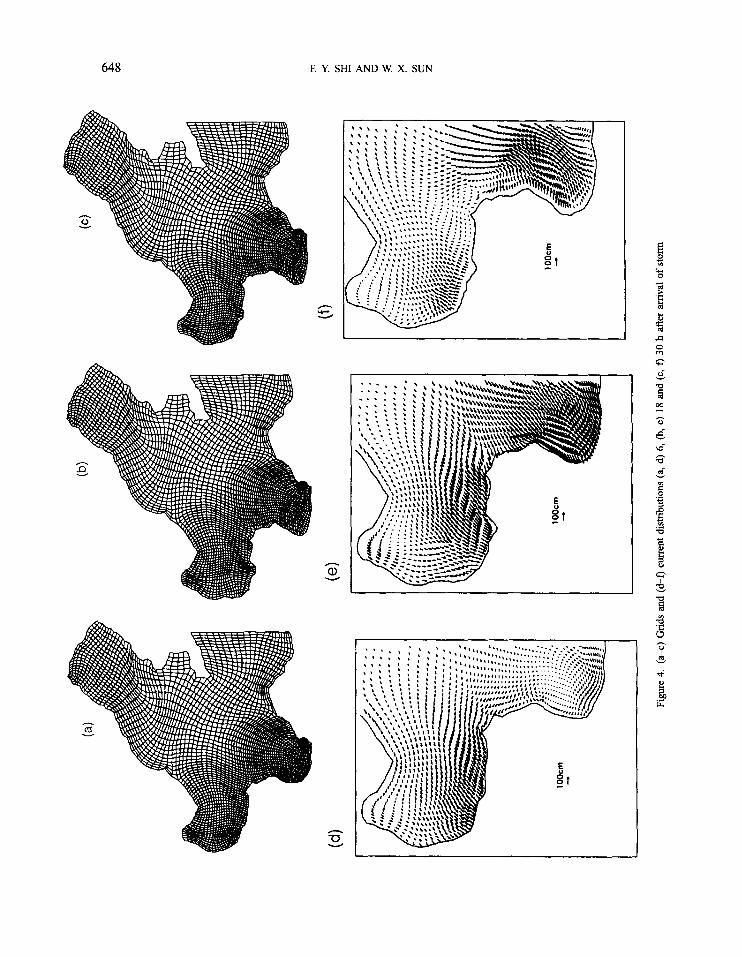
Figures 4(a)-4(c) show the different grids generated at various times (6, 18 and 30 h after the amval of the storm) during the flooding process; the corresponding current distributions in the Huanghe Delta are shown in Figures 4(dp(f). The maximum intrusion line calculated in the present paper is shown in Figure 5. For comparison, the observed inundation area and the result of Johns' model are also given in the same figure.

In order to analyse the predicted error, the relative error of the predicted inundation area (RE) is defined by

C ]predicted error in areal observed inundation area '

RE=

In the SAM model, RE = 16.O%, which is 2.6% less than that of Johns' model. It is clear indeed in Figure 5 that the result of Johns' model is unsatisfactory in the Taoerhe River where the coastline is excessively shearing relative to the collected co-ordinates. It is also seen that the result of the SAM model is better than that of Johns' model in most of the analysed area, except in the southern part of

MODEL OF STORM SURGE FLOODING 65 1

Yangjiaogou where the topography is extremely complicated and the extended grid of the S A M model is not as fine as that of Johns’ model.

To compare with the WDM model, the result of the WDM model is shown in Figure 6 instead of that of Johns’ model in Figure 5. RE obtained by the WDM model is 19.2%, which is the largest among the four models. It may be concluded that the boundary conditions have obvious effects on calculations of storm surge flooding.

CONCLUSIONS

In computations of problems involving shallow sea dynamics with variable lateral fluid boundaries,

(i) utilization of the kinematical boundary condition, which embodies the non-linear effect of

(ii) automatic conformation of the self-adaptive grid to complicated boundary lines without zigzag

(iii) automatic adjustment of the grid density according to the rate of physical variables or

the self-adaptive grid method has several advantages as listed below:

variable boundaries

effects caused by the Cartesian grid

topography.

There are still many problems unsolved, such as the control of the grid density on boundaries and the treatment of complicated topographies, which could lead to a complicated shape of the boundary line. In spite of these, the present model remains a feasible and ideal method for the computation of storm surge floods, tides with a broad tidal range, ocean circulation, etc. The self-adaptive grid model should have wide applications in the field of ocean computations.

REFERENCES

1. R. A. Flather and N. S. Heaps, ‘Tidal computations for Morecambe Bay’, Geophys. 1 R. Astron. Soc., 42,489-5 17 (1975). 2. J. J. Leendertse and E. C. Gritton, ‘A water quality simulation model for well mixed estuaries and coastal seas’, in

3. B. Johns, ‘The simulation of a continuously deforming lateral boundary in problems involving the shallow water equations’,

4. F. Y. Shi and W. X. Sun, ‘A variable boundary model and its application’, Oceanol. Limnol. Sinica, 26, (1995). 5 . W. X. Sun, ‘A further study of ultra-shallow water storm surge model’, 1 Shandong College ofoceanol., 17, 3 4 4 5 (1987). 6. W. X. Sun, 2. Y. Yang and F. Y. Shi, ‘On the numerical prediction model of storm surge inundation’, 1 Ocean Univ. Qingdao,

7. J. U. Brackbill and J. S. Saltzman, ‘Adaptive zoning for singular problems in two dimensions’, J Comput. Phys., 46,342-368

8 . F. Y. Shi and W. X. Sun, ‘Numerical simulations of the inundation of storm surges in partial areas of the Bohai Sea’, Oceanol.

Computation Procedures, Vol. 11, The Rand Corporation, New York, 1971, pp. 29-33.

Comput. Fluids, 10, 105-116 (1982).

24, 293-299 (1994).

(1 982).

Limnol. Sinica, 24, 16-23 (1993).