water

Article

Positive Surge Propagation in Sloping Channels

Daniele Pietro Viero 1,* ID , Paolo Peruzzo 1 and Andrea Defina 1,2

1 Department ICEA, University of Padova, Via Loredan 20, 35131 Padova, Italy;paolo.peruzzo@dicea.unipd.it (P.P.); andrea.defina@dicea.unipd.it (A.D.)

2 Intl Center of Tidal Hidro- and Morphodynamics, University of Padova, 35131 Padova, Italy* Correspondence: daniele.viero@unipd.it; Tel.: +39-049-827-5659

Received: 22 June 2017; Accepted: 9 July 2017; Published: 13 July 2017

Abstract: A simplified model for the upstream propagation of a positive surge in a sloping,rectangular channel is presented. The model is based on the assumptions of a flat water surface andnegligible energy dissipation downstream of the surge, which is generated by the instantaneousclosure of a downstream gate. Under these hypotheses, a set of equations that depends only on timeaccurately describes the surge wave propagation. When the Froude number of the incoming flow isrelatively small, an approximate analytical solution is also proposed. The predictive ability of themodel is validated by comparing the model results with the results of an experimental investigationand with the results of a numerical model that solves the full shallow water equations.

Keywords: breaking and undular surge; environmental hydraulics; laboratory experiments;open-channel flow; physical modelling; shallow water modelling

1. Introduction

A positive surge in an open channel is a sudden increase of flow depth that looks like a movinghydraulic jump; it can be generated by either natural or artificial causes [1–5]. The early contributionson surges include the works of Favre [6], Benjamin and Lighthill [7], and Peregrin [8]. Especially notableis the more recent work of Chanson and his co-workers, who mainly focus on tidal bore, i.e., a surgewave generated by a relatively rapid rise of the tide ( [9–13], e.g., among the many).

In the present work, we distinguish tidal bore from positive surge since the former isproduced by a fast increase of the downstream water level, whereas the latter is produced by arapid reduction, often to zero, of the downstream flow rate. The two phenomena share manysimilarities; however, differences are such that the two waves are not likely to be confused witheach other. Here, the focus is on positive surge.

Despite the significant progress in understanding the dynamics of surges and bores in riversand channels, some problems of practical interest still remain. Most studies of positive surges assumea horizontal channel, whereas many practical applications encompass positive surges propagatingupstream on downward sloping channels; e.g., rejection surges in canals serving hydropower stationsproduced by the sudden decrease or complete interruption of power production, or surges in drainagechannels ending at a pumping station when a sudden stopping of pumping occurs.

When a positive surge propagates upstream on a steep slope over an incoming supercritical flow,it progressively decelerates and asymptotically tends toward a stationary hydraulic jump [10];when, instead, a positive surge propagates upstream on a mild slope over an incoming subcritical flow,the wavefront progressively reduces its height until the surge vanishes. Interestingly, the latteroccurrence has never been reported and discussed in the literature and, as it happens, solutions toopen channel flow problems never ceases to amaze by showing unexpected behaviours even withinsimple and schematic frameworks (e.g., [14–20]).

Water 2017, 9, 518; doi:10.3390/w9070518 www.mdpi.com/journal/water

Water 2017, 9, 518 2 of 13

Numerical models can provide accurate solutions to the problem; however, analytical solutions orconceptual models can help knowing how flow and geometry parameters affect the surge propagation,and can provide quick answers to a number of practical questions.

In this paper, the problem of positive surge propagation against an either subcritical orsupercritical uniform flow is faced within the framework of one-dimensional shallow water flow.Section 2 presents an approximate, zero-dimensional model for the description of the surge propagation.The capability of the model in predicting the characteristics of the surge propagation is validatedthrough the comparison of model prediction with the results of laboratory and numerical experiments.Section 3 describes the laboratory setup and the experimental procedures, and the numerical modelthat solves the shallow water equations. The comparison between model prediction and the resultsof the laboratory and numerical experiments is discussed in Section 4. Conclusions of this study areshortly drawn in Section 5.

2. The Model

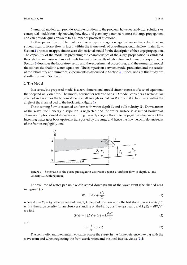
In a sense, the proposed model is a zero-dimensional model since it consists of a set of equationsthat depend only on time. The model, hereinafter referred to as 0D model, considers a rectangularchannel and assumes the bottom slope, s small enough so that cos θ ≈ 1, sin θ ≈ tan θ = s, with θ theangle of the channel bed to the horizontal (Figure 1).

The incoming flow is assumed uniform with water depth Y0 and bulk velocity U0. Downstreamof the wave front, energy dissipation is neglected and the water surface is assumed horizontal.These assumptions are likely accurate during the early stage of the surge propagation when most of theincoming water goes back upstream transported by the surge and hence the flow velocity downstreamof the front is negligibly small.

U1

U0

a

Y1 Y

0

L

ga

te

x

h

θ

Figure 1. Schematic of the surge propagating upstream against a uniform flow of depth Y0 andvelocity U0, with notation.

The volume of water per unit width stored downstream of the wave front (the shaded areain Figure 1) is

W = L∆Y +L2s2

, (1)

where ∆Y = Y1−Y0 is the wave front height, L the front position, and s the bed slope. Since a = dL/dt,with a the surge celerity for an observer standing on the bank, positive upstream, and U0Y0 = dW/dt,we find

U0Y0 = a (∆Y + Ls) + Ld∆Y

dt(2)

and

L =∫ t

0a(ξ)dξ. (3)

The continuity and momentum equation across the surge, in the frame reference moving with thewave front and when neglecting the front acceleration and the local inertia, yields [21]:

Water 2017, 9, 518 3 of 13

a = −U0 +√

gY0

√1 +

32

∆YY0

+12

∆Y2

Y20

. (4)

The set of Equations (2)–(4) can be integrated in time to yield ∆Y, a, and L (a simple numericalintegration procedure is given in Appendix A). In addition, the water depth, h(t), at the mostdownstream section (see Figure 1) is given by

h(t) = Y0 + sL + ∆Y, (5)

and it quickly grows approximately with sL since the reduction with time of ∆Y is relatively slow.In order to make the model analysis more robust, we introduce suitable time and length scales for

model variables and parameters. Both a and U0 are scaled with the small wave celerity c0 =√

gY0,the wave front height, as well as all vertical lengths, are scaled with the undisturbed flow depth Y0,whereas the front position L is scaled with Y0/s. With this, from Equation (2), a suitable timescale, τ,is found

τ =1s

√Y0

g. (6)

It is worth noting that τ actually measures the front propagation time since it is also givenas the ratio of the scale length for the front position (i.e., Y0/s) to the scale velocity for a (i.e., c0).Interestingly, with the above scaling, the solutions a(t/τ)/c0, ∆Y(t/τ)/Y0, and L(t/τ)s/Y0, turn outto depend only on the Froude number of the incoming flow, F0 = U0/

√gY0.

When the incoming flow is subcritical, the surge progressively reduces its height whilepropagating upstream until the front vanishes. The distance, LM, travelled by the surge beforevanishing can be estimated with Equation (2) that is here rewritten as

L =U0Y0 − a∆Y

as + d∆Ydt

. (7)

When the wave front vanishes, at t = tM, ∆Y reduces to zero and the front velocity reduces to theabsolute small wave celerity a = −U0 +

√gY0 so that

LM =Y0

sF0

1− F0

(1 + 1

sU0d∆Y

dt

∣∣∣t=tM

) . (8)

The numerical solution of model equations for a wide range of values of model parametersconfirms that the term between brackets at the denominator of Equation (8) depends only on F0.Therefore, Equation (8) can be written as

LM =Y0

sΦ(F0). (9)

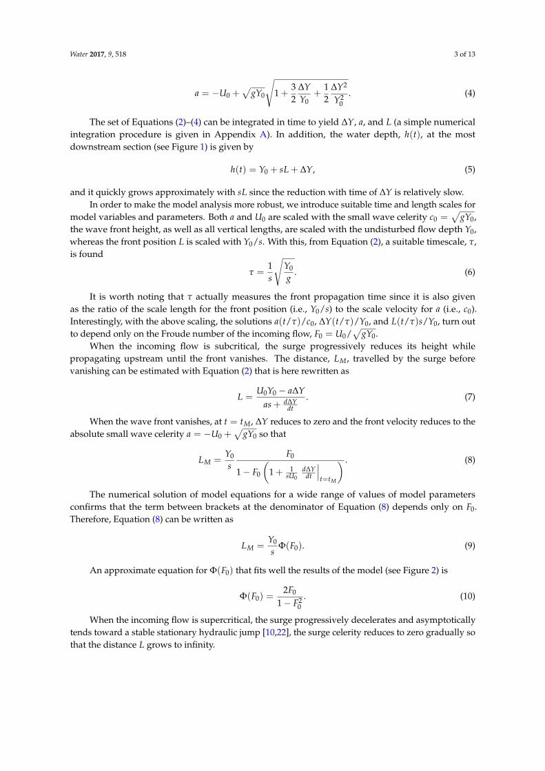
An approximate equation for Φ(F0) that fits well the results of the model (see Figure 2) is

Φ(F0) =2F0

1− F20

. (10)

When the incoming flow is supercritical, the surge progressively decelerates and asymptoticallytends toward a stable stationary hydraulic jump [10,22], the surge celerity reduces to zero gradually sothat the distance L grows to infinity.

Water 2017, 9, 518 4 of 13

0

5

10

15

20

25

0.0 0.2 0.4 0.6 0.8 1.0

Φ(F0)

F0

0.0 0.5 1.00.01

0.1

1

100

F0

Φ(F0)

Figure 2. Plot of Φ(F0) as a function of F0. White circles denote the results of the 0D model, the blackline is the approximation (10). The inset shows the same plot, with Φ(F0) on the log-scale.

An Approximate Analytical Solution

When F0 is relatively small (i.e., approximately F0 < 0.6), which is the case in manypractical problems, the time behaviour of the wave front velocity is extremely well approximated by asecond order polynomial as

ac0

=a0

c0− k1(t/τ) + k2(t/τ)2, (11)

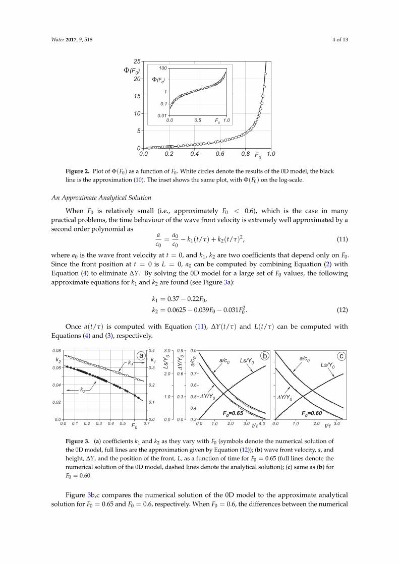
where a0 is the wave front velocity at t = 0, and k1, k2 are two coefficients that depend only on F0.Since the front position at t = 0 is L = 0, a0 can be computed by combining Equation (2) withEquation (4) to eliminate ∆Y. By solving the 0D model for a large set of F0 values, the followingapproximate equations for k1 and k2 are found (see Figure 3a):

k1 = 0.37− 0.22F0,

k2 = 0.0625− 0.039F0 − 0.031F20 . (12)

Once a(t/τ) is computed with Equation (11), ∆Y(t/τ) and L(t/τ) can be computed withEquations (4) and (3), respectively.

F0=0.65

0.0 1.0 2.0 3.0 4.00.3

0.5

0.7

0.9

0.4

0.6

a/c

0

t/τ

0.0

0.3

0.6

0.9

∆Y

/Y0

0.0

1.0

2.0

3.0

Ls/Y

0

Ls/Y0

a/c0

∆Y/Y0

b

F0=0.60

0.0 1.0 2.0 3.0t/τ

Ls/Y0

a/c0

∆Y/Y0

c

0.0

0.02

0.04

0.06

0.08

0.0 0.1 0.2 0.3 0.4 0.5 0.7F

0

0.0

0.1

0.2

0.3

0.4

k1

k2

k2

k1

a

Figure 3. (a) coefficients k1 and k2 as they vary with F0 (symbols denote the numerical solution ofthe 0D model, full lines are the approximation given by Equation (12)); (b) wave front velocity, a, andheight, ∆Y, and the position of the front, L, as a function of time for F0 = 0.65 (full lines denote thenumerical solution of the 0D model, dashed lines denote the analytical solution); (c) same as (b) forF0 = 0.60.

Figure 3b,c compares the numerical solution of the 0D model to the approximate analyticalsolution for F0 = 0.65 and F0 = 0.6, respectively. When F0 = 0.6, the differences between the numerical

Water 2017, 9, 518 5 of 13

and analytical solutions are negligibly small; at smaller Froude number, the numerical and analyticalsolutions are indistinguishable.

3. Numerical and Laboratory Experiments

In order to check the predictive capability of the 0D model, the model results are compared to theresults of an experimental investigation as well as with the results of a numerical model that solves thefull shallow water equations, for a wide range of flow and geometric conditions.

Laboratory experiments are performed in a flume that is relatively short if compared to thedistance that a surge can normally cover; the results of these experiments are used to check thecapability of the model in predicting the first stage of formation and propagation of the surge.The numerical experiments are then used to test the model over the longer distances.

3.1. Laboratory Setup and Experimental Procedures

The experiments are performed in a 20 m long, 0.38 m wide, tilting flume with Perspex wallsand bottom. Water is recirculated via a constant head tank that maintains steady flow conditions,and the flow rate is measured by a magnetic flowmeter (accuracy of about 0.2%). In order toachieve uniform flow, a downstream weir can adjust water depth when the flow is subcritical,whereas an upstream, vertical sluice gate adjusts the supercritical water depth. A vertical sluice gate,approximately 0.5 m upstream of the downstream gate, is used to generate the positive surge byquasi-instantaneously stopping the flow (frame by frame analysis of some gate closures recorded witha camera at 12.5 Hz frame rate allowed to estimate the gate closure time that is less than 0.2 s).

We use five ultrasonic probes, calibrated against a pointer gauge, to measure both uniform andunsteady water depth (accuracy of about 0.13 mm, acquisition frequency = 100 Hz) [23]. The fiveprobes (S1 to S5) are located at the channel centreline and at XS = 0.15 m , 3.0 m, 5.96 m, 8.96 m,and 11.89 m, upstream of the sluice gate used to generate the surge. The bed slope is varied betweens = 0.0002 and s = 0.0052 in order to vary the Froude number of the incoming uniform flow in the range0.3 < F0 < 1.4. Each run was repeated three times with negligible differences in the recorded waterdepth. Some preliminary experiments, aimed at gaining confidence with the phenomenon, are alsoperformed in a smaller flume, 0.3 m wide and 6 m long, equipped the same as the the larger flume.Experimental conditions are summarized in Table 1 for both the flumes.

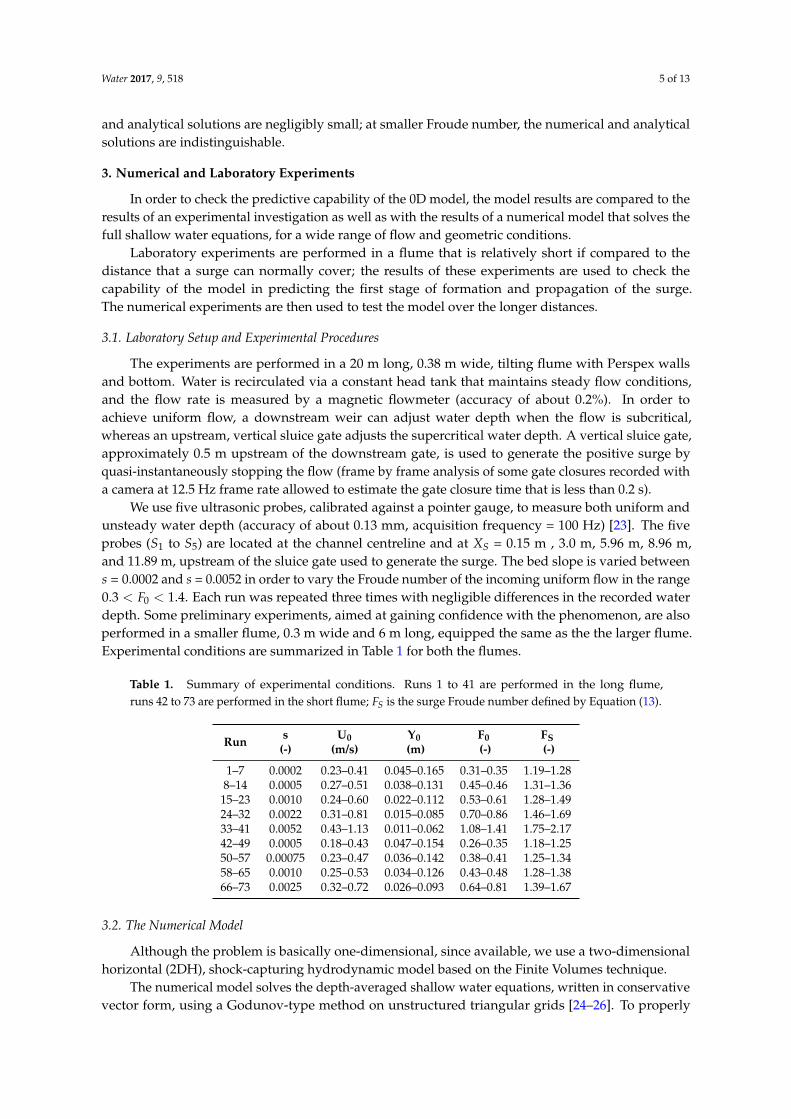
Table 1. Summary of experimental conditions. Runs 1 to 41 are performed in the long flume,runs 42 to 73 are performed in the short flume; FS is the surge Froude number defined by Equation (13).

s U0 Y0 F0 FSRun (-) (m/s) (m) (-) (-)

1–7 0.0002 0.23–0.41 0.045–0.165 0.31–0.35 1.19–1.288–14 0.0005 0.27–0.51 0.038–0.131 0.45–0.46 1.31–1.36

15–23 0.0010 0.24–0.60 0.022–0.112 0.53–0.61 1.28–1.4924–32 0.0022 0.31–0.81 0.015–0.085 0.70–0.86 1.46–1.6933–41 0.0052 0.43–1.13 0.011–0.062 1.08–1.41 1.75–2.1742–49 0.0005 0.18–0.43 0.047–0.154 0.26–0.35 1.18–1.2550–57 0.00075 0.23–0.47 0.036–0.142 0.38–0.41 1.25–1.3458–65 0.0010 0.25–0.53 0.034–0.126 0.43–0.48 1.28–1.3866–73 0.0025 0.32–0.72 0.026–0.093 0.64–0.81 1.39–1.67

3.2. The Numerical Model

Although the problem is basically one-dimensional, since available, we use a two-dimensionalhorizontal (2DH), shock-capturing hydrodynamic model based on the Finite Volumes technique.

The numerical model solves the depth-averaged shallow water equations, written in conservativevector form, using a Godunov-type method on unstructured triangular grids [24–26]. To properly

Water 2017, 9, 518 6 of 13

deal with sloping channel, the model uses a second-order accurate description of the channel bed, i.e.,bottom elevations are defined at the grid nodes and are assumed to vary linearly within each element ofthe mesh [27,28]. The model is made adaptive inasmuch as data at cell faces are reconstructed selectingeither primitive or conservative variables according to the local Froude number [29], thus avoidingthe generation of unphysical discontinuities at cell faces even in the case of smooth flows. First-orderadaptive schemes, which utilize a second-order accurate description of terrain, were shown to be robust,efficient, and accurate for many engineering applications [29]. In addition, the model performanceis increased in terms of computational cost by using the Local Time Stepping method as describedin [30].

Simulations are performed over a rectangular domain, formally 1.0 m wide, having a length, LM,in the range 100–2000 m depending on the distance travelled by the surge before vanishing or beforeturning into a quasi-stationary hydraulic jump. The number of triangular computational elementsis kept constant and equal to 4000; hence, the size of grid elements in the longitudinal directionis LM/2000 m.

4. Discussion

4.1. Comparison between the 0D Model Prediction and the Laboratory Experiments

Laboratory experiments are used to check the 0D model assumptions and its capability inpredicting the first stage of formation and propagation of the surge.

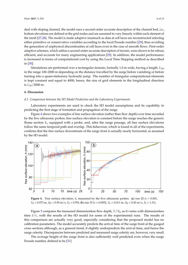
Figure 4 shows two examples of free surface elevation (rather than flow depth) over time recordedby the five ultrasonic probes; free surface elevation is constant before the surge reaches the genericflume section Si, equipped with a probe, and, after the surge passage, all free surface elevationsfollow the same temporal path and overlap. This behaviour, which is found in all of the experiments,confirms that the free surface downstream of the surge front is actually nearly horizontal, as assumedby the 0D model.

0 5 10 15 2560

80

100

120

140

time (s)

fre

e s

urf

ace

ele

va

tio

n,

h (

mm

) a

0

20

40

60

80

100

0 50 100 150time (s)

b

fre

e s

urf

ace

ele

va

tio

n,

h (

mm

)

25 75

Figure 4. Free surface elevation, h, measured by the five ultrasonic probes. (a) run 20 (s = 0.001,Y0 = 0.073 m, U0 = 0.50 m/s, F0 = 0.59); (b) run 33 (s = 0.0052, Y0 = 0.011 m, U0 = 0.43 m/s, F0 = 1.31).

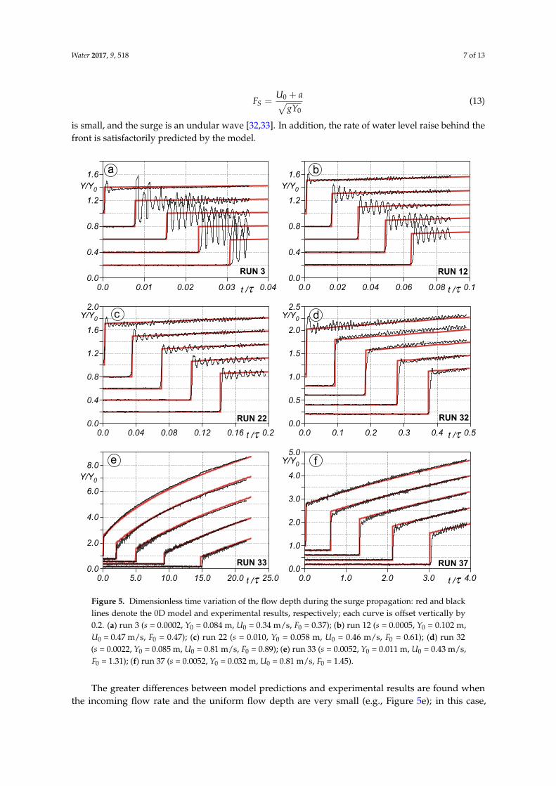
Figure 5 compares the measured dimensionless flow depth, Y/Y0, as it varies with dimensionlesstime t/τ, with the results of the 0D model for some of the experimental runs. The results ofthis comparison are actually very good, especially considering that the proposed model has nocalibration parameters. The model accurately predicts the arrival time of the surge front at the gaugedcross sections although, as a general trend, it slightly underpredicts the arrival time, and hence thesurge celerity. Discrepancies between predicted and measured surge celerity are, however, very small.

The average height of the surge front is also sufficiently well predicted even when the surgeFroude number, defined to be [31]

Water 2017, 9, 518 7 of 13

FS =U0 + a√

gY0(13)

is small, and the surge is an undular wave [32,33]. In addition, the rate of water level raise behind thefront is satisfactorily predicted by the model.

RUN 37

0.0 1.0 2.0 3.0 4.0t /τ

0.0

1.0

2.0

3.0

4.0

5.0

Y/Y0 f

RUN 330.0

2.0

4.0

6.0

8.0

0.0 5.0 10.0 15.0 20.0 25.0

Y/Y0

t /τ

e

0.0

0.4

0.8

1.2

1.6

2.0

Y/Y0

0.0 0.04 0.08 0.12 0.16 0.2t /τ

c

RUN 22

0.0 0.1 0.2 0.3 0.4 0.5t /τ

RUN 320.0

0.5

1.0

1.5

2.0

2.5

Y/Y0 d

0.0

0.4

0.8

1.2

1.6

0.0 0.02 0.04 0.06 0.08 0.1

Y/Y0

t /τ

b

RUN 120.0

0.4

0.8

1.2

1.6

0.0 0.01 0.02 0.03 0.04

Y/Y0

t /τ

a

RUN 3

Figure 5. Dimensionless time variation of the flow depth during the surge propagation: red and blacklines denote the 0D model and experimental results, respectively; each curve is offset vertically by0.2. (a) run 3 (s = 0.0002, Y0 = 0.084 m, U0 = 0.34 m/s, F0 = 0.37); (b) run 12 (s = 0.0005, Y0 = 0.102 m,U0 = 0.47 m/s, F0 = 0.47); (c) run 22 (s = 0.010, Y0 = 0.058 m, U0 = 0.46 m/s, F0 = 0.61); (d) run 32(s = 0.0022, Y0 = 0.085 m, U0 = 0.81 m/s, F0 = 0.89); (e) run 33 (s = 0.0052, Y0 = 0.011 m, U0 = 0.43 m/s,F0 = 1.31); (f) run 37 (s = 0.0052, Y0 = 0.032 m, U0 = 0.81 m/s, F0 = 1.45).

The greater differences between model predictions and experimental results are found whenthe incoming flow rate and the uniform flow depth are very small (e.g., Figure 5e); in this case,

Water 2017, 9, 518 8 of 13

the Reynolds number, Re = U0Y0/ν, with ν the kinematic viscosity, is small (e.g., Re = 4730 for flowconditions of Figure 5e) and viscosity is likely to affect the flow.

It is also interesting to observe in Figure 5e that the front height reduces significantly during thesurge propagation (∆Y/Y0 ≈ 1.5 at XS1, ∆Y/Y0 ≈ 0.6 at XS5) and this behaviour is correctly predictedby the model.

As a general trend, the model slightly underpredicts surge wave celerity and overpredicts thesurge height compared to experimental results; indeed, differences between experimental results andmodel predictions increase with the increasing of channel bed slope. From the comparison betweenmodel predictions and experimental results, we can conclude that the model performs satisfactorily atleast during the early stage of surge formation and propagation.

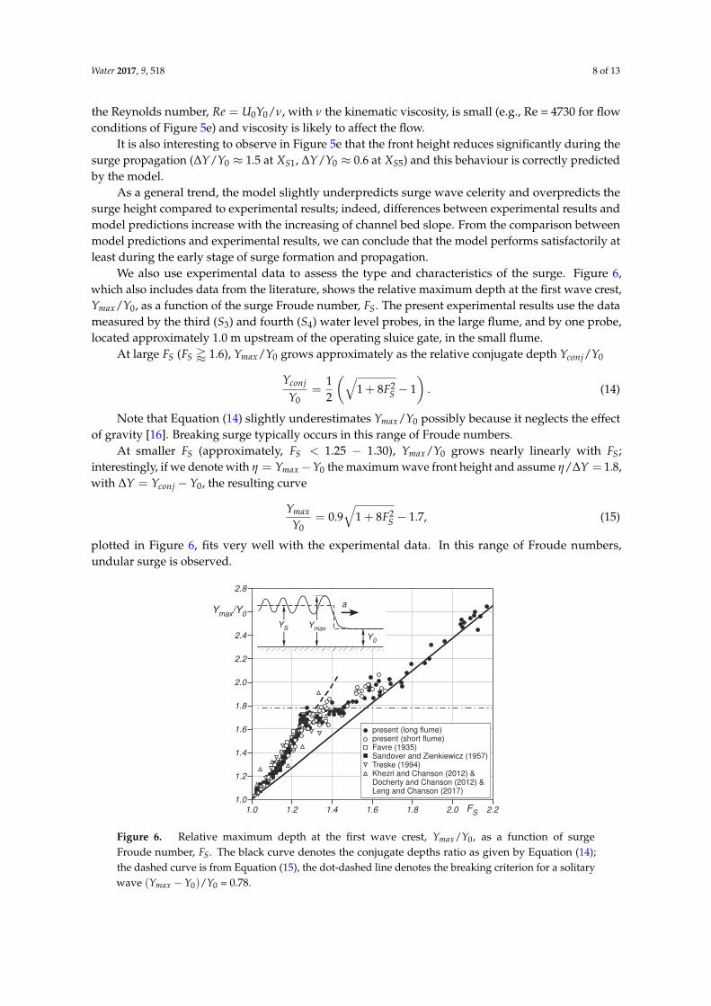
We also use experimental data to assess the type and characteristics of the surge. Figure 6,which also includes data from the literature, shows the relative maximum depth at the first wave crest,Ymax/Y0, as a function of the surge Froude number, FS. The present experimental results use the datameasured by the third (S3) and fourth (S4) water level probes, in the large flume, and by one probe,located approximately 1.0 m upstream of the operating sluice gate, in the small flume.

At large FS (FS ' 1.6), Ymax/Y0 grows approximately as the relative conjugate depth Yconj/Y0

Yconj

Y0=

12

(√1 + 8F2

S − 1)

. (14)

Note that Equation (14) slightly underestimates Ymax/Y0 possibly because it neglects the effectof gravity [16]. Breaking surge typically occurs in this range of Froude numbers.

At smaller FS (approximately, FS < 1.25 − 1.30), Ymax/Y0 grows nearly linearly with FS;interestingly, if we denote with η = Ymax−Y0 the maximum wave front height and assume η/∆Y = 1.8,with ∆Y = Yconj −Y0, the resulting curve

Ymax

Y0= 0.9

√1 + 8F2

S − 1.7, (15)

plotted in Figure 6, fits very well with the experimental data. In this range of Froude numbers,undular surge is observed.

1.0

1.2

1.4

1.6

1.8

2.0

2.2

2.4

2.6

2.8

1.0 1.2 1.4 1.6 1.8 2.0 2.2

Ymax

/Y0

a

Y0

Ymax

YS

present (long flume) present (short flume) Favre (1935) Sandover and Zienkiewicz (1957) Treske (1994) Khezri and Chanson (2012) & Docherty and Chanson (2012) & Leng and Chanson (2017)

FS

Figure 6. Relative maximum depth at the first wave crest, Ymax/Y0, as a function of surgeFroude number, FS. The black curve denotes the conjugate depths ratio as given by Equation (14);the dashed curve is from Equation (15), the dot-dashed line denotes the breaking criterion for a solitarywave (Ymax −Y0)/Y0 = 0.78.

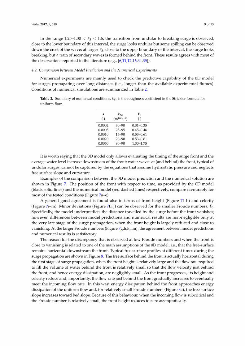
Water 2017, 9, 518 9 of 13

In the range 1.25–1.30 < FS < 1.6, the transition from undular to breaking surge is observed;close to the lower boundary of this interval, the surge looks undular but some spilling can be observeddown the crest of the wave; at larger FS, close to the upper boundary of the interval, the surge looksbreaking, but a train of secondary waves is formed behind the front. These results agrees with most ofthe observations reported in the literature (e.g., [6,11,12,16,34,35]).

4.2. Comparison between Model Prediction and the Numerical Experiments

Numerical experiments are mainly used to check the predictive capability of the 0D modelfor surges propagating over long distances (i.e., longer than the available experimental flumes).Conditions of numerical simulations are summarized in Table 2.

Table 2. Summary of numerical conditions. kSt is the roughness coefficient in the Strickler formula foruniform flow.

s kSt F0(-) (m1/3s-1) (-)

0.0002 30–90 0.31–0.350.0005 25–95 0.45–0.460.0010 15–90 0.53–0.610.0020 20–90 0.53–0.610.0050 80–90 1.30–1.75

It is worth saying that the 0D model only allows evaluating the timing of the surge front and theaverage water level increase downstream of the front; water waves at (and behind) the front, typical ofundular surges, cannot be captured by the equations that assume hydrostatic pressure and neglectsfree surface slope and curvature.

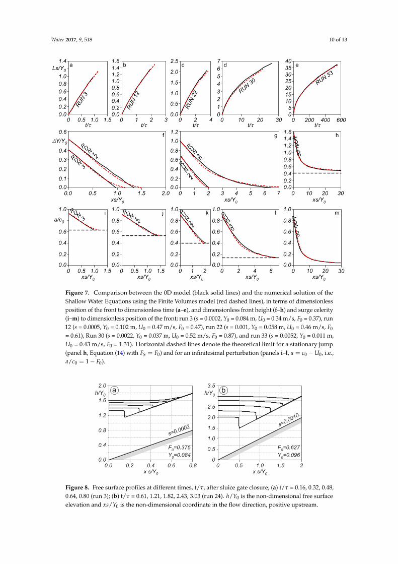
Examples of the comparison between the 0D model prediction and the numerical solution areshown in Figure 7. The position of the front with respect to time, as provided by the 0D model(black solid lines) and the numerical model (red dashed lines) respectively, compare favourably formost of the tested conditions (Figure 7a–e).

A general good agreement is found also in terms of front height (Figure 7f–h) and celerity(Figure 7i–m). Minor deviations (Figure 7f,i,j) can be observed for the smaller Froude numbers, F0.Specifically, the model underpredicts the distance travelled by the surge before the front vanishes;however, differences between model predictions and numerical results are non-negligible only atthe very late stage of the surge propagation, when the front height is largely reduced and close tovanishing. At the larger Froude numbers (Figure 7g,h,k,l,m), the agreement between model predictionsand numerical results is satisfactory.

The reason for the discrepancy that is observed at low Froude numbers and when the front isclose to vanishing is related to one of the main assumptions of the 0D model, i.e., that the free-surfaceremains horizontal downstream the front. Typical free surface profiles at different times during thesurge propagation are shown in Figure 8. The free surface behind the front is actually horizontal duringthe first stage of surge propagation, when the front height is relatively large and the flow rate requiredto fill the volume of water behind the front is relatively small so that the flow velocity just behindthe front, and hence energy dissipation, are negligibly small. As the front progresses, its height andcelerity reduce and, importantly, the flow rate just behind the front gradually increases to eventuallymeet the incoming flow rate. In this way, energy dissipation behind the front approaches energydissipation of the uniform flow and, for relatively small Froude numbers (Figure 8a), the free surfaceslope increases toward bed slope. Because of this behaviour, when the incoming flow is subcritical andthe Froude number is relatively small, the front height reduces to zero asymptotically.

Water 2017, 9, 518 10 of 13

0.0

0

0.6

0.0

0.2

0.4

1.0

0.5 1.0 1.5 0 0.5 1.0 1.5

0.6

0.2

0.4

0.8

1.0

0 1 2

0.6

0.0

0.2

0.4

0.8

1.0

0 2 4

0.6

0.0

0.2

0.4

0.8

1.0

6 0 10 20

0.6

0.0

0.2

0.4

0.8

1.0

30

a/c0

xs/Y0

i j k l mRU

N 3

RU

N 12

RU

N 2

2

RU

N 3

0

RU

N 3

3

1.6

0.2

0.4

0.6

0.8

1.0

1.2

1.4

0.0

0 10 20 30

h

RU

N 3

3

0 1 2 3 4 5 6 7

0.6

0.0

0.2

0.4

0.8

1.2

1.0

RU

N 2

2RUN 3

0

g

0.0

0.1

0.2

0.3

0.4

0.6

∆Y/Y0

0.0 0.5 1.0 1.5 2.0

RU

N 3

RU

N 12

f

0 0.5 1.0 1.5

0.6

0.0

1.4

0.4

0.2

0.8

1.0

0 1 2

0.6

0.0

1.6

1.2

0.4

0.2

0.8

1.0

3

1.4

0 2 4

1.0

0.0

2.5

2.0

0.5

1.5

0 10 20

2

0

7

5

1

3

6

4

30 0 200 400

15

0

40

30

5

20

35

25

600

10

Ls/Y0

t/τ t/τ t/τ t/τ t/τ

a b c d e

RU

N 3

RU

N 1

2

RU

N 2

2 RUN 3

0R

UN

33

xs/Y0

xs/Y0

xs/Y0

xs/Y0

xs/Y0

xs/Y0

xs/Y0

Figure 7. Comparison between the 0D model (black solid lines) and the numerical solution of theShallow Water Equations using the Finite Volumes model (red dashed lines), in terms of dimensionlessposition of the front to dimensionless time (a–e), and dimensionless front height (f–h) and surge celerity(i–m) to dimensionless position of the front; run 3 (s = 0.0002, Y0 = 0.084 m, U0 = 0.34 m/s, F0 = 0.37), run12 (s = 0.0005, Y0 = 0.102 m, U0 = 0.47 m/s, F0 = 0.47), run 22 (s = 0.001, Y0 = 0.058 m, U0 = 0.46 m/s, F0

= 0.61), Run 30 (s = 0.0022, Y0 = 0.037 m, U0 = 0.52 m/s, F0 = 0.87), and run 33 (s = 0.0052, Y0 = 0.011 m,U0 = 0.43 m/s, F0 = 1.31). Horizontal dashed lines denote the theoretical limit for a stationary jump(panel h, Equation (14) with FS = F0) and for an infinitesimal perturbation (panels i–l, a = c0 −U0, i.e.,a/c0 = 1− F0).

s=0.00

02

0.0

0.4

0.8

1.2

1.6

2.0

0.0 0.2 0.4 0.6 0.8

h/Y0

a

x s/Y0

0

0.5

2.0

2.5

3.5

0 0.5 1.0

h/Y0

b

s=0.0010

1.5

1.0

21.5

x s/Y0

F0=0.375

Y0=0.084

F0=0.627

Y0=0.096

Figure 8. Free surface profiles at different times, t/τ, after sluice gate closure; (a) t/τ = 0.16, 0.32, 0.48,0.64, 0.80 (run 3); (b) t/τ = 0.61, 1.21, 1.82, 2.43, 3.03 (run 24). h/Y0 is the non-dimensional free surfaceelevation and xs/Y0 is the non-dimensional coordinate in the flow direction, positive upstream.

Water 2017, 9, 518 11 of 13

The results of the numerical simulations show that the deviation from horizontal of the free-surfacedownstream of the front decreases with bed slope increasing, and finally reverses when F0 is relativelylarge (see, e.g., Figure 8b). The concavity of the free-surface profile downstream of the surge is likelyrelated to flow unsteadiness; as water depth increases in time, flow rate per unit width decreasesfrom U1Y1, just downstream of the front, to zero at the gate section. This condition is somehowsimilar to the case of a distributed outflow from a channel when the flow is steady and subcritical;in such a case, the free-surface profile is known to have a positive gradient in the flow direction and anegative curvature [21].

Interestingly, when the incoming flow is supercritical and the surge tends to a stationary hydraulicjump (Figure 7h,m), the main model assumption (i.e., horizontal free surface downstream the front)always holds. Indeed, the front height does not reduce to zero and the velocity behind the front is thusconsiderably smaller than the incoming flow velocity.

5. Conclusions

In this work, a simple zero-dimensional model to simulate the propagation of a positive surgein a sloping channel is proposed and its predictive capability is checked against experimental andnumerical data. The studied surge is generated by the instantaneous closure of a downstream gate.

When comparing the 0D model results with experimental data, small discrepancies are observed,which are mainly caused by the strongly nonlinear effects produced by free surface slope and curvature.As a general trend, the model slightly underpredicts the surge wave celerity and overpredicts thesurge height; differences between experimental results and the 0D model predictions increase with theincreasing of channel bed slope.

From the comparison between the numerical results and the predictions of the proposed model,it emerges that the 0D model can accurately simulate the initial stage of the surge formation andpropagation. During the late stage of surge propagation, and when the Froude number of the incomingflow is small, so that the fate of the front is to vanish, the assumption of horizontal free surface behindthe front stops holding true and the surge front reduces its height slower than that predicted bythe model. However, this discrepancy between model predictions and numerical results is possiblyunimportant from a practical point of view since it occurs during the late stage of surge propagationwhen the front height is largely reduced.

As a whole, the proposed 0D model, and even more so its analytical solution for F0 < 0.6,are simple tools that allow for a quick preliminary estimate of flow conditions following thedevelopment of a positive surge in a sloping channel and are of help in the design process as theyclearly show the impact of channel geometry and flow conditions on the characteristics of the surge.

Acknowledgments: We wish to acknowledge Jacopo Buziol, Mattia Chillon, Marco Rossi Denza, Alberto Sartorato,and Massimo Zennaro, for their contribution to the experimental investigation.

Author Contributions: D.P.V. dealt with theoretical and numerical models and wrote the paper; P.P. performedexperiments, reviewed and edited the manuscript; A.D. conceived the study, dealt with the theoretical model, andreviewed the manuscript.

Conflicts of Interest: The authors declare no conflict of interest.

Appendix A. Numerical Solution of Model Equations

The front position at time t is approximated as

L =∫ t−∆t

0a(ξ)dξ + a∆t = L′ + a∆t, (A1)

with ∆t the integration time step and L′ the front position at t − ∆t. Equation (2), with theapproximation (A1), is then rewritten as

Water 2017, 9, 518 12 of 13

U0Y0 = a(∆Y + L′s + as∆t

)+ (L′ + a∆t)

d∆Ydt

. (A2)

Central finite difference discretisation of the time derivative in (A2) yields

∆Y =

[U0Y0

a+ (L′ + a∆t)

(∆Y′

a∆t− s)](

L′

a∆t+ 2)−1

, (A3)

with ∆Y′ the wave front height at t− ∆t.The set of Equations (4) and (A3) is solved iteratively. Starting with a first guess for

a (e.g., a′ = a(t− ∆t)), Equation (A3) is solved for ∆Y; with this, Equation (4) is used to find anew guess for a. The whole process is repeated until convergence. Once convergence is achieved,all variables of the problem are updated.

References

1. Castro-Orgaz, O.; Chanson, H. Ritter’s dry-bed dam-break flows: Positive and negative wave dynamics.Environ. Fluid Mech. 2017, 17, 665–694.

2. Triki, A. Resonance of free-surface waves provoked by floodgate maneuvers. J. Hydrol. Eng. 2014, 19,1124–1130.

3. Triki, A. Further investigation on the resonance of free-surface waves provoked by floodgate maneuvers:Negative surge waves. Ocean Eng. 2017, 133, 133–141.

4. Valiani, A.; Caleffi, V.; Zanni, A. Case Study: Malpasset Dam-Break Simulation using a Two-DimensionalFinite Volume Method. J. Hydraul. Eng. ASCE 2002, 128, 460–472.

5. Viero, D.P.; D’Alpaos, A.; Carniello, L.; Defina, A. Mathematical modeling of flooding due to river bankfailure. Adv. Water Resour. 2013, 59, 82–94.

6. Favre, H. Etude Théoretique et Expérimentale des Ondes de Translation Dans les Canaux Découverts; Dunod:Paris, France, 1935.

7. Benjamin, T.B.; Lighthill, M.J. On cnoidal waves and bores. Proc. R. Soc. Lond. Ser. A 1954, 224, 448–460.8. Peregrin, D.H. Calculations of the development of an undular bore. J. Fluid Mech. 1966, 25, 321–330.9. Chanson, H. Undular Tidal Bores: Basic Theory and Free-surface Characteristics. J. Hydraul. Eng. ASCE

2010, 136, 940–944.10. Chanson, H. Turbulent shear stresses in hydraulic jumps, bores and decelerating surges. Earth Surf.

Process. Landf. 2011, 36, 180–189.11. Khezri, N.; Chanson, H. Undular and Breaking Tidal Bores on Fixed and Movable Gravel Beds.

J. Hydraul. Res. 2012, 50, 353–363.12. Docherty, J.; Chanson, H. Physical modeling of unsteady turbulence in breaking tidal bores. J. Hydraul.

Eng. ASCE 2012, 138, 412–419.13. Leng, X.; Chanson, H. Coupling between free-surface fluctuations, velocity fluctuations and turbulent

Reynolds stresses during the upstream propagation of positive surges, bores and compression waves.Environ. Fluid Mech. 2016, 16, 695–719.

14. Ben Meftah, M.; Mossa, M.; Pollio, A. Considerations on shock wave/boundary layer interaction inundular hydraulic jumps in horizontal channels with a very high aspect ratio. Eur. J. Mech. B Fluids 2010,29, 415–429.

15. Castro-Orgaz, O.; Chanson, H. Minimum Specific Energy and Transcritical Flow in UnsteadyOpen-Channel Flow. J. Irrig. Drain. Eng. ASCE 2016, 142, 351–363.

16. Leng, X.; Chanson, H. Upstream Propagation of Surges and Bores: Free-Surface Observations. Coast. Eng. J.2017, 59, 1750003.

17. Stoesser, T.; McSherry, R.; Fraga, B. Secondary Currents and Turbulence over a Non-Uniformly RoughenedOpen-Channel Bed. Water 2015, 7, 4896–4913.

18. Viero, D.P.; Defina, A. Extended theory of hydraulic hysteresis in open channel flow. J. Hydraul. Eng. ASCE2017, 143, 06017014.

19. Viero, D.P.; Defina, A. Multiple states in the flow through a sluice gate. J. Hydraul. Res. 2017, under review.

Water 2017, 9, 518 13 of 13

20. Viero, D.P.; Pradella, I.; Defina, A. Free surface waves induced by vortex shedding in cylinder arrays.J. Hydraul. Res. 2017, 55, 16–26.

21. Henderson, F.M. Open-Channel Flow; McMillan Publishing Co.: New York, NY, USA, 1966.22. Defina, A.; Susin, F.M.; Viero, D.P. Bed friction effects on the stability of a stationary hydraulic jump in a

rectangular upward sloping channel. Phys. Fluids 2008, 20, 036601.23. Visconti, F.; Stefanon, L.; Camporeale, C.; Susin, F.; Ridolfi, L.; Lanzoni, S. Bed evolution measurement

with flowing water in morphodynamics experiments. Earth Surf. Process. Landf. 2012, 37, 818–827.24. Defina, A.; Susin, F.M.; Viero, D.P. Numerical study of the Guderley and Vasilev reflections in steady

two-dimensional shallow water flow. Phys. Fluids 2008, 20, 097102.25. Defina, A.; Viero, D.P.; Susin, F.M. Numerical simulation of the Vasilev reflection. Shock Waves 2008,

18, 235–242.26. Viero, D.P.; Susin, F.; Defina, A. A note on weak shock wave reflection. Shock Waves 2013, 23, 505–511.27. Begnudelli, L.; Sanders, B.F. Unstructured Grid Finite-Volume Algorithm for Shallow-Water Flow and

Scalar Transport with Wetting and Drying. J. Hydraul. Eng. ASCE 2006, 132, 371–384.28. Defina, A.; Viero, D.P. Open channel flow through a linear contraction. Phys. Fluids 2010, 22, 036602.29. Begnudelli, L.; Sanders, B.F.; Bradford, S.F. Adaptive Godunov-Based Model for Flood Simulation.

J. Hydraul. Eng. ASCE 2008, 134, 714–725.30. Sanders, B.F. Integration of a shallow water model with a local time step. J. Hydraul. Res. 2008, 46, 466–475.31. Koch, C.; Chanson, H. Turbulence measurements in positive surges and bores. J. Hydraul. Res. 2009,

47, 29–40.32. Prüser, H.H.; Zielke, W. Undular bores (Favre Waves) in Open Channels Theory and Numerical Simulation.

J. Hydraul. Res. 1994, 32, 337–354.33. Castro-Orgaz, O.; Hager, W.H.; Dey, S. Depth-averaged model for undular hydraulic jump. J. Hydraul. Res.

2015, 53, 351–363.34. Sandover, J.A.; Ziekiewicz, P. Experiments on Surge Waves. Water Power 1957, 9, 418–424.35. Treske, A. Undular bores (Favre-waves) in open channels—Experimental studies. J. Hydraul. Res.

1994, 32, 355–370.

c© 2017 by the authors. Licensee MDPI, Basel, Switzerland. This article is an open accessarticle distributed under the terms and conditions of the Creative Commons Attribution(CC BY) license (http://creativecommons.org/licenses/by/4.0/).