SOFTWARE-PRACTICE AND EXPERIENCE, VOL. 20(3), 283-300 (MARCH 1990)

A Tool to Minimize the Time Costs of Parallel Computations through Optimal

Processing Power Allocation

BIN Q I N Computer Science Department, Ford Hall, Brandeis University, Waltham, MA 02254,

U S A .

AND

HOWARD A. SHOLL AND REDA A. AMMAR Computer Science & Engineering Department, The University of Connecticut, Stom, CT

06269-3155, U.S.A.

SUMMARY

In this paper, we present a software system, OPAS (Optimal Allocation System), that incorporates the optimal allocation policy in the analysis of the time-cost behaviour of parallel computations. OPAS assumes that the underlying system which supports the executions of parallel computations has a finite number of processors, that all the processors have the same speed and that the communication is achieved through a shared memory. OPAS defines the time cost as a function of the input, the algorithm, the data structure, the processor speed, the number of processors and the processing power allocation. In analysing the time cost of a computation, OPAS first uses the optimal allocation policy that we developed previously to determine the amount of processing power each node receives and then derives the computation's time cost. OPAS can evaluate different time-cost behaviours, such as the minimum time cost, the maximum time cost, the average time cost and the time-cost variance. It can also determine the speed-up and efficiency, and plot the time-cost curve and time-cost distribution.

KEY WORDS Parallel computation Optimal allocation Time cost

1. INTRODUCTION

The time cost of a computation, especially a parallel computation, depends on many factors such as the input, the algorithm, the data structure, the processor speed, the number of processors, the processing power allocation, the communication, the execution environment and the execution overhead.'! In this paper, we define the time cost as a function of the input, the algorithm, the data structure, the processor speed, the number of processors and the processing power allocation. Since the time cost is a function of these six factors, once the first five factors are fixed (typically, once the number of processors is given), the time cost solely depends on how the processing power is allocated. Different allocation policies will yield different time costs. Therefore, one would like to search for the optimal allocation policy to minimize the time cost and observe how the time cost behaves when the optimal allocation policy is used.

0038-0644/90/030283- 18$09.00 0 1990 by John Wiley & Sons, Ltd.

Received 26 October 1988 Revised 21 August 1989

284 B . QIN, H . A. SHOLL A N D R. A . AMMAR

Generally, the optimal allocation problem is essentially an NP-complete p r ~ b l e m . ~ Fortunately, our recent work has shown that if only the input, the algorithm, the data structure, the processor speed, the number of processors and the processing power allocation are considered, then for any parallel structure, there exist an X and I.’ such that the optimal allocations exist when the processing power P satisfies P€(O,Al orPE(I-,+m).‘ In this paper, we present a software system, OPAS (Optimal Allocation System) that incorporates the optimal allocation policy in the analysis of the time-cost behaviour of parallel computations. It is assumed in OPAS that the underlying computer system has a finite number of processors, that all the processors have the same speed and that they communicate with each other through a shared memory. The modified computation structure m0de1~3~ is used in OPAS as the underlying model. In analysing the time cost of a computation, OPAS first uses the optimal allocation policies that we developed previously to determine the amount of processing power each node receives and then derives the computation’s time cost. Therefore, the time cost obtained from OPAS is the minimum time cost one can expect under the optimal allocation. Thus, by using OPAS, the user can find the best time-cost behaviour of a computation.

This paper is organized as follows. The execution and time-cost modellings are first presented in Sections 2 and 3 . The optimal allocation policies are discussed in Section 4. The general structure of OPAS and how it works are shown in Section 5. An example is used in Section 6 to illustrate the use of OPAS, followed by the conclusion in Section 7 .

2. EXECUTION MODELLING

The model used in this paper is a subset of the modified computation structure mode12v5 that describes the detailed execution and time-cost behaviour of computations. This model has been used as the underlying model in TCAS (Time Cost Analysis System).2 In this section, we briefly describe this model. More details about this model can be found in reference 2.

A computation in the modified computation structure model is represented as two directed graphs, a control graph and a data graph. The control graph shows the order in which operations are performed, whereas the data graph shows the relations between operations and data. In this paper, only the control graph is used.

It is assumed in the model that the underlying computer system has a finite number of processors, that all the processors have the same speed and that they communicate with each other through a shared memory. Typically, we may assume that each processor has unit processing power. Under such an assumption, one processor is equivalent to one unit of processing power.

It is assumed that there are activation signals and that the execution of a computation is triggered when an activation signal enters the control graph of the computation. An activation signal has the ability to carry processing power and allocation policy as it travels in the control graph of a computation. I t is assumed that the processing power allocation and release are carried out at the beginning and end of a computation’s execution, respectively. That is, a computation will hold the same amount of processing power during its execution. The amount of processing power carried to a computation by an activation signal is what is allocated to the computation, and the allocation policy carried to a computation is the one passed to the computation. When an activation

A TOOL T O MINIMIZE TIME COSTS 285

signal reaches a node in the computation, the node receives all the processing power and the allocation policy carried by the signal, and it uses them to perform the specified operations. After the specified operations are performed, the signal carries the same amount of processing power and the same allocation policy, and leaves the node. When the execution of a computation is over, the signal leaves the computation; and the processing power and the allocation policy carried by the signal are returned to the underlying computer system.

The control graph of a sequential computation contains a start node, an end node, operation nodes, decision nodes and or nodes. The start and end nodes indicate the beginning and end of the computation, an operation node specifies an operation to be performed, a decision node checks conditions at a branch point and an or node serves as a junction point. The execution of a computation is triggered when an activation signal enters the start node of the computation's control graph. When a signal enters an operation node, the operation specified by the node is performed and the signal then leaves the node. When a signal arrives at a decision node, the decision node checks some conditions and the signal leaves the node from one of its outgoing edges depending on the results. When a signal arrives at an or node from one of its incoming edges, it immediately leaves the node from its outgoing edge. When an activation signal finally arrives at the end node, the execution terminates.

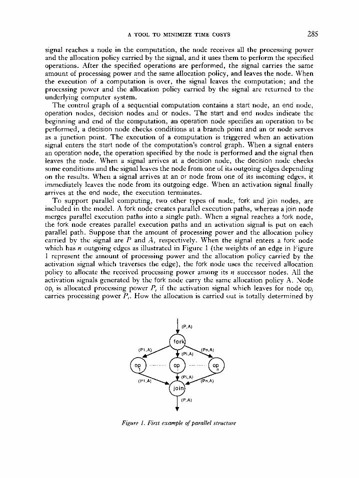
T o support parallel computing, two other types of node, fork and join nodes, are included in the model. A fork node creates parallel execution paths, whereas a join node merges parallel execution paths into a single path. When a signal reaches a fork node, the fork node creates parallel execution paths and an activation signal is put on each parallel path. Suppose that the amount of processing power and the allocation policy carried by the signal are P and A, respectively. When the signal enters a fork node which has n outgoing edges as illustrated in Figure 1 (the weights of an edge in Figure 1 represent the amount of processing power and the allocation policy carried by the activation signal which traverses the edge), the fork node uses the received allocation policy to allocate the received processing power among its n successor nodes. All the activation signals generated by the fork node carry the same allocation policy A. Node opj is allocated processing power Pj if the activation signal which leaves for node op; carries processing power Pi. How the allocation is carried out is totally determined by

Figure I. First example of parallel structure

286 B . Q I N , H . A. SHOLL AND R . A. AMMAR

the allocation policy A. The only restrictions put on the allocation are as follows:

n

cPi=P, O<P;IP i= 1

When a join node, as illustrated in Figure 1, receives one signal from each of its incoming edges, an activation signal is created and it leaves the join node from its outgoing edge. The signal created by the join node carries allocation policy A, and if the activation signal coming from node op, carries processing power PI, the activation

signal generated by the join node then carries processing power P = CP,. I1

I = I

3 . TIME-COST MODELLING

The time cost of a computation is defined as follows. Each node in the control graph is associated with a time cost which is equal to the time needed to perform the operations specified by the node. When a node with time cost C receives all the required activation signals, the execution of the specified operations are started and, after an amount of time C, activation signals leave the node. The time cost of a computation is then defined as the time for an activation signal to travel from the start node to the end node. However, the time cost of a node depends on the amount of processing power and the allocation policy it receives. If the amount of processing power and the allocation policy a node 1. receives are P and A, respectively, the time cost of V is defined as Cost,-(P,A). Note that it is not necessary for P to be an integer number. The only restriction put on P is P > 0. P 2 1 means that node I‘ uses more than unity processing power. P < 1 means that 1’ shares one processor with other nodes and that node I’ can only obtain PX 100 per cent of the processor time.

For the parallel structure as illustrated in Figure 1, if the amount of processing power and the allocation policy received by the fork node are P and A , respectively, we define its time cost as

For a node I’ which contains no parallel paths, we define its base time cost (BTC) as its time cost given that unit processing power is provided. Since such a node does not contain any parallel paths, its time cost is independent of the processing power allocation. Therefore, its BTC is equal to Cost,- (1 , .4’) whereil’ is any allocation policy. Suppose that processing power P is provided to node I , then we define the time cost of node V as

where A and A’ are any allocation policies. The above definition indicates that the BTC of a node that contains no parallel paths

is the best time cost one can obtain; providing more than unit processing power to

A TOOL T O MINIMIZE TIME COSTS 287

such a node will not reduce its time cost, and providing less than unit processing power to such a node will force the node to wait during its execution, therefore resulting in an increase of its time cost.

According to the model, a node will hold the same amount of processing power during the time in which the operations specified by the node are being performed. If we further assume that every time a signal arrives at a node it brings the same amount of processing power to the node, then the allocation used in the model is equiv- alent to the static allocation. Based on this assumption, the following procedure, ALLOCATE(G,P,A), can be used to determine the amount of processing power that each node in a computation can receive. ALLOCATE(G, P,A) is designed as a recursive procedure where G is the control graph of the computation, P and A are the pro- cessing power and allocation policy passed to the computation, respectively. ALLOCATE (G,P,A) works as follows:

1. For each node that is not contained in a parallel structure, the processing power it receives is P.

2. For each parallel path, PATH,, of a parallel structure that is not contained in another parallel structure, do the following:

2.1. Use A to determine the amount of processing power that PATH, can

2.2. Consider PATH, as a control graph and recursively call ALLOCATE(PATH,, receive (suppose it is PI) .

p,, A ) .

4. OPTIMAL ALLOCATION TECHNIQUES

In this section, we present two optimal allocation policies, the sequential allocation policy and the enough allocation policy, that can be used to minimize the time cost.

Definition 1 For a computation, define its sequential execution time cost (SETC) as follows:

1. The SETC of a Computation is equal to its BTC. 2. For a parallel structure as given in Figure 1, assume that the SETCs of the fork,

op, (each op, may represent a subgraph) and loin are SETC,,SETC, and SETC,, respectively. The SETC of the parallel structure is

n

SETCf + SETC,+SETC, i= 1

(3)

3. For a computation, its SETC is determined as follows:

the SETC of the parallel structure.

SETC is SETCi, the SETC of the computation is

3.1. Replace each parallel structure with a single node and set its SETC to

3.2. If the new computation has n nodes, the ith is executed Ei times and its

i= 1

288 B . QIN, H. A . SHOLL A N D R . A . AMMAR

T o determine the S E T C of a computation in step 3.2, one can apply time-cost analysis techniques for sequential computationsG8 on the computation.

Definition 2 For each computation, define its iriinimurn time cost (MTC) as its time cost given

that each node in the computation gets at least unit processing power.

It can be seen that the M T C of a sequential computation is equal to its BTC and its SETC, and that the M T C of a general computation represents the best time-cost behaviour one can expect for it. T o determine a computation’s MTC, one can set the time cost of each node in the computation to its BTC and then use a time-cost analysis technique for parallel computation^^*^ to derive the computation’s MTC.

Definition 3

as follows: For a computation, define its almost rninimiim atrioicnt of processiq power (AMAPP)

1. The AMAPP of a sequential node is 1. 2. For a parallel structure which has the form as given in Figure 1, assume that the

MTC, SETC and AhlAPP of op, are MTC,, SETC, and AMAPP, respectively. Define the required processing poxer (RP) for each op,. The RP of op, is defined as follows:

MTC, x ARIAPP, RP, = _____ if SETC, > max{MTC,, ..., MTC,,} (4)

max{ MTC,, . . . , MTC,,}

__ if SETC, 5 max{MTC1, ..., MTC,,} (5) SETC,

max{ R/ITC1, . . . , MTC,,} RP I--- ’

The AMAPP of the parallel structure is then defined as follows

I,

i= 1

3 . For a computation, its AhIAPP is determined in the following way:

3.1. Replace each parallel structure with a single node and set the AMAPP

3.2. The AMAPP of the computation is then equal to maximum AMAPP of the node to the AMAPP of the parallel structure.

among all the nodes in the new computation.

Definition 4 Define the sequential allocation policy as follows. Given the parallel structure in

Figure I , suppose that the S E T C of op, is SETC, and that processing power P is provided to the parallel structure, then the sequential allocation policy will allocate the

A TOOL TO MINIMIZE TIME COSTS 289

following amount of processing power to op;:

SETC; P;=P ,I

CSETC, j = 1

( 7 )

Definition 5 Define the enough allocation policy as follows. Given the parallel structure in Figure

1, assume that the RP of op; is RP;. If processing power P is provided to the parallel structure, the enough allocation policy will allocate the following amount of processing power to op,:

R P; P;=P 7

;= 1

Theorem 1

and processing power P is provided to the parallel structure, where Given the parallel structure in Figure 1, suppose that the SETC of op; is SETC;

P I - I='

max{SETC,, ..., SETC,,}

The sequential allocation policy is then the optimal allocation policy for such a parallel structure.

Theorem 2

processing power P is provided to the parallel structure and P satisfies Given the parallel structure in Figure 1, assume that the RP of op; is RP;. If

i= 1

then the enough allocation policy is the optimal allocation policy for such a parallel structure.

The proofs of Theorems 1 and 2 can be found in Reference 4. Theorems 1 and 2 indicate that for any parallel structure as given in Figure 1, there

290 B. QIN, H . A. SHOLL AND R . A . AMMAR

exist an A- and a where

2 SETC, -~ I = 1 x=

max{ SETC;, . . . , SETC,,}

Y = C R P ,

(9)

1 ' 1

(11) RIITC, X ANIAPP,

max{ MTCl , . . . , MTC,,}

SETC, max{MTC1, ..., MTC,,)

RP, = _____ if SETC, > max{RIITC1, ..., MTC,,}

if SETC, 5 max{MTC1, ..., MTC,,) RP, =

such that the optimal allocation can be achieved if P E (O,Lkl or P E [Y,+w). We call (0,A-] and [ Y , + z ) the optimal ranges and (A-,17) the non-optimal range. It has been proved that for the parallel structure in Figure 1, i f each op; is sequential, thenX = Y.'

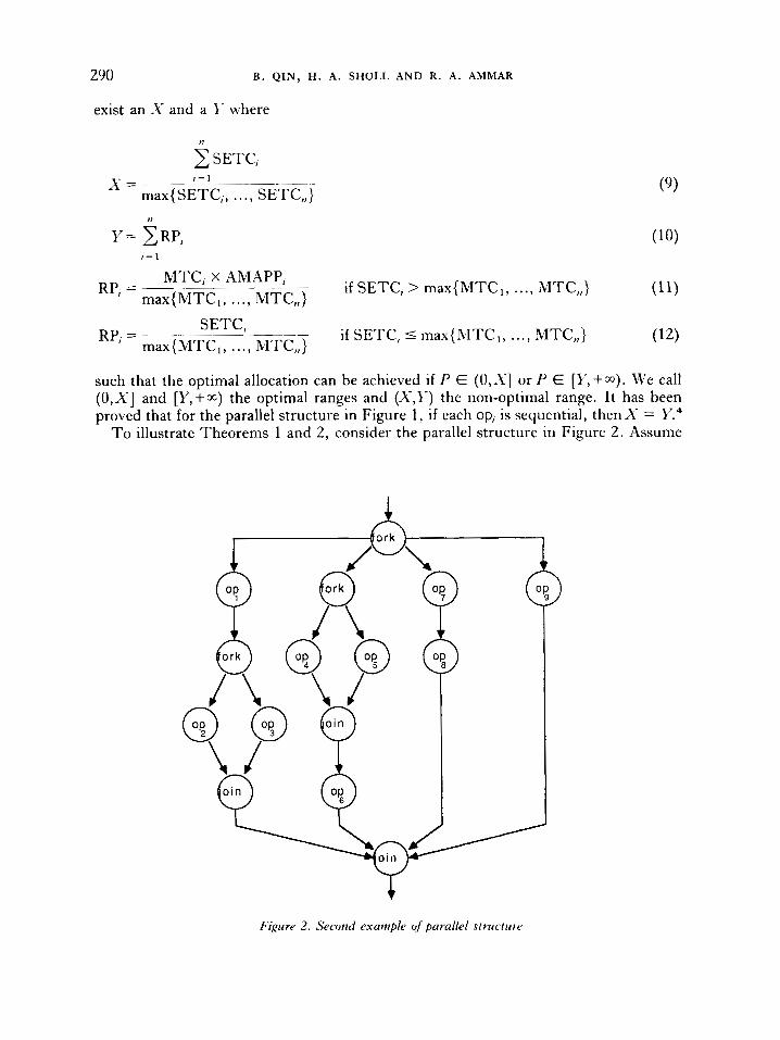
T o illustrate Theorems 1 and 2, consider the parallel structure in Figure 2. Assume

1

Y Figure 2. Second example of parallel structiirr

A TOOL TO MINIMIZE TIME COSTS 29 1

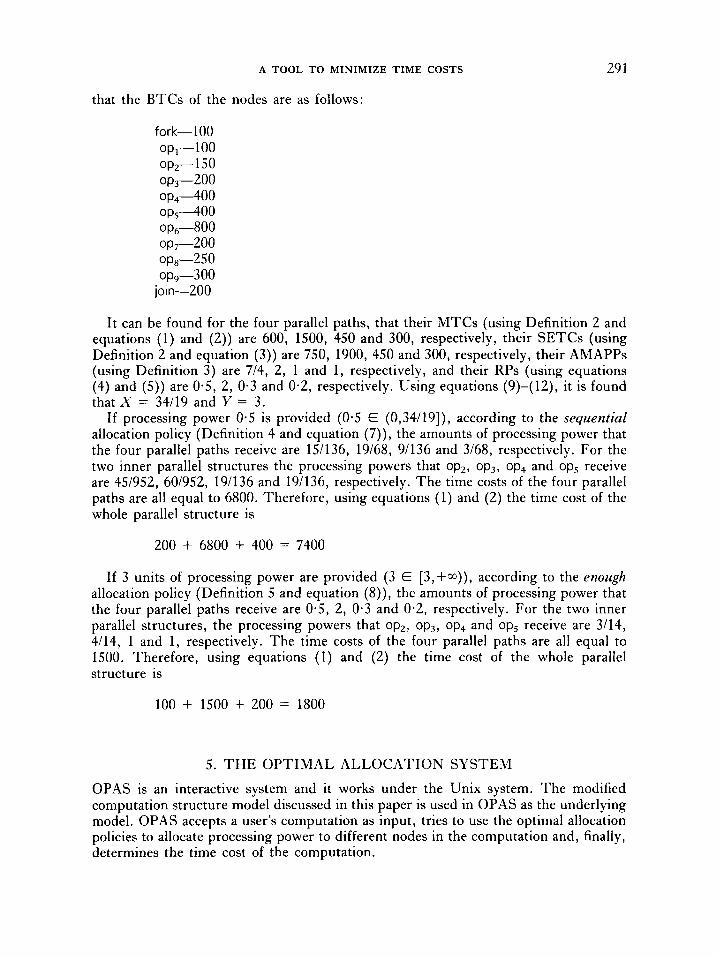
that the BTCs of the nodes are as follows:

fork-100 op,-100 op,-150 op,-200

op,800 op,-zoo op,-250

joi n-200

OP,-400 OPS-400

0p9-300

It can be found for the four parallel paths, that their MTCs (using Definition 2 and equations (1) and (2)) are 600, 1500, 450 and 300, respectively, their SETCs (using Definition 2 and equation (3)) are 750, 1900, 450 and 300, respectively, their AMAPPs (using Definition 3) are 7/4, 2, 1 and 1, respectively, and their RPs (using equations (4) and (5)) are 0.5, 2, 0.3 and 0.2, respectively. Using equations (9)-(12), it is found that X = 34/19 and Y = 3.

If processing power 0.5 is provided (0.5 E (0,34/19]), according to the sequential allocation policy (Definition 4 and equation (7)), the amounts of processing power that the four parallel paths receive are 151136, 19/68, 9/136 and 3/68, respectively. For the two inner parallel structures the processing powers that op,, 0p3, 0p4 and op, receive are 45/952, 60/952, 191136 and 19/136, respectively. The time costs of the four parallel paths are all equal to 6800. Therefore, using equations (1) and (2) the time cost of the whole parallel structure is

200 + 6800 + 400 = 7400

If 3 units of processing power are provided (3 E [3,+@~)), according to the enough allocation policy (Definition 5 and equation (8)), the amounts of processing power that the four parallel paths receive are 0.5, 2, 0.3 and 0.2, respectively. For the two inner parallel structures, the processing powers that op,, 0p3, op, and op, receive are 3/14, 4/14, 1 and 1, respectively. The time costs of the four parallel paths are all equal to 1500. Therefore, using equations (1) and (2) the time cost of the whole parallel structure is

100 + 1500 + 200 = 1800

5. T H E OPTIMAL ALLOCATION SYSTEM

OPAS is an interactive system and it works under the Unix system. The modified computation structure model discussed in this paper is used in OPAS as the underlying model. OPAS accepts a user’s computation as input, tries to use the optimal allocation policies to allocate processing power to different nodes in the computation and, finally, determines the time cost of the computation.

292 B . QIN, H . A . SHOLL A N D R . A. AMMAR

I user interface 1 4

time cost evaluator

time cost analyzer

processing power at locater

t

t

t

t flow analyzer

control graph deriver

4

library

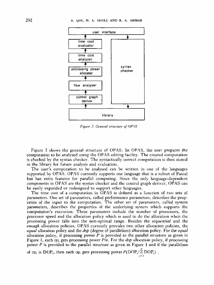
Figure 3. General stndctwe of 0P.AS

Figure 3 shows the general structure of OPAS. In OPAS, the user prepares the computation to be analysed using the OPAS editing facility. The created computation is checked by the syntax checker. The syntactically correct computation is then stored in the library for future analysis and evaluation.

The user’s computation to be analysed can be written in one of the languages supported by OPAS. OPAS currently supports one language that is a subset of Pascal but has extra features for parallel computing. Since the only language-dependent components in OPAS are the syntax checker and the control graph deriver, OPAS can be easily expanded or redesigned to support other languages.

The time cost of a computation in OPAS is defined as a function of two sets of parameters. One set of parameters, called performance parameters, describes the prop- erties of the input to the computation. The other set of parameters, called system parameters, describes the properties of the underlying system which supports the computation’s execution. These parameters include the number of processors, the processor speed and the allocation policy which is used to do the allocation when the processing power falls into the non-optimal range. Besides the sequential and the enough allocation policies, OPAS currently provides two other allocation policies, the equal allocation policy and the dop (degree of parallelism) allocation policy. For the equal allocation policy, if processing power P is provided to the parallel structure as given in Figure 1 , each op, gets processing power Phi. For the dop allocation policy, if processing power P is provided to the parallel structure as given in Figure 1 and if the parallelism

of op, is DOP,, then each op, gets processing powerP(DOP,/X DOP,) . > I

J = l

A TOOL TO MINIMIZE TIME COSTS 293

T o do time cost analysis and evaluation on a computation, the computation is retrieved from the library and the control graph deriver derives from it the correspond- ing control graph. The control graph derived is simply a graph, it is language indepen- dent and it contains all the information necessary to carry out time-cost analysis. Typically, each node in the graph has a base time cost and each edge has a flow that indicates the number of times activation signals traverse the edge. The way the base time cost is derived in OPAS is similar to the methods used in TCAS' and RTS."

Once the control graph of the computation is derived, the flow analyser applies a flow balance technique2," on the control graph to determine the flow of each edge, which represents the number of times the edge is traversed by activation signals. Typically, these flows are functions in some parameters that represent loops' number of iterations and conditions' results. In this way, the number of times each node in the computation is executed can be determined.

To allocate processing power to each node, the processing power allocator first determines the optimal and non-optimal ranges. The optimal allocation policy is used if the processing power provided is within the optimal range. If the processing power provided falls into the non-optimal range, the allocation policy provided by the OPAS user is used to carry out the allocation.

to determine the time cost of the computation. The dervied time cost is then sent to the time cost evaluator for further evaluation.

The time-cost evaluator contains a number of packages to evaluate different time cost behaviours of a computation, such as the minimum time cost, the maximum time cost, the average time cost and the time-cost variance. It also contains packages to compute speed-up and efficiency (the speed-up and efficiency in OPAS are defined as the rough speed and rough efficiency", and plot the time-cost curve and the time-cost distribution. In evaluating a given time-cost behaviour, the time-cost evaluator may call the time cost analyser and the processing power allocator several times. For example, to determine the maximum time cost of a computation assuming that the value of a performance parameter varies from x1 to x2, the time-cost evaluator will call the time-cost analyser and the processing power allocator x2-x1 + 1 times (assume that the incremental step is 1) and, each time, the performance parameter is assigned a different value which is between x1 and x2.

The time-cost analyser uses an analytic

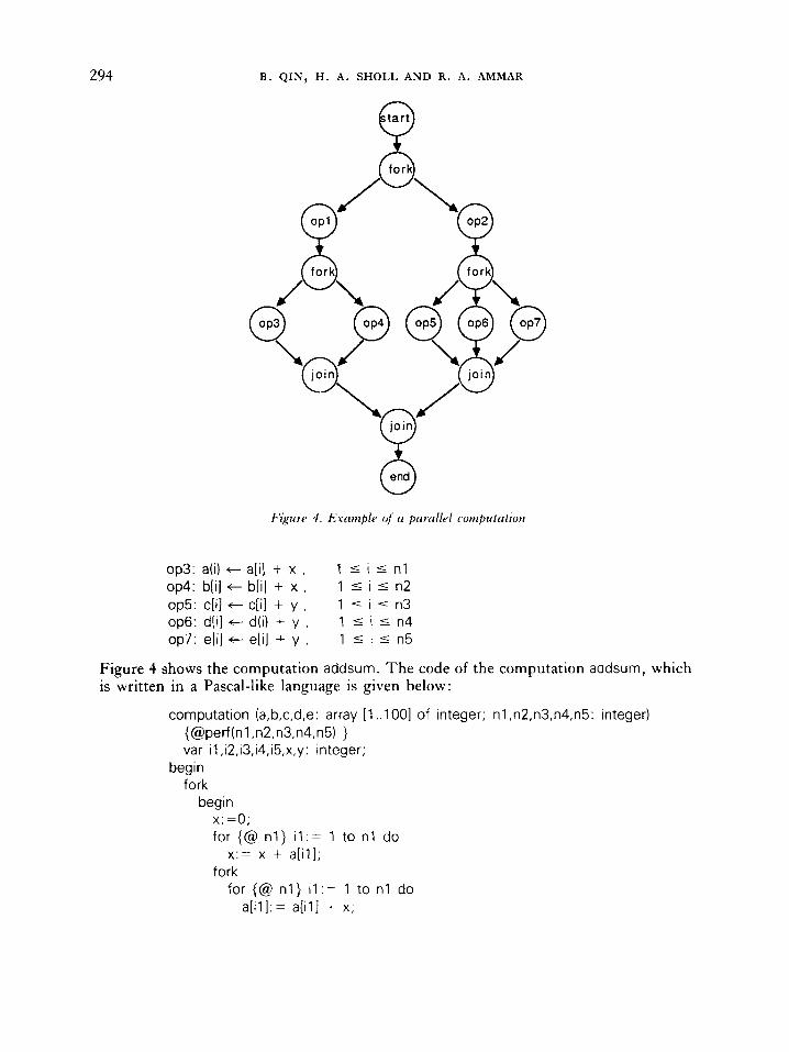
6. EXAMPLE T o illustrate the use of OPAS, assume that there are five arrays a , b, c, d and e with n l , n2, n3, n4 and n5 elements, respectively. A computation addsum is designed to perform the following seven operations :

n l

opl : x t Cab] i = l

n3

op2: y t C c [ i j i = l

294 B . QIN, H . A . SHOLL AND R. A . AMMAR

Figwe 4 . Ernnzple vf a parczllel coiiipictntrorr

op3: a(i) t a[i] + x , op4: b[i] t b[i] + x , op5: c[i] t c[i] + y , op6: d(i1 t d(i) + y , op7: e[i] t e[I] + y ,

1 I i 5 n l 1 5 i 5 n2 1 5 i I n3 1 5 i 5 n4 1 I i 5 n5

Figure 4 shows the computation addsum. T h e code of the computation addsum, which is written in a Pascal-like language is given below:

computation (a,b,c,d,e: array 11 ..I001 of integer; n l ,n2,n3,n4,n5: integer) { @perf(n 1 , n2, n3,n4, n5) } var i l ,i2,13,i4,i5,x.y: integer;

begin fork

begin x : =o; for {@ n l } i l : = 1 to n l do

fork x:= x + a [ i l l ;

for {@ n l } i l : = 1 to n l do a[ i l l := a[ i l l + x;

A TOOL TO MINIMIZE TIME COSTS 295

for {@ n2) i2:= 1 to n2 do b[i21:= b[i21 + x

join end; begin

y := 0; for {@ n3) i3:= 1 to n3 do

fork y:= y + c[i31;

for {@ n3) i3:= 1 to n3 do

for {@ n4) i4:= 1 to n4 do

for {@ n5) i5:= 1 to n5 do

c[i3]:= C[i31 + y;

d[i41:= dIi41 + y;

e[i51:= eli51 + y join

end join

end

In the above, fork-join statements are used to create parallel paths. Special comments starting with '@' signs are used to provide information needed for time-cost analysis. The first special comment indicates that the computation has five performance par- ameters, n l , n2, n3, n4 and n5. Each for loop statement has a special comment to indicate the number of times the body of the loop is executed. For example, for the first for loop statement in the computation, the corresponding special comment shows the body of the loop is executed n l times.

The range command in OPAS can be used to determine the optimal and non-optimal ranges. Assume that n l = 10, n2 = 30, n3 = 50, n4 = 60, n5 = 70 and that the processor speed is the same as the speed of a PDP-11 processor. The following range command determines the corresponding optimal and non-optimal ranges (the chg command sets the processor speed) :

command: chg m PDP11 command: range addsum(lO,30,50,60,70) addsum: control graph derived non-optimal range: (1.2221.3.0090)

Assume that n l = 40, n2 = 20, n3 = 25, n4 = 30, n5 = 35 and that the processor speed is the same as the speed of a Vax processor. The corresponding non-optimal range is given by

command: chg m vax command : range addsu m(40.20.25.30.35) addsum: control graph derived non-optimal range: (1,8506, 3.4636)

296 B . QIN, H . A . SHOLL AND R. A . AMMAR

One can find as the processor speed and properties of the input to the computation change, the optimal and non-optimal ranges also change.

Assume that n l = 40, n2 = 20, n3 = 25, n4 = 30, n5 = 35, that the underlying system has one \.'ax processor and that the e)iougIi allocation policy is used if the optimal allocation policy is not applicable. The following cost command determines the corresponding time cost (note that the performance parameters and system par- ameters are separated by a semicolon) :

command: cost addsum(40.20.25.30.35; 1 ,vax,enough) addsum: control graph derived time cost of addsum: 3287.86

Assume that the performance parameters have the same values as before, that the underlying system has one \.'as processor and that the equal allocation policy is provided. The corresponding time cost IS given by

command: cost addsum(40,20,25,30,35; 1 ,vax,equal) addsum: control graph derived time cost of addsum: 3287.86

It can be seen the time cost of addsum is the same no matter whether the enough or the equal allocation policy is provided. This is because the processing power provided is within the optimal range (1 E (0,1.8506]) and as a result, the optimal allocation policy (i.e. the seyrreiitial allocation policy) instead of the one provided by the OPAS user is used.

Assume that the performance parameters have the same values as before and there are four Vax processors. The corresponding time cost is given by

command: cost addsum(40,20,25,30,35; 4,vax) addsum: control graph derived time cost of addsum: 1193.40

Assume that the performance parameters have the same Lalues as before and there are five Vax processors. T h e corresponding time cost is given by

command: cost addsum(40,20,25,30,35; 5,vax) addsum: control graph derived time cost of addsum: 1193.40

One can find that the time cost of addsum is the same no matter whether four or five Vax processors are provided. This is because the optimal range is [ 3 . 4 6 3 6 , + ~ ) and when the processing power provided falls into this range, the eirough allocation policy is used. According to the properties of the e)iough allocation policy, the computation addsum can obtain its best time-cost behaviour if the processing power provided is no less than 3.4636 and if the enough allocation policy is used.'

Assume that the performance parameters have the same values as before, that there are three Vax processors and that the dop allocation policy is provided. T h e correspond- ing time cost is given by

A TOOL TO MINIMIZE TIME COSTS 297

command: cost addsum(40,20,25,30,35; 3,vax,dop) addsum: control graph derived time cost of addsum; 1613.01

Assume that the performance parameters have the same values as before, that there are three Vax processors and that the sequential allocation policy is provided. The corresponding time cost is given by

command: cost addsum(40.20.25.30.35; 3,vax,sequential) addsum: control graph derived time cost of addsum: 1250.93

One can see that for the above two examples, providing different allocation policies results in different time costs. This is because the processing power provided is within the non-optimal range and, as a result, the allocation policy provided by the OPAS user is used to carry out the allocation.

Assume that the performance parameters have the same values as before and that there are four Vax processors. The speedup command in OPAS determines the corresponding speed-up:

command: speedup addsum(40.20.25.30.35; 4,vax) addsum: control graph derived speedup of addsum: 2.7550

Assume that the performance parameters have the same values as before, that there are three Vax processors and that the equal allocation policy is used. The effic command in OPAS determines the corresponding efficiency :

command: effic addsum(40,20,25,30,35; 3,vax.equal) addsum: control graph derived efficiency of addsum: 0.7513

Assume that n l varies from 10 to 50 and is binomially distributed with p = 0-4, that other performance parameters have the same values as before, that there are three Vax processors and that the enough allocation policy is used. The mean command in OPAS determines the corresponding average time cost :

command: mean binomial addsum( 10:50,20,25,30,35; 3,vax,enough) addsum: control graph derived value for parameter p: 0.4 average time cost of addsum: 11 10.30

The OPAS user can also obtain the time-cost curves. Assume that performance parameters have the same values as before, that the processor speed of the underlying system is the same as the speed of a Vax processor, that the processing power provided varies from 1 to 4 and its incremental step is 0.05 (i.e. the processing power takes the values 1.00, 1.05, 1.10, 1.15, ..., etc.) and that the allocation policies provided are

298 B . QIN, H . A . SHOLL A N D R. A . AMMAR

4000 - 4000 -

1000 , - , . , . , - I P 1000

::::I 3000 -

2000 -

I . I - I . I . 1P 0 1 2 3 4 5 0 1 2 3 4 5

Figure 5. Time-cost curce of addsum with equal Figuw 6 . Time-cost curve of addsum with dop allocation allocation

4000 -

3000 -

2000 -

1000,

4000 -

\ ::::: < . I . I - I . I . I

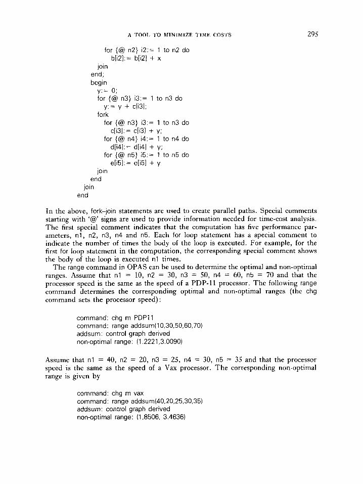
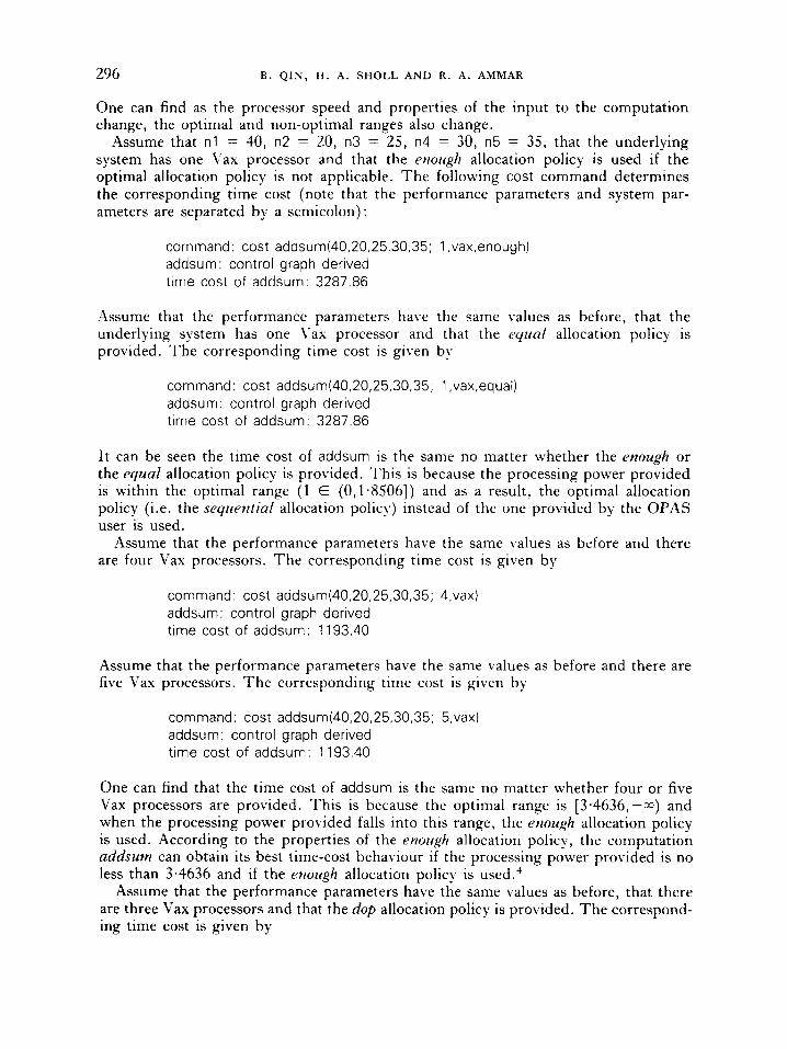
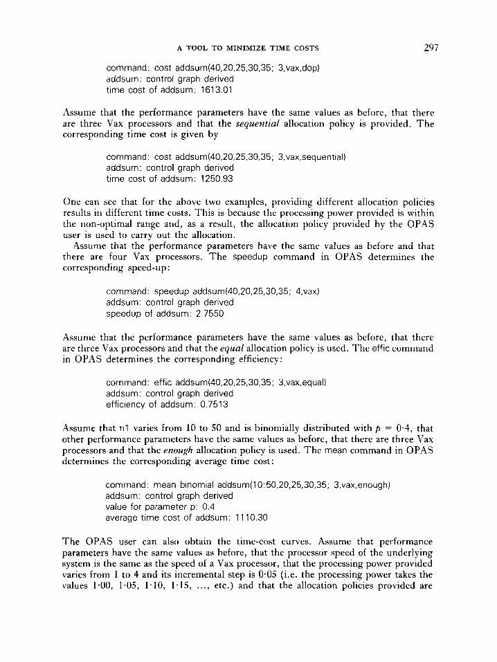
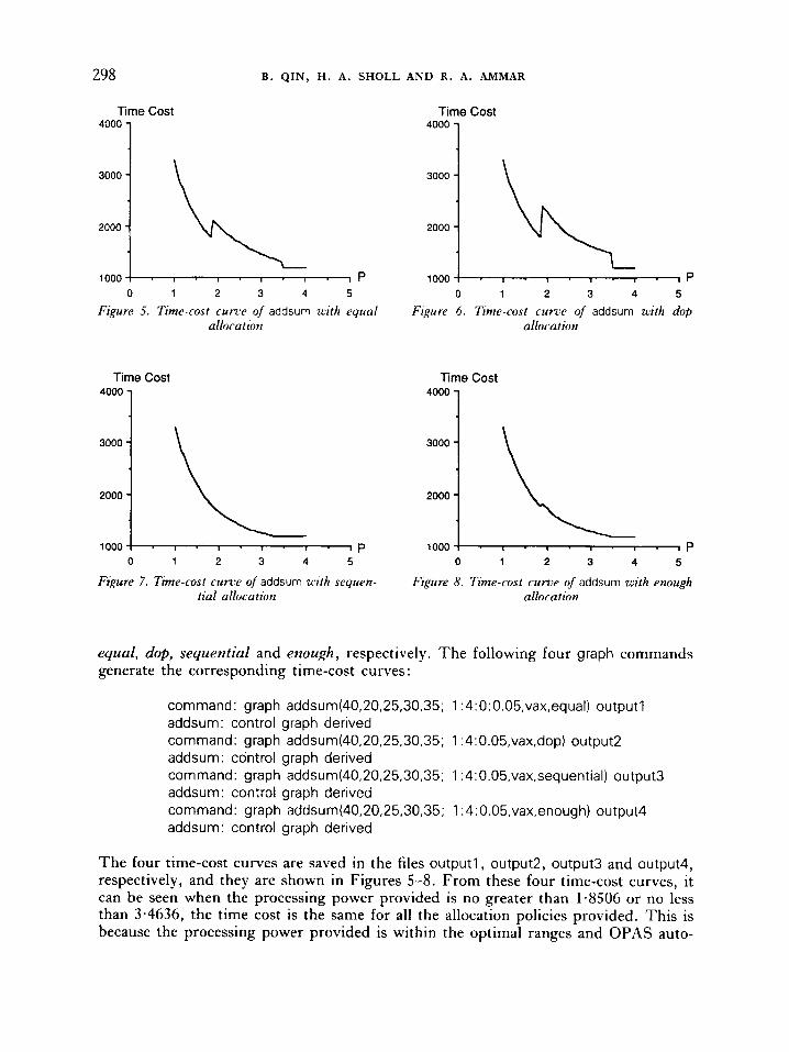
equal, dop, sequential and enough, respectively. The following four graph commands generate the corresponding time-cost curves:

P 1000

command : graph addsum(40,20,25,30,35; 1 : 4: 0: 0.05,vax.equal) outputl addsum: control graph derived command: graph addsum(40,20,25,30.35; 1 :4:0.05,vax,dop) output2 addsum: control graph derived command: graph addsum(40,20,25,30,35; 1 :4: 0.05,vax,sequential) output3 addsum: control graph derived command: graph addsum(40,20,25,30,35; 1 :4:0.05,vax,enough) output4 addsum: control graph derived

I - I - I . I . i P

The four time-cost curves are saved in the files outputl , output2, output3 and output4, respectively, and they are shown in Figures 5-8. From these four time-cost curves, it can be seen when the processing power provided is no greater than 1.8506 or no less than 3.4636, the time cost is the same for all the allocation policies provided. This is because the processing power provided is within the optimal ranges and OPAS auto-

A TOOL TO MINIMIZE TIME COSTS 299

matically uses the optimal allocation policies. However, when the processing power provided falls into the range (1.8506,3*4636), different allocation policies yield different time costs. I t seems that, for the given performance parameters and the system parameters, the dop allocation policy generates the worst time-cost behaviour (Figure 6) and the sequential allocation policy generates the best time cost behaviour (Figure 7) *

7. CONCLUSION

A time-cost analysis tool, OPAS, has been presented in this paper. OPAS relates the time cost of a parallel computation to the input, the algorithm, the data structure, the processor speed, the number of processors and the processing power allocation. OPAS is an analytic tool and it incorporates the optimal processing power allocation in the time-cost analysis of parallel computations. OPAS is different from other time-cost analysis toolsz. lo in that the optimal processing power allocation is always used to carry out the allocation whenever it is possible. Therefore, the time cost obtained from OPAS is the minimum time cost one can expect.

OPAS is useful for several reasons. It allows the user to observe how the time cost of a parallel computation behaves when the optimal processing power allocation is used and it helps the user find the minimum time cost of a parallel computation given that the input, the algorithm, the data structure, the processor speed and the number of processors are fixed. With OPAS, the user can verify whether a parallel computation meets its time cost requirements, find how some key factors affect a parallel computa- tion’s time cost and locate the most time-consuming sections in a parallel computations. All these can lead to the better understanding of the time cost characteristics of parallel computations and better designs of parallel computations with improved time cost behaviour .

ACKNOWLEDGEMENTS

This work was partially supported by the U.S. Naval Underwater Systems Center through U.S. National Science Foundation grant CCR8701839.

REFERENCES

1 . T . L. Booth and C. A. Wiecek, ‘Performance abstract data types as a tool in software performance analysis and design’, IEEE Trans. Software Engineering, SE-6, ( 3 ) , 138-15 1 (1980).

2. Reda A. Ammar and B . Qin, ‘Time cost analysis of parallel computations in a shared memory environment’, Proceedings of the ISMA4 International Conference on Mini and Microcomputers From Micros to Supercomputers, Miami Beach, Florida, 1988.

3 . L. Kleinrock, ‘Distributed systems’, IEEE Computer, 18, ( l l ) , 90-103 (1985). 4. B . Qin, H. A. Sholl and R. A. Ammar, ‘Allocating processing power to minimize the time cost’, to

appear In the Proceedings of the 23rd Hawaii International Conference on System Sciences, Hawaii, January 1990.

5. H . A. Sholl and T. L. Booth, ‘Software performance modeling using computation structures’, IEEE Trans. Software Engineen’ng, SE-1, (4), 414-420 (1975).

6 . T. L. Booth, D. Zhu, M. Kim, B. Qin and C. Albertoli, ‘PASS: a performance analysis software system to aid the design of high performance software’, Proceedings of the First Beijing International Conference on Computers and Applications, IEEE Computer Society Press, Silver Spring, MD, 1984,

7. J . Cohen and C. Zuckerman, ‘Two languages for estimating program efficiency’, Communications of pp. 317-323.

ACM, 17, ( 6 ) , 301-308 (1974).

3 00 B. UIN, H . A . SHOLL AND R . A . AMMAR

8. B. Qin, ‘PPAS: a performance analysis tool for software designs’, MS Thesis, Technical Report CSEI CMC-TR-84-4, Computer Science & Engineering Department, University of Connecticut, 1984.

9. R. A. Ammar and B. Qin, ‘A technique to derive time costs of parallel computations’, COMPSAC88, Pmceedings of the 12th .4nnital International Computer Software 3 Applications Conference, IEEE Computer Society Press, Chicago, IL., 1988, pp. 113-119.

10. 13. Qin, H. A. Sholl and R. A. Ammar, ‘RTS: a system to simulate the real time cost behaviour of parallel computations’, Sqfttcat-e-Pt-actice Expenkrrce, 18, ( lo) , 967-985 ( 1988).

11. R . .4. Xmmar and B. Qin, ‘.A flow analysis technique for parallel computations’, Proceedings of the 7th Annual International Phoenix C’or2ference on (’oniprttet-s and C’omttiir~iicatiotis, IEEE Computer Society Press, Washington, D.C., 1988, pp. 286-290.

12. L. H. Jamieson, D. B. Gannon and R . J . Douglas, The (’hntnctetistics of Purallel Algoiithms, M I T Press, Cambridge, Mass., 1987.