a thesis entitled structural reliability study of highway
TRANSCRIPT

A Thesis
entitled
Structural Reliability Study of Highway Bridge Girders Based on AASTHO LRFD
Bridge Design Specifications
by
Pramish Shakti Dallakoti
Submitted to the Graduate Faculty as partial fulfillment of the requirements for the
Master of Science Degree in Civil Engineering
___________________________________________
Dr. Douglas K. Nims, Committee Chair
___________________________________________
Dr. Luis A. Mata, Committee Member
___________________________________________
Dr. Alex Spivak, Committee Member
___________________________________________
Dr. Amanda C. Bryant-Friedrich, Dean
College of Graduate Studies
The University of Toledo
May 2020

Copyright 2020, Pramish Shakti Dallakoti
This document is copyrighted material. Under copyright law, no parts of this document
may be reproduced without the expressed permission of the author.

iii
An Abstract of
Structural Reliability Study of Highway Bridge Girders Based on AASTHO LRFD
Bridge Design Specifications
by
Pramish Shakti Dallakoti
Submitted to the Graduate Faculty as partial fulfillment of the requirements for the
Master of Science Degree in Civil Engineering
The University of Toledo
May 2020
In structural reliability analysis, load and resistance factors are calibrated using various
methodologies. Proper calibration of load and resistance factor is essential to obtain the
design confidence to meet the design consistency or to obtain a desirable reliability index.
The reliability index thus calculated is the measure of the reliability of the structural design.
Closed-form solution is an elemental method to determine the reliability index for simpler
loads and resistance cases. In some basic cases such as when both loads and resistance are
normally or log normally distributed, exact solutions are obtained. But in almost all cases,
loads have normal distribution, and resistance has log-normal distribution. In such cases,
more rigorous and advance calibration techniques are used to calculate the safety index
such as Rackwitz - Fiessler procedure and Monte Carlo Method. In this study, the
computer-based Monte Carlo Method was used to calculate the safety index or reliability
index. The objective of this study is to describe such methodologies to determine the
reliability of the structural designs.

iv
In this study, reliability analyses are performed to calibrate load and resistance factors
using AASTHO LRFD bridge design specifications for reinforced concrete T-beam bridge
girders. Reliability indices are calculated for the three spans continuous bridges with equal
span length. Both exterior and interior girders are studied to understand the effect of loads
and their trends. Reliability analysis suggests that bending moment is governing over shear.
Similarly, there is a significant increase in contributions of dead loads over live load for
bending and shear with the increase in span length. Systematic variations of the load and
resistance parameters are done to investigate the change in reliability index. Various graphs
for reliability index versus sets of statistical and design parameters are plotted for the
parametric study. Separate graphs are plotted to understand the trend of the change in the
reliability index with such parameters. The study showed that there is an increase in
reliability index with gradual increase in magnitude of load modifier, live load scalar, and
resistance bias for both bending and shear effects. However, there is no significant changes
in the reliability index for the increase in dead load scalar and the reliability index decreases
with an increase in live load bias. This study will facilitate the users of load and resistance
factor design specifications such as AASTHO LRFD for understanding the calibration
process of load and resistance factor. This will assist the designer to incorporate the local
experience and data while designing the reliable structures.

v
Acknowledgements
I would like to express my sincere gratitude to my advisor, Professor Dr. Douglas K. Nims
for his continuous support, guidance and motivation throughout my Master of Science
study and completion of my thesis. I am thankful to my thesis committee members, Dr.
Luis A. Mata and Dr. Alex Spivak, for their time and sharing their knowledge. Similarly,
I would like to thank Dr. Ashok Kumar for funding me for my MS Study and making my
research easier.
I would also like to thank my parents, my friends, brothers and sisters for their moral,
scholar, and emotional supports in every stages of my life.

vi
Contents
Abstract ............................................................................................................................. iii
Acknowledgements ............................................................................................................v
Table of Contents ............................................................................................................. vi
List of Tables .................................................................................................................... ix
List of Figures .....................................................................................................................x
List of Abbreviations ..................................................................................................... xiii
List of Symbols ............................................................................................................... xiv
1 Introduction 1
1.1 Background .......................................................................................................... 1
1.2 Statement of Problem ........................................................................................... 3
1.3 Objective of the Study ......................................................................................... 4
1.4 Outline of the Thesis ............................................................................................ 5
1.5 Significance of Research Work ........................................................................... 6
2 Literature Review 8
2.1 General ................................................................................................................. 8
2.2 Code Calibration ................................................................................................ 16
vii
2.2.1 NCHRP Project 12-33: Development of a Comprehensive Bridge
Specification and Commentary .............................................................. 17
2.2.2 NCHRP Report 368: Calibration of LRFD Bridge Design Code .......... 17
2.2.3 NCHRP 20-7/186: Updating the Calibration Report for AASTHO
LRFD Code ............................................................................................ 19
2.2.4 Transportation Research Circular E-C079: Calibration to Determine
Load and Resistance Factor for Geotechnical and Structural Design ... 21
2.3 American Association of State Highway and Transportation Officials
(AASTHO) LRFD Bridge Design Specifications.............................................. 22
2.3.1 The LRFD Equation: ............................................................................. 23
2.3.2 Load Combination ................................................................................. 24
2.3.3 Multiple presence ................................................................................... 26
2.3.4 Dynamic effects ..................................................................................... 27
2.3.5 Live load Distribution Factor ................................................................. 27
3 Overview of Calibration Approach 31
3.1 General ............................................................................................................... 31
3.2 Calibration Methods........................................................................................... 32
3.2.1 Closed Form Solution ............................................................................ 35
3.2.1 Rackwitz-Fiessler Procedure ................................................................. 36
3.1.1 Monte Carlo Method .............................................................................. 39
3.3 Reliability Index................................................................................................. 43
3.4 Target Reliability Index ..................................................................................... 46

viii
3.5 Load and Resistance Factor ............................................................................... 48
4 Structural Load and Resistance Model 53
4.1 General Load Model .......................................................................................... 53
4.1.1 Structural Load Model ........................................................................... 54
4.2.1 Dead Load .............................................................................................. 56
4.2.2 Live Load ............................................................................................... 58
4.2 Resistance Model ............................................................................................... 61
5 Reliability Analysis and Parametric Study............................................................. 65
6 Conclusion and Recommendation ........................................................................... 94
6.1 Conclusion ......................................................................................................... 94
6.2 Recommendation ............................................................................................... 95
References ........................................................................................................................ 97
A Load Analysis 99
B Monte Carlo Method of Simulation Sample Speadsheet 114

ix
List of Tables
2.1 Multiple Presence Factors. ....................................................................................... 26
3.1 Load Factor Specified in AASTHO LRFD Bridge Design
Specifications, 2014 ................................................................................................. 51
3.2 Resistance Factors Specified in AASTHO LRFD Bridge Design Specifications,
2014 for Moment and Shear .................................................................................... 52
4.1 Representative Statistical Parameters of Dead Load (Kulicki et al. 2007) .............. 57
4.2 Representative Statistical Parameters of Live Load with Impact Factor ................. 61
4.3 Statistical Parameters of Resistance (Kulicki et al., 2007)………………………...63
5.1 List of Design Parameters Considered for Parametric Study .................................. 67
x
List of Figures
3-1 Flowchart-Basic Calibration Procedure................................................................... 34
3-2 Reliability Index and Corresponding Probability of Failure (Nowak, 1999) .......... 44
3-3 Margin of Safety, Probability of Failure, and Reliability Index (Adopted from
Allen, Nowak, & Bathurst, 2005) ............................................................................ 45
3-4 Mean Load, Design Load, and Factored Load (Kulicki, Prucz, Clancy, Mertz, &
Nowak, 2007) ........................................................................................................... 49
3-5 Mean Resistance, Design Resistance and Factored Load........................................ 49
4-1 AASTHO HL-93 Design Truck Model (Source: Internet) ...................................... 59
4-2 AASTHO HL-93 Design Tandem Model (Source: Internet) .................................. 59
4-3 AASTHO HL-93 Truck Load Positioning for Maximum Sagging Moment in Span
First (Source: Internet) ............................................................................................. 60
5-1 Longitudinal Profile of T-Beam Girder Bridges ..................................................... 66
5-2 Cross-section of T-Beam Girder Bridges ................................................................ 66
5-3 Effect of ɸ on β for Moment (Interior and Exterior Girder) .................................... 71
5-4 Effect of ɸ on β for Shear (Interior and Exterior Girder) ........................................ 72
5-5 Effect of ɳ on β for Moment (Interior and Exterior Girder) .................................... 73
5-6 Effect of ɳ on β for Shear (Interior and Exterior Girder) ........................................ 74
5-7 Effect of λ LL on β for Moment (Interior and Exterior Girder) ................................ 75
5-8 Effect of λ LL on β for Shear (Interior and Exterior Girder) .................................... 76

xi
5-9 Effect of L Scalar on β for Moment (Interior and Exterior Girder) ......................... 77
5-10 Effect of L Scalar on β for Shear (Interior and Exterior Girder).............................. 78
5-11 Effect of D1 Scalar on β for Moment (Interior and Exterior Girder) ...................... 79
5-12 Effect of D1 Scalar on β for Shear (Interior and Exterior Girder) ........................... 80
5-13 Effect of D2 Scalar on β for Moment (Interior and Exterior Girder) ....................... 81
5-14 Effect of D2 Scalar on β for Shear (Interior and Exterior Girder) ........................... 82
5-15 Effect of λR on β for Moment (Interior and Exterior Girder) ................................... 83
5-16 Effect of λR on β for Shear (Interior and Exterior Girder) ....................................... 84
5-17 Variation of Reliability Index with Span Length for Moment ................................ 86
5-18 Variation of Reliability Index with Resistance Factor for Given Span Length ....... 86
5-19 Variation of Reliability Index with Load Modifier for Given Span Length ........... 87
5-20 Variation of Reliability Index with Live Load Bias for Given Span Length .......... 87
5-21 Variation of Reliability Index with Live Load Scalar for Given Span Length ....... 88
5-22 Variation of Reliability Index with Dead Load Scalar (D1) for Given Span
Length.. ................................................................................................................... 88
5-23 Variation of Reliability Index with Dead Load Scalar (D2) for Given Span
Length.. ................................................................................................................... 89
5-24 Variation of Reliability Index with Resistance Bias for Given Span Length .......... 89
5-25 Variation of Reliability Index with Span Length for Shear ..................................... 90
5-26 Variation of Reliability Index with Resistance Factor for Given Span Length ....... 90
5-27 Variation of Reliability Index with Load Modifier for Given Span Length ........... 91
5-28 Variation of Reliability Index with Live Load Bias for Given Span Length .......... 91
5-29 Variation of Reliability Index with Live Load Scalar (L) for Given Span Length . 92

xii
5-30 Variation of Reliability Index with Dead Load Scalar (D1) for Given Span
Length.. ................................................................................................................... 92
5-31 Variation of Reliability Index with Dead Load Scalar (D2) for Given Span
Length… .................................................................................................................. 93
5-32 Variation of Reliability Index with Resistance Bias for Given Span Length .......... 93
A-1 Longitudinal Profile of 40ft. Uniform Span Length Bridge .................................. 100
A-2 Moment Diagram for Dead Component, Dead Wearing, and Live Loads
(Interior Girder) ..................................................................................................... 100
A-3 Shear Diagram for Dead Component, Dead Wearing, and Live Loads
(Interior Girder) ..................................................................................................... 101
A-4 Strength I Envelope for Moment (Interior Girder) ................................................ 101
A-5 Strength I Envelope for Shear (Interior Girder) ..................................................... 102
B-1 Sample Spreedsheet of Monte Carlo Method to Calcualte Reliability Index for
Interior Girder (Moment) ....................................................................................... 115
B-2 Sample Spreedsheet of Monte Carlo Method to Calcualte Reliability Index for
Exterior Girder (Moment) ...................................................................................... 116
B-3 Sample Spreedsheet of Monte Carlo Method to Calcualte Reliability Index for
Interior Girder (Shear) ........................................................................................... 117
B-4 Sample Spreedsheet of Monte Carlo Method to Calcualte Reliability Index for
Exterior Girder (Shear) .......................................................................................... 118

xiii
List of Abbreviations
AASTHO ...................American Association of State Highway and Transportation
Officials
ADTT .........................Average Daily Truck Traffic
ASD............................Allowable Stress Design
ASCE .........................American Society of Civil Engineers
CDF ............................Cumulative Distribution Function
CIP .............................Cast in Place
COV ...........................Coefficient of Variation
DR ..............................Doubly Reinforced
FEA ............................Finite Element Analysis
FEM ...........................Finite Element Method
FS ...............................Factor of Safety
LFD ............................Load Factor Design
LRFD .........................Load and Resistance Factor Design
MCS ...........................Monte Carlo Simulation
NCHRP ......................National Cooperative Highway Research program
NA ..............................Neutral Axis
PDF ............................Probability Distribution Function
RC ..............................Reinforced Concrete
SR ...............................Singly Reinforced
TRB ............................Transportation Research Board
WSDOT .....................Washington State Department of Transportation

xiv
List of Symbols
𝑅 .................................Resistance value
𝑄 .................................Load value
𝑔 .................................Limit State Function
𝐷𝐶 ..............................Load from dead components
𝐷𝑊 .............................Dead load from wearing surface
𝐿𝐿 ...............................Live load
𝐿𝐿 + 𝐼𝑀 .....................Live load plus impact load
𝑆 .................................Spacing of girder
𝐿 .................................Length of Span
w .................................Roadway width
𝑀 ................................Margin of Safety
𝑛 .................................Number of failures
𝑁 ................................Number of Simulations
𝑅𝑛 ...............................Nominal resistance
𝜂𝑖 ................................Load modification factor
𝛾𝑖 ................................Load factor
𝑄𝑖 ................................Load random variable
ɸ .................................Resistance factor
𝜂𝐷 ...............................Ductility factor
𝜂𝑅 ...............................Redundancy factor
𝜂𝐼 ................................Operational importance factor
β .................................Reliability index or safety index
𝐾𝑔 ...............................Longitudinal stiffness parameter
𝑒𝑔 ................................Girder eccentricity
Ig .................................Moment of inertia of the girder
𝑡𝑠 ................................Thickness of slab
𝜇𝑅 ...............................Mean value of resistance
𝜇𝑄 ...............................Mean value of load
𝑉𝑅 ...............................Coefficient of variation of resistance
𝑉𝑄 ...............................Coefficient of variation of load
𝜎𝑄 ...............................Standard deviation of total load
𝑅∗ ...............................Value of resistance at design point
𝑄∗ ...............................Value of load at design point
𝐹𝑅 ...............................Cumulative distribution function of resistance
𝐹𝑄 ...............................Cumulative distribution function of load

xv
𝑓𝑅 ................................Probability distribution function of resistance
𝑓𝑄 ................................Probability distribution function of load
𝑃𝑓 ................................Probability of Failure
𝐷𝑛 ...............................Nominal dead load
𝐿𝑛 ...............................Nominal live load plus impact
𝜆𝐷 ...............................Bias of dead load
𝐷𝑖 ...............................Random normal variable for dead load.
𝜎𝐷 ...............................Standard deviation of random dead load
𝜆𝐿 ................................Bias of live load
𝐿𝑖 ................................Random normal variable for live load.
𝜎𝐿 ................................Standard deviation of random live load
𝑢𝑅𝑖 .............................Uniformly distributed random number for resistance
𝛷−1 .............................Inverse standard normal distribution function
𝜎𝑀 ...............................Standard deviation of margin of safety
𝛾𝑄 ...............................Load factor
𝜆𝑄 ...............................Bias factor for the load
𝑛𝑄 ...............................A constant representing the number of standard deviations from
the mean needed to obtain the probability of exceedance.
𝜇𝑄 ...............................Mean of total load
𝜇𝐷𝐿..............................Mean of dead load
𝜇𝐿𝐿 ..............................Mean of live load
𝜇𝐼𝑀 .............................Mean of dynamic load
𝜆𝐷𝐿 ..............................Bias of total load
f’c ................................Compressive strength of Concrete
fy .................................Yield Strength of rebar
Nb ...............................Number of beams
Loverhang .......................Length of overhang
θ ..................................Angle of skew
unitwt ...........................Unit weight of concrete

1
Chapter 1
Introduction
1.1 Background
AASTHO LRFD is mostly acceptable and widely used bridge design specifications which
is based on Load and Resistance Factor Design approach. In the LRFD design approach,
load and resistance factors are calculated based on theory of reliability which is established
on the ground of available statistical data on structural loads, and performance of the
structure with the response to such load effects (e.g. bending moments and shears).
Structural reliability concepts are applied to the design of new and existing buildings to
determine whether the structures designed using the available design codes and
specifications are safe and consistent or not.
The basis of AASTHO LRFD bridge design specification that was developed and updated
over time, was statistical parameters from the 1970s and 1980s. Major changes are seen in
the load part of the design formula for different limit states. HL-93 live load model had
replaced the live load model using HS-20 truck load. Load factors specified in current

2
AASTHO LRFD specification are lower in magnitude than previously used (Nowak &
Latsko, 2017).
In structural reliability analysis, load and resistance factors are calibrated using various
methodologies. Proper calibration of load and resistance factor is essential to obtain the
design confidence to meet the design consistency, in other words, to obtain a desirable
reliability index. Various researches and studies have been done after the original
calibration of design code and specifications. An improvised database of material
properties such as compressive strength of concrete, strength of rebar and prestressed
strands is available for determining the load carrying capacity of bridge girders. Due to the
availability of more advanced quality control procedures, it has been easier to predict the
material properties more accurately; the coefficient of variation of resistance has been
reduced.
In the probabilistic design approach, reliability index (β) or often called safety index is
calculated by following the calibration process. The reliability index thus calculated is the
measure of the reliability of the structural design. Closed-form solutions is an elemental
method to determine the reliability index for simpler loads and resistance cases. In some
basic cases such as when both loads and resistance are normally or log-normally
distributed, exact solutions are obtained (Allen, Nowak, & Bathurst, 2005). But in almost
all cases, loads have normal distribution and resistance has log-normal distribution. In such
cases, more rigorous and advanced calibration techniques are used to calculate the safety
index such as Rackwitz-Fiessler procedure and Monte Carlo Method. Reliability index

3
calculated by following either of the available methods are compared to the target
reliability index to ascertain the design confident for a structure designed for a specific
design life. Based on the literature review and recent studies, the target reliability index is
recommended as 3.5.
1.2 Statement of Problem
Numerous studies and experiments have been conducted to understand the nature of
structural loads and resistance of the structure in the response of such loads. With time,
there has been gradual and significant increase in the volume of structural statistical data
and quality of various methodologies implemented to ascertain such data have increased
the reliability of the data as well. With advancement of technologies, computer-based
calibration methods are proven to be beneficial to address the gradual change in statistical
data.
Although there is a continual refinement in the calibration methods, there are not enough
resources to describe the calibration process of load and resistance factor used in the Load
and Resistance Factor Design (LRFD) specifications. Lacking enough understanding of the
calibration process, users of LRFD specifications have trouble attaining the level of safety
desired by the users according to available resources and data. It is essential to understand
the nature of various parameters of random variables used for reliability analysis. Without
a proper understanding of the relationship of these parameters with reliability index and

4
effects of their variation in reliability analysis, a safe and rational design of structure could
not be achieved.
1.3 Objective of the Study
The Objectives of this research work are:
1. Review the literature regarding structural reliability, its history, calibration
methods, application, and limitations.
2. Outline the calibration process for load and resistance factors based on available
statistical data and experience.
3. Facilitate the user of AASTHO LRFD to understand the procedure to determine
load and resistance factor and calculate the safety index and probability of failure
associated with the structural components.
4. Study on effects of dead and live loads in terms of moment and shear for exterior
and interior girders of reinforced concrete T-beam girder bridge.
5. Investigate the change in reliability index (β) with systematic variation of load and
resistance factor and scalar parameters through a parametric study.
6. Study the relationship of reliability index with statistical and design parameters and
investigate the trend for a given span length.

5
1.4 Outline of the Thesis
The thesis begins with introduction and literature review on structural reliability as applied
to bridge girders and progress through overview of calibration approach, structural load
and resistance models, reliability analysis and parametric study, conclusion, and ends with
recommendation for future work.
Chapter 1 – Introduction
The introduction has the topic, overview, problem statement, objective, and significance
of the research.
Chapter 2 - Literature Review
This chapter review the literature on structural reliability analysis, its background, and its
application on calibration of Load and Resistance Factor Design (LRFD) specifications
and codes for bridge design.
Chapter 3 - Overview of the Calibration Approach
This chapter discusses the available methods to calibrate the load and resistance factors,
concepts of reliability index, target reliability index and probability of failure.
Chapter 4 – Structural Load and Resistance Models
Loads acting in the bridge and performance of structural components in response to the
load effects are presented in the form of structural load and resistance model. These models
are essential to perform reliability analysis of bridge girders.

6
Chapter 5 – Reliability Analysis and Parametric Study
Reliability indices are calculated for reinforced concrete T-beam girders of various sections
and bridge span lengths that are considered for the study. Systematic variations of statistical
parameters are done to understand the effects of change in such parameters to reliability
index. Parametric study was carried out to understand the relationship between reliability
index and parameters in reliability analysis of the bridge girders.
Chapter 6 – Conclusions and Recommendation
This section discusses the results obtained from reliability analysis and parametric study
and concludes the work. It also mentions the future works that need to be done and the
direction of more research.
1.5 Significance of Research Work
While designing any structures, designers follow the provisions of relevant codes and
specifications to ensure their design are safe and adequate. Codes and standards are merely
the minimum criteria or requirements that the designer should follow so that their designs
are acceptable. In some cases, they serve as guidelines to design the structures and their
components. Not only designers know how to design code-compliant structures, they
should be confident enough about the reliability of the design.
This study will facilitate the users of load and resistance factor design specifications such
as AASTHO LRFD for understanding the calibration process of load and resistance factor

7
and calculate the safety index and probability of failure associated with the structure
components.
Furthermore, the parametric study will provide knowledge on effect of variation of
statistical parameters of loads and resistance of the structural components on reliability
index and exploit this understanding for optimum and economical design of a structure
using reliability-based design methods.

8
Chapter 2
Literature Review
2.1 General
Available concrete design codes specify a specific constant value of load and resistance
factors for flexural and shear design of the structural components. However, load and
resistance are not treated as constant, they are considered as random variables. Using
constant values of load and resistance factor may not provide safe and economical designs.
Hence, more accurate statistical parameters and proper reliability assessments are needed
for reliable design of the structures. Calibration of load and resistance factor using
appropriate reliability methods allows the designer to manipulate the level of safety
according to the importance of the structures. Load and resistance factors represent safety
reserve of the structures designed using available design code and specifications.
Without proper and accurate assessment of load and resistance factors appropriate use of
design code is not possible. Traditionally, bridges were designed using work stress and
load factor methods. However, these methods were not able to address probabilistic
variation of loads and resistance to such loads while designing the structure (Nowak, 1999).

9
With the advent of load and resistance factor design (LRFD) method, proper assessment of
uncertainty associated with the loads and structural performance is achieved.
Previous design practices and consistent level of safety as implied by safety factor (FS) in
past design specifications such as Allowable Stress Design (ASD) are the basis for
selecting the target reliability index. In strength limit state design, resistance factor for
structural design are determined such that target reliability index is 3.5 and corresponding
probability of failure is around 1 in 5000 (Allen, Nowak, & Bathurst, 2005).
American Association of State Highway and Transportation Officials (AASTHO) code
was used before the advent of AASTHO Load and Resistance Factor Design (LRFD)
specification, which was based on allowable stress method and load factor design method.
There were many changes and adjustments in bridge engineering after the introduction of
AASTHO code which demanded a new approach to design the bridges. Nowak (1995)
reviewed the procedures for development of new load and resistance factor design (LRFD)
bridge code, for AASTHO (Standard 1992) or AASTHO code was incorporating LRFD
design method. The paper summarized a newly proposed live load model and dynamic load
model keeping an account of bridge and vehicle dynamic as well as road roughness for the
range of bridge spans and materials. AASTHO code used live load model based on HS-20
truck, lane or military loading and was not representing the actual load effects (moment
and shear) from heavy trucks on the highway; actual load effects were much higher than
design loads (Nowak, 1995). New method of GDF was discussed in the paper which
depends on both span length and girder spacing. The paper presented the calibration
procedure for determining the load and resistance factors for new LRFD code and

10
summarized the statistical load and resistance model for non-composite steel, composite
steel, reinforced concrete, and prestressed concrete bridges. An iterative method based on
normal approximation to non-normal distributions at the design point was used to calculate
the reliability index.
Akbari (2018) illustrated the probabilistic design of singly, doubly reinforced and T-beam
concrete beams for bending moment. Load and resistance factor for dead and live loads
were calculated for specified safety index and loading ratios. Monte Carlo Simulation
technique was used to estimate the reliability index. Number of simulations (N) was fixed
to 10000 cycles and probability of failure was given by 1/N. The results showed that on
increasing the loading ratio (moment due to dead load by total moment due to live and dead
loads), safety index increases. It was considered reasonable as coefficient of variation of
live loads are greater than dead loads. Doubly reinforced (DR) concrete beams were found
to have more reliability index than singly reinforced (SR) beams suggesting DR as more
economical and safe beams. The study concluded that amount of reinforcement is very
sensitive to loading ratio rather than compressive strength of concrete. For lower loading
ratio, area of reinforcement is found to be higher. This suggests using high strength
concrete does not necessarily gives economic design; loading condition is also an important
factor to consider. For this study target reliability index was set to 3.0. From the study,
variation of load and resistance factors for given safety index and loading ratios were
developed. The graphs provided in the paper can be used to design the singly and doubly
reinforced concrete beams for any safety index and loading ratios.

11
Tabsh & Nowak developed a resistance model for reliability analysis of highway bridge
girders. Resistance was calculated for composite and non-composite steel girders,
reinforced concrete T-beams, and prestressed concrete girders. The model was based on
available materials and test data and it determined the bridge capacity in term of failure
truck load from moment curvature of bridge girder developed using strain incremental
approach. Load models were based on truck-weight surveys. Reliability index using the
load and resistance models for the girders were calculated for performing structural
reliability. From the results, it was found that reliability indices of non-composite steel
were at a range of 3-3.5, for composite steel they were 2.5-3.5, and for reinforced concrete
and prestressed concrete 3.5-4.
Nowak & Latsko (2017) reviewed the original calibration used to calculate the earlier
versions of LRFD specifications and recommended new load and resistance factors. New
sets of load and resistance factor for various bridges are described as the optimum factors
for the desired reliability index or target reliability index. Proposed load and resistance
factor were checked on a set of the representative bridges described in NCHRP Report 368,
the original calibration report on AASTHO LRFD specification. Although load resistance
factors are about 10% lower than the current factors, reliability analysis showed good
agreement. Based on the calculations, dead load factor and live load factors are
recommended as 1.20 and 1.60 respectively. New load and resistance factors generated
higher reliability index compared to AASTHO LRFD bridge design specifications, 2014.
However, required moment capacity of the bridge girders were increased by 3% to 5% and
shear capacity by 5%; recommended resistance factors were less than the resistance factor

12
specified in the AASTHO LRFD. New resistance factor for reinforced T beams is
recommended as 0.80 which is about 11% less than the specified resistance factor.
Historical structures have higher target reliability index than existing and new structures;
historical structures have greater economic, social, and political values. Generally, newly
designed and existing structures have multiple load paths. Since they are analyzed in the
reference time period less than design period (generally 50-75 years), they have smaller
maximum moment and shear effects but larger coefficient of variation of loads. Inspection
of such structures are performed more often which reduces the uncertainty related to load
and resistance; lower reliability index is acceptable (Nowak & Kaszynska).
Redundancy is the capacity of the bridge to carry out the loads even after the collapse of
one or more of its members; loads acting on collapse members are redistributed and picked
up by remaining members making the structure stand. Ghosan & Moses developed a
framework to consider the redundancy inherent in the structure during it design using
available standards. This framework allows the designer to design the members more or
less conservatively by applying the load modifiers during the bridge design. For typical
bridge configurations, the paper has provided the tables for load modifier otherwise a direct
analysis approach is described and is recommended to use. Redundancy in the system can
also be measured by reliability analysis. Difference between system reliability index and
member reliability index measures redundancy of the structures. Study suggested that
redundancy of the representative simple span bridges is more sensitive on bridge
configurations rather than sectional properties. The paper suggested further research to

13
investigate the relationship between member ductility and redundancy for continuous
bridges.
Mahmoud et al. (2017) performed reliability analysis of one and two lanes concrete slab
straight bridges with different span length for bending moments. Moments were calculated
using simplified empirical live load equations specified in AASTHO LRFD bridge design
specifications and by finite-element analysis (FEA) using SAP2000. Resulting moment
and reliability index were compared and bias of moments using these two approaches were
calculated. AASTHO standards do not consider very essential factors such as transverse
position of a truck or tandem in a specific lane while calculating live load moments. The
study showed that simplified method overestimated live load moment for shorter spans and
slightly underestimated moment for longer spans of reinforced concrete bridges when
compared to results from FEA. To meet the target reliability index of 3.5 and in order to
ensure the consistent design of reinforced concrete bridge, the paper suggested live load
factor of 2.07 for one lane and 1.8 for two lanes for shorter spans. Similarly, for longer
spans, it is recommended to use live load factor of 2.07 for single lane and 1.95 for two
lanes.
Tabsh (1992) conducted a parametric study on typical prestressed concrete I-girder (regular
I-beam and AASTHO Type V I-Beam) and spread box beams for simply supported
bridges. Reliability analysis method was used to investigate the structural safety using
AASTHO Specifications. Systematic variations in initial prestress, section size and
allowable concrete stresses were performed to investigate their effect on the required

14
number of strands and the reliability index. In practice, prestressed concrete structures are
designed for allowable initial and final stresses at service load conditions; ultimate flexural
capacity is checked later which generally does not govern the design. The paper concluded
that number of design strands was increased with decrease in section size and initial
prestress resulting higher reliability indices.
Lin & Frabgopol (1996) presented two optimization approaches to design the reinforced
concrete girders for highway bridges based in AASTHO standard specifications for
highway bridges. The paper studied the effects of steel to concrete cost ratio and allowable
reliability level on the optimum solutions and quantify them using nonlinear optimization
solutions. Arafah performed reliability-based sensitivity analysis of flexural strength of
reinforced concrete rectangular beam sections and investigated the relationships between
reinforcement ratios (tension and compression) with reliability index. Both ductile and
brittle failure modes were considered. Results indicated higher reliability index for low
tension reinforcement ratio; reliability index decreased from 4.0 to 2.5 on increasing the
reinforcement ratio from 40% of maximum permissible to 100%.
Rackwitz & Flessler (1978) presented an iteration algorithm to calculate structural
reliability for any type of loading conditions. The algorithm approximates any type of non-
normal distribution independent random variables by normal distributions for continuous
limit state criterion.

15
Biondini et.al (2004) considered a direct and systematic approach to study the structural
reliability of reinforced and prestressed concrete structures subjected to static loads. The
proposed procedure was applied for structural reliability analysis of an existing arch
bridges considering mechanical and geometrical non-linearity of the structure. The paper
verified the effectiveness of proposed approach and Monte Carlo method for the evaluation
of existing structures for strength and serviceability limit states for change in loads than
design loads. Grubisic et.al (2019) performed non-linear modelling of the reinforced
concrete (RC) planar frame using Finite Element Method (FEM) considering material and
geometrical nonlinearities. Reliability analyses were carried out using different numerical
methods: Mean-Value First-Order Second-Moment, First-Order Reliability Method,
Second-Order Reliability Method and Monte Carlo simulation (MCS). The paper
recommended MCS method over other methods for reliability analysis of the structures.
In structural reliability analysis, probabilistic and physical models are generated which are
based on statistical parameters. Such statistical parameters have inherent uncertainties.
Measure of reliability index considering the effect of such uncertainties is defined as
predictive reliability index. Kiureghian (2008) described the methods for computing
predictive reliability index and corresponding probability of failure. The paper illustrates a
method – simple approximation formula – and computed the predictive reliability index
and corresponding probability of failure for a linear function of random variables and
validated the accuracy of the method.

16
The major basis for the selection of target reliability index are evaluation of existing
structures and design practices. In LRFD specifications, codes which were based on partial
factor of safety and design methods such as ASD and LFD were referred to determine
target reliability index of 3.5. This approach of taking reference of different design
principle for estimating target reliability index may not reflect the actual probability of
failure and cost associated with it. Ditlevsen (1997) suggested a probability code format
that serves as a reference to determine the uniform reliability index considering the
previous and available design codes.
2.2 Code Calibration
The basis of AASTHO LRFD bridge design specification that was developed and updated
over the time, was statistical parameters from the 1970s and 1980s. Major changes are seen
in load part of design formula for different limit states. HL-93 live load model had replaced
live load model using HS-20 truck load. Load factors specified in current AASTHO LRFD
specification are lower in magnitude than previously used (Nowak & Latsko, 2017). There
has been significant increase in availability of high-quality data for calibration of LRFD
specification since their initial development. Accessibility of adequate and reliable data has
made it possible to determine more accurate statistical parameters needed for reliability
analysis. With the advancement in technologies, research methods, and high-end
computers, more rigorous and efficient methods of calibration such as Monte Carlo
Simulation are recommended for assessment of design reliability (Allen, Nowak, &

17
Bathurst, 2005). Major reports on application of structural reliability in code calibration
are reviewed in the subsections below.
2.2.1 NCHRP Project 12-33: Development of a Comprehensive Bridge
Specification and Commentary
LRFD bridge design specifications was developed under National Cooperative Highway
Research program (NCHRP) 12-33 for which wide ranges of bridges (approximately 200)
were selected representing type of structures, materials and geographical location of
bridges inside United States. During the development of specification, special
considerations were made for achieving consistent materials and design practice
throughout the country as well as attention to future trends were given. Characteristic
bridges build during 1980’s and earlier were designed by Allowable Stress Design (ASD)
or Load Factor Design (LFD) methods. AASTHO Standard Specifications, 1989 edition,
was used for calculating nominal or design values of resistance of representative bridges.
Similarly, load effects (moment and shear) from available statistical data were projected to
capture the maximum design period and future trends. (Kulicki, Prucz, Clancy, Mertz, &
Nowak, 2007)
2.2.2 NCHRP Report 368: Calibration of LRFD Bridge Design Code
In 1999, Transportation Research Board conducted a project on “Calibration of LRFD
Bridge Design Code” as a part of National Cooperative Highway Research Program
(NCHRP). Nowak (1999) studied the calibration of the load and resistance factors for the

18
AASTHO LRFD Bridge Design Specifications and presented a report (NCHRP 368
Report) as a part of NCHRP Project 12-33.
This report described the procedure to calculate the load and resistance factor for a new
LRFD code and compared the reliability indices for the bridge designed with AASTHO
code. The study also recommended load factors for various load combinations. For the
study, bridges designed with AASTHO code were selected. Reliability index of the bridges
for various span length and girder spacing were calculated using iteration technique based
on Rackwitz and Fiessler procedure. Based on the calculated reliability index of various
existing bridges designed according to current AASTHO code, target reliability index (β)
was determined as 3.5. Nevertheless, target reliability index is always the function of cost
and probability of failure. AASTHO Code was based on Load Factor Design with load
factors as 1.3 dead load and 2.17 for live load and impact. For the reinforced concrete T-
beams, the report recommended the resistance factor of 0.9 for both moment and shear
effects for new LRFD code. Multiple presence factor corresponding to number of loaded
lanes were also recommended based on truck survey; lower values of presence factor were
recommended for increasing loaded lanes. The minimum required resistance for moment
and shear effects based of LRFD code was found to be higher than that of AASTHO code
for reinforced concrete T-beams for various girder spacing.
The criteria for selecting the resistance factor is achieving closeness to the target value of
reliability index. For new LRFD code, load factor for dead components was recommended
as 1.25 and for dead load from wearing surface was given as 1.5. Live load factor was
19
recommended as 1.7 including the impact using ADTT of 1000. However, the report
suggested that recalculation of load factors should be done in case there is future growth in
truck weight. The statistical parameters (bias and coefficient of variations) of loads and
resistance were presented based on available statistical data, tests and research. The report
concluded that the bridges designed using the new LRFD design code had uniform and
consistent safety level for wide range of materials and spans.
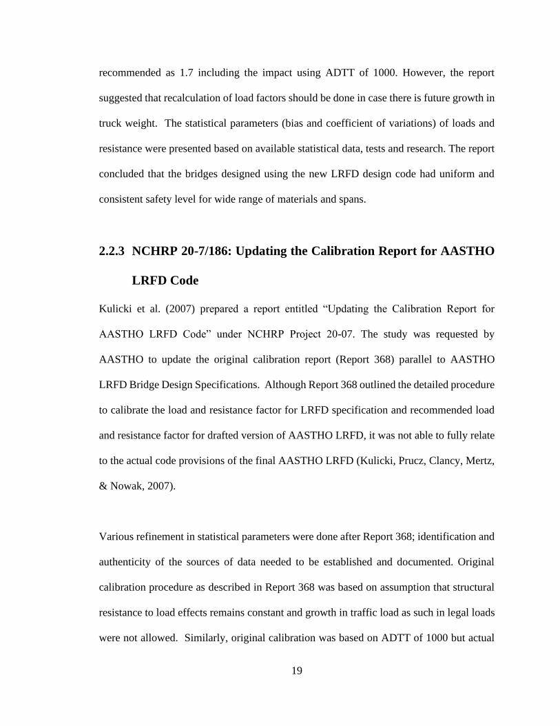
2.2.3 NCHRP 20-7/186: Updating the Calibration Report for AASTHO
LRFD Code
Kulicki et al. (2007) prepared a report entitled “Updating the Calibration Report for
AASTHO LRFD Code” under NCHRP Project 20-07. The study was requested by
AASTHO to update the original calibration report (Report 368) parallel to AASTHO
LRFD Bridge Design Specifications. Although Report 368 outlined the detailed procedure
to calibrate the load and resistance factor for LRFD specification and recommended load
and resistance factor for drafted version of AASTHO LRFD, it was not able to fully relate
to the actual code provisions of the final AASTHO LRFD (Kulicki, Prucz, Clancy, Mertz,
& Nowak, 2007).
Various refinement in statistical parameters were done after Report 368; identification and
authenticity of the sources of data needed to be established and documented. Original
calibration procedure as described in Report 368 was based on assumption that structural
resistance to load effects remains constant and growth in traffic load as such in legal loads
were not allowed. Similarly, original calibration was based on ADTT of 1000 but actual

20
AASTHO LRFD specified ADTT of 5000. Hence, original calibration procedure,
statistical data, parameters (bias and coefficient of variations) as described in Report 368
were reviewed to make them more compatible to LRFD Specifications and accommodate
the future trends of bridge mechanisms and services. Reliability analysis of the various
bridge girders of different materials and span lengths were performed using the specified
load and resistance factors in AASTHO LRFD. This project also included redundancy of
bridge systems and comparative reliability analysis were done for bridges designed
according to Allowable Stress Design (ASD), Load Factor Design (LFD), and Load and
Resistance Factor Design (LRFD) methods.
Change form ADTT of 1000 to 5000 resulted in the increase of 75 year mean maximum
live load effect and live load biases were also increased. To accommodate the increase in
ADTT, live load previously determined were projected by introducing multipliers of 1.025
and 1.035 for live load bias factor for moment and shear effect respectively. Live load bias
from HL-93 design loading was found to be significantly lower than that of HS-20 design
loading. Final adaptation of dynamic load allowance as 0.33 applied to truck load only was
done in AASTHO LRFD. Although, Report 368 suggested the same dynamic allowance
but in reality, live load effect was converted to live load plus impact by using a multiplier
of 1.10.
124 real bridges from the bridge database were analyzed by the Monte Carlo method of
simulation for Strength Limit State Load Combination I as specified in AASTHO LRFD.
Sensitivity analysis was performed to understand the relationship among load and
21
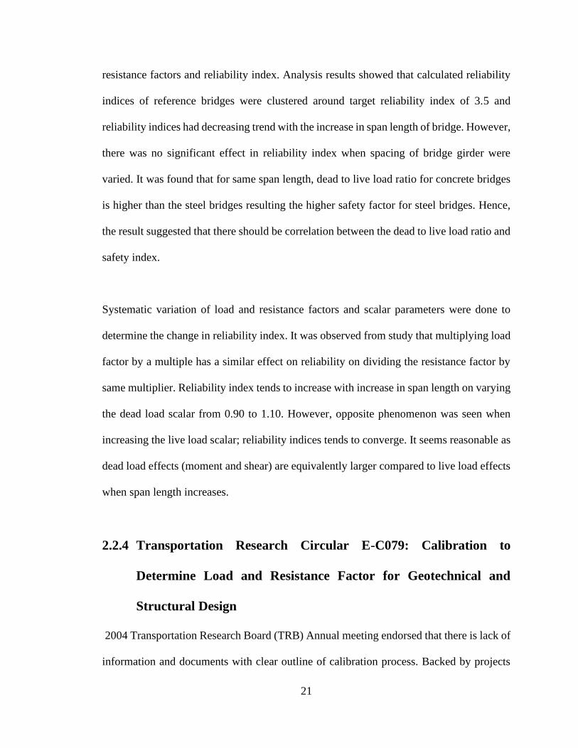
resistance factors and reliability index. Analysis results showed that calculated reliability
indices of reference bridges were clustered around target reliability index of 3.5 and
reliability indices had decreasing trend with the increase in span length of bridge. However,
there was no significant effect in reliability index when spacing of bridge girder were
varied. It was found that for same span length, dead to live load ratio for concrete bridges
is higher than the steel bridges resulting the higher safety factor for steel bridges. Hence,
the result suggested that there should be correlation between the dead to live load ratio and
safety index.
Systematic variation of load and resistance factors and scalar parameters were done to
determine the change in reliability index. It was observed from study that multiplying load
factor by a multiple has a similar effect on reliability on dividing the resistance factor by
same multiplier. Reliability index tends to increase with increase in span length on varying
the dead load scalar from 0.90 to 1.10. However, opposite phenomenon was seen when
increasing the live load scalar; reliability indices tends to converge. It seems reasonable as
dead load effects (moment and shear) are equivalently larger compared to live load effects
when span length increases.
2.2.4 Transportation Research Circular E-C079: Calibration to
Determine Load and Resistance Factor for Geotechnical and
Structural Design
2004 Transportation Research Board (TRB) Annual meeting endorsed that there is lack of
information and documents with clear outline of calibration process. Backed by projects

22
such as NCHRP 12-55 and SPR-03(072), the circulation to facilitate the understanding of
calibration process for development of LRFD specifications and to address the structural
calibration issue was developed. The circular describes the procedure for collection,
documentation, and interpretation of structural statistical data required for calibration of
load and resistance factor and determination of reliability index.
This circular describes procedures to utilize local experience and data to calibrate user
defined load and resistance factor for more consistent and accurate structural and
geotechnical design. Important consideration should be given while selecting the target
reliability factor. Target safety index are selected such that design using LRFD
specification are consistent across all limit states. Target beta index is established so that
design satisfies desirable probability of failure. Past design practices recognized target
reliability index of 3.5 for structural design. However, for geotechnical design, it is
recommended to use value of 3.0.
2.3 American Association of State Highway and
Transportation Officials (AASTHO) LRFD Bridge Design
Specifications
In Load and Resistance Factor Design method designer should check for following limit
states: Service Limit, Strength Limit, Fatigue and Fracture Limit, and Extreme Event
Limit. Service limit states are performed to restrict the stress, deformations and crack width

23
of bridge components for regular service conditions for its service life. Fatigue and fracture
limit states are restrictions on stress range caused by single design truck. They are checked
to limit crack growth under repetitive loads thus preventing the fracture of the bridge during
its design life. The aim of the strength limit states is to provide enough resistance or
strength for the loads and their combined actions that a bridge is expected to endure during
its design life. In strength limit states, resistances for bending, shear, torsion and axial
effects for load are assessed. Extreme limit states are evaluated to ensure the structural
safety of the bridge during major event such as earthquake, collision, scouring and flooding
(Nowak & Collins, Reliability of Structures, 2013). In this study, structural reliability
analysis is limited to Strength Limit state I only.
2.3.1 The LRFD Equation:
The basic general design equation that must be satisfied for LRFD limit states both at local
and global levels is specified in AASTHO LRFD Bridge Specifications is given as,
Ʃ 𝜂𝑖𝛾𝑖𝑄𝑖 = ɸ𝑅𝑛 (2.1)
Where,
𝑄𝑖 is the force effect due to loads
𝛾𝑖 is the statistically based load factor
ɸ is the statistically based resistance factor
Rn is nominal resistance factor
𝜂𝑖 is the load modification factor

24
Load modifier (η)
It accounts the ductility, redundancy and operational importance of the bridge. It is applied
to load factor, γ, and is expressed as,
𝜂𝑖 = 𝜂𝐷𝜂𝑅𝜂𝐼 ≥ 0.95 (2.2)
Where,
𝜂𝐷 is ductility factor
𝜂𝑅 is redundancy factor
𝜂𝐼 is the operational importance factor
Ductility, redundancy and operational importance play importance role for the marginal
safety of the bridge. Ductility factor accounts the capacity of the structure to redistribute
the applied load locally and globally. Limitation of flexural reinforcement and confinement
with stirrups and hoops ensures the ductility in reinforced concrete design. Redundant
structure has more restraints than that are necessary to satisfy equilibrium. Structural
system with multiple load paths is more robust than non-redundant system (Nowak &
Collins, 2012). Operational importance factor is subjective. It is applied to the strength and
extreme-event limit state.
2.3.2 Load Combination
In LRFD design approach designer need to examine the various load combination for
different design limit states: Service, Fatigue and Fracture, Strength, and Extreme-Event

25
Limit states. Loads occur in the bridge simultaneously. However, there is low probability
of simultaneous occurrence of extreme event load with other basic loads in a bridge during
its design life. Hence, there are different load factor for different load combinations.
AASTHO LRFD [A3.4] describes various load factors and load combinations for above
mentioned design limit states. In this study, we are only considering the Strength Limit
State I. Strength Limit State I refers to basic load combinations for normal vehicular use
of the bridge without wind. Only basic loads- dead and live load with impact- are
considered in this limit state. The general design formula for Strength Limit State I in the
current AASTHO LRFD specifications is as below.
1.25𝐷𝐶 + 1.50𝐷𝑊 + 1.75(𝐿𝐿 + 𝐼𝑀) < 𝛷𝑅𝑛 (2.3)
Where,
𝐷𝐶 is permanent dead load from structural components of bridge.
𝐷𝑊 is dead load from wearing surface
(𝐿𝐿 + 𝐼𝑀) is live load with impact
𝛷 is resistance factor applied to nominal resistance (𝑅𝑛) of structure
Load factor for limit state I specified in the specification are based on calibration of bridges
yielding safety index close to the target value of β = 3.5.
26
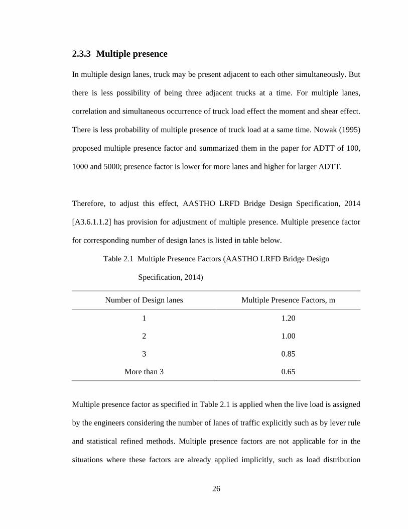
2.3.3 Multiple presence
In multiple design lanes, truck may be present adjacent to each other simultaneously. But
there is less possibility of being three adjacent trucks at a time. For multiple lanes,
correlation and simultaneous occurrence of truck load effect the moment and shear effect.
There is less probability of multiple presence of truck load at a same time. Nowak (1995)
proposed multiple presence factor and summarized them in the paper for ADTT of 100,
1000 and 5000; presence factor is lower for more lanes and higher for larger ADTT.
Therefore, to adjust this effect, AASTHO LRFD Bridge Design Specification, 2014
[A3.6.1.1.2] has provision for adjustment of multiple presence. Multiple presence factor
for corresponding number of design lanes is listed in table below.
Table 2.1 Multiple Presence Factors (AASTHO LRFD Bridge Design
Specification, 2014)
Number of Design lanes Multiple Presence Factors, m
1 1.20
2 1.00
3 0.85
More than 3 0.65
Multiple presence factor as specified in Table 2.1 is applied when the live load is assigned
by the engineers considering the number of lanes of traffic explicitly such as by lever rule
and statistical refined methods. Multiple presence factors are not applicable for in the
situations where these factors are already applied implicitly, such as load distribution

27
factors outlined in (AASTHO LRFD Bridge Design Specification, 2014) [A4.6.2].
Additionally, multiple presence factor is also not applicable for fatigue limit state as only
one design truck is used regardless of the number of design lanes.
2.3.4 Dynamic effects
When a vehicle moves along the bridge, its static weight may not be constant during its
motion. Its instantaneous weight is higher than its static weight when there is upward
acceleration caused by reaction of dynamic nature of road surface and its suspension
system (compression and extension effect). This phenomenon is called impact and code
has specified the dynamic allowance factor for this account. In NCHRP Report 368,
calibration was performed using ADTT of 1000 using HS20 design truck. Static and
dynamic component of vehicle load were studied separately. Dynamic allowance
associated with the maximum 75-year two-lane live load was 10% and combined COV of
live load and dynamic load was 0.18. Recalibration to this study, NCHRP 20-07/186
calibrated by combining static and dynamic components for ADTT of 5000 using HL-93
design truck. From the results, it was found that the live load factor increased from 1.7 to
1.75. In current AASTHO LRFD Bridge Design Specifications, dynamic allowance of 0.33
of design truck only with no dynamic load factor applied to the uniformly distributed load
is specified.
2.3.5 Live load Distribution Factor
The total load acting on a bridge is distributed among the girders (interior and exterior) by
using empirically based formulas established from various refined methods such as beam-

28
girder analysis, 2D, 3D analysis. This analysis method takes account to relative stiffness of
various components, geometry and load configurations for determining the distribution of
internal actions throughout the structures by introducing the distribution factor. Nowak
(1995) described new method of GDF by Zokaie et.al which depends on both span length
and girder spacing.
Empirical formulas for determining the distributions factor for various cases are outlined
in AASTHO [A4.6.2.2] that are applicable for regular bridges. In this study, distribution
factor for interior and exterior girder for one or multiple lane loaded conditions are
calculated using the empirical formula specified in that section as follows.
I) Interior Girder Load Distribution Factor
i. Moment
One design lane loaded:
𝑚𝑔𝑚𝑜𝑚𝑒𝑛𝑡𝑆𝐼 = 0.06 + (
𝑆
14)
0.4
(𝑆
𝐿)
0.3
+ (𝐾𝑔
12𝐿𝑡𝑠3)
0.1
(2.4)
Two or more design lanes loaded:
𝑚𝑔𝑚𝑜𝑚𝑒𝑛𝑡𝑆𝐼 = 0.075 + (
𝑆
9.5)
0.6
(𝑆
𝐿)
0.3
+ (𝐾𝑔
12𝐿𝑡𝑠3)
0.1
(2.5)

29
ii. Shear
One design lane loaded:
𝑚𝑔𝑠ℎ𝑒𝑎𝑟𝑆𝐼 = 0.36 +
𝑆
25 (2.6)
Two or more design lanes loaded:
𝑚𝑔𝑠ℎ𝑒𝑎𝑟𝑆𝐼 = 0.2 +
𝑆
12− (
𝑆
35)
2
(2.7)
II) Exterior Girder Load Distribution Factor
i. Moment
One design lane loaded: Use lever rule.
Two or more design lanes loaded:
𝑚𝑔𝑚𝑜𝑚𝑒𝑛𝑡𝑀𝐸 = e ( 𝑚𝑔𝑚𝑜𝑚𝑒𝑛𝑡
𝑀𝐸 )
𝑒 = 0.77 + 𝑑𝑒
9.1 ≥ 1.0
(2.8)
ii. Shear
One design lane loaded: Use lever rule.
Two or more design lanes loaded:
𝑚𝑔𝑠ℎ𝑒𝑎𝑟𝑀𝐸 = e ( 𝑚𝑔𝑠ℎ𝑒𝑎𝑟
𝑀𝐸 )
𝑒 = 0.77 + 𝑑𝑒
10
(2.9)

30
For Nb = 3, Use lever rule.
Where,
𝑆 = girder spacing (ft)
𝐿 = span length (ft)
𝑡𝑠 = slab thickness (in.)
𝐾𝑔 = longitudinal stiffness parameter (in.4)
𝐾𝑔 = 𝑛(𝐼𝑔 + 𝑒𝑔2𝐴)
Where,
n = modular ratio (𝐸𝑔𝑖𝑟𝑑𝑒𝑟/𝐸𝑑𝑒𝑐𝑘)
𝐼𝑔 = moment of inertia of the girder (in.4)
𝑒𝑔 = girder eccentricity, which is the
A = Area of girder.
de = Distance of curb to resultant of reaction at exterior girder. It is positive if girder is
inside of barrier, otherwise negative.

31
Chapter 3
Overview of Calibration Approach
3.1 General
In reliability study, calibration is defined as process of collecting statistical data, refining
them to get statistical design parameters, and determining the load and resistance factors
to achieve desirable margins of safety of all design components (Allen, Nowak, & Bathurst,
2005).
The total load is considered as normal random variable and is summation of several load
components acting on the bridge (Nowak & Latsko, 2017). The cumulative distribution
functions (CDF) plotted by analyzing the maximum moment and shear effect from the
truck survey showed that live load effects (moments and shear) are not distributed normally
however summation of loads tends to a normal distribution (Kulicki, Prucz, Clancy, Mertz,
& Nowak, 2007).
Literature review, research, tests, engineering standards and relevant internet sites are
major sources for obtaining the statistical data needed for calibration procedure. Data that

32
obtained should be consistent and sufficient to define the minimum statistical parameters
(mean, bias, and coefficient of variations) and distribution of data needed for mathematical
calculations. Larger the number of statistical data higher the confidence limit and it also
affects the extent of extrapolation required during reliability analyses. Similarly,
coefficient of variation of statistical data is measure of quality of data used. Statistical
parameters should incorporate uncertainties associated with resistance and load data
resulting from materials variability, tests procedures, handling and collecting data. Error
associated may be systematic or nonsystematic errors and one should always work on
minimizing such errors. Kulicki et al. (2007) mentioned the acceptable criteria for treating
the outliners during statistical characterizations. Special attention should be given for the
data in tail regions of commutative distribution functions of random variable as they are
very sensitive to determine the design points and calculating the load and resistance factor
during the analyses.
Bias and Coefficient of Variation (COV) calculated from available statistical data should
reflect the degree of uncertainty associated with random variables. In general, sources of
uncertainty are: systematic error, inherent spatial variability, model error, and error
intrinsic to quality and quantity of data (Allen, Nowak, & Bathurst, 2005).
3.2 Calibration Methods
There are various procedures available for calculating reliability index. These procedures
vary depending on nature of statistical data, types of random parameters in limit state

33
function and their approach to generate solution. Generally, such procedures can be
categorized into three groups: closed form solution, iterative numerical procedure, and
simulation-based procedure. One procedure from each of three groups is briefly described
in the following sub-sections. The basic framework of calibration process is illustrated in
the figure below.

34
Calibration
Framework
Formulate the limit state function
Determine Load
Parameters
Determine Resistance
Parameters
Develop Statistical Load
Model Develop Statistical
Resistance Model
Select a Reliability Analysis
Procedure and Target Reliability
Index (βT)
Select Load and Resistance
Factor
Is β ≥ βT?
Calculate Reliability Index (β)
Modify Load and
Resistance Factor End
Figure 3-1 Flowchart-Basic Calibration Procedure
Yes No

35
3.2.1 Closed Form Solution
When both load (Q) and resistance (R) random variables have same statistical distribution
reliability index (β) can be calculated by using closed form solutions. Exact solutions are
available for the cases: 1) both resistance and loads are distributed normally, 2) both
resistance and loads have log-normal distribution. If resistance and load have different type
of distribution, closed form solution will generate only approximate value of β (Allen,
Nowak, & Bathurst, 2005).
Case 1
If R and Q both are normal random variables and the limit state function is linear, the
reliability index (β) can be calculated using the following formula,
𝛽 =𝜇𝑅 − 𝜇𝑄
√𝜎𝑅2 + 𝜎𝑄
2
(3.1)
Where,
𝜇𝑅 and 𝜇𝑄 are mean value of resistance and load distribution respectively.
𝜎𝑅 and 𝜎𝑄 are standard deviation of resistance and load distribution respectively.
Case 2
For lognormal distribution of R and Q, limit state function is multiple of random variable
and expressed as 𝑔 =𝑅
𝑄− 1. For this case, β is calculated as (Allen, Nowak, & Bathurst,
2005),

36
𝛽 =
𝐿𝑁 [𝜇𝑅 𝜇𝑄√(1 + 𝑉𝑅2) (1 + 𝑉𝑄
2)⁄⁄ ]
√𝐿𝑁[(1 + 𝑉𝑅2)(1 + 𝑉𝑄
2)]
(3.2)
Where,
𝜇𝑅 and 𝜇𝑄 are mean value of resistance and load distribution respectively.
𝑉𝑅 and 𝑉𝑄 are coefficient of variation of resistance and load distribution respectively.
Nevertheless, resistance and load have different statistical distribution in practice; load is
normally distributed, and resistance is log-normally distributed. Therefore, reliability index
calculated by using closed form solutions are only approximate for such a case. However,
more advanced technique such as Rackwitz-Fiessler procedure and Monte Carlo method
can determine more exact value in such case.
3.2.1 Rackwitz-Fiessler Procedure
Rackwitz-Fiessler is a procedure to calculate the value of reliability index by method of
iteration. This method requires the knowledge of probability distributions of all the random
variables in limit state equation. It does not require detail information on the type of
distribution for each of the random variables. However, if we know the exact distribution,
the results would be more accurate.
In this method, normal approximation is done for non-normal random variable at design
point. Design point (𝑅∗, 𝑄∗) is defined as the point of maximum probability of failure on

37
the failure boundary given by limit state function (Nowak, 1999). At failure boundary,
resistance and loads are equal and limit state function is expressed as 𝑔 = 𝑅 − 𝑄 = 0.
Since design points are located at failure boundary,
Mathematically, 𝑅∗ = 𝑄∗.
Where,
𝑅∗ is the value of resistance and 𝑄∗ is the value of load at design point.
At first, initial estimation of design points is done. Generally, design point is predicted at
a location within the tails of the cumulative load and resistance distribution. Let FR and FQ
be the cumulative distribution function (CDF) of resistance and load respectively.
Similarly, fR and fQ be their corresponding probability density function (PDF).
At design point, PDF and CDF of load is approximated to normal distribution (𝑄′), such
that
𝐹𝑄′ (𝑄∗) = 𝐹𝑄(𝑄∗)
𝑓𝑄′(𝑄∗) = 𝑓𝑄(𝑄∗)
And, the equivalent standard deviation and mean of 𝑄′ are given by,
𝜎𝑄′ = 𝛷{𝛷−1[𝐹𝑄(𝑄∗)]}/𝑓𝑄(𝑄∗)
(3.3)
𝑚𝑄′ = 𝑄∗ − 𝜎𝑄
′ 𝛷−1[𝐹𝑄(𝑄∗)] (3.4)

38
Similarly, distribution of resistance is approximated to normal distribution (𝑅′), such that
𝐹𝑅′ (𝑅∗) = 𝐹𝑅(𝑅∗)
𝑓𝑅′(𝑅∗) = 𝑓𝑅(𝑅∗)
And, the equivalent standard deviation and mean of 𝑅′ are given by,
𝜎𝑅′ = 𝛷{𝛷−1[𝐹𝑅(𝑅∗)]}/𝑓𝑅(𝑅∗)
(3.5)
𝑚𝑅′ = 𝑅∗ − 𝜎𝑅
′ 𝛷−1[𝐹𝑅(𝑅∗)] (3.6)
For the initial design point, reliability index is calculated as,
𝛽 =𝑚𝑅
′ − 𝑚𝑄′
√𝜎𝑅′2 + 𝜎𝑄′
2
(3.7)
For next iteration, new design point is calculated from the following equations:
𝑅∗ = 𝑚𝑅′ − 𝛽 ∗
𝜎𝑅′2
√𝜎𝑅′2 + 𝜎𝑄′
2
(3.8)

39
𝑄∗ = 𝑚𝑄′ − 𝛽 ∗
𝜎𝑄′2
√𝜎𝑅′2 + 𝜎𝑄′
2
(3.9)
In next iteration, all the steps mentioned above are followed for new design point. Iteration
is performed until there is acceptable convergence of value of design point or reliability
index. This procedure is programmable in computer to generate the final value of reliability
index. A graphical version of Rackwitz-Fiessler procedure is also available to calculate the
reliability index (Nowak & Collins, Reliability of Structures, 2013). Cumulative
probability distributions of resistance and load are plotted on normal probability paper and
trial design point is selected. Mean and standard deviation of load and resistance are
determined directly by using tangents to the distribution curves at the design point selected.
Reliability index is calculated by using equation (3.7). This process is continued for several
design points until there is convergence of reliability index.
3.1.1 Monte Carlo Method
Monte Carlo method is computer-based numerical integration technique to calculate the
reliability index. In practice, either load and resistance or both are not normally distributed.
In some cases, we are unable to determine the type of distribution of parameters in limit
state function. Similarly, sometimes quantity of materials and load data are not adequate to
calculate reliability index more accurately. In such cases, more rigorous technique like
Monte Carlo method provides only feasible way to determine the probability of failure.

40
With the availability of advanced computers more precise and effective method of
calibration, Monte Carlo Simulations Method, was used for reliability analyses rather than
Rackwitz and Fiessler (Kulicki, Prucz, Clancy, Mertz, & Nowak, 2007). The basic inputs
needed to perform this method are value of mean and standard deviation of all the random
variable in the limit state function. Monte Carlo technique does not require to determine
exact location of the design point, but it is necessary to fit the data in the region of the
design point. Sometimes, extrapolation of data to larger value of standard normal variable
(z) is done to best fit the curve in the region of design point.
Using this method, we are also able to generate the vast number of simulated values of
random variables and corresponding limit state function. Number of times (n) that
simulated limit state function satisfy failure criteria (𝑔 < 0) are counted and probability of
failure (𝑃𝑓) is calculated as
𝑃𝑓 =𝑛
𝑁
(3.10)
Where n is the total number of failure and N is the total simulated values of limit state
function.
Alternatively, probability of failure can be determined by plotting the simulated values of
limit state along X-axis and standard normal variable in Y-axis on normal probability paper
(Nowak & Collins, Reliability of Structures, 2013) . From the plot, value of reliability
index is determined as value of standard normal variable at which plotted data curve
intersect Y-axis. Large the number of simulated data, more accurate the value of probability

41
of failure estimated by using this method. If plotted curve does not intersect the vertical
axis, the plotted data curve can be extrapolated, or number of simulations can be increased.
However, increasing the number of simulations is more preferred.
In this study, reliability analysis is done for interior and exterior T-beam bridge girder for
moment and shear effects. Load and resistance are the random variables in the limit state
function. Load are considered as normally distributed and resistance as log-normally
distributed. Basic parameters (mean and bias) are adopted from the literature reviewed.
Failure rate and corresponding reliability index are calculated through Monte Carlo
simulation using MS Excel. Computational procedure for Monte Carlo simulation is
adopted from NCHRP 20-07(186) Report. Basic steps of computational procedure that
were followed are outlined below:
i. Determine nominal dead load (𝐷𝑛) and nominal live load plus impact load
(𝐿𝑛).
ii. Calculate nominal resistance (𝑅𝑛) for the bridge girder according to the
AASTHO LRFD Bridge Design Specifications.
iii. Take initial value of i as 1.
iv. Using Command RAND in MS Excel, generate a uniformly distributed
random number 0 ≤ 𝑢𝐷𝑖 ≤ 1 for dead load.
v. Using bias (𝜆𝐷) and coefficient of variation ( 𝑉𝐷), calculate a random
normal variable for dead load, 𝐷𝑖 ,

42
𝐷𝑖 = 𝜇𝐷 + 𝜎𝐷ɸ−1(𝑢𝐷𝑖 ) (3.11)
Where,
𝛷−1 = inverse standard normal distribution function. Use command
NORMSINV
𝜇𝐷 = 𝜆𝐷𝐷𝑛 (3.12)
𝜎𝐷 = 𝑉𝐷𝜇𝐷 (3.13)
vi. Similarly, generate a uniformly distributed random number 0 ≤ 𝑢𝐿𝑖 ≤ 1
for live load plus impact using command RAND.
vii. Calculate a random normal variable for live plus impact load, 𝐿𝑖 ,
𝐿𝑖 = 𝜇𝐿 + 𝜎𝐿ɸ−1(𝑢𝐿𝑖 ) (3.14)
Where,
ɸ−1 = inverse standard normal distribution function. Use command
NORMSINV
𝜇𝐿 = 𝜆𝐿𝐿𝑛 (3.15)
𝜎𝐿 = 𝑉𝐿𝜇𝐿 (3.16)
viii. Likewise, for resistance, generate a uniformly distributed random number
0 ≤ 𝑢𝑅𝑖 ≤ 1 using the command RAND.
ix. Calculate a log-normal random variable for resistance, 𝑅𝑖 ,
𝑅𝑖 = 𝑒𝑥𝑝(𝜇𝑙𝑛𝑅 + 𝜎𝑙𝑛𝑅ɸ−1(𝑢𝑅𝑖 )) (3.17)
Where,
ɸ−1 = inverse standard normal distribution function. Use command
NORMSINV.

43
𝜇𝑙𝑛𝑅 = ln(𝜇𝑅) − 12⁄ 𝜎𝑙𝑛𝑅
2 (3.18)
𝜎𝑙𝑛𝑅 = (ln(𝑉𝑅2 + 1))1/2
(3.19)
x. Calculate limit state function, 𝑔𝑖 = 𝑅𝑖 − (𝐷𝑖 + 𝐿𝑖).
xi. Assume i = i+1. Go to step (iii) and iterate until the desired number of
simulations, N, is obtained.
xii. Rank the value of 𝑔𝑖 using command RANK for corresponding values of i
in ascending order.
xiii. Using the ranked i, calculate its probability as below.
𝑃𝑖 =𝑖
(1 + 𝑁)
(3.20)
xiv. Using command NORMSINV, calculate the corresponding values of the
inverse standard normal distribution function, ɸ−1(𝑃𝑖 ).
xv. Plot cumulative distribution function (CDF) of limit state function value (g).
i.e. plot ɸ−1(𝑃𝑖 ) versus 𝑔𝑖 .
xvi. From the plot, reliability index is determined as the negative value of
standard normal variable for g=0.
3.3 Reliability Index
Probability of failure is a measure of safety of structural elements and system. However, it
is difficult and sometimes impossible to calculate probability of failure directly. Therefore,

44
structural safety is often measured in terms of reliability index (β). Reliability index is
defined as the function of probability of failure and expressed as
𝛽 = ɸ−1(𝑃𝑓) (3.21)
Where, ɸ−1 is inverse standard normal distribution function.
Each value of reliability index has its corresponding probability of failure some of which
are listed in the figure below.
Figure 3-2 Reliability Index and Corresponding Probability of Failure (Nowak, 1999)
Relationship between safety index and probability of failure can also be given by:
𝑃𝑓 = 1 − 𝑁𝑂𝑅𝑀𝑆𝐷𝐼𝑆𝑇(𝛽) (3.22)

45
Where,
𝑁𝑂𝑅𝑀𝑆𝐷𝐼𝑆𝑇(𝛽) is an Excel Function that returns standard normal cumulative distribution
function (CDF) for the desired value of reliability index. The above equation is more
accurate for random variables with normal distribution, otherwise it gives approximate
values (Allen, Nowak, & Bathurst, 2005).
Sometimes, difference between performances of structure (𝑅) for system of loads acting in
the structure (𝑄) expressed as 𝑅 − 𝑄 is termed as the margin of safety (𝑀). Figure 3-3
illustrates the concept of frequency distribution of random variables (load and resistance),
limit state margin of safety, probability of failure, and reliability index.
Figure 3-3 Margin of Safety, Probability of Failure, and Reliability Index (Adopted from
Allen, Nowak, & Bathurst, 2005)

46
Hence, Reliability index can also be expressed as (Kulicki, Prucz, Clancy, Mertz, &
Nowak, 2007),
𝛽 =�̅�
𝜎𝑀
(3.23)
Where, �̅� and 𝜎𝑀 are mean and standard deviation of margin of safety.
3.4 Target Reliability Index
Selecting the target reliability index is very vital step in reliability analysis of a structure.
Target reliability index or target safety factor is determined to produce consistent and safe
designs for all the limit states as possible. Target safety index represents the probability of
occurrence of detrimental loading conditions and severity of consequence of failure for
different limit states during the design life of a structure.
The severity of consequence of failure for different limit states may be significantly
difference. For instance, deformation of a component of a structure is not severe in terms
of collapse and loss of life and property as compared to collapse of structure due to its
incapability to withstand the design loads. Special attentions should be given to load paths,
primary and secondary components and duration of time associated with the structures
(Nowak & Kaszynska). For example, consequences of failure from primary components
are more severe and are about 10 times larger than those of secondary components. Brittle

47
failure such as by shear failure have severe consequence compared to ductile failure like
flexural failure. Similarly, beam failures are local failure as compared to column failure
which result to failure of whole system of structure.
It is acceptable to have lower value of target safety index for limit states with low
probability of occurrence of load combination during its design life such as extreme events
loading (e.g., earthquake) than a more general loading conditions such as that of strength
limit. Redundancy inherent in the system has vital contribution for determination of target
reliability index of a structure. Literature reviewed suggested that more the redundancy of
structure, more the allowable probability of failure and lower is the desired reliability
index.
Previous design practice and consistent level of safety as implied by safety factor (FS) in
past design specifications such as ASD are the basis for selecting the target reliability
index. In strength limit state design, resistance factor for structural design are determined
such that target reliability index is 3.5 and corresponding probability of failure is around 1
in 5000 (Allen, Nowak, & Bathurst, 2005). However, geotechnical design practice
recommends target reliability index of 3.0 for foundation design for probability of failure
of 1 in 1000. But, if there is no redundancy in structure such as for a single drilled shaft, it
is recommended to use target beta index of 3.5 (Allen, Nowak, & Bathurst, 2005).
In calibration process, load and resistance factors are estimated based on target reliability
index. The objective of calibration is to select load and resistance factors to achieve the

48
target probability of failure (Pf). Different sets of load and resistance factor can generate
same target reliability index. Each value of reliability index is associated with the value of
probability of failure. Current LRFD based codes prescribe the target reliability index as
3.5 (Pf ≈ 1 in 5000) for strength limit state design of structural components. Higher value
of reliability index refers to lower probability of failure. Designing the structure such that
its probability of failure is significantly low might be possible but, might not be practical
in terms of higher cost of construction.
3.5 Load and Resistance Factor
The objective of calibration is finding the load and resistance factor in order of achieving
the value of reliability index closer or greater than the target reliability index of 3.5.
Estimating the load and resistance factor is the beginning step in the calibration process.
For a desired probability of failure (Pf) or reliability index (β), there are many combinations
of load and resistance factor.
Load and resistance factors are selected such that structures designed using the design
codes provide uniform reliability and desired safety of margin. Primarily, load factor
increases the design loads such that there is less probability of occurring the loads equal or
more than design loads during the design life of structures. Similarly, design resistance is
obtained using resistance factor to ensure the low probability of occurrence of structural
performance of such a low magnitude. Hence, there is always a reserve of safety while
designing a structure. If resistance factor equals to 1 or remain constant and only load

49
factors are modified, margin of safety will remain in loads only. Appropriate selection of
load and resistance factor is essential for rational and optimum design with desired margin
of safety.
Figure 3-4 Mean Load, Design Load, and Factored Load (Kulicki et al., 2007)
Figure 3-5 Mean Resistance, Design Resistance and Factored Load (Kulicki et al., 2007)

50
Estimation of Load Factor
Generally, load factor is set to value greater than 1.0 and resistance factors below 1.0 during
the initial estimation of these factors. However, this may not be true for some cases
depending on the nature of prediction method employed. For a various load component,
load factor, 𝛾𝑄, is calculated using statistical data from using the formula below (Allen,
Nowak, & Bathurst, 2005)
𝛾𝑄 = 𝜆𝑄 (1 + 𝑛𝑄𝑉𝑄) 3.24
Where,
𝛾𝑄 is load factor
𝜆𝑄 is bias factor for the load
𝑉𝑄 is coefficient of various of load
𝑛𝑄 is a constant representing the number of standard deviations from the mean needed to
obtain the desired probability of exceedance.
Nowak and Collins (2013) assumed the value of 𝑛𝑄 as 2 (factor load is two standard
deviation from the mean). Based on practical experience, the value of 𝑛𝑄 = 2 is
recommended which corresponds to the probability of exceeding any load factor is
approximately 0.02.

51
Estimation of Resistance Factor
After selecting the appropriate load and resistance factor, the resistance factor is estimated
using various available calibration methods. For a set of load factors, resistance factor is
calculated by using closed form formula and iteration techniques to achieve the desirable
reliability index. There are different calibration methods to calculate the resistance factor;
only closed form solution, Rackwitz-Fiessler, and Monte Carlo Methods are described in
this study. Generally, resistance factors are round off to the nearest 0.05. Since, the load
factor for Strength Limit I are pre-defined as specified by AASTHO LRFD specification,
we are varying the resistance factor with range of 0.75 to 1.0 with 0.5 as incremental value.
Specified Load and Resistance Factor
AASTHO LRFD has specified the load factors for different limit states and load
components. Similarly, resistance factors are also prescribed in the code for different
materials and force effects (moment, shear). Load and resistance factor specified by the
code for Limit State I are tabulated as below.
Table 3.1 Load Factor Specified in AASTHO LRFD Bridge Design Specifications, 2014
Load Component Load Factor, γ
Dead Load (DC): components and attachment 1.25
Wearing surface and Utilities (DW) 1.5
Live load (including dynamic load allowance) 1.75

52
Table 3.2 Resistance Factors Specified in AASTHO LRFD Bridge Design Specifications,
2014 for Moment and Shear
Material
Moment Shear
Resistance Factor, ɸ Resistance Factor, ɸ
Composite and Non-Composite Steel 1.0 1.0
Reinforced Concrete 0.9 0.85
Prestressed Concrete 1.0 0.9

53
Chapter 4
Structural Load and Resistance Model
4.1 General Load Model
In order to design a bridge and perform the reliability analysis, designers should understand
types and magnitude of the load expected to act on bridge during its design service life. All
the loads acting on a bridge are categorized into three types based on the characteristic of
the load phenomenon and types of statistical data that are available (Nowak & Collins,
2013). In Type I, load data consider only their intensity rather than their frequency of
occurrence. Dead and sustained live loads are Type I loads. Type II category loads are time
dependent and are measured at prescribed periodic time intervals. Examples of loads in
this category are severe winds, snow loads, and transient live load. Type III category loads
are loads occur at extreme events such as earthquake and tornadoes. This type of load is
time dependent, but their occurrence is rare and unpredictable hence are often non-
periodical.
In boarder sense, structural loads acting on bridge can be categorized into two different
load types: Permanent and Transient. Permanent loads are long-lasting loads acting on the
54
bridge during its entire service life. The permanent loads include dead loads and earth loads
(Mertz, 1999). Dead load consists of weight of wearing surface, future overlays, utilities,
and structural self-weight. In this study, dead loads considered are loads from structural
components, wearing surface, barriers and future wearing surface only. Transient loads
are the loads that are not always acting in the bridge. They consist of moving loads and
their magnitude varies during the life of the bridge. Transient loads include live loads, wind
loads, environmental loads and water loads. Only vehicular live loads are considered for
the study.
4.1.1 Structural Load Model
The major load acting on highway bridges are dead load, live load (static and dynamic),
environmental loads and other loads (collision emergency braking). However, the basic
combination of loads simultaneously acting on a bridge is of dead, live and dynamic load.
For short and medium span of bridges, dead load, live load and dynamic loads govern the
design rather than other loads like earthquake loads and special loads (breaking and
collision forces) (Tabsh & Nowak).
Available statistical data, surveys and other observations are used to develop the load
model. Various load components are treated as random variables. Statistical characteristics
of components such as cumulative distribution function (CDF), mean value and coefficient
of variation are used to define the statistical parameters of the total load acting in a bridge.
In order to perform reliability analysis of any structure, we need at least mean, variance
55
(coefficient of variation or standard deviation), and type of statistical distribution of
different components of load.
Mean
The mean of total load, Q, is the sum of the mean values of its individual components
(Kulicki, Prucz, Clancy, Mertz, & Nowak, 2007). And, mean value of a load component is
the product of its bias (λ) and nominal (design) value.
𝜇𝑄 = 𝜇𝐷𝐿 + 𝜇𝐿𝐿 + 𝜇𝐼𝑀 (4.1)
𝜇𝐷𝐿 = 𝜆𝐷𝐿 ∗ (𝑛𝑜𝑚𝑖𝑛𝑎𝑙 𝑣𝑎𝑙𝑢𝑒 𝑜𝑓 𝑑𝑒𝑎𝑑 𝑙𝑜𝑎𝑑) (4.2)
Where,
𝜇𝑄 = mean of total load
𝜇𝐷𝐿= mean of Dead load
𝜇𝐿𝐿= mean of Live Load
𝜇𝐼𝑀= mean of dynamic load
𝜆𝐷𝐿= bias of dead load
Coefficient of Variation
It is the ratio of standard deviation of load to its mean value. The variance of load is equal
to square of its standard deviation. The variance of the total load is the sum of the variance
of individual components,

56
𝜎2𝑄 = 𝜎2
𝐷𝐿 + 𝜎2𝐿𝐿 + 𝜎2
𝐼𝑀 (4.3)
𝑉𝑄 =𝜎𝑄
𝜇𝑄 (4.4)
Where,
𝜎𝑄 = Standard deviation of total load
𝜇𝑄 = Mean of total load
𝑉𝑄 = Coefficient of variation of total load
All components of dead loads, live loads and impact loads are treated as normal random
variable. Hence, statistical distribution of the basic loads used for reliability analysis of a
bridge is assumed as normally distributed.
4.2.1 Dead Load
Dead loads are gravity loads due to weight of the structural components and other
permanent structural components in a bridge. Their magnitude almost remains constant
throughout the design life of a bridge. Due different degree of variation of structural and
non-structural components, dead load is divided into following components (Nowak,
1999).
D1 = weight of factory-made elements (steel, precast concrete),
D2 = weight of cast-in-place concrete,
D3 = weight of the wearing surface;

57
D4= miscellaneous weight (e.g. railing, luminaries)
All the components of dead loads are treated as normal random variables. The distribution
type is normal distribution for all types of loads (Nowak & Collins, Reliability of
Structures, 2013). Table 4.1 lists the statistical parameters (bias and coefficient of
variation) for dead load components that are considered for this study.
Table 4.1 Representative Statistical Parameters of Dead Load (Kulicki et al., 2007)
Dead Load Component Bias Factor, λ Coefficient of Variation, V
Factory made elements, DL1 1.03 0.08
Cast-in-place, DL2 1.05 0.10
Wearing Surface, DL3 1.0 0.25
Miscellaneous, DL4 1.03 ⁓ 1.05 0.08 ⁓ 0.10
This study will be focusing on reinforced concrete T-Beam bridge girders with span length
of 20ft, 40ft, 60ft, and 80 ft. The weights of different load components are calculated by
using their unit weight combined with the geometry. The density of concrete is taken as
150 pcf and nominal value of wearing surface is assumed as 140 pcf.

58
4.2.2 Live Load
Live load in the bridge is produced by the vehicle moving on the bridge. Various structural
parameters such as span length, design truck, design tandem, design lane, number of lanes,
girder spacing, number of vehicles on the bridge, axle loads, configurations etc. determines
the effect of the live load.
AASTHO code, before incorporating LRFD design approach, used live load model based
on HS-20 truck, lane or military loading and was not representing the actual load effects
(moment and shear) from heavy trucks on the highway; actual load effects were much
higher than design loads. Nowak (1995) described new live load model consisted HS-20
truck with uniform load (640lb/ft) or tandem load with uniform load (640lb/ft). The new
LRFD live load model that is used in current AASTHO LRFD bridge design specifications
has lower bias of load effect than the load model used in AASTHO code (Nowak, 1995).
The LRFD specification Live load Model
For the study, HL-93 AASTHO vehicular live loading is used for calculating the live load
effects. HL-93 load model is a theoretical live loading proposed by AASTHO in 1993 and
it is used for design live loading for the highway structures. AASTHO HL-93 vehicular
live load is the combination of following distinct live loads.
1. Design Truck (formally HS20-44 truck)
2. Design Tandem
3. Design Lane

59
1. Design Truck:
It consists of three axles: one front and two rear axles. Front axle weights 8 kips (35 KN)
and each rear axle weight 32 kips (145 KN). Front axle is positioned at 14ft apart from rear
axle and two axles are positioned at varying distance of 14ft to 30 ft. The distance between
the wheels in each axle is kept at 6”. Generally, center of the outside wheel must be at least
2’ from the edge of curb or barrier.
Figure 4-1 AASTHO HL-93 Design Truck Model (Source: Internet)
2. Design Tandem:
It consists of two axles each weighting 25kips spaced at 4 ft. apart. Like design truck,
distance between the wheels is 6”.
Figure 4-2 AASTHO HL-93 Design Tandem Model (Source: Internet)

60
3. Design Lane:
It consists of uniformly distributed load of 0.64 kip/ft. (9.3 N/mm) in longitudinal direction.
Transversely, it is assumed to occupy the region of 10 ft.
Design truck, tandem and lane load should be positioned is such a way that extreme load
effect is obtained for the design. An example of live loads positioning is shown in Figure
4-3. The influence function for a loading condition is used to establish the load position for
maximum moment and shear effects. Maximum of design truck load and tandem load
effects is superimposed with design lane load to determine the design live load. In this
study, QConBridge, a live load analysis software, is used to generate the moment and shear
envelope for live load. The calculations are carried out for span length of 20 ft. through
100 ft. Once these envelopes are generated, maximum values of moment and shear are
taken as design live load effects for the calibration.
Figure 4-3 AASTHO HL-93 Truck Load Positioning for Maximum Sagging Moment
in Span First (Source: Internet)

61
The available statistical parameters for bridge live load have been determined from truck
surveys and by simulations that are adopted from literature review. Design life of 75 years
was taken for the calculation of the loads. Values of bias and coefficient of variation of live
load random variables are taken for ADTT of 5000 from literature review of (Kulicki et.al,
2007) and (Nowak,1999). The representative static live load parameter with dynamic
allowance is listed in the table below.
Table 4-2 Representative Statistical Parameters of Live Load with Impact Factor
Live load with dynamic allowance Bias Factor Coefficient of variation
Moment 1.175 0.12
Shear 1.13 0.12
4.2 Resistance Model
Resistance of a bridge refers to load carrying capacity of its components and connections.
Resistance (R) of a component is a random variable which depends on materials strength,
geometry, and dimensions. Reinforcing or pre restressing steel area and effective depth
play vital role in structural reliability of reinforced and prestressed concrete girders. In
contrast, variation of dynamic load, slab dimensions, or concrete strength has less effects
in structural reliability (Tabsh & Nowak). Variability and uncertainty of resistance of

62
component are quantified by the resistance factors: Materials factor, Fabrication factor, and
Professional factor. Resistance is calculated as the product of these factors and nominal
resistance (Rn) as given by equation (4.5). As resistance is the product of several
parameters, it is considered as log-normal random variable.
Resistance model is expressed mathematically as below:
𝑅 = 𝑅𝑛. 𝑀. 𝐹. 𝑃 (4.5)
Mean of resistance (𝜇𝑅) and coefficient of variation of resistance (𝑉𝑅) are calculated by
the following equations.
𝜇𝑅 = 𝑅𝑛. 𝜇𝑀. 𝜇𝐹 . 𝜇𝑃 (4.6)
𝑉𝑅 = √𝑉𝑀2 + 𝑉𝐹
2 + 𝑉𝑃2 (4.7)
Where,
Rn is nominal resistance
M is material factor
F is fabrication factor
P is analysis factor
Material factor accounts uncertainty in estimating strength, modulus of elasticity, cracking
strength, and chemical composition. Fabrication factor considers the uncertainties related
to geometric, dimensions and section modulus. Similarly, analysis factor refers to

63
variability arises following various approximate methods of analysis and idealized stress
and strain model. In practice, bias and coefficient of variation of material and fabrication
factors are combined. Statistical parameters (bias and COV) of resistance for different type
of structures are tabulated in table below.
Table 4.3 Statistical Parameters of Resistance (Kulicki et al., 2007)
Type of Stress Bias, λ Coefficient of Variation, V
Moment 0.14 0.13
Shear with steel 1.20 0.155
Shear no steel 1.40 0.17
Nominal resistance (Rn)
Nominal Resistance is resistance calculated using design code. Nominal resistances for
flexure and shear are calculated according to design equations from AASTHO LRFD
Bridge Design Specification, 2014. During reliability analyses, design over-strengths are
neglected. For this, design limit states other than strength limit strength such as service
limit strength which is generally governing geometric characterization of structural
elements are not considered (Kulicki, Prucz, Clancy, Mertz, & Nowak, 2007). Structural
performance in term of resistance are taken corresponding to the value of summation of
factored load to desired factor of resistance rather than actual resistance. Nominal
resistance can be expressed in term of limit state equations. For strength limit state I,

64
general equation for calculating nominal resistance for given resistance factor is expressed
as below.
𝑅𝑛 =1.25𝐷𝐶 + 1.5𝐷𝑊 + 1.75𝐿𝐿
ɸ (4.8)
In sensitivity study of reliability analysis, resistance factors are varied from values ranging
from 0.75 to 1.0 with incremental of 0.5.

65
Chapter 5
Reliability Analysis and Parametric Study
For this study, systematic variations of load and resistance factors are made for reinforced
concrete T-beam girders. The girders are assumed to have uniform spacing with skew angle
of 30 degrees. Reliability indices are calculated for each of the span length corresponding
to the sets of parameters summarized. In the study, parameters are varied for Strength Limit
State Combination I using equation below based on AASTHO LRFD Bridge Design
Specifications, 2014.
ɳ [(𝐷1 𝑆𝑐𝑎𝑙𝑎𝑟) ∗ 1.25 ∗ 𝐷𝐶 + (𝐷2 𝑆𝑐𝑎𝑙𝑎𝑟) ∗ 1.5 ∗ 𝐷𝑊
+ (𝐿 𝑆𝑐𝑎𝑙𝑎𝑟) ∗ 1.75 ∗ 𝐿𝐿] = ɸ 𝑅
(5.1)
Where,
ɳ = Load modifier; a factor relating to ductility, redundancy, and operational classification.
D1 Scalar = a factor applied to load factor for site and factory-made dead components.
D2 Scalar = a factor applied to load factor for weight of asphaltic wearing surfaces and
utilities.
L Scalar = a factor applied to load factor for live load plus impact.

66
ɸ = Resistance factor
For this study, hypothetical reinforced concrete bridges with T-beam girders were
considered. A textbook of Barker & Puckett (2013) forms the basis of selecting the
charactersitics of bridges to capture more realistic design features. Bridges with different
span lengths and girders having different cross-sectional properties based on the span
length are considered. Each of the bridges has three spans of equal length and roadway
width of 44 ft. and skew angle of 30 degrees. Logitudinal profile and cross-section of
reinforced concrete T-beam girders that are used in this study are shown in the figures
below.
Figure 5-1 Longitudinal Profile of T-Beam Girder Bridges
Figure 5-2 Cross-section of T-Beam Girder Bridges

67
Design parameters that are considered for the load and resistance models and parametric
study are listed in the table below.
Table 5.1 List of Design Parameters Considered for Parametric Study
Roadway width, w = 44 ft.
Length of span of each bridge L = varies (20 ft. / 40ft. / 60ft. / 80ft.)
T-beam girder spacing S = 8 ft.
Compressive strength of Concrete f’c = 4.5 ksi
Yield strength of rebar fy = 60 ksi
Number of beams Nb = 6
Length of overhang Loverhang = 3.25 ft.
Roadway part of overhang loverhang = 3.25 ft. – 1.25 ft. = 2 ft.
Angle of skew θ = 30 degrees
Unit weight of concrete unitwt = 0.15 kip/ft3
The reinforced concrete T-beams bridges that are studied are 3 spans continuous bridges.
Load analysis program (QConBridge) is used for calculating the moment and shear
envelopes for live and dead loads. It is a load analysis program for continuous bridge
frames developed by Washington State Department of Transportation (WSDOT) and it is
available for free download at WSDOT website. Appendix A illustrates an example of load
analysis of a bridge using QConBridge. Sample calculation of loads effects (moment and

68
shear) in an interior and exterior girder resulting from dead and live loads are attached in
the Appendix A.
During reliability analyses, design over-strengths are neglected. For this, design limit states
other than strength limit strength such as service limit strength which is generally
governing geometric characterization of structural elements are not considered (Kulicki,
Prucz, Clancy, Mertz, & Nowak, 2007). Structural performance in term of resistance are
taken corresponding to the value of summation of factored load to desired factor of
resistance rather than actual resistance. Nominal resistance can be expressed in term of
limit state equations. For strength limit state I, general equation for calculating nominal
resistance for given resistance factor is expressed as below.
𝑅𝑛 =1.25𝐷𝐶 + 1.5𝐷𝑊 + 1.75𝐿𝐿
ɸ (5.2)
For the parametric study on structural reliability, resistance factors are varied from values
ranging from 0.75 to 1.0 with incremental of 0.5 and resistance are calculated at failure
boundary; resistance and loads are equal and limit state function is expressed as
𝑔 = 𝑅 − 𝑄 = 0.
For this research, the excel sheets are formulated for calculating the reliability index.
Reliability analysis are performed for bridges of various span lengths (20ft, 40ft, 60ft, &
80ft) by varying series of variables in the equation (5.2). Both interior and exterior girders

69
are studied for moment and shear effects. Appendix B contains sample spreadsheets of
reliability analysis of exterior and interior girders using Monte Carlo Method of simulation.
Using the Equation (5.1) and systematic variation of various scalars, load modifier,
resistance factor, and load factors, this study investigates the change in the reliability index
(β). Figure 5-3 through Figure 5-16 show the variation of reliability index for a systematic
variation of parameters as indicated in the figures. Figure 5-3 through Figure 5-16 contains
following information:
i. Figure 5-3 shows the results of varying the resistance factor (ɸ) on reliability index
for bending moment.
ii. Figure 5-4 shows the results of varying the resistance factor (ɸ) on reliability index
for shear.
iii. Figure 5-5 shows the results of varying the load modifier (ɳ) on reliability index for
bending moment.
iv. Figure 5-6 shows the results of varying the load modifier (ɳ) on reliability index for
shear.
v. Figure 5-7 shows the results of varying the live load bias (λLL) on reliability index
for bending moment.
vi. Figure 5-8 shows the results of varying the live load bias (λLL) on reliability index
for shear.
vii. Figure 5-9 shows the results of varying the live load scalar (L) on reliability index
for bending moment.
70
viii. Figure 5-10 shows the results of varying the live load scalar (L) on reliability index
for shear.
ix. Figure 5-11 shows the results of varying the dead load scalar (D1) on reliability
index for bending moment.
x. Figure 5-12 shows the results of varying the dead load scalar (D1) on reliability
index for shear.
xi. Figure 5-13 shows the results of varying the dead load scalar (D2) on reliability
index for bending moment.
xii. Figure 5-14 shows the results of varying the dead load scalar (D2) on reliability
index for shear.
xiii. Figure 5-15 shows the results of varying the resistance bias (λR) on reliability index
for bending moment.
xiv. Figure 5-16 shows the results of varying the resistance bias (λR) on reliability index
for shear.

71
Reinforced Concrete T-Beams - Moment
Input Parameters (Interior Girder)
Variable Series 1 Series 2 Series 3 Series 4 Series 5
Series
6
ɸ = 0.75 0.8 0.85 0.9 0.95 1
ɳ , D1, D2 , L = 1.0 1.0 1.0 1.0 1.0 1.0
Span (ft.) Reliability Index (LRFD), Beta value
20 4.804 4.436 4.082 3.739 3.410 3.094
40 4.804 4.434 4.076 3.731 3.397 3.075
60 4.779 4.408 4.047 3.698 3.360 3.034
80 4.735 4.359 3.995 3.642 3.300 2.969
Reinforced Concrete T-Beams - Moment
Input Parameters (Exterior Girder)
Variable Series 1 Series 2 Series 3 Series 4 Series 5 Series 6
ɸ = 0.75 0.8 0.85 0.9 0.95 1
ɳ , D1, D2 , L = 1.0 1.0 1.0 1.0 1.0 1.0
Span (ft.) Reliability Index (LRFD), Beta value
20 4.792 4.424 4.068 3.725 3.395 3.078
40 4.782 4.411 4.053 3.706 3.371 3.048
60 4.759 4.386 4.025 3.675 3.337 3.011
80 4.715 4.339 3.974 3.621 3.279 2.948
Figure 5-3 Effect of ɸ on β for Moment (Interior and Exterior Girder)

72
Reinforced Concrete T-Beams - Shear
Input Parameters (Interior Girder)
Variable Series 1 Series 2 Series 3 Series 4 Series 5 Series 6
ɸ = 0.75 0.8 0.85 0.9 0.95 1
ɳ , D1, D2 , L = 1.0 1.0 1.0 1.0 1.0 1.0
Span (ft.) Reliability Index (LRFD), Beta value
20 4.509 4.217 3.931 3.653 3.383 3.121
40 4.488 4.193 3.906 3.627 3.355 3.09
60 4.445 4.148 3.859 3.576 3.302 3.035
80 4.421 4.123 3.833 3.549 3.273 3.005
Reinforced Concrete T-Beams - Shear
Input Parameters (Exterior Girder)
Variable Series 1 Series 2 Series 3 Series 4 Series 5 Series 6
ɸ = 0.75 0.8 0.85 0.9 0.95 1
ɳ , D1, D2 , L = 1.0 1.0 1.0 1.0 1.0 1.0
Span (ft.) Reliability Index (LRFD), Beta value
20 4.488 4.194 3.907 3.628 3.357 3.098
40 4.457 4.161 3.872 3.591 3.318 3.052
60 4.405 4.107 3.816 3.532 3.255 2.987
80 4.376 4.076 3.783 3.498 3.22 2.95
Figure 5-4 Effect of ɸ on β for Shear (Interior and Exterior Girder)
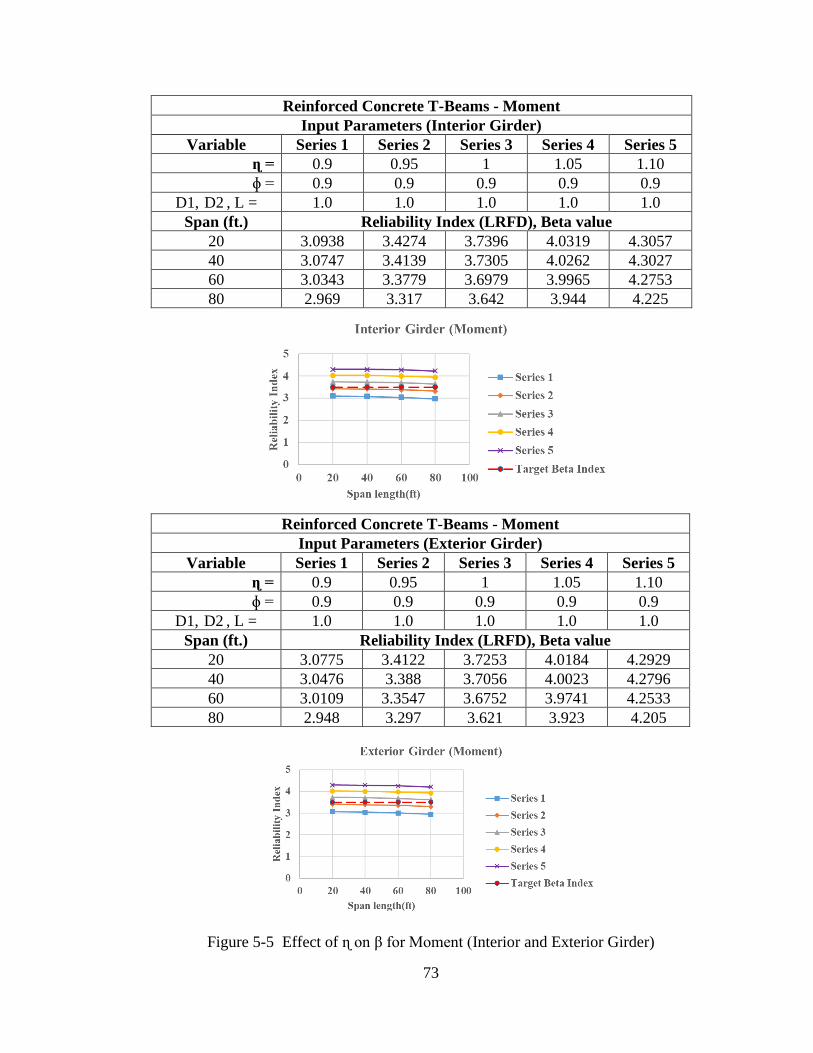
73
Reinforced Concrete T-Beams - Moment
Input Parameters (Interior Girder)
Variable Series 1 Series 2 Series 3 Series 4 Series 5
ɳ = 0.9 0.95 1 1.05 1.10
ɸ = 0.9 0.9 0.9 0.9 0.9
D1, D2 , L = 1.0 1.0 1.0 1.0 1.0
Span (ft.) Reliability Index (LRFD), Beta value
20 3.0938 3.4274 3.7396 4.0319 4.3057
40 3.0747 3.4139 3.7305 4.0262 4.3027
60 3.0343 3.3779 3.6979 3.9965 4.2753
80 2.969 3.317 3.642 3.944 4.225
Reinforced Concrete T-Beams - Moment
Input Parameters (Exterior Girder)
Variable Series 1 Series 2 Series 3 Series 4 Series 5
ɳ = 0.9 0.95 1 1.05 1.10
ɸ = 0.9 0.9 0.9 0.9 0.9
D1, D2 , L = 1.0 1.0 1.0 1.0 1.0
Span (ft.) Reliability Index (LRFD), Beta value
20 3.0775 3.4122 3.7253 4.0184 4.2929
40 3.0476 3.388 3.7056 4.0023 4.2796
60 3.0109 3.3547 3.6752 3.9741 4.2533
80 2.948 3.297 3.621 3.923 4.205
Figure 5-5 Effect of ɳ on β for Moment (Interior and Exterior Girder)
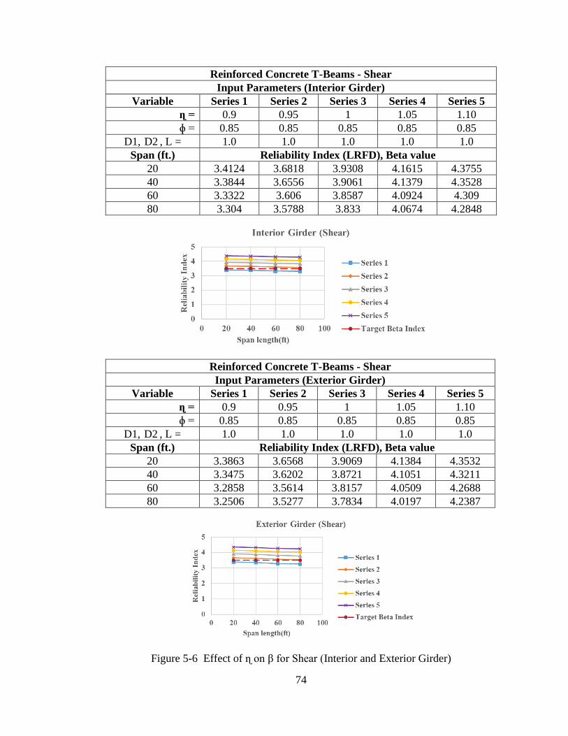
74
Reinforced Concrete T-Beams - Shear
Input Parameters (Interior Girder)
Variable Series 1 Series 2 Series 3 Series 4 Series 5
ɳ = 0.9 0.95 1 1.05 1.10
ɸ = 0.85 0.85 0.85 0.85 0.85
D1, D2 , L = 1.0 1.0 1.0 1.0 1.0
Span (ft.) Reliability Index (LRFD), Beta value
20 3.4124 3.6818 3.9308 4.1615 4.3755
40 3.3844 3.6556 3.9061 4.1379 4.3528
60 3.3322 3.606 3.8587 4.0924 4.309
80 3.304 3.5788 3.833 4.0674 4.2848
Reinforced Concrete T-Beams - Shear
Input Parameters (Exterior Girder)
Variable Series 1 Series 2 Series 3 Series 4 Series 5
ɳ = 0.9 0.95 1 1.05 1.10
ɸ = 0.85 0.85 0.85 0.85 0.85
D1, D2 , L = 1.0 1.0 1.0 1.0 1.0
Span (ft.) Reliability Index (LRFD), Beta value
20 3.3863 3.6568 3.9069 4.1384 4.3532
40 3.3475 3.6202 3.8721 4.1051 4.3211
60 3.2858 3.5614 3.8157 4.0509 4.2688
80 3.2506 3.5277 3.7834 4.0197 4.2387
Figure 5-6 Effect of ɳ on β for Shear (Interior and Exterior Girder)
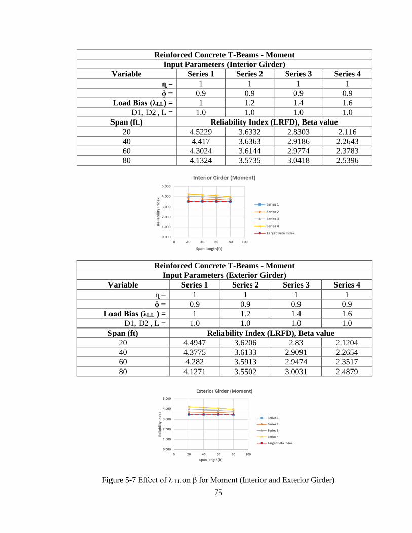
75
Reinforced Concrete T-Beams - Moment
Input Parameters (Interior Girder)
Variable Series 1 Series 2 Series 3 Series 4
ɳ = 1 1 1 1
ɸ = 0.9 0.9 0.9 0.9
Load Bias (λLL) = 1 1.2 1.4 1.6
D1, D2 , L = 1.0 1.0 1.0 1.0
Span (ft.) Reliability Index (LRFD), Beta value
20 4.5229 3.6332 2.8303 2.116
40 4.417 3.6363 2.9186 2.2643
60 4.3024 3.6144 2.9774 2.3783
80 4.1324 3.5735 3.0418 2.5396
Reinforced Concrete T-Beams - Moment
Input Parameters (Exterior Girder)
Variable Series 1 Series 2 Series 3 Series 4
ɳ = 1 1 1 1
ɸ = 0.9 0.9 0.9 0.9
Load Bias (λLL ) = 1 1.2 1.4 1.6
D1, D2 , L = 1.0 1.0 1.0 1.0
Span (ft) Reliability Index (LRFD), Beta value
20 4.4947 3.6206 2.83 2.1204
40 4.3775 3.6133 2.9091 2.2654
60 4.282 3.5913 2.9474 2.3517
80 4.1271 3.5502 3.0031 2.4879
Figure 5-7 Effect of λ LL on β for Moment (Interior and Exterior Girder)

76
Reinforced Concrete T-Beams - Shear
Input Parameters (Interior Girder)
Variable Series 1 Series 2 Series 3 Series 4
ɳ = 1 1 1 1
ɸ = 0.85 0.85 0.85 0.85
Load Bias (λLL) = 1 1.2 1.4 1.6
D1, D2 , L = 1.0 1.0 1.0 1.0
Span (ft) Reliability Index (LRFD), Beta value
20 4.3873 3.6931 3.0466 2.4498
40 4.3251 3.6869 3.0875 2.5289
60 4.2298 3.6637 3.1263 2.6199
80 4.1777 3.6508 3.148 2.6714
Reinforced Concrete T-Beams - Shear
Input Parameters (Exterior Girder)
Variable Series 1 Series 2 Series 3 Series 4
ɳ = 1 1 1 1
ɸ = 0.85 0.85 0.85 0.85
Load Bias (λLL) = 1 1.2 1.4 1.6
D1, D2 , L = 1.0 1.0 1.0 1.0
Span (ft) Reliability Index (LRFD), Beta value
20 4.3465 3.6776 3.0523 2.4727
40 4.2702 3.6635 3.0911 2.5552
60 4.1639 3.6323 3.1256 2.6456
80 4.1043 3.6139 3.1438 2.6958
Figure 5-8 Effect of λ LL on β for Shear (Interior and Exterior Girder)

77
Reinforced Concrete T-Beams - Moment
Input Parameters (Interior Girder)
Variable Series 1 Series 2 Series 3 Series 4
ɳ = 1 1 1 1
ɸ = 0.9 0.9 0.9 0.9
Live Load Scalar (L) = 0.95 1 1.05 1.1
D1, D2 = 1.0 1.0 1.0 1.0
Span (ft.) Reliability Index (LRFD), Beta value
20 3.481 3.740 3.985 4.217
40 3.500 3.731 3.949 4.158
60 3.492 3.698 3.895 4.083
80 3.470 3.642 3.808 3.967
Reinforced Concrete T-Beams -Moment
Input Parameters (Exterior Girder)
Variable Series 1 Series 2 Series 3 Series 4
ɳ = 1 1 1 1
ɸ = 0.9 0.9 0.9 0.9
Live Load Scalar (L) = 0.95 1 1.05 1.1
D1, D2 = 1.0 1.0 1.0 1.0
Span (ft.) Reliability Index (LRFD), Beta value
20 3.470 3.725 3.987 4.196
40 3.479 3.706 3.921 4.127
60 3.468 3.675 3.874 4.063
80 3.443 3.621 3.792 3.956
Figure 5-9 Effect of L Scalar on β for Moment (Interior and Exterior Girder)

78
Reinforced Concrete T-Beams - Shear
Input Parameters (Interior Girder)
Variable Series 1 Series 2 Series 3 Series 4
ɳ = 1 1 1 1
ɸ = 0.85 0.85 0.85 0.85
Live Load Scalar (L) = 0.95 1 1.05 1.1
D1, D2 = 1.0 1.0 1.0 1.0
Span (ft) Reliability Index (LRFD), Beta value
20 3.728 3.931 4.122 4.301
40 3.718 3.906 4.084 4.251
60 3.689 3.859 4.020 4.172
80 3.673 3.833 3.984 4.128
Reinforced Concrete T-Beams - Shear
Input Parameters (Exterior Girder)
Variable Series 1 Series 2 Series 3 Series 4
ɳ = 1 1 1 1
ɸ = 0.85 0.85 0.85 0.85
Live Load Scalar (L) = 0.95 1 1.05 1.1
D1, D2 = 1.0 1.0 1.0 1.0
Span (ft.) Reliability Index (LRFD), Beta value
20 3.710 3.907 4.092 4.266
40 3.692 3.872 4.043 4.204
60 3.655 3.816 3.969 4.115
80 3.633 3.783 3.927 4.064
Figure 5-10 Effect of L Scalar on β for Shear (Interior and Exterior Girder)

79
Reinforced Concrete T-Beams - Moment
Input Parameters (Interior Girder)
Variable Series 1 Series 2 Series 3 Series 4
ɳ = 1 1 1 1
ɸ = 0.9 0.9 0.9 0.9
Dead Load Scalar (D1) = 0.95 1 1.05 1.1
D2, L = 1.0 1.0 1.0 1.0
Span (ft.) Reliability Index (LRFD), Beta value
20 3.700 3.740 3.779 3.818
40 3.666 3.731 3.795 3.858
60 3.609 3.698 3.785 3.870
80 3.523 3.642 3.758 3.871
Reinforced Concrete T-Beams - Moment
Input Parameters (Exterior Girder)
Variable Series 1 Series 2 Series 3 Series 4
ɳ = 1 1 1 1
ɸ = 0.9 0.9 0.9 0.9
Dead Load Scalar (D1) = 0.95 1 1.05 1.1
D2, L = 1.0 1.0 1.0 1.0
Span (ft.) Reliability Index (LRFD), Beta value
20 3.678 3.725 3.772 3.818
40 3.631 3.706 3.779 3.850
60 3.581 3.675 3.767 3.857
80 3.498 3.621 3.740 3.856
Figure 5-11 Effect of D1 Scalar on β for Moment (Interior and Exterior Girder)

80
Reinforced Concrete T-Beams - Shear
Input Parameters (Interior Girder)
Variable Series 1 Series 2 Series 3 Series 4
ɳ = 1 1 1 1
ɸ = 0.85 0.85 0.85 0.85
Dead Load Scalar (D1) = 0.95 1 1.05 1.1
D2, L = 1.0 1.0 1.0 1.0
Span (ft) Reliability Index (LRFD), Beta value
20 3.897 3.931 3.964 3.998
40 3.860 3.906 3.952 3.997
60 3.794 3.859 3.922 3.983
80 3.7593 3.8326 3.9043 3.9743
Reinforced Concrete T-Beams - Shear
Input Parameters (Exterior Girder)
Variable Series 1 Series 2 Series 3 Series 4
ɳ = 1 1 1 1
ɸ = 0.85 0.85 0.85 0.85
Dead Load Scalar (D1) = 0.95 1 1.05 1.1
D2, L = 1.0 1.0 1.0 1.0
Span (ft.) Reliability Index (LRFD), Beta value
20 3.864 3.907 3.949 3.991
40 3.815 3.872 3.929 3.984
60 3.738 3.816 3.891 3.965
80 3.696 3.783 3.869 3.952
Figure 5-12 Effect of D1 Scalar on β for Shear (Interior and Exterior Girder)

81
Reinforced Concrete T-Beams - Moment
Input Parameters (Exterior Girder)
Variable Series 1 Series 2 Series 3 Series 4
ɳ = 1 1 1 1
ɸ = 0.9 0.9 0.9 0.9
Dead Load Scalar (D2) = 1.2 1.25 1.3 1.4
D1, L = 1.0 1.0 1.0 1.0
Span (ft.) Reliability Index (LRFD), Beta value
20 3.740 3.729 3.750 3.761
40 3.713 3.731 3.748 3.765
60 3.678 3.698 3.718 3.737
80 3.616 3.642 3.668 3.694
Reinforced Concrete T-Beams - Moment
Input Parameters (Interior Girder)
Variable Series 1 Series 2 Series 3 Series 4
ɳ = 1 1 1 1
ɸ = 0.9 0.9 0.9 0.9
Dead Load Scalar (D2) = 1.2 1.25 1.3 1.4
D1, L = 1.0 1.0 1.0 1.0
Span (ft.) Reliability Index (LRFD), Beta value
20 3.718 3.725 3.733 3.741
40 3.693 3.706 3.718 3.730
60 3.662 3.675 3.689 3.702
80 3.603 3.621 3.638 3.656
Figure 5-13 Effect of D2 Scalar on β for Moment (Interior and Exterior Girder)

82
Reinforced Concrete T-Beams - Shear
Input Parameters (Interior Girder)
Variable Series 1 Series 2 Series 3 Series 4
ɳ = 1 1 1 1
ɸ = 0.85 0.85 0.85 0.85
Dead Load Scalar (D2) = 1.2 1.25 1.3 1.4
D1, L = 1.0 1.0 1.0 1.0
Span (ft.) Reliability Index (LRFD), Beta value
20 3.922 3.931 3.940 3.949
40 3.894 3.906 3.918 3.930
60 3.844 3.859 3.873 3.887
80 3.816 3.833 3.849 3.865
Reinforced Concrete T-Beams - Shear
Input Parameters (Exterior Girder)
Variable Series 1 Series 2 Series 3 Series 4
ɳ = 1 1 1 1
ɸ = 0.85 0.85 0.85 0.85
Dead Load Scalar (D2) = 1.2 1.25 1.3 1.4
D1, L = 1.0 1.0 1.0 1.0
Span (ft.) Reliability Index (LRFD), Beta value
20 3.900 3.907 3.914 3.921
40 3.863 3.872 3.882 3.891
60 3.805 3.816 3.827 3.838
80 3.771 3.783 3.796 3.808
Figure 5-14 Effect of D2 Scalar on β for Shear (Interior and Exterior Girder)

83
Reinforced Concrete T-Beams - Moment
Input Parameters (Interior Girder)
Variable Series 1 Series 2 Series 3 Series 4
ɳ = 1 1 1 1
ɸ = 0.9 0.9 0.9 0.9
Resistance Bias (λ ) = 1 1.1 1.2 1.3
D1, D2 , L = 1.0 1.0 1.0 1.0
Span (ft.) Reliability Index (LRFD), Beta value
20 2.934 3.5227 4.0467 4.5143
40 2.912 3.5106 4.0412 4.5129
60 2.8693 3.4757 4.0116 4.487
80 2.8016 3.4168 3.9592 4.4392
Reinforced Concrete T-Beams - Moment
Input Parameters (Exterior Girder)
Variable Series 1 Series 2 Series 3 Series 4
ɳ = 1 1 1 1
ɸ = 0.9 0.9 0.9 0.9
Resistance Bias (λ ) = 1 1.1 1.2 1.3
D1, D2 , L = 1.0 1.0 1.0 1.0
Span (ft.) Reliability Index (LRFD), Beta value
20 2.9171 3.5078 4.0333 4.5019
40 2.8842 3.485 4.0173 4.4903
60 2.846 3.4527 3.9893 4.4654
80 2.7804 3.3956 3.9383 4.4187
Figure 5-15 Effect of λR on β for Moment (Interior and Exterior Girder)

84
Reinforced Concrete T-Beams - Shear
Input Parameters (Interior Girder)
Variable Series 1 Series 2 Series 3 Series 4
ɳ = 1 1 1 1
ɸ = 0.85 0.85 0.85 0.85
Resistance Bias (λ ) = 1 1.1 1.2 1.3
D1, D2 , L = 1.0 1.0 1.0 1.0
Span (ft.) Reliability Index (LRFD), Beta value
20 3.0179 3.5046 3.9308 4.3059
40 2.9866 3.4772 3.9601 4.283
60 2.9301 3.4259 3.8587 4.2386
80 2.8993 3.3978 3.8326 4.2142
Reinforced Concrete T-Beams - Shear
Input Parameters (Exterior Girder)
Variable Series 1 Series 2 Series 3 Series 4
ɳ = 1 1 1 1
ɸ = 0.85 0.85 0.85 0.85
Resistance Bias (λ ) = 1 1.1 1.2 1.3
D1, D2 , L = 1.0 1.0 1.0 1.0
Span (ft.) Reliability Index (LRFD), Beta value
20 2.9898 3.4789 3.9069 4.2833
40 2.9473 3.4409 3.8721 4.2509
60 2.881 3.3802 3.8127 4.1979
80 2.8434 3.3455 3.7834 4.1675
Figure 5-16 Effect of λR on β for Shear (Interior and Exterior Girder)

85
Similarly, various graphs are plotted to investigate the trend of reliability index with change
in span length, resistance factor, load modifier, live load bias, live load scalar, dead load
scalars (D1 and D2) and resistance bias separately. Figure 5‒17 to Figure 5‒32 shows the
trend; best fitted equation and R square values are shown in the individual graphs for
moment and shear effects. Investigations are done for interior girders of the T-beam Bridge.

86
Figure 5-17 Variation of Reliability Index with Span Length for Moment
Figure 5-18 Variation of Reliability Index with Resistance Factor for Given Span
Length
3.7393.731
3.698
3.642y = -3E-05x2 + 0.0014x + 3.7235
R² = 1
3.62
3.64
3.66
3.68
3.7
3.72
3.74
3.76
0 20 40 60 80 100
Re
liab
ility
In
de
x (β
)
Span Length (ft)
Span Length Vs Reliability Index (Moment)
Trend
Poly. (Trend)
4.8044.434
4.0763.731
3.3973.075
y = 2.4x2 - 11.115x + 11.79R² = 1
0
1
2
3
4
5
6
0.7 0.75 0.8 0.85 0.9 0.95 1 1.05
Re
liab
ilty
Ind
ex
(β)
Resistance Factor(ɸ)
Resistance Factor (ɸ) Vs Reliability Index (Moment)
40 ft.
Poly. (40 ft.)

87
Figure 5-19 Variation of Reliability Index with Load Modifier for Given Span Length
Figure 5-20 Variation of Reliability Index with Live Load Bias for Given Span Length
y = -4.18x2 + 14.497x - 6.5861R² = 1
0
1
2
3
4
5
0.8 0.85 0.9 0.95 1 1.05 1.1 1.15
Re
liab
ilty
Ind
ex
(β)
Load Modifier(ɳ)
Load Modifier (η) Vs Reliability Index (Moment)
40 ft.
Poly. (40 ft.)
y = 0.79x2 - 5.6419x + 9.2689R² = 1
0
1
2
3
4
5
0.9 1 1.1 1.2 1.3 1.4 1.5 1.6 1.7
Re
liab
ilty
Ind
ex
(β)
Live Load Bias (λLL)
Live Load Bias (λLL) Vs Reliability Index (Moment)
40 ft.
Poly. (40 ft.)

88
Figure 5-21 Variation of Reliability Index with Live Load Scalar (L) for Given Span
Length
Figure 5-22 Variation of Reliability Index with Dead Load Scalar (D1) for Given Span
Length
y = -2.18x2 + 8.8498x - 2.9394R² = 1
0
1
2
3
4
5
0.9 1 1.1 1.2
Re
liab
ilty
Ind
ex
(β)
Live Load Scalar (L)
Live Load Scalar (L) Vs Reliability Index (Moment)
40 ft.
Poly. (40 ft.)
y = -0.19x2 + 1.6689x + 2.2516R² = 1
0
1
2
3
4
5
0.9 1 1.1 1.2
Re
liab
ilty
Ind
ex
(β)
Dead Load Scalar (D1)
Dead Load Scalar (D1) Vs Reliability Index (Moment)
40 ft.
Poly. (40 ft.)

89
Figure 5-23 Variation of Reliability Index with Dead Load Scalar (D2) for Given Span
Length
Figure 5-24 Variation of Reliability Index with Resistance Bias for Given Span Length
y = -0.5564x2 + 1.6307x + 2.7379R² = 0.9983
0
1
2
3
4
5
1.1 1.15 1.2 1.25 1.3 1.35 1.4 1.45
Re
liab
ilty
Ind
ex
(β)
Dead Load Scalar (D2)
Dead Load Scalar (D2) Vs Reliability Index (Moment)
40 ft.
Poly. (40 ft.)
y = -3.1725x2 + 12.63x - 6.5451R² = 1
0
1
2
3
4
5
0.9 1 1.1 1.2 1.3 1.4
Re
liab
ilty
Ind
ex
(β)
Resistance Bias (λR )
Resistance Bias (λR ) Vs Reliability Index (Moment)
40 ft.
Poly. (40 ft.)

90
Figure 5-25 Variation of Reliability Index with Span Length for Shear
Figure 5-26 Variation of Reliability Index with Resistance Factor for Given Span
Length
3.931
3.906
3.859
3.833
y = 3.9683e-4E-04x
R² = 0.9843
3.82
3.84
3.86
3.88
3.9
3.92
3.94
0 20 40 60 80 100
Re
liab
ility
In
de
x (β
)
Span Length (ft)
Span Length Vs Reliability Index (Shear)
Trend
Expon. (Trend)
4.4884.193
3.9063.627
3.3553.09
y = 1.5x2 - 8.2153x + 9.8055R² = 1
0
1
2
3
4
5
0.7 0.75 0.8 0.85 0.9 0.95 1 1.05
Re
liab
ilty
Ind
ex
(β)
Resistance Factor(ɸ)
Resistance Factor (ɸ) Vs Reliability Index (Shear)
40 ft.
Poly. (40 ft.)

91
Figure 5-27 Variation of Reliability Index with Load Modifier for Given Span Length
Figure 5-28 Variation of Reliability Index with Live Load Bias for Given Span Length
y = -3.7514x2 + 12.341x - 4.6835R² = 1
0
1
2
3
4
5
0.8 0.85 0.9 0.95 1 1.05 1.1 1.15
Re
liab
ilty
Ind
ex
(β)
Load Modifier (ɳ)
Load Modifier (η) Vs Reliability Index (Shear)
40 ft.
Poly. (40 ft.)
y = 0.4975x2 - 4.2875x + 8.1152R² = 1
0
1
2
3
4
5
0.9 1 1.1 1.2 1.3 1.4 1.5 1.6 1.7
Re
liab
ilty
Ind
ex
(β)
Live Load Bias (λLL)
Live Load Bias (λLL) Vs Reliability Index (Shear)
40 ft.
Poly. (40 ft.)

92
Figure 5-29 Variation of Reliability Index with Live Load Scalar (L)
for Given Span Length
Figure 5-30 Variation of Reliability Index with Dead Load Scalar (D1)
for Given Span Length
y = -2.07x2 + 7.7989x - 1.8229R² = 1
0
1
2
3
4
5
0.9 1 1.1 1.2
Re
liab
ilty
Ind
ex
(β)
Live Load Factor (L)
Live Load Scalar (L) Vs Reliability Index (Shear)
40 ft.
Poly. (40 ft.)
y = -0.14x2 + 1.1982x + 2.8479R² = 1
3.000
4.000
5.000
0.9 1 1.1 1.2
Re
liab
ilty
Ind
ex
(β)
Dead Load Scalar (D1)
Dead Load Scalar (D1) Vs Reliability Index (Shear)
40 ft.
Poly. (40 ft.)

93
Figure 5-31 Variation of Reliability Index with Dead Load Scalar (D2)
for Given Span Length
Figure 5-32 Variation of Reliability Index with Resistance Bias
for Given Span Length
y = -0.7745x2 + 2.2728x + 2.1009R² = 0.9983
0
1
2
3
4
1.1 1.15 1.2 1.25 1.3 1.35 1.4 1.45
Re
liab
ilty
Ind
ex
(β)
Dead Load Scalar (D2)
Dead Load Scalar (D2) Vs Reliability Index (Shear)
40 ft.
Poly. (40 ft.)
y = -4.1925x2 + 14.015x - 6.8434R² = 0.9988
0
1
2
3
4
5
0.9 1 1.1 1.2 1.3 1.4
Re
liab
ilty
Ind
ex
(β)
Resistance Bias (λR )
Resistance Bias (λR) Vs Reliability Index (Shear)
40 ft.
Poly. (40 ft.)

94
Chapter 6
Conclusion and Recommendation
6.1 Conclusion
1. For reinforced T-beam continuous bridges having equal span length, interior girders
have larger shears and exterior girder have larger moments for the bridge with spans
of 20ft, 40ft, and 60ft.
But, for a reinforced T-beam continuous bridge with equal span of 80ft, both larger
moments and shears are observed in exterior girders.
2. For all the bridges that are studied, reliability index for bending moments is greater
than target reliability index i.e. 3.5 for resistance factor 0.9 and below. This signifies
the recommended resistance factor of 0.9 for bending moment in current AASTHO
LRFD Bridge Design Specification is reasonable.
3. Study shows reliability indices for shear are greater than target reliability index of
3.5 for resistance factor of 0.85 and below. Current AASTHO LRFD recommends
resistance factor of 0.85 for shear and this study validates it.
4. From the reliability analysis, it is observed that bending moment is governing over
shear.

95
5. Study of moment and shear envelopes showed that there is significant increase in
contributions of dead components over live load for bending and shear with the
increase in span length.
6. Results showed that reliability index decreases on increasing the resistance factor
for a bridge girder for both moment and shear. It is also observed that reliability
index decreases with increase in span length of a bridge.
7. With gradual increase in the load modifier from 0.9 to 1.10 there is increase in
reliability index for bending moment and shear, however reliability index decreases
with increase in span length. Results is similar for live load scalar.
8. There are no significant changes in reliability index for the increase in Dead load
scalar (D1 and D2) from 0.95 to 1.1.
9. With the increase in bias of resistance there is increase in reliability index for all
bridge girders for both moment and shear effects. However, reliability index
decreases with increase in live load bias.
6.2 Recommendation
1. Redundancy inherent in the structural system has very important role in
determining the target reliability index. Literature reviewed suggested that more the
redundancy of structure, more the allowable probability of failure and lower is the
desired reliability index. This study focuses on reliability analysis of structural
component i.e. girder only. Reliability analysis should be done for structural system
to understand the contribution of redundancy.
96
2. Reliability analysis is very important approach to access the margin of safety and
probability of failure associated with the structure that are designed using available
design codes. We can design the structure to reduce the probability of failure but
reducing the probability of failure beyond the optimum level is not always
economical. Parametric study illustrated the effects of change in statistical and
structural parameters to the reliability index. More study should be done to
determine the optimum load and resistance factors and corresponding safety level.

97
References
AASTHO LRFD Bridge Design Specification. (2014). 7th. Washigton, D.C.: American
Association of State Highway and Transportation Officials.
Akbari, J. (2018, June). Calibration of Load and Resistance Factors for Reinforced
Concrete Beams. Civil Engineering Infrastructures Journal. doi:DOI:
10.7508/ceij.2018.01.012
Allen, T. M., Nowak, A. S., & Bathurst, R. J. (2005, September). Calibration to
Determine Load and Resistance Factor for Geotechnical and Structural Design.
TRANSPORTATION RESEARCH CIRCULAR E-C079. Washington, D.C:
Transportation Research Board.
Arafah, A. M. (n.d.). Reliability of Reinforced Concrete Beam Section as Affected by
Their Reinforcement Ratio. 8th ASCE Specialty Conference on Probabilistic
Mechanics and Structrural Reliability .
Barker, R. M., & Puckett, J. A. (2013). Design of Highway Bridges (Third ed.). John
Wiley & Sons, Inc.
Biondini, F., Bontempi, F., Frangopol, D. M., & Malerba, P. G. (2004). Reliability of
Material and Geometrically Non-Linear Reinforced and Prestressed Concrete
Structures. Computers and Structures, 82(13), 1021-1031. doi:
10.1016/j.compstruc.2004.03.010
Ditlevsen, O. D. (1997). Structural Reliability Codes for Probabilistic Design - a Debate
Paper Based on Elementary Relaibility and Decision Analysis Concepts.
Structural Safety, 19(3), 253-270.
Ghosan, M., & Moses, F. (n.d.). Redundancy in Highway Bridge Superstructures.
Grubisic, M., Ivosevic, J., & Grubisic, A. (2019, May). Reliability Analysis of
Reinforced Concrete Frame by Finite Element Method with Implicit Limit State
Functions. Buildings, 9(5). doi:10.3390/buildings9050119
Kiureghian, A. D. (2008). Analysis of Structural Reliability Under Parameter
Uncertainties. Probabilistic Engineering Mechanics, 23(4), 351-358.
Kulicki, J. M., Prucz, Z., Clancy, C. M., Mertz, D. R., & Nowak, A. S. (2007). Updating
the Calibration Report for AASTHO LRFD Code.

98
Lin, K.-Y., & Frabgopol, D. M. (1996). Reliability-Based Optimum Design of
Reinforced Concrete Girders. Structural Safety, 239-258.
Mahmoud, A., Najjar, S., Mabsout, M., & Tarhini, K. (2017). Reliability Analysis of
Reinforced Concrete Slab Bridges. International Journal of GEOMATE, 13(36),
44-49.
Mertz, D. R. (1999). Loads & Reliability.
Njord, J. (n.d.). TRANSPORTATION RESEARCH BOARD 2005 EXECUTIVE
COMMITTEE OFFICERS Chair.
Nowak, A. S. (1995, August). Calibration of LRFD Bridge Code. Journal of Structural
Engineering. doi:10.1061/(ASCE)0733-9445(1995)121:8(1245)
Nowak, A. S. (1999). Calibration of LRFD Bridge Design Code. Transportation Research
Board. Washington, D.C: National Academy Press.
Nowak, A. S., & Collins, K. R. (2013). Reliability of Structures (Second ed.). CRC Press.
Nowak, A. S., & Latsko, O. (2017, May-June). Revised Load and Resistance Factors for
the AASTHO LRFD Bridge Design Specifications. PCI Journal.
Nowak, A. S., & Szerszen, M. (2000, March). Structural reliability as applied to highway
bridges. Progress in Structural Engineering and Materials 2.
Nowak, A., & Kaszynska, M. (n.d.). Target Reliability for New, Existing and Historical
Structures.
Rackwitz, R., & Flessler, B. (1978, November). Structural Reliability Under Combined
Random Load Sequences. Computers and Structures, 9(5), 489-494.
Tabsh, S. W. (1992, September-October). Reliability Based Parametric Study of
Pretensioned AASTHO Bridge Girder. PCI Journal.
Tabsh, S. W., & Nowak, A. S. (n.d.). Reliability of Highway Girder Bridges. Journal of
Structural Engineering. doi:DOI: 10.1061/(ASCE)0733-9445(1991)117:8(2372)
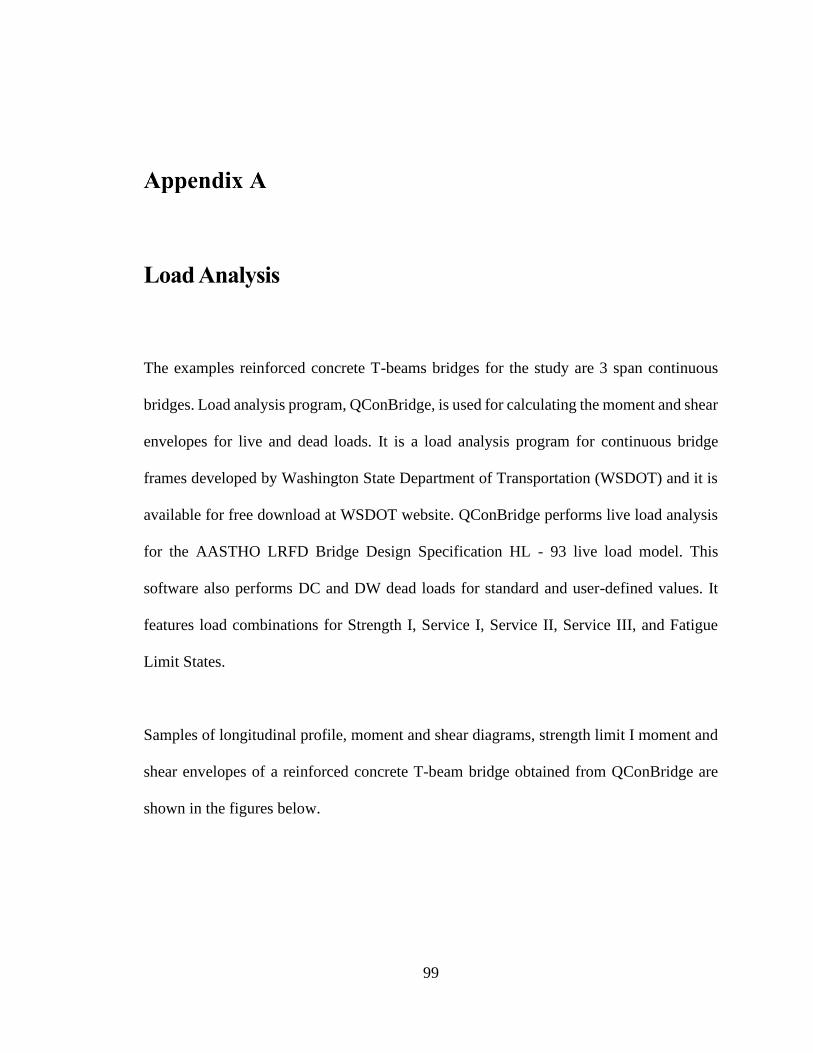
99
Load Analysis
The examples reinforced concrete T-beams bridges for the study are 3 span continuous
bridges. Load analysis program, QConBridge, is used for calculating the moment and shear
envelopes for live and dead loads. It is a load analysis program for continuous bridge
frames developed by Washington State Department of Transportation (WSDOT) and it is
available for free download at WSDOT website. QConBridge performs live load analysis
for the AASTHO LRFD Bridge Design Specification HL - 93 live load model. This
software also performs DC and DW dead loads for standard and user-defined values. It
features load combinations for Strength I, Service I, Service II, Service III, and Fatigue
Limit States.
Samples of longitudinal profile, moment and shear diagrams, strength limit I moment and
shear envelopes of a reinforced concrete T-beam bridge obtained from QConBridge are
shown in the figures below.
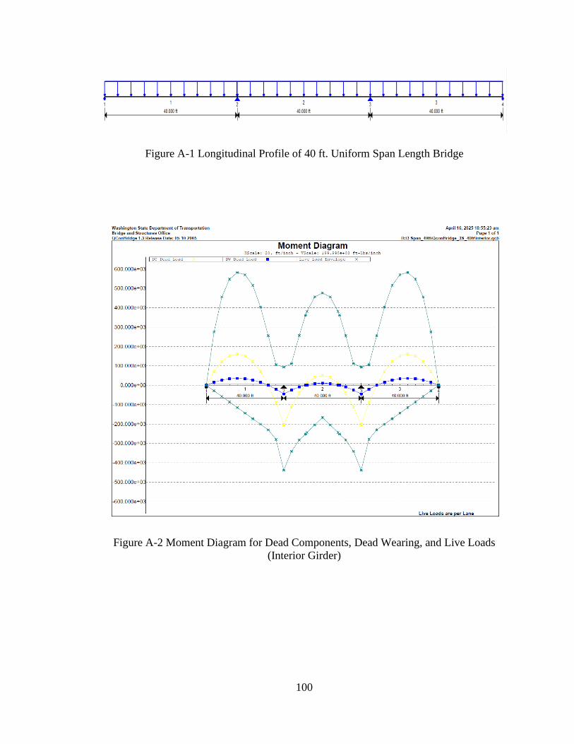
100
Figure A-1 Longitudinal Profile of 40 ft. Uniform Span Length Bridge
Figure A-2 Moment Diagram for Dead Components, Dead Wearing, and Live Loads
(Interior Girder)

101
Figure A-3 Shear Diagram for Dead Components, Dead Wearing, and Live Loads
(Interior Girder)
Figure A-4 Strength I Envelope for moment (Interior Girder)

102
Figure A-5 Strength I Envelope for Shear (Interior Girder)
During reliability analyses, design over-strength is neglected. For this, design limit states
other than strength limit strength such as service limit strength which is generally
governing geometric characterization of structural elements are not considered (Kulicki,
Prucz, Clancy, Mertz, & Nowak, 2007). Preliminary selection of girder section and
calculation of girder distribution factor necessary for calculation of dead and live loads are
done according to the procedure mentioned in Barker & Puckett (2013).
The Mathcad file for preliminary selection of section of girder and calculation of girder
distribution factor is attached in the next page.

103
LOAD CALCUALTION OF T-BEAM BRIDGE GIRDER:
• Three Span Bridge with uniform span length.
• Uniform spacing of girder.
• Skew angle of 30 .
• HL-93 Live Load.
• AASTHO (2012) LFRD Bridge Specifications.
• Design for Service Limit I and Strength Limit I.
Roadway width,
Length of each span of Bridge,
T-beam Girder spacing,
Compressive Strength of Concrete,
Yield Strength of Rebar,
Number of Beam,
Length of overhang,
Roadway part of overhang,
Angle of Skew,
Unit wt. of Concrete,
A] DEVELOP TYPICAL SECTION AND DESIGN BASIS:
1) Top Flange Thickness: [A5.14.1.5.1a]
Minimum depth of concrete deck = 7 in. [A9.7.1.1]
Assume thickness of slab,

104
2) Web Thickness: [A5.14.1.5.1c and C5.14.1.5.1c]
a) Minimum of 8 in. without prestressing ducts.
b) Minimum concrete cover for main bars, exterior 2.0 in. [A5.12.3]
c) Three No.11 bars in one row require a beam width of [A5.10.3.1.1]
Diameter of No. 11 bar,
Assume web thickness,
3) Structural Depth (including deck): [Table A2.5.2.6.3-1]
Minimum depth continuous spans,
Assume total depth,
B] CALCULATIONS OF LIVE LOAD FORCE EFFECTS:
I) DISTRIBUTION FACTOR CALCULATIONS:
(A) FOR INTERIOR GIRDER:
= K =1 {For Preliminary Design}
Girder spacing,
Span length,

105
Number of Design Lanes (NL): [A3.6.1.1.1]
Hence, the number of design lanes is,
Cross-section Type (e), [Table 4.6.2.2.1.1]
Girder spacing,
Thickness of slab,
Length of each span,
Number of beam
For Moments:
i) For one lane loaded:
ii) For two or more lane loaded:

106
Distribution of Live Loads for Moment in Interior Beams,
For Shear:
i) For one lane loaded:
ii) For two or more lane loaded:
Distribution of Live Loads for Shear in Interior Beams,
(B) FOR EXTERIOR GIRDER:
For Moment:
i) For one lane loaded: [Lever Rule]
Multiple presence factor,
Reaction in exterior Girder,
Distribution factor for single lane,

107
ii) For two or more lane loaded:
Distance of Curb to Resultant of Reaction at Exterior Girder,
Distribution factor for multiple lane,
Distribution of Live Loads for Moment in Exterior Beams,
For Shear:
i) For one lane loaded: [Lever Rule]
Multiple presence factor,
Reaction in exterior Girder,
Distribution factor for single lane,
ii) For two or more lane loaded:
Distance of Curb to Resultant of Reaction at Exterior Girder,

108
Distribution factor for multiple lane,
Distribution of Live Loads for Shear in Exterior Beams,
Skew Correction Factors Calculations: [A4.6.2.2.2e]
- used to adjust the computed distribution factors to address the effects of skewed
supports.
Angle of Skew:
For Bending Moment:
= K =1 {For Preliminary Design}
Reduction Factor,
For Shear:
= K =1 {For Preliminary Design}

109
Reduction Factor,
FINAL LIVE LOAD DISTRIBUTION FACTOR:
A] INTERIOR GIRDER:
i) Moment:
ii) Shear:
B] EXTERIOR GIRDER:
i) Moment:
ii) Shear:
II) DISTRIBUTED LIVE LOADS:
[QconBridge Software was used to develop the moment and shear envelopes due to Truck,
Tandem, and Lane Load. Only the maximum values from the resulting envelopes were
used for design purposes]
A] INTERIOR GIRDER:
a) Moment from live load with impact (maximum):
Undistributed positive moment,

110
Undistributed negative moment,
Distributed positive moment,
Distributed negative moment,
b) Shear from live load with impact :
Undistributed maximum shear,
Distributed maximum shear,
B] EXTERIOR GIRDER:
a) Moment from live load with impact (maximum):
Undistributed positive moment,
Undistributed negative moment,
Distributed positive moment,
Distributed negative moment,
b) Shear from live load with impact :
Undistributed maximum shear,
Distributed maximum shear,
C] FORCE EFFECTS FROM OTHER LOADS:
I) INTERIOR GIRDER:
(i) Calculations of DC1. per girder :
Unit wt. of Concrete,

111
Girder spacing,
Thickness of deck,
Weight of:
(ii) Wearing Surface load Calculations (DW):
Load Summary:
II) EXTERIOR GIRDER:
(i) Calculations of DC1. per girder:
Unit wt. of Concrete,

112
Girder spacing,
Thickness of deck,
Weight of:
Length of overhang,
Weight of Overhang,
Hence,
(ii) Calculations of DC2:
Weight of Barrier,
Hence,
(iii) Wearing Surface load Calculations (DW):
Unit weight of FWS,

113
Distance of center of exterior girder to the inner edge of the curb,
Load Summary:

114
Monte Carlo Method of Simulation Sample Spreadsheet
Sample spreadsheets to calculate the reliability index using Monte Carlo method are
given in the figures below. Reliability index was calculated for moments and shear
effects for interior and exterior girders.
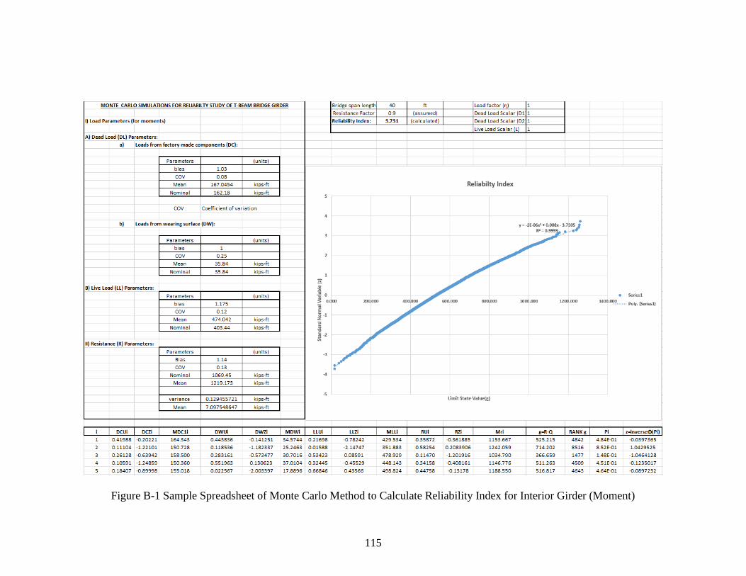
115
Figure B-1 Sample Spreadsheet of Monte Carlo Method to Calculate Reliability Index for Interior Girder (Moment)

116
Figure B-2 Sample Spreadsheet of Monte Carlo Method to Calculate Reliability Index for Exterior Girder (Moment)

117
Figure B-3 Sample Spreadsheet of Monte Carlo Method to Calculate Reliability Index for Interior Girder (Shear)

118
Figure B-4 Sample Spreadsheet of Monte Carlo Method to Calculate Reliability Index for Exterior Girder (Shear)