a survey of attitude error representations

A Survey Of Attitude Error Representations

Ahmad Bani Younes� James D. Turnery Daniele Mortariz

John L. Junkinsx

Texas A&M University, College Station, TX 77843-3141

Several attitude error representations are developed for describing the tracking orien-tation error kinematics. Compact forms of attitude error equation are derived for eachcase. The attitude error is initially de�ned as the quaternion (rotation) error betweenthe current and the estimated orientation. The nonlinear kinematic models are valid forarbitrarily large relative rotations and rotation rates. These modes have been developedfor supporting the development of nonlinear spacecraft maneuver formulations. All of thekinematic formulations assume that a reference state has been de�ned. These results areexpected to be broadly useful for generalizing extended Kalman �ltering formulations. Thebene�ts of paper are discussed.

I. Introduction

The diversity of attitude representations has been one of the important issues to be considered for scienceand engineering applications. Various attitude representations are available for use.5,6, 8, 9, 17 Selecting theappropriate representation is highly linked with the kind of the problem being considered. Euler parameters(quaternion) are a frequently used set of attitude variables, consisting of four components; non-singular,redundant coordinates to describe a rigid body orientation.15 Classical Rodrigues Parameters (CRP’s) isanother attitude representation that consists of three components; after eliminating the redundant com-ponent. The transformation from classical Rodridues Parameters to Quaternion, and vice-versa, is easilyperformed, similarly for CRP’s. The more recently developed Modi�ed Rodrigues Parameters representationis a vector-based, three-component, attitude description. More about these representations and other repre-sentations can be found in many references.5,6, 9, 12,15,17For applications requiring large and rapid rotationalmotions there exists a need for developing attitude error kinematic models that exactly describe arbitrarylarge rotational motions. The main contribution of this work is to develop exact large motion error kinematicand dynamic representations using quaternions, CRP’s and MRP’s.

Several attitude parameterizations are compared by solving a nonlinear spacecraft tracking problem.Several authors have considered feedback control strategies. Markley and Coppola12 have considered di�erentattitude error representations for estimating the state of a maneuvering spacecraft. They have clari�edthe relationship between the four-component quaternion representation of attitude and the MultiplicativeExtended Kalman Filter. Crassidis, Vadali, Markley, and Coppola4 investigated a variable-structure controlstrategy for maneuvering vehicles. In their work, they used a feedback linearizing technique and added anadditional term to the spacecraft maneuvers to deal with model uncertainties. The addition of the simple termin the control law always provides an optimal response. Ahmed, Coppola, and Bernstein1 extended previouswork to consider adaptive asymptotic tracking during maneuvers while estimating inertia properties. Theyused a Lyapunov argument to generate an unconditionally robust control law with respect to their assumedparametric uncertainty. Bani Younes, Turner, Majji, and Junkins18,19 considered generalized optimal control

�Graduate Research Assistant, 701 H.R. Bright Building, Aerospace Engineering, Texas A&M University, College Station,TX 77843-3141, and AIAA Member.yProfessor, 701 H.R. Bright Building, Aerospace Engineering, Texas A&M University, College Station, TX 77843-3141, and

AIAA Member.zProfessor, 701 H.R. Bright Building, Aerospace Engineering, Texas A&M University, College Station, TX 77843-3141, and

AIAA Member.xFellow AAS, Distinguished Professor, 701 H.R. Bright Building, Aerospace Engineering, Texas A&M University, College

Station, TX 77843-3141, and AIAA Member.

1 of 16

American Institute of Aeronautics and Astronautics

AIAA/AAS Astrodynamics Specialist Conference13 - 16 August 2012, Minneapolis, Minnesota

AIAA 2012-4422

Copyright © 2012 by Ahmad Bani Younes. Published by the American Institute of Aeronautics and Astronautics, Inc., with permission.

Dow

nloa

ded

by J

ames

Tur

ner

on M

arch

5, 2

014

| http

://ar

c.ai

aa.o

rg |

DO

I: 1

0.25

14/6

.201

2-44

22

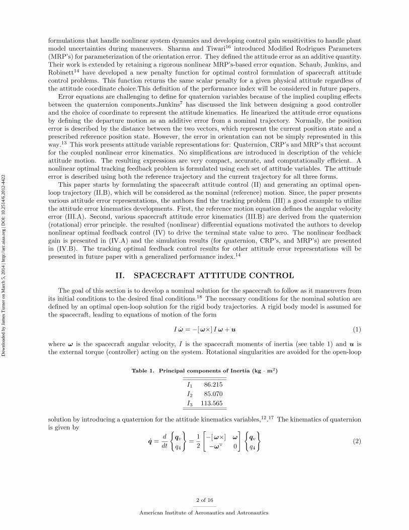
formulations that handle nonlinear system dynamics and developing control gain sensitivities to handle plantmodel uncertainties during maneuvers. Sharma and Tiwari16 introduced Modi�ed Rodrigues Parameters(MRP’s) for parameterization of the orientation error. They de�ned the attitude error as an additive quantity.Their work is extended by retaining a rigorous nonlinear MRP’s-based error equation. Schaub, Junkins, andRobinett14 have developed a new penalty function for optimal control formulation of spacecraft attitudecontrol problems. This function returns the same scalar penalty for a given physical attitude regardless ofthe attitude coordinate choice.This de�nition of the performance index will be considered in future papers.

Error equations are challenging to de�ne for quaternion variables because of the implied coupling e�ectsbetween the quaternion components.Junkins7 has discussed the link between designing a good controllerand the choice of coordinate to represent the attitude kinematics. He linearized the attitude error equationsby de�ning the departure motion as an additive error from a nominal trajectory. Normally, the positionerror is described by the distance between the two vectors, which represent the current position state and aprescribed reference position state. However, the error in orientation can not be simply represented in thisway.13 This work presents attitude variable representations for: Quaternion, CRP’s and MRP’s that accountfor the coupled nonlinear error kinematics. No simpli�cations are introduced in description of the vehicleattitude motion. The resulting expressions are very compact, accurate, and computationally e�cient. Anonlinear optimal tracking feedback problem is formulated using each set of attitude variables. The attitudeerror is described using both the reference trajectory and the current trajectory for all three forms.

This paper starts by formulating the spacecraft attitude control (II) and generating an optimal open-loop trajectory (II.B), which will be considered as the nominal (reference) motion. Since, the paper presentsvarious attitude error representations, the authors �nd the tracking problem (III) a good example to utilizethe attitude error kinematics developments. First, the reference motion equation de�nes the angular velocityerror (III.A). Second, various spacecraft attitude error kinematics (III.B) are derived from the quaternion(rotational) error principle. the resulted (nonlinear) di�erential equations motivated the authors to developnonlinear optimal feedback control (IV) to drive the terminal state value to zero. The nonlinear feedbackgain is presented in (IV.A) and the simulation results (for quaternion, CRP’s, and MRP’s) are presentedin (IV.B). The tracking optimal feedback control results for other attitude error representations will bepresented in future paper with a generalized performance index.14

II. SPACECRAFT ATTITUDE CONTROL

The goal of this section is to develop a nominal solution for the spacecraft to follow as it maneuvers fromits initial conditions to the desired �nal conditions.18 The necessary conditions for the nominal solution arede�ned by an optimal open-loop solution for the rigid body trajectories. A rigid body model is assumed forthe spacecraft, leading to equations of motion of the form

I _! = �[!�] I ! + u (1)

where ! is the spacecraft angular velocity, I is the spacecraft moments of inertia (see table 1) and u isthe external torque (controller) acting on the system. Rotational singularities are avoided for the open-loop

Table 1. Principal components of Inertia (kg � m2)

I1 86.215

I2 85.070

I3 113.565

solution by introducing a quaternion for the attitude kinematics variables,12.17 The kinematics of quaternionis given by

_q =d

dt

(qv

q4

)=

1

2

"�[!�] !

�!T 0

# (qv

q4

)(2)

2 of 16


Dow

nloa

ded

by J

ames

Tur

ner

on M

arch

5, 2

014

| http

://ar

c.ai

aa.o

rg |

DO

I: 1

0.25

14/6

.201

2-44

22

where qv = e sin

��

2

�, q4 = cos

��

2

�, � denotes the principal angle, e denotes the unit vector, and [ e�] =264 0 �e3 e2

e3 0 �e1�e2 e1 0

375 is the cross product matrix operator. These nonlinear equations are used for developing

rigorous error kinematic and dynamic models that are suitable for optimal control solution strategies. Thequaternion variables are useful for large motions, but the norm constraint complicates the feedback controlapproach.

A. Classical/Modi�ed Rodrigues Parameter Kinematic Formulation

The quaternion equations of Eq. (2) is useful for de�ning the open-loop reference solution, but the feedbacklaw is plagued by having to deal with the norm constraint. This problem is overcome by shifting to analternative attitude representation. This problem is remedied, motivated by the developments of Sharmaand Tiwari,16 by introducing Modi�ed Rodrigues Parameters (MRP’s) for parametrization of the orientationerror. Both Modi�ed Rodrigues Parameters (CRP’s) and MRP’s have the desired property of having zerovalues for the terminal boundary conditions. The work of Sharma and Tiwari is generalized in this paperby retaining a rigorous nonlinear CRP- and MRP-based error equation. As a result, our feedback statevariables are nonlinear in both the kinematic and dynamic variables, which motivate our exploration of 2nd

order tensor control feedback terms for suppressing the nonlinear behavior of the system. The singularity-freequaternion-based open-loop solution is transformed in terms of Modi�ed Rodrigues Parameters for generatingthe reference kinematic state for the feedback control problem formulation.

B. Optimal Control Problem: Open-Loop Solution

The open-loop reference trajectory is obtained by minimizing the following optimal control performanceindex:10

J =1

2

Z tf

t0

(xTQx+ uTRu) dt: (3)

subject to the nonlinear state equation_x = f(x) +B u (4)

where f(x) is a vector function containing the nonlinear terms. Let the state variables be the spacecraftangular velocity and the quaternion parameters q; yielding, the seven-element state vector x = f!T; qTgT.The Hamiltonian H for this system of equations is2,3, 10

H =1

2(xTQx+ uTRu) + �T _x (5)

Invoking the standard necessary condition for optimality (i.e., _� =@H

@x), after some algebraic manipulation,

results in the following Co-state di�erential equations:

_�1 = �q1jxj ��2K2x3 + �3K3x2 +

1

2(�4x7 + �5x6 � �6x5 + �7x4)

�_�2 = �q2jxj �

��1K1x3 + �3K3x1 �

1

2(�4x6 � �5x7 � �6x4 � �7x5)

�_�3 = �q3jxj �

��1K1x2 + �2K2x1 +

1

2(�4x5 � �5x4 + �6x4 + �7x6)

�_�4 = �q4jxj +

1

2(�5x3 � �6x2 � �7x1)

_�5 = �q5jxj �1

2(�4x3 � �6x1 + �7x2)

_�6 = �q6jxj +1

2(�4x2 � �5x1 � �7x3)

_�7 = �q7jxj �1

2(�4x1 + �5x2 + �6x3)

(6)

3 of 16


Dow

nloa

ded

by J

ames

Tur

ner

on M

arch

5, 2

014

| http

://ar

c.ai

aa.o

rg |

DO

I: 1

0.25

14/6

.201

2-44

22

where K1 = (I2 � I3)=I1, K2 = (I3 � I1)=I2, and K3 = (I1 � I2)=I3. The optimal control is given by the�rst-order necessary conditions for an extremum, Hu = 0leading to u = �R�1BT�.

A �xed-time and �xed �nal-state open-loop optimal control solution is obtained for maneuvering non-linear spacecraft. The initial and �nal state variable conditions for this example are given in Table 2. Forsimplicity the weighting matrix Q and R are chosen to be identity matrices. However, one can sweep thosepenalties to obtain di�erent solutions sets. The numerical solution is obtained using a shooting method(MATLAB fsolve) to solve the boundary value problem (BVP) in the Co-state equation.11

time (s) quaternion q angular velocity ! (rad/s)

0

p2

2f1; 0; 0; 1gT f0:1; 0:2; 0:3]T

50 f0; 0; 0; 1gT f0; 0; 0gT

Table 2. Initial/Boundary Conditions.

Figure 1. Open-Loop Solution

Figure 1 presents the open-loop solution for the nonlinear optimal control problem. Solution historiesare provided for of the spacecraft angular velocities, quaternion, MRP’s and the open-loop control. Thefull model derivation is given in the following section. One can easily see that the MRP’s have the verydesirable property that all of its components are identically zero at the �nal time, whereas the quaternion �naltime values clearly do not vanish. The open-loop optimal solution achieves the initial and �nal boundaryconditions. The quaternion norm constraint is preserved throughout the maneuver. The quaternion andangular velocity solutions de�ne the nominal trajectories for the maneuver.

III. Tracking Problem

The goal is to force the system response to follow a pre-de�ned solution path, where the maneuver timeis �xed.10 An exact nonlinear error kinematics and dynamics model is developed for spacecraft trackingmaneuvers. The new nonlinear error dynamics models are shown to lead to 2nd and 3rd order models. Threefeedback control approaches are considered where the spacecraft attitude motion is described by quaternion,

4 of 16


Dow

nloa

ded

by J

ames

Tur

ner

on M

arch

5, 2

014

| http

://ar

c.ai

aa.o

rg |

DO

I: 1

0.25

14/6

.201

2-44

22

CRP’s, MRP’s, Euler angles, principal axis and principal angle, direction cosine matrix, and Cayley-Klein.

A. Reference motion equation

Nonlinear tracking system dynamics models are developed in terms of the angular velocity error �!. Thedesired motion is de�ned in terms of the open-loop reference angular velocity19 !,

I _! = �[!�] I ! + � (assume � = 0) (7)

which is used for the open-loop solution. A nonlinear tracking error dynamics equation is derived by de�ningthe angular velocity error:19

�! = ! � ! (8)

and

� _! = �I�1f[!�]I � [(I!)�]g�! � I�1[(�!)�]I�!+

+I�1u� _! � I�1[!�]I!(9)

B. Spacecraft Attitude Error

The attitude error is originally represented in underlying quaternion error kinematics equations. Then di�er-ent attitude error equations are developed using kinematic identities to formulate the nonlinear kinematicsmodel. These developments are numerically veri�ed to the machine error.

1. Quaternion Error Kinematics

The kinematic solution for the reference trajectory quaternion de�nes the desired rotational motion for thespacecraft. The quaternion rotational error is de�ned as18,19

�q = q q�1 (10)

where q�1 is quaternion inverse of the reference quaternion rotation and represents the quaternion product.Note that the error, �q, is a quaternion, that is, a unit-vector. The quaternion rotational error rate isrepresented as,

� _q = _q q�1 + q _q�1 (11)

The quaternion kinematics evolve in time according to the di�erential equation

_q =1

2

(!

0

) q =

1

2

"�[!�] !

�!T 0

#q =

1

2(!)q (12)

performing the derivative of the identity q q�1 = f0; 0; 0; 1gT, that is, _q q�1 + q _q�1 = 0, we obtainthat the inverse quaternion evolves as

_q�1 = �1

2q�1

(!

0

)= �1

2�(!)q�1 (13)

Substituting Eq. (12) and Eq. (13) that into Eq. (11), yields

� _q =1

2(!)�q � 1

2q q�1

(!

0

)=

1

2(!)�q � 1

2�q

(!

0

)(14)

and we can write

�q

(!

0

)=

"[!�] !

�!T 0

#�q = �(!)�q (15)

where �(!) is the reference angular velocity matrix. The quaternion error rate equation becomes

� _q =1

2[(!)� �(!)]�q (16)

5 of 16


Dow

nloa

ded

by J

ames

Tur

ner

on M

arch

5, 2

014

| http

://ar

c.ai

aa.o

rg |

DO

I: 1

0.25

14/6

.201

2-44

22

by substituting the angular velocity error Eq. (8) into Eq. (16), one obtains the bilinear di�erential equationfor the tracking error kinematics

� _q =1

2[(�! + !)� �(!)]�q =

1

2[(�!)� ��(!)]�q (17)

where �� is a matrix de�ned as

��(!) = (!)� �(!) =

"�2[!�] 0

0T 0

#(18)

The quaternion error is a four-dimensional vector, de�ned as

�q =

(�qv

�q4

)(19)

with �qv = f�q1; �q2; �q3gT = e sin

��

2

�and �q4 = cos

��

2

�, and where e is the principal (Euler) axis and

� is the principal (Euler) angle. Eq. (17) can be rewritten in the following compact form

� _q =1

2

"�([�!�] + 2[!�]) �!

��!T 0

#(�qv

�q4

)(20)

This can be split into the scalar and vector part of the quaternion as follows8><>:� _qv =

1

2f� ([�!�] + 2[!�]) �qv + �q4�!g

� _q4 = �1

2�!T�qv

(21)

2. Classical Rodrigues Parameter Error Kinematics

Classical Rodrigues Parameters (CRP) are a minimum attitude parametrization. CRP vector is de�ned interms of quaternion parameters as,15

� =qvq4

= e tan

��

2

�(22)

where the inverse transformation is given by (�2 = �T�)

q4 =1p

1 + �2and qv =

�p1 + �2

: (23)

Note that the attitude error given in Eq. (21) is represented in quaternion. Since we have used full non-linear model in quaternion, with no approximation, the quaternion unit constraint is always preserved. Thisimplies that the quaternion (attitude) error still represents a �nite orientation that can be mapped to anyother attitude representations. Here, we will map the quaternion (attitude) error to Classical RodriguesParameters (CRP’s) using Eq. (22). Thus, CRP error vector is expressed as

�� =�qv�q4

(24)

and the inverse mapping for quaternion variables follow as (��2 = ��T��)

�q4 =1p

1 + ��2and �qv =

��p1 + ��2

: (25)

A governing di�erential equation for the CRP’s error follows on taking the time derivative of Eq. (24)

� _� =� _qv�q4� � _q4�qv

(�q4)2 (26)

6 of 16


Dow

nloa

ded

by J

ames

Tur

ner

on M

arch

5, 2

014

| http

://ar

c.ai

aa.o

rg |

DO

I: 1

0.25

14/6

.201

2-44

22

substituting Eq. (21) and Eq. (25) into Eq. (26), yielding

� _� =

�([�!�] + 2[!�])��p1 + ��2

+�!p

1 + ��2

21p

1 + ��2

+

�!T��p1 + ��2

��p1 + ��2

21

1 + ��2

The equation can be simpli�ed to the compact (nonlinear, third-order) form

� _� =1

2[� ([�!�] + 2[!�]) ��+ �!] +

1

2(�!T��) �� (27)

Equation (27) provides the desired nonlinear kinematic di�erential equations for the vehicle rotational mo-tion.

3. Modi�ed Rodrigues Parameter Error Kinematics

Modi�ed Rodrigues Parameters (MRP’s) are an elegant addition to the family of attitude parameters. MRP’svector is de�ned in terms of the quaternion parameters as the transformation,15

� =qv

1 + q4= e tan

��

4

�(28)

the inverse transformation is given by

q4 =1� �2

1 + �2and qv =

2�

1 + �2: (29)

Similarly, since the attitude error in Eq. (21) is still quaternion, we can perform the mapping into Modi�edRodrigues Parameters (MRP’s) using Eq. (28). Thus, MRP’s error vector is expressed as

�� =�qv

1 + �q4(30)

and the inverse mapping for quaternion variables follow as,

�q4 =1� ��2

1 + ��2and �qv =

2��

1 + ��2(31)

A governing di�erential equation for the MRP’s error follows on taking the time derivative of Eq. (30)

� _� =� _qv

1 + �q4� � _q4�qv

(1 + �q4)2(32)

substituting Eq. (21) and Eq. (31) into Eq. (32), yields

� _� =

1

2

��([�!�] + 2[!�])2��

1 + ��2+

1� ��2

1 + ��2�!

�1 +

1� ��2

1 + ��2

+

2�!T��

1 + ��2

2��

1 + ��2

2

�1 +

1� ��2

1 + ��2

�2

This equation can be clearly simpli�ed to the compact (nonlinear, third-order) form

� _� =1

4

��2 ([�!�] + 2[!�]) �� + (1� ��2)�!

�+

1

2(�!T��) �� (33)

Equation (33) provides the desired nonlinear kinematic di�erential equations for the vehicle rotational mo-tion.

7 of 16


Dow

nloa

ded

by J

ames

Tur

ner

on M

arch

5, 2

014

| http

://ar

c.ai

aa.o

rg |

DO

I: 1

0.25

14/6

.201

2-44

22

4. Euler Angles Kinematics

The three angles (��1; ��2; ��3) giving the three rotation matrices are called Euler angles. There are severalconventions for Euler angles, depending on the axes about which the rotations are carried out. In general,the rotation follows an arbitrary sequence (roll-pitch-yaw, yaw-roll-yaw,...). In the following derivation,we assume the rotation is performed following (roll-pitch-yaw or 123) sequence and (yaw-roll-yaw or 313)sequence. We start from the mapping equations from quaternion to Euler angles.9 For the (3-1-3) set, thetransformation is given by

"�qv

�q4

#=

26664sin( ��22 ) cos( ��1��32 )

sin( ��22 ) sin( ��1��32 )

cos( ��22 ) sin( ��1+��32 )

cos( ��22 ) cos( ��1+��32 )

37775313

= �313(��1; ��2; ��3) (34)

by di�erentiating Eq. (34) "� _qv

� _q4

#= H313(��1; ��2; ��3)

264� _�1

� _�2

� _�3

375313

(35)

where H313(��1; ��2; ��3) is a (4� 3) matrix. Thus, Euler angles rates can be written in the following leastsquare solution 264� _�1

� _�2

� _�3

375313

= (HT313H313)�1HT

313

"� _qv

� _q4

#(36)

substituting Eq. (20) and making use of Eq. (34)264� _�1

� _�2

� _�3

375313

=1

2(HT

313H313)�1HT313

"�([�!�] + 2[!�]) �!

��!T 0

#�313(��1; ��2; ��3) (37)

Similarly, for the (1-2-3) set, the transformation is given by

"�qv

�q4

#=

26664sin( ��12 ) cos( ��22 ) cos( ��32 ) + cos( ��12 ) sin( ��22 ) sin( ��32 )

cos( ��12 ) sin( ��22 ) cos( ��32 )� sin( ��12 ) cos( ��22 ) sin( ��32 )

cos( ��12 ) cos( ��22 ) sin( ��32 ) + sin( ��12 ) sin( ��22 ) cos( ��32 )

cos( ��12 ) cos( ��22 ) cos( ��32 )� sin( ��12 ) sin( ��22 ) sin( ��32 )

37775123

= �123(��1; ��2; ��3) (38)

by di�erentiating Eq. (38) "� _qv

� _q4

#= H123(��1; ��2; ��3)

264� _�1

� _�2

� _�3

375123

(39)

where H123(��1; ��2; ��3) is a (4� 3) matrix. Thus, Euler angles rates can be written in the following leastsquare solution 264� _�1

� _�2

� _�3

375123

= (HT123H123)�1HT

123

"� _qv

� _q4

#(40)

substituting Eq. (20) and making use of Eq. (38)264� _�1

� _�2

� _�3

375123

=1

2(HT

123H123)�1HT123

"�([�!�] + 2[!�]) �!

��!T 0

#�123(��1; ��2; ��3) (41)

Other rotation sequences can also be easily derived in the same manner.

8 of 16


Dow

nloa

ded

by J

ames

Tur

ner

on M

arch

5, 2

014

| http

://ar

c.ai

aa.o

rg |

DO

I: 1

0.25

14/6

.201

2-44

22

5. Principal Axis and Angle Kinematics

A simple rotation can be de�ned to be about an axis (e) by an angle (�). To derive the kinematics of theprincipal axis/angle for attitude error, we start from the de�nition of the quaternion

�q4 = cos(��=2) and �qv = �e sin(��=2) (42)

taking the time derivative and solving for � _� and (� _e)

� _� = � 2 � _q4sin(��=2)

and � _e =� _qv � 1

2�e�_� cos(��=2)

sin(��=2)(43)

substituting Eq. (21) and making use of �qv = �e sin (��=2) (where �e = �ep�eT �e

)

� _� = �!T �e (44)

and

� _e = �1

2

�([�!�] + 2[!�]) �e +

��!T �e

��e� �!

�cot(��=2)

�(45)

6. Direction Cosine Matrix Kinematics

The direction cosine matrix error can be written as

�C = C C T (46)

performing the derivative we obtain

� _C = _C C T + C_C T (47)

The DCM kinematics evolves in time according to the di�erential equation

_C = �[!�]C (48)

performing the derivative of the identity matrix C C T = I3�3, that is,_C C T + C

_C T = 03�3, we obtain that

the inverse DCM evolves as_C T = �C T _

C C T (49)

substituting in Eq. (47) we obtain

� _C = _C C T � C C T _C C T = �[!�]C C T � �C _

C C T =

= �[!�] �C � �C _C C T = �[!�] �C + �C [!�] C C T =

= �[(�! + !)�]�C + �C[!�]

and, �nally, we obtain

� _C = �[�!�]�C � [!�]�C + �C[!�] (50)

7. Cayley-Klein Parameters

Cayley-Klein parameters are derived from quaternion

�K = �q4I + i (�q1�1 + �q2�2 + �q3�3) (51)

�K =

"�q4 + i�q3 �q2 + i�q1

��q2 + i�q1 �q4 � i�q3

#(52)

where �1 =

"0 1

1 0

#, �2 =

"0 i

�i 0

#, and �3 =

"1 0

0 �1

#. The principal angle can be computed from

�� = 2 arccos

�1

2tr (�K)

�(53)

9 of 16


Dow

nloa

ded

by J

ames

Tur

ner

on M

arch

5, 2

014

| http

://ar

c.ai

aa.o

rg |

DO

I: 1

0.25

14/6

.201

2-44

22

by rewriting Eq. (52) in a vector form

vec(�K) =

26664�K1;1

�K2;1

�K1;2

�K2;2

37775 =

26664�q4 + i�q3

��q2 + i�q1

�q2 + i�q1

�q4 � i�q3

37775 (54)

note Eq. (54) can also be written (in another linear form)

vec(�K) =

26664�K1;1

�K2;1

�K1;2

�K2;2

37775 =

266640 0 i 1

i �1 0 0

i 1 0 0

0 0 �i 1

37775"�qv

�q4

#= 0�q (55)

where 0 =

266640 0 i 1

i �1 0 0

i 1 0 0

0 0 �i 1

37775 is a constant and an invertible matrix. By time di�erentiating Eq. (55) yields

vec(� _K) = 0� _q (56)

substituting Eq. (20) into Eq. (56)

vec(� _K) =1

20

"�([�!�] + 2[!�]) �!

��!T 0

#(�qv

�q4

)(57)

using Eq. (55) to solve for �q and substituting it in Eq. (57)

vec(� _K) =1

20

"�([�!�] + 2[!�]) �!

��!T 0

#�10 vec(�K) (58)

where the vec(�K) has to satisfy the constraint equation �qT �q = 1 = vec(�K)T�T0 �10 vec(�K) orvec(�K)T vec(�K) = 2

IV. Optimal Tracking Control Formulation

An error tracking dynamics state vector is de�ned by combining error dynamics and attitude equations,

_xi = aij1xj1 + cijklxjxkxl + timnxmxn + di + bij2uj2 (59)

where the state variables are the spacecraft angular velocity error and the spacecraft attitude error. Notethat the state coe�cients depend on the attitude error representation; for instance cijkl = 0 when attitudeerror is described using the quaternion error.

A �nite-time optimal control problem is designed by minimizing the following performance index:

J =1

2�(tf ;x(tf )) +

1

2

Z tf

t0

fxTQx+ uTRug dt =

=1

2�(tf ;x(tf )) +

1

2

Z tf

t0

fqj3j4xj3xj4 + rj5j6uj5uj6g dt (60)

subject to the state equation given in Eq. (59), where �(tf ;x(tf )) is a soft terminal constraint that is afunction of the �nal time tf and the �nal state xf . The Hamiltonian for this system of equations is

H =1

2(qj3j4xj3xj4 + rj5j6uj5uj6) + �i1(ai1j1xj1 + ci1jklxjxkxl + ti1mnxmxn + di1 + bi1j2uj2)

10 of 16


Dow

nloa

ded

by J

ames

Tur

ner

on M

arch

5, 2

014

| http

://ar

c.ai

aa.o

rg |

DO

I: 1

0.25

14/6

.201

2-44

22

The necessary condition for optimality yields: (1) the Co-state equations _� = �@H@x

, and (2) the optimal

control@H

@u= 0. The Co-state di�erential follows as:

_�i =� @H

@x= �1

2(qj3j4xj3�ij4 + qj3j4xj4�ij3)+

� �i1 [ai1j1�ij1 + ci1jkl(xjxk�il + xjxl�ik + xkxl�ij) + ti1mn(xm�in + xn�im)]

or_�i = �qij4xj4�i1(ai1i + ci1jkixjxk + ci1jilxjxl + ci1iklxkxl + ti1mixm + ti1inxn) (61)

and the control follows as

@H

@u= 0 =

1

2frj5j6uj5�i3j6 + rj5j6uj6�i3j5g+ �i2bi2j7�i3j7

oruj6 = �r�1i3j6bi2i3�i2 (62)

where r�1i3j6 denotes the i3j6-th element in the inverse of the matrix R (with elements de�ned by ri3j6).

A. Nonlinear Feedback Gain

Since the tracking state equation turns to be highly nonlinear, the choice of the feedback control becomesnon trivial. By observing the state equation, we can break it in three categories: 1) Linear term, 2) nonlinear(polynomial) term, and 3) the disturbance term. To solve the feedback problem, an appropriate Co-statestructure is assumed, which leads to tensor-based gain equations that de�ne the time history for the feedbackcontrol solution. Three di�erent forms of the feedback control are assumed,2,3,18:19

� A classical linear feedback gain: which is governed by a matrix Riccati equation.

� A disturbance rejection term: Since the tracking state equation is perturbed with a disturbance,resulting from the reference open-loop torque, a disturbance rejection tracking term is introduced thatprovides explicit links to the reference motion torque.

� A quadratic term: The quadratic feedback gain strategy seeks to suppress second- and third-ordererror terms in the tracking error dynamics equations.

Because the gain equations lead to 3rd order tensor equations, it is more natural to develop the governingequations by invoking the use of Eistein’s summation notation, leading to a Co-state equations of the form

�i4 = si4j9j10xj9xj10 + ki4j8xj8 + pi4 (63)

where si4j9j10 , ki4j8 and pi4 are the control gains sought. By substituting Eq. (63) into the Co-state equationEq. (61) and Eq. (62) and carrying out the ensuing algebra, we are led to the following equations

_�i =� qij4xj4 � ki1j8ai1ixj8 � ki1j8ci1jkixjxkxj8 � ki1j8ci1jilxjxlxj8� ki1j8ci1iklxkxlxj8 � ki1j8ti1mixmxj8 � ki1j8ti1inxnxj8� si1j9j10ai1ixj9xj10 � si1j9j10ci1jkixjxkxj9xj10 (64)

� si1j9j10ci1jilxjxlxj9xj10 � si1j9j10ci1iklxkxlxj9xj10� si1j9j10ti1mixmxj9xj10 � si1j9j10ti1inxnxj9xj10 � pi1ai1i� pi1ci1jkixjxk � pi1ci1iklxkxl � pi1ti1mixm � pi1ti1inxn

and

uj6 =� r�1i3j6bi2i3fsi2j9j10xj9xj10 + ki2j8xj8 + pi2g =

=� r�1i3j6bi2i3si2j9j10xj9xj10 � r�1i3j6

bi2i3ki2j8xj8 � r�1i3j6bi2i3pi2or (65)

=� r�1i5j6bi6i5si6j31j32xj31xj32 � r�1i5j6

bi6i5ki6j30xj30 � r�1i5j6bi6i5pi6

11 of 16


Dow

nloa

ded

by J

ames

Tur

ner

on M

arch

5, 2

014

| http

://ar

c.ai

aa.o

rg |

DO

I: 1

0.25

14/6

.201

2-44

22

by time-di�erentiating Eq. (63) and plugging the state equation Eq. (59) in it, the Co-state equationbecomes

_�i4 = _ki4j8xj8 + ki4j8aj8j1xj1 + ki4j8cj8jklxjxkxl + ki4j8tj8mnxmxn

+ ki4j8dj8 + ki4j8bj8j2uj2 + _si4j9j10xj9xj10 + si4j9j10aj9j1xj10xj1

+ cj9jklsi4j9j10xj10xjxkxl + tj9mnsi4j9j10xj10xmxn + si4j9j10dj9xj10 (66)

+ si4j9j10bj9j2uj2xj10 + si4j9j10aj10j1xj9xj1 + cj10jklsi4j9j10xj9xjxkxl

+ tj10mnsi4j9j10xj9xmxn + si4j9j10dj10xj9 + si4j9j10bj10j2uj2xj9 + _pi4

also substituting Eq. (64) and Eq. (65) into the Co-state equation Eq. (66) and simplifying,

qi4j4xj4 + ki1j8ai1i4xj8 + ki1j8ci1jki4xjxkxj8 + ki1j8ci1ji4lxjxlxj8 + ki1j8ci1i4klxkxlxj8

+ ki1j8ti1mi4xmxj8 + ki1j8ti1i4nxnxj8 + si1j9j10ai1i4xj9xj10 + si1j9j10ci1jki4xjxkxj9xj10

+ si1j9j10ci1ji4lxjxlxj9xj10 + si1j9j10ci1i4klxkxlxj9xj10 + si1j9j10ti1mi4xmxj9xj10

� si1j9j10ti1i4nxnxj9xj10 + pi1ai1i4 + pi1ci1jki4xjxk + pi1ci1i4klxkxl + pi1ti1mi4xm + pi1ti1i4nxn

+ _ki4j8xj8 + ki4j8aj8j1xj1 + ki4j8cj8jklxjxkxl + ki4j8tj8mnxmxn + ki4j8dj8

� ki4j8bj8j2r�1i5j2bi6i5si6j31j32xj31xj32 � ki4j8bj8j2r�1i5j2

bi6i5ki6j30xj30 � ki4j8bj8j2r�1i5j6bi6i5pi6+ _si4j9j10xj9xj10 + si4j9j10aj9j1xj10xj1 + cj9jklsi4j9j10xj10xjxkxl (67)

+ tj9mnsi4j9j10xj10xmxn + si4j9j10dj9xj10 � si4j9j10bj9j2r�1i5j2bi6i5si6j31j32xj31xj32xj10� si4j9j10bj9j2r�1i5j2bi6i5ki6j30xj30xj10 � si4j9j10bj9j2r

�1i5j6

bi6i5pi6xj10 + si4j9j10aj10j1xj9xj1

+ cj10jklsi4j9j10xj9xjxkxl + tj10mnsi4j9j10xj9xmxn + si4j9j10dj10xj9

� si4j9j10bj10j2r�1i5j2bi6i5si6j31j32xj31xj32xj9� si4j9j10bj10j2r�1i5j2bi6i5ki6j30xj30xj9 � si4j9j10bj10j2r

�1i5j6

bi6i5pi6xj9 + _pi4 = 0

note that in Eq. (67), there is ONLY one FREE index, which is (i4), and the others are dummy indices.Therefore, the dummy indices can be renamed to collect the same power terms. Thus Eq. (67) can bewritten as

(ki4j8dj8 + _pi4 � ki4j8bj8j2r�1i5j6bi6i5pi6 + pi1ai1i4)

+ (ki1j40ai1i4 + _ki4j40 � ki4j8bj8j2r�1i5j2bi6i5ki6j40 + ki4j8aj8j40 + si4j40j10dj10 + si4j9j40dj9

� si4j9j40bj9j2r�1i5j6bi6i5pi6 � si4j40j10bj10j2r�1i5j6

bi6i5pi6 + qi4j40 + pi1ti1j40i4 + pi1ti1i4j40)xj40

+ (ki1j42ti1j41i4 + ki1j42ti1i4j41 + si1j41j42ai1i4 + +ki4j8tj8j41j42 + si4j9j41ai9i42

� ki4j8bj8j2r�1i5j2bi6i5si6j41j42 + _si4j41j42 � si4j9j42bj9j2r�1i5j2bi6i5ki6j41 + si4j41j10aj10j42

� si4j42j10bj10j2r�1i5j2bi6i5ki6j41 + pi1ci1j41j42i4 + pi1ci1j41i4j42 + pi1ci1i4j41j42)xj41xj42

+ (ki1j45ci1j43j44i4 + ki1j45ci1j43i4j44 + ki1j45ci1i4j43j44 + si1j44j45ti1j43i4

+ si1j44j45ti1i4j43 + ki4j8cj8j43j44j45 � si4j45j10bj10j2r�1i5j2bi6i5si6j43j44+ tj9j44j45si4j9j43 � si4j9j45bj9j2r�1i5j2bi6i5si6j43j44 + tj10j44j45si4j43j10)xj43xj44xj45

+ (si1j48j49ci1j46j47i4 + si1j48j49ci1j46i4j47 + si1j48j49ci1i4j46j47

+ cj9j47j48j49si4j9j46 + cj10j47j48j49si4j46j10)xj46xj47xj48xj49 = 0

therefore, the gain di�erential equation can be written as

_pi =� kijdj + kijbjkr�1lk bmlpm � pnani

_kij =� kkjaki + kilblmr�1nmbonkoj � kilalj � sijpdp � siqjdq

+ siqjbqmr�1nmbonpo + sijpbpmr

�1nmbonpo � qij � prtrji � prtrij

_sijk =� klktlji � klktlij � sljkali � kimtmjk � sinjank+ kimbmor

�1po bqpsqjk + sinkbnor

�1po bqpkqj � sijrark

+ sikrbror�1po bqpkqj � pscsjki � pscsjik � pscsijk

12 of 16


Dow

nloa

ded

by J

ames

Tur

ner

on M

arch

5, 2

014

| http

://ar

c.ai

aa.o

rg |

DO

I: 1

0.25

14/6

.201

2-44

22

The gain di�erential equations are integrated backward in time with the following boundary conditions:pi(tf ) = 0, kij(tf ) = Kf , and sijk(tf ) = 0.

B. Simulation Results

Figure 2. Quaternion Error Representation: Feedback solution

Figure 3. Quaternion Error Representation: Attitude error principal angle

The comparison between the attitude error representation is also summarized in table 3.Figure 2, 4, and 5 present the feedback solution for the nonlinear optimal control problem. Solution

histories are provided for of the spacecraft angular velocities, quaternion, CRP’s and MRP’s. One caneasily see that both CRP’s and MRP’s have the very desirable property that all of its error components

13 of 16


Dow

nloa

ded

by J

ames

Tur

ner

on M

arch

5, 2

014

| http

://ar

c.ai

aa.o

rg |

DO

I: 1

0.25

14/6

.201

2-44

22

Figure 4. CRP’s Error Representation: Feedback solution

Figure 5. MRP’s Error Representation: Feedback solution

are identically zero at the �nal time, whereas the quaternion-error �nal time values clearly do not vanish.The quaternion norm constraint is preserved throughout the maneuver. Figure 3 presents the attitude errorangle obtained in the quaternion error case. Due to previously mentioned, the attitude error angle has a bad

14 of 16


Dow

nloa

ded

by J

ames

Tur

ner

on M

arch

5, 2

014

| http

://ar

c.ai

aa.o

rg |

DO

I: 1

0.25

14/6

.201

2-44

22

Figure 6. CRP’s and MRP’s Error Representation: Attitude trajectory

Table 3. Attitude Error Representation Comparisons

Quaternion MRP’s CRP’s

Speed [sec:] 62.2875 25.2622 23.1926

Convergence Error 1:9540� 10�5 2:1159� 10�5 2:1155� 10�5

Performance Index 3:2153� 10+4 59.5791 115.5169

Control Input k u k2 3:8910� 10+4 553.4828 1:1357� 10+3

Principal Angle @tf 0.7697 6:4575� 10�6 3:4725� 10�6

convergence at the �nal time compared to the attitude error angle in CRP’s and MRP’s case, see Figure 6,which summaries the comparison between the norm error of CRP’s and MRP’s.

We mention the evident truth that minimization of quadratic penalties of tracking errors in each of thecoordinate choices, while convenient, is not physically consistent across the above examples. This is becausea quadratic penalty on the MRP’s error is clearly not "the same" physically as a quadratic penalty on theclassical Rodrigues parameters. Reference (14) introduces a universal" way to measure attitude error. Weanticipate extending the current paper to utilize this universal attitude error measure expressed throughapproximate transformations as a positive function of each of the above coordinate choices.

V. Conclusions

A compact attitude motion error is derived for various attitude error representations. No simpli�cationsare introduced in the derivation. These equations are very e�cient to simulate. Fixed �nal time, �xed�nal state nonlinear optimal tracking control formulations have been considered where the state equationconsists of the nonlinear state variables with disturbance rejection. A reference trajectory is de�ned bysolving optimal open-loop spacecraft maneuvers control. The full nonlinear error dynamics for kinematics

15 of 16


Dow

nloa

ded

by J

ames

Tur

ner

on M

arch

5, 2

014

| http

://ar

c.ai

aa.o

rg |

DO

I: 1

0.25

14/6

.201

2-44

22

and the equation of motion are retained, yielding a tensor-based series solution for the Co-State as a functionof error dynamics. Classical Rodrigues Parameters (CRP’s), Modi�ed Rodrigues Parameters (MRP’s) andquaternion are used for describing the tracking orientation error dynamics. The resulting expressions arevery compact, accurate, and computationally e�cient. Both CRP’s and MRP’s produced a well-convergedand inexpensive solution, compared to quaternion error. The unsuccessful convergence in the quaternionerror solution is believed be related to the implicit requirement for maintaining the norm of the quaternionerror variable, while the error feedback control is designed for achieving a �nal state of zero magnitude, notexplicitly aimed at maintaining a zero norm constraint error. This issue will be resolved before we submitthis paper for journal publication.

References

1J. Ahmed, V. T. Coppola, and D. S. Bernstein. Adaptive Asympototic Tracking of Spacecraft Attitude Motion withInertia Matrix Identi�cation. Journal of Guidance, Control, and Dynamics, 21(5), September 1998.

2C. K. Carrington and J. L. Junkins. Nonlinear Feedback Control for Spacecraft Slew Maneuvers. Journal of AstronauticalSciences, 32(1), 1984.

3C. K. Carrington and J. L. Junkins. Optimal Nonlinear Feedback Control for Spacecraft Attitude Maneuvers. Journalof Guidance, 9(1), 1986.

4J. L. Crassidis, S. R. Vadali, F. Markley, and Coppola. Optimal Variable-Structure Control Tracking of SpacecraftManeuvers. Journal of Guidance, Control, and Dynamics, 23(3), March 2000.

5H. Goldstein. Classical mechanics. Addison-Wesley series in physics. Addison-Wesley Pub. Co., 1980.6P.C. Hughes. Spacecraft attitude dynamics. J. Wiley, 1986.7J. L. Junkins. Journal of Guidance, Control, and Dynamics.8J. L. Junkins and P. Singla. How Nonlinear Is It? A Tutorial on Nonlinearity of Orbit and Attitude Dynamics. Journal

of the Astronautical Sciences, 52(1-2):7{60, 2004.9J.L. Junkins and J.D. Turner. Optimal spacecraft rotational maneuvers. Studies in astronautics. Elsevier, 1986.

10F.L. Lewis and V.L. Syrmos. Optimal Control. A Wiley-Interscience publication. J. Wiley, 1995.11F. Li and P. M. Bainum. A improved Shooting Method for Solving Minimum-Time Maneuver Problems. ASME, Winter

Annual Meeting, Nov. 26-30 1990.12F. Landis Markley. Attitude Error Representations for Kalman Filtering. Journal of nce, Control, and Dynamics,

26(2):311{317, March 2003.13D. Mortari. The attitude error estimator. King College, Cambridge, England, July 1418 2002. International Conference

on Dynamics and Control of Systems and Structures in Space 2002.14H. Schaub, J. L. Junkins, and R. D. Robinett. New Penalty Functions and Optimal Control Formulation for Spacecraft

Attitude Control Problems. Journal of Guidance, Control, and Dynamics, 20(3):428 { 434, 1997.15H. Schaub and J.L. Junkins. Analytical Mechanics of Space Systems. AIAA Education Series. American Institute of

Aeronautics and Astronautics, 2003.16R. Sharma and A. Tewari. Optimal nonlinear tracking of spacecraft attitude maneuvers. Control Systems Technology,

IEEE Transactions on, 12(5):677 { 682, sept. 2004.17M. D. Shuster. Survey of attitude representations. Journal of the Astronautical Sciences, 41(4):439{517, 1993.18A. Bani Younes, J. Turner, M. Majji, and J. Junkins. An investigation of state feedback gain sensitivity calculations.

Number AIAA-2010-8274, Toronto, Ontario, Canada, 5 August 2010. Presented to AIAA/AAS Astrodynamics Specialist Conf.19A. Bani Younes, J. Turner, M. Majji, and J. Junkins. Nonlinear tracking control of maneuvering rigid spacecraft. Number

AAS 11-168, New Orleans, LA, 13-17 Feb 2011. presented at 21st AAS/AAS Space Flight Mechanics Meeting.

16 of 16


Dow

nloa

ded

by J

ames

Tur

ner

on M

arch

5, 2

014

| http

://ar

c.ai

aa.o

rg |

DO

I: 1

0.25

14/6

.201

2-44

22

a survey of attitude error representations

Documents