April 16, 2009 18:39 International Journal of Control IJC_corrected

International Journal of ControlVol. 00, No. 00, DD Month 200x, 121

A robust sensorless output feedback controller of the induction motor drives: Newdesign and experimental validation

M. GHANES A1∗, J-B. BARBOT A1+, J. DE LEON A2 & A. GLUMINEAU A3

A1 Equipe Commande des Systèmes (ECS), ENSEA, 6 Avenue du Ponceau, 95014 Cergy-Pontoise Cedex, France+ EP Alien, INRIA

A2 U.N.A.L, Department of Electrical Engineering, P.O Box 148-F, 66450, Nuevo Leon, MexicoA3 IRCCyN, UMR CNRS 6597, ECN, BP 92101,1 Rue de la Noe, 44312, Nantes Cedex 3, France

(Received 00 Month 200x; In nal form 00 Month 200x)

In this paper, a sensorless output feedback controller is designed in order to drive the Induction Motor (IM ) without the use of ux andspeed sensors. Firstly, an observer that uses only the measured stator currents is synthesized to estimate the mechanical variables (speedand load torque) and the magnetic variables (uxes) by structurally taking into account the unobservability phenomena of the SensorlessIM (SIM ) and the parametric uncertainties. Secondly, a current-based eld oriented sliding mode control, that uses the ux and thespeed estimates given by the former observer is developed so as to steer the estimated speed and ux magnitude to the desired references.Since the observer error dynamic is independent from the known input control and depends on the IM parametric uncertainties, akind of separation principle is introduced to guarantee the practical stability of the whole closed-loop system "observer -controller"("O-C") according to observability and unobservability time variation. A signicant benchmark taking into account the unobservabilityphenomena of the SIM is presented to show the performances of the whole control scheme against experimental set-up.

1 Introduction

High performance electrical drives based on the use of the IM can be implemented by means of speed/uxcontrollers which rely on eld orientation concepts `Blaschke et al. (1972)'. Generally speaking, a eldorientation algorithm is an output feedback controller based on currents and rotor speed/positionmeasurements. In such controllers, a shaft encoder or a resolver is usually used to measure the motorspeed. Meanwhile, the presence of this sensor increases the cost and the complexity of the drive systemand reduces the reliability of the overall system. Recently, considerable research eorts are focused onthe SIM control problem, see `Holtz et al. (2006)' for an exhaustive overview of IM sensorless controlmethods. The aim of sensorless techniques is to provide methods of estimating the mechanical speed byusing only electrical applied voltages and line currents, as close as possible to the sensor case. Becausethe load torque is in general unknown, the resistances are temperature varying, the rotor ux and speedare not measurable, several theoretical and practical solutions have been proposed in the open literature.For instance, a speed estimation method is proposed in `Tajima et al. (1993)' and incorporated in aeld-orientation control scheme. In `Kubota et al. (1994)' an algorithm for simultaneous estimation ofmotor speed and rotor resistance is proposed. In `Peresada et al. (1999)', a backstepping output feedbackcontroller based on an indirect eld-oriented control is presented. Moreover, estimations of load torqueand angle of rotor ux are obtained. By using the estimations of load torque and angle of rotor ux,the controller provides a global asymptotic tracking of smooth speed and ux reference trajectories.In addition, a rotor speed and rotor ux observer which is adaptive with respect to rotor resistanceis presented in `Lin et al. (2000)'. This observer is combined with a state feedback controller which isadaptive with respect to the load torque. In `Feemster et al. (2001)' a semi-global exponential rotorvelocity and ux tracking algorithm is proved assuming the machine parameters are well known and therotor ux is measured. In `Marino et al. (2005)' a sensorless controller based on a speed/ux observer is

∗Corresponding author. Email: Malek.Ghanes@ensea.fr

inria

-004

5096

3, v

ersi

on 1

- 15

Sep

201

0Author manuscript, published in "International Journal of Control (2010)"

April 16, 2009 18:39 International Journal of Control IJC_corrected

2

designed under the assumptions of unknown rotor/stator uxes but with known and smooth load torque.This controller guarantees the local exponential rotor ux tracking with explicit computable attractiondomain. Other results dealing with the SIM control problem without load torque knowledge can be foundin `Marino et al. (2007)'.On the other hand, removing the speed sensors aects the IM observability properties. Importantcontributions in this direction have been reported in `Canudas de Wit et al. (2000)', `Ibarra-Rojas et al.(2004)' and `Ghanes et al. (2006)', where under some operating conditions (low speed) the IM is notobservable. Furthermore, strategies based on IM spatial saliency methods with fundamental excitationand high frequency signal injection `Holtz et al. (2006)', extended Kalman lter techniques `Zein et al.(2000)' and adaptive system approaches `Montanari et al. (2006)' have been studied.

The rst main contribution of this paper is to design an interconnected observer for the SIM by astructural consideration of the unobservability phenomena1. It is also shown that this observer enables toestimate the speed, the load torque and the magnetic variables by using only stator current measurementsaccording to the observability and unobservability time variation.

Secondly, by using the estimated IM ux and speed given by the observer, a sensorless control scheme isdesigned. This later is based on a combination of eld oriented control (FOC) methodology and robustsliding mode technique. Due to parametric uncertainties of the IM and following partially a "separationprinciple" introduced in `Atassi et al. (1999)' and `Jankovic et al. (1997)', a practical stability of theclosed loop system "O-C" is achieved according to the ratio between the unobservable and observable timeintervals.

Furthermore, a Sensorless Control Benchmark is designed in order to test and to evaluate the performanceof sensorless controllers, particularly when the IM remains in the unobservable conditions (very low speed:zero frequency).This paper is organized as follows. In section 2, the IM model is reminded. In section 3, sucient conditionsto ensure the observer convergence by taking into account the SIM unobservability phenomena are given.To achieve the tracking control objective, a sensorless feedback controller combining the FOC and SlidingMode techniques is designed in Section 4. In Section 5, the closed loop stability analysis using the proposed"O-C" scheme is presented. In Section 6, the benchmark and experimental results showing the eciencyof the proposed control methodology are given2. Finally, some conclusions are drawn.

2 Observer design under unobservability phenomena of IM

2.1 IM Model

In the (α, β) xed reference frame, the dynamics of the IM reads

φrα

φrβ

isαisβΩr

=

−aφrα − pΩrφrβ + aMsrisα−aφrβ + pΩrφrα + aMsrisβb(aφrα + pΩrφrβ)− γisαb(aφrβ − pΩrφrα)− γisβm(φrαisβ − φrβisα)− cΩr

+

0 0 00 0 0

m1 0 00 m1 00 0 − 1

J

usα

usβ

Tl

(1)

where isα, isβ, φrα, φrβ, usα, usβ, Ωr, Tl respectively denote the stator currents, the rotor uxes, the statorinput voltages, the angular rotor speed and the load torque. While, the subscripts s and r refer to thestator and rotor. The parameters a, b, c, γ, Υ, m and m1 are dened by a = (Rr/Lr), b = (Msr/ΥLsLr),

1see section 2.2 for more details2The proposed control algorithm is experimentally tested and validated using this Benchmark on an experimental set-up located atIRCCyN laboratory of Nantes, France

inria

-004

5096

3, v

ersi

on 1

- 15

Sep

201

0

April 16, 2009 18:39 International Journal of Control IJC_corrected

3

c = (fv/J), γ =(

L2rRs+M2

srRr

ΥLsL2r

), Υ =

(1− (M2

sr/LsLr)), m = (pMsr/JLr), m1 = (1/ΥLs). In which Rs

and Rr are the resistances, Ls and Lr are the self-inductances, Msr is the mutual inductance between thestator and rotor windings, p is the number of pole-pairs, J is the inertia of the system (motor and load)and fv is the viscous damping coecient. The control inputs are the stator voltages. Only stator currentsand stator voltages are measured. Furthermore, an operating domain D is dened by:Definition 2.1 : Operation Domain DΦrα

max, Φrβmax, Isβ

max, Isβmax, Ωr

max and Tlmax are respectively the actual maximum values for the uxes,

currents, speed and load torque such that |φrα| ≤ Φrαmax, |φrβ| ≤ Φrβ

max, |isα| ≤ Isαmax, |isβ| ≤

Isβmax, |Ωr| ≤ Ωmax

r , |Tl| ≤ Tlmax. In the following, the maximum values of parameter variations will

be also included for the stability analysis.

2.2 Quick Recall on the Observability Phenomena of SIM

The observability phenomena of induction motor has been studied by several authors (see for instanceCanudas de Wit et al. (2000), Ibarra-Rojas et al. (2004)). Following the ideas of these works, we have pre-sented in Ghanes et al. (2006) some cases under which the induction motor is observable and unobservable.The problem was to characterize the condition under which the state x of the sensorless induction motorcan be observed from measures (currents). The result is that the induction motor observability cannot beestablished in the particular case when the uxes φrα, φrβ and the speed Ωr are constant even if we usethe higher derivatives of currents. This is a sucient condition for lost of observability. This operating casematch to the following physically interpretation :1) when the uxes are constant (φrβ = φrβ = 0), or equivalently, the excitation voltage is zero (Ωs = 0), itimplies that: pΩr + RrTe

pφ2d

= Ωs = 0 or: Tem = −KΩr where Tem is the electromagnetic torque and K = p2φ2d

Rr.

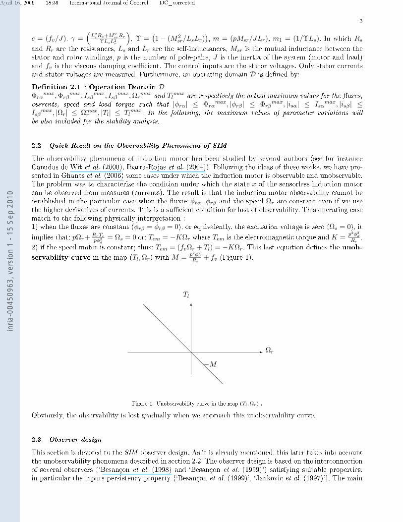
2) if the speed motor is constant; thus: Tem = (fvΩr + Tl) = −KΩr. This last equation denes the unob-servability curve in the map (Tl, Ωr) with M = p2φ2

d

Rr+ fv (Figure 1).

-

6

Ωr

Tl

@@

@@

@@

@@

@@

@@

@

−M

Figure 1. Unobservability curve in the map (Tl, Ωr) .

Obviously, the observability is lost gradually when we approach this unobservability curve.

2.3 Observer design

This section is devoted to the SIM observer design. As it is already mentioned, this later takes into accountthe unobservability phenomena described in section 2.2. The observer design is based on the interconnectionof several observers (`Besançon et al. (1998) and `Besançon et al. (1999)') satisfying suitable properties,in particular the inputs persistency property (`Besançon et al. (1999)', `Jankovic et al. (1997)'). The main

inria

-004

5096

3, v

ersi

on 1

- 15

Sep

201

0

April 16, 2009 18:39 International Journal of Control IJC_corrected

4

idea is to design a set of observers for the whole system from the individual synthesis of an observer for eachsubsystem. The key issue is that, for each of this observer, the state of the other subsystems is available.In this context, the IM model (1) can be rewritten in the following interconnected extended compact formwith parametric uncertainties

Σ :

Σ1 :

X1 = [A1(X2) + ∆A1(X2)]X1 + g1(u, y,X2) + ∆g1(u, y, X2)y1 = C1X1

Σ2 :

X2 = [A2(X1) + ∆A2(X1)]X2 + ϕ(u, y) + ∆ϕ(u, y)y2 = C2X2

(2)

where X1 = (isα, Ωr,Tl )T and X2 = (isβ, φrα, φrβ)T are the state of the rst and the second subsystem re-spectively. u = [usα, usβ]T and y = [isα, isβ ]T are the input and the output vectors of the whole system, and

A1 =

−γ bpφrβ 00 −c − 1

J0 0 0

, A2 =

−γ −bpΩr ab0 −a −pΩr

0 pΩr −a

, g1 =

m1usα + abφrα

mφrαisβ −mφrβisα0

, ϕ =

m1usβ

aMsrisαaMsrisβ

C1 = C2 =(1 0 0

).

u ∈ U is the set of admissible inputs and ni is the dimension of each subsystem (n1 = n2 = 3). Tl isan unknown load torque which is assumed constant. The terms ∆A1(X2), ∆A2(X1), ∆g1(u, y, X2) and∆ϕ(u, y) represent the uncertain terms of A1(X2), A2(X1), g1(u, y, X2), ϕ(u, y) respectively.

Let us now introduce the following property and denition:Property 2.2 a- Since A1(X2) and A2(X1) are linear, they are respectively globally Lipschitz with respectto X2, X1.b- g1(u, y, X2) is Lipschitz with respect to the ux and uniformly with respect to (u, y) as long as the IM(1) state remains in D.c- Due to the fact that the matrix A1 is Lyapunov stable (γ > 0 and c > 0), there exists a positive matrixS1 > 0 such that AT

1 S1 + S1A1 = −Q where Q ≥ 0.d- Due to the fact that the matrix A2 is exponentially stable (γ > 0, a > 0), there exists a positive matrixS2 > 0 such that AT

2 S2 + S2A2 = −I.Definition 2.3 Let D = detOJ , where OJ = ∂

∂X(O) is the jacobian observability matrix

and X = (isα isβ φrα φrβ Ωr Tl)T . The IM associated observability subspace O is generated byO =

(isα isβ i

(1)sα i

(1)sβ i

(2)sα i

(2)sβ

)T.

Dmin is the smallest value of D chosen such that the IM is in the observable area.Now, from property 2.2, denition 2.3 and taking into account the unobservability phenomena of the SIMdescribed in section 2.2, sucient conditions are given in the sequel such that system (3) is a practicalexponential observer for the whole system (2).

O :

O1 :

Z1 = A1(Z2)Z1 + g1(u, y, Z2) + MS−11 CT

1 (y1 − y1)S1 = M(−θ1S1 −AT

1 (Z2)S1 − S1A1(Z2) + CT1 C1)

y1 = C1Z1

O2 :

Z2 = A2(Z1)Z2 + ϕ(u, y) + MS−12 CT

2 (y2 − y2)S2 = M(−θ2S2 −AT

2 (Z1)S2 − S2A2(Z1) + CT2 C2)

y2 = C2Z2

M = 1 if |D| > Dmin; M = |D|Dmin

if |D| < Dmin;M = 0 if |D| = 0

(3)

inria

-004

5096

3, v

ersi

on 1

- 15

Sep

201

0

April 16, 2009 18:39 International Journal of Control IJC_corrected

5

where Z1 = (isα, Ωr, Tl)T , Z2 = (isβ, φrα, φrβ)T , Si = STi > 0, i=1,2. θ1 and θ2 are positive constants. Note

that S−11 CT

1 and S−12 CT

2 are the respective gains of observers (O1) and (O2). Furthermore, when the IMis no longer in the observable area, observer (3) can not work any more. Then, a solution based on the IMobservability property is introduced by using a soft switch function M such that observer (3) operates asan estimator.

Remark 1 1. Z2 and Z1 are considered as inputs for subsystems (O1) and (O2), the solutions of S1 and S2

are symmetric positive denite matrices (see annexe for the positiveness proof of Si(t), i = 1, 2).2. When the IM is in the observable area, Z2 and Z1 satisfy the regularly persistence condition.3. When the IM is in the unobservable area, Z2 and Z1 do not satisfy the regularly persistence conditionand the observer operates as an estimator.4. It is worth noticing that ‖S1‖ and ‖S2‖ are bounded when the IM is in the observable area.

2.4 Observer convergence

In order to prove the convergence of the proposed observer (3), sucient conditions are established. Deningthe estimation errors

ε1 = X1 − Z1

ε2 = X2 − Z2.

According to system (2) and observer (3), their errors dynamics read

Σε :

ε1 = [A1(Z2)−MS−11 CT

1 C1]ε1 + g1(u, y, X2) + ∆g1(u, y, X2)− g1(u, y, Z2)+ [A1(X2) + ∆A1(X2)−A1(Z2)]X1

ε2 = [A2(Z1)−MS−12 CT

2 C2]ε2 + ∆ϕ(u, y) + [A2(X1) + ∆A2(X1)−A2(Z1)]X2.(4)

Proposition 2.4 Consider system (2) with property 2.2. Then, system (3) is a practical exponentialobserver1 for system (2), for θ1 > 0 and θ2 > 0 suciently large.

Proof Consider the following Lyapunov function candidate

Vo = V1 + V2 (5)

where V1 = εT1 S1ε1 and V2 = εT

2 S2ε2.

Remark 2 The Lyapunov function candidate (5) is well chosen since Si(t), i = 1, 2 is positive denite (seeannexe for more details)

Its time derivative along (4) is

Vo = −MεT1 CT

1 C1ε1 −Mθ1εT1 S1ε1 + εT

1 [AT1 (Z2)S1 + S1A1(Z2)]ε1(1−M)

+2εT1 S1[A1(X2) + ∆A1(X2)−A1(Z2)]X1 + 2εT

1 S1[g1(u, y, X2) + ∆g1(u, y, X2)− g1(u, y, Z2]

−MεT2 CT

2 C2ε2 −Mθ2εT2 S2ε2 + εT

2 [A2(Z1)T S2 + S2A2(Z1)]ε2(1−M)

+2εT2 S2[A2(X1) + ∆A2(X1)−A2(Z1)]X2 + 2εT

2 S2∆ϕ(u, y)X2.

1the observer is exponentially convergent to a ball Br

inria

-004

5096

3, v

ersi

on 1

- 15

Sep

201

0

April 16, 2009 18:39 International Journal of Control IJC_corrected

6

By introducing the norm, it follows

Vo ≤ − MεT1 CT

1 C1ε1 −Mθ1εT1 S1ε1 −Mθ1ε

T1 S1ε1 + εT

1

AT

1 (Z2)S1 + S1A1(Z2)

ε1(1−M)

+2 ‖ε1‖ ‖S1‖ ‖A1(X2) + ∆A1(X2)−A1(Z2)‖ ‖X1‖+2 ‖ε1‖ ‖S1‖ ‖g1(u, y, X2) + ∆g1(u, y, X2)− g1(u, y, Z2)‖ (6)−MεT

2 CT2 C2ε2 −Mθ2ε

T2 S2ε2 + εT

2

AT

2 (Z1)S2 + S2A2(Z1)

ε2(1−M)

+2 ‖ε2‖ ‖S2‖ ‖A2(X1) + ∆A2(X1)−A2(Z1)‖ ‖X2‖+ 2 ‖ε2‖ ‖S2‖ ‖∆ϕ(u, y)‖ ‖X2‖ .

From property 2.2-a-b, the set inequalities hold

‖S1‖ ≤ k1; ‖A1(X2)−A1(Z2)‖ ≤ k2 ‖ε2‖ ; ‖X1‖ ≤ k3;‖g1(u, y, X2)− g1(u, y, Z2)‖ ≤ k4 ‖ε2‖ ; ‖S2‖ ≤ k5;‖A2(X1)−A2(Z1)‖ ≤ k6 ‖ε1‖ ; ‖X2‖ ≤ k7

Using the above inequalities and because the fact pointed in property 2.2-c and 2.2-d, (6) becomes

Vo ≤ − MεT1 CT

1 C1ε1 −Mθ1εT1 S1ε1 − εT

1 Qε1(1−M) + 2µ1 ‖ε1‖ ‖ε2‖+ 2µ2 ‖ε1‖ ‖ε2‖− εT

2 ε2(1−M) + µ4 ‖ε1‖ −MεT2 CT

2 C2ε2 −Mθ2εT2 S2ε2 + 2µ3 ‖ε2‖ ‖ε1‖+ µ5 ‖ε2‖ (7)

where µ1 = k1k2k3, µ2 = k1k4, µ3 = k5k6k7, µ4 = 2(k1k3ρ1 + k1ρ3), µ5 = 2(k5k7ρ2 + k5ρ4).

The parameters kj , j = 1, ..., 8 and ρi, i = 1, ..., 4 are positives constants which are computed bydetermining the maximal values of A1, A2, g1, S1, S2, ∆A1(X2), ∆A2(X1), ∆g1(u, y, X2) and ∆ϕ(u, y) inthe physical domain D of IM (see denition 2.1).

Since 0 ≤ M ≤ 1, Q ≥ 0 and CTi Ci ≥ 0, i = 1, 2, (7) follows

Vo ≤ − Mθ1εT1 S1ε1 + 2µ1 ‖ε1‖ ‖ε2‖+ 2µ2 ‖ε1‖ ‖ε2‖ (8)

+ µ4 ‖ε1‖ −Mθ2εT2 S2ε2 + 2µ3 ‖ε2‖ ‖ε1‖+ µ5 ‖ε2‖

Using the following inequalities

λmin(Si) ‖εi‖2 ≤ ‖εi‖2Si≤ λmax(Si) ‖εi‖2

‖εi‖2Si

= εTi Siεi, i = 1, 2

where λmin(Si) and λmax(Si) are respectively the minimal and maximal eigenvalues of Si.

By writing (8) in terms of functions V1 and V2, it follows that

Vo ≤ −M(θ1V1 − θ2V2) + 2(µ1 + µ2 + µ3)√

V1

√V2 + µ4 ‖ε1‖+ µ5 ‖ε2‖ (9)

where µi = µi√λmin(S1)

√λmin(S2)

, i = 1, 2, 3.

Next, by using the following inequality√

V1

√V2 ≤ υ

2V1 + 12υV2, ∀υ ∈]0, 1[, one get

inria

-004

5096

3, v

ersi

on 1

- 15

Sep

201

0

April 16, 2009 18:39 International Journal of Control IJC_corrected

7

Vo ≤ −(Mθ1 −Nυ)V1 − (Mθ2 − N

υ)V2 + µ4 ‖ε1‖+ µ5 ‖ε2‖ . (10)

where N = µ1 + µ2 + µ3. µi = µi√λmin(S1)

√λmin(S2)

, i = 1, 2, 3. µ1 = k1k2k3, µ2 = k1k4, µ3 = k5k6k7,µ4 = 2(k1k3ρ1 + k1ρ3), µ5 = 2(k5k7ρ2 + k5ρ4).

Tacking account µ = max(µ4, µ5), it follows that:

1) when M = 1 (observable conditions), (10) becomes:

Vo(M = 1) ≤ −δ′Vo + r,

where

δ′ = (δ − 12υ )

r = µ2 υ2

δ = min(δ1, δ2)δ1 = (θ1 −Nυ) > 0δ2 = (θ2 − N

υ ) > 0

(11)

By choosing δ > 12υ , it implies that the origin of system (4) is practically exponentially stable (more

details about practical stability can be found in `Laskhmikanthan et al. (1990)' and `Panteley et al. (1998)').

2) when M = 0 (unobservable conditions), (10) becomes:

Vo(M = 0) ≤ K ′Vo + r,

where K ′ = (K + 12υ ) and K = max(Nυ, N

υ ).

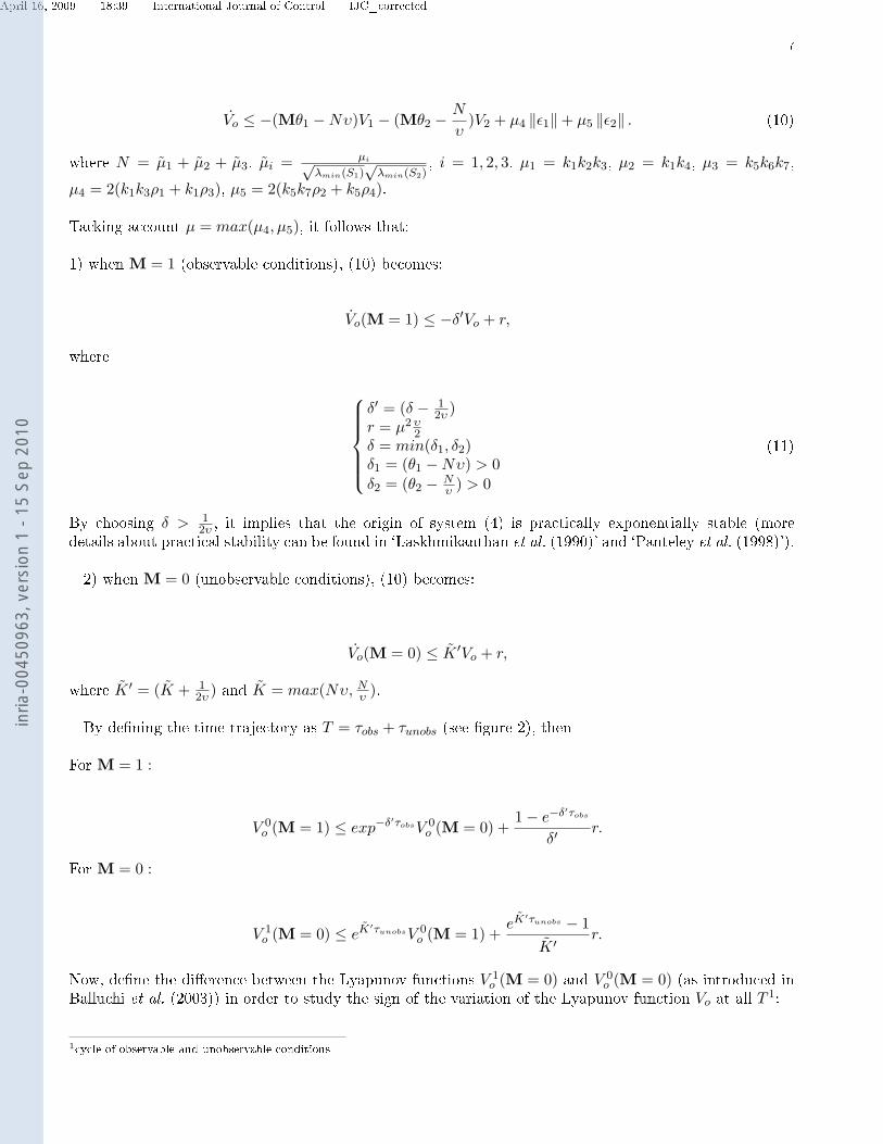
By dening the time trajectory as T = τobs + τunobs (see gure 2), then

For M = 1 :

V 0o (M = 1) ≤ exp−δ′τobsV 0

o (M = 0) +1− e−δ′τobs

δ′r.

For M = 0 :

V 1o (M = 0) ≤ eK′τunobsV 0

o (M = 1) +eK′τunobs − 1

K ′ r.

Now, dene the dierence between the Lyapunov functions V 1o (M = 0) and V 0

o (M = 0) (as introduced inBalluchi et al. (2003)) in order to study the sign of the variation of the Lyapunov function Vo at all T 1:

1cycle of observable and unobservable conditions

inria

-004

5096

3, v

ersi

on 1

- 15

Sep

201

0

April 16, 2009 18:39 International Journal of Control IJC_corrected

8

∆Vo ≤ V 1o (M = 0)− V 0

o (M = 0) : = (eK′τunobs−δ′τobs − 1)V 0o (M = 0)

+ [eK′τunobs(1− e−δ′τobs

δ′) +

eK′τunobs − 1K ′ ]r.

It is obvious that only practical stability is obtained for

K ′τunobs − δ′τobs < 0. (12)

(12) ensures that the Lyapunov function V0 converges into the interval [0, V max0 ] where

V max0 =

[eK′τunobs(1−e−δ′τobs

δ′ ) + eK′τunobs−1K′ ]r

1− K ′τunobs − δ′τobs

.

If r = 0, then exponential convergence to zero is obtained. ¤

tt

Figure 2. Lyapunov function Vo for T = τobs + τunobs.

3 FOC via Sliding Mode TechniquesIn this section, a controller is designed by combining the FOC method (`Blaschke et al. (1972)') withSliding Mode Control method (SMC, `Utkin et al. (1992)'). The design procedure is based on theassumption of current-fed IM.

Field Oriented Control . In the rotating (d-q) reference frame, the IM dynamic model (1) reads (Chiassonet al. (2005))

Ωr = mφrdisq − cΩr − 1J Tl

˙φrd = −aφrd + aMsrisdρ = pΩr + aMsr

φrdisq

isd = −γisd + abφrd + pΩrisq + aMsr

φrdi2sq + m1usd

isq = −γisq − bpΩrφrd − pΩrisd − aMsr

φrdisdisq + m1usq

(13)

where respectively isd, isq and usd, usq are the stator currents and stator voltages. The electromagnetic

inria

-004

5096

3, v

ersi

on 1

- 15

Sep

201

0

April 16, 2009 18:39 International Journal of Control IJC_corrected

9

torque Tem = pMsr

Lrφrdisq is proportional to the product of φrd and isq . Thus, by holding constant the

magnitude of the rotor ux, a linear relationship between isq and Tem is obtained. In order to cancel thenonlinear dynamics of isd and isq , the system is forced into current-command mode using high gain feedback(see Chiasson et al. (2005)). More precisely, the following IP current controllers

Vsd = Kivd

∫ t0 (i∗sd − isd )dt + Kpvd (i∗sd − isd )

Vsq = Kivq

∫ t0 (i∗sq − isq)dt + Kpvq(i∗sq − isq)

(14)

are used to force isd and isq to track their respective references i∗sd and i∗sq and produce fast responses whenlarge feedback gains are used. Hence, assuming that i∗sd and i∗sq as the new inputs, it follows that

Ωr = mφrdi

∗sq − cΩr − Tl

J˙φrd = −aφrd + aMsri

∗sd

(15)

In order to solve the ux and speed trajectory tracking problem, the following assumption is introduced.Assumption 3.1 a- The state initial conditions of the IM are in the physical domain D.b- The desired trajectories (φ∗rd and Ω∗r) are in the physical domain D.c- The actual load torque is assumed to be bounded by a maximal xed value %. This maximal value ischosen in accordance to the realistic torque characteristics of the chosen drive: |Tl| < %.Sliding Mode Control .

Flux controller design. From (15), consider the following IM ux dynamic equation with uncertainties

φrd = −aφrd + ∆aφrd + κi∗sd (16)

where κ = aMsr and ∆a is the uncertainty term of parameter a. In order to design a ux sliding modecontroller, dene the ux tracking error eφrd

= φrd − φ∗rd where φ∗rd is the ux reference. The associatederror dynamics is

eφrd= −aeφrd

+ κi∗sd − aφ∗rd − φ∗rd + ∆aφrd (17)

From SMC theory, dene the φrd ux sliding manifold as

σφrd= eφrd

− (kφrd− a)

∫ t

0eφrd

(τ)dτ.

The associated Lyapunov function is selected as

Vσφrd=

12σ2

φrd. (18)

Its time derivative is given by

Vσφrd= σφrd

[σφrd1 + σφrd2i∗sd + ∆aφrd]

where σφrd1 = kφrdeφrd

+ aφ∗rd + φ∗rd and σφrd2 = κ.

inria

-004

5096

3, v

ersi

on 1

- 15

Sep

201

0

April 16, 2009 18:39 International Journal of Control IJC_corrected

10

Therefore, the sliding mode controller follows

i∗sd = i∗sd ,equ + i∗sd ,n (19)

In this equation i∗sd ,equ = −σφrd 1

σφrd 2− lφrd

σφrdis the equivalent control and i∗sd,n = − udn

σφrd2is the discontinuous

control where udn = ηφrdsgn(σφrd

) with

sgn(σφrd) :

1 if σφrd> 0

−1 if σφrd< 0

∈ [−1, 1] if σφrd= 0.

Then (18) becomes

Vσφrd= −lφrd

Vσφrd+ σφrd

[−ηφrdsgn(σφrd

) + ∆aφrd].

Choosing lφrd> 0 and ηφrd

> max‖∆aφrd‖ (dened hereafter) it follows that Vσφrd≤ 0. As

Vσφrdis contracting and from assumption (3.1-a-b) then maxφrd := Kmax

φrdcan not be greater than

maxφrd(0), φ∗rd+ |∆eφrd(0)|. Consequently, ∆aφrd is bounded and can be set as ηφrd

= ∆amaxKmaxφrd

+bφ,with bφ a small positive constant. Furthermore, all the trajectories reach the sliding manifold σφrd

= 0 ina nite time and remain there. Therefore σφrd

= 0 and equation (17) becomes

eφrd= (kφrd

− a)eφrd. (20)

Hence, the ux tracking error eΩrexponentially converges to 0 for (kφrd

− a) < 0.Now, choosing (19) to force φrd to track its reference φ∗rd ensures that the ux is properly established inthe motor. Hence, after the IM is uxed (φrd = φ∗rd = constant), the electromagnetic torque (Tem) canbe rewritten as Tem = KT i∗sq , where KT is the motor torque constant dened by KT = pMsr

Lrφrd. As a

consequence, the linear relationship between the input i∗sq and the speed dynamics Ωr is obtained. Then,the speed control is obtained through the input i∗sq via a speed controller described below.

Speed controller design. Consider the mechanical equation of (15) including uncertainties

Ωr = −cΩr − Tl

J+ hi∗sq + dΩr

(21)

where h = mφrd and dΩr= −∆cΩr − Tl

J is the term uncertainty. Dening the speed tracking erroreΩr

= Ωr − Ω∗r , it follows

eΩr= −ceΩr

+ hi∗sq − cΩ∗r − Ω∗

r + dΩr(22)

Dene now the sliding manifold as

σΩr= eΩr

− (k − c)∫ t

0eΩr

(τ)dτ (23)

The Lyapunov candidate function associated to the sliding manifold (23) is dened as

VσΩr=

12σ2

Ωr.

inria

-004

5096

3, v

ersi

on 1

- 15

Sep

201

0

April 16, 2009 18:39 International Journal of Control IJC_corrected

11

By computing its time derivative, one obtain

VσΩr= σΩr

σΩr

= σΩr[σΩr1 + σΩr2i

∗sq + dΩr] (24)

where σΩr1 = keΩr+ cΩ∗r + Ω∗r and σΩr2 = h.

Then, the speed controller reads

i∗sq = i∗sq,equ + i∗sq,n (25)

where i∗sq,equ = −σΩr 1

σΩr 2− lΩr

σΩris the equivalent control and i∗sq,n = − uqn

σΩr2, with uqn = ηΩr

sgn(σΩr) and

sgn(σΩr) :

1 if σΩr> 0;

−1 if σΩr< 0;

∈ [−1, 1] if σΩr= 0.

(24) becomes

VσΩr= −lΩr

VσΩr+ σΩr

[−ηΩrsgn(σΩr

) + dΩr].

By choosing lΩr> 0 and ηΩr

> max‖dΩr‖ (dened hereafter) it follows that VσΩr

≤ 0. AsVσΩr

is contracting and from assumption (3.1-a-b) then maxΩr := KmaxΩr

can not be greater thanmax|Ωr(0)|, |Ω∗r| + |∆eΩr

(0)|. Consequently, as dΩr= ∆cΩr + Tl

J then dΩris bounded. Finally, ηΩr

is set as ηΩr= ∆cKmax

Ωr+ %

J + bΩr, with bΩr

a small positive constant. Furthermore, all the trajectoriesreach the sliding manifold σ = 0 in a nite time and remain there. Therefore, σ = 0 and equation (22)implies

eΩr= (kΩr

− c)eΩr(26)

which makes that the speed tracking error eΩrexponentially converges to 0 for (kΩr

− c) < 0.Proposition 3.2 . Consider IM model (15) and assume that assumption 3.1 is satised. Then underthe action of speed controller (25) and ux controller (19), the rotor speed and the ux track their desiredtrajectories.ProofUsing

Vc =12σ2

φrd+

12σ2

Ωr

as a Lyapunov function candidate, then the time derivative

Vc = −lφrdVσφrd

+ [−ηφrdsgn(σφrd

) + ∆aφrd]− lΩrVσΩr

+ [−ηΩrsgn(σΩr

) + dΩr]

is less than 0. ¤

4 Stability analysis of the closed-loop system

In order to implement controllers (19) and (25), the speed/ux measures are replaced by their estimatesresulting in the new controllers

inria

-004

5096

3, v

ersi

on 1

- 15

Sep

201

0

April 16, 2009 18:39 International Journal of Control IJC_corrected

12

i∗sd = −lφrdσφrd

+kφrd

eφrd+ aφ∗rd + φ∗rd − ηφrd

sgn(σφrd)

κ(27)

i∗sq = −lΩrσΩr

+kΩr

eΩr+ cΩ∗

r + Ω∗r − ηΩr

sgn(σΩr)

mφrd

(28)

where

eφrd= φ∗rd − φrd

eΩr= Ωr − Ω∗r

σφrd= eφrd

+ (kφ − a)∫ t0 eφrd

dτ

σΩr= eΩr

+ (kΩr− c)

∫ t0 eΩr

dτ

The IM observer must already be uxed to ensure estimated speed tracking. In order to avoid the singularityin (28), the observer (3) is initialized with initial conditions dierent from zero. In practice, electricalengineers overcome this singularity by starting to track rstly the ux φrd to its reference φ∗rd = constant.The same trick is adopted for the estimated ux φrd by adding an oset ε = 0.05Wb such as

i∗sq = −lΩrσΩr

+kΩr

eΩr+ cΩ∗r + Ω∗r − ηΩr

sgn(σΩr)

maxφrd, εm(29)

To analyze the stability of the closed-loop system ("O-C"), the following procedure is adopted.Argument 4.1 If it is proved that the controller (27)-(29) enables to track the estimated ux and estimatedspeed to their desired trajectory (e = Z −X∗ → 0 as t →∞), then, it is ensured that the IM ux and thespeed practically converge to their desired trajectories.-Estimated ux tracking. Dene the candidate Lyapunov function Vσφrd

= 12σ2

φrd

, which time derivativeis Vσφrd

= −lφrdVσφrd

− σφrd[ηφrd

sgn(σφrd) + Mgφrd

εisβ], where gφrd

is the gain of the estimated ux φrd.By choosing lφrd

> 0 and ηφrd> maxM

∥∥∥gφrd

∥∥∥∥∥εisβ

∥∥ (dened hereafter) it follows that Vσφrd≤ 0. Now,

imposing the initial states of the observer to be in D and as Vσφrdis contracting, then from assumption

(3.1-b), maxφrd := Kmaxφrd

can not be greater than maxφrd(0), φ∗rd+ |∆eφrd(0)|. From where it can be

deduced that∥∥∥gφrd

∥∥∥ is bounded. Moreover, as V0 = V1 + V2 (see the proposition 2.4 proof) is practicallystable and does not depend on u, then

∥∥εisβ

∥∥ is bounded. Finally, ηφrdis set as

ηφrd= Kmax

gφrd

Kmaxεisβ

+ c1, c1 > 0. (30)

-Estimated speed tracking. Consider the candidate Lyapunov function VΩr= 1

2 Ω2r , which time derivative

is VσΩr= −lΩr

VΩr− σφrd

[ηΩrsgn(σΩr

) + MgΩrεisα

], where gΩris the gain of the estimated speed Ωr.

By choosing lΩr> 0 and ηΩr

> maxM∥∥∥gΩr

∥∥∥ ‖εisα‖ it follows that VΩr

≤ 0. Following the same ideas asabove leads to

ηΩr= Kmax

gΩrKmax

εisα+ c2, c2 > 0. (31)

inria

-004

5096

3, v

ersi

on 1

- 15

Sep

201

0

April 16, 2009 18:39 International Journal of Control IJC_corrected

13

Lemma 4.2 Consider observer (3) initialized in D and assume that assumption (3.1-a-b) holds. Then,under the action of the controller (27)-(29), the rotor ux and rotor speed estimations track their desiredtrajectories.Proof Using

Vc =12σ2

φrd+

12σ2

Ωr

as a Lyapunov function candidate, it follows

Vc = −lφrdVσφrd

− σφrd[ηφrd

sgn(σφrd) + Mgφrd

εisβ]− lΩr

VσΩr− σΩr

[ηΩrsgn(σΩr

) + MgΩrεisα

] ≤ 0.

¤

Now, a practical stability result of the proposed observer based control for the IM is given.Theorem 4.3 Consider the controller (27)-(29) and property (2.2). If the observer (3) is initialized on Dand assuming the assumption (3.1) is satised, then

• The IM estimated state practically converges to the real state.• The estimated ux and speed exponentially converge to their desired trajectories.• Finally, the real ux and speed of IM converge practically to their desired trajectories.

Proof The proof follows from proposition (2.4), lemma (4.2) and argument (4.1). ¤

5 EXPERIMENTAL RESULTS

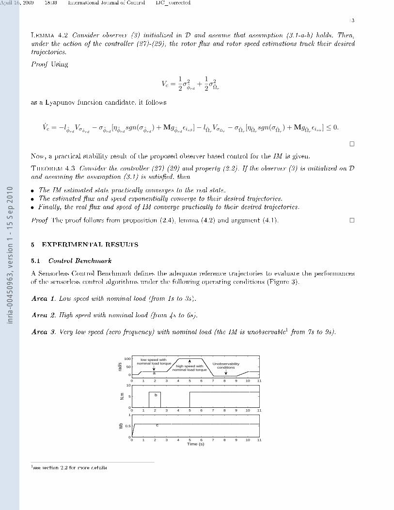
5.1 Control Benchmark

A Sensorless Control Benchmark denes the adequate reference trajectories to evaluate the performancesof the sensorless control algorithms under the following operating conditions (Figure 3).

Area 1. Low speed with nominal load (from 1s to 3s).

Area 2. High speed with nominal load (from 4s to 6s).

Area 3. Very low speed (zero frequency) with nominal load (the IM is unobservable1 from 7s to 9s).

0 1 2 3 4 5 6 7 8 9 10 11

0

50

100

rad/

s

0 1 2 3 4 5 6 7 8 9 10 110

5

10

N.m

0 1 2 3 4 5 6 7 8 9 10 110

0.5

1

Time (s)

Wb

a

b

c

low speed with nominal load torque

high speed withnominal load torque

Unobservabilityconditions

1see section 2.2 for more details

inria

-004

5096

3, v

ersi

on 1

- 15

Sep

201

0

April 16, 2009 18:39 International Journal of Control IJC_corrected

14

Figure 3. Control benchmark trajectories: a- Reference speed: Ω∗ (rad/s), b- Reference load: T ∗l (N.m), c-Reference ux: φ∗rd (Wb).

5.2 Experimental results

Here, the experimental results obtained with the proposed controller using the observer are given. The testshave been performed with the following induction motor values:

Nominal rate power 1.5kW Rs 1.47ΩNominal angular speed 1430 rpm Rr 0.79ΩNumber of pole pairs 2 Ls 0.105H

Nominal voltage 220 V Lr 0.094HNominal current 6.1 A J, fv 0.0077Kg.m2, 0.0029Nm/rad/s

and the guidelines parameters tuning for the observer and the controller are given as follows :

- For the observer given by (3), θ1 and θ1 are chosen to satisfy (11). From (11), it is easy to see thatθ1 > Nυ and θ2 >

N

υwhere υ ∈]01]. So, θ1 is proportional to υ while θ2 is inversely proportional. We

choose θ1 = 1 and θ2 = 5000.

- For the controller given by (14), the parameters Kpvd, Kpvq, KIvd, KIvq are determined as follows :

Considering the dynamic equations of isd and isq given by (13) without nonlinearities and coupling terms

isd = −γisd + m1usd

isq = −γisq + m1usq(32)

Writing the transfer function which lies the stator currents of (32) with their references given by (14) as asecond order system in closed loop, it follows

isdi∗sd

=w2

nd

s2 + 2ζwnd + w2nd

isqi∗sq

=w2

nq

s2 + 2ζwnq + w2nq

By imposing ζ = 1 to avoid peaking and a currents bands-widths FBD at least less than a middle ofFe = 1/Te where Te = 200µs is the sampling time:

ζ = 1wnd = 2πFBD

wnq = 2πFBD,

the parameters Kpvd, Kpvq, KIvd, KIvq can be established:

Kpvd =2ζ − γ

m1, T ivd =

2ζ − γ

w2nd

Kpvq =2ζ − γ

m1, T ivq =

2ζ − γ

w2nq

where KIvd =Kpvd

Tivdand KIvq =

Kpvq

Tivq. We choose Kpvd = 2, Kpvq = 2, KIvd = 0.05, KIvq = 0.05.

inria

-004

5096

3, v

ersi

on 1

- 15

Sep

201

0

April 16, 2009 18:39 International Journal of Control IJC_corrected

15

- For the controller given by (27)-(29), lφrd> 0, lΩr

> 0 and the parameters kφrd, kΩr

, ηφrdand ηΩr

arechosen to satisfy respectively (20), (26), (30), (31) . We choose ηφrd

= 10, kφrd= −80, lφrd

= 4, ηΩr= 5,

kΩr= −40, lΩr

= 2.

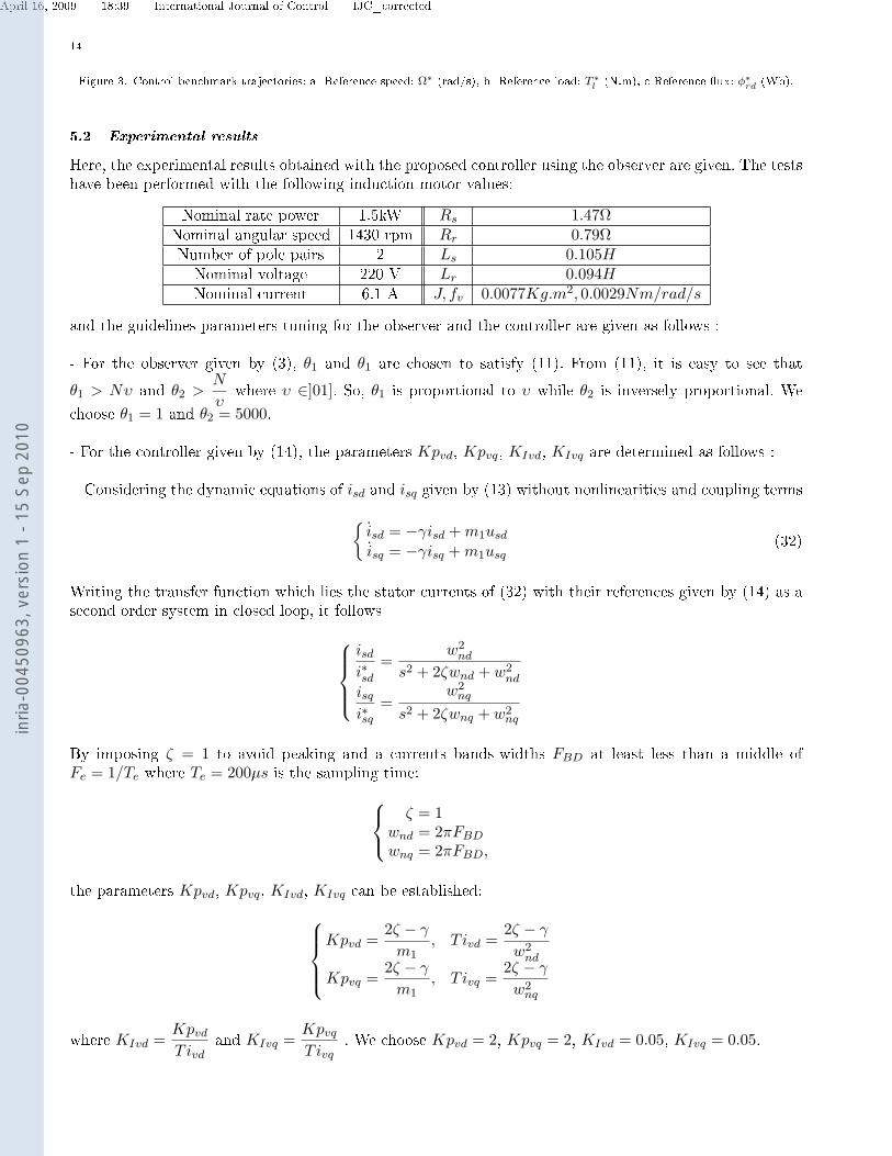
The block diagram scheme used in experimental set-up to test the law control with observer is presentedin gure 4. The block "Intercon. observers" is constituted by the two interconnected observers we havedesigned. This block uses only the current and stator measurements in the reference xed frame (α−β) toestimate the speed, the ux amplitude and the ux angle. The block "Sliding and Field Oriented Control"contains the proposed controller. This block uses the estimates of speed, ux amplitude and ux angle givenby the block "Intercon. observers" and the current measurements after using the transformation of Parkand Concordia. Then, it gives the inputs control in the reference xed frame (a,b,c) after using the inversetransformations of Park and Concordia. These control inputs drive the inverter to impose the speed andux reference trajectories (dened by the "Control Benchmark"). The track of the reference load torquetrajectory (also dened in the "Control Benchmark") is imposed by the connected synchronous motor.

Figure 4. Diagram of the controller-observer scheme.

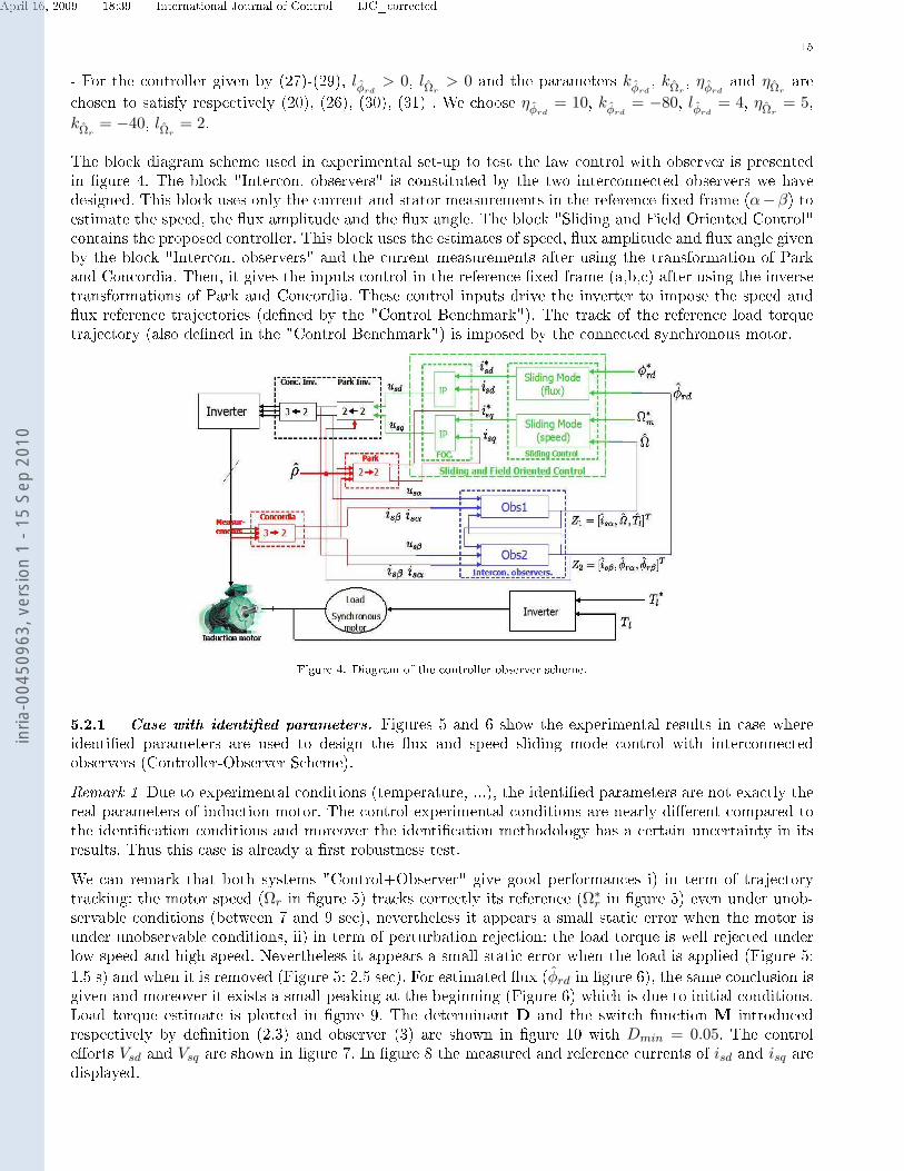
5.2.1 Case with identied parameters. Figures 5 and 6 show the experimental results in case whereidentied parameters are used to design the ux and speed sliding mode control with interconnectedobservers (Controller-Observer Scheme).Remark 1 Due to experimental conditions (temperature, ...), the identied parameters are not exactly thereal parameters of induction motor. The control experimental conditions are nearly dierent compared tothe identication conditions and moreover the identication methodology has a certain uncertainty in itsresults. Thus this case is already a rst robustness test.We can remark that both systems "Control+Observer" give good performances i) in term of trajectorytracking: the motor speed (Ωr in gure 5) tracks correctly its reference (Ω∗r in gure 5) even under unob-servable conditions (between 7 and 9 sec), nevertheless it appears a small static error when the motor isunder unobservable conditions, ii) in term of perturbation rejection: the load torque is well rejected underlow speed and high speed. Nevertheless it appears a small static error when the load is applied (Figure 5:1.5 s) and when it is removed (Figure 5: 2.5 sec). For estimated ux (φrd in gure 6), the same conclusion isgiven and moreover it exists a small peaking at the beginning (Figure 6) which is due to initial conditions.Load torque estimate is plotted in gure 9. The determinant D and the switch function M introducedrespectively by denition (2.3) and observer (3) are shown in gure 10 with Dmin = 0.05. The controleorts Vsd and Vsq are shown in gure 7. In gure 8 the measured and reference currents of isd and isq aredisplayed.

inria

-004

5096

3, v

ersi

on 1

- 15

Sep

201

0

April 16, 2009 18:39 International Journal of Control IJC_corrected

16

0 2 4 6 8 10−20

0

20

40

60

80

100

120

Time (s)

rad/

sΩ

r

Ωr*

estimate

Figure 5. Reference speed Ω∗r , motor speed Ωr,estimated speed Ωr (rad/s)

0 2 4 6 8 100

0.1

0.2

0.3

0.4

0.5

0.6

0.7

0.8

0.9

1

Time (s)

Wb

φrd*

estimate

Figure 6. Flux, (Wb)

0 2 4 6 8 10−100

−50

0

50

100

150

Time (s)

V

Vsd

Vsq

Figure 7. Vsd and Vsq (V)

0 2 4 6 8 10

0

5

10

A

0 2 4 6 8 10−5

0

5

10

Time (s)

Aisq

isq*

isd

isd*

Figure 8. isd and isq , (A)

0 2 4 6 8 10−1

0

1

2

3

4

5

6

7

8

Time (s)

N.m

Tl*

estimate

Figure 9. T ∗l and Tl (N.m)

0 1 2 33 4 5 6 7 8 9 10 110

0.5

1

1.5

2

2.5

3

Time (s)

D a

nd M

DM

Figure 10. D and M

Case 1: experimental results with identied parameters.

5.2.2 Robustness cases. The interest now is to check the robustness of the designed Control-Observerwith respect to motor parameters variation. We have considered two robustness cases : a stator resistancevariation of +50% and a rotor resistance variation of +50% with respect to the values of the previous case.Case with +50% of Rr: the results that we have obtained are depicted in gures 11 and 12.

inria

-004

5096

3, v

ersi

on 1

- 15

Sep

201

0

April 16, 2009 18:39 International Journal of Control IJC_corrected

17

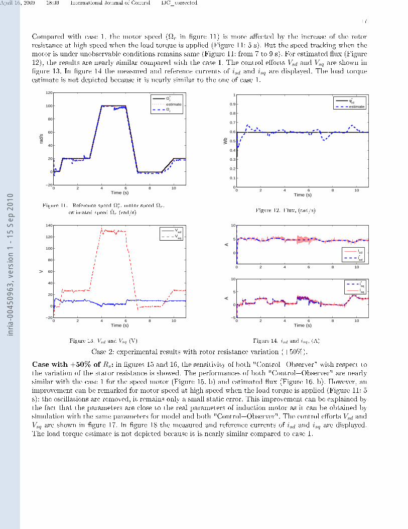
Compared with case 1, the motor speed (Ωr in gure 11) is more aected by the increase of the rotorresistance at high speed when the load torque is applied (Figure 11: 5 s). But the speed tracking when themotor is under unobservable conditions remains same (Figure 11: from 7 to 9 s). For estimated ux (Figure12), the results are nearly similar compared with the case 1. The control eorts Vsd and Vsq are shown ingure 13. In gure 14 the measured and reference currents of isd and isq are displayed. The load torqueestimate is not depicted because it is nearly similar to the one of case 1.

0 2 4 6 8 10−20

0

20

40

60

80

100

120

Time (s)

rad/

s

Ωr*

estimateΩ

r

Figure 11. Reference speed Ω∗r , motor speed Ωr,estimated speed Ωr (rad/s)

0 2 4 6 8 100

0.1

0.2

0.3

0.4

0.5

0.6

0.7

0.8

0.9

1

Time (s)

Wb

φrd*

estimate

Figure 12. Flux, (rad/s)

0 2 4 6 8 10−20

0

20

40

60

80

100

120

140

Time (s)

V

Vsd

Vsq

Figure 13. Vsd and Vsq (V)

0 2 4 6 8 10

0

5

10A

0 2 4 6 8 10−5

0

5

10

Time (s)

A

isd

isd*

isq*

isq

Figure 14. isd and isq , (A)

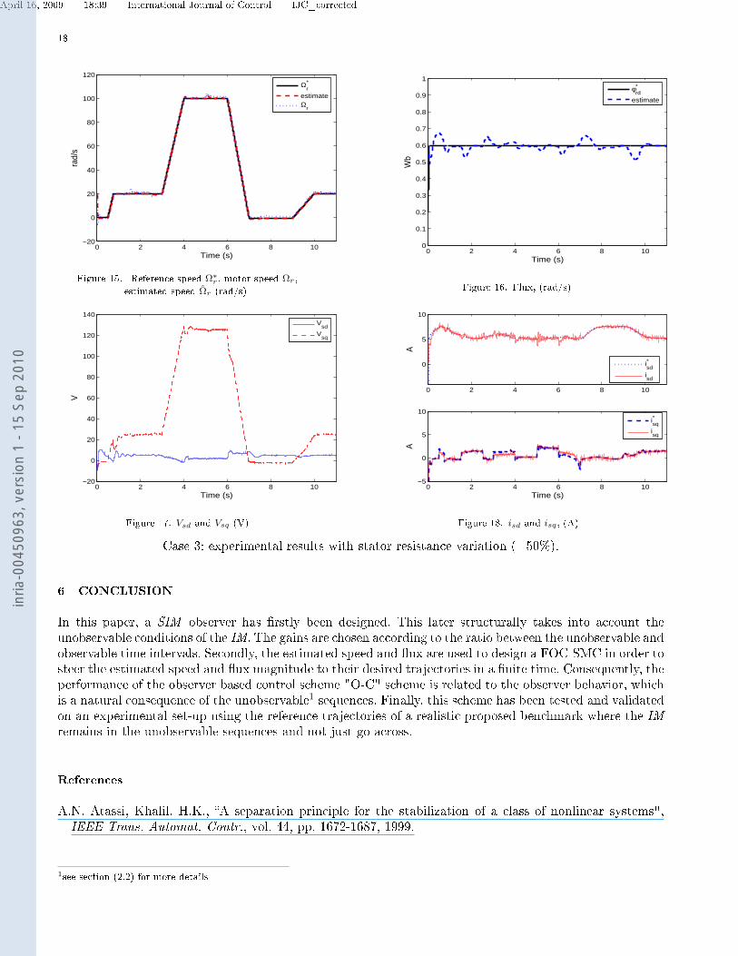
Case 2: experimental results with rotor resistance variation (+50%).Case with +50% of Rs: in gures 15 and 16, the sensitivity of both "Control+Observer" with respect tothe variation of the stator resistance is showed. The performances of both "Control+Observer" are nearlysimilar with the case 1 for the speed motor (Figure 15. b) and estimated ux (Figure 16. b). However, animprovement can be remarked for motor speed at high speed when the load torque is applied (Figure 11: 5s): the oscillations are removed, it remains only a small static error. This improvement can be explained bythe fact that the parameters are close to the real parameters of induction motor as it can be obtained bysimulation with the same parameters for model and both "Control+Observer". The control eorts Vsd andVsq are shown in gure 17. In gure 18 the measured and reference currents of isd and isq are displayed.The load torque estimate is not depicted because it is nearly similar compared to case 1.

inria

-004

5096

3, v

ersi

on 1

- 15

Sep

201

0

April 16, 2009 18:39 International Journal of Control IJC_corrected

18

0 2 4 6 8 10−20

0

20

40

60

80

100

120

Time (s)

rad/

sΩ

r*

estimateΩ

r

Figure 15. Reference speed Ω∗r , motor speed Ωr,estimated speed Ωr (rad/s)

0 2 4 6 8 100

0.1

0.2

0.3

0.4

0.5

0.6

0.7

0.8

0.9

1

Time (s)

Wb

φrd*

estimate

Figure 16. Flux, (rad/s)

0 2 4 6 8 10−20

0

20

40

60

80

100

120

140

Time (s)

V

Vsd

Vsq

Figure 17. Vsd and Vsq (V)

0 2 4 6 8 10

0

5

10

A

0 2 4 6 8 10−5

0

5

10

Time (s)

A

isd*

isd

isq*

isq

Figure 18. isd and isq , (A)

Case 3: experimental results with stator resistance variation (+50%).

6 CONCLUSION

In this paper, a SIM observer has rstly been designed. This later structurally takes into account theunobservable conditions of the IM. The gains are chosen according to the ratio between the unobservable andobservable time intervals. Secondly, the estimated speed and ux are used to design a FOC-SMC in order tosteer the estimated speed and ux magnitude to their desired trajectories in a nite time. Consequently, theperformance of the observer based control scheme "O-C" scheme is related to the observer behavior, whichis a natural consequence of the unobservable1 sequences. Finally, this scheme has been tested and validatedon an experimental set-up using the reference trajectories of a realistic proposed benchmark where the IMremains in the unobservable sequences and not just go across.

References

A.N. Atassi, Khalil, H.K., A separation principle for the stabilization of a class of nonlinear systems",IEEE Trans. Automat. Contr., vol. 44, pp. 1672-1687, 1999.

1see section (2.2) for more details

inria

-004

5096

3, v

ersi

on 1

- 15

Sep

201

0

April 16, 2009 18:39 International Journal of Control IJC_corrected

19

A. Balluchi, M.D. Di Benedetto, L. Benvenuti, A. L. Sangiovanni-Vincentelli, Observability for HybridSystems, IEEE Conf. Decision. Contr., Maui, Hawaii, 2003.

G. Besançon and H. Hammouri, On Observer Design for Interconnected Systems, Journal of MathematicalSystems, Estimation and Control, 8, 4, 1998.

G. Besançon, "A viewpoint on Observability and Observer Design for Nonlinear Systems, New Directionsin Nonlinear Observer Design, Lecture Notes in Control and information Sciences, Springer, No.244,1999.

F. Blaschke, The principle of eld orientation applied to the new transvector closed-loop control systemfor rotating eld machines", Siemens-Rev., 39, pp. 217220, 1972.

C. Canudas de Wit, A. Youssef, J.P. Barbot, Ph. Martin and F. Malrait, Observability Conditions ofInduction Motors at low frequencies, IEEE Conference on Decision and Control, Sydney, Australia,2000.

J. Chiasson, Modeling and High-Performance Control of Electric Machines", IEEE Series on Power Engi-neering, Wiley-Interscience, 2005.

M. Feemster, P. Aquino, D. M. Dawson and A. Behal, Sensorless rotor velocity tracking control for induc-tion motors, IEEE Transactions on Control Systems Technology, 9, 4, pp. 645653, 2001.

M. Ghanes, J. DeLeon, and A. Glumineau, Observability Study and Observer-Based Interconnected Formfor Sensorless Induction Motor", IEEE Conference on Decision and Control CDC, San Diego, California,USA, 2006.

J. Holtz, Sensorless control of induction machines-with or without signal injection IEEE Trans. Ind.Electron., 53, 1, pp. 7-30, 2006.

S. Ibarra-Rojas, J. Moreno and G. Espinosa, Global observability analysis of sensorless induction motor,Automatica, Vol. 40, Issue 6, pp. 10791085, 2004.

M. Jankovic, Adaptative Nonlinear Output Feedback Tracking with a Partial High-Gain Observer Back-stepping", IEEE Trans. Automat. Contr., 42, 1, pp. 106-113, 1997.

H. Kubota and K. Matsuse, Speed sensorless led-oriented control of induction motor with rotor resistanceadaptation IEEE Transactions on Industry Applications, 30, 5, pp.344348, Mar./Apr., 1994.

Laskhmikanthan, V., Leila, S. and Martynyuk, A.A., "Practical stability of nonlinear systems". WordScientic. ISBN 978-9810203566. 1990.

Y. C. Lin, Fu, L. C., and Tsai, C. Y., Non-linear sensorless indirect adaptive speed control of inductionmotor with unknown rotor resistance andload, International Journal of Adaptive Control and SignalProcessing, 14, pp. 109140, 2000.

R. Marino, P. Tomei and C. M. Verrelli, A nonlinear tracking control for sensorless induction motorsAutomatica, 41, 6, pp. 1071-1077, 2005.

R. Marino, P. Tomei and C. M. Verrelli, A nonlinear tracking control for sensorless induction motors withuncertain load torque Inter. J. of Adaptive Contr. and Signal Processing, March, 2007.

M. Montanari, S. Peresada, A. Tilli, A speed-sensorless indirect eld-oriented control for induction motorsbased on high gain speed estimation, Automatica Vol. 42, Issue 10, pp. 1637-1650, 2006.

S. Peresada, A. Tonielli and R. Morici (1999). High performance indirect eld oriented output feedbackcontrol of induction motors, Automatica Vol. 35, Issue 6, pp. 1033-1047, 1999.

E. Panteley and A. Loria, On global uniform asymptotic stability of cascade time-varying systems incascasde, Systems and Control Letters, 33, pp.131138, 1998.

H. Tajima and Y. Hori, Speedsensorless eld-orientation control of the induction machine, IEEE Trans-actions on Industry Applications, 29, 1, pp. 175180, 1993.

Utkin, V.I. "Sliding Modes in Control Optimization". Springer-Verlag. ISBN 9780387535166. (1992).I. Zein, "Extended Filter Kalman and Luenberger Observer Application to Control of Induction Motor",

Phd thesis, Université de Technologie de Compiegne, septembre 2000.

inria

-004

5096

3, v

ersi

on 1

- 15

Sep

201

0

April 16, 2009 18:39 International Journal of Control IJC_corrected

20

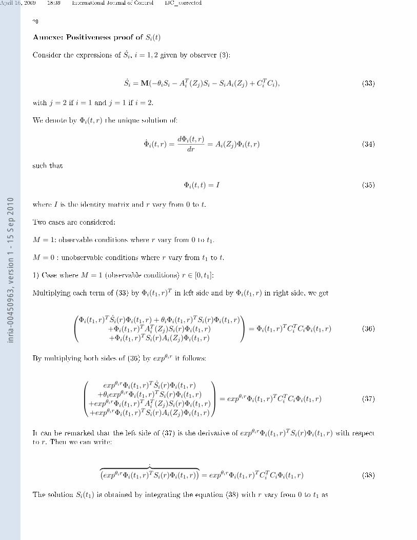
Annexe: Positiveness proof of Si(t)

Consider the expressions of Si, i = 1, 2 given by observer (3):

Si = M(−θiSi −ATi (Zj)Si − SiAi(Zj) + CT

i Ci), (33)

with j = 2 if i = 1 and j = 1 if i = 2.

We denote by Φi(t, r) the unique solution of:

Φi(t, r) =dΦi(t, r)

dr= Ai(Zj)Φi(t, r) (34)

such that

Φi(t, t) = I (35)

where I is the identity matrix and r vary from 0 to t.

Two cases are considered:

M = 1: observable conditions where r vary from 0 to t1.

M = 0 : unobservable conditions where r vary from t1 to t.

1) Case where M = 1 (observable conditions) r ∈ [0, t1]:

Multiplying each term of (33) by Φi(t1, r)T in left side and by Φi(t1, r) in right side, we get

Φi(t1, r)T Si(r)Φi(t1, r) + θiΦi(t1, r)T Si(r)Φi(t1, r)+Φi(t1, r)T AT

i (Zj)Si(r)Φi(t1, r)+Φi(t1, r)T Si(r)Ai(Zj)Φi(t1, r)

= Φi(t1, r)T CT

i CiΦi(t1, r) (36)

By multiplying both sides of (36) by expθir it follows:

expθirΦi(t1, r)T Si(r)Φi(t1, r)+θiexpθirΦi(t1, r)T Si(r)Φi(t1, r)

+expθirΦi(t1, r)T ATi (Zj)Si(r)Φi(t1, r)

+expθirΦi(t1, r)T Si(r)Ai(Zj)Φi(t1, r)

= expθirΦi(t1, r)T CT

i CiΦi(t1, r) (37)

It can be remarked that the left side of (37) is the derivative of expθirΦi(t1, r)T Si(r)Φi(t1, r) with respectto r. Then we can write:

˙︷ ︸︸ ︷(expθirΦi(t1, r)T Si(r)Φi(t1, r)

)= expθirΦi(t1, r)T CT

i CiΦi(t1, r) (38)

The solution Si(t1) is obtained by integrating the equation (38) with r vary from 0 to t1 as

inria

-004

5096

3, v

ersi

on 1

- 15

Sep

201

0

April 16, 2009 18:39 International Journal of Control IJC_corrected

21

∫ t1

0

˙︷ ︸︸ ︷(expθirΦi(t1, r)T Si(r)Φi(t1, r)

)dr =

∫ t1

0expθirΦi(t1, r)T CT

i CiΦi(t1, r)dr (39)

Then, equation (39) gives

expθit1Φi(t1, t1)T Si(t1)Φi(t1, t1)− Φi(t1, 0)T Si(0)Φi(t1, 0) =∫ t1

0expθirΦi(t1, r)T CT

i CiΦi(t1, r)dr (40)

Finally, by using the property (35) in equation (40), the solution Si(t1) yields

Si(t1) = exp−θit1Φi(t1, 0)T Si(0)Φi(t1, 0) +∫ t

0exp−θi(t1−r)Φi(t1, r)T CT

i CiΦi(t1, r)dr (41)

From (41), we can remark that Si(t1) is denite positive with Si(0) > 0 due to the fact that Z1 and Z2 ofequations (34) are regularly persistent (see remark 1.2). Then the positiveness of Si(t1) is demonstrated.

2) Case where M=0 (unobservable conditions) r ∈ [t1, t]:

Equation (33) becomes:

Si(r) = 0 (42)

By integrating equation (42) with r varying from t1 to t, we get

Si(t) = Si(t1) (43)

It can be noted that the nal condition Si(t1) of the interval time where IM is observable is equal to thenal condition Si(t) of the interval time where IM is unobservable since Si remains constant during thisunobservable interval of time. Then Si(t) (equation 43) is positive denite.

This ends the proof.inria

-004

5096

3, v

ersi

on 1

- 15

Sep

201

0