arX

iv:p

hysi

cs/0

0050

54v1

[ph

ysic

s.fl

u-dy

n] 2

2 M

ay 2

000 A Numerical Study of Capillary and Viscous

Drainage in Porous Media

Eyvind Aker,1,2,4 Alex Hansen1,2,3 and Knut Jørgen Maløy4

1 Department of Physics, University of Science and Technology, N-7491 Trondheim,Norway

2 Niels Bohr Institute, DK-2100 Copenhagen, Denmark3 Nordic Institute for Theoretical Physics, DK-2100 Copenhagen, Denmark

4 Department of Physics, University of Oslo, N-0316 Oslo, Norway

ABSTRACT

This paper concentrates on the flow prop-erties when one fluid displaces another fluidin a two-dimensional (2D) network of poresand throats. We consider the scale whereindividual pores enter the description andwe use a network model to simulate the dis-placement process.

We study the interplay between the pres-sure build up in the fluids and the dis-placement structure in drainage. We findthat our network model properly describesthe pressure buildup due to capillary andviscous forces and that there is good cor-respondence between the simulated evolu-tion of the fluid pressures and earlier resultsfrom experiments and simulations in slowdrainage.

We investigate the burst dynamics indrainage going from low to high injectionrate at various fluid viscosities. The burstsare identified as pressure drops in the pres-sure signal across the system. We find thatthe statistical distribution of pressure dropsscales according to other systems exhibitingself-organized criticality. We compare ourresults to corresponding experiments.

We also study the stabilization mecha-nisms of the invasion front in horizontal 2Ddrainage. We focus on the process whenthe front stabilizes due to the viscous forcesin the liquids. We find that the differencein capillary pressure between two differentpoints along the front varies almost linearlyas function of length separation in the di-rection of the displacement. The numer-ical results support new arguments aboutthe displacement process from those earliersuggested for viscous stabilization. Our ar-guments are based on the observation that

nonwetting fluid flows in loopless strands(paths) and we conclude that earlier sug-gested theories are not suitable to drainagewhen nonwetting strands dominate the dis-placement process. We also show that thearguments might influence the scaling be-havior of the front width as function of theinjection rate and compare some of our re-sults to experimental work.

1 INTRODUCTION

Two-phase displacements in porous mediahave received much attention during thelast two decades. In modern physics, theprocess is of great interest due to the varietyof structures obtained when changing thefluid properties like wettability, interfacialtension, viscosities and displacement rate.The different structures obtained have beenorganized into three flow regimes: viscousfingering [1,2], stable displacement [3], andcapillary fingering [4–6]. Viscous fingeringis characterized by an unstable front of fin-gers that is generated when nonwetting andless viscous fluid is displacing wetting andmore viscous fluid at relative high injectionrate. The fingering structure is found tobe fractal with fractal dimension D = 1.62[1, 2]. Stable displacement is named afterthe relative flat and stable front that is be-ing generated when a nonwetting and moreviscous fluid displaces a wetting and lessviscous fluid at relative high injection rate.The last scenario, capillary fingering, is ob-tained when a nonwetting fluid very slowlydisplaces a wetting fluid. At sufficiently lowinjection rate the invasion fluid generatesa pattern similar to the cluster formed byinvasion percolation [4, 7–9]. The displace-

1

ment is now solely controlled by the capil-lary pressure, that is the pressure differencebetween the two fluids across a meniscus ina pore.

Fluid flow in porous media has also beenintensively studied because of importantapplications in a wide range of differenttechnologies. The most important areasthat to a great extent depend on proper-ties of fluid flow in porous media, are oilrecovery and hydrology. In oil recovery,petroleum engineers are continuously de-volving improved techniques to increase theamount of oil they are able to achieve fromthe oil reservoirs. In hydrology, one impor-tant concern is often to avoid pollution ofground water from human activity.

The simulation model presented in thispaper is developed to study the dynamics ofthe temporal evolution of the fluid pressureswhen a nonwetting fluid displaces a wettingfluid at constant injection rate. With themodel we study the pressure in the fluidscaused by the viscous forces as well as thecapillary forces due to the menisci in thepores. The model porous medium consistsof a tube network where the tubes are con-nected together to form a square lattice.

Numerical simulations of fluid flow inporous media using a network of tubeswas first proposed by Fatt [10] in 1956.Since then a large number of publicationsrelated to network models and pore-scaledisplacements have appeared in the litera-ture [1, 3, 11–23]. Often mentioned is theclassic work of Lenormand et al. [3] whowere the first to systematically classify thedisplacement structures into the three flowregimes: viscous fingering, stable displace-ment and capillary fingering. Including thework of Lenormand et al., it appears that

most network models have been used tostudy statistical properties of the displace-ment structures or to calculate macroscopicproperties like fluid saturations and relativepermeabilities.

There have been several attempts to sim-ulate the displacement process by usingdifferent types of growth algorithms. In1983 Wilkinson and Willemsen [9] formu-lated a new form of percolation theory, in-vasion percolation (IP), that corresponds toslow drainage, i.e. capillary fingering. In1984 Paterson [24] was the first to discoverthe remarkable parallels between diffusion-limited aggregation (DLA) [25] and viscousfingering. He also showed similarities be-tween anti-DLA and stable displacement.The disadvantage with the growth algo-rithms is that they do not contain any phys-ical time and they have so far not been suit-able to study the cross over between thedifferent flow regimes. However, attemptshave been made to use DLA and IP to studydynamics of viscous fingering [26] and slowdrainage [27, 28], respectively.

In slow drainage it is observed that theinvasion of nonwetting fluid occurs in a se-ries of bursts accompanied by sudden neg-ative drops in the pressure called Hainesjumps [27–29] (see Fig. 1). This type of dy-namics is very important for the temporalevolution of the pressure in drainage, and inmost network models the effect is neglected.Consequently, only very few network mod-els [21] have been used to study the inter-play between fluid pressures and displace-ment structures, and many questions ad-dressing this topic are still open. We willattempt to answer some of them in thispaper, by making a model whose proper-ties are closer to those of real porous me-

2

Pore neck

Figure 1: Nonwetting fluid (white) invadesa 2D porous medium initially filled withwetting fluid (shaded). As the nonwettingfluid is pumped into the system (a) themenisci move into narrower parts of thepore necks and the capillary pressure in-creases (b). During a burst the invadingfluid covers new pores and the neighbor-ing menisci readjust back to larger radii andthe capillary pressure decreases everywhere(c) [27]. The arrow in (a) is pointing at apore neck having a shape of an hourglass.

dia. To model the burst dynamics, we havebeen motivated by the hourglass shapedpore necks in Fig. 1. As a result we letthe tubes in our network model behave as ifthey were hourglass shaped with respect tothe capillary pressure. Thus, the capillarypressure of a meniscus starts at zero whenthe meniscus enters the tube and increasestowards a maximum value at the middle ofthe tube where the tube is most narrow, be-fore the capillary pressure decreases to zeroagain when the meniscus leave the tube.

The advantage of the above approach isa network model that reproduces the burstdynamics and the corresponding pressureevolution. We are also able to study in de-tail the capillary pressure of each meniscusalong the front as it moves through the net-work. Similar measurements can hardly bedone experimentally.

We use the model to study the burst dy-namics going from low to high displacementrates. To do so, we examine the statisticalproperties of the sudden negative pressuredrops due to bursts. We find that for awide range of displacement rates and fluidviscosities, the pressure drops act in anal-ogy to theoretical predictions of systemsexhibiting self-organized criticality, such asIP. Even at high injection rates, where theconnection between the displacement pro-cess and IP is more open, the pressure dropsbehave similar to the case of extreme lowinjection rate, where IP apply.

Further, we report on the behavior ofthe capillary pressure along the invasionfront and investigate the stabilization mech-anisms of horizontal drainage. We presenttheoretical arguments predicting the behav-ior of the pressure along the front, and weconclude that the difference in pressure be-tween two different points along the frontshould depend almost linearly as function ofthe distance between the two points in thedirection of the displacement. The theoret-ical arguments are based on the observationthat the nonwetting fluid displaces the wet-ting fluid through separate loopless strands(paths). Numerical simulations of the cap-illary pressure along the front supports thetheoretical arguments. We note that earliersuggested views [30–33] concerning the be-havior of the pressure along the front, is notcompatible with our results.

Unfortunately, the detailed modeling ofthe menisci’s movements and their capillarypressures makes the model computationallyheavy and reduces the system size that isattainable within feasible amount of CPUtime.

The paper is organized as follows. In Sec-

3

tion 2 we present the network model anddescribe briefly its numerical implementa-tion. The rest of the sections discuss themain results that we have got from numer-ical experiments with the network model.In section 3 we discuss the evolution of thesimulated pressure in drainage and calcu-late the statistics of the bursts. We alsocompare some of our results to experimentalwork. Section 4 presents theoretical argu-ments about the stabilization mechanismsof the front in drainage. The arguments aresupported by numerical simulations withthe network model. This section also con-tains experimental work that is related tothe numerical simulations. A summary ofthe results and concluding remarks are pro-vided in Section 5.

2 SIMULATION

MODEL

The network model is thoroughly discussedin Ref. [34], and it has also been presentedbriefly in Refs. [35, 36]. Therefore, only itsmain features are described in this section.

The model porous medium consists of asquare lattice of cylindrical tubes of lengthd oriented at 45◦ to the longest side of thelattice. Four tubes meet at each intersec-tion where we put a node having no volume.The disorder is introduced by (1) assigningthe tubes a radius r chosen at random insidethe interval [λ1d, λ2d] where 0≤λ1 <λ2≤1or (2) moving the intersections a randomlychosen distance away from their initial po-sitions. The randomly chosen distances areless than 1/2 of the distance between thenearest neighbor intersections to avoid over-

Figure 2: Example of a displacement struc-ture from one simulation. The nonwettingfluid (black) is injected from below and dis-places the wetting fluid (grey) that escapesalong the top row. The front between thenonwetting and wetting phase is definedas the line separating the compact wettingphase and the nonwetting fluid. Note thetrapped regions of wetting fluid that are leftbehind and surround by nonwetting fluid.

lapping nodes. In (1) all tubes have equald but different r. (2) results in a distortedsquare lattice giving the tubes different d’s.In (2) r = d/2α where α is the aspect ra-tio between the tube length and its radius.The reason for making a distorted lattice oftubes is to get closer to a real pore-throatgeometry as shown in Fig. 1 [36].

Figure 2 shows an example of a displace-ment structure that is obtained from onesimulation. The nonwetting fluid (black)of viscosity µnw is injected along the in-let (bottom row) and displaces the wettingfluid (grey) of viscosity µw. The fluids flowfrom the bottom to the top of the lattice,and there are periodical boundary condi-tions in the orthogonal direction. We as-

4

sume that the fluids are immiscible and in-compressible.

A meniscus is located in the tubes wherenonwetting and wetting fluids meet. Thecapillary pressure pc of a meniscus in acylindrical tube of radius r is given byYoung-Laplace law,

pc =2γ

rcos θ, (1)

under the assumption that the principalradii of the curvature of the meniscus areequal to the radius of the tube. θ denotesthe wetting angle between the cylinder walland the wetting fluid, i.e. 0◦ ≤ θ < 90◦ indrainage.

In the network model we treat the tubesas if they were hourglass shaped with re-spect to the capillary pressure. Therefore,we let the capillary pressure depend onwhere the meniscus is situated in the tube.Instead of Eq. (1) we let pc of a meniscusvary in the following way:

pc =2γ

r

[1 − cos

(2πx

d

)]. (2)

Here we have assumed that the wetting fluidperfectly wets the medium, i.e. θ = 0. Inthe above relation x denotes the position ofthe meniscus in the tube (0 ≤ x ≤ d), giv-ing that pc = 0 at the entrance and at theexit of the tube and reaches a maximum of4γ/r in the middle of the tube (x = d/2).Practically, the wetting angle of a meniscusand thereby its capillary pressure may gen-erally be different depending on whether themeniscus retires from or invades the tube.To avoid numerical complications this effectis neglected in the present model.

We solve the volume flux through eachtube by using Hagen-Poiseuille flow for cy-

lindrical tubes and the Washburn approxi-mation [37] for menisci under motion. Letqij denote the volume flux through the tubefrom the ith to the jth node, then we have

qij = −σijkij

µij

1

dij(∆pij − pc,ij). (3)

Here kij is the permeability of the tube(r2

ij/8) and σij is the cross section (πr2ij)

of the tube. µij denotes the effective vis-cosity, that is the sum of the volume frac-tions of each fluid inside the tube multipliedby their respective viscosities. The pres-sure drop across the tube is ∆pij = pj − pi,where pi and pj is the pressures at node iand j, respectively. The capillary pressurepc,ij is the sum of the capillary pressuresof each menisci [given by Eq. (2)] that arepresent inside the tube. A tube partiallyfilled with both liquids is allowed to con-tain at maximum two menisci. For a tubewithout menisci, pc,ij = 0. We only con-sider horizontal flow, and therefore we ne-glect gravity.

We have conservation of volume flux ateach node giving

∑

j

qij = 0. (4)

The summation on j runs over the near-est neighbor nodes to the ith node while iruns over all nodes that do not belong tothe top or bottom rows, that is, the inter-nal nodes. Eqs. (3) and (4) constitute a setof linear equations which we solve for thenodal pressures pi, with the constraint thatthe pressures at the nodes belonging to theupper and lower rows are kept fixed. Theset of equations is solved by using the Con-jugate Gradient method [38].

5

In the simulations we impose the injec-tion rate Q on the inlet, therefore we haveto find the pressure across the lattice ∆P ,that corresponds to the given Q. Havingfound ∆P we use this pressure to calculatethe correct pi’s in Eq. (3). In short, we find∆P by considering the relation

Q = A∆P + B. (5)

The first part of Eq. (5) results from Darcy’slaw for single phase flow through porousmedia. The second part comes from thecapillary pressure between the two fluids(i.e. B = 0 if no menisci are present in thenetwork). Eq. (5) has two unknowns, A andB, which we calculate by solving Eq. (4)twice for two different applied pressures∆P ′ and ∆P ′′, across the lattice. Fromthose two solutions we find the correspond-ing injection rates Q′ and Q′′. InsertingQ′, Q′′, ∆P ′, and ∆P ′′ into Eq. (5) resultsin two equations which we solve for A andB. Finally, we find the correct ∆P due tothe imposed Q by rewriting Eq. (5), giving∆P = (Q−B)/A. See Refs. [34,35] for fur-ther details on how the pi’s are calculatedafter ∆P is found.

Given the correct solution of pi we calcu-late the volume flux qij through each tubein the lattice, using Eq. (3). Having foundthe qij ’s, we define a time step ∆t such thatevery meniscus is allowed to travel at mosta maximum step length ∆xmax during thattime step. Each meniscus is moved a dis-tance (qij/σij)∆t and the total time lapseis recorded before the nodal pressures pi,are solved for the new fluid configuration.Menisci that are moved out of a tube dur-ing a time step are spread into neighboringtubes as described in Refs. [34, 35].

3 TEMPORAL EVO-

LUTION OF FLUID

PRESSURE

To characterize the different fluid propertiesused in the simulations, we use the capil-lary number Ca and the viscosity ratio M .The capillary number indicates the ratio be-tween viscous and capillary forces and inthe simulations it is defined as

Ca ≡Qµ

Σγ. (6)

Here Q is the injection rate of the nonwet-ting fluid, µ is the maximum viscosity ofthe nonwetting and wetting fluid and Σ isequal to the length of the inlet times theaverage thickness of the lattice, i.e. Σ is thecross section of the inlet. γ is the fluid-fluidinterface tension.

The viscosity ratio M , is defined as

M ≡µnw

µw

, (7)

where µnw and µw is the viscosity of theinvading nonwetting fluid and the defendingwetting fluid, respectively.

3.1 TRAPPED FLUID AND

PRESSURE BUILDUP

The pressure across the system is foundfrom Eq. (5) giving

∆P =Q

A+ Pcg, (8)

where Pcg ≡ −B/A defines the global cap-illary pressure of the system. As will be-come clear below, Pcg contains the capil-lary pressures of the menisci surrounding

6

0 50 100 150Time (s)

0.0

2.0

4.0

6.0

8.0

10.0

12.0

14.0

Pres

sure

(10

3 dyn

/cm

2 )

0 50 100 150Time (s)

0

10

20

30

40

50

A0/

A

(a)

(b)

(c)

40×40 nodes

Ca=4.6×10−3

M=100

Figure 3: ∆P (a), Pcg (b), and A0/A (c) asfunction of injection time. Ca = 4.6×10−3

and M = 100. The vertical dashed line isdrawn at the saturation time, ts.

the trapped wetting fluid (cluster menisci)and the capillary pressures of the meniscialong the invasion front (front menisci) (seeFig. 2).

Figure 3 shows the simulated pressures∆P and Pcg for a displacement at Ca =4.6×10−3 and M = 100. The front widthwas observed to stabilize after some time ts,and a typical compact pattern of small clus-ters of wetting fluid developed behind thefront. From Fig. 3 we observe that both ∆Pand Pcg increases as the more viscous fluidis pumped into the system. When t > tsthey even tend to increase linearly as func-tion of time.

The driving mechanism in the displace-ment is the pressure gradient between theinlet and the front causing a viscous dragon the trapped clusters. At moderate in-jection rates these clusters are immobile,thus the viscous drag is balanced by capil-

lary forces along the interface of the cluster.On average the sum of the capillary forcesfrom each cluster contributes to Pcg by acertain amount making Pcg proportional tothe number of clusters behind the front. Af-ter the front has saturated with fully devel-oped clusters behind (t > ts), the numberof clusters are expected to increase linearlywith the amount of injected fluid. Sincethe injection rate is held fixed we recognizethat Pcg must increase linearly as functionof time. The argument does not apply whent < ts, due to the fractal development of thefront before saturation.

In Fig. 3 we have also plotted A0/A whichis the normalized difference between ∆Pand Pcg [see Eq. (8)]. A0 is equal to theproportionality factor between Q and ∆Pwhen only one phase flows through the lat-tice (i.e. Pcg = 0). We observe that A0/Atends to increase linearly as function of timewhen t > ts. From Eq. (5) we interpretA as the total conductance of the lattice,and the reciprocal of that is the total re-sistance. The total resistance depends onthe fluid configuration and the geometryof the network. Locally, the fluid config-uration changes as nonwetting fluid invadesthe system, however, the linear behaviorof A0/A indicates that the overall displace-ment structure is statistically invariant withrespect to the injection time. That means,after the front has saturated (t > ts) thedisplacement structure might be assigned aconstant resistance per unit length.

In the special case when M = 1 (vis-cosity matched fluids) the total resistance,1/A, was found to be constant indepen-dent of the injection rate or displacementstructure. This somewhat surprising resultmight be explained by the following con-

7

0 200 400 600 800Time (s)

-1.0

0.0

1.0

2.0

Nor

mal

ized

pre

ssur

e

Ca=3.5×10-4

M=1.0×10-3

(a)

(b)

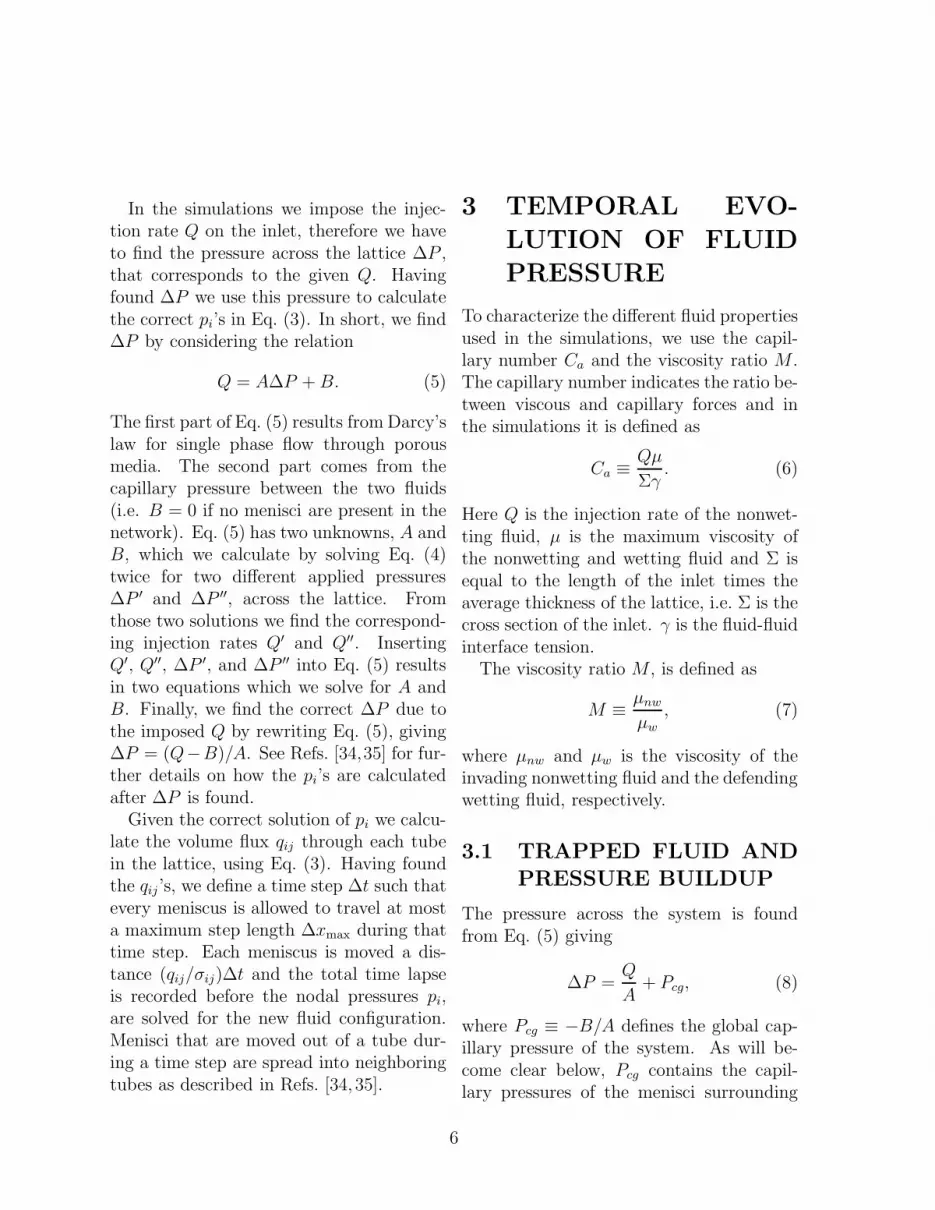
Figure 4: Pcf (a) and Pcg (b) as function ofinjection time at Ca = 3.5×10−4 and M =1.0×10−3. To avoid overlapping curves Pcg

was subtracted by 1000 dyn/cm2 before itwas normalized.

sideration. When M = 1 the effective vis-cosity µij, of each tube is independent ofthe amount of wetting and nonwetting fluidthat occupies the tube. Hence, each tubehas a constant mobility of kij/µij giving aconstant total resistance of the network.

At low Ca we approach the regime ofcapillary fingering and the viscous drag onthe clusters becomes negligible. Hence, Pcg

is no longer a linear function of the in-jection time, but reduces to that describ-ing the capillary pressure along the front.This is observed in Fig. 4 where we com-pare Pcg with the calculated average cap-illary pressure along the front, Pcf . Inthe simulations, Pcf is calculated by takingthe mean of the capillary pressures of thefront menisci. From the figure we see thatPcg ≃ Pcf , as expected. The big jumps inthe pressure functions in Fig. 4 are causedby the variations in the capillary pressure

as menisci move through the “hourglass”shaped tubes. The negative jumps are iden-tified as bursts where a meniscus proceedsabruptly [27, 29] to fill the tube with non-wetting fluid (see also Sec. 3.2 for furtherdetails).

From the above discussion we concludethat the behavior of Pcg at large times (t >ts) may be formulated as

Pcg = ∆mch + Pmf , (9)

where ∆mc is the proportionality factor be-tween Pcg and the average front position habove the inlet. ∆mc is given by the viscousdrag on the clusters and Pmf is the variationin the capillary pressure when the invasionfront covers new tubes. h is only defined af-ter the front has saturated, i.e. hs < h < L,where hs is the average front position at tsand L is the length of the system. Since theinjection rate is held fixed, h is proportionalto the injection time t. In the limit of verylow injection rates, ∆mc → 0.

When the average front position hasreached the outlet, i.e. h = L in Eq. (9),only invading fluid flows through the sys-tem and Pmf = 0. In this limit Darcy’s lawapplied on the nonwetting phase gives U =(Ke/µnw)(∆P/L), where Ke is the effec-tive permeability of the nonwetting phase.From Eqs. (8) and (9) we find that ∆P =Q/A+∆mcL, which inserted into the Darcyequation gives

Ke =µnw

1/σT + ∆mc/U. (10)

Here σT ≡ AL/Σ denotes the total con-ductivity of the lattice. Thus, we mightconsider the effective permeability of thenonwetting phase as a function of the con-ductivity of the lattice and an additional

8

term due to the viscous drag on the clus-ters (∆mc/U). Note that the U dependencyin Eq. (10) only indicates changes in ∆mc

between displacements executed at differentinjection rates. The behavior when the flowrate changes during a given displacement isnot discussed here.

3.2 BURST DYNAMICS

In the simulations a burst starts when thepressure drops suddenly and stops whenthe pressure has raised to a value abovethe pressure that initiated the burst (seeFig. 5). Thus, a burst may consist of alarge pressure valley containing a hierarchi-cal structure of smaller pressure jumps (i.e.bursts) inside. A pressure jump, indicatedas ∆p in Fig. 5, is the pressure differencefrom the point when the pressure starts de-creasing minus the pressure when it stopsdecreasing. We define the size of the pres-sure valley (valley size) to be χ ≡

∑i ∆pi,

where the summation index i runs over allthe pressure jumps ∆pi inside the valley.The definition is motivated by experimen-tal work in Ref. [28]. For slow displace-ments we have that χ is proportional to thegeometric burst size s, being invaded dur-ing the pressure valley. This statement hasbeen justified in Ref. [28], where it was ob-served that in stable periods, the pressureincreased linearly as function of the volumebeing injected into the system. Later, in anunstable period where the pressure dropsabruptly due to a burst, this pressure dropis proportional to s. At fast displacementsthe pressure may no longer be a linear func-tion of the volume injected into the system.Therefore, a better estimate of s there, isto compute the time period T of the pres-

315 320 325 330 335 340 345t (s)

1900

2100

2300

2500

2700

2900

3100

P(t)

(dy

n/cm

2 )

burst

∆p

t1t2

Figure 5: The pressure signal as function ofinjection time, P (t), for one simulation atlow displacement rate in a narrow time in-terval. The horizontal line defines the pres-sure valley of a burst that last a time periodT = t2 − t1. Note that the valley may con-tain a hierarchical structure of smaller val-leys inside. The vertical line indicates thesize of a local pressure jump ∆p inside thevalley.

sure valley (Fig. 5). Since the displacementsare performed with constant rate, it is rea-sonable to assume that T is always propor-tional to the volume being injected duringthe valley and hence, T ∝ s.

In Fig. 6 we have plotted the hierarchi-cal valley size distribution Nall(χ), for sixsimulations between low and high Ca withM = 1 and 100 on a lattice of 40 × 60 and25×35 nodes, respectively. Nall(χ) was cal-culated by including all valley sizes and thehierarchical smaller ones within a large val-ley (see Fig. 5). To obtain reliable averagequantities we did 10 to 20 different simula-tions at each Ca. In order to calculate the

9

1 2 3 4 5log10 χ

−6

−4

−2

0

log 10

[Nal

l(χ)/

Nal

l(10)

]

Ca=1.6×10−5

Ca=1.9×10−4

Ca=1.6×10−3

Ca=3.1×10−4

Ca=3.1×10−3

Ca=2.1×10−2

Figure 6: The hierarchical valley size distri-butions Nall(χ), for six simulations betweenlow and high Ca with M = 1 (◦ , ,⋄) andM = 100 (△ ,⊳ ,▽). The slope of the solidline is −1.9.

valley sizes at large Ca, we subtract the av-erage drift in the pressure signal due to vis-cous forces such that the pressure becomes afunction that fluctuates around some meanpressure.

By assuming a power law Nall(χ) ∝ χ−τall

our best estimate from Fig. 6 is τall = 1.9±0.1, indicated by the slope of the solid line.At low χ in Fig. 6, typically only one tubeis invaded during the valley and we do notexpect the power law to be valid. Similarresults were obtained when calculating thehierarchical distribution of the time periodsT of the valleys, denoted as Nall(T ).

In invasion percolation (IP) the distribu-tion of burst sizes N(s), where s denotesthe burst size, is found to obey the scalingrelation [27, 28, 39, 40]

N(s) ∝ s−τ ′

g(sσ(f0 − fc)). (11)

Here fc is the percolation threshold of thesystem and g(x) is some scaling function,which decays exponentially when x ≫ 1and is a constant when x → 0. τ ′ is re-lated to percolation exponents like τ ′ =1 + Df/D − 1/(Dν) [40], where Df and Dis the fractal dimension of the front and themass of the percolation cluster, respectively.ν is the correlation length exponent in per-colation theory and σ = 1/(νD) [41]. InEq. (11) a burst is defined as the connectedstructure of sites that is invaded followingone root site of random number f0, alongthe invasion front. All sites in the bursthave random numbers smaller than f0, andthe burst stops when the random numberof the next site to be invaded is larger thanf0 [42].

By integrating Eq. (11) over all f0 in theinterval [0, fc] Maslov [43] deduced a scal-ing relation for the hierarchical burst sizedistribution Nall(s) following

Nall(s) ∝ s−τall , (12)

where τall = 2.In the low Ca regime in Fig. 6, the dis-

placements are in the capillary dominatedregime and the invading fluid generates agrowing cluster similar to IP [4, 7–9]. Inthis regime we also have that χ ∝ s [28]and hence Nall(χ) corresponds to Nall(s) inEq. (12). Thus, in the low Ca regime we ex-pect that Nall(χ) follows a power law withexponent τall = 2 which is confirmed by ournumerical results. Similar results were ob-tained in Ref. [28].

The evidence in Fig. 6, that τall does notseem to depend on Ca, is very interesting.At high Ca when M = 0.01 an unstable vis-cous fingering structure generates and when

10

M ≥ 1 a stable front develops. It is an openquestion how these displacement processesmap to the proposed scaling in Eq. (12). Wenote that in the high Ca regime the relationχ ∝ s may not be correct and T is preferredwhen computing Nall. However, the simu-lations show that Nall(χ) ∼ Nall(T ) even athigh Ca.

In Ref. [43] τall was pointed out to besuper universal for a broad class of self-organized critical models including IP. Theresult in Fig. 6 indicates that the simulateddisplacements might belong to the same su-per universality class even at high injectionrates where there is no clear mapping be-tween the displacement process and IP.

Basak et al. [44,45] performed four drain-age experiments where they used a 110×180mm transparent porous model consistingof a mono-layer of randomly placed glassbeads of 1 mm, sandwiched between twoPlexiglas plates. The experimental setupwas similar to the one used in Ref. [27].The model was initially filled with a water-glycerol mixture of viscosity 0.17 P. Thewater-glycerol mixture was withdrawn fromone of the short side of the system at con-stant rate by letting air enter the systemfrom the other short side. The pressurein the water-glycerol mixture on the with-drawn side was measured with a pressuresensor of our own construction.

From the recorded pressure signal we cal-culated the hierarchical distribution of timeperiods of the valleys, Nall(T ). At low Ca

this corresponds to Nall(s) in Eq. (12). Be-cause of the relative long response time ofthe pressure sensor, rapid and small pres-sure jumps due to small bursts are presum-ably smeared out by the sensor and therecorded pressure jumps are only reliable

−3 −2 −1 0 1 2 3log10 [T/<T>]

−6

−4

−2

0

2

log 10

[Nal

l(T)/

<N

all(T

)>]

Ca=3.3×10−6

Ca=1.3×10−5

Ca=3.3×10−5

Ca=6.6×10−5

Ca=1.1×10−4

Ca=2.2×10−4

Ca=4.3×10−4

Ca=1.7×10−3

Figure 7: The hierarchical distributionNall(T ) of the valley time T during a burstfor experiments (open symbols) and simu-lations (filled symbols) at various Ca withM = 0.017 and M = 0.01, respectively.The slope of the solid line is −1.9.

for larger bursts. Hence, from the recordedpressure signal T appears to be a better es-timate of the burst sizes than χ.

In Fig. 7 we have plotted the logarithmof Nall(T ) for experiments (open symbols)and simulations (filled symbols) performedat four different Ca, respectively. To col-lapse the data Nall(T ) and T were nor-malized by their means. In the simula-tions M = 0.01 while in the experimentsM = 0.017 where we have assumed airto have viscosity 0.29×10−2 P. We observethat the experimental result is consistentwith our simulations and we conclude thatNall(T ) ∝ T 1.9±0.1. This confirms the scal-ing of Nall(χ) in Fig. 6.

From Figs. 6 and 7 we conclude thatτall = 1.9 ± 0.1 for all displacement sim-ulations going from low to high injection

11

rates when M = 0.01, 1, and 100. Thisis also confirmed by drainage experimentsperformed at various injection rates withM = 0.017. The evidence that τall is in-dependent of the injection rate, may indi-cate that the displacement process belongsto the same super universality class as theself-organized critical models in Ref. [43](τall = 2), even where there is no clear map-ping between the displacement process andIP.

4 STABILIZATION

MECHANISMS OF

THE FRONT

When the displacements are oriented out ofthe horizontal plane and the injection rate islow, gravity acting on the system, may sta-bilize the front due to density differences be-tween the fluids. Several authors [30,46–48]have confirmed, by experiments and sim-ulations, that the saturated front widthws scales with the strength of gravity likews ∝ Bo

−ν/(1+ν). Here Bo (Bond number)is the ratio between gravitational and capil-lary forces, given by Bo = ∆ρga2/γ, where∆ρ is the density difference between the flu-ids, g the acceleration due to gravity, a theaverage pore size, and γ the fluid-fluid in-terface tension. Furthermore, ν denotes thecorrelation length exponent in percolation.

A similar consensus concerning the sta-bilization mechanisms when the displace-ments are oriented within the horizontalplane, has not yet been reached. In hori-zontal displacements, viscous forces replacegravitational forces, and in the literaturethere exist different suggestions about the

scaling of ws as function of Ca. The capil-lary number Ca is the ratio between viscousand capillary forces according to the defi-nition in Eq. (6). In 3D, where trappingof wetting fluid is assumed to be of littleimportance, Wilkinson [30] was the first touse percolation to deduce a power law likews ∝ Ca

−α where α = ν/(1 + t − β + ν).Here t and β is the conductivity and orderparameter exponent in percolation, respec-tively. Later, Blunt et al. [32] suggested in3D that α = ν/(1 + t + ν). This is identi-cal to the result of Lenormand [31] findinga power law as function of system size forthe domain boundary in the Ca–M planebetween capillary fingering and stable dis-placement in 2D porous media.

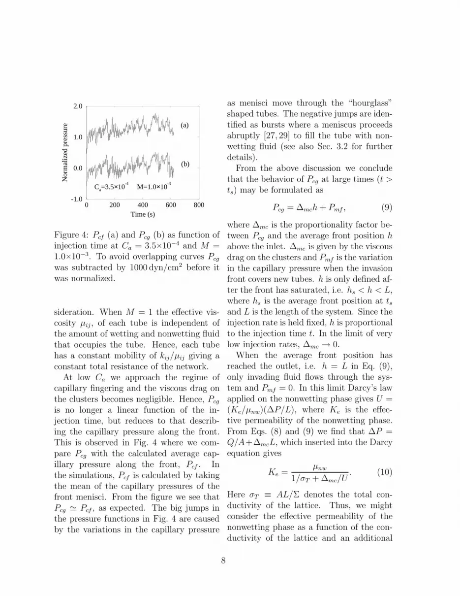
More recently, Xu et al. [33] used the ar-guments of Gouyet et al. [49] and Wilkin-son [30] to show that the pressure drop∆Pnw over a length ∆h in the nonwettingphase of the front should scale as ∆Pnw ∝

∆ht/ν+DE−1−β/ν (see Fig. 8). Here DE de-notes the Euclidean dimension of the spacein which the front is embedded, i.e. in ourcase DE = 2. The pressure drop in the wet-ting phase ∆Pw, was argued to be linearlydependent on ∆h due to the compact phasethere (Fig. 8). In Ref. [32] Blunt et al. alsosuggested a scaling relation for ∆Pnw, how-ever, in 3D they found ∆Pnw ∝ ∆ht/ν+1.This is different from the result of Xu et al.when DE = 3.

In the next section, Sec. 4.1, we presentan alternative view on the displacementprocess from those initiated by Wilkin-son [30], but include the evidence that non-wetting fluid flows in separate strands (seeFig. 9). The alternative view leads to an-other scaling of ∆Pnw than the one Xu etal. [33] would predict in 2D, and we show

12

∆h∆Pw

Front

Outlet

Inlet

∆P

Bwetting

non-wetting

A

nw

Figure 8: A schematic picture of the frontthat travels across the system from the in-let to the outlet. ∆Pnw and ∆Pw denote theviscous pressure drop going from A to B inthe nonwetting and wetting phase, respec-tively. A and B are separated a distance∆h along the short side of the system.

that it may influence α in the scaling be-tween ws and Ca. The new scaling of ∆Pnw

is supported by numerical experiments us-ing the network model.

4.1 LOOPLESS STRANDS

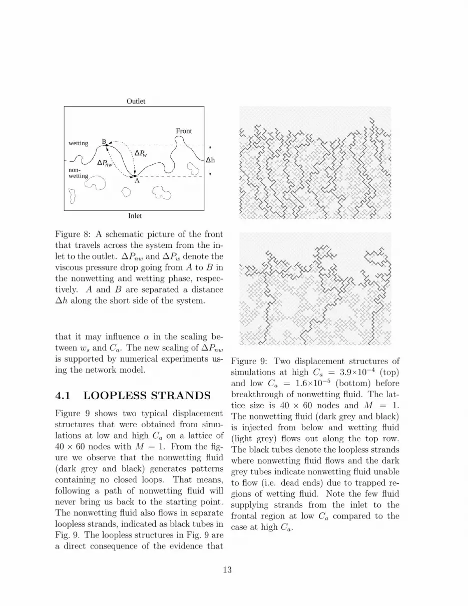
Figure 9 shows two typical displacementstructures that were obtained from simu-lations at low and high Ca on a lattice of40 × 60 nodes with M = 1. From the fig-ure we observe that the nonwetting fluid(dark grey and black) generates patternscontaining no closed loops. That means,following a path of nonwetting fluid willnever bring us back to the starting point.The nonwetting fluid also flows in separateloopless strands, indicated as black tubes inFig. 9. The loopless structures in Fig. 9 area direct consequence of the evidence that

Figure 9: Two displacement structures ofsimulations at high Ca = 3.9×10−4 (top)and low Ca = 1.6×10−5 (bottom) beforebreakthrough of nonwetting fluid. The lat-tice size is 40 × 60 nodes and M = 1.The nonwetting fluid (dark grey and black)is injected from below and wetting fluid(light grey) flows out along the top row.The black tubes denote the loopless strandswhere nonwetting fluid flows and the darkgrey tubes indicate nonwetting fluid unableto flow (i.e. dead ends) due to trapped re-gions of wetting fluid. Note the few fluidsupplying strands from the inlet to thefrontal region at low Ca compared to thecase at high Ca.

13

a tube filled with wetting fluid and sur-rounded on both sides by nonwetting fluid istrapped due to volume conservation of wet-ting fluid [50]. We note that this evidencemay easily be generalized to 3D, and there-fore our arguments should apply there too.We also note that trapping of wetting fluidis more difficult in real porous media dueto a more complex topology of pores andthroats there. Loopless IP patterns haveearlier been observed in Refs. [51–53].

From Fig. 9 we may separate the dis-placement patterns into two parts. Oneconsisting of the frontal region continuouslycovering new tubes, and the other consist-ing of the more static structure behind thefront. The frontal region is supplied bynonwetting fluid through a set of strandsthat connect the frontal region to the inlet.When the strands approach the frontal re-gion they are more likely to split. Since weare dealing with a square lattice, a splittingstrand may create either two or three newstrands. As the strands proceed upwards inFig. 9, they split repeatedly until the frontalregion is completely covered by nonwettingstrands.

On IP patterns without loops [51, 53, 54]the length l of the minimum path betweentwo points separated an Euclidean distanceR scales like l ∝ RDs where Ds is the frac-tal dimension of the shortest path. We as-sume that the displacement pattern of thefrontal region for length less than the cor-relation length (in our case ws) is statis-tically equal to IP patterns in Ref. [51].Therefore, the length of a strand in thefrontal region is proportional to ∆hDs when∆h is less than ws. If we assume that onthe average every tube in the lattice hassame mobility (kij/µij), this causes the fluid

pressure within a single strand to drop like∆hDs as long as the strand does not split.When the strand splits volume conserva-tion causes the volume fluxes through thenew strands to be less than the flux in thestrand before it splits. Hence, following apath where strands split will cause the pres-sure to drop as ∆hκ where κ ≤ Ds. FromFig. 9, we note that at high Ca the lengthsof individual strands in the frontal regionapproach the minimum length due to thetubes. Therefore, in this limit finite size ef-fects are expected to cause Ds → 1.

From the above arguments we concludethat the pressure drop ∆Pnw, in the nonwet-ting phase of the frontal region (that is thestrands) should scale as ∆Pnw ∝ ∆hκ whereκ ≤ Ds. In 2D two different values forDs have been reported: Ds = 1.22 [53, 54]for loopless IP with and without trappingand growing around a central seed, andDs = 1.14 [51] for the single strand con-necting the inlet to the outlet when non-wetting fluid percolates the system. In2D the result of Xu et al. [33] would giveκ = t/ν + DE − 1 − β/ν ≈ 1.9 where wehave inserted t = 1.3, ν = 4/3, β = 5/36,and DE = 2. This result for κ is largerthan Ds and therefore not compatible withour arguments.

To confirm numerically that κ ≤ Ds,we have calculated the difference in cap-illary pressure ∆Pc between menisci alongthe front by using our network model. ∆Pc

as function of ∆h is calculated by takingthe mean of the capillary pressure differ-ences between all pairs of menisci along thefront, separated a distance ∆h in the direc-tion of the displacement. ∆Pc of a pair ofmenisci is calculated by taking the capillarypressure of the meniscus closest to the inlet

14

0 10 20 30∆h (in units of tube length)

0

200

400

600

800

1000

∆Pc (

dyn/

cm2 )

Ca=1.5×10−3

, M=100Ca=3.7×10

−4, M=100

Ca=1.6×10−5

, M=1

Figure 10: ∆Pc as function of ∆h for threedifferent Ca’s with M = 100 and 1 on lat-tices of 25 × 35 and 40 × 60 nodes, respec-tively.

minus the capillary pressure of the meniscusclosest to the outlet.

Figure 10 shows ∆Pc as function of ∆hfor simulations performed at high, interme-diate and low Ca, with M = 1 or 100. Thesimulations with M = 100 were performedon a 25 × 35 nodes lattice with µnw = 10P, µw = 0.10 P, and γ = 30 dyn/cm.The disorder was introduced by choosingthe tube radii at random in the interval0.05d ≤ rij ≤ d. The tube length wasd = 0.1 cm. The simulations with M = 1were performed on a distorted lattice of40 × 60 nodes where 0.02 cm ≤ dij ≤ 0.18cm and rij = dij/2α with α = 1.25. Hereµnw = µw = 0.5 P. We did 10–30 simu-lations at each Ca to obtain reliable aver-age quantities. From the plot we observethat ∆Pc increases roughly linearly as func-tion of ∆h. The simulations also show that∆Pc ≃ ∆Pnw−∆Pw and that ∆Pw depends

linearly on ∆h due to the compact wettingphase there (see Fig. 8). Hence our sim-ulations give that ∆Pnw ∼ ∆Pc ∝ ∆hκ

where κ ≃ 1.0. This supports the argu-ments giving κ ≤ Ds, and we conclude thatearlier proposed theories [30–33] which donot consider the evidence that nonwettingfluid flows in strands, are incompatible withdrainage when strands are important.

To save computation time and thereby beable to study ∆Pc on larger lattices in thelow Ca regime, we have generated bond in-vasion percolation (IP) patterns with trap-ping on lattices of 200 × 300 nodes. Thebonds in the IP lattice correspond to thetubes in the network model. The occupa-tion of bonds started at the bottom row,and the next bond to be occupied wasalways the bond with the lowest randomnumber f from the set of empty bonds alongthe invasion front. We applied a small gra-dient in the random numbers of the bondsto stabilize the front [30, 47].

When the IP patterns became well de-veloped with trapped (wetting) clusters ofsizes between the bond length and the frontwidth, the tubes in our network model werefilled with nonwetting and wetting fluid ac-cording to occupied and empty bonds inthe IP lattice. Furthermore, the radii rof the tubes were mapped properly to therandom numbers f of the bonds by first re-moving the gradient in f and then assigningr = 1 − f [36]. The last transformation isnecessary because in the IP algorithm thenext bond to be invaded is the one with thelowest random number, opposite to the net-work model, where the widest tube will beinvaded first.

Having initialized the tube network, thenetwork model was started and the simu-

15

lations were run a limited number of timesteps while recording ∆Pc. The number oftime steps where chosen sufficiently largeto let the menisci along the front adjustaccording to the viscous pressure set upby the injection rate. By this method wesave the computation time that would havebeen required if the displacement patternsshould have been generated by the networkmodel instead of the much faster IP algo-rithm. However, to make this method self-consistent we have to assume that the IPpatterns are statistically equal to the corre-sponding structures that would have beengenerated by the network model.

Totally, we generated four IP patternswith different sets of random numbers andevery pattern was loaded into the networkmodel. The result of the calculated ∆Pc

versus ∆h is shown in Fig. 11 for Ca =9.5×10−5 and M = 100. If we assumea power law ∆Pc ∝ ∆hκ, we find κ =1.0 ± 0.1. The slope of the straight line inFig. 11 is 1.0. We have also calculated ∆Pc

for Ca = 2×10−6 with M = 1 and M = 100by using one of the generated IP patterns.The result of those simulations is consistentwith Fig. 11 which indeed show the similarbehavior as the results in Fig. 10.

An important issue, arising at low Ca, isthe effect of bursts on the capillary pres-sure. A burst occurs when a meniscus alongthe front becomes unstable and nonwettingfluid abruptly covers new tubes [28]. Thetube where the burst initiates will duringthe burst, experiences a much higher fluidtransport relative to tubes far away. De-scribing the pressure behavior between thetube of the burst and the rest of the front isnontrivial. However, simulations show thateven during bursts, we find that ∆Pc in-

0 1 2 3log10(∆h)

0

0.5

1

1.5

2

2.5

log 10

(∆P c)

Figure 11: The logarithm of ∆Pc as func-tion of the logarithm of ∆h for simulationsinitiated on IP patterns at Ca = 9.5×10−5

and M = 100. The slope of the solid line is1.0.

creases linearly with ∆h.The evidence that κ ≃ 1.0 may influence

the exponent α in ws ∝ Ca−α. Assum-

ing Darcy flow where the pressure drop de-pends linearly on the injection rate, we con-jecture that ∆Pc ∝ Ca∆hκ. Here ∆Pc de-notes the capillary pressure difference overa height ∆h when the front is stationary.That means, ∆Pc excludes situations wherenonwetting fluid rapidly invades new tubesdue to local instabilities (i.e. bursts). Theabove conjecture is supported by simula-tions showing that in the low Ca regime∆Pc ∝ Ca∆hκ where κ ≃ 1.0. Note, that∆Pc 6≃ ∆Pc in Fig. 10 since the latter in-cludes both stable situations and bursts.

At sufficiently low Ca where only thestrength of the capillary pressure decideswhich tube should be invaded or not, wemay map the displacement process to per-

16

colation giving ∆Pc ∝ f−fc ∝ ξ−1/ν [30,47,49]. Here f is the random numbers in thepercolation lattice, fc is the critical percola-tion threshold, and ξ ∝ ws is the correlationlength. Combining the above relations for∆Pc gives ws ∝ Ca

−α where α = ν/(1+νκ).In 2D ν = 4/3 and by inserting κ = 1.0 weobtain α ≈ 0.57. Note that this is differ-ent to results suggested in Refs. [30, 32, 33]giving α ≈ 0.37–0.38 in 2D.

At high Ca the nonwetting fluid is foundto invade simultaneously everywhere alongthe front, and consequently the front neverreaches a stationary state [36]. In this limitsimulations show a nonlinear dependencybetween ∆Pc and Ca. Therefore, in the highCa regime it is not clear if the above map-ping to percolation is valid, and we expectanother type of relation between ws and Ca.

4.2 COMPARISON WITH

EXPERIMENTS

Frette et al. [55] have performed two-phase drainage experiments in a 2D porousmedium with viscosity matched fluids(M = 1). They reported on the stabi-lization of the front and measured the sat-urated front width ws, as function of Ca.Their best estimate on the exponent inws ∝ Ca

−α was α = 0.6 ± 0.2. This isconsistent with the above conjecture (α =0.57), however, corresponding simulationson 40×60 nodes lattices give α = 0.3±0.1.Figure 12 contains the data of Frette etal. (filled circles) and the result of oursimulations (open diamonds). The simu-lations are performed at Ca ≥ 1.0×10−5

while most of the experiments where doneat Ca ≤ 1.0×10−5. Since the range of the

−7 −6 −5 −4 −3 −2log10(Ca)

0

0.5

1

1.5

2

log 10

(ws)

ExperimentsSimulations

Figure 12: log10(ws) as function of log10(Ca)for experiments from [55] and simulationson the lattice of 40 × 60 nodes. In bothexperiments and simulations M = 1. Theslope of the solid and dashed line is -0.6 and-0.3, respectively.

two does not overlap it is difficult to com-pare the result of the simulations with thoseof the experiments. However, the changein α from 0.6 to 0.3, might be consistentwith a crossover to another behavior at highCa according to the discussion in Sec. 4.1.We also note, that in the simulations atCa ≃ 1.0×10−5, the front width approachesthe maximum width due to the system size,making it difficult to observe any possibleα ≈ 0.57 regime at low Ca. We emphasizethat more simulations on larger systems andat lower Ca are needed before any conclu-sion on α can be drawn.

4.3 DISCUSSION

The evidence that the nonwetting fluid dis-places the wetting fluid in a set of loopless

17

strands opens new questions about the dis-placement process. Returning to Fig. 9 itis striking to observe the different patternsof strands at high and low Ca. At low Ca

few strands are supplying the frontal regionwith nonwetting fluid, and the strands splitmany times before the whole front is cov-ered. At high Ca the horizontal distancebetween each strand in the static structureis much shorter, and only a few splits arerequired to cover the front. We conjecturethat the average horizontal distance be-tween the fluid supplying strands dependson the front width. However, further inves-tigation of the displacement patterns is re-quired before any conclusions can be drawn.

So far the arguments in Sec. 4.1 only con-sider displacements where the nonwettingstrands contain no loops. A very interestingquestion that has to be answered is: Whathappens to κ when different strands in thefront connect to generate loops. In ordinarybond or site percolation loops generally oc-cur. Loops are also observed in experimentscorresponding to those of Frette et al. [55].In the experiments it is more difficult totrap wetting fluid due to the more complextopology of pores and throats (see Fig. 1).Consequently, loops will more easily gen-erate there, than in the case of a regularsquare lattice. Loops might also be createdwhen neighboring menisci along the frontoverlap and coalesce depending on the wet-ting properties of the nonwetting fluid [5,6].

As a first approximation we conjecturethat creation of loops will not cause κ tochange significantly. Note that in the frontthe different nonwetting strands connectingto each other to create loops, must at somelater time split. Otherwise successive con-nections will cause the different strands to

coalesce into one single strand of nonwet-ting fluid. Moreover, after the front widthhas saturated, the number of places wheredifferent strands connect must on averagebe balanced by the number of places wherestrands split. Therefore, we believe thatthe influence on κ due to connections (i.e.loops) will be compensated by the splits andthe overall behavior of κ will remain thesame. We emphasize that further simula-tions and experiments are required to in-vestigate the effect of loops on κ.

According to the discussion in Sec. 4.3,the evidence that the displacement patternsconsist of loopless strands may easily begeneralized to 3D. Therefore our argumentsgiving κ ≤ Ds, might be valid in 3D aswell. Note also that in 3D it is less proba-ble that different strands meet. Hence, evenif they were supposed to connect to createloops, the number of created loops are ex-pected to be few. In 3D the fractal dimen-sion of the shortest path for loopless IP isDs = 1.42 [53].

5 CONCLUSION

We conclude that our 2D network modelproperly simulates the temporal evolutionof the pressure in the fluids during drainage.We have seen that capillary forces situ-ated around isolated and trapped regions ofwetting fluid, contribute to the total pres-sure across the lattice, as well as the capil-lary fluctuations due invasion of nonwettingfluid along the front.

We have found that the model reproducesthe typical burst dynamics at low injectionrates and we have investigated the statis-tics of the bursts by calculating the hierar-

18

chical valley size distribution Nall(χ). Weconclude that Nall(χ) follows a power law,Nall(χ) ∝ χ−τall where τall = 1.9 ± 0.1 isindependent of the injection rate and vis-cosity ratio. Similar result is obtained fromexperiments. At low injection rates theresult is consistent with the prediction inRef. [43] (τall = 2), which was deduced fora broad spectrum of different self-organizedcritical models including IP. The evidencethat τall is independent of the injection rate,may indicate that the displacement pro-cess belongs to the same super universalityclass as the self-organized critical models inRef. [43], even where there is no clear map-ping between the displacement process andIP.

We have also simulated the behavior ofthe capillary pressure along the front. Sim-ulations show that the capillary pressuredifference ∆Pc between two points alongthe front varies almost linearly as functionof distance ∆h in the direction of the dis-placement. The numerical result supportsarguments based on the observation thatnonwetting fluid flows in separate strandswhere wetting fluid is displaced. From thearguments we find that ∆Pc ∝ ∆hκ whereκ ≤ Ds. Here Ds denotes the fractal dimen-sion of the nonwetting strands.

Several attempts have been made todescribe the stabilization mechanisms indrainage due to viscous forces, however,none of them consider the evidence thatnonwetting fluid displaces wetting fluidthrough strands. Therefore, we concludethat earlier suggested theories fail to de-scribe the stabilization of the invasion frontwhen strands dominate the displacements.

ACKNOWLEDGMENTS

E. Aker and A. Hansen wish to thank theNiels Bohr Institute and the Nordic Insti-tute for Theoretical Physics for their hospi-tality. The work has received support fromthe Norwegian Research Council through a“SUP” program and from the Niels BohrInstitute.

REFERENCES

[1] J.-D. Chen and D. Wilkinson, Phys.Rev. Lett. 55, 1892 (1985).

[2] K. J. Maløy, J. Feder, and T. Jøssang,Phys. Rev. Lett. 55, 2688 (1985).

[3] R. Lenormand, E. Touboul, andC. Zarcone, J. Fluid Mech. 189, 165(1988).

[4] R. Lenormand and C. Zarcone, Phys.Rev. Lett. 54, 2226 (1985).

[5] M. Cieplak and M. O. Robbins, Phys.Rev. Lett. 60, 2042 (1988).

[6] M. Cieplak and M. O. Robbins, Phys.Rev. B. 41, 11508 (1990).

[7] P. G. de Gennes and E. Guyon, J. Mec.(Paris) 17, 403 (1978).

[8] R. Chandler, J. Koplik, K. Lerman,and J. F. Willemsen, J. Fluid Mech.119, 249 (1982).

[9] D. Wilkinson and J. F. Willemsen, J.Phys. A 16, 3365 (1983).

[10] I. Fatt, Petroleum Trans. AIME 207,144 (1956).

19

[11] J. Koplik and T. J. Lasseter, SPEJournal 22, 89 (1985).

[12] M. M. Dias and A. C. Payatakes, J.Fluid Mech. 164, 305 (1986).

[13] P. R. King, J. Phys. A 20, L529 (1987).

[14] M. Blunt and P. King, Phys. Rev. A42, 4780 (1990).

[15] M. Blunt and P. King, Transp. PorousMedia 6, 407 (1991).

[16] P. C. Reeves and M. A. Celia, WaterResour. Res. 32, 2345 (1996).

[17] G. N. Constantinides and A. C. Pay-atakes, AIChE Journal 42, 369 (1996).

[18] E. W. Pereira, W. V. Pinczewski,D. Y. C. Chan, L. Paterson, and P. E.Øren, Transp. Porous Media 24, 167(1996).

[19] D. H. Fenwick and M. J. Blunt. In proc.of the SPE Annual Tech. Conf., SPE38881, San Antonio, Texas, U.S.A.,Oct. 1997.

[20] P. E. Øren, S. Bakke, and O. J.Arntzen. In proc. of the SPE AnnualTech. Conf., SPE 38880, San Antonio,Texas, U.S.A., Oct. 1997.

[21] S. C. van der Marck, T. Matsuura, andJ. Glas, Phys. Rev. E 56, 5675 (1997).

[22] D. H. Fenwick and M. J. Blunt, Adv.Water Res. 21, 121 (1998).

[23] H. K. Dahle and M. A. Celia, Comp.Geosci. 3, 1 (1999).

[24] L. Paterson, Phys. Rev. Lett. 52, 1621(1984).

[25] T. A. Witten and L. M. Sander, Phys.Rev. Lett. 47, 1400 (1981).

[26] K. J. Maløy, F. Boger, J. Feder, andT. Jøssang, Phys. Rev. A 36, 318(1987).

[27] K. J. Maløy, L. Furuberg, J. Feder, andT. Jøssang, Phys. Rev. Lett. 68, 2161(1992).

[28] L. Furuberg, K. J. Maløy, and J. Feder,Phys. Rev. E 53, 966 (1996).

[29] W. B. Haines, J. Agric. Sci. 20, 97(1930).

[30] D. Wilkinson, Phys. Rev. A 34, 1380(1986).

[31] R. Lenormand, Proc. R. Soc. London,Ser. A 423, 159 (1989).

[32] M. Blunt, M. J. King, and H. Scher,Phys. Rev. A 46, 7680 (1992).

[33] B. Xu, Y. C. Yortsos, and D. Salin,Phys. Rev. E 57, 739 (1998).

[34] E. Aker, K. J. Maløy, A. Hansen, andG. G. Batrouni, Transp. Porous Media32, 163 (1998).

[35] E. Aker, K. J. Maløy, and A. Hansen,Phys. Rev. E 58, 2217 (1998).

[36] E. Aker, K. J. Maløy, and A. Hansen,Phys. Rer. E 61, 2936 (2000).

[37] E. W. Washburn, Phys. Rev. 17, 273(1921).

20

[38] G. G. Batrouni and A. Hansen, J. Stat.Phys. 52, 747 (1988).

[39] B. Sapoval, M. Rosso, and J. F.Gouyet. In Fractals’ Physical Ori-gin and Properties, edited by L.Pietronero, Plenum Press, New York,1989.

[40] N. Martys, M. O. Robbins, andM. Cieplak, Phys. Rev. B. 44, 12294(1991).

[41] D. Stauffer and A. Aharony. Introduc-tion to Percolation Theory. Taylor &Francis, London, 1992.

[42] S. Roux and E. Guyon, J. Phys. A:Math. Gen. 22, 3693 (1989).

[43] S. Maslov, Phys. Rev. Lett. 74, 562(1995).

[44] S. Basak and K. J. Maløy. Unpub-lished, 1996.

[45] E. Aker, K. J. Maløy, A. Hansen,and S. Basak. Burst dynamics dur-ing drainage displacements in porousmedia: Simulations and experiments.Accepted in Euro. Phys. Lett., 2000.

[46] D. Wilkinson, Phys. Rev. A 30, 520(1984).

[47] A. Birovljev, L. Furuberg, J. Feder, T.Jøssang, K. J. Maløy, and A. Aharony,Phys. Rev. Lett. 67, 584 (1991).

[48] P. Meakin, A. Birovljev, V. Frette, J.Feder, T. Jøssang, K. J. Maløy, and A.Aharony, Physica A 191, 227 (1992).

[49] J.-F. Gouyet, M. Rosso, and B. Sapo-val, Phys. Rev. B 37, 1832 (1988).

[50] E. Aker, K. J. Maløy, and A. Hansen,Phys. Rev. Lett. 84, 4589 (2000).

[51] M. Sahimi, M. Hashemi, and J. Ghas-semzadeh, Physica A 260, 231 (1998).

[52] H. Kharabaf and Y. C. Yortsos, Phys.Rev. E 55, 7177 (1997).

[53] M. Cieplak, A. Maritan, and J. R.Banavar, Phys. Rev. Lett. 76, 3754(1996).

[54] M. Porto, S. Havlin, S. Schwarzer, andA. Bunde, Phys. Rev. Lett. 79, 4060(1997).

[55] O. I. Frette, K. J. Maløy, J. Schmit-tbuhl, and A. Hansen, Phys. Rev. E.55, 2969 (1997).

21