nonlinear oscillations of viscous liquid drops

J . Fluid Me&. (1992), vol. 241, pp. 16S198

Printed in Great Britain

169

Nonlinear oscillations of viscous liquid drops

By OSMAN A. BASARAN Chemical Technology Division, Oak Ridge National Laboratory, Oak Ridge, TN 37831, USA

(Received 27 February 1991 and in revised form-26 December 1991)

A fundamental understanding of nonlinear oscillations of a viscous liquid drop is needed in diverse areas of science and technology. In this paper, the moderate- to large-amplitude axisymmetric oscillations of a viscous liquid drop, which is immersed in dynamically inactive surroundings, are analysed by solving the free boundary problem comprised of the Navier-Stokes system and appropriate interfacial conditions at the dropambient fluid interface. The means are the Galerkin/finite- element technique, an implicit predictor-corrector method, and Newton’s method for solving the resulting system of nonlinear algebraic equations. Attention is focused here on oscillations of drops that are released from an initial static deformation. Two dimensionless groups govern such nonlinear oscillations : a Reynolds number, Re, and some measure of the initial drop deformation. Accuracy is attested by demonstrating that (i) the drop volume remains virtually constant, (ii) dynamic response to small- and moderate-amplitude disturbances agrees with linear and perturbation theories, and (iii) large-amplitude oscillations compare well with the few published predictions made with the marker-and-cell method and experiments. The new results show that viscous drops that are released from an initially two-lobed configuration spend less time in prolate form than inviscid drops, in agreement with experiments. Moreover, the frequency of oscillation of viscous drops released from such initially two-lobed configurations decreases with the square of the initial amplitude of deformation as Re gets large for moderate-amplitude oscillations, but the change becomes less dramatic as Re falls and/or the initial amplitude of deformation rises. The rate at which these oscillations are damped during the first period rises as initial drop deformation increases ; thereafter the damping rate is lower but remains virtually time- independent regardless ofRe or the initial amplitude of deformation. The new results also show that finite viscosity has a much bigger effect on mode coupling phenomena and, in particular, on resonant mode interactions than might be anticipated based on results of computations incorporating only an infinitesimal amount of viscosity.

1. Introduction Oscillations of liquid drops play a central role in diverse areas of science and

technology, e.g. in cloud physics (Beard, Ochs & Kubesh 1989), in various mass transfer operations of chemical engineering (Basaran, Scott & Byers 1989), and in containerless processing in low gravity (Carruthers & Testardi 1983). Unfortunately, as discussed below, previous theoretical work on oscillations of drops having arbitrary viscosity is restricted almost exclusively to small-amplitude motions and that on nonlinear oscillations is virtually limited to motions of drops of inviscid or slightly viscous liquids. A goal of this paper is to remedy this situation.

The system of interest is a free drop of incompressible, Newtonian liquid which is oscillating in dynamically inactive surroundings, i.e. a vacuum or a gas of

170 0. A . Basaran

- IT

Ambient fluid

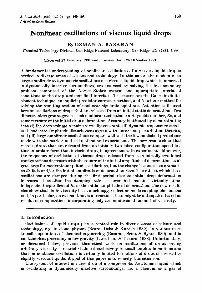
FIQURE 1 . A liquid drop oscillating in a vacuum or a gas of negligible density and viscosity: ( a ) definition sketch and ( 6 ) computational domain.

negligible density and viscosity, as shown in figure 1 (a ) . The drop has an undisturbed radius R, viscosity p, and density p, and the surface tension of the liquid/gas interface is CT. The starting points for theoretical analysis of drop oscillations are the statements of mass and momentum conservation, i.e. the continuity and Navier-Stokes equations : -

V . 6 = 0, (1)

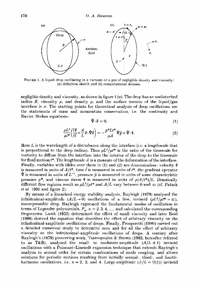
Here L is the wavelength of a disturbance along the interface (i.e. a lcngthscale that is proportional to the drop radius). Thus pL2/pt* is the ratio of the timescale for vorticity to diffuse from the interface into the interior of the drop to the timescale for fluid motion t*. The lengthscale A is a measure of the deformation of the interface. Finally, variables with tildes over them in ( 1 ) and (2) are dimensionless: velocity 5 is measured in units of A / t * , time [is measured in units oft*, the gradient operator

is measured in units of L-l, pressure 9 is measured in units of some characteristic pressure p*, and viscous stress ? is measured in units of p(A/ t* ) /L . Drastically different flow regimes result as pL2/,ut* and AIL vary between 0 and co (cf. Patzek et aE. 1991 and figure 2).

By means of a linearized encrgy stability analysis, Rayleigh (1879) analysed the infinitesimal-amplitude (AIL -+ 0) oscillations of a free, inviscid (pL2/pt* + a), incompressible drop. Rayleigh expressed the fundamental modes of oscillation in terms of Legendre polynomials, Pn, n = 2 , 3 , 4 , . . . , and calculated the corresponding frequencies. Lamb (1932) determined the effect of small viscosity and later Reid (1960) derived the equation that describes the effect of arbitrary viscosity on the infinitesimal-amplitude oscillations of drops. Finally, Prosperetti (1980) carried out a detailed numerical study to determine once and for all the effect of arbitrary viscosity on the infinitesimal-amplitude oscillations of drops. A century after Rayleigh's ( 1879) pioneering work, Tsamopoulos & Brown ( 1983, hereafter referred to as T&B), analysed the small- to moderate-amplitude ( A I L 1) inviscid oscillations with a Poincark-Linstedt, expansion technique that extends Rayleigh's analysis to second order for certain combinations of mode coupling, and allows solutions for periodic motions resulting from initially second-, third-, and fourth- harmonic oscillations, i.e. n = 2, 3, and 4. Largc-amplitude (AIL = O ( 1 ) ) inviscid

Nonlinear oscillations of viscous liquid drops 171

coI I r---- 1

I I I I

oscillation I (quasi-static deformation)

I I I I

1 1 I I I I

I

r---- 1r- - - - - 1 I I

I I1

I I I1

I I I1

IMansour (1988) I I Mansour (1988) I I I1 I

I I r - i I I1

I I I I

I Lundgren & I I Lundgren &

I I IPatzek er al. (1991)

0 1

Ratio of timescales, pLz/pt*

FIGURE 2. A liquid drop oscillating in a vacuum or a gas of negligible density and viscosity: previous work and opportunities for analysis.

oscillations were recently studied by Lundgren & Mansour (1988, hereafter referred to as L&M), and Patzek et al. (1991). L&M employed a boundary-integral method and focused on high-frequency (n 2 4) drop oscillations. Patzek et al. (1991) employed the Galerkin/finite-element method and focused on low-frequency oscillations. L&M also extended their method to account for the effects of an ‘infinitesimal ’ amount of viscosity on drop oscillations. However, by its nature and as pointed out by L&M, the boundary-integral method cannot model nonlinear drop oscillations when viscous effects are ‘large ’.

The perturbation analysis of T&B predicts, among other things, a decrease in frequency with increasing amplitude of oscillation. The predicted frequency shift of the second mode is in excellent agreement with the finite-element calculations of Patzek et al. (1991). Experiments of Trinh & Wang (1982), performed with acoustically levitated drops of low viscosity that were nearly neutrally buoyant in the surrounding liquid, and the few numerical simulations made with the marker- and-cell (MAC) method by Foote (1973), Alonso (1974) and Alonso, LeBlanc & Wilson (1982), of the axisymmetric oscillations of viscous liquid drops that are surrounded by a dynamically inactive environment, show systematic deviations from the inviscid predictions. Unfortunately, the small number of MAC calculations available is inadequate to draw general and quantitative conclusions on the effects of viscosity on finite-amplitude drop oscillations. Supplying this missing insight is another goal of this paper.

The MAC method is complicated: it requires computations on a pair of finite- difference grids, one fixed and one moving (Harlow 1963). Nevertheless, Harlow, Amsden & Nix (1976) and Nix & Strottman (1982) have extended the MAC analysis

172 0. A . Basaran

to fluid motions in three dimensions. Because of its complexity, the MAC method cannot compete in computational efficiency with, for example, finite-element (see e.g. Gresho, Lee & Sani 1979) or spectral (see e.g. Orszag 1980) methods. Hence, in the past decade, MAC methods for solving free-surface flow problems have been superseded by both boundary-integral methods when they are applicable and finite- element and finite-difference methods in general (cf. Kistler & Scriven 1983; Tsamopoulos 1989, Patzek et al. 1991).

Therefore, in this paper, a simple and flexible method based on the Galerkin/finite- element method is employed for studying large-amplitude oscillations of axisymmetric, viscous free drops. The method features simultaneous solution of mass and momentum conservation equations for the velocity and pressure fields and free- surface location. The present method grew out of methods developed for simulation of steady (Saito & Scriven 1981 ; Kist,ler & Scriven 1983) and unsteady (Kheshgi & Scriven 1983) viscous free-surface film flows and inviscid drop oscillations (Patzek et al. 1991).

Section 2 presents the theory and formulation of the governing equations. Section 3 summarizes the Galerkin/finite-element weighted residuals and outlines the method for solving the transient problem. Section 4 present new results for moderate- and large-amplitude oscillations of axisymmetric drops and compares them, when possible, to previous investigations.

2. Mathematical formulation The system is a drop of a Newtonian, incompressible liquid of volume V bounded

by a free surface S(t) that separates the liquid from a fluid that exerts uniform pressure and negligible viscous drag on the drop. Variables and equations that follow are made dimensionless by measuring length in units of R and time in units of (pR3/cr)4. Also, tildes are suppressed hereafter for simplicity.

In spherical polar coordinates ( r , 8, @) with the origin a t the centre-of-mass of the drop, the axisymmetric drop shape and the field of outward-pointing unit normals to the drop surface are, respectively,

fe, - f o eo n, = (f z+ f ;);' (4)

where f(8,t) is the interface shape function, (er,eo,e,) are the unit vectors in the coordinate directions and fo = af/aO - see figure 1 ( b ) .

The fluid motion satisfies the Navier-Stokes system

V . u = O in V , ( 5 )

Re - + v V v = V - T in V. (E * ) I n (6), the Reynolds number Re = (1 /u ) (crR/p)i, where u = p/p, and the stress tensor of a Newtonian fluid T = - p / + [ V v + (Vu)'], where I is the identity tensor. Furthermore, in (6) and throughout this paper, the effects of gravitational forces are taken to be negligible compared to those due to viscous, inertial, and surface forces.

At the drop/ambient fluid interface, the dynamically inactive exterior phase exerts negligible shear and virtually hydrostatic pressure, which is taken to be the


pressure datum. Then, the traction boundary condition, which expresses momentum conservation, is

n,. T = Re (2H) n, on 8(t), (7)

where 2H(x,, t ) , twice the local mean curvature of 8(t), is given by the negative of the surface divergence V, of the outward unit normal n, to s(t) (Weatherburn 1927), i.e. 2H(x,, t ) = -V,-n, .

The drop shape is of course unknown a priori, but is a material surface provided there is no mass transfer across it. The kinematic condition is then simply

n, - (u -u , ) = 0 on s(t). In ( 8 a ) o and us are the velocities of points located in V and on 8(t), respectively. Equivalently, the kinematic condition (8a ) can be restated in terms of the interface shape function f(8, t ) as

D - [ r - f (O, t ) ] = 0 on 8(t), Dt

where D/Dt is the material derivative. Equation (8a), or ( 8 b ) , is not treated as a boundary condition, but instead is used to determine the unknown location of the interface (cf. Saito & Scriven 1981 ; Kistler & Scriven 1983; Kheshgi & Scriven 1983).

Additionally, because the drop oscillations considered are axisymmetric,

fo = 0 at 8 = O,x, n ’ . u = O on S’,

n’t’:T = 0 on S,

where n’ and t‘ are unit vectors that are perpendicular and parallel to the axis of symmetry S’ (figure l b ) .

We seek oscillatory solutions of the nonlinear, time-dependent partial differential equations (5)-(6) subject to boundary conditions (7)-( 11) . Initial conditions must be specified to complete the mathematical statement of the problem. In this paper, attention is restricted to situations in which the drops are released from an initial static deformation

S(0) = So, (12)

u(x, 0) = 0, p ( x , 0) = 0, (13)

where X E V. Such an initial condition is realized in experiments by means of acoustic and/or electric fields (see e.g. Trinh & Wang 1982; Scott, Basaran & Byers 1990). Two types of initial drop shapes are considered here. The first is a prolate or an oblate spheroid

(14)

where a is the length of the semi-major axis of the spheroid and b is the length of its semi-minor axis. The two dimensionless axis lengths are so related that ab2 = 1 , because the dimensional volume of the spheroidal drop is equal to that of a spherical drop of radius R. The second is a drop shape whose departure from a sphere is proportional to the nth spherical harmonic

f(e,O)=y,[l+f,P,(cose)] for O G O G K , n = 2 , 3 ,... ~ (15)

174 0. A . Basaran

where f, is the amplitude of the initial deformation. The multiplicative factor y,, is a function off, and ensures that drops subjected to different initial deformations all enclose the same dimensional volume 3 R 3 (or dimensionless volume $n). Thus

for n = 2, 35

"' = 35+ 21f + 2f: ' I

for n = 3, y3 =

for n = 4, 3003

y4 = 3003 + 1001f: + 54f:

for n = 5. 11

Y 6 = m

Spherical harmonics corresponding to n = 0 and 1 are not considered because the n = 0 mode violates the constraint that the drop volume remains fixed and the n = 1 mode moves the centre-of-mass of the drop. Also, disturbances of large n are not used here because a finite basis set is incapable of representing them accurately.

The oscillations of liquid drops considered in this paper are therefore governed by two parameters : (i) a Reynolds number, Re, and (ii) some measure of the initial drop deformation. For spheroidal deformations, a convenient measure of the initial deformation is the prolate aspect ratio a/b, or its reciprocal the oblate aspect ratio b/a. Henceforward, aspect ratio will stand for prolate aspect ratio unless otherwise stated. For spherical harmonic deformations, a convenient measure of the initial deformation is the disturbance amplitude f,. Moreover, for second-spherical- harmonic deformations, it is sometimes useful to present results in terms of a/b instead off, ; in this case a/b = (1 +f,)/( 1 -if,).

3. Galerkinlfinite-element analysis Conservation equations (5)-(6) are solved in this paper by the Galerkin/finite-

element method in the mixed interpolation sense (see e.g. Huyakorn et al. 1978). The Galerkin weighted residuals of the continuity equation ( 5 ) and momentum equations (6) are

R,,,=Jv$*V.udV=O, i = l , ..., M ,

Rt,* = pie) = /v#'ek- [Reg+u-Vu)-V.T]dV= 0, i = 1, ..., N , (21) R I ~ r

where ek is either er or e,. Here M is the number of finite-element basis functions @. used in representing the pressure

and N is the number of finite-element basis functions q5' used in representing the velocity


In (23) u and v represent the 8- and r-components of the velocity, respectively. Residuals of the kinematic condition (8) weighted by a set of basis functions $*(8), that is a subset of the set of basis functions $#(r ,8 ) , furnish the additional NB equations needed to determine the drop shape :

r

The free surface is represented as

The p,, ut, vi and ft are the unknown coefficients. The residuals of the momentum equations can be simplified by (a) applying the

divergence theorem to the stress terms in (21) and (b) incorporating into the resulting expression as natural boundary conditions the traction boundary conditions (7) and (1 1) along the drop surface and the axis of symmetry :

2H($'e,).ndS = 0, i = 1, ..., N . (26)

The surface divergence theorem specialized to a closed surface (Weatherburn 1927),

2H($'e,).n d8 = V,. ($*e,) ds, (27 ) -Js I, is then applied to the curvature term in (26). For an axisymmetric surface, it can be shown, using relations found in standard textbooks on vectors and tensors (see e.g. Aris 1962), that

where = d$*/d9. The drop volume V = ((8, r ) : 0 < 9 < x , 0 < r < j (9 , t ) } is partitioned or tessellated

into a set of No x Nr quadrilateral elements. The elements are bordered by the j k e d spines (Kistler & Scriven 1983) 92t-l

( i - 1) x e2r-1 = - , i = 1 ,..., No+l, No

which move proportionally to the free surface along the spines. In this paper, the

176 0. A . Basaran

spines are uniformly spaced coordinate lines and the weights wZi-, are to be defined shortly, Equations (30) and (31) prescribe the positions of only the vertex nodes of the elements. Mid-side and mid-element nodes are located by rcquiring mid-element spines to satisfy O,, = i(82t-1 + 02i+1), i = 1, . . . , N*, and by requiring the weights to satisfy wzj = i(w,,-, + ~ ~ , + ~ ) , j = 1, . . ., N,..

The Galerkin weighted residuals of the continuity equation (20), the momentum equations (26) with (27)-(29), and the kinematic condition (24) require continuity of the basis functions that represent the dependent variables (Strang & Fix 1973) ; thus we choose admissible Co basis functions. In the current mixed-interpolation formulation, nine-node biquadratic basis functions are used for the velocity field and four-node bilinear ones are used for the pressure field. The free surface is interpolated in terms of the standard set of three one-dimensional, quadratic basis functions.

The Galerkin/finite-element weighted residuals are a large set of nonlinear ordinary differential equations in time. Time derivatives are discretized at the pth time step, At = t, - t,-,, by either first-order backward-differences or second-order trapezoid rule. With time discretization in place, the resulting system of nonlinear algebraic equations is solved by Newton iteration. Initial conditions specified need not satisfy the governing equations and boundary conditions exactly. Four backward-difference time steps with fixed At, provide the necessary smoothing (Luskin & Rannacher 1982) before the trapezoid rule is used. A first-order forward-difference predictor is used with the backward-difference method. A second-order Adams-Bashforth predictor is used with the trapezoid rule. The L , norm of the correction provided by Newton iteration, Jldp+lllm, is an estimate of the local time truncation error of the trapezoid rule (Gresho et al. 1979). The time step is chosen adaptively by requiring the norm of time truncation error a t the next time step to be equal to a prescribed value, e (Gresho et al. 1979),

P

Atp+, = A~&/l l~ ,+1I lm)~. (32)

Relative error of 0.1 YO per time step, e = The algorithm was programmed in FORTRAN and the resulting code was run on a

Cray X-MP/4 supercomputer and an IBM 6000-320H workstation at the Oak Ridge National Laboratory and a Cray Y-MP/4 supercomputer a t the Florida State University (FSU) Computer Center with Hood’s (1976) frontal solver, as modified and improved by Silliman (1979), Walters (1980), Kheshgi & Scriven (1983), and Coyle ( 1984).

is prescribed here.

4. Results The computations were carried out by dividing the drop into a set ofN, = 8, 12, or

16 uniformly spaced elements in the &direction and N, = 4, 6 , 8 , or 12 uniformly and non-uniformly spaced elements in the r-direction. Table 1 shows the meshes used, the number of unknowns for each mesh, and typical computation times. For the meshes that contained elements that were non-uniformly spaced in the r-direction, the element sizes in the r-direction formed an arithmetic progression: along a spine of fixed 8, the length of the side along the r-direction of the N t h element from the drop surface wasf(0, t) times N/;(N,(N, .+ l)) , A’ = 1, ..., N,.. Because quadratic elements were used, the ratio of the radial distance measured along a spine between a node on the free surface and the one closest to it in the interior of the drop, Ar, to the distance from the origin to the drop surface, f(0, t ) , was &for mesh IIIB and for mesh IVB.

Tables 2 and 3 show the sensitivity of calculated solutions to mesh refinement (cf.


CPU Mesh No N, N, Nu time

I 8 4 32 368 1.0 I1 12 6 72 766 2.7 I11 16 8 128 1308 5.5

IIIB 16 8 128 1308 5.5 I V 16 12 192 1904 11.1

IVB 16 12 192 1904 11.1

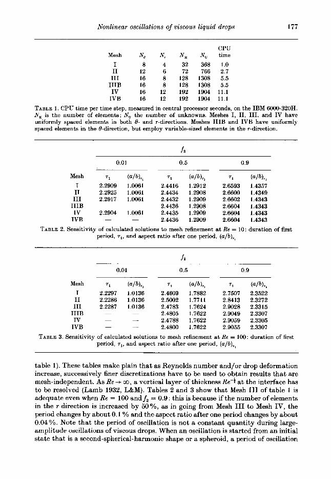
TABLE 1. CPU time per time step, measured in central processor seconds, on the IBM 6000-320H. N , is the number of elements; Nu the number of unknowns. Meshes I, 11, 111, and I V have uniformly spaced elements in both 0- and r-directions. Meshes IIIB and IVB have uniformly spaced elements in the @-direction, but employ variable-sized elements in the r-direction.

0.01

Mesh 71 (alb),l I 2.2909 1.0061 I1 2.2925 1.0061 I11 2.2917 1.0061

IV 2.2904 1.0061 IIIB

IVB

- -

- -

0.5

71 (alb),l 2.4416 1.2912 2.4434 1.2908 2.4432 1.2909 2.4436 1.2908 2.4435 1.2909 2.4436 1.2909

0.9

71 (alb),l 2.6593 1.4357 2.6600 1.4349 2.6602 1.4343 2.6604 1.4343 2.6604 1.4343 2.6604 1.4343

TABLE 2. Sensitivity of calculated solutions to mesh refinement at Re = 10: duration of first period, 71, and aspect ratio after one period, ( ~ / b ) , ~

0.01 0.5

Mesh 71 (a/b),l I 2.2297 1.0136 I1 2.2286 1.0136 I11 2.2287 1.0136

IITB IV

IVB -

- -

- -

-

71 (alb)TI 2.4609 1.7882 2.5002 1.7711 2.4783 1.7624 2.4805 1.7622 2.4788 1.7622 2.4800 1.7622

0.9

71 (alb)71 2.7507 2.3522 2.8413 2.3272 2.9028 2.3315 2.9049 2.3307 2.9059 2.3305 2.9055 2.3307

TABLE 3. Sensitivity of calculated solutions to mesh refinement at Re = 100: duration of first period, 71, and aspect ratio after one period, (alb),,

table 1 ) . These tables make plain that as Reynolds number and/or drop deformation increase, successively finer discretizations have to be used to obtain results that are mesh-independent. As Re-+ co, a vortical layer of thickness Re-: at the interface has to be resolved (Lamb 1932, L&M). Tables 2 and 3 show that Mesh I11 of table 1 is adequate even when Re = 100 and fi = 0.9 : this is because if the number of elements in the r-direction is increased by 50Y0, as in going from Mesh I11 to Mesh IV, the period changes by about 0.1 YO and the aspect ratio after one period changes by about 0.04 YO. Note that the period of oscillation is not a constant quantity during large- amplitude oscillations of viscous drops. When an oscillation is started from an initial state that is a second-spherical-harmonic shape or a spheroid, a period of oscillation

178 0. A . Basaran

Re = 10 Re = 100

~ F E 73 (‘/6)r,FE E ~ F E 7 E ( W , , F E W),~ E

2.2904 - 1.0061 - 2.2287 2.2218 1.0136 1.0135

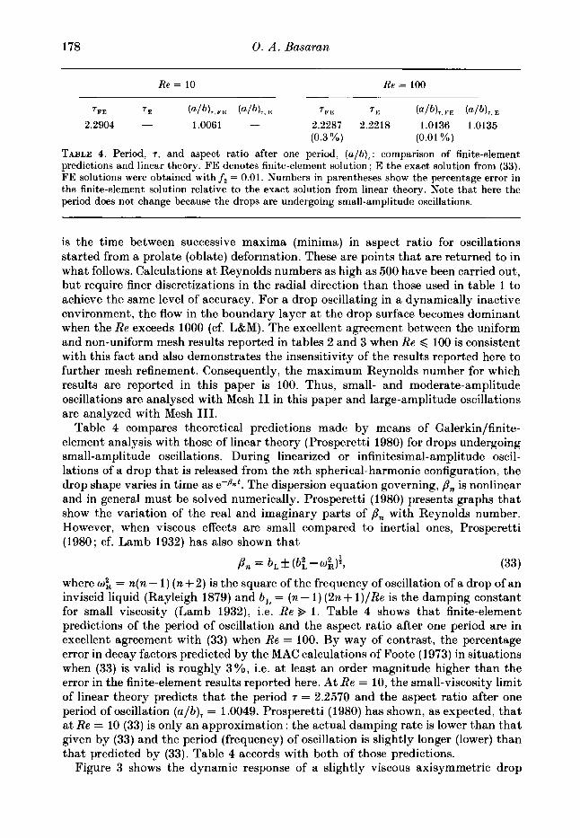
TABLE 4. Period, 7, and aspect ratio after one period, (alb),: comparison of finite-element predictions and linear theory. FE denotes finite-element solution; E the exact solution from (33). FE solutions were obtained with f i = 0.01. Numbers in parentheses show the percentage error in the finite-element solution relative to the exact solution from linear theory. Kote that here the period does not change because the drops are undergoing small-amplitude oscillations.

(0.3 Yo) (0.01 Yo)

is the time between successive maxima (minima) in aspect ratio for oscillations started from a prolate (oblate) deformation. These are points that are returned to in what follows. Calculations a t Reynolds numbers as high as 500 have been carried out, but require finer discretizations in the radial direction than those used in table 1 to achieve the same level of accuracy. For a drop oscillating in a dynamically inactive environment, the flow in the boundary layer a t the drop surface becomes dominant when the Re exceeds 1000 (cf. L&M). The excellent agreement between the uniform and non-uniform mesh results reported in tables 2 and 3 when Re Q 100 is consistent with this fact and also demonstrates the insensitivity of the results reported here to further mesh refinement. Consequently, the maximum Reynolds number for which results are reported in this paper is 100. Thus, small- and moderate-amplitude oscillations are analysed with Mesh I1 in this paper and large-amplitude oscillations are analyzed with Mesh 111.

Table 4 compares theoretical predictions made by means of Galerkin/finite- element analysis with those of linear theory (Yrosperetti 1980) for drops undergoing small-amplitude oscillations. During linearized or infinitesimal-amplitude oscillations of a drop that is released from the nth spherical-harmonic configuration, the drop shape varies in time as e-flnt. The dispersion equation governing, p, is nonlinear and in general must be solved numerically. Prosperetti (1980) presents graphs that show the variation of the real and imaginary parts of p, with Reynolds number. However, when viscous effects are small compared to inertial ones, Prosperetti (1980; cf. Lamb 1932) has also shown that

where wk = n(n- 1) (n + 2) is the square of the frequency of oscillation of a drop of an inviscid liquid (Rayleigh 1879) and b , = (n- 1 ) (2n+ l)/Re is the damping constant for small viscosity (Lamb 1932), i.e. Re 9 1. Table 4 shows that finite-element predictions of the period of oscillation and the aspect ratio after one period are in excellent agreement with (33) when Re = 100. By way of contrast, the percentage error in decay factors predicted by the MAC calculations of Foote (1973) in situations when (33) is valid is roughly 3%, i.e. a t least an order magnitude higher than the error in the finite-element results reported here. At Re = 10, the small-viscosity limit of linear theory predicts that the period 7 = 2.2570 and the aspect ratio after one period of oscillation (a /b) , = 1.0049. Prosperetti (1980) has shown, as expected, that a t Re = 10 (33) is only an approximation : the actual damping rate is lower than that given by (33) and the period (frequency) of oscillation is slightly longer (lower) than that predicted by (33). Table 4 accords with both of those predictions.

Figure 3 shows the dynamic response of a slightly viscous axisymmetric drop


-2 - 1 :/01 t 1.198 I

k I

1.624

101

- 2 - 1 0 1 2 - 2 - 1 0 1 2 - 2 - 1 0 I 2 - 2 - 1 0 1 2 - 2 - 1 0 1 2 - 2 - 1 0 1 2

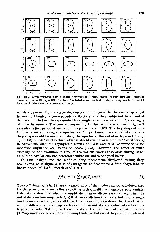
FIGURE 3. Drop released from a static deformation. Initial shape : second (prolate)-spherical harmonic; Re = 100, fa = 0.9. The time t is listed above each drop shape in figures 3, 6, and 20 because the time step is chosen adaptively.

which is released from a static deformation proportional to the second-spherical harmonic. Plainly, large-amplitude oscillations of a drop subjected to an initial deformation that can be represented by a single pure mode, here n = 2, show signs of other harmonics. The time corresponding to the last shape shown in figure 3 exceeds the first period of oscillation by approximately 10 YO. The drop shape at time t = 0 is re-entrant along the equator, i.e. 0 = in. Linear theory predicts that the drop shape would be re-entrant along the equator at the end of each period, t = 71, T ~ , . . . , Figure 3 shows that this feature is absent during large-amplitude oscillations, in agreement with the asymptotic results of T&B and MAC computations for moderate-amplitude oscillations of Foote (1973). However, the effect of finite viscosity on the evolution in time of the various modes that arise during large- amplitude oscillations was heretofore unknown and is analysed below.

To gain insight into the mode-coupling phenomena displayed during drop oscillations, as in figure 3, it is advantageous to decompose a drop shape into its linear modes (cf. L&M, Patzek et al. 1991):

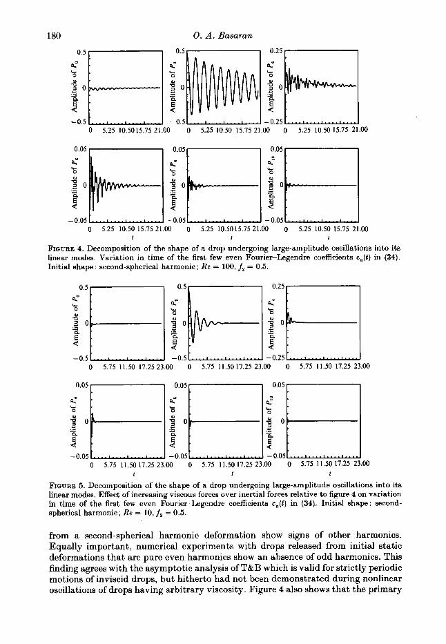
The coefficients c,( t ) in (34) are the amplitudes of the modes and are calculated here by Gaussian quadrature, after exploiting orthogonality of Legendre polynomials. Calculations show that when the amplitude of the oscillations is small, e.g. when the initial deformation amplitude f n < 0.01, an oscillation that is started from a single mode remains virtually so for all time. By contrast, figure 4 shows that the situation is quite different when a drop is released from an initial static deformation having a large amplitude. Not only is there a shift in the frequency of oscillation of the primary mode (see below), but large-amplitude oscillations of drops that are released

180

0.5

4' - 8 . a 0-

d . -0.5

' r .

* - . .- i ? .

.... I .... I . . . . I . . . .

0. A . Basaran

0.5

c .- Q E d - 0.25

4

8 a 0

d -0.5

b 0

c .- - 2

0.05

4' L

- 3 0 * .- - E d

-0.05 - * . I . . . . . 1 . . . .

0.05 +?Fl[jj $ 0 e .d - Q

d E d

-0.05 - 0.05

0 5.75 11.50 17.25 23.00 0 5.75 11.5017.25 23.00 0 5.75 11.50 17.25 23.00

0.05

b : ~l(;~~r; a

Q Q

u .- - u 3 0

z .- - * .- - d d 4

-0.05 -0.05 - 0.05 0 5.75 11.50 17.25 23.00 0 5.75 11.50 17.25 23.00 0 5.75 11.50 17.25 2

t r r

FIQURE 5. Decomposition of the shape of a drop undergoing large-amplitude oscillations into its linear modes. Effect of increasing viscous forces over inertial forces relative to figure 4 on variation in time of the first few even Fourier-Legendre coefficients c,( t ) in (34). Initial shape: seeond- spherical harmonic ; Re = 10, fi = 0.5.

from a second-spherical harmonic deformation show signs of other harmonics. Equally important, numerical experiments with drops released from initial static deformations that are pure even harmonics show an absence of odd harmonics. This finding agrees with the asymptotic analysis of T&B which is valid for strictly periodic motions of inviscid drops, but hitherto had not been demonstrated during nonlinear oscillations of drops having arbitrary viscosity. Figure 4 also shows that the primary


-2.5

0

-2.5

-2.5

-2.5 -2.5 0 2.5 -2.5 0 2.5-2.5 0 2.5 -2.5 0 2.5 -2.5 0 2.5 -2.5 0 2.5

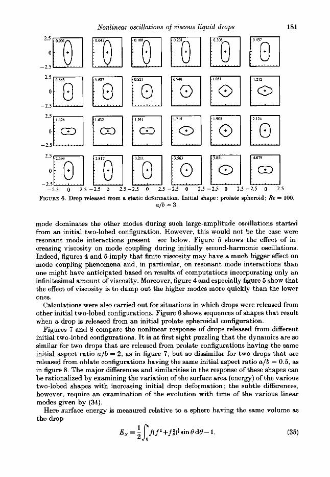
FIGURE 6. Drop released from a static deformation. Initial shape : prolate spheroid ; Re = 100, a/b = 3.

mode dominates the other modes during such large-amplitude oscillations started from an initial two-lobed configuration. However, this would not be the case were resonant mode interactions present -see below. Figure 5 shows the effect of increasing viscosity on mode coupling during initially second-harmonic oscillations. Indeed, figures 4 and 5 imply that finite viscosity may have a much bigger effect on mode coupling phenomena and, in particular, on resonant mode interactions than one might have anticipated based on results of computations incorporating only an infinitesimal amount of viscosity. Moreover, figure 4 and especially figure 5 show that the effect of viscosity is to damp out the higher modes more quickly than the lower ones.

Calculations were also carried out for situations in which drops were released from other initial two-lobed configurations. Figure 6 shows sequences of shapes that result when a drop is released from an initial prolate spheroidal configuration.

Figures 7 and 8 compare the nonlinear response of drops released from different initial two-lobed configurations. It is at first sight puzzling that the dynamics are so similar for two drops that are released from prolate configurations having the same initial aspect ratio a lb = 2, as in figure 7 , but so dissimilar for two drops that are released from oblate configurations having the same initial aspect ratio a/b = 0.5, as in figure 8. The major differences and similarities in the response of these shapes can be rationalized by examining the variation of the surface area (energy) of the various two-lobed shapes with increasing initial drop deformation ; the subtle differences, however, require an examination of the evolution with time of the various linear modes given by (34).

Here surface energy is measured relative to a sphere having the same volume as the drop

182 0. A . Basaran

0 4 8 12 16 20 24

FIUURE 7. Dynamic response of prolate drops having slightly different initial shapes : one released from a static deformation proportional to the second-spherical harmonic, f, = 0.5 (-), and the other from a prolate spheroidal configuration, a/6 = 2 (----) ; Re = 100.

t

0 4 8 12 16 20 24

FIUURE 8. Dynamic response of oblate d r o p having slightly different initial shapes : one released from a static deformation proportional to the second-spherical harmonic,f, = -0.4 (-), and the other from an oblate spheroidal configuration, a/6 = 0.5 (----) ; Re = 100.

t

Equation (35) is already dimensionless because energy is measured in units of 47cuR2. For small deformations, i.e. e < 1, where E = (a /b) - 1 for prolate shapes and 8 = @/a) - 1 for oblate shapes, i t is easy to show that

E, = &e2+pe3+ ... . (36) For the initial shapes considered, p = -% for a prolate second-spherical harmonic shape, ,!3 = -a for an oblate second-spherical harmonic shape, p = -& for a


1.00 1.25 1.50 1.75 2.00 2.25 2.50 2.75 3.00 Maximum prolate (oblate) aspect ratio, a / b (b/a)

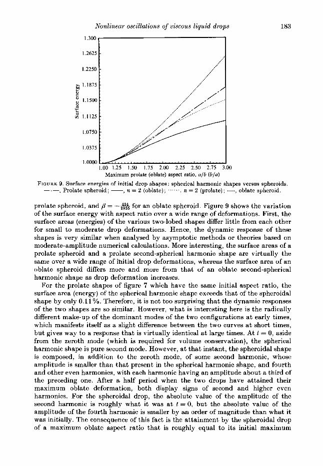
FIGURE 9. Surface energies of initial drop shapes : spherical harmonic shapes versus spheroids. , Prolate spheroid ; -, n = 2 (oblate) ; ......, 12 = 2 (prolate) ; ----, oblate spheroid.

prolate spheroid, and /3 = --* for an oblate spheroid. Figure 9 shows the variation of the surface energy with aspect ratio over a wide range of deformations. First, the surface areas (energies) of the various two-lobed shapes differ little from each other for small to moderate drop deformations. Hence, the dynamic response of these shapes is very similar when analysed by asymptotic methods or theories based on moderate-amplitude numerical calculations. More interesting, the surface areas of a prolate spheroid and a prolate second-spherical harmonic shape are virtually the same over a wide range of ihitial drop deformations, whereas the surface area of an oblate spheroid differs more and more from that of an oblate second-spherical harmonic shape as drop deformation increases.

For the prolate shapes of figure 7 which have the same initial aspect ratio, the surface area (energy) of the spherical harmonic shape exceeds that of the spheroidal shape by only 0.11 %. Therefore, it is not too surprising that the dynamic responses of the two shapes are so similar. However, what is interesting here is the radically different make-up of the dominant modes of the two configurations at early times, which manifests itself as a slight difference between the two curves at short times, but gives way to a response that is virtually identical a t large times. At t = 0, aside from the zeroth mode (which is required for volume conservation), the spherical harmonic shape is pure second mode. However, at that instant, the spheroidal shape is composed, in addition to the zeroth mode, of some second harmonic, whose amplitude is smaller than that present in the spherical harmonic shape, and fourth and other even harmonics, with each harmonic having an amplitude about a third of the preceding one. After a half period when the two drops have attained their maximum oblate deformation, both display signs of second and higher even harmonics. For the spheroidal drop, the absolute value of the amplitude of the second harmonic is roughly what it was at t = 0, but the absolute value of the amplitude of the fourth harmonic is smaller by an order of magnitude than what it was initially. The consequence of this fact is the attainment by the spheroidal drop of a maximum oblate aspect ratio that is roughly equal to its initial maximum

184 0. A . Basaran

(4

n / \ r 0 2 4 6 8 10 12 14 16

t

LI (b ) 8 0.14

2 4 6 8 10 12 14 16 t

0 2 4 6 8 10 12 14 16 t

h - v 4-1.0 l'::

0 2 4 6 8 10 12 14 16 t

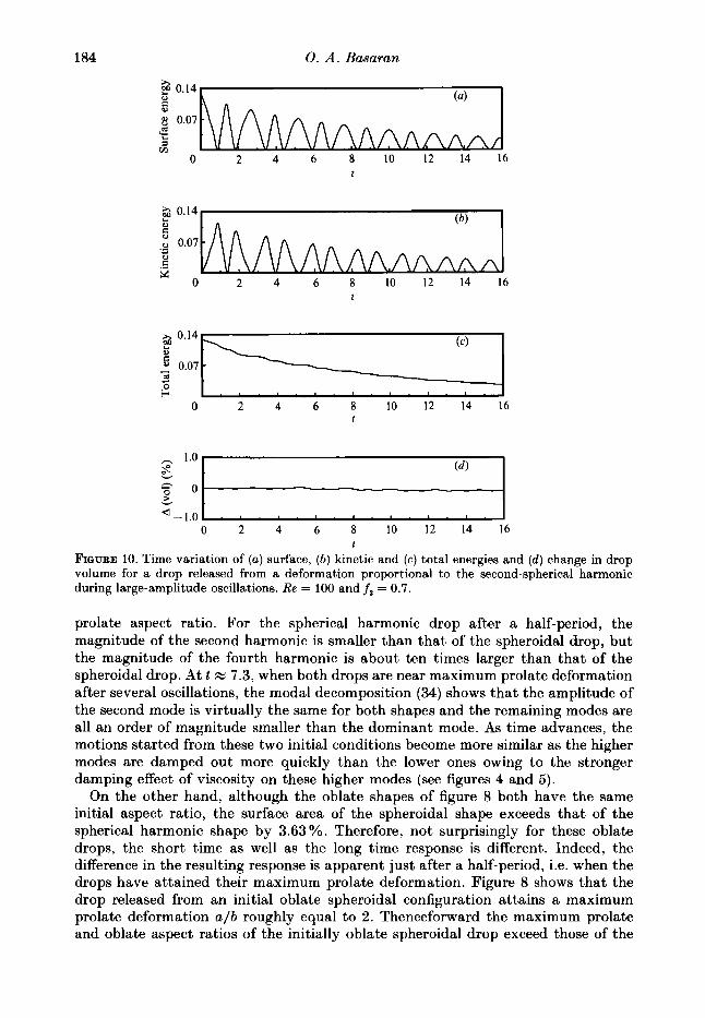
FIGURE 10. Time variation of (a) surface, (6) kinetic and (c) total energies and (d ) change in drop volume for a drop released from a deformation proportional to the second-spherical harmonic during large-amplitude oscillations. Re = 100 and fi = 0.7.

prolate aspect ratio. For the spherical harmonic drop after a half-period, the magnitude of the second harmonic is smaller than that of the spheroidal drop, but the magnitude of the fourth harmonic is about ten times larger than that of the spheroidal drop. At t x 7.3, when both drops are near maximum prolate deformation after several oscillations, the modal decomposition (34) shows that the amplitude of the second mode is virtually the same for both shapes and the remaining modes are all an order of magnitude smaller than the dominant mode. As time advances, the motions started from these two initial conditions become more similar as the higher modes are damped out more quickly than the lower ones owing to the stronger damping effect of viscosity on these higher modes (see figures 4 and 5 ) .

On the other hand, although the oblate shapes of figure 8 both have the same initial aspect ratio, the surface area of the spheroidal shape exceeds that of the spherical harmonic shape by 3.63 YO. Therefore, not surprisingly for these oblate drops, the short time as well as the long time response is different. Indeed, the difference in the resulting response is apparent just after a half-period, i.e. when the drops have attained their maximum prolate deformation. Figure 8 shows that the drop released from an initial oblate spheroidal configuration attains a maximum prolate deformation a/b roughly equal to 2. Thenceforward the maximum prolate and oblate aspect ratios of the initia.lly oblate spheroidal drop exceed those of the


1.0 1.5 2.0 2.5 3.0 3.5 Maximum prolate aspect ratio, 4 6

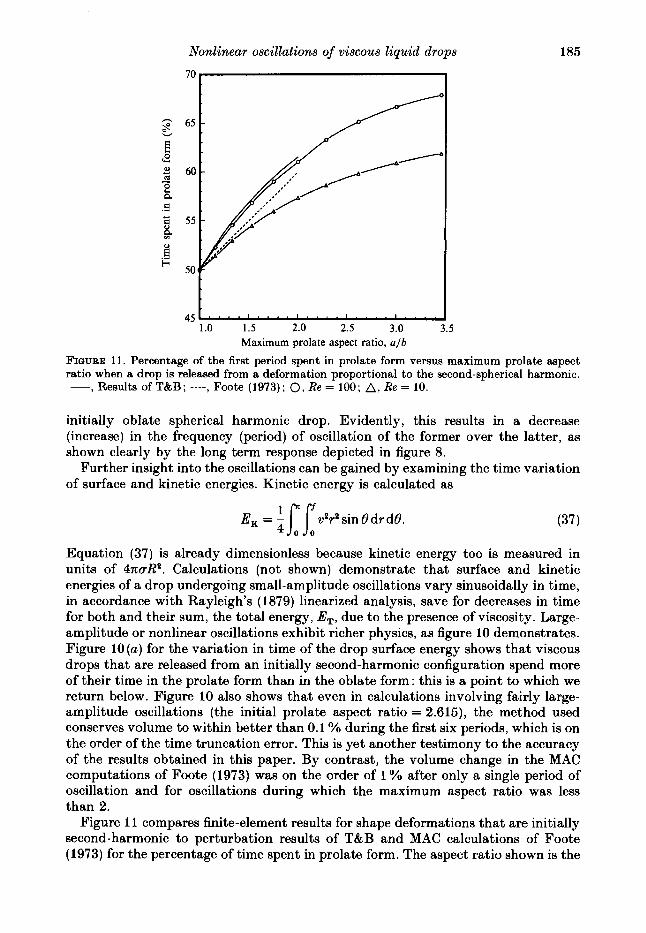
FIUTJRE 11. Percentage of the first period spent in prolate form versus maximum prolate aspect ratio when a drop is released from a deformation proportional to the second-spherical harmonic. -, Results of T&B; ----, Foote (1973); 0 , Re = 100; A, Re = 10.

initially oblate spherical harmonic drop. Evidently, this results in a decrease (increase) in the frequency (period) of oscillation of the former over the latter, as shown clearly by the long term response depicted in figure 8.

Further insight into the oscillations can be gained by examining the time variation of surface and kinetic energies. Kinetic energy is calculated as

E , = 1 Lv ' r ' sin 8 dr do. (37)

Equation (37) is already dimensionless because kinetic energy too is measured in units of 47rcR'. Calculations (not shown) demonstrate that surface and kinetic energies of a drop undergoing small-amplitude oscillations vary sinusoidally in time, in accordance with Rayleigh's (1879) linearized analysis, save for decreases in time for both and their sum, the total energy, E,, due to the presence of viscosity. Large- amplitude or nonlinear oscillations exhibit richer physics, as figure 10 demonstrates. Figure 10 ( a ) for the variation in time of the drop surface energy shows that viscous drops that are released from an initially second-harmonic configuration spend more of their time in the prolate form than in the oblate form : this is a point to which we return below. Figure 10 also shows that even in calculations involving fairly large- amplitude oscillations (the initial prolate aspect ratio = 2.615), the method used conserves volume to within better than 0.1 Yo during the first six periods, which is on the order of the time truncation error. This is yet another testimony to the accuracy of the results obtained in this paper. By contrast, the volume change in the MAC computations of Foote (1973) was on the order of 1 % after only a single period of oscillation and for oscillations during which the maximum aspect ratio was less than 2.

Figure 11 compares finite-element results for shape deformations that are initially second-harmonic to perturbation results of T&B and MAC calculations of Foote (1973) for the percentage of time spent in prolate form. The aspect ratio shown is the

186 0. A . Basaran

1.8 i

I .6

1.4

; 1.2

1 .o

0.8

0.6 0 4 8 12 16 20 24 28 32

t

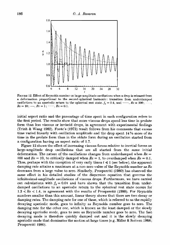
FIQLJRE 12. Effect of Reynolds number on large-amplitude oscillations when a drop is released from a deformation proportional to the second-spherical harmonic : transition from underdamped oscillations to an aperiodic return to the spherical rest state. f, = 0.4, and -, Re = 1 0 0 ; ---, Re = 10; ____,Re = 1; ...... , Re = 0.1.

initial aspect ratio and the percentage of time spent in each configuration refers to the first period. The results show that more viscous drops spend less time in prolate form than less viscous or inviscid drops, in agreement with experimental findings (Trinh & Wang 1982). Foote’s (1973) result follows from his comments that excess time varied linearly with oscillation amplitude and the drop spent 14% more of its time in the prolate form than in the oblate form during an oscillation started from a configuration having an aspect ratio of 1.7.

Figure 12 shows the effect of increasing viscous forces relative to inertial forces on large-amplitude drop oscillations that are all started from the same initial deformation. The nature of the oscillations changes from underdamped when Re = 100 and Re = 10, to critically damped when Re = 1, to overdamped when Re = 0.1. Thus, perhaps with the exception of very early times t < 1 (see below), the apparent damping rate attains a maximum at a non-zero value of the Reynolds number as Re decreases from a large value to zero. Similarly, Prosperetti (1980) has observed the same effect in his detailed studies of the dispersion equation that governs the infinitesimal-amplitude oscillations of viscous drops. Furthermore, we have carried out calculations with fi = 0.01 and have shown that the transition from underdamped oscillations to an aperiodic return to the spherical rest state occurs for 1.3 < Re < 1.4, in agreement with the results of Prosperetti (1980). For Reynolds numbers smaller than this amount, linear theory shows that there are two decay or damping rates. The damping rate for one of these, which is referred to as the rapidly decaying aperiodic mode, goes to infinity as Reynolds number goes to zero. The damping rate for the other one, which is known as the least damped or the slowly decaying aperiodic mode, goes to zero as Reynolds number goes to zero. The fast decaying mode is therefore quickly damped out and it is the slowly decaying aperiodic mode that dominates the motion a t large times (e.g. Miller & Scriven 1968; Prosperetti 1980).

Nonlinear oscillations of viscous liquid drops

2.00 I

187

1.75

I .so

- h

1.25

1 .oo

0.75

0.50 0 4 8 12 16 20 24

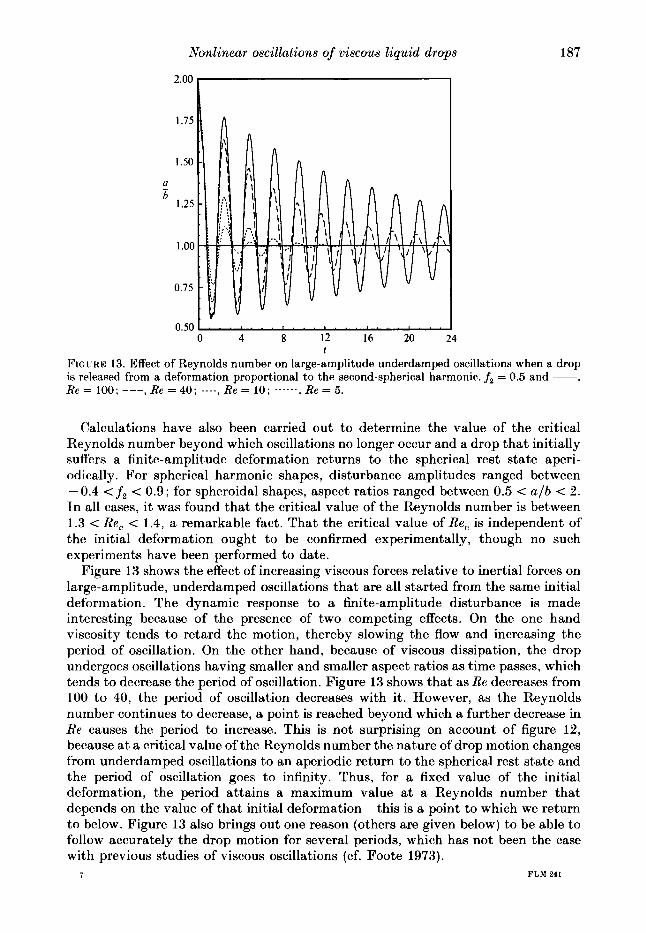
FIGURE 13. Effect of Reynolds number on large-amplitude underdamped oscillations when a drop is released from a deformation proportional to the second-spherical harmonic. f, = 0.5 and -, Re = 100; ---, Re = 40; ----, Re = 10; ......, Re = 5.

1

Calculations have also been carried out to determine the value of the critical Reynolds number beyond which oscillations no longer occur and a drop that initially suffers a finite-amplitude deformation returns to the spherical rest state aperi- odically. For spherical harmonic shapes, disturbance amplitudes ranged between -0.4 < fi c 0.9; for spheroidal shapes, aspect ratios ranged between 0.5 < a /b < 2. In all cases, it was found that the critical value of the Reynolds number is between 1.3 < Re, < 1.4, a remarkable fact. That the critical value of Re, is independent of the initial deformation ought to be confirmed experimentally, though no such experiments have been performed to date.

Figure 13 shows the effect of increasing viscous forces relative to inertial forces on large-amplitude, underdamped oscillations that are all started from the same initial deformation. The dynamic response to a finite-amplitude disturbance is made interesting because of the presence of two competing effects. On the one hand viscosity tends to retard the motion, thereby slowing the flow and increasing the period of oscillation. On the other hand, because of viscous dissipation, the drop undergoes oscillations having smaller and smaller aspect ratios as time passes, which tends to decrease the period of oscillation. Figure 13 shows that as Re decreases from 100 to 40, the period of oscillation decreases with it. However, as the Reynolds number continues to decrease, a point is reached beyond which a further decrease in Re causes the period to increase. This is not surprising on account of figure 12, because a t a critical value of the Reynolds number the nature of drop motion changes from underdamped oscillations to an aperiodic return to the spherical rest state and the period of oscillation goes to infinity. Thus, for a fixed value of the initial deformation, the period attains a maximum value a t a Reynolds number that depends on the value of that initial deformation -this is a point to which we return to below. Figure 13 also brings out one reason (others are given below) to be able to follow accurately the drop motion for several periods, which has not been the case with previous studies of viscous oscillations (cf. Foote 1973).

7 FLM 241

188 0. A . Basaran

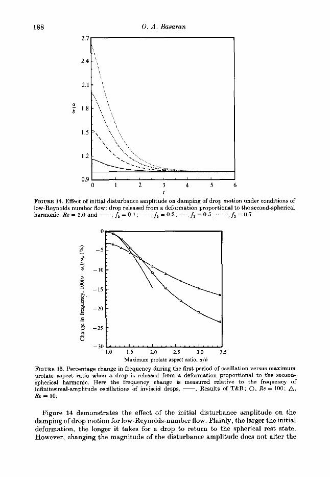
FIGURE 14. Effect of initial disturbance amplitude on damping of drop motion under conditions of low-Reynolds number flow : drop released from a deformation proportional to the second-spherical harmonic. Re = 1.0 and -, fz = 0.1; ---,fz = 0.3; ----,fi = 0.5; . . . . . . ,fz = 0.7.

C .- 8 m 8

1.0 1.5 2.0 2.5 3.0 3.5 Maximum prolate aspect ratio, a /b

FIGURE 15. Percentage change in frequency during the first period of oscillation versus maximum prolate aspect ratio when a drop is released from a deformation proportional to the second- spherical harmonic. Here the frequency change is measured relative to the frequency of infinitesimal-amplitude oscillations of inviscid drops. -, Results of T&B; 0, Re = 100; A, Re = 10.

Figure 14 demonstrates the effect of the initial disturbance amplitude on the damping of drop motion for low-Reynolds-number flow. Plainly, the larger the initial deformation, the longer it takes for a drop to return to the spherical rest state. However, changing the magnitude of the disturbance amplitude does not alter the


.

1.0 1.5 2.0 2.5 3.0 3.5

Maximum prolate aspect ratio, a/h

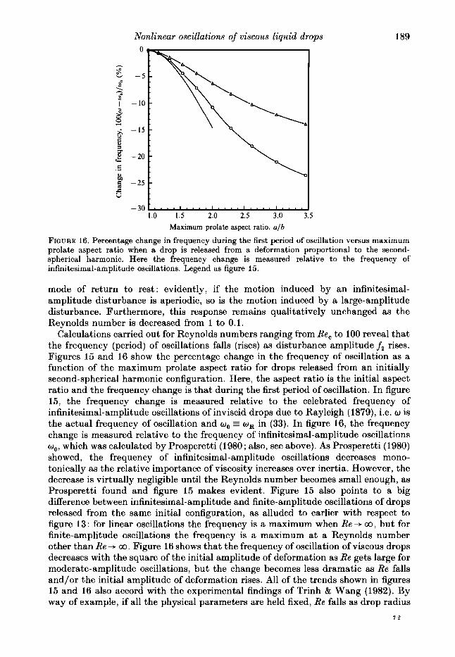
FIGURE 16. Percentage change in frequency during the first period of oscillation versus maximum prolate aspect ratio when a drop is released from a deformation proportional to the second- spherical harmonic. Here the frequency change is measured relative to the frequency of infinitesimal-amplitude oscillations. Legend as figure 15.

mode of return to rest: evidently, if the motion induced by an infinitesimal- amplitude disturbance is aperiodic, so is the motion induced by a large-amplitude disturbance. Furthermore, this response remains qualitatively unchanged as the Reynolds number is decreased from 1 to 0.1.

Calculations carried out for Reynolds numbers ranging from Re, to 100 reveal that the frequency (period) of oscillations falls (rises) as disturbance amplitude fi rises. Figures 15 and 16 show the percentage change in the frequency of oscillation as a function of the maximum prolate aspect ratio for drops released from an initially second-spherical harmonic configuration. Here, the aspect ratio is the initial aspect ratio and the frequency change is that during the first period of oscillation. In figure 15, the frequency change is measured relative to the celebrated frequency of infinitesimal-amplitude oscillations of inviscid drops due to Rayleigh (1879), i.e. w is the actual frequency of oscillation and wo = wR in (33). I n figure 16, the frequency change is measured relative to the frequency of infinitesimal-amplitude oscillations w,,, which was calculated by Prosperetti (1980 ; also, see above). As Prosperetti (1980) showed, the frequency of infinitesimal-amplitude oscillations decreases mono- tonically as the relative importance of viscosity increases over inertia. However, the decrease is virtually negligible until the Reynolds number becomes small enough, as Prosperetti found and figure 15 makes evident. Figure 15 also points to a big difference between infinitesimal-amplitude and finite-amplitude oscillations of drops released from the same initial configuration, as alluded to earlier with respect to figure 13: for linear oscillations the frequency is a maximum when Re+ co, but for finite-amplitude oscillations the frequency is a maximum a t a Reynolds number other than Re + co. Figure 16 shows that the frequency of oscillation of viscous drops decreases with the square of the initial amplitude of deformation as Re gets large for moderate-amplitude oscillations, but the change becomes less dramatic as Re falls and/or the initial amplitude of deformation rises. All of the trends shown in figures 15 and 16 also accord with the experimental findings of Trinh & Wang (1982). By way of example, if all the physical parameters are held fixed, Re falls as drop radius

7-2

190 0. A . Basaran

I -.-

I00

I 2 3 4 5 6 Period or prolate/oblate cycle number

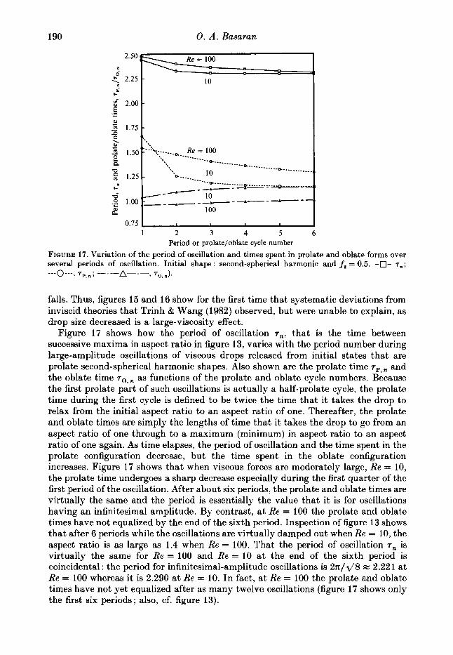
FIQURE 17. Variation of the period of oscillation and times spent in prolate and oblate forms over several periods of oscillation. Initial shape : second-spherical harmonic and f, = 0.5. -0- 7, ; ---o---

,7p,n; 1 7o.n).

falls. Thus, figures 15 and 16 show for the first time that systematic deviations from inviscid theories that Trinh & Wang (1982) observed, but were unable to explain, as drop size decreased is a large-viscosity effect.

Figure 17 shows how the period of oscillation T,, that is the time between successive maxima in aspect ratio in figure 13, varies with the period number during large-amplitude oscillations of viscous drops released from initial states that are prolate second-spherical harmonic shapes. Also shown are the prolate time 7p, and the oblate time 7 0 , ~ as functions of the prolate and oblate cycle numbers. Because the first prolate part of such oscillations is actually a half-prolate cycle, the prolate time during the first cycle is defined to be twice the time that i t takes the drop to relax from the initial aspect ratio to an aspect ratio of one. Thereafter, the prolate and oblate times are simply the lengths of time that it takes the drop to go from an aspect ratio of one through to a maximum (minimum) in aspect ratio to an aspect ratio of one again. As time elapses, the period of oscillation and the time spent in the prolate configuration decrease, but the time spent in the oblate configuration increases. Figure 17 shows that when viscous forces are moderately large, Re = 10, the prolate time undergoes a sharp decrease especially during the first quarter of the first period of the oscillation. After about six periods, the prolate and oblate times are virtually the same and the period is essentially the value that it is for oscillations having an infinitesimal amplitude. By contrast, a t Re = 100 the prolate and oblate times have not equalized by the end of the sixth period. Inspection of figure 13 shows that after 6 periods while the oscillations are virtually damped out when Re = 10, the aspect ratio is as large as 1.4 when Re = 100. That the period of oscillation 7, is virtually the same for Re = 100 and Re = 10 at the end of the sixth period is coincidental : the period for infinitesimal-amplitude oscillations is 2 x / 4 8 x 2.221 a t Re = 100 whereas i t is 2.290 a t Re = 10. I n fact, a t Re = 100 the prolate and oblate times have not yet equalized after as many twelve oscillations (figure 17 shows only the first six periods; also, cf. figure 13).


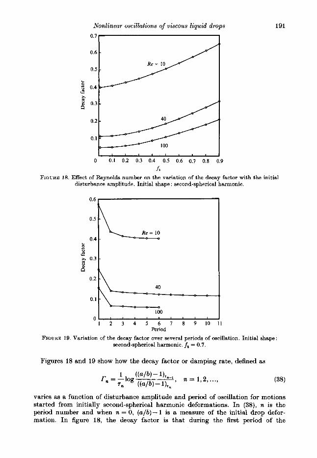
FIGURE 18. Effect of Reynolds number on the variation of the decay factor with disturbance amplitude. Initial shape : second-spherical harmonic.

8 d 3 0.3

4

B 0.2

0.1

0

40

100 , , , I t

1 2 3 4 5 6 7 8 9 10 Period

I " " " " ' 1 2 3 4 5 6 7 8 9 10

Period 1

the initial

FIGURE 19. Variation of the decay factor over several periods of oscillation. Initial shape : second-spherical harmonic. f, = 0.7.

Figures 18 and 19 show how the decay factor or damping rate, defined as

varies as a function of disturbance amplitude and period of oscillation for motions started from initially second-spherical harmonic deformations. In (38)) n is the period number and when n = 0, (a /b) - 1 is a measure of the initial drop deformation. In figure 18, the decay factor is that during the first period of the

192 0. A . Basaran

0 - I -2 ;Dl 0.111 pj - I - 2

0.531

-2

10.575 I 0.632

M - 2 - 1 0 1 2 - 2 - 1 0 I 2 -2-1 0 1 2 - 2 - 1 0 1 2 - 2 - 1 0 1 2 - 2 - 1 0 I 2

FIGURE 20. Drop released from a static deformation. Initial shape : fourth-spherical harmonic: Re = 100, f, = 0.5.

oscillation. Figure 18 shows for the first time that the decay factor is fairly insensitive to the initial disturbance amplitude during small- and moderate-amplitude oscillations : this explains why Trinh &, Wang (1982) found it difficult to draw definite conclusions based on their experimental observations, although they could perceive an increasing trend in damping rate with increasing drop deformation. At Re = 100, the decay factor goes from 0.05 when f, = 0.01 to 0.21 when f2 = 0.9. As the relative importance of viscous forces to inertial ones increases, the relative increase in the decay factor with the initial disturbance amplitude becomes more modest : at Re = 10, the decay factor goes from 0.40 when f , = 0.01 to 0.65 when f , = 0.9. Figure 19 shows how the decay factor varies with the period during large-amplitude oscillations ( fi = 0.7). At all Reynolds numbers, the decay factor decreases with increasing period number. The decay factor changes most rapidly during the first period, the relative amount of the change increasing as Reynolds number increases. Thereafter, the decay factor changes only slightly with increasing time. The relative flatness of the curves for the decay factor after the first period also corroborates Trinh & Wang's (1982) experimental observation that the damping rate appears to be independent of time for a drop that is released from a steady acoustic drive. Figure 19 makes plain why drop oscillations a t moderate Reynolds numbers take so long to get damped out. Also, it is worth noting that a t Re = 100, the decay factor at the start of the oscillations is more than three times that of infinitesimal-amplitude oscillations. By contrast, a t Re = 10, the decay factor during the first period is less than 1.5 times that of oscillations having an infinitesimal amplitude. For drops undergoing underdamped oscillations, figures 18 and 19 show that the lower the Reynolds number the higher the damping rate.

Modal decomposition of drop profiles that are seen during oscillations started from initial shapes that suffer deformations that are pure odd harmonics reveals the presence of odd as well as even harmonics : the same conclusion was reached by T&B and Patzek et al. (1991) in their studies of inviscid oscillations. However, there are


0 2 4 6 8 10 12

FIGURE 21. Disturbance amplitude a t the pole, f(0, t ) - 1, as a function of time for a drop released from a static deformation proportional to the fourth-spherical harmonic. Re = 100; f4 = 0.3.

t

also striking differences between odd as well as even multi-lobed oscillations analysed here and by others. It is shown below that one of the differences is due to the proper accounting in this paper for the presence of a finite amount of viscosity. The other difference lies in the methods of analysis used : whereas both this paper and the works of L&M and Patzek et al. (1991) approach the problem of drop oscillations as initial- value problems, T&B's method, by its very nature, restricts them to time-periodic solutions.

Figure 20 shows sequences of drop shapes that result for a drop that is released from an initially four-lobed spherical harmonic configuration. Figure 21 shows the disturbance amplitude at the pole, f(0, t ) - 1, as a function of time for initially four- lobed oscillations. When Re > 2000, L&M found that every third amplitude peak is lower than the other two. Figure 21 and calculations at lower values of the Reynolds number show that when Re < 100 this is not the case initially. However, the new calculations also show that every third amplitude is lower than the other two at large times, for example when dimensionless time exceeds 6 at Re = 100 in figure 21. Increasing the magnitude of the initial drop deformation does not affect this behaviour. Experimental verification of this finite-viscosity effect is pending.

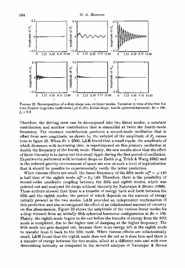
T&B found that at second-order in disturbance amplitude, only the zeroth, second, fourth, sixth, and eighth modes are excited and have modal amplitudes that oscillate a t twice the frequency of the fourth (primary) mode. By contrast, L&M found that the situation is quite different in the context of an initial-value problem. To gain further insight into initially four-lobed oscillations and also to elucidate the effect of finite viscosity on such multi-lobed oscillations, figure 22 shows the amplitudes of the first few leading modes during the oscillations of a slightly viscous drop. Evidently, the dominant feature of the dynamics of the second mode is that it oscillates with the natural (Rayleigh) frequency of the second mode, mio) = 4 8 . L&M have suggested that this second-mode excitation is caused by second-order quadratic coupling with the fundamental fourth mode. Physically, the second mode is an oscillator with natural frequency wi0) , but driven in proportion to the square of the fourth mode.

194 0. A . Busurun

0.3

d ' L

5 .- I * om- a . E d .

-0.3 . . 1 . . 1 . . I , . .

0.3 0.3

4" L L

c .- - f$ d

-0.3 -0.3 -0.3 0 3.25 6.50 9.75 13.00 0 3.25 6.50 9.75 13.00 0 3.25 6.50 9.75 13.00

L ;~~~:f---J s o .d

.- +

d

-0.3 -0.3

Therefore, the driving term can be decomposed into two linear modes: a constant contribution and another contribution that is sinusoidal a t twice the fourth-mode frequency. The constant contribution produces a second-mode oscillation that is offset from zero amplitude, as shown by the subplot of the amplitude of Pz versus time in figure 22. When Re > 2000, L&M found that a small ripple, the amplitude of which decreases with increasing time, is superimposed on this primary oscillation at double the frequency of the fourth mode. Plainly, the new results show that the effect of finite viscosity is to damp out this small ripple during the first period of oscillation. Experiments performed with levitated drops on Earth (e.g. Trinh & Wang 1982) and in the reduced gravity environment of space are now a t such a level of sophistication that it should be possible to experimentally verify the latter prediction.

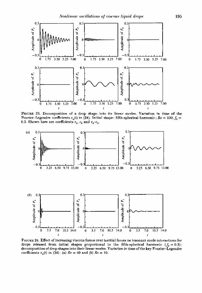
When viscous effects are small, the linear frequency of the fifth mode uko) = dl40 is half that of the eighth mode uio) = 24140. Therefore, there is the possibility of second-order quadratic coupling between the fifth and eighth modes, which was pointed out and analysed for drops without viscosity by Natarajan & Brown (1986). These authors showed that there is a transfer of energy back and forth between the fifth and the eighth modes, the period of which depends on the amount of energy initially present in the two modes. L&M provided an independent confirmation of this prediction and also investigated the effect of an infinitesimal amount of viscosity on this phenomenon. Figure 23 shows the amplitude of the various linear modes for a drop released from an initially fifth-spherical harmonic configuration at Re = 100. Plainly, the eighth mode begins to die out before the transfer of energy from the fifth mode is completed, due to the higher rate of damping at the higher frequency. The fifth mode too gets damped out, because there is no energy left in the eighth mode to transfer from i t back to the fifth mode. When viscous effects are infinitesimally small, L&M found that the eighth mode does not die out as it does here and there is a transfer of energy between the two modes, albeit at a different rate and with ever diminishing intensity as compared to the inviscid analysis of Natarajan & Brown

Nonlinear oscillutions of viscous liquid drops

lit 4"

8 L

d .- - a 0

4- .* - s o 9.

c .- - d

8 d

k d

-0.3 -0.3 -0.3 0 1.75 3.50 5.25 7.00 0 1.75 3.50 5.25 7.00 0 1.75 3.50 5.25 7.00

0.3

d 4- a 0 3 0 7

E d d . -0.3 -0.3 -0.3 . . , . . , . . , .

0 1.75 3.50 5.25 7.00 0 1.75 3.50 5.25 7.00 0 1.75 3.50 5.25

195

t t t

FIGURE 23. Decomposition of a drop shape into its linear modes. Variation in time of the Fourier-Legendre coefficients c,(t) in (34). Initial shape : fifth-spherical harmonic ; Re = 100, f5 = 0.3. Shown here are coefficients c5, c8 and co-c3.

0 3.25 6.50 9.75 13.00 0 3.25 6.50 9.75 13.00 0 3.25 6.50 9.75 13.00

0 3.5 7.0 10.5 14.0 0 3.5 7.0 10.5 14.0 0 3.5 7.0 10.5 14.0 1 t t

FIGURE 24. Effect of increasing viscous forces over inertial forces on resonant mode interactions for drops released from initial shapes proportional to the fifth-spherical harmonic ( f5 = 0.3) : decomposition of drop shapes into their linear modes. Variation in time of the key Fourier-Legendre coefficients c,(t) in (34): (a) Re = 40 and (b) Re = 10.

196 0. A . Basaran

(1986). Figure 23 also shows that the second mode, which is excited a t its natural frequency by the same mechanism proposed for fourth-mode oscillations by L&M, plays a more significant role than it does when viscous effects are infinitesimally small. Moreover, the new computations show that even this amount of viscosity is enough to alter and make completely uninteresting the dynamics of modes other than the fifth, eighth, and second, in contrast to the infinitesimal viscosity calculations of L&M. Figure 24 shows that further increasing the importance of viscous forces relative to inertial forces can prevent altogether the fascinating resonant mode interaction between the fifth and the eighth modes from occurring.

5. Discussion The Galerkinlfinite-element method as applied in this paper is an example of ‘the

method of lines ’ and is readily extended to more complex cases. For example, there are many applications, such as the diverse mass transfer operations of chemical engineering, in which the environment surrounding the drop is far from inactive. One prominent example is solvent extraction, where the fluid surrounding the liquid drops is another viscous liquid and solid boundaries abound. As shown by Miller & Scriven (1968), and also as pointed out by L&M, the effect of viscosity is much greater at the interface of an oscillating drop in liquid-liquid systems and cannot be accounted for even for low-viscosity fluids by the boundary-integral method developed by L&M.

Figures 12-14 in particular, and some of the other results presented in this paper, have important implications for recently developed technologies that utilize electric fields to enhance heat and/or mass transfer to or from liquid drops (see e.g. Scott et al. 1990). It has been found that the most economical way to run such field-enhanced transport operations is to use a pulsed-d.c. field. Ideally, the goals are (i) to have the field on for a short period of time, thereby causing the drop to attain a large deformation almost instantaneously, as in figures 12-14, (ii) to keep the field off while the drop undergoes several oscillations, and (iii) to repeat the cycle. The oscillations can induce appreciable convection in the drop, and around it as well if there is a liquid phase outside, and thereby enhance the rate of transport. Plainly, figures 12-14 and ones like them for liquid-liquid systems are indispensable for gaining a fundamentally based understanding of and properly designing and running field- enhanced transport operations. Often, drop qize is set by other considerations and surface tension is the only parameter left to attain a desired range of Reynolds numbers. In practice, surface tension in liquid-gas systems and interfacial tension in liquid-liquid systems can be changed readily by means of surfactants. However, the presence of surfactants and/or trace impurities a t the interface of an oscillating drop will cause interfacial tension gradients along it, in addition to changing the equilibrium interfacial tension. Such Marangoni-type convection can sometimes dominate these flows, the proper analyses of which requires simultaneous solution of the equations presented in this paper with those that govern the transport of the surfactant in and around the fluid interface. Analysis of the effects of surfactants on large-amplitude deformation and break-up of drops has been considered (Stone & Leal 1990). However, similar analyses have not been carried out in the context of drop oscillations and is a goal of future research.

The results of this paper also show that a drop subjected to an initial static deformation that is proportional to the second-spherical harmonic does not break-up or fission for finite-amplitude deformations as large as fi = 1.3. Viscous drops (Trinh

Nonlinea,r oscillations of viscous liquid drops 197

& Wang 1982) and inviscid drops (L&M and Patzek et al. 1991) that are impulsively set in motion do break up by fissioning when the amplitude of the initial disturbance (impulse) is large enough. Therefore, there is a need to investigate theoretically the effect of finite viscosity on the break-up of liquid drops that are set in motion by an impulse in the form of an electric or an acoustic field.

Experiments of Trinh & Wang (1982) and the asymptotic analyses of Natarajan & Brown (1986, 1987) show that large-amplitude axisymmetric oscillations of liquid drops can become unstable with respect to non-axisymmetric disturbances, i.e. the instability generates finite-amplitude circumferential waves. Thus, another goal of future research is to extend the present work to analyse fully three-dimensional oscillations (Basaran & Patzek 1991).

This research was supported by the Division of Chemical Scicnccs, Office of Basic Energy Sciences (BES), US Department of Energy (DOE) under contract DE-AC05- 840R21400 with Martin Marietta Energy Systems, Inc. Calculations reported here were made possible by (1) the Office of Laboratory Computing and the Computing and Telecommunications Division a t the Oak Ridge National Laboratory (ORNL) which subsidized a large portion of the computations on a Cray X-MP/4 at ORNL, (2) a grant from the BES Office of the US DOE a t the Florida State University (FSU) Computing Center, and (3) Dr L. J. Gray of ORNL who generously made available his IBM 6000-320H. Also, the author thanks Mr D. L. Cooper, a participant in the Oak Ridge Science and Engineering Research Semester (ORSERS) program, for his assistance in the development of the plotting programs that were used to generate some of the figures in this paper.

R E F E R E N C E S

ALONSO, C. T. 1974 The dynamics of colliding and oscillating drops. In Proc. Intl Colloq. on Drops and Bubbles (ed. D. J. Collins, M. S. Plesset t M. M. Saffren), vol. 1, pp. 139-157. Je t Propulsion Laboratory, Pasadena, CA.

ALONSO, C. T., LEBLANC, J. M. & WILSON, J. R. 1982 Studies of the nuclear equation of state using numerical calculations of nuclear drop collisions. In Proc. Second Intl Colloq. on Drops and Bubbles (ed. D. H. LeCroissette), pp. 268-279. Jet Propulsion Laboratory, Pasadena, CA.

ARIS, R. 1962 Vectors, Tensors, and the Basic Equations of Fluid Mechanics. Prentice-Hall. BASARAN, 0. A. t PATZER, T. W. 1991 Three-dimensional oscillations of liquid drops. Paper

BASARAN, 0. A,, SCOTT, T. C. t BYERS, C. H. 1989 Drop oscillations in liquid-liquid systems.

BEARD, K. V., OCHS, H. T. t KUBESH, R. J. 1989 Natural oscillations of small raindrops. Nature 342, 408410.

CARRUTHERS, J. R. 6 TESTARDI, L. R. 1983 Materials processing in the reduced-gravity of space. Ann. Rev. Muter. Sci. 13, 247-278.

COYLE, D. J. 1984 The fluid mechanics of roll coating : steady flows, stability, and rheology. Ph.D. thesis, University of Minnesota. Available from University Microfilms, Inc., AnnArbor, MI.

FOOTE, G . B. 1973 A numerical method for studying simple drop behavior : simple oscillation. J. Comput. Phys. 11, 507-530.

GRESHO, P. M., LEE, R. L. & SANI, R. C. 1979 On the time-dependent solution of the incompressible NavierStokes equations in two and three dimensions. In Recent Advances in Numerical Methods in Fluids (ed. C. Taylor & K. Morgan), vol. 1, pp. 27-79. Swansea: Pineridge.

1963 The particle-in-cell method for numerical solution of problems in fluid dynamics. Proc. Symp. Appl . M a t h 15, 269-288.

presented at the Winter Annual Meeting of the AIChE, 17-22 Nov. 1991, Los Angeles.

AIChE J . 35, 1263-1270.

HARLOW, F. H.

198 0. A . Basaran

HARLOW, F. H., AMSDEN, A. A. & NIX, J . R. 1976 Relativistic fluid dynamics calculations with the particle-in-cell technique. J . Comput. Phys. 20, 11S129.

HOOD, P. 1976 Frontal solution program for unsymmetric matrices. Zntl J . Numer. Meth. Engng 10, 379-399 (and Correction, Zntl J . k m e r . Meth. Engr. 11, (1977), 1055).

HUYAKORN, P. S., TAYLOR, C., LEE, R. L. & GRESHO, P. M. 1978 A comparison of various mixed interpolation finite elements in the velocity-pressure formulation of the Kavier-Stokes equations. Computers Fluids 6 . 25-35

KHESHGI, H. S. & SCRIVEN, L. E. 1983 Penalty finite element analysis of unsteady free surface flows. In Finite Elements in Fluids (ed. R. H. Gallagher, J. T. Oden, 0. C. Zienkiewicz, T. Kawai & M. Kawahara), vol. 5, pp. 393434. Wiley.

KISTLER, S. F. & SCRIVEN, L. E. 1983 Coating flows. In Computational Analysis of Polymer Processing (ed. J. R. A. Pearson & S. M. Richardson), pp. 243-299. Applied Science Publishers.

LAMB, H. 1932 Hydrodynamics. Dover. LUNDGREN, T. S. & MANSOUR, K. E. 1988 Oscillations of drops in zero gravity with weak viscous

effects. J . Fluid Mech. 194, 479-510 (referred to herein as TAM). LUSKIN, M. & RANNACHER, R. 1982 On the smoothing property of the Crank-Nicholson scheme.

Applicable Anal. 14, 117-135. MILLER, C. A. & SCRIVEN, L. E. 1968 The oscillations of a droplet immersed in another fluid. J .

Fluid Mech. 32, 417-435. KATARAJAN, R. & BROWN, R. A. 1986 Quadratic resonance in the three-dimensional oscillations

of inviscid drops with surface tension. Phys. Fluids 29, 2788-2797. KATARAJAN, R. & BROWN, R. A. 1987 Third-order resonance effects and the nonlinear stability

of drop oscillations. J . Fluid Nech. 183, 95-121. BIX, J. R. & STROTTMANN, D. 1982 Fluid dynamical description of relativistic nuclear collisions.

In Proc. Second Intl Colloq. on Drops and Bubblea (ed. D. H. LeCroissette), pp. 260-267. Je t Propulsion Laboratory, Pasadena, CA.

ORSZAG, S. A. 1980 Spectral methods for problems in complex geometries. J . Comput. Phys. 37, 70-92.

PATZEK, T. W., BENNER, R. E., BASARAX, 0. $. & SCRIVEN, L. E. 1991 Eonlinear oscillations of

PROSPERETTI, A. 1980 Pu’ormal-mode analysis for the oscillations of a viscous liquid drop in an

RAYLEIGH, LORD 1879 On the capillary phenomena of jets. Proc. R . Soe. Lond. 29, 71-97. REID, W. H. 1960 The oscillations of a viscous liquid drop. &. Appl . Maths 18, 8G89. SAITO, H. & SCRIVEN, L. E. 1981 Study of coating flow by the finite element method. J . Comput.

SCOTT, T. C., BASARAN, 0. A. & BYERS, C. H. 1990 Characteristics of electric-field-induced

SILLIMAN, W. J. 1979 Viscous film flows with contact lines. Ph.D. thesis, University of Minnesota.

STONE, H. A. & LEAL, L. G. 1990 The effects of surfactants on drop deformation and breakup. J .

STRANG, G. & FIX, G. J. 1973 A n Analysis of the Finite Element Method. Prentice-Hall. TRINH, E. & WANG, T. G. 1982 Large-amplitude free and driven drop-shape oscillations:

experimental observations. J . Fluid Mech. 122, 315-338. TSAMOPOULOS, J. A. 1989 Nonlinear dynamics and break-up of charged drops. In AIP Conf. Proc.

197: Third Intl Colloq. on Drops and Bubbles (ed. T . G . Wang), pp. 16S187. American Institute of Physics.

TSAMOPOULOS, J. A. & BROWN, R. A. 1983 Konlinear oscillations of inviscid drops and bubbles. J . Fluid Mech. 127, 519-537 (referred to herein as T&B).

WALTERS, R. A. 1980 The frontal method in hydrodynamics simulations. Computers Fluids 8 , 265-272.

WEATHERBURN, C. E. 1927 Differential Geometry of Three Dimensions. Cambridge University Press.

inviscid free drops. J . Comput. Phys. 97. 489-515.

immiscible liquid. J . Mdc. 19, 149-182.

Phys. 42, 53-76.

oscillations of translating liquid droplets. Zndust. Engng Chem. Res. 29, 901-909.

Available from University Microfilms, Inc., AnnArbor, MI.

Fluid Mech. 220, 161-186.

nonlinear oscillations of viscous liquid drops

Documents