1 2 3 4 5 6 7 8 9 10 11 12 13 14 15 16 17 18 19 20 21 22 23 24 25 26 27 28 29 30 31 32 33 34 35 36 37 38 39 40 41 42 43 44 45 46 47 48 49 50 51 52 53 54 55 56 57 58 59 60 61 62 63 64 65

1

A novel steady-state approach for the analysis of gas-burner supplemented direct

expansion solar assisted heat pumps

Federico Scarpa*, Luca A. Tagliafico, Vincenzo Bianco

University of Genoa – DIME/TEC - Division of Thermal Energy and Environmental Conditioning

Via All'Opera Pia 15 A – (I) 16145 Genoa – Italy

(*) corresponding author- e-mail: fscarpa@ditec.unige.it, Fax +39 010311870

DOI: 10.1016/j.solener.2013.07.016

Abstract

Design and control strategy suggestions for direct expansion solar assisted heat pump (DX-SAHP) water heaters

are stated as a result of a novel steady-state primary energy consumption analysis based on a model developed

around the fluid-independent Carnot cycle. The study is devoted to devices committed to hot sanitary water

production and supplemented by an instantaneous gas burner. The paper addresses several suggestions about the

correct design and the optimal working conditions needed to minimize the use of primary energy, based on

averaged working conditions.

The maximization of primary energy savings has been selected as the criterion to define our concept of ―optimal

performance‖ since this approach benefits from the use of a direct language that permits a larger, also non-

specialized, audience to acquire the basic concepts of optimal behavior, increasing the transfer of knowledge to

actual embodiments. Apart from the particular criterion selected in this study, the focus is on the proposed steady

state approach which, without any use of refrigerant fluid properties, allows us to extract general rules as a

function of the main features of the plant and of its relevant interactions with the surroundings, making all the

relationship between the involved variables explicit and meaningful. Results obtained using the present approach

agree with data coming from an already consolidated dynamic simulator.

Keywords: Optimal control; Solar; Heat pump; Water heater; Fluid-less approach, Primary Energy

*Accepted ManuscriptClick here to view linked References

pre-p

rint

1 2 3 4 5 6 7 8 9 10 11 12 13 14 15 16 17 18 19 20 21 22 23 24 25 26 27 28 29 30 31 32 33 34 35 36 37 38 39 40 41 42 43 44 45 46 47 48 49 50 51 52 53 54 55 56 57 58 59 60 61 62 63 64 65

2

Nomenclature

Symbols

A heat transfer area (panel/evap.), m2

COP coeff. of performance

DHW domestic hot water

E energy transfer J

G solar irradiation, Wm-2

M mass, kg

Mc thermal capacity, J K-1

Pc compressor power, W

q heat transfer rate, W

Q heat energy J

T temperature, K

U global heat transfer coeff. Wm-2K-1

VCC variable capacity compressor

W work J

Subscripts

aux auxiliary

b burner

c compressor

cd of the condensing fluid

Cr of the Carnot cycle

ev to the evaporating fluid

e of the ambient (environmental)

ev of the evaporating fluid

e of the ambient (environmental)

el electric

f fluid

G relative to solar insolation

hp heat pump

II second law

id ideal

in in to the fluid

m monthly

p solar panel

s stagnation

stg storage tank, reservoir

tap tap water

u user

Greek symbols

absorbance

saved primary energy index,

t time interval s, h

specific electric energy consumption

efficiency

transmittance

maximum II law efficiency

pre-p

rint

1 2 3 4 5 6 7 8 9 10 11 12 13 14 15 16 17 18 19 20 21 22 23 24 25 26 27 28 29 30 31 32 33 34 35 36 37 38 39 40 41 42 43 44 45 46 47 48 49 50 51 52 53 54 55 56 57 58 59 60 61 62 63 64 65

3

1. Introduction

In recent years, many improvements have been made in the field of air conditioning, heating and cooling, thanks

to the diffusion of heat pump (HP) systems, usually reversible, which allow water heating and air heating or

cooling to be carried out with considerable savings compared to conventional gas and electric systems (De

Swardt and Meyer, 2001, Sarkar et al. 2006). Scientific research is focused on the development and

improvement of these technologies and on their integration with other ones; seawater heat exchangers (Li et al.,

2011; Yu et al. 2012), geothermal tubes (Ozgener and Hepbasli, 2005; Xi and Hongxing, 2012, Bayer et al.,

2012), absorption systems (Garcia-Casals , 2006; Wang et al., 2011), hybrid solar collectors (Chow, 2010;

Amrizal et al., 2012). Refined control techniques aimed to obtain ―optimal performance‖ from a system (Dong et

al., 1998) are quickly diffusing also in the field of vapor compression refrigeration technology (Qi and Deng,

2009), also with the use of neural networks (Mohanraj et al., 2012). In addition, there is a growing interest

around DX-SAHP technology, where the DX prefix is used to specify that the traditional vapor compression heat

pump is integrated into a solar panel, directly used as the evaporator of the inverse cycle system. These systems

are also known as ―integrated solar assisted heat pumps‖ (ISAHP).

The aim of this work, once a proper representation for the DX-SAHP steady state behavior is given, is to analyze

its performance using a very simple model which is able to avoid the need of calculations of refrigerant fluid

(typically a freon) thermophysical properties. The maximization of primary energy savings (PES) is selected as

the criterion to define our concept of ―optimal performance‖, due to its simplicity and practical relevance.

Available literature data (Ozgener and Hepbasli, 2007) is indeed plentiful of complex exergy (availability)

analyses devoted to solar assisted heat pump performance, but seldom the conclusions of these works can be

easily synthesized to give practical suggestions for the design of these systems and for the setting of the ―best‖

working conditions of actual devices embedded in ―real world‖ applications. Indeed, these analyses often neglect

the presence of the auxiliary power source needed to grant the user with hot water at the correct temperature.

When facing with standard refrigerators and, to some extent, with heat pump systems, the performance of the

device can be quantified by means of the COP, the ratio between obtained thermal and spent electric power. The

higher the COP values, the lower the paid electric energy for the same thermal or refrigeration user demand.

Furthermore, when referring to the same working context and user load, COP values can be also used to compare

different devices. On the contrary, when dealing with solar assisted heat pumps (SAHP), COP and solar collector

efficiency have to be concurrently taken into account. In fact, they both depend on panel temperature, which may

be, in turn, very different from the ambient one, therefore an ―optimal‖ behavior can be achieved only by means

pre-p

rint

1 2 3 4 5 6 7 8 9 10 11 12 13 14 15 16 17 18 19 20 21 22 23 24 25 26 27 28 29 30 31 32 33 34 35 36 37 38 39 40 41 42 43 44 45 46 47 48 49 50 51 52 53 54 55 56 57 58 59 60 61 62 63 64 65

4

of the right balance between the two following contrasting needs: (i) a panel temperature very close to or even

lower than that of the environment, in order to minimize thermal losses or even drain heat from the ambient and

utilize a greater fraction of the available solar radiation; (ii) a high panel temperature, near to the condenser one,

to attain high COP values, thus decreasing the need of expensive electric power, whose cost depends on the kind

of primary energy utilized. The presence of an auxiliary power source further complicates the analysis, since its

intervention has to be balanced to the one of the heat pump system. A PES analysis takes care of all these

aspects, also considering the different "cost" of electric and gas consumptions.

In the present study, some basic design and control rules are extracted as a function of both the main features of

the plant and all its relevant interactions with the surroundings. In particular, the focus is on the steady state

approach based on the idea of linking key variables of the system by means of a parameter, here assumed

constant, often reported as "second law efficiency" of the inverse cycle machine. This approach, successfully

implemented by Scarpa et al. (2013) in the dynamic analysis of systems based on an inverse cycle, is applied to

the general steady state description of a DX-SAHP. Results are eventually compared with those coming from a

validated dynamic simulator described in (Scarpa et al., 2011) which makes use of real weather conditions

(environmental temperature and solar radiation) and of a stochastic model of variable water consumption.

2. Basic DX-SAHP system modeling

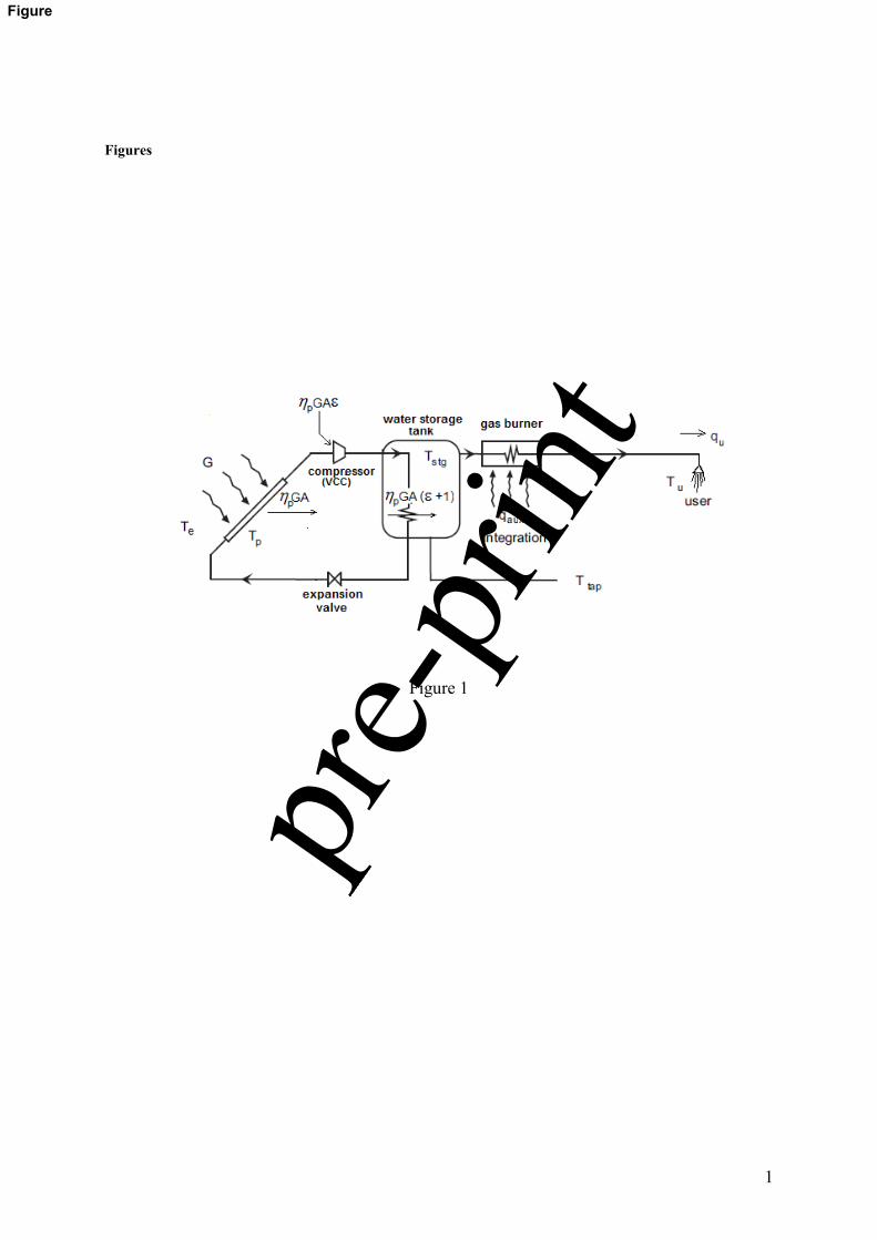
Figure 1 depicts a simplified solar water heater apparatus along with user load and instantaneous gas burner

integration. It ideally consists of an unglazed flat plate working as the evaporator (the solar panel), a variable

capacity compressor (VCC), a coil tube heat exchanger inside the water storage tank as the condenser and an

expansion valve.

The basic task considered in this study is the production of domestic hot water (DHW) at the desired temperature

(e.g. 45 °C), using also some thermal energy by means of an auxiliary burner, when needed.

The relevant concepts reported in this study are developed starting from simple steady-state energy balance

operations relative to the work and heat transfers sketched in figure 1. The reference integration period is

arbitrary and it can be for instance one day or one month. Accordingly, steady state variables and calculations

will refer to the averaged values assumed over the considered time period

Thermal power, GAp , from the surroundings, (perpendicular solar irradiation component GA plus, or minus,

other convective and irradiative heat transfers), enters the collector at temperature Tp and, by means of a heat

pump having a specific electric energy consumption , is transferred to a water tank reservoir at the temperature

pre-p

rint

1 2 3 4 5 6 7 8 9 10 11 12 13 14 15 16 17 18 19 20 21 22 23 24 25 26 27 28 29 30 31 32 33 34 35 36 37 38 39 40 41 42 43 44 45 46 47 48 49 50 51 52 53 54 55 56 57 58 59 60 61 62 63 64 65

5

Tstg. Hot water is supplied to the user through an instantaneous gas burner which assures the desired constant

temperature Tu. The environment is at temperature Te while the reservoir is fed by water at temperature Ttap.

With reference to figure 1, if we integrate thermal and mechanical (i.e. electrical in our simplified description)

power over a selected time interval of interest, say one month, we obtain the following energy balance quantities:

Net thermal energy from the collector to the HP working fluid Gpin QQ (1)

Mechanical (electrical) work spent by the compressor Gpc QW (2)

Thermal energy transferred to the water reservoir 1Gphp QQ (3)

Auxiliary thermal energy supplied by the gas burner )0( hpuaux QQQ (4)

Useful thermal energy delivered to the user )( tapuu TTMcQ (5)

Please note that eq.(4) underlines that the auxiliary heat cannot be negative (see also Eqs. 18 and 25)

The incident solar irradiation per unit area G [Wm-2] and its energy counterpart QG [J] over the selected period

mt , are related by:

mm

m

G tGA

t

dGAQ

)( (6)

where A is the active surface area of the solar collector, M the mass of hot sanitary water demanded by the user

over the selected period mt and c its specific heat. mG indicates the monthly averaged solar irradiation per

unit area. Let us for sake of simplicity assume mt =1 month.

In Eqs. (1) and (2), Ginp QQ / and inc QW / refer to the average collector efficiency and to the monthly

specific electric energy consumption, respectively. For the sake of simplicity, in what follows we will not use the

average line symbol on p , , etc..

To avoid misinterpretation, we underline that, as usual in steady state descriptions, all the aforementioned

quantities are to be considered constant only during a reference averaging period, but are allowed to vary from

one period to another, for example from day to day or from month to month.

As usual, to link all the relevant variables of the system, we make use of balance relations plus some definitions.

So, along with Eqs. (1)-(6), we utilize the storage tank steady state thermal balance

tapstghp TTMcQ (7)

pre-p

rint

1 2 3 4 5 6 7 8 9 10 11 12 13 14 15 16 17 18 19 20 21 22 23 24 25 26 27 28 29 30 31 32 33 34 35 36 37 38 39 40 41 42 43 44 45 46 47 48 49 50 51 52 53 54 55 56 57 58 59 60 61 62 63 64 65

6

and the collector efficiency p . Since Qin is composed by two terms, solar energy effectively collected by the

panel and the one, Qe, exchanged with the environment, it will be:

eGin QQQ )( (8)

G

eGp

Q

QQ

)( (9)

that is, as usual:

ep

m

p TTG

U )( (10)

where and are the collector absorbance and transmittance respectively ( =1 in case of bare panels, as often

happens with DX-SAHP) , U the overall heat transfer coefficient. We note that, when dealing with a solar

assisted heat pump, the panel temperature can be lower than the one of the environment. In such a condition the

collector efficiency can assume values greater than one.

At this point, to close the model, all we need is the relation between input work and heat which characterizes the

heat pump. In other words, we have to state the specific electric energy consumption, inc QW / , as a

function of the other variables of the system. To do this task, we can proceed by following different lines.

The first, accurate though demanding, is the so called (Scarpa M. et al., 2012) ―detailed thermodynamic

approach‖ which considers the actual thermodynamics associated to a simple vapor compression inverse cycle

machine, along with a suitable working fluid (Hulin et al, 1999), (Moreno-Rodríguez et al., 2012). The need of

evaluating enthalpy and entropy values associated to specific points of the inverse cycle precludes the possibility

of linking explicitly all the variables of the system.

A more ―practical‖ approach, is to follow the technical specification CEN TC 113 - EN 14825 (2012) and to use

the performance tables and charts given by heat pump manufacturers, as in (Tagliafico et al., 2012b). This

approach corrects the value of the COP () given for nominal conditions (full load, nominal condenser and

evaporator temperatures, nominal temperature drop at evaporator and condenser, nominal fluid composition)

depending on the actual operating and environmental conditions imposed to the heat pump. In this way, any

detailed description of the refrigerant fluid thermophysical properties is avoided at the cost of introducing a

series of corrective coefficients which are valid only for specific appliance, under specified working conditions.

pre-p

rint

1 2 3 4 5 6 7 8 9 10 11 12 13 14 15 16 17 18 19 20 21 22 23 24 25 26 27 28 29 30 31 32 33 34 35 36 37 38 39 40 41 42 43 44 45 46 47 48 49 50 51 52 53 54 55 56 57 58 59 60 61 62 63 64 65

7

A similar, less accurate but more physics grounded path, is to follow the idea presented by Scarpa et al.(2013) in

case of dynamic modeling and used, for instance, by Capozza et al.(2013) in case of steady state ground-source

heat pumps.

In this case the elimination of the cycle thermodynamics is achieved by assuming a constant ratio between the

Carnot performance index of the plant and the real one, that is, by utilizing the following relation:

evcd

evII

TT

TCOP

(11)

in conjunction to the key assumption:

.constII (12)

where Tev and Tcd are the fluid temperatures at the evaporator and at the condenser, respectively.

Although the idea is not new, it has been applied to simple or ground source heat pumps whose working

conditions are by far more quiet in respect to the ones of solar assisted heat pumps. Furthermore, it has never

been used to develop explicit relations among all the variables of the system in view of a performance analysis.

The use of the equations (11) and (12) is central to this work: by means of this link between the working

temperatures of the heat pump, we are now able to explicitly describe the steady-state behavior of the DX-SAHP

without using the thermodynamic properties of the working fluid.

Neglecting the thermal resistances associated to the evaporator (solar panel), the condenser and the one between

the condenser and the storage water, we can assume the evaporating and condensing fluid temperatures to be

almost equal to the ones of the panel and of the storage water respectively. Referring furthermore to the specific

electric energy consumption, , we can modify Eq. (11) in the following way:

pII

pstg

T

TT

(13)

Then, from Eqs. (1) to (13) the average collector efficiency can be written as:

IIm

IItape

mp

Mc

tUA

TTG

U

1/11

1/)( (14)

Only independent operating variables and system characteristics appear on the right side of equation (14), so that

all the relevant temperatures and energy transfers of the system can be calculated and it is possible to describe

pre-p

rint

1 2 3 4 5 6 7 8 9 10 11 12 13 14 15 16 17 18 19 20 21 22 23 24 25 26 27 28 29 30 31 32 33 34 35 36 37 38 39 40 41 42 43 44 45 46 47 48 49 50 51 52 53 54 55 56 57 58 59 60 61 62 63 64 65

8

the behavior of the DX-SHAP as a function of independent variables. For instance , the collector and the storage

temperatures will follow as:

pm

epU

GTT )( (15)

pIIstg TT )1( (16)

To summarized, various simplifications have been assumed while developing the analysis:

- steady-state description, in particular the reservoir behavior is not explicitly described nor its capacity is

given (Steady state fully mixed mode. see Eq. 7);

- absence of any thermal resistance between condenser and water reservoir;

- absence of any thermal dispersion to the environment (except the one from the collector);

- heat-pump behavior independent on refrigerant fluid properties and exclusively described through the

Carnot coefficient of performance coupled to a constant second law of thermodynamics efficiency (Eqs.

11-12).

Actually, the last one is the basis of the model rather than a simplification. Obviously, different refrigeration

plants have different second law efficiencies II , which in turn depends also on the actual working point of the

heat pump and on the particular working fluid utilized in the plant. Nevertheless its value, strongly linked to the

compressor efficiency, does not change too much once the heat pump device has been chosen, and a value in the

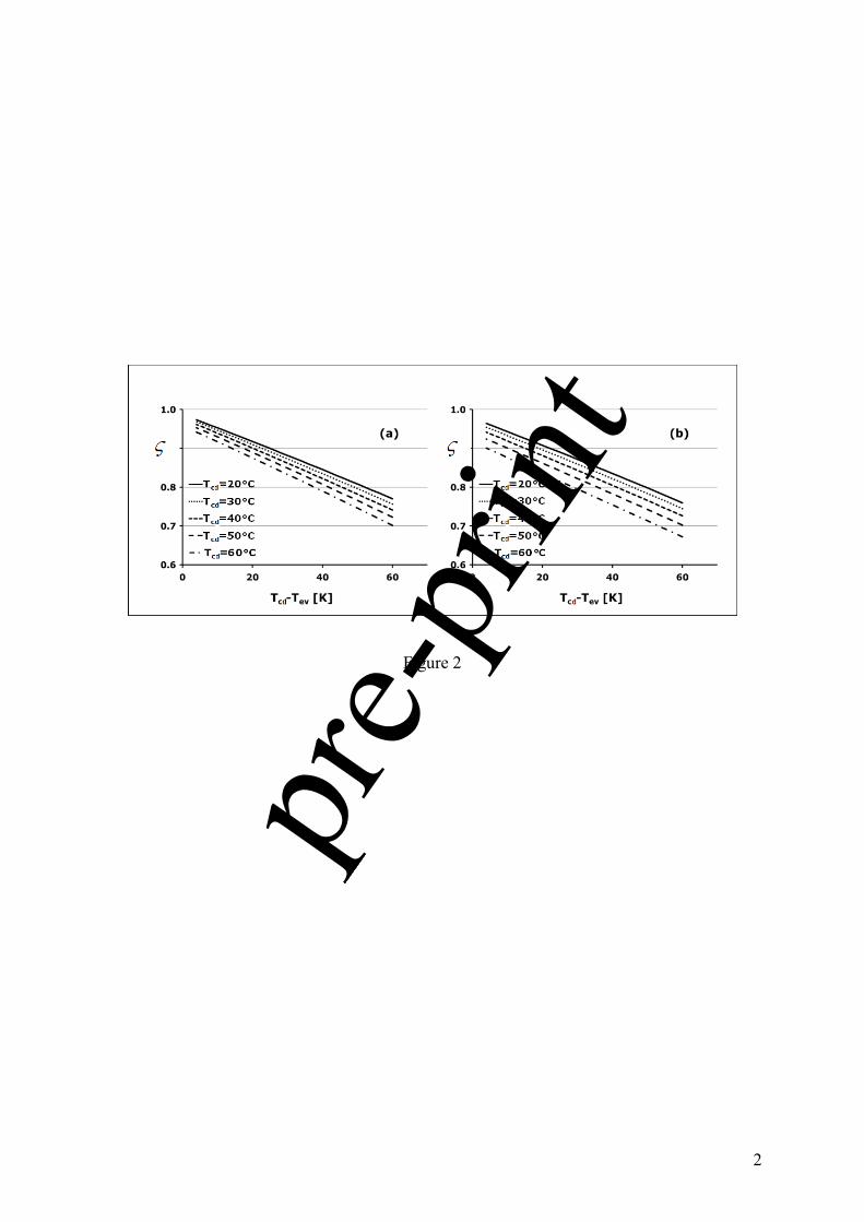
range 0.3-0.5 is typical for this kind of systems. It is important to mention that II changes also with the

considered refrigerant as shown in figure 2, adapted from (Scarpa et al., 2013), where results from two

commonly used refrigerant fluids, R600 and R134a, are reported. In fact, Eq. 11 can be rewritten highlighting

the main parameters influencing II :

c

idc

Crin

Crin

inc

Crin

Crin

c

in

Cr

IIW

W

Q

Q

Q

W

W

Q

COP

COP

,

,

,,

, (17)

where Win,Cr represents the net input work of the inverse Carnot cycle, while Wc,id is the ideal isentropic work

spent in the compression process.

Eq. (17) shows the explicit dependence of second law efficiency on isentropic efficiency, c, of the compressor

and on the parameter which, given a particular working condition, only depends on the selected fluid and

represents the maximum second law efficiency achievable in case of isentropic compression (c =1). Under our

simplified assumptions of no superheating and sub cooling , figure 2 puts in evidence, beyond the weak

pre-p

rint

1 2 3 4 5 6 7 8 9 10 11 12 13 14 15 16 17 18 19 20 21 22 23 24 25 26 27 28 29 30 31 32 33 34 35 36 37 38 39 40 41 42 43 44 45 46 47 48 49 50 51 52 53 54 55 56 57 58 59 60 61 62 63 64 65

9

parameter dependence on temperature conditions, that values are marginally affected by the fluid choice.

Fluid data were collected from the standard NIST database (Lemmon et al., 2002).

To conclude, our assumption of constant II is likely to be verified during normal operations, especially in a

averaged sense. We assigned it a value of 0.4 assuming an average compressor efficiency of 0.5 (small

appliance) and a maximum ―internal‖ second law of thermodynamics efficiency =0.8.

3. Primary energy savings criterion

The presented fluid-less model is applied to the assessment of the performance of a DX-SAHP system controlled

in such way to maximize primary energy savings in respect to a reference system which makes only use of a gas

burner for the same duty, that is to produce a given amount of domestic hot water at 45 °C, for a given tap water

temperature of 15°C.

So, introducing el , the conversion efficiency from primary-to-electric energy and b , the combustion efficiency

of the gas burner, we express the primary energy consumption of the DX-SAHP as:

b

aux

el

cprim

QWE

(Qaux ≥ 0) (18)

and utilize the following saved primary energy index, , defined as the ratio between the actual saved primary

energy and the primary energy needed in the case of gas burner alone (assumed as a reference), as a measure of

performance of the system:

bu

primbu

Q

EQ

//

(19)

which becomes:

aux

el

cb

u

QW

Q

11 (20)

and finally:

11

el

bp

u

G

Q

Q

(21)

Appling the results of the previous paragraph, is obtained as a function of all the relevant operating and

characteristic data of the system and of the three given temperatures describing the environment and the load,

that is Te, Ttap, Tu :

pre-p

rint

1 2 3 4 5 6 7 8 9 10 11 12 13 14 15 16 17 18 19 20 21 22 23 24 25 26 27 28 29 30 31 32 33 34 35 36 37 38 39 40 41 42 43 44 45 46 47 48 49 50 51 52 53 54 55 56 57 58 59 60 61 62 63 64 65

10

11

1/1

1/1

el

b

II

m

IItape

tapu

tUA

Mc

TU

GT

TT

(22)

In which, beyond the variable , that we consider an indirect control variable since it is linked to the compressor

power, we clearly identify:

- given environmental variables G, Te, Ttap,

- design and system variables Tu, )/( mtAUMc , /U, II

- context variables elb /

In the sequel, we avoid any analytical minimum search and prefer to parametrically evaluate expression (22) as a

function of a limited set of variables to give an idea of the basic performance of the DX-SAHP. or, better, the

coefficient of performance of the heat pump, COPhp=1+1/, will be used as the main varied parameter in the

analysis of the performance of the system.

We underline that important system elements, such as various thermal resistances associated to the system, have

been deliberately omitted for the sake of simplicity and to focus to the more relevant factors influencing the

behavior of the plant. A more detailed analysis could easily take into account these further system

characteristics.

4. Analysis and discussion

To investigate the effectiveness of the proposed approach, we analyze the saved primary energy index outcomes

of the DX-SAHP, when some parameters are varied. Of course, other performance parameters can be profitably

constructed and investigated such as electric power consumption, CO2 production, overall cost, et cetera.

In Eq. (22) both environmental variables and system/design variables are included. Among the first we have the

temperature of the environment, the one of the tap water and the mean solar irradiation G. The temperature of the

requested hot water belongs to the design variables. It is usually assumed equal to 45°C for sanitary water but we

can investigate cases of different final use target. These variables are strictly related to the response of the system

to external input and thus interesting from a system control perspective.

The active surface area, A, of the solar collector and the user load, Qu, belong to the design variables and

contribute in defining the size of the plant. The user request can be simply expressed by the mass, M, of sanitary

pre-p

rint

1 2 3 4 5 6 7 8 9 10 11 12 13 14 15 16 17 18 19 20 21 22 23 24 25 26 27 28 29 30 31 32 33 34 35 36 37 38 39 40 41 42 43 44 45 46 47 48 49 50 51 52 53 54 55 56 57 58 59 60 61 62 63 64 65

11

hot water used the reference time mt that, in typical DX-SAHP design, is related to the surface area A. As one

can see from Eqs. (14) and (22), this size parameter appears as part of the factor

Mc

tUA m .

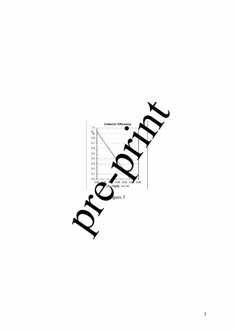
The collector type and characteristics belong to the system parameters too, although the collector efficiency

depends also upon external and internal variables (see Eqs.10 and 14). In our analysis we consider, as an

example, an unglazed active surface characterized by an efficiency curve comparable to data available in

literature (Kalogirou, 2004) and reported in figure 3.

Some suitable value for the combustion efficiency of the burner, b, and of the conversion efficiency from

primary-to-electric energy, el , has also to be assumed. In the present paper the conventional value b=0.87

(European Council, 1992) is considered. As for el, it can be determined according to the structure of the

electricity generation facilities of a specific country, because it represents the average ratio between the electric

energy produced (delivered to the user) and primary energy consumed. The reference value el =0.36 is assumed

in this paper, this figure being the global average conversion efficiency for all fossil fuels (International Energy

Agency, 2008). Different scenarios shall have to assume different b and el values. All the operating and

geometrical data used in the calculations are available in Table 1, although equations can be also handled in non-

dimensional form. It is evident that the parameters are so many that, for the sake of simplicity , only the

influence of a limited number of them will be analyzed in the sequel.

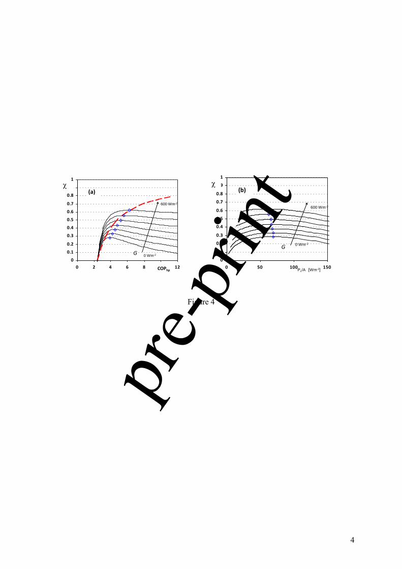
Figures 4a and 4b show the performance parameter as a function of the heat pump performance parameter,

COPhp, and of the specific (per unit area of the solar collector surface) averaged compressor power respectively,

defined as:

mpc GAP / (23)

/11hpCOP (24)

The average solar radiation G is varied from 0 to 600 Wm-2.

The figures depict the behavior of the DX-SAHP device from two different points of view, but the information

given is essentially the same. The dashed (red) line divides the plane of figure 4a in two parts; only the results

placed on the right of this line have a physical meaning, since the left part correspond to negative auxiliary

power input. In this case, a proper mixing with tap water should occur to keep the delivered water temperature at

pre-p

rint

1 2 3 4 5 6 7 8 9 10 11 12 13 14 15 16 17 18 19 20 21 22 23 24 25 26 27 28 29 30 31 32 33 34 35 36 37 38 39 40 41 42 43 44 45 46 47 48 49 50 51 52 53 54 55 56 57 58 59 60 61 62 63 64 65

12

Tu (45°C) when the storage temperature is higher than Tu . This limiting curve can be inferred from Eqs. (4) and

(20) in case of Qaux=0, that is:

hp

elb

el

cb

u COP

W

Q

/111lim

(25)

As a consequence, figure 4a correctly addresses the issue that there is no advantage (from the primary energy

saving point of view) in operating the system at COPhp values lower than 2.4, since all that is gained from

environmental (free) resources is paid in terms of compressor electric energy consumption. The value of this

limit can be inferred, in a rough way, also from Eq. (21) where it looks clear that COPhp has to be greater than

elb / (2.4 in this study) to provide useful operations, i.e. > 0, in respect to those of a gas burner alone.

For a given value of solar irradiation, G, an optimal value of COPhp exists, which provides a maximum (diamond

symbols in Fig. 4) of the saved primary energy index. It can be noted that this optimal COPhp value increases

along with the solar irradiation. This typical behavior needs further clarifications also to better explain the use of

the present averaged steady state analysis. We already mentioned how COPhp (that is ε) variations are in some

way equivalent to Pc control. The analysis quantifies the solar irradiation level over which the use of solar

assisted heat pumps is no longer suitable, that is the G value over which Qaux<0; in this specific case around 550

Wm-2.

As said, an optimal behavior of the DX-SAHP is feasible only by means of the right equilibrium of two

contrasting needs: a high panel temperature, near the condenser one, to attain a high COPhp value, thus

enhancing the system performance; a low panel temperature, near the surroundings one, to utilize a greater

fraction of the available solar radiation. To fulfill these requirements, the DX-SAHP control logic has to shape

the power making it in some way proportional to the solar irradiation in order to take out at any time the right

heat rate from the panel. According to this logic the power is increased with high solar irradiation in a way that

seems to contradict the ―suggestions‖ coming from Figure 4b, which shows a decreasing (optimal) power and an

associated increasing COPhp (Fig 4a) as the solar irradiation varies from zero to 600 [Wm-2]. To understand this

apparent incongruity, it is important to underline that the rules extracted by the present analysis refer to steady

state averaged conditions and not to the real time behavior. It is the monthly average power that has to be

decreased when the monthly average solar irradiation increases. As an example, if we look at a possible

empirical regulation law expressed by Eq. (26) as

GKPc (26)

pre-p

rint

1 2 3 4 5 6 7 8 9 10 11 12 13 14 15 16 17 18 19 20 21 22 23 24 25 26 27 28 29 30 31 32 33 34 35 36 37 38 39 40 41 42 43 44 45 46 47 48 49 50 51 52 53 54 55 56 57 58 59 60 61 62 63 64 65

13

it will be the ―constant‖ K to obey the rule expressed by Figure 4, slowly following average seasonal conditions,

that is decreasing in summer, when G and Te are high, with respect to winter. On the contrary the on-line

regulation during daily operations will increase or decrease the compressor power following the sun rise or the

sun set, respectively. Thus, the information coming from the previous analysis can be utilized to make the

"constant" K a proper function of the average solar irradiation and external temperature in such a way Eq. (26)

can automatically adapt to seasonal weather conditions.

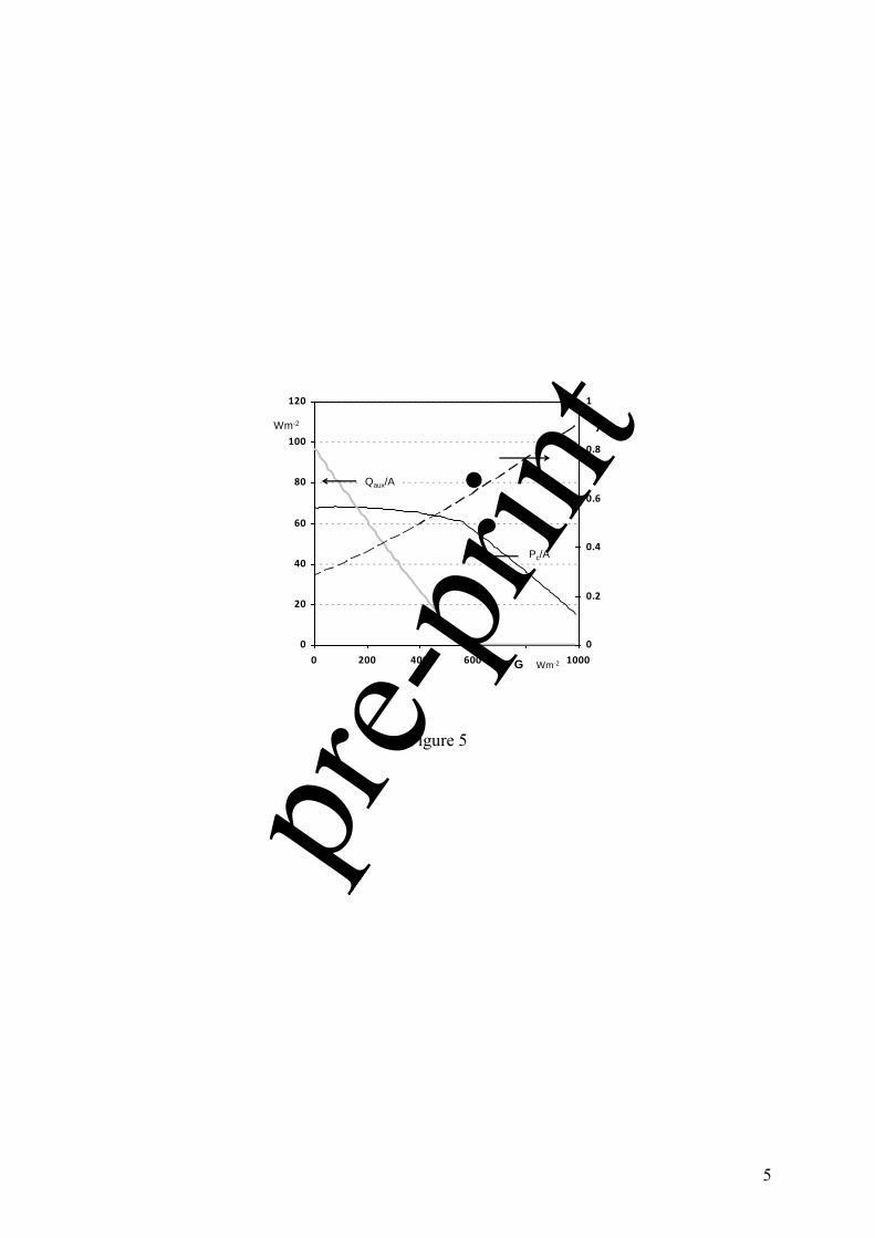
Figure 5 synthesizes the results of the previous parametric analysis. It reports the maximum points (diamonds in

fig 4b) putting in evidence the optimum mean power requested by the system. As said, when the average solar

irradiation increases the power has to be reduced. The dashed line shows the corresponding increase of the

primary energy saving index, while the grey line depicts the auxiliary power contribution Qaux/A, which is

roughly linear and become zero for irradiation value above 550 [Wm-2]. Beyond this limit point the burner is no

longer required in an averaged sense.

In the last years, at least in Europe and particularly in Italy, el, has substantially increased due to the

implementation of aggressive policies to sustain renewable resources development and a value of el, =0.6

relative to Italy for the year 2011 (Terna, 2012) is also assumed to give an idea of the sensitivity of the system to

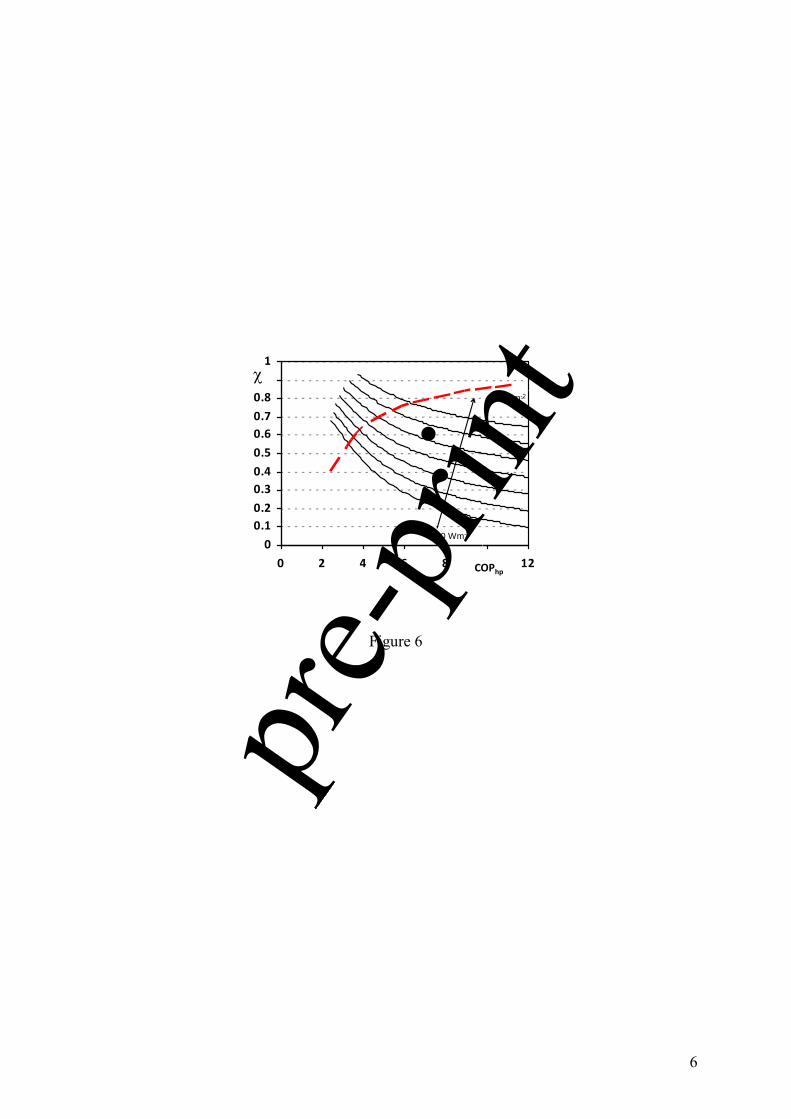
this parameter. Results associated to this last very high value of el are reported in Figure 6, which has to be

directly compared to figure 4a.

The figure shows that the dashed line is shifted to the left and all the maximum points are pushed on the left, out

of the actual range of operating conditions, so that the limit curve given by Eq. 25 (i.e. the dashed line on the

figure) describes the maximum achievable in terms of saved primary energy for a given irradiation. Clearly,

from the perspective of the index, the context characterized by higher el is by far preferable, with

maximum values in the range 0.55 – 0.8.

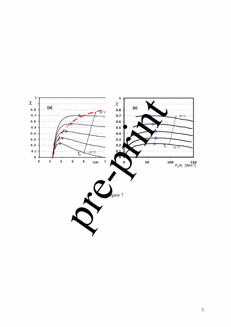
The external temperature affects the system performance in a similar way. Figures 7a and 7b are the analogous

of figure 4, again with el =0.36. The same comments previously made in the case of a variation of solar

irradiation, can be made when it is the external temperature Te to vary with seasonal changes. Both figures 4a

and 7a show that the saved primary energy index starts rising from a value of COPhp equal to about 2.5 and,

after a sharp increase, it reaches a maximum value around 0.7. Thereafter tends to slowly decrease. As

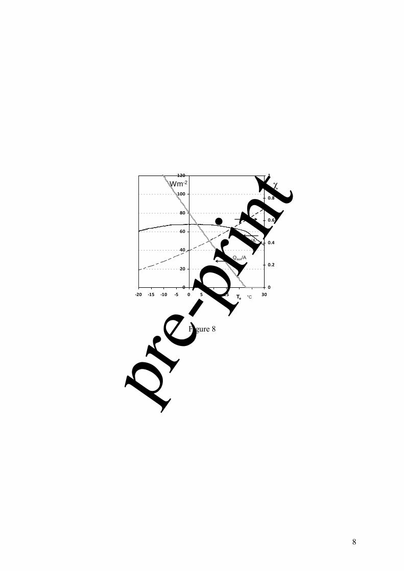
before, figure 8 collects the maximum points obtained in figure 7 and summarizes the optimal behavior of the

DX-SAHP as a function of the COPhp and of the per unit area compressor power, but the varied parameter is the

pre-p

rint

1 2 3 4 5 6 7 8 9 10 11 12 13 14 15 16 17 18 19 20 21 22 23 24 25 26 27 28 29 30 31 32 33 34 35 36 37 38 39 40 41 42 43 44 45 46 47 48 49 50 51 52 53 54 55 56 57 58 59 60 61 62 63 64 65

14

external temperature, which ranges from -20 °C up to 30 °C. The notable outcome is the presence of the

maximum point which moves along with the varied parameter, thus highlighting the necessity of a seasonal

tuning of the control law, e.g. a setting of the K parameter in Eq. (26) to be changed monthly, or at least

seasonally.

4.1 Comparison to detailed DX-SAHP dynamic model

The described overall behavior coming from the proposed steady state averaged approach, has been compared to

outcomes obtained in (Scarpa et al., 2011) by means of an accurate dynamic simulator based on a dynamic

model for refrigeration devices described and validated in (Tagliafico et al., 2012a) and adapted to the DX-

SAHP plant.

It is based on a simplified lumped description of a system operating along an inverse cycle. The interested reader

should refer to this last work for a deeper description of such dynamic model. The approach just accounts for the

differential equations governing the time-temperature history of the different devices involving heat transfer

(with the refrigerant fluid and with the outside such as refrigerated cell content, condenser and evaporator heat

exchangers, and so on) while neglecting the dynamics of physical phenomena having time constants below a few

minutes. Simulations were performed using, over a period of one year, actual climatic conditions (environmental

temperature and solar radiation) occurred in Genoa and sampled with 30 min time interval according to (DIAM,

2004). A four-member typical family was selected as ―the user‖ and the behavior of the DX-SAHP has been

investigated regarding its ability to deliver about 250 l/day of sanitary water (e.g., about 4 showers) with a

temperature of 45 °C (i.e. around 1000 MJ/month). This thermal load was dynamically simulated as a stochastic

process reproducing the typical random use of sanitary water for hygienic purposes during the day, e.g. to have a

few showers.

The system includes a 300 liters water storage tank and a variable capacity compressor whose power is

controlled in open loop, making it linked to the actual incident solar radiation, see Eq. (26).

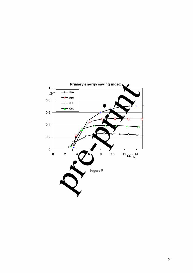
Results are derived as sample means from the application of the ―Monte Carlo‖ technique (100 runs) and can be

synthesized by figure 9, which can be qualitatively compared to figures 4a and 7a.

The graphs are indeed similar, but each curve in figure 9 refers to a different month (dynamically simulate by

actual time varying data) rather than to various average solar irradiation or average environmental temperature

(as calculated for Figures 4 and 7 by using the present method). Four different months (January, April, July and

October) have been selected as representative of different weather conditions during the year.

pre-p

rint

1 2 3 4 5 6 7 8 9 10 11 12 13 14 15 16 17 18 19 20 21 22 23 24 25 26 27 28 29 30 31 32 33 34 35 36 37 38 39 40 41 42 43 44 45 46 47 48 49 50 51 52 53 54 55 56 57 58 59 60 61 62 63 64 65

15

Although the numerical values are clearly different, the general trend of the relation between saved primary

energy index and COPhp is confirmed, along with its dependence on external conditions.

As a further test, we made an attempt to replicate the maximum points coming from figure 9 under such variable

(dynamic) working conditions, setting in the present simplified model the right monthly averaged values of

temperatures, irradiation and all the other operating parameters . These data were set on the basis of the average

values found in the dynamic analysis relative to each month. The results of the comparison are reported in table

2, which shows the maximum values of the parameter resulting from the two different calculation

procedures. We recall that the more detailed dynamic model is able to better follow the time variations of the

plant, and is therefore able to achieve optimized values slightly higher than those promised by the simplified

steady-state approach. However an acceptable agreement between the two techniques is evidenced, with errors

always smaller than 8.0 % (July).

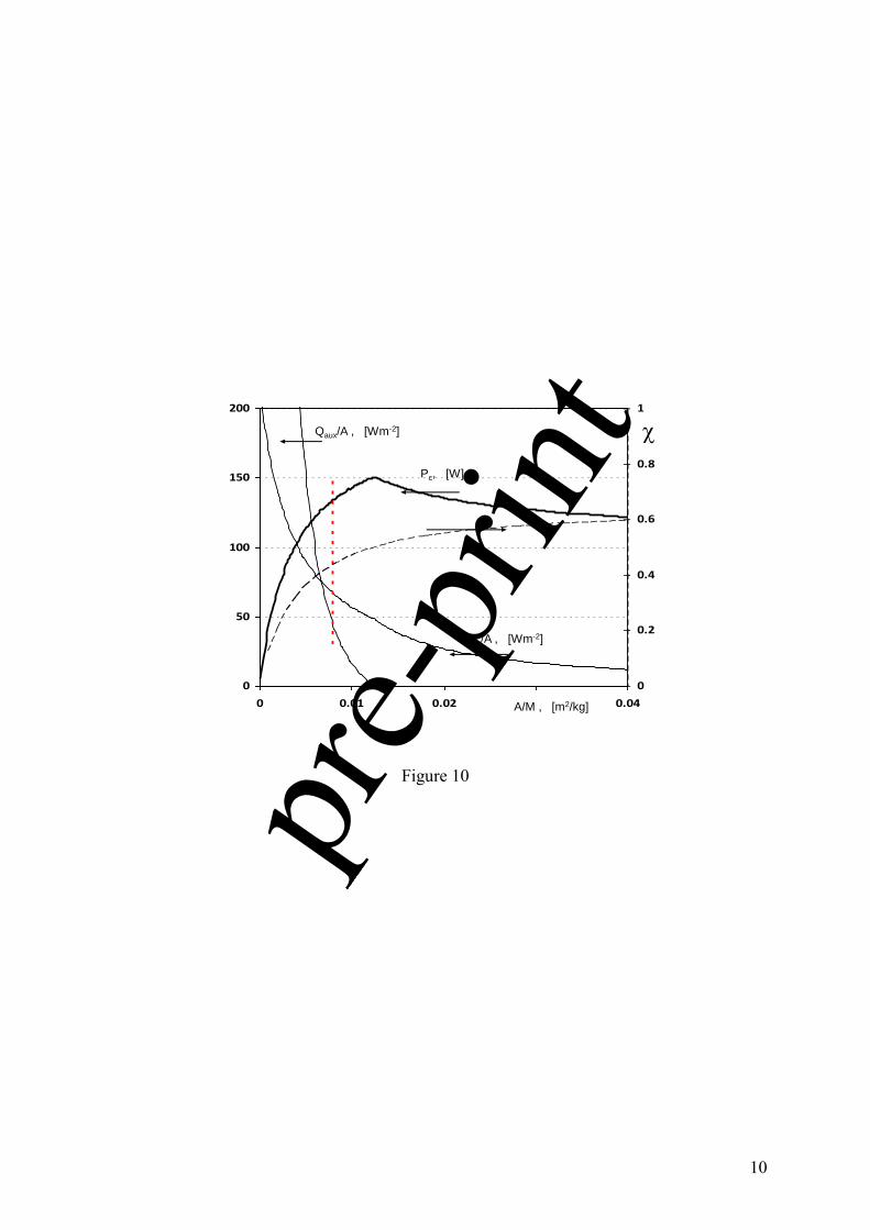
4.2 The present model as a design tool

Finally, as an example of design study, we briefly analyze the influence of the ratio A/M on the performance of

the DX-SAHP. We set the mean external temperature equal to 10 °C and the mean solar irradiation to 300 [Wm-

2]. We then investigate the variation of the performance index as a function of the A/M ratio for different

user loads and surface areas. At first we report the results in the case of Tu=45 °C. Results are reported in figure

10 and they refer to optimal condition with respect to saved primary energy, like figures 5 and 8.

As expected, as the ratio A/M increases the saved primary energy increases and the "per unit area‖ mean

compressor power (that is total energy consumption over the reference time) requested by the system decreases.

Also the "per unit area" thermal power delivered by the gas burner decreases. However, the actual electrical

power, with reference to a user request of 250 kg/day, raises as long as the burner power becomes zero. At this

point, the DX-SAHP no longer needs an auxiliary burner and the aid requested to the heat pump reduces as the

overall collected solar energy increases due to the increased collector area.

Being in this specific case the solar irradiance rather low (300Wm-2) and the environmental temperature not so

high (10°C) the calculation results suggest that even with great A/M values, the Pc/A specific power does not

vanishes, since the solar panel surface temperature hardly reaches the required user water temperature of 45°C.

Without deepening this interesting aspect, since it is out of the scope of the present study, we limit ourselves to

underline that this limit behavior of a DX-SAHP is related to the value of the panel stagnation temperature

pre-p

rint

1 2 3 4 5 6 7 8 9 10 11 12 13 14 15 16 17 18 19 20 21 22 23 24 25 26 27 28 29 30 31 32 33 34 35 36 37 38 39 40 41 42 43 44 45 46 47 48 49 50 51 52 53 54 55 56 57 58 59 60 61 62 63 64 65

16

defined as Ts= Te+ ()G/U. In the reported case, Ts is lower than Tu and, according to the model, as the

panel surface area increases, the panel temperature asymptotically rises toward Ts . In this case the compressor

power never vanishes but approaches a well defined value. Conversely, when the stagnation temperature is

higher than Tu, the panel temperature reaches the value of Tu (=Tstg) and the compressor power vanishes since

there is no further needs of heat pump boosting. It is clear that, in these limit conditions, the present analytic

description of the plant is far from representing the actual device behavior, even the averaged steady state one.

The previously considered base case, with M=250 kg/day and A= 2 m2, shows a value of A/M equal to 0.008

evidenced in Figure 10 by the dotted vertical line. Maybe, a greater value is advisable to obtain a better

performance index, . We note that, using a suitable collector area, the compressor has not to be changed .

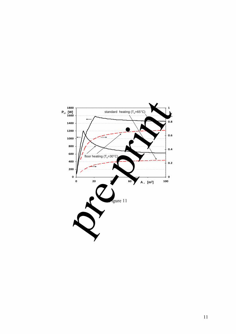
4.3 Space heating applications

To conclude, we depart from the DHW scenario and we focus on a winter heating case. The potential benefits of

DX-SAHP applications are calculated with reference to a mean external temperature of 0°C, and reported in

figure 11 to compare two possible different heating approaches: a traditional heating system with Tu= 65 °C and

a floor heating system demanding for water at Tu= 30 °C. Both the cases refer to a daily load of 200MJ/day that

is about 55 kWh/day.

For a simple reading of the results the values of compressor power Pc and of saved primary energy index have

been reported as a function of the active collector area A.

As it could be expected, the lower temperature floor heating arrangement grants a substantially higher savings

(more than twice), than the traditional heating method for the same collector area. While with the 65°C

traditional heating system the auxiliary gas burner is required to integrate temperature levels if the collector

surface area is smaller than about 21m2, the floor heating system can avoid the burner support if the collector

surface area is greater than about 8m2. Furthermore, the compressor power required by the standard system

appears markedly higher in comparison to that required by the floor heating system. These results refer to

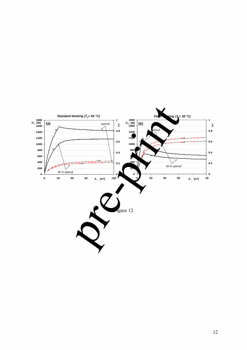
optimal conditions with respect to saved primary energy (maximum ). We can noticeably reduce the required

compressor power if a design solution that reach, for example, the 90% of the optimal saved primary energy

index, is considered adequate. Figures 12a and 12b depict the results of this choice in comparison to the previous

one for the traditional (a) and the floor (b) heating system, respectively.

pre-p

rint

1 2 3 4 5 6 7 8 9 10 11 12 13 14 15 16 17 18 19 20 21 22 23 24 25 26 27 28 29 30 31 32 33 34 35 36 37 38 39 40 41 42 43 44 45 46 47 48 49 50 51 52 53 54 55 56 57 58 59 60 61 62 63 64 65

17

Obviously, the present analysis covers only the energetic aspect of the system. Thermo economic considerations

are left out from the present study but it will be not difficult to utilize the same tool with different optimization

criteria.

5. Conclusions

In the present study, a novel methodology aimed to inverse cycle system analysis is presented and its potential

revealed in the case of its application for the plant analysis and optimization of a number of selected cases. The

basic idea is to explicitly link input to output variables of the system with the aid of the second law of

thermodynamics efficiency (assumed constant) for the calculation of the COP of the inverse cycle device. The

developed steady state analysis applied to time-averaged mean values of the input variables, puts in evidence the

methodology effectiveness and is applied, as an example, to the study of the behavior of direct expansion solar

assisted heat pumps (DX-SAHP), from the perspective of primary energy consumption minimization for given

user loads.

Results show the ability of this type of investigation to capture, in an effortless way, the essential features of the

plant, with acceptable accuracy with respect to a more demanding dynamic simulation tools.

Apart from the particular optimization criterion selected in this study, the focus is on the proposed steady state

approach, which allows us to extract general design and operational rules as a function of the main features of

the plant and of its relevant interactions with the surroundings. Despite the many simplifications adopted in the

description of the plant, the results fairly agree to those based on more demanding dynamic simulations. The

approach appears therefore advisable also when a fast survey of the behavior of a DX-SAHP system is required,

with reference to a lot of different potential working conditions.

The strength of the proposed technique is to avoid the use of refrigerant fluid thermophysical properties and thus

their calculations. Furthermore, it is likely to be applicable also to direct power cycles, such as standard water

steam cycles, and in much more general thermo-economical optimization analyses.

Acknowledgements

The present work was supported by the Genuense Atheneum.

pre-p

rint

1 2 3 4 5 6 7 8 9 10 11 12 13 14 15 16 17 18 19 20 21 22 23 24 25 26 27 28 29 30 31 32 33 34 35 36 37 38 39 40 41 42 43 44 45 46 47 48 49 50 51 52 53 54 55 56 57 58 59 60 61 62 63 64 65

18

References

Amrizal, N., Chemisana D., Rosell, J.I., 2012. Hybrid photovoltaic–thermal solar collectors dynamic modeling.

Appl. Energy 101, 797-807.

Bayer,P., Saner, D., Bolay, S., Rybach, L., Blum, P., 2012. Greenhouse gas emission savings of ground source

heat pump systems in Europe: A review, Renew. Sust. Energ. Rev. 16(2), 1256-1267.

Capozza, A., De Carli, M., Zarrella, A., 2013. Investigations on the influence of aquifers on the ground

temperature in ground-source heat pump operation. Applied Energy 107, 350-363

CEN TC 113 WG 7. EN 14825:2012. Air conditioners, liquid chilling packages and heat pumps, with

electrically driven compressors, for space heating and cooling. Testing and rating at part load conditions

and calculation of seasonal performance.

Chow, T.T., 2010. A review on photovoltaic/thermal hybrid solar technology, Appl. Energy 87(2), 365-379.

De Swardt, C.A., Meyer, J. P., 2001. A performance comparison between an air-source and a ground-source

reversible heat pump. Int. J. Energy Res. 25 (10) , 899 – 910.

DIAM (Dept. of ambient engineering), 2004. http://www.diam.unige.it/~meteo/cambiaso/text_files/dati/. Univ.

of Genova, Italy (last time accessed: 06.09.2013).

Dong, X.D., Liu, S., Asada, H., Itoh, H., 1998. Multivariable Control of Vapor Compression Systems.

HVAC&R Res. 4 (3), 205-230.

European Council Directive 92/42/EEC,1992. The Boiler Efficiency Directive: Council Directive on Efficiency

Requirements for New Hot-Water Boilers Fired with Liquid or Gaseous Fuels. Official Journal L 167,

22/06/1992 17 - 28

Garcia-Casals, X., 2006. Solar Absorption cooling in Spain: Perspectives and outcomes from the simulation of

recent installations. Renew. Energy 31, 1371-1389.

International Energy Agency, 2008. Energy Efficiency Indicators for Public Electricity Production from Fossil

Fuels. IEA Information paper, In Support of the G8 Plan of Action. © OECD /IEA , July 2008, p.5.

http://www.iea.org/publications/freepublications/publication/En_Efficiency_Indicators.pdf (last time

accessed: 06.09.2013)

Kalogirou, S.A., 2004. Solar thermal collectors and applications. Prog. Energy Combust. Sci. 30, 231–295.

Lemmon, E.W., Mc Linden, M.O., Huber, M.L., 2002. Standard Reference Database 23, Version 7.0. Physical

and Chemical Properties Division. National Institute of Standard and Technology (NIST), © 2002 by the

U.S. Secretary of Commerce.

pre-p

rint

1 2 3 4 5 6 7 8 9 10 11 12 13 14 15 16 17 18 19 20 21 22 23 24 25 26 27 28 29 30 31 32 33 34 35 36 37 38 39 40 41 42 43 44 45 46 47 48 49 50 51 52 53 54 55 56 57 58 59 60 61 62 63 64 65

19

Li, Q., You, S., Zheng, X., 2011. Applications of seawater source heat pump in buildings, Adv. Mater. Res. 280,

238-241.

Mohanraj, M., S. Jayaraj S., C. Muraleedharan C., 2012. Applications of artificial neural networks for

refrigeration, air-conditioning and heat pump systems—A review. Renew. Sust. Energ. Rev. 16(2), 1340-

1358.

Ozgener, O., Hepbasli, A., 2007. A review on the energy and exergy analysis of solar assisted heat pump

systems. Renew. Sust. Energ. Rev. 11, 482-496.

Ozgener, O., Hepbasli, A., 2005. Experimental performance analysis of a solar assisted ground-source heat pump

greenhouse heating system. Energy Build. 37(1), 101-110.

Qi, Q., Deng, S., 2009. Multivariable control of indoor air temperature and humidity in a direct expansion (DX)

air conditioning (A/C) system. Build. Environ. 44 (8),1659-1667.

Sarkar, J., Souvik Bhattacharyya, M. Ram Gopal, 2006. Transcritical CO2 heat pump systems: exergy analysis

including heat transfer and fluid flow effects. Energy Conv. Manag. 46, 2053-2067.

Scarpa, F., Tagliafico, L.A., Tagliafico, G., 2011. Integrated Solar-Assisted Heat Pumps for water heating

coupled to gas burners; control criteria for dynamic operation, Appl. Therm. Eng. 31, 59-68.

Scarpa, F., Tagliafico, L.A., Bianco, V., 2013. Inverse cycles modeling without refrigerant property

specification. Int. J. Refrig. , in press, 1-14, 10.1016/j.ijrefrig.2013.04.003.

(www.sciencedirect.com/science/article/pii/S0140700713000789).

Scarpa M., Emmi, G., Michele De Carli, M., 2012. Validation of a numerical model aimed at the estimation of

performance of vapor compression based heat pumps. Energy Build. 47, 411-420.

Tagliafico, L.A., Scarpa, F., Tagliafico, G., 2012a. A compact dynamic model for household vapor compression

refrigerated systems. Appl. Therm. Eng. 35, 1-8.

Tagliafico, L.A., Scarpa, F., Tagliafico, G., Valsuani, F., 2012b. An approach to energy saving assessment of

solar assisted heat pumps for swimming pool water heating. Energy Build.,, 833-840.

Terna S.p.A., Italian Trasmission System Operator, 2012.

http://www.terna.it/default/home_en/electric_system/statistical_data.aspx (last time accessed: 06.09.2013).

Wang Kai, Abdelaziz Omar, Kisari Padmaja, Vineyard Edward A., 2011. State-of-the-art review on

crystallization control technologies for water/LiBr absorption heat pumps. Int. J. Refrig. 34(6), 1325-1337.

Xi Chen, Hongxing Yang, 2012. Performance analysis of a proposed solar assisted ground coupled heat pump

system. Appl. Energy 97, 888-896.

pre-p

rint

1 2 3 4 5 6 7 8 9 10 11 12 13 14 15 16 17 18 19 20 21 22 23 24 25 26 27 28 29 30 31 32 33 34 35 36 37 38 39 40 41 42 43 44 45 46 47 48 49 50 51 52 53 54 55 56 57 58 59 60 61 62 63 64 65

20

Yu, J., Zhang, H., You, S., Dong, L., 2012. Heat transfer and economic analysis of seawater-source heat pump

system with casted heat exchanger. Asia-Pacific Power and Energy Engineering Conference, APPEEC, art.

no. 6307207.

pre-p

rint

1 2 3 4 5 6 7 8 9 10 11 12 13 14 15 16 17 18 19 20 21 22 23 24 25 26 27 28 29 30 31 32 33 34 35 36 37 38 39 40 41 42 43 44 45 46 47 48 49 50 51 52 53 54 55 56 57 58 59 60 61 62 63 64 65

21

Figure captions

Figure 1. A solar assisted heat pump water heater with gas burner integration. Sketch of the relevant energy

transfer rates and working temperatures.

Figure 2. Maximum second law efficiency as a function of the difference between condensation Tc and

evaporation Tev temperature (Tc varied), in case of R600a (a) and R134a (b) as operating fluid. Adapted from

(Scarpa et al., 2013). Fluid properties from NIST database (Lemmon et. al., 2002).

Figure 3- Instantaneous collector efficiency in case of unglazed panels. Adapted from (Kalogirou, 2004).

Figure 4 - Saved primary energy index as a function of the COPhp (a) and of the "per (solar panel) unit area"

compressor power (b), solar irradiation G varied from 0 up to 600 [Wm-2]. Te= 10 °C, el =0.36, other data in

table 1. Only operating points on the right of the dashed curve in figure 4a are meaningful.

Figure 5 – Optimal input power as a function of the solar irradiation ,G, extracted from data of Fig.4.

Continuous lines (black and grayed) represent the specific per unit area compressor power Pc/A and auxiliary

thermal power Qaux/A respectively. The dashed line is the corresponding saved primary energy index .

Figure 6 - Saved primary energy index as a function of the COPhp; solar irradiation G varied from 0 up to 600

[Wm-2]. Same data as in figure 4a; the value of el varied from 0.36 up to 0.6.

Figure 7 - Saved primary energy index as a function of the COPhp (a) and of the "per unit area" compressor

power (b); external temperature Te varied from -10°C up to 30°C. Solar irradiation G= 300 [Wm-2], other data in

table 1.

Figure 8 - Optimal input power conditions as a function of the external temperature, Te, extracted from data of

fig. 7. Continuous and grayed lines represent the per unit area compressor power and auxiliary thermal power

respectively. The dashed line is the saved primary energy index. The compressor power is stable around 60Wm-2

in any external temperature operating condition.

Figure 9 - Primary energy saving index, , as a function of the COPhp for four representative months in a DX-

SAHP application. Results from dynamic simulations (adapted from Scarpa et al., 2011)

Figure 10 - Primary energy saving index, (dashed lines), compressor power and auxiliary thermal power per

unit area as a function of the ratio, A/M, between the collector area and the hot water daily load. The Pc[W]

curve refers to a fixed daily load M=250kg/day, with variable solar panel surface area. The vertical dotted line

represent the operating point of the analysis developed in §4.1

Figure 11 - Primary energy saving index, (dashed lines), and compressor power (continuous lines), as a

function of the collector area in the case of floor heating (higher curves) and traditional heating (lower curves).

pre-p

rint

1 2 3 4 5 6 7 8 9 10 11 12 13 14 15 16 17 18 19 20 21 22 23 24 25 26 27 28 29 30 31 32 33 34 35 36 37 38 39 40 41 42 43 44 45 46 47 48 49 50 51 52 53 54 55 56 57 58 59 60 61 62 63 64 65

22

Figure 12 - Primary energy saving index, (dashed lines), and compressor power (continuous lines), as a

function of the collector area, A. Comparison between optimal and suboptimal (90%) design. Suboptimal

conditions avoid Pc peaks, thus requiring lower compressor nominal power and giving opportunities for multi

target optimization design. Traditional heating (a); floor heating (b).

pre-p

rint

1

Figures

Figure 1

Figure

pre-p

rint

2

Figure 2

pre-p

rint

3

Figure 3

pre-p

rint

4

0

0.1

0.2

0.3

0.4

0.5

0.6

0.7

0.8

0.9

1

0 2 4 6 8 10 12

G

600 Wm-2

0 Wm-2

COPhp

(a)

0

0.1

0.2

0.3

0.4

0.5

0.6

0.7

0.8

0.9

1

0 50 100 150

G

600 Wm-2

0 Wm-2

Pc/A [Wm-2]

(b)

Figure 4

pre-p

rint

5

0

20

40

60

80

100

120

0 200 400 600 800 1000

0

0.2

0.4

0.6

0.8

1

Pc/A

Qaux/A

G Wm-2

Wm-2

Figure 5

pre-p

rint

6

0

0.1

0.2

0.3

0.4

0.5

0.6

0.7

0.8

0.9

1

0 2 4 6 8 10 12

G

600 Wm-2

0 Wm-2

COPhp

Figure 6

pre-p

rint

7

0

0 .1

0 .2

0 .3

0 .4

0 .5

0 .6

0 .7

0 .8

0 .9

1

0 2 4 6 8 10 12

Te

30 C

-10 C

COP

(a)

0

0.1

0.2

0.3

0.4

0.5

0.6

0.7

0.8

0.9

1

0 50 100 150

Te

30 C

-10 C

Pc/A [Wm-2]

(b)

Figure 7

pre-p

rint

8

0

20

40

60

80

100

120

-20 -15 -10 -5 0 5 10 15 20 25 30

0

0.2

0.4

0.6

0.8

1

Pc/A

Qaux/A

Te C

Wm-2

Figure 8

pre-p

rint

9

Primary energy saving index

0

0.2

0.4

0.6

0.8

1

0 2 4 6 8 10 12 14

Jan

Apr

Jul

Oct

COPhp

Figure 9

pre-p

rint

10

0

50

100

150

200

0 0.01 0.02 0.03 0.04

0

0.2

0.4

0.6

0.8

1

A/M , [m2/kg]

Pc/A , [Wm-2]

Qaux/A , [Wm-2]

Pc, [W]

Figure 10

pre-p

rint

11

0

200

400

600

800

1000

1200

1400

1600

1800

0 20 40 60 80 100

0

0.2

0.4

0.6

0.8

1

A , [m2]

Pc, [W]

floor heating (Tu=30 C)

standard heating (Tu=65 C)

Figure 11

pre-p

rint

12

0

200

400

600

800

1000

1200

1400

1600

1800

0 20 40 60 80 100

0

0.2

0.4

0.6

0.8

1

A , [m2]

Pc, [W] optimal

90 % optimal

Standard Heating (Tu= 65 C)

(a)

0

200

400

600

800

1000

1200

1400

1600

1800

0 20 40 60 80 100

0

0.2

0.4

0.6

0.8

1

A , [m2]

Pc, [W] optimal

90 % optimal

Floor Heating (Tu= 30 C)

(b)

Figure 12

pre-p

rint

1

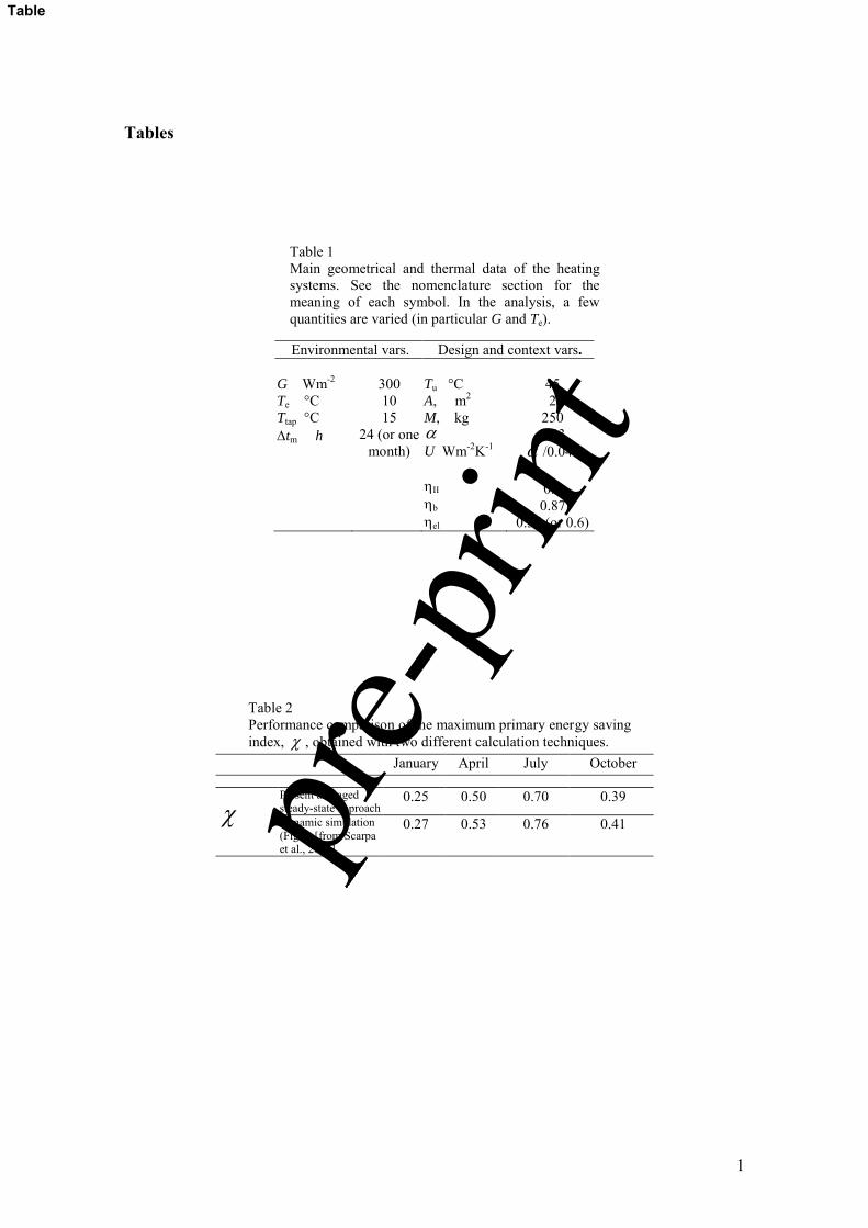
Tables

Table 1 Main geometrical and thermal data of the heating systems. See the nomenclature section for the meaning of each symbol. In the analysis, a few quantities are varied (in particular G and Te).

Environmental vars. Design and context vars.

G Wm-2 Te °C Ttap °C tm h

300 10 15

24 (or one month)

Tu °C A, m2 M, kg U Wm-2K-1

II

b el

45 2

250 0.93

/0.048

0.4 0.87

0.36 (or 0.6)

Table 2 Performance comparison of the maximum primary energy saving index, , obtained with two different calculation techniques.

January April July October

Present averaged steady-state approach

0.25 0.50 0.70 0.39

Dynamic simulation (Fig.9) [from Scarpa et al., 2011]

0.27 0.53 0.76 0.41

Table

pre-p

rint