A model-based framework for the phenotypiccharacterization of the flowering of Medicago truncatula

DELPHINE MOREAU, CHRISTOPHE SALON & NATHALIE MUNIER-JOLAIN

Institut National de la Recherche Agronomique (INRA) – Unité de Recherche en Génétique et Ecophysiologie desLégumineuses, 17 Rue Sully – BP 86510, 21065 Dijon cedex, France

ABSTRACT

To facilitate the phenotypic characterization of Medicagotruncatula, our aim was to provide a framework of analysisof flowering in response to environmental factors. The flow-ering of the line A17 was analysed in different conditions oftemperature, duration of vernalization and photoperiod.Flowering was characterized using three descriptors at theaxis level: the position of the first reproductive node (1RN),the date of beginning of flowering (DBF) and the floro-chron (RFa-1) corresponding to the reciprocal of the rate ofprogression of flowering along each axis. As for vegetativedevelopment, it was found that flowering could be analysedas a function of thermal time using a base temperature (Tb)of 5 °C. Vernalization displayed a sound impact on the flow-ering. For all the studied axes, increasing the duration ofvernalization lowered the 1RN and hastened the DBF. Bycontrast, for most of the studied axes, RFa-1 was onlyslightly affected by vernalization. For the branch B0, RFa-1

was a genotypic constant when thermal time was used. Con-sidering B0 as a reference axis, an ecophysiological modelwas developed to simulate the impact of environmentalfactors on the three components of flowering. Concretepractical applications of the model-based framework pre-sented herein are proposed for helping the genetic andgenomic studies of M. truncatula.

Key-words: modelling; photoperiod; temperature; thermaltime; vernalization.

INTRODUCTION

Medicago truncatula has been developed as a model plantto improve our knowledge of the genetic and moleculardeterminisms implied in traits specific to the legumes (Cook1999). This species, with its simple genetic properties, itswide genetic resource and its forthcoming genomicsequence, provides a unique opportunity for achieving acomplete understanding of legume plant functioning, fromgene to phenotype. However, to take full advantage of thepowerful genetic and genomic tools currently available,undertaking a reproducible and relevant phenotyping ofthe genetic resource is crucial.

To facilitate phenotyping approaches, a framework ofanalysis of the vegetative development that allows describ-ing, analysing and predicting plant development is available(Moreau, Salon & Munier-Jolain 2006). However, as amodel plant, M. truncatula also requires a framework ofanalysis of the reproductive development in order to beable to analyse flowering in response to environmentalconditions. In the scope of phenotyping studies, such aframework can be useful for characterizing and analysinggenotypic variability. For experimental concerns, it can be ofpractical interest for helping the users of M. truncatula tochoose relevant environmental conditions or to betterschedule plant observation and data collection. Besides,extensive studies have been performed to elucidate thedeterminism of the date of beginning of flowering (DBF)and, using the model plant Arabidopsis thaliana, manygenetic pathways controlling the response of flowering timeto environmental factors have been identified (for review,see Bernier & Périlleux 2005; Welch et al. 2005). However,A. thaliana has a determinate development and, as such, M.truncatula, with its indeterminate development, provides arelevant model for the study of the reproductive develop-ment of (both legume and non-legume) indeterminatespecies (Duc 2000).

The indeterminate pattern of the development of M.truncatula results from the presence on each axis of (1) anapical meristem from which leaves are initiated; (2) vegeta-tive axillary meristems likely to produce branches; and (3)reproductive axillary meristems, from a varying nodenumber, whose development gives rise to flowers (Benllochet al. 2003). As for pea (Ney & Turc 1993) and soybean(Munier-Jolain, Ney & Duthion 1993), the indeterminatedevelopment of M. truncatula is characterized by thesequential progression of flowering along each axis, fromthe first reproductive node (1RN) to the apex, and leads toa staggering of flowering during plant cycle.

The influence of the main environmental factors affectingthe DBF on the whole plant has been well documented forM. truncatula. A long vernalization (i.e. a cold treatment ofimbibed or germinated seeds), a high temperature aftervernalization and a long photoperiod have all been shownto reduce the time to appearance of the first flower on thewhole plant (Aitken 1955; Clarkson & Russell 1975; vanHeerden 1984; Hochman 1987). Different mathematicalmodels that allow predicting the time to appearance of the

Correspondence: Delphine Moreau. Fax: 33 (0)3 80 69 32 62; e-mail:moreau@dijon.inra.fr

Plant, Cell and Environment (2007) 30, 213–224 doi: 10.1111/j.1365-3040.2006.01620.x

Journal compilation © 2007 Blackwell Publishing LtdNo claim to original French government works 213

first flower as a function of environmental factors havebeen described (Clarkson & Russell 1979; van Heerden1984; Hochman 1987). However, most of these models havebeen developed in order to predict flowering in field con-ditions and are inappropriate for use in controlled environ-ment (e.g. glasshouse and growth chamber). Only the modelof van Heerden (1984) can be of practical use in order topredict the DBF in controlled conditions. Nevertheless,based on response curves to vernalization for differentphotoperiods, it does not consider the impact of thetemperature.

Whereas the DBF on the whole plant has been quite wellcharacterized on M. truncatula, the sequential progressionof flowering within the plant has to our knowledge neverbeen investigated. Little is known about the progression offlowering, and its environmental control, for the branchedarchitecture of the line A17, commonly used as a referenceby the M. truncatula community. Whereas vernalization,temperature and photoperiod are all known to affect theDBF on the whole plant, it remains unknown how theyinfluence both the DBF of the different axes on a plant andthe rate of progression of the flowering along the differentaxes.

By contrast, the progression of flowering within the planthas been characterized in other legume species. On a peaplant, the DBF occurs almost simultaneously on the mainaxis (MA) and on the first developed branches, whereasflowering is delayed for higher ranks of branches (Jeudy &Munier-Jolain 2005). On a given axis, the DBF is linked tothe position of its 1RN. Based on this relationship, Truong &Duthion (1993) modelled the DBF of the MA of pea, con-sidering that flowering occurred at the date when the leafsituated at the 1RN appeared. In pea (Ney & Turc 1993) andsoybean (Munier-Jolain et al. 1993), the rate of progressionof flowering (RFa) on the MA is strongly affected by tem-perature. So, when time is expressed by taking into accountmean daily temperature (Tm) according to the concept ofthermal time (for review, see Bonhomme 2000; Trudgillet al. 2005), the RFa on the MA is stable within a wide rangeof environmental conditions, in the absence of stresses, andappears to be a genotypic constant. Accordingly, the frame-work of analysis of the reproductive development of peaand soybean, based on thermal time, provides a powerful

means for describing, analysing and also predicting thesequential progression of flowering within the plant.

For M. truncatula, a framework of analysis of the vegeta-tive development is available (Moreau et al. 2006). In thecontinuity of this work, the objective of the present paperwas to provide a framework for the analysis of the repro-ductive development in response to environmental condi-tions. Because one of the particularities of M. truncatula isthe indeterminate habit of its development, it was essentialto develop a framework that takes into account the sequen-tial progression of flowering within the plant. Firstly, wecharacterized the impact of temperature on the RFa inorder to determine if the use of thermal time was appropri-ate for analysing the flowering of M. truncatula plants.Then,the dynamics of the progression of flowering within theplant was characterized for the reference line A17 by study-ing, for different axes, three descriptors of flowering: theposition of the 1RN, the DBF and the RFa-1 along eachstudied axis.The influence of the vernalization was analysedin order to identify which descriptors of flowering werespecifically altered in response to a vernalization treatment.Finally, using the data obtained in varied environmentalconditions, the combined effect of temperature, photope-riod and vernalization on the progression of flowering wasanalysed and, by coupling models available in the literature,a model of prediction of flowering was proposed for M.truncatula plants.

MATERIALS AND METHODS

Five glasshouse and one growth chamber experiments wereconducted on the cultivar Jemalong genotype A17 in Dijon(France) under varied conditions of photoperiod and tem-perature, and with different durations of vernalization. Thedifferent experiments, which were named according to theirmean daily photoperiod, are presented in Table 1.

Cultural conditions

Vernalization treatmentsSeven vernalization treatments, corresponding to differentdurations of vernalization, were applied in Exp P12: 1, 3, 5,

Table 1. Environmental conditions in the different experiments

Exp LocationDurations of thevernalization (d)

Daily photoperiod (h) Daily temperature (°C)

Mean SD Mean SD

P12 Glasshouse 1, 3, 5, 7, 9, 12 and 14 12.2 0.6 15.3 2.0P14 Glasshouse 1, 4, 7, 10, 14 and 21 14.0 0.0 19.7 0.6P16 Glasshouse 1, 4, 7, 10, 14 and 21 16.0 0.0 19.9 0.6P14′ Glasshouse 4 14.3 1.0 22.0 1.2P15′ Glasshouse 2 14.7 0.6 18.9 1.4P16′ Growth chamber 4 16.0 0.0 21.3 1.2

The different experiments are named according to their mean daily photoperiod. Means and SDs are calculated from sowing date to the endof the experiment.In Exps P12, P14 and P15′, the SDs for daily photoperiod were different from zero, as daily photoperiod varied with natural photoperiod.

214 D. Moreau et al.

Journal compilation © 2007 Blackwell Publishing LtdNo claim to original French government works, Plant, Cell and Environment, 30, 213–224

7, 9, 12 and 14 d. Six different durations of vernalizationwere used in Exps P14 and P16: 1, 4, 7, 10, 14 and 21 d. InExps P12, P14 and P16, the different vernalization treat-ments started sequentially so that all the treatments couldbe sown at the same date. In Exps P14′, P15′ and P16′, aunique duration of the vernalization was applied: 4, 2 and4 d, respectively.

In all experiments, vernalization was performed usingthe procedure taken from the M. truncatula Handbook(Chabaud et al. 2007). Seeds were mechanically scarifiedwith sandpaper, placed on filter paper in Petri dishes andimbibed with deionized water for 3 h.They were then trans-ferred into a vernalization cabinet at 4 °C during 1–21 daccording to the vernalization treatment.

Seed germination and plant cultureSeed germination and plant culture were performed usingthe same protocol in the six experiments. After vernaliza-tion, the seeds were transferred into a germination cabinetfor 1 d in order to synchronize germination among treat-ments. During germination, day and night temperatureswere 22 and 18 °C, respectively, and photoperiod was 16 h.Thereafter, germinated seeds were sown in the glasshouseinto 1 L pots filled with a 1:1 mixture of expanded clay andattapulgite. Two seeds per pot were sown after inoculationwith Rhizobium meliloti (strain 2011).They were thinned toone plant per pot when the plants carried two trifoliateleaves. In all experiments, a nutrient solution made up ofphosphorus, potassium, oligoelements and a limited amountof nitrogen was provided by automatic watering of pots(Barkers et al. 2007).

Environmental conditions during plant cultureEnvironmental conditions in the different experiments arepresented in Table 1. In each experiment, air temperaturewas measured at 600 s intervals, using PT100 sensors, andwas stored in a data logger (DL2e; Delta-T Devices,Cambridge, England).According to the experiment, the dif-ference between mean day and mean night temperatureswas between 4 and 5 degrees (data not shown). In Exps P12,P14, P16 and P15′, additional light was supplied with sodiumlamps (MACS 400 W; Mazda, Dijon, France) with a meanphotosynthetically active radiation (PAR) at 130 mE m-2 s-1.In Exps P14 and P16, additional light allowed the mainte-nance of a constant photoperiod. In Exps P12 and P15′,natural light was complemented with additional light during10 and 12 h, respectively, in order to obtain a photoperiodhigher or equal to 10 and 12 h, respectively, throughoutplant cycle. In Exp P16′, conducted in a growth chamber,light was provided by sodium lamps during 16 h with amean PAR of 700 mE m-2 s-1. Natural photoperiod andradiation were used in Exp P14′.

Plant observations

In Exps P12, P14 and P16, each vernalization treatmentconsisted of 7, 8 and 8 plants, respectively. In Exps P14′, P15′

and P16′, 10, 5 and 6 plants, respectively, were used. In allexperiments, non-destructive observations were regularlyperformed on each plant in order to characterize its devel-opmental stage (see Moreau et al. 2006 for details about theterminology and the system of notation of the developmen-tal stages). In Exp P12, the MA and the seven first ranks ofprimary branches (from B0 to B6) were observed at leastweekly in order to determine, for each axis, (1) the numberof appeared leaves, (2) the 1RN and (3) the number ofreproductive nodes. In Exps P14, P14′and P16, the 1RN andthe number of reproductive nodes were observed on B0. InExps P15′ and P16′, the 1RN and the DBF were observedon B0.

In all experiments, a node was considered as reproductivefrom the moment when it bore at least one open flower, asillustrated in Moreau et al. (2006). Whatever the axis, the1RN was counted from the round leaf of the MA, consid-ered as the node 0. For example, when a 1RN was located atthe axil of the third leaf of B2, it was counted at 5 (twotrifoliate leaves on the MA + 3 leaves on B2); when a 1RNwas situated at the axil of the fifth leaf of B0, it was countedat 5 (zero trifoliate leaf on the MA + 5 leaves on B0). Char-acterizing the 1RN at the plant level using this methodallowed facilitating the comparisons between axes.

Calculations

The number of appeared leaves and the number of repro-ductive nodes per axis were related to time.Time was eithercalendar time (expressed in number of days) or thermaltime (expressed in degree-days).Time was calculated eithersince the date of appearance of the first trifoliate leaf on theMA (Moreau et al. 2006) or since the DBF of a given axis.For each vernalization treatment (Exps P12, P14 and P16)or each experiment (P14′, P15′ and P16′), means and SDswere calculated for each axis as the means and the SDs ofthe replicates.

Date of appearance of the branches andphyllochron (RLa-1)The date of appearance of each branch was calculated asthe time expressed in degree-days, when the branch carriedone appeared leaf, using the linear regression between themean number of appeared leaves and thermal time. It wascalculated since the appearance of the first trifoliate leaf onthe MA.

RLa-1 is defined as the time interval, expressed in degree-days, between the appearance of two successive flattenedleaves on an axis. It was calculated as the reciprocal of therate of leaf appearance (RLa) estimated by the slope of thelinear regression between the number of appeared leavesand thermal time.

DBF, RFa and florochron (RFa-1)The DBF was calculated for each axis as the time, expressedin degree-days, when the axis carried one reproductive

Phenotypic characterization of the flowering of M. truncatula 215

Journal compilation © 2007 Blackwell Publishing LtdNo claim to original French government works, Plant, Cell and Environment, 30, 213–224

node, using the linear regression between the mean numberof reproductive nodes and thermal time. It was calculatedsince the date of appearance of the first trifoliate leaf on theMA.

The RFa (or rate of flower appearance) was calculatedfor each axis as the slope of the linear regression betweenthe mean number of reproductive nodes per axis and time,expressed either in number of days or in degree-days. RFa-1,defined as the time interval between the appearance of twosuccessive reproductive nodes on an axis, was calculated asthe reciprocal of the RFa.

Thermal time and base temperature (Tb)Thermal time was expressed in degree-days. It was calcu-lated as the sum of the mean daily effective temperatures,that is, Tm minus the Tb (for review, see Bonhomme 2000;Trudgill et al. 2005):

Thermal time max ; d0

t

= −( )[ ]∫ 0 T T tm b

Tb is defined as the temperature below which the develop-ment is supposed to be nil (Bonhomme 2000; Trudgill et al.2005). One objective of this study was to estimate Tb forthe reproductive development. Towards this goal, thex-intercept of the linear regression between the RFa(expressed in number of reproductive nodes per calendarday; for calculation, see previous section) and Tm during theprogression of flowering (expressed in °C) was calculated.The Tb for the RFa was determined by studying only thefirst primary branch (B0) whose development is known tobe highly dependent upon temperature (Moreau et al.2006).

Curve adjustment and statistical analysesParameters estimation for curve adjustment was performedusing the Microsoft Excel solver tool. Statistical analyseswere performed with the general linear model (GLM) pro-cedure of SAS (SAS Institute 1987). Means were comparedusing the Student–Newman–Keuls test at the 0.05 probabil-ity level.

RESULTS

Impact of Tm on the RFa

In a previous study (Moreau et al. 2006), Tm was shown tohave a strong impact on the rate of leaf initiation (RLi) andthe RLa (Fig. 1), indicating that plant vegetative develop-ment could be analysed as a function of thermal time usinga unique Tb of 5 °C. Likewise, our aim in this section was tocharacterize the influence of Tm on plant reproductivedevelopment. Towards this goal, the RFa on the firstprimary branch (B0) was analysed as a function of Tm infour experiments (P12, P14, P16 and P14′). In each vernal-ization treatment, Tm during the progression of flowering onB0 was stable throughout the plant cycle (data not shown).

As shown in the insert of Fig. 1, the number of reproduc-tive nodes on B0 increased linearly as a function of thenumber of days in a given experiment. So, the RFa on B0,expressed in number of reproductive nodes per calendarday, was stable in a given experiment when Tm was constant.Because the RFa and the Tm only slightly varied amongvernalization treatments of a given experiment, a mean RFaand a mean Tm were calculated for each experiment. Usingthese data, the RFa was related to Tm during the progres-sion of flowering on B0 (Fig. 1): the RFa increased linearlywith Tm, with an x-intercept close to 5.2 °C.

Statistical analyses indicate that the response of the RFato Tm was not different from the response of the RLa to Tm.They also reveal that the Tb for the RFa was not signifi-cantly different from the Tb for the vegetative development.Plant reproductive development can consequently beanalysed as a function of thermal time with a Tb at 5 °C.

Timing of progression of flowering withinthe plant, and impact of the duration ofthe vernalization

Our aim was to analyse how flowering progressed withinthe plant both in space and time, and to analyse how it wasaffected by the duration of the vernalization. Towards thisgoal, a detailed analysis of the dynamics of the progressionof flowering was undertaken at the plant scale by observing

Tm (°C)

0 5 10 15 20 25

Ra

te o

f d

eve

lop

me

nt

(d–

1)

0.0

0.1

0.2

0.3

0.4

0.5

0.6

Days

0 10 20 30 40 50

NR

N

0

2

4

6

8

10

Figure 1. Impact of mean daily temperature (Tm) on the rate ofleaf initiation (RLi), the rate of leaf appearance (RLa) and therate of progression of flowering (RFa) on the first primarybranch (B0). The RLi (�) and the RLa (�) are both expressedin number of leaves per day; the RFa (�) is expressed in numberof reproductive nodes per day, and Tm is expressed in °C. Eachvalue on the graph corresponds to one experiment. The data ofRLa and the RLi are taken from Moreau et al. (2006). The linesare linear regressions fitted to the data: dash line for RLi, solidline for RLa and dotted line for RFa. Inset: changes over time inthe number of reproductive nodes (NRN) on B0. Time isexpressed in calendar days from the date of beginning offlowering (DBF) of B0. �, Exp P12; �, Exp P14. For eachexperiment, all the vernalization treatments are represented.Each value is the mean of the replicates. The solid lines are linearregressions fitted to the data.

216 D. Moreau et al.

Journal compilation © 2007 Blackwell Publishing LtdNo claim to original French government works, Plant, Cell and Environment, 30, 213–224

the MA and the seven first ranks of primary branches (fromB0 to B6) in Exp P12 (Table 1). The appearance of thereproductive nodes was analysed as a function of thermaltime (for calculation, see Materials and Methods) with a Tb

of 5 °C (see previous section). Each axis was characterizedby (1) the 1RN, (2) the DBF and (3) the RFa-1. For eachvariable, the influence of the duration of the vernalizationtreatment was quantified.

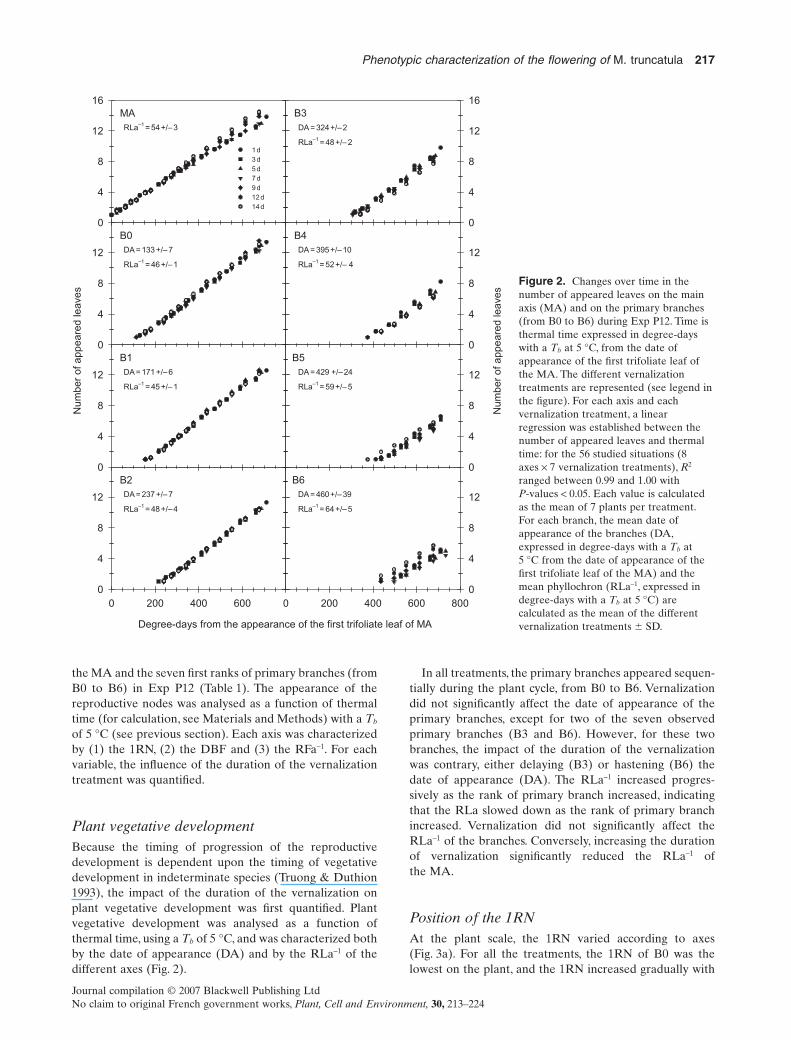
Plant vegetative developmentBecause the timing of progression of the reproductivedevelopment is dependent upon the timing of vegetativedevelopment in indeterminate species (Truong & Duthion1993), the impact of the duration of the vernalization onplant vegetative development was first quantified. Plantvegetative development was analysed as a function ofthermal time, using a Tb of 5 °C, and was characterized bothby the date of appearance (DA) and by the RLa-1 of thedifferent axes (Fig. 2).

In all treatments, the primary branches appeared sequen-tially during the plant cycle, from B0 to B6. Vernalizationdid not significantly affect the date of appearance of theprimary branches, except for two of the seven observedprimary branches (B3 and B6). However, for these twobranches, the impact of the duration of the vernalizationwas contrary, either delaying (B3) or hastening (B6) thedate of appearance (DA). The RLa-1 increased progres-sively as the rank of primary branch increased, indicatingthat the RLa slowed down as the rank of primary branchincreased. Vernalization did not significantly affect theRLa-1 of the branches. Conversely, increasing the durationof vernalization significantly reduced the RLa-1 ofthe MA.

Position of the 1RNAt the plant scale, the 1RN varied according to axes(Fig. 3a). For all the treatments, the 1RN of B0 was thelowest on the plant, and the 1RN increased gradually with

0

4

8

12

0

4

8

12

0 200 400 600 800

0

4

8

12N

um

ber

of

ap

pe

are

d lea

ves

0

4

8

12

16

Degree-days from the appearance of the first trifoliate leaf of MA

0 200 400 600

0

4

8

12

B2

0

4

8

12

0

4

8

12

Nu

mbe

r o

f a

pp

ea

red

le

ave

s

0

4

8

12

16

1 d

3 d

5 d

7 d

9 d

12 d

14 d

MA

B0

B1

B4

B5

B6

B3

DA = 324 +/– 2

RLa–1

= 48 +/– 2

RLa–1

= 54 +/– 3

DA = 133 +/– 7

RLa–1

= 46 +/– 1

DA = 171 +/– 6

RLa–1

= 45 +/– 1

DA = 237 +/– 7

RLa–1

= 48 +/– 4

DA = 395 +/– 10

RLa–1

= 52 +/– 4

DA = 429 +/– 24

RLa–1

= 59 +/– 5

DA = 460 +/– 39

RLa–1

= 64 +/– 5

Figure 2. Changes over time in thenumber of appeared leaves on the mainaxis (MA) and on the primary branches(from B0 to B6) during Exp P12. Time isthermal time expressed in degree-dayswith a Tb at 5 °C, from the date ofappearance of the first trifoliate leaf ofthe MA. The different vernalizationtreatments are represented (see legend inthe figure). For each axis and eachvernalization treatment, a linearregression was established between thenumber of appeared leaves and thermaltime: for the 56 studied situations (8axes ¥ 7 vernalization treatments), R2

ranged between 0.99 and 1.00 withP-values < 0.05. Each value is calculatedas the mean of 7 plants per treatment.For each branch, the mean date ofappearance of the branches (DA,expressed in degree-days with a Tb at5 °C from the date of appearance of thefirst trifoliate leaf of the MA) and themean phyllochron (RLa-1, expressed indegree-days with a Tb at 5 °C) arecalculated as the mean of the differentvernalization treatments � SD.

Phenotypic characterization of the flowering of M. truncatula 217

Journal compilation © 2007 Blackwell Publishing LtdNo claim to original French government works, Plant, Cell and Environment, 30, 213–224

the rank of primary branches.The 1RN of the MA was highcompared to the 1RN of the branches.

Variations in the duration of vernalization signifi-cantly affected the 1RN (Fig. 3a). For all the axes, the 1RNwas progressively lowered when the duration of thevernalization treatment increased. For instance, the 1RNfor B0 decreased from 14 after 1 d of vernalization to 4 after14 d of vernalization. However, the 1RN remained steadyfor vernalization longer than 7 or 9 d, according to theprimary branch. This indicates that, from 7 or 9 d of vernal-ization, further exposure to cold did not significantly affectthe 1RN.

DBFOn a given plant, the DBF did not occur at the same date indegree-days on the different axes (Fig. 3b). For all the treat-ments, the primary branches started to flower successivelyin the order of their appearance on the plant, from B0 to B6.The first primary branches to flower were B0 and B1, whose

DBF did not significantly differ. The DBF of the MA at theplant scale was variable according to the vernalizationtreatment: the MA was the last axis to flower after a 1 dvernalization treatment, whereas it started to flower at thesame time as the two first branches (B0 and B1) after a 14 dvernalization treatment.

For all the axes, the DBF was all the more early as theduration of the vernalization treatment increased (Fig. 3b).Changing the duration of vernalization from 1 to 14 d accel-erated the DBF of about 400 degree-days for the primarybranches, and of about 700 degree-days for the MA. For theprimary branches, the DBF was unchanged when the dura-tion of vernalization was higher than 7 or 9 d, according tothe primary branch. This indicates that, from 7 or 9 d ofvernalization, further exposure to cold did not hasten flow-ering. Conversely, the DBF of the MA did not stagnate inthe range of duration of vernalization that was investigated.Compared with the flowering of branches, the DBF of theMA seemed therefore more responsive to vernalization.

RFa-1

For each axis and each vernalization treatment, the numberof reproductive nodes increased linearly as a function ofthermal time (Fig. 4). For a given axis and a given vernal-ization treatment, the RFa, expressed using degree-days,was therefore stable. Mean values of the RFa-1, expressed indegree-days, of the different axes for all the vernalizationtreatments are given in Fig. 4.The first primary branch (B0)had the shortest RFa-1, indicating that it produced repro-ductive nodes more rapidly than the other axes. RFa-1

increased progressively with the rank of primary branches.The RFa-1 of the MA was among the longest. For thebranches B0 to B5, RFa-1 did not statistically vary amongvernalization treatments. By contrast, RFa-1 was moreunstable between treatments for B6 and the MA.

Combined effect of temperature, photoperiodand vernalization on the progression of theflowering, and modelling approach

Our aim was to analyse to which extent variations of pho-toperiod and temperature could affect the response of flow-ering to the duration of the vernalization.Towards this goal,flowering was observed in three experiments (P12, P14 andP16) varying both by photoperiod and Tm conditions andconducted with different durations of the vernalization(Table 1). The first primary branch B0 used to be the firstflowering axis on the plant (data not shown). So, the resultspresented in this section are restricted to the characteriza-tion of the flowering of B0 which can be used as a referenceaxis for analysing flowering in response to environmentalfactors.

Modelling the RFa-1 from Tm usingthermal timeThe RFa-1 of B0 was calculated in degree-days for eachexperiment. It was stable between environmental condi-

1R

N

0

2

4

6

8

10

12

14

16

18

20

MA

B0

B1

B2

B3

B4

B5

B6

Duration of vernalization (d)

0 2 4 6 8 10 12 14

DB

F (

de

gre

e-d

ays)

0

200

400

600

800

1000

1200

(a)

(b)

Figure 3. Impact of the duration of vernalization on (a) theposition of the first reproductive node (1RN) and (b) the date ofbeginning of flowering (DBF), of the main axis (MA) and theprimary branches (from B0 to B6) during Exp P12. The durationof vernalization is expressed in number of days. The DBF isexpressed in degree-days with a base temperature (Tb) at 5 °C,from the date of appearance of the first trifoliate leaf of the MA.The different vernalization treatments are represented (seelegend in the figure). Each value is calculated as the mean of 7plants per treatment, and vertical bars indicate � SD.

218 D. Moreau et al.

Journal compilation © 2007 Blackwell Publishing LtdNo claim to original French government works, Plant, Cell and Environment, 30, 213–224

tions, with a mean of the different experiments estimated at47 � 4 degree-days, corresponding to the slope of theregression calculated from Fig. 1.

Modelling the 1RN from the durationof vernalizationFor the different conditions of temperature and photope-riod, increasing the duration of the vernalization loweredthe 1RN of B0 (Fig. 5). However, the 1RN did not respondto vernalization when the duration of vernalization washigher than 7, 9 or 10 d. These findings, obtained using datacollected in different temperature and photoperiod condi-tions, corroborate the results previously presented for asingle experiment (P12) (Fig. 3a).

For a given vernalization treatment, increasing both thephotoperiod and the temperature significantly lowered the1RN. In given photoperiod and temperature conditions,variations of the duration of the vernalization could lead todifferences of 1RN of 13 nodes, whereas for a given vernal-ization treatment, the maximal differences of 1RN induced

by variations of both the photoperiod and the temperaturewere lower than four nodes (calculated from Fig. 5). So, inthe range of treatments experimented, the 1RN was muchmore responsive to variations of the duration of the veria-tions than to variations of the other environmental factors.

In reference to van Heerden (1984), the response curveof the 1RN to the duration of vernalization (DV) was mod-elled using an exponential function. Because the responsecurves only slightly varied between experiments, we used aunique function whose equation was

1 1RN DV= + ×a b r( ) (1)

with a, b and r as parameters which were estimated: a at2.80, b at 5.40 and r at 0.77. The R2 of the relationship was0.95 (Fig. 5).

The ability of the model to predict the 1RN from theduration of the vernalization was tested using two type ofdata sets: the data set consisting of the experiments whichwere used to develop the model (P12, P14, P16), and anindependent data set consisting of three other experiments

Degree-days from the beginning of flowering of each axis

00

2

4

6

8

0

2

4

6

8

0

2

4

6

8

0

2

4

6

8

10

1 day3 days5 days7 days9 days12 days14 days

Num

ber

of r

epro

duct

ive

node

s

0

2

4

6

8

0

2

4

6

8B0

B2

B4

B5

B6

0

2

4

6

8

10MA

0

2

4

6

8B1

B3

Num

ber

of r

epro

duct

ive

node

s

RFa–1 = 75 +/– 28

RFa–1 = 51 +/– 3

RFa–1 = 55 +/– 5

RFa–1 = 54 +/– 4

RFa–1 = 57 +/– 4

RFa–1 = 64 +/– 10

RFa–1 = 54 +/– 3 RFa–1

= 77 +/– 23

4003002001000 400300200100

Figure 4. Changes over time in thenumber of reproductive nodes on themain axis (MA) and on the primarybranches (from B0 to B6) during ExpP12. Time is thermal time expressed indegree-days with a base temperature (Tb)at 5 °C, from the date of beginning offlowering (DBF) of each axis. Thedifferent vernalization treatments arerepresented (see legend in the figure). Foreach axis and each vernalizationtreatment, a linear regression wasestablished between the number ofreproductive nodes and thermal time: forthe 56 studied situations (8 axes ¥ 7vernalization treatments), R2 rangedbetween 0.93 and 1.00 withP-values < 0.05 except for one treatment(MA at 1 d of vernalization: P = 0.12).Each value is calculated as the mean of 7plants per treatment. For each branch, themean florochron (RFa-1, expressed indegree-days with a Tb at 5 °C) iscalculated as the mean of the differentvernalization treatments � SD. For B0,the dotted line corresponds to the linearregression between the number ofappeared leaves [counted from the firstreproductive node (1RN)] and thermaltime.

Phenotypic characterization of the flowering of M. truncatula 219

Journal compilation © 2007 Blackwell Publishing LtdNo claim to original French government works, Plant, Cell and Environment, 30, 213–224

(P14′, P15′ and P16′). For all the experiments, simulated1RN was plotted against observed 1RN (Fig. 6a). Thequality of the prediction was estimated using two criteriacommonly used to evaluate models of simulation: the coef-ficient of determination (R2) and the mean squared error ofprediction (MSEP) (Wallach 2006). For Exps P12, P14 andP16, the model accurately predicted the 1RN: all the pointswere close to the first bissectrice line and R2 was high (0.94).The mean error of prediction, estimated by the squared rootof MSEP, was satisfactory with a value at 0.94 node, close tothe experimental error. Considering the independent dataset, discrepancies between observed and simulated 1RN(calculated as the difference between observed and simu-lated 1RN divided by observed 1RN) ranged between 12and 24% (Fig. 6a).

Modelling the DBF from the 1RN and constantsof vegetative developmentThe DBF of the first primary branch B0 was modelled,using the following formalism (adapted from Truong &Duthion 1993):

DBF DA RN RLa= + +( ) × −1 2 1 (2)

As shown in Fig. 7, the model assumed that the time toreach the DBF of B0 corresponded to the delay necessaryfor B0 to appear (DA, date of appearance), to which wasadded the number of leaves to appear (1RN + 2) multipliedby the time needed for each leaf to appear (RLa-1). Thedate of appearance of B0 was estimated at 103 � 37 degree-days (base 5) in a wide range of environmental conditions,and the RLa-1 was shown to be a genotypic trait of A17 witha mean value at 46 � 4 degree-days (Moreau et al. 2006).Atthe 1RN, the appearance of the leaf and the first floweropening were not synchronous (as for pea: Truong &Duthion 1993; Roche, Jeuffroy & Ney 1998). Using the datacollected in varied environmental conditions, it wasobserved that, at the date of flowering of the 1RN, thenumber of appeared leaves above the 1RN could rangebetween 1.6 and 3.0 (data not shown), but it was commonlyclose to 2. This is illustrated in Fig. 4 in which the linearregression between the number of appeared leaves(counted from the 1RN) and thermal time was representedfor B0: the difference between the number of appearedleaves and the number of reproductive nodes, observed atthe y-intercept, corresponds to two nodes. As a result, amean value of 2 leaves was added in the model.

In the model, the 1RN can either be used as an inputvariable or can be estimated from the duration of the ver-nalization, using Eqn 1. The ability of the model to predictthe DBF from the duration of the vernalization (combina-tion of Eqns 1 and 2) was tested using the two types of datasets presented in the previous section. Simulated DBF wasplotted against observed DBF for all the experiments(Fig. 6b). For the Exps P12, P14 and P16, the model accu-rately predicted the DBF: all the points were close to the

Duration of vernalization (d)

0 5 10 15 20

1R

N

0

2

4

6

8

10

12

14

16

18

20

Figure 5. Impact of the duration of vernalization (DV) on theposition of the first reproductive node (1RN) of the first primarybranch (B0) for different photoperiod and temperatureconditions. The DV is expressed in number of days. Each value iscalculated as the mean of the different replicates per treatment,and vertical bars indicate �SD. All the data are fitted to anexponential curve (R2 = 0.95): 1RN = 2.80 (1 + 5.40 ¥ 0.77DV). �,Exp P12; �, Exp P14; �, Exp P16.

Observed 1RN

0 3 6 9 12 15 18

Sim

ula

ted 1

RN

0

3

6

9

12

15

18

Observed DBF (degree-days)

0 150 300 450 600 750 900

Sim

ula

ted D

BF

(de

gre

e-d

ays)

0

150

300

450

600

750

900(a) (b)

Figure 6. Relationships between simulated and observed (a) position of the first reproductive node (1RN) and (b) date of beginning offlowering (DBF) for the first primary branch (B0). �, Exp P12; �, Exp P14; �, Exp P16; �, independent data set consisting of Exps P14′,P15′ and P16′. For each treatment, observed values correspond to the mean of the replicates, and horizontal bars indicate � SD. The 1RNis simulated using Eqn 1, and the DBF [expressed in degree-days from the date of appearance of the first trifoliate leaf of the main axis(MA)] is simulated using both Eqns 1 and 2. The solid lines indicate the 1:1 line, and the dotted lines are �15% lines.

220 D. Moreau et al.

Journal compilation © 2007 Blackwell Publishing LtdNo claim to original French government works, Plant, Cell and Environment, 30, 213–224

first bissectrice line, and R2 was high (0.86). The mean errorof prediction, estimated by the squared root of MSEP, wassatisfactory with a value at 68 degree-days, close to theexperimental error. Considering the independent data set,discrepancies between observed and simulated DBF (cal-culated as the difference between observed and simulatedDBF divided by observed DBF) ranged between 9 and 17%(Fig. 6b).

DISCUSSION

A standard framework that allows analysing plant vegeta-tive development using temperature inputs was formerlyproposed (Moreau et al. 2006). The objective of the presentpaper was to complete this framework by developing asimilar approach to the characterization of the sequentialprogression of flowering.

Both plant vegetative and reproductivedevelopment can be analysed usinga unique Tb

The RFa expressed in number of reproductive nodes perday along the first primary branch B0 was soundly affected

by the Tm: it increased linearly with Tm according to aunique relationship that was valid for varied environmentalconditions of temperature, photoperiod and duration of thevernalization (Fig. 1). Interestingly, the impact of Tm on theRFa was identical to its impact on the RLa, revealing thatthese two developmental processes were governed by tem-perature in the same manner. Moreover, the Tb for the RFawas not different from the Tb previously estimated for plantvegetative development (Moreau et al. 2006). Accordingly,as for pea (Munier-Jolain et al. 1993) and soybean(Duthion, Ney & Munier-Jolain 1994), both plant vegeta-tive and plant reproductive development can be analysed asa function of thermal time using a unique Tb, which wasestimated at 5 °C for Medicago truncatula A17.

Hence, based on thermal time, a framework of analysis ofthe flowering was established for M. truncatula plants. Inthis framework, the dynamics of the progression of flower-ing was characterized both in space and time at the axislevel, using three descriptors: the 1RN, the DBF (expressedin degree-days base 5) and the RFa-1 (expressed in degree-days base 5).

General characteristics of the sequentialprogression of flowering within A17 plants

By applying the framework to the description of the flow-ering of different axes, a detailed characterization of theprogression of flowering was undertaken at the plant level.

The 1RN was low for the first primary branch (B0), and itgradually increased with the rank of primary branches, fromB0 to B6; the 1RN of the MA was among the highest(Fig. 3a). Altogether, these results suggest that, as for pea(Jeudy & Munier-Jolain 2005), the date of flower initiationwas not synchronous on the whole plant, being delayed forthe higher ranks of branches and the MA. In agreementwith Truong & Duthion (1993), these differences of 1RNbetween axes explained largely the differences of the DBFbetween axes of a given plant (Fig. 3b).

RFa-1 was constant for a given axis in a given experimen-tal treatment when thermal time was used. However, itshowed instability: when the rank of branches increased, (1)it gradually lengthened from B0 to B6, and (2) graduallybecame more unstable between experimental treatments;moreover, (3) it was highly variable for the MA (Fig. 4).Similar results were obtained when studying the RLa (Fig. 2and Moreau et al. 2006). They suggest a trophic limitationthat would affect both plant vegetative and plant reproduc-tive development (Ney & Turc 1993; Lebon et al. 2004). Forinstance, Ney & Turc (1993) observed for pea that RFa-1 waslinked to plant growth rate, suggesting that plant reproduc-tive development could depend upon photoassimilateavailability.

Vernalization is the main factor affectingflowering, modifying both 1RN and DBF

Using the framework of analysis, we analysed the impact ofenvironmental factors on the dynamics of the progression

Degree-days

Node number(B0)

1RN

Date of appearanceof the first trifoliate leaf on MA

RLa

RFa

DBFDA

1RN + 2

Figure 7. Relationships between the variables describing theprogression of flowering on the first primary branch (B0) ofMedicago truncatula. The diagram considers both a temporaldimension [x-axis, expressed in degree-days with a basetemperature (Tb) at 5 °C from the date of appearance of the firsttrifoliate leaf of the main axis (MA)] and a spatial dimension(y-axis, indicating the node number). A horizontal readingindicates, for a given node, the date of appearance of its leaf andthe date of its flowering. A vertical reading indicates the numberof leaves and reproductive nodes on B0 at a given thermal time.The first reproductive node (1RN) starts to flower at the date ofbeginning of flowering (DBF) of B0, occurring when the branchbears (1RN + 2) appeared leaves. So the DBF can be predictedfrom three inputs (Eqn 2): the date of appearance (DA) of B0,the rate of leaf appearance (RLa) and the 1RN (which can eitherbe observed or predicted from the duration of the vernalizationusing Eqn 1). The date of flowering of each reproductive node onB0 can then be estimated using the rate of progression offlowering (RFa). This framework can be applied to any genotypeif DA, RLa and RFa are known. In the case of the genotype A17,DA was estimated at 103 � 37 degree-days in a wide range ofenvironmental conditions, and phyllochron (RLa-1) was shown tobe a genotypic constant with a mean value at 46 � 4 degree-days(Moreau et al. 2006). In this study, florochron (RFa-1) was agenotypic constant with a mean value at 47 � 4 degree-days.

Phenotypic characterization of the flowering of M. truncatula 221

Journal compilation © 2007 Blackwell Publishing LtdNo claim to original French government works, Plant, Cell and Environment, 30, 213–224

of the flowering within the plant. This study focused on thefirst primary branch (B0), which was considered as a refer-ence axis.

In the range of treatments experimented, the duration ofthe vernalization was the main environmental factor affect-ing the 1RN (Fig. 5) and, as a consequence (Truong &Duthion 1993), the DBF. This finding can be explained by alimited range of temperature (between 15.3 and 22.0 °C)and photoperiod (between 12.2 and 16.0 h) investigated inthis paper. For the studied branches, the impact of the ver-nalization on the flowering was nearly independent of thetiming of establishment of the vegetative organs. So, for thestudied branches, the impact of vernalization was specifi-cally focused on the date of flower initiation (Lang 1965)without additional effects. The impact of the vernalizationon the MA was more complex: increasing the duration ofthe vernalization not only gradually lowered the 1RN butalso gradually increased the RLa, resulting in a markedresponse of the DBF to the vernalization (Fig. 3b).

The RFa-1 on the first primary branch B0 varied slightlybetween environmental conditions when thermal time wasused, in spite of environmental differences between treat-ments. This finding shows that RFa-1 only depended on Tm

(Fig. 1), confirming the crucial role of temperature on plantdevelopment (Poethig 2003). Because RFa-1 expressed indegree-days was stable over a range of situations, it can beconsidered as a reproducible phenotypic trait of the geno-type A17 (Munier-Jolain et al. 1993; Ney & Turc 1993;Tardieu 2003).

Modelling as a framework for analysingflowering in response to environmental factors

Based on these findings, modelling tools predicting the dif-ferent descriptors of flowering at the axis level were pro-posed, by adapting models available in the literature. Theywere developed for B0, considered as a reference axis andestablished using A17 plants, whose nitrogen nutritionmainly relied on the symbiotic fixation of atmosphericnitrogen, in a certain range of environmental conditions: Tm

between 15 and 20 °C, photoperiod between 12 and 16 hand vernalization between 1 and 21 d. These conditionsdefine the domain of validity of the model, which is close tothe most commonly applied conditions for the culture of M.truncatula plants in controlled environments (unpublisheddata, gathered from a network).

In reference to Ney & Turc (1993), the relationshipsbetween the variables describing the progression of flower-ing on B0 can be represented in a diagram considering botha temporal (x-axis) and a spatial (y-axis) dimensions(Fig. 7).A horizontal reading indicates, for a given node, thedate of appearance of its leaf and the date of its flowering.A vertical reading indicates the number of leaves andreproductive nodes at a given thermal time.

Because RFa-1 was shown to only depend on Tm, it wassimply simulated from Tm inputs, using thermal time(Munier-Jolain et al. 1993; Ney & Turc 1993) with a Tb

at 5 °C.

The 1RN was predicted, using an exponential function,from the duration of the vernalization (van Heerden 1984),whatever temperature and photoperiod conditions (Eqn 1).This model is empirical but its parameters have a physi-ological meaning that provides indications for analysing theresponse to the vernalization. Indeed, the parameter a cor-responds to the plateau of the relationship: its value (2.80)is close to the mean observed 1RN (2.75 � 0.35) for thelongest duration of the vernalization (21 d).The parametersb and r both describe the magnitude of the response to thevernalization. So, analysing the derivative of Eqn 1 forDV = 0 provides indications for comparing the cold require-ments of different genotypes (van Heerden 1984).

The DBF is a complex integrative trait for which it wasnecessary to undertake a more mechanistic modellingapproach allowing to dissect the DBF into intermediatevariables (Truong & Duthion 1993). As presented in thediagram of Fig. 7, the DBF of B0 is predicted from (Eqn 2):(1) the date of appearance of the branch, (2) the RLa and(3) the 1RN that can either be used as an input variable orcan be estimated from the duration of the vernalizationusing Eqn 1. An evaluation of the quality of the simulationrevealed a tendency for overestimation at the highest tem-peratures and longest photoperiods (Exps P14 and P16),and for underestimation at the lowest temperature andshortest photoperiod (Exp P12) (Fig. 6b). This result prob-ably originated from the fact that a unique curve was usedto simulate the 1RN. Our data set did not allow a cleardifferentiation of the impact of photoperiod and Tm.However, the impact of these two factors is minor in com-parison to the influence of vernalization, and as a conse-quence, difficult to dissociate from the biological error(variability between plants).

Practical applications for the users ofM. truncatula

To our knowledge, this study, which focused on the geno-type A17, was the first to precisely describe and model thedynamics of the progression of the flowering of M. trunca-tula plants, both in space and in time. To complete thisframework, further investigations are necessary for analys-ing the progression of the seed developmental stages (Gal-lardo et al. 2003), using a similar approach. However, theecophysiological tools developed in this paper alreadyallow different practical applications.

Suggestion of simplified notations for thephenotypic characterization of the floweringThis study was confined to a detailed analysis of the lineA17. From our results, simplified notations can be proposedfor characterizing other genotypes by estimating their con-stants of development. The first primary branch (B0) is thefirst axis to flower on the plant in varied environmentalconditions and, contrary to the MA whose developmentwas atypical, its RFa was stable between situations whenthermal time was used. So, as for the study of the vegetative

222 D. Moreau et al.

Journal compilation © 2007 Blackwell Publishing LtdNo claim to original French government works, Plant, Cell and Environment, 30, 213–224

development (Moreau et al. 2006), B0 can be considered asa reference axis to perform notations of flowering. Besides,as the RFa was shown to be constant when thermal time wasused, a limited number of observations are sufficient inorder to calculate the RFa. So, as such, the modelling toolspresented herein allow simulating the flowering of A17 forwhich parameters (RFa-1 of B0 and the parameters ofEqn 1) were estimated in this study. Interestingly, the modelcan be used to simulate the flowering of any other geno-types if parameters are preliminarily estimated using thesimplified notations.

Modelling as a decision tool for choosingenvironmental conditions during experimentsThe impact of the environmental conditions on the flower-ing is not well-known by the users of M. truncatula, makingdifficult the choice of the cultural conditions for glasshouseor growth chamber experiments (Grusak & Landry 2001).By coupling the models predicting the 1RN and the DBF,different scenarios of Tm and duration of vernalization canbe tested before an experiment, in order to identify favour-able conditions allowing to reach the beginning of floweringof A17 plants at the desired date.Thus, the ecophysiologicaltools presented here can be used by experimenters as deci-sion tools for choosing the conditions of temperature andvernalization of glasshouse and growth chamberexperiments.

Modelling as a prediction toolThe modelling tools presented herein allow predicting theprogression of flowering from the duration of the vernal-ization and the Tm (Fig. 7). So, associated to temperaturemeasurements, their use should be helpful to schedule bothplant observation and data collection better. Moreover, thedate of flowering of each node of B0 can be estimated usingthe diagram of Fig. 7. So, for a known duration of the ver-nalization, if temperature has been measured throughoutplant culture, the physiological age of the reproductiveorgans that have been used for metabolic or gene expres-sion analyses can be evaluated a posteriori.Thus, these toolscan be of practical importance when checking if data pro-duced with plants grown under different environments havebeen obtained using organs with similar physiological ages,making the comparison of data arising from differentexperiments more relevant.

Modelling as a phenotyping tool for analysingthe environmental and genetic variabilityThe methodology developed in this paper allowed analys-ing the impact of environmental factors on the progressionof flowering within M. truncatula plants. It therefore pro-vides a relevant basis for further analysing the influence ofother environmental factors, such as light quality andquantity (Bernier & Périlleux 2005), or water (Clarkson &Russell 1976) and mineral (Bernier & Périlleux 2005)availability.

Besides, our methodology can be of practical importancefor facilitating phenotyping studies. In this paper, theresponse of the flowering of the line A17 to environmentalfactors was characterized by a set of parameters (RFa-1 ofB0 and the parameters of Eqn 1). As proposed by Tardieu(2003), these parameters could reflect genotypic informa-tion. A wide genotypic variability exists in the response offlowering to environmental factors, as environmental con-ditions are sensed by complex genetic pathways involvingnumerous genes (Blázquez, Ahn & Weigel 2003; Lempeet al. 2005; Balasubramanian et al. 2006). So, as such, ourmethodology can be used as a framework for analysingdifferences between genotypes in their response to environ-mental conditions. When studying different genotypes, twosituations can be found. In a first case, it can be envisagedthat the equations of the model presented in the paperallow accounting for the response of the flowering of thestudied genotype to environmental factors but that thevalues of the parameters vary according to the consideredgenotype (Reymond et al. 2003; Tardieu 2003). For instance,it can be the case of a genotype for which flowering is lessresponsive to vernalization (the parameters of Eqn 1 wouldbe modified). In a second case, it can be envisaged that theequations of the model are not sufficient to account for theresponse of the flowering of the studied genotype to envi-ronmental factors, because of the impact of other environ-mental factors that are not taken into account in the presentversion of the model. It can be the case of a genotype forwhich flowering is highly responsive to photoperiod. Tocharacterize such genotypes, the model can be comple-mented with additional equations. Thus, practical applica-tions in the phenotypic analysis of mutants and of thenatural genetic diversity should be envisaged. Moreover,applications in quantitative genetics should also be consid-ered. Indeed, most of the phenotypic traits that are com-monly measured for characterizing lines are affected byenvironmental conditions (Keller et al. 1999). It is thereforedifficult to compare genotypes using such variables. By con-trast, some parameters of ecophysiological models corre-spond to phenotypic traits that are independent of theenvironmental conditions in which the plants are grown(Tardieu 2003). In this paper, it was the case of the RFa-1 ofB0; the parameters of Eqn 1 can also reflect genotypic infor-mation. As already shown for rice (Nakagawa et al. 2005)and barley (Yin et al. 2005), comparing genotypes usingsuch parameters provide a relevant method for analysingthe genotypic variability and also detecting QTLs (quanti-tative trait loci) implied in flowering.

ACKNOWLEDGMENTS

We thank J.M. Prosperi for providing seeds, P. Mathey forhis excellent technical assistance, and C. Dürr and F. Des-saint for their help in statistical analyses. This work wassupported by the European Project Grain Legumes (FP6-2002-FOOD-1-506223), UNIP (Union Nationale Interpro-fessionnelle des Plantes Riches en Protéines) and theRegional Council of Burgundy (France).

Phenotypic characterization of the flowering of M. truncatula 223

Journal compilation © 2007 Blackwell Publishing LtdNo claim to original French government works, Plant, Cell and Environment, 30, 213–224

REFERENCES

Aitken Y. (1955) Flower initiation in pasture legumes. III. Flowerinitiation in Medicago tribuloides Desr. and other annual medics.Australian Journal of Agricultural Research 6, 258–264.

Balasubramanian S., Sureshkumar S., Lempe J. & Weigel D. (2006)Potent induction of Arabidopsis thaliana flowering by elevatedgrowth temperature. PLoS Genetics 2, e106.

Barker D.G., Pfaff T., Moreau D., Groves E., Ruffel S., Lepetit M.,Whitehand S., Maillet F., Nair R.M. & Journet E.P. (2007)Growing M.truncatula: choice of substrates and growth condi-tions. Medicago truncatula Handbook. http://www.noble.org/MedicagoHandbook/pdf/GrowingMedicagotruncatula.pdf

Benlloch R., Navarro C., Beltrán J.P. & Cañas L.A. (2003) Floraldevelopment of the model legume Medicago truncatula: ontog-eny studies as a tool to better characterise homeotic mutations.Sexual Plant Reproduction 15, 231–241.

Bernier G. & Périlleux C. (2005) A physiological overview of thegenetics of flowering time control. Plant Biotechnology Journal3, 3–16.

Blázquez M.A., Ahn J.H. & Weigel D. (2003) A thermosensorypathway controlling flowering time in Arabidopsis thaliana.Nature genetics 33, 168–171.

Bonhomme R. (2000) Bases and limits to using ‘degree.day’ units.European Journal of Agronomy 13, 1–10.

Chabaud M., Lichtenzveig J., Ellwood S., Pfaff T. & Journet E.P.(2007) Vernalization, crossings and testing for pollen viability.Medicago truncatula Handbook. http://www.noble.org/MedicagoHandbook/pdf/Vernalization.pdf

Clarkson N.M. & Russell J.S. (1975) Flowering response to vernal-ization and photoperiod in annual medics (Medicago spp.).Australian Journal of Agricultural Research 26, 831–838.

Clarkson N.M. & Russell J.S. (1976) Effect of water stress on thephasic development of annual Medicago species. AustralianJournal of Agricultural Research 27, 227–234.

Clarkson N.M. & Russell J.S. (1979) Effect of temperature on thedevelopment of two annual medics. Australian Journal of Agri-cultural Research 30, 909–916.

Cook D.R. (1999) Medicago truncatula – a model in the making!Current Opinion in Plant Biology 2, 301–304.

Duc G. (2000) The potential of M. truncatula as a model plant tohasten genomics in grain legume crops. Grain Legumes 28,18–19.

Duthion C., Ney B. & Munier-Jolain N.M. (1994) Development andgrowth of white lupin: implications for crop management.Agronomy Journal 86, 1039–1045.

Gallardo K., Le Signor C., Vandekerckhove J., Thompson R.D. &Burstin J. (2003) Proteomics of Medicago truncatula seed devel-opment establishes the time frame of diverse metabolic pro-cesses related to reserve accumulation. Plant Physiology 133,664–682.

Grusak M.A. & Landry C.L (2001) Time to flowering in Medicagotruncatula A17: how short a life cycle can we achieve? In Book ofAbstracts. 4th Medicago truncatula workshop, 7–9 July 2001,Madison, WI, USA.

van Heerden J.M. (1984) Influence of temperature and daylengthon the phenological development of annual Medicago specieswith particular reference to M. truncatula cv. Jemalong. SouthAfrican Journal of Plant and Soil 1, 73–78.

Hochman Z. (1987) Quantifying vernalization and temperaturepromotion effects on time of flowering of three cultivars of Medi-cago truncatula Gaertn. Australian Journal of AgriculturalResearch 38, 279–286.

Jeudy C. & Munier-Jolain N. (2005) Développement des ramifica-tions. In Agrophysiologie du Pois Protéagineux (eds N. Munier-

Jolain, V. Biarnès, I. Chaillet, J. Lecoeur & M.H. Jeuffroy), pp51–58. INRA-ARVALIS Institut du végétal-UNIP-ENSAM,Paris.

Keller M., Karutz C., Schmid J.E., Stamp P., Winzeler M., Keller B.& Messmer M.M. (1999) Quantitative trait loci for lodging resis-tance in a segregating wheat x spelt population. Theoretical andApplied Genetics 98, 1171–1182.

Lang A. (1965) Physiology of flower initiation. In Encyclopedia ofPlant Physiology (ed. W. Ruhland), pp. 1371–1536. Springer-Verlag, Berlin.

Lebon E., Pellegrino A., Tardieu F. & Lecoeur J. (2004) Shootdevelopment in grapevine (Vitis vinifera) is affected by themodular branching pattern of the stem and intra- and inter-shoottrophic competition. Annals of Botany 93, 263–274.

Lempe J., Balasubramanian S., Sureshkumar S., Singh A., SchmidM. & Weigel D. (2005) Diversity of flowering responses in wildArabidopsis thaliana strains. PLoS Genetics 1, e6.

Moreau D., Salon C. & Munier-Jolain N. (2006) Using a standardframework for the phenotypic analysis of Medicago truncatula:an effective method for characterising the plant material usedfor functional genomics approaches. Plant, Cell & Environment29, 1087–1098.

Munier-Jolain N., Ney B. & Duthion C. (1993) Sequential develop-ment of flowers and seeds on the mainstem of an indeterminatesoybean. Crop Science 33, 768–771.

Nakagawa H., Yamagishi J., Miyamoto N., Motoyama M., Yano M.& Nemoto K. (2005) Flowering response of rice to photoperiodand temperature: a QTL analysis using a phenological model.Theoretical and Applied Genetics 110, 778–786.

Ney B. & Turc O. (1993) Heat-unit-based description of the repro-ductive development of pea. Crop Science 33, 510–514.

Poethig R.S. (2003) Phase change and the regulation of develop-mental timing in plants. Science 301, 334–336.

Reymond M., Muller B., Leonardi A., Charcosset A. & Tardieu F.(2003) Combining quantitative trait loci analysis and an eco-physiological model to analyse the genetic variability of theresponses of maize leaf growth to temperature and water deficit.Plant Physiology 131, 664–675.

Roche R., Jeuffroy M.H. & Ney B. (1998) A model to simulated thefinal number of reproductive nodes in pea (Pisum sativum L.).Annals of Botany 81, 545–555.

SAS Institute (1987) SAS/STAT Guide for Personal Computer,Version 6. SAS Institute, Cary, NC.

Tardieu F. (2003) Virtual plants: modelling as a tool for the genom-ics of tolerance to water deficit. Trends in Plant Science 8, 9–14.

Trudgill D.L., Honek A., Li D. & van Straalen N.M. (2005)Thermal time – concepts and utility. Annals of Applied Biology146, 1–14.

Truong H.H. & Duthion C. (1993) Time of flowering of pea (Pisumsativum L.) as function of leaf appearance rate and node of firstflower. Annals of Botany 72, 133–142.

Wallach D. (2006) Evaluating crop models. In Working withDynamics Crop Models (eds D. Wallach, D. Makowski & J.W.Jones), pp 11–50. Elsevier Science Publishing Co., Oxford, UK.

Welch S.M., Dong Z., Roe J.L. & Sas S. (2005) Flowering timecontrol: gene network modelling and the link to quantitativegenetics. Australian Journal of Agricultural Research 56, 919–936.

Yin X., Struik P.C., van Eeuwijk F.A., Stam P. & Tang J. (2005) QTLanalysis and QTL-based prediction of flowering phenology inrecombinant inbred lines of barley. Journal of ExperimentalBotany 56, 967–976.

Received 12 July 2006; received in revised form 2 November 2006;accepted for publication 13 November 2006

224 D. Moreau et al.

Journal compilation © 2007 Blackwell Publishing LtdNo claim to original French government works, Plant, Cell and Environment, 30, 213–224