a mathematical model of regional variations in plankton

A MATHEMATICAL MODEL OF REGIONAL VARIATIONS IN PLANKTON

Gordon A. Riley Tnstitutc of Oceanography, Dalhousic University, Halifax, Nova Scotia

ABSTIiACC

The relationships of phytoplankton, zooplankton, and a limiting nutrient (phosphate) arc cxamincd in a simple two-layered model in which the upper layer corresponds with the maximum limits of the euphotic zone and is regulated in its depth by the effect of the chlorophyll content of the phytoplankton upon light absorption. The model is applied to quasi-steady state conditions in summer, when radiation values are similar over wide geo- graphical areas, so that rxliation is treated as a constant. Basic environmental variables include a) phosphate concentration in the dcepwater mass underlying the euphotic zone, b) the rate of mixing bctwecn the two layers, and c) temperature, which is postulated to be important in affecting the sinking rate of phytoplankton. For any given array of environmental factors, steady state concentrations of phytoplankton, zooplankton, and phosphate in the upper layer can bc calculated. Tn two areas in the Atlantic Ocean, one in boreal waters of the North Sea and one in the subtropics off Bermuda, environmental factors and populations have been dctcrmined with sufficient precision for a good test of the model, and the results are realistic. Chlorophyll data are then cxamincd on a broader regional scale, and again thcrc are indications that the model provides a reasonable fit for most of the obscrvcd variations.

INTRODUCIXON

Riley, Stommcl, and Bumpus ( 1949) developed a theoretical model of food chain relations in which certain controlling ecological factors that are typical of a particular area and time can be used to determine the quantity of plankton that can exist as a steady state population in the environment in question.

Steele (1958, 1961) dcvelopcd a model that was similar in ecological concept but simpler in its basic assumptions and methods of computation. It was suitable either for steady state analysts or for construction of seasonal cycles. The present paper is an outgrowth of Steele’s model, the main differences being a) the depth of the euphotic zone varies with chlorophyll concentration instead of being arbitrarily fixed, and b ) the carbon : chlorophyll ratio in the phytoplankton increases with decreasing nutrient availability. Steady state solutions will be used to evaluate regional variations of plankton in summer. This presupposes that the plankton exists in a quasi-steady state from late spring to early autumn in most oceanic areas. This is a debatable point, and the argument is allowed to rest on the analytical results as they develop.

Calculation of seasonal cycles is possible but more laborious than in Steele’s orginal method. However, in few oceanic regions is there enough information to warrant seasonal analysis. Hence the present paper will be concerned only with a limited aspect of the problem.

METHODS

Steclc’s ( 1958) model postulated a two- laycrcd system with homogeneous mixing in each layer and with a coefficient of cx- change between the two layers that is designated m and represents the fraction of the upper layer that is transferred to the lower layer in a day’s time, with a corresponding replacement of water from the lower layer. Phytoplankton growth is con- fined to the upper layer, and phytoplankton transferred to the lower layer by mixing and sinking is assumed to be diluted so that the concentration is insignificantly small. Conversely, the controlling nutrient in the planktonic system, here designated as phosphate, is assumed to remain constant in the lower layer irrespective of any change in its rate of transfer to the upper layer. Thus the model presents in simplified form a situation that is realistic because the pro-

R202

MATHEMATICAL MODEL OF REGIONAL VARIATIONS IN PLANKTON R203

ductivity of the surface layer is ultimately dependent on the rate of transfer of esscn- tial nutrients from the dccpwater reservoir.

With this basic system in mind but with certain alterations of Steclc’s notation and method of analysis, we may write

dP -&= P(p,-gh-+n),

A (1)

where P is the concentration of phytoplankton in the upper layer expressed as g carbon/m3. P, is the average coefficient of net phytoplankton production in the upper layer, and 6’ is the grazing coefficient of the herbivore zooplankton popuIation h, the latter also being expressed as g C/m”. The mean sinking rate of the phytoplankton crop in m/day is 0, and L is the depth of the upper layer in meters. Thus, v/L rcp- resents the fraction of the phytoplankton population that sinks out of the cuphotic zone in a ,day’s time. In short, the rate of change of the phytoplankton po,pulation with respect to time depends on the dif- ference between production and combined losses due to predation, sinking, and down- ward mixing.

Accurate modeling of phytoplankton dynamics obviously requires a realistic production coefficient. Physiological information now available is not altogether ade- quatc for the purpose, although improve- ments can bc made on earlier models. Steclc’s original equation postulated that production P, was equal to the differcncc bc- tween photosynthesis and respiration, and the latter was assigned a constant value of 0.035. The photosynthetic coefficient was assumed to be 0.3 when the phosphate concentration was large. Below 0.4 pg-at. P/ liter, photosynthesis was limited by and pro- portional to phosphate concentration; that is, photosynthesis = 0.75p, where p = pg- at. P04+-P/liter.

Riley et al. ( 1949), like Steele, proposed an equation in which photosynthesis was dependent upon phosphate. EIcrc the ob- scrvational data were in terms of oxygen production per unit of plant pigments, These were translated into carbon production per unit of phytoplankton carbon, Data then

available suggcstcd that carbon : chlorophyll ratios varied regionally, and this was taken into account in developing conversion factors.

Ryther and Yentsch (1957) devclopcd a simpler cxprcssion for photosynthesis per unit of chlorophyll that involved only variations in light intensity and did not include a factor-for nutrient limitation. Their predic- tion scheme seemed to bc applicable to available data for New England coastal waters ( Ryther and Yentsch 19,58). During most of their cruises, the phytoplankton w.as existing in a quasi-steady state with a rclativcly low nutrient concentration. Com- parison with earlier experiments by Riley ( 1941) on Gcorgcs Bank indicated similarly good agreement under similar co,nditions. However, in spring, with an abundant nutrient supply, the ratio of photosynthesis to chlorophyll necdcd to bc approximately doubled to bring the Ryther-Yentsch formula into agrccmcnt with observations.

More recently, Stcelc and Baird ( 1961) have dcmonstratcd a seasonal variation in carbon : chlorophyll ratios, with low values in winter and high ones in summer. Indica- tions of this are also seen in organic matter : chlorophyll ratios reported by Harris and Riley ( 1956). Such changes need to be considcrod in any treatment of production coefficients. In the light of present information, it would stem that the amount of photosynthesis per unit of chlorophyll varies slightly, perhaps no more than by a factor of two, through the whole range of observed nutrient concentrations in the sea. ETowever, the carbon : chJorophyl1 ratio increases with declining nutrients in summer, with the net result that photosynthesis per unit of carbon is strongly nutrient depcn- dent.

From physiological expcrimcnts, it is well known that a decrease in algal chlorophyll content is associated with both increasing light intensity and a deficiency in nitrogen sources. Nitrogen has been used less commonly than phosphate as a factor in theoretical models bccausc of incompIetc data; often ammonia rather than nitrate is the key to the nutrient situation at low levels,

11204 GORDON A. RILEY

TABLE 1. Physiological coefficients chosen for model construction, listed in relation to phosphate coucentmtion (pg-at. P/liter) in the euphotic zone. P, = net phytoplankton production in g carbon per g of cnrhon in the standing crop of phytoplankton. Photosynthesis Pi, is listed relative to ph@oplankton carbon P und chlorophzjll a (Cl,,)

Phosphate ---_ _. 0.40 0.35 0.30 0.25 0.20 0.15 0.10 0.05 0.02 0.00

- --__-

PT O-265- 0.232 0.198 0.165 0.132 0.099 O.OG6 0.033 0.013 0.000

-- -_

0.300 0.267 0.234 0.200 0.167 0.134 0.101 0.068 0.048 0.035

-PA/c,

-9.oi 8.4G 7.88 7.31 6.75 6.19 5.62 5.06, 4.70 4.50

- - P/C,& .- 30.0 - 31.7 33.6' 36.6, 405 46.1

Z:Z 102 12.8

and ammonia observations are too scarce for US to have adequate information on the relationship to production. However, nitrogen and phosphorus vary more: or less together ( Redfield 1934; Redfield, Ketchum, and Richards 1963), and a significant rcla- tionship between phosphate and photosynthesis has been demonstrated in circum- stances where nitrogen was more likely to bc the directly limiting factor, Hence thcrc is no serious objection to following Steclc’s model in designating phosphate as an index of nutrient deficiency and going a step further in correlating phosphate concentration with carbon : chlorophyll ratios, cvcn though the relationship may be indirect.

It will be convenient to adhere to Steele’s scheme of analysis in that surface light intensity will be regarded as a constant, pro- ducing an average photosynthetic coefficient of 0.3 in the euphotic zone when phosphate is not limiting. This scheme is applicable to, summer conditions in broad areas of the world oceans, where radiation varies only within narrow limits. For example, Sverdrnp, Johnson, and Fleming ( 1942, p. 103) list data showing a range in mean June radiation of only 0.267-0.329 cal cm-2 min-l between latitudes 0 and 60” N in the North Atlantic Ocean. A corrcc- tion factor for varying radiation might be developed from the analysis of Ryther and Yentsch ( 1957), but this is an unnecessary refinemcn t for present purposes.

Following Steele’s system of allowing a constant value of 0.035 for respiration, the maximum net pro8duction coefficient will then bc 0.265, and this coefficient will be assumed to decrease linearly with a reduction in phosphate concentration. Following this scheme, the relationships of phosphate, photosynthesis, and net production are arbitrarily defined in the first three columns of Table 1.

It is possible for the production per unit of chlorophyll to be nutrient dependent, but less markedly so than production per unit of carbon, provided the carbon : chlorophyll ratio in the phytoplankton increases with decreasing phosphate. A suggested arrangement of these values is presented in Table 1. It assumes that net production per unit of carbon will be reduced to zero when phosphate is lacking, and photosynthesis per unit of chIorophyl1 will be halved. These assumptions are arbitrary but in accord with generalities of the situation as des- cribod above. To, fulfill these assumptions, the carbon : chlorophyll ratios must be as shown in the last column of the table, and the later discussion will indicate that this is a realistic range of values.

Steele assigned a value of 3 m/day to the sinking rate vu. The same value will be used in some of the analyses here. ETow- ever, the sinking rate can be expected to vary with the viscosity of the water, other things being equal, and in regional analyses it will be desirable to postulate higher values for warm water associations. Specif- ically, sinking rates of 3 and 6 m/day will bc considered.

The layer depth L was orginally defined as a thermocline depth, although it also had the sense of separating an upper, productive layer from a lower layer in which the phytoplankton concentration was nil. In the present case, L is defined as the depth of the euphotic zone, calculated as the depth at which the light intensity is 1% of the surface value. This in turn dcpcnds upon a relation between extinction coefficients and the chlorophyll content of the phytoplankton given by Riley (1956) as

k = 0.04 + 0.0088Ch + 0.054 C]?‘“, (2)


where k is the extinction coefficient of vis- ible light, and Ch is chlorophyll a in pg/ liter.

The relationship described in equation (2) is usable over a wide range of values in oceanic waters where light extinction is largely controlled by plankton, particulate organic matter of pelagic origin, and by the water itself, and where the effects of suspcnsoids derived from land and from bottom stirring are negligible. Use of this relationship makes the depth of the euphotic zone a biologically controlled variable, as it should be in regional comparisons. I-Iow- ever, this may in some casts create dif- ficultics in establishing reasonable mixing rates. The model is not likely to be realistic if there is a sharp thermocline well above the limits of the euphotic zone or if the phytoplankton exists in a well mixed surface layer that considerably exceeds the depth of the euphotic zone. It is intended pri- marily for situations in which the depth of the euphotic zone more or less coincides with thermocline depth, or for a commonly observed summer situation in which there is enough stability in the surface layer to in- hibit mixing at all depths but not enough to provide an insuperable barrier. In such cases, most of the phytoplankton crop will be found in a depth range equal to or slightly greater than that of the euphotic zone, and thcrc will bc only a slight over- simplification involved in redefining layer depth in terms of light penetration and rates of mixing at the lower limit of this layer.

The grazing coefficient 6/ was dcsignatcd by Steele as 3.4 liters of water swept clear of phytoplankton food in a day by a unit quantity ( 1 g C/m”) of the herbivore zooplankton feeding in the euphotic zone. In his model, the total depth of water was 140 m, and the zooplankton might vary in its position but would be able to feed effectively only in the cup’hotic zone. By assuming an equal amount of time at all depths, hc set the feeding cocfficicnt at 3.4/140 and computed the total hcrbivorc population in terms of g C/m” of sea sur- fact. In the present case, realizing that

feeding coefficients cannot bc established with any degree of precision, it stems sim- plcr to set ‘g = 3.4, which will establish an order of magnitude for the concentration of herbivores that can be supported within the cuphotic zone, although the actual depth distribution may bc considerably greater.

The equation for a limiting nutrient in the euphotic zone, here designated as phos- phatc p, is given as

dP ,=cWgh-P,) $m(p()-p) ) (3)

which represents biological changes within the euphotic zone plus the cffcct of mixing bctwecn p and the underlying source of supply p,. The conversion factor c between pg-at. P/liter and g carbon/m” is assigned a numerical value of 0.774. The change in phosphate associated with phytoplankton production will be -cPPV. Steele’s analysis included this factor but did not allow for effects of animal metabolism, which are included in equation ( 3). Here &P represents total carbon consumed by the hcr- bivore population, and the phosphorus content of the food is cghP. Assuming that growth efficiency is of the order of 15%, and the remaining phosphorus is cxcretcd in soluble form, regeneration may be reprc- sented by a coefficient e with a numerical value of 0.85. Total regcncration then will bc ceghP = 2.2hP.

A general equation for the rate oi change of the herbivore population, analogous to equation ( 1) for phytoplankton, is

dh ,,=h(gP-r,-fc), (4)

whcrc gP is the rate of consumption of food, rl‘ is the respiratory requirement of the herbivores, and f is the feeding coefficient of carnivores C. By empirical methods, Steele was able to establish an alternative equation,

dH -&- = 4P - O.OlH2,

where II is the total herbivore crop/m2. Thcorctical grounds for this relationship are not entirely clear, but Steele’s formula is

R206 GORDON A. RILEY

acceptable as a first approximation. Also, in further developing the analysis, the observed relation between carnivores and herbivores provides a convenient way of relating herbivore and phytoplankton concentrations. From equation (4)) in a steady state

and this may be translated, using equation (5), into

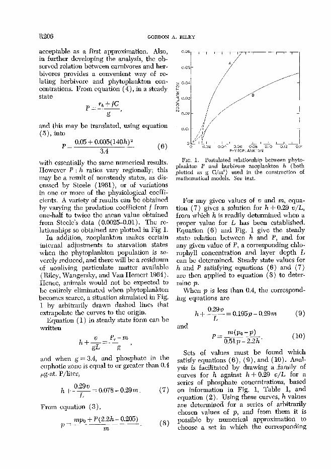
p = 0.05 + 0.005( 140h)2 3.4 - (6)

with essentially the same numerical results. IIowever P : h ratios vary regionally; this may be a result of nonsteady states, as discussed by Steele ( 1961)) or of variations in one or more of the physiological cocffi- cients. A variety of results can be obtained by varying the predation coefficient % from one-half to twice the mean value obtained from Steele’s data (0.0025-0.01). The relationships so obtained are plotted in Fig 1.

In addition, zooplankton makes certain internal adjustments to starvation states when the phytoplankton population is se- verely reduced, and there will be a residuum of nonliving particulate matter available ( Riley, Wangersky, and Van Hemcrt 1964). Hence, animals would not be expected to bc entirely eliminated when phytoplankton becomes scarce, a situation simulated in Fig. 1 by arbitrarily drawn dashed lines that extrapolate the curves to the origin.

Equation ( 1) in steady state form can be written

h+k P,-m ZZ-

is ’

and when g = 3.4, and phosphate in the cuphotic zone is equal to or greater than 0.4 /kg-at. P/liter,

h+ 0.29v ~ = 0.078 - 0.29m.

I, (7)

From equation ( 3))

mpo + P (2.2h - 0.205) P=----- m (8)

FIG. 1. Postulated relationship between phytoplankton P and herbivore zooplankton h (both plotted as g C/m”) used in the construction of mathematical models. See text.

For any given values of v and m, equation ( 7) gives a solution for h + 0.29 v/L, from which h is readily determined when a proper value for L has been established. Equation (6) and Fig. 1 give the steady state relation between h and P, and for any given value of P, a corresponding chlorophyll concentration and layer depth L can be determined. Steady state values for h and P satisfying equations (6) and ( 7) arc then applied to equation (8) to determine p.

When p is less than 0.4, the corresponding equations are

h + 0.29v ~ = 0.195p - 0.29m

L (9)

an d

P= MPo-PI o.51p - 2.2h ’ (10)

Sets of values must be found which satisfy equations (6)) (9)) and ( 10). Anal- ysis is facilitated by drawing a family of curves for h against h + 0.29 v/L for a series of phosphate concentrations, based on information in Fig. 1, Table 1, and equation (2). Using these curves, h values are determined for a series of arbitrarily chosen values of p, and from them it is possible by numerical approximation to choose a set in which the corresponding

MATHEMATICAL MODEL OE REGIONAL VAISIATIONS IN PLANKTON R207

0.

0 ! I I 0.001 0.01 0.1

LOG m

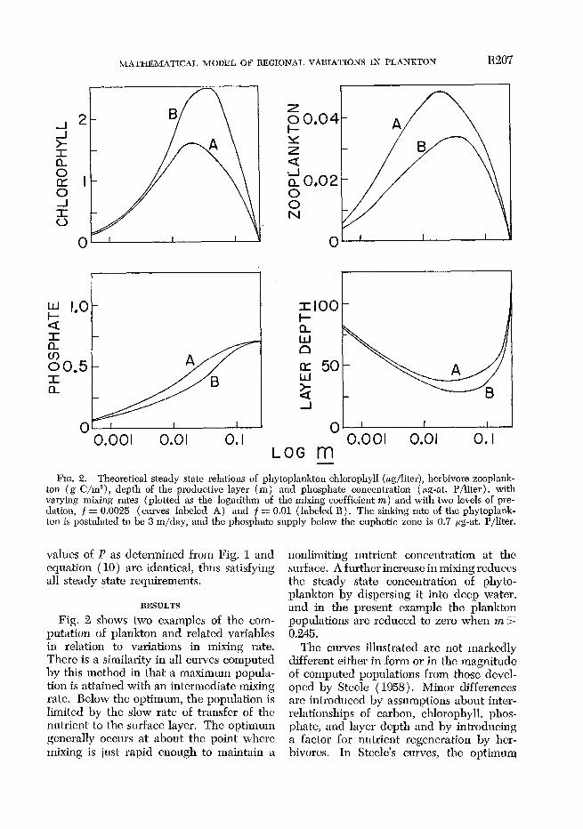
FIG. 2. Theoretical steady state relations of phytoplankton chlorophyll (pglliter), herbivore zooplankton (g C/m”), depth of the productive layer (m) and phosphate concentration ( pg-at. P/liter), with varying mixing rates (plotted as the logarithm of the mixing coefficient nz) and with two levels of predation. f = 0.0025 ( curves labeled A) and f = 0.01 ( labclcd 13). The sinking rate of the phytoplank-

losphate supply below the euphotic zone is 0.7 pg-at. P/liter. ton is postulated to be 3 m/day, and the pb

values of P as dctermincd from Fig. equation ( 10) are identical, thus sat i all steady state requirements,

1 and sf ying

RESULTS

Fig. 2 shows two examples of the computation of plankton and related variables in relation to variations in mixing rate. Thcrc is a similarity in all curves cojmputed by this method in that a maximum population is attained with an intermediate mixing rate. Below the optimum, the population is limited by the slow rate of transfer of the nutrient to the surface layer. The optimum gcncrally occurs at about the point where mixing is just rapid enough to maintain a

nonlimiting nutrient concentration at the surface. A further increase in mixing rcduccs the steady state concentration of phytoplankton by dispersing it into deep water, an d in the present example the plankton populations arc reduced to zero when m 5 0.245.

The curves illustrated are not markedly different either in form or in the magnitude of computed populations from those devcl- oped by Steele ( 1958). Minor differences are introduced by assumptions about inter- relationships of carbon, chlorophyll, phosphate, and layer depth and by introducing a factor for nutrient reg,eneration b,y hcrbivorcs. In Steele’s curves, the optimum

li208 GORDON A. RILEY

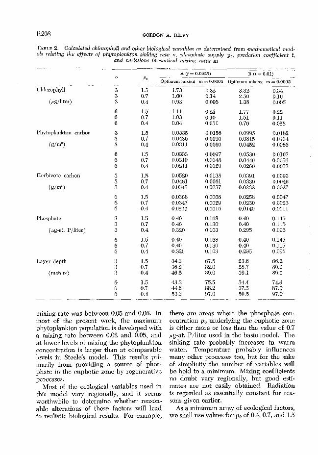
TABLE 2. Calculated chlorophyll und other biological variables a.s determined from ma,thematical models relating the effects of phytoplankton sinking rate v, phosphate supply pO, predation coefficient f,

und variations in vwtical mixing rates m - .

Chlorophyll

(tallifcr)

Phytoplankton carbon

( g/m3>

E Icrbivorc carbon

(fi/m”)

l’l~ospllntc

jpg-a t. P/liter)

Luycr depth

(mctcrs)

V

3

3 3

6 6 61

3 3 3

6 6 6

3 3 3

6 6 6

3 3 3

6 6 6

3 3 3

6 6 6

-

A (f = 0.0025) B (f = 0.01) PO --____ .--,

Optimum mixing m = 0.0005 Optimum mixing m. = 0.0005 ---- 1.5 0.7 0.4

1.5 0.7 0.4

1.5 0.7 0.4

1.5 0.7 0.4

1.5 0.7 0.4

1.5 0.7 0.4

1.5 0.7 0.4,

1.5 0.7 0.4

1.5 0.7 0.4

1.5 0.7 0.4

1.73 0.32 3.32 0.34 1.60 0.14 2.50 0.16, 0.93 0.095 1.38 0.095

1.11 0.21 1.77 0.22 1.03 0.10 1.51 0.11 0.64 0.051 0.76 0.058

0.0535 0.0156, 0.0995 0.0182 0.0480 0.0090 0.0815 0.0104 0.0311 0.0060 0.0452 0.0066

0.0333 0.0097 0.0530 0.0107 0.0310 0.0048 0.0440 0.0056 0.0211 0.0029 0.0260, 0.0032

0.0520 0.0135 0.0391 0.0090 0.0481 0.0061 0.0339 0.0046 0.0345 0.0037 0.0232 0.0027

0.0368 0.0068 0.0258 0.0047 0.0347 0.0029 0.0230 0.0023 0.0211 0.0015 0.0140 0.0011

0.40 0.168 0.40 0.145, 0.40 0.130 0.40 0.115 0.320 0.103 0.295 0.096,

0.40 0.168 0.40 0.145 0.40 0.130 0.40 0.115 0.320 0.103 0.295 0.096

34.3 67.5 23.6 66.2 36.2 82.0 28.7 80.0 46.5 89.0 39.1 89.0

43.3 75.5 34.4 74.8 44.6 88.2 37.5 87.0 53.3 97.0 50.5 97.0

mixing rate was between 0.05 and 0.06. In most of the present work, the maximum phytoplankton population is developed with a mixing rate between 0.02 and 0.05, and at lower levels of mixing the phytoplankton concentration is larger than at comparable levels in Steele’s model. This results pri- marily from providing a source of phosphate in the euphotic zone by regenerative processes.

Most of the ecological variables used in this model vary regionally, and it seems worthwhile to determine whether rcason- able alterations of these factors will lead to realistic biological results. For example,

there are areas where the phosphate concentration “pO underlying the euphotic zone is either more or less than the value of 0.7 p,g-at. P/liter used in the basic model. The sinking rate probably increases in warm water. Temperature probably influences many other processes too, but for the sake of simplicity the number of variables will be held to a minimum. Mixing coefficients no doubt vary regionally, but good estimates are not easily obtained. Radiation is regarded as essentially constant for rca- sons given earlier.

As a minimum array of ecological factors, we shall use values for p. of 0.4, 0.7, and 1.5


pg-at. P/liter; sinking rates of u = 3 m and 6 m/day; predation coefficients of f = 0.0025 and 0.01; the mixing rate varies between a low value of m = 0.0005 and the optimum rate for maintenance of a maximum steady state population. The computed array of results is shown in Table 2, and these will be discussed in relation to such observations as are available for comparison.

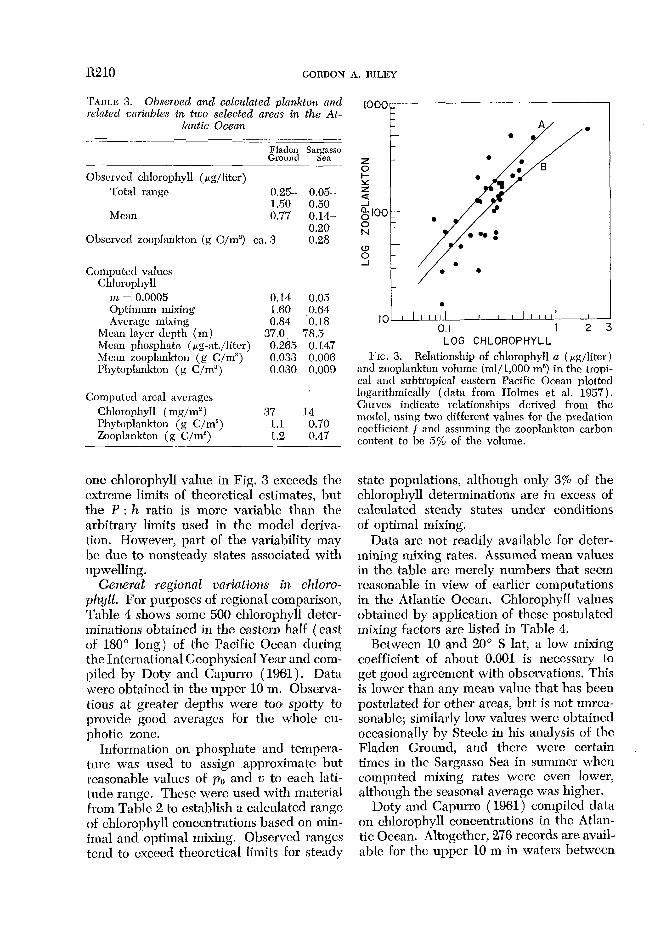
Flaclen Ground, North Sen. This is the arca used by Steele ( 1958) in his model studies, and additional data were given by Stcelc and Baird ( 1961). During the period of summer stability from May to October, chlorophyll values ranged from 0.25 to 1.5 ,.&liter, and the mean was about 0.77. Mixing coefficients were computed ( Steele 1958) from the observed seasonal tcmpera- turc progression. Calculated coefficients between successive periods of observation varied from 0 to 0.05. Large values were common at the beginning and end of the season; between mid-May and mid-september the average was m = 0.0042. This, together with ZJ = 3, po = 0.7, and f = 0.0025, leads to an estimated average chlorophyll value of 0.84 pg/liter. Other results of the computation are shown in Table 3. Most of the results are realistic; however, the estimated zooplankton population is somewhat too small, and some of the observed carbon : chlorophyll ratios were larger than the ones postulated in the present analysis.

Snrgnsso Sea. Menzel and Ryther ( 1960) have dcscribcd the seasonal cycle of chlorophyll in subtropical waters off Bermuda, This is an arca of moderate stability and poor nutrient supply that is best illustrated in Table 2 by the example p. = 0.4, ZJ = 6. Ob,served chlorophyll concentrations varied frolm 0.05 to 0.5 jAg/liter during the smnmcr period, with nonsteady state flowering conditions apI>roaching 1.0 in spring and fall. Summer zooplankton collections (Menzel and Ryther 1961) averaged 0.57 g ash fret dry wcight/m2 in the upper 500 m, presum- ably equivalent to about 0.28 g C/m2.

Mixing coefficients cannot be computed at this station, because horizontal advection during the summer season seriously in-

terferes with estimates of vertical heat flux. Temperature observations described by Ri- Icy ( 1957) in the Sargasso Sea at 35” N lat, 48” W long appear to be free of this dif- ficulty. There, the mean summer mixing coefficient, assuming an 80-m layer depth, is found to bc 0.0021. Combining this value with the other factors used in the Sargasso Sea computation gives a mean chlorophyll value of 0.18 pg/liter. In comparison, the obscrvcd avcragc found by Menzd and Ryther was about 0.14 in the upper 801 m, which is approximately the depth of the computed cuphotic zone; however, consid- crable quantities of chlorophyll were found below this depth, and the average for the upper 100 m from May through September appears to be about 0.2. Table 3 gives further details of the comparison between observations and theoretical estimates for the Sargasso Sea station.

North Pacific Ocean. McGary and Graham ( 1960) described an area (Stations 45-60, 45”-52” N lat, 159”-174” W long) where the surface layer was underlain by a sharp phosphate gradient with concentrations of the order of 1.5 pg-at. P/liter within 100 m of the surface. Twenty-three mcasuremcnts of chlorophyll n at the surface ranged from 0.28 to 3.02 pg/liter. The mean zooplankton displacement vohune was 197 ml/l,000 m3. The carbon content of temperate and boreal zooplankton is commonly 5-10s of the wet weight, leading to an estimate of 0.01-0.02 g C/m3. These results arc in good agrcc- ment with the computations shown in Table 2 of the general range of steady states for p. = 1.5, v = 3, and f = 0.01.

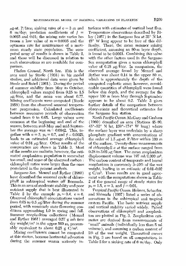
Tropical Pacific Ocean. Holmes, Schaefer, and Shimada (1957) listed a series of observations in the subtropical and tropical eastern Pacific. The basic nutrient supply and vertical stability varied widely. Paired observations of chlorophyll and zooplankton arc plotted in l?ig. 3. Zooplankton estimates are derived from measurcmcnts of “small” animals ( individually less than 5 ml volume), and assuming a carbon content of 5% of the wet weight. Theoretical curves in Fig. 3 are based on all computations in Table 2 for a sinking rate of 6 m/day, Only

R210 GORDON A. RILEY

TAHLE 3. Observed and calculated plankton and relntecl vnrinbles in two selected areas in the At-

kzntic Ocean ~- -_-- -. -- -___ ---

Fladcn Sargyo Ground ‘

-~___

Obscrvcd chlorophyll (pg/liter) Total range

Mean

0.2% 0.05- 1.50 0.50 0.77 0.14-

0.20 Obscrvcd zooplankton (g C/m”) ca. 3 0.28

Computccl values Cllloropllyll

m = 0.0005 0.14 0.05 Optimum mixing 1.60 0.64 Average mixing 0.84 0.18

Mean layer depth (m) 37.0 78.5 Mean phosphate (pg-at./Iitcr) 0.265 0.147 Mean zooplankton (g C/m’) 0.033 0.006 Phytoplankton (g C/m’) 0.030, 0.0091

Computed areal avcragcs Chlorophyll (mg/m’) Phytoplankton (g C/m’) Zooplankton (g C/m2)

37 14 1.1 0.70 1.2 0.47

one chlorophyll value in Fig. 3 exceeds the cxtrcme limits of theoretical estimates, but the P : h ratio is more variable than the arbitrary limits used in the model dcriva- tion. However, part of the variability may bc due to nonsteady states associated with upwelling.

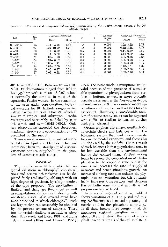
General regional variations in chlorophzjll. For purposes of regional comparison, Table 4 shows some 500 chlorophyll determinations obtained in the eastern half ( east of 180” long) of the Pacific Ocean during the International Geophysical Year and compiled by Doty and Capurro, ( 1961). Data were obtained in the upper 10 m. Observa- tions at greater depths were too spotty to provide good averages for the whole euphotic zone.

Information on phosphate and temperature was used to assign approximate but reasonable values of p. and v to each latitude range. These were used with material from Table 2 to establish a calculated range of chlorophyll concentrations based on min- imal and optimal mixing. Observed ranges tend to exceed theoretical limits for steady

t

0.1 1 2 3

LOG CHLOROPHYLL Frc. 3. Relationship of chlorophyll a (,ug/liter)

and zooplankton volume (ml/l,000 n-P) in the tropical and subtropical eastern Pacific Ocean plotted logarithmically (data from IIolmes et al. 1957). Curves indicate relationships derived from the model, using two different values for the predation coefficient f and assuming the zooplankton carbon content to be 5% of the volume.

state populations, although only 3% of the chlorophyll determinations are in excess of calculated steady states under conditions of optimal mixing.

Data are not readily available for detcr- mining mixing rates. Assumed mean values in the table are merely numbers that stem reasonable in view of earlier computations in the Atlantic Ocean. Chlorophyll values obtained by application of these postulated mixing factors are listed in Table 4.

Between 10 and 20” S lat, a low mixing coefficient of about 0.001 is necessary to get good agreement with observations. This is lower than any mean value that has been postulated for other areas, but is not unrca- sonable; similarly low values were obtained occasionally by Steclc in his analysis of the Fladen Ground, and there were certain times in the Sargasso Sea in summer when computed mixing rates were even lower, although the seasonal average was higher.

Doty and Capurro ( 1961) compiled data on chlorophyll concentrations in the Atlan- tic Ocean, Altogether, 276 records are available for the upper 10 m in waters between

AIATHEMATICAL MODEL OF REGIONAL VARIATIONS IN PLANKTON R211

TABLE 4. Ohserfied and computed

Lat No. obs.

60-70" N 50-60" 40-50" 86 30-40" 19 20-30" 27 10-20" 54

O-10" 181 o- 5"s 34 5-10" 10

10-20" 27

chlorophyll, eastern half latitude ranges

of the Pacific Oceun, averaged by 10"

Observed chlorophyll

Range Mean PO V

Assumed Computed chlorophyll mean,

m Range Mean

0.14- 3.66 1.53 1.5 3 0.004 0.32-3.32 1.77 0.02-12.50 1.03 1.5 3 0.004 0.32-3.32 1.77 O.ll- 3.60 0.73 0.7 3 0.004 0.14-2.50 0.82 O.l& 2.30 0.82 0.7 3 0.004 0.14-2.50 0.82 0.02- 1.90 0.2,6 0.4 6 0.003 0.05-0.76 0.24 0.04- 0.82 0.18 0.4 6 0.002 0.05-0.76 0.17 O.OO- 1.42 0.19 0.4 6 0.002 0.05-0.76 0.17 O.Ol- 2.00 0.28 0.7 6 0.002 0.10-1.51 0.32 0.06- 0.27 0.14 0.4 6 0.002 0.05-0.76 0.17 0.03- 0.22 0.10 0.4 6 0.001 0.05-0.76 0.11

40” N and 20” S lat. Between 0” and 10” N lat, 18 observations ranged from 0.01 to 1.33 pug/liter with a mean of 0.27, which is essentially the same as in most of the equatorial Pacific waters. In the remainder of the area under consideration, individ- ual averages for 10” latitude ranges varied within narrow limits of 0.15-0.21, which is similar to tropical and subtropical Pacific averages and is suitably modeled by p. = 0.4, v = 6, and m = 0.0015-0.0025. Only two observations exceeded the theoretical maximum steady state concentration of 0.76 predicted by the model.

There were 98 observations north of 40” N lat taken in April and October. They are interesting from the standpoint of seasonal variations but are inapplicable to the problem of summer steady states.

DISCUSSION

The results leave little doubt that regional variations in chlorophyll concentrations and certain other factors can be depicted fairly realistically, although with no high degree of precision, by simple models of the type proposed. The application is limited, and there are theoretical as well as computational difficulties in dealing with nonsteady states. Also several areas have been described in which chlorophyll levels are higher than can reasonably be obtained by the present scheme of analysis. These include certain shallow areas such as Aber- deen Bay (Steele and Baird 1961) and Long Island Sound ( Riley and Conover 1956))

where the basic model assumptions are in- valid because of the presence of considerable quantities of phytoplankton from surface to bottom, as well as more typically oceanic areas such as the Norwegian deeps, where Steele ( 1958) has examined model ap- plications and has discussed reasons for dis- agreement. However, a considerable number of oceanic steady states can be depicted with sufficient realism to warrant further ecological discussion.

Oceanographers are aware, qualitatively, of certain checks and balances within the biological system that tend to compensate for environmental variations, and these also are depicted by the models. The net result of such balances is that populations tend to be less variable than the environmental factors that control them. Vertical mixing tends to reduce the concentration of phytoplankton in the euphotic zone but at the same time increases the rate of supply of nutrients and hence stimulates growth. An increased sinking rate also reduces the phytoplankton concentration, but this automat- ically increases transparency and deepens the euphotic zone, so that growth is not proportionately reduced.

In terms of regional variation, Table 4 shows variations of 4 : 1 in postulated mixing coefficients, 2 : 1 in sinking rates, and nearly 4 : 1 in the phosphate supply, po. If all these factors were compounded, the maximum regional variation would be about 30 : 1. Instead, the ratio of chlorophyll concentrations is of the order of 15 : 1.

1~212 GORDON A. l~TLF,I’

With an es timatcd mean layer depth of 37 m bctwecn 60 and 70” N lat and 88 m bctwecn 10 and 20” S lat, the ratio of total chlorophyll/m2 in the euphotic zone is further rcduccd to 6.4 : 1. Ratios of phytoplankton carbon arc less variable than chlorophyll bccausc of postulated nutrient cfEects, SO that the maximum variation in C/m” is 9.2 : 1, and for total C/m2 in the euphotic zone it is 3.9 : 1.

The basic assumption that carbon : chlorophyll ratios vary within limits OE 30 : 1 to slightly more than 100 : 1 was derived from studies of net phytoplankton collections and laboratory cultures (Harris and Riley 1956; Parsons, Stephens, and S trickland 1961) . Steele and Baird (1961., 1962) have obtained considerably higher ratios in scnesccnt cultures of Skeletonema costatum and have demonstrated ratios of total particulate carbon to chlorophyll in the North Sea that are as high as 300 : 1. Thus, the assumptions that have been made in the model about the limits of variation in this ratio are con- servative. The reasons for this are as fol- lows :

1. Analyses of net phytoplankton collections do not show the same degree oE nitrogen or phosphorus dcEicicncy that is achicvcd in senescent laboratory populations ( Harris and Riley 1956). It is sus- pected that senescent populations cannot persist in the sea and that results obtained with such cultures have little bearing on the natural situation.

2. Steele and Baird ( 1961.) and more rc- ccntly Menzel and Ryther (1964) have assumed that variations in nonliving particulate organic matter are unrelated to variations in living phytoplankton; hence the slope of the carbon-chlorophyll regression is indicative of the ratio in living phytoplankton, This assumption is not verified by examining the samples. Visual examination of naturally occurring particulatcs by Riley ct al. ( 1964) in subtropical and tropical waters has revealed a high dcgrec of corre- lation between phytoplankton and nonliving particulate matter, so that results based only on chemical analysts are likely to bc misleading. IIence, the present model is

predicated on carbon : chlorophyll ratios that seem to be typical of clean net collections and cultures in the logarithmic growth phase.

The model is deficient in not considering the role of nonliving particulate matter, which is abundant in the sea and probably is suitable food for animals (Baylor and SutclifEe 1963). Th e investigations 0E Sut- chffc, Baylor, and Menzel ( 1963) and Riley ( 1963) indicate that particulate matter can bc formed by adsorption processes in the surface layer even when phytoplankton is scarce, and this may help to alleviate starvation cEfccts. In addition, part of the photosynthetic production of phytoplankton is secreted in a dissolved form which is capable of being transformed into particulate matter by adsorption processes (Riley et al. 1964). Such processes will need to be incorporated into ecological models cventu- ally, but this will require more knowledge than is now available.

Vertical transfer of essential nutrients has been dealt with only in terms of vertical mixing, and an objection might be raised that upwelling is an important aspect of phytoplankton ecology in some OE the areas that have been examined, particularly in equatorial waters. Upwelling can cause nonsteady states and can produce general regional enrichment, both of which need to be discussed in the context of the model.

Stcclc ( 1961) d iscussed the nonlinearity in P : h relations that occurs during a seasonal cycle in temperate waters as a result of the time lag between plant and animal production, and he further pointed out the possibility of essentially similar spatial nonlinearity that might arise in areas of tropical upwelling. For example, if an area is strongly fertilized by upwelling, there will be a corresponding development of phytoplankton, initially leading to a high P : h ratio. If the water is gradually moving away Erom the locus of upwelling, one expects to find a point at some distance from the origin where the zooplankton begins to ovcrcomc its early lag and to graze down the phytoplankton crop. In short, one expects to Eind

MATIIEMATICAL MODEL 017 REGIONAL VARIATJONS IN PLANKTON R213

the temporal aspects of a seasonal cycle ar- ranged spatially along the line of flow.

The only obvious criteria of this situation arc a) the existence of phytoplankton populations larger than one would expect a steady state population to be, and b ) large anomalies in the P : h ratio. The first cri; tcrion was seldom rcalizcd, but variations in the P : h ratio were sometimes large, as indicated in Fig. 3, and nonsteady states may have been responsible.

General enrichmcn t by upwelling could bc incorporated into the model easily if the magnitude of the physical process wcrc known, If a given amount of deep water moves upward into the euphotic zone, thereby increasing the nutrient supply and diluting the phytoplankton population, mass continuity requires that an equal volume of water be transferred horizontally out of the water column in question. The cffcct of thcsc two advective transfers is the same as that of a vertical mixing exchange of the same volume. The primary cffcct of upwcll- ing, then, is to increase the apparent mixing coefficient. Secondarily, vertical movement of the water mass will reduce the net sinking rate of the phytoplankton. IIowevcr, tropical upwelling is generally supposed to be less than 1 m/day, so that if the phytoplankton sinking rate is of the order of 6 m/ day, the reduction due to upwelling will bc minor.

Upwelling may either increase or decrease the population, depending on the magnitude of the processes that arc involved. Consider the example in Table 2 where p. = 1.5, v = 6, and f = 0.01. The phytoplankton has a maximum steady state concentration when m has a relatively low value of 0.008. As the mixing coefficient in- crcascs from a low value of 0.0005 to 0.008, there is nearly a tenfold increase in chlorophyll. Alternatively, an equivalent increase could bc obtained by superimposing a small amount of upwelling upon a mixing coefficient of 0.0005. IZxcluding the minor cf- feet due to alteration of the phytoplankton sinking rate, the rate of upwelling neccs- sary to produce this apparent increase in m

would be 0.26 m/day. Any more than this

would bc equivalent to supra-optimal mixing and would reduce the chlorophyll con- ccntra tion.

Upwelling may bc important in any particular arca whcrc it happens to occur, cspc- cially if the water is stable and mixing co- cfficicnts arc low. Barring nonsteady state situations, howcvcr, the general range of phytoplankton concentrations should fall approximately within the same limits that arc predicted by the range of values in Table 2.

The slight maxima in chlorophyll con- ccn trations near the equator in both Pacific and Atlantic waters shown in the available observations might bc ascribed to upwelling. IIowcvcr, the available phosphate below the cuphotic zone is slightly greater than in the waters to the north and south, and this is sufficient to account for the observed incrcasc in phytoplankton without any incrcasc in apparent vertical movcmcnt. In a’limitcd arca between 2” N and 4” S lat in the eastern Pacific, I-Iolmcs ct al. (1957) rcportcd chlorophyll concentrations avcrag- ing 0.56 pg/litcr. Maintenance of a steady state crop of this size would require a) a mixing rate of m = 0.004; b ) in the com- pletc absence of mixing, an upwelling rate of 0.28 m/day; or c) some intermediate combination of mixing and upwelling.

Phytoplankton-zooplankton relationships always prcscnt difficulties in models bc- cause of uncertainty about proper values for coefficients of grazing and predation. In addition, vertical movements of zooplankton not only arc difficult to fit into simpli- ficd model terms but also introduce com- plcxitics into the comparison of calculated results and field observations. The present model theoretically provides an estimate of the mean concentration of hcrbivorcs that can acquire ncccssary food within the euphotic zone, and the product of this concentration and the depth of the cuphotic zone should then be the total crop per unit area of sea surface, regardless of the actual vertical distribution. This is too simple a statc- mcnt OE the problem and there are large errors, as is apparent Erom Table 3.

Although oceanographic literature has cm-

R.214 GORDON A. RILEY

phasized the importance of vertical migra- tion, recent work (Banse 1964) demonstrates that half or more than half of the surface feeding population remains in the surface layer at all times. IIcncc surface tows may bc more useful than some investigators have supposed as an indication of the quantity of animals that can bc fed within the cuphotic zone. This provides a rationale for comparisons of regional abundance (as in Fig. 3), although there may be systematic errors in the results for reasons given above.

The sinking rates used here are based on theoretical considerations developed by Riley et al. ( 1949) and Steele ( 1958) indi- cating that sinking rates of this magnitude are necessary, in conjunction with the com- putcd rates of vertical diffusion, to maintain a realistic vertical distribution of phytoplankton. The concept of a slight increase in sinking rates in warm water is essential to model the variations in vertical distribution that are found in the sea. IIowevcr, biologists find it difficult to accept thr: idea that even the average sinking rates of natural populations should be so nearly constant or should vary so precisely with viscosity. Measured sinking rates vary by orders of magnitude, and many variables are involved, including cell size and shape and physiological state. The problem has never been studied thoroughly. In the present state of our knowledge, the situation is best characterized as merely a conflict bctwecn theoretical and biological intuition. The writer suspects that the conflict may bc re- solved by demonstration of an apparent sinking rate due to vertical convection that would be related to the vertical temperature structure of the water.

I’inally, cstimatcs of net production are readily derived from the models, the ncces- sary information being the production coefficient ( Table 1) in relation to steady state phosphate concentration, the quantity of phytoplankton carbon P, and the depth of the euphotic zone. As an example of the kind of results obtained, computed values for the Sargasso Sea station and the Fladen Ground arc respectively 0.07 and 0.26 g C me2 day-l. The total range in areal avcr-

ages, using data from Table 4, is 0.04-0.48. These figures appear to be of the right order of magnitude as compared with cxpcriment- ally de tcrmincd 13C uptake, although estimates for tropical and subtropical waters may be too low. Menzel and Ryther (1960) found an annual net production of 72 g C/ m” at a Sargasso Sea station, or a mean of 0.20 g C/day. Much of this production oc- curred during the period from January to the end of April, and the average for the rcmaindcr of the year appears to be about 0.11 g, which is approximately 60% higher than the theoretical cstimatc given above. On the Fladen Ground, in situ 14C experiments in summer (Steele and Baird 1961) averaged 0.29 g C mm2 day-l, or 10% higher than the theoretical computation.

REFERENCES

~ANslC, K. 1964. On the vertical distribution of zooplankton in the sea, p, 53-125. In M. Sears [ed.], Progress in oceanography, v. 2. Pergamon, Oxford.

RAYLm, E. R., AND W. H. SUKLIWE. 1963. Dis- solved organic matter in seawater as a source of particulate food. Limnol. Occanog., 8: 369-37 1.

Don, M. S., AND I,. 1~. A. CALW~I~~. 1961. Pro- ductivity mcnsuremcnts in the: world ocean. Intern. Gcophys. Year Occanog. Rcpt. No. 4: l-625. Natl. Acacl. Sci., Natl. Res. Council, Washington, D.C.

IIARUIS, IL, AND G. A. RJLRY. 19S6. Oceanog- raphy of Long Island Souncl, 1952-1954. VIII. Chemical composition of the plankton. Bull. Bingham Occanog. Collection, 15: 315-323.

HOLMES, R. W., M. B. SCIIAEFEI<, AND B. M. SHIMADA. 1957. Primary production, chlorophyll, and zooplankton volumes in the tropical eastern Pacific Ocean. Bull. Inter-Am. Tropi- cal Tuna Con-ml., 2: 128-169.

MCCAIXY, J. W., AND J. J. GRAIIAM. 1960. Bio- logical and oceanographic observations in the central North Pacific July-Septcmbcr 1958. U.S. Fish Wildlife Serv., Spcc. Sci. Rcpt., Fishcrics, 358 : l-107.

MENZEL, D. W., AND J. II. RYTIIEJ~. 1960. The annual cycle of primary production in the Snr- gasso Sea off Bcrmudn. Deep-Sea Rcs., 6: 351-367.

-2 AND -. 1961. Zooplankton in the Sargasso Sea off Bcrmnda and its relation to primary production. J. Conseil, Conseil Pam. Intern. Exploration Me-r, 26: 250-258.

-> AND -. 1964. The composition of - particulate organic matter in the western North Atlantic. Limnol. Oceanog., 9: 179- 186.

MATIIE’,MATICAL MODEL OF RJ%GIONRL VAI~IATIONS IN PLANKTON R215

PARSONS, T. R., K. STEPHENS, AND J. D. II. STRICK- LAND. 196,l. On the chemical composition of eleven species of marine phytoplankters. J. Fishcrics Rcs. Board Can., 18: 1001-1016~.

REDPIELL), A. C. 1934. On the proportions of organic dcrivntives in sea water and their rcla- tion to the composition of plankton, p. 171- 192. In James Johnstonc Memorial Volume. Univ. Liverpool Press.

-, B. H. KETCIIUM, AND F. A. BICIIARIX. 1963,. The influence of organisms on the composition of sea-water, p. 26-77. In M. N. IIill [cd.], The sea, v. 2. Interscicncc, New York.

RILEY, G. A. 1941. Plankton studies. IV. Georgcs 13ank. Bull. Binghnm Occnnog. Collection, 7 : l-73.

-. 1956. Oceanography of Long Island Sound, 1952-1954. II. Physical oceanography. Bull. Bingham Oceanog. Collection, 25: 15- 46.

-. 19,57. Phytoplankton of the north ccn- tral Sargasso Scn. Limnol. Occanog., 2: 252- 270.

-. 1963. Organic aggregates in scawatcr and the dynamics of their formation and utili- zation. Limnol. Occanog., 8: 372-381.

-, AND S. M. CONOVEX. 1956. Ocennog- raphy of Long Island Sound, 1952-19,54. JTI. Chemical oceanography. Bull. Bingham Occanog. Collection, 15 : 47-61.

-, H. STOMMEL, AND D. F. BUMPUS. 1949. Quantitative ecology of the plankton of the

western North Atlantic. Bull. Bingham Occanog. Collection, 12 : l-169.

-> I’. J. WANGEASKY, AND D. VAN HEMIMT. 1964. Organic aggregates in tropical and subtropical surface waters of the North Atlan- tic Occnn. Limnol. Occanog., 9: 546-550.

RY?‘IIEIZ, J, H., AND c. S. YENTSCII. 1957. The estimation of phytoplankton production in the ocean from chlorophyll and light data. Limnol. Odeanog., 2 : 281-286.

-, AND -. 19,58. Primary production of continental shelf waters off New York. Limnol. Occanog., 3 : 3,27-335.

STEELE, J, H. 1958. Plant production in the northern North Sea. Marine Res., Scot. Home Dept., 1958 ( 7 ) : 1-36.

-* 1961. Primary production, p. 519-538. In M. Scars [cd.], Oceanography. AAAS Publ. 67. Washington, D.C.

-, AND I. E:. Bnrmx 1961. Relations bc- twccn primary production, chlorophyll and particulate carbon. Limnol. Occnnog., G : 68- 78.

-> AND -. 1962. Carbon-chlorophyll relations in cultures. Limnol. Occanog., 7: 101-102.

SUTCLIFFE, W. H., IX. R. BAYLOR, AND D. W. JMENZEL. 1963. Sea surface chemistry and Langmuir circulation. Deep-Sea Rcs., 20: 233-243.

SVERDRUL~, E-1. U., M. W. JOHNSON, AND R. II. ~~‘LEZMING. 1942. The oceans. Prcnticc-Hall, Englewood Cliffs, N.J. 1087 p.

a mathematical model of regional variations in plankton

Documents