Electronic copy available at: http://ssrn.com/abstract=2461150

1

A CONTINUOUS-TIME DYNAMICS OF INTEREST CASH FLOWS

FROM A BANK’S LOAN PORTFOLIO

(A case of sudden stepwise change in yield curve)

Ihor Voloshyn

July 2014

Version 1

Working paper

Ihor Voloshyn

PhD., senior scientist at Academy of Financial Management

of Ministry of Finance of Ukraine

38-44, Degtyarivska str.,

04119, Kyiv, Ukraine

Tel. +38 044 486 5214

vologor@i.ua

Electronic copy available at: http://ssrn.com/abstract=2461150

2

Abstract

A continuous-time deterministic model for analytical simulation of impact of the

change in yield curve on bank’s interest income from a fixed rate loans portfolio is

presented. It is considered both differential and integral presentations of equations

for dynamics of principal and interest cash flows. The model allows taking into

account the arbitrary movements in interest rates. Examples of calculation of total

(from portfolio) and partial (across maturities) interest cash flows and

corresponding interest rates on those cash flows are given. The sensitivity of total

interest cash flows is evaluated for some changes in yield curve on loans that obeys

the Nelson-Siegel model.

Key words: bullet loan, fixed rate loan, loan portfolio, principal cash flow, interest

cash flow, interest accrual, sensitivity of interest cash flows, yield curve, Nelson-

Siegel model, sudden stepwise change, interest rate risk, continuous-time model,

differential advective equation, Volterra integral equation

JEL Classifications: G17, G21, G32, C61, C63

3

1. INTRODUCTION

Interest rate risk is one of the main types of risk that significantly affects the

change in bank’s earnings and capital. “Variation in earnings is an important focal

point for interest rate risk analysis because reduced earnings or outright losses can

threaten the financial stability of an institution by undermining its capital adequacy

and by reducing market confidence.” (BIS, 2004).

It is well-known that the sources of interest rate risk are repricing risk, yield

curve risk, basis risk and optionality (BIS, 2004).

In practice banks face two issues. The first of these is to define interest rate

risk exposure. Banks operate under constant reproduction of their asset and

liability contracts. New interest-bearing assets and liabilities continuously replace

old matured assets and liabilities. Due to this fact the bank’s interest rate risk

exposure is unceasingly changed.

And the second of these is to forecast the potential course of future interest

rates. Yield curves may in the future vary their slope, curvature and shape.

To solve these two issues it is suitable a dynamic simulation approach which

allows taking into account “more detailed assumptions about the future course of

interest rates and expected changes in a bank's business activity” (BIS, 2004).

The paper is focused on theoretical analysis of the impact of changes in

interest rates on a bank’s accrual earnings. The continuous-time model is going to

use for this research. Such a model allows integrating the balance sheet, income

statement and ALM (asset liability management) forecasting processes into a

single process giving a forward-looking and integrating view on the issue.

Note that “transfer to a continuous-time model … allows using a rich store

of methods of functional analysis”, “giving a qualitative picture of a bank’s

business activity”, “discovering general regularities of bank’s dynamics…”

(Linder, 1998).

4

2. MODEL

Let an interest-bearing portfolio of a bank consist of the fixed interest rate bullet

loans in which only interest is paid continuously for the lifetime of loan; the

principal is paid in one lump sum at the end of the term to maturity (Business

Dictionary). The portfolio is changed due to repayment of the existing loans and

issuance of the new ones from different borrowers. The loans of the existing

borrowers are not rolled over. Each new loan is issued to a new borrower.

Moreover, influence of default and prepayment on cash flows is neglected.

Let the new principal cash flows CFp(t,w) from the new loans with the

primary term to maturity w at the time t be originated with interest rate r(t,w). The

existing principal cash flow with the remaining term w to maturity at the time t has

other yield of rr(t,w). Assume that interests are accrued according to the simple

interest approach.

Note that to take the term structure of interest rate into account it is followed

to use a dynamic model for bank’s cash flows. Voloshyn (2004), Freedman (2004),

Selyutin and Rudenko (2013) are developed the continuous-time models which are

based on the partial differential equations of advective type. Voloshyn (2007)

proposed to distinguish the cash flows of principals and interests. He showed that

dynamics of principal and interest cash flows is described by the similar equations:

),(),(),(

wtSw

wtCF

t

wtCFp

pp

, (1a)

),(),(),(

wtSw

wtCF

t

wtCFi

ii

, (2a)

where CFp(t,w) and CFi(t,w) are the cash flows of principals and interests,

respectively, with the remaining term w to maturity at time t;

Sp(t,w) and Si(t,w) are the intensities of appearance of the new cash flows of

principals and interests, respectively, with the primary maturity w at the time t. In

other words, there are demands for principal and interest;

t is the time;

w is the (primary or remaining) term to maturity;

5

t

and

w

are the partial derivatives respect to time t and term w to maturity,

respectively.

It should be noted that the cash flows CFp(t,w) and CFi(t,w) are partial

(across terms to maturity) cash flows.

A loan demand function may depend on interest rate on loans, rollover ratio,

macroeconomic parameters, etc. But for simplification such dependences will be

abandoned. Besides, the loan demand is supposed to be a deterministic function.

Note that the above mentioned assumptions may be released.

The equations (1a and 2a) have the following integral representations

(Voloshyn, 2004; Selyutin and Rudenko, 2013):

dsswtsSwtwtCF

t

ppp 0

),()(),( (1b)

dsswtsSwtwtCF

t

iii 0

),()(),( (2b)

where s is the time parameter, φp(t+w) and φi(t+w) are the initial conditions for

CFp(t,w) and CFi(t,w), respectively. If it is needed to find an unknown demand

function that the equations (1b and 2b) will become linear Volterra equations of the

second kind.

Note that the principal Sp(t,w) and interest Si(t,w) intensities are linked

through interest rate r(t,w):

Si(t,w)=Sp(t,w)∙r(t,w), (3)

and the cash flows of principals CFp(t,w) and interests CFi(t,w) are linked through

interest rate rr(t,w):

CFi(t,w)= CFp(t,w)∙rr(t,w), (4)

where r(t,w) and rr(t,w) are the interest rates on the new and existing principal cash

flows, respectively, or the yield curves for the primary and remaining terms to

maturity. Note that r(t,w) and rr(t,w) are the interest rates on cash flows.

Consider the portfolio parameters. So, the dynamics of the portfolio volume

B(t) is described by the following equation (Volosyn, 2005):

6

dwwtStCFdt

tdB

o

pp

),()0,()(

, (5a)

where B(t) is the portfolio volume.

The first term in right side of the equation (5a) is debit turnover and the

second term is the credit turnover of the portfolio.

Instead the equation (5a) knowing CFp(t,w) it is easy to find the volume of

the loan portfolio at the time t or the total (from the portfolio) principal cash flow:

dwwtCFtBo

p

),()( . (5b)

This expression (5b) shows that the total principal cash flows generated by

the loan portfolio consist of all existing non-matured principal cash flows.

Further consider the interest cash flow from the portfolio or the velocity of

portfolio interest accrual (Volosyn, 2007):

dt

tdIItRtBtCF

)()()()( , (6)

where CF(t) is the interest cash flow from the portfolio at the time t, R(t) is the

interest rate on the portfolio, II(t) is the interest income from the portfolio. Note

that R(t) is an interest rate on the loan balance.

Then, dynamics of CF(t) can be describe by the next equation (Volosyn,

2007):

dwwtStCFdt

tdCF

o

ii

),()0,()(

. (7a)

The first term in right side of the equation (7a) is the total outflows of

interest cash flows caused by the repayment of matured principal cash flows and

the second term is the total inflows of interest cash flows caused origination of new

loans.

Instead the equation (7a) knowing CFi(t,w) it is easy to find the interest cash

flow from the portfolio at the time t:

dwwtCFtCFo

i

),()( . (7b)

7

This expression (7b) shows that the total interest cash flows generated by the

loan portfolio consist of all existing non-matured interest cash flows.

3. EXAMPLE

Consider how a sudden stepwise change (at time t>0) in yield curve for loans

affects a bank’s interest income.

Let the yield curve follows the Nelson-Siegel model (James and Webber,

2005):

1

2

1

1210 exp

exp1

),(

w

w

w

wr , (8)

where w is the term to maturity, Λ{β0, β1, β2, τ1} is the vector of the model’s

parameters, exp(x) is the exponential function. The long rate is equal to β0 and the

short rate is equal to β0+β1. β2 and τ1 control location and height of the hump.

Note that the Nelson-Siegel model allows describing changes in slope,

curvature and shape of the yield curve. In particular, it defines normal, inverted, ∩,

U- and S-shaped yield curves.

The stationary solution

To get the stationary solution for interest cash flows it is conveniently to use the

differential equations (2a and 7a) with the following conditions:

0),(

t

wtCFi and 0)(

dt

tdCF.

Then, dropping time t the equation (2a) is reduced to the form:

)()(

wSdw

wdCFi

i (9)

with the initial condition (7a):

dwwSCFo

ii

)()0( . (10)

Then, integrating the equation (9) with the initial condition (10) leads to the

following stationary distribution of interest cash flows:

8

dwwSwCFw

ii

)()( . (11)

Arguing similarly, using the equations (1a and 5a) and dropping time t the

following stationary distribution of principal cash flows is obtained:

dwwSwCFw

pp

)()( . (12)

The non- stationary solution

For simplicity, but without loss of generality, assume that the intensity of the

appearance of new principal cash flows from new loans is stationary and obeys the

exponential law of distribution respect to maturity w:

22

exp)(

wSwS p , (13)

where τ2 is the characteristic maturity of loan portfolio; dwwSS p

0

is the total

intensity of appearance of new cash flows. Then, the distribution of principal cash

flows has the following stationary form:

2

exp)()(

w

SwwCF pp . (14)

Let the initial condition φi(w) for the equation (2b) be stationary and equal

to:

dmmrmS

ww

i

),(exp)( 1

22 .

Let the yield curve with the parameters’ vector Λ1 be suddenly (at time t>0)

step-wisely changed on the one with the parameters’ vector Λ2.

Then, the intensity (3) of appearance of interest cash flow is equal to:

),(exp),()()( 2

22

2

wr

wSwrwSwS pi

.

Herewith, the interest rates R(t) on the portfolio (from the equation (6)) and

the one rr(t,w) on the principal cash flows with the remaining term w to maturity

(from the equation (4)) are equal to, respectively:

9

)(

)()(

tB

tCFtR and

),(

),(),(

wtCF

wtCFwtrr

p

i .

The sensitivity of the portfolio interest cash flows may be estimated by the

following formula:

1)0(

)1()0()0( 21

CF

CFttS , (15)

where CF(1) and CF(0) are the portfolio interest cash flows at t=0 and t=1 year,

respectively. This measure is a simple indicator of interest rate risk.

The sensitivity (15) shows how will be relatively changed the interest cash

flows from portfolio during 1 year caused by the sudden stepwise change in the

yield curve at time t>0. Input data for calculation is given in Table 1.

Table 1. Input data for calculation

Parameters Designation Value at time t=0 Value at time t>0

The total intensity of appearance of

new cash flows

S 1 1

The portfolio volume B 1 1

The characteristic maturity of loan

portfolio

τ2 1.5 year 1.5 year

Results of calculation are presented on Fig. 1-5.

Fig. 1. Isolines of interest cash flows CFi(t,w) under β0 =5%, β1=-1%, β2=-6%, τ1=1

at the time t=0 and β2=6% at the time t>0

10

Fig. 2. Dynamics of interest rate R(t) on the loan portfolio under β0 =5%, β1=-1%,

β2=-6%, τ1=1 at the time t=0 and β2=6% at the time t>0

Fig. 3. Interest rate rr(t,w) on principal cash flows and the one r(w,β2) on new cash

flows under β0 =5%, β1=-1%, β2=-6%, τ1=1 at the time t=0 and β2=6% at the time

t>0

11

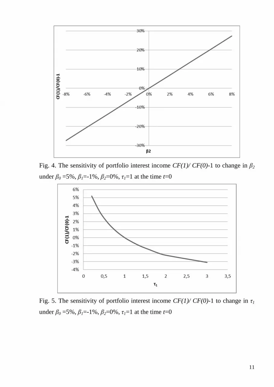
Fig. 4. The sensitivity of portfolio interest income CF(1)/ CF(0)-1 to change in β2

under β0 =5%, β1=-1%, β2=0%, τ1=1 at the time t=0

Fig. 5. The sensitivity of portfolio interest income CF(1)/ CF(0)-1 to change in τ1

under β0 =5%, β1=-1%, β2=0%, τ1=1 at the time t=0

12

4. SUMMARY

Dynamics of a bank’s loan portfolio may be described by only the four equations

for total and partial cash flows of principals and interests. This model is an

internal (relatively market) model of bank’s activity.

Besides, it needs to use a model for loan demand (intensity of appearance of

new principal cash flows) and an interest rate model. Note that the loan demand

function is an interim model of interaction between market and the bank. And the

interest rate model is an external model that describes market behavior.

Theoretical result is useful to give general regularities of bank’s dynamics

and, for example, to debug computer programs. To employ the developed model in

practice it needs to pass to a discrete presentation of the obtained equations.

The questions related to:

the more realistic assumptions on a loan demand function, including the

inherent uncertainty of demand and renewal effect,

the uncertainty caused by default and prepayment,

a non-stationary dynamics of interest rate, etc.

are remained for further research.

LITERATURE

1. Basel Committee on Banking Supervision (2004). Principles for the

Management and Supervision of Interest Rate Risk.

http://www.bis.org/publ/bcbs108.pdf.

2. Business Dictionary. “Bullet loan”.

http://www.businessdictionary.com/definition/bullet-loan.html.

3. James, J. and Webber, N. (2005). Interest Rate Modelling. J. Wiley & Sons,

654p.

4. Freedman, B. (2004) An Alternative Approach to Asset-Liability

Management. 14-th Annual International AFIR Colloquium (Boston).

http://www.actuaries.org/AFIR/Colloquia/Boston/Freedman.pdf.

13

5. Linder, N. (1998). A Continuous-Time Model for Bank’s Cash Management

// Finansovye Riski (Ukraine). #3, p.107–111.

6. Selyutin, V. and Rudenko, M. (2013). Mathematical Model of Banking Firm

as Tool for Analysis, Management and Learning. http://ceur-ws.org/Vol-

1000/ICTERI-2013-p-401-408-ITER.pdf.

7. Voloshyn, I.V. (2004). Evaluation of bank risk: new approaches. – Kyiv:

Elga, Nika-Center, 216 p. http://www.slideshare.net/igorvoloshyn3/ss-

15546686.

8. Voloshyn, I.V. (2005) A transitional dynamics of bank’s liquidity gaps //

Visnyk NBU (Ukraine). #9, p.26–28.

http://www.bank.gov.ua/doccatalog/document?id=40077.

9. Voloshyn, I.V. (2007). A Dynamic Model of the Cash Flows of an Ideal

Interest Bank / Upravlenie riskom (Russia). #4(44), p.46–50.

http://www.ankil.info/lib/3.