A Computationally Efficient EvolutionaryAlgorithm for Real-Parameter Optimization

Kalyanmoy Deb deb@iitk.ac.inKanpur Genetic Algorithms Laboratory (KanGAL), Indian Institute of TechnologyKanpur, Kanpur, PIN 208 016, India

Ashish Anand ashi@iitk.ac.inKanpur Genetic Algorithms Laboratory (KanGAL), Indian Institute of TechnologyKanpur, Kanpur, PIN 208 016, India

Dhiraj Joshi djoshi@cse.psu.eduDepartment of Computer Science and Engineering, Pennsylvania State University, 2307Plaza Drive, State College, PA 16801, USA

Abstract

Due to increasing interest in solving real-world optimization problems using evo-lutionary algorithms (EAs), researchers have recently developed a number of real-parameter genetic algorithms (GAs). In these studies, the main research effort is spenton developing an efficient recombination operator. Such recombination operators useprobability distributions around the parent solutions to create an offspring. Some op-erators emphasize solutions at the center of mass of parents and some around the par-ents. In this paper, we propose a generic parent-centric recombination operator (PCX)and a steady-state, elite-preserving, scalable, and computationally fast population-alteration model (we call the G3 model). The performance of the G3 model with thePCX operator is investigated on three commonly used test problems and is comparedwith a number of evolutionary and classical optimization algorithms including otherreal-parameter GAs with the unimodal normal distribution crossover (UNDX) and thesimplex crossover (SPX) operators, the correlated self-adaptive evolution strategy, thecovariance matrix adaptation evolution strategy (CMA-ES), the differential evolutiontechnique, and the quasi-Newton method. The proposed approach is found to consis-tently and reliably perform better than all other methods used in the study. A scale-upstudy with problem sizes up to 500 variables shows a polynomial computational com-plexity of the proposed approach. This extensive study clearly demonstrates the powerof the proposed technique in tackling real-parameter optimization problems.

Keywords

Real-parameter optimization, simulated binary crossover, self-adaptive evolutionstrategy, covariance matrix adaptation, differential evolution, quasi-Newton method,parent-centric recombination, scalable evolutionary algorithms.

1 Introduction

Over the past few years, there has been a surge of studies related to real-parametergenetic algorithms (GAs), despite the existence of specific real-parameter evolutionaryalgorithms (EAs), such as evolution strategy and differential evolution. Although, inprinciple, such real-parameter GA studies have been shown to have a similar theoret-ical behavior on certain fitness landscapes with proper parameter tuning in an earlier

c©2002 by the Massachusetts Institute of Technology Evolutionary Computation 10(4): 371-395

K. Deb, A. Anand, and D. Joshi

study (Beyer and Deb, 2001), in this paper we investigate the performance of a cou-ple of popular real-parameter genetic algorithms and compare extensively with theabove-mentioned real-parameter EAs and with a commonly used classical optimiza-tion method.

A good description of different real-parameter GA recombination operators canbe found in Herrara et al. (1998) and Deb (2001). Of different approaches, the unimodalnormal distribution crossover (UNDX) operator (Ono and Kobayashi, 1997), the simplexcrossover (SPX) operator (Higuchi et al., 2000), and the simulated binary crossover (SBX)(Deb and Agrawal, 1995) are well studied. The UNDX operator uses multiple parentsand creates offspring solutions around the center of mass of these parents. A smallprobability is assigned to solutions away from the center of mass. On the other hand,the SPX operator assigns a uniform probability distribution for creating offspring in arestricted search space around the region marked by the parents. These mean-centricoperators have been applied with a specific GA model (the minimum generation gap(MGG) model suggested by Satoh et al. (1996)). The MGG model is a steady-state GAin which 200 offspring solutions are created from a few parent solutions and only twosolutions are selected. Using this MGG model, a recent study (Higuchi et al., 2000)compared both UNDX and SPX and observed that the SPX operator performs betterthan the UNDX operator on a number of test problems. Since the SPX operator usesa uniform probability distribution for creating an offspring, a large offspring pool size(200 members) was necessary to find a useful progeny. On the other hand, the UNDXoperator uses a normal probability distribution to create an offspring, giving more em-phasis to solutions close to the center of mass of the parents. Therefore, such a largeoffspring pool size may not be optimal with the UNDX operator. Despite the exten-sive use of these two recombination operators, we believe that adequate parametricstudies were not performed in any earlier study to establish the best parameter settingsfor these GAs. In this paper, we perform a parametric study by varying the offspringpool size and the overall population size and report interesting outcomes. For a fixednumber of function evaluations, the UNDX operator with a biased (normal) probabilitydistribution of creating offspring solutions around the centroid of parents works muchbetter with a small offspring pool size and outperforms the SPX operator, which uses auniform probability distribution over a simplex surrounding the parents.

Working with nonuniform probability distribution for creating offspring, it is notintuitively clear whether biasing the centroidal region (mean-centric approach as in theUNDX operator) or biasing the parental region (parent-centric approach as in the SBXor fuzzy recombination) is a better approach. A previous study (Deb and Agrawal,1995) has shown that the binary-coded GAs with the single-point crossover operator,when applied to continuous search spaces, use an inherent probability distribution bi-asing the parental region, rather than the centroidal region. Using variable-wise recom-bination operators, a past study (Deb and Beyer, 2000) has clearly shown the advantageof using a parent-centric operator (SBX) over a number of other recombination opera-tors. Motivated by these studies, in this paper, we suggest a generic parent-centricrecombination (PCX) operator, which allows a large probability of creating a solutionnear each parent, rather than near the centroid of the parents. In order to make theMGG model computationally faster, we also suggest a generalized generation gap (G3)model, which replaces the roulette-wheel selection operator of the MGG model witha block selection operator. The proposed G3 model is a steady-state, elite-preserving,and computationally fast algorithm for real-parameter optimization. The efficacy of theG3 model with the proposed PCX operator is investigated by comparing it with UNDX

372 Evolutionary Computation Volume 10, Number 4

An Efficient Real-Parameter EA

and SPX operators on three test problems.To further investigate the performance of the proposed G3model with the PCX op-

erator, we also compare it to the correlated self-adaptive evolution strategy and the dif-ferential evolution method. To really put the proposed GA to the test, we also compareit to a commonly used classical optimization procedure – the quasi-Newton methodwith BFGS update procedure (Reklaitis et al., 1983). Finally, the computational com-plexity of the proposed GA is investigated by performing a scale-up study on threechosen test problems having as many as 500 variables.

Simulation studies show remarkable performance of the proposed GA with thePCX operator. Since the chosen test problems have been well studied, we also com-pare the results of this paper with past studies where significant results on these testproblems have been reported. The extensive comparison of the proposed approachwith a number of challenging competitors chosen from evolutionary and classical op-timization literature clearly demonstrates the superiority of the proposed approach. Inaddition, the polynomial computational complexity observed with the proposed GAshould encourage the researchers and practitioners to test and apply it to more com-plex and challenging real-world search and optimization problems.

2 Evolutionary Algorithms for Real-Parameter Optimization

Over the past few years, many researchers have been paying attention to real-codedevolutionary algorithms, particularly for solving real-world optimization problems.In this context, three different approaches have been popularly practiced: (i) self-adaptive evolution strategies (Back, 1997; Hansen and Ostermeier, 1996; Rechenberg,1973; Schwefel, 1987), (ii) differential evolution (Storn and Price, 1997), and (iii) real-parameter genetic algorithms (Deb, 2001; Herrera et al., 1998). However, some recentstudies have shown the similarities in search principles between some of these differ-ent approaches (Beyer and Deb, 2001; Kita et al., 1999) on certain fitness landscapes.Details of all these different evolutionary techniques can be found in respective stud-ies. Here, we discuss some fundamental approaches to real-parameter GAs, as ourproposed optimization algorithm falls in this category.

Among numerous studies on the development of different recombination opera-tors for real-parameter GAs, blend crossover (BLX), SBX, UNDX, and SPX are commonlyused. A number of other recombination operators, such as arithmetic crossover, inter-mediate crossover, and extended crossover are similar to the BLX operator. A detailedstudy of many such operators can be found elsewhere (Deb, 2001; Herrara et al., 1998).In the recent past, GAs with some of these recombination operators have been demon-strated to exhibit self-adaptive behavior similar to that observed in evolution strategyand evolutionary programming approaches.

Beyer and Deb (2001) argued that a variation operator (a combination of the re-combination and the mutation operator) should have the following two properties:

1. Population mean decision variable vector should remain the same before and afterthe variation operator.

2. Variance of the intramember distances must increase due to the application of thevariation operator.

Since variation operators usually do not use any fitness function information explic-itly, the first argument makes sense. The second argument comes from the realizationthat the selection operator has a tendency to reduce the population variance. Thus,

Evolutionary Computation Volume 10, Number 4 373

K. Deb, A. Anand, and D. Joshi

population variance must be increased by the variation operator to maintain adequatediversity in the population. In the context of real-parameter optimization, a recombina-tion operator alone can introduce arbitrary diversity in the offspring population. Sincein this study we have not used any mutation operator, a real-parameter recombinationoperator should satisfy the above two properties.

It is interesting that the population mean can be preserved in several ways. Onemethod would be to have individual recombination events producing offspring nearthe centroid of the participating parents. We call this approach mean-centric recombi-nation. The other approach would be to have individual recombination events biasingoffspring to be created near the parents, but assigning each parent an equal probabilityof creating offspring in its neighborhood. This will also allow that the expected popula-tion mean of the entire offspring population is identical to that of the parent population.We call this latter approach parent-centric recombination.

Recombination operators such as UNDX and BLX are mean-centric approaches,whereas the SBX and fuzzy recombination (Voigt et al., 1995) are parent-centric ap-proaches. Beyer and Deb (2001) have also shown that these operators may exhibit simi-lar performance if the variance growth under recombination operation can be matchedby fixing their associated parameters. In this paper, we treat the UNDX operator as arepresentative mean-centric recombination operator and a multiparent version of theSBX operator as a parent-centric recombination operator.

2.1 Mean-Centric Recombination

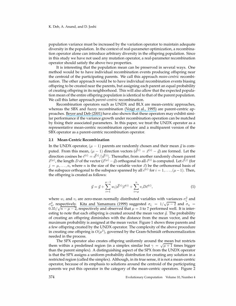
In the UNDX operator, (µ − 1) parents are randomly chosen and their mean ~g is com-

puted. From this mean, (µ − 1) direction vectors (~d(i) = ~x(i) − ~g) are formed. Let the

direction cosines be ~e(i) = ~d(i)/|~d(i)|. Thereafter, from another randomly chosen parent~x(µ), the length D of the vector (~x(µ) −~g) orthogonal to all ~e(i) is computed. Let ~e(j) (forj = µ, . . . , n, where n is the size of the variable vector ~x) be the orthonormal basis ofthe subspace orthogonal to the subspace spanned by all ~e(i) for i = 1, . . . , (µ−1). Then,the offspring is created as follows:

~y = ~g +

µ−1∑

i=1

wi|~d(i)|~e(i) +

n∑

i=µ

viD~e(i), (1)

where wi and vi are zero-mean normally distributed variables with variances σ2ζ and

σ2η , respectively. Kita and Yamamura (1999) suggested σζ = 1/

√µ − 2 and ση =

0.35/√

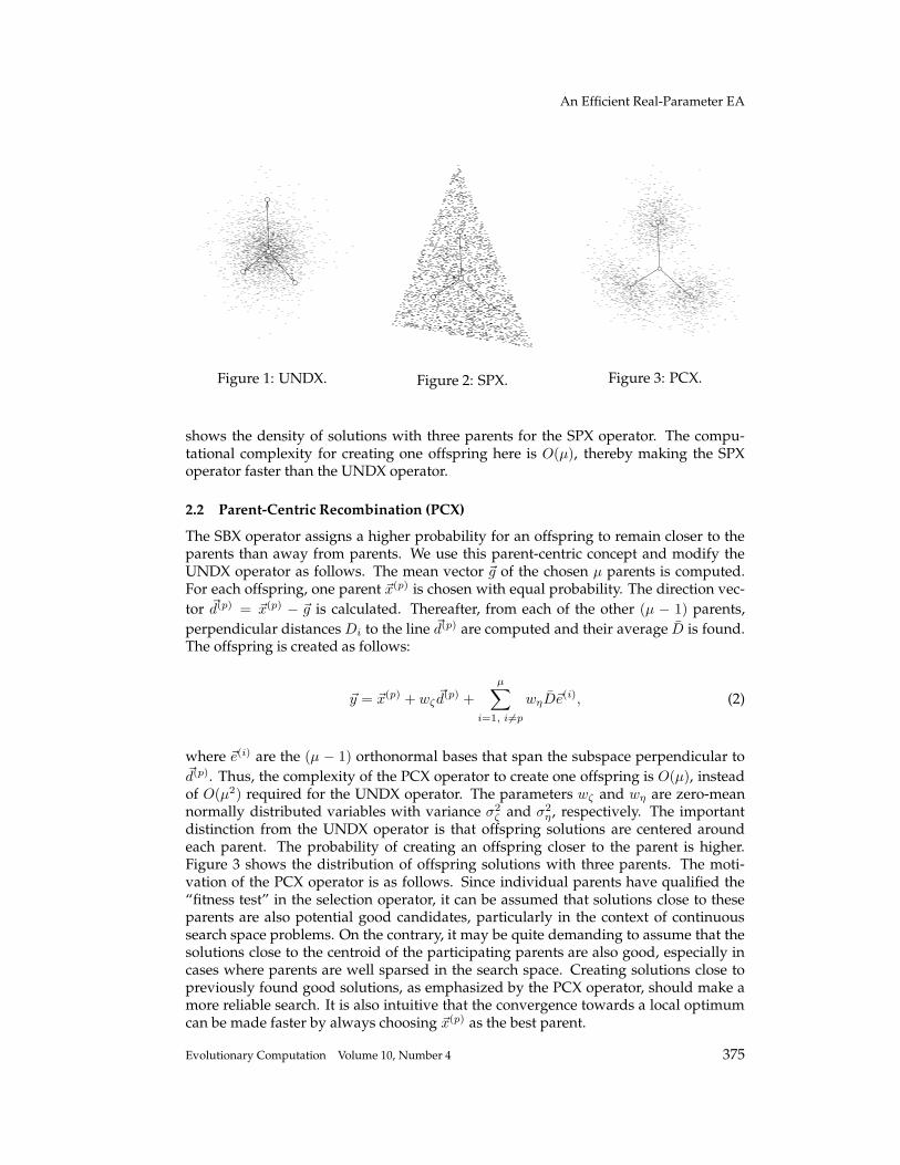
n − µ − 2, respectively and observed that µ = 3 to 7 performed well. It is inter-esting to note that each offspring is created around the mean vector ~g. The probabilityof creating an offspring diminishes with the distance from the mean vector, and themaximum probability is assigned at the mean vector. Figure 1 shows three parents anda few offspring created by the UNDX operator. The complexity of the above procedurein creating one offspring is O(µ2), governed by the Gram-Schmidt orthonormalizationneeded in the process.

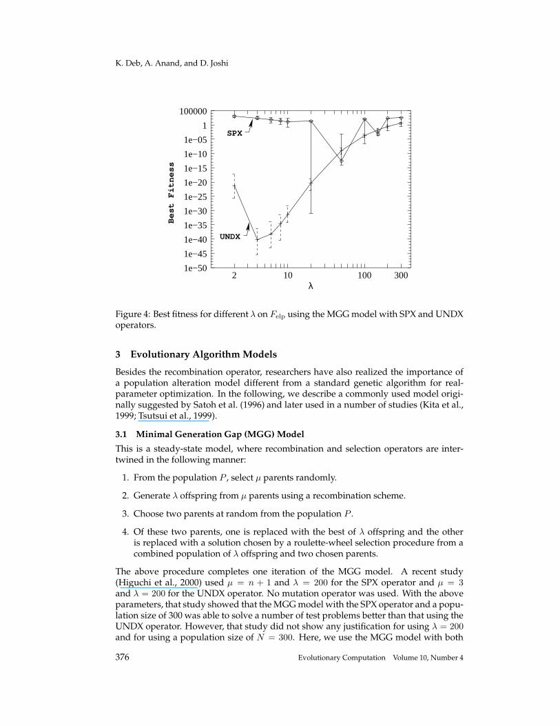
The SPX operator also creates offspring uniformly around the mean but restrictsthem within a predefined region (in a simplex similar but γ =

õ + 1 times bigger

than the parent simplex). A distinguishing aspect of the SPX from the UNDX operatoris that the SPX assigns a uniform probability distribution for creating any solution in arestricted region (called the simplex). Although, in its true sense, it is not amean-centricoperator, because of its emphasis to solutions around the centroid of the participatingparents we put this operator in the category of the mean-centric operators. Figure 2

374 Evolutionary Computation Volume 10, Number 4

An Efficient Real-Parameter EA

Figure 1: UNDX. Figure 2: SPX. Figure 3: PCX.

shows the density of solutions with three parents for the SPX operator. The compu-tational complexity for creating one offspring here is O(µ), thereby making the SPXoperator faster than the UNDX operator.

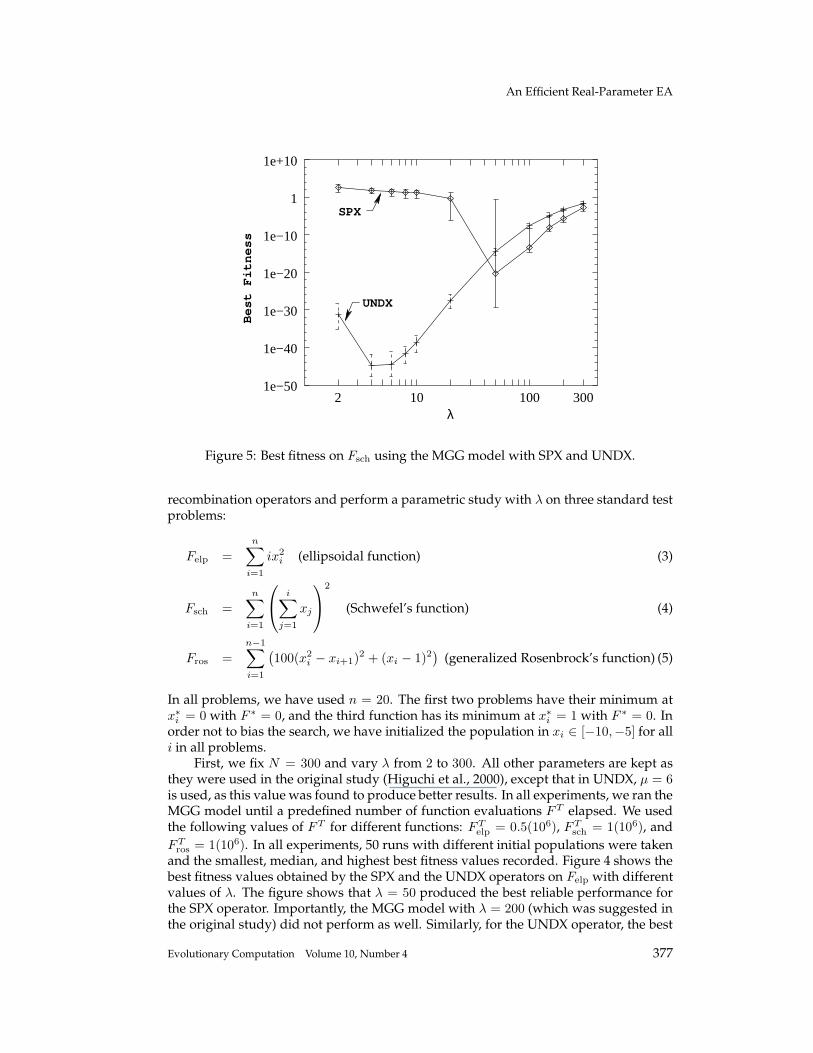
2.2 Parent-Centric Recombination (PCX)

The SBX operator assigns a higher probability for an offspring to remain closer to theparents than away from parents. We use this parent-centric concept and modify theUNDX operator as follows. The mean vector ~g of the chosen µ parents is computed.For each offspring, one parent ~x(p) is chosen with equal probability. The direction vec-

tor ~d(p) = ~x(p) − ~g is calculated. Thereafter, from each of the other (µ − 1) parents,

perpendicular distances Di to the line ~d(p) are computed and their average D is found.The offspring is created as follows:

~y = ~x(p) + wζ~d(p) +

µ∑

i=1, i6=p

wηD~e(i), (2)

where ~e(i) are the (µ − 1) orthonormal bases that span the subspace perpendicular to~d(p). Thus, the complexity of the PCX operator to create one offspring is O(µ), insteadof O(µ2) required for the UNDX operator. The parameters wζ and wη are zero-meannormally distributed variables with variance σ2

ζ and σ2η , respectively. The important

distinction from the UNDX operator is that offspring solutions are centered aroundeach parent. The probability of creating an offspring closer to the parent is higher.Figure 3 shows the distribution of offspring solutions with three parents. The moti-vation of the PCX operator is as follows. Since individual parents have qualified the“fitness test” in the selection operator, it can be assumed that solutions close to theseparents are also potential good candidates, particularly in the context of continuoussearch space problems. On the contrary, it may be quite demanding to assume that thesolutions close to the centroid of the participating parents are also good, especially incases where parents are well sparsed in the search space. Creating solutions close topreviously found good solutions, as emphasized by the PCX operator, should make amore reliable search. It is also intuitive that the convergence towards a local optimumcan be made faster by always choosing ~x(p) as the best parent.

Evolutionary Computation Volume 10, Number 4 375

K. Deb, A. Anand, and D. Joshi

UNDX

SPX

1e−50

1e−45

1e−40

1e−35

1e−30

1e−25

1e−20

1e−15

1e−10

1e−05

1

100000

2 10 100 300

Best Fitness

λ

Figure 4: Best fitness for different λ on Felp using the MGGmodel with SPX and UNDXoperators.

3 Evolutionary AlgorithmModels

Besides the recombination operator, researchers have also realized the importance ofa population alteration model different from a standard genetic algorithm for real-parameter optimization. In the following, we describe a commonly used model origi-nally suggested by Satoh et al. (1996) and later used in a number of studies (Kita et al.,1999; Tsutsui et al., 1999).

3.1 Minimal Generation Gap (MGG) Model

This is a steady-state model, where recombination and selection operators are inter-twined in the following manner:

1. From the population P , select µ parents randomly.

2. Generate λ offspring from µ parents using a recombination scheme.

3. Choose two parents at random from the population P .

4. Of these two parents, one is replaced with the best of λ offspring and the otheris replaced with a solution chosen by a roulette-wheel selection procedure from acombined population of λ offspring and two chosen parents.

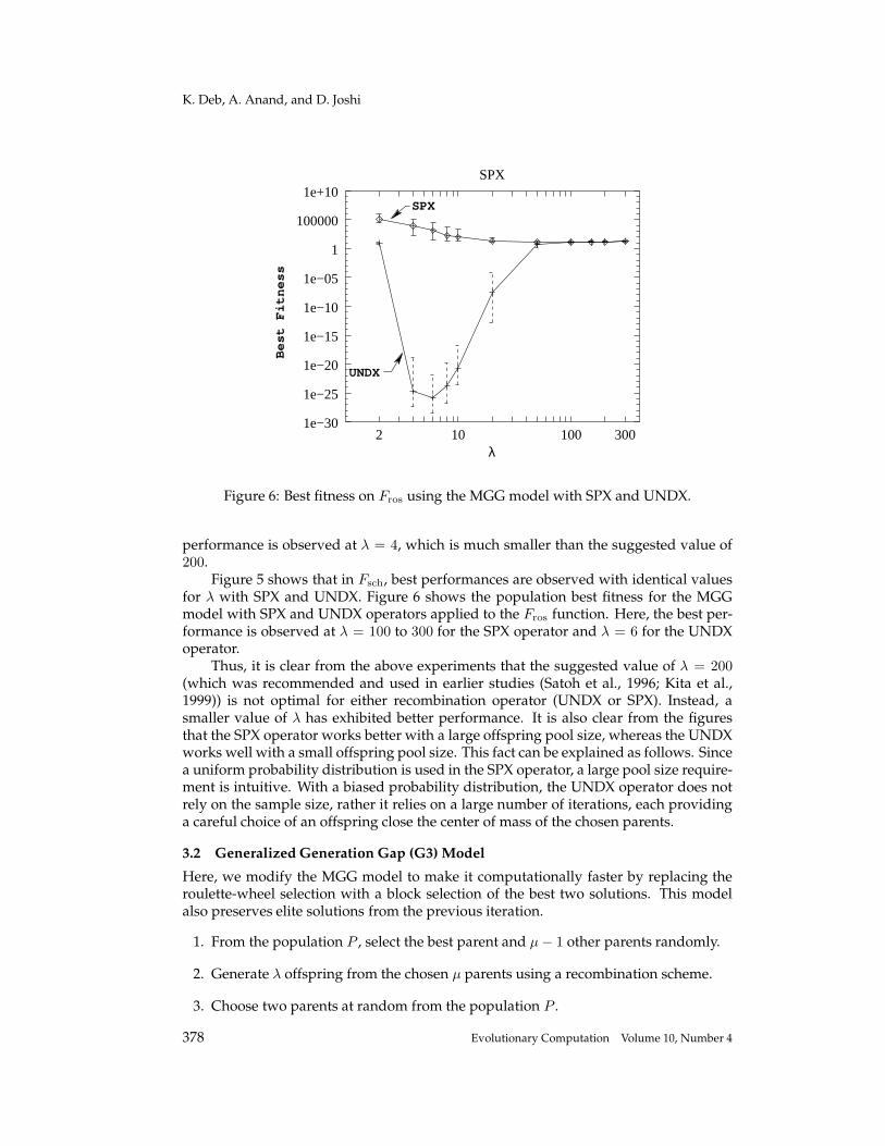
The above procedure completes one iteration of the MGG model. A recent study(Higuchi et al., 2000) used µ = n + 1 and λ = 200 for the SPX operator and µ = 3and λ = 200 for the UNDX operator. No mutation operator was used. With the aboveparameters, that study showed that theMGGmodel with the SPX operator and a popu-lation size of 300 was able to solve a number of test problems better than that using theUNDX operator. However, that study did not show any justification for using λ = 200and for using a population size of N = 300. Here, we use the MGG model with both

376 Evolutionary Computation Volume 10, Number 4

An Efficient Real-Parameter EA

UNDX

SPX

1e−50

1e−40

1e−30

1e−20

1e−10

1

1e+10

2 10 100 300

Best Fitness

λ

Figure 5: Best fitness on Fsch using the MGGmodel with SPX and UNDX.

recombination operators and perform a parametric study with λ on three standard testproblems:

Felp =

n∑

i=1

ix2i (ellipsoidal function) (3)

Fsch =n

∑

i=1

i∑

j=1

xj

2

(Schwefel’s function) (4)

Fros =

n−1∑

i=1

(

100(x2i − xi+1)

2 + (xi − 1)2)

(generalized Rosenbrock’s function) (5)

In all problems, we have used n = 20. The first two problems have their minimum atx∗

i = 0 with F ∗ = 0, and the third function has its minimum at x∗i = 1 with F ∗ = 0. In

order not to bias the search, we have initialized the population in xi ∈ [−10,−5] for alli in all problems.

First, we fix N = 300 and vary λ from 2 to 300. All other parameters are kept asthey were used in the original study (Higuchi et al., 2000), except that in UNDX, µ = 6is used, as this value was found to produce better results. In all experiments, we ran theMGG model until a predefined number of function evaluations FT elapsed. We usedthe following values of FT for different functions: FT

elp = 0.5(106), FTsch = 1(106), and

FTros = 1(106). In all experiments, 50 runs with different initial populations were taken

and the smallest, median, and highest best fitness values recorded. Figure 4 shows thebest fitness values obtained by the SPX and the UNDX operators on Felp with differentvalues of λ. The figure shows that λ = 50 produced the best reliable performance forthe SPX operator. Importantly, the MGG model with λ = 200 (which was suggested inthe original study) did not perform as well. Similarly, for the UNDX operator, the best

Evolutionary Computation Volume 10, Number 4 377

K. Deb, A. Anand, and D. Joshi

SPX

UNDX

1e−30

1e−25

1e−20

1e−15

1e−10

1e−05

1

100000

1e+10

2 10 100 300

Best Fitness

λ

SPX

Figure 6: Best fitness on Fros using the MGG model with SPX and UNDX.

performance is observed at λ = 4, which is much smaller than the suggested value of200.

Figure 5 shows that in Fsch, best performances are observed with identical valuesfor λ with SPX and UNDX. Figure 6 shows the population best fitness for the MGGmodel with SPX and UNDX operators applied to the Fros function. Here, the best per-formance is observed at λ = 100 to 300 for the SPX operator and λ = 6 for the UNDXoperator.

Thus, it is clear from the above experiments that the suggested value of λ = 200(which was recommended and used in earlier studies (Satoh et al., 1996; Kita et al.,1999)) is not optimal for either recombination operator (UNDX or SPX). Instead, asmaller value of λ has exhibited better performance. It is also clear from the figuresthat the SPX operator works better with a large offspring pool size, whereas the UNDXworks well with a small offspring pool size. This fact can be explained as follows. Sincea uniform probability distribution is used in the SPX operator, a large pool size require-ment is intuitive. With a biased probability distribution, the UNDX operator does notrely on the sample size, rather it relies on a large number of iterations, each providinga careful choice of an offspring close the center of mass of the chosen parents.

3.2 Generalized Generation Gap (G3) Model

Here, we modify the MGG model to make it computationally faster by replacing theroulette-wheel selection with a block selection of the best two solutions. This modelalso preserves elite solutions from the previous iteration.

1. From the population P , select the best parent and µ − 1 other parents randomly.

2. Generate λ offspring from the chosen µ parents using a recombination scheme.

3. Choose two parents at random from the population P .

378 Evolutionary Computation Volume 10, Number 4

An Efficient Real-Parameter EA

PCX

UNDX

SPX

913

1000

10000

100000

1e+06

2 4 10 20 50 100 300

Function Evaluations

λ

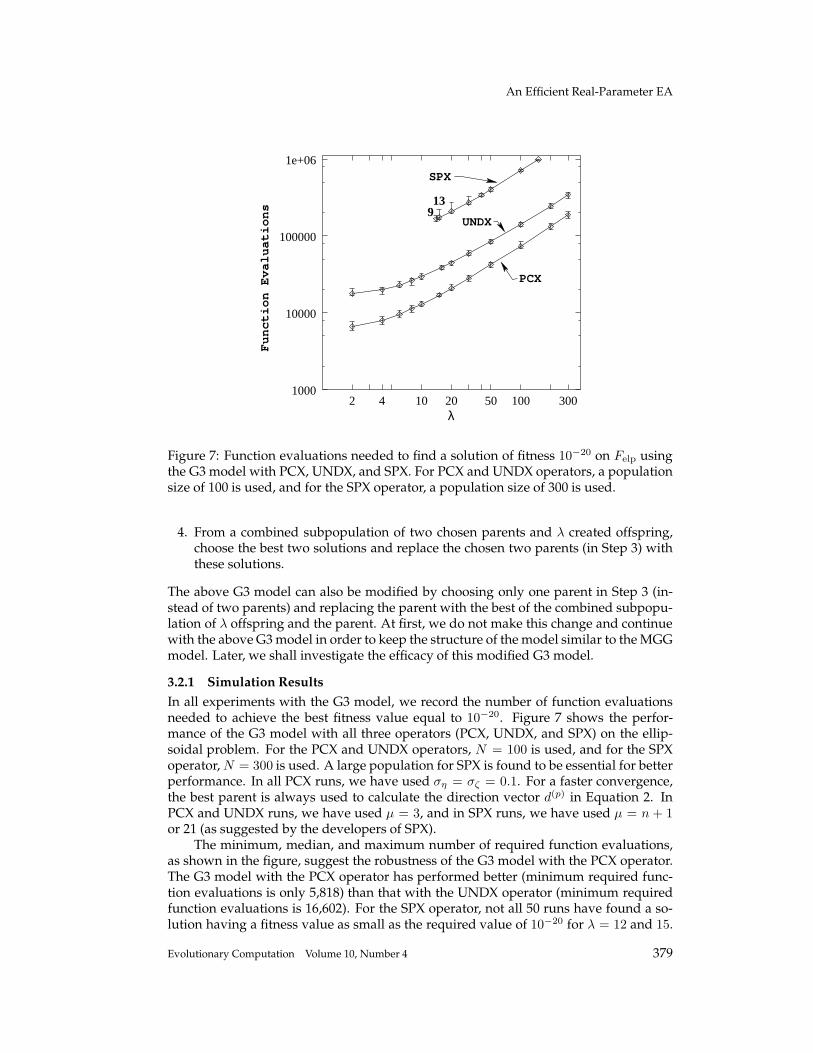
Figure 7: Function evaluations needed to find a solution of fitness 10−20 on Felp usingthe G3 model with PCX, UNDX, and SPX. For PCX and UNDX operators, a populationsize of 100 is used, and for the SPX operator, a population size of 300 is used.

4. From a combined subpopulation of two chosen parents and λ created offspring,choose the best two solutions and replace the chosen two parents (in Step 3) withthese solutions.

The above G3 model can also be modified by choosing only one parent in Step 3 (in-stead of two parents) and replacing the parent with the best of the combined subpopu-lation of λ offspring and the parent. At first, we do not make this change and continuewith the above G3model in order to keep the structure of the model similar to theMGGmodel. Later, we shall investigate the efficacy of this modified G3 model.

3.2.1 Simulation Results

In all experiments with the G3 model, we record the number of function evaluationsneeded to achieve the best fitness value equal to 10−20. Figure 7 shows the perfor-mance of the G3 model with all three operators (PCX, UNDX, and SPX) on the ellip-soidal problem. For the PCX and UNDX operators, N = 100 is used, and for the SPXoperator, N = 300 is used. A large population for SPX is found to be essential for betterperformance. In all PCX runs, we have used ση = σζ = 0.1. For a faster convergence,the best parent is always used to calculate the direction vector d(p) in Equation 2. InPCX and UNDX runs, we have used µ = 3, and in SPX runs, we have used µ = n + 1or 21 (as suggested by the developers of SPX).

The minimum, median, and maximum number of required function evaluations,as shown in the figure, suggest the robustness of the G3 model with the PCX operator.The G3 model with the PCX operator has performed better (minimum required func-tion evaluations is only 5,818) than that with the UNDX operator (minimum requiredfunction evaluations is 16,602). For the SPX operator, not all 50 runs have found a so-lution having a fitness value as small as the required value of 10−20 for λ = 12 and 15.

Evolutionary Computation Volume 10, Number 4 379

K. Deb, A. Anand, and D. Joshi

PCX

UNDX

SPX

1000

10000

100000

1e+06

50 70 100 150 200 300 400 500

Function Evaluations

Population Size

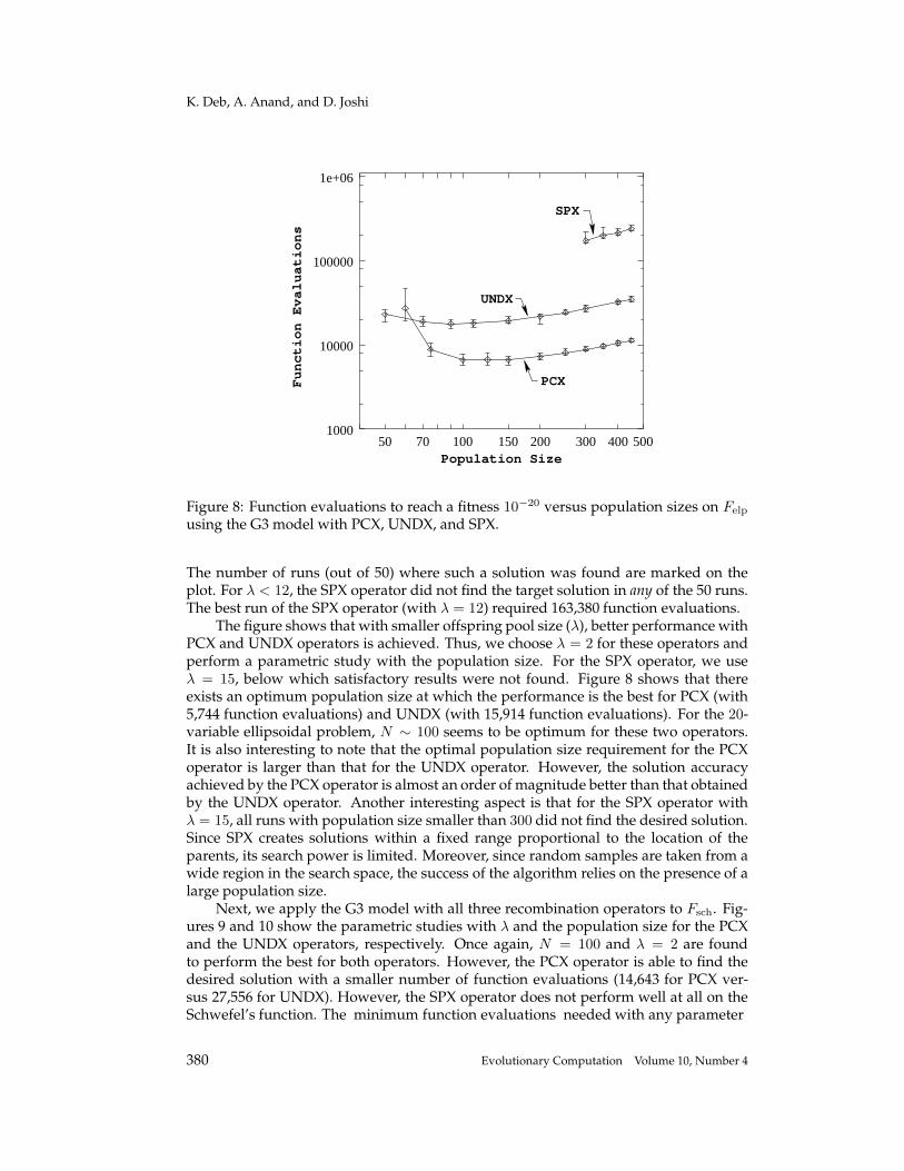
Figure 8: Function evaluations to reach a fitness 10−20 versus population sizes on Felp

using the G3 model with PCX, UNDX, and SPX.

The number of runs (out of 50) where such a solution was found are marked on theplot. For λ < 12, the SPX operator did not find the target solution in any of the 50 runs.The best run of the SPX operator (with λ = 12) required 163,380 function evaluations.

The figure shows that with smaller offspring pool size (λ), better performance withPCX and UNDX operators is achieved. Thus, we choose λ = 2 for these operators andperform a parametric study with the population size. For the SPX operator, we useλ = 15, below which satisfactory results were not found. Figure 8 shows that thereexists an optimum population size at which the performance is the best for PCX (with5,744 function evaluations) and UNDX (with 15,914 function evaluations). For the 20-variable ellipsoidal problem, N ∼ 100 seems to be optimum for these two operators.It is also interesting to note that the optimal population size requirement for the PCXoperator is larger than that for the UNDX operator. However, the solution accuracyachieved by the PCX operator is almost an order of magnitude better than that obtainedby the UNDX operator. Another interesting aspect is that for the SPX operator withλ = 15, all runs with population size smaller than 300 did not find the desired solution.Since SPX creates solutions within a fixed range proportional to the location of theparents, its search power is limited. Moreover, since random samples are taken from awide region in the search space, the success of the algorithm relies on the presence of alarge population size.

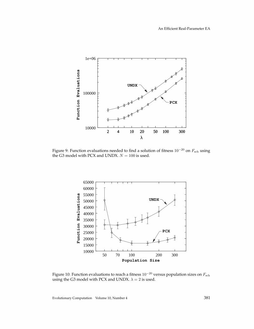
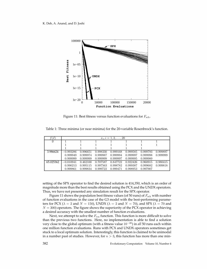
Next, we apply the G3 model with all three recombination operators to Fsch. Fig-ures 9 and 10 show the parametric studies with λ and the population size for the PCXand the UNDX operators, respectively. Once again, N = 100 and λ = 2 are foundto perform the best for both operators. However, the PCX operator is able to find thedesired solution with a smaller number of function evaluations (14,643 for PCX ver-sus 27,556 for UNDX). However, the SPX operator does not perform well at all on theSchwefel’s function. The minimum function evaluations needed with any parameter

380 Evolutionary Computation Volume 10, Number 4

An Efficient Real-Parameter EA

PCX

UNDX

10000

100000

1e+06

2 4 10 20 50 100 300

Function Evaluations

2 4 10 20 50 100 300

λ

Figure 9: Function evaluations needed to find a solution of fitness 10−20 on Fsch usingthe G3 model with PCX and UNDX. N = 100 is used.

UNDX

PCX

10000

20000

25000

30000

35000

40000

45000

50000

55000

60000

65000

50 70 100 200 300

Function Evaluations

Population Size

15000

Figure 10: Function evaluations to reach a fitness 10−20 versus population sizes on Fsch

using the G3 model with PCX and UNDX. λ = 2 is used.

Evolutionary Computation Volume 10, Number 4 381

K. Deb, A. Anand, and D. Joshi

UNDX

PCX

SPX

1e−20

1e−15

1e−10

1e−05

1

100000

0 50000 100000 150000 200000

Best Fitness

Function Evaluations

Figure 11: Best fitness versus function evaluations for Fsch.

Table 1: Three minima (or near minima) for the 20-variable Rosenbrock’s function.

f(~x) xi, i = 1, 2, . . . , 200 1 1 1 1 1 1 1

1 1 1 1 1 1 11 1 1 1 1 1

3.986624 −0.993286 0.996651 0.998330 0.999168 0.999585 0.999793 0.9998970.999949 0.999974 0.999987 0.999994 0.999997 0.999998 0.9999990.999999 0.999999 0.999999 0.999997 0.999995 0.999989

65.025362 −0.010941 0.462100 0.707587 0.847722 0.922426 0.960915 0.9804150.990213 0.995115 0.997563 0.998782 0.999387 0.999682 0.9998180.999861 0.999834 0.999722 0.999471 0.998953 0.997907

setting of the SPX operator to find the desired solution is 414,350, which is an order ofmagnitudemore than the best results obtained using the PCX and the UNDX operators.Thus, we have not presented any simulation result for the SPX operator.

Figure 11 shows the population best fitness values (of 50 runs) of Fsch with numberof function evaluations in the case of the G3 model with the best-performing parame-ters for PCX (λ = 2 and N = 150), UNDX (λ = 2 and N = 70), and SPX (λ = 70 andN = 300) operators. The figure shows the superiority of the PCX operator in achievinga desired accuracy with the smallest number of function evaluations.

Next, we attempt to solve the Fros function. This function is more difficult to solvethan the previous two functions. Here, no implementation is able to find a solutionvery close to the global optimum (with a fitness value 10−20) in all 50 runs each withinone million function evaluations. Runs with PCX and UNDX operators sometimes getstuck to a local optimum solution. Interestingly, this function is claimed to be unimodalin a number past of studies. However, for n > 3, this function has more than one min-

382 Evolutionary Computation Volume 10, Number 4

An Efficient Real-Parameter EA

35

42

4339

384342

43333638

43

44 3839 41

3946

42

4042

40

40

44

PCX

UNDX

10000

100000

1e+06

2 4 10 20 50 100 300λ

Function Evaluations

20

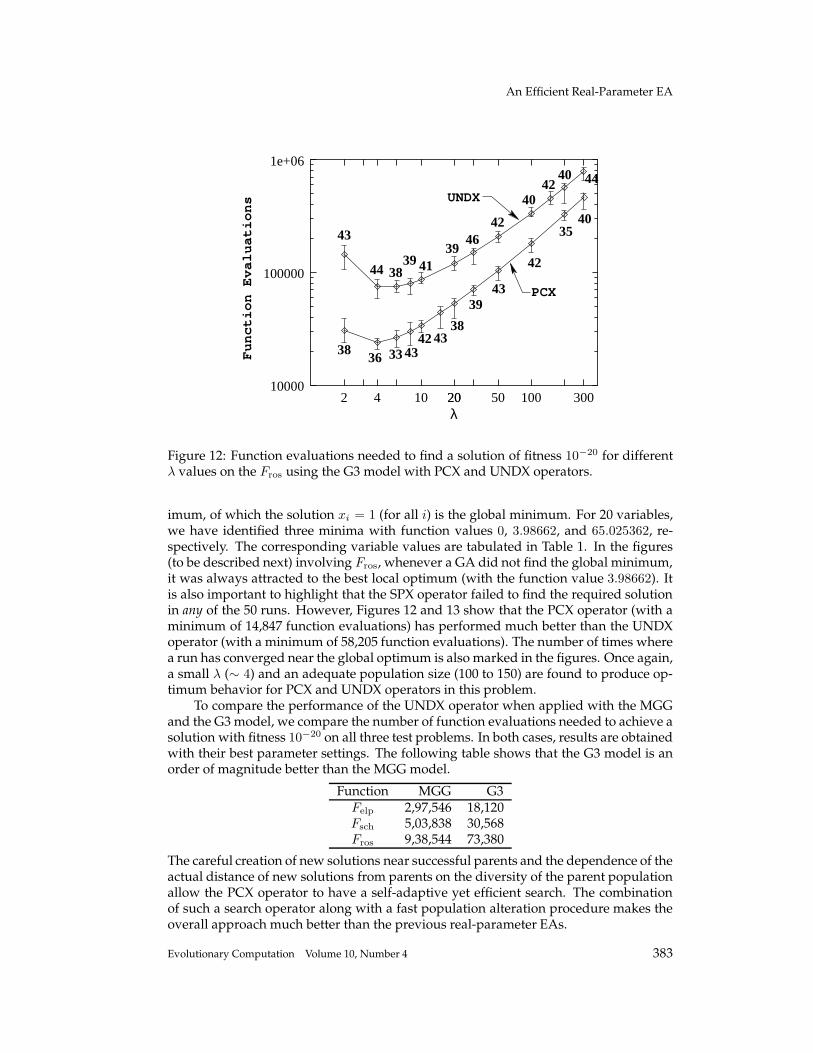
Figure 12: Function evaluations needed to find a solution of fitness 10−20 for differentλ values on the Fros using the G3 model with PCX and UNDX operators.

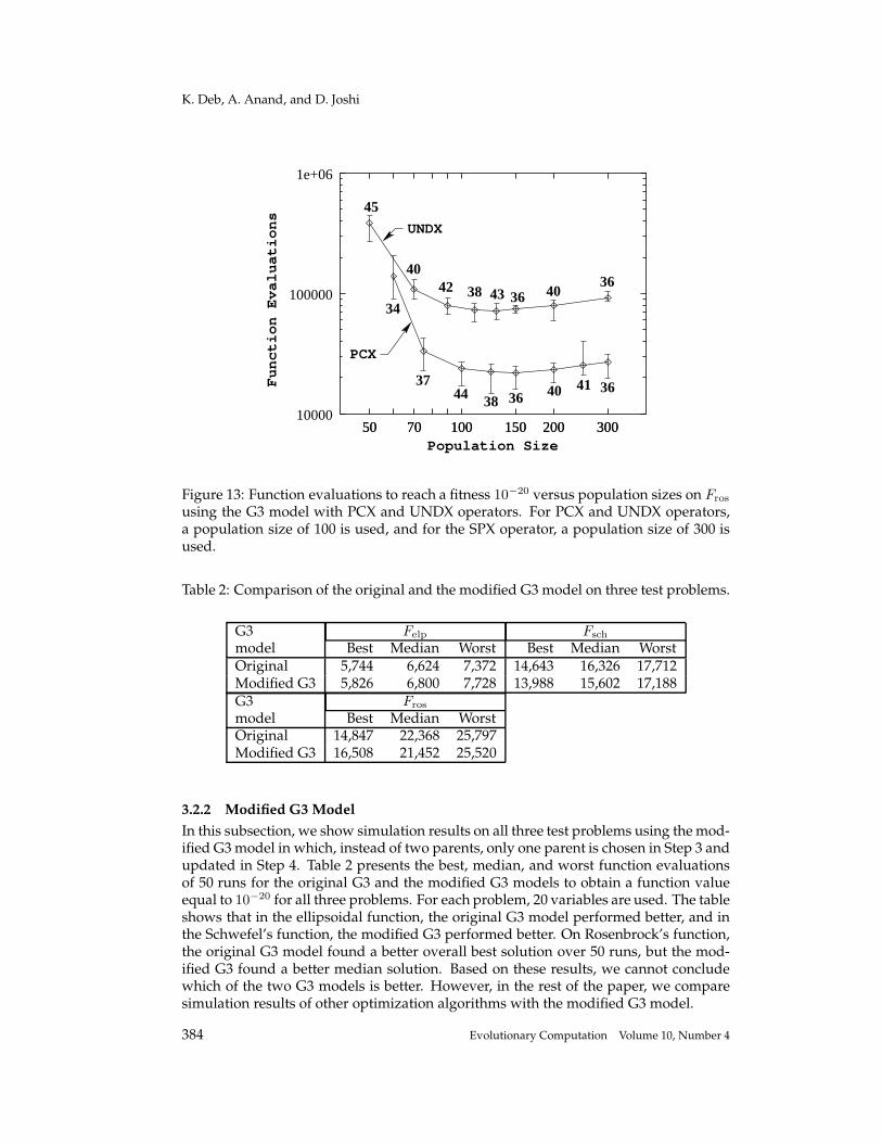
imum, of which the solution xi = 1 (for all i) is the global minimum. For 20 variables,we have identified three minima with function values 0, 3.98662, and 65.025362, re-spectively. The corresponding variable values are tabulated in Table 1. In the figures(to be described next) involving Fros, whenever a GA did not find the global minimum,it was always attracted to the best local optimum (with the function value 3.98662). Itis also important to highlight that the SPX operator failed to find the required solutionin any of the 50 runs. However, Figures 12 and 13 show that the PCX operator (with aminimum of 14,847 function evaluations) has performed much better than the UNDXoperator (with a minimum of 58,205 function evaluations). The number of times wherea run has converged near the global optimum is also marked in the figures. Once again,a small λ (∼ 4) and an adequate population size (100 to 150) are found to produce op-timum behavior for PCX and UNDX operators in this problem.

To compare the performance of the UNDX operator when applied with the MGGand the G3 model, we compare the number of function evaluations needed to achieve asolution with fitness 10−20 on all three test problems. In both cases, results are obtainedwith their best parameter settings. The following table shows that the G3 model is anorder of magnitude better than the MGG model.

Function MGG G3Felp 2,97,546 18,120Fsch 5,03,838 30,568Fros 9,38,544 73,380

The careful creation of new solutions near successful parents and the dependence of theactual distance of new solutions from parents on the diversity of the parent populationallow the PCX operator to have a self-adaptive yet efficient search. The combinationof such a search operator along with a fast population alteration procedure makes theoverall approach much better than the previous real-parameter EAs.

Evolutionary Computation Volume 10, Number 4 383

K. Deb, A. Anand, and D. Joshi

3744

34

38 36 40 41 36

38 43 36 4036

45

4042

UNDX

PCX

50 70 100 150 200 30010000

100000

1e+06

50 70 100 150 200 300Population Size

Function Evaluations

Figure 13: Function evaluations to reach a fitness 10−20 versus population sizes on Fros

using the G3 model with PCX and UNDX operators. For PCX and UNDX operators,a population size of 100 is used, and for the SPX operator, a population size of 300 isused.

Table 2: Comparison of the original and the modified G3 model on three test problems.

G3 Felp Fsch

model Best Median Worst Best Median WorstOriginal 5,744 6,624 7,372 14,643 16,326 17,712Modified G3 5,826 6,800 7,728 13,988 15,602 17,188G3 Fros

model Best Median WorstOriginal 14,847 22,368 25,797Modified G3 16,508 21,452 25,520

3.2.2 Modified G3 Model

In this subsection, we show simulation results on all three test problems using the mod-ified G3model in which, instead of two parents, only one parent is chosen in Step 3 andupdated in Step 4. Table 2 presents the best, median, and worst function evaluationsof 50 runs for the original G3 and the modified G3 models to obtain a function valueequal to 10−20 for all three problems. For each problem, 20 variables are used. The tableshows that in the ellipsoidal function, the original G3 model performed better, and inthe Schwefel’s function, the modified G3 performed better. On Rosenbrock’s function,the original G3 model found a better overall best solution over 50 runs, but the mod-ified G3 found a better median solution. Based on these results, we cannot concludewhich of the two G3 models is better. However, in the rest of the paper, we comparesimulation results of other optimization algorithms with the modified G3 model.

384 Evolutionary Computation Volume 10, Number 4

An Efficient Real-Parameter EA

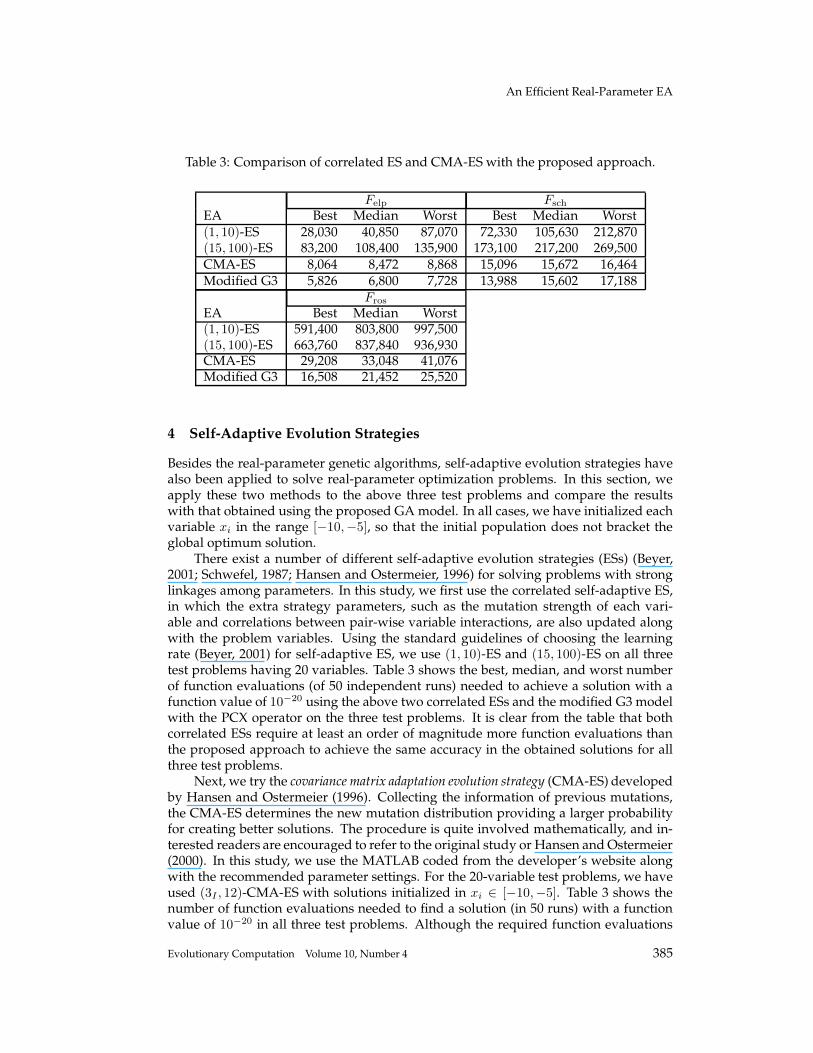
Table 3: Comparison of correlated ES and CMA-ES with the proposed approach.

Felp Fsch

EA Best Median Worst Best Median Worst(1, 10)-ES 28,030 40,850 87,070 72,330 105,630 212,870(15, 100)-ES 83,200 108,400 135,900 173,100 217,200 269,500CMA-ES 8,064 8,472 8,868 15,096 15,672 16,464Modified G3 5,826 6,800 7,728 13,988 15,602 17,188

Fros

EA Best Median Worst(1, 10)-ES 591,400 803,800 997,500(15, 100)-ES 663,760 837,840 936,930CMA-ES 29,208 33,048 41,076Modified G3 16,508 21,452 25,520

4 Self-Adaptive Evolution Strategies

Besides the real-parameter genetic algorithms, self-adaptive evolution strategies havealso been applied to solve real-parameter optimization problems. In this section, weapply these two methods to the above three test problems and compare the resultswith that obtained using the proposed GA model. In all cases, we have initialized eachvariable xi in the range [−10,−5], so that the initial population does not bracket theglobal optimum solution.

There exist a number of different self-adaptive evolution strategies (ESs) (Beyer,2001; Schwefel, 1987; Hansen and Ostermeier, 1996) for solving problems with stronglinkages among parameters. In this study, we first use the correlated self-adaptive ES,in which the extra strategy parameters, such as the mutation strength of each vari-able and correlations between pair-wise variable interactions, are also updated alongwith the problem variables. Using the standard guidelines of choosing the learningrate (Beyer, 2001) for self-adaptive ES, we use (1, 10)-ES and (15, 100)-ES on all threetest problems having 20 variables. Table 3 shows the best, median, and worst numberof function evaluations (of 50 independent runs) needed to achieve a solution with afunction value of 10−20 using the above two correlated ESs and the modified G3 modelwith the PCX operator on the three test problems. It is clear from the table that bothcorrelated ESs require at least an order of magnitude more function evaluations thanthe proposed approach to achieve the same accuracy in the obtained solutions for allthree test problems.

Next, we try the covariance matrix adaptation evolution strategy (CMA-ES) developedby Hansen and Ostermeier (1996). Collecting the information of previous mutations,the CMA-ES determines the new mutation distribution providing a larger probabilityfor creating better solutions. The procedure is quite involved mathematically, and in-terested readers are encouraged to refer to the original study or Hansen andOstermeier(2000). In this study, we use the MATLAB coded from the developer’s website alongwith the recommended parameter settings. For the 20-variable test problems, we haveused (3I , 12)-CMA-ES with solutions initialized in xi ∈ [−10,−5]. Table 3 shows thenumber of function evaluations needed to find a solution (in 50 runs) with a functionvalue of 10−20 in all three test problems. Although the required function evaluations

Evolutionary Computation Volume 10, Number 4 385

K. Deb, A. Anand, and D. Joshi

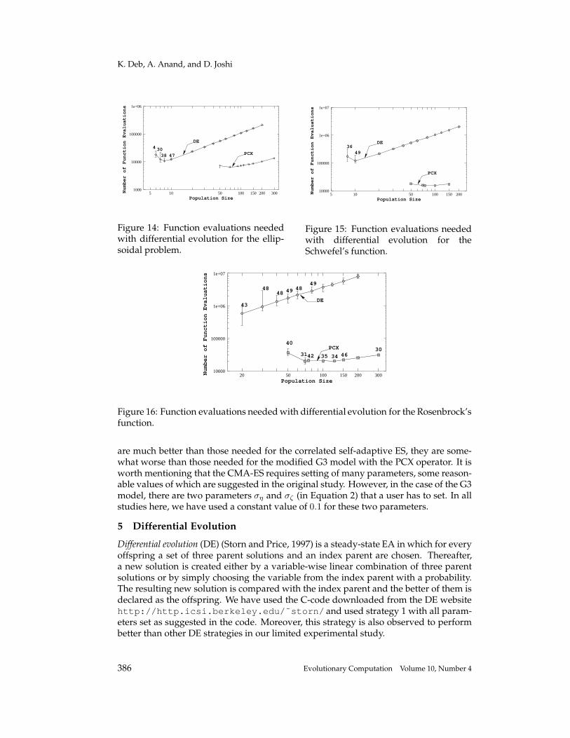
DE

PCX4 30

38 47

1000

10000

100000

1e+06

5 10 50 100 150 200 300Number of Function Evaluations

Population Size

Figure 14: Function evaluations neededwith differential evolution for the ellip-soidal problem.

DE

PCX

3649

10000

100000

1e+06

1e+07

5 10 50 100 150 200Population Size

Number of Function Evaluations

Figure 15: Function evaluations neededwith differential evolution for theSchwefel’s function.

PCX

43

4848 49 48

49

DE

40

3142 35 34 4630

10000

100000

1e+06

1e+07

20 50 100 150 200 300Number of Function Evaluations

Population Size

Figure 16: Function evaluations neededwith differential evolution for the Rosenbrock’sfunction.

are much better than those needed for the correlated self-adaptive ES, they are some-what worse than those needed for the modified G3 model with the PCX operator. It isworth mentioning that the CMA-ES requires setting of many parameters, some reason-able values of which are suggested in the original study. However, in the case of the G3model, there are two parameters ση and σζ (in Equation 2) that a user has to set. In allstudies here, we have used a constant value of 0.1 for these two parameters.

5 Differential Evolution

Differential evolution (DE) (Storn and Price, 1997) is a steady-state EA in which for everyoffspring a set of three parent solutions and an index parent are chosen. Thereafter,a new solution is created either by a variable-wise linear combination of three parentsolutions or by simply choosing the variable from the index parent with a probability.The resulting new solution is compared with the index parent and the better of them isdeclared as the offspring. We have used the C-code downloaded from the DE websitehttp://http.icsi.berkeley.edu/˜storn/ and used strategy 1 with all param-eters set as suggested in the code. Moreover, this strategy is also observed to performbetter than other DE strategies in our limited experimental study.

386 Evolutionary Computation Volume 10, Number 4

An Efficient Real-Parameter EA

Figures 14, 15, and 16 compare the function evaluations neededwith DE to achievea solution with a function value of 10−20 on three test problems with the modified G3model and the PCX operator. We have applied DE with different population sizes eachperformed with 50 independent runs. It is interesting to note that in all three problems,an optimal population size is observed. In the case of the Rosenbrock’s function, onlya few runs out of 50 runs find the true optimum with a population size smaller than20. All three figures demonstrate that the best performance of the modified G3 withthe PCX operator is better than the best performance of the DE. To highlight the bestperformances of both methods, we have tabulated corresponding function evaluationsin the following table:

Felp Fsch

Method Best Median Worst Best Median WorstDE 9,660 12,033 20,881 102,000 119,170 185,590Modified G3 5,826 6,800 7,728 13,988 15,602 17,188

Fros

Method Best Median WorstDE 243,800 587,920 942,040Modified G3 16,508 21,452 25,520

The table shows that except for the ellipsoidal function, the modified G3 requires anorder of magnitude less number of function evaluations than DE.

6 Quasi-Newton Method

The quasi-Newton method for unconstrained optimization is a popular and efficientapproach (Deb, 1995; Reklaitis et al., 1983). Here, we have used the BFGS quasi-Newtonmethod along with a mixed quadratic-cubic polynomial line search approach availablein MATLAB (Branch and Grace, 1996). The code computes gradients numerically andadjusts step sizes in each iteration adaptively for a fast convergence to the minimum.This method is found to produce the best performance among all optimization proce-dures coded in MATLAB, including the steepest-descent approach.

In Table 4, we present the best, median, and worst function values obtained froma set of 10 independent runs started from random solutions with xi ∈ [−10,−5]. Themaximum number of function evaluations allowed in each test problem is determined

Table 4: Solution accuracy obtained using the quasi-Newton method. FE denotes themaximum allowed function evaluations. In each case, the G3 model with the PCXoperator finds a solution with a function value smaller than 10−20.

Func. FE Best Median Worst

Felp 6,000 8.819(10−24) 9.718(10−24) 2.226(10−23)Fsch 15,000 4.118(10−12) 1.021(10−10) 7.422(10−9)Fros 15,000 6.077(10−17) 4.046(10−10) 3.987

Felp 8,000 5.994(10−24) 1.038(10−23) 2.226(10−23)Fsch 18,000 4.118(10−12) 4.132(10−11) 7.422(10−9)Fros 26,000 6.077(10−17) 4.046(10−10) 3.987

Evolutionary Computation Volume 10, Number 4 387

K. Deb, A. Anand, and D. Joshi

slope = 1.88

100

1000

10000

100000

1e+06

1e+07

5 50 100 200 500Number of Variables

Number of Function Variables

Figure 17: Scale-up study for the ellipsoidal function using the modified G3 model andthe PCX operator.

from the best and worst function evaluations needed for the G3 model with the PCXoperator to achieve an accuracy of 10−20. These limiting function evaluations are alsotabulated. The tolerances in the variables and in the function values are set to 10−30.The table shows that the quasi-Newton method has outperformed the G3 model withPCX for the ellipsoidal function by achieving a better function value. Since the el-lipsoidal function has no linkage among its variables, the performance of the quasi-Newton search method is difficult to match with any other method. However, it isclear from the table that the quasi-Newton method is not able to find the optimumwith an accuracy of 10−20 within the allowed number of function evaluations in moreepistatic problems (Schwefel’s and Rosenbrock’s functions).

7 Scalability of the Proposed Approach

In the above sections, we have considered only 20-variable problems. In order to inves-tigate the efficacy of the proposed G3 model with the PCX operator, we have attemptedto solve each of the three test problems with a different number of variables. For eachcase, we have chosen the population size and variances (ση and σζ ) based on someparametric studies. However, we have kept λ to a fixed value. In general, it is observedthat for a problem with an increasing number of variables, a large population size andsmall variances are desired. The increased population size requirement with increasedproblem size is also in agreement with past studies (Goldberg et al., 1992; Harik et al.,1999). The reduced requirement for variances can be explained as follows. As the num-ber of variables increases, the dimensionality of the search space increases. In order tosearch reliably in a large dimensional search space, smaller step sizes in variables mustbe chosen. Each case is run 10 times from different initial populations (initialized inxi ∈ [−10,−5] for all variables) and the best, median, and worst function evaluationsneeded to achieve a function value equal to 10−10 are presented.

388 Evolutionary Computation Volume 10, Number 4

An Efficient Real-Parameter EA

slope = 1.71

100

1000

10000

100000

1e+06

1e+07

5 50 100 200 500Number of Variables

Number of Function Evaluations

Figure 18: Scale-up study for the Schwefel’s function using the modified G3 model andthe PCX operator.

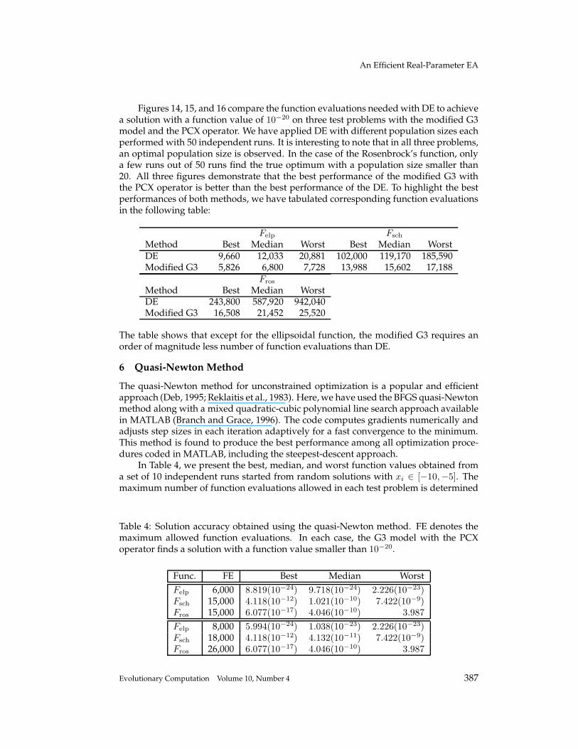
Figure 17 shows the experimental results for the ellipsoidal test problem havingas large as 500 variables. The use of two offspring (λ = 2) is found to be the best inthis case. The figure is plotted in a log-log scale. A straight line is fitted through theexperimental points. The slope of the straight line is found to be 1.88, meaning thatthe function evaluations vary approximately polynomially as O(n1.88) over the entirerange of the problem size in n ∈ [5, 500].

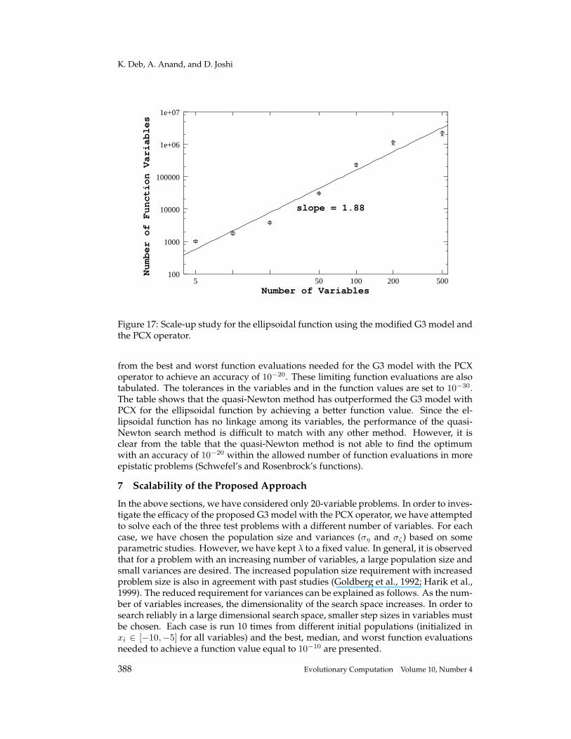
Next, we do a similar scale-up study for the Schwefel’s function. Figure 18 showsthe outcome of the study with λ = 2. A similar curve-fitting finds that the number offunction evaluations required to obtain a solution with 10−10 varies as O(n1.71) overthe entire range n ∈ [5, 500] of problem size.

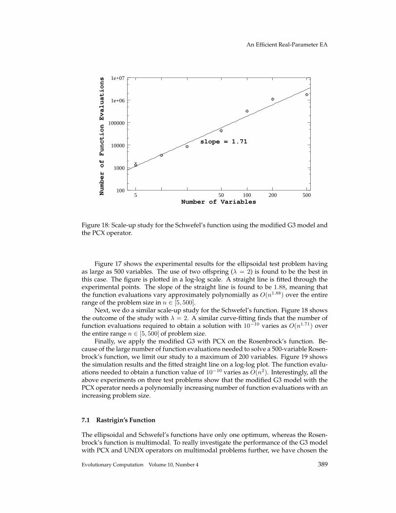
Finally, we apply the modified G3 with PCX on the Rosenbrock’s function. Be-cause of the large number of function evaluations needed to solve a 500-variable Rosen-brock’s function, we limit our study to a maximum of 200 variables. Figure 19 showsthe simulation results and the fitted straight line on a log-log plot. The function evalu-ations needed to obtain a function value of 10−10 varies as O(n2). Interestingly, all theabove experiments on three test problems show that the modified G3 model with thePCX operator needs a polynomially increasing number of function evaluations with anincreasing problem size.

7.1 Rastrigin’s Function

The ellipsoidal and Schwefel’s functions have only one optimum, whereas the Rosen-brock’s function is multimodal. To really investigate the performance of the G3 modelwith PCX and UNDX operators on multimodal problems further, we have chosen the

Evolutionary Computation Volume 10, Number 4 389

K. Deb, A. Anand, and D. Joshi

slope = 2.00

1000

10000

100000

1e+06

1e+07

5 50 100 200Number of Variables

Number of Function Evaluations

Figure 19: Scale-up study for the Rosenbrock’s function using the modified G3 modeland the PCX operator.

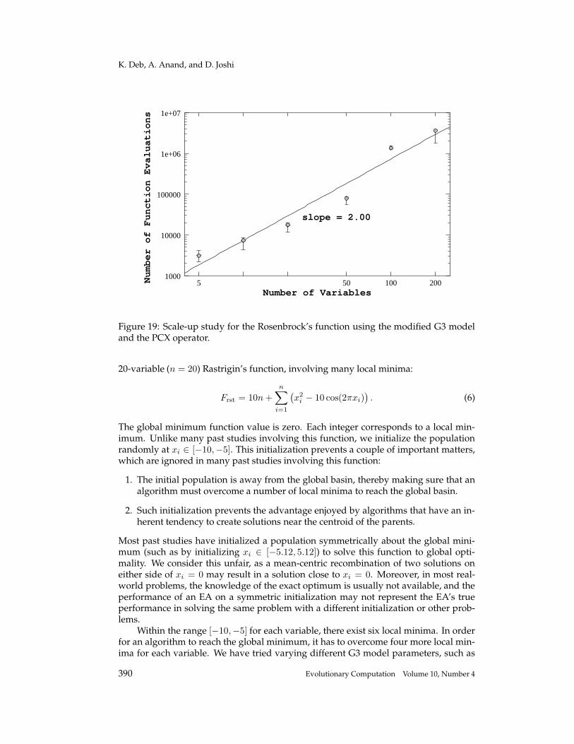
20-variable (n = 20) Rastrigin’s function, involving many local minima:

Frst = 10n +

n∑

i=1

(

x2i − 10 cos(2πxi)

)

. (6)

The global minimum function value is zero. Each integer corresponds to a local min-imum. Unlike many past studies involving this function, we initialize the populationrandomly at xi ∈ [−10,−5]. This initialization prevents a couple of important matters,which are ignored in many past studies involving this function:

1. The initial population is away from the global basin, thereby making sure that analgorithm must overcome a number of local minima to reach the global basin.

2. Such initialization prevents the advantage enjoyed by algorithms that have an in-herent tendency to create solutions near the centroid of the parents.

Most past studies have initialized a population symmetrically about the global mini-mum (such as by initializing xi ∈ [−5.12, 5.12]) to solve this function to global opti-mality. We consider this unfair, as a mean-centric recombination of two solutions oneither side of xi = 0 may result in a solution close to xi = 0. Moreover, in most real-world problems, the knowledge of the exact optimum is usually not available, and theperformance of an EA on a symmetric initialization may not represent the EA’s trueperformance in solving the same problem with a different initialization or other prob-lems.

Within the range [−10,−5] for each variable, there exist six local minima. In orderfor an algorithm to reach the global minimum, it has to overcome four more local min-ima for each variable. We have tried varying different G3 model parameters, such as

390 Evolutionary Computation Volume 10, Number 4

An Efficient Real-Parameter EA

λ, population size and variances. For both PCX and UNDX operators, no solution inthe global basin is found in a maximum of one million function evaluations over mul-tiple runs. From typical function values of the order of 103, which exist in the initialpopulation, the G3 model with the PCX and UNDX operators finds best solutions withfunction values equal to 15.936 and 19.899, respectively. Since these function values areless than 20 × 1 (the best local minimum on each variable has a function value equalto one) or 20, at least one variable (xi ∈ [−0.07157, 0.07157]) lies close to the globaloptimum value of xi = 0. Although this itself is a substantial progress made by bothmodels despite the existence of many local minima, it would be interesting to investi-gate if there exists a better global approach to solve this problem starting from an initialpopulation far away from the global optimum.

8 Review of Current Results with Respect to Past Studies

There exists a plethora of past studies attempting to solve the four test problems usedin this study. In this section, we put the results of this study in perspective to the paststudies in which significant results on the above functions were reported.

8.1 Skewed Initialization

The need for a skewed initialization, in which the initial population is not centeredaround the global optimum, in tackling test problems with known optima is reportedin a number of studies. Fogel and Beyer (1995) indicated that an initial populationcentered around the true optimum produces an undesired bias for some recombina-tion operators. Based on this observation, Eiben and Back (1997) used a skewed ini-tial population in their experimental studies with correlated self-adaptive evolutionstrategy. For the 30-variable Schwefel’s function, an initialization of the population atxi ∈ [60, 65], the best reported solution (with a (16, 100)-ES) corresponds to a functionvalue larger than 1.0 obtained with 100,000 function evaluations. For the 30-variableRastrigin’s function, the population was initialized at xi ∈ [4, 5], and the best functionvalue larger than 10.0 was achieved with 200,000 function evaluations. Although theinitialization is different from what we have used here, this study also showed the im-portance of using a skewed population in controlled experiments with test problems.

Chellapilla and Fogel (1999) solved the 10-variable Rastrigin’s function by initial-izing the population at xi ∈ [8, 12]. Compared to a symmetric initialization, this studyshowed negative improvement in best function values with the skewed initialization.

Patton et al. (1999) also considered a skewed initialization (but bracketing the min-imum) for the 10-variable Schwefel’s and Rosenbrock’s functions. For a maximum of50,000 function evaluations, their strategy found the best solution with Fsch = 1.2(10−4)and Fros = 2.37, which are much worse than our solutions obtained with an order ofmagnitude smaller number of function evaluations.

Deb and Beyer (2000) used real-parameter GAs with the SBX operator to solve anellipsoidal function started with a skewed initial population. The convergence proper-ties of the GA were found to be similar to that of a correlated ES.

8.2 Scale-Up Study

On the ellipsoidal problem, Salomon (1999) performed a scale-up study with 10, 100,and 1,000 variables. Since his deterministic GA (DGA) starts with variable-wise opti-mization requiring linear computational complexity, it is not surprising that the simu-lation study found the same for the ellipsoidal function. However, since our algorithmdoes not assume separability of variables, we cannot compare the performance of our

Evolutionary Computation Volume 10, Number 4 391

K. Deb, A. Anand, and D. Joshi

algorithm with that of the variable-wise DGA.Higuchi et al. (2000) performed a scale-up study on the Rosenbrock’s function with

10, 20, and 30 variables. In their simulation study, the population was initialized withinxi ∈ [−2.048, 2.048]. Even with this centered initialization, the MGG model with SPXrequired 275,896, 1,396,496, and 3,719,887 function evaluations, respectively. The orig-inal study did not mention the target accuracy used, but even if it were 10−20 as usedhere, we have found such high-accuracy solutions with much better computationalcomplexities.

Kita (2000) reported a scale-up study on the Rosenbrock’s function with 5, 10, and20 variables. The MGG model with the UNDX operator (µ = 3 and λ = 100) finds so-lutions with function values 2.624(10−20), 1.749(10−18), and 3.554(10−9), respectively,with a maximum of one million function evaluations. As we have shown earlier, theG3 model with the PCX operator requires much fewer function evaluations to obtain amuch better solution (with a function value of 10−20 or smaller).

Hansen and Ostermeier (2000) applied their CMA evolution strategy to the firstthree functions up to 320 variables and reported interesting results. They started theiralgorithm one unit away from the global optimum in each variable (for example, for

the Schwefel’s function, x(0)i = 1 was used, whereas the optimum of Fsch is at x∗

i = 0).For ellipsoidal and Schewfel’s functions, the scale-up is between O(n1.6) to O(n1.8),whereas for the Rosenbrock’s function, it is O(n2). For all these functions, our studyhas also found similar computational complexities up to a wider range of problemsizes, despite the use of a more skewed initial population (xi ∈ [−10,−5]) in our study.On the 20-variable Rastrigin’s function, the CMA-ESwas started with a solution initial-ized in xi ∈ [−5.12, 5.12], and function values within 30.0 to 100.0 were obtained with2,000 to 3,000 function evaluations. Our study with a simple parent replacement strat-egy with offspring created with a computationally efficient vector-wise parent-centricrecombination operator and without the need of any strategy parameter has shown asimilar performance in all four test problems to that obtained using CMA-ES involvingO(n2) strategy parameters to be updated in each iteration.

Wakunda and Zell (2000) did not perform a scale-up study but compared a numberof real-parameter EAs to the three problems used in this study to find the correspond-ing optimum with an accuracy of 10−20. For the 20-variable ellipsoidal function, morethan 25,000 function evaluations, for the 20-variable Schwefel’s function, more than40,000 function evaluations, and for the 20-variable Rosenbrock’s function, more than90,000 function evaluations were the best results reported. Although this is the onlystudy where solutions with an accuracy as high as that considered in our study werereported, the required function evaluations are much larger than that needed by the G3model with the PCX operator.

9 Conclusions

The ad-hoc use of a uniformly distributed probability for creating an offspring oftenimplemented in many real-parameter evolutionary algorithms (such as the use of SPX,BLX, or arithmetic crossover) and the use of a mean-centric probability distribution(such as that used in UNDX) have been found not to be as efficient as the proposedparent-centric approach in this paper. The parent-centric recombination operator fa-vors solutions close to parents, rather than the region close to the centroid of the par-ents or any other region in the search space. Systematic studies on three 20-variabletest problems started with a skewed population not bracketing the global optimumhave shown that a parent-centric recombination is a meaningful and efficient way of

392 Evolutionary Computation Volume 10, Number 4

An Efficient Real-Parameter EA

solving real-parameter optimization problems. In any case, the use of a uniform proba-bility distribution for creating offspring has not been found to be efficient compared toa biased probability distribution favoring the search region represented by the parentsolutions. Moreover, it has been observed that the offspring pool size used in previousreal-parameter EA studies is too large to be computationally efficient.

Furthermore, the use of an elite-preserving, steady-state, scalable, and computa-tionally fast evolutionary model (named as the G3 model) has been found to be effec-tive with both PCX and UNDX recombination operators. In all simulation runs, the G3model with the PCX operator has outperformed both the UNDX and SPX operators interms of the number of function evaluations needed in achieving a desired accuracy.The proposed PCX operator has also been found to be computationally faster. Unlikemost past studies on test problems, this study has stressed the importance of initializingan EA run with a skewed population.

To further investigate the performance of the G3 model with the PCX operator, wehave compared the results with three other commonly used evolutionary algorithms:correlated self-adaptive evolution strategy, covariance matrix adaptation (CMA-ES),and differential evolution, and with a commonly used classical unconstrained opti-mization method, the quasi-Newton algorithm, with the BFGS update method. Com-pared to all these state-of-the-art optimization algorithms, the proposed model withthe PCX operator has consistently and reliably performed better (in some cases, morethan an order of magnitude better in terms of required function evaluations).

A scale-up study on three chosen problems over a wide range of problem sizes (upto 500 variables) has demonstrated a polynomial (of a maximum degree of two) com-putational complexity of the proposed approach. Compared to existing studies with anumber of different GAs and a number of different self-adaptive evolution strategies,the proposed approach has shown better performance than most studies on the fourtest problems studied here. However, compared to a CMA-based evolution strategyapproach (Hansen and Ostermeier, 2000), which involves an update of O(n2) strategyparameters in each iteration, our G3 approach with a computationally efficient proce-dure of creating offspring (with the PCX operator) and a simple parent replacementstrategy has shown a similar scale-up effect to all test problems studied here. Thisstudy clearly demonstrates that the search power involved in the strategy-parameterbased self-adaptive evolution strategies (CMA-ES) in solving real-parameter optimiza-tion problems can be matched with an equivalent evolutionary algorithm (G3 model)without explicitly updating any strategy parameter, but with an adaptive recombina-tion operator. A similar outcome was also reported elsewhere (Deb and Beyer, 2000)showing the equivalence of a real-parameter GA (with the SBX operator) and the cor-related ES. Based on the plethora of general-purpose optimization algorithms appliedto these problems over the years, we tend to conclude that the computational complex-ities observed here (and that reported in the CMA-ES study as well) are probably thebest that can be achieved on these problems.

Based on this extensive study and computational advantage demonstrated overother well-known optimization algorithms (evolutionary or classical), we recommendthe use of the proposed G3 model with the PCX operator on more complex problemsand on real-world optimization problems.

Acknowledgments

We thank Hajime Kita for letting us use his UNDX code. Simulation studies for thedifferential evolution strategy and the CMA-ES are performed with the C code down-

Evolutionary Computation Volume 10, Number 4 393

K. Deb, A. Anand, and D. Joshi

loaded from http://www.icsi.berkeley.edu/˜ storn/code.html and the MATLAB codedownloaded from http://www.bionik.tu-berlin.de/user/niko, respectively. For thequasi-Newton study, the MATLAB optimization module is used.

References

Back, T. (1997). Self-adaptation. In Back, T., Fogel, D., and Michalewicz, Z., editors, Handbook ofEvolutionary Computation, pages C7.1:1–15, Institute of Physics Publishing, Bristol, UK, andOxford University Press, New York, New York.

Beyer, H.-G. (2001). The Theory of Evolution Strategies. Springer, Berlin, Germany.

Beyer, H.-G. and Deb, K. (2001). On self-adaptive features in real-parameter evolutionary algo-rithms. IEEE Transactions on Evolutionary Computation, 5(3):250–270.

Branch, M. A. and Grace, A. (1996). Optimization toolbox for use with MATLAB, The MathWorks,Inc., Natick, Massachusetts.

Chellapilla, K. and Fogel, D. B. (1999). Fitness distributions in evolutionary computation: Analy-sis of local extrema in the continuous domain. Proceedings of the IEEE Congress on Evolution-ary Computation (CEC-1999), pages 1885–1892, IEEE Press, Piscataway, New Jersey.

Deb, K. (1995). Optimization methods for engineering design, Prentice-Hall, New Delhi, India.

Deb, K. (2001). Multi-objective optimization using evolutionary algorithms. John Wiley and Sons,Chichester, UK.

Deb, K. and Agrawal, R. B. (1995). Simulated binary crossover for continuous search space. Com-plex Systems, 9(2):115–148.

Deb, K. and Beyer, H.-G. (2000). Self-adaptive genetic algorithms with simulated binarycrossover. Evolutionary Computation, 9(2):197–221.

Eiben, A. E. and Back, T. (1997). Empirical investigation of multiparent recombination operatorsin evolution strategies. Evolutionary Computation, 5(3):347–365.

Fogel, D. B. and Beyer, H.-G. (1995). A note on the empirical evaluation of intermediate recombi-nation. Evolutionary Computation, 3(4):491–495.

Goldberg, D. E., Deb, K., and Clark, J. H. (1992). Genetic algorithms, noise, and the sizing ofpopulations. Complex Systems, 6(4):333–362.

Hansen, N. and Ostermeier, A. (1996). Adapting arbitrary normal mutation distributions in evo-lution strategies: The covariance matrix adaptation. In Proceedings of the IEEE InternationalConference on Evolutionary Computation, pages 312–317, IEEE Press, Piscataway, New Jersey.

Hansen, N. and Ostermeier, A. (2000). Completely derandomized self-adaptation in evolutionstrategies. Evolutionary Computation, 9(2):159–195.

Harik, G. et al. (1999). The gambler’s ruin problem, genetic algorithms, and the sizing of popula-tions. Evolutionary Computation, 7(3):231–254.

Herrera, F., Lozano, M., and Verdegay, J. L. (1998). Tackling real-coded genetic algorithms: Oper-ators and tools for behavioural analysis. Artificial Intelligence Review, 12(4):265–319.

Higuchi, T., Tsutsui, S., and Yamamura, M. (2000). Theoretical analysis of simplex crossover forreal-coded genetic algorithms. In Schoenauer, M. et al., editors, Parallel Problem Solving fromNature (PPSN-VI), pages 365–374, Springer, Berlin, Germany.

Kita, H. (2000). A comparison study of self-adaptation in evolution strategies and real-codedgenetic algorithms. Evolutionary Computation 9(2):223–241.

394 Evolutionary Computation Volume 10, Number 4

An Efficient Real-Parameter EA

Kita, H. and Yamamura, M. (1999). A functional specialization hypothesis for designing geneticalgorithms. Proceedings of the 1999 IEEE International Conference on Systems, Man, and Cyber-netics, pages 579–584, IEEE Press, Piscataway, New Jersey.

Kita, H., Ono, I., and Kobayashi, S. (1999). Multi-parental extension of the unimodal normaldistribution crossover for real-coded genetic algorithms. In Porto, V. W., editor, Proceedingsof the 1999 Congress on Evolutionary Computation, pages 1581–1587, IEEE Press, Piscataway,New Jersey.

Ono, I. and Kobayashi, S. (1997). A real-coded genetic algorithm for function optimization usingunimodal normal distribution crossover. In Back, T., editor, Proceedings of the Seventh Inter-national Conference on Genetic Algorithms (ICGA-7), pages 246–253, Morgan Kaufmann, SanFrancisco, California.

Patton, A. L., Goodman, E. D., and Punch, W. F. (1999). Scheduling variance loss using pop-ulation level annealing for evolutionary computation. Proceedings of the IEEE Congress onEvolutionary Computation (CEC-1999), pages 760–767, IEEE Press, Piscataway, New Jersey.

Rechenberg, I. (1973). Evolutionsstrategie: Optimierung Technischer Systeme nach Prinzipien der Biol-ogischen Evolution. Frommann-Holzboog Verlag, Stuttgart, Germany.

Reklaitis, G. V., Ravindran, A., and Ragsdell, K. M. (1983). Engineering Optimization Methods andApplications. John Wiley and Sons, New York, New York.

Salomon, R. (1999). The deterministic genetic algorithm: Implementation details and some re-sults. Proceedings of the IEEE Congress on Evolutionary Computation (CEC-1999), pages 695–702, IEEE Press, Piscataway, New Jersey.

Satoh, H., Yamamura, M., and Kobayashi, S. (1996). Minimal generation gap model for GAs con-sidering both exploration and exploitation. In Yamakawa, T. and Matsumoto, G., editors,Proceedings of the IIZUKA: Methodologies for the Conception, Design, and Application of Intelli-gent Systems, pages 494–497, World Scientific, Singapore.

Schwefel, H.-P. (1987). Collective intelligence in evolving systems. In Wolff, W., Soeder, C. J.,and Drepper, F., editors, Ecodynamics – Contributions to Theoretical Ecology, pages 95–100,Springer, Berlin, Germany.

Storn, R. and Price, K. (1997). Differential evolution – a fast and efficient heuristic for globaloptimization over continuous spaces. Journal of Global Optimization, 11:341–359.

Tsutsui, S., Yamamura, M., and Higuchi, T. (1999). Multi-parent recombination with simplexcrossover in real-coded genetic algorithms. In Banzhaf, W. et al., editors, Proceedings of theGenetic and Evolutionary Computation Conference (GECCO-99), pages 657–664, Morgan Kauf-mann, San Francisco, California.

Voigt, H.-M., Muhlenbein, H., and Cvetkovic, D. (1995). Fuzzy recombination for the BreederGenetic Algorithm. In Eshelman, L., editor, Proceedings of the Sixth International Conference onGenetic Algorithms, pages 104–111, Morgan Kaufmann, San Francisco, California.

Wakunda, J. and Zell, A. (2000). Median-selection for parallel steady-state evolution strategies. InSchoenauer, M. et al., editors, Proceedings of the Parallel Problem Solving from Nature, (PPSN-VI), pages 405–414, Springer, Berlin, Germany.

Evolutionary Computation Volume 10, Number 4 395