HAL Id: hal-01672519https://hal.archives-ouvertes.fr/hal-01672519

Submitted on 25 Dec 2017

HAL is a multi-disciplinary open accessarchive for the deposit and dissemination of sci-entific research documents, whether they are pub-lished or not. The documents may come fromteaching and research institutions in France orabroad, or from public or private research centers.

L’archive ouverte pluridisciplinaire HAL, estdestinée au dépôt et à la diffusion de documentsscientifiques de niveau recherche, publiés ou non,émanant des établissements d’enseignement et derecherche français ou étrangers, des laboratoirespublics ou privés.

A computationally efficient approach to modelingcontact problems and fracture closure using

superposition methodHanyi Wang, Shiting yi, Mukul M Sharma

To cite this version:Hanyi Wang, Shiting yi, Mukul M Sharma. A computationally efficient approach to modeling con-tact problems and fracture closure using superposition method. Theoretical and Applied FractureMechanics, Elsevier, 2018, 93, pp.276 - 287. �10.1016/j.tafmec.2017.09.009�. �hal-01672519�

*:1) This is uncorrected proof

2) Citation Export: H. Wang, S. Yi, Mukul.M. Sharma. 2018. A Computationally Efficient Approach to Modeling Contact Problems

and Fracture Closure Using Superposition Method. Theoretical and Applied Fracture Mechanics, Vol(93): 276-287. doi:

https://doi.org/10.1016/j.tafmec.2017.09.009

A computationally efficient approach to modeling contact problems and fracture closure using superposition method*

HanYi Wang, ShiTing Yi and Mukul. M. Sharma Petroleum & Geosystems Engineering Department, The University of Texas at Austin, 200 E. Dean Keeton St., Stop C0300 Austin, TX 78712-1585, United States

Abstract

The shape of fractures in an elastic medium under different stress distributions have been well studied in the literature,

however, the fracture closure process during unloading has not been investigated thoroughly. The fracture surface is

normally assumed to be perfectly smooth so that only the width and stress intensity at the fracture tip are critical in the

analysis. In reality, the creation of a fracture in a rock seldom produces smooth surfaces and the resulting asperities on the

fracture surfaces can impact fracture closure. Correctly modeling this fracture closure behavior has numerous applications in

structural engineering and earth sciences. In this article, we present an approach to model fracture closure behavior in a 2D

and 3D elastic media. The fracture surface displacements under arbitrary normal load are derived using superposition

method. The contact stress, deformation, and fracture volume evolution can be estimated in a computationally efficient

manner for various fracture surface properties. When compared with the traditional integral transform methods used to

model fracture closure, the superposition method presented in this study produces comparable results with significant less

computation time. In addition, with the aid of parallel computation, large scale fracture closure and contact problems can be

successfully simulated using our proposed dynamic fracture closure model (DFCM) with very modest computation times.

Keywords: Fracture Closure; Contact Problem; Asperities; Contact Stress; Fracture Width; Superposition

1. Introduction

Fracture widths in a solid elastic medium are governed by the stress field around the crack tip and by parameters that

describe the resistance of the material to the imposed stress. Thus, the analysis of stresses near the crack tip constitutes an

essential part of fracture mechanics. For brittle materials exhibiting linear elastic behavior, methods of elasticity are used to

obtain stresses and displacements in cracked bodies. England and Green (1963) studied 2D crack problems using complex

variable techniques and the crack displacement was expressed as a double integral over the fracture length. Sneddon (1946)

investigated the distribution of stresses produced in the interior of an elastic solid by the opening of an internal crack under

the action of pressure applied to its surface. The solutions are derived from Westergaard’s stress function (1939) and the

critical crack propagation pressure under uniform load is obtained based on the rate of energy dissipation that proposed by

Griffith (1920). Shah and Kobayashi (1971) presented solutions of stresses and the stress intensity factor for an elliptical

crack embedded in an elastic solid and subjected to complex pressure distributions expressible in terms of a 2D polynomial

function. The foundation of this work is based on the potential function proposed by Segedin (1967). Bell (1979) derived the

solution for stresses and displacements due to arbitrarily distributed normal and tangential loads acting on a circular crack in

an infinite body, in the form of series of Bessel function integrals. Understanding the effect of stress and load conditions on

crack geometry is fundamental to solving crack propagation problems in solid materials. These stresses can be a result of

pressured liquid injection, such as magma driven dykes (Rubin 1995), sub-glacial drainage of water (Tsai and Rice 2010),

underground CO2 or waste repositories (Abou-Sayed et al. 1989) or intentionally induced hydraulic fractures for stimulating

hydrocarbon reservoirs (Economides and Nolte 2000) or for geothermal energy exploitation (Nemat-Nasser et al. 1983).

Although hydraulic fracturing can be dated back to the 1930s (Grebe and Stoesser, 1935), it has been in the last twenty years

that this practice has become commonplace. Combining the analytic solutions of stresses and displacements with a material

balance on the injected fluid, leads to the development of extensively used pressurized fracture propagation models, such as

the KGD model (Geertsma and De Klerk 1969; Khristianovich and Zheltov 1955), the PKN model (Nordgren 1972; Perkins

and Kern 1961), and the radial model (Abe et al. 1976). Besides using analytic methods (e.g., complex potential function

method and the integral transform method) to relate load, stress and displacement, numerical methods such as discrete

element methods (McClure et al. 2016; Sesetty and Ghassemi 2015; Zhao 2014), cohesive zone methods (Bryant et al. 2015;

Wang et al. 2016), and extended finite element methods (Dahi-Taleghani and Olson, 2011; Gordeliy and Peirce, 2013;

Wang 2015; Wang 2016) can be used to solve stress and displacement fields that are coupled with material balance and

lubrication equations to model fluid driven fracture propagation. Even though these numerical methods enable us to model

fracture propagation with complex interactions under fully coupled physics, just as analytic models, they assume smooth

crack surfaces. This assumption is legitimate for modeling fracture initiation and propagation when internal load exerts

sufficient pressure on the fracture surface to prop it open and maintain a finite fracture aperture. However, during the

unloading process, the fracture gradually closes and the stress acting normal to the fracture plane results in fracture apertures

approaching the scale of the surface roughness, and fracture surfaces can no longer be treated as perfectly smooth.

With the assumption of a pressurized fracture with perfectly smooth surfaces imbedded in an elastic medium, the opposite

surfaces will come into contact all at once when the internal pressure acting on fracture surfaces drops to zero, and the

fracture is then completely mechanically closed. In reality, the creation of cracks seldom produces perfectly smooth surfaces.

It is well established that the fracture properties of brittle heterogeneous materials such as rock, concrete, ceramics, wood,

and various composites strongly depend on the microstructure and on the damage process of the material. Both these

parameters are also at the source of the roughness of crack surfaces (Morel et al. 2000). This is especially the case for large

scale subsurface fractures, such as those generated by hydraulic fracturing. Van Dam et al. (2000) presented scaled

laboratory experiments on hydraulic fracture closure behavior. Their work shows that the roughness of the fracture surfaces

appears as a characteristic pattern of radial grooves and it is influenced by the externally applied stress. They also observed

up to a15% residual aperture long after shut-in. Fredd et al. (2000) used sandstone cores from the East Texas Cotton Valley

formation to show sheared fracture surface asperities that had an average height of about 0.09 inches. Warpinski et al. (1993)

reported fracture surface asperities of about 0.04 and 0.16 inches for nearly homogeneous sandstones and sandstones with

coal and clay rich bedding planes, respectively. Field measurements (Warpinski et al. 2002) using a down-hole tiltmeter

array indicated that the fracture closure process is a smooth, continuous one which often leaves 20%-30% residual fracture

width.

Fractures play a decisive role in determining production and its decline trend. In natural fractures, the most important

properties that affect the fluid flow are the fracture width, normal stress, contact area and the roughness of the fracture

surfaces. These properties are all interdependent and directly affect each other. In propped fractures, the stress distribution

after closure can substantially influence the crushing or embedment of proppants and the resulting conductivity (Warpinski

2010). In addition, the fracture closure behavior significantly impact our estimation and correct interpretation of in-situ

stress through diagnostic fracture injection tests (McClure et al. 2016; Wang and Sharma 2017b) or pump-in and flow back

tests (Raaen et al. 2001; Savitski and Dudley 2011). The changes of fracture compliance during closure is the key input

parameter for flow back analysis (Fu et al. 2017).

An extensive literature exists on the relationship between fracture aperture, conductivity, internal pressure, and effective

stress. These studies include analytical models (Greenwood and Williamson, 1966; Gangi, 1978; Brown and Scholz, 1985;

Cook, 1992; Adams and Nosonovsky, 2000; Myer, 1999) and numerical approaches (Pyrak-Nolte and Morris, 2000; Lanaro,

2000; Kamali and Pournik 2016) as well as experimental studies (Barton et al. 1985; Brown et al. 1998; Marache et al. 2008;

Matsuki et al. 2008). However, all these studies focus on detailed investigations of the closure of fractures modeled as two

parallel plates with rough surfaces, and ignore the impact of the fracture geometry and the evolution of the stress re-

distribution during fracture closure.

Even though analytic methods can give closed from solutions for fracture displacement and stress distribution under

arbitrary load, it requires a priori knowledge of load distribution (i.e., the arbitrary load can be written as a function of local

coordinates). However, in contact problems, the total pressure/stress acting on the opposite surfaces of fracture is a dynamic

process and coupled with fracture displacement, so it is not known in advance and does not have a general form that can be

represented by smooth analytic functions. To resolve this issue, Wang and Sharma (2017a) presented an integral transform

method to model contact problem with analytic solutions that relate load and displacement, the solution integrals have to be

divided into piecewise segments to approximate the distribution of possible discrete internal loads, however, this method is

not very efficient because the number of integrals that need to be evaluated grows exponentially with increasing number of

segments. Using numerical methods (such as finite element method, finite volume method, boundary element method, etc.)

to model fracture closure and contact problems also face challenges, because in many cases there is a sharp contrast of

scales between fracture geometry (e.g., tens or hundreds of meters for subsurface fractures) and surface asperities (normally

in the range of µm or mm). For a numerical model to capture both large scale fracture deformation and small scale contact

behavior during fracture closure, the mesh or element size has to be extremely small (equivalent to the scale of the fracture

aperture), which makes this effort very computationally expensive. In addition, contact problems are often non-linear and

require a large number of iterations to converge, this makes numerical modeling of fracture closure processes more

challenging, especially when the fracture size is large or a large number of fractures need to be modeled simultaneously.

In this article, we propose a new method and general algorithms to model the dynamic behavior of fracture closure on rough

fracture surfaces and asperities. Analytic solutions that relate fracture width with arbitrary normal net pressure/stress using

superposition are derived. Coupling analytic solutions with a general contact law that up-scales surfaces roughness and

asperities, large scale 2D and 3D fracture closure behavior can be modeled efficiently. Different methods of modeling

fracture closure behavior and their computation efficiency are also compared and investigated.

2. Fracture Surface Displacement with Arbitrary Normal Load

When the internal pressure of a fracture declines, the fracture aperture diminishes accordingly until the fracture faces come

into contact when the asperities of opposing fracture walls touch each other. This induces an additional normal load (i.e.,

contact stress) acting on the area of contact and changes the subsequent fracture closure behavior as the internal pressure

declines further. Here we are not seeking a general solution that relates displacement to the load, because the load itself is

dynamically related to fracture geometry, material properties and surface roughness during the fracture closure process.

Instead, we determine the displacement based on superposition, by adding the influence of discretized fracture

segment/surface areas that subject to constant computed loads. In this section, we present a method to determine fracture

aperture under an arbitrary normal load in a two and three dimensional elastic medium using superposition.

2. 1 Two Dimensional Fracture

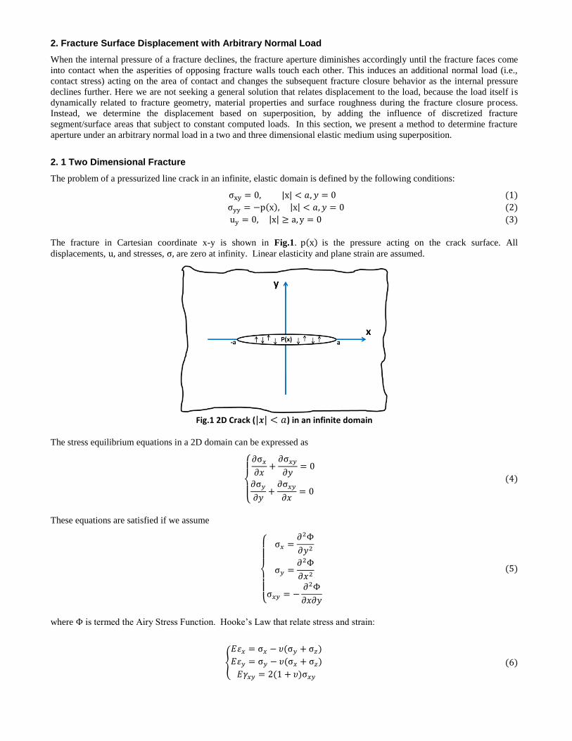
The problem of a pressurized line crack in an infinite, elastic domain is defined by the following conditions:

The fracture in Cartesian coordinate x-y is shown in Fig.1. is the pressure acting on the crack surface. All

displacements, and stresses, are zero at infinity. Linear elasticity and plane strain are assumed.

Fig.1 2D Crack ( ) in an infinite domain

The stress equilibrium equations in a 2D domain can be expressed as

These equations are satisfied if we assume

where is termed the Airy Stress Function. Hooke’s Law that relate stress and strain:

where is Young's modulus and is Poisson’s ratio, and , are normal and shear strain respectively. For plane stress

condition, and for plane strain condition, .

A convenient equation that represent three strains are defined in terms of derivatives of only two displacements is given by

Substituting Eq.(5) into Eq.(6), and using Eq.(7), the stress equilibrium can be expressed as,

Westergaard (1939) found an Airy Stress Function of complex numbers can be the solution for the stress field in an infinite

plate containing a crack. He discussed several Mode I crack problems that could be solved using:

where and Im denote the real and imaginary part, and

z is a complex number. Then, the stresses can be calculated by taking derivatives of the Airy Stress Function:

Where,

For plane strain and symmetric loading on y=0, , and the displacement field at x-direction, and y-direction,

can be determined:

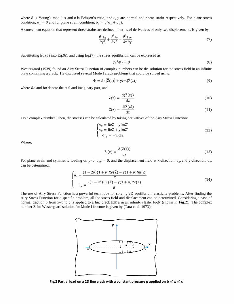
The use of Airy Stress Function is a powerful technique for solving 2D equilibrium elasticity problems. After finding the

Airy Stress Function for a specific problem, all the stress field and displacement can be determined. Considering a case of

normal traction p from x=b to c is applied to a line crack |x|≤ a in an infinite elastic body (shown in Fig.2). The complex

number Z for Westergaard solution for Mode I fracture is given by (Tara et al. 1973):

Fig.2 Partial load on a 2D line crack with a constant pressure p applied on

And the imaginary part of the first derivative of over z is:

Finally, the width of a fracture, , along x-direction can be calculated by set y=0 in Eq.(14):

where is plane strain Young’s modulus.

For a special case, when b=-a and c=a, Eq.(17) is reduced to the analytical solution for a constant internal pressure:

If the fracture from –a to a is divided into a total number of n line segments, and in the ith

( ) segment, there exists

a uniform pressure that acts on the opposite fracture surface. If n is large enough, the pressure distribution can be

approximated to any distribution of . The solution of fracture width for each individual segment with constant pressure

is given in Eq.(17). Use superposition by adding the influence of each individual segment over the entire fracture, the final

fracture width profile for any given pressure distribution can be obtained:

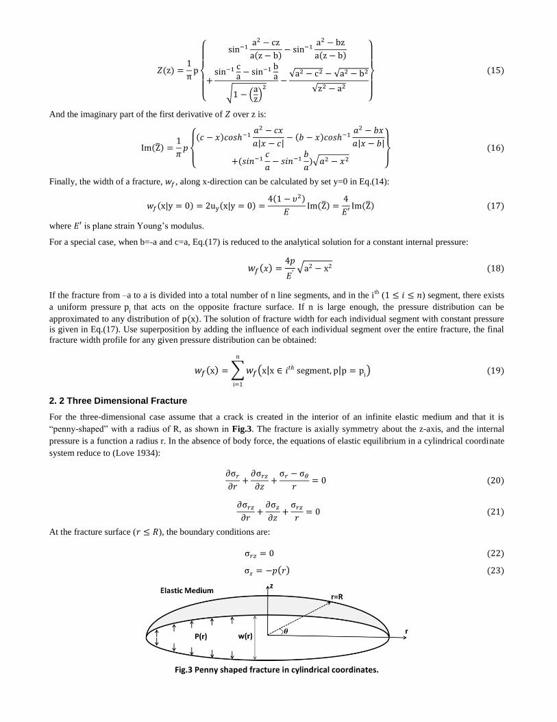
2. 2 Three Dimensional Fracture

For the three-dimensional case assume that a crack is created in the interior of an infinite elastic medium and that it is

“penny-shaped” with a radius of R, as shown in Fig.3. The fracture is axially symmetry about the z-axis, and the internal

pressure is a function a radius r. In the absence of body force, the equations of elastic equilibrium in a cylindrical coordinate

system reduce to (Love 1934):

At the fracture surface ( ), the boundary conditions are:

Fig.3 Penny shaped fracture in cylindrical coordinates.

Through integral transforms, the fracture aperture for a given internal pressure, , can be obtained as a double integral

(Sneddon 1946):

where is a dummy variable, is fracture width along r-direction. Eq.(24) is not suitable for contact problems because

is itself coupled with , which is not known in the first place. To determine based on superposition, we first

need the solution of when is constant over a circular area. Let’s assume p(r) is imposed within a radius :

Let be the inner integral of Eq.(24):

Eq.(26) has to be evaluated piecewise for different ranges of r. When

When

The outer integral of Eq.(24) also needs to be evaluated in a piecewise manner. When

When

Eq.(29) and (30) give the fracture width distribution under the load given by Eq.(25). The integrals in the solutions can’t be

evaluated analytically without resorting to elliptic integrals of the second kind (Abramowitz and Stegun 1972). With the

above derivation, the solution of fracture width as a function of fracture radius, for a constant pressure applied in the circular

region of , can be obtained using superposition, as shown in Fig.4.

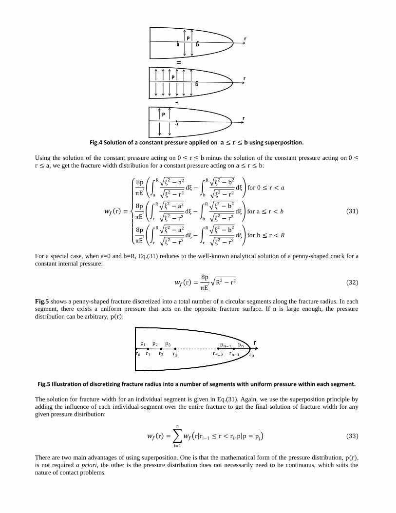
Fig.4 Solution of a constant pressure applied on using superposition.

Using the solution of the constant pressure acting on minus the solution of the constant pressure acting on , we get the fracture width distribution for a constant pressure acting on :

For a special case, when a=0 and b=R, Eq.(31) reduces to the well-known analytical solution of a penny-shaped crack for a

constant internal pressure:

Fig.5 shows a penny-shaped fracture discretized into a total number of n circular segments along the fracture radius. In each

segment, there exists a uniform pressure that acts on the opposite fracture surface. If n is large enough, the pressure

distribution can be arbitrary, .

Fig.5 Illustration of discretizing fracture radius into a number of segments with uniform pressure within each segment.

The solution for fracture width for an individual segment is given in Eq.(31). Again, we use the superposition principle by

adding the influence of each individual segment over the entire fracture to get the final solution of fracture width for any

given pressure distribution:

There are two main advantages of using superposition. One is that the mathematical form of the pressure distribution, , is not required a priori, the other is the pressure distribution does not necessarily need to be continuous, which suits the

nature of contact problems.

3. Solution Dependent Contact Load

If the fracture surface is perfectly smooth, according to Eq.(18) and Eq.(32), the entire fracture surface area will come into

contact all at once when the internal pressure drops to zero. However, as discussed previously, depending on material

properties, heterogeneity and loading conditions, the generated crack or fracture surface is always rough with asperities

distributed across the surface area. So fractures can retain a finite aperture after mechanical closure due to a mismatch of

asperities on the fracture walls, this is especially the case for subsurface fractures that are stimulated in hydrocarbon and

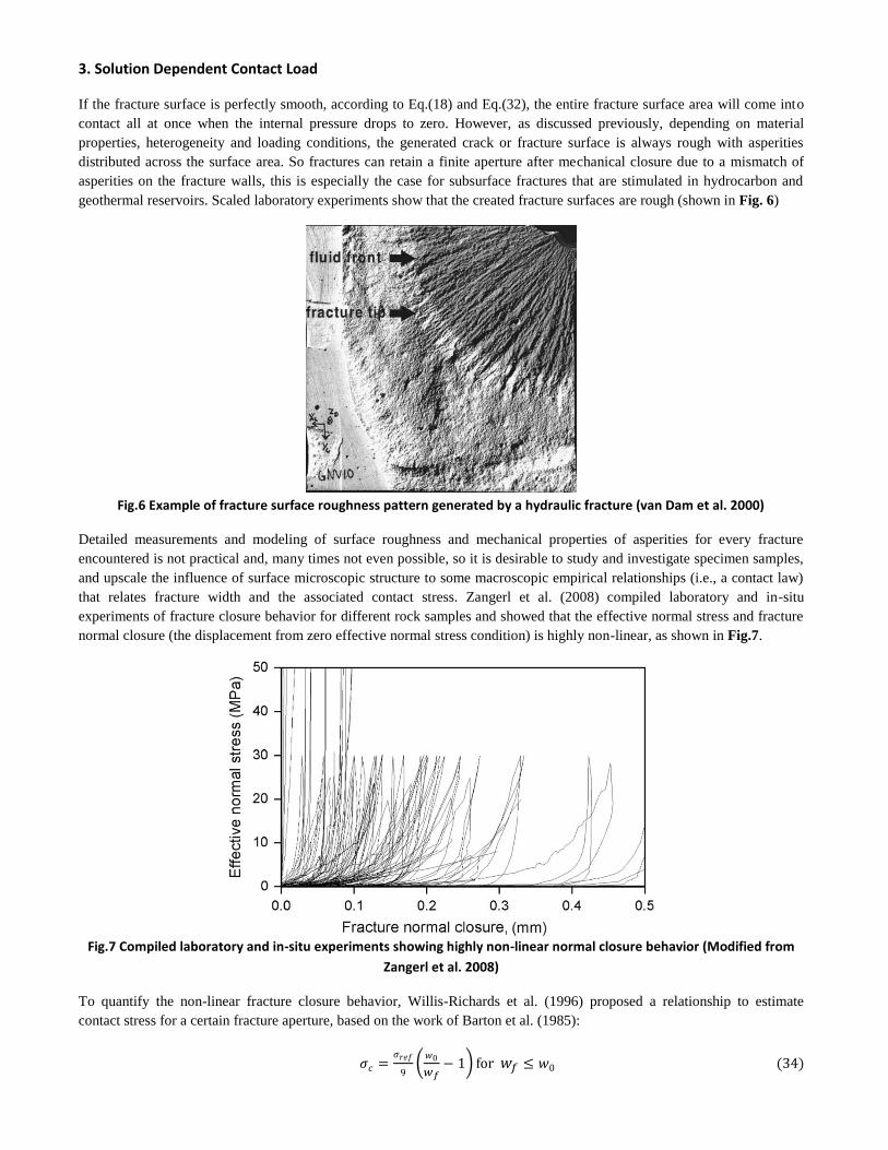
geothermal reservoirs. Scaled laboratory experiments show that the created fracture surfaces are rough (shown in Fig. 6)

Fig.6 Example of fracture surface roughness pattern generated by a hydraulic fracture (van Dam et al. 2000)

Detailed measurements and modeling of surface roughness and mechanical properties of asperities for every fracture

encountered is not practical and, many times not even possible, so it is desirable to study and investigate specimen samples,

and upscale the influence of surface microscopic structure to some macroscopic empirical relationships (i.e., a contact law)

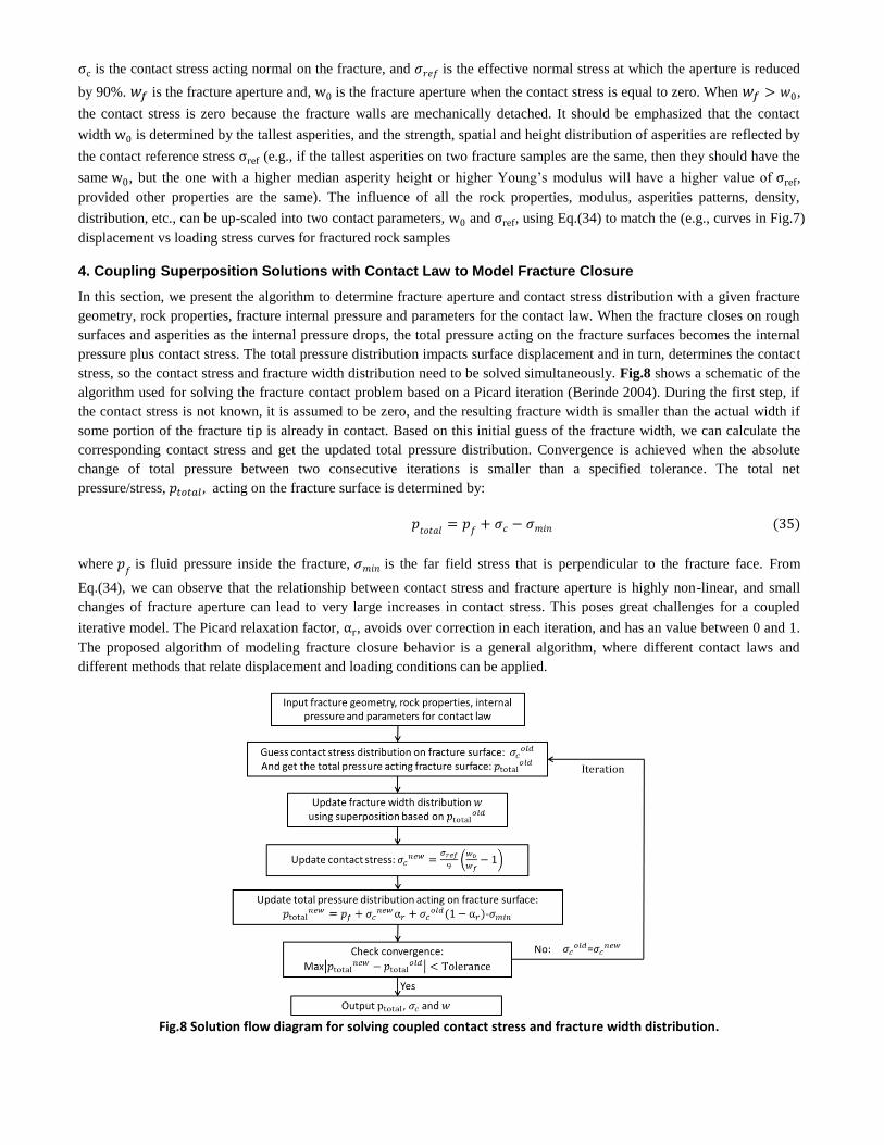
that relates fracture width and the associated contact stress. Zangerl et al. (2008) compiled laboratory and in-situ

experiments of fracture closure behavior for different rock samples and showed that the effective normal stress and fracture

normal closure (the displacement from zero effective normal stress condition) is highly non-linear, as shown in Fig.7.

Fig.7 Compiled laboratory and in-situ experiments showing highly non-linear normal closure behavior (Modified from

Zangerl et al. 2008)

To quantify the non-linear fracture closure behavior, Willis-Richards et al. (1996) proposed a relationship to estimate

contact stress for a certain fracture aperture, based on the work of Barton et al. (1985):

is the contact stress acting normal on the fracture, and is the effective normal stress at which the aperture is reduced

by 90%. is the fracture aperture and, is the fracture aperture when the contact stress is equal to zero. When ,

the contact stress is zero because the fracture walls are mechanically detached. It should be emphasized that the contact

width is determined by the tallest asperities, and the strength, spatial and height distribution of asperities are reflected by

the contact reference stress (e.g., if the tallest asperities on two fracture samples are the same, then they should have the

same , but the one with a higher median asperity height or higher Young’s modulus will have a higher value of ,

provided other properties are the same). The influence of all the rock properties, modulus, asperities patterns, density,

distribution, etc., can be up-scaled into two contact parameters, and , using Eq.(34) to match the (e.g., curves in Fig.7)

displacement vs loading stress curves for fractured rock samples

4. Coupling Superposition Solutions with Contact Law to Model Fracture Closure

In this section, we present the algorithm to determine fracture aperture and contact stress distribution with a given fracture

geometry, rock properties, fracture internal pressure and parameters for the contact law. When the fracture closes on rough

surfaces and asperities as the internal pressure drops, the total pressure acting on the fracture surfaces becomes the internal

pressure plus contact stress. The total pressure distribution impacts surface displacement and in turn, determines the contact

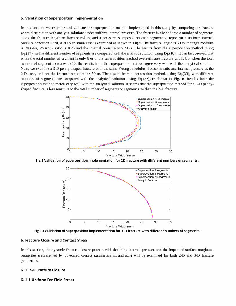
stress, so the contact stress and fracture width distribution need to be solved simultaneously. Fig.8 shows a schematic of the

algorithm used for solving the fracture contact problem based on a Picard iteration (Berinde 2004). During the first step, if

the contact stress is not known, it is assumed to be zero, and the resulting fracture width is smaller than the actual width if

some portion of the fracture tip is already in contact. Based on this initial guess of the fracture width, we can calculate the

corresponding contact stress and get the updated total pressure distribution. Convergence is achieved when the absolute

change of total pressure between two consecutive iterations is smaller than a specified tolerance. The total net

pressure/stress, acting on the fracture surface is determined by:

where is fluid pressure inside the fracture, is the far field stress that is perpendicular to the fracture face. From

Eq.(34), we can observe that the relationship between contact stress and fracture aperture is highly non-linear, and small

changes of fracture aperture can lead to very large increases in contact stress. This poses great challenges for a coupled

iterative model. The Picard relaxation factor, , avoids over correction in each iteration, and has an value between 0 and 1.

The proposed algorithm of modeling fracture closure behavior is a general algorithm, where different contact laws and

different methods that relate displacement and loading conditions can be applied.

Fig.8 Solution flow diagram for solving coupled contact stress and fracture width distribution.

5. Validation of Superposition Implementation

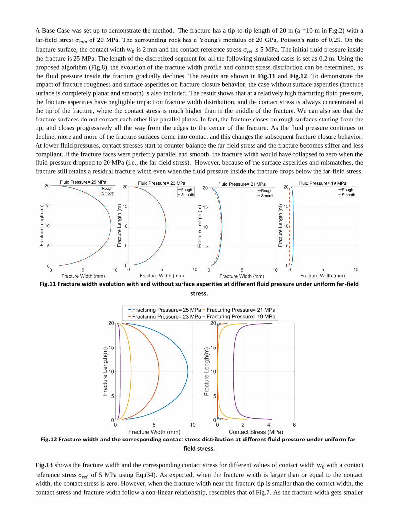
In this section, we examine and validate the superposition method implemented in this study by comparing the fracture

width distribution with analytic solutions under uniform internal pressure. The fracture is divided into a number of segments

along the fracture length or fracture radius, and a pressure is imposed on each segment to represent a uniform internal

pressure condition. First, a 2D plan strain case is examined as shown in Fig.9. The fracture length is 50 m, Young's modulus

is 20 GPa, Poisson's ratio is 0.25 and the internal pressure is 5 MPa. The results from the superposition method, using

Eq.(19), with a different number of segments are compared with the analytic solution, using Eq.(18). It can be observed that

when the total number of segment is only 6 or 8, the superposition method overestimates fracture width, but when the total

number of segment increases to 10, the results from the superposition method agree very well with the analytical solution.

Next, we examine a 3-D penny-shaped fracture with the same Young's modulus, Poisson's ratio and internal pressure as the

2-D case, and set the fracture radius to be 50 m. The results from superposition method, using Eq.(33), with different

numbers of segments are compared with the analytical solution, using Eq.(32),are shown in Fig.10. Results from the

superposition method match very well with the analytical solution. It seems that the superposition method for a 3-D penny-

shaped fracture is less sensitive to the total number of segments or segment size than the 2-D fracture.

Fig.9 Validation of superposition implementation for 2D fracture with different numbers of segments.

Fig.10 Validation of superposition implementation for 3-D fracture with different numbers of segments.

6. Fracture Closure and Contact Stress

In this section, the dynamic fracture closure process with declining internal pressure and the impact of surface roughness

properties (represented by up-scaled contact parameters and ) will be examined for both 2-D and 3-D fracture

geometries.

6. 1 2-D Fracture Closure

6. 1.1 Uniform Far-Field Stress

A Base Case was set up to demonstrate the method. The fracture has a tip-to-tip length of 20 m (a =10 m in Fig.2) with a

far-field stress of 20 MPa. The surrounding rock has a Young's modulus of 20 GPa, Poisson's ratio of 0.25. On the

fracture surface, the contact width is 2 mm and the contact reference stress is 5 MPa. The initial fluid pressure inside

the fracture is 25 MPa. The length of the discretized segment for all the following simulated cases is set as 0.2 m. Using the

proposed algorithm (Fig.8), the evolution of the fracture width profile and contact stress distribution can be determined, as

the fluid pressure inside the fracture gradually declines. The results are shown in Fig.11 and Fig.12. To demonstrate the

impact of fracture roughness and surface asperities on fracture closure behavior, the case without surface asperities (fracture

surface is completely planar and smooth) is also included. The result shows that at a relatively high fracturing fluid pressure,

the fracture asperities have negligible impact on fracture width distribution, and the contact stress is always concentrated at

the tip of the fracture, where the contact stress is much higher than in the middle of the fracture. We can also see that the

fracture surfaces do not contact each other like parallel plates. In fact, the fracture closes on rough surfaces starting from the

tip, and closes progressively all the way from the edges to the center of the fracture. As the fluid pressure continues to

decline, more and more of the fracture surfaces come into contact and this changes the subsequent fracture closure behavior.

At lower fluid pressures, contact stresses start to counter-balance the far-field stress and the fracture becomes stiffer and less

compliant. If the fracture faces were perfectly parallel and smooth, the fracture width would have collapsed to zero when the

fluid pressure dropped to 20 MPa (i.e., the far-field stress). However, because of the surface asperities and mismatches, the

fracture still retains a residual fracture width even when the fluid pressure inside the fracture drops below the far-field stress.

Fig.11 Fracture width evolution with and without surface asperities at different fluid pressure under uniform far-field

stress.

Fig.12 Fracture width and the corresponding contact stress distribution at different fluid pressure under uniform far-

field stress.

Fig.13 shows the fracture width and the corresponding contact stress for different values of contact width with a contact

reference stress of 5 MPa using Eq.(34). As expected, when the fracture width is larger than or equal to the contact

width, the contact stress is zero. However, when the fracture width near the fracture tip is smaller than the contact width, the

contact stress and fracture width follow a non-linear relationship, resembles that of Fig.7. As the fracture width gets smaller

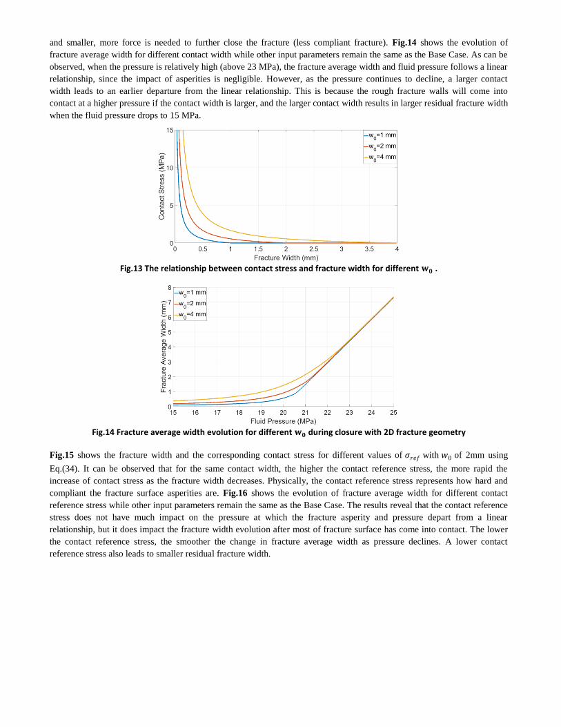
and smaller, more force is needed to further close the fracture (less compliant fracture). Fig.14 shows the evolution of

fracture average width for different contact width while other input parameters remain the same as the Base Case. As can be

observed, when the pressure is relatively high (above 23 MPa), the fracture average width and fluid pressure follows a linear

relationship, since the impact of asperities is negligible. However, as the pressure continues to decline, a larger contact

width leads to an earlier departure from the linear relationship. This is because the rough fracture walls will come into

contact at a higher pressure if the contact width is larger, and the larger contact width results in larger residual fracture width

when the fluid pressure drops to 15 MPa.

Fig.13 The relationship between contact stress and fracture width for different .

Fig.14 Fracture average width evolution for different during closure with 2D fracture geometry

Fig.15 shows the fracture width and the corresponding contact stress for different values of with of 2mm using

Eq.(34). It can be observed that for the same contact width, the higher the contact reference stress, the more rapid the

increase of contact stress as the fracture width decreases. Physically, the contact reference stress represents how hard and

compliant the fracture surface asperities are. Fig.16 shows the evolution of fracture average width for different contact

reference stress while other input parameters remain the same as the Base Case. The results reveal that the contact reference

stress does not have much impact on the pressure at which the fracture asperity and pressure depart from a linear

relationship, but it does impact the fracture width evolution after most of fracture surface has come into contact. The lower

the contact reference stress, the smoother the change in fracture average width as pressure declines. A lower contact

reference stress also leads to smaller residual fracture width.

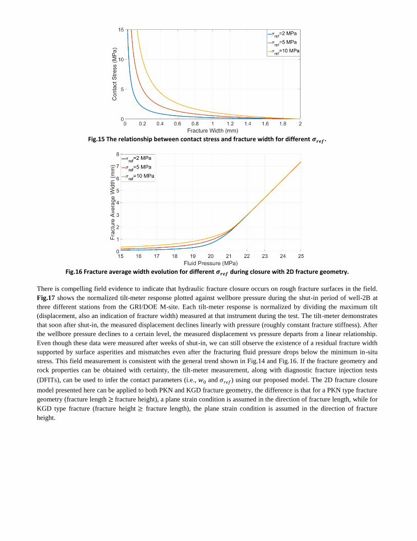
Fig.15 The relationship between contact stress and fracture width for different .

Fig.16 Fracture average width evolution for different during closure with 2D fracture geometry.

There is compelling field evidence to indicate that hydraulic fracture closure occurs on rough fracture surfaces in the field.

Fig.17 shows the normalized tilt-meter response plotted against wellbore pressure during the shut-in period of well-2B at

three different stations from the GRI/DOE M-site. Each tilt-meter response is normalized by dividing the maximum tilt

(displacement, also an indication of fracture width) measured at that instrument during the test. The tilt-meter demonstrates

that soon after shut-in, the measured displacement declines linearly with pressure (roughly constant fracture stiffness). After

the wellbore pressure declines to a certain level, the measured displacement vs pressure departs from a linear relationship.

Even though these data were measured after weeks of shut-in, we can still observe the existence of a residual fracture width

supported by surface asperities and mismatches even after the fracturing fluid pressure drops below the minimum in-situ

stress. This field measurement is consistent with the general trend shown in Fig.14 and Fig.16. If the fracture geometry and

rock properties can be obtained with certainty, the tilt-meter measurement, along with diagnostic fracture injection tests

(DFITs), can be used to infer the contact parameters (i.e., and ) using our proposed model. The 2D fracture closure

model presented here can be applied to both PKN and KGD fracture geometry, the difference is that for a PKN type fracture

geometry (fracture length fracture height), a plane strain condition is assumed in the direction of fracture length, while for

KGD type fracture (fracture height fracture length), the plane strain condition is assumed in the direction of fracture

height.

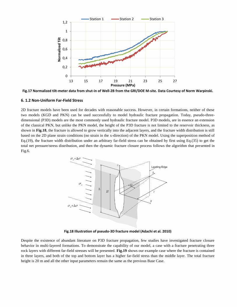
Fig.17 Normalized tilt-meter data from shut-in of Well-2B from the GRI/DOE M-site. Data Courtesy of Norm Warpinski.

6. 1.2 Non-Uniform Far-Field Stress

2D fracture models have been used for decades with reasonable success. However, in certain formations, neither of these

two models (KGD and PKN) can be used successfully to model hydraulic fracture propagation. Today, pseudo-three-

dimensional (P3D) models are the most commonly used hydraulic fracture model. P3D models, are in essence an extension

of the classical PKN, but unlike the PKN model, the height of the P3D fracture is not limited to the reservoir thickness, as

shown in Fig.18, the fracture is allowed to grow vertically into the adjacent layers, and the fracture width distribution is still

based on the 2D plane strain conditions (no strain in the x-direction) of the PKN model. Using the superposition method of

Eq.(19), the fracture width distribution under an arbitrary far-field stress can be obtained by first using Eq.(35) to get the

total net pressure/stress distribution, and then the dynamic fracture closure process follows the algorithm that presented in

Fig.6.

Fig.18 Illustration of pseudo-3D fracture model (Adachi et al. 2010)

Despite the existence of abundant literature on P3D fracture propagation, few studies have investigated fracture closure

behavior in multi-layered formations. To demonstrate the capability of our model, a case with a fracture penetrating three

rock layers with different far-field stresses will be presented. Fig.19 shows our example case where the fracture is contained

in three layers, and both of the top and bottom layer has a higher far-field stress than the middle layer. The total fracture

height is 20 m and all the other input parameters remain the same as the previous Base Case.

0

0,2

0,4

0,6

0,8

1

1,2

13 15 17 19 21 23 25 27

No

rmal

ize

d T

ilt

Pressure (MPa)

Station 1 Station 2 Station 3

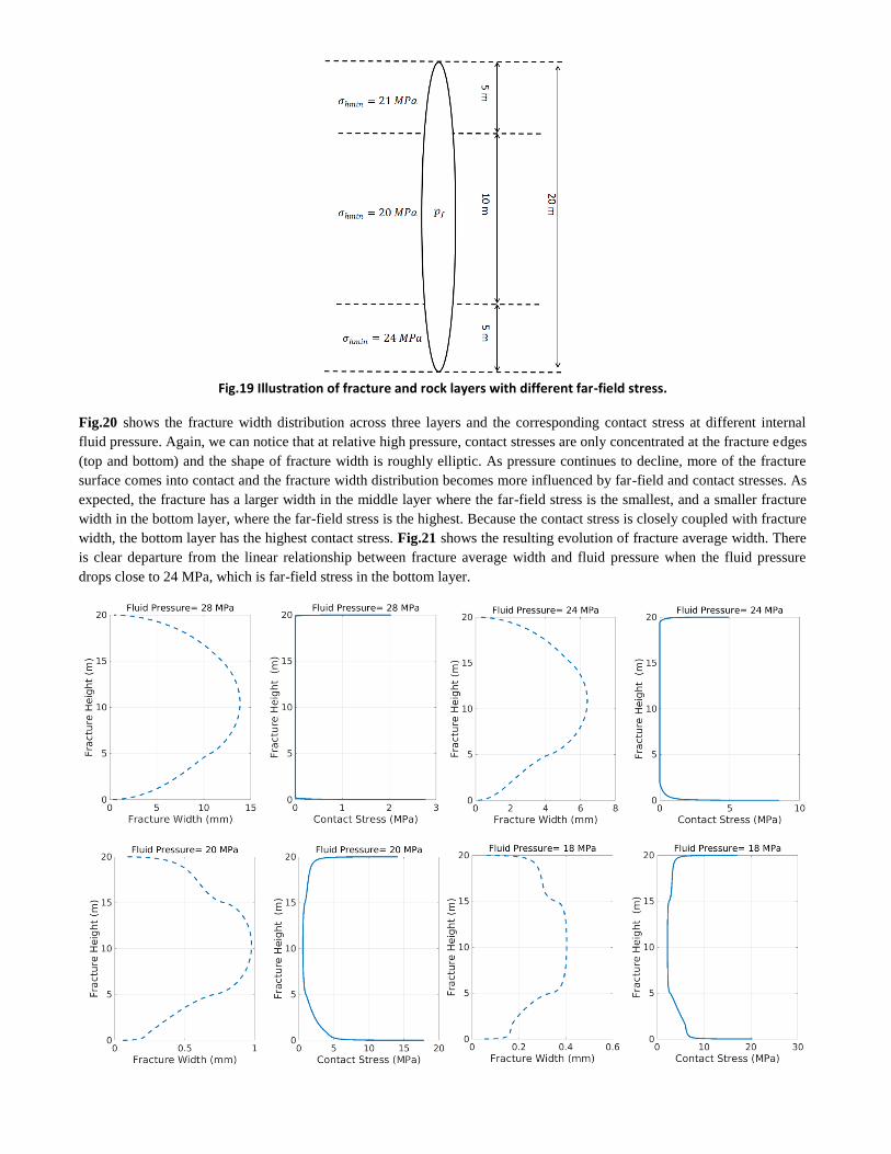
Fig.19 Illustration of fracture and rock layers with different far-field stress.

Fig.20 shows the fracture width distribution across three layers and the corresponding contact stress at different internal

fluid pressure. Again, we can notice that at relative high pressure, contact stresses are only concentrated at the fracture edges

(top and bottom) and the shape of fracture width is roughly elliptic. As pressure continues to decline, more of the fracture

surface comes into contact and the fracture width distribution becomes more influenced by far-field and contact stresses. As

expected, the fracture has a larger width in the middle layer where the far-field stress is the smallest, and a smaller fracture

width in the bottom layer, where the far-field stress is the highest. Because the contact stress is closely coupled with fracture

width, the bottom layer has the highest contact stress. Fig.21 shows the resulting evolution of fracture average width. There

is clear departure from the linear relationship between fracture average width and fluid pressure when the fluid pressure

drops close to 24 MPa, which is far-field stress in the bottom layer.

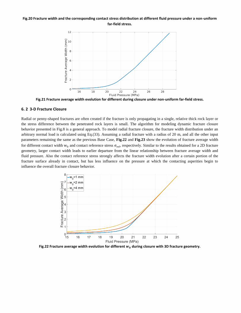
Fig.20 Fracture width and the corresponding contact stress distribution at different fluid pressure under a non-uniform

far-field stress.

Fig.21 Fracture average width evolution for different during closure under non-uniform far-field stress.

6. 2 3-D Fracture Closure

Radial or penny-shaped fractures are often created if the fracture is only propagating in a single, relative thick rock layer or

the stress difference between the penetrated rock layers is small. The algorithm for modeling dynamic fracture closure

behavior presented in Fig.8 is a general approach. To model radial fracture closure, the fracture width distribution under an

arbitrary normal load is calculated using Eq.(33). Assuming a radial fracture with a radius of 20 m, and all the other input

parameters remaining the same as the previous Base Case, Fig.22 and Fig.23 show the evolution of fracture average width

for different contact width and contact reference stress , respectively. Similar to the results obtained for a 2D fracture

geometry, larger contact width leads to earlier departure from the linear relationship between fracture average width and

fluid pressure. Also the contact reference stress strongly affects the fracture width evolution after a certain portion of the

fracture surface already in contact, but has less influence on the pressure at which the contacting asperities begin to

influence the overall fracture closure behavior.

Fig.22 Fracture average width evolution for different during closure with 3D fracture geometry.

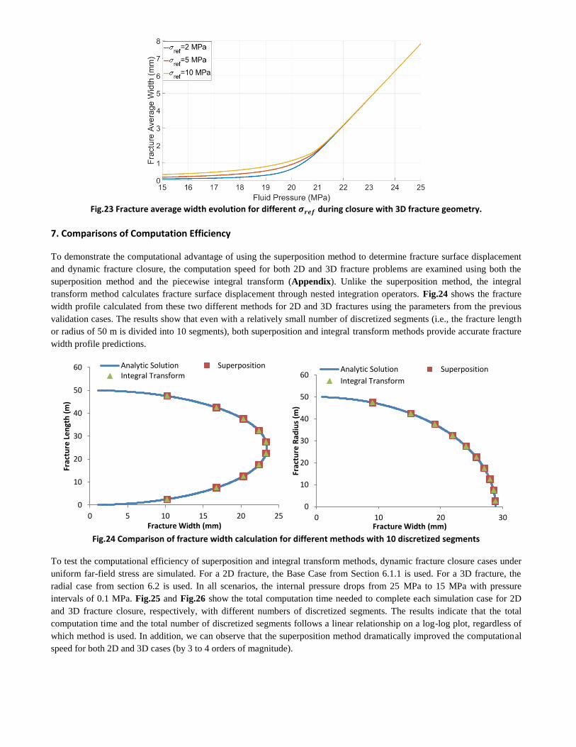
Fig.23 Fracture average width evolution for different during closure with 3D fracture geometry.

7. Comparisons of Computation Efficiency

To demonstrate the computational advantage of using the superposition method to determine fracture surface displacement

and dynamic fracture closure, the computation speed for both 2D and 3D fracture problems are examined using both the

superposition method and the piecewise integral transform (Appendix). Unlike the superposition method, the integral

transform method calculates fracture surface displacement through nested integration operators. Fig.24 shows the fracture

width profile calculated from these two different methods for 2D and 3D fractures using the parameters from the previous

validation cases. The results show that even with a relatively small number of discretized segments (i.e., the fracture length

or radius of 50 m is divided into 10 segments), both superposition and integral transform methods provide accurate fracture

width profile predictions.

Fig.24 Comparison of fracture width calculation for different methods with 10 discretized segments

To test the computational efficiency of superposition and integral transform methods, dynamic fracture closure cases under

uniform far-field stress are simulated. For a 2D fracture, the Base Case from Section 6.1.1 is used. For a 3D fracture, the

radial case from section 6.2 is used. In all scenarios, the internal pressure drops from 25 MPa to 15 MPa with pressure

intervals of 0.1 MPa. Fig.25 and Fig.26 show the total computation time needed to complete each simulation case for 2D

and 3D fracture closure, respectively, with different numbers of discretized segments. The results indicate that the total

computation time and the total number of discretized segments follows a linear relationship on a log-log plot, regardless of

which method is used. In addition, we can observe that the superposition method dramatically improved the computational

speed for both 2D and 3D cases (by 3 to 4 orders of magnitude).

0

10

20

30

40

50

60

0 5 10 15 20 25

Frac

ture

Le

ngt

h (

m)

Fracture Width (mm)

Analytic Solution Superposition Integral Transform

0

10

20

30

40

50

60

0 10 20 30

Frac

ture

Rad

ius

(m)

Fracture Width (mm)

Analytic Solution Superposition

Integral Transform

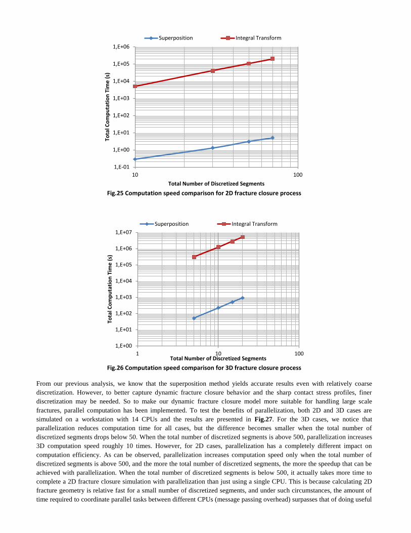
Fig.25 Computation speed comparison for 2D fracture closure process

Fig.26 Computation speed comparison for 3D fracture closure process

From our previous analysis, we know that the superposition method yields accurate results even with relatively coarse

discretization. However, to better capture dynamic fracture closure behavior and the sharp contact stress profiles, finer

discretization may be needed. So to make our dynamic fracture closure model more suitable for handling large scale

fractures, parallel computation has been implemented. To test the benefits of parallelization, both 2D and 3D cases are

simulated on a workstation with 14 CPUs and the results are presented in Fig.27. For the 3D cases, we notice that

parallelization reduces computation time for all cases, but the difference becomes smaller when the total number of

discretized segments drops below 50. When the total number of discretized segments is above 500, parallelization increases

3D computation speed roughly 10 times. However, for 2D cases, parallelization has a completely different impact on

computation efficiency. As can be observed, parallelization increases computation speed only when the total number of

discretized segments is above 500, and the more the total number of discretized segments, the more the speedup that can be

achieved with parallelization. When the total number of discretized segments is below 500, it actually takes more time to

complete a 2D fracture closure simulation with parallelization than just using a single CPU. This is because calculating 2D

fracture geometry is relative fast for a small number of discretized segments, and under such circumstances, the amount of

time required to coordinate parallel tasks between different CPUs (message passing overhead) surpasses that of doing useful

1,E-01

1,E+00

1,E+01

1,E+02

1,E+03

1,E+04

1,E+05

1,E+06

10 100

Tota

l Co

mp

uta

tio

n T

ime

(s)

Total Number of Discretized Segments

Superposition Integral Transform

1,E+00

1,E+01

1,E+02

1,E+03

1,E+04

1,E+05

1,E+06

1,E+07

1 10 100

Tota

l Co

mp

uta

tio

n T

ime

(s)

Total Number of Discretized Segments

Superposition Integral Transform

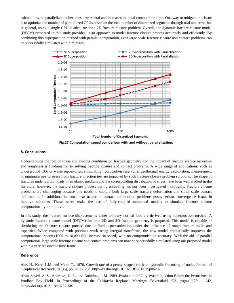
calculations, so parallelization becomes detrimental and increases the total computation time. One way to mitigate this issue

is to optimize the number of parallelized CPUs based on the total number of discretized segments through trial and error, but

in general, using a single CPU is adequate for a 2D fracture closure problem. Overall, the dynamic fracture closure model

(DFCM) presented in this study provides us an approach to model fracture closure process accurately and efficiently. By

combining this superposition method with parallel computation, even large scale fracture closure and contact problems can

be successfully simulated within minutes.

Fig.27 Computation speed comparison with and without parallelization.

8. Conclusions

Understanding the role of stress and loading conditions on fracture geometry and the impact of fracture surface asperities

and roughness is fundamental to solving fracture closure and contact problems. A wide range of applications, such as

underground CO2 or waste repositories, stimulating hydrocarbon reservoirs, geothermal energy exploitation, measurement

of minimum in-situ stress from fracture injection test are impacted by such fracture closure problem solutions. The shape of

fractures under certain loads in an elastic medium and the corresponding distribution of stress have been well studied in the

literature, however, the fracture closure process during unloading has not been investigated thoroughly. Fracture closure

problems are challenging because one needs to capture both large scale fracture deformation and small scale contact

deformation. In addition, the non-linear nature of contact deformation problems poses serious convergence issues in

iterative solutions. These issues make the use of fully-coupled numerical models to simulate fracture closure

computationally prohibitive.

In this study, the fracture surface displacements under arbitrary normal load are derived using superposition method. A

dynamic fracture closure model (DFCM) for both 2D and 3D fracture geometry is proposed. This model is capable of

simulating the fracture closure process due to fluid depressurization under the influence of rough fracture walls and

asperities. When compared with previous work using integral transforms, the new model dramatically improves the

computational speed (1000 to 10,000 fold increase in speed) with no compromise on accuracy. With the aid of parallel

computation, large scale fracture closure and contact problems can now be successfully simulated using our proposed model

within a very reasonable time frame.

Reference

Abe, H., Keer, L.M. and Mura, T., 1976. Growth rate of a penny‐shaped crack in hydraulic fracturing of rocks. Journal of

Geophysical Research, 81(35), pp.6292-6298. http://dx.doi.org/ 10.1029/JB081i035p06292

Abou-Sayed, A. S., Andrews, D. E., and Buhidma, I. M. 1989. Evaluation of Oily Waste Injection Below the Permafrost in

Prudhoe Bay Field. In Proceedings of the California Regional Meetings, Bakersfield, CA, pages 129 – 142,

https://doi.org/10.2118/18757-MS

1,E-01

1,E+00

1,E+01

1,E+02

1,E+03

1,E+04

1,E+05

1,E+06

1,E+07

1,E+08

10 100 1000

Tota

l Co

mp

uta

tio

n T

ime

(s)

Total Number of Discretized Segments

2D Superposition 2D Superposition with Parallelization

3D Superposition 3D Superposition with Parallelization

Abramowitz, M., and Stegun, I.A.1972. Handbook of Mathematical Functions. New York: Dover

Adachi, J.I., Detournay, E. and Peirce, A.P., 2010. Analysis of the classical pseudo-3D model for hydraulic fracture with

equilibrium height growth across stress barriers. International Journal of Rock Mechanics and Mining Sciences, 47(4),

pp.625-639. http://doi.org/10.1016/j.ijrmms.2010.03.008

Adams, G.G., Nosonovsky, M., 2000. Contact modeling-forces. Int. J. Rock Mech. Min. Sci. 33 (5–6), 431–442.

http://dx.doi.org/10.1016/S0301-679X(00)00063-3.

Barton, N., S. Bandis, K. Bakhtar. 1985. Strength, deformation and conductivity coupling of rock joints. International

Journal of Rock Mechanics and Mining Sciences & Geomechanics Abstracts 22 (3): 121-140,

http://dx.doi.org/10.1016/0148-9062(85)93227-9.

Bell.J.C. 1979. Stresses from arbitrary loads on a circular crack. International Journal of Fracture Vol.15(01):85-104.

http://www.doi.org/ 10.1007/BF00115911

Berinde, V., 2004. Picard iteration converges faster than Mann iteration for a class of quasi-contractive operators. Fixed

Point Theory and Applications,Vol (2):1-9. http://dx.doi.org/ 10.1155/S1687182004311058

Brown, S.R., Scholz, C.H., 1985. Closure of random elastic surfaces in contact. J. Geophys. Res. 90 (B7), 5531–5545.

http://dx.doi.org/10.1029/JB090iB07p05531.

Brown, S.R., Scholz, C.H., 1985. Closure of random elastic surfaces in contact. J. Geophys. Res. 90 (B7), 5531–5545.

http://dx.doi.org/10.1029/JB090iB07p05531.

Bryant, E.C., Hwang, J. and Sharma, M.M., 2015, February. Arbitrary Fracture Propagation in Heterogeneous Poroelastic

Formations Using a Finite Volume-Based Cohesive Zone Model. In SPE Hydraulic Fracturing Technology Conference.

Society of Petroleum Engineers. http://dx.doi.org/10.2118/173374-MS

Cook, N.G.W., 1992. Natural joints in rock: mechanical, hydraulic, and seismic behavior and properties under normal stress.

Int. J. Rock Mech. Min. Sci. Geomech. Abstr. 29 (3), 198–223. http://dx.doi.org/10.1016/0148-9062(92)93656-5.

Dahi-Taleghani, A. and Olson, J. E. 2011. Numerical Modeling of Multi-stranded Hydraulic Fracture Propagation :

Accounting for the Interaction between Induced and Natural Fractures. SPE Journal, 16(03):575-581.

http://dx.doi.org/10.2118/124884-PA

Economides, Michael J., Kenneth G. Nolte. 2000. Reservoir Stimulation, 3rd edition. Chichester, England; New York, John

Wiley.

England, A.H. and Green, A.E., 1963. Some two-dimensional punch and crack problems in classical elasticity. In Proc.

Camb. Phil. Soc, Vol. 59(2):489. http://www.doi.org/10.1017/S0305004100037099

Fredd, C. N., McConnell, S. B., Boney, C. L., & England, K. W. 2000. Experimental Study of Hydraulic Fracture

Conductivity Demonstrates the Benefits of Using Proppants. Paper SPE 60326 presented at the

SPE Rocky Mountain Regional/Low-Permeability Reservoirs Symposium and Exhibition, Denver, Colorado, 12-15 March.

http://dx.doi.org/10.2118/60326-MS

Fu, Y., Dehghanpour, H., Ezulike, D. O., and Jones, R. S. 2017. Estimating Effective Fracture Pore Volume From Flowback

Data and Evaluating Its Relationship to Design Parameters of Multistage-Fracture Completion. SPE Production &

Operations (PrePrint). https://doi.org/10.2118/175892-PA

Gangi, A.F., 1978. Variation of whole and fractured porous rock permeability with confining pressure. Int. J. Rock Mech.

Min. Sci. Geomech. Abstr. 15 (5), 249–257. http://dx.doi.org/10.1016/0148-9062(78)90957-9.

Geertsma, J. and De Klerk, F. 1969. A rapid method of predicting width and extent of hydraulic induced fractures. Journal

of Petroleum Technology, 246:1571–1581. SPE-2458-PA. http://dx.doi.org/10.2118/2458-PA.

Gordeliy. E., and Peirce.A. 2013. Implicit level set schemes for modeling hydraulic fractures using the XFEM. Computer

Methods in Applied Mechanics and Engineering, 266:125–143. http://dx.doi.org/10.1016/j.cma.2013.07.016

Grebe, J., and Stoesser, M. 1935. Increasing crude production 20,000,000 bbl. from established fields. World Petroleum

Journal (August), 473–482.

Greenwood, J.A., Williamson, J.B.P., 1966. Contact of nominally flat surfaces. Proc. R. Soc. Lond. 295 (1442), 300–319.

http://dx.doi.org/10.1098/rspa.1966.0242.

Griffith. A.A.1920. The Phenomena of Rupture and Flow in Solids. Phil. Trans. Roy. Soc., Lond. A. Vol. 221:163.

Kamali, A. and Pournik, M., 2016. Fracture closure and conductivity decline modeling–Application in unpropped and acid

etched fractures. Journal of Unconventional Oil and Gas Resources, 14, pp.44-55.

http://dx.doi.org/10.1016/j.juogr.2016.02.001

Khristianovich, S., and Zheltov, Y. 1955. Formation of vertical fractures by means of highly viscous fluids. Proc. 4th World

Petroleum Congress, Rome, Sec. II, 579–586.

Lanaro, F., 2000. A random field model for surface roughness and aperture of rock fractures. Int. J. Rock Mech. Min. Sci.

37 (8), 1195–1210. http://dx.doi.org/10.1016/S1365-1609(00)00052-6.

Love, A.E.H., 1934. A treatise on the mathematical theory of elasticity. Cambridge university press.

Marache, A., Riss, J., Gentier, S., 2008. Experimental and modelled mechanical behavior of a rock facture under normal

stress. Int. J. Rock Mech. Rock Eng. 41(6), 869–892. http://dx.doi.org/10.1007/s00603-008-0166-y.

Matsuki, K., Wang, E.Q., Giwelli, A.A., et al., 2008. Estimation of closure of a fracture under normal stress based on

aperture data. Int. J. Rock Mech. Min. Sci. 45 (2),194–209. http://dx.doi.org/10.1016/j.ijrmms.2007.04.009.

McClure, M.W., Babazadeh, M., Shiozawa, S. and Huang, J., 2016. Fully coupled hydromechanical simulation of hydraulic

fracturing in 3D discrete-fracture networks. SPE Journal 21(04):1302-1320. http://dx.doi.org/10.2118/173354-PA

McClure, M.W., Jung, H., Cramer, D.D. and Sharma, M.M., 2016. The Fracture Compliance Method for Picking Closure

Pressure from Diagnostic Fracture-Injection Tests. SPE Journal 21(04):1321-1339. http://dx.doi.org/10.2118/179725-PA

Morel, S., Schmittbuhl, J., Bouchaud, E. and Valentin, G., 2000. Scaling of crack surfaces and implications for fracture

mechanics. Physical review letters, 85(8), p.1678.

Myer, L.R., 1999. Fractures as collections of cracks. Int. J. Rock Mech. Min. Sci. 37 (1–2), 231–243.

http://dx.doi.org/10.1016/S1365-1609(99)00103-3.

Nemat-Nasser, S., Abe, H. and Hirakawa, S. Mechanics of elastic and inelastic solids Vol(5): Hydraulic fracturing and

geothermal energy. Springer, Netherlands, 1983.

Nordgren, R. 1972. Propagation of vertical hydraulic fractures. Journal of Petroleum Technology, 253:306–314. SPE-3009-

PA . http://dx.doi.org/10.2118/3009-PA.

Perkins, T. and Kern, L. 1961. Widths of hydraulic fractures. Journal of Petroleum Technology, Trans. AIME, 222:937–949.

http://dx.doi.org/10.2118/89-PA.

Pyrak-Nolte, L.J., Morris, J.P., 2000. Single fractures under normal stress: the relation between fracture specific stiffness

and fluid flow. Int. J. Rock Mech. Min. Sci. 37(1–2), 245–262. http://dx.doi.org/10.1016/S1365-1609(99)00104-5.

Raaen, A.M., Skomedal, E., Kjørholt, H., Markestad, P. and Økland, D., 2001. Stress determination from hydraulic

fracturing tests: the system stiffness approach. International Journal of Rock Mechanics and Mining Sciences,38(4), pp.529-

541. http://dx.doi.org/10.1016/S1365-1609(01)00020-X

Rubin, A. 1995. Propagation of magma filled cracks. Annual Review of Earth and Planetary Sciences, 23, 287–336.

http://dx.doi.org/10.1146/annurev.ea.23.050195.001443

Savitski, A., and Dudley, J. W. 2011. Revisiting Microfrac In-situ Stress Measurement via Flow Back - A New Protocol.

SPE Paper 147248 presented at the SPE Annual Technical Conference and Exhibition, Denver, Colorado, USA, 30 October-

2 November. http://dx.doi.org/10.2118/147248-MS

Segedin, C. M. 1967, Some Three-Dimensional Mixed Boundary Value Problems in Elasticity. Report 67-3, Dept. of

Aeronautics and Astronautics, College of Engineering, University of Washington.

Sesetty, V. and Ghassemi, A., 2015, November. Simulation of Simultaneous and Zipper Fractures in Shale Formations.

In 49th US Rock Mechanics/Geomechanics Symposium. American Rock Mechanics Association. ARMA-2015-558

Shah, R.C. and Kobayashi, A.S.,1971. Stress intensity factor for an elliptical crack under arbitrary normal loading.

Engineering Fracture Mechanics, Vol.3(1):71-96. http://dx.doi.org/10.1016/0013-7944(71)90052-X

Sneddon. 1946. The Distribution of Stress in the Neighborhood of a Crack in an Elastic Solid. Proc. R. Soc. Lond. A 1946

187 229-260. http://www.doi.org/10.1098/rspa.1946.0077.

Sneddon, I. N. and Lowengrub, M., Crack Problems in the Classical Theory of Elasticity. John Wiley & Sons, Inc., New

York, 1969

Tada, H., Paris, P.C. and Irwin, G.R., 1973. The stress analysis of cracks. Del Research Corp, Hellertown PA.

Tsai, V., and Rice, J. 2010. A model for turbulent hydraulic fracture and application to crack propagation at glacier beds.

Journal of Geophysical Research, Vol (115):1–18. http://dx.doi.org/ 10.1029/2009JF001474

van Dam, D.B., de Pater, C.J. and Romijn, R., 2000. Analysis of Hydraulic Fracture Closure in Laboratory

Experiments. SPE Production & Facilities,15(03), pp.151-158. http://dx.doi.org/10.2118/65066-PA

Wang, H and Sharma, M.M. 2017a. A Non-Local Model for Fracture Closure on Rough Fracture Faces and Asperities.

Journal of Petroleum Science and Engineering , Vol(154):425-437. https://dx.doi.org/10.1016/j.petrol.2017.04.024

Wang, H and Sharma, M.M. 2017b. A New Variable Compliance Method for Estimating Closure Stress and Fracture

Compliance from DFIT data. Paper SPE 187348 presented at the SPE Annual Technical Conference and Exhibition held in

San Antonio, TX, USA, 09 – 11 October. http://dx.doi.org/10.2118/ 187348-MS

Wang, H. 2015. Numerical Modeling of Non-Planar Hydraulic Fracture Propagation in Brittle and Ductile Rocks using

XFEM with Cohesive Zone Method. Journal of Petroleum Science and Engineering, Vol (135):127-140.

http://dx.doi.org/10.1016/j.petrol.2015.08.010

Wang, H. 2016. Numerical Investigation of Fracture Spacing and Sequencing Effects on Multiple Hydraulic Fracture

Interference and Coalescence in Brittle and Ductile Reservoir Rocks. Engineering Fracture Mechanics, Vol (157): 107-124.

http://dx.doi.org/10.1016/j.engfracmech.2016.02.025

Wang, H., Marongiu-Porcu, M., and Economides, M. J. 2016. SPE-168600-PA. Poroelastic and Poroplastic Modeling of

Hydraulic Fracturing in Brittle and Ductile Formations, Journal of SPE Production & Operations, 31(01): 47–59.

http://dx.doi.org/10.2118/168600-PA

Warpinski, N.R., 2010. Stress Amplification and Arch Dimensions in Proppant Beds Deposited by Waterfracs. SPE

Production & Operations, 25(04), pp.461-471. http://dx.doi.org/10.2118/119350-PA

Warpinski, N.R., Branagan, P.T., Engler, B.P., Wilmer,R., and Wolhart, S.L. 2002. Evaluation of a downhole tiltmeter array

for monitoring hydraulic fractures. International Journal of Rock Mechanics and Mining Sciences, Vol (34)3-4: 329.e1–

329.e13. http://dx.doi.org/ 10.1016/S1365-1609(97)00074-9

Warpinski, N.R., Lorenz, J.C., Branagan, P.T., Myal, F.R. and Gall, B.L., 1993. Examination of a Cored Hydraulic Fracture

in a Deep Gas Well (includes associated papers 26302 and 26946). SPE Production & Facilities, 8(03), pp.150-158.

http://dx.doi.org/10.2118/22876-PA

Westergaard, H.M., 1939. Bearing Pressures and Cracks. Journal of Applied Mechanics, Vol. 6, pp. A49- A53.

Willis-Richards, J., K. Watanabe, H. Takahashi. 1996. Progress toward a stochastic rock mechanics model of engineered

geothermal systems. Journal of Geophysical Research 101 (B8): 17481-17496, http://dx.doi.org/10.1029/96JB00882.

Zangerl, C., Evans, K.F., Eberhardt, E. and Loew, S., 2008. Normal stiffness of fractures in granitic rock: a compilation of

laboratory and in-situ experiments. International Journal of Rock Mechanics and Mining Sciences, 45(8), pp.1500-1507.

http://dx.doi.org/10.1016/j.ijrmms.2008.02.001

Zhao, Q., Lisjak, A., Mahabadi, O., Liu, Q. and Grasselli, G., 2014. Numerical simulation of hydraulic fracturing and

associated microseismicity using finite-discrete element method. Journal of Rock Mechanics and Geotechnical

Engineering, 6(6), pp.574-581. http://dx.doi.org/10.1016/j.jrmge.2014.10.003

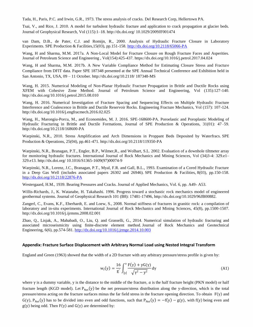
Appendix: Fracture Surface Displacement with Arbitrary Normal Load using Nested Integral Transform

England and Green (1963) showed that the width of a 2D fracture with any arbitrary pressure/stress profile is given by:

where is a dummy variable, y is the distance to the middle of the fracture, is the half fracture height (PKN model) or half

fracture length (KGD model). Let be the net pressure/stress distribution along the y-direction, which is the total

pressure/stress acting on the fracture surfaces minus the far field stress in the fracture opening direction. To obtain and

, has to be divided into even and odd functions, such that , with being even and

being odd. Then and are determined by:

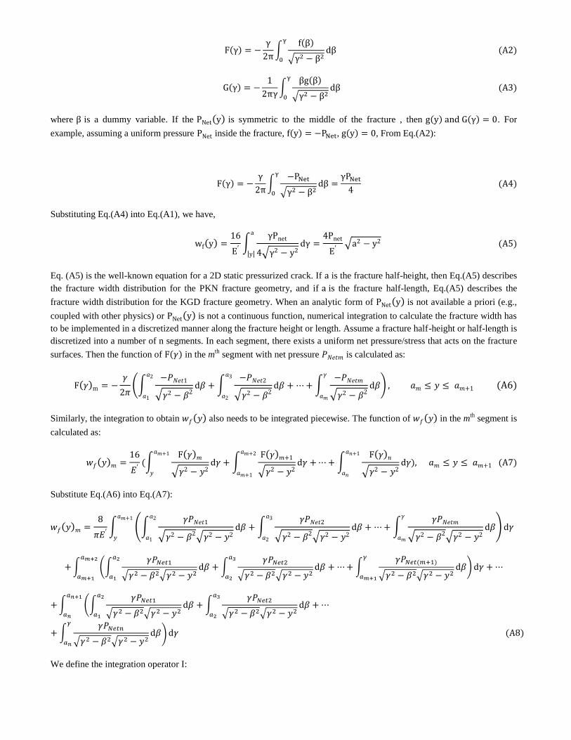
where is a dummy variable. If the is symmetric to the middle of the fracture , then . For

example, assuming a uniform pressure inside the fracture, , , From Eq.(A2):

Substituting Eq.(A4) into Eq.(A1), we have,

Eq. (A5) is the well-known equation for a 2D static pressurized crack. If is the fracture half-height, then Eq.(A5) describes

the fracture width distribution for the PKN fracture geometry, and if is the fracture half-length, Eq.(A5) describes the

fracture width distribution for the KGD fracture geometry. When an analytic form of is not available a priori (e.g.,

coupled with other physics) or is not a continuous function, numerical integration to calculate the fracture width has

to be implemented in a discretized manner along the fracture height or length. Assume a fracture half-height or half-length is

discretized into a number of n segments. In each segment, there exists a uniform net pressure/stress that acts on the fracture

surfaces. Then the function of in the mth

segment with net pressure is calculated as:

Similarly, the integration to obtain also needs to be integrated piecewise. The function of in the mth

segment is

calculated as:

Substitute Eq.(A6) into Eq.(A7):

We define the integration operator I:

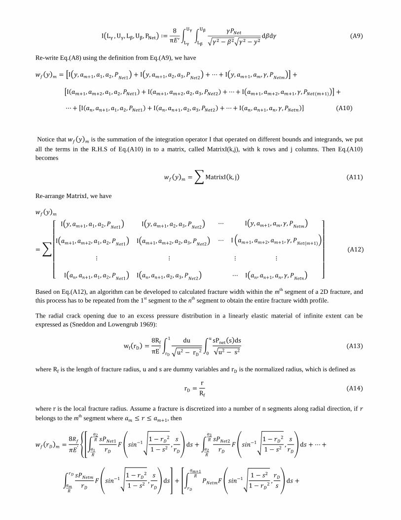
Re-write Eq.(A8) using the definition from Eq.(A9), we have

Notice that is the summation of the integration operator I that operated on different bounds and integrands, we put

all the terms in the R.H.S of Eq.(A10) in to a matrix, called MatrixI(k,j), with k rows and j columns. Then Eq.(A10)

becomes

Re-arrange , we have

Based on Eq.(A12), an algorithm can be developed to calculated fracture width within the mth

segment of a 2D fracture, and

this process has to be repeated from the 1st segment to the n

th segment to obtain the entire fracture width profile.

The radial crack opening due to an excess pressure distribution in a linearly elastic material of infinite extent can be

expressed as (Sneddon and Lowengrub 1969):

where is the length of fracture radius, and are dummy variables and is the normalized radius, which is defined as

where is the local fracture radius. Assume a fracture is discretized into a number of n segments along radial direction, if

belongs to the mth

segment where , then

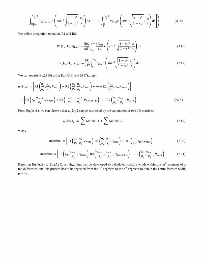
We define integration operators R1 and R2:

We can rewrite Eq.(A15) using Eq.(A16) and (A17),to get:

From Eq.(A18), we can observe that can be expressed by the summation of two 1D matrices:

where

Based on Eq.(A19) to Eq.(A21), an algorithm can be developed to calculated fracture width within the mth

segment of a

radial fracture, and this process has to be repeated from the 1st segment to the n

th segment to obtain the entire fracture width

profile.