A Branch-and-Cut Algorithm for theMultiple Depot Vehicle Scheduling ProblemMatteo Fischetti�, Andrea Lodio, Paolo Totho� Dipartimento di Elettronica e Informatica, Universit�a di Padova, Italyo Dipartimento di Elettronica, Informatica e Sistemistica, Universit�a di Bologna, ItalyE-mail: fisch@dei.unipd.it, falodi,ptothg@deis.unibo.itAbstractThe Vehicle Scheduling Problem is an important combinatorial optimization prob-lem arising in the management of transportation companies. It consists in assigninga set of time-tabled trips to a set of vehicles so as to minimize a given objectivefunction. In particular, we consider the Multiple Depot version of the problem (MD-VSP), in which one also has to assign vehicles to depots. This problem is knownto be NP-hard. In this paper we introduce two main classes of valid inequalitiesfor MD-VSP, and propose e�cient separation algorithms along with e�ective heuris-tic strategies to speed up cutting-plane convergence. These results are used within abranch-and-cut scheme for the exact solution of the problem. The method uses a newbranching strategy based on the concept of \fractionality persistency", a completelygeneral criterion that can be extended to other combinatorial problems. The perfor-mance of the branch-and-cut scheme is evaluated through extensive computationalexperiments on several classes of both random and real-world test instances.1 IntroductionThe Multiple-Depot Vehicle Scheduling Problem (MD-VSP) is an important combinatorialoptimization problem arising in the management of transportation companies. In thisproblem we are given a set of n trips, T1; T2; : : : ; Tn, each trip Tj (j = 1; : : : ; n) beingcharacterized by a starting time sj and an ending time ej, along with a set of m depots,D1; D2; : : : ; Dm, in the k-th of which rk � n vehicles are available. All the vehicles aresupposed to be identical. In the following we assume m � n.Let �ij be the time needed for a vehicle to travel from the end location of trip Ti tothe starting location of trip Tj. A pair of consecutive trips (Ti; Tj) is said to be feasible ifthe same vehicle can cover Tj right after Ti, a condition implying ei + �ij � sj. For eachfeasible pair of trips (Ti; Tj), let ij � 0 be the cost associated with the execution, in theduty of a vehicle, of trip Tj right after trip Ti, where ij = +1 if (Ti; Tj) is not feasible, orif i = j. For each trip Tj and each depot Dk, let kj (respectively, ~ jk) be the non-negativecost incurred when a vehicle of depot Dk starts (resp., ends) its duty with Tj. The overall1

cost of a duty (Ti1 ; Ti2 ; : : : ; Tih) associated with a vehicle of depot Dk is then computed as ki1 + i1i2 + : : :+ ih�1ih + ~ ihk.MD-VSP consists of �nding an assignment of trips to vehicles in such a way that:i) each trip is assigned to exactly one vehicle;ii) each vehicle in the solution covers a sequence of trips (duty) in which consecutivetrip pairs are feasible;iii) each vehicle starts and ends its duty at the same depot;iv) the number of vehicles used in each depot Dk does not exceed depot capacity rk;v) the sum of the costs associated with the duty of the used vehicles is a minimum(unused vehicles do not contribute to the overall cost).Depending on the possible de�nition of the above costs, the objective of the optimizationis to minimize:a) the number of vehicles used in the optimal solution, if kj = 1 and ~ jk = 0 for eachtrip Tj and each depot Dk, and ij = 0 for each feasible pair (Ti; Tj);b) the overall cost, if the values ( ij), ( kj) e (~ jk) are the operational costs associatedwith the vehicles, including penalities for dead-heading trips, idle times, etc.;c) any combination of a) and b).MD-VSP is NP-hard in the general case, whereas it is polynomially solvable if m = 1.It was observed in Carpaneto, Dell'Amico, Fischetti and Toth [3] that the problem is alsopolynomially solvable if the costs kj and ~ jk are independent of the depots.Several exact algorithms for the solution of MD-VSP have been presented in the lit-erature, which are based on di�erent approaches. Carpaneto, Dell'Amico, Fischetti andToth [3] proposed a Branch-and-Bound algorithm based on additive lower bounds. Ribeiroand Soumis [11] studied a column generation approach, whereas Forbes, Holt and Watts[6] analyzed a three-index integer linear programming formulation. Bianco, Mingozzi andRicciardelli [1] introduced a more e�ective set-partitioning solution scheme based on theexplicit generation of a suitable subset of duties; although heuristic in nature, this approachcan provide a provably-optimal output in several cases. Heuristic algorithms have beenproposed, among others, by Dell'Amico, Fischetti and Toth [4]. Both exact and heuristicapproaches were recently proposed by L�obel [7, 8] for constrained versions of the problem.In this paper we consider a branch-and-cut [9] approach to solve MD-VSP to provenoptimality, in view of the fact that branch-and-cut methodology proved very successfulfor a wide range of combinatorial problems; see e.g. the recent annotated bibliography ofCaprara and Fischetti [2]. 2

The paper is organized as follows. In Section 2 we discuss a graph theory and aninteger linear programming model for MD-VSP. In Section 3 we propose a basic class ofvalid inequalities for the problem, and in Section 3.1 we address the associated separationproblem. A second class of inequalities is introduced in Section 4 along with a separationheuristic. Our branch-and-cut algorithm is outlined in Section 5. In particular, we describean e�ective branching scheme in which the branching variable is chosen according to theconcept of \fractionality persistency", a completely general criterion that can be extendedto other combinatorial problems. In Section 6 we report extensive computational exper-iments on a test-bed made by 135 randomly generated and real-world test instances, allof which are available on the web page http://www.or.deis.unibo.it/ORinstances/.Some conclusions are �nally drawn in Section 7.2 ModelsWe consider a directed graph G = (V;A) de�ned as follows. The set of vertices V =f1; : : : ; m + ng is partitioned into two subsets: the subset W = f1; : : : ; mg containing avertex k for each depot Dk, and the subset N = fm+ 1; : : : ; m+ ng in which each vertexm + j is associated with a di�erent trip Tj. We assume that graph G is complete, i.e.,A = f(i; j) : i; j 2 V g. Each arc (i; j) with i; j 2 N corresponds to a transition betweentrips Ti�m and Tj�m, whereas arcs (i; j) with i 2 W (respectively, j 2 W ) correspond tothe start (resp., to the end) of a vehicle duty. Accordingly, the cost associated with eacharc (i; j) is de�ned as: cij = 8>>>>><>>>>>: i�m;j�m if i; j 2 N ; i;j�m if i 2 W; j 2 N ;~ i�m;j if i 2 N; j 2 W ;0 if i; j 2 W; i = j;+1 if i; j 2 W; i 6= j.Note that arcs with in�nite cost correspond to infeasible transitions, hence they couldbe removed from the graph (we keep them in the arc set only to simplify the notation).Moreover, the subgraph obtained from G by deleting the arcs with in�nite costs along withthe vertices in W is acyclic.By construction, each �nite-cost subtour visiting (say) vertices k; v1; v2; : : : ; vh; k, wherek 2 W and v1; : : : ; vh 2 N , corresponds to a feasible duty for a vehicle located in depot Dkthat covers consecutively trips Tv1�m; : : : ; Tvh�m, the subtour cost coinciding with the costof the associated duty. Finite-cost subtours visiting more than one vertex in W , instead,correspond to infeasible duties starting and ending in di�erent depots.MD-VSP can then be formulated as the problem of �nding a min-cost set of subtours,each containing exactly one vertex in W , such that all the trip-vertices in N are visitedexactly once, whereas each depot-vertex k 2 W is visited at most rk times.The above graph theory model can be reformulated as an integer linear programmingmodel as in Carpaneto, Dell'Amico, Fischetti and Toth [3]. Let decision variable xij assumevalue 1 if arc (i; j) 2 A is used in the optimal solution of MD-VSP, and value 0 otherwise.3

v(MD � V SP ) = minXi2V Xj2V cij xij (1)Xi2V xij = rj; j 2 V (2)Xj2V xij = ri; i 2 V (3)X(i;j)2P xij � jP j � 1; P 2 � (4)xij � 0 integer, i; j 2 V (5)where we have de�ned ri := 1 for each i 2 N , and � denotes the set of the inclusion-minimal infeasible paths, i.e., the simple and �nite-cost paths connecting two di�erentdepot-vertices in W .The degree equations (2) and (3) impose that each vertex k 2 V must be visited exactlyrk times. Notice that variables xkk (k 2 W ) act as slack variables for the constraints (2)-(3)associated with k, i.e., xkk gives the number of unused vehicles in depot Dk.Constraints (4) forbid infeasible subtours, i.e., subtours visiting more than one vertexin W . Finally, constraints (5) state the nonnegativity and integrality conditions on thevariables; because of (2)-(3), they also imply xij 2 f0; 1g for each arc (i; j) incident withat least one trip-vertex in N .In the single-depot case (m = 1), set � is empty and model (1)-(5) reduces to thewell-known Transportation Problem (TP), hence it is solvable in O(n3) time.3 Path Elimination Constraints (PECs)The exact solution of MD-VSP can be obtained through enumerative techniques whosee�ectiveness strongly depends on the possibility of computing, in an e�cient way, tightlower bounds on the optimal solution value. Unfortunately, the continuous relaxation ofmodel (1)-(5) typically yields poor lower bounds. In this section we introduce a new class ofconstraints for MD-VSP, called Path Elimination Constraints, which are meant to replacethe weak constraints (4) forbidding infeasible subtours.Let us consider any nonempty Q � W , and de�ne Q := W nQ. Given any �nite-costinteger solution x� of model (1)-(5), letA� := f(i; j) 2 A : x�ij 6= 0gdenote the multiset of the arcs associated with the solution, in which each arc (k; k) withk 2 W appears x�kk times. As already observed, A� de�nes a collection of Pmk=1 rk subtoursof G, Pmk=1 x�kk of which are loops and correspond to unused vehicles.Now suppose removing from G (and then from A�) all the vertices in Q, thus breakinga certain number of subtours in A�. The removal, however, cannot a�ect any subtour4

visiting the vertices k 2 Q, hence A� still contains Pk2Q rk subtours through the verticesk 2 Q. This property leads to the following Path Elimination Constraints (PECs):Xi2S[Q Xj2(NnS)[Qxij � Xk2Q rk; for each S � N; S 6= ;: (6)Note that the variables associated with the arcs incident in Q do not appear in the con-straint.By subtracting constraint (6) from the sum of the equations (3) for each i 2 Q[ S, weobtain the following equivalent formulation of the path elimination constraints:Xi2QXj2S xij +Xi2SXj2S xij +Xi2SXj2Qxij � jSj; for each S � N; S 6= ;; (7)where we have omitted the left-hand-side term Pi2QPj2Q xij as it involves only in�nite-cost arcs. This latter formulation generally contains less nonzero entries than the originalone in the coe�cient matrix, hence it is preferable for computation.Constraints (7) state that a feasible solution cannot contain any path starting from avertex a 2 Q and ending in a vertex b 2 Q. This condition is then related to the oneexpressed by constraints (4). However, PEC constraints (7) dominate the weak constraints(4). Indeed, consider any infeasible path P = f(a; v1); (v1; v2); : : : ; (vt�1; vt); (vt; b)g, wherea; b 2 W , a 6= b, and S := fv1; : : : ; vtg � N . Let Q be any subset of W such that a 2 Qand b 62 Q. The constraint (4) corresponding to path P has the same right-hand side valueas in the PEC associated with sets S and Q (as jP j = t+1 and jSj = t), but each left-handside coe�cient in (4) is less or equal to the corresponding coe�cient in the PEC.We �nally observe that, for any given pair of sets S and Q, the corresponding PECdoes not change by replacing S with S := N n S and Q with Q := W n Q. Indeed, thePEC for pair (S;Q) can be obtained from the PEC associated with (S;Q) by subtractingequations (2) for each j 2 S [Q, and by adding to the result equations (3) for i 2 S [Q.As a result, it is always possible to halve the number of relevant PECs by imposing, e.g.,1 2 Q.3.1 PEC Separation AlgorithmsGiven a family F of valid MD-VSP constraints and a (usually fractional) solution x� � 0,the separation problem for F aims at determining a member of F which is violated byx�. The exact or heuristic solution of this problem is of crucial importance for the use ofthe constraints of family F within a branch-and-cut scheme. In practice, the separationalgorithm tries to determine a large number of violated constraints, chosen from amongthose with large degree of violation. This usually accelerates the convergence of the overallscheme.In the following we denote by G� = (V;A�) the support graph of x�, where A� :=f(i; j) 2 A : x�ij 6= 0g. 5

Next we deal with the separation problem for the PEC family. Suppose, �rst, that thesubset Q � W in the PEC has been �xed. The separation problem then amounts to �ndinga subset S � N maximizing the violation of PEC (6) associated with the pair (S;Q). Weconstruct a ow network obtained from G� as follows:1. for each w 2 W , we add to G� a new vertex w0, and we let W 0 := fw0 : w 2 Wg;2. we replace each arc (i; w) 2 A� entering a vertex w 2 W with the arc (i; w0), andde�ne x�iw0 := x�iw and x�iw := 0;3. we de�ne the capacity of each arc (i; j) 2 A� as x�ij;4. we add two new vertices, s (source) and d (sink);5. for each w 2 Q, we add two arcs with very large capacity, namely (s; w) and (w0; d).By construction:� the ow network is acyclic;� no arc enters vertices w 2 Q := W nQ, and no arc leaves vertices w0 2 W 0;� for each w 2 W , the network contains an arc (w;w0) with capacity x�ww.� the network depends on the chosen Q only for the arcs incident with s and d (steps1{4 being independent of Q).One can easily verify that a minimum-capacity cut in the network with shore (say)fsg [ Q [ S corresponds to the most violated PEC (6) (among those for the given Q).Therefore, such a highly violated PEC cut can be determined, in O(n3) time, through analgorithm that computes a maximum ow from the source s to the sink d in the network.In practice, the computing time needed to solve such a problem is much less than in theworst case, as A� is typically very sparse and contains only O(n) arcs.As to the choice of the set Q, one possibility is to enumerate all the 2m�1 � 1 propersubsets of W that contain vertex 1. In that way, the separation algorithm requires, inthe worst case, O(2m�1n3) time, hence it is still polynomial for any �xed m. In practice,the computing time is acceptable for values of m not larger than 5. For a greater numberof depots, a possible heuristic choice consists of enumerating only the subsets of W withjW j � �, where parameter � is set e.g. to 5.Once a PEC is detected, we re�ne it by �xing its trip-node set S and by re-computing(through a simple greedy scheme) the depot-vertex set Q so as to maximize the degree ofviolation.Preliminary computational experiments showed that the lower bounds obtained throughthe separation algorithm described are very tight, but often require a large computingtime because the number of PECs generated at each iteration is too small. It is then very6

important to be able to identify a relevant number of violated PECs at each round ofseparation.PEC decompositionA careful analysis of the PECs generated through the max- ow algorithm showed thatthey often \merge" several violated PECs de�ned on certain subsets of S. A natural ideais therefore to decompose a violated PEC into a series of PECs with smaller support.To this end, let S and Q be the two subsets corresponding to a most-violated PEC(e.g., the one obtained through the max- ow algorithm). Consider �rst the easiest casein which x� is integer, and contains a collection of q � 2 paths P1; : : : Pq starting froma vertex in Q, visiting some vertices in S, and ending in a vertex in Q. Now, considerthe subsets S1; : : : ; Sq � S containing the vertices in S visited by the paths P1; : : : ; Pq,respectively. It is easy to see that all the q PECs associated to the subsets S1; : : : ; Sq areviolated (assuming that S is inclusion minimal, and letting Q be unchanged). Even if itis not possible to establish a general dominance relation between the new PECs and theoriginal PEC, our computational results showed that this re�ning procedure guarantees afaster convergence of the branch-and-cut algorithm.When x� is fractional the re�ning of the original PEC is obtained in a similar way,by de�ning S1; : : : ; Sq as the connected components of the undirected counterpart of thesubgraph of G� induced by the vertex set S.Infeasible path enumerationA second method to increase the number of violated PECs found by the separationscheme consists in enumerating the paths contained in G� so as to identify infeasible pathsof the form P = f(a; v1); (v1; v2); : : : ; (vt�1; vt); (vt; b)g with a; b 2 W , a 6= b, and suchthat the corresponding constraint (7) is violated for S := fv1; : : : ; vtg � N and Q := fag.Since the graph G� is typically very sparse, this enumeration usually needs acceptablecomputing times. According to our computational experience, enumeration is indeed veryfast, although it is unlike to identify violated PECs for highly fractional solutions.PECs with nested supportThe above separation procedures are intended to identify a number of violated PECchosen on the basis of their individual degree of violation, rather than on an estimate oftheir combined e�ect. However, it is a common observation in cutting plane methods thatthe e�ectiveness of a set of cuts belonging to a certain family depends heavily on theiroverall action, an improved performance being gained if the separation generates certainhighly-e�ective patterns of cuts.A known example of this behavior is the travelling salesman problem (TSP), for whichcommonly-applied separation schemes based on vertex shrinking, besides reducing thecomputational e�ort spent in each separation, have the important advantage of producingat each call a noncrossing family of violated subtour elimination constraints.7

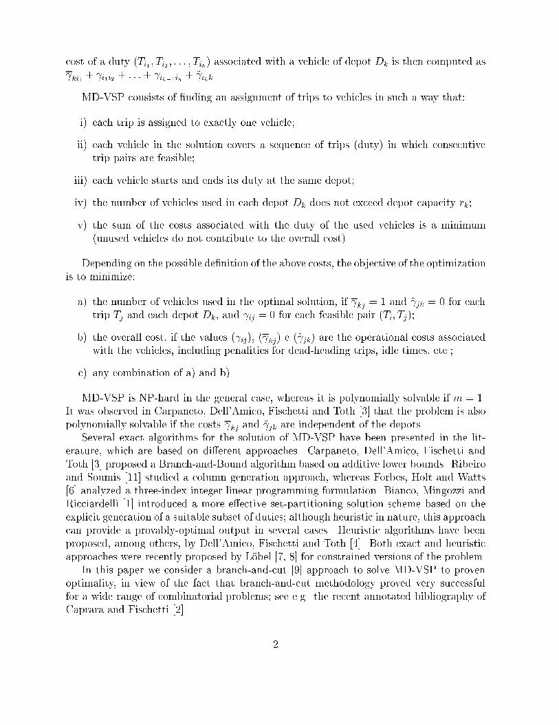
A careful analysis of the PECs having a nonzero dual variable in the optimal solution ofthe LP relaxation of our model showed that highly-e�ective patterns of PECs are typicallyassociated with sets S de�ning an almost nested family, i.e., only a few pairs S cross eachother. We therefore implemented the following heuristic \shrinking" mechanism to forcethe separation to produce violated PECs with nested sets S.For each given depot subset Q, we �rst �nd a minimum-capacity cut in which the shoreof the cut containing the source node, say fsg [ Q [ S1, is minimal with respect to setinclusion. If violated, we store the PEC associated with S1, and continue in the attempt atdetermining, for the same depot subset Q, additional violated PECs associated with sets Sstrictly containing S1. This is achieved by increasing to a very large value the capacity ofall network arcs having both terminal vertices in Q[S1, and by re-applying the separationprocedure in the resulting network (for the same Q) so as to hopefully produce a sequenceof violated PECs associated with nested sets S1 � S2 � � � � St.In order to avoid stalling on the same cut, at each iteration we increase slightly (in arandom way) the capacity of the arcs leaving the shore fsg [Q[ Si of the current cut. Insome (rare) cases, this random perturbation step needs to be iterated in order to force themax- ow computation to �nd a new cut.As shown in the computational section, the simple scheme above proved very successfulin speeding up the convergence of the cutting-plane phase.4 Lifted Path Inequalities (LPIs)The �nal solution x� that we obtain after separating all the PECs can often be expressedas a linear combination of the characteristic vectors of feasible subtours of G. As an illus-tration, suppose that x� can be obtained as the linear combination, with 1/2 coe�cients,of the characteristic vectors of the following three feasible subtours (among others):C1 = f(a; i1); (i1; i2); (i2; a)g,C2 = f(a; i1); (i1; i3); (i3; a)g,C3 = f(b; i2); (i2; i3); (i3; b)g,where a; b 2 W , a 6= b, and i1, i2 and i3 are three distinct vertices in N (see Figure 1).Notice that, because of the degree equations on the trip-nodes, only one of the abovethree subtours can actually be selected in a feasible solution.The solution x� of our arc-variable formulation then has: x�ai1 � 1=2 + 1=2 = 1, x�i1i2 �1=2, x�i2i3 � 1=2, x�i1i3 � 1=2, x�i3b � 1=2, hence it violates the following valid inequality,obtained as a reinforcement of the obvious constraint forbidding the path (a; i1), (i1; i2),(i2; i3), (i3; b): xai1 + xi1i2 + xi2i3 + xi3b + 2xi1i3 � 3: (8)8

j jj

- - �- JJJJJJ �I ��a bi2i1i3Figure 1: A possible fractional point x� with x�ij = 1=2 for each drawn arc.The example shows that constraints of type (8) can indeed improve the linear modelthat includes all degree equations and PECs. As a result, the lower bound achievable bymeans of (8) can be strictly better than those obtainable through the set-partitioning orthe 3-index formulations from the literature [1, 6, 11].Constraints (8) can be improved and generalized, thus obtaining a more general familyof constraints that we call Lifted Path Inequalities (LPIs):Xi2Qa Xj2I1[I3 xij +Xi2I1 Xj2I2[Qb xij +Xi2I2 Xj2I2[I3 xij +Xi2I3 Xj2Qb xij + 2Xi2I1 Xj2I1[I3 xij+2Xi2I3 Xj2I3 xij � 3 + 2(jI1j � 1) + (jI2j � 1) + 2(jI3j � 1); (9)where (Qa; Qb) is any proper partition of W , whereas I1, I2 and I3 are three pairwisedisjoint and nonempty subsets of N .Validity of LPIs follows from the fact that they are rank-1 Chv�atal-Gomory cuts ob-tained by combining the following valid MD-VSP inequalities:1=3 times PEC(I1 [ I2 [ I3; Qa),2=3 times PEC(I1 [ I3; Qa),1=3 times SEC(I1),2=3 times SEC(I2),1=3 times SEC(I3),2=3 times CUT-OUT(I1),2=3 times CUT-IN(I3), 9

where PEC(S;Q) is the inequality (7) associated to the sets S � N andQ � W , whereas foreach S � N we denote by SEC(S), CUT-OUT(S) and CUT-IN(S) the following obviouslyvalid (though dominated) constraints:SEC(S) : Xi2SXj2S xij � jSj � 1CUT-OUT(S) : Xi2S Xj2V nS xij � jSjCUT-IN(S) : Xi2V nSXj2S xij � jSjA separation algorithm for the \basic" LPIs (9) having jI1j = jI2j = jI3j = 1 is ob-tained by enumerating all the possible triples of trip-vertices, and by choosing the partition(Qa; Qb) that maximizes the degree of violation of the corresponding LPI. In practice, thecomputing time needed for this enumeration is rather short, provided that simple testsare implemented to avoid generating triples that obviously cannot correspond to violatedconstraints.For the more general family, we have implemented a shrinking procedure that contractsinto a single vertex all paths made by arcs (i; j) with i; j 62 W and x�ij = 1, and then appliesto the shrunk graph the above enumeration scheme for basic LPIs.5 A Branch-and-Cut AlgorithmIn this section we present an exact branch-and-cut algorithm for MD-VSP, which followsthe general framework proposed by Padberg and Rinaldi [9]; see Caprara and Fischetti [2]for a recent annotated bibliography.The algorithm is a lowest-�rst enumerative procedure in which lower bounds are com-puted by means of an LP relaxation that is tightened, at run time, by the addition of cutsbelonging to the classes discussed in the previous sections.5.1 Lower Bound ComputationAt each node of the branching tree, we initialize the LP relaxation by taking all theconstraints present in the last LP solved at the father node. For the root node, instead,only the degree equations (2)-(3) are taken, and an optimal LP basis is obtained throughan e�cient code for the min-sum Transportation Problem.After each LP solution we call, in sequence, the separation procedures described in theprevious section that try to generate violated cuts. At each round of separation, we checkboth LPIs and PECs for violation. The constraint pool is instead checked only when nonew violated cut is found. In any case, we never add more than NEWCUTS = 15 newcuts to the current LP. 10

Each detected PEC is �rst re�ned, and then added to the current LP (if violated) inits � form (7), with pair (S;Q) complemented if this produces a smaller support. In orderto avoid adding the same cut twice we use a hashing-table mechanism.A number of tailing-o� and node-pausing criteria are used. In particular we abort thecurrent node and branch if the current LP solution is fractional, and one (at least) of thefollowing conditions hold:1. we have applied the pricing procedure more than 50 times at the root node, or morethan 10 times at the other nodes.2. the (rounded) lower bound did not improve in the last 10 iterations;3. the current lower bound exceeds by more than 10 units (a hard-wired parameter) thebest lower bound associated with an active branch-decision node; in this situation,the current node is suspended and re-inserted (with its current lower bound) in thebranching queue.According to our computational experience, a signi�cant speed-up in the convergenceof the cutting plane phase is achieved at each branching node by using an \aggressive"cutting policy consisting in replacing the extreme fractional solution x� to be separated bya new point y� obtained by moving x� towards the interior of the polytope associated tothe current LP relaxation; see Figure 2 for an illustration. A similar idea was proposed byReinelt [10].

���������@@@@@

@����������������������uu

conv(MD � V SP )x�xH2 �������

�uu y�u������������������ y�

xH1 current relaxation@@Iu���������������Figure 2: Moving the fractional point x� towards the integer hull conv(MD � V SP ).11

In our implementation, the point y� is obtained as follows. Let xH1 and xH2 denotethe incidence vector of the best and second-best feasible MD-VSP found, respectively. We�rst de�ne the point y� = 0:1 x� + 0:9 (xH1 + xH2)=2and give it on input to the separation procedures in order to �nd cuts which are violatedby y�. If the number of generated cuts is less than NEWCUTS, we re-de�ne y� asy� = 0:5 x� + 0:5 (xH1 + xH2)=2and re-apply the separation procedures. If again we did not obtain a total of NEWCUTSvalid cuts, the classical separation with respect to x� is applied.5.2 PricingWe use a pricing/�xing scheme akin to the one proposed in Fischetti and Toth [5] to dealwith highly degenerated primal problems. A related method, called Lagrangian pricing,was proposed independently by L�obel [7, 8].The scheme computes the reduced costs associated with the current LP optimal dualsolution. In the case of negative reduced costs, the classical pricing approach consists ofadding to the LP some of the negative entries, chosen according to their individual values.For highly-degenerated LP's, this strategy may either result in a long series of uselesspricings, or in the addition of a very large number of new variables to the LP; see Fischettiand Toth [5] for a discussion of this behavior.The new pricing scheme, instead, uses a more clever and \global" selection policy, con-sisting of solving on the reduced-cost matrix the Transportation Problem (TP) relaxationof MD-VSP. Only the variables belonging to the optimal TP solution are then added to theLP, along with the variables associated with an optimal TP basis and some of the variableshaving zero reduced-cost after the TP solution; see [5] for details.Important by-products of the new separation scheme are the availability of a valid lowerbound even in the case of negative reduced costs, and an improved criterion for variable�xing.In order to save computing time, the Transportation Problem is not solved if the numberof negative reduced-cost arcs does not exceed maxf50; ng, in which case all the negativereduced-cost arcs are added to the current LP.As to the pricing frequency, we start by applying our pricing procedure after each LPsolution. Whenever no variables are added to the current LP, we skip the next 9 pricingcalls. In this way we alternate dynamically between a pricing frequency of 1 and 10. Ofcourse, pricing is always applied before leaving the current branching node.12

5.3 BranchingBranching strategies play an important role in enumerative methods. After extensive com-putational testing, we decided to use a classical \branch-on-variables" scheme, and adoptedthe following branching criteria to select the arc (a; b) corresponding to the fractional vari-able x�ab of the LP solution to branch with. The criteria are listed in decreasing priorityorder, i.e., the criteria are applied in sequence so as to �lter the list of the arcs that arecandidates for branching.1. Degree of fractionality: Select, if possibile, an arc (a; b) such that 0:4 � x�ab � 0:6.2. Fractionality persistency: Select an arc (a; b) whose associated x�ab was persistentlyfractional in the last optimal LP solutions. The implementation of this criterionrequires initializing fij = 0 for all arcs (i; j), where fij counts the number of consec-utive optimal LP solutions for which x�ij is fractional. After each LP solution, we setfij = fij + 1 for all fractional x�ij's, and set fij = 0 for all integer variables. Whenbranching has to take place, we compute fmax := max fij, and select a branchingvariable (a; b) such that fab � 0:9fmax.3. 1-paths from a depot: Select, if possible, an arc (a; b) such that vertex a can bereached from a depot by means of a 1-path, i.e, of a path only made by arcs (i; j)with x�ij = 1.4. 1-paths to a depot: Select, if possible, an arc (a; b) such that vertex b can reach adepot by means of a 1-path.5. Heuristic recurrence: Select an arc (a; b) that is often chosen in the heuristic solutionsfound during the search. The implementation of this mechanism is similar to thatused for fractionality persistency. We initialize hij = 0 for all arcs (i; j), where hijcounts the number of times arc (i; j) belongs to an improving heuristic solution. Eachtime a new heuristic solution improving the current upper bound is found, we sethij = hij + 1 for each arc (i; j) belonging to the new incumbent solution. Whenbranching has to take place, we select a branching variable (a; b) such that hab is amaximum.5.4 Upper Bound ComputationAn important ingredient of our branch-and-cut algorithm is an e�ective heuristic to detectalmost-optimal solutions very early during the computation. This is very important forlarge instances, since in practical applications the user may need to stop code executionbefore a provably-optimal solution is found. In addition, the success of our \aggressive"cutting plane policy depends heavily on the early availability of good heuristic solutionsxH1 and xH2 . 13

We used the MD-VSP heuristic framework proposed by Dell'Amico, Fischetti and Toth[4], which consists of a constructive heuristic based on shortest-path computations onsuitably-de�ned arc costs, followed by a number of re�ning procedures.The heuristic is applied after each call of the pricing procedure, even if new variableshave been added to the current LP. In order to exploit the primal and the dual informationavailable after each LP/pricing call, we drive the heuristic by giving on input to it certainmodi�ed arc costs c0ij obtained from the original costs as follows:c0ij = cij � 100 x�ijwhere cij are the (LP or TP) reduced costs de�ned within the pricing procedure, and x�is the optimal LP solution of the current LP. Variables �xed to zero during the branchingcorrespond to very large arc costs c0ij. Of course, the modi�ed costs c0ij are used only duringthe constructive part of the heuristic, whereas the re�ning procedures always deal with theoriginal costs cij.6 Computational ExperimentsThe overall algorithm has been coded in FORTRAN 77 and run on a Digital Alpha 533MHz. We used the CPLEX 6.0 package to solve the LP relaxations of the problem.The algorithm has been tested on both randomly generated problems from the literatureand real-world instances.In particular, we have considered test problems randomly generated so as to simulatereal-world public transport instances, as proposed in [3] and considered in [1, 4, 11]. All thetimes are expressed in minutes. Let �1; � � � ; �� be the � relief points (i.e., the points wheretrips can start or �nish) of the transport network. We have generated them as uniformlyrandom points in a (60 � 60) square and computed the corresponding travel times �ab asthe Euclidean distance (rounded to the nearest integer) between relief points a and b. Asfor the trip generation, we have generated for each trip Tj (j = 1; � � � ; n) the starting andending relief points, �0j and �00j respectively, as uniformly random integers in (1; �). Hencewe have �ij = ��00i �0j for each pair of trips Ti and Tj. The starting and ending times, sj andej respectively, of trip Tj have been generated by considering two classes of trips: shorttrips (with probability 40%) and long trips (with probability 60%).(i) Short trips: sj as uniformly random integer in (420, 480) with probability 15%, in(480, 1020) with probability 70%, and in (1020, 1080) with probability 15%, ej asuniformly random integer in (sj + ��0j�00j + 5; sj + ��0j�00j + 40);(ii) Long trips: sj as uniformly random integer in (300, 1200) and ej as uniformly randominteger in (sj + 180; sj + 300). In addition, for each long trip Tj we impose �00j = �0j.As for the depots, we have considered three values of m, m 2 f2; 3; 5g. With m = 2,depots D1 and D2 are located at the opposite corners of the (60 � 60) square. Withm = 3, D1 and D2 are in the opposite corners while D3 is randomly located in the (60 �14

60) square. Finally, with m = 5, D1, D2, D3 and D4 are in the four corners whereas D5is located randomly in the (60 � 60) square. The number rk of vehicles stationed at eachdepot Dk has been generated as a uniformly random integer in (3 + n=(3m); 3 + n=(2m)).The costs have been obtained as follows:(i) ij = b10 �ij + 2(sj � ei � �ij)c, for all compatible pairs (Ti; Tj);(ii) k;j = b10 (Euclidean distance between Dk and �0j)c+ 5000, for all Dk and Tj;(iii) ~ j;k = b10 (Euclidean distance between �00j and Dk)c+ 5000, for all Tj and Dk.The addition of a big value of 5000 to the cost of both the arcs starting and endingat a depot (cases (ii) and (iii) above) copes with the aim of considering as an objective ofthe optimization the minimization of both the number of used vehicles and the sum of theoperational costs (see Section 1).Five values of n, n 2 f100; 200; 300; 400; 500g, have been considered, and the corre-sponding value of � is a uniformly random integer in (n=3; n=2).In Table 1, we consider the case of 2 depots (m = 2). 50 instances have been solved, 10for each value of n 2 f100; 200; 300; 400; 500g. For each instance, we report the instanceidenti�er (ID, built as m-n-NumberOfTheInstance, see Appendix A), the percentage gap ofboth the Transportation Problem (LB0) and the improved (Root) lower bounds, computedat the root node with respect to the optimal solution value, the number of nodes (nd)and the number of PEC (PEC) and LPI (LPI) inequalities generated along the wholebranch-decision tree. The next four columns in Table 1 concern the heuristic part ofthe algorithm: the �rst and the third give the percentage gaps of the initial upper bound(UB0) with respect to the initial lower bound (LB0) and the optimal solution value (OPT),respectively; the second and the fourth columns, instead, give the computing times neededto close to 1% the gaps between the current upper bound (UB) with respect to the currentlower bound (LB) and OPT, respectively. In other words, from each pair of columns in thispart of the table we obtain an indication of the behavior of the branch-and-cut if it is usedas a heuristic: for the �rst pair the gap is computed on line by comparing the decreasingupper bound (UB) with the increasing lower bound (LB), whereas for the second pair thecomputation is o� line with respect to the optimal solution value. Finally, the last threecolumns in Table 1 refer to the optimal solution value (OPT), to the number of vehiclesused in the optimal solution (nv), and to the overall computing time (time), respectively.Moreover, for each pair (m;n) the results of the 10 reported instances are summarized inthe table by an additional row with the average values of the above-mentioned entries.Note that the percentage gaps reported in this table and in the following ones areobtained by purging the solution values of the additional costs of the vehicles (2 times5000, for each used vehicle) in order to have more signi�cant values.Tables 2 and 3 report the same information for the cases of 3 and 5 depots, respectively.In particular, 40 instances are shown in Table 2, which correspond to four values of n 2f100; 200; 300; 400g, whereas in Table 3 we consider 30 instances corresponding to threevalues of n 2 f100; 200; 300g. 15

Table 1: Randomly generated instances with m = 2; computing times are in Digital Alpha533 MHz seconds.% Gap LB % Gap time to 1% % Gap time to 1%ID LB0 Root nd PEC LPI UB0�LB0LB0 UB�LBLB UB0�OPTOPT UB�OPTOPT OPT nv time2-100-01 0.2444 0.0000 1 102 9 1.69 0.05 1.44 0.03 279463 25 0.352-100-02 0.9400 0.0000 1 120 11 1.30 0.29 0.35 0.02 301808 27 0.382-100-03 0.9198 0.0000 1 126 9 2.91 0.32 1.96 0.22 341528 31 0.452-100-04 1.7379 0.0000 1 170 19 3.23 0.34 1.44 0.32 289864 26 0.672-100-05 2.5750 0.0000 1 277 26 4.04 1.14 1.36 0.09 328815 30 1.452-100-06 0.8830 0.0000 1 68 8 0.96 0.01 0.07 0.00 360466 33 0.282-100-07 0.5411 0.0000 1 102 7 1.51 0.01 0.97 0.00 290865 26 0.422-100-08 1.0636 0.0000 1 118 13 3.61 0.40 2.51 0.22 337923 31 0.502-100-09 0.6601 0.0000 1 223 20 2.26 0.59 1.59 0.07 270452 24 0.902-100-10 0.4427 0.0000 1 170 15 0.89 0.01 0.45 0.00 291400 26 0.63Average 1.0008 0.0000 1.0 147.6 13.7 2.24 0.32 1.21 0.10 { 27.9 0.602-200-01 0.5599 0.0000 1 392 30 0.94 0.09 0.38 0.08 545188 49 5.232-200-02 0.8168 0.0000 3 668 22 2.03 3.80 1.20 1.03 617417 56 13.582-200-03 1.4321 0.0123 14 839 41 2.22 4.23 0.75 0.10 666698 61 26.732-200-04 0.2559 0.0000 1 319 38 1.29 0.34 1.03 0.14 599404 54 4.172-200-05 0.6807 0.0045 3 1354 49 1.46 4.20 0.77 0.07 626991 56 27.732-200-06 0.6262 0.0000 1 312 30 1.60 3.08 0.96 0.10 592535 54 5.152-200-07 0.8525 0.0441 7 3467 79 1.28 3.34 0.42 0.07 611231 55 77.432-200-08 0.7922 0.0231 4 2595 61 1.87 4.68 1.06 2.00 586297 53 61.022-200-09 0.4396 0.0000 1 634 32 1.53 2.03 1.09 1.40 596192 54 9.102-200-10 0.4629 0.0000 1 261 29 0.84 0.06 0.37 0.05 618328 56 2.88Average 0.6919 0.0084 3.6 1084.1 41.1 1.51 2.59 0.80 0.50 { 54.8 23.302-300-01 1.0487 0.0169 23 4778 71 2.75 22.19 1.67 8.62 907049 83 349.382-300-02 0.6277 0.0025 3 1306 74 1.44 9.13 0.81 0.48 789658 71 46.302-300-03 0.2890 0.0123 19 1234 67 1.31 3.61 1.02 0.66 813357 74 61.122-300-04 0.6514 0.0000 1 1312 51 1.37 12.91 0.71 0.33 777526 70 51.372-300-05 0.4559 0.0000 1 557 46 1.61 9.75 1.15 7.47 840724 76 19.252-300-06 0.5946 0.0205 5 1499 50 1.24 6.18 0.64 0.23 828200 75 66.552-300-07 0.4223 0.0090 3 1200 49 1.14 4.30 0.72 0.12 817914 74 30.672-300-08 0.5443 0.0000 1 880 60 1.53 1.08 0.97 0.15 858820 78 33.022-300-09 0.6855 0.0073 3 1902 68 1.57 11.54 0.88 0.27 902568 82 77.202-300-10 0.8440 0.0142 3 2580 55 1.70 14.00 0.84 0.55 797371 72 106.72Average 0.6163 0.0083 6.2 1724.8 59.1 1.57 9.47 0.94 1.89 { 75.5 84.162-400-01 0.4177 0.0058 7 5559 95 1.26 12.34 0.84 1.02 1084141 98 431.272-400-02 0.6690 0.0000 1 3153 81 1.76 24.42 1.08 6.75 1028509 93 171.452-400-03 0.8149 0.0000 1 2530 127 1.85 31.27 1.02 1.47 1152954 105 137.852-400-04 0.7740 0.0107 5 5593 86 1.89 20.16 1.10 5.71 1112589 101 412.782-400-05 0.7163 0.0306 9 7743 89 1.46 19.61 0.73 0.78 1141217 104 670.772-400-06 0.3347 0.0000 1 1270 79 1.19 5.12 0.85 0.77 1100988 100 61.572-400-07 1.3563 0.0000 1 4175 111 2.67 76.70 1.28 6.13 1237205 113 398.302-400-08 0.5709 0.0000 1 2569 74 1.46 25.05 0.88 0.43 1111077 101 158.922-400-09 0.8082 0.0000 1 4286 90 2.34 79.45 1.51 13.95 1104559 100 410.672-400-10 0.6185 0.0021 3 2444 72 1.84 27.33 1.21 4.70 1086040 99 125.85Average 0.7081 0.0049 3.0 3932.2 90.4 1.77 32.15 1.05 4.17 { 101.4 297.942-500-01 0.5132 0.0051 5 10994 112 2.26 58.38 1.74 26.06 1296920 118 1222.152-500-02 0.5425 0.0115 22 19595 126 0.84 0.99 0.29 0.98 1490681 136 2667.482-500-03 0.6780 0.0059 5 7540 151 2.10 77.52 1.41 35.77 1328290 121 854.772-500-04 0.4815 0.0032 3 12196 185 1.47 67.62 0.98 0.70 1373993 125 1351.382-500-05 0.4315 0.0008 5 7928 143 1.29 26.53 0.85 1.38 1315829 119 807.682-500-06 0.6797 0.0017 14 11265 113 1.61 57.39 0.92 0.92 1358140 124 1155.472-500-07 0.8368 0.0063 3 5175 103 2.53 141.60 1.67 66.40 1436202 131 1025.732-500-08 0.5110 0.0000 1 2941 64 1.59 52.30 1.07 2.09 1279768 116 356.932-500-09 0.6671 0.0000 1 5331 163 1.47 74.96 0.79 2.98 1462176 134 588.922-500-10 0.7041 0.0008 3 8085 95 1.96 86.75 1.24 13.28 1390435 127 1576.82Average 0.6045 0.0035 6.2 9105.0 125.5 1.71 64.40 1.10 15.06 { 125.1 1160.7316

Table 2: Randomly generated instances with m = 3; computing times are in Digital Alpha533 MHz seconds.% Gap LB % Gap time to 1% % Gap time to 1%ID LB0 Root nd PEC LPI UB0�LB0LB0 UB�LBLB UB0�OPTOPT UB�OPTOPT OPT nv time3-100-01 1.4330 0.0938 11 867 12 3.60 2.14 2.12 1.35 307705 28 9.223-100-02 1.1900 0.0000 1 222 12 1.50 0.97 0.30 0.02 300505 27 1.053-100-03 1.2729 0.0000 1 441 14 1.78 0.80 0.48 0.02 316867 29 2.223-100-04 2.3361 0.0000 1 468 13 2.72 1.05 0.32 0.02 336026 31 2.373-100-05 0.5087 0.0000 1 223 12 2.32 0.10 1.80 0.10 278896 25 1.253-100-06 2.4235 0.0035 3 419 19 2.91 1.35 0.42 0.02 368925 34 2.353-100-07 1.5778 0.0000 1 368 14 2.80 2.48 1.18 0.08 287190 26 2.783-100-08 2.4476 0.0000 1 436 10 4.61 1.53 2.05 0.66 338436 31 3.553-100-09 1.3260 0.0000 1 270 9 1.34 0.42 0.00 0.02 275943 25 1.133-100-10 2.8307 0.0000 1 306 12 4.98 1.95 2.01 1.02 285930 26 2.03Average 1.7346 0.0097 2.2 402.0 12.7 2.86 1.28 1.07 0.33 { 28.2 2.803-200-01 0.9718 0.0832 14 4108 49 2.69 10.86 1.69 3.60 551657 50 151.053-200-02 1.1254 0.0502 25 3943 59 2.39 3.68 1.24 0.35 543805 50 124.933-200-03 1.2151 0.0000 1 290 15 2.63 3.68 1.38 3.41 615675 57 7.183-200-04 2.2455 0.0169 3 2752 34 4.62 16.40 2.27 5.12 557339 51 112.223-200-05 1.1319 0.0000 1 1692 33 2.03 6.49 0.88 0.22 626364 57 55.123-200-06 0.9749 0.0000 1 405 12 2.40 3.60 1.40 1.32 558414 51 6.653-200-07 1.5283 0.0044 3 1053 24 3.75 7.80 2.16 2.45 595605 55 33.483-200-08 1.2196 0.0000 1 779 24 1.99 6.65 0.74 0.08 562311 51 15.223-200-09 1.7184 0.0549 11 4553 19 2.91 13.31 1.14 5.51 671037 62 196.083-200-10 1.1409 0.0000 1 1308 43 3.30 6.73 2.12 2.23 565053 52 25.50Average 1.3272 0.0210 6.1 2088.3 31.2 2.87 7.92 1.50 2.43 { 53.6 72.743-300-01 0.9527 0.0047 7 1778 32 2.21 23.63 1.23 1.35 834240 77 87.433-300-02 1.0743 0.0185 20 10943 77 2.94 30.31 1.84 9.60 830089 76 706.753-300-03 1.9330 0.0117 3 3358 44 4.55 34.40 2.53 8.95 799803 74 286.573-300-04 1.2872 0.0042 3 2260 44 2.90 46.55 1.58 14.59 850929 78 166.173-300-05 1.0288 0.0222 5 5264 26 2.97 55.72 1.92 10.77 837460 77 576.203-300-06 0.9292 0.0000 1 2758 33 2.63 21.13 1.67 10.37 795110 73 142.053-300-07 0.5823 0.0013 3 2276 43 2.03 21.72 1.43 1.34 774873 70 138.103-300-08 1.2559 0.0045 3 2739 26 3.51 76.69 2.21 20.62 916484 85 261.423-300-09 1.3253 0.0282 9 6254 36 3.25 32.35 1.88 10.48 830364 77 560.773-300-10 1.0055 0.0199 21 8900 96 2.21 19.15 1.19 5.37 850515 78 472.95Average 1.1374 0.0115 7.5 4653.0 45.7 2.92 36.17 1.75 9.34 { 76.5 339.843-400-01 1.5358 0.0074 5 10679 65 3.83 211.20 2.24 102.55 1141067 106 3188.923-400-02 0.4626 0.0167 13 21240 97 1.18 7.83 0.71 0.60 1059717 97 1617.233-400-03 0.6149 0.0053 8 14811 79 1.30 50.25 0.68 1.37 1124169 103 2205.483-400-04 1.1152 0.0246 35 24730 74 2.68 66.53 1.53 25.66 1091238 101 5142.953-400-05 0.7706 0.0000 1 4548 65 2.11 61.78 1.33 3.47 1159027 107 429.153-400-06 1.2421 0.0195 21 26217 139 2.97 117.21 1.69 17.11 1042121 96 4476.553-400-07 1.0737 0.0255 21 25868 111 2.16 83.86 1.06 14.51 1104156 101 4144.123-400-08 0.9852 0.0398 43 32159 102 2.21 91.88 1.21 11.98 1050490 97 5480.953-400-09 1.1130 0.0000 1 5732 57 2.69 58.85 1.54 38.39 1007810 93 775.323-400-10 0.5863 0.0203 32 34646 130 1.48 34.92 0.89 1.10 1063571 98 4315.67Average 0.9499 0.0159 18.0 20063.0 91.9 2.26 78.43 1.29 21.67 { 99.9 3177.6317

Table 3: Randomly generated instances with m = 5; computing times are in Digital Alpha533 MHz seconds.% Gap LB % Gap time to 1% % Gap time to 1%ID LB0 Root nd PEC LPI UB0�LB0LB0 UB�LBLB UB0�OPTOPT UB�OPTOPT OPT nv time5-100-01 3.3840 0.0000 1 738 5 6.28 3.25 2.68 0.68 365591 34 6.875-100-02 2.1433 0.0000 1 454 3 4.00 1.64 1.77 0.74 295568 27 2.955-100-03 4.6979 0.1824 21 3240 10 7.53 9.60 2.48 9.16 314117 29 58.025-100-04 1.5884 0.0552 13 1516 5 2.63 3.17 1.00 0.07 340785 31 25.185-100-05 0.9784 0.0000 1 245 1 2.27 0.55 1.27 0.44 306369 28 1.255-100-06 4.0112 0.1091 2 1012 5 6.38 3.42 2.11 1.30 333833 31 11.325-100-07 3.2928 0.0895 11 1871 8 6.66 6.30 3.15 1.50 296816 27 30.075-100-08 2.6971 0.1091 14 1862 14 5.99 6.85 3.13 6.85 355657 33 34.185-100-09 1.5456 0.0075 3 581 2 3.20 1.46 1.61 0.88 306721 28 4.585-100-10 4.3193 0.2840 24 3499 8 6.19 3.90 1.60 0.60 291832 27 50.48Average 2.8658 0.0837 9.1 1501.8 6.1 5.11 4.01 2.08 2.22 { 29.5 22.495-200-01 2.4575 0.1190 13 8467 8 6.10 83.42 3.49 74.33 619511 58 603.505-200-02 2.4653 0.0463 6 2971 3 5.53 19.05 2.93 14.73 601049 56 123.455-200-03 1.9709 0.0435 5 4452 4 6.40 44.23 4.30 32.41 623685 58 247.735-200-04 5.5508 0.1391 31 12267 14 10.05 82.40 3.94 35.05 622408 58 883.225-200-05 2.1769 0.0000 1 4681 2 4.87 45.24 2.59 6.42 597086 55 221.125-200-06 1.9155 0.0253 4 3938 1 2.90 28.09 0.93 0.37 479571 44 160.575-200-07 2.4430 0.0000 1 2624 2 4.83 27.24 2.27 26.72 553880 51 128.225-200-08 1.6582 0.0574 11 6393 0 3.33 70.28 1.62 43.35 595291 55 594.385-200-09 1.4916 0.0000 1 3991 0 4.33 45.66 2.77 34.16 588537 54 220.325-200-10 1.1019 0.0207 9 4869 16 2.10 14.03 0.97 0.43 593183 54 231.77Average 2.3232 0.0451 8.2 5465.3 5.0 5.04 45.96 2.58 26.80 { 54.3 341.435-300-01 1.3620 0.0139 7 10383 7 3.09 153.03 1.68 9.77 784685 72 2006.655-300-02 2.1725 0.0426 13 11445 16 4.55 188.02 2.28 129.37 856341 80 1899.325-300-03 2.6642 0.0233 6 14724 5 5.42 319.76 2.61 148.86 900205 84 3040.725-300-04 2.1696 0.0072 3 6277 1 4.04 111.28 1.78 109.95 815586 76 847.635-300-05 1.9572 0.0393 21 20860 14 4.23 153.60 2.19 153.60 868503 81 4506.175-300-06 1.9015 0.0561 9 21257 20 5.17 278.69 3.17 166.24 787059 73 4863.875-300-07 1.5106 0.0131 13 13876 5 4.25 129.78 2.67 11.70 811301 75 2799.875-300-08 1.8754 0.0576 12 25377 9 4.73 307.65 2.77 67.12 780788 72 5796.385-300-09 1.9037 0.0098 6 13507 0 3.79 168.88 1.81 24.00 850934 79 3148.935-300-10 2.2229 0.0220 15 15177 8 5.53 179.31 3.19 65.81 819068 76 2395.40Average 1.9740 0.0285 10.5 15288.3 8.5 4.48 199.00 2.42 88.64 { 76.8 3130.49As expected, the larger the number of depots the harder the instance for our branch-and-cut approach, both in terms of computing times and the number of cuts that need tobe generated. The number of branching nodes, instead, increases only slightly with m.The behavior of the algorithm as a heuristic is quite satisfactory, in that short comput-ing time is needed to reduce to 1% the gap between the heuristic value UB and the optimalsolution value. For the case of 2 depots, this is not surprising as the initial heuristic ofDell'Amico, Fischetti and Toth [4] is already very tight; for the other cases (m 2 f3; 5g),the information available during the cutting-plane phase proved very important to drivethe heuristic. The overall scheme also exhibits a good behavior as far as the speed ofimprovement of the lower bound is concerned, which is important to provide an on-lineperformance guaranteed of the heuristic quality.In Table 4, the instances of the previous tables are aggregated in classes given by thepair (m;n), and the average computing times in Tables 1-3 are decomposed by consideringthe main parts of the branch-and-cut algorithm. In particular, we consider the time spent18

for solving the linear programming relaxations (LP), the pricing time (PRI), the separationtime (SEP), the time spent at the root node (ROOT) and the time spent for the heuris-tic part of the algorithm (HEUR). Finally, the last two columns compare the computingtimes obtained by our branch-and-cut algorithm with those reported in Bianco, Mingozziand Ricciardelli [1] for their set-partitioning approach (algorithms B&C and BMR, respec-tively). As a rough estimate, our Digital Alpha 533 MHz is about 50 times faster than thePC 80486/33 Mhz used in [1].Table 4: Randomly generated instances: average computing times over 10 instances; CPUseconds on a Digital Alpha 533 MHz.Partial Computing Times Overallm n LP PRI SEP ROOT HEUR B&C BMR100 0.25 0.10 0.10 0.60 0.07 0.60 81200 14.04 2.36 2.97 13.34 0.90 23.30 647�2 300 52.42 10.91 7.39 46.56 3.83 84.16 755�400 195.86 29.08 30.65 225.28 9.42 297.94 {500 787.99 100.59 106.97 712.47 35.96 1160.73 {100 1.69 0.22 0.33 2.30 0.20 2.80 109200 53.03 5.10 5.33 39.80 1.96 72.74 835�3 300 254.41 21.65 22.07 213.68 9.30 339.84 1472�400 2549.43 151.46 160.82 1187.70 44.94 3177.63 {100 16.00 1.06 2.29 9.31 0.63 22.49 1865 200 271.52 10.75 24.45 189.98 8.00 341.43 1287�300 2645.93 68.97 133.37 1562.15 45.23 3130.49 1028�� Average values over 4 instances ([1]; BMR computing times are CPU seconds on a PC80486/33).A direct comparison between algorithms B&C and BMR in Table 4 is not immediate,since the instances considered in the two studies are not the same. Moreover, for n � 200the set-partitioning approach was tested by its authors on only 4 (as opposed to 10)instances, and no instance with m = 2 and n � 400 nor with m � 3 and n � 400was considered by BMR. More importantly, the set-partitioning solution scheme adoptedby BMR is heuristic in nature, in that it generates explicitly only a subset of the possiblefeasible duties, chosen as those having a reduced cost below a given threshold. Thereforeits capability of proving the optimality of the set-partitioning solution with respect to theoverall (exponential) set of columns depends heavily on the number of columns �tting thethreshold criterion, a �gure that can be impractically large in some cases.Table 5 presents the results obtained on a subset of the instances (chosen as thelargest ones), by disabling in turn one of the following branch-and-cut mechanisms: thefractionality-persistency criterion within the branching rule (\without FP"), the convexcombination of heuristic solutions when cutting the fractional point (\without CC"), the19

generation of nested cuts within PEC separation (\without NC"). Finally, the last twocolumns in Table 5 give the results obtained by using a basic branch-and-cut algorithm(\basic B&C") that incorporates none of the above tools. In the table, the �rst two columnsidentify, as usual, the class of instances considered. For each version of the algorithm twocolumns are given, which report averages (over the 10 instances) on the number of nodesand the computing time, respectively. A time limit of 10,000 CPU seconds has been im-posed for each instance. The number of possibly unsolved instances within the time limitis given in brackets. The number of nodes and the computing time considered for un-solved instances are those reached at the time limit, i.e., averages are always computedover 10 instances so as to give a lower bound on the worsening of the branch-and-cut algo-rithm without the considered tools (a larger time limit would have produced even greaterworsenings).Table 5: Randomly generated instances: di�erent versions of the branch-and-cut algorithm.Average computing times over 10 instances; CPU seconds on a Digital Alpha 533 MHz.B&C without FP without CC without NC basic B&Cm n nd time nd time nd time nd time nd time300 6.2 84.16 7.8 96.01 7.1 94.07 5.3 105.55 9.2 141.692 400 3.0 297.94 9.1 466.32 4.5 325.90 8.4 519.42 31.3 1239.70500 6.2 1160.73 17.5 1691.56 8.1 1238.22 10.3 1389.99 60.3 6171.15 (3)3 300 7.5 339.84 10.5 422.39 8.7 380.73 8.6 562.11 17.6 509.06400 18.0 3177.63 196.3 5281.56 (4) 188.5 5010.50 (2) 125.1 4395.07 (2) 326.1 6385.34 (6)5 200 8.2 341.43 16.0 457.92 11.5 615.87 15.8 562.11 20.4 810.90300 10.5 3130.49 24.8 4011.97 (1) 640.9 7716.95 (6) 10.8 3611.57 415.3 7745.74 (5)The results of Table 5 prove the e�ectiveness of the improvements we proposed inspeeding up the branch-and-cut convergence. This is particuarly interesting in view ofthe fact that these rules are quite general and can be applied/extended easily to otherproblems.In Figure 3 we give an example of how, at the root node, the speed of convergenceof the lower bound depends on the di�erent versions of the branch-and-cut algorithmconsidered in the previous table (except for the version without fractionality-persistencyin the branching rule, that of course does not di�er from B&C at the root node). Theinstance 2-500-01 is considered: the �nal lower bound at the root node is obtained in 800CPU seconds by B&C, in 1100 CPU seconds when the nested cuts are not generated, in1400 CPU seconds when the convex combination is disabled, and in 2300 CPU seconds bythe basic B&C.Finally, Table 6 reports the results obtained by the branch-and-cut algorithm on a set of5 real-world instances (with n 2 f184; 285; 352; 463; 580g) that we obtained from an Italianbus company. The bus company currently has m = 3 bus depots to cover the area underconsideration, and was interested in simulating the consequences of adding/removing somedepots. This \what-if" analysis resulted in 3 instances for each set of trips, each associated20

0.000

0.010

0.020

0.030

0.040

0.050

0.060

0.070

0.080

0.090

0.100

020

040

060

080

010

0012

0014

0016

0018

0020

0022

00

Computing Time (CPU seconds)

% L

B G

ap (

w.r

.t. t

he o

ptim

al s

olut

ion

valu

e)

B&C

without CC

without NC

basic B&C

Figure 3: Instance 2-500-01: lower bound convergence at the root node for di�erentversions of the cutting plane generation.with a di�erent pattern of depots (i.e., m 2 f2; 3; 5g). As for the randomly generatedinstances, a big value of 5000 is added to the cost of each arc visiting a depot.The entries in the table are the same as in Tables 1-3. In addition, as in Table 4, wereport the computing times of the main components of the algorithm.The real-world instances appear considerably easier to solve for our branch-and-cut al-gorithm than those considered in the randomly-generated test bed. Indeed, the computingtimes reported in Table 6 are signi�cantly smaller than those corresponding to randominstances, and the number of branching nodes is always very small. In our view, this ismainly due to the increased average number of trips covered by the duty of each vehicle:in the real-world instances of Table 6, each duty covers on average 7-9 trips, whereas forrandom instances this �gure drops to the (somehow unrealistic) value of 3-4 trips per duty.This improved performance is an important feature of our approach, in that set-partitioningsolution approaches are known to exhibit the opposite behavior, and run into trouble whenthe number of nonzero entries of each set-partitioning \column" (duty) increases.21

Table 6: Real-world instances: computing times in Digital Alpha 533 Mhz seconds.% Gap LB % Gap time to 1% % Gap time to 1% Computing TimesID LB0 Root nd PEC LPI UB0�LB0LB0 UB�LBLB UB0�OPTOPT UB�OPTOPT OPT nv LP PRI SEP ROOT HEUR B&C2-184-00 0.2471 0.0000 1 175 18 1.26 2.23 1.01 0.16 320304 26 0.4 4.5 0.3 6.0 0.4 6.003-184-00 1.1120 0.0000 1 1272 17 2.88 10.62 1.73 6.69 318904 26 9.9 8.7 3.0 28.2 2.4 28.205-184-00 1.7884 0.0428 4 2972 4 5.01 85.78 3.13 85.78 316083 26 48.3 122.1 12.9 135.6 8.8 209.302-285-00 0.1859 0.0000 1 1243 120 0.86 0.38 0.67 0.38 488767 40 14.8 7.2 6.4 38.4 3.7 38.433-285-00 0.5990 0.0127 7 4948 97 2.66 37.45 2.04 34.89 486315 40 109.2 60.2 23.6 153.1 19.9 258.485-285-00 0.9542 0.0160 9 15089 23 4.53 146.29 3.53 114.05 481113 40 556.1 187.0 108.4 536.3 79.5 1135.702-352-00 0.1080 0.0000 1 1865 76 0.95 0.57 0.84 0.57 541814 44 30.5 13.8 12.2 77.9 8.6 77.883-352-00 0.3195 0.0000 1 3483 86 1.82 50.05 1.50 26.47 539221 44 107.8 35.4 25.4 243.3 38.8 243.355-352-00 0.6884 0.0118 21 13705 20 3.27 250.27 2.56 199.75 533404 44 1066.2 427.1 137.3 1189.8 194.4 2138.832-463-00 0.0420 0.0000 8 11353 498 0.73 0.98 0.69 0.98 660839 53 394.1 79.0 189.0 574.3 41.8 920.933-463-00 0.1262 0.0024 7 16614 148 1.49 87.09 1.36 58.05 657555 53 1233.5 165.2 205.6 1179.4 120.5 1974.925-463-00 0.2691 0.0033 15 35272 35 2.18 1041.57 1.91 812.77 650382 53 5300.8 650.2 788.7 5719.9 1049.4 8874.922-580-00 0.0195 0.0000 1 8508 556 0.30 1.42 0.28 1.42 838643 68 393.4 86.2 223.6 924.8 51.9 924.803-580-00 0.0273 0.0000 1 8256 114 0.76 3.52 0.73 3.52 834031 68 618.5 115.5 164.4 1139.9 137.4 1139.955-580-00 0.1386 0.0209 1 30578 2 1.38 578.79 1.24 510.60 823549o 68 4200.2 519.7 1554.9 10000.0 3125.2 10000.00o Best solution found within the time limit of 10,000 seconds, lower bound value 823519.

22

7 ConclusionsVehicle scheduling is a fundamental issue in the management of transportation companies.In this paper we have considered the multiple-depot version of the problem, which belongsto the class of the NP-hard problems.We argued that a \natural" ILP formulation based on arc variables has some advantagesover the classical \set partitionig" or \multi-commodity ow" formulations, commonly usedin the literature, mainly for the cases in which only few depots are present.We addressed a basic ILP formulation based on variables associated with trip tran-sitions, whose LP relaxation is known to produce rather weak lower bounds. We thenenhanced substantially the basic model by introducing new families of valid inequalities,for which exact and heuristic separation procedures have been proposed. These resultsare imbedded into an exact branch-and-cut algorithm, which also incorporates e�cientheuristic procedures and new branching and cutting criteria.The performance of the method was evaluated through extensive computational testingon a test-bed containing 135 random and real-life instances, all of which are made publiclyavailable for future benchmarking.The outcome of the computational study is that our branch-and-cut method is com-petitive with the best published algorithms in the literature when 2-3 depots are speci�ed,a situation of practical relevance for medium-size bus companies. As expected, when sev-eral depots are present the performance of the method deteriorates due to the very largenumber of cuts that need to be generated.The performance of our branch-and-cut method turned out to be greatly improved forreal-world instances in which each vehicle duty covers, on average, 7-9 trips (as opposedto the 3-4 trips per duty in the random problems). Evidently, the increased number oftrip combinations leading to a feasible vehicle duty has a positive e�ect on the quality ofour model and on the number of cuts that need to be generated explicitly. This behavioris particularly important in practice, in that the performance of set-partitioning methodsis known to deteriorate in those cases where each set-partitioning \column" (duty) tendsto contain more than 3-5 nonzero entries. Hence our methods can pro�tably be used toaddress the cases which are \hard" for set-partitioning approaches.We have also shown experimentally the bene�ts deriving from the use of simple cutselection policies (nested cuts and deeper fractional points) and branching criteria (frac-tionality persistency) on the overall branch-and-cut algorithm performance.Finally, signi�cant quality improvements of the heuristic solutions provided by themethod of Dell'Amico, Fischetti and Toth [4] have been obtained by exploiting the primaland dual information available at early stages of our branch-and-cut code.Future directions of work include the incorporation in the model of some of the ad-ditional constraints arising in practical contexts, including \trip-objections" that make itimpossible for some trips to be covered by vehicles of certain pre-speci�ed types or depots.23

AcnowledgementsWork supported by C.N.R., \Progetto Finalizzato Trasporti II", Italy.References[1] L. Bianco, A. Mingozzi and S. Ricciardelli. \A Set Partitioning Approach to theMultiple Depot Vehicle Scheduling Problem". Optimization Methods and Software 3,163{194, 1994.[2] A. Caprara, M. Fischetti. \Branch-and-Cut Algorithms". In M. Dell'Amico, F. Ma�-oli, and S. Martello, editors, Annotated Bibliographies in Combinatorial Optimization,pages 45{63. John Wiley & Sons, Chichester, 1997.[3] G. Carpaneto, M. Dell'Amico, M. Fischetti, P. Toth. \A Branch and Bound Algorithmfor the Multiple Depot Vehicle Scheduling Problem". Networks 19, 531{548, 1989.[4] M. Dell'Amico, M. Fischetti, P. Toth. \Heuristic Algorithms for the Multiple DepotVehicle Scheduling Problem". Management Science 39(1), 115{125, 1993.[5] M. Fischetti, P. Toth, \A Polyhedral Approach to the Asymmetric Traveling SalesmanProblem", Management Science 43, 11, 1520-1536, 1997.[6] M.A. Forbes, J.N. Holt, A.M. Watts. \An Exact Algorithm for the Multiple DepotBus Scheduling Problem". European Journal of Operational Research 72(1), 115-124,1994.[7] A. L�obel. \Optimal Vehicle Schedule in Public Transport". PhD dissertation, 1998.[8] A. L�obel. \Vehicle Scheduling in Public Transit and Lagrangean Pricing", Manage-ment Science 44, 12, 1637{1649, 1999.[9] M. Padberg, G. Rinaldi. \A Branch-and-cut Algorithm for the resolution of a Large-scale Symmetric Traveling Salesman Problems". SIAM Review 33, 60{100, 1991.[10] G. Reinelt. Oral communication, 1999.[11] C. Ribeiro, F. Soumis. \A Column Generation Approach to the Multiple Depot VehicleScheduling Problem". Operations Research 42(1), 41{52, 1994.Appendix A: Format of the instances in the test-bedThe instances on which we tested our algorithm are made publicly available for bench-marking. 24

The data set is composed by 120 random instances generated as in [3] (see Section 6),and by 15 real-world instances. Each instance is associated with a unique identi�er, whichis a string of the form m-n-NumberOfTheInstance. E. g., ID = 3-200-05 corresponds tothe 5-th instance with 3 depots and 200 trips. For real-world instances, the identi�er hasinstead the form ID = m-n-00.For each instance ID we distribute two �les, namely ID.cst and ID.tim, containingthe cost matrix and the starting and ending time vectors of instance ID, respectively.The �rst line of each ID.cst �le contains the m + 2 entries m, n, and nv(i) for i =1; : : : ; m (where nv(i) is the number of vehicles available at depot Di), whereas the nextlines give the complete (n+m)�(n+m) cost matrix, whose entries are listed row-wise. Each�le of type ID.tim contains the n trip starting-times followed by the n trip ending-times,all expressed in minutes from midnight.

25