a beginner's guide to fragility, vulnerability, and risk - spa
TRANSCRIPT
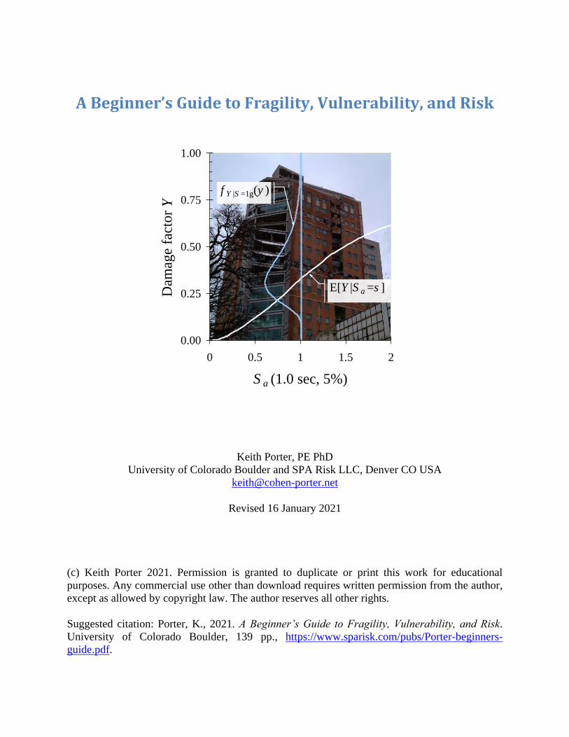
A Beginner’s Guide to Fragility, Vulnerability, and Risk
Keith Porter, PE PhD
University of Colorado Boulder and SPA Risk LLC, Denver CO USA
Revised 16 January 2021
(c) Keith Porter 2021. Permission is granted to duplicate or print this work for educational
purposes. Any commercial use other than download requires written permission from the author,
except as allowed by copyright law. The author reserves all other rights.
Suggested citation: Porter, K., 2021. A Beginner’s Guide to Fragility, Vulnerability, and Risk.
University of Colorado Boulder, 139 pp., https://www.sparisk.com/pubs/Porter-beginners-
guide.pdf.
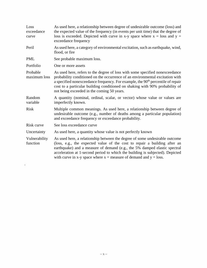
0.00
0.25
0.50
0.75
1.00
0 0.5 1 1.5 2
S a (1.0 sec, 5%)
Dam
age
fact
or
Y
E[Y |S a =s ]
f Y |S =1g(y )
– ii –
Contents
1. Introduction ................................................................................................................................. 1
1.1 Objectives ............................................................................................................................. 1
1.2 An engineering approach to risk analysis ............................................................................. 1
1.3 Organization of the guide ...................................................................................................... 2
2. Fragility ....................................................................................................................................... 2
2.1 Uncertain quantities .............................................................................................................. 2
2.1.1 Brief introduction to probability distributions ............................................................... 2
2.1.2 Normal, lognormal, and uniform distributions .............................................................. 4
2.1.3 The clarity test .............................................................................................................. 11
2.1.4 Aleatory and epistemic uncertainties ........................................................................... 12
2.2 Meaning and form of a fragility function ........................................................................... 15
2.2.1 What is a fragility function .......................................................................................... 15
2.2.2 Common form of a fragility function ........................................................................... 16
2.2.3 A caution about ill-defined damage states ................................................................... 17
2.3 Multiple fragility functions ................................................................................................. 18
2.3.1 Sequential damage states ............................................................................................. 18
2.3.2 Simultaneous damage states ........................................................................................ 19
2.3.3 MECE damage states ................................................................................................... 20
2.4 Creating fragility functions ................................................................................................. 20
2.4.1 Three general classes of fragility functions ................................................................. 20
2.4.2 Data that cannot be used to derive fragility functions ................................................. 21
2.4.3 What to know before trying to derive a fragility function ........................................... 21
2.4.4 Actual failure excitation ............................................................................................... 21
2.4.5 Bounding-failure excitation ......................................................................................... 22
2.4.6 Other data conditions ................................................................................................... 23
2.4.7 Dealing with under-representative specimens ............................................................. 23
2.4.8 Dealing with fragility functions that cross ................................................................... 25
2.5 Some useful sources of component fragility functions ....................................................... 28
3. Vulnerability ............................................................................................................................. 29
3.1 Empirical vulnerability functions ....................................................................................... 29
3.2 Analytical vulnerability functions ....................................................................................... 30
3.3 Expert opinion vulnerability functions ............................................................................... 33
3.4 How to express a vulnerability function ............................................................................. 34
– iii –
4. Hazard ....................................................................................................................................... 36
4.1 What are earthquakes? ........................................................................................................ 36
4.1.1 Why earthquakes occur ................................................................................................ 36
4.1.2 How an earthquake causes ground shaking ................................................................. 38
4.1.3 Distinction between magnitude and ground motion .................................................... 39
4.1.4 Effect of soil stiffness .................................................................................................. 39
4.2 Ground motion prediction equations .................................................................................. 40
4.3 Probabilistic seismic hazard analysis .................................................................................. 43
4.4 Hazard rate versus probability ............................................................................................ 45
4.5 Measures of seismic excitation ........................................................................................... 46
4.5.1 Some commonly used measures of ground motion ..................................................... 46
4.5.2 Conversion between instrumental and macroseismic intensity ................................... 49
4.5.3 Some commonly used measures of component excitation .......................................... 51
4.6 Hazard deaggregation ......................................................................................................... 52
4.7 Convenient sources of hazard data ..................................................................................... 54
5. Risk for a single asset ............................................................................................................... 55
5.1 Risk ..................................................................................................................................... 55
5.2 Expected failure rate for a single asset ............................................................................... 55
5.3 Probability of failure during a specified period of time ...................................................... 57
5.4 Expected annualized loss for a single asset ........................................................................ 57
5.5 One measure of benefit: expected present value of reduced EAL ...................................... 59
5.6 Risk curve for a single asset ................................................................................................ 61
5.6.1 Risk curve for a lognormally distributed loss measure ................................................ 61
5.6.2 Risk curve for a binomially distributed loss measure .................................................. 62
5.6.3 Risk curve for a binomially distributed loss measure with large N ............................. 64
5.7 Probable maximum loss for a single asset .......................................................................... 64
5.8 Common single-site risk software ...................................................................................... 65
6. Portfolio risk analysis ............................................................................................................... 65
6.1 Two common measures of portfolio risk ............................................................................ 65
6.1.1 Portfolio loss exceedance curve ................................................................................... 65
6.1.2 Portfolio expected annualized loss............................................................................... 68
6.2 Common analytical stages of portfolio catastrophe risk analysis ....................................... 68
6.3 Asset data and asset analysis ............................................................................................... 70
6.4 Portfolio hazard analysis ..................................................................................................... 71
– iv –
6.4.1 Earthquake rupture forecasts. How to select branch(es) and simulate sequence(s) .... 71
6.4.3 Simulating properly spatially correlated ground motion ............................................. 71
6.4.4 Options for scenario shaking (foregoing or 3D), fault offset, liquefaction, landsliding
............................................................................................................................................... 76
6.4.5 Comparing median maps and 3D ................................................................................. 76
6.5 Portfolio loss analysis ......................................................................................................... 76
6.6 Decision making ................................................................................................................. 76
6.7 Correlation in portfolio catastrophe risk ............................................................................. 76
6.7.1 Why correlation matters to portfolio catastrophe risk ................................................. 76
6.7.2 Sources of correlation in portfolio catastrophe risk ................................................ 78
6.8 Common portfolio risk tools ............................................................................................... 79
7. Some mathematical tools .......................................................................................................... 79
7.1 Monte Carlo simulation ...................................................................................................... 79
7.2 Moment matching ............................................................................................................... 81
8. Exercises ................................................................................................................................... 87
Exercise 1. Parts of a lognormal fragility function ................................................................... 87
Exercise 2. Basic elements of an earthquake rupture forecast .................................................. 88
Exercise 3. Hazard curves ......................................................................................................... 90
Exercise 4. The lognormal distribution ..................................................................................... 94
Exercise 5. Hazard deaggregation ............................................................................................. 94
Exercise 6. Estimate MMI from ground motion ....................................................................... 95
Exercise 7. Write the equation for component failure rate ....................................................... 96
Exercise 8. Sequential damage states ........................................................................................ 97
Exercise 9. Simultaneous damage states ................................................................................... 97
Exercise 10. MECE damage states ........................................................................................... 98
Exercise 11. Risk curve for number of injuries ........................................................................ 99
9. References ............................................................................................................................... 103
Appendices .................................................................................................................................. 106
Appendix A: Tornado diagram for deterministic sensitivity ...................................................... 106
Introduction: which inputs matter most to an uncertain quantity? ......................................... 106
Tornado-diagram procedure .................................................................................................... 108
Advantages and disadvantages ............................................................................................... 110
Example tornado diagram problem ......................................................................................... 110
Combining tornado diagrams and moment matching ............................................................. 112
Appendix B: Assigning a monetary value to statistical injuries ................................................. 116
– v –
Appendix C: How to write and defend your thesis ..................................................................... 117
C.1 Your thesis outline ........................................................................................................... 117
C.2 Simplify as much as possible but no more ....................................................................... 119
C.3 Style guide ........................................................................................................................ 121
C.4 Capitalization ................................................................................................................... 122
C.5 Defending your thesis....................................................................................................... 127
Appendix D: How to write a research article .............................................................................. 129
Appendix E: Why an annuity can substitute for random future natural-hazard losses ............... 132
E.1 Introduction .................................................................................................................. 132
E.2 Deriving present value of uncertain future losses ........................................................ 132
E.3 Sample calculation and comparison with simulation ................................................... 134
Appendix F: Revision history ..................................................................................................... 138
– vi –
Index of Figures
Figure 1. An engineering approach to risk analysis ........................................................................ 2
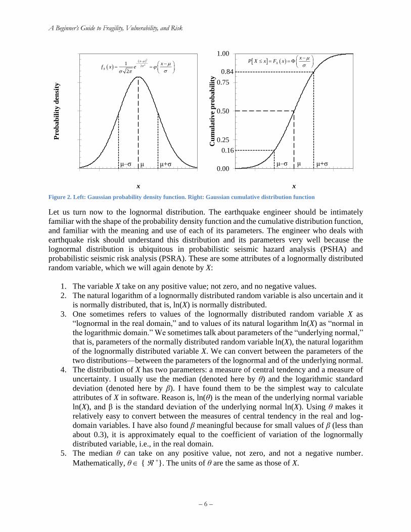
Figure 2. Left: Gaussian probability density function. Right: Gaussian cumulative distribution
function ........................................................................................................................................... 6
Figure 3. Left: Lognormal probability density function. Right: Lognormal cumulative distribution
function ........................................................................................................................................... 9
Figure 4. Normal and lognormal distributions with the same mean and standard deviation ........ 10
Figure 5. Left: Uniform probability density function. Right: Uniform cumulative distribution
function ......................................................................................................................................... 11
Figure 6. John Collier's 1891 Priestess of Delphi (a hypothetical clairvoyant). ........................... 11
Figure 7. Derailed counterweight at 50 UN Plaza after the 1989 Loma Prieta earthquake (R
Hamburger) ................................................................................................................................... 12
Figure 8. Left: a die (alea) literally symbolizes aleatory uncertainty. Right: Thomas Bayes, under
whose eponymous viewpoint all undercertainty is epistemic (both images licensed for reuse) .. 12
Figure 9. Does a coin toss represent an irreducible uncertainty? (image credit: ICMA Photos,
Attribution-ShareAlike 2.0 Generic license) ................................................................................ 13
Figure 10. A. Keller's (1986) curves separating coin-toss solutions for heads and tails for a coin
tossed from elevation 0 with initial upward velocity u and angular velocity ω. B. Diaconis et al.'s
(2007) coin-tossing device ............................................................................................................ 14
Figure 11. Suffolk Downs starting gate during a live horse race, from August 1, 2007. Can the
probability mass function of its outcome be said to exist in nature? (Image credit: Anthony92931,
Creative Commons Attribution-Share Alike 3.0 Unported license) ............................................. 15
Figure 12. Increasing beta and adjusting theta to account for under-representative samples ....... 25
Figure 13. Illustration of maximum likelihood estimation of lognormal fragility functions with
type-B data and multiple sequential damage states, solution ....................................................... 28
Figure 14. Regression analysis of damage to woodframe buildings in the 1994 Northridge
earthquake (Wesson et al. 2006) ................................................................................................... 30
Figure 15. Analytical methods for estimating seismic vulnerability of a single asset (Porter 2003).
....................................................................................................................................................... 31
Figure 16. Accounting for variability in design within the asset class, one can extend PBEE to
estimate seismic vulnerability of an asset class ............................................................................ 31
Figure 17. Example analytical vulnerability function for highrise post-1980 reinforced concrete
moment frame office building in the Western United States (Kazantzi et al. 2013) .................... 32
Figure 18. Mantle convection (By Surachit, CC BY-SA 3.0,
https://commons.wikimedia.org/w/index.php?curid=2574349) ................................................... 36
Figure 19. Tectonic plates of the world (Public domain,
https://commons.wikimedia.org/w/index.php?curid=535201) ..................................................... 37
Figure 20. Three types of fault: A. Strike-slip. B. Normal. C. Reverse. (Public Domain,
https://commons.wikimedia.org/w/index.php?curid=3427397) ................................................... 37
Figure 21. Aerial photo of the San Andreas Fault in the Carrizo Plain, northwest of Los Angeles
(By Ikluft; CC BY-SA-4.0; https://en.wikipedia.org/wiki/Earthquake#/media/File:Kluft-photo-
Carrizo-Plain-Nov-2007-Img_0327.jpg) ...................................................................................... 37
Figure 22. Earthquake magnitudes and energy release, and comparison with other natural and man-
made events. (Gavin Hayes, public domain, https://earthquake.usgs.gov/learn/topics/mag-
intensity/) ...................................................................................................................................... 38

– vii –
Figure 23. A (A. Public domain, https://commons.wikimedia.org/w/index.php?curid=308657 .. 39
Figure 24. USGS interactive hazard deaggregation website ........................................................ 53
Figure 25. Sample output of the USGS’ interactive hazard deaggregation website ..................... 54
Figure 26. Calculating failure rate with hazard curve (left) and fragility function (right) ........... 56
Figure 27. The cashflow diagram illustrates the present value (PV) of a sequence of t years of
annual losses of value EAL........................................................................................................... 58
Figure 28. Cashflow diagrams of annualized losses to an asset (A) before mitigation and (B) after
mitigation. ..................................................................................................................................... 60
Figure 29. Two illustrative risk curves ......................................................................................... 61
Figure 30. Example portfolio loss exceedance curve, also called a risk curve ............................. 67
Figure 31. Common elements of a catastrophe risk model ........................................................... 68
Figure 32. Simpler form of a catastrophe risk model ................................................................... 70
Figure 33. Four sample random fields of a standard normal variate with spatial correlation
appropriate to 1-second spectral acceleration response per Jayaram and Baker (2009) ............... 74
Figure 34. Monte Carlo simulation is very powerful and relatively simple, but can be
computationally demanding and can converge slowly, meaning it can take a lot samples to get a
reasonably accurate result. Moment matching offers a more efficient alternative. (Image by Ralf
Roletschek, permission under CC BY-SA 3.0.) ........................................................................... 82
Figure 35. 5-point moment matching for a lognormal probability distribution ............................ 85
Figure 36. Three-point moment matching for a lognormal probability distribution .................... 87
Figure 37. Exercise 1 fragility function ........................................................................................ 88
Figure 38. 475-year (10%/50-year) Sa(0.2 sec, 5%) hazard deaggregation at LA City Hall ....... 95
Figure 39. Risk curve for exercise 11 ......................................................................................... 102
Figure 40. A sample tornado diagram that depicts how the earthquake-induced repair cost for a
particular building is affected by various model parameters (Porter et al. 2002). ...................... 108
Figure 41. Tornado diagram for professional society meal ........................................................ 111
Figure 42. Using moment matching with tornado-diagram analysis to estimate the cumulative
distribution function of cost in the party-planning exercise ....................................................... 115
Figure 43. Avoid streetlight-effect simplifications (Fisher 1942) .............................................. 120
Figure 44. Avoid spherical-cow simplifications ......................................................................... 121
Figure 45. Are the present values of these two cashflows really equivalent? ............................ 134
Figure 46. Sample calculation functions: (A) Hazard curve G(x), (B) Cumulative distribution
function FX(x), and (C) Mean vulnerability function y(x) .......................................................... 136
Index of Tables
Table 1. Example maximum likelihood estimation of lognormal fragility functions with type-B
data and multiple sequential damage states, initial guess ............................................................. 27
Table 2. Example maximum likelihood estimation of lognormal fragility functions with type-B
data and multiple sequential damage states, solution ................................................................... 27
Table 3. MMI and EMS-98 macroseismic intensity scales (abridged) ......................................... 48
Table 4. Parameter values for Worden et al. (2012) GMICE for California ................................ 50
Table 5. Approximate relationship between PGA and MMI using Worden et al. (2012) ............ 50
Table 6. Parameter values for Atkinson and Kaka (2007) GMICE for the United States ............ 51
Table 7. Constructing a loss exceedance curve in a portfolio catastrophe risk analysis .............. 66
– viii –
Table 8. Example of Monte Carlo simulation of the sum of two normally distributed random
variables ........................................................................................................................................ 81
Table 9. Substitute points (the substitute set) and weights for 5-point moment matching of a
lognormal random variable ........................................................................................................... 84
Table 10. Five-point moment matching substitute set for two uncorrelated lognormal random
variables X and Y .......................................................................................................................... 86
Table 11. Three-point moment matching substitute set for one lognormal random variable X ... 86
Table 12. Three-point moment matching substitute set for two lognormal random variables X and
Y .................................................................................................................................................... 87
Table 13. Exercise 2 quantities of P[H ≥ h | m,r,v,a] .................................................................... 89
Table 14. Numerical solution to exercise 7 .................................................................................. 97
Table 15. Vulnerability and hazard functions for exercise 11 .................................................... 100
Table 16. P[Y≥y|S=s] for exercise 11 ......................................................................................... 101
Table 17. Summands and sums for exercise 11 .......................................................................... 102
Table 18. Tabulating input values for a tornado diagram ........................................................... 108
Table 19. Tabulating output values for a tornado diagram ......................................................... 109
Table 20. Tornado diagram example problem ............................................................................ 110
Table 21. Professional society meal cost tornado diagram quantities ........................................ 111
Table 22. Party-planning example with moment matching ........................................................ 114
Table 23. Federal values of statistical deaths and injuries avoided, in 1994 US$. ..................... 117
– ix –
Glossary
Asset An entity with exchange or commercial value, or with nonmonetary value such
as memorabilia.
Asset
definition
An enumeration and valuation of asset attributes, usually just the attributes that
matter in an analytical context.
BCR See benefit-cost ratio
Benefit-cost
ratio
The ratio of benefit (such as the reduction in the present value of future losses
that is attributable to some mitigation measure) to the cost (e.g., the capital and
present value of maintenance costs for the mitigation measure)
Catastrophe As used here, an event in which a very high loss occurs.
Decision As used here, and irreversible allocation of resources to one of two or more
alternatives.
Environmental
excitation
As used here, degree of engineering demand on an element of the built
environment, such as 3-second peak gust velocity at 10-meter elevation or 5%
damped elastic spectral acceleration response at 1-second period.
Expected
annualized
loss
The long-term average degree of loss per year.
Failure An event in which a defined limit state is exceeded, such as a column losing its
vertical load-carrying capacity,
Fragility
function
As used here, a relationship between probability that some undesirable
outcome occurs (e.g., the probability that a beam-column joint loses its vertical
load-carrying capacity) and a measure of demand (e.g., the estimated ratio of
the imposed bending moment on the joint to the estimated yield capacity of the
joint). Depicted with curve in x-y space where x = measure of demand and y =
occurrence probability.
Hazard Multiple common meanings. As used here, a relationship between degree of
environmental excitation (e.g., 3-second peak gust velocity at 10-meter
elevation) and exceedance frequency (events per unit time with greater degree)
or exceedance probability (chance of exceedance in a given period such as the
coming calendar year). In other contexts (not here), it can refer to a category
of environmental excitation such as wind. Depicted with curve in x-y space
where x = degree of environmental excitation and y = exceedance frequency.
LEC See loss exceedance curve.
Loss A measure of undesirable outcome, such as repair cost, number of fatal or
nonfatal injuries, or the time required to restore a facility to full functionality
(“dollars, deaths, and downtime”).
– x –
Loss
exceedance
curve
As used here, a relationship between degree of undesirable outcome (loss) and
the expected value of the frequency (in events per unit time) that the degree of
loss is exceeded. Depicted with curve in x-y space where x = loss and y =
exceedance frequency
Peril As used here, a category of environmental excitation, such as earthquake, wind,
flood, or fire
PML See probable maximum loss.
Portfolio One or more assets
Probable
maximum loss
As used here, refers to the degree of loss with some specified nonexceedance
probability conditioned on the occurrence of an environmental excitation with
a specified nonexceedance frequency. For example, the 90th percentile of repair
cost to a particular building conditioned on shaking with 90% probability of
not being exceeded in the coming 50 years.
Random
variable
A quantity (nominal, ordinal, scalar, or vector) whose value or values are
imperfectly known.
Risk Multiple common meanings. As used here, a relationship between degree of
undesirable outcome (e.g., number of deaths among a particular population)
and exceedance frequency or exceedance probability.
Risk curve See loss exceedance curve
Uncertainty As used here, a quantity whose value is not perfectly known
Vulnerability
function
As used here, a relationship between the degree of some undesirable outcome
(loss, e.g., the expected value of the cost to repair a building after an
earthquake) and a measure of demand (e.g., the 5% damped elastic spectral
acceleration at 1-second period to which the building is subjected). Depicted
with curve in x-y space where x = measure of demand and y = loss.
.
Porter: A Beginner’s Guide to Fragility, Vulnerability, and Risk
- 1 -
1. Introduction
1.1 Objectives This work provides a primer for earthquake-related fragility, vulnerability, and risk. It is written
for new graduate students who are studying natural-hazard risk, but should also be useful for the
newcomer to catastrophe risk modeling, such as users and consumers of catastrophe models by
RMS, Applied Insurance Research, EQECAT, Global Earthquake Model, or the US Federal
Emergency Management Agency (FEMA). Many of its concepts can be applied to other perils.
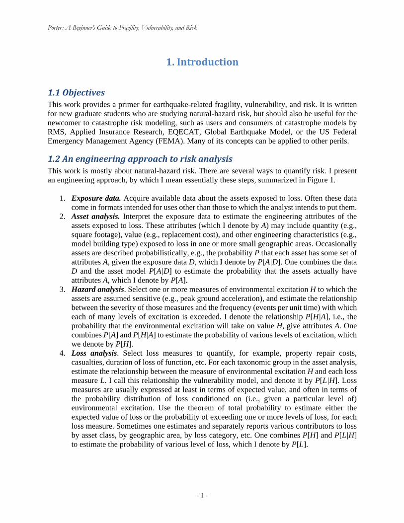
1.2 An engineering approach to risk analysis This work is mostly about natural-hazard risk. There are several ways to quantify risk. I present
an engineering approach, by which I mean essentially these steps, summarized in Figure 1.
1. Exposure data. Acquire available data about the assets exposed to loss. Often these data
come in formats intended for uses other than those to which the analyst intends to put them.
2. Asset analysis. Interpret the exposure data to estimate the engineering attributes of the
assets exposed to loss. These attributes (which I denote by A) may include quantity (e.g.,
square footage), value (e.g., replacement cost), and other engineering characteristics (e.g.,
model building type) exposed to loss in one or more small geographic areas. Occasionally
assets are described probabilistically, e.g., the probability P that each asset has some set of
attributes A, given the exposure data D, which I denote by P[A|D]. One combines the data
D and the asset model P[A|D] to estimate the probability that the assets actually have
attributes A, which I denote by P[A].
3. Hazard analysis. Select one or more measures of environmental excitation H to which the
assets are assumed sensitive (e.g., peak ground acceleration), and estimate the relationship
between the severity of those measures and the frequency (events per unit time) with which
each of many levels of excitation is exceeded. I denote the relationship P[H|A], i.e., the
probability that the environmental excitation will take on value H, give attributes A. One
combines P[A] and P[H|A] to estimate the probability of various levels of excitation, which
we denote by P[H].
4. Loss analysis. Select loss measures to quantify, for example, property repair costs,
casualties, duration of loss of function, etc. For each taxonomic group in the asset analysis,
estimate the relationship between the measure of environmental excitation H and each loss
measure L. I call this relationship the vulnerability model, and denote it by P[L|H]. Loss
measures are usually expressed at least in terms of expected value, and often in terms of
the probability distribution of loss conditioned on (i.e., given a particular level of)
environmental excitation. Use the theorem of total probability to estimate either the
expected value of loss or the probability of exceeding one or more levels of loss, for each
loss measure. Sometimes one estimates and separately reports various contributors to loss
by asset class, by geographic area, by loss category, etc. One combines P[H] and P[L|H]
to estimate the probability of various level of loss, which I denote by P[L].
A Beginner’s Guide to Fragility, Vulnerability, and Risk
– 2 –
5. Decision making. The results of the loss analysis are almost always used to inform some
risk-management decision. Such decisions always involve choosing between two or more
alternative actions, and often require the analyst to repeat the analysis under the different
conditions of each alternative, such as as-is and assuming some strengthening occurs.
Figure 1. An engineering approach to risk analysis
1.3 Organization of the guide Section 2 discusses fragility, by which I mean the probability of an undesirable outcome as a
function of excitation. Section 3 discusses vulnerability, by which I mean the degree of loss as a
function of excitation. Note the distinction: fragility is measured in terms of probability,
vulnerability in terms of loss such as repair cost. Section 4 briefly discusses seismic hazard. See
Section 5 for a brief discussion of risk to point assets. Section 6 is a work in progress, discussing
risk to a portfolio of assets. Solved exercises are presented in Section 7. References are presented
in Section 8. Several appendices provide guidance on miscellaneous subjects: (A) how to perform
a deterministic sensitivity study called a tornado diagram analysis; (B) assigning monetary value
to future statistical injuries to unknown persons; (C) how to write and defend a thesis, and (D)
revision history.
2. Fragility
2.1 Uncertain quantities
2.1.1 Brief introduction to probability distributions
To understand fragility it is necessary first to understand probability and uncertain quantities. Since
some undergraduate engineering programs do not cover these topics, let us discuss them briefly
here before moving on to fragility.
Exposure
P[A]
A: assets in
engineering
terms, e.g.,
structure types
D
Asset
analysis
Hazard
analysis
Hazard model
P[H|A]
H: Hazard., e.g.,
3-sec wind gust
velocity at 33 ft
elevation
D: data of
exposure
locations,
values, features
Loss
analysis
Vulnerability
model
P[L|H]
Loss
P[L]
L: ground-up loss,
e.g., people killed
Hazard
P[H]
Exposure
data
How to
manage
risk?
Asset model
P[A|D]
Decision-
making
A Beginner’s Guide to Fragility, Vulnerability, and Risk
– 3 –
Many of the terms used here involve uncertain quantities, often called random variables. This
section is offered for the student who has not studied probability elsewhere. “Uncertain” is
sometimes used here to mean something broader than “random” because “uncertain” applies both
to quantities that change unpredictably (e.g., whether a tossed coin will land heads or tails side up
on the next toss), and to quantities that do not vary but that are not known with certainty. For
example, a particular building’s capacity to resist collapse in an earthquake may not vary much
over time, but one does not know that capacity before the building collapses, so it is uncertain. In
this work, uncertain variables are denoted by capital letters, e.g., D, particular values are denoted
by lower case, e.g., d, probability is denoted by P[ ], and conditional probability is denoted by
P[A|B], that is, probability that statement A is true given that statement B is true. In any case, more
engineers use the expression “random variable” than use “uncertain quantity,” so I will tend to use
the former. (Sidenote: many well-known quantities are not entirely certain, such as the speed of
light in a vacuum, but the uncertainty is so small that it is usually practical to ignore it and to treat
the quantity as certain.)
Random variables are quantified using probability distributions. Three kinds of probability
distributions are discussed here: probability density functions, probability mass functions, and
cumulative distribution functions. Only scalar random variables are discussed here. For the present
discussion, let us denote the random variable by a capital letter X, and any particular value that it
might take on with a lower-case x.
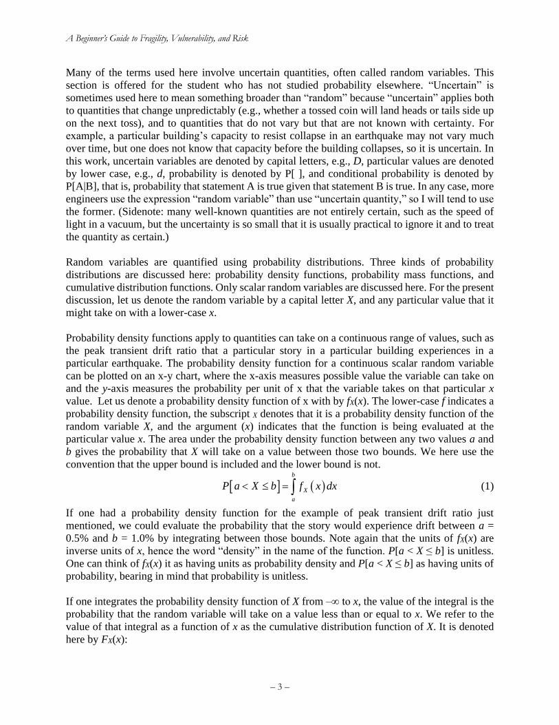
Probability density functions apply to quantities can take on a continuous range of values, such as
the peak transient drift ratio that a particular story in a particular building experiences in a
particular earthquake. The probability density function for a continuous scalar random variable
can be plotted on an x-y chart, where the x-axis measures possible value the variable can take on
and the y-axis measures the probability per unit of x that the variable takes on that particular x
value. Let us denote a probability density function of x with by fX(x). The lower-case f indicates a
probability density function, the subscript X denotes that it is a probability density function of the
random variable X, and the argument (x) indicates that the function is being evaluated at the
particular value x. The area under the probability density function between any two values a and
b gives the probability that X will take on a value between those two bounds. We here use the
convention that the upper bound is included and the lower bound is not.
( )b
X
a
P a X b f x dx = (1)
If one had a probability density function for the example of peak transient drift ratio just
mentioned, we could evaluate the probability that the story would experience drift between a =
0.5% and b = 1.0% by integrating between those bounds. Note again that the units of fX(x) are
inverse units of x, hence the word “density” in the name of the function. P[a < X ≤ b] is unitless.
One can think of fX(x) it as having units as probability density and P[a < X ≤ b] as having units of
probability, bearing in mind that probability is unitless.
If one integrates the probability density function of X from –∞ to x, the value of the integral is the
probability that the random variable will take on a value less than or equal to x. We refer to the
value of that integral as a function of x as the cumulative distribution function of X. It is denoted
here by FX(x):
A Beginner’s Guide to Fragility, Vulnerability, and Risk
– 4 –
( )x
X
z
P X x f z dz=−
= (2)
Equation (2) uses the dummy variable z because the upper bound x here is a fixed, particular value,
the value at which we are evaluating the cumulative distribution function.
Some variables can only take on discrete values, such as whether a particular window in a
particular building in a particular earthquake survives undamaged, or it cracks without any glass
falling out, or cracks and has glass fall out. Let X now denote such a discrete random variable. We
use a probability mass function to express the probability that X takes on any given value x. In the
case of the broken window, one might express X as an index to the uncertain damage state, which
can take on values x = 0 (undamaged), x = 1 (cracked, not fallen), or x = 2 (cracked and fallen out).
Let us denote by pX(x) the probability mass function. The lower-case p indicates a probability mass
function, the subscript X denotes that it is a probability mass function of the random variable X,
and the argument (x) indicates that the function is being evaluated at the particular value x. Just to
be clear about notation:
( )XP X x p x= = (3)
One can express the cumulative distribution function of a discrete random variable the same as a
continuous one:
( )
( )
x
X
z
x
X
z
P X x p z dz
p z
=−
=−
=
=
(4)
2.1.2 Normal, lognormal, and uniform distributions
Aside from the foregoing definitions, fX(x), pX(x), and FX(x) do not have to take on a parametric
form, i.e., they are not all necessarily described with an equation that has parameters, coefficients,
and so on. But it is often convenient to approximate them with parametric distributions. There are
many such distributions; only three or so will be used in the present document, because they are
used so frequently in applications of fragility, vulnerability and risk, and are used later in this
document. They are the normal (also called Gaussian), lognormal (sometime spelled with a hyphen
between “log” and “normal”), and uniform distributions. Anyone who deals with engineering risk
should understand and use these three distributions, at least to the extent discussed here. Only the
most relevant aspects of the distributions are described here; for more detail see for example the
Wikipedia articles. A few features to remember:
1. If a quantity X is normally distributed with mean (expected, average) value μ and standard
deviation σ, it can take on any scalar value in – < X < . Mathematically,
X { }, meaning that X can take on any real scalar value
2. The larger μ, the more like X is to take on a higher value, all else being equal.
3. The mean μ can take on any real value. Mathematically,
A Beginner’s Guide to Fragility, Vulnerability, and Risk
– 5 –
μ { }, meaning that μ is any real scalar value
4. The larger σ, the more uncertain is X. It must take on a nonnegative value. It has the same
units as X and μ. If X were measured in dollars, so would μ and σ.
5. If σ = 0, that means that X = μ, meaning that X is known exactly, that it is not uncertain.
The standard deviation σ cannot take on a negative value, in a sense because we the smaller
the σ, the more certainly we know what values X can take on, and we cannot know any
more about X if it is known exactly.
The Gaussian probability density function is expressed as in Equation (5), and as shown there is
sometimes expressed in the normalized form shown in the second line of the equation with the
lower-case Greek letter φ.
( )( )
2
221
2
x
Xf x e
x
−−
=
− =
(5)
Virtually all mathematical software provide a built-in function for the Gaussian probability density
function, e.g., in Microsoft Excel, φ(z) is evaluated using the function normdist(z). The cumulative
distribution function (CDF) can be expressed as follows:
( )( )
2
221
2
X
zx
P X x F x
e dz
x
−−
−
=
=
− =
(6)
where commonly denotes the standard normal cumulative distribution function. It too is
available in all mathematical software, e.g., normsdist( ) in Microsoft Excel. Equations (5) and (6)
are illustrated in Figure 2.
Inverting the normal cumulative distribution function. One can find the value x associated with
a specified nonexceedance probability, p by inverting the cumulative distribution function at p:
( )
( )
1
1
:p p
p X
x x P X x p
x F p
p
−
−
= =
=
= +
(7)
A Beginner’s Guide to Fragility, Vulnerability, and Risk
– 6 –
Figure 2. Left: Gaussian probability density function. Right: Gaussian cumulative distribution function
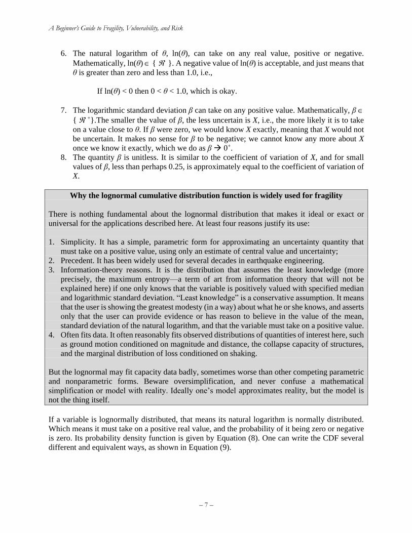
Let us turn now to the lognormal distribution. The earthquake engineer should be intimately
familiar with the shape of the probability density function and the cumulative distribution function,
and familiar with the meaning and use of each of its parameters. The engineer who deals with
earthquake risk should understand this distribution and its parameters very well because the
lognormal distribution is ubiquitous in probabilistic seismic hazard analysis (PSHA) and
probabilistic seismic risk analysis (PSRA). These are some attributes of a lognormally distributed
random variable, which we will again denote by X:
1. The variable X take on any positive value; not zero, and no negative values.
2. The natural logarithm of a lognormally distributed random variable is also uncertain and it
is normally distributed, that is, ln(X) is normally distributed.
3. One sometimes refers to values of the lognormally distributed random variable X as
“lognormal in the real domain,” and to values of its natural logarithm ln(X) as “normal in
the logarithmic domain.” We sometimes talk about parameters of the “underlying normal,”
that is, parameters of the normally distributed random variable ln(X), the natural logarithm
of the lognormally distributed variable X. We can convert between the parameters of the
two distributions—between the parameters of the lognormal and of the underlying normal.
4. The distribution of X has two parameters: a measure of central tendency and a measure of
uncertainty. I usually use the median (denoted here by θ) and the logarithmic standard
deviation (denoted here by β). I have found them to be the simplest way to calculate
attributes of X in software. Reason is, ln(θ) is the mean of the underlying normal variable
ln(X), and β is the standard deviation of the underlying normal ln(X). Using θ makes it
relatively easy to convert between the measures of central tendency in the real and log-
domain variables. I have also found β meaningful because for small values of β (less than
about 0.3), it is approximately equal to the coefficient of variation of the lognormally
distributed variable, i.e., in the real domain.
5. The median θ can take on any positive value, not zero, and not a negative number.
Mathematically, θ { +}. The units of θ are the same as those of X.
0.00
0.25
0.50
0.75
1.00
0.0 0.5 1.0 1.5 2.0 2.5 3.0
Pro
bab
ilit
y d
ensi
ty
x
μμ‒σ μ+σ
( )( )
2
221
2
x
X
xf x e
−− −
= =
0.00
0.25
0.50
0.75
1.00
0 0.5 1 1.5 2 2.5 3
Cu
mu
lati
ve
pro
bab
ilit
y
x
0.16
μμ‒σ
( )X
xP X x F x
− = =
0.84
μ+σ
A Beginner’s Guide to Fragility, Vulnerability, and Risk
– 7 –
6. The natural logarithm of θ, ln(θ), can take on any real value, positive or negative.
Mathematically, ln(θ) { }. A negative value of ln(θ) is acceptable, and just means that
θ is greater than zero and less than 1.0, i.e.,
If ln(θ) < 0 then 0 < θ < 1.0, which is okay.
7. The logarithmic standard deviation β can take on any positive value. Mathematically, β
{ +}.The smaller the value of β, the less uncertain is X, i.e., the more likely it is to take
on a value close to θ. If β were zero, we would know X exactly, meaning that X would not
be uncertain. It makes no sense for β to be negative; we cannot know any more about X
once we know it exactly, which we do as β → 0+.
8. The quantity β is unitless. It is similar to the coefficient of variation of X, and for small
values of β, less than perhaps 0.25, is approximately equal to the coefficient of variation of
X.
Why the lognormal cumulative distribution function is widely used for fragility
There is nothing fundamental about the lognormal distribution that makes it ideal or exact or
universal for the applications described here. At least four reasons justify its use:
1. Simplicity. It has a simple, parametric form for approximating an uncertainty quantity that
must take on a positive value, using only an estimate of central value and uncertainty;
2. Precedent. It has been widely used for several decades in earthquake engineering.
3. Information-theory reasons. It is the distribution that assumes the least knowledge (more
precisely, the maximum entropy—a term of art from information theory that will not be
explained here) if one only knows that the variable is positively valued with specified median
and logarithmic standard deviation. “Least knowledge” is a conservative assumption. It means
that the user is showing the greatest modesty (in a way) about what he or she knows, and asserts
only that the user can provide evidence or has reason to believe in the value of the mean,
standard deviation of the natural logarithm, and that the variable must take on a positive value.
4. Often fits data. It often reasonably fits observed distributions of quantities of interest here, such
as ground motion conditioned on magnitude and distance, the collapse capacity of structures,
and the marginal distribution of loss conditioned on shaking.
But the lognormal may fit capacity data badly, sometimes worse than other competing parametric
and nonparametric forms. Beware oversimplification, and never confuse a mathematical
simplification or model with reality. Ideally one’s model approximates reality, but the model is
not the thing itself.
If a variable is lognormally distributed, that means its natural logarithm is normally distributed.
Which means it must take on a positive real value, and the probability of it being zero or negative
is zero. Its probability density function is given by Equation (8). One can write the CDF several
different and equivalent ways, as shown in Equation (9).
A Beginner’s Guide to Fragility, Vulnerability, and Risk
– 8 –
( )( )( )
( )
2
2
ln
21
2
ln
x
Xf x ex
x
−
=
=
(8)
( )
( )
ln
ln
ln ln
ln
ln
X
X
X
P X x F x
x
x
x
=
−=
=
−=
(9)
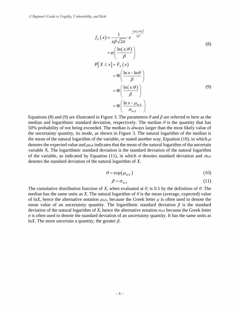
Equations (8) and (9) are illustrated in Figure 3. The parameters θ and β are referred to here as the
median and logarithmic standard deviation, respectively. The median θ is the quantity that has
50% probability of not being exceeded. The median is always larger than the most likely value of
the uncertainty quantity, its mode, as shown in Figure 3. The natural logarithm of the median is
the mean of the natural logarithm of the variable, or stated another way, Equation (10), in which
denotes the expected value and lnX indicates that the mean of the natural logarithm of tha uncertain
variable X. The logarithmic standard deviation is the standard deviation of the natural logarithm
of the variable, as indicated by Equation (11), in which denotes standard deviation and lnX
denotes the standard deviation of the natural logarithm of X.
( )lnexp X = (10)
ln X = (11)
The cumulative distribution function of X, when evaluated at θ, is 0.5 by the definition of θ. The
median has the same units as X. The natural logarithm of θ is the mean (average, expected) value
of lnX, hence the alternative notation μlnX, because the Greek letter μ is often used to denote the
mean value of an uncertainty quantity. The logarithmic standard deviation β is the standard
deviation of the natural logarithm of X, hence the alternative notation σlnX because the Greek letter
σ is often used to denote the standard deviation of an uncertainty quantity. It has the same units as
lnX. The more uncertain a quantity, the greater β.
A Beginner’s Guide to Fragility, Vulnerability, and Risk
– 9 –
Figure 3. Left: Lognormal probability density function. Right: Lognormal cumulative distribution function
Inverting the lognormal cumulative distribution function. The value x associated with a specified
nonexceedance probability, p is given by inverting Equation (9) at p:
( )
( )( )
1
1exp
p Xx F p
p
−
−
=
= (12)
It is sometimes desirable to calculate θ and β in terms of μ and σ. Here are the conversion equations.
Let v denote the coefficient of variation of X. It expresses uncertainty in X relative to mean value.
Then
v
= (13)
( )2ln 1 v = + (14)
21 v
=
+ (15)
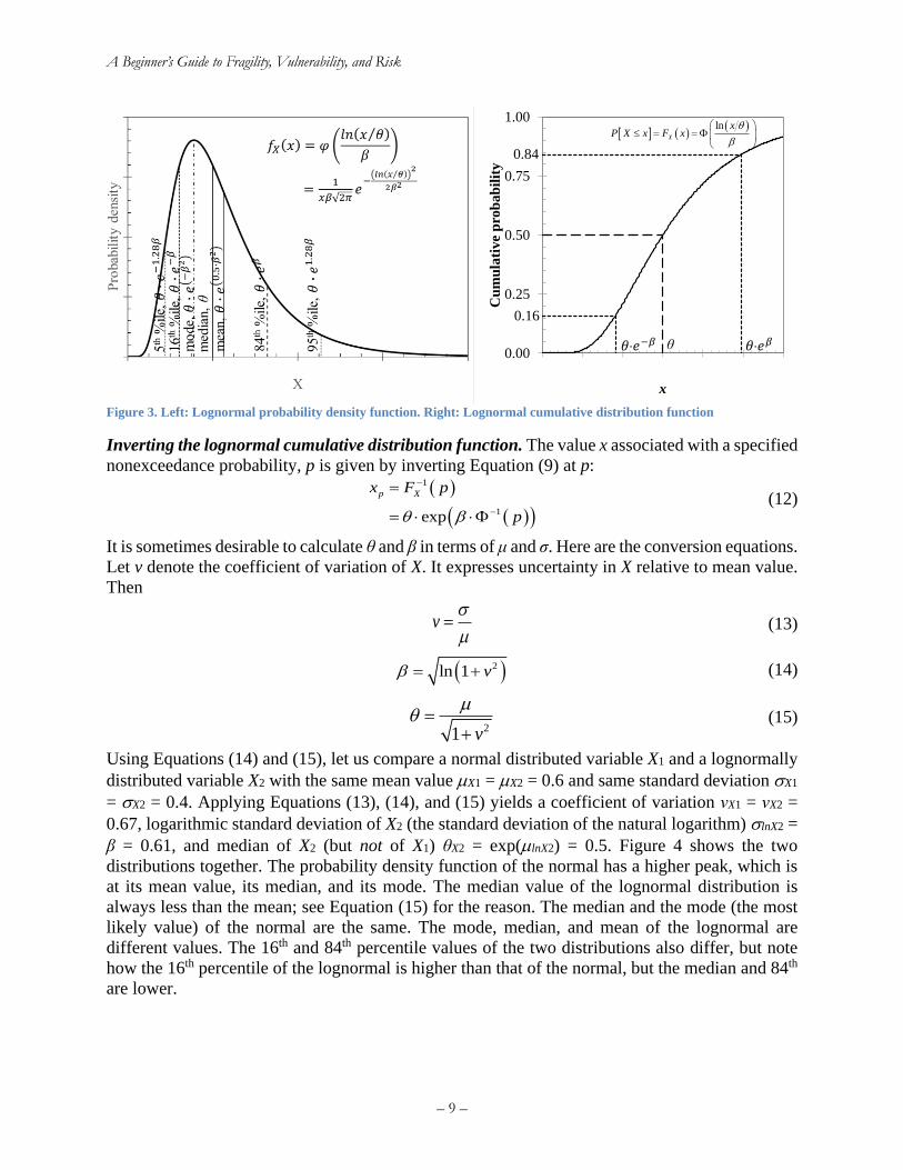
Using Equations (14) and (15), let us compare a normal distributed variable X1 and a lognormally
distributed variable X2 with the same mean value X1 = X2 = 0.6 and same standard deviation X1
= X2 = 0.4. Applying Equations (13), (14), and (15) yields a coefficient of variation νX1 = νX2 =
0.67, logarithmic standard deviation of X2 (the standard deviation of the natural logarithm) lnX2 =
β = 0.61, and median of X2 (but not of X1) θX2 = exp(lnX2) = 0.5. Figure 4 shows the two
distributions together. The probability density function of the normal has a higher peak, which is
at its mean value, its median, and its mode. The median value of the lognormal distribution is
always less than the mean; see Equation (15) for the reason. The median and the mode (the most
likely value) of the normal are the same. The mode, median, and mean of the lognormal are
different values. The 16th and 84th percentile values of the two distributions also differ, but note
how the 16th percentile of the lognormal is higher than that of the normal, but the median and 84th
are lower.
0.00
0.25
0.50
0.75
1.00
0 0.5 1 1.5 2 2.5 3
Cu
mu
lati
ve
pro
ba
bil
ity
x
0.16
0.84
( )( )ln
X
xP X x F x
= =
θ
A Beginner’s Guide to Fragility, Vulnerability, and Risk
– 10 –
Figure 4. Normal and lognormal distributions with the same mean and standard deviation
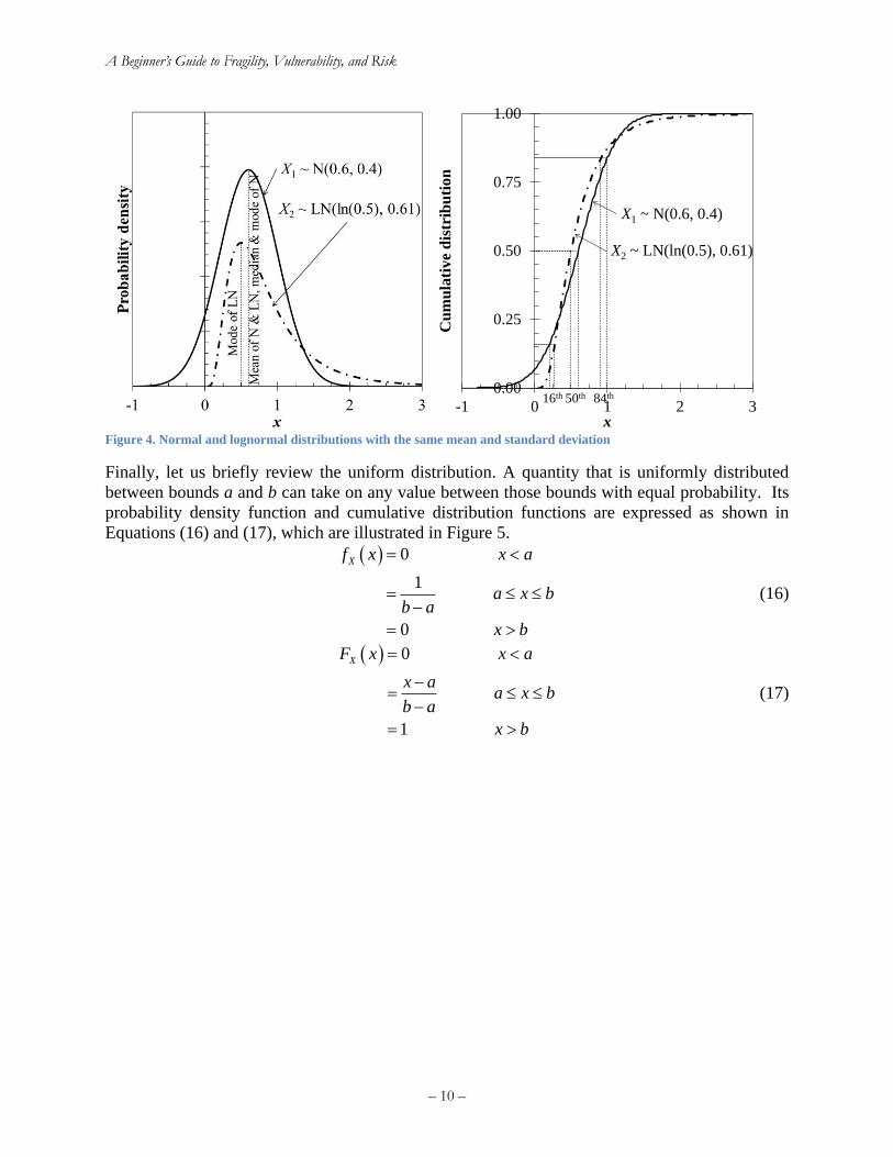
Finally, let us briefly review the uniform distribution. A quantity that is uniformly distributed
between bounds a and b can take on any value between those bounds with equal probability. Its
probability density function and cumulative distribution functions are expressed as shown in
Equations (16) and (17), which are illustrated in Figure 5.
( ) 0
1
0
Xf x x a
a x bb a
x b
=
= −
=
(16)
( ) 0
1
XF x x a
x aa x b
b a
x b
=
−=
−
=
(17)
0.00
0.25
0.50
0.75
1.00
-1 0 1 2 3
Cu
mu
lati
ve
dis
trib
uti
on
x
X1 ~ N(0.6, 0.4)
X2 ~ LN(ln(0.5), 0.61)
16th 50th 84th
A Beginner’s Guide to Fragility, Vulnerability, and Risk
– 11 –
Figure 5. Left: Uniform probability density function. Right: Uniform cumulative distribution function
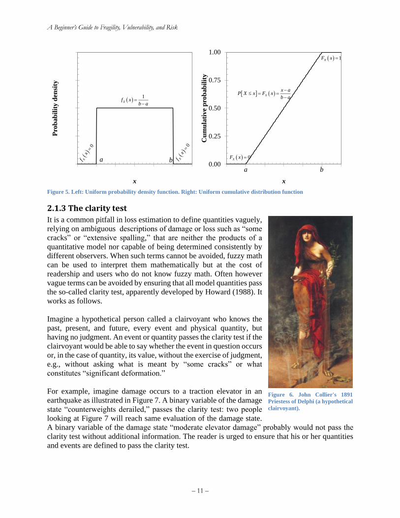
2.1.3 The clarity test
It is a common pitfall in loss estimation to define quantities vaguely,
relying on ambiguous descriptions of damage or loss such as “some
cracks” or “extensive spalling,” that are neither the products of a
quantitative model nor capable of being determined consistently by
different observers. When such terms cannot be avoided, fuzzy math
can be used to interpret them mathematically but at the cost of
readership and users who do not know fuzzy math. Often however
vague terms can be avoided by ensuring that all model quantities pass
the so-called clarity test, apparently developed by Howard (1988). It
works as follows.
Imagine a hypothetical person called a clairvoyant who knows the
past, present, and future, every event and physical quantity, but
having no judgment. An event or quantity passes the clarity test if the
clairvoyant would be able to say whether the event in question occurs
or, in the case of quantity, its value, without the exercise of judgment,
e.g., without asking what is meant by “some cracks” or what
constitutes “significant deformation.”
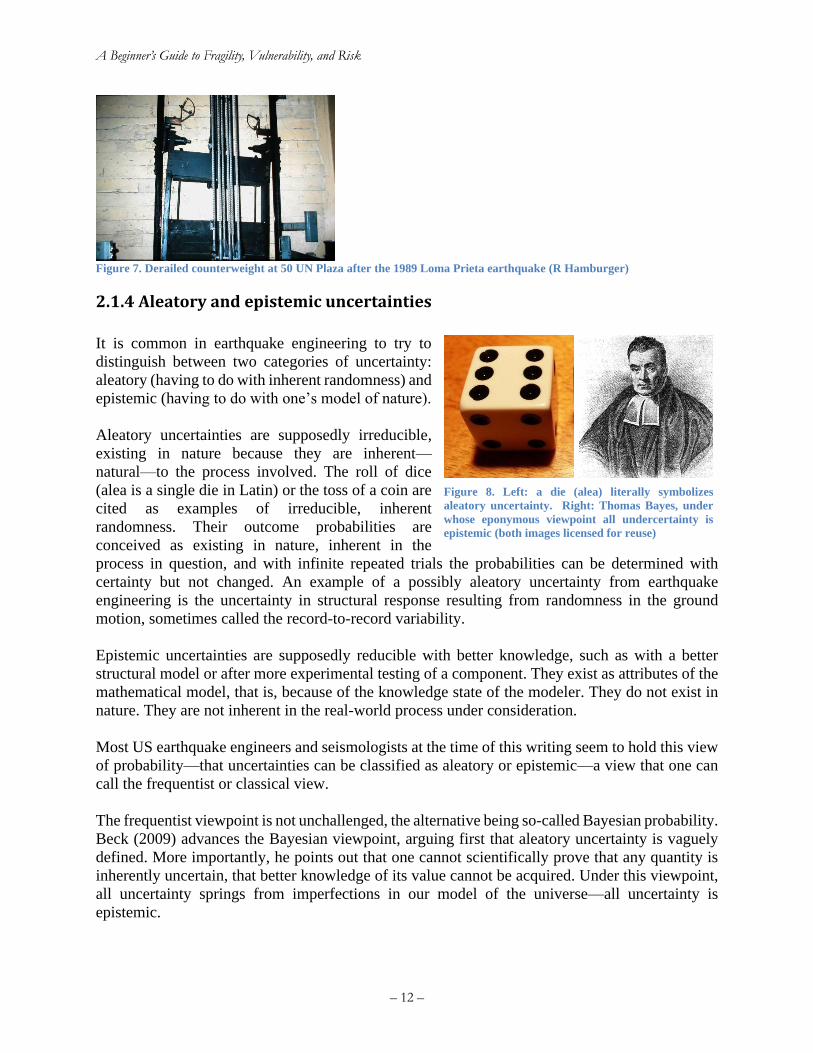
For example, imagine damage occurs to a traction elevator in an
earthquake as illustrated in Figure 7. A binary variable of the damage
state “counterweights derailed,” passes the clarity test: two people
looking at Figure 7 will reach same evaluation of the damage state.
A binary variable of the damage state “moderate elevator damage” probably would not pass the
clarity test without additional information. The reader is urged to ensure that his or her quantities
and events are defined to pass the clarity test.
0.00
0.25
0.50
0.75
1.00
0.0 0.5 1.0 1.5 2.0 2.5 3.0
Pro
bab
ilit
y d
ensi
ty
x
ba
( )1
Xf xb a
=−
()
0
Xfx
=
()
0
Xfx
=
0.00
0.25
0.50
0.75
1.00
0 0.5 1 1.5 2 2.5 3
Cu
mu
lati
ve
pro
bab
ilit
y
x
( )X
x aP X x F x
b a
− = =
−
( ) 0XF x =
( ) 1XF x =
ba
Figure 6. John Collier's 1891
Priestess of Delphi (a hypothetical
clairvoyant).
A Beginner’s Guide to Fragility, Vulnerability, and Risk
– 12 –
Figure 7. Derailed counterweight at 50 UN Plaza after the 1989 Loma Prieta earthquake (R Hamburger)
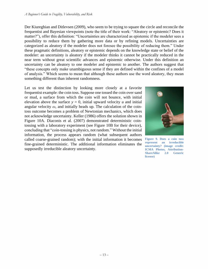
2.1.4 Aleatory and epistemic uncertainties
It is common in earthquake engineering to try to
distinguish between two categories of uncertainty:
aleatory (having to do with inherent randomness) and
epistemic (having to do with one’s model of nature).
Aleatory uncertainties are supposedly irreducible,
existing in nature because they are inherent—
natural—to the process involved. The roll of dice
(alea is a single die in Latin) or the toss of a coin are
cited as examples of irreducible, inherent
randomness. Their outcome probabilities are
conceived as existing in nature, inherent in the
process in question, and with infinite repeated trials the probabilities can be determined with
certainty but not changed. An example of a possibly aleatory uncertainty from earthquake
engineering is the uncertainty in structural response resulting from randomness in the ground
motion, sometimes called the record-to-record variability.
Epistemic uncertainties are supposedly reducible with better knowledge, such as with a better
structural model or after more experimental testing of a component. They exist as attributes of the
mathematical model, that is, because of the knowledge state of the modeler. They do not exist in
nature. They are not inherent in the real-world process under consideration.
Most US earthquake engineers and seismologists at the time of this writing seem to hold this view
of probability—that uncertainties can be classified as aleatory or epistemic—a view that one can
call the frequentist or classical view.
The frequentist viewpoint is not unchallenged, the alternative being so-called Bayesian probability.
Beck (2009) advances the Bayesian viewpoint, arguing first that aleatory uncertainty is vaguely
defined. More importantly, he points out that one cannot scientifically prove that any quantity is
inherently uncertain, that better knowledge of its value cannot be acquired. Under this viewpoint,
all uncertainty springs from imperfections in our model of the universe—all uncertainty is
epistemic.
Figure 8. Left: a die (alea) literally symbolizes
aleatory uncertainty. Right: Thomas Bayes, under
whose eponymous viewpoint all undercertainty is
epistemic (both images licensed for reuse)
A Beginner’s Guide to Fragility, Vulnerability, and Risk
– 13 –
Der Kiureghian and Ditlevsen (2009), who seem to be trying to square the circle and reconcile the
frequentist and Bayesian viewpoints (note the title of their work: “Aleatory or epistemic? Does it
matter?”), offer this definition: “Uncertainties are characterized as epistemic if the modeler sees a
possibility to reduce them by gathering more data or by refining models. Uncertainties are
categorized as aleatory if the modeler does not foresee the possibility of reducing them.” Under
these pragmatic definitions, aleatory or epistemic depends on the knowledge state or belief of the
modeler: an uncertainty is aleatory if the modeler thinks it cannot be practically reduced in the
near term without great scientific advances and epistemic otherwise. Under this definition an
uncertainty can be aleatory to one modeler and epistemic to another. The authors suggest that
“these concepts only make unambiguous sense if they are defined within the confines of a model
of analysis.” Which seems to mean that although these authors use the word aleatory, they mean
something different than inherent randomness.
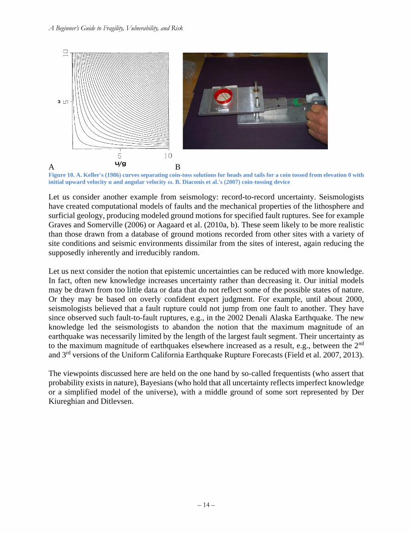
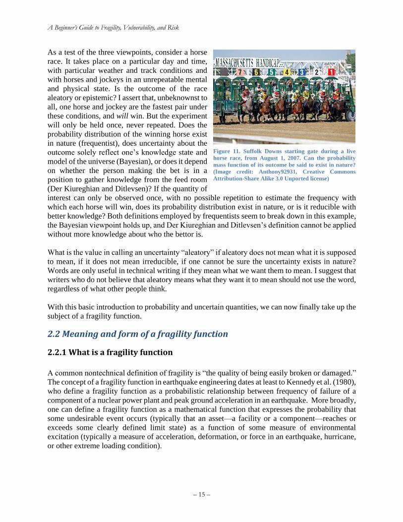
Let us test the distinction by looking more closely at a favorite
frequentist example: the coin toss. Suppose one tossed the coin over sand
or mud, a surface from which the coin will not bounce, with initial
elevation above the surface y = 0, initial upward velocity u and initial
angular velocity ω, and initially heads up. The calculation of the coin-
toss outcome becomes a problem of Newtonian mechanics, which does
not acknowledge uncertainty. Keller (1986) offers the solution shown in
Figure 10A. Diaconis et al. (2007) demonstrated deterministic coin-
tossing with a laboratory experiment (see Figure 10B for their device),
concluding that “coin-tossing is physics, not random.” Without the initial
information, the process appears random (what subsequent authors
called coarse-grained random); with the initial information it becomes
fine-grained deterministic. The additional information eliminates the
supposedly irreducible aleatory uncertainty.
Figure 9. Does a coin toss
represent an irreducible
uncertainty? (image credit:
ICMA Photos, Attribution-
ShareAlike 2.0 Generic
license)
A Beginner’s Guide to Fragility, Vulnerability, and Risk
– 14 –
A B Figure 10. A. Keller's (1986) curves separating coin-toss solutions for heads and tails for a coin tossed from elevation 0 with
initial upward velocity u and angular velocity ω. B. Diaconis et al.'s (2007) coin-tossing device
Let us consider another example from seismology: record-to-record uncertainty. Seismologists
have created computational models of faults and the mechanical properties of the lithosphere and
surficial geology, producing modeled ground motions for specified fault ruptures. See for example
Graves and Somerville (2006) or Aagaard et al. (2010a, b). These seem likely to be more realistic
than those drawn from a database of ground motions recorded from other sites with a variety of
site conditions and seismic environments dissimilar from the sites of interest, again reducing the
supposedly inherently and irreducibly random.
Let us next consider the notion that epistemic uncertainties can be reduced with more knowledge.
In fact, often new knowledge increases uncertainty rather than decreasing it. Our initial models
may be drawn from too little data or data that do not reflect some of the possible states of nature.
Or they may be based on overly confident expert judgment. For example, until about 2000,
seismologists believed that a fault rupture could not jump from one fault to another. They have
since observed such fault-to-fault ruptures, e.g., in the 2002 Denali Alaska Earthquake. The new
knowledge led the seismologists to abandon the notion that the maximum magnitude of an
earthquake was necessarily limited by the length of the largest fault segment. Their uncertainty as
to the maximum magnitude of earthquakes elsewhere increased as a result, e.g., between the 2nd
and 3rd versions of the Uniform California Earthquake Rupture Forecasts (Field et al. 2007, 2013).
The viewpoints discussed here are held on the one hand by so-called frequentists (who assert that
probability exists in nature), Bayesians (who hold that all uncertainty reflects imperfect knowledge
or a simplified model of the universe), with a middle ground of some sort represented by Der
Kiureghian and Ditlevsen.
A Beginner’s Guide to Fragility, Vulnerability, and Risk
– 15 –
As a test of the three viewpoints, consider a horse
race. It takes place on a particular day and time,
with particular weather and track conditions and
with horses and jockeys in an unrepeatable mental
and physical state. Is the outcome of the race
aleatory or epistemic? I assert that, unbeknownst to
all, one horse and jockey are the fastest pair under
these conditions, and will win. But the experiment
will only be held once, never repeated. Does the
probability distribution of the winning horse exist
in nature (frequentist), does uncertainty about the
outcome solely reflect one’s knowledge state and
model of the universe (Bayesian), or does it depend
on whether the person making the bet is in a
position to gather knowledge from the feed room
(Der Kiureghian and Ditlevsen)? If the quantity of
interest can only be observed once, with no possible repetition to estimate the frequency with
which each horse will win, does its probability distribution exist in nature, or is it reducible with
better knowledge? Both definitions employed by frequentists seem to break down in this example,
the Bayesian viewpoint holds up, and Der Kiureghian and Ditlevsen’s definition cannot be applied
without more knowledge about who the bettor is.
What is the value in calling an uncertainty “aleatory” if aleatory does not mean what it is supposed
to mean, if it does not mean irreducible, if one cannot be sure the uncertainty exists in nature?
Words are only useful in technical writing if they mean what we want them to mean. I suggest that
writers who do not believe that aleatory means what they want it to mean should not use the word,
regardless of what other people think.
With this basic introduction to probability and uncertain quantities, we can now finally take up the
subject of a fragility function.
2.2 Meaning and form of a fragility function
2.2.1 What is a fragility function
A common nontechnical definition of fragility is “the quality of being easily broken or damaged.”
The concept of a fragility function in earthquake engineering dates at least to Kennedy et al. (1980),
who define a fragility function as a probabilistic relationship between frequency of failure of a
component of a nuclear power plant and peak ground acceleration in an earthquake. More broadly,
one can define a fragility function as a mathematical function that expresses the probability that
some undesirable event occurs (typically that an asset—a facility or a component—reaches or
exceeds some clearly defined limit state) as a function of some measure of environmental
excitation (typically a measure of acceleration, deformation, or force in an earthquake, hurricane,
or other extreme loading condition).
Figure 11. Suffolk Downs starting gate during a live
horse race, from August 1, 2007. Can the probability
mass function of its outcome be said to exist in nature?
(Image credit: Anthony92931, Creative Commons
Attribution-Share Alike 3.0 Unported license)
A Beginner’s Guide to Fragility, Vulnerability, and Risk
– 16 –
There is an alternative and equivalent way to conceive of a fragility function. Anyone who works
with fragility functions should know this second definition as well: a fragility function represents
the cumulative distribution function of the capacity of an asset to resist an undesirable limit state.
Capacity is measured in terms of the degree of environment excitation at which the asset exceeds
the undesirable limit state. For example, a fragility function could express the uncertain level of
shaking that a building can tolerate before it collapses. The chance that it collapses at a given level
of shaking is the same as the probability that its strength is less than that required to resist that
level of shaking.
Here, “cumulative distribution function” means the probability that an uncertain quantity will be
less than or equal to a given value, as a function of that value. The researcher who works with
fragility functions should know both definitions and be able to distinguish between them.
Some people use the term fragility curve to mean the same thing as fragility function. Some use
fragility and vulnerability interchangeably. This work will not do so, and will not use the
expression “fragility curve” or “vulnerability curve” at all. A function allows for a relationship
between loss and two or more inputs, which a curve does not, so “function” is the broader, more
general term.
2.2.2 Common form of a fragility function
The most common form of a seismic fragility function (but not universal, best, always proper, etc.)
is the lognormal cumulative distribution function (CDF). It is of the form
( )
( )
1,2,...
ln
d D
d
d
F x P D X x d N
x
d
= =
=
(18)
where
P[A|B]= probability that A is true given that B is true
D = uncertain damage state of a particular component. It can take on a value in {0,1,... nD}, where
D = 0 denotes the undamaged state, D = 1 denotes the 1st damage state, etc.
d = a particular value of D, i.e., with no uncertainty
nD = number of possible damage states, nD {1, 2, …}
X = uncertain excitation, e.g., peak zero-period acceleration at the base of the asset in question.
Here excitation is called demand parameter (DP), using the terminology of FEMA P-58
(Applied Technology Council 2012). FEMA P-58 builds upon work coordinated by the
Pacific Earthquake Engineering Research (PEER) Center and others. PEER researchers
use the term engineering demand parameter (EDP) to mean the same thing. Usually
0X but it doesn’t have to be. Note that 0X means that X is a real,
nonnegative number.
x = a particular value of X, i.e., with no uncertainty
Fd(x) = a fragility function for damage state d evaluated at x.
Φ(s)= standard normal cumulative distribution function (often called the Gaussian) evaluated at s,
e.g., normsdist(s) in Excel.
A Beginner’s Guide to Fragility, Vulnerability, and Risk
– 17 –
ln(s) = natural logarithm of s
θd = median capacity of the asset to resist damage state d measured in the same units as X. Usually
0d but it could have a vector value. The subscript d appears because a component
can sometimes have nD > 1.
βd = the standard deviation of the natural logarithm of the capacity of the asset to resist damage
state d. Since “the standard deviation of the natural logarithm” is a mouthful to say, a
shorthand form that you can use, as long as you define it early in your thesis and defense,
is logarithmic standard deviation.
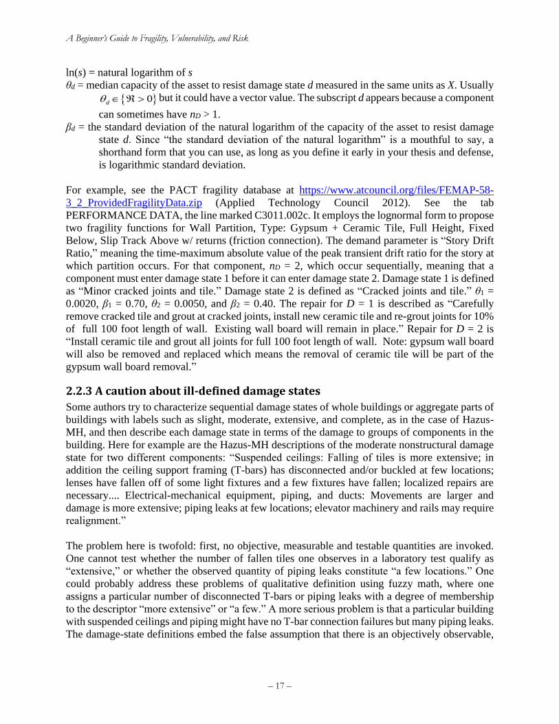
For example, see the PACT fragility database at https://www.atcouncil.org/files/FEMAP-58-
3_2_ProvidedFragilityData.zip (Applied Technology Council 2012). See the tab
PERFORMANCE DATA, the line marked C3011.002c. It employs the lognormal form to propose
two fragility functions for Wall Partition, Type: Gypsum + Ceramic Tile, Full Height, Fixed
Below, Slip Track Above w/ returns (friction connection). The demand parameter is “Story Drift
Ratio,” meaning the time-maximum absolute value of the peak transient drift ratio for the story at
which partition occurs. For that component, nD = 2, which occur sequentially, meaning that a
component must enter damage state 1 before it can enter damage state 2. Damage state 1 is defined
as “Minor cracked joints and tile.” Damage state 2 is defined as “Cracked joints and tile.” θ1 =
0.0020, β1 = 0.70, θ2 = 0.0050, and β2 = 0.40. The repair for D = 1 is described as “Carefully
remove cracked tile and grout at cracked joints, install new ceramic tile and re-grout joints for 10%
of full 100 foot length of wall. Existing wall board will remain in place.” Repair for D = 2 is
“Install ceramic tile and grout all joints for full 100 foot length of wall. Note: gypsum wall board
will also be removed and replaced which means the removal of ceramic tile will be part of the
gypsum wall board removal.”
2.2.3 A caution about ill-defined damage states
Some authors try to characterize sequential damage states of whole buildings or aggregate parts of
buildings with labels such as slight, moderate, extensive, and complete, as in the case of Hazus-
MH, and then describe each damage state in terms of the damage to groups of components in the
building. Here for example are the Hazus-MH descriptions of the moderate nonstructural damage
state for two different components: “Suspended ceilings: Falling of tiles is more extensive; in
addition the ceiling support framing (T-bars) has disconnected and/or buckled at few locations;
lenses have fallen off of some light fixtures and a few fixtures have fallen; localized repairs are
necessary.... Electrical-mechanical equipment, piping, and ducts: Movements are larger and
damage is more extensive; piping leaks at few locations; elevator machinery and rails may require
realignment.”
The problem here is twofold: first, no objective, measurable and testable quantities are invoked.
One cannot test whether the number of fallen tiles one observes in a laboratory test qualify as
“extensive,” or whether the observed quantity of piping leaks constitute “a few locations.” One
could probably address these problems of qualitative definition using fuzzy math, where one
assigns a particular number of disconnected T-bars or piping leaks with a degree of membership
to the descriptor “more extensive” or “a few.” A more serious problem is that a particular building
with suspended ceilings and piping might have no T-bar connection failures but many piping leaks.
The damage-state definitions embed the false assumption that there is an objectively observable,
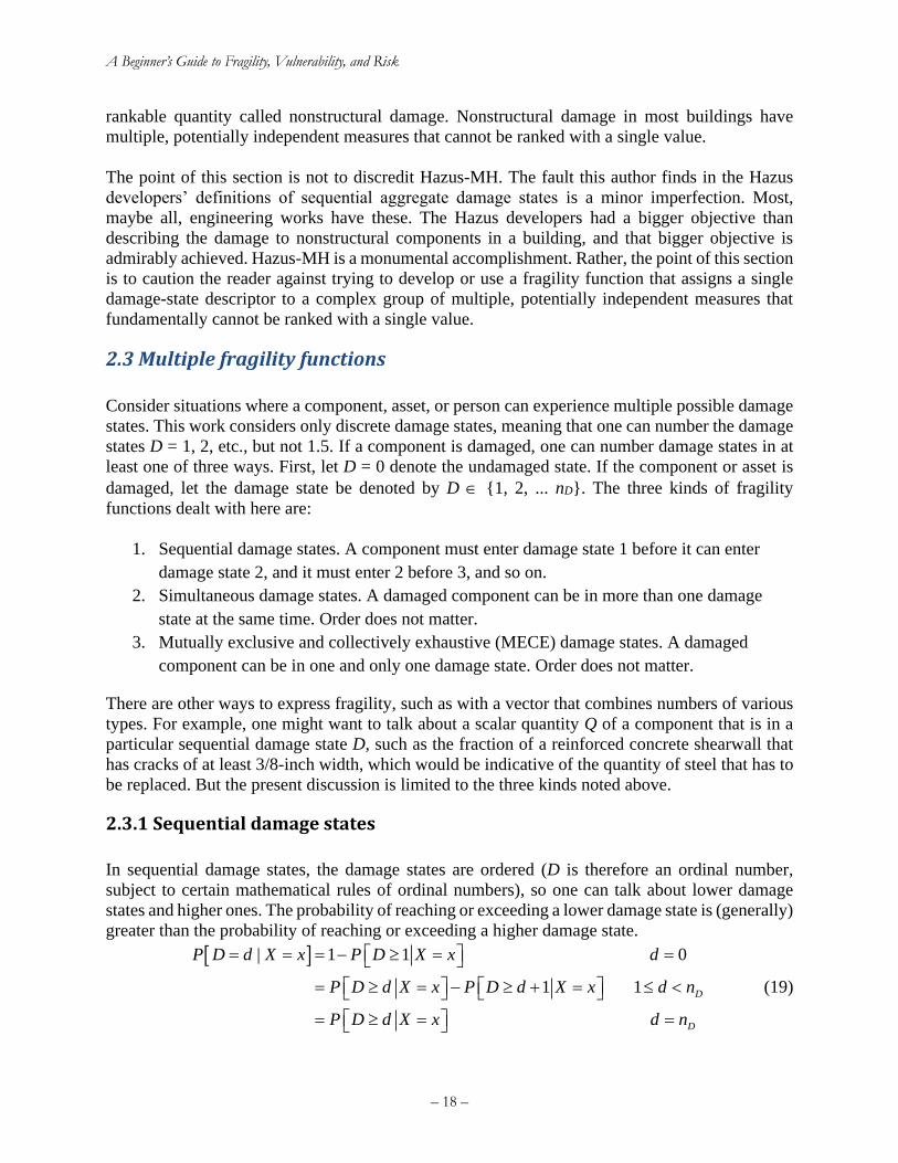
A Beginner’s Guide to Fragility, Vulnerability, and Risk
– 18 –
rankable quantity called nonstructural damage. Nonstructural damage in most buildings have
multiple, potentially independent measures that cannot be ranked with a single value.
The point of this section is not to discredit Hazus-MH. The fault this author finds in the Hazus
developers’ definitions of sequential aggregate damage states is a minor imperfection. Most,
maybe all, engineering works have these. The Hazus developers had a bigger objective than
describing the damage to nonstructural components in a building, and that bigger objective is
admirably achieved. Hazus-MH is a monumental accomplishment. Rather, the point of this section
is to caution the reader against trying to develop or use a fragility function that assigns a single
damage-state descriptor to a complex group of multiple, potentially independent measures that
fundamentally cannot be ranked with a single value.
2.3 Multiple fragility functions
Consider situations where a component, asset, or person can experience multiple possible damage
states. This work considers only discrete damage states, meaning that one can number the damage
states D = 1, 2, etc., but not 1.5. If a component is damaged, one can number damage states in at
least one of three ways. First, let D = 0 denote the undamaged state. If the component or asset is
damaged, let the damage state be denoted by D {1, 2, ... nD}. The three kinds of fragility
functions dealt with here are:
1. Sequential damage states. A component must enter damage state 1 before it can enter
damage state 2, and it must enter 2 before 3, and so on.
2. Simultaneous damage states. A damaged component can be in more than one damage
state at the same time. Order does not matter.
3. Mutually exclusive and collectively exhaustive (MECE) damage states. A damaged
component can be in one and only one damage state. Order does not matter.
There are other ways to express fragility, such as with a vector that combines numbers of various
types. For example, one might want to talk about a scalar quantity Q of a component that is in a
particular sequential damage state D, such as the fraction of a reinforced concrete shearwall that
has cracks of at least 3/8-inch width, which would be indicative of the quantity of steel that has to
be replaced. But the present discussion is limited to the three kinds noted above.
2.3.1 Sequential damage states
In sequential damage states, the damage states are ordered (D is therefore an ordinal number,
subject to certain mathematical rules of ordinal numbers), so one can talk about lower damage
states and higher ones. The probability of reaching or exceeding a lower damage state is (generally)
greater than the probability of reaching or exceeding a higher damage state.
| 1 1 0
1 1 D
D
P D d X x P D X x d
P D d X x P D d X x d n
P D d X x d n
= = = − = =
= = − + =
= = =
(19)
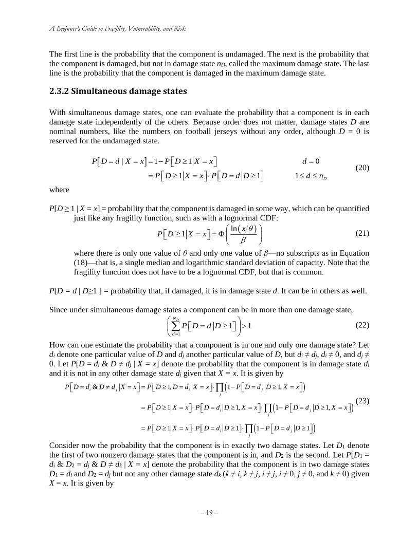
A Beginner’s Guide to Fragility, Vulnerability, and Risk
– 19 –
The first line is the probability that the component is undamaged. The next is the probability that
the component is damaged, but not in damage state nD, called the maximum damage state. The last
line is the probability that the component is damaged in the maximum damage state.
2.3.2 Simultaneous damage states
With simultaneous damage states, one can evaluate the probability that a component is in each
damage state independently of the others. Because order does not matter, damage states D are
nominal numbers, like the numbers on football jerseys without any order, although D = 0 is
reserved for the undamaged state.
| 1 1 0
1 1 1 D
P D d X x P D X x d
P D X x P D d D d n
= = = − = =
= = =
(20)
where
P[D ≥ 1 | X = x] = probability that the component is damaged in some way, which can be quantified
just like any fragility function, such as with a lognormal CDF:
( )ln
1x
P D X x
= =
(21)
where there is only one value of θ and only one value of β—no subscripts as in Equation
(18)—that is, a single median and logarithmic standard deviation of capacity. Note that the
fragility function does not have to be a lognormal CDF, but that is common.
P[D = d | D≥1 ] = probability that, if damaged, it is in damage state d. It can be in others as well.
Since under simultaneous damage states a component can be in more than one damage state,
1
1 1DN
d
P D d D=
=
(22)
How can one estimate the probability that a component is in one and only one damage state? Let
di denote one particular value of D and dj another particular value of D, but di ≠ dj, di ≠ 0, and dj ≠
0. Let P[D = di & D ≠ dj | X = x] denote the probability that the component is in damage state di
and it is not in any other damage state dj given that X = x. It is given by
( )
( )
( )
& 1, 1 1,
1 1, 1 1,
1 1 1 1
i j i j
j
i j
j
i j
j
P D d D d X x P D D d X x P D d D X x
P D X x P D d D X x P D d D X x
P D X x P D d D P D d D
= = = = = − = =
= = = = − = =
= = = − =
(23)
Consider now the probability that the component is in exactly two damage states. Let D1 denote
the first of two nonzero damage states that the component is in, and D2 is the second. Let P[D1 =
di & D2 = dj & D ≠ dk | X = x] denote the probability that the component is in two damage states
D1 = di and D2 = dj but not any other damage state dk (k ≠ i, k ≠ j, i ≠ j, i ≠ 0, j ≠ 0, and k ≠ 0) given
X = x. It is given by
A Beginner’s Guide to Fragility, Vulnerability, and Risk
– 20 –
( )
1 2& &
1 1 1 1 1
i j k
i j k
k
P D d D d D d X x
P D X x P D d D P D d D P D d D
= = = =
= = = = − = (24)
One could repeat for 3 damage states i, j, and k by repeating the pattern. It is the product of the
probabilities that the component is in each damage state i, j, and k, and the probabilities that it is
not in each remaining damage state l, m, n, etc.
2.3.3 MECE damage states
Remember that MECE means that, if the component is damaged (denoted by D ≥ 1), it is in one
and only one nonzero damage state. One can evaluate it by
1 1 0
1 1 1,2,... D
P D d X x P D X x d
P D X x P D d D d N
= = = − = =
= = =
(25)
where
P[D ≥ 1 | X = x] = probability that the component is damaged in some way, which one evaluates
with a single fragility function. If the fragility function is taken as a lognormal CDF, see
Equation (21). Note that the fragility function does not have to be a lognormal CDF, but
that is common.
P[D = d | D ≥ 1 ] = probability that, if damaged, it is damaged in damage state d (and not any other
value of D). Since under MECE damage states a component can only be in one damage
state,
1
1 1DN
d
P D d D=
= =
(26)
2.4 Creating fragility functions
2.4.1 Three general classes of fragility functions
One can distinguish three general classes of fragility functions by the method used to create them:
1. Empirical. An empirical fragility function is one that is created by fitting a function to
approximate observational data from the laboratory or the real world. The observational
data are one of: (1) ordered pairs of environmental excitation and a binary indicator of
failure (i.e., reaching or exceeding the specified limit state), for each of a set of individual
assets; or (2) ordered sets of environmental excitation, number of assets exposed to that
level of excitation, and the number of those that failed when subjected to the environmental
excitation. Empirical fragility functions have been used in earthquake engineering at least
since Kustu et al. (1982). See Merz (1991) for a notable work creating earthquake-related
fragility functions for power-plant equipment.
A Beginner’s Guide to Fragility, Vulnerability, and Risk
– 21 –
2. Analytical. An analytical fragility function is one derived for an asset of class of assets by
creating and analyzing a structural model of the asset class. One could argue that
Czarnecki’s (1973) doctoral thesis presents one of the earliest works deriving building-
component fragility functions by structural analysis.
3. Expert opinion or judgment-based. An expert opinion fragility function is one created by
polling one or more people who have experience with the asset class in question, where the
experts guess or judge failure probability as a function of environmental excitation. ATC-
13 (Applied Technology Council 1985) compiles a large number of judgment-based
fragility functions for California buildings.
One can create fragility functions by a combination of these methods, for example by using
judgment to create a fragility function for one limit state based on empirical data or an analytical
model of another. One could argue that many of the fragility function in Hazus-MH’s earthquake
module are created by such a hybrid approach. Or one can use Bayesian updating to modify a
judgment-based fragility function using observational data. Although all three methods have been
used for decades, Porter et al. (2007) may have been the first to categorize them and offer standard
procedures for creating fragility function by any of these methods.
2.4.2 Data that cannot be used to derive fragility functions
Consider now how fragility functions are made. First, some notes about kinds of data that cannot
be used to derive fragility functions. One kind is data that are biased with respect to damage state.
That is, specimens were observed because they were damaged, or because the damage was
prominent or interesting in some way. Failure data gathered by reconnaissance surveys tend to be
biased in this way and therefore cannot be used to create fragility functions. Another kind is data
where all the specimens were subjected to the same level of excitation. (Technically one could fit
a 1-parameter fragility function to those data, but this author has never seen failure data that look
as if they would be well approximated by a 1-parameter curve.)
2.4.3 What to know before trying to derive a fragility function
Before trying to derive a fragility function, define failure in unambiguous terms that do not require
the exercise of judgment, i.e., where two people observing the same specimen would reach the
same conclusion as to whether a specimen has failed or not. Beware damage scales that do not
meet this test. Second, define the excitation to which specimens are subjected (maximum base
acceleration, peak transient drift ratio, etc.) in similarly unambiguous terms. Third, select
specimens without bias with respect to failure or nonfailure.
2.4.4 Actual failure excitation
In the unusual case where specimens were all tested in a laboratory to failure and the actual
excitation at which each specimen failed is known, then one can fit a lognormal fragility function
to the data as follows. This kind of data is referred to here as type-A data, A for actual failure
excitation. Before using the following math, the analyst must clearly define “failure” and should
A Beginner’s Guide to Fragility, Vulnerability, and Risk
– 22 –
know both the means of observing specimen excitation and failure, as well as a clear definition of
the component or other asset category in question.
ni = number of specimens, ni ≥ 2
i = index to specimens, i {1, 2, … ni}
ri = excitation at which specimen i failed
( )1
1ln
in
i
ii
rn
=
= (27)
( )( )2
1
1ln
1
in
i
ii
rn
=
=−
(28)
2.4.5 Bounding-failure excitation
Suppose one possesses observations where at least one specimen did not fail, at least one specimen
did fail, and one knows the peak excitation to which each specimen was subjected, but not the
actual excitation at which each specimen failed. These data are referred to here as bounding, or
Type-B, data. Specimens are grouped by the maximum level of excitation to which each specimen
was subjected. Assume the fragility function is reasonably like a lognormal cumulative distribution
function and find the parameter values θ (median) and β (logarithmic standard deviation) as
follows.
mi = numbers of levels of excitation among the data, referred to here as bins, mi ≥ 2
i = bin index, i {1, 2, … mi}
ri = maximum excitation to which specimens in bin i were subjected
ni = number of specimens in bin i, ni {1, 2, … }
fi = number of specimens in bin i that failed, fi {0, 1, … ni}
One proper way to estimate θ and β is by the maximum likelihood method, i.e., by finding the
values of θ and β that have the highest likelihood of producing the observed data. At any level of
excitation ri, there is a probability of any individual specimen failing that is given by the lognormal
CDF. Let pi denote this probability:
( )ln i
i
rp
=
(29)
Assume that the failure of any two different specimens is independent conditioned on excitation.
In that case, if one were to estimate the number of failed specimens in bin i, it would be proper to
take that number as a random variable with a binomial distribution. Let Fi denote that random
variable. The following equation gives the probability that one will observe fi failures among ni
specimens with the per-occurrence failure probability pi:
( )
( )!
1! !
i iin ffi
i i i i
i i i
nP F f p p
f n f
−= = −
− (30)
This is the binomial distribution. One finds the θ and β values that maximize the likelihood of
observing all the data {n1, f1, n2, f2, ….} given excitations {r1, r2, …}. That likelihood is given by

A Beginner’s Guide to Fragility, Vulnerability, and Risk
– 23 –
the product of the probabilities in equation 3, multiplied over all the bins. That is, find θ and β that
maximize L(θ, β) in:
( ) 1
,im
i i
i
L P F f =
= = (31)
One can explicitly maximize L(θ,β), but it is easier to use Excel or similar Matlab or other software.
Excel’s solver is straightforward.
It may be easier to remember a more approximate approach, which takes advantage of the fact that
for large ni, the binomial approximates the Gaussian distribution, in which case it is proper to
minimize the weighted squares of the difference between the observed data and the idealized
fragility function. That is, find θ and β that minimize the squared error term ε2(θ,β) in:
( )2
2
1
,im
ii i
i i
fn p
n
=
= −
(32)
The difference between the fragility functions derived by these two different methods appears to
be small compared with the scatter about the regression lines, so arguments about what is more
proper tend to be academic compared with the choice of which one is easier. There is at least one
more reasonable approach, called logistic regression, but again this approach tends to produce
roughly the same values of θ and β, with differences that are small compared with data scatter.
2.4.6 Other data conditions
There are cases where none of the specimens failed (type-C, or capable, data), where failure is
derived by structural analysis (type-D data), where expert opinion is used (type-E), or where
Bayesian updating is used to update an existing fragility function with new evidence (type U). For
such situations, see Porter et al. (2007).
2.4.7 Dealing with under-representative specimens
If the specimens used to create the fragility function are very few in number or unrepresentative
of the broader class whose fragility is desired, or if the excitation to which they were subjected
was unlike real-world earthquake shaking, one can reflect added uncertainty associated with
unrepresentative conditions by increasing the fragility function’s logarithmic standard deviation.
The FEMA P-58 guidelines for example suggest always increasing the logarithmic standard
deviation of a fragility function that is derived from test data or observations, as follows.
2 2
u = + (33)
where β’ is the new, increased value of the logarithmic standard deviation of the fragility function,
β is the value derived using the test or post-earthquake observation data, and βu is a term to reflect
uncertainty that the tests represent real-world conditions of installation and loading, or uncertainty
that the available data are an adequate sample size to accurately represent the true variability.
FEMA P-58 recommends values of βu depending on how under-representative are the data. If any
of the following is true, use a minimum value of βu = 0.25, otherwise, use βu = 0.10.
A Beginner’s Guide to Fragility, Vulnerability, and Risk
– 24 –
1. Data are available for five or fewer specimens.
2. In an actual building, a component can be installed in a number of different configurations, but
all specimens were tested with the same configuration.
3. All specimens were subjected to the same loading protocol.
4. Actual behavior of the component is expected to be dependent on two or more demand
parameters (e.g., simultaneous drift in two orthogonal directions), but specimens were loaded
using only one demand parameter.
In the case of Type-B data, increasing β using Equation (33) introduces a bias in long-term failure
probability and can cause the fragility function not to pass through the actual failure data well. If
the data generally lie at excitation levels below the derived median capacity θ, which is common,
then increasing β without adjusting θ will cause the fragility function to move up (to higher
probabilities) relative to the data. To increase β while still ensuring that the derived fragility
function passes through the data, one can adjust θ as follows:
1
1
i
i
N
i i
i
N
i
i
r n
r
n
=
=
=
(34)
( )r
r
−
=
(35)
In the case of type-A data, use ni = 1 for all i in Equation (34). For example, imagine that 17
suspended ceilings of identical construction are installed in a large, stiff single-story building, a
block away from a 2-story building with 3 suspended ceilings on the upper floor. A ceiling in the
1-story building and two ceilings in the 2-story building collapse in a particular earthquake. The
estimated roof accelerations in the two buildings are 0.25 and 0.45g, respectively. These type-B
data are used to derive a fragility function in terms of peak floor acceleration, with β = 0.3 and θ
= 0.4g. These conditions meet FEMA P-58’s criteria 2 and 3, so βu = 0.25. Applying the FEMA
P-58 recommended value βu = 0.25 and evaluating Equations (33), (34), and (35) yields
2 20.3 0.25 0.39 = + =
( )17 0.25 3 0.45
0.2820
r +
= =
( )0.39 0.300.28
0.28 0.450.4
−
= =
Figure 12 illustrates the data, the fragility function before increasing β (the solid line), and the
fragility function after increasing β. Note how the two curves cross at r = r and how θ’ > θ. The
solid curve passes through the data because there are only two data points, but it passes over the
first data point and below the second, closer to the first because the first represents more data.
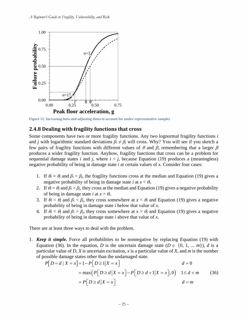
A Beginner’s Guide to Fragility, Vulnerability, and Risk
– 25 –
Figure 12. Increasing beta and adjusting theta to account for under-representative samples
2.4.8 Dealing with fragility functions that cross
Some components have two or more fragility functions. Any two lognormal fragility functions i
and j with logarithmic standard deviations βi ≠ βj will cross. Why? You will see if you sketch a
few pairs of fragility functions with different values of and , remembering that a larger
produces a wider fragility function. Anyhow, fragility functions that cross can be a problem for
sequential damage states i and j, where i < j, because Equation (19) produces a (meaningless)
negative probability of being in damage state i at certain values of x. Consider four cases:
1. If i = j and βi < βj, the fragility functions cross at the median and Equation (19) gives a
negative probability of being in damage state i at x < i.
2. If i = j and βi > βj, they cross at the median and Equation (19) gives a negative probability
of being in damage state i at x > i.
3. If i < j and βi < βj, they cross somewhere at x < i and Equation (19) gives a negative
probability of being in damage state i below that value of x.
4. If i < j and βi > βj, they cross somewhere at x > j and Equation (19) gives a negative
probability of being in damage state i above that value of x.
There are at least three ways to deal with the problem.
1. Keep it simple. Force all probabilities to be nonnegative by replacing Equation (19) with
Equation (36). In the equation, D is the uncertain damage state (D {0, 1, ... m}), d is a
particular value of D, X is uncertain excitation, x is a particular value of X, and m is the number
of possible damage states other than the undamaged state.
( )
| 1 1 0
max 1 ,0 1
P D d X x P D X x d
P D d X x P D d X x d m
P D d X x d m
= = = − = =
= = − + =
= = =
(36)
0.00
0.25
0.50
0.75
1.00
0.00 0.25 0.50 0.75
Fa
ilu
re p
rob
ab
ilit
y
Peak floor acceleration, g
n=17
n=3
θ′θ
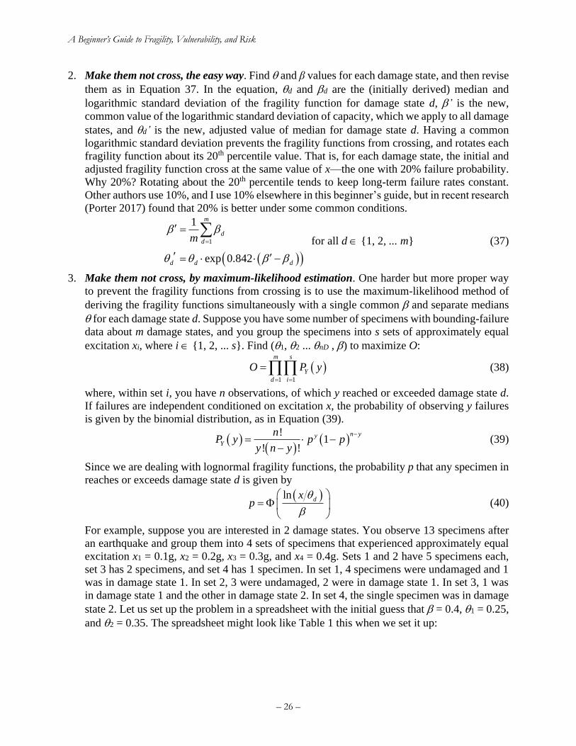
A Beginner’s Guide to Fragility, Vulnerability, and Risk
– 26 –
2. Make them not cross, the easy way. Find and β values for each damage state, and then revise
them as in Equation 37. In the equation, d and d are the (initially derived) median and
logarithmic standard deviation of the fragility function for damage state d, ’ is the new,
common value of the logarithmic standard deviation of capacity, which we apply to all damage
states, and d’ is the new, adjusted value of median for damage state d. Having a common
logarithmic standard deviation prevents the fragility functions from crossing, and rotates each
fragility function about its 20th percentile value. That is, for each damage state, the initial and
adjusted fragility function cross at the same value of x—the one with 20% failure probability.
Why 20%? Rotating about the 20th percentile tends to keep long-term failure rates constant.
Other authors use 10%, and I use 10% elsewhere in this beginner’s guide, but in recent research
(Porter 2017) found that 20% is better under some common conditions.
( )( )
1
1
exp 0.842
m
d
d
d d d
m
=
=
= −
for all d {1, 2, ... m} (37)
3. Make them not cross, by maximum-likelihood estimation. One harder but more proper way
to prevent the fragility functions from crossing is to use the maximum-likelihood method of
deriving the fragility functions simultaneously with a single common and separate medians
for each damage state d. Suppose you have some number of specimens with bounding-failure
data about m damage states, and you group the specimens into s sets of approximately equal
excitation xi, where i {1, 2, ... s}. Find (1, 2 ... nD , ) to maximize O:
( )1 1
m s
Y
d i
O P y= =
= (38)
where, within set i, you have n observations, of which y reached or exceeded damage state d.
If failures are independent conditioned on excitation x, the probability of observing y failures
is given by the binomial distribution, as in Equation (39).
( )( )
( )!
1! !
n yy
Y
nP y p p
y n y
−= −
− (39)
Since we are dealing with lognormal fragility functions, the probability p that any specimen in
reaches or exceeds damage state d is given by
( )ln dx
p
=
(40)
For example, suppose you are interested in 2 damage states. You observe 13 specimens after
an earthquake and group them into 4 sets of specimens that experienced approximately equal
excitation x1 = 0.1g, x2 = 0.2g, x3 = 0.3g, and x4 = 0.4g. Sets 1 and 2 have 5 specimens each,
set 3 has 2 specimens, and set 4 has 1 specimen. In set 1, 4 specimens were undamaged and 1
was in damage state 1. In set 2, 3 were undamaged, 2 were in damage state 1. In set 3, 1 was
in damage state 1 and the other in damage state 2. In set 4, the single specimen was in damage
state 2. Let us set up the problem in a spreadsheet with the initial guess that = 0.4, 1 = 0.25,
and 2 = 0.35. The spreadsheet might look like Table 1 this when we set it up:
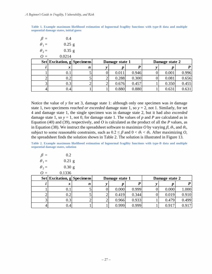
A Beginner’s Guide to Fragility, Vulnerability, and Risk
– 27 –
Table 1. Example maximum likelihood estimation of lognormal fragility functions with type-B data and multiple
sequential damage states, initial guess
Notice the value of y for set 3, damage state 1: although only one specimen was in damage
state 1, two specimens reached or exceeded damage state 1, so y = 2, not 1. Similarly, for set
4 and damage state 1, the single specimen was in damage state 2, but it had also exceeded
damage state 1, so y = 1, not 0, for damage state 1. The values of p and P are calculated as in
Equation (40) and (39), respectively, and O is calculated as the product of all the P values, as
in Equation (38). We instruct the spreadsheet software to maximize O by varying , 1, and 2,
subject to some reasonable constraints, such as 0.2 ≤ and 0 < 1 < 2. After maximizing O,
the spreadsheet finds the solution shown in Table 2. The solution is illustrated in Figure 13.
Table 2. Example maximum likelihood estimation of lognormal fragility functions with type-B data and multiple
sequential damage states, solution
= 0.4
1 = 0.25 g
2 = 0.35 g
O = 0.0214
Set Excitation, g Specimens
i x n y p P y p P
1 0.1 5 0 0.011 0.946 0 0.001 0.996
2 0.2 5 2 0.288 0.300 0 0.081 0.656
3 0.3 2 2 0.676 0.457 1 0.350 0.455
4 0.4 1 1 0.880 0.880 1 0.631 0.631
Damage state 1 Damage state 2
= 0.2
1 = 0.21 g
2 = 0.30 g
O = 0.1336
Set Excitation, g Specimens
i x n y p P y p P
1 0.1 5 0 0.000 0.999 0 0.000 1.000
2 0.2 5 2 0.419 0.344 0 0.019 0.910
3 0.3 2 2 0.966 0.933 1 0.479 0.499
4 0.4 1 1 0.999 0.999 1 0.917 0.917
Damage state 1 Damage state 2
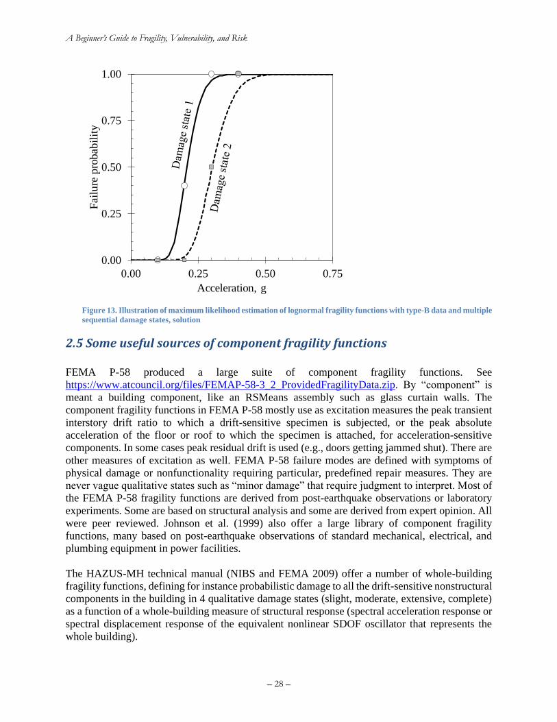
A Beginner’s Guide to Fragility, Vulnerability, and Risk
– 28 –
Figure 13. Illustration of maximum likelihood estimation of lognormal fragility functions with type-B data and multiple
sequential damage states, solution
2.5 Some useful sources of component fragility functions
FEMA P-58 produced a large suite of component fragility functions. See
https://www.atcouncil.org/files/FEMAP-58-3_2_ProvidedFragilityData.zip. By “component” is
meant a building component, like an RSMeans assembly such as glass curtain walls. The
component fragility functions in FEMA P-58 mostly use as excitation measures the peak transient
interstory drift ratio to which a drift-sensitive specimen is subjected, or the peak absolute
acceleration of the floor or roof to which the specimen is attached, for acceleration-sensitive
components. In some cases peak residual drift is used (e.g., doors getting jammed shut). There are
other measures of excitation as well. FEMA P-58 failure modes are defined with symptoms of
physical damage or nonfunctionality requiring particular, predefined repair measures. They are
never vague qualitative states such as “minor damage” that require judgment to interpret. Most of
the FEMA P-58 fragility functions are derived from post-earthquake observations or laboratory
experiments. Some are based on structural analysis and some are derived from expert opinion. All
were peer reviewed. Johnson et al. (1999) also offer a large library of component fragility
functions, many based on post-earthquake observations of standard mechanical, electrical, and
plumbing equipment in power facilities.
The HAZUS-MH technical manual (NIBS and FEMA 2009) offer a number of whole-building
fragility functions, defining for instance probabilistic damage to all the drift-sensitive nonstructural
components in the building in 4 qualitative damage states (slight, moderate, extensive, complete)
as a function of a whole-building measure of structural response (spectral acceleration response or
spectral displacement response of the equivalent nonlinear SDOF oscillator that represents the
whole building).
0.00
0.25
0.50
0.75
1.00
0.00 0.25 0.50 0.75
Fai
lure
pro
bab
ilit
y
Acceleration, g
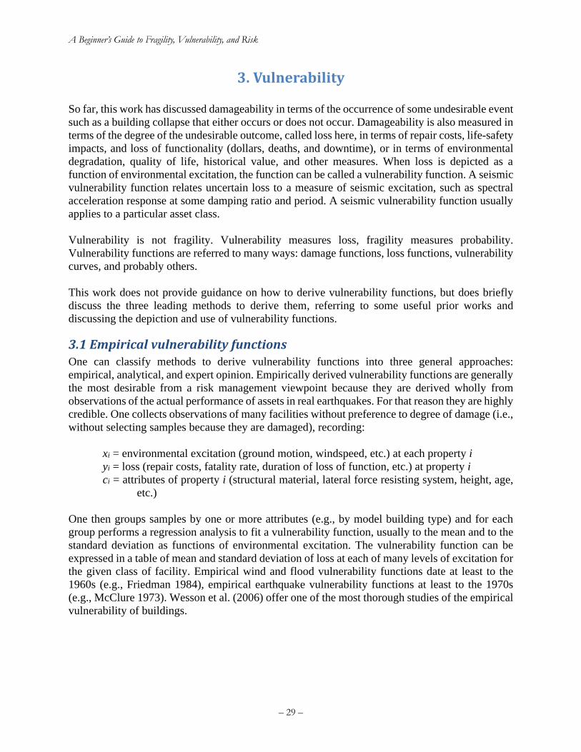
A Beginner’s Guide to Fragility, Vulnerability, and Risk
– 29 –
3. Vulnerability
So far, this work has discussed damageability in terms of the occurrence of some undesirable event
such as a building collapse that either occurs or does not occur. Damageability is also measured in
terms of the degree of the undesirable outcome, called loss here, in terms of repair costs, life-safety
impacts, and loss of functionality (dollars, deaths, and downtime), or in terms of environmental
degradation, quality of life, historical value, and other measures. When loss is depicted as a
function of environmental excitation, the function can be called a vulnerability function. A seismic
vulnerability function relates uncertain loss to a measure of seismic excitation, such as spectral
acceleration response at some damping ratio and period. A seismic vulnerability function usually
applies to a particular asset class.
Vulnerability is not fragility. Vulnerability measures loss, fragility measures probability.
Vulnerability functions are referred to many ways: damage functions, loss functions, vulnerability
curves, and probably others.
This work does not provide guidance on how to derive vulnerability functions, but does briefly
discuss the three leading methods to derive them, referring to some useful prior works and
discussing the depiction and use of vulnerability functions.
3.1 Empirical vulnerability functions One can classify methods to derive vulnerability functions into three general approaches:
empirical, analytical, and expert opinion. Empirically derived vulnerability functions are generally
the most desirable from a risk management viewpoint because they are derived wholly from
observations of the actual performance of assets in real earthquakes. For that reason they are highly
credible. One collects observations of many facilities without preference to degree of damage (i.e.,
without selecting samples because they are damaged), recording:
xi = environmental excitation (ground motion, windspeed, etc.) at each property i
yi = loss (repair costs, fatality rate, duration of loss of function, etc.) at property i
ci = attributes of property i (structural material, lateral force resisting system, height, age,
etc.)
One then groups samples by one or more attributes (e.g., by model building type) and for each
group performs a regression analysis to fit a vulnerability function, usually to the mean and to the
standard deviation as functions of environmental excitation. The vulnerability function can be
expressed in a table of mean and standard deviation of loss at each of many levels of excitation for
the given class of facility. Empirical wind and flood vulnerability functions date at least to the
1960s (e.g., Friedman 1984), empirical earthquake vulnerability functions at least to the 1970s
(e.g., McClure 1973). Wesson et al. (2006) offer one of the most thorough studies of the empirical
vulnerability of buildings.
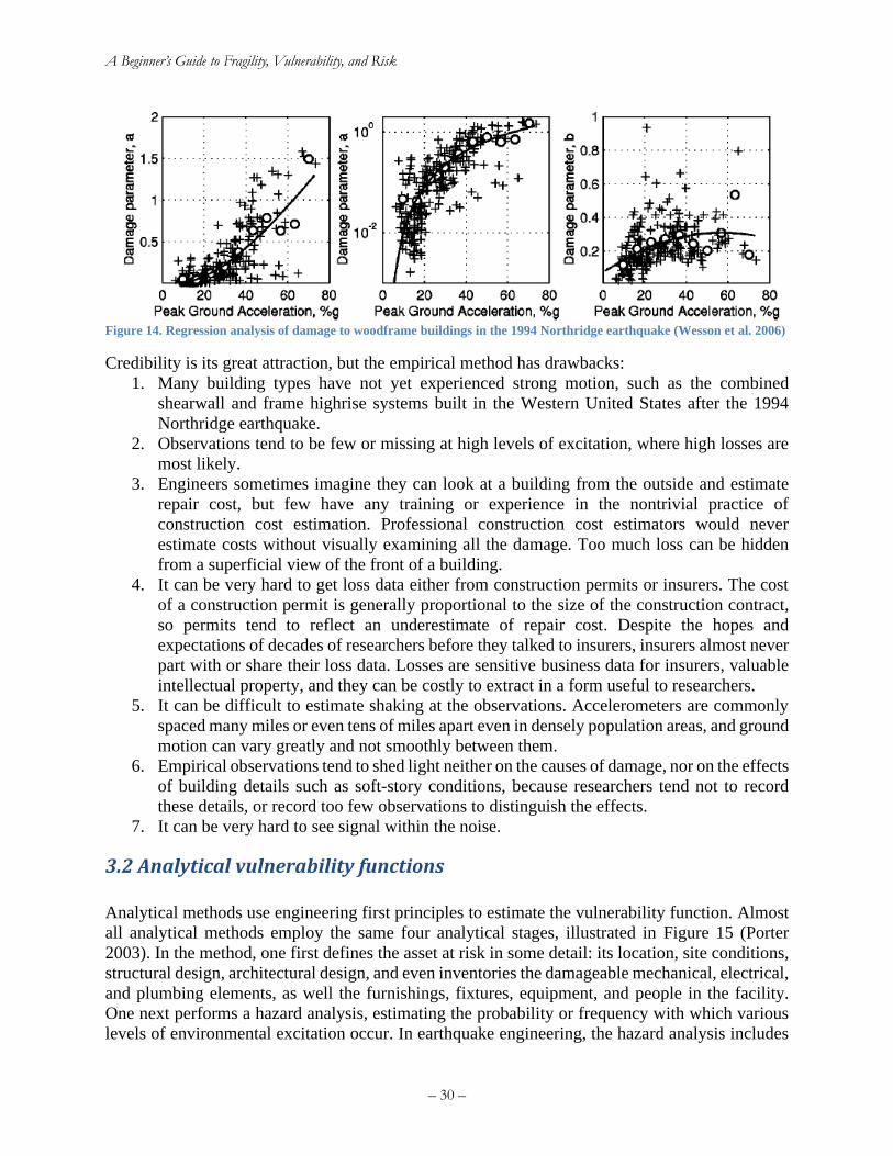
A Beginner’s Guide to Fragility, Vulnerability, and Risk
– 30 –
Figure 14. Regression analysis of damage to woodframe buildings in the 1994 Northridge earthquake (Wesson et al. 2006)
Credibility is its great attraction, but the empirical method has drawbacks:
1. Many building types have not yet experienced strong motion, such as the combined
shearwall and frame highrise systems built in the Western United States after the 1994
Northridge earthquake.
2. Observations tend to be few or missing at high levels of excitation, where high losses are
most likely.
3. Engineers sometimes imagine they can look at a building from the outside and estimate
repair cost, but few have any training or experience in the nontrivial practice of
construction cost estimation. Professional construction cost estimators would never
estimate costs without visually examining all the damage. Too much loss can be hidden
from a superficial view of the front of a building.
4. It can be very hard to get loss data either from construction permits or insurers. The cost
of a construction permit is generally proportional to the size of the construction contract,
so permits tend to reflect an underestimate of repair cost. Despite the hopes and
expectations of decades of researchers before they talked to insurers, insurers almost never
part with or share their loss data. Losses are sensitive business data for insurers, valuable
intellectual property, and they can be costly to extract in a form useful to researchers.
5. It can be difficult to estimate shaking at the observations. Accelerometers are commonly
spaced many miles or even tens of miles apart even in densely population areas, and ground
motion can vary greatly and not smoothly between them.
6. Empirical observations tend to shed light neither on the causes of damage, nor on the effects
of building details such as soft-story conditions, because researchers tend not to record
these details, or record too few observations to distinguish the effects.
7. It can be very hard to see signal within the noise.
3.2 Analytical vulnerability functions
Analytical methods use engineering first principles to estimate the vulnerability function. Almost
all analytical methods employ the same four analytical stages, illustrated in Figure 15 (Porter
2003). In the method, one first defines the asset at risk in some detail: its location, site conditions,
structural design, architectural design, and even inventories the damageable mechanical, electrical,
and plumbing elements, as well the furnishings, fixtures, equipment, and people in the facility.
One next performs a hazard analysis, estimating the probability or frequency with which various
levels of environmental excitation occur. In earthquake engineering, the hazard analysis includes
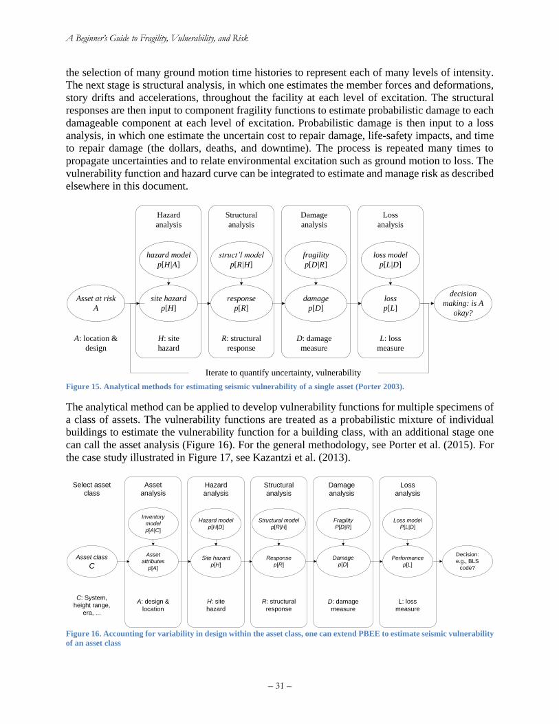
A Beginner’s Guide to Fragility, Vulnerability, and Risk
– 31 –
the selection of many ground motion time histories to represent each of many levels of intensity.
The next stage is structural analysis, in which one estimates the member forces and deformations,
story drifts and accelerations, throughout the facility at each level of excitation. The structural
responses are then input to component fragility functions to estimate probabilistic damage to each
damageable component at each level of excitation. Probabilistic damage is then input to a loss
analysis, in which one estimate the uncertain cost to repair damage, life-safety impacts, and time
to repair damage (the dollars, deaths, and downtime). The process is repeated many times to
propagate uncertainties and to relate environmental excitation such as ground motion to loss. The
vulnerability function and hazard curve can be integrated to estimate and manage risk as described
elsewhere in this document.
Figure 15. Analytical methods for estimating seismic vulnerability of a single asset (Porter 2003).
The analytical method can be applied to develop vulnerability functions for multiple specimens of
a class of assets. The vulnerability functions are treated as a probabilistic mixture of individual
buildings to estimate the vulnerability function for a building class, with an additional stage one
can call the asset analysis (Figure 16). For the general methodology, see Porter et al. (2015). For
the case study illustrated in Figure 17, see Kazantzi et al. (2013).
Figure 16. Accounting for variability in design within the asset class, one can extend PBEE to estimate seismic vulnerability
of an asset class
site hazard
p[H]
H: site
hazard
Asset at risk
A
decision
making: is A
okay?
Hazard
analysis
Structural
analysis
struct’l model
p[R|H]
R: structural
response
A: location &
design
Damage
analysis
fragility
p[D|R]
damage
p[D]
D: damage
measure
Loss
analysis
loss model
p[L|D]
loss
p[L]
L: loss
measure
response
p[R]
hazard model
p[H|A]
Iterate to quantify uncertainty, vulnerability
Site hazard
p[H]
H: site
hazard
Asset
attributes
p[A]
Hazard
analysis
Structural
analysis
Structural model
p[R|H]
R: structural
response
A: design &
location
Damage
analysis
Fragility
P[D|R]
Damage
p[D]
D: damage
measure
Loss
analysis
Loss model
P[L|D]
Performance
p[L]
L: loss
measure
Hazard model
p[H|D]
Response
p[R]
Asset
analysis
Asset class
C
C: System,
height range,
era, ...
Select asset
class
Inventory
model
p[A|C]
Decision:
e.g., BLS
code?
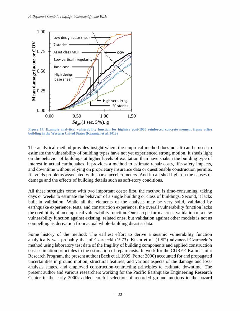
A Beginner’s Guide to Fragility, Vulnerability, and Risk
– 32 –
Figure 17. Example analytical vulnerability function for highrise post-1980 reinforced concrete moment frame office
building in the Western United States (Kazantzi et al. 2013)
The analytical method provides insight where the empirical method does not. It can be used to
estimate the vulnerability of building types have not yet experienced strong motion. It sheds light
on the behavior of buildings at higher levels of excitation than have shaken the building type of
interest in actual earthquakes. It provides a method to estimate repair costs, life-safety impacts,
and downtime without relying on proprietary insurance data or questionable construction permits.
It avoids problems associated with sparse accelerometers. And it can shed light on the causes of
damage and the effects of building details such as soft-story conditions.
All these strengths come with two important costs: first, the method is time-consuming, taking
days or weeks to estimate the behavior of a single building or class of buildings. Second, it lacks
built-in validation. While all the elements of the analysis may be very solid, validated by
earthquake experience, tests, and construction experience, the overall vulnerability function lacks
the credibility of an empirical vulnerability function. One can perform a cross-validation of a new
vulnerability function against existing, related ones, but validation against other models is not as
compelling as derivation from actual whole-building disaster data.
Some history of the method: The earliest effort to derive a seismic vulnerability function
analytically was probably that of Czarnecki (1973). Kustu et al. (1982) advanced Czarnecki’s
method using laboratory test data of the fragility of building components and applied construction
cost-estimation principles to the estimation of repair costs. In work for the CUREE-Kajima Joint
Research Program, the present author (Beck et al. 1999, Porter 2000) accounted for and propagated
uncertainties in ground motion, structural features, and various aspects of the damage and loss-
analysis stages, and employed construction-contracting principles to estimate downtime. The
present author and various researchers working for the Pacific Earthquake Engineering Research
Center in the early 2000s added careful selection of recorded ground motions to the hazard
0.00
0.25
0.50
0.75
1.00
0.00 0.50 1.00 1.50
Mea
n d
am
age
fact
or
or
CO
V
Sagm(1 sec, 5%), g
Low design base shear
7 stories
Asset class MDF
Low vertical irregularity
Base case
High designbase shear
20 stories
High vert. irreg.
COV
A Beginner’s Guide to Fragility, Vulnerability, and Risk
– 33 –
analysis, incremental dynamic analysis (IDA), separate treatment of collapse, and large databases
of ground motion and component damage. The Applied Technology Council (Applied Technology
Council 2012) encoded the procedures developed by the present author, other PEER researchers,
and various others into professional guidelines for performance-based earthquake engineering.
In earlier work for FEMA, Kircher et al. (1997) developed an analytical vulnerability procedure
for the national risk-management software Hazus-MH (e.g., NIBS and FEMA 2012). The building
is idealized as a single-degree-of-freedom nonlinear oscillator. The method employs nonlinear
pseudostatic structural analysis to estimate the acceleration and displacement of the oscillator,
which is then translated to acceleration and drift imposed on three aggregate building components:
structural, nonstructural drift-sensitive, and nonstructural accelerations-sensitive components.
Four damage states are defined for each (defined using sometimes troublesomely qualitative or
subjective language) along with repair costs and other consequences. The great power of the
methodology is that the authors estimated all the parameters required to estimate repair costs and
other consequences for virtually every building type in the United States.
3.3 Expert opinion vulnerability functions
Where empirical data are lacking and analytical methods are too costly, one can draw on expert
opinion, as was done in the seminal work ATC-13 (Applied Technology Council 1985). Formal
methods to elicit expert opinion date at least to the 1960s, when the RAND Corporation (Gordon
and Helmer 1964) and developed a procedure dubbed the Delphi Process (a reference to the Oracle
of Delphi) to elicit opinion on a variety of scientific and social of the coming 50 years. For
example, the RAND experts predicted a world population of 5.1 billion by 2000 (it was 6.1 billion,
reasonably close at a distance of 36 years), controlled thermonuclear power as a common energy
source (the first nuclear power plant was online 10 years previous), functional regional weather
control, high-IQ machines, mining on the moon, and various other hits and misses.
The authors of ATC-13 employed the Delphi Process to elicit seismic vulnerability functions for
78 classes of facility (buildings, bridges, and others) in terms of dollars, deaths, and downtime
versus MMI. Essentially the process involves collecting a few experts (on the order of 5 to 10) in
a room, presenting them with an asset class of interest, and asking them to guess (or judge, to
dignify the process somewhat) losses to the asset class at various levels of excitation. ATC-13 had
the experts self-rate their expertise. Recent earthquake engineering researchers have applied
methods to objectively measure the expertise of each contributor. The guesses are treated as if they
were actual observations, weighted in proportion to the self-judged or tested expertise, and
combined to produce vulnerability functions for the class.
Expert opinion is very efficient, capable of produce a new vulnerability function at the cost of a
few person-hours each, of estimating the performance of buildings that have not yet experienced
strong motion, and of estimating the effects of building features such as soft-story conditions. Its
great disadvantages are: (1) lack of credibility because it cannot be objectively tested other than
through cross-validation; and (2) underestimation of uncertainty. Experts often have an
exaggerated idea of their own sagacity. Item 2 can be controlled with careful conditioning of the
experts, though this seems never to have been done in the few earthquake engineering applications
of which the author is aware.
A Beginner’s Guide to Fragility, Vulnerability, and Risk
– 34 –
3.4 How to express a vulnerability function
When a vulnerability function measures repair cost, it is commonly normalized by replacement
cost new (RCN), a term which here means the cost of a similar new property having the nearest
equivalent utility as the property being appraised, as of a specific date (American Society of
Appraisers 2013). RCN excludes land value and usually refers to part or all of the fixed
components of a building or other asset (structural, architectural, mechanical, electrical, and
plumbing components) or to its contents. Repair cost divided by RCN is referred to here as damage
factor (DF). Some authors call it damage ratio, fractional loss, or other terms. The expected value
of DF conditioned on excitation is commonly called mean damage factor (MDF). Sometimes it is
assumed that if DF exceeds some threshold value such as 0.6, the property is not worth repairing
and is a total loss, so repair-cost vulnerability functions can jump abruptly from 0.6 (or other
threshold value) to 1.0 with increasing excitation. In principle DF can exceed 1.0 because it can
cost more to repair a building than to replace it.
When a vulnerability function measures life-safety impacts, it commonly measures the fraction of
indoor occupants who become casualties (that is, they are killed or experience a nonfatal injury to
some specified degree) as a function of excitation. There are a variety of human-injury scales,
some used by civil engineers and others used by public health professionals. Before using a terms
such a minor injury, one should be sure its meaning is entirely clear and meaningful to the intended
user of the vulnerability information. Civil engineers sometimes use casualty scales that are
ambiguous or not useful to public health professionals.
Downtime is commonly measured in terms of days or fractions of a year during which the asset
cannot be used for its intended purposes. Sometimes it measures the time from the environmental
shock (the earthquake, in the case of a seismic vulnerability function) to the time when all repairs
are completed, which includes both the time required to perform the repairs and a previous period
during which damage is assessed, repairs are designed, financing is arranged, repairs are bid out,
and the repair contractor mobilizes to the site.
Many vulnerability functions are expressed with conditional probability distributions that give a
probability that loss will not exceed some specified value given the excitation, for a particular asset
class. The distribution is often assigned a parametric form such as lognormal or beta, in which case
the parameters of the distribution are all required, some or all of them conditioned on excitation.
For use in subsequent discussion of earthquake risk, let
X = uncertain loss
y(s) = expected value of loss given shaking s, called the mean seismic vulnerability function
FX|S=s(x) = P[X≤x|S=s] = the cumulative probability distribution function of loss conditioned on
shaking S = s. It is sometimes taken as lognormal, sometimes a beta distributed (see the
sidebar)
Sidebar: the beta distribution
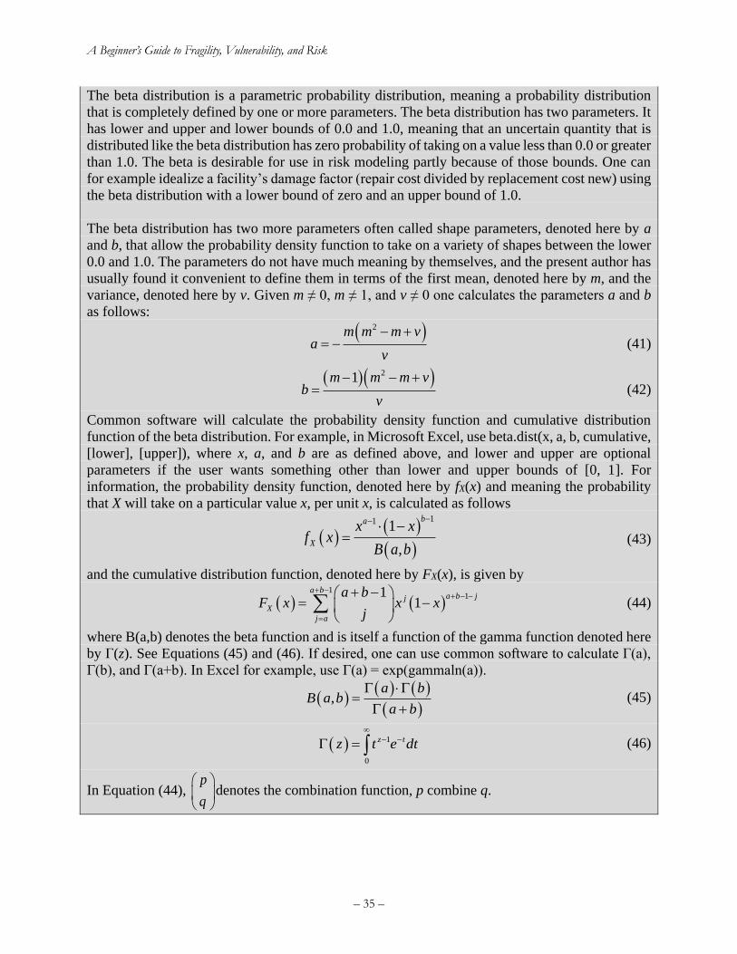
A Beginner’s Guide to Fragility, Vulnerability, and Risk
– 35 –
The beta distribution is a parametric probability distribution, meaning a probability distribution
that is completely defined by one or more parameters. The beta distribution has two parameters. It
has lower and upper and lower bounds of 0.0 and 1.0, meaning that an uncertain quantity that is
distributed like the beta distribution has zero probability of taking on a value less than 0.0 or greater
than 1.0. The beta is desirable for use in risk modeling partly because of those bounds. One can
for example idealize a facility’s damage factor (repair cost divided by replacement cost new) using
the beta distribution with a lower bound of zero and an upper bound of 1.0.
The beta distribution has two more parameters often called shape parameters, denoted here by a
and b, that allow the probability density function to take on a variety of shapes between the lower
0.0 and 1.0. The parameters do not have much meaning by themselves, and the present author has
usually found it convenient to define them in terms of the first mean, denoted here by m, and the
variance, denoted here by v. Given m ≠ 0, m ≠ 1, and v ≠ 0 one calculates the parameters a and b
as follows:
( )2m m m v
av
− += − (41)
( )( )21m m m v
bv
− − += (42)
Common software will calculate the probability density function and cumulative distribution
function of the beta distribution. For example, in Microsoft Excel, use beta.dist(x, a, b, cumulative,
[lower], [upper]), where x, a, and b are as defined above, and lower and upper are optional
parameters if the user wants something other than lower and upper bounds of [0, 1]. For
information, the probability density function, denoted here by fX(x) and meaning the probability
that X will take on a particular value x, per unit x, is calculated as follows
( )( )
( )
11 1
,
ba
X
x xf x
B a b
−− −= (43)
and the cumulative distribution function, denoted here by FX(x), is given by
( ) ( )1
111
a ba b jj
X
j a
a bF x x x
j
+ −+ − −
=
+ − = −
(44)
where B(a,b) denotes the beta function and is itself a function of the gamma function denoted here
by Γ(z). See Equations (45) and (46). If desired, one can use common software to calculate Γ(a),
Γ(b), and Γ(a+b). In Excel for example, use Γ(a) = exp(gammaln(a)).
( )( ) ( )
( ),
a bB a b
a b
=
+ (45)
( ) 1
0
z tz t e dt
− − = (46)
In Equation (44), p
q
denotes the combination function, p combine q.
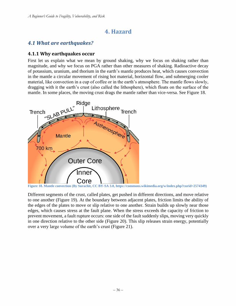
A Beginner’s Guide to Fragility, Vulnerability, and Risk
– 36 –
4. Hazard
4.1 What are earthquakes?
4.1.1 Why earthquakes occur
First let us explain what we mean by ground shaking, why we focus on shaking rather than
magnitude, and why we focus on PGA rather than other measures of shaking. Radioactive decay
of potassium, uranium, and thorium in the earth’s mantle produces heat, which causes convection
in the mantle a circular movement of rising hot material, horizontal flow, and submerging cooler
material, like convection in a cup of coffee or in the earth’s atmosphere. The mantle flows slowly,
dragging with it the earth’s crust (also called the lithosphere), which floats on the surface of the
mantle. In some places, the moving crust drags the mantle rather than vice-versa. See Figure 18.
Figure 18. Mantle convection (By Surachit, CC BY-SA 3.0, https://commons.wikimedia.org/w/index.php?curid=2574349)
Different segments of the crust, called plates, get pushed in different directions, and move relative
to one another (Figure 19). At the boundary between adjacent plates, friction limits the ability of
the edges of the plates to move or slip relative to one another. Strain builds up slowly near those
edges, which causes stress at the fault plane. When the stress exceeds the capacity of friction to
prevent movement, a fault rupture occurs: one side of the fault suddenly slips, moving very quickly
in one direction relative to the other side (Figure 20). This slip releases strain energy, potentially
over a very large volume of the earth’s crust (Figure 21).
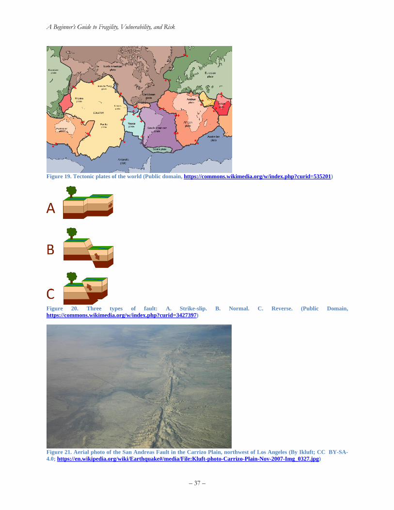
A Beginner’s Guide to Fragility, Vulnerability, and Risk
– 37 –
Figure 19. Tectonic plates of the world (Public domain, https://commons.wikimedia.org/w/index.php?curid=535201)
Figure 20. Three types of fault: A. Strike-slip. B. Normal. C. Reverse. (Public Domain,
https://commons.wikimedia.org/w/index.php?curid=3427397)
Figure 21. Aerial photo of the San Andreas Fault in the Carrizo Plain, northwest of Los Angeles (By Ikluft; CC BY-SA-
4.0; https://en.wikipedia.org/wiki/Earthquake#/media/File:Kluft-photo-Carrizo-Plain-Nov-2007-Img_0327.jpg)
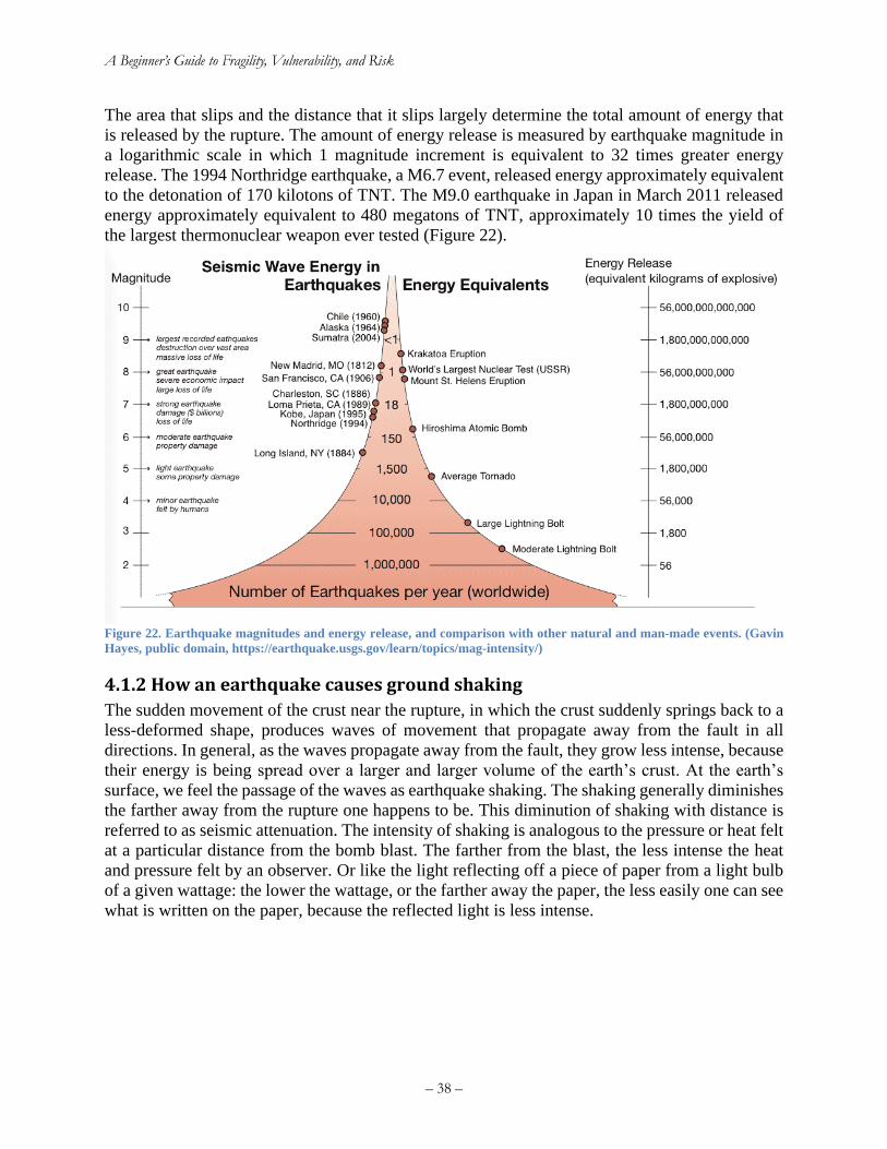
A Beginner’s Guide to Fragility, Vulnerability, and Risk
– 38 –
The area that slips and the distance that it slips largely determine the total amount of energy that
is released by the rupture. The amount of energy release is measured by earthquake magnitude in
a logarithmic scale in which 1 magnitude increment is equivalent to 32 times greater energy
release. The 1994 Northridge earthquake, a M6.7 event, released energy approximately equivalent
to the detonation of 170 kilotons of TNT. The M9.0 earthquake in Japan in March 2011 released
energy approximately equivalent to 480 megatons of TNT, approximately 10 times the yield of
the largest thermonuclear weapon ever tested (Figure 22).
Figure 22. Earthquake magnitudes and energy release, and comparison with other natural and man-made events. (Gavin
Hayes, public domain, https://earthquake.usgs.gov/learn/topics/mag-intensity/)
4.1.2 How an earthquake causes ground shaking
The sudden movement of the crust near the rupture, in which the crust suddenly springs back to a
less-deformed shape, produces waves of movement that propagate away from the fault in all
directions. In general, as the waves propagate away from the fault, they grow less intense, because
their energy is being spread over a larger and larger volume of the earth’s crust. At the earth’s
surface, we feel the passage of the waves as earthquake shaking. The shaking generally diminishes
the farther away from the rupture one happens to be. This diminution of shaking with distance is
referred to as seismic attenuation. The intensity of shaking is analogous to the pressure or heat felt
at a particular distance from the bomb blast. The farther from the blast, the less intense the heat
and pressure felt by an observer. Or like the light reflecting off a piece of paper from a light bulb
of a given wattage: the lower the wattage, or the farther away the paper, the less easily one can see
what is written on the paper, because the reflected light is less intense.
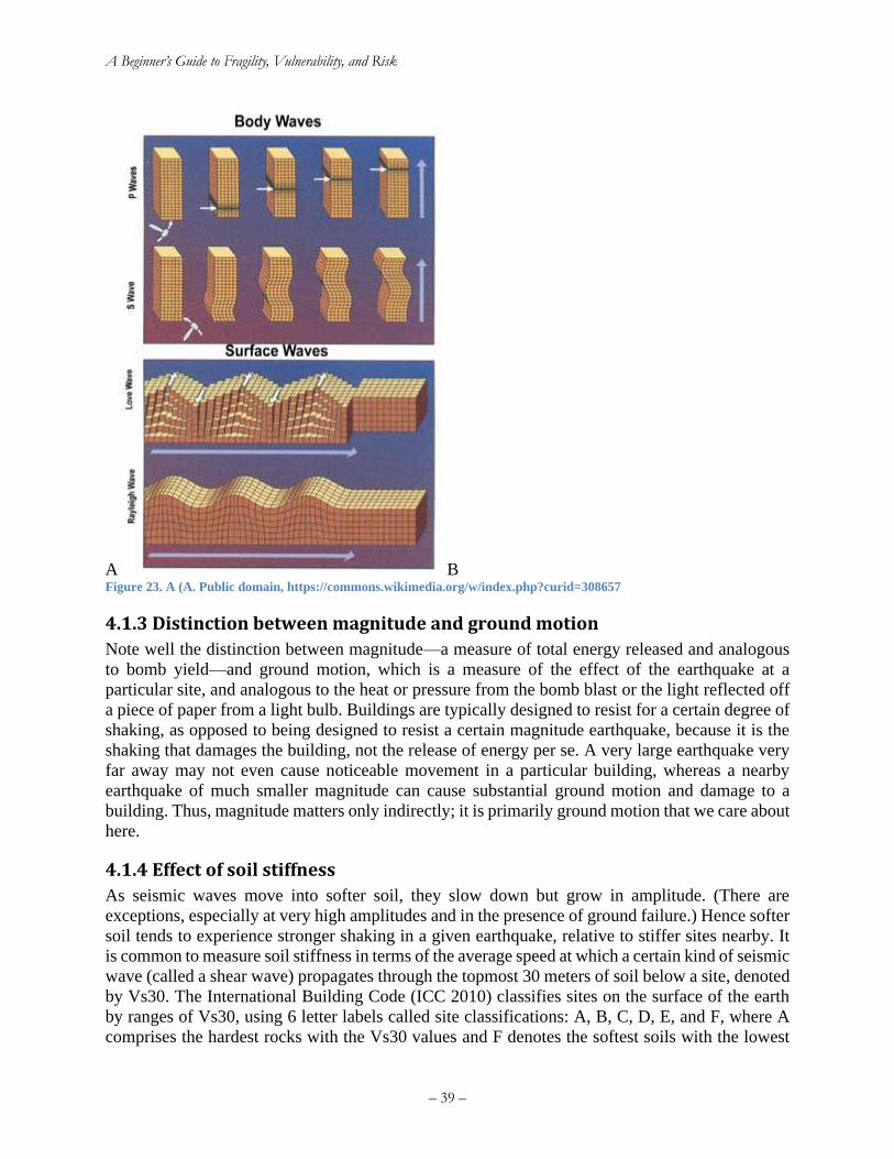
A Beginner’s Guide to Fragility, Vulnerability, and Risk
– 39 –
A B Figure 23. A (A. Public domain, https://commons.wikimedia.org/w/index.php?curid=308657
4.1.3 Distinction between magnitude and ground motion
Note well the distinction between magnitude—a measure of total energy released and analogous
to bomb yield—and ground motion, which is a measure of the effect of the earthquake at a
particular site, and analogous to the heat or pressure from the bomb blast or the light reflected off
a piece of paper from a light bulb. Buildings are typically designed to resist for a certain degree of
shaking, as opposed to being designed to resist a certain magnitude earthquake, because it is the
shaking that damages the building, not the release of energy per se. A very large earthquake very
far away may not even cause noticeable movement in a particular building, whereas a nearby
earthquake of much smaller magnitude can cause substantial ground motion and damage to a
building. Thus, magnitude matters only indirectly; it is primarily ground motion that we care about
here.
4.1.4 Effect of soil stiffness
As seismic waves move into softer soil, they slow down but grow in amplitude. (There are
exceptions, especially at very high amplitudes and in the presence of ground failure.) Hence softer
soil tends to experience stronger shaking in a given earthquake, relative to stiffer sites nearby. It
is common to measure soil stiffness in terms of the average speed at which a certain kind of seismic
wave (called a shear wave) propagates through the topmost 30 meters of soil below a site, denoted
by Vs30. The International Building Code (ICC 2010) classifies sites on the surface of the earth
by ranges of Vs30, using 6 letter labels called site classifications: A, B, C, D, E, and F, where A
comprises the hardest rocks with the Vs30 values and F denotes the softest soils with the lowest
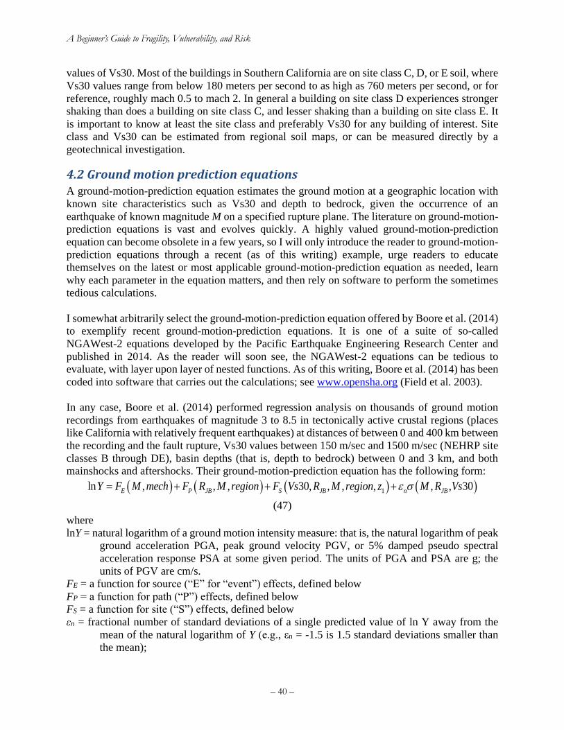
A Beginner’s Guide to Fragility, Vulnerability, and Risk
– 40 –
values of Vs30. Most of the buildings in Southern California are on site class C, D, or E soil, where
Vs30 values range from below 180 meters per second to as high as 760 meters per second, or for
reference, roughly mach 0.5 to mach 2. In general a building on site class D experiences stronger
shaking than does a building on site class C, and lesser shaking than a building on site class E. It
is important to know at least the site class and preferably Vs30 for any building of interest. Site
class and Vs30 can be estimated from regional soil maps, or can be measured directly by a
geotechnical investigation.
4.2 Ground motion prediction equations A ground-motion-prediction equation estimates the ground motion at a geographic location with
known site characteristics such as Vs30 and depth to bedrock, given the occurrence of an
earthquake of known magnitude M on a specified rupture plane. The literature on ground-motion-
prediction equations is vast and evolves quickly. A highly valued ground-motion-prediction
equation can become obsolete in a few years, so I will only introduce the reader to ground-motion-
prediction equations through a recent (as of this writing) example, urge readers to educate
themselves on the latest or most applicable ground-motion-prediction equation as needed, learn
why each parameter in the equation matters, and then rely on software to perform the sometimes
tedious calculations.
I somewhat arbitrarily select the ground-motion-prediction equation offered by Boore et al. (2014)
to exemplify recent ground-motion-prediction equations. It is one of a suite of so-called
NGAWest-2 equations developed by the Pacific Earthquake Engineering Research Center and
published in 2014. As the reader will soon see, the NGAWest-2 equations can be tedious to
evaluate, with layer upon layer of nested functions. As of this writing, Boore et al. (2014) has been
coded into software that carries out the calculations; see www.opensha.org (Field et al. 2003).
In any case, Boore et al. (2014) performed regression analysis on thousands of ground motion
recordings from earthquakes of magnitude 3 to 8.5 in tectonically active crustal regions (places
like California with relatively frequent earthquakes) at distances of between 0 and 400 km between
the recording and the fault rupture, Vs30 values between 150 m/sec and 1500 m/sec (NEHRP site
classes B through DE), basin depths (that is, depth to bedrock) between 0 and 3 km, and both
mainshocks and aftershocks. Their ground-motion-prediction equation has the following form:
( ) ( ) ( ) ( )1ln , , , 30, , , , , , 30E P JB S JB n JBY F M mech F R M region F Vs R M region z M R Vs = + + +
(47)
where
lnY = natural logarithm of a ground motion intensity measure: that is, the natural logarithm of peak
ground acceleration PGA, peak ground velocity PGV, or 5% damped pseudo spectral
acceleration response PSA at some given period. The units of PGA and PSA are g; the
units of PGV are cm/s.
FE = a function for source (“E” for “event”) effects, defined below
FP = a function for path (“P”) effects, defined below
FS = a function for site (“S”) effects, defined below
εn = fractional number of standard deviations of a single predicted value of ln Y away from the
mean of the natural logarithm of Y (e.g., εn = -1.5 is 1.5 standard deviations smaller than
the mean);
A Beginner’s Guide to Fragility, Vulnerability, and Risk
– 41 –
σ = total standard deviation of the model, defined below
M = moment magnitude
mech = an index to mechanism: 0, 1, 2, and 3 for unspecified, strike-slip, normal, and reverse,
respectively
RJB = Joyner-Boore fault distance in km, defined as the shortest distance from the site to the surface
projection of the rupture surface
region = an index to regional: 0 if no regional correction is to be made (default value); 1 for
California, New Zealand, and Taiwan (this also provides no correction); 2 for China and
Turkey; and 3 for Italy and Japan
( )( ) ( )
( )
2
0 1 2 3 4 5
0 1 2 3 4
, h h hE
h h
e U e SS e NS e RS e M M e M M M MF M mech
e U e SS e NS e RS e M M M M
+ + + + − + − =
+ + + + −
(48)
where U, SS, NS, and RS are dummy variables, with a value of 1 to specify unspecified, strike-slip,
normal-slip, and reverse-slip fault types, respectively, and 0 if the fault type is unspecified; the
hinge magnitude Mh is period-dependent, and e0 to e6 are model coefficients that the authors
tabulate in an electronic supplement to their article that the reader must download. The path
function is given by
( ) ( ) ( ) ( )( )1 2 3 3, , lnP JB ref ref refF R M region c c M M R R c c R R = + − + + −
(49)
where
2 2
JBR R h= + (50)
and c1, c2, c3, Δc3, Mref, Rref and h are model coefficients that the authors tabulate in their electronic
supplement. (Note that h looks like a depth to the rupture surface, but it just a parameter value.)
Parameter Δc3 depends on the geographic region, as discussed later. The site function is given by
( ) ( ) ( ) ( )11 130, , , , ln lnS JB lin nl zF Vs R M region z F F F z = + + (51)
where Flin represents the linear component of site amplification, Fnl represents the nonlinear
component of site amplification, and Fδz1 represents the effects of basin depth, defined as follows.
( )
30ln 30
ln
ln 30
c
ref
lin
cc
ref
Vsc Vs V
VF
Vc Vs V
V
=
(52)
where c and Vc are period-dependent model parameters the authors tabulate and Vref = 760 m/sec.
The function Fnl is defined as follows:
( ) 31 2
3
ln ln rnl
PGA fF f f
f
+= +
(53)
where f1, f2, and f3 are model coefficients and PGAr is the median peak horizontal acceleration for
reference rock. For a given RJB, M, and region, PGAr is obtained by evaluating equation (47) with
Vs30 = 760 m/s. Parameter f2 is evaluated as
( )( ) ( ) 2 4 5 5exp min 30,760 360 exp 760 360f f f Vs f = − − − (54)
A Beginner’s Guide to Fragility, Vulnerability, and Risk
– 42 –
where f4 and f5 are model coefficients that the authors tabulate. The term Fδz1 is an adjustment to
the base model to consider the effects of basin depth on ground motion amplitude, calculated as
follows:
( )1 1 6 1 1 7 6
7 1 7 6
0 0.65sec
0.65sec&
0.65sec&
z
T
F z f z T z f f
f T z f f
=
(55)
where f6 and f7 are model coefficients, f7/f6 has units of km, and δz1 (also in km) is computed as
( )1 1 1 30zz z Vs = − (56)
where μz1(Vs30) is the prediction of an empirical model relating depth to bedrock with 1,000 m/sec
shearwave velocity (z1) to Vs30. The authors provide estimates of μz1(Vs30) for California and
Japan:
( )
( )( )
( )( )
4 4
4 4
1 2 2
2 2
30 570.947.15ln ln 1000 California
4 1360 570.94ln
30 412.395.23ln ln 1000 Japan
2 1360 412.39
z
Vs
Vs
+− −
+ =
+−− +
(57)
where μz1 and Vs30 have units of km and m/s, respectively. These relationships can be used to
estimate a representative depth z1 for any given Vs30. Where z1 is unknown, the authors suggest
using δz1 = 0.0, which turns off this adjustment factor (i.e., Fδz1 = 0).
Equations (47) through (57) just give the expected value of lnY; one also needs two uncertainty
terms: the within-event standard deviation and between-event standard deviation . The between-
event standard deviation reflects how from one earthquake to another, the overall average ground
motion can be higher or lower than median estimates. The within-event standard deviation
reflects how in a single earthquake, the motion at a given site can be higher or lower than the
median value one would expect even given the between-event term. The two standard deviations
of the natural logarithm of ground motion Y are calculated as follows. Estimating within-event
standard deviation requires evaluating three nested functions:
( ) ( )( )1
1 2 1
2
4.5
4.5 4.5 5.5
5.5
M
M M M
M
= + − −
(58)
( )
( )
( )( )
( )
( )
1
1
1 2
2 1
2
ln,
ln
JB
JB
JB R JB
R JB
M R R
R RM R M R R R
R R
M R R
= +
+
(59)
A Beginner’s Guide to Fragility, Vulnerability, and Risk
– 43 –
( )
( )
( )( )
( )
( )
2
2
1 2
2 1
1
, 30
ln 30, , 30 , 30
ln
, 30
JB
JB JB V
JB V
M R Vs V
V VsM R Vs M R V Vs V
V V
M R Vs V
= −
−
(60)
The between-event standard deviation is evaluated as a function of M:
( ) ( )( )1
1 2 1
2
4.5
4.5 4.5 5.5
5.5
M
M M M
M
= + − −
(61)
Finally, if one is only concerned with the total standard deviation of the natural logarithm of Y, the
terms combine as follows:
( ) ( )( ) ( )( )2 2
, , 30 , , 30JB JBM R Vs M R Vs M = + (62)
4.3 Probabilistic seismic hazard analysis
Seismic hazard refers here to an uncertain relationship between the level of some measure seismic
excitation and the frequency or probability of a particular location experiencing at least that level
of excitation. As used here, hazard is that relationship. It is not the measure of excitation, the
occurrence of an earthquake, nor the probability or frequency of excitation. These terms are not to
be used interchangeably.
Seismic hazard is quantified many ways. One is through a hazard curve, commonly depicted on
an x-y chart where the x-axis measures shaking intensity at a site (shaking intensity means the
severity of the ground motion, which is the environmental excitation that nature imposes on the
facility) and the y-axis measures either exceedance probability in a specified period of time or
exceedance rate in events per unit time. Cornell (1968) applied the theorem of total probability to
create a hazard curve. What follows here is a summary of current procedures to perform
probabilistic seismic hazard analysis (PSHA), but is conceptually identical to Cornell’s work.
Engineers sometimes refer to the quantity by which intensity is measured as the intensity measure.
Earth scientists call it ground motion. The present work uses the term intensity measure (IM).
Some authors distinguish between the intensity measure type (IMT), such as 5% damped spectral
acceleration response at 0.2 second period, and the intensity measure level (IML), a particular
value of the IM such as 0.4g. In any case, IMT must be completely specified. If using damped
elastic spectral acceleration response, one states the period, damping ratio, and whether one is
referring to the geometric mean of two orthogonal directions or the maximum direction or other
directional reference.
To estimate seismic hazard, one applies the theorem of total probability to combine the uncertain
shaking at the site caused by a particular fault rupture and the occurrence frequency or probability
of that rupture. Earth scientists create models called earthquake rupture forecasts that specify the
locations and rates at which various fault produce earthquakes of various sizes, e.g., the Uniform
A Beginner’s Guide to Fragility, Vulnerability, and Risk
– 44 –
California Earthquake Rupture Forecast version 2 (UCERF2, Field et al. 2007). The uncertain
shaking given a fault rupture is quantified using a relationship variously called an attenuation
relationship or a ground-motion prediction equation, such as the next-generation attenuation
(NGA) relationships presented in the February 2008 issue of Earthquake Spectra. Mathematically,
a hazard curve is created as follows. Let:
H = uncertain severity of ground motion at the building site, maybe Sa(T, 5%)
h = a particular value of H
G(h) = frequency (events per unit time) with which H > h, i.e., the number of events per unit time
in which at least once during the event, H > h
nE = number of earthquake rupture forecast models to consider, nE {1, 2, ...}. For example, in
UCERF2, there were 480 discrete combinations of fault model, rupture model, magnitude-
area relationship, and several other modeling choices that together are represented by a
logic tree that begins with fault model, branches to rupture model, then to magnitude-area
relationship, etc. For UCERF2, nE= 480.
E = the “correct” earthquake rupture forecast, which is uncertain. E {1, 2, … nE}
e = an index to a particular earthquake rupture forecast, e {1, 2, ... nE}
P[E=e] = Bayesian probability assigned to earthquake rupture forecast e. In UCERF2, this would
be the product of the conditional probabilities (weights) of the individual branches in the
logic tree that represents UCERF2. By conditional probability is meant that each branch’s
probability can (though only sometimes do) depend on which choices came before it.
nA = number of attenuation relationships (also called ground motion prediction equations) to be
employed, nA {1, 2, ... }
A = the “correct” ground-motion-prediction equation, i.e., the one that expresses the true state of
nature, which is uncertain
a = an index to ground-motion prediction equations
P[A=a] = Bayesian probability assigned to ground-motion-prediction equation a, i.e., the
probability that ground-motion-prediction equation a actually reflect the state of nature,
the way nature actually work, is the correct ground-motion-prediction equation
nF(e) = number of fault sections in earthquake rupture forecast e, nF(e) {1, 2, ...}
f = an index to faults section, f {1, 2, ... nF(e)}
m0 = minimum magnitude to consider
Δm = an increment of magnitude, say Δm = 0.1
Mmax(f|E=e) = maximum magnitude of which fault f is deemed capable under earthquake rupture
forecast e, Mmax(f|E=e) {m0+ ½·Δm, m0+3/2·Δm, ... }
no(f,m) = number of locations within fault section f that can generate a rupture of magnitude m,
no(f,m) {1, 2, ... }
o = an index to locations on fault section f, in o {1, 2, ... no(f,m)}
G(f,m,o|E=e) = frequency (events per unit time) with which fault section f ruptures at location o
producing earthquake of magnitude m ± ½·Δm given earthquake rupture forecast e
VS = uncertain site soil, potentially measured by NEHRP site soil classification or shearwave
velocity in the top 30m of soil (Vs30), or something else.
v = a particular value of V
P[H > h | m,r,v,a] = probability that H > h given earthquake magnitude m at distance r on soil with
soil type v using ground-motion-prediction equation a. Note that, given a known site
location, fault segment f and location along the fault segment o, distance r from the site to
A Beginner’s Guide to Fragility, Vulnerability, and Risk
– 45 –
the fault is known. Note that ground-motion prediction equations use a variety of distance
measures. As of this writing, most ground-motion prediction equations give an equation
for the mean of the natural logarithm of H given m, r, and v, for the logarithmic standard
deviation of H (i.e., the standard deviation of the natural logarithm of H), and assume a
lognormal distribution of H conditioned on m, r, and v. Let mlnH and slnH denote the mean
of ln(H) and the standard deviation of ln(H), respectively, given m, r, and v, assuming
ground-motion-prediction equation a. Under these conditions,
( ) ln
ln
ln, , , 1
H
H
h mP H h m r v a
s
− = −
(63)
One can now estimate the hazard curve by applying the theorem of total probability. Suppose one
always knew soil conditions V with certainty. Then
( ) ( ) ( )( ) ,
1 1 1 1
, , , , ,f oE A
n e n f mn n
e a f m o
G h P H h m r v a G m f o E e P A a P E e= = = =
= = = = (64)
where the summation over m means that one considers each m {m0 + ½·Δm, m0 + 3/2·Δm...
Mmax(f|E=e)}.
4.4 Hazard rate versus probability
Seismic hazard is often expressed in terms of exceedance probability, rather than in terms of
exceedance rate. The distinction is this: exceedance probability is the probability that shaking of
H > h will occur at least once in a given period of time. That means that it is the probability that it
H > h will occur exactly once, plus the probability that it will occur exactly twice, etc. For some
calculations the analyst wants rate (number of events per unit time) not probability (change that it
occurs one or more times in a given time period).
The two can be related using a concept called a Poisson process. From the Wikipedia’s article on
the Poisson Process: “In probability theory, a Poisson process is a stochastic process which counts
the number of events and the time that these events occur in a given time interval. The time between
each pair of consecutive events has an exponential distribution with parameter G [the parameter is
the occurrence rate per unit time] and each of these inter-arrival times is assumed to be independent
of other inter-arrival times [meaning that the time between the 2nd and 3rd occurrence is
independent of the time between the 1st and 2nd occurrence—knowing one tells you nothing about
the other]. The process is named after the French mathematician Siméon-Denis Poisson and is a
good model of radioactive decay, telephone calls, and requests for a particular document on a web
server, among many other phenomena.”
Modeling earthquakes as Poisson arrivals is convenient in part because in a Poisson process, arrival
rate and occurrence probability have this relationship:
( )ln 1 P
Gt
− −= (65)
where
G = occurrence rate, i.e., events per unit time
P = probability that at least one event will occur in time t
A Beginner’s Guide to Fragility, Vulnerability, and Risk
– 46 –
So if a hazard curve were represented as the P(h), the probability that H > h at least once in a
particular period of time t, one could use Equation (65) to estimate the occurrence rate G(h), the
average number of times that H ≥ h per unit time. One can also rearrange Equation (65) to give
probability as a function of rate:
1 G tP e− = − (66)
So with the occurrence rate G(h) of earthquakes causing H > h, one can calculate the probability
that at least one earthquakes with H > h will occur in a given time t.
4.5 Measures of seismic excitation
These are many common measures of seismic excitation. Some measure ground motion and some
measure structural response or excitation to which the components of a building, bridge, or other
structural system are subjected. This section introduces common ones. The earthquake engineer
should be very familiar with any measure of ground motion that he or she commonly uses1.
4.5.1 Some commonly used measures of ground motion
Peak ground acceleration (PGA). This is the maximum value of acceleration of a particular point
on the ground at any time during an earthquake. Often PGA is estimated as the geometric mean
(the square root of the product) of the maximum values of PGA parallel to each of two orthogonal
axes. PGA is sometimes called zero-period acceleration (ZPA), meaning the spectral acceleration
response of a single-degree-of-freedom elastic oscillator with zero, or near-zero, period. Before
using a PGA value, be sure you know whether it refers to geometric mean, maximum-direction
value, or something else.
Peak ground velocity (PGV). Like PGA, except maximum velocity of a point on the ground rather
than acceleration.
Peak ground displacement (PGD). Like PGA, except maximum displacement relative to a fixed
datum.
Spectral acceleration response (Sa(T,z)). This usually refers to damped elastic spectral
acceleration response at some specified index period such as T = 0.3 sec, 1.0 sec, 3.0 sec, etc. and
specified damping ratio such as z = 5%, at a particular point on the ground. To be precise, Sa(T,z)
is the absolute value of the maximum acceleration relative to a fixed datum of a damped elastic
single-degree-of-freedom harmonic oscillator with period T and damping ratio z when subjected
to a particular one-degree-of-freedom ground motion time history at its base. In practice, it
typically refers to the geometric mean of spectral acceleration response parallel to each of two
orthogonal horizontal axes. It is so often measured for z = 5% that damping ratio is often not
mentioned. Before using Sa(T,z), be sure you know T, z, and whether it is a geometric mean value
or the maximum-direction value or something else.
1 Again the CU graduate student should be able to explain it in his or her thesis defense.

A Beginner’s Guide to Fragility, Vulnerability, and Risk
– 47 –
Spectral displacement response (Sd(T,z)). Like Sa(T,z) but for relative spectral displacement
(displacement of the oscillator relative to its base, not relative to a fixed datum) rather than absolute
acceleration of the oscillator.
Pseudoacceleration response (PSA(T,z)). PSA(T,z) is defined as Sd(T,z)·ω2, where ω is angular
frequency, 2·π/T. Some authors prefer to use PSA(T,z) rather than Sa(T,z), but for values of z less
than about 20%, the two measures are virtually identical.
Modified Mercalli Intensity (MMI) and European Macroseismic Scale (EMS). These are
macroseismic intensity measures, meaning that they measure seismic excitation over a large area,
not at a particular point on the ground. They are measured with an integer scale in Roman numerals
from I to XII. They measure whether and how people in a region such as a neighborhood or city
felt and reacted to earthquake motion (did they run outside?) and what they observed to happen to
the ground, buildings, and contents around them, such as plates rattling and weak masonry being
damaged. They are subjective and generally easier for nontechnical audiences to understand than
instrumental measures. On the MMI scale, building damage begins around MMI VI and it is rare
for an earthquake to produce shaking of MMI ≥ X. EMS is similar to MMI, but building-damage
observations are related to common European building types. A version of EMS defined in 1998
is often referred to as EMS-98. For detail see Table 3,
http://en.wikipedia.org/wiki/Modified_Mercalli_intensity, and
http://en.wikipedia.org/wiki/European_Macroseismic_Scale.
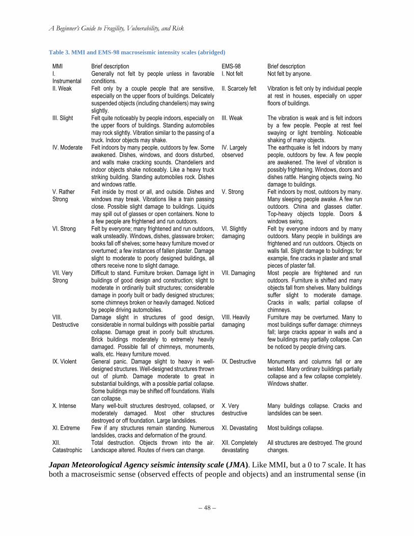
A Beginner’s Guide to Fragility, Vulnerability, and Risk
– 48 –
Table 3. MMI and EMS-98 macroseismic intensity scales (abridged)
MMI Brief description EMS-98 Brief description I. Instrumental
Generally not felt by people unless in favorable conditions.
I. Not felt Not felt by anyone.
II. Weak Felt only by a couple people that are sensitive, especially on the upper floors of buildings. Delicately suspended objects (including chandeliers) may swing slightly.
II. Scarcely felt Vibration is felt only by individual people at rest in houses, especially on upper floors of buildings.
III. Slight Felt quite noticeably by people indoors, especially on the upper floors of buildings. Standing automobiles may rock slightly. Vibration similar to the passing of a truck. Indoor objects may shake.
III. Weak The vibration is weak and is felt indoors by a few people. People at rest feel swaying or light trembling. Noticeable shaking of many objects.
IV. Moderate Felt indoors by many people, outdoors by few. Some awakened. Dishes, windows, and doors disturbed, and walls make cracking sounds. Chandeliers and indoor objects shake noticeably. Like a heavy truck striking building. Standing automobiles rock. Dishes and windows rattle.
IV. Largely observed
The earthquake is felt indoors by many people, outdoors by few. A few people are awakened. The level of vibration is possibly frightening. Windows, doors and dishes rattle. Hanging objects swing. No damage to buildings.
V. Rather Strong
Felt inside by most or all, and outside. Dishes and windows may break. Vibrations like a train passing close. Possible slight damage to buildings. Liquids may spill out of glasses or open containers. None to a few people are frightened and run outdoors.
V. Strong Felt indoors by most, outdoors by many. Many sleeping people awake. A few run outdoors. China and glasses clatter. Top-heavy objects topple. Doors & windows swing.
VI. Strong Felt by everyone; many frightened and run outdoors, walk unsteadily. Windows, dishes, glassware broken; books fall off shelves; some heavy furniture moved or overturned; a few instances of fallen plaster. Damage slight to moderate to poorly designed buildings, all others receive none to slight damage.
VI. Slightly damaging
Felt by everyone indoors and by many outdoors. Many people in buildings are frightened and run outdoors. Objects on walls fall. Slight damage to buildings; for example, fine cracks in plaster and small pieces of plaster fall.
VII. Very Strong
Difficult to stand. Furniture broken. Damage light in buildings of good design and construction; slight to moderate in ordinarily built structures; considerable damage in poorly built or badly designed structures; some chimneys broken or heavily damaged. Noticed by people driving automobiles.
VII. Damaging Most people are frightened and run outdoors. Furniture is shifted and many objects fall from shelves. Many buildings suffer slight to moderate damage. Cracks in walls; partial collapse of chimneys.
VIII. Destructive
Damage slight in structures of good design, considerable in normal buildings with possible partial collapse. Damage great in poorly built structures. Brick buildings moderately to extremely heavily damaged. Possible fall of chimneys, monuments, walls, etc. Heavy furniture moved.
VIII. Heavily damaging
Furniture may be overturned. Many to most buildings suffer damage: chimneys fall; large cracks appear in walls and a few buildings may partially collapse. Can be noticed by people driving cars.
IX. Violent General panic. Damage slight to heavy in well-designed structures. Well-designed structures thrown out of plumb. Damage moderate to great in substantial buildings, with a possible partial collapse. Some buildings may be shifted off foundations. Walls can collapse.
IX. Destructive Monuments and columns fall or are twisted. Many ordinary buildings partially collapse and a few collapse completely. Windows shatter.
X. Intense Many well-built structures destroyed, collapsed, or moderately damaged. Most other structures destroyed or off foundation. Large landslides.
X. Very destructive
Many buildings collapse. Cracks and landslides can be seen.
XI. Extreme Few if any structures remain standing. Numerous landslides, cracks and deformation of the ground.
XI. Devastating Most buildings collapse.
XII. Catastrophic
Total destruction. Objects thrown into the air. Landscape altered. Routes of rivers can change.
XII. Completely devastating
All structures are destroyed. The ground changes.
Japan Meteorological Agency seismic intensity scale (JMA). Like MMI, but a 0 to 7 scale. It has
both a macroseismic sense (observed effects of people and objects) and an instrumental sense (in
A Beginner’s Guide to Fragility, Vulnerability, and Risk
– 49 –
terms of ranges of PGA). See
http://en.wikipedia.org/wiki/Japan_Meteorological_Agency_seismic_intensity_scale for details.
Instrumental intensity measure (IMM). This is a positively valued measure of intensity that can
take on fractional values, e.g., 6.4. This is an estimate of MMI using functions of instrumental
ground-motion measures such as PGA and PGV.
4.5.2 Conversion between instrumental and macroseismic intensity
It is often desirable to convert between instrumental ground motion measures such as PGA or PGV
and macroseismic intensity measures, especially MMI. One reason is that MMI observations can
be made by people exposed to shaking or who make post-earthquake observations, and whereas
instrumental measures require an instrument.
Ground-motion-to-intensity-conversion equations (GMICE). These estimate macroseismic
intensity as a function of instrumental measures of ground motion. There are several leading
GMICEs. When selecting among them, try to match the region, magnitude range, and distance
range closest to the conditions where the GMICE will be applied. More data for conditions like
the ones in question are generally better than less data, all other things being equal. When
considering building response, GMICE that convert from Sa(T,z) to macroseismic intensity are
generally better than those that use PGA or PGV, which do not reflect anything building-specific.
Two recent GMICE for the United States are as follows:
As of this writing, Worden et al.’s (2012) relationships in Equations (67) and (68) seem to be the
best choice for estimating MMI from ground motion and vice versa for California earthquakes.
Reason is they employ a very large dataset of California (ground motion, MMI) observations and
they are conveniently bidirectional, meaning that one can rearrange the relationships to estimate
instrumental measures in terms of MMI, as well as MMI in terms of instrumental measures. The
dataset includes 2092 PGA-MMI observations and 2074 PGV-MMI observations from 1207
California earthquakes M=3.0-7.3, MMI 2.0-8.6, R=4-500 km. It includes no observations from
continental interior. It includes regressions for Sa(0.3 sec, 5%), Sa(1.0 sec, 5%), Sa(3.0 sec, 5%),
PGA, and PGV that operate in both directions,. The reason that the relationships are bidirectional
is that Worden et al. (2012) used a total least squares data modeling technique in which
observational errors on both dependent and independent variables are taken into account. Equation
(68) includes the option to account for the apparent effects of magnitude M and distance R. The
columns for residual standard deviations show a modest reduction in uncertainty when accounting
for M and R.
( ) ( )
( ) ( )
1 2 10 10 1
3 4 10 10 1
log log
log log
MMI c c Y Y t
c c Y Y t
= +
= + (67)
( ) ( )
( ) ( )
1 2 10 5 6 10 7 2
3 4 10 5 6 10 7 2
log log
log log
MMI c c Y c c R c M MMI t
c c Y c c R c M MMI t
= + + + +
= + + + + (68)
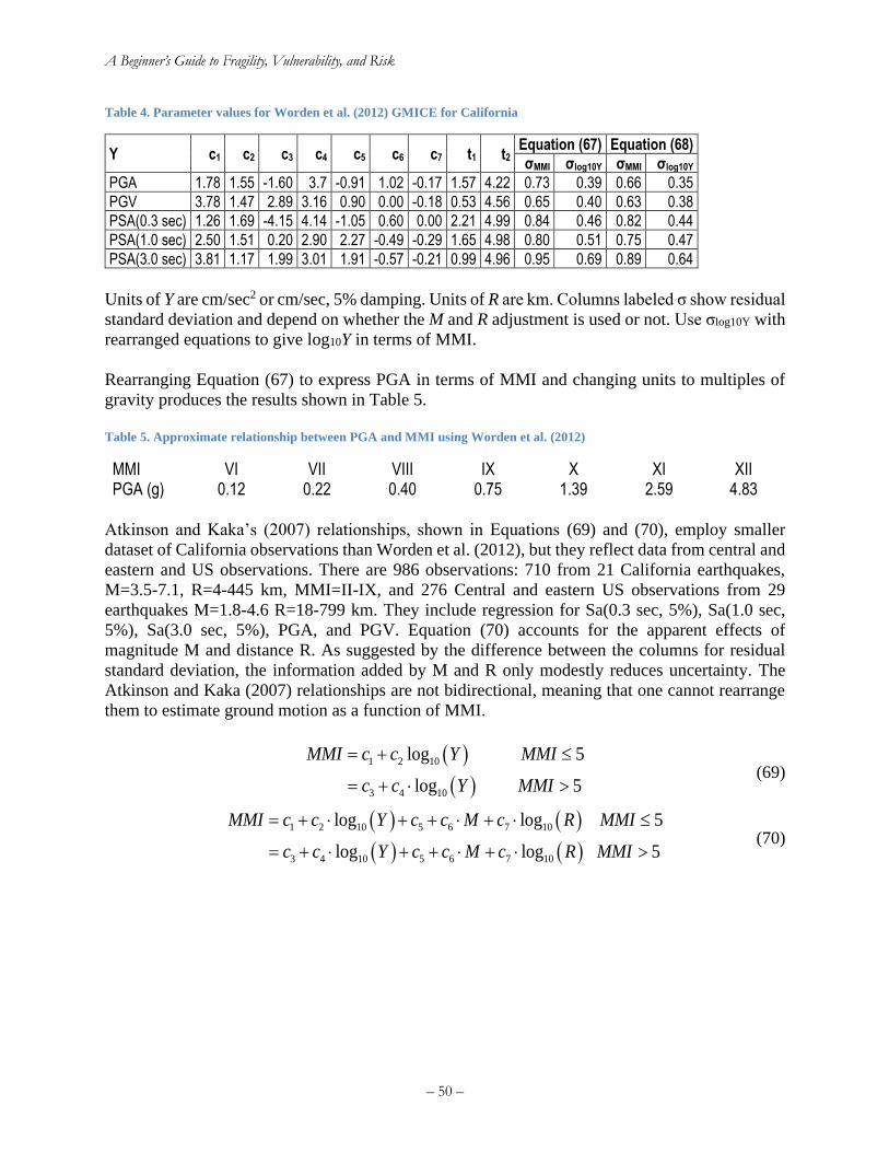
A Beginner’s Guide to Fragility, Vulnerability, and Risk
– 50 –
Table 4. Parameter values for Worden et al. (2012) GMICE for California
Y c1 c2 c3 c4 c5 c6 c7 t1 t2 Equation (67) Equation (68)
σMMI σlog10Y σMMI σlog10Y
PGA 1.78 1.55 -1.60 3.7 -0.91 1.02 -0.17 1.57 4.22 0.73 0.39 0.66 0.35
PGV 3.78 1.47 2.89 3.16 0.90 0.00 -0.18 0.53 4.56 0.65 0.40 0.63 0.38
PSA(0.3 sec) 1.26 1.69 -4.15 4.14 -1.05 0.60 0.00 2.21 4.99 0.84 0.46 0.82 0.44
PSA(1.0 sec) 2.50 1.51 0.20 2.90 2.27 -0.49 -0.29 1.65 4.98 0.80 0.51 0.75 0.47
PSA(3.0 sec) 3.81 1.17 1.99 3.01 1.91 -0.57 -0.21 0.99 4.96 0.95 0.69 0.89 0.64
Units of Y are cm/sec2 or cm/sec, 5% damping. Units of R are km. Columns labeled σ show residual
standard deviation and depend on whether the M and R adjustment is used or not. Use σlog10Y with
rearranged equations to give log10Y in terms of MMI.
Rearranging Equation (67) to express PGA in terms of MMI and changing units to multiples of
gravity produces the results shown in Table 5.
Table 5. Approximate relationship between PGA and MMI using Worden et al. (2012)
MMI VI VII VIII IX X XI XII PGA (g) 0.12 0.22 0.40 0.75 1.39 2.59 4.83
Atkinson and Kaka’s (2007) relationships, shown in Equations (69) and (70), employ smaller
dataset of California observations than Worden et al. (2012), but they reflect data from central and
eastern and US observations. There are 986 observations: 710 from 21 California earthquakes,
M=3.5-7.1, R=4-445 km, MMI=II-IX, and 276 Central and eastern US observations from 29
earthquakes M=1.8-4.6 R=18-799 km. They include regression for Sa(0.3 sec, 5%), Sa(1.0 sec,
5%), Sa(3.0 sec, 5%), PGA, and PGV. Equation (70) accounts for the apparent effects of
magnitude M and distance R. As suggested by the difference between the columns for residual
standard deviation, the information added by M and R only modestly reduces uncertainty. The
Atkinson and Kaka (2007) relationships are not bidirectional, meaning that one cannot rearrange
them to estimate ground motion as a function of MMI.
( )
( )
1 2 10
3 4 10
log 5
log 5
MMI c c Y MMI
c c Y MMI
= +
= + (69)
( ) ( )
( ) ( )
1 2 10 5 6 7 10
3 4 10 5 6 7 10
log log 5
log log 5
MMI c c Y c c M c R MMI
c c Y c c M c R MMI
= + + + +
= + + + + (70)
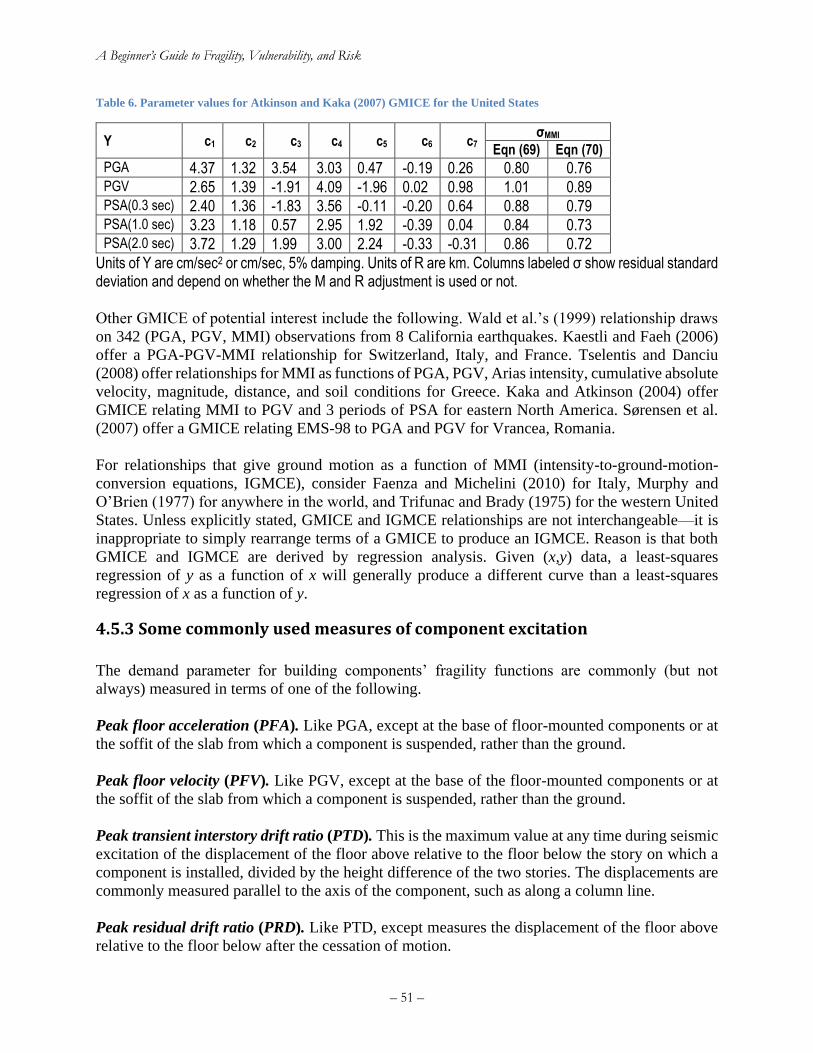
A Beginner’s Guide to Fragility, Vulnerability, and Risk
– 51 –
Table 6. Parameter values for Atkinson and Kaka (2007) GMICE for the United States
Y c1 c2 c3 c4 c5 c6 c7 σMMI
Eqn (69) Eqn (70)
PGA 4.37 1.32 3.54 3.03 0.47 -0.19 0.26 0.80 0.76 PGV 2.65 1.39 -1.91 4.09 -1.96 0.02 0.98 1.01 0.89 PSA(0.3 sec) 2.40 1.36 -1.83 3.56 -0.11 -0.20 0.64 0.88 0.79 PSA(1.0 sec) 3.23 1.18 0.57 2.95 1.92 -0.39 0.04 0.84 0.73 PSA(2.0 sec) 3.72 1.29 1.99 3.00 2.24 -0.33 -0.31 0.86 0.72
Units of Y are cm/sec2 or cm/sec, 5% damping. Units of R are km. Columns labeled σ show residual standard deviation and depend on whether the M and R adjustment is used or not.
Other GMICE of potential interest include the following. Wald et al.’s (1999) relationship draws
on 342 (PGA, PGV, MMI) observations from 8 California earthquakes. Kaestli and Faeh (2006)
offer a PGA-PGV-MMI relationship for Switzerland, Italy, and France. Tselentis and Danciu
(2008) offer relationships for MMI as functions of PGA, PGV, Arias intensity, cumulative absolute
velocity, magnitude, distance, and soil conditions for Greece. Kaka and Atkinson (2004) offer
GMICE relating MMI to PGV and 3 periods of PSA for eastern North America. Sørensen et al.
(2007) offer a GMICE relating EMS-98 to PGA and PGV for Vrancea, Romania.
For relationships that give ground motion as a function of MMI (intensity-to-ground-motion-
conversion equations, IGMCE), consider Faenza and Michelini (2010) for Italy, Murphy and
O’Brien (1977) for anywhere in the world, and Trifunac and Brady (1975) for the western United
States. Unless explicitly stated, GMICE and IGMCE relationships are not interchangeable—it is
inappropriate to simply rearrange terms of a GMICE to produce an IGMCE. Reason is that both
GMICE and IGMCE are derived by regression analysis. Given (x,y) data, a least-squares
regression of y as a function of x will generally produce a different curve than a least-squares
regression of x as a function of y.
4.5.3 Some commonly used measures of component excitation
The demand parameter for building components’ fragility functions are commonly (but not
always) measured in terms of one of the following.
Peak floor acceleration (PFA). Like PGA, except at the base of floor-mounted components or at
the soffit of the slab from which a component is suspended, rather than the ground.
Peak floor velocity (PFV). Like PGV, except at the base of the floor-mounted components or at
the soffit of the slab from which a component is suspended, rather than the ground.
Peak transient interstory drift ratio (PTD). This is the maximum value at any time during seismic
excitation of the displacement of the floor above relative to the floor below the story on which a
component is installed, divided by the height difference of the two stories. The displacements are
commonly measured parallel to the axis of the component, such as along a column line.
Peak residual drift ratio (PRD). Like PTD, except measures the displacement of the floor above
relative to the floor below after the cessation of motion.
A Beginner’s Guide to Fragility, Vulnerability, and Risk
– 52 –
4.6 Hazard deaggregation
When evaluating the risk to an asset, it is often desirable to perform nonlinear dynamic structural
analyses at one or more intensity measure levels. To do so, one needs a suite of ground motion
time histories scaled to the desired intensity. The ground motion time histories should be consistent
with the seismic environment. That is, they should reflect the earthquake magnitudes m and
distances r that would likely cause that level of excitation in that particular place. The reason is
that magnitude and distance affect the duration and frequency content of the ground-motion time
history, which in turn affects structural response.
There is another term (commonly denoted by ε) that also matters. It relates to how the spectral
acceleration response at a specified period in a particular ground motion time history differs from
its expected value, given magnitude and distance. Let y denote the natural logarithm of the intensity
measure level, e.g., the natural logarithm of the spectral acceleration response at the building’s
estimated small-amplitude fundamental period of vibration. Let μ and σ denote the expected value
and standard deviation of the natural logarithm of the intensity measure level, respectively,
calculated from a ground-motion-prediction equation. The ε term is a normalized value of y, as
follows:
y
−= (71)
When calculating the motion y0 that has a specified exceedance probability p0, one labels the ε
from a specific source and this particular value of motion y0 as ε0. The equation is the same as
Equation (71), except with the subscript 0 on y and ε. It is practical to calculate for a given location,
intensity measure type, and intensity measure level, the contribution of each fault segment,
magnitude, rupture location, and value of ε0 to the frequency with which the site is expected to
experience ground motion of at least the specified intensity measure level. In fact, Equation (64)
shows that the site hazard is summed from such values. (For simplicity that equation omits mention
of ε, but the extension is modest.)
Rather than leading the reader through the math, suffice it to say that there are online tools to do
that hazard deaggregation, and an example is given here. The USGS offers a website that does
interactive hazard deaggregation for the United States. As of this writing, the URL includes the
year associated with the hazard model, so it will change over time. The most recent tool at ths
writing is https://geohazards.usgs.gov/deaggint/2008/. When that site becomes obsolete the reader
should be able to find the current one by Googling “interactive hazard deaggregation USGS.”
Consider an imaginary 12-story building in San Diego, California at 1126 Pacific Hwy, San Diego
CA, whose geographic coordinates are 32.7166 N -117.1713 E (North America has negative east
longitude). Suppose its small-amplitude fundamental period of vibration is 1.0 sec, its Vs30 is 325
m/sec, and its depth to bedrock (defined as having a shearwave velocity of 2500 m/sec) is 1.0 km.
One wishes to select several ground motion time histories with geometric-mean Sa(1.0 sec, 5%)
equal to that of the motion with 10% exceedance probability in 50 years. The input data look like
Figure 24. The results look like Figure 25, which shows that 10%/50-year motion at this site tends
to result from earthquakes with Mw 6.6 at 1.8 km distance and a value of ε0 = -1.22. One can then
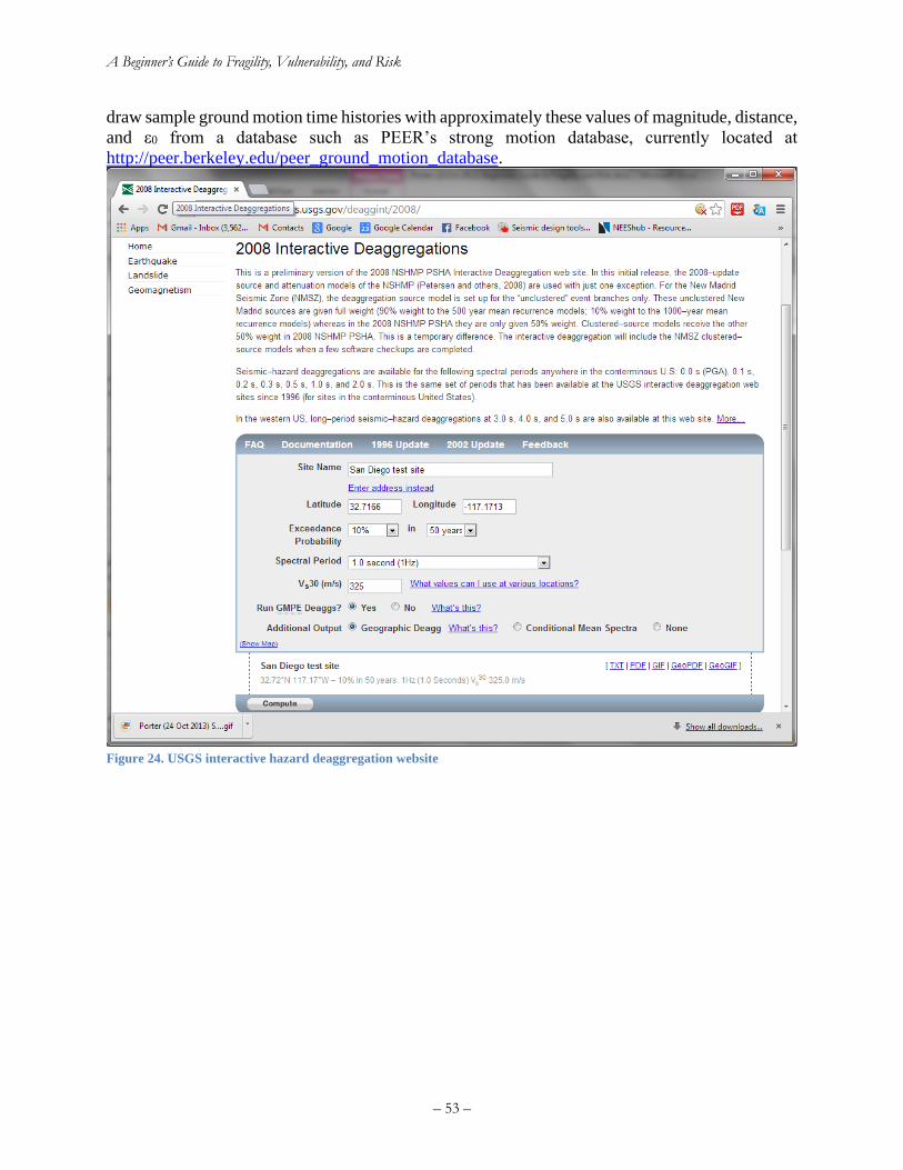
A Beginner’s Guide to Fragility, Vulnerability, and Risk
– 53 –
draw sample ground motion time histories with approximately these values of magnitude, distance,
and ε0 from a database such as PEER’s strong motion database, currently located at
http://peer.berkeley.edu/peer_ground_motion_database.
Figure 24. USGS interactive hazard deaggregation website
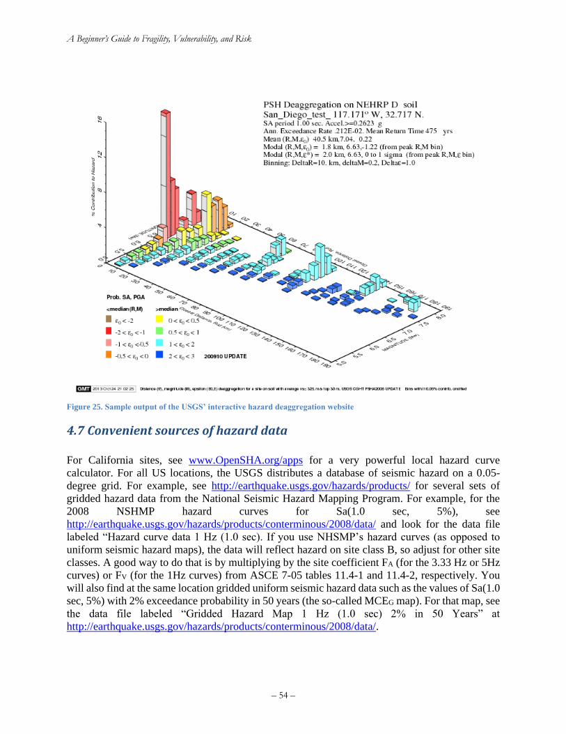
A Beginner’s Guide to Fragility, Vulnerability, and Risk
– 54 –
Figure 25. Sample output of the USGS’ interactive hazard deaggregation website
4.7 Convenient sources of hazard data
For California sites, see www.OpenSHA.org/apps for a very powerful local hazard curve
calculator. For all US locations, the USGS distributes a database of seismic hazard on a 0.05-
degree grid. For example, see http://earthquake.usgs.gov/hazards/products/ for several sets of
gridded hazard data from the National Seismic Hazard Mapping Program. For example, for the
2008 NSHMP hazard curves for Sa(1.0 sec, 5%), see
http://earthquake.usgs.gov/hazards/products/conterminous/2008/data/ and look for the data file
labeled “Hazard curve data 1 Hz (1.0 sec). If you use NHSMP’s hazard curves (as opposed to
uniform seismic hazard maps), the data will reflect hazard on site class B, so adjust for other site
classes. A good way to do that is by multiplying by the site coefficient FA (for the 3.33 Hz or 5Hz
curves) or FV (for the 1Hz curves) from ASCE 7-05 tables 11.4-1 and 11.4-2, respectively. You
will also find at the same location gridded uniform seismic hazard data such as the values of Sa(1.0
sec, 5%) with 2% exceedance probability in 50 years (the so-called MCEG map). For that map, see
the data file labeled “Gridded Hazard Map 1 Hz (1.0 sec) 2% in 50 Years” at
http://earthquake.usgs.gov/hazards/products/conterminous/2008/data/.
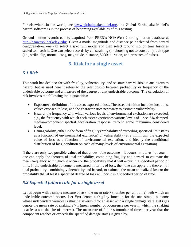
A Beginner’s Guide to Fragility, Vulnerability, and Risk
– 55 –
For elsewhere in the world, see www.globalquakemodel.org. the Global Earthquake Model’s
hazard software is in the process of becoming available as of this writing.
Ground motion records can be acquired from PEER’s NGAWest-2 strong-motion database at
http://ngawest2.berkeley.edu/. Given a modal magnitude and distance pair selected from hazard
deaggregation, one can select a spectrum model and then select ground motion time histories
scaled to match it. One can select records by constraining (or choosing not to constrain) fault type
(i.e., strike-slip, normal, etc.), magnitude, distance, Vs30, duration, and presence of pulses.
5. Risk for a single asset
5.1 Risk
This work has dealt so far with fragility, vulnerability, and seismic hazard. Risk is analogous to
hazard, but as used here it refers to the relationship between probability or frequency of the
undesirable outcome and a measure of the degree of that undesirable outcome. The calculation of
risk involves the following input quantities:
• Exposure: a definition of the assets exposed to loss. The asset definition includes locations,
values exposed to loss, and the characteristics necessary to estimate vulnerability.
• Hazard: the frequency with which various levels of environmental excitation are exceeded,
e.g., the frequency with which each asset experiences various levels of 1-sec, 5%-damped,
median-component spectral acceleration response, zero to some maximum considered
level.
• Damageability, either in the form of fragility (probability of exceeding specified limit states
as a function of environmental excitation) or vulnerability (at a minimum, the expected
value of loss as a function of environmental excitation, and ideally the conditional
distribution of loss, condition on each of many levels of environmental excitation).
If there are only two possible values of that undesirable outcome—it occurs or it doesn’t occur—
one can apply the theorem of total probability, combining fragility and hazard, to estimate the
mean frequency with which it occurs or the probability that it will occur in a specified period of
time. If the undesirable outcome is measured in terms of loss, then one can apply the theorem of
total probability, combining vulnerability and hazard, to estimate the mean annualized loss or the
probability that at least a specified degree of loss will occur in a specified period of time.
5.2 Expected failure rate for a single asset
Let us begin with a simple measure of risk: the mean rate λ (number per unit time) with which an
undesirable outcome occurs. Let F(s) denote a fragility function for the undesirable outcome
whose independent variable is shaking severity s for an asset with a single damage state. Let G(s)
denote the mean rate of shaking S ≥ s (mean number of occurrence per year in which the shaking
is at least s at the site of interest). The mean rate of failures (number of times per year that the
component reaches or exceeds the specified damage state) is given by
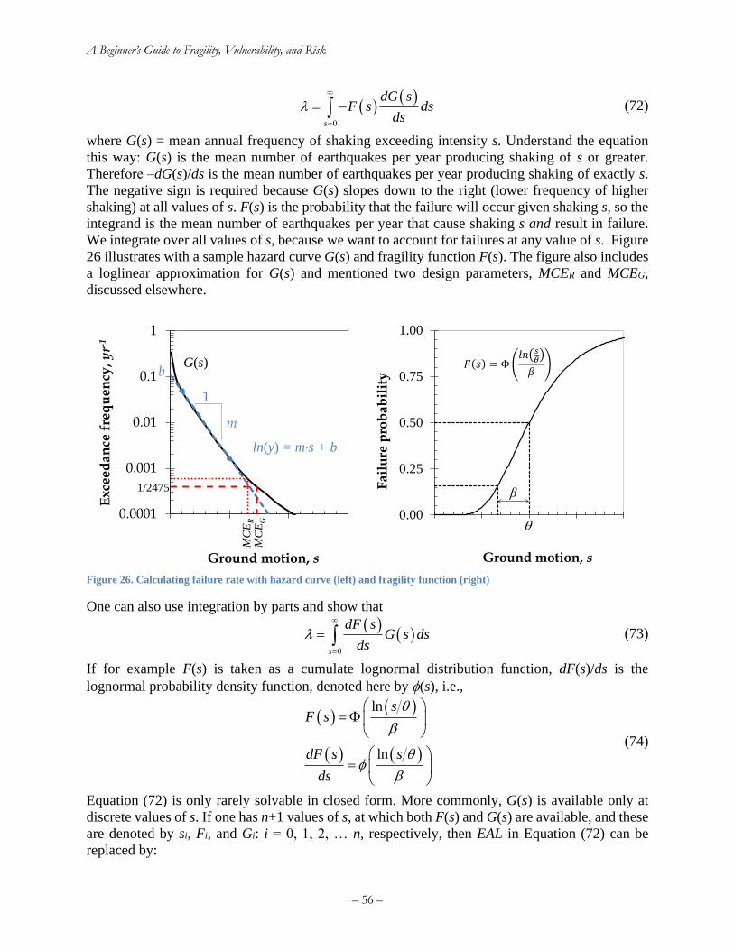
A Beginner’s Guide to Fragility, Vulnerability, and Risk
– 56 –
( )( )
0s
dG sF s ds
ds
=
= − (72)
where G(s) = mean annual frequency of shaking exceeding intensity s. Understand the equation
this way: G(s) is the mean number of earthquakes per year producing shaking of s or greater.
Therefore ‒dG(s)/ds is the mean number of earthquakes per year producing shaking of exactly s.
The negative sign is required because G(s) slopes down to the right (lower frequency of higher
shaking) at all values of s. F(s) is the probability that the failure will occur given shaking s, so the
integrand is the mean number of earthquakes per year that cause shaking s and result in failure.
We integrate over all values of s, because we want to account for failures at any value of s. Figure
26 illustrates with a sample hazard curve G(s) and fragility function F(s). The figure also includes
a loglinear approximation for G(s) and mentioned two design parameters, MCER and MCEG,
discussed elsewhere.
Figure 26. Calculating failure rate with hazard curve (left) and fragility function (right)
One can also use integration by parts and show that
( )
( )0s
dF sG s ds
ds
=
= (73)
If for example F(s) is taken as a cumulate lognormal distribution function, dF(s)/ds is the
lognormal probability density function, denoted here by (s), i.e.,
( )( )
( ) ( )
ln
ln
sF s
dF s s
ds
=
=
(74)
Equation (72) is only rarely solvable in closed form. More commonly, G(s) is available only at
discrete values of s. If one has n+1 values of s, at which both F(s) and G(s) are available, and these
are denoted by si, Fi, and Gi: i = 0, 1, 2, … n, respectively, then EAL in Equation (72) can be
replaced by:
0.0001
0.001
0.01
0.1
1
Ex
cee
da
nce
fre
qu
en
cy, yr-1
Ground motion, s
G(s)
ln(y) = ms + b
1/2475
MC
EG
MC
ER
1
m
b
0.00
0.25
0.50
0.75
1.00
Fail
ure
pro
bab
ilit
y
Ground motion, s
β
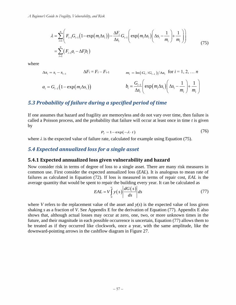
A Beginner’s Guide to Fragility, Vulnerability, and Risk
– 57 –
( )( ) ( )
( )
1 1 1
1
1
1
1 11 exp exp
ni
i i i i i i i i
i i i i
n
i i i i
i
FF G m s G m s s
s m m
F a Fb
− − −
=
−
=
= − − − +
= −
(75)
where
1i i is s s − = − Fi = Fi – Fi-1 ( )1lni i i im G G s−= for i = 1, 2, … n
( )( )1 1 expi i i ia G m s−= − ( )1 1 1expi
i i i i
i i i
Gb m s s
s m m
−
= − +
5.3 Probability of failure during a specified period of time
If one assumes that hazard and fragility are memoryless and do not vary over time, then failure is
called a Poisson process, and the probability that failure will occur at least once in time t is given
by
( )1 expfP t= − − (76)
where λ is the expected value of failure rate, calculated for example using Equation (75).
5.4 Expected annualized loss for a single asset
5.4.1 Expected annualized loss given vulnerability and hazard
Now consider risk in terms of degree of loss to a single asset. There are many risk measures in
common use. First consider the expected annualized loss (EAL). It is analogous to mean rate of
failures as calculated in Equation (72). If loss is measured in terms of repair cost, EAL is the
average quantity that would be spent to repair the building every year. It can be calculated as
( )( )
0
dG sEAL V y s ds
ds
= (77)
where V refers to the replacement value of the asset and y(s) is the expected value of loss given
shaking s as a fraction of V. See Appendix E for the derivation of Equation (77). Appendix E also
shows that, although actual losses may occur at zero, one, two, or more unknown times in the
future, and their magnitude in each possible occurrence is uncertain, Equation (77) allows them to
be treated as if they occurred like clockwork, once a year, with the same amplitude, like the
downward-pointing arrows in the cashflow diagram in Figure 27.
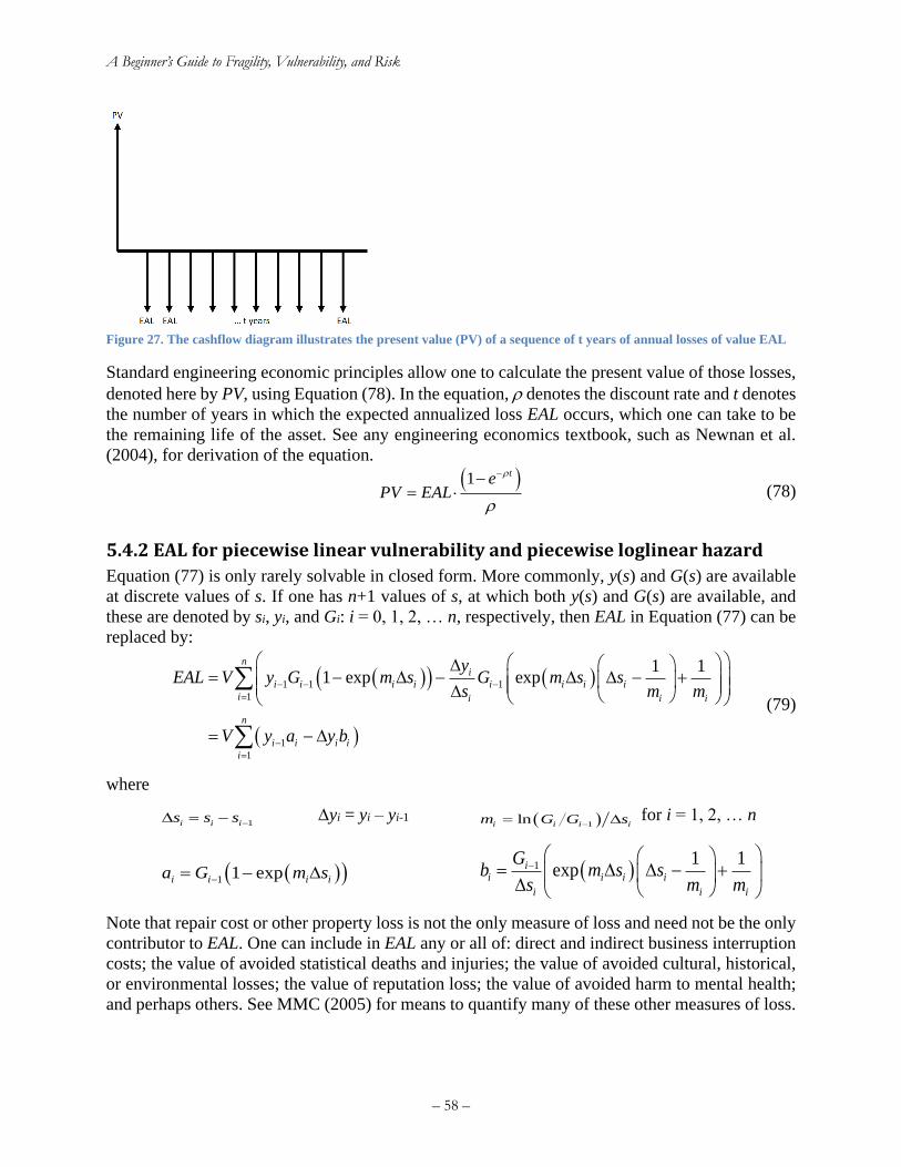
A Beginner’s Guide to Fragility, Vulnerability, and Risk
– 58 –
Figure 27. The cashflow diagram illustrates the present value (PV) of a sequence of t years of annual losses of value EAL
Standard engineering economic principles allow one to calculate the present value of those losses,
denoted here by PV, using Equation (78). In the equation, denotes the discount rate and t denotes
the number of years in which the expected annualized loss EAL occurs, which one can take to be
the remaining life of the asset. See any engineering economics textbook, such as Newnan et al.
(2004), for derivation of the equation.
( )1 te
PV EAL
−−= (78)
5.4.2 EAL for piecewise linear vulnerability and piecewise loglinear hazard
Equation (77) is only rarely solvable in closed form. More commonly, y(s) and G(s) are available
at discrete values of s. If one has n+1 values of s, at which both y(s) and G(s) are available, and
these are denoted by si, yi, and Gi: i = 0, 1, 2, … n, respectively, then EAL in Equation (77) can be
replaced by:
( )( ) ( )
( )
1 1 1
1
1
1
1 11 exp exp
ni
i i i i i i i i
i i i i
n
i i i i
i
yEAL V y G m s G m s s
s m m
V y a y b
− − −
=
−
=
= − − − +
= −
(79)
where
1i i is s s − = − yi = yi – yi-1 ( )1lni i i im G G s−= for i = 1, 2, … n
( )( )1 1 expi i i ia G m s−= − ( )1 1 1expi
i i i i
i i i
Gb m s s
s m m
−
= − +
Note that repair cost or other property loss is not the only measure of loss and need not be the only
contributor to EAL. One can include in EAL any or all of: direct and indirect business interruption
costs; the value of avoided statistical deaths and injuries; the value of avoided cultural, historical,
or environmental losses; the value of reputation loss; the value of avoided harm to mental health;
and perhaps others. See MMC (2005) for means to quantify many of these other measures of loss.
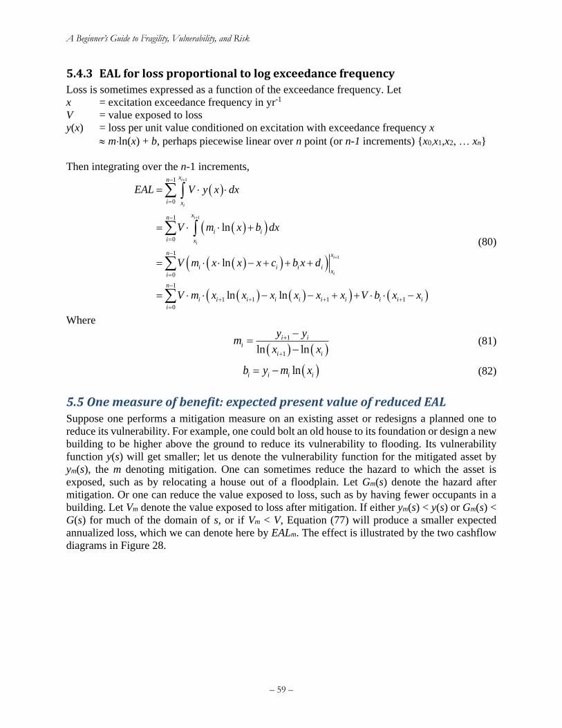
A Beginner’s Guide to Fragility, Vulnerability, and Risk
– 59 –
5.4.3 EAL for loss proportional to log exceedance frequency
Loss is sometimes expressed as a function of the exceedance frequency. Let
x = excitation exceedance frequency in yr-1
V = value exposed to loss
y(x) = loss per unit value conditioned on excitation with exceedance frequency x
mln(x) + b, perhaps piecewise linear over n point (or n-1 increments) {x0,x1,x2, … xn}
Then integrating over the n-1 increments,
( )
( )( )
( )( )( )
( ) ( )( ) ( )
1
1
1
1
0
1
0
1
0
1
1 1 1 1
0
ln
ln
ln ln
i
i
i
i
i
i
xn
i x
xn
i i
i x
n x
i i i ix
i
n
i i i i i i i i i i
i
EAL V y x dx
V m x b dx
V m x x x c b x d
V m x x x x x x V b x x
+
+
+
−
=
−
=
−
=
−
+ + + +
=
=
= +
= − + + +
= − − + + −
(80)
Where
( ) ( )
1
1ln ln
i ii
i i
y ym
x x
+
+
−=
− (81)
( )lni i i ib y m x= − (82)
5.5 One measure of benefit: expected present value of reduced EAL Suppose one performs a mitigation measure on an existing asset or redesigns a planned one to
reduce its vulnerability. For example, one could bolt an old house to its foundation or design a new
building to be higher above the ground to reduce its vulnerability to flooding. Its vulnerability
function y(s) will get smaller; let us denote the vulnerability function for the mitigated asset by
ym(s), the m denoting mitigation. One can sometimes reduce the hazard to which the asset is
exposed, such as by relocating a house out of a floodplain. Let Gm(s) denote the hazard after
mitigation. Or one can reduce the value exposed to loss, such as by having fewer occupants in a
building. Let Vm denote the value exposed to loss after mitigation. If either ym(s) < y(s) or Gm(s) <
G(s) for much of the domain of s, or if Vm < V, Equation (77) will produce a smaller expected
annualized loss, which we can denote here by EALm. The effect is illustrated by the two cashflow
diagrams in Figure 28.
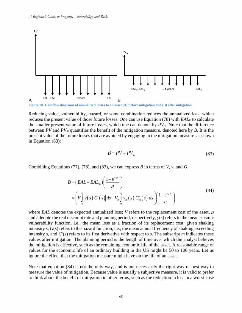
A Beginner’s Guide to Fragility, Vulnerability, and Risk
– 60 –
A B Figure 28. Cashflow diagrams of annualized losses to an asset (A) before mitigation and (B) after mitigation.
Reducing value, vulnerability, hazard, or some combination reduces the annualized loss, which
reduces the present value of those future losses. One can use Equation (78) with EALm to calculate
the smaller present value of future losses, which one can denote by PVm. Note that the difference
between PV and PVm quantifies the benefit of the mitigation measure, denoted here by B. It is the
present value of the future losses that are avoided by engaging in the mitigation measure, as shown
in Equation (83):
mB PV PV= − (83)
Combining Equations (77), (78), and (83), we can express B in terms of V, y, and G.
( )
( ) ( ) ( ) ( )0 0
1 e
1 e
t
m
t
m m m
B EAL EAL
V y s G s ds V y s G s ds
−
−
−= −
− = −
(84)
where EAL denotes the expected annualized loss; V refers to the replacement cost of the asset,
and t denote the real discount rate and planning period, respectively, y(s) refers to the mean seismic
vulnerability function, i.e., the mean loss as a fraction of its replacement cost, given shaking
intensity s, G(s) refers to the hazard function, i.e., the mean annual frequency of shaking exceeding
intensity s, and G′(s) refers to its first derivative with respect to s. The subscript m indicates these
values after mitigation. The planning period is the length of time over which the analyst believes
the mitigation is effective, such as the remaining economic life of the asset. A reasonable range of
values for the economic life of an ordinary building in the US might be 50 to 100 years. Let us
ignore the effect that the mitigation measure might have on the life of an asset.
Note that equation (84) is not the only way, and is not necessarily the right way or best way to
measure the value of mitigation. Because value is usually a subjective measure, it is valid to prefer
to think about the benefit of mitigation in other terms, such as the reduction in loss in a worst-case
A Beginner’s Guide to Fragility, Vulnerability, and Risk
– 61 –
or other extreme scenario. A self-selected committee of volunteers directed the San Francisco
Community Action Plan for Seismic Safety, for example, to measure benefit in terms of the
expected reduction in the number of collapsed buildings, red-tagged buildings, and yellow-tagged
buildings in four particular earthquake scenarios, with an emphasis on one in particular. See for
example Porter and Cobeen (2012) for more details.
Note also that the discount rate in Equation (84) might differ between measures of loss. Some
writers find the discounting of human life (as in the reduction deaths and injuries) untenable, and
apply a different discount rate to financial outcomes than to deaths and injuries.
5.6 Risk curve for a single asset
5.6.1 Risk curve for a lognormally distributed loss measure
It is often desirable to know the probability that loss will exceed a particular value during a given
time period t as a function of loss. Another, very similar question with a nearly identical answer is
the frequency (in event per unit time) that loss will exceed a particular value. Here, both
relationships are expressed with a function called a risk curve. It is like the hazard curve, except
that the x-axis measures loss instead of environment excitation. Figure 29 illustrates two risk
curves. They could both express risk to the same asset using two different models, one with less
and one with more uncertainty.
Figure 29. Two illustrative risk curves
How to calculate the risk curve? Suppose one knows the hazard curve and the uncertain
vulnerability function for a single asset. The risk curve for a single asset can be calculated as
( ) ( )( )
0
1s
dG sR x P X x S s ds
ds
=
= − − = (85)
where
X = uncertain degree of loss to an asset, such as the uncertain damage factor
x = a particular value of X
0.0001
0.001
0.01
0.1
1
0.0001 0.001 0.01 0.1 1
Exce
edan
ce r
ate,
yr-1
Loss, fraction of mean value
1/250-year loss
Less uncertain
More
uncertain
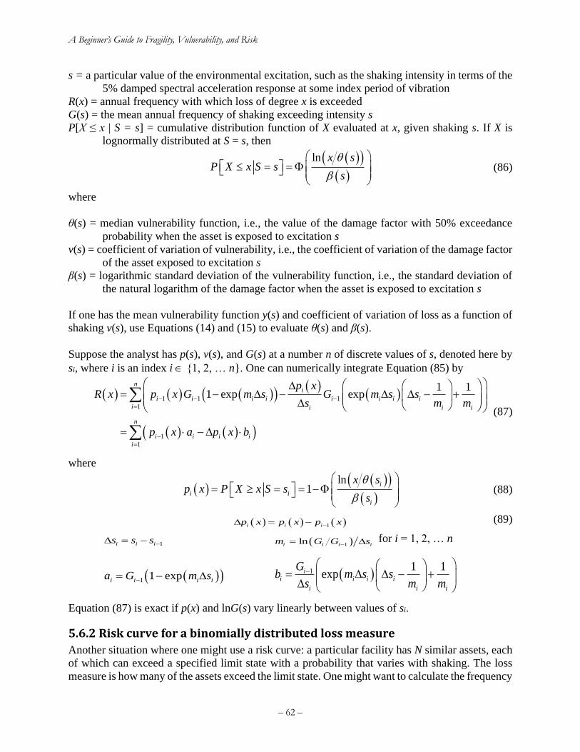
A Beginner’s Guide to Fragility, Vulnerability, and Risk
– 62 –
s = a particular value of the environmental excitation, such as the shaking intensity in terms of the
5% damped spectral acceleration response at some index period of vibration
R(x) = annual frequency with which loss of degree x is exceeded
G(s) = the mean annual frequency of shaking exceeding intensity s
P[X ≤ x | S = s] = cumulative distribution function of X evaluated at x, given shaking s. If X is
lognormally distributed at S = s, then
( )( )
( )
ln x sP X x S s
s
= =
(86)
where
θ(s) = median vulnerability function, i.e., the value of the damage factor with 50% exceedance
probability when the asset is exposed to excitation s
v(s) = coefficient of variation of vulnerability, i.e., the coefficient of variation of the damage factor
of the asset exposed to excitation s
β(s) = logarithmic standard deviation of the vulnerability function, i.e., the standard deviation of
the natural logarithm of the damage factor when the asset is exposed to excitation s
If one has the mean vulnerability function y(s) and coefficient of variation of loss as a function of
shaking v(s), use Equations (14) and (15) to evaluate θ(s) and β(s).
Suppose the analyst has p(s), v(s), and G(s) at a number n of discrete values of s, denoted here by
si, where i is an index i {1, 2, … n}. One can numerically integrate Equation (85) by
( ) ( ) ( )( )( )
( )
( ) ( )( )
1 1 1
1
1
1
1 11 exp exp
ni
i i i i i i i i
i i i i
n
i i i i
i
p xR x p x G m s G m s s
s m m
p x a p x b
− − −
=
−
=
= − − − +
= −
(87)
where
( )( )( )
( )
ln1
i
i i
i
x sp x P X x S s
s
= = = −
(88)
( ) ( ) ( )1i i ip x p x p x− = − (89)
1i i is s s − = − ( )1lni i i im G G s−= for i = 1, 2, … n
( )( )1 1 expi i i ia G m s−= − ( )1 1 1expi
i i i i
i i i
Gb m s s
s m m
−
= − +
Equation (87) is exact if p(x) and lnG(s) vary linearly between values of si.
5.6.2 Risk curve for a binomially distributed loss measure
Another situation where one might use a risk curve: a particular facility has N similar assets, each
of which can exceed a specified limit state with a probability that varies with shaking. The loss
measure is how many of the assets exceed the limit state. One might want to calculate the frequency
A Beginner’s Guide to Fragility, Vulnerability, and Risk
– 63 –
with which y assets exceed the limit state in a single event during a period t, or similarly the
probability that, during some period of t years, at least y assets exceed the limit state in a single
event. For example, the assets might be occupants and the limit state, injuries of at least some
specified severity.
For clarity, let us proceed by discussing the example of injuries in a building. The math presented
here is generally applicable to other assets and limit states, such as the number of identical
components that overturn in a single event.
Let E[Y|S=s] denote the expected value of the number of injuries at some level of ground motion
s. If we have a value of E[Y|S=s] for each of many levels of s, we refer to the set of pairs {(s,
E[Y|S=s])} as the mean vulnerability function. One can then estimate that the probability f(s) that
any individual person would be injured given ground motion s using Equation (90):
( )E Y S s
f sN
= = (90)
If we assume that injuries are not correlated, that is, that the probability of injury to person A is
unaffected by whether person B is injured, and that both people have the same injury probability
at shaking s, then one can take the uncertain number of injuries Y as distributed like the binomial
distribution. The probability that at least y people are injured is then given by Equation (91):
( ) ( )( )( )
C 1N mm
N m
N
m y
P Y y S s f s f s=
− −
= = (91)
Where NCm denotes the number of combinations of m elements out of N, i.e., N choose m:
( )
!
! !N m
NC
m N m=
− (92)
Let G(s) denote the hazard function, i.e., the frequency (measured in events per year) with which
shaking of at least s occurs. Then the occurrence rate of events injuring at least y people is given
by Equation (93), which is a slight extension of the theorem of total probability. Here R[Y≥y|1 yr]
denotes the rate (events per year) of at least y injuries, or R(y) for shorthand:
( )
( )
( )
0
0
1
s
s
R y R Y y yr
dG sP Y y S s ds
ds
dG sP Y y S s ds
ds
=
=
=
= =
= − =
(93)
( ) ( ) ( )( )( )
( )
( ) ( )( )
1 1 1
1
1
1
1 11 exp exp
ni
i i i i i i i i
i i i i
n
i i i i
i
p xR y p y G m s G m s s
s m m
p y a p y b
− − −
=
−
=
= − − − +
= −
(94)
where
A Beginner’s Guide to Fragility, Vulnerability, and Risk
– 64 –
( ) ( ) ( )( )( )
C 1N mm
N m i i
N
i i
m y
p sp y P Y y S ss p−
=
= = = − (95)
( ) ( ) ( )1i i ip y p y p y− = − (96)
1i i is s s − = − ( )1lni i i im G G s−= for i = 1, 2, … n
( )( )1 1 expi i i ia G m s−= − ( )1 1 1expi
i i i i
i i i
Gb m s s
s m m
−
= − +
If we idealize earthquake occurrence as a Poisson process, i.e., as a memoryless process, then the
probability that at least y injuries occur in time t years is given by the Poisson cumulative
distribution function:
( )( )1 expP Y t R y ty = − − (97)
5.6.3 Risk curve for a binomially distributed loss measure with large N
Equation (91) can be hard to calculate for large N, e.g., when there are a large number of building
occupants, because of the N! term in the numerator of Equation (92). However, when N becomes
large, the binomial resembles the Gaussian distribution with expected value and variance given by
( )E Y S s N f s = = (98)
( ) ( )( )1Var Y S s N f s f s = = − (99)
Then instead of calculating pi(y) using Equation (95), use
( )( )
( ) ( )( )1
1
i
i i
i i
y N f sp y P Y y S s
N f s f s
− = = = − −
(100)
5.7 Probable maximum loss for a single asset
There is no universally accepted definition of probable maximum loss (PML) for purposes of
earthquake risk analysis, but it is often understood to mean the loss with 90% nonexceedance
probability given shaking with 10% exceedance probability in 50 years. Under this definition,
PML is more accurately called a measure of vulnerability rather than one of risk. For a single asset,
PML can be calculated from the seismic vulnerability function by inverting the conditional
distribution of loss at 0.90, when conditioned on shaking with 10% exceedance probability in 50
years.
For example, assume that loss is lognormally distributed conditioned on shaking s, with median
θ(s) and logarithmic standard deviation β(s) as described near Equation (86), which are related to
the mean vulnerability function y(s) and coefficient of variation v(s) as in Equations (14) and (15)
. Under the assumption of Poisson arrives of earthquakes, shaking with 10% exceedance
probability in 50 years is the shaking with exceedance rate G(sPML) = 0.00211 per year, so PML
can be estimated as a fraction of value exposed by
A Beginner’s Guide to Fragility, Vulnerability, and Risk
– 65 –
( ) ( )( )exp 1.28PML PMLPML s s = (101)
where sPML = G-1(0.00211 yr-1), that is, the hazard curve (events per year) inverted at 0.00211.
5.8 Common single-site risk software The professional reader may be interested in software options to calculate single-site risk. Several
developers have created useful software. In the US as of this writing, the most popular commercial
single-site earthquake risk tool is probably ST-RISK (http://www.st-risk.com/). Its developers
describe it as “a software package used by insurance and mortgage due-diligence investigators and
structural engineers to perform detailed earthquake risk analysis for individual buildings. These
analyses and reports are used by mortgage brokers to make lending decisions, insurance brokers
to rate assessments, and building owners to make seismic retrofit plans.” It essentially pairs a
hazard model from the USGS with a proprietary vulnerability model. The user provides the
building’s latitude, longitude, optionally Vs30, and a few attributes of the building such as age,
structural system, height, and optionally more-detailed features as specified by ASCE 31-03
(ASCE 2003). The vulnerability model “uniquely blends insurance loss data with post earthquake
observed loss obtained as part of engineering reconnaissance information to generate damage
functions that most accurately reflect reported losses from earthquakes.” The user can alternatively
use Hazus-based vulnerability functions. In either case, the vulnerability model probably relies
substantially on expert opinion.
FEMA P-58 (ATC 2012) offers a much more labor-intensive but probably sounder empirical and
analytical basis for estimating single-site risk in the form of its PACT software. The user must
create a nonlinear structural model of the building in question, perform multiple nonlinear dynamic
structural analyses of the building, add information about the structural and nonstructural
components of the building, input hazard data, and the software calculates risk.
6. Portfolio risk analysis This chapter is incomplete.
6.1 Two common measures of portfolio risk
6.1.1 Portfolio loss exceedance curve
Portfolio catastrophe risk analysis refers to calculating the probability distribution of the sum of
losses to a set of two or more assets—a portfolio of assets. The assets may be effectively points on
a map, such as buildings spread out over a community, state, or nation. Sometimes the assets are
more readily idealized on a map by lines, networks, or geographically distributed systems such as
highway bridges, water pipeline networks, or an electric generation, transmission, and distribution
system.
The spatial extent of a portfolio matters because its elements do not experience the same level of
environmental excitation simultaneously in a catastrophe. For those reasons, with at least one
exception, one usually calculates portfolio risk by aggregating losses over scenarios. That is, one
characterizes the loss in one or more events, often discretized to approximate a mutually exclusive
and collectively exhaustive set of possibilities to which the portfolio is subject. One can then use
the theorem of total probability to describe the portfolio probabilistic risk, as in equation (102).
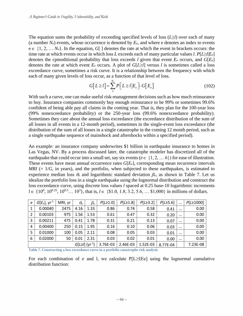
A Beginner’s Guide to Fragility, Vulnerability, and Risk
– 66 –
The equation sums the probability of exceeding specified levels of loss (L≥l) over each of many
(a number Ne) events, whose occurrence is denoted by Ee, and where e denotes an index to events
e {1, 2, … Ne}. In the equation, G[ ] denotes the rate at which the event in brackets occurs: the
time rate at which events occur in which loss L exceeds each of many particular values l. P[L≥l|Ee]
denotes the cpmoditional probability that loss exceeds l given that event Ee occurs, and G[Ee]
denotes the rate at which event Ee occurs. A plot of G[L≥l] versus l is sometimes called a loss
exceedance curve, sometimes a risk curve. It is a relationship between the frequency with which
each of many given levels of loss occur, as a function of that level of loss.
eN
e e
e
G L l P L l E G E = (102)
With such a curve, one can make useful risk-management decisions such as how much reinsurance
to buy. Insurance companies commonly buy enough reinsurance to be 99% or sometimes 99.6%
confident of being able pay all claims in the coming year. That is, they plan for the 100-year loss
(99% nonexceedance probability) or the 250-year loss (99.6% nonexceedance probability).
Sometimes they care about the annual loss exceedance (the exceedance distribution of the sum of
all losses in all events in a 12-month period), sometimes in the single-event loss exceedance (the
distribution of the sum of all losses in a single catastrophe in the coming 12 month period, such as
a single earthquake sequence of mainshock and aftershocks within a specified period).
An example: an insurance company underwrites $1 billion in earthquake insurance to homes in
Las Vegas, NV. By a process discussed later, the catastrophe modeler has discretized all of the
earthquake that could occur into a small set, say six events (e {1, 2, … 6}) for ease of illustration.
These events have mean annual occurrence rates G[Ee], corresponding mean recurrence intervals
MRI (= 1/G, in years), and the portfolio, when subjected to these earthquakes, is estimated to
experience median loss e and logarithmic standard deviation e, as shown in Table 7. Let us
idealize the portfolio loss in a single earthquake using the lognormal distribution and construct the
loss exceedance curve, using discrete loss values l spaced at 0.25 base-10 logarithmic increments
l {100, 100.25, 100.5… 103}, that is, l {$1.0, 1.8, 3.2, 5.6, … $1,000} in millions of dollars.
e G[Ee], yr-1 MRI, yr e e P[L≥1.0] P[L≥1.8] P[L≥3.2] P[L≥5.6] … P[L≥1000]
1 0.00040 2475 4.16 1.33 0.86 0.74 0.58 0.41 … 0.00
2 0.00103 975 1.56 1.53 0.61 0.47 0.32 0.20 … 0.00
3 0.00211 475 0.41 1.78 0.31 0.21 0.13 0.07 … 0.00
4 0.00400 250 0.15 1.95 0.16 0.10 0.06 0.03 … 0.00
5 0.01000 100 0.05 2.11 0.08 0.05 0.03 0.01 … 0.00
6 0.02000 50 0.01 2.31 0.03 0.02 0.01 0.00 … 0.00
G[L≥l] (yr-1) 3.76E-03 2.46E-03 1.52E-03 8.77E-04 7.23E-08 Table 7. Constructing a loss exceedance curve in a portfolio catastrophe risk analysis
For each combination of e and l, we calculate P[L≥l|Ee] using the lognormal cumulative
distribution function:
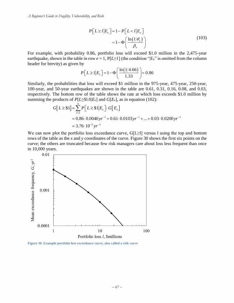
A Beginner’s Guide to Fragility, Vulnerability, and Risk
– 67 –
( )
1
ln1
e e
e
e
P L l E P L l E
l
= −
= −
(103)
For example, with probability 0.86, portfolio loss will exceed $1.0 million in the 2,475-year
earthquake, shown in the table in row e = 1, P[L≥1] (the condition “|Ee” is omitted from the column
header for brevity) as given by
( )
1
ln 1 4.661 1 0.86
1.33P L E
= − =
Similarly, the probabilities that loss will exceed $1 million in the 975-year, 475-year, 250-year,
100-year, and 50-year earthquakes are shown in the table are 0.61, 0.31, 0.16, 0.08, and 0.03,
respectively. The bottom row of the table shows the rate at which loss exceeds $1.0 million by
summing the products of P[L≥$l.0|Ee] and G[Ee], as in equation (102):
6
1
1 1 1
3 1
$1 $1
0.86 0.0040 0.61 0.0103 ... 0.03 0.0200
3.76 10
e e
e
G L P L E G E
yr yr yr
yr
=
− − −
− −
=
= + + +
=
We can now plot the portfolio loss exceedance curve, G[L≥l] versus l using the top and bottom
rows of the table as the x and y coordinates of the curve. Figure 30 shows the first six points on the
curve; the others are truncated because few risk managers care about loss less frequent than once
in 10,000 years.
Figure 30. Example portfolio loss exceedance curve, also called a risk curve
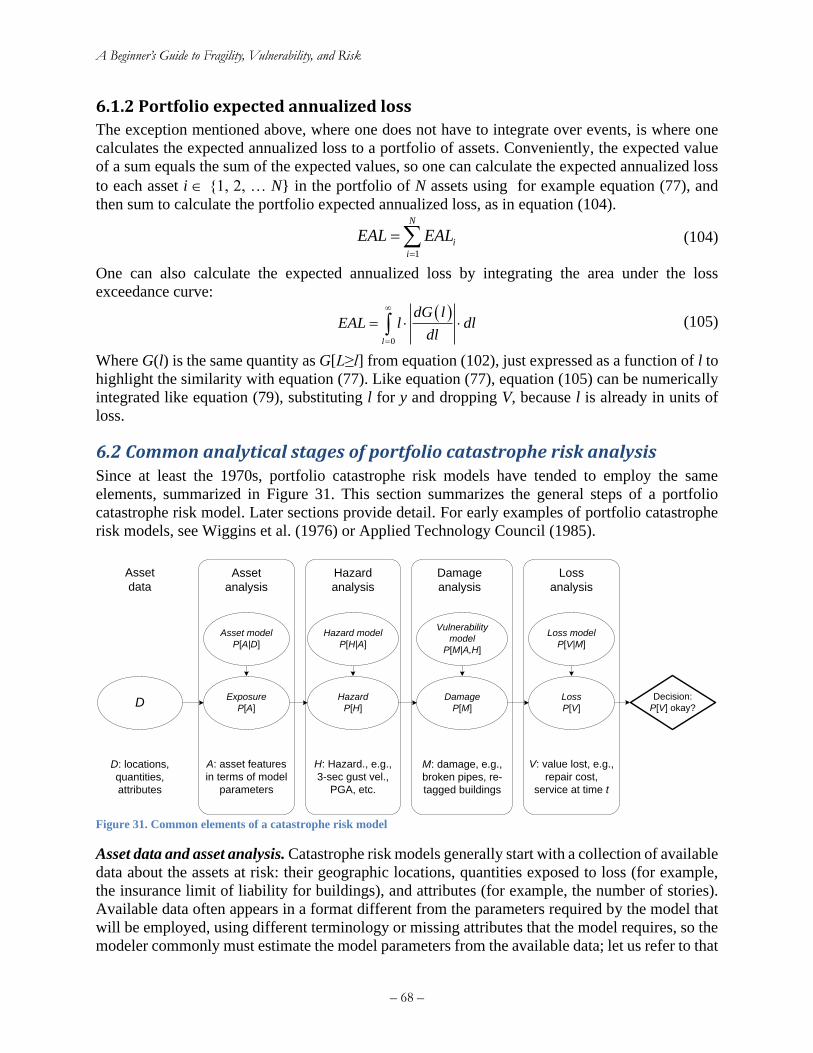
A Beginner’s Guide to Fragility, Vulnerability, and Risk
– 68 –
6.1.2 Portfolio expected annualized loss
The exception mentioned above, where one does not have to integrate over events, is where one
calculates the expected annualized loss to a portfolio of assets. Conveniently, the expected value
of a sum equals the sum of the expected values, so one can calculate the expected annualized loss
to each asset i {1, 2, … N} in the portfolio of N assets using for example equation (77), and
then sum to calculate the portfolio expected annualized loss, as in equation (104).
1
N
i
i
EAL EAL=
= (104)
One can also calculate the expected annualized loss by integrating the area under the loss
exceedance curve:
( )
0l
dG lEAL l dl
dl
=
= (105)
Where G(l) is the same quantity as G[L≥l] from equation (102), just expressed as a function of l to
highlight the similarity with equation (77). Like equation (77), equation (105) can be numerically
integrated like equation (79), substituting l for y and dropping V, because l is already in units of
loss.
6.2 Common analytical stages of portfolio catastrophe risk analysis Since at least the 1970s, portfolio catastrophe risk models have tended to employ the same
elements, summarized in Figure 31. This section summarizes the general steps of a portfolio
catastrophe risk model. Later sections provide detail. For early examples of portfolio catastrophe
risk models, see Wiggins et al. (1976) or Applied Technology Council (1985).
Figure 31. Common elements of a catastrophe risk model
Asset data and asset analysis. Catastrophe risk models generally start with a collection of available
data about the assets at risk: their geographic locations, quantities exposed to loss (for example,
the insurance limit of liability for buildings), and attributes (for example, the number of stories).
Available data often appears in a format different from the parameters required by the model that
will be employed, using different terminology or missing attributes that the model requires, so the
modeler commonly must estimate the model parameters from the available data; let us refer to that
Exposure
P[A]
A: asset features
in terms of model
parameters
D
Asset
analysis
Hazard
analysis
Hazard model
P[H|A]
H: Hazard., e.g.,
3-sec gust vel.,
PGA, etc.
D: locations,
quantities,
attributes
Damage
analysis
Vulnerability
model
P[M|A,H]
Damage
P[M]
M: damage, e.g.,
broken pipes, re-
tagged buildings
Loss
analysis
Loss model
P[V|M]
Loss
P[V]
V: value lost, e.g.,
repair cost,
service at time t
Hazard
P[H]
Asset
data
Decision:
P[V] okay?
Asset model
P[A|D]
A Beginner’s Guide to Fragility, Vulnerability, and Risk
– 69 –
process as an asset analysis. When the available data contain less information than the model
requires, the modeler can perform a probabilistic asset analysis, estimating the probability
distribution of model parameters conditioned on the input data.
Hazard analysis. Assets are exposed to uncertain environmental excitation, whether from future
earthquake shaking, future tornado winds, or other natural or anthropogenic peril. One selects a
hazard model. In the case of earthquake, the hazard model typically involves two elements: an
earthquake rupture forecast, which comprises a mathematical model of the locations of seismic
sources and the rate at which each source produces earthquakes of various magnitudes, and ground
motion prediction equations, which estimate earthquake excitation at any location conditioned on
the earthquake source characteristics (magnitude, distance, focal mechanism, etc.) and path and
site characteristics (for example, average shearwave velocity in the upper 30 meters of soil and
depth to bedrock with 2.5 km/sec shearwave velocity). The hazard model is applied to the asset
locations to estimate the hazard at each asset, for example the probability distribution of peak
ground velocity to which each asset is exposed conditioned on the occurrence of a particular
earthquake.
Damage analysis. Damage is best, though not always, defined in terms of observable damage
states—measures of the degradation of the asset defined unambiguously so that two observers,
examining a damaged asset, both reach the same conclusions about its damage state without
significant reliance on judgment or interpretation. One selects or develops a vulnerability model,
which characterizes the (uncertain) physical damage to various classes of asset as a function of
environmental excitation. One then applies the results of the hazard model to estimate the
(typically uncertain) damage state of each asset.
Loss analysis. Loss is best, though not always, defined in terms of observable and unambiguous
measures of loss that consumers of the analysis care about, usually financial consequences, safety
impacts, and duration of loss of function (“dollars, deaths, and downtime”). One selects or creates
a loss model that estimate value lost as a function of asset damage, applies the outputs of the
damage analysis to the loss model, and estimates the (potentially uncertain) loss. Consumers of
the analysis usually use the output of the loss analysis to make some risk-management decision,
such as whether to accept the existing risk or how to transfer or remediate it.
Note that the term “hazard analysis” is fairly common, but the author is unaware of standard
terminology for the asset, damage and loss analyses, so the reader should not assume that they are
commonly understood.
The distinction between damage and loss analysis can be artificial, for example when one uses
vulnerability functions that relate asset category and environmental excitation directly to loss as a
fraction of value exposed, as in equation (77), where V denotes value of exposed to loss, y(s) is the
vulnerability function, and G(s) is the hazard curve. Figure 32 presents a simpler form.
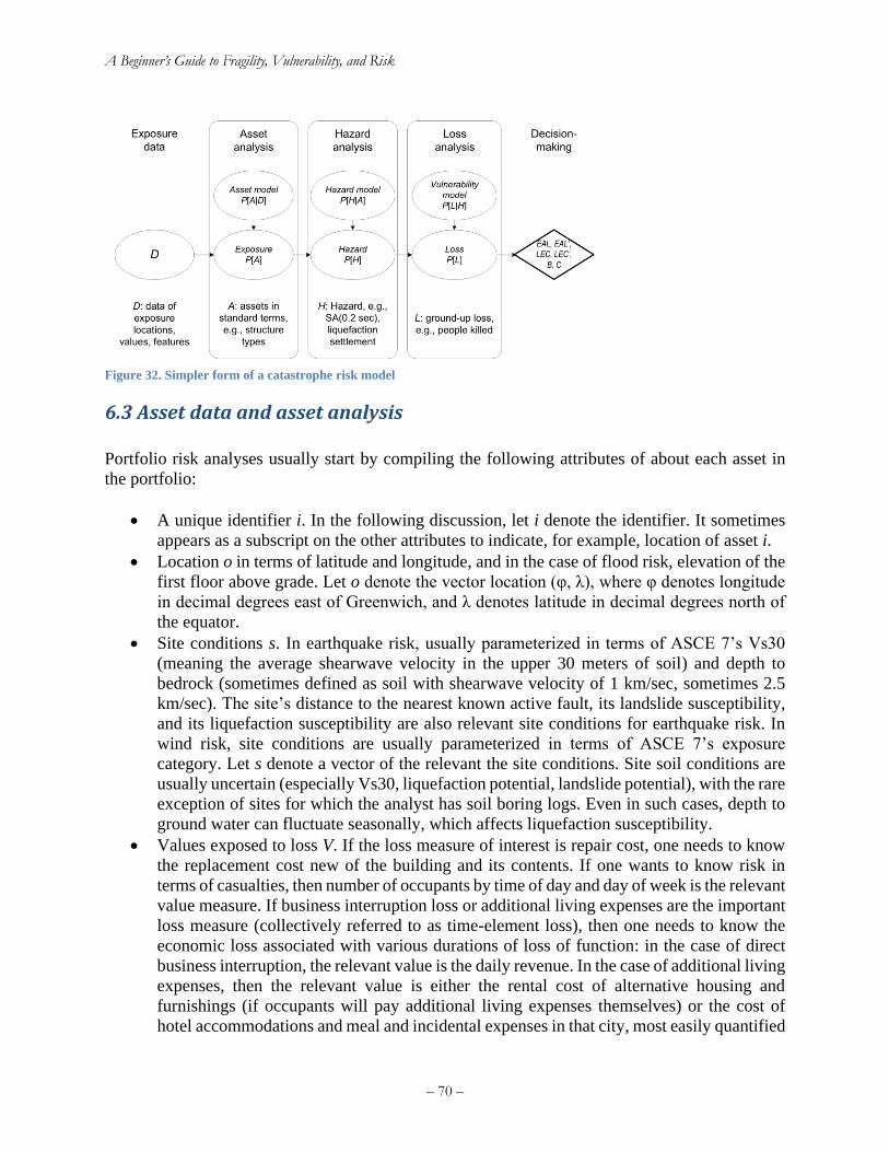
A Beginner’s Guide to Fragility, Vulnerability, and Risk
– 70 –
Figure 32. Simpler form of a catastrophe risk model
6.3 Asset data and asset analysis
Portfolio risk analyses usually start by compiling the following attributes of about each asset in
the portfolio:
• A unique identifier i. In the following discussion, let i denote the identifier. It sometimes
appears as a subscript on the other attributes to indicate, for example, location of asset i.
• Location o in terms of latitude and longitude, and in the case of flood risk, elevation of the
first floor above grade. Let o denote the vector location (φ, λ), where φ denotes longitude
in decimal degrees east of Greenwich, and λ denotes latitude in decimal degrees north of
the equator.
• Site conditions s. In earthquake risk, usually parameterized in terms of ASCE 7’s Vs30
(meaning the average shearwave velocity in the upper 30 meters of soil) and depth to
bedrock (sometimes defined as soil with shearwave velocity of 1 km/sec, sometimes 2.5
km/sec). The site’s distance to the nearest known active fault, its landslide susceptibility,
and its liquefaction susceptibility are also relevant site conditions for earthquake risk. In
wind risk, site conditions are usually parameterized in terms of ASCE 7’s exposure
category. Let s denote a vector of the relevant the site conditions. Site soil conditions are
usually uncertain (especially Vs30, liquefaction potential, landslide potential), with the rare
exception of sites for which the analyst has soil boring logs. Even in such cases, depth to
ground water can fluctuate seasonally, which affects liquefaction susceptibility.
• Values exposed to loss V. If the loss measure of interest is repair cost, one needs to know
the replacement cost new of the building and its contents. If one wants to know risk in
terms of casualties, then number of occupants by time of day and day of week is the relevant
value measure. If business interruption loss or additional living expenses are the important
loss measure (collectively referred to as time-element loss), then one needs to know the
economic loss associated with various durations of loss of function: in the case of direct
business interruption, the relevant value is the daily revenue. In the case of additional living
expenses, then the relevant value is either the rental cost of alternative housing and
furnishings (if occupants will pay additional living expenses themselves) or the cost of
hotel accommodations and meal and incidental expenses in that city, most easily quantified
A Beginner’s Guide to Fragility, Vulnerability, and Risk
– 71 –
using the General Services Administration’s per diem rates (accommodations plus meals
and incidental expenses) per person. If the loss measure of interest is whether the building
will be habitable, then one needs to know how many people live or work there. Let V
denote value exposed to loss. It is usually uncertain, even though many catastrophe risk
models ignore that uncertainty.
• Asset category a, sometimes called structure type, construction type, building type, or
model building type. There are many classification systems. The Hazus-MH taxonomy is
commonly used. It identifies buildings by structural material, lateral force resisting system,
height category, code era, and occupancy classification. See http://goo.gl/XfdsjY for
details. The Global Earthquake Model (GEM) Building Taxonomy version 2
(http://goo.gl/m6JVUL) is almost infinitely flexible, allowing the user to classify buildings
by any combination of 13 attributes, including those of the Hazus-MH taxonomy and
several others. The commercial catastrophe risk models (e.g., RMS, AIR and EQECAT)
have their own proprietary taxonomies that do not always relate one-to-one. Some models
refer to some attributes as modifiers that are used to adjust losses calculated for a broad
category to account for the effect of the attribute, such as soft story conditions in an
earthquake risk analysis. The modifiers are treated here as merely a further subdivision of
the category system. Asset category is usually uncertain, with the rare exception of a
portfolio whose asset categories have been established by a structural engineer examining
structural drawings.
• Contract details c for contracts that transfer risk from the property owner, tenant, or other
entity experiencing damage to a second party such as an insurer or the seller of a bond that
acts like insurance. These risk-transfer contracts relate property repair costs, duration of
loss of function, and casualties to the economic liability of the second party. Think of the
contract details c as a mathematical function that takes as input the various repair costs,
loss-of-function duration, and casualties, and the value of the function is the financial
liability of the second party. The function usually has additional parameters, especially the
deductible d (the repair cost that the insured must pay before the insurer’s liability begins),
limit of liability l (the maximum amount that the insurer must pay), and pro rata share p
(the fraction of loss in excess of the deductible that the insurer must pay). There are various
details about how d, l, and p apply. For example, in some contracts, there are separate
deductibles for the building, contents, and time-element losses.
TBD: a table summarizing parameters, indicating uncertainty.
6.4 Portfolio hazard analysis
6.4.1 Earthquake rupture forecasts. How to select branch(es) and simulate sequence(s)
TBD
6.4.3 Simulating properly spatially correlated ground motion
Ground motion at an arbitrarily location that is shaken by an earthquake with a given magnitude,
location, and faulting mechanism can be highly uncertain. Engineering seismologists currently
characterize the uncertainty in two parts: variation between events, called the inter-event (or more
intuitive between-event) term, and between different locations in the same event, called the intra-
A Beginner’s Guide to Fragility, Vulnerability, and Risk
– 72 –
event (more easily remembered as within-event) term. Recent ground-motion-prediction equations
commonly offer a parameter value for each term. The parameter measures the standard deviation
of the natural logarithm of uncertainty in ground motion.
The between-event variability (denoted here by ) measures the standard deviation of the natural
logarithm of how one earthquake produces uniformly higher or lower ground motion than does
another of the same magnitude, location, faulting mechanism, and so on. For example, an
earthquake of a specific magnitude can release all its energy more slowly or more quickly than
another of the same magnitude, with resulting differences in the ground motion across the entire
shaken area. Every location in the shaken area will feel that slightly higher or lower motion because
of the inter-event variability. The between-event term is perfectly correlated between different
sites in the same earthquake.
The within-event variability (denoted here by ) measures the standard deviation of the natural
logarithm of how a location experiences higher or lower ground motion than the median value for
a location with given site conditions and at a given distance from the rupture. The within-event
term is spatially correlated between two sites. Sites that are next door to each other are nearly
perfectly correlated. If one experiences higher-than-average motion in a given earthquake, so will
its next-door neighbor. The farther apart the two sites are, the less the correlation. At sufficiently
large separation distance, conditioned on the inter-event term, the intra-event variability of two
sites is uncorrelated. Jayaram and Baker (2009) quantify that spatial correlation.
One way to quantify the effects of that spatial correlation in intensity involves simulating a suite
of events with properly spatially correlated intensity. Simulating a spatially correlated random
field can be hard. Suppose one wants to characterize the field with an N x N grid of points.
Excitation at each gridpoint has some degree of correlation with that of every other gridpoint,
meaning N2 x N2 = N4 correlation coefficients. To simulate a correlated random field of N2 grid
points can require solving an eigenproblem for the N2 x N2 correlation matrix. In the case of
earthquakes, the grid spacing might need to be on the order of 1 km, and one might want to simulate
a field 200 km on a side, meaning N2 40,000 gridpoints. It can be very computationally
demanding to solve the 40,000 x 40,000 eigenproblem, and one generally does not want to do so
on the fly, many times for each of many earthquakes or other disasters. How can one generate
spatially correlated ground motions without solving on-the-fly eigenproblems?
Let
o = an index to a geographic location
i = an index to a realization of M spatially correlated random ground motion fields, i {0, 1, …
M-1}
yo(i) = realization i of ground motion at o, with inter- and intra-event uncertainty and spatial
correlation
�̂�𝑜= median ground motion at location o
σo = intra-event uncertainty term in ground-motion prediction equation at location o
τ = inter-event uncertainty term in ground-motion prediction equation
zo(i) = realization i of spatially correlated standard normal variate at location o for intra-event
uncertainty
A Beginner’s Guide to Fragility, Vulnerability, and Risk
– 73 –
r(i) = realization i of a correlated standard normal variate for inter-event uncertainty. Notice that
location o doesn’t matter to r.
Notice that the suite of values zo(i) for a given realization i represents a normalized, correlated
random field that depends only on spatial locations and the spatial correlation between points, not
on the absolute intensity at any point—it is independent of the earthquake magnitude, location,
distance, etc. One can simulate a suite of M correlated random fields of zo(i) and use them over and
over again for a variety of different earthquakes. In any given earthquake, the excitation at location
o in realization i can be simulated as:
𝑦𝑜(𝑖)
= �̂�𝑜𝑒(𝑧𝑜
(𝑖)𝜎𝑜+𝑟
(𝑖)𝜏) (106)
We have kicked the can down the road a little by demanding a suite of fields zo(i). Let us now show
how to produce them. Let
Z = uncertain N2 x 1 vector of N2 values of the uncertain normalized shaking
ΣZZ = N2 x N2 covariance matrix of Z. Because values of Z have zero mean and unit variance, its
covariance matrix is also it correlation matrix. The element of the matrix at row x, column
y has the value 2(x,y), which refers to the square of the spatial correlation on motion
between the two points x and y. Jayaram and Baker (2009) suggest a correlation in 5%
damped spectral acceleration response at period T seconds between two points x and y,
spatially separated by a distance h (in kilometers) as
𝜌(ℎ) = 𝑒(−3ℎ 𝑏⁄ ) (107)
𝑏 = 40.7 − 15.0𝑇 for T < 1 sec (108)
𝑏 = 22.0 + 3.7𝑇 for T ≥ 1 sec (109)
Note that Jayaram and Baker (2009) offer two equations for T < 1 sec; the one shown here is for
the case that closely spaced locations are likely to have similar site characteristics, particularly the
average shearwave velocity in the upper 30 meters of soil, denoted by Vs30. That is likely to be
the case, so the alternative is ignored here.
U = N2 x 1 vector of uncorrelated standard normal random variables (unit standard deviation, zero
mean, normally distributed)
U(i) = realization (i) of U, that is, one sample of an N2 x 1 vector of uncorrelated standard normal
random variables
DZ = N2 x N2 diagonal matrix of square roots of eigenvalues of ΣZZ
Dpp = diagonal matrix of square roots of p positive eigenvalues of ΣZZ; p is the rank of ΣZZ
LZ = eigenvectors of ΣZZ
Ln2p = N2 x p partitioned matrix of the p eigenvectors of ΣZZ
𝑍(𝑖) = 𝐿𝑛2𝑝𝐷𝑝𝑝𝑈(𝑖) (110)
The notation for Z may be a little confusing. Here, the capital letter without any superscript
represents the whole spatially correlated normalized random field of motions at N2 locations. One
realization (indexed by i) of Z is denoted by Z(i), and still represents the whole field of N2 locations.
One location in the field Z(i), where the location is indexed by o, is denoted zo(i). Similarly, we can
denote by Y the spatially correlated, non-normalized field of N2 motions, with one realization of Y
denoted by Y(i) and the value at one location in that field denoted by yo(i).
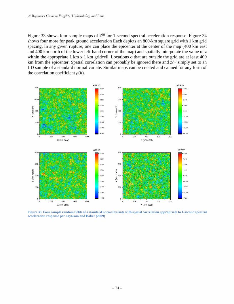
A Beginner’s Guide to Fragility, Vulnerability, and Risk
– 74 –
Figure 33 shows four sample maps of Z(i) for 1-second spectral acceleration response. Figure 34
shows four more for peak ground acceleration Each depicts an 800-km square grid with 1 km grid
spacing. In any given rupture, one can place the epicenter at the center of the map (400 km east
and 400 km north of the lower left-hand corner of the map) and spatially interpolate the value of z
within the appropriate 1 km x 1 km gridcell. Locations o that are outside the grid are at least 400
km from the epicenter. Spatial correlation can probably be ignored there and zo(i) simply set to an
IID sample of a standard normal variate. Similar maps can be created and canned for any form of
the correlation coefficient ρ(h).
Figure 33. Four sample random fields of a standard normal variate with spatial correlation appropriate to 1-second spectral
acceleration response per Jayaram and Baker (2009)
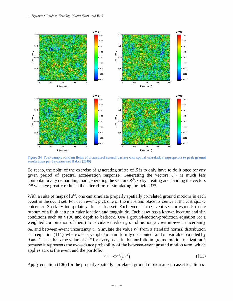
A Beginner’s Guide to Fragility, Vulnerability, and Risk
– 75 –
Figure 34. Four sample random fields of a standard normal variate with spatial correlation appropriate to peak ground
acceleration per Jayaram and Baker (2009)
To recap, the point of the exercise of generating suites of Z is to only have to do it once for any
given period of spectral acceleration response. Generating the vectors U(i) is much less
computationally demanding than generating the vectors Z(i), so by creating and canning the vectors
Z(i) we have greatly reduced the later effort of simulating the fields Y(i).
With a suite of maps of z(i), one can simulate properly spatially correlated ground motions in each
event in the event set. For each event, pick one of the maps and place its center at the earthquake
epicenter. Spatially interpolate zo for each asset. Each event in the event set corresponds to the
rupture of a fault at a particular location and magnitude. Each asset has a known location and site
conditions such as Vs30 and depth to bedrock. Use a ground-motion-prediction equation (or a
weighted combination of them) to calculate median ground motion ˆoy , within-event uncertainty
0, and between-event uncertainty . Simulate the value r(i) from a standard normal distribution
as in equation (111), where ur(i) is sample i of a uniformly distributed random variable bounded by
0 and 1. Use the same value of ur(i) for every asset in the portfolio in ground motion realization i,
because it represents the exceedance probability of the between-event ground motion term, which
applies across the event and the portfolio.
( ) ( )( )1i i
rr u−= (111)
Apply equation (106) for the properly spatially correlated ground motion at each asset location o.
A Beginner’s Guide to Fragility, Vulnerability, and Risk
– 76 –
6.4.4 Options for scenario shaking (foregoing or 3D), fault offset, liquefaction, landsliding
TBD
6.4.5 Comparing median maps and 3D
TBD
6.5 Portfolio loss analysis TBD.
Usually some form of Monte Carlo simulation. Illustrated.
6.6 Decision making TBD.
How to construct and read the risk curve, also known as portfolio loss exceedance curve. Important
points on the risk curve. How treatment of uncertainty affects the shape of the risk curve.
.... Those decisions are sometimes informed by a portfolio loss exceedance curve, which expresses
on an x-y chart the frequency with which loss to the portfolio exceeds various values. Loss appears
on the x-axis and exceedance frequency (or sometimes 1-year exceedance probability) on the y-
axis. Insurers and reinsurers are usually most interested in the loss with 1% or 0.4% annual
exceedance probability, or almost equivalently, the 100-year or 250-year loss. They use these
figures to ensure liquidity, that is, to ensure that they have sufficient reinsurance and capital
reserves to survive a rare loss. They use the 100-year loss (or in some cases the 250-year loss) as
a benchmark for a rare loss.
Some decision-makers want to know the expected value of loss or some upper fractile such as the
90th percentile of loss in a particular scenario event, such as a large earthquake. The large
earthquake is a different proxy for the rare event, and the 90th percentile in that event is sometimes
used as the definition of the probable maximum loss.
6.7 Correlation in portfolio catastrophe risk
6.7.1 Why correlation matters to portfolio catastrophe risk
Portfolio catastrophe risk analysis refers to calculating the probability distribution of the sum of
losses to a set of two or more assets. Beyond merely summing results of multiple single-site risk
analyses, portfolio risk differs from single-site risk analysis in a fundamental way: the uncertain
catastrophe-induced losses to individual assets are usually correlated, potentially several different
ways. First, let us see why correlation matters. Later we can examine the sources of correlation
and learn how to treat them.
In portfolio risk analysis, we are usually concerned with the probability distribution of the sum of
losses, particularly the upper tail of the distribution, meaning values with high probability of not
being exceeded. Insurers for example often need to buy reinsurance to be confident that they will
remain financially liquid in the coming year with 99% or even 99.6% confidence (that is, they can
survive a 100-year or 250-year loss). The expected value of a sum of random variables equals the
A Beginner’s Guide to Fragility, Vulnerability, and Risk
– 77 –
sum of their expected value. But the higher moments—the variance, skewness, etc. that affect the
upper tail of the distribution—do not sum so easily, and are strongly affected by correlation. Let
us illustrate the effect of correlation on the upper tail of the distribution of portfolio loss with a
very simple model.
Let the portfolio comprise n assets indexed by i = {1, 2, … n}, each asset with identically
distributed uncertain loss X, mean loss i = X for all i, standard deviation i = X for all i and
correlation coefficient ij = for all i j, and 0 ≤ ij ≤ 1. Let
Xi = uncertain loss to asset i
Y= uncertain portfolio loss
E[ ] = expected value of the quantity in brackets
Std[ ] = standard deviation of the quantity in brackets
CoV[ ] = coefficient of variation of the quantity in brackets
By definition,
1
n
i
i
Y X=
= (112)
The sum of normally distributed random variables is normal, so Y is normally distributed. And
1
1
1
n
i
i
n
i
i
n
i
i
X
E Y E X
E X
n
=
=
=
=
=
=
=
(113)
( )
2 2
1 1
2 2 2
n n n
Y i i j ij
i i j i
X Xn n n
= =
= +
= + −
(114)
Let us examine how , n, and the coefficient of variation of X, denoted by X, affect the coefficient
of variation of Y, denoted here by Y.
Y
Y
Y
= (115)
Substituting and rearranging,
( )
( )
2 2 2
2
X X
Y
X
X
n n n
n
n n n
n
+ − =
+ − =
(116)
A Beginner’s Guide to Fragility, Vulnerability, and Risk
– 78 –
Equation (116) shows that Y increases in proportion to X. If losses were uncorrelated ( = 0), Y
would decrease with 1 n . For example, for a portfolio of 10,000 assets, Y = 0.01X. As n gets
large, without correlation, Y vanishes and Y becomes nearly certain regardless of how uncertain
X may be. With perfect correlation ( = 1), Y = X, meaning that Y remains as uncertain as X. In
the case of earthquake-induced building repair costs, a realistic range for uncertainty in X is about
0.5 ≤ X ≤ 2.5 (Porter 2010).
What does all that mean for the insurer who has to buy enough reinsurance to cover, say, the 250-
year loss? Let Yz denote the loss with nonexceedance probability z. In the case of the 250-year loss,
that means z = 1 – 1/250 = 0.996. Recall that under our simplifying assumptions, Y is normally
distributed, so for any value of z, we can calculate:
( )
( )( )
1
11
z Y Y
Y Y
Y z
z
−
−
= +
= + (117)
Recall that for = 0, Y 0, so Yz Y regardless of z, including the 250-year loss. With = 1, Y
= X, -1(0.996) = 2.65, and YZ = Y(1 + 2.65X). So with X 1.5, the 250-year loss Y0.996 5Y,
a factor of 5 larger than the case with zero correlation. For an insurance company half of whose
budget pays for reinsurance (as is the case for the California Earthquake Authority, 2017), a 5
times difference between bounds of the possible demand for reinsurance is huge.
6.7.2 Sources of correlation in portfolio catastrophe risk
Some of sources of correlation in portfolio catastrophe risk arise because of how we create our
model: we use systems to estimate asset value, assign assets to classes, characterize the
environmental excitation to which they are subjected, and characterize their vulnerability and loss.
Let us refer to these sources as correlation from model formation. Many engineers and earth
scientists call this source “epistemic,” from the word epistemology, the theory of knowledge.
If the method used to estimate asset value consistently under- or over-estimates all asset values,
we could call that a source of perfect correlation. If a catastrophe risk modeler chose to assign all
buildings whose structural system is only known to be made of concrete to the best or worst class
of reinforced concrete, and similarly attempted to give the best or worst assignments to all other
building types, that could be another source of perfect correlation. The vulnerability functions
assigned to each type could likewise exhibit systematic error high or low, which would similarly
induce a high degree of correlation from model formation.
Other sources of correlation arise more out of how assets and nature actually work than from how
we model it. Assets located near each other tend to experience similar environmental excitation:
the same ground motion, windspeeds, landslides, fire, and floods tend affect nearby buildings
similarly. Buildings in the same development may experience similar damage because of common
construction features or defects. Buildings in the same community will be subject to common
economic or legal pressures, such as higher labor rates among repair contractors or common legal
requirements to build back better. Let us refer to these sources as correlation from nature. Many
risk scholars and practitioners call this source “aleatory,” from the word alea, meaning dice. A
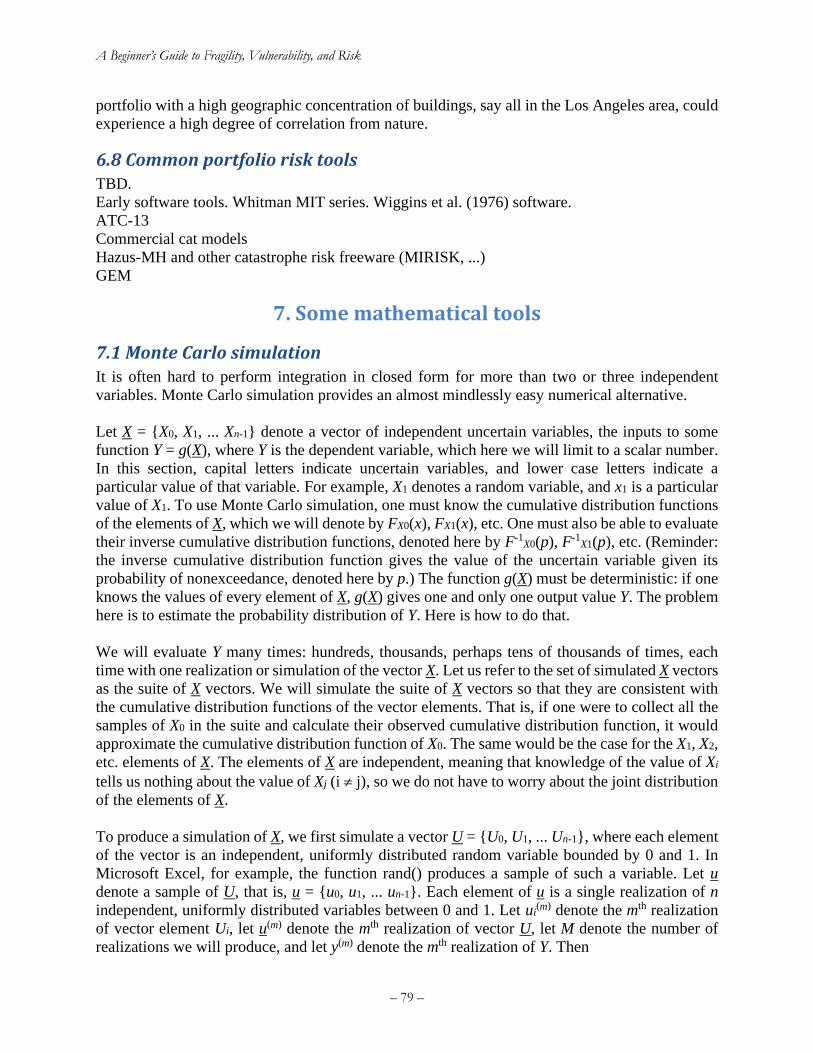
A Beginner’s Guide to Fragility, Vulnerability, and Risk
– 79 –
portfolio with a high geographic concentration of buildings, say all in the Los Angeles area, could
experience a high degree of correlation from nature.
6.8 Common portfolio risk tools TBD.
Early software tools. Whitman MIT series. Wiggins et al. (1976) software.
ATC-13
Commercial cat models
Hazus-MH and other catastrophe risk freeware (MIRISK, ...)
GEM
7. Some mathematical tools
7.1 Monte Carlo simulation It is often hard to perform integration in closed form for more than two or three independent
variables. Monte Carlo simulation provides an almost mindlessly easy numerical alternative.
Let X = {X0, X1, ... Xn-1} denote a vector of independent uncertain variables, the inputs to some
function Y = g(X), where Y is the dependent variable, which here we will limit to a scalar number.
In this section, capital letters indicate uncertain variables, and lower case letters indicate a
particular value of that variable. For example, X1 denotes a random variable, and x1 is a particular
value of X1. To use Monte Carlo simulation, one must know the cumulative distribution functions
of the elements of X, which we will denote by FX0(x), FX1(x), etc. One must also be able to evaluate
their inverse cumulative distribution functions, denoted here by F-1X0(p), F-1
X1(p), etc. (Reminder:
the inverse cumulative distribution function gives the value of the uncertain variable given its
probability of nonexceedance, denoted here by p.) The function g(X) must be deterministic: if one
knows the values of every element of X, g(X) gives one and only one output value Y. The problem
here is to estimate the probability distribution of Y. Here is how to do that.
We will evaluate Y many times: hundreds, thousands, perhaps tens of thousands of times, each
time with one realization or simulation of the vector X. Let us refer to the set of simulated X vectors
as the suite of X vectors. We will simulate the suite of X vectors so that they are consistent with
the cumulative distribution functions of the vector elements. That is, if one were to collect all the
samples of X0 in the suite and calculate their observed cumulative distribution function, it would
approximate the cumulative distribution function of X0. The same would be the case for the X1, X2,
etc. elements of X. The elements of X are independent, meaning that knowledge of the value of Xi
tells us nothing about the value of Xj (i j), so we do not have to worry about the joint distribution
of the elements of X.
To produce a simulation of X, we first simulate a vector U = {U0, U1, ... Un-1}, where each element
of the vector is an independent, uniformly distributed random variable bounded by 0 and 1. In
Microsoft Excel, for example, the function rand() produces a sample of such a variable. Let u
denote a sample of U, that is, u = {u0, u1, ... un-1}. Each element of u is a single realization of n
independent, uniformly distributed variables between 0 and 1. Let ui(m) denote the mth realization
of vector element Ui, let u(m) denote the mth realization of vector U, let M denote the number of
realizations we will produce, and let y(m) denote the mth realization of Y. Then
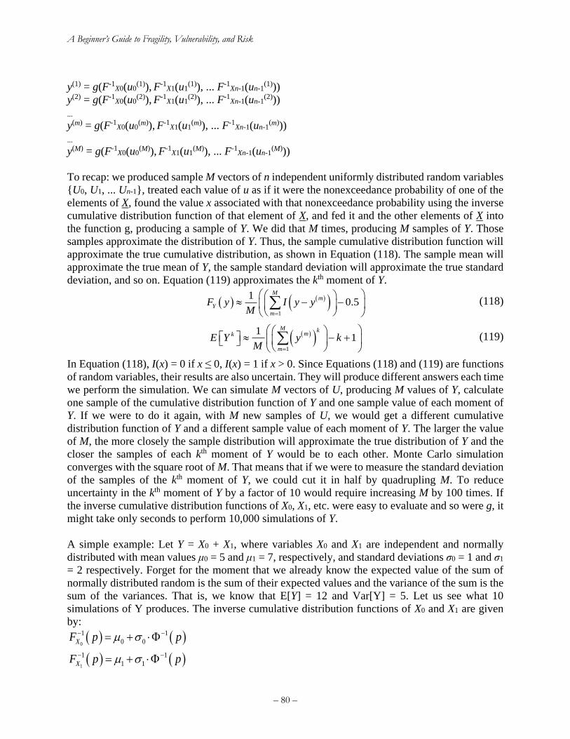
A Beginner’s Guide to Fragility, Vulnerability, and Risk
– 80 –
y(1) = g(F-1X0(u0
(1)), F-1X1(u1
(1)), ... F-1Xn-1(un-1
(1)))
y(2) = g(F-1X0(u0
(2)), F-1X1(u1
(2)), ... F-1Xn-1(un-1
(2)))
...
y(m) = g(F-1X0(u0
(m)), F-1X1(u1
(m)), ... F-1Xn-1(un-1
(m)))
...
y(M) = g(F-1X0(u0
(M)), F-1X1(u1
(M)), ... F-1Xn-1(un-1
(M)))
To recap: we produced sample M vectors of n independent uniformly distributed random variables
{U0, U1, ... Un-1}, treated each value of u as if it were the nonexceedance probability of one of the
elements of X, found the value x associated with that nonexceedance probability using the inverse
cumulative distribution function of that element of X, and fed it and the other elements of X into
the function g, producing a sample of Y. We did that M times, producing M samples of Y. Those
samples approximate the distribution of Y. Thus, the sample cumulative distribution function will
approximate the true cumulative distribution, as shown in Equation (118). The sample mean will
approximate the true mean of Y, the sample standard deviation will approximate the true standard
deviation, and so on. Equation (119) approximates the kth moment of Y.
( ) ( )( )1
10.5
Mm
Y
m
F y I y yM =
− −
(118)
( )( )1
11
M kmk
m
E Y y kM =
− +
(119)
In Equation (118), I(x) = 0 if x ≤ 0, I(x) = 1 if x > 0. Since Equations (118) and (119) are functions
of random variables, their results are also uncertain. They will produce different answers each time
we perform the simulation. We can simulate M vectors of U, producing M values of Y, calculate
one sample of the cumulative distribution function of Y and one sample value of each moment of
Y. If we were to do it again, with M new samples of U, we would get a different cumulative
distribution function of Y and a different sample value of each moment of Y. The larger the value
of M, the more closely the sample distribution will approximate the true distribution of Y and the
closer the samples of each kth moment of Y would be to each other. Monte Carlo simulation
converges with the square root of M. That means that if we were to measure the standard deviation
of the samples of the kth moment of Y, we could cut it in half by quadrupling M. To reduce
uncertainty in the kth moment of Y by a factor of 10 would require increasing M by 100 times. If
the inverse cumulative distribution functions of X0, X1, etc. were easy to evaluate and so were g, it
might take only seconds to perform 10,000 simulations of Y.
A simple example: Let Y = X0 + X1, where variables X0 and X1 are independent and normally
distributed with mean values μ0 = 5 and μ1 = 7, respectively, and standard deviations σ0 = 1 and σ1
= 2 respectively. Forget for the moment that we already know the expected value of the sum of
normally distributed random is the sum of their expected values and the variance of the sum is the
sum of the variances. That is, we know that E[Y] = 12 and Var[Y] = 5. Let us see what 10
simulations of Y produces. The inverse cumulative distribution functions of X0 and X1 are given
by:
( ) ( )0
1 1
0 0XF p p − −= +
( ) ( )1
1 1
1 1XF p p − −= +
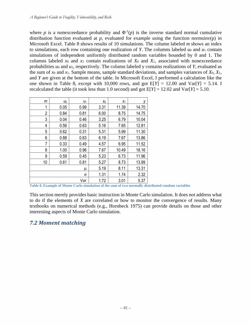
A Beginner’s Guide to Fragility, Vulnerability, and Risk
– 81 –
where p is a nonexceedance probability and Φ-1(p) is the inverse standard normal cumulative
distribution function evaluated at p, evaluated for example using the function normsinv(p) in
Microsoft Excel. Table 8 shows results of 10 simulations. The column labeled m shows an index
to simulations, each row containing one realization of Y. The columns labeled u0 and u1 contain
simulations of independent uniformly distributed random variables bounded by 0 and 1. The
columns labeled x0 and x1 contain realizations of X0 and X1, associated with nonexceedance
probabilities u0 and u1, respectively. The column labeled y contains realizations of Y, evaluated as
the sum of x0 and x1. Sample means, sample standard deviations, and samples variances of X0, X1,
and Y are given at the bottom of the table. In Microsoft Excel, I performed a calculation like the
one shown in Table 8, except with 10,000 rows, and got E[Y] = 12.00 and Var[Y] = 5.14. I
recalculated the table (it took less than 1.0 second) and got E[Y] = 12.02 and Var[Y] = 5.10.
m u0 u1 x0 x1 y
1 0.05 0.99 3.31 11.39 14.70
2 0.84 0.81 6.00 8.75 14.75
3 0.04 0.46 3.25 6.79 10.04
4 0.56 0.63 5.16 7.65 12.81
5 0.62 0.31 5.31 5.99 11.30
6 0.88 0.63 6.19 7.67 13.86
7 0.33 0.49 4.57 6.95 11.52
8 1.00 0.96 7.67 10.49 18.16
9 0.59 0.45 5.23 6.73 11.96
10 0.61 0.81 5.27 8.73 13.99
μ 5.19 8.11 13.31
σ 1.31 1.74 2.32
Var 1.72 3.01 5.37 Table 8. Example of Monte Carlo simulation of the sum of two normally distributed random variables
This section merely provides basic instruction in Monte Carlo simulation. It does not address what
to do if the elements of X are correlated or how to monitor the convergence of results. Many
textbooks on numerical methods (e.g., Hornbeck 1975) can provide details on those and other
interesting aspects of Monte Carlo simulation.
7.2 Moment matching

A Beginner’s Guide to Fragility, Vulnerability, and Risk
– 82 –
Figure 35. Monte Carlo simulation is very powerful and relatively simple, but can be computationally demanding and can
converge slowly, meaning it can take a lot samples to get a reasonably accurate result. Moment matching offers a more
efficient alternative. (Image by Ralf Roletschek, permission under CC BY-SA 3.0.)
This section offers an alternative to Monte Carlo simulation for evaluating functions of random
variables, especially for catastrophe risk modeling and 2nd-generation performance-based
earthquake engineering (PBEE-2). Cat models and PBEE-2 commonly deal with functions of
lognormally distributed random variables, e.g., to characterize uncertain ground motion, structural
response, component damage, and sometimes repair cost and downtime.
Monte Carlo simulation offers a conceptually simple but sometimes computationally demanding
approach. Moment matching offers an efficient alternative. Moment matching is an extension of
Gaussian quadrature (see the Wikipedia article here: https://goo.gl/wux6xA) and another name for
the extended Kalman filter proposed by Julier et al. (2000). Ching et al. (2009) detail its application
to PBEE-2. This section offers a simple practical introduction for the beginner.
Let us first treat the problem of Y, which can be calculated as a deterministic function of a single
uncertain independent random variable X. Let an upper-case letter denote the uncertain quantity,
and a lower-case letter denote a particular value of that uncertain quantity. That is, x is a particular
value of the uncertain quantity X, and similarly y is a particular value of the uncertainty quantity
Y.
Let us illustrate with a simple example. Let X denote the uncertain number of students who will
attend a seminar, and let Y denote the number of pizzas that must be ordered. We might want to
order one pizza for every 4 students, i.e.,
A Beginner’s Guide to Fragility, Vulnerability, and Risk
– 83 –
( )
4
y g x
x
=
=
(120)
Where z denotes the roof function: the smallest integer that is greater than or equal to z. For x=2,
y=1; for x=6, y=2, etc. We know our function completely, but if X is uncertain, so is Y. Suppose
we could estimate the probability distribution of X, and wanted to estimate the mean and standard
deviation of Y for budgeting purposes. If X can only take on discrete values (as in the case of
students attending a seminar), then one can use the theorem of total probability and the moment-
generating function for y to estimate the nth moment of y:
( )( ) mm
x
E Y g x P X x
=−
= = (121)
If we evaluate the equation with m = 1, that gives the 1st moment, i.e., the mean of Y. The equation
says that the mean value of Y is the probability that X will take on a particular value x times the
value of Y if X does take on that value x, summed over all possible values of X. If X can take on
any scalar value, then one can generalize equation (121) as follows.
( )( ) ( )mm
X
x
E Y g x f x dx
=−
= (122)
where fX(x) is the probability density function of X evaluated at a particular value x—essentially
the probability that X will take on exactly the value x.
Notice how equation (121) looks a little easier to evaluate than equation (122), especially if there
are only a few possible values of X and we know the probability of each? The basic idea of moment
matching is to substitute a set of discrete values of X for its continuous distribution. One does that
by selecting the discrete values and their associated probabilities so that the first few moments of
the discrete set approximately equal the same moments of the continuous distribution. Let S denote
the substituted, approximately equivalent set of X values. Let z+1 denote the number of possible
values of S, and let us index them with an index i, that is, S can take on the values s0, s1, ... si, ... sz.
i.e., And let us denote their respective probabilities by wi, that is, P[S=si] = wi. We are free to
choose z, and the values that we will allow S to take on, and their respective probabilities, with the
constraint that the probabilities wi must sum to 1.0. We are even free to allow the wi values to be
negative or to exceed 1.0, in recognition of which we will call them weights instead of
probabilities. We will choose the substitute set of S values and their weights w so that
( )
0
m m
zm
X i i
i
E X E S
x f x dx s w
=−
=
= (123)
for the first few moments, i.e., m = 1, 2, 3, etc. We can then substitute the discrete S values s0, s1,
... sz and their weights w0, w1, ... wz for the continuous independent variable X and its probability
density function fX(x)as follows:
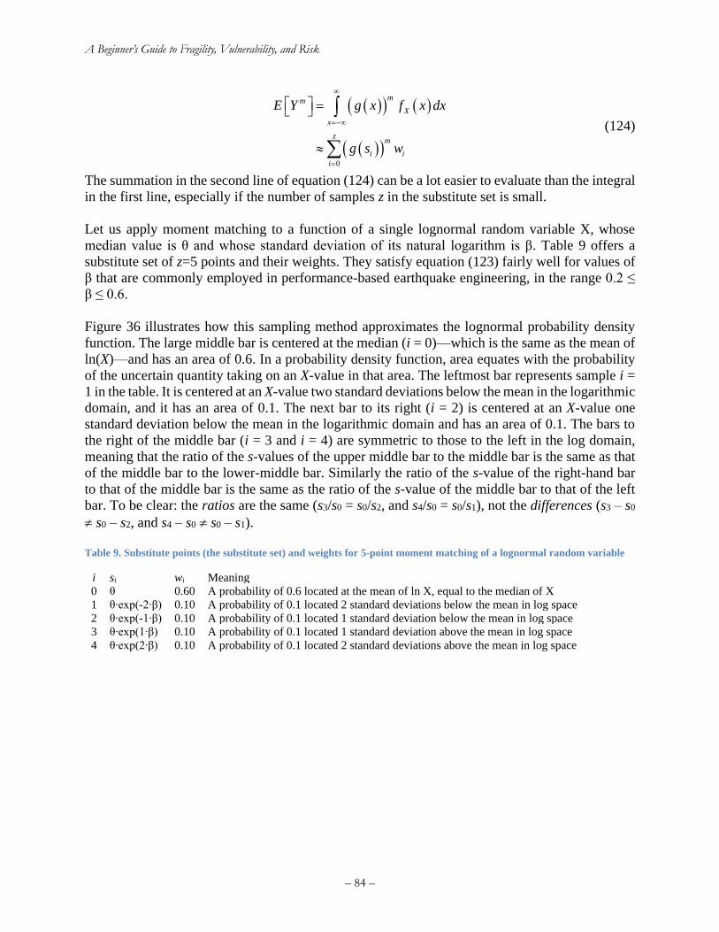
A Beginner’s Guide to Fragility, Vulnerability, and Risk
– 84 –
( )( ) ( )
( )( )0
mm
X
x
zm
i i
i
E Y g x f x dx
g s w
=−
=
=
(124)
The summation in the second line of equation (124) can be a lot easier to evaluate than the integral
in the first line, especially if the number of samples z in the substitute set is small.
Let us apply moment matching to a function of a single lognormal random variable X, whose
median value is θ and whose standard deviation of its natural logarithm is β. Table 9 offers a
substitute set of z=5 points and their weights. They satisfy equation (123) fairly well for values of
β that are commonly employed in performance-based earthquake engineering, in the range 0.2 ≤
β ≤ 0.6.
Figure 36 illustrates how this sampling method approximates the lognormal probability density
function. The large middle bar is centered at the median (i = 0)—which is the same as the mean of
ln(X)—and has an area of 0.6. In a probability density function, area equates with the probability
of the uncertain quantity taking on an X-value in that area. The leftmost bar represents sample i =
1 in the table. It is centered at an X-value two standard deviations below the mean in the logarithmic
domain, and it has an area of 0.1. The next bar to its right (i = 2) is centered at an X-value one
standard deviation below the mean in the logarithmic domain and has an area of 0.1. The bars to
the right of the middle bar (i = 3 and i = 4) are symmetric to those to the left in the log domain,
meaning that the ratio of the s-values of the upper middle bar to the middle bar is the same as that
of the middle bar to the lower-middle bar. Similarly the ratio of the s-value of the right-hand bar
to that of the middle bar is the same as the ratio of the s-value of the middle bar to that of the left
bar. To be clear: the ratios are the same (s3/s0 = s0/s2, and s4/s0 = s0/s1), not the differences (s3 – s0
s0 – s2, and s4 – s0 s0 – s1).
Table 9. Substitute points (the substitute set) and weights for 5-point moment matching of a lognormal random variable
i si wi Meaning
0 θ 0.60 A probability of 0.6 located at the mean of ln X, equal to the median of X
1 θ∙exp(-2∙β) 0.10 A probability of 0.1 located 2 standard deviations below the mean in log space
2 θ∙exp(-1∙β) 0.10 A probability of 0.1 located 1 standard deviation below the mean in log space
3 θ∙exp(1∙β) 0.10 A probability of 0.1 located 1 standard deviation above the mean in log space
4 θ∙exp(2∙β) 0.10 A probability of 0.1 located 2 standard deviations above the mean in log space
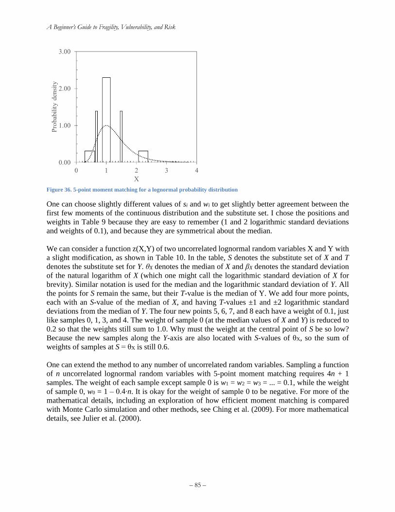
A Beginner’s Guide to Fragility, Vulnerability, and Risk
– 85 –
Figure 36. 5-point moment matching for a lognormal probability distribution
One can choose slightly different values of si and wi to get slightly better agreement between the
first few moments of the continuous distribution and the substitute set. I chose the positions and
weights in Table 9 because they are easy to remember (1 and 2 logarithmic standard deviations
and weights of 0.1), and because they are symmetrical about the median.
We can consider a function z(X,Y) of two uncorrelated lognormal random variables X and Y with
a slight modification, as shown in Table 10. In the table, S denotes the substitute set of X and T
denotes the substitute set for Y. θX denotes the median of X and βX denotes the standard deviation
of the natural logarithm of X (which one might call the logarithmic standard deviation of X for
brevity). Similar notation is used for the median and the logarithmic standard deviation of Y. All
the points for S remain the same, but their T-value is the median of Y. We add four more points,
each with an S-value of the median of X, and having T-values ±1 and ±2 logarithmic standard
deviations from the median of Y. The four new points 5, 6, 7, and 8 each have a weight of 0.1, just
like samples 0, 1, 3, and 4. The weight of sample 0 (at the median values of X and Y) is reduced to
0.2 so that the weights still sum to 1.0. Why must the weight at the central point of S be so low?
Because the new samples along the Y-axis are also located with S-values of θX, so the sum of
weights of samples at S = θX is still 0.6.
One can extend the method to any number of uncorrelated random variables. Sampling a function
of n uncorrelated lognormal random variables with 5-point moment matching requires 4n + 1
samples. The weight of each sample except sample 0 is w1 = w2 = w3 = ... = 0.1, while the weight
of sample 0, w0 = 1 – 0.4∙n. It is okay for the weight of sample 0 to be negative. For more of the
mathematical details, including an exploration of how efficient moment matching is compared
with Monte Carlo simulation and other methods, see Ching et al. (2009). For more mathematical
details, see Julier et al. (2000).
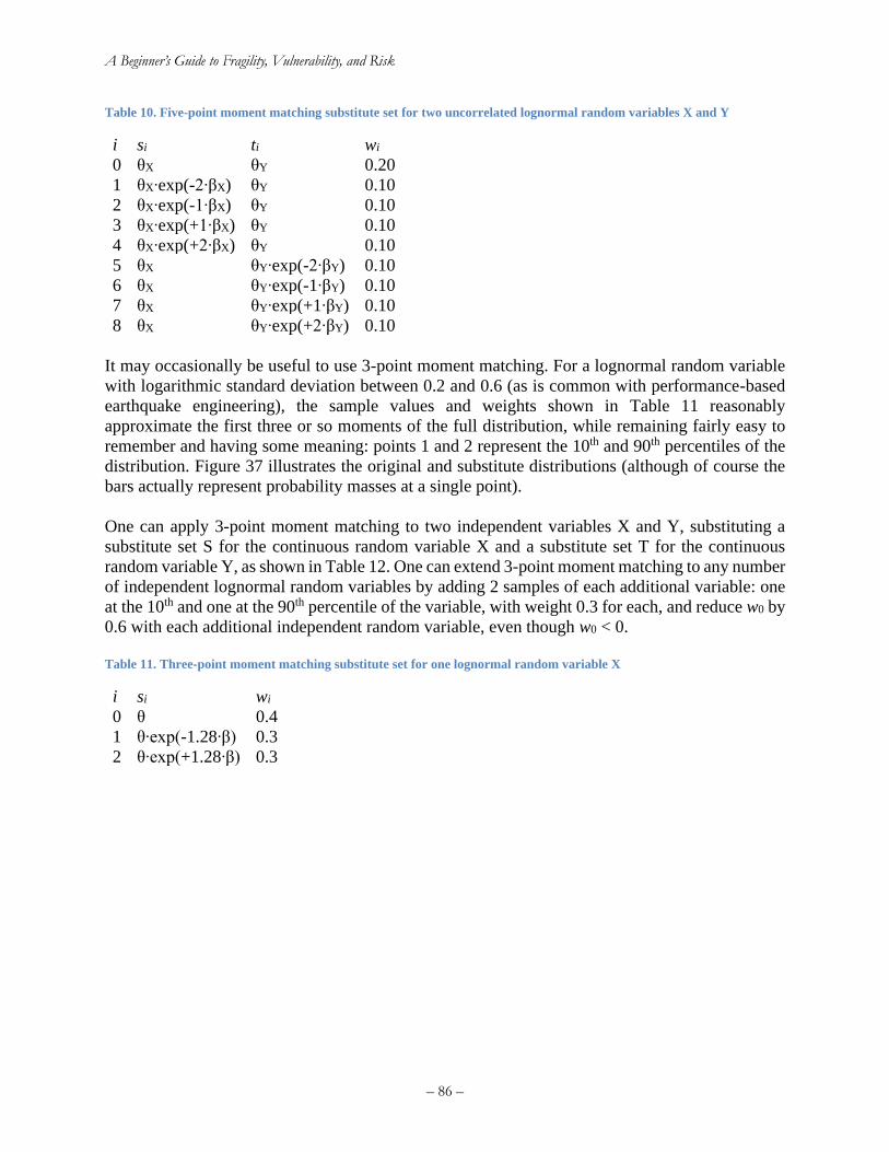
A Beginner’s Guide to Fragility, Vulnerability, and Risk
– 86 –
Table 10. Five-point moment matching substitute set for two uncorrelated lognormal random variables X and Y
i si ti wi
0 θX θY 0.20
1 θX∙exp(-2∙βX) θY 0.10
2 θX∙exp(-1∙βX) θY 0.10
3 θX∙exp(+1∙βX) θY 0.10
4 θX∙exp(+2∙βX) θY 0.10
5 θX θY∙exp(-2∙βY) 0.10
6 θX θY∙exp(-1∙βY) 0.10
7 θX θY∙exp(+1∙βY) 0.10
8 θX θY∙exp(+2∙βY) 0.10
It may occasionally be useful to use 3-point moment matching. For a lognormal random variable
with logarithmic standard deviation between 0.2 and 0.6 (as is common with performance-based
earthquake engineering), the sample values and weights shown in Table 11 reasonably
approximate the first three or so moments of the full distribution, while remaining fairly easy to
remember and having some meaning: points 1 and 2 represent the 10th and 90th percentiles of the
distribution. Figure 37 illustrates the original and substitute distributions (although of course the
bars actually represent probability masses at a single point).
One can apply 3-point moment matching to two independent variables X and Y, substituting a
substitute set S for the continuous random variable X and a substitute set T for the continuous
random variable Y, as shown in Table 12. One can extend 3-point moment matching to any number
of independent lognormal random variables by adding 2 samples of each additional variable: one
at the 10th and one at the 90th percentile of the variable, with weight 0.3 for each, and reduce w0 by
0.6 with each additional independent random variable, even though w0 < 0.
Table 11. Three-point moment matching substitute set for one lognormal random variable X
i si wi
0 θ 0.4
1 θ∙exp(-1.28∙β) 0.3
2 θ∙exp(+1.28∙β) 0.3
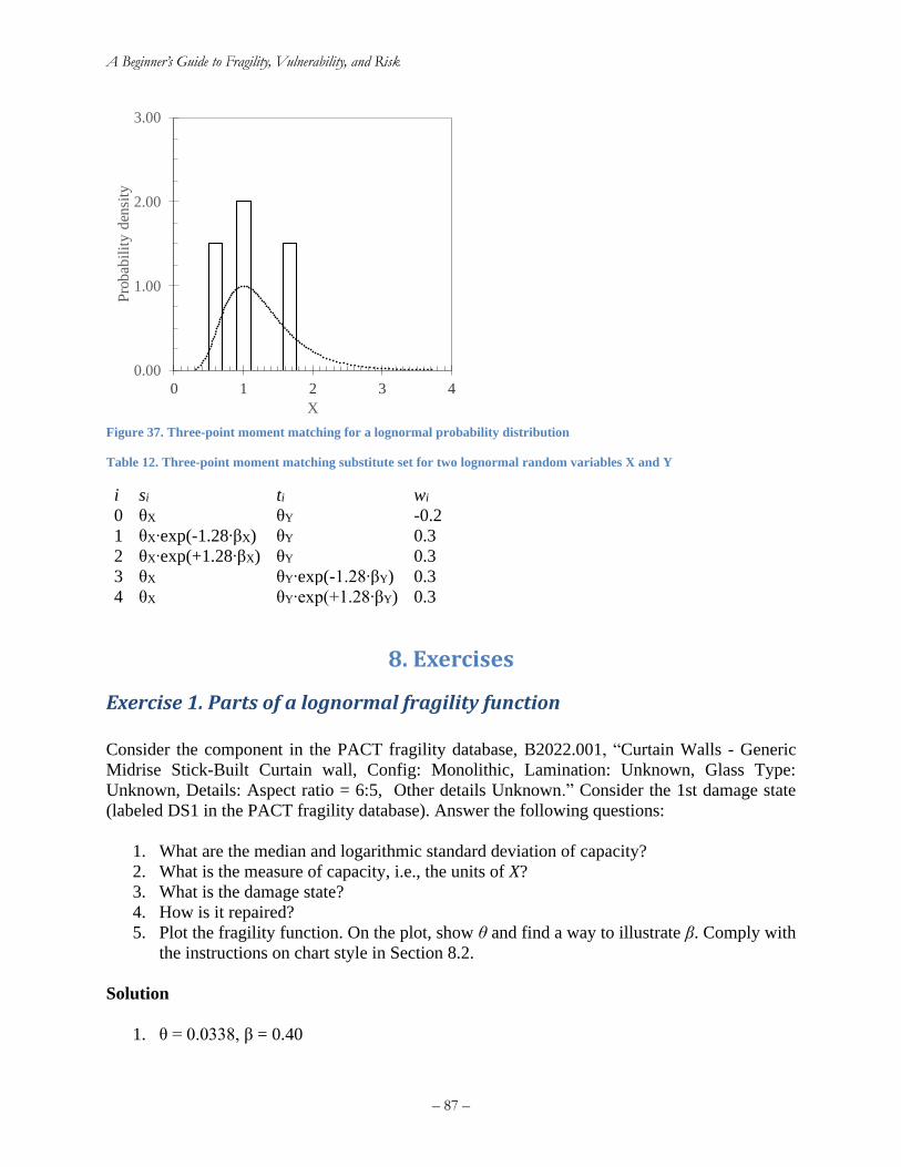
A Beginner’s Guide to Fragility, Vulnerability, and Risk
– 87 –
Figure 37. Three-point moment matching for a lognormal probability distribution
Table 12. Three-point moment matching substitute set for two lognormal random variables X and Y
i si ti wi
0 θX θY -0.2
1 θX∙exp(-1.28∙βX) θY 0.3
2 θX∙exp(+1.28∙βX) θY 0.3
3 θX θY∙exp(-1.28∙βY) 0.3
4 θX θY∙exp(+1.28∙βY) 0.3
8. Exercises
Exercise 1. Parts of a lognormal fragility function
Consider the component in the PACT fragility database, B2022.001, “Curtain Walls - Generic
Midrise Stick-Built Curtain wall, Config: Monolithic, Lamination: Unknown, Glass Type:
Unknown, Details: Aspect ratio = 6:5, Other details Unknown.” Consider the 1st damage state
(labeled DS1 in the PACT fragility database). Answer the following questions:
1. What are the median and logarithmic standard deviation of capacity?
2. What is the measure of capacity, i.e., the units of X?
3. What is the damage state?
4. How is it repaired?
5. Plot the fragility function. On the plot, show θ and find a way to illustrate β. Comply with
the instructions on chart style in Section 8.2.
Solution
1. θ = 0.0338, β = 0.40
0.00
1.00
2.00
3.00
0 1 2 3 4
Pro
bab
ilit
y den
sity
X
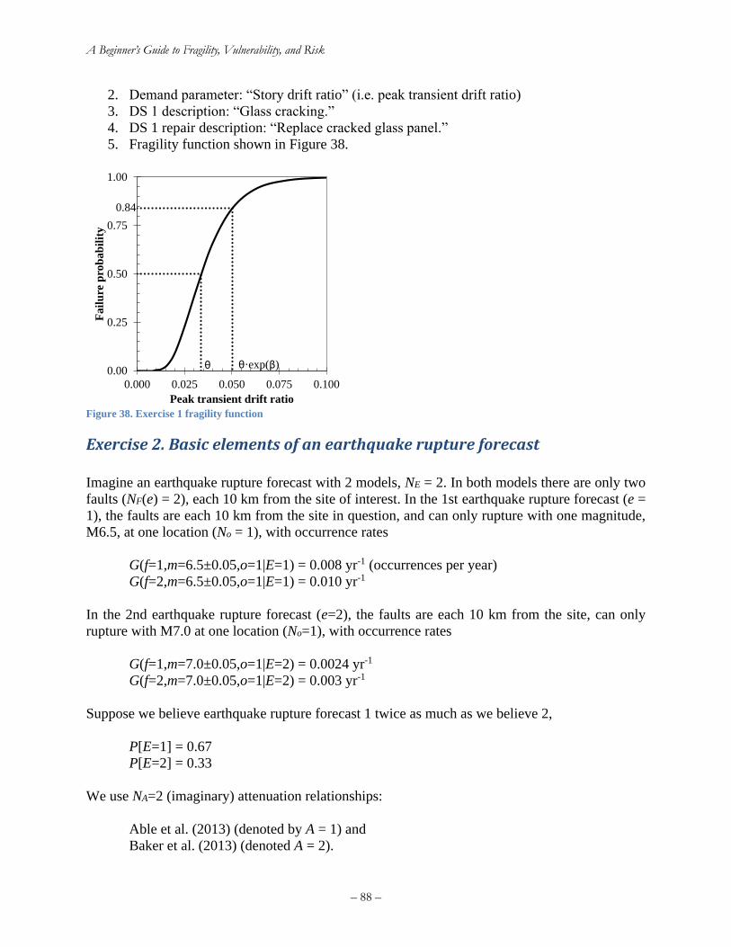
A Beginner’s Guide to Fragility, Vulnerability, and Risk
– 88 –
2. Demand parameter: “Story drift ratio” (i.e. peak transient drift ratio)
3. DS 1 description: “Glass cracking.”
4. DS 1 repair description: “Replace cracked glass panel.”
5. Fragility function shown in Figure 38.
Figure 38. Exercise 1 fragility function
Exercise 2. Basic elements of an earthquake rupture forecast
Imagine an earthquake rupture forecast with 2 models, NE = 2. In both models there are only two
faults (NF(e) = 2), each 10 km from the site of interest. In the 1st earthquake rupture forecast (e =
1), the faults are each 10 km from the site in question, and can only rupture with one magnitude,
M6.5, at one location (No = 1), with occurrence rates
G(f=1,m=6.5±0.05,o=1|E=1) = 0.008 yr-1 (occurrences per year)
G(f=2,m=6.5±0.05,o=1|E=1) = 0.010 yr-1
In the 2nd earthquake rupture forecast (e=2), the faults are each 10 km from the site, can only
rupture with M7.0 at one location (No=1), with occurrence rates
G(f=1,m=7.0±0.05,o=1|E=2) = 0.0024 yr-1
G(f=2,m=7.0±0.05,o=1|E=2) = 0.003 yr-1
Suppose we believe earthquake rupture forecast 1 twice as much as we believe 2,
P[E=1] = 0.67
P[E=2] = 0.33
We use NA=2 (imaginary) attenuation relationships:
Able et al. (2013) (denoted by A = 1) and
Baker et al. (2013) (denoted A = 2).
0.00
0.25
0.50
0.75
1.00
0.000 0.025 0.050 0.075 0.100
Fail
ure
pro
bab
ilit
y
Peak transient drift ratio
θ θ·exp(β)
0.84
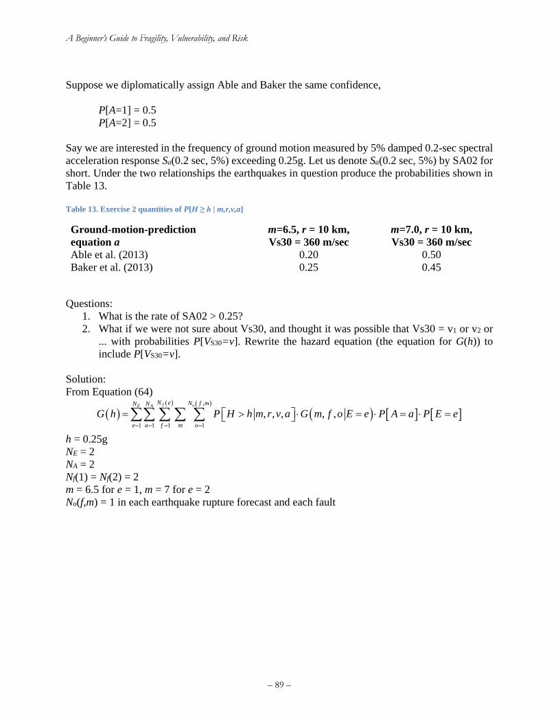
A Beginner’s Guide to Fragility, Vulnerability, and Risk
– 89 –
Suppose we diplomatically assign Able and Baker the same confidence,
P[A=1] = 0.5
P[A=2] = 0.5
Say we are interested in the frequency of ground motion measured by 5% damped 0.2-sec spectral
acceleration response Sa(0.2 sec, 5%) exceeding 0.25g. Let us denote Sa(0.2 sec, 5%) by SA02 for
short. Under the two relationships the earthquakes in question produce the probabilities shown in
Table 13.
Table 13. Exercise 2 quantities of P[H ≥ h | m,r,v,a]
Ground-motion-prediction
equation a
m=6.5, r = 10 km,
Vs30 = 360 m/sec
m=7.0, r = 10 km,
Vs30 = 360 m/sec
Able et al. (2013) 0.20 0.50
Baker et al. (2013) 0.25 0.45
Questions:
1. What is the rate of SA02 > 0.25?
2. What if we were not sure about Vs30, and thought it was possible that Vs30 = v1 or v2 or
... with probabilities P[VS30=v]. Rewrite the hazard equation (the equation for G(h)) to
include P[VS30=v].
Solution:
From Equation (64)
( ) ( ) ( )( ) ,
1 1 1 1
, , , , ,f oE A
N e N f mN N
e a f m o
G h P H h m r v a G m f o E e P A a P E e= = = =
= = = =
h = 0.25g
NE = 2
NA = 2
Nf(1) = Nf(2) = 2
m = 6.5 for e = 1, m = 7 for e = 2
No(f,m) = 1 in each earthquake rupture forecast and each fault
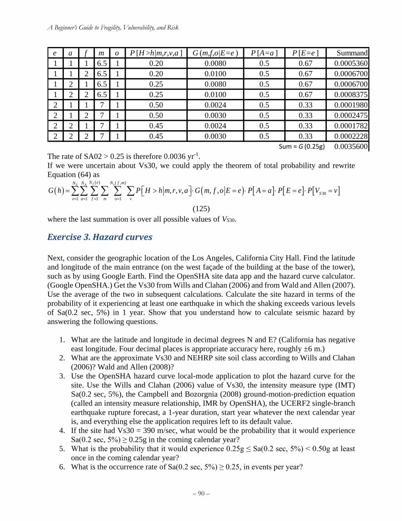
A Beginner’s Guide to Fragility, Vulnerability, and Risk
– 90 –
e a f m o P [H >h|m,r,v,a ] G (m,f,o|E=e ) P [A=a ] P [E=e ] Summand
1 1 1 6.5 1 0.20 0.0080 0.5 0.67 0.0005360
1 1 2 6.5 1 0.20 0.0100 0.5 0.67 0.0006700
1 2 1 6.5 1 0.25 0.0080 0.5 0.67 0.0006700
1 2 2 6.5 1 0.25 0.0100 0.5 0.67 0.0008375
2 1 1 7 1 0.50 0.0024 0.5 0.33 0.0001980
2 1 2 7 1 0.50 0.0030 0.5 0.33 0.0002475
2 2 1 7 1 0.45 0.0024 0.5 0.33 0.0001782
2 2 2 7 1 0.45 0.0030 0.5 0.33 0.0002228
Sum = G (0.25g) 0.0035600
The rate of SA02 > 0.25 is therefore 0.0036 yr-1.
If we were uncertain about Vs30, we could apply the theorem of total probability and rewrite
Equation (64) as
( ) ( ) ( )( ) ,
30
1 1 1 1
, , , , ,f oE A
N e N f mN N
S
e a f m o v
G h P H h m r v a G m f o E e P A a P E e P V v= = = =
= = = = =
(125)
where the last summation is over all possible values of VS30.
Exercise 3. Hazard curves
Next, consider the geographic location of the Los Angeles, California City Hall. Find the latitude
and longitude of the main entrance (on the west façade of the building at the base of the tower),
such as by using Google Earth. Find the OpenSHA site data app and the hazard curve calculator.
(Google OpenSHA.) Get the Vs30 from Wills and Clahan (2006) and from Wald and Allen (2007).
Use the average of the two in subsequent calculations. Calculate the site hazard in terms of the
probability of it experiencing at least one earthquake in which the shaking exceeds various levels
of Sa(0.2 sec, 5%) in 1 year. Show that you understand how to calculate seismic hazard by
answering the following questions.
1. What are the latitude and longitude in decimal degrees N and E? (California has negative
east longitude. Four decimal places is appropriate accuracy here, roughly ±6 m.)
2. What are the approximate Vs30 and NEHRP site soil class according to Wills and Clahan
(2006)? Wald and Allen (2008)?
3. Use the OpenSHA hazard curve local-mode application to plot the hazard curve for the
site. Use the Wills and Clahan (2006) value of Vs30, the intensity measure type (IMT)
Sa(0.2 sec, 5%), the Campbell and Bozorgnia (2008) ground-motion-prediction equation
(called an intensity measure relationship, IMR by OpenSHA), the UCERF2 single-branch
earthquake rupture forecast, a 1-year duration, start year whatever the next calendar year
is, and everything else the application requires left to its default value.
4. If the site had Vs30 = 390 m/sec, what would be the probability that it would experience
Sa(0.2 sec, 5%) ≥ 0.25g in the coming calendar year?
5. What is the probability that it would experience 0.25g ≤ Sa(0.2 sec, 5%) < 0.50g at least
once in the coming calendar year?
6. What is the occurrence rate of Sa(0.2 sec, 5%) ≥ 0.25, in events per year?
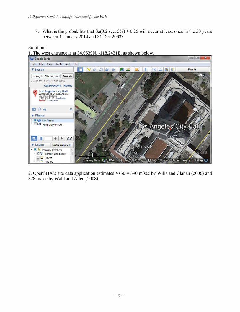
A Beginner’s Guide to Fragility, Vulnerability, and Risk
– 91 –
7. What is the probability that Sa(0.2 sec, 5%) ≥ 0.25 will occur at least once in the 50 years
between 1 January 2014 and 31 Dec 2063?
Solution:
1. The west entrance is at 34.0539N, -118.2431E, as shown below.
2. OpenSHA’s site data application estimates Vs30 = 390 m/sec by Wills and Clahan (2006) and
378 m/sec by Wald and Allen (2008).
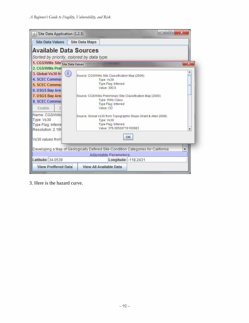
A Beginner’s Guide to Fragility, Vulnerability, and Risk
– 92 –
3. Here is the hazard curve.
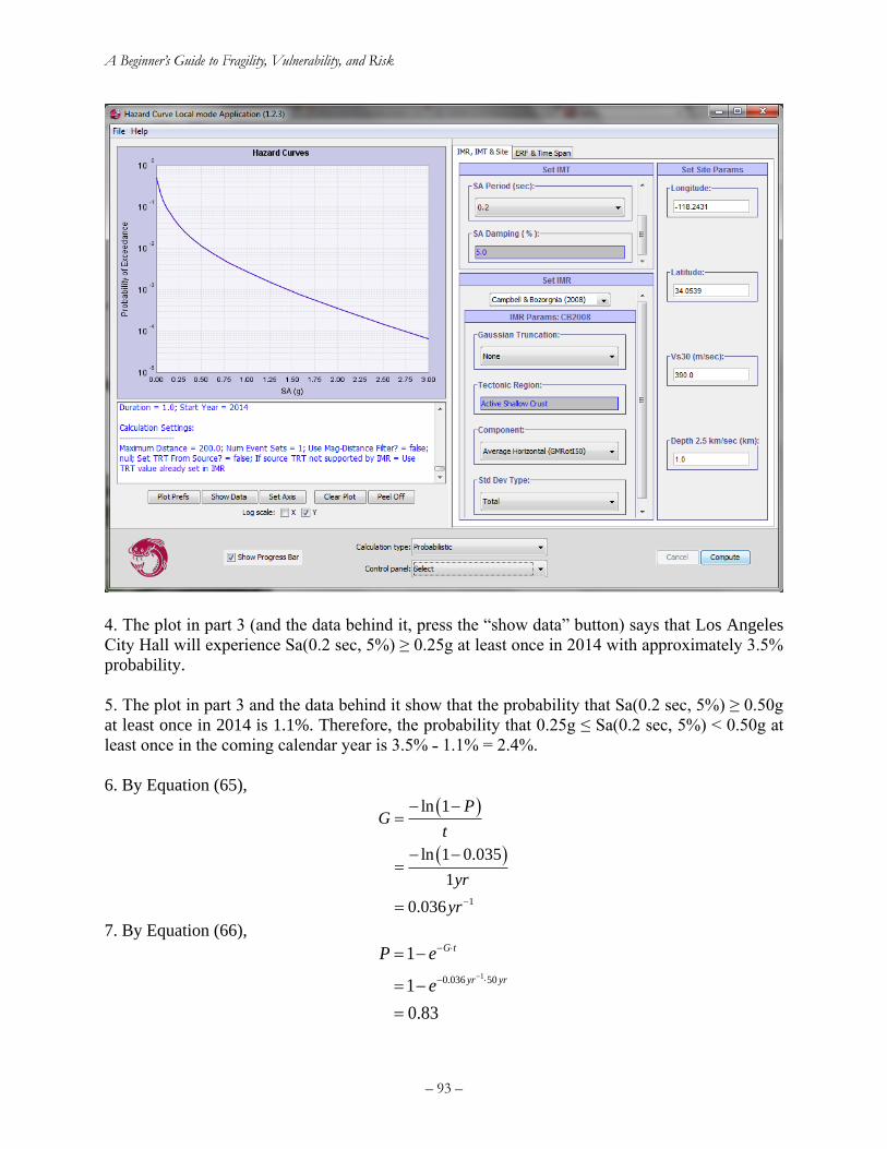
A Beginner’s Guide to Fragility, Vulnerability, and Risk
– 93 –
4. The plot in part 3 (and the data behind it, press the “show data” button) says that Los Angeles
City Hall will experience Sa(0.2 sec, 5%) ≥ 0.25g at least once in 2014 with approximately 3.5%
probability.
5. The plot in part 3 and the data behind it show that the probability that Sa(0.2 sec, 5%) ≥ 0.50g
at least once in 2014 is 1.1%. Therefore, the probability that 0.25g ≤ Sa(0.2 sec, 5%) < 0.50g at
least once in the coming calendar year is 3.5% ˗ 1.1% = 2.4%.
6. By Equation (65),
( )
( )
1
ln 1
ln 1 0.035
1
0.036
PG
t
yr
yr−
− −=
− −=
=
7. By Equation (66),
10.036 50
1
1
0.83
G t
yr yr
P e
e−
−
−
= −
= −
=
A Beginner’s Guide to Fragility, Vulnerability, and Risk
– 94 –
Exercise 4. The lognormal distribution
Questions:
1. Why must a quantity that is lognormally distributed be positive?
2. Suppose P[X ≤ 2] = 0.75 and P[X ≤ 3] = 0.95. What is P[2 < X ≤ 3]?
3. In Equations (18), (63), and (6), why do the inequalities switch direction, and why is there
sometimes a 1 – Φ and sometimes just Φ?
4. Why is the numerator in the argument sometimes a difference and sometimes the natural
logarithm of a ratio?
Solution:
1. A lognormally distributed random variable is one whose natural logarithm is normally
distributed. A normally distributed random variable can take on any value between – and
+, which means the natural logarithm of the random variable can take on any value
between – and +, which means that the variable itself can take on any value between e–
and e+, which is the same as saying any positive (nonzero, nonnegative) scalar value.
2. P[2 < X ≤ 3] = P[X ≤ 3] – P[X ≤ 2] = 0.95 – 0.75 = 0.2.
3. The inequality in Equation (18) refers to the probability that a component with uncertain
damage will exceed damage state d given excitation x. In Equation (6), the inequality
indicates that the term on the right hand side is a cumulative distribution function, which
gives the probability that the uncertainty capacity X is less than or equal to x. In Equation
(63), we are concerned with the probability that a lognormally distributed variable H
exceeds h, which is the same as 1 minus the probability that it is less than or equal to h,
which is the same as 1 minus the cumulative distribution function of H evaluated at h.
4. The natural logarithm of a ratio ln(a/b) is the same as the difference lna – lnb.
Exercise 5. Hazard deaggregation
Consider the site and soil conditions from Exercise 3. Hazard curve. Find the modal magnitude M,
distance R, and ε0 associated with Sa(0.2 sec, 5%) that has 1/475-yr exceedance frequency.
Solution. From https://geohazards.usgs.gov/deaggint/2008/, the modal M = 6.6, R = 5 km, as
shown in Figure 39.
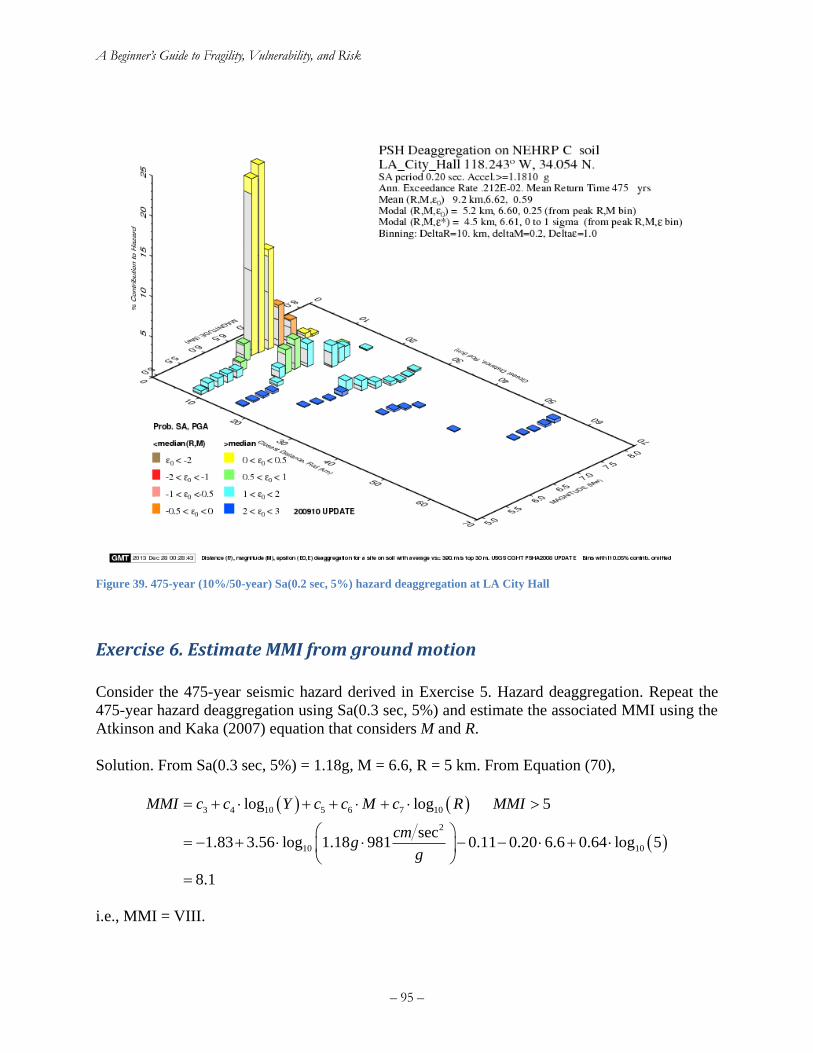
A Beginner’s Guide to Fragility, Vulnerability, and Risk
– 95 –
Figure 39. 475-year (10%/50-year) Sa(0.2 sec, 5%) hazard deaggregation at LA City Hall
Exercise 6. Estimate MMI from ground motion
Consider the 475-year seismic hazard derived in Exercise 5. Hazard deaggregation. Repeat the
475-year hazard deaggregation using Sa(0.3 sec, 5%) and estimate the associated MMI using the
Atkinson and Kaka (2007) equation that considers M and R.
Solution. From Sa(0.3 sec, 5%) = 1.18g, M = 6.6, R = 5 km. From Equation (70),
( ) ( )
( )
3 4 10 5 6 7 10
2
10 10
log log 5
sec1.83 3.56 log 1.18 981 0.11 0.20 6.6 0.64 log 5
8.1
MMI c c Y c c M c R MMI
cmg
g
= + + + +
= − + − − +
=
i.e., MMI = VIII.
A Beginner’s Guide to Fragility, Vulnerability, and Risk
– 96 –
Exercise 7. Write the equation for component failure rate
1. Explain Equation (72) in words. Why is there a negative sign in the integrand?
2. Explain Equation (73) in words. Why did the negative sign go away?
3. Imagine that a component with median peak floor acceleration capacity of θ = 0.25g and
logarithmic standard deviation of β = 0.4 were located on the roof of a 0.2-sec building at
the location from “Exercise 3. Hazard curve.” Write out the equation for the probability
that it would experience the selected damage state at least once in the coming calendar year
in terms of F(x) (the fragility function) and G(x) (the hazard curve in terms of exceedance
frequency). Evaluate it by Equation (72). Evaluate it by Equation (73).
Solution
1. The failure rate is the probability of failure at any given level of excitation x times the
occurrence rate of x, integrated over all x. The failure probability given x is denoted by
F(x), and the occurrence rate of x is the negative first derivative of the exceedance rate of
x. The negative sign is there because the exceedance rate has a negative slope, so its first
derivative is negative.
2. Using integration by parts, the failure rate is the product of the failure probability given x
and the exceedance rate of x, minus the integral of the product of the first derivative of the
failure probability and the exceedance rate of x, the difference evaluated over all x. The
minus signs cancel. The initial product is zero at x = 0 because the failure probability is
zero. The initial product is zero at x = infinity because the exceedance rate is zero.
3. Recall that ( )( )1
1
1
ln xF x
=
. Equation (72) becomes
( ) ( )
0
ln
x
x dG xdx
dx
=
= −
Evaluating numerically, this becomes
( ) ( )( ) ( )( )
11
1
1
ln ln1
2
Ni i
i i
i
x xG x G x
−+
+
=
+ −
The summands are shown in Table 14, the column labeled “Eq 27.” The sum is 0.042,
meaning an average of 0.042 failure-causing earthquakes per year, or a mean failure
recurrence interval of 24 years. The table shows some of the summands ate the beginning,
middle, and end of the x values. Equation (73) becomes
( )
( )0
ln
x
xd
G x dxdx
=
=
Numerically using the trapezoidal rule, this becomes
( ) ( )( )( ) ( )1
1
1
1
ln ln1
2
Ni i
i i
i
x xG x G x
−+
+
=
+ −
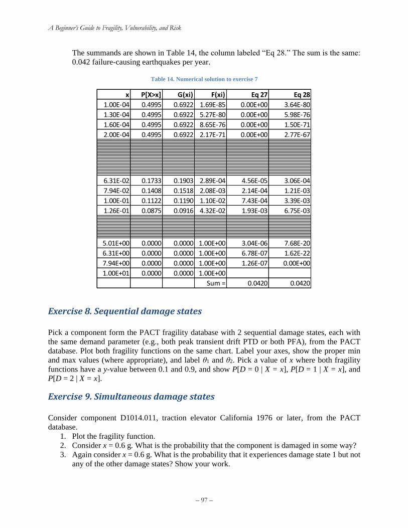
A Beginner’s Guide to Fragility, Vulnerability, and Risk
– 97 –
The summands are shown in Table 14, the column labeled “Eq 28.” The sum is the same:
0.042 failure-causing earthquakes per year.
Table 14. Numerical solution to exercise 7
Exercise 8. Sequential damage states
Pick a component form the PACT fragility database with 2 sequential damage states, each with
the same demand parameter (e.g., both peak transient drift PTD or both PFA), from the PACT
database. Plot both fragility functions on the same chart. Label your axes, show the proper min
and max values (where appropriate), and label θ1 and θ2. Pick a value of x where both fragility
functions have a y-value between 0.1 and 0.9, and show P[D = 0 | X = x], P[D = 1 | X = x], and
P[D = 2 | X = x].
Exercise 9. Simultaneous damage states
Consider component D1014.011, traction elevator California 1976 or later, from the PACT
database.
1. Plot the fragility function.
2. Consider x = 0.6 g. What is the probability that the component is damaged in some way?
3. Again consider x = 0.6 g. What is the probability that it experiences damage state 1 but not
any of the other damage states? Show your work.
x P[X>x] G(xi) F(xi) Eq 27 Eq 28
1.00E-04 0.4995 0.6922 1.69E-85 0.00E+00 3.64E-80
1.30E-04 0.4995 0.6922 5.27E-80 0.00E+00 5.98E-76
1.60E-04 0.4995 0.6922 8.65E-76 0.00E+00 1.50E-71
2.00E-04 0.4995 0.6922 2.17E-71 0.00E+00 2.77E-672.50E-04 0.4995 0.6922 4.00E-67 0.00E+00 1.01E-623.20E-04 0.4995 0.6922 1.46E-62 0.00E+00 9.67E-594.00E-04 0.4995 0.6922 1.40E-58 2.94E-62 6.79E-555.00E-04 0.4995 0.6922 9.82E-55 3.41E-58 4.73E-516.30E-04 0.4995 0.6922 6.83E-51 1.37E-53 1.98E-477.90E-04 0.4995 0.6922 2.86E-47 2.88E-49 8.38E-441.00E-03 0.4995 0.6922 1.21E-43 3.15E-45 2.15E-401.26E-03 0.4995 0.6922 3.11E-40 1.80E-41 3.40E-371.58E-03 0.4995 0.6921 4.92E-37 9.47E-38 5.21E-342.00E-03 0.4993 0.6918 7.53E-34 2.22E-34 4.40E-312.51E-03 0.4990 0.6911 6.37E-31 3.80E-31 2.94E-283.16E-03 0.4981 0.6894 4.27E-28 4.16E-28 1.43E-253.98E-03 0.4961 0.6854 2.08E-25 2.86E-25 4.89E-235.01E-03 0.4921 0.6775 7.20E-23 1.28E-22 1.21E-206.31E-03 0.4849 0.6634 1.82E-20 3.63E-20 2.10E-187.94E-03 0.4733 0.6411 3.24E-18 6.88E-18 2.63E-161.00E-02 0.4560 0.6089 4.24E-16 8.46E-16 2.31E-141.26E-02 0.4326 0.5667 3.97E-14 6.90E-14 1.43E-121.59E-02 0.4030 0.5159 2.68E-12 3.77E-12 6.22E-112.00E-02 0.3682 0.4593 1.30E-10 1.41E-10 1.92E-092.51E-02 0.3296 0.3999 4.61E-09 3.59E-09 4.19E-083.16E-02 0.2891 0.3412 1.18E-07 6.39E-08 6.47E-073.98E-02 0.2484 0.2856 2.18E-06 7.99E-07 7.08E-065.01E-02 0.2094 0.2350 2.94E-05 7.11E-06 5.52E-05
6.31E-02 0.1733 0.1903 2.89E-04 4.56E-05 3.06E-04
7.94E-02 0.1408 0.1518 2.08E-03 2.14E-04 1.21E-03
1.00E-01 0.1122 0.1190 1.10E-02 7.43E-04 3.39E-03
1.26E-01 0.0875 0.0916 4.32E-02 1.93E-03 6.75E-031.58E-01 0.0665 0.0689 1.27E-01 3.80E-03 9.50E-032.00E-01 0.0492 0.0505 2.86E-01 5.72E-03 9.44E-032.51E-01 0.0354 0.0360 5.05E-01 6.73E-03 6.62E-033.16E-01 0.0247 0.0250 7.22E-01 6.44E-03 3.28E-033.98E-01 0.0168 0.0170 8.78E-01 5.26E-03 1.15E-035.01E-01 0.0112 0.0113 9.59E-01 3.89E-03 2.85E-046.31E-01 0.0073 0.0073 9.90E-01 2.72E-03 4.96E-057.94E-01 0.0045 0.0045 9.98E-01 1.84E-03 6.02E-061.00E+00 0.0027 0.0027 1.00E+00 1.20E-03 5.01E-071.26E+00 0.0015 0.0015 1.00E+00 7.36E-04 2.81E-081.58E+00 0.0008 0.0008 1.00E+00 4.17E-04 1.04E-092.00E+00 0.0004 0.0004 1.00E+00 2.11E-04 2.48E-112.51E+00 0.0001 0.0001 1.00E+00 9.32E-05 3.78E-133.16E+00 0.0001 0.0001 1.00E+00 3.53E-05 3.60E-153.98E+00 0.0000 0.0000 1.00E+00 1.13E-05 2.12E-17
5.01E+00 0.0000 0.0000 1.00E+00 3.04E-06 7.68E-20
6.31E+00 0.0000 0.0000 1.00E+00 6.78E-07 1.62E-22
7.94E+00 0.0000 0.0000 1.00E+00 1.26E-07 0.00E+00
1.00E+01 0.0000 0.0000 1.00E+00
Sum = 0.0420 0.0420

A Beginner’s Guide to Fragility, Vulnerability, and Risk
– 98 –
Solution.
Part 1.
θ = 0.39 g peak floor acceleration (at ground level, meaning peak ground acceleration)
β = 0.45
Part 2.
( )ln 0.6 0.391 0.6
0.45
0.83
P D X g
= =
=
Part 3.
P[D=1|D≥1] = 0.26
P[D=2|D≥1] = 0.79
P[D=3|D≥1] = 0.68
P[D=4|D≥1] = 0.17.
By Equation (23),
( )
( ) ( ) ( )
4
2
1& 2,3,4 0.6 1 0.6 1 1 1 1
0.83 0.26 1 0.79 1 0.68 1 0.17
0.012
j
j
P D D X g P D X g P D D P D d D=
= = = = = − =
= − − −
=
Exercise 10. MECE damage states
Consider the PACT database component D5092.032k, Diesel generator - Capacity: 1200 to 2000
kVa - Vibration isolated equipment that is not snubbed or restrained - Equipment fragility only.
1. Plot the fragility function
2. Suppose the generator were subjected to PFA = 0.8g. Evaluate P[D = d |X = x] for all d.
Show your work.
Solution
0.00
0.25
0.50
0.75
1.00
0.0 0.5 1.0 1.5
Fail
ure
pro
bab
ilit
y
Peak floor acceleration (g)
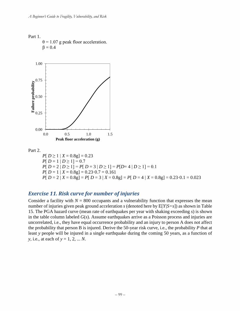
A Beginner’s Guide to Fragility, Vulnerability, and Risk
– 99 –
Part 1.
θ = 1.07 g peak floor acceleration.
β = 0.4
Part 2.
P[ D ≥ 1 | X = 0.8g] = 0.23
P[ D = 1 | D ≥ 1] = 0.7
P[ D = 2 | D ≥ 1] = P[ D = 3 | D ≥ 1] = P[D= 4 | D ≥ 1] = 0.1
P[ D = 1 | X = 0.8g] = 0.23·0.7 = 0.161
P[ D = 2 | X = 0.8g] = P[ D = 3 | X = 0.8g] = P[ D = 4 | X = 0.8g] = 0.23·0.1 = 0.023
Exercise 11. Risk curve for number of injuries Consider a facility with N = 800 occupants and a vulnerability function that expresses the mean
number of injuries given peak ground acceleration s (denoted here by E[Y|S=s]) as shown in Table
15. The PGA hazard curve (mean rate of earthquakes per year with shaking exceeding s) is shown
in the table column labeled G(s). Assume earthquakes arrive as a Poisson process and injuries are
uncorrelated, i.e., they have equal occurrence probability and an injury to person A does not affect
the probability that person B is injured. Derive the 50-year risk curve, i.e., the probability P that at
least y people will be injured in a single earthquake during the coming 50 years, as a function of
y, i.e., at each of y = 1, 2, ... N.
0.00
0.25
0.50
0.75
1.00
0.0 0.5 1.0 1.5
Fail
ure
pro
bab
ilit
y
Peak floor acceleration (g)
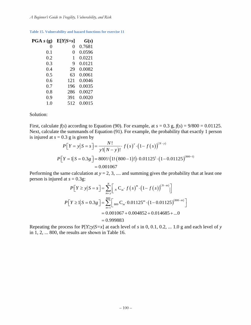
A Beginner’s Guide to Fragility, Vulnerability, and Risk
– 100 –
Table 15. Vulnerability and hazard functions for exercise 11
PGA s (g) E[Y|S=s] G(s)
0 0 0.7681
0.1 0 0.0596
0.2 1 0.0221
0.3 9 0.0121
0.4 29 0.0082
0.5 63 0.0061
0.6 121 0.0046
0.7 196 0.0035
0.8 286 0.0027
0.9 391 0.0020
1.0 512 0.0015
Solution:
First, calculate f(s) according to Equation (90). For example, at s = 0.3 g, f(s) = 9/800 = 0.01125.
Next, calculate the summands of Equation (91). For example, the probability that exactly 1 person
is injured at s = 0.3 g is given by
( )( ) ( )( )
( )
( )( ) ( )( )800 11
1
800!/ 1! 800 1 ! 0.01125 1 0.
!
! !
1 0. 01125
0.001
3
067
N yyNP Y y S s
y N y
P Y S g
f s f s−
−
− = = = −
= = =
=
− −
Performing the same calculation at y = 2, 3, .... and summing gives the probability that at least one
person is injured at s = 0.3g:
( ) ( )( )( )
( )( )800
80
800
1
0
C 1
C 0.01125 1 0.01125
0.001067 0.004852 0.014685 ...0
1
0.999883
0.3
N mm
N m
mm
m
N
m y
m
f s fP Y y S s
P Y g
s
S
=
=
−
−
−
= =
−
+ + +
=
= =
=
Repeating the process for P[Y≥y|S=x] at each level of s in 0, 0.1, 0.2, ... 1.0 g and each level of y
in 1, 2, ... 800, the results are shown in Table 16.
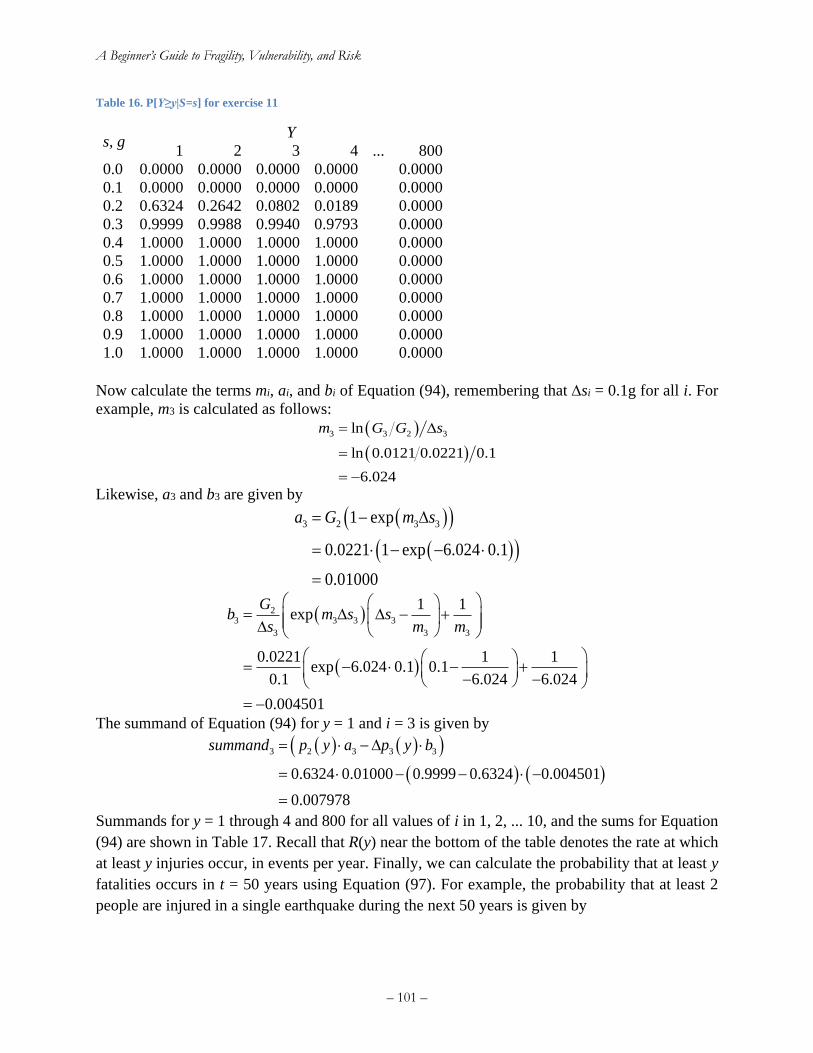
A Beginner’s Guide to Fragility, Vulnerability, and Risk
– 101 –
Table 16. P[Y≥y|S=s] for exercise 11
s, g Y
1 2 3 4 ... 800
0.0 0.0000 0.0000 0.0000 0.0000 0.0000
0.1 0.0000 0.0000 0.0000 0.0000 0.0000
0.2 0.6324 0.2642 0.0802 0.0189 0.0000
0.3 0.9999 0.9988 0.9940 0.9793 0.0000
0.4 1.0000 1.0000 1.0000 1.0000 0.0000
0.5 1.0000 1.0000 1.0000 1.0000 0.0000
0.6 1.0000 1.0000 1.0000 1.0000 0.0000
0.7 1.0000 1.0000 1.0000 1.0000 0.0000
0.8 1.0000 1.0000 1.0000 1.0000 0.0000
0.9 1.0000 1.0000 1.0000 1.0000 0.0000
1.0 1.0000 1.0000 1.0000 1.0000 0.0000
Now calculate the terms mi, ai, and bi of Equation (94), remembering that si = 0.1g for all i. For
example, m3 is calculated as follows:
( )
( )
3 3 2 3ln
ln 0.0121 0.0221 0.1
6.024
m G G s=
=
= −
Likewise, a3 and b3 are given by
( )( )
( )( )3 2 3 3
0.0221 1 exp 6.024 0.1
0.010
1 ex
00
pa G m s
− −
=
= −
=
( )
( )
23 3 3 3
3 3 3
1 1exp
0.0221 1 1exp 6.024 0.1 0.
0
10.1 6.024 6.02
.004501
4
Gb m s s
s m m
= − +
= − − +
−
−
−
=
The summand of Equation (94) for y = 1 and i = 3 is given by
( ) ( )( )
( ) ( )
3 2 3 3 3
0.6324 0.010 0.9999 0.00 0.004501
0.00797
32
8
6 4
summand p y a p y b= −
=
=
− − −
Summands for y = 1 through 4 and 800 for all values of i in 1, 2, ... 10, and the sums for Equation
(94) are shown in Table 17. Recall that R(y) near the bottom of the table denotes the rate at which
at least y injuries occur, in events per year. Finally, we can calculate the probability that at least y
fatalities occurs in t = 50 years using Equation (97). For example, the probability that at least 2
people are injured in a single earthquake during the next 50 years is given by
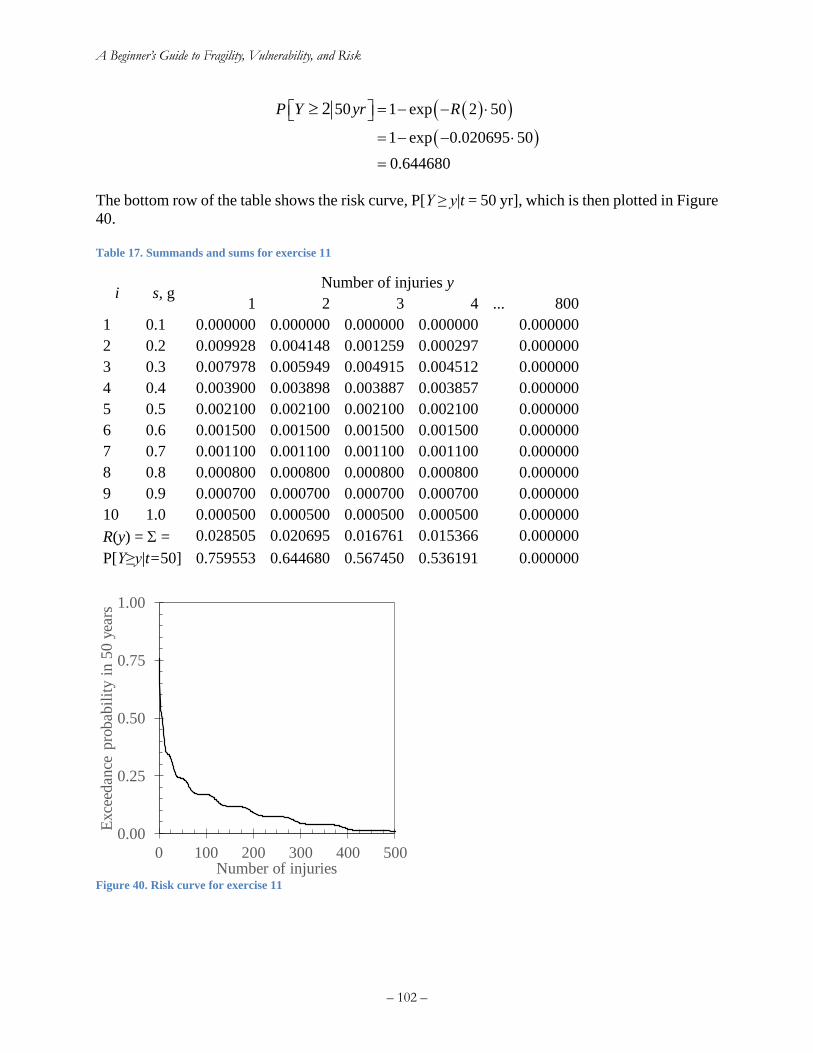
A Beginner’s Guide to Fragility, Vulnerability, and Risk
– 102 –
( )( )
( )
50 1 exp 2 50
1 exp 0.020695 50
0.644680
2P Y yr R = − −
= − −
=
The bottom row of the table shows the risk curve, P[Y ≥ y|t = 50 yr], which is then plotted in Figure
40.
Table 17. Summands and sums for exercise 11
i s, g Number of injuries y
1 2 3 4 ... 800
1 0.1 0.000000 0.000000 0.000000 0.000000 0.000000
2 0.2 0.009928 0.004148 0.001259 0.000297 0.000000
3 0.3 0.007978 0.005949 0.004915 0.004512 0.000000
4 0.4 0.003900 0.003898 0.003887 0.003857 0.000000
5 0.5 0.002100 0.002100 0.002100 0.002100 0.000000
6 0.6 0.001500 0.001500 0.001500 0.001500 0.000000
7 0.7 0.001100 0.001100 0.001100 0.001100 0.000000
8 0.8 0.000800 0.000800 0.000800 0.000800 0.000000
9 0.9 0.000700 0.000700 0.000700 0.000700 0.000000
10 1.0 0.000500 0.000500 0.000500 0.000500 0.000000
R(y) = = 0.028505 0.020695 0.016761 0.015366 0.000000
P[Y≥y|t=50] 0.759553 0.644680 0.567450 0.536191 0.000000
Figure 40. Risk curve for exercise 11
0.00
0.25
0.50
0.75
1.00
0 100 200 300 400 500
Exce
edan
ce p
rob
abil
ity
in 5
0 y
ears
Number of injuries
A Beginner’s Guide to Fragility, Vulnerability, and Risk
– 103 –
9. References
(AAAM) Association for the Advancement of Automotive Medicine (2001). The Abbreviated Injury Scale,
1990 Revision, Update 98, Barrington, IL, 68 pp.
Aagaard, B.T., R.W. Graves, D.P. Schwartz, D.A. Ponce, and R.W. Graymer, 2010a. Ground-motion
modeling of Hayward Fault scenario earthquakes, part I: construction of the suite of scenarios. Bulletin
of the Seismological Society of America, 100 (6) 2927–2944
Aagaard, B.T., R.W. Graves, A. Rodgers, T.M. Brocher, R.W. Simpson, D. Dreger, N.A. Petersson, S.C.
Larsen, S. Ma, and R.C. Jachens, 2010b. Ground-motion modeling of Hayward Fault scenario
earthquakes, part II: simulation of long-period and broadband ground motions. Bulletin of the
Seismological Society of America, 100 (6) 2945–2977
American Society of Appraisers (2013). Definitions of Value Relating to MTS Assets.
(ASCE) American Society of Civil Engineers, 2003. SEI/ASCE 31-03: Seismic Evaluation of Existing
Buildings, Washington, DC, 444 pp.
(ATC) Applied Technology Council (1985). ATC-13, Earthquake Damage Evaluation Data for California.
Redwood City, CA, 492 pp.
(ATC) Applied Technology Council (2012). FEMA P-58: Guidelines for Seismic Performance Assessment
of Buildings, 100% Draft. Redwood City, CA.
Atkinson, G. M. and Kaka, S.I. (2007). Relationships between felt intensity and instrumental ground
motion. Bulletin of the Seismological Society of America, 97, 497–510
Beck. J.L. (2009). A probability logic framework for treating model uncertainty for prior and posterior
robust predictive system analyses. Workshop on Statistical Methods for Dynamic System Models,
Vancouver, June 4-6 2009, http://people.stat.sfu.ca/~dac5/workshop09/James_Beck.html [viewed 29
May 2015]
Beck, J.L., A. Kiremidjian, S. Wilkie, A. Mason, T. Salmon, J. Goltz, R. Olson, J. Workman, A. Irfanoglu,
and K. Porter (1999). Decision Support Tools for Earthquake Recovery of Businesses, Final Report,
CUREe-Kajima Joint Research Program Phase III, Consortium of Universities for Earthquake
Engineering Research, Richmond, CA.
Boore, D.M., J.P. Stewart, E, Seyhan, and G.M. Atkinson (2014). NGA-West2 equations for predicting
PGA, PGV, and 5% damped PSA for shallow crustal earthquakes. Earthquake Spectra, 30 (3), 1057-
1085.
California Earthquake Authority (2017). The Strength to Rebuild: Financial Foundations of the California
Earthquake Authority. Sacramento, CA, 7 p.
https://www.earthquakeauthority.com/Eqa/media/PDF/press-room/CEA-Financial-Overview-
Documentas-of-6-30-2017.pdf [viewed 28 Feb 2020]
Ching, J.Y., K.A. Porter, and J.L. Beck (2009). Propagating uncertainties for loss estimation in
performance-based earthquake engineering using moment matching. Structure and Infrastructure
Engineering. 5 (3): 245-262. http://www.tandfonline.com/doi/abs/10.1080/15732470701298323
Cornell, C. A. (1968). Engineering seismic risk analysis. Bulletin of the Seismological Society of America.
58 (5), 1583-1606.
Czarnecki, R.M. (1973). Earthquake Damage to Tall Buildings, Structures Publication 359. Massachusetts
Institute of Technology, Cambridge, MA, 125 pp.
Der Kiureghian, A., and O. Ditlevsen (2009). Aleatory or epistemic? Does it matter? Structural Safety 31
105–112. http://www.ripid.ethz.ch/Paper/DerKiureghian_paper.pdf [accessed 29 May 2015]
Diaconis, P., S. Holmes, and R. Montgomery (2007). Dynamical bias in the coin toss. SIAM Review 49 (2),
211-235, http://epubs.siam.org/doi/abs/10.1137/S0036144504446436?journalCode=siread
A Beginner’s Guide to Fragility, Vulnerability, and Risk
– 104 –
(FAA) Federal Aviation Administration (1998). Economic Values for Evaluation of FAA Investment and
Regulatory Decisions, Report FAA-APO-98-8
Faenza, L., & Michelini, A. (2010). Regression analysis of MCS intensity and ground motion parameters
in Italy and its application in ShakeMap. Geophysical Journal International. 180, 1138-1152
(FHWA) Federal Highway Administration (1994). Technical Advisory: Motor Vehicle Accident Costs,
Technical Advisory #7570.2, U.S. Department of Transportation, Washington, D.C.
Field, E.H., T.H. Jordan, and C.A. Cornell (2003). OpenSHA: a developing community-modeling
environment for seismic hazard analysis. Seismological Research Letters, 74 (4), 406-419
Field, E. H., Dawson, T. E., Felzer, K. R., Frankel, A. D., Gupta, V., Jordan, T. H., Parsons, T., Petersen,
M. D., Stein, R. S., Weldon II, R. J., & Wills, C. J. (2007). The Uniform California Earthquake Rupture
Forecast, Version 2 (UCERF 2). USGS Open File Report 2007-1437
Field, E.H., G.P. Biasi, P. Bird, T.E. Dawson, K.R. Felzer, D.D. Jackson, K.M. Johnson, T.H. Jordan, C.
Madden, A.J. Michael, K.R. Milner, M.T. Page, T. Parsons, P.M. Powers, B.E. Shaw, W.R. Thatcher,
R.J. Weldon II, and Y. Zeng (2013). Uniform California Earthquake Rupture Forecast, Version 3
(UCERF3)—The Time-Independent Model. U.S. Geological Survey Open-File Report 2013–1165, 97
p., California Geological Survey Special Report 228, and Southern California Earthquake Center
Publication 1792, http://pubs.usgs.gov/of/2013/1165/
Friedman, D.G., 1984. Natural hazard risk assessment for an insurance program. The Geneva Papers on
Risk and Insurance, 9 (30): 57-128
Graves, R.W. and P.G. Somerville, 2006. Broadband ground motion simulations for scenario ruptures of
the Puente Hills Fault. Proc. 8th National Conference on Earthquake Engineering, ~18-21 Apr 2006,
San Francisco CA
Hornbeck, R.W., 1975. Numerical Methods. Quantum Publishers, Inc., New York, 310 pp.
Howard, R.A., 1988. Decision analysis: practice and promise. Management Science 34 (6), 679-695,
http://goo.gl/0LVJaA
Jayaram, N., and Baker, J.W. (2009). Correlated motion for spatially distributed ground-motion intensities.
Earthquake Engineering and Structural Dynamics, 38, 1687-1708
Julier, S., Uhlmann, J., & Durrant-Whyte, H. F. (2000). A new method for the nonlinear transformation of
means and covariances in filters and estimators. IEEE Transactions on Automatic Control, 45(3), 477-
482.
Kaestli, P. & Faeh, D. (2006). Rapid estimation of macroseismic effects and ShakeMaps using
macroseismic data. Proc. First European Conference on Earthquake Engineering and Seismology,
Geneva, Switzerland
Kaka, S. I., & Atkinson, G. M. (2004). Relationships between instrumental ground-motion parameters and
Modified Mercalli intensity in Eastern North America. Bulletin of the Seismological Society of
America, 94 (5), 1728–1736
Kazantzi, A.K., D. Vamvatsikos, K. Porter, and I. Cho, 2013. Developing Analytical Vulnerability
Functions for Highrise Buildings: a Case Study. Global Vulnerability Consortium, Available from
www.nexus.globalquakemodel.org/gem-vulnerability/posts/
Keller, J.B., 1986. The probability of heads. The American Mathematical Monthly, 93 (3), 191-197,
http://links.jstor.org/sici?sici=0002-
9890%28198603%2993%3A3%3C191%3ATPOH%3E2.0.CO%3B2-R
Kennedy, R.P., C.A. Cornell, R.D. Campbell, S. Kaplan, and H.F. Perla, 1980. Probabilistic seismic safety
study of an existing nuclear power plant. Nuclear Engineering and Design. 59: 315-338.
Kircher, C.A., A.A. Nassar, O. Kustu, and W.T. Holmes (1997). Development of building damage functions
for earthquake loss estimation. Earthquake Spectra, 13 (4): 663-682
A Beginner’s Guide to Fragility, Vulnerability, and Risk
– 105 –
Kustu, O., D.D. Miller, and S.T. Brokken (1982). Development of Damage Functions for Highrise Building
Components, for the US Department of Energy, URS/John A Blume & Associates, San Francisco, CA
McClure, F.E. (1973). Performance of Single-Family Dwellings in the San Fernando Earthquake of
February 9, 1971, National Oceanic and Atmospheric Administration, Washington, D.C., 95 pp.
Merz, K., 1991. Generic Seismic Ruggedness of Power Plant Equipment. EPRI NP-5223-SL Revision 1.
Electric Power Research Institute, Oakland, CA, 248 pp.
(MMC) Multihazard Mitigation Council (2005). Natural Hazard Mitigation Saves: An Independent Study
to Assess the Future Savings from Mitigation Activities, National Institute of Building Sciences,
Washington, DC. http://www.nibs.org/?page=mmc_projects#nhms
Murphy, J. R. & O'Brien, L. J. (1977). The correlation of peak ground acceleration amplitude with seismic
intensity and other physical parameters. Bulletin of the Seismological Society of America, 67, 877-915
Newnan, D.G., J.P. Lavelle, and T.G. Eschenbach (2004). Engineering Economic Analysis, 9th Ed. Oxford
University Press, 624 p.
(NIBS and FEMA) National Institute of Building Sciences and Federal Emergency Management Agency
(2012). Multi-hazard Loss Estimation Methodology Earthquake Model Hazus®-MH 2.1 Technical
Manual. Federal Emergency Management Agency, Washington, DC, 718 pp.
NIST and SEMATECH (2012). NIST/SEMATECH e-Handbook of Statistical Methods. National Institute
of Standards and Technology, Gaithersburg, Maryland, http://www.itl.nist.gov/div898/handbook/
Porter, K.A. (2000). Assembly-Based Vulnerability of Buildings and its Uses in Seismic Performance
Evaluation and Risk-Management Decision-Making. Doctoral Dissertation, Stanford University,
Stanford, CA, 196 pp. http://www.sparisk.com/pubs/Porter-2001-ABV-thesis.pdf
Porter, K.A., J.L. Beck, and R.V. Shaikhutdinov (2002). Sensitivity of building loss estimates to major
uncertain variables. Earthquake Spectra, 18 (4), 719-743, www.sparisk.com/pubs/Porter-2002-
Sensitivity.pdf
Porter, K.A. (2003). An overview of PEER’s performance-based earthquake engineering methodology.
Proc. Ninth International Conference on Applications of Statistics and Probability in Civil Engineering
(ICASP9) July 6-9, 2003, San Francisco, CA. Civil Engineering Risk and Reliability Association
(CERRA), 973-980, http://spot.colorado.edu/~porterka/Porter-2003-PEER-Overview.pdf
Porter, K.A., K. Shoaf, and H. Seligson (2006). Value of injuries in the Northridge Earthquake. Earthquake
Spectra, 22 (2), May 2006, http://www.sparisk.com/pubs/Porter-2006-VOI.pdf
Porter, K.A., Kennedy, R. P., and Bachman, R. E. (2007). Creating fragility functions for performance-
based earthquake engineering. Earthquake Spectra. 23 (2), 471-489
Porter, K.A. (2010). Cracking an open safe: uncertainty in HAZUS-based seismic vulnerability functions.
Earthquake Spectra 26 (3), 893-900
Porter, K.A., and K. Cobeen (2012). Informing a retrofit ordinance: a soft-story case study. Proc. 2012
Structures Congress, Chicago IL, March 29-31, 2012, http://www.sparisk.com/pubs/Porter-2012-
SSSC12-CAPSS.pdf.
Porter, K.A., E.H. Field, and K. Milner (2012). Trimming the UCERF2 hazard logic tree. Seismological
Research Letters, 83 (5), 815-828
Porter, K., K. Farokhnia, D. Vamvatksikos, and I. Cho (2015). Guidelines for Component-Based Analytical
Vulnerability Assessment of Buildings and Nonstructural Elements, Global Vulnerability Consortium,
Available from http://www.sparisk.com/pubs/Porter-2015-GEM-Analytical-Vulnerability.pdf
Porter, K. (2017). When addressing epistemic uncertainty in a lognormal fragility function, how should one
adjust the median? Paper 2617, Proc., 16th World Conference on Earthquake Engineering, Santiago
Chile, January 9 to 13, 2017 http://www.sparisk.com/pubs/Porter-2016-16WCEE-Rotation-point.pdf
A Beginner’s Guide to Fragility, Vulnerability, and Risk
– 106 –
Sørensen, M. B., Stromeyer, D., & Grünthal, G. (2007). Deliverable 4.1: Generation of area-specific
relationships between ground motion parameters (PGA, PGV) at certain sites, magnitude M and
distance R to the causative fault and site intensities in terms of EMS-98. Databank of Intensity Data
Points and Related Parameters, Seismic Early Warning for Europe. GFZ Potsdam 19.
Trifunac, M. D. & Brady, A. G. (1975). On the correlation of seismic intensity scales with the peaks of
recorded strong ground motion. Bulletin of the Seismological Society of America 65, 139-162.
Tselentis, G. A. & Danciu, L. (2008). Empirical relationships between Modified Mercalli Intensity and
engineering ground-motion parameters in Greece. Bulletin of the Seismological Society of America 98,
1863–1875.
Urban Institute (1991). The Costs of Highway Crashes, Final Report, Federal Highway Administration
Contract DTFH61-85-C-00107, The Urban Institute, Washington, DC, 144 pp.
Wald, D. J., Quitoriano, V., Heaton, T. H., & Kanamori, H. (1999). Relationships between peak ground
acceleration, peak ground velocity and Modified Mercalli Intensity in California. Earthquake Spectra,
15 (3), 557-564
Wald, D. J. & Allen, T. I. (2007). Topographic slope as a proxy for seismic site conditions and
amplification. Bulletin of the Seismological Society of America, 97, 1379-1395
Wesson, R.L., D.M. Perkins, E.V. Leyendecker, R.J. Roth, and M.D. Petersen (2004). Losses to single-
family housing from ground motions in the 1994 Northridge, California, Earthquake. Earthquake
Spectra, 20 (3), 1021-1045. DOI:10.1193/1.1775238
Wiggins, J.H., J. Slosson, and J. Krohn, 1976. Natural Hazards: Earthquake, Landslide, Expansive Soil
Loss Models. J.H. Wiggins Company, Redondo Beach, CA
Wills, C. J. & Clahan, K. B. (2006). Developing a map of geologically defined site-conditions categories
for California. Bulletin of the Seismological Society of America, 96 (4A), 1483-1501
Worden, C. B., Gerstenberger, M. C., Rhoades, D. A. & Wald, D. J. (2012). Probabilistic relationships
between ground-motion parameters and Modified Mercalli Intensity in California. Bulletin of the
Seismological Society of America, 102 (1), 204–221
Appendices
Appendix A presents a useful tool for deterministic sensitivity studies, to choose which parameters
in a mathematical model matter, and for which ones you can safely ignore their uncertainty.
Appendix B has to do with assigning an acceptable cost to avoid future statistical injuries and
deaths. Appendix C gives additional guidance to my graduate students on how to write and defend
your thesis. Appendix D contains a revision history for my own reference.
Appendix A: Tornado diagram for deterministic sensitivity
Introduction: which inputs matter most to an uncertain quantity?
Mathematical models of an uncertain real-world quantity y (such as the uncertain future cost to
repair a building after an earthquake) often involve a set of uncertain input parameters x (such as
how strongly the ground shakes). Analysts are commonly faced with one of two problems in such
a situation: (1) it may be costly to study each input x sufficiently to quantify its probability
distribution, or (2) each calculation of y may be costly, so it becomes costly to allow all of the
inputs x to vary. In the former case, the analyst might want to deeply investigate only the important
x values—those that contribute most strongly to uncertainty in y—and accept reasonable guesses
A Beginner’s Guide to Fragility, Vulnerability, and Risk
– 107 –
as to the distributions of the other x values. In either case, the analyst might want to simplify the
model by setting those x values that do not matter much at deterministic, best-estimate values. But
how can one defensibly determine which inputs x matter? How much does uncertainty in each
input parameter x (each independent variable) affect the result y (the dependent variable)?
An x might vary wildly but have little effect on y. An x might not vary much at all, but y could be
very sensitive to it. We say that the x values whose uncertainty has strong effect on y are the ones
that matter, the ones that we might need to know more about. The others don’t matter, and we can
take them at typical or best-estimate values, as if they did not vary at all for practical purposes.
Once an analyst identifies the most important uncertainties, he or she can focus on understanding
and quantifying those quantities and their effect on the quantity of interest y, and ignore the
variability of the others, or at least treat them more causally.
One can use a tool called a tornado-diagram analysis to identify those important uncertainties. The
tool produces a diagram (see Figure 41 for an example) that depicts the approximate effect of each
uncertain input x on the quantity of interest y in the form of a horizontal bar chart that resembles a
tornado in profile, hence the name. The method comes from the field of decision analysis (Howard
1988 may be the earliest work). Porter et al. (2002) may be its first proposed use in earthquake
engineering. Other authors have used it in performance-based earthquake engineering and
seismology a few times since then. Here first is a brief overview of the procedure; there follow
step-by-step instructions, a short list of advantages and disadvantages of the method, and an
example problem completely worked out.
A brief overview of tornado-diagram analysis
1. Define the output variable y of interest.
2. Define its inputs x. Make sure the definitions of x and y pass the clarity test (chapter 2).
3. Create a mathematical function f(x) to relate y to x, that is, y = f(x).
4. Find or guess a low, typical (or best estimate), and high value of each x, i.e., xlow, xtyp, and xhigh.
5. Evaluate a baseline value of y as using all the typical x values, i.e., ybaseline = f(x1typ, x2typ, ...)
6. Estimate y using typical x values except one, which is set at its low value.
7. Repeat with the same input set to its high value. The difference between the last two outputs
is referred to as the swing associated with the one input that was varied.
8. That input is then set back to its typical value and repeat the process for the next input, again
setting all the other inputs to their typical value.
9. Sort the labels for the inputs in decreasing order of the swing associated with that input.
10. Create a horizontal bar chart by depicting the swing associated with each input variable as a
bar whose ends are at the low and high values of the output produced by changing just that
input. The horizontal axis is the value of the output y. The bars are arranged with the input that
has the highest swing on the top, then the input with the second-highest swing, etc. A vertical
line is drawn through the baseline value. See Figure 41 for an example. It shows that an output
parameter labeled damage factor depends most on something called assembly capacity, then
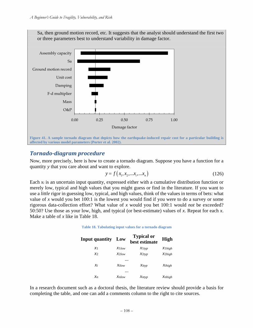
A Beginner’s Guide to Fragility, Vulnerability, and Risk
– 108 –
Sa, then ground motion record, etc. It suggests that the analyst should understand the first two
or three parameters best to understand variability in damage factor.
Figure 41. A sample tornado diagram that depicts how the earthquake-induced repair cost for a particular building is
affected by various model parameters (Porter et al. 2002).
Tornado-diagram procedure Now, more precisely, here is how to create a tornado diagram. Suppose you have a function for a
quantity y that you care about and want to explore.
( )1 2, ,... ,...i ny f x x x x= (126)
Each xi is an uncertain input quantity, expressed either with a cumulative distribution function or
merely low, typical and high values that you might guess or find in the literature. If you want to
use a little rigor in guessing low, typical, and high values, think of the values in terms of bets: what
value of x would you bet 100:1 is the lowest you would find if you were to do a survey or some
rigorous data-collection effort? What value of x would you bet 100:1 would not be exceeded?
50:50? Use those as your low, high, and typical (or best-estimate) values of x. Repeat for each x.
Make a table of x like in Table 18.
Table 18. Tabulating input values for a tornado diagram
Input quantity Low Typical or
best estimate High
x1 x1low x1typ x1high
x2 x2low x2typ x2high
...
xi xilow xityp xihigh
...
xn xnlow xntyp xnhigh
In a research document such as a doctoral thesis, the literature review should provide a basis for
completing the table, and one can add a comments column to the right to cite sources.
0.00 0.25 0.50 0.75 1.00
O&P
Mass
F-d multiplier
Damping
Unit cost
Ground motion record
Sa
Assembly capacity
Damage factor
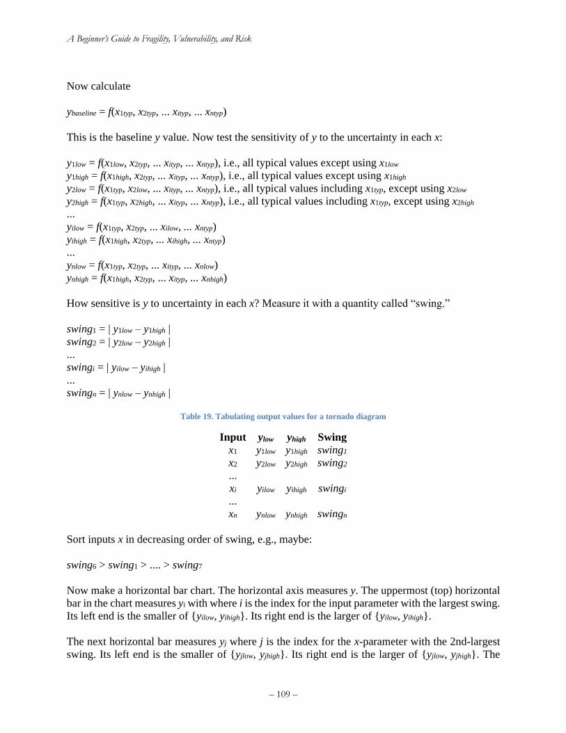
A Beginner’s Guide to Fragility, Vulnerability, and Risk
– 109 –
Now calculate
ybaseline = f(x1typ, x2typ, ... xityp, ... xntyp)
This is the baseline y value. Now test the sensitivity of y to the uncertainty in each x:
y1low = f(x1low, x2typ, ... xityp, ... xntyp), i.e., all typical values except using x1low
y1high = f(x1high, x2typ, ... xityp, ... xntyp), i.e., all typical values except using x1high
y2low = f(x1typ, x2low, ... xityp, ... xntyp), i.e., all typical values including x1typ, except using x2low
y2high = f(x1typ, x2high, ... xityp, ... xntyp), i.e., all typical values including x1typ, except using x2high
...
yilow = f(x1typ, x2typ, ... xilow, ... xntyp)
yihigh = f(x1high, x2typ, ... xihigh, ... xntyp)
...
ynlow = f(x1typ, x2typ, ... xityp, ... xnlow)
ynhigh = f(x1high, x2typ, ... xityp, ... xnhigh)
How sensitive is y to uncertainty in each x? Measure it with a quantity called “swing.”
swing1 = | y1low – y1high |
swing2 = | y2low – y2high |
...
swingi = | yilow – yihigh |
...
swingn = | ynlow – ynhigh |
Table 19. Tabulating output values for a tornado diagram
Input ylow yhigh Swing
x1 y1low y1high swing1
x2 y2low y2high swing2
...
xi yilow yihigh swingi
...
xn ynlow ynhigh swingn
Sort inputs x in decreasing order of swing, e.g., maybe:
swing6 > swing1 > .... > swing7
Now make a horizontal bar chart. The horizontal axis measures y. The uppermost (top) horizontal
bar in the chart measures yi with where i is the index for the input parameter with the largest swing.
Its left end is the smaller of {yilow, yihigh}. Its right end is the larger of {yilow, yihigh}.
The next horizontal bar measures yj where j is the index for the x-parameter with the 2nd-largest
swing. Its left end is the smaller of {yjlow, yjhigh}. Its right end is the larger of {yjlow, yjhigh}. The

A Beginner’s Guide to Fragility, Vulnerability, and Risk
– 110 –
result looks like a tornado in profile. Draw a vertical line at ybaseline. Now you can explore the 2 or
3 or 4 x-parameters that matter most, and ignore the rest or treat them more casually, that is, with
less effort to quantify or propagate their uncertainty.
Advantages and disadvantages
The tornado diagram is relatively easy to create, requiring only reasonable guesses as to the range
of values of the input parameters, plus 2n+1 evaluations of the quantity of interest, where n is the
number of uncertain input parameters. It does not require absolute minima, maxima, or mean
values of the input parameters. The diagram is intuitive to read. It helps the analyst identify which
parameters to focus on, to spend the most time quantifying and understanding. But they do not
present probabilistic information. The baseline value does not necessarily represent an expected
value of the quantity of interest. The diagram gives only a general sense of the variability of the
quantity of interest. In a probabilistic analysis, the quantity of interest is evaluated as an uncertain
function of the jointly distributed uncertain input parameters, or at least all the important ones—
the ones at the top of the tornado diagram.
Example tornado diagram problem
Let us consider an example problem. You are arranging a party for everyone in your local
professional society and need to make a budget. You consider five uncertain quantities for your
budget, need to budget for approximately the 90th percentile of cost, and have time to investigate
only one or two to improve your budget estimate. You model your cost, Y, using Equation (127),
whose variables are listed in Table 20, along with your estimates of the lower bound, best estimate,
and upper bound of each quantity.
( ) ( )1 2 2 3 4 51y x x x x x x= + + (127)
Table 20. Tornado diagram example problem
Quantity Meaning Low Best High
x1 Number of current members 1,900 2,000 2,200
x2 Fraction who will attend 0.01 0.05 0.15
x3 Fraction who will bring a guest 0.01 0.05 0.10
x4 Cost per meal $25.00 $50.00 $75.00
x5 Meals wasted to accommodate attendee choice 1% 10% 20%
Here are sample calculations of ybaseline and y2low. (This example uses the subscript “best” for best
estimate rather than “typ” because in this case one does not know the typical value.)
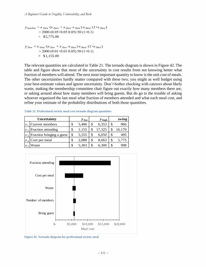
A Beginner’s Guide to Fragility, Vulnerability, and Risk
– 111 –
y baseline = x 1best ∙(x 2best + x 2best ∙x 3best )∙x 4best ∙(1+x 5best )
= 2000∙(0.05+0.05∙0.05)∙50∙(1+0.1)
= 5,775.00$
y 2low = x 1best ∙(x 2low + x 2low ∙x 3best )∙x 4best ∙(1+x 5best )
= 2000∙(0.01+0.01∙0.05)∙50∙(1+0.1)
= 1,155.00$
The relevant quantities are calculated in Table 21. The tornado diagram is shown in Figure 42. The
table and figure show that most of the uncertainty in cost results from not knowing better what
fraction of members will attend. The next most important quantity to know is the unit cost of meals.
The other uncertainties hardly matter compared with these two; you might as well budget using
your best-estimate values and ignore uncertainty. Don’t bother checking with caterers about likely
waste, making the membership committee chair figure out exactly how many members there are,
or asking around about how many members will bring guests. But do go to the trouble of asking
whoever organized the last meal what fraction of members attended and what each meal cost, and
refine your estimate of the probability distributions of both those quantities.
Table 21. Professional society meal cost tornado diagram quantities
y low y high swing
x 1 Current members 5,486$ 6,353$ 866$
x 2 Fraction attending 1,155$ 17,325$ 16,170$
x 3 Fraction bringing a guest 5,555$ 6,050$ 495$
x 4 Cost per meal 2,888$ 8,663$ 5,775$
x 5 Waste 5,303$ 6,300$ 998$
Uncertainty
$- $5,000 $10,000 $15,000 $20,000
Meal cost
Fraction attending
Cost per meal
Waste
Number of members
Bring guest
Figure 42. Tornado diagram for professional society meal
A Beginner’s Guide to Fragility, Vulnerability, and Risk
– 112 –
Combining tornado diagrams and moment matching
Suppose one set out to estimate the low, best, and high estimates to represent particular percentiles
of their distributions, for example by asking oneself (or other experts) for the quantities with 10%,
50%, and 90% nonexceedance probability. Put more simply, when setting low and high values of
x, one asks oneself or other experts what quantities they would bet 10 to 1 for and against being
exceeded (our estimate of the 10th and 90th percentiles). For the best estimate, one estimates the
quantity one would bet even odds against being exceeded (the 50th percentile). One can then
perform the tornado-diagram analysis as specified above, then combine the results—the values of
ybaseline, ylow, and yhigh—using moment matching to estimate the first few moments of y with little
additional computational effort.
In the example party-planning problem, if the xlow, xbest, and xhigh estimates represent 10th, 50th, and
90th percentiles, then one can estimate the first several moments as in the moment-generating
function shown in equation (128). In the equation, if n = 1, then the equation gives the expected
value of y. If n = 2, it gives the expected value of the square of y, and so on. One can calculate the
variance, standard deviation, and coefficient of variation of y as in equations (129), (130), and
(131), respectively. If we treat y as if it were lognormally distributed, then we can estimate its
median θy and logarithmic standard deviation βy as in equations (132) and (133), respectively.
Finally, we can estimate the cumulative distribution function of y using equation (134).
n n
i i
i
E y w y = (128)
( )22Var y E y E y = − (129)
Stdev y Var y= (130)
Stdev yCoV y
E y= (131)
( )2
1y
E y
Cov y
=
+
(132)
( )( )2
ln 1y CoV y = + (133)
( )ln y
y
yP Y y
=
(134)
Note that we estimated the cumulative distribution function of y using just the outputs of the
tornado-diagram analysis, based on the assumption that the low, best, and high values of the
independent variables corresponded to their 10th, 50th, and 90th percentiles.
We can check to see how well the moment-matching approach to estimating the CDF of y agrees
with a Monte Carlo simulation approach. To do the latter, we must estimate the logarithmic
standard deviation of each of the independent variables, which we do using (135). The equation
recognizes that the 90th and 10th percentiles of a normally distributed random variable lie 2.56
standard deviations apart.
A Beginner’s Guide to Fragility, Vulnerability, and Risk
– 113 –
( )high lowln
2.56x
x x = (135)
Now, with the median and logarithmic standard deviation of each independent variable x, we can
simulate y and evaluate its cumulative distribution from the resulting simulations. Table 22 and
Figure 43 presents the results of this exercise. The figure shows that the tornado-diagram approach
gives a reasonable approximation of the median of the distribution, and a so-so job of estimating
the cumulative distribution function of party cost. However, considering its computational
simplicity, the combination of tornado diagram analysis with moment matching may provide a
reasonable initial estimate.
It was easy to perform Monte Carlo simulation on this toy problem, but not all problems are this
simple. There are some problems where Monte Carlo simulation may be computationally
prohibitively expensive, while moment matching with a tornado-diagram analysis may be the best
one can do.
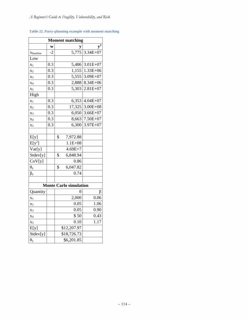
A Beginner’s Guide to Fragility, Vulnerability, and Risk
– 114 –
Table 22. Party-planning example with moment matching
Moment matching
w y y2
xbaseline -2 5,775 3.34E+07
Low
x1 0.3 5,486 3.01E+07
x2 0.3 1,155 1.33E+06
x3 0.3 5,555 3.09E+07
x4 0.3 2,888 8.34E+06
x5 0.3 5,303 2.81E+07
High
x1 0.3 6,353 4.04E+07
x2 0.3 17,325 3.00E+08
x3 0.3 6,050 3.66E+07
x4 0.3 8,663 7.50E+07
x5 0.3 6,300 3.97E+07
E[y] $ 7,972.88
E[y2] 1.1E+08
Var[y] 4.69E+7
Stdev[y] $ 6,848.94
CoV[y] 0.86
θy $ 6,047.82
βy 0.74
Monte Carlo simulation
Quantity θ β
x1 2,000 0.06
x2 0.05 1.06
x3 0.05 0.90
x4 $ 50 0.43
x5 0.10 1.17
E[y] $12,207.97
Stdev[y] $18,726.73
θy $6,201.85
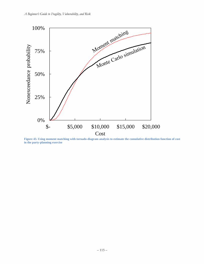
A Beginner’s Guide to Fragility, Vulnerability, and Risk
– 115 –
Figure 43. Using moment matching with tornado-diagram analysis to estimate the cumulative distribution function of cost
in the party-planning exercise
0%
25%
50%
75%
100%
$- $5,000 $10,000 $15,000 $20,000
Non
exce
edan
ce p
rob
abil
ity
Cost
A Beginner’s Guide to Fragility, Vulnerability, and Risk
– 116 –
Appendix B: Assigning a monetary value to statistical injuries
The following largely quotes from Porter et al. (2006). There are a number of methodologies for
estimating the value of injuries; this appendix reflects only one. The phrase “statistical injuries” is
used here to indicate nonfatal or fatal injuries to unknown people at an unknown future date. This
text does not deal with how to value the life of particular people in an immediate situation, such
as how much is reasonable to spend on search and rescue. Nor does it deal with reasonable
compensation for past injuries.
The values discussed here are commonly used to estimate the benefits of regulatory action and risk
remediation. The US Department of Transportation assigned dollar values to statistical injuries
avoided, based on a study by the Urban Institute (1991). These values have been used by the
Federal Aviation Administration (FAA 1998) and Federal Highway Administration (FHWA
1994). The Urban Institute (1991) figures are comprehensive costs for statistical injuries, reflecting
pain and lost quality of life, medical and legal costs, lost earnings, lost household production, etc.
The comprehensive cost is dominated by pain and lost quality of life, which represent 60-80% of
the total. Lost wages represent 5-18%, while medical costs represent a relatively small portion of
the comprehensive cost, typically 5-6%.
These values can be controversial, so some discussion is warranted. The Urban Institute’s (1991)
comprehensive costs were not limited to highway safety. They were averaged from 49 distinct
studies of the value of small changes in safety, of which only 11 had to do with automobiles. They
included 30 studies of the additional wages that people demand to accept elevated safety risks; five
of the market prices for products that provide additional safety (e.g., safer cars, smoke detectors,
houses in less polluted areas); six of the cost of safety behavior (e.g., roadway speed choice and
decisions about smoking); and eight surveys (e.g., about auto safety and fire safety).
The 49 studies produced fairly consistent values. They ranged from $1.0 M to $3.6 million for the
value of a statistical fatality avoided. Their average was $2.2 million; their standard deviation, $0.6
million. The Urban Institute (1991) authors addressed the value of nonfatal injuries by multiplying
the value of fatal risk reduction by the ratio of the years of lost life in a fatality versus the years of
functional capacity at risk (meaning pain or impaired mobility, cognition, self care, and other
measure of quality of life).
Again, these values are not arbitrary figures selected by a government agency or contractor. Nor
are they values that people would demand to receive a known injury (“how much money would
you take to receive a minor scalp laceration right now?”). Rather they are values of such an injury
implied by what people have paid or demand to be paid for slight increases or decreases in life
safety. For example, if people have been observed to pay $100 to decrease by 1 in 10,000 their
chance of death from some particular peril, the implied value of avoiding one statistical fatality
would be $100/0.0001, or $1 million.
The US government’s dollar values to prevent statistical injuries, as of about 2006, are shown in
Table 23. They are expressed in terms of the Abbreviated Injury Severity (AIS) code, a
classification system developed by the Association for the Advancement of Automotive Medicine
(AAAM 2001). The AIS scale is an anatomical scoring system, in that it reflects the nature of the
A Beginner’s Guide to Fragility, Vulnerability, and Risk
– 117 –
injuries and resulting threat to life. It was originally developed for use in quantifying automobile-
related injuries, but has been broadened to include other types and causes of injuries. The AIS
dictionary (AAAM 2001) currently lists approximately 1,300 injuries, each with a distinct 7-digit
numerical injury identifier. Table 23 shows a few example injuries from each AIS level.
Table 23. Federal values of statistical deaths and injuries avoided, in 1994 US$.
AIS level Sample injuries (drawn from AAAM 2001) Comprehensive cost
(FHWA 1994)
1 Minor Shoulder sprain, minor scalp laceration, scalp contusion $5,000
2 Moderate Knee sprain; scalp laceration > 10 cm long and into
subcutaneous tissue; head injury, unconscious < 1 hr
$40,000
3 Serious Femur fracture, open, displaced, or comminuted; head
injury, 1-6 hr unconsciousness; scalp laceration, blood loss >
20% by volume
$150,000
4 Severe Carotid artery laceration, blood loss > 20% by volume; Lung
laceration, with blood loss > 20% by volume
$490,000
5 Critical Heart laceration, perforation; cervical spine cord laceration $1,980,000
6 Fatal Injuries that immediately or ultimately result in death. $2,600,000
The comprehensive costs shown in Table 23 are not uncertain. They are not mean values with
statistical distributions, but rather discrete values chosen by the agencies of the Federal
government to represent the benefit associated with avoiding one such statistical injury. Note also
that each AIS level 1 through 5 represents a range of injuries. Despite that, and regardless of how
the reader would value any particular sample injury or how he or she imagines it would be treated,
the Federal government assigns it the value shown for use in benefit-cost analysis.
For an example of how one might apply these values, see Porter et al. (2006), in which my
coauthors and I quantify in monetary terms what the US federal government would have
considered an acceptable cost to avoid all the deaths and injuries in the 1994 Northridge
earthquake.
Appendix C: How to write and defend your thesis
This appendix tells you
C1. One reasonable, common form of a thesis outline
C2. Pitfalls of simplification
C3. Basic writing style, actually a reference to a short but important work, Strunk & White
C4. A guide to capitalization, which Strunk and White do not treat at sufficient length
C5. How to present and defend your thesis
C.1 Your thesis outline
Find and download the university’s thesis guidelines before you write anything. Write your thesis
for a reader who has not studied this field, someone at the level of another graduate structural
engineering student, not for your advisor, and not for other PhDs. Write your thesis as soon as you
A Beginner’s Guide to Fragility, Vulnerability, and Risk
– 118 –
start your literature review, starting with the outline and filling in the thesis as you do your
research.
Your outline will generally be as follows:
Chapter 1. Introduction
Section 1.1 Background. Frame the problem to be addressed. In 1 paragraph or so, sketch a general
issue or problem that virtually any engineering reader can understand. In another 1 paragraph or
so, explain what we know about the problem or how we deal with it. Then, in a final paragraph,
identify a lack of information, a problem, at the boundary of the field.
Section 1.2 Objectives. How will this thesis to advance our understanding of the problem just
identified? Explain what you will and will not try to accomplish.
Section 1.3 Organization of thesis summarizes the organization of the thesis. Just list the chapters
and explain what is in each one.
Chapter 2. Literature Review
Identify 3-6 relevant topics. Have one subsection for each topic. In each subsection, identify and
summarize 5-10 important works including the earliest on the topic, the most cited on the topic,
and the ones that mark the current research boundaries on the topic.
This is important: cite the pioneers, the truly valuable works. Do not cite works just because they
are easy to find, or because they were written by your advisor, or by an author from a prestigious
university, or by members of some other group to whom you have some allegiance. Do not ignore
works just because the author falls outside the preferred group or is a rival of yours or of someone
in the preferred group. Although it is a common practice for research groups to cite each other
rather than seminal authors, it is poor scholarship and may evidence intellectual dishonesty.
Write 3-6 sentences on each reference, summarizing the authors’ objectives, how they went about
achieving them, the novelty they introduced, and how their work relates to the present research.
Cite everything as “Author (YYYY) said that….” or “A concept or assertion (Author YYYY).”
Citations are always “Author (YYYY)” for one author, “Author and Author (YYYY)” for two
authors, or “Author et al. (YYYY)” for three or more authors. Do not include first names or initials
here. Do not write “et. al (YYYY)” or “et al (YYYY).”
Chapter 3. Methodology
Presents a general procedure to solve the problem you are addressing. It is not the case study.
Never make an assertion that you have not already supported. Defend in depth. When choosing
among procedures where there are more than one reasonable choice, explain the pros and cons of
each and explain which one you chose and why. Anticipate arguments and defend your choice.
You are not lecturing to willing students or to lay readers, you are arguing a position to a potentially
hostile audience. Do not mix the proposed procedure with the illustration or case studies; those
come in chapter 4. Make sure all quantities and events employed in this chapter pass the clarity
test.
Chapter 4. Illustration or case studies
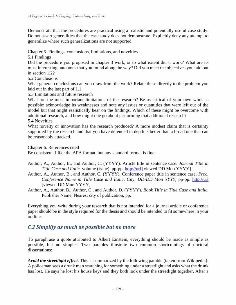
A Beginner’s Guide to Fragility, Vulnerability, and Risk
– 119 –
Demonstrate that the procedures are practical using a realistic and potentially useful case study.
Do not assert generalities that the case study does not demonstrate. Explicitly deny any attempt to
generalize where such generalizations are not supported.
Chapter 5. Findings, conclusions, limitations, and novelties.
5.1 Findings
Did the procedure you proposed in chapter 3 work, or to what extent did it work? What are its
most interesting outcomes that you found along the way? Did you meet the objectives you laid out
in section 1.2?
5.2 Conclusions
What general conclusions can you draw from the work? Relate these directly to the problem you
laid out in the last part of 1.1.
5.3 Limitations and future research
What are the most important limitations of the research? Be as critical of your own work as
possible: acknowledge its weaknesses and note any issues or quantities that were left out of the
model but that might realistically bear on the findings. Which of these might be overcome with
additional research, and how might one go about performing that additional research?
5.4 Novelties
What novelty or innovation has the research produced? A more modest claim that is certainty
supported by the research and that you have defended in depth is better than a broad one that can
be reasonably attacked.
Chapter 6. References cited
Be consistent. I like the APA format, but any standard format is fine.
Author, A., Author, B., and Author, C. (YYYY). Article title in sentence case. Journal Title in
Title Case and Italic. volume (issue), pp-pp. http://url [viewed DD Mon YYYY]
Author, A., Author, B., and Author, C. (YYYY). Conference paper title in sentence case. Proc.
Conference Name in Title Case and Italic, City, DD-DD Mon YYYY, pp-pp. http://url
[viewed DD Mon YYYY]
Author, A., Author, B., Author, C., and Author, D. (YYYY). Book Title in Title Case and Italic.
Publisher Name, Nearest city of publication, pp.
Everything you write during your research that is not intended for a journal article or conference
paper should be in the style required for the thesis and should be intended to fit somewhere in your
outline.
C.2 Simplify as much as possible but no more
To paraphrase a quote attributed to Albert Einstein, everything should be made as simple as
possible, but no simpler. Two parables illustrate two common shortcomings of doctoral
dissertations:
Avoid the streetlight effect. This is summarized by the following parable (taken from Wikipedia):
A policeman sees a drunk man searching for something under a streetlight and asks what the drunk
has lost. He says he lost his house keys and they both look under the streetlight together. After a
A Beginner’s Guide to Fragility, Vulnerability, and Risk
– 120 –
few minutes the policeman asks if he is sure he lost them here, and the drunk replies, no, he lost
them in the park. The policeman asks why he is searching here. The drunk replies, “This is where
the light is.” A 1942 Mutt and Jeff cartoon tells the same story.
Figure 44. Avoid streetlight-effect simplifications (Fisher 1942)
Avoid spherical-cow simplifications. This is summarized by the following parable (modified from
Wikipedia’s article): Milk production at a dairy farm was low, so the farmer wrote to the local
university, asking for help from academia. A multidisciplinary team of professors was assembled,
headed by a theoretical physicist, and two weeks of intensive on-site investigation took place. The
scholars then returned to the university, notebooks crammed with data, where the task of writing
the report was left to the team leader. Shortly thereafter the physicist returned to the farm, saying
to the farmer “I have the solution. First, we idealize the farm as consisting of spherical cows with
1-meter radius in an unbounded vacuum….” (That’s the punch line.) The point is that real-world
realities are almost certainly omitted from the physicist’s model that bear far more on the quantity
of interest—milk-production—than any of the quantities that remain in the model, which are most
likely selected because those are the ones a physicist is comfortable addressing. Do not be that
physicist.
A Beginner’s Guide to Fragility, Vulnerability, and Risk
– 121 –
Figure 45. Avoid spherical-cow simplifications
C.3 Style guide
Have a peer proofread your thesis before your submit it. If English is your second language, please
get a native English-speaker to review and correct your writing, preferably early and often. The
peer should be someone with your level of education but no experience in the thesis topic. If the
proofreader does not understand completely what you have done, why, how, what you found, and
what is novel about it, your thesis is not clear enough. Practice distilling the what, why, how,
findings, and novelties into a few words, enough that you can speak them in 60 seconds or less.
That will be your abstract. If you speak your abstract to a peer and the peer cannot repeat it back
essentially correctly, your abstract is not clear enough.
Read Strunk and White’s Elements of Style. The University of Colorado Library offers online
access to the Chicago Manual of Style. Find it and be prepared to use it while writing your thesis.
In text, active voice. 1st person when you are an important part of the story, as in “I made the choice
among the available ones,” and use 3rd person otherwise, as in “The fragility function reflects
damage to component X.” To the extent possible, remove yourself from the narrative: keep the
focus on the observations, concepts, and conclusions.
In your literature review, never denigrate the prior work of others. Focus on what they added to
the field. If you are a good scholar, your contribution will further expand knowledge, building on
prior work, not correcting what you perceive as shortcomings in prior work. All prior work is
limited. Its importance lies in what it added, not where it stopped.
It is okay to name alternative labels for technical terms when they are first introduced, but
afterwards always use the same technical term, and where you are building on my work or that of
someone else, use the same term as me or them unless there is a strong reason to change.
Charts:
A Beginner’s Guide to Fragility, Vulnerability, and Risk
– 122 –
1. Don’t use Excel’s defaults for anything, they look sloppy in many ways.
2. Font: all Times New Roman or Baskerville 24 pt. Use the same font in your thesis text.
3. Include a horizontal x-axis label, vertical rotated y-axis label, and show units
4. Include axis tick marks: major ticks cross the line, minor ticks inside
5. Exclude gridlines unless they clearly provide value
6. Make all axis lines and tick marks black
7. Make the plot area border black (the area bounded by the min & max x and y values)
8. Do not include any chart border (the area around the entire chart)
9. Include units in axis labels
10. Use consistent and sensible number formats. For example, on the vertical axis that is
bounded by 0.0 and 1.0, have major units of 0.25 and minor units of 0.05. In such a case,
used fixed 0.00 format.
11. If you are providing multiple charts show similar information, have the same min and max
x and y values.
12. Make all text & lines monochrome (black and white) unless color is absolutely needed.
13. If you need color and you have multiple series and there is an order to the series, then make
the color scale intuitive and consistent (cold to hot colors, etc.).
14. If you can avoid color, and you have multiple series, and there is an order to the series, use
intuitive line styles. For example, ordered from dotted line to dashed line to solid line to
thick solid line.
Miscellaneous common stylistic errors:
1. Know the difference between i.e. (which means “that is”) and e.g. (“for example”).
2. Watch noun-verb agreement (e.g., “a building collapses,” versus “two or more buildings
collapse”).
C.4 Capitalization
This appendix recaps what the Chicago Manual of Style (CMS) says about capitalization. Heading
numbers are from CMS.
5.5 Common nouns
A common noun is the generic name of one item in a class or group {a chemical} {a river} {a
pineapple}.5 It is not capitalized unless it begins a sentence or appears in a title. Common nouns
are often broken down into three subcategories: concrete nouns, abstract nouns, and collective
nouns. A concrete noun denotes something solid or real, something perceptible to the physical
senses {a building} {the wind} {honey}. An abstract noun denotes something you cannot see, feel,
taste, hear, or smell {joy} {expectation} {neurosis}. A collective noun—which can be viewed as
a concrete noun but is often separately categorized—refers to a group or collection of people or
things {a crowd of people} {a flock of birds} {a committee}.
5.6 Proper nouns
A proper noun is the specific name of a person, place, or thing {John Doe} {Moscow} {the Hope
Diamond}, or the title of a work {Citizen Kane}. A proper noun is always capitalized, regardless
A Beginner’s Guide to Fragility, Vulnerability, and Risk
– 123 –
of how it is used. A common noun may become a proper noun {Old Hickory} {the Big Easy}, and
sometimes a proper noun may be used figuratively and informally, as if it were a common noun
{like Moriarty, he is a Napoleon of crime} (Napoleon here connoting an ingenious mastermind
who is ambitious beyond limits). Proper nouns may be compounded when used as a unit to name
something {the Waldorf-Astoria Hotel} {Saturday Evening Post}. Over time, some proper nouns
(called eponyms) have developed common-noun counterparts, such as sandwich (from the Earl of
Sandwich) and china (from China, where fine porcelain was produced).
7.48 Capitals for emphasis
Initial capitals, once used to lend importance to certain words, are now used only ironically (but
see 8.93).
“OK, so I’m a Bad Mother,” admitted Mary cheerfully.
8.1 Chicago’s preference for the “down” style
Proper nouns are usually capitalized, as are some of the terms derived from or associated with
proper nouns. For the latter, Chicago’s preference is for sparing use of capitals—what is sometimes
referred to as a “down” style. Although Brussels (the Belgian city) is capitalized, Chicago prefers
brussels sprouts—which are not necessarily from Brussels (see 8.60). Likewise, President Obama
is capitalized, but the president is not (see 8.18–32). (In certain nonacademic contexts—e.g., a
press release—such terms as president may be capitalized.)
8.3Personal names—additional resources
For names of well-known deceased persons, Chicago generally prefers the spellings in Merriam-
Webster’s Biographical Dictionary or the biographical section of Merriam-Webster’s Collegiate
Dictionary (referred to below as Webster’s). For living persons, consult Who’s Who or Who’s
Who in America, among other sources. (See bibliog. 4.1 for these and other useful reference
works.) Where different spellings appear in different sources (e.g., W. E. B. DuBois versus W. E.
B. Du Bois), the writer or editor must make a choice and stick with it. The names of known and
lesser-known persons not in the standard references can usually be checked and cross-checked at
any number of officially sponsored online resources (e.g., for authors’ names, online library
catalogs or booksellers). The name of a living person should, wherever possible, correspond to
that person’s own usage.
8.5 Names with particles
Many names include particles such as de, d’, de la, von, van, and ten. Practice with regard to
capitalizing and spacing the particles varies widely, and confirmation should be sought in a
biographical dictionary or other authoritative source. When the surname is used alone, the particle
is usually retained, capitalized or lowercased and spaced as in the full name (though always
capitalized when beginning a sentence). Le, La, and L’ are always capitalized when not preceded
by de; the, which sometimes appears with the English form of a Native American name, is always
lowercased. See also 8.7, 8.8, 8.9, 8.10, 8.11, 8.14, 8.33.

A Beginner’s Guide to Fragility, Vulnerability, and Risk
– 124 –
Alfonse D’Amato; D’Amato
Diana DeGette; DeGette
Walter de la Mare; de la Mare
Paul de Man; de Man
8.7 French names
The particles de and d’ are lowercased (except at the beginning of a sentence). When the last name
is used alone, de (but not d’) is often dropped. Its occasional retention, in de Gaulle, for example,
is suggested by tradition rather than logic. (When a name begins with closed-up de, such as
Debussy, the d is always capitalized.)
Jean d’Alembert; d’Alembert
Alfred de Musset; Musset
Alexis de Tocqueville; Tocqueville
but
Charles de Gaulle; de Gaulle
When de la precedes a name, la is usually capitalized and is always retained when the last name is
used alone. The contraction du is usually lowercased in a full name but is retained and capitalized
when the last name is used alone. (When a name begins with closed-up Du, such as Dupont, the d
is always capitalized.)
Jean de La Fontaine; La Fontaine
René-Robert Cavelier de La Salle; La Salle
Philippe du Puy de Clinchamps; Du Puy de Clinchamps
When the article le accompanies a name, it is capitalized with or without the first name.
Gustave Le Bon; Le Bon
Initials standing for a hyphenated given name should also be hyphenated.
Jean-Paul Sartre; J.-P. Sartre; Sartre
Since there is considerable variation in French usage, the guidelines and examples above merely
represent the most common forms.
8.25 Religious titles
Religious titles are treated much like civil and military titles (see 8.21, 8.23).
the rabbi; Rabbi Avraham Yitzhak ha-Kohen Kuk; the rabbinate
the cantor or hazzan; Deborah Bard, cantor; Cantor Bard
the sheikh; Sheikh Ibrahim el-Zak Zaky
the imam; Imam Shamil
8.31 Titles of nobility
A Beginner’s Guide to Fragility, Vulnerability, and Risk
– 125 –
Unlike most of the titles mentioned in the previous paragraphs, titles of nobility do not denote
offices (such as that of a president or an admiral). Whether inherited or conferred, they form an
integral and, with rare exceptions, permanent part of a person’s name and are therefore usually
capitalized. The generic element in a title, however (duke, earl, etc.), is lowercased when used
alone as a short form of the name. (In British usage, the generic term used alone remains capitalized
in the case of royal dukes but not in the case of nonroyal dukes; in North American usage such
niceties may be disregarded.) For further advice consult The Times Style and Usage Guide
(bibliog. 1.1), and for a comprehensive listing consult the latest edition of Burke’s Peerage,
Baronetage, and Knightage (bibliog. 4.1). See also 8.22.
the prince; Prince Charles; the Prince of Wales
the duke; the duchess; the Duke and Duchess of Windsor
the marquess; the Marquess of Bath; Lord Bath
the marchioness; the Marchioness of Bath; Lady Bath
8.59 When to capitalize
Adjectives derived from personal names are normally capitalized. Those in common use may be
found in Webster’s, sometimes in the biographical names section (e.g., Aristotelian, Jamesian,
Machiavellian, Shakespearean). If not in the dictionary, adjectives can sometimes be coined by
adding ian (to a name ending in a consonant) or an (to a name ending in e or i)—or, failing these,
esque. As with Foucault and Shaw, the final consonant sometimes undergoes a transformation as
an aid to pronunciation. If a name does not seem to lend itself to any such coinage, it is best
avoided. See also 8.60, 8.78.
Baudelaire; Baudelairean
Bayes; Bayesian
Dickens; Dickensian
Foucault; Foucauldian
Jordan; Jordanesque (à la Michael Jordan)
8.67 Institutions and companies—capitalization
The full names of institutions, groups, and companies and the names of their departments, and
often the shortened forms of such names (e.g., the Art Institute), are capitalized. A the preceding
a name, even when part of the official title, is lowercased in running text. Such generic terms as
company and university are usually lowercased when used alone (though they are routinely
capitalized in promotional materials, business documents, and the like).
the University of Chicago; the university; the University of Chicago and Harvard University;
Northwestern and Princeton Universities; the University of Wisconsin–Madison
the Department of History; the department; the Law School
the University of Chicago Press; the press
8.68 Names with unusual capitalization

A Beginner’s Guide to Fragility, Vulnerability, and Risk
– 126 –
Parts of names given in full capitals on the letterhead or in the promotional materials of particular
organizations may be given in upper- and lowercase when referred to in other contexts (e.g., “the
Rand Corporation” rather than “the RAND Corporation”). Company names that are spelled in
lowercase letters in promotional materials may be capitalized (e.g., DrKoop.net rather than
drkoop.net). Names like eBay and iPod, should they appear at the beginning of a sentence or
heading, need not take an initial capital in addition to the capitalized second letter. See also 8.153
8.84 Academic subjects
Academic subjects are not capitalized unless they form part of a department name or an official
course name or are themselves proper nouns (e.g., English, Latin).
She has published widely in the history of religions.
They have introduced a course in gender studies.
He is majoring in comparative literature.
She is pursuing graduate studies in philosophy of science.
but
Jones is chair of the Committee on Comparative Literature.
8.93 Platonic ideas
Words for transcendent ideas in the Platonic sense, especially when used in a religious context,
are often capitalized. See also 7.48.
Good; Beauty; Truth; the One
8.153 Names like eBay and iPod
Brand names or names of companies that are spelled with a lowercase initial letter followed by a
capital letter (eBay, iPod, iPhone, etc.) need not be capitalized at the beginning of a sentence or
heading, though some editors may prefer to reword. This departure from Chicago’s former usage
recognizes not only the preferred usage of the owners of most such names but also the fact that
such spellings are already capitalized (if only on the second letter). Company or product names
with additional, internal capitals (sometimes called “midcaps”) should likewise be left unchanged
(GlaxoSmithKline, HarperCollins, LexisNexis). See also 8.4.
eBay posted strong earnings.
User interfaces varied. iTunes and its chief rival, Amazon.com, . . .
In text that is set in all capitals, such distinctions are usually overridden (e.g., EBAY, IPOD,
HARPERCOLLINS); with a mix of capitals and small capitals, they are preserved (e.g., EBAY).
10.20 Academic degrees
A Beginner’s Guide to Fragility, Vulnerability, and Risk
– 127 –
Chicago recommends omitting periods in abbreviations of academic degrees (BA, DDS, etc.)
unless they are required for reasons of tradition or consistency with, for example, a journal’s
established style. In the following list of some of the more common degrees, periods are shown
only where uncertainty might arise as to their placement. Spelled-out terms, often capitalized in
institutional settings (and on business cards and other promotional items), should be lowercased
in normal prose. See also 8.28.
AB
artium baccalaureus (bachelor of arts)
AM
artium magister (master of arts)
BA
bachelor of arts
BD
bachelor of divinity
BFA
bachelor of fine arts
BM
bachelor of music
BS
bachelor of science
C.5 Defending your thesis
Here are some preparation hints for defending your thesis.
(1) Try to explain your research frequently to your mother, father, impatient siblings, and to
children ages 12 to 18. If you can explain it to them, you know it. If you cannot, you don’t.
(2) Try summarizing your thesis in 3 minutes in a bar or café to a non-engineer. If you can do
that and the other person understands what your thesis is about, then you understand what
your thesis is about. If not, you don’t.
(3) Organize your presentation in the same order as your thesis. Often this will be:
introduction, problem statement, objectives, organization of the presentation, literature
review, proposed methodology, findings, conclusions.
(4) Organize your presentation so that you present facts and only afterwards present
conclusions that follow from those facts. Do not make assertions for which you have not
already presented the evidence.
(5) Near the end, have a slide on the weaknesses of your research. Your committee will think
of many of them and possibly others. Thinking in advance about weaknesses will help you
eliminate some.
(6) Know what is new about your thesis and what is not. Have a slide on that point after the
weaknesses slide.
(7) When you don’t know the answer to a committee member’s question, say “I don’t know”
and then stop talking. I cannot not help you answer questions from another committee
member without defeating the purpose of the exam.

A Beginner’s Guide to Fragility, Vulnerability, and Risk
– 128 –
(8) Practice your defense with colleagues. Your objective is to teach them, not impress them.
It is okay to use technical terms of art, but only after you have explained them in plain
English, and only if the term of art is much more concise than plain English. Your
colleagues should leave the practice defense knowing how to repeat your research, what it
was for, and what novelty you introduced.

A Beginner’s Guide to Fragility, Vulnerability, and Risk
– 129 –
Appendix D: How to write a research article
This appendix is borrowed from University of Colorado Boulder Professor Wil Srubar III, with
trivial modifications. Thanks, Wil.
Step 1. Define the scope of work. Start by writing down the objective of the study. The objective
should be (a) specific, (b) novel, and (c) relevant to the broad scientific community. What questions
are you answering? Why does the questions matter? What do others in the literature have to say
about this question? Are you furthering their work? How and why are you doing that? What
materials are used and what methods are employed to answer your questions? The materials and
methods must directly support answering your main questions. If they do not support answering
your main questions, then they should not be included in the scope of work. We will be constantly
refining these each week during your individual meetings with me.
In our university, we perform experimental and computational studies. This means that, for those
performing experiments, we use physical samples made in the lab to investigate the effect of
independent variables on dependent variables. Examples of this: the effect of time, acid exposure,
or molecular weight (which we control) on mechanical properties (a property of interest). In
computational studies, we use virtual samples made by computers to investigate the effect of
independent variables on properties of interest. Examples of this: the effect of geographic location
(which we control) on the energy performance (a property of interest) for commercial buildings
with transparent wood-composite windows.
Step 2. Consider co-authorship. The list of co-authors will most likely include your primary
research advisor and any other person that has made some “intellectual contribution” to the study.
For example: (1) a fellow student who designs and runs a supporting experiment; (2) another
faculty member who helps you decipher or analyze some complicated data that is pertinent to your
conclusions; or (3) someone who helps organize and write significant parts of the manuscript – all
should be included as co-authors.
Someone who gives you minor feedback or trains you on a piece of equipment (without designing
experiments or analyzing results pertinent to your study) does not merit inclusion as a co-author.
However, these critical supporting actors should be gratefully acknowledged in the
Acknowledgments section of the manuscript. I prefer acknowledgments, not acknowledgements.
Step 3. Specify co-authorship contributions. Once the list of co-authors is identified, it is
imperative to concur with all parties the order of authors. Start with me; I may give you some
guidance on the proper order – there may be particular customs in your field (for example, the
Principal Investigator should be listed last). Generally, those with the most involvement are listed
first, beginning with the author contributing most of the work (which is likely you—meaning that
you will probably be first author, and I will probably, though not necessarily, be second). It is
critical to get consensus on who is going to contribute and what they are contributing before the
first drafts of the manuscript. This proactive preparation will save you from potentially stressful
situations in the long run.
Action: Once the scope of work has been defined, talk to me to ensure your experimental
design effectively and efficiently answers the questions of interest.
A Beginner’s Guide to Fragility, Vulnerability, and Risk
– 130 –
1.
Step 4. Identify a target journal and download its Guide for Authors. This selection is often
made in consultation with your advisor. Journals with high impact factors (which is a measure of
quality of the journal) are typically preferred. However, not all research is of the right caliber for
some journals. Self-awareness of where your research fits into the field is key here, and a
compromise must be struck with quality of the research with quality of the anticipated journals. In
some instances, other metrics of the journal may be more important than impact factor (e.g., review
speed). Read through the Guide for Authors, noting any special instructions for the journal (e.g.,
Graphical Abstract, Reference Format, Number of Figures, Font Size and Spacing). Take a look
at 2-3 current papers that were published in that journal to get an idea of the expected writing style,
length, sections, etc. Some journals in which we have published: Earthquake Spectra, Natural
Hazards, ASCE Structural Journal, and Seismological Research Letters. For most studies, it is
useful to have a reach journal (a high-impact-factor journal that you hope you can get into, e.g.,
Earthquake Spectra), a match journal (a good-impact-factor journal that you think is most suited
for your work), and a safety journal (one that you know you can get into if your manuscript is
declined for review in your reach and match journals).
Step 5. Sketch out your illustrations, figures, and tables. What data are you collecting and what
will be included in the figures and tables? What general trends are you anticipating (i.e., what is
your hypothesis/hypotheses)? Write drafts of captions for your figures and tables. In general,
journal articles should have anywhere from 1-5 tables and 3-10 figures, depending on the journal’s
Guide for Authors. Once the data is collected, format your figures and rewrite the text of any
captions.
Step 6. Draft an outline of the journal article according to the Guide for Authors. In general,
articles should have a Title, Authors (names and affiliation), Abstract, Keywords, Introduction,
Materials and Methods, Results and Discussion, Conclusion, and Reference sections. Include
headings and subheadings for each section. Include a topic sentence for each paragraph you intend
to write. Topic sentences should encapsulate the main idea discussed in the paragraph. The reader
should understand your main point discussed in the paragraph by reading the topic sentence. The
succeeding sentences should only support the topic sentence of the paragraph.
Action: Once co-authorship is considered, check with me about your co-authorship plans and
expected contributions. This will help determine the appropriate author order.
Action: After you have made a shortlist, consult with me to discuss what journal would be a
good fit for your particular study.
Action: Submit a draft of your outline, complete with figure captions, to me for initial
feedback.
Action: Submit another draft of your outline to me for review.
A Beginner’s Guide to Fragility, Vulnerability, and Risk
– 131 –
Step 7. Complete a full draft. Once the outline and topic sentences are agreed upon, the lead
author should complete the full draft of the text, involving for clarification/contribution. Once the
full text has been drafted, the lead author circulates the draft and obtains reviews and suggested
edits from all co-authors on a publication. It helps to have a systematic hand-off process – for
example, “John will review while tracking changes and submit to Jill. Jill will review and submit
to Jack. Once reviewed, Jack will send the manuscript with all comments back to me.” Deadlines
for each of the mini-reviews will help. It may also help to call a group meeting if the list of authors
is long.
Step 8. Repeat the editing process. Once the edits are addressed, send another version of the
manuscript out to the authors in a similar round-robin fashion. Much iteration may be necessary
before all authors are in consensus. Only until everyone signs off on the manuscript are we able to
submit it to the journal for peer-review.
Style Guidelines
1. I cannot stress this enough – begin each paragraph with a strong topic sentence. Each
subsequent sentence in that paragraph should support the topic sentence. If it doesn’t, you need
a better topic sentence, or that particular point does not belong in the paragraph. This rule is
also true of slide titles and data on each slide in presentations!
2. Spell out all numbers at the beginning of sentences, and always spell out numbers 0-9. You
may use numeric characters for other numbers (i.e., 10, 25, 105). Always hyphenate numbers
past 20 if it begins a sentence (i.e., Twenty-one).
3. Careful of your use of adverbs – let the data speak for itself. Example: Sample A exhibited a
significantly higher elastic modulus. Your technical writing will be stronger.
4. I am a fan of the Oxford comma, so please use it in all of your written reports, articles, and
book chapters. I use it here, there, and everywhere. (See my examples?)
5. I prefer that text of manuscripts be written in Times New Roman, subheadings be written in
Times New Roman Italics (i.e., 1.1 Materials), and titles and main headings (i.e., 1.0
Introduction, 2.0 Materials and Methods) be written in Arial Bold. I have a template for you
to follow, so please ask me for it.
6. If a format for including references in the text is not given by the author guide, I prefer that
references be referenced in numerical [1] order.
Action: Submit a full draft to me for review and start circulating to other co-authors for edits.
Action: Finish all edits until all authors are satisfied with the manuscript, then it is ready for
journal submission. Send to me for submission, along with any supporting information needed
by the journal (i.e., cover letter). I will be designated corresponding author on all submissions,
unless we decide otherwise.
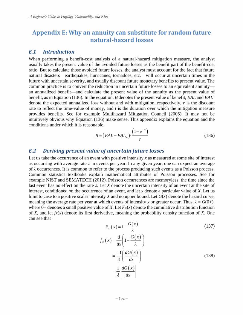
A Beginner’s Guide to Fragility, Vulnerability, and Risk
– 132 –
Appendix E: Why an annuity can substitute for random future natural-hazard losses
E.1 Introduction When performing a benefit-cost analysis of a natural-hazard mitigation measure, the analyst
usually takes the present value of the avoided future losses as the benefit part of the benefit-cost
ratio. But to calculate those avoided future losses, the analyst must account for the fact that future
natural disasters—earthquakes, hurricanes, tornadoes, etc.—will occur at uncertain times in the
future with uncertain severity, and usually discount future monetary benefits to present value. The
common practice is to convert the reduction in uncertain future losses to an equivalent annuity—
an annualized benefit—and calculate the present value of the annuity as the present value of
benefit, as in Equation (136). In the equation, B denotes the present value of benefit, EAL and EAL’
denote the expected annualized loss without and with mitigation, respectively, r is the discount
rate to reflect the time-value of money, and t is the duration over which the mitigation measure
provides benefits. See for example Multihazard Mitigation Council (2005). It may not be
intuitively obvious why Equation (136) make sense. This appendix explains the equation and the
conditions under which it is reasonable.
( )( )1 rt
m
eB EAL EAL
r
−−= − (136)
E.2 Deriving present value of uncertain future losses Let us take the occurrence of an event with positive intensity x as measured at some site of interest
as occurring with average rate λ in events per year. In any given year, one can expect an average
of λ occurrences. It is common to refer to the process producing such events as a Poisson process.
Common statistics textbooks explain mathematical attributes of Poisson processes. See for
example NIST and SEMATECH (2012). Poisson occurrences are memoryless: the time since the
last event has no effect on the rate λ. Let X denote the uncertain intensity of an event at the site of
interest, conditioned on the occurrence of an event, and let x denote a particular value of X. Let us
limit to case to a positive scalar intensity X and no upper bound. Let G(x) denote the hazard curve,
meaning the average rate per year at which events of intensity x or greater occur. Thus, λ = G(0+),
where 0+ denotes a small positive value of X. Let FX(x) denote the cumulative distribution function
of X, and let fX(x) denote its first derivative, meaning the probability density function of X. One
can see that
( )( )
1X
G xF x
= − (137)
( )( )
( )
( )
1
1
1
X
G xdf x
dx
dG x
dx
dG x
dx
= −
−=
=
(138)
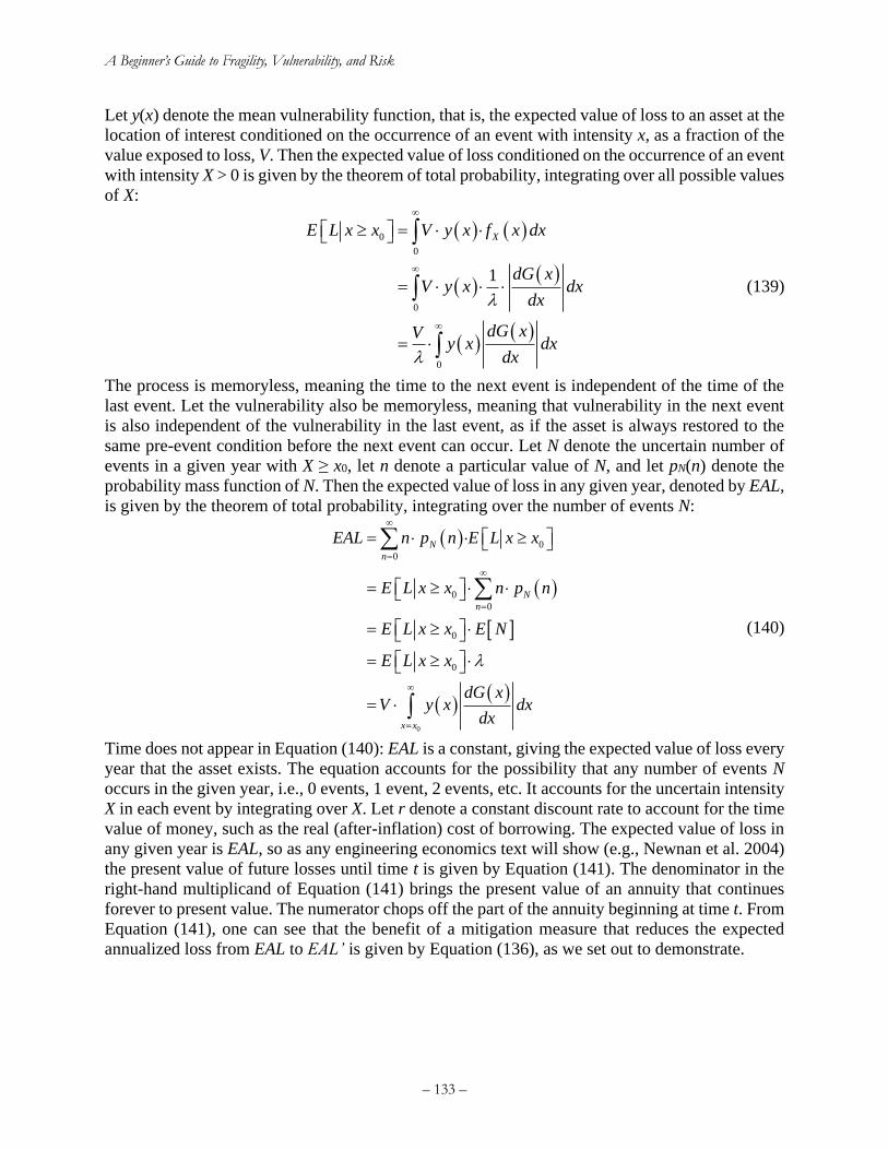
A Beginner’s Guide to Fragility, Vulnerability, and Risk
– 133 –
Let y(x) denote the mean vulnerability function, that is, the expected value of loss to an asset at the
location of interest conditioned on the occurrence of an event with intensity x, as a fraction of the
value exposed to loss, V. Then the expected value of loss conditioned on the occurrence of an event
with intensity X > 0 is given by the theorem of total probability, integrating over all possible values
of X:
( ) ( )
( )( )
( )( )
0
0
0
0
1
XE L x x V y x f x dx
dG xV y x dx
dx
dG xVy x dx
dx
=
=
=
(139)
The process is memoryless, meaning the time to the next event is independent of the time of the
last event. Let the vulnerability also be memoryless, meaning that vulnerability in the next event
is also independent of the vulnerability in the last event, as if the asset is always restored to the
same pre-event condition before the next event can occur. Let N denote the uncertain number of
events in a given year with X ≥ x0, let n denote a particular value of N, and let pN(n) denote the
probability mass function of N. Then the expected value of loss in any given year, denoted by EAL,
is given by the theorem of total probability, integrating over the number of events N:
( )
( )
( )( )
0
0
0
0
0
0
0
N
n
N
n
x x
EAL n p n E L x x
E L x x n p n
E L x x E N
E L x x
dG xV y x dx
dx
=
=
=
=
=
=
=
=
(140)
Time does not appear in Equation (140): EAL is a constant, giving the expected value of loss every
year that the asset exists. The equation accounts for the possibility that any number of events N
occurs in the given year, i.e., 0 events, 1 event, 2 events, etc. It accounts for the uncertain intensity
X in each event by integrating over X. Let r denote a constant discount rate to account for the time
value of money, such as the real (after-inflation) cost of borrowing. The expected value of loss in
any given year is EAL, so as any engineering economics text will show (e.g., Newnan et al. 2004)
the present value of future losses until time t is given by Equation (141). The denominator in the
right-hand multiplicand of Equation (141) brings the present value of an annuity that continues
forever to present value. The numerator chops off the part of the annuity beginning at time t. From
Equation (141), one can see that the benefit of a mitigation measure that reduces the expected
annualized loss from EAL to EAL’ is given by Equation (136), as we set out to demonstrate.
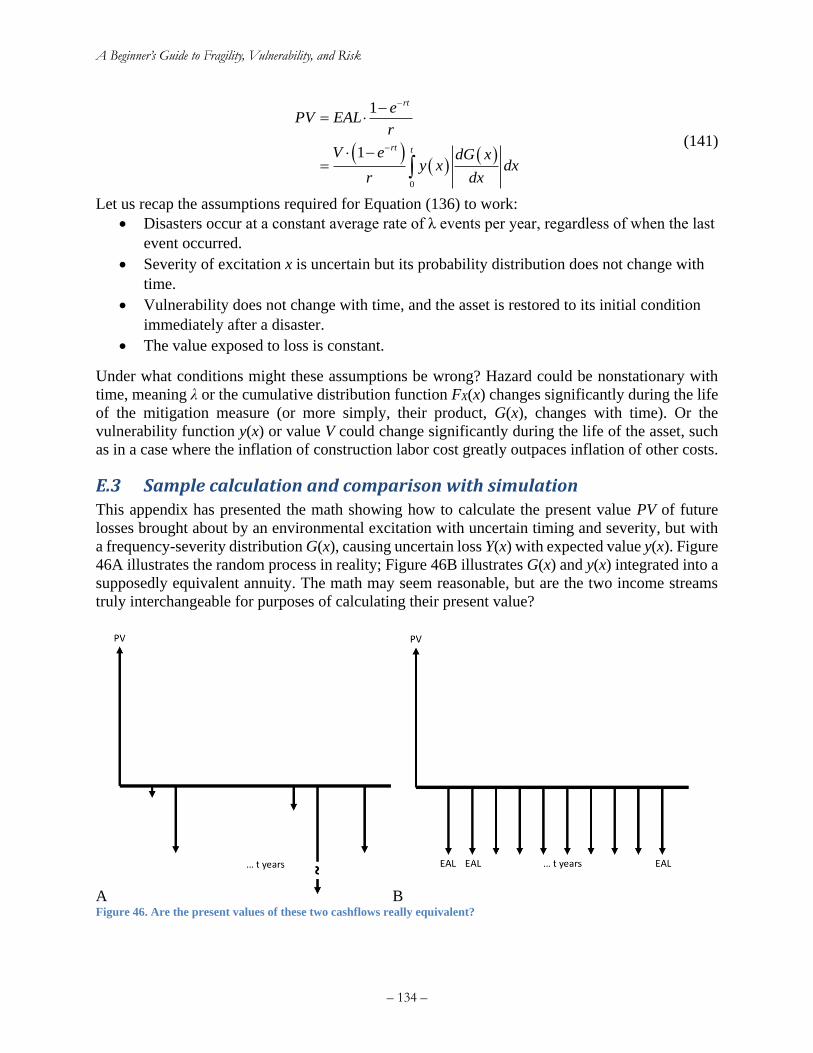
A Beginner’s Guide to Fragility, Vulnerability, and Risk
– 134 –
( )
( )( )
0
1
1
rt
rt t
ePV EAL
r
V e dG xy x dx
r dx
−
−
−=
−=
(141)
Let us recap the assumptions required for Equation (136) to work:
• Disasters occur at a constant average rate of λ events per year, regardless of when the last
event occurred.
• Severity of excitation x is uncertain but its probability distribution does not change with
time.
• Vulnerability does not change with time, and the asset is restored to its initial condition
immediately after a disaster.
• The value exposed to loss is constant.
Under what conditions might these assumptions be wrong? Hazard could be nonstationary with
time, meaning λ or the cumulative distribution function FX(x) changes significantly during the life
of the mitigation measure (or more simply, their product, G(x), changes with time). Or the
vulnerability function y(x) or value V could change significantly during the life of the asset, such
as in a case where the inflation of construction labor cost greatly outpaces inflation of other costs.
E.3 Sample calculation and comparison with simulation This appendix has presented the math showing how to calculate the present value PV of future
losses brought about by an environmental excitation with uncertain timing and severity, but with
a frequency-severity distribution G(x), causing uncertain loss Y(x) with expected value y(x). Figure
46A illustrates the random process in reality; Figure 46B illustrates G(x) and y(x) integrated into a
supposedly equivalent annuity. The math may seem reasonable, but are the two income streams
truly interchangeable for purposes of calculating their present value?
A B Figure 46. Are the present values of these two cashflows really equivalent?
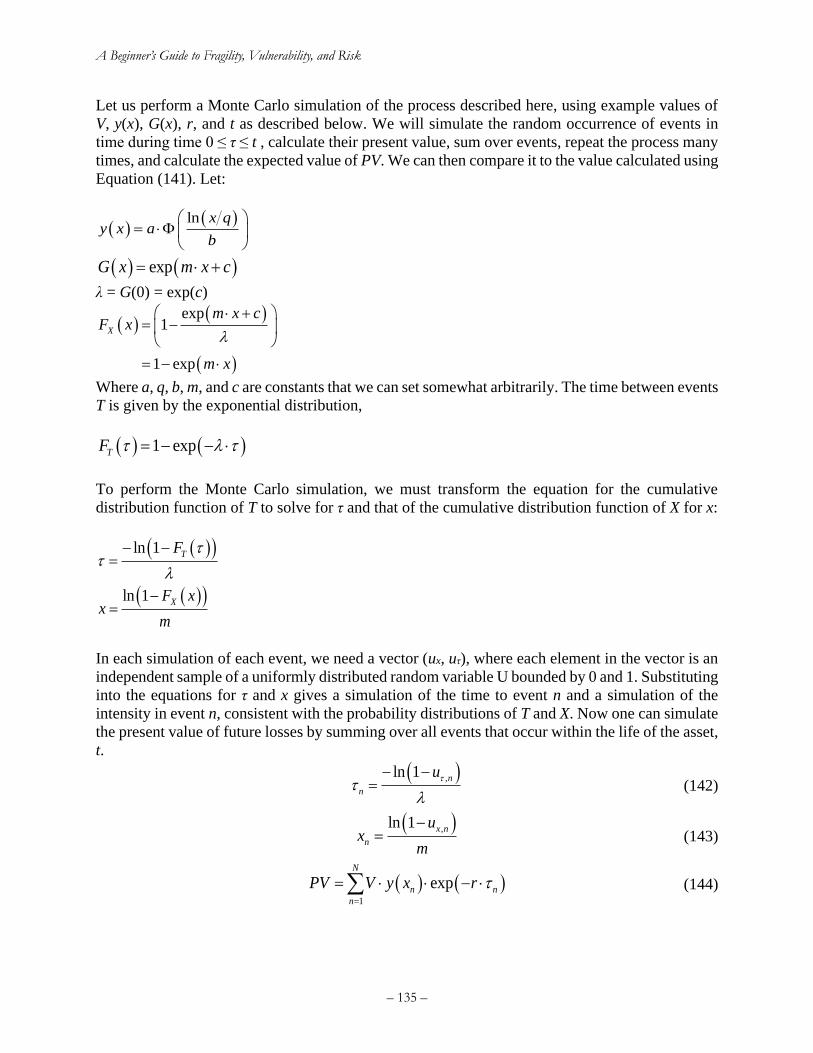
A Beginner’s Guide to Fragility, Vulnerability, and Risk
– 135 –
Let us perform a Monte Carlo simulation of the process described here, using example values of
V, y(x), G(x), r, and t as described below. We will simulate the random occurrence of events in
time during time 0 ≤ τ ≤ t , calculate their present value, sum over events, repeat the process many
times, and calculate the expected value of PV. We can then compare it to the value calculated using
Equation (141). Let:
( )( )ln x q
y x ab
=
( ) ( )expG x m x c= +
λ = G(0) = exp(c)
( )( )
( )
exp1
1 exp
X
m x cF x
m x
+ = −
= −
Where a, q, b, m, and c are constants that we can set somewhat arbitrarily. The time between events
T is given by the exponential distribution,
( ) ( )1 expTF = − −
To perform the Monte Carlo simulation, we must transform the equation for the cumulative
distribution function of T to solve for τ and that of the cumulative distribution function of X for x:
( )( )ln 1 TF
− −=
( )( )ln 1 XF xx
m
−=
In each simulation of each event, we need a vector (ux, uτ), where each element in the vector is an
independent sample of a uniformly distributed random variable U bounded by 0 and 1. Substituting
into the equations for τ and x gives a simulation of the time to event n and a simulation of the
intensity in event n, consistent with the probability distributions of T and X. Now one can simulate
the present value of future losses by summing over all events that occur within the life of the asset,
t.
( ),ln 1 n
n
u
− −= (142)
( ),ln 1 x n
n
ux
m
−= (143)
( ) ( )1
expN
n n
n
PV V y x r =
= − (144)
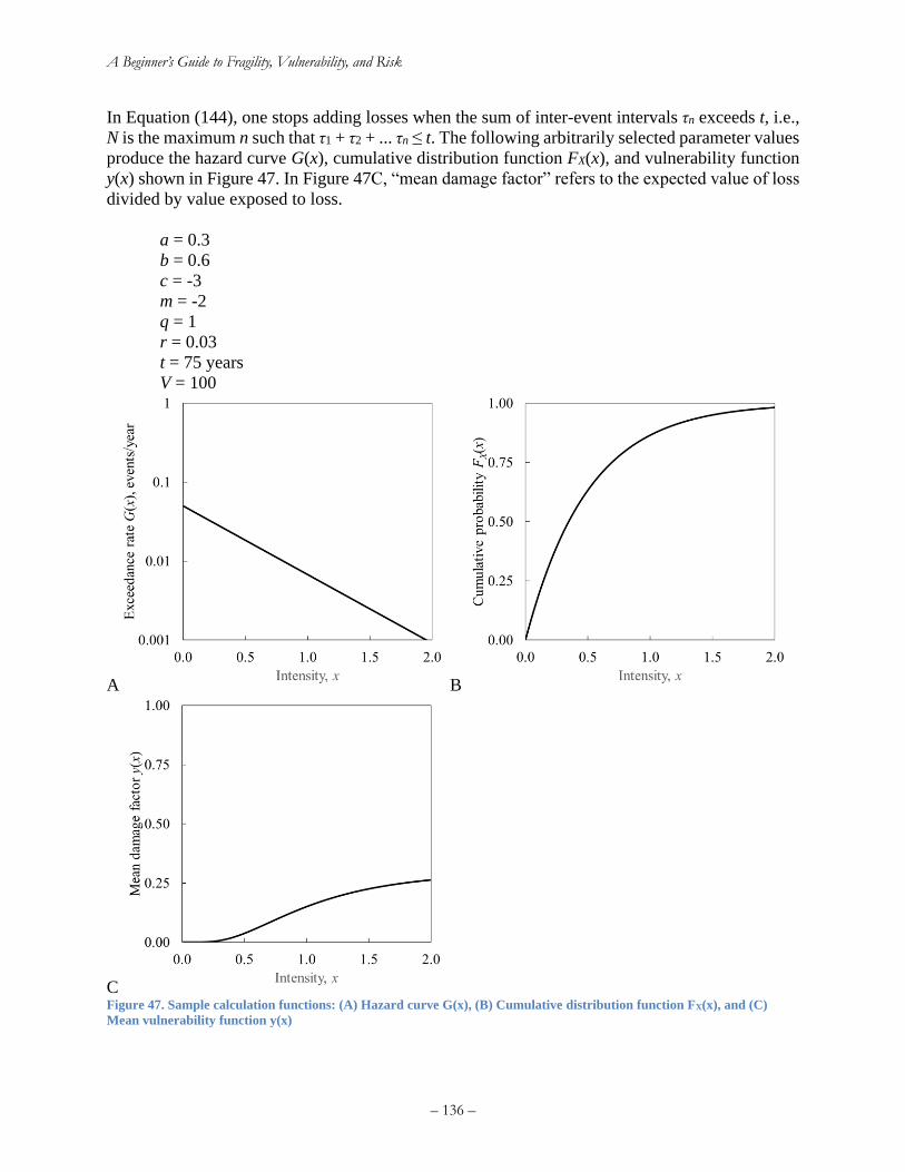
A Beginner’s Guide to Fragility, Vulnerability, and Risk
– 136 –
In Equation (144), one stops adding losses when the sum of inter-event intervals τn exceeds t, i.e.,
N is the maximum n such that τ1 + τ2 + ... τn ≤ t. The following arbitrarily selected parameter values
produce the hazard curve G(x), cumulative distribution function FX(x), and vulnerability function
y(x) shown in Figure 47. In Figure 47C, “mean damage factor” refers to the expected value of loss
divided by value exposed to loss.
a = 0.3
b = 0.6
c = -3
m = -2
q = 1
r = 0.03
t = 75 years
V = 100
A B
C Figure 47. Sample calculation functions: (A) Hazard curve G(x), (B) Cumulative distribution function FX(x), and (C)
Mean vulnerability function y(x)

A Beginner’s Guide to Fragility, Vulnerability, and Risk
– 137 –
Evaluating Equation (141) with the foregoing parameters produces PV = 7.71. Performing 10,000
simulations of a 75-year sequence of events using Equations (142) through (144) results in a
distribution of PV with mean equal to 7.77, confirming the analytical solution within 1% at a
fraction of the effort.

A Beginner’s Guide to Fragility, Vulnerability, and Risk
– 138 –
Appendix F: Revision history Rev Date Comments
1 19 Jun 2013 Initial draft
2 26 Jun 2013 Change to outline form. Add thm of tot probability & PSHA. Add exercise
“basic elements of earthquake rupture forecast.” Add multiple fragility
functions. Change some ASCII equations to standard math notation.
3 26 Jun 2013 Rest of MathType
4 17 Jul 2013 Add to style guide
5 28 Jul 2013 Flesh out risk integral. Definite component type and sites in exercises.
6 30 Jul 2013 Remove ref to normal fragility function in Ex 4 “know the lognormal”
Add section on measures of seismic excitation
Correct misc typos
Add section on GMICE and IGMCE.
7 14 Aug 2013 Misc edits: fix refs in Exercise 1, discuss notation for uncertainty quantities just
before on the meaning of D in Sec 1. Add exercise to test reader’s understanding
of the theorem of total probability.
8 13 Sep 2013 Misc edits.
9 17 Sep 2013 Add sec on how to derive fragility functions, add TOC, add section on
defending your thesis.
10 2 Oct 2013 Fix equations for probability of 1 or 2 simultaneous damage states
11 18 Oct 2013 Edit MECE damage state problem to be less confusing
12 24 Oct 2013 Add hazard deaggregation section and text on how to deal with
underrepresentative samples. Add placeholders for a section on vulnerability
functions and initial text for a section on risk in terms of degree of loss.
13 7 Nov 2013 Improve transitions between sections
14 11 Nov 2013 Streetlight effect and spherical cows
15 18 Nov 2013 Add short section on convenient sources for hazard data
16 27 Feb 2014 Fix typo in hazard deaggregation exercise
17 28 Apr 2014 Reorganize (intro, fragility, vulnerability, hazard, risk, exercises, refs,
appendices). Edit for brevity & to use 3rd person. Move revision history to
appendix.
18 30 Apr 2014 Delete the words trapezoidal rule from exercise 7, equation for component
failure rate.
19 2 Oct 2014 Fix typos
20 16 Oct 2014 Reorganize appendices, add appendix C, tornado diagram analysis
21 31 Oct 2014 Add Mutt & Jeff cartoon to illustrate streetlight effect and add figure with
hazard curve and fragility function to illustrate failure rate
22 16 Nov 2014 Add stub of appendix D on assigning value to human life
23 10 Dec 2014 Move and expand on probability distributions, with equations and figures for
N, LN, and U; add 2 definitions of fragility function; enhance instructions on
clarity in the style guide; discuss advantages and disadvantages of tornado
diagram.
24 29 May 2015 3 methods for deriving vulnerability functions. History of tornado diagrams.
Aleatory and epistemic uncertainty. More about the lognormal.
25 30 May 2015 More lognormal
26 31 May 2015 Add the clarity test
27 5 Jun 2015 Begin portfolio risk analysis. Caution about ill-defined damage states.
28 3 Sep 2015 Add “three general classes of fragility functions”
29 5 Sep 2015 Add illustrative risk curves & start section on common single-site risk software.
Expand on single-site EAL.
A Beginner’s Guide to Fragility, Vulnerability, and Risk
– 139 –
Rev Date Comments
30 7 Sep 2015 Add Keller coin-toss illustration, Diaconis et al. coin-toss device, and elevator
illustration of the clarity test
31 23 Dec 2015 Minor edits
32 11 Feb 2016 Minor edits; thanks Luis Esquivel, Universidad de Costa Rica
33 11b Feb 2016 Add text and exercise for a risk curve for binomially distributed loss measure
34 22 Feb 2016 Add section on risk curve for discrete damage count and large N
35 28 Feb 2016 Add section 6.1, a brief summary of portfolio risk analysis, adapted from the
HayWired levee damage scenario.
36 10 Mar 2016 Add example problem with sample calcs for tornado diagram
37 13 Jun 2016 Correct errors in discussion of lognormal. Thanks, Stoyan Andreev.
38 15 Aug 2016 Typos; more on aleatory vs. epistemic more; fix misstatements about LN
39 11 Nov 2016 Expand appendix C.1 Your thesis outline.
40 12 Feb 2017 New intro section summarizing an engineering approach to risk analysis
41 15 May 2017 New appendix D on how to write a research article
42 13 Jun 2017 New chapter 8 for mathematical tools, with sec 8.2 on moment matching
43 15 Jul 2017 Minor edit to appendix A, language of independent and dependent variables
44 6 Sep 2017 New section of dealing with fragility functions that cross
45 19 Mar 2018 Add 3-point moment matching. Combine with tornado-diagram analysis.
46 20 Jul 2018 Add more detail about the parameters of normal and lognormal
47 24 Mar 2019 New appendix E with derivation of EAL and benefit
48 27 Mar 2019 Corrected appendix E figure with vulnerability function
49 28 Mar 2019 Add section on Monte Carlo simulation
50 27 Aug 2019 Add section on what are earthquakes
51 4 Nov 2019 Add section on simulating suites of correlated ground motion fields
52 6 Feb 2020 Add cashflow diagrams to illustrate the benefit of mitigation
53 20 Feb 2020 Add cashflow diagrams to E.3 for the random process and the annuity
54 1 Mar 2020 Add section on correlation in portfolio catastrophe risk. Complete sections on
portfolio loss exceedance, portfolio expected annualized loss, and simulating
properly spatially correlated ground motion. Complete a section of ground-
motion-prediction equations.
55 7 Sep 2020 Add numerical integration of EAL from piecewise linear loss versus
ln(exceedance frequency)
56 20 Oct 2020 Expands C1
57 24 Dec 2020 Expand on spatially correlated ground motion
58 16 Jan 2021 Add glossary
End