2021moultriemd.pdf - enlighten: theses
TRANSCRIPT

Moultrie, Christopher E.J. (2021) Queueing theory applied to pre-hospital
and retrieval medicine. MD thesis.
https://theses.gla.ac.uk/82402/
Copyright and moral rights for this work are retained by the author
A copy can be downloaded for personal non-commercial research or study,
without prior permission or charge
This work cannot be reproduced or quoted extensively from without first
obtaining permission in writing from the author
The content must not be changed in any way or sold commercially in any
format or medium without the formal permission of the author
When referring to this work, full bibliographic details including the author,
title, awarding institution and date of the thesis must be given
Enlighten: Theses
https://theses.gla.ac.uk/ [email protected]
Queueing Theory Applied to
Pre-Hospital and Retrieval Medicine
Dr Christopher E J Moultrie
MBChB, DRCOG, FRCEM
Submitted in fulfilment of the requirements for the degree of:
Doctor of Medicine (MD)
Institute of Health and Wellbeing
College of Medical, Veterinary and Life Sciences
University of Glasgow
August 2021

I
Abstract
Background: Pre-hospital and Retrieval Medicine is a healthcare specialty focussed on
the provision of advanced, specialist care to patients in any clinical setting - from the
roadside to a major hospital. The ScotSTAR division of the Scottish Ambulance Service
has a national remit for providing such services within Scotland. High clinical acuity and
long travel time challenge the service by generating a significant workload from relatively
few patients. ScotSTAR teams comprise only one or two servers, so waiting times are
potentially long, and there is a relatively high per-patient cost.
Aims: Firstly, this thesis aims to investigate if standard queueing theory could be used to
describe two ScotSTAR teams: the Scottish Paediatric Retrieval Service (SPRS) and the
Emergency Medical Retrieval Service (EMRS). The thesis then aims to develop a Discrete
Event Simulation (DES) model and validate it against the real-world. From this model, the
thesis then aims to describe the performance of the ScotSTAR teams using metrics which
are unmeasurable in the real-world. Finally, the thesis aims to establish the performance
frontiers of the ScotSTAR teams.
Methods: Analysis of the ScotSTAR teams to map their operation with standard queueing
theory was undertaken. This was used to develop a DES model, which performed 1000
simulation iterations of a 4-year period. The output was compared to the real-world data
for accuracy with regard to: number of missions, activation time of day, inter-arrival time,
mission duration, and server utilization. The validated model was then used to derive
values for length of queue, waiting time, and proportion of simultaneous retrievals. Finally,
the model was run in an extended Monte-Carlo format to establish the relationship of the
current system to proposed performance frontiers based on waiting time, simultaneous
retrievals, and missed missions.
Results: This thesis demonstrated that standard queueing theory could describe the
operations of the ScotSTAR systems, describing M/G/1 and M/G/2 queue types for SPRS
and EMRS respectively. The DES model based on this was able to accurately replicate the
real-world system in retrospective simulation (mean model accuracy: SPRS = 91.0%,
EMRS = 91.9%), and partially replicate the contemporaneous state of the system (mean
model accuracy: SPRS = 82.2%, EMRS = 89.0%). The model then derived plausible
values for length of queue, waiting times, and simultaneous retrieval proportions. Lastly,
the model demonstrated a 95th percentile of waiting time (Wq95) of 1 hour for secondary
retrievals as being the most significant performance frontier. SPRS was demonstrated to be
operating approximately 196 missions per year over this frontier, EMRS had capacity for
an extra 26 primary or 23 secondary missions per year before reaching the frontier.
Conclusions: Standard queueing theory is able to accurately describe the constituent
parameters of the ScotSTAR systems. A discrete event simulation model can, with some
limitations, accurately replicate the real-world to allow the derivation of performance
descriptors which are unmeasurable in the real-world. Furthermore, such a model can also
demonstrate the relationship between the current state of the system and potential
performance frontiers.

II
Contents
Preamble
Abstract ............................................................................................................................... I
List of Abbreviations ........................................................................................................IX
List of Tables ..................................................................................................................... X
List of Figures ...................................................................................................................XI
Accompanying Material ................................................................................................. XX
Preface ......................................................................................................................... XXII
Acknowledgements .................................................................................................... XXIII
Author’s Declaration .................................................................................................. XXIV
Part 1: Defining Applicable Queueing Theory
1.1. Introduction ................................................................................................................ 3
1.2. Background ................................................................................................................. 5
1.2.1. Pre-Hospital and Retrieval Medicine ............................................................................... 6
1.2.2. Scottish Ambulance Service, ScotSTAR Division .......................................................... 9
1.2.3. Scottish Paediatric Retrieval Service (SPRS) .................................................................. 9
1.2.4. Emergency Medical Retrieval Service (EMRS) ............................................................ 10
1.2.5. Scottish Neonatal Transport Service (SNTS) ................................................................ 12
1.3. Queueing Theory ..................................................................................................... 14
1.3.1. Basic Queueing Theory.................................................................................................. 14
1.3.2. Calculation of Descriptive Values ................................................................................. 17
1.3.3. Networks of queues........................................................................................................ 21
1.4. Literature Review ...................................................................................................... 24
1.4.1. Literature search............................................................................................................. 25
1.4.2. Reviewed papers ............................................................................................................ 29
1.4.3. Queueing theory applied to the ScotSTAR system ........................................................ 34
1.5. Aims .......................................................................................................................... 36
1.6. Methods ..................................................................................................................... 38
1.6.1. General ........................................................................................................................... 38
1.6.2. Inter-arrival Time Distribution (A) ................................................................................ 38
1.6.3. Correction of time-dependent Poisson distributions ...................................................... 39
1.6.4. Service Time (S) ............................................................................................................ 49
1.6.5. Number of Servers (c) .................................................................................................... 50
1.6.6. Number of places in system (K) .................................................................................... 50
1.6.7. Population (N) ................................................................................................................ 50
1.6.8. Queueing Discipline (D) ................................................................................................ 51
1.7. Results ...................................................................................................................... 53
III
1.7.1. Scottish Paediatric Retrieval Service (SPRS) ................................................................ 53
1.7.1.1. Description of SPRS queue operation .................................................................... 53
1.7.1.2. SPRS inter-arrival time distribution ....................................................................... 55
1.7.1.3. SPRS mission durations ......................................................................................... 61
1.7.1.4. SPRS number of servers ........................................................................................ 63
1.7.1.5. SPRS system capacity ............................................................................................ 63
1.7.1.6. SPRS population .................................................................................................... 63
1.7.1.7. SPRS queueing discipline ...................................................................................... 64
1.7.1.8. Formulation of SPRS system in Kendall’s notation .............................................. 64
1.7.2. Emergency Medical Retrieval Service (EMRS) ............................................................ 65
1.7.2.1. Description of EMRS queue operation .................................................................. 65
1.7.2.2. EMRS inter-arrival time distribution ..................................................................... 68
1.7.2.3. EMRS mission durations ....................................................................................... 81
1.7.2.4. EMRS number of servers ....................................................................................... 84
1.7.2.5. EMRS system capacity .......................................................................................... 84
1.7.2.6. EMRS population................................................................................................... 84
1.7.2.7. EMRS queueing discipline .................................................................................... 87
1.7.2.8. Formulation of EMRS system in Kendall’s notation ............................................. 87
1.7.3. Summary of SPRS & EMRS queue descriptions........................................................... 88
1.7.4. Formulaic calculation of operational values .................................................................. 89
1.7.4.1. Selection of applicable queueing theory ................................................................ 89
1.7.4.2. SPRS formulaic results .......................................................................................... 89
1.7.4.3. EMRS formulaic results ......................................................................................... 92
1.8. Discussion ......................................................................................................................... 94
1.8.1. Arrivals processes and effect on classical queueing theory ...................................... 94
1.8.2. Service times ............................................................................................................. 98
1.8.3. Number of servers ................................................................................................... 102
1.8.4. Number of places in the system .............................................................................. 102
1.8.5. Applicable (retrievable) population ........................................................................ 103
1.8.6. Queueing discipline ................................................................................................ 105
1.8.7. Formulaic results ..................................................................................................... 105
1.9. Conclusions ..................................................................................................................... 108

IV
Part 2: Modelling and Simulation of ScotSTAR Systems
2.1. Introduction ............................................................................................................ 111
2.1.1. Introduction to simulation types .................................................................................. 111
2.1.1.1. Discrete Event Simulation (DES) ........................................................................ 111
2.1.1.2. Agent Based Modelling (ABM) ........................................................................... 112
2.1.1.3. System Dynamics (SD) Modelling ...................................................................... 113
2.1.1.4. Suitability of simulation methodologies for ScotSTAR ...................................... 114
2.2. Literature Review ................................................................................................... 116
2.2.1. Literature search........................................................................................................... 116
2.2.2. Reviewed papers .......................................................................................................... 120
2.2.3. Applications of simulation in wider healthcare ........................................................... 123
2.2.4. Application of simulation to ScotSTAR ...................................................................... 124
2.3. Aims ....................................................................................................................... 127
2.4. Methods .................................................................................................................. 129
2.4.1. Methods – modelling and simulation ........................................................................... 129
2.4.1.1. General ................................................................................................................. 129
2.4.1.2. Mission generation ............................................................................................... 130
2.4.1.3. Exclusion Sampling ............................................................................................. 131
2.4.1.4. Entity attributes .................................................................................................... 139
2.4.1.5. Mission duration allocation .................................................................................. 139
2.4.1.6. Running of Simulation ......................................................................................... 141
2.4.2. Parameter analysis ....................................................................................................... 142
2.4.2.1. Comparison to real-world. ................................................................................... 143
2.4.2.2. Total number of missions comparison ................................................................. 143
2.4.2.3. Distribution of missions through simulation period comparison ......................... 143
2.4.2.4. Activation time of day comparison ...................................................................... 143
2.4.2.5. Inter-arrival time distribution comparison ........................................................... 144
2.4.2.6. Mission duration comparison ............................................................................... 144
2.4.2.7. Server utilization comparison .............................................................................. 145
2.4.3. Summation ................................................................................................................... 145
2.5. Results of simulation of SPRS operations .............................................................. 147
2.5.1 Retrospective simulation of SPRS operations .............................................................. 149
2.5.1.1. Retrospective simulation of SPRS mission count ................................................ 150
2.5.1.2. Retrospective simulation of SPRS activation time of day ................................... 155
2.5.1.3. Retrospective simulation of SPRS inter-arrival times ......................................... 159
2.5.1.4. Retrospective simulation of SPRS mission durations .......................................... 165
2.5.1.5. Retrospective simulation of SPRS server utilization ........................................... 171
2.5.1.6. Summary of SPRS retrospective simulation results............................................. 174
2.5.2. Contemporaneous simulation of SPRS operations ...................................................... 175
2.5.2.1. Contemporaneous simulation of SPRS mission count ........................................ 177

V
2.5.2.2. Contemporaneous SPRS activation times of day ................................................ 180
2.5.2.3. Contemporaneous SPRS inter-arrival times ....................................................... 184
2.5.2.4. Contemporaneous simulation of SPRS mission durations .................................. 190
2.5.2.5. Contemporaneous simulation of SPRS server utilization ................................... 198
2.5.2.6. Contemporaneous simulation of SPRS team - summary .................................... 201
2.5.3. Summary of results from simulations of SPRS operations ........................................... 202
2.6. Results of simulation of EMRS operations ............................................................ 206 2.6.1. Retrospective simulation of EMRS operations ............................................................ 209
2.6.1.1. Retrospective simulation of EMRS mission count .............................................. 209
2.6.1.2. Retrospective simulation of EMRS activation times of day ................................ 216
2.6.1.3. Retrospective simulation of EMRS inter-arrival times ........................................ 224
2.6.1.4. Retrospective simulation of EMRS mission durations ........................................ 237
2.6.1.5. Retrospective simulation of EMRS server utilization .......................................... 249
2.6.1.6. Summary of EMRS retrospective simulation results ........................................... 254
2.6.2. Contemporaneous simulation of EMRS operations ..................................................... 255
2.6.2.1. Contemporaneous simulation of EMRS mission count ....................................... 256
2.6.2.2. Contemporaneous EMRS activation times of day ............................................... 262
2.6.2.3. Contemporaneous EMRS inter-arrival times ....................................................... 269
2.6.2.4. Contemporaneous simulation of EMRS mission durations ................................. 278
2.6.2.5. Contemporaneous simulation of EMRS server utilization................................... 292
2.6.2.6. Contemporaneous simulation of EMRS team – summary ................................... 296
2.6.3. Summary of results from simulations of EMRS operations ........................................ 297
2.7. Discussion of modelling and simulation of ScotSTAR systems ............................ 301
2.7.1. Simulation methodology ............................................................................................ 301
2.7.2. Simulated number of missions ................................................................................... 302
2.7.3. Activation time of day ................................................................................................. 303
2.7.4. Inter-arrival times ....................................................................................................... 305
2.7.5. Mission Durations ...................................................................................................... 306
2.7.6. Utilization .................................................................................................................. 310
2.7.7. Refinements and future studies .................................................................................... 311
2.8. Conclusions ........................................................................................................ 314

VI
Part 3: Deriving System Descriptors and Performance Frontiers
3.1. Introduction ............................................................................................................ 317
3.1.1. Deriving system descriptors from validated ScotSTAR models.................................. 317
3.1.2. Unsuitability of standard queueing theory parameters ................................................ 319
3.1.3. Calculation of descriptive values ................................................................................. 321
3.1.4. Performance frontiers................................................................................................... 321
3.1.5. Establishing system specifications ............................................................................... 322
3.1.6. Defining new performance specifications .................................................................... 323
3.1.7. The Pareto limit ........................................................................................................... 326
3.1.8. Possible simulation methodologies .............................................................................. 326
3.1.9. Application of extended Monte Carlo simulation ........................................................ 327
3.2. Aims ....................................................................................................................... 330
3.3. Methods .................................................................................................................. 332
3.3.1. Derived performance descriptors ............................................................................... 332
3.3.1.1. Average length of queue (Lq) ................................................................................ 332
3.3.1.2. Waiting times in queue (Wq and Wq95) ................................................................. 332
3.3.1.3. Simultaneous retrievals ......................................................................................... 333
3.3.2. Unobservable phenomena ............................................................................................ 333
3.4. Results of derived performance descriptors from the SPRS simulation ................. 336
3.4.1. SPRS retrospective simulation period ......................................................................... 337
3.4.1.1. Mean length of queue (Lq) ................................................................................... 338
3.4.1.2. Waiting time in queue – mean waiting time (Wq) ................................................ 341
3.4.1.3. Waiting time in queue – 95th percentile of waiting time (Wq95) ........................ 344
3.4.1.4. Simultaneous retrievals ........................................................................................ 347
3.4.2. SPRS contemporaneous simulation period .................................................................. 350
3.4.2.1. Mean length of queue (Lq) ................................................................................... 351
3.4.2.2. Waiting time in queue – mean waiting time (Wq). ............................................... 353
3.4.2.3. Waiting time in queue – 95th percentile of waiting time (Wq95) .......................... 355
3.4.2.4. Simultaneous retrievals ........................................................................................ 357
3.4.3. Summary of SPRS derived system descriptors results ................................................ 359
3.5. Results of simulating SPRS performance frontiers through unobservable
phenomena ...................................................................................................................... 362
3.5.1. SPRS extended Monte-Carlo simulation output ......................................................... 364
3.5.2. Waiting time in queue – 95th percentile of waiting time (Wq95) ................................ 366
3.5.3. Simultaneous retrievals ............................................................................................... 369
3.5.4. Addition of a second SPRS team ................................................................................ 374
3.5.5. Summary – SPRS performance specifications ............................................................ 377
VII
3.6. Results of derived performance descriptors from the EMRS simulation ................ 380
3.6.1. Retrospective simulation period .................................................................................. 381
3.6.1.1. Mean length of queue (Lq) ................................................................................... 382
3.6.1.2. Waiting time in queue – mean waiting time (Wq) ................................................ 383
3.6.1.3. Waiting time in queue – 95th percentile of waiting time (Wq95) .......................... 384
3.6.1.4. Simultaneous retrievals ........................................................................................ 387
3.6.2. EMRS contemporaneous simulation period ................................................................ 390
3.6.2.1. Mean length of queue (Lq) ................................................................................... 391
3.6.2.2. Waiting time in queue – mean waiting time (Wq). ............................................... 393
3.6.2.3. Waiting time in queue – 95th percentile of waiting time (Wq95) .......................... 395
3.6.2.4. Simultaneous retrievals ........................................................................................ 400
3.6.3. Summary of EMRS derived system descriptors results ............................................... 403
3.7. Simulation of EMRS performance limits through unobservable phenomena ........ 406
3.7.1. EMRS extended Monte-Carlo simulation output ......................................................... 408
3.7.2. Revision of EMRS model ........................................................................................... 410
3.7.2.1. Simultaneous retrievals ........................................................................................ 410
3.7.2.2. 95th percentile of waiting time (Wq95) – all missions. ......................................... 417
3.7.2.3. Assessment of non-similarity, and subsequent model changes............................ 419
3.7.3. 95th Percentile of waiting time (Wq95) – revised EMRS model ................................. 421
3.7.3.1. All missions Wq95 ................................................................................................ 421
3.7.3.2. Wq95 – secondary missions ............................................................................... 422
3.7.3.3. Wq95 – primary missions .................................................................................. 424
3.7.4. Simultaneous retrievals ............................................................................................ 426
3.7.5. Missed primary missions ............................................................................................. 432
3.7.6. EMRS Summary .......................................................................................................... 435
3.8. Discussion ............................................................................................................... 438
3.8.1. Derived performance descriptors ................................................................................. 438
3.8.1.1. Assumption of validity. ........................................................................................ 438
3.8.1.2. Contemporaneous values ..................................................................................... 438
3.8.1.3. Mean length of queue (Lq) and mean waiting time (Wq) ..................................... 439
3.8.1.4. 95th percentile of waiting time (Wq95) ................................................................. 440
3.8.1.5. Simultaneous retrievals ........................................................................................ 440
3.8.1.6. Current considerations ......................................................................................... 442
3.8.2. Unobservable phenomena ............................................................................................ 443
3.8.2.1. Validity and applicability of the model ................................................................ 443
3.8.2.2. 95th percentile of waiting time ............................................................................ 443
3.8.2.3. Simultaneous retrievals ....................................................................................... 444
3.8.2.4. Changes to SPRS service .................................................................................... 445
3.8.2.5. Missed primary missions .................................................................................. 446
3.9. Conclusions ............................................................................................................ 449

VIII
Epilogue
Summary of thesis .......................................................................................................... 452
Review of thesis ............................................................................................................. 453
Fidelity to the Real-World System ......................................................................................... 453
Fidelity to Mathematical Relationships .................................................................................. 456
Real-world Operational Applicability ..................................................................................... 458
Limitations and Strengths ............................................................................................... 460
Limitations .............................................................................................................................. 460
Strengths ................................................................................................................................. 463
Implications .................................................................................................................... 464
Research Implications ............................................................................................................. 464
Clinical Implications ............................................................................................................... 466
Future Research and Development ................................................................................. 470
Final Conclusions ........................................................................................................... 474
Appendices
Appendix 1: SPRS simulation model ............................................................................. 477
Appendix 2: EMRS original simulation model .............................................................. 478
Appendix 3: EMRS revised simulation model ............................................................... 479
Glossary ...................................................... 481
References .................................................. 483
Bibliography ................................................. 487

IX
L i st o f Abbrev iat ions
ABM Agent Based Modelling
CI Confidence Interval
DES Discrete Event Simulation
ECDF Empirical Cumulative Distribution Function
ECMO Extra-Corporeal Membrane Oxygenation (of blood)
ED Emergency Department (hospital department)
EM Emergency Medicine (medical specialty)
EMRS Emergency Medical Retrieval Service (part of ScotSTAR)
ICM Intensive Care Medicine (medical specialty)
ICU / ITU Intensive Care Unit (hospital department. ITU abbreviation retained from
former UK nomenclature: Intensive Therapy Unit).
K-S Kolmogorov-Smirnov (statistical test)
Lq Average length of queue
PDF Probability Density Function
PHaRM Pre-Hospital and Retrieval Medicine
PI Prediction Interval
RSI Rapid Sequence Induction (see Glossary)
SAS Scottish Ambulance Service
ScotSTAR Scotland’s Specialist teams for Transport and Retrieval (a division of SAS)
SD System Dynamics (Modelling)
SNTS Scottish Neonatal Transport Service (part of ScotSTAR)
SPRS Scottish Paediatric Retrieval Service (part of ScotSTAR)
Wq Average waiting time in queue
Wq95 95th percentile of waiting time in queue

X
L i st o f Tables
Part 1:
Table 1.1: Summary of papers included in literature review (1 of 2) .............................. 27
Table 1.2: Summary of papers included in literature review (2 of 2) ............................. 28
Table 1.3: Number of SPRS missions by year. ............................................................... 55
Table 1.4: Number of EMRS missions by year. .............................................................. 67
Table 1.5: Summary of SPRS and EMRS queue descriptors. ......................................... 88
Part 2:
Table 2.1: Summary of papers included in Part 2 literature review .............................. 119
Table 2.2: Summary of results from SPRS retrospective simulation ............................ 203
Table 2.3: Summary of results from SPRS contemporaneous simulation .................... 204
Table 2.4: Summary of results from EMRS retrospective simulation .......................... 298
Table 2.5: Summary of results from EMRS contemporaneous simulation .................... 299
Part 3:
Table 3.1: Summary of derived values from SPRS retrospective simulation ............... 360
Table 3.2: Summary of derived values from SPRS contemporaneous simulation ........ 360
Table 3.3: Current SPRS performance relative to specification limits ......................... 378
Table 3.4: Summary of derived values from EMRS retrospective simulation .............. 404
Table 3.5: Summary of derived values from EMRS contemporaneous simulation ...... 404
Table 3.6: Current EMRS performance relative to specification limits ........................ 436
XI
L i st o f F igures
Part 1:
Fig. 1.1: Location and type of healthcare facilities served by EMRS .............................. 11
Fig. 1.2: Average waiting time by arrival rate with constant service rate ........................ 20
Fig. 1.3: Literature search methodology and number of results ....................................... 26
Fig. 1.4: EMRS probability of activation by time of day example. .................................. 41
Fig. 1.5: EMRS probability of activation by time of day with kernel distribution. .......... 42
Fig. 1.6: ECDFs of uniform activation distribution and kernel distribution. ................... 43
Fig. 1.7: I-ECDF of real-world activation time of day example. ..................................... 44
Fig. 1.8: Correction curve to transform time-dependent arrivals to uniform arrivals ...... 45
Fig. 1.9: Probability of activation by time of day after correction for time-dependency . 46
Fig. 1.10: Number of activations by hour after correction for time-dependency ............. 47
Fig. 1.11: Comparison of time-corrected number of missions with expected Poisson
distribution ................................................................................................................... 48
Fig. 1.12: Diagrammatic representation of SPRS queueing system ................................. 53
Fig. 1.13: Probability density histogram of SPRS inter-arrival times with fitted
exponential distribution ............................................................................................... 56
Fig. 1.14: Probability of SPRS activation by time of day. ............................................... 57
Fig. 1.15: Probability of SPRS activation by time of day after correction for time-
dependency .................................................................................................................. 58
Fig. 1.16: Probability density histogram of SPRS inter-arrival times with fitted
exponential distribution .............................................................................................. 59
Fig. 1.17: Comparison of raw and corrected SPRS inter-arrival exponential distributions
....................................................................................................................................... 60
Fig. 1.18: Probability density histogram of SPRS mission durations with fitted gamma
distribution ................................................................................................................... 62
Fig. 1.19: Diagrammatic representation of EMRS queueing system ............................... 65
Fig. 1.20: Probability of EMRS secondary mission activation by time of day. ............... 69
Fig. 1.21: Probability of EMRS primary mission activation by time of day. ................... 70
Fig. 1.22: Probability density histogram of EMRS secondary mission inter-arrival times
with fitted exponential distribution .............................................................................. 71
Fig. 1.23: Probability density histogram of EMRS primary mission inter-arrival times
with fitted exponential distribution .............................................................................. 72
Fig. 1.24: Probability of EMRS secondary mission activation by time of day after
correction for time dependency ................................................................................... 73
XII
Fig. 1.25: Probability of EMRS primary mission activation by time of day after
correction for time dependency ................................................................................... 74
Fig. 1.26: Probability density histogram of EMRS secondary mission inter-arrival times
after correction for time-dependency, with fitted exponential distribution ................. 75
Fig. 1.27: Probability density histogram of EMRS primary mission inter-arrival times
after correction for time-dependency, with fitted exponential distribution ................. 76
Fig. 1.28: Comparison of PDFs for calculated, raw and corrected EMRS secondary
mission inter-arrival time exponential distributions .................................................... 77
Fig. 1.29: Comparison of PDFs for calculated, raw and corrected EMRS primary mission
inter-arrival time exponential distributions .................................................................. 78
Fig. 1.30: Probability density histogram of EMRS secondary mission durations, with
fitted gamma distribution ............................................................................................. 82
Fig. 1.31: Probability density histogram of EMRS primary mission durations, with fitted
gamma distribution ...................................................................................................... 83
Fig. 1.32: Approximate geographical boundary of EMRS area of operation for secondary
missions ........................................................................................................................ 85
Fig. 1.33: Approximate geographical boundary of EMRS area of operation for primary
missions ........................................................................................................................ 86
Fig. 1.34: Probability density histogram of EMRS primary mission duration
demonstrating possible modes within the data ............................................................ 99
Fig. 1.35: Probability density histogram of EMRS stood-down primary mission durations,
with fitted gamma distribution ................................................................................... 100
Fig. 1.36: Probability density histogram of EMRS stood-down primary mission durations
after exclusion of stood-down missions, with fitted gamma distribution .................. 101
Part 2:
Fig. 2.1: Part 2 literature search methodology, number of results and exclusions ......... 118
Fig. 2.2: SPRS probability of activation by time of day example .................................. 132
Fig. 2.3: Comparison of μR and μmin PDFs ..................................................................... 133
Fig. 2.4: Screen capture of Simulink initial entity generation blocks ............................ 134
Fig. 2.5: Histogram of uniform maximised probability of activation by time of day .... 135
Fig. 2.6: Histogram of relative probability of activation by time of day ........................ 136
Fig. 2.7: Screen capture of Simulink blocks to effect exclusion sampling ..................... 137
Fig. 2.8: Histogram demonstrating effect of exclusion sampling on generated uniform
probability of activation ............................................................................................. 138
Fig. 2.9: Illustrative summary of data split ..................................................................... 140
Fig. 2.10: Diagrammatic representation of SPRS queueing system ............................... 147
Fig. 2.11: Boxplot of number of missions ...................................................................... 151
XIII
Fig. 2.12: Cumulative mission counts ............................................................................ 152
Fig. 2.13: ECDF of cumulative daily mission counts ..................................................... 153
Fig. 2.14: Simulated probability of activation by time of day ........................................ 155
Fig. 2.15: Real-world probability of activation by time of day ...................................... 156
Fig. 2.16: ECDFs of activation by time of day ............................................................... 157
Fig. 2.17: Probability density histogram of simulated inter-arrival times, with fitted
exponential distribution ............................................................................................. 160
Fig. 2.18: Probability density histogram of real-world inter-arrival times, with fitted
exponential distribution ............................................................................................. 161
Fig. 2.19: Fitted inter-arrival time exponential distribution PDFs ................................. 162
Fig. 2.20: ECDFs of inter-arrival times .......................................................................... 163
Fig. 2.21: Boxplot of median mission durations ............................................................. 166
Fig. 2.22: Probability density histogram of simulated mission durations by hour, with
fitted gamma distribution ........................................................................................... 167
Fig. 2.23: Probability density histogram of real-world mission durations by hour, with
fitted gamma distribution. .......................................................................................... 168
Fig. 2.24: Fitted mission duration gamma distribution PDFs ......................................... 169
Fig. 2.25: ECDFs of mission durations .......................................................................... 170
Fig. 2.26: Boxplot of SPRS server utilization quotient .................................................. 172
Fig. 2.27: Cumulative mission counts ............................................................................ 177
Fig. 2.28: Boxplot of current number of missions at end of 2015 calendar year ........... 178
Fig. 2.29: ECDF of cumulative daily mission counts ..................................................... 179
Fig. 2.30: Simulated probability of activation by time of day ........................................ 180
Fig. 2.31: Real-world probability of activation by time of day ...................................... 181
Fig. 2.32: ECDFs of activation by time of day ............................................................... 182
Fig. 2.33: Probability density histogram of simulated inter-arrival times, with fitted
exponential distribution ............................................................................................. 185
Fig. 2.34: Probability density histogram of real-world inter-arrival times, with fitted
exponential distribution ............................................................................................. 186
Fig. 2.35: Fitted inter-arrival time exponential distribution PDFs ................................. 187
Fig. 2.36: ECDFs of inter-arrival times .......................................................................... 188
Fig. 2.37: Progressive value of median mission duration ............................................... 191
Fig. 2.38: Boxplot of current median mission durations at end of 2015 calendar year .. 192
Fig. 2.39: Probability density histogram of simulated mission durations by hour, with
fitted gamma distribution ........................................................................................... 193

XIV
Fig. 2.40: Probability density histogram of real-world mission durations by hour, with
fitted gamma distribution ........................................................................................... 194
Fig. 2.41: Fitted mission duration gamma distribution PDFs ......................................... 195
Fig. 2.42: ECDFs of mission durations .......................................................................... 196
Fig. 2.43: Progressive value of SPRS server utilization quotient ................................... 198
Fig. 2.44: Boxplot of current SPRS server utilization quotient at end of 2015 calendar
year ............................................................................................................................. 199
Fig. 2.45: Diagrammatic representation of EMRS system ............................................. 206
Fig. 2.46: Boxplot of number of secondary missions ..................................................... 210
Fig. 2.47: Boxplot of number of primary missions ........................................................ 211
Fig. 2.48: Cumulative secondary mission count ............................................................. 212
Fig. 2.49: Cumulative primary mission count ................................................................ 213
Fig. 2.50: ECDF of cumulative secondary mission counts ............................................ 214
Fig. 2.51: ECDF of cumulative primary mission counts ................................................ 215
Fig. 2.52: Simulated probability of secondary mission activation by time of day ......... 217
Fig. 2.53: Real-world probability of secondary mission activation by time of day ....... 218
Fig. 2.54: Simulated probability of primary mission activation by time of day ............. 219
Fig. 2.55: Real-world probability of primary mission activation by time of day ........... 220
Fig. 2.56: ECDFs of secondary mission activations by time of day ............................... 221
Fig. 2.57: ECDFs of primary mission activations by time of day .................................. 222
Fig. 2.58: Probability density histogram of simulated secondary mission inter-arrival
times, with fitted exponential distribution ................................................................. 225
Fig. 2.59: Probability density histogram of real-world secondary mission inter-arrival
times, with fitted exponential distribution ................................................................. 226
Fig. 2.60: Fitted secondary mission inter-arrival time exponential distribution PDFs ... 227
Fig. 2.61: Probability density histogram of simulated primary mission inter-arrival times,
with fitted exponential distribution ............................................................................ 228
Fig. 2.62: Probability density histogram of real-world primary mission inter-arrival times,
with fitted exponential distribution ............................................................................ 229
Fig. 2.63: Fitted primary mission inter-arrival time exponential distribution PDFs ...... 230
Fig. 2.64: ECDFs of secondary mission inter-arrival times ........................................... 231
Fig. 2.65: ECDFs of primary mission inter-arrival times ............................................... 232
Fig. 2.66: Probability density histogram of simulated primary mission inter-arrival times,
with fitted exponential distribution after correction for time-dependency ................ 233
Fig. 2.67: Probability density histogram of real-world primary mission inter-arrival times,
with fitted exponential distribution after correction for time-dependency ................ 234
XV
Fig. 2.68: ECDFs of primary mission inter-arrival times after correction for time-
dependency ................................................................................................................ 235
Fig. 2.69: Boxplot of median secondary mission durations ........................................... 238
Fig. 2.70: Boxplot of median primary mission durations ............................................... 239
Fig. 2.71: Probability density histogram of simulated secondary mission durations by
hour, with fitted gamma distribution ......................................................................... 240
Fig. 2.72: Probability density histogram of real-world secondary mission durations by
hour, with fitted gamma distribution ......................................................................... 241
Fig. 2.73: Fitted secondary mission duration gamma distribution PDFs ....................... 242
Fig. 2.74: Probability density histogram of simulated primary mission durations by hour,
with fitted gamma distribution ................................................................................... 243
Fig. 2.75: Probability density histogram of real-world primary mission durations by hour,
with fitted gamma distribution ................................................................................... 244
Fig. 2.76: Fitted secondary mission duration gamma distribution PDFs ....................... 245
Fig. 2.77: ECDFs of secondary mission durations ......................................................... 246
Fig. 2.78: ECDFs of primary mission durations ............................................................. 247
Fig. 2.79: Boxplot of overall EMRS server utilisation quotient ..................................... 250
Fig. 2.80: Boxplot of EMRS Duty One server utilisation quotient ................................ 251
Fig. 2.81: Boxplot of EMRS Duty Two server utilisation quotient ................................ 252
Fig. 2.82: Cumulative secondary mission count ............................................................. 256
Fig. 2.83: Cumulative primary mission count ................................................................ 257
Fig. 2.84: Boxplot of number of secondary missions ..................................................... 258
Fig. 2.85: Boxplot of number of primary missions ........................................................ 259
Fig. 2.86: ECDF of cumulative secondary mission counts ............................................ 260
Fig. 2.87: ECDF of cumulative primary mission counts ................................................ 261
Fig. 2.88: Simulated probability of secondary mission activation by time of day ......... 262
Fig. 2.89: Real-world probability of secondary mission activation by time of day ....... 263
Fig. 2.90: Simulated probability of primary mission activation by time of day ............. 264
Fig. 2.91: Real-world probability of primary mission activation by time of day ........... 265
Fig. 2.92: ECDFs of secondary mission activations by time of day ............................... 266
Fig. 2.93: ECDFs of primary mission activations by time of day .................................. 267
Fig. 2.94: Probability density histogram of simulated secondary mission inter-arrival
times, with fitted exponential distribution ................................................................. 270
Fig. 2.95: Probability density histogram of real-world secondary mission inter-arrival
times, with fitted exponential distribution ................................................................. 271
Fig. 2.96: Fitted secondary mission inter-arrival time exponential distribution PDFs ... 272
XVI
Fig. 2.97: Probability density histogram of simulated primary mission inter-arrival times,
with fitted exponential distribution ............................................................................ 273
Fig. 2.98: Probability density histogram of real-world primary mission inter-arrival times,
with fitted exponential distribution ............................................................................ 274
Fig. 2.99: Fitted primary mission inter-arrival time exponential distribution PDFs ...... 275
Fig. 2.100: ECDFs of secondary mission inter-arrival times ......................................... 276
Fig. 2.101: ECDFs of primary mission inter-arrival times ............................................. 277
Fig. 2.102: Progressive value of median secondary mission duration ........................... 279
Fig. 2.103: Progressive value of median primary mission duration ............................... 280
Fig. 2.104: Boxplot of current median secondary mission durations at end of 2015
calendar year .............................................................................................................. 281
Fig. 2.105: Boxplot of current median primary mission durations at end of 2015 calendar
year ............................................................................................................................. 282
Fig. 2.106: Probability density histogram of simulated secondary mission durations by
hour, with fitted gamma distribution ......................................................................... 283
Fig. 2.107: Probability density histogram of real-world secondary mission durations by
hour, with fitted gamma distribution ......................................................................... 284
Fig. 2.108: Fitted secondary mission duration gamma distribution PDFs ..................... 285
Fig. 2.109: Probability density histogram of simulated primary mission durations by hour,
with fitted gamma distribution ................................................................................... 286
Fig. 2.110: Probability density histogram of real-world primary mission durations by
hour, with fitted gamma distribution ......................................................................... 287
Fig. 2.111: Fitted secondary mission duration gamma distribution PDFs ..................... 288
Fig. 2.112: ECDFs of secondary mission durations ....................................................... 289
Fig. 2.113: ECDFs of primary mission durations ........................................................... 290
Fig. 2.114: ECDF of primary mission durations and CDF of real-world testing data
durations gamma distribution .................................................................................... 291
Fig. 2.115. Progressive value of overall EMRS server utilization quotient ................... 293
Fig. 2.116: Boxplot of current EMRS server utilization quotient at end of 2015 calendar
year ............................................................................................................................. 294
Fig. 2.117: Comparison of real-world testing and learning datasets mission duration
gamma distributions ................................................................................................... 308

XVII
Part 3:
Fig. 3.1: Screen capture of Simulink models demonstrating time-out component for
primary missions ........................................................................................................ 333
Fig. 3.2: Boxplot of mean length of queue (Lq) .............................................................. 340
Fig. 3.3: Boxplot of mean waiting time in queue (Wq) .................................................. 343
Fig. 3.4: Boxplot of iterative median 95th percentile of waiting time in queue (Wq95) .. 345
Fig. 3.5: ECDF of waiting time in queue. ....................................................................... 346
Fig. 3.6: Boxplot of number of simultaneous retrievals ................................................. 348
Fig. 3.7: Boxplot of simultaneous retrieval proportion ................................................. .349
Fig. 3.8: Boxplot of mean length of queue (Lq) at end of 2015 calendar year ............... 352
Fig. 3.9: Boxplot of mean waiting time in queue (Wq) at end of 2015 calendar year .... 354
Fig. 3.10: Boxplot of iterative 95th percentile of waiting time in queue (Wq95) at end of
2015 calendar year ..................................................................................................... 355
Fig. 3.11: ECDF of waiting time in queue at end of 2015 calendar year. ...................... 356
Fig. 3.12: Boxplot of number of simultaneous retrievals at end of 2015 calendar year. 357
Fig. 3.13: Boxplot of simultaneous retrieval proportion at end of 2015 calendar year. . 358
Fig. 3.14: Cumulative number of missions by date for original SPRS simulation ......... 364
Fig. 3.15: Cumulative number of missions by date for SPRS extended Monte-Carlo
simulation ................................................................................................................... 365
Fig. 3.16: Wq95 by number of missions ........................................................................... 367
Fig. 3.17: Wq95 by number of missions to achieve 1hr performance specification ........ 368
Fig. 3.18: Number of simultaneous retrieval requests by number of missions .............. 370
Fig. 3.19: Number of simultaneous retrieval requests by number of missions (zoomed for
clarity) ........................................................................................................................ 371
Fig. 3.20: Proportion of simultaneous retrievals by number of missions. ...................... 372
Fig. 3.21: Proportion of simultaneous retrievals by number of missions to achieve 10%
performance specification .......................................................................................... 373
Fig. 3.22: Simulation output of Wq95 by offered load ..................................................... 375
Fig. 3.23: Simulation output of Wq95 by offered load, illustrating effect of second SPRS
team ............................................................................................................................ 375
Fig. 3.24: Boxplot of mean length of queue (Lq) ............................................................ 382
Fig. 3.25: Boxplot of mean waiting time in queue (Wq) ................................................ 383
Fig. 3.26: Boxplot of iterative 95th percentile of waiting time in queue (Wq95) ............. 384
Fig. 3.27: ECDF of waiting time in queue. ..................................................................... 385
Fig. 3.28: Boxplot of iterative 97.5th percentile of waiting time in queue (Wq97.5) ........ 386
XVIII
Fig. 3.29: Boxplot of number of simultaneous retrievals ............................................... 387
Fig. 3.30: Boxplot of simultaneous retrieval proportion ................................................ 389
Fig. 3.31: Progressive value of mean length of queue (Lq) ............................................ 391
Fig. 3.32: Boxplot of mean length of queue (Lq) at end of 2015 calendar year ............. 392
Fig. 3.33: Progressive value of mean waiting time in queue (Wq) ................................. 393
Fig. 3.34: Boxplot of mean waiting time in queue (Wq) at end of 2015 calendar year .. 394
Fig. 3.35: Progressive value of 95th percentile of waiting time in queue (Wq95) ............ 396
Fig. 3.36: Boxplot of iterations 95th percentile of waiting time in queue (Wq95) at end of
2015 calendar year ..................................................................................................... 397
Fig. 3.37: ECDF of waiting time in queue. ..................................................................... 398
Fig. 3.38: Boxplot of iterations 95th percentile of waiting time in queue (Wq97.5) at end of
2015 ............................................................................................................................ 399
Fig. 3.39: Progressive value of proportion of simultaneous retrievals ........................... 400
Fig. 3.40: Number of simultaneous retrievals at end of 2015 calendar year .................. 401
Fig. 3.41: Simultaneous retrieval proportion at end of 2015 calendar year ................... 402
Fig. 3.42: Illustration of EMRS extended Monte-Carlo simulation output .................... 409
Fig. 3.43: Number of simultaneous retrievals by number of missions ........................... 411
Fig. 3.44: Number of simultaneous retrievals by number of missions, with illustrative
plane ........................................................................................................................... 412
Fig. 3.45: Plane x = y plot of number of simultaneous retrievals by number of missions
..................................................................................................................................... 413
Fig. 3.46: Proportion of simultaneous retrievals by number of missions ....................... 414
Fig. 3.47: Plane x = y plot of simultaneous retrievals by number of missions ............... 415
Fig. 3.48: Contour plot of proportion of simultaneous retrievals by number of missions
..................................................................................................................................... 416
Fig. 3.49: Contour plot of Wq95 by number of missions ................................................. 417
Fig. 3.50: Plane x = y plot of Wq95 by number of missions ............................................ 418
Fig. 3.51: Diagrammatic representation of revised EMRS model .................................. 420
Fig. 3.52: Screen capture of Simulink models demonstrating time-out component for
primary missions ........................................................................................................ 420
Fig. 3.53: Contour plot of Wq95 by number of missions – revised EMRS model .......... 421
Fig. 3.54: Contour plot of Wq95 for secondary missions, by number of missions – revised
EMRS model .............................................................................................................. 423
Fig. 3.55: Contour plot of Wq95 for primary missions, by number of missions – revised
EMRS model .............................................................................................................. 425

XIX
Fig. 3.56: Simultaneous retrieval proportion by number of missions – revised EMRS
model .......................................................................................................................... 427
Fig. 3.57: Contour plot of simultaneous retrieval proportion by number of missions –
revised EMRS model ................................................................................................. 429
Fig. 3.58: Contour plot of simultaneous retrieval proportion by number of missions –
revised EMRS model (zoomed for clarity) ................................................................ 431
Fig. 3.59: Proportion of reneged primary missions by number of missions – revised
EMRS model ............................................................................................................. 433
Fig. 3.60: Contour plot of proportion of reneged primary missions by number of missions
– revised EMRS model .............................................................................................. 434

XX
Accompanying Mater ia l
Ethics:
No personally identifiable data is used and all data is collected as part of the routine
operations of the ScotSTAR services. Ethical approval was therefore not required for this
research. A formal ethical waiver was granted by the University of Glasgow ethics
committee on 16th January 2015. All data was handled in accordance with the Scottish
Ambulance Service and NHS Scotland Data Protection policies.
Funding:
This research was funded from the research budget of the Scottish Ambulance Service
ScotSTAR division.
Clinical Research Fellow:
My primary clinical role relating to this research was undertaken as an embedded
Clinical Research Fellow with the ScotSTAR Emergency Medical Retrieval Service. This
role was also supported by NHS Greater Glasgow and Clyde, and NHS Education for
Scotland.
XXI
Published Abstracts:
Moultrie C, Corfield A, Pell J, Mackay D. 45 Frontiers of performance: using a
mathematical model to discover unobservable performance limits in a pre-hospital and
retrieval service. BMJ Open 2017;7.
Moultrie C, Corfield A, Pell J, Mackay D. 46 Forecasting the demand profile for a
physician-led pre-hospital care service using a mathematical model. BMJ Open 2017.
Conference Presentations and Prizes:
Moultrie C. Demand and process modelling for retrieval medicine. Oral presentation to
EUPHOREA (European Pre-Hospital Research Alliance) conference, Glasgow. April
2017.
Moultrie C. Retrieval 11111100001: Developing a Computer Model of a Physician-Led
Aeromedical Retrieval Service. Oral presentation to Retrieval 2017, Glasgow. April
2017. Winner of best oral presentation.
Moultrie C, Corfield A, Pell J, Mackay D. Frontiers of performance: using a mathematical
model to discover unobservable performance limits in a pre-hospital and retrieval
service. Poster presentation to EMS2017, Copenhagen. May 2017.
Moultrie C, Corfield A, Pell J, Mackay D. Forecasting the demand profile for a physician-
led pre-hospital care service using a mathematical model. Poster presentation to
EMS2017, Copenhagen. May 2017.
XXII
Preface
This thesis will examine queueing theory as applied to the pre-hospital and retrieval
medicine (PHaRM) systems of the Scottish Ambulance Service’s ScotSTAR division.
ScotSTAR is one of several services that operate in the UK to deliver advanced medical
care to patients at the scene of an accident or transfer them over long distances between
healthcare facilities. However, due to the random nature of emergencies which comprise
the work of the service, standard performance measures such as waiting time or service
utilisation can be difficult to determine. This thesis will aim to describe the performance of
this high-value system and define its limitations in a manner which is operationally useful
and, more importantly, helpful to the patients whose care requires involvement of the
specialist ScotSTAR teams.
In Part 1, the ScotSTAR systems will be defined according to conventional queueing
theory. The challenges of applying queueing theory to the system are identified and
discussed to explain the limitations of using formulaic queueing theory in particular.
In Part 2, computer models of the ScotSTAR systems will be developed and their ability
to replicate the real world, through simulation, will be shown by analysis of a number of
directly comparable parameters.
In Part 3, having shown the models’ abilities and limitations in replicating the real world,
the computer models will be used to generate the standard queueing theory descriptors of
the system. The limitations of these descriptors are explored and alternative, more useful,
derived performance values for the ScotSTAR systems will be generated. The models will
then be used to define the system’s performance frontiers by considering situations that are
currently unobservable in the real world.
At the conclusion of the thesis, a progression through core theory, modelling and
simulation should result in a clinically and operationally relevant analysis of the ScotSTAR
systems. This analysis should be able to directly specify, for the ScotSTAR teams,
referring rural clinicians, patients and their families, what the capabilities of the ScotSTAR
services are, and the level of service they should expect from their integrated national
critical care transport system.
XXIII
Acknowledgements
I would like to acknowledge the following people:
My supervisory team, for their continual support, guidance, teaching and review during my
research:
Professor Danny Mackay Professor Jill Pell
Dr Alasdair Corfield Mr Malcolm Gordon
My academic reviewers who ensured that my educational goals were achieved:
Dr Oarabile Molaodi Dr Claudia Geue
The data analysts at ScotSTAR who assisted with data export from the ScotSTAR systems:
Mrs Shruti Babre Mr Colin Devon
For their ongoing support of the project from within ScotSTAR and the Scottish
Ambulance Service:
Dr Nicola Littlewood Ms Kay Burley
Mr Jim Dickie Dr Drew Inglis
Mr Kenny Mitchell Dr Andrew Cadamy
For those without whom this research would never have started:
Dr Stephen Hearns Ms Carole Morton
Dr Fiona Russell Dr Iain Young
Dr Andrea Calderwood Dr Randal McRoberts
For my most dedicated reviewer and the biggest supporter of my research - without whom
this thesis would never have been finished:
Dr Nicola Moultrie
And all the rest of my family for their love and support, but particularly:
Miss Ellen Moultrie Miss Aila Moultrie
Mr Brian Moultrie Mrs Carole Moultrie
XXIV
Author’s Declaration
This thesis, except where stated, is the result of my own work.
Other than the listed abstracts, this work has not been published in any form.
This work has not been submitted previously for examination or degree at either the
University of Glasgow or any other institution.
Dr Christopher E J Moultrie
1st August 2021

Part 1:
Defining Applicable
Queueing Theory

Part 1 Chapter 1
Introduction
Part 1 | Chapter 1 Introduction 3
1.1. Int roduct ion
Pre-Hospital and Retrieval Medicine (PHaRM) is a medical sub-specialty focussed on
the provision of advanced, specialist care to patients in a broad range of clinical
environments. These environments range from: the pre-hospital arena, which includes
patients’ homes, the roadside, remote countryside, factories and mountains (amongst
others) – through remote and rural healthcare settings including general practice surgeries
and community hospitals – to patients in major hospitals who need specialist clinical care
during transfer to another healthcare facility.
The common feature of all of these environments is the imperative to take high-quality,
specialist care to the patient and maintain that high standard of care – especially during
inter-hospital transfers when the patient is taken out of the hospital and into the healthcare-
austere transport environment.
The effectiveness of PHaRM systems is predicated on the ability to transport such
specialists, often with extensive equipment, across significant distances or challenging
terrain in the shortest time possible, in order to minimize the time to initiation of
potentially life-saving treatment. In Scotland, significant mountainous terrain, numerous
inhabited offshore islands, and the requirement to serve hospital sites almost 300 miles
distant to the teams’ base necessitates air transport, using both fixed and rotary wing
modalities, in addition to road ambulances.
To effectively meet these challenges, this care is provided by Scotland’s Specialist Teams
for Transport and Retrieval (ScotSTAR), a division of the Scottish Ambulance Service
which is, in turn, part of the National Health Service (NHS) Scotland. ScotSTAR
comprises three services: the Scottish Neonatal Transport Service (SNTS), the Scottish
Paediatric Retrieval Service (SPRS) and the Emergency Medical Retrieval Service
(EMRS). The clinical load of the ScotSTAR teams is characterised by high acuity,
undifferentiated pathologies, unpredictable mission requirements, high probability of time-
sensitive illnesses or injuries and a need for rapid triage of patients to the correct team. As
a result of these drivers, ScotSTAR operates a system which delivers very high quality,
timely clinical care to some of the most unwell patients anywhere in the healthcare system.
However, such quality, capability and adaptability come with a correspondingly high
financial demand on the Scottish Ambulance Service budget. Clearly, given the current

Part 1 | Chapter 1 Introduction 4
austere fiscal climate, there is a continual drive to maximise the number of patients to
whom this type of care is delivered both for the benefit of patients, but also to reduce the
per-patient cost. However, this must be balanced against the attendant risk of team non-
availability or delayed arrival to a patient with time-critical pathology because they are
already engaged in another mission. Achieving an optimal balance between resource
utilisation and ability to respond in a time-critical fashion to such requests is vital to the
ongoing delivery of effective Pre-Hospital and Retrieval Medicine. The ability to
demonstrate fiscal responsibility within the scope of current operations while clearly
defining the limits of what is financially achievable will be pivotal in the future growth of
the ScotSTAR service.
To achieve such a delicate balance, clear descriptors of the ScotSTAR system’s
performance first need to be developed in order to reliably describe both the current system
state, and its specification limits. The very nature of the work undertaken by ScotSTAR
makes this extremely challenging, as the varied clinical nature of missions, the transport
platforms and even time of day that the teams are called upon preclude the definition of
anything as an “average” mission. Queueing theory was considered as a possible solution
to these substantial challenges. Because it is based within the concept of stochastic
processes it has, even in describing some of its most basic parameters, the potential ability
to resolve much of the uncertainty associated with the perceived random nature of arrivals
to the ScotSTAR systems. This ability stems, fundamentally, from the analysis of
probability distributions within the data, rather than simply using a single average value. If
it can be successfully applied, queueing theory may be able to reduce these seemingly
random processes to clear, useful descriptors of the ScotSTAR systems performance.
This thesis was therefore developed to investigate the application of queueing theory to
the ScotSTAR Pre-Hospital and Retrieval Medicine system. The thesis aimed, overall, to
establish if queueing theory could be used to define useful system descriptors for the
ScotSTAR systems. These descriptors could then directly support decisions pertaining to
the operational provision of the ScotSTAR teams by better defining both the current state
and the potential performance limits of this high-quality, high-cost healthcare service.

Part 1 Chapter 2
Background
Part 1 | Chapter 2 Background 6
1.2. Background
Pre-Hospital and Retrieval Medicine (PHaRM) is a relatively young medical sub-
specialty focussed on the provision of advanced, critical-care-level interventions to patients
in remote, rural and limited critical care environments in both the out-of-hospital and in-
hospital settings.
The origin of physician-led pre-hospital emergency care can be traced back to the 1970s
and 1980s when physician treatment teams from local hospital emergency departments
could be dispatched to the scene of a major incident or major trauma. This continued to
develop into stand-alone services such as London’s Helicopter Emergency Medical Service
(HEMS), a physician-staffed helicopter established in 1990. By 2018, there were 440
operational aeromedical pre-hospital care services across 24 European countries (Jones et
al., 2018). An industry magazine review article of aeromedical providers in the USA in
2007 documented 840 air ambulance helicopters in 2009, representing an estimated $2.5-
billion industry (Adams, C., 2017). In 2019, an estimate by the UK Association of Air
Ambulances estimated the total number of HEMS missions at approximately 25,000 per
year (Association of Air Ambulances, 2020). In addition to this pre-hospital role, PHaRM
also encompasses the inter-hospital transfer of critically ill patients (Retrieval Medicine)
from remote healthcare facilities, or between major hospitals. As an archetypal retrieval
service, the Australian Royal Flying Doctor Service (Royal Flying Doctor Service
Federation, 2019) transferred over 38,000 patients in the 2018-19 financial year with a
A$337-million budget. As illustrated, PHaRM is a global, high-value healthcare system.
1.2.1. Pre-Hospital and Retrieval Medicine
PHaRM generally implies the provision of physician-led care which falls outside the
purview of paramedic practice, either by the use of advanced procedures or non-paramedic
formulary drugs. PHaRM services operate with a group of specially trained personnel. This
usually consists of a senior physician or nurse from an emergency medicine, intensive care
medicine or anaesthesia background for adult and paediatric retrieval services - with
neonatal specialists providing a dedicated neonatal transport service. The senior care
provider is usually assisted by a second team member consisting of a specialist retrieval
practitioner from a nursing, paramedic, or more junior medical background.

Part 1 | Chapter 2 Background 7
The provision of PHaRM care is normally described in two broad categories:
1. Pre-Hospital Care (also known as Primary Retrieval) involves attending a patient at
the site of their illness or injury – such as in their own home, in factories, inside
road vehicles, at the roadside or in remote countryside, mountainous and maritime
locations, amongst many others. The purpose of attending such patients, and indeed
the almost sole raison d'être of pre-hospital teams worldwide is reduction of the
time to life-saving intervention by taking major critical care interventions directly
to the patient at the scene, rather than them having to be transferred to a hospital.
This may seem an arbitrary distinction within the urban environment however, in
Scotland the geography - including mountains and numerous islands - can
significantly prolong that journey to definitive care. Using the town of Dunoon as
an example: it is less than 25 miles from the trauma centre of the Queen Elizabeth
University Hospital, Glasgow in a straight line - but it is a 75 mile road journey,
approaching 90 minutes duration even for an emergency land ambulance.
Responding by helicopter from the ScotSTAR base at Glasgow Airport, the EMRS
team could expect to be in attendance at a patient in Dunoon in less than 30
minutes. Logically, the initiation of a blood transfusion to a haemorrhaging patient
- or endotracheal intubation and mechanical ventilation of a patient with a severe
head injury - one hour earlier than would be achievable if the patient had to be
transferred to hospital is of clear benefit to the patient. But, the conduct of such
procedures obviously takes time, and another facet of pre-hospital care is ensuring
the right balance between undertaking interventions which are clearly necessary for
the patient’s safety and survival before they arrive at hospital versus procedures
which will not have a significant overall effect on the patient’s outcome but will
delay their arrival at a place of definitive care.
Clearly, it requires a specialist team to balance the required clinical skills with the
challenges of the resource-limited pre-hospital environment and the transport
logistics (including those posed by the Scottish weather), often in remote locations,
for the patient’s ultimate benefit.
Part 1 | Chapter 2 Background 8
2. Secondary Retrieval involves attending a critically unwell patient who is already in a
healthcare facility but who needs the input of a specialist retrieval team for one of
three main reasons:
a) The patient is in a facility which is unable to deliver initial critical care - e.g.
a General Practice (GP) surgery or a community hospital that does not have an
on-site anaesthetist or emergency physician.
b) The patient is in a facility which is unable to provide ongoing critical care -
e.g. a rural general hospital or a community hospital with an on-site
anaesthetist or emergency physician. Such sites are normally able to initiate
critical care interventions but, due to the small number of patients who would
require it, are not equipped with an intensive care unit for the patient’s ongoing
treatment.
c) The patient is already established in a high-acuity healthcare setting: a
neonatal unit or intensive care unit - but requires transfer to a regional centre
for the purposes of specific specialist input e.g. neurosurgery. This may be
referred to as a Tertiary Retrieval.
- This group also includes patients transferred to a national centre for the
purposes of ultra-specialist intervention e.g. ECMO – in which case it may
be termed a Quaternary Retrieval.
The major challenge of secondary retrievals comes after the initial resuscitation,
stabilisation, and initiation of critical care – whether undertaken by a local hospital
team, or by the attendance of a ScotSTAR team at the patient. At the conclusion of
this process, the patient is usually clinically stabilised and is residing within a fully-
equipped but merely critical-care limited healthcare facility – conveying a state of
both clinical and geographical safety. Clearly, however, it is not a definitive place
of care and so the team must remove the patient from such a location, somewhat
exposing them to the elements as they are loaded onto a transport road vehicle or
aircraft. The transfer, which may be over several hours then takes place on a
platform which is potentially cold, dark, and will subject them to vibration and
acceleration forces (which have more profound effects on more haemodynamically
unstable patients). It is universally the case that the transport platform will be a
more challenging environment in which to deliver high-quality critical care than

Part 1 | Chapter 2 Background 9
even the most rural healthcare facilities in Scotland. Again, it is clear that a
properly trained, experienced and equipped team is necessary to manage the risk
and complexity of such transfers.
1.2.2. Scottish Ambulance Service, ScotSTAR Division
The Scottish Ambulance Service (SAS) is the national ambulance service of Scotland. It
is a fully government-funded ambulance service forming part of National Health Service
(NHS) Scotland. There is no cost to the patient at the point of care delivery – all funding
for NHS Scotland healthcare (including ambulance care) is gathered through the UK and
Scottish tax systems.
The Scottish Ambulance Service’s ScotSTAR division is comprised of three services: the
Scottish Neonatal Transport Service (SNTS), the Scottish Paediatric Retrieval Service
(SPRS) and the Emergency Medical Retrieval Service (EMRS). The service maxim of
“critical care, anywhere” reflects the delivery of these services in the wide range of
environments that define Pre-Hospital and Retrieval Medicine. The services are able to
deliver standard critical care including, but not limited to: induction and maintenance of
general anaesthesia, intubation, ventilation, invasive monitoring and advanced drug
infusions through all stages of the patient journey. To serve such a wide clinical and
geographical range, the ScotSTAR teams are supported by the transport assets of the
Scottish Ambulance Service including dedicated road ambulances, rapid response cars, and
the fixed and rotary wing aircraft of the SAS Air Wing. It should be noted that the Scottish
Ambulance Service operate the only government-funded air-ambulances in the UK. There
is no reliance upon charity or fund-raising and, in keeping with the rest of the NHS, there
is no direct cost to the patient.
1.2.3. Scottish Paediatric Retrieval Service (SPRS)
The Scottish Paediatric Retrieval Service originally operated jointly from two sites at the
Royal Hospitals for Sick Children in Edinburgh and Glasgow. In April 2015, the services
were combined into a single operation from the ScotSTAR base at Glasgow Airport. The
service has a national remit to transfer critically unwell children from any healthcare
facility in Scotland to the paediatric intensive care units (PICUs) in the Royal Hospital for

Part 1 | Chapter 2 Background 10
Children, Glasgow and the Royal Hospital for Sick Children, Edinburgh. For less severely
ill children, the high-dependency units (HDUs) of the Royal Aberdeen Children’s Hospital
or the Tayside Children’s Hospital, Dundee are also available destinations. The service
operates as a two-person team of a senior clinician (nurse consultant, consultant physician
or registrar) with a specialist paediatric transport nurse. During the research period the
SPRS team undertook an average of approximately 270 missions each year.
1.2.4. Emergency Medical Retrieval Service (EMRS)
The Emergency Medical Retrieval Service was established in 2004 to provide outreach
critical care to patients in GP community hospitals in the Argyll and Clyde health board
area. Since then, it has grown to provide a secondary aeromedical retrieval service to all of
the remote West of Scotland including the highlands and islands from Stranraer to
Stornoway, the far north of the Scottish mainland, and the Orkney and Shetland Isles (Fig.
1.1). The provision of secondary retrieval services and dedicated critical care support to
these locations remains the service’s principal function. In 2009, the service formally
introduced a primary pre-hospital care service covering West and Central Scotland. It is the
only ScotSTAR service which operates in the pre-hospital arena. In addition to standard
critical-care procedures, EMRS also routinely carries three units of O-negative blood for
emergency transfusion, can transfer patients undergoing cardio-pulmonary resuscitation
(CPR) by using an AutoPulse mechanical CPR device (Zoll Medical Corporation,
Massachusetts, USA) and can perform life-saving surgical procedures including
resuscitative thoracotomy. The service is delivered by a two-person team comprised of a
Consultant in Emergency Medicine, Intensive Care or Anaesthesia – accompanied by a
specialist Retrieval Practitioner (from a nursing or paramedic background) or a second
doctor (of higher specialty trainee level in one of the stated specialties). During the studied
period, the service undertook approximately 270 secondary retrievals and just under 500
primary (pre-hospital) retrievals each year. In addition, the service receives around 350
telephone calls for specialist advice to support remote and rural clinicians delivering care
to their patients locally, thereby reducing the requirement to transfer patients away from
their homes and families.

Part 1 | Chapter 2 Background 11
Fig. 1.1: Location and type of healthcare facilities served by EMRS for secondary retrievals. Information
courtesy of EMRS. (Map copyright OpenStreetMap contributors. Use in accordance with terms)
Rural General Hospital
Community Hospital
Isolated GP Surgery
(>60 mins from hospital)

Part 1 | Chapter 2 Background 12
1.2.5. Scottish Neonatal Transport Service (SNTS)
The Scottish Neonatal Transport Service has been operating for over 20 years. It has a
national remit to transfer babies less than 28 days old in need of specialist care,
intervention or investigation between delivery units, specialist neonatal units and neonatal
intensive care units (NICUs). This service is provided by 3 teams:
SNTS West - based at the ScotSTAR base, Glasgow Airport
SNTS South-East - based at the Royal Hospital for Sick Children, Edinburgh
SNTS North - jointly provided by teams from the Royal Aberdeen
Children’s Hospital and Ninewells Hospital, Dundee
Each service has both consultant neonatologists and specialist neonatal transport nurses
who can flexibly combine into a team tailored to the clinical demands of a given transfer.
For routine work and where practicable, teams will provide the service for their own
respective geographic region. The SNTS service undertakes approximately 1500 transfers
each year.
However, approximately 73% of the SNTS missions are elective or planned missions
which occur at an arranged time. These missions therefore do not follow the same arrivals
process as either the SNTS emergency missions or the SPRS and EMRS missions. The
queueing theory explored in this thesis is applicable to SNTS emergency missions because
of their expected random arrivals. However, both emergency and elective SNTS missions
in a given geographical area are undertaken by the single serving team, with emergency
missions being prioritised. Therefore, the random arrivals process will only describe a
small amount of the work undertaken by the team, the remaining 73% will be expected to
have a deterministic arrivals process, reflective of the planned nature of elective missions.
Although there is clearly a role for the analysis of SNTS teams, a separate and specific
facet of queueing theory focusses on the deterministic arrivals and priority queues which
define the majority of SNTS work. Resolving the operational queueing discipline and
constructing the applicable methodology to describe this system is outside the scope of this
thesis and the Scottish Neonatal Transport Service will not therefore be analysed.

Part 1 Chapter 3
Queueing Theory

Part 1 | Chapter 3 Queueing Theory 14
1.3. Queueing Theory
As outlined in sections 1.2.3 – 1.2.5, this thesis will focus on the services of the
ScotSTAR systems that respond purely to emergency missions: the Scottish Paediatric
Retrieval Service (SPRS) and the Emergency Medical Retrieval Service (EMRS). Both of
these services respond to critically ill or injured patients, for whom the onset of such
pathologies are generally considered random events. Answering many of the questions
pertaining to the provision of pre-hospital and retrieval services relies upon resolving the
random variation inherent in the system. It was postulated that due to its foundations in the
stochastic processes of random-arrival service industries, queueing theory may be a
suitable analytical technique for the studied systems. An initial understanding of the
fundamentals of queueing theory was developed before a focussed literature review was
undertaken to establish its applicability to healthcare systems. This is a general
introduction to a well-established field in which reference is made to the publications listed
in the Bibliography, unless otherwise specifically cited.
1.3.1. Basic Queueing Theory
Queueing theory emerged from the concept of Markov probability chains, with the prime
publication by Erlang in 1909 based on his work regarding calls through the Copenhagen
telephone exchange. He identified the mathematical solution for random telephone traffic
in the system, coincidentally providing insight into the context-dependent nature of
queueing theory (Gross et al. Fundamentals of Queueing Theory, 2008). Defining a
specific queue type was simplified in the later work by Kendall who, in 1953, published a
paper outlining the three major characteristics linking a physical queuing system to its
descriptive theory. The system which he described, known as Kendall’s notation, continues
to be the primary descriptor of queues to the present day (Kendall, 1953).
Part 1 | Chapter 3 Queueing Theory 15
Kendall originally described 3 components of queueing theory which describe a queue in
the form A/S/c. The components are defined as:
A: Inter-arrival time distribution: defined as the frequency distribution of the time
difference between the nth and (n+1)th arrivals into the system. This is
exponentially distributed (Markovian) in the case of a random system.
S: Service time distribution: defined as the frequency distribution of the time
difference between the beginning of service and the time at which the server
would be able to serve the next arrival.
c: Number of servers available.
For both the inter-arrival and service times, the distribution is described in Kendall’s
notation by using one of the following abbreviations:
M (Markov) - Exponentially distributed inter-arrival or service times
(coefficient of variation = 1).
Ek (Erlang) - Gamma distributed inter-arrival or service times, with
integer shape parameter = k. A special case of the
gamma distribution.
D (Deterministic) - A constant inter-arrival time or homogeneous service
times.
G (General) - Inter-arrival or service times not following a specific
distribution.
PH (Phase-Type) - Times from a stochastic mixture of a number of
exponential distributions.
H0 (Hypo-exponential) - Sum of sequential exponentially distributed times
(with resulting coefficient of variation < 1).
H2 (Hyper-exponential) - Sum of multiple parallel-sampled exponentially-
distributed times (with resulting coefficient of variation
> 1).
Part 1 | Chapter 3 Queueing Theory 16
The notation was subsequently extended to the form A/S/c/K/N/D, by the inclusion of
three additional parameters:
K: The number of places in the system. In this case: the number of patients which
the system can physically accommodate, including those in service and those
queueing – with patients who would increase the number above this maximum
being turned away. Patients may not be turned away - in which case the queue
could potentially become infinite.
N: The size of the population from which patients (customers) are drawn. If this is
of the scale of being significantly (i.e. several orders of magnitude) larger than
the number of servers, it can be considered infinite.
D: Finally, the queueing discipline – the mechanism by which the queue orders the
arrivals. First-in-first-out (FIFO, aka First-come-first-served) is a common and
relatable queue discipline. First-in-last-out may occur with pooled stock or
resources.
Queueing discipline also includes options for describing:
Prioritisation - a higher priority patient will proceed to the front of the
queue, regardless of arrival time relative to those ahead.
Pre-emption - a higher priority patient will displace a patient already
receiving service, requiring the displaced patient to be
queued again.
Thus, in Kendall’s notation: M/D/3/∞/∞/FIFO would describe a queue with Markovian
(random) arrivals, 3 identical servers with deterministic service times, infinite places in the
queue, infinite population and first-in-first-out queueing discipline. By convention, infinite
places in the queue, infinite population and FIFO queue discipline are omitted from
Kendall’s notation so this queue would be simplified to M/D/3.

Part 1 | Chapter 3 Queueing Theory 17
1.3.2. Calculation of Descriptive Values
Several classical equations are used to describe queues, particularly those with
Markovian arrivals and service times (exponentially distributed inter-arrival times and
service times). An initial understanding of these equations is required to establish if they
can be used to generate meaningful operational information about the ScotSTAR systems.
Firstly, the general relationships applicable to a wide range of queue types (any which fit
the G/G/c descriptor) are considered. An important concept in queuing theory relates to
server utilisation – the proportion of the available server time which is used in providing
service. By comparing the average rate of arrivals to the system (λ), the number of servers
(c) and the average service rate (1/service time) of a given server (μ) then the “traffic
intensity” or “offered load” (ρ) for a system is described by:
ρ = λ
c μ (1)
The measure of traffic intensity (ρ) is interchangeable with the utilization of a server – the
proportion of time (probability) the server is busy (pb) – when ρ < 1. However, clearly
arrivals to the system have the potential to exceed the total service rate (cμ) which will
ultimately saturate the server, whose utilisation obviously cannot exceed 1, therefore
describing: max0 ≤ 𝜌
𝑝𝑏 = 1. Some care must therefore be taken in the application of these very
similar terms.
The ability to develop operational parameters for queueing systems is then derived from
the eponymous Little’s formulae. Little’s original formulae describe the relationships
between number of patients in the system (L), number of patients in the queue (Lq), total
time in the system (W), time spent waiting in the queue (Wq) and arrival rate (λ) as:
𝐿 = 𝜆𝑊 (2)
and
𝐿𝑞 = 𝜆𝑊𝑞 (3)
It also follows that since mean total time in the system (W) must be equal to the sum of
mean time in the queue (Wq) plus the mean service time (S):
𝑊 = 𝑊𝑞 + 𝑆 (4)

Part 1 | Chapter 3 Queueing Theory 18
then by considering service time as the inverse of service rate (μ, as previously):
𝑊 = 𝑊𝑞 +1
𝜇 (5)
From these relationships, it can be derived that for an M/M/1 type queue, the useful
parameter of average waiting time in the queue is:
𝑊𝑞 =𝜌
𝜇−𝜆 (6)
For the studied systems, the number of servers is overtly known, and it would be relatively
straightforward to establish arrival rate (λ) and service rate (μ). Using the formulae on the
previous page, the utilization (ρ) could easily be calculated and (as above) the mean
queueing time (Wq) would follow simply thereafter. Wq and ρ could both be useful initial
descriptors of any ScotSTAR system as they would describe the average time which a
patient would wait before their retrieval mission commenced and what proportion of the
team’s time was being used in relation to a given service budget.
Furthering this, consider the probability of simultaneous retrieval requests – that is any
request arriving when the required team is already engaged on another mission. For a
single server team such as SPRS, the probability of a new referral encountering a busy
server (pb) is equal to the utilisation of the server as a result of the “Poisson Arrivals See
Time Averages” (PASTA) property pertaining to such arrivals.
For M/M/c systems, the expected number of customers (patients) receiving service (r)
across all servers is described by:
𝑟 = 𝜆
𝜇 (7)
From this, the probability (Pw) of an arriving patient having to wait (experiencing a non-
zero waiting time) can be calculated for an M/M/c (exponentially distributed inter-arrival
and service times with c servers) system using the Erlang-C formula:
𝑃𝑤 =
𝑟𝑐
𝑐!(1−𝜌)
(𝑟𝑐
𝑐!(1− 𝜌)+ ∑
𝑟𝑛
𝑛!𝑐−1𝑛=0 )
(8)
The probability of an arriving patient having to wait (Pw) is synonymous with the
simultaneous retrieval probability and could form another potentially useful analysis of any
ScotSTAR service by generating a descriptor which has a clear relationship to service

Part 1 | Chapter 3 Queueing Theory 19
performance limits - in particular, via the Erlang-C formula being potentially applied to the
EMRS system with 2 servers.
A critical consideration in using queueing theory is that its application relies on the
system being in a steady state. This is defined for queueing theory as a value of ρ < 1.
Should the system operate such that ρ ≥ 1 (with the exception of a purely deterministic
system when ρ = 1), then the length of queue and the waiting time will continue to grow
indefinitely. The concept of a “steady state” is a point of contention in queueing theory and
is also likely to be in its application for the ScotSTAR teams because, by definition, it
refers to ρ < 1; but by application it is generally assumed to also refer to a stationary
arrivals rate (i.e. a uniform probability of activation with respect to time).
Considering the earlier formulae:
𝜌 = 𝜆
𝑐 𝜇 and 𝑊𝑞 =
𝜌
𝜇−𝜆
these can be re-combined for a single server (c = 1) system as:
𝑊𝑞 =
𝜆
𝜇
𝜇−𝜆 (9)
so
𝑊𝑞 = 𝜆
𝜇∗
1
𝜇−𝜆 =
𝜆
𝜇(𝜇−𝜆) (10)
thus,
𝑊𝑞 = 𝜆
𝜇2−𝜇𝜆 (11)
So, for a constant average service rate (μ), an increasing arrival rate (λ) both increases
the numerator and decreases the denominator (through subtraction of an increasing value
of μλ), producing an exponential rise in Wq. This is illustrated overleaf (Fig. 1.2) for an
arbitrary time unit where μ = 10 (10 served per unit time). If the relationship of Wq to the
number of retrieval requests can be defined for the ScotSTAR systems, then a clear limit as
to the number of missions which can be undertaken in order to achieve a specified average
waiting time will be available. This could be used to inform on service provision strategy.

Part 1 | Chapter 3 Queueing Theory 20
Fig 1.2: Average waiting time in queue (Wq) as calculated for constant server rate (μ) of 10 per arbitrary
unit time, by arrival rate. Demonstrating exponential relationship.
The illustrated exponential relationship demonstrates that care must be taken in
application of classical queueing theory to non-stationary arrivals processes – which are
likely to be the case with the ScotSTAR systems. With time-varying arrivals, it would
appear that because of the exponential relationship: busy periods would be expected to be a
bigger influencer of the absolute waiting time than quiet periods for any given average Wq
value. Simply using Wq would therefore risk significantly under-estimating the absolute
waiting time at the busiest times of day. It is likely that the same limitation would be
present in the application of the Erlang-C formula to describe additional retrieval requests
and it would risk under-reporting the simultaneous retrieval probability at the times of
maximum service demand.
In describing these limitations, it becomes apparent that the application of queueing
theory is context dependent. Of the equations on the preceding pages which can potentially
calculate descriptive values, utilisation (ρ) is generalized, but average waiting time in the
queue (Wq) and the proportion of simultaneous retrievals (Pw) are specific to the M/M/c
queue system. To use these calculations in the ScotSTAR systems, it will be necessary to
prove that the ScotSTAR systems follow the M/M/c queue type – and if not then an
accurate definition of the applicable queue type will be needed in order for the correct
queueing theory components to be applied.
Part 1 | Chapter 3 Queueing Theory 21
1.3.3 Networks of queues
One further concept in queueing theory which applies to the ScotSTAR system is that
of a network of queues. There are a number of elements of ScotSTAR operations which
could be considered to be represented by a network of queues. For example, each of the
complete missions within the ScotSTAR system could be considered as a sequence of
individual events which may include: waiting for a transport asset, travel times to different
locations and different medical procedures or care, each with a corresponding different
duration.
The description of networks of queues was initially provided by Jackson et al (Jackson et
al., 1959). Networks able to meet the following properties can be described as a Jackson
network:
1. Arrivals to the system, to any given node, have exponentially distributed inter-
arrival times.
2. Service times at each node are independent and exponentially distributed.
3. The probability that a customer at node i will go next to node j is independent of
the state of the system and is represented as routing probability rij . Routing to node
0 means leaving the system.
Patients in a Jackson network can enter the system by any node, traverse the system by any
path, re-visit nodes, miss nodes entirely, or return to nodes for an infinite number of times,
potentially remaining within the system indefinitely (Gross et al., Fundamentals of
Queueing Theory).
The systems in ScotSTAR may therefore be better described as series queues because the
system does not, fundamentally, give any option of choice to the “customer” (patient) to
re-visit nodes. A patient entering the system will generally proceed through the given
process without deviation or early departure – nor can they elect to return to the start of the
system or re-visit one of the nodes e.g. once flown to a destination, they cannot simply
decide for the aircraft to immediately return them to their point of origin. Thus, the process
becomes strictly serialized, unidirectional (feed-forward), with the only option being to
arrive at the first node and depart from the last.
If a ScotSTAR mission progressing from initial referral through to the patient being
handed over to the receiving hospital team is arbitrarily considered as 5 nodes, numbered
Part 1 | Chapter 3 Queueing Theory 22
sequentially, then arrivals to Node 1 would be expected to be represented by a Poisson
distribution with rate λi and routing probability 𝑟𝑖𝑗𝑖 ∈{1,2,3,4}
𝑗=(𝑖+1)
= 1 (i.e. at the first 4 nodes, the
patients will only proceed to the next node in the system). At the final node the sole routing
probability r5,0 = 1 (i.e. all patients leave the system). Arrivals to the (i+1)th node are equal
to the inter-arrival distribution for M/M/c models. Thus, each component of the system
could be relatively simply modelled for the ScotSTAR system if inter-arrival and service
times could be demonstrated to be exponentially distributed.

Part 1 Chapter 4
Literature Review
Part 1 | Chapter 4 Literature Review 24
1.4. Literature Review
There are multiple published studies pertaining to the application of queueing theory to
healthcare systems. However, a large number of these relate to applications in elective
surgery and outpatient clinics which are not applicable to this thesis. Understandably, as
elective surgery and outpatient medicine vastly outnumber the number of emergency
admissions for both medicine and surgery for any given day, they account for a larger
proportion of the healthcare system’s workload. In non-public healthcare systems, these
are also a significant source of revenue for the hospital and are effectively a business
stream with the attendant financial benefits to the hospital by their optimization.
However, more critically, these operate as “pull” systems. For surgery, as an example,
patient are entered into a waiting list (itself a queue), weeks or months in length, with a
relatively large number of servers in the form of operating theatres and surgical teams
(including the embedded surgeons, anaesthetists and nursing staff), to which patients are
allocated. The surgeries performed are relatively standardised for any given procedure and
thus the service time becomes closer to deterministic. The nature of the system also allows
a degree of flexibility: there is no treatment imperative and a patient’s surgery can be
cancelled right up to the very last minute, with them being returned to the waiting list and
experiencing a very low overall probability of an adverse outcome as a result. So, while
these models provide useful insight and collateral information on the application of
queueing theory to healthcare, they are not appropriate analogies for the systems being
studied in this thesis. For ScotSTAR, arrivals are expected to be random, the causative
pathology and hence length of service time is unpredictable and there is a treatment
imperative, with patients not being accepted for service having a significant risk of adverse
outcome. Operationally, even emergency surgery or acute medical admissions do not
experience the same level of acuity as many ScotSTAR patients. Emergency surgical
patients have the opportunity for some temporizing management in an Emergency
Department or Intensive Care Unit prior to surgery.
The ScotSTAR pre-hospital and retrieval systems are therefore considered to be best
aligned with ambulance services, emergency departments and intensive care units which
share, to a varying degree, some characteristics: expected times of demand, unpredictable
pathologies and a treatment imperative. Prior basic investigation of the ScotSTAR system
demonstrated several challenging aspects to its analysis, namely varying demand by hour
of day and the range of missions which are undertaken - resulting in varying mission

Part 1 | Chapter 4 Literature Review 25
durations. While conducting this literature review, particular interest was given to studies
considering non-stationary arrival processes, and non-deterministic or non-Markovian
service times.
1.4.1. Literature search
During the initial background reading it became apparent that relatively few studies
specifically describe queueing theory as applied to ambulance or PHaRM services. It was
considered prudent therefore to include the partially analogous systems of emergency
departments and intensive care units in the initial literature search. Because the specific
components of queueing theory are relatively ill-defined in PHaRM contexts, some care
was required to ensure that relevant papers were not missed. It was accepted that a large
number of search results with significant manual screening would be required. Three
databases were searched: Web of Science, PubMed and EMBASE, according to the search
algorithms shown overleaf (Fig. 1.3). English language papers were searched for title,
abstract and keywords using the string:
queu* AND theory AND
[ambulance* OR emergency OR intensive OR pre-hospital OR prehospital]
This search was considered to include the required terms and applications, while being
tolerant of spelling differences, including regional variation. Given its scope beyond
healthcare research, “AND health*” was included in the Web of Science search to better
focus the results.
390 papers were found during the initial literature search. 73 duplicates were
electronically excluded. The remaining results were manually screened, with exclusions for
non-healthcare applications, non-emergency healthcare or use in a setting which did not
pertain directly to patient care (e.g. ambulance call centres).
Following this, 79 papers were assessed for eligibility. Exclusions were made on the
grounds of queueing theory merely being mentioned but not applied to a real-world
system, the specific queue type (e.g. M/M/c) not being described, or queueing theory being
used only for a sub-component of the system (e.g. initiation of a dedicated chest pain
pathway). At the conclusion of this, 17 papers were included in the Part 1 literature review.
These are summarised in Table 1.1 and 1.2.
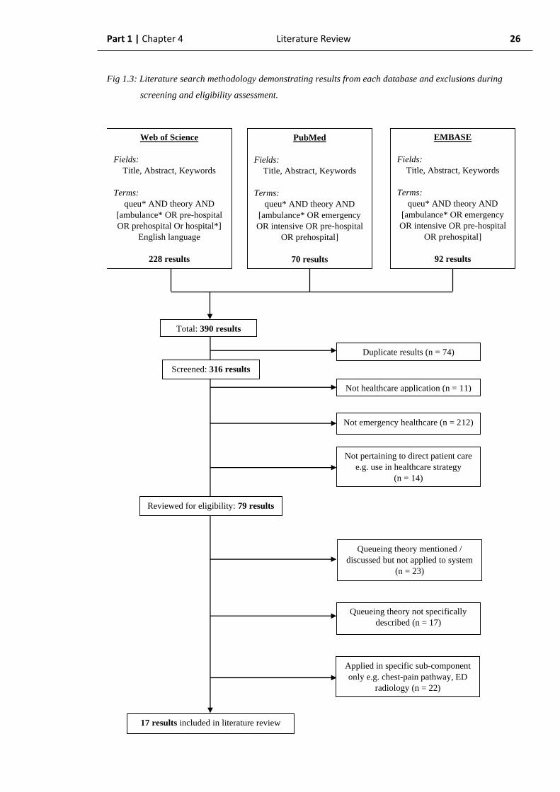
Part 1 | Chapter 4 Literature Review 26
Fig 1.3: Literature search methodology demonstrating results from each database and exclusions during
screening and eligibility assessment.
Web of Science
Fields:
Title, Abstract, Keywords
Terms:
queu* AND theory AND
[ambulance* OR pre-hospital
OR prehospital Or hospital*]
English language
228 results
PubMed
Fields:
Title, Abstract, Keywords
Terms:
queu* AND theory AND
[ambulance* OR emergency
OR intensive OR pre-hospital
OR prehospital]
70 results
EMBASE
Fields:
Title, Abstract, Keywords
Terms:
queu* AND theory AND
[ambulance* OR emergency
OR intensive OR pre-hospital
OR prehospital]
92 results
Total: 390 results
Duplicate results (n = 74)
Not healthcare application (n = 11)
Not emergency healthcare (n = 212)
Not pertaining to direct patient care
e.g. use in healthcare strategy
(n = 14)
Queueing theory mentioned /
discussed but not applied to system
(n = 23)
Queueing theory not specifically
described (n = 17)
Applied in specific sub-component
only e.g. chest-pain pathway, ED
radiology (n = 22)
17 results included in literature review
Screened: 316 results
Reviewed for eligibility: 79 results

Part 1 | Chapter 4 Literature Review 27
Table 1.1: Summary of papers included in literature review (1 of 2):
Au
tho
r
(Yea
r)
Co
un
try
S
yst
em S
tud
ied
Q
ueu
e T
yp
e
Ma
jor
Res
ult
s
Bel
l et
al.
(19
69
) U
SA
A
mb
ula
nce
Ser
vic
e
(No
n-p
hy
sici
an)
M/M
/c
- P
ois
son
arr
ival
s p
roce
ss o
f ca
lls
to a
mb
ula
nce
ser
vic
e
- D
escr
ipti
on
of
serv
ice
tim
e as
wh
ole
am
bu
lan
ce u
se t
ime
- N
on
-sta
tio
nar
y a
rriv
al r
ates
not
spec
ific
ally
acc
ou
nte
d f
or
Sco
tt e
t al
.
(19
78
) U
SA
A
mb
ula
nce
Ser
vic
e
(No
n-p
hy
sici
an)
M/M
/c
- P
ois
son
arr
ival
s p
roce
ss o
f ca
lls
to a
mb
ula
nce
ser
vic
e
- E
xp
on
enti
ally
dis
trib
ute
d r
esp
on
se t
imes
- T
ime-
var
yin
g d
eman
d f
or
serv
ice
no
ted
Sin
ger
& D
ono
so
(20
08
) C
hil
e
Am
bu
lan
ce S
erv
ice
(No
n-p
hy
sici
an)
M/G
/c
- D
emo
nst
rate
d t
ime
var
yin
g d
eman
d f
or
amb
ula
nce
s
- U
sed
Po
isso
n a
rriv
als
pro
cess
- D
escr
ibed
gam
ma
dis
trib
ute
d a
mb
ula
nce
ser
vic
e d
ura
tion
s
Ch
an e
t al
.
(20
17
) U
SA
H
osp
ital
ED
& I
CU
M
/M/c
-
No
ted
eff
ect
of
del
ay f
or
an I
CU
bed
on
ED
ser
vic
e ti
me
- S
yst
em l
oad
gro
ws
fast
er t
han
1 –
(1
/ ρ
)
Fit
zger
ald
et
al.
(20
17
) U
SA
H
osp
ital
Em
erg
ency
Dep
artm
ent
(ED
) M
/G/c
- P
rim
aril
y f
ocu
ssed
on
sim
ula
tio
n o
f an
em
erg
ency
dep
artm
ent
- D
escr
ibes
a n
on
-sta
tio
nar
y P
ois
son
arr
ival
s p
roce
ss
- U
se o
f g
amm
a-d
istr
ibu
ted
ser
vic
e ti
mes
Gre
en e
t al
.
(20
06
) U
SA
H
osp
ital
ED
M
/M/c
- U
se o
f q
ueu
ing
th
eory
mo
del
to
op
tim
ize
uti
liza
tio
n o
f re
sourc
es
- H
om
og
eneo
us
arri
val
s ra
te, n
ot
tim
e-v
ary
ing
- E
xp
on
enti
ally
dis
trib
ute
d s
ervic
e ti
mes
Go
ldw
asse
r et
al.
(20
16
) B
razi
l H
osp
ital
IC
U
M/M
/c
- In
stab
ilit
y o
f sy
stem
ass
oci
ated
wit
h t
ime-v
ary
ing
arr
ival
s
- E
xp
on
enti
al r
elat
ion
ship
bet
wee
n r
eso
urc
e u
tili
zati
on
an
d w
aiti
ng
tim
e
Hag
en e
t al
.
(20
13
) U
SA
H
osp
ital
IC
U
M/M
/c/P
2
- U
se o
f co
nst
ant
long
-ter
m a
rriv
al r
ate,
no
t ti
me-
var
yin
g
- P
rio
rity
fu
nct
ion
acc
ord
ing t
o s
ever
ity
of
pat
ien
t il
lnes
s
Jian
g e
t al
.
(20
19
) T
aiw
an
Ho
spit
al E
D
M/M
/c/K
-
Dem
on
stra
ted
Po
isso
n a
rriv
als
and
exp
on
enti
ally
dis
trib
ute
d s
erv
ice
tim
es
- U
sed
a s
yst
em w
ith
fin
ite
cap
acit
y

Part 1 | Chapter 4 Literature Review 28
Table 1.2: Summary of papers included in literature review (2 of 2):
Au
tho
r
(Yea
r)
Co
un
try
S
yst
em S
tud
ied
Q
ueu
e T
yp
e
Ma
jor
Res
ult
s
Lan
tz e
t al
.
(20
14
) S
wed
en
Ho
spit
al E
D (
tria
ge
pro
cess
) M
/M/1
M/M
/2
- T
ime
var
yin
g d
eman
d f
or
ED
- U
se o
f P
oll
acze
k-K
hin
tin
chin
fo
rmu
la t
o c
alcu
late
av
erag
e w
aiti
ng
tim
e
Lin
et
al.
(20
14
) C
anad
a H
osp
ital
ED
M
/G/c
/∞
- D
escr
ibes
a t
wo
-par
t q
ueu
e as
in
seq
uen
tial
ED
pro
cess
es
- P
rim
aril
y f
ocu
ssed
on
eff
ect
of
exit
blo
ck a
t en
d o
f p
roce
ss
Liu
et
al.
(20
18
) C
hin
a H
osp
ital
ED
M
/M/c
-
Use
of
qu
euei
ng
th
eory
to d
escr
ibe
syst
em p
erfo
rman
ce
- A
ble
to
im
pro
ve
syst
em p
erfo
rman
ce w
ith
ou
t im
pac
t o
n r
esou
rces
May
hew
et
al.
(20
08
) U
K
Ho
spit
al E
D
M/G
/c
- C
on
sid
ered
at
qu
euei
ng
th
eory
wit
h r
esp
ect
to 4
-ho
ur
ED
tre
atm
ent
tim
e ta
rget
- N
ote
d c
hal
len
ges
to
pro
vid
ing e
xp
onen
tial
ly d
istr
ibu
ted
ser
vic
e ti
mes
in
ED
Mo
ren
o-C
arri
llo
et
al.
(20
19
) C
olu
mb
ia
Ho
spit
al E
D (
tria
ge
pro
cess
) M
/M/c
-
Fo
cuss
ed a
pp
lica
tio
n o
f q
ueu
ein
g t
heo
ry t
o h
osp
ital
tri
age.
- S
ho
rt s
erv
ice
tim
e (<
5 m
ins)
McM
anu
s et
al.
(20
04
) U
SA
H
osp
ital
Pae
dia
tric
In
ten
siv
e
Car
e U
nit
(P
ICU
) M
/M/c
/K
- D
emo
nst
rate
d r
eal-
wo
rld
ap
pli
cati
on
of
Mar
ko
via
n s
erv
ice
tim
e
- E
xp
on
enti
al r
elat
ion
ship
bet
wee
n I
CU
res
ou
rce
uti
liza
tio
n a
nd
wai
tin
g t
ime
- S
pec
ific
ex
amp
le w
her
e n
um
ber
of
serv
ers
= s
pac
es i
n t
he
syst
em (
c =
k)
Wil
er e
t al
.
(20
13
) U
SA
H
osp
ital
ED
M
/GI/
c/K
+ G
I
- P
erm
itte
d r
eneg
ing
/ b
aulk
ing
pat
ien
ts f
rom
th
e sy
stem
if
exce
ssiv
e w
ait
- U
ses
thre
e st
atio
nar
y a
rriv
als
po
ints
to
ev
alu
ate
syst
em u
nd
er l
ow
-lo
ad a
nd
hig
h-l
oad
co
nd
itio
ns
McM
anu
s et
al.
(20
04
) U
SA
H
osp
ital
Pae
dia
tric
In
ten
siv
e
Car
e U
nit
(P
ICU
) M
/M/c
/K
- D
emo
nst
rate
d r
eal-
wo
rld
ap
pli
cati
on
of
Mar
ko
via
n s
erv
ice
tim
e
- E
xp
on
enti
al r
elat
ion
ship
bet
wee
n I
CU
res
ou
rce
uti
liza
tio
n a
nd
wai
tin
g t
ime
- S
pec
ific
ex
amp
le w
her
e n
um
ber
of
serv
ers
= s
pac
es i
n t
he
syst
em (
c =
k)
Zh
u e
t al
.
(20
13
) C
hin
a H
osp
ital
ED
M
/M/c
M/G
/1
- U
sed
tw
o q
ueu
es a
s p
art
of
a Ja
ckso
n n
etw
ork
.
- D
emo
nst
rate
d r
ou
tin
g p
rob
abil
ity
use
in
th
e E
D

Part 1 | Chapter 4 Literature Review 29
1.4.2. Reviewed papers
There were only three studies identified which applied queueing theory specifically to a
pre-hospital system. All of these applications were to urban ambulance services, not
physician-led PHaRM services.
The earliest of the reviewed papers was Bell and Allen (Bell and Allen, 1969). This
paper considered the use of base queueing theory in mathematically modelling the
utilisation of an ambulance service in order to maximise server availability. The authors
use an M/M/c queueing system to examine the number of ambulances which are free to
immediately respond at any given time. The authors also, importantly, describe the service
time as being the entire ambulance allocation time: from receipt of call, through delivery of
patient care and transport to the hospital until the ambulance becomes free again. The
authors state the challenges of non-stationary arrival rates but suggest the application of the
described processes to relatively steady state periods of demand.
Scott et al. (Scott et al., 1978) described the response times of ambulances in Houston,
Texas, USA. They applied several of the fundamental components of queueing theory to
describe the ambulance service using an M/M/c queue. The authors described a Poisson
arrival process with an average arrival rate λ = 5.86 calls per hour and an exponentially
distributed response time μ = 0.502 hours. However, the authors plot a histogram within
the paper which appears to demonstrate either a mixture or gamma distribution of service
times. The authors noted time-varying demand for ambulances, but no clear corrective
methodology is described. Nonetheless, the authors demonstrated the mathematical
model’s close approximation of the real-world which would suggest that either a correction
was in fact applied, or that the effect of time-varying demand on the overall analysis was
negligible.
The more recent third paper focussed on ambulance services was by Singer and Donoso
(Singer and Donoso, 2008). This paper used an M/M/c model to describe the operations of
the ambulance control centre in answering emergency calls, and an M/G/c model to
describe the ambulance vehicle service times. Of note, the authors clearly plot a gamma-
distributed ambulance service time and pragmatically note that the service time includes
the time to return to base and re-stock equipment. Only when this is complete is the end of
the service time reached and the ambulance is ready for re-allocation. The authors state the
on-scene time for ambulances to be in the region of 30 – 40 minutes. The duration
Part 1 | Chapter 4 Literature Review 30
probability histogram demonstrated the vast majority of missions to be completed in under
3 hours.
Because ScotSTAR comprises deterministic travel times to and from a patient location,
with the potential for relatively long on-scene times, it is considered likely that the
ScotSTAR system will be most broadly analogous to the system studied by Singer and
Donoso, also demonstrating gamma-distributed service times.
Then considering the other 14 studies which referred to the analogous systems of
hospital emergency departments and intensive care units. A number of these studies (Chan
et al., 2017, Green et al., 2006, Liu and Xie, 2018, Moreno-Carrillo et al., 2019,
Goldwasser et al., 2016) use an M/M/c queueing system to describe the operations of either
a hospital Emergency Department or Intensive Care Unit. Within these papers, a number of
pertinent results were identified.
Green et al. (Green et al., 2006) used a queueing theory model to optimise staffing
utilisation within the Emergency Department, with an intention to reduce waiting times.
However, the queue type is of the M/M/c variety and uses a stationary, independent period
by period (SIPP) methodology to account for the non-homogeneous Poisson arrivals
process. Liu et al. (Liu and Xie, 2018) used a similar approach to an M/M/c system in
order to describe the number of physicians required to meet a specified emergency
department waiting time. Both papers were able to demonstrate an improvement in waiting
times by optimization of the current resources, rather than the often-stated solution of
providing more servers.
Goldwasser et al. (Goldwasser et al., 2016) used a time-series model to predict a
number of admissions to intensive care units in Rio de Janeiro, similarly to that proposed
within the ScotSTAR system. They then used an M/M/c queue model to simulate the effect
of differing arrival rates on the stability of the system and to specify a number of beds
which would be required to meet a given performance standard. Again, this is similar to
that proposed within ScotSTAR. However, they do not comment on the time-dependency
of the arrival rate – and the use of an M/M/c queue now appears unlikely to correlate with
the overall ScotSTAR model given the previous papers citing gamma-distributed
ambulance service times. Interestingly, however, their output graph describes the waiting
time against the number of remaining ICU beds as a negative exponential relationship.
This initially seems at odds with the expected results (see Fig. 1.2), but as the remaining
number of beds is effectively 1 – Utilisation, then Goldwasser et al.’s plot is merely the
Part 1 | Chapter 4 Literature Review 31
expected appearance reflected about a vertical axis and the exponential increase in waiting
time with increasing utilisation is maintained. This paper illustrates well the applicability
of this relationship to the healthcare setting, particularly in the context of utilizing
relatively scarce resources.
Moreno-Carrillo et al. (Moreno-Carrillo et al., 2019) and Lantz and Rosen (Lantz and
Rosen, 2016) focussed on the ED triage process as an M/M/c queue. However, the target
waiting time in both these papers is very short (approximately 5 minutes) and refers to a
relatively short ED process, which is much more likely to demonstrate true Markovian
(exponentially-distributed) service times than the ScotSTAR systems, which will clearly
experience a significantly longer service time. Of note, Lantz et al. rationalized the number
of servers (c) to either 1 or 2, corresponding to the number of nurses operating the triage
service, according to the time of day. They were then able to use the Pollaczek-Khinchin
formula (discussed later, section 1.7.4) to derive the expected average waiting time.
Recognizing the limitations of the M/M/c queue methodology, some studies developed
the model with further parameters.
Hagen et al. (Hagen et al., 2013) also used an M/M/c queue with a constant long-term
arrival rate, but added a priority function according to patient illness severity. Given that
the ScotSTAR teams studied in this thesis generally do not prioritise patients, this approach
is not directly relatable.
McManus et al. (Mcmanus et al., 2004) applied the M/M/c/k queue system to a paediatric
intensive care unit (PICU). The authors effectively demonstrated the exponentially
distributed PICU length of stay (Markovian quality) and, similarly to the ScotSTAR
system, took the point of referral as the de facto entry point into the system. The paper also
plots the ICU utilisation rate and plots the exponential relationship between ICU utilisation
and patient rejection rate (i.e. patients being diverted to another ICU) – analogous to the
simultaneous / missed retrieval rate of the ScotSTAR teams and commensurate with the
expected relationship between utilisation and Lq in standard queueing theory. In
developing upon the initial M/M/c model, the authors defined the system as having a finite
capacity (K), equal to the number of beds in the PICU. A similar study, but applied to an
emergency department, was undertaken by Jiang et al. (Jiang et al., 2019).
An alternative development of the M/M/c queue was undertaken by Chan et al. (Chan et
al., 2017) who identified that demand which exceeded capacity introduced delay and
Part 1 | Chapter 4 Literature Review 32
inefficiency into the system. More than simply delaying the arrival of a patient in the ICU,
the authors demonstrated that increasing congestion actually increases service time. As a
result, they used a non-standard M/M(f)/c queueing model, where M(f) describes service
time as a function of underlying congestion. This likely has some similarity to ScotSTAR
as the presence of multiple simultaneous retrieval calls may require the team to briefly
diverge from the management of the current patient in order to provide telephone advice,
for example. This will clearly increase the service time of the current patient, delaying the
team’s availability to the next patient.
A number of papers had identified non-Markovian service times and therefore analysed
their respective systems with an M/G/c queue.
Fitzgerald et al. (Fitzgerald et al., 2017) used a MATLAB Monte-Carlo simulation of an
M/G/c queuing system to simulate the effects of adding a fast-track queue to the
Emergency department. This study describes a non-stationary arrival Poisson-process with
an inter-arrival time exponential distribution μ-value = 5 minutes. The method by which
the non-stationary arrival process was generated is not stated. The authors state the service
time to be gamma distributed, with shape dependent on the acuity level of the patient, to
some degree analogous to the ScotSTAR EMRS model of primary vs secondary mission
types. However, the process which patients go through from arrival at triage and
subsequent distribution within the department clearly differs. The use of MATLAB in this
study was of interest due to the stated intention of using the same program in the research
for this thesis.
Wiler et al (Wiler et al., 2013) used an M/GI/c/K + GI queueing model to represent their
Emergency Department. The authors in this paper address the problem of not having an
underlying stationary Poisson process (on which the M/GI/r/s + GI model relies) by
evaluating their process at three relatively stationary time periods which correspond with
periods of relatively low and relatively high demand, in principle allowing extrapolation of
the situations between. This is achievable in the Emergency Department context because
the higher number of patient presentations allow an accurate analysis of the frequency
distributions in any given time period. The authors used two two-hour time slots in which
to analyse their model – representing 8304 and 4239 patients over the course of the whole
study. As a conservative estimate, the quieter of the two periods still corresponds to a
median arrival rate of 11 patients per hour. ScotSTAR teams on the other hand, may go for
several days without a referral in a given 2-hour period and so such an analysis method

Part 1 | Chapter 4 Literature Review 33
would not be appropriate for the ScotSTAR system. The authors also added a component
to describe patients who left without being treated due to the busyness of the department.
This draws parallels with one aspect of the ScotSTAR system because it includes the
possibility of patients reneging from the system if the waiting time is too long. For
ScotSTAR, this occurs almost exclusively in the context of primary, pre-hospital missions.
If the pre-hospital waiting time is prolonged, then a patient will be reneged from the
system, being transferred to hospital by a road ambulance with paramedic crew, rather than
waiting for the EMRS Trauma Team to arrive. This process ensures that time to life-saving
intervention is not delayed, instead being performed in a hospital rather than at the
roadside. However, a large proportion of these patients will have been identified by
ambulance control as likely to have a long wait and will never be referred to the ScotSTAR
EMRS team. As such, the number of patients in this situation is unknown.
Lin et al (Lin et al., 2014) described a two-part queue: but with the initial queue
demonstrating an M/G/c1/∞ pattern. Fundamentally, the paper focusses on the effect of
blocking departures from the system (“exit block”) which although is a major challenge for
the emergency department, does not constitute a significant problem for the ScotSTAR
services because a suitable bed will generally be pre-identified. However, finding an
available bed may be a lengthy process – which may prolong the mission duration, but
generally does not result in exit block from the ScotSTAR system.
In their study examining the use of queueing theory with regard to the UK’s 4-hour ED
waiting time target, Mayhew and Smith (Mayhew and Smith, 2008), used an M/G/c
queueing system. In particular, they demonstrated that service time in the emergency
department was gamma-distributed, resulting from the sum of multiple sub-processes, each
with exponentially-distributed service times. The primary objective of this paper was to
assess the required ED performance against the 4-hour target. The paper demonstrated the
difficulties in doing this for 98% of patients, as was then the target. This approach could
have some utility with ScotSTAR in respect of a performance standard. However, the
ScotSTAR target would likely pertain more to the arrival of the team at the patient than the
overall mission duration.
Finally, Zhu et al. (Zhu et al., 2013) studied multiple queues within an emergency
department: with M/M/c for general service and M/G/1 re-queueing for people who
required further medical review prior to ED discharge. The probability of patients
following each of these paths (routing probability) was combined with the queueing
Part 1 | Chapter 4 Literature Review 34
discipline in order to generate a Jackson network representing service within the
Emergency Department. The Jackson network is a good reflection of ED operations but
does not apply to the ScotSTAR system through which the movement of patients is strictly
serialized.
1.4.3. Queueing theory applied to the ScotSTAR system
Based on the studied literature it could be expected that the ScotSTAR systems would
most likely demonstrate queueing systems approximating the M/G/c type. An a priori
prediction would expect arrivals to the system to occur randomly, with a long-term average
value, but displaying a non-stationary, time-dependent Poisson component. Mission
durations are unlikely to be Markovian due to the addition of the deterministic component
of transport times to and from the patient, with the care of the patient itself likely involving
multiple exponentially-distributed processes. It may be the case that the time on-scene can
be approximated by the exponential distribution, in which case the overall distribution may
be able to be approximated by a Markovian descriptor if this is the major contributor,
rather than transport time. It is clear however that, by nature, queueing theory is context
dependent and that an accurate understanding and representation of the system is required
before any relevant facets of queueing theory can be accurately applied.
Firstly, the ScotSTAR systems must be analysed to establish, with respect to Kendall’s
notation, the applicable queueing systems. This has the potential to significantly contribute
to a gap in existing knowledge by accurately describing a time-varying arrival process with
respect to inter-arrival time distributions and by correctly attributing the appropriate
distribution to the service times of a pre-hospital and retrieval medical system.
Thereafter, the applicable Kendall’s notation definition of each queueing system could be
used to establish if a primary formulaic solution exists and if it is able to describe the
performance of the system sufficiently to achieve the overall research objectives.

Part 1 Chapter 5
Aims
Part 1 | Chapter 5 Aims 36
1.5. Aims
Part One of this thesis aims to:
1. Investigate if the major individual queueing theory parameters (with respect to
Kendall’s notation) of the ScotSTAR SPRS and EMRS services are commensurate
with standard queuing theory – specifically:
- Inter-arrival time distribution
- Service time distribution
- Number of servers
- Places within the system
- Population
- Queueing discipline
2. Describe the complete queueing systems of the ScotSTAR SPRS and EMRS
services using Kendall’s notation.
3. Derive system performance descriptors using queueing theory formulae and
establish their validity and applicability for the real-world system.

Part 1 Chapter 6
Methods

Part 1 | Chapter 6 Methods 38
1.6. Methods
1.6.1. General
1. The operations of the ScotSTAR SPRS and EMRS retrieval teams
were reviewed with regard to the relevant parameters of queueing
theory, as outlined below (sections 1.6.2 – 1.6.8).
2. All data were collected from the ScotSTAR retrieval teams’
electronic databases (Microsoft Access and Microsoft Excel:
Microsoft Corporation, Redmond, Washington, USA) for the 4 year
period of calendar years 2013 to 2016.
3. Data were exported from the databases in Microsoft Excel format.
4. The number of each mission type undertaken by each team, per
calendar year, were counted.
4. Analysis of inter-arrival times, service times and the associated
probability distributions were undertaken using the Mathworks
MATLAB software suite (version R2016a: Mathworks Corporation,
Natick, Massachusetts, USA).
1.6.2. Inter-arrival Time Distribution (A)
1 The arrival times (team activation times) of patients referred to the
SPRS and EMRS systems were sorted and the time difference
between consecutive activations of each team were calculated to
generate the inter-arrival times.
2. An expected inter-arrival time exponential probability distribution
was calculated from the number of missions undertaken.
3. The raw inter-arrival times were plotted as a histogram with one-
hour bins.

Part 1 | Chapter 6 Methods 39
4. An inter-arrival time exponential probability distribution was fitted
to the raw inter-arrival time data using the MATLAB Statistics
Toolbox distribution fitting function. The goodness-of-fit to the raw
data was assessed using the Kolmogorov-Smirnov test.
5. It was noted that the non-uniform probability of activation by time
of day created a non-exponentially distributed inter-arrival time and
a corrective time-transform (section 1.6.3) was applied.
6. The difference between successive transformed activation times
were calculated as the corrected inter-arrival times.
7. The corrected inter-arrival times were plotted as a histogram with
one-hour bins.
8. An inter-arrival time exponential probability distribution was fitted
to the corrected inter-arrival time data. The goodness-of-fit was
assessed using the Kolmogorov-Smirnov test.
9. The parameter values of the calculated, raw and corrected inter-
arrival time distributions were compared.
1.6.3. Correction of time-dependent Poisson
distributions
During the inter-arrival time analysis it was identified that referrals to the system vary by
time of day and are not uniform across a 24-hour period despite the precipitating event
(critical illness or injury) being considered random in onset (conferring Markovian
arrivals). This therefore represented a stochastic, rather than truly random system which
would present a time-varying Poisson arrivals process. It was suspected that this could
affect the inter-arrival time distribution, as from one day to the next the most likely
activation time would be 24 hours apart. Given the relatively small number of activations
per day for the ScotSTAR systems, then after enough days of operation, a number of
modes could be expected to develop at intervals of approximately 24 hours inter-arrival
time. It was therefore proposed that a time transform could be undertaken to correct for the
time-dependent Poisson component and establish the underlying inter-arrival distribution.
Part 1 | Chapter 6 Methods 40
Based on first principles, if the time-transform is to successfully establish the underlying
distribution, then it should correct the probability of activation so as to be uniform across
the 24-hour period as time, and the number of missions, tend to infinity.
A correction method was therefore devised. Outwardly, the correction is a time-based
transform similar to a Box-Cox transform. The correction was predicated on the principle
that, with a uniform probability of activation per hour, the cumulative proportion of
missions by time should equal the elapsed proportion of the day - i.e. 25% of missions
would be expected to occur by 25% of the day (0600h).
Using this principle, the mission times could be corrected. For example, if the 25th
percentile of the number of missions was found to occur at 1100h (the 45th percentile of
time of day) then it could be considered that these missions were 5 hours “late” compared
to their expected time given a uniform probability of activation (which should also be the
25th percentile of time). Subtracting 5 hours from the activation times of missions starting
at 1100h would therefore correct the activation time to that expected of a uniform
distribution – the 25th percentile of time, or 0600h.
This method was expanded to apply over the whole of the 24-hour day by using an
inverse empirical cumulative distribution function, allowing the correction value to change
through the day in accordance with the varying probability of activation by time. The
correction could therefore be applied dynamically to missions occurring at any time of day.
By applying the correction in this fashion, it was possible to correct for the time-dependent
component of mission activations while preserving the otherwise random nature of
referrals to the ScotSTAR teams.
The EMRS Primary Missions data is shown below as an example (N.B. this section deals
only with the application of the time transform, the effect on inter-arrival times is
illustrated in the section of each respective team – sections 1.7 and 1.8):

Part 1 | Chapter 6 Methods 41
1. The probability of activation by time of day was calculated from the mission activation
times and plotted as a histogram with one-hour bins (Fig. 1.4).
Fig 1.4: Raw probability of activation by time-of-day histogram (normalized to area under plot = 1)
demonstrating maximal probability of activation in 1500h – 1600h time-period, with low probability
of activation between 1800h – 0800h.

Part 1 | Chapter 6 Methods 42
2. A non-parametric kernel distribution (Epanechnikov-type) was fitted to the activation
probability, by hour of day (Fig. 1.5).
Fig 1.5: Raw probability of activation by time-of-day histogram with fitted kernel distribution curve
(Epanechnikov-type).

Part 1 | Chapter 6 Methods 43
3. The kernel distribution empirical cumulative distribution function was calculated and
plotted with the uniform probability cumulative distribution function (Fig. 1.6).
Fig 1.6: ECDF curve of fitted kernel distribution (red line) and expected CDF line of uniform distribution
(blue line) by time of day.
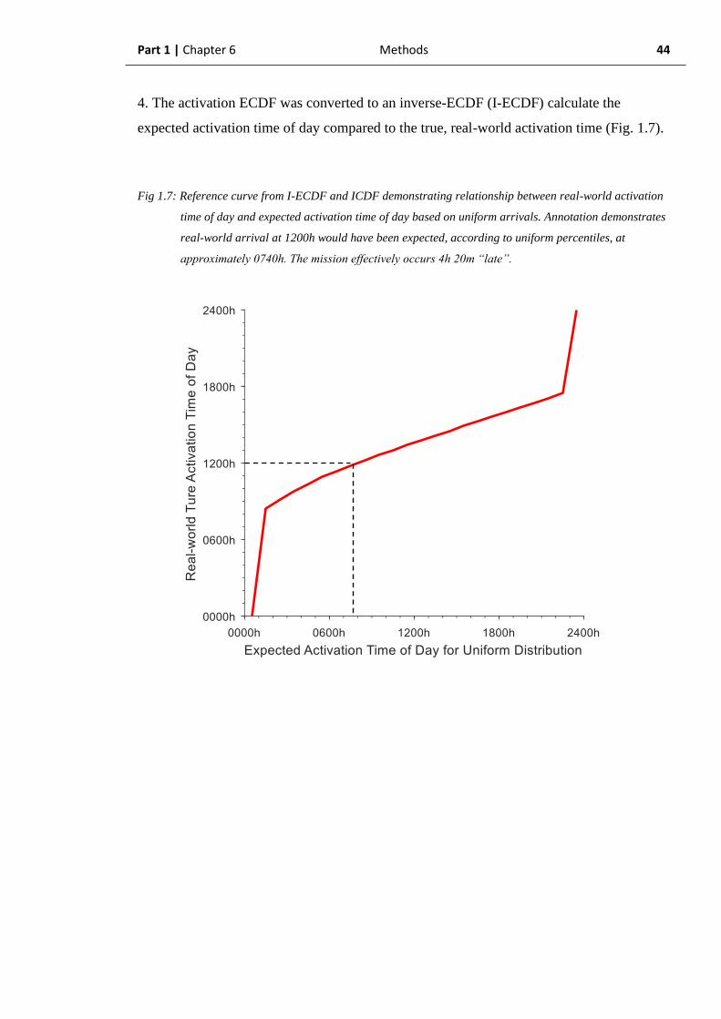
Part 1 | Chapter 6 Methods 44
4. The activation ECDF was converted to an inverse-ECDF (I-ECDF) calculate the
expected activation time of day compared to the true, real-world activation time (Fig. 1.7).
Fig 1.7: Reference curve from I-ECDF and ICDF demonstrating relationship between real-world activation
time of day and expected activation time of day based on uniform arrivals. Annotation demonstrates
real-world arrival at 1200h would have been expected, according to uniform percentiles, at
approximately 0740h. The mission effectively occurs 4h 20m “late”.
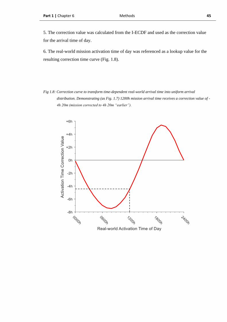
Part 1 | Chapter 6 Methods 45
5. The correction value was calculated from the I-ECDF and used as the correction value
for the arrival time of day.
6. The real-world mission activation time of day was referenced as a lookup value for the
resulting correction time curve (Fig. 1.8).
Fig 1.8: Correction curve to transform time-dependent real-world arrival time into uniform arrival
distribution. Demonstrating (as Fig. 1.7) 1200h mission arrival time receives a correction value of -
4h 20m (mission corrected to 4h 20m “earlier”).

Part 1 | Chapter 6 Methods 46
7. The correction value is applied to the original mission activation datetime (N.B:
date and time, not just hour of activation – it is therefore possible to correct arrival times
across midnight).
8. The correction process is applied across all the activation datetimes for all of the
same team and mission types.
9. After the time-transform is applied, the corrected activation times of day are
extracted and plotted as a histogram with one-hour bins (Fig. 1.9). This should be
contrasted with the un-corrected inter-arrival time distribution (Fig. 1.4).
Fig 1.9: Histogram showing normalized (area under plot = 1) probability of activation by time of day after
correction for time-dependency.

Part 1 | Chapter 6 Methods 47
A uniform probability of activation should result in the number of activations in hourly
time bins being Poisson distributed around a mean (λ) which is 1/24th of the total number
of missions in the studied period, as the time-period tends to infinity. Given 1945 primary
retrieval missions undertaken by EMRS, this would be expected to produce 81 missions
per 1-hour bin (1945 ÷ 24) in the case of a pure uniform distribution (Fig 1.10). As this is a
Poisson arrivals process, the actual probability distribution of mission occurring in each 1-
hour time period conforming a uniform probability of activation is therefore expected to be
a Poisson distribution with λ = 81. The final probability distribution (Fig. 1.11) appears to
be well approximated to the expected Poisson distribution (outliers ~ n = 50 are noted).
The corrected data distribution and the expected Poisson distribution were not significantly
different on Kolmogorov-Smirnov testing (p = 0.62).
Fig. 1.10: Frequency distribution histogram demonstrating number of activations in each one-hour time
period after application of the time-transform. Expected Poisson λ-value = 81 missions per one-
hour time period for uniform probability of activation by time of day is illustrated (red line).
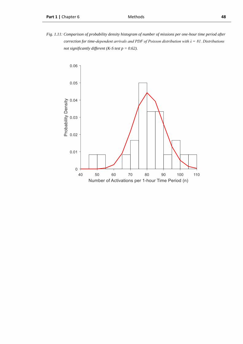
Part 1 | Chapter 6 Methods 48
Fig. 1.11: Comparison of probability density histogram of number of missions per one-hour time period after
correction for time-dependent arrivals and PDF of Poisson distribution with λ = 81. Distributions
not significantly different (K-S test p = 0.62).
Part 1 | Chapter 6 Methods 49
1.6.4. Service Time (S)
1. The time between activation of a team for one mission and the point
at which the team became available for their next mission was
defined as the service time. Practically, this was calculated as the
time difference between mission activation and the team’s return to
base time, as recorded in the relevant electronic retrieval database.
2. The endpoint for mission duration was the return to base time. As
this requires a separate process to enter into the retrieval medical
notes, it is liable to be missed by the teams. When not specifically
documented, this time was bootstrapped using the time distribution
from the previous recorded checkpoint: the time at which the patient
was handed over to the receiving hospital. The hospital handover
checkpoint has multiple opportunities and mechanisms for the time
to be recorded and was therefore much more reliably recorded than
the return to base time. This also applied to stood-down primary
missions, where the team were activated but did not, for any one of a
number of reasons, actually attend a patient.
3. The mission durations were calculated and plotted as a probability
density histogram.
4. A suitable probability distribution was fitted to the histogram and
the goodness-of-fit assessed using the Kolmogorov-Smirnov test.

Part 1 | Chapter 6 Methods 50
1.6.5. Number of Servers (c)
1. The number of servers were defined as the number of clinical teams
available to treat patients at any given time. The ScotSTAR teams
are staffed and available 24/7, without variation in the number of
available servers over time. The number of servers is therefore
constant for the respective teams:
SPRS 1 server (team).
EMRS 2 servers (teams).
1.6.6. Number of places in system (K)
1. The number of places within the system (receiving service and queueing)
was calculated based upon the general description of the relevant
ScotSTAR system. There is no physical limit on the number of patients
who can be within the system for either of the studied teams and this
value was therefore set at infinity for all systems. The practical
implications for this will be discussed later.
1.6.7. Population (N)
1. The size of population from which the patient is drawn. This was
defined as the entire population meeting the respective service’s age
inclusion criteria within the geographical area of operation.
2. The applicable population for SPRS was defined using public
information from the National Records of Scotland (National
Records of Scotland Mid-2015 Population Estimate for Scotland).
3. The applicable population for EMRS was defined using the NASA
SEDAC population estimator (NASA Earthdata Socioeconomic
Data and Applications Centre, Columbia University, Palisades NY,
via URL: https://sedac.ciesin.columbia.edu) according to the
approximate geographical boundaries of EMRS operations.

Part 1 | Chapter 6 Methods 51
1.6.8. Queueing Discipline (D)
1. From the general description and system process map for each
service, the queuing discipline was calculated and defined. Both
SPRS and EMRS only undertake emergency missions which are
universally operated on a first-in-first-out (FIFO) queueing
methodology and this could therefore be set as a constant queue
discipline.

Part 1 Chapter 7
Results
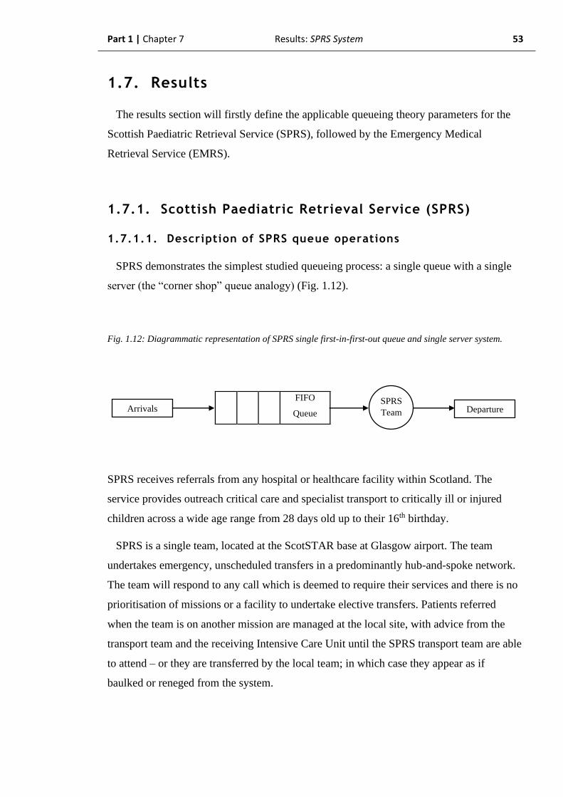
Part 1 | Chapter 7 Results: SPRS System 53
1.7. Results
The results section will firstly define the applicable queueing theory parameters for the
Scottish Paediatric Retrieval Service (SPRS), followed by the Emergency Medical
Retrieval Service (EMRS).
1.7.1. Scottish Paediatric Retrieval Service (SPRS)
1.7.1.1. Description of SPRS queue operations
SPRS demonstrates the simplest studied queueing process: a single queue with a single
server (the “corner shop” queue analogy) (Fig. 1.12).
Fig. 1.12: Diagrammatic representation of SPRS single first-in-first-out queue and single server system.
SPRS receives referrals from any hospital or healthcare facility within Scotland. The
service provides outreach critical care and specialist transport to critically ill or injured
children across a wide age range from 28 days old up to their 16th birthday.
SPRS is a single team, located at the ScotSTAR base at Glasgow airport. The team
undertakes emergency, unscheduled transfers in a predominantly hub-and-spoke network.
The team will respond to any call which is deemed to require their services and there is no
prioritisation of missions or a facility to undertake elective transfers. Patients referred
when the team is on another mission are managed at the local site, with advice from the
transport team and the receiving Intensive Care Unit until the SPRS transport team are able
to attend – or they are transferred by the local team; in which case they appear as if
baulked or reneged from the system.
FIFO
Queue Arrivals Departure
SPRS
Team
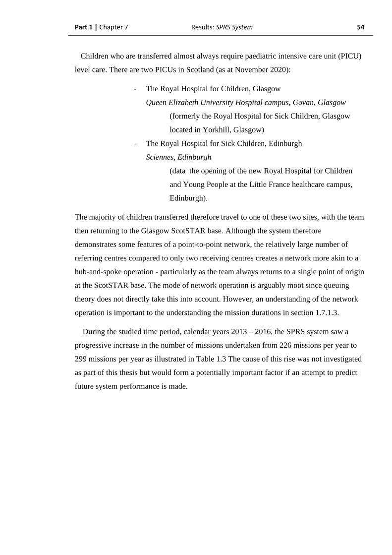
Part 1 | Chapter 7 Results: SPRS System 54
Children who are transferred almost always require paediatric intensive care unit (PICU)
level care. There are two PICUs in Scotland (as at November 2020):
- The Royal Hospital for Children, Glasgow
Queen Elizabeth University Hospital campus, Govan, Glasgow
(formerly the Royal Hospital for Sick Children, Glasgow
located in Yorkhill, Glasgow)
- The Royal Hospital for Sick Children, Edinburgh
Sciennes, Edinburgh
(data the opening of the new Royal Hospital for Children
and Young People at the Little France healthcare campus,
Edinburgh).
The majority of children transferred therefore travel to one of these two sites, with the team
then returning to the Glasgow ScotSTAR base. Although the system therefore
demonstrates some features of a point-to-point network, the relatively large number of
referring centres compared to only two receiving centres creates a network more akin to a
hub-and-spoke operation - particularly as the team always returns to a single point of origin
at the ScotSTAR base. The mode of network operation is arguably moot since queuing
theory does not directly take this into account. However, an understanding of the network
operation is important to the understanding the mission durations in section 1.7.1.3.
During the studied time period, calendar years 2013 – 2016, the SPRS system saw a
progressive increase in the number of missions undertaken from 226 missions per year to
299 missions per year as illustrated in Table 1.3 The cause of this rise was not investigated
as part of this thesis but would form a potentially important factor if an attempt to predict
future system performance is made.
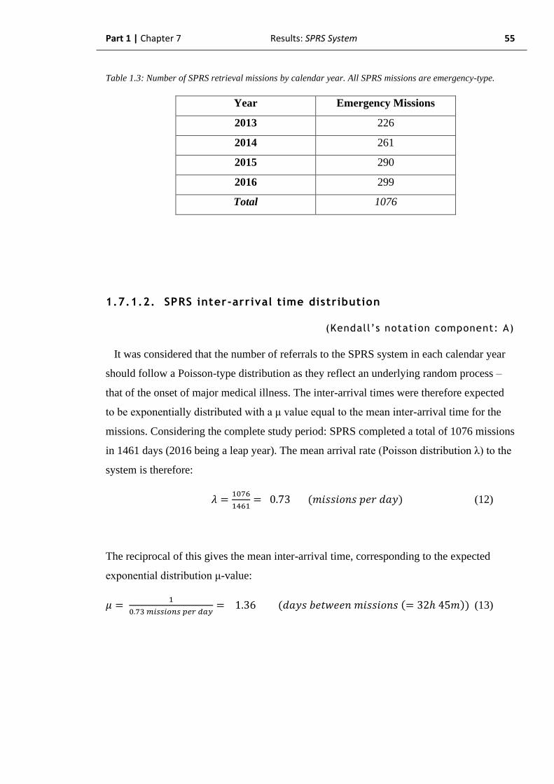
Part 1 | Chapter 7 Results: SPRS System 55
Table 1.3: Number of SPRS retrieval missions by calendar year. All SPRS missions are emergency-type.
Year Emergency Missions
2013 226
2014 261
2015 290
2016 299
Total 1076
1.7.1.2. SPRS inter-arrival time distribution
(Kendall’s notation component: A)
It was considered that the number of referrals to the SPRS system in each calendar year
should follow a Poisson-type distribution as they reflect an underlying random process –
that of the onset of major medical illness. The inter-arrival times were therefore expected
to be exponentially distributed with a μ value equal to the mean inter-arrival time for the
missions. Considering the complete study period: SPRS completed a total of 1076 missions
in 1461 days (2016 being a leap year). The mean arrival rate (Poisson distribution λ) to the
system is therefore:
𝜆 =1076
1461= 0.73 (𝑚𝑖𝑠𝑠𝑖𝑜𝑛𝑠 𝑝𝑒𝑟 𝑑𝑎𝑦) (12)
The reciprocal of this gives the mean inter-arrival time, corresponding to the expected
exponential distribution μ-value:
𝜇 = 1
0.73 𝑚𝑖𝑠𝑠𝑖𝑜𝑛𝑠 𝑝𝑒𝑟 𝑑𝑎𝑦= 1.36 (𝑑𝑎𝑦𝑠 𝑏𝑒𝑡𝑤𝑒𝑒𝑛 𝑚𝑖𝑠𝑠𝑖𝑜𝑛𝑠 (= 32ℎ 45𝑚)) (13)

Part 1 | Chapter 7 Results: SPRS System 56
The probability density of the raw inter-arrival times by hour were plotted as a histogram.
With the expectation of a Markovian arrivals process, an exponential distribution was
fitted to the data (Fig. 1.13). The fitted distribution demonstrated μ = 1.29 (95%
Confidence Interval: 1.22 – 1.37). The fitted distribution appeared a good fit for the real-
world data and was not significantly different on Kolmogorov-Smirnov testing (p = 0.10,
test statistic = 0.04).
The expected exponential distribution μ-value of 1.36 was contained within the
confidence intervals of the fitted distribution and the two distributions are therefore not
considered significantly different.
Fig. 1.13: Histogram demonstrating probability density of raw inter-arrival times for SPRS missions during
calendar years 2013-2016, with fitted exponential distribution (μ = 1.29). Fitted distribution not
significantly different to raw data (K-S test p = 0.10).

Part 1 | Chapter 7 Results: SPRS System 57
However, it is generally known that referrals to the ScotSTAR teams vary through the day
and it was considered that this may affect the inter-arrival distribution. Subsequent analysis
of the probability of activation by time of day revealed that, as expected, the distribution is
not uniform but is time-variable. Thus, the process is not pure Poisson but time-dependent
Poisson and a pure exponential distribution does not apply to the system when considered
across the full 24-hours of day.
This is reflective of more people generally seeking medical attention during the day,
which translates to a higher number of retrieval requests. The number of retrievals
increases sharply after 0800h to a peak probability of activation between 0900h-1000h.
After this the probability of activation gradually decreases until approximately 2100h,
following which the probability of activation falls more rapidly to the overnight values
(Fig. 1.14).
Fig. 1.14: Histogram of relative probability of activation (area under plot = 1) by time of day (1 hour bins)
for SPRS missions in calendar years 2013 – 2016. Plot demonstrates mode probability of
activation in 0900h – 1000h time period and diurnal variation in probability of activation by time
of day.
Part 1 | Chapter 7 Results: SPRS System 58
Based on this finding, the correction described in methodology section 1.6.3 was applied
to the mission activations to create a more uniform probability of activation over the course
of the day (Fig. 1.15). After applying this time-dependency correction, the inter-arrival
time histogram (Fig. 1.16) demonstrated a closer approximation of the fitted exponential
distribution than the uncorrected data (see Fig. 1.13). This was most noticeable in the 12-
24h inter-arrival time period. Although, the effect of the time-dependent Poisson process
on the inter-arrival time distribution was not as marked in the SPRS system as it was for
EMRS - which will be discussed later. The exponential distribution fitted to the corrected
data demonstrated μ = 1.29 (95% CI: 1.22 – 1.37). The μ values and confidence intervals
for the corrected vs uncorrected data were identical and they would therefore not be
considered significantly different. Comparing the fitted distribution to the data
demonstrated no significant difference to Kolmogorov-Smirnov testing, and the corrected
data more closely resembled the fitted exponential distribution due to the lower K-S test
statistic value when compared to the raw data (p = 0.30, test statistic = 0.03).
Fig. 1.15: Histogram of relative probability of activation (area under plot = 1) by time of day (1 hour bins)
for SPRS missions, after correction for time-dependency of arrivals process in calendar years
2013 – 2016. Plot demonstrates mode probability of activation in 0000h – 0100h time period and
relatively uniform probability of activation through 24-hour period.

Part 1 | Chapter 7 Results: SPRS System 59
Fig. 1.16: Histogram demonstrating probability density of inter-arrival times after correction for time-
dependent arrivals. SPRS missions during calendar years 2013-2016, with fitted exponential
distribution (μ = 1.29). The data are not significantly different to the fitted distribution and are
more closely approximated than the raw dataset (K-S test p = 0.30, test statistic = 0.03).

Part 1 | Chapter 7 Results: SPRS System 60
The μ-value of the raw and corrected inter-arrival times were equal and the distributions
can therefore be considered to not be significantly different (Fig. 1.17). This is an
important finding as it demonstrates that the correction methodology does not mutilate the
data.
Fig. 1.17: Comparison of fitted exponential distributions for SPRS missions inter-arrival times, showing
calculated inter-arrival time exponential PDF, μ = 1.26 (green line); raw inter-arrival time
exponential PDF (red line) and time-dependency corrected exponential PDF (blue line) curves.
The raw and time-dependency corrected PDF lines are superimposed as the parameter values are
identical (μ = 1.29).
With the inter-arrival time clearly demonstrating an equal exponential distribution in both
time-dependency corrected and uncorrected data, the SPRS arrivals are Markovian (“M” in
Kendall’s notation) in both raw and corrected forms.
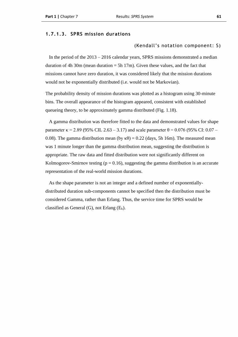
Part 1 | Chapter 7 Results: SPRS System 61
1.7.1.3. SPRS mission durations
(Kendall’s notation component: S)
In the period of the 2013 – 2016 calendar years, SPRS missions demonstrated a median
duration of 4h 30m (mean duration = 5h 17m). Given these values, and the fact that
missions cannot have zero duration, it was considered likely that the mission durations
would not be exponentially distributed (i.e. would not be Markovian).
The probability density of mission durations was plotted as a histogram using 30-minute
bins. The overall appearance of the histogram appeared, consistent with established
queueing theory, to be approximately gamma distributed (Fig. 1.18).
A gamma distribution was therefore fitted to the data and demonstrated values for shape
parameter κ = 2.89 (95% CIL 2.63 – 3.17) and scale parameter θ = 0.076 (95% CI: 0.07 –
0.08). The gamma distribution mean (by κθ) = 0.22 (days, 5h 16m). The measured mean
was 1 minute longer than the gamma distribution mean, suggesting the distribution is
appropriate. The raw data and fitted distribution were not significantly different on
Kolmogorov-Smirnov testing (p = 0.16), suggesting the gamma distribution is an accurate
representation of the real-world mission durations.
As the shape parameter is not an integer and a defined number of exponentially-
distributed duration sub-components cannot be specified then the distribution must be
considered Gamma, rather than Erlang. Thus, the service time for SPRS would be
classified as General (G), not Erlang (Ek).

Part 1 | Chapter 7 Results: SPRS System 62
Fig. 1.18: Histogram of probability density of mission duration (30-minute bins) for SPRS missions in
calendar years 2013 – 2016, with fitted gamma distribution (κ = 2.89, Θ = 0.076) . Plot
demonstrates mode duration in 3h 00m – 3h 30m range (median duration = 4h 30m, mean
duration = 5h 17m). Data and fitted distribution are not significantly different (K-S test p = 0.16).

Part 1 | Chapter 7 Results: SPRS System 63
1.7.1.4. SPRS number of servers
(Kendall’s notation component: c)
SPRS operates one team, available 24/7. The number of servers (c) can therefore be set at
a constant value of one.
1.7.1.5. SPRS system capacity
(Kendall’s notation component: K)
In the context of queueing theory, there is no physical limit to the number of patients who
can be queued and so it is considered that K = ∞.
In reality, however, there is a practical limit to the number of patients who can be in the
queue, but the value of this limit is currently unknown and the infinity value is considered
acceptable for this thesis. This will be further explored in the discussion section.
1.7.1.6. SPRS population
(Kendall’s notation component: N)
SPRS operates across the whole of Scotland, so the applicable population is considered
to be all children in Scotland between the ages of 28 days (younger being served by SNTS)
and 16 years (older being served by EMRS).
Assuming that children under 28 days old represent 28/365 of the population under 1
year old, the population served by the SPRS is approximately 915,000. As this is
approximately 5 orders of magnitude larger than the number of servers, it is considered for
the purposes of defining the relevant queueing theory that for SPRS, N ≈ ∞.

Part 1 | Chapter 7 Results: SPRS System 64
1.7.1.7. SPRS queueing discipline
(Kendall’s notation component: D)
In day-to-day SPRS system operations, there may be two referrals which arrive
sufficiently close together for an ad-hoc triage to be undertaken by the retrieval clinician
for the purposes of determining mission priority – but this is relatively rare. Generally, the
inter-arrival times are such that it is not appropriate to “wait and see” if a more urgent
referral arrives and the team will usually respond immediately to an activation request. The
system therefore operates with a first-in-first-out (FIFO) queueing method; all patients are
effectively the same priority and there is no pre-emption.
1.7.1.8. Formulation of SPRS system in Kendall’s notation
As described in section 1.3.1, Kendall’s notation follows the form A/S/c/K/N/D
representing arrival time (A), service time (S), number of servers (c), number of places in
the system (K), size of population (N) and queueing discipline (D) respectively.
Based on the above analysis, SPRS demonstrates:
- Markovian (M) arrivals
- Gamma distributed (a variant of general (G)) service time
- One server
- Infinite places in the system
- Infinite population
- First-in-first-out (FIFO) queueing
Using Kendall’s notation, this is written in full as:
M/G/1/∞/∞/FIFO
By convention, infinite places within the system, infinite sampling population and FIFO
queue discipline are omitted from the notation. The ScotSTAR SPRS system therefore
demonstrates an overall queueing system of the type:
M/G/1
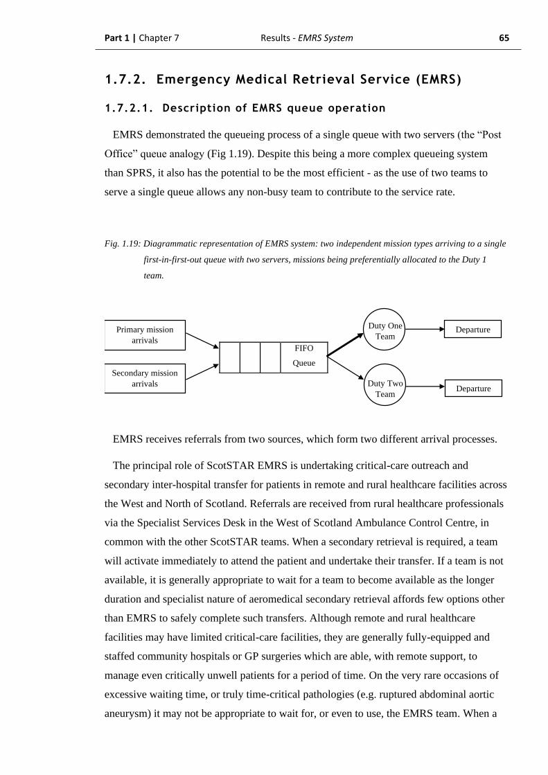
Part 1 | Chapter 7 Results - EMRS System 65
1.7.2. Emergency Medical Retrieval Service (EMRS)
1.7.2.1. Description of EMRS queue operation
EMRS demonstrated the queueing process of a single queue with two servers (the “Post
Office” queue analogy (Fig 1.19). Despite this being a more complex queueing system
than SPRS, it also has the potential to be the most efficient - as the use of two teams to
serve a single queue allows any non-busy team to contribute to the service rate.
Fig. 1.19: Diagrammatic representation of EMRS system: two independent mission types arriving to a single
first-in-first-out queue with two servers, missions being preferentially allocated to the Duty 1
team.
EMRS receives referrals from two sources, which form two different arrival processes.
The principal role of ScotSTAR EMRS is undertaking critical-care outreach and
secondary inter-hospital transfer for patients in remote and rural healthcare facilities across
the West and North of Scotland. Referrals are received from rural healthcare professionals
via the Specialist Services Desk in the West of Scotland Ambulance Control Centre, in
common with the other ScotSTAR teams. When a secondary retrieval is required, a team
will activate immediately to attend the patient and undertake their transfer. If a team is not
available, it is generally appropriate to wait for a team to become available as the longer
duration and specialist nature of aeromedical secondary retrieval affords few options other
than EMRS to safely complete such transfers. Although remote and rural healthcare
facilities may have limited critical-care facilities, they are generally fully-equipped and
staffed community hospitals or GP surgeries which are able, with remote support, to
manage even critically unwell patients for a period of time. On the very rare occasions of
excessive waiting time, or truly time-critical pathologies (e.g. ruptured abdominal aortic
aneurysm) it may not be appropriate to wait for, or even to use, the EMRS team. When a
FIFO
Queue
FIFO
Queue
SPRS
Team Arrivals Departure SPRS
Team
Primary mission
arrivals
SPRS
Team
Secondary mission
arrivals
Departure Duty One
Team
Duty Two
Team Departure
Part 1 | Chapter 7 Results - EMRS System 66
team is activated they will, generally, not deviate from that mission until it is complete.
Due to the specialist equipment, procedures and drugs involved – and the need to minimise
the quantities carried to reduce weight for air transfers, the team is not usually able to
proceed to another mission without first returning to base to re-stock any consumables
used during the mission. Missions are therefore fully complete, with a full start-to-finish
duration recorded before the next mission would be considered to have started.
Primary, pre-hospital missions (predominantly major trauma patients) are referred via a
dedicated Trauma Desk in the West of Scotland Ambulance Control Centre. At the Trauma
Desk, a specialist clinician screens all the 999 calls arriving to ambulance control centres
across Scotland to identify those for which the activation of a pre-hospital critical care
team such as the EMRS Trauma Team may be of benefit. Those occurring within the
EMRS area of operations for primary missions (see Fig. 1.33) will result in the tasking of
the EMRS team. On receipt of such a tasking a team will, if available, respond in a time-
critical fashion either by road vehicle using blue lights and sirens, or by helicopter. The
Duty 1 team will always be tasked first when available, otherwise the mission will be
tasked to the Duty 2 team. The entire premise of an EMRS team attending patients in the
pre-hospital environment is that of reducing time to life-saving interventions which cannot
be provided by an ambulance service paramedic and would ordinarily need to be
performed in a hospital. Resuscitative surgical procedures, establishing a definitive airway
and emergency blood transfusion, amongst others, can be taken into the field by the EMRS
trauma team – thereby allowing the intervention to occur earlier in the patient journey. If
there is no team available to respond then such patients are generally reneged from the
system. A prolonged wait for a team could result in a patient remaining in the healthcare-
austere pre-hospital environment when a “scoop-and-run” to hospital would have resulted
in them receiving their life-saving intervention at the same point in time – but simply at a
hospital, rather than by EMRS in the field. Clearly, therefore, it is not appropriate for
patients to wait a significant time for EMRS to attend primary missions. It is important to
note that the EMRS Trauma Team response is only funded, and therefore only available,
between 0800h – 1800h (although 365 days per year).
During the studied time period: calendar years 2013 – 2016, the EMRS system saw an
overall increase in the number of primary missions undertaken from 391 to 565 missions
per year, and a fall in the number of secondary missions from 299 to 268 per year (Table
1.4). It was recognized that as the primary missions service became established (EMRS
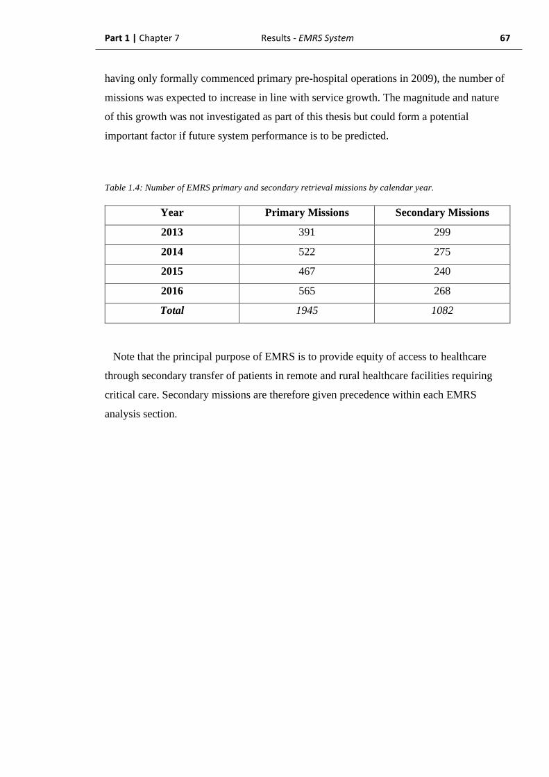
Part 1 | Chapter 7 Results - EMRS System 67
having only formally commenced primary pre-hospital operations in 2009), the number of
missions was expected to increase in line with service growth. The magnitude and nature
of this growth was not investigated as part of this thesis but could form a potential
important factor if future system performance is to be predicted.
Table 1.4: Number of EMRS primary and secondary retrieval missions by calendar year.
Year Primary Missions Secondary Missions
2013 391 299
2014 522 275
2015 467 240
2016 565 268
Total 1945 1082
Note that the principal purpose of EMRS is to provide equity of access to healthcare
through secondary transfer of patients in remote and rural healthcare facilities requiring
critical care. Secondary missions are therefore given precedence within each EMRS
analysis section.
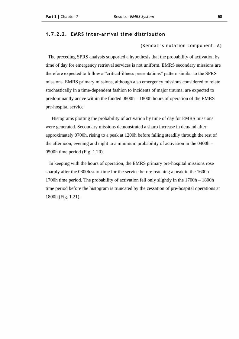
Part 1 | Chapter 7 Results - EMRS System 68
1.7.2.2. EMRS inter-arrival time distribution
(Kendall’s notation component: A)
The preceding SPRS analysis supported a hypothesis that the probability of activation by
time of day for emergency retrieval services is not uniform. EMRS secondary missions are
therefore expected to follow a “critical-illness presentations” pattern similar to the SPRS
missions. EMRS primary missions, although also emergency missions considered to relate
stochastically in a time-dependent fashion to incidents of major trauma, are expected to
predominantly arrive within the funded 0800h – 1800h hours of operation of the EMRS
pre-hospital service.
Histograms plotting the probability of activation by time of day for EMRS missions
were generated. Secondary missions demonstrated a sharp increase in demand after
approximately 0700h, rising to a peak at 1200h before falling steadily through the rest of
the afternoon, evening and night to a minimum probability of activation in the 0400h –
0500h time period (Fig. 1.20).
In keeping with the hours of operation, the EMRS primary pre-hospital missions rose
sharply after the 0800h start-time for the service before reaching a peak in the 1600h –
1700h time period. The probability of activation fell only slightly in the 1700h – 1800h
time period before the histogram is truncated by the cessation of pre-hospital operations at
1800h (Fig. 1.21).
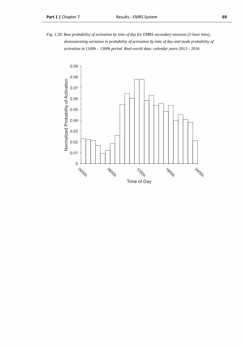
Part 1 | Chapter 7 Results - EMRS System 69
Fig. 1.20: Raw probability of activation by time of day for EMRS secondary missions (1-hour bins),
demonstrating variation in probability of activation by time of day and mode probability of
activation in 1100h – 1300h period. Real-world data: calendar years 2013 – 2016.

Part 1 | Chapter 7 Results - EMRS System 70
Fig. 1.21: Raw probability of activation by time of day for EMRS primary missions (1-hour bins),
demonstrating variation in probability of activation by time of day and mode probability of
activation in 1500h – 1600h period. Real-world data: calendar years 2013 – 2016.
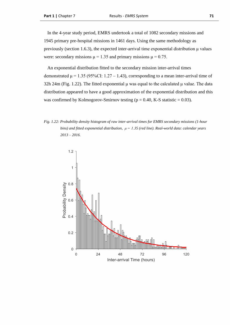
Part 1 | Chapter 7 Results - EMRS System 71
In the 4-year study period, EMRS undertook a total of 1082 secondary missions and
1945 primary pre-hospital missions in 1461 days. Using the same methodology as
previously (section 1.6.3), the expected inter-arrival time exponential distribution μ values
were: secondary missions μ = 1.35 and primary missions μ = 0.75.
An exponential distribution fitted to the secondary mission inter-arrival times
demonstrated μ = 1.35 (95%CI: 1.27 – 1.43), corresponding to a mean inter-arrival time of
32h 24m (Fig. 1.22). The fitted exponential μ was equal to the calculated μ value. The data
distribution appeared to have a good approximation of the exponential distribution and this
was confirmed by Kolmogorov-Smirnov testing (p = 0.40, K-S statistic = 0.03).
Fig. 1.22: Probability density histogram of raw inter-arrival times for EMRS secondary missions (1-hour
bins) and fitted exponential distribution, μ = 1.35 (red line). Real-world data: calendar years
2013 – 2016.
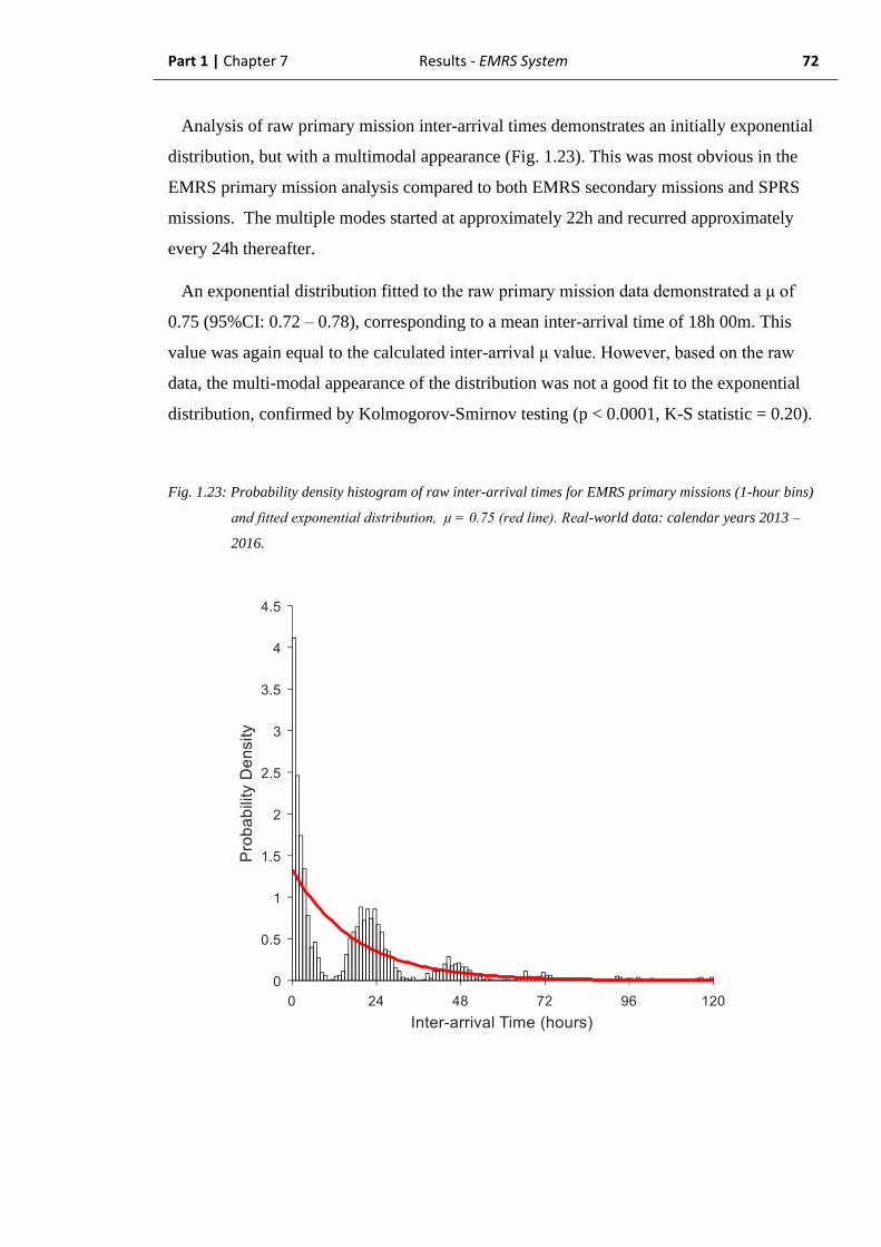
Part 1 | Chapter 7 Results - EMRS System 72
Analysis of raw primary mission inter-arrival times demonstrates an initially exponential
distribution, but with a multimodal appearance (Fig. 1.23). This was most obvious in the
EMRS primary mission analysis compared to both EMRS secondary missions and SPRS
missions. The multiple modes started at approximately 22h and recurred approximately
every 24h thereafter.
An exponential distribution fitted to the raw primary mission data demonstrated a μ of
0.75 (95%CI: 0.72 – 0.78), corresponding to a mean inter-arrival time of 18h 00m. This
value was again equal to the calculated inter-arrival μ value. However, based on the raw
data, the multi-modal appearance of the distribution was not a good fit to the exponential
distribution, confirmed by Kolmogorov-Smirnov testing (p < 0.0001, K-S statistic = 0.20).
Fig. 1.23: Probability density histogram of raw inter-arrival times for EMRS primary missions (1-hour bins)
and fitted exponential distribution, μ = 0.75 (red line). Real-world data: calendar years 2013 –
2016.

Part 1 | Chapter 7 Results - EMRS System 73
Applying the time transform described in 1.6.2 to correct for the time-dependent
probability of activation resulted in a more uniform appearance of the secondary mission
activation time of day (Fig. 1.24) and the inter-arrival time distribution with an apparent
reduction in the multi-modality of the histogram (Fig 1.25). The fitted exponential
distributions after correction for time-dependent probability of activation demonstrated a
secondary mission μ = 1.30 (95% CI: 1.22 – 1.37) which was not significantly different to
the uncorrected distribution as each μ value was reciprocally contained within the other’s
95% confidence interval. The corrected data were not significantly different to the fitted
distribution on Kolmogorov-Smirnov testing and appeared to more closely approximate the
distribution, with a lower test statistic value (p = 0.71, K-S test statistic = 0.02).
Fig. 1.24: Normalized histogram (area under plot = 1) of time-dependency corrected probability of
activation by time of day (hourly bins) for EMRS secondary missions. Mode probability of
activation 0800h – 0900h. Real-world data: calendar years 2013 – 2016.

Part 1 | Chapter 7 Results - EMRS System 74
Fig. 1.25: Probability density histogram of inter-arrival times for EMRS secondary missions (1-hour bins)
after correction for time-dependency. Fitted exponential distribution μ = 1.30 (red line). Real-
world data: calendar years 2013 – 2016.

Part 1 | Chapter 7 Results - EMRS System 75
The most noticeable improvement, however, was in the primary missions inter-arrival
data where the substantially more uniform probability of activation by time of day (Fig.
1.26) resulted in the multi-modality of the inter-arrival times being corrected to a close
approximation of the exponential distribution (Fig 1.27). The corrected exponential
distribution demonstrated μ = 0.74 (95% CI: 0.71 – 0.78). The corrected and uncorrected μ
values were contained reciprocally within the opposing confidence interval and the two
values are therefore not statistically significantly different. In contrast to the raw data, the
corrected inter-arrival times were not statistically significant to the fitted distribution on
Kolmogorov-Smirnov testing (p = 0.34, K-S test statistic = 0.02).
Fig. 1.26: Normalized histogram (area under plot = 1) of time-dependency corrected probability of
activation by time of day (hourly bins) for EMRS primary missions. Mode probability of activation
1300h – 1400h. Real-world data: calendar years 2013 – 2016.
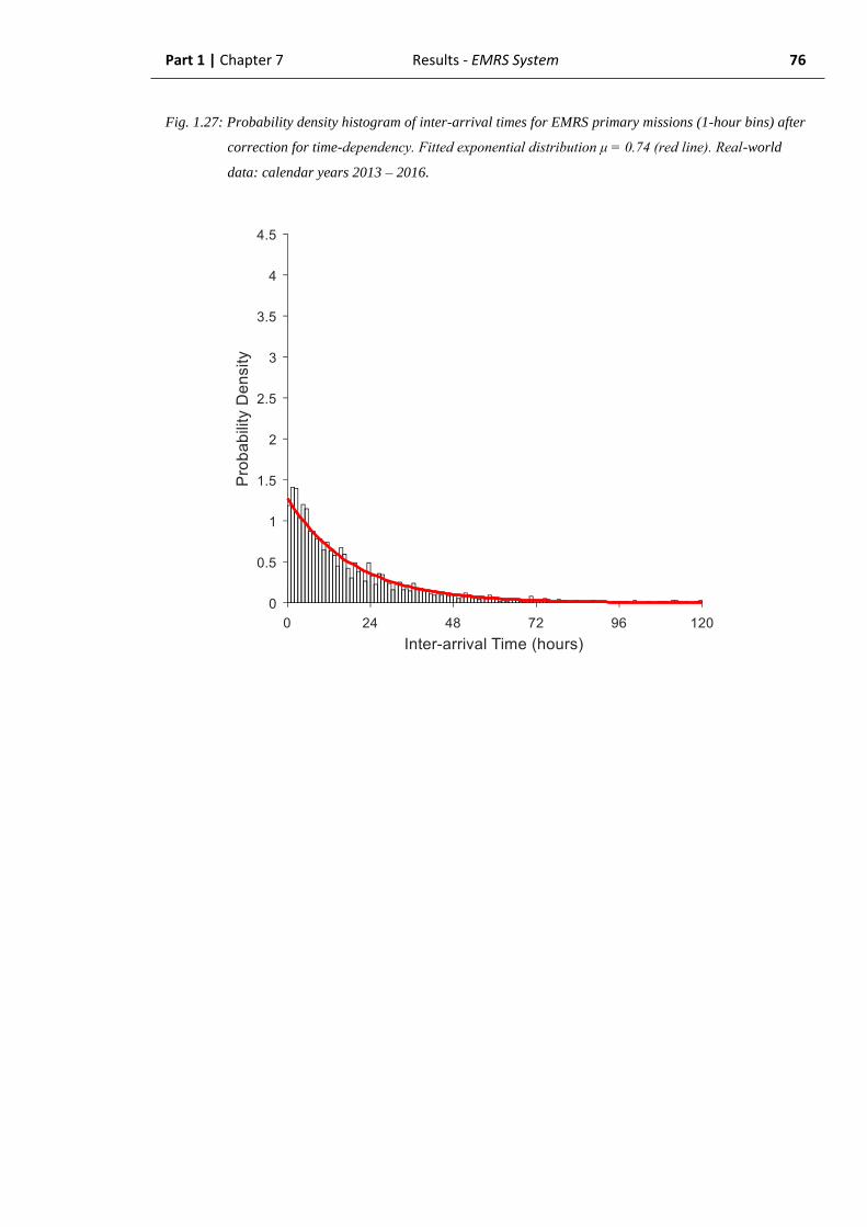
Part 1 | Chapter 7 Results - EMRS System 76
Fig. 1.27: Probability density histogram of inter-arrival times for EMRS primary missions (1-hour bins) after
correction for time-dependency. Fitted exponential distribution μ = 0.74 (red line). Real-world
data: calendar years 2013 – 2016.
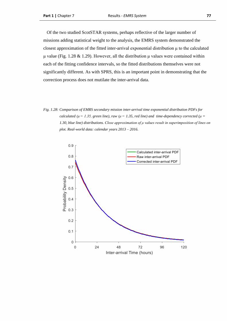
Part 1 | Chapter 7 Results - EMRS System 77
Of the two studied ScotSTAR systems, perhaps reflective of the larger number of
missions adding statistical weight to the analysis, the EMRS system demonstrated the
closest approximation of the fitted inter-arrival exponential distribution μ to the calculated
μ value (Fig. 1.28 & 1.29). However, all the distribution μ values were contained within
each of the fitting confidence intervals, so the fitted distributions themselves were not
significantly different. As with SPRS, this is an important point in demonstrating that the
correction process does not mutilate the inter-arrival data.
Fig. 1.28: Comparison of EMRS secondary mission inter-arrival time exponential distribution PDFs for
calculated (μ = 1.35, green line), raw (μ = 1.35, red line) and time-dependency corrected (μ =
1.30, blue line) distributions. Close approximation of μ values result in superimposition of lines on
plot. Real-world data: calendar years 2013 – 2016.
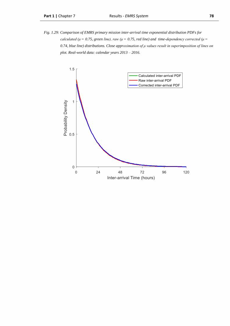
Part 1 | Chapter 7 Results - EMRS System 78
Fig. 1.29: Comparison of EMRS primary mission inter-arrival time exponential distribution PDFs for
calculated (μ = 0.75, green line), raw (μ = 0.75, red line) and time-dependency corrected (μ =
0.74, blue line) distributions. Close approximation of μ values result in superimposition of lines on
plot. Real-world data: calendar years 2013 – 2016.

Part 1 | Chapter 7 Results - EMRS System 79
The time-transform used (as described in section 1.6.3) corrects the time distribution
across a 24-hour period. However, the pre-hospital (primary retrievals) component of
EMRS does not operate outside the hours of 0800h – 1800h. As a result, it is theoretically
impossible for a mission to be undertaken in the 1800h – 0800h period. Missions which
occur at 1700h on Monday and 0900h on Tuesday are therefore, to the system, two hours
apart; not 16 hours apart.
The calculated inter-arrival exponential μ value is representative of the mean inter-arrival
time in days: i.e. μ = 0.75 = 0.75 days = 18h mean inter-arrival time.
However, in the EMRS context, 0.75 days would be more accurately considered 0.75
operational days – an operational day being 10 hours long. Therefore, considering the
inter-arrival time in the context of operational days:
(μ = 0.75) 𝑥 (10ℎ 𝑜𝑝𝑒𝑟𝑎𝑡𝑖𝑜𝑛𝑎𝑙 𝑑𝑎𝑦)
= 7.5ℎ (7h 30min) interarrival time during operating hours
7.5 ÷ 24 = μ = 0.31 if extrapolated to a 24-hour process. (14)
or
0.75−1 = 1.333 missions average per operating day. (15)
so
1.333 𝑥 (24
10) = 3.2 missions per 24h day by extrapolation (16)
therefore
1 𝑑𝑎𝑦
3.2 𝑚𝑖𝑠𝑠𝑖𝑜𝑛𝑠 = 𝜇 = 0.31 (7h 30 mins mean inter-arrival time) for 24h operations. (17)

Part 1 | Chapter 7 Results - EMRS System 80
This application of operational hours is important in later analyses when the potential for
simultaneous retrievals is considered. Based on a 10h operational day the difference
between an average inter-arrival time of 7h 30m and 18h 00m is substantial. There is
clearly an obvious operational difference with regard to service demand and the potential
for team non-availability between these two results.
Given that EMRS treats both mission types with equal priority in a first-in-first-out
queue, then the complete inter-arrival time distribution is an exponential distribution based
on combination of both the primary (λp) and secondary (λs) mission arrival rates. The
resulting exponential distribution will demonstrate μ = 1
𝜆𝑝+ 𝜆𝑠 .
Secondary missions, with inter-arrival time exponential distribution μ = 1.33 accounted
for 35.7% of the missions. Primary missions accounted for 64.3% of missions, with an
absolute μ = 0.75 or μ = 0.31 if extrapolated for operations over a 24-hour period.
Each of the mission types demonstrates exponentially-distributed inter-arrival times after
correction for time-dependency. This indicates that these are time-dependent Poisson
processes. Secondary missions demonstrated an inter-arrival distribution which was not
significantly different to exponential on raw values and so these missions clearly represent
Markovian arrivals. Primary missions were not exponentially distributed on raw data
analysis and so would be considered a general (G) inter-arrival time, but which can be
corrected to an exponential (M) inter-arrival time. The ability to correct to an exponential
distribution which does not demonstrate a significantly different μ value to the raw data
distribution suggests that application of standard queueing theory to the corrected
distribution could still yield appropriate average values. The EMRS missions can therefore
be considered to also demonstrate corrected Markovian (M) arrivals.
Part 1 | Chapter 7 Results - EMRS System 81
1.7.2.3. EMRS mission durations
(Kendall’s notation component: S)
Secondary Missions
During the studied period, EMRS secondary retrievals demonstrated a median mission
duration of 6h 15m (mean duration = 6h 34m). As with SPRS, a zero-time mission
duration is impossible and the durations were therefore expected not to demonstrate an
exponential (Markov service times) distribution.
The mission durations were plotted as a probability density histogram with 15-minute
bins (Fig. 1.30). Again, in keeping with established queueing theory, the missions appeared
to demonstrate an overall distribution consistent with a gamma distribution.
A gamma distribution was therefore fitted to the data, this demonstrated parameter values
κ = 6.50 (95% CI: 5.98 – 7.07) and θ = 0.04 (94% CI: 0.04 – 0.05). The fitted gamma
distribution mean (by κθ) = 0.27 (6h 32m). The gamma distribution mean was 2 minutes
shorter than measured data mean, suggesting that the distribution is appropriate.
It could be argued that there are two gamma distributions within the secondary mission
data with modes around 5h 30m and 8h durations. This may could correspond to North vs
West sector missions – or rotary-wing vs fixed wing transport. The raw data distribution
was not significantly different to the fitted gamma distribution on Kolmogorov-Smirnov
testing (p = 0.37). With the raw data demonstrating a good approximation of the fitted
gamma distribution, it was considered that specifically establishing the factors which may
generate two underlying gamma distributions was outside the scope of this thesis.
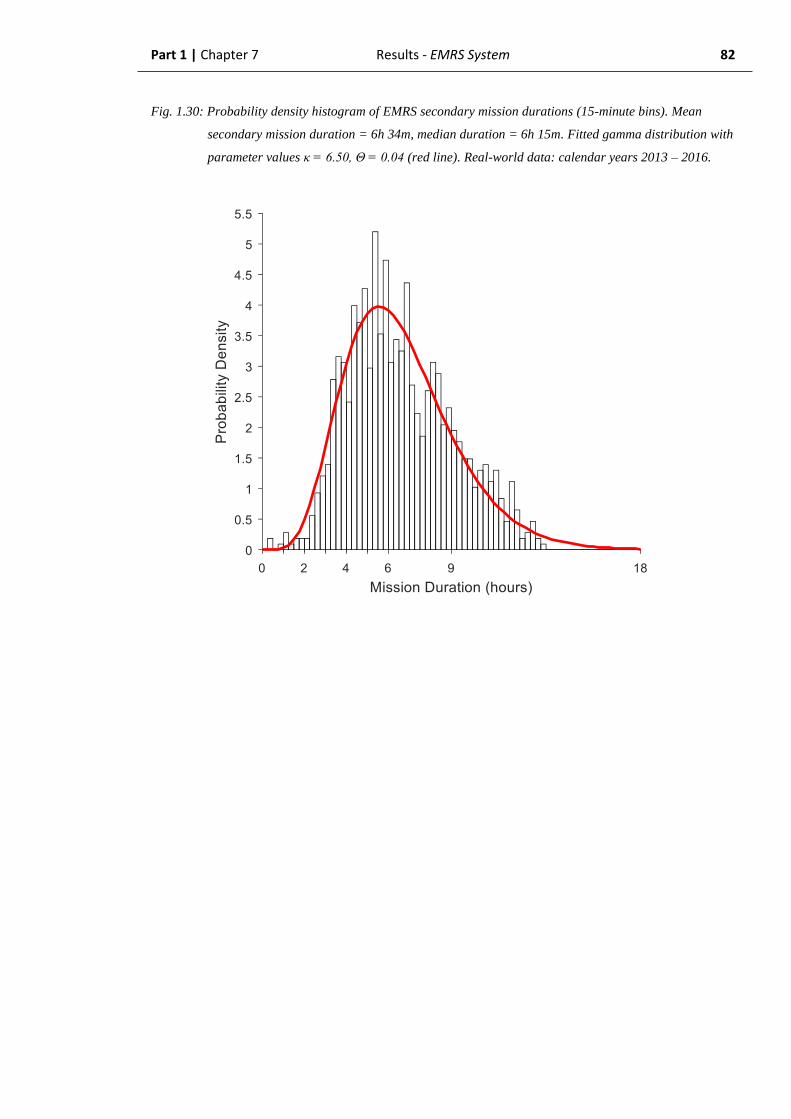
Part 1 | Chapter 7 Results - EMRS System 82
Fig. 1.30: Probability density histogram of EMRS secondary mission durations (15-minute bins). Mean
secondary mission duration = 6h 34m, median duration = 6h 15m. Fitted gamma distribution with
parameter values κ = 6.50, Θ = 0.04 (red line). Real-world data: calendar years 2013 – 2016.

Part 1 | Chapter 7 Results - EMRS System 83
Primary Missions
EMRS primary missions demonstrated a median duration of 1h 19m (mean duration = 1h
32m) and appeared overall to be a good approximation of the fitted gamma distribution
(Fig. 1.31) with parameter values κ = 1.96 (95% CI: 1.85 – 2.08) and θ = 0.03 (95% CI:
0.03 – 0.03). The fitted gamma distribution mean (by κθ) = 0.06 (1h 27m). The gamma
distribution mean was 5 minutes shorter than measured data mean, suggesting that the
distribution is appropriate. Kolmogorov-Smirnov testing, however, demonstrated the
difference between the fitted distribution and the raw data to be at the limit of non-
significance (p = 0.05).
Based upon this, the EMRS servers were deemed to exhibit service times which were the
sum of two gamma distributions, with proportional representation of each based on the
different number of secondary to primary retrievals. This would be classed as a type of
general (“G” in Kendall’s notation) service time.
Fig. 1.31: Probability density histogram of EMRS primary mission durations (15-minute bins). Mean
primary mission duration = 1h 32m, median duration = 1h 19m. Fitted gamma distribution with
parameter values κ = 1.96, θ = 0.03 (red line). Real-world data: calendar years 2013 – 2016.
Part 1 | Chapter 7 Results - EMRS System 84
1.7.2.4. EMRS number of servers
(Kendall’s notation component: c)
ScotSTAR EMRS operates 2 teams, available 24 hours, 365 days a year – and this value
can therefore be set at a constant of 2.
Operationally, missions are allocated to Duty 1 first, being allocated to Duty 2 only if the
Duty 1 team is unavailable. This has no direct implication for the queueing theory
described here, however.
1.7.2.5. EMRS system capacity
(Kendall’s notation component: K)
There is no physical limit to the number of patients who can wait to be retrieved and so it
is considered that K = ∞. As with the other teams, there is likely to be a practical limit to
the number of patients who will wait for retrieval as opposed to being transferred by
another means. This is perhaps most relevant to the EMRS primary missions, but the value
is currently undefined. This will be explored further in the discussion section.
1.7.2.6. EMRS population
(Kendall’s notation component: N)
EMRS operates secondary missions across the rural west and far-north of Scotland (Fig.
1.32), serving an approximate population of 289,000 people aged 16 and over. For primary
missions, EMRS serves the western central belt, the rural south-west and areas of the
Borders and Highlands of Scotland, predominantly (Fig. 1.33). This area has an
approximate population of 2.9 million. As the only ScotSTAR service which undertakes
pre-hospital primary missions, EMRS covers all ages in the pre-hospital domain. The
populations applicable to both mission types are significantly larger than the 2 EMRS
teams (servers) by a minimum of 5 orders of magnitude. It is therefore considered that N ≈
∞.

Part 1 | Chapter 7 Results - EMRS System 85
Fig. 1.32: Approximate geographical boundary of EMRS area of operation for secondary missions (shaded
red). Map copyright OpenStreetMap contributors. Reproduced in accordance with the terms.

Part 1 | Chapter 7 Results - EMRS System 86
Fig. 1.33: Approximate geographical boundary of EMRS area of operation for primary missions (shaded
red). Map copyright OpenStreetMap contributors. Reproduced in accordance with the terms.

Part 1 | Chapter 7 Results - EMRS System 87
1.7.2.7. EMRS queueing discipline
(Kendall’s notation component: D)
The system works with a first-in-first-out (FIFO) process. The availability of two teams
serving the single queue also simplifies this process as even two missions arriving
simultaneously will generally not require triage if both teams are available as they will
both activate immediately. Although the more time-critical nature of primary missions has
been discussed, they are also most able to be transferred by another means and be in an
urban location where definitive care is not too far away – in contrast to remote secondary
retrievals with no other means of transfer. The availability of two teams also creates a
situation where there is deemed sufficient capacity within the system such that a “wait-
and-see” approach pending a higher-acuity transfer is not appropriate. These idiosyncrasies
of real-world EMRS operations are generally considered to simplify to an FIFO process,
without priority or pre-emption.
1.7.2.8. Formulation of EMRS system in Kendall’s notation
After analysing all the components above, the EMRS system can be defined in terms of:
- Markovian (M) arrivals as the sum of:
- Markovian secondary mission arrivals
- Markovian primary mission arrivals (after correction from
General)
- Sum of two gamma-distributed (therefore general (G)) service time
- Two servers
- Infinite places in the system
- Infinite population
- FIFO queueing
Using Kendall’s notation (see section 1.3.1), then with infinite places in the system,
infinite population and FIFO queueing omitted by convention – the raw EMRS system
would be described by:
G/G/2
Which, when corrected for the non-homogeneous Poisson arrivals process becomes:
M/G/2
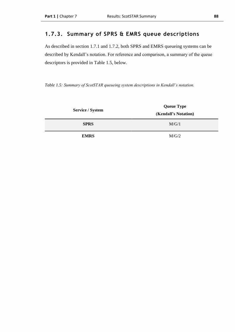
Part 1 | Chapter 7 Results: ScotSTAR Summary 88
1.7.3. Summary of SPRS & EMRS queue descriptions
As described in section 1.7.1 and 1.7.2, both SPRS and EMRS queueing systems can be
described by Kendall’s notation. For reference and comparison, a summary of the queue
descriptors is provided in Table 1.5, below.
Table 1.5: Summary of ScotSTAR queueing system descriptions in Kendall’s notation.
Service / System Queue Type
(Kendall’s Notation)
SPRS M/G/1
EMRS M/G/2

Part 1 | Chapter 7 Results: Formulaic Calculations 89
1.7.4. Formulaic calculation of operational values
Having ascertained the applicability of queueing theory to the ScotSTAR systems and
described their queueing processes using Kendall’s notation (as section 1.7.3), the
matching queueing theory formulae can be selected and their respective values can be
calculated to establish if this is able to adequately describe the studied systems.
1.7.4.1. Selection of applicable queueing theory
Of the studied systems, only SPRS, of the M/G/1 queue type has formulaic answers for
the major queueing theory parameters of average length of queue (Lq) and waiting time in
the queue (Wq) by way of the Pollaczek-Khinchin formulae.
EMRS can be represented as an M/G/c system or be generalised to the G/G/c system and
the Wq calculated using Whitt’s method (Whitt, 2000). Unfortunately, calculation of the
result is mathematically complex and requires numerous assumptions with regard to the
underlying inter-arrival time distributions which cannot be validated for the EMRS system.
It is considered that even if a value can be calculated for the EMRS system, it is unlikely to
be an accurate measure of the real-world.
1.7.4.2. SPRS formulaic results
The SPRS system can be described in terms of Lq and Wq by means of the Pollaczek-
Khinchin formulae. Using server utilisation (ρ), mean arrival rate in missions per day (λ)
and variance of the service time (σ2s (as κθ2) from the parameter values of the gamma
distribution of SPRS service times), the first formula describes the average length of queue
(Lq) as:
𝐿𝑞 = 𝜌2+ 𝜆2𝜎𝑠
2
2(1−𝜌) (18)
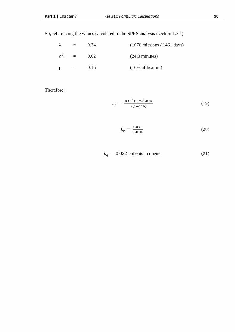
Part 1 | Chapter 7 Results: Formulaic Calculations 90
So, referencing the values calculated in the SPRS analysis (section 1.7.1):
λ = 0.74 (1076 missions / 1461 days)
σ2s = 0.02 (24.0 minutes)
ρ = 0.16 (16% utilisation)
Therefore:
𝐿𝑞 = 0.162+ 0.742∗0.02
2(1−0.16) (19)
𝐿𝑞 = 0.037
2∗0.84 (20)
𝐿𝑞 = 0.022 patients in queue (21)

Part 1 | Chapter 7 Results: Formulaic Calculations 91
Then, by adaptation of the above formula using one of Little’s formulae:
𝐿𝑞 = 𝜆 𝑊𝑞 (22)
or, when rearranged:
𝑊𝑞 = 𝐿𝑞
𝜆 (23)
The second Pollaczek-Khinchin formula - for the calculation of Wq - is obtained as:
𝑊𝑞 = (
𝜌2+ 𝜆2𝜎𝑠2
2(1−𝜌))
𝜆 (24)
so,
𝑊𝑞 = (
𝜌2
𝜆+ 𝜆𝜎𝑠
2)
2(1 −𝜌) (25)
Then, using the same values for mission arrivals rate (λ), utilisation (ρ), and service time
variance (σ2s) then average waiting time in the queue (Wq) can be calculated as:
𝑊𝑞 = (
0.162
0.74+ 0.74∗0.02)
2(1 −0.16) (26)
𝑊𝑞 = 0.049
1.68 (27)
𝑊𝑞 = 0.029 (days) = 42 minutes (28)
Formulaically therefore, the SPRS system was calculated to demonstrate a mean length of
queue (Lq) of 0.022 patients in the queue and a mean waiting time in the queue (Wq) of 42
minutes.

Part 1 | Chapter 7 Results: Formulaic Calculations 92
1.7.4.3. EMRS formulaic results
As stated in section 1.7.4.1, there are few queueing theory results which pertain to the
G/G/2 or M/G/2 queue. Those which do are either mathematically complex (Hokstad,
1979), are only applicable to a specific service time circumstance (Knessl et al., 1990), or
are simply outside the mathematical scope of application by clinicians (Boxma et al.,
2002). There are therefore no applicable formulaic results for EMRS within the scope of
this thesis.

Part 1 Chapter 8
Discussion

Part 1 | Chapter 8 Discussion 94
1.8. Discussion
Overall, the analyses above have demonstrated that the ScotSTAR systems are (perhaps
unexpectedly) well represented by some basic descriptors from standard queueing theory.
This is a positive finding as it suggests that queueing theory in general, and results derived
from it, should prove useful in describing, analysing and generating specifications for the
studied systems. However, clearly there are significant challenges in applying formulaic
queueing theory to the SPRS and EMRS systems, with several components of the real-
world system, such as non-stationary arrivals, having the potential to render the results of
such analysis invalid.
1.8.1. Arrivals processes and effect on classical
queueing theory
The studied systems have the common feature of attending patients who, on a continuum
of clinical severity, have the most critical pathologies or highest need for specialist medical
care. Such patients attended by the ScotSTAR teams do not choose the nature of their
illnesses and injuries, nor the time of day at which they occur and so referrals to the system
are considered broadly random in nature. Initially, it would seem reasonable to assume that
these events would be sufficiently unpredictable as to occur with uniform probability
across any time of the day or night in the long-term – thereby demonstrating a pure Poisson
process with the expectation of exponentially-distributed inter-arrival times (Markovian
arrivals).
However, there are some factors - such as circadian rhythm affecting medical illnesses or
relatively little major trauma occurring when most people are asleep at night – which make
these events more likely to occur at certain times of day. For example, the higher number
of pedestrians and buses during rush hour makes it more likely that a pedestrian will
sustain a major injury inflicted by a bus during this time than in the middle of the night.
However, the number of such instances would not bear a fixed, predictable, relationship to
either the number of pedestrians or buses – instead, the relationship would be stochastic. It
could, however, be expected for a long-term average number of pedestrian versus bus
accidents to remain relatively constant given a sufficiently long sampling time (e.g. per
year).

Part 1 | Chapter 8 Discussion 95
Much of queueing theory relies on the two fundamentals of a steady-state system and a
stationary arrivals process. Steady state is defined by queueing theory as a traffic intensity
(ρ) of less than one. This can easily be seen to hold true mathematically for the ScotSTAR
systems as the mean mission duration multiplied by the number of missions generates a
total workload which is substantially less than the number of server hours available.
Using SPRS as an example:
1076 missions x 5h 17m mean duration ≈ 5685 hours of work in 4 years
24h x 1461days x 1 server = 35064 available server-hours in 4 years
5685 ÷ 35064 = 16.2% traffic intensity (ρ) = utilization
This can also be seen to hold true from the first-principles perspective in that all patients
who are referred are indeed retrieved, with some spare time within the system. This
demonstrates that the queue must be, at least transiently, zero and so ρ must be less than
one. If the system instead demonstrated ρ greater than 1, the queue length would grow
indefinitely. Also, because ρ is less than 1, it can be stated that ρ = utilization (as section
1.3.2).
Stationary arrivals refer to a system in which the number of arrivals in successive equal
time periods follow a Poisson distribution with a constant long-term average value (λ).
While this may be true in the context of the number of ScotSTAR missions undertaken per
month or per year, it is clearly not the case when successive hours of the day are
considered. As demonstrated in each of the inter-arrival time (A) analyses (sections 1.7.1.2
& 1.7.2.2), the number of missions occurring can vary greatly from one hour to the next.
The ScotSTAR systems, therefore, are able to exhibit the queueing theory requirement of
steady state, but not that of stationary arrivals.
This non-stationary, daily-cycle arrivals process created an unanticipated appearance of
the raw inter-arrival distribution: the multi-modal component (see example: Fig 1.21). If,
for example, the peak activation times for one mission type is 3pm on a given day, then the
most likely time for another activation is 3pm: either immediately (as a true exponential
inter-arrival time) or 3pm on the next day, or 3pm on the nth day. Thus, the inter-arrival
modes tend towards being 24 hours apart as the number of studied days tends to infinity.
Based on this, using classical queueing theory it could be argued that as the inter-arrival
time data are not exponentially distributed (and so do not display the Markov property),
Part 1 | Chapter 8 Discussion 96
then the system is not truly random. However, this argument would be based on the
assumption of stationary arrivals. When this is considered a time-dependent Poisson
process, in which arrivals to the system vary stochastically by time of day, the initial
assumption of a random arrivals process is not violated; but it is illustrated that
conventional queueing theory does not account for this factor.
It was considered that if the time-dependent variability of the Poisson process could be
corrected then this conflict would be resolved and the ScotSTAR systems could be
analysed within the domain of conventional queueing theory. However, there are few
published methodologies for correcting time-dependent Poisson processes. When the
suitability of such methodologies for use by non-mathematicians is considered, there are
even fewer. A methodology similar to that of Wiler et al. (Wiler et al., 2013) – of confining
analysis of inter-arrival times to busy periods or using a two-rate arrivals process could
potentially be applied to reduce the effect of time-varying demand. Clearly defining the
busy and non-busy periods would be potentially possible for EMRS primary missions (Fig
1.20) which have defined hours of operation. However, it could be argued that this would
create an artificial and arbitrary change in arrival rate which does not accurately reflect the
nuances of delivering this service in the real world. In some of the other studied systems
(e.g. SPRS emergency missions - Fig 1.14) it would be challenging to define the transition
times between busy and non-busy periods either because of non-binary differences in
activation rate, or fluctuations in the activation rates precluding the definition of a discrete
point at which the rate change would occur. Furthermore, such an approach would
inevitably require averaging of the arrivals across a high or low rate period. This would
diminish the ability to detect the highest probability of additional retrieval requests,
expected to coincide with the maximum probability of activation, and would instead spread
them evenly through the whole high-rate period. Engaging such a methodology, which
would intrinsically fail to capture data on the stated performance indicator of additional
retrieval requests, would be inappropriate.
Subsequently, it was considered that calculating inter-arrival times only for missions
occurring on the same day could provide some correction for the reduction in demand
experienced by the services overnight. However, as many of the systems have an arrivals
rate of less than one per day, the number of opportunities for such an analysis would be
limited and could not be argued as being representative of the whole process.

Part 1 | Chapter 8 Discussion 97
Lastly, methods to examine the system only at points where the time-dependent
variability was minimised were considered. This could be accomplished by effectively
removing a block of time from each day (a “saturated system” approach). For example: if
the busy time of day, with little variability, was deemed to be between 1400 and 1800, then
the hours between 1800 and 1400 would be excluded. In such analysis, activations
occurring at 1759 on Monday and 1401 on Tuesday would be considered to be 2 minutes
apart, not 20 hours and 2 minutes apart. However, it was considered that this was both too
restrictive as it would only demonstrate that referrals to the system were random during the
studied hours and, depending on the number of missions occurring within the selected time
period, could represent only a minority of the missions. Therefore, it was deemed that in
order to accurately define the ScotSTAR systems, an alternative correcting model was
required - which could be applied to all the data across a 24-hour period and would
accurately correct the time-dependent variability of the arrivals process.
In this thesis a computationally straightforward, potentially novel method was therefore
developed to correct for the time-dependency of the processes across a full 24-hour cycle.
The process used for the correction was similar to a Box-Cox transform used as a standard
statistical tool, but this would appear, from the literature review, to be its first application
in effecting a time-dependency correction for arrivals to a healthcare system. The results
have also demonstrated that this methodology is able to correct the combination
exponential and multi-modal inter-arrival distribution to that of a pure exponential
distribution. The number of missions activated during certain hours of the day, even when
collected over the 4 year period of this study may be small (e.g. EMRS missions overnight
– Fig 1.20), which creates a still relatively coarse data resolution by restricting the
sampling interval to hourly or longer. The calculation of the minute-by-minute correction
value is based on a linear interpolation of these hourly values which themselves are
averaged over the 4-year period of analysis. The correction is therefore also an average and
may be imperfect for any individual instance of time-dependency correction. The
correction method also appears to incompletely correct to the extreme ends of the analysis
period (see Fig 1.22). Greater accuracy may be achievable with a higher resolution of data.
It is conceivable that this method’s use of the cumulative distribution function (CDF) could
be developed to create a progressive, adaptive correction value for individual missions and
this may be a suitable target for future work.

Part 1 | Chapter 8 Discussion 98
Overall, the applied methodology does appear to correct for the time dependent nature of
the systems’ Poisson processes, despite limitations of coarse data points and long-term
averaging, because none of the corrected inter-arrival distributions were significantly
different to the exponential distribution on Kolmogorov-Smirnov testing. It is my future
intent to publish this methodology in a peer-reviewed journal both for external critical
review and, to be a useful contribution to the field of queueing theory if it can be shown
that the correction allows the subsequent use of normal formulaic calculation.
Using the described time transform has converted the multi-modal distribution of the
inter-arrival times to a pure exponential distribution. It has therefore allowed the inter-
arrival times to be classed as Markovian (M) in Kendall’s notation – and, particularly for
the purposes of SPRS missions, allowed the use of some standard queueing theory
features: namely, average length of queue (Lq) and average waiting time in queue (Wq) via
the Pollaczek-Khinchin formula. This, however, does still present some challenges as the
technique used to correct for time-dependency does not permit the calculated Lq or Wq
values to be converted back to include time-dependency. This will be discussed further in
specific reference to the formulaic calculation of parameters, below (section 1.8.7), but
may be another target for future, more mathematically focussed, research.
1.8.2. Service times
Arguably, service times (mission durations) in the ScotSTAR system represent the single
biggest deviation from published healthcare queueing theory – the vast majority of which,
as discussed in section 1.3.4, use Markovian (i.e. exponentially-distributed) service times.
Whereas the studied ScotSTAR services have been demonstrated to be gamma-distributed.
The gamma distributions of ScotSTAR mission durations (service time) indicates a
process which is comprised of multiple sub-processes with independent, exponentially-
distributed service times. Some aspects, for example flight times, are deterministic or
normally distributed and although approximated by the gamma distribution, the service
times may, technically, be better defined as a mixture distribution. There is also, to some
degree, a deterministic component applicable to the mission durations of all the ScotSTAR
teams because they all serve certain sites from which a patient is more likely to be
retrieved, potentially skewing the mission durations towards the sum of travel and on-
scene times for this one referring location.

Part 1 | Chapter 8 Discussion 99
In the EMRS mission durations distribution, particularly for the pre-hospital primary
missions, there may be a subtle multi-modal distribution – marked by the slight plateaus on
the histogram (Fig. 1.34). This could potentially be explained by stood-down primary
missions versus missions in which the patient was attended by the team. However,
interestingly, when these missions were excluded from the analysis (Fig 1.35), the
remaining mission durations demonstrated a distribution which more strongly suggested
the presence of two remaining modes around 2h and 3h mission durations (Fig 1.36). It is
therefore considered likely that there are multiple sub-groups in this data which could be
further analysed in order to fully define the EMRS mission durations. Such groups may be
reflective of the differences between patients who do not receive major EMRS
interventions and those who require extensive critical care input at the roadside, or the
difference between road and air transport missions.
Fig. 1.34: EMRS primary missions duration distribution histogram with 1-hour bins and fitted gamma
distribution (red line) demonstrating three possible peaks within the data (annotated) which may
betray the presence of three underlying distributions.

Part 1 | Chapter 8 Discussion 100
Fig. 1.35: EMRS primary mission durations distribution histogram for stood-down primary missions
subgroup demonstrating overall distribution and fitted gamma distribution (red line).

Part 1 | Chapter 8 Discussion 101
Fig. 1.36: EMRS primary missions duration distribution histogram with 1-hour bins, after removal of stood-
down primary missions. Fitted gamma distribution (red line) and two possible, more clearly
visible, peaks remaining within the data (annotated).
The true distribution will likely have stochastic components relating to the probability of
intervention or of a particular transport type. It may be argued that this is a somewhat
academic point, given the non-significant difference of the data to the gamma distribution
on Kolmogorov-Smirnov testing. However, the difference was at the limit of non-
significance, suggesting a better fit may be able to be achieved. Newer analytical
techniques, such as machine learning, may be able to develop a more accurate and detailed
definition for these distributions. Although outside the scope of this thesis and my ability at
the time, I would potentially now be able to pursue this this with the skills gained during
this thesis. This is highly likely to be a target for further development as the applicability
of machine learning will also be discussed in relation to Part 2 of this thesis.

Part 1 | Chapter 8 Discussion 102
1.8.3. Number of servers
It is considered, for both of the studied systems, that the number of servers is constant at
one for SPRS and two for EMRS. While this is fundamentally the case, there is one
operational consideration which potentially impacts upon this: team fatigue. Clearly, there
is only a finite amount of work which one team can do, or so long they can work for before
they will be too tired to continue to work safely. At this point, the team will go offline.
Often, the time at which a team will become fatigued will bridge the time at which the next
shift comes on-line and there are contingencies within each service to provide for an
additional team if a time-sensitive emergency arrives. Therefore, although there is the
potential for a time-varying number of servers to include a value of zero due to team
fatigue, this is sufficiently rare occurrence as to be able to be excluded from this analysis.
Should, however, there be a change in the shift pattern or a significant increase in the
number of missions being undertaken this may change. In such circumstances, team fatigue
may have the potential to impact significantly on the team’s ability to respond and an
analytical method which includes this consideration may need to be sought.
1.8.4. Number of places in the system
For each of the teams, the number of places in the system (K), has been considered as
being infinite. That is to say: no patients will be balked from the queue regardless of the
number of patients already in the system. While this is technically correct, there are
practical / operational considerations which create a differing behaviour in the real-world
system.
The number of missions presented are assumed to be indicative of the true input of
missions to the studied services. However, as an example, EMRS primary pre-hospital
missions are allocated by a dedicated specialist clinician working on the ambulance control
“Trauma Desk”. There are no hard criteria-based definitions of what should result in team
activation and the team will not be diverted if they are already engaged in a mission (no
pre-emption) unless there is an overwhelming need. Patients who would otherwise be
served by the EMRS team are therefore transferred, appropriately, without EMRS
intervention. This will ensure they reach hospital before the EMRS team would be able to
respond to their original location. Such patients are, in real-terms, reneged from the queue -
but because they have never been referred to a ScotSTAR service, they never appear to
Part 1 | Chapter 8 Discussion 103
join a ScotSTAR queue and so never appear in the data. If all the patients who would
require the attendance of a ScotSTAR service could be captured at an earlier point in the
process, a potentially different analysis could be required. It could be argued in this
circumstance that EMRS is a two-queue, two-server system. One queue (for secondary
retrievals) would retain the infinite places property, the other (for primary missions) would
baulk new patients when there were already 2 receiving service. Investigation into the
feasibility of collecting data on potential retrievals should be considered in light of this.
The same principle, effectively, applies to all of the ScotSTAR teams. However, in
practical terms, the system will be more concerned by the waiting time in the queue, rather
than the absolute length of the queue. It is the need to define the maximum acceptable
waiting time which is one of the primary purposes of applying queueing theory to the
ScotSTAR systems. So, when considering the number of queueing places within the
system, it is the relationship between queue length and queueing time which decides the
point at which the queue length becomes unacceptable. At this point, the patient will be
reneged from the respective ScotSTAR system and transferred by another means - using
the local hospital staff for example – which then depletes their resources. Clearly, avoiding
this situation is in both the patient’s and the remote healthcare facility’s interests.
1.8.5. Applicable (retrievable) population
SPRS operates a fully national service: effectively retrieving patients from any hospital
in Scotland, with the exception of the national children’s hospitals in Glasgow and
Edinburgh. While the teams may be requested to undertake a return to base hospital
transfer or a quaternary transfer to an ultra-specialist unit - Great Ormond Street Hospital
for example – children in these hospitals, generally do not need retrieved. Thus, the
population applicable to each of these services could be considered as the national
population of under 16s, minus the current number of inpatients in the major children’s
hospitals - although this is considered negligible in comparison to the total. Although
EMRS operates over a smaller geographical area, its operational remit covers all the
population over the age of 16 for secondary retrievals and the entire population from birth
within its geographical bounds (sometimes outside) for primary missions. For all teams,
therefore, the absolute size of the population served is several orders of magnitude larger
than the number of servers.
Part 1 | Chapter 8 Discussion 104
However, it should be considered that there may be an underlying phenomenon of a
“retrievable population”. It has been stated in the analysis for each service that the
applicable population (N) is equal to the entire population of a given geographical area and
thus can be considered as infinite, relative to the number of servers. But it may be the case
that, particularly for the case of secondary retrieval, the number of people who are actually
likely to be retrieved is much smaller. People in good health and without a chronic disease
are unlikely to develop a sudden critical illness requiring the input of a ScotSTAR critical
care team. People in this category do still become unwell: trauma, myocardial infarction, or
severe infection (e.g. pneumonia, meningitis) being potential pathologies – but these are
generally rare and random events which can be considered in an almost purely stochastic
manner. By contrast, people in the covered geographical areas with significant chronic
disease e.g. COPD or cardiovascular disease, could be considered to be at higher than
population baseline risk of being retrieved by a ScotSTAR team when their pre-existing
medical condition deteriorates. When considering therefore the number of patients who are
“likely to be retrieved” then they are likely to come from one of two sub-groups:
a) a large population at background low random risk of developing a sudden,
spontaneous critical illness or;
b) a relatively small population with a higher probability of retrieval because of
their underlying chronic disease or in-patient status.
The former group does, effectively represent the whole population as although the
probability of retrieval may be very low, it will be impossible to predict who will be
affected, when or where. The latter group, however, may not exhibit the same probabilities.
When someone who is considered at high risk of retrieval due to a pre-existing condition is
retrieved, then there is “one less person” who can become unwell in the immediate future
from this sub-group and the “retrievable population” decreases by one. Hence, it can
therefore be seen how the latter group may not display the “memoryless” property of the
former.
Further investigation would be necessary to establish the exact prevalence of each of
these two groups and may involve the matching of two separate queueing theory models
reflecting the different circumstances described above, to establish which best matches the
end output data.
.
Part 1 | Chapter 8 Discussion 105
1.8.6. Queueing discipline
All the ScotSTAR teams operate a first-in-first out (FIFO) queueing system from a data
analysis standpoint. On the rare occasion that two missions arrive in such a short time-
frame as to require prioritisation then this is done on an ad-hoc basis and the missions will
be entered sequentially into the database, in the order in which they are completed. There
is no pre-determined predictor as to which mission is prioritised and so, for the purposes,
of discerning which is undertaken first, they are interchangeable. Thus, regardless of such
circumstances occurring or not, the missions will always appear to be undertaken as a first-
in-first-out queue discipline both as they appear on the database and operationally. The
impact of such solutions to simultaneous retrieval requests is considered to be negligible
and the rare occasion of an ad-hoc prioritisation of one mission over another is therefore
ignored in the analysis.
1.8.7. Formulaic results
The SPRS queueing system is the only studied system with a published formulaic
solution for its native queue type (M/G/1). For the M/G/1 queue, the Pollaczek-Khinchin
formulae provide for the calculation of the waiting time in the queue (Wq) and the length of
queue (Lq). EMRS has two independent mission types (primary and secondary retrievals)
and therefore two arrivals processes. Although individually these could be considered to be
Markovian arrivals (after correction for time dependency), when combined they describe a
hyper-exponential distribution. Published queueing theory does not provide for formulaic
analysis of hyper-exponential inter-arrival distributions.
The EMRS system, natively, is a G/G/2 system, as the primary mission inter-arrival
time distribution differs significantly from an exponential distribution. As a variant of
G/G/k, a formulaic calculation is possible via Whitt’s methods (Whitt, 2000). However,
this is simply too complex for use by non-mathematicians. Even in its corrected form,
EMRS only simplifies as far as an M/G/2 system. The formulaic use of this system
assumes the time-transform preserves the components of queueing theory sufficiently to
generate valid results after its application to the data. This is an unproven methodology, so
could be a target for future research. However, whether the EMRS system is defined as
M/G/2 or G/G/2 is somewhat moot. The formulaic results for M/G/2 are still too complex

Part 1 | Chapter 8 Discussion 106
for use by a clinician and several of the published results are only valid for certain, specific
contexts.
The single biggest challenge facing the calculation of formulaic results for ScotSTAR is
the significant heterogeneity in arrivals rate – with which standard queueing theory copes
poorly. Therefore, even if EMRS is described as M/G/2 then the validity of any result
would still be questionable given the number of included assumptions and approximations.
Indeed, this extends to all the studied ScotSTAR systems as all display a non-stationary
arrivals process. Any results subsequently obtained from a formulaic analysis reliant on
stationary arrivals may not be valid.
Based upon all of this, it was decided that the only ScotSTAR system which could be
acceptably approximated by published queueing theory was the SPRS system, with an
M/G/1 queue. However, this may still display inaccuracy as the time-varying demand for
the service cannot be accounted for using the Pollaczek-Khinchin formula. The formulaic
approach has achieved the description of the average waiting time in the queue (Wq) for
the SPRS system. While this is a useful initial descriptor of system performance, it remains
to be seen if this is an adequate operational descriptor for such a complex and vital service
or if another measure, one not formulaically defined, is required.

Part 1 Chapter 9
Conclusions
Part 1 | Chapter 9 Conclusions 108
1.9. Conclusions
All the ScotSTAR systems demonstrated that their major components: inter-arrival times,
service times, servers, system capacity, population and queueing discipline can be
described by established queueing theory. A potentially novel process for correcting the
time dependency has been described which is able to convert the non-exponential
distribution of the inter-arrival times caused by time-dependent probability of activation
into a pure exponential distribution. This transform is able to preserve the Markov property
of random inter-arrival times and maintain consistency of the ScotSTAR systems with
established queueing theory. Indeed, it is with remarkable accuracy that the exponential
distribution describes some of the inter-arrival time distribution, and the gamma
distribution describes mission durations (service times). Clearly, this indicates the
applicability of queueing theory, as an overall concept, to the ScotSTAR services.
This approach allowed the analysis of one service – the Scottish Paediatric Retrieval
Service (SPRS) to be undertaken formulaically using the Pollaczek-Khinchin equations.
However, as with all formulaic queueing theory, this is unable to adapt to a non-stationary,
time-dependent Poisson arrivals process. This may under-estimate the potential impact of
peak time demand for the services on team non-availability and waiting time. Additionally,
it provides only an average value for the waiting time which does not convey sufficient
information on system performance. This will be further explored later in this thesis.
There is no usable formulaic solution for the Emergency Medical Retrieval Service
(EMRS) which is able to accommodate the complexities of the service without significant
approximations likely to invalidate any results obtained.
Clearly, the overall concept of queueing theory is applicable to ScotSTAR and can
describe the systems with surprising accuracy. However, the intended objectives and
analysis cannot be achieved using classical, formulaic methods in queueing theory.
An alternative approach to producing results for these questions which are unanswerable
through conventional queueing theory must be sought. Such an approach will need to
account for the time-varying demand for services, non-Markovian inter-arrival and service
times, and multiple servers. The simulation of ScotSTAR operations using a de novo
developed model of the SPRS and EMRS systems will be explored in Part 2 to establish if
this is an appropriate method to overcome the limitations which preclude effective analysis
of the systems using the solutions explored in Part 1.
Part 2
Modelling and Simulation of ScotSTAR Systems

Part 2 Chapter 1
Introduction

Part 2 | Chapter 1 Introduction 111
2.1. Introduction
Having established in Part 1 that only the SPRS system was amenable to achieving
formulaic results, albeit with potential limitations due to the time-dependent Poisson
arrivals process, an alternative analysis methodology was sought. A number of the papers
reviewed in the Part 1 literature review had gone on to apply queueing theory to the real-
world system via simulation. It was therefore considered that a computer simulation,
performed upon a suitable queueing theory derived model of the SPRS and EMRS
systems, would have the best potential for replicating the real-world. From this, it may be
possible to derive the queueing theory parameters which will describe the performance of
the ScotSTAR systems, as per the overall research objectives.
2.1.1. Introduction to simulation types
Simulation, with regard to queueing theory, fundamentally follows one of three general
methodologies, namely:
- Discrete Event Simulation (DES)
- Agent-Based Modelling / Simulation (ABM)
- System Dynamics Simulation (SD)
2.1.1.1. Discrete Event Simulation (DES)
Discrete Event Simulation (DES), in this context, comprises a process model, upon
which a computer simulation maps the parameters of an individual patient journey at a
number of points in the process. The model “steps” from one specific event to the next (the
“discrete events”) based on the parameters provided for inter-arrival time, mission duration
etc.
For example: within a given 24 hr period, a mission duration of 6h, entering into the
simulation of a single server at 1200h will change server utilization from 0 to 1, and step
forward to the next time point, 1800h. A server utilization of 1 will be registered during
that time, returning to zero at 1800h. The simulation would then step forward again to the
end of the simulation at midnight. Each of these actions is a “Discrete Event”. Subsequent
analysis of this would then reveal a utilization of one for 6 hours (1200h – 1800h) and zero
for 18 hours (0000h – 1200h & 1800h – 2400h): producing an overall utilization of 25%.

Part 2 | Chapter 1 Introduction 112
This same process can be extended to include queues, multiple servers and can include
different mission priorities: with each new arrival to the system (a new discrete event)
being used to update its overall state.
DES is particularly suited to this project because of its focus on queues, servers and
producing measures of utilization and waiting times. Also, as the ScotSTAR systems are
most frequently in an empty state, the ability of DES to produce discrete values for each
individual entity which transits the system allows a time distribution to be generated for
waiting time as more entities are generated. This is particularly useful for ScotSTAR as the
normally empty state of the system will skew any analysis which relies on a simple mean
and a more robust statistical descriptor is required. Furthermore, by describing the systems
in terms of probability distributions, DES would appear to be a “good fit” for the stochastic
processes in ScotSTAR.
2.1.1.2. Agent Based Modelling (ABM)
Agent Based Modelling (ABM) concerns the interaction of an “individual” (the patient)
within an “environment” (the ScotSTAR system). It relies upon pre-determined rules by
which the individuals interact with each other and the environment, producing information
on the system operation in the process.
The concept of pre-defined rules initially appears at odds with the discussion around
stochastic systems. However, as explored during Part 1, the ScotSTAR systems effectively
operate with a number of rules (see EMRS example: section 1.7.2.1.). For example,
primary missions may be baulked if the waiting time is excessive, whereas secondary
missions are not. Similarly, mission durations are conditional upon the mission type, with
secondary missions having a longer duration than primary missions.
Therefore, it could be considered that ABM does, in fact, provide an excellent
approximation of the real-world system, with components such as baulking from a busy
system or the distribution from which the mission duration is sampled being chosen
according to a rule based on mission type. Pre-loading the model with an interpretation of
such information would seem, logically, to represent the real-world situation. If this could
also be undertaken in a probabilistic fashion, rather than defining absolute rules, then ABM
has the potential to very accurately replicate the stochastic nature of the ScotSTAR
systems.

Part 2 | Chapter 1 Introduction 113
2.1.1.3. System Dynamics (SD) Modelling
System Dynamics is the study of the “flow” of entities around the system. In the
ScotSTAR case, this would be the flow of patients from one time point in their journey to
another based on service time, capacity and available routing. SD allows complex analysis
of systems with feedback loops, and inter-dependent arrival and service rates.
Fundamentally, it focusses on the concepts of stock (patients) and flow (their movement
around the system).
While the concepts of feedback loops and flow could be useful with regard to ScotSTAR,
the small number of servers could frequently reduce the feedback to that of a binary, on-off
system which simply gates the flow of patients to a given server. Although this could
generate the required performance information it would appear to add unnecessary
complexity, while at the same time wasting the capabilities of SD by reducing the system
to simple binary servers.
Perhaps most significantly, SD will produce a deterministic result for waiting time, based
on overall flow rate through the system – which will be based on an averaged or smoothed
arrival process and may not accurately represent the extremes of waiting time expected to
coincide with the peak activation times. In particular, the performance metrics generated
from an SD model could be skewed when the average includes the normally empty state of
the system, producing a mean waiting time which is neither operationally useful or valid.
Finally, the flow through the real-world system is, essentially, one-way and very rarely
deviates from this. Each of these considerations simplifies the complex ScotSTAR
operation, probabilistically, into relatively simple, series processes. As a result, the
feedback mechanisms inherent to SD add complexity and the potential for error without, it
would seem, any analytical superiority in terms of deriving operationally relevant
information.

Part 2 | Chapter 1 Introduction 114
2.1.1.4. Suitability of simulation methodologies for ScotSTAR
SD clearly has a role in modelling complex systems and although this would be
considered a complex system, the uni-directional flow in the system, the binary availability
of a small number of servers and the need to derive stochastic information from the end
results would appear to make DES or ABM more suitable methodologies for ScotSTAR.
For other, similar, systems which do have a strong feedback relationship – exit block
preventing Emergency Department flow to hospital inpatient wards for example, SD-based
analysis would appear to be useful.
Based on the analysis undertaken in Part 1, it is likely that ScotSTAR will be best
modelled by a hybrid DES and ABM model. Such a model would, ideally, maintain the
stochastic properties associated with the random arrivals and gamma-distributed service
times while introducing rules which define the appropriate inter-arrival time and service
time sampling distributions according to the mission type.

Part 2 Chapter 2
Literature Review
Part 2 | Chapter 2 Literature Review 116
2.2. Literature Review for Part 2
The previous literature review in Part 1 had also examined the systems of emergency
departments and intensive care units. These applications were considered analogous to
ScotSTAR with regard to the application of queueing theory, particularly in terms of
arrival patterns. However, when it comes to modelling the systems, these systems cease to
be fully analogous to ScotSTAR. EDs and ICUs generally have a substantially larger
number of servers (beds) compared to ScotSTAR, as well as triage mechanisms and an
ability to manage patients in other settings if no servers are available. For example, in the
case of there being no intensive care beds, a patient could be managed in the ED
resuscitation room. Although this delays their arrival physically on the intensive care unit,
it does not delay their access to critical care.
In conducting the literature review with regard to simulation of pre-hospital and retrieval
medical services, it was therefore decided that the literature search needed to be primarily
confined to the pre-hospital and retrieval domain.
Again, it was accepted that the search, in order not to miss applicable papers would need to
be extensive, followed by significant manual screening.
2.2.1. Literature search
A literature search was undertaken using the Web of Science, PubMed and EMBASE
databases according to the search algorithms shown overleaf (Figure 2.1). English
language papers were searched for title, abstract and keywords using the string:
[discrete* OR DES OR D.E.S* OR agent* OR ABM OR A.B.M*]
AND simulat*
AND [ambulance* OR pre-hospital OR prehospital OR retrieval]
This search was considered to include the required terms and applications, while being
tolerant of spelling differences, including regional variation. Given its scope beyond
healthcare research, “AND health*” was included in the Web of Science search to better
focus the results.
1146 papers were returned in the initial literature search. 136 duplicates were
electronically removed. The initial manual screening relatively easily allowed the removal

Part 2 | Chapter 2 Literature Review 117
of a large number of papers on the grounds of either non-healthcare or non-emergency
healthcare applications.
38 results were assessed for eligibility. Exclusions were made on the grounds of
predominantly hospital-focussed applications (e.g. re-direction of ambulances), not relating
to direct patient care (e.g. ambulance call centres) and pre-hospital emergency medicine
not in a generalisable application (e.g. mass casualty management). Despite multiple
attempts, including an attempt to contact the authors, one full-text article was unobtainable.
At the conclusion of this, 9 papers were included in the Part 2 literature review. These
are summarised in Table 2.1. Several papers reviewed in Part 1 are also reviewed in Part 2.
These papers had initially described the applicable queueing theory (used in Part 1) before
then going on to describe its use in a simulation of the respective system (as will be
reviewed in Part 2).

Part 2 | Chapter 2 Literature Review 118
Fig. 2.1: Part 2 literature search methodology demonstrating results from each database and exclusions
during screening and eligibility assessment (PRISMA-type).
Web of Science
Fields:
Title, Abstract, Keywords
Terms:
[discrete* OR DES OR
D.E.S* OR agent* OR ABM
OR A.B.M*]
AND simulat*
AND [ambulance* OR pre-
hospital OR prehospital OR
retrieval]
AND health*
437 results
PubMed
Fields:
Title, Abstract, Keywords
Terms:
[discrete* OR DES OR
D.E.S* OR agent* OR ABM
OR A.B.M*]
AND simulat*
AND [ambulance* OR pre-
hospital OR prehospital OR
retrieval]
70 results
EMBASE
Fields:
Title, Abstract, Keywords
Terms:
[discrete* OR DES OR
D.E.S* OR agent* OR ABM
OR A.B.M*]
AND simulat*
AND [ambulance* OR pre-
hospital OR prehospital OR
retrieval]
228 results
Total: 1146 results
Duplicate results (n = 136)
Not relevant application.
Includes: non-healthcare, non-
emergency healthcare.
(n = 972)
Predominantly hospital application
e.g. ambulance re-direction
(n = 6)
Non-equivalnent pre-hospital
application e.g. mass casualty
(n = 7)
Not direct patient application.
e.g ambulance control centre,
healthcare strategy.
(n = 15)
Full-text unobtainable (n = 1)
9 results included in literature review
Screened: 1010 results
Reviewed for eligibility: 38 results
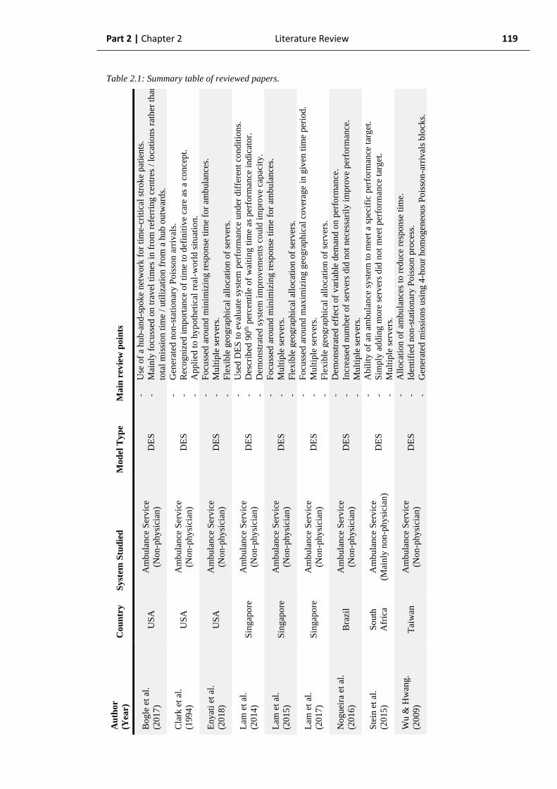
Part 2 | Chapter 2 Literature Review 119
Table 2.1: Summary table of reviewed papers.
Au
tho
r
(Yea
r)
Co
un
try
S
yst
em S
tud
ied
M
od
el T
yp
e
Ma
in r
evie
w p
oin
ts
Bo
gle
et
al.
(20
17
) U
SA
A
mb
ula
nce
Ser
vic
e
(No
n-p
hy
sici
an)
DE
S
- U
se o
f a
hu
b-a
nd-s
po
ke
net
work
for
tim
e-cr
itic
al s
tro
ke
pat
ien
ts.
- M
ain
ly f
ocu
ssed
on
tra
vel
tim
es i
n f
rom
ref
erri
ng
cen
tres
/ l
oca
tio
ns
rath
er t
han
tota
l m
issi
on
tim
e /
uti
liza
tio
n f
rom
a h
ub
ou
twar
ds.
Cla
rk e
t al
.
(19
94
) U
SA
A
mb
ula
nce
Ser
vic
e
(No
n-p
hy
sici
an)
DE
S
- G
ener
ated
non
-sta
tio
nar
y P
ois
son
arr
ival
s.
- R
eco
gn
ized
im
port
ance
of
tim
e to
def
init
ive
care
as
a co
nce
pt.
- A
pp
lied
to
hy
po
thet
ical
rea
l-w
orl
d s
itu
atio
n.
En
yat
i et
al.
(20
18
) U
SA
A
mb
ula
nce
Ser
vic
e
(No
n-p
hy
sici
an)
DE
S
- F
ocu
ssed
aro
und
min
imiz
ing r
esp
on
se t
ime
for
amb
ula
nce
s.
- M
ult
iple
ser
ver
s.
- F
lex
ible
geo
gra
ph
ical
all
oca
tio
n o
f se
rver
s.
Lam
et
al.
(20
14
) S
ing
apo
re
Am
bu
lan
ce S
erv
ice
(No
n-p
hy
sici
an)
DE
S
- U
sed
DE
S t
o e
val
uat
e sy
stem
per
form
ance
un
der
dif
fere
nt
con
dit
ion
s.
- D
escr
ibed
90
th p
erce
nti
le o
f w
aiti
ng
tim
e as
per
form
ance
indic
ato
r.
- D
emo
nst
rate
d s
yst
em i
mp
rov
emen
ts c
ou
ld i
mpro
ve
cap
acit
y.
Lam
et
al.
(20
15
) S
ing
apo
re
Am
bu
lan
ce S
erv
ice
(No
n-p
hy
sici
an)
DE
S
- F
ocu
ssed
aro
und
min
imiz
ing r
esp
on
se t
ime
for
amb
ula
nce
s.
- M
ult
iple
ser
ver
s.
- F
lex
ible
geo
gra
ph
ical
all
oca
tio
n o
f se
rver
s.
Lam
et
al.
(20
17
) S
ing
apo
re
Am
bu
lan
ce S
erv
ice
(No
n-p
hy
sici
an)
DE
S
- F
ocu
ssed
aro
und
max
imiz
ing
geo
gra
ph
ical
co
ver
age
in g
iven
tim
e p
erio
d.
- M
ult
iple
ser
ver
s.
- F
lex
ible
geo
gra
ph
ical
all
oca
tio
n o
f se
rver
s.
No
gu
eira
et
al.
(20
16
) B
razi
l A
mb
ula
nce
Ser
vic
e
(No
n-p
hy
sici
an)
DE
S
- D
emo
nst
rate
d e
ffec
t o
f v
aria
ble
dem
and o
n p
erfo
rman
ce.
- In
crea
sed
nu
mb
er o
f se
rver
s did
no
t n
eces
sari
ly i
mpro
ve
per
form
ance
.
- M
ult
iple
ser
ver
s.
Ste
in e
t al
.
(20
15
)
So
uth
Afr
ica
Am
bu
lan
ce S
erv
ice
(Mai
nly
non
-ph
ysi
cian
) D
ES
- A
bil
ity
of
an a
mb
ula
nce
sy
stem
to
mee
t a
spec
ific
per
form
ance
tar
get
.
- S
imp
ly a
dd
ing
mo
re s
erv
ers
did
no
t m
eet
per
form
ance
tar
get
.
- M
ult
iple
ser
ver
s.
Wu
& H
wan
g.
(20
09
) T
aiw
an
Am
bu
lan
ce S
erv
ice
(No
n-p
hy
sici
an)
DE
S
- A
llo
cati
on
of
amb
ula
nce
s to
red
uce
res
pon
se t
ime.
- Id
enti
fied
no
n-s
tati
on
ary
Po
isso
n p
roce
ss.
- G
ener
ated
mis
sio
ns
usi
ng
4-h
ou
r ho
mog
eneo
us
Po
isso
n-a
rriv
als
blo
cks.

Part 2 | Chapter 2 Literature Review 120
2.2.2. Reviewed papers
The applications of simulation to pre-hospital care services in the studied literature were
based solely on discrete event simulation (DES). All studies involved non-physician,
primary response ambulance services. The majority of studies were based in urban
locations with correspondingly short travel times. No studies were found which relate DES
to a national-scale, physician-led pre-hospital care service.
The most relevant paper to this project was Clark et al. (Clark et al., 1994). They used a
discrete event simulation to identify the optimal location for an air-ambulance helicopter
for the rural trauma system in Maine, USA. The primary objective in this paper was to
identify the optimal location for the helicopter base so as to minimise the time required to
deliver its paramedic team, with their higher-level clinical care abilities to the scene of a
severely injured patient. They also noted the importance of transferring a patient to a site of
definitive care and that the return-to-base time needed to be considered in the process.
They also identified the varying incidence of trauma by time of day, describing how this
generates a non-homogeneous Poisson process. Methodologically, the authors describe the
use of a standard “thinning” algorithm to generate non-stationary Poisson arrivals to the
process (Ross, 2013). Using geospatial data of locations of major trauma, a number of
locations were then tested using discrete event simulation to predict the number of
missions which could be completed, minimize the mean time to scene and compare the
times to transfer the patient to the trauma centre. The simulation does not appear to take
into account the potential of additional retrieval requests or the waiting time for the service
when it is otherwise busy. Clearly also, this is a hypothetical situation which, although
bounded by a finite number of real-world base locations, does not have a suitable real-
world control to demonstrate the accuracy of the model in replicating a real-world system.
This paper, now over 25 years old, displays perhaps the closest application relevance to
ScotSTAR EMRS with a pre-hospital trauma response helicopter. Additionally, the authors
have highlighted the importance of time-to-patient and time-to-definitive care and have
used simulation rather than empirical mathematical analysis to accurately replicate a non-
stationary Poisson process. However, its basis in a predominantly hypothetical
environment and without a process to establish accuracy with a real-world system means
methodological development is required in order to meet the demands of analysing the
ScotSTAR system.

Part 2 | Chapter 2 Literature Review 121
Bogle et al. (Bogle et al., 2017) used a DES model to evaluate the transfer of stroke
patients to a specialist stroke centre as opposed to their local hospital. This paper was
particularly focussed on decision-making and decision support relating to clinical outcome
rather than the utilization of the transport service itself. The specific details of the model
building, arrivals process, service times and subsequent accuracy of describing the real-
world are not discussed. However, the transfer of a patient to a defined centre rather than
simply the nearest hospital has relevance to the ScotSTAR systems, arguably more-so for
EMRS primary missions in the context of the evolving Scottish Trauma Network.
A number of studies considered DES models in order to reduce ambulance response times:
Wu and Hwang (Wu and Hwang, 2009) demonstrated the use of a DES simulation for
allocating ambulances to minimise response times in Tainan City, Taiwan. They identified
a non-homogeneous Poisson arrivals process and generated a uniform inter-arrival time
during a short time period. The model was compared to the real-world by using a t-test
comparing the real mean to simulated mean response times of the systems, in which the
authors found no significant differences during any of the time periods studied. The
authors state that the model did account for differing on-scene times but this is not
described in the paper. The results showed the effect of the number of servers on a defined
performance standard (90% of calls responded to within 9 minutes).
The first paper by Lam et al. (Lam et al., 2014) demonstrated the use of a DES model
with time-varying demand for ambulances in Singapore. The paper examined the effects of
three different policies on the availability and response time of ambulances. In particular, it
examined the 90th percentile of response time rather than the average value. The paper
demonstrated that a substantial improvement in system performance could be achieved
with changes to ambulance allocation and dispatch policy. The improvement was
equivalent to adding 10 ambulances to the system. Although it is stated in the paper that it
was validated by comparison to historical data, further information on the methodology of
this was not provided.
The second paper by Lam et al. (Lam et al., 2015) again used a DES model to maximize
the number of calls which could be achieved within an 11-minute national ambulance
response time target. This was done by allocating ambulances to particular locations
according to the geospatial probability of an emergency call.

Part 2 | Chapter 2 Literature Review 122
Nogueira et al. (Nogueira et al., 2016) also used a geospatial DES model in order to
optimally position ambulances to minimize travel times in Belo Horizonte city, Brazil. The
authors demonstrated time-varying demand for the ambulance service, although this was
averaged across a number of hours in 4 discrete time periods. Similarly to Lam et al.
previously (Lam et al., 2014), the authors demonstrated that optimization of the resources
in the system, by strategically placing ambulance bases could improve the system
performance without requiring additional resources. This paper compares an optimized
system process to a discrete event simulation of the real-world. However, it is unclear as to
whether this model was validated with regard to its ability to replicate the real-world first.
The third reviewed paper by Lam et al. (Lam et al., 2017) aimed to minimize the overall
ambulance response time by dynamically re-allocating ambulances during the course of a
shift in order to provide coverage to the areas with the maximum number of ambulance
calls. In particular, this paper validated the DES model by comparing its output to
historical real-world data, including response time and utilization. This paper also
demonstrated time-varying demand for ambulance calls, but simplified its inclusion in the
DES model by splitting the day into 4-hour segments considered to represent homogeneous
demand.
A similar study was undertaken by Enayati et al. (Enayati et al., 2018). This paper studied
the application of a DES-based dynamic re-allocation model on the workload of
ambulances and the proportion of calls responded to within a 10-minute time period. The
model used a time-varying Poisson arrivals process, but used exponentially-distributed
service times with a mean duration of 65-minutes.
In their study of the ambulance system in Cape Town, South Africa, Stein et al. (Stein et
al., 2015) used two separate simulation models to decide an optimal solution for reducing
the response time for the highest priority calls. The authors state that non-transport primary
response vehicles (which can deliver clinicians to a patient, but cannot transport a patient)
can be staffed by either a paramedic or occasionally a doctor and only respond to major
incidents (somewhat analogous to EMRS). However, this specific group were not the
target for optimization in this study. The authors also state that the model was verified
against a random sample of real-world data and that the error was sufficiently small that
the model could be considered as a true representation of the real-world system. The
authors also made two important conclusions applicable to ScotSTAR: firstly, that the
simple addition of resources to the system in order to meet a performance specification was
Part 2 | Chapter 2 Literature Review 123
unfeasible and secondly, that the relative sparsity of primary response vehicles lengthened
their average response time for missions.
The majority of studies reviewed urban ambulance services with multiple servers and
focussed on reducing the time to patient. This is relevant to the ScotSTAR EMRS primary
missions, in which time-to-patient is a major factor. However, ScotSTAR must operate
from a fixed geographical location (a helicopter base) because of the need to respond by
both air and road. The helicopter cannot be dynamically re-deployed to an arbitrary
location. Furthermore, ScotSTAR has a national transfer remit and simply measuring the
response time to patients is inappropriate as the flight times to some of the more remote
areas in the network are deterministic and there is very little which can be done to affect
them. Similarly, given the differences in distance involved, it is difficult to define a “catch
all” value for response time. Even if the target value were set considerably longer than for
urban ambulances, the suitability of a 2-hour time-to-patient would be very context
dependent. Attending a critically unwell patient in the Victoria Hospital, Rothesay, Isle of
Bute - approximately 21 nautical miles from the base by helicopter - then a 2-hour time-to-
patient would be considered poor performance. By contrast, attending a patient in the
Gilbert Bain Hospital, Lerwick, Shetland – approximately 260 miles from base by fixed
wing aircraft, followed by a 25-mile road journey – within 2 hours would be considered
good performance.
Additionally, there is an obvious difference between an ambulance service with tens of
available ambulances and the ScotSTAR services, with a maximum of two servers
available. The redundancy within an urban ambulance service which allows cross-cover
from a free vehicle for one which is busy is simply not an option in the ScotSTAR system
and so the optimization strategies described in the above studies do not apply. Instead, the
performance of ScotSTAR must be linked to either team non-availability (due to
simultaneous retrieval requests) or to waiting time for the mission to commence.
2.2.3. Applications of simulation in wider healthcare
In background reading, outside the literature review, an example of DES applied in the
wider healthcare setting was the study by Day et al (Day et al., 2013). This study was
conducted in an emergency department and is perhaps the most applicable study to
ScotSTAR from the wider healthcare domain. In this paper, the authors discuss the use of
Part 2 | Chapter 2 Literature Review 124
DES modelling to replicate the real-world processes of an emergency department and
simulate changes in the number of healthcare providers (servers). This study used DES to
predict the pre- and post-intervention values for mean length of stay (LOS) and percentage
of 6-hour lengths of stay. The paper therefore has some clear relevance to this project’s
overall aims of defining performance descriptors for the system. Most importantly in this
paper, the authors verified the model performance against the real-world in calculating
both mean length of stay and percentage of patients spending more than six hours in the
department. By the authors’ reference to the percentage LOS greater than 6 hours, it can be
inferred that as well as generating a simple mean, the overall distribution of LOS times can
be accurately predicted by the DES model. Although the specific nature of the DES model
components is unknown, it is based on real-world patient encounters and is therefore likely
to exhibit a time-dependent Poisson process in keeping with other emergency departments.
This paper demonstrates the ability of DES to accurately re-create a real-world system and
in particular, its ability to generate useful system performance metrics, not only a simple
mean value. In this context it is used in an emergency department with approximately
20,000 patient attendances per annum. There are 14 available patient beds in the ED and it
is staffed by 4 physicians – who spread their service times between the patients in the
department. This clearly illustrates the numerical difference when comparing such systems
to ScotSTAR. It also illustrates the operational difference, with ScotSTAR having one
server which spends 100% of the service time with the patient. These factors render these
applications significantly different to ScotSTAR with respect to a designed model, even in
the context of this, the most relevant of the hospital applications.
2.2.4. Application of simulation to ScotSTAR
It is clear that all the proposed simulation methodologies: DES, ABM and SD have
applicability, and are effective, in modelling healthcare systems. In the pre-hospital
domain, the majority of reviewed applications pertain to urban ambulance services with a
large number of servers and in which the primary objective is reducing the response time
to the patient. Each of these studies has a significant limitation in the transfer of
methodology to ScotSTAR, including: application only in a hypothetical environment, or
not being validated against the real-world. Furthermore, none of the reviewed papers
pertained to the operation of a physician-led or critical-care PHaRM service.
Part 2 | Chapter 2 Literature Review 125
An overall objective of this project is to develop an understanding of the performance
limits of the ScotSTAR teams. To achieve this, any simulation will need to create a
representation of the systems under conditions which differ significantly from the current
number of patients served. It is therefore essential that the underlying distributions for
inter-arrival time and mission durations are proven to be accurate replications of the real-
world if the assumption of validity is to be made when vastly different numbers of
missions are simulated. This means that when models are constructed for the ScotSTAR
teams, that they must be able to manage multiple arrivals processes, time-dependent
arrivals and non-Markovian service times if they are to accurately replicate the real-world
in simulation. It is likely that a successful model will be a hybrid ABM-DES model.
In a hybrid ABM-DES model, patients would enter the ScotSTAR system and transit it
according to a pre-defined set of rules in an ABM fashion. After these rules are applied, an
application of DES could define the time of entry to service, service duration and time of
departure from the system. In doing so, this could also generate the relevant probability
distributions for measures such as waiting time and allow operationally useful information
to be derived.
This thesis therefore has the potential to contribute significantly to the knowledge in this
domain by being the first application of simulation to a national, physician-led, pre-
hospital and retrieval medical service. It may also be able to enhance existing knowledge
in demonstrating the accuracy of a DES-type model in replicating multiple real-world
parameters by simulating a challenging operational healthcare system.

Part 2 Chapter 3
Aims

Part 2 | Chapter 3 Aims 127
2.3. Aims
1. This analysis aimed to establish if a hybrid discrete event simulation / agent-based
modelling simulation of the ScotSTAR SPRS and EMRS systems could accurately
recreate the real-world systems with regard to following parameters:
- Total number of missions and distribution
- Probability of activation by time of day
- Inter-arrival time distribution
- Mission duration and distribution
- Server utilization
when simulated in two separate time periods with differing simulation methodologies:
- Retrospective simulation: replicating calendar years 2013 – 2014
- Contemporaneous simulation: replicating calendar year 2015.

Part 2 Chapter 4
Methods

Part 2 | Chapter 4 Methods 129
2.4. Methods
2.4.1. Methods – modelling and simulation
2.4.1.1. General
1. A computer model of the SPRS system (appendix A) and the EMRS system (appendix
B) were built using the Simulink discrete event simulation program of the MATLAB
software suite.
2. Each model contained components to generate:
- Primary or secondary retrievals (as applicable).
- Activation probability variable by time of day.
- An FIFO queue.
- The requisite number of servers.
- Server behaviour with regard to allocation order.
- Mission duration according to mission type.
3. The Simulink model was run through a period of 1461 seconds, with the design of the
model such that one Simulink second equalled one real-world day (2016 being a leap-
year). The simulation was started at a real-world equivalent of 00:00:00 on 01/01/2013 and
ended after 1461 days at 00:00:00 on 01/01/2017.
Part 2 | Chapter 4 Methods 130
2.4.1.2. Mission generation
1. From the real-world data, the number of missions undertaken per calendar month were
counted and used to generate a time-series with a time-varying arrival rate (λ), averaged
over each calendar month.
2. Using the simulation time as the lookup datetime value, the current λ value was
interpolated from the month-by-month time-series values.
3. This λ-value was used as a primer for the minimized inter-arrival time distribution
within the exclusion sampling process to define the time-varying mission arrivals
(section 2.4.1.3). For entity generation, this process generated a time-varying,
minimized, exponential inter-arrival time distribution.
4. From this minimized distribution, an entity inter-generation time was randomly selected.
5. After the inter-generation time had elapsed, another entity (patient / mission) was
generated using the same methodology. The datetime of each mission creation was
recorded.
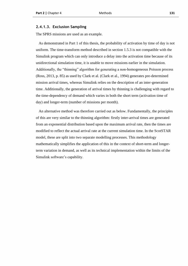
Part 2 | Chapter 4 Methods 131
2.4.1.3. Exclusion Sampling
The SPRS missions are used as an example.
As demonstrated in Part 1 of this thesis, the probability of activation by time of day is not
uniform. The time-transform method described in section 1.5.3 is not compatible with the
Simulink program which can only introduce a delay into the activation time because of its
unidirectional simulation time, it is unable to move missions earlier in the simulation.
Additionally, the “thinning” algorithm for generating a non-homogeneous Poisson process
(Ross, 2013, p. 85) as used by Clark et al. (Clark et al., 1994) generates pre-determined
mission arrival times, whereas Simulink relies on the description of an inter-generation
time. Additionally, the generation of arrival times by thinning is challenging with regard to
the time-dependency of demand which varies in both the short term (activation time of
day) and longer-term (number of missions per month).
An alternative method was therefore carried out as below. Fundamentally, the principles
of this are very similar to the thinning algorithm: firstly inter-arrival times are generated
from an exponential distribution based upon the maximum arrival rate, then the times are
modified to reflect the actual arrival rate at the current simulation time. In the ScotSTAR
model, these are split into two separate modelling processes. This methodology
mathematically simplifies the application of this in the context of short-term and longer-
term variation in demand, as well as its technical implementation within the limits of the
Simulink software’s capability.
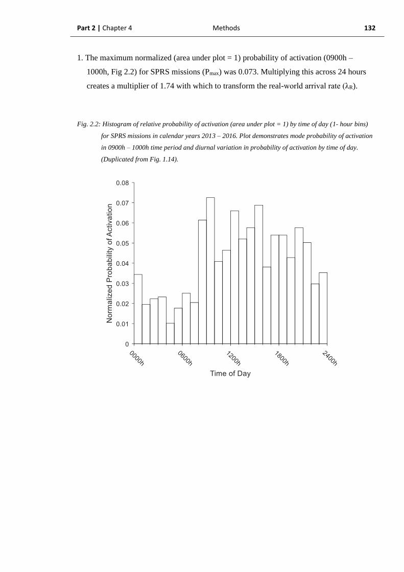
Part 2 | Chapter 4 Methods 132
1. The maximum normalized (area under plot = 1) probability of activation (0900h –
1000h, Fig 2.2) for SPRS missions (Pmax) was 0.073. Multiplying this across 24 hours
creates a multiplier of 1.74 with which to transform the real-world arrival rate (λR).
Fig. 2.2: Histogram of relative probability of activation (area under plot = 1) by time of day (1- hour bins)
for SPRS missions in calendar years 2013 – 2016. Plot demonstrates mode probability of activation
in 0900h – 1000h time period and diurnal variation in probability of activation by time of day.
(Duplicated from Fig. 1.14).

Part 2 | Chapter 4 Methods 133
2. Using a real-world arrival rate (λR) of 20 missions per month (0.67 missions per day) as
an example, multiplication by 1.74 generates a maximized arrival rate (λmax) of 35
missions per month (1.17 missions per day).
3. The real exponential inter-arrival time distribution:
𝜇𝑅 = 1
𝜆𝑅 =
1
0.67= 1.50 (29)
is thus converted to a minimized inter-arrival time exponential distribution (Fig. 2.3):
𝜇𝑚𝑖𝑛 = 1
𝜆𝑚𝑎𝑥=
1
1.17= 0.86 (30)
Fig. 2.3: Comparison of PDFs of example baseline calculated inter-arrival exponential distribution with
baseline inter-arrival time μR = 1.50 (blue line) and minimized inter-arrival exponential distribution
μmin = 0.86 (red line).
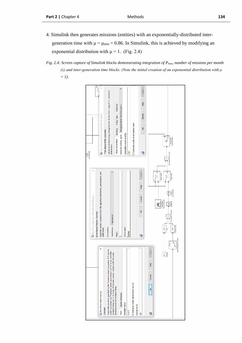
Part 2 | Chapter 4 Methods 134
4. Simulink then generates missions (entities) with an exponentially-distributed inter-
generation time with μ = μmin = 0.86. In Simulink, this is achieved by modifying an
exponential distribution with μ = 1. (Fig. 2.4)
Fig. 2.4: Screen capture of Simulink blocks demonstrating integration of Pmax, number of missions per month
(λ) and inter-generation time blocks. (Note the initial creation of an exponential distribution with μ
= 1).

Part 2 | Chapter 4 Methods 135
5. At this stage, no account has been made of time-varying demand. Therefore, a uniform
probability of activation, with all time periods demonstrating the same value, equal to
Pmax is created as time tends to infinity. (Fig. 2.5).
Fig. 2.5: Histogram of probability of activation by time of day in arbitrary uniform distribution generated at
maximum probability of activation in any learning data bin (values of all bins = Pmax = 0.073, area
under plot = 1.74).
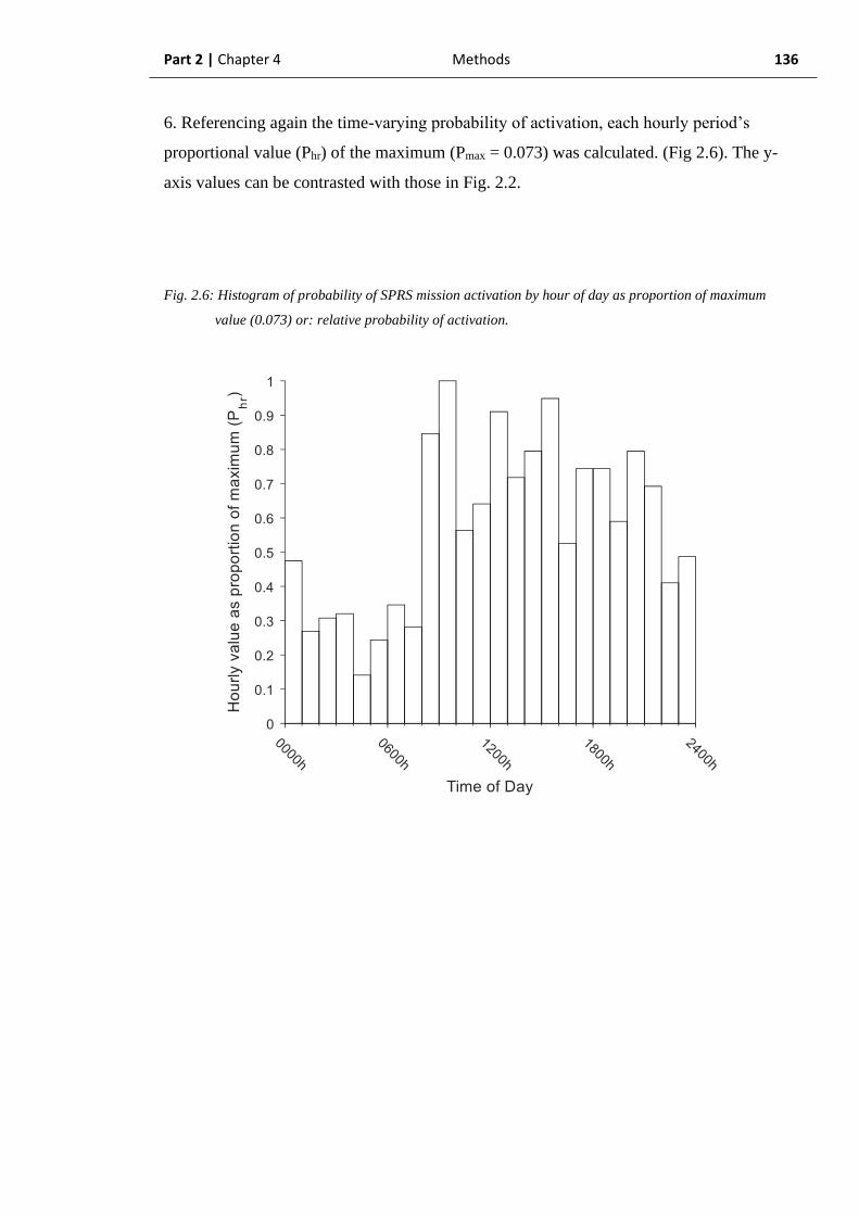
Part 2 | Chapter 4 Methods 136
6. Referencing again the time-varying probability of activation, each hourly period’s
proportional value (Phr) of the maximum (Pmax = 0.073) was calculated. (Fig 2.6). The y-
axis values can be contrasted with those in Fig. 2.2.
Fig. 2.6: Histogram of probability of SPRS mission activation by hour of day as proportion of maximum
value (0.073) or: relative probability of activation.

Part 2 | Chapter 4 Methods 137
7. The time of day from the simulated mission (entity) generation time (equivalent to
activation datetime) was used as a lookup value for the proportional hourly probability of
activation by time of day (Phr). The corresponding Phr value was read by a Simulink block.
As an example, with reference to Fig. 2.6, a mission occurring in the 0000h – 0100h time
period demonstrates Phr = 0.47.
8. Each generated mission (entity) was subjected to a single Bernoulli trial (n = 1) with
probability of success = Phr (as generated in the previous step). Trials returning a value of 1
allowed the entity to continue within the system. Trials returning a value of 0 resulted in
the entity being rejected (Fig. 2.7).
Fig. 2.7: Screen capture of MATLAB Simulink program demonstrating blocks to read outcome of Bernoulli
trial as rejection attribute and route to sink or allow to continue in the model.
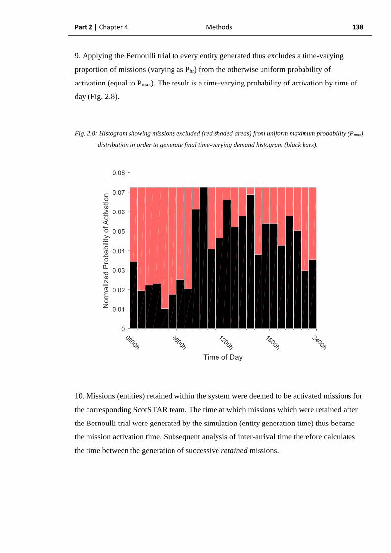
Part 2 | Chapter 4 Methods 138
9. Applying the Bernoulli trial to every entity generated thus excludes a time-varying
proportion of missions (varying as Phr) from the otherwise uniform probability of
activation (equal to Pmax). The result is a time-varying probability of activation by time of
day (Fig. 2.8).
Fig. 2.8: Histogram showing missions excluded (red shaded areas) from uniform maximum probability (Pmax)
distribution in order to generate final time-varying demand histogram (black bars).
10. Missions (entities) retained within the system were deemed to be activated missions for
the corresponding ScotSTAR team. The time at which missions which were retained after
the Bernoulli trial were generated by the simulation (entity generation time) thus became
the mission activation time. Subsequent analysis of inter-arrival time therefore calculates
the time between the generation of successive retained missions.
Part 2 | Chapter 4 Methods 139
2.4.1.4. Entity attributes
1. The mission type (primary or secondary) and mission duration were applied as attributes
to the mission entity within the Simulink program. This defined the nature of a generated
mission / patient’s interaction with the system and formed the agent-based-modelling
(ABM) component of the simulation.
2.4.1.5. Mission duration allocation
Missions which were retained by the system were assigned a mission duration. It was
recognized as a potential risk that the mission duration could differ between the learning
and testing distributions. A hold-out validation process, described below, was therefore
used to maximize the generalizability of mission duration distribution. A summary figure
is included (Fig. 2.9)
1. For each simulation period (see analysis, section 2.4.2). The mission durations were
separated in a standard 70:30, learning and testing split.
2. Within the learning dataset, one thousand training data sub-sets were made, each
sampling 70% of the data without replacement.
3. To each training data sub-set, a gamma distribution was fitted using the MATLAB
distribution fitting function.
4. Each gamma distribution was then tested in a 5-fold hold-out validation process. Thus,
each gamma distribution was tested against five 20% hold-out sub-sets of the learning
dataset.

Part 2 | Chapter 4 Methods 140
Fig. 2.9: Illustrative summary of data split, showing testing dataset, learning dataset and hold-out validation
sample sub-sets.
5. Each of the five hold-out sub-sets were tested against the Cumulative Density Function
(CDF) of one gamma distribution using a one-sample Kolmogorov-Smirnov test. The K-S
test statistic comparing the hold-out data to the gamma distribution was recorded as a
goodness-of-fit value for each fold. Five K-S statistic values were therefore generated for
each gamma distribution. This was repeated for all one thousand gamma distributions
generated in step 3.
5. The most generalisable gamma distribution was selected by minimization of the root
mean squared (RMS) values of the five K-S test statistic values recorded in each 5-fold
hold-out validation step. As a perfect fit will generate a K-S test statistic value of zero, this
is equivalent to the Root Mean Squared Error (RMSE) of the K-S test statistic values.
6. The selected distribution was used to randomly generate corresponding mission
durations for the missions retained in the system (i.e. those missions not rejected by
exclusion sampling).
ScotSTAR complete dataset
(for simulation period)
Learning
dataset
Testing
dataset
Hold-out validation samples (x5)

Part 2 | Chapter 4 Methods 141
2.4.1.6. Running of Simulation
1. All simulations were performed on a desktop computer (baseboard: X79-UP4: Gigabyte
Technology Company, New Taipei City, Taiwan) with a water-cooled, 3.70GHz quad-core
processor (Core i7-4820K: Intel Corporation, Santa Clara, California, USA) and 16GB
DDR3 RAM (Corsair Vengeance: Corsair Gaming Incorporated, Fremont, California,
USA).
2. Patients (entities) retained by the system (i.e. not rejected by exclusion sampling) were
run through a discrete event simulation model corresponding to the appropriate queue and
server structure of the corresponding ScotSTAR system (appendices A & B).
3. Each generated patient proceeded through the system according to the mission type and
generated mission duration (ABM format).
4. The progress of each patient through the system was recorded at discrete time
checkpoints corresponding to arrival time (entry to the queue), commencement of service
(departure from the queue) and completion of service (departure from the system) in a DES
format.
5. The waiting time, queue length and server utilization were read directly from the model
at each discrete time step in the simulation.
6. After 1461 simulated days (equivalent to 00:00:00 01/01/2013 to 00:00:00 01/01/2017)
the simulation was terminated and reset.
7. A total of one-thousand iterations of each (SPRS and EMRS) simulation were
performed.

Part 2 | Chapter 4 Methods 142
2.4.2. Parameter analysis
1. For analysis, the simulation output was divided into three time periods:
Retrospective simulation period: - 00:00:00 01/01/2013 to 00:00:00 01/01/2015
- All data during this period was analysed and made available to the model, even if in
the future to the model’s current simulated time
Contemporaneous simulation period: - 00:00:00 01/01/2015 to 00:00:00 01/01/2016
- Only real mission data retrospective to the model’s current simulated time was
available to the model, thereby assessing its ability to generate the current state of the
system.
Prospective simulation period: - 00:00:00 01/01/2016 to 00:00:00 01/01/2017
- No real-world mission data would be made available to the model during this period,
it was forced to rely on the projected mission numbers, mission durations etc. with
the intention of assessing the model’s ability to prospectively predict the future daily
state of the system.
- This simulation period required the use of multiple predictive models to generate the
predicted future values for monthly number of missions, mission durations etc. The
analysis and fitting of this was deemed to be outside the scope of this thesis and the
output of this simulation period is not included in any of the subsequent analyses.
- This has no effect on the findings of this thesis, and it is intended that the output of
the prospective simulation period will instead form components for future
publication.
2. For each simulation period, the activation time, queue entry and exit time, service entry
and exit time were recorded for every patient retained within the system (not rejected by
the exclusion sampling process).
3. From these times, the number of missions, activation time of day, inter-arrival times,
waiting time, mission duration and server utilization were calculated.
Part 2 | Chapter 4 Methods 143
2.4.2.1. Comparison to real-world.
1. The calculated parameter values were compared to their real-world equivalents to
establish the validity of the model in replicating the real-world. Discrete event simulation
across multiple iterations requires an additional step of processing to resolve the stochastic
nature of the simulation which generates different values for each parameter in each
simulation iteration.
2.4.2.2. Total number of missions comparison
1. The total number of missions generated in each iteration were counted at the end of each
simulation iteration and plotted as a box-plot.
2. The median value of these totals (iterative median) was compared to the real-world
number of missions in the same time period for accuracy (as 1 – error rate), and statistical
significance using the Mann-Whitney U-test.
2.4.2.3. Distribution of missions through simulation period comparison
1. The cumulative total of missions by date was counted for each simulation iteration and
plotted. The iterative median value was plotted for each date. The 2.5th and 97.5th values of
the daily total were plotted as a 95% prediction interval.
2. The real-world daily total number of missions was counted and plotted on the same
chart.
3. The daily cumulative totals were compared using the 95% prediction interval, and by
comparing the ECDFs using Kolmogorov-Smirnov testing.
2.4.2.4. Activation time of day comparison
1. The activation time of day was extracted from the simulation activation times and
plotted as a normalized (area under plot = 1) probability histogram.
2. The simulated activation time of day histogram bin values (1-hour bins) were compared
to the real-world missions in the testing dataset activation times histograms. The median
accuracy was recorded (as 1 – error rate).
Part 2 | Chapter 4 Methods 144
3. The distribution of simulated mission activations across the 24-hour period was
compared to the real-world by comparison of the ECDFs with Kolmogorov-Smirnov
testing.
2.4.2.5. Inter-arrival time distribution comparison
1. The difference in arrival time between sequential simulated activated missions (i.e.
sequential missions not rejected by exclusion sampling) was calculated as the inter-arrival
time.
2. The simulated inter-arrival times and real-world test dataset inter-arrival times were
plotted as a probability density histograms with 1-hour bins.
3. Exponential distributions were fitted to the simulated missions’ inter-arrival times and to
the testing sample of the real-world inter-arrival times.
4. The exponential distributions were compared using the respective μ-values and
confidence intervals.
5. The simulated inter-arrival times and the real-world testing sample inter-arrival times
were compared using ECDFs and Kolmogorov-Smirnov testing.
2.4.2.6. Mission duration comparison
1. The difference between a patient commencing service and finishing service was
calculated as the mission duration.
2. For each simulation iteration, the median mission duration was calculated. At the
conclusion of all iterations, the median value of each iteration’s median mission duration
was calculated as the overall model iterative median.
3. The iterative median value was compared to the real-world median value for accuracy
(as 1 – error rate), and statistical significance using the Mann-Whitney U-test.
4. All simulated mission durations across all iterations and the real-world test dataset
mission durations were plotted as probability density histograms with 30-minute bins.
5. Gamma distributions were fitted to all simulated mission durations and to the testing
sample of real-world mission durations.
Part 2 | Chapter 4 Methods 145
6. The fitted gamma distributions were compared by κ and θ parameter values.
7. All simulated mission durations and the testing sample of real-world mission durations
were compared using ECDFs and Kolmogorov-Smirnov testing.
2.4.2.7. Server utilization comparison
1. The total hours of work undertaken by a ScotSTAR team in each simulation iteration,
and in the complete real-world dataset were calculated as the sum of all mission durations.
2. The total hours of work in each iteration, and in the real-world, were divided by the total
server time available for each simulation period. A utilization quotient was therefore
generated.
3. The utilization quotients from each simulation iteration were plotted using boxplots for
comparison to the real-world values.
4. The iterative median utilization and the real-world utilization were compared for
accuracy (as 1 – error rate), and for statistical significance using the Mann-Whitney U-test.
2.4.3. Summation
1. After the individual comparison of all model components to the real-world as outlined
above, an overall qualitative assessment of the effectiveness of the model in replicating
the real-world was made.

Part 2 Chapter 5
Results:
Simulation of SPRS operations

Part 2 | Chapter 5 Results: SPRS simulation 147
2.5. Results of simulation of SPRS operations
This analysis section will assess the accuracy of the SPRS system model in replicating
real-world queueing theory components to ultimately validate the overall similarity
between the model and the real-world system.
The SPRS system, as derived in Part 1 of the thesis (section 1.7) receives Markovian
arrivals to a single queue feeding a single server with gamma-distributed (general) service
times. In Kendall’s notation, it was described as:
M/G/1
The single server and single queue are analogous to a “corner shop” queue, as illustrated
in Fig. 2.10.
Fig. 2.10: Diagrammatic representation of SPRS showing single arrivals process, single queue and single
server.
The analysis of this model will compare several queueing theory components to their
real-world equivalents:
- Number of missions undertaken (including cumulative number and pattern).
- Activation time of day.
- Inter-arrival time.
- Mission duration.
- Server Utilization.
FIFO
Queue Arrivals Departure
SPRS
Team
Part 2 | Chapter 5 Results: SPRS simulation 148
The analysis of the SPRS system will be undertaken in two simulation periods:
Retrospective simulation: comprising calendar years 2013-2014. This model is
provided with the most information in this project, spanning the whole of the 2-year
period – even if this is “future” to the current simulation point. Its purpose is to
prime the subsequent models, provide demonstration of equivalence between the
model and real-world, and to ensure non-mutilation of the learning data.
Contemporaneous simulation: comprising calendar year 2015. This model is provided
with the priming data from the retrospective simulation and then receives new
information for the 2015 calendar year up to the current simulation point. No future
information is available. The purpose of this simulation is primarily to demonstrate
the ability of the model to replicate the immediate, current, state of the real-world
SPRS system.
Further information on particular aspects of each simulation period will be discussed in
more detail in the relevant chapters.
Overall, one thousand iterations of the SPRS simulation were performed in a single
simulation run, representing the calendar years 2013 – 2016. The median simulation time
was 2.53 seconds, and the simulation was completed in a total of 1h 17m.
Part 2 | Chapter 5 Results: SPRS simulation 149
2.5.1. Retrospective simulation of SPRS operations
In this section, the performance of the SPRS model for each of the stated parameters is
considered in a two-year simulation period comprising the calendar years 2013 and 2014.
With regard to the SPRS simulation, “retrospective” refers to the simulation being
provided with a complete dataset from the entire simulation period with which to generate
mission data. This creates the paradox where a model can receive information about the
current state of the system based on future data. For example, mission durations for
missions in January 2013 are selected from a distribution which also includes data from
December 2014.
Clearly this is impossible in the real-world and the only way that this simulation can be
truly valid is for the results to be compared at the end of the two-year simulation period,
when the simulation model has reached the time point at which all the data would be
available to it. When this is done, the simulation output and analysis will generate
descriptive statistics representative of the entire two-year period, but not any specific point
therein.
The purpose of this simulation is therefore three-fold:
- Firstly, it aims to demonstrate that the model does not mutilate the data during
analysis and is able to replicate the real-world even after the data has been de-
constructed and re-constructed within the model.
- Secondly, it primes the model with a working data set prior to the
contemporaneous time-period, in which the data provided to the model is
produced (section 2.5.2).
- Thirdly, and most importantly, it aims to demonstrate that the relationships
between the real-world processes and the model processes are valid. As shown
in the methodology, the model has very carefully been designed around the
underlying distributions, as described by queueing theory, not the empirical
distributions of the real-world data. In doing so, the model is effectively
creating de novo data which is then being compared to the real-world. The
model is not, as is sometimes the case with DES, simply re-sampling the real-
world data. The assumption of validity in the model replicating not only the
real-world values but the real-world relationships between system components,
is critical for the overall objectives of this project. If the results of any derived
Part 2 | Chapter 5 Results: SPRS simulation 150
(as opposed to measured or observed) descriptive values calculated in this
thesis are to be considered valid, then it must be inferred that the underlying
mathematical relationship between the system components is valid. Therefore,
if it can be proven that the model, with these mathematical relationships coded
into its operation, is able to replicate the real-world accurately, then it implies
that the real-world systems must also follow the same mathematical
relationships. Validity is thus also implied for any descriptive performance
values which rely upon the mathematical relationship between system
components in their derivation.
It should be noted that because of the different time period used, the results in this
retrospective simulation (calendar years 2013 and 2014) will differ from the equivalent
results in Part 1 (calculated over calendar years 2013 – 2016). It is, however, expected that
the overall distributions will be similar.
2.5.1.1. Retrospective simulation of SPRS mission count
As demonstrated in section 1 (section 1.7.1.8), the queueing system applicable to SPRS
is of the M/G/1 type. All arrivals to the system are expected to follow the Markovian (M)
pattern – that of an exponentially distributed inter-arrival time, reflective of an underlying
Poisson process (albeit time-varying).
The ability of the model to correctly generate the stated Markovian arrival pattern is
firstly dependent on its ability to correctly represent the underlying Poisson process. In this
analysis section, the ability of the simulation to output the correct number of missions with
respect to time (i.e. replication of the underlying Poisson process) will be analysed for the
SPRS model.
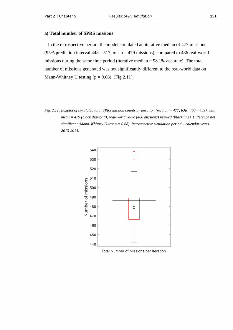
Part 2 | Chapter 5 Results: SPRS simulation 151
a) Total number of SPRS missions
In the retrospective period, the model simulated an iterative median of 477 missions
(95% prediction interval 448 – 517, mean = 479 missions), compared to 486 real-world
missions during the same time period (iterative median = 98.1% accurate). The total
number of missions generated was not significantly different to the real-world data on
Mann-Whitney U testing (p = 0.68). (Fig 2.11).
Fig. 2.11: Boxplot of simulated total SPRS mission counts by iteration (median = 477, IQR: 466 – 489), with
mean = 479 (black diamond), real-world value (486 missions) marked (black line). Difference not
significant (Mann-Whitney U-test p = 0.68). Retrospective simulation period – calendar years
2013-2014.
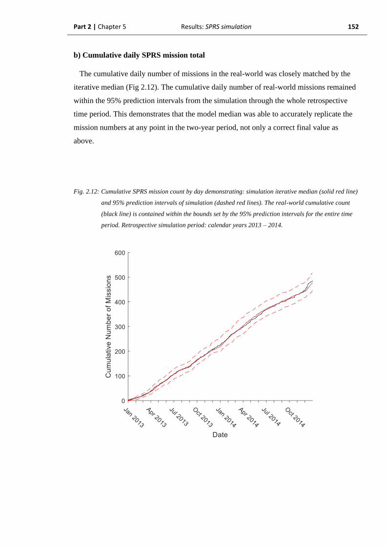
Part 2 | Chapter 5 Results: SPRS simulation 152
b) Cumulative daily SPRS mission total
The cumulative daily number of missions in the real-world was closely matched by the
iterative median (Fig 2.12). The cumulative daily number of real-world missions remained
within the 95% prediction intervals from the simulation through the whole retrospective
time period. This demonstrates that the model median was able to accurately replicate the
mission numbers at any point in the two-year period, not only a correct final value as
above.
Fig. 2.12: Cumulative SPRS mission count by day demonstrating: simulation iterative median (solid red line)
and 95% prediction intervals of simulation (dashed red lines). The real-world cumulative count
(black line) is contained within the bounds set by the 95% prediction intervals for the entire time
period. Retrospective simulation period: calendar years 2013 – 2014.

Part 2 | Chapter 5 Results: SPRS simulation 153
c) Empirical Cumulative Distribution Function (ECDF) of number of SPRS missions
by date
Comparison of the ECDFs demonstrated the simulation output to appear closely aligned
with the real-world data (Fig 2.13). The distributions were not statistically significant on
Kolmogorov-Smirnov testing (p = 0.88). This demonstrates that the model is generating
the correct pattern of monthly mission numbers versus time, as well as the correct number
of missions, as above. Thus, the model would be expected to respond appropriately in
adapting the seasonal demand pattern to a change in overall mission numbers.
Fig. 2.13: Comparison of ECDFs of cumulative daily mission count by date for: simulation iterative median
(red line) and real-world (black line). Kolmogorov-Smirnov test p = 0.88. Retrospective
simulation period: calendar years 2013 – 2014.

Part 2 | Chapter 5 Results: SPRS simulation 154
d) Summary: SPRS number of missions, retrospective simulation
When provided with the entirety of the dataset for the studied time period, the SPRS
model was able to replicate the real-world with respect to total number of missions,
cumulative daily number of missions and distribution of missions through the studied time
period. It is therefore considered that the arrival rate (λ) of missions is accurate and that
this should confer an accurate μ-value (as 1/λ) for the base exponential inter-arrival
distribution.

Part 2 | Chapter 5 Results: SPRS simulation 155
2.5.1.2. Retrospective simulation of SPRS activation by time of
day
The overall accuracy of the long-term SPRS mission arrival rate (λ) has been
demonstrated. However, as was demonstrated in Part 1 (section 1.7.1.2), SPRS demand
varies through the course of the day. This section will analyse the ability of the model to
replicate the time-varying arrivals of the single (emergency) mission type undertaken by
SPRS, by using the exclusion sampling method described in section 2.4.1.3.
a) Probability of SPRS activation by time of day
In the retrospective simulation period, activation times of day were grossly similar to the
real-world test data. The simulated missions peak time of activation (Fig. 2.14) was 1100h-
1200h compared to 0800h-0900h in the real-world test dataset (Fig 2.15). Both datasets
demonstrated a sharp increase in the number of missions around 0800h, with lowest
demand through the night. The median accuracy of the prediction by hour of day was
73.3%.
Fig. 2.14: Normalized probability histogram (area under plot = 1) of simulated mission activations by hour
of day. Mode at 1100h – 1200h period. Retrospective simulation period: calendar years 2013 –
2014.
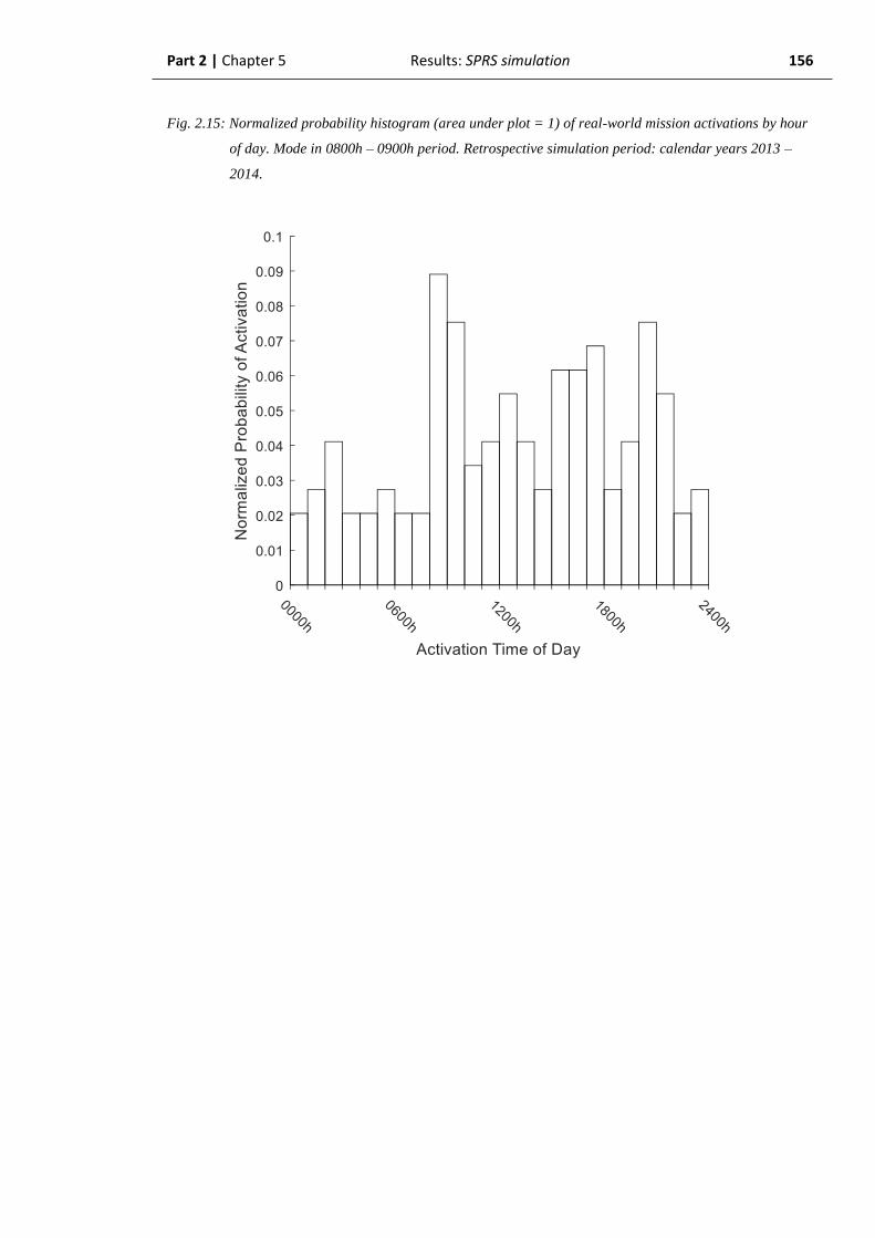
Part 2 | Chapter 5 Results: SPRS simulation 156
Fig. 2.15: Normalized probability histogram (area under plot = 1) of real-world mission activations by hour
of day. Mode in 0800h – 0900h period. Retrospective simulation period: calendar years 2013 –
2014.

Part 2 | Chapter 5 Results: SPRS simulation 157
b) Empirical Cumulative Distribution Function (ECDF) of SPRS activations by time
of day
The simulation activation time of day ECDF appeared to closely approximate the real-
world testing data, including an inflection point in the 0700h-0800h period (Fig. 2.16). The
simulated activation times were not significantly different to the real-world testing data
distribution on Kolmogorov-Smirnov testing (p = 0.51).
Fig. 2.16: ECDFs of SPRS mission activations by time of day for simulation output (red line) and real-world
test dataset (black line). Kolmogorov-Smirnov test p = 0.51. Retrospective simulation period:
calendar years 2013 – 2014.

Part 2 | Chapter 5 Results: SPRS simulation 158
c) Summary: SPRS activations by time of day, retrospective simulation
This section demonstrates that, when provided with the entirety of the dataset for the
simulation period, the SPRS model is able to generate missions with the same time-varying
demand as the real-world. Furthermore, it clearly validates the exclusion-sampling
methodology in converting the simulation from entities generated by a uniform Poisson
process into a time-dependent Poisson process during the simulation.
Part 2 | Chapter 5 Results: SPRS simulation 159
2.5.1.3. Retrospective simulation of SPRS inter-arrival times
The two components analysed so far are combined when the mission arrival rate (λ) is
modified by the time-varying demand for the SPRS team in a time-dependent Poisson
process. The expected result of this is a distribution similar to that demonstrated in section
1.7.1.2, where SPRS missions were shown to be generally exponentially distributed with a
mild multi-modal component, reflective of the time between peak probability of activation
on subsequent days.
To accurately reflect the real-world, the model must also generate both the same overall
exponential distribution and the associated multi-modal component. This will be critical to
the future accurate assessment of waiting time, and the probability of simultaneous
retrieval requests – these being more likely to occur at the times of day when demand is
highest.
In this analysis section, the ability of the SPRS model to accurately replicate the real-
world inter-arrival time distribution will be assessed.

Part 2 | Chapter 5 Results: SPRS simulation 160
a) Probability (PDF) of inter-arrival time by hour, SPRS missions
In the retrospective simulation period, the simulation output demonstrated inter-arrival
times distributed similarly to the real-world testing data. Both sets of data demonstrated an
approximately exponential distribution (Fig. 2.17 & 2.18). The real-world testing data are a
relatively small sub-set (comprising 144 data points) of the real-world data, compared to
the inter-arrival times from the complete simulation output (comprising 481,020 data
points). As a result, the simulation data is much higher resolution and the multi-modal
component, although subtle, is clearly visible. The multi-modal component is not as clear
in the real-world data, particularly when compared to the distribution demonstrated in Part
1, Fig. 1.13.
Fig. 2.17: Probability density histogram of simulated SPRS mission inter-arrival times with one-hour bins.
Fitted exponential distribution μ = 1.52 (red line). Retrospective simulation period: calendar
years 2013 – 2014.

Part 2 | Chapter 5 Results: SPRS simulation 161
Fig. 2.18: Probability density histogram of real-world mission inter-arrival times with one-hour bins. Fitted
exponential distribution μ = 1.50 (red line). Retrospective simulation period: calendar years 2013
– 2014.
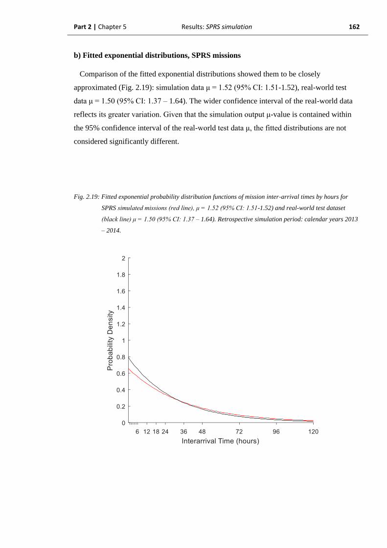
Part 2 | Chapter 5 Results: SPRS simulation 162
b) Fitted exponential distributions, SPRS missions
Comparison of the fitted exponential distributions showed them to be closely
approximated (Fig. 2.19): simulation data μ = 1.52 (95% CI: 1.51-1.52), real-world test
data μ = 1.50 (95% CI: 1.37 – 1.64). The wider confidence interval of the real-world data
reflects its greater variation. Given that the simulation output μ-value is contained within
the 95% confidence interval of the real-world test data μ, the fitted distributions are not
considered significantly different.
Fig. 2.19: Fitted exponential probability distribution functions of mission inter-arrival times by hours for
SPRS simulated missions (red line), μ = 1.52 (95% CI: 1.51-1.52) and real-world test dataset
(black line) μ = 1.50 (95% CI: 1.37 – 1.64). Retrospective simulation period: calendar years 2013
– 2014.
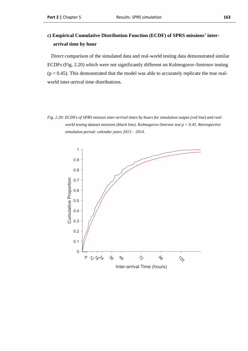
Part 2 | Chapter 5 Results: SPRS simulation 163
c) Empirical Cumulative Distribution Function (ECDF) of SPRS missions’ inter-
arrival time by hour
Direct comparison of the simulated data and real-world testing data demonstrated similar
ECDFs (Fig. 2.20) which were not significantly different on Kolmogorov-Smirnov testing
(p = 0.45). This demonstrated that the model was able to accurately replicate the true real-
world inter-arrival time distributions.
Fig. 2.20: ECDFs of SPRS mission inter-arrival times by hours for simulation output (red line) and real-
world testing dataset missions (black line). Kolmogorov-Smirnov test p = 0.45. Retrospective
simulation period: calendar years 2013 – 2014.

Part 2 | Chapter 5 Results: SPRS simulation 164
d) Summary: SPRS inter-arrival times, retrospective simulation
This section demonstrates that, when provided with the entirety of the dataset for the
simulation period, the SPRS model is able to generate missions with the same inter-arrival
distribution as the real-world. This accuracy includes both the overall exponential
distribution and the subtle multi-modal component of the inter-arrival times, the latter
assessed by comparison of the ECDFs.
Methodologically, this validates both the use of an exponentially-distributed inter-arrival
time base and its subsequent modification using the exclusion-sampling methodology.
Part 2 | Chapter 5 Results: SPRS simulation 165
2.5.1.4. Retrospective simulation of SPRS mission durations
Analysis of the mission durations now shifts focus from arrivals to the server: the SPRS
team itself.
Having accurately established the number of arrivals to the system, the accurate
replication of mission durations is critical to the subsequent calculation of service
utilization. This is an important step in the accurate calculation of simultaneous retrievals
and waiting time which will be addressed later in this thesis.
With the model having accurately replicated the number of real-world missions in the
retrospective simulation period (section 2.5.1.1), the real-world server utilization could
now be replicated by the model from an accurate mean mission duration alone. However,
the accuracy of subsequent – arguably more useful – performance parameters would be
reduced by use of a simple mean duration. For example, the calculation of simultaneous
retrieval rates, or the waiting time for retrieval, would have to be assumed to follow the
normal distribution if the mean mission duration was used. It is known from section 1.7.1.3
that the SPRS mission durations are not normally distributed, instead being gamma
distributed.
In this analysis section, the ability of the model to accurately replicate the true real-world
mission durations. and distribution, for the SPRS team will be assessed.
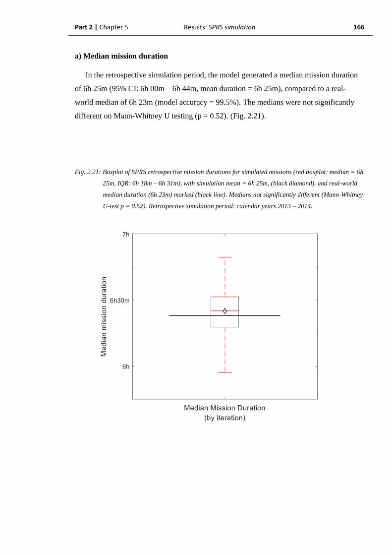
Part 2 | Chapter 5 Results: SPRS simulation 166
a) Median mission duration
In the retrospective simulation period, the model generated a median mission duration
of 6h 25m (95% CI: 6h 00m – 6h 44m, mean duration = 6h 25m), compared to a real-
world median of 6h 23m (model accuracy = 99.5%). The medians were not significantly
different on Mann-Whitney U testing (p = 0.52). (Fig. 2.21).
Fig. 2.21: Boxplot of SPRS retrospective mission durations for simulated missions (red boxplot: median = 6h
25m, IQR: 6h 18m – 6h 31m), with simulation mean = 6h 25m, (black diamond), and real-world
median duration (6h 23m) marked (black line). Medians not significantly different (Mann-Whitney
U-test p = 0.52). Retrospective simulation period: calendar years 2013 – 2014.

Part 2 | Chapter 5 Results: SPRS simulation 167
b) Probability (PDF) of SPRS mission durations by elapsed time
Both the simulation output data and the real-world test data demonstrated an overall
gamma distribution. The simulated data much more closely approximated the gamma
distribution than the real-world data, being generated directly from the distribution – as
opposed to the real-world data merely having the distribution fitted to it.
The fitted gamma distributions appeared similar. Simulated missions were gamma
distributed with parameter values κ = 4.28 (95% CI: 4.27 – 4.30) and θ = 0.07 (95% CI:
0.07 – 0.07). Real-world test data were gamma distributed with parameter values κ = 3.78
(95%CI: 2.76 – 5.19) and θ = 0.08 (95% CI: 0.06 – 0.11). Both parameter values of the
simulation distribution were contained within the confidence intervals of their respective
real-world parameters, indicating the distributions are not significantly different (Fig.
2.24).
Fig. 2.22: Probability density histogram of SPRS simulated mission durations with 30-minute bins and fitted
gamma distribution: parameter values κ = 4.28 and θ = 0.07. Retrospective simulation period:
calendar years 2013 – 2014.
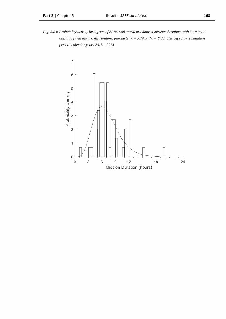
Part 2 | Chapter 5 Results: SPRS simulation 168
Fig. 2.23: Probability density histogram of SPRS real-world test dataset mission durations with 30-minute
bins and fitted gamma distribution: parameter κ = 3.78 and θ = 0.08. Retrospective simulation
period: calendar years 2013 – 2014.

Part 2 | Chapter 5 Results: SPRS simulation 169
Fig. 2.24: Comparison of fitted SPRS mission duration gamma-distribution PDFs for SPRS simulated
missions (red line), parameter values κ = 4.28 (95% CI: 4.27 – 4.30) and θ = 0.07 (95% CI: 0.07
– 0.07) and real-world test dataset missions (black line), parameter values κ = 3.78 (95%CI: 2.76
– 5.19) and θ = 0.08 (95% CI: 0.06 – 0.11). Retrospective simulation period: calendar years 2013
– 2014.

Part 2 | Chapter 5 Results: SPRS simulation 170
c) Empirical Cumulative Distribution Function (ECDF) of SPRS mission durations
by elapsed time
Comparison of the simulated and real-world test data in the retrospective simulation
period demonstrated a similar ECDF. The difference was not significant on Kolmogorov-
Smirnov testing (p = 0.61).
Fig. 2.25: ECDFs of SPRS mission durations by hours for simulation output (red line) and real-world test
dataset missions (black line). Kolmogorov-Smirnov test p = 0.61. Retrospective simulation period:
calendar years 2013 – 2014.
Part 2 | Chapter 5 Results: SPRS simulation 171
d) Summary: SPRS mission durations, retrospective simulation period
The combination of non-significant differences in closely approximated medians and the
non-significant Kolmogorov-Smirnov test results for both fitted gamma distributions and
ECDFs all strongly suggest that the model was able to accurately replicate the real-world
mission durations when provided with the complete dataset for the retrospective simulation
period.
2.5.1.5 Retrospective simulation of SPRS server utilization
Combining two properties - number of missions and mission durations - leads to the first
derived value and first system performance parameter: server utilization.
To accurately reflect the real world, the model must combine two successfully simulated
components to generate the server utilization value – which must also be proven to be
correct with respect to its real-world equivalent.
This is an important step in the future derivation of further system performance
parameters as it will provide important evidence for the assumption that the derived
performance values (e.g. Wq) calculated from the model are valid. If the model can
accurately replicate utilization as a derived value, it would suggest that both the model and
real-world processes which generate these system performance values exhibit the same
mathematical relationships.
In this analysis section, the ability of the model to accurately replicate the server
utilization of the SPRS team will be assessed.
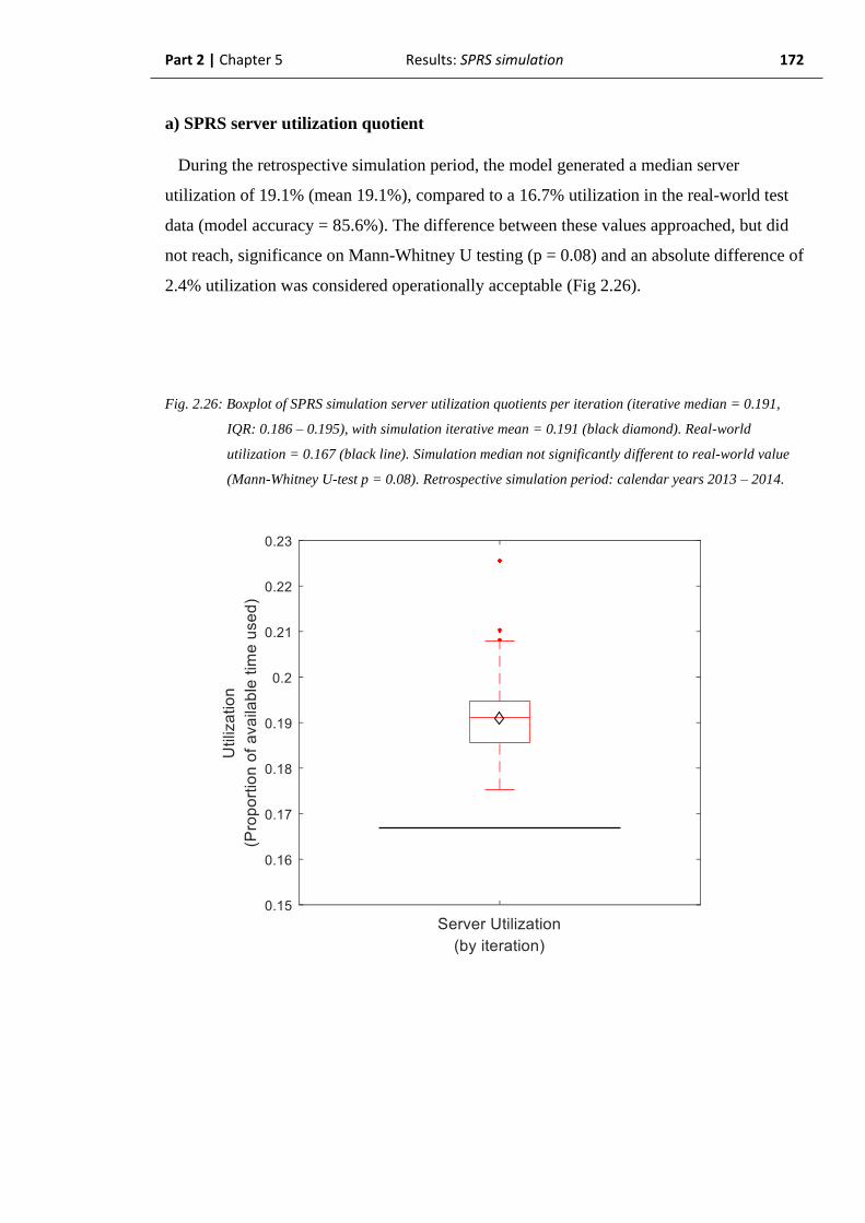
Part 2 | Chapter 5 Results: SPRS simulation 172
a) SPRS server utilization quotient
During the retrospective simulation period, the model generated a median server
utilization of 19.1% (mean 19.1%), compared to a 16.7% utilization in the real-world test
data (model accuracy = 85.6%). The difference between these values approached, but did
not reach, significance on Mann-Whitney U testing (p = 0.08) and an absolute difference of
2.4% utilization was considered operationally acceptable (Fig 2.26).
Fig. 2.26: Boxplot of SPRS simulation server utilization quotients per iteration (iterative median = 0.191,
IQR: 0.186 – 0.195), with simulation iterative mean = 0.191 (black diamond). Real-world
utilization = 0.167 (black line). Simulation median not significantly different to real-world value
(Mann-Whitney U-test p = 0.08). Retrospective simulation period: calendar years 2013 – 2014.
Part 2 | Chapter 5 Results: SPRS simulation 173
b) Summary: SPRS server utilization, retrospective simulation
It was considered that the SPRS model had accurately replicated the real-world server
utilization. This was considered in the context of a 2.4% absolute error which generated an
overall model accuracy of 85.6% and a non-significant Mann-Whitney U-test result. This
was reinforced by the earlier analyses demonstrating successful replication of both the total
number of missions and the mission duration distributions – the two contributors to server
utilization.
Part 2 | Chapter 5 Results: SPRS simulation 174
2.5.1.6. Summary of SPRS retrospective simulation results
The SPRS model is considered to have accurately replicated all the real-world
components studied during the retrospective simulation period. This included the
calculation of a derived value, server utilization.
The results lend validity to the assumption of mathematical similarity between the
components of the model and the corresponding real-world processes. It is therefore
considered that subsequent derived system performance values (e.g. Waiting time in the
queue, Wq) will also be valid in their representation of the real-world during the
retrospective simulation period.

Part 2 | Chapter 5 Results: SPRS simulation 175
2.5.2. Contemporaneous simulation of SPRS operations
In this section, the performance of the SPRS M/G/1 model will be assessed using the
same parameters for a one-year simulation period comprising the calendar year 2015.
In contrast to the previous section, the model will now be assessed in a
“contemporaneous” format. The model, after priming using the data from the retrospective
time period, was only provided with information available prior to the current simulated
time. In this format, the simulation output at any point is its representation of the current
(contemporaneous) state of the system.
For example, an inter-arrival time distribution produced on the 1st July would contain
information from 1st January to 1st July, but not 2nd July to 31st December (all of which
would have been available if the simulation was again run according to the retrospective
format).
However, the ability to repeatedly test all the mission distributions was not available
during this project due to a combination of my relative coding inexperience and a lack of
suitable computing power to undertake such analysis in a reasonable period of time
(including a number of Simulink blocks which did not support hardware acceleration
through parallel processing). As a result, three parameters are not able to be described in a
true, day-by-day, contemporaneous format:
Activation time of day distribution:
The probability of activation by time of day is not described by a specific
distribution or median value. The probability of activation by time of day is therefore
described for the entire simulation period, not daily.
Inter-arrival time distribution:
Despite the relatively high specification of the computer used for running the
simulation, re-fitting of the inter-arrival time distribution and comparing to the real-
world at the end of every day, across one thousand simulation iterations resulted in
an unacceptably long simulation time, to the point of simulation failure. Given that
some period of time is required to sample enough missions to generate a suitable
distribution, the inter-arrival time distribution is described for the entire simulation
period, not daily. However, the inter-arrival distribution μ-vale can be calculated (as
1/λ) from the mission arrival rate (λ) which is simulated and compared daily through
Part 2 | Chapter 5 Results: SPRS simulation 176
the cumulative number of missions. A suitable surrogate marker is therefore
considered to be present.
Mission duration distribution:
Again, despite the seemingly adequate specification of the computer used for
simulation, re-fitting of the mission duration distribution and comparing to the real-
world at the end of every simulated day resulted in an unacceptably long simulation
time, again to the point of simulation failure. However, the iterative median
mission duration could be generated on a daily basis and this is reported
contemporaneously. Only the overall distribution is not analysed.
The purposes of this simulation are fundamentally similar to the retrospective simulation
except that this analysis will aim to demonstrate that the model is capable of describing the
immediate, current state of the SPRS system, effectively in real-time, at any point during
the simulation period.

Part 2 | Chapter 5 Results: SPRS simulation 177
2.5.2.1. Contemporaneous simulation of SPRS mission count
a) Cumulative daily SPRS mission total
The daily cumulative number of real-world missions remained within the 95% prediction
intervals for the simulation through the whole contemporaneous simulation period (Fig.
2.27). This demonstrates that the model median value was able to accurately replicate the
mission numbers at any point in the two-year period.
Fig. 2.27: Cumulative daily mission count by day demonstrating: SPRS simulation iterative median (solid
red line) and 95% prediction intervals of the simulation (dashed red lines). The real-world
cumulative count (black line) is contained within the 95% prediction intervals for the entire
simulation period. Contemporaneous simulation period: calendar year 2015.

Part 2 | Chapter 5 Results: SPRS simulation 178
b) Total number of SPRS missions
At the end of the contemporaneous simulation period, the model simulated an iterative
median of 281 missions (95% Prediction Interval 245 – 314, mean = 279), compared to
287 real-world missions during the same time period (iterative median = 97.9% accurate).
The total number of missions generated was not significantly different to the real-world on
Mann-Whitney U-testing (p = 0.72). (Fig. 2.28).
Fig. 2.28: Boxplot of simulated total mission count (median = 281, IQR: 267 – 291), with simulation mean
(279 missions) marked (black diamond) and real-world value (287 missions) marked (black line).
Difference not significant (Mann-Whitney U-test p = 0.72). Contemporaneous simulation period –
calendar year 2015.

Part 2 | Chapter 5 Results: SPRS simulation 179
c) Empirical Cumulative Distribution Function (ECDF) of number of SPRS missions
by date
The ECDF of the daily cumulative number of missions in the real-world was closely
matched by the iterative median ECDF (Fig. 2.29). The ECDFs were not significantly
different to Kolmogorov-Smirnov testing (K-S test p = 0.95).
Fig. 2.29: ECDF of cumulative daily mission count by date for: SPRS simulation iterative median (red line)
and real-world (black line). Kolmogorov-Smirnov test p = 0.95. Contemporaneous simulation
period: calendar year 2015.
d) Summary: SPRS mission count, contemporaneous simulation
The SPRS model has accurately replicated the daily number of missions, the total
number of missions and the temporal distribution of missions in the contemporaneous
simulation period. It is therefore considered that the SPRS model was able to accurately
replicate the current, contemporaneous total of real-world SPRS missions.

Part 2 | Chapter 5 Results: SPRS simulation 180
2.5.2.2 Contemporaneous simulation of SPRS activation times of
day
As discussed earlier, in the contemporaneous simulation, there was no straightforward
metric by which a progressive daily measurement of the model accuracy could be
undertaken. This analysis assesses the model’s ability to generate an accurate overall
activation time of day distribution at the conclusion of the simulation period. This will be
explored further in the discussion.
a) Probability of SPRS activation by time of day
In the contemporaneous simulation period, activation times of day were grossly similar
in distribution to the real-world. The peak time of simulated activation was the 1100h –
1200h period (Fig. 2.30) compared to two equal peaks at 1300h – 1400h and 1500h –
1600h for the real-world testing data (Fig. 2.31). The median model accuracy by hour of
day was 60.9%.
Fig. 2.30: Normalized probability histogram (area under plot =1) of simulated mission activations by hour of
day. Mode in 1100h – 1200h period. Contemporaneous simulation period: calendar year 2015.
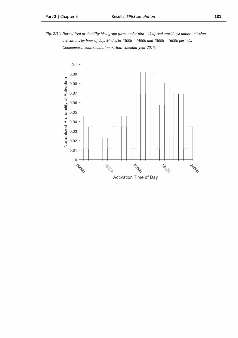
Part 2 | Chapter 5 Results: SPRS simulation 181
Fig. 2.31: Normalized probability histogram (area under plot =1) of real-world test dataset mission
activations by hour of day. Modes in 1300h – 1400h and 1500h – 1600h periods.
Contemporaneous simulation period: calendar year 2015.
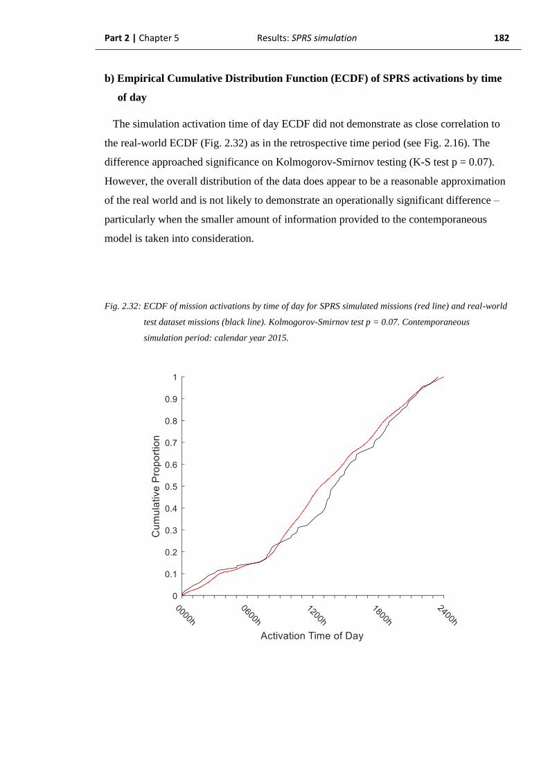
Part 2 | Chapter 5 Results: SPRS simulation 182
b) Empirical Cumulative Distribution Function (ECDF) of SPRS activations by time
of day
The simulation activation time of day ECDF did not demonstrate as close correlation to
the real-world ECDF (Fig. 2.32) as in the retrospective time period (see Fig. 2.16). The
difference approached significance on Kolmogorov-Smirnov testing (K-S test p = 0.07).
However, the overall distribution of the data does appear to be a reasonable approximation
of the real world and is not likely to demonstrate an operationally significant difference –
particularly when the smaller amount of information provided to the contemporaneous
model is taken into consideration.
Fig. 2.32: ECDF of mission activations by time of day for SPRS simulated missions (red line) and real-world
test dataset missions (black line). Kolmogorov-Smirnov test p = 0.07. Contemporaneous
simulation period: calendar year 2015.

Part 2 | Chapter 5 Results: SPRS simulation 183
c) Summary: SPRS activations by time of day, contemporaneous simulation
The analysis demonstrated an overall similar appearance between the simulated mission
activation times of day and the real-world testing data histograms. The model accuracy was
relatively low (60.9%) however, given its sensitivity, the non-significant K-S test result
was strongly reassuring.
As the distributions could not be compared on a daily basis, the comparison has been
made over the entire one year simulation period, but retaining the contemporaneous
simulation methodology. It is therefore considered that the model was able to accurately
replicate the current, contemporaneous real-world activation time of day distribution at the
end of the 2015 calendar year, based on a one-year sampling window.

Part 2 | Chapter 5 Results: SPRS simulation 184
2.5.2.3. Contemporaneous simulation of SPRS inter-arrival times
Similarly to the real-world activation times, repeated fitting of distributions to the
existing data in order to progressively describe an inter-arrival time distribution was too
computationally demanding to permit full investigation in the available time. This analysis
also therefore considers the inter-arrival time distribution through the complete
contemporaneous simulation period.
a) Probability (PDF) of inter-arrival time by hour, SPRS missions
In the contemporaneous simulation period, the model generated an exponential mission
inter-arrival time distribution (see Fig. 2.33) with a fitted exponential distribution μ = 1.30
(95% CI: 1.30-1.31).
The histogram was grossly similar to the real-world testing data (Fig. 2.34) which
demonstrated a fitted exponential distribution μ = 1.26 (95% CI: 1.13 – 1.42). The much
smaller dataset of the real-world data in this time period clearly degrades its quality. The
real-world testing data does, however, appear to maintain an overall exponential
distribution.
The simulation μ-value falls within the 95% confidence interval of the real-world data so
the two distributions are not considered significantly different (Fig. 2.35).

Part 2 | Chapter 5 Results: SPRS simulation 185
Fig. 2.33: Probability density histogram of simulated mission inter-arrival times with one-hour bins. Fitted
exponential distribution with μ = 1.30 (red line). Contemporaneous simulation period: calendar
year 2015.
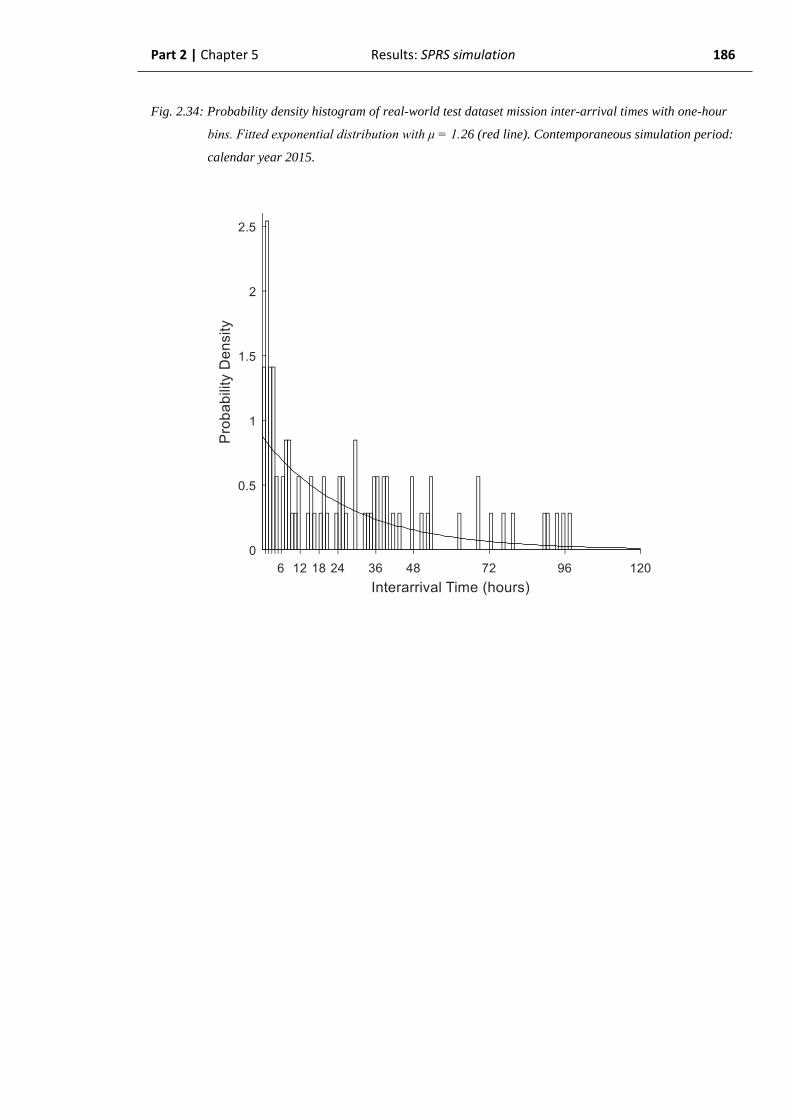
Part 2 | Chapter 5 Results: SPRS simulation 186
Fig. 2.34: Probability density histogram of real-world test dataset mission inter-arrival times with one-hour
bins. Fitted exponential distribution with μ = 1.26 (red line). Contemporaneous simulation period:
calendar year 2015.

Part 2 | Chapter 5 Results: SPRS simulation 187
Fig. 2.35: Fitted exponential probability distribution functions of mission inter-arrival times by hours for
SPRS simulated missions (red line), μ = 1.30 (95% CI: 1.30-1.31) and real-world test dataset
(black line) μ = 1.26 (95% CI: 1.13 – 1.42). Contemporaneous simulation period: calendar year
2015.

Part 2 | Chapter 5 Results: SPRS simulation 188
b) Empirical Cumulative Distribution Function (ECDF) of inter-arrival time by hour,
SPRS missions
On direct comparison of the data, the ECDFs of the simulated and real-world testing data
appeared to relatively closely approximate (Fig 2.36). However, on Kolmogorov-Smirnov
testing, the difference between the data were at the limit of non-significance (K-S test p =
0.05).
Fig. 2.36: ECDFs of mission inter-arrival times by hours for SPRS simulation output (red line) and real-
world (black line). Kolmogorov-Smirnov test p = 0.05. Contemporaneous simulation period:
calendar year 2015.
Part 2 | Chapter 5 Results: SPRS simulation 189
d) Summary: SPRS inter-arrival times, contemporaneous simulation
The analysis demonstrated an overall similar appearance between the simulated mission
inter-arrival times and the real-world testing data histograms, with no significant difference
demonstrated to the fitted exponential distributions or the ECDFs. Although, the difference
between the ECDFs was at the limit of non-significance.
As the distributions could not be compared on a daily basis, the comparison has been
made over the entire one-year simulation period, but retaining the contemporaneous
simulation methodology. It is therefore considered that the model was able to accurately
replicate the current, contemporaneous real-world inter-arrival time at the end of the 2015
calendar year based on a one-year sampling window.
Part 2 | Chapter 5 Results: SPRS simulation 190
2.5.2.4. Contemporaneous simulation of SPRS mission durations
Again, similarly to the inter-arrival times and activation times of day, the mission
durations distribution was only able to be calculated in respect of the entire simulation
period due to the computational requirements. The median mission duration is therefore
used as the daily, contemporaneous descriptor.
a) Progressive values of SPRS median mission duration by date
In the contemporaneous simulation period, the simulation output median mission
duration, after some initial volatility, remained relatively steady throughout the simulation
period, demonstrating a maximum of 6h 26m in May, then falling gradually to a final value
of 6h 21m (Fig. 2.37).
After initial volatility, the real-world test dataset median mission duration remained
relatively steady with a minimum of 3h 27m at the end of June. After this, the real-world
median rose in sequential steps to a final value of 4h 57m (Fig. 2.37). The real-world test
dataset median duration was outside the 95% prediction interval of the simulation
throughout the studied time period, other than a brief period during January. This coincides
with the most volatility in the real-world calculation and any assumption of similarity is
likely to represent a type 2 error.

Part 2 | Chapter 5 Results: SPRS simulation 191
Fig. 2.37: Median SPRS mission durations by day, comparing simulation iterative median (solid red line)
and 95% prediction intervals (dashed red lines) to the real-world test dataset median duration
(black line). Contemporaneous simulation period: calendar year 2015.

Part 2 | Chapter 5 Results: SPRS simulation 192
b) Median mission durations: final values
At the conclusion of the contemporaneous simulation period, the simulation output
demonstrated an iterative median of current median mission duration of 6h 21m (95%
Prediction Interval: 6h 00m – 6h 36m, mean = 6h 34m), compared to a real-world testing
data median mission duration of 4h 57m (model accuracy = 71.7%) (Fig. 2.38). The
medians were significantly different on Mann-Whitney U-testing (p < 0.001).
Fig. 2.38: Boxplot of final value of median mission duration by iteration at conclusion of contemporaneous
simulation period (median = 6h 21m, IQR 6h 15m – 6h 34m), with iterative mean = 6h 34m (black
diamond) and real-world testing data median = 4h 57m (black line). Iterative median and real-
world testing data median mission durations are significantly different (Mann-Whitney U-test p <
0.001). Contemporaneous simulation period: calendar year 2015.
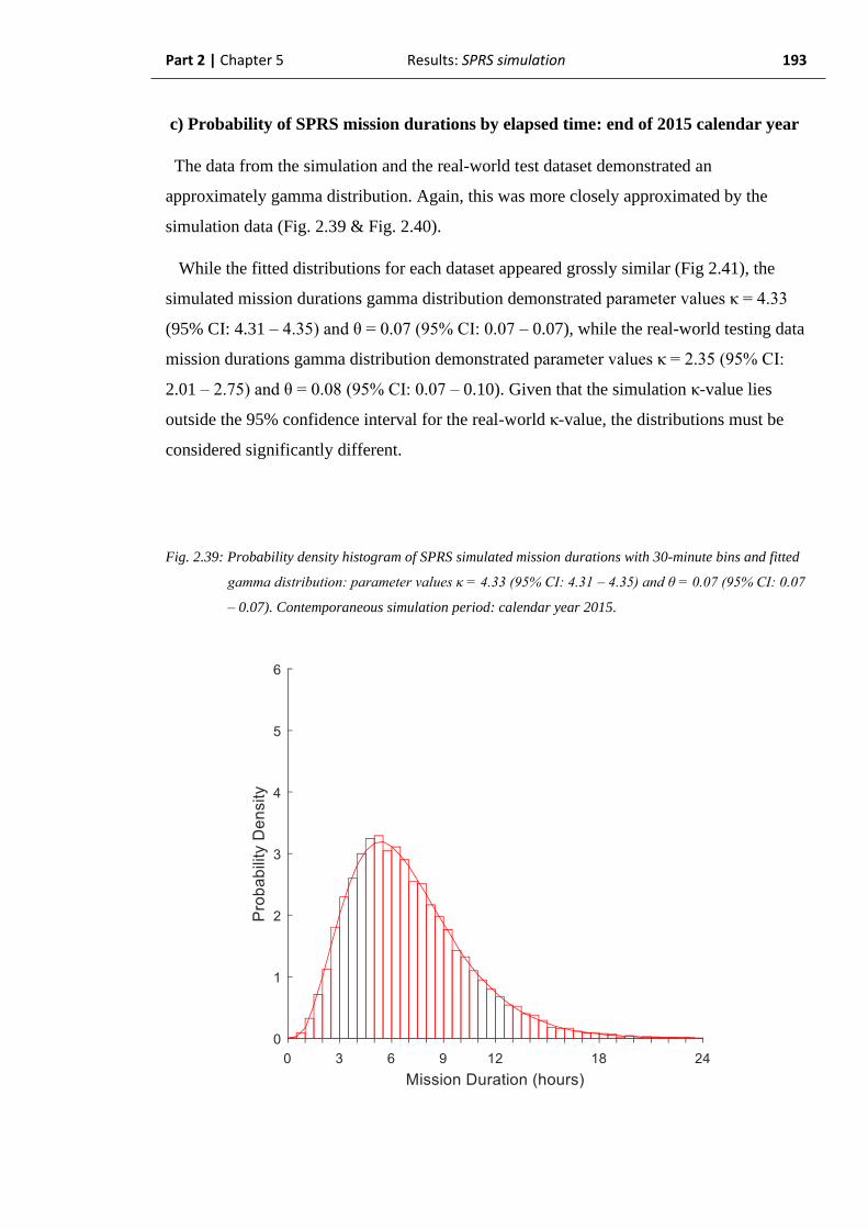
Part 2 | Chapter 5 Results: SPRS simulation 193
c) Probability of SPRS mission durations by elapsed time: end of 2015 calendar year
The data from the simulation and the real-world test dataset demonstrated an
approximately gamma distribution. Again, this was more closely approximated by the
simulation data (Fig. 2.39 & Fig. 2.40).
While the fitted distributions for each dataset appeared grossly similar (Fig 2.41), the
simulated mission durations gamma distribution demonstrated parameter values κ = 4.33
(95% CI: 4.31 – 4.35) and θ = 0.07 (95% CI: 0.07 – 0.07), while the real-world testing data
mission durations gamma distribution demonstrated parameter values κ = 2.35 (95% CI:
2.01 – 2.75) and θ = 0.08 (95% CI: 0.07 – 0.10). Given that the simulation κ-value lies
outside the 95% confidence interval for the real-world κ-value, the distributions must be
considered significantly different.
Fig. 2.39: Probability density histogram of SPRS simulated mission durations with 30-minute bins and fitted
gamma distribution: parameter values κ = 4.33 (95% CI: 4.31 – 4.35) and θ = 0.07 (95% CI: 0.07
– 0.07). Contemporaneous simulation period: calendar year 2015.
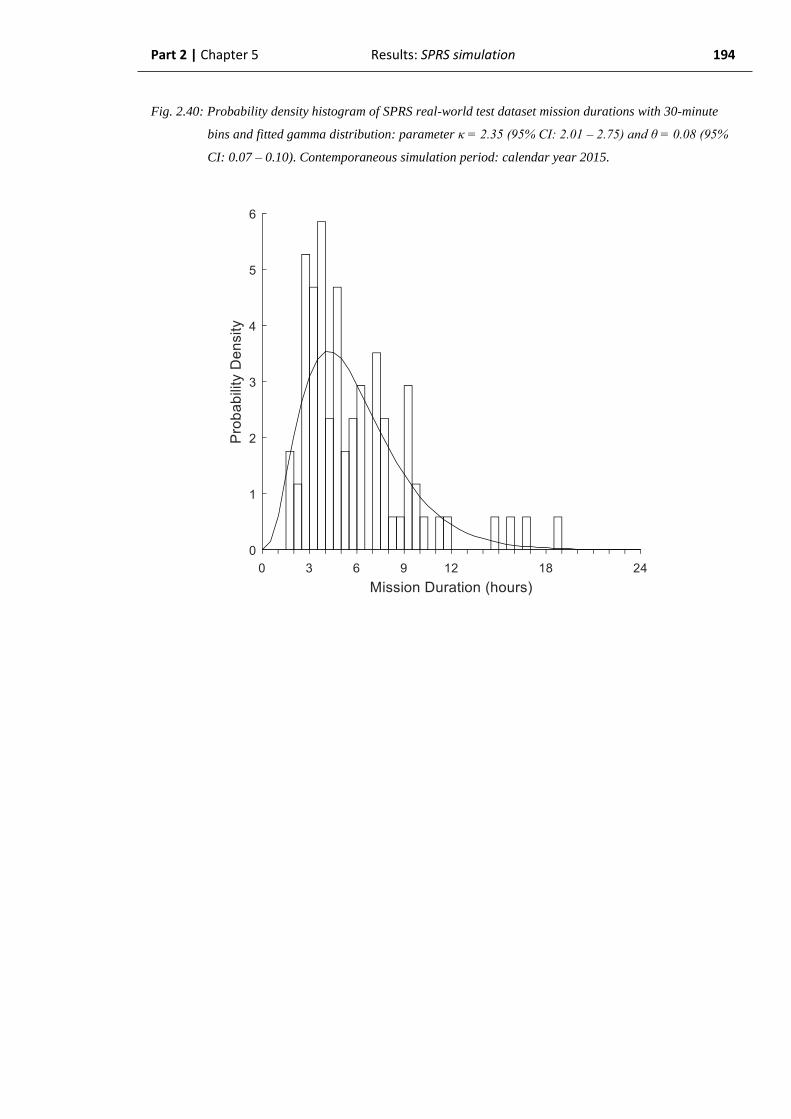
Part 2 | Chapter 5 Results: SPRS simulation 194
Fig. 2.40: Probability density histogram of SPRS real-world test dataset mission durations with 30-minute
bins and fitted gamma distribution: parameter κ = 2.35 (95% CI: 2.01 – 2.75) and θ = 0.08 (95%
CI: 0.07 – 0.10). Contemporaneous simulation period: calendar year 2015.
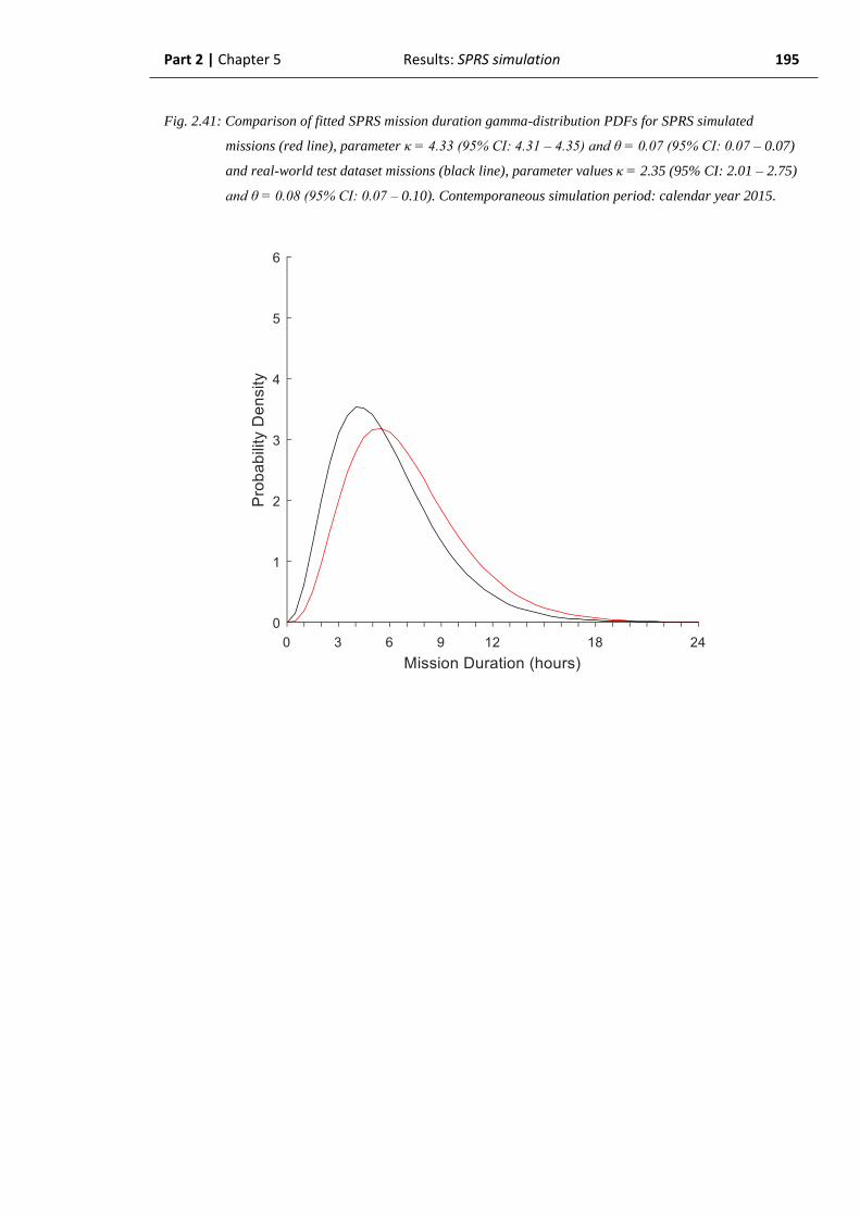
Part 2 | Chapter 5 Results: SPRS simulation 195
Fig. 2.41: Comparison of fitted SPRS mission duration gamma-distribution PDFs for SPRS simulated
missions (red line), parameter κ = 4.33 (95% CI: 4.31 – 4.35) and θ = 0.07 (95% CI: 0.07 – 0.07)
and real-world test dataset missions (black line), parameter values κ = 2.35 (95% CI: 2.01 – 2.75)
and θ = 0.08 (95% CI: 0.07 – 0.10). Contemporaneous simulation period: calendar year 2015.
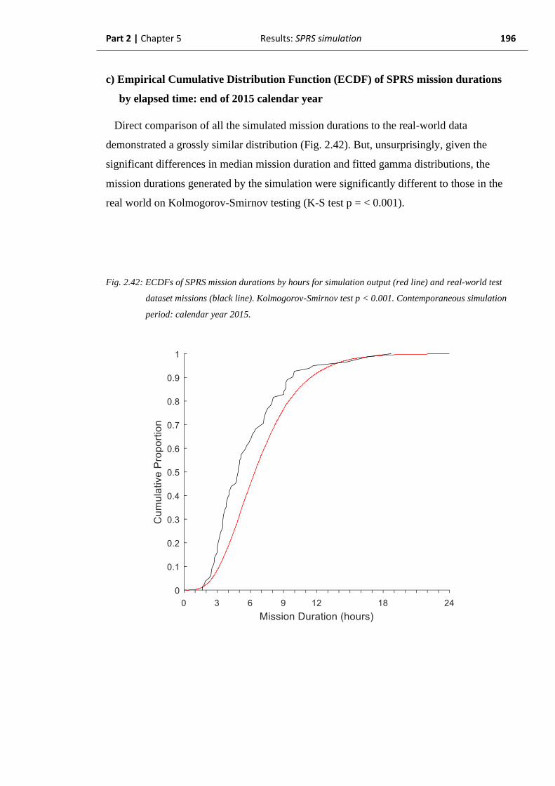
Part 2 | Chapter 5 Results: SPRS simulation 196
c) Empirical Cumulative Distribution Function (ECDF) of SPRS mission durations
by elapsed time: end of 2015 calendar year
Direct comparison of all the simulated mission durations to the real-world data
demonstrated a grossly similar distribution (Fig. 2.42). But, unsurprisingly, given the
significant differences in median mission duration and fitted gamma distributions, the
mission durations generated by the simulation were significantly different to those in the
real world on Kolmogorov-Smirnov testing (K-S test p = < 0.001).
Fig. 2.42: ECDFs of SPRS mission durations by hours for simulation output (red line) and real-world test
dataset missions (black line). Kolmogorov-Smirnov test p < 0.001. Contemporaneous simulation
period: calendar year 2015.
Part 2 | Chapter 5 Results: SPRS simulation 197
d) Summary: SPRS mission durations, contemporaneous simulation period
The daily progressive real-world testing data median mission duration was outside the
95% prediction interval of the simulation output for almost the entirety of the simulation
period (see Fig. 2.37), with the duration values at the end of the 2015 calendar year also
being significantly different. Furthermore, the fitted gamma distributions were
significantly different, as were the overall mission duration ECDFs.
It is therefore considered that the SPRS model was unable to accurately replicate the
contemporaneous mission durations of the real-world system at any point in the 2015
calendar year.
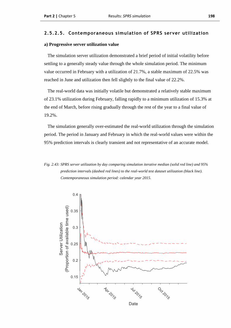
Part 2 | Chapter 5 Results: SPRS simulation 198
2.5.2.5. Contemporaneous simulation of SPRS server utilization
a) Progressive server utilization value
The simulation server utilization demonstrated a brief period of initial volatility before
settling to a generally steady value through the whole simulation period. The minimum
value occurred in February with a utilization of 21.7%, a stable maximum of 22.5% was
reached in June and utilization then fell slightly to the final value of 22.2%.
The real-world data was initially volatile but demonstrated a relatively stable maximum
of 23.1% utilization during February, falling rapidly to a minimum utilization of 15.3% at
the end of March, before rising gradually through the rest of the year to a final value of
19.2%.
The simulation generally over-estimated the real-world utilization through the simulation
period. The period in January and February in which the real-world values were within the
95% prediction intervals is clearly transient and not representative of an accurate model.
Fig. 2.43: SPRS server utilization by day comparing simulation iterative median (solid red line) and 95%
prediction intervals (dashed red lines) to the real-world test dataset utilization (black line).
Contemporaneous simulation period: calendar year 2015.
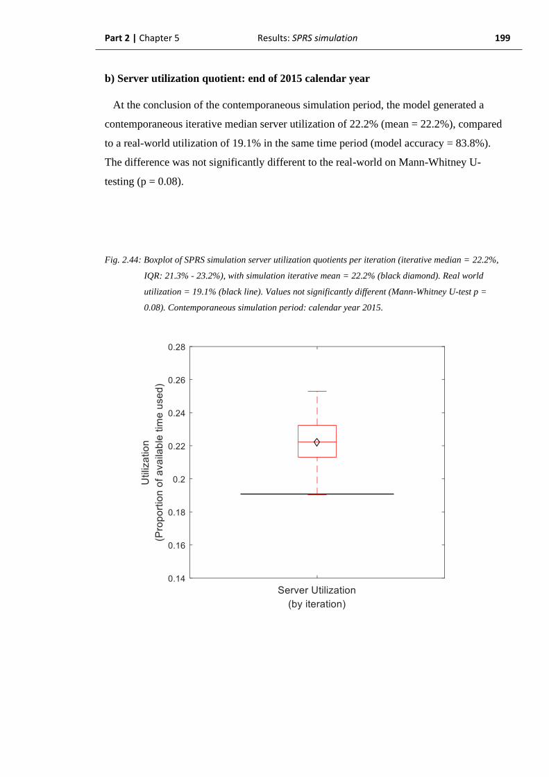
Part 2 | Chapter 5 Results: SPRS simulation 199
b) Server utilization quotient: end of 2015 calendar year
At the conclusion of the contemporaneous simulation period, the model generated a
contemporaneous iterative median server utilization of 22.2% (mean = 22.2%), compared
to a real-world utilization of 19.1% in the same time period (model accuracy = 83.8%).
The difference was not significantly different to the real-world on Mann-Whitney U-
testing (p = 0.08).
Fig. 2.44: Boxplot of SPRS simulation server utilization quotients per iteration (iterative median = 22.2%,
IQR: 21.3% - 23.2%), with simulation iterative mean = 22.2% (black diamond). Real world
utilization = 19.1% (black line). Values not significantly different (Mann-Whitney U-test p =
0.08). Contemporaneous simulation period: calendar year 2015.
Part 2 | Chapter 5 Results: SPRS simulation 200
c) Summary: SPRS server utilization, contemporaneous simulation
The daily progressive real-world SPRS server utilization lay outside the 95% prediction
interval of the model for the majority of the contemporaneous simulation period. It is
therefore considered that the model could not accurately replicate the contemporaneous
utilization of the real-world system at all times through the 2015 calendar year.
At the conclusion of the 2015 calendar year, the median simulation output of server
utilization had an accuracy of 83.8% and was not significantly different to the real world.
The model over-estimated the real-world utilization which is likely to result in derived
values reflecting poorer performance than is true in the real-world (a “worst-case
scenario”) which still is able to provide useful performance information. It is therefore
considered that the model potentially could generate an operationally acceptable
replication of the contemporaneous real-world server utilization based on a one-year
sampling window at the end of the 2015 calendar year.

Part 2 | Chapter 5 Results: SPRS simulation 201
2.5.2.6. Contemporaneous simulation of SPRS team - summary
The model was able to accurately replicate the current, contemporaneous real-world state
of the SPRS system at any time during the 2015 calendar year with regard to the number of
missions and arrival rate (λ).
The model was able to accurately replicate the current, contemporaneous distribution of
activation time of day and inter-arrival time at the end of the 2015 calendar year, based on
a one-year sampling window.
The model was able to able to replicate the current, contemporaneous value of server
utilization at the end of the 2015 calendar year, based on a one-year sampling window to
an operationally useful standard. However, the model failed to replicate the progressive
contemporaneous value of the server utilization at all times through the simulation period.
The model did not replicate the real-world mission durations, either as final median value
or by progressive value at all points in the 2015 calendar year.

Part 2 | Chapter 5 Results: SPRS simulation 202
2.5.3. Summary of results from simulations of SPRS
operations
The simulation of the SPRS missions successfully replicated all components of the
system in the retrospective simulation period when the simulation was provided with the
full data for the entire simulation period (Table 2.2). The model can be considered to be an
accurate representation of the real-world SPRS system under retrospective simulation
conditions, demonstrating a mean component accuracy of 91.0%. In this capacity, it is able
to provide a general overview of the system representative of the entire studied time
period. In doing so, it has demonstrated the validity of the assumed mathematical
relationships between the real-world components.
The contemporaneous simulation was able to partially replicate the current,
contemporaneous state of the real-world (Table 2.3). The mean component accuracy for
the contemporaneous simulation was 82.2%. For server utilization it was able to replicate
the real-world only equivocally with a final utilization value, representing a one-year
sampling window. Given that this was an over-estimate then there may still be some utility
in subsequent derived values because the real-world performance could be expected to be
better than the model’s prediction. The model did not, however, accurately replicate the
real-world mission durations at any point during the contemporaneous simulation.

Part 2 | Chapter 5 Results: SPRS simulation 203
Table 2.2: Summary of SPRS retrospective simulation results:
Parameter Model value Real-world
value Accuracy
Statistical
similarity
Operational
similarity
Number of SPRS missions 477 486 98.1% Yes Yes
Activation time of day - - 73.3% Yes Yes
Inter-arrival times μ = 1.52 μ = 1.50 98.7% Yes Yes
Mission durations 6h 25m 6h 23 99.5% Yes Yes
Server utilization 19.1% 16.7% 85.6% Yes Yes

Part 2 | Chapter 5 Results: SPRS simulation 204
Table 2.3: Summary of SPRS contemporaneous simulation results:
Parameter Model
value
Real-world
value Accuracy
Statistical
similarity
Operational
similarity
Number of SPRS missions 281 287 97.9% Yes Yes
Activation time of day - - 60.9% Yes Yes
Inter-arrival times μ = 1.30 μ = 1.26 96.8% Yes Yes
Mission durations 6h 21m 4h 57m 71.7% No No
Server utilization 22.2% 19.1% 83.8% Yes No
Part 2 Chapter 6
Results:
Simulation of EMRS operations
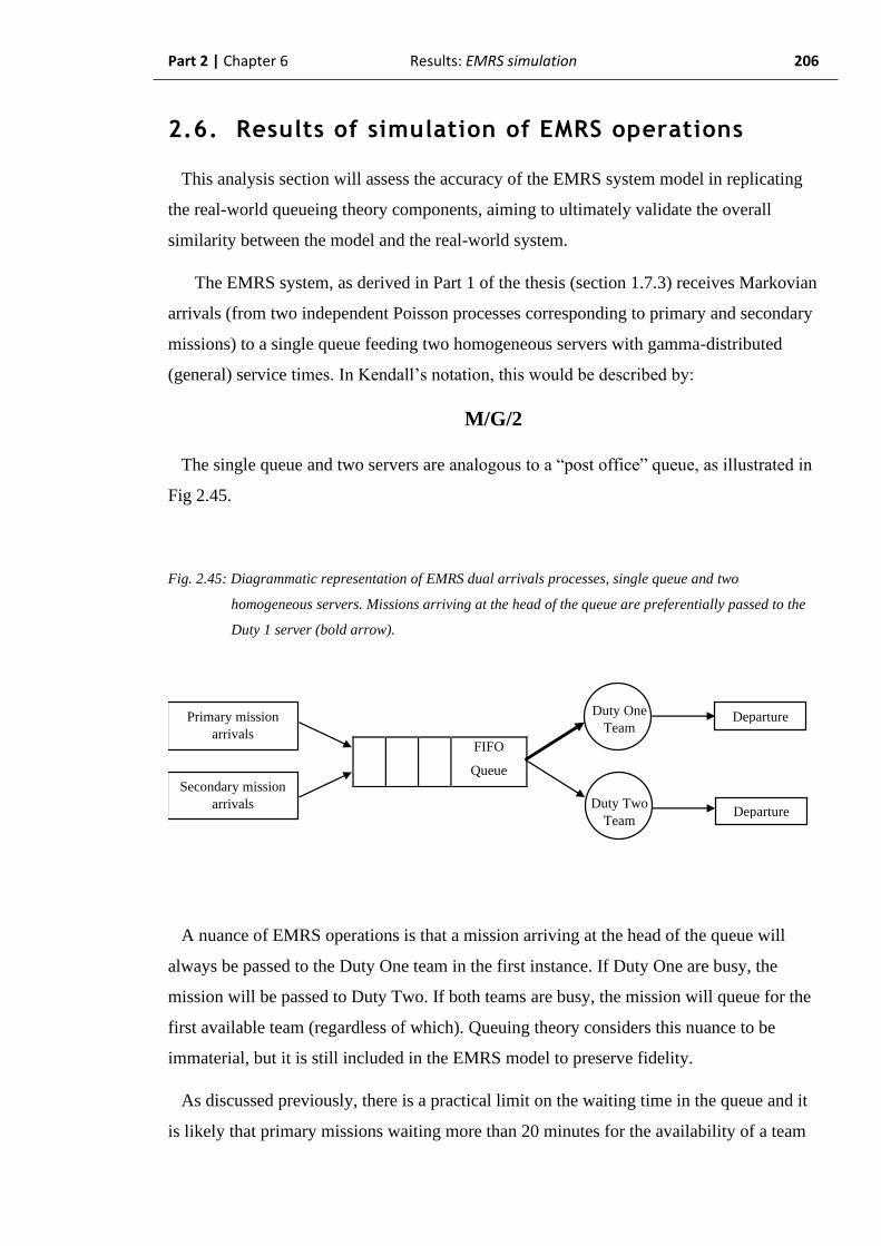
Part 2 | Chapter 6 Results: EMRS simulation 206
2.6. Results of simulation of EMRS operations
This analysis section will assess the accuracy of the EMRS system model in replicating
the real-world queueing theory components, aiming to ultimately validate the overall
similarity between the model and the real-world system.
The EMRS system, as derived in Part 1 of the thesis (section 1.7.3) receives Markovian
arrivals (from two independent Poisson processes corresponding to primary and secondary
missions) to a single queue feeding two homogeneous servers with gamma-distributed
(general) service times. In Kendall’s notation, this would be described by:
M/G/2
The single queue and two servers are analogous to a “post office” queue, as illustrated in
Fig 2.45.
Fig. 2.45: Diagrammatic representation of EMRS dual arrivals processes, single queue and two
homogeneous servers. Missions arriving at the head of the queue are preferentially passed to the
Duty 1 server (bold arrow).
A nuance of EMRS operations is that a mission arriving at the head of the queue will
always be passed to the Duty One team in the first instance. If Duty One are busy, the
mission will be passed to Duty Two. If both teams are busy, the mission will queue for the
first available team (regardless of which). Queuing theory considers this nuance to be
immaterial, but it is still included in the EMRS model to preserve fidelity.
As discussed previously, there is a practical limit on the waiting time in the queue and it
is likely that primary missions waiting more than 20 minutes for the availability of a team
FIFO
Queue
FIFO
Queue
SPRS
Team Arrivals Departure SPRS
Team
Primary mission
arrivals
SPRS
Team
Secondary mission
arrivals
Departure Duty One
Team
Duty Two
Team Departure

Part 2 | Chapter 6 Results: EMRS simulation 207
will be reneged from the system. As these missions never appear to exist to EMRS, then
they are not included in the EMRS data. As the model relies upon the EMRS data, and
therefore only recognises missions actually undertaken by the servers, it is not appropriate
to include reneging of primary missions in the Simulink model without data to support it.
The analysis of this model will, as with SPRS, compare several queueing theory
components to their real-world equivalents:
For EMRS secondary and primary missions:
- Overall number of missions (including cumulative number and pattern).
- Activation time of day.
- Inter-arrival time.
- Mission duration.
For the whole EMRS system, as well as for individual duty one and duty two teams:
- Server utilization.
As previously, the EMRS system will also be undertaken in two simulation periods:
Retrospective simulation: comprising calendar years 2013-2014. This model is
provided with the most information and creates a generalised description of the
model and system over the entire two-year time period.
Contemporaneous simulation: comprising calendar year 2015. This model is provided
with priming data from the retrospective simulation and then receives new
information for the 2015 calendar year up to the current simulation point only,
thereby describing the contemporaneous state of the model and system (where
able). It has the same limitations with regard to demonstrating distributions for
inter-arrival times, activation times of day and mission durations as the SPRS
simulation (see section 2.5.2).
Further information on particular aspects of each simulation period will be discussed in
more detail in the relevant chapters.
Overall, one thousand iterations of the EMRS simulation were performed in a single
simulation run, representing the calendar years 2013 – 2016. The median simulation time
was 14.85 seconds and the simulation was completed in a total of 5h 19m.

Part 2 | Chapter 6 Results: EMRS simulation 208
The principal purpose of EMRS is to provide equity of access to healthcare through
secondary transfer of patients in remote and rural healthcare facilities requiring critical
care. Note that, as a result, secondary missions are given precedence within each EMRS
analysis section.
Part 2 | Chapter 6 Results: EMRS simulation 209
2.6.1 Retrospective simulation of EMRS operations
In this section, the performance of the EMRS model for each of the state parameters is
considered in a two-year simulation period comprising the calendar years 2013 and 2014.
In the retrospective simulation period, the EMRS model is provided with the full dataset
comprising the entire simulation period of calendar years 2013 and 2014 upon which to
generate the required parameters. As a result, the model output will be a representation of
the general system state over the entire time period.
As with the SPRS retrospective analysis, the purpose of this simulation is to:
1. Demonstrate that the model does not mutilate the data.
2. Prime the model with a working dataset prior to a reduction in the available data for
the contemporaneous simulation period.
3. Demonstrate the validity of the mathematical relationships between individual
components of the real-world system by showing that the same mathematical
relationships within the model produce the same data values as are generated in the
real-world.
Again, it should be noted that the analysis time period is different to that of the EMRS
analyses in Part 1 (section 1.7.2) and the values are therefore expected to be different. The
overall distributions are expected to remain similar, however.
2.6.1.1 Retrospective simulation of EMRS mission count
Each of the primary and secondary mission profiles for EMRS individually have been
shown to follow a Markovian arrival pattern. Being able to replicate the correct number of
missions undertaken by EMRS is an important basic descriptor of the system operations,
and the first step in generating an accurate inter-arrival time distribution for missions.
In this section, the ability of the simulation to create the correct number of mission
activations will be analysed for the EMRS model. As the two mission types occur
independently of each other, they will be analysed separately.
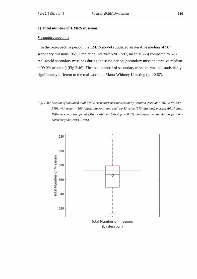
Part 2 | Chapter 6 Results: EMRS simulation 210
a) Total number of EMRS missions
Secondary missions
In the retrospective period, the EMRS model simulated an iterative median of 567
secondary missions (95% Prediction Interval: 520 – 597, mean = 566) compared to 573
real-world secondary missions during the same period (secondary mission iterative median
= 99.0% accurate) (Fig 2.46). The total number of secondary missions was not statistically
significantly different to the real-world on Mann-Whitney U testing (p = 0.67).
Fig. 2.46: Boxplot of simulated total EMRS secondary missions count by iteration (median = 567, IQR: 549 –
579), with mean = 566 (black diamond) and real-world value (573 missions) marked (black line).
Difference not significant (Mann-Whitney U-test p = 0.67). Retrospective simulation period –
calendar years 2013 – 2014.

Part 2 | Chapter 6 Results: EMRS simulation 211
Primary missions
In the same simulation, the model generated an iterative median of 907 primary missions
(95% Prediction Interval: 856 – 992) compared to 912 real-world primary missions during
the same time period (primary mission model = 99.5% accurate) (Fig 2.47). The total
number of primary missions generated was not statistically significantly different to the
real-world on Mann-Whitney U testing. (p = 0.79).
Fig. 2.47: Boxplot of simulated total EMRS primary missions count by iteration (median = 907, IQR: 887 –
928), with mean = 908 (black diamond) and real-world value (912 missions) marked (black line).
Difference not significant (Mann-Whitney U-test p = 0.79). Retrospective simulation period –
calendar years 2013 – 2014.

Part 2 | Chapter 6 Results: EMRS simulation 212
b) Cumulative daily EMRS mission total
The cumulative daily number of missions in the real-world were closely matched by their
respective iterative median for both primary and secondary missions (Fig. 2.48 & Fig.
2.49). The median cumulative number of missions remained within the 95% prediction
intervals for both components of the simulation throughout the entire retrospective analysis
period. This was particularly relevant for the primary missions where the seasonal
variation is visible as the cyclical variation in gradient of each line.
Fig. 2.48: Cumulative EMRS secondary mission count by day demonstrating: simulation iterative median
(solid red line) and 95% prediction intervals of simulation (dashed red lines). The real-world
cumulative count (black line) is contained within the bounds set by the 95% prediction intervals for
the entire time-period. Retrospective simulation period: calendar years 2013 – 2014.

Part 2 | Chapter 6 Results: EMRS simulation 213
Fig. 2.49: Cumulative EMRS primary mission count by day demonstrating: simulation iterative median (solid
red line) and 95% prediction intervals of simulation (dashed red lines). The real-world cumulative
count (black line) is contained within the bounds set by the 95% prediction intervals for the entire
time-period. Retrospective simulation period: calendar years 2013 – 2014.
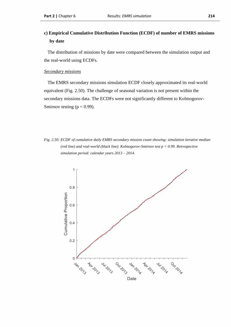
Part 2 | Chapter 6 Results: EMRS simulation 214
c) Empirical Cumulative Distribution Function (ECDF) of number of EMRS missions
by date
The distribution of missions by date were compared between the simulation output and
the real-world using ECDFs.
Secondary missions
The EMRS secondary missions simulation ECDF closely approximated its real-world
equivalent (Fig. 2.50). The challenge of seasonal variation is not present within the
secondary missions data. The ECDFs were not significantly different to Kolmogorov-
Smirnov testing (p = 0.99).
Fig. 2.50: ECDF of cumulative daily EMRS secondary mission count showing: simulation iterative median
(red line) and real-world (black line). Kolmogorov-Smirnov test p = 0.99. Retrospective
simulation period: calendar years 2013 – 2014.

Part 2 | Chapter 6 Results: EMRS simulation 215
Primary missions
The primary missions simulation ECDF also appeared to closely match the real-world
ECDF (Fig. 2.51), including the seasonal variation through the time period. The ECDFs
were not significantly different on Kolmogorov-Smirnov testing (p = 0.98).
Fig. 2.51: ECDF of cumulative daily EMRS primary mission count showing: simulation iterative median (red
line) and real-world (black line). Kolmogorov-Smirnov test p = 0.97. Retrospective simulation
period: calendar years 2013 – 2014.
d) Summary: EMRS number of missions, retrospective simulation
When provided with the entirety of the dataset for the studied time period, the EMRS
model was able to replicate the real-world for both secondary retrieval and primary pre-
hospital missions with respect to total number of missions, cumulative daily number of
missions and distribution of missions through the studied time period. It is therefore
considered that the arrival rate (λ) of missions is accurate and that this should confer an
accurate μ-value (as 1/λ) for the base exponential inter-arrival distribution.
Part 2 | Chapter 6 Results: EMRS simulation 216
2.6.1.2. Retrospective simulation of EMRS activation times of day
The overall validity of the λ value for the EMRS Poisson distribution has been
demonstrated by correctly producing the real-world number of missions both in total and
by month. However, as with the other services, it is generally known that demand for the
service varies through the course of the day. It will be critical to the future calculation of
system performance parameters such as simultaneous retrievals that the time of arrivals is
also calculated. This is particularly the case for the EMRS primary mission demand
because this service is only provided (with exceptions for major incidents or specific
clinician requests) in the 0800h – 1800h time period. Almost all the missions must
therefore be generated in the same 0800h – 1800h period if any meaningful deductions are
to be made concerning the performance of the system. It is expected that compression of
missions into this short time period will have an effect on the number of simultaneous
retrieval requests.
In this analysis section, the ability of the model to replicate the time-varying demand for
each mission type will be assessed. Each of the mission types are independent and so are
analysed separately against the corresponding real-world testing dataset.

Part 2 | Chapter 6 Results: EMRS simulation 217
a) Probability of EMRS activation by time of day
Secondary missions
In the retrospective simulation period, activation times of day for secondary missions
(Fig. 2.52) were grossly similar in distribution to the real world (Fig. 2.53). Activations
peaked in the 1000h-1100h period, compared to 1300h-1400h in the real-world. Both
simulation output and real-world data demonstrated an overall peak around late morning
and midday, with a gradual reduction in demand through the rest of the day, and lowest
demand in the overnight period. The median model accuracy was 77.9%
Fig. 2.52: Normalized probability histogram (area under plot = 1) of simulated EMRS secondary mission
activations by hour of day. Mode in 1000h – 1100h period. Retrospective simulation period:
calendar years 2013 – 2014.

Part 2 | Chapter 6 Results: EMRS simulation 218
Fig. 2.53: Normalized probability histogram (area under plot = 1) of real-world test dataset EMRS
secondary mission activations by hour of day. Mode in 1300h – 1400h period. Retrospective
simulation period: calendar years 2013 – 2014.

Part 2 | Chapter 6 Results: EMRS simulation 219
Primary missions
The maximum probability of simulated primary mission activations occurred in two
peaks at 1200h-1300h and 1500h-1600h (Fig. 2.54), compared to 1300h-1400h in the real-
world testing data (Fig 2.55). The missions demonstrated a clear increase in activations
correlating with the commencement of the service provision period and a clear decrease
following the cessation of services at 1800h. The morning commencement of demand did
start slightly earlier in the simulation output, corresponding with the 0700h-0800h period,
as opposed to the 0800h-0900h period for the real-world data. The median accuracy of the
prediction by hour of the day was 84.2%.
Fig. 2.54: Normalized probability histogram (area under plot = 1) of simulated EMRS primary mission
activations by hour of day. Mode in 1300h – 1400h period. Retrospective simulation period:
calendar years 2013 – 2014.
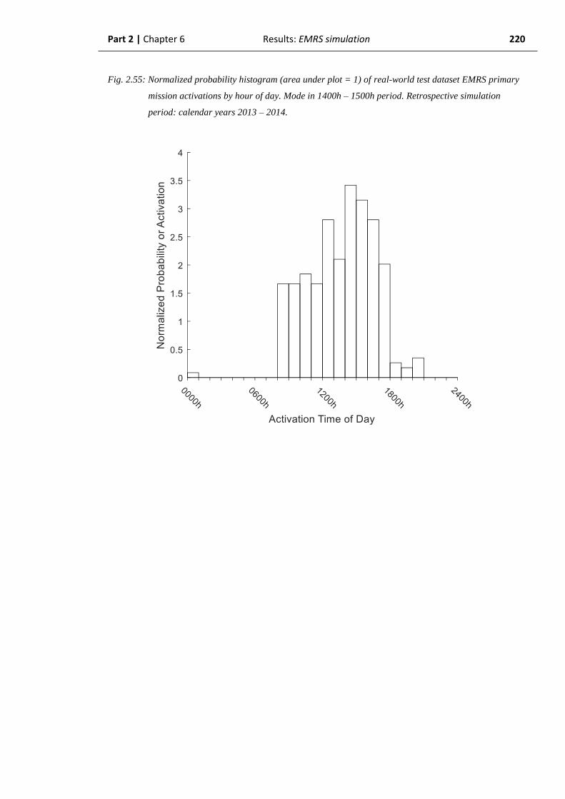
Part 2 | Chapter 6 Results: EMRS simulation 220
Fig. 2.55: Normalized probability histogram (area under plot = 1) of real-world test dataset EMRS primary
mission activations by hour of day. Mode in 1400h – 1500h period. Retrospective simulation
period: calendar years 2013 – 2014.

Part 2 | Chapter 6 Results: EMRS simulation 221
b) Empirical Cumulative Distribution Function (ECDF) of EMRS activations by time
of day
Secondary missions
Simulated EMRS secondary missions demonstrated a curve which approximated the
real-world testing dataset (Fig. 2.56). The earlier peak of secondary missions demonstrated
by the simulation output is evident in the somewhat higher proportion of simulation
missions in the 0800h-1400h period. The difference between these ECDFs was at the limit
of non-significance on Kolmogorov-Smirnov testing (p = 0.05).
Fig. 2.56: ECDFs of EMRS secondary mission activations by time of day for simulation output (red line) and
real-world test dataset (black line). Kolmogorov-Smirnov test p = 0.05. Retrospective simulation
period: calendar years 2013 – 2014.
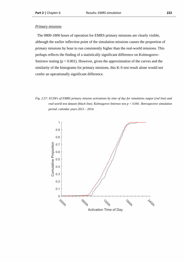
Part 2 | Chapter 6 Results: EMRS simulation 222
Primary missions
The 0800-1800 hours of operation for EMRS primary missions are clearly visible,
although the earlier inflection point of the simulation missions causes the proportion of
primary missions by hour to run consistently higher than the real-world missions. This
perhaps reflects the finding of a statistically significant difference on Kolmogorov-
Smirnov testing (p < 0.001). However, given the approximation of the curves and the
similarity of the histograms for primary missions, this K-S test result alone would not
confer an operationally significant difference.
Fig. 2.57: ECDFs of EMRS primary mission activations by time of day for simulation output (red line) and
real-world test dataset (black line). Kolmogorov-Smirnov test p < 0.001. Retrospective simulation
period: calendar years 2013 – 2014.

Part 2 | Chapter 6 Results: EMRS simulation 223
c) Summary: EMRS activations by time of day, retrospective simulation
This analysis would suggest that the model was able to accurately replicate the real-
world activation time of day for both primary and secondary EMRS missions in the
retrospective simulation period. One K-S test result, that of the EMRS primary mission
activations, is statistically significant but the difference is not considered operationally
significant. The K-S test result may be related to the limitations of applying the test to a
relatively large dataset, but with only a small effective range of values which contribute to
the ECDF.
Part 2 | Chapter 6 Results: EMRS simulation 224
2.6.1.3. Retrospective simulation of EMRS inter-arrival times
The combination of the EMRS components so far analysed are combined when the inter-
arrival rate (λ) is modified by the time-varying demand for the service into a time-
dependent Poisson process. Whereas a uniform Poisson process would generate purely
exponentially-distributed inter-arrival times, the time-dependent Poisson process is
expected to generate an overall exponential distribution of the inter-arrival times with a
multi-modal component, as demonstrated in section 1.6.3.
This section assesses the ability of the model to accurately replicate the inter-arrival times
of each mission type to the EMRS system. These independent components will be analysed
separately and compare simulation output to a testing dataset of the real-world data.
a) Probability (PDF) of inter-arrival time by hour, EMRS missions
Secondary missions
In the retrospective simulation period, the simulated EMRS secondary missions (Fig.
2.58) and real-world testing dataset secondary missions (Fig. 2.59) displayed inter-arrival
times with an overall approximately exponential distribution). Secondary missions exhibit
a subtle multi-modal inter-arrival time distribution, consistent with a time-dependent
Poisson process. This can be seen more clearly in the simulation output data.
Comparison of the fitted exponential distributions demonstrated a close approximation
between the simulation and real-world testing data (Fig. 2.60). Simulated EMRS secondary
missions demonstrated an exponential distribution μ = 1.28 (95% CI: 1.28-1.29), compared
to a real-world testing data μ = 1.24 (95% CI: 1.15 – 1.35). As the simulation μ-value was
contained within the confidence intervals of the real-world data, they would not be
considered significantly different. Comparing the μ-values, model accuracy was 96.7%

Part 2 | Chapter 6 Results: EMRS simulation 225
Fig. 2.58: Probability density histogram of simulated EMRS secondary mission inter-arrival times with one-
hour bins. Fitted exponential distribution μ = 1.28 (red line). Retrospective simulation period:
calendar years 2013 – 2014.

Part 2 | Chapter 6 Results: EMRS simulation 226
Fig. 2.59: Probability density histogram of real-world test dataset EMRS secondary mission inter-arrival
times with one-hour bins. Fitted exponential distribution μ = 1.24 (black line). Retrospective
simulation period: calendar years 2013 – 2014.

Part 2 | Chapter 6 Results: EMRS simulation 227
Fig. 2.60: Comparison of fitted exponential probability distribution functions of EMRS secondary mission
inter-arrival times by hour for: simulated missions (red line), μ = 1.28 (95% CI: 1.28-1.29) and
real-world test dataset missions (black line), data μ = 1.24 (95% CI: 1.15 – 1.35). Retrospective
simulation period: calendar years 2013 – 2014.

Part 2 | Chapter 6 Results: EMRS simulation 228
Primary missions
EMRS operates a primary mission service between 0800-1800 resulting in strongly time-
varying demand which generates a clear multi-modal inter-arrival time distribution (Fig
2.61). The simulation output generated an inter-arrival time histogram which appeared
generally similar to the real-world (Fig. 2.62).
The fitted exponential distributions for simulated EMRS primary missions appeared to
closely approximate the real-world fitted distribution (Fig 2.63). The simulation
distribution parameter value μ = 0.80 (95% CI: 0.80 – 0.80) was equal to the real-world
test data fitted distribution μ = 0.80 (95% CI: 0.75 – 0.85). By comparison of the μ values,
the model accuracy was 100%.
Fig. 2.61: Probability density histogram of simulated EMRS primary mission inter-arrival times with one-hour
bins. Fitted exponential distribution μ = 0.80 (red line). Retrospective simulation period: calendar
years 2013 – 2014.

Part 2 | Chapter 6 Results: EMRS simulation 229
Fig. 2.62: Probability density histogram of real-world test dataset EMRS primary mission inter-arrival times
with one-hour bins. Fitted exponential distribution μ = 0.80 (black line). Retrospective simulation
period: calendar years 2013 – 2014.
.
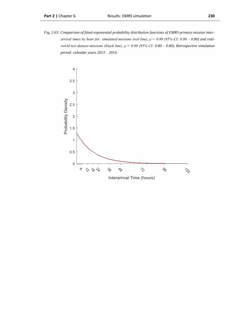
Part 2 | Chapter 6 Results: EMRS simulation 230
Fig. 2.63: Comparison of fitted exponential probability distribution functions of EMRS primary mission inter-
arrival times by hour for: simulated missions (red line), μ = 0.80 (95% CI: 0.80 – 0.80) and real-
world test dataset missions (black line), μ = 0.80 (95% CI: 0.80 – 0.80). Retrospective simulation
period: calendar years 2013 – 2014.

Part 2 | Chapter 6 Results: EMRS simulation 231
c) Empirical Cumulative Distribution Function (ECDF) of EMRS missions inter-
arrival time by hour
Secondary Missions
Direct comparison of the simulated and real-world secondary missions data demonstrated
visually similar curves (Fig. 2.64). This was reflected in a non-significant Kolmogorov-
Smirnov test result (p = 0.86). When interpreted with the associated similarity of the ECDF
curves, the difference would also not be operationally significant.
Fig. 2.64: ECDFs of EMRS secondary mission inter-arrival times by hours for simulation output (red line)
and real-world testing dataset missions (black line). Kolmogorov-Smirnov test p = 0.86.
Retrospective simulation period: calendar years 2013 – 2014.

Part 2 | Chapter 6 Results: EMRS simulation 232
Primary missions
On direct comparison of the simulated EMRS primary missions and real-world testing
data ECDFs, the curves appeared grossly similar. In particular, the multi-modal
distribution of the inter-arrival times generated can be seen in both ECDFs and this
component did appear to be well-replicated by the simulation (Fig. 2.65). Despite this, on
Kolmogorov-Smirnov testing, the distributions were found to be significantly different (p
= 0.03). It is considered unlikely that this difference was operationally significant,
however.
Fig. 2.65: ECDFs of EMRS primary mission raw inter-arrival times by hours for simulation output (red line)
and real-world testing dataset missions (black line). Kolmogorov-Smirnov test p = 0.03.
Retrospective simulation period: calendar years 2013 – 2014.

Part 2 | Chapter 6 Results: EMRS simulation 233
When the correction for time-dependency as described in Part 1 (section 1.6.3) was
applied to the data, the multi-modal appearance of the raw inter-arrival time histograms
was corrected to approximate an exponential distribution (Fig. 2.66 & Fig. 2.67) with
simulated missions μ = 0.77 (95% CI: 0.77 – 0.77) and real-world testing dataset missions
μ = 0.81 (95% CI: 0.72 – 0.91). Interestingly, comparison of the time-dependency
corrected ECDFs (Fig. 2.68) with the Kolmogorov-Smirnov test then yielded a non-
significant result (p = 0.31).
Fig. 2.66: Probability density histogram of simulated EMRS primary missions inter-arrival times with one-
hour bins: after correction for time-dependency. Fitted exponential distribution μ = 0.77 (red
line). Retrospective simulation period: calendar years 2013 – 2014.
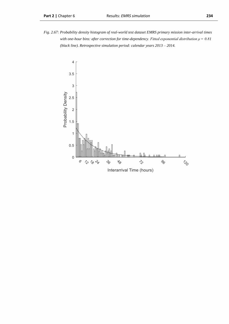
Part 2 | Chapter 6 Results: EMRS simulation 234
Fig. 2.67: Probability density histogram of real-world test dataset EMRS primary mission inter-arrival times
with one-hour bins: after correction for time-dependency. Fitted exponential distribution μ = 0.81
(black line). Retrospective simulation period: calendar years 2013 – 2014.
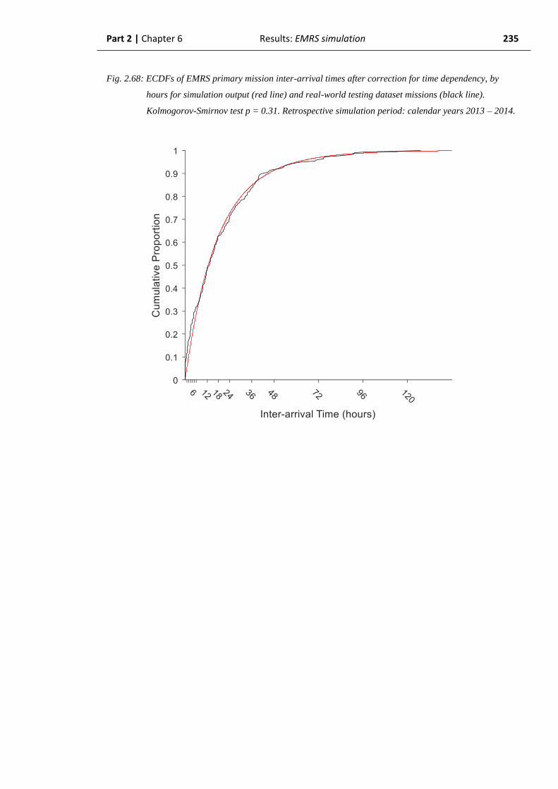
Part 2 | Chapter 6 Results: EMRS simulation 235
Fig. 2.68: ECDFs of EMRS primary mission inter-arrival times after correction for time dependency, by
hours for simulation output (red line) and real-world testing dataset missions (black line).
Kolmogorov-Smirnov test p = 0.31. Retrospective simulation period: calendar years 2013 – 2014.
Part 2 | Chapter 6 Results: EMRS simulation 236
d) Summary: EMRS inter-arrival times, retrospective simulation
For secondary missions, all analysed components: histograms, fitted distributions and
ECDFs appeared closely approximated and, where applicable, demonstrated statistically
and operationally non-significant differences.
Primary missions also demonstrated closely-approximating histograms and fitted
exponential distributions which were not significantly different between the simulation and
the real-world. Although the ECDFs demonstrated a statistically significant K-S test result,
the overall approximation of the ECDFs was considered to be very close, with the
exponential and multi-modal properties of the histogram which ultimately generates the
ECDF being particularly well replicated. As such, the difference between the primary
mission ECDFs was considered not to be operationally significant.
Overall, in the retrospective simulation period, when the full dataset was available to the
EMRS model, the model was able to replicate the real-world inter-arrival distributions to
an operationally acceptable standard.

Part 2 | Chapter 6 Results: EMRS simulation 237
2.6.1.4. Retrospective simulation of EMRS mission durations
Following the methodology as with SPRS, analysis of the mission durations will assess
the ability of the model to replicate the real-world server performance, in addition to the
arrivals process to the system.
The two EMRS teams are co-located and both undertake missions in exactly the same
operational fashion. The EMRS teams are therefore considered homogeneous for the
purposes of calculation of mission durations (service time). The duration distribution is
calculated for each mission type, but because of server homogeneity, there is no
requirement to assess separately for individual teams.
In this analysis section, the ability of the model to replicate the real-world mission
duration distribution for the EMRS system will be assessed.

Part 2 | Chapter 6 Results: EMRS simulation 238
a) Median mission durations
Secondary missions
In the retrospective simulation period, the simulation generated a median mission
duration of 7h 20m (95% PI: 7h 1m – 7h 37m, mean duration = 7h 19m), compared to a
real-world median duration of 7h 12m (model accuracy = 98.1%) (Fig 2.69). The medians
were not significantly different on Mann-Whitney U-testing (p = 0.30).
Fig. 2.69: Boxplot of simulated EMRS secondary mission durations across all iterations (median = 7h 20m,
IQR: 7h 13m – 7h 25m), with mean = 7h 19m (black diamond) and real-world median (7h 12m)
marked (black line). Medians not significantly different to real-world (Mann-Whitney U-test p =
0.30). Retrospective simulation period: calendar years 2013 – 2014.

Part 2 | Chapter 6 Results: EMRS simulation 239
Primary missions
In the retrospective simulation period, the simulation generated primary missions with a
median mission duration of 2h 51m (95% PI: 2h 46m – 2h 57m, mean duration = 2h 51m)
compared to a real-world testing dataset median of 2h 15m (model accuracy = 72.3%) (Fig.
2.70). The 36-minute absolute difference in medians was significantly different on Mann-
Whitney U-testing (p < 0.001). It is likely that this constitutes an operationally significant
difference.
Fig. 2.70: Boxplot of simulated EMRS primary mission median durations across all iterations (median = 2h
51m, IQR: 2h 49m – 2h 53m), with simulation mean = 2h 51m (black diamond), real-world
median (2h 15m, solid black line). Median significantly different to real-world (Mann-Whitney U-
test p = < 0.001). Retrospective simulation period: calendar years 2013 – 2014.

Part 2 | Chapter 6 Results: EMRS simulation 240
b) Mission duration distributions
Secondary missions
Simulated EMRS secondary mission durations were gamma distributed (Fig. 2.71) with
parameter values κ = 6.61 (95% CI: 6.58 – 6.63) and θ = 0.05 (95% CI: 0.05 – 0.05). By
comparison, the real-world data (Fig. 2.72) demonstrated κ = 6.39 (95% CI: 5.70 – 7.15)
and θ = 0.05 (95% CI: 0.04 – 0.06). Given that the simulated values lie within the 95%
confidence intervals of the real-world data, the distributions can be considered not
significantly different and the fitted gamma distribution for simulated missions appeared to
match its real-world equivalent closely (Fig. 2.73).
Fig. 2.71: Probability density histogram of simulated EMRS secondary mission durations with 30-minute
bins. Fitted gamma distribution (red line) parameter values: κ = 6.61 and θ = 0.05. Retrospective
simulation period: calendar years 2013 – 2014.
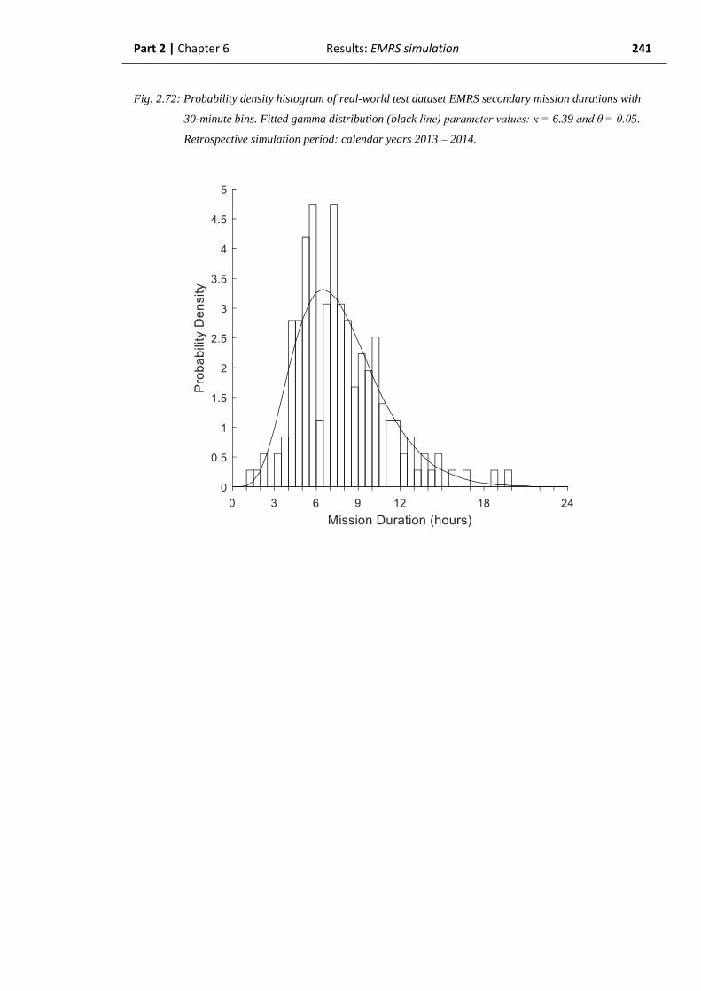
Part 2 | Chapter 6 Results: EMRS simulation 241
Fig. 2.72: Probability density histogram of real-world test dataset EMRS secondary mission durations with
30-minute bins. Fitted gamma distribution (black line) parameter values: κ = 6.39 and θ = 0.05.
Retrospective simulation period: calendar years 2013 – 2014.
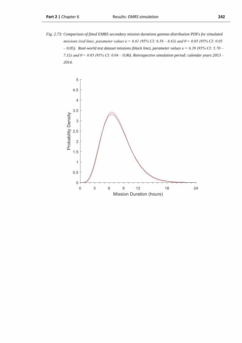
Part 2 | Chapter 6 Results: EMRS simulation 242
Fig. 2.73: Comparison of fitted EMRS secondary mission durations gamma-distribution PDFs for simulated
missions (red line), parameter values κ = 6.61 (95% CI: 6.58 – 6.63) and θ = 0.05 (95% CI: 0.05
– 0.05). Real-world test dataset missions (black line), parameter values κ = 6.39 (95% CI: 5.70 –
7.15) and θ = 0.05 (95% CI: 0.04 – 0.06). Retrospective simulation period: calendar years 2013 –
2014.

Part 2 | Chapter 6 Results: EMRS simulation 243
Primary missions
The fitted gamma distributions for EMRS primary missions appeared broadly similar
between the simulation data (Fig. 2.74) and the real-world testing dataset durations (Fig.
2.75). Simulated missions were gamma distributed with parameter values κ = 6.64 (95%
CI: 6.62 – 6.66) and θ = 0.02 (95% CI: 0.02 – 0.02). By comparison, the real-world data
demonstrated κ = 5.24 (95% CI: 4.71 – 5.83) and θ = 0.02 (95% CI: 0.02 – 0.02). Given
that the simulation parameter value for κ lies outside the 95% confidence interval for the
real-world distribution, the overall mission duration distributions are significantly different
(Fig. 2.76).
Fig. 2.74: Probability density histogram of simulated EMRS primary mission durations with 30-minute bins.
Fitted gamma distribution (red line) parameter values: κ = 6.64 and θ = 0.02. Retrospective
simulation period: calendar years 2013 – 2014.

Part 2 | Chapter 6 Results: EMRS simulation 244
Fig. 2.75: Probability density histogram of real-world test dataset EMRS primary mission durations with 30-
minute bins. Fitted gamma distribution (black line) parameter values: κ = 5.24 and θ = 0.02.
Retrospective simulation period: calendar years 2013 – 2014.
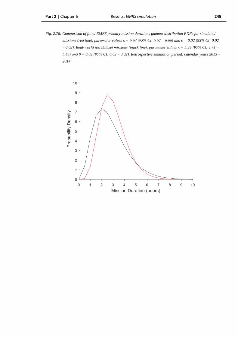
Part 2 | Chapter 6 Results: EMRS simulation 245
Fig. 2.76: Comparison of fitted EMRS primary mission durations gamma-distribution PDFs for simulated
missions (red line), parameter values κ = 6.64 (95% CI: 6.62 – 6.66) and θ = 0.02 (95% CI: 0.02
– 0.02). Real-world test dataset missions (black line), parameter values κ = 5.24 (95% CI: 4.71 –
5.83) and θ = 0.02 (95% CI: 0.02 – 0.02). Retrospective simulation period: calendar years 2013 –
2014.

Part 2 | Chapter 6 Results: EMRS simulation 246
c) Empirical Cumulative Distribution Function (ECDF) of EMRS mission durations
by elapsed time
Secondary missions
Direct comparison of the ECDFs of simulated EMRS secondary mission durations and
real-world testing data mission durations demonstrated them to be very closely aligned
(Fig. 2.77). This was confirmed by a non-significant difference on Kolmogorov-Smirnov
testing (p = 0.84).
Fig. 2.77: ECDFs of EMRS secondary mission durations by hours for simulation output (red line) and real-
world test dataset missions (black line). Kolmogorov-Smirnov test p = 0.84. Retrospective
simulation period: calendar years 2013 – 2014.
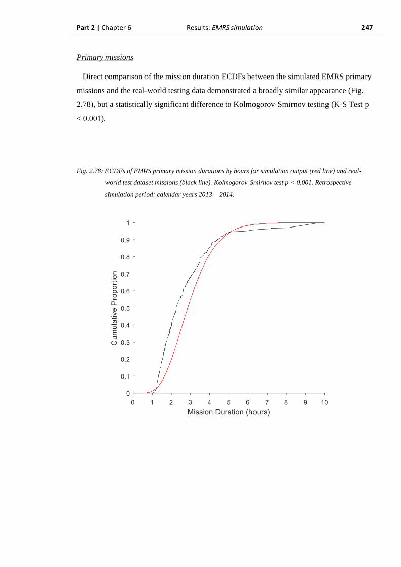
Part 2 | Chapter 6 Results: EMRS simulation 247
Primary missions
Direct comparison of the mission duration ECDFs between the simulated EMRS primary
missions and the real-world testing data demonstrated a broadly similar appearance (Fig.
2.78), but a statistically significant difference to Kolmogorov-Smirnov testing (K-S Test p
< 0.001).
Fig. 2.78: ECDFs of EMRS primary mission durations by hours for simulation output (red line) and real-
world test dataset missions (black line). Kolmogorov-Smirnov test p < 0.001. Retrospective
simulation period: calendar years 2013 – 2014.
Part 2 | Chapter 6 Results: EMRS simulation 248
d) Summary: EMRS mission durations, retrospective simulation period
The EMRS model has accurately replicated the real-world secondary mission durations,
demonstrating close approximations of the median mission durations and no significant
difference in either fitted gamma distributions or ECDFs.
The model’s replication of the real-world primary missions is, however, sub-optimal.
The accuracy of the simulated median was 72.3% with an absolute difference of 36
minutes to the real-world testing data median it is likely, but not certain, to be
operationally significant. The difference between the medians, fitted gamma distributions
and ECDFs were, however, all statistically significant.

Part 2 | Chapter 6 Results: EMRS simulation 249
2.6.1.5. Retrospective simulation of EMRS server utilization
Both EMRS duty teams undertake primary and secondary missions, which are distributed
on a first-in-first-out (FIFO) queue basis to the Duty One team. If they are unavailable, the
mission is passed to the Duty Two team. Server utilization is therefore split by team, not by
primary / secondary mission type. Consideration of the utilization by individual team will
assist in establishing if the distribution of missions is correct between each of the two
teams.
a) EMRS server utilization quotient – whole service
During the retrospective simulation period, the model generated an iterative median total
EMRS server utilization of 19.4% (95% PI:18.2% - 20.3%, mean = 19.4%), compared to a
real-world value of 19.6% utilization (model accuracy: 99.0%) (Fig. 2.79). Commensurate
with this, Mann-Whitney U-testing did not find the 0.2% difference to be statistically
significant (p = 0.77), nor would this be considered operationally significant, given the
model’s accuracy.
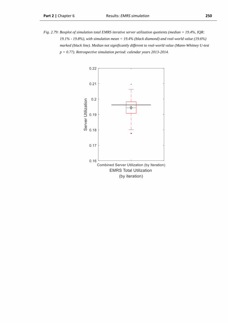
Part 2 | Chapter 6 Results: EMRS simulation 250
Fig. 2.79: Boxplot of simulation total EMRS iterative server utilization quotients (median = 19.4%, IQR:
19.1% - 19.8%), with simulation mean = 19.4% (black diamond) and real-world value (19.6%)
marked (black line). Median not significantly different to real-world value (Mann-Whitney U-test
p = 0.77). Retrospective simulation period: calendar years 2013-2014.

Part 2 | Chapter 6 Results: EMRS simulation 251
b) EMRS server utilization quotient – Duty One team
When the utilization was examined by individual team, the simulation generated a
median server utilization of 27.9% (95% PI: 26.3% – 29.2%, mean = 27.2%) for the Duty
One team, compared to a 31.8% utilization in the real-world testing data (model accuracy =
87.5%) (Fig. 2.80). The difference between these values approached significance on Mann-
Whitney U testing (p = 0.09). Therefore, the model under-estimated the utilization of the
Duty One team, but not by a statistically significant margin. Whether the 3.9% absolute
error is operationally significant is unknown.
Fig. 2.80: Boxplot of simulation EMRS duty 1 team iterative server utilization quotients (median = 27.9%,
IQR: 27.4% – 28.2%), with simulation mean = 27.2% (black diamond) and real-world value
(31.8%) marked (black line). Median not significantly different to real-world value (Mann-
Whitney U-test p = 0.09). Retrospective simulation period: calendar years 2013-2014.

Part 2 | Chapter 6 Results: EMRS simulation 252
c) EMRS server utilization quotient – Duty Two team
In the same simulation period, the model generated a median server utilization for the
Duty 2 team of 11.2% (95% PI: 9.8% - 12.1%, mean = 11.1%) compared to a real-world
utilization of 7.4% (model accuracy = 48.6%) (Fig. 2.81). The difference between these
values also approached significance with a Mann-Whitney U test p = 0.08. Given the
smaller utilization value, the 3.7% difference between the model and real-world would
have to be considered operationally significant for the Duty 2 team.
Fig. 2.81: Boxplot of simulation EMRS duty 2 team iterative server utilization quotients (median = 11.2%,
IQR: 10.7% - 11.5%), with simulation mean = 11.1% (black diamond), and real-world value
(7.4%) marked (black line). Median not significantly different to real-world value (Mann-Whitney
U-test p = 0.08). Retrospective simulation period: calendar years 2013-2014.
Part 2 | Chapter 6 Results: EMRS simulation 253
d) Summary: EMRS server utilization, retrospective simulation
Based on this analysis, it is considered that the model had correctly replicated the real-
world total EMRS server utilization.
On balance of all the factors contributing to the analysis of individual server utilization, it
appears that the model under-estimated the utilization of the Duty One team, while over-
estimating the utilization of the Duty Two team. It is likely this has been because of the
allocation of an excess of missions to the Duty One team by the model. The reason for this
is unclear but will be further explored in the Part 2 discussion section. Given that that, at
this stage, the parameters investigated with regard to system performance do not rely on
individual team utilizations, this will not be analysed further in this thesis.
Part 2 | Chapter 6 Results: EMRS simulation 254
2.6.1.6 Summary of EMRS retrospective simulation results
The EMRS model is considered to have accurately replicated the real-world with regard
to all the secondary mission components studied during the retrospective simulation
period.
The model has also accurately replicated the real-world primary mission components
with the exception of mission durations.
However, the model has accurately replicated the real-world value of a derived variable:
total server utilization. As a derived variable, the server utilization is a product of two other
variables – in this case number of missions and mission durations. The server utilization
has therefore incorporated the primary mission duration estimation, with its associated
difference to the real-world. As this does not appear to have translated into a significant
difference in server utilization, it is likely that there is some resilience within the system to
absorb errors in the magnitude of 36 minutes for median primary mission duration. As a
result of this, it is considered that the model, overall, replicated the real-world to an
operationally acceptable standard.
The model has generated an acceptable replication of the real-world and, in particular, has
derived an accurate server utilization value. These results lend validity to the assumption of
mathematical similarity between the components of the model and the corresponding real-
world processes. It is therefore considered that subsequent derived system performance
values (e.g. Waiting time in the queue, Wq) will also be valid. Any derived performance
values can therefore be expected to provide an operationally acceptable overall
representation of the real-world system during the 2013 – 2014 calendar years.

Part 2 | Chapter 6 Results: EMRS simulation 255
2.6.2. Contemporaneous simulation of EMRS operations
In this section, the performance of the EMRS M/G/2 model will be assessed using the
same parameters for a one-year simulation period comprising the calendar year 2015.
The model will be run in a “contemporaneous” format, primed with data from the
retrospective simulation period, and receiving new data only up to the current simulation
time. The output of the simulation at any point in time should be a contemporaneous
representation of the real-world system state.
The purpose of this analysis is to establish if the model is capable of describing the
immediate, current state of the SPRS system, effectively in real-time, at any point during
the simulation period.
As with the SPRS contemporaneous simulation, the distributions of activation time of
day, inter-arrival time and mission duration were unable to be calculated on a daily basis
due to a lack of computing power. These distributions are therefore compared based on the
whole 2015 calendar year as the sampling period (see section 2.5.2 for further details).

Part 2 | Chapter 6 Results: EMRS simulation 256
2.6.2.1. Contemporaneous simulation of EMRS mission count
a) Progressive daily EMRS mission total
The daily cumulative number of missions were closely matched between the real-world
and the simulation iterative median for both mission types. The real-world cumulative
value remained within the 95% prediction intervals for both primary and secondary
missions throughout the entire simulated time period (Fig. 2.82).
Fig. 2.82: Cumulative EMRS secondary mission count by day demonstrating: simulation iterative median
(solid red line) and 95% prediction intervals of simulation (dashed red lines). The real-world
cumulative count (black line) is contained within the bounds set by the 95% prediction intervals
for the entire time period. Contemporaneous simulation period: calendar year 2015.
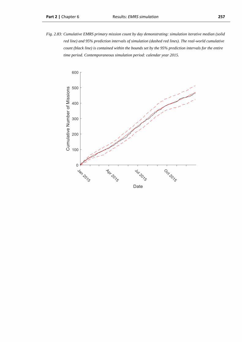
Part 2 | Chapter 6 Results: EMRS simulation 257
Fig. 2.83: Cumulative EMRS primary mission count by day demonstrating: simulation iterative median (solid
red line) and 95% prediction intervals of simulation (dashed red lines). The real-world cumulative
count (black line) is contained within the bounds set by the 95% prediction intervals for the entire
time period. Contemporaneous simulation period: calendar year 2015.

Part 2 | Chapter 6 Results: EMRS simulation 258
b) Total number of EMRS missions
Secondary missions:
In the contemporaneous period, the model generated an iterative median of 240 EMRS
secondary missions (95% Prediction Interval: 213 – 276m, mean = 242) compared to 239
real-world primary missions during the same time period (iterative median = 99.6%
accurate) (Fig. 2.84). The median total number of secondary missions was not statistically
significantly different to the real-world (Mann-Whitney U test p = 0.77)
Fig. 2.84: Boxplot of simulated total EMRS secondary missions count by iteration (median = 240, IQR: 233
– 249), with mean = 242 (black diamond) and real-world value (239 missions) marked (black
line). Difference not significant (Mann-Whitney U-test p = 0.77). Contemporaneous simulation
period: calendar year 2015.
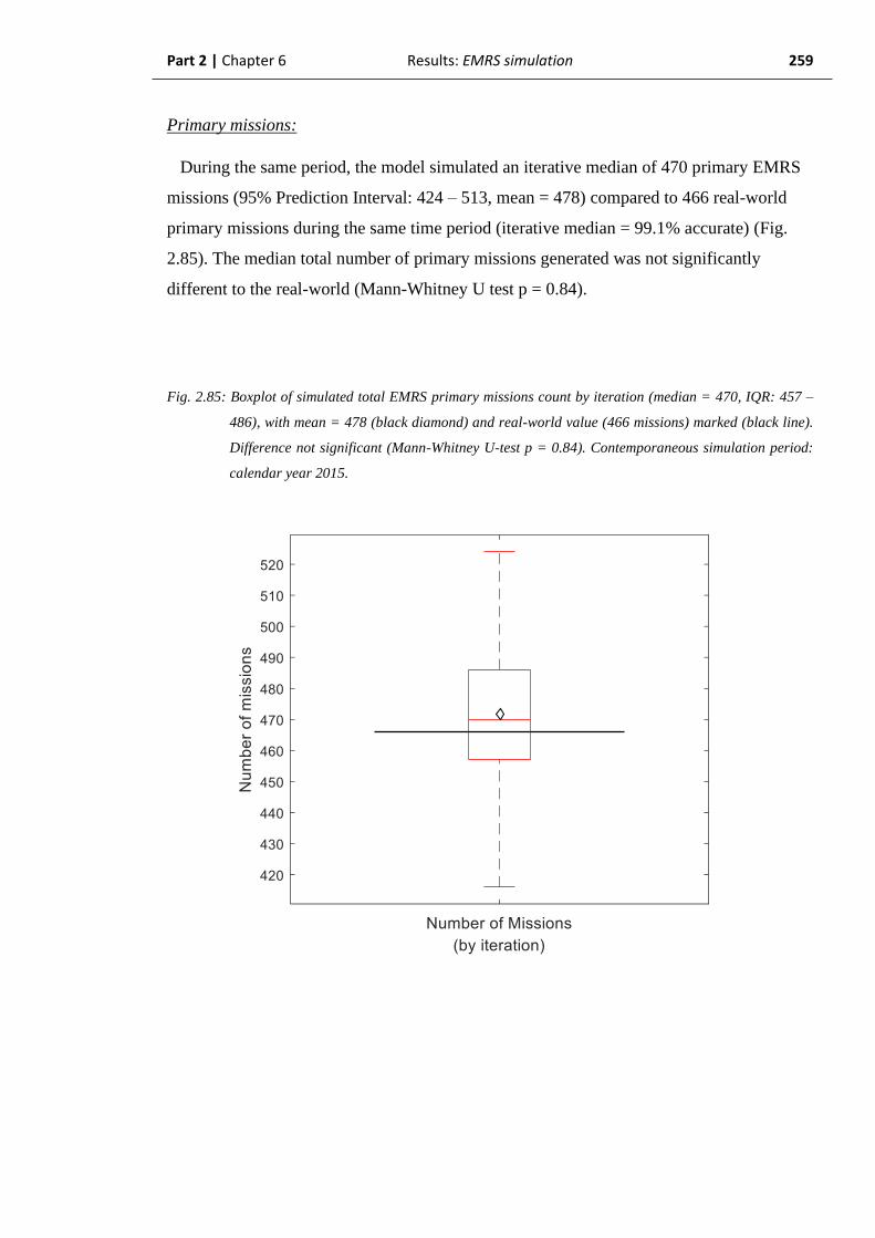
Part 2 | Chapter 6 Results: EMRS simulation 259
Primary missions:
During the same period, the model simulated an iterative median of 470 primary EMRS
missions (95% Prediction Interval: 424 – 513, mean = 478) compared to 466 real-world
primary missions during the same time period (iterative median = 99.1% accurate) (Fig.
2.85). The median total number of primary missions generated was not significantly
different to the real-world (Mann-Whitney U test p = 0.84).
Fig. 2.85: Boxplot of simulated total EMRS primary missions count by iteration (median = 470, IQR: 457 –
486), with mean = 478 (black diamond) and real-world value (466 missions) marked (black line).
Difference not significant (Mann-Whitney U-test p = 0.84). Contemporaneous simulation period:
calendar year 2015.
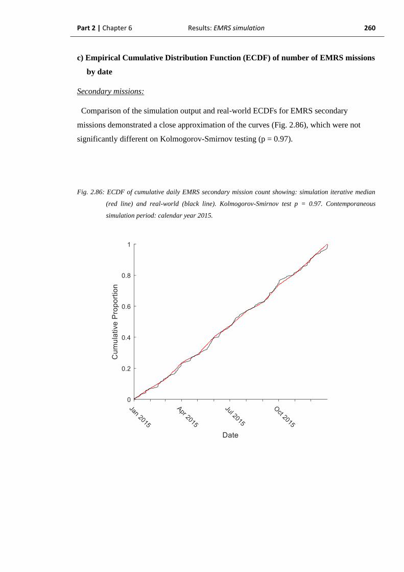
Part 2 | Chapter 6 Results: EMRS simulation 260
c) Empirical Cumulative Distribution Function (ECDF) of number of EMRS missions
by date
Secondary missions:
Comparison of the simulation output and real-world ECDFs for EMRS secondary
missions demonstrated a close approximation of the curves (Fig. 2.86), which were not
significantly different on Kolmogorov-Smirnov testing (p = 0.97).
Fig. 2.86: ECDF of cumulative daily EMRS secondary mission count showing: simulation iterative median
(red line) and real-world (black line). Kolmogorov-Smirnov test p = 0.97. Contemporaneous
simulation period: calendar year 2015.
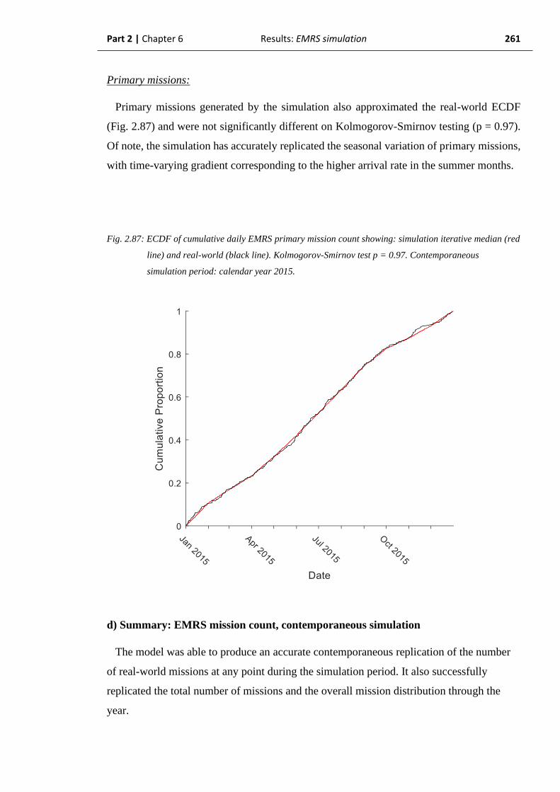
Part 2 | Chapter 6 Results: EMRS simulation 261
Primary missions:
Primary missions generated by the simulation also approximated the real-world ECDF
(Fig. 2.87) and were not significantly different on Kolmogorov-Smirnov testing (p = 0.97).
Of note, the simulation has accurately replicated the seasonal variation of primary missions,
with time-varying gradient corresponding to the higher arrival rate in the summer months.
Fig. 2.87: ECDF of cumulative daily EMRS primary mission count showing: simulation iterative median (red
line) and real-world (black line). Kolmogorov-Smirnov test p = 0.97. Contemporaneous
simulation period: calendar year 2015.
d) Summary: EMRS mission count, contemporaneous simulation
The model was able to produce an accurate contemporaneous replication of the number
of real-world missions at any point during the simulation period. It also successfully
replicated the total number of missions and the overall mission distribution through the
year.

Part 2 | Chapter 6 Results: EMRS simulation 262
2.6.2.2 Contemporaneous EMRS activation times of day
There is no progressive measure by which to compare the simulated and real-world
activation times. This analysis is therefore reflective of the entire contemporaneous
simulation period.
a) Probability of EMRS activation by time of day
Secondary missions
Simulated secondary missions displayed a peak probability of activation in the 1000h –
1100h period (Fig. 2.88), compared to 1100h – 1200h in the real-world testing dataset
missions (Fig. 2.89). There was an overall similarity of the pattern but, as expected, with
variability in the real-world histogram. The median model accuracy by hour was 71.7%.
Fig. 2.88: Normalized probability histogram (area under plot = 1) of simulated EMRS secondary mission
activations by hour of day. Mode in 1000h – 1100h period. Contemporaneous simulation period:
calendar year 2015.

Part 2 | Chapter 6 Results: EMRS simulation 263
Fig. 2.89: Normalized probability histogram (area under plot = 1) of real-world test dataset EMRS
secondary mission activations by hour of day. Mode in 1100h – 1200h period. Contemporaneous
simulation period: calendar year 2015.

Part 2 | Chapter 6 Results: EMRS simulation 264
Primary missions
During the contemporaneous simulation period, the model generated primary missions
(Fig. 2.90) in a distribution which did not display as obvious a peak in activations as the
real-world testing data (median model accuracy by hour = 78.0%). Simulated primary
mission activations were maximal in the 1300h – 1400h time period, the same as real-
world testing dataset (Fig. 2.91).
Fig. 2.90: Normalized probability histogram (area under plot = 1) of simulated EMRS primary mission
activations by hour of day. Mode in 1300h – 1400h period. Contemporaneous simulation period:
calendar year 2015.
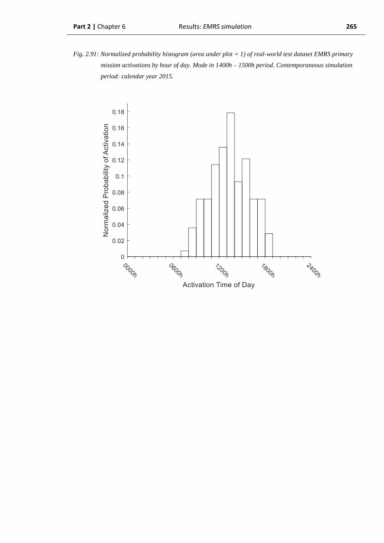
Part 2 | Chapter 6 Results: EMRS simulation 265
Fig. 2.91: Normalized probability histogram (area under plot = 1) of real-world test dataset EMRS primary
mission activations by hour of day. Mode in 1400h – 1500h period. Contemporaneous simulation
period: calendar year 2015.
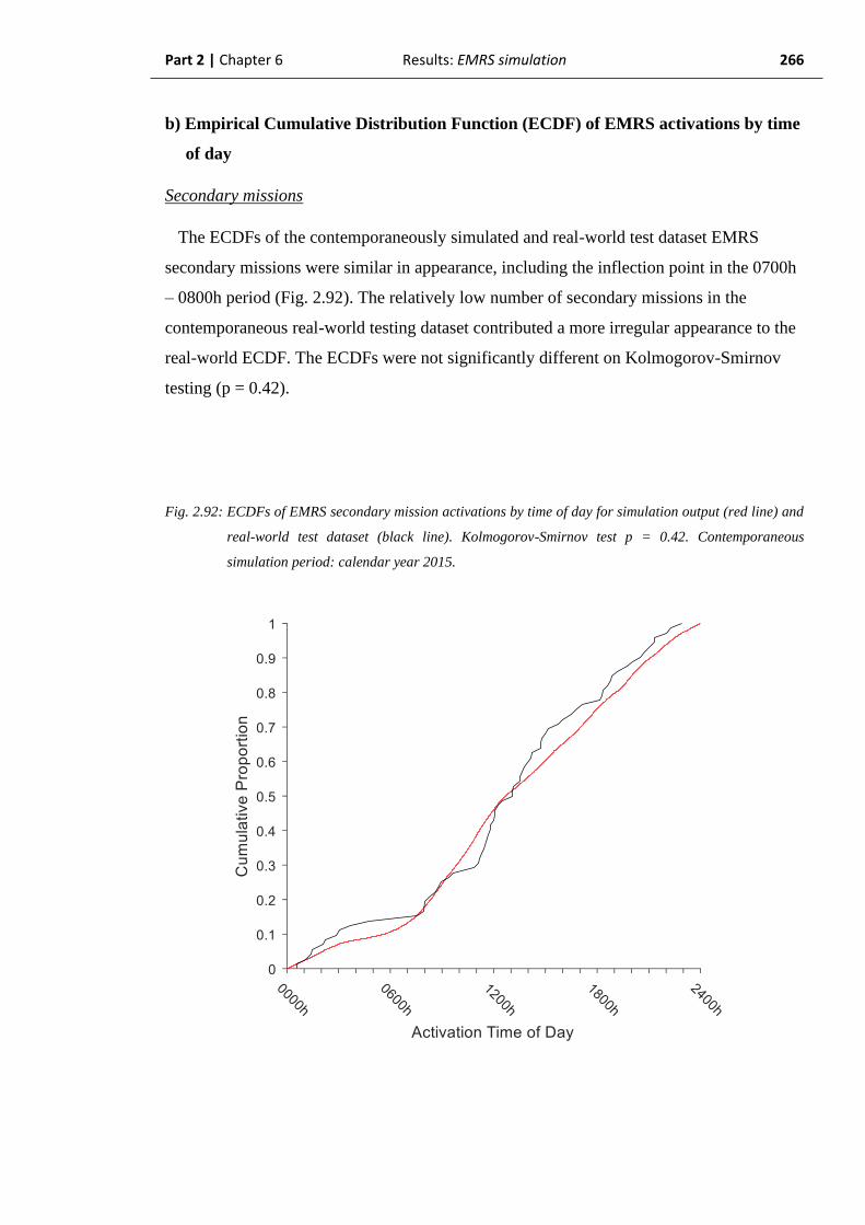
Part 2 | Chapter 6 Results: EMRS simulation 266
b) Empirical Cumulative Distribution Function (ECDF) of EMRS activations by time
of day
Secondary missions
The ECDFs of the contemporaneously simulated and real-world test dataset EMRS
secondary missions were similar in appearance, including the inflection point in the 0700h
– 0800h period (Fig. 2.92). The relatively low number of secondary missions in the
contemporaneous real-world testing dataset contributed a more irregular appearance to the
real-world ECDF. The ECDFs were not significantly different on Kolmogorov-Smirnov
testing (p = 0.42).
Fig. 2.92: ECDFs of EMRS secondary mission activations by time of day for simulation output (red line) and
real-world test dataset (black line). Kolmogorov-Smirnov test p = 0.42. Contemporaneous
simulation period: calendar year 2015.

Part 2 | Chapter 6 Results: EMRS simulation 267
Primary missions
Comparison of the ECDFs for EMRS primary mission activation times in the
contemporaneous simulated period demonstrated outwardly similar curves (Fig. 2.93), with
a strong sigmoid-shape reflecting the hours of operation for the primary missions.
However, despite the outward similarity, the ECDFs were significantly different on
Kolmogorov-Smirnov testing (p < 0.001). This principally appears to have been accounted
for by the simulated missions starting earlier than in the real-world testing dataset. It is
unlikely, however, that this difference would be operationally significant given the overall
similarity of the curves.
Fig. 2.93: ECDFs of EMRS primary mission activations by time of day for simulation output (red line) and
real-world test dataset (black line). Kolmogorov-Smirnov test p < 0.001. Contemporaneous
simulation period: calendar year 2015.

Part 2 | Chapter 6 Results: EMRS simulation 268
c) Summary: EMRS activations by time of day, contemporaneous simulation
The contemporaneous EMRS simulation is considered to have accurately replicated the
real-world activation times of day with regard to secondary missions.
The simulation’s performance in replicating the real-world primary missions is
operationally acceptable. It has adequately replicated the working hours of the EMRS
primary missions service, albeit with a somewhat different histogram appearance, and a
correspondingly lower accuracy measure. The primary missions ECDFs appeared visually
very similar and are considered unlikely to be operationally different, although they were
statistically different.

Part 2 | Chapter 6 Results: EMRS simulation 269
2.6.2.3. Contemporaneous simulation of EMRS inter-arrival times
Similarly to the activation time of day distribution, a suitable progressive measure of
inter-arrival time distribution was not available. There was inadequate computational
power to repeatedly fit and compare exponential distributions throughout the simulation
period. Simpler measures such as measuring the mean or median inter-arrival time
effectively duplicates the results of contemporaneously simulating the total number of
missions. The inter-arrival time distribution is therefore also calculated based on the entire
contemporaneous simulation period dataset.
a) Probability (PDF) of inter-arrival time by hour, EMRS missions
Secondary missions
Secondary missions in the contemporaneous simulation period demonstrated a strongly
exponential distribution of inter-arrival times (Fig 2.94) with evidence of multi-modality
within. Neither the overall distribution nor multi-modality was as clearly demonstrated in
the real-world testing data (Fig 2.95). The relative sparsity of data points in the real-world
testing dataset would appear to contribute somewhat to the histogram appearance. Despite
this, the fitted exponential distributions were not significantly different: real-world μ =
1.38 (95% CI: 1.21 – 1.57) compared to a simulation μ = 1.50 (95% CI: 1.50 – 1.51) (Fig.
2.96).

Part 2 | Chapter 6 Results: EMRS simulation 270
Fig. 2.94: Probability density histogram of simulated EMRS secondary mission inter-arrival times with one-
hour bins. Fitted exponential distribution μ = 1.38 (red line). Contemporaneous simulation
period: calendar year 2015.

Part 2 | Chapter 6 Results: EMRS simulation 271
Fig. 2.95: Probability density histogram of real-world test dataset EMRS secondary mission inter-arrival
times with one-hour bins. Fitted exponential distribution μ = 1.50 (black line). Contemporaneous
simulation period: calendar year 2015.

Part 2 | Chapter 6 Results: EMRS simulation 272
Fig. 2.96: Comparison of fitted exponential probability distribution functions of EMRS secondary mission
inter-arrival times by hour for: simulated missions (red line), μ = 1.50 (95% CI: 1.50 – 1.51) and
real-world test dataset missions (black line), μ = 1.38 (95% CI: 1.21 – 1.57). Contemporaneous
simulation period: calendar year 2015.
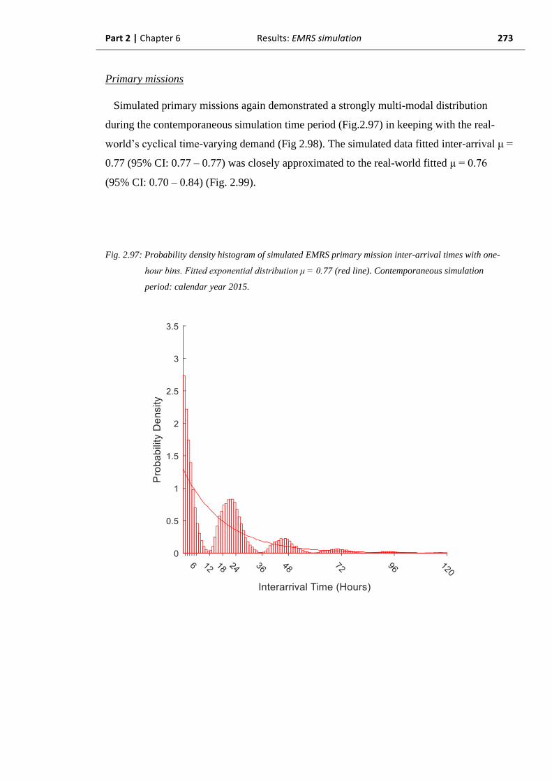
Part 2 | Chapter 6 Results: EMRS simulation 273
Primary missions
Simulated primary missions again demonstrated a strongly multi-modal distribution
during the contemporaneous simulation time period (Fig.2.97) in keeping with the real-
world’s cyclical time-varying demand (Fig 2.98). The simulated data fitted inter-arrival μ =
0.77 (95% CI: 0.77 – 0.77) was closely approximated to the real-world fitted μ = 0.76
(95% CI: 0.70 – 0.84) (Fig. 2.99).
Fig. 2.97: Probability density histogram of simulated EMRS primary mission inter-arrival times with one-
hour bins. Fitted exponential distribution μ = 0.77 (red line). Contemporaneous simulation
period: calendar year 2015.

Part 2 | Chapter 6 Results: EMRS simulation 274
Fig. 2.98: Probability density histogram of real-world test dataset EMRS primary mission inter-arrival times
with one-hour bins. Fitted exponential distribution μ = 0.76 (black line). Contemporaneous
simulation period: calendar year 2015.
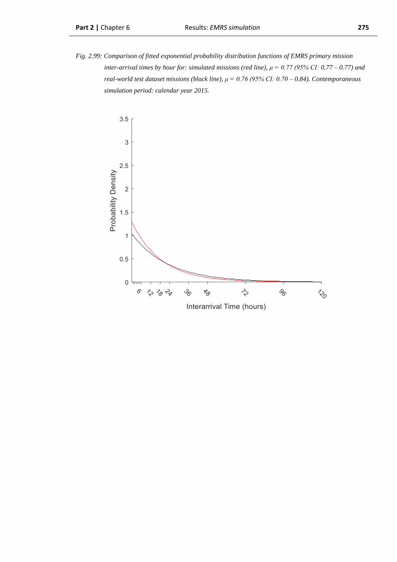
Part 2 | Chapter 6 Results: EMRS simulation 275
Fig. 2.99: Comparison of fitted exponential probability distribution functions of EMRS primary mission
inter-arrival times by hour for: simulated missions (red line), μ = 0.77 (95% CI: 0.77 – 0.77) and
real-world test dataset missions (black line), μ = 0.76 (95% CI: 0.70 – 0.84). Contemporaneous
simulation period: calendar year 2015.
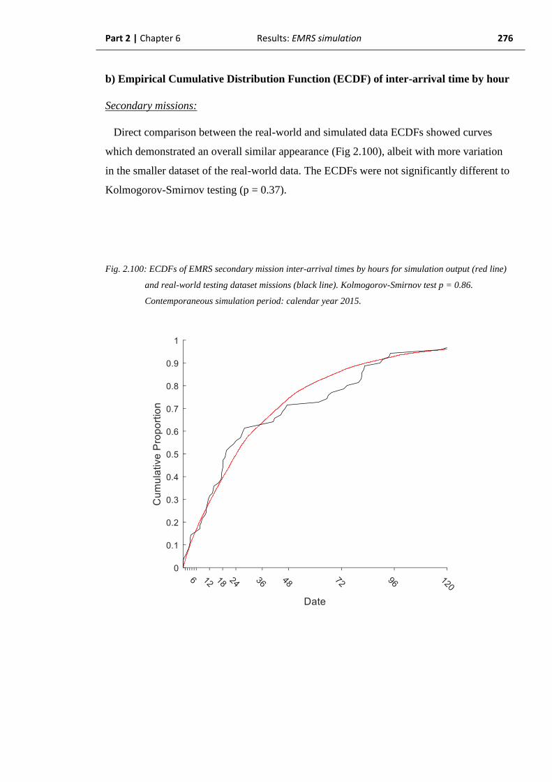
Part 2 | Chapter 6 Results: EMRS simulation 276
b) Empirical Cumulative Distribution Function (ECDF) of inter-arrival time by hour
Secondary missions:
Direct comparison between the real-world and simulated data ECDFs showed curves
which demonstrated an overall similar appearance (Fig 2.100), albeit with more variation
in the smaller dataset of the real-world data. The ECDFs were not significantly different to
Kolmogorov-Smirnov testing (p = 0.37).
Fig. 2.100: ECDFs of EMRS secondary mission inter-arrival times by hours for simulation output (red line)
and real-world testing dataset missions (black line). Kolmogorov-Smirnov test p = 0.86.
Contemporaneous simulation period: calendar year 2015.

Part 2 | Chapter 6 Results: EMRS simulation 277
Primary missions:
Comparison of the primary missions raw simulated inter-arrival times to the real-world
testing data ECDFs showed curves which appeared to grossly approximate (Fig 2.101), and
demonstrated the cyclical time-varying demand of the system. The ECDFs were
significantly different on Kolmogorov-Smirnov testing (p = 0.03) but given the overall
similarity of the ECDFs, this may not be an operationally significant difference.
Fig. 2.101: ECDFs of EMRS primary mission inter-arrival times by hours for simulation output (red line)
and real-world testing dataset missions (black line). Kolmogorov-Smirnov test p = 0.03.
Contemporaneous simulation period: calendar year 2015.
Part 2 | Chapter 6 Results: EMRS simulation 278
d) Summary: EMRS inter-arrival times, contemporaneous simulation
In the contemporaneous simulation period, the model has accurately replicated the inter-
arrival time distribution for the EMRS secondary missions.
The model generated a histogram for primary mission inter-arrival times which appeared
to show a very good approximation of the real-world, associated with an ECDF which also
produced an outwardly similar appearance, despite the findings of the ECDFs being
significantly different. On balance, it is considered that the model did adequately replicate
the real-world primary mission inter-arrival times adequately for operational purposes.
As the distributions could not be compared on a daily basis, the comparison has been
made over the entire one-year simulation period, whilst retaining the contemporaneous
simulation methodology. It is therefore considered that the model was able to accurately
replicate the current, contemporaneous real-world inter-arrival time distribution based on a
one-year sampling window corresponding with the 2015 calendar year.
2.6.2.4. Contemporaneous simulation of EMRS mission durations
This analysis section demonstrates the ability of the model to contemporaneously
replicate the real-world EMRS mission durations. The median mission duration is used as
the principal measure of the model accuracy, progressively through the simulation period.
The overall simulation output is then analysed at the end of the 2015 calendar year.

Part 2 | Chapter 6 Results: EMRS simulation 279
a) Progressive values of EMRS median mission duration
Secondary missions
The simulated median mission duration, after exhibiting initial volatility demonstrated a
stable maximum of 7h 27m during March, falling to a stable minimum of 7h 16m in
October before rising slightly to a final value of 7h 19m. The 95% prediction intervals
narrowed progressively in keeping with the increasing available data. After also displaying
initial volatility, the real-world testing data demonstrated a stable maximum of 7h 30m at
the end of April. The median value appeared closely approximated by the real-world for
the majority of the year until the real-world value began to diverge at the beginning of
September, reaching a minimum value of 6h 55m in November. Despite the change in the
real-world median value, which was not tracked by the model, it was contained within the
95% prediction interval of the simulation output throughout the entire time period (Fig.
2.102)
Fig. 2.102: Median EMRS secondary mission durations by day, comparing progressive simulation median
(solid red line) and 95% prediction intervals (dashed red lines) to the real-world test dataset
median duration (black line). Contemporaneous simulation period: calendar year 2015.
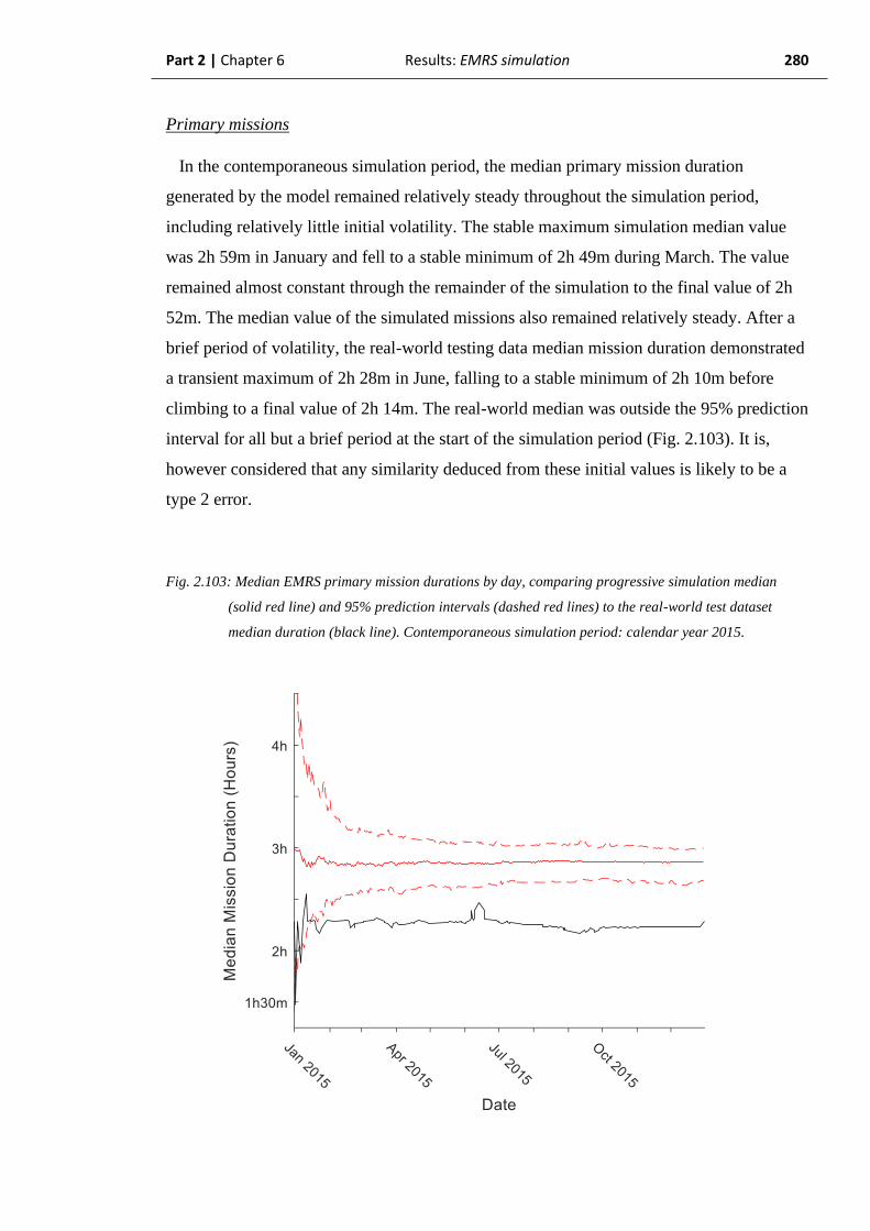
Part 2 | Chapter 6 Results: EMRS simulation 280
Primary missions
In the contemporaneous simulation period, the median primary mission duration
generated by the model remained relatively steady throughout the simulation period,
including relatively little initial volatility. The stable maximum simulation median value
was 2h 59m in January and fell to a stable minimum of 2h 49m during March. The value
remained almost constant through the remainder of the simulation to the final value of 2h
52m. The median value of the simulated missions also remained relatively steady. After a
brief period of volatility, the real-world testing data median mission duration demonstrated
a transient maximum of 2h 28m in June, falling to a stable minimum of 2h 10m before
climbing to a final value of 2h 14m. The real-world median was outside the 95% prediction
interval for all but a brief period at the start of the simulation period (Fig. 2.103). It is,
however considered that any similarity deduced from these initial values is likely to be a
type 2 error.
Fig. 2.103: Median EMRS primary mission durations by day, comparing progressive simulation median
(solid red line) and 95% prediction intervals (dashed red lines) to the real-world test dataset
median duration (black line). Contemporaneous simulation period: calendar year 2015.

Part 2 | Chapter 6 Results: EMRS simulation 281
b) Durations of all simulated EMRS missions
Secondary missions
At the conclusion of the contemporaneous time period, the simulation had generated a
final median secondary mission duration of 7h 19m (95% PI: 6h 53m – 7h 41m, mean = 7h
19m), compared to a real-world testing dataset mission duration of 6h 56m (model
accuracy = 94.5%) (Fig. 2.104). The median was not significantly different to the real-
world value on Mann-Whitney U testing (p = 0.90).
Fig. 2.104: Boxplot of simulated EMRS secondary mission durations (median = 7h 19m, IQR: 7h 10m – 7h
28m), with simulation mean = 7h 19m (black diamond), and real-world value (2h 14m) marked
(black line). Medians not significantly different (Mann-Whitney U-test p = 0.90).
Contemporaneous simulation period: calendar year 2015.

Part 2 | Chapter 6 Results: EMRS simulation 282
Primary missions
At the conclusion of the contemporaneous simulation period, the simulation output had
generated a final median primary mission duration of 2h 52m (95% PI: 2h 41m – 3h 00m,
mean = 2h 52m), compared to a real-world testing dataset mission duration of 2h 14m
(model accuracy = 71.7%) (Fig. 2.105). The simulation and real-world medians were
significantly different to Mann-Whitney U-testing (p < 0.0001). This result is similar to
that obtained in the retrospective simulation period and its operational significance is
uncertain.
Fig. 2.105: Boxplot of simulated EMRS primary mission durations (median = 2h 52m, IQR: 2h 49m – 2h
55m), with simulation mean = 2h 52m (black diamond), and real-world value (2h 14m) marked
(black line). Medians significantly different (Mann-Whitney U-test p < 0.0001). Contemporaneous
simulation period: calendar year 2015.
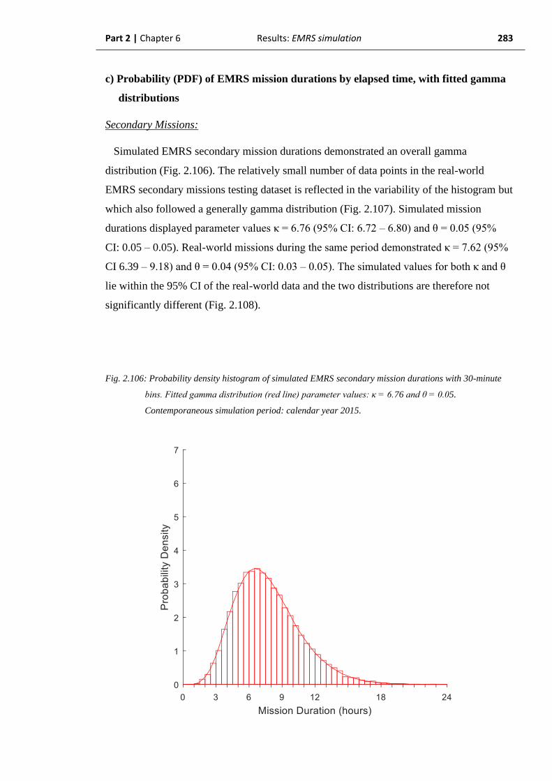
Part 2 | Chapter 6 Results: EMRS simulation 283
c) Probability (PDF) of EMRS mission durations by elapsed time, with fitted gamma
distributions
Secondary Missions:
Simulated EMRS secondary mission durations demonstrated an overall gamma
distribution (Fig. 2.106). The relatively small number of data points in the real-world
EMRS secondary missions testing dataset is reflected in the variability of the histogram but
which also followed a generally gamma distribution (Fig. 2.107). Simulated mission
durations displayed parameter values κ = 6.76 (95% CI: 6.72 – 6.80) and θ = 0.05 (95%
CI: 0.05 – 0.05). Real-world missions during the same period demonstrated κ = 7.62 (95%
CI 6.39 – 9.18) and θ = 0.04 (95% CI: 0.03 – 0.05). The simulated values for both κ and θ
lie within the 95% CI of the real-world data and the two distributions are therefore not
significantly different (Fig. 2.108).
Fig. 2.106: Probability density histogram of simulated EMRS secondary mission durations with 30-minute
bins. Fitted gamma distribution (red line) parameter values: κ = 6.76 and θ = 0.05.
Contemporaneous simulation period: calendar year 2015.

Part 2 | Chapter 6 Results: EMRS simulation 284
Fig. 2.107: Probability density histogram of real-world test dataset EMRS secondary mission durations with
30-minute bins. Fitted gamma distribution (black line) parameter values: κ = 7.62 and θ = 0.04.
Contemporaneous simulation period: calendar year 2015.

Part 2 | Chapter 6 Results: EMRS simulation 285
Fig. 2.108: Comparison of fitted EMRS secondary mission durations gamma-distribution PDFs for simulated
missions (red line), parameter values κ = 6.76 (95% CI: 6.72 – 6.80) and θ = 0.05 (95% CI: 0.05 –
0.05). Real-world test dataset missions (black line), parameter κ = 7.62 (95% CI 6.39 – 9.18) and
θ = 0.04 (95% CI: 0.03 – 0.05). Contemporaneous simulation period: calendar year 2015.

Part 2 | Chapter 6 Results: EMRS simulation 286
Primary Missions:
Both the simulated (Fig. 2.109) and real-world testing dataset (Fig. 2.110) EMRS
primary missions demonstrated overall gamma-distributed mission durations. Given that
the medians appeared significantly different, with a relatively low value for model
accuracy, it was unsurprising that the fitted gamma distributions also appeared to be
significantly different with regard to their κ parameter values.
The simulated EMRS primary missions demonstrated a gamma distribution with
parameter values κ = 6.74 (95% CI: 6.71 – 6.77) and θ = 0.02 (95% CI: 0.02 – 0.02). The
simulated value κ value did not lie within the confidence interval of the corresponding real-
world gamma distribution with parameter values κ = 4.87 (95% CI: 4.20 – 5.65), θ = 0.02
(95% CI: 0.02-0.03) (Fig. 2.111).
Fig. 2.109: Probability density histogram of simulated EMRS primary mission durations with 30-minute bins.
Fitted gamma distribution (red line) parameter values: κ = 6.74 and θ = 0.02. Contemporaneous
simulation period: calendar year 2015.
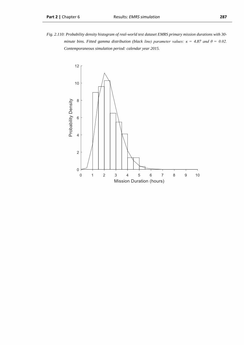
Part 2 | Chapter 6 Results: EMRS simulation 287
Fig. 2.110: Probability density histogram of real-world test dataset EMRS primary mission durations with 30-
minute bins. Fitted gamma distribution (black line) parameter values: κ = 4.87 and θ = 0.02.
Contemporaneous simulation period: calendar year 2015.

Part 2 | Chapter 6 Results: EMRS simulation 288
Fig. 2.111: Comparison of fitted EMRS primary mission durations gamma-distribution PDFs for simulated
missions (red line), parameter values κ = 6.74 (95% CI: 6.71 – 6.77) and θ = 0.02 (95% CI: 0.02 –
0.02). Real-world test dataset missions (black line), parameter κ = 4.87 (95% CI: 4.20 – 5.65), θ =
0.02 (95% CI: 0.02-0.03). Contemporaneous simulation period: calendar year 2015.

Part 2 | Chapter 6 Results: EMRS simulation 289
d) Empirical Cumulative Distribution Function (ECDF) of EMRS mission durations
by elapsed time
Secondary Missions
In keeping with the findings of similarity in progressive median, end-value median and
gamma distributions, direct comparison of the ECDFs for EMRS secondary missions
demonstrated a close approximation of the simulation output and the real-world testing
data (Fig. 2.112). The ECDFs were not significantly different on Kolmogorov-Smirnov
testing (p = 0.34).
Fig. 2.112: ECDFs of EMRS secondary mission durations by hours for simulation output (red line) and real-
world test dataset missions (black line). Kolmogorov-Smirnov test p = 0.34. Contemporaneous
simulation period: calendar year 2015.

Part 2 | Chapter 6 Results: EMRS simulation 290
Primary Missions
In contrast to the secondary missions, but again in keeping with the previous analyses,
the ECDFs of mission durations demonstrated grossly similar, but not well-approximated
curves between the simulation output and the real-world testing data (Fig. 2.113). The
ECDFs were significantly different on two-sample Kolmogorov-Smirnov testing (p <
0.001).
However, it was noted that comparing the simulation output ECDF to the real-world
testing data gamma distribution CDF (Fig. 2.114), that the difference ceased to be
statistically significant (one-sample Kolmogorov-Smirnov p = 0.22).
Fig. 2.113: ECDFs of EMRS primary mission durations by hours for simulation output (red line) and real-
world test dataset missions (black line). Two-sample Kolmogorov-Smirnov test p < 0.001
Contemporaneous simulation period: calendar year 2015.

Part 2 | Chapter 6 Results: EMRS simulation 291
Fig. 2.114: Comparison of EMRS primary mission durations by hours demonstrating: ECDF of simulation
output (red line) and CDF of real-world test data duration fitted gamma distribution (black line).
One-sample Kolmogorov-Smirnov test p = 0.22. Contemporaneous simulation period: calendar
year 2015.
e) Summary: EMRS mission durations, contemporaneous simulation period
The EMRS model was able to accurately replicate the contemporaneous state of the real-
world with regard to secondary mission durations at any point in the 2015 calendar year.
The EMRS model generated multiple parameters which were statistically significantly
different to the real-world with regard to primary mission durations. The model was not
able to progressively replicate the current real-world system state with regard to primary
mission durations. Its ability to contemporaneously represent the system at the end of the
2015 calendar year, with a one-year sampling window is equivocal.
Part 2 | Chapter 6 Results: EMRS simulation 292
2.6.2.5. Contemporaneous simulation of EMRS server utilization
This analysis section demonstrates the ability of the model to contemporaneously
replicate the real-world EMRS server utilization. The iterative median server utilization is
used as the primary measure of the model accuracy, progressively through the simulation
period. The overall simulation output is then analysed for the entire simulation period.
Utilization is a derived value, being a factor of both the mission durations and the number
of missions.
a) Progressive value of total EMRS server utilization quotient
The EMRS total server utilization demonstrated some initial volatility and an initial value
of 28.8% utilization which rapidly decreased during the first month of the simulation to a
stable maximum of 18.4% in February, then falling gradually to a stable minimum of
17.8% utilization in August before a minimal rise to a final value of 17.9% (Fig. 2.115).
The real-world demonstrated considerably more variation of the utilization value than the
simulation. After initial volatility, the real-world utilization reaches a minimum of 13.6%
during February, then stabilises at approximately 15.5% utilization. Through May, June
and July the real-world utilization increased (perhaps correlating with increased primary
mission activity) to remain stable at approximately 17.5% utilization. A stable peak of
18.0% utilization was reached in October, before the real-world utilization reduced again
to the final value of 17.1%.
The real-world value was contained within the simulation 95% prediction intervals for a
short period during January, and then from mid-June until the end of the simulation. This
would suggest that an appropriate sampling window over which utilization could be
contemporaneously reported would be approximately 6 months.

Part 2 | Chapter 6 Results: EMRS simulation 293
Fig. 2.115: Median total EMRS server utilization by day, comparing simulation iterative median (solid red
line) and 95% prediction intervals (dashed red lines) to the real-world test dataset median
duration (black line). Final values not significantly different (Mann-Whitney U-test p = 0.19).
Contemporaneous simulation period: calendar year 2015.

Part 2 | Chapter 6 Results: EMRS simulation 294
b) EMRS server utilization quotient: end of 2015 calendar year
At the end of the 2015 calendar year, the EMRS simulation had generated a current
iterative median total server utilization of 17.9% (95% PI: 16.6% - 19.9%, mean = 18.0%),
compared to a real-world utilization of 17.1% in the same time period (model accuracy =
95.3%) (Fig. 2.116). The difference was not significantly different on Mann-Whitney U-
testing (p = 0.19), nor would the 0.8% absolute difference be considered operationally
significant.
Fig. 2.116: Boxplot of simulation total EMRS iterative server utilization quotients (median = 17.9%, IQR:
17.5% - 18.4%), simulation mean = 18.0% (black diamond) and real-world value (17.1%) marked
(black line). Median not significantly different to real-world value (Mann-Whitney U-test p =
0.19). Contemporaneous simulation period: calendar year 2015.

Part 2 | Chapter 6 Results: EMRS simulation 295
c) Summary: EMRS server utilization, contemporaneous simulation
The contemporaneous simulation of EMRS server utilization demonstrated some success
by accurately replicating the current server utilization quotient from June onwards and
demonstrating a small, non-significant difference in the final utilization value.
The model has therefore accurately replicate the current, contemporaneous real-world
server utilization quotient at any time in the second-half of the 2015 calendar year, based
on a 6-month sampling window.
The relative utilization of each server (Duty One and Duty Two teams) within the EMRS
system is not required for the ongoing queueing-theory based analysis of the system and
has not been undertaken for the contemporaneous simulation period.

Part 2 | Chapter 6 Results: EMRS simulation 296
2.6.2.6 Contemporaneous simulation of EMRS team – summary
The EMRS model was able, in contemporaneous simulation, to accurately replicate the
current real-world state of the EMRS system at any time during the 2015 calendar year
with regard to number of missions and arrival rate (λ).
The model was able to replicate the derived value of server utilization progressively
through the second half of the year, using a minimum of a 6-month sampling window. The
model was able to accurately replicate the overall server utilization at the conclusion of the
simulation period.
The model was able to accurately replicate the current, contemporaneous median value
of secondary mission durations at all times through the simulation period. It was not able to
accurately replicate the primary mission durations either progressively or as a final
iterative median value. The main impact of this would be on server utilization, which the
model was able to accurately replicate, demonstrating some computational resilience for
errors in derived component values.
In summary, the model would perhaps best be described as able to indicate, rather than
accurately replicate, the contemporaneous state of the EMRS system. Despite this, it is
considered that the model is able to still provide operationally useful information on the
current state of the EMRS system. Relatively small further developments would likely
produce a substantial increase in model performance.

Part 2 | Chapter 6 Results: EMRS simulation 297
2.6.3 Summary of results from simulations of EMRS
operations
The simulation of the EMRS missions successfully replicated all components of the real-
world system to an operationally acceptable level in the retrospective simulation period
when the simulation was provided with the full data for the entire simulation period (Table
2.4). The model can therefore be considered an accurate representation of the real-world
EMRS system under retrospective simulation conditions, demonstrating a mean component
accuracy of 91.9%. In this capacity, it is able to provide a general overview of the system,
representative of the entire studied time period. In doing so, it has demonstrated the
validity of the assumed mathematical relationships between the real-world EMRS
components.
The contemporaneous simulation was able to partially replicate the current,
contemporaneous state of the real-world. The mean component accuracy for the
contemporaneous simulation was 89.0% although there was a notable difference between
the relatively high accuracy of the secondary mission components and the lower accuracy
of primary mission parameters (Table 2.5). For server utilization, the model was able to
replicate the real-world in real-time during the second half of 2015, when provided with a
preceding 6-month sampling window. It is therefore expected that the model could also
provide further contemporaneous derived values (e.g. Waiting time in queue, Wq) over the
same time-period, with the same sampling window.

Part 2 | Chapter 6 Results: EMRS simulation 298
Table 2.4: Summary of EMRS retrospective simulation results:
Parameter Model
value
Real-world
value Accuracy
Statistical
similarity
Operational
similarity
Number of secondary missions 567 573 99.0% Yes Yes
Number of primary missions 907 912 99.5% Yes Yes
Activation time of day –
secondary missions - - 77.9% Yes Yes
Activation time of day -
primary missions - - 84.2% No Yes
Inter-arrival times: secondary
missions μ = 1.28 μ = 1.24 96.7% Yes Yes
Inter-arrival times: primary
missions μ = 0.80 μ = 0.80 100% No Yes
Mission durations: secondary
missions 7h 20m 7h 12m 98.1% Yes Yes
Mission durations: primary
missions 2h 51m 2h 15m 72.3% No Yes
Server utilization: whole
service 19.4% 19.6% 99.0% Yes Yes

Part 2 | Chapter 6 Results: EMRS simulation 299
Table 2.5: Summary of EMRS contemporaneous simulation results:
Parameter Model
value
Real-world
value Accuracy
Statistical
similarity
Operational
similarity
Number of secondary missions 240 239 99.6% Yes Yes
Number of primary missions 470 466 99.1% Yes Yes
Activation time of day –
secondary missions - - 71.7% Yes Yes
Activation time of day -
primary missions - - 78.0% No Yes
Inter-arrival times: secondary
missions μ = 1.38 μ = 1.50 92.0% Yes Yes
Inter-arrival times: primary
missions μ = 0.77 μ = 0.76 98.7% No Yes
Mission durations: secondary
missions 7h 19m 6h 56m 94.5% Yes Yes
Mission durations: primary
missions 2h 52m 2h 14m 71.7% No No
Server utilization: whole
service 17.9% 17.1% 95.3% Yes Yes

Part 2 Chapter 7
Discussion
Part 2 | Chapter 7 Discussion 301
2.7 Discussion of modelling and simulation of
ScotSTAR systems
2.7.1 Simulation methodology
The simulation of the designed ScotSTAR model appears to have operated, as intended,
using a hybrid discrete event simulation (DES) and agent-based modelling (ABM) process.
The model was initialized using the ABM components to independently generate primary
missions, secondary missions and define mission durations according to a set of stochastic,
statistical rules. These rules were defined for each parameter by a probability distribution
calculated from a real-world learning dataset, comprising 70% of the data in that time
period (the other 30% being used for testing of the simulation output). By defining the
rules according to specific system descriptors (e.g. number of missions per month) which
are easily calculated in the real-world, the model provides a clear and simple link to the
real-world data. This also means that the model can be rapidly adapted to any changes in
the real-world, while still maintaining the underlying distributions which link the model to
its base queueing theory.
The ABM-developed rules then dictated the subsequent passage of the entity through the
discrete event simulation component of the ScotSTAR simulation. At the point of arrival in
the queue, the models proceeded to each subsequent time checkpoint (departure from
queue / entry into service, completion of service / departure from system) in a sequential
manner, with the simulation “stepping” to each of these discrete events. Every defined step
of every mission therefore was associated with a discrete time value which could then be
recorded and the inter-arrival times, service times and (in Part 3) waiting times calculated.
Because the ABM rules which govern the movement of entities through this part of the
model are pre-defined, it also makes the model easily adaptable to future changes in the
system, simply by adding or removing rules, and how the DES interprets them.
This approach had been chosen for its ability to preserve the distributions within the data
rather than creating an over-simplification. Because DES permits the recording of the time
steps of every mission, it is a straightforward task to describe a probability distribution of
the time between each step. Correspondingly, the majority of the results described have
been presented in a form which includes a probability distribution, so this intention has
clearly been realized within the model. This is considered a very important step in
preparing a model which is capable of generating useful performance data for the real-

Part 2 | Chapter 7 Discussion 302
world system. By preserving the data distributions, the model is best equipped to correctly
interpret some of the nuances of the real-world operations (e.g. time of peak probability of
activation) to ensure that performance data is not degraded by inappropriate averaging or
smoothing.
As a whole, it is considered that models have been generated for each of the ScotSTAR
SPRS and EMRS systems which effectively combine ABM and DES. The model therefore
preserves the stochastic nature of the real-world, accurately reflects the real-world
processes and produces an output which is interpretable in an operationally useful format.
2.7.2 Simulated number of missions
The model was able to accurately replicate the number of missions for both ScotSTAR
teams in both simulation types. In particular, in the contemporaneous simulation period,
the model was able to closely align the cumulative number of missions with the real-world
values, indicating that the model was able to replicate the current number of missions at
any point in the simulation process. The comparison of the ECDFs demonstrated that,
additionally, the model had successfully recreated the correct pattern of missions across
each of the simulated periods. Although the model was provided with all data up to the
point of simulation, it does demonstrate that each model was agile enough to respond to
variations in demand such that the model did not at any point deviate significantly from the
real-world.
The success in generating the total number of missions and mission distribution also
partially validates the use of the exclusion sampling methodology (section 2.4.1.3). The
model was designed to significantly over-generate missions (up to 174% of the real-world
value) in order to permit the time-varying demand generation process within the model to
exclude the excess missions down to the correct demand by time of day. Achieving an
accurate total number of missions suggests that this exclusion sampling process has at least
excluded the right number of missions, although it does not prove the correct distribution.
The calculation of the number of missions is the component in which the model has
performed best. Given its success in this regard, this component could be a target for the
future development of a prospective predictor of service demand if a suitable forecasting
model could be found. One limitation of forecasting using this model was the lack of
feedback provided within the model. Although it did not affect the analysis undertaken in
this project, if the model was wrong at any point in the contemporaneous prediction of the

Part 2 | Chapter 7 Discussion 303
current number of missions, the root cause of the error could not be corrected; it was
simply provided with the correct value at the next time step and the model run again. As a
result, there was the potential for the model to repeatedly generate a small error. If applied
prospectively, unless feedback was used to fine-tune the model, a small error could
multiply if a forecast further into the future was made.
2.7.3 Activation time of day
Activation time of day was generated, as described in methodology (section 2.4.1.3), by
an exclusion sampling technique. I would consider this to be one of the strongest
components of this project as, based on the literature review, exclusion sampling is not
mentioned in regard to accurately generating time-varying demand and this potentially
represents a significant contribution to the field.
Having established that arrivals to the system were a time-dependent Poisson system
then the inter-arrival times would, reciprocally, be a time-dependent exponential
distribution (with time-varying μ). Therefore, the generation of time-varying demand was
initially attempted by simply changing the inter-generation time exponential distribution μ-
parameter within the Simulink entity generation module. However, as this changes the
inter-arrival time to the next generated entity, a lag is introduced in the rate change. Given
the relatively low frequency of arrivals to the ScotSTAR systems, this lag could be quite
prolonged. This method, although relatively accurately replicating the time-variance of
demand, did so with an obvious phase-shift which generated a different time-varying
pattern to the real-world.
As stated in the introduction, the Simulink model only caters for a unidirectional time
component and the method used in Part 1 (section 1.6.3) of using a time transform to
correct the arrival times of missions “earlier” or “later” could not be applied. Additionally,
because the primary mechanism for generating entities in Simulink comes from the inter-
generation time, the standard “thinning” algorithm could not be used to simply generate a
sequence of activation times. During the course of general reading around simulation, the
concept of exclusion sampling was identified and integrated into the project.
The exclusion sampling methodology did appear from first principles to be a good fit for
the time-dependent Poisson process. Being able to generate inter-arrival times based on an
underlying exponential distribution was a pragmatic reversal of the process used in Part 1

Part 2 | Chapter 7 Discussion 304
to remove time-dependency from the Poisson-process and demonstrate an otherwise
exponentially-distributed inter-arrival time distribution. Then, by over-generating missions
to this exponential distribution and excluding a given number of missions generated in any
hour, the final inter-arrival distribution was maintained. Thus, by maintaining a fixed μ
over-sampling value and excluding a proportion per hour, the model was able to rapidly
adapt to hourly changes in demand – in contrast to the initial varying-μ approach.
The exclusion itself also managed to preserve the essence of a stochastic system. The
exclusion process was effected by conducting a Bernoulli trial upon each generated entity
to decide if it would be included in or rejected from the system. A probability of success
was known, but the absolute outcome of any given trial could not be certain: preserving the
independency of individual generated missions while creating time-dependency in demand.
The resulting missions were generated in an hourly pattern which generally appeared to
be a good approximation of the real-world. All the histograms appeared similar as did the
ECDFs. Despite this, however, the EMRS primary missions demonstrated a significant
difference between the real-world test dataset and the simulated activation times of day on
Kolmogorov-Smirnov testing. Given the similarity of the histograms and ECDFs, it was
appropriate to consider the difference to not be operationally significant. There may have
been some benefit in confining the application of the K-S test to only the EMRS hours of
operation to limit the confounding effect of even a small number of activations outside the
operating hours on the K-S test result. The limitations of the K-S test will be discussed
further in relation to inter-arrival time distributions.
This was the first of the analyses to use split learning and testing datasets. This was done
in the interest of statistical validity. One drawback to this was that, particularly in the
contemporaneous simulation period, the number of missions in the real-world testing
dataset could be relatively small. This had the potential for the testing dataset to exhibit a
different distribution to the learning dataset, upon which the model is based, simply by
sampling error (in effect, a type-1 error). As the activation time of day did not have a
distribution fitted to it, a prospective mechanism to mitigate this risk could not be
implemented and an alternative may need to be considered.
Part 2 | Chapter 7 Discussion 305
2.7.4 Inter-arrival times
The model was able to generate inter-arrival times which generally appeared to fit the
real-world. This also seemed to be a strong component of the model as it clearly generated
a multi-modal inter-arrival time distribution for ScotSTAR missions and for EMRS
primary missions in particular (section 2.5.2.3). This suggests that the exclusion sampling
method is effective in generating a multi-modal inter-arrival distribution. No mention of a
similar application or finding is made in the reviewed literature. This may therefore be a
novel illustration of this inter-arrival distribution within healthcare and particularly for a
pre-hospital care system.
The overall accuracy of the distribution, and overall similarity of the ECDFs of the inter-
arrival distributions suggests that the difference between the simulation and the real-world
was not operationally significant. However, it was disappointing to discover that the
EMRS primary mission inter-arrival times, which appeared to have been successfully
replicated in both histograms and ECDFs, were significantly different on Kolmogorov-
Smirnov testing. Both demonstrated a K-S test p-value less than 0.001. As the difference
between the distributions did not appear operationally significant, it was considered that
this finding may be a limitation of the Kolmogorov-Smirnov test, with a resulting type-one
error (falsely rejecting the null hypothesis that the data are from the same distribution).
The results of the EMRS primary mission tests may suggest that the Kolmogorov-
Smirnov test, though robust, is too sensitive for this application. The test itself may
therefore deem the model to be statistically different to the real-world despite it actually
being accurate enough to confer operational usefulness. This is perhaps due to the K-S
test’s use of a maximum difference between the two ECDFs. For “steep” ECDFs such as
the EMRS primary missions, a relatively small absolute difference in the inter-arrival times
can confer a large maximum difference in the ECDF curves, even when the overall ECDFs
are well approximated. It is also a recognized limitation of the Kolmogorov-Smirnov test
that with a large enough dataset, the K-S test will detect statistical significance in
arbitrarily small differences. Simulating approximately 900 primary missions in the
retrospective simulation over 1000 iterations generated approximately 900,000 inter-arrival
times. It is conceivable that this is a large enough dataset for the Kolmogorov-Smirnov test
to find statistical significance in an arbitrarily small difference from the real-world data.
It would certainly be of benefit to use a statistical test which did not have such
limitations, as this would have the potential to either confirm or refute the above
Part 2 | Chapter 7 Discussion 306
considerations of the Kolmogorov-Smirnov test. Currently, it is recognized that the
conclusion of an operationally non-significant difference may be a type two error and that
the model has truly failed to replicate the real-world. Cramer von-Mises testing could
possibly be more appropriate in considering more broadly the similarity of distribution
ECDFs. Alternatively, there may be a simpler method of applying the Kolmogorov-
Smirnov test: such as truncating the ECDFs to only reflect the hours of operation of EMRS
primary missions, or correcting for the time-dependent component before applying the K-S
test. Correcting for time-dependency was shown in section 2.6.1.4 (Fig. 2.68) to generate a
statistically non-significant K-S test p-value (p = 0.31) for EMRS primary missions.
Clearly there is opportunity within this section for further refinement and development.
However, the successful generation of a multi-modal inter-arrival time distribution has
provided validation for the exclusion sampling methodology and appears to be a novel
analysis within pre-hospital care.
2.7.5 Mission Durations
Mission durations were arguably the most challenging component to accurately model.
Based on the findings of Part 1, the missions were modelled as being gamma distributed.
However, it can be seen that while the missions were well approximated by the gamma
distribution in Part 1 of the thesis (sections 1.7.1.3 & 1.7.2.3), it is apparent that this
similarity is much more variable in the Part 2 analyses (e.g. EMRS secondary mission
durations, Fig. 2.107) because of the smaller datasets involved. It is recognized, therefore,
that there may be some contributing components which cause deviation from the generated
pure gamma distribution.
Nonetheless, it was decided that the preferred method would be for the mission duration
distribution to be generated by the model as a gamma distribution. This method, rather than
using an empirical distribution, would better preserve fidelity with the underlying queueing
theory, providing greater validity to the assumption of a consistent (but undefined)
mathematical relationship between components of the real-world. By contrast, the use of
an empirical distribution would have been likely to most closely approximate the real-
world in the Part 1 analysis (section 1.7.2.3 for example) when the analysis was applied to
the entire dataset. However, this assumes that a 4-year sample of missions is a
representative sample of all possible mission durations (i.e. the “population”). With this
Part 2 | Chapter 7 Discussion 307
project being the first application of such a modelling process to a PHaRM system, it was
considered that the 4-year period could not be assumed as being representative of the entire
mission duration “population”. As a result, it was decided that the gamma distribution
should be used in order to preserve generalisability of the simulated mission durations.
Part 1 had demonstrated the overall gamma distribution when all missions in a 4-year
period were analysed. Although intended to improve validity, splitting the data in Part 2
into learning and testing datasets did present other challenges. When the already smaller
datasets in Part 2 (comprising 1 or 2 years of data versus 4 years in Part 1), the resulting
testing dataset is relatively small. As a result, the potential for the mission durations
between the learning dataset, on which the model is programmed - and the testing dataset,
with which the model is compared, is potentially significant purely as a result of sampling
error.
In order to minimize this risk, it was necessary to fit a gamma distribution which was as
generalisable as possible to any possible combination of learning and testing data. This
needed to be achieved in a statistically robust fashion which was attempted using a two-
stage technique (section 2.4.1.3). Firstly, a large number of gamma distributions were
generated using random samples of the learning dataset and then compared using a 5-fold
holdout validation methodology. Minimization of the square of the Kolmogorov-Smirnov
statistic was then used as a variant of the sum of squared estimate of errors (SSE). This
appeared in the fitting and model selection stage to generate a very generalisable model.
However, despite this, the EMRS primary mission durations in the contemporaneous
simulation period still differed significantly from the real-world data. Interestingly
however, the simulation data were not significantly different to the real-world distribution.
(see Fig. 2.114). This perhaps suggests that the real-world testing dataset did not follow the
gamma distribution as closely as predicted. This could have also been the result of a
sampling bias, and other than splitting the missions into primary and secondary missions,
no stratification was undertaken in the data split to preserve fidelity to the random nature
of the real-world data.
It was noted that there was a difference between the fitted gamma distributions of the
learning dataset and the testing dataset (Fig 2.117), with there being no inclusion of either
parameter value in the 95% confidence intervals of the other distribution. It could therefore
be argued that if the model accurately replicated the learning dataset then it was always
going to be different to the testing dataset. However, regardless of the difference in
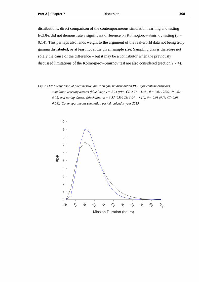
Part 2 | Chapter 7 Discussion 308
distributions, direct comparison of the contemporaneous simulation learning and testing
ECDFs did not demonstrate a significant difference on Kolmogorov-Smirnov testing (p =
0.14). This perhaps also lends weight to the argument of the real-world data not being truly
gamma distributed, or at least not at the given sample size. Sampling bias is therefore not
solely the cause of the difference – but it may be a contributor when the previously
discussed limitations of the Kolmogorov-Smirnov test are also considered (section 2.7.4).
Fig. 2.117: Comparison of fitted mission duration gamma distribution PDFs for contemporaneous
simulation learning dataset (blue line): κ = 5.24 (95% CI: 4.71 – 5.83), θ = 0.02 (95% CI: 0.02 –
0.02) and testing dataset (black line): κ = 3.57 (95% CI: 3.04 – 4.19), θ = 0.03 (95% CI: 0.03 –
0.04). Contemporaneous simulation period: calendar year 2015.
Part 2 | Chapter 7 Discussion 309
In defining the true mission duration distribution, although the use of a gamma
distribution is considered logically appropriate for the first application to ScotSTAR, it
may over-simplify the true distribution. For example, as a concept, aeromedical missions
could be considered as: an outbound flight, time on scene and a return flight. For any given
single patient location, each of these components will have their own time distribution:
whether deterministic (as a normal distribution), gamma or exponentially distributed. The
mission duration distribution to any one rural healthcare site will be the sum of these
individual components. When this is expanded to a national clinical network, the
contributors to the overall distribution become more complex, as the overall mission
duration distribution is generated from the sum of each individual served location’s
mission distributions. However, clearly, the flight time from Glasgow Airport to Dunoon
(approximately 18 nautical miles) will be less than the flight time from Glasgow Airport to
Barra (approximately 120 nautical miles). Therefore, Barra missions would be expected to
confer a much longer average mission duration than Dunoon missions. As a result, the
overall service’s mission duration distribution is reflective of both the individual location
mission durations, but also the proportion of missions which serve each individual remote
hospital site.
This description could outwardly define the mission durations as a phase-type
distribution, but the ScotSTAR system did not fully meet the definition for this because it
cannot be assumed that individual sub-components of the mission duration experience
exponentially-distributed durations themselves. Therefore, the mission distributions in this
project could perhaps be better described as being suitably approximated by the gamma
distribution. This provides some explanation of the significant difference between the
simulation output data and the real-world data.
Furthermore, although the contemporaneous mission duration distribution was updated
daily, it was still primed with data from the retrospective simulation period (20% of data,
equivalent to one hold-out validation sample). However, given the retrospective period is
twice as long as the contemporaneous simulation, numerically, this 20% of retrospective
data is equivalent to 40% of the contemporaneous data. It may simply be the case that the
model is too “tied” to the priming data and is simply not agile enough to adapt to changes
in the real-world system.
Clearly, as future work, a mechanism to better approximate the mission durations is
required. A possible refinement of this will be discussed later in this section.

Part 2 | Chapter 7 Discussion 310
2.7.6 Utilization
Utilization was generally well replicated in time periods where the two determinants;
number of missions and mission duration, could be accurately matched to the real-world
data. However, given that there were two contributing values, any potential error in either
of them could be multiplied and so this calculation was perhaps particularly sensitive to
deviation from the real-world systems.
One peculiarity noted in the EMRS system was that of the overall utilization being
accurate, but the distribution of workload between the Duty One and Duty Two teams
being incorrect. The EMRS system operates on a “Duty One before Duty Two” allocation.
Patients arriving to the system will be allocated to Duty One in the first instance. If they
are busy, the mission will pass to Duty Two. If Duty Two are also busy, the mission will
wait on the first available team, regardless of which, who will undertake the mission. This
operational component was able to be included in the model, and it was considered that
such allocation, even in the real-world, was straightforward, rule-based and not subject to
individual variation. However, clearly there is an aspect of this process which is not
correctly replicated in the model. It may simply be a factor of the model over-estimating
the mission durations, in particular the primary mission durations, as the majority of these
missions are undertaken by the Duty One team. As a result, the Duty One team will have
longer periods of non-availability when engaged on a primary mission during which time a
long-duration secondary retrieval request could be made, and the Duty Two team activated.
The Duty One team would then finish their relatively short duration primary mission.
Therefore, the Duty One utilization remains relatively low due to the distribution being
skewed toward shorter mission duration, and the Duty Two utilization is artificially
increased by an inappropriately large number of long-duration secondary retrievals being
passed to them in the model. A future improvement may be to also consider if the teams
receive the correct ratio of primary to secondary missions. With a two-server system,
however, the effect of this perturbation on the overall analysis will be negligible as the
subsequent queueing theory applications are concerned only with the overall server
utilization within the model – which was demonstrated as being correct.
In the contemporaneous EMRS utilization simulation, the real-world value was noted to
lie at a stable value outside the simulation prediction intervals until approximately the end
of May to mid-June (Fig. 2.115), before an increase in the real-world utilization brought it
back within the prediction intervals. This may correlate with the increased volume of pre-

Part 2 | Chapter 7 Discussion 311
hospital missions which occur during the summer months – and which may therefore
contribute to an increase in server utilization. Being primed with the retrospective data, the
simulation model was perhaps not sensitive enough to reflect this and a more agile model
could be investigated in future.
Of note, the overall utilization value for EMRS appears to be preserved despite the
finding of significantly different mission durations for primary missions. However, given
their substantially longer durations, secondary missions contribute more to the utilization
than primary missions, despite there being numerically more of the latter. There is perhaps
some resilience therefore in the analysis which allows the preservation of useful values
such as utilization, even in the context of imperfect simulation of their components.
2.7.7 Refinements and future studies
Two main challenges were identified in the analysis. Firstly, although appearing
relatively straightforward to generate, and producing an appropriate histogram and ECDF,
the inter-arrival time distribution for EMRS primary missions did not accurately replicate
the real-world on Kolmogorov-Smirnov testing. Further investigation is required, including
through the intended peer-review, to establish if this is a limitation of the dataset, the
analysis method (the Kolmogorov-Smirnov test in particular), the fitted distribution or
indeed the model’s mission generation process itself. In the first instance, replication of the
same methodology with the additional 5 years of additional ScotSTAR data which can now
be included would be warranted.
Beyond this, the major component which is likely to benefit from methodological
improvement is mission duration. As discussed above (section 2.7.5) and with reference to
the EMRS primary mission duration distributions (Fig. 2.75 and Fig 2.110) in particular,
the mission durations are perhaps actually a mixture or phase-type distribution which is
merely approximated by the gamma distribution, as opposed to being truly gamma
distributed. However, it is considered a strength of this project that the model did not
merely replicate mission durations from an arbitrary empirical distribution, but generated
them de-novo from a fitted gamma distribution. It has also been discussed that the mission
durations are actually comprised of a number of sub-components, each likely to express a
unique distribution. Some of these mission components are predictable, the differing,
deterministic flight times to different locations is an obvious example. If the number of
Part 2 | Chapter 7 Discussion 312
missions to a given location can be modelled, then the contribution of travel time to the
overall mission duration could be estimated.
Given the time constraints of the project and the limitations of my coding and modelling
skills in this as a first major research undertaking, the programming of a model which was
able to include the geographical distribution of missions was unrealistic, as was a machine-
learning approach to defining the mission duration distribution. However, with the
experience gained through this project with respect to data analysis, computer
programming and statistics – I would argue that these are challenges I could now approach.
This could improve the accuracy of the mission durations, and of the contemporaneous
analysis in particular - improving the model’s ability to convey the current state of the
ScotSTAR system.

Part 2 Chapter 8
Conclusions
Part 2 | Chapter 7 Conclusions 314
2.8 Conclusions
In Part 2, it has been demonstrated that the SPRS model, of an M/G/1 queueing system
and the EMRS model, of an M/G/2 queueing system, were able to accurately replicate the
majority of real-world components to an operationally acceptable standard.
The statistical power which is bestowed by the very large number of data points generated
by the model does have the potential to find statistical significance in small absolute data
differences. As this is, fundamentally, a pilot project, operational similarity was therefore
given precedence over statistically significant differences.
The accuracy and effectiveness of any model is sensitive to the size of the dataset and, to
some degree, to the availability of all the data for a given time period, as shown by the
better accuracy of the models in the retrospective simulation period. The models of both
systems were able to provide an operationally acceptable representation of their real-world
ScotSTAR equivalents during the retrospective period. It is therefore better at reflecting
the overall performance of the system through a given time period than it is at representing
the current, contemporaneous state of the system.
Although the models were not able to fully replicate the real-world contemporaneously,
they generally erred on the side of over-estimating: initially mission durations, and by
association, server utilization. As a result, it is considered that these values still retain some
utility as they, and any parameters derived from them, will also be considered likely to
over-estimate their real-world equivalent – providing a potential “worst case scenario” of
the ScotSTAR systems performance. This must be undertaken with appropriate regard for
the applications in which the models have been shown to be valid. The SPRS model is able
to demonstrate a derived contemporaneous value at the end of the 2015 calendar year with
a one-year sampling window. The EMRS model is able to generate contemporaneous
values in the second half of the 2015 calendar year with a six-month sampling window.
As the models were built with strict reference to the underlying queueing theory, their
ability to replicate the real-world from this foundation lends validity to the understanding
that the real-world exhibits the same mathematical relationships as exist within the
computer model. As a result, where it is appropriate to derive system performance values
from the model, then they are considered likely to be accurate derivations of the same
values in the real-world system.

Part 3 Deriving System Descriptors
and Performance frontiers

Part 3 Chapter 1
Introduction

Part 3 | Chapter 1 Introduction 317
3.1. Introduction
3.1.1. Deriving system descriptors from validated
ScotSTAR models
Overall, Part 2 demonstrated that the models of the ScotSTAR systems were able to
accurately replicate their real-world equivalent parameters. Some limitations to this
process were identified: the time-period over which a contemporaneous replication of the
system can be achieved or the propensity of the model to over-estimate mission durations
for example.
All the values generated by the model so far are directly measurable in the real-world and
so their replication by the model could appear to be of academic interest, but limited
operational importance. However, by replicating these values, the model has successfully
demonstrated that, where one existed, the queueing-theory-based relationships between the
real-world components must be the same as those linking the model components. For
example, the overall inter-arrival time distribution mathematically links the exponentially-
distributed arrivals with time-varying probability of activation.
Server utilization is another value which is derived from the mathematical relationship
between two components: the number of missions and the mission durations. It is perhaps
the single most important result in Part 2 because it is derived from two fully definable
real-world values and specifically assesses the model’s ability to generate an accurate
derived value. In fact, server utilization is the only derived value which it is possible,
because of the limitations of the ScotSTAR dataset, to directly compare between the model
and the real world (the SPRS waiting time in queue and length of queue are partially
comparable, as will be explored later in Part 3). So, by showing the accuracy of the
simulation derived value in replicating its real-world equivalent, the result lends validity to
the assumption of the model and real-world being mathematically congruent. From this,
the validity of other derived values which cannot be directly measured in the real-world is
implied. The parameters in Part 2 were chosen because they were directly measurable in
the real-world.
As well as being arguably the most important aspect of the model for validation
purposes, measurement of utilization is the first component which begins to bridge the

Part 3 | Chapter 1 Introduction 318
divide between theory and operational utility. As was discussed in the introduction to Part
1, increasing utilization (primarily through increasing the number of patients transferred by
the ScotSTAR teams) within a fixed ScotSTAR budget confers a decreased per-patient cost
within the system. However, this would not be a desirable result if it were to significantly
increase the waiting time for critically ill patients who are in need of urgent medical
retrieval, with the attendant risk of a poor clinical outcome. So, until the limits of all the
performance components are defined, these parameters are simply general information
about the system, not operational performance indicators.
One particular challenge of the ScotSTAR systems, and the data used therein – is that it
is difficult to generate specific performance descriptors which relate to the balance
between utilization and waiting time. As an example, the databases all record the time at
which the mission actually commences, but not all record the time at which the initial
telephone call was received. This, therefore, has the potential to incorrectly show that, on
all occasions, the start time of the mission is coincident with the requirement for retrieval –
when this is not always the case. For example, if the team had been engaged on another
transfer at the time the call was received, the second mission would be recorded as
commencing at some point after the conclusion of the first, as the team become available to
undertake the mission. This effectively results in the waiting time being recorded as zero,
even though the patient may have been waiting for some time for the team to complete the
original mission. Even those missions for which the time of the initial call is recorded may
have the potential for bias as a number of calls are managed with advice initially, before it
becomes apparent if the patient will actually need to be retrieved. In this circumstance, the
waiting time could appear to be in the order of several hours despite an empty system.
Until such time as there is a reliable, accurate mechanism for recording the time at which
the decision to retrieve (the “go” decision) is actually being made, there will be no reliable
way to measure this in the real-world. However, given that Part 2 of this thesis
demonstrated how a computer model is able to accurately replicate a real-world system,
then the simulation can potentially generate these values instead. This relies on the
assumption of the real-world and the model exhibiting the same mathematical relationship,
to which validity is given by the results in Part 2. Generating such parameters from the
model would allow the systems to begin to address a number of questions pertaining to
service demand, capacity and waiting times.

Part 3 | Chapter 1 Introduction 319
Therefore, Part 3 of this thesis addresses the use of the models which were validated in
Part 2 to generate useful performance metrics for the real-world and to define the
relationship of those metrics to identifiable real-world descriptors (e.g. utilization, number
of missions).
3.1.2. Unsuitability of standard queueing theory
parameters
To transition from simple service information to performance specifications, it is
necessary to describe the specification limits for the system. Conventional queueing theory
describes the performance of a queue by two main parameters: the average length of the
queue (Lq) and the average waiting time in the queue (Wq). The waiting time in the queue
has much more relevance to ScotSTAR, almost irrespective of the queue length. However,
while these are standard descriptors in queueing theory, they are primarily designed for
systems that exhibit the properties of stationary arrivals and ρ less than 1, such that the
queue reaches a steady state described by Lq and Wq. As was previously discussed in
section 1.8.1, it is arguable to what degree ScotSTAR exhibits this property. Even then,
given that most of the systems generally operate with an empty queue, it would be
expected that calculation of Lq would result in a value less than one. This is both difficult
to interpret and is of questionable operational value, conveying little information beyond
that which is already known. In fact, the average number in the queue, or indeed the actual
number in the queue at any given point are of minimal clinical significance; the waiting
time is a much more useful metric.
In classical queueing theory applications, the number of customers in the queue conveys
either an un-met need or is considered to relate to the probability of customers baulking
due to the length of the queue. Both of these translate to a loss of business in the systems to
which queueing theory normally pertains. In ScotSTAR, the patient never actually sees the
length of the queue and their experience of the system is purely based upon the waiting
time. Therefore, a large Lq does not of itself indicate poor system performance or a high
probability of a patient being baulked from the system other than by its intrinsic
relationship to Wq. Thus, many of the business considerations which are reflected in
measurement of Lq are simply not applicable to the ScotSTAR systems. Instead, it is the
waiting time in the queue which determines the likelihood of a patient being baulked or

Part 3 | Chapter 1 Introduction 320
reneging from the system. In classical queueing theory, this is described by the average
waiting time in the queue (Wq). Simply how many patients are in the queue does not matter
provided the waiting time can be kept sufficiently short, although clearly in any real-world
system these two values are not wholly separable.
In clinical terms, Wq provides a more useful measure of clinical systems than Lq because
clinical decisions are considered much more with respect to time - either in the context of
time taken to respond to an emergency, or the time-frame by which a patient can be
transferred to a major hospital centre or intensive care unit. Of itself, Wq does provide
somewhat of a useful indicator given its focus on the time domain. However, it describes
the mean length of time in the queue which, for the ScotSTAR system has two major
limitations:
1. All systems demonstrated a utilization of less than 50%. Therefore, the majority
of arriving patients would be expected to experience a zero-time wait for service
(by the “PASTA” property). So, the waiting time distribution would be expected
to have a median of zero. Since waiting time cannot be negative, this would imply
the waiting time distribution to be significantly non-normal and therefore not
accurately described by the mean.
2. The mean value of waiting time in the queue, Wq is not particularly useful in the
context of deriving a clinical performance standard. While it superficially
describes “patients who require retrieval by ScotSTAR wait, on average, n hours”,
it conveys relatively little about the expected time-frame for any individual patient
and has the potential to describe the actual waiting time poorly given its expected
non-normal distribution.
Therefore, in the context of ScotSTAR striving to produce a high-reliability system
which provides equity of healthcare across Scotland, and its support of remote and rural
practitioners in contributing to that aim, a much more robust performance indicator is
required. Using the median waiting time addresses some of the limitations of the non-
normal distribution but would be expected to have a value of zero when the PASTA
property is applied to a utilization considerably less than 50%. The median waiting time
has the benefit of being translatable to the real-world in the sense that 50% of patients will
experience a zero-time wait for service. However, the waiting time of the remaining 50%
Part 3 | Chapter 1 Introduction 321
of patients is undefined – with the potential that a significant proportion of these patients
could experience an unacceptable waiting time.
In the context of ScotSTAR retrievals, it is therefore considered that the most appropriate
descriptor of the system could be the 95th percentile of the waiting time (Wq95). This would
be useful as it describes a meaningful value of the length of time patients and their
supporting rural clinicians could expect, 19 times out of 20, their retrieval mission to be
underway.
3.1.3. Calculation of descriptive values
As was discussed in earlier parts of this thesis, the formulaic results of standard queueing
theory (where they can even be calculated) are not considered to provide accurate
representations of the system, because of the non-stationary arrivals process, manifested as
time-varying demand for the ScotSTAR teams. Furthermore, the published formulaic
analyses provide only for the calculation of Lq and Wq. As discussed above, these values
are not useful descriptors of the ScotSTAR system. The values of Lq and Wq are difficult to
interpret for a queueing system in which the queue length is most commonly zero, and the
information which it provides to service users is limited because of the anticipated non-
normal distribution of waiting times and the varying waiting time through the day. It is
therefore only through simulation, discrete event simulation in particular, that more useful
descriptors of service performance can actually be calculated. Because, in Part 2, a DES
model has been used, a full distribution of absolute waiting times is generated and
calculation of the 95th percentile is now computationally straightforward.
3.1.4. Performance frontiers
As has been discussed through this thesis, a major purpose of the system has been to
define the effective capacity of the system. While it is understood in the real-world that
maximising service utilization is clearly at odds with minimizing response time, the actual
relationship between the two is unclear. It is generally perceived that the ScotSTAR
systems are under-utilized in this regard: and that there is some capacity within the system
to increase the number of missions undertaken without significantly compromising
Part 3 | Chapter 1 Introduction 322
response times. As a result, there is a persistent drive to increase the number of missions
performed by the service. The addition of a new hospital site to the referring centres will
produce an additional number of missions which correlates with the size of the hospital and
the population it serves. The ability for the service to absorb this addition is clearly
dependent on its proximity to a performance frontier: and it may reach a point at which the
service can accept an additional referring location of a certain size, but not larger.
Therefore, defining the performance frontiers is integral to the ability to accurately plan for
the future of the ScotSTAR services both with regard to availability of services for
patients, but also for service efficiency for the taxpayer.
Although it is generally considered that the system does have excess capacity, given that
the performance frontiers are, as yet, undefined, the possibility must be considered that the
service has already reached a performance frontier. In this circumstance, patients may be
waiting an unduly long time for retrieval to be undertaken and steps should be taken to off-
load the system: by the provision of additional resources, increasing mission efficiency or,
as a last resort, reducing the number of patients served.
3.1.5. Establishing system specifications
Ideally, the required mission parameters would be guided by an evidence base founded in
patient outcomes. However, with regard to parameters such as waiting time, it is likely that
such evidence is at least a decade away. A long data collection period would be required to
generate sufficient power to demonstrate any difference in the overall low mortality of
secondary inter-hospital transfer patients in Scotland with the relatively small sub-group
transferred by ScotSTAR.
However, for all the reasons discussed earlier, there still needs to be some effort to define
the, currently unknown, distance between the present system state and the performance
frontiers. It is considered that a combination of expert opinion and the mathematical
analysis used within this system will make some inroads into addressing this problem in
the absence of an evidence-based solution.

Part 3 | Chapter 1 Introduction 323
3.1.6. Defining new performance specifications
Combining my own clinical experience and the opinions of multiple expert clinicians
from across the ScotSTAR services, an initial consensus was formed on appropriate
performance specifications. These performance characteristics would be used to describe
ScotSTAR and define the limits of its performance in a more applicable and interpretable
way than with standard queueing theory.
The consensus was formed around three defining parameters:
1. Simultaneous retrieval proportion
It was considered that simultaneous retrieval proportion – the proportion of mission
requests arriving while a team is already engaged on another mission – would be one
appropriate marker of service performance. It was perceived that a high simultaneous
retrieval probability - i.e. a large proportion of missions experiencing a non-zero wait
time was potentially indicative of an un-met need. Also, as the mission demand is
time-dependent, it is expected that the maximum probability of simultaneous
retrieval will coincide with the maximum probability of activation. It is considered
that because of this, the actual simultaneous retrieval proportion will be greater than
would be expected by applying the PASTA property to server utilization. As
discussed earlier in relation to Lq, this is not of itself an unacceptable problem for the
patient if the waiting time remains sufficiently low. However, simultaneous mission
requests can present a significant problem for the ScotSTAR teams who could be
required to give clinical and logistical advice while involved in the care of a critically
unwell patient and in a remote location. A high number of “back-to-back” missions
is also very fatiguing for the clinical team, with the attendant risk of clinical error.
2. Waiting Time
With respect to the patient experience of the ScotSTAR system, arguably the most
important criterion is waiting time. There is no current evidence base to indicate the
relationship between absolute waiting time for secondary retrieval and patient
outcomes. However, it would be considered that earlier access to critical care results
in earlier correction of pathological physiological derangements and logically leads
to improved patient outcomes. Conversely, it is also recognized that critical care

Part 3 | Chapter 1 Introduction 324
interventions can confer a high clinical risk and a period of active resuscitation,
stabilisation and optimization of the patient’s physiology is an important preparatory
step before the initiation of advanced critical care. In certain cases, aggressive
resuscitation may even be successful in avoiding the need for ongoing critical care
altogether. A number of these resuscitative measures can be implemented without the
need for the critical care team to be in direct attendance on the patient and therefore
some degree of delay before the team attends can be appropriate, whilst also taking
travel time to remote healthcare facilities into account.
Contrasting this is the pre-hospital (primary) retrieval missions of EMRS for which
the target population is patients with life-threatening, time-critical injuries. The
purpose of team attendance in these missions is to minimize time to life-saving
intervention. Although, again, there are a number of important interventions (e.g.
extricating a trapped patient from a vehicle) which can occur prior to the arrival of
the EMRS Trauma Team, the time period in which this needs to occur is very much
shorter than in the secondary retrieval missions. EMRS does not operate a separate
service for primary pre-hospital missions, they are referred and responded to with the
same priority as secondary missions. The overall waiting time for retrieval must
therefore also consider the specific effect on the team’s immediate availability to
respond to primary pre-hospital missions.
3. System stability
It was also discussed that the service should operate, as far as possible in a “stable”
state for demand and waiting time. This is based upon the exponential relationships
between Lq, Wq, the number of simultaneous retrieval requests (N.B. not
simultaneous retrieval proportion) and the number of missions undertaken (as traffic
intensity / utilization). Even without applying queueing theory, it is a recognized
phenomenon in emergency healthcare settings that increasing demand will eventually
reach a point at which the system “decompensates”. This coincides with the
transition from low-rate to high-rate dynamics in the exponential relationship
between utilization and Lq or Wq.
It was therefore considered that the ScotSTAR systems would be “stable” when the
service operated within the area described by the exponential relationship with a
Part 3 | Chapter 1 Introduction 325
gradient less than one. On this area of the curve, a unit increase in the independent
variable (e.g. number of missions undertaken) would result in a less-than-unit
increase in the dependent variable (e.g. number of simultaneous retrievals). As the
demand for the service increases, by virtue of the exponential relationship, then a
transition will occur after which a unit increase in the number of missions will
introduce a greater-than-unit increase in the number of simultaneous retrieval
requests (high-rate dynamics). At this point, the simulation would be considered to
be operating in an unstable condition, with the potential to experience an
exponentially worsening system performance with even a small further increase in
the number of missions undertaken.
Ideally, the stability of the system would also be assessed with respect to the same
parameters of simultaneous retrieval proportion and waiting time, Wq95 in particular.
However, unless the independent and dependent variables are measured in equivalent
units, then the gradient can exceed one at an entirely arbitrary relational point – and
the resulting information is not meaningful. The ability to define such potentially
complex mathematical relationships was deemed outside the scope of this thesis.
4. Missed primary missions
Primary missions not attended by EMRS because of team non-availability will
result in a patient potentially experiencing a delay to their life-saving intervention.
There is now published evidence that links involvement of a pre-hospital critical care
team with improved patient outcomes (Maddock et al., 2020). Therefore, clearly, it is
in patients’ interests to minimize the number of instances in which a pre-hospital
critical care team is unavailable through being engaged in a mission. However, as
discussed previously (see section 2.6), EMRS missions which are reneged because of
a lack of an available team are effectively invisible to the EMRS system. As a result,
the true number of these missed primary missions is unknown, with the potential for
each to have a sub-optimal patient outcome.
The construction of the EMRS model does, however, have the potential to
facilitate, to some degree, such an analysis. A component can be added to the model
which will renege primary missions subjected to a waiting time greater than a
prescribed value. The current data, derived from the number of missions undertaken

Part 3 | Chapter 1 Introduction 326
(not referred) would be the baseline so the absolute number of missed primary
missions would remain unknown, but the excess number of missed primary missions
in relation to increasing the number of referred primary missions could then be
calculated by the model.
3.1.7. The Pareto limit
The utilization of the ScotSTAR EMRS system could be considered as being made up of
two “commodities” – primary and secondary missions. Primary missions are generally of
shorter duration than secondary missions - therefore for a given utilization, the service will
effectively be able to “trade” a given number of secondary missions for a larger number of
primary missions. The maximum number of each mission type would be defined by a
frontier up to which the specified number could be undertaken without breaching a
performance specification. This would be analogous to the industrial concept of the
production-possibility frontier (also referred to as a Pareto limit) in trading production of
one item against another. An understanding of the relationship of the Pareto limit between
primary and secondary missions is essential for EMRS – if the service is to be able to
accurately describe its remaining capacity for further work. Without consideration of the
relationship between different mission types, then expansion of services would risk either
inefficiency or overload if a simple, single, value of additional missions was applied to the
wrong mission type. Defining the production-possibility frontier for the ScotSTAR
services will also be essential to ensure that future capacity for additional work can be
accurately informed – whether lowering the threshold for primary activations to generate
more pre-hospital missions, or taking on a new referring site with the expectation of a
smaller increase in the number of secondary retrievals.
3.1.8. Possible simulation methodologies
Two methodological strategies were considered to answer the question of system
performance under varying conditions. Firstly, it had been considered that if a specific
intervention or system change could be identified then it could simply be incorporated into
the simulation undertaken in Part 2. Then, by running the simulation in otherwise exactly
the same fashion, the system performance under the new conditions would be output.
Part 3 | Chapter 1 Introduction 327
However, while this would be considered accurate for the simulated circumstances, it
would not describe the relationship between the dependent and independent parameters.
This would make it difficult to ascertain the operational value of such an intervention, or if
further improvement could be achieved with only a little extra service resource. It also
required the description of a specific change to the system, but without knowledge of what
the potential effects of any such changes might be. This method would also be relatively
heavy in computational resource – requiring a full simulation run to accurately account for
even relatively small changes in the number of missions for example. This would preclude
its effective use as a real-world reference for anything more than a few specific
circumstances.
The alternate strategy would be to extend the Monte-Carlo approach used in Part 2 to
generate a number of mission profiles across a much wider range of mission numbers.
Although for any given mission number this would potentially reduce the accuracy of that
value by only producing a few iterations of any one system state, it would potentially
compensate for this by describing the overall relationship between parameters (e.g.
utilization and Wq). By describing the relationship in general terms, it would also mitigate
any potential inaccuracy generated by any given single data point if a suitable regression
model could be fitted between multiple data points. This would be very much less
computationally intensive – and would provide a much more useful real-world resource
which could be relatively easily interpreted to gain an overall understanding of the effects
of changes to the system.
Allowing for the limitations of both methodologies, it was concluded that the extended
Monte-Carlo approach, which should have the ability to describe the relationships between
number of missions (i.e. utilization) and a given specification parameter (e.g. Wq95) would
be optimal. The first stated method of iteratively simulating a specific number of missions
could then, potentially, be used for further refinement of the result, if required.
3.1.9 Application of extended Monte Carlo simulation
It was considered that defining the relationship between the measured parameters and the
tangible real-world descriptors could be achieved using the same models as Part 2.
Although the simulations run in Part 2 were undertaken using a Monte-Carlo approach, the
intention was to spread the number of missions across a range of values which were

Part 3 | Chapter 1 Introduction 328
possible as the result of natural (Poisson) variation in the real world. The introduced
variation in the simulations for Part 3 would substantially extend the range of that variation
to include numbers of missions which are unobservable in the real-world and would
therefore not have been generated within the Part 2 Monte-Carlo simulation. It was
considered that this extended Monte-Carlo simulation would require to generate some
values which were vastly, even impossibly, smaller or larger than the real-world and Part 2
simulated values in order to effectively demonstrate the relationship between the studied
variables.

Part 3 Chapter 2
Aims
Part 3 | Chapter 2 Aims 330
3.2 Aims
Part 3 of this thesis aims to:
1. Derive from the ScotSTAR team models critical system performance values which are
not able to be calculated from real-world data.
Specifically:
- Average length of queue (Lq)
- Average waiting time in queue (Wq)
- 95th percentile of waiting time in queue (Wq95)
- Proportion of simultaneous retrievals
2. Establish the current system performance with respect to the performance limits of:
- Wq95 less than 1 hour (secondary missions)
- Proportion of simultaneous retrievals less than 10%
- Wq95 less than 15 minutes (primary missions, where applicable)
- Proportion of baulked / reneged (missed) primary missions less than 10%
(where applicable)

Part 3 Chapter 3
Methods
Part 3 | Chapter 3 Methods 332
3.3. Methods
3.3.1 Derived performance descriptors
Using the models that were developed and tested in Part 2 of this thesis, the discrete
event simulation output was interrogated to generate:
3.3.1.1 Average length of queue (Lq)
1. The times of queue entry and service entry were read from the entity attributes.
2. From this, the number of entities (patients) in the queue at any point could be
ascertained and was plotted against time.
3. The area under the curve was divided by the simulation time to calculate the average
length of the queue.
3.3.1.2 Waiting times in queue (Wq and Wq95)
1. The times of queue entry and service entry were read from the entity attributes.
2. The difference between these times was the time spent in the queue for that entity
(patient).
3. The sum of the generated entities (patients) queueing times in each iteration was divided
by the number of entities to calculate the average queueing time (Wq).
4. The 95th percentile value of the waiting time from all entities generated within each
iteration was calculated (Wq95).
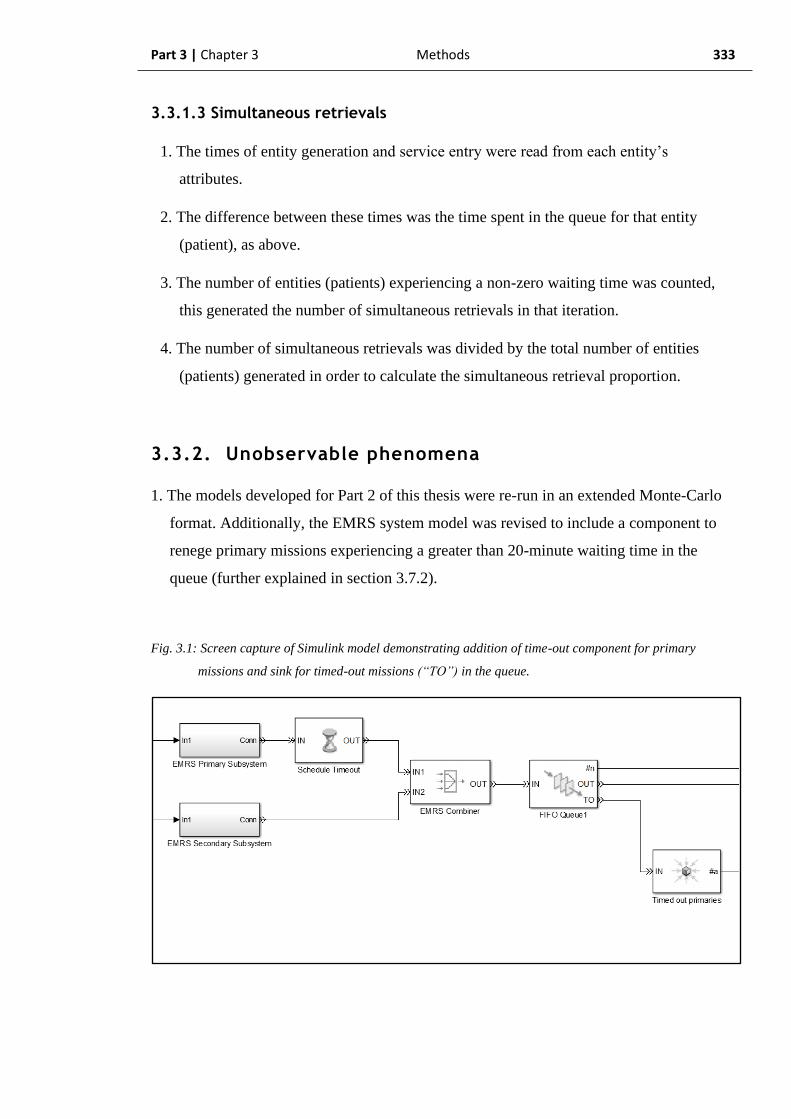
Part 3 | Chapter 3 Methods 333
3.3.1.3 Simultaneous retrievals
1. The times of entity generation and service entry were read from each entity’s
attributes.
2. The difference between these times was the time spent in the queue for that entity
(patient), as above.
3. The number of entities (patients) experiencing a non-zero waiting time was counted,
this generated the number of simultaneous retrievals in that iteration.
4. The number of simultaneous retrievals was divided by the total number of entities
(patients) generated in order to calculate the simultaneous retrieval proportion.
3.3.2. Unobservable phenomena
1. The models developed for Part 2 of this thesis were re-run in an extended Monte-Carlo
format. Additionally, the EMRS system model was revised to include a component to
renege primary missions experiencing a greater than 20-minute waiting time in the
queue (further explained in section 3.7.2).
Fig. 3.1: Screen capture of Simulink model demonstrating addition of time-out component for primary
missions and sink for timed-out missions (“TO”) in the queue.
Part 3 | Chapter 3 Methods 334
2. The number of missions generated by the model was varied by dividing the Simulink
entity inter-generation time by a randomly generated value from a uniform distribution,
in the range 0.01 – 5 for primary missions, and 0.01 – 10 for secondary missions. The
same multiplier value was retained for any one given iteration.
3. From each simulation iteration, the Wq95 for each mission type and simultaneous
retrieval values for each mission type were calculated as above.
4. Each of the performance descriptors (Wq95, simultaneous retrieval proportion, proportion
of missed primary missions) were plotted against the number of missions undertaken in
the simulation iteration. This was a two-dimensional plot for SPRS and a three-
dimensional plot for EMRS (plotted against both mission types).
5. A reference line was fitted to the two-dimensional data and a contour plot (using an
initial 3-D surface fit) was fitted to the three-dimensional data.
6. The location on the graph of the applicable performance limit was established.
7. The current state of the system was compared to the defined performance limits as in
sections 3.5 and section 3.7.
Part 3 Chapter 4
Results:
Derived performance descriptors from
the SPRS simulation
Part 3 | Chapter 4 Results: SPRS Derived Values 336
3.4 Results of derived performance descriptors
from the SPRS simulation
All of the results in this section are generated on the assumption that the model and the
real-world behave in the same mathematical fashion. Although this cannot be explicitly
proven, the findings of model components being able to accurately replicate the
corresponding real-world values and distributions would suggest that such an assumption
is indeed valid. The system performance descriptors calculated herein are therefore
considered to be a true representation of the real-world.
There are no direct equivalents of the parameters in this part of the thesis that can be
measured in the real-world. The ScotSTAR dataset simply does not record data at suitable
time checkpoints for these real-world values to be directly measured. Two SPRS
parameters have a formulaic result which can be used to add gross validity, but as
previously discussed, these are subject to limitations when applied to the non-stationary
Poisson processes of the ScotSTAR systems. Where available, however, such formulaic
results are used for illustration.
The derived values are those of standard queueing theory, with additional parameters
pertinent to the ScotSTAR operations.
Specifically, the parameters described from standard queueing theory are:
- Mean length of queue (Lq)
- Mean waiting time in queue (Wq)
And those developed for this thesis as being specifically relevant to ScotSTAR operations:
- 95th percentile of waiting time in queue (Wq95)
- Simultaneous retrieval proportion

Part 3 | Chapter 4 Results: SPRS Derived Values 337
3.4.1. SPRS retrospective simulation period
In the SPRS retrospective simulation period, Part 2, section 2.5.1, it was demonstrated
that the Simulink model could accurately replicate the real-world. It is therefore considered
appropriate to derive from the model the values of system descriptors which are not
measurable in the real-world system.
The information in this section is directly derived from the same model and simulation
used in Part 2 of this thesis. It is therefore, as in Part 2, based on the information available
through the entire simulation period: both past and future to any given point of the
simulation. This will generate a value for each of the derived performance parameters
representative of the entire retrospective simulation period: calendar years 2013 and 2014.
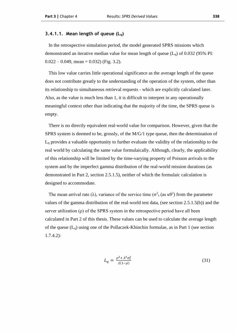
Part 3 | Chapter 4 Results: SPRS Derived Values 338
3.4.1.1. Mean length of queue (Lq)
In the retrospective simulation period, the model generated SPRS missions which
demonstrated an iterative median value for mean length of queue (Lq) of 0.032 (95% PI:
0.022 – 0.049, mean = 0.032) (Fig. 3.2).
This low value carries little operational significance as the average length of the queue
does not contribute greatly to the understanding of the operation of the system, other than
its relationship to simultaneous retrieval requests - which are explicitly calculated later.
Also, as the value is much less than 1, it is difficult to interpret in any operationally
meaningful context other than indicating that the majority of the time, the SPRS queue is
empty.
There is no directly equivalent real-world value for comparison. However, given that the
SPRS system is deemed to be, grossly, of the M/G/1 type queue, then the determination of
Lq provides a valuable opportunity to further evaluate the validity of the relationship to the
real world by calculating the same value formulaically. Although, clearly, the applicability
of this relationship will be limited by the time-varying property of Poisson arrivals to the
system and by the imperfect gamma distribution of the real-world mission durations (as
demonstrated in Part 2, section 2.5.1.5), neither of which the formulaic calculation is
designed to accommodate.
The mean arrival rate (λ), variance of the service time (σ2s (as κθ2) from the parameter
values of the gamma distribution of the real-world test data, (see section 2.5.1.5(b)) and the
server utilization (ρ) of the SPRS system in the retrospective period have all been
calculated in Part 2 of this thesis. These values can be used to calculate the average length
of the queue (Lq) using one of the Pollaczek-Khinchin formulae, as in Part 1 (see section
1.7.4.2):
𝐿𝑞 = 𝜌2+ 𝜆2𝜎𝑠
2
2(1−𝜌) (31)

Part 3 | Chapter 4 Results: SPRS Derived Values 339
So, referencing the real-world values calculated in Part 2:
λ = 0.67 (486 missions / 730 days)
σ2s = 0.02 (28.8 minutes)
ρ = 0.17 (17% utilization)
Therefore:
𝐿𝑞 = 0.172+ 0.672∗0.02
2(1−0.17) (32)
𝐿𝑞 = 0.038
2∗0.83 (33)
𝐿𝑞 = 0.023 (34)
The Pollaczek-Khinchin (P-K) result for mean length of queue (Lq) is grossly
comparable to the calculated value obtained directly from the Simulink model (above). The
P-K result lies within the 95% prediction interval (0.022 – 0.049) of the simulation output
and is not significantly different to the simulation output on Mann-Whitney U testing (p =
0.09).
The difference between the results is also in keeping with the findings in Part 2 section
2.5.1.6 where the simulation mildly over-estimated the server utilization which would, in
itself, result in an increase in the average length of the queue: increased server utilization
increasing the probability of an arriving mission having to wait. The difference in the value
could also be representative of the variation present within the time-dependent Poisson
process which has, as discussed in Part 1, met the property of steady state by ρ < 1, but not
by uniform probability of activation by time of day. This results in a higher probability of
arrival at the same time as a higher probability of a busy server – contributing further to the
expectation of a non-uniform queue length, variable by time of day.
Accounting for all these aspects, it is considered that the P-K formulaic result is in
keeping with the calculated simulation output result. This finding adds validity to the
assumption of mathematical similarity between the processes of the simulation and the

Part 3 | Chapter 4 Results: SPRS Derived Values 340
real-world as the two values, derived by two entirely different mechanisms and from two
different datasets, are consistent and complimentary.
Fig. 3.2: Boxplot of simulation iterative median of mean length of queue (Lq) values (median = 0.032, IQR:
0.028 – 0.036), with simulation iterative mean = 0.032 (black diamond) and Pollaczek-Khinchin
formula calculated result = 0.023 (black line). ). Iterative median not significantly different to
Pollaczek-Khinchin result (Mann-Whitney U-test p = 0.09). Retrospective simulation period:
calendar years 2013-2014.
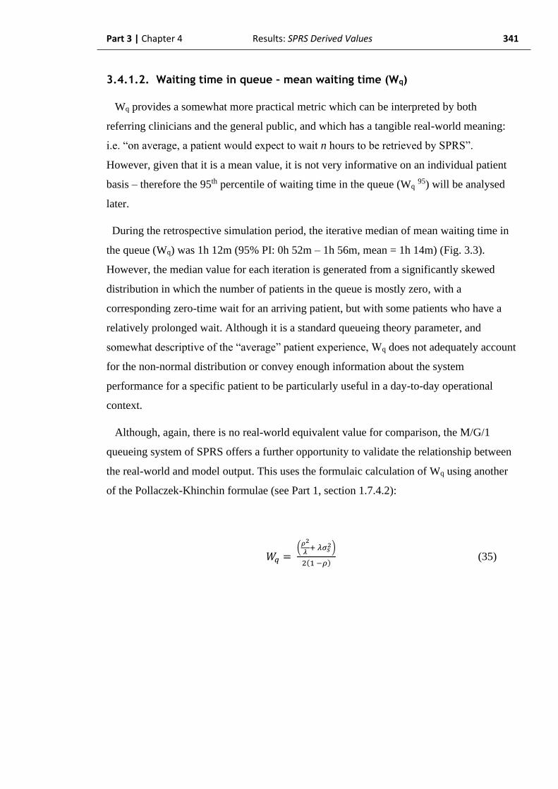
Part 3 | Chapter 4 Results: SPRS Derived Values 341
3.4.1.2. Waiting time in queue – mean waiting time (Wq)
Wq provides a somewhat more practical metric which can be interpreted by both
referring clinicians and the general public, and which has a tangible real-world meaning:
i.e. “on average, a patient would expect to wait n hours to be retrieved by SPRS”.
However, given that it is a mean value, it is not very informative on an individual patient
basis – therefore the 95th percentile of waiting time in the queue (Wq 95) will be analysed
later.
During the retrospective simulation period, the iterative median of mean waiting time in
the queue (Wq) was 1h 12m (95% PI: 0h 52m – 1h 56m, mean = 1h 14m) (Fig. 3.3).
However, the median value for each iteration is generated from a significantly skewed
distribution in which the number of patients in the queue is mostly zero, with a
corresponding zero-time wait for an arriving patient, but with some patients who have a
relatively prolonged wait. Although it is a standard queueing theory parameter, and
somewhat descriptive of the “average” patient experience, Wq does not adequately account
for the non-normal distribution or convey enough information about the system
performance for a specific patient to be particularly useful in a day-to-day operational
context.
Although, again, there is no real-world equivalent value for comparison, the M/G/1
queueing system of SPRS offers a further opportunity to validate the relationship between
the real-world and model output. This uses the formulaic calculation of Wq using another
of the Pollaczek-Khinchin formulae (see Part 1, section 1.7.4.2):
𝑊𝑞 = (
𝜌2
𝜆+ 𝜆𝜎𝑠
2)
2(1 −𝜌) (35)

Part 3 | Chapter 4 Results: SPRS Derived Values 342
Again, referencing the real-world values generated for the retrospective simulation period
in Part 2 (section 2.5.1.5) of the thesis:
λ = 0.67 (486 missions / 730 days)
σ2s = κθ2 = 3.13 * 0.082
= 0.02 days (variance = 28.8 minutes)
ρ = 0.17 (17% utilization)
Therefore:
𝑊𝑞 = (
0.172
0.67+ 0.67∗0.02)
2(1 −0.17) (36)
𝑊𝑞 = 0.057
1.66 (37)
𝑊𝑞 = 0.034 days = 49 minutes
This value is smaller than the simulation-derived value (Fig. 3.3), but is a plausible value
when the consideration of non-uniform probability of activation – with the most likely
activation time also being the most likely time for the server to be busy – generating a
time-varying Wq through the day is applied. The formulaic calculated Wq was at the limit
of statistical non-significance for its difference to the simulation output on Mann-Whitney
U testing (p = 0.05), but the formulaic value does lie outside the 95% prediction interval
for the model, suggesting that the difference is operationally significant. This is likely due
to the limitations of the formulaic result not accounting for either time-dependent Poisson
arrivals or imperfectly gamma-distributed service times.

Part 3 | Chapter 4 Results: SPRS Derived Values 343
Fig. 3.3: Boxplot of simulation iterative mean waiting time in queue (Wq) values (median = 1h 12m, IQR: 1h
5m – 1h 22m), with simulation iterative mean = 1h 14m (black diamond) and Pollaczek-Khinchin
formula calculated result = 49m (black line). Iterative median not significantly different to
Pollaczek-Khinchin result (Mann-Whitney U-test p = 0.05). Retrospective simulation period:
calendar years 2013-2014.
Part 3 | Chapter 4 Results: SPRS Derived Values 344
3.4.1.3. Waiting time in queue – 95th percentile of waiting time (Wq95)
As discussed earlier, the 95th percentile of waiting time (Wq95) was considered to be a
more useful performance metric than Wq. By using the 95th percentile of waiting time, the
time in which 95% of patients will be retrieved is described. Although clearly still
stochastic, Wq95 is much more useful as a service descriptor which is relevant to patients
and rural clinicians: as it describes the time by which they as an individual (the value being
applicable to 19 out of 20 patients) can expect their transfer to be underway.
In the case of the SPRS simulation output, the model generated an iterative median 95th
percentile of waiting time of 8h 8m (95% PI: 6h 1m – 12h 27m, mean = 8h 13m) (Fig.
3.4). This was a somewhat surprising result, given that the overall utilization of the SPRS
system appeared to be relatively low. Examination of the Wq95 ECDF (Fig. 3.5)
demonstrated a markedly skewed distribution, in which Wq95 became non-zero only above
the 83rd percentile. The ECDF therefore shows that 83% of patients will encounter a zero-
time wait for retrieval on entering the system but that the waiting time escalates in a
relatively rapid, linear fashion above this. This is a further illustration of the time-
dependent Poisson process which results in a higher probability of patients encountering a
busy system than utilization alone would imply. Thus, when a patient does have to wait,
their waiting time is more likely to be prolonged.
There is no real-world equivalent value or formulaic approximation for comparison.
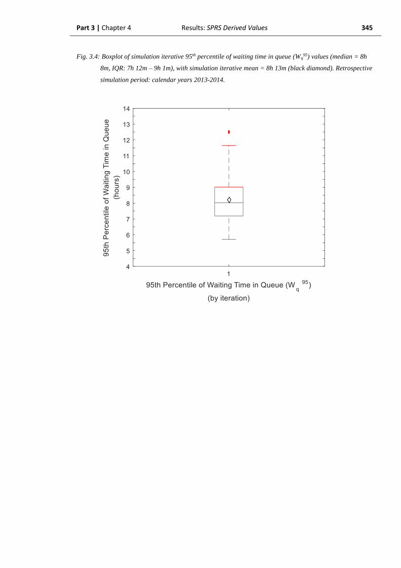
Part 3 | Chapter 4 Results: SPRS Derived Values 345
Fig. 3.4: Boxplot of simulation iterative 95th percentile of waiting time in queue (Wq95) values (median = 8h
8m, IQR: 7h 12m – 9h 1m), with simulation iterative mean = 8h 13m (black diamond). Retrospective
simulation period: calendar years 2013-2014.
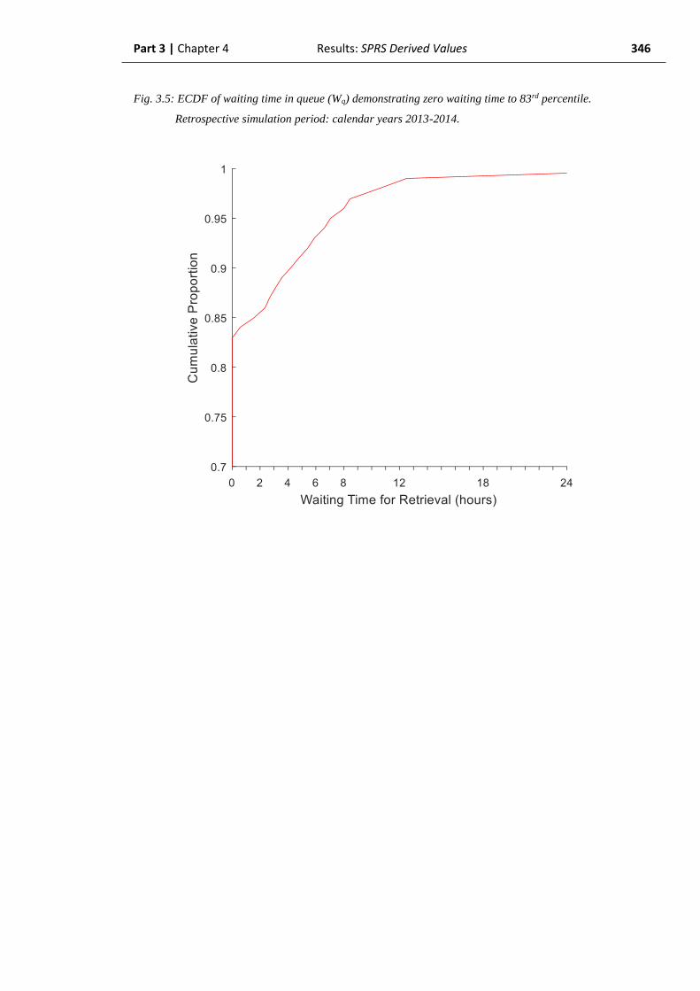
Part 3 | Chapter 4 Results: SPRS Derived Values 346
Fig. 3.5: ECDF of waiting time in queue (Wq) demonstrating zero waiting time to 83rd percentile.
Retrospective simulation period: calendar years 2013-2014.
Part 3 | Chapter 4 Results: SPRS Derived Values 347
3.4.1.4. Simultaneous retrievals
The nature of the data collected by the ScotSTAR teams at the time of this project does
not allow the capture of simultaneous retrievals, as the time at which the retrieval is
required is not reliably captured; only the time at which the retrieval is commenced is
recorded. There may be some time between the two, and the true number of simultaneous
retrievals could be under-estimated if the recorded data creates the appearance from the
commencement time that one retrieval immediately followed another, whereas the retrieval
may have actually been required while the first mission was ongoing. Despite this, the
simultaneous retrieval rate is an important service descriptor to calculate because it implies
an un-met need for patients requiring retrieval.
A high simultaneous retrieval rate may, in fact, be acceptable in the context of a suitably
low Wq95. However, as has been demonstrated above, the Wq
95 for SPRS is considerable
and analysis of the simultaneous retrieval rate may provide an indication as to whether an
increase in the number of SPRS teams could facilitate a reduction in Wq95.
In this section, the model output during the retrospective simulation was analysed to
establish the number of simultaneous retrievals and convert this into a proportion of
missions affected. By nature of the Poisson Arrivals See Time Averages (PASTA)
property of Markov queueing systems, it would be expected that the probability of an
arriving mission encountering a non-zero wait time was equal to the server utilization – in
this case approximately 17% (Part 2, section 2.5.1.6). However, this relationship to
utilization is reliant on a uniform, pure-Poisson arrival process. It is known that the Poisson
arrival process for SPRS is time-dependent and that activations, and therefore utilization,
are higher at certain times of day (see Part 1, section 1.7.1.2). This generates the situation
in which any given arrival is more likely to find the server occupied than would be
predicted by utilization with respect to the PASTA property. It is therefore important to the
accuracy of the information provided as a system descriptor that this anticipated difference
is accounted for - this necessitates the use of simulation output, rather than simply quoting
the easily calculated real-world utilization value.

Part 3 | Chapter 4 Results: SPRS Derived Values 348
The output data from the simulation were analysed to count the number of simultaneous
retrievals. A simultaneous retrieval was recorded when a generated mission encountered a
non-zero wait for service at the SPRS server.
Number of simultaneous retrievals:
During the retrospective simulation period, the SPRS simulation generated an iterative
median of 105 simultaneous retrievals (95% PI: 76 – 130, mean = 103) (Fig. 3.6).
Fig. 3.6: Boxplot of number of simultaneous retrievals (non-zero wait time) by iteration (median = 105, IQR:
93 - 112), with simulation iterative mean = 103 (black diamond). Retrospective simulation period:
calendar years 2013 -2014.

Part 3 | Chapter 4 Results: SPRS Derived Values 349
Proportion of simultaneous retrievals:
When the number of simultaneous retrievals was divided by the iteration’s total number
of generated missions, an iterative median simultaneous retrieval proportion of 21.8%
(95% PI: 16.5% - 25.7%, mean = 21.4%) was generated (Fig. 3.7). This value is
commensurate with the waiting time distribution, both producing a zero-time wait for
approximately 80% of patients. The value was, as expected, greater than the simultaneous
retrieval proportion calculated from the server utilization value (19.1%) although the two
values were not significantly different on Mann-Whitney U-testing (p = 0.28).
Fig. 3.7: Boxplot of simultaneous retrieval proportion (non-zero wait time) by iteration (median = 21.8%,
IQR: 16.5% - 23.3%), with simulation iterative mean = 21.4% (black diamond). Expected value =
utilization = 19.1% (black line), from SPRS simulation based on PASTA property. Iterative median
not significantly different to expected value (Mann-Whitney U-test p = 0.28). Retrospective
simulation period: calendar years 2013-2014.

Part 3 | Chapter 4 Results: SPRS Derived Values 350
3.4.2. SPRS contemporaneous simulation period
In keeping with the previous analysis in Part 2, the contemporaneous simulation period
will now be analysed, using the same model as Part 2, and the same methodology – in
which the model only receives information up to the current simulation point, it has no
“look-forward” capability. This is important to the project as it shows the ability of the
model to describe the immediate, current performance of the system instead of a general
description of performance through a time period as was demonstrated by the retrospective
simulation.
Part 2, section 2.5.2.6 demonstrated that the SPRS model was unable to generate a daily
contemporaneous derived value which was comparable to the real-world. It did
demonstrate, however, that the model could correctly replicate the current utilization value
at the end of the 2015 calendar year, with a one-year data sampling window. Reflective of
this, the following derived SPRS results in the contemporaneous simulation period are also
reported as representing the current state at the conclusion of the simulation period, with a
one-year data sampling window corresponding to the 2015 calendar year.
Part 3 | Chapter 4 Results: SPRS Derived Values 351
3.4.2.1. Mean length of queue (Lq)
In the contemporaneous simulation period, SPRS missions demonstrated an iterative
median value for the current mean length of queue (Lq) at the end of the 2015 calendar
year, with a one-year data sampling window, of 0.042 (95% Prediction Interval: 0.026 –
0.072, mean = 0.045) (Fig. 3.8).
Although there is no directly measurable real-world equivalent value, an approximation
of Lq using the P-K formula was again performed with reference to the real-world testing
dataset values calculated in Part 2, section 2.5.2.5:
λ = 0.79 (287 missions / 365 days)
σ2s = κθ2 = 2.35 * 0.082
= 0.015 (variance = 21.7 minutes)
ρ = 0.22 (22% utilization)
𝐿𝑞 = 𝜌2+ 𝜆2𝜎𝑠
2
2(1−𝜌) (38)
𝐿𝑞 = 0.037
The formulaic result of Lq = 0.037 (97.4% of simulated value) was not significantly
different to the simulation result on Mann-Whitney U-testing (p = 0.37).
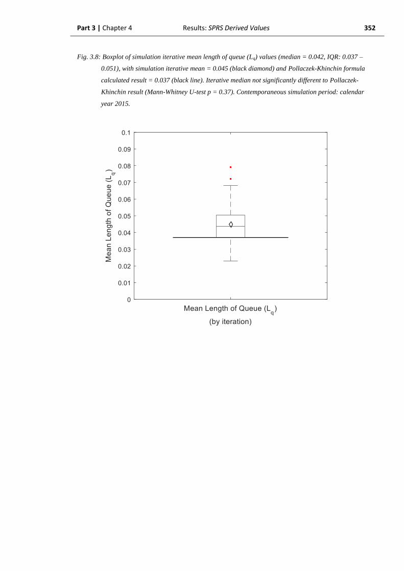
Part 3 | Chapter 4 Results: SPRS Derived Values 352
Fig. 3.8: Boxplot of simulation iterative mean length of queue (Lq) values (median = 0.042, IQR: 0.037 –
0.051), with simulation iterative mean = 0.045 (black diamond) and Pollaczek-Khinchin formula
calculated result = 0.037 (black line). Iterative median not significantly different to Pollaczek-
Khinchin result (Mann-Whitney U-test p = 0.37). Contemporaneous simulation period: calendar
year 2015.
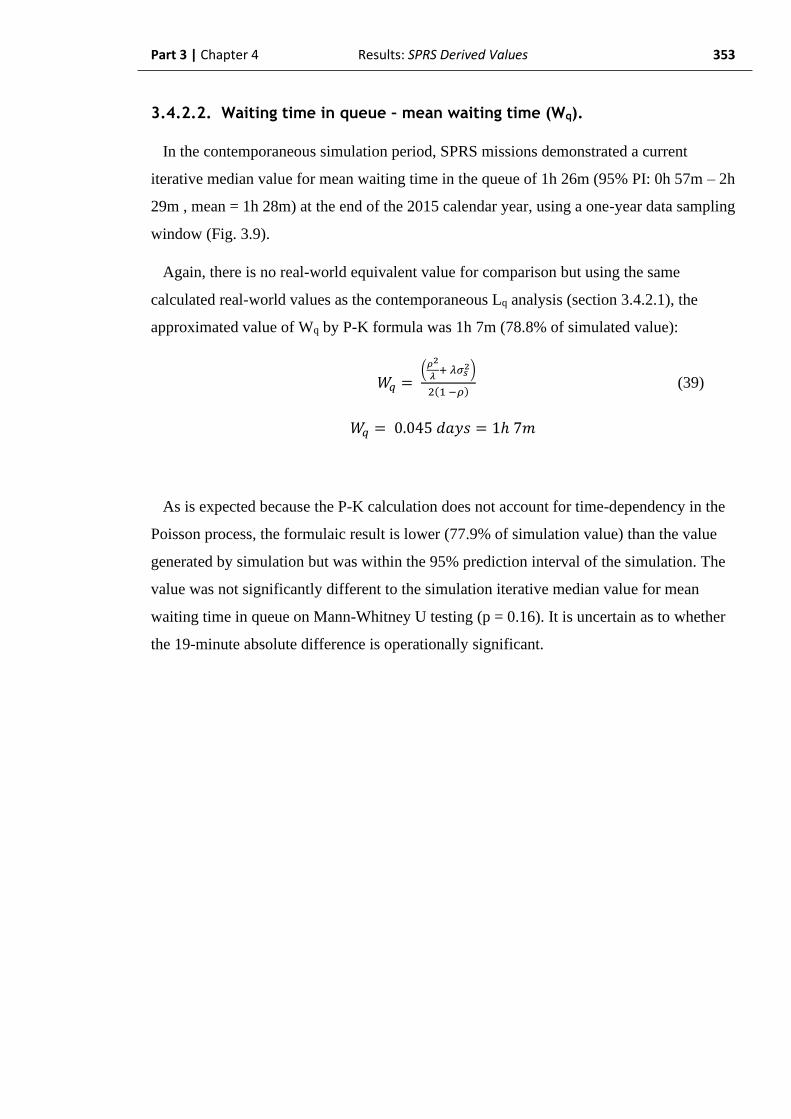
Part 3 | Chapter 4 Results: SPRS Derived Values 353
3.4.2.2. Waiting time in queue – mean waiting time (Wq).
In the contemporaneous simulation period, SPRS missions demonstrated a current
iterative median value for mean waiting time in the queue of 1h 26m (95% PI: 0h 57m – 2h
29m , mean = 1h 28m) at the end of the 2015 calendar year, using a one-year data sampling
window (Fig. 3.9).
Again, there is no real-world equivalent value for comparison but using the same
calculated real-world values as the contemporaneous Lq analysis (section 3.4.2.1), the
approximated value of Wq by P-K formula was 1h 7m (78.8% of simulated value):
𝑊𝑞 = (
𝜌2
𝜆+ 𝜆𝜎𝑠
2)
2(1 −𝜌) (39)
𝑊𝑞 = 0.045 𝑑𝑎𝑦𝑠 = 1ℎ 7𝑚
As is expected because the P-K calculation does not account for time-dependency in the
Poisson process, the formulaic result is lower (77.9% of simulation value) than the value
generated by simulation but was within the 95% prediction interval of the simulation. The
value was not significantly different to the simulation iterative median value for mean
waiting time in queue on Mann-Whitney U testing (p = 0.16). It is uncertain as to whether
the 19-minute absolute difference is operationally significant.

Part 3 | Chapter 4 Results: SPRS Derived Values 354
Fig. 3.9: Boxplot of simulation iterative mean waiting time in queue (Wq) values (median = 1h 26m, IQR: 1h
16m – 1h 39m), with simulation iterative mean = 1h 28m (black diamond) and Pollaczek-Khinchin
formula calculated result = 1h 7m (black line). Iterative median not significantly different to
Pollaczek-Khinchin result (Mann-Whitney U-test p = 0.16). Contemporaneous simulation period:
calendar year 2015.
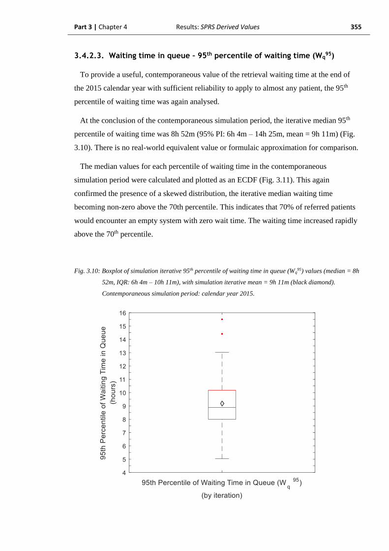
Part 3 | Chapter 4 Results: SPRS Derived Values 355
3.4.2.3. Waiting time in queue – 95th percentile of waiting time (Wq95)
To provide a useful, contemporaneous value of the retrieval waiting time at the end of
the 2015 calendar year with sufficient reliability to apply to almost any patient, the 95th
percentile of waiting time was again analysed.
At the conclusion of the contemporaneous simulation period, the iterative median 95th
percentile of waiting time was 8h 52m (95% PI: 6h 4m – 14h 25m, mean = 9h 11m) (Fig.
3.10). There is no real-world equivalent value or formulaic approximation for comparison.
The median values for each percentile of waiting time in the contemporaneous
simulation period were calculated and plotted as an ECDF (Fig. 3.11). This again
confirmed the presence of a skewed distribution, the iterative median waiting time
becoming non-zero above the 70th percentile. This indicates that 70% of referred patients
would encounter an empty system with zero wait time. The waiting time increased rapidly
above the 70th percentile.
Fig. 3.10: Boxplot of simulation iterative 95th percentile of waiting time in queue (Wq95) values (median = 8h
52m, IQR: 6h 4m – 10h 11m), with simulation iterative mean = 9h 11m (black diamond).
Contemporaneous simulation period: calendar year 2015.

Part 3 | Chapter 4 Results: SPRS Derived Values 356
Fig. 3.11: ECDF of waiting time in queue (Wq) demonstrating zero waiting time to 70th percentile.
Contemporaneous simulation period: calendar year 2015.
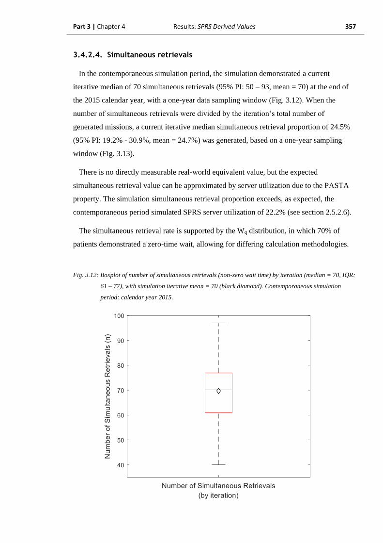
Part 3 | Chapter 4 Results: SPRS Derived Values 357
3.4.2.4. Simultaneous retrievals
In the contemporaneous simulation period, the simulation demonstrated a current
iterative median of 70 simultaneous retrievals (95% PI: 50 – 93, mean = 70) at the end of
the 2015 calendar year, with a one-year data sampling window (Fig. 3.12). When the
number of simultaneous retrievals were divided by the iteration’s total number of
generated missions, a current iterative median simultaneous retrieval proportion of 24.5%
(95% PI: 19.2% - 30.9%, mean = 24.7%) was generated, based on a one-year sampling
window (Fig. 3.13).
There is no directly measurable real-world equivalent value, but the expected
simultaneous retrieval value can be approximated by server utilization due to the PASTA
property. The simulation simultaneous retrieval proportion exceeds, as expected, the
contemporaneous period simulated SPRS server utilization of 22.2% (see section 2.5.2.6).
The simultaneous retrieval rate is supported by the Wq distribution, in which 70% of
patients demonstrated a zero-time wait, allowing for differing calculation methodologies.
Fig. 3.12: Boxplot of number of simultaneous retrievals (non-zero wait time) by iteration (median = 70, IQR:
61 – 77), with simulation iterative mean = 70 (black diamond). Contemporaneous simulation
period: calendar year 2015.
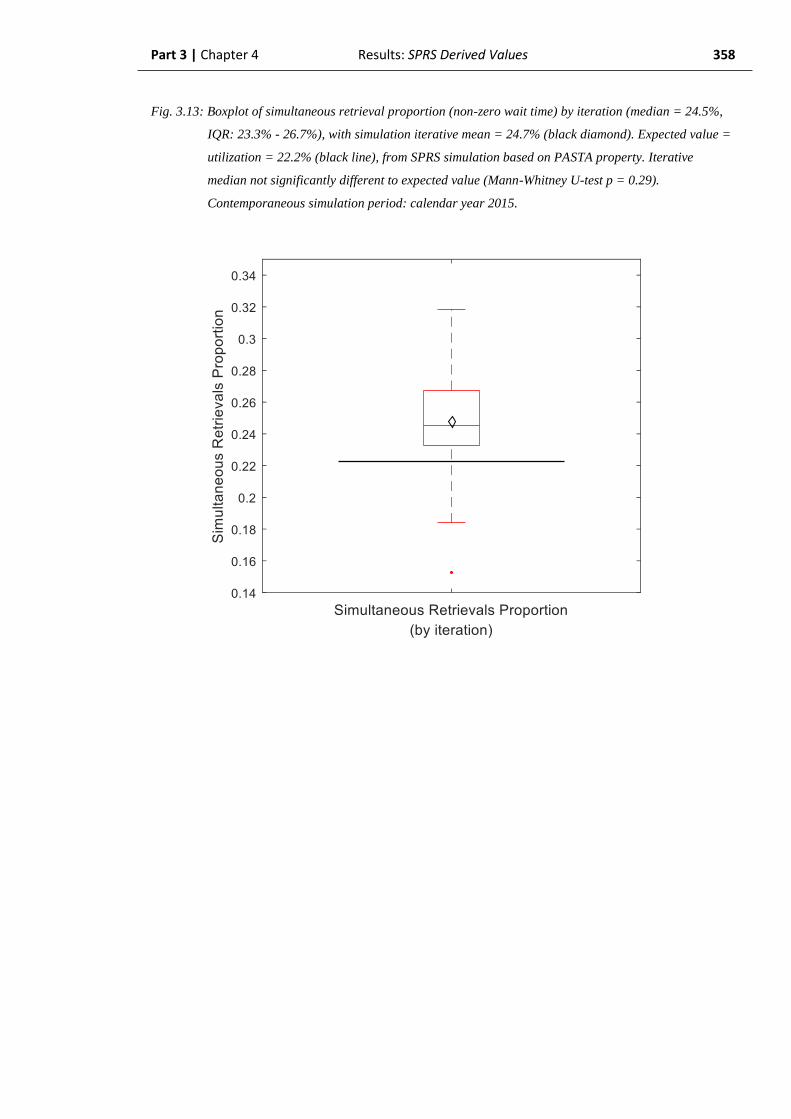
Part 3 | Chapter 4 Results: SPRS Derived Values 358
Fig. 3.13: Boxplot of simultaneous retrieval proportion (non-zero wait time) by iteration (median = 24.5%,
IQR: 23.3% - 26.7%), with simulation iterative mean = 24.7% (black diamond). Expected value =
utilization = 22.2% (black line), from SPRS simulation based on PASTA property. Iterative
median not significantly different to expected value (Mann-Whitney U-test p = 0.29).
Contemporaneous simulation period: calendar year 2015.
Part 3 | Chapter 4 Results: SPRS Derived Values 359
3.4.3. Summary of SPRS derived system descriptors
results
The SPRS model has generated the standard queueing theory descriptors of Lq and Wq by
simulation rather than by formulaic calculation. This has generated plausible, but larger
values for each of the studied parameters than those for which a real-world formulaic
solution exists. This reinforces the principle of formulaic queueing theory being only
applicable to systems in which there is a stationary arrivals process, which SPRS does not
demonstrate. The magnitude of the difference is relatively small, and it may therefore be
the case that the formulaic results provide an adequate approximation of the real-world
values for the SPRS system. Such formulaic results, however, do not adequately describe
the system for the patients and users of the SPRS service and there is no formulaic answer
which describes the 95th percentile of waiting time (Wq95). This inadequate description of
the system primarily stems from the skewed distribution of waiting times, which generate a
substantial difference between the standard queueing theory descriptor of Wq, and the Wq95
value – the latter providing a much better indication to patients of the service which they,
as an individual, can expect to receive.
Summary tables of the simulation output are provided for reference overleaf (Table 3.1 &
Table 3.2)
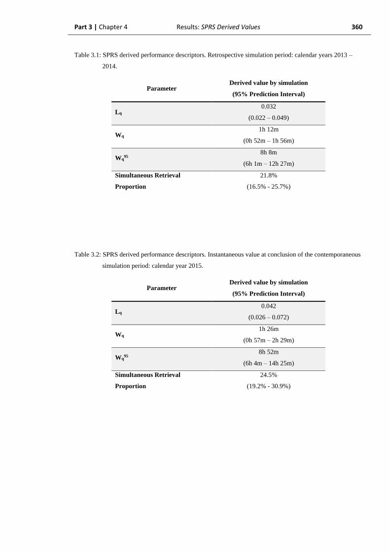
Part 3 | Chapter 4 Results: SPRS Derived Values 360
Table 3.1: SPRS derived performance descriptors. Retrospective simulation period: calendar years 2013 –
2014.
Parameter Derived value by simulation
(95% Prediction Interval)
Lq 0.032
(0.022 – 0.049)
Wq 1h 12m
(0h 52m – 1h 56m)
Wq95
8h 8m
(6h 1m – 12h 27m)
Simultaneous Retrieval
Proportion
21.8%
(16.5% - 25.7%)
Table 3.2: SPRS derived performance descriptors. Instantaneous value at conclusion of the contemporaneous
simulation period: calendar year 2015.
Parameter Derived value by simulation
(95% Prediction Interval)
Lq 0.042
(0.026 – 0.072)
Wq 1h 26m
(0h 57m – 2h 29m)
Wq95
8h 52m
(6h 4m – 14h 25m)
Simultaneous Retrieval
Proportion
24.5%
(19.2% - 30.9%)
Part 3 Chapter 5
Results:
Simulating SPRS performance
frontiers through
unobservable phenomena

Part 3 | Chapter 5 Results: SPRS Performance Limits 362
3.5. Results of simulating SPRS performance
frontiers through unobservable phenomena
The results from the preceding section have shown that the Wq95 and simultaneous
retrieval proportions of the SPRS system lie above the respective specification limits of 1
hour and 10% (see Table 3.1 and Table 3.2). Therefore, the model and, by inference, the
real-world system simply never experience a low enough utilization to generate a Wq95 less
than 1 hour or a simultaneous retrieval probability less than 10%. The yearly number of
missions which correspond to these performance limits are therefore unobservable in the
real-world. Accordingly, the values are not generated within a simulation specifically
designed to replicate the real-world.
Therefore, to simulate unobservable real-world phenomena, the SPRS model developed
in Part 2 was run in an extended Monte-Carlo format to generate a wide number of mission
totals per year. This allowed the model to simulate yearly mission totals which would not
be experienced in the real-world system or the original SPRS simulations.
This allowed the demonstration of the mathematical relationships between observed real-
world values for the SPRS system and the important system performance descriptors which
have been discussed. In particular, this simulation methodology gives the opportunity to
correlate the expected, but unproven, relationships extrapolated from simpler aspects of
queueing theory (e.g. exponential relationship between utilization and Wq) in the complex
SPRS system with its time-dependent Poisson arrivals process in particular.
Part 3 | Chapter 5 Results: SPRS Performance Limits 363
Having reviewed the system descriptors obtained as derived values from the simulation
(section 3.4), it was considered that the SPRS team was likely operating beyond a
performance frontier due to over-capacity. It was therefore considered most relevant to
approach the analysis of the SPRS operational system with regard to three operational
questions:
1. What is the difference between the current state of the SPRS system and that
required for a target simultaneous retrieval rate < 10%?
2. What is the difference between the current state of the SPRS system and that
required for a target Wq95 less than 1 hour?
3. What would be the effect on waiting time for retrieval of adding a second team
to the system?
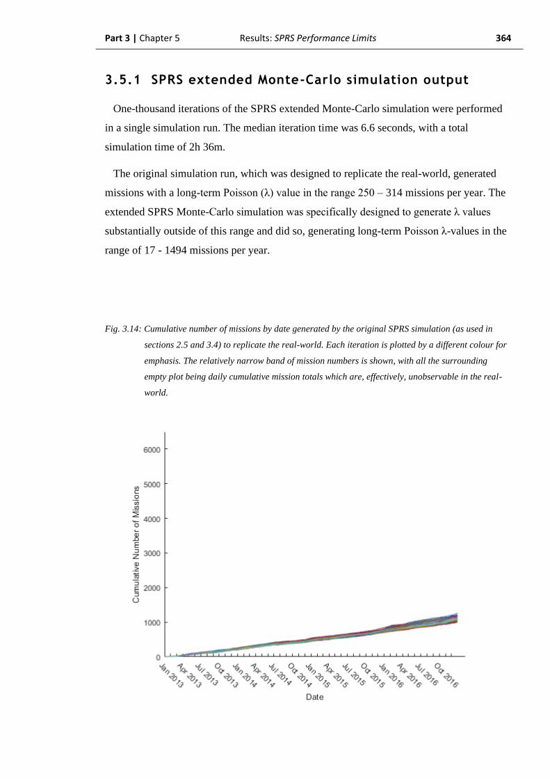
Part 3 | Chapter 5 Results: SPRS Performance Limits 364
3.5.1 SPRS extended Monte-Carlo simulation output
One-thousand iterations of the SPRS extended Monte-Carlo simulation were performed
in a single simulation run. The median iteration time was 6.6 seconds, with a total
simulation time of 2h 36m.
The original simulation run, which was designed to replicate the real-world, generated
missions with a long-term Poisson (λ) value in the range 250 – 314 missions per year. The
extended SPRS Monte-Carlo simulation was specifically designed to generate λ values
substantially outside of this range and did so, generating long-term Poisson λ-values in the
range of 17 - 1494 missions per year.
Fig. 3.14: Cumulative number of missions by date generated by the original SPRS simulation (as used in
sections 2.5 and 3.4) to replicate the real-world. Each iteration is plotted by a different colour for
emphasis. The relatively narrow band of mission numbers is shown, with all the surrounding
empty plot being daily cumulative mission totals which are, effectively, unobservable in the real-
world.

Part 3 | Chapter 5 Results: SPRS Performance Limits 365
Fig. 3.15: Cumulative number of missions by date generated by the SPRS extended Monte-Carlo simulation.
Each iteration is a different colour for emphasis. The black triangle approximately indicates the
output block from the original SPRS simulation, as Fig. 3.14. The output from all iterations which
lie outside this triangle are the simulated cumulative daily mission totals which were unobservable
in the real-world.
Part 3 | Chapter 5 Results: SPRS Performance Limits 366
3.5.2. Waiting time in queue – 95th percentile of waiting
time (Wq95) (Specification limit: 1 hour)
Although no relationship involving Wq95 is described by standard queueing theory, it is
generally accepted that waiting time increases exponentially with increasing utilization.
This was not the case with the extended Monte-Carlo simulation output Wq95 values.
Analysis of the simulation data demonstrated that the relationship between total number of
missions and 95th percentile of waiting time (Wq95) was complex, requiring the use of a
polynomial model to generate an acceptable approximation, but did not appear to follow an
exponential relationship at the studied values.
Consulting the fitted reference curve at the value corresponding to a yearly λ of 257
missions, the Monte-Carlo simulation predicted a Wq95 of 9h 15m. This compared
favourably with the simulation output calculated value for Wq95 in the contemporaneous
simulation period (section 3.4.2.3) in which 257 simulated missions had a calculated Wq95
of 8h 52m. There was a threshold at approximately 50 missions per year below which the
95th percentile of waiting time was consistently zero.
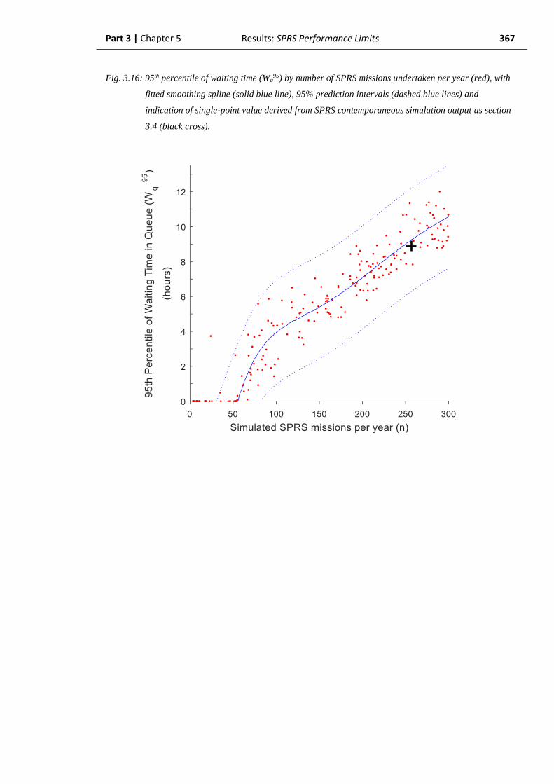
Part 3 | Chapter 5 Results: SPRS Performance Limits 367
Fig. 3.16: 95th percentile of waiting time (Wq95) by number of SPRS missions undertaken per year (red), with
fitted smoothing spline (solid blue line), 95% prediction intervals (dashed blue lines) and
indication of single-point value derived from SPRS contemporaneous simulation output as section
3.4 (black cross).

Part 3 | Chapter 5 Results: SPRS Performance Limits 368
Target: Wq95 < 1 hour
By reference to the fitted polynomial model, a Wq95 less than one hour could only be
achieved with an SPRS missions yearly λ of approximately 61 missions per year (95% PI:
41 – 101). It is therefore considered, in similarity to the simultaneous retrieval result,
highly unlikely that the current system would be able to achieve a 95th percentile of waiting
time less than 1 hour as this would require the system to perform only approximately one-
quarter of its current workload.
Fig. 3.17: 95th percentile of waiting time (Wq95) by number of SPRS missions undertaken per year (red) with
fitted reference polynomial (solid blue line) and 95% prediction intervals. Indication of single-
point value derived from section 3.4 (black cross). Target Wq95 = 60 minutes (red line) with point
estimate value = 61 missions (solid black line) and associated range of mission number yearly λ
values shown (black dashed lines).
Part 3 | Chapter 5 Results: SPRS Performance Limits 369
3.5.3. Simultaneous retrievals
(Specification limit: 10% proportion)
a) Number of simultaneous retrievals
From each iteration of the SPRS extended Monte-Carlo simulation, the total number of
missions generated in the iteration was plotted against the number of simultaneous
retrievals (i.e. the number of arriving patients experiencing a non-zero wait).
The simulation output demonstrated that the relationship between number of missions
and number of simultaneous retrievals appeared generally exponential, in keeping with
established queueing theory (Fig. 3.18). A reference curve was fitted describing the
relationship between number of missions and number of simultaneous retrievals. As there
can be no simultaneous retrievals when there are no missions, the line was forced through
the origin.
Using the fitted reference curve, the extended Monte-Carlo simulation output for a yearly
λ = 257 missions (equivalent to SPRS missions in the 2015 calendar year) was predicted to
generate 62 simultaneous retrievals (Fig. 3.19). The derived value from the original
simulation (section 3.4.2.4) predicted 70 simultaneous retrievals in the 2015 calendar year.
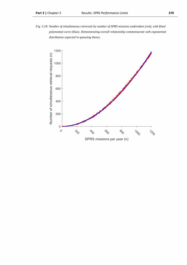
Part 3 | Chapter 5 Results: SPRS Performance Limits 370
Fig. 3.18: Number of simultaneous retrievals by number of SPRS missions undertaken (red), with fitted
polynomial curve (blue). Demonstrating overall relationship commensurate with exponential
distribution expected in queueing theory.
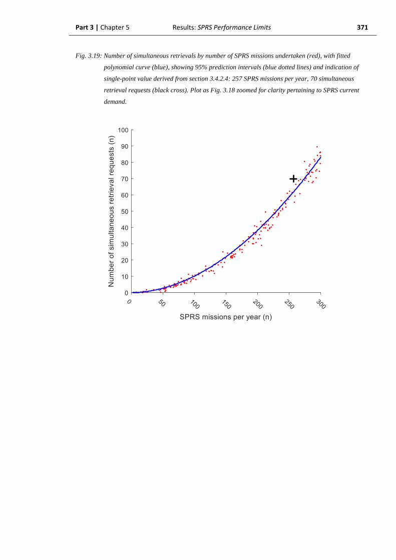
Part 3 | Chapter 5 Results: SPRS Performance Limits 371
Fig. 3.19: Number of simultaneous retrievals by number of SPRS missions undertaken (red), with fitted
polynomial curve (blue), showing 95% prediction intervals (blue dotted lines) and indication of
single-point value derived from section 3.4.2.4: 257 SPRS missions per year, 70 simultaneous
retrieval requests (black cross). Plot as Fig. 3.18 zoomed for clarity pertaining to SPRS current
demand.

Part 3 | Chapter 5 Results: SPRS Performance Limits 372
b) Proportion of simultaneous retrievals
When the number of simultaneous retrievals was divided by the total number of missions
in that iteration, a simultaneous retrieval proportion (as a percentage) was generated. This
simultaneous retrieval proportion demonstrated an approximately linear increase with an
increasing number of missions (Fig. 3.20). A reference line was fitted to the data. Again, as
zero missions must confer a simultaneous retrieval proportion of zero, the line was forced
though the origin.
Using the reference line, 257 missions per year (equivalent to SPRS missions in the 2015
calendar year) was predicted to generate a simultaneous retrieval proportion of 24.2%. The
derived value from the original simulation (section 4.2.4) predicted a 24.5% simultaneous
retrieval proportion in the 2015 calendar year.
Fig. 3.20: Simultaneous retrieval proportion by number of SPRS missions undertaken (red), with fitted linear
regression model (solid blue line). Indicative single-point value derived from section 3.4.2.4: 257
missions = 24.5% simultaneous retrieval proportion (black cross) compared to regression line
predicted value = 24.2%.

Part 3 | Chapter 5 Results: SPRS Performance Limits 373
c) Proportion of simultaneous retrievals (Target < 10%)
From the above-generated reference line, the required yearly λ to generate a simultaneous
retrieval proportion of 10% or less was calculated from the point at which the fitted
reference line crossed the 10% simultaneous retrieval threshold.
Based on this, a simultaneous retrieval proportion ≤ 10% would only be achievable with
an SPRS missions yearly λ of approximately 104 missions (95% PI: 70 – 142). This would
suggest that the current system would face significant challenges in achieving a target of ≤
10% simultaneous retrievals – requiring to undertake less than half the current number of
missions.
Fig. 3.21: Simultaneous retrieval proportion by number of SPRS missions undertaken (red), with fitted linear
regression model (solid blue line), 95% prediction intervals (dashed blue lines). Indicative single-
point value derived from section 3.4.2.4: 257 missions = 24.5% simultaneous retrieval proportion
(black cross). Mission number to achieve 10% simultaneous retrieval rate indicated (red dashed
line) with 95% prediction intervals (black dashed lines).
Part 3 | Chapter 5 Results: SPRS Performance Limits 374
3.5.4. Addition of a second SPRS team
Where the arrival rate (λ) and service rate (μ) are unchanged, increasing the number of
SPRS servers (c) to two would have the effect of halving the SPRS system traffic intensity,
by the relationship:
𝜌 = 𝜆
𝑐 𝜇 (40)
The extended Monte-Carlo simulation output was therefore interrogated with regard to
traffic intensity (ρ) rather than raw number of missions versus 95th percentile of waiting
time (Wq95).
Assuming that the mission duration distribution does not change, ρ varies as the number
of missions. The relationship of ρ to Wq95 is therefore outwardly similar to that between the
number of missions and Wq95. The extended Monte-Carlo simulation generated a
predicted Wq95 of 9h 8m from a traffic intensity of 19.3%. This compared favourably with
the results from section 3.4.2.3 where, in the contemporaneous simulation period, a Wq95 of
8h 52m was calculated from a simulated traffic intensity of 19.3% (Fig. 3.22).
Adding a second team to the system has the effect of halving the overall utilization of the
server from 19.3% to 9.7%. Interpolation from the reference curve suggests that this would
produce a reduction in the 95th percentile of waiting time from 9h 8m to 4h 9m (50.8%
reduction) (Fig. 3.23). Although this would not reach the target threshold of the 95th
percentile of waiting time < 60 minutes, it would bring the Wq95 value towards the top of
the steepest part of the line, potentially allowing a synergistic improvement if a further
utilization-reducing intervention (e.g. faster team deployment to reduce mission durations)
could be implemented. This should be contrasted with the probability of simultaneous
retrieval in a multi-server system as shown for EMRS in section 3.6.1.4 and further
explored in the discussion (section 3.8.2.4).

Part 3 | Chapter 5 Results: SPRS Performance Limits 375
Fig. 3.22: Monte-Carlo simulation output of 95th percentile of waiting time (Wq95) by traffic intensity for
SPRS team (red points), with fitted polynomial reference line (blue line) and indication of single-
point value derived from contemporaneous simulation (257 missions) ρ = 0.193, Wq95 = 8h 52m
(black cross).

Part 3 | Chapter 5 Results: SPRS Performance Limits 376
Fig. 3.23: 95th percentile of waiting time (Wq95) by SPRS team utilization (red points), with fitted polynomial
reference line (blue line) and indication of smoothing spline and single-point indication of single-
point value derived from contemporaneous simulation (257 missions) ρ = 0.193, Wq95 = 8h 52m
(black cross). Effect of adding additional SPRS team (halving of offered load) of new Wq95 = 4h
29m (dashed black lines).

Part 3 | Chapter 5 Results: SPRS Performance Limits 377
3.5.5 Summary – SPRS performance specifications
In this analysis, the SPRS system has been demonstrated to have Lq and Wq values which
are compatible with the real-world formulaic values for the same parameters. This lends
validity to the results of the purely simulation-derived critical system performance
descriptors of Wq95 and simultaneous retrieval proportions. In which case, these results
demonstrate that the SPRS system currently operates with substantial challenges in respect
of both Wq95 and simultaneous retrieval proportion.
Wq95 demonstrates that patients can only be reliably informed that their retrieval is likely
to commence in 7h 42m or less. In the context of a critically unwell patient in a remote
healthcare facility, this may be considered an unacceptably long timeframe by the referring
clinicians. The simultaneous retrieval proportion aligned with this finding, demonstrating
that 20 – 25% of patients will be referred to a non-empty system, potentially incurring a
significant wait. Both of these results indicate that the paediatric service is operating
beyond the proposed performance limits of Wq95 less than one hour and simultaneous
retrieval proportion less than 10%.
Furthermore, when the relationships demonstrated by analysis of unobservable real-
world phenomena are also considered, it is apparent that there are no easy solutions for the
SPRS system. The Monte-Carlo simulation demonstrated that an unachievable reduction in
the number of missions undertaken would need to be performed to bring either the Wq95
below the target of 1 hour or the simultaneous retrieval proportion under the 10% target.
The most promising change simulated was that of adding a second SPRS team. This would
marginally better than halve (49.5%) the Wq95 value; but it would have the potential to act
synergistically with any other interventions which reduce the SPRS server utilization.
The relationship of the current SPRS performance to the specification limits is
summarised overleaf (Table 3.3).

Part 3 | Chapter 5 Results: SPRS Performance Limits 378
Table 3.3: Current SPRS performance relative to specification limits.
Specification
Current real-
world value
(2015 calendar year)
Proportion of
Target
Required change in
utilization to meet target.
Simultaneous retrieval
proportion < 10% 22.6% 226%
Reduce by
153 missions
per year
Wq95 < 1-hour 8h 52m 887%
Reduce by
196 missions
per year
Part 3 Chapter 6
Results:
Derived performance descriptors
from the EMRS simulation

Part 3 | Chapter 6 Results: EMRS Derived Values 380
3.6 Results of derived performance descriptors
from the EMRS simulation
Following from the EMRS section in Part 2 of this thesis, in which the ability of the
model to accurately reflect the real-world in the retrospective and contemporaneous
simulation periods were established, the analysis will now progress towards establishing
useful descriptive system performance parameters derived from the EMRS model.
All the results in this section assume that the model and the real-world behave
comparably. In contrast to the SPRS analysis, there is no formulaic result for the M/G/2
system with non-homogeneous Poisson arrivals which describes EMRS. And no
comparative real-world values are available due to the limitations of the ScotSTAR
datasets. The validity of the EMRS results is therefore inferred from the similarity of the
model and real-world results described in Part 2. Some additional validity is gained by
extension of the results of the SPRS system, the EMRS model being an increased-
complexity evolution of the SPRS model.
As previously, the analysis will define for the EMRS system a number of standard
queueing theory parameters:
- Mean length of queue (Lq)
- Mean waiting time in queue (Wq)
And those developed specifically for this project as being specifically relevant to
ScotSTAR operations:
- 95th percentile of waiting time in queue (Wq95)
- Simultaneous retrieval proportion
Missions arriving to the system are strictly allocated to the Duty One team in the first
instance. The servers are otherwise homogeneous and there is otherwise no difference
between the teams with respect to service time distributions or type of missions served.

Part 3 | Chapter 6 Results: EMRS Derived Values 381
3.6.1. Retrospective simulation period
In the EMRS retrospective simulation period (Part 2, section 2.6.1), it was demonstrated
that the model could accurately replicate the real-world. It is therefore considered
appropriate to derive from the model the values of system descriptors which are not
measurable in the real-world system.
The information in this section is directly derived from the same Simulink model and
simulation used in the EMRS retrospective analysis in Part 2. It is therefore, as in Part 2,
based on information available to the model throughout the simulation period: both past
and future to any given simulated time instance. This will generate a value for each of the
derived performance parameters representative of the entire retrospective simulation
period: calendar years 2013 and 2014.

Part 3 | Chapter 6 Results: EMRS Derived Values 382
3.6.1.1. Mean length of queue (Lq)
In the retrospective simulation period, EMRS missions demonstrated an iterative median
value for mean length of queue (Lq) of 0.012 (95% PI: 0.010 – 0.016, mean = 0.013) (Fig.
3.24)
Lq is demonstrated as a standard queueing theory parameter. Given its value is
considerably less than one it indicates that, the majority of the time, the EMRS queue is
empty. Lq does have a relationship to the number of simultaneous retrieval requests and to
the waiting time, but as both of these will be explicitly calculated then Lq, in itself, does not
currently convey any useful operational significance.
Fig. 3.24: Boxplot of simulation iterative mean length of EMRS queue (Lq) values (median = 0.012, IQR:
0.011 – 0.014), with iterative mean = 0.013 (black diamond). Retrospective simulation period:
calendar years 2013 – 2014.
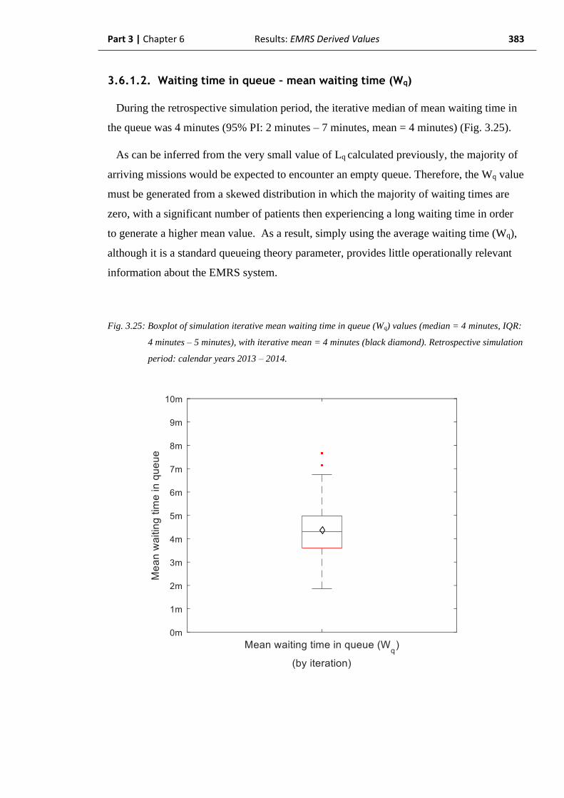
Part 3 | Chapter 6 Results: EMRS Derived Values 383
3.6.1.2. Waiting time in queue – mean waiting time (Wq)
During the retrospective simulation period, the iterative median of mean waiting time in
the queue was 4 minutes (95% PI: 2 minutes – 7 minutes, mean = 4 minutes) (Fig. 3.25).
As can be inferred from the very small value of Lq calculated previously, the majority of
arriving missions would be expected to encounter an empty queue. Therefore, the Wq value
must be generated from a skewed distribution in which the majority of waiting times are
zero, with a significant number of patients then experiencing a long waiting time in order
to generate a higher mean value. As a result, simply using the average waiting time (Wq),
although it is a standard queueing theory parameter, provides little operationally relevant
information about the EMRS system.
Fig. 3.25: Boxplot of simulation iterative mean waiting time in queue (Wq) values (median = 4 minutes, IQR:
4 minutes – 5 minutes), with iterative mean = 4 minutes (black diamond). Retrospective simulation
period: calendar years 2013 – 2014.
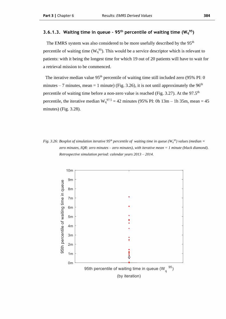
Part 3 | Chapter 6 Results: EMRS Derived Values 384
3.6.1.3. Waiting time in queue – 95th percentile of waiting time (Wq95)
The EMRS system was also considered to be more usefully described by the 95th
percentile of waiting time (Wq95). This would be a service descriptor which is relevant to
patients: with it being the longest time for which 19 out of 20 patients will have to wait for
a retrieval mission to be commenced.
The iterative median value 95th percentile of waiting time still included zero (95% PI: 0
minutes – 7 minutes, mean = 1 minute) (Fig. 3.26), it is not until approximately the 96th
percentile of waiting time before a non-zero value is reached (Fig. 3.27). At the 97.5th
percentile, the iterative median Wq97.5 = 42 minutes (95% PI: 0h 13m – 1h 35m, mean = 45
minutes) (Fig. 3.28).
Fig. 3.26: Boxplot of simulation iterative 95th percentile of waiting time in queue (Wq95) values (median =
zero minutes, IQR: zero minutes – zero minutes), with iterative mean = 1 minute (black diamond).
Retrospective simulation period: calendar years 2013 – 2014.
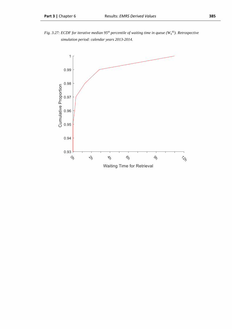
Part 3 | Chapter 6 Results: EMRS Derived Values 385
Fig. 3.27: ECDF for iterative median 95th percentile of waiting time in queue (Wq95). Retrospective
simulation period: calendar years 2013-2014.

Part 3 | Chapter 6 Results: EMRS Derived Values 386
Fig. 3.28: Boxplot of simulation iterations 97.5th percentile of waiting time in queue (Wq97.5) values (median
= 42 minutes, IQR: 0h 29m – 1h 1m), with iterative mean = 45 minutes (black diamond).
Retrospective simulation period: calendar years 2013 – 2014.

Part 3 | Chapter 6 Results: EMRS Derived Values 387
3.6.1.4. Simultaneous retrievals
As with the previous simultaneous retrieval analyses; at the time of the project, the
ScotSTAR dataset does not allow the capture of the true number of simultaneous retrievals
in the EMRS system. Therefore, the only mechanism by which this useful performance
parameter can be studied is by derivation from the simulation output.
Number of simultaneous retrievals:
Firstly, the simulation output data were analysed to count the number of simultaneous
retrievals: defined as a non-zero wait for service in the EMRS queue. For this analysis, a
differentiation between primary and secondary missions was not made, but this will be
discussed later.
During the retrospective simulation period, the EMRS system generated an iterative
median of 21 simultaneous retrievals (95% PI: 14 – 27, mean = 21) (Fig. 3.29).
Fig. 3.29: Boxplot of number of simultaneous retrievals (non-zero wait time) by iteration (median = 21, IQR:
19 – 23), with iterative mean = 21 (black diamond). Retrospective simulation period: calendar
years 2013 – 2014.
Part 3 | Chapter 6 Results: EMRS Derived Values 388
Proportion of simultaneous retrievals:
When the number of simultaneous retrievals were divided by the respective iteration’s
mission total, an iterative median simultaneous retrieval proportion of 4.4% (95% PI: 3.2%
- 5.4%, mean = 4.4%) was generated (Fig. 3.30).
In the single-server uniform-arrival Poisson process, the probability of simultaneous
retrieval is equal to the server utilization quotient, by virtue of the PASTA property of
Poisson systems. However, in the two-server system, simultaneous retrieval requires both
servers to be busy at the same time. In the context of the uniform, homogeneous server
system this would describe the relationship of simultaneous retrievals to server utilization
and number of servers (n) as:
𝑃𝑟𝑜𝑝𝑜𝑟𝑡𝑖𝑜𝑛 𝑜𝑓 𝑆𝑖𝑚𝑢𝑙𝑡𝑎𝑛𝑒𝑜𝑢𝑠 𝑅𝑒𝑡𝑟𝑖𝑒𝑣𝑎𝑙𝑠 = 𝑢𝑡𝑖𝑙𝑖𝑧𝑎𝑡𝑖𝑜𝑛𝑛
If the EMRS system was simplified to uniform arrivals and homogeneous servers with
total utilization = 19.4% (as Part 2, Section 2.6.1.6), then the expected simultaneous
retrieval rate would be expected as 0.1942 = 3.7%. This calculated value is 84.1% of the
simulated value but is not significantly different on Mann-Whitney U-testing (p = 0.20).

Part 3 | Chapter 6 Results: EMRS Derived Values 389
Fig. 3.30: Boxplot of simultaneous retrieval (non-zero wait time) proportion by iteration (median = 4.4%,
IQR: 4.1% - 4.8%), with iterative mean = 4.4% (black diamond) and expected value based on
utilizationn = 3.7% (black line). Retrospective simulation period: calendar years 2013 – 2014.

Part 3 | Chapter 6 Results: EMRS Derived Values 390
3.6.2. EMRS contemporaneous simulation period
Having demonstrated the model output as an average value over the whole of the
retrospective simulation period, the model was run as a contemporaneous simulation to
establish the immediate, current performance of the system. The same model as Part 2, and
the same methodology were used – in which the model only receives information up to the
current simulation point.
Part 2, section 2.5.2.6 demonstrated that the EMRS model was able to generate a daily
contemporaneous derived value which replicated the real-world equivalent during the
second half of the calendar year, using a six-month data sampling window. Reflective of
this, the following derived EMRS results in the contemporaneous simulation period are
only considered valid in the second half of the calendar year, and in respect of the final
value representing the entire one-year period.
For each of the following descriptors, the model was firstly primed with the final value
data from the retrospective simulation period, before then being interrogated at the end of
each contemporaneous simulated day and the corresponding performance value plotted.
This shows the progression of the given performance metric through the simulation period.
This progression is calculated from the start of the contemporaneous simulation period to
the current simulated day, thereby generating a progressively lengthening window which
ultimately contains one year of data – as opposed to a shorter, fixed, rolling average
computation. This was done to gain insight into a suitable timeframe over which to
calculate a rolling value and to observe a reduction in volatility of the data as the sample
size increased.
Note again that, in contrast to SPRS, there are no measurable or formulaic real-world
results which can be used to validate the output of the simulation, with the partial
exception of simultaneous retrieval proportion. The real-world application is assumed, with
validity inferred from the results of the EMRS analysis in Part 2 and by the expansion of
the successful SPRS model.

Part 3 | Chapter 6 Results: EMRS Derived Values 391
3.6.2.1. Mean length of queue (Lq)
Progressive Lq Value
In keeping with the demonstrated contemporaneous simulation model validity in Part 2,
(see section 2.5.2.6), Lq performance value is described during the second half of the 2015
calendar year with a minimum 6-months data sampling window. For overall clarity and
simplicity the progressive Lq value for the entire 2015 calendar year is shown, however it
can only be considered validated from July onwards.
The Lq value was relatively stable from a starting value in July of 0.0071. The value
reached a peak of 0.0073 in October before following a generally downward trend to the
final, minimum value of 0.0070 (Fig 3.31).
Fig. 3.31: Progression of the iterative median (red line) and 95% prediction interval (red dashed lines)
values of queue length (Lq) for the contemporaneous simulation period – calendar year 2015. The
results are considered valid from July onwards (black line).

Part 3 | Chapter 6 Results: EMRS Derived Values 392
Final Contemporaneous Lq Value
At the conclusion of the contemporaneous simulation period, the EMRS simulation
demonstrated an iterative median value for mean length of queue (Lq) = 0.007 (95% PI:
0.005 – 0.010, mean = 0.007) (Fig. 3.32).
There is no real-world or equivalent formulaic value for comparison.
Fig. 3.32: Boxplot of mean length of queue (Lq) by iteration at the conclusion of the contemporaneous
simulation period (median = 0.007, IQR: 0.006 – 0.008), mean = 0.007 (black diamond).
Contemporaneous simulation period: calendar year 2015.
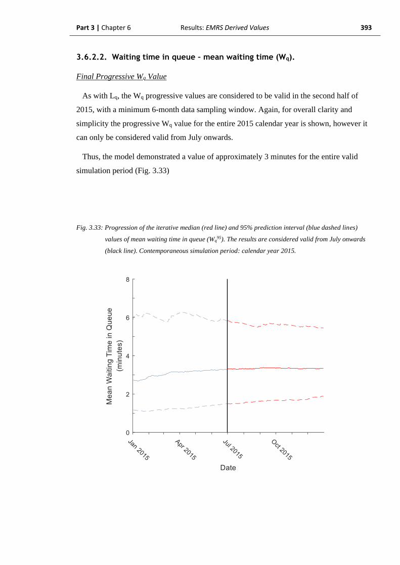
Part 3 | Chapter 6 Results: EMRS Derived Values 393
3.6.2.2. Waiting time in queue – mean waiting time (Wq).
Final Progressive Wq Value
As with Lq, the Wq progressive values are considered to be valid in the second half of
2015, with a minimum 6-month data sampling window. Again, for overall clarity and
simplicity the progressive Wq value for the entire 2015 calendar year is shown, however it
can only be considered valid from July onwards.
Thus, the model demonstrated a value of approximately 3 minutes for the entire valid
simulation period (Fig. 3.33)
Fig. 3.33: Progression of the iterative median (red line) and 95% prediction interval (blue dashed lines)
values of mean waiting time in queue (Wq95). The results are considered valid from July onwards
(black line). Contemporaneous simulation period: calendar year 2015.
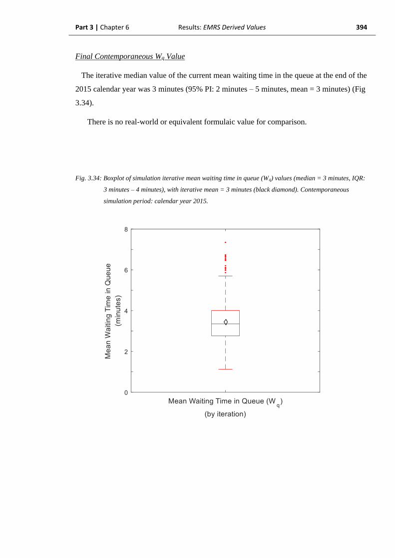
Part 3 | Chapter 6 Results: EMRS Derived Values 394
Final Contemporaneous Wq Value
The iterative median value of the current mean waiting time in the queue at the end of the
2015 calendar year was 3 minutes (95% PI: 2 minutes – 5 minutes, mean = 3 minutes) (Fig
3.34).
There is no real-world or equivalent formulaic value for comparison.
Fig. 3.34: Boxplot of simulation iterative mean waiting time in queue (Wq) values (median = 3 minutes, IQR:
3 minutes – 4 minutes), with iterative mean = 3 minutes (black diamond). Contemporaneous
simulation period: calendar year 2015.
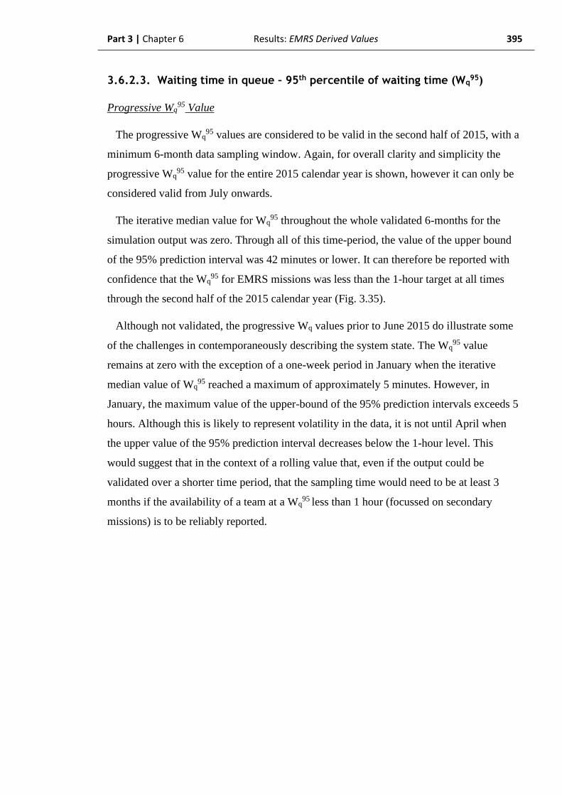
Part 3 | Chapter 6 Results: EMRS Derived Values 395
3.6.2.3. Waiting time in queue – 95th percentile of waiting time (Wq95)
Progressive Wq95 Value
The progressive Wq95 values are considered to be valid in the second half of 2015, with a
minimum 6-month data sampling window. Again, for overall clarity and simplicity the
progressive Wq95 value for the entire 2015 calendar year is shown, however it can only be
considered valid from July onwards.
The iterative median value for Wq95 throughout the whole validated 6-months for the
simulation output was zero. Through all of this time-period, the value of the upper bound
of the 95% prediction interval was 42 minutes or lower. It can therefore be reported with
confidence that the Wq95 for EMRS missions was less than the 1-hour target at all times
through the second half of the 2015 calendar year (Fig. 3.35).
Although not validated, the progressive Wq values prior to June 2015 do illustrate some
of the challenges in contemporaneously describing the system state. The Wq95 value
remains at zero with the exception of a one-week period in January when the iterative
median value of Wq95 reached a maximum of approximately 5 minutes. However, in
January, the maximum value of the upper-bound of the 95% prediction intervals exceeds 5
hours. Although this is likely to represent volatility in the data, it is not until April when
the upper value of the 95% prediction interval decreases below the 1-hour level. This
would suggest that in the context of a rolling value that, even if the output could be
validated over a shorter time period, that the sampling time would need to be at least 3
months if the availability of a team at a Wq95 less than 1 hour (focussed on secondary
missions) is to be reliably reported.
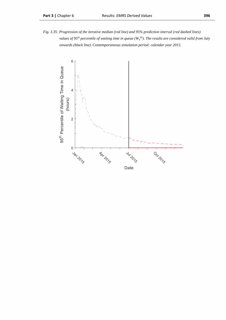
Part 3 | Chapter 6 Results: EMRS Derived Values 396
Fig. 3.35: Progression of the iterative median (red line) and 95% prediction interval (red dashed lines)
values of 95th percentile of waiting time in queue (Wq95). The results are considered valid from July
onwards (black line). Contemporaneous simulation period: calendar year 2015.
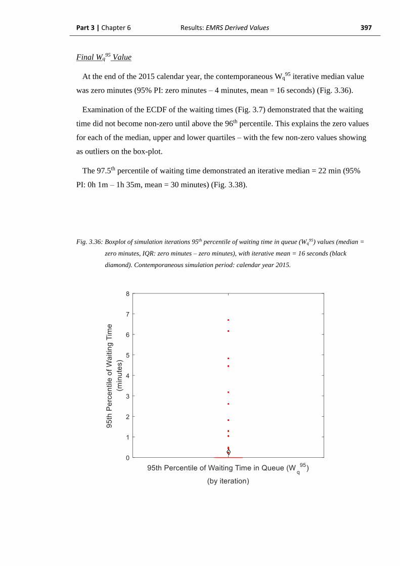
Part 3 | Chapter 6 Results: EMRS Derived Values 397
Final Wq95 Value
At the end of the 2015 calendar year, the contemporaneous Wq95 iterative median value
was zero minutes (95% PI: zero minutes – 4 minutes, mean = 16 seconds) (Fig. 3.36).
Examination of the ECDF of the waiting times (Fig. 3.7) demonstrated that the waiting
time did not become non-zero until above the 96th percentile. This explains the zero values
for each of the median, upper and lower quartiles – with the few non-zero values showing
as outliers on the box-plot.
The 97.5th percentile of waiting time demonstrated an iterative median = 22 min (95%
PI: 0h 1m – 1h 35m, mean = 30 minutes) (Fig. 3.38).
Fig. 3.36: Boxplot of simulation iterations 95th percentile of waiting time in queue (Wq95) values (median =
zero minutes, IQR: zero minutes – zero minutes), with iterative mean = 16 seconds (black
diamond). Contemporaneous simulation period: calendar year 2015.

Part 3 | Chapter 6 Results: EMRS Derived Values 398
Fig. 3.37: ECDF of iterative median values for simulated percentiles of waiting time in queue (Wq95).
Contemporaneous simulation period: calendar year 2015
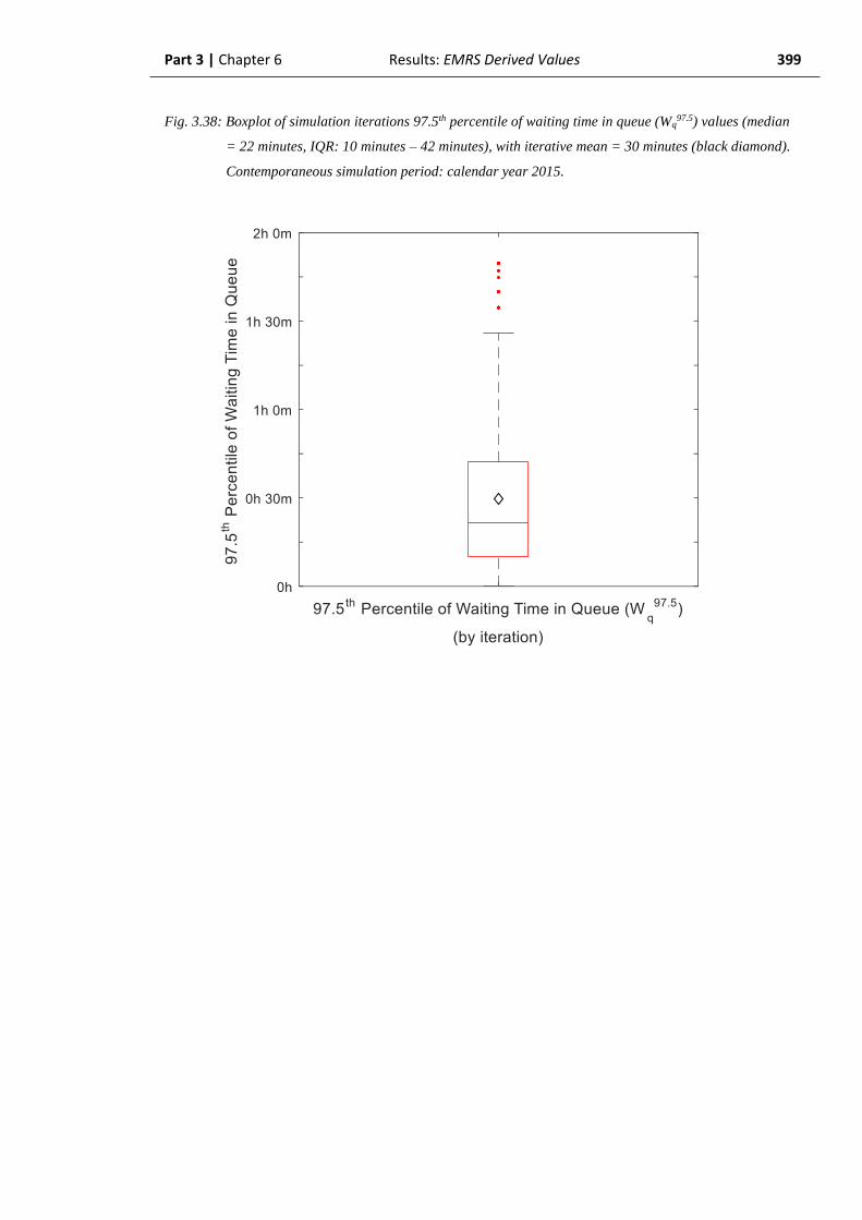
Part 3 | Chapter 6 Results: EMRS Derived Values 399
Fig. 3.38: Boxplot of simulation iterations 97.5th percentile of waiting time in queue (Wq97.5) values (median
= 22 minutes, IQR: 10 minutes – 42 minutes), with iterative mean = 30 minutes (black diamond).
Contemporaneous simulation period: calendar year 2015.

Part 3 | Chapter 6 Results: EMRS Derived Values 400
3.6.2.4. Simultaneous retrievals
Progressive simultaneous retrieval proportion
The progressive simultaneous retrieval proportion values are considered to be valid in the
second half of 2015, with a minimum 6-month data sampling window. Again, for overall
clarity and simplicity the progressive simultaneous retrieval value for the entire 2015
calendar year is shown, however it can only be considered valid from July onwards.
Within the period of validity, the iterative median simultaneous retrieval rate climbed
from an initial value of 3.7% in July to a maximum of 3.9% in September, before falling
slightly to the final value of 3.8% (Fig 3.39).
Fig. 3.39: Progression of the iterative median (red line) and 95% prediction interval (red dashed lines)
values for proportion of simultaneous retrievals. The results are considered valid from July
onwards (black line). Contemporaneous simulation period: calendar year 2015.
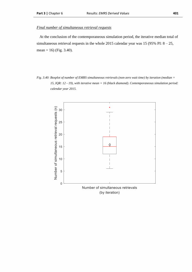
Part 3 | Chapter 6 Results: EMRS Derived Values 401
Final number of simultaneous retrieval requests
At the conclusion of the contemporaneous simulation period, the iterative median total of
simultaneous retrieval requests in the whole 2015 calendar year was 15 (95% PI: 8 – 25,
mean = 16) (Fig. 3.40).
Fig. 3.40: Boxplot of number of EMRS simultaneous retrievals (non-zero wait time) by iteration (median =
15, IQR: 12 - 19), with iterative mean = 16 (black diamond). Contemporaneous simulation period:
calendar year 2015.

Part 3 | Chapter 6 Results: EMRS Derived Values 402
Final simultaneous retrieval proportion
At the conclusion of the contemporaneous simulation period, the iterative median
proportion of simultaneous retrievals was 3.8% (95% PI: 2.7% - 5.0%, mean = 3.8%) (Fig.
3.41).
Calculated from the server utilization of 2 servers (n = 2) by utilizationn (as in the
retrospective period, section 3.6.1.4), the expected simultaneous retrieval proportion would
be 2.9%. This was not significantly different to the simulation output on Mann-Whitney U
testing (p = 0.20) but may be approaching operational significance at only 76.3% of the
simulation value. This does suggest that the result generated by the simulation is plausible
but the difference may be representative of the calculated value not accounting for a time-
varying arrival rate.
Fig. 3.41: Boxplot of proportion of simultaneous retrieval requests (non-zero wait time) by iteration (median
= 3.8%, IQR: 3.4% - 4.2%), with iterative mean = 3.8% (black diamond). Contemporaneous
simulation period: calendar year 2015. Expected value 3.2% (black line).
Part 3 | Chapter 6 Results: EMRS Derived Values 403
3.6.3. Summary of EMRS derived system descriptors
results
The EMRS model has generated the standard queueing theory descriptors of Lq and Wq
by simulation rather than by formulaic calcluation. There is no equivalent real-world or
calculable value which can be used to assess the plausibility of the Lq and Wq results but
by inference from the simpler SPRS model, they appear to be appropriate values. EMRS
demonstrates a much lower utilization quotient than SPRS, by virtue of its two servers,
despite a higher overall number of missions. This is reflected in the EMRS results which
show the system to be performing well within the stated specifications. These results
would suggest that capacity remains within the EMRS system to undertake additional work
– which will be explored in the next section.
Summary tables of the simulation output values are provided for reference overleaf
(Table 3.4 and Table 3.5)

Part 3 | Chapter 6 Results: EMRS Derived Values 404
Table 3.4: EMRS derived performance descriptors. Retrospective simulation period: calendar years 2013 –
2014.
Parameter Derived value by simulation
(95% Prediction Interval)
Lq 0.012
(0.010 – 0.016)
Wq 4 minutes
(2 minutes – 7 minutes)
Wq95
0 minutes
(0 minutes – 7 minutes)
Simultaneous Retrieval
Proportion
4.4%
(3.2% - 5.4%)
Table 3.5: EMRS derived performance descriptors. Instantaneous value at conclusion of the
contemporaneous simulation period: calendar year 2015.
Parameter Final derived value by simulation
(95% Prediction Interval)
Lq 0.007
(0.005 – 0.010)
Wq 3 minutes
(2 minutes – 5 minutes)
Wq95
0 minutes
(0 minutes – 4 minutes)
Simultaneous Retrieval
Proportion
3.8%
(2.7% - 5.0%)

Part 3 Chapter 7
Results:
Simulation of EMRS performance
frontiers through
unobservable phenomena

Part 3 | Chapter 7 Results: EMRS Performance Specifications 406
3.7. Simulation of EMRS performance limits
through unobservable phenomena
In this section, the EMRS simulation model was run in an extended Monte-Carlo format,
with the total number of missions undertaken being deliberately varied to include values
not seen in the real-world system.
Having reviewed the results obtained as derived values from the simulation (above) and
their relationships to the real-world system, it was considered likely that the EMRS system
exhibited some spare capacity to undertake additional missions - both primary and
secondary. However, the number of missions which could be undertaken without
degrading system performance is not known. Therefore, the performance frontier with
respect to number of missions at which system performance could deteriorate needs to be
defined.
In keeping with the previous analyses, the expert consensus of the ScotSTAR clinicians
suggested that the number of simultaneous retrievals - where another mission is requested
when there is no available team - should remain below 10%. The consensus suggested that
1 hour was a reasonable expectation for a secondary retrieval to start. It also suggested that
15 minutes would be an acceptable wait for a team to commence a time-critical primary
missions – longer than this would risk adding delay in the time to life-saving intervention
or would otherwise unnecessarily prolong the patient journey. Each of these were set as the
respective targets for the primary and secondary missions’ 95th percentile of waiting time
(Wq95).
During the course of this analysis, it became apparent that another unobservable
phenomenon: baulked or reneged primary missions, would be a factor to be considered in
the system. Discussion with the clinicians operating the dedicated trauma tasking desk
suggested that a number of primary missions which should have required team attendance
were simply not tasked to a team, because no team was available. It was considered that
the realistic absolute maximum for which a primary mission would be able to be held
awaiting an EMRS team was approximately 20 minutes before it had to be allowed to
proceed to its conclusion without team involvement. As a result, as the average waiting
time approached 20 minutes, it was likely that an increasing number of missions would be
reneged from the EMRS system to be treated and transported by the local ambulance crews
Part 3 | Chapter 7 Results: EMRS Performance Specifications 407
alone. It was therefore considered that this had potential to cause an under-estimation of
the number of EMRS primary missions as the waiting time increased, and also to skew the
waiting time distribution. As a result, it was decided that the number of missed (baulked /
reneged) primary missions would need to be implemented as a performance indicator for
the EMRS system.
Therefore, the EMRS model was used in an extended Monte-Carlo simulation to
establish operational performance frontiers for the system with regard to 3 separate
questions:
1. How many additional missions could EMRS undertake before the 95th percentile of
waiting time (Wq95) reaches the specification (from clinical consensus) limits of:
a. 1 hour for secondary missions?
b. 15 minutes for primary missions?
2. How many additional missions (secondary and primary) could EMRS undertake
before the overall simultaneous retrieval proportion exceeds 10%?
3. What is the current state of the EMRS system with regarding the number of missed
(baulked / reneged) primary missions and does this indicate a potential performance
frontier?
Part 3 | Chapter 7 Results: EMRS Performance Specifications 408
3.7.1. EMRS extended Monte-Carlo simulation output
One thousand iterations of the simulation were undertaken in a single simulation run.
During each run, the number of primary missions and the number of secondary missions
were independently varied in a Monte-Carlo fashion by altering the exponentially
distributed μ-value of mission inter-arrival times. The median iteration time was 42
seconds with a total simulation time of 11h 28m.
The original simulation run, used in all EMRS model analyses preceding this, was
designed to replicate the real-world as closely as possible. These simulations generated
missions with a long-term λ value of 486 primary pre-hospital missions (Poisson
distribution 95th percentile range: 443 – 529) and 280 secondary missions (Poisson
distribution 95th percentile range: 238 – 302) per year. The extended EMRS Monte-Carlo
simulation was specifically designed to generate long-term number of mission λ values
substantially outside this range and did so: generating a range of 8 – 2399 primary
missions per year and 2 – 2733 secondary missions per year.
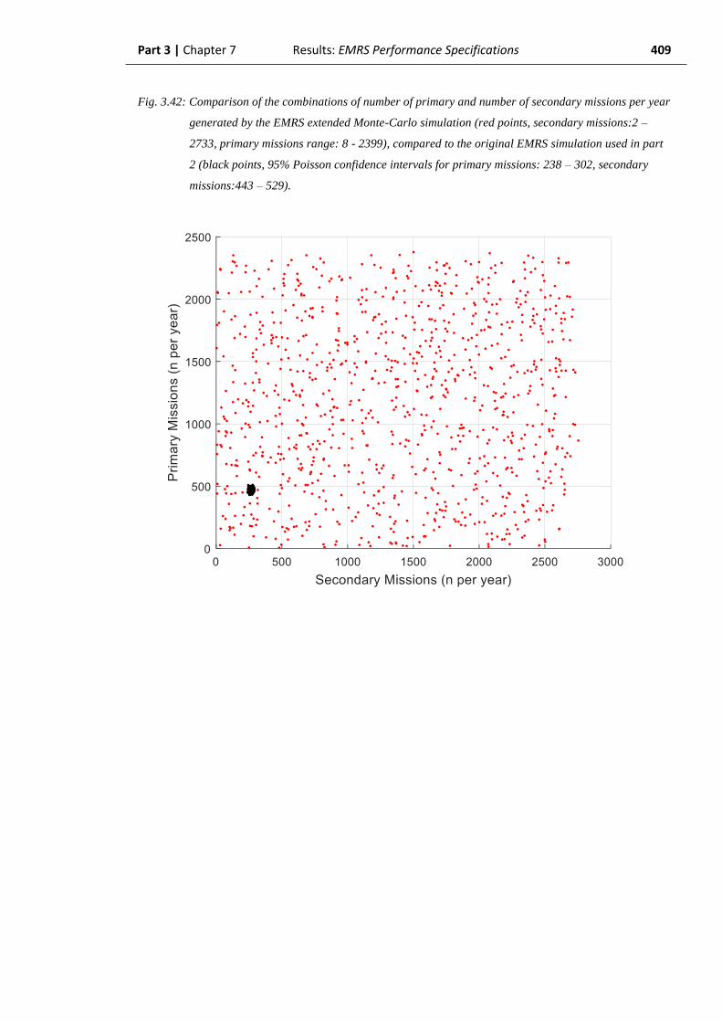
Part 3 | Chapter 7 Results: EMRS Performance Specifications 409
Fig. 3.42: Comparison of the combinations of number of primary and number of secondary missions per year
generated by the EMRS extended Monte-Carlo simulation (red points, secondary missions:2 –
2733, primary missions range: 8 - 2399), compared to the original EMRS simulation used in part
2 (black points, 95% Poisson confidence intervals for primary missions: 238 – 302, secondary
missions:443 – 529).
Part 3 | Chapter 7 Results: EMRS Performance Specifications 410
3.7.2. Revision of EMRS model
In the initial extended Monte-Carlo simulations using the same EMRS model as all the
preceding analyses, the simultaneous retrieval proportion and Wq95 values demonstrated
relationships to the mission numbers which did not correlate with the findings in the
derived values section (section 3.6). This led to a revision of the EMRS model, as
explained below.
3.7.2.1. Simultaneous retrievals
At the end of each simulation iteration, the number of simultaneous retrievals (the
number of arriving patients experiencing a non-zero wait) was plotted three-dimensionally
with the corresponding number of primary and secondary missions generated. An
interpolated reference surface was fitted to the points for illustration and further
calculations (Fig. 3.43).
It can be seen that the three-dimensional chart approximately demonstrates the
exponential distribution between increasing mission numbers and number of simultaneous
retrievals but this relationship is more clearly illustrated on the slice of the three-
dimensional chart (Fig. 3.44) plotting the number of Simultaneous Retrievals (z-axis)
along a plane defined by x = y (i.e. number of primary missions per year = number of
secondary missions per year) (Fig. 3.45). The overall relationship between increasing
number of missions and number of simultaneous retrievals demonstrated an approximately
exponential relationship as would be expected with standard queueing theory and the plot
appears outwardly appropriate.
However, it can also be seen on the three-dimensional chart that there is a clustering of
points along a line at the highest edge of the plane. This corresponds to the highest rate of
mission arrivals such that the system is quickly saturated and the number of simultaneous
retrievals equals the total number of missions generated, minus only the first two missions
which experience zero wait due to the empty servers at that time.
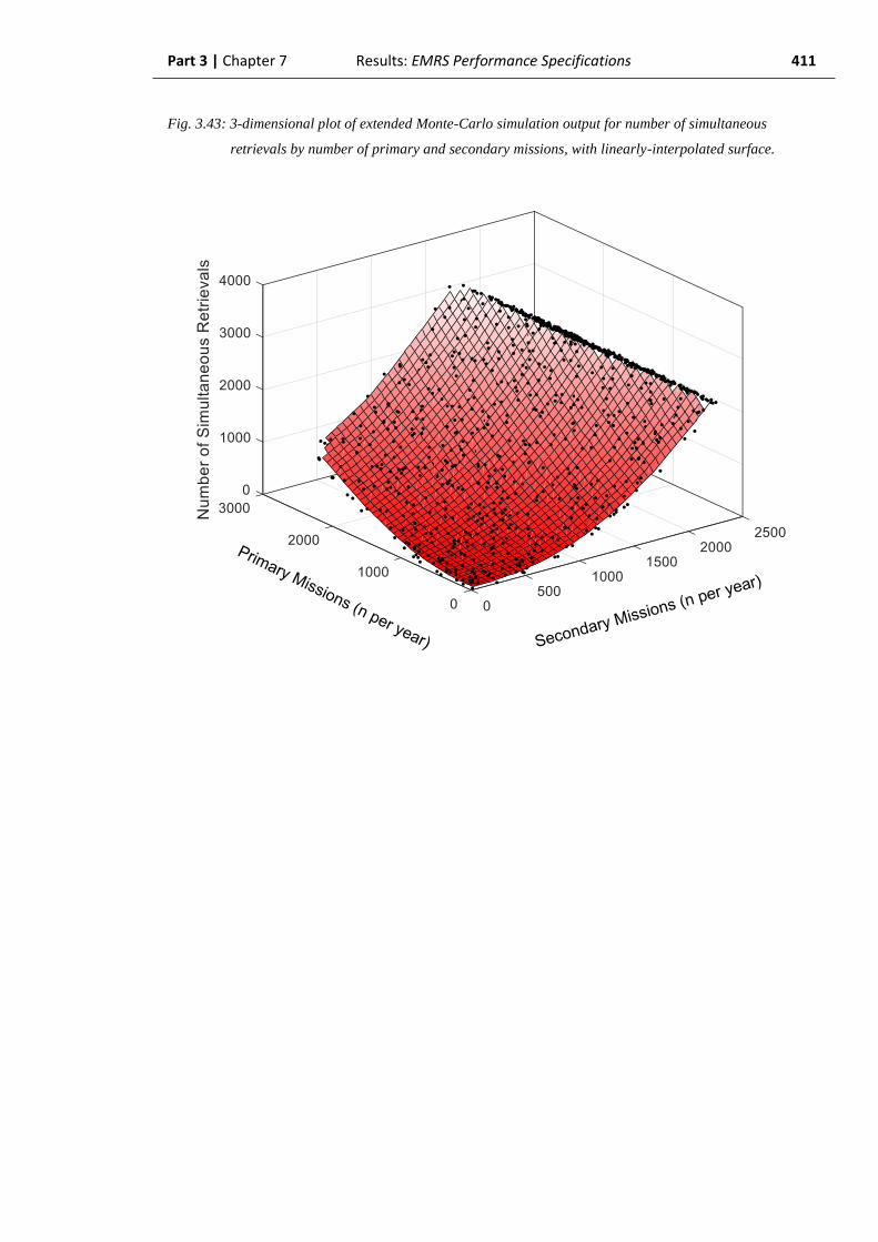
Part 3 | Chapter 7 Results: EMRS Performance Specifications 411
Fig. 3.43: 3-dimensional plot of extended Monte-Carlo simulation output for number of simultaneous
retrievals by number of primary and secondary missions, with linearly-interpolated surface.
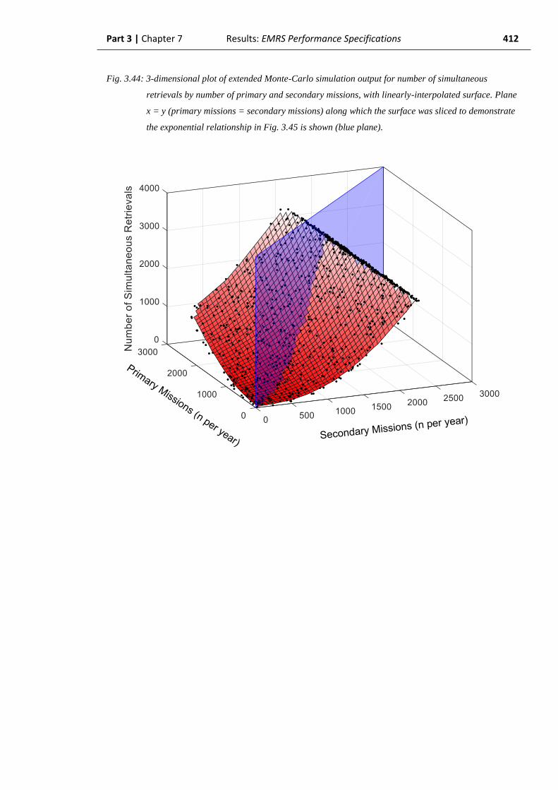
Part 3 | Chapter 7 Results: EMRS Performance Specifications 412
Fig. 3.44: 3-dimensional plot of extended Monte-Carlo simulation output for number of simultaneous
retrievals by number of primary and secondary missions, with linearly-interpolated surface. Plane
x = y (primary missions = secondary missions) along which the surface was sliced to demonstrate
the exponential relationship in Fig. 3.45 is shown (blue plane).
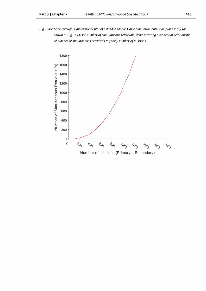
Part 3 | Chapter 7 Results: EMRS Performance Specifications 413
Fig. 3.45: Slice through 3-dimensional plot of extended Monte-Carlo simulation output on plane x = y (as
shown in Fig. 3.44) for number of simultaneous retrievals, demonstrating exponential relationship
of number of simultaneous retrievals to yearly number of missions.

Part 3 | Chapter 7 Results: EMRS Performance Specifications 414
By dividing the number of simultaneous retrievals by the total number of missions from
the same iteration, the proportion of simultaneous retrievals was calculated. Again, this
was plotted three-dimensionally with the corresponding number of primary and secondary
missions from the same iteration. A simple linearly-interpolated surface was fitted to the
points for illustration and reference.
Once again, the plot demonstrates a clustering of missions approaching the 1.0
simultaneous retrieval probability. In the context of simultaneous retrieval rate, this is a
more tangible natural limit of the system, as the simultaneous retrieval probability is equal
to the probability of queueing, which cannot exceed one. When the three-dimensional
surface is plotted on a slice along the plane x = y (Fig. 3.46), the overall relationship
between increasing number of missions and simultaneous retrieval proportion
demonstrated an approximately linear increase (Fig. 3.47). This relationship would also be
expected in queueing theory by the PASTA property, with the proportion of simultaneous
retrievals varying as a factor of server utilization.
Fig. 3.46: 3-dimensional plot of extended Monte-Carlo simulation output for proportion of simultaneous
retrievals by number of primary and secondary missions, with linearly-interpolated surface. Plane
x = y (primary missions = secondary missions) along which the surface was sliced to demonstrate
the exponential relationship in Fig. 3.47 is shown (blue plane).

Part 3 | Chapter 7 Results: EMRS Performance Specifications 415
Fig. 3.47: Slice through 3-dimensional plot (Fig. 3.46) of extended Monte-Carlo simulation output on plane x
= y for proportion of simultaneous retrievals, demonstrating linear relationship of proportion of
simultaneous retrievals to yearly number of missions.

Part 3 | Chapter 7 Results: EMRS Performance Specifications 416
From the interpolated surface, a contour plot demonstrating the proportion of
simultaneous retrievals with regard to mission numbers was generated. Initially, plotting
the 2015 real-world values of 240 secondary missions and 466 primary missions
demonstrated a predicted simultaneous retrieval proportion of 11.2% (Fig. 3.48). This was
substantially different to the 3.8% simultaneous retrieval rate derived from the EMRS
contemporaneous simulation in section 3.6.2.4. The reasons for this will be discussed
following the review of the initial Wq95 findings.
Fig. 3.48: Contour plot generated from 3-dimensional plot in Fig. 3.46 demonstrating proportion of
simultaneous retrievals by number of primary and secondary missions (red contours) with EMRS
real-world values for 2015 calendar year plotted: 240 secondary missions, 466 primary missions,
11.2% simultaneous retrieval proportion (black cross). Plot zoomed for clarity. N.B. No reneging
of primary missions by model.
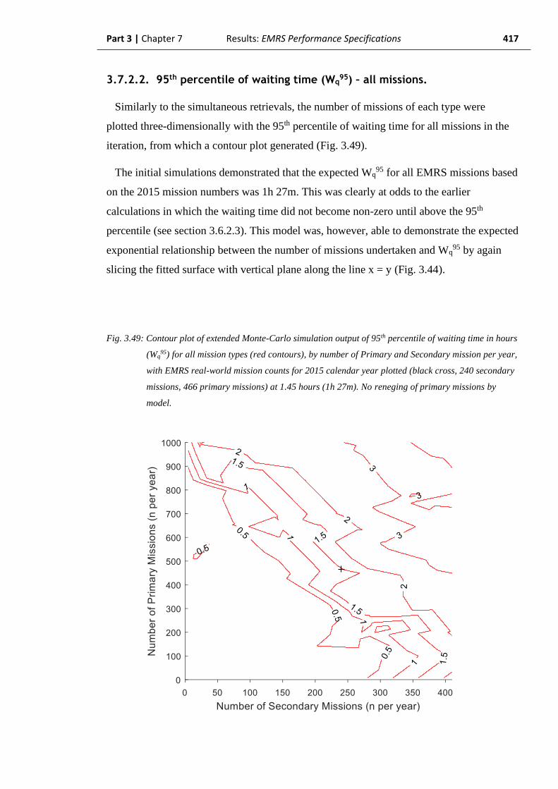
Part 3 | Chapter 7 Results: EMRS Performance Specifications 417
3.7.2.2. 95th percentile of waiting time (Wq95) – all missions.
Similarly to the simultaneous retrievals, the number of missions of each type were
plotted three-dimensionally with the 95th percentile of waiting time for all missions in the
iteration, from which a contour plot generated (Fig. 3.49).
The initial simulations demonstrated that the expected Wq95 for all EMRS missions based
on the 2015 mission numbers was 1h 27m. This was clearly at odds to the earlier
calculations in which the waiting time did not become non-zero until above the 95th
percentile (see section 3.6.2.3). This model was, however, able to demonstrate the expected
exponential relationship between the number of missions undertaken and Wq95 by again
slicing the fitted surface with vertical plane along the line x = y (Fig. 3.44).
Fig. 3.49: Contour plot of extended Monte-Carlo simulation output of 95th percentile of waiting time in hours
(Wq95) for all mission types (red contours), by number of Primary and Secondary mission per year,
with EMRS real-world mission counts for 2015 calendar year plotted (black cross, 240 secondary
missions, 466 primary missions) at 1.45 hours (1h 27m). No reneging of primary missions by
model.
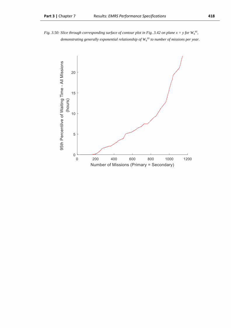
Part 3 | Chapter 7 Results: EMRS Performance Specifications 418
Fig. 3.50: Slice through corresponding surface of contour plot in Fig. 3.42 on plane x = y for Wq95,
demonstrating generally exponential relationship of Wq95 to number of missions per year.
Part 3 | Chapter 7 Results: EMRS Performance Specifications 419
3.7.2.3. Assessment of non-similarity, and subsequent model changes
Investigating this apparent error, it was realised that at larger numbers of missions,
unobservable in the real-world, the model was queueing primary missions in particular for
long periods of time when both servers were busy – this is the group who are never
actually seen by EMRS in the real-world as they would have been treated and transferred
by local ambulance teams before EMRS could arrive on-scene. When the model’s long
queueing time for these missions was interpolated across the wider range of missions in the
extended Monte-Carlo simulation, it resulted in a long waiting time at even the equivalent
values to the real-world. In the extended Monte-Carlo simulation, the base EMRS model
had therefore violated a fundamental principle in that it had ceased to behave the same way
(either practically or mathematically) as the real-world system.
It was perceived by the Trauma Desk clinicians that realistically, team non-availability
exceeding 20 minutes would likely result in a missed (baulked / reneged) primary mission.
The initial EMRS model would, however, allow such missions to queue indefinitely for a
team. The Simulink model was therefore revised to renege primary missions which were
generated and entered into the queue but experienced a waiting time for service greater
than 20 minutes. This “time out” function is represented diagrammatically in Fig.3.51, with
the relevant Simulink blocks illustrated in Fig. 3.52. As will be shown in the following
sections, this appears to have been effective in creating a model which behaves more in
keeping with the real-world.
It is possible that a similar effect would be experienced with secondary missions at a
much longer Wq, but it was considered that the this was likely to occur sufficiently
infrequently as to have a negligible effect.

Part 3 | Chapter 7 Results: EMRS Performance Specifications 420
Fig. 3.51: Diagrammatic representation of EMRS queueing system, including reneging of primary missions
in queue when waiting time reaches 20 minutes.
Fig. 3.52: Screen capture of Simulink blocks demonstrating allocation of time-out to primary missions and
sink for reneged entities (as Fig. 3.1).
The revised model was then also run for one-thousand iterations with the modification to
renege primary missions with an absolute waiting time (Wq) greater than 20 minutes in
place. This simulation demonstrated a median iteration time of 49.2 seconds. The
simulation was completed in 14h 21m. All subsequent results are generated from this
model.
FIFO
Queue
FIFO
Queue
SPRS
Team Arrivals Departure SPRS
Team
Primary mission
arrivals
Primary missions
with waiting time
≥ 20 mins
SPRS
Team
Secondary mission
arrivals
Departure Duty One
Team
Duty Two
Team Departure
Departure
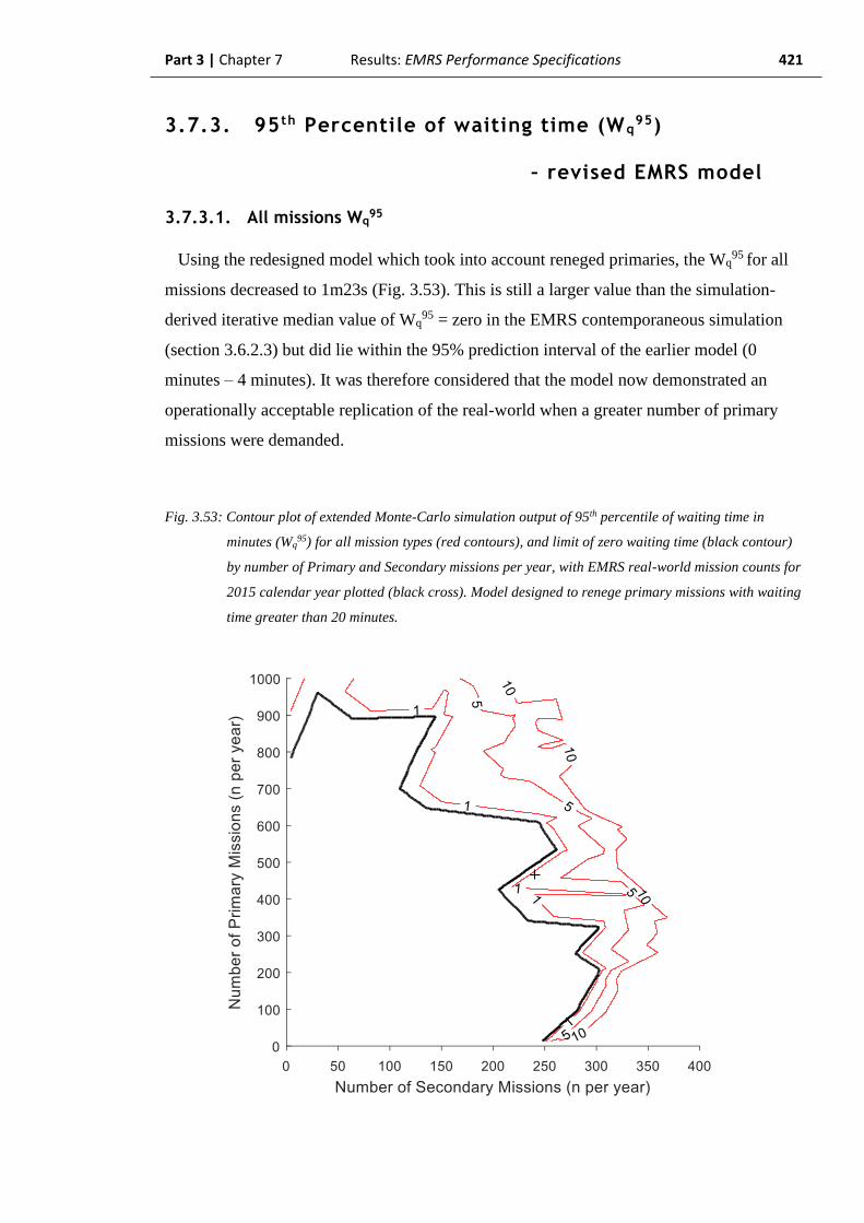
Part 3 | Chapter 7 Results: EMRS Performance Specifications 421
3.7.3. 95th Percentile of waiting time (Wq95)
– revised EMRS model
3.7.3.1. All missions Wq95
Using the redesigned model which took into account reneged primaries, the Wq95 for all
missions decreased to 1m23s (Fig. 3.53). This is still a larger value than the simulation-
derived iterative median value of Wq95 = zero in the EMRS contemporaneous simulation
(section 3.6.2.3) but did lie within the 95% prediction interval of the earlier model (0
minutes – 4 minutes). It was therefore considered that the model now demonstrated an
operationally acceptable replication of the real-world when a greater number of primary
missions were demanded.
Fig. 3.53: Contour plot of extended Monte-Carlo simulation output of 95th percentile of waiting time in
minutes (Wq95) for all mission types (red contours), and limit of zero waiting time (black contour)
by number of Primary and Secondary missions per year, with EMRS real-world mission counts for
2015 calendar year plotted (black cross). Model designed to renege primary missions with waiting
time greater than 20 minutes.
Part 3 | Chapter 7 Results: EMRS Performance Specifications 422
3.7.3.2 Wq95 – secondary missions (Specification limit: 1 hour)
From each iteration of the simulation performed on the revised EMRS model, the
secondary missions were separated as a sub-group and their specific waiting times were
calculated separately to those of the primary missions.
The 95th percentile of waiting time (Wq95) in the secondary missions sub-group was
plotted three-dimensionally against the number of primary and secondary missions. A
linear-interpolated surface was fitted and a contour plot generated from it (Fig. 3.54).
Based on this, the number of EMRS missions in 2015 would be expected to produce a
Wq95 of 45 minutes for secondary missions. This is less than the specified performance
limit for secondary missions Wq95 of 1 hour.
Using the fitted reference surface, the EMRS system could undertake an additional 23
secondary missions (a total of 263 versus 240 per year in 2015) or an additional 26 primary
missions (a total of 492 per year versus the 466 in 2015) before the Pareto limit for
secondary missions Wq95 = 1 hour was reached.
This result demonstrates that the EMRS secondary missions are closer to the
performance frontier of a Wq95 less than 1 hour than was perhaps realised within the
service. Any intention to increase the number of secondary missions undertaken by EMRS
will need a concomitant strategy to mitigate the risk of an increase in Wq95 for secondary
missions to over 1 hour.
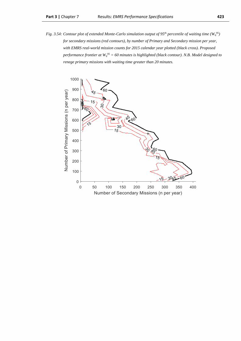
Part 3 | Chapter 7 Results: EMRS Performance Specifications 423
Fig. 3.54: Contour plot of extended Monte-Carlo simulation output of 95th percentile of waiting time (Wq95)
for secondary missions (red contours), by number of Primary and Secondary mission per year,
with EMRS real-world mission counts for 2015 calendar year plotted (black cross). Proposed
performance frontier at Wq95 = 60 minutes is highlighted (black contour). N.B. Model designed to
renege primary missions with waiting time greater than 20 minutes.
Part 3 | Chapter 7 Results: EMRS Performance Specifications 424
3.7.3.3. Wq95 – primary missions (Specification limit: 15 minutes)
From each iteration of the extended Monte-Carlo simulation using the revised EMRS
model, the primary missions were analysed as a sub-group.
The 95th percentile of waiting time (Wq95) for the primary missions sub-group was
plotted three-dimensionally against the number of primary and secondary missions. A
linear-interpolated surface was fitted and a contour plot generated from it (Fig. 3.55). This
demonstrated that the 2015 yearly values of EMRS missions (240 secondary missions, 466
primary missions) would produce an expected Wq95 for primary missions of zero minutes.
This is in keeping with the earlier findings (see section 3.6.2.3) in which the waiting time
for all missions only became non-zero above the 96th percentile.
However, from this analysis, it was discovered that the performance frontier at 15
minutes could not be established, and the Pareto limit for the corresponding number of
primary and secondary missions could not be defined. This was the result of the reneged
primary missions which created a skewed distribution in the data. If an immutable absolute
limit of 20 minutes was set for reneging primary missions then as the number of primary
missions tended to a suitably large value, both Wq and Wq95 would asymptotically
converge towards 20 minutes. No primary mission could experience a waiting time greater
than 20 minutes because it would simply be reneged from the queue. In the studied
situation, this would appear to describe the case where missions either experience a very
short waiting time (as conferred by the current Wq95 = zero) or they experience such a long
waiting time that they are reneged. As a result, the 95th percentile of Wq appears to never
reach 15 minutes.

Part 3 | Chapter 7 Results: EMRS Performance Specifications 425
Fig. 3.55: Contour plot of extended Monte-Carlo simulation output of 95th percentile of waiting time (Wq95)
for primary missions (red contours), by number of Primary and Secondary mission per year, with
EMRS real-world mission counts for 2015 calendar year plotted (black cross). Threshold of non-
zero Wq95 is illustrated (black contour). N.B. Model designed to renege primary missions with
waiting time greater than 20 minutes and therefore the 15 and 20-minute contours are undefined.

Part 3 | Chapter 7 Results: EMRS Performance Specifications 426
3.7.4. Simultaneous retrievals (Specification limit: 10%)
a) Simulation output from revised EMRS model
At the end of each simulation iteration using the revised EMRS model, the number of
simultaneous retrievals (the number of arriving patients experiencing a non-zero wait) was
divided by the total number of missions generated in that iteration to generate the
simultaneous retrieval proportion. This was plotted three-dimensionally with the
corresponding number of primary and secondary missions generated. An interpolated
reference surface was fitted to the points for illustration and further calculations (Fig.
3.56).
The effect of reneging primary missions with a waiting time greater than 20 minutes was
demonstrated by a plot which showed a noticeably different relationship between primary
missions undertaken, secondary missions undertaken and proportion of simultaneous
retrievals (compared to Fig. 3.46). The 3D plot is clearly truncated and the contour chart
demonstrates a limit of observability beyond which the servers never actually see the given
number of primary missions because they are reneged from the queue due to excessive
waiting time (Fig. 3.56).

Part 3 | Chapter 7 Results: EMRS Performance Specifications 427
Fig. 3.56: 3-dimensional plot of Monte-Carlo simulation output for proportion of simultaneous retrievals
by number of primary and secondary missions, with linearly-interpolated surface. Revised
EMRS model with primary missions reneged at waiting times ≥ 20 minutes.
Part 3 | Chapter 7 Results: EMRS Performance Specifications 428
Using this interpolated surface as a reference, a contour plot was generated. This
demonstrated that a yearly λ of 240 secondary missions and 466 primary missions
(corresponding to the 2015 calendar year) generated a predicted simultaneous retrieval
probability of 3.9% (Fig. 3.57). This compared much more favourably with the value of
3.8% derived from the EMRS contemporaneous simulation (section 3.6.2.4.). The
similarity of the result generated by the revised EMRS model to that derived from the
original EMRS contemporaneous simulation suggests that the revisions to the model were
appropriate and that reneged primary missions are more significant than previously
thought. Particularly with regard to the number that occur, their contribution to reducing
the total number of retrievals undertaken and correspondingly reducing the proportion of
simultaneous retrievals.
The increasing number of reneged primary missions as utilization increases contributes to
a paradox where, under certain conditions, increasing the number of primary missions
appears to reduce the proportion of simultaneous retrievals. An example of this can be seen
in the lower-right corner of the chart with greater than approximately 1800 secondary
retrievals (see Fig. 3.57). However, this is reflective of the majority of generated primary
missions being reneged. When translated to the real world in the context of team non-
activation to the scene of severely injured patients, this is clearly not promoting equity of
access to critical care. Therefore, it is imperative that an accurate reflection of the system
also includes an assessment of the number of these missed (baulked / reneged) primary
missions. A specific performance marker relating to the number of missed primary
missions is therefore required. This was added, as stated in the introduction to section 3.7
and will be analysed later in this chapter.
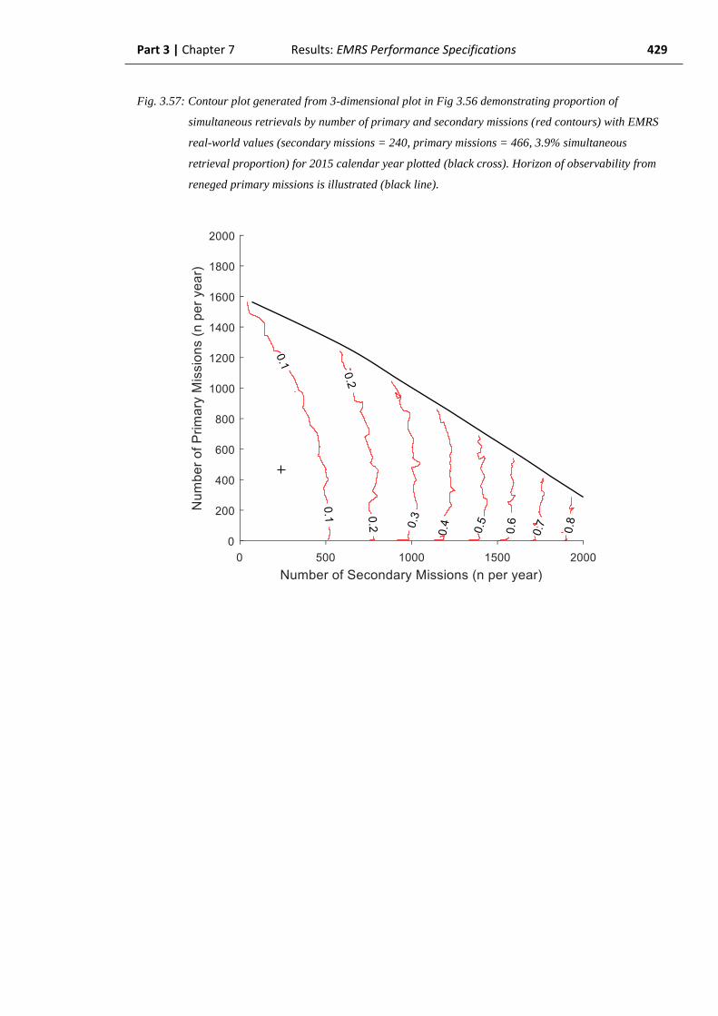
Part 3 | Chapter 7 Results: EMRS Performance Specifications 429
Fig. 3.57: Contour plot generated from 3-dimensional plot in Fig 3.56 demonstrating proportion of
simultaneous retrievals by number of primary and secondary missions (red contours) with EMRS
real-world values (secondary missions = 240, primary missions = 466, 3.9% simultaneous
retrieval proportion) for 2015 calendar year plotted (black cross). Horizon of observability from
reneged primary missions is illustrated (black line).

Part 3 | Chapter 7 Results: EMRS Performance Specifications 430
b) Proportion of simultaneous retrievals (Target < 10%)
Focussing on defining the specified 10% simultaneous retrieval limit, the updated model
designed to renege primary missions waiting greater than 20 minutes was used. From this,
the required yearly λ to generate a simultaneous retrieval proportion of 10% was calculated
using the 10% contour of the surface fitted to the data (Fig. 3.58). Based on this, the
simultaneous retrieval proportion would reach 10% according to a Pareto limit generated
from the undernoted relationship between primary and secondary missions.
Based on this analysis: as of 2015, EMRS would be able to undertake an additional 747
primary missions (a total of 1213 missions per year versus the current 466) or 263
secondary missions (a total of 503 missions per year versus the current 240) before
reaching the calculated Pareto performance frontier. The difference between the number of
additional available primary missions compared to secondary missions reflects the greater
server utilization of secondary missions (mainly through longer mission durations) as
described by the gradient, below.
The Pareto limit of 10% simultaneous retrieval proportion demonstrates a y-axis
intercept of 1567 primary missions (zero secondary missions) and an x-axis intercept of
487 secondary missions (zero primary missions). The line is curved, but the centre section
of the line has an approximate gradient of -2.08. This indicates that the ratio of primary
missions to secondary missions for any given utilization is approximately 2:1, again
reflective of the longer mission durations of secondary missions, such that they contribute
twice as much to server busyness and therefore to simultaneous retrievals than primary
missions. The respective number of primary and secondary missions at which a 10%
simultaneous retrieval proportion will be reached can be described approximately by the
relationship:
1567 = 𝑃𝑟𝑖𝑚𝑎𝑟𝑦 𝑀𝑖𝑠𝑠𝑖𝑜𝑛𝑠 + (2.08 ∗ 𝑆𝑒𝑐𝑜𝑛𝑑𝑎𝑟𝑦 𝑀𝑖𝑠𝑠𝑖𝑜𝑛𝑠)
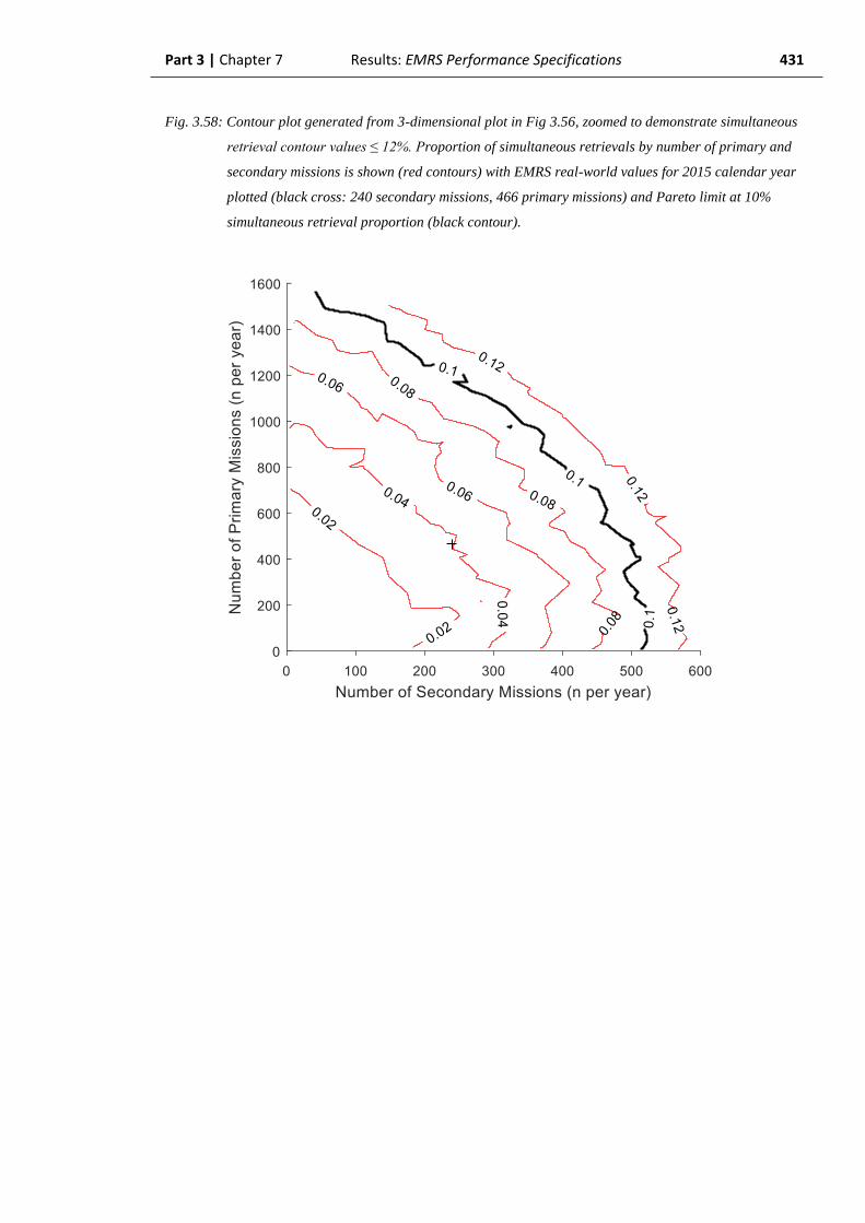
Part 3 | Chapter 7 Results: EMRS Performance Specifications 431
Fig. 3.58: Contour plot generated from 3-dimensional plot in Fig 3.56, zoomed to demonstrate simultaneous
retrieval contour values ≤ 12%. Proportion of simultaneous retrievals by number of primary and
secondary missions is shown (red contours) with EMRS real-world values for 2015 calendar year
plotted (black cross: 240 secondary missions, 466 primary missions) and Pareto limit at 10%
simultaneous retrieval proportion (black contour).
Part 3 | Chapter 7 Results: EMRS Performance Specifications 432
3.7.5. Missed primary missions
In the real-world EMRS system there is not a process for identifying the primary
missions that would have been tasked to an EMRS team, were one available, but are
instead baulked (never enter the queue) or reneged (enter the queue but then leave prior to
being served) because of team non-availability. These “missed” primary missions are
effectively invisible to the EMRS system currently and so their potential impact cannot be
directly measured. The revised EMRS model, which reneges primary missions with a
waiting time greater than 20 minutes, has the potential to contribute greatly to the
understanding of the limitations of the service if an accurate number of real-world missed
primary missions (indicative of an unmet need) can be inferred.
Using the revised EMRS model, the number of missed primary missions in each iteration
was counted and divided by the total number of primary missions (the number of
secondary missions was excluded) in that iteration to generate a proportion of missed
primary missions. This was plotted three-dimensionally (Fig. 3.59) against the respective
number of primary and secondary missions from that iteration, and a contour plot was
again generated (Fig. 3.60).
The EMRS system, based on 2015 real-world data (240 secondary missions, 466 primary
missions per year), would be expected to generate a missed primary missions rate of 9.3%
- i.e. for approximately every 11 primary missions undertaken by EMRS, one would have
been missed because of team non-availability. This would never have been visible to the
EMRS system in the real-world.
Arbitrarily defining the specification limit for missed primaries as 10% in line with
overall simultaneous retrievals (section 3.7.4) demonstrates that the EMRS system could
undertake an additional 27 secondary missions on average per year (a Poisson λ value of
267 versus the current 240) or an additional 35 primary missions on average per year (a
Poisson λ value of 501 versus current 466).
Note that this value is calculated differently to, and therefore gives a different result to
the calculation of the real-world simultaneous retrieval proportion for all missions (3.8%,
section 3.6.3), as explained above. Additionally, this figure is representative of both
baulked missions (never join the queue) and reneged missions (join the queue but then
leave) due to excessive waiting times, potentially accounting for its higher value. Both of
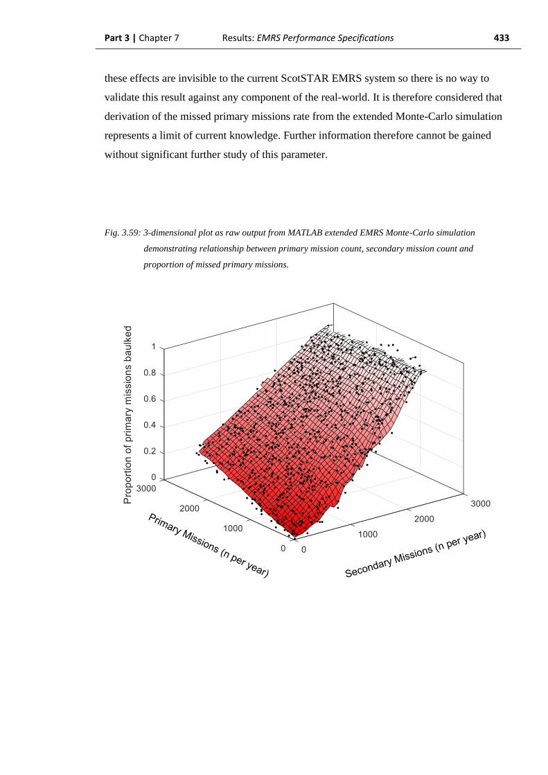
Part 3 | Chapter 7 Results: EMRS Performance Specifications 433
these effects are invisible to the current ScotSTAR EMRS system so there is no way to
validate this result against any component of the real-world. It is therefore considered that
derivation of the missed primary missions rate from the extended Monte-Carlo simulation
represents a limit of current knowledge. Further information therefore cannot be gained
without significant further study of this parameter.
Fig. 3.59: 3-dimensional plot as raw output from MATLAB extended EMRS Monte-Carlo simulation
demonstrating relationship between primary mission count, secondary mission count and
proportion of missed primary missions.

Part 3 | Chapter 7 Results: EMRS Performance Specifications 434
Fig. 3.60: Contour plot (converted from 3-dimensional plot) demonstrating relationship between primary
mission count, secondary mission count and proportion of missed primary missions. The defined
performance limit of 10% missed primary missions is marked (black contour). The real-world
values corresponding to the 2015 calendar year (240 secondary missions, 466 primary missions)
is shown (black cross).

Part 3 | Chapter 7 Results: EMRS Performance Specifications 435
3.7.6. EMRS Summary
In this analysis, the EMRS system has been demonstrated to have Lq and Wq values
which are plausible with regard to their real-world equivalents.
The simulation-derived critical performance descriptors of Wq95 and simultaneous
retrieval proportions are reassuringly low in the EMRS system. At the end of the 2015
calendar year, the Wq95 value for all missions was zero. This confers that, for 95% of all
patients, when required, a retrieval mission can be reliably expected to be underway
immediately. This is also reflected in the low overall simultaneous retrieval probability of
3.8%.
The simultaneous retrieval and Wq95 results suggest that there is some capacity within the
system to undertake additional primary or secondary missions. This should also inspire
some confidence in the system’s resilience and potential for growth. It may additionally
result in some drive to increase the EMRS service utilization, reducing the per-patient cost
of the service. However, the unobservable phenomena simulation has very usefully
demonstrated that this must be undertaken with caution.
Section 3.7.3.2 has demonstrated that the EMRS system is operating close to a
performance frontier with regards to waiting time for secondary missions. Based on the
missions in the 2015 calendar year, the Wq95 for secondary missions is approximately 45
minutes (75% of limit value) and the service can only undertake an additional 23 missions
per year (long-term Poisson λ value) before the Wq95 for secondary missions will exceed
one hour – this would be approximately equivalent to the service taking on one additional
West-sector referring centre. However, this is reliant upon the baulking or reneging of
primary missions to achieve the target and theoretically accounts for 1 in 11 primary
missions currently – 93% of the limit value if this specification was also set at 10%.
Because primary missions with a waiting time greater than 20 minutes will be reneged, the
specification limit of 15 minutes Wq95 for primary missions will, effectively, never be
reached. For the system in its current state, this is therefore not an appropriate performance
parameter.
At the Pareto limit of 246 secondary missions and 482 primary missions for a secondary
mission Wq95 lying on the specification limit of one hour: the Wq
95 for primary missions
would be predicted as zero minutes (0% of limit value) and the simultaneous retrieval

Part 3 | Chapter 7 Results: EMRS Performance Specifications 436
proportion would increase to 4.2% (42% of limit value). The proportion of missed
primaries would rise to 9.7% (97% of limit value).
Although the proportion of missed primary missions is closest to the limit value, it is
Wq95 for secondary missions which displays the lowest capacity to increase the number of
missions undertaken. Therefore, Wq95 for secondary missions is the extant limiting
parameter for the EMRS system. As the service’s principal role is secondary retrieval to
provide equity of healthcare across remote and rural Scotland, care must be taken to ensure
that any additional workload does not majorly increase the secondary mission Wq95 as this
would degrade the service’s ability to perform its fundamental function.
The relationship of the current EMRS performance to the specification limits is
summarised below (Table 3.6).
Table 3.6: Current EMRS performance relative to specification limits.
Specification
Current real-
world value
(2015 calendar year)
Proportion
of target Remaining capacity
Simultaneous retrieval
proportion < 10% 2.9% 29%
263 secondary missions
or
503 primary missions
Wq95 < 1-hour for
secondary missions 45 minutes 75%
23 secondary missions
or
26 primary missions
Wq95 < 15-minutes for
primary missions 0 minutes 0% N/A
Proportion of primary
missions missed < 10% 9.3% 93%
27 secondary missions
or
35 primary missions

Part 3 Chapter 8
Discussion

Part 3 | Chapter 8 Discussion 438
3.8. Discussion
3.8.1. Derived performance descriptors
3.8.1.1. Assumption of validity
Clearly the analysis presented in Part 3 is dependent upon the real-world behaviour of the
system matching that of the model. An assumption is made that the relationship between
the individual model parameters (inter-arrival time, activation time of day, mission
duration etc.) and the derived parameters (utilization, Wq95, Simultaneous Retrieval Rate)
hold true between the real-world and simulations. The assumption which follows is that the
parameters derived from the model will therefore also be accurate. However, the degree of
accuracy in such a relationship cannot actually be demonstrated in the current ScotSTAR
datasets as a result of the recorded real-world mission time checkpoints not being reflective
of these parameters and the intrinsic, unconscious, processes which clinicians use to
manage patient flow through the system. It should be possible in the future for the mission
checkpoints to be adjusted so that the derived parameters can be compared to their
measured real-world equivalents.
3.8.1.2. Contemporaneous values
In the EMRS contemporaneous simulation period, the model was used only in the second
half of 2015 due to its demonstrated validity, contemporaneously replicating the real-world
only within that time period. The progressive, daily representation of both the real-world
and model values are based upon a time-period up to the current simulation point. The
simulation output is therefore based on a progressively lengthening data sampling window,
commencing on the 01/01/2015 and continuing to the current simulation time-point. This is
reflected in the narrowing prediction intervals as the model gathers more data (see Fig.
3.35 as an example). For each of the contemporaneous, progressive measures, the model
was primed with the corresponding value from the retrospective simulation period. Along
with other refinements in the model to improve the overall accuracy of the model in the
contemporaneous simulation period, an understanding of a suitable data sampling window
must also be gained. Clearly, where a parameter relies upon a distribution (e.g. Wq95 relies

Part 3 | Chapter 8 Discussion 439
on the distribution of waiting times), then a sufficiently large sample must be obtained by
which to prevent a sampling error (of a type-2 nature). As the number of missions (and
therefore data points) is essentially a function of time, then a suitable sampling time must
elapse. Some insight has been gained into this with regard to Wq95 where it was
demonstrated that the confidence intervals only narrowed sufficiently to reliably report a
Wq95 of less than one hour after a sampling period of approximately 4 months (Fig. 3.35).
This should be contrasted with the earlier analysis (e.g. Part 2, section 2.6.2.1) in which the
absolute value of the number of missions could be calculated on a daily basis. Some
parameters are therefore much closer to real-time than others, even in the contemporaneous
simulation. How close to real-time a value can be generated is therefore dependent on the
length of the sampling window. Minimizing the duration of the sampling window to
generate an “as near to real-time as possible” performance value must be balanced against
having enough data to make the result reliable. As an important concept in managing data
quality for describing the overall state of the ScotSTAR systems, this is considered a likely
objective for future investigation.
3.8.1.3. Mean length of queue (Lq) and mean waiting time (Wq)
The Lq and Wq values were the first descriptive parameters to be derived purely from the
ScotSTAR team models. For SPRS this was another opportunity to provide some
validation of the model by comparing the simulation output to the expected formulaic Lq
and Wq values from the Pollaczek-Khinchin formulae. Each of the values for Lq and Wq
appeared plausible with regard to the respective P-K formula although the model did
consistently produce values for these parameters which exceeded the expected value based
on the P-K calculation. This is likely a factor of the non-stationary Poisson arrivals process
generating non-normally distributed waiting times.
There was no formulaic value available for EMRS and so the simulation output values
can only be assumed to be accurate, based on the extrapolation of the model complexity
from SPRS, and the preceding demonstration of its similarity to the real-world.

Part 3 | Chapter 8 Discussion 440
3.8.1.4. 95th percentile of waiting time (Wq95)
When the analysis was extended to the 95th percentile of waiting time (Wq95), the marked
difference from the Wq values was clearly illustrated. For the SPRS contemporaneous
simulation, the Wq of 1h 26m was associated with a Wq95 of 8h 52m. Clearly, the long tail
of the waiting time distribution is not adequately represented by a simple description using
the Wq alone. This is an important consideration as it firstly justifies the use of Wq95 as an
alternative system measure. Additionally, it illustrates the challenges of accurately
describing the system for the purposes of its users. Describing the system by an “average
wait of 1h 26m” could result in the service not meeting expectations when 5% of the
patients will in fact wait nearly 9 hours.
Of note, in the unobservable phenomena simulation, the relationship between increasing
number of missions (effectively, utilization when the mission duration distribution is
similar) and Wq95 for SPRS missions demonstrated a polynomial, not exponential
relationship. As an extension of Wq, it would be expected that Wq95 would follow an
exponential relationship, as described by standard queueing theory. The reason for the
difference is not known but is likely to relate to a combination of the non-stationary
arrivals process and the non-normal distribution of waiting times. Although, it is also
possible that the model has simply not simulated missions over a wide enough range to
fully generate the Wq95 distribution.
3.8.1.5. Simultaneous retrievals
For both SPRS and EMRS results, the proportion of simultaneous retrievals results
appeared plausible with regard to the calculated result based on each team’s respective
utilization value. As explained, for a pure Poisson distribution, with a uniform probability
of activation across an entire 24-hour period (representative of a stationary arrivals
process), the number of simultaneous retrieval requests should be equal to the utilization of
the team.
This is the PASTA (Poisson Arrivals See Time Averages) property of a Poisson arrival
system. The PASTA property is relatively straightforward to understand from first
principles, with the utilization of the system being the proportion of time in which a team
is busy (e.g. in a 24-hour period). Using a 25% utilization as an example, a team would

Part 3 | Chapter 8 Discussion 441
therefore work 6 hours in any 24-hour period. Missions arriving during the 6-hour server-
busy period will require to queue (therefore being a simultaneous retrieval request). If the
probability of arrival is uniform through the 24-hour period, then the number of missions
arriving in any 6-hour period will be 25% of the total. Thus, the proportion of simultaneous
retrievals for a one-server system equals the server utilization.
However, as has been discussed throughout this thesis, the ScotSTAR systems do not
demonstrate a uniform probability of activation, they are a time-dependent Poisson
process. The probability of activation for SPRS reaches a peak at approximately 0900h –
1000h (see Part 1, Fig. 1.14) – this is therefore both the time at which the server is most
likely to be busy, and the time at which a further referral is likely to arrive, requiring it to
queue. As these two probabilities converge, they would be expected to produce a
simultaneous retrieval proportion which exceeds that calculated as equal to utilization. This
has been demonstrated to be true in each of the ScotSTAR models. Although the difference
from the expected value has perhaps been relatively small (approximately 2% for the SPRS
system) and not statistically significant, it has been a consistent feature that the simulation
has exceeded the expected simultaneous retrieval proportion calculated by utilization
alone. This would strongly support the idea that the PASTA property does not hold fully
true for time-varying Poisson arrivals processes.
However, as the magnitude of the difference is relatively small and not statistically
significant, it could still be stated that the overall simultaneous retrieval proportion can be
approximated by the server utilization value. Within the scope of this thesis, a specific
point at which this difference becomes operationally significant has not been defined. For
the EMRS contemporaneous simulation period, the calculated value was 76.3% of the
simulated value, which is strongly considered to be approaching operational significance.
A future study could relatively easily, through simulation, relate varying levels of arrival
time-dependency and total number of missions to the difference between the calculated
(from utilization) and observed (from the model) simultaneous retrieval proportion. This
would help establish the limits of formulaic queueing theory in providing an acceptable
approximation of a real-world system, even outside the defined application of a stationary
Poisson arrivals process. Ultimately, this could also be compared to the real world if a
suitable dataset becomes available.
Part 3 | Chapter 8 Discussion 442
3.8.1.6 Current considerations
As has been discussed on multiple occasions through this thesis, the ScotSTAR dataset
does not currently provide for the calculation of the Lq, Wq, Wq95 and simultaneous
retrieval proportions. This is due to limitations of the ScotSTAR data in which the time a
retrieval is required (as either secondary or primary missions) cannot be recorded, it is
only the time at which the retrieval commences (the activation time) which is recorded.
Therefore, the time delay between the team being required and the retrieval mission being
underway is not known - hence the need to derive these values from the validated model.
As a result of the challenges in data analysis identified in this thesis, changes have been
made within the ScotSTAR database so that it is capable of supplying data suitable for the
purpose of measuring the performance values. This is aided by the use of independent
databases for the Trauma Desk (tasking primary missions) and the Specialist Services Desk
(tasking secondary missions) which now record the time of calls arriving into the system,
even when there is not a serving team available. The natural argument which follows
therefore is whether the availability of such data now makes the analysis undertaken in this
thesis redundant. The new data could allow the direct calculation of Wq95, simultaneous
retrieval proportion etc. values for the real-world system. It would therefore negate the
future need for these values to be derived from the model. But, to establish the historical
values in order to assess system progression over time, the analysis undertaken here would
still be required as the historical data will still lack the required detail. Additionally, even
with the stated values directly calculated from a suitable real-world dataset, these would
still only fall within the realms of the “observable” phenomena.
In order to establish the frontiers of performance, the model would still be required in
order to demonstrate the performance of the system under conditions which are
unobservable in the real-world. In this setting, the additional data would instead most
usefully provide further opportunity for model validation. If Lq, Wq, Wq95 and
simultaneous retrieval proportions could now have real-world values and distributions
which could be directly compared to the model (as in Part 2) then its validity for simulating
these values under unobservable conditions could be inferred.

Part 3 | Chapter 8 Discussion 443
3.8.2 Unobservable phenomena
3.8.2.1 Validity and applicability of the model
The analysis of unobservable phenomena was an important component of this thesis
because it is the single component of the thesis which cannot be fully replaced by
improvements in data quality in the real-world system and yet is the component that is
most critical to the understanding of the limitations of the current system.
Even in the context of SPRS, which has been proven by direct derivation from the model
to be operating above its target performance frontier, the model is required to demonstrate
how much the system must be offloaded to achieve the required performance standard. For
EMRS, it would still be required to demonstrate that the performance frontier lies just
outside the window of observability in the real-world and that the system operates perhaps
closer than expected to this limit.
The operational validity of the unobservable components model is wholly reliant on the
mathematical relationships between the individual components being the same for both the
model and the real-world. As long as the performance frontiers lie outside the observable
conditions of the real-world, then it will always be the case that the model is used on the
assumption of validity – it can never be expressly proven. Future iterations of the
ScotSTAR model with, hopefully, the associated improvement in data quality conferred by
the improved dataset may allow the validation step to be moved closer to the unobservable
phenomena process if the validation can then include the values which were only able to be
derived in this thesis (Lq, Wq, Wq95 and simultaneous retrieval proportion).
3.8.2.2. 95th percentile of waiting time
When the model was revised to renege primary missions waiting more than 20 minutes, a
performance frontier for a Wq95 less than 15 minutes could no longer be established within
the model. As stated, this was considered to be caused by arriving missions either
experiencing a very short waiting time due, predominantly, to encountering an empty
system – or missions encountering a busy system, in which case they would experience a
long waiting time related to the remaining service time for the preceding missions. When
this was applied to the revised EMRS model, the result would have been a relatively binary
outcome: a short waiting time contributing to a low primary missions value of Wq95 or

Part 3 | Chapter 8 Discussion 444
being reneged, with no effect on Wq95. Thus, the distribution is skewed in favour of the
missions which are not reneged, with a correspondingly short Wq95. This could perhaps be
addressed in a future version of the model by measuring the waiting time for all missions,
including those reneged for excessive waiting time. In which case, a more complete
distribution of waiting times could be described, but which would obviously be truncated
at 20 minutes. Again, this was not undertaken because it did not reflect the real-world
available data. However, it is apparent that Wq95 alone is not a suitable indicator, in the
current system, of EMRS pre-hospital performance. The reneged missions are currently
invisible to the system and will also prevent the real-world Wq95 ever reaching 15 minutes,
except in the context of an excessive number of missed missions. Clearly, a large number
of missed primary missions has the potential for detriment to patient outcomes and is
perhaps the strongest indicator of an un-met service need.
3.8.2.3. Simultaneous retrievals
There was some contrast between the systems with regard to the proportion of
simultaneous retrievals. SPRS is operating substantially beyond the specification limit,
whereas EMRS is operating considerably under its limit. It was interesting, however, that
the simultaneous retrieval proportion did not appear to be the major performance frontier
for either service. Instead, Wq95 was the frontier which would be reached with the smallest
increase in the number of missions. It had generally been perceived by the clinicians in
ScotSTAR that a significant increase in waiting time would only occur alongside an
equivalent rise in the proportion of simultaneous retrievals.
Also of note is the substantial margin which EMRS has for increasing the number of
missions undertaken before the simultaneous retrieval proportion becomes a consideration.
The number of missions available before simultaneous retrievals reach 10% is an order of
magnitude greater than that which will see the service reaching the limit for Wq95 or missed
primary missions. This is likely to be reflective of the two servers within the EMRS
system, and the relatively short duration of the EMRS primary missions.
This finding demonstrates that the services are not perhaps impacted by simultaneous
retrievals as much as first thought. When this is considered, it perhaps explains why the
addition of a second SPRS team, which substantially reduces the number of simultaneous
retrievals, does not generate as large an improvement on waiting time.
Part 3 | Chapter 8 Discussion 445
3.8.2.4. Changes to SPRS service
Part 3 of this thesis demonstrated that the SPRS system appears to operate some distance
beyond the defined specification limits. To bring the system within the limits would
require the number of missions to be reduced by an unachievable figure. This finding came
as somewhat of a surprise to the ScotSTAR clinicians. It was generally perceived that the
SPRS system was under some pressure, but not to the extent that the waiting time was
considered to be excessive. This may be explained in the percentiles of waiting time:
where most missions experience immediate activation when referred, and the relatively
low number of SPRS missions, such that the average time period between successive long-
wait missions is sufficiently long that it is not perceived as a regular occurrence. There was
also not the belief that a long wait conferred a compromise of patient care – perhaps
reflective of the often more advanced healthcare locations which refer for SPRS transfer
than for EMRS. It may therefore be the case that the acceptable waiting time for SPRS is
longer than the 1-hour Wq95 stated in this thesis, as this specification was generated by
expert consensus from the ScotSTAR clinicians and is not evidence-based. Nonetheless, by
being able to define a value for waiting time for SPRS for the first time, this thesis has
provoked useful discussion about what is an acceptable waiting time for paediatric
retrieval. As it has been shown, simply adding another server does not appear to provide
the solution and alternative strategies may need to be considered. The consideration of a
two-priority system, reflecting the differing needs of patients in major hospitals versus
those in remote healthcare facilities may be one possible option.
Additionally, contrast should be made between the simultaneous retrieval rate, calculated
for n servers as utilizationn (as for EMRS in section 3.6.1.4) which would be expected to
result in a reduction of the simultaneous retrieval probability from approximately 16.7%
(real-world value, retrospective simulation period, as section 2.5.1.5) to approximately
2.8%. Contrasting this to the value of Wq95 by offered load (ρ) after the addition of a
second server, it appears that further analysis is required to fully explore the disparity
whereby adding a second server seemingly has a profound effect on the simultaneous
retrieval probability, but not Wq95. This is an example of a real-world system change which
would require a new model built and simulation run. As suggested in section 3.1.8, this
output was not within the overall aims of this thesis and so not been further pursued - but is
likely to be a target for future research.

Part 3 | Chapter 8 Discussion 446
3.8.2.5. Missed primary missions
The necessity of mathematical similarity is demonstrated within this model by the effect
of the missed primary missions on the unobservable phenomena simulation. Because the
original model was based on the ScotSTAR data, which records the missions actually
undertaken by the team, then it intrinsically only measures missions which have not been
baulked or reneged. Although it was a generally held understanding that primary missions
waiting more than twenty minutes for a team would be reneged, this could not be proven
because such missions are effectively invisible to the ScotSTAR dataset. As a result, no
provision for such a qualifier was made in the original EMRS model. However, when the
model then simulated a larger number of missions, corresponding to those outside the
current observability window and interpolated the results, it demonstrated a much longer
than expected waiting time compared to the real-world. It was apparent with the increasing
number of missions that this was being accounted for by an excessive waiting time for
non-reneged primary missions. When a modifier was added to reject primary missions that
waited more than 20 minutes in the queue, a value much more in keeping with the
expected real-world value was demonstrated.
This raises the question of whether the modifier to renege primary missions should have
been used in the original EMRS model used in Part 2. It was considered that the problem in
Part 3 was that the increased number of missions generated by the extended Monte-Carlo
simulation changed the behaviour of the base model such that it no longer replicated the
real-world. Although, clearly in the real-world the same relationship exists, the number of
missions currently undertaken by EMRS is not enough for missed primaries to be a
significant factor. When it was also then factored in that the real-world data did not
account for baulked or reneged primary missions, it became clear that it would in fact be
inappropriate to re-run the original EMRS analysis with primary missions being reneged.
As the dataset represents all the missions undertaken by ScotSTAR and (as perceived by
ScotSTAR) all the missions offered to ScotSTAR, then exclusion of any of them would
represent an error by the model. However, it indicates that this is clearly a component that
is not factored into real-world operations, but which has the potential to have a significant
impact on patients or the system if not adequately accounted for.
The result would suggest that the system currently must, and arguably should, baulk or
renege primary missions when a team are unable to respond timeously to ensure that
patients in the pre-hospital arena receive their potentially life-saving intervention in a

Part 3 | Chapter 8 Discussion 447
timely fashion and in a hospital if necessary. This does, however, risk creating a situation
in which the waiting time (the Wq95 in particular) is only representative for patients who
are actually attended by EMRS and is not generalizable to all patients at the moment of
injury.
Clearly, further investigation to more precisely define this relationship, particularly if
supported by an updated ScotSTAR dataset which is able to directly measure these
contributing factors by recording the real-world incidence of missed primary missions,
would be operationally useful.

Part 3 Chapter 9
Conclusions

Part 3 | Chapter 9 Conclusions 449
3.9 Conclusions
The simulation models of the SPRS and EMRS systems have been demonstrated as
capable of producing standard queueing theory parameters of Lq and Wq which are either
not calculable or, because of non-stationary arrivals, not valid from standard queueing
theory formulae. However, the potential risks of using Wq in particular, as it does not
adequately describe the waiting time to allow any real degree of applicability to an
individual real-world patient is illustrated in the difference between the SPRS Wq and Wq95
values.
Based on the resultant values, it can be concluded that the SPRS system is operating
outside the proposed performance limits for both Wq95 and simultaneous retrieval
proportion. EMRS, conversely, is safely within the proposed specification limits for both
Wq95 and simultaneous retrieval proportions.
The SPRS and EMRS models can then be used in an extended Monte-Carlo simulation
for the purposes of establishing the relationship between the current system state and the
frontiers of performance for the stated specification limits. The extended simulation has
proven that the overall relationship between service utilization and waiting time is
exponential, which is commensurate with published queueing theory and continues to
support the use of such methodology in the analysis of the ScotSTAR systems. However, it
did demonstrate that at the number of missions generally undertaken by the ScotSTAR
teams, and for SPRS in particular, that the relationship is not exponential. This is likely
related to some operational nuances, but particularly to the time-dependent probability of
activations. This again confirms simulation, rather than formulaic analysis, as the optimal
strategy for the ScotSTAR systems.
This thesis has demonstrated that the SPRS system is unlikely to be able to meet the
specifications set out without extensive changes to the service, and calls into question the
applicability of the stated specifications for the service given the overall perception that
SPRS is providing a good service. The extended simulation has demonstrated that EMRS
is operating within the service specifications, albeit with a smaller available margin to
increase the number of missions undertaken than was perceived within the service. The
simulation also demonstrated that for the ScotSTAR services, the likely limiting
performance aspect will be Wq95 for inter-hospital transfer missions.
Part 3 | Chapter 9 Conclusions 450
The simulations have also demonstrated that the model must adequately account for all
behaviours within the system, even those which are not accounted for in the dataset – such
as EMRS primary missions being baulked or reneged if they experience an excessive
waiting time. While the magnitude of this effect was sufficiently small as to not affect the
results derived from the model in replication of the real-world, it became significant when
the model was used to simulate conditions which were unobservable in the real-world.
Caution must therefore be used when using, or interpreting results from, a DES model of a
real-world system when performance outside the observable conditions is being simulated.
Clearly, this thesis has shown that even with only mild deviations from the real-world
operation in terms of the model, that the accuracy can be significantly compromised. This
lends a particular note of caution to the analysis of healthcare systems by using proprietary
“black box” discrete event simulation software, where inadequate knowledge of the
internal mathematical model could render the output very unreliable.

Epilogue
Review of thesis
Epilogue Review of Thesis 452
Summary
Part 1 of this thesis defined the SPRS and EMRS systems according to standard
queueing theory descriptions. The time dependency of the arrivals process was shown
along with a methodology to correct for it, allowing the demonstration of exponentially-
distributed inter-arrival times for each individual mission type within the ScotSTAR
system. The mission durations for each studied mission type were demonstrated as being
gamma distributed, with different median durations for SPRS missions, EMRS secondary
and EMRS primary missions. The remaining applicable components of queueing theory for
the purposes of describing Kendall’s notation were explored with regard to space within
the system, queueing discipline and the applicable population. Possible formulaic means to
describe the ScotSTAR systems were examined but a number of limitations were identified
which would adversely affect the applicability of such calculations or render them
unusable altogether. The main limitation in the applicability of formulaic queueing theory
was the requirement to have a stationary arrivals process, which had been explicitly proven
as not being the case with the ScotSTAR teams.
Part 2 explored whether simulation could address the shortcomings of formulaic
queuing theory. Computer models of the SPRS and EMRS systems were designed and one
thousand iterations of the simulation were run to establish their accuracy in replicating the
real-world. The models demonstrated an ability to accurately replicate the real-world
through a period of retrospective simulation, and to partially replicate the real-world in
contemporaneous simulation. This included the derived value of server utilization which
required the model to combine two other calculated components correctly. The model’s
overall success lent validity to the assumption of similar mathematical relationships
between the components of the model and the real-world system. By inference, when the
model was used to derive values which cannot (due to limitations within the ScotSTAR
dataset) be calculated directly in the real-world system then these may be assumed to be
valid also.
Part 3 used the validated models of the ScotSTAR systems to calculate the standard
queueing theory parameters of Lq and Wq using simulation. In addition to these, the

Epilogue Review of Thesis 453
descriptors of Wq95 and simultaneous retrieval proportion were considered to be more
relevant to the patients and service users, as well as being more operationally applicable
than Lq and Wq. An extended Monte-Carlo simulation was then used to generate limits for
the number of missions each service could undertake before the service performance
deteriorated with respect to Wq95, simultaneous retrievals and (for EMRS) missed primary
missions.
Review of thes i s
As each part has developed and refined the applied components of queueing theory,
modelling and simulations, this thesis has demonstrated the applicability of queueing
theory as one possible mechanism for analysing a pre-hospital and retrieval medical
system. Central to its overall effectiveness in describing, modelling, and informing on the
performance of the ScotSTAR service are three major themes which unite this thesis:
fidelity to the real-world system, fidelity to the mathematical relationships and real-world
operational applicability.
Fidelity to the Real-World System
Care has been taken to maintain a demonstrable fidelity with the real-world system so as
to accurately describe the intricacies of ScotSTAR operations rather than apply
assumptions or simplifications in order to “make the system fit” with established queueing
theory.
Several reviewed papers which applied base queueing theory to PHaRM systems
simplified the time-varying arrivals process by performing the analysis at times in which
there was relatively constant demand (steady-state arrivals). Bell & Allen (Bell & Allen,
1969) generalised this to any “steady-state” arrival period; Noguiera et al. (Nogueira et al.,
2016) used 6-hourly averages; Wu et al. (Wu et al., 2009), 4-hourly averages; while Wiler
et al. (Wiler et al., 2013) used two discrete 2-hour periods corresponding to moderate and
high arrival rates. By so confining their analyses to steady-state periods, each created
analyses which could use standard queueing theory but whose validity is reliant upon the
assumption of the true real-world system – a non-homogeneous, continuously variable
time-dependent Poisson arrivals process – behaving in the same way as a discrete

Epilogue Review of Thesis 454
homogeneous Poisson arrival period, or a sequential collection thereof. This thesis did not
make that assumption and instead sought to fully define the non-homogeneous, time-
dependent Poisson arrivals process; allowing for the practical constraint of one-hourly
sampling periods due to the relatively limited number of data points. However, the model
interpolated values between successive points to produce a continuously-varying demand
profile. This is particularly applicable to the EMRS primary mission arrivals, where the
“in-hours” operation of the system creates a very strongly non-homogeneous demand
profile. Likely because of this, EMRS primary missions demonstrated a significantly non-
exponential (i.e. non-Markovian) inter-arrival time distribution (section 1.7.2.2). This
contrasts with the EMRS secondary missions (section 1.7.2.2) and the SPRS missions
(section 1.7.1.2) which, although overtly demonstrating a time-dependent Poisson arrivals
process, demonstrated inter-arrival time distributions which were not significantly different
to the exponential distribution on Kolmogorov-Smirnov testing. This would suggest that
there is a threshold of time-variability in the number of mission activations below which
the time between arrivals can be approximated by the exponential distribution.
Where the inter-arrival distributions did not differ significantly from exponential,
formulaic queuing theory (which assumes Markovian arrivals) may still be able to provide
some results which describe the real-world system. However, after simulation of the SPRS
service with a model specifically designed to replicate the time-varying arrivals rate in Part
2 (sections 2.5.1.2 & 2.5.2.2), it was then shown in Part 3 (sections 3.4.1 & 3.4.2) that
formulaic queueing theory appeared to under-estimate the Lq and Wq values. It could
perhaps be expected that this effect would also increase with increasing time-variability of
arrivals to the system until a threshold is reached at which the formulaic result and the
simulation result differ significantly. Although this threshold was not reached in this thesis
for the SPRS system (the only system for which formulaic queueing theory could be
applied), it is nonetheless considered that fidelity to the real-world, with preservation of the
time-dependent Poisson arrivals processes characteristic of ScotSTAR, has generated
results which are more likely to be representative of the real-world system, particularly
with regard to performance at times of peak demand.
Knowing that the difference between the formulaic and simulation results exists for the
SPRS system, and with the expectation that the difference will increase with increasing
time-variability in demand, it is considered that this will have the biggest effect on the
EMRS primary missions analysis. As these missions demonstrated a significantly non-
Epilogue Review of Thesis 455
exponential inter-arrival time in Part 1, which the model in Part 2 aimed to preserve, then
the acceptance of validity in the operational description of the ScotSTAR services from the
Part 3 requires considerably fewer assumptions than in the above-noted studies which
generate generalized system descriptions based on arrivals within a chosen homogeneous
arrival-rate period.
Beyond the arrivals process alone, this thesis demonstrated the service times for
ScotSTAR teams to be approximated by the gamma distribution (i.e. general service times)
rather than the exponential distribution (Markov service times). This aligns with the
findings of Singer and Donoso (Singer and Donoso, 2008) but differs to the other two
reviewed ambulance service focussed papers (Bell & Allen, 1969. Scott et al., 1978) in
which Markovian service times were considered. If argued therefore that EMRS, because
of the significantly non-exponential distribution of primary mission inter-arrival times,
represents a G/G/2 (rather than correcting to an M/G/2) system then this thesis can be
considered to be unique in its description of the studied system, when compared to the
reviewed literature (as summarised in Tables 1.1 and 1.2).
A final aspect of this fidelity to the real-world system was acutely demonstrated in Part 3
with the consideration of missed primary missions. In the initial model, which did not
renege primary missions with an excessive queueing time, running the extended Monte-
Carlo simulation to assess the system’s performance under unobservable phenomena
produced results which were implausible and would not have been reflective of real-world
operations, even considering the unobservability of such events. In the real-world: in the
absence of an imminently available EMRS pre-hospital care team, a patient would not
remain at the scene for longer than necessary pending EMRS arrival; instead, they would
simply be transported to hospital to receive the required specialist life-saving intervention.
Although it is not operationally defined, nor indeed measurable in the real-world, this facet
of real-world operations generates a practical upper limit on the waiting time for pre-
hospital (primary mission) patients before they, effectively, renege from the EMRS queue.
Even though this was, by definition, unobservable within the EMRS data, it still had to be
factored into the model to maintain fidelity to the real-world system’s operations during
the extended Monte-Carlo simulation.

Epilogue Review of Thesis 456
Fidelity to Mathematical Relationships (and their limitations)
The second theme which unites the components of this thesis is fidelity to the underlying
mathematical relationships, based on queueing theory.
Bridging from fidelity to the real-world system (above), it was demonstrated in Part 1
that standard queueing theory did not provide formulaic results for parameters applicable
to the EMRS system in particular. This was achieved by demonstrating a clear difference
between the distributions which describe the ScotSTAR services, and the mathematical
conditions which had to be met in order to obtain formulaic queueing theory results. In Part
1, the specific distributions pertaining to inter-arrival times (predominantly exponential /
Markov) and the mission duration distribution (Gamma) were described. By describing
these underlying distributions in some detail, and by careful consideration of the additive
effects of two separate arrivals processes (primary and secondary mission types) to one
service (EMRS), it was made clear that even if the significant mathematical challenge in
deriving formulaic values for the system parameters could be overcome (section 1.7.4.3),
the validity of the results would still be questionable because the arrivals process could not,
logically, be reduced to purely Markovian. This finding therefore necessitated, and
justified, the use of simulation as an analysis strategy.
When the model was built for simulation in Part 2, again, this was done with care taken
to preserve the mathematical relationships of the modular components to those described
by standard queueing theory. Predominantly, this was done by ensuring that the constituent
data were randomly selected from the corresponding distributions – with time-dependence
generated in a methodologically robust fashion which preserved stochasticity, rather than
simply being empirically sampled from the real-world data as could easily have been done
for a basic DES model.
As proof of the real-world conformance of the mathematical relationships, this thesis
actively sought to prove the similarity between the simulation output and the
corresponding real-world values. Where it has been shown in Part 2 that the output of the
simulation is indeed able to accurately replicate the real-world then, as the model has been
built specifically to preserve the mathematical relationships which connect the inter-arrival
time distributions and mission durations to then derive server utilization, it is very likely
that the real-world also operates with the same relationship (based on a non-significant
difference between the results - e.g. section 2.6.1.5). At face value, this may appear to be
Epilogue Review of Thesis 457
an academic point, and it is not strictly necessary for the discrete event simulation of the
current system state. However, when considered in the context of the extended Monte-
Carlo simulation undertaken in Part 3 – which established the performance frontiers of the
ScotSTAR system – it is a critical methodological step. Using inter-arrival times as an
example: by maintaining an underlying exponential inter-arrival distribution which is then
modified to generate time dependency (section 2.4.1.3), the number of missions generated
can be varied, while still maintaining both stochasticity and time-dependency, simply by
altering the exponential inter-arrival distribution µ-value. Had this instead been undertaken
using an empirically sampled distribution then varying the number of missions could only
be increased by sampling with replacement. Given the relatively low number of missions
in certain datasets (e.g. SPRS mission durations in 2015 calendar year, n = 290), and the
proportion of discrete values within them, then the risk of generating an inter-arrival time
or activation time of day distribution which is different to the real-world due to sample
duplication could be considerable.
Illustrating the context-specific application of formulaic queuing theory outlined above,
SPRS was demonstrated to have, in the real-world, an exponentially distributed inter-
arrival time (which was then modified for time-dependency) and a gamma-distributed
service time for the single SPRS team - an M/G/1 queueing system (section 1.7.1.8). By so
describing these distributions, the mathematical criteria for use of the Pollaczek-Khinchin
formula to derive Lq and Wq for SPRS (sections 3.4.1 & 3.4.2) were fulfilled and its result
could be considered potentially valid. However, because the simulation used a model
which also generated the same distributions and used the same mathematical relationships,
then the formulaic and simulation results could be directly, and validly, compared. Such
comparison suggested, firstly, that the simulation output value was itself valid and,
secondly, that the Pollaczek-Khinchin formula would under-estimate the Wq and Lq values
for systems which experience time-dependent arrival rates.
Epilogue Review of Thesis 458
Real-world Operational Applicability.
Fidelity to the real-world system structure and the fidelity to the underlying mathematical
relationships has laid the foundations for the thesis results to be numerically valid. This
was proven in Part 2 where the simulation output was shown to accurately reflect
comparable real-world system values, strongly suggesting that the simulation output values
were indeed numerically accurate. When the accuracy of these results was reinforced by
valid mathematical methodology (as described in the preceding section), it was considered
that, in Part 3, the derived values of Lq and Wq would also accurately represent the
corresponding real-world values.
Having successfully derived standard queueing theory descriptors of Lq and Wq through
simulation in this first application of queueing theory to a pre-hospital and retrieval
medical system, it may have been academically acceptable thereto conclude this thesis.
However, it was a stated aim to achieve operationally useful descriptions of the system and
an effective transition needed to be facilitated from the mathematical, theoretical domain
into results which were of practical value to service operation, development and,
ultimately, patients. It was considered that Lq and Wq did not provide the requisite utility in
this regard (section 3.1.2). As a value, Lq was considered to be largely irrelevant to the
ScotSTAR operations and, although more relevant, Wq was considered to describe the
waiting time distribution inadequately to provide any use to service users. A descriptor
which better met these requirements: the 95th percentile of waiting time (Wq95) was
therefore calculated.
The importance of a clinically useful waiting time descriptor is illustrated in the SPRS
results. The ECDF of waiting time for SPRS (Fig. 3.5) demonstrates that 83% of patients
will actually experience no queue (i.e. arrive to an empty system) and therefore zero
waiting time. However, there are substantial practical differences between: the 83% of
patients experiencing no queue, the SPRS average waiting time (Wq = 1h 12m, Fig. 3.3)
and the 95th percentile of waiting time (8h 8m, Fig. 3.4). While Lq, Wq and Wq95 are all
valid descriptors of service performance, only Wq95 provides a truly useful service measure
for patients and rural clinicians. In the SPRS context, the Wq95 value confers a non-
negligible probability that any given patient may wait more than 8 hours for availability of
a critical care team.

Epilogue Review of Thesis 459
Given the premise of calculating a Wq95 value is that it increases operational
applicability, a waiting time distribution which only really applies to 17% of patients
(those experiencing a non-zero wait), may be argued as conferring questionable operational
relevance. More so, when it is also considered that a proportion of these patients will be
fully established in a critical care setting within a major hospital, it may be further argued
that the proportion of patients for whom the waiting time is likely to be clinically
significant is even less. However, in the case of a remote GP delivering care to a critically
unwell child in the critical-care-limited environment of a rural healthcare facility - then
even if this waiting time applies to only a few such patients, the potential impact that
delayed access to critical care may have on their end outcome clearly becomes clinically
very significant. In the context of ScotSTAR’s principal objective being to facilitate equity
of access to critical care across Scotland, particularly for remote and rural communities, it
becomes clear that a long waiting time will most significantly clinically affect patients in
these isolated healthcare settings. This illustrates that even when a non-zero wait only
clinically applies to less than 17% of patients, it remains highly applicable to ScotSTAR’s
operational clinical practice.
The ability to usefully describe the current state of the system in relevant terms confers
one aspect of operational applicability. However, beyond this is the need to quantify how
many patients can be effectively served given the current number of ScotSTAR teams.
Describing the current system state in isolation would only produce a binary indication of
there either being capacity remaining, or not. Any future service development would likely
involve the addition, or subtraction, of a greater-than-unitary number of missions from the
long-term Poisson average value (e.g. addition of a further rural general hospital could be
expected to produce approximately 25 additional missions per year for EMRS). Therefore,
full assessment of the remaining service capacity should not simply consider if any
capacity remains, but also if this is sufficient to absorb the number of missions which a
practical service change would produce. Reciprocally, it could also indicate specifically the
number of missions which would need to be offloaded from the service to meet a given
performance target. Thus, the extended Monte-Carlo simulation was a necessary addition
to define the system performance limits and produce an analysis which could truly be
considered operationally relevant in the real-world.

Epilogue Limitations & Strengths 460
L imitat ions and St rengths
L imi ta t i on s
Internal Validity and Historical Data
The major limitation to current internal validity comes from the data in this thesis now
being somewhat historical - with the most recent data points being over 5 years old as of
April 2021. A number of changes to the service have occurred over this time and there is
therefore a strong possibility that the analyses in this thesis (for EMRS in particular, as
outlined below) no longer accurately describe the ScotSTAR systems’ current states. This
reflects both the time taken to perform research with such a wide scope, and the time taken
to write the thesis alongside my clinical work, still affected at the time of submission by
the ongoing COVID-19 pandemic. My initial research role with ScotSTAR was undertaken
from August 2014 – August 2018, at which time the data collection and analysis concerned
a much more timely representation of the system.
Since the time periods studied in this thesis, there have been multiple significant
operational changes within EMRS in particular. EMRS has extended its hours of operation
from 0700h – 2300h, now maintains a specialist trauma clinician in the ambulance control
centre 24 hours per day, and operates three duty clinical teams (rather than two duty teams
operation considered in this thesis) in a 24-hour period. Notwithstanding the structural
changes to the model which are required to reflect the operations of three clinical teams, it
is expected that these changes will have resulted in a change to the number of simultaneous
retrievals, number of missed primary missions, waiting time value, and the activation time
of day profile. For these reasons, it is probable that the results of this thesis do not describe
the current state of the EMRS system in particular.
An initial intent of the project was to also test and develop a prospective simulation
model and assess its ability to demonstrate the future state of the ScotSTAR systems. This
would potentially have addressed some of the shortcomings in the use of historical data –
but it became clear that this would not be achievable within the scope of the thesis. Even
though this was not undertaken, the model did demonstrate some ability within the
contemporaneous simulation to adapt in a sufficiently-near-real-time fashion to accurately
replicate the real-world. Clearly, the model is better able to do this in some areas (e.g.
number of EMRS missions, section 2.6.2.1) than in others (e.g. median SPRS mission

Epilogue Limitations & Strengths 461
duration: section 2.5.2.4). Despite this, there is certainly some relevance in including
historical data in building a robust, stable model - as some mission parameters may not
change significantly, despite the major structural changes within the service. For example,
increased hours of operation for EMRS primary missions would be expected to result in
more activations but, assuming that the clinical cases which the teams attend are similar,
the mission duration distribution could reasonably be expected to follow a similar
distribution to that described in this thesis (section 1.7.2.3).
All of the data analysis undertaken within the thesis, and in particular the operation of the
simulation model has been programmed using MATLAB scripts, rather than being
undertaken as stand-alone statistical analyses. Data from the ScotSTAR databases only
requires initial basic manual data cleaning to identify mis-labelled data before being
imported – thereafter all processing is accomplished through the MATLAB scripts.
Undeniably, the process of learning how to code in MATLAB added to the duration of my
research and added time between the initial data collection and the production of the end
results. However, this time investment is considered to have been worthwhile as any future
analysis of the entire, up-to-date, ScotSTAR system (after the relatively minor task of
implementing any structural changes to the Simulink model) fundamentally now only
requires a new data export. This would be most applicable to the SPRS service which has
not undergone the same structural changes as EMRS - meaning that the SPRS model used
in this thesis remains a valid structural representation of the real-world SPRS service to
this day.
As services which are committed to improving clinical care, it is likely that there will be
further changes as the ScotSTAR system evolves. For example, as clinical experience in
the Ambulance Control Centre increases, accuracy of major trauma triage may improve -
with a resulting increased specificity in activation of the EMRS Trauma Teams. This
should, however, be contrasted with the imminent initiation of the Scottish Trauma
Network (Scottish Trauma Network, 2020) which is deliberately designed with over-triage
in order to increase the sensitivity of the system for detecting major trauma and initiating
advanced critical care interventions. It is very difficult to account for the effects of these
interventions prospectively, particularly when combined. Even more fundamentally, the
definition of what major trauma requires the attendance of a physician-led pre-hospital
critical care team remains an open question in PHaRM research – and a question which has
clinical, operational and geographical context-specific answers for individual patients.

Epilogue Limitations & Strengths 462
All of these challenges indicate the need for a model which is not simply able to
didactically analyse the empirical data it is presented with. Instead, an effective model
must be agile enough to maintain contemporaneous validity through its responses to
moderate changes in the system yet retain enough stability for its output to be considered
reliable.
External Validity
This thesis has studied queueing theory as applied to the specific operations of two
ScotSTAR teams which operate in very specific roles and within a very specific
geographical area. Such operations may differ from other pre-hospital care services in the
UK, Europe, and the rest of the world. In particular, EMRS’ pre-hospital, primary missions
are predominantly focussed on the management of major trauma. This differs somewhat to
services in continental Europe particularly - where physician-staffed air ambulances are
embedded components of the routine ambulance service response to a number of medical
conditions (Association of Air Ambulances, 2020; Kruger et al., 2013; Pittet et al., 2014).
In Part 3 (section 3.7.2.3), it was highlighted that in order for the results to be considered
internally valid, the simulation model must accurately replicate the real-world in both
structure and behaviour. Naturally, this creates a model which is unique to the operational
intricacies of each studied service (e.g. Duty 1 always activated before Duty 2 for EMRS).
Reflecting this, the Simulink models which were built and validated for this project (as
illustrated in Appendices 1 - 3) are not, in themselves, able to be simply copied to another
service unless it is, coincidentally, operationally identical. Perhaps paradoxically, the
results of Part 3 - which are stated as being the most operationally useful findings for the
real-world ScotSTAR teams - are the conclusion of such an individualised process for the
studied teams as to render the results useful only to the studied teams. A number of the
concepts described in Part 3 - the exponential relationship between EMRS utilization and
Wq95 (Fig. 3.50) for example - would be expected to generalize to other services and could
provide useful insight into the potential for service deterioration at high utilization values.
However, the specific utilization values at which a given Wq95 or simultaneous retrieval
proportion occur are considered specific to the studied ScotSTAR SPRS and EMRS teams.

Epilogue Limitations & Strengths 463
S t reng ths
Reciprocally to the argument that operational usefulness for ScotSTAR comes at the
expense of generalisability (as above), it is base queueing theory - the component which
was considered to carry limited internal operational usefulness (section 1.8.7) - which is
likely to be the most generalisable outside ScotSTAR.
This dichotomy in generalisability is bridged by the model design and simulation
methodology used within the thesis. In the thesis, models have been created which,
although not immediately generalisable, are easily adaptable and should maintain their
validity when altered to represent a different system because of their modular construction
(Appendices 1 - 3). Some of this is an intrinsic capability of the Simulink program, and
some relates to the mathematical processes and simulation methodology undertaken, but all
combine to produce a model from which the simulation output is directly compared to the
equivalent real-world parameters (in Part 2) and which derives subsequent results (in Part
3) with methodological transparency for the end-user. This transparency should allow the
end-user to independently verify the validity and accuracy of any service model based on
the ScotSTAR model, and mitigate some of the risks of a “black box” analysis (in which
the user simply inputs data and then receives a result, all computation having been
undertaken within a metaphorical “black box” into which the user cannot see) which may
be present in proprietary discrete event simulation software.

Epilogue Implications 464
Impl icat ions: Research and C l in ica l
Research Imp l i ca t i on s
The wider research scope of a thesis compared to a peer-reviewed paper allowed me to
explore a number of aspects of queueing theory, modelling and simulation in a pathfinder
approach. The predominant purpose of this thesis has been to examine the usefulness of
queueing theory, with derived models and simulations, in the first application to a
specialist pre-hospital and retrieval medical service. The design of the study therefore
solely considers the ability of these queueing theory-based components to replicate and
derive useful information about the real-world. From this basis, this thesis simply set out to
establish if queueing theory was an appropriate methodology; not if it was the best
methodology for describing the ScotSTAR systems. This statement alone should clearly
precipitate future consideration in conducting very similar research focussed on an
alternative methodology: System Dynamics for example.
The purpose of the thesis being to assess the suitability of queueing theory alone in
describing the ScotSTAR system was reflected in the searched literature. The literature
review suggested that queueing theory could be an appropriate analytical technique for
ScotSTAR as a number of analogous healthcare systems all described its application.
However, the number of reviewed papers overall is relatively small, reflecting the
relatively infrequent application of queueing theory in this domain despite it having
demonstrably been used for over fifty years (Bell et al. 1969). What is noticeable however
is that the literature search has returned papers which almost exclusively indicate a positive
application of queueing theory in the respective settings. This was not selection bias on my
part, but instead indicates a lack of negative results in the published literature describing
when queueing theory is not an appropriate analysis methodology. It is therefore likely that
some degree of publication bias exists within the domain of queueing theory in acute
healthcare as it seems logically improbable that queuing theory is universally accurate in
describing the systems to which it is applied. Given that the design of this thesis was
focussed solely on the application of queueing theory, and has also demonstrated its utility,
there is some risk that it will contribute bias in favour of queueing theory. This could
perhaps be considered an “indirect” or “unintended” publication bias as the result would
still have carried the same academic merit had its findings been negative - they merely
happen, in this case, to be positive.
Epilogue Implications 465
Not all the findings in this thesis have been positive, however. The contemporaneous
simulation of mission durations (sections 2.5.2.4 & 2.6.2.4) was unable to fully replicate
the real world, it was highlighted in an earlier discussion regarding the potential for sub-
groups within the data (section 1.8.2). As a result, I have suggested that gamma
distributions may not be the correct distribution for mission durations in this domain and
this should caution future researchers in the application of a gamma distribution to describe
pre-hospital and retrieval mission durations. When this is added to the suggested non-
suitability of Lq and Wq, then it may be argued that, in fact, queueing theory is not the
optimal mechanism by which to measure the performance of the ScotSTAR systems.
However, firstly, this does not necessarily imply that queueing theory is an inappropriate
analysis tool. In fact, as stated in the opening chapters of Part 1 (section 1.3) there are a
number of aspects, particularly with respect to queueing theory’s ability to resolve
stochastic processes, which provide clear support for its use in the ScotSTAR setting. This
is reinforced by its use in multiple healthcare settings including ambulance services (e.g.
Bell et al., 1969. Scott et al., 1978. Singer & Donoso, 2008.), emergency departments (e.g.
Mayhew & Smith, 2008. Fitzgerald et al., 2017.) and intensive care units (e.g. Goldwasser
et al., 2016. McManus et al., 2004.) - all of which will demonstrate a zero-time wait for
service in their un-saturated server state and all of which are considered to be partially
representative of referrals to ScotSTAR through the stochastic onset of either critical injury
resulting in pre-hospital medical response or critical illness requiring transfer in the
retrieval medicine domain.
As previously stated, this research was not designed to find the best method for
describing the ScotSTAR system performance, instead aiming to investigate if queueing
theory specifically could provide a useful description. I consider that it has been successful
in this objective as it has, for the first time, demonstrated the application of queueing
theory to a pre-hospital and retrieval medical system, and has extended standard queueing
theory descriptors to more usefully describe ScotSTAR operations.

Epilogue Implications 466
C l in i ca l Imp l i ca t i on s
The predominant clinical implication of this thesis is describing the need to exercise
caution in any expansion of the services as they are either considered close to the limit of
the stated specification limits or are, in the case of SPRS, operating beyond them.
SPRS
In keeping with the findings of Stein et al. (Stein et al., 2015), simply increasing the
number of servers in the SPRS system will not result in the system falling within the
prescribed specification limits and it can therefore be considered that other changes will
need to be considered if the target specification is to be achieved.
This thesis has demonstrated the SPRS service to have a Wq95 of 8h 8m in the
retrospective simulation (section 3.4.1.3). This was a somewhat unexpected result which
illustrated a difference between the perceptions of the ScotSTAR clinicians and the system
performance, given that the clinicians considered that a Wq95 less than one hour was a
realistic performance target. Although not obtained through a formal Delphi (see
Niederberger and Spranger, 2020) or similar process, the views obtained on a target
waiting time were nonetheless considered to be representative of the expert body which
comprises the ScotSTAR clinicians. As discussed in section 3.8.2.4, there is no implication
either from within the organization or externally that patients retrieved by SPRS
experience a poor outcome related to delayed access to critical care. From this, it could be
inferred that 8h 8m is an acceptable Wq95 value for SPRS but, given the lack of evidence to
support this finding, the logical argument remains that a long Wq95 does not confer equity
of access to critical care as this wait would not be acceptable for a patient within a major
mainland hospital. SPRS must therefore give consideration to the clinical ramifications of
this result. Firstly, this pertains to the question of whether this Wq95 value is operationally
acceptable.
Thus:
- If the Wq95 value is considered clinically acceptable, then:
o Availability of telephone consultations or support for the managing clinicians
may be an appropriate action by which to monitor clinical progression and
maintain situational awareness during the relatively long waiting time.
Epilogue Implications 467
o Further evidence to support the argument of the waiting time being acceptable
should be actively sought. An acceptable Wq95 for SPRS secondary missions
was estimated at one hour based on the expert opinions of the ScotSTAR
clinicians. By implication, the Wq95 value of more than 8 hours is not an
acceptable waiting time; yet, it is not perceived from day-to-day that the
waiting time is either operationally or clinically unacceptable. Clearly,
therefore, further research relating to the relationship between Wq95 and clinical
outcome is required to resolve this apparent discrepancy.
- If the Wq95 for team availability is considered unacceptable then strategies to reduce
this may be required, including:
o As has been discussed earlier in the epilogue (see “Real-World Operational
Applicability”), this may also need to focus on the different requirements
between patients in a major hospital compared to those in a remote or rural
healthcare setting. An operating model which prioritises remote and rural
facilities may address the potential clinical significance of a long Wq95 for
patients in these locations.
o There may also be the option to consider “elective” transfers of patients from
major hospitals at times of low probability of emergency transfers, similarly to
the processes already used by the Scottish Neonatal Transport Service (SNTS).
EMRS
Considering the EMRS results, the simulation output would indicate that caution must be
exercised in any expansion of the service with regard to the number of missed primary
missions. Although the result confers an increasing number of patients attended; this must
be balanced against the increasing proportion (Fig. 3.59) of missed primary missions which
reflects an increasing inequity of care, most pertinent to the critically injured patients who
do not receive the benefits of a pre-hospital critical care team.
This thesis also demonstrates the clinical utility of models to investigate situations which
are unobservable in the real world. Although in this context it involves unobservable
phenomena in the delivery of an operational medical service, the same principles could be
applied to a clinical or physiological model where it can be described with sufficient

Epilogue Implications 468
accuracy as to replicate the real-world and by a sufficiently robust mathematical
relationship as to remain valid beyond the frontiers of real-world observability.
Perhaps one of the most significant clinical implications of this research lies outside the
PHaRM domain altogether - in the hospital Emergency Department. This thesis has
examined the application of alternate queue descriptors and the utility of the 95th percentile
of waiting time (Wq95) in particular. This percentile aligns exactly with the current UK “4-
hour target” for Emergency Department treatment. The “4-hour target” dictates that, at the
time of writing, 95% of patients who attend a UK emergency department – either in
Scotland (Health and Social Care Directorate, 2015) or England (Department of Health and
Social Care & Public Health England, 2021) - should have their treatment completed and
leave the department, either by being discharged from the ED or admitted to an inpatient
bed, within 4 hours of arrival. Effectively meeting this target will, by definition, result in a
Wq95 for the emergency department of less than four hours. This value is perhaps more
useful than the standard Wq value which, although somewhat descriptive of the ED process
is, in similarity to the ScotSTAR analysis, unlikely to adequately describe the full waiting
time distribution adequately for the purpose of relating it to the 4-hour target. By
comparing the calculated Wq95 value to the target value of 4 hours then a useful measure of
the current ED process capability may be generated and be deliverable as a real-world
interpretable performance metric for patients.
The data used in this thesis is primary data from the ScotSTAR electronic retrieval
databases which archive the medical records of all patients attended by a ScotSTAR team.
However, these electronic records are transcribed from (not scanned copies of) the paper
notes completed contemporaneously during the retrieval missions. There is therefore no
software error checking (e.g. for missing values) at the point of recording (on the paper
notes) and there always remains the potential for transcription error at the point of
subsequent electronic entry. The accuracy of any model therefore has the potential to be
degraded by the quality of data provided to it from the electronic retrieval records and care
must be taken to ensure data quality is maintained. ScotSTAR is now actively engaged in
the procurement of a fully electronic medical record entry system which will permit the use
of software error checking and simplify a number of recording processes at the time of
contemporaneous medical record-keeping and should confer an associated improvement in
data quality. Indeed, as was discussed in section 3.1.1, the ScotSTAR dataset is, to some
degree, incomplete with regard to the ability to verify the extended components of

Epilogue Implications 469
queueing theory because ScotSTAR simply does not collect the required data to calculate
the Wq and Lq directly. This thesis’ findings have driven a change in the ScotSTAR dataset
such that similar research in the future should be able to directly compare the model output
to the expected queueing theory parameters.

Epilogue Future Research and Development 470
Future Research and Development
This thesis covers a relatively wide application of queueing theory, modelling and
simulation. Clinically useful operational information was successfully generated, however
there are clearly opportunities for more detailed research on specific, individual
components within the thesis as well as future expansion of the research as a whole.
Suggested further research falls under four major headings:
1. Mathematical and Base Queueing Theory
Undertaking a thesis which is entirely my own work created a limit on the
complexity of the base queuing theory commensurate with my own mathematical
ability. The opportunity in future to work collaboratively with an academic
mathematician could provide an opportunity to use this real-world application to make
significant contributions to base queueing theory – particularly with regard to:
- Management of the non-homogeneous / time-dependent Poisson arrivals process
and correction of multi-modal inter-arrival times. In particular, comparing the
results of Pollaczek-Khinchin formulae for stationary versus non-stationary arrivals
processes using the respective simulation findings.
- Mathematically describing the waiting time CDF and explaining the difference
between the expected exponential relationship of Wq95 to utilization for EMRS
(Fig. 3.50), compared to the non-exponential relationship of Wq95 to utilization for
SPRS (Fig. 3.16).
2. Modelling, Simulation, and Performance Data
A number of challenges and possible refinements to the models and simulations
have been discussed within this thesis. All are possible targets for future research, with
the most pertinent being:
- Updating the models to reflect the current system and repeating the analysis to
describe the current state of the ScotSTAR system, accounting for the time elapsed
and structural changes to the system since the results of this thesis.
- Validating against a more extensive dataset like the current iteration of the
ScotSTAR dataset which, as a result of the arguments presented in this thesis, now
provides for the ability to directly measure the values of Lq, Wq and Wq95.
Epilogue Future Research and Development 471
- Refinement of the mission duration distributions, in particular. This may potentially
include additional factors such as mission location in order to better define the
specific sub-distributions (section 1.8.2). This may be a target for more advanced
analysis methods including machine learning.
- Developing models which are able to more accurately describe the
contemporaneous states of the ScotSTAR systems – potentially leading to models
which can prospectively predict the future state of the systems.
- Use of an alternate simulation methodology e.g. System Dynamics. Ultimately, this
should lead to the ability to compare and deduce the optimal strategy for describing
ScotSTAR, or similar PHaRM systems.
3. Clinical Utility
While there is undoubtedly academic merit in undertaking specific research on
components within this thesis, furthering the research as a whole with a view to driving
forward clinical utility of the output should remain a high priority. Possible
mechanisms to support this include:
- Undertaking a more formalised process of specification and target setting using an
established Delphi process or similar.
- Using the model to simulate different team configurations, triage methodologies
and operational pathways in order to optimise system performance, capacity, and
team availability.
- In an extensive, long-term project: relating the waiting time, simultaneous retrieval
proportion and missed primary mission proportion to patient outcomes. This is
likely to require an extensive data linkage project to correlate the ScotSTAR
performance descriptors to clinical outcome indicators (e.g. ICU admissions /
length of stay, Injury Severity Score (Baker et al., 1974)) over a significant time
period to generate an adequately powered study and manage confounding factors.
4. Operationalizing Output
As a final development, it must be considered essential to operationalize the output of
this research. This is partially underway at the time of writing in that the mission

Epilogue Future Research and Development 472
duration distributions and the contemporaneous mission count are used to define the
service utilization and respective workloads for EMRS primary and secondary missions
as general service information. As the specification requirements are developed further,
and the model is able to more accurately reflect the contemporaneous performance of
the ScotSTAR systems, it is intended that more of the descriptive parameters (e.g.
Wq95) will be reported as measures of system performance in the operational setting.

Epilogue
Final Conclusions
Epilogue Final Conclusions 474
Fina l Conc lus ions
From this thesis, the following conclusions can be drawn with regard to the Scottish
Paediatric Retrieval Service (SPRS) and Emergency Medical Retrieval Service (EMRS), as
systems of the Scottish Ambulance Service (SAS) ScotSTAR division:
When a time-transform based around the Box-Cox methodology is applied to correct for
the time-dependent Poisson process of arrivals to the SPRS and EMRS systems, standard
queueing theory can provide an accurate description of the main components of the system,
including the inter-arrival time distribution and service times. Kendall’s notation therefore
describes the SPRS and EMRS systems as M/G/1 and M/G/2 queues, respectively.
A hybrid ABM-DES computer model based around queueing theory principles, modified
to replicate a non-stationary arrival process by using an exclusion-sampling methodology
can be designed which is able to simulate the real-world to an operationally acceptable
value in a retrospective time period. The model can partially replicate the immediate,
current real-world state of each system in a contemporaneous methodology. This is subject
to a suitable data sampling window which has a currently demonstrated minimum duration
of 6 months. It is expected, however, that improvements in the model and analysis
processes will reduce the data sampling window and increase model accuracy.
Performance descriptors which are not measurable in the real-world system and which
cannot be calculated by formulaic means can be derived from the model and are deemed
valid by the demonstration of the model’s accuracy in replicating measurable real-world
values. Where formulaic results exist, their accuracy in describing the real-world systems
is diminished by the non-stationary arrivals process to the ScotSTAR systems.
Furthermore, the classical queueing theory descriptive parameters (Lq and Wq) do not
adequately describe the performance of the ScotSTAR systems such as to be operationally
useful.
This thesis has generated new performance descriptors for the ScotSTAR systems which
are more applicable to the patients and service users than the standard descriptors used in
queueing theory. For these new metrics, performance specifications that define the
maximum number of missions which can be undertaken while still demonstrating
acceptable performance can be derived using an extended Monte-Carlo simulation.
Epilogue Final Conclusions 475
From the results, it can be concluded that the ScotSTAR SPRS system operates
significantly beyond a performance frontier for both Wq95 and simultaneous retrievals. In
the current operational climate, the SPRS service is highly unlikely to meet the intended
performance targets of Wq95 less than 1 hour or a simultaneous retrieval proportion less
than 10%. The addition of a second SPRS team would go some way to meeting these
performance specifications but would clearly involve a significant cost. Even if a second
team could be implemented, additional measures to reduce total utilization of the SPRS
service will still be required to achieve the stated targets. There may, however, be
alternative working strategies for SPRS which are more effective at reducing waiting time.
It can be concluded that EMRS operates with a relatively small margin by which the
number of missions can be increased in order to reduce the per-patient cost of the system.
Increasing the number of EMRS missions is likely to encounter a foremost performance
frontier corresponding to a Wq95 of 1 hour for secondary missions, with simultaneous
retrieval proportion being less of a constraint. On the understanding that primary missions
which have to wait more than 20 minutes for a team response are reneged from the system,
a Wq95 of less than 15 minutes is in fact not an appropriate specification for primary pre-
hospital response performance and the proportion of missed primary missions is more
likely to produce an operationally useful metric in this domain.
This thesis describes the first applications of queueing theory, discrete event and agent-
based simulation, and the derivation of performance descriptors, to a physician-led pre-
hospital care and retrieval system. It also describes the first use of an extended Monte-
Carlo simulation to produce system performance specifications for a patient transport
service. All of this has been undertaken using a bespoke, non-proprietary, transparent
model - in which each component has been statistically tested for real-world validity and
its operation tightly controlled to reflect the operational nuances of the modelled system.
Changes have already been made to the real-world ScotSTAR system as a result of the
findings of this thesis, particularly with regard to data collection, system performance
reporting and quality control. There are clearly opportunities for further research into the
application of queueing theory to ScotSTAR which have the potential to make a significant
contribution to the field of queueing theory and its application to healthcare systems. Most
importantly, there is the opportunity for this research to directly drive future development
of the ScotSTAR services: reducing time to life-saving interventions, increasing equity of
access to critical care, and ultimately improving outcomes for patients across Scotland.

Appendices
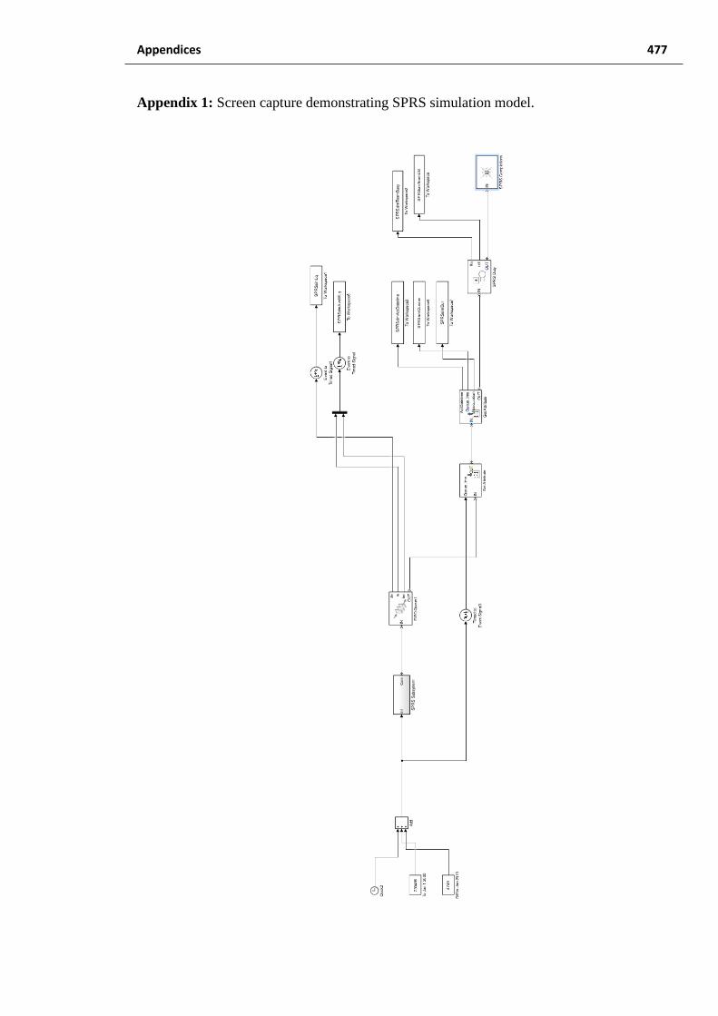
Appendices 477
Appendix 1: Screen capture demonstrating SPRS simulation model.
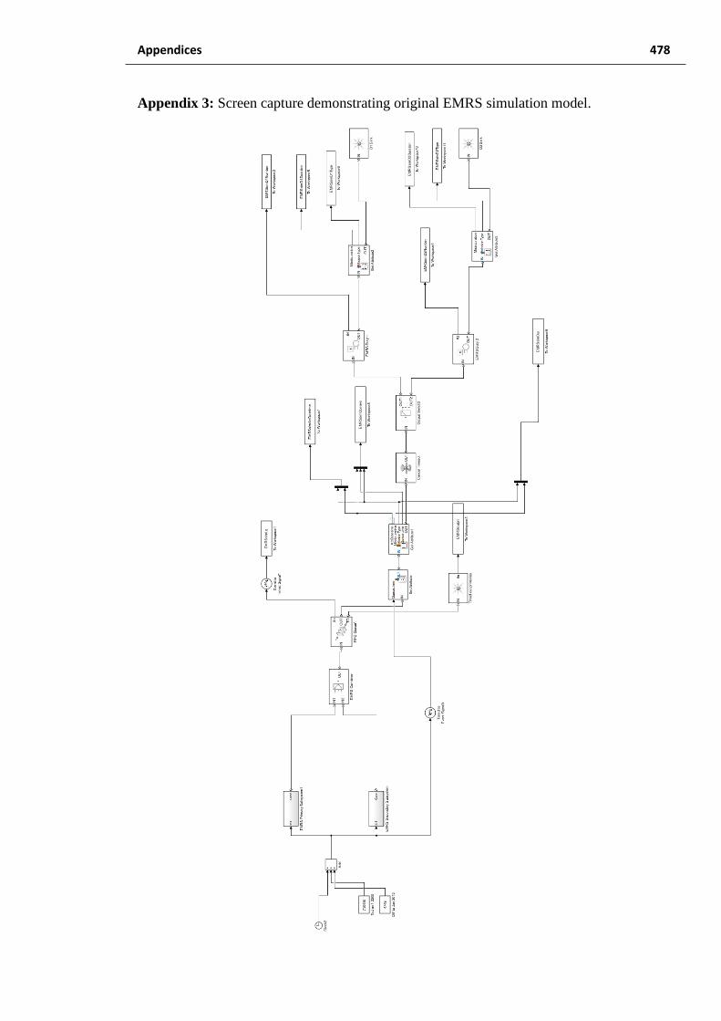
Appendices 478
Appendix 3: Screen capture demonstrating original EMRS simulation model.

Appendices 479
Appendix 3: Screen capture demonstrating revised EMRS simulation model.

480
Glossary
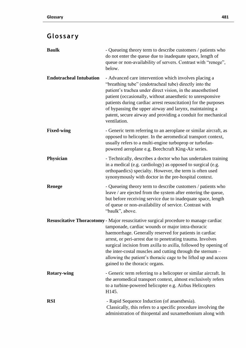
Glossary 481
Glossary
Baulk - Queueing theory term to describe customers / patients who
do not enter the queue due to inadequate space, length of
queue or non-availability of servers. Contrast with “renege”,
below.
Endotracheal Intubation - Advanced care intervention which involves placing a
“breathing tube” (endotracheal tube) directly into the
patient’s trachea under direct vision, in the anaesthetised
patient (occasionally, without anaesthetic to unresponsive
patients during cardiac arrest resuscitation) for the purposes
of bypassing the upper airway and larynx, maintaining a
patent, secure airway and providing a conduit for mechanical
ventilation.
Fixed-wing - Generic term referring to an aeroplane or similar aircraft, as
opposed to helicopter. In the aeromedical transport context,
usually refers to a multi-engine turboprop or turbofan-
powered aeroplane e.g. Beechcraft King-Air series.
Physician - Technically, describes a doctor who has undertaken training
in a medical (e.g. cardiology) as opposed to surgical (e.g.
orthopaedics) specialty. However, the term is often used
synonymously with doctor in the pre-hospital context.
Renege - Queueing theory term to describe customers / patients who
leave / are ejected from the system after entering the queue,
but before receiving service due to inadequate space, length
of queue or non-availability of service. Contrast with
“baulk”, above.
Resuscitative Thoracotomy - Major resuscitative surgical procedure to manage cardiac
tamponade, cardiac wounds or major intra-thoracic
haemorrhage. Generally reserved for patients in cardiac
arrest, or peri-arrest due to penetrating trauma. Involves
surgical incision from axilla to axilla, followed by opening of
the inter-costal muscles and cutting through the sternum –
allowing the patient’s thoracic cage to be lifted up and access
gained to the thoracic organs.
Rotary-wing - Generic term referring to a helicopter or similar aircraft. In
the aeromedical transport context, almost exclusively refers
to a turbine-powered helicopter e.g. Airbus Helicopters
H145.
RSI - Rapid Sequence Induction (of anaesthesia).
Classically, this refers to a specific procedure involving the
administration of thiopental and suxamethonium along with

Glossary 482
cricoid pressure (Sellick manoeuvre) to quickly effect
endotracheal intubation for the purposes of emergency
surgery with minimum risk of de-oxygenation or aspiration
for the patient. In more modern usage, it is considered
synonymous with rapid induction of emergency anaesthesia –
a catch-all term which encompasses a variety of drugs and
techniques to induce anaesthesia for the purposes of
mechanical ventilation, emergency surgery or other major
intervention, also while minimizing risk to the patient.
Triage - (French, lit: “sort”) the process of establishing priority of
treatment of patients according to severity of illness or injury.

483
References
Adams. C., 2017. 7 Years Ago: Top 10 US HEMS Providers. Retrieved from URL:
https://www.rotorandwing.com/2017/07/14/7-years-ago-top-ten-hems-providers/.
Rotor & Wing International, Portland, USA.
Association of Air Ambulances (as Air Ambulances UK), 2020. Retrieved from URL:
www.airambulancesuk.org, Association of Air Ambulances, London, UK.
Baker, S. P, O’Neill, B., Haddon, W. & Long, W. B. 1974. The Injury Severity Score: A
Method for Describing Patients with Multiple Injuries and Evaluating Emergency
Care. Journal of Trauma: Injury, Infection and Critical Care, 14, 187-196.
Bell, C. E. & Allen, D. 1969. Optimal planning of an emergency ambulance service. Socio
Econ.Planning Sci, 3, 95-101.
Bogle, B. M., Asimos, A. W. & Rosamond, W. D. 2017. Regional Evaluation of the
Severity-Based Stroke Triage Algorithm for Emergency Medical Services Using
Discrete Event Simulation. Stroke, 48, 2827-2835.
Boxma, O. J., Deng, Q. & Zwart, A. P. 2002. Waiting-Time Asymptotics for the M/G/2
Queue with Heterogeneous Servers. Queueing Systems, 40, 5-31.
Chan, C. W., Farias, V. F. & Escobar, G. J. 2017. The Impact of Delays on Service Times
in the Intensive Care Unit. Management Science, 63, 2049-2072.
Clark, D. E., Hahn, D. R., Hall, R. W. & Quaker, R. E. 1994. OPTIMAL LOCATION
FOR A HELICOPTER IN A RURAL TRAUMA SYSTEM - PREDICTION USING
DISCRETE-EVENT COMPUTER-SIMULATION. Journal of the American
Medical Informatics Association, 888-892.
Day, T. E., Al-Roubaie, A. R. & Goldlust, E. J. 2013. Decreased length of stay after
addition of healthcare provider in emergency department triage: a comparison
between computer-simulated and real-world interventions. Emergency Medicine
Journal, 30, 134-138.
Department of Health and Social Care & Public Health England. Handbook to the NHS
Consitution for England. 2021. 4th February 2021 Edition. Retrieved from
URL:https://www.gov.uk/government/publications/supplements-to-the-nhs-
constitution-for-england/the-handbook-to-the-nhs-constitution-for-england. Her
Majesty’s Government, London, UK.
Enayati, S., Mayorga, M. E., Rajagopalan, H. K. & Saydam, C. 2018. Real-time ambulance
redeployment approach to improve service coverage with fair and restricted
workload for EMS providers. Omega-International Journal of Management Science,
79, 67-80.
Fitzgerald, K., Pelletier, L. & Reznek, M. A. 2017. A Queue-Based Monte Carlo Analysis
to Support Decision Making for Implementation of an Emergency Department Fast
Track. J Healthc Eng, 2017, 6536523.
Goldwasser, R. S., Lobo, M. S., De Arruda, E. F., Angelo, S. A., Lapa E Silva, J. R., De
Salles, A. A. & David, C. M. 2016. Difficulties in access and estimates of public
beds in intensive care units in the state of Rio de Janeiro. Rev Saude Publica, 50, 19.
Green, L. V., Soares, J., Giglio, J. F. & Green, R. A. 2006. Using queueing theory to
increase the effectiveness of emergency department provider staffing. Academic
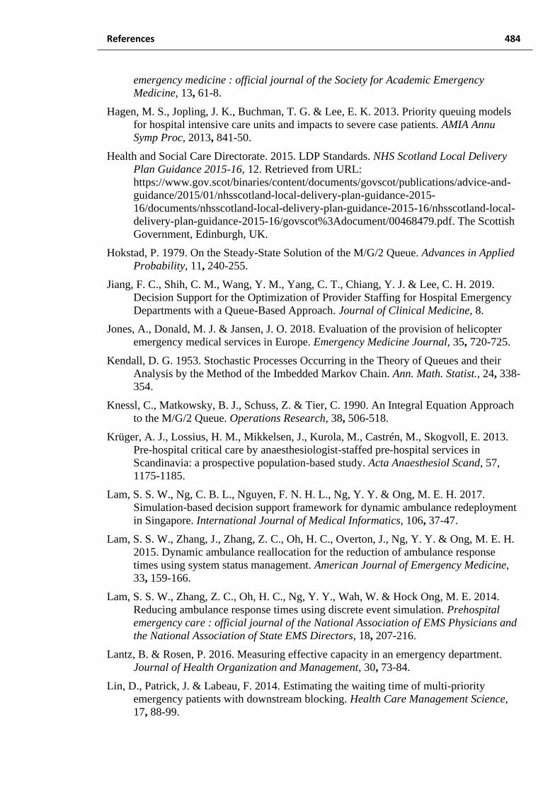
References 484
emergency medicine : official journal of the Society for Academic Emergency
Medicine, 13, 61-8.
Hagen, M. S., Jopling, J. K., Buchman, T. G. & Lee, E. K. 2013. Priority queuing models
for hospital intensive care units and impacts to severe case patients. AMIA Annu
Symp Proc, 2013, 841-50.
Health and Social Care Directorate. 2015. LDP Standards. NHS Scotland Local Delivery
Plan Guidance 2015-16, 12. Retrieved from URL:
https://www.gov.scot/binaries/content/documents/govscot/publications/advice-and-
guidance/2015/01/nhsscotland-local-delivery-plan-guidance-2015-
16/documents/nhsscotland-local-delivery-plan-guidance-2015-16/nhsscotland-local-
delivery-plan-guidance-2015-16/govscot%3Adocument/00468479.pdf. The Scottish
Government, Edinburgh, UK.
Hokstad, P. 1979. On the Steady-State Solution of the M/G/2 Queue. Advances in Applied
Probability, 11, 240-255.
Jiang, F. C., Shih, C. M., Wang, Y. M., Yang, C. T., Chiang, Y. J. & Lee, C. H. 2019.
Decision Support for the Optimization of Provider Staffing for Hospital Emergency
Departments with a Queue-Based Approach. Journal of Clinical Medicine, 8.
Jones, A., Donald, M. J. & Jansen, J. O. 2018. Evaluation of the provision of helicopter
emergency medical services in Europe. Emergency Medicine Journal, 35, 720-725.
Kendall, D. G. 1953. Stochastic Processes Occurring in the Theory of Queues and their
Analysis by the Method of the Imbedded Markov Chain. Ann. Math. Statist., 24, 338-
354.
Knessl, C., Matkowsky, B. J., Schuss, Z. & Tier, C. 1990. An Integral Equation Approach
to the M/G/2 Queue. Operations Research, 38, 506-518.
Krüger, A. J., Lossius, H. M., Mikkelsen, J., Kurola, M., Castrén, M., Skogvoll, E. 2013.
Pre-hospital critical care by anaesthesiologist-staffed pre-hospital services in
Scandinavia: a prospective population-based study. Acta Anaesthesiol Scand, 57,
1175-1185.
Lam, S. S. W., Ng, C. B. L., Nguyen, F. N. H. L., Ng, Y. Y. & Ong, M. E. H. 2017.
Simulation-based decision support framework for dynamic ambulance redeployment
in Singapore. International Journal of Medical Informatics, 106, 37-47.
Lam, S. S. W., Zhang, J., Zhang, Z. C., Oh, H. C., Overton, J., Ng, Y. Y. & Ong, M. E. H.
2015. Dynamic ambulance reallocation for the reduction of ambulance response
times using system status management. American Journal of Emergency Medicine,
33, 159-166.
Lam, S. S. W., Zhang, Z. C., Oh, H. C., Ng, Y. Y., Wah, W. & Hock Ong, M. E. 2014.
Reducing ambulance response times using discrete event simulation. Prehospital
emergency care : official journal of the National Association of EMS Physicians and
the National Association of State EMS Directors, 18, 207-216.
Lantz, B. & Rosen, P. 2016. Measuring effective capacity in an emergency department.
Journal of Health Organization and Management, 30, 73-84.
Lin, D., Patrick, J. & Labeau, F. 2014. Estimating the waiting time of multi-priority
emergency patients with downstream blocking. Health Care Management Science,
17, 88-99.

References 485
Liu, R. & Xie, X. L. 2018. Physician Staffing for Emergency Departments with Time-
Varying Demand. Informs Journal on Computing, 30, 588-607.
Maddock, A., Corfield, A. R., Donald, M. J., Lyon, R. M., Sinclair, N., Fitzpatrick, D.,
Carr, D. & Hearns, S. 2020. Prehospital critical care is associated with increased
survival in adult trauma patients in Scotland. Emergency Medicine Journal, 37, 141-
145.
Mayhew, L. & Smith, D. 2008. Using queuing theory to analyse the Government's 4-h
completion time target in Accident and Emergency departments. Health Care
Management Science, 11, 11-21.
Mcmanus, M. L., Long, M. C., Cooper, A. & Litvak, E. 2004. Queuing theory accurately
models the need for critical care resources. Anesthesiology, 100, 1271-6.
Moreno-Carrillo, A., Arenas, L. M. A., Fonseca, J. A., Caicedo, C. A., Tovar, S. V. &
Munoz-Velandia, O. M. 2019. Application of queuing theory to optimize the triage
process in a tertiary emergency care ("ER") department. Journal of Emergencies
Trauma and Shock, 12, 268-273.
Niederberger, M. & Spranger, J. 2020. Delphi Technique in Health Sciences: A Map.
Frontiers in Public Health, 8, 457.
Nogueira, L. C., Jr., Pinto, L. R. & Silva, P. M. S. 2016. Reducing Emergency Medical
Service response time via the reallocation of ambulance bases. Health Care
Management Science, 19, 31-42.
Pitter, V., Burnand, B., Yersin, B., Carron, P. 2014. Trends of pre-hospital emergency
medical services activity over 10 years: a population-based registry analysis. BMC
Health Serv Res, 14, 380.
Ross, S. M. 2013. Simulation, Oxford, UK, Elsevier Academic Press.
Royal Flying Doctor Service. 2019. Royal Flying Doctor Service Annual Report
2018/2019. Retrieved from URL: www.flyingdoctor.org.au. Royal Flying Doctor
Service Federation, Canberra, Australia.
Scott, D. W., Factor, L. E. & Gorry, G. A. 1978. Predicting the response time of an urban
ambulance system. Health Services Research, 13, 404-17.
Scottish Trauma Network. 2020. Scottish Trauma Network Annual Report 2019/20, 4.
Retrieved from URL: https://scottishtraumanetwork.com/wp-
content/uploads/2020/07/2019-20-AR-STN-1.0-1.pdf. NHS Scotland, Edinburgh,
UK.
Singer, M. & Donoso, P. 2008. Assessing an ambulance service with queuing theory.
Computers & Operations Research, 35, 2549-2560.
Stein, C., Wallis, L. & Adetunji, O. 2015. Meeting national response time targets for
priority 1 incidents in an urban emergency medical services system in South Africa:
More ambulances won't help. South African Medical Journal, 105, 840-844.
Whitt, W. 2000. The impact of a heavy-tailed service-time distribution upon the M/GI/s
waiting-time distribution. Queueing Systems, 36, 71-87.
Wiler, J. L., Bolandifar, E., Griffey, R. T., Poirier, R. F. & Olsen, T. 2013. An emergency
department patient flow model based on queueing theory principles. Academic
emergency medicine : official journal of the Society for Academic Emergency
Medicine, 20, 939-46.

References 486
Wu, C.-H. & Hwang, K. P. 2009. Using a Discrete-event Simulation to Balance
Ambulance Availability and Demand in Static Deployment Systems. Academic
Emergency Medicine, 16, 1359-1366.
Zhu, H. B., Gong, J., Tang, J. F. & Ieee 2013. A Queuing Network Analysis Model in
Emergency Departments. 2013 25th Chinese Control and Decision Conference.

487
Bib l iography
Gross, D., Shortle, J. F., Thompson, J.M., Harris, C. M. 2008. Fundamentals of Queueing
Theory. Fourth Edition. Wiley, Hoboken NJ, USA.
Ross, S. M. 2013. Simulation. Fifth Edition. Elsevier Academic Press, San-Diego CA,
USA.
Ortúzar, J., Willumsen, L. G. 2014. Modelling Transport. Fourth Edition. Wiley,
Chichester, UK.