diplomarbeit - othes.univie.ac.atothes.univie.ac.at/15649/1/2011-08-24_0400942.pdf · diplomarbeit...
TRANSCRIPT
DIPLOMARBEIT
Titel der Diplomarbeit
Differential Equation Models for SurfaceReactions of SnO2 Nanowire Gas Sensors
and their Inverse Modeling
angestrebter akademischer Grad
Magistra der Naturwissenschaften (Mag. rer. nat.)
Verfasserin: Marina RehrlStudienkennzahl lt. Studienblatt: A 405Studienrichtung lt. Studienblatt: MathematikBetreuer: Univ.-Ass. Priv.-Doz. DI Dr. Clemens Heitzinger
Wien, August 2011

Overview
In the line of the Vienna Science and Technology Fund (WWTF) project “Mathematics andNano-Sensors” a working relationship between the Austrian Institute of Technology (AIT)and the Wolfgang Pauli Institute (WPI) was established to build and test AIT fashioned tinoxide nanowire gas sensors and provide mathematical models to predict the outcome of gasmeasurements. As state of the art gas sensors still suffer from low selectivity, the detailedmodeling of the surface reactions to different test gases is essential to overcome this issue.
Despite the considerable amount of papers giving detailed discussions of experimentalresults in various gas atmospheres (a critic review can be found in [Comini et al. 2009]),the discussed surface reaction models in the literature mainly concentrate on more simpletest gases like oxygen, carbon oxide and inert gases. Therefore we were highly interested inproviding surface models for additional gases like, for example hydrogen sulfide or nitrogendioxide, which are known to be important for environmental control systems and various otherapplications.
The developed response models, described in this work, are composed of a surface reactionmodel and a charge transport model and predict the change of conductance of the sensor uponchanges in the thermal and chemical environment. Different transport models in the form offunctional equations were derived for different types of sensor structures. The surface reactionmodels consist of rate equations in the form of a system of parameter dependent ordinarydifferential equations (ODEs), which differ depending on temperature, type of modeled gas aswell as possible interactions with other gases.
In order to facilitate the simulation of the sensor response, the theory of inverse model-ing of dynamic models, with special regard to the estimation of model parameters throughnonlinear least squares estimators and suitable optimization algorithms, was discussed.
The simulation of the response of a gas sensor with a bundle of a nanowires as sensingelement in an inert atmosphere was accomplished by the fitting of 1 parameter in the chargetransport model and 5 parameters in the surface state model through nonlinear least squaresestimation.
i
Overview
This work is therefore organized as follows:
Chapter 01 intends to familiarize the reader with the technical aspect of gas sensor and givesan overview to their functionality.
Chapter 02 derives charge transport models for currently researched sensor architectures anddiscusses their properties and applicability. Depending on the state of carrier depletionin the sensor element different transport models were considered.
Chapter 03 gives a detailed derivation and discussion of parameter dependent ordinary dif-ferential equation models that describe the chemical reactions between different typesof gases and the surface of a tin oxide sensor. Detailed surface reaction models werederived for the most important test gas species.
Chapter 04 discusses the different types of surface reaction models and structures them intoa hierarchy starting with intrinsic model, oxygen model to combinations of test gasmodels. Then we will analyze the qualitative properties of the most important surfacemodels to prove the existence and uniqueness of their solution.
Chapter 05 addresses the estimation of parameters for models consisting of ordinary differ-ential equations. The standard form of an dynamical model is stated to aid the discussionof the general course of action for estimating an ODE model with regard to a suitableoptimization algorithm. In the second part we will cover the theory of Nonlinear LeastSquares Estimators and discuss and prove their asymptotic properties.
Chapter 06 presents the quantitative analysis of the derived charge transport models incombination with the intrinsic surface state trapping model. The response of a sen-sor consisting of a bundle of nanowires in an inert atmosphere was simulated and theparameters for the surface reaction model as well as the charge transport model werefitted.
ii
Contents
Overview i
1 Introduction 1
2 Charge Transport in the Sensors 52.1 Potential Barrier Theory . . . . . . . . . . . . . . . . . . . . . . . . . . . . . . . 62.2 Diffusion Theory . . . . . . . . . . . . . . . . . . . . . . . . . . . . . . . . . . . 82.3 Thermoelectronic Emission Theory . . . . . . . . . . . . . . . . . . . . . . . . . 92.4 The Surface Potential Barrier Vs and Depletion of Charge Carriers . . . . . . . 11
2.4.1 Partial Depletion . . . . . . . . . . . . . . . . . . . . . . . . . . . . . . . 112.4.2 Complete Depletion . . . . . . . . . . . . . . . . . . . . . . . . . . . . . 12
2.5 The Conductance Formulas . . . . . . . . . . . . . . . . . . . . . . . . . . . . . 13
3 Surface Reaction Models 173.1 Introduction . . . . . . . . . . . . . . . . . . . . . . . . . . . . . . . . . . . . . . 173.2 Intrinsic Surface States . . . . . . . . . . . . . . . . . . . . . . . . . . . . . . . . 183.3 Extrinsic Surface States . . . . . . . . . . . . . . . . . . . . . . . . . . . . . . . 19
3.3.1 Adsorption of Oxygen (O2) . . . . . . . . . . . . . . . . . . . . . . . . . 193.3.2 The influence of Humidity (H2O) . . . . . . . . . . . . . . . . . . . . . . 223.3.3 Reducing Gases . . . . . . . . . . . . . . . . . . . . . . . . . . . . . . . . 233.3.4 Oxidizing Gases . . . . . . . . . . . . . . . . . . . . . . . . . . . . . . . 30
4 The Combination of different types of Surface Reaction Models and theirSolution 374.1 The Interlinking of Surface Reaction Models . . . . . . . . . . . . . . . . . . . . 37
4.1.1 Intrinsic Model: Sensor response to an inert gas . . . . . . . . . . . . . 374.1.2 Oxygen Model: Sensor Response to dry synthetic air . . . . . . . . . . . 384.1.3 Mixtures of oxygen and an additional gas . . . . . . . . . . . . . . . . . 39
4.2 Existence and Uniqueness of the Solution . . . . . . . . . . . . . . . . . . . . . 404.2.1 Intrinsic Model . . . . . . . . . . . . . . . . . . . . . . . . . . . . . . . . 414.2.2 Oxygen Model . . . . . . . . . . . . . . . . . . . . . . . . . . . . . . . . 42
iii
Contents
5 Parameter Estimation for Dynamic Models 455.1 Structure and Challenges of Dynamical Models . . . . . . . . . . . . . . . . . . 45
5.1.1 Computation of the objective function . . . . . . . . . . . . . . . . . . . 475.1.2 Optimization Methods . . . . . . . . . . . . . . . . . . . . . . . . . . . . 47
5.2 The Objective Function and Nonlinear Least Squares Estimators . . . . . . . . 495.2.1 Nonlinear Least Squares Estimation . . . . . . . . . . . . . . . . . . . . 505.2.2 Consistency of the Nonlinear Least Squares Estimator . . . . . . . . . . 525.2.3 Asymptotic Normality . . . . . . . . . . . . . . . . . . . . . . . . . . . . 56
6 Quantitative Analysis and Simulation 596.1 Description of Data . . . . . . . . . . . . . . . . . . . . . . . . . . . . . . . . . . 596.2 Calculation of nNs from measured data . . . . . . . . . . . . . . . . . . . . . . 606.3 Simulation of nNs and G . . . . . . . . . . . . . . . . . . . . . . . . . . . . . . 63
Bibliography I
Acknowledgments VII
Abstract IX
Zusammenfassung X
Curriculum Vitae XI
iv

Chapter 1
Introduction
Gas sensors are a type of chemical sensors, which are devices able to convert chemical statesinto electrical signals, and are used to detect the concentration and hereby the presence ofcertain target gases in the atmosphere. The detection of gases is important for many fields ofapplications:
• safety engineering,
• health care,
• bio-sciences and
• environmental monitoring
if only to name a few. A quiet extensive (but still not exhaustive) list of current and possiblefuture applications can be found in [Zima 2009].
To meet this demand for the applicability to different fields, considerable research intonew types of sensors is needed, including efforts to enhance the performance and understandthe working principles of these sensor devices. Necessary properties of gas sensor are selectivity(i.e., response only to the targeted gas) and sensitivity (i.e., providing of sufficiently measurablesensor response). Current gas sensors however are highly cross sensitive, especially regardinggas species that show similar reducing or oxidizing properties. The mathematical modeling ofthe underlying sensing mechanisms, which is the modeling of the occurring surface reactions,helps in the scientific understanding of these devices and is the key for further advancementof the sensors to overcome the issue of cross selectivity.
The principle of gas detection with SnO2, or nearly every other metal oxide semiconductor,is based on the measurable change of the electrical conductance upon the adsorption of gasspecies, as there usually occurs a charge transfer between adsorbed gas molecules and thesensor surface. As gas sensors are usually operated in an oxygen atmosphere, adsorbed oxygenextracts electrons from the semiconductor and, if the sensing material conducts by electrons,decreases the conductance. If, for example, carbonic target gas species are present in the
1

Chapter 1 Introduction
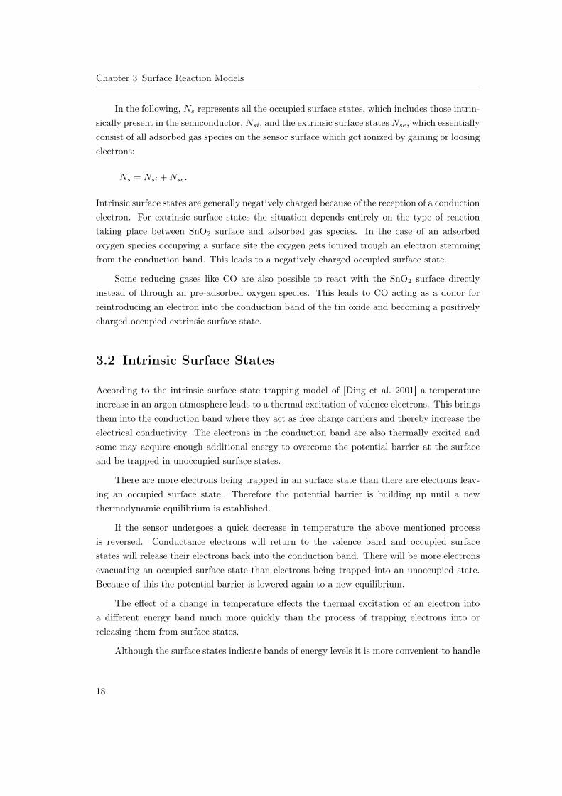
atmosphere, they become ionized by pre-adsorbed negatively charged oxygen, when reactingwith the sensor surface, and return electrons into the solid. This leads to an increase inconductivity. The conductance of a sensor is therefore much higher if a type of reducing gas,like carbon monoxide, is present in the atmosphere then it is in “clean” air. Because of the largesurface-to-volume ratio of a nanowire-structured sensor device, the response of a nanowire gassensor is also very sensitive to changes in chemistry and dielectric properties of the surface,caused by this exchange of charge carriers.
(a) (b) (c)
Figure 1.1: A schematic representation of the interaction of a SnO2 nanowire with O2 andCO. Figure (a) shows oxygen, in atomic and molecular form in the atmospherearound the nanowire. In the second figure oxygen species are bound to the surfaceof the nanowire by extracting electrons from the bulk material. Figure (c) showsthe effect of CO as it extracts the oxygen species from the surface and reintroducesthe previously bound electrons into the nanowire.
It was known for many years that the electrical properties of semiconductors are sensitiveto ambient gases. After physical studies done by Brattain&Bardeen and Morrison in 1953and since Seiyama et al. discovered in 1962 that the presence of reactive gas species in theatmosphere causes a tremendous change in the electrical conductivity of ZnO, the use of metaloxides semiconductors for gas sensing purposes was intensively studied.
Tin oxide arose as an especially favorable material for these purposes as it possesses ahigh sensitivity to various target gases and is a generally well understood and easily fabricatedmaterial [Zima 2009]. SnO2 was also used for the first commercial gas sensors, a Taguchi-typesensor, manufactured by Figaro in Japan.
The semiconducting behavior of tin oxide arises, as is typical for metal oxides, fromdeviations of the stoichiometry of the material, as otherwise ideal stoichiometric SnO2 wouldbe an isolator at room temperature. Therefore the termination of the periodic structure atthe surface of tin oxide may form surface-localized electronic states within the semiconductorband gab. The n-conducting properties of the tin oxide stems from the electron donor effect ofthe oxygen surface defects (e.g., oxygen vacancies) in the crystal lattice, which can be singlyand doubly ionized and play a significant role in the process of gas sensing. Those oxygenvacancies are mainly formed in the manufacturing process, as oxygen atoms may escape into
2
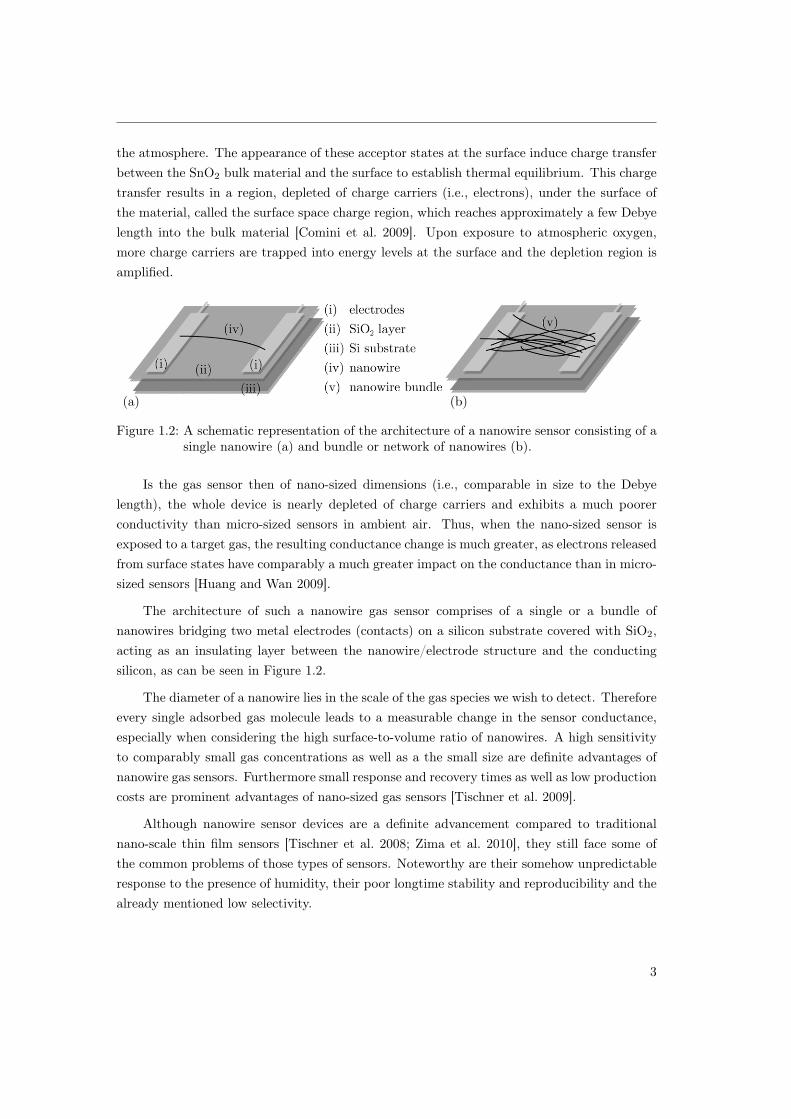
the atmosphere. The appearance of these acceptor states at the surface induce charge transferbetween the SnO2 bulk material and the surface to establish thermal equilibrium. This chargetransfer results in a region, depleted of charge carriers (i.e., electrons), under the surface ofthe material, called the surface space charge region, which reaches approximately a few Debyelength into the bulk material [Comini et al. 2009]. Upon exposure to atmospheric oxygen,more charge carriers are trapped into energy levels at the surface and the depletion region isamplified.
(a) (b)
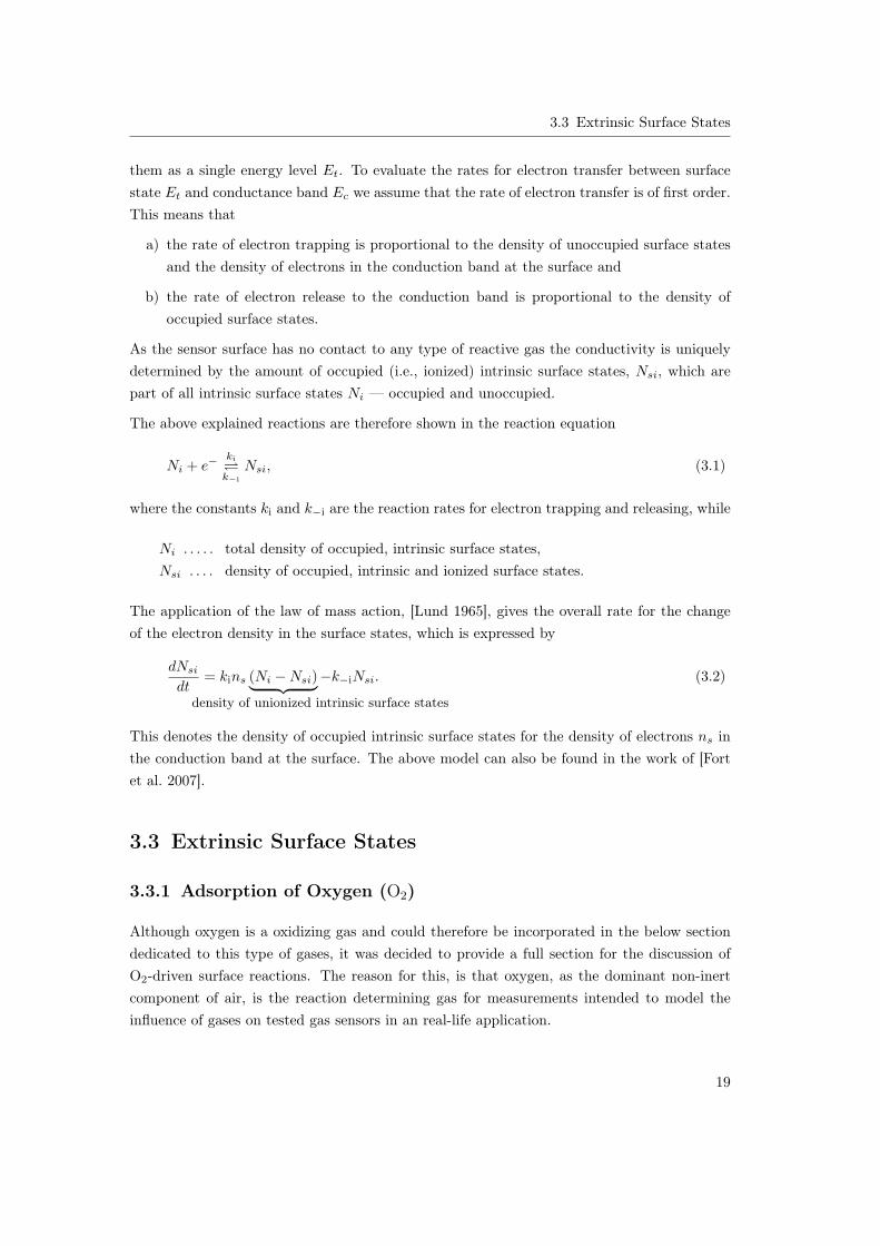
Figure 1.2: A schematic representation of the architecture of a nanowire sensor consisting of asingle nanowire (a) and bundle or network of nanowires (b).
Is the gas sensor then of nano-sized dimensions (i.e., comparable in size to the Debyelength), the whole device is nearly depleted of charge carriers and exhibits a much poorerconductivity than micro-sized sensors in ambient air. Thus, when the nano-sized sensor isexposed to a target gas, the resulting conductance change is much greater, as electrons releasedfrom surface states have comparably a much greater impact on the conductance than in micro-sized sensors [Huang and Wan 2009].
The architecture of such a nanowire gas sensor comprises of a single or a bundle ofnanowires bridging two metal electrodes (contacts) on a silicon substrate covered with SiO2,acting as an insulating layer between the nanowire/electrode structure and the conductingsilicon, as can be seen in Figure 1.2.
The diameter of a nanowire lies in the scale of the gas species we wish to detect. Thereforeevery single adsorbed gas molecule leads to a measurable change in the sensor conductance,especially when considering the high surface-to-volume ratio of nanowires. A high sensitivityto comparably small gas concentrations as well as a the small size are definite advantages ofnanowire gas sensors. Furthermore small response and recovery times as well as low productioncosts are prominent advantages of nano-sized gas sensors [Tischner et al. 2009].
Although nanowire sensor devices are a definite advancement compared to traditionalnano-scale thin film sensors [Tischner et al. 2008; Zima et al. 2010], they still face some ofthe common problems of those types of sensors. Noteworthy are their somehow unpredictableresponse to the presence of humidity, their poor longtime stability and reproducibility and thealready mentioned low selectivity.
3

Chapter 1 Introduction
(a) (b)
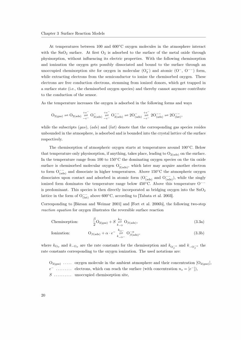
Figure 1.3: Picture of a single nanowire (a) and a bundle/network of nanowires (b). The singlenanowire is positioned between two contacts. According to References [Köck et al.2009] and [Tischner et al. 2009].
For definitions to chemical and physical terminologies and concepts in this and the fol-lowing chapters, the interested reader is referred to the work of [Zima 2009].
4

Chapter 2
Charge Transport in the Sensors
The mechanism of charge transfer in a semiconductor gas sensor depends strongly on itsmorphology. If the sensitive part of a sensor structure is fashioned as a sensor film, a generaldistinction between compact and porous layers can be made. Compact sensing layers excludethe possibility of gas penetrating the sensing layer. In this case the interaction with gas takesplace only on the geometric surface, where else porous sensing layers allow for the gas to accessthe sensing layer. Their active surface reaches therefore into the sensing layer.
For compact sensing layers or sensors consisting of single nanowires a formula for theconductance, as the product of conductivity and a geometry factor, for electrical devices witha uniform cross section is applicable. When combined with an additional equation for thedensity of electrons on the sensor surface the resulting conductance formula is applicable tosensor with grain boundaries. This approach is referred to as the Potential Barrier Theory(PBT) by a number of authors, [Ding et al. 2001; Morrison 1990].
The Thermoelectronic Emission Theory (TEET), also called Diode Theory, as well as theDiffusion Theory (DT), which can be found in [Bârsan and Weimar 2001; Broniatowski 1985],explain the link between surface phenomena and the measured conductance for porous sensorfilms with grains larger than the Debye length λD.
All the above theories will then lead to an expression of the conductance as a function ofthe surface potential barrier Vs. A further equation is therefore needed to link the value of Vsto the concentration of surface states Ns, which are derived from surface reaction models inChapter 3.
Actually, both sensor constructions can be divided into two additional cases — thick andthin sensing layers/nanowires, where the deciding factor is the ratio between the layer/wirethickness and the Debye length. Depending on the actual morphology of the grain-graincontact region the respective transport mechanism is determined. But ultimately the resultingconductance formulas for the above mentioned sensor structures are basically the same andonly differ in a multiplicative constant.
5
Chapter 2 Charge Transport in the Sensors
2.1 Potential Barrier Theory
The existence of surface states at a surface gives rise to a difference between the energy levelof the surface state and the conduction band of the bulk material. This enables electrons toalternate between conduction band and surface states. The conduction electrons, which wereable to cross over and thereafter occupy a surface state, create a repulsive potential barrierat the surface to further prevent the trapping of conduction electrons into unoccupied surfacestates. Such potential barriers are a particular hindrance for electrons when they occur at thecontact areas between single grains, which are anyway rather narrow. In order to contributeto the conductance, these electrons have to acquire enough kinetic energy to overcome thesurface potential barrier Vs while traveling through the grain contact areas.
When discussing the conductance G, one has to start with the microscopic conductivityσ. The electric conductivity of a semiconductor crystal has a electronic/hole and a ionic part.However, as tin oxide gas sensors are usually operated in temperatures between 200◦ and400◦C, the ionic component of the conductivity can be neglected [Zima 2009]. Furthermore,because of SnO2 being a n-type semiconductor, one refers to the electronic part of the overallconductivity/conductance. The electronic conductivity in a homogeneous single crystal istherefore given by
σ = σe + σp +∑
σion,i ≈ σe + σp ≈ σe = q · µ · n,
where q gives the elementary charge, n is defined as the electron concentration and µ statestheir mobility.
The relation between the conductivity σ and the conductance G for the case of an n-typesemiconductor is given by
G = const · σ = const · q · µ · ns (2.1)
for a constant factor const depending on the geometry of the sensor. As the conductance isdominated by the electron transfer across the surface potential barrier at the inter-granularcontact regions, G is proportional to the density ns of electrons that are responsible for theconduction at the surface. The density of electrons n can therefore be set to ns
To complete this relation we have to derive a equation to set the density of surface electronin a relation to the potential barrier at the surface.
6
2.1 Potential Barrier Theory
The Density of Electrons at the Surface ns
To calculate the electron density ns on the surface of a semiconducting material we have tostart with the bulk value nb. First we consider the density of charge carriers or occupied statesper unit volume and energy n(E), which is simply the product of the density of available statesin the conduction band gc(E) = 8π
√2
h3 m?e
32√E − EF and the probability that each of these
states is occupied, which is the Fermi-Dirac probability function f(E). The density of occupiedstates is therefore given by
n(E) = gc(E) · f(E).
The density of electrons in the semiconductor bulk material is then obtained by integratingthe density of carriers over all possible energies within a band, as seen in equation
nb =
top of conduction band∫bottom of conduction band
gc(E) · f(E)dE
=
∞∫Ec
8π√
2
h3m?e
32
√E − EF ·
1
1 + exp(E−EFkT
)dE.As the Fermi function converges to zero for rising energies the actual location of the top ofthe conduction band needs not be known and can be replaced by infinity. Assuming that theFermi level is at least 2kT away from the conduction band edge (i.e., Ec − EF > 2kT ), thisallows for the replacement of the Fermi distribution by the Boltzmann distribution. Theseconsiderations leads us to
nb =
∞∫Ec
8π√
2
h3m?e
32
√E − EF · exp
(EF − EkT
)dE
=8π√
2
h3m?e
32
∞∫Ec
√E − EF · exp
(EF − EkT
)dE
=8π√
2
h3m?e
32 · kT
32
2
√π · exp
(EF − EC
kT
)= Nc exp
(EF − EC
kT
)
with Nc = 2(
2πm?ekTh2
) 32
the effective density of states in the conduction band. The density ofelectrons at the surface of an n-type semiconductor ns is then given by the previous equationmultiplied by a Boltzmann factor, taking the potential barrier at the surface into account.Therefore, the density ns of free electrons energized enough to overcome the surface potential
7
Chapter 2 Charge Transport in the Sensors
barrier Vs, is given by
ns = Nc exp
(− (qVs + Ec − EF )
kT
)= nb exp
(−qVskT
), (2.2)
according to [Morrison 1990]. The conduction formula according to the Potential BarrierTheory becomes therefore
G = const · qµnb exp
(−qVskT
). (2.3)
2.2 Diffusion Theory
If the depletion layer is large compared to the mean free path of electrons, the Diffusion Theoryis applicable, as in this case the concepts of drift and diffusion are valid. To derive a equationfor the conductance we will consider the potential barriers on the two sides of the grainboundary separately and then join the solutions under the condition of current continuity. Weconsider the case of a n-type semiconductor like SnO2. Then the Diffusion Theory gives thecurrent density across the grain boundary as the sum of contributions from the dependence ofthe current on field intensity and diffusion resulting from the gradient in the carrier density:
j(t) = σ(x, t)E(x, t) + qD∂n
∂x
= −qµn(x, t)∂V (x, t)
∂x+ µkT
∂n(x, t)
∂x
for
D = µkTq . . . . . . . . . . . . . . . . . . carrier diffusion coefficient,
V (x, t) . . . . . . . . . . . . . . . . . . . . electrostatic potential,E(x, t) = −∂V (x,t)
∂x . . . . . . . . . electric field.
As solution of the above equation, the following expression for the current density in thediffusion case is given, [Broniatowski 1985], by
j(t) = qµEinb
(exp
(−q (Va + Vi)
kT
)− exp
(−qVikT
))
for Ei the electric field strength on the ith side. Equating the current density for the left sidei = 1 and right side i = 2 gives us
E1
(exp
(−q (Va + Vi)
kT
)− exp
(−qV1
kT
))= E2
(exp
(−q (Va + Vi)
kT
)− exp
(−qV2
kT
)),
8
2.3 Thermoelectronic Emission Theory
E2 exp
(−qV2
kT
)− E1 exp
(−qV1
kT
)= (E2 − E1) exp
(−q (Va + Vi)
kT
),
which in turn leads to
exp
(−q (Va + Vi)
kT
)=E2 exp
(− qV2
kT
)− E1 exp
(− qV1
kT
)E2 − E1
.
Insertion of the last relation into the equation for charge density for one side of the barrierleads us to
j(t) =qµE2nbE2 − E1
(E2 exp
(−qV2
kT
)− E1 exp
(−qV1
kT
)− (E2 − E1) exp
(−qV2
kT
))
=qµE1E2nbE2 − E1
(exp
(−qV2
kT
)− exp
(−qV1
kT
))
=qµEsnb
2exp
(−qV2
kT
)(1− exp
(−qVakT
)),
where we set the applied voltage Va = V1−V2 to zero to get the barrier height Vs as well as fieldstrength Es = E1 = −E2 at the boundary. When we differentiate the current density withrespect to Va we get the slope of the current-voltage characteristics, which is the conductivity(according to [Taylor et al. 1952]), when we set the applied voltage Va to zero. The conductivityis therefore given by
σ =dj
Va
∣∣∣∣Va=0
=q2µ
2kTEsnb exp
(−qVskT
)=q5/2n
3/2b µV
1/2s√
2εkTexp
(−qVskT
)
as Es equals√
2qnbVsε according to [Broniatowski 1985]. By multiplying the conductivity with
an factor const, which is the effective area seen by electrons while traveling from grain tograin, we obtain
GDT = constq5/2n
3/2b µV
1/2s√
2εkTexp
(−qVskT
), (2.7)
the conduction formula of the Diffusion Theory.
2.3 Thermoelectronic Emission Theory
For the case that the surface potential barrier width is much smaller than the mean free pathof electrons (λ ≥ x0), the current density is proportional to the difference of the electron fluxescrossing the interface. Therefore only those electrons with kinetic energy equal or larger than
9

Chapter 2 Charge Transport in the Sensors
the potential barrier height are able to cross the boundary. This is reflected in the currentdensity
j(t) = qnbvth
(exp
(−qV2
kT
)− exp
(−qV1
kT
)),
where the mean thermal velocity of electrons vth is given by√
8kTπm? andm? denotes the effective
mass of electrons. As the applied voltage or bias is given by Va = V1 − V2 we can rewrite thecurrent density as
j(t) = qnbvth exp
(−qV2
kT
)(1− exp
(−qVakT
)).
Differentiation of the current density with respect to Va results in the electrical conductivity
σ =dj
Va
∣∣∣∣Va=0
=q2nbvthkT
exp
(−qVskT
)when we set the applied voltage to zero. By multiplication with an area factor we get theconduction formula for the Thermoelectronic Emission Theory
GTEET = const · q2nbvthkT
exp
(−qVskT
). (2.8)
The previous section revealed that the conductance formulas derived for Potential BarrierTheory, Diffusion Theory as well as Thermoelectronic Emission Theory are of a similar form
G = const · q v nb exp
(−qVskT
), (2.9)
while v denotes a velocity term given by
v =
µ Potential Barrier Theoryq
2kT µEs Diffusion TheoryqkT vth Thermoelectronic Emission Theory,
whose exact form depends on the underlying theory.
In order to relate the above conductance formula to the density of occupied surface statesNs, which in the following chapter is obtained from surface states models, we need to derivethe surface potential barrier Vs as a function of Ns. For this purpose we also have to consider
10
2.4 The Surface Potential Barrier Vs and Depletion of Charge Carriers
the state of charge depletion in the respective nanostructure.
2.4 The Surface Potential Barrier Vs and Depletion of
Charge Carriers
The actual link between the measured quantity of conductance and the occupied surface statesNs is given by either the Schottky relation or a more close examination of the geometry of thesensor structure. The choice of the type of approach depends on the width of the nanostructurew in relation to the width of its depletion region, which scale can be described by the Debyelength λD. The case λD � w applies to sensors whose depletion region does not reach veryfar into the nanostructure. These sensing areas have therefore a inner region unaffected bysurface phenomena. In the case of λD ≈ w, the sensor is completely depleted of bulk electronsand surface phenomena therefore influence the conductance of the whole sensing area.
In both cases we will derive an expression for the surface potential barrier in terms ofthe surface state density, which will then be used to include the value of Ns into the alreadyderived conductance formulas.
2.4.1 Partial Depletion
For nanostructures which are not completely depleted of charge carriers (λD � w), we derivethe Schottky relation from the one-dimensional Poisson equation
d2ψ
dx2=qNiε,
with ψ the electrical potential and Ni the ion density in the space-charge region. The Poissonequation describes the change in the electrical potential as a function of the distance throughthe space charge region. We change the coordinates to V (x) = ψ0−ψ(x), with ψ0 the electricalpotential in the bulk material, in order to gain the relation
V =qNi (x− x0)
2
2ε,
after solving the Poisson equation with the boundary condition dVdx = V = 0 for x = x0,
while x0 denotes the thickness of the depletion layer, 0 ≤ x ≤ x0. As for n-type materialNi = ND, which is the density of electrons in the semiconductor. The factor NDx0 denotesthen the number of electrons extracted from the space charge region. As the electroneutralitycondition states that the charge in the depletion layer equals the charge captured on thesurface, [Bârsan and Weimar 2001], the product NDx0 also denotes the density of charged
11
Chapter 2 Charge Transport in the Sensors
surface states Ns. This calculation leads us finally to the Schottky relation
Vs =qN2
s
2εND, (2.10)
with Vs the surface potential barrier for x = 0, where ε states the electrical permittivity of thesemiconductor material.
According to [Madou and Morrison 1989] all the donors in SnO2 are ionized at roomtemperature and above so the density of ionized donors ND can be considered constant, [Dinget al. 2001; Fort et al. 2006b]. Then, according to [Bârsan and Weimar 2001], the density ofelectrons in the bulk for a semiconductor with completely ionized donors and little acceptorsequals the density of donors:
nb = ND. (2.11)
2.4.2 Complete Depletion
For thin nanostructures with a scale of diameter comparable to the Debye length (λD ≈ w), theSchottky relation is not applicable. In this case we first consider the nanowire as a cylinderwith radius R, a depletion region of thickness x0 and charge density equal to ND, as wasproposed by [Fort et al. 2010]. We introduce cylindrical coordinates and write the electricalfield in the depletion region as
E(r) =qND2ε
(r − (R− x0)
2
r
)
and get the electrical potential
V (r) =qND2ε
(r2
2− (R− x0)
2ln(r)
)
from the relationship dV (r)dr = E(r). This implies that the surface potential barrier Vs is the
difference between the electrical potential on the surface and the potential at the begin of thedepletion region
Vs = V (R)− V (R− x0)
=qND2ε
(2Rx0 − x2
0
2− (R− x0)
2ln
(R
R− x0
))
=qND4ε
R2 for R ≈ x0.
(2.12)
12
2.5 The Conductance Formulas
So, in the case of a complete depletion of the wire (R ≈ x0), we find that the surface poten-tial barrier is not depending directly on the Ns but rather through the value of donor densityND. The corresponding relationship can be found through the electroneutrality condition
qNs · 2πRl = qND · π(R2 − (R− x0)
)2
,
according to which the electrical charge on the surface of the nanowire equals the charge in thedepletion region throughout the nanowire, while l denotes the length of the nanowire. Thisimplies
x0 = R−√R2 − 2
NsND
R ⇒ ND ≈ 2NsR
if we regard the depletion region with R ≈ x0. Therefore the density of bulk donors cannotbe considered constant and equal to the density of ionized donors ND anymore, but varyingwith the density of occupied surface states. Hence, [Fort et al. 2010] found the density of freeelectrons in the bulk material nb as
nb = ND − 2NsR, (2.13)
which is the difference between the density of donors and the electrons occupying the surface.
2.5 The Conductance Formulas
Equations (2.10) and (2.12) show clearly that a change in the density of occupied surfacestates Ns effects the potential barrier and results consequently in a change in conductance.Therefore, in combination with the conductance formulas (2.9) and the relationships for thedensity of bulk electrons given in (2.11) and (2.13), the equation
G(T, Vs) =
G0
(1− Ns
NDR
)exp
(−q2ND4εkT
)+GC for λD ≈ w
G0 exp(− q2N2
s
2εNDkT
)+GC for λD � w.
(2.14)
describes the conductance of a sensor, depending on the grade of carrier depletion. The caseλD ≈ w marks the completely depleted nanowire and λD � w applies to a nanostructure ofgreater diameter/width, so that there exists a inner region unaffected of surface phenomena.
The pre-exponential factor G0 has the form of
G0 = const · q v nb, (2.15)
13
Chapter 2 Charge Transport in the Sensors
while the velocity term v changes depending on the underlying theory. For a partly depletednanostructures the nb can be set to the density of donors ND, according to (2.11). In the caseof complete charge depletion the value of nb was excluded from G0 and separately considered,as described by equation (2.13).
The additive term GC in equation (2.14) is a parameter used to provide for variousconduction phenomena, like a drift in the sensor signal, and to give the baseline level. Thisparameter as addition to the conductance formula was introduced by [Ding et al. 2001].
The diffusion theory states the dependence of G0 on V 1/2s . Given the already exponential
dependence of G on Vs in the second term of (2.14), this can be neglected. The same reasoningis applicable to the temperature-dependence of the pre-exponential factor, since µs ∝ T−3/2
according to [Madou and Morrison 1989]. Some authors like Fort et al. have neverthelesschosen to express G0 as G′0T−3/2 and regard G′0 as a constant. Otherwise, the whole pre-exponential factor G0 is often regarded as a constant and can therefore be estimated, alongwith GC , in a parameter fitting process.
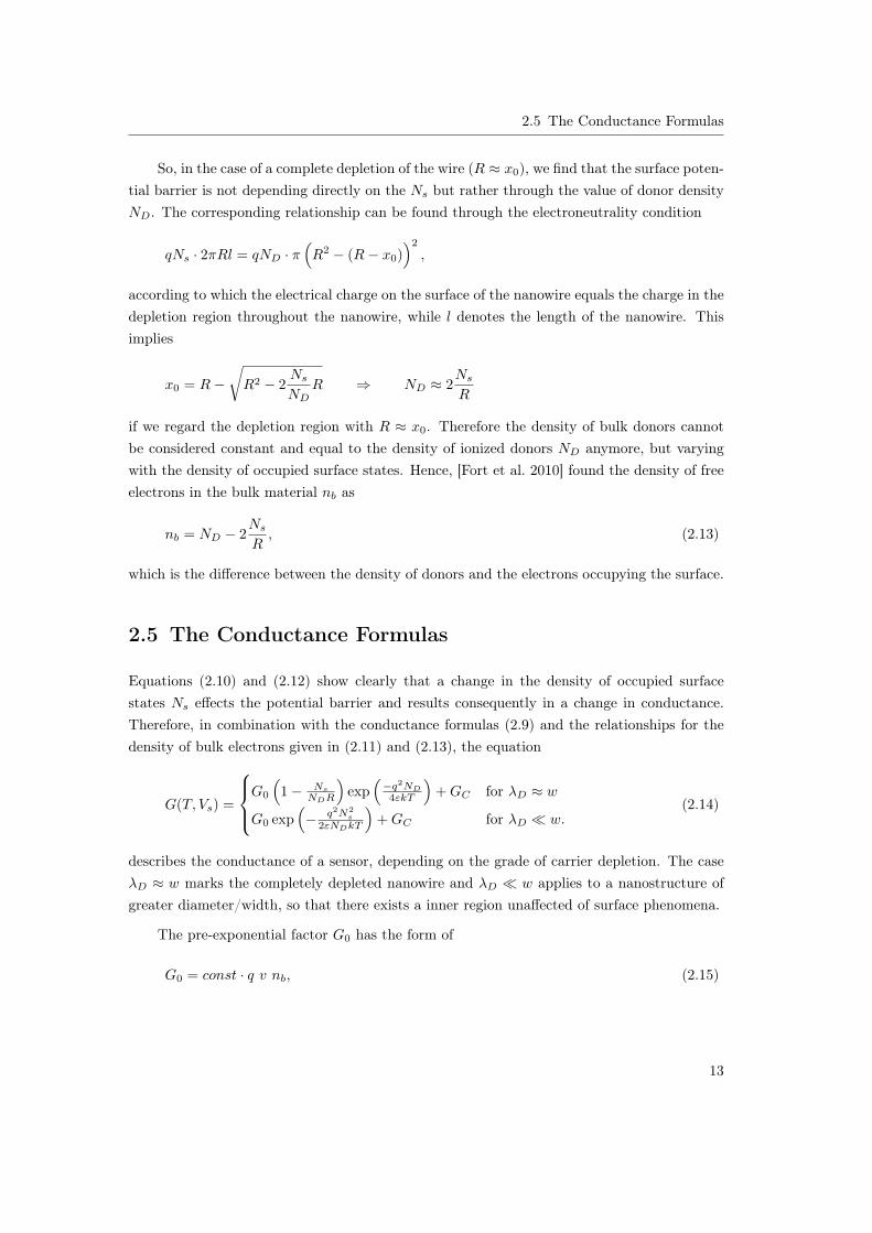
Figure 2.1: Illustration of the conduction in a network of nanowires. The charge depletionregion under the surface of the nanowires is due to the adsorption of oxygen species.The resulting potential barrier between touching nanowires is depicted in the banddiagram where Ec, Ef , Ev and Eg are the conduction band, Fermi level, valenceband and the band gap. qVs denotes the height of the surface potential barrier.See [Choi et al. 2008], Figure 4 and [Zima 2009], Figure 2.14.
Despite the fact that equations like (2.14) were intended to describe the conductance inlayer of semiconducting material, [Fort et al. 2010] argued their applicability to a bundle ofsemiconducting nanowires. The current path consists of many nanowires with small contact
14
2.5 The Conductance Formulas
regions. For this type of sensor the contact points between nanowires act similarly to thecontact regions between the grains in a porous layer and therefore build up a surface potentialbarrier, which electrons have to overcome in order to contribute to the charge flow and add tothe sensor conductance. Indeed, according to [Comini et al. 2009], the conduction mechanismof nanowire bundles is dominated by the intercrystalline boundaries at the connection regionsbetween nanowires, as these contact points provide most of the resistance of the sample.
Regarding the modeling of conductance in a single nanowire sensor the same group ofauthors have shown that also in this case the conduction model (2.14) is applicable, [Fortet al. 2009]. Despite this, the case of a single nanowire, can also be modeled through classicalsemiconductor transport equations like the Drift-Diffusion Model or the Poisson-Boltzmannequation, [Katterbauer 2010].
15

Chapter 3
Surface Reaction Models
This section will give surface reaction models derived from chemical reaction equations, whichdepict the interaction of different kinds of gases and a metal oxide surface, or, to be morespecific, on tin oxide (SnO2).
3.1 Introduction
The ability of gas sensors to detect the presence of chemicals in the atmosphere depends onthe interaction between gas and sensor surface. A strong interaction is possible due to the factthat at the surface of the sensing area the periodicity of the crystal lattice is disrupted, thusincreasing the reactivity of the sensing area. Also factors like doping, alloying, adsorbates orimpurities would influence the reactivity of a surface.
In these cases localized energy states arise at the surface, which are able to exchange electronswith the sensor bulk atoms. These energy levels are called surface states. The fundamentaltheory to the idea of surface states can be found in the work of [Morrison 1990; Madou andMorrison 1989]. The group Ding et al., who based their work on Morrison et al., differentiatebetween intrinsic and extrinsic surface states and characterize them as follows:
Intrinsic surface states: They are created by the semiconductor itself, and include energy lev-els stemming from impurities, doping and oxygen vacancies in the metal oxide lattice.These energy states are the cause for the sensor response to inert gases, like Argon (Ar)in [Ding et al. 2001] and Nitrogen (N2) in [Lu et al. 2006], where there is no reactionpossible between gas and surface.
Extrinsic surface states: These localized surface energy levels, on the other hand, are createdthrough adsorbed gas molecules at the SnO2 surface, like adsorbed oxygen.
In both cases the exchange of electrons between the conduction band of the metal oxide anda surface state leads to an occupied and consequently charged surface state.
17
Chapter 3 Surface Reaction Models
In the following, Ns represents all the occupied surface states, which includes those intrin-sically present in the semiconductor, Nsi, and the extrinsic surface states Nse, which essentiallyconsist of all adsorbed gas species on the sensor surface which got ionized by gaining or loosingelectrons:
Ns = Nsi +Nse.
Intrinsic surface states are generally negatively charged because of the reception of a conductionelectron. For extrinsic surface states the situation depends entirely on the type of reactiontaking place between SnO2 surface and adsorbed gas species. In the case of an adsorbedoxygen species occupying a surface site the oxygen gets ionized trough an electron stemmingfrom the conduction band. This leads to a negatively charged occupied surface state.
Some reducing gases like CO are also possible to react with the SnO2 surface directlyinstead of through an pre-adsorbed oxygen species. This leads to CO acting as a donor forreintroducing an electron into the conduction band of the tin oxide and becoming a positivelycharged occupied extrinsic surface state.
3.2 Intrinsic Surface States
According to the intrinsic surface state trapping model of [Ding et al. 2001] a temperatureincrease in an argon atmosphere leads to a thermal excitation of valence electrons. This bringsthem into the conduction band where they act as free charge carriers and thereby increase theelectrical conductivity. The electrons in the conduction band are also thermally excited andsome may acquire enough additional energy to overcome the potential barrier at the surfaceand be trapped in unoccupied surface states.
There are more electrons being trapped in an surface state than there are electrons leav-ing an occupied surface state. Therefore the potential barrier is building up until a newthermodynamic equilibrium is established.
If the sensor undergoes a quick decrease in temperature the above mentioned processis reversed. Conductance electrons will return to the valence band and occupied surfacestates will release their electrons back into the conduction band. There will be more electronsevacuating an occupied surface state than electrons being trapped into an unoccupied state.Because of this the potential barrier is lowered again to a new equilibrium.
The effect of a change in temperature effects the thermal excitation of an electron intoa different energy band much more quickly than the process of trapping electrons into orreleasing them from surface states.
Although the surface states indicate bands of energy levels it is more convenient to handle
18
3.3 Extrinsic Surface States
them as a single energy level Et. To evaluate the rates for electron transfer between surfacestate Et and conductance band Ec we assume that the rate of electron transfer is of first order.This means that
a) the rate of electron trapping is proportional to the density of unoccupied surface statesand the density of electrons in the conduction band at the surface and
b) the rate of electron release to the conduction band is proportional to the density ofoccupied surface states.
As the sensor surface has no contact to any type of reactive gas the conductivity is uniquelydetermined by the amount of occupied (i.e., ionized) intrinsic surface states, Nsi, which arepart of all intrinsic surface states Ni — occupied and unoccupied.
The above explained reactions are therefore shown in the reaction equation
Ni + e−kik−i
Nsi, (3.1)
where the constants ki and k−i are the reaction rates for electron trapping and releasing, while
Ni . . . . . total density of occupied, intrinsic surface states,Nsi . . . . density of occupied, intrinsic and ionized surface states.
The application of the law of mass action, [Lund 1965], gives the overall rate for the changeof the electron density in the surface states, which is expressed by
dNsidt
= kins (Ni −Nsi)︸ ︷︷ ︸density of unionized intrinsic surface states
−k−iNsi. (3.2)
This denotes the density of occupied intrinsic surface states for the density of electrons ns inthe conduction band at the surface. The above model can also be found in the work of [Fortet al. 2007].
3.3 Extrinsic Surface States
3.3.1 Adsorption of Oxygen (O2)
Although oxygen is a oxidizing gas and could therefore be incorporated in the below sectiondedicated to this type of gases, it was decided to provide a full section for the discussion ofO2-driven surface reactions. The reason for this, is that oxygen, as the dominant non-inertcomponent of air, is the reaction determining gas for measurements intended to model theinfluence of gases on tested gas sensors in an real-life application.
19
Chapter 3 Surface Reaction Models
At temperatures between 100 and 600◦C oxygen molecules in the atmosphere interactwith the SnO2 surface. At first O2 is adsorbed to the surface of the metal oxide throughphysisorption, without influencing its electric properties. With the following chemisorptionand ionization the oxygen gets possibly dissociated and bound to the surface through anunoccupied chemisorption site for oxygen in molecular (O−2 ) and atomic (O−, O−−) form,while extracting electrons from the semiconductor to ionize the chemisorbed oxygen. Theseelectrons are free conduction electrons, stemming from ionized donors, which get trapped ina surface state (i.e., the chemisorbed oxygen species) and thereby cannot anymore contributeto the conduction of the sensor.
As the temperature increases the oxygen is adsorbed in the following forms and ways
O2(gas) O2(ads)
+e−
−e−
O−2(ads)
+e−
−e−
O−−2(ads) 2O−(ads)
+e−
−e−
2O−−(ads) 2O−−(lat),
while the subscripts (gas), (ads) and (lat) denote that the corresponding gas species residesunbounded in the atmosphere, is adsorbed and is bounded into the crystal lattice of the surfacerespectively.
The chemisorption of atmospheric oxygen starts at temperatures around 100◦C. Belowthat temperature only physisorption, if anything, takes place, leading to O2(ads) on the surface.In the temperature range from 100 to 150◦C the dominating oxygen species on the tin oxidesurface is chemisorbed molecular oxygen O−2(ads), which later may acquire another electronto form O−−(ads) and dissociate in higher temperatures. Above 150◦C the atmospheric oxygendissociates upon contact and adsorbed in atomic form (O−(ads) and O−−(ads)), while the singlyionized form dominates the temperature range below 450◦C. Above this temperature O−−
is predominant. This species is then directly incorporated as bridging oxygen into the SnO2
lattice in the form of O−−(lat) above 600◦C, according to [Tabata et al. 2003].
Corresponding to [Bârsan and Weimar 2001] and [Fort et al. 2006b], the following two-stepreaction equation for oxygen illustrates the reversible surface reaction
Chemisorption:β
2O2(gas) + S
kOk−O
Oβ(ads), (3.3a)
Ionization: Oβ(ads) + α · e−kO−
k−O−O−αβ(ads), (3.3b)
where kOβ and k−Oβ are the rate constants for the chemisorption and kO−αβ
and k−O−αβ
therate constants corresponding to the oxygen ionization. The used notations are:
O2(gas) . . . . . oxygen molecule in the ambient atmosphere and their concentration [O2(gas)],e− . . . . . . . . . electrons, which can reach the surface (with concentration ns = [e−]),S . . . . . . . . . . unoccupied chemisorption site,
20
3.3 Extrinsic Surface States
Oβ(ads) . . . . . chemisorbed oxygen species occupying a chemisorption site for oxygen atthe surface (their concentration is denoted as NOβ = [Oβ(ads)]),
O−αβ(ads) . . . . . chemisorbed and ionized oxygen species with concentration NO−αβ
,
St . . . . . . . . . unoccupied or occupied chemisorption site on the surface,
while
α =
1 for singly ionized forms,
2 for doubly ionized formsand β =
1 for atomic forms,
2 for molecular forms.
As above mentioned, for temperature ranges below 150◦C the molecular oxygen speciesare dominant (β = 2), while above this temperature oxygen chemisorbs in atomic form, bothin singly ionized form (α = 1). At elevated temperatures around 400◦C the doubly ionizedoxygen species (α = 2 and β = 1) is predominant.
The presence of these species leads to the formation of a depletion layer and subsequenta space-charge region at the surface of the tin oxide. This region then leads to a potentialbarrier at the surface of the semiconductor. This process decreases the conductance of SnO2,depending on the density of the chemisorbed surface oxygen on the semiconductor surface,which itself depends on the partial pressure or the concentration of oxygen in the atmosphere.
Rate Equation
The activation energies for adsorption and desorption included in the reaction constants, kOβ ,k−Oβ , kO−α
βand k−O−α
βas well as the mass action law applied to (3.3) yield
kOβ ([St]−NOβ −NO−αβ
)[O2(gas)]β/2 = k−OβNOβ , (3.4a)
kO−αβnαsNOβ = k−O−α
βNO−α
β, (3.4b)
while a first order adsorption reaction is assumed, which complies to the majority of literatureregarding the derivation of surface reaction models, [Fort et al. 2006b; Ding et al. 2001].
On these bases we get the rate equations in the form of differential equations, describing therate of adsorbed (neutral and ionized) oxygen density change, which read like
dNOβ
dt= kOβ ([St]−NOβ −NO−α
β)[O2(gas)]
β/2 − k−OβNOβ −dNO−α
β
dt, (3.5a)
dNO−αβ
dt= kO−α
βnαsNOβ − k−O−α
βNO−α
β. (3.5b)
21

Chapter 3 Surface Reaction Models
3.3.2 The influence of Humidity (H2O)
Humidity is an ubiquitous factor for the operation of gas sensors in ambient air, therefore theinfluence of gaseous H2O on the sensor response should be analyzed. At temperatures between100 and 500◦C, the interaction of a metal oxide surface with water vapor leads to molecularwater and hydroxyl groups adsorption, although above 200◦C no more molecular water canbe found on a SnO2 surface.
There are three types of mechanisms explaining the experimentally proven (as seen in[Bârsan and Weimar 2001]) increase of surface conductivity in the presence of water vapor.All of them take into account that
a) water vapor increases surface conductance and
b) the effect is reversible.
Nevertheless, after studying the adsorption mechanism of CO under the influence of humidity,[Bârsan and Weimar 2003] strongly suggests that the reaction mechanism
H2O(gas) + Sn(lat) + O(lat)
kH2O
k−H2O
(Sn+(lat) −OH−(ads)) + (OH)+
(lat) + e−
is chosen, where (Sn+ − OH−) is a so called isolated OH group and OH+(lat) a rooted one.
The electron on the right hand side, which is subsequently injected into the conduction band,stems from the rooted hydroxyl group as it gets ionized and becomes a donor.
To derive a rate equation based surface reaction model we simplify the above reactionequation such that the lattice oxygen and tin species are treated as unoccupied surface sites[S]. This consideration leads to
H2O(gas) + 2SkH2O
k−H2O
OH−(ads) + H+(ads) + e−. (3.6)
If we would anticipate chemical reactions between the hydroxyl groups and other adsorbinggas species we give separate rate equations for [OH−(ads)] and [H+
(ads)], but otherwise those twoadsorbed species can be represented through the joint rate equation
d[OH−(ads) + H+(ads)]
dt= kH2O[H2O][S]2 − k−H2Ons[OH−(ads) + H+
(ads)]. (3.7)
The link to other reaction models would be provided by the equation for unoccupied surfacesites [S] = [St] − [OH−(ads) + H+
(ads)] minus the concentration of various other adsorbed gasspecies.
22
3.3 Extrinsic Surface States
To avoid such a complicated expansion of existing surface reaction models, the effect ofhumidity on the operation of a metal oxide gas sensor can be circumvented by only takingmeasurements in a dry atmosphere. Should one nevertheless want to quantify the effect ofwater adsorption on the charge carrier concentration, ns (which is normally proportional tothe measured conductance), one could include the effect of water by considering the effect ofan increased background of free charge carriers on the adsorption of varying gases. This ofcourse is a simplification that would work if the respective test gas is not probable to reactwith OH− groups on the surface, as, for example, CO clearly is [Zima 2009]. To find humidityas a reaction product from surface reactions of hydrogen-containing test gases is also possible.As a consequence all subsequent surface reaction models are intended for a dry atmosphere.
We will now turn our attention to surface reactions stemming from various gas species.The mechanism of gas detection is usually intimately related to reactions between a targetgas and previously adsorbed oxygen species, although a direct adsorption of gas species ontothe surface is also possible for various gas species. Independent of the use of pre-adsorbedgas species as an intermediary step, gases can be classified into two major groups, dependingon their mode of operation in a reduction-oxidation reaction. The chemical reactions on aSnO2 surface can therefore by divided into two basic cases, depending on the type of targetgas causing it:
Reducing Gases: Gases acting as reducing agents in a redox reaction generally are electrondonors. These gas species therefore increase the conductance of the semiconductor uponadsorption, by releasing electrons into the conduction band of the sensor.
Oxidizing Gases: Oxidizing gases act as an oxidizing agent in a redox reaction and operatein a reversed manner to a reducing gas by becoming an electron acceptor. This type ofgases cause a decrease in the semiconductor conductance by binding free electrons intounoccupied surface states.
3.3.3 Reducing Gases
It is considered in [Fort et al. 2006b] that, if the reducing gas concentration [Red(gas)] is low withrespect to the oxygen concentration in the carrier gas (at most 400 ppm (i.e., 0,04%) [Red(gas)]
versus 2.1× 10⁵ ppm (i.e., 21%) [O2]), then the most probable reaction would be: A reducinggas Red(gas) reacts with the chemisorbed oxygen O−(ads) in the atomic and singly charged form(α = β = 1) on the semiconductor surface, releasing electrons into the semiconductor anddesorbing as the gaseous reaction product RedO(gas) from the semiconductor surface, [Häusler
23
Chapter 3 Surface Reaction Models
2004]:
Red(gas) + O−(ads)
kRedO−−−−→ RedO(gas) + S + e− (3.8)
with S a vacant chemisorption site, formerly occupied by the oxygen reacting with the reducedgas and kRedO the rate constant for the oxidation reaction (i.e., the rate for the RedO(gas)
production). In this case the reaction is irreversible, as shown by the reaction arrow.
The release of the charge carriers into the conduction band of the semiconductor leads toan increase in conductance on the semiconductor surface, depending on the concentration ofreducing gas in the atmosphere.
We modify the rate equations of oxygen adsorption (3.5) to consider the reaction between thereducing gas and the ionized oxygen, which leads us to
dNO
dt= kO([St]−NO −NO−)p
1/2O2− k−ONO −
dNO−
dt, (3.9a)
dNO−
dt= kO−nsNO − k−O−NO− −
[RedO(gas)]
dt, (3.9b)
[RedO(gas)]
dt= kRedO[Red(gas)]NO− . (3.9c)
As this model describes the most basic of possible reactions caused by a reducing gas,it can be implemented to model the sensor response to all reducing gases, or more generally,gases ultimately increasing the sensor conductance. But, as even surface reactions caused by awell researched gas like CO are quiet varied, a sensor model derived from the actual chemicalreactions caused by a specific gas can be much more detailed.
Carbon Monoxide (CO)
Carbon Monoxide is a highly inflammable gas which occurs in combustion motors as well asa side product through the burning of fossil fuels. A careful screening of CO levels is requirednot only because carbon monoxide is a respiratory poison in higher quantities, but also tomonitor the combustion efficiency and pollutant emission in various industrial settings.
CO is considered to react with pre-adsorbed oxygen or lattice oxygen if there are nooxygen adsorbates. If there is no pre-adsorbed oxygen on the surface of the metal oxide,the CO reacts with lattice oxygen and donates electrons, therefore increasing the surfaceconductivity, according to the reaction equation
Chemisorption: CO(gas) + SkCO
k−CO
CO(ads), (3.10a)
24
3.3 Extrinsic Surface States
Ionization: CO(ads)
kCO+
k−CO+
CO+(ads) + e−. (3.10b)
This yields the rate equations for CO, which describe the sensor dynamics in the presence ofcarbon monoxide:
dNCO
dt= kCO[S][CO]− k−CONCO −
dNCO+
dt, (3.11a)
dNCO+
dt= kCO+NCO − k−CO+nsNCO+ , (3.11b)
for [S] = [St]−NCO −NCO+ .
Equations (3.10) refer to the case of CO measurements in an atmosphere consisting ofinert gases. However in an air atmosphere, which indicates the presence of adsorbed oxygenat the surface, CO increases the surface conductance, according to [Bârsan and Weimar 2001].This phenomenon is explained in
CO(gas) + O−(ads)
kCO2−−−→ CO2(gas) + e− + S, (3.12)
with the reaction constant kCO2for carbon dioxide production.
The application of the law of mass action gives us
d[CO2(gas)]
dt= kCO2pCONO− ,
the corresponding rate equation for CO, which can be added to equations (3.3) in the mannerdescribed in (3.9).
According to [Hahn et al. 2003], depending on the amount of oxygen in the atmosphere,both of the reaction mechanisms described above can occur, especially in low concentrationsof O2 (about 25 to 50 ppm or 0.0025 to 0.005%) as opposed to 250ppm CO (i.e., 0.025 %).However the higher the amount of oxygen in the atmosphere and therefore in adsorbed andionized form on the SnO2 surface, the more likely is reaction (3.12). A combination of thesetwo reaction mechanisms for CO and the rate equations for oxygen leads to
dNO
dt= kO[S][O2]1/2 − k−ONO −
dNO−
dt(3.13a)
dNO−
dt= kO−nsNO − k−O−NO− −
d[CO2(gas)]
dt(3.13b)
d[CO2(gas)]
dt= kCO2 [CO]NO− (3.13c)
dNCO
dt= kCO[S][CO]− k−CONO −
dNCO+
dt(3.13d)
dNCO+
dt= kCO+NCO − k−CO+nsNCO+ (3.13e)
25
Chapter 3 Surface Reaction Models
with [S] = ([St]−NO−NO− −NCO−NCO+), the concentration of unoccupied surface states.
Molecular Hydrogen (H2)
Hydrogen is a highly combustible gas and is regarded as a promising candidate as future energycarrier for rocket fuel or fuel cells. It is also a contaminating component in chemical industries,which necessitates the reliable detection of hydrogen.
At comparatively low temperatures (100 to 300◦C) there is no dissociation of H2, accord-ing to [Gong et al. 2004]. Therefore, the hydrogen molecules react directly with the adsorbedoxygen species on the surface. In this range of temperature the adsorbed oxygen is comprisedof molecular and atomic singly ionized species (O−2 and O−). As already mentioned, for tem-peratures below 150◦C the molecular oxygen species (O−2 ) is dominant on the sensor surface.Therefore reaction
2H2(gas) + O−2kH2(1)−−−−→ 2H2O(gas) + S + e− (3.14)
is likely to occur. In combination with the reaction kinetics for oxygen adsorption it leads to
dNO2
dt= kO2
[S][O2]− k−O2NO2
−dNO−
2
dt, (3.15a)
dNO−2
dt= kO−
2nsNO2 − k−O−
2NO−
2−d[H2O(gas)]
dt, (3.15b)
d[H2O(gas)]
dt= kH2(1)[H2]NO−
2, (3.15c)
while [S] = ([St]−NO2 −NO−2
).
In a temperature regime above 150◦C the singly charged atomic oxygen species (O−) isdominant and makes reaction
H2(gas) + O−kH2(2)−−−−→ H2O(gas) + S + e− (3.16)
more likely to occur. If we derive the corresponding rate equation and combine it with thereaction kinetics of oxygen adsorption (in O− form) we get
dNO
dt= kO[S][O2]1/2 − k−ONO −
dNO−
dt, (3.17a)
dNO−
dt= kO−nsNO − k−O−NO− −
d[H2O(gas)]
dt, (3.17b)
d[H2O(gas)]
dt= kH2(2)[H2]NO− (3.17c)
with [S] = ([St] − NO − NO−) the concentration of unoccupied surface states. This second
26
3.3 Extrinsic Surface States
reaction mechanism for H2 was also employed to derive a response model in the work of[Yamazoe and Shimanoe 2010].
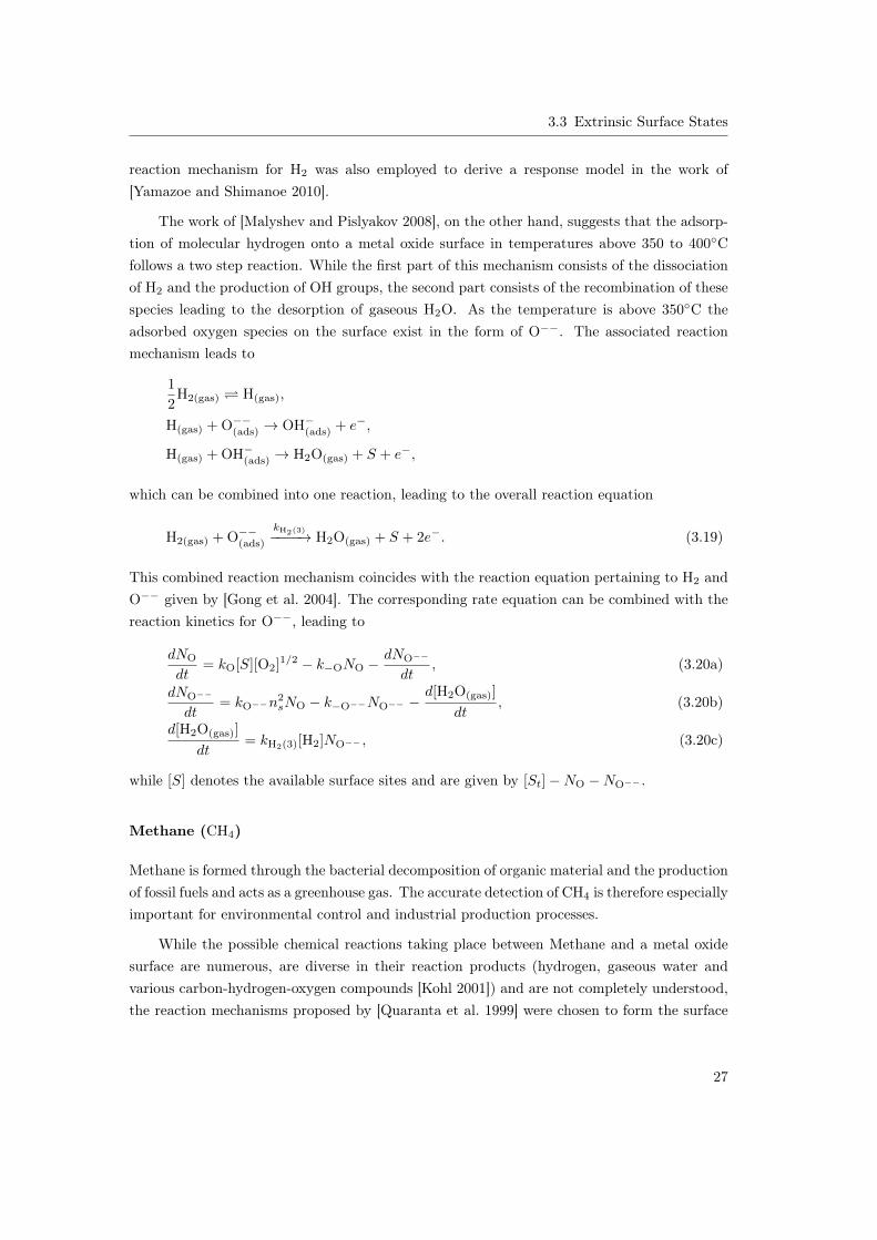
The work of [Malyshev and Pislyakov 2008], on the other hand, suggests that the adsorp-tion of molecular hydrogen onto a metal oxide surface in temperatures above 350 to 400◦Cfollows a two step reaction. While the first part of this mechanism consists of the dissociationof H2 and the production of OH groups, the second part consists of the recombination of thesespecies leading to the desorption of gaseous H2O. As the temperature is above 350◦C theadsorbed oxygen species on the surface exist in the form of O−−. The associated reactionmechanism leads to
1
2H2(gas) H(gas),
H(gas) + O−−(ads) → OH−(ads) + e−,
H(gas) + OH−(ads) → H2O(gas) + S + e−,
which can be combined into one reaction, leading to the overall reaction equation
H2(gas) + O−−(ads)
kH2(3)−−−−→ H2O(gas) + S + 2e−. (3.19)
This combined reaction mechanism coincides with the reaction equation pertaining to H2 andO−− given by [Gong et al. 2004]. The corresponding rate equation can be combined with thereaction kinetics for O−−, leading to
dNO
dt= kO[S][O2]1/2 − k−ONO −
dNO−−
dt, (3.20a)
dNO−−
dt= kO−−n2
sNO − k−O−−NO−− −d[H2O(gas)]
dt, (3.20b)
d[H2O(gas)]
dt= kH2(3)[H2]NO−− , (3.20c)
while [S] denotes the available surface sites and are given by [St]−NO −NO−− .
Methane (CH4)
Methane is formed through the bacterial decomposition of organic material and the productionof fossil fuels and acts as a greenhouse gas. The accurate detection of CH4 is therefore especiallyimportant for environmental control and industrial production processes.
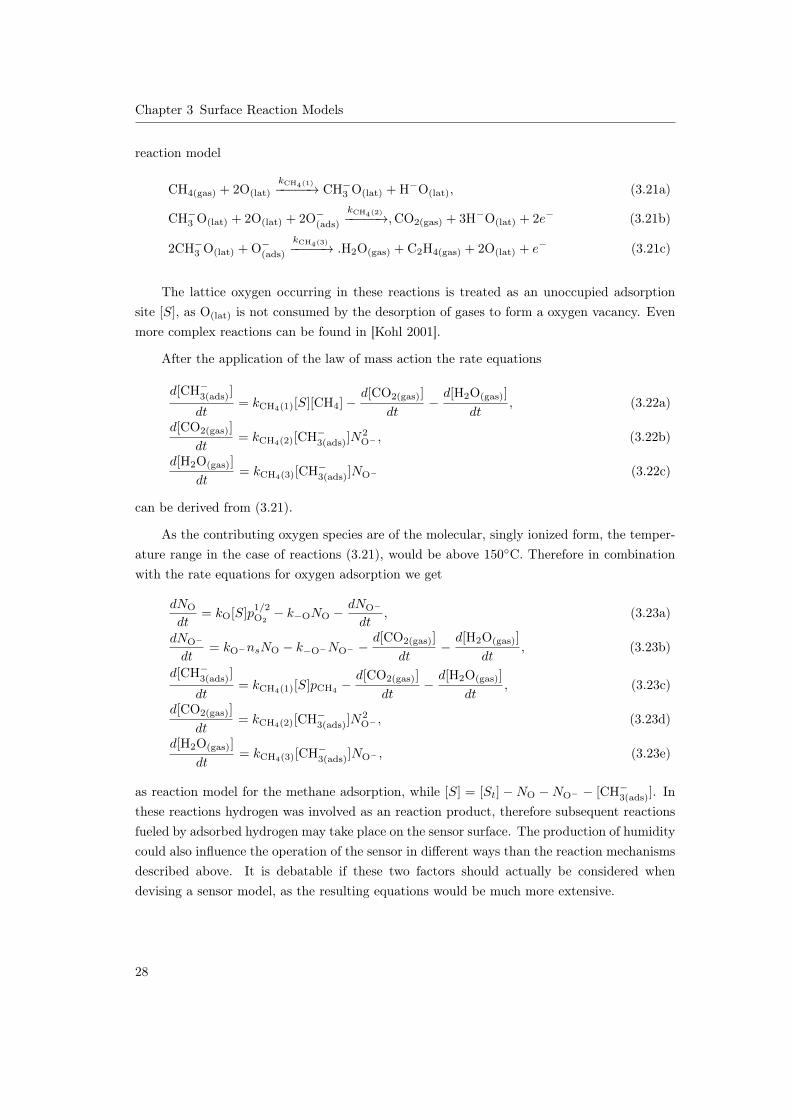
While the possible chemical reactions taking place between Methane and a metal oxidesurface are numerous, are diverse in their reaction products (hydrogen, gaseous water andvarious carbon-hydrogen-oxygen compounds [Kohl 2001]) and are not completely understood,the reaction mechanisms proposed by [Quaranta et al. 1999] were chosen to form the surface
27
Chapter 3 Surface Reaction Models
reaction model
CH4(gas) + 2O(lat)
kCH4(1)−−−−−→ CH−3 O(lat) + H−O(lat), (3.21a)
CH−3 O(lat) + 2O(lat) + 2O−(ads)
kCH4(2)−−−−−→,CO2(gas) + 3H−O(lat) + 2e− (3.21b)
2CH−3 O(lat) + O−(ads)
kCH4(3)−−−−−→ .H2O(gas) + C2H4(gas) + 2O(lat) + e− (3.21c)
The lattice oxygen occurring in these reactions is treated as an unoccupied adsorptionsite [S], as O(lat) is not consumed by the desorption of gases to form a oxygen vacancy. Evenmore complex reactions can be found in [Kohl 2001].
After the application of the law of mass action the rate equations
d[CH−3(ads)]
dt= kCH4(1)[S][CH4]−
d[CO2(gas)]
dt−d[H2O(gas)]
dt, (3.22a)
d[CO2(gas)]
dt= kCH4(2)[CH−3(ads)]N
2O− , (3.22b)
d[H2O(gas)]
dt= kCH4(3)[CH−3(ads)]NO− (3.22c)
can be derived from (3.21).
As the contributing oxygen species are of the molecular, singly ionized form, the temper-ature range in the case of reactions (3.21), would be above 150◦C. Therefore in combinationwith the rate equations for oxygen adsorption we get
dNO
dt= kO[S]p
1/2O2− k−ONO −
dNO−
dt, (3.23a)
dNO−
dt= kO−nsNO − k−O−NO− −
d[CO2(gas)]
dt−d[H2O(gas)]
dt, (3.23b)
d[CH−3(ads)]
dt= kCH4(1)[S]pCH4
−d[CO2(gas)]
dt−d[H2O(gas)]
dt, (3.23c)
d[CO2(gas)]
dt= kCH4(2)[CH−3(ads)]N
2O− , (3.23d)
d[H2O(gas)]
dt= kCH4(3)[CH−3(ads)]NO− , (3.23e)
as reaction model for the methane adsorption, while [S] = [St] −NO −NO− − [CH−3(ads)]. Inthese reactions hydrogen was involved as an reaction product, therefore subsequent reactionsfueled by adsorbed hydrogen may take place on the sensor surface. The production of humiditycould also influence the operation of the sensor in different ways than the reaction mechanismsdescribed above. It is debatable if these two factors should actually be considered whendevising a sensor model, as the resulting equations would be much more extensive.
28
3.3 Extrinsic Surface States
Hydrogen Sulfide (H2S)
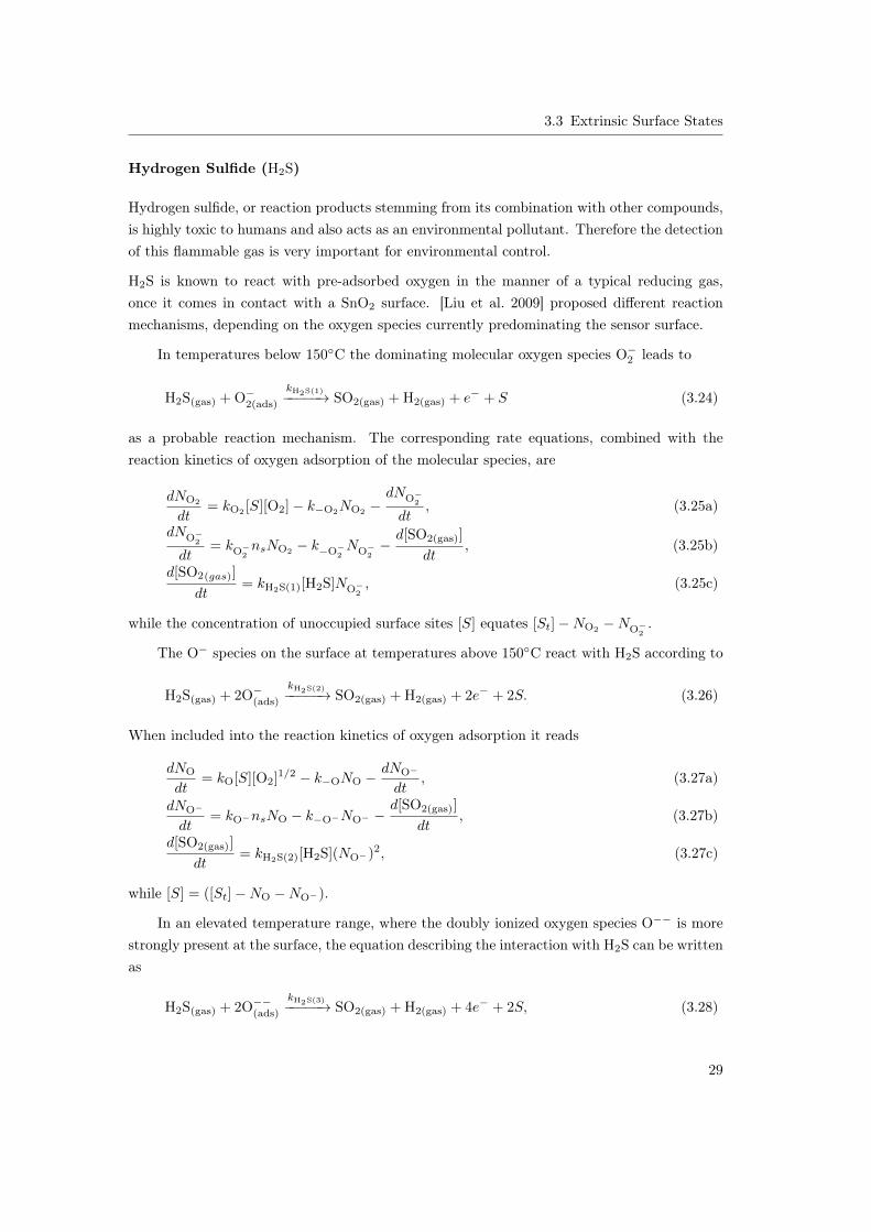
Hydrogen sulfide, or reaction products stemming from its combination with other compounds,is highly toxic to humans and also acts as an environmental pollutant. Therefore the detectionof this flammable gas is very important for environmental control.
H2S is known to react with pre-adsorbed oxygen in the manner of a typical reducing gas,once it comes in contact with a SnO2 surface. [Liu et al. 2009] proposed different reactionmechanisms, depending on the oxygen species currently predominating the sensor surface.
In temperatures below 150◦C the dominating molecular oxygen species O−2 leads to
H2S(gas) + O−2(ads)
kH2S(1)−−−−−→ SO2(gas) + H2(gas) + e− + S (3.24)
as a probable reaction mechanism. The corresponding rate equations, combined with thereaction kinetics of oxygen adsorption of the molecular species, are
dNO2
dt= kO2 [S][O2]− k−O2NO2 −
dNO−2
dt, (3.25a)
dNO−2
dt= kO−
2nsNO2
− k−O−2NO−
2−d[SO2(gas)]
dt, (3.25b)
d[SO2(gas)]
dt= kH2S(1)[H2S]NO−
2, (3.25c)
while the concentration of unoccupied surface sites [S] equates [St]−NO2−NO−
2.
The O− species on the surface at temperatures above 150◦C react with H2S according to
H2S(gas) + 2O−(ads)
kH2S(2)−−−−−→ SO2(gas) + H2(gas) + 2e− + 2S. (3.26)
When included into the reaction kinetics of oxygen adsorption it reads
dNO
dt= kO[S][O2]1/2 − k−ONO −
dNO−
dt, (3.27a)
dNO−
dt= kO−nsNO − k−O−NO− −
d[SO2(gas)]
dt, (3.27b)
d[SO2(gas)]
dt= kH2S(2)[H2S](NO−)2, (3.27c)
while [S] = ([St]−NO −NO−).
In an elevated temperature range, where the doubly ionized oxygen species O−− is morestrongly present at the surface, the equation describing the interaction with H2S can be writtenas
H2S(gas) + 2O−−(ads)
kH2S(3)−−−−−→ SO2(gas) + H2(gas) + 4e− + 2S, (3.28)
29
Chapter 3 Surface Reaction Models
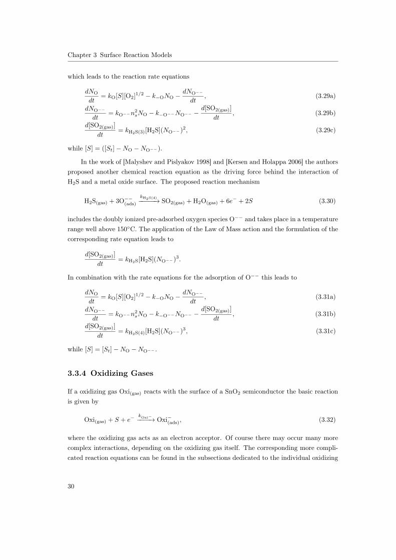
which leads to the reaction rate equations
dNO
dt= kO[S][O2]1/2 − k−ONO −
dNO−−
dt, (3.29a)
dNO−−
dt= kO−−n2
sNO − k−O−−NO−− −d[SO2(gas)]
dt, (3.29b)
d[SO2(gas)]
dt= kH2S(3)[H2S](NO−−)2, (3.29c)
while [S] = ([St]−NO −NO−−).
In the work of [Malyshev and Pislyakov 1998] and [Kersen and Holappa 2006] the authorsproposed another chemical reaction equation as the driving force behind the interaction ofH2S and a metal oxide surface. The proposed reaction mechanism
H2S(gas) + 3O−−(ads)
kH2S(4)−−−−−→ SO2(gas) + H2O(gas) + 6e− + 2S (3.30)
includes the doubly ionized pre-adsorbed oxygen species O−− and takes place in a temperaturerange well above 150◦C. The application of the Law of Mass action and the formulation of thecorresponding rate equation leads to
d[SO2(gas)]
dt= kH2S[H2S](NO−−)3.
In combination with the rate equations for the adsorption of O−− this leads to
dNO
dt= kO[S][O2]1/2 − k−ONO −
dNO−−
dt, (3.31a)
dNO−−
dt= kO−−n2
sNO − k−O−−NO−− −d[SO2(gas)]
dt, (3.31b)
d[SO2(gas)]
dt= kH2S(4)[H2S](NO−−)3, (3.31c)
while [S] = [St]−NO −NO−− .
3.3.4 Oxidizing Gases
If a oxidizing gas Oxi(gas) reacts with the surface of a SnO2 semiconductor the basic reactionis given by
Oxi(gas) + S + e−kOxi−−−−−→ Oxi−(ads), (3.32)
where the oxidizing gas acts as an electron acceptor. Of course there may occur many morecomplex interactions, depending on the oxidizing gas itself. The corresponding more compli-cated reaction equations can be found in the subsections dedicated to the individual oxidizing
30
3.3 Extrinsic Surface States
gases.
In the above basic equation (3.32) kOxi denotes the rate constant for the Oxi−(ads) produc-tion. Once again a reversion of this reaction is not likely, as denoted by the one sided arrow.The electron needed for this reaction is taken from the conduction band of the SnO2 bulkmaterial, thus decreasing the overall conductance.
The application of the law of mass action leads to the rate equation for oxidizing gases,which, in combination with the rate equations corresponding to oxygen (3.5), leads to
dNO
dt= kO[O2]1/2[S]− k−ONO −
dNO−
dt, (3.33a)
dNO−
dt= kO−NO − k−O−nsNO− , (3.33b)
[Oxi−(ads)]
dt= kOxi[Oxi]ns[S]. (3.33c)
Here once again the factor [S] = ([St]−NO−NO−− [Oxi−(ads)]) denotes the number of availableunoccupied surface sites for chemisorption, with [St] the total number of chemisorption sitesand NO, NO− and [Oxi−(ads)] the concentration of occupied surface states generated throughadsorbed oxygen in neutral and negatively charged form and the adsorbed ionized speciesOxi−(ads).
Nitrogen Dioxide (NO2)
As NO2 gas is one of the most dangerous air pollutants responsible for ozone and acid rain itsdetection and screening is very important for environmental purposes.
The tin oxide surface reactions in the presence of nitrogen dioxide are somewhat more complex,as there are several possibilities of interaction between the sensor surface and the oxidizinggas not exclusively depending on temperature variation.
At temperatures below 200◦C the dominating oxygen species on the SnO2 surface is O−2 ,which NO2 is unlikely to react with in a direct way, according to [Ruhland et al. 1998] and[Ionescu et al. 2003]. The NO2 molecules therefore react directly with the surface tin ions andget ionized themselves:
Ionosorption: NO2(gas) + S + e−kNO2(1)−−−−−→ NO−2(ads), (3.34a)
Disintegration: NO−2(ads)
kNO2(2)−−−−−→ NO(gas) + O−(ads). (3.34b)
The electron in reaction (3.34a) can originate not only from the conduction band of the SnO2
bulk material but also from an already ionized O−2 species as the NO2 molecules forms sur-face acceptor levels deeper than surface oxygen ions. This reaction leads to an decrease in
31
Chapter 3 Surface Reaction Models
conductivity as the height of the surface potential barrier is increased.
A direct reversal of reaction (3.34a) is unlikely but the adsorbed and ionized NO2 moleculescan be disintegrated into a desorbed NO and an ionized surface oxygen ion, as seen in equation(3.34b). Because of this interaction the surface Fermi energy level is increased and the heightof the potential barrier at the surface is lowered leading to an increase in conductance.
By applying the law of mass action to the above equations we get
d[NO−2(ads)]
dt= kNO2(1)ns[NO2][S]︸ ︷︷ ︸
Ionosorption
− kNO2(2)[NO−2(ads)]︸ ︷︷ ︸Disintegration of NO2
,
with the concentration of unoccupied surface states [S].
Combining them with the rate equations for oxygen adsorption (in the molecular oxygenspecies in this case) leads to the reaction kinetics
dNO2
dt= kO2
[O2][S]− k−O2NO2
−dNO−
2
dt, (3.35a)
dNO−2
dt= kO−
2nsNO2
− k−O−2NO−
2, (3.35b)
dNO
dt= kO[O2]1/2[S]− k−ONO −
dNO−
dt, (3.35c)
dNO−
dt= kO−nsNO − k−O−NO− + kNO2(2)[NO−2(ads)], (3.35d)
d[NO−2(ads)]
dt= kNO2(1)ns[NO2][S]− kNO2(2)[NO−2(ads)], (3.35e)
where the concentration of unoccupied surface sites [S] is denoted by ([St] − NO2 − NO−2−
NO −NO− − [NO−2(ads)]).
It is debatable if the attribution of the NO2 dissociation to the concentration of O− should betaken into account, as the molecular oxygen species is dominant in this temperature range.
According to [Leo et al. 1999], the adsorption of NO2 onto the semiconductor surface cango hand in hand with the disintegration of O−2 :
NO2(gas) + O−2(ads) + 2S + 2e−kNO2
(3)−−−−−→ NO−2(ads) + 2O−(ads). (3.36)
The nitrogen dioxide gets ionosorbed onto the surface and therefore occupies a chemisorptionsite and extracts a conduction electron from the semiconductor. The O−2(ads) surface specieson the other hand disintegrates into two atomic ionized oxygen species, while consuming an
32
3.3 Extrinsic Surface States
conduction electron. This chemical reaction would lead to
d[NO−2(ads)]
dt= kNO2(3)n
2s[NO2]NO−
2[S]2.
In combination with the equations pertaining to oxygen adsorption (in atomic and molecularform, but both only singly ionized, i.e., α = 1) we get the kinetic equations to reaction (3.36),which reads like
dNO2
dt= kO2
[O2][S]− k−O2NO2
−dNO−
2
dt, (3.37a)
dNO−2
dt= kO−
2nsNO2 − k−O−
2NO−
2,−
d[NO−2(ads)]
dt(3.37b)
dNO
dt= kO[O2]1/2[S]− k−ONO −
dNO−
dt, (3.37c)
dNO−
dt= kO−nsNO − k−O−NO− ,+
d[NO−2(ads)]
dt
1/2
(3.37d)
d[NO−2(ads)]
dt= kNO2(3)[NO2]n2
sNO−2
[S]2 (3.37e)
for [S] = ([St]−NO2−NO−
2−NO −NO− − [NO−2(ads)]).
It is not clear if the disintegration of adsorbed molecular oxygen is in any way propelled bythe adsorption of NO2(ads), or if it takes place uninfluenced, as is expected in a temperatureregion around 150 to 250◦C, where the dominance of oxygen species on a surface shifts frommolecular to atomic forms.
[Ionescu et al. 2003] suggested a reverse reaction instead of the disintegration of NO2(ads)
in equations (3.34) for temperatures above 240◦C. As we have done for oxygen we split theionosorption reaction into a chemisorption and ionization part:
Chemisorption: NO2(gas) + SkNO2(3)
k−NO2(3)
NO2(ads), (3.38a)
Ionization: NO2(ads) + e−kNO2(4)
k−NO2(4)
NO−2(ads). (3.38b)
[Ionescu et al. 2003] also based their model for oxidizing gases on these reaction equations, al-though they used a combined reaction mechanism for chemisorption and ionization of nitrogendioxide. In combination with the reaction equations for oxygen adsorption this would lead to
dNO
dt= kO[O2]1/2[S]− k−ONO −
dNO−
dt, (3.39a)
dNO−
dt= kO−nsNO − k−O−NO− , (3.39b)
33

Chapter 3 Surface Reaction Models
dNNO2
dt= kNO2(3)[NO2][S]− k−NO2(3)NNO2 −
dNNO−2
dt, (3.39c)
dNNO−2
dt= kNO2(4)nsNNO2
− k−NO2(4)NNO−2, (3.39d)
with [S] = ([St]−NO−NO−−NNO2−NNO−
2), while NNO2
and NNO−2denote the concentration
of nitrogen dioxide adsorbed on the sensor surface in neutral and charged form.
At higher temperatures well above 250◦C the copious amounts of O− and the increasingamount of trapped surface charge makes a sensor response similar to reducing gases possible,[Ruhland et al. 1998]. This is because the potential barrier at the surface is raised along withthe surface charge, making an direct ionosorption of NO2 to the SnO2 surface unlikely. Whichresults in
NO2(gas) + O−(ads)
kNO2(5)
−−−−−→ NO(gas) + O2(gas) + S + e−, (3.40)
where NO2(gas) participated in an oxidizing reaction with O−(ads). The corresponding reactionkinetics in combination with the rate equations for oxygen adsorption are therefore
dNO
dt= kO[O2]1/2[S]− k−ONO −
dNO−
dt, (3.41a)
dNO−
dt= kO−nsNO − k−O−NO− −
d[NO2(gas)]
dt, (3.41b)
d[NO2(gas)]
dt= kNO2(5)[NO2]NO− , (3.41c)
while [S] = ([St]−NO −NO−).
As the above reaction is likely to deplete the concentration of O− on the surface, [Ruhlandet al. 1998] suggests a reaction mechanism like (3.34). This leads to the reaction kinetics
dNO
dt= kO[S][O2]1/2 − k−ONO −
dNO−
dt, (3.42a)
dNO−
dt= kO−nsNO − k−O−NO− + kNO2(2)[NO−2(ads)], (3.42b)
d[NO−2(ads)]
dt= kNO2(1)[NO2]ns[S]− kNO2(2)[NO−2(ads)], (3.42c)
when combined with rate equations for oxygen adsorption (3.5), with [S] = [St]−NO−NO−−[NO−2(ads)].
Ozone (O3)
Although ozone is very important for the earth environment as it acts as a protective film inthe higher atmosphere, it is also an air pollutant in lower levels of the atmosphere and has
34
3.3 Extrinsic Surface States
harmful effects on the respiratory system of humans and animals.
In an ozone atmosphere the possible SnO2 surface reactions are
O3(gas) + S + e−kO3
(1)−−−−→ O−3(ads), (3.43a)
O3(gas) + S + e−kO3
(2)−−−−→ O2(gas) + O−(ads). (3.43b)
The first reaction is likely to occur in temperatures well below 150◦C, as suggested by [Gurloet al. 1998], while reaction (3.43b) happens in elevated temperatures above 150◦C, accordingto [Naydenov et al. 1995]. This later reaction is attributed to the unstable character of ozonein elevated temperatures, thus leading to the dissociative reaction in equation (3.43b).
If we once again include this two reactions into the reaction kinetics of oxygen adsorption(in molecular and atomic form, depending on the temperature) we obtain
dNO2
dt= kO2
pO2[S]− k−O2
NO2−dNO−
2
dt(3.44a)
dNO−2
dt= kO−
2nsNO2 − k−O−
2NO−
2(3.44b)
[O−3(ads)]
dt= kO3(1)pO3
ns[S] (3.44c)
[S] = [St]−NO2−NO−
2− [O−3(ads)] (3.44d)
as probable reaction kinetics for temperatures below 150◦C. The reaction kinetics for moreelevated temperatures (above 150◦C) are given by
dNO
dt= kOp
1/2O2
[S]− k−ONO −dNO−
dt, (3.45a)
dNO−
dt= kO−nsNO − k−O−NO− +
[O3(gas)]
dt, (3.45b)
[O3(gas)]
dt= kO3(2)pO3
ns[S] (3.45c)
[S] = [St]−NO −NO− (3.45d)
35

Chapter 4
The Combination of different types ofSurface Reaction Models and theirSolution
4.1 The Interlinking of Surface Reaction Models
In the previous chapter we derived a multitude of surface reaction models, while distinguishingbetween intrinsic and extrinsic reactions. As intrinsic surface states arise from the dynamicsof the sensor alone they should be taken into account for all kind of measurements. Therefore,for measurements in non-inert gases, it is necessary to combine the intrinsic and extrinsicmodels to form a system of ordinary differential equations. The measurements as well as theestimation of model parameters have to be carried successively from the intrinsic surface statemodel to the surface reaction model for oxygen to mixtures of synthetic air and one test gas.The different types of surface reaction models therefore form a hierarchy of models.
4.1.1 Intrinsic Model: Sensor response to an inert gas
To explain the response of a sensor in an atmosphere consisting of an inert gas the intrinsicsurface state model
dNsidt
= kins(Ni −Nsi)− k−iNsi (4.1)
was adopted. As the concentration of free electrons on the surface can be derived from theconcentration of all free electrons (i.e., donors) ND in the sensor and the height of the potentialbarrier at the surface VS , the concentration of free surface electrons ns is given by (2.2)
ns = ND exp
(− q2N2
s
2εNDkT
). (4.2)
37
Chapter 4 The Combination of different types of Surface Reaction Models and their Solution
This equation can therefore easily be used to modify equation (4.1), to express ns as a functionof the occupied surface states Ns.
As the reaction rate constants vary with different temperatures, we assume that thesereaction rates are of a Arrhenius form. The empirical Arrhenius equation
kx = Ax exp
(−ExkT
)(4.3)
describes the dependence of rate constants kx, stemming of chemical reactions x, on the tem-perature T and the activation energy Ex for reaction x. Ax denotes the pre-exponentialconstant. The temperature-dependence of Ax can be neglected when compared to the expo-nential dependence in the second factor. We apply equations (4.2) and (4.3) to the intrinsicsurface state model (4.1) and obtain
dNsidt
= Ai exp
(− Ei
kT
)ND exp
(− q2N2
si
2εNDkT
)(Ni −Nsi)
−A−i exp
(−E−i
kT
)Nsi,
(4.4)
which describes the response of a gas sensor to an inert atmosphere.
Independent of subsequent mechanisms for charge transport, this equation is comprisedof seven parameters, which need to be found—be it through a parameter estimation procedureor by setting them to reasonable values found in the literature. These seven parameters are:the density of ionized donors ND, the density of total intrinsic surface states Ni, the pre-exponential constants A±i and the activation energies E±i.
4.1.2 Oxygen Model: Sensor Response to dry synthetic air
When describing the response of a sensor to an atmosphere of synthetic air (SA), additionallyto the rate equations (3.5) for oxygen adsorption, the intrinsic surface state mechanism has tobe taken into account. In this case the behavior of the sensor is due to the superimposition ofthe intrinsic and extrinsic dynamics. Therefore, after applying Arrhenius equation (4.3) andthe formula for free surface electrons (4.2), the surface reaction model describing the sensorresponse to air is given by
dNsidt
= Ai exp
(− Ei
kT
)ND exp
(− q2N2
s
2εNDkT
)(Ni −Nsi)
−A−i exp
(−E−i
kT
)Nsi,
(4.5a)
38
4.1 The Interlinking of Surface Reaction Models
dNO◦β
dt= AOβ exp
(−EOβ
kT
)([St]−NO◦
β−NO−α
β)[O2]β/2
−A−Oβ exp
(−E−Oβ
kT
)NO◦
β−dNO−α
β
dt,
(4.5b)
dNO−αβ
dt= AO−α
βexp
(−EO−α
β
kT
)ND exp
(− q2N2
s
2εNDkT
)αNO◦
β
−A−O−αβ
exp
(−E−O−α
β
kT
)NO−α
β,
(4.5c)
Ns = Nsi +NO−αβ. (4.5d)
In this case, the density of occupied surface states Ns is the sum of all occupied surfacestate—intrinsic and extrinsic. Therefore we can utilize relationship (4.5d) to express the heightof the potential barrier due to charged particles trapped at the surface as
VS =
q
(Nsi +NO−α
β
)2
2εND. (4.6)
By using relationship (4.2), the concentration of electrons ns able to reach the surface, dependsboth on the intrinsic and extrinsic behavior of the sensor, and therefore couples the twodynamics.
Additional to the parameters for the intrinsic model, the following parameters have tobe estimated: the concentration of all chemisorption sites on the surface [S], the two pre-exponential factors and two activation energies for the reaction constants of the respectiveoxygen chemisorption and ionization.
As the type of oxygen species adsorbed at the sensor surface acutely depends on theambient temperature, the parameters α and β have to be set to the appropriate numbers,depending on the temperature. Below 150◦C singly ionized molecular oxygen is dominant,therefore α and β should be set to 1 and 2, respectively. Above this temperature α = 1 andβ = 1 would be appropriate. Above 300 to 400◦C the singly ionized atomic oxygen speciesusually gain an additional electron, which means α = 2 and β = 1. As the usual workingtemperature of tin oxide gas sensors tend to be between 100◦ and 400◦C the setting of α = 1
and β = 1 would be appropriate.
4.1.3 Mixtures of oxygen and an additional gas
In order to model the sensor response to a reducing gas, like CO or an oxidizing agent likeNO2, in addition to synthetic air, a three step approach is taken. As a first and second step
39
Chapter 4 The Combination of different types of Surface Reaction Models and their Solution
the model parameters and reaction constants for the intrinsic model and the oxygen surfacestate model are estimated. In a third step the previously gained parameters were incorporatedinto a whole equation model consisting of the reaction kinetics for the intrinsic surface statesand the oxygen surface states (already combined in equations (4.5)) in combination with themodel equations for the particular test gas. This necessitates that measurements are taken inan inert atmosphere, in synthetic air as well as in a oxygen and test gas mixture under thesame temperature conditions for the same sensor.
In the case of carbon monoxide, the model equations (3.13) are added to (4.4) through therelation of occupied surface states Ns = Nsi +NO− −NCO+ . As the equations (3.11) regardthe direct impact of CO on a gas sensor without an intermediate interaction with oxygen,additional measurements of carbon monoxide in an inert atmosphere are needed to estimatethe corresponding model parameters.
For nitrogen dioxide there are a multitude of possible reactions depending on the temper-ature. Also in this case the selected model equation (3.35), (3.37), (3.39), (3.41) or (3.42) canbe linked to the inert model (4.4) through the concentration of occupied surface states Ns.
4.2 Existence and Uniqueness of the Solution
In this section we will investigate the properties of the solution of the surface state modelsconsisting of ordinary differential equations. To accomplish this we will use the Theorem ofPicard-Lindelöf, in the usual and generalized version, which can be found in [Cronin 2008] and[Kolgmogorov and Fomin 1970] respectively.
Theorem 4.1 (Picard-Lindelöf). Let (t0, x0) be in an open set D and let a, b be suchthat the set R = {(t, x)| |t − t0| ≤ a, |x − x0| ≤ b} is constrained in D. Suppose thefunction f(t, x) is defined and continuous on D and satisfies a Lipschitz condition with re-spect to x on R. Then the IVP x′ = f(t, x), x(t0) = x0 has a unique solution on (t0 −min(a, 1
b max(t,x)∈R |f(t, x)|), t0 + min(a, 1b max(t,x)∈R |f(t, x)|)).
Proof A proof of this theorem can be found in [Cronin 2008]. �
Theorem 4.2 (Generalization of Picard-Lindelöf). Let U be an open subset of Rn+1 andlet the continuous function f be defined as f(t, x1, ·, xn) : U ⊂ Rn+1 → Rn. If (t0, x10, · · · , xn0) ∈U and f satisfies the Lipschitz condition
|fi(t, x1, · · · , xn)− fi(t, x1, · · · , xn)| ≤ L max1≤j≤n
|xj − xj |
40
4.2 Existence and Uniqueness of the Solution
in the variables x1, · · · , xn ∈ U , with L a constant. Then the system of ordinary equations
dx1
dt= f1(t, x1, · · · , xn),
...dxndt
= fn(t, x1, · · · , xn)
with initial conditions x1(t0) = x10, · · · , xn(t0) = xn0 has an unique solution.
Proof A proof of this theorem can be found in [Kolgmogorov and Fomin 1970]. �
Based on these results we are able to proof the two important properties of existence anduniqueness of the solution of the surface state models. To be able to more easily handle thesurface state model we decided to perform an normalization on the surface state densities Nsi,NO◦
βand NO−α
βto gain the normalized surface state densities nNsi, nNO◦
βand nNO−α
β, which
was accomplished by using a normalization factor
α =q√
2εNDk(4.7)
to transform a densities X into its normalized form nX = αX = q X√2εNDk
.
4.2.1 Intrinsic Model
In the following Lemma we will prove the existence as well as the uniqueness of the solutionto the inert surface state model (4.4) with the help of the Theorem of Picard-Lindelöf.
Lemma 1. Let a function f : I ⊂ R→ R , defined as
f(nNsi) = Ai exp
(−Ei
kT
)ND exp
(−nN
2si
T
)(nNi − nNsi)−A−i exp
(−E−i
kT
)nNsi
for nonnegative parameters A±i, E±i and nNi, be C1 on D. When f builds the right hand sideof the ordinary differential equation d(nNsi)
dt = f(nNsi), then, for an initial value nNsi(0) =
nN0si, the above differential equation possesses a unique solution.
Proof To derive an estimated upper bound for the function f we will first calculate the
41
Chapter 4 The Combination of different types of Surface Reaction Models and their Solution
derivative with respect to nNsi
f ′(nNsi) = Ai exp
(− Ei
kT
)ND exp
(−nN
2si
T
)(1− nNi)
2nNsiT
−Ai exp
(− Ei
kT
)ND exp
(−nN
2si
T
)−A−i exp
(−E−i
kT
).
We use the maximum norm ‖nNsi‖∞ to get an upper bound for nNsi and can thereforeapproximate the derivative of f as follows
∣∣f ′(nNsi)∣∣ ≤∣∣∣∣∣Ai exp
(− Ei
kT
)ND −Ai exp
(− Ei
kT
)NDnNi
∣∣∣∣∣∣∣∣∣2‖nNsi‖∞T
∣∣∣∣−
∣∣∣∣∣Ai exp
(− Ei
kT
)ND −A−i exp
(−E−i
kT
)∣∣∣∣∣ = L
from the approximation
exp
(−nN
2si
T
)≤ 1
as nN2si is significantly higher than the temperature of 700◦ K at most. This assumption is
justified as values for nNsi found in the literature are well above 60. Through the applicationof the mean value theory we get for some fixed value nNsi in the
f ′(nNsi) =f(nNsi)− f( ˜nNsi)
nNsi − ˜nNsi⇒
∣∣∣f(nNsi)− f( ˜nNsi)∣∣∣ ≤ L ∣∣∣nNsi − ˜nNsi
∣∣∣for some constant L. We have therefore shown that f satisfies a Lipschitz condition on I,which allows for the application of the Theorem of Picard-Lindelöf and prove the existenceand uniqueness of the solution to the initial value problem d(nNsi)
dt = f(nNsi). �
4.2.2 Oxygen Model
To prove the desired properties for the solution of the oxygen model, we can fall back on theproof for the inert model, as the oxygen model incorporates the equation for inert surfacestates as a third equation. The overall course of action for the oxygen model will essentiallybe the same as for the intrinsic model, although we make use of the generalization of thePicard-Lindelöf Theorem.
42
4.2 Existence and Uniqueness of the Solution
Lemma 2. Let a function f : D ⊂ R4 → R3 , defined as
f1(nNsi) = Ai exp
(− Ei
kT
)ND exp
− (nNsi + nNO−αβ
)2
T
(nNi − nNsi)
−A−i exp
(−E−i
kT
)nNsi,
f2(nNO◦β) = AOβ exp
(−EOβ
kT
)([St]− nNO◦
β− nNO−α
β)[O2]β/2
−A−Oβ exp
(−E−Oβ
kT
)nNO◦
β−dnNO−α
β
dt,
f3(nNO−αβ
) = AO−αβ
exp
(−EO−α
β
kT
)ND exp
− (nNsi + nNO−αβ
)2
T
α
nNO◦β
−A−O−αβ
exp
(−E−O−α
β
kT
)nNO−α
β,
for nonnegative parameters A±x, E±x and nNi, be C1 on D. Let the function f build the righthand side of a system of ordinary differential equations
d(nNsi)
dt= f1(nNsi),
d(nNO◦β)
dt= f2(nNO◦
β),
d(nNO−αβ
)
dt= f3(nNO−α
β).
(4.8)
Then, for some initial values, the above differential equation possesses a unique solution.
Proof First we define the vector nN ∈ D as (nNsi, nNO◦β, nNO−α
β)>. After calculating
∇nNfi = ( ∂fi∂nNsi
, ∂fi∂nNO◦
β
, ∂fi∂nN
O−αβ
)> for i = 1, 2, 3 we use the same approach as in the previous
proof to gain an upper bound Lji for every single partial derivative ∂fi∂nNj
for j = si, O◦β , O−αβ .This leads to
|∇nNfi(nNsi, nNO◦β, nNO−α
β)| ≤ Li,
for Li = (Lsii , LO◦β
i , LO−αβ
i )>. We can therefore use the mean value theorem for real valuedfunctions in several variables to gain
fi(nN)− fi(nN) = ∇nNfi(nN)(nN − nN) ≤ Li(nN − nN)
43

Chapter 4 The Combination of different types of Surface Reaction Models and their Solution
for some vector nN ∈ nNnN while nN , nN , nN ∈ D. It follows easily that
|fi(nN)− fi(nN)| ≤ |Li(nN − nN)| ≤ maxjLji (max
j|nNj − ˜nNj |)
for i = 1, 2, 3. Hence we can use the Generalized Theorem of Picard Lindelöf to prove theexistence and uniqueness of the solution to the system of ordinary differential equations (4.8).�
44
Chapter 5
Parameter Estimation for DynamicModels
In this chapter we will deal with the theory behind the estimation of parameters for the typeof models relevant to simulate surface reactions—parameter dependent ordinary differentialequations. These mathematical models describe the chemical processes on the surface and thusexplain the behavior of the observed data. The unknown model parameters will be obtained byminimizing a suitable objective function, which is a measure of the deviation of the data fromthe model, i.e., the lack of fit. For a survey of parameter estimation for differential equationsthe reader is referred to [Bard 1974], while [Engl et al. 2009] gives a more general review ofinverse problems in applications.
5.1 Structure and Challenges of Dynamical Models
In general, the model equations can be written in the form
dx(t)
dt= f(x(t),u;θ) with x(t0) = x0, (5.1a)
y(t) = g(x(t);θ), (5.1b)
where the included variables and relations are defined as follows:
θ = (θ(1), θ(2), . . . , θ(P ))> is the vector of unknown parameters, which are quantities likeAi, Ei or Ni in (4.4), that have to be estimated. In this set of parameters some mayappear only in equation (5.1a) and others only in equation (5.1b).
t vector of independent variables—e.g., the time.
u is a vector of variables which are either precisely known or have been measured, e.g.,quantities like the Boltzmann constant k.
45
Chapter 5 Parameter Estimation for Dynamic Models
x = (x(1), x(2), . . . , x(M))> defines a vector of state variables, which are functions of t andθ, for example Ns. These functions are determined through the ordinary differen-tial equation (5.1a). In a special case the state variables are variables that can bemeasured through experiments and are therefore observed variables.
x0 is a vector of initial conditions for the state variables.
f defines the M -dimensional vector function forming the right side of the differentialequation of state variables.
y = (y(1), y(2), . . . , y(L))> is the set of observed variables that are measured experimen-tally, like the conductance G.
g is a known L-dimensional vector function that relates the state vector x to the outputvector of observed variables y—e.g., the conductance formula (2.14).
Experiments measure the value of y for given values of t, which permits the calculation ofthe values of the state variables x but usually not allow for the calculation of the values of thederivative of x. In this case the model equations cannot be used directly for the estimation ofthe parameters θ. [Bard 1974] lists ways to overcome this problem:
(1) Differentiation of Data: To calculate approximate values of the derivative of x in themodel equation by calculating a difference quotient between adjacent values. Thenxn+1−xntn+1−tn can give an approximation for dxn
dt . This method is of limited accuracy, it isdifficult to access the errors and it is furthermore only applicable if the separation be-tween data points in not too large.
(2) Integration of Equations: Depending on the fact if the model equation can be solved ana-lytically or just numerically, the integration of the differential model is a possible way togain an equation in the form of
x = h(t;θ).
If equation (5.1a) can be solved analytically, h can be explicitly given, while for the casethat only numerical integration is possible, h is only implicitly defined.
(3) Integration of Data: If it is possible to integrate out all the derivatives in the differentialequation one gains integral equations. The data may therefore be integrated numericallyto obtain the values for the integrals appearing in the model equation. Like for method(1), the data is required to be dense and it is generally only applicable to a limited num-ber of cases, although numerical integration is in general more accurate than numericaldifferentiation.
46
5.1 Structure and Challenges of Dynamical Models
Overall, [Bard 1974] recommends to integrate the model equation when computationally pos-sible, and to fall back on the manipulation of data through integration or differentiation if oneonly wants to obtain an initial guess.
5.1.1 Computation of the objective function
To estimate the parameters θ we must be able to compute the objective function for any givenvalue of parameters. This usually works by use of some initial estimates for the parametersto gain the initial values in (5.1a). An integration of the differential equation in (5.1a) istherefore possible and gain the values xi, i = 1, . . . , N of state variables, for N the number ofmeasurements or data points. Equation (5.1b) is then used to calculate values of y, which thendetermine the residuals ei = yi− y, the difference of measured value yi and model calculatedvalue yi. The residuals are then used to calculate the objective function to facilitate theprocess of parameter estimation. Each function evaluation is therefore in itself a complexprocedure that requires the solution of a set of ordinary differential equations, which may beaccomplished by the use of standard methods [Bard 1974].
5.1.2 Optimization Methods
To minimize the objective function, like the nonlinear least squares objective function (5.2), amultitude of optimization algorithms may be used. Essentially all these algorithms adhere tothe same working principle. These iterative methods start at an initial value for the parameterand iteratively compute a new value while following a rule of calculation, until a minimumis reached. The algorithms find iteratively a new value θ(j+1) to the current value θ(j) bymoving it along a specified search direction d(j) for a certain amount s(j):
θ(j+1) = θ(j) + s(j)d(j).
A stopping rule is usually incorporated to specify when the algorithm has found a sufficientlyclose enough estimation for θ, the minimum of the objective function Q(θ). Different al-gorithms are characterized by their different choices for s(j) and d(j), although the searchdirection usually in some form incorporates the gradient of the objective function. We setg(θ) to the gradient ∇θQ(θ) of the objective function and denote g(j) = g(θ(j)). Furthermorewe define H(j) as the Hessian matrix of Q(θ) evaluated at θ(j).
Steepest Descent Method. This method, also called gradient descent, calculates the parametervalues by iterating into the opposite direction of the gradient:
θ(j+1) = θ(j) −g>(j)g(j)
g>(j)H(j)g(j)
g(j).
47
Chapter 5 Parameter Estimation for Dynamic Models
This method is often very inefficient and is not recommended for applications. Thesteepest descent algorithm may have problems for objective function that, for exampleare flat around the minimum, as the algorithm may iterate back and forward in this planewhen following the inverse direction of the gradient. This problem can be avoided byusing the following algorithm.
Newton’s Method. This historic algorithm operates by linearizing the objective function andtherefore iteratively using the roots of the gradient as an approximation to the root of theobjective function:
θ(j+1) = θ(j) −H−1(j)g(j).
This Algorithm may lead in a false direction when the Hessian is not positive definite, forexample when the objective function is concave at θ(j).
Gauss-Newton Algorithm. By using Newton’s Method as a basis and utilizing a quadraticapproximation instead of the objective function in every iteration the Gauss-Newton Al-gorithm reads like
θ(j+1) = θ(j) + (∇θ(j)y(θ(j))
>∇θ(j)y(θ(j)))
−1∇θ(j)y(θ(j))(θ − y(θ(j))).
The approximation to the Hessian that is used in this algorithm is guaranteed to be posi-tive definite and this method avoids therefore the computation of second order derivatives.
Levenberg-Marquardt Algorithm. This method combines the Gauss-Newton Algorithm with aregularization technique of the Hessian that insures decreasing objective function values.As to insure the positive definiteness of the Hessian H(j) it is possible to correct theinverse of the Hessian at each step by adding a correction matrix to gain a correctedinverse Hessian H−1
(j) for further computations, such that
H−1(j) = H−1
(j) + c(j)I,
for an appropriate c(j) ∈ R+.
Quasi-Newton Method. This method is an advancement of Newton’s Method, as it calculatesthe inverse of the Hessian H−1
(j) by iteratively adding a symmetric correction matrix C(j),such that
H−1(j) = H−1
(j) +C(j).
Prominent examples of Quasi-Newton Methods are the BFGS and DFP algorithm, whichdiffer in the form of the correction matrix.
48
5.2 The Objective Function and Nonlinear Least Squares Estimators
A more detailed discussion to the above algorithms, especially regarding their computationalrestrictions or their suitability to specific problems, can be found in [Björck 1996].
Nevertheless, essentially almost any optimization method may be used to minimize theobjective function Q(θ). Although, according to [Bard 1974], the Gauss-Newton Method is themost suitable algorithm to solve dynamic models. This is because, as every function evaluationrequires the integration of equations (5.1a), the use of a quadratically convergent method likethe Newton-Gauss Algorithm is favorable.
5.2 The Objective Function and Nonlinear Least Squares
Estimators
The majority of estimation methods found in Estimation Theory, like maximum a posterioriprobability or minimum variance estimation, require statistical knowledge of all or at leastsome of the random variables involved in a model. The Maximum Likelihood Estimationfor example, demands at least knowledge of the probability density of the observation errors,while assuming the statistical properties of the parameters to be estimated are not known. Ifhowever no probabilistic information about any of the variables of the models is known, thisextreme case, in terms of Estimation Theory, is handled by finding the least squares fit amongthe observations.
As the objective function is a suitable measure of the overall deviation of the model calcu-lated values from the measurements, its choice dictates not only the values of the parametersbut also their statistical properties, [Englezos and Kalogerakis 2001].
We will therefore express the objective function of a parameter estimation problem, thatis to be minimized, in terms of Least Squares Estimators. The Least Squares Technique (LS)is one of the most used estimation technique for various applications and can firstly be dividedinto linear or Ordinary Least Squares (OLS) and Nonlinear Least Squares (NLS). In thissection we will mainly concentrate on the nonlinear variant NLS, as the equation occurringin dynamic models are highly nonlinear. Therefore we will use the works of [Englezos andKalogerakis 2001; Kuan 2004] and [Davidson and MacKinnon 1993] as guide.
The least squares objective function
Q(θ) =
N∑i=1
ei(θ)>Wiei(θ) (5.2)
for the number of measurements N . It is given by the sum of squares of the residuals ei(θ) withrespect to θ. The residual equals the difference between measurements and model calculatedvalues of observable variables y (an exact definition will be given below). Depending on the
49
Chapter 5 Parameter Estimation for Dynamic Models
choice of weighting matrix Wi there are several different cases of estimators:
(1) Simple Least Squares (SLS) Estimation. In this case the sum of squares of errors is mini-mized without a weighting factor. Therefore equation (5.2) reduces to
Q(θ) =
N∑i=1
ei(θ)>ei(θ),
as the weighting matrix can be set to identity, i.e., Wi = I.
(2) Weighted Least Squares (WLS) Estimation. If the weighting matrix does not change fordifferent experiments (Wi = W for i = 1, 2, . . . , N), the estimator
Q(θ) =
N∑i=1
ei(θ)>Wei(θ)
is referred to as Weighted Least Squares.
(3) Generalized Least Squares (GLS) Estimation. When the weighted sum of squares of er-rors is estimated with different weights in every experiment the LS estimator is calledGeneralized Least Squares Estimator.
For all the above cases, the choice of weighting matrix W can be facilitated by MaximumLikelihood considerations, as can be seen in [Englezos and Kalogerakis 2001]. We will nowhave a closer look at the simple nonlinear least squares estimation.
5.2.1 Nonlinear Least Squares Estimation
For simplification we assume the univariate case, regarding the observed variables. We considery to be a scalar and L to be therefore zero. The N distinct measurements of the output vectory are related to the value, calculated through the model equation y, using true parametervalues θ, in the following way:
εi = yi − y(ti; θ) for i = 1, . . . , N, (5.3)
while the error term εi accounts for the measurement error and model inadequacies. Therefore,the output vector y is comprised of the deterministic part calculated by the model and thestochastic part given by the error term. To quantify the deviation of an individual measurementfrom the model calculated value we state:
Definition (Residual) The residual of a Nonlinear Least Squares estimator is defined as
ei = yi − y(t;θ),
50
5.2 The Objective Function and Nonlinear Least Squares Estimators
where the model function y(t,θ) is evaluated with the use of the estimated parameter values.
To clarify the distinction between the residual and the error term: While the residual eicorresponds to the estimated parameter values θ, the error term εi refers to the true parametervalues θ.
Given the number of measurements N of y and t we combine all measurements into onevector and adopt the notation
y = y(t1, . . . , tN ;θ) + e(θ),
for y = (y1, . . . , yN )>, e = (e1, . . . , eN )> and y(t1, . . . , tN ;θ) = (y(t1;θ), . . . , y(tN ;θ))>.
To estimate the parameter vector θ we can minimize the LS objective function
Q(θ) =1
N(y − y(t1, . . . , tN ;θ))>(y − y(t1, . . . , tN ;θ))
=1
N
N∑i=1
(yi − y(ti;θ))2,(5.4)
which is given by the weighted sum of squares of the residuals (i.e., the sum of squares error),with respect to θ.
Our goal is tho find a K-dimensional surface that fits the data (yi,xi), for i = 1, . . . , N .The first order condition of the NLS optimization problem is a system of nonlinear equationswith K unknown parameters. We define ∇θy(t1, . . . , tN ;θ) = (∇θy(t1;θ), . . . ,∇θy(tN ;θ))
as the gradient of y and can therefore state the first order optimality condition
∇θQ(θ) = − 2
N∇θy(t1, . . . , tN ;θ)(y − y(t1, . . . , tN ;θ) = 0. (OC-1)
Additionally we define the second order optimality condition as
∇2θQ(θ) =− 2
N∇2θy(θ)(y − y(t1, . . . , tN ;θ))
+2
N∇θy(t1, . . . , tN ;θ)∇θy(t1, . . . , tN ;θ)> is positive definite.
(OC-2)
We now can state the definition of a minimizer to the objective function.
Definition (Least Squares Estimator) The estimated parameter value θ that minimizesthe sum of squares error (5.2), by solving (OC-1) and satisfying (OC-2), is defined as theLeast Squares Estimator and is denoted as θ.
Theorem 5.1. Let y(x; ·) be twice continuously differentiable in the second argument. Given
51

Chapter 5 Parameter Estimation for Dynamic Models
the minimization problem
y = y(t1, . . . , tN ;θ) + e(θ)
we suppose that for given data (yi,xi), i = 1, . . . , N , the second order condition (OC-2) holdsfor some interior point of Θ. Then there exists a solution that minimizes the NLS objectivefunction (5.4).
While the second order optimality condition ensures that a minimum of S can be found,it is no guarantee to the uniqueness of the solution. This infers the possibility of the existenceof multiple local minima for a given data set in the NLS minimization problem. From the firstorder condition we saw that
∇θQ(θ) = − 2
N∇θy(t1, . . . , tN ; θ)e(θ) = 0
Therefore, the residual vector is orthogonal to the column vectors of ∇θy(t1, . . . , tN ; θ)>. Ina geometric sense y(t1, . . . , tN ;θ) defines a surface on Θ and ∇θy(t1, . . . , tN ;θ)> defines a K-dimensional linear subspace tangent at the point y(t1, . . . , tN ;θ) for any θ ∈ Θ. Therefore thevector of observables y is orthogonally projected onto the mentioned surface at y(t1, . . . , tN ; θ),which means that the residual vector e is orthogonal to the tangent space at this point. As, incontrast to the linear case—there may exist more than one such orthogonal projections, theremay be multiple solutions to the Nonlinear Least Squares problem.
5.2.2 Consistency of the Nonlinear Least Squares Estimator
A sequence of estimators θ for a parameter θ0 is said to be (asymptotically) consistent, if θconverges in probability to θ0. This implies that the distributions of the estimators becomemore and more concentrated near the true value of the parameter being estimated. In this casethe probability that the estimator θ is arbitrarily close to θ0 converges to one. The definitionof this idea is given by
Definition (Consistency) A sequence of NLS estimators θN for N ≥ 0 is called strongly
(weakly) consistent for the parameter θ0 if θNa.s.(P)−−−−→ θ0 as N →∞.
We first have to give some basic definitions about statistical convergence and the laws oflarge numbers to facilitate a proof of the consistency of a NLS estimator.
Definition (Stochastic Convergence) Let (tn)n≥0 be a sequence of random variables.
(i) The sequence tn converges in probability towards t (tnP−→ t), if for all ε > 0
limn→∞
P(|tn − t| ≥ ε) = 0.
52
5.2 The Objective Function and Nonlinear Least Squares Estimators
(ii) The sequence tn converges almost surely towards t (tna.s.−−→ t), if
P( limn→∞
tn = t) = 1.
(iii) The sequence tn converges in distribution towards t (tnD−→ t), if for Fn and F the
cumulative distribution functions of tn and t, if
limn→∞
Fn(x) = F (x),
for some x ∈ R, for which F is continuous.
Convergence in probability ensures that the probability of an unlikely outcome becomes smallerand smaller as n grows. Almost sure convergence implies convergence in probability. StochasticConvergence also introduces a new concept of boundedness, as seen in the following definition.
Definition (Stochastic Boundedness) A sequence of random variables (tn)n≥0 is boundedin probability, if tn
P−→ 0 or if for every ε > 0 there is a δ <∞ such that P(|tn| ≥ δ) < ε.
Next we will briefly discuss the Law of Large Numbers (LLN), which concerns the aver-aging behavior of random variables. There are various types of Laws of Large Numbers fordifferent types of random variables (details can be found in [Kuan 2004]). We will deal withthe most elemental of definitions.
Lemma 3 (Law of Large Numbers). The Strong (Weak) Law of Large Numbers statesthat the sample average of the sequence tn converges almost surely (in probability) to the
expected value t, that is tna.s.(P)−−−−→ t.
To apply the idea of a Law of Large Numbers to not only random variables, but functions ofrandom variables, a Uniform Law of Large Numbers (ULLN) is needed.
Lemma 4 (Uniform Law of Large Numbers). Let Q(θ) be a function of θ ∈ Θ. Whenthe conditions
(1) Q(θ) obeys a Strong (Weak) Law of Large Numbers for each θ ∈ Θ,
(2) for θ,θ† ∈ Θ:
(i) |Q(θ −Q(θ†)| ≤ C||θ − θ†|| a.s.,
(ii) for C, a random variable which is bounded almost surely (in probability) and is notdependent on θ,
are met, the function Q(θ) is said to obey a Strong (Weak) Uniform Law of Large Numbers,
53
Chapter 5 Parameter Estimation for Dynamic Models
which in turn, is defined as
supθ∈Θ|Q(θ)− E(Q(θ))| a.s.(P)−−−−→ 0.
Proof A way to derive the property of an Uniform of Large Numbers for a function obeyingthe above assumption, is shown in [Kuan 2004]. For details and discussion about the necessityof different assumptions for the strong and weak case of the theorem, we also refer to [Kuan2004]. �
To show the consistency of the NLS estimator we have to introduce one last inequality.
Lemma 5 (Markov’s inequality). Let t be a random variable with finite pth moment. ThenMarkov’s inequality states that
P(|t| ≥ a) ≤ E(|t|p)ap
for a ∈ R+.
Theorem 5.2 (Consistency). Let y(x; ·) be twice continuously differentiable in the secondargument. In addition to the the second order condition (OC-2) let us assume the conditions
[C1] Let θ be in Θ, a compact and convex set, then
(i) the sequences (y2i )i≥0, (yiy(ti;θ))i≥0 and (y(ti;θ)2)i≥0 all obey a weak law of large
numbers for each θ ∈ Θ,
(ii) yi, y(ti;θ) and ∇θy(ti;θ) have bounded second moment uniformly in θ ∈ Θ,
[C2] There exists a unique parameter vector θ0 such that E(Q(θ)) attains its unique globalminimum at θ0.
hold. Then the NLS estimator θ is weakly consistent for θ0.
For an detailed discussion of the conditions [C1] and [C2] the interested reader is referred to[Kuan 2004].
Proof As the condition [C1](i) assures that all components of the NLS objective functionQ(θ) = 1
N
∑Ni=1(y2
i − 2yiy(ti;θ) + y(ti;θ)2) obey a weak law of large numbers, the firstrequirement for an ULLN is satisfied.
As our parameter space Θ is compact and convex we use the mean-value theorem as wellas the Cauchy-Schwartz inequality to establish the Lipschitz-like continuity condition
|Q(θ)−Q(θ†)| ≤ ‖∇θQ(θ)‖‖θ − θ†‖ a.s.,
54
5.2 The Objective Function and Nonlinear Least Squares Estimators
with θ,θ† ∈ Θ and θ their mean value. Therefore we set the Lipschitz-type constant to
C = supθ∈Θ∇θQ(θ).
Hence we have to prove that ∇θQ(θ) = − 2N
∑Ni=1∇θy(ti;θ)(yi − y(ti;θ)) is bounded in
probability. To this end we use condition [C1](ii) to gain
P(|∇θQ(θ)| ≥ a) ≤ 1
aE(|∇θQ(θ)|)
≤ 2
aN
N∑i=1
(‖∇θy(ti;θ)‖‖yi‖+ ‖∇θy(ti;θ)‖‖y(ti;θ)‖
≤ D,
for some constant D independent of θ. This relation implies that ∇θQ(θ) is bounded inprobability by Markov’s inequality. Therefore we have shown the second condition for anULLN.
Condition [C2] requires θ0 to be a global minimum of E(Q(θ)). Therefore Q(θ) has aWULLN effect, that is
supθ∈Θ|Q(θ)− E(Q(θ))| P−→ 0.
As E(Q(θ)) is continuous on the compact set Θ, we set θ0 as the unique, global minimumof E(Q(θ)). Furthermore, as θ is the NLS estimator we can write
Q(θ) = infΘQ(θ).
Let T be an open neighborhood of θ0, then we set
ε = infθ∈TC∩Θ
E(Q(θ))− E(Q(θ0)). (5.5)
Let A be the event “ |E(Q(θ))−Q(θ)| < ε/2 for all θ”. Then
A⇒ Q(θ) > E(Q(θ))− ε/2 (5.6)
and
A⇒ E(Q(θ0)) > Q(θ0)− ε/2. (5.7)
55

Chapter 5 Parameter Estimation for Dynamic Models
Because of Q(θ) ≤ Q(θ0), we can derive from (5.6) that
A⇒ Q(θ0) > E(Q(θ))− ε/2. (5.8)
which in turn implies, with the help of equations (5.7) and (5.8), that
A⇒ E(Q(θ0)) > Q(θ0)− ε/2 > E(Q(θ))− ε
⇒ E(Q(θ))− E(Q(θ0)) < ε = infθ∈TC∩Θ
E(Q(θ))− E(Q(θ0))
⇒ E(Q(θ)) < infθ∈TC∩Θ
E(Q(θ))
⇒ θ ∈ Θ.
(5.9)
We therefore see that A ⇒ θ ∈ T , from which we can conclude that P(A) ≤ P(θ ∈ T ). Andas the WULLN property of Q(θ) implies that limP(A) = limP(|Q(θ)− E(Q(θ))| < ε/2) = 1,we see that limP(θ ∈ T ) = 1. As B was arbitrary, θ must converge to θ0 in probability. �
As the above theorem is concerned with the convergence to a global minima instead ofa local one, it is not completely satisfactory. This is because an iterative algorithm can, ingeneral, only be expected to find local minima. According to [Kuan 2004], a simple prooffor local consistency is not yet available, so they only state that the Nonlinear Least SquaresEstimator converges in probability to a local minimum.
5.2.3 Asymptotic Normality
Definition (Asymptotic Normality) An estimator θ that is consistent for θ0, is asymp-totically normal if the sequence of random variables (
√N(θ−θ0))N≥0 tends in distribution to
a normal distribution with zero mean an finite covariance matrix for growing sample size N .
To prove asymptotic normality we also need the Central Limit Theorem (CLT). If a CLTholds, the distributions of suitably normalized averages of random variables are close to thestandard normal distribution in the limit, regardless of the original distributions of theserandom variables. As for the Law of Large Numbers there are different CLTs for differentkinds of random variables, [Kuan 2004].
Lemma 6 (Central Limit Theorem). The Central Limit Theorem states for the sampleaverage tn of a sequence of random variables tn with mean µ and variance σ2 > 0 that
√N(tn − µ)
σ
D−→ N (0, 1).
56
5.2 The Objective Function and Nonlinear Least Squares Estimators
Theorem 5.3 (Asymptotic Normality). Let θ be consistent for θ0. In addition to the thefirst and second order conditions (OC-1) and (OC-2) let us assume the following conditionshold
[N1] The sequence (∇2θQ(θ))N≥0 obeys a WULLN.
[N2] E(∇2θQ(θ)) is continuous in θ.
[N3] The sequence (√N∇θQ(θ))N≥0 obeys a CLT.
Then the NLS estimator θ is asymptotically normal.
Proof We first use the mean value theorem to expand ∇θQ(θ) about θ0 to gain
∇θQ(θ) = ∇θQ(θ0) +∇2θQ(θ†)(θ − θ0),
with θ† the mean value of θ and θ0. As θ is the NLS estimator and solves the first ordercondition (OC-1), the left hand side must be zero. As the second order condition holds, theHessian is invertible and therefore
√N(θ − θ0) = −∇2
θQ(θ†)−1√N∇θQ(θ0).
Which implies that√N(θ− θ0) and the right hand side are of the same distribution. Let A⊥
denote the vector formed by adjoining the rows of the matrix A to each other. Therefore
‖(∇2θQ(θ†)) ⊥ −(E(∇2
θQ(θ0)))⊥‖
≤ ‖(∇2θQ(θ†))⊥ − (E(∇2
θQ(θ†)))⊥‖
− ‖(E(∇2θQ(θ†)))⊥ − (E(∇2
θQ(θ0)))⊥‖,
(5.10)
according to the triangle equation. Because of ∇2θQ(θ) obeying a WULLN, the first term in
(5.10) converges to zero in probability. The consistency of θ also implies that the mean valueθ† converges to θ0 in probability. This, given condition [N2] holds, implies that the secondterm of relation (5.10) also converges to zero in probability, which implies that ∇2
θQ(θ†))P−→
E(∇2θQ(θ0)) and that
√N(θ−θ0) is of the same distribution as −E(∇2
θQ(θ0))−1√N∇θQ(θ0).
As, according to [N3],√N∇θQ(θ0) obeys a CLT, we have(√
Var(√N∇θQ(θ0))
)−1√N∇θQ(θ0)
D−→ N (0,1),
which in turn implies(√V 0
)−1√N(θ − θ0)
D−→ N (0,1)
57

Chapter 5 Parameter Estimation for Dynamic Models
for V 0 the covariance matrix (For details regarding the composition of the covariance matrix,see [Kuan 2004; Davidson and MacKinnon 1993]). We have therefore shown that
√N(θ− θ0)
follows a zero mean normal distribution. �
58
Chapter 6
Quantitative Analysis and Simulation
We will now have a closer look at the behavior of the inert gas model (4.4) in combinationwith the conductance formulas (2.14) stated in Chapter 2. We will consider the equations inthe normalized form, after applying the normalization factor α from equation (4.7), as shownin Chapter 4. The model equations therefore read as
d(nNsi)
dt= Ai exp
(− Ei
kT
)ND exp
(−nN
2si
T
)(nNi − nNsi)−A−i exp
(−E−i
kT
)nNsi,
(6.1a)
G (T, Vs) =
G∗0T−3/2 (1− βnNs) exp
(− γT
)complete depletion of electrons,
G∗0T−3/2 exp
(−nN
2s
T
)partial depletion of electrons,
(6.1b)
while some factors in the conductance formula for the completely depleted case where combinedinto the parameters β and γ, as was recommended by [Fort et al. 2010]. Also the temperaturedependence of the pre-exponential factor G0 was expressed separately.
We decided to not make use of the additional term GC in the conductance models (2.14)while estimating the model parameters, as the corresponding values for GC reported in thework of Fort et al. were generally very small.
6.1 Description of Data
The data, which was graciously provided by the Austrian Institute of Technology (AIT), wasderived by measuring the change in voltage for a constant current of 1 nA generated by abundle of nanowires acting as sensing element. The measurements where taken in a dry
59
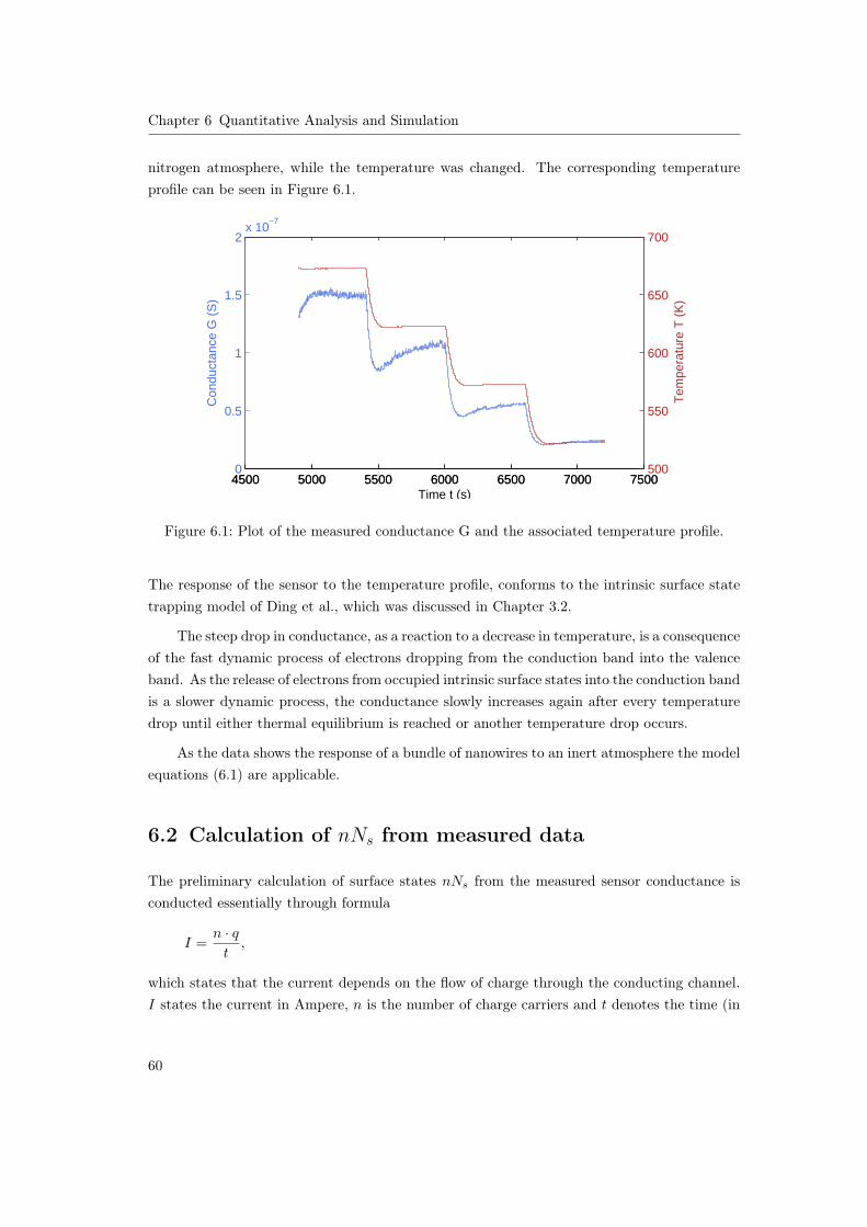
Chapter 6 Quantitative Analysis and Simulation
nitrogen atmosphere, while the temperature was changed. The corresponding temperatureprofile can be seen in Figure 6.1.
4500 5000 5500 6000 6500 7000 75000
0.5
1
1.5
2x 10
−7
Time t (s)
Con
duct
ance
G (
S)
4500 5000 5500 6000 6500 7000 7500500
550
600
650
700
Tem
pera
ture
T (
K)
Figure 6.1: Plot of the measured conductance G and the associated temperature profile.
The response of the sensor to the temperature profile, conforms to the intrinsic surface statetrapping model of Ding et al., which was discussed in Chapter 3.2.
The steep drop in conductance, as a reaction to a decrease in temperature, is a consequenceof the fast dynamic process of electrons dropping from the conduction band into the valenceband. As the release of electrons from occupied intrinsic surface states into the conduction bandis a slower dynamic process, the conductance slowly increases again after every temperaturedrop until either thermal equilibrium is reached or another temperature drop occurs.
As the data shows the response of a bundle of nanowires to an inert atmosphere the modelequations (6.1) are applicable.
6.2 Calculation of nNs from measured data
The preliminary calculation of surface states nNs from the measured sensor conductance isconducted essentially through formula
I =n · qt,
which states that the current depends on the flow of charge through the conducting channel.I states the current in Ampere, n is the number of charge carriers and t denotes the time (in
60
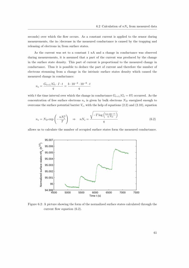
6.2 Calculation of nNs from measured data
seconds) over which the flow occurs. As a constant current is applied to the sensor duringmeasurements, the in-/decrease in the measured conductance is caused by the trapping andreleasing of electrons in/from surface states.
As the current was set to a constant 1 nA and a change in conductance was observedduring measurements, it is assumed that a part of the current was produced by the changein the surface state density. This part of current is proportional to the measured change inconductance. Thus it is possible to deduce the part of current and therefore the number ofelectrons stemming from a change in the intrinsic surface states density which caused themeasured change in conductance:
ns =Gt+1/Gt · I · t
q=b · 10−2 · 10−9 · t
q
with t the time interval over which the change in conductance Gt+1/Gt = b% occurred. As theconcentration of free surface electrons ns is given by bulk electrons ND energized enough toovercome the surface potential barrier Vs, with the help of equations (2.2) and (2.10), equation
ns = ND exp
(−nN
2s
T
)⇒ nNs =
√−T log
(b·t·10−11
q ND
)q
(6.2)
allows us to calculate the number of occupied surface states form the measured conductance.
4500 5000 5500 6000 6500 7000 750094.999
95
95.001
95.002
95.003
95.004
95.005
95.006
95.007
Time t (s)
Nor
mal
ized
sur
face
sta
tes
nNs (
K1/
2 )
Figure 6.2: A picture showing the form of the normalized surface states calculated through thecurrent flow equation (6.2).
61

Chapter 6 Quantitative Analysis and Simulation
The occupied surface states calculated in that manner, follow changes in the sensor con-ductance very closely. Which also implies that the nNs would react to abrupt changes intemperature as swiftly as the conduction does. This indicates a different behavior of nNs thanDing et al. predicted.
The parameters for the conductance formulas of (6.1b) where estimated by fitting a nonlin-ear least squares error in the cases of complete and partial depletion. The resulting parametersare shown in Table 6.1.
Case of carrier depletion Parameters G∗0 β γ
Complete depletionValues
1.396e+02 1.050e−02 3.306e+03Partial depletion 1.952e+03
Table 6.1: Conduction parameter sets for the cases of partial and complete depletion.
The conductance parameters in Table 6.1 were then used to calculate the normalizedsurface state densities nNs for both cases of charge depletion from the measured conductanceG.
The first plot in Figure 6.3 refers to the density of normalized surface states calculatedunder the assumption of a complete depletion of charge carriers throughout the nanowires. Inthis case the nNs behave quite similar to the normalized surface states calculated through thecurrent flow formula (6.2). This is due to the fact that the second term in
nNs =1
β
(1− exp
(γ
T
)G
G0T 3/2
), (6.3)
which was derived from (6.1b), dictates a form negative to the conductance for the nNs.This also implies the immediate response of nNs to changes of temperature, which does notconform to the intrinsic surface state trapping model of Ding et al. If one would consider theapproximate real values for the parameters β and γ (which would be of order 10−6 and 1011
respectively), no plausible values for nNs would be reached, as the second term in (6.3) wouldbe too high, resulting in extremely high, negative values for the nNs.
Figure 6.3(b) shows that the surface state density behaves like the intrinsic surface statetrapping model predicts. The Ns react slowly to a step in temperature and decrease as theconductance increases.
62
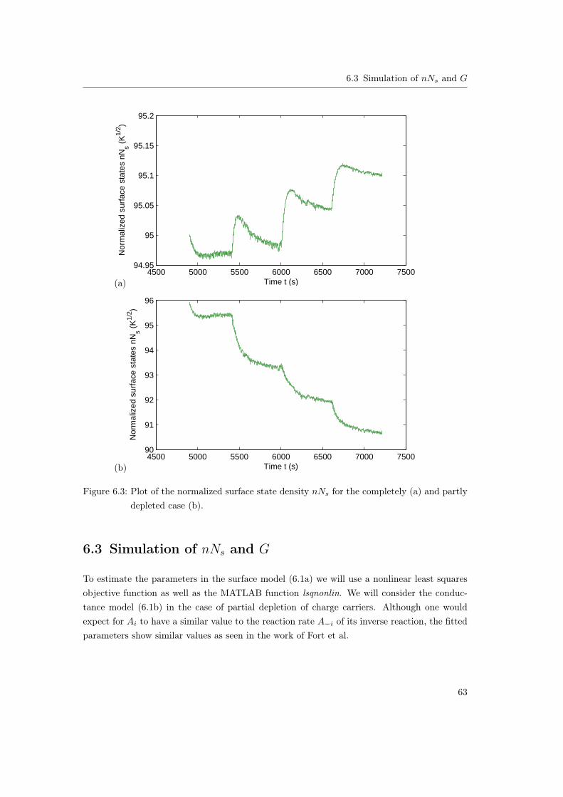
6.3 Simulation of nNs and G
4500 5000 5500 6000 6500 7000 750094.95
95
95.05
95.1
95.15
95.2
Time t (s)
Nor
mal
ized
sur
face
sta
tes
nNs (
K1/
2 )
(a)
4500 5000 5500 6000 6500 7000 750090
91
92
93
94
95
96
Time t (s)
Nor
mal
ized
sur
face
sta
tes
nNs (
K1/
2 )
(b)
Figure 6.3: Plot of the normalized surface state density nNs for the completely (a) and partlydepleted case (b).
6.3 Simulation of nNs and G
To estimate the parameters in the surface model (6.1a) we will use a nonlinear least squaresobjective function as well as the MATLAB function lsqnonlin. We will consider the conduc-tance model (6.1b) in the case of partial depletion of charge carriers. Although one wouldexpect for Ai to have a similar value to the reaction rate A−i of its inverse reaction, the fittedparameters show similar values as seen in the work of Fort et al.
63
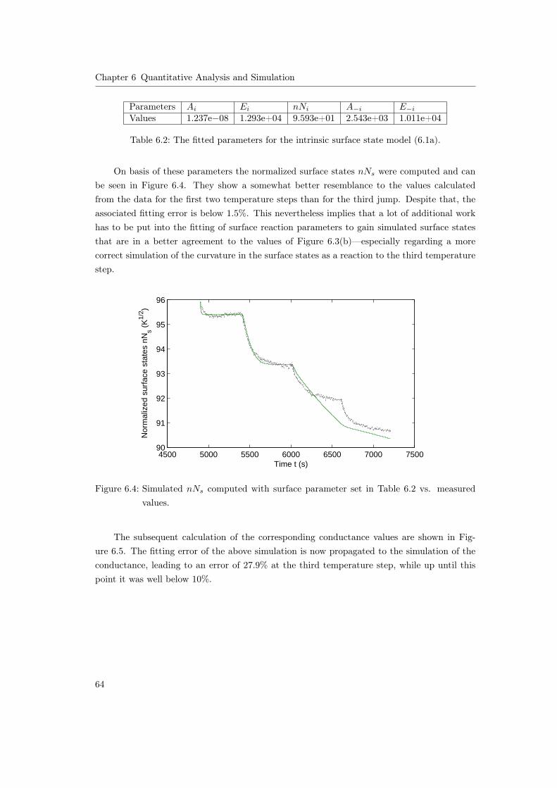
Chapter 6 Quantitative Analysis and Simulation
Parameters Ai Ei nNi A−i E−iValues 1.237e−08 1.293e+04 9.593e+01 2.543e+03 1.011e+04
Table 6.2: The fitted parameters for the intrinsic surface state model (6.1a).
On basis of these parameters the normalized surface states nNs were computed and canbe seen in Figure 6.4. They show a somewhat better resemblance to the values calculatedfrom the data for the first two temperature steps than for the third jump. Despite that, theassociated fitting error is below 1.5%. This nevertheless implies that a lot of additional workhas to be put into the fitting of surface reaction parameters to gain simulated surface statesthat are in a better agreement to the values of Figure 6.3(b)—especially regarding a morecorrect simulation of the curvature in the surface states as a reaction to the third temperaturestep.
4500 5000 5500 6000 6500 7000 750090
91
92
93
94
95
96
Time t (s)
Nor
mal
ized
sur
face
sta
tes
nNs (
K1/
2 )
Figure 6.4: Simulated nNs computed with surface parameter set in Table 6.2 vs. measuredvalues.
The subsequent calculation of the corresponding conductance values are shown in Fig-ure 6.5. The fitting error of the above simulation is now propagated to the simulation of theconductance, leading to an error of 27.9% at the third temperature step, while up until thispoint it was well below 10%.
64
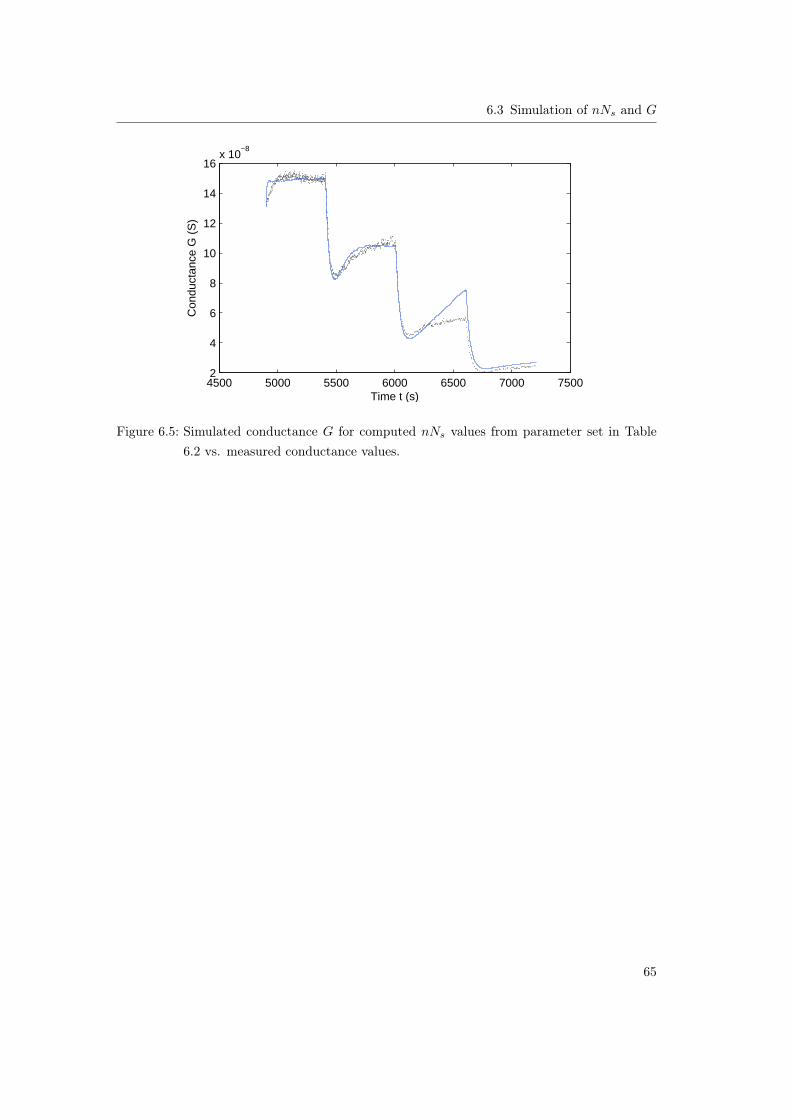
6.3 Simulation of nNs and G
4500 5000 5500 6000 6500 7000 75002
4
6
8
10
12
14
16x 10
−8
Time t (s)
Con
duct
ance
G (
S)
Figure 6.5: Simulated conductance G for computed nNs values from parameter set in Table6.2 vs. measured conductance values.
65

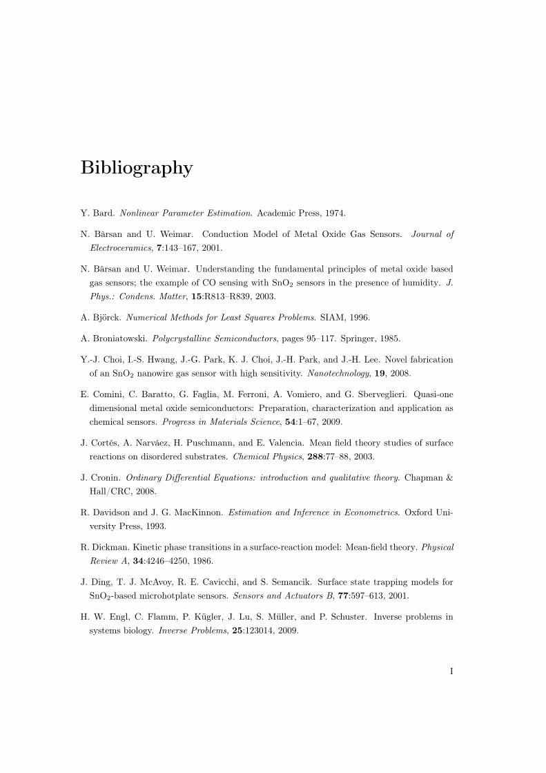
Bibliography
Y. Bard. Nonlinear Parameter Estimation. Academic Press, 1974.
N. Bârsan and U. Weimar. Conduction Model of Metal Oxide Gas Sensors. Journal ofElectroceramics, 7:143–167, 2001.
N. Bârsan and U. Weimar. Understanding the fundamental principles of metal oxide basedgas sensors; the example of CO sensing with SnO2 sensors in the presence of humidity. J.Phys.: Condens. Matter, 15:R813–R839, 2003.
A. Björck. Numerical Methods for Least Squares Problems. SIAM, 1996.
A. Broniatowski. Polycrystalline Semiconductors, pages 95–117. Springer, 1985.
Y.-J. Choi, I.-S. Hwang, J.-G. Park, K. J. Choi, J.-H. Park, and J.-H. Lee. Novel fabricationof an SnO2 nanowire gas sensor with high sensitivity. Nanotechnology, 19, 2008.
E. Comini, C. Baratto, G. Faglia, M. Ferroni, A. Vomiero, and G. Sberveglieri. Quasi-onedimensional metal oxide semiconductors: Preparation, characterization and application aschemical sensors. Progress in Materials Science, 54:1–67, 2009.
J. Cortés, A. Narváez, H. Puschmann, and E. Valencia. Mean field theory studies of surfacereactions on disordered substrates. Chemical Physics, 288:77–88, 2003.
J. Cronin. Ordinary Differential Equations: introduction and qualitative theory. Chapman &Hall/CRC, 2008.
R. Davidson and J. G. MacKinnon. Estimation and Inference in Econometrics. Oxford Uni-versity Press, 1993.
R. Dickman. Kinetic phase transitions in a surface-reaction model: Mean-field theory. PhysicalReview A, 34:4246–4250, 1986.
J. Ding, T. J. McAvoy, R. E. Cavicchi, and S. Semancik. Surface state trapping models forSnO2-based microhotplate sensors. Sensors and Actuators B, 77:597–613, 2001.
H. W. Engl, C. Flamm, P. Kügler, J. Lu, S. Müller, and P. Schuster. Inverse problems insystems biology. Inverse Problems, 25:123014, 2009.
I
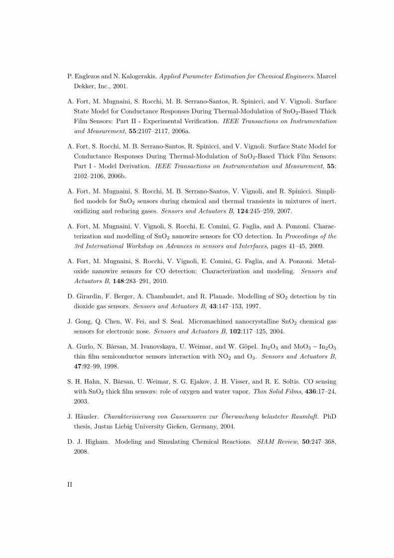
P. Englezos and N. Kalogerakis. Applied Parameter Estimation for Chemical Engineers. MarcelDekker, Inc., 2001.
A. Fort, M. Mugnaini, S. Rocchi, M. B. Serrano-Santos, R. Spinicci, and V. Vignoli. SurfaceState Model for Conductance Responses During Thermal-Modulation of SnO2-Based ThickFilm Sensors: Part II - Experimental Verification. IEEE Transactions on Instrumentationand Measurement, 55:2107–2117, 2006a.
A. Fort, S. Rocchi, M. B. Serrano-Santos, R. Spinicci, and V. Vignoli. Surface State Model forConductance Responses During Thermal-Modulation of SnO2-Based Thick Film Sensors:Part I - Model Derivation. IEEE Transactions on Instrumentation and Measurement, 55:2102–2106, 2006b.
A. Fort, M. Mugnaini, S. Rocchi, M. B. Serrano-Santos, V. Vignoli, and R. Spinicci. Simpli-fied models for SnO2 sensors during chemical and thermal transients in mixtures of inert,oxidizing and reducing gases. Sensors and Actuators B, 124:245–259, 2007.
A. Fort, M. Mugnaini, V. Vignoli, S. Rocchi, E. Comini, G. Faglia, and A. Ponzoni. Charac-terization and modelling of SnO2 nanowire sensors for CO detection. In Proceedings of the3rd International Workshop on Advances in sensors and Interfaces, pages 41–45, 2009.
A. Fort, M. Mugnaini, S. Rocchi, V. Vignoli, E. Comini, G. Faglia, and A. Ponzoni. Metal-oxide nanowire sensors for CO detection: Characterization and modeling. Sensors andActuators B, 148:283–291, 2010.
D. Girardin, F. Berger, A. Chambaudet, and R. Planade. Modelling of SO2 detection by tindioxide gas sensors. Sensors and Actuators B, 43:147–153, 1997.
J. Gong, Q. Chen, W. Fei, and S. Seal. Micromachined nanocrystalline SnO2 chemical gassensors for electronic nose. Sensors and Actuators B, 102:117–125, 2004.
A. Gurlo, N. Bârsan, M. Ivanovskaya, U. Weimar, and W. Göpel. In2O3 and MoO3 − In2O3
thin film semiconductor sensors interaction with NO2 and O3. Sensors and Actuators B,47:92–99, 1998.
S. H. Hahn, N. Bârsan, U. Weimar, S. G. Ejakov, J. H. Visser, and R. E. Soltis. CO sensingwith SnO2 thick film sensors: role of oxygen and water vapor. Thin Solid Films, 436:17–24,2003.
J. Häusler. Charakterisierung von Gassensoren zur Überwachung belasteter Raumluft. PhDthesis, Justus Liebig University Gießen, Germany, 2004.
D. J. Higham. Modeling and Simulating Chemical Reactions. SIAM Review, 50:247–368,2008.
II
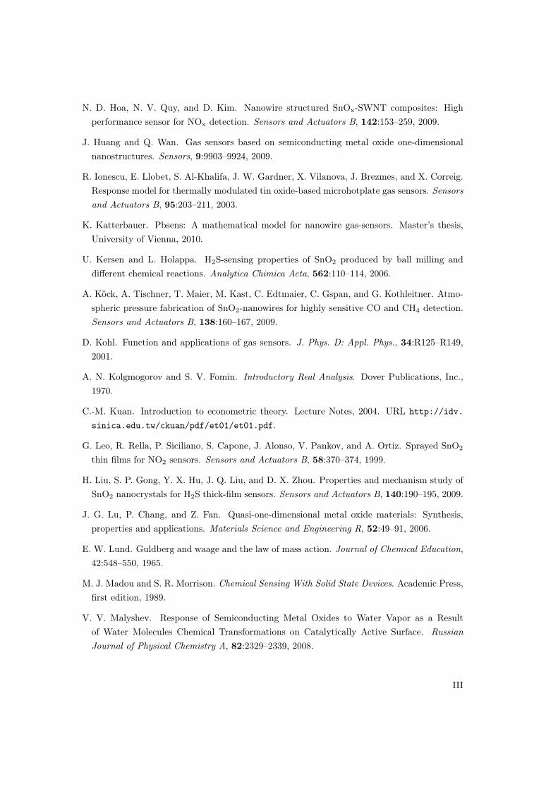
N. D. Hoa, N. V. Quy, and D. Kim. Nanowire structured SnOx-SWNT composites: Highperformance sensor for NOx detection. Sensors and Actuators B, 142:153–259, 2009.
J. Huang and Q. Wan. Gas sensors based on semiconducting metal oxide one-dimensionalnanostructures. Sensors, 9:9903–9924, 2009.
R. Ionescu, E. Llobet, S. Al-Khalifa, J. W. Gardner, X. Vilanova, J. Brezmes, and X. Correig.Response model for thermally modulated tin oxide-based microhotplate gas sensors. Sensorsand Actuators B, 95:203–211, 2003.
K. Katterbauer. Pbsens: A mathematical model for nanowire gas-sensors. Master’s thesis,University of Vienna, 2010.
U. Kersen and L. Holappa. H2S-sensing properties of SnO2 produced by ball milling anddifferent chemical reactions. Analytica Chimica Acta, 562:110–114, 2006.
A. Köck, A. Tischner, T. Maier, M. Kast, C. Edtmaier, C. Gspan, and G. Kothleitner. Atmo-spheric pressure fabrication of SnO2-nanowires for highly sensitive CO and CH4 detection.Sensors and Actuators B, 138:160–167, 2009.
D. Kohl. Function and applications of gas sensors. J. Phys. D: Appl. Phys., 34:R125–R149,2001.
A. N. Kolgmogorov and S. V. Fomin. Introductory Real Analysis. Dover Publications, Inc.,1970.
C.-M. Kuan. Introduction to econometric theory. Lecture Notes, 2004. URL http://idv.
sinica.edu.tw/ckuan/pdf/et01/et01.pdf.
G. Leo, R. Rella, P. Siciliano, S. Capone, J. Alonso, V. Pankov, and A. Ortiz. Sprayed SnO2
thin films for NO2 sensors. Sensors and Actuators B, 58:370–374, 1999.
H. Liu, S. P. Gong, Y. X. Hu, J. Q. Liu, and D. X. Zhou. Properties and mechanism study ofSnO2 nanocrystals for H2S thick-film sensors. Sensors and Actuators B, 140:190–195, 2009.
J. G. Lu, P. Chang, and Z. Fan. Quasi-one-dimensional metal oxide materials: Synthesis,properties and applications. Materials Science and Engineering R, 52:49–91, 2006.
E. W. Lund. Guldberg and waage and the law of mass action. Journal of Chemical Education,42:548–550, 1965.
M. J. Madou and S. R. Morrison. Chemical Sensing With Solid State Devices. Academic Press,first edition, 1989.
V. V. Malyshev. Response of Semiconducting Metal Oxides to Water Vapor as a Resultof Water Molecules Chemical Transformations on Catalytically Active Surface. RussianJournal of Physical Chemistry A, 82:2329–2339, 2008.
III

V. V. Malyshev and A. V. Pislyakov. SnO2-based thick-film-resistive sensor for H2S detectionin the concentration range of 1-10 mg m−3. Sensors and Actuators B, 47:181–188, 1998.
V. V. Malyshev and A. V. Pislyakov. Investigation of gas-sensitivity of sensor structuresto hydrogen in a wide range of temperature, concentration and humidity of gas medium.Sensors and Actuators B, 134:913–921, 2008.
S. R. Morrison. The Chemical Physics of Surfaces. Plenum Press, second edition, 1990.
A. Naydenov, R. Stoyanova, and D. Mehandjiev. Ozone decomposition and CO oxidation onCeO2. Journal of Molecular Catalysis A: Chemical, 98:9–14, 1995.
H.-Y. Pan and H. J. Wang. A two-species surface reaction model of the mixing type. PhysicaA, 227:234–238, 1996.
F. Quaranta, R. Rella, P. Siciliano, S. Capone, M. Epifani, L. Vasanelli, A. Licciulli, andA. Zocco. A novel gas sensor based on SnO2/Os thin film for the detection of methane atlow temperature. Sensors and Actuators B, 58:350–355, 1999.
B. Ruhland, T. Becker, and G. Müler. Gas-kinetic interaction of nitrous oxides with SnO2
surfaces. Sensors and Actuators B, 50:85–94, 1998.
I. Sayago, J. Gutihrez, L. Ads, J. Robla, M. Horrillo, J. Getino, and J. Agapito. The interactionof different oxidizing agents on doped tin oxide. Sensors and Actuators B, 24-25:512–515,1995.
K. Tabata, T. Kawabe, Y. Yamaguchi, and Y. Nagasawa. Chemisorbed oxygen species overthe (110) face of SnO2. Catalysis Surveys from Asia, 7:251–259, 2003.
W. E. Taylor, N. H. Odell, and H. Y. Fan. Grain boundary barriers in germanium. PhysicalReview, 88:867–875, 1952.
A. Tischner, T. Maier, C. Stepper, and A. Köck. Ultrathin SnO2 gas sensors fabricated byspray pyrolysis for the detection of humidity and carbon monoxide. Sensors and ActuatorsB, 134:796–802, 2008.
A. Tischner, A. Köck, T. Maier, C. Edtmaier, C. Gspan, and G. Kothleitner. Tin oxidenanocrystalline films and nanowires for gas sensing applications. Microelectronic Engineer-ing, 86:1258–1261, 2009.
Z. L. Wang. ZnO nanowire and nanobelt platform for nanotechnology. Material Science andEngineering R, 64:33–71, 2009.
N. Yamazoe and K. Shimanoe. Theory of power laws for semiconductor gas sensors. Sensorsand Actuators B, 128:566–573, 2008.
IV

N. Yamazoe and K. Shimanoe. Theoretical approach to the rate of response of semiconductorgas sensors. Sensors and Actuators B, 154:277–282, 2010.
A. Zima. Development of highly sensitive nano-gassensors based on nanocrystalline tin dioxidethin film and single-crystalline tin dioxide nanowires. PhD thesis, Vienna University ofTechnology, 2009.
A. Zima, A. Köck, and T. Maier. In- and sb-doped tin oxide nanocrystalline films for selectivegas sensing. Microelectronic Engineering, 87:1467–1470, 2010.
V

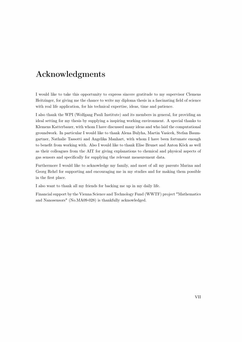
Acknowledgments
I would like to take this opportunity to express sincere gratitude to my supervisor ClemensHeitzinger, for giving me the chance to write my diploma thesis in a fascinating field of sciencewith real life application, for his technical expertise, ideas, time and patience.
I also thank the WPI (Wolfgang Pauli Institute) and its members in general, for providing anideal setting for my thesis by supplying a inspiring working environment. A special thanks toKlemens Katterbauer, with whom I have discussed many ideas and who laid the computationalgroundwork. In particular I would like to thank Alena Bulyha, Martin Vasicek, Stefan Baum-gartner, Nathalie Tassotti and Angelika Manhart, with whom I have been fortunate enoughto benefit from working with. Also I would like to thank Elise Brunet and Anton Köck as wellas their colleagues from the AIT for giving explanations to chemical and physical aspects ofgas sensors and specifically for supplying the relevant measurement data.
Furthermore I would like to acknowledge my family, and most of all my parents Marina andGeorg Rehrl for supporting and encouraging me in my studies and for making them possiblein the first place.
I also want to thank all my friends for backing me up in my daily life.
Financial support by the Vienna Science and Technology Fund (WWTF) project "Mathematicsand Nanosensors" (No.MA09-028) is thankfully acknowledged.
VII

Abstract
This thesis deals with the modeling of metal oxide nanowire gas sensors, which are technicaldevices in the scale of nanometers, that are used to detect different gases in different concen-trations in the atmosphere. As state of the art gas sensors show a low selectivity, the detailedmodeling of the surface reactions caused by different test gases is essential to overcome thisissue.
The developed response models, described in this work, are composed of an ODE surfacereaction model and a charge transport model (both parameter dependent) and predict thechange of conductance of the sensor upon changes in the thermal and chemical environment.In this diploma thesis we present surface reaction models for the most important and test gasspecies that are relevant for applications, show their derivation and give a detailed discussionof their properties.
In order to facilitate the simulation of the sensor response, the theory of inverse model-ing of dynamic models, with special regard to the estimation of model parameters throughnonlinear least squares estimators and suitable optimization algorithms, is discussed.
A one parameter transport model in combination with a five parameter surface reactionmodel is used to simulate the response of a gas sensor consisting of a bundle of nanowires inan inert atmosphere. Reaction as well as conduction parameters is fitted in a nonlinear leastsquares estimation process, using inverse modeling techniques.
IX
Zusammenfassung
Diese Diplomarbeit behandelt die mathematische Modellierung von Nanowire Gassen-soren, also Sensoren in der Größenordnung einiger Nanometer die zur Detektion verschiedenerGase und deren Konzentration in der Umgebungsluft verwendet werden. Aktuell erforschte undenwickelte Gassensoren können schwer zwischen bestimmten Gasen unterscheiden, desswegenermöglicht die mathematischen Modellierung ein tiefergehendes Verständnis der für den Sen-sorausschlag verantwortlichen Oberflächereaktionen auch eine Verbesserung dieser Kreuzselek-tivität.
Die in dieser Arbeit hergeleiteten Sensormodelle setzen sich jeweils aus einem Oberflächen-modell, bestehend aus gewöhlichen Differentialgleichungen, und einem Ladungstransportmod-ell – beide paramterabhängig – zusammen und sagen die Änderung der Leitfähigkeit, verur-sacht durch eine Änderung der Temperature und der chemischen Zusammensetzung der Umge-bungsluft, voraus. Wir präsentieren Oberflächenmodelle für alle wichtigen, für Anwendungenrelevanten Gassorten, leiten sie her und diskutieren sie im Detail.
Um eine spätere quantitative Analyse von Modellen und Messdaten zu ermöglichen,wurde die Theorie der Inversen Modellierung von dynamischen Modellen behandelt. Hierbeiwurde besondere Aufmerksamkeit auf die asymptotische Theorie nichtlinearer Least SquaresSchätzmethoden und auf dafür passende Optimierungsalgorithmen verwendet.
Ein einparametriges Transportmodell in Kombination mit einem Oberflächenreaktion-smodell, bestehend aus 5 Parametern, wird benutzt um das Verhalten eines Geassensors,bestehend aus einem Netzwerk von Nanodrähten, in einer Edelgasatmosphäre zu simulieren.Hierzu wurden die Reaktionskonstanten und Parameter beider Modelle durch einen nichtlin-earen Least Sqares Schätzprozesses gefittet, unter zuhilfenahme von Inverser Modellierung.
X

Curriculum Vitae
Personal data
Name: Marina RehrlDate of Birth: 9th of March, 1985Place of Birth: Braunau am Inn, Upper AustriaCitizenship: Austria
Education
1999 to 2004: Federal Secondary College of Engineering, LinzGraphic and Communicational Design
July 2004: Diploma thesis in the course of graduation with honor“Creation of a Corporate Identity for an oral surgeon”
since Autumn 2004: Diploma Studies of Mathematics, University of ViennaApplied mathematics and scientific computing
Work Experience
July to August 2006: Erste Bank Holding, ViennaGroup Rating Methods
September 2009: Allianz Elementar Versicherung, ViennaRealtor Service
March to June 2010 and Austrian Financial Market Authority, ViennaSeptember 2010 to March 2011: Actuarial Issues and Models
XI