detailed scheduling and planning session 1 inventory management: order planning
TRANSCRIPT
Detailed Scheduling and Planning
Session 1Inventory Management:
Order Planning
1-2
Visual
Detailed Scheduling and Planning, ver. 1
Purpose of Inventory Strategy
Service Level Dependent Demand Independent Demand Demand Variability Seasonality Lead Time Fluctuation Company Policy
1-3
Visual
Detailed Scheduling and Planning, ver. 1
Definition of Inventory
Those stocks or items used to support production (raw materials and work-in-process items), supporting activities (maintenance, repair, and operating supplies), and customer service (finished goods and spare parts). Demand for inventory may be dependent or independent. Inventory functions are anticipation, hedge, cycle (lot size), fluctuation (safety, buffer, or reserve), transportation (pipeline), and service parts. Source: APICS Dictionary, 9th ed., 1998
1-4
Visual
Detailed Scheduling and Planning, ver. 1
Types of Inventory
Raw Materials (RAW) Work in Process (WIP) Finished Goods (FG) Maintenance, Repair, and Operating
Supplies (MRO)
1-5
Visual
Detailed Scheduling and Planning, ver. 1
Classifications of Inventory
Excess Surplus Inactive Obsolete Consignment Vendor Managed
1-6
Visual
Detailed Scheduling and Planning, ver. 1
Types of Order Review Methodologies
Material Requirements Planning (MRP) Time-Phased Order Point Reorder Point Periodic Review Visual Review Kanban
1-7
Visual
Detailed Scheduling and Planning, ver. 1
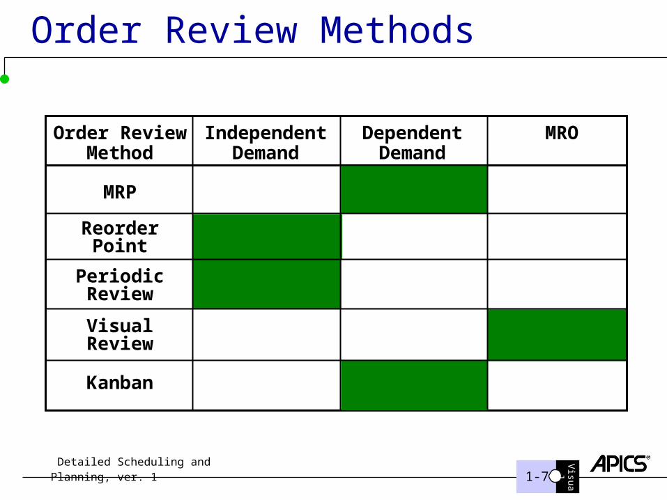
Order Review Methods
Order Review Independent Dependent MROMethod Demand Demand
MRP
ReorderPoint
PeriodicReview
VisualReview
Kanban

1-8
Visual
Detailed Scheduling and Planning, ver. 1
What They Answer
What is the net demand? What is the available balance? What quantity will need to be ordered? When will the orders need to be released? When will the orders need to be received?
1-9
Visual
Detailed Scheduling and Planning, ver. 1
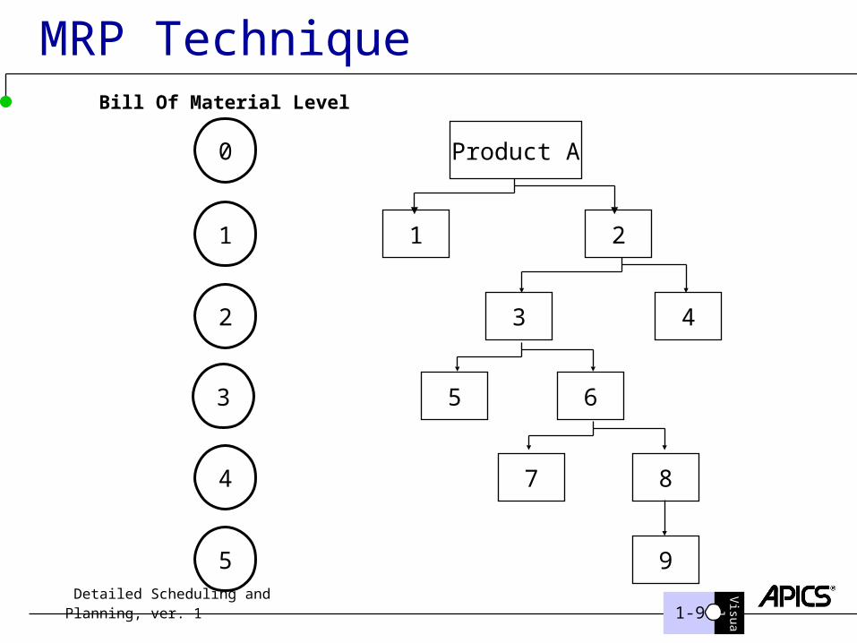
MRP Technique
0
1
2
3
4
5
Product A
1 2
43
5 6
7 8
9
Bill Of Material Level
1-10
Visual
Detailed Scheduling and Planning, ver. 1
MRP
MRP (Material Requirement Planning) is a computerized information system which was developed specifically to aid companies manage demand inventory and schedule replenishment orders.
Determine # of parts, components, materials, time schedule when ordered or produced.
Accommodate ordering strategies for parts with both dependent and independent profiles
1-11
Visual
Detailed Scheduling and Planning, ver. 1
Two types of demand
(1) product demand The first is known customers who have placed specific
orders, such as those generated by sales personnel, or from interdepartmental transactions.
The second source is forecast demand which is from the known customers and the forecast demand.
(2) demand for repair parts and supplies The demand when customers order specific parts and
components either as spares, or for service and repair.
1-12
Visual
Detailed Scheduling and Planning, ver. 1
Dependent Demand
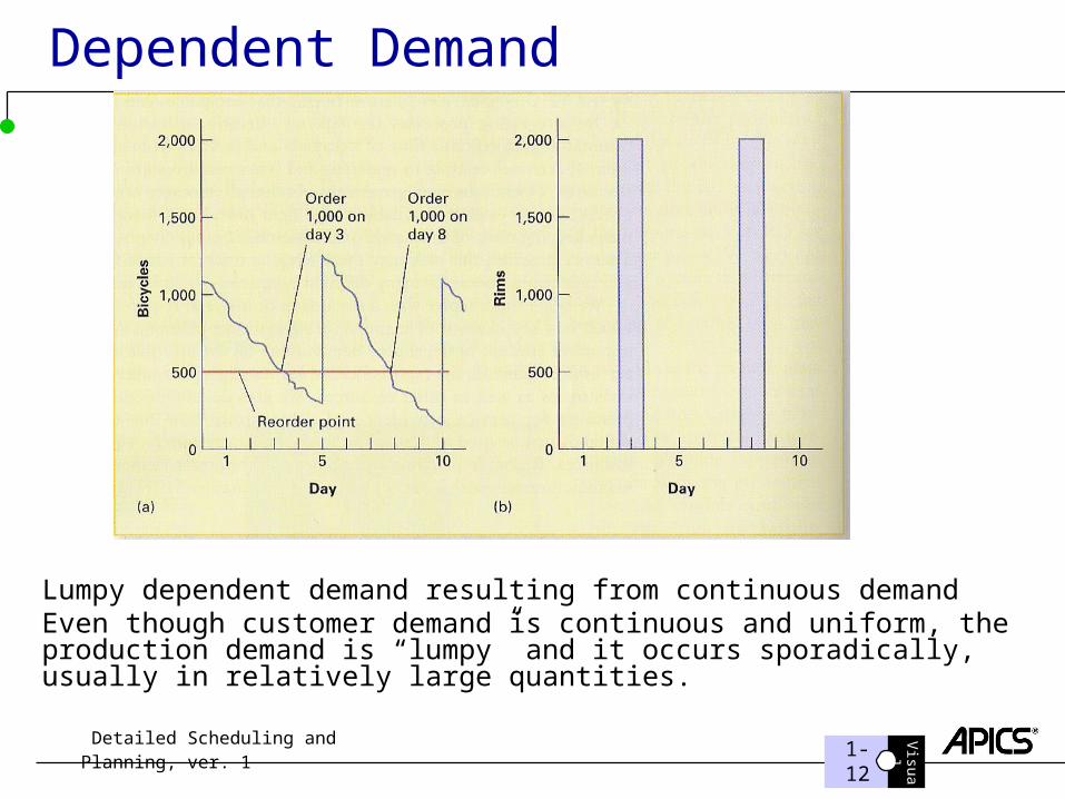
Lumpy dependent demand resulting from continuous demandEven though customer demand is continuous and uniform, the production demand is “lumpy” and it occurs sporadically, usually in relatively large quantities.
1-13
Visual
Detailed Scheduling and Planning, ver. 1
3 main inputs to MRP
3 key inputs to the MRPI. Master production schedules (MPS) II. A bill of materials database (BOM)III. An inventory record database
An MRP system translates the MPS and other sources of demand, such as independent demand for replacement parts and maintenance items, into the requirements for all subassemblies, components, and raw materials.
1-14
Visual
Detailed Scheduling and Planning, ver. 1
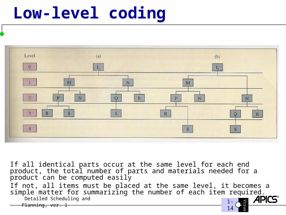
Low-level coding
If all identical parts occur at the same level for each end product, the total number of parts and materials needed for a product can be computed easilyIf not, all items must be placed at the same level, it becomes a simple matter for summarizing the number of each item required.
1-15
Visual
Detailed Scheduling and Planning, ver. 1
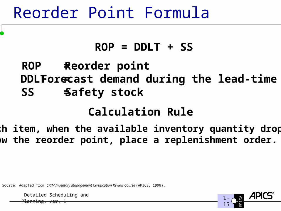
ROP = DDLT + SS
ROP = Reorder pointDDLT = Forecast demand during the lead-timeSS = Safety stock
Calculation Rule
For each item, when the available inventory quantity drops toor below the reorder point, place a replenishment order.
Source: Adapted from CPIM Inventory Management Certification Review Course (APICS, 1998).
Reorder Point Formula
1-16
Visual
Detailed Scheduling and Planning, ver. 1
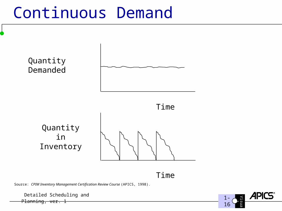
Continuous Demand
QuantityDemanded
Quantityin
Inventory
Time
TimeSource: CPIM Inventory Management Certification Review Course (APICS, 1998).
1-17
Visual
Detailed Scheduling and Planning, ver. 1
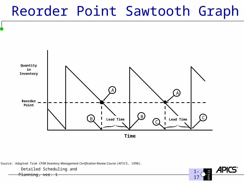
Reorder Point Sawtooth Graph
BC
B C
AA
Lead TimeLead Time
Quantityin
Inventory
ReorderPoint
Source: Adapted from CPIM Inventory Management Certification Review Course (APICS, 1998).
Time
1-18
Visual
Detailed Scheduling and Planning, ver. 1
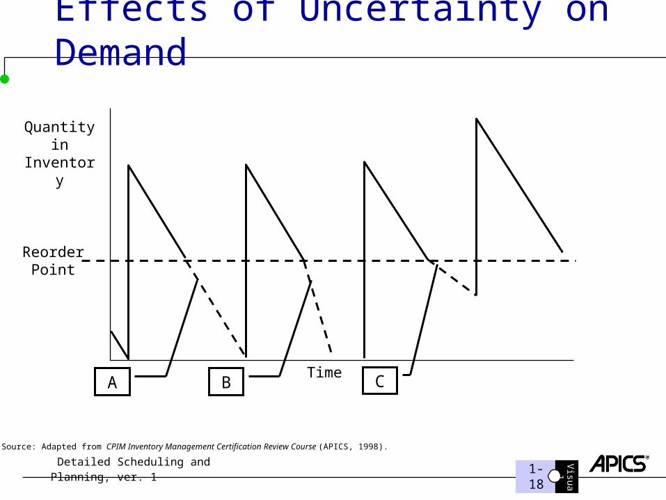
Effects of Uncertainty on Demand
A B C
Quantityin
Inventory
ReorderPoint
Time
Source: Adapted from CPIM Inventory Management Certification Review Course (APICS, 1998).
1-19
Visual
Detailed Scheduling and Planning, ver. 1
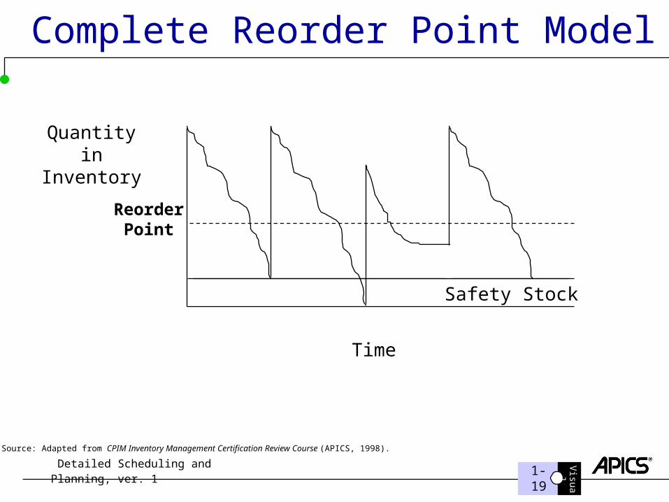
Complete Reorder Point Model
Safety Stock
Quantityin
Inventory
Time
Source: Adapted from CPIM Inventory Management Certification Review Course (APICS, 1998).
ReorderPoint
1-20
Visual
Detailed Scheduling and Planning, ver. 1
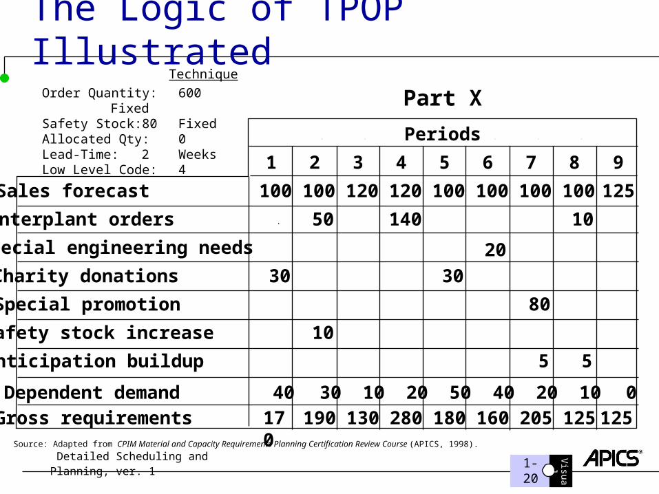
The Logic of TPOP Illustrated
Order Quantity: 600 FixedSafety Stock: 80 FixedAllocated Qty: 0Lead-Time: 2 WeeksLow Level Code: 4
Technique
Source: Adapted from CPIM Material and Capacity Requirements Planning Certification Review Course (APICS, 1998).
Part X
1 2 3 4 5 6 7 9
Sales forecast 100 100 120 120 100 100 100 125
Interplant orders 50 140 10
Special engineering needs
Charity donations 30 30
Special promotion 80
Safety stock increase 10
Anticipation buildup 5 5
Dependent demand 40 30 10 20 50 40 20 0Gross requirements 170 190 130 280 180 160 205 125
8
100
10125
Periods
20
1-21
Visual
Detailed Scheduling and Planning, ver. 1
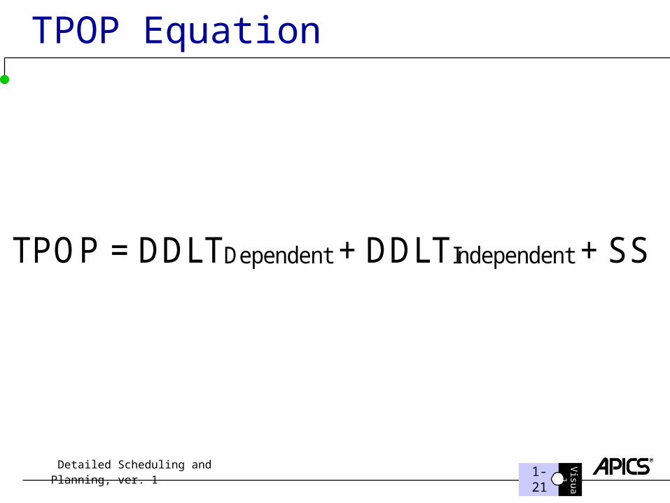
TPOP Equation
TPOP = DDLTDependent + DDLTIndependent + SS
1-22
Visual
Detailed Scheduling and Planning, ver. 1
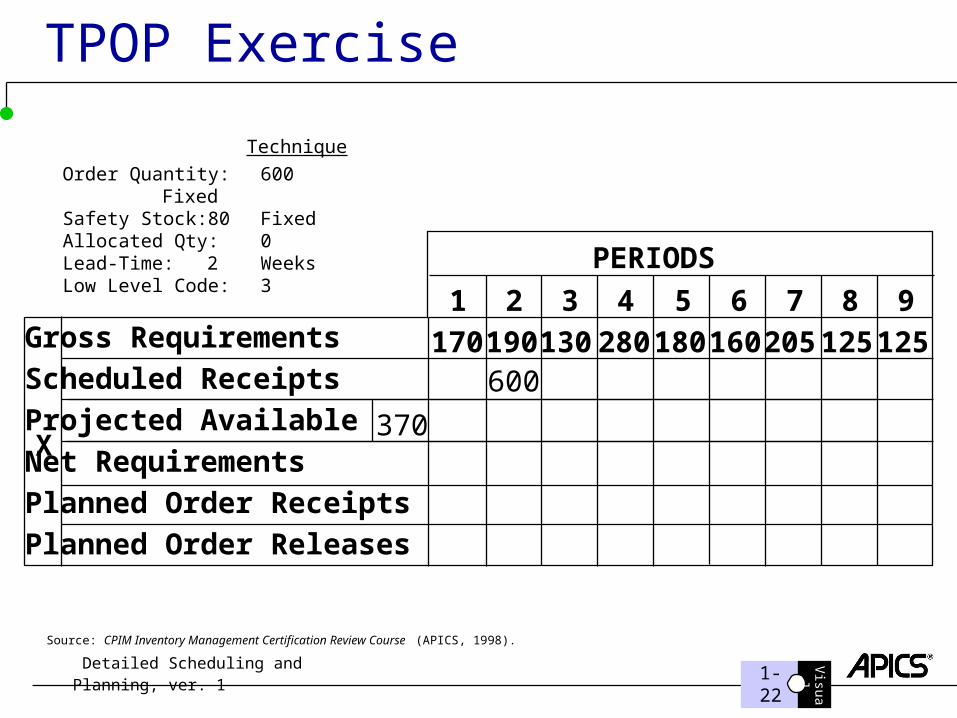
TPOP Exercise
Source: CPIM Inventory Management Certification Review Course (APICS, 1998).
Gross Requirements
Scheduled Receipts
Projected Available
Net Requirements
Planned Order Receipts
Planned Order Releases
1 2 43 9765
PERIODS
370X
170 190 130 280 180 160 205 125600
8
Order Quantity: 600 FixedSafety Stock: 80 FixedAllocated Qty: 0Lead-Time: 2 WeeksLow Level Code: 3
Technique
125
1-23
Visual
Detailed Scheduling and Planning, ver. 1
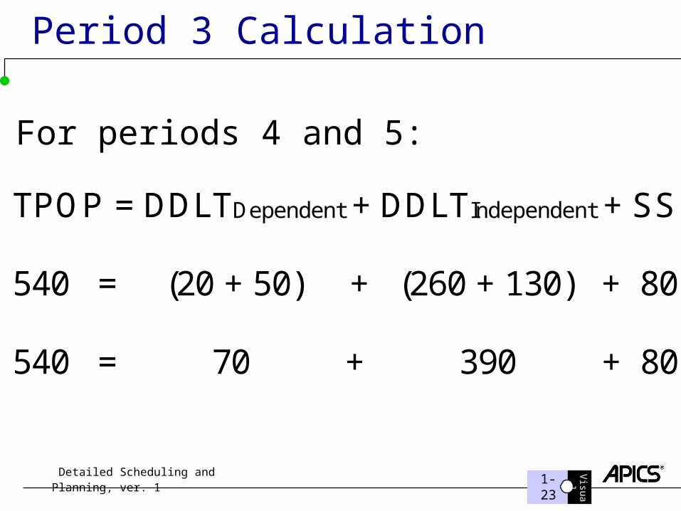
TPOP = DDLTDependent + DDLTIndependent + SS
540 = (20 + 50) + (260 + 130) + 80
540 = 70 + 390 + 80
Period 3 Calculation
For periods 4 and 5:
1-24
Visual
Detailed Scheduling and Planning, ver. 1
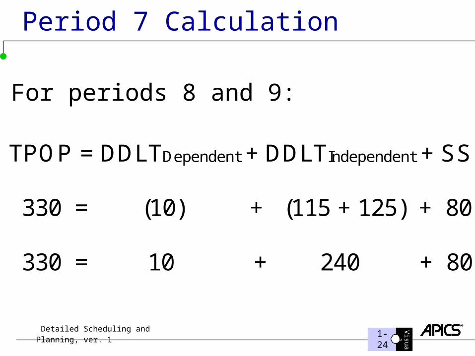
Period 7 Calculation
TPOP = DDLTDependent + DDLTIndependent + SS
330 = (10) + (115 + 125) + 80
330 = 10 + 240 + 80
For periods 8 and 9:
1-25
Visual
Detailed Scheduling and Planning, ver. 1
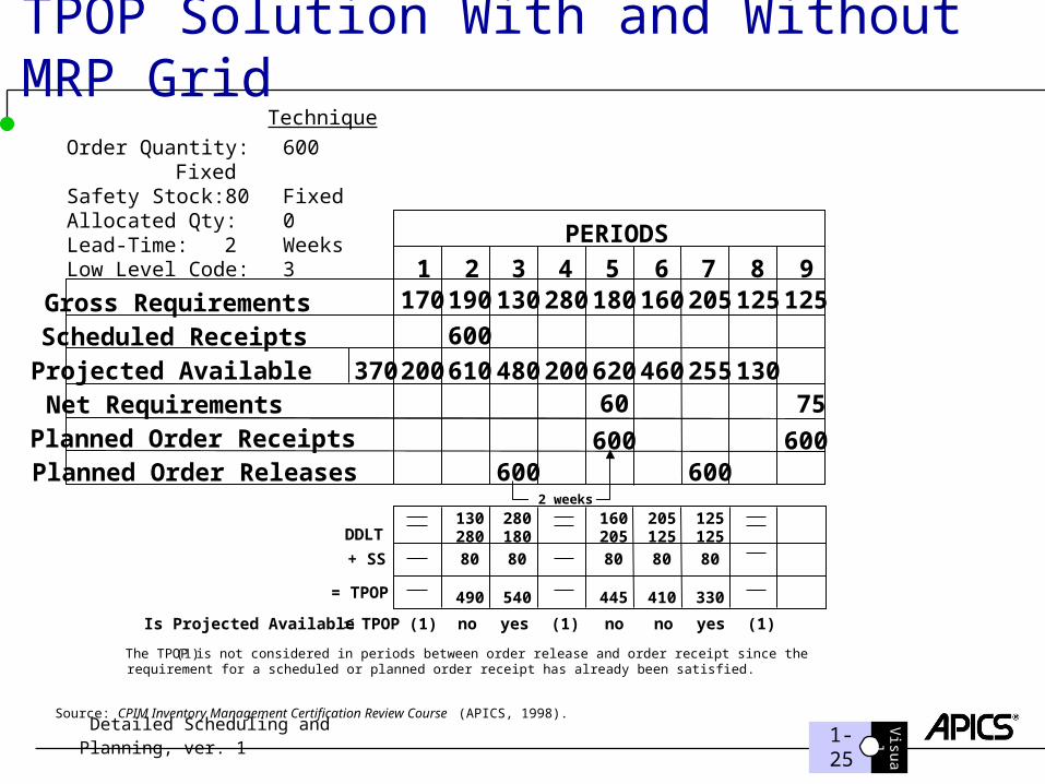
TPOP Solution With and Without MRP Grid
Source: CPIM Inventory Management Certification Review Course (APICS, 1998).
2 weeks
Gross RequirementsScheduled ReceiptsProjected AvailableNet RequirementsPlanned Order ReceiptsPlanned Order Releases
1 2 43 9765
PERIODS
2808
370 200600610
170
200
190 180
620
160
460
205
255
125
130
125
600
130
48075
600
60
600600
330
125125
80
(1) The TPOP is not considered in periods between order release and order receipt since therequirement for a scheduled or planned order receipt has already been satisfied.
DDLT
+ SS
540
280180
80
445
160205
80
410
205125
80
490
130280
80
= TPOP
Is Projected Available TPOP (1) no yes (1) no no yes (1)
Order Quantity: 600 FixedSafety Stock: 80 FixedAllocated Qty: 0Lead-Time: 2 WeeksLow Level Code: 3
Technique
1-26
Visual
Detailed Scheduling and Planning, ver. 1
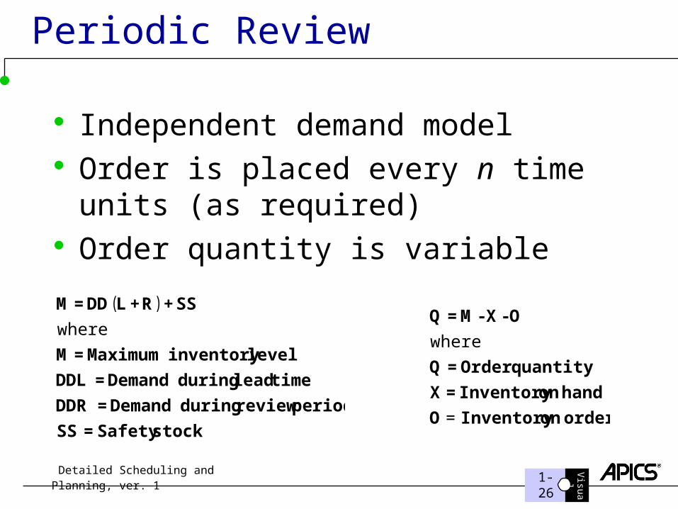
Periodic Review
Independent demand model Order is placed every n time units (as
required) Order quantity is variable
order on InventoryO
hand on Inventory=X
quantity Order=Q
O-X-M=Q
=
where
( )
stock Safety=SS
periodreview during Demand=DDR
time lead during Demand=DDL
level inventory Maximum=M
SS+R+LDD=M
where
1-27
Visual
Detailed Scheduling and Planning, ver. 1
Visual Review
Reordering is based on actually looking at the inventory on hand
Min/Max is a commonly used technique
1-28
Visual
Detailed Scheduling and Planning, ver. 1
Kanban
Kanban is a signal for replenishment The quantity for replacement is determined
from the rate-based MRP as a fixed-order quantity, order point method
Upstream station does not start producing parts until it receives a signal
1-29
Visual
Detailed Scheduling and Planning, ver. 1
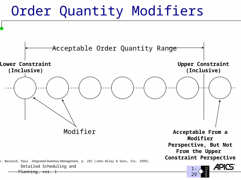
Order Quantity Modifiers
Acceptable Order Quantity Range
Lower Constraint(Inclusive)
Upper Constraint(Inclusive)
Modifier Acceptable From a ModifierPerspective, But Not From the
Upper Constraint Perspective
Source: Bernard, Paul. Integrated Inventory Management, p. 291 (John Wiley & Sons, Inc. 1999).
1-30
Visual
Detailed Scheduling and Planning, ver. 1
Order Quantity Constraints
Minimum quantity can be used to meet a supplier minimum Maximum quantity can be set to recognize storage or
transportation limits Minimum dollar can be used to order at least a supplier- or
purchasing-established minimum purchase order charge Maximum dollar can be used to limit inventory investment
levels Minimum days’ supply can be used to prevent multiple orders
for the same period Maximum day’s supply is used to support inventory turns and
targets, and to recognize shelf-life constraints
1-31
Visual
Detailed Scheduling and Planning, ver. 1
Order Quantity Modifiers
A price break quantity can be ensured on an individual order basis by setting one of the price break quantities as the supplier minimum
Rounding quantities can be used to meet container multiples Minimum demand quantity recognizes that certain items are
subject to large issue Order quantity multiplier accounts for scrap or yield conditions
1-32
Visual
Detailed Scheduling and Planning, ver. 1
Costs Associated with Order Quantity Decisions
The cost to carry inventory– Storage facility cost– Counting, transporting, and handling– Risk of obsolescence– Insurance and taxes– Risk of loss– Opportunity costs
The cost of placing orders
1-33
Visual
Detailed Scheduling and Planning, ver. 1
Opportunity Costs
A company’s cost of capital Typically the largest portion of the carrying
costs Represents the rate of return the company
could earn from investment opportunities
1-34
Visual
Detailed Scheduling and Planning, ver. 1
Cost of Placing Orders
Differs between orders placed to outside suppliers and orders placed in a factory for production
Usually expressed as the cost to place a single order in absolute dollars
1-35
Visual
Detailed Scheduling and Planning, ver. 1
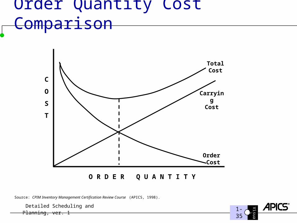
Order Quantity Cost Comparison
OrderCost
CarryingCost
TotalCost
O R D E R Q U A N T I T Y
C
O
S
T
Source: CPIM Inventory Management Certification Review Course (APICS, 1998).
1-36
Visual
Detailed Scheduling and Planning, ver. 1
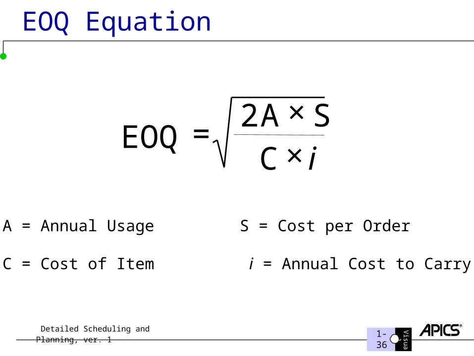
EOQ Equation
A = Annual Usage S = Cost per Order
C = Cost of Item i = Annual Cost to Carry
iCSA2
EOQ××
=
1-37
Visual
Detailed Scheduling and Planning, ver. 1
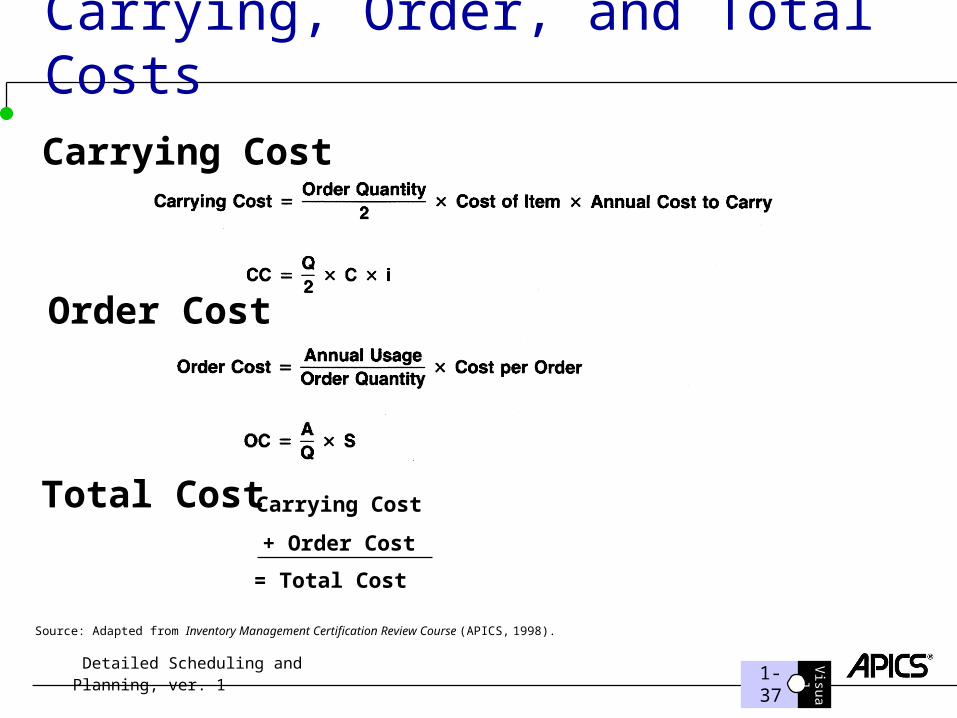
Carrying, Order, and Total Costs
Carrying Cost
Order Cost
Source: Adapted from Inventory Management Certification Review Course (APICS, 1998).
Total Cost Carrying Cost
+ Order Cost
= Total Cost
1-38
Visual
Detailed Scheduling and Planning, ver. 1
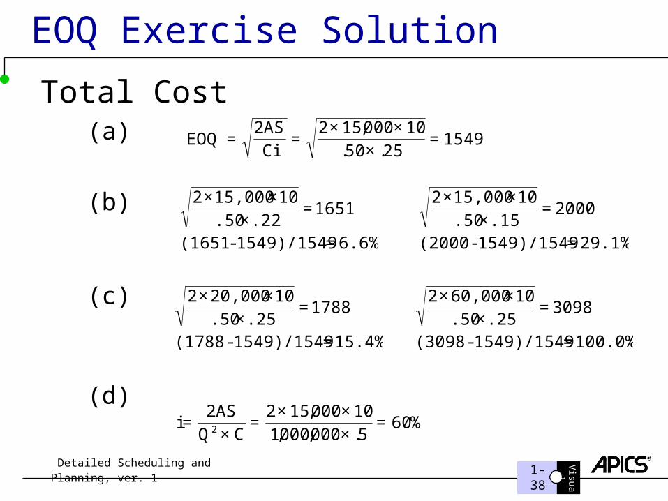
EOQ Exercise Solution
Total Cost(a)
(b)
(c)
(d)
100.0%=1549)/1549 - (3098
3098=.25×.50
10×60,000×2
%605.000,000,110000,152
CQAS2
i 2 =×××
=×
=
15.4%=1549)/1549 - (1788
1788=.25×.50
10×20,000×2
29.1%=1549)/1549 - (2000
2000=.15×.50
10×15,000×2
6.6%=1549)/1549 - (1651
1651=.22×.50
10×15,000×2
154925.50.
10000,152CiAS2
EOQ =×
××==
1-39
Visual
Detailed Scheduling and Planning, ver. 11-35a
Visual
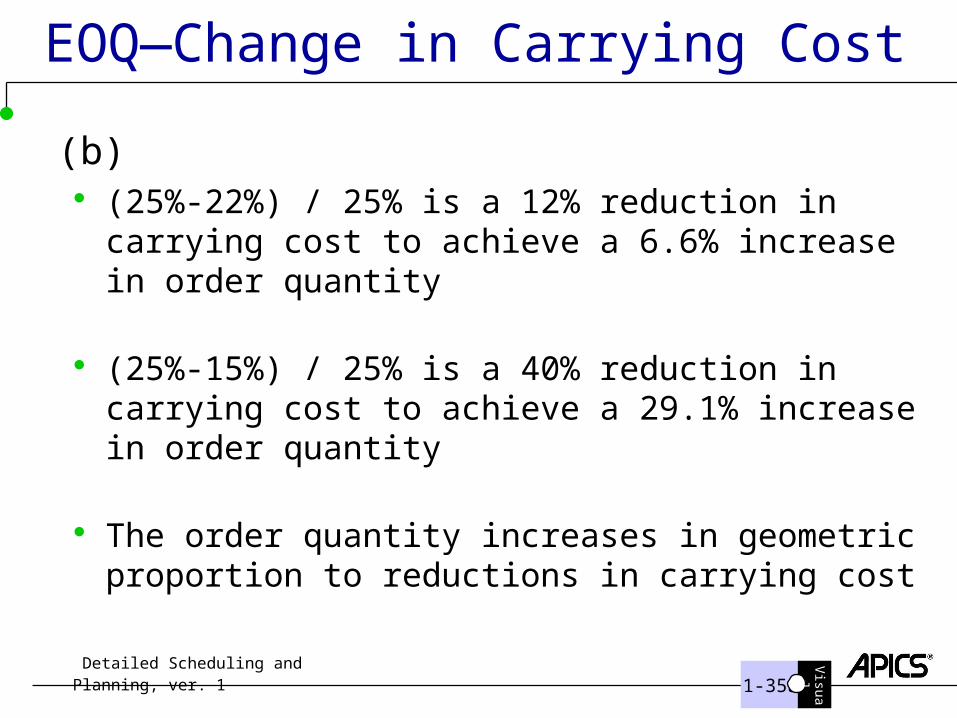
EOQ—Change in Carrying Cost
(b) (25%-22%) / 25% is a 12% reduction in carrying
cost to achieve a 6.6% increase in order quantity
(25%-15%) / 25% is a 40% reduction in carrying cost to achieve a 29.1% increase in order quantity
The order quantity increases in geometric proportion to reductions in carrying cost
1-40
Visual
Detailed Scheduling and Planning, ver. 11-36
Visual
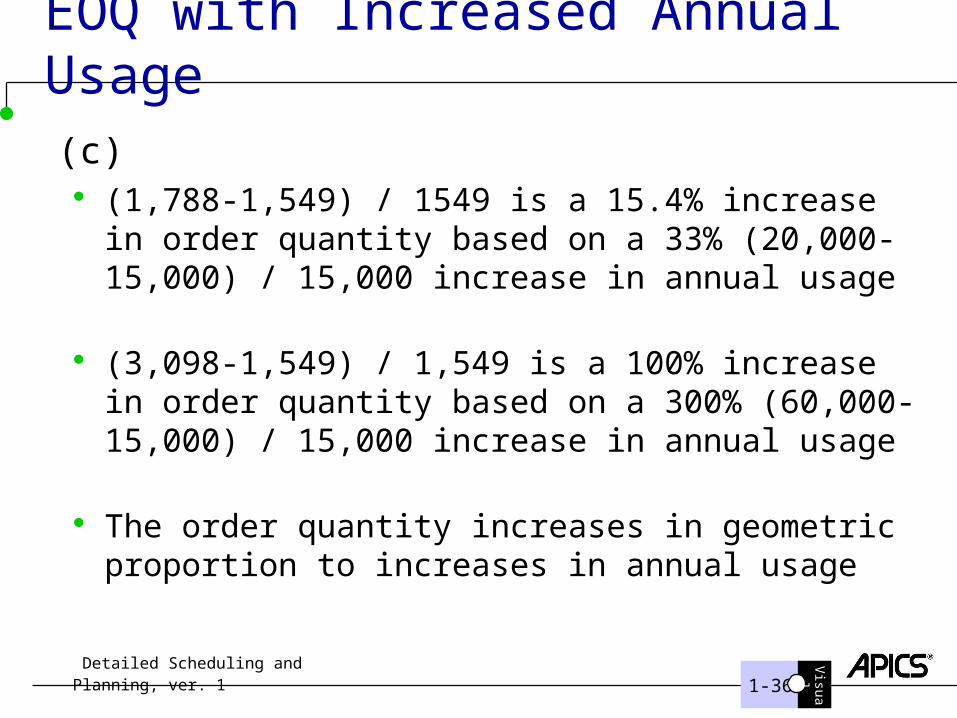
EOQ with Increased Annual Usage
(c) (1,788-1,549) / 1549 is a 15.4% increase in order
quantity based on a 33% (20,000-15,000) / 15,000 increase in annual usage
(3,098-1,549) / 1,549 is a 100% increase in order quantity based on a 300% (60,000-15,000) / 15,000 increase in annual usage
The order quantity increases in geometric proportion to increases in annual usage
1-41
Visual
Detailed Scheduling and Planning, ver. 11-37
Visual
EOQ—Order Quantity 1,000 Units
(d) 60% is too high for a carrying cost.
Something in the area of 24% is more reasonable.
A high carrying cost cannot be used as an excuse for reducing the order quantity.
1-42
Visual
Detailed Scheduling and Planning, ver. 11-38
Visual
Fixed-Order Quantity
Use of a fixed-order quantity is usually dictated by some condition related to shipping, handling, or line replenishment
Regardless of demand variability, suppliers receive consistent orders with consistent order quantities, but at a variable frequency
It may be determined very informally, or it might be based on some form of calculation, such as EOQ
1-43
Visual
Detailed Scheduling and Planning, ver. 1
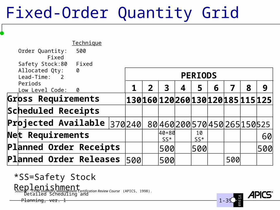
Fixed-Order Quantity Grid
Source: CPIM Inventory Management Certification Review Course (APICS, 1998).
1-39
Visual
Gross Requirements
Scheduled Receipts
Projected Available
Net Requirements
Planned Order Receipts
Planned Order Releases
1 2 43 9765
PERIODS
150
130 160 120 260 130 120 185 125
8
Order Quantity: 500 FixedSafety Stock: 80 FixedAllocated Qty: 0Lead-Time: 2 PeriodsLow Level Code: 0
Technique
115
37060
8010
SS*
200 570 450 265240 460
500 500500
40+80SS*
500 500
*SS=Safety Stock Replenishment
525
500
Visual
Detailed Scheduling and Planning, ver. 1
Period Order Quantity
Lot size is equal to the net requirements for a given number of periods
The number of planning periods included within the “ordering” period can be determined based on the EOQ equation
With fairly steady demand, the order quantity for the “ordering” period generally balances ordering and carrying cost
The intent is to eliminate remnants
1-40
Visual
Detailed Scheduling and Planning, ver. 1
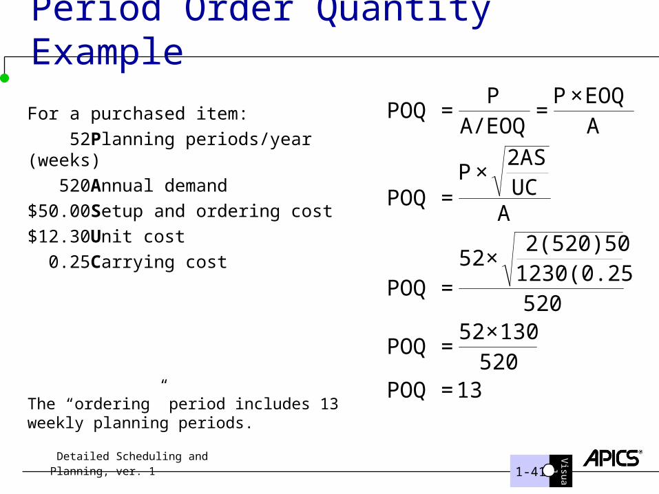
Period Order Quantity Example
For a purchased item:
52 Planning periods/year (weeks)
520 Annual demand
$50.00 Setup and ordering cost
$12.30 Unit cost
0.25 Carrying cost
The “ordering” period includes 13 weekly planning periods.
13=POQ520
130×52=POQ
5201230(0.25)2(520)50
×52=POQ
AUC2AS
×P=POQ
AEOQ×P
=A/EOQ
P=POQ
1-41
1-46
Visual
Detailed Scheduling and Planning, ver. 1
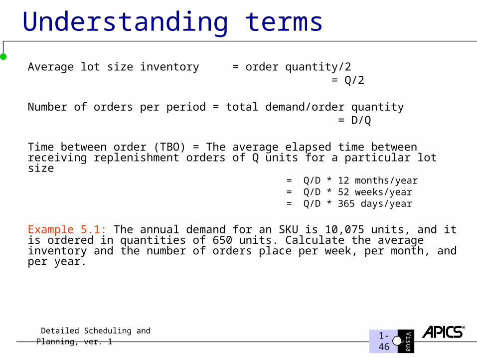
Understanding terms
Average lot size inventory = order quantity/2 = Q/2
Number of orders per period = total demand/order quantity = D/Q
Time between order (TBO) = The average elapsed time between receiving replenishment orders of Q units for a particular lot size
= Q/D * 12 months/year = Q/D * 52 weeks/year = Q/D * 365 days/year
Example 5.1: The annual demand for an SKU is 10,075 units, and it is ordered in quantities of 650 units. Calculate the average inventory and the number of orders place per week, per month, and per year.
1-47
Visual
Detailed Scheduling and Planning, ver. 1
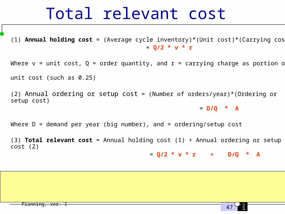
Total relevant cost
(1) Annual holding cost = (Average cycle inventory)*(Unit cost)*(Carrying cost) = Q/2 * v * r
Where v = unit cost, Q = order quantity, and r = carrying charge as portion of unit cost (such as 0.25)
(2) Annual ordering or setup cost = (Number of orders/year)*(Ordering or setup cost) = D/Q * A
Where D = demand per year (big number), and = ordering/setup cost
(3) Total relevant cost = Annual holding cost (1) + Annual ordering or setup cost (2) = Q/2 * v * r + D/Q * A
1-48
Visual
Detailed Scheduling and Planning, ver. 1
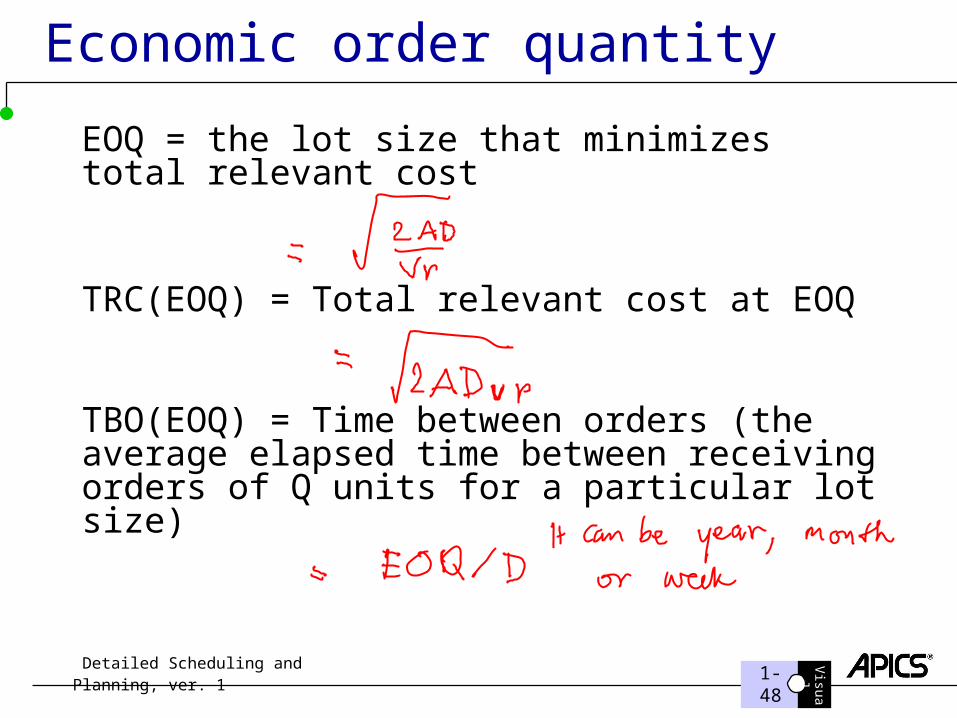
Economic order quantity
EOQ = the lot size that minimizes total relevant cost
TRC(EOQ) = Total relevant cost at EOQ
TBO(EOQ) = Time between orders (the average elapsed time between receiving orders of Q units for a particular lot size)
1-49
Visual
Detailed Scheduling and Planning, ver. 1
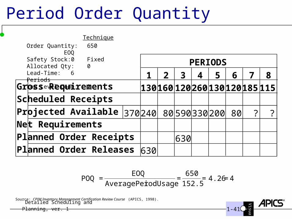
Period Order Quantity
Source: CPIM Inventory Management Certification Review Course (APICS, 1998).
1-41a
Visual
Gross Requirements
Scheduled Receipts
Projected Available
Net Requirements
Planned Order Receipts
Planned Order Releases
1 2 43 765
PERIODS
?
130 160 120 260 130 120 185
8
Order Quantity: 650 EOQSafety Stock: 0 FixedAllocated Qty: 0Lead-Time: 6 PeriodsLow Level Code: 2
Technique
115
370 80 330 200 80 ?240 590
630630
4=4.26152.5650
=iodUsageAveragePer
EOQ=POQ =
1-50
Visual
Detailed Scheduling and Planning, ver. 11-42
Visual
Lot for Lot
The sum of requirements for a period.With MRP replanning nightly, the periods can be as short as one day
Visual
Detailed Scheduling and Planning, ver. 1
Session 1 Review
Identify types of inventory and how they are assessed from their different requirements and impacts on the planning process
Describe order review methodologies and apply them to different types of inventory and inventory strategies
Identify lot sizing techniques, including the effects of order quantity constraints, and modifiers
1-43