©Copyright 2013

Yunior I. Cruz

An Algorithm for Autonomous Formation Obstacle Avoidance

Yunior I. Cruz

A thesis

submitted in partial fulfillment of the

requirements for the degree of

Master of Science in Aeronautics and Astronautics

University of Washington

2013

Committee:

Juris Vagners

Kristi Morgansen

Christopher Lum

Program Authorized to Offer Degree:

Aeronautics and Astronautics

The views expressed in this article are those of the author and do not reflect the official policy or

position of the United States Air Force, Department of Defense, or the U.S. Government.

ii

University of Washington

Abstract

An Algorithm for Autonomous Formation Obstacle Avoidance

Yunior I. Cruz

Chair of Supervisory Committee:

Juris Vagners, Professor Emeritus

Department of Aeronautics and Astronautics

The level of human interaction with Unmanned Aerial Systems varies greatly from remotely

piloted aircraft to fully autonomous systems. In the latter end of the spectrum, the challenge lies

in designing effective algorithms to dictate the behavior of the autonomous agents. A swarm of

autonomous Unmanned Aerial Vehicles requires collision avoidance and formation flight

algorithms to negotiate environmental challenges it may encounter during the execution of its

mission, which may include obstacles and chokepoints. In this work, a simple algorithm is

developed to allow a formation of autonomous vehicles to perform point to point navigation

while avoiding obstacles and navigating through chokepoints. Emphasis is placed on

maintaining formation structures. Rather than breaking formation and individually navigating

around the obstacle or through the chokepoint, vehicles are required to assemble into

appropriately sized/shaped sub-formations, bifurcate around the obstacle or negotiate the

chokepoint, and reassemble into the original formation at the far side of the obstruction. The

algorithm receives vehicle and environmental properties as inputs and outputs trajectories for

each vehicle from start to the desired ending location. Simulation results show that the algorithm

safely routes all vehicles past the obstruction while adhering to the aforementioned requirements.

The formation adapts and successfully negotiates the obstacles and chokepoints in its path while

maintaining proper vehicle separation.

iii

TABLE OF CONTENTS

LIST OF FIGURES ........................................................................................................................ v

Chapter 1. Introduction. ................................................................................................................. 1

1.1 Problem Definition ........................................................................................................... 2

1.2 Assumptions ...................................................................................................................... 3

Chapter 2. Review of Collision Avoidance Algorithms ................................................................. 4

2.1 Decentralized Reactive Collision Avoidance ................................................................... 4

2.1.1 Overview ................................................................................................................... 4

2.1.2 Collision Cones ......................................................................................................... 5

2.1.3 Algorithm .................................................................................................................. 6

2.1.4 Applicability .............................................................................................................. 7

2.2 Artificial Potential Fields ................................................................................................. 7

2.2.1 Overview ................................................................................................................... 7

2.2.2 Calculating Force Vectors ........................................................................................ 8

2.2.3 Algorithm .................................................................................................................. 8

2.2.4 Applicability .............................................................................................................. 8

Chapter 3. Review of Formation Flight Algorithms ...................................................................... 9

3.1 Leader-Follower Approach .............................................................................................. 9

3.1.1 Overview ................................................................................................................... 9

3.1.2 Simultaneous Tracking in Finite Time ...................................................................... 9

3.1.3 Applicability .............................................................................................................. 9

3.2 Control Graph Theory .................................................................................................... 10

3.2.1 Overview ................................................................................................................. 10

3.2.2 Modeling Formations.............................................................................................. 10

Chapter 4. Algorithm Development ............................................................................................. 12

iv

4.1 Phase 1 ................................................................................................................................ 14

4.2 Phase 2 ................................................................................................................................ 15

4.2.1 Determining Bifurcation Behavior ......................................................................... 15

4.2.2 Determining Vehicles’ Locations at End of Phase 2 .............................................. 17

4.2.3 Computing Trajectories during Phase 2 ................................................................. 22

4.3 Phase 3 ................................................................................................................................ 22

4.4 Phase 4 ................................................................................................................................ 23

Chapter 5. Test Setup and Results ............................................................................................... 24

5.1 Head-on Obstacle in Free Space ........................................................................................ 25

5.2 Offset Obstacle in Free Space ............................................................................................. 27

5.3 Head-on Obstacle with Spatial Restrictions ....................................................................... 28

5.4 Offset Obstacle with Spatial Restrictions ............................................................................ 31

5.5 Chokepoint .......................................................................................................................... 32

Chapter 6. Conclusion ................................................................................................................... 34

6.1 Future Work ........................................................................................................................ 34

Works Cited .................................................................................................................................. 36

APPENDIX A ............................................................................................................................... 37

v

LIST OF FIGURES

Figure 2.1 DRCA algorithm flow chart [3] ................................................................................... 5

Figure 2.2. The collision cone is defined as the area between the two dotted lines. If the relative

velocity vector v lies within this area, the vehicles are said to be in conflict [3] ........................... 6

Figure 3.1. Control graph describing one possible formation configuration for a group of six

vehicles [8] .................................................................................................................................... 10

Figure 3.2. Formation change using Control Graph Theory [9] .................................................. 11

Figure 4.1. Algorithm overview scenario .................................................................................... 12

Figure 4.2. Chokepoint scenario .................................................................................................. 13

Figure 4.3. Overview of phases of algorithm .............................................................................. 14

Figure 4.4. Sampling of formation configurations....................................................................... 14

Figure 4.5. Formation leader's x-coordinate at end of Phase 2 .................................................... 18

Figure 4.6. Formation leader's x-coordinate during left avoidance maneuver ............................ 19

Figure 4.7. Formation leader's x-coordinate to minimize travel distance .................................... 19

Figure 4.8. Formation leader's x-coordinate at end of Phase 2 when left opening is less than or

equal to the original formation's width ......................................................................................... 20

Figure 4.9. Simplest way to define leader's y-coordinate for safe avoidance .............................. 20

Figure 4.10. Result of iteration process to produce furthest possible sub-formation leader ending

y-coordinate .................................................................................................................................. 21

Figure 5.1. Formation of 10 vehicles to avoid circular obstacle in path of travel ....................... 25

Figure 5.2. Trajectories followed by 10 vehicles as they bifurcate around obstacle ................... 25

Figure 5.3. Minimum vehicle separation during 10 vehicle avoidance maneuver ...................... 26

Figure 5.4. Formation of 10 vehicles to avoid elliptical obstacle partially in its path .................. 27

Figure 5.5. Trajectories followed by 10 vehicles as they bifurcate around elliptical obstacle ..... 27

Figure 5.6. Minimum vehicle separation during 10 vehicle avoidance maneuver ....................... 28

Figure 5.7. Formation of 12 vehicles avoiding elliptical obstacle head-on with spacing

constraints ..................................................................................................................................... 29

Figure 5.8. Effect of larger right to left spacing ratio on formation bifurcation behavior ........... 30

Figure 5.9. Minimum vehicle separations during 12 vehicle obstacle avoidance for smaller (left)

and larger (right) available right spacing ...................................................................................... 30

vi

Figure 5.10. Effect of larger in-formation vehicle separation on minimum vehicle separations

during 12 vehicle obstacle avoidance for smaller (left) and larger (right) available right spacing

....................................................................................................................................................... 31

Figure 5.11. Formation of 13 vehicles avoiding offset elliptical obstacle with spacing constraints

....................................................................................................................................................... 32

Figure 5.12. Formation of 10 vehicles navigating through a chokepoint .................................... 32

Figure 5.13. Formation of 10 vehicles navigating through a narrow offset chokepoint .............. 33

vii

ACKNOWLEDGEMENTS

I would like to thank Dr. Juris Vagners and Dr. Christopher Lum for their oversight and

guidance. Their support and advice proved instrumental to my success. Dr. Lum’s early work on

the subject served as inspiration for my work, and his inputs and ideas during the initial portion

of my research proved invaluable. Dr. Vagners’ continuous feedback kept me engaged and

striving for excellence all throughout. I would also like to thank LtCol Barret McCann, SSgt

Levar Jackson, as well as Mrs. Wanda Frederick for their unwavering support and advice during

my time at the University of Washington. Finally, thanks to my family and friends for their

continuing support. May God bless you all.

viii

DEDICATION

I dedicate this work the most important person in my life, my mother. Mama, I know you look

down upon me from the heavens and are very proud of what I have done. I will strive to

continue making you proud for the rest of my life. I know you will be there with me when I

fulfill my childhood dreams of slipping the surly bonds of Earth and dancing the skies on

laughter-silvered wings. May God bless and keep you in His wings until we meet again.

1

Chapter 1. Introduction.

Interest in Unmanned Aerial Vehicle (UAV) research has significantly surged over the past

decade. Commonly referred to as drones, these systems provide many advantages over their

manned counterparts, including reduced risk to human life and the ability to persist over a target

area for extended periods of time limited only by the amount of fuel the can carry. The level of

human interaction with UAVs varies greatly from remotely piloted aircraft (RPA), where a pilot

directly controls the vehicle from a ground station, to fully autonomous systems, where a

computer is in charge of deciding and executing most or all of the system’s functions while

human interaction is limited to high level strategic decisions. This work focuses on the latter end

of the spectrum. Autonomous UAVs require algorithms to dictate their behavior and determine

how they interact with their environment as well as other manned and unmanned systems.

UAVs can be used for a wide variety of missions, including Intelligence, Surveillance, and

Reconnaissance (ISR), survey of natural disasters, and even armed combat. In some cases, it

proves advantageous to use multiple UAVs for a given mission. For instance, instead of using

one large, fast, expensive vehicle to search an area of interest, it may be more convenient to use

several smaller, slower, less expensive vehicles to perform the same mission in the same amount

of time. The hindrance on mission success incurred by the risk of losing a vehicle is

significantly reduced in latter case. When multiple autonomous vehicles are used, collision

avoidance algorithms are needed to ensure safety through proper vehicle separation. It is often

desirable to have a swarm of autonomous vehicles move within the environment in distinct,

structured formations. This in turn requires formation flight algorithms to prescribe overall

formation behavior as well as vehicle-formation interactions. The first part of this work provides

a survey of some existing collision avoidance and formation flight algorithms.

A formation of autonomous UAVs may encounter various environmental obstacles during

the execution of its mission such as large buildings, mountainous regions, or heavily defended

airspace that must be avoided. It may also encounter chokepoints like canyon entrances or

narrow openings in air defenses that require adjustments in formation structures to be safely

negotiated. The main goal of this work is to develop a simple algorithm to prescribe the strategy

a formation of autonomous UAVs should follow to bifurcate around an obstacle or navigate

through a chokepoint in its environment while maintaining formation structures whenever

possible.

2

This thesis is organized as follows. The main problem to be addressed in this work is

presented in further detail in the next section. Chapters 2 and 3 present a brief literature review

of existing collision avoidance and formation flight algorithms, respectively. Two collision

avoidance algorithms (Decentralized Reactive Collision Avoidance (DRCA) and Artificial

Potential Field (APF)) and two formation flight algorithms (Leader-Follower Approach and

Formation Graph Theory Approach) are discussed in detail. The proposed algorithm is presented

in Chapter 4, which represents the bulk of this thesis. Test setup and simulation results are

presented in Chapter 5. Finally, Chapter 6 presents the conclusion and recommendations for

future improvements.

1.1 Problem Definition

The problem of navigating a swarm of UAVs through cluttered and dynamic environments has

been studied before. In their work with Boeing, Lum et al [1] used vector field navigation to

synthesize an algorithm that successfully navigated a formation of small scale quadrotor UAVs

through chokepoints and around static and moving obstacles. This modular algorithm consisted

of three different classes of controllers. The Class 1 controller was in charge of obstacle

avoidance and was used when the formation needed to bifurcate around an obstacle. The Class 2

controller was implemented to navigate the formation through a chokepoint. Finally, the Class 3

controller moved the formation in free space and maintained proper inter-vehicle separation.

The basic idea was that if the formation encountered an obstacle or chokepoint, vehicles would

break formation and navigate past the obstruction in a similar manner that fluid particles would;

i.e. vehicles would ride the streamlines created by fluid flow around the obstacle or through the

chokepoint. The algorithm was tested in a high fidelity simulation environment before small-

scale quadrotor UAVs were used to validate the algorithm in the Boeing Vehicle Swarm

Technology Laboratory (VSTL).

The present work deals with tackling the problem of formation bifurcation around an

obstacle and chokepoint navigation from a different perspective. It is desired to design an

algorithm that provides the logic a formation should follow to subdivide into appropriately

sized/shaped sub-formations, navigate around the obstacle or through the chokepoint, and merge

into the original formation at the far end. These requirements must be met while maintaining

proper inter-vehicle separation.

3

The algorithm is be designed to work in two dimensions, with the justification that a two

dimensional domain is more restrictive than a three dimensional domain. With some

modifications, the algorithm would in theory be adaptable to three dimensions. Furthermore, in

a two dimensional setting, the algorithm could be used for autonomous surface vehicles.

1.2 Assumptions

Environmental factors like weather and wind are ignored, and it is assumed that each

vehicle’s position is known exactly at all times. It is further assumed that the position of the

obstacle is known and that the obstacle can be modeled as an ellipse having length, width, and

orientation. The algorithm is considered to be a high level controller, with low level

maneuvering of individual vehicles assumed to be handled by onboard inner-loop controllers.

As such, the algorithm’s main outputs are waypoint commands to each vehicle, and the vehicle’s

inner-loop controller is assumed to follow said commands exactly.

4

Chapter 2. Review of Collision Avoidance Algorithms

Collision avoidance algorithms are necessary for a group of autonomous UAVs to safely interact

with each other and with the environment. The main goal of any collision avoidance algorithm

is to allow vehicles to follow their desired controllers while maintaining safety through proper

vehicle separation. Collision avoidance strategies can be grouped into three main categories:

optimized, prescribed, and force fields [2], [3]. Optimized approaches make use of optimization

schemes to minimize some cost function in order to find the best possible solution to the

collision avoidance problem. Prescribed approaches utilize discrete controllers combined with

vehicle continuous dynamics to have vehicles follow some prescribed protocol such as executing

right hand turns when in conflict with oncoming vehicles. Force field approaches model

vehicles as charged particles and use feedback techniques to compute appropriate controls.

Following is an overview of two well-known collision avoidance algorithms from the literature,

as well as a brief discussion of their applicability to the present work.

2.1 Decentralized Reactive Collision Avoidance

2.1.1 Overview

The Decentralized Reactive Collision Avoidance (DRCA) algorithm is based on the collision

cones concept [4] and consists of two main parts: an optimization-based deconfliction maneuver

followed by a force field approach for long term deconfliction maintenance [3]. The algorithm

defines a conflict as a situation in which, if two vehicles continue on their current path with

constant velocity they will enter a collision sometime in the future. A collision is defined as a

situation in which two vehicles come within some minimum distance of each other. Being partly

an optimized approach, this algorithm guarantees the existence of solutions given certain

constraints on the initial conditions. The DRCA algorithm is distributed by not decentralized

and requires all-to-all communication [3]. Furthermore, it is assumed that vehicles can be

modeled as point masses. The overall approach is depicted below.

5

Figure 2.1 DRCA algorithm flow chart [3]

If the vehicles are initially sufficiently separated, they are allowed to follow their desired

controller. If not, then the algorithm looks at whether or not the vehicles are in a conflict

according to the aforementioned definition. If no conflict is detected, then the deconfliction

maintenance controller continues to keep the vehicles out of conflict. If a conflict is detected,

then the deconfliction maneuver is executed to bring the vehicles out of conflict.

2.1.2 Collision Cones

The DRCA algorithm makes use of the collision cones concept, which is a set of relative

velocities between two vehicles that will produce a collision in the absence of inputs (see Figure

2). The angle between the relative position vector ̃ and the relative velocity vector ̃ being

greater than or equal to the angle between the relative position vector and the end of the

collision cone is a necessary and sufficient condition to assure that there is no conflict, the proof

of which can be found in [4].

6

Figure 2.2. The collision cone is defined as the area between the two dotted lines. If the relative velocity vector v lies

within this area, the vehicles are said to be in conflict [3]

2.1.3 Algorithm

The DRCA Algorithm provides collision avoidance guarantees based on three theorems.

1. The deconfliction maintenance controller is guaranteed to keep vehicles conflict free if

the group of vehicles starts conflict free.

2. The deconfliction maneuver controller is guaranteed to steer vehicles out of conflict and

prevent them from colliding during the maneuver.

3. There needs to be a conservative separation criterion to ensure the deconfliction

maneuver will bring the vehicles to a conflict free state

Note: Proofs are omitted for brevity but can be found in [3].

The first step of DRCA is to decide when a vehicle needs to perform its deconfliction

maneuver. To do this, is defined to be the set of vehicles performing a deconfliction maneuver

or in the deconfliction maintenance phase. It is assumed that each vehicle in is able to

broadcast its position and velocity to all other vehicles in . A vehicle is allowed to follow its

controller until it comes into conflict with another vehicle. When the vehicle enters into a

conflict, it becomes part of and executes a deconfliction maneuver.

The deconfliction maneuver entails choosing a conflict-free velocity vector based on the

collision cone and quickly accelerating towards it. The vehicle broadcasts its desired conflict-

free velocity vector while executing this maneuver so as to ensure safety during the maneuver

7

and after the new velocity is established. Once the vehicle is out of conflict with all other

vehicles in , it switches to deconfliction maintenance.

The deconfliction maintenance phase entails calculating how far a given vehicle’s velocity

vector is from causing a conflict based on the collision cone [3]. This measure is then used to

compute how much control can be applied in each direction before a conflict arises. The

algorithm then manages how much input is applied in each direction so as to stay away from

these control limits that would cause a conflict.

2.1.4 Applicability

When vehicles move in formation, their velocities are nearly identical. According to the

definitions prescribed by the DRCA algorithm, each vehicle’s velocity vector is on the verge of

conflict with every other vehicle’s velocity vector. The DRCA algorithm will therefore

command each vehicle’s velocity vector to diverge from every other vehicle’s velocity vector,

causing the formation to break up. As a result, the DRCA requires extensive modification if it is

to be applied to each vehicle individually for the purpose of formation maintenance and

navigation. However, if the formation is treated as a single cohesive unit, the DRCA algorithm

could be implemented between the formation and a static or moving obstacle in the environment.

2.2 Artificial Potential Fields

2.2.1 Overview

Collision avoidance based on artificial potential fields is a reactive approach that takes its

inspiration from physics. Vehicles are modeled as charged particles, with equally charged

particles repelling each other and differently charged particles attracting each other [5]. As such,

vehicles are arbitrarily assigned negative charges, while their corresponding desired waypoints

take on positive charges. Force vectors computed based on these charges are then used to

calculate each vehicle’s direction of travel.

8

2.2.2 Calculating Force Vectors

The key step in developing a potential field algorithm is to define a way to calculate the force

vectors. There are various ways to implement a force field algorithm, and the level of

complexity depends on many variables such as the aircraft model used as well as the required

level of fidelity. The presently discussed application is a relatively simple implementation that

was developed for fixed wing aircraft.

First, some arbitrary parameters such as an oval shaped ‘safety’ zone around each aircraft as

well as distance traveled in one second are used to define a distance at which the repulsive force

from another aircraft becomes negligible. This distance is then used in conjunction with other

parameters such as negative charge constants from other vehicles to calculate the repulsive force

emitted by other vehicles. These repulsive forces are then scaled based on relative angles

between vehicles to calculate the actual repulsive forces felt by the vehicle in question. The

attractive force felt from the vehicle’s desired waypoint is taken as a constant. Finally, the

attractive force is added to all the repulsive forces from other vehicles to calculate the total force

felt by a given vehicle, which determines its direction of travel. Calculation details and

equations can be found in [5], [6].

2.2.3 Algorithm

The main complexity in force-field based collision avoidance lies in how the repulsive and

attractive forces are calculated. Once these forces are added into a single force vector for each

aircraft, the algorithm to execute the collision avoidance is quite simple. If the force vector lies

outside the maximum turn rate of the particular aircraft model used, then the algorithm

commands the vehicle to turn as quickly as it can towards the force vector direction. If the force

vector lies within the turn rate limit of the vehicle, then the algorithm commands the vehicle to

turn to match the prescribed force vector angle exactly.

2.2.4 Applicability

A simple implementation of force field based collision avoidance can be used on each vehicle within

a formation to maintain proper inter-vehicle separation. However, due to their reactive nature,

artificial potential field algorithms are not as effective for high level formation obstacle avoidance.

9

Chapter 3. Review of Formation Flight Algorithms

Formation flight algorithms are necessary for a group of autonomous UAVs to safely navigate its

environment in a structured formation. The main goal of any formation flight algorithm is to

dictate the rules and strategies individual vehicles should follow as they perform various tasks in

close formation to other vehicles while maintaining proper inter-vehicle separation. Inherent in

any formation flight algorithm is the need for collision avoidance guarantees. This can often be

accomplished with various tools from the literature such as a potential field approach like the one

discussed in the preceding section. Following is an overview of two formation flight algorithms,

as well as a brief discussion of their applicability to the present work.

3.1 Leader-Follower Approach

3.1.1 Overview

This approach addresses the UAV formation flight problem from a leader-follower perspective

using optimal control theory, where a designated formation leader receives and follows

formation trajectory commands and the followers derive their trajectories relative to the leader

[7]. Vehicles are modeled as points of unit mass with decoupled, second order dynamics. The

model is purely kinematic with direct control of acceleration in each of the three dimensions.

Computed relative to the leader, each follower’s position is determined based on current

formation needs and environmental factors such as spatial restrictions.

3.1.2 Simultaneous Tracking in Finite Time

The algorithm uses an optimal control approach to track multiple trajectories in finite time.

Given twice differentiable set of desired trajectories, the algorithm defines an error signal in each

of the states and uses this information to compute the control law to drive the system to track the

desired trajectory [7].

3.1.3 Applicability

The overall formation strategy used in the present work is a simple implementation of the leader-

follower idea. High level formation maneuvering is prescribed by one part of the algorithm,

10

which decides how the formation behaves as it encounters an obstacle (i.e. divide into sub-

formations). The paths to be followed by the other vehicles in the formation are then derived

relative to the leader. These desired trajectories can then be made twice differentiable via

filtering and applied to a given aircraft model’s inverse dynamics to derive the appropriate

controls using optimal control theory.

3.2 Control Graph Theory

3.2.1 Overview

Control graph theory prescribes and enumerates all possible control graphs (or formation

representations) and coordinates the transition between any two formation configurations for a

given set of nonholonomic vehicles [8], [9]. Formations are modeled as triples describing the

leader, the shape, and the control graph. This approach is a tool that can be useful in the

development of a formation flight algorithm, for it provides a framework to represent and model

a formation of autonomous vehicles mathematically using simple matrix manipulation.

3.2.2 Modeling Formations

Groups of mobile robots can be described by a triple ( ), where is a group variable

representing the motion of the leader, is a set of shape variables which dictates the position of

the followers relative to the leader, and is a control graph describing the strategy or behavior

that the members of the formation should follow. Figure 3 below shows an example of a control

graph, presented in both visual (left) and graphical or matrix (right) form.

Figure 3.1. Control graph describing one possible formation configuration for a group of six vehicles [8]

The absence of 1’s in the first column indicates that the leader (R1) derives its control from no

other vehicle in the formation. The 1 in the first row of the second column indicates that R2

derives its control relative to R1 only, while the 1’s in the first and second rows of the third

11

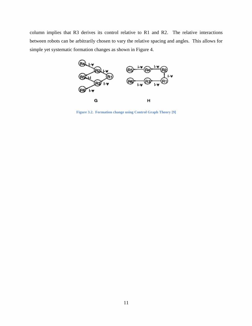
column implies that R3 derives its control relative to R1 and R2. The relative interactions

between robots can be arbitrarily chosen to vary the relative spacing and angles. This allows for

simple yet systematic formation changes as shown in Figure 4.

Figure 3.2. Formation change using Control Graph Theory [9]

12

Chapter 4. Algorithm Development

The main goal of this algorithm is to provide the strategy that a formation of autonomous

vehicles should follow as it transverses the space between two points while avoiding an obstacle

or navigating through a chokepoint along the way. The overall scenario is displayed in Figure 5.

The obstacle is modeled as an ellipse having a major axis, minor axis, and orientation. The

algorithm intakes vehicle properties such as number of vehicles, desired speed, starting and

desired ending formation leader location, as well as obstacle properties such as location, shape,

and side clearances (represented by artificial horizontal barriers), and outputs the trajectories that

each vehicle should follow as the formation bifurcates around the obstacle with the requirement

that each subgroup of vehicles should assemble into appropriately sized/shaped sub-formations.

Figure 4.1. Algorithm overview scenario

In a real world scenario, the formation’s starting and ending locations can take any values,

producing any value for the heading the formation travels in. For simplicity, this algorithm

assumes that the real world scenario has undergone a coordinate transformation so as to orient

the path of travel from south to north as depicted, with the justification that the desired vehicle

trajectories outputted by this algorithm can then be easily transformed back to the real world

scenario using the inverse coordinate transformation. In the absence of any obstacles, the

formation should follow a straight path from the desired starting to the desired ending location.

The obstacle may be exactly aligned with or partially obstructing the formation’s path. The

algorithm should decide whether to route the entire formation around the obstacle or split it into

13

smaller sub-formations. Spacing constraints on both sides of the obstacle are included to allow

for the algorithm to handle other environmental obstacles such as chokepoints (by closing off

one path) as depicted in Figure 6. The artificially imposed barriers could also represent the

beginning of restricted airspace or other areas that must be avoided. The algorithm must

therefore consider lateral spacing constraints in addition to the obstacle’s relative positioning in

deciding how to split the formation.

Figure 4.2. Chokepoint scenario

The algorithm is broken down into four phases, each of which handles a portion of the

maneuvering from starting to ending location. During Phase 1, the formation travels in a straight

path for an arbitrary amount of time, simulating the time period before the formation receives

information about the presence of the obstacle. During Phase 2, the algorithm decides whether

or how to split the formation and directs the formation(s) to the appropriate lateral positioning

alongside the obstacle and parallel to the formation’s original heading (vertical). In Phase 3, the

formation or sub-formations travel alongside and clear the obstacle. Finally, in Phase 4, the

formations converge on the desired ending location and morph into the original formation. All

phases are depicted in Figure 7. Phases 1 and 3 are straight line trajectories while Phases 2 and 4

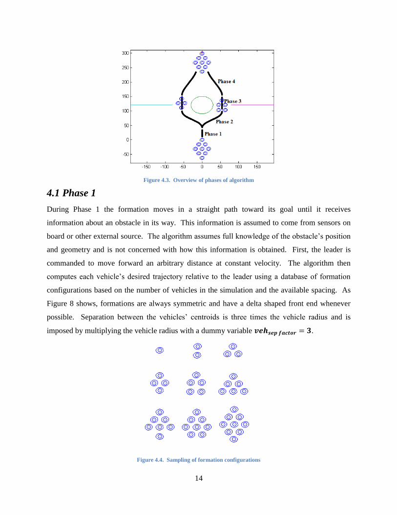
are sinusoidal. The remainder of this section describes how the algorithm executes each phase.

14

Figure 4.3. Overview of phases of algorithm

4.1 Phase 1

During Phase 1 the formation moves in a straight path toward its goal until it receives

information about an obstacle in its way. This information is assumed to come from sensors on

board or other external source. The algorithm assumes full knowledge of the obstacle’s position

and geometry and is not concerned with how this information is obtained. First, the leader is

commanded to move forward an arbitrary distance at constant velocity. The algorithm then

computes each vehicle’s desired trajectory relative to the leader using a database of formation

configurations based on the number of vehicles in the simulation and the available spacing. As

Figure 8 shows, formations are always symmetric and have a delta shaped front end whenever

possible. Separation between the vehicles’ centroids is three times the vehicle radius and is

imposed by multiplying the vehicle radius with a dummy variable .

Figure 4.4. Sampling of formation configurations

15

4.2 Phase 2

During Phase 2, the formation prepares to clear the obstacle by changing its shape, lining up to

either side of the obstacle, splitting into smaller sub-formations, or a combination thereof.

Factors such as obstacle positioning and relative clearance on either side of the obstacle are

considered.

4.2.1 Determining Bifurcation Behavior

The first step in executing Phase 2 is deciding how many vehicles to send to each side of the

obstacle. This is done by evaluating a series of conditional statements involving the obstacle’s

position, side clearances, and number of vehicles in the simulation.

First, some useful parameters are computed to be compared to the prescribed clearance on

either side of the obstacle to aid in the execution of the conditional statements to follow. The

variable , the minimum distance that any vehicle may be from the obstacle, is

defined to be equal to the vehicle radius. Next, is defined as the minimum clearance

required for a single vehicle to pass through and is calculated as follows

( ) (1)

Similarly, the minimum clearances required for two, three, and four vehicles to pass through

side by side are calculated. These measures aid in the algorithm’s decision process to determine

how/if to split up the formation.

( ) (2)

[ ( ) ] (3)

( ) (4)

The starting formation’s width is then calculated based on the number of vehicles used and

the formation catalog from Figure 8. If the left clearance is smaller than and the right clearance

is at least as large as , then all vehicles are routed to the right side of the obstacle. On

the other hand, if the right clearance is smaller than and the left clearance is at least as large as

, all vehicles are routed to the obstacle’s left side. If the clearances on both sides of the

obstacle are smaller than this minimum single vehicle spacing requirement, then the algorithm

commands the formation to stop at the end of Phase 1. If none of these conditions are met,

further conditional statements are imposed.

16

If the obstacle’s x-position places it to the left of the formation centroid at the end of Phase

1, the following protocol is used. If the clearance on the right side is at least as large as

or it is smaller than provided that the left clearance is also smaller than , then

the algorithm commands all vehicles that at the end of Phase 1 are lined up with or to the right of

the obstacle’s centroid to move to right of the obstacle. The remaining vehicles move left.

Failure to meet these requirements indicates that the right clearance only allows vehicles to move

through in a single file (inefficient due to dramatic formation changes required) and that the left

clearance is at least as large as .

The obstacle’s positioning (left of the formation) would favor sending more vehicles to the

right; however, clearance constraints (large clearance of the left, small on the right) would favor

sending more vehicles to the left. Because moving a large number of vehicles in a single file is

inefficient, a compromise must be reached. First, the algorithm counts how many vehicles are

lined up with or to the right of the obstacle’s centroid. Clearly, due to the geometry of this

situation more vehicles are lined up with or to the right of the obstacle centroid. Since it is

desired to avoid the inefficient situation in which a large number of vehicles move in single file,

the algorithm routes one half of the counted vehicles to the right, sending the remainder to the

left.

If the obstacle’s x-position places it to the right of the formation’s centroid at the end of

Phase 1, the exact opposite of the aforementioned protocol is employed. In the case where the

obstacle centroid lies directly in the path of the formation, further conditional statements are

imposed.

If the either the right or left clearances are greater than the formation’s width, then the

following logic is employed. If the clearance on the right side is at least as large as or it

is smaller than provided that the left clearance is also smaller than , then

vehicles lined up to the right of the obstacle centroid are routed right, and vehicles that are

initially left of the centroid are routed left. Because formations are triangular in shape whenever

possible and symmetric, in the case where the obstacle and formation centroids are in line there

will always be one or more vehicles that are exactly aligned with the obstacle’s centroid. These

vehicles are split evenly during the bifurcation, and the right is given the additional vehicle in

case of an odd number. If the right clearance is less than and the left clearance is greater than

17

(failure to meet previous conditional statement), then the additional vehicle is assigned

to the left side when an odd number of vehicles are aligned with the obstacle’s centroid.

In the case where neither the right nor left clearances are greater than the formation’s width,

the following protocol is used. The number of vehicles directed to each side is proportioned

according to the relative sizing of the clearances; i.e. if the left clearance is 30% greater than the

right clearance, vehicles are given assignments such that 30% more vehicles will end up

avoiding the obstacle around its left side, rounded to the nearest vehicle. This procedure is not

also used in the case where side clearances are large (as discussed in preceding paragraph)

because in that case obstacle positioning proves more relevant than clearance measures. The

entire decision process to determine how many vehicles to send to each side of the obstacle is

depicted in a flow chart in Figure A1 of Appendix A.

At this point, the algorithm has decided how many vehicles will go to each side of the

obstacle. The next step is to determine vehicle ending locations at the end of phase 2.

4.2.2 Determining Vehicles’ Locations at End of Phase 2

In order to determine each vehicle’s trajectory during Phase 2, the algorithm needs to have

knowledge of the vehicles’ starting locations and desired ending locations at the end of this

phase. These starting and ending coordinates are then fed to a different part of the algorithm

which computes smooth sinusoidal trajectories for each vehicle (to be discussed later). The

ending locations depend on a combination of factors as the following process will show.

Because vehicles’ locations are computed relative to a chosen leader, the algorithm must first

determine each sub-formation’s leader’s desired location and the end of Phase 2. These ending

locations depend on the obstacle’s positioning, available side clearances, number of vehicles

assigned to each side of the obstacle, and corresponding formation configuration derived from all

of the above.

The first immediate task for the algorithm at this point is to compute the x and y coordinates

of each sub-formation leader’s ending locations at the end of Phase 2.

In the case where the algorithm has decided that all vehicles should be routed to the left of

the obstacle, the following logic is used. First, the left formation’s width is calculated based on

the number of vehicles routed left (in this case all), the left clearance, and the appropriate

formation shape. The formation shape is changed as required to ensure it fits through the left

18

opening using a modified version of the same function used to compute the relative position of

vehicles in the original formation. The way the algorithm is set up, the starting formation

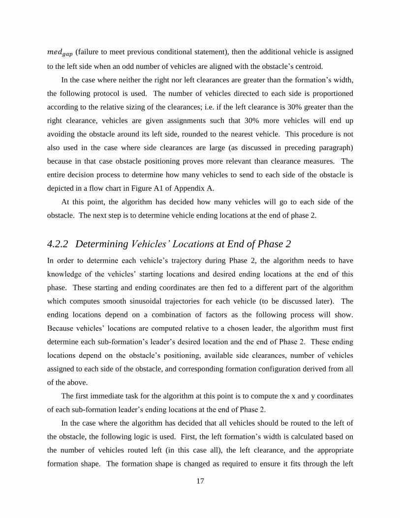
location and the goal location are aligned vertically; i.e. have the same x-coordinates. If the

formation’s right edge is left of the obstacle’s left edge and the formation’s left edge is right of

the left barrier’s end, then the formation leader’s ending x-coordinate for Phase 2 is the same as

the goal’s x-coordinate as shown in Figure 9. The ending x-coordinate is depicted as a line

because the y-coordinate is later computed using an iterative process (to be later discussed)

which ensures the formation covers the least possible distance during the avoidance maneuver.

Figure 4.5. Formation leader's x-coordinate at end of Phase 2

Still considering the case where all vehicles are routed left, if the obstacle’s left edge is left

of the formation’s right edge and the left clearance is large enough to not necessitate a formation

change, then the leader’s x-coordinate at the end of Phase 2 is defined such that the formation

will pass through the left opening as close to the obstacle’s left edge as possible (but never less

than the minimum allowed distance ). Figure 10 depicts this scenario.

19

Figure 4.6. Formation leader's x-coordinate during left avoidance maneuver

On the other extreme, if the left barrier end is right of the formation’s left edge, the

algorithm defines the formation leader’s x-coordinate at the end of Phase 2 such that the

formation travels the least possible distance to the goal as shown in Figure 11.

Figure 4.7. Formation leader's x-coordinate to minimize travel distance

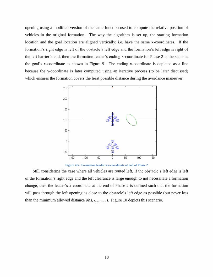
Finally, if the left clearance is less than or equal to the formation’s width, the algorithm

defines the leader’s x-coordinate exactly in the middle of the opening regardless of obstacle

positioning as shown in Figure 12.

20

Figure 4.8. Formation leader's x-coordinate at end of Phase 2 when left opening is less than or equal to the original

formation's width

With the formation leader’s x-coordinate at the end of Phase 2 defined, the algorithm then

computes the leader’s y-coordinate. The simplest way to ensure the formation clears the obstacle

safely is to define the y-coordinate such that the formation leader’s position at the end of Phase 2

is aligned horizontally with the obstacle’s bottom edge as in Figure 11.

Figure 4.9. Simplest way to define leader's y-coordinate for safe avoidance

However, given the possible complexity of the obstacle’s geometry, a more intricate

approach should be used to ensure the vehicles follow the shortest path around the obstacle from

start to goal. Starting with the case shown in Figure 13, the algorithm computes each vehicle’s

sinusoidal trajectory from starting location to the Phase 2 ending locations shown in Figure 13.

As long as no vehicle’s trajectory comes within of the obstacle’s edge, the

algorithm moves the leader’s y-position forward by an arbitrarily small amount and repeats this

procedure. The other vehicle’s positions are recomputed relative to the leader’s new position

21

and the sinusoidal trajectories are recomputed. Once any vehicle’s trajectory breaks this

minimum separation requirement with the obstacle’s edge, the algorithm chooses the last safe

leader’s y-coordinate as the optimal value. Figure 14 depicts this process.

Figure 4.10. Result of iteration process to produce furthest possible sub-formation leader ending y-coordinate

If the optimal y-coordinate according to the presented scheme is such that the southernmost

vehicle in the formation ends up being north of the obstacle’s upper edge at the end of Phase 2,

the algorithm chooses the leader’s y-coordinate at the end of Phase 2 such that the southernmost

vehicle is aligned with the obstacle’s upper edge. This ensures the vehicles can begin their

convergence maneuver onto the goal as early as possible. In this case, the algorithm skips Phase

3 and goes immediately into Phase 4.

In the case where the algorithm has decided that all vehicles should be routed to the right

of the obstacle, a similar approach as the one presented above is used with all conditions

reversed and all equivalent values mirrored across the vertical axis. The last case to consider is

where the formation splits into two smaller formations as it bifurcates around the obstacle. In

this case the algorithm also follows the same overall approach treating each side of the problem

as individual entities with their corresponding number of vehicles and formation shapes, given

the problem geometry.

At this point, the algorithm knows each sub-formation leader’s location at the end of Phase 2

and computes each vehicle’s ending location relative to the leaders. It also knows the number of

vehicles assigned to each side of the obstacle, but lacks knowledge of which vehicles should go

to which side. The next step is to assign specific vehicles to each side based on the total number

22

of vehicles and the outcome of the decision process in section 4.2.1, and to compute their

trajectories during Phase 2.

4.2.3 Computing Trajectories during Phase 2

At this point the algorithm has knowledge of all vehicles’ starting locations in the original

formation, the number of vehicles assigned to each side of the obstacle, as well as each desired

sub-formation configuration and position at the end of Phase 2. The next step is to decide which

vehicles to send to each side. Once these assignments are made, the trajectory computation

phase reduces down to inputting each vehicle’s starting as well as its corresponding location at

the end of Phase 2 (as previously computed) into a function that defines a sinusoidal trajectory

between those two points.

The assignment process is done in a systematic way and is hard coded into an extensive file

containing a large number of conditional statements that cover all possibilities for assignments

given the problem geometry. As an example, if the algorithm decides a formation of 10 vehicles

should be split such that three vehicles go right and the right clearance is large enough for a delta

formation of three to pass through, the algorithm commands the three right-most vehicles in the

original formation to break off. Based on their positions in the original formation, these vehicles

are assigned positions in the smaller sub-formation such that their individual sinusoidal

trajectories will not intercept one another during the maneuver. Once all trajectories are defined

for Phase 2, the algorithm proceeds to defining trajectories for Phase 3 if necessary.

4.3 Phase 3

During Phase 3, the vehicles move straight past and parallel to the obstacle’s vertical axis. This

phase only exists for a given side if that sub-formation’s southernmost vehicle is south of the

obstacle’s upper edge at the end of Phase 2. In this case, the algorithm commands the sub-

formation forward until the southernmost vehicle is aligned with the obstacle’s northernmost

point. The algorithm then enters the final phase as it commands the sub-formations to converge

onto the goal and reform into a single unit.

23

4.4 Phase 4

In this phase, the algorithm reverses the process done during Phase 2. It assigns each vehicle in

the sub-formations to their original positions in the initial formation. Taking each vehicle’s

position at the end of Phase 3 and their supposed positions in the final formation, the algorithm

computes smooth sinusoidal trajectories for each vehicle. These trajectories do not intercept and

keep the vehicles out of conflict.

24

Chapter 5. Test Setup and Results

The algorithm is synthesized and runs on Matlab. It takes information about the vehicles and the

environment as inputs and outputs the trajectories each vehicle should follow to move in

structured formations from a starting to a goal location while avoiding an obstacle given possible

side spacing constraints. Being parameterized by time, the trajectories can then be used in

conjunction with a specific vehicle model’s inverse dynamics to produce appropriate inputs to

drive the system to track the trajectories.

For testing purposes, several scenarios were chosen to demonstrate the algorithm’s effectiveness

at accomplishing the task it is designed for. In the proceeding section, these scenarios are shown

along with corresponding discussions.

1. The formation is to encounter an obstacle head on, split into approximately equally sized

sub-formations as it bifurcates around the obstacle, and reform at the far end.

2. The formation is to encounter an obstacle at an angle, recognize the need to route the

entire or part of the formation around the obstacle, and reach a target point at the far end

of the obstacle.

3. The formation is to encounter an obstacle head on or at an angle, recognize spacing

constraints on either side of the obstacle, divide into appropriately sized/shaped sub-

formations as it bifurcations around the obstacle, and reform at the far end.

4. A chokepoint is placed in the formation’s path both head-on and offset to one side,

requiring the formation to change its shape to successfully navigate through it.

25

5.1 Head-on Obstacle in Free Space

The first scenario has a formation of 10 vehicles encountering a circular obstacle directly in its

path with no lateral spacing constraints as depicted in Figure 15

Figure 5.1. Formation of 10 vehicles to avoid circular obstacle in path of travel

In this case, the algorithm’s logic dictates that the formation split up into equally sized sub-

formations as it bifurcates around the obstacle. Figure 16 shows that the formation behaves as

expected; it sub-divides into two 5-vehicle formations, transverses the obstacle parallel to its

longitudinal axis, and reforms at the end. At the end of the maneuver, each vehicle assumes its

original position in the larger formation.

Figure 5.2. Trajectories followed by 10 vehicles as they bifurcate around obstacle

26

Figure 17 below shows the minimum distance that any vehicle comes from any other vehicle

at any point during the maneuver. Notice that no vehicle’s centroid ever comes within

of any other vehicle’s centroid (a condition which would indicate a collision).

Figure 5.3. Minimum vehicle separation during 10 vehicle avoidance maneuver

During Phase 1, all vehicles move in formation towards the goal. Their separation remains

constant as they stay in formation during this phase. This is denoted by the horizontal line on the

initial portion of the plot in Figure 17. In Phase 2, vehicles break formation as they move to their

assigned locations on either side of the obstacle and begin forming up in their respective sub-

formations. During this phase, some vehicles may speed up while others may slow down as they

attempt to establish their positions in the sub-formations at the same point in time. As a result,

minimum inter-vehicle separation decreases but stays far from reaching the collision threshold of

twice the vehicle radius.

As vehicles reform into their smaller sub-formations, the minimum separation distance once

again regains its original constant value, indicating their relative velocities have stabilized to zero

and the vehicles are moving in rigid formations past the obstacle. Analogous but opposite to the

behavior in Phase 2, during Phase 4 vehicles once again come closer to one another as they

accelerate toward their original positions in the initial formation and attempt to reach their goals

simultaneously.

27

5.2 Offset Obstacle in Free Space

The second scenario shows a formation of 10 vehicles encountering an elliptical obstacle

partially in the formation’s path with no lateral spacing constraints as depicted in Figure 18

Figure 5.4. Formation of 10 vehicles to avoid elliptical obstacle partially in its path

Consistent with the bifurcation behavior described in the algorithm development, in this case

vehicles initially aligned left of the obstacle’s centroid are to diverge to the left while those lined

up to the right of the obstacle’s centroid are supposed to move right to avoid the obstacle. This

ensures vehicles cover the least possible distance during the maneuver. Figure 19 shows that the

formation behaves as expected, with each vehicle assuming a position on the smaller sub-

formation which keeps its trajectory out of conflict with other vehicles during the maneuver.

Figure 5.5. Trajectories followed by 10 vehicles as they bifurcate around elliptical obstacle

28

Figure 20 shows that as expected, no vehicle’s centroid ever comes within of any

other vehicle’s centroid at any time during the simulation.

Figure 5.6. Minimum vehicle separation during 10 vehicle avoidance maneuver

The minimum separation between vehicles behaves in a similar fashion as previously

discussed. During Phases 1 and 3, minimum separation remains constant and corresponds to the

pre-determined separation distance imposed by the algorithm as vehicles move in formation

during these phases. Minimum separation approaches but stays far from collision distance when

vehicles split up and reform into the appropriate formation configurations based on the present

phase.

5.3 Head-on Obstacle with Spatial Restrictions

The next scenario used to test the algorithm involves a formation of 12 vehicles encountering an

obstacle directly in its path as shown in Figure 21. This time, however, spacing restrictions have

been included to evaluate the algorithm’s behavior under this more restrictive environment.

29

Figure 5.7. Formation of 12 vehicles avoiding elliptical obstacle head-on with spacing constraints

In the absence of the spacing constraints, the algorithm would evenly divide the formation.

However, due to the larger opening on the right side of the obstacle, the algorithm proportionally

divides the formation according to the relative spacing available. The spacing available on the

left requires vehicles to form up in single file, while vehicles on the right assemble into as wide a

formation as possible given the spacing restriction. Figure 22 below shows that under the same

scenario as that depicted above, a larger right opening allows the algorithm to assemble the right

sub-formation into a wider diamond shape for more time efficient maneuvering.

Furthermore, due to a larger right to left spacing ratio, Figure 22 shows that the algorithm

routes an extra vehicle to the right of the obstacle. However, as previously discussed, in the case

where the space available on either side is larger than the width of the original formation, the

algorithm does not follow this relative proportioning protocol. In the present case, unrestricted

right spacing coupled with such a routing logic would produce a situation in which all vehicles

are routed to the right of the obstacle, which is a less efficient than sending some vehicles

through the small opening on the left of the obstacle given the obstacle’s central positioning.

30

Figure 5.8. Effect of larger right to left spacing ratio on formation bifurcation behavior

Figure 23 shows the minimum distance that any vehicle comes from any other vehicle at any

point during the simulations shown in Figures 21 and 22, respectively. Note the typical graph

shapes consistent with the algorithm’s behavior previously explained. The approximate

symmetries displayed by the dynamic portions of the graph at the beginning and end of the

maneuver is a testament to the fact that Phase 4 acts very much like a mirror or reverse version

of Phase 2 as vehicles move to regain their original positions in the larger formation.

Figure 5.9. Minimum vehicle separations during 12 vehicle obstacle avoidance for smaller (left) and larger (right)

available right spacing

Due to the larger number of vehicles used coupled with the spacing restrictions, Figure 23

shows that the minimum distances that any vehicle gets from any other vehicle during these

simulations come very close to the minimum allowed distance of . Though not by

much, the minimum distance during the second simulation is greater than the first. This seems

31

reasonable given that the total available clearance is larger for the latter, allowing the right sub-

formation to assemble into a wider diamond shape.

An argument could be made that vehicles effectively collide during the above simulations.

However this could be easily remedied by conservatively modeling vehicles’ radii as their actual

radii plus some fixed constant amount. Assuming that this is not feasible, another way to

conservatively implement the algorithm to ensure safety would be to make the standard in-

formation vehicle separation larger. Recall that the variable is used as an

arbitrary variable by which the vehicle radius is multiplied to define the separation distance for

vehicles in a formation. Figure 24 shows the effect of increasing in-formation vehicle separation

by setting . Notice that the minimum separation distances during these

simulations remain well off the collision distance.

Figure 5.10. Effect of larger in-formation vehicle separation on minimum vehicle separations during 12 vehicle obstacle

avoidance for smaller (left) and larger (right) available right spacing

5.4 Offset Obstacle with Spatial Restrictions

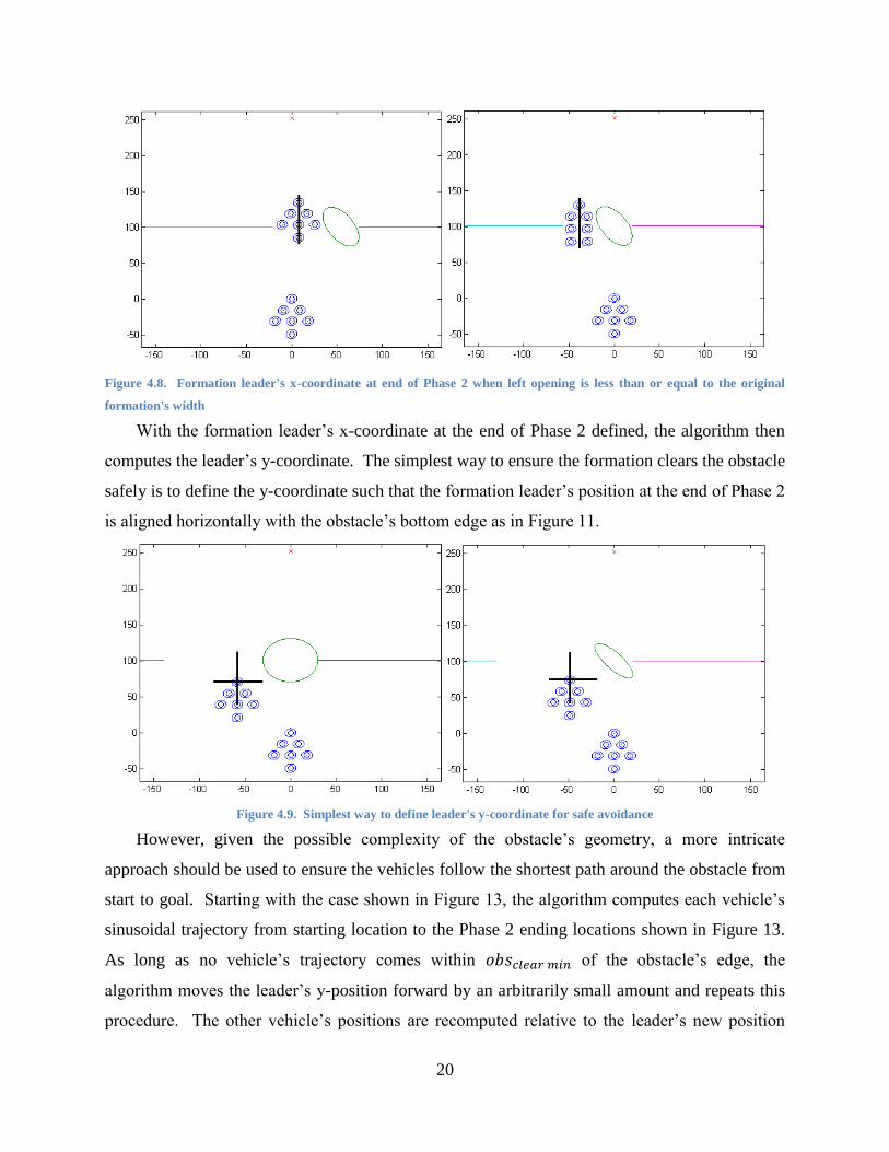
Next, let us consider a scenario in which the algorithm must carefully weigh the obstacle’s

positioning versus the spatial constraints to decide how to divide the formation. Figure 25 shows

a formation of 14 vehicles avoiding an obstacle partially in its path with complex lateral spacing

constraints. In-formation vehicle separation factor has been kept at . The

obstacle’s location (left of the formation’s centroid) favors routing more vehicles to the right of

the obstacle, while the larger space on the obstacle’s left favors routing more vehicles to the

32

obstacle’s left side. Following the logic and conditional flow presented in the Phase 2 flowchart

in Appendix A, the algorithm decides to send 7 vehicles left and 6 to the right. The minimum

vehicle separation chart on the right shows characteristic behavior consistent with previous

scenarios.

Figure 5.11. Formation of 13 vehicles avoiding offset elliptical obstacle with spacing constraints

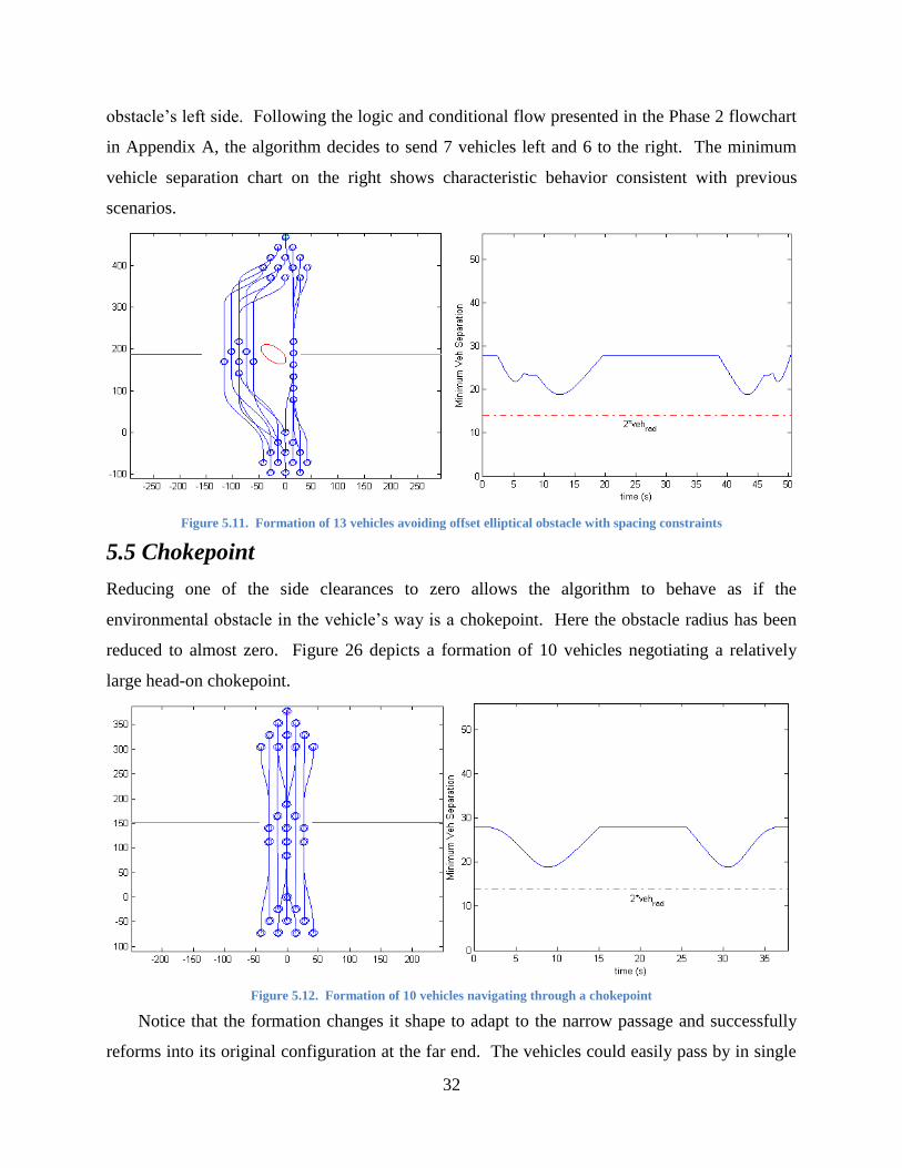
5.5 Chokepoint

Reducing one of the side clearances to zero allows the algorithm to behave as if the

environmental obstacle in the vehicle’s way is a chokepoint. Here the obstacle radius has been

reduced to almost zero. Figure 26 depicts a formation of 10 vehicles negotiating a relatively

large head-on chokepoint.

Figure 5.12. Formation of 10 vehicles navigating through a chokepoint

Notice that the formation changes it shape to adapt to the narrow passage and successfully

reforms into its original configuration at the far end. The vehicles could easily pass by in single

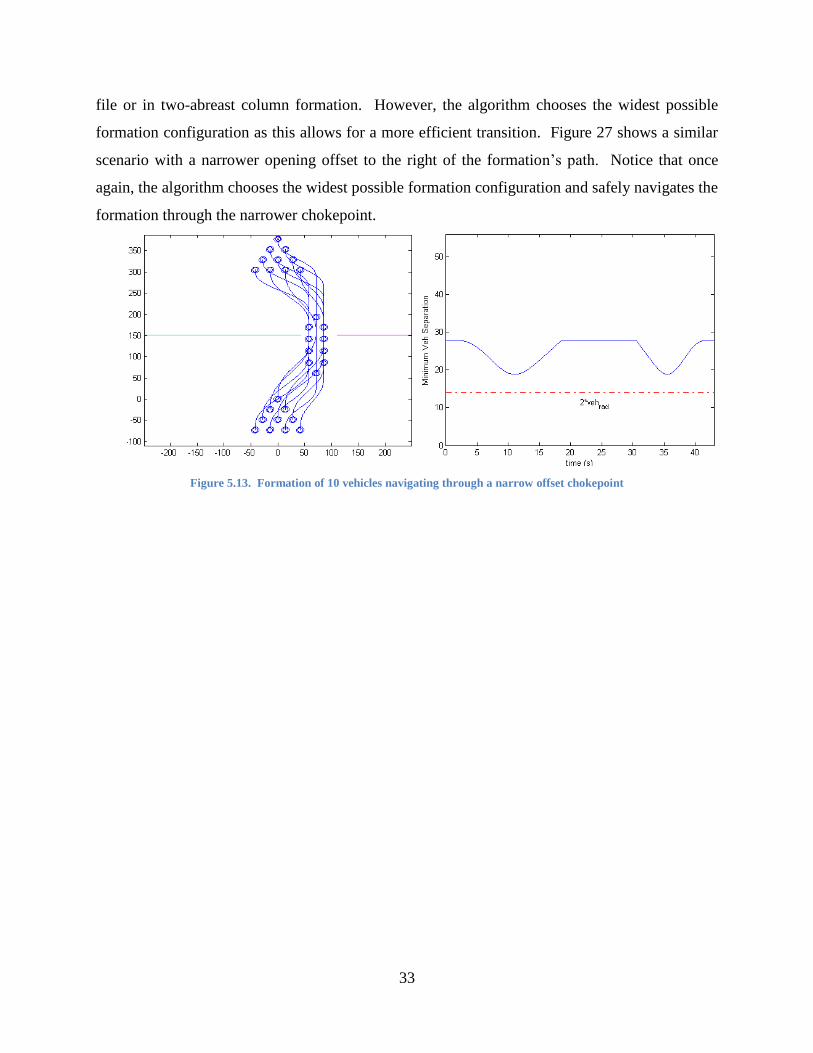
33

file or in two-abreast column formation. However, the algorithm chooses the widest possible

formation configuration as this allows for a more efficient transition. Figure 27 shows a similar

scenario with a narrower opening offset to the right of the formation’s path. Notice that once

again, the algorithm chooses the widest possible formation configuration and safely navigates the

formation through the narrower chokepoint.

Figure 5.13. Formation of 10 vehicles navigating through a narrow offset chokepoint

34

Chapter 6. Conclusion

The algorithm presented in this work provides the strategy that a group of autonomous vehicles

should follow to navigate between two points in structured formations while negotiating

environmental obstructions such as obstacles and chokepoints. The algorithm takes in

information about the environment such as vehicle properties as well as location and geometry of

the obstruction and outputs trajectories for each vehicle to follow as they bifurcate around the

obstacle or navigate through a chokepoint. These trajectories could then be used in conjunction

with a particular vehicle model’s inverse dynamics to produce the appropriate inputs and track

the desired trajectories.

Simulation results show that the algorithm successfully performs the task it was designed

for. The formation is able to adapt to its environment as it transverses the space from the starting

point to its goal location. The algorithm commands the formation to divide and/or change its

shape to navigate around the obstacle or through chokepoints. Sub-formations acquire

appropriate shapes to account for lateral spacing constraints. Minimum vehicle separation

analysis showed that increasing the default in-formation inter-vehicle separation reduces the

chance of vehicles coming within collision distance of one another vehicle during the dynamic

phases of the maneuvering. Overall, the algorithm proved effective at safely navigating a large

group of vehicles through environmental obstructions such as obstacles and chokepoints.

6.1 Future Work

There are several ways in which this work could be furthered or improved in preparation for

implementation on a real system. At present, individual vehicle assignments to a given position

within a given sub-formation are made based on an extensive hard coded list of possible

scenarios depending on parameters such as number of vehicles assigned to each side (which is

determined based on the flow chart presented in Appendix A), available side clearances, and

obstacle’s geometry and positioning. Finding a way to automate this assignment process would

greatly simplify the computational burden currently imposed by the nearly ten thousand lines of

code this assignment process currently requires given the large number of possibilities. Due to

this limitation, the present algorithm works for up to fourteen vehicles. Automating the

assignment process would allow for any number of vehicles to be used in the simulations.

35

Furthermore, a simple force field collision avoidance algorithm could be implemented on each

vehicle to provide a layer of collision avoidance guarantees as the current basis for collision

avoidance lies in the algorithm’s heuristic vehicle assignment processes previously discussed.

Another topic of future work would be to validate the algorithm’s usefulness by tracking the

outputted trajectories with vehicle dynamics and implementing it on a real system like the small

scale quadrotors in use at the Boeing VSTL.

36

Works Cited

[1] C. Lum, J. Vagners, M. Vavrina and J. Vian, "Formation Flight of Swarms of Autonomous

Vehicles In Obstructed Environments Using Vector Field Navigation," in International

Conference on Unmanned Aircraft Systems, 2012.

[2] J. Kuchar and L. Yang, "A review of conflict detection and resolution modeling methods," in

IEEE Transactions on Intelligent Transportation Systems, 2000.

[3] Lalish and Morgansen, "Distributed Reactive Collision Avoidance," Autonomous Robots, no.

Special Issue, p. 32(3), 2012.

[4] A. Chakravarthy and D. Ghose, "Obstacle avoidance in a dynamic environment: A collision

cone approach," in IEEE Transactions on Systems, Man, and Cybernetics, 1998.

[5] O. Khatib, "Real-time obstacle avoidance for manipulators and mobile robots," International

Journal of Robotics Research, vol. 5, pp. 90-98, 1986.

[6] J. Holt, "Comparison of Aerial Collision Avoidance Algorithms in a Simulated

Environment," Auburn, 2012.

[7] J. Koo and S. Shabruz, "Formation of a Group of Unmanned Aerial Vehicles (UAVs)," in

Proceedings of the American Control Conference, Arlington, 2001.

[8] J. Desai, J. Ostrowski and V. Kumar, "Modeling and Control of Formations of

Nonholonomic Mobile Robots," in IEEE Transactions on Robotics and Automation, 2001.

[9] J. Desai, V. Kumar and J. Ostrowski, "Control of changes in formation for a team of mobile

robots," in IEEE International Conference on Robotics and Automation, Detroit, 1999.

37

APPENDIX A

Figure A1