1

2

Comparison of the 2010 Highway Capacity Manual 3

Urban Street Facilities Analysis Procedure 4

with other Traffic Analysis Tools 5

6 7 8 9 10 11

Ken Courage 12 University of Florida 13

365 Weil Hall, PO Box 116580 14 Gainesville, FL 32611-6580 15

386-314-1906 16 kcourage@ufl.edu 17

18 19 20 21

Submitted to the Transportation Research Board 90th annual meeting 22 for presentation and publication 23

24 July 2010 25

26 27

28 Word Count 4370 Exhibits: 12 @ 250 3000 Total 7370

Abstract 1

Chapter 16 of the 2010 Highway Capacity Manual (HCM) presents a complete procedure for 2 evaluating the level of service (LOS) of an urban arterial street facility in terms of the average 3 speed of the through vehicles on the facility. This paper examines the characteristics of the new 4 procedure and compares those characteristics with the HCM 2000 procedure and with some 5 commonly used deterministic and stochastic traffic analysis tools. While the new procedure is 6 multimodal in scope, the discussion focuses on the automobile mode to facilitate comparisons 7 with alternative tools. 8 9 A case study based on one of the sample calculations in the 2010 HCM was used for this 10 purpose. The primary relationships that were explored include the effect of demand volume on 11 the signal phase times, the effect of demand volume the average arterial speed and the effect of 12 progression quality on the average arterial speed. The results obtained from the HCM 2000 13 procedure, CORSIM, Synchro 7 and TRANSYT-7F were compared to determine their 14 similarities and differences with respect to the new HCM procedure. 15 16 Based on this study, it was concluded that the new procedure offers a substantial contribution to 17 the methodology of highway capacity and level of service analysis. The numerical results could 18 not be expected to match those of the alternative tools identically because of differences in 19 model formulation. The agreement was close enough, however, that no judgment could be 20 offered as to the absolute accuracy of any tool. 21 22 23

Courage TRB 2011 _______________________________________________________________________________ Page 2

Introduction 1

Chapter 16 of the 2010 Highway Capacity Manual (HCM) presents a complete procedure for 2 evaluating the level of service (LOS) of an urban arterial street facility in terms of the average 3 speed of the through vehicles on the facility. This procedure was developed in response to 4 criticism of the lack of detail in the HCM 2000 version. The limitations of that version have led 5 many users to alternative traffic analysis tools for urban street facility analysis. The new 6 procedure is based on the work of Bonneson et al [1]. 7 8 This paper examines the characteristics of the new procedure and compares those characteristics 9 with the HCM 2000 procedure and with some commonly used deterministic and stochastic 10 traffic analysis tools. While the new procedure is multimodal in scope, this discussion will focus 11 on the automobile mode to facilitate comparisons with alternative tools. 12

Enhancements to the HCM 2000 Procedure 13

The procedure offers significant improvements over the methodology presented in the HCM 14 2000. It represents one of the most important enhancements to the 2010 version. Exhibit 1 15 summarizes the principal new features that have been added to the procedure. Reference 1 16 provides more detailed information on the model development. 17 18

Exhibit 1: Significant enhancements to the urban street facilities analysis procedure 19 Feature HCM 2000 Treatment HCM 2010 Treatment

Movements considered Arterial through traffic only All intersection movements Periods analyzed Single period Multiple periods with residual queue

carryover Signal timing Plan User entry of g/C ratio Computation of phase times from specified

traffic-actuated controller parameters Arterial progression effects

User entry of arrival type (1-6) Macroscopic flow model computes vehicle arrival profiles over the cycle based on user specified offsets

Running speed Model based on free flow speed and intersection spacing

Additional factors such as traffic volume and mid-segment activities are considered.

Control at segment boundaries

Signalized intersections only Signalized or unsignalized intersections

Turns from cross streets entering the arterial

Ignored Recognized in the computation of arrival profiles

Access points on the route

Ignored Recognized in the determination of running speed and delay

Modal scope Automobile mode only Multimodal 20 21 22 23

Courage TRB 2011 _______________________________________________________________________________ Page 3

Chapters 16 of the 2010 HCM describe the general features of the HCM procedure, including its 1 stated limitations. Chapter 29 provides more detail on the analysis methodology and illustrates 2 the use of commonly used alternative tools to overcome those limitations. No comparisons 3 between the results from different tools were presented in Chapter 29. The purpose of this 4 discussion is to extend the analysis in Chapter 29 to include a comparison of the following 5 relationships using a case study example: 6

� The effect of demand volume on the signal timing plan 7 � The effect of demand volume on the average speed 8 � The effect of progression quality on the average speed 9

10 A case study example will be used for this purpose. Example calculation 16-1, presented in 11 Chapter 16 of the HCM 2010 provides an ideal starting point for the discussion because it 12 presents some detailed results from the new procedure. 13

Case Study Description 14

The arterial route contains five segments as shown in Exhibit 2. Each segment has two access 15 points (i.e., driveways). The explicit treatment of access points is one of the new features in 16 2010. 17

Exhibit 2: Case study configuration and demand volumes (Source: HCM 2010, Chapter 16)

Courage TRB 2011 _______________________________________________________________________________ Page 4

1 The following additional information was provided as a part of the case study description: 2

� 200 ft left turn bays are provided on each approach. 3 � All movements have 3% heavy vehicles. 4 � Right turn on red (RTOR) volume was estimated as 5% of the right turn volume, but 5

RTOR was eliminated to facilitate comparison of tools. 6 � 1.5 ft curb and gutter is provided on both sides. 7 � Arterial approaches have protected/permitted left turns from 200 ft bays. 8 � Cross street approaches have permitted left turns from 200 ft bays. 9 � Minimum green times are 5 sec for left turns and 18 sec for through movements. 10 � All intersections operate under coordinated semi-actuated control with a background 11

cycle length of 100 sec. Nominal signal phase splits are 12 o EW left turns: 20 sec 13 o EW green 45 sec 14 o NS green 35 sec 15

� Yellow + all-red times are 4 sec for all movements. 16 � Passage time is 2 sec for all detected approaches. 17

18 Additional information was provided to evaluate other modes of travel but it will not be included 19 in this discussion, which is limited to the automobile mode. 20 21 Saturation flow rates provided with the problem description were obtained from the Chapter 18 22 (Signalized Intersections) procedure. The following values were given in units of vphg/lane: 23

� EB & WB: 1760 left, 1829 through and right 24 � NB & SB: 1826 left, 1838 through and right 25

26 To establish the relationships for investigation, the demand volumes were varied from 100% to 27 180% of the specified values. The 180% demand level produced a degree of saturation close to 28 100%. To balance the degree of saturation at this level, it was necessary to adjust the nominal 29 signal phase splits from those given in the original example. The 100 sec cycle was retained and 30 the splits were adjusted as follows: 31

� EW left turns: 13 sec 32 � EW green 45 sec 33 � NS green 42 sec 34

35 The original signal offsets were designed for balanced progression in both directions. To create 36 two different progression schemes for comparison, the offsets were changed to give full band 37 progression eastbound at the expense of the westbound flow. So the eastbound progression will 38 be close to “ideal” and the westbound progression will be mediocre at best. This difference 39 should be reflected in the average speed results for all tools. The new offsets starting at the west 40 end of the facility are 0, 26, 51, 77, 92 and 6 seconds, respectively, referenced to beginning of 41 the arterial green. The resulting progression quality is shown in terms of the progression band 42 widths in Exhibit 3, which covers the demand range up to 180% of the initial volumes.. 43

44

Courage TRB 2011 _______________________________________________________________________________ Page 5

1 Exhibit 3: Progression band widths in both directions on the route 2

3 Note that the progression band width decreases in both directions with increasing demand 4 because the arterial green times are reduced as the demand on the actuated movements increases. 5 This phenomenon will be discussed in more detail later. 6

Data Preparation 7

Results from the following analysis tools will be used for comparison with the 2010 urban street 8 facilities analysis procedure: 9

� HCM 2000 Procedure [2] 10 � CORSIM [3] 11 � Synchro 7 [4] 12 � TRANSYT-7F [5] 13

14 Data preparation for each of the tools must consider the differences in the way that they define 15 and perform computations. The data preparation for each tool will be discussed here to illustrate 16 the different requirements and to provide guidance on their use. 17

Demand Volumes 18

To create the required range of demand volumes for investigation, the initial volumes given for 19 the intersections were adjusted as shown in Exhibit 4. 20 21

Percent EWLT EW Thru EWRT NSLT NS Thru

NSRT

100 80 640 80 60 480 60

120 96 768 96 72 576 72

140 112 896 112 84 672 84

160 128 1024 128 96 768 96

180 144 1152 144 108 864 108

Exhibit 4: Adjusted intersection volumes by percent of initial volumes 22 23

0

10

20

30

40

50

60

70

80

100 120 140 160 180

Pro

gres

sion

Ban

d W

idth

(se

c)

Percent of Initial Demand Volume

Favorable (EB)

Unfavorable (WB)

Courage TRB 2011 _______________________________________________________________________________ Page 6

The access point adjustments require more explanation. Initial experiments with an “across the 1 board” adjustment indicated that the volumes entering the arterial from the access point became 2 large enough to cause congestion at the access points. Essentially, these points operated as 3 unsignalized intersections, which was not the intent of the case study. So, the volumes entering 4 at the access points were kept constant, and only the arterial volumes were increased by the 5 specified percentage. 6

Arterial Volume Continuity 7

Traffic volume counts at the intersections are often taken on different days, so a typical volume 8 input data set for an arterial facility will not maintain volume continuity along the route. If the 9 total link input does not match the total link output, then some adjustment will be necessary. The 10 adjustment methodology differs among tools and can therefore affect the comparison of results. 11 The link volume balancing methodology of the analysis tools discussed here is summarized in 12 Exhibit 5. 13 14 Analysis Tool Link Volume Balancing Procedure HCM 2000 None: HCM 2010 Proportional adjustment of output flows to match the total input. Capacity

constraints are applied to the input flows. TRANSYT-7F Proportional adjustment plus warning if balance limits are exceeded Synchro Proportional adjustment combined with synthesized mid block flow CORSIM No balancing necessary because volumes are only specified at input nodes.

Internal volume specifications are treated as proportions of the total link volume. When severe unbalance occurs, the volumes processed by CORSIM at any intersection could differ substantially from the specified volumes.

Exhibit 5: Link volume balancing methodology of traffic analysis tools 15

16 Because of the differences shown in this table, it is clear that comparison of results is best 17 accomplished with balanced volume data. The initial volume data for the example was balanced. 18 The total exiting volume at each signalized intersection exceeded the total entering volume by 40 19 vph. This loss was balanced by a gain of 40 vph at the access points. However, when the 20 intersection volumes are increased and the access point entry is held constant, as explained 21 previously, the balance will be disturbed because some traffic will be lost. 22 23 The lost volume can be offset by specifying a mid-segment entry volume with tools that 24 recognize mid-segment entry. TRANSYT-7F, Synchro and CORSIM all recognize mid-segment 25 entry as explicit inputs. The HCM 2010 procedure accommodates mid-segment entry through 26 access points. 27

Speed Definitions 28

The average speed on any segment is determined by dividing the length of the segment by the 29 time taken by each vehicle to traverse the segment. All of the deterministic tools compute the 30 travel time as the sum of two components: 31

1. The time required to travel the segment at the running speed 32 2. The delay time at the intersection due to the traffic control. 33

34

Courage TRB 2011 _______________________________________________________________________________ Page 7

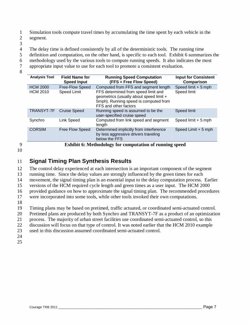
Simulation tools compute travel times by accumulating the time spent by each vehicle in the 1 segment. 2 3 The delay time is defined consistently by all of the deterministic tools. The running time 4 definition and computation, on the other hand, is specific to each tool. Exhibit 6 summarizes the 5 methodology used by the various tools to compute running speeds. It also indicates the most 6 appropriate input value to use for each tool to promote a consistent evaluation. 7 8 Analysis Tool Field Name for

Speed Input Running Speed Computation

(FFS = Free Flow Speed) Input for Consistent

Comparison HCM 2000 Free-Flow Speed Computed from FFS and segment length Speed limit + 5 mph HCM 2010 Speed Limit FFS determined from speed limit and

geometrics (usually about speed limit + 5mph). Running speed is computed from FFS and other factors

Speed limit

TRANSYT-7F Cruise Speed Running speed is assumed to be the user-specified cruise speed

Speed limit

Synchro Link Speed Computed from link speed and segment length

Speed limit + 5 mph

CORSIM Free Flow Speed Determined implicitly from interference by less aggressive drivers traveling below the FFS

Speed Limit + 5 mph

Exhibit 6: Methodology for computation of running speed 9 10

Signal Timing Plan Synthesis Results 11

The control delay experienced at each intersection is an important component of the segment 12 running time. Since the delay values are strongly influenced by the green times for each 13 movement, the signal timing plan is an essential input to the delay computation process. Earlier 14 versions of the HCM required cycle length and green times as a user input. The HCM 2000 15 provided guidance on how to approximate the signal timing plan. The recommended procedures 16 were incorporated into some tools, while other tools invoked their own computations. 17 18 Timing plans may be based on pretimed, traffic actuated, or coordinated semi-actuated control. 19 Pretimed plans are produced by both Synchro and TRANSYT-7F as a product of an optimization 20 process. The majority of urban street facilities use coordinated semi-actuated control, so this 21 discussion will focus on that type of control. It was noted earlier that the HCM 2010 example 22 used in this discussion assumed coordinated semi-actuated control. 23 24 25

Courage TRB 2011 _______________________________________________________________________________ Page 8

Exhibit 7 summarizes the methodology used by traffic analysis tools to estimate the timing plan 1 for an intersection with coordinated semi-actuated control. All of the tools considered here 2 model this type of control to assign unused time between phases but the computational 3 methodology differs among tools. 4 5

Analysis Tool Timing Plan Inputs

Computational Methodology

HCM 2000 g/C required None HCM 2010 Actuated

controller parameters

Deterministic modeling of traffic actuated control. Unused time from actuated phases is transferred to other phases.

TRANSYT-7F Dual ring phase times

Phase times are estimated by a separate iterative process that reassigns green times. The results may be used for evaluation.

Synchro Actuated controller parameters

Stochastic model estimates green times at 10% to 90% levels. Unused time from actuated phases is reassigned to the coordinated phase

CORSIM Actuated controller parameters

Emulation of a NEMA or Type 170 controller with detector inputs from microscopic simulation

Exhibit 7: Coordinated semi-actuated timing plan estimation methodology 6 7 The timing plan results for these tools will now be examined. Each tool wes used with a range of 8 demand volumes from 100 to 180% of the initial volumes. The v/c ratios for the initial volumes 9 were very low, so a significant transfer of time from the actuated phases to the coordinated phase 10 (EW through) could be expected. At higher demand levels, less time will be transferred and the 11 timing plan should converge to the nominal splits. 12

HCM 2010 Timing Plans 13

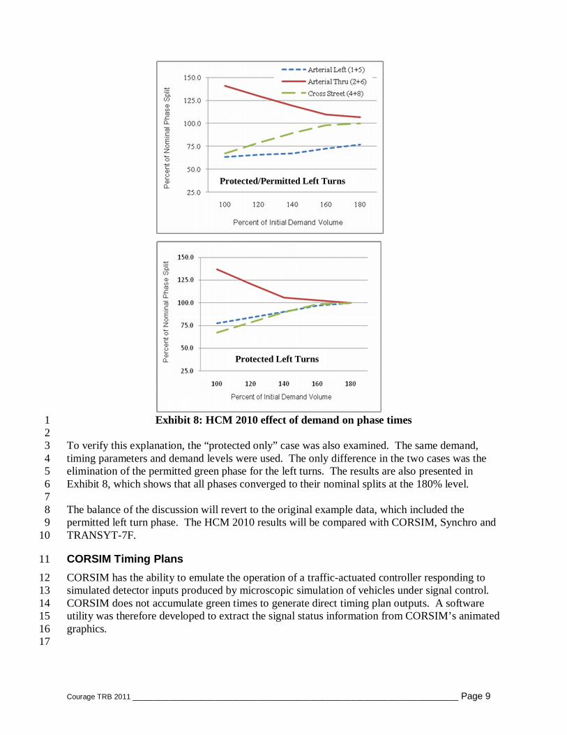
The HCM 2010 timing plan estimation results are presented in Exhibit 8. The green times are 14 shown in terms of their percent of nominal splits as a function of the percent of initial demand 15 volume. Separate relationships are plotted for the arterial left turns, arterial through movements 16 and the cross street phase times. There were no protected left turn phase for the cross streets. 17 18 The results are generally as anticipated. At low demand levels, the arterial through phase 19 receives significant unused time from the actuated phases and its time exceeds the nominal split 20 time. This effect diminishes as the demand level increases. The actuated phase times start off 21 well below their nominal splits because of lack of demand. The required time increases with 22 demand and eventually reaches 100% of the nominal split. 23 24 Full convergence to 100% was not achieved with protected-permitted phasing. Even at 180% of 25 the initial demand, the arterial left turn phase only reached 75% of the nominal split. It could be 26 expected to converge at higher demand levels, but the upper limit was constrained to 180% to 27 accommodate all of the other experiments at a degree of saturation below 1.0. The 180% 28 demand amounts to 128 vph or 3.5 veh per cycle for the left turn. The permitted green and 29 sneakers are likely to accommodate most of the left turns. 30 31

Courage TRB 2011 _______________________________________________________________________________ Page 9

Exhibit 8: HCM 2010 effect of demand on phase times 1 2 To verify this explanation, the “protected only” case was also examined. The same demand, 3 timing parameters and demand levels were used. The only difference in the two cases was the 4 elimination of the permitted green phase for the left turns. The results are also presented in 5 Exhibit 8, which shows that all phases converged to their nominal splits at the 180% level. 6 7 The balance of the discussion will revert to the original example data, which included the 8 permitted left turn phase. The HCM 2010 results will be compared with CORSIM, Synchro and 9 TRANSYT-7F. 10

CORSIM Timing Plans 11

CORSIM has the ability to emulate the operation of a traffic-actuated controller responding to 12 simulated detector inputs produced by microscopic simulation of vehicles under signal control. 13 CORSIM does not accumulate green times to generate direct timing plan outputs. A software 14 utility was therefore developed to extract the signal status information from CORSIM’s animated 15 graphics. 16 17

Protected Left Turns

Protected/Permitted Left Turns

Courage TRB 2011 _______________________________________________________________________________ Page 10

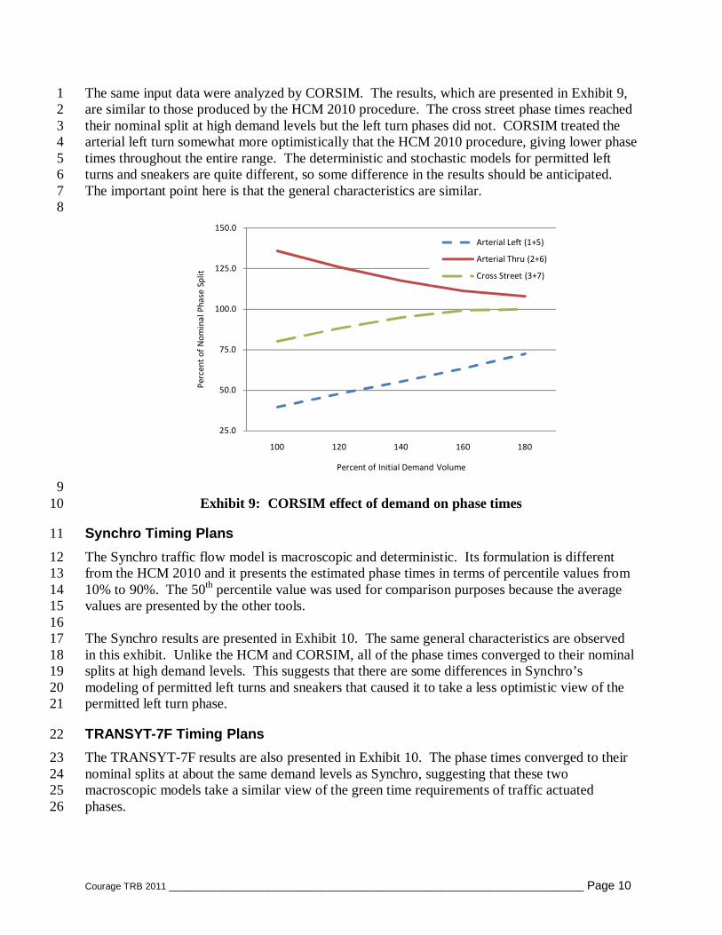
The same input data were analyzed by CORSIM. The results, which are presented in Exhibit 9, 1 are similar to those produced by the HCM 2010 procedure. The cross street phase times reached 2 their nominal split at high demand levels but the left turn phases did not. CORSIM treated the 3 arterial left turn somewhat more optimistically that the HCM 2010 procedure, giving lower phase 4 times throughout the entire range. The deterministic and stochastic models for permitted left 5 turns and sneakers are quite different, so some difference in the results should be anticipated. 6 The important point here is that the general characteristics are similar. 7 8

9 Exhibit 9: CORSIM effect of demand on phase times 10

Synchro Timing Plans 11

The Synchro traffic flow model is macroscopic and deterministic. Its formulation is different 12 from the HCM 2010 and it presents the estimated phase times in terms of percentile values from 13 10% to 90%. The 50th percentile value was used for comparison purposes because the average 14 values are presented by the other tools. 15 16 The Synchro results are presented in Exhibit 10. The same general characteristics are observed 17 in this exhibit. Unlike the HCM and CORSIM, all of the phase times converged to their nominal 18 splits at high demand levels. This suggests that there are some differences in Synchro’s 19 modeling of permitted left turns and sneakers that caused it to take a less optimistic view of the 20 permitted left turn phase. 21

TRANSYT-7F Timing Plans 22

The TRANSYT-7F results are also presented in Exhibit 10. The phase times converged to their 23 nominal splits at about the same demand levels as Synchro, suggesting that these two 24 macroscopic models take a similar view of the green time requirements of traffic actuated 25 phases. 26

25.0

50.0

75.0

100.0

125.0

150.0

100 120 140 160 180

Pe

rce

nt

of

No

min

al

Ph

ase

Sp

lit

Percent of Initial Demand Volume

Arterial Left (1+5)

Arterial Thru (2+6)

Cross Street (3+7)

Courage TRB 2011 _______________________________________________________________________________ Page 11

Exhibit 10: Effect of demand on phase times for Synchro and TRANSYT-7F 1

Average Speed Results 2

Level of service estimates in the HCM are based on the computed value of the average speed. 3 The average speed on any segment is determined for all tools by dividing the length of the 4 segment by the time taken by each vehicle to traverse the segment. The average speed for the 5 facility divides the sum of the segment lengths by the sum of the segment travel times. The 6 modeling differences among tools were discussed earlier. Differences in results could be due to 7 differences in the computation of running speeds or control delay on each segment. 8 9 Since the demand volumes are the same in both directions, differences in the overall speed can 10 be attributed entirely to differences in progression quality. In the results for each tool, two 11 phenomena should be observed: 12

1. The overall speed should decrease as demand increases because of lower running speeds 13 and higher delays. 14

2. The direction favored by the progression design (eastbound) should have lower speeds 15 than the reverse direction (westbound). 16

17

50.0

75.0

100.0

125.0

150.0

100 120 140 160 180

Per

cent

of

Nom

inal

pha

se S

plit

Percent of Initial Demand Volume

Arterial Left (1+5)

Arterial Thru (2+6)

Cross Street (4+8)

50.0

75.0

100.0

125.0

150.0

100 120 140 160 180

Per

cent

of

Nom

inal

Pha

se S

plit

Percent of Initial Demand Volume

Arterial Left (1+5)

Arterial Thru (2+6)

Cross Street (4+8)

Synchro

TRANSYT-7F

Courage TRB 2011 _______________________________________________________________________________ Page 12

HCM 2000 and 2010 Speeds 1

The investigation will begin with a comparison of the HCM 2000 and HCM 2010 results. This 2 comparison will provide some insight into the differences between the two procedures. It will 3 also establish the clear superiority of the new procedure. 4 5 The HCM 2000 procedure does not perform any signal timing computations. The g/C time for 6 each segment is a user input. To apply the HCM 2000 urban street analysis procedure, the 7 timing plan computed by the HCM 2010 procedure was entered into the HCM 2000 urban streets 8 software. 9 10 Progression quality is another user input to the HCM 2000 procedure. It is generally entered in 11 terms of an arrival type (AT). To provide a complete picture, the analysis was repeated for AT 12 1-5 as defined in the HCM 2000. The results are presented in Exhibit 11. Each arrival type is 13 represented by a different line in this figure. As expected, AT 1 (worst progression) shows the 14 lowest speeds and AT 5 (best progression) shows the highest speeds. The average speed value 15 ranges from about 12 mph to 30 mph. 16 17

18 Exhibit 11: Effect of demand volume on average speed in the 1000 and 2010 HCM 19 20 The HCM 2010 procedure eliminates the need for an educated guess at the arrival type by 21 modeling the progression of traffic from segment to segment. The results for the two 22 progression cases from this example are also shown in Exhibit 11, superimposed on the HCM 23 2000 results. By way of comparison, it appears that the favored direction (eastbound) had an 24 equivalent Arrival type between 4 and 5. The reverse direction was between AT-2 and AT-3 for 25 most of the demand range. A direct comparison of the two methods cannot be made based on 26 arrival type alone because the HCM 2010 procedure is also sensitive to other inputs. 27 28

0.00

5.00

10.00

15.00

20.00

25.00

30.00

35.00

100 120 140 160 180

Ave

rage

Spe

ed (

mph

)

Percent of Initial Demand Volume

AT­1

AT­2

AT­3

AT­4

AT­5

Fwd

Rev

Courage TRB 2011 _______________________________________________________________________________ Page 13

Average Speed Comparison for all Tools 1

It is interesting to look at a side-by-side comparison of the results for each progression case. The 2 two cases have been described as “favorable” and “unfavorable.” The results for all tools are 3 presented in Exhibit 12. The HCM 2000 procedure was excluded from this comparison because 4 of its limited treatment of progression quality. 5

6

7

Exhibit 12: Comparison of average speeds for all tools. 8 9 All tools reported higher delays with unfavorable progression. The average ratio of unfavorable 10 progression delay to favorable progression delay throughout the demand range was as follows: 11

� Synchro 1.36 12 � CORSIM 1.64 13 � TRANSYT-7F 2.31 14 � HCM 2010 2.39 15

0.0

5.0

10.0

15.0

20.0

25.0

100 120 140 160 180

Ave

rag

e S

pe

ed

(m

ph

)

Percent of Initial Demand Volume

Favorable Progression

HCM 2010

CORSIM

Synchro

TRANSYT­7F

0.0

5.0

10.0

15.0

20.0

25.0

100 120 140 160 180

Ave

rag

e S

pe

ed

(m

ph

)

Percent of Initial Demand Volume

Unfavorable Progression

Courage TRB 2011 _______________________________________________________________________________ Page 14

1

2 A few interesting observations can be made from these results, keeping in mind that they apply 3 to this example only: 4

� In general, the demand-speed relationships of all of the tools conformed to the expected 5 shape. 6

� There was a greater divergence in the results with favorable progression, especially at 7 high demands. This suggests that there are some differences in the modeling of platoon 8 propagation among the tools that were examined. 9

� CORSIM and Synchro produced very similar results. The differences were 10 indistinguishable in the unfavorable progression case. With favorable progression the 11 Synchro speeds were slightly lower than CORSIM’s. 12

� The HCM 2010 procedure consistently estimated speeds that were slightly higher than 13 the other tools. The lowest speed estimates were produced by Synchro with favorable 14 progression and by TRANSYT-7F with unfavorable progression. 15

� There was a substantial difference in the treatment of progression among the tools in 16 determining delay. The effect of progression quality on delay was lowest in Synchro and 17 highest in the HCM 2010. 18

Conclusions 19

The objective of this case study exercise was to examine the new procedure for analysis of urban 20 street facilities published in the 2010 edition of the HCM. Several data sets were created with 21 different demand volumes progression characteristics and phasing plans. Parallel data sets were 22 created for commonly used alternative analysis tools for comparison purposes. Based on this 23 study, the following conclusions are offered: 24

� The new procedure represents a substantial improvement over the previous version 25 published in the HCM 2000. It internalizes computations that had to be approximated 26 or carried out externally in the previous version. 27

� The computational engine that implemented the procedure performed in a robust 28 manner 29

� There were no internal inconsistencies or anomalous behaviors in the results 30 � The relationships between demand levels, phase times and average speeds conformed 31

generally to expectations. 32 � The numerical results could not be expected to match those of the alternative tools 33

because of differences in model formulation. The agreement was close enough that 34 no judgment could be offered as to the absolute accuracy of any tool. 35

36 A single case study does not constitute a complete evaluation of any traffic analysis tool. 37 However, within the limits of this study, it can be said that the performance of the HCM 2010 38 procedure in the automobile mode supports the conclusion that it provides a credible method for 39 evaluating the operation of an urban street facility. It offers a substantial contribution to the 40 methodology of highway capacity and level of service analysis. For the sake of uniformity, 41 developers of macroscopic traffic analysis tools should be encouraged to consider incorporating 42 the results of the underlying research into their products. 43

Courage TRB 2011 _______________________________________________________________________________ Page 15

Acknowledgements 1

The effort described in this paper was supported by NCHRP Project 3-85. The material 2 presented here represents an abridged version of one of the appendices in the final report for that 3 project. 4 5

References 6

1. Bonneson, J., M. Pratt, and M. Vandehey. Predicting the Performance of Automobile 7 Traffic on Urban Streets. Final Report. NCHRP Project 3-79. Transportation Research 8 Board, Washington, D.C., January 2008. 9

2. Highway Capacity Manual, Transportation Research Board, 2000 10 3. CORridor-microscopic SIMulation program (CORSIM) Version 6.1 User's Guide, 11

University of Florida, 2008 12 4. Husch, D. and J. Albeck. Synchro Studio 7 User’s Guide. Trafficware, Ltd., 2006. 13 5. Wallace, C., K. Courage, M. Hadi, and A. Gan. TRANSYT-7F User’s Guide, Vol. 4 in a 14

Series: Methodology for Optimizing Signal Timing. University of Florida, Gainesville, 15 Fla., March 1998. 16