approved corrections and changes for the highway capacity ... corrections to hcm... · approved...

Updated 7/8/2005 Previous update 2/27/2004

of 7

Approved Corrections and Changes for the Highway Capacity Manual 2000

TRB Committee AHB40, Highway Capacity and Quality of Service

Unless stated otherwise, corrections apply to both the U.S. Customary and Metric versions.

NEW

PAGE

ITEM

CORRECTION APPROVAL

DATE Chapter 6 Update variable symbol and definition according to changes

made in Equation 20-16. 10/13/2004

7-3

Last sentence on page

Change the last sentence to read “The space mean speed is 38.3 mi/h, calculated as (60)[3 ÷ (2.0 + 1.5 + 1.2)].”

1/13/2003

7-6 4th paragraph Change first sentence to read "The slope of any ray line drawn from the origin of the speed-flow curve represents the inverse of density, based …"

6/29/2002

8-2

Pedestrian Characteristics

Change the third sentence to read “An average walking speed of 4.0-ft/s is appropriate…”.

1/13/2003

8-12

Exhibit 8-12 Change Facility descriptions for Detroit, MI to be “I-96 Jeffries Freeway at Warren” and “Lodge at W. Grand Blvd.”

1/13/2003

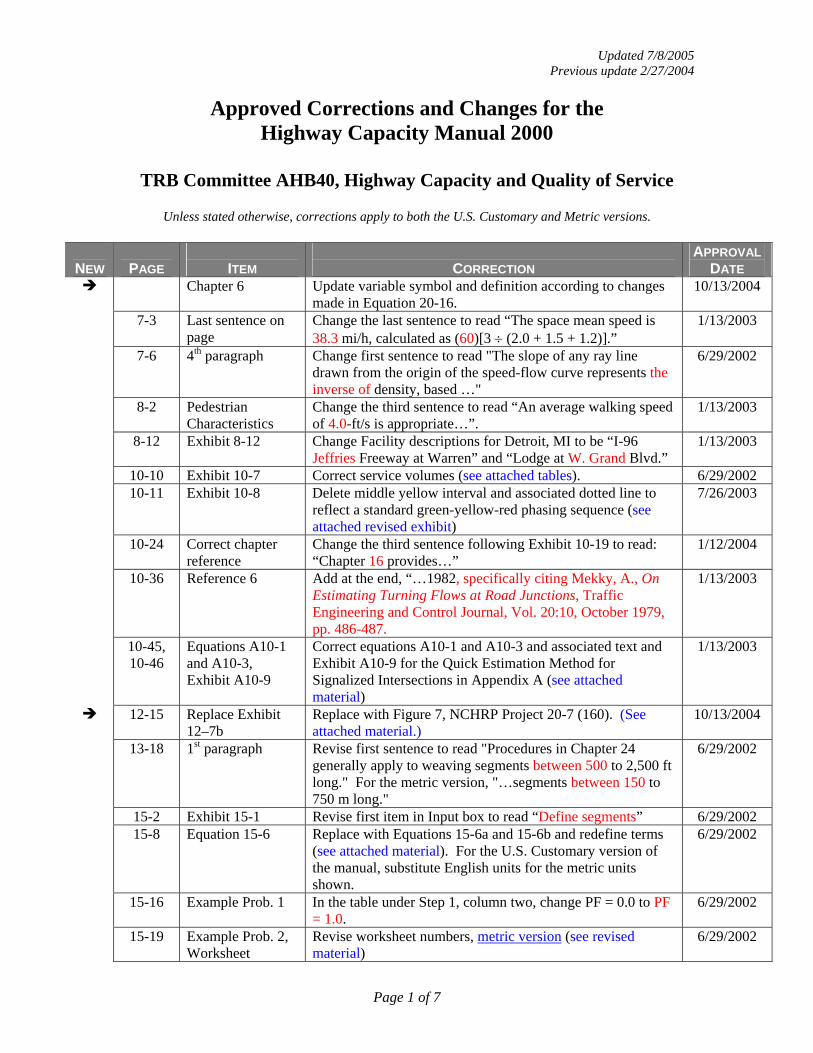
10-10 Exhibit 10-7 Correct service volumes (see attached tables). 6/29/2002 10-11 Exhibit 10-8 Delete middle yellow interval and associated dotted line to

reflect a standard green-yellow-red phasing sequence (see attached revised exhibit)

7/26/2003

10-24 Correct chapter reference

Change the third sentence following Exhibit 10-19 to read: “Chapter 16 provides…”

1/12/2004

10-36

Reference 6 Add at the end, “…1982, specifically citing Mekky, A., On Estimating Turning Flows at Road Junctions, Traffic Engineering and Control Journal, Vol. 20:10, October 1979, pp. 486-487.

1/13/2003

10-45, 10-46

Equations A10-1 and A10-3, Exhibit A10-9

Correct equations A10-1 and A10-3 and associated text and Exhibit A10-9 for the Quick Estimation Method for Signalized Intersections in Appendix A (see attached material)

1/13/2003

12-15 Replace Exhibit 12–7b

Replace with Figure 7, NCHRP Project 20-7 (160). (See attached material.)

10/13/2004

13-18 1st paragraph Revise first sentence to read "Procedures in Chapter 24 generally apply to weaving segments between 500 to 2,500 ft long." For the metric version, "…segments between 150 to 750 m long."

6/29/2002

15-2 Exhibit 15-1 Revise first item in Input box to read “Define segments” 6/29/2002 15-8 Equation 15-6 Replace with Equations 15-6a and 15-6b and redefine terms

(see attached material). For the U.S. Customary version of the manual, substitute English units for the metric units shown.

6/29/2002

15-16 Example Prob. 1 In the table under Step 1, column two, change PF = 0.0 to PF = 1.0.

6/29/2002

15-19

Example Prob. 2, Worksheet

Revise worksheet numbers, metric version (see revised material)

6/29/2002


of 7

NEW

PAGE

ITEM

CORRECTION

APPROVAL DATE

15-20 Correct appendix reference

Change the fourth checked sentence under The Facts to read: “Segment lengths…described in Appendix B,”

1/12/2004

15-22, 15-23

Example Prob. 4, solution steps and worksheet

Revise value in Step 4 for k = 0.4. Revise calculated values based on this change in other steps and worksheet on next page (see revised material).

6/29/2002

15-24, 15-25

Example Prob. 5, solution steps

Revise formula in Step 3 for d. Revise value in Step 4 for k = 0.4. Revise subsequent values in other steps based on these changes (see revised material).

6/29/2002

15-25 Appendix A Revise step 3 under LOS analysis to be: 3. Convert the hourly directional volumes to through-

movement 15-min flow rates by subtracting the turn movement volumes served by exclusive turn-lane lane groups and then divide this difference by the PHF.

6/29/2002

15-25, 15-26

Appendix A Revise the second set of seven steps under the planning analysis procedures (see revised material)

6/29/2002

15-27 Appendix B Redefine steps 2, 4, and 5: 2. Determine the appropriate FFS for each street segment. 4. Make test-car travel time runs over each street segment

during the… 5. Total travel speed for the entire urban street section

should also…

6/29/2002

16-19, 16-152

Equation 16-10, Equation G16-8

Apply the following constraints for the delay and queuing progression factor formulas: (i) PF ≥ 1.0 and PF2 ≥ 1.0 for Arrival Types 1 and 2 (ii) PF ≤ 1.0 and PF2 ≤ 1.0 for Arrival Types 4 to 6 (iii) P ≤ 0.95 (Rp ≤ 0.95/u) for both PF and PF2 (iv) Rp ≤ 0.95/yL for both PF and PF2 (v) PF2 = 1.0 for yL ≥ u (XL ≥ 1.0) (vi) Rp ≥(1 − 0.95*(1 − u)/yL)/u for both PF and PF2, and (vii) Rp = 1.0 (P = u), therefore, PF = 1.0 and PF2 = 1.0 for

yL ≥ 0.95 (viii) If conditions (iii), (iv) and (vi) create inconsistent

constraints on Rp and P, set Rp = 1.0 and P = u, therefore, PF = 1.0 and PF2 = 1.0

May 2001

16-39 Box 19 Change v/c to v/s Feb. 2004 16-47 Capacity

worksheet Add flow ratios to WB direction = 0.313 And to NB direction = 0.289

Feb. 2004

16-50 Box 24 Change v/c to v/s Feb. 2004 16-61 Example Prob. 2,

Supplemental Worksheet for Ped/Bike Effects on Permitted Left and Right Turns

The EB left effective pedestrian green time should be 23.4 seconds. The subsequent calculations for the EB left will change slightly, with no change in the final ped-bike left turn adjustment factor. The WB right is already shown as 23.4 seconds, thus no change is required.

7/28/2001


of 7

NEW

PAGE

ITEM

CORRECTION APPROVAL

DATE 16-73 Capacity

worksheet Add flow ratios: NBpro = 0.084 NBper =0.000 SBper = 0.418 SBThRt = 0.322 EBper = 0.237 EBThRt = 0.170 WBThRt = 0.233.

16-144 Correct Equation F16-3 (both versions)

The last part of Equation F16-3 should read:

[ ])X,1min(1QcT1u...

b

−−=

1/12/2004

16-151, 16-152

Equations G16-2 through G16-5

Replace NLG in the denominator of each equation with (fLU*NLG)

1/14/2002

16-153 Equation G16-9 All places where (XL−1) appears should be replaced with (XL−1) + QbL/(cL*T). All places where kBXL appears should be replaced with kBX. The results should be expressed in its simplest form.

1/14/2002

16-153 Terms under Equation G16-9

Define kB as "second-term incremental factor" 1/14/2002

17-7 1st paragraph and sidebar

Change the third sentence in top paragraph to read "Base values of tc and tf are shown for two- and four-lane major streets. Due to limitations in the available data, this procedure is not applicable to intersections with six-lane major streets." Delete the sidebar - "Base values for a six-lane major street are assumed to be the same as those for a four-lane major street." and replace with "This procedure is not applicable to intersections with six-lane major streets."

7/28/2001, 6/29/2002

17-15 Equations 17-18, 17-19 and surrounding text

“ The time to discharge the vehicles that arrive during the red is given by Equation 17-18.

gq1 =v C (1− P)

s (17-18)

where v is either vT or vL,prot.

The time to discharge the vehicles that arrive on the green and join the back of the queue is given by equation 17-19.

gq2 =v C P gq1

s geff − v C P (17-19)

where v is either vT or vL,prot.”

6/29/2002


of 7

NEW

PAGE

ITEM

CORRECTION

APPROVAL DATE

17-16 Exhibit 17-12 Replace with two figures (see attached figures). 6/29/2002 17-16 Redefining f “f = the proportion of through and protected left turn traffic

which departs the upstream signalized intersection and subsequently arrives at the subject two-way stop-controlled intersection with respect to the through and protected left turn traffic departing the upstream signalized intersection. If there are no opportunities for vehicles to leave the roadway between the upstream signalized intersection and the TWSC intersection, then f is equal to 1.”

6/29/2002

17-16 Add Equation 17-21b and text

“The downstream flow after a period equal to the green time after the platoon reaches the unsignalized intersection is vc,g and is given by:

qggpmax,cpg,c )F1)(fvRv(fvRv −

−−+=

Again, v is either vT or vL,prot

6/29/2002

17-17 Equation 17-22 Replace with the multi-part equation and following text (see attached material).

6/29/2002

17-19 Equation 17-28 The equation 17-28 should read

⎪⎩

⎪⎨

⎧−>

−−=

otherwise

pvvifp

pvvv xcxc

x

xcxc

xuc

0

)1(5.1)1(5.1

min,,min,,

,,

Remove the definition “s” under equation 17-28 and add “vc,min = as defined on page 17-17”

6/29/2002, modified 7/26/2003


of 7

NEW

PAGE

ITEM

CORRECTION APPROVAL

DATE 17-19 New Equation

17-28a Below equation 17-28 and the references to the variables in the equation, insert the following: “The user can provide values of the proportion of unblocked time for a particular unsignalized intersection movement caused by upstream signals, the px values. Similarly the flow in the blocked period can also be given as vblock in veh/h. The appropriate conflicting flow for the unblocked period is given by Equation 17-28a.

⎪⎩

⎪⎨

⎧−>

−−=

otherwise

pvvifp

pvvv xblockxc

x

xblockxc

xuc

0

)1()1(

,,

,,

(see attached material)

7/26/2003

17-21 Flared Minor-Street Approaches

Modify procedure (see attached material) 6/29/2002

17-36 4th paragraph, 2nd sentence

“The volume on the subject approach is increased incrementally until the degree of utilization on any one approach exceeds 1.0.”

1/12/2004

17-53, 17-61, 17-62, 17-71, App. A

Correct Worksheet 5a and 5b

Correct Worksheet 5a and 5b by changing the left column heading under “Movement 2” and “Movement 5” to VT instead of VT,prog.

1/12/2004

18-24 Correct Example Problem 3, Step 4

The top equation in step 4 should read: vtot = 48 + 27 + 40 + 21 + 20 = 156 p/cycle

1/12/2004

18-25 Correct Example Problem 3, Step 5

The last equation in step 5 should read:

s1.170.16

14*7.20.40.462.3t =⎟

⎠⎞

⎜⎝⎛++=

1/12/2004

20-1 Revise text Paragraph to be added after the first paragraph under the section titled - Limitations of the Methodology " The operational analysis methodologies in this chapter are not intended to address capacity and traffic flow on two-lane highways in developed areas. Typically, two-lane highway segments in these areas (for example, a two-lane highway through a small town) are subject to lower speed limits and have few to no passing zones. In addition, the effects of operations at signalized and/or unsignalized intersections, which may be significant, are not accounted for in the current methodology."

10/13/2004


of 7

NEW

PAGE

ITEM

CORRECTION

APPROVAL DATE

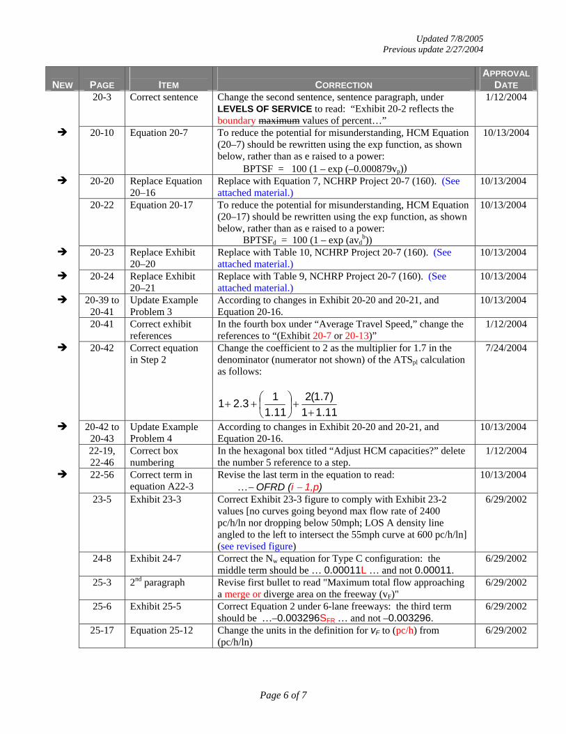
20-3 Correct sentence Change the second sentence, sentence paragraph, under LEVELS OF SERVICE to read: “Exhibit 20-2 reflects the boundary maximum values of percent…”

1/12/2004

20-10 Equation 20-7 To reduce the potential for misunderstanding, HCM Equation (20–7) should be rewritten using the exp function, as shown below, rather than as e raised to a power: BPTSF = 100 (1 – exp (–0.000879vp))

10/13/2004

20-20 Replace Equation 20–16

Replace with Equation 7, NCHRP Project 20-7 (160). (See attached material.)

10/13/2004

20-22 Equation 20-17 To reduce the potential for misunderstanding, HCM Equation (20–17) should be rewritten using the exp function, as shown below, rather than as e raised to a power: BPTSFd = 100 (1 – exp (avd

b))

10/13/2004

20-23 Replace Exhibit 20–20

Replace with Table 10, NCHRP Project 20-7 (160). (See attached material.)

10/13/2004

20-24 Replace Exhibit 20–21

Replace with Table 9, NCHRP Project 20-7 (160). (See attached material.)

10/13/2004

20-39 to 20-41

Update Example Problem 3

According to changes in Exhibit 20-20 and 20-21, and Equation 20-16.

10/13/2004

20-41 Correct exhibit references

In the fourth box under “Average Travel Speed,” change the references to “(Exhibit 20-7 or 20-13)”

1/12/2004

20-42 Correct equation in Step 2

Change the coefficient to 2 as the multiplier for 1.7 in the denominator (numerator not shown) of the ATSpl calculation as follows:

11.11)7.1(2

11.113.21

++⎟

⎠⎞

⎜⎝⎛++

7/24/2004

20-42 to 20-43

Update Example Problem 4

According to changes in Exhibit 20-20 and 20-21, and Equation 20-16.

10/13/2004

22-19, 22-46

Correct box numbering

In the hexagonal box titled “Adjust HCM capacities?” delete the number 5 reference to a step.

1/12/2004

22-56 Correct term in equation A22-3

Revise the last term in the equation to read: …− OFRD (i − 1,p)

10/13/2004

23-5

Exhibit 23-3 Correct Exhibit 23-3 figure to comply with Exhibit 23-2 values [no curves going beyond max flow rate of 2400 pc/h/ln nor dropping below 50mph; LOS A density line angled to the left to intersect the 55mph curve at 600 pc/h/ln] (see revised figure)

6/29/2002

24-8 Exhibit 24-7 Correct the Nw equation for Type C configuration: the middle term should be … 0.00011L … and not 0.00011.

6/29/2002

25-3 2nd paragraph Revise first bullet to read "Maximum total flow approaching a merge or diverge area on the freeway (vF)"

6/29/2002

25-6 Exhibit 25-5 Correct Equation 2 under 6-lane freeways: the third term should be …–0.003296SFR … and not –0.003296.

6/29/2002

25-17 Equation 25-12 Change the units in the definition for vF to (pc/h) from (pc/h/ln)

6/29/2002


of 7

NEW

PAGE

ITEM

CORRECTION APPROVAL

DATE 27-10

Top paragraph Revise last sentence of top paragraph to read, “For certain

special conditions, users should multiply the base values by 1.2 (12) for heavy two-way flow (25-50% of passengers moving in the opposite direction) through a single door channel, and by 0.9 (16) for a low-floor bus. For primarily single-direction flow through either double-stream doors or two single-stream doors, the exhibit reduces the base values for a single door channel by a factor of 0.6 (14,15).”

1/13/2003

27-38 Correct chapter reference

In the first checked sentence under “Comments” change the last reference to “(from Chapter 16);”

1/12/2004

30-6 to 30-8

Equations 30-5, 30-6, 30-7, 30-8, Exhibit 30-4

Correct equations and exhibit under section titled “Determining Link Speed” (see attached material)

6/29/2002

30-35 Correct Equation A30-15 (both versions)

Correct Equation A30-15 by adding brackets as shown:

⎥⎥⎦

⎤

⎢⎢⎣

⎡+−+−++=

TvX8)1x()1X(T900

vX36005D

22

1/12/2004

31-31 Add a reference Add an additional reference after number 1: 1a. Elefteriadou, L., G. List, J. Leonard, H. Lieu, M.

Thomas, R. Giguere, R. Brewish, G. Johnson. Beyond the Highway Capacity Manual: A Framework for Selecting Simulation Models in Traffic Operational Analyses. In Transportation Research Record 1678, TRB, National Research Council, Washington, D.C., 1999, pp. 96−106.

10/13/2004

Highway Capacity Manual 2000

Chapter 10 - Urban Street Concepts 10-10Signalized Intersections

RECOMMENDED CHANGES FOR ERRATA (US CUSTOMARY)

EXHIBIT 10-7. EXAMPLE SERVICE VOLUMES FOR URBAN STREETS(SEE FOOTNOTES FOR ASSUMED VALUES)

This table containsapproximate values. It ismeant for illustrativepurposes only. The valuesare highly dependent onthe assumptions used. Itshould not be used foroperational analyses orfinal design. This tablewas derived usingassumed values listed inthe footnote.

Service Volumes (veh/h)

Lanes A B C D E

Class I

1 N /A 850 920 1010 11302 N/A 1710 1850 2020 22803 N/A 2570 2770 3050 34204 N/A 3440 3700 4060 4560

Class II

1 N /A N/A 670 840 8802 N/A N/A 1470 1690 17703 N/A N/A 2280 2540 26604 N/A N/A 3090 3390 3550

Class III


Class IV

1 N/A N/A N/A 780 8002 N/A N/A N/A 1570 16203 N/A N/A N/A 2370 24304 N/A N/A N/A 3160 3250

NotesN/A - not achievable given assumptions below.This table was derived from the conditions listed in the following table.

ClassI II III IV

Signal density (sig/mi) 0.8 3 5 10Free-flow speed (mi/h) 50 40 35 30Cycle length (s) 110 90 80 70Effective green ratio 0.45 0.45 0.45 0.45Adj. sat. flow rate 1850 1800 1750 1700Arrival type 3 4 4 5Unit extension (s) 3 3 3 3Initial queue 0 0 0 0Other delay 0 0 0 0Peak-hour factor 0.92 0.92 0.92 0.92% lefts, % rights 10 10 10 10Left-turn bay Yes Yes Yes YesLane utilization factor According to Exhibit 10-23, Default Lane Utilization

Factors


Chapter 10 - Urban Street Concepts 10-10Signalized Intersections

RECOMMENDED CHANGES FOR ERRATA (METRIC)

EXHIBIT 10-7. EXAMPLE SERVICE VOLUMES FOR URBAN STREETS(SEE FOOTNOTES FOR ASSUMED VALUES)

This table containsapproximate values. It ismeant for illustrativepurposes only. The valuesare highly dependent onthe assumptions used. Itshould not be used foroperational analyses orfinal design. This tablewas derived usingassumed values listed inthe footnote.

Service Volumes (veh/h)

Lanes A B C D E

Class I

1 N /A 830 940 1030 11302 N/A 1690 1900 2060 22703 N/A 2550 2850 3110 34004 N/A 3410 3800 4150 4530

Class II


Class III


Class IV

1 N/A N/A N/A 660 7802 N/A N/A N/A 1460 15703 N/A N/A N/A 2260 23704 N/A N/A N/A 3050 3170

NotesN/A - not achievable given assumptions below.This table was derived from the conditions listed in the following table.

ClassI II III IV

Signal density (sig/km) 0.5 2 3 6Free-flow speed (km/h) 80 65 55 45Cycle length (s) 110 90 80 70Effective green ratio 0.45 0.45 0.45 0.45Adj. sat. flow rate 1850 1800 1750 1700Arrival type 3 4 4 5Unit extension (s) 3 3 3 3Initial queue 0 0 0 0Other delay 0 0 0 0Peak-hour factor 0.92 0.92 0.92 0.92% lefts, % rights 10 10 10 10Left-turn bay Yes Yes Yes YesLane utilization factor According to Exhibit 10-23, Default Lane Utilization

Factors

7/7/2005

Replace Exhibit 12-7b with the following figure:

0

10

20

30

40

50

60

70

80

90

100

0 200 400 600 800 1,000 1,200 1,400 1,600 1,800 2,000

Directional Flow Rate (pc/h)

Perc

ent T

ime-

Spen

t-Fol

low

ing

Opposing Flow = 200 pc/h

Opposing Flow = 1600 pc/h

7/7/2005

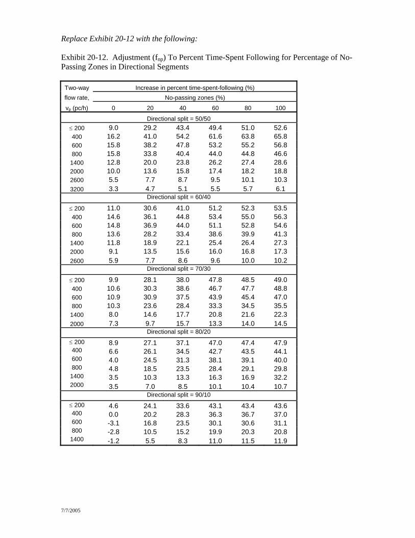
Replace Exhibit 20-12 with the following:

Exhibit 20-12. Adjustment (fnp) To Percent Time-Spent Following for Percentage of No-Passing Zones in Directional Segments

Two-way Increase in percent time-spent-following (%) flow rate, No-passing zones (%)

vp (pc/h) 0 20 40 60 80 100

Directional split = 50/50 ≤ 200 9.0 29.2 43.4 49.4 51.0 52.6 400 16.2 41.0 54.2 61.6 63.8 65.8 600 15.8 38.2 47.8 53.2 55.2 56.8 800 15.8 33.8 40.4 44.0 44.8 46.6

1400 12.8 20.0 23.8 26.2 27.4 28.6 2000 10.0 13.6 15.8 17.4 18.2 18.8 2600 5.5 7.7 8.7 9.5 10.1 10.3 3200 3.3 4.7 5.1 5.5 5.7 6.1

Directional split = 60/40

≤ 200 11.0 30.6 41.0 51.2 52.3 53.5 400 14.6 36.1 44.8 53.4 55.0 56.3 600 14.8 36.9 44.0 51.1 52.8 54.6 800 13.6 28.2 33.4 38.6 39.9 41.3

1400 11.8 18.9 22.1 25.4 26.4 27.3 2000 9.1 13.5 15.6 16.0 16.8 17.3 2600 5.9 7.7 8.6 9.6 10.0 10.2


≤ 200 9.9 28.1 38.0 47.8 48.5 49.0 400 10.6 30.3 38.6 46.7 47.7 48.8 600 10.9 30.9 37.5 43.9 45.4 47.0 800 10.3 23.6 28.4 33.3 34.5 35.5

1400 8.0 14.6 17.7 20.8 21.6 22.3 2000 7.3 9.7 15.7 13.3 14.0 14.5


≤ 200 8.9 27.1 37.1 47.0 47.4 47.9 400 6.6 26.1 34.5 42.7 43.5 44.1 600 4.0 24.5 31.3 38.1 39.1 40.0 800 4.8 18.5 23.5 28.4 29.1 29.8

1400 3.5 10.3 13.3 16.3 16.9 32.2 2000 3.5 7.0 8.5 10.1 10.4 10.7


≤ 200 4.6 24.1 33.6 43.1 43.4 43.6 400 0.0 20.2 28.3 36.3 36.7 37.0 600 -3.1 16.8 23.5 30.1 30.6 31.1 800 -2.8 10.5 15.2 19.9 20.3 20.8

1400 -1.2 5.5 8.3 11.0 11.5 11.9

7/7/2005

Replace Exhibit 20-21 with the following: Exhibit 20-21. Values of Coefficients Used in Estimating Percent Time-Spent Following for Directional Segments.

Opposing demand flow rate, vo (pc/h) a b

≤ 200 –0.0014 0.973 400 –0.0022 0.923 600 –0.0033 0.870 800 –0.0045 0.833

1000 –0.0049 0.829 1200 –0.0054 0.825 1400 –0.0058 0.821

≥ 1600 –0.0062 0.817 Replace Equation 20-16 with the following:

where: PTSFd = percent time-spent-following in the direction analyzed, BPTSFd = base percent time-spent-following in the direction analyzed, fnp = adjustment for percent no-passing zones in the direction analyzed Vd = directional passenger-car equivalent flow rate (pc/h) V0 = opposing direction passenger-car equivalent flow rate (pc/h)

⎟⎟⎠

⎞⎜⎜⎝

⎛+

+=0d

dnpdd VV

VfBPTSFPTSF


23-5 Chapter 23 - Basic Freeway SegmentsMethodology

fN = adjustment for number of lanes from Exhibit 23-6 (mi/h); andfID = adjustment for interchange density from Exhibit 23-7 (mi/h).

EXHIBIT 23-3. SPEED-FLOW CURVES AND LOS FOR BASIC FREEWAY SEGMENTS

0 400 800 1200 1600 2000 2400

Flow Rate (pc/h/ln)

Aver

age

Pass

enge

r-C

ar S

peed

(mi/h

)

80

70

60

50

40

30

20

10

0

C

13001450

16001750

LOS A B D E

Free-Flow Speed, FFS = 75 mi/h70 mi/h65 mi/h60 mi/h55 mi/h

Dens

ity =

11

pc/m

i/ln

18 pc

/mi/ln

26 pc/

mi/ln

35 pc/mi/ln

45 pc/mi/ln

Note:Capacity varies by free-flow speed. Capacity is 2400, 2350, 2300, and 2250 pc/h/ln at free-flow speeds of 70 and greater, 65,60, and 55 mi/h, respectively.For 70 < FFS ≤ 75

(3400 – 30FFS) < vp ≤ 2400

S = FFS − FFS − 1603

vp + 30FFS − 3400

30FFS − 1000

2.6

For 55 ≤ FFS ≤ 70 and for flow rate (vp )(3400 – 30FFS) < vp ≤ (1700 + 10FFS),

S = FFS − 19

7FFS − 340( ) vp + 30FFS − 3400

40FFS − 1700

2.6

For 55 ≤ FFS ≤ 75 andvp ≤ (3400 – 30FFS),S = FFS

BFFS

Estimation of FFS for an existing or future freeway segment is accomplished byadjusting a base free-flow speed downward to reflect the influence of four factors: lanewidth, lateral clearance, number of lanes, and interchange density. Thus, the analyst isrequired to select an appropriate BFFS as a starting point.

Adjustment for Lane Width

The base condition for lane width is 12 ft or greater. When the average lane widthacross all lanes is less than 12 ft, the base free-flow speed (e.g., 75 mi/h) is reduced.Adjustments to reflect the effect of narrower average lane width are given in Exhibit23-4.


Chapter 30 - Areawide Analysis 30-6Methodology

wherec = capacity (veh/h),

PHF = peak-hour factor, andg/C = effective green time per cycle.

Refer to Equation 16-4 for definitions of all other factors.

See Chapter 16, “Signalized Intersections,” for the adjustment factor values. SeeChapter 10, “Urban Street Concepts,” for default values and approximation proceduresfor adjustment factors.

For arterials with all-way stops controlling the link capacity, procedures in Chapter17, “Unsignalized Intersections,” should be used to estimate the through movementcapacity at each intersection.

Capacity Tables

The accuracy of the speed estimates are highly dependent on the accuracy of theestimated capacity for the facility. Consequently, it is recommended that each analyst usecapacities that are specific to each link whenever possible. However, it is recognized thatthis procedure is not always feasible. The analyst may select sets of default values for thevarious capacity adjustment factors that vary by functional class (freeway, highway,arterial, collector, local), area type (downtown, urban, suburban, rural), terrain type(level, rolling, mountainous), and other conditions. These default values may besubstituted into the above capacity equations to develop tables of link capacity values thatvary by functional class, area type, general terrain, and number of lanes.

Determining Link SpeedTraversal time plus nodedelay equals segmenttravel time

The vehicle speed for the link is computed using Equation 30-4.

S = L

R + D3600

(30-4)

whereS = link speed (mi/h),L = link length (mi),R = link traversal time (h), andD = node delay for link (s).

See Appendix A formethods to estimatenode delay

Node delay is computed only for signal- or stop-sign-controlled intersections at theend of the link. All other intersection-related delays that occur in the middle of the linkare incorporated into the link traversal time calculation. The node delay estimationprocedure is described in Appendix A. The calculation requires information on all of theintersection approaches at the node in order to compute the delay on each link feeding theintersection.

If the available travel demand model software package is unable to compute nodedelay, it can be approximated by using the node approach capacity rather than the linkcapacity in the computation of traversal time. In this situation the node delay is set tozero in Equation 30-4.

The link traversal time, R, is computed using Equation 30-5.

R = Ro + Do +0.25T (X −1) + (X −1)2 +16J * X * L2

T 2

(30-5)

whereR = link traversal time (h),

Ro = link traversal time at link FFS (h),Do = zero-flow control delay at signalized intersection (h),

Rick Dowling

See following page for new equation

Revisions [new equation]

(30-5)

( )

∗+−+−+++= 22

2*162)1(125.0TN

LXJXXNTDDRR Moo

where: [add the following]

DM = segment delay between signals (equals zero if no signals)(h) N = number of Signals (equals one if no signals)


30-7 Chapter 30 - Areawide AnalysisMethodology

T = expected duration of demand (typically 1 h) (h),X = link demand to capacity ratio,J = calibration parameter, andL = link length (mi).

The link traversal time for free-flow conditions (Ro) is computed from the FFS,

using Equation 30-6.

Ro = LSo

(30-6)

whereRo = FFS link traversal time (h),L = link length (mi), and

So = link FFS (mi/h).

The zero-flow control delay for signalized intersections (if any) on the link iscomputed using Equation 30-7.

Do = N3600

* DF *C2

1 − gC

2

(30-7)

whereDo = zero-flow control delay at signal (h),N = number of signals on link,

3600 = conversion from seconds to hours,g/C = average effective green time per cycle for signals on link (see Exhibit

10-12 for default values) (s),C = average cycle length for all signals on link (see Exhibit 10-12 for

default values) (s), andDF = adjustment factor to compute zero-flow control delay (0.9 for

uncoordinated traffic-actuated signals, 1.0 for uncoordinated fixed-timesignals, 1.2 for coordinated signals with unfavorable progression, 0.90for coordinated signals with favorable progression, and 0.60 forcoordinated signals with highly favorable progression).

Calibration parameter J isused to arrive at a predictedmean speed when demandequals capacity

The calibration parameter J is selected so that the traversal time equation will predictthe mean speed of traffic when demand is equal to capacity. Substituting x = 1.00 in thetraversal time equation and solving for J yields Equation 30-8:

J =(Rc −Ro )2

L2 (30-8)

whereJ = calibration parameter,

Rc = link traversal time when demand equals capacity (h),Ro = FFS link traversal time (h), andL = link length (mi).

See Appendix C foralternative approach usingBPR curve

Exhibit 30-4 shows values for J that were selected to reproduce the traversal times atcapacity predicted by the analysis procedures in Part III of this manual. Some oldersoftware may not be able to implement Equation 30-8, so the formula and recommendedparameters for the more traditional BPR curve are provided in Appendix C as analternative method for estimating link traversal times.

Rick Dowling

Place "Note that the free flow speed..." text on the following page here.

Rick Dowling

Place "Insert 1" text here

Rick Dowling

See new equation for 30-8

(30-6) Note that the free flow speed (SO) for signalized streets is defined as the mid-block free flow speed between signals. For this reason a zero flow control delay (DO) and a segment delay (DM ) are added to the link travel time at zero flow.

(30-7) Insert 1: The segment delay between signals (DM) is computed by subtracting the Segment Running Time per mile (TR) (obtained from Exhibit 15-3) from the free flow travel time per mile for the signalized urban street and multiplying the result by the total length of the street. DM equals zero if there are no signals on the street or if they are so far apart that they do not affect the speed of traffic between signals. The segment delay (DM) is computed according to Equation 30-7a.

3600)( oRM TTLD −•= (30-7a) where: [add the following]

DM = segment delay (h) L = link length (mi) TR = running time per mile (sec) TO = running time per mile at free flow speed (sec) The running time per mile (TR) is obtained from Exhibit 15-3 according to the urban street class, free flow speed, and the average distance between signals on the link. The running time per mile at free flow speed (TO) is computed according to Equation 30-7b. oo SLT = (30-7b) where: L = Link length (mi) TO = running time per mile at free flow speed (sec) SO = free flow speed (mi/h)

(30-8)

( )

2

2

LDDRRJ Mooc −−−=

where: [add the following] D0 = zero flow control Delay (h) DM = segment delay between signals (h)


Chapter 30 - Areawide Analysis 30-8Methodology

EXHIBIT 30-4. RECOMMENDED PARAMETERS FOR TRAVERSAL TIME J

Facility Type Signals per mi Free-Flow Speed(mi/h)

Speed at Capacity(mi/h)

J(h2/mi2)

Freeway N/A 75 54 2.69 x 10-5

Freeway N/A 70 53 2.10 x 10-5

Freeway N/A 65 52 1.48 x 10-5

Freeway N/A 60 51 8.65 x 10-6

Freeway N/A 55 50 3.31 x 10-6

Multilane Highway N/A 60 55 2.30 x 10-6




Two-Lane Highway N/A 69 44 6.91 x 10-5





Arterial Class I 0.2 50 33 5.67 x 10-5



Arterial Class II 0.3 40 25 1.28 x 10-4



Arterial Class III 1.3 35 11 2.24 x 10-3



Arterial Class IV 2.5 30 6 8.12 x 10-3



Note:N/A = not applicable.

Determining Performance Measures

Computation of performance measures for intensity, duration, extent, variability, andaccessibility is described.

Intensity

The possible performance measures for measuring the intensity of congestion on oneof the highway subsystems (freeway, rural highway, and arterial) are computed from oneor more of the following: person-hours of travel, person-hours of delay, mean trip speed,and mean trip delay. If average vehicle occupancy (AVO) data are not available, theperformance measures are computed in terms of vehicle-hours rather than person-hours.Equation 30-9 is used to compute person-hours of travel.

PHT = AVOi *v i *Li

Si(30-9)

wherePHT = total person-hours of travel,

vi = vehicle demand on Link i,AVOi = average vehicle occupancy on Link i,

Li = length of Link i (mi), andSi = mean speed of Link i (mi/h).

Rick Dowling

See revised Exhibit 30-4 on the following page

Revised information for: EXHIBIT 30-4. RECOMMENDED PARAMETERS FOR TRAVERSAL TIME J

Facility type Signals per mi Free-Flow Speed Speed at Capacity J (h2/mi2)

Freeway Freeway Freeway Freeway Freeway

53

2.95 x 10-5

Multilane Highway Multilane Highway Multilane Highway Multilane Highway

Two-Lane Highway Two-Lane Highway Two-Lane Highway Two-Lane Highway Two-Lane Highway

65 60 55 50 45

40 35 30 25 20

9.04 x 10-5

1.39 x 10-4

2.24 x 10-4

3.89 x 10-4

7.48 x 10-4 Arterial Class I Arterial Class I Arterial Class I

0.5 2.0 4.0

2.21 x 10-5

2.04 x 10-4

1.25 x 10-3 Arterial Class II Arterial Class II Arterial Class II

1.0 2.0 3.0

4.99 x 10-5

2.00 x 10-4

7.91 x 10-4 Arterial Class III Arterial Class III Arterial Class III

3.0 5.0 6.0

8.01 x 10-4

1.78 x 10-3

3.18 x 10-3 Arterial Class IV Arterial Class IV Arterial Class IV

6.0 8.0

10.0

3.17 x 10-3

4.99 x 10-3

7.11 x 10-3 Note: N/A = not applicable [please add the following] This table is provided for the convenience of the analyst and should be considered approximate. Precise values of “J” can be computed using Equation 30-8.

approved corrections and changes for the highway capacity ... corrections to hcm... · approved...

Documents