comp 381 by m. hamdi 1 comp 381 design and analysis of computer architectures...
Post on 21-Dec-2015
233 views
TRANSCRIPT
1COMP 381 by M. Hamdi
COMP 381COMP 381Design and Analysis of Design and Analysis of
Computer Architectures Computer Architectures
http://www.cs.ust.hk/~hamdi/Class/COMP381-07/http://www.cs.ust.hk/~hamdi/Class/COMP381-07/
Mounir HamdiMounir Hamdi
Professor - Computer Science and Engineering Professor - Computer Science and Engineering DepartmentDepartment
Director – Master of Science in Information Director – Master of Science in Information Technology Technology

2COMP 381 by M. Hamdi
Administrative Details Administrative Details
Instructor: Prof. Mounir Hamdi Office #: 3545Email: [email protected] Phone: 2358 6984 Office hours: Wednesdays: 10:00am -
12:00am (or by appointments).
Teaching Assistants: 1 Demonstrator2 TAs

3COMP 381 by M. Hamdi
Administrative Details Administrative Details Textbook
John L. Hennessy and David A. Patterson. Computer Architecture: A Quantitative Approach. Morgan Kaufman Publishers, Fourth Edition, 2007.
Reference BookWilliam Stallings. Computer Organization and Architecture: Designing for Performance. Prentice Hall Publishers, 2006.
Grading SchemeHomeworks/Project: 35%. Midterm Exam = 30%. Final Exam = 35%.

4COMP 381 by M. Hamdi
Breakdown of a Computing Problem
Instruction Set Architecture (ISA)Instruction Set Architecture (ISA)Instruction Set Architecture (ISA)Instruction Set Architecture (ISA)
ProblemProblemProblemProblem AlgorithAlgorithmsmsAlgorithAlgorithmsms
Programming inProgramming inHigh-Level LanguageHigh-Level LanguageProgramming inProgramming inHigh-Level LanguageHigh-Level Language
Compiler/Assembler/Compiler/Assembler/LinkerLinkerCompiler/Assembler/Compiler/Assembler/LinkerLinker
System LevelSystem LevelSystem LevelSystem Level
Human LevelHuman LevelHuman LevelHuman Level
System architectureSystem architectureSystem architectureSystem architecture
Target Machine Target Machine (one implementation)(one implementation)Target Machine Target Machine (one implementation)(one implementation)Micro-architectureMicro-architectureMicro-architectureMicro-architecture
Functional units/Functional units/Data Path Data Path Functional units/Functional units/Data Path Data Path
Gates Level Gates Level Design Design
Gates Level Gates Level Design Design
TransistorsTransistorsTransistorsTransistors ManufacturingManufacturingManufacturingManufacturing
RTL Level RTL Level RTL Level RTL Level
Logic Level Logic Level Logic Level Logic Level
Circuit Level Circuit Level Circuit Level Circuit Level
Silicon Level Silicon Level Silicon Level Silicon Level
Architect’sTerritory
Technology Trend
Apps Trend

5COMP 381 by M. Hamdi
Course Description and GoalWhat will COMP 381 give me?
A brief understanding of the inner-workings of modern computers, their evolution, and trade-offs present at the hardware/software boundary.
An brief understanding of the interaction and design of the various components at hardware level (processor, memory, I/O) and the software level (operating system, compiler, instruction sets).
Equip you with an intellectual toolbox for dealing with a host of system design challenges.

6COMP 381 by M. Hamdi
Course Description and Goal (cont’d)
To understand the design techniques, machine structures, technology factors, and evaluation methods that will determine the form of computers in the 21st Century
TechnologyProgrammingLanguages
OperatingSystems History
Applications
Measurement &
Evaluation
Computer Architecture:• Instruction Set Design• Organization• Hardware

7COMP 381 by M. Hamdi
Course Description and Goal (cont’d)
Will I use the knowledge gained in this subject in my profession?
Remember
Few people design entire computers or entire instruction sets
ButMany computer engineers design computer componentsAny successful computer engineer/architect needs to
understand, in detail, all components of computers – in order to design any successful piece of hardware or software.

8COMP 381 by M. Hamdi
Computer Architecture in General
SOFTWARESOFTWARE
When building a Cathedral numerous practical considerations need to be taken into account:
• Available materials• Worker skills• Willingness of the client to pay the
price• Space
Similarly, Computer Architecture is about working within constraints:
• What will the market buy?• Cost/Performance• Tradeoffs in materials and
processes
Notre Damede Paris

9COMP 381 by M. Hamdi
Computer ArchitectureComputer Architecture
• Computer Architecture involves 3 inter-related components– Instruction set architecture (ISA): The actual
programmer-visible instruction set and serves as the boundary between the software and hardware.
– Implementation of a machine has two components:
• Organization: includes the high-level aspects of a computer’s design such as: The memory system, the bus structure, the internal CPU unit which includes implementations of arithmetic, logic, branching, and data transfer operations.
• Hardware: Refers to the specifics of the machine such as detailed logic design and packaging technology.

10COMP 381 by M. Hamdi
• Desktop Computing
– Personal computer and workstation: $1K - $10K– Optimized for price-performance
• Server– Web server, file sever, computing sever: $10K - $10M– Optimized for: availability, scalability, and throughput
• Embedded Computers– Fastest growing and the most diverse space: $10 - $10K
• Microwaves, washing machines, palmtops, cell phones, etc.
– Optimizations: price, power, specialized performance
Three Computing Classes Today

11COMP 381 by M. Hamdi
Three Computing Classes Today
Feature Desktop Server Embedded
Price of the system
$500-$5K $5K-$5Me.g., Web server, file sever, computing sever
$10-$100K (including network routers at high end)e.g. Microwaves, washing machines, palmtops, cell phones, network processors
Price of the processor
$50-$500 $200-$10K $0.01 - $100
Sold per year
250M 6M 500M(only 32-bit and 64-bit)
Critical system design issues
Price-performance, graphics performance
Throughput, availability, scalability
Price, power consumption, application-specific performance
12COMP 381 by M. Hamdi
Desktop Computers
• Largest market in dollar terms• Spans low-end (<$500) to high-end ($5K) systems• Optimize price-performance
– Performance measured in the number of calculations and graphic operations
– Price is what matters to customers
• Arena where the newest, highest-performance and cost-reduced microprocessors appear
• Reasonably well characterized in terms of applications and benchmarking
• What will a PC of 2015 do?• What will a PC of 2020 do?
13COMP 381 by M. Hamdi
Servers
• Provide more reliable file and computing services (Web servers)
• Key requirements– Availability – effectively provide service 24/7/365
(Yahoo!, Google, eBay)– Reliability – never fails– Scalability – server systems grow over time, so the
ability to scale up the computing capacity is crucial– Performance – transactions per minute
• Related category: clusters / supercomputers

14COMP 381 by M. Hamdi
Embedded Computers
• Fastest growing portion of the market
• Computers as parts of other devices where their presence is not obviously visible– E.g., home appliances, printers, smart cards,
cell phones, palmtops, set-top boxes, gaming consoles, network routers
• Wide range of processing power and cost $0.1 (8-bit, 16-bit processors), $10 (32-bit capable to execute 50M
instructions per second), $100-$200 (high-end video gaming consoles and network switches)
• Requirements– Real-time performance requirement
(e.g., time to process a video frame is limited)
– Minimize memory requirements, power
• SOCs (System-on-a-chip) combine processor cores and application-specific circuitry, DSP processors, network processors, ...

15COMP 381 by M. Hamdi
The Task of a Computer Designer
Evaluate ExistingEvaluate ExistingSystems for Systems for BottlenecksBottlenecks
Simulate NewSimulate NewDesigns andDesigns and
OrganizationsOrganizations
Implement NextImplement NextGeneration SystemGeneration System
TechnologyTrends
Benchmarks
Workloads
ImplementationComplexity

16COMP 381 by M. Hamdi
Job Description of a Computer Architect
• Make trade-off of performance, complexity effectiveness, power, technology, cost, etc.
• Understand application requirements– General purpose Desktop (Intel Pentium class, AMD Athlon)– Game and multimedia (STI’s Cell+Nvidia, Wii, Xbox 360)– Embedded and real-time (ARM, MIPS, Xscale)– Online transactional processing (OLTP), data warehouse servers
(Sun Fire T2000 (UltraSparc T1), IBM POWER (p690), Google Cluster)
– Scientific (finite element analysis, protein folding, weather forecast, defense related (IBM BlueGene, Cray T3D/T3E, IBM SP2)
– Sometimes, there is no boundary …
• New responsibilities– Power Efficiency, Availability, Reliability, Security

17COMP 381 by M. Hamdi
Levels of Abstraction
Instruction Set Architecture
Applications
Operating System
Firmw areCompiler
Instruction Set Processor I/O System
Datapath & Control
Digital Design
Circuit Design
Layout
S/W and H/W consists of hierarchical layers of abstraction, each hides details of lower layers from the above layer
The instruction set arch. abstracts the H/W and S/W interface and allows many implementation of varying cost and performance to run the same S/W
Topics to be covered in this Topics to be covered in this classclass
We are particularly interested in the architectural aspects of making a high-performance computer
•Fundamentals of Computer Architecture
• Instruction Set Architecture
•Pipelining & Instruction Level Parallelism
•Memory Hierarchy
• Input/Output and Storage Area Networks
•Multi-cores and Multiprocessors

Computer Architecture TopicsComputer Architecture Topics
Instruction Set Architecture
Pipelining, Hazard Resolution,Superscalar, Reordering, ILP Branch Prediction, Speculation
Cache DesignBlock size, Associativity
L1 Cache
L2 Cache
DRAM
Disks and Tape
Coherence,Bandwidth,Latency
Emerging TechnologiesInterleaving
RAIDInput/Outputand Storage
MemoryHierarchy
Processor Design
Addressing modes, formats

Computer Architecture TopicsComputer Architecture Topics
M
Interconnection NetworkS
PMPMPMP° ° °
Topologies, Routing, Bandwidth, Latency, Reliability
Network Interfaces
Shared Memory,Message Passing
Multi-cores, Multiprocessors Networks and Interconnections

21COMP 381 by M. Hamdi
10
100
1
2003 2005 2007 2009 2011 2013
Increasing HW
Threads HT
Multi-core Era
Scalar and Parallel
Applications
Many-core Era
Massively Parallel
Applications
Multiprocessing within a chip: Many-Core
Intel predicts Intel predicts 100’s of cores 100’s of cores on a chip in on a chip in 20152015

22COMP 381 by M. Hamdi
Trends in Computer Trends in Computer ArchitecturesArchitectures
• Computer technology has been advancing at an alarming rate
You can buy a computer today that is more powerful than a supercomputer in the 1980s for 1/1000 the price.
• These advances can be attributed to advances in technology as well as advances in computer design
– Advances in technology (e.g., microelectronics, VLSI, packaging, etc) have been fairly steady
– Advances in computer design (e.g., ISA, Cache, RAID, ILP, Multi-Cores, etc.) have a much bigger impact (This is the theme of this class).

23COMP 381 by M. Hamdi
Processor PerformanceProcessor Performance

24COMP 381 by M. Hamdi
Growth in processor performance
1
10
100
1000
10000
1978 1980 1982 1984 1986 1988 1990 1992 1994 1996 1998 2000 2002 2004 2006
Pe
rfo
rma
nce
(vs. V
AX
-11
/78
0)
25%/year
52%/year
20%/year
• VAX : 25%/year 1978 to 1986• RISC + x86: 52%/year 1986 to 2002• RISC + x86: 20%/year 2002 to present
From Hennessy and Patterson, Computer Architecture: A Quantitative Approach, 4th edition, October, 2006

25COMP 381 by M. Hamdi
Trends in TechnologyTrends in Technology
• Trends in Technology followed closely Moore’s Law “Transistor density of chips doubles every 1.5-2.0 years”
• As a consequence of Moore’s Law:
– Processor speed doubles every 1.5-2.0 years
– DRAM size doubles every 1.5-2.0 years
– Etc.
• These constitute a target that the computer industry aim for.

26COMP 381 by M. Hamdi
Intel 4004 Die PhotoIntel 4004 Die Photo
• Introduced in 1970– First microprocessor
• 2,250 transistors
• 12 mm2
• 108 KHz

27COMP 381 by M. Hamdi
Intel 8086 Die ScanIntel 8086 Die Scan
• Introduced in 1979– Basic architecture of the
IA32 PC
• 29,000 transistors
• 33 mm2
• 5 MHz

28COMP 381 by M. Hamdi
Intel 80486 Die ScanIntel 80486 Die Scan
• Introduced in 1989– 1st pipelined
implementation of IA32
• 1,200,000 transistors
• 81 mm2
• 25 MHz
29COMP 381 by M. Hamdi
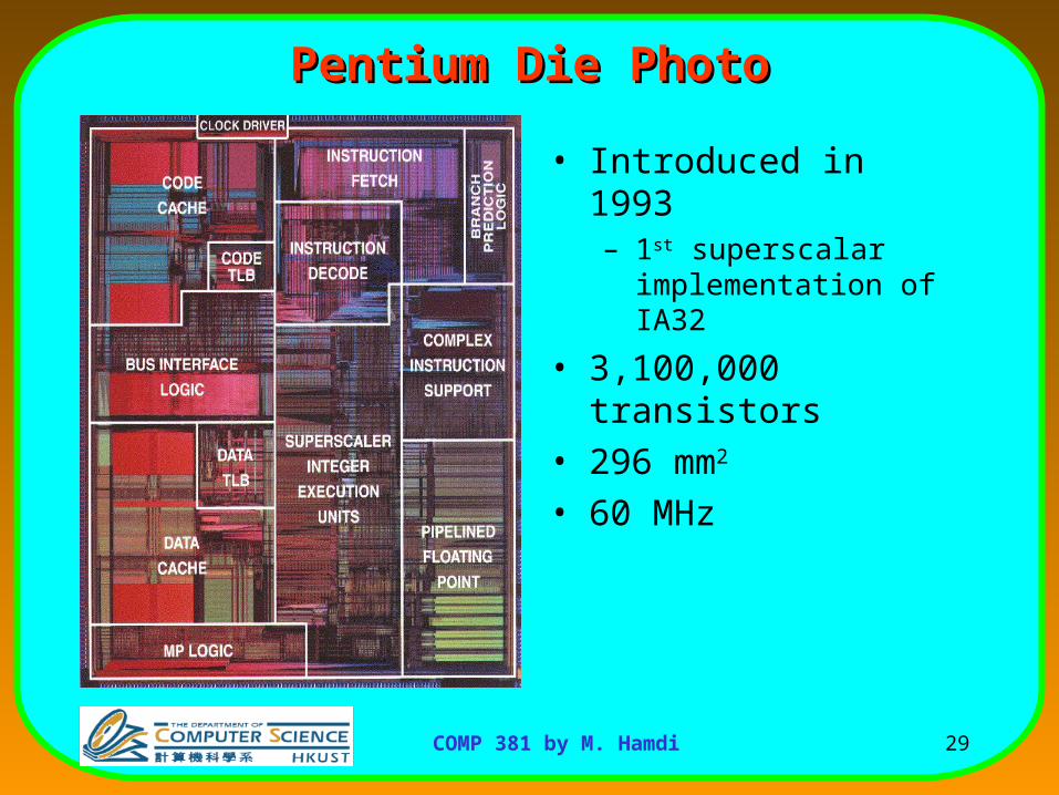
Pentium Die PhotoPentium Die Photo
• Introduced in 1993– 1st superscalar
implementation of IA32
• 3,100,000 transistors
• 296 mm2
• 60 MHz

30COMP 381 by M. Hamdi
Pentium IIIPentium III
• Introduced in 1999
• 9,5000,000 transistors
• 125 mm2
• 450 MHz

31COMP 381 by M. Hamdi
Pentium IV and Duo
Intel P4 – 55M tr(2001)
Intel Itanium – 221M tr.(2001)
Intel Core 2 Extreme Quad-core 2x291M tr.(2006)
32COMP 381 by M. Hamdi
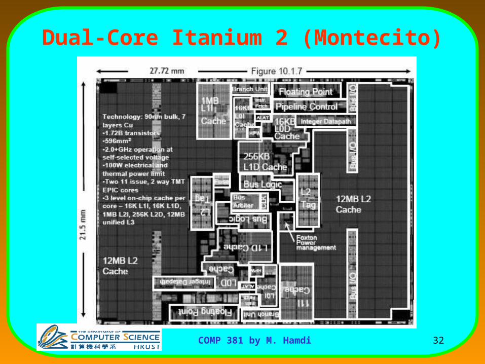
Dual-Core Itanium 2 (Montecito)

33COMP 381 by M. Hamdi
Moore’s Law
Exponential growthExponential growth2,25
0
Transistor count will be doubled every 18 monthsTransistor count will be doubled every 18 months Gordon Moore, Intel co-founder
42millions
1.7 billionsMontecito
10 μm13.5mm2
0.09 μm596 mm2

34COMP 381 by M. Hamdi
Integrated Circuits Capacity

35COMP 381 by M. Hamdi
Processor Transistor Count (from http://en.wikipedia.org/wiki/Transistor_count)
Processor Transistor count
Date of intro-duction
Manufactu-rer
Intel 4004 2300 1971 Intel
Intel 8008 2500 1972 Intel
Intel 8080 4500 1974 Intel
Intel 8088 29 000 1978 Intel
Intel 80286 134 000 1982 Intel
Intel 80386 275 000 1985 Intel
Intel 80486 1 200 000 1989 Intel
Pentium 3 100 000 1993 Intel
AMD K5 4 300 000 1996 AMD
Pentium II 7 500 000 1997 Intel
AMD K6 8 800 000 1997 AMD
Pentium III 9 500 000 1999 Intel
AMD K6-III 21 300 000 1999 AMD
AMD K7 22 000 000 1999 AMD
Pentium 4 42 000 000 2000 Intel
Processor Transistor count
Date of introdu-ction
Manufacturer
Itanium 25 000 000 2001 Intel
Barton 54 300 000 2003 AMD
AMD K8 105 900 000 2003 AMD
Itanium 2 220 000 000 2003 Intel
Itanium 2 with 9MB cache
592 000 000 2004 Intel
Cell 241 000 000 2006 Sony/IBM/Toshiba
Core 2 Duo 291 000 000 2006 Intel
Core 2 Quadro 582 000 000 2006 Intel
Dual-Core Itanium 2
1 700 000 000 2006 Intel

36COMP 381 by M. Hamdi
Memory Capacity Memory Capacity (Single Chip DRAM)(Single Chip DRAM)
year size(Mb)cyc time
1980 0.0625250 ns
1983 0.25220 ns
1986 1190 ns
1989 4165 ns
1992 16145 ns
1996 64120 ns
2000 256 100 ns2007 2G
52 ns
Moore’s Law for Memory: Transistor capacity increases by 4x every 3 years

37COMP 381 by M. Hamdi
MOORE’s MOORE’s LAWLAW
µProc50%/yr.
DRAM9%/yr.(2X/10 yrs)1
10
100
1000
198
0198
1 198
3198
4198
5 198
6198
7198
8198
9199
0199
1 199
2199
3199
4199
5199
6199
7199
8 199
9200
0
DRAM
CPU198
2
Processor-MemoryPerformance Gap:(grows 50% / year)
Per
form
ance
“Moore’s Law”
Processor-DRAM Memory Gap (latency)
38COMP 381 by M. Hamdi
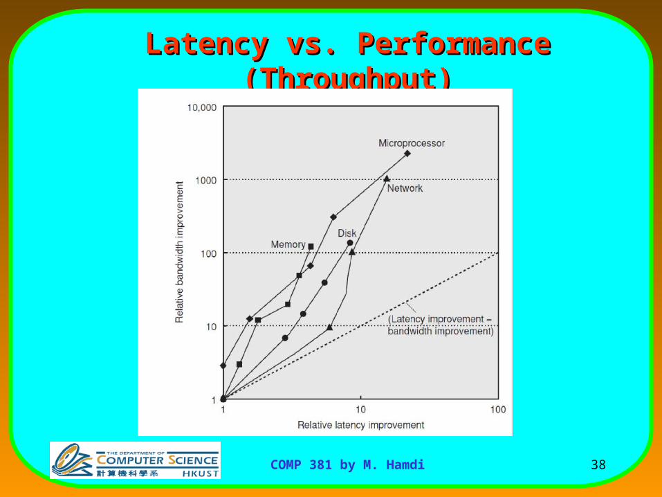
Latency vs. Performance Latency vs. Performance (Throughput)(Throughput)

39COMP 381 by M. Hamdi
Technology TrendsTechnology TrendsCapacity Speed
(latency)
Logic 2x in 3 years 2x in 3 years
DRAM 4x in 3 years 2x in 10 years
Disk 4x in 3 years 2x in 10 years• Speed increases of memory and I/O Speed increases of memory and I/O have not kept pace with processor speed have not kept pace with processor speed increases.increases.
•That is why you are taking this classThat is why you are taking this class
• This phenomena is extremely This phenomena is extremely important in numerous important in numerous processing/computing devices processing/computing devices
•Always remember thisAlways remember this

40COMP 381 by M. Hamdi
Processor-Memory Gap: We need a balanced Computer System
Memory Bus [Bandwidth]
CPU
Memory SecondaryStorage
[Clock Period,CPI,
Instruction count]
[Capacity,Cycle Time]
[Capacity,Data Rate]
Computer System
Chain: As strong as its Weakest ring

41COMP 381 by M. Hamdi
Cost and Trends in CostCost and Trends in Cost• Cost is an important factor in the design of any computer
system (except may be supercomputers)
• Cost changes over time – The learning curve and advances in technology lowers the
manufacturing costs (Yield: the percentage of manufactured devices that survives the testing procedure).
– High volume products lowers manufacturing costs (doubling the volume decreases cost by around 10%)
• More rapid progress on the learning curve
• Increases purchasing and manufacturing efficiency
• Spreads development costs across more units
– Commodity products decreases cost as well
• Price is driven toward cost
• Cost is driven down

42COMP 381 by M. Hamdi
Cost, Price, and Their Trends
• Price – what you sell a good for• Cost – what you spent to produce it • Understanding cost
– Learning curve principle – manufacturing costs decrease over time (even without major improvements in implementation technology)
• Best measured by change in yield – the percentage of manufactured devices that survives the testing procedure
– Volume (number of products manufactured)• doubling the volume decreases cost by around 10%)• decreases the time needed to get down the learning curve• decreases cost since it increases purchasing and manufacturing efficiency
– Commodities – products sold by multiple vendors in large volumes which are essentially identical
• Competition among suppliers lower cost

43COMP 381 by M. Hamdi
Processor PricesProcessor Prices
44COMP 381 by M. Hamdi
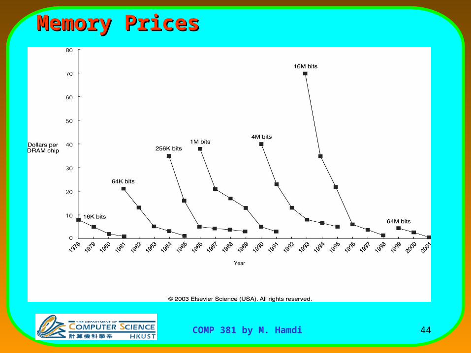
Memory PricesMemory Prices

45COMP 381 by M. Hamdi
Trends in Cost:The Price of Pentium4 and PentiumM

46COMP 381 by M. Hamdi
Integrated Circuit CostsIntegrated Circuit Costs
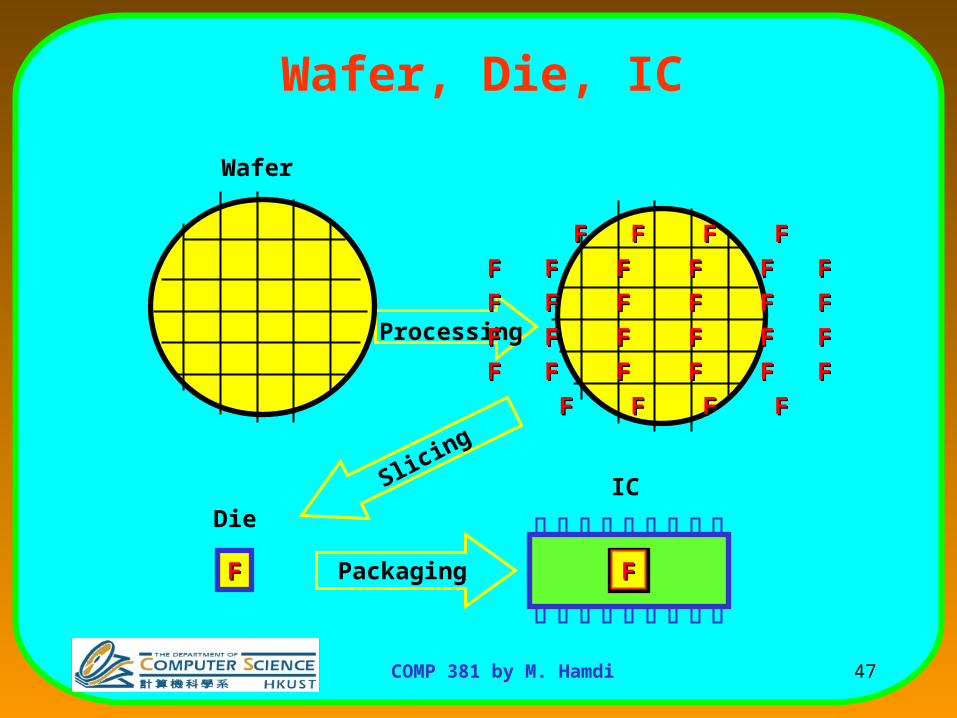
• Each copy of the integrated circuit appears in a die
• Multiple dies are placed on each wafer
• After fabrication, the individual dies are separated, tested, and packaged
Wafer
Die
47COMP 381 by M. Hamdi
Wafer, Die, IC
Processing
F F F F
F F F F F F
F F F F F F
F F F F F F
F F F F F F
F F F F
F F F F
F F F F F F
F F F F F F
F F F F F F
F F F F F F
F F F F
FF
Die
FF
IC
Packaging
Slicing
Wafer

48COMP 381 by M. Hamdi
Integrated Circuit CostsIntegrated Circuit Costs
Wafer
Die
Pentium 4 Processor

49COMP 381 by M. Hamdi
Integrated Circuit CostsIntegrated Circuit Costs
Processing
Packaging
TestingTestingTestingTestingYields =good dies
processed dies
IC Cost = Die Cost + IC Cost = Die Cost + Testing costTesting cost + Packaging Cost + Packaging CostFinal Test YieldFinal Test Yield
WaferDie
TestingTestingTestingTesting

50COMP 381 by M. Hamdi
Integrated Circuits CostsIntegrated Circuits Costs
Die costDie cost = Wafer cost Dies per Wafer x Die yieldDie costDie cost = Wafer cost Dies per Wafer x Die yield
IC cost = Die cost + Testing cost + Packaging cost Final test yieldIC cost = Die cost + Testing cost + Packaging cost Final test yield

51COMP 381 by M. Hamdi
Integrated Circuits CostsIntegrated Circuits Costs
IC cost = Die cost + Testing cost + Packaging costIC cost = Die cost + Testing cost + Packaging cost Final test yieldFinal test yieldDie cost = Wafer costDie cost = Wafer cost Dies per WaferDies per Wafer x Die yield x Die yield
IC cost = Die cost + Testing cost + Packaging costIC cost = Die cost + Testing cost + Packaging cost Final test yieldFinal test yieldDie cost = Wafer costDie cost = Wafer cost Dies per WaferDies per Wafer x Die yield x Die yield
( Wafer_diameter/2)2
Die AreaDies per Wafer =
( Wafer_diameter )
2 * Die Area12
52COMP 381 by M. Hamdi
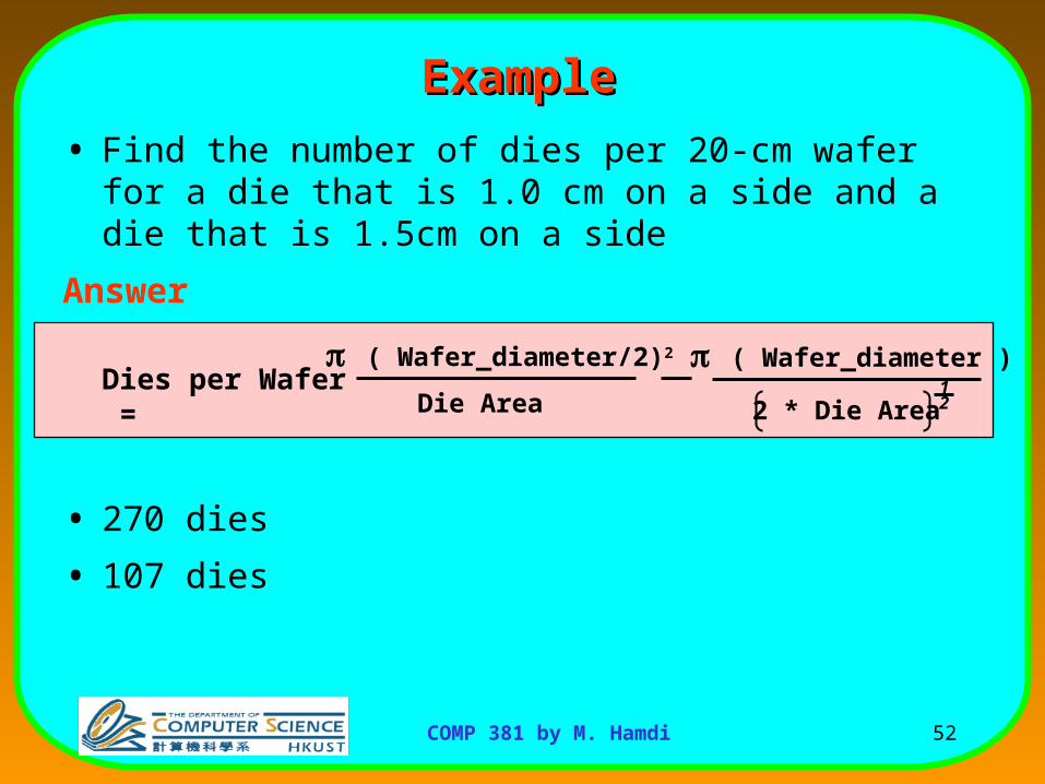
ExampleExample
• Find the number of dies per 20-cm wafer for a die that is 1.0 cm on a side and a die that is 1.5cm on a side
Answer
• 270 dies
• 107 dies
( Wafer_diameter/2)2
Die AreaDies per Wafer =
( Wafer_diameter )
2 * Die Area12
53COMP 381 by M. Hamdi
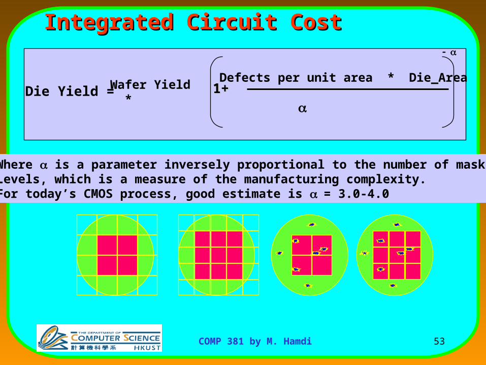
Integrated Circuit CostIntegrated Circuit Cost
Where is a parameter inversely proportional to the number of maskLevels, which is a measure of the manufacturing complexity.For today’s CMOS process, good estimate is = 3.0-4.0
Wafer Yield * Die Yield = Defects per unit area * Die_Area
1+1+

54COMP 381 by M. Hamdi
Integrated Circuits Costs
example : defect density : 0.8 per cm2
= 3.0
case 1: 1 cm x 1 cm die yield = (1+(0.8x1)/3)-3 = 0.49
case 2: 1.5 cm x 1.5 cm die yield = (1+(0.8x2.25)/3)-3 = 0.24
20-cm-diameter wafer with 3-4 metal layers : $3500
case 1 : 132 good 1-cm2 dies, $27case 2 : 25 good 2.25-cm2 dies, $140
Die Cost goes roughly with (die area)4
55COMP 381 by M. Hamdi
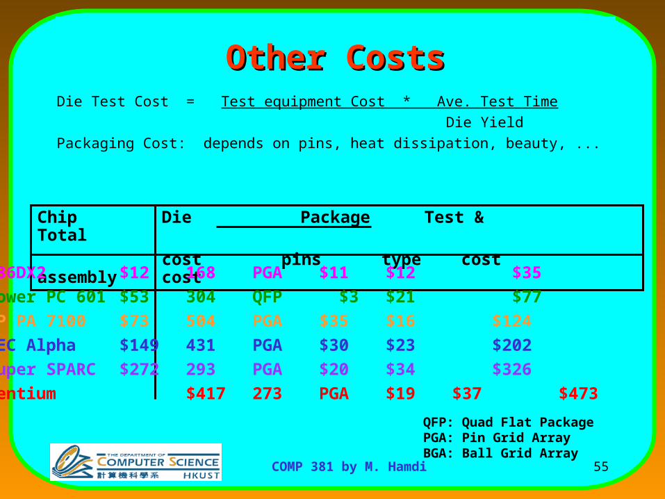
Die Test Cost = Test equipment Cost * Ave. Test Time
Die Yield
Packaging Cost: depends on pins, heat dissipation, beauty, ...
Other CostsOther Costs
Chip Die Package Test & Total
cost pins type cost assembly cost
QFP: Quad Flat PackagePGA: Pin Grid ArrayBGA: Ball Grid Array
486DX2 $12 168 PGA $11 $12 $35
Power PC 601 $53 304 QFP $3 $21 $77
HP PA 7100 $73 504 PGA $35 $16 $124
DEC Alpha $149 431 PGA $30 $23 $202
Super SPARC $272 293 PGA $20 $34 $326
Pentium $417 273 PGA $19 $37 $473

56COMP 381 by M. Hamdi
Cost/PriceWhat is Relationship of Cost to Price?
Component Costs
List Price
100%Component Cost100%

57COMP 381 by M. Hamdi
Cost/PriceWhat is Relationship of Cost to Price?
• Component Costs
List Price
100% Direct Cost 20% to 28%
72% to 80%ComponentCost
• Direct Costs (add 25% to 40% to component cost) Recurring costs: labor, purchasing, scrap, warranty

58COMP 381 by M. Hamdi
Cost/PriceWhat is Relationship of Cost to Price?
• Component Costs
List PricePC’s -- Lower gross margin- Lower R&D expense- Lower sales cost
Mail order, Phone order, retail store…- Higher competition Lower profit, volume sale,...
Gross margin varies depending on the productsHigh performance large systems vs Lower end machines
GrossMargin
45% to 65%
Direct Cost 10% to 11%
Component Cost
25 % to 44%
100%
• Direct Costs (add 25% to 40%) recurring costs: labor, purchasing, scrap, warranty
• Gross Margin (add 82% to 186%) nonrecurring costs: R&D, marketing, sales, equipment maintenance, rental, financing cost, pretax profits, taxes

59COMP 381 by M. Hamdi
Cost/PriceWhat is Relationship of Cost to Price?
• Component Costs
100%
AverageDiscount
List Price
25% to 40%
GrossMargin
Avg. Selling Price
34% to 39%
Direct Cost 6% to 8%
ComponentCost
15% to 33%
• Direct Costs (add 25% to 40%) recurring costs: labor, purchasing, scrap, warranty• Gross Margin (add 82% to 186%) nonrecurring costs:
R&D, marketing, sales,equipment maintenance, rental, financing cost, pretax profits, taxes
• Average Discount to get List Price (add 33% to 66%): volume discounts and/or retailer markup
60COMP 381 by M. Hamdi
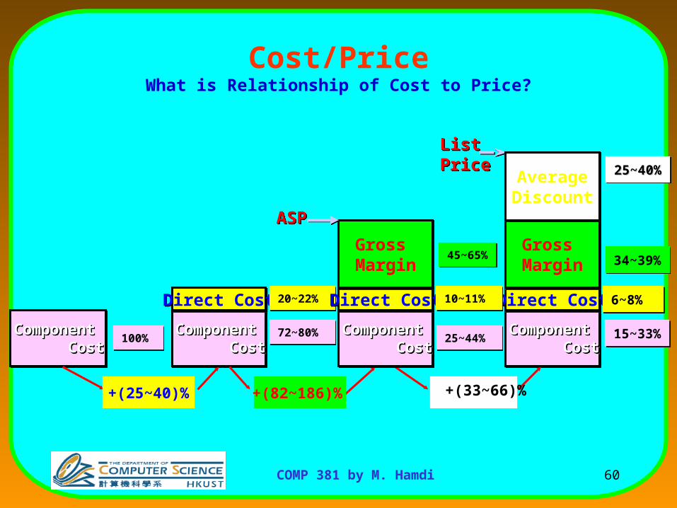
Cost/PriceWhat is Relationship of Cost to Price?
ComponentComponent CostCostComponentComponent CostCost
100%100%
Direct CostDirect Cost
ComponentComponent CostCostComponentComponent CostCost
72~80%72~80%
20~22%20~22%
+(25~40)%
List PriceList Price
Direct CostDirect Cost
Gross MarginGross Margin
Average Discount Average Discount
ComponentComponent CostCostComponentComponent CostCost
15~33%15~33%
6~8%6~8%
34~39%34~39%
25~40%25~40%25~40%25~40%
+(33~66)%+(82~186)%
Direct CostDirect Cost
Gross MarginGross Margin
ComponentComponent CostCostComponentComponent CostCost
25~44%25~44%
10~11%10~11%
45~65%45~65%
ASPASP

61COMP 381 by M. Hamdi
Trends in Power in ICs
• Power Issues– How to bring it in and distribute around the chip?
(many pins just for power supply and ground, interconnection layers for distribution)
– How to remove the heat (dissipated power)
• Why worry about power?– Battery life in portable and mobile platforms– Power consumption in desktops, server farms
• Cooling costs, packaging costs, reliability, timing• Power density: 30 W/cm2 in Alpha 21364
(3x of typical hot plate)
– Environment?• IT consumes 10% of energy in the US
Power becomes a first class architectural design constraint

62COMP 381 by M. Hamdi
Why worry about power? -- Power Dissipation
P6Pentium ®
486
3862868086
80858080
80084004
0.1
1
10
100
1971 1974 1978 1985 1992 2000Year
Po
wer
(W
atts
)Lead microprocessors power continues to increaseLead microprocessors power continues to increase
Power delivery and dissipation will be prohibitivePower delivery and dissipation will be prohibitiveSource: Borkar, De Intel

63COMP 381 by M. Hamdi
Performance Evaluation Performance Evaluation of Computersof Computers

64COMP 381 by M. Hamdi
Metrics for PerformanceMetrics for Performance
• The hardware performance is one major factor for the success of a computer system.
How to measure performance? A computer user is typically interested in
reducing the response time (execution time) - the time between the start and completion of an event.
A computer center manager is interested in increasing the throughput - the total amount of work done in a period of time.
65COMP 381 by M. Hamdi
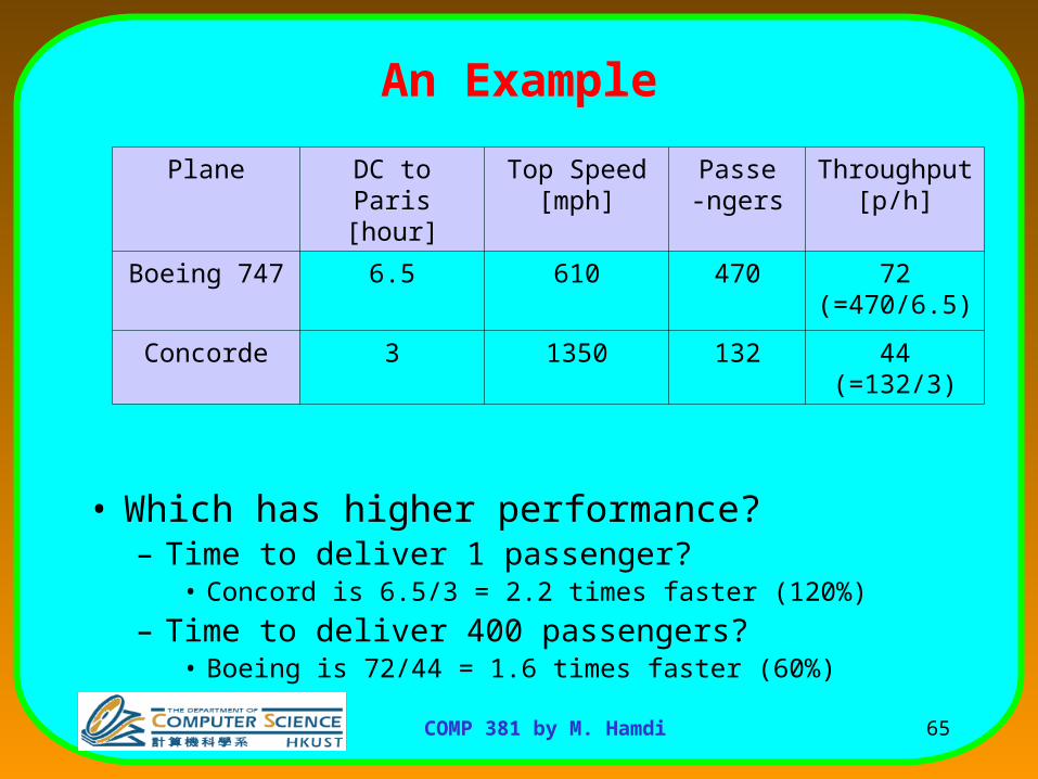
An Example
• Which has higher performance?– Time to deliver 1 passenger?
• Concord is 6.5/3 = 2.2 times faster (120%)
– Time to deliver 400 passengers?• Boeing is 72/44 = 1.6 times faster (60%)
Plane DC to Paris[hour]
Top Speed[mph]
Passe-ngers
Throughput[p/h]
Boeing 747 6.5 610 470 72 (=470/6.5)
Concorde 3 1350 132 44 (=132/3)

66COMP 381 by M. Hamdi
Definition of Performance
• We are primarily concerned with Response Time
• Performance [things/sec]
• “X is n times faster than Y”
• As faster means both increased performance and decreased execution time, to reduce confusion will use “improve performance” or “improve execution time”
)(_)(
xtimeExecutionxePerformanc
1
)(
)(
)(_
)(_
yePerformanc
xePerformanc
xtimeExecution
ytimeExecutionn
67COMP 381 by M. Hamdi
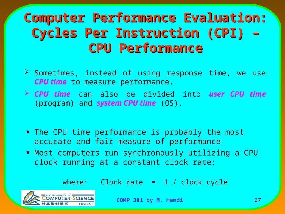
Computer Performance Computer Performance Evaluation:Evaluation:
Cycles Per Instruction (CPI) – CPU Cycles Per Instruction (CPI) – CPU PerformancePerformance
Sometimes, instead of using response time, we use CPU time to measure performance.
CPU time can also be divided into user CPU time (program) and system CPU time (OS).
• The CPU time performance is probably the most accurate and fair measure of performance
• Most computers run synchronously utilizing a CPU clock running at a constant clock rate:
where: Clock rate = 1 / clock cycle
68COMP 381 by M. Hamdi
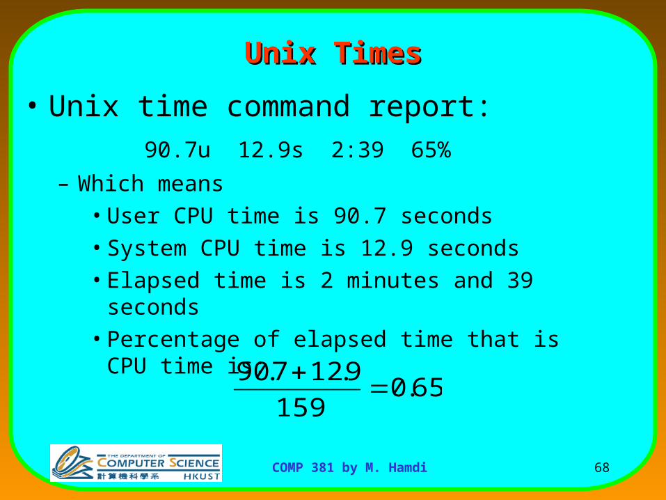
Unix TimesUnix Times
• Unix time command report:90.7u 12.9s 2:39 65%
– Which means• User CPU time is 90.7 seconds• System CPU time is 12.9 seconds• Elapsed time is 2 minutes and 39 seconds• Percentage of elapsed time that is CPU time
is:
65.0159
9.127.90

69COMP 381 by M. Hamdi
Cycles Per Instruction (CPI) – CPU Cycles Per Instruction (CPI) – CPU PerformancePerformance
• A computer machine instruction is comprised of a number of elementary or micro operations which vary in number and complexity depending on the instruction and the exact CPU organization and implementation.– A micro operation is an elementary hardware operation that can
be performed during one clock cycle.
– This corresponds to one micro-instruction in microprogrammed CPUs.
– Examples: register operations: shift, load, clear, increment, ALU operations: add , subtract, etc.
• Thus a single machine instruction may take one or more cycles to complete termed as the Cycles Per Instruction (CPI).

70COMP 381 by M. Hamdi
CPU Performance EquationCPU Performance Equation
CPU time = CPU clock cycles for a program X Clock cycle time
or: CPU time = CPU clock cycles for a program / clock rate CPI (clock cycles per instruction):
CPI = CPU clock cycles for a program / I
where I is the instruction count.

71COMP 381 by M. Hamdi
CPU Execution Time: The CPU CPU Execution Time: The CPU EquationEquation
• A program is comprised of a number of instructions, I– Measured in: instructions/program
• The average instruction takes a number of cycles per instruction (CPI) to be completed. – Measured in: cycles/instruction
• CPU has a fixed clock cycle time C = 1/clock rate – Measured in: seconds/cycle
• CPU execution time is the product of the above three parameters as follows:
CPU Time = I x CPI x C
CPU time = Seconds = Instructions x Cycles x Seconds
Program Program Instruction Cycle
CPU time = Seconds = Instructions x Cycles x Seconds
Program Program Instruction Cycle

72COMP 381 by M. Hamdi
CPU Execution TimeCPU Execution Time
For a given program and machine:
CPI = Total program execution cycles / Instructions count
CPU clock cycles = Instruction count x CPI
CPU execution time =
= CPU clock cycles x Clock cycle
= Instruction count x CPI x Clock cycle = I x CPI x C

73COMP 381 by M. Hamdi
CPU Execution Time: ExampleCPU Execution Time: Example• A Program is running on a specific machine with
the following parameters:– Total instruction count: 10,000,000 instructions– Average CPI for the program: 2.5 cycles/instruction.– CPU clock rate: 200 MHz.
• What is the execution time for this program:
CPU time = Instruction count x CPI x Clock cycle
= 10,000,000 x 2.5 x 1 / clock rate
= 10,000,000 x 2.5 x 5x10-9
= .125 seconds
CPU time = Seconds = Instructions x Cycles x Seconds
Program Program Instruction Cycle
CPU time = Seconds = Instructions x Cycles x Seconds
Program Program Instruction Cycle

74COMP 381 by M. Hamdi
Factors Affecting CPU Factors Affecting CPU PerformancePerformanceCPU time = Seconds = Instructions x Cycles x
Seconds
Program Program Instruction Cycle
CPU time = Seconds = Instructions x Cycles x Seconds
Program Program Instruction Cycle
CPI Clock Cycle CInstruction Count I
Program
Compiler
Organization
Technology
Instruction SetArchitecture (ISA)
X
X
X
X
X
X
X X
X

75COMP 381 by M. Hamdi
Performance Comparison: Performance Comparison: ExampleExample• Using the same program with these changes:
– A new compiler used: New instruction count 9,500,000
New CPI: 3.0– Faster CPU implementation: New clock rate = 300
MHZ
• What is the speedup with the changes?
Speedup = (10,000,000 x 2.5 x 5x10-9) / (9,500,000 x 3 x 3.33x10-9 )
= .125 / .095 = 1.32 or 32 % faster after the changes.
Speedup = Old Execution Time = Iold x CPIold x Clock cycleold
New Execution Time Inew x CPInew x Clock Cyclenew
Speedup = Old Execution Time = Iold x CPIold x Clock cycleold
New Execution Time Inew x CPInew x Clock Cyclenew

76COMP 381 by M. Hamdi
Metrics of Computer Metrics of Computer PerformancePerformance
Compiler
Programming Language
Application
DatapathControl
Transistors Wires Pins
ISA
Function UnitsCycles per second (clock rate).
Megabytes per second.
Execution time: Target workload,SPEC95, etc.
Each metric has a purpose, and each can be misused.
(millions) of Instructions per second – MIPS(millions) of (F.P.) operations per second – MFLOP/s

77COMP 381 by M. Hamdi
Choosing Programs To Evaluate Choosing Programs To Evaluate PerformancePerformance
Levels of programs or benchmarks that could be used to evaluate performance:– Actual Target Workload: Full applications that run on the
target machine.
– Real Full Program-based Benchmarks: • Select a specific mix or suite of programs that are typical of
targeted applications or workload (e.g SPEC95, SPEC CPU2000).
– Small “Kernel” Benchmarks: • Key computationally-intensive pieces extracted from real
programs.– Examples: Matrix factorization, FFT, tree search, etc.
• Best used to test specific aspects of the machine.
– Microbenchmarks:
• Small, specially written programs to isolate a specific aspect of performance characteristics: Processing: integer, floating point, local memory, input/output, etc.

78COMP 381 by M. Hamdi
Actual Target Workload
Full Application Benchmarks
Small “Kernel” Benchmarks
Microbenchmarks
Pros Cons
• Representative• Very specific.• Non-portable.• Complex: Difficult to run, or measure.
• Portable.• Widely used.• Measurements useful in reality.
• Easy to run, early in the design cycle.
• Identify peak performance and potential bottlenecks.
• Less representative than actual workload.
• Easy to “fool” by designing hardware to run them well.
• Peak performance results may be a long way from real application performance
Types of BenchmarksTypes of Benchmarks

79COMP 381 by M. Hamdi
SPEC: System Performance SPEC: System Performance Evaluation CooperativeEvaluation Cooperative
The most popular and industry-standard set of CPU benchmarks.SPECmarks, 1989:
– 10 programs yielding a single number (“SPECmarks”).
• SPEC92, 1992:– SPECInt92 (6 integer programs) and SPECfp92 (14 floating point programs).
• SPEC95, 1995:– SPECint95 (8 integer programs):
• go, m88ksim, gcc, compress, li, ijpeg, perl, vortex– SPECfp95 (10 floating-point intensive programs):
• tomcatv, swim, su2cor, hydro2d, mgrid, applu, turb3d, apsi, fppp, wave5– Performance relative to a Sun SuperSpark I (50 MHz) which is given a score of SPECint95 = SPECfp95 = 1
• SPEC CPU2000, 1999:– CINT2000 (11 integer programs). CFP2000 (14 floating-point intensive programs)
– Performance relative to a Sun Ultra5_10 (300 MHz) which is given a score of SPECint2000 = SPECfp2000 = 100
• SPEC CPU2006:– CINT2006 (12 integer programs). CFP2006 (17 floating-point intensive programs)
– Performance relative to a Sun SPARC Enterprise M8000 which is given a score of SPECint2006 = 11.3 SPECfp2006 = 12.4
80COMP 381 by M. Hamdi
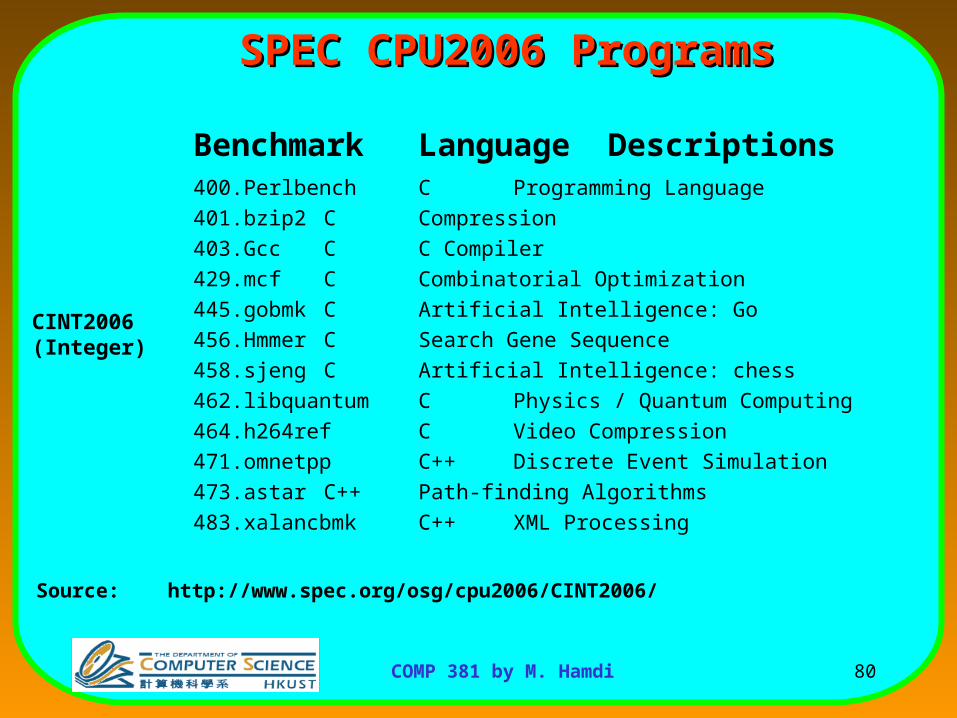
SPEC CPU2006 ProgramsSPEC CPU2006 Programs
Benchmark Language Descriptions 400.Perlbench C Programming Language
401.bzip2 C Compression
403.Gcc C C Compiler
429.mcf C Combinatorial Optimization
445.gobmk C Artificial Intelligence: Go
456.Hmmer C Search Gene Sequence
458.sjeng C Artificial Intelligence: chess
462.libquantum C Physics / Quantum Computing
464.h264ref C Video Compression
471.omnetpp C++ Discrete Event Simulation
473.astar C++ Path-finding Algorithms
483.xalancbmk C++ XML Processing
CINT2006(Integer)
Source: http://www.spec.org/osg/cpu2006/CINT2006/
81COMP 381 by M. Hamdi
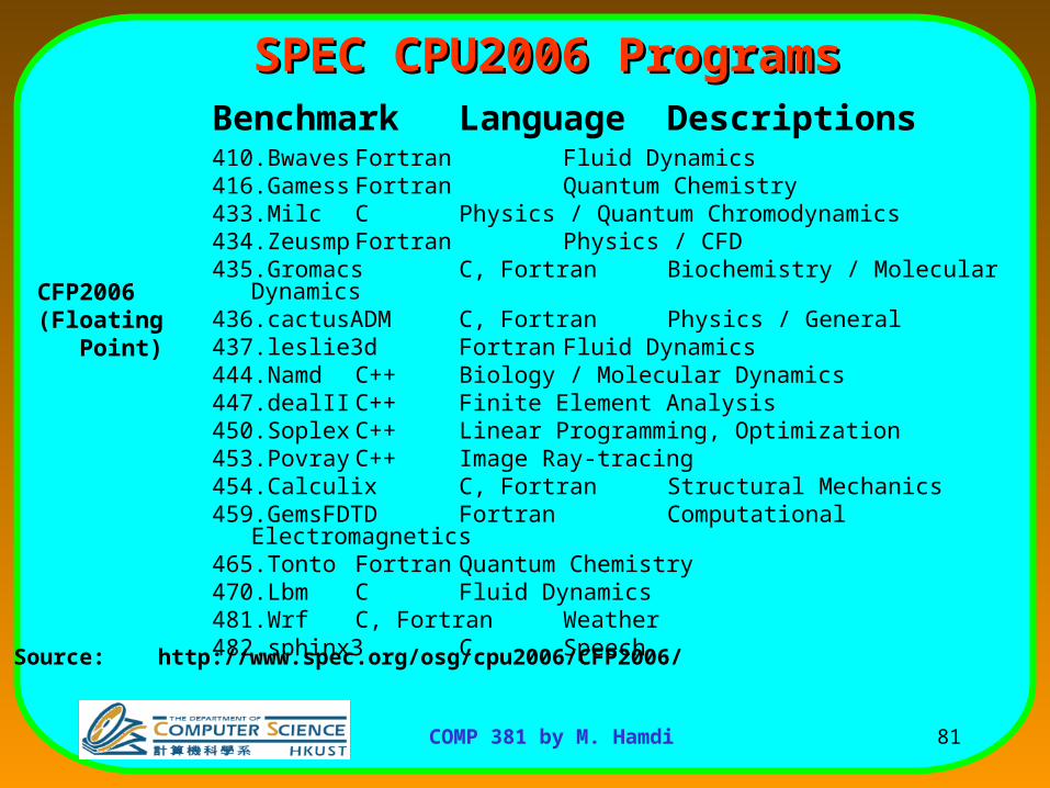
SPEC CPU2006 ProgramsSPEC CPU2006 ProgramsBenchmark Language Descriptions410.Bwaves Fortran Fluid Dynamics 416.Gamess Fortran Quantum Chemistry433.Milc C Physics / Quantum
Chromodynamics 434.Zeusmp Fortran Physics / CFD435.Gromacs C, Fortran Biochemistry / Molecular Dynamics 436.cactusADM C, Fortran Physics / General 437.leslie3d Fortran Fluid Dynamics 444.Namd C++ Biology / Molecular Dynamics 447.dealII C++ Finite Element Analysis 450.Soplex C++ Linear Programming, Optimization 453.Povray C++ Image Ray-tracing 454.Calculix C, Fortran Structural Mechanics 459.GemsFDTD Fortran Computational Electromagnetics465.Tonto Fortran Quantum Chemistry470.Lbm C Fluid Dynamics 481.Wrf C, Fortran Weather482.sphinx3 C Speech
CFP2006(Floating Point)
Source: http://www.spec.org/osg/cpu2006/CFP2006/

82COMP 381 by M. Hamdi
Top 20 SPEC CPU2006 Results (As of August 2007)
# MHz Processor int peak int base MHz Processor fp peak fp base
1 3000 Core 2 Duo E6850 22.6 20.2 4700 POWER6 22.4 17.8
2 4700 POWER6 21.6 17.8 3000 Core 2 Duo E6850 19.3 18.7
3 3000 Xeon 5160 21.0 17.9 1600 Dual-Core Itanium 2 9050 18.117.3
4 3000 Xeon X5365 20.8 18.9 1600 Dual-Core Itanium 2 9040 17.817.0
5 2666 Core 2 Duo E6750 20.5 18.3 2666 Core 2 Duo E6750 17.7 17.1
6 2667 Core 2 Duo E6700 20.0 17.9 3000 Xeon 5160 17.7 17.1
7 2667 Core 2 Quad Q6700 19.7 17.6 3000 Opteron 2222 17.4 16.0
8 2666 Xeon X5355 19.1 17.3 2667 Core 2 Duo E6700 16.9 16.3
9 2666 Xeon 5150 19.1 17.3 2800 Opteron 2220 16.7 13.3
10 2666 Xeon X5355 18.9 17.2 3000 Xeon 5160 16.6 16.1
11 2667 Xeon X5355 18.6 16.8 2667 Xeon X5355 16.6 16.1
12 2933 Core 2 18.5 17.8 2667 Core 2 Quad Q6700 16.6 16.1
13 2400 Core 2 Quad Q6600 18.5 16.5 2666 Xeon X5355 16.6 16.1
14 2600 Core 2 Duo X7800 18.3 16.4 2933 Core 2 Extreme X6800 16.216.0
15 2667 Xeon 5150 17.6 16.6 2400 Core 2 Quad Q6600 16.0 15.4
16 2400 Core 2 Duo T7700 17.6 16.6 1400 Dual-Core Itanium 2 9020 15.915.2
17 2333 Xeon E5345 17.5 15.9 2667 Xeon 5150 15.9 15.5
18 2333 Xeon 5148 17.4 15.9 2333 Xeon E5345 15.4 14.9
19 2333 Xeon 5140 17.4 15.7 2600 Opteron 2218 15.4 12.5
20 2660 Xeon X5355 17.4 15.7 2400 Xeon X3220 15.3 15.1
Source: http://www.spec.org/cpu2006/results/cint2006.html
Top 20 SPECfp2006Top 20 SPECint2006

83COMP 381 by M. Hamdi
Performance Evaluation Using Performance Evaluation Using BenchmarksBenchmarks
• “For better or worse, benchmarks shape a field”
• Good products created when we have:– Good benchmarks
– Good ways to summarize performance
• Given sales depend in big part on performance relative to competition, there is big investment in improving products as reported by performance summary
• If benchmarks inadequate, then choose between improving product for real programs vs. improving product to get more sales;Sales almost always wins!

84COMP 381 by M. Hamdi
How to Summarize PerformanceHow to Summarize Performance
Benchmark
SP
EC
Perf
0
100
200
300
400
500
600
700
800
gcc
ep
resso
sp
ice
dod
uc
nasa7 li
eq
nto
tt
matr
ix3
00
fpp
pp
tom
catv
85COMP 381 by M. Hamdi
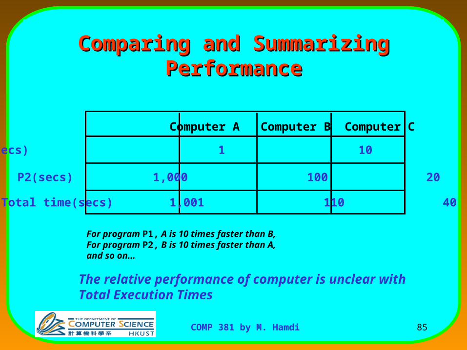
Comparing and Summarizing PerformanceComparing and Summarizing Performance
For program P1, A is 10 times faster than B, For program P2, B is 10 times faster than A, and so on...
The relative performance of computer is unclear with Total Execution Times
Computer A Computer B Computer C
P1(secs) 1 10 20
P2(secs) 1,000 100 20
Total time(secs) 1,001 110 40

86COMP 381 by M. Hamdi
Summary MeasureSummary Measure
Arithmetic Mean n Execution Timei
i=1
1
nGood, if programs are run equally in the workload

87COMP 381 by M. Hamdi
Arithmetic Mean
• The arithmetic mean can be misleading if the data are skewed or scattered.– Consider the execution times given in the table below. The performance
differences are hidden by the simple average.

88COMP 381 by M. Hamdi
Unequal Job MixUnequal Job Mix
Weighted Arithmetic Mean n Weighti x Execution Timei
i=1
Relative Performance
• Normalized Execution Time to a reference machine
Arithmetic Mean Geometric Mean
n Execution Time Ratioi
i=1n Normalized to the
reference machine
• Weighted Execution Time

89COMP 381 by M. Hamdi
Weighted Arithmetic MeanWeighted Arithmetic Mean
W(i)j x Timejj=1
nWAM(i) =
A B C W(1) W(2) W(3)
P1 (secs) 1.00 10.00 20.00 0.50 0.909 0.999
P2(secs) 1,000.00 100.00 20.00 0.50 0.091 0.001
1.0 x 0.5 + 1,000 x 0.5
WAM(1) 500.50 55.00 20.00
WAM(2) 91.91 18.19 20.00
WAM(3) 2.00 10.09 20.00

90COMP 381 by M. Hamdi
Normalized Execution TimeNormalized Execution Time
P1 1.0 10.0 20.0 0.1 1.0 2.0 0.05 0.5 1.0
P2 1.0 0.1 0.02 10.0 1.0 0.2 50.0 5.0 1.0
Normalized to A
Normalized to B Normalized to C
A B C A B C A B C
Geometric Mean = n Execution time ratioiI=1
n
Arithmetic mean 1.0 5.05 10.01 5.05 1.0 1.1 25.03 2.75 1.0
Geometric mean 1.0 1.0 0.63 1.0 1.0 0.63 1.58 1.58 1.0
A B CP1 1.00 10.00 20.00P2 1,000.00 100.00 20.00

91COMP 381 by M. Hamdi
Disadvantages Disadvantages of Arithmetic Meanof Arithmetic Mean
Performance varies depending on the reference machine
1.0 10.0 20.0 0.1 1.0 2.0 0.05 0.5 1.0 1.0 0.1 0.02 10.0 1.0 0.2 50.0 5.0 1.0
1.0 5.05 10.01 5.05 1.0 1.1 25.03 2.75 1.0
B is 5 times slower than A
A is 5 times slower than B
C is slowest C is fastest
Normalized to A
Normalized to B Normalized to C
A B C A B C A B C
P1
P2
Arithmetic mean

92COMP 381 by M. Hamdi
The Pros and Cons Of The Pros and Cons Of Geometric MeansGeometric Means
• Independent of running times of the individual programs
• Independent of the reference machines
• Do not predict execution time– the performance of A and B is the same : only true when P1 ran 100
times for every occurrence of P2
P2 1.0 0.1 0.02 10.0 1.0 0.2 50.0 5.0 1.0
P1 1.0 10.0 20.0 0.1 1.0 2.0 0.05 0.5 1.0
1(P1) x 100 + 1000(P2) x 1= 10(P1) x 100 + 100(P2) x 1
Geometric mean 1.0 1.0 0.63 1.0 1.0 0.63 1.58 1.58 1.0
Normalized to A Normalized to B Normalized to C
A B C A B C A B C
93COMP 381 by M. Hamdi
Geometric Mean
• The real usefulness of the normalized geometric mean is that no matter which system is used as a reference, the ratio of the geometric means is consistent.
• This is to say that the ratio of the geometric means for System A to System B, System B to System C, and System A to System C is the same no matter which machine is the reference machine.

94COMP 381 by M. Hamdi
Geometric Mean
• The results that we got when using System B and System C as reference machines are given below.
• We find that 1.6733/1 = 2.4258/1.4497.
95COMP 381 by M. Hamdi
Geometric Mean
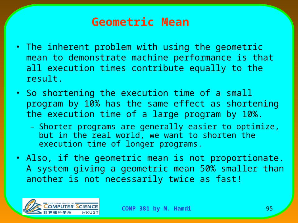
• The inherent problem with using the geometric mean to demonstrate machine performance is that all execution times contribute equally to the result.
• So shortening the execution time of a small program by 10% has the same effect as shortening the execution time of a large program by 10%.– Shorter programs are generally easier to optimize, but in the real world,
we want to shorten the execution time of longer programs.
• Also, if the geometric mean is not proportionate. A system giving a geometric mean 50% smaller than another is not necessarily twice as fast!
96COMP 381 by M. Hamdi
Computer Performance Measures :Computer Performance Measures : MIPS MIPS (Million Instructions Per Second)(Million Instructions Per Second)
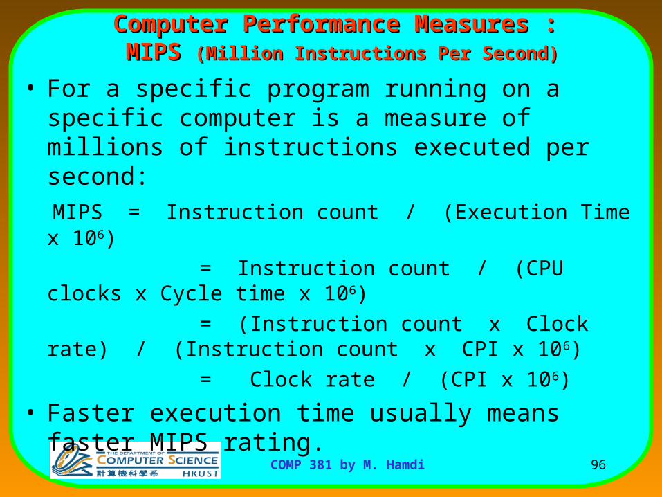
• For a specific program running on a specific computer is a measure of millions of instructions executed per second:
MIPS = Instruction count / (Execution Time x 106)
= Instruction count / (CPU clocks x Cycle time x 106)
= (Instruction count x Clock rate) / (Instruction count x CPI x 106)
= Clock rate / (CPI x 106)
• Faster execution time usually means faster MIPS rating.

97COMP 381 by M. Hamdi
Computer Performance Measures :Computer Performance Measures : MIPS MIPS (Million Instructions Per Second)(Million Instructions Per Second)
• MMeaningless IIndicator of PProcessor PPerformance
• Problems:– No account for instruction set used.
– Program-dependent: A single machine does not have a single MIPS rating.
– Cannot be used to compare computers with different instruction sets.
– A higher MIPS rating in some cases may not mean higher performance or better execution time. i.e. due to compiler design variations.

98COMP 381 by M. Hamdi
Compiler Variations, MIPS, Performance: Compiler Variations, MIPS, Performance: An ExampleAn Example
• For the machine with instruction classes:
• For a given program two compilers produced the following instruction counts:
• The machine is assumed to run at a clock rate of 100 MHz
Instruction class CPI A 1 B 2 C 3
Instruction counts (in millions) for each instruction class Code from: A B C Compiler 1 5 1 1 Compiler 2 10 1 1

99COMP 381 by M. Hamdi
Compiler Variations, MIPS, Compiler Variations, MIPS, Performance: Performance:
An Example (Continued)An Example (Continued)MIPS = Clock rate / (CPI x 106) = 100 MHz / (CPI x 106)
CPI = CPU execution cycles / Instructions count
CPU time = Instruction count x CPI / Clock rate
• For compiler 1:– CPI1 = (5 x 1 + 1 x 2 + 1 x 3) / (5 + 1 + 1) = 10 / 7 = 1.43– MIP1 = 100 / (1.428 x 10⁶) = 70.0– CPU time1 = ((5 + 1 + 1) x 106 x 1.43) / (100 x 106) = 0.10 seconds
• For compiler 2:– CPI2 = (10 x 1 + 1 x 2 + 1 x 3) / (10 + 1 + 1) = 15 / 12 = 1.25– MIP2 = 100 / (1.25 x 10⁶) = 80.0– CPU time2 = ((10 + 1 + 1) x 106 x 1.25) / (100 x 106) = 0.15 seconds
CPU clock cyclesi i
i
n
CPI C
1

100COMP 381 by M. Hamdi
Computer Performance Measures :Computer Performance Measures : MFOLPS MFOLPS (Million FLOating-Point Operations Per
Second)
• A floating-point operation is an addition, subtraction, multiplication, or division operation applied to numbers represented by a single or double precision floating-point representation.
• MFLOPS, for a specific program running on a specific computer, is a measure of millions of floating point-operation (megaflops) per second:
MFLOPS = Number of floating-point operations / (Execution time x 106 )
101COMP 381 by M. Hamdi
Computer Performance Measures :Computer Performance Measures : MFOLPS MFOLPS (Million FLOating-Point Operations Per
Second)
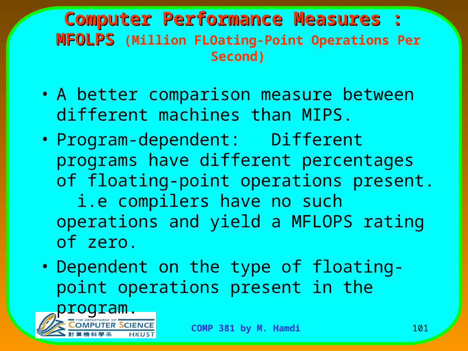
• A better comparison measure between different machines than MIPS.
• Program-dependent: Different programs have different percentages of floating-point operations present. i.e compilers have no such operations and yield a MFLOPS rating of zero.
• Dependent on the type of floating-point operations present in the program.

102COMP 381 by M. Hamdi
Quantitative Principles Quantitative Principles of Computer Designof Computer Design
• Amdahl’s Law:Amdahl’s Law: The performance gain from improving some portion of
a computer is calculated by:
Speedup = Performance for entire task using the enhancement Performance for the entire task without using the enhancement
or Speedup = Execution time without the enhancement Execution time for entire task using the enhancement

103COMP 381 by M. Hamdi
Performance Enhancement Performance Enhancement Calculations:Calculations:
Amdahl's Law Amdahl's Law
• The performance enhancement possible due to a given design improvement is limited by the amount that the improved feature is used
• Amdahl’s Law:Performance improvement or speedup due to
enhancement E:
Execution Time without E Performance with E
Speedup(E) = -------------------------------------- = --------------------- Execution Time with E Performance
without E

104COMP 381 by M. Hamdi
Performance Enhancement Performance Enhancement Calculations:Calculations:
Amdahl's Law Amdahl's Law• Suppose that enhancement E accelerates a fraction F of the
execution time by a factor S and the remainder of the time is unaffected then:
Execution Time with E = ((1-F) + F/S) X Execution Time
without E
Hence speedup is given by:
Execution Time without E 1Speedup(E) = --------------------------------------------------------- =
----------------
((1 - F) + F/S) X Execution Time without E (1 - F) +F/S
105COMP 381 by M. Hamdi
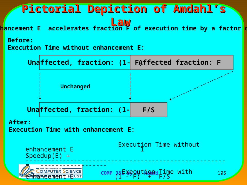
Pictorial Depiction of Amdahl’s Pictorial Depiction of Amdahl’s LawLaw
Before: Execution Time without enhancement E:
Unaffected, fraction: (1- F)
After: Execution Time with enhancement E:
Enhancement E accelerates fraction F of execution time by a factor of S
Affected fraction: F
Unaffected, fraction: (1- F) F/S
Unchanged
Execution Time without enhancement E 1Speedup(E) = ------------------------------------------------------ = ------------------ Execution Time with enhancement E (1 - F) + F/S
106COMP 381 by M. Hamdi
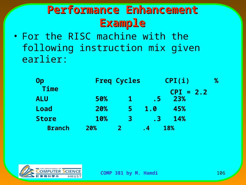
Performance Enhancement Performance Enhancement ExampleExample
• For the RISC machine with the following instruction mix given earlier:
Op Freq Cycles CPI(i) % Time
ALU 50% 1 .5 23%
Load 20% 5 1.0 45%
Store 10% 3 .3 14% Branch 20% 2 .4 18%
CPI = 2.2
107COMP 381 by M. Hamdi
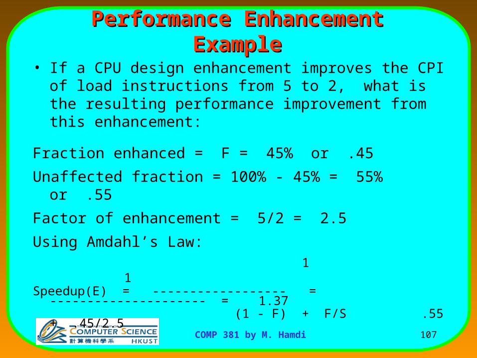
Performance Enhancement Performance Enhancement ExampleExample
• If a CPU design enhancement improves the CPI of load instructions from 5 to 2, what is the resulting performance improvement from this enhancement:
Fraction enhanced = F = 45% or .45
Unaffected fraction = 100% - 45% = 55% or .55
Factor of enhancement = 5/2 = 2.5
Using Amdahl’s Law: 1 1Speedup(E) = ------------------ = --------------------- = 1.37 (1 - F) + F/S .55 + .45/2.5

108COMP 381 by M. Hamdi
An Alternative Solution Using CPU An Alternative Solution Using CPU EquationEquation
• If a CPU design enhancement improves the CPI of load instructions from 5 to 2, what is the resulting performance improvement from this enhancement:
Old CPI = 2.2
New CPI = .5 x 1 + .2 x 2 + .1 x 3 + .2 x 2 = 1.6
Original Execution Time Instruction count x old CPI x clock cycleSpeedup(E) = ------------------------------- = ---------------------------------------------------------- New Execution Time Instruction count x new CPI x clock cycle
old CPI 2.2= ------------ = --------- = 1.37
new CPI 1.6
Which is the same speedup obtained from Amdahl’s Law in the first solution.
109COMP 381 by M. Hamdi
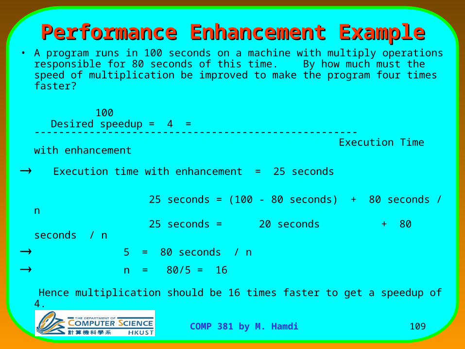
Performance Enhancement Performance Enhancement ExampleExample• A program runs in 100 seconds on a machine with multiply
operations responsible for 80 seconds of this time. By how much must the speed of multiplication be improved to make the program four times faster?
100 Desired speedup = 4 = ----------------------------------------------------- Execution Time with enhancement
Execution time with enhancement = 25 seconds
25 seconds = (100 - 80 seconds) + 80 seconds / n 25 seconds = 20 seconds + 80 seconds / n
5 = 80 seconds / n
n = 80/5 = 16
Hence multiplication should be 16 times faster to get a speedup of 4.

110COMP 381 by M. Hamdi
Performance Enhancement Performance Enhancement ExampleExample
• For the previous example with a program running in 100 seconds on a machine with multiply operations responsible for 80 seconds of this time. By how much must the speed of multiplication be improved to make the program five times faster?
100Desired speedup = 5 = ----------------------------------------------------- Execution Time with enhancement
Execution time with enhancement = 20 seconds
20 seconds = (100 - 80 seconds) + 80 seconds / n 20 seconds = 20 seconds + 80 seconds / n
0 = 80 seconds / n
No amount of multiplication speed improvement can achieve this.

111COMP 381 by M. Hamdi
Another Amdahl’s Law Example
• New CPU 10X faster• I/O-bound server, so 60% time waiting for I/O
56.1
64.0
1
100.4
0.4 1
1
Speedup
Fraction Fraction 1
1 Speedup
enhanced
enhancedenhanced
overall
• Apparently, it’s human nature to be attracted by 10X faster, vs. keeping in perspective it’s just 1.6X faster