an empirical assessment of the q-factor model: … · presented by gordon and shapiro (1956). 2.1....

The Lahore Journal of Economics 22 : 2 (Winter 2017): pp. 117–138

An Empirical Assessment of the Q-Factor Model: Evidence

from the Karachi Stock Exchange

Humaira Asad* and Faraz Khalid Cheema**

Abstract

This paper tests the validity of the q-factor model on stocks listed on the Karachi Stock Exchange in Pakistan. The q-factor model is an investment-based factor model that explains stock returns based on market, profitability, investment and size factors and it tends to outperform the traditional CAPM, the Fama and French (1993) three-factor model and Carhart (1997) four-factor model, with some exceptions. While the model has been tested using data from stock markets in developed countries, the dynamics of emerging stock markets are significantly different, warranting a reapplication of the model to average stock returns in a developing market. We use data from the Karachi Stock Exchange to test the model in an emerging market context. The results show that, as firms increase their investment, their stock returns decline. Hence, a firm’s investment is conditional on a given level of profitability. The size effect is strongly significant for small firms, but absent for large firms. Finally, the study identifies new factors that give a better understanding of returns in the context of an emerging economy such as Pakistan.

Keywords: Asset pricing, q-factor model, Karachi Stock Exchange, stock return.

JEL classification: G11, G12.

1. Introduction

This study investigates which factors determine the returns on stocks listed on the Karachi Stock Exchange (KSE) by applying the q-factor model developed by Hou, Xue and Zhang (2012, 2015). The q-factor model is an investment-based factor model derived from Tobin’s q theory, which explains several anomalies of average returns not explained by earlier asset pricing models. This study empirically tests the validity of the factors identified by the q-factor model – market, investment, profitability and size – in relation to stocks listed on the KSE.

* Assistant Professor, Institute of Business Administration, University of the Punjab, Lahore. ** Research scholar, Institute of Business Administration, University of the Punjab, Lahore.

Humaira Asad and Faraz Khalid Cheema 118

Hou et al. (2012, 2015) developed a q-factor model that explains several average-return anomalies, most significantly the momentum effect. The q-factor model explains the impact of a firm’s investment behavior and profitability on expected average stock returns – factors not explained by the Fama and French (1993) three-factor model. The q-factor model derives the investment and profitability factors and their relation to expected returns from Tobin’s q theory (Tobin, 1969), which states that the firm’s investment decisions depend on the ratio of the market value of capital to the replacement cost of capital – termed the marginal q. Firms tend to invest more when the marginal q is high and less when it is low. Similarly, all else equal, a high cost of capital means low investment and a low cost of capital means high investment.

The model considers the combined effect of profitability and investment because the relationship between the firm’s investment and stock returns is conditional on a certain level of profitability, as high-investment firms tend to have higher levels of profitability (Fama & French, 2006). Thus, for a given expected profitability for the firm, its expected returns will decrease with increasing investment; for a given level of investment, its expected returns will increase with increasing profitability. Similarly, the positive relationship between profitability and returns is conditional on a given level of investment, as profitability may also be associated with higher investment. Specifically, the q-factor model states that the expected returns of a portfolio are explained by its sensitivity to four factors: market excess returns, the difference between the returns on small and large capitalization stocks, the difference between the returns on low and high investment-to-asset (I/A) stocks and the difference between the returns on high and low return-on-equity (ROE) stocks.

The three-factor model does not explain high asset growth in stocks (see Fama & French, 1993). Acknowledging the new q-factor model presented by Hou et al. (2012), but using a different theoretical framework, Fama and French (2015) test a comprehensive five-factor model that incorporates the investment and profitability effects into their earlier three-factor model. They find that the five-factor model outperforms the latter. However, the value factor becomes redundant and the five-factor model fails to capture the low returns on small stocks that have invested more despite low profitability. Accordingly, they suggest dropping the value factor if the objective is to measure regression intercepts, but retaining all five factors if the portfolios possess size, value, profitability and investment premiums. Fama and French (2017) tested the five-factor model for a sample drawn from North America, Europe and Japan, which largely

Assessment of the Q-Factor Model for the Karachi Stock Exchange 119

explained average returns, but with wide variability among factors across regions. The investment and profitability factors were strongest for North America, but insignificant for Japan and the Asia-Pacific region, where the value factor is strong.

Using data from the New York Stock Exchange, Hou, Xue and Zhang (2017) compared the performance of the q-factor model, the capital asset pricing model (CAPM), the Fama–French three-factor model, Carhart’s (1997) four-factor model, Pástor and Stambaugh’s (2003) model and Fama and French’s (2015) five-factor model in explaining hundreds of stock return anomalies. They found that the two closely related investment-based models, the q-factor and five-factor models, outperform the others in explaining the maximum number of anomalies as well as expected returns. They termed the five-factor model a noisy version of the q-factor model. The q-factor model also explained the momentum effect identified by Jegadeesh and Titman (1993) better than other models, including that presented by Carhart et al. (1996), which also contains a momentum factor. While the q-factor model best captured the effect of momentum and profitability, the five-factor model explained value-versus-growth anomalies better than other models.

The q-factor model is a recent addition to the literature on asset pricing and there have been very few attempts to validate the model empirically. This study empirically tests the validity of the q-factor model based on the portfolio construction methodology developed by Fama and French (1993, 1996). Our sample consists of 100 companies listed on the KSE over the period June 2004 to May 2014. The objective is to determine the significance of the four factors identified by the q-factor model, i.e., market, size, investment and profitability. The study also estimates the explanatory power of excess market returns, small market capitalization (MC), a low I/A ratio and a high ROE ratio in KSE stock returns. This could help stock market investors determine whether one or more of the factors identified by the q-factor model can be used as a criterion for investment and portfolio formation. It will also help researchers and financial analysts better understand stock movements.

The next section discusses the relevant literature. Section 3 explains the theoretical framework. Section 4 describes the study’s methodology and Section 5 discusses its findings. The article concludes with a set of policy implications, recommendations and limitations.


2. Theoretical Framework

The q-factor model generates hypotheses based on Tobin’s q theory (see Tobin, 1969; Cochrane, 1991), while Fama and French (2015) derived their investment-based factor model from the dividend discount model presented by Gordon and Shapiro (1956).

2.1. Tobin’s Q Theory

Tobin’s (1969) theory of investment connects the financial market with the goods and services market. It suggests that the rate of investment is based on the ratio of the market value of a firm’s capital to its replacement cost. Tobin’s Q, also called average Q, is expressed as

𝑄 =𝑀𝑎𝑟𝑘𝑒𝑡 𝑣𝑎𝑙𝑢𝑒 𝑜𝑓 𝑓𝑖𝑟𝑚 𝑐𝑎𝑝𝑖𝑡𝑎𝑙

𝑅𝑒𝑝𝑙𝑎𝑐𝑒𝑚𝑒𝑛𝑡 𝑐𝑜𝑠𝑡 𝑜𝑓 𝑐𝑎𝑝𝑖𝑡𝑎𝑙 (1)

Tobin’s q theory provides certain guidelines for investment. The market value of the firm’s capital is represented by the stock price. The firm’s capital investment decision depends on where Q is in relation to 1. The theory states that firms should invest more capital when Q > 1 (which will bring it down to 1) and disinvest their capital stock when Q < 1 (which will raise it to 1). This means that capital has more value within the firm when Q > 1 and outside the firm when Q < 1. In a state of equilibrium, Q = 1 and there is no need for capital investment or disinvestment. However, an increase or decrease in capital is not free of cost. Tobin’s q theory assumes that adjustment costs (such as installation costs) are associated with investment.

2.2. Dividend Discount Model

Hou et al. (2015) use the q theory of investment to derive their q-factor model. The model can also be estimated by applying the dividend discount model, following Fama and French (2015), according to which the worth of a stock is equal to the sum of all future dividends discounted to their present value (Gordon & Shapiro, 1956; Gordon, 1962). The model can be represented as follows:

𝑃0 =∑ 𝐸(𝑑𝑡)∞

𝑛=1

(1+𝑘𝑒)𝑡 (2)

where 𝑃0 is the share price at time 0, 𝐸(𝑑𝑡) is the expected dividend per share at time t and ke is the internal rate of return. The dividend at time t


can be expressed as the difference between total and retained earnings (the portion of earnings that is reinvested).

The present market value of the firm is represented as:

𝑃0 =∑ 𝑇𝐸𝑡

∞𝑡=1 −𝑅𝐸𝑡

(1+𝑘𝑒)𝑡 (3)

where 𝑇𝐸𝑡 denotes total earnings at time t and 𝑅𝐸𝑡 denotes retained earnings at time t. Retained earnings can be further expressed as the difference between the book values of equity.

According to Miller and Modigliani (1961), the market value of a stock can be shown as follows:

𝑃0 =∑ (𝑇𝐸𝑡−(𝐵𝑡−𝐵𝑡−1))∞

𝑡=1

(1+𝑘𝑒)𝑡 (4)

Here, (𝐵𝑡 − 𝐵𝑡−1) is the change in the book value of equity. The equation implies that higher earnings 𝑇𝐸𝑡, reflected by profitability, will lead to higher expected returns, while higher growth in equity (𝐵𝑡 − 𝐵𝑡−1), i.e., higher investment, will lead to lower expected returns. We draw on the q-theory of investment as discussed above for our theoretical model.

3. Research Methodology

The four factors included in the q-factor model are market, size, investment and profitability. The market factor is derived from the CAPM. MC is used as a proxy for size, the I/A ratio as a proxy for investment and the ROE as a proxy for profitability. The study employs stock portfolios instead of individual stocks. Blume (1970) suggests that the motivation for creating stock portfolios is to reduce idiosyncratic risk, as the errors of individual stocks will offset each other if they are grouped in a portfolio. The three factors are constructed using the standard methodology developed by Fama and French (1993, 1996).

3.1. Data Source and Sample

The data was obtained from companies’ financial statements, the KSE data portal and the State Bank of Pakistan’s website over the sample period. The population consisted of all the stocks listed on the KSE during 2004–14. The number of listed companies in 2004 was 701, which dropped to 600 by 2014 (Securities and Exchange Commission of Pakistan, 2014). Thus, any companies that had been delisted for any


reason were not included in the study. The population also excluded 11 nonfinancial company sectors whose earnings did not rely on capital investments, namely, banks, development finance institutions, microfinance banks, leasing companies, investment banks, mutual funds, modarabas, exchange companies, insurance companies, housing finance and venture capital (State Bank of Pakistan, 2015). Additionally, any stocks with negative book equity were omitted.

The sample, which represents about 25 percent of the population, consists of 100 stocks listed on the KSE for the period starting June 2004 and ending May 2014. According to Hair et al. (2010), the suggested ratio of observations to the number of predictors is 15 to 20. We have data from 100 companies and four predictors, giving us an observation-to-predictor ratio of 25 – well above the minimum requirement. The stocks were selected using simple random sampling. This was done by assigning a serial number to each firm and then randomly selecting 100 serial numbers. The nonfinancial sectors from which the data was collected are listed in Table 1.

Table 1: Sectors of nonfinancial companies listed on the KSE

Sector Number of companies

Textiles 152

Sugar 31

Food 16

Chemicals, chemical products and pharmaceuticals 45

Manufacturing 32

Mineral products 8

Cement 20

Motor vehicles, trailers and auto parts 20

Fuel and energy 22

Information, communication and transport services 13

Coke and refined petroleum products 10

Paper, paperboard and products 9

Electrical machinery and apparatus 7

Other services activities 11

Source: State Bank of Pakistan (2015).

The unit of study is the portfolio (formed by combining a group of stocks). A portfolio comprises stocks with similar characteristics such as size, investment and profitability. The sample portfolios are dynamic and updated each year to maintain their specific characteristics. Thus, a stock


whose characteristics have changed over the year can jump from one portfolio to another.

3.2. Excess Monthly Returns

We use a one-month horizon for the tests by taking the closing price on the last day of each month. The monthly stock returns are calculated by applying the formula given in equation (5):

𝑅𝑡 =(𝑃𝑡−𝑃𝑡−1)

𝑃𝑡−1 (5)

where 𝑅𝑡 is the stock return in the current month t, 𝑃𝑡 is the closing price of stock i at the end of the current month t and 𝑃𝑡−1 is the closing price of stock i at the end of the previous month t – 1.

The benchmark KSE 100 index is taken as a proxy for the market portfolio. The monthly market returns are calculated by dividing the change in the KSE 100 over a month by its closing value for the previous month:

𝑅𝑚𝑡 =(𝐾𝑆𝐸𝑡 − 𝐾𝑆𝐸𝑡−1)

𝐾𝑆𝐸𝑡−1 (6)

where 𝑅𝑚𝑡 is the return on the market portfolio in the current month t, 𝐾𝑆𝐸𝑡 is the closing value of the KSE 100 at the end of the current month t and 𝐾𝑆𝐸𝑡−1 is the closing value of the KSE 100 at the end of the previous month t – 1.

The risk-free return is subtracted from the value-weighted return on the portfolio to obtain the excess return. The three-month T-bill rate is used as a proxy for the risk-free rate (see Harrington, 1987). Similarly, the excess market return is calculated by subtracting the risk-free return from the market return. The annualized three-month T-bill return is converted into a monthly return using the formula below:

𝑀𝑜𝑛𝑡ℎ𝑙𝑦 𝑟𝑒𝑡𝑢𝑟𝑛 = (1 + 𝑎𝑛𝑛𝑢𝑎𝑙 𝑟𝑒𝑡𝑢𝑟𝑛)1

12 − 1 (7)

3.3. MC, ROE and I/A Ratio

The value of MC at the end of each year is obtained by multiplying the stock price by outstanding shares:

𝑀𝐶 = 𝑠ℎ𝑎𝑟𝑒 𝑝𝑟𝑖𝑐𝑒 × 𝑜𝑢𝑡𝑠𝑡𝑎𝑛𝑑𝑖𝑛𝑔 𝑠ℎ𝑎𝑟𝑒𝑠


The current value of ROE is obtained by dividing net income by one-year-lagged book equity:

𝑅𝑂𝐸𝑡 =𝑛𝑒𝑡 𝑖𝑛𝑐𝑜𝑚𝑒

𝑏𝑜𝑜𝑘 𝑒𝑞𝑢𝑖𝑡𝑦𝑡−1 (8)

The I/A ratio is calculated as the annual change in gross property, plant and equipment plus the annual change in inventory divided by the lagged book value of assets (see Chen, Novy-Marx & Zhang, 2011). The change in property, plant and equipment is taken as a standard measure of firm-level investment (Eberly, Rebelo & Vincent, 2008). The change in inventory captures investment in short-lived assets during an operating cycle:

𝐼

𝐴=

(𝑃𝑃𝐸𝑡−𝑃𝑃𝐸𝑡−1)+(𝑖𝑛𝑣𝑡−𝑖𝑛𝑣𝑡−1)

𝑇𝑜𝑡𝑎𝑙 𝑎𝑠𝑠𝑒𝑡𝑠𝑡−1 (9)

3.4. Portfolio Formation

The percentile technique is used to sort the 100 stocks by size, investment and profitability. The portfolios are constructed by a triple two-by-three-by-three sorting of MC, the I/A ratio and ROE. For the size factor, the stocks are split into two groups by applying a breakpoint at the 50th percentile of the ranked values of MC. For the investment factor, the stocks are split into three groups, using breakpoints at the 30th and 70th percentiles of the ranked values of the I/A ratio. For the profitability factor, the stocks are split into three groups, using breakpoints at the 30th and 70th percentiles of the ranked values of ROE. Two MC, three I/A ratio and three ROE groups intersect to create 18 portfolios. Each portfolio is created by combining stocks whose MC, I/A ratio and ROE intersect with each other. These portfolios are presented in Table 2.

Table 2: Portfolios ranked by MC, I/A ratio and ROE

ROE MC

I/A 1st tercile 2nd tercile 3rd tercile

1st tercile P1 P3 P5 1st median

P2 P4 P6 2nd median

2nd tercile P7 P9 P11 1st median

P8 P10 P12 2nd median

3rd tercile P13 P15 P17 1st median

P14 P16 P18 2nd median

Source: Authors’ estimates.


Since it is possible for the sampled companies to change rankings due to changes in size, investment and profitability, we revise the ranking and sorting of stocks for every year in June. This allows stocks to move freely from one portfolio to another at the end of each year. The stocks are required to match the characteristics of the corresponding I/A ratio and ROE tercile or MC median only for the current year.

3.5. Value-Weighted Portfolio Returns

The weighted average monthly returns of each portfolio are calculated by assigning weights based on the MC of their constituent stocks. The large-capitalization stocks in each portfolio have greater weight than the smaller ones and thus contribute more to total portfolio returns.

3.6. Factor Construction

The stocks in the first ROE tercile (P1, P2, P7, P8, P13, P14) are low-profitability stocks and those in the third ROE tercile (P5, P6, P11, P12, P17, P18) are high-profitability stocks. The stocks in the first I/A tercile (P1, P2, P3, P4, P5, P6) are low-investment stocks and those in the third I/A tercile (P13, P14, P15, P16, P17, P18) are high-investment stocks. The stocks in the first MC median (P1, P3, P5, P7, P9, P11, P13, P15, P17) are small stocks and those in the second MC median (P2, P4, P6, P8, P10, P12, P14, P16, P18) are large stocks.

The size factor in the q-factor model is represented by MCSMB. MCSMB is constructed by subtracting the average returns of all nine small-capitalization portfolios from the average returns of all nine large-capitalization portfolios for each month. The subtraction represents taking a long position on small portfolios and a short position on large portfolios. The investment factor is represented by I/ALMH. I/ALMH is formulated by subtracting the average returns of all six high-I/A ratio portfolios from the average returns of all six low-I/A ratio portfolios for each month. Here, subtraction represents taking a long position on low-investment portfolios and a short position on high-investment portfolios. The profitability factor is represented by ROEHML. ROEHML is formulated by subtracting the average returns of all six low-ROE portfolios from the average returns of all six low-ROE portfolios for each month. Here, subtraction represents taking a long position on high-profitability portfolios and a short position on low-profitability portfolios.


3.7. Empirical Model

The q-factor model has the following multivariate linear expression:

𝐸(𝑅𝑝) − 𝑅𝑓 = 𝛽𝑜 + 𝛽1(𝑅𝑚 − 𝑅𝑓) + 𝛽2𝑀𝐶𝑆𝑀𝐵 + 𝛽3𝐼/𝐴𝐿𝑀𝐻 + 𝛽4𝑅𝑂𝐸𝐻𝑀𝐿 + 𝜖 (10)

where 𝐸(𝑅𝑝) = expected return of portfolio p, 𝑅𝑓 = monthly risk-free rate of

return, 𝐸(𝑅𝑝) − 𝑅𝑓 = monthly excess return on portfolio, (𝑅𝑚 − 𝑅𝑓) =

monthly excess market return, 𝑀𝐶𝑆𝑀𝐵 = long position on small portfolios and short position on large portfolios, 𝐼/𝐴𝐿𝑀𝐻 = long position on low-investment portfolios and short position on high-investment portfolios, and 𝑅𝑂𝐸𝐻𝑀𝐿 = long position on high-profitability portfolios and short position on low-profitability portfolios. 𝛽1, 𝛽2, 𝛽3 and 𝛽4 are the regression coefficients of the independent variables, 𝛽0 is the intercept and 𝜖 is the error term.

The regression is applied to all 18 portfolios. The monthly excess

portfolio returns are taken as the dependent variable. (𝑅𝑚 − 𝑅𝑓), 𝑀𝐶𝑆𝑀𝐵,

𝐼/𝐴𝐿𝑀𝐻 and 𝑅𝑂𝐸𝐻𝑀𝐿 are the independent variables. The 18 portfolios are also tested using the CAPM and the results compared with those for the q-factor model.

3.8. Hypotheses

The hypotheses we test are as follows:

H1: The excess returns of the portfolios are positively related to excess market returns.

H2: The excess returns of small-MC portfolios are positively related to MCSMB.

H3: The excess returns of low-I/A portfolios are positively related to I/ALMH.

H4: The excess returns of high-ROE portfolios are positively related to ROEHML.

4. Empirical Results

To test the validity of the q-factor model using data from the KSE 100, we estimate equation (10) for each of the 18 portfolios. This involves multiple regression analysis with robust standard errors, given that heteroskedasticity is observed in eight of the portfolios. The descriptive


statistics in Table 3 show that the mean values of the average returns vary from 1.004 to 1.040 with a standard deviation of 0.07–0.136. The minimum return is 0.57 and the maximum is 1.95.

Table 3: Descriptive statistics

Portfolio Obs. Mean SD Min Max

P1 120 1.031038 0.1056943 0.83888 1.51049

P2 120 1.019340 0.0875300 0.79465 1.22562

P3 120 1.025833 0.0963303 0.80818 1.38102

P4 120 1.020513 0.0871659 0.67345 1.28651

P5 120 1.015764 0.0894201 0.69221 1.26382

P6 120 1.014576 0.0896182 0.57560 1.42166

P7 120 1.005441 0.0799410 0.75066 1.24733

P8 120 1.011772 0.0902566 0.61363 1.25116

P9 120 1.017096 0.0731724 0.81726 1.21686

P10 120 1.014072 0.0776979 0.82504 1.32364

P11 120 1.032450 0.1124963 0.82307 1.78466

P12 120 1.022794 0.0744963 0.85264 1.27880

P13 120 1.019339 0.1118930 0.71383 1.49122

P14 120 1.004073 0.0867751 0.75049 1.25894

P15 120 1.021825 0.0860618 0.81543 1.32749

P16 120 1.017632 0.0856179 0.69147 1.24887

P17 120 1.019526 0.1000590 0.79966 1.42179

P18 120 1.041620 0.1359149 0.66342 1.95311


The results of these estimations are given in Tables 4, 5 and 6. The market factor (𝛽1) is positive and significant at 1 percent for all portfolios except P5. For all nine large portfolios, the market factor has the highest beta of all four factors being tested in the q-factor model. However, the average size factor (𝛽4) of the nine small portfolios is stronger than their average market factor. The average 𝛽1 for the 18 portfolios is 0.8769. The highest 𝛽1 is for portfolio P13 and the lowest 𝛽1 for P9. There is no marked variation in the strength of market betas across the portfolios.


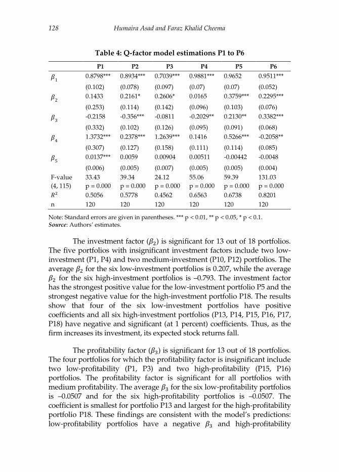
Table 4: Q-factor model estimations P1 to P6

P1 P2 P3 P4 P5 P6

𝛽1 0.8798*** 0.8934*** 0.7039*** 0.9881*** 0.9652 0.9511***

(0.102) (0.078) (0.097) (0.07) (0.07) (0.052)

𝛽2 0.1433 0.2161* 0.2606* 0.0165 0.3759*** 0.2295***

(0.253) (0.114) (0.142) (0.096) (0.103) (0.076)

𝛽3 -0.2158 -0.356*** -0.0811 -0.2029** 0.2130** 0.3382***

(0.332) (0.102) (0.126) (0.095) (0.091) (0.068)

𝛽4 1.3732*** 0.2378*** 1.2639*** 0.1416 0.5266*** -0.2058**

(0.307) (0.127) (0.158) (0.111) (0.114) (0.085)

𝛽5 0.0137*** 0.0059 0.00904 0.00511 -0.00442 -0.0048

(0.006) (0.005) (0.007) (0.005) (0.005) (0.004)

F-value

(4, 115)

33.43

p = 0.000

39.34

p = 0.000

24.12

p = 0.000

55.06

p = 0.000

59.39

p = 0.000

131.03

p = 0.000

𝑅2 0.5056 0.5778 0.4562 0.6563 0.6738 0.8201

n 120 120 120 120 120 120

Note: Standard errors are given in parentheses. *** p < 0.01, ** p < 0.05, * p < 0.1. Source: Authors’ estimates.

The investment factor (𝛽2) is significant for 13 out of 18 portfolios. The five portfolios with insignificant investment factors include two low-investment (P1, P4) and two medium-investment (P10, P12) portfolios. The average 𝛽2 for the six low-investment portfolios is 0.207, while the average 𝛽2 for the six high-investment portfolios is –0.793. The investment factor has the strongest positive value for the low-investment portfolio P5 and the strongest negative value for the high-investment portfolio P18. The results show that four of the six low-investment portfolios have positive coefficients and all six high-investment portfolios (P13, P14, P15, P16, P17, P18) have negative and significant (at 1 percent) coefficients. Thus, as the firm increases its investment, its expected stock returns fall.

The profitability factor (𝛽3) is significant for 13 out of 18 portfolios. The four portfolios for which the profitability factor is insignificant include two low-profitability (P1, P3) and two high-profitability (P15, P16) portfolios. The profitability factor is significant for all portfolios with medium profitability. The average 𝛽3 for the six low-profitability portfolios is –0.0507 and for the six high-profitability portfolios is –0.0507. The coefficient is smallest for portfolio P13 and largest for the high-profitability portfolio P18. These findings are consistent with the model’s predictions: low-profitability portfolios have a negative 𝛽3 and high-profitability


portfolios have a positive 𝛽3, with some exceptions. Thus, as the firm’s profitability increases, its expected stock returns also increase.


P8 P9 P10 P11 P12

𝛽1 0.9451*** 0.6996*** 0.7769*** 0.9264*** 0.7388***

(0.118) (0.073) (0.077) (0.097) (0.062)

𝛽2 -0.4041*** -0.253*** 0.1361 -0.3741* 0.0515

(0.132) (0.107) (0.107) (0.209) (0.09)

𝛽3 -0.6064*** -0.2152** -0.2752** 0.6264** 0.2489***

(0.12) (0.095) (0.111) (0.279) (0.08)

𝛽4 -0.0673 0.6360*** -0.0561 1.5500*** -0.0432

(0.133) (0.118) (0.164) (0.283) (0.1)

𝛽5 0.0012 0.00338 0.00169 0.00667 0.00591

(0.006) (0.005) (0.005) (0.006) (0.004)

F-value

(4, 115)

27.97

p = 0.000

25.71

p = 0.000

29.86

p = 0.000

24.44

p = 0.000

49.57

p = 0.000

𝑅2 0.625 0.4721 0.5899 0.6225 0.6329

n 120 120 120 120 120



P13 P14 P15 P16 P17 P18

𝛽1 1.0098*** 0.8412*** 0.857*** 0.8716*** 0.976*** 0.8258***

(0.102) (0.07) (0.069) (0.076) (0.077) (0.135)

𝛽2 -1.008*** -0.757*** -0.607*** -0.309*** -0.726*** -1.351***

(0.18) (0.083) (0.101) (0.007) (0.113) (0.269)

𝛽3 -0.859*** -0.628*** -0.0778 -0.1196 0.4585*** 0.9224***

(0.158) (0.07) (0.09) (0.1) (0.101) (0.317)

𝛽4 1.1099*** -0.0757 1.076*** -0.1465 0.9995*** 0.3738

(0.17) (0.107) (0.112) (0.124) (0.125) (0.32)

𝛽5 0.008 -0.0051 0.0045 0.0035 -0.0036 0.0174***

(0.006) (0.005) (0.005) (0.005) (0.005) (0.008)

F-value

(4, 115)

32.05

p = 0.000

52.92

p = 0.000

54.46

p = 0.000

38.82

p = 0.000

61.85

p = 0.000

18.09

p = 0.000

𝑅2 0.6819 0.6157 0.6545 0.5745 0.6827 0.5742

n 120 120 120 120 120 120



The size factor is significant for 10 out of 18 portfolios. The size factor is significant for four of the five small portfolios and tends to be stronger than their market factors. The average 𝛽4 for the small portfolios is 1.017 while the average 𝛽4 for the nine large portfolios is 0.017. The largest size coefficient is for the small portfolio P11 and the smallest size coefficient is for the large portfolio P6. These findings confirm the model’s predictions: small portfolios have a strong, positive 𝛽4 and large portfolios have an insignificant or negative 𝛽4. Thus, as the firm’s size increases, its expected stock returns decrease.

In a perfect asset-pricing model explaining excess returns above the risk-free rate, the value of the intercept must be close to 0 (Black, Jensen & Scholes, 1972). A zero-intercept is based on the risk-return relationship according to which there should be no return on taking no risk. A non-zero intercept indicates the model’s failure to explain excess returns. The same rationale is extended to the q-factor model such that the intercept value is expected to be 0. The results show that the intercept values for all the portfolios are close to 0. This implies that the model is specified correctly (see Hou et al., 2017) and that it explains excess returns without needing additional variables.

The F-test for all 18 regressions is significant, with a p-value of 0.000. The average R-squared for all portfolios is 0.61. The highest R-squared is 0.82 for portfolio P6 and the smallest is 0.45 for portfolio P3. The R-squared values lie in a similar range for all groups of portfolios ranked by investment, size and profitability. The data used for these estimations is also used to estimate a CAPM, the results of which are significant for all 18 portfolios (Table 7). The F-test for each regression is significant, with a p-value of 0.000. The average R-squared for all portfolios is 0.38. Overall, the q-factor model has greater explanatory power than the CAPM.


Table 7: CAPM regression analysis

Portfolio Intercept p-value β p-value R2 F test p-value

P1 0.01773 0.048 0.5912 0.000 0.172 24.42 0.000

P2 0.00384 0.508 0.8306 0.000 0.490 113.40 0.000

P3 0.01368 0.102 0.4658 0.000 0.128 17.34 0.000

P4 0.00402 0.411 0.9388 0.000 0.633 203.80 0.000

P5 -0.00058 0.914 0.9235 0.000 0.580 162.80 0.000

P6 -0.00298 0.467 1.0564 0.000 0.757 367.70 0.000

P7 -0.00821 0.175 0.6307 0.000 0.339 60.56 0.000

P8 -0.00386 0.522 0.8466 0.000 0.480 108.90 0.000

P9 0.00447 0.441 0.5168 0.000 0.271 43.82 0.000

P10 -0.00090 0.853 0.7740 0.000 0.541 139.20 0.000

P11 0.01875 0.049 0.6341 0.000 0.174 24.91 0.000

P12 0.00775 0.078 0.7807 0.000 0.600 176.90 0.000

P13 0.00620 0.518 0.5730 0.000 0.144 19.77 0.000

P14 -0.01023 0.115 0.7016 0.000 0.356 65.17 0.000

P15 0.00882 0.209 0.5583 0.000 0.230 35.21 0.000

P16 0.00193 0.719 0.8532 0.000 0.542 139.60 0.000

P17 0.00487 0.532 0.7382 0.000 0.296 49.71 0.000

P18 0.02736 0.020 0.6950 0.000 0.143 19.70 0.000


Post-estimation, we test for multicollinearity using the variance inflation factor test. No multicollinearity is observed in the model (see Table A1 in the Appendix). The Breusch–Godfrey LM test results show that there is no autocorrelation at the first lag. Campbell et al. (2001) divide stock volatility into three components – market, industry and idiosyncratic, all of which exhibit time variation. The Breusch–Pagan test is carried out to test for heteroskedasticity, which emerges in eight out of 18 portfolios (see Table A2 in the Appendix). To remove the impact of heteroskedasticity on the estimators, we carry out the regressions with robust standard errors.

5. Discussion

This empirical study applies the q-factor model to a sample of stocks listed on the KSE by analyzing data from 100 companies for the period June 2004 to May 2014. The analysis involves running regressions on 18 portfolios with distinct characteristics. The average R-squared for all portfolios using the q-factor model is 0.61, while that for all portfolios using the CAPM is 0.38. This implies that the q-factor model vastly outperforms the CAPM. Since the intercept of the q-factor model is close to 0, we can assume the model is accurately specified.


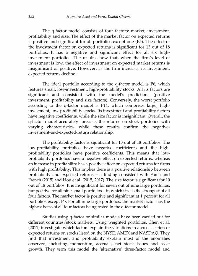
The q-factor model consists of four factors: market, investment, profitability and size. The effect of the market factor on expected returns is positive and significant for all portfolios except one (P5). The effect of the investment factor on expected returns is significant for 13 out of 18 portfolios. It has a negative and significant effect for all six high-investment portfolios. The results show that, when the firm’s level of investment is low, the effect of investment on expected market returns is insignificant or positive. However, as the firm increases its investment, expected returns decline.

The ideal portfolio according to the q-factor model is P6, which features small, low-investment, high-profitability stocks. All its factors are significant and consistent with the model’s predictions (positive investment, profitability and size factors). Conversely, the worst portfolio according to the q-factor model is P14, which comprises large, high-investment, low-profitability stocks. Its investment and profitability factors have negative coefficients, while the size factor is insignificant. Overall, the q-factor model accurately forecasts the returns on stock portfolios with varying characteristics, while these results confirm the negative-investment-and-expected-return relationship.

The profitability factor is significant for 13 out of 18 portfolios. The low-profitability portfolios have negative coefficients and the high-profitability portfolios have positive coefficients. This means that low-profitability portfolios have a negative effect on expected returns, whereas an increase in profitability has a positive effect on expected returns for firms with high profitability. This implies there is a positive relationship between profitability and expected returns – a finding consistent with Fama and French (2015) and Hou et al. (2015, 2017). The size factor is significant for 10 out of 18 portfolios. It is insignificant for seven out of nine large portfolios, but positive for all nine small portfolios – in which size is the strongest of all four factors. The market factor is positive and significant at 1 percent for all portfolios except P5. For all nine large portfolios, the market factor has the highest betas of all four factors being tested in the q-factor model.

Studies using q-factor or similar models have been carried out for different countries/stock markets. Using weighted portfolios, Chen et al. (2011) investigate which factors explain the variations in a cross-section of expected returns on stocks listed on the NYSE, AMEX and NASDAQ. They find that investment and profitability explain most of the anomalies observed, including momentum, accruals, net stock issues and asset growth. They term this model the ‘alternative’ three-factor model and


show that it yields significantly better results than the Fama–French three-factor model for stocks in the US.

Ammann, Odonia and Oesch (2012) evaluate the performance of an investment-based factor model by employing the I/A ratio and ROE for a sample of European stock markets (Austria, Belgium, Finland, France, Germany, Italy, Ireland, the Netherlands, Portugal and Spain) over 1990–2006. They find that the investment-based model performs better than the CAPM or Fama–French three-factor model in explaining asset return anomalies such as asset growth, short-term prior returns, net stock issues, total accruals and value effects. Fan and Yu (2013) investigate the momentum anomaly otherwise not explainable by the CAPM and Fama–French three-factor model. They use the investment-based alternative three-factor model and find that it explains the momentum anomaly in 12 out of 13 G-12 country stock markets and yields significantly lower intercept values.

Fama and French (2015) add the investment and profitability factors derived from the q theory of investment to their earlier three-factor model to form a comprehensive five-factor model directed at capturing the impact of size, value, profitability and investment. They find that it outperforms the earlier model. Their results also indicate that small high-investment stocks have lower returns than high-investment, low-profitability stocks. However, the value factor becomes redundant in the presence of the other four factors, especially investment and profitability.

Finally, Walkshäusl and Lobe (2014) test the q theory-based model, which employs investment and profitability, and the Fama–French three-factor model for a global portfolio of 40 non-US markets in emerging and developed countries. They conclude that the q theory-based model outperforms the three-factor model in capturing the momentum anomaly, but has less explanatory power in relation to average returns. This could mean that the investment-based model is sample-specific.

6. Conclusion

This study contributes to the literature by validating the factors identified in the q-factor model as predictors of the expected returns on investments in the KSE. This implies that the four factors taken up in the q-factor model are useful predictors of average returns not only in developed markets, but also in developing markets. The model adds investment and profitability as predictors of expected market returns in factor-based asset pricing.


Our results are largely in accordance with the q theory and other findings relevant to US and other markets, where all the factors are found to be significant (see Hou et al., 2015, 2017). In a study on the Vietnamese stock market, however, Nguyen, Ulku and Zhang (2015) show that profitability and investment are important determinants of asset returns, along with size and value. The Vietnamese stock market is distinct from other stock markets in that the state owns a large volume of stocks.

Of the two new factors identified in the q-factor model, profitability (measured by ROE) has been traditionally used in fundamental analysis. However, our results show that investment, represented by the I/A ratio, can also be used as a tool of fundamental analysis for individual stocks. Further, investors can trade against the investment and profitability factors to increase their returns. Finally, the q-factor model has better explanatory power than the traditional CAPM and can be used to explain various anomalies, allowing better portfolio valuation.


References

Ammann, M., Odonia, S., & Oesch, D. (2012). An alternative three-factor model for international markets: Evidence from the European Monetary Union (Working Papers on Finance No. 2012/2). St. Gallen: Swiss Institute of Banking and Finance.

Black, F., Jensen, M. C., & Scholes, M. S. (1972). The capital asset pricing model: Some empirical tests. In M. C. Jensen (ed.), Studies in the theory of capital markets. New York: Praeger.

Blume, M. E. (1970). Portfolio theory: A step toward its practical application. Journal of Business, 43(2), 152–173.

Campbell, J. Y., Lettau, M., Malkiel, B. G., & Xu, Y. (2001). Have individual stocks become more volatile? An empirical exploration of idiosyncratic risk. Journal of Finance, 56(1), 1–43.

Carhart, M. M. (1997). On persistence in mutual fund performance. Journal of Finance, 52(1), 57–82.

Carhart, M. M., Krail, R. J., Stevens, R. J., & Welch, K. E. (1996). Testing the conditional CAPM. Unpublished manuscript, University of Chicago, Graduate School of Business, Chicago, IL.

Chen, L., Novy-Marx, R., & Zhang, L. (2011). An alternative three-factor model. Unpublished manuscript. Available at https://dx.doi.org/10.2139/ssrn.1418117

Cochrane, J. H. (1991). Production-based asset pricing and the link between stock returns and economic fluctuations. Journal of Finance, 46(1), 209–237.

Eberly, J., Rebelo, S., & Vincent, N. (2008). Investment and value: A neoclassical benchmark (Working Paper No. 13866). Cambridge, MA: National Bureau of Economic Research.

Fama, E. F., & French, K. R. (1993). Common risk factors in the returns on stocks and bonds. Journal of Financial Economics, 33(1), 3–56.

Fama, E. F., & French, K. R. (1996). Multifactor explanations of asset pricing anomalies. Journal of Finance, 51(1), 55–84.

Fama, E. F., & French, K. R. (2006). The value premium and the CAPM. Journal of Finance, 61(5), 2163–2185.


Fama, E. F., & French, K. R. (2015). A five-factor asset pricing model. Journal of Financial Economics, 116(1), 1–22.

Fama, E. F., & French, K. R. (2017). International tests of a five-factor asset pricing model. Journal of Financial Economics, 123(3), 441–463.

Fan, S., & Yu, L. (2013). Does the alternative three-factor model explain momentum anomaly better in G12 countries? Journal of Finance and Accountancy, 12, 120–134.

Gordon, M. J. (1962). The investment, financing and valuation of the corporation. Homewood, IL: R. Irwin.

Gordon, M. J., & Shapiro, E. (1956). Capital equipment analysis: The required rate of profit. Management Science, 3(1), 102–110.

Hair, J. F., Black, W. C., Babin, B. J., & Anderson, R. E. (2010). Multivariate data analysis, 7th ed. London: Pearson.

Harrington, D. (1987). Modern portfolio theory, the capital asset pricing model, and arbitrage pricing theory: A user’s guide, 2nd ed. Upper Saddle River, NJ: Prentice Hall.

Hou, K., Xue, C., & Zhang, L. (2012). Digesting anomalies: An investment approach (Working Paper No. 18435). Cambridge, MA: National Bureau of Economic Research.

Hou, K., Xue, C., & Zhang, L. (2015). Digesting anomalies: An investment approach. Review of Financial Studies, 28(3), 650–705.

Hou, K., Xue, C., & Zhang, L. (2017). A comparison of new factor models (Working Paper No. 2015-03-05). Columbus, OH: Fisher College of Business.

Jegadeesh, N., & Titman, S. (1993). Returns to buying winners and selling losers: Implications for stock market efficiency. Journal of Finance, 48(1), 65–91.

Miller, M., & Modigliani, F. (1961). Dividend policy, growth and the valuation of shares. Journal of Business, 34, 411–433.

Nguyen, N., Ulku, N., & Zhang, J. (2015). Fama–French five-factor model: Evidence from Vietnam. Unpublished manuscript, University of Otago, Dunedin, New Zealand.


Pástor, L., & Stambaugh, R. F. (2003). Liquidity risk and expected stock returns. Journal of Political Economy, 111(3), 642–685.

Securities and Exchange Commission of Pakistan. (2014). Number of listed companies – 2014. Retrieved from https://www.secp.gov.pk/data-and-statistics/corporates/

State Bank of Pakistan. (2015). Financial statement analysis of financial sector (2011–2015). Karachi: Author.

Tobin, J. (1969). A general equilibrium approach to monetary theory. Journal of Money, Credit and Banking, 1(1), 15–29.

Walkshäusl, C., & Lobe, S. (2014). The alternative three‐factor model: An alternative beyond US markets? European Financial Management, 20(1), 33–70.


Appendix

Table A1: Vector inflation factors of variables

Variable VIF 1/VIF

Market factor 1.17 0.855147

Size factor 1.16 0.865533

Profitability factor 1.08 0.928310

Investment factor 1.08 0.928425

Mean VIF 1.12


Table A2: Breusch–Pagan/Cook–Weisberg test for heteroskedasticity

Portfolio chi2(1) Prob. > chi2 Portfolio chi2(1) Prob. > chi2

P1 8.77 0.0031* P10 6.44 0.0111*

P2 0.67 0.4134 P11 66.96 0.0000*

P3 3.01 0.0829 P12 1.44 0.2308

P4 17.44 0.0000* P13 7.06 0.0079*

P5 1.36 0.2441 P14 5.94 0.0148*

P6 1.56 0.2121 P15 2.95 0.0859

P7 0.04 0.8326 P16 2.04 0.1535

P8 12.28 0.0005* P17 1.67 0.1959

P9 0.80 0.3726 P18 51.32 0.0000*

Note: * Heteroscedasticity is present. Source: Authors’ estimates.

an empirical assessment of the q-factor model: … · presented by gordon and shapiro (1956). 2.1....

Documents