a unified theory of tobin's q, corporate investment ... · a uniﬁed theory of tobin’s q,...

A Unified Theory of Tobin’s q, Corporate Investment,

Financing, and Risk Management∗

Patrick Bolton† Hui Chen‡ Neng Wang§

August 24, 2010

∗We are grateful to Andrew Abel, Peter DeMarzo, Janice Eberly, Andrea Eisfeldt, Mike Faulkender, Michael

Fishman, Dirk Hackbarth, Pete Kyle, Yelena Larkin, Robert McDonald, Stewart Myers, Marco Pagano, Gordon

Phillips, Robert Pindyck, David Scharfstein, Jiang Wang, Toni Whited, and seminar participants at Boston College,

Boston University, Columbia Business School, Duke Fuqua, MIT Sloan, NYU Stern and NYU Economics, U.C.

Berkeley Haas, Yale SOM, University of Maryland Smith, Northwestern University Kellogg, Princeton, Lancaster,

Virginia, IMF, HKUST Finance Symposium, AFA, the Caesarea Center 6th Annual Academic Conference, European

Summer Symposium on Financial Markets (ESSFM/CEPR), and Foundation for the Advancement of Research in

Financial Economics (FARFE) for their comments.†Columbia University, NBER and CEPR. Email: [email protected]. Tel. 212-854-9245.‡MIT Sloan School of Management and NBER. Email: [email protected]. Tel. 617-324-3896.§Columbia Business School and NBER. Email: [email protected]. Tel. 212-854-3869.

A Unified Theory of Tobin’s q, Corporate Investment, Financing,

and Risk Management

Abstract

We propose a model of dynamic corporate investment, financing, and risk management for

a financially constrained firm. The model highlights the central importance of the endogenous

marginal value of liquidity (cash and credit line) for corporate decisions. Our three main results

are: 1) investment depends on the ratio of marginal q and marginal value of liquidity, and

the relation between investment and marginal q changes with the marginal source of funding;

2) optimal external financing and payout are characterized by an endogenous double barrier

policy for the firm’s cash-capital ratio; 3) liquidity management and derivatives hedging are

complementary risk-management tools.

When firms face external financing costs, they must deal with complex and closely intertwined

investment, financing, and risk management decisions. How to formalize the interconnections

among these margins in a dynamic setting and how to translate the theory into day-to-day risk

management and real investment policies remains largely to be determined. Questions such as how

corporations should manage their cash holdings, which risks they should hedge and by how much,

or to what extent holding cash is a substitute for financial hedging are not well understood.

Our goal in this article is to propose the first elements of a tractable dynamic corporate risk

management framework — as illustrated in Figure 1 — in which cash inventory, corporate invest-

ment, external financing, payout, and dynamic hedging policies are characterized simultaneously

for a “financially constrained” firm. We emphasize that risk management is not just about financial

hedging; instead, it is tightly connected to liquidity management via daily operations. By bringing

these different aspects of risk management into a unified framework, we show how they interact

with and complement each other.

The baseline model we propose introduces only the essential building blocks, which are: i) the

workhorse neoclassical q model of investment1 featuring constant investment opportunities as in

Hayashi (1982); ii) constant external financing costs, which give rise to a corporate cash inventory

problem as in Miller and Orr (1966); and, iii) four basic financial instruments: cash, equity, credit

line, and derivatives (e.g., futures). This parsimonious model already captures many situations

that firms face in practice and yields a rich set of prescriptions.

With external financing costs the firm’s investment is no longer determined by equating the

marginal cost of investing with marginal q, as in the neoclassical Modigliani-Miller (MM) model

(with no fixed adjustment costs for investment). Instead, investment of a financially constrained

1Brainard and Tobin (1968) and Tobin (1969) define the ratio between the firm’s market value to the replacementcost of its capital stock, as “Q” and propose to use this ratio to measure the firm’s incentive to invest in capital.This ratio has become known as Tobin’s average Q. Hayashi (1982) provides conditions under which average Q isequal to marginal q. Abel and Eberly (1994) develop a unified q theory of investment in neoclassic settings. Lucasand Prescott (1971) and Abel (1983) are important early contributions.

1

Financial

Hedging

Dynamic

Risk Management

Cash

Management

Cash

Hoarding

Equity Credit LineInvestment Asset Sales

Real

Investment

External

Financing

Payout

Figure 1: A Unified Framework for Risk Management.

firm is determined by the ratio of marginal q to marginal cost of financing :

marginal cost of investing =marginal q

marginal cost of financing.

When firms are flush with cash, the marginal cost of financing is approximately one, so that this

equation is approximately the same as the one under MM. But when firms are close to financial

distress, the marginal cost of financing, which is endogenous, may be much larger than one so that

optimal investment may be far lower than the level predicted under MM. A key contribution of

our article is to characterize both analytically and quantitatively the marginal value of cash to

a financially constrained firm as a function of the firm’s investment opportunities, cash holding,

leverage, external financing costs, and hedging opportunities it faces.2

2Hennessy, Levy, and Whited (2007) derive a related optimality condition for investment. As they assume thatthe firm faces quadratic equity issuance costs, the optimal policy for the firm in their setting is to either issue equityor pay out dividends at any point in time. In other words, the firm does not hold any cash inventory and does notface a cash management problem as in our setting.

2

An important result that follows from the first-order condition above is that the relation between

marginal q and investment differs depending on whether cash or credit line is the marginal source of

financing. When the marginal source of financing is cash, both marginal q and investment increase

with the firm’s cash holdings, as more cash makes the firm less financially constrained. In contrast,

when the marginal source of financing is credit line, we show that marginal q and investment move

in opposite directions. On the one hand, investment decreases with leverage, as the firm cuts

investment to delay incurring equity issuance costs. On the other hand, marginal q increases with

the firm’s leverage, because an extra unit of capital helps relax the firm’s borrowing constraint by

lowering the debt-to-capital ratio, and this effect becomes increasingly more important as leverage

rises. Thus, there is no longer a monotonic relation between investment and marginal q in the

presence of credit line, and average q can actually be a more robust indicator for investment.

A second key result concerns the firm’s optimal cash-inventory policy. Much of the empirical

literature on firms’ cash holdings tries to identify a target cash-inventory for a firm by weighing the

costs and benefits of holding cash.3 The idea is that this target level helps determine when a firm

should increase its cash savings and when it should dissave.4 Our analysis, however, shows that the

firm’s cash-inventory policy is much richer, as it involves a combination of a double-barrier policy

characterized by a single variable, the cash-capital ratio, and the continuous management of cash

reserves in between the barriers through adjustments in investment, asset sales, as well as the firm’s

hedging positions. While this double-barrier policy is not new (it goes back to the inventory model

of Miller and Orr 1966 in corporate finance), our model provides substantial new insight on how the

different boundaries depend on factors such as the growth rate and volatility of earnings, financing

costs, cash holding costs, as well as the dynamics of cash holdings in between these boundaries.

Besides cash inventory management, our model can also give concrete prescriptions for how a firm

choose its investment, financing, hedging, and payout policies, which are all important parts of

3See Almeida, Campello, and Weisbach (2004, 2008), Faulkender and Wang (2006), Khurana, Martin, and Pereira(2006), and Dittmar and Mahrt-Smith (2007).

4Recent empirical studies have found that corporations tend to hold more cash when their underlying earningsrisk is higher or when they have higher growth opportunities (see e.g. Opler, Pinkowitz, Stulz, and Williamson (1999)and Bates, Kahle, and Stulz (2009)).

3

dynamic corporate financial management.

For example, when the cash-capital ratio is higher, the firm invests more and saves less, as

the marginal value of cash is smaller. When the firm is approaching the point where its cash

reserves are depleted, it optimally scales back investment and may even engage in asset sales.

This way the firm can postpone or avoid raising costly external financing. Since carrying cash

is costly, the firm optimally pays out cash at the endogenous upper barrier of the cash-capital

ratio. At the lower barrier the firm either raises more external funds or closes down. The firm

optimally chooses not to issue equity unless it runs out of cash. Using internal funds (cash) to

finance investment defers both the cash-carrying costs and external financing costs.5 Thus, with

a constant investment/financing opportunity set our model generates a dynamic pecking order of

financing between internal and external funds. The stationary cash-inventory distribution from

our model shows that firms respond to the financing constraints by optimally managing their cash

holdings so as to stay away from financial distress situations most of the time.

A third new result is that our model integrates two channels of risk management, one via a

state non-contingent vehicle (cash), the other via state-contingent instruments (derivatives). In the

presence of external financing costs, firm value is sensitive to both idiosyncratic and systematic risk.

To limit its exposure to systematic risk, the firm can engage in dynamic hedging via derivatives

(such as oil or currency futures). To mitigate the impact of idiosyncratic risk, it can manage its

cash reserves by modulating its investment outlays and asset sales, and also by delaying or moving

forward its cash payouts to shareholders. Financial hedging (derivatives) and liquidity management

(cash, investment, financing, payout) thus play complementary roles in risk management. When

dynamic hedging involves higher transactions costs, such as tighter margin requirements, we also

show that the firm reduces its hedging positions and relies more on cash for risk management.

There is only a handful of theoretical analyses of firms’ optimal cash, investment and risk man-

agement policies. A key first contribution is by Froot, Scharfstein, and Stein (1993), who develop a

5This result is reminiscent of not prematurely exercising an American call option on a non-dividend paying stock.

4

static model of a firm facing external financing costs and risky investment opportunities.6 Subse-

quent contributions on dynamic risk management literature focus on optimal hedging policies and

abstract away from corporate investment and cash management. Notable exceptions include Mello,

Parsons, and Triantis (1995) and Morellec and Smith (2007), who analyze corporate investment

together with optimal hedging. Mello and Parsons (2000) study the interaction between hedging

and cash management, but do not model investment. However, none of these models consider

external financing or payout decisions. Our dynamic risk management problem uses the same

contingent-claim methodology as in the dynamic capital structure/credit-risk models of Fischer,

Heinkel, and Zechner (1989) and Leland (1994), but unlike these theories we explicitly model the

wedge between internal and external financing of the firm and the firm’s cash accumulation process.

Our model extends these latter theories by introducing capital accumulation and thus integrates

the contingent-claim approach with the dynamic investment/financing literature.

Our model also provides new and empirically testable predictions on investment and financing

constraints. Fazzari, Hubbard, and Petersen (1988) (FHP) are the first to use the sensitivity of

investment to cash flow (controlling for q) as a measure of a firm’s financing constraints. Kaplan

and Zingales (1997) provide an important critique on FHP and successors from both a theoretical

(using a static model) and empirical perspective. Recently, there is growing interest in using

dynamic structural models to address this empirical issue, which we discuss next.

Gomes (2001) and Hennessy and Whited (2005, 2007) numerically solve discrete-time dynamic

capital structure models with investment for financially constrained firms. They allow for stochas-

tic investment opportunities but have no adjustment costs for investment.7 However, these studies

do not model a cash accumulation equation and do not consider how cash inventory management

interacts with investment and dynamic hedging policies. Hennessy, Levy, and Whited (2007) char-

acterize a related investment first-order condition for a financially constrained firm to ours, but

6See also Kim, Mauer, and Sherman (1998). Another more recent contribution by Almeida, Campello, andWeisbach (2008) extends the Hart and Moore (1994) theory of optimal cash holdings by introducing cash flow andinvestment uncertainty in a three-period model.

7Recently, Gamba and Triantis (2008) have extended Hennessy and Whited (2007) to introduce issuance costs ofdebt and hence obtain the simultaneous existence of debt and cash.

5

they consider a model with quadratic equity issuance costs, which leads to a fundamentally dif-

ferent cash management policy from ours. Using a model related to Hennessy and Whited (2005,

2007), Riddick and Whited (2009) show that saving and cash flow can be negatively related after

controlling for q, because firms use cash reserves to invest when receiving a positive productivity

shock.8

In contrast to the impressive volume of work studying how adjustment costs affect investment,9

very few analytical results are available on the impact of external financing costs on investment.

Our model fills this gap by exploiting the simplicity of a framework that is linearly homogeneous

in cash and capital, and for which a complete analytical characterization of the firm’s optimal

investment and financing policies, as well as its dynamic hedging policy and its use of credit lines

is possible. In terms of methodology, our paper is also related to Decamps, Mariotti, Rochet, and

Villeneuve (2006), who explore a continuous-time model of a firm facing external financing costs.

Unlike our set-up, their firm only has a single infinitely-lived project of fixed size, so that they

cannot consider the interaction of the firm’s real and financial policies.

The paper that is most closely related to ours is DeMarzo, Fishman, He, and Wang (2010),

henceforth DFHW. Both our paper and DFHW consider models of corporate investment that in-

tegrate dynamic agency frictions into the neoclassic q theory of investment (e.g. Hayashi (1982)).

The approach taken in DFHW is more microfounded around an explicit dynamic contracting prob-

lem with moral hazard, where investors dynamically manage the agent’s continuation payoff based

on the firm’s historical performance. The key state variable is their dynamic contracting problem

is thus the manager’s continuation payoff.10 Their dynamic contracting framework endogenizes the

firm’s financing constraints in a similar way to ours, even though firm value in their framework is

expressed as a function of a different state variable. One key difference, however, between the two

8In a related study, DeAngelo, DeAngelo, and Whited (2009) model debt as a transitory financing vehicle to meetthe funding needs associated with random shocks to investment opportunities.

9See Caballero (1999) for a survey on this literature.10The manager’s continuation payoff gives the agent’s present value of his future payments, discounted at his own

rate. Interestingly, it can be interpreted as a measure of distance to liquidation/refinancing and can be linked tofinancial slack via (non-unique) financial implementation.

6

models is in the dynamics of the state variable measuring financial slack. In DFHW, the manager’s

equilibrium effort choice affects the volatility of financial slack but not directly the drift. In our

model, in contrast, the manager directly influences the drift, but not the volatility of the dynamics

of financial slack. As a result, investment is monotonically linked to marginal q in DFHW, while

investment is linked to the ratio between marginal q and the endogenous marginal value of finan-

cial slack in our model. This distinction leads to different implications on corporate investment,

financing policies, and payout to investors in the two models.

The remainder of the paper proceeds as follows. Section I sets up our baseline model. Section

II presents the model solution. Section III continues with quantitative analysis. Section IV and

V extend the baseline model to allow for financial hedging and credit line financing. Section VI

concludes.

I Model Setup

We first describe the firm’s physical production and investment technology, then introduce the firm’s

external financing costs and its opportunity cost of holding cash, and finally state firm optimality.

A. Production Technology

The firm employs physical capital for production. The price of capital is normalized to unity. We

denote by K and I respectively the level of capital stock and gross investment. As is standard in

capital accumulation models, the firm’s capital stock K evolves according to:

dKt = (It − δKt) dt, t ≥ 0, (1)

where δ ≥ 0 is the rate of depreciation.

The firm’s operating revenue at time t is proportional to its capital stock Kt, and is given by

7

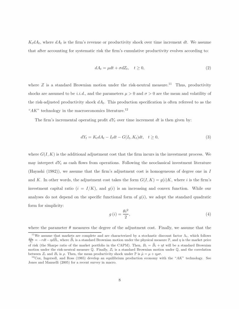
KtdAt, where dAt is the firm’s revenue or productivity shock over time increment dt. We assume

that after accounting for systematic risk the firm’s cumulative productivity evolves according to:

dAt = µdt+ σdZt, t ≥ 0, (2)

where Z is a standard Brownian motion under the risk-neutral measure.11 Thus, productivity

shocks are assumed to be i.i.d., and the parameters µ > 0 and σ > 0 are the mean and volatility of

the risk-adjusted productivity shock dAt. This production specification is often refereed to as the

“AK” technology in the macroeconomics literature.12

The firm’s incremental operating profit dYt over time increment dt is then given by:

dYt = KtdAt − Itdt−G(It,Kt)dt, t ≥ 0, (3)

where G(I,K) is the additional adjustment cost that the firm incurs in the investment process. We

may interpret dYt as cash flows from operations. Following the neoclassical investment literature

(Hayashi (1982)), we assume that the firm’s adjustment cost is homogeneous of degree one in I

and K. In other words, the adjustment cost takes the form G(I,K) = g(i)K, where i is the firm’s

investment capital ratio (i = I/K), and g(i) is an increasing and convex function. While our

analyses do not depend on the specific functional form of g(i), we adopt the standard quadratic

form for simplicity:

g (i) =θi2

2, (4)

where the parameter θ measures the degree of the adjustment cost. Finally, we assume that the

11We assume that markets are complete and are characterized by a stochastic discount factor Λt, which followsdΛt

Λt= −rdt−ηdB̂t, where B̂t is a standard Brownian motion under the physical measure P, and η is the market price

of risk (the Sharpe ratio of the market portfolio in the CAPM). Then, Bt = B̂t + ηt will be a standard Brownianmotion under the risk-neutral measure Q. Finally, Zt is a standard Brownian motion under Q, and the correlationbetween Zt and Bt is ρ. Then, the mean productivity shock under P is µ̂ = µ + ηρσ.

12Cox, Ingersoll, and Ross (1985) develop an equilibrium production economy with the “AK” technology. SeeJones and Manuelli (2005) for a recent survey in macro.

8

firm can liquidate its assets at any time. The liquidation value Lt is proportional to the firm’s

capital, Lt = lKt, where l > 0 is a constant.

Note that these classic AK–production technology assumptions, plus the quadratic adjustment

cost, and the liquidation technology imply that the firm’s investment opportunities are constant

over time. Without financing frictions, the firm’s investment-capital ratio, average and marginal

q are therefore all constant over time. We intentionally choose such a simple setting in order

to highlight the dynamic effects of financing frictions, keeping investment opportunities constant.

Moreover, these assumptions allow us to deliver the key results in a parsimonious and analytically

tractable way.13 See also Eberly, Rebelo, and Vincent (2009) for empirical evidence in support of

the Hayashi homogeneity assumption for the upper size-quartile of Compustat firms.

B. Information, Incentives and Financing Costs

Neoclassical investment models (Hayashi (1982)) assume that the firm faces frictionless capital

markets and that the Modigliani and Miller (1958) theorem holds. However, in reality, firms often

face important external financing costs due to asymmetric information and managerial incentive

problems. Following the classic writings of Jensen and Meckling (1976), Leland and Pyle (1977),

and Myers and Majluf (1984), a large empirical literature has sought to measure these costs. For

example, Asquith and Mullins (1986) found that the average stock price reaction to the announce-

ment of a common stock issue was −3% and the loss in equity value as a percentage of the size

of the new equity issue was −31%. Also, Calomiris and Himmelberg (1997) have estimated the

direct transactions costs firms face when they issue equity. These costs are also substantial. In

their sample the mean transactions costs, which include underwriting, management, legal, auditing

and registration fees as well as the firm’s selling concession, are 9% of an issue for seasoned public

offerings and 15.1% for initial public offerings.

We do not explicitly model information asymmetries and incentive problems. Rather, to be able

13Non-convex adjustment costs and decreasing returns to scale production function will substantially complicatethe analysis and do not permit a closed-form characterization of investment and financing policies.

9

to work with a model that can be calibrated we directly model the costs arising from information

and incentive problems in reduced form. Thus in our model, whenever the firm chooses to issue

external equity we summarize the information, incentive, and transactions costs it then incurs by

a fixed cost Φ and a marginal cost γ. Together these costs imply that the firm will optimally tap

equity markets only intermittently, and when doing so it raises funds in lumps, consistent with

observed firm behavior.

To preserve the linear homogeneity of our model, we further assume that the firm’s fixed cost

of issuing external equity is proportional to capital stock K, so that Φ = φK. In practice, external

costs of financing scaled by firm size are likely to decrease with firm size. With this caveat in mind,

we point out that there are conceptual, mathematical, and economic reasons for modeling these

costs as proportional to firm size. First, by modeling the fixed financing costs proportional to firm

size, we ensure that the firm does not grow out of the fixed costs.14 Second, the information and

incentive costs of external financing may to some extent be proportional to firm size. Indeed, the

negative announcement effect of a new equity issue affects the firm’s entire capitalization. Similarly,

the negative incentive effect of a more diluted ownership may also have costs that are proportional

to firm size. Finally, this assumption allows us to keep the model tractable, and generates stationary

dynamics for the firm’s cash-capital ratio.

Having said that, a weakness of our model is that it will be mis-specified as a structural model of

firms outside equity issue decisions. The model is likely to work best when applied to mature firms

and worst when applied to start-ups and growth firms, as small firms are not scaled-down versions

of mature firms in reality. To get sharper quantitative predictions of the effects of external financing

costs, would require extending the model to a two-dimensional framework with both capital and

cash as state variables. However, the main qualitative predictions of our current model are likely

to be robust to this two-dimensional extension. In particular, the endogenous marginal value of

cash will continue to play a critical role in determining corporate investment and other financial

14Indeed, this is a common assumption in the investment literature. See Cooper and Haltiwanger (2006) andRiddick and Whited (2009), among others. If the fixed cost is independent of firm size, it will not matter when firmsbecome sufficiently big in the long run.

10

decisions.

We denote by Ht the firm’s cumulative external financing up to time t and hence by dHt

the firm’s incremental external financing over time interval (t, t + dt). Similarly, let Xt denote

the cumulative costs of external financing up to time t, and dXt the incremental costs of raising

incremental external funds dHt. The cumulative external equity issuance H and the associated

cumulative costs X are stochastic controls chosen by the firm. In the baseline model of this section,

the only source of external financing is equity.

We next turn to the firm’s cash inventory. Let Wt denote the firm’s cash inventory at time t.

In our baseline model with no debt, provided that the firm’s cash is positive, the firm survives with

probability one. However, when the firm runs out of cash (Wt = 0) and has no option to borrow, it

has to either raise external funds to continue operating, or it must liquidate its assets. If the firm

chooses to raise external funds, it must pay the financing costs specified above. In some situations

the firm may prefer liquidation, for example, when the cost of financing is too high or when the

return on capital is too low. Let τ denote the firm’s (stochastic) liquidation time. If τ =∞, then

the firm never chooses to liquidate.

The rate of return that the firm earns on its cash inventory is the risk-free rate r minus a

carry cost λ > 0 that captures in a simple way the agency costs that may be associated with free

cash in the firm.15 Alternatively, the cost of carrying cash may arise from tax distortions. Cash

retentions are tax disadvantaged as interest earned by the corporation on its cash holdings is taxed

at the corporate tax rate, which generally exceeds the personal tax rate on interest income (Graham

2000 and Faulkender and Wang 2006). The benefit of a payout is that shareholders can invest at

the risk-free rate r, which is higher than (r − λ) the net rate of return on cash within the firm.

However, paying out cash also reduces the firm’s cash balance, which potentially exposes the firm

to current and future under-investment and future external financing costs. The tradeoff between

15This assumption is standard in models with cash. For example, see Kim, Mauer, and Sherman (1998) and Riddickand Whited (2009). If λ = 0, the firm will never pay out cash since keeping cash inside the firm has no costs but stillhas the benefits of relaxing financing constraints. If the firm is better at identifying investment opportunities thaninvestors, we have λ < 0. In that case, raising funds for earning excess return is potentially a positive NPV project.We do not explore the cases where λ ≤ 0.

11

these two factors determines the optimal payout policy. We denote by Ut the firm’s cumulative

(non-decreasing) payout to shareholders up to time t, and by dUt the incremental payout over time

interval dt. Distributing cash to shareholders may take the form of a special dividend or a share

repurchase.16

Combining cash flow from operations dYt given in (3), with the firm’s financing policy given by

the cumulative payout process U and the cumulative external financing process H, the firm’s cash

inventory W evolves according to the following cash-accumulation equation:

dWt = dYt + (r − λ) Wtdt + dHt − dUt, (5)

where the second term is the interest income (net of the carry cost λ), the third term dHt is the

cash inflow from external financing, and the last term dUt is the cash outflow to investors, so that

(dHt − dUt) is the net cash flow from financing. This equation is a general accounting identity,

where dHt, dUt, and dYt are endogenously determined by the firm.

The firm’s financing opportunities are time-invariant in our model, which is not realistic. How-

ever, as we will show, even in this simple setting, the interactions of fixed/proportional financing

costs with real investment generate several novel and economically significant insights.

Firm optimality. The firm chooses its investment I, payout policy U , external financing policy

H, and liquidation time τ to maximize shareholder value defined below:

E

[∫ τ

0

e−rt (dUt − dHt − dXt) + e−rτ (lKτ +Wτ )

]. (6)

The expectation is taken under the risk-adjusted probability. The first term is the discounted

value of net payouts to shareholders and the second term is the discounted value from liquidation.

Optimality may imply that the firm never liquidates. In that case, we have τ =∞. We impose the

16A commitment to regular dividend payments is suboptimal in our model. We exclude any fixed or variable payoutcosts, which can be added to the analysis.

12

usual regularity conditions to ensure that the optimization problem is well posed. Our optimization

problem is most obviously seen as characterizing the benchmark for the firm’s efficient investment,

cash-inventory, dynamic hedging, payout, and external financing policy when the firm faces external

financing and cash-carrying costs.

C. The Neoclassical Benchmark

As a benchmark, we summarize the solution for the special case without financing frictions, in

which the Modigliani-Miller theorem holds. The firm’s first-best investment policy is given by

IFBt = iFBKt, where17

iFB = r + δ −

√(r + δ)2 − 2 (µ− (r + δ)) /θ. (7)

The value of the firm’s capital stock is qFBKt, where qFB is Tobin’ s q,

qFB = 1 + θiFB. (8)

Three observations are in order. First, due to the homogeneity property in production tech-

nology, marginal q is equal to average (Tobin’s) q, as in Hayashi (1982). Second, gross investment

It is positive if and only if the expected productivity µ is higher than r + δ. With µ > r + δ and

hence positive investment, installed capital earns rents. Therefore, Tobin’s q is greater than unity

due to adjustment costs. Third, idiosyncratic productivity shocks have no effect on investment or

firm value. Next, we analyze the problem of a financially constrained firm.

17For the first-best investment policy to be well defined, the following parameter restriction is required: (r + δ)2 −2 (µ − (r + δ)) /θ > 0.

13

II Model Solution

When the firm faces costs of raising external funds, it can reduce future financing costs by retain-

ing earnings (i.e. hoarding cash) to finance its future investments. Firm value then depends on

two natural state variables, its stock of cash W and its capital stock K. Let P (K,W ) denote

the firm value. We show that firm decision-making and firm value then depend on which of the

following three regions it finds itself in: i) an external funding/liquidation region, ii) an internal

financing region, and iii) a payout region. As will become clear below, the firm is in the external

funding/liquidation region when its cash stock W is less than or equal an endogenous lower barrier

W . It is in the payout region when its cash stock W is greater than or equal an endogenous upper

barrier W . And it is in the internal financing region when W is in between W and W . We first

characterize the solution in the internal financing region.

A. Internal Financing Region

In this region, firm value P (K,W ) satisfies the following Hamilton-Jacobi-Bellman (HJB) equation:

rP (K,W ) = maxI

(I − δK)PK + [(r − λ)W + µK − I −G(I,K)]PW +σ2K2

2PWW . (9)

The first term (the PK term) on the right side of (9) represents the marginal effect of net investment

(I − δK) on firm value P (K,W ). The second term (the PW term) represents the effect of the firm’s

expected saving on firm value, and the last term (the PWW term) captures the effects of the volatility

of cash holdings W on firm value.

The firm finances its investment out of the cash inventory in this region. The convexity of

the physical adjustment cost implies that the investment decision in our model admits an interior

solution. The investment-capital ratio i = I/K then satisfies the following first-order condition:

1 + θi =PK(K,W )

PW (K,W ). (10)

14

With frictionless capital markets (the MM world) the marginal value of cash is PW = 1, so

that the neoclassical investment formula obtains: PK(K,W ) is the marginal q, which at the op-

timum is equal to the marginal cost of adjusting the capital stock 1 + θi. With costly external

financing, on the other hand, the investment Euler equation (10) captures both real and financial

frictions. The marginal cost of adjusting physical capital (1 + θi) is now equal to the ratio of

marginal q, PK(K,W ), to the marginal cost of financing (or equivalently, the marginal value of

cash), PW (K,W ). Thus, the more costly the external financing (the higher PW ) the less the firm

invests, ceteris paribus.

A key simplification in our setup is that the firm’s two-state optimization problem can be

reduced to a one-state problem by exploiting homogeneity. That is, we can write firm value as

P (K,W ) = K · p (w) , (11)

where w = W/K is the firm’s cash-capital ratio, and reduce the firm’s optimization problem to a

one-state problem in w. The dynamics of w can be written as:

dwt = (r − λ)wtdt− (i(wt) + g(i(wt))dt + (µdt+ σdZt). (12)

The first term on the right-hand side is the interest income net of cash-carrying costs. The

second term is the total flow-cost of (endogenous) investment (capital expenditures plus adjustment

costs). While most of the time we have i(wt) > 0, the firm may sometimes want to engage in asset

sales (i.e. set i(wt) < 0) in order to replenish its stock of cash and thus delay incurring external

financing costs. Finally, the third term is the realized revenue per unit of capital (dA). In accounting

terms, this equation provides the link between the firm’s income statement (source and use of funds)

and its balance sheet.

Instead of solving for firm value P (K,W ), we only need to solve for the firm’s value-capital

ratio p (w). Note that marginal q is PK (K,W ) = p (w) − wp′ (w), the marginal value of cash

15

is PW (K,W ) = p′ (w), and PWW = p′′ (w) /K. Substituting these terms into (9) we obtain the

following ordinary differential equation (ODE) for p (w):

rp(w) = (i(w) − δ)(p (w)− wp′ (w)

)+ ((r − λ)w + µ− i(w) − g(i(w))) p′ (w) +

σ2

2p′′ (w) . (13)

We can also simplify the FOC (10) to obtain the following equation for the investment-capital

ratio i(w):

i(w) =1

θ

(p(w)

p′(w)− w − 1

). (14)

Using the solution p(w) and substituting for this expression of i(w) in (12) we thus obtain the

equation for the firm’s optimal accumulation of w.

To completely characterize the solution for p(w), we must also determine the boundaries w at

which the firm raises new external funds (or closes down), how much to raise (the target cash-capital

ratio after issuance), and w at which the firm pays out cash to shareholders.

B. Payout Region

Intuitively, when the cash-capital ratio is very high, the firm is better off paying out the excess

cash to shareholders to avoid the carry carry cost. The natural question is how high the the cash-

capital ratio needs to be before the firm pays out. Let w denote this endogenous payout boundary.

Intuitively, if the firm starts with a large amount of cash (w > w), then it is optimal for the firm to

distribute the excess cash as a lump-sum and bring the cash-capital ratio w down to w. Moreover,

firm value must be continuous before and after cash distribution. Therefore, for w > w, we have

the following equation for p(w):

p(w) = p(w) + (w − w) , w > w. (15)

Since the above equation also holds for w close to w, we may take the limit and obtain the

16

following condition for the endogenous upper boundary w:

p′ (w) = 1. (16)

At w the firm is indifferent between distributing and retaining one dollar, so that the marginal

value of cash must equal one, which is the marginal cost of cash to shareholders. Since the payout

boundary w is optimally chosen, we also have the following “super contact” condition (see, e.g.

Dumas (1991)):

p′′ (w) = 0. (17)

C. External Funding/Liquidation Region

When the firm’s cash-capital ratio w is less than or equal to the lower barrier w, the firm either

incurs financing costs to raise new funds or liquidates. Depending on parameter values, it may

prefer either liquidation or refinancing by issuing new equity. Although the firm can choose to

liquidate or raise external funds at any time, we show that it is optimal for the firm to wait until

it runs out of cash, i.e. w = 0. The intuition is as follows. First, because investment incurs convex

adjustment cost and the production is an efficient technology (in the absence of financing costs),

the firm does not want to prematurely liquidate. Second, in the case of external financing, cash

within the firm earns a below-market interest rate (r − λ), while there is also time value for the

external financing costs. Since investment is smooth (due to convex adjustment cost), the firm can

always pay for any level of investment it desires with internal cash as long as w > 0. Thus, without

any benefit for early issuance, it is always better to defer external financing as long as possible. The

above argument highlights the robustness of the pecking order between cash and external financing

in our model. With stochastic financing cost or stochastic arrival of growth options, the firm may

time the market by raising cash in times when financing costs are low. See Bolton, Chen, and

Wang (2010).

17

When the expected productivity µ is low and/or cost of financing is high, the firm will prefer

liquidation to refinancing. In that case, because the optimal liquidation boundary is w = 0, firm

value upon liquidation is thus p(0)K = lK. Therefore, we have

p(0) = l. (18)

If the firm’s expected productivity µ is high and/or its cost of external financing is low, then it

is better off raising costly external financing than liquidating its assets when it runs out of cash. To

economize fixed issuance costs (φ > 0), firms issue equity in lumps. With homogeneity, we can show

that total equity issue amount is mK, where m > 0 is endogenously determined as follows. First,

firm value is continuous before and after equity issuance, which implies the following condition for

p(w) at the boundary w = 0:

p(0) = p(m)− φ− (1 + γ)m. (19)

The right side represents the firm value-capital ratio p(m) minus both the fixed and the proportional

costs of equity issuance, per unit of capital. Second, since m is optimally chosen, the marginal value

of the last dollar raised must equal one plus the marginal cost of external financing, 1 + γ. This

gives the following smoothing pasting boundary condition at m:

p′(m) = 1 + γ. (20)

D. Piecing the Three Regions Together

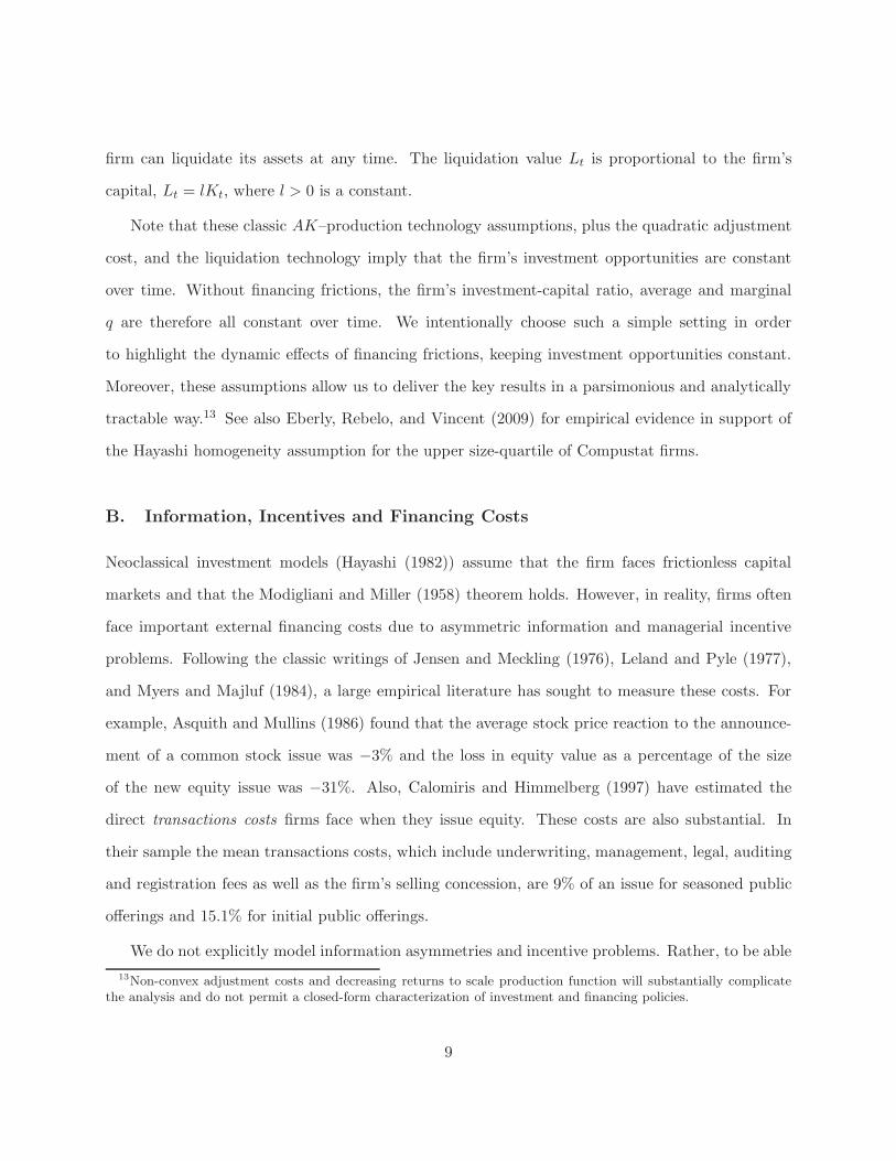
To summarize, for the liquidation case, the complete solution for the firm’s value-capital ratio p (w)

and its optimal dynamic investment policy is given by: i) the HJB equation (13); ii) the investment-

capital ratio equation (14), and; iii) the liquidation (18) and payout boundary conditions (16)-(17).

Similarly, when it is optimal for the firm to refinance rather than liquidate, the complete solution

18

for the firm’s value-capital ratio p (w) and its optimal dynamic investment and financing policy is

given by: i) the HJB equation (13); ii) the investment-capital ratio equation (14); iii) the equity-

issuance boundary condition (19); iv) the optimality condition for equity issuance (20), and; v) the

endogenous payout boundary conditions (16)-(17). Finally, to verify that refinancing is indeed the

firm’s global optimal solution, it is sufficient to check that p(0) > l.

III Quantitative Analysis

We now turn to quantitative analysis of the baseline model. For the benchmark case, we set the

mean and volatility of the risk-adjusted productivity shock to µ = 18% and σ = 9%, respectively,

which are in line with the estimates of Eberly, Rebelo, and Vincent (2009) for large US firms.

The riskfree rate is r = 6%. The rate of depreciation is δ = 10.07%. These parameters are all

annualized. The adjustment cost parameter is θ = 1.5 (see Whited 1992). The implied first-best q

in the neoclassical model is qFB = 1.23, and the corresponding first-best investment-capital ratio is

iFB = 15.1%. We then set the cash-carrying cost parameter to λ = 1%. The proportional financing

cost is γ = 6% (see Altinkihc and Hansen 2000) and the fixed cost of financing is φ = 1%, which

jointly generate average equity financing costs that are consistent with the data. Finally, for the

liquidation value we take l = 0.9 (as suggested in Hennessy and Whited 2007). Table I Panel A

recapitulates all the key variables and parameters in the model.

Before analyzing the impact of costly external equity financing, we first consider a special case

where the firm is forced to liquidate when it runs out of cash. While this is an extreme form of

financing constraint, it may be the relevant constraint in a financial crisis.

Case I: Liquidation. Figure 2 plots the solution in the liquidation case. In Panel A, the firm’s

value-capital ratio p(w) starts at l = 0.9 (liquidation value) when cash balance is equal to 0, is

concave in the region between 0 and the endogenous payout boundary w = 0.22, and becomes

linear (with slope 1) beyond the payout boundary (w ≥ w). In Section II, we have argued that

19

Table I: Summary of Key Variables and Parameters

This table summarizes the symbols for the key variables used in the model and the parametervalues in the benchmark case. For each upper-case variable in the left column (except K, A, andF ), we use its lower case to denote the ratio of this variable to capital. All the boundary variablesare in terms of the cash-capital ratio wt.

Variable Symbol Parameters Symbol Value

A. Baseline model

Capital stock K Riskfree rate r 6%Cash holding W Rate of depreciation δ 10.07%Investment I Risk-neutral mean productivity shock µ 18%Cumulative productivity shock A Volatility of productivity shock σ 9%Investment adjustment cost G Adjustment cost parameter θ 1.5Cumulative operating profit Y Proportional cash-carrying cost λ 1%Cumulative external financing H Capital liquidation value l 0.9Cumulative external financing cost X Proportional financing cost γ 6%Cumulative payout U Fixed financing cost φ 1%Firm value P Market Sharpe ratio η 0.3Average q qa Correlation between market and firm ρ 0.8Marginal q qmPayout boundary wFinancing boundary wReturn cash-capital ratio m

B. Hedging

Hedge ratio ψ Margin requirement π 5Fraction of cash in margin account κ Flow cost in margin account ǫ 0.5%Futures price F Market volatility σm 20%Maximum-hedging boundary w−

Zero-hedging boundary w+

C. Credit line

Credit line limit c 20%Credit line spread over r α 1.5%

20

0 0.05 0.1 0.15 0.2 0.250.8

1

1.2

1.4

1.6

w →

A. firm value-capital ratio: p(w)

first-bestliquidationl +w

0 0.05 0.1 0.15 0.2 0.25

5

10

15

20

25

30B. marginal value of cash: p′(w)

0 0.05 0.1 0.15 0.2 0.25−0.8

−0.6

−0.4

−0.2

0

0.2

cash-capital ratio: w = W/K

C. investment-capital ratio: i(w)

first-bestliquidation

0 0.05 0.1 0.15 0.2 0.250

5

10

15

20D. investment-cash sensitivity: i′(w)


Figure 2: Case I. Liquidation. This figure plots the solution for the case when the firm has to liquidate

when it runs out of cash (w = 0).

the firm will never liquidate before its cash balance hits 0. Panel A of Figure 2 provides a graphic

illustration of this result, where p (w) lies above the liquidation value l+w (normalized by capital)

for all w > 0.

Panel B of Figure 2 plots the marginal value of cash p′ (w) = PW (K,W ). The marginal value

of cash increases as the firm becomes more constrained and liquidation becomes more likely. It also

confirms that the firm value is concave in the internal financing region (p′′(w) < 0). The external

financing constraint makes the firm hoard cash today in order to reduce the likelihood that it will

be liquidated in the future, which effectively induces “risk aversion” for the firm. Consider the

effect of a mean-preserving spread of cash holdings on the firm’s investment policy. Intuitively, the

marginal cost from a smaller cash holding is higher than the marginal benefit from a larger cash

holding because the increase in the likelihood of liquidation outweighs the benefit from otherwise

21

relaxing the firm’s financing constraints. It is the concavity of the value function that gives rise to

the demand for risk management. Observe also that the marginal value of cash reaches a value of

30 as w approaches 0. In other words, an extra dollar of cash is worth as much as $30 to the firm

in this region. This is because more cash helps keep the firm away from costly liquidation, which

would permanently destroy the firm’s future growth opportunities. Such high marginal value of

cash highlights the importance of cash in periods of extreme financing frictions, which is what we

have witnessed in the recent financial crisis.

Panel C plots the investment-capital ratio i(w) and illustrates under-investment due to the

extreme external financing constraints. Optimal investment by a financially constrained firm is

always lower than first-best (iFB = 15.1%), but especially when the firm’s cash inventory w is

low. When w is sufficiently low the firm will disinvest by selling assets to raise cash and move

away from the liquidation boundary. Note that disinvestment is costly not only because the firm is

underinvesting but also because it incurs physical adjustment costs when lowering its capital stock.

For the parameter values we use, asset sales (disinvestments) are at the annual rate of over 60% of

the capital stock when w is close to zero! The firm tries very hard not to be forced into liquidation.

Even at the payout boundary, the investment-capital ratio is only i(w) = 10.6%, about 30% lower

than the first best level iFB . On the margin, the firm is trading off the cash-carrying costs with

the cost of underinvestment. It will optimally choose to hoard more cash and invest more at the

payout boundary when the cash-carrying cost λ is lower.

Finally, we consider a measure of investment-cash sensitivity given by i′(w). Taking the deriva-

tive of investment-capital ratio i(w) in (14) with respect to w, we get

i′(w) = −1

θ

p(w)p′′(w)

p′ (w)2> 0. (21)

The concavity of p ensures that i′(w) > 0 in the internal financing region, as shown in Panel D

of Figure 2. Remarkably, the investment-cash sensitivity i′(w) is not monotonic in w. In particu-

lar, when the cash holding is sufficiently low, i′(w) actually increases with the cash-capital ratio.

22

Formally, the slope of i′(w) depends on the third derivative of p(w), for which we do not have an

analytical characterization.

Clearly, certain liquidation when the firm runs out of cash is an extreme form of financing

constraint, which is why the marginal value of cash can be as high as $30, and asset sales as high

as an annual rate of 60% when the firm runs out of cash. An important insight however from this

scenario is that an extreme financing constraint causes the firm to hold more cash, defer payout,

and cut investment aggressively even when its cash balances are relatively low. Remarkably, all of

these actions help the firm stay away from states of extreme financing constraints most of the time,

as our simulations below show.

Case II: Refinancing. Next we consider the setting where the firm is allowed to issue equity.

Figure 3 displays the solutions for both the case with fixed financing costs (φ = 1%) and without

(φ = 0). Observe that at the financing boundary w = 0, the firm’s value-capital ratio p(w)

is strictly higher than l, so that external equity financing is preferred to liquidation under this

model parameterization. Comparing with the liquidation case, we find that the endogenous payout

boundary (marked by the solid vertical line on the right) is w = 0.19 when φ = 1%, lower than the

payout boundary for the case where the firm is liquidated (w = 0.22). Not surprisingly, firms are

more willing to pay out cash when they can raise new funds in the future. The firm’s optimal return

cash-capital ratio is m = 0.06, marked by the vertical line on the left in Panel A. Without fixed

cost (φ = 0), the payout boundary drops further to w = 0.14, and the firm’s return cash-capital

ratio is zero, as the firm raises just enough funds to keep w above 0.

Panel B plots the marginal value of cash p′(w). which is positive and decreasing between 0 and

w, confirming that p(w) is strictly concave in this case. Conditional on issuing equity and having

paid the fixed financing cost, the firm optimally chooses the return cash-capital ratio m such that

the marginal value of cash p′(m) is equal to the marginal cost of financing 1 + γ. To the left of the

return cash-capital ratio m, the marginal value of cash p′(w) lies above 1+γ, reflecting the fact that

the fixed cost component in raising equity increases the marginal value of cash. When the firm runs

23

0 0.05 0.1 0.15 0.21

1.1

1.2

1.3

1.4

←m(φ = 1%)

w(φ = 1%)→

← w(φ = 0)


φ = 1%φ = 0

0 0.05 0.1 0.15 0.21

1.2

1.4

1.6

1.8B. marginal value of cash: p′(w)

φ = 1%φ = 0

0 0.05 0.1 0.15 0.2−0.3

−0.2

−0.1

0

0.1

0.2



φ = 1%φ = 0

0 0.05 0.1 0.15 0.20

2

4

6

8

10

12


D. investment-cash sensitivity: i′(w)

φ = 1%φ = 0

Figure 3: Case II. Optimal refinancing. This figure plots the solution for the case of refinancing.

out of cash, the marginal value of cash is around 1.7, much higher than 1 + γ = 1.06. This result

highlights the importance of fixed financing costs: even a moderate fixed cost can substantially

raise the marginal value of cash in the low-cash region.

As in the liquidation case, the investment-capital ratio i(w) is increasing in w, and reaches the

peak at the payout boundary w, where i(w) = 11%. Higher fixed cost of financing increases the

severity of financing constraints, therefore leading to more underinvestment. This is particularly

true in the region to the left of the return cash-capital ratio m, where the investment-capital ratio

i(w) drops rapidly. Asset sales go down quickly (i′(w) > 10) when w moves away from zero. This

is because both asset sales and equity issuance are very costly. Removing the fixed financing costs

greatly alleviates the under-investment problem, where both the marginal value of cash and the

investment-capital ratio become essentially flat except for very low w.

24

Average q, marginal q, and investment. We now turn to the model’s predictions on average

and marginal q. We take the firm’s enterprise value – the value of all the firm’s marketable claims

minus cash, P (K,W ) −W – as our measure of the value of the firm’s capital stock. Average q,

denoted by qa(w), is then the firm’s enterprise value divided by its capital stock:

qa(w) =P (K,W )−W

K= p(w)− w. (22)

First, average q increases with w. This is because the marginal value of cash is never below 1, so

that q′a(w) = p′(w) − 1 ≥ 0. Second, average q is concave provided that p(w) is concave, in that

q′′a(w) = p′′(w).

In our model where external financing is costly, marginal q, denoted by qm(w), is given by

qm(w) =d (P (K,W )−W )

dK= p(w)− wp′(w) = qa(w) −

(p′(w) − 1

)w, (23)

where qa(w) = p(w)−w (see Equation (22)). An increase in capital stock K has two effects on the

firms enterprise value. First, the more capital stock, the higher the enterprise value. This is the

standard average q channel, where qa(w) = p(w)−w. Second, increasing capital stock mechanically

lowers the cash-capital ratio w = W/K for W > 0, thus making the firm more constrained. The

wedge between marginal q and average q, − (p′(w) − 1)w, reflects this effect of financing constraint

on firm value. With p′(w) > 1 and w > 0, that wedge is negative, and marginal q is smaller than

average q. Third, both marginal q and average q increase with w for w > 0, because p(w) is strictly

concave. Finally, as a special case, under MM, p′(w) = 1 and hence average q equals marginal q.

Figure 4 plots the average and marginal q for the liquidation case, the refinancing case with no

fixed costs (φ = 0), and the case with fixed costs (φ = 1%). The average and marginal q are below

the first best level, qFB = 1.23, in all three cases, and they become lower as external financing

becomes more costly.

25

0 0.05 0.1 0.15 0.2 0.250.9

0.95

1

1.05

1.1

1.15

1.2


A. average q

case II (φ = 1%)case II (φ = 0)case I

0 0.05 0.1 0.15 0.2 0.250.9

0.95

1

1.05

1.1

1.15

1.2


B. marginal q

case II (φ = 1%)case II (φ = 0)case I

Figure 4: Average q and marginal q. This figure plots the average q and marginal q from the three

special cases of the model. Case I is the liquidation case. Case II and III are with external financing. The

right end of each line corresponds to the respective payout boundary, beyond which both qa and qa are flat.

Stationary distributions of w, p(w), p′(w), i(w), average q, and marginal q. We next

investigate the stationary distributions for the key variables tied to optimal firm policies in the

benchmark case with refinancing case (φ = 1%).18 We first simulate the cash-capital ratio under

the physical probability measure. To do so, we calibrate the Sharpe ratio of the market portfolio

η = 0.3, and assume that the correlation between the firm technology shocks and the market return

is ρ = 0.8. Then, the mean of the productivity shock under the physical probability is µ̂ = 0.20.

Figure 5 shows the distributions for the cash-capital ratio w, the value-capital ratio p (w), the

marginal value of cash p′ (w), and the investment-capital ratio i (w). Since p(w), p′(w), i(w) are all

monotonic in this case, the densities for their stationary distributions are connected with that of w

through (the inverse of) their derivatives.

Strikingly, the cash holdings of a firm are relatively high most of the time, and hence the

probability mass for i(w) is concentrated at the highest values in the relevant support of w, while

p′(w) is mostly around unity. Thus, the firm’s optimal cash management policies appear to be

effective at shielding itself most of the time from the states with the most severe financing constraints

18We conduct additional analysis of the effects of various parameters on the distributions of cash and investmentin Appendix B.

26

0 0.05 0.1 0.15 0.20

5

10

15

20

25A. cash-capital ratio: w

−0.2 −0.1 0 0.10

10

20

30

40

50

60B. investment-capital ratio: i(w)

1.1 1.2 1.3 1.40

5

10

15

20

25C. firm value-capital ratio: p(w)

1 1.2 1.4 1.60

5

10

15

20

25

30

35D. marginal value of cash: p′(w)

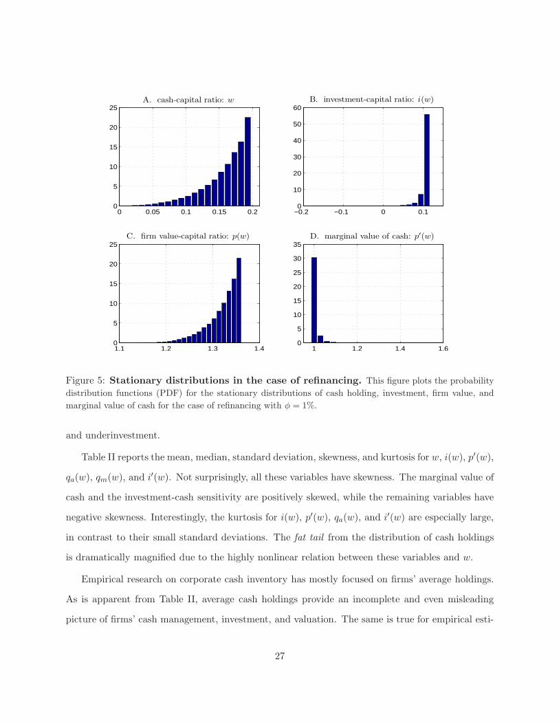
Figure 5: Stationary distributions in the case of refinancing. This figure plots the probability

distribution functions (PDF) for the stationary distributions of cash holding, investment, firm value, and

marginal value of cash for the case of refinancing with φ = 1%.

and underinvestment.

Table II reports the mean, median, standard deviation, skewness, and kurtosis for w, i(w), p′(w),

qa(w), qm(w), and i′(w). Not surprisingly, all these variables have skewness. The marginal value of

cash and the investment-cash sensitivity are positively skewed, while the remaining variables have

negative skewness. Interestingly, the kurtosis for i(w), p′(w), qa(w), and i′(w) are especially large,

in contrast to their small standard deviations. The fat tail from the distribution of cash holdings

is dramatically magnified due to the highly nonlinear relation between these variables and w.

Empirical research on corporate cash inventory has mostly focused on firms’ average holdings.

As is apparent from Table II, average cash holdings provide an incomplete and even misleading

picture of firms’ cash management, investment, and valuation. The same is true for empirical esti-

27

Table II: Moments from the stationary distribution of the refinancing case

This table reports the population moments for cash-capital ratio (w), investment-capital ratio(i(w)), marginal value of cash (p′(w)), average q (qa(w)), and marginal q (qm(w)) from the station-ary distribution in the case with refinancing (φ = 1%).

cash investment marginal investment-cashcapital ratio capital ratio value of cash average q marginal q sensitivity

w i(w) p′(w) qa(w) qm(w) i′(w)

mean 0.159 0.104 1.006 1.164 1.163 0.169median 0.169 0.108 1.001 1.164 1.164 0.064

std 0.034 0.013 0.018 0.001 0.001 0.376skewness -1.289 -6.866 9.333 -8.353 -3.853 8.468kurtosis 4.364 76.026 146.824 106.580 22.949 122.694

mates of the marginal value of cash and investment-cash sensitivity, which are generally interpreted

as capturing how financially constrained a firm is. Even though the median and the mean of p′(w)

are close to 1 (and those of i′(w) close to 0), and even though both distributions have rather small

standard deviations, the kurtosis is huge for both, indicating that the firm could become severely

financially constrained.

The impact of these low probability yet severe financing constraint states is evident. The mean

and median of qa(w) are 1.16, which is about 5% lower than qFB = 1.23, the average q for a

firm without external financing costs. Similarly, the mean and median of i(w) is 0.104, which

is about 31% lower than iFB = 0.151, the investment-capital ratio for a firm without external

financing costs. Therefore, simply looking at the first two moments for the marginal value of cash or

investment-cash sensitivity, provides a highly misleading description of firms’ financing constraints.

Firms endogenously respond to their financing constraints by adjusting their cash management

and investment policies, which in turn reduces the time variations in investment, marginal value of

cash, etc. However, the impact of financing constraints remains large on average.

The analysis above highlight that, by providing a more complete picture of firms’ capital expen-

ditures and cash holdings over the time series and in the cross section, this model helps us better

28

understand the empirical patterns of cash holdings. The model’s ability to match the empirical

distributions can be further improved if we allow for changing investment and financing opportunity

sets and firm heterogeneity.

IV Dynamic Hedging

In addition to cash inventory management, the firm can also reduce its cash flow risk through

financial hedging (e.g., using options or futures contracts). Consider, for example, the firm’s hedging

policy using market index futures.19 Let Ft denote the futures price on the market index at time

t. Under the risk-adjusted probability, Ft evolves according to:

dFt = σmFtdBt, (24)

where σm is the volatility of the aggregate market portfolio, and Bt is a standard Brownian motion

that is partially correlated with firm productivity shock driven by the Brownian motion Zt, with

correlation coefficient ρ.

Let ψt denote the hedge ratio, i.e., the position in the market index futures (the notional

amount) as a fraction of the firm’s total cash Wt. Futures contracts often require that the investor

hold cash in a margin account, which is costly. Let κt denote the fraction of the firm’s total cash

Wt held in the margin account (0 ≤ κt ≤ 1). In addition to the carry cost for cash in the standard

interest-bearing account, cash held in this margin account also incurs the additional flow cost ǫ

per unit of cash. We assume that the firm’s futures position (in absolute value) cannot exceed a

19In this analysis we only consider hedging of systematic risk by the firm. In practice firms also hedge idiosyncraticrisk by taking out insurance contracts. Our model can be extended to introduce insurance contracts, but this isbeyond the scope of this article.

29

constant multiple π of the amount of cash κtWt in the margin account.20 That is, we require

|ψtWt| ≤ πκtWt. (25)

As the firm can costlessly reallocate cash between the margin account and its regular interest-

bearing account at any time, the firm will optimally hold the minimum amount of cash necessary

in the margin account. That is, provided that ǫ > 0, optimality implies that the inequality (25)

holds as an equality. When the firm takes a hedging position in the index future, its cash balance

evolves as follows:

dWt = Kt (µdAt + σdZt)− (It +Gt) dt+ dHt − dUt + (r − λ)Wtdt− ǫκtWtdt+ ψtσmWtdBt. (26)

Next, we investigate the special case where there are no margin requirements for hedging.

A. Optimal Hedging with No Frictions

With no margin requirement (π = ∞), the firm carries all its cash in the regular interest-bearing

account and is not constrained in the size of the index futures position ψ. Since firm value P (K,W )

is concave in W (i.e. PWW < 0), the firm will completely eliminate its systematic risk exposure via

dynamic hedging. The firm thus behaves exactly in the same way as the firm in our baseline model

but the firm is only subject to idiosyncratic risk with volatility σ√

1− ρ2. It is easy to show that

the optimal hedge ratio ψ is constant in this case,

ψ∗(w) = −ρσ

wσm. (27)

Thus, for a firm with size K, the total hedge position is |ψW | = (ρσ/σm)K, which linearly increases

with firm size K.

20For simplicity, we abstract from any variation of margin requirement, so that π is constant.

30

B. Optimal Hedging with Margin Requirements

Next, we consider the important effects of margin requirements and hedging costs. We will show

that financing constraints fundamentally alter hedging, investment/asset sales, and cash manage-

ment. The firms HJB equation now becomes:

rP (K,W ) = maxI,ψ,κ

(I − δK)PK(K,W ) + ((r − λ)W + µK − I −G(I,K) − ǫκW )PW (K,W )

+1

2

(σ2K2 + ψ2σ2

mW2 + 2ρσmσψWK

)PWW (K,W ), (28)

subject to:

κ = min

{|ψ|

π, 1

}. (29)

Equation (29) indicates that there are two candidate solutions for κ (the fraction of cash in the

margin account): one interior and one corner. If the firm has sufficient cash, so that its hedging

choice ψ is not constrained by its cash holding, the firm sets κ = |ψ|/π. This choice of κ minimizes

the cost of the hedging position subject to meeting the margin requirement. Otherwise, when the

firm is short of cash, it sets κ = 1, thus putting all its cash in the margin account to take the

maximum feasible hedging position: |ψ| = π.

The direction of hedging (long (ψ > 0) or short (ψ < 0)) is determined by the correlation

between the firm’s business risk and futures return. With ρ > 0, the firm will only consider taking

a short position in the index futures as we have shown. If ρ < 0, the firm will only consider taking

a long position. Without loss of generality, we focus on the case where ρ > 0, so that ψ < 0.

We show that there are three endogenously determined regions for optimal hedging. First,

consider the cash region with an interior solution for ψ (where the fraction of cash allocated to the

margin account is given by κ = −ψ/π < 1). The FOC with respect to ψ is:

ǫ

πWPW +

(σ2mψW

2 + ρσmσWK)PWW = 0.

31

Using homogeneity, we may simplify the above equation and obtain:

ψ∗(w) =1

w

(−ρσ

σs−ǫ

π

p′(w)

p′′(w)

1

σ2s

). (30)

Consider next the low-cash region. The benefit of hedging is high in this region (p′(w) is high

when w is small). The constraint κ ≤ 1 is then binding, hence ψ∗(w) = −π for w ≤ w−, where the

endogenous cutoff point w− is the unique value satisfying ψ∗(w−) = −π in (30). We refer to w− as

the maximum-hedging boundary.

Finally, when w is sufficiently high, the firm chooses not to hedge, as the net benefit of hedging

approaches zero while the cost of hedging remains bounded away from zero. More precisely, we have

ψ∗(w) = 0 for w ≥ w+, where the endogenous cutoff point w+ is the unique solution of ψ∗(w+) = 0

using Equation (30). We refer to w+ as the zero-hedging boundary.

We now provide quantitative analysis for the impact of hedging on the firm’s decision rules and

firm value. We choose the following parameter values: ρ = 0.8, σm = 20%, π = 5 (corresponding

to 20% margin requirement), and ǫ = 0.5%. The remaining parameters are those for the baseline

case. These parameters and the key variables for the hedging case are also summarized in Table I.

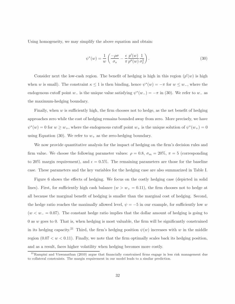
Figure 6 shows the effects of hedging. We focus on the costly hedging case (depicted in solid

lines). First, for sufficiently high cash balance (w > w+ = 0.11), the firm chooses not to hedge at

all because the marginal benefit of hedging is smaller than the marginal cost of hedging. Second,

the hedge ratio reaches the maximally allowed level, ψ = −5 in our example, for sufficiently low w

(w < w− = 0.07). The constant hedge ratio implies that the dollar amount of hedging is going to

0 as w goes to 0. That is, when hedging is most valuable, the firm will be significantly constrained

in its hedging capacity.21 Third, the firm’s hedging position ψ(w) increases with w in the middle

region (0.07 < w < 0.11). Finally, we note that the firm optimally scales back its hedging position,

and as a result, faces higher volatility when hedging becomes more costly.

21Rampini and Viswanathan (2010) argue that financially constrained firms engage in less risk management dueto collateral constraints. The margin requirement in our model leads to a similar prediction.

32

0 0.05 0.1 0.15 0.2−10

−8

−6

−4

−2

0

A. hedge ratio: ψ(w)

costly marginfrictionless

0 0.05 0.1 0.15 0.2−0.4

−0.2

0

0.2B. investment-capital ratio: i(w)

frictionlesscostly marginno hedging

0 0.05 0.1 0.15 0.21.1

1.2

1.3

1.4


C. firm value-capital ratio: p(w)


0 0.05 0.1 0.15 0.21

1.5

2

2.5

3


D. marginal value of cash: p′(w)


Figure 6: Optimal hedging. This figure plots the optimal hedging and investment policies, the firm

value-capital ratio, and the marginal value of cash for Case II with hedging (with or without margin require-

ments). In Panel A, the hedge ratio for the frictionless case is cut off at −10 for display. The right end of

each line corresponds to the respective payout boundary.

With hedging, the firm holds less cash, pays out to shareholders earlier, and raises less cash

each time it issues equity. As shown in Panel B and D, as long as it is not too constrained, the

firm also invests more and has a lower marginal value of cash (for the same cash-capital ratio) with

hedging. Panel C shows that firm value also rises with hedging. The cash management policies will

affect the dynamics of cash holdings, which ultimately determines the dynamics of hedge ratios.

For instance, under costly hedging, the stationary distribution of cash holdings will be similar to

Figure 5, which implies that the firm will not engage in financial hedging most of the time.

Second, for sufficiently low cash, the firm may underinvest more when hedging becomes less

costly (see Panel B). This might appear surprising, as Froot, Scharfstein, and Stein (1993) show

33

that hedging mitigates underinvestment in a static model. However, in our dynamic model, hedging

raises the firm’s going concern value. At times of severe financing constraints, it is optimal to

aggressively scale back investment in the short run in order to better manage risk and preserve firm

value for the long run.

Specifically, as equation (14) shows, investment depends on the ratio p(w)/p′(w). When w

becomes sufficiently small, not only is p(w) higher with hedging, but also the marginal value of

cash p′(w), as shown in Panel D. There are two reasons hedging increases p′(w) for low w. First, as

Panel A shows, the margin constraint is binding when w is sufficiently low. Thus, each extra dollar

of cash can be put in the margin account, which helps move the firm closer to optimal (frictionless)

hedging. Second, when the volatility of cash flow is reduced through hedging, an extra dollar of

cash becomes more effective in helping the firm avoid issuing equity (especially when cash is low).

When w is sufficiently small, the effect of hedging on the marginal value of cash can exceed its effect

on firm value, which leads to lower investment. In summary, hedging can lead to more demand for

precautionary savings, hence more underinvestment for a severely financially constrained firm.

Many existing models of risk management focus on financial hedging while treating the oper-

ations of the firm as exogenous. Our analysis highlights a central theme that cash management,

financial hedging, and asset sales are integral parts of dynamic risk management. It is therefore

important to examine these different ways of managing risk in a unified framework.

How much value does hedging add to the firm? We answer this question by computing the net

present value (NPV) of optimal hedging to the firm for the case with costly margin requirements.

The NPV of hedging is defined as follows. First, we compute the cost of external financing as the

difference in Tobin’s q under the first-best case and q under Case II without hedging. Second, we

compute the loss in adjusted present value (APV), which is the difference in the Tobin’s q under

the first-best case and q under Case II with costly margin. Then, the difference between the costs

of external financing and the loss in APV is simply the value created through hedging. On average,

when measured relative to Tobin’s q under hedging with a costly margin, the costs of external

financing is about 6%, the loss in APV is about 5%, so that the NPV of costly hedging is of the

34

order of 1%, a significant creation of value to say the least for a purely financial operation.

V Credit Line

Our baseline model of Section I can also be extended to allow the firm to access a credit line. This

is an important extension to consider, as many firms in practice are able to secure such lines, and

for these firms, access to a credit line is an important alternative source of liquidity.

We model the credit line as a source of funding the firm can draw on at any time it chooses up

to a limit. We set the credit limit to a maximum fraction of the firm’s capital stock, so that the

firm can borrow up to cK, where c > 0 is a constant. The logic behind this assumption is that the

firm must be able to post collateral to secure a credit line and the highest quality collateral does

not exceed the fraction c of the firm’s capital stock. We may thus interpret cK to be the firm’s

short-term debt capacity. For simplicity, we treat c as exogenous in this paper. It is straightforward

to endogenize the credit line limit by assuming that banks charge a commitment fee on the unused

part of the credit line. We investigate this case in Appendix D. We also assume that the firm pays

a constant spread α over the risk-free rate on the amount of credit it uses. Sufi (2009) shows that

a firm on average pays 150 basis points over LIBOR on its credit lines, leading us to set α = 1.5%.

Since the firm pays a spread α over the risk-free rate to access credit, it will optimally avoid

using its credit line before exhausting its internal funds (cash) to finance investment. As long as

the interest rate spread α is not too high, credit line will be less expensive than external equity,

so the firm also prefers to first draw on the line before tapping equity markets.22 Our model thus

generates a pecking order among internal funds, credit lines, and external equity financing.

When credit line is the marginal source of financing (w < 0), p(w) solves the following ODE:

rp(w) = (i(w) − δ)(p (w)− wp′ (w)

)+ ((r + α)w + µ− i(w) − g(i(w))) p′ (w) +

σ2

2p′′ (w) . (31)

22When α is high and equity financing costs (φ, γ) are low, the firm may not exhaust its credit line before accessingexternal equity markets. For our parameter values, we find that the pecking order results apply between the creditline and external equity.

35

−0.2 −0.1 0 0.1 0.20.9

1.1

1.3

1.5

←m(c = 0.2)

← w(c = 0.2)

m(c = 0)→

w(c = 0)→


c = 0.2c = 0

−0.2 −0.1 0 0.1 0.21

1.2

1.4

1.6


c = 0.2c = 0

−0.2 −0.1 0 0.1 0.2−0.25

−0.15

−0.05

0.05

0.15



c = 0.2c = 0

−0.2 −0.1 0 0.1 0.20

3

6

9

12


D. investment-cash sensitivity: i′(w)

c = 0.2c = 0

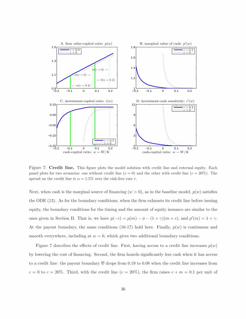
Figure 7: Credit line. This figure plots the model solution with credit line and external equity. Each

panel plots for two scenarios: one without credit line (c = 0) and the other with credit line (c = 20%). The

spread on the credit line is α = 1.5% over the risk-free rate r.

Next, when cash is the marginal source of financing (w > 0), as in the baseline model, p(w) satisfies

the ODE (13). As for the boundary conditions, when the firm exhausts its credit line before issuing

equity, the boundary conditions for the timing and the amount of equity issuance are similar to the

ones given in Section II. That is, we have p(−c) = p(m)− φ− (1 + γ)(m+ c), and p′(m) = 1 + γ.

At the payout boundary, the same conditions (16-17) hold here. Finally, p(w) is continuous and

smooth everywhere, including at w = 0, which gives two additional boundary conditions.

Figure 7 describes the effects of credit line. First, having access to a credit line increases p(w)

by lowering the cost of financing. Second, the firm hoards significantly less cash when it has access

to a credit line: the payout boundary w drops from 0.19 to 0.08 when the credit line increases from

c = 0 to c = 20%. Third, with the credit line (c = 20%), the firm raises c +m = 0.1 per unit of

36

capital when it exhausts its credit line. Without credit line (c = 0), the firm issues m = 0.06 per

unit of capital when it runs out of cash. Thus, for our parameter choices, the firm with a credit line

issues more equity. Fourth, with the credit line, the marginal value of cash at w = 0 is p′(0) = 1.01,

which is substantially lower than p′(0) = 1.69 without credit line (c = 0).

Credit line also substantially mitigates the firms underinvestment problem (see Panel C of

Figure 7). With the credit line (c = 20%), the firms investment-capital ratio when it runs out

of cash (w = 0) is i(0) = 11.7%, which is substantially higher than i(0) = −21.4% (indicating

significant asset sales) when the firm is about to run out of cash and has no access to credit line.

Even when the firm has exhausted its credit line (w = −20%), it engages in much less costly asset

sales: i(−c) = −7.9%. The investment-cash sensitivity i′(w) is also substantially lower when the

firm has access to a credit line. For example, i′(0) decreases from 11.8 to 0.27 when the firm’s

credit line is increased from zero to 0.2.

Next, we turn to the effect of liquidity (cash and credit) on average q, marginal q, and in-

vestment. The left panel of Figure 8 plots the firm’s marginal q and average q for two otherwise

identical firms: one with a credit line (c = 20%), and the other without a credit line (c = 0).

We see that average q still increases with cash-capital ratio w in both credit and cash regions, as

q′a(w) = p′(w)− 1 ≥ 0, where the inequality follows from the financing constraints (p′(w) ≥ 1).

Unlike average q, marginal q is no longer monotonic in w. Its relation with w now depends on

whether the marginal source of financing is cash or credit. This can be seen from the following:

q′m(w) = −p′′(w)w.

Firm value is concave in both the cash and credit line regions (p′′(w) < 0). Thus, marginal q

increases in w in the cash region (w > 0) and decreases in w in the credit region (w < 0).

The different behavior of marginal q in these two regions is due to the opposite effects of

increasing K on financial constraints. When the firm uses its internal cash to finance investment,

increasing K lowers the cash-capital ratio w, making the firm more constrained. When the firm

37

−0.2 −0.1 0 0.1 0.21.14

1.16

1.18

1.2

1.22

1.24

1.26

1.28

1.3


A. average q and marginal q

qa (c = 0.2)qm (c = 0.2)qa (c = 0)qm (c = 0)

qFB

−0.2 −0.1 0 0.10.8

0.9

1

1.1

1.2

1.3


B. investment and q

q

qaqmqm/p

′

i

−0.2 −0.1 0 0.1−0.1

−0.05

0

0.05

0.1

0.15

i

Figure 8: Investment and q with credit line. The left panel plots the average q (qa) and marginal

q (qm) from the case with credit line (c = 0.2) and without credit line (c = 0) up to the respective payout

boundaries. The right panel plots the average q, marginal q, the ratio of marginal q to marginal value of

liquidity (qm/p′) on the left axis, and investment-capital ratio (i) on the right axis. These results are for the

case with credit line (c = 0.2).

is on the borrowing margin, increasing K makes w less negative, hence lowering firm leverage and

relaxing its financing constraint.

Recall that in the cash region, marginal q is always lower than average q as seen in (23). However,

marginal q is higher than average q in the credit region (w < 0). When the debt capacity mechanism

is sufficiently strong, marginal q in the credit region can be even larger than the first-best q.23

The above results have crucial implications for the relationship between q and investment. It is

sometimes argued that when there are no fixed costs of investment, marginal q is a more accurate

measure than average q for the firm’s investment opportunities.24 This is indeed true in the MM

world, but it is not generally valid when firms face financing constraints, even in the absence of

fixed costs for investment. The right panel of Figure 8 shows that while the investment-capital

23This result does not appear in contracting models such as DFHW due to the manager’s voluntary participationconstraints.

24Caballero and Leahy (1996) show that average q can be a better proxy for investment opportunities in thepresence of fixed costs of investment.

38

ratio i(w) and average q increase with w in the credit region, marginal q decreases with w. To

understand this result, first recall that the concavity of p(w) implies that average q and investment

move in the same direction with w in both regions. However, marginal q increases with |w| for

w < 0 due to the debt capacity mechanism we sketched out earlier. Therefore, average q rather

than marginal q can be a more robust predictor of investment in the presence of credit line.

VI Conclusion

We propose a tractable and operational model that demonstrates how the presence of external

financing costs influences a firm’s optimal investment, financing, and risk management policies.

The marginal value of liquidity, which is endogenous, plays a central in these corporate decisions.

We show that investment depends on the ratio of marginal q and marginal value of liquidity; the

optimal cash inventory policy takes the form of a double-barrier policy; liquidity management and

financial hedging are complementary risk-management tools.

We see a few directions for related future research. The recent financial crisis suggests that

market financing conditions can change abruptly for reasons orthogonal to the firm’s own charac-

teristics. Campello, Graham, and Harvey (2009) and Campello, Giambona, Graham, and Harvey

(2010) find that the financially constrained firms planned deeper cuts in investment, spending,

burned more cash, drew more credit from banks, and also engaged in more asset sales in the re-

cent financial crisis. By enriching our model proposed in this paper to accommodate for credit

supply/external financing shocks, we can analyze and provide a more accurate description of the

effect of financial crisis on corporate financial policies. Bolton, Chen, and Wang (2010) extend our

model to allow for time-varying investment and financing opportunities. This richer model pro-

duces predictions that are broadly in line with the empirical findings in the above papers. Another

significant omission in this paper is long-term debt. We leave the study of the optimal maturity

structure of debt to future research.

39

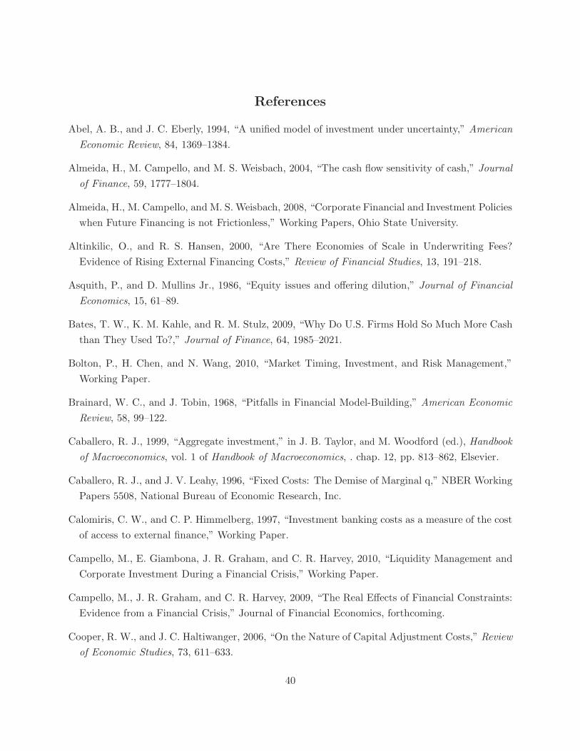
References

Abel, A. B., and J. C. Eberly, 1994, “A unified model of investment under uncertainty,” American

Economic Review, 84, 1369–1384.

Almeida, H., M. Campello, and M. S. Weisbach, 2004, “The cash flow sensitivity of cash,” Journal

of Finance, 59, 1777–1804.

Almeida, H., M. Campello, and M. S. Weisbach, 2008, “Corporate Financial and Investment Policies

when Future Financing is not Frictionless,” Working Papers, Ohio State University.

Altinkilic, O., and R. S. Hansen, 2000, “Are There Economies of Scale in Underwriting Fees?

Evidence of Rising External Financing Costs,” Review of Financial Studies, 13, 191–218.

Asquith, P., and D. Mullins Jr., 1986, “Equity issues and offering dilution,” Journal of Financial

Economics, 15, 61–89.

Bates, T. W., K. M. Kahle, and R. M. Stulz, 2009, “Why Do U.S. Firms Hold So Much More Cash

than They Used To?,” Journal of Finance, 64, 1985–2021.

Bolton, P., H. Chen, and N. Wang, 2010, “Market Timing, Investment, and Risk Management,”

Working Paper.

Brainard, W. C., and J. Tobin, 1968, “Pitfalls in Financial Model-Building,” American Economic

Review, 58, 99–122.

Caballero, R. J., 1999, “Aggregate investment,” in J. B. Taylor, and M. Woodford (ed.), Handbook

of Macroeconomics, vol. 1 of Handbook of Macroeconomics, . chap. 12, pp. 813–862, Elsevier.

Caballero, R. J., and J. V. Leahy, 1996, “Fixed Costs: The Demise of Marginal q,” NBER Working

Papers 5508, National Bureau of Economic Research, Inc.

Calomiris, C. W., and C. P. Himmelberg, 1997, “Investment banking costs as a measure of the cost

of access to external finance,” Working Paper.

Campello, M., E. Giambona, J. R. Graham, and C. R. Harvey, 2010, “Liquidity Management and

Corporate Investment During a Financial Crisis,” Working Paper.

Campello, M., J. R. Graham, and C. R. Harvey, 2009, “The Real Effects of Financial Constraints:

Evidence from a Financial Crisis,” Journal of Financial Economics, forthcoming.

Cooper, R. W., and J. C. Haltiwanger, 2006, “On the Nature of Capital Adjustment Costs,” Review

of Economic Studies, 73, 611–633.

40

Cox, J. C., J. E. Ingersoll, Jr., and S. A. Ross, 1985, “An Intertemporal General Equilibrium Model

of Asset Prices,” Econometrica, 53, 363–384.

DeAngelo, H., L. DeAngelo, and T. Whited, 2009, “Capital Structure Dynamics and Transitory

Debt,” Working Paper.

Decamps, J., T. Mariotti, J. Rochet, and S. Villeneuve, 2006, “Issuance Costs and Stock Return

Volatility,” Working paper, Toulouse University.

DeMarzo, P., M. Fishman, Z. He, and N. Wang, 2009, “Dynamic agency and the q theory of

investment,” Working Paper, Stanford University.

Dittmar, A., and J. Mahrt-Smith, 2007, “Corporate Governance and the Value of Cash Holdings,”

Journal of Financial Economics, 83, 599–634.

Dumas, B., 1991, “Super contact and related optimality conditions,” Journal of Economic Dynam-

ics and Control, 4, 675–685.

Eberly, J., S. Rebelo, and N. Vincent, 2009, “Investment and Value: A Neoclassical Benchmark,”

Working Paper, Northwestern University.

Faulkender, M., and R. Wang, 2006, “Corporate Financial Policy and the Value of Cash,” Journal

of Finance, 61, 1957–1990.

Fazzari, S. M., R. G. Hubbard, and B. C. Petersen, 1988, “Financing Constraints and Corporate

Investment,” Brookings Papers on Economic Activity, 1988, pp. 141–206.

Fischer, E. O., R. Heinkel, and J. Zechner, 1989, “Dynamic Capital Structure Choice: Theory and

Tests,” Journal of Finance, 44, 19–40.

Froot, K., D. Scharfstein, and J. Stein, 1993, “Risk Management, Coordinating Corporate Invest-

ment, and Financing Policies,” Journal of Finance, 48, 1629–1658.

Gamba, A., and A. Triantis, 2008, “The Value of Financial Flexibility,” Journal of Finance, 63,

2263–2296.

Gomes, J. F., 2001, “Financing Investment,” American Economic Review, 91, 1263–1285.

Graham, J. R., 2000, “How Big Are the Tax Benefits of Debt?,” Journal of Finance, 55, 1901–1941.

Hart, O., and J. Moore, 1994, “A theory of debt based on the inalienability of human capital,”

Quarterly Journal of Economics, 109, 841–879.

41

Hayashi, F., 1982, “Tobin’s marginal Q and average Q: A neoclassical interpretation,” Economet-

rica, 50, 215–224.

Hennessy, C. A., A. Levy, and T. M. Whited, 2007, “Testing Q theory with financing frictions,”


Hennessy, C. A., and T. M. Whited, 2005, “Debt Dynamics,” Journal of Finance, 60, 1129–1165.

Hennessy, C. A., and T. M. Whited, 2007, “How Costly Is External Financing? Evidence from a

Structural Estimation,” Journal of Finance, 62, 1705–1745.

Jensen, M. C., and W. H. Meckling, 1976, “Theory of the Firm: Managerial Behavior, Agency

Costs and Ownership Structure,” Journal of Financial Economics, 3, 305–360.

Jones, L. E., and R. E. Manuelli, 2005, “Neoclassical Models of Endogenous Growth: The Effects

of Fiscal Policy, Innovation and Fluctuations,” in Philippe Aghion, and Steven Durlauf (ed.),

Handbook of Economic Growth.

Kaplan, S. N., and L. Zingales, 1997, “Do Investment-Cash Flow Sensitivities Provide Useful Mea-

sures of Financing Constraints?,” Quarterly Journal of Economics, 112, 169–215.

Khurana, K., X. Martin, and R. Pereira, 2006, “Financial Development and the Cash Flow Sensi-

tivity of Cash,” Journal of Financial and Quantitative Analysis, 41, 787–807.

Kim, C.-S., D. C. Mauer, and A. E. Sherman, 1998, “The Determinants of Corporate Liquidity:

Theory and Evidence,” Journal of Financial and Quantitative Analysis, 33, 335–359.

Leland, H., 1994, “Corporate Debt Value, bond covenants, and Optimal Capital Structure,” Journal

of Finance, 49, 1213–1252.

Leland, H. E., and D. H. Pyle, 1977, “Informational Asymmetrics, Financial Structure, and Finan-

cial Intermediation,” Journal of Finance, 32, 371–387.

Lucas, Robert E, J., and E. C. Prescott, 1971, “Investment Under Uncertainty,” Econometrica, 39,

659–681.

Mello, A. S., and J. E. Parsons, 2000, “Hedging and Liquidity,” Review of Financial Studies, 13,

127–53.

Mello, A. S., J. E. Parsons, and A. J. Triantis, 1995, “An integrated model of multinational flexi-

bility and financial hedging,” Journal of International Economics, 39, 27–51.

42

Miller, M. H., and D. Orr, 1966, “A model of demand for money by firms,” Quarterly Journal of

Economics, 80, 413–435.

Modigliani, F., and M. Miller, 1958, “The Cost of Capital, Corporation Finance, and the Theory

of Investment,” American Economic Review, 53, 261–297.

Morellec, E., and J. Clifford W. Smith, 2007, “Agency Conflicts and Risk Management,” Review

of Finance, 11, 1–23.

Myers, S. C., and N. S. Majluf, 1984, “Corporate Financing and Investment Decisions when Firms

Have Information That Investors do not Have,” Journal of Financial Economics, 13, 187–221.

Opler, T., L. Pinkowitz, R. Stulz, and R. Williamson, 1999, “The Determinants and Implications

of Cash Holdings,” Journal of Financial Economics, 52, 3–46.

Rampini, A. A., and S. Viswanathan, 2010, “Collateral, risk management, and the distribution of

debt capacity,” Journal of Finance, forthcoming.

Riddick, L. A., and T. M. Whited, 2009, “The Corporate Propensity to Save,” Journal of Finance,

64, 1729–1766.

Sufi, A., 2009, “Bank Lines of Credit in Corporate Finance: An Empirical Analysis,” Review of

Financial Studies, 22, 1057–1088.

Tobin, J., 1969, “A General Equilibrium Approach to Monetary Theory,” Journal of Money, Credit

and Banking, 1, 15–29.

Whited, T. M., 1992, “Debt, Liquidity Constraints, and Corporate Investment: Evidence from

Panel Data,” Journal of Finance, 47, 1425–60.

43

Internet Appendix for

“A Unified Theory of Tobin’s q, Corporate Investment, Financing,

and Risk Management”

Patrick Bolton∗ Hui Chen† Neng Wang‡

October 18, 2010

This appendix is organized as follows. Section A examines our model’s implication for the risk

and return on equity, in particular, on how beta changes with the firm’s cash holdings. Section

B studies the comparative statics of the stationary cash-capital ratio distributions. Section C

calculates the endogenous average financing costs. Section D presents a model that endogenizes

the credit line limit, and Section E illustrates the stationary distribution for the general case where

the firm has access to a credit line. Finally, Section F derives the boundary conditions and outlines

our numerical procedure.

A. Risk and return

In this section, we investigate how the firm’s investment, financing, and cash management policies

affect the risk and return of the firm. Livdan, Sapriza, and Zhang (2009) also study the effect of

financing constraints on stock returns. Their model does not allow for cash accumulation, which is

the focus of our analysis.

In order to highlight the impact of financing constraints on the firm’s risk and returns, we

∗Columbia University, NBER and CEPR. Email: [email protected]. Tel. 212-854-9245.†MIT Sloan School of Management and NBER. Email: [email protected]. Tel. 617-324-3896.‡Columbia Business School and NBER. Email: [email protected]. Tel. 212-854-3869.

IA-1

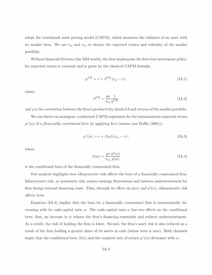
adopt the benchmark asset pricing model (CAPM), which measures the riskiness of an asset with

its market beta. We use rm and σm to denote the expected return and volatility of the market

portfolio.

Without financial frictions (the MM world), the firm implements the first-best investment policy.

Its expected return is constant and is given by the classical CAPM formula:

µFB = r + βFB (rm − r) , (IA.1)

where

βFB =ρσ

σm

1

qFB, (IA.2)

and ρ is the correlation between the firm’s productivity shock dA and returns of the market portfolio.

We can derive an analogous conditional CAPM expression for the instantaneous expected return

µr(w) of a financially constrained firm by applying Ito’s lemma (see Duffie (2001)):

µr(w) = r + β(w) (rm − r) , (IA.3)

where

β(w) =ρσ

σm

p′(w)

p(w)(IA.4)

is the conditional beta of the financially constrained firm.

Our analysis highlights how idiosyncratic risk affects the beta of a financially constrained firm.

Idiosyncratic risk, as systematic risk, causes earnings fluctuations and induces underinvestment for

firm facing external financing costs. Thus, through its effect on p(w) and p′(w), idiosyncratic risk

affects beta.

Equation (IA.4) implies that the beta for a financially constrained firm is monotonically de-

creasing with its cash-capital ratio w. The cash-capital ratio w has two effects on the conditional

beta: first, an increase in w relaxes the firm’s financing constraint and reduces underinvestment.

As a result, the risk of holding the firm is lower. Second, the firm’s asset risk is also reduced as a

result of the firm holding a greater share of its assets in cash (whose beta is zero). Both channels

imply that the conditional beta β(w) and the required rate of return µr(w) decreases with w.

IA-2

Interestingly, when w is sufficiently high, the beta for a firm facing external financing costs can

be even lower than the beta for the neoclassical firm (facing no financing costs). We may illustrate

this point by rewriting the conditional beta as follows:

β(w) =ρσ

σm

p′(w)

(p(w) − w) + w=

ρσ

σm

p′(w)

qa(w) + w, (IA.5)

where qa(w) = p(w) − w is the firm’s average q (the ratio of the firm’s enterprise value and its

capital stock). Although qa(w) < qFB and p′(w) > 1, the second term, w, in the denominator of

β(w) can be so large that β(w) < βFB . Intuitively, as a financially constrained firm hoard cash to

reduce external financing costs, the firm beta becomes a weighted average of the asset beta and the

beta of cash (zero). With a large enough buffer stock of cash holdings relative to its assets, this

firm can be even safer than neoclassical firms facing no financing costs and holding no cash.

Panel A of Figure IA.1 plots the firm’s value-capital ratio p(w) for three different levels of

idiosyncratic volatility (5%, 15%, 30%). The other parameter values for this calculation are rm −

rf = 6%, σm = 20%, and the systematic volatility is fixed at ρσ = 7.2% (assuming ρ = 0.8 and

σ = 9%). As expected, it shows that firm value is higher and the payout boundary w is lower for

lower levels of idiosyncratic volatility.

Panel B plots the marginal value of cash p′(w) for the same three levels of idiosyncratic volatility.

It shows, as expected, that p′(w) is decreasing in w for each level of idiosyncratic volatility. The

figure also reveals that for high values of w, the marginal value of cash p′(w) is higher for higher

levels of idiosyncratic volatility. But, more surprisingly, for low values of w the marginal value of

cash is actually decreasing in idiosyncratic volatility. The reason is that when the firm is close to

financial distress, a dollar is more valuable for a firm with lower idiosyncratic volatility, which is

more likely to avoid raising external funds.

Panel C plots the investment-capital ratio for the three different levels of idiosyncratic volatility.

We see again that for sufficiently high w, investment is decreasing in idiosyncratic volatility, whereas

for low w, it is increasing. That is, when w is low, firms with low idiosyncratic volatility engage in

more asset sales. Again, this latter result is driven by the fact that a marginal dollar has a higher

value for a firm with lower idiosyncratic volatility. Therefore, such a firm will sell more assets to

IA-3

0 0.2 0.4 0.6 0.81

1.2

1.4

1.6

1.8

2A. firm value-capital ratio: p(w)

idio vol: 5%idio vol: 15%idio vol: 30%

0 0.2 0.4 0.6 0.81

1.1

1.2

1.3

1.4

1.5

1.6



0 0.2 0.4 0.6 0.8−0.3

−0.2

−0.1

0

0.1

0.2




0 0.2 0.4 0.6 0.80.6

0.8

1

1.2

1.4

1.6

1.8


D. conditional beta: β(w)/βFB


Figure IA.1: Idiosyncratic volatility, firm value, investment, and beta. In the refinanc-

ing case (φ = 1%), fixing all other parameters while using three different levels of idiosyncratic volatility

(5%, 15%, 30%), this figure plots the firm value-capital ratio, marginal value of cash, investment-capital ratio,

and the ratio of the conditional beta of a constrained firm to that of an unconstrained firm (first best). The

right end of each line corresponds to the respective payout boundary.

replenish its cash holdings.

Panel D plots conditional betas normalized by the first-best beta: β(w)/βFB . For the same

firm, β(w) is decreasing in the cash-capital ratio w. At low levels of w, the firm’s normalized beta

β(w)/βFB can approach a value as high as 1.8 for idiosyncratic volatility of 5%. On the other hand,

β(w) is actually lower than βFB for high w. For example, the conditional beta can be as low as

60% of the first-best beta in the case of 30% idiosyncratic volatility. As we have explained above,

this is due to the fact that a financially constrained firm endogenously hoards significant amounts

of cash, a perfectly safe asset, so that the mix of a constrained firm’s assets may actually be safer

than the asset mix of an unconstrained firm, which does not hoard any cash.

IA-4

The rankings of beta across the firms with different idiosyncratic volatility depends on w. For

large cash-capital ratio w, the beta is increasing in the idiosyncratic volatility. However, when the

level of w is low, firms with low idiosyncratic volatility actually have higher beta. The rankings of

beta are driven by the ratio p′(w)/p(w), which can be inferred from the top two panels.

These observations from Panel D have important implications about cross sectional studies of

betas and cash holdings for financially constrained firms. First, after controlling for technology

parameters and financing costs, the model predicts an inverse relation between returns and corpo-

rate cash holdings, which has been documented by Dittmar and Mahrt-Smith (2007) among others.

Our analysis points out that this negative relation may not just be due to agency problems, as they

emphasize, but may also be driven by the changing asset risk composition of the firm.

Second, for a cross section of firms with heterogeneous production technologies and external

financing costs, it is crucial to take into account the endogeneity of cash holdings when we compare

firm betas. As we have seen, a constrained firm’s beta can be either higher or lower than the beta

of an unconstrained firm. Similarly, a firm with high external financing costs is more likely to hold

a lot of cash, but its conditional beta (and expected return) may still be higher than for a firm with

low financing costs and low cash holdings. Thus, a positive relation between returns and corporate

cash holdings in the cross section of heterogenous firms may still be consistent with our model (see

Palazzo 2008 for a related model and supporting empirical evidence).

We close this section by briefly considering the implications of costly external financing for the

internal rate of return (IRR) of an investor who seeks to purchase shares in an all-equity firm for

a fixed buy-and-hold horizon T . We use the same parameter values as the beta calculation above,

except that we fix the total earnings volatility to σ = 9% (the benchmark value). Starting with

a given initial value w0 and fixing a holding period T , we simulate sample paths of productivity

shocks. On each path, we use the optimal decision rules to determine the dynamics of cash holdings,

investment, financing, and payout to shareholders and to compute the value of the firm at time T .

We then compute the IRR for the simulated cash flows from the investment. We report the IRR

solutions in Figure IA.2 for investment horizon (holding period) T ranging from 0 to 30 years and

for firms with initial w ranging from the 5% lowest to the 75% highest cash-holding firms in the

population (note that a firm among the 5% lowest cash inventory holders would have a cash-capital

IA-5

0 5 10 15 20 25 300.065

0.07

0.075

0.08

0.085

0.09

0.095

holding period (years)

IRR

(%)

w - 5th percentilew - 25th percentilew - 50th percentilew - 75th percentile

Figure IA.2: Conditional IRR. This figure plots the conditional internal rate of return from investing

in the firm in Case II over different horizons at different levels of cash-capital ratios w. These values of w

correspond to 5, 25, 50, 75th percentile of the stationary distribution.

ratio smaller than w = 0.09). For an investor with a very short investment horizon (say, less than

a year), buying shares in an all-equity firm among the 5% lowest holders of cash may require a

return as high as 9.1%, compared to 6.9% for an otherwise identical firm among the 25% highest

holders of cash.

B. Comparative statics

In this section, we conduct comparative static analysis of firm cash holdings and investment for

the following six parameters: µ, θ, r, σ, φ, λ. We divide these parameters into two categories. The

first three (µ, θ, r) are parameters on the physical side and have direct effects on investment (see

iFB in Equation (7)); the rest (σ, φ, λ) only affect investment and firm value through financing

constraints. We examine the effects of these parameters through their impact on the distributions

of cash holdings and investment in Figure IA.3 and IA.4.

In Figure IA.3, the left panels (A, C, and E) plot the cumulative stationary distributions (CDF)

of the cash holdings w, and the right panels (B, D, and F) plot the cumulative distributions of firm

IA-6

0 0.05 0.1 0.15 0.20

0.5

1A. CDF (w)

µ = 18%µ = 17%µ = 16%

−0.2 −0.1 0 0.10

0.5

1B. CDF (i)

µ = 18%µ = 17%µ = 16%

0 0.05 0.1 0.15 0.20

0.5

1C. CDF (w)

θ = 1.5θ = 2θ = 10

−0.2 −0.1 0 0.10

0.5

1D. CDF (i)

θ = 1.5θ = 2θ = 10

0 0.05 0.1 0.15 0.20

0.5

1

cash-capital ratio: w

E. CDF (w)

r = 6%r = 7%r = 8%

−0.2 −0.1 0 0.10

0.5

1

investment-capital ratio: i(w)

F. CDF (i)

r = 6%r = 7%r = 8%

Figure IA.3: Comparative statics I: µ, θ, and r. This figure plots the cumulative distribution

function for the stationary distribution of cash-capital ratio (w) and investment-capital ratio (i(w)) for

different values of the mean of productivity shocks µ, investment adjustment cost θ, and interest rate r.

investments i. As Panel A highlights, when mean productivity increases (from µ = 16% to µ = 18%)

firms tend to hold more cash. That is, the cumulative distributions of firms for higher values of µ

first-order stochastically dominate the distributions for lower values of µ. This is intuitive, since the

return on investment increases with µ so that the shadow value of cash increases. Still, one might

expect firms to spend their cash more quickly for higher µ as the value of investment opportunities

rises, so that the net effect on firm cash holdings is ambiguous a priori. In our baseline model, the

net effect on w of a higher µ is positive, because investment adjustment costs induce firms to only

gradually increase their investment outlays in response to an increase in µ.

The effect of an increase in µ on investment is highlighted in Panel B. Firms respond to an

IA-7

increase in µ by increasing investment. For µ = 16% firms are disinvesting as i(w) is negative for

all firms. For µ = 17% nearly all firms are making positive investments, with most firms bunched

at an investment level of roughly i(w) = 3.5%. Finally, for µ = 18% most firms are investing close

to i(w) = 11%.

The effects of an increase in investment adjustment cost θ and interest rate r on cash holdings

and investment are also quite intuitive. As Panel D shows, an increase in θ has a negative effect

on investment. If firms invest less, one should expect their cash holdings to increase almost me-

chanically. However, this turns out not to be the case. Firms have a lower shadow value of cash

if they anticipate lower future investment outlays. Therefore they end up holding less cash, as is

illustrated in Panel C. Similar comparative statics hold for increases in the risk-free rate r: with

higher interest rates firms invest less and therefore hold less cash. This is indeed the case, as is

illustrated in Panel E and F.

The effects of an increase in the idiosyncratic volatility of productivity shocks are shown in

Panels A and B of Figure IA.4, where the stationary distribution is plotted for values of σ = 7%,

σ = 9% and σ = 11%. We change σ by changing the idiosyncratic volatility while holding the

systematic volatility fixed, so that the risk-adjusted mean productivity shock µ is unaffected. Again,

it is intuitive that firms respond to greater underlying volatility of productivity shocks by holding

more cash. Higher cash reserves, in turn, tend to raise the average cost of investment, so that

one might expect a higher σ to induce firms to scale back investment. Similarly, an increase in

external costs of financing φ ought to induce firms to increase their precautionary cash holdings

and to scale back their capital expenditures. This is exactly what our model predicts, as shown

in Panel C and D. The effect of an increase in the carry cost λ ought to be to induce firms to

spend their cash more readily, by disbursing it more frequently to shareholders or investing more

aggressively. Interestingly, although cash holdings decrease with λ, as seen in Panel E, the net

effect on investment is negative, as Panel F shows. A higher λ makes it more expensive for firms

to maintain its buffer-stock cash holdings and indirectly raises the cost of investment.

Finally, one clear difference between Figure IA.3 and IA.4 is that, unlike the physical parameters,

the parameters σ, φ, λ have rather limited effects on investment. This result implies that firms can

effectively adjust their cash/payout/financing policies in response to changes in financing or cash

IA-8

0 0.05 0.1 0.15 0.2 0.250

0.5

1A. CDF (w)

σ = 7%σ = 9%σ = 11%

−0.2 −0.1 0 0.10

0.5

1B. CDF (i)

σ = 7%σ = 9%σ = 11%

0 0.05 0.1 0.15 0.2 0.250

0.5

1C. CDF (w)

φ = 0φ = 1%φ = 5%

−0.2 −0.1 0 0.10

0.5

1D. CDF (i)

φ = 0φ = 1%φ = 5%

0 0.05 0.1 0.15 0.2 0.250

0.5

1

cash-capital ratio: w

E. CDF (w)

λ = 0.5%λ = 1.0%λ = 1.5%

−0.2 −0.1 0 0.10

0.5

1

investment-capital ratio: i(w)

F. CDF (i)

λ = 0.5%λ = 1.0%λ = 1.5%

Figure IA.4: Comparative statics II: σ, φ, and λ. This figure plots the cumulative distribution

function for the stationary distribution of cash-capital ratio (w) and investment-capital ratio (i(w)) for

different values of the volatility of productivity shocks σ, fixed costs of external financing φ, and carry cost

of cash λ.

management costs, limiting the impact on the real side (investment).

C. Financing costs

While the financing constraint depends crucially on the magnitude of the fixed cost parameter φ,

it is not easy to gauge what is a reasonable range for φ. Empirical studies estimating external

financing costs have measured the average cost of external financing, defined as the ratio of total

IA-9

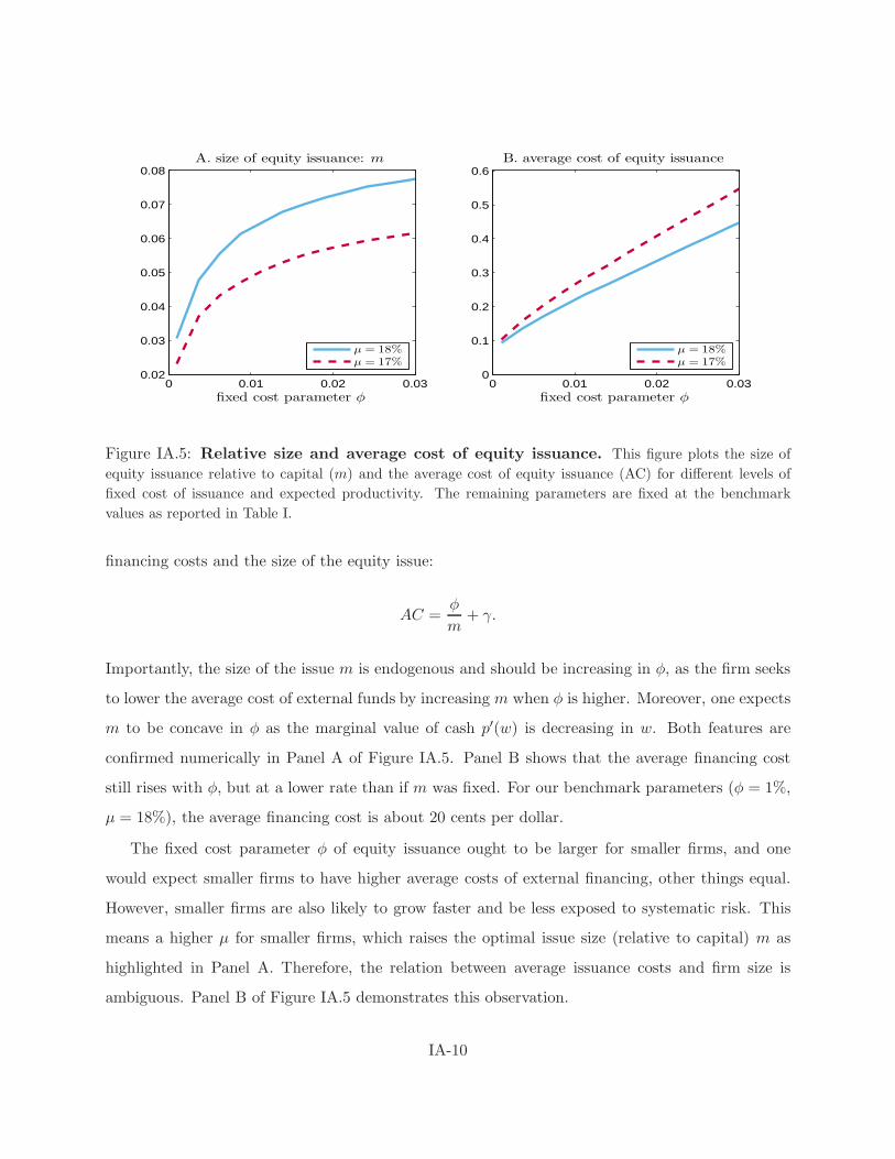
0 0.01 0.02 0.030.02

0.03

0.04

0.05

0.06

0.07

0.08A. size of equity issuance: m

fixed cost parameter φ

µ = 18%µ = 17%

0 0.01 0.02 0.030

0.1

0.2

0.3

0.4

0.5

0.6B. average cost of equity issuance

fixed cost parameter φ

µ = 18%µ = 17%

Figure IA.5: Relative size and average cost of equity issuance. This figure plots the size of

equity issuance relative to capital (m) and the average cost of equity issuance (AC) for different levels of

fixed cost of issuance and expected productivity. The remaining parameters are fixed at the benchmark

values as reported in Table I.

financing costs and the size of the equity issue:

AC =φ

m+ γ.

Importantly, the size of the issue m is endogenous and should be increasing in φ, as the firm seeks

to lower the average cost of external funds by increasing m when φ is higher. Moreover, one expects

m to be concave in φ as the marginal value of cash p′(w) is decreasing in w. Both features are

confirmed numerically in Panel A of Figure IA.5. Panel B shows that the average financing cost

still rises with φ, but at a lower rate than if m was fixed. For our benchmark parameters (φ = 1%,

µ = 18%), the average financing cost is about 20 cents per dollar.

The fixed cost parameter φ of equity issuance ought to be larger for smaller firms, and one

would expect smaller firms to have higher average costs of external financing, other things equal.

However, smaller firms are also likely to grow faster and be less exposed to systematic risk. This

means a higher µ for smaller firms, which raises the optimal issue size (relative to capital) m as

highlighted in Panel A. Therefore, the relation between average issuance costs and firm size is

ambiguous. Panel B of Figure IA.5 demonstrates this observation.

IA-10

This discussion highlights the importance of heterogeneity and endogeneity issues when mea-

suring issuance costs. It helps explain why there may not be a clear relation between firm size and

average costs of equity issues in the data. It sheds light, in particular, on the empirical debate over

the nature of scale economies in equity issuance, and whether equity issuance costs are primarily

fixed or variable (see Lee et al. 1996, Calomiris and Himmelberg 1997, and Calomiris, Himmelberg,

and Wachtel 1995).

D. Endogenous credit line limit

We can endogenize the amount of credit line that a firm obtains by introducing a commitment fee

ν on any unused credit line commitment, in addition to the spread α it pays on the used credit line.

To maintain the homogeneity, we assume that the credit line commitment is proportional to the

firm’s capital stock. For illustration, we consider the case where there is no fixed cost for financing

(φ = 0). There is no difficulty to add the fixed cost.

We first solve for the value function for an exogenously chosen credit line limit c. Then, in the

cash region (w > 0), the value function p(w; c) satisfies:

rp = (i(w) − δ)(p− wp′

)+ ((r − λ)w − νc + µ− i(w) − g(i(w))) p′ +

σ2

2p′′, (IA.6)

where νc is the commitment fee the firm pays for having the credit line commitment c.

In the credit line region (w < 0), p(w) satisfies the following ODE:

rp = (i(w) − δ)(p− wp′

)+ ((r + α)w − ν (c + w) + µ− i(w)− g(i(w))) p′ +

σ2

2p′′, (IA.7)

where ν(c + w) is the commitment fee for unused credit line c + w. The boundary conditions are

similar to those in Section V, except that in the absence of fixed financing cost, the condition

p′(−c) = 1 + γ replaces the old boundary condition for p(−c), and there is no longer a target

cash-capital ratio m.

Next, the optimal amount of credit line commitment c∗ that the firm chooses will depend on its

current cash holding. For example, if the current cash holding is high, the firm is expected to stay

IA-11

−0.2 −0.1 0 0.10.8

0.9

1

1.1

1.2

1.3

1.4

w →

←−c∗

cash regioncredit region

A. firm value-capital ratio: p(w; c∗)

cash-capital ratio: w = W/K−0.2 −0.1 0 0.11

1.01

1.02

1.03

1.04

1.05

1.06

1.07

1.08B. marginal value of cash: p′(w; c∗)


Figure IA.6: Endogenous Credit Line. This figure plots the solution for the case with endogenous

credit line limit.

in the cash region for a long time before accessing credit line. Other things equal, the firm will then

choose a lower credit line limit to reduce the commitment fees. This choice in turn affect the firm’s

investment, payout, and financing policies. In particular, it will lead to a higher payout boundary

w. There is, however, a natural upper bound for the payout boundary wmax and correspondingly

a lower bound for the credit line limit c∗min. For initial cash-capital ratio w0 > wmax, the firm will

immediately pay out lump sum w0 − wmax, and the optimal credit line limit will be the same as

when w0 = wmax.

Specifically, for an initial cash-capital ratio w0, the optimal credit line limit c∗ is the one that

maximizes the firm value:

c∗ = argmaxc

p(w0; c).

As a numerical example, we set the commitment fee ν = 0.2%. The remaining parameters

are from Table I. Figure IA.6 illustrates the solution for initial cash-capital ratio w0 = 0. The

optimal credit limit is c∗ = 0.1425, while the payout boundary is w = 0.0821. We can then define

a cash-credit line (limit) ratio of w/c∗ = 0.58. As conjectured, the credit line limit falls as w0 rises,

but the change is very small (with c∗min = 0.1400).

IA-12

E. Stationary distribution in the case of credit line

In this section, we analyze the stationary distribution of firms with access to credit line. To

understand the different behavior in the cash and the credit regions, we report the first four moments

of the distribution plus the medians of the variables of interests (w, i(w), p′(w), qa(w), and qm(w))

for both the credit region and cash region in Table IA.I. The most significant observation is that the

availability of credit makes the firm’s stationary distribution for these variables much less skewed

and fat-tailed in the cash region. Because liquidity is more abundant with a credit line, the firm’s

marginal value of cash is effectively unity throughout the cash region. However, the skewness and

fat-tails of the distribution now appear in the credit region (note, for example, the high kurtosis

(126) for marginal q in the credit region). Although the firm has a credit line of up to 20% of its

capital stock, it only uses about 4% of its line on average. The reason is that the firm does not

spend much time around the credit line limit. The risk of facing a large fixed cost of equity induces

the firm to immediately move away from its credit limit.1

The cash-capital ratio w, i(w), qa(w), and qm(w) are all skewed to the left in the cash region,

as in our baseline model without a credit line. The intuition is similar to the one provided in

the baseline model. Moreover, because of the firm’s optimal buffer-stock cash holding, there is

effectively no variation in the cash region for the firm’s investment and value. Note also that the

mean and median of marginal q and average q are all equal to 1.189, up to the third decimal point.

Even for the investment-capital ratio i(w), the difference between its median and mean values only

appear at the third decimal point.

Unlike in the cash region, not only is the marginal value of credit p′(w) skewed to the left, but

so is marginal q in the credit region. The left skewness of marginal q and p′(w) are both driven

by the fact that every so often the firm hits the credit limit and incurs large financing costs. In

other words, there is much more variation in the credit region than in the cash region for marginal

q and the marginal value of liquidity p′(w). As marginal q and the marginal value of liquidity move

in the same direction in the credit region, there is, however, much less variation in i(w), which is

monotonically related to the ratio qm(w)/p′(w).

1DeAngelo, DeAngelo and Whited (2009) make a similar observation.

IA-13

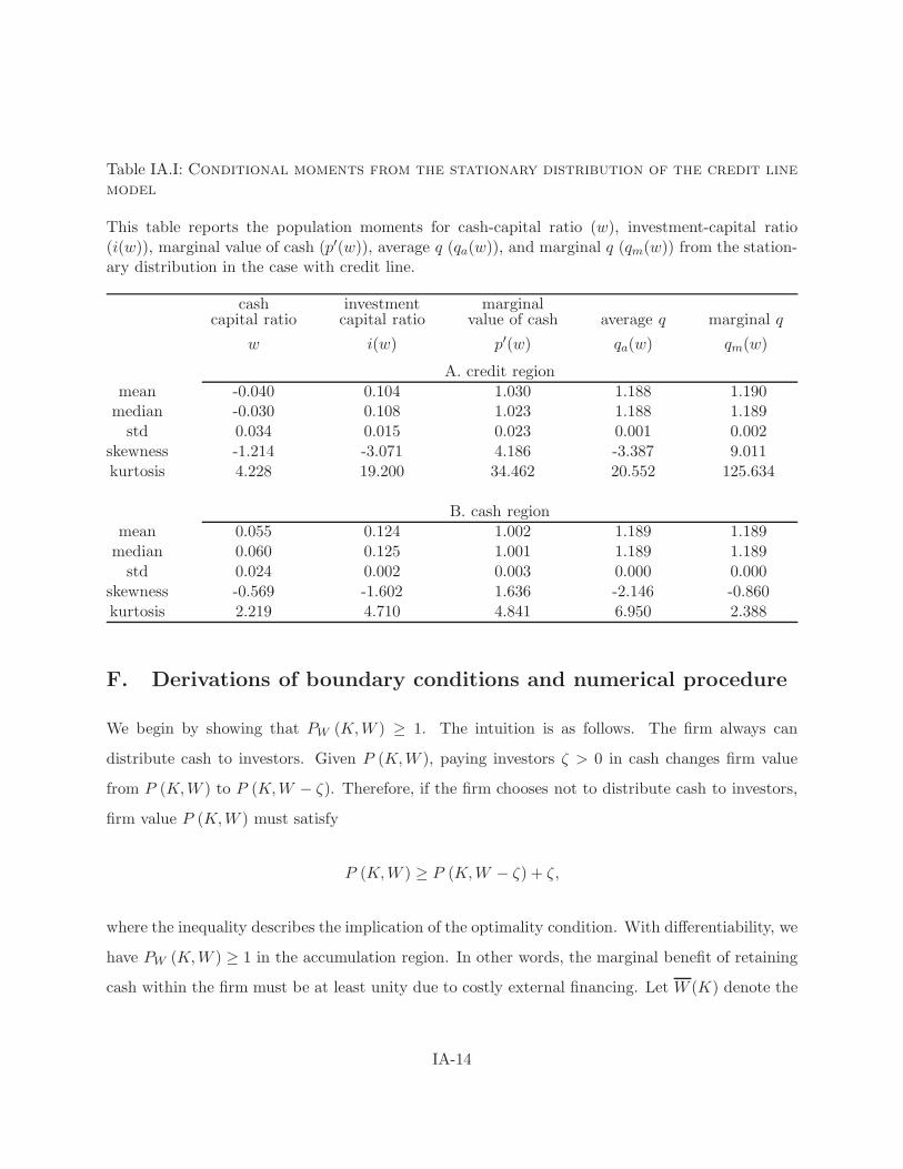
Table IA.I: Conditional moments from the stationary distribution of the credit line

model

This table reports the population moments for cash-capital ratio (w), investment-capital ratio(i(w)), marginal value of cash (p′(w)), average q (qa(w)), and marginal q (qm(w)) from the station-ary distribution in the case with credit line.

cash investment marginalcapital ratio capital ratio value of cash average q marginal q

w i(w) p′(w) qa(w) qm(w)

A. credit regionmean -0.040 0.104 1.030 1.188 1.190

median -0.030 0.108 1.023 1.188 1.189std 0.034 0.015 0.023 0.001 0.002

skewness -1.214 -3.071 4.186 -3.387 9.011kurtosis 4.228 19.200 34.462 20.552 125.634

B. cash regionmean 0.055 0.124 1.002 1.189 1.189

median 0.060 0.125 1.001 1.189 1.189std 0.024 0.002 0.003 0.000 0.000

skewness -0.569 -1.602 1.636 -2.146 -0.860kurtosis 2.219 4.710 4.841 6.950 2.388

F. Derivations of boundary conditions and numerical procedure

We begin by showing that PW (K,W ) ≥ 1. The intuition is as follows. The firm always can

distribute cash to investors. Given P (K,W ), paying investors ζ > 0 in cash changes firm value

from P (K,W ) to P (K,W − ζ). Therefore, if the firm chooses not to distribute cash to investors,

firm value P (K,W ) must satisfy

P (K,W ) ≥ P (K,W − ζ) + ζ,

where the inequality describes the implication of the optimality condition. With differentiability, we

have PW (K,W ) ≥ 1 in the accumulation region. In other words, the marginal benefit of retaining

cash within the firm must be at least unity due to costly external financing. Let W (K) denote the

IA-14

threshold level for cash holding, where W (K) solves

PW

(K,W (K)

)= 1. (IA.8)

The above argument implies the following payout policy:

dUt = max{Wt −W (Kt) , 0},

where W (K) is the endogenously determined payout boundary. Note that paying cash to investors

reduces cash holding W and involves a linear cost. The following standard condition, known as

super contact condition, characterizes the endogenous upper cash payout boundary (see e.g., Dumas

1991):

PWW (K,W (K)) = 0. (IA.9)

When the firm’s cash balance is sufficiently low (W ≤W ), under-investment becomes too costly.

The firm may thus rationally increase its internal funds to the amount W by raising total amount

of external funds (1 + γ) (W −W ). Optimality implies that

P (K,W ) = P (K,W )− (1 + γ) (W −W ), W ≤W. (IA.10)

Taking the limit by letting W →W in (IA.10), we have

PW (K,W (K)) = 1 + γ. (IA.11)

Numerical procedure. We use the following procedure to solve the free boundary problem

specified by ODE (13) and the boundary conditions associated with the different cases. First,

we postulate the value of the free (upper) boundary w, and solve the corresponding initial value

problem using the Runge-Kutta method. For each value of w we can compute the value of p(w)

over the interval [0, w]. We can then search for the w that will satisfy the boundary condition

for p at w = 0. In the cases with additional free boundaries, including Case II and the model

of hedging with margin requirements, we search for w jointly with the other free boundaries by

IA-15

imposing additional conditions at the free boundaries.

References

Calomiris, C. W., and C. P. Himmelberg, 1997, “Investment banking costs as a measure of the cost

of access to external finance,” Working Paper.

Calomiris, C. W., C. P. Himmelberg, and P. Wachtel, 1995, “Commercial paper, corporate finance,

and the business cycle: a microeconomic perspective,” Carnegie-Rochester Conference Series on

Public Policy, 42, 203–250.

Dittmar, A., and J. Mahrt-Smith, 2007, “Corporate Governance and the Value of Cash Holdings,”


Duffie, D., 2001, Dynamic Asset Pricing Theory, Princeton University Press, Princeton, 3rd edn.

Dumas, B., 1991, “Super contact and related optimality conditions,” Journal of Economic Dynam-

ics and Control, 4, 675–685.

Lee, I., S. Lochhead, J. R. Ritter, and Q. Zhao, 1996, “The Costs of Raising Capital,” Journal of

Financial Research, 19, 59–74.

Livdan, D., H. Sapriza, and L. Zhang, 2009, “Financially Constrained Stock Returns,” Journal of

Finance, 64, 1827–1862.

Palazzo, D., 2008, “Firm’s Cash Holdings and the CrossSection of Equity Returns,” Working Paper.

IA-16

a unified theory of tobin's q, corporate investment ... · a uniﬁed theory of tobin’s q,...

Documents