an econometric model for estimating the...
TRANSCRIPT

AN ECONOMETRIC MODEL FOR
ESTIMATING THE COST OF CAPITAL FOR A PUBLIC UTILITY
Eugene F. Brigham, Dilip K. Shame, and Thomas A. Bankston
Revised May 1979

...l~
I. INTRODUCTION_---...l__... _
Of the many issues that arise in public utility rate
cases, probably none is more controversial than the proper
estimation of the cost of equity capital. In an earlier
paper, we discussed the risk premium approach to measuring
equity costs. Now we consider the use of an econometric
model based on the Discounted Cash Flow (DCF), or Gordon
Model, approach.
We begin with a brief discussion of the traditional DCF
approach, after which we consider econometric modelling as a
general methodology. Next, we apply the model to a sample
of thirteen telephone companies and then illustrate its use
in estimating the cost of equity capital. Finally, we apply
the model to a sample of electric utilities. Our general
conclusions are (1) that the econometric approach is useful,
but (2) that substantial judgments are involved both in the
development of the model and in deriving from it a company-
specific cost of capital. Because of the judgmental elements
inherent in the model, it should never be used as the sole
criterion for a rate case cost of capital estimate--results
generated by the model should always be compared with cost
of capital estimates developed by other methods.
IE. F. Brigham and D. K. Shome, "Risk Premiums on CommonStocks," PURC Working Paper 1-79.

basic model,
-2-
The Traditional OCF Approach
The constant growth OCF model as developed by M. J. Gordon
has seen wide acceptance in rate cases in recent years.
Indeed, we have examined the testimony in over one hundred
cases, and we have not seen even one (since the late 1960's)
where at least one witness did not use some form of the
0 1k = - + g,
Po
where k is the OCF cost of equity, 0 1 is the dividend expected
during the coming year, Po is the current price of the stock, and
1g is the expected future growth rate.
Although rate of return witnesses sometimes bastardize the
model by using past values for the dividend and stock price data,
rather than 0 1 and Po as the theoretical model demands, the
biggest problem by far with implementing the traditional OCF
approach is to ob~ain a correct estimate of the value of g that investors
at the margin are expecting. Rate of return analysts use a variety
of techniques, ranging from simply extrapolating past growth trends
to surveying investors, to estimate the g factor. Some of these
analysts are very astute and knowlegeable, while others are less
so, but it is often hard for utility commissioners to decide
who is right and who is wrong when two supposedly expert witnesses
make radically different recommendations. I
"An::EC:onomet"ric Model Approach
Econometric models have two major advantages over the
lFor the development of the model, see E. F. Brigham, FinancialManagement, 2nd Edition, Chapter 4.

-3-
pure DCF method. First, the models can help IIhold other things
constant." It is useful to check estimates by comparisons with
other firms. However, because utilities (and other companies)
differ from one another with regard to their operating territories,
financial leverage, investment opportunities, regulatory climate,
and so on, if we are to compare required rates of return among a
set of companies, we need to hold constant factors such as these.
Econometric techniques can help in this task, and thus aid us in
obtaining better estimates of the cost of equity. Second, econometric
models can help to quantify the accuracy of cost of capital estimates.
Analysts generally estimate a most likely single value of the
cost of common equity, and then talk about an arbitrarily specified
"range of reasonableness. II Econometric techniques can be used
both to judge the precision of the point estimate and also to
specify more precisely the range within which the "true" figure
probably lies.
The econometric model that we use is based on standard DCF
concepts. Two key assumptions are made whenever the cost of e~~ity
is calculated using the constant growth DCF model:
(1) The model is correctly specified; that is, the sum
of the dividend yield plus the single growth rate does,
in fact, add up to the required rate of return.
(2) We can obtain correct values for both the dividend
yield for the coming year and the constant expected
future growth rate. "Correct ll means the values that are
actuaTly used by marginal investors who set the price
of the stock in question.

-4-
The validity of these assumptions cannot be tested by applying
the DCF equation to a single firm. However, the model can be
tested by econometric techniques with a sample of firms.
If the model's specification is correct, and if the variables
are measured without significant errors, we would obtain a regres
sion equation that had the following properties:
(1) There would be a reasonably good fit between the de
pendent variable as predicted by the regression equation
and the actual values of the dependent variables. The
goodness of fit is measured by the coefficient of deter-
. mination (R2 ) '.
(2) There would be a relatively small standard error of the
estimate.
(3) The regression coefficients would be significant, and each
would have the correct sign.
(4) The regression equation would satisfy, to a reasonable
extent, all the assumptions of least squares regression
analysis.
If the model had these properties, then we could be reasonably
confident that our estimated cost of capital was close to the
true value. Further, we could actually specify confidence limits
and ·use them for establishing a "range of reasonableness" for
ratemaking purposes. Even so, we would still want to compare
the model-estimated cost of capital with estimates based on other
methods. If the various estimates agreed with one another, this
would increase our confidence in the results. If they did not

- 5-
agree, we would face the dilemma of choosing between them.
In this case, the model's statistical properties should form
the basis for assigning weights to the various techniques; if
the statistical properties were good, then a heavier weight should
be given to the model, and conversely if the model's properties
were not particularly good.
DeveToping the Mod'el.
The basic OCF constant growth model (the
Gordon Model) states that k = 0l/PO + g. To use the
model, one me,~ely calcu~at~.~ ..~l./p.~.'. ,~~~ di~idend
yield term, and adds to it an estimate of the growth term, g.
Unfortunately, it ..,~~, impossible to te~,,~__ :t=:~~~_validity of our estimate
because it is impossible to observe the true value of k, the
expected rate of return. However, it is possible to rewrite
the Gordon equation into a testable form. Here we use the
price/book ratio (P/B) and develop it as a function.ofthe
rate of return on book equity as follows:
1. According to the constant-growth Gordon
model,
where
01= k - g' (1)
Po = current price of a firm's stock,
k = the firm's cost of equity capital,
= dividends per share expected duringthe next period, and
g = expected future growth rate individends. g is "expect~tionally
constant," meaning that while

-6-
investors know that the growth ratewill actually vary from year to year,the current expectation of the growth ratefor any future year is the same as for anyother year; that is, E(gt) = E(gt+l) forall values of t.
2. Expected earnings per share in any future
year t, Et , is equal to the expected rate of
return, ROE, times the book value at the
beginning of the period, Bt - l :
3. If a constant fraction of earnings, b, is
retained, then the dividend payout ratio (PO)
(2)
will be equal to (1 - b), and expected dividends
per share in any year t can be estimated as
follows:
Dt = (1 - b)Et = (1 - h) (ROE) Bt - l . ,(3)
4. The expected growth rate in earnings, dividends
and share prices, assuming b and ROE are constant,
is found as follows:
g = b (ROE) • (4)
5. Letting t = 1 and substituting equations (3)
and (4) into (1) , we see that
Dl (1 - b) (ROE) (Bt )P = =k - g k - b(ROE)
Transposing the B term (and dropping the t sub-
sucript) produces this expression for P/B:
P = (1 - b) (ROE)B k - b(ROE)
(5)

-7-
Equation 5 has some interesting and useful implications for
rate cases. Note that if (1) commissioners actually identify the
true cost of equity, k, and then allow utilities to earn this
rate of return on their book equity, then (2) investors will use
the allowed ROE as the expected future ROE, and (3) the P/B ratio
will be equal to 1.0. If the allowed ROE is below k, then the
P/B ratio will be less than 1.0, while if allowed ROE exceeds k,
P/B will be greater than 1.0.
Equation 5 forms the theoretical basis for the empirical regression
model which we use to estimate the cost of equity. First, note that
the relationship between P/B and ROE as expressed in Equation
5 is nonlinear; the exact relationship is graphed in Figure 1
under the assumption that k - 14% and b - 30%. The shape of the
graph will vary somewhat depending on the values of k and b, and
it will also be different if we assume that new stock is sold at
prices significantly different from the book value. However, as a
generalization, the graph is not very sensitive to these factors
so long as they stay within reasonable bounds. l
lSee E. F. Brigham andT. A. Bankston, "The Relationship between a UtilityCompany's Market Price and Book Value," Public Utility Research Center, Universityof Florida, November, 1973, for a more detailed discussion of this point. Inbrief, the curve would be slightly steeper if the retention rate were higher than30%, less steep if it were lower, but it would still pass through the pointp/B = 1.0, ROE = 14%. The effect of a chan~e in the retention rate depends onthe level of ROE; changes of 10% or less "in the retention rate have very littleeffect on the curve when ROE is in the range 12% to 16%.
It should also be noted that, if the company is expected to issuestock, then the P/B ratio will be less than 1.0 if ROE = k, with the declinedepending on (1) the percentage flotation cost and (2) the amount of stock expectedto be sold. Selling stock also causes the curve to be steeper, indicating lower P/Bratios if k > ROE but higher P/B ratios if ROE> k.

P/B
2.0
-8-
Figure 1
Relationship between PIB andthe Allowed Rate of Return
(Assumes k = 14%, b = 30%)
(1 - b) ROEk - b ROE1.0 --- ... ----~.-•
I II "
.7ROEI I .14 - .3ROEI I
.0.5 I I
I I
I .1\
I I
II
I
5 10 12 14 16 20 ROE (%)0(k)
-9-
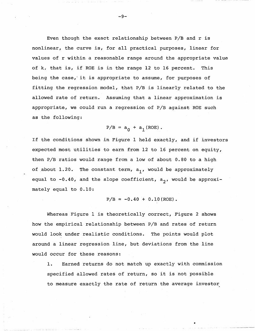
Even though the exact relationship between p/B and r is
nonlinear, the curve is, for all practical purposes, linear for
values of r within a reasonable range around the appropriate value
of k, that is, if ROE is in the range 12 to 16 percent. This
being the case,' it is appropriate to assume, for purposes of
fitting the regression model, that P/B is linearly related to the
allowed rate of return. Assuming that a linear approximation is
appropriate, we could run a regression of P/B against ROE such
as the following:
P/B = a O + al(ROE).
If the conditions shown in Figure 1 held exactly, and if investors
expected most utilities to earn from 12 to 16 percent on equity,
then p/B ratios would range "from a low of about 0.80 to a high
of about 1.20. The constant term, aI' would be approximately
equal to -0.40, and the slope coefficient, a 2 , would be approxi
mately equal to 0.10:
P/B = -0.40+ O.lO(ROE).
Whereas Figure 1 is theoretically correct, Figure 2 shows
how the empirical relationship between P/B and rates of return
would look under realistic conditions. The points would plot
around a linear regression line, but deviations from the line
would occur for these reasons:
1. Earned returns do not match up exactly with commission
specified allowed rates of return, so it is not possible
to measure exactly the rate of return the average investor
•

-10-
Figure 2
Linear Relationship between P/B and ROE.(Assumes k = 14%, b = 30%, and expected
ROE ranges from 12% to 16%.) \
p/B
XI'J.ii1.10 p/B = -0.40 + .10~OE:
X X X Ii
X Iy. I
I- ~ ..-._,----~-- X1 .. 00
X X I. /
I I
X // -
I X I/X X I IIX.90 /I I
X I
X 1II
XIJ
I .II
0 12 13 14 15 16 ROE (%)
1.20

-11-
expects a utility to earn in the future. One could use as
a proxy for this expected future return the company's actual
earned return in the recent past, an average of returns earned
over some longer past period, the rate of return allowed in
the latest rate case, rates of return earned by other utilities,
or any combination of these returns. Still, the true expected
return for many of the companies will be measured with some
degree of error, and this will cause actual P/B ratios to
deviate from their predicted values. l
lIf errors in measuring expected ROE are randomly distributed, then there willbe no bias in the estimate of the relationship between P/B and ROE as derivedfrom the regression. However, if the errors are not random, then there willbe a bias. For example, suppose some event occurred which caused the ROE'sof many or all utilities to fall sharply to some level below the true valuesof k for the different companies. However, suppose investors think the decline
• in ROE is temporary and that when the current problem is over, ROE's will returnto a "normal" level. In this event, the regression line in Figure 2 would beshifted to the left. If this shifted regression line were used as the basisfor setting the allowed rate of return, then it would not produce the desiredp/B ratio--the p/B would end up below the target p/B. --
In our statistical models, we use average values over the past five years inan effort to eliminate this type of bias. Individual companies may have temporarilyhigh or low returns, but, hopefully, the smoothed figures will be sufficientlyaccurate so as to produce a nonbiased regression line·. Unfortunately, we cannotbe sure whether the biases are present or not, for if therewere a svstematicunderstatement or overstatement in the data, we could obtain high R2 values yet
still have an invalid model.

-12-
2. The companies in the sample will differ in their riskiness
as viewed by investors. This, in turn, will cause the true cost
of equity, k, to differ among firms. If one company had a high
equity ratio, a strong bond rating, conservative accounting
methods, and a commission which operates without undue lags,
then a given rate of return on equity would produce a relatively
high P/B ratio, and the "X" representing this company would
plot above the regression line. Opposite conditions would
result in a low P/B ratio, and the company's "X" would plot
below the regression line.
3. It is often argued that people who invest in utility stocks
are more interested in current dividend income than in future
capital gains. If this were true (and it has never been proven),
then companies that have a high payout ratio would, other things
held constant, have high P/B ratios and plot above the re-
gression line in Figure 2.
4. Companies that have significant amounts of unregulated
as well as regulated assets (i.e., companies with nonrate
base assets) could have P/B ratios that are above or below
the regression line, depending on the profitability of these
other assets.
Because of these factors, and others, it is apparent (1) that the
basic model must be expanded to include risk variables and (2)
that measuring the expected ROE is a critical step in the analysis.
If n risk variables were included, then our regression model would
be in the form
n+l
P/B = aO + a 1 (ROE) + ~ ai xi'
i=2

-13-
where x. represents the n risk variables.1
We have analyzed a number of risk variables, including (l)
times interest earned ratios, (2) equity ratios, (3) allowance
for funds used during construction (AFUDC) expressed as a percentage
of net income, (4) the company's method of accounting for deferred
taxes (flow through vs. normalize), (5) security analysts' ranking
of regulatory climate, (6) security analysts' rankings of "quality
of earnings," (7) bond ratings, and (8) stability of earnings
measures (standard deviations, of ROE and ROI). For the telephone
industry, we also used a dummy variable that differentiates between
the Bell System companies and the independent telephone companies.
In addition to these risk variables, we also considered a
number of ways of estimating the expected ROE's. First, we
calculated past realized rates of return over various time periods
and then used these values as proxies for current expectations.
For example, we looked at last year's ROE as a proxy for expected
future ROE'S, and at the average of the last two, three, four,
and five years~ both unweighted and also weighted to give more
weight to the most recent data. In addition, we looked at
commission-authorized ROE's. Finally, we examined a pair of surrogate
variables that should reflect investor's expectations for ROE.
The surrogate variables recognize that returns must either be
paid out as dividends or retained, so expected ROE can be split
into two components, as "dividend yield" component and a "growth-
from-retention" component:
= =
ROE = Earnings yield
EB
= Book dividend yield + Growth yield
D RB + i3.
-14-
Here E = earnings, B = book value, D = dividends, and R =
retained earnings. l Ther term D/B is defined as the company's
Statistically, the book yield plus growth rate surrogate
for ROE gave us a better fit in the regression model (higher
values of R2 and more significant regression coefficients) than
did any of our other measures of ROE. We can offer two explana-
tions for these results. (1) It may be that investors, when they
value utility stocks, treat the dividend yield and growth yield
components separately rather than looking at the sum of these two
components as reflected in ROE. (2) An alternative explanation
is that current dividends provide better information about long-run
earnings than do current earnings, especially during times when
current earnings, hence reported ROE's, are varying considerably
from year to year. If current earnings, hence ROEls, are unstable,
and if companies base their dividend payments on normalized earnings,
then dividends actually paid will be a better proxy for normalized
earnings than are current earnings, and book yield plus growth will
be a better proxy for normalized ROE's than are actual ROEls.
IThese values can be expressed either as totals or on a per sharebasis; ROE is the same either way.
2To see why RIB = g, first recall that g = b(ROE), and then note that
E - D Eb = E and ROE = B
Therefore, with R = E - D, we have
g = b(ROE) = E - DE
EB
=E - D
B

-15-
Since the book yield model is just as sound as the earnings yield
model from a theoretical standpoint, and since it is superior from
a statistical standpoint, we focus most of our attention on book
yields. l
lour model is similar in this respect to that of D.A. Burkhardtand M. A. Viren, "Investor Criteria for Valuing utility CommonStocks," Public utilities Fortnightly, July 20, 1978, and alsoto the Salomon Brothers model described in their quarterly reports.

-16-
II. THE TELEPHONE INDUSTRY
We applied the model to the thirteen domestic telephone
companies for which data are reported on the Compustat tapes. The
sample consists of AT&T, the six publicly owned Bell affiliates
(Cincinnati Bell, Mountain Bell, New England Telephone, Pacific
Northwest Bell, Pacific Telephone, and Southern New England
Telephone), and the six largest independent companies (Central
Telephone, Continental Telephone, GT&E, Mid-Continent Telephone,
Rochester Telephone, and united Telecommunications).
As noted in the preceding section, we examined a number
of different risk variables and a number of different methods
for estimating the value of ROE expected by investors. As we shall
see in a later section, for the electric utilities several of
the risk variables have significant effects on the P/B ratio,
hence on the estimated cost of equity. Included are the equity
ratio, the proportion of AFUDC included in net income, whether or
not a company uses flow through accounting, the ranking of the
regulatory climate in a company·s operating territory, and analysts'
appraisal of the overall quality of a firm's earnings. However,
in the telephone industry, none of these variables show up as
being significant. The reasons for the variables' insignificance
are all simple and straightforward: (I) The Bell Companies all
have very similar equity ratios, as do the independents. There
is a pronounced difference between Bell and non-Bell companies,
but not much difference within the groups. Therefore, equity ~
ratios really measure Bell versus non-Bell status. {2} None

-17-
of the telephone companies have very much AFUDC (as compared
to the average electric company), and there is very little
difference in the AFUDC/Net income ratios among companies.
(3) Flow through versus normalization, regulatory climate ranking,
and earnings quality ranking generally reflect conditions in the state
in which a utility operates. These variables show up as being
significant for the electric companies, but since most of the
telephone companies operate in several states, or in states with
"average" conditions, these variables are not significant for
th 1 h . d 1e te ep one ln ustry.
Although the above-mentioned variables did not help much in
explaining P/B ratios, a dummy variable set equal to zero for
Bell and 1.0 for non-Bell companies did show up as being strongly
significant. Therefore, our regression model for the telephone
industry was specified as follows:
P/B = a O + al(Book yield) + a 2 (Growth) + a 3 (Dummy).
In the next several sections we describe how the variables used
in the model were estimated.
The P/B Ratio
We measured the P/B ratio in two ways:
= Ave·rage stock price during December 19781978 year-end book value per share 't'
and
P/B 2 =1978 year-end closing price
1978 year-end book value per share
The point here was to test the sensitivity of the results to
lAlso, note that with a sample of only thirteen companies, we arelimited in the number of variables that can be included in theanalysis without significant loss of degrees of freedom, hencestatistical significance.

INote that
-18-
the use of a spot price versus an average of recent prices.
Book Yield and Growth rate
We measured the expected book yield (BKYLD) as the product
1of the expected ROE times the expected dividend payout rate (PO)
BKYLD = (ROE) (PO) •
w~ measured the'e~p~cted growth rate (qROBR) as the product of the
expected retention rate [b =(1 - PO)] times the expected ROE:
GROBR = (1 - PO) (ROE) = b(ROE).
It is apparent that the values of ROE, PO, and b which investors
expect in the future are critical for the measurement of both
book yield and growth. However, data are available only for the
past, not for the future. We can use historic data as a basis
for forming expectations about future patterns, but (1) there
are different procedures for setting up time series models to
predict future values from past data, (2) we have no way of telling
a priori what procedure most investors actually use, and (3) in
any event, subjective, nonquantifiable inputs as well as past
data go into real world formations of expectations about future
events. 2 Accordingly, we considered several different procedures
for estimating expected retention rates, payout rates, and ROE's:
BKYLD = ~ = (:) (~) = (ROE) (Payout) •
2L . D. Brown and M. S. Rozeff, in the lead article in the March 1978issue of the Journal of Finance ("The Superiority of Analyst Forecasts as Measures of Expectations: Evidence from Earnings,"pages 1-16) prove conclusively that security analysts, using judgmental inputs and knowledge about specific companies and industries,can predict earnings growth better than even quite sophisticated,time series models that use only historic data. With this in mind,we plan to extend our econometric analysis using explicit analystgrowth forecasts rather than a model based purely on historic datasuch as the one described in the current version of this paper.
-19-
1. Current levels. If we assume that the best estimates
of future values for ROE's and payout ratios are represented by
the most recent levels of these variables, then
We used year-end 1978 values for the runs reported in this paper. l
With ROE and PO measured as described above, we then calculate
book yield and growth as follows:
and
GROBR = (1 1
These values form the basis for Model .I,_ or Equation 1.
2. "Normali-zed values." Year-to-year fluctuations often
occur in earnings data, so there is a great deal of logic in
assuming that-investors form expectations about future events on
the basis of average data over the recent past. With this in
mind, we also measured PO and ROE as follows:
P02 = A simple average of payout rates over the past 5 years
(
1978_." E- t=1974
=
P00/SoExpected EPS
Expected average book value per share
= (Expected DPS ') // " 1 )lExpected PO i (Expected book value )
lIn a later version, we plan to obtain data going back in time todetermine how stable the model is over time. We have done timeseries studies with a similar model, but not with the model versionreported herein.

DPS1978 (1 + g)= (P02 ) (Average book value1978 ) (1 + g)
DPS1978= (P02 ) (Average book value1978 )
This ROE estimate makes use of the facts (1) t~at dividends are
far more stable than earni~gs and (2) that dividends may be used as a
basis for estimating "normalized" EPS. In any event, we can
use P02 and ROE 2 to develop a second set of book yield and
growth rate estimates:
and
3. Trended Estimates. Investors are often sensitive to
trends in key variables and therefore give greater weight to more
recent data than to earlier data. With this in mind, we
developed exponentially smoothed weighted averages for the payout
ratio and then used these values in our estimates of book yield
and growth:
(P03 ) (Average book value1978 )
P03 = Exponentially smoothed 5 year average payout.
DPS1978ROE 3 =

-21-
Dummy Variable
As noted earlier, the types of risk variables that are
useful for distinguishing riskiness among the electric
utilities are not useful for the telephone companies. Rather,
the factor which seems to best capture differences among the
telephone companies is a dummy variable set equal to 0 for
Bell System Companies and to 1.0 for independent telephone
companies.
Data Sources
We obtained 1978 data from individual company annual reports,
and data for earlier years from the Compustat tapes.
Regression Equations
We ran a total of six regression equations as shown in
Table 1, after which we derived the estimated cost of equity
figures shown in Table 2. The R2 values shown in the table (which
have been corrected for degrees of freedom) are all highly
significant, which indicates that the regression equation predicts
P/B ratios with a relatively high degree of accuracy. From
82 to 90 percent of the variability in P!B ratios among the
sample companies is explained by the model. The regression
coefficients all have the correct signs--companies with higher
book yields and growth rates have higher P/B ratios, and the
negative signs of the dummy variable coefficients indicate
that Bell System Companies, other things held constant,

Table 1. Telephone Company Regression Equations
{P/B = aO + a1 (BKYLD) + a2 (GROBR) + a3 (Dummy) ]
R2 StandardModel Description aO a l a2 a3 Error-
I. P/B Based on Dec. Avg. PriceIP/BIJ.1. 1978 data [R0Et,P01 , BKYLD1 , .GROBR1] -0.4725 16.621 1.9951 -0.0425 .88 .0551
(-2.105) (5.695) (2.301) (-0. 794)
2. 5-year avg.[ROE2 , P02 , BKYLD2 , GROBR
2] -0.3941 15.082 3.6057 -0. 12l.0 .89 .0537
(-1.936) (5.933) (3.024) (-1.939) Il\Jl\J
3. Exponential smoothing [BKYLD3
, GROBR3
) -0.2250 13.440 2.0168 -0.0475 .82 .0670 I
(-0.946) (4.229) (1.627) (-0.691)
II. p/B Based on 1978 Year-end Price (P IB2)
4. 1978 data [ROE1 , POI' BKYLD1 , GROBR1] -0.4553 16.399 2,0621 -0.0498 .87 .0569(-1.965) (5.445) (2.305) (-0.901)
5. 5-year avg.[ROE2 , P02 , BKYLD2 , GROBR2] -0.4055 14.963 4~1866 -0.1461 .90 .0483
(-2.215) (6.545) (3.905) (-2.540)
6. Exponential [BKYLD3 , GROBR3] ....0.2128 13~036 2,4418 .,..0~0590 .82 .0659(-0,910) (4 .. 222) (2,002) ( .....0.873)
Note: t values are shown in parentheses

Table 2. Cost of Capital Estimates for the Telephone Companies UsingA1ternativeP/B Models
Company Model 1 Model 2 Model 3 Model 4 Model 5 Model 6(R 2 ) (.88) (.89) (.82) (.87) ~ (.90) (.82)
1. AT&T 13.78% 13.00% 13.72% 13.75% 12~93% 13.70%
2. Cincinnati Bell 18.77 15.14 17.60 18.67 14.88 17.26
3. Mountain States Bell 13.99 12.94 13.96 13.96 12;87 13.93
4. New England States T&T 12.45 11.14 12.68 12.44 11.20 12.72
5. Pacific Northwest Bell 14.52 12.98 14.43 14.49 12.91 14.36
6. Pacific T&T 11.27 12.04 11.93 11.27 12.04 12.02I
N7. Southern New England T&T 15.15 12.24 13.99 15.11 12.23 13.95 w
I
Bell System Mean 14.28% 12.78% 14.04% 14.24% 12.72% 13.99%(Standard Deviation) (2.37) (1.24) (1.791 (2.34) (1.14) (1.65)
8. Central Telephone Corporation 14.75 15.38 15.20 14.79 15.41 15.26
9. Continental Telephone Corp. 14.05 13.81 13.86 14.09 13.95 14.00
10. GT&E 15.00 14.87 15.18 15.04 14.94 15.24
11. Mid Continental Telephone 15.42 14.69 15.35 15.46 14.77 15.39
12. Rochester Telephone 14.80 16.05 16.28 14.84 16.03 16.27
13. United Telecommunications 15.53 14.58 15.55 15.56 14.67 15.58
Independent Company Maan 14.93% 14.90% 15.24% 14.96% 14.96% 15.29%(Standard Deviation) (0.53) (0. 76) (0. 79) (0.53) (6.71) (0.74)
4.
-24-
tend to sell at higher P/B ratios. This suggests that AT&T and
the other Bell Companies are regarded as being less risky than
the independent telcos. This is reasonable in view of the
Bell Companies' 'higher equity ratios.
We used the model~' to derive CO$t of capttal es.timates
as shown in Table 2. These estimates were calculated as follows:
1. We demonstrated earlier that if a firm's expected ROE
is equal to its cost of equity, then the company will
sell at its book value, that is P/B = 1.0.
2. Assuming that our regression models accurately describe
the valuation process (and the high R2 values suggest
that they do), then we can set P/B = 1.0 and find the
value of ROE that produces this solution. That ROE
value is an estimate of the DCF cost of equity, k.
3. Set BKYLD = (ROE) (PO) and GROBR = (ROE) (1 - PO), and
then insert these values into the regression equation
with P/B = 1.0:
P/B = 1.0 = a O + al[ROE x PO] + a 2 [ROE(1 - PO)] + a 3 [Dummy].
For AT&T, using values for Modell for 1978,
we have
1.0 = -0.4725 + l6.62l[ROE x 0.5943] + 1.995l[ROE(1 - 0.5943)] + 0
= -0.4725 + 9.8779[ROE] + 0.8094[ROE]
10.6873ROE = 1.4725
ROE = 1.4725/10.6873 = 13.78%.

....·25-
Therefore, according to Modell, if AT&T were allowed
to earn 13.78%, then the stock would sell at a P/B
ratio of 1.0.
Similar calculations were made with the other models for
AT&T, and for the other companies, and the derived cost of capital
estimates for the thirteen companies are shown in Table 2.
Significant features of the table include the following:
1. The Bell System Companies, on average, seem to have lower
costs of capital than the independents. This is consistent
with the hypothesis that the independents are riskier because
of their generally higher debt ratios.
2. The independent telcos have calculated costs of capital
that are closer to one another than do the Bell System
Companies. This point is reflected in the standard deviations
for the two groups.
3. Models 1 and 4, which use 1978 data only, show more
variability across companies (that is, the range from the lowest
to the highest cost company is larger) than is true for Models 2,
3, 5, and 6, which are based on data averaged over five years.
This reflects the fact that earnings, hence payout ratios, do
tend to vary over time. This averaging effect tends to improve
the RZ's as shown at the top of each column.
4. The derived cost of capital estimates tend to be higher in
Models 1 and 4 than in the others. This reflects primarily the
fact that rates of return have been trending up in recent years, and
this upward ROE trend has caused payout ratios to decline. The

-26-
most critical element in the model is the book yield proxy,
(ROE) (PO). If PO is relatively low, this tends to produce a
high estimated cost of equity, and vice versa.
5. While it ~s impossible to say that any of the data or cost
of capital estimates are obviously :~good" or "bad, II or "right"
or "wrong," some of the figures in Table 2 are at least highly
suspicious. For example, Pacific Telephone is widely regarded
as being riskier than either AT&T or the other Bell System
Companies, yet its calculated cost of capital in most of the
model runs is the lowest of any telephone company. Similarly,
there is no obvious reason why Cincinnati Bell should have
such a high cost of capital in comparison to the other Bell
Companies. Indeed, most of the evidence we have seen (other
than the model output presented here) suggests that, with the
exception of Pacific Telephone, all of the Bell System Companies
are equally risky, hence they should have about the same costs
of capital. Quite possibly, the observed differences reflect
random errors in measuring expectations. If we examine the
underlying data, we see that Cincinnati Bell in 1978 had a
very low payout ratio (about 40%) while Pacific Tel had a
high ratio (about 75%). Thus, the model's sensitivity to high
or low payout ratios, combined w~th random variations in these
.. f . 1 . 1ratios, is probably produc~ng erroneous cost 0 cap~ta est~mates.
lWhen we examine the electric company data, we see even moreclear-cut cases of incorrect cost of capital estimates.

-27-
6. A virtue of Models 2, #3, #5, a.nd 6, which are based on
five-year average data, is that they avoid the extremes that
come with the use of data for a single year. Thus, the apparent
problems with· Pacific Tel and Cincinnati Bell are much less
pronounced in Models 2, #3, #5, and 6. On the other hand, using
the five-year average data is less important for the geographically
diversified telephone companies, as their diversif.ication
causes them to be less cyclical, especially with regard to
regional economic developments and rate case decisions.
7. In spite of the problems noted above, the high R2 values
show that the models do, on balance, provide useful insights if
not exact values for the cost of capital. In this connection,
we should point out that the kinds of problems noted above could
also exist in traditional cost of capital estimates, but the
estimating techniques are such that the problems are not so
apparent. Because they are so specific, models are easy to
attack, but this should not be regarded as a weakness.
8. Having defended the models above, we should mention yet
another potential problem. As noted, averaging past data smoothes
out aberiations in the data, which results in somewhat better
statistical "fits" as measured by R2 and the regression
coefficients' t statistics. However, these statistical
properties could mislead us into choosi~g the wrong model,
hence the wrong cost of capital estimate. To see what is involved
-28-
here, first refer back to Figure 2 and note that if the actual,
plotted ROE's for all (or most) companies were systematically
lower than the expected long-run ROE's then the fitted regression
line would be shifted to the left of the true line of relation
ship by the amount of the average understatement. This would
be reflected in a systematic understatement of the model's
cost of capital estimates from the true values of k. We
have no way of knowing for sure that a downward bias is
reflected in the cost of capital estimates derived from
Models 2, #3, #5, and 6, but this bias could indeed exist.
If it does, then the cost of capital estimates derived
from Models I and 4 would be more accurate in spite of their
slightly poorer statistical fits.

-29-
III. THE ELECTRIC UTILITY INDUSTRY
In our empirical studies, we followed essentially the same
procedures for the electric utility industry as for the telephone
industry. However, there were some differences: (1) There are
many more large,'publicly-traded electric companies than telephone
companies. Thus, our sample size is much larger for the electrics.
(2) There is no dichotomy in the electric industry as there is
between Bell and non-Bell telephone companies. Rather, with regard
to size, debt ratios, and so on, the electrics show a more or less
continuous range of values. (3) Although there are some multi-state
electric holding companies, most of the electrics operate within a
single state. (Even when holding companies cross boundaries, their
several states, being contiguous~ have similar economic and often
political characteristics.) (4) While different telephone companies
may use somewhat different technology, from an investment standpoint
there is less difference between telephone companies than between
electric companies with radically di£ferent generating systems
(coal versus oil versus nuclear versus hydro), and with regard to the
phase of their construction cycles, hence the amount of construction
work in progress (CWIP) included in total assets.
Because of these differences, it is logical to expect a
somewhat different set of variables to be significant in the
regression analysis, and this is indeed the case. Here we
use as risk-differentiating variables the equity ratio 1 AFUDC,

-30-
a dummy variable to distinguish flow through from normalizing
companies, and another dummy variable to distinguish among
utilities' "regulatory climates."
Our electric sample consisted of the one hundred largest
electric utilities as reported by Salomon Brothers in their
monthly publication Electric Utility Common Stock Market Data.
The one hundred companies are listed in Appendix A.
The regression equation used is
~/B = a O + al(BKYLD) + a 2 (GROBR) + a 3 (EQRATIO) + a 4 (AFUDC)
+ as (Flow through dummy) + a 6 (Commission rank dummy),
and the exact variable definitions are given below:
BKYLD
= 1978 year-end price dividend by 12/31/78
book value. Since the telephone sample results
showed little sensitivity to whether we used
year-end or December average prices, and since the
year-end price is both more reflective of conditions
as of the estimating date and easier to obtain, we
did not analyze December average prices for the
one hundred electrics.
= BKYLDl
and BKYLD2
as defined in the telephone
section. BKYLDl is based on 1978 data only, while
BKYLD2
is based on data over the period 1974-1978.
We dropped the exponential smoothing approach for
electrics because, in the telephone company analysis;
it produced it produced poorer results than the
unweighted averages.

GROBR
EQRATIO
AFUDC
FlowtfirOughDummy
CommissionRanki5UiIimy
-31-
= GROBRI and GROBR2 as defined in the telephone
section.
= 12/31/78 Common equity divided by the sum of12/31/78 Common equity, Preferred stock, Longterm debt, and Short-term interest bearing debt.
= 1978 AFUDC divided by 1978 Net income availableto common stockholders.
1.0 for companies that use flow through accounting= for accelerated depreciation and zero for companies
that normalize.
1.0 for companies whose commissions are ranked= high (A or B) by Salomon Brothers and zero for
all other companies.
Therefore, for the electrics, we ran two models, one with book
yields and growth rates based only on 1978 data and one in which
these variables are based on data from 1974 through 1978.
We obtained data from the following sources: Salomon Brothers
[(1) Electric utility Common Stock Market Data; (2) Electric
Utility Quality Measureme~ts and Earnings Forecasts; and (3)
Electric Utility Coverages], the Wall Street Journal, and Compu-
stat tapes for pre-1978 data.
The regression equations for the electrics are given in
Table 3. As with the telephone sample, the most important deter-
minants of the P/B ratio are book yields and growth rates. In
addition, the ranking of each utility's commission is highly
significant. The other variables are not significant at the 5
percent confidence level, although they do contribute to the
estimation of P/B ratios and their coefficients do have the
expected signs. The R2 values (about 0.75) are lower than in

Table 3. Electric Utility Regression Models
P/B = ao + al[BKYLD] + a2[GROBR]+ as[EQRATIO] + a4[AFUDC] + as[F1ow through Dummy] + a6[Commission Rank Dummy]
. Modell. Current (1978)Data
-0.1018(-1.003)
a.l
9.3911 1.3232(14.223) (4.156)
0.3656(1.705)
-0.0401(-1.390)
-0.0007(-0.051)
StandardR2 Error
.0.0847 0.74 0.0564(5.686)
Model 2. Average (1974- 1976) -0.01125 8.4084 1.1822 '0.3578Data (~0.116) (14.650) (3.225) (1.652)
Note: t values are in parentheses.
-.02341(-0.819)
-0.0244(-1.822)
0.0785 0.75 0.0561(5.191)
1Lvtv'I

-33-
the telephone sample, but they nevertheless show that the model
is reasonably accurate as a predictor/explainer of the P/B ratios.
We can use the regression data to derive cost of capital
estimates for the individual electric companies: Table 4 shows
values for two companies, Wisconsin Public Service and Portland
Seneral Electric. These two were selected to illustrate the
results for a company whose data are relatively stable (Wisconsin
Public Service) and for one whose recent data have been highly
unstable (Portland General Electric). The method of calculating
the costs of capital is the same as was described for AT&T, so
sample calculations are not given here.
Some of the electric companies have had highly variable
earnings over the last few years. They tend to maintain or even
increase dividends over time, even in the face of an earnings
decline, if they think the earnings decline is only temporary.
Under such conditions, the dividend payout ratio will become
quite large, as it has been for PGE in recent years. Further,
since the derived cost of capital is highly sensitive to the
payout ratio, if a company has an abnormally high or low payout
ratio, its calculated cost of capital will tend also to be
abnormally high or low.
The relationship between the payout ratio and the calculated
cost of capital explains why PGE's cost of capital is so much lower
than WPS's. The terms (ROE) (PO) and ROE(l - PO.) are in the basic
regression equations which we use to find the cost of capital:

-34---
Table 4. Sample Costs of Capital for ElectricCompanies: Wisconsin Public Service (WPS) and
Portland General Electric (PGE)
Estimated Cost of CapitalWPS PGE
Model 1 (Current data)
Model 2 (1974-1978 data)
13.51%
13.07%
8.71%
Payout RatiosWPS PGE
1978
Average 1974-1978
62.5%
66.1%
128.0%
98.0%

-35-
indeed, we set PIB = i.o, solve the equation for ROE, and
then assume that this solution value is equal to k, the cost
of capital. Yet if we are measuring PO with error--that is,
if the value we use is not approximately equal to the average
investor's long-run expected payout ratio, then our estimated
cost of equity will be erroneous. Clearly, that is what is
happening with PGE, for PGE's true cost of equity is certainly
above its cost of debt!
Wisconsin Public Service has had more stable earnings,
and the combination of relatively stable earnings and a
stable dividend policy has produced a stable, "reasonable"
payout ratio. This stable payout, when used in the model,
produces a cost of capital that is not obviously unreasonable.
We cannot say that WPS's estimated cost of capital, which
lies in the range of 13.1% to 13.5%, is truly accurate, but
neither can we say that it is obviously wrong.
Of course, if our estimates were as bad for all companies
as they are for PGE, then our R2 would probably be close to
zero. The fact that R2 = 0.75 therefore indicates that the
model does have some utility for deriving cost of capital
estimates for electric utilities. Clearly, the model-
derived cost of capital estimates should not be accepted
without question or without checking them against cost of
capital estimates produced by other methods, but equally
clearly, the model's output should be given some weight.

-36-
IV. FURTHER RESEARCH
As we noted at the outset, this paper is part of an ongoing
study, and we plan to do further work on the econometric model
approach to estimating the cost of capital. Some specific planned
research is outlined below.
Tests of the Models' Statistical Properties
We have already carried out preliminary tests to check the
models' statistical validity. For example, we have examined the
simple correlation matrix to check for multicollinearity and have
made plots of residuals against independent variables to check for
heteroscedasticity and autocorrelations. These tests are good
preliminary indicators, but a more in-depth analysis is clearly
needed. We plan to carry out quantitative tests to determine whether
all the assumptions of the random error model are satisfied.
- Specifically, we will test for multicollinearity, autocorrelation,
heteroscedasticity, measurement errors, and specification errors.
Stability of the Model over Time
Our analysis so far has been for a single cross-section year.
We need to study the stability of the model over time. We plan to
run the regressions with data going back ten years or so in order to
see whether the coefficients are stable and the "fits" are good. We
ran such tests with an earlier version of the model, but we have not
done so with this version.
Incorporation of a Firm-Effect Variable in the Model
The R2 values, which measure the goodness of fit, were
considerably lower for the one hundred electrics than for the

telephone companies (R2= 0.75 for the electrics versus R2 ,s generally
in the range of 0.82 to 0.90 for the telephone companies). When we
test for the model's stability over time, if we see stable (and large)
residuals for certain companies, we will attempt to improve the
model's specification by adding a "firm-effect variable." The
logici-behind using the firm-effect variable is developed next.
The most likely reasons for obtaining a poor fit are these:
1. Ommission of a relevant variable. It is difficult to
identify and include all the variables that help to explain
the P/B ratio of a company. This is particularly true of
the variables that measure risk.
2. Errors in Measurements of Variables. The DCF model, like
all cost of capital models, is an ex ante model in which the
stock price depends on expected earnings and expected growth
rates. Since we use past data to develop proxies for expected
yalues, there is always a possibility that measurement errors
exist.
If it can be established that omitted variable and/or measurement
errors have a consistent influence from one year to the next, then
the use of residuals from year t - 1 as a variable in year t should
help to correct for the omission and/or measurement errors. This
added variable is called a "firm-effect variable." Essentially, the
firm-effect variable is designed to account for some unidentifiable
aspect of risk and/or to correct for errors in measurement which

-38-
may distinguish some stocks consistently from others. For example,
one of the assumptions we made in measuring growth rates (GROBR) is
that the effects of stock financing on growth rates can be ignored
because new issues are made at a PIB ratio nearly equal to 1.0.
However, we can see from available data that some utilities have had
PIB ratios consistently greater than 1.0 while others had ratios
consistently below 1.0. Similar patterns could also exist for
other variables.
Whether or not there is a consistent influence that is not
being picked up by the independent variables can be judged by
observing the correlation coefficients between the residual error
terms for a company from one year to the next. If the coefficients
are consistently high, then the use of the firm-effect variable is
justified. The technique has been used in similar studies in the
1past.
lFor examples of the use of the firm-effect variable, see
(1) Friend, Irwin, and M. Puckett, "Dividends and Stock Prices,"The American Economic Review, September 1964, pages 656-682.
(2) Bower, R. S., and D. H. Bower, "Risk and Valuation ofCommon Stock," The Journal of Political Economy, May-June 1969,pages 349-362.
(3) Chung, P. S., "An Investigation of the Firm-Effects' Influencein the Analysis of Earnings to Price Ratios of IndustrialCommon Stocks," Journal of Financial and Quantitative Analysis,December 1974, pages 1009-1029.
Our "firm-effect" analysis would actually involve the
following steps:
1. Run the regression equation using cross section data
for several past years.
2. Determine the correlation coefficients between the
residuals obtained tor each year.
3. If these coefficients are consistently high, we can use
the firm-effect variable as an additional explanatory
variable. The firm-effect variable used in year t would
be residual in year t - I (RESt_I).
4. The final model in any year t would be of the form
P/Bt = a O + al(BKYLD)t + a 2 (GROBR)t + a 3 (EQRATIO)t + a 4 (AFUDC)t
+ as{FTD)t + a 6 (COMRK)t + a 7 {RES)t_l"
We expect that the inclusion of this additional variable
would improve the R2 ,s for the electrics, but that it would not
have much effect on the R2 ,s for the telephones, which are already
high. We will report our findings in a future working paper.
Pooling of Electrics and Telephone Companies
One problem with our analysis of telephone companies is that
the sample size is so small. To get around this problem, we will
study a pooled sample of electrics and telephones. However, rather
than use all the electrics, we will probably select from the
electric sample the "high grade electrics," defined as those with
bond ratings of double and triple A, and use these in a
model with the double and triple A telephone companies. The
object of this procedure is to obtain a more homogeneous risk
class while still having a reasonably large sample size. Other
variables that could be used to help screen for risk class would
include S&P stock ratings, earnings variability, and perhaps
beta coefficients, although we are not optimistic about the latter.
Further Analysis of Flow Through and AFUDC
Earlier studies done at PURC have given some indication of the
effects on the cost of capital of the use of flow through versus
normalization. 1 Our model in this study includes a flow through
dummy for the electrics. The~sign of the variable in our regression
is negative, indicating that companies on flow through have a
higher cost of capital than those which normalize, but neither
the t statistic nor the regression coefficient is high, indicating
that the effect of flow through is not terribly important.
However, this conclusion is probably not warranted; the flow
through dummy is correlated with certain other risk variables,
so multicollinearity problems may well be distorting the true
effects of flow through. We plan to look further at this issue.
Exactly the same problems seem to hold for the AFUDC variable--
its coefficient is negative', indicating a higher cost of capital
for firms with a higher percentage of AFUDC to net income, but
(1) neither the economic nor the statistical significance of the
IE. F. Brigham and J. L. Pappas, Liberalized Depreciation andthe Cost of Capital (East Lansing: Michigan state UniversitYh1970); E. F. Brigham and T. J. Nantell, "Normalization versus .Flow Through for Utility Companies Using Liberalized Tax Depreciation "The Accounting Review, July 1974. Pages 436-447. 1

-41-
coefficients are high and (2) multicollinearity problems
may well be biasing downward the true effects of AFUDC. A
PURC-supported Ph.D. dissertation now nearing completion has
investigated this issue further, and when it has been com-
pleted we plan to explore the AFUDC/CWIP issue to an even
greater extent.
IGeraldine Westmoreland, Electric Utilities' Accounting forConstruction Work in Progress: The Effects of Alternative Methodson the Financial Statements, Utility Rates, and Market to BookRatios. This dissertation is scheduled to be completed inAugust, 1979.

-42~
APPENDIX A
THE ELECTRIC UTILITY SAMPLE
.~_ ALLEGHENY POWER~ AMF.RICAN ELEC PWR~ ARIZONA PUBLIC SVCIt-ATLANTIC CITY ELEC
j$ BALTIMORE GAS & EL
6 B05TO~J EDISONi 7 CAIH)L I~JA pw~ " LTi' CENTRAL HUDSON G&E'9 CENTRAL ILL LIGHT~O CEn I LL PUB SVC
Ll CErHPAL LA E~JEQ.GY.~ CENTRAL MAINE PWR
_~.l ..~ CENTRAL SOUTH WESTCENTRAL VT PUB SVC
i::: CUK PJNAT I G & E
16 CLEVELAND EL ILLU17 COL & SO OHIO ELECl~ COMMONWEALTH ED!9 COp.o~UNITYPUB SVCfO ccrj";'';L lDATEO ED
II CONSUMERS POWERin. ')A fT1'J POWER & l r~l CELMARVA PWR & Lf~.~ DET~OIT EDrSONil-!')UI(E POWERi
2.6 DUOUEsr;E L1GnT~7 EL PASO ElECT~ICi~ EMPIRE DIST ELEC2q FLORIDA POWER CORPi~O FL1RIDA.PWR & LT'
S! r;E';E~AL PIJe UT!LS·32. GuLF STATES UTIlS:33 HAWA I IAN ELECT RICS~ HO~STON INDUST~IES3S' IDAHO POWERI;35 fi:.LINOIS POWER:~7 INDIM~APOLIS P & LI;, INTERSTATE POWER39 rQw~ ELEC LT & PWR140 IOWA-I LL GAS & EL
i41 IOWA POWER & LIGHT42 IOWA PUBLIC svc43 IOWA SOUTHERN UTlL
:44 KANSAS CITY P & L45 .KANSAS GAS & ELEC
46 KANSAS POWER. LT.'7 KENTUCKY UTILITIES.'8 LO~ ISLAND LTHG" LOUISVILLE ~ C f
,so MAO liON GAl , IUC
51 MIDDLE SOUTH UTILS52 MINNESOTA PWR & LT53 MONTANA DAKOTA UT54 MONTANA POWER55 NEVADA POWCR
56 NEW ENGLAND ELEC57 NEW ENG G & E ASSO58 NEW YORK STATE E&G59 NIAGARA MOHAWK PWR60 NORTHEAST UTILS
61 NORTHERN IND P S62 NORTHERN STATES PR63 NORTHWESTERN P S64 OHIO EDISON65 OKLAHOMA GAS & EL
66 ORANGE & ROCK UTIL67 OTTER TAll POWER68 PACIFIC GAS & ELEC69 PACIFIC POWER & LT70 PENNSYLVANIA P & L
71 PHILADELPHIA ElEC72 PORTLAND GEN ELEC73 POTOMAC ElEC POWER74 PUB SVC COLORADO75 PUB SVC ELEC & GAS
76 PUB SVC INDIANA77 PUB SVC NEW HAMP78 PUB SVC NEW MEXICO'79 PUGET SOUND P & L80 ROCHESTER GAS & EL
81 SAN DIEGO GAS & EL82 SAVANNAH ELEC & PR83 SIERRA PAC PWR CO84 S~UTH CAROLINA E.G85 SOUTHERN tALIF ED
86 SOUTHERN COMPANY87 SOUTHERN IND G & E.88 SOUTHWESTERN P 589 TAMPA ELECTRIC90 TEXAS UTILITIES
91 TOLEDO EDISON92 TUCSON GAS & ElEC93 UNION ELECTRIC94 UNITED I LLUMINATNG95 UTAH POWER & LIGHT
96 VIRGINIA ELEC & PR97 WASHINGTON WTR PWR98 WISCONSIN ELEC PWR~9 WISCONSIN PWR & LT
100 WISCONSIN PUB SVC