An Algebraic Framework for Diffie-Hellman Assumptions

Alex Escala1, Gottfried Herold2, Eike Kiltz∗2, Carla Rafols2, and Jorge Villar†3

1Scytl Secure Electronic Voting, Spain, alex.escala@scytl.com2Horst-Gortz Institute for IT Security and Faculty of Mathematics, Ruhr-Universitat

Bochum, Germany, {gottfried.herold,eike.kiltz,carla.rafols}@rub.de3Universitat Politecnica de Catalunya, Spain, jvillar@ma4.upc.edu

Abstract

We put forward a new algebraic framework to generalize and analyze Diffie-Hellman like DecisionalAssumptions which allows us to argue about security and applications by considering only algebraicproperties. Our D`,k-MDDH assumption states that it is hard to decide whether a vector in G` islinearly dependent of the columns of some matrix in G`×k sampled according to distribution D`,k. Itcovers known assumptions such as DDH, 2-Lin (linear assumption), and k-Lin (the k-linear assumption).Using our algebraic viewpoint, we can relate the generic hardness of our assumptions in m-linear groupsto the irreducibility of certain polynomials which describe the output of D`,k. We use the hardness resultsto find new distributions for which the D`,k-MDDH-Assumption holds generically in m-linear groups. Inparticular, our new assumption 2-SCasc is generically hard in bilinear groups and, compared to 2-Lin, hasshorter description size, which is a relevant parameter for efficiency in many applications. These resultssupport using our new assumption as a natural replacement for the 2-Lin Assumption which was alreadyused in a large number of applications.

To illustrate the conceptual advantages of our algebraic framework, we construct several fundamentalprimitives based on any MDDH-Assumption. In particular, we can give many instantiations of a primitivein a compact way, including public-key encryption, hash-proof systems, pseudo-random functions, andGroth-Sahai NIZK and NIWI proofs. As an independent contribution we give more efficient NIZK proofsfor membership in a subgroup of G`, for validity of ciphertexts and for equality of plaintexts. The resultsimply very significant efficiency improvements for a large number of schemes, most notably Naor-Yungtype of constructions.

Keywords: Diffie-Hellman Assumption, Generic Hardness, Groth-Sahai proofs, Hash Proof Systems,Public-key Encryption.

∗Funded by a Sofja Kovalevskaja Award of the Alexander von Humboldt Foundation and the German Federal Ministry forEducation and Research.†Partially supported by the Spanish Government through projects MTM2009-07694 and Consolider Ingenio 2010 CDS2007-

00004 ARES.

Contents

1 Introduction 11.1 The Matrix Diffie-Hellman Assumption . . . . . . . . . . . . . . . . . . . . . . . . . . . . . . 11.2 Basic Applications . . . . . . . . . . . . . . . . . . . . . . . . . . . . . . . . . . . . . . . . . . 3

2 Preliminaries 42.1 Notation . . . . . . . . . . . . . . . . . . . . . . . . . . . . . . . . . . . . . . . . . . . . . . . . 42.2 Representing elements in groups . . . . . . . . . . . . . . . . . . . . . . . . . . . . . . . . . . 42.3 Standard Diffie-Hellman Assumptions . . . . . . . . . . . . . . . . . . . . . . . . . . . . . . . 52.4 Key Encapsulation Mechanisms . . . . . . . . . . . . . . . . . . . . . . . . . . . . . . . . . . . 52.5 Hash Proof Systems . . . . . . . . . . . . . . . . . . . . . . . . . . . . . . . . . . . . . . . . . 62.6 Pseudo-random Functions . . . . . . . . . . . . . . . . . . . . . . . . . . . . . . . . . . . . . . 6

3 Matrix DH assumptions 63.1 Definition . . . . . . . . . . . . . . . . . . . . . . . . . . . . . . . . . . . . . . . . . . . . . . . 63.2 Basic Properties . . . . . . . . . . . . . . . . . . . . . . . . . . . . . . . . . . . . . . . . . . . 73.3 Generic Hardness of Matrix DH . . . . . . . . . . . . . . . . . . . . . . . . . . . . . . . . . . . 83.4 Examples of D`,k-MDDH . . . . . . . . . . . . . . . . . . . . . . . . . . . . . . . . . . . . . . . 9

4 Uniqueness of One-Parameter Matrix DH Problems 104.1 Hardness . . . . . . . . . . . . . . . . . . . . . . . . . . . . . . . . . . . . . . . . . . . . . . . 114.2 Isomorphic Problems . . . . . . . . . . . . . . . . . . . . . . . . . . . . . . . . . . . . . . . . . 12

5 Basic applications 135.1 Public-Key encryption . . . . . . . . . . . . . . . . . . . . . . . . . . . . . . . . . . . . . . . . 135.2 Hash Proof System . . . . . . . . . . . . . . . . . . . . . . . . . . . . . . . . . . . . . . . . . . 145.3 Pseudo-random Functions . . . . . . . . . . . . . . . . . . . . . . . . . . . . . . . . . . . . . . 145.4 Groth-Sahai Non-interactive Zero-Knowledge Proofs . . . . . . . . . . . . . . . . . . . . . . . 15

6 More efficient proofs for some CRS dependent languages 186.1 More efficient subgroup membership proofs . . . . . . . . . . . . . . . . . . . . . . . . . . . . 186.2 More efficient proofs of validity of ciphertexts . . . . . . . . . . . . . . . . . . . . . . . . . . . 196.3 More efficient proofs of plaintext equality . . . . . . . . . . . . . . . . . . . . . . . . . . . . . 20

A Proof of Theorem 7 23

B Proofs for the Generic Hardness results 25B.1 Proof of Theorem 3 . . . . . . . . . . . . . . . . . . . . . . . . . . . . . . . . . . . . . . . . . . 25B.2 Proof of Theorem 4 and Generalizations . . . . . . . . . . . . . . . . . . . . . . . . . . . . . . 27

C Proof of Theorem 10 28

D Details of the proofs for some CRS dependent languages 29D.1 More efficient NIZK subgroup membership proofs . . . . . . . . . . . . . . . . . . . . . . . . . 30D.2 More efficient NIZK proof of validity of ciphertexts . . . . . . . . . . . . . . . . . . . . . . . . 32D.3 More efficient NIZK proofs for plaintext equality . . . . . . . . . . . . . . . . . . . . . . . . . 34D.4 Commitment schemes . . . . . . . . . . . . . . . . . . . . . . . . . . . . . . . . . . . . . . . . 36D.5 Subgroup membership proofs for 2-Lin . . . . . . . . . . . . . . . . . . . . . . . . . . . . . . . 36

E Concrete Examples from the k-SCasc Assumption 37E.1 Key Encapsulation . . . . . . . . . . . . . . . . . . . . . . . . . . . . . . . . . . . . . . . . . . 37E.2 Pseudo-random function . . . . . . . . . . . . . . . . . . . . . . . . . . . . . . . . . . . . . . . 38

1 Introduction

Arguably, one of the most important cryptographic hardness assumptions is the Decisional Diffie-Hellman(DDH) Assumption. For a fixed additive group G of prime order q and a generator P of G, we denoteby [a] := aP ∈ G the implicit representation of an element a ∈ Zq. The DDH Assumption states that([a], [r], [ar]) ≈c ([a], [r], [z]) ∈ G3, where a, r, z are uniform elements in Zq and ≈c denotes computationallyindistinguishability of the two distributions. It has been used in numerous important applications such assecure encryption [12], key-exchange [21], hash-proof systems [13], pseudo-random functions [34], and manymore.

Bilinear Groups and the Linear Assumption. Bilinear groups (i.e., groups G,GT of prime order qequipped with a bilinear map e : G × G → GT ) [25, 4] revolutionized cryptography in recent years andand are the basis for a large number of cryptographic protocols. However, relative to a (symmetric) bilinearmap, the DDH Assumption is no longer true in the group G. (This is since e([a], [r]) = e([1], [ar]) and hence[ar] is not longer pseudorandom given [a] and [r].) The need for an “alternative” decisional assumption in Gwas quickly addressed with the Linear Assumption (2-Lin) introduced by Boneh, Boyen, and Shacham [3]. Itstates that ([a1], [a2], [a1r1], [a2r2], [r1+r2]) ≈c ([a1], [a2], [a1r1], [a2r2], [z]) ∈ G5, where a1, a2, r1, r2, z ← Zq.2-Lin holds in generic bilinear groups [3] and it has virtually become the standard decisional assumption inthe group G in the bilinear setting. It has found applications to encryption [28, 7, 5, 35], signatures [3], zero-knowledge proofs [22], pseudorandom functions [6] and many more. More recently, the 2-Lin Assumption wasgeneralized to the (k-Lin)k∈N Assumption family [24, 42] (1-Lin = DDH), a family of increasingly (strictly)weaker Assumptions which are generically hard in k-linear maps.

Subgroup membership problems. Since the work of Cramer and Shoup [13] it has been recognizedthat it is useful to view the DDH Assumption as a hard subgroup membership problem in G2. In thisformulation, the DDH Assumption states that it is hard to decide whether a given element ([r], [t]) ∈ G2

is contained in the subgroup generated by ([1], [a]). Similarly, in this language the 2-Lin Assumption saysthat it is hard to decide whether a given vector ([r], [s], [t]) ∈ G3 is in the subgroup generated by the vectors([a1], [0], [1]), ([0], [a2], [1]). The same holds for the (k-Lin)k∈N Assumption family: for each k, the k-Linassumption can be naturally written as a hard subgroup membership problem in Gk+1. This alternativeformulation has conceptual advantages for some applications, for instance, it allowed to provide more in-stantiations of the original DDH-based scheme of Cramer and Shoup and it is also the most natural pointof view for translating schemes originally constructed in composite order groups into prime order groups[19, 33, 41, 40].

Linear Algebra in Bilinear Groups. In its formulation as subgroup decision membership problem, thek-Lin assumption can be seen as the problem of deciding linear dependence “in the exponent.” Recently, anumber of works have illustrated the usefulness of a more algebraic point of view on decisional assumptionsin bilinear groups, like the Dual Pairing Vector Spaces of Okamoto and Takashima [37] or the SubspaceAssumption of Lewko [30]. Although these new decisional assumptions reduce to the 2-Lin Assumption,their flexibility and their algebraic description have proven to be crucial in many works to obtain complexprimitives in strong security models previously unrealized in the literature, like Attribute-Based Encryption,Unbounded Inner Product Encryption and many more (see [30, 39, 38], just to name a few).

This work. Motivated by the success of this algebraic viewpoint of decisional assumptions, in this paper weexplore new insights resulting from interpreting the k-Lin decisional assumption as a special case of what wecall a Matrix Diffie-Hellman Assumption. The general problem states that it is hard to distinguish whethera given vector in G` is contained in the space spanned by the columns of a certain matrix [A] ∈ G`×k, whereA is sampled according to some distribution D`,k. We remark that even though all our results are stated insymmetric bilinear groups, they can be naturally extended to the asymmetric setting.

1.1 The Matrix Diffie-Hellman Assumption

A new framework for DDH-like Assumptions. For integers ` > k let D`,k be an (efficiently samplable)distribution over Z`×kq . We define the D`,k-Matrix DH (D`,k-MDDH) Assumption as the following subgroup

1

decision assumption:D`,k-MDDH : [A||A~r] ≈c [A||~u] ∈ G`×(k+1), (1)

where A ∈ Z`×kq is chosen from distribution D`,k, ~r ← Zkq , and ~u← G`. The (k-Lin)k∈N family correspondsto this problem when ` = k + 1, and D`,k is the specific distribution Lk (formally defined in Example 2).

Generic hardness. Due to its linearity properties, the D`,k-MDDH Assumption does not hold in (k +1)-linear groups. In Section 3.3 we give two different theorems which state sufficient conditions for theD`,k-MDDH Assumption to hold generically in m-linear groups. Theorem 3 is very similar to the Uber-Assumption [2, 9] that characterizes hardness in bilinear groups (i.e., m = 2) in terms of linear independenceof polynomials in the inputs. We generalize this to arbitrary m using a more algebraic language. Thisalgebraic formulation has the advantage that one can use additional tools (e.g. Grobner bases or resultants)to show that a distribution D`,k meets the conditions of Theorem 3, which is specially important for large m.It also allows to prove a completely new result, namely Theorem 4, which states that a matrix assumptionwith ` = k + 1 is generically hard if a certain determinant polynomial is irreducible.

New Assumptions for bilinear groups. We propose other families of generically hard decisional as-sumptions that did not previously appear in the literature, e.g., those associated to Ck,SCk, ILk definedbelow. For the most important parameters k = 2 and ` = k + 1 = 3, we consider the following examples ofdistributions:

C2 : A =

a1 01 a20 1

SC2 : A =

a 01 a0 1

L2 : A =

a1 00 a21 1

IL2 : A =

a 00 a+ 11 1

,

for uniform a, a1, a2 ∈ Zq as well as U3,2, the uniform distribution in Z3×2q (already considered in [5, 35, 20,

43]). All assumptions are hard in generic bilinear groups. It is easy to verify that L2-MDDH = 2-Lin. We de-fine 2-Casc := C2-MDDH (Cascade Assumption), 2-SCasc := SC2-MDDH (Symmetric Cascade Assumption),and 2-ILin := IL2-MDDH (Incremental Linear Assumption). In Section 3.4, we show that 2-SCasc⇒ 2-Casc,2-ILin ⇒ 2-Lin and that U3,2-MDDH is the weakest of these assumptions (which extends the results of[20, 43, 19] for 2-Lin). Although originally [17] 2-ILin and 2-SCasc were thought to be incomparable assump-tions, in Section 4 we show that 2-SCasc and 2-ILin are indeed equivalent assumptions. The equivalenceresult, together with the fact that 2-ILin⇒ 2-Lin, imply that 2-SCasc is a stronger assumption than 2-Lin. 1

Efficiency improvements. As a measure of efficiency, we define the representation size REG(D`,k) of anD`,k-MDDH assumption as the minimal number of group elements needed to represent [A] for any A← D`,k.This parameter is important since it affects the performance (typically the size of public/secret parameters) ofschemes based on a Matrix Diffie-Hellman Assumption. 2-Lin and 2-Casc have representation size 2 (elements([a1], [a2])), while 2-SCasc only 1 (element [a]). Hence our new assumptions directly translate into shorterparameters for a large number of applications (see the Applications in Section 5). Further, our result pointsout a tradeoff between efficiency and hardness which questions the role of 2-Lin as the “standard decisionalassumption” over a bilinear group G.

New Families of Weaker Assumptions. By defining appropriate distributions Ck, SCk, ILk over

Z(k+1)×kq , for any k ∈ N, one can generalize all three new assumptions naturally to k-Casc, k-SCasc, and

k-ILin with representation size k, 1, and 1, respectively. Using our results on generic hardness, it is easy toverify that all three assumptions are generically hard in k-linear groups. Actually, in Section 4 we show thatk-SCasc, and k-ILin are equivalent for every k. Since all these assumptions are false in (k + 1)-linear groupsthis gives us three new families of increasingly strictly weaker assumptions2. In particular, the k-SCasc(equivalently, k-ILin) assumption family is of great interest due to its compact representation size of only 1element.

1This was unknown prior to this full version.2We actually assume that k and ` are considered as constants, i.e. they do not depend on the security parameter. Otherwise,

for a general D`,k it is not so easy to solve the D`,k-MDDH problem with the only help of a (k + 1)-linear map, becausedeterminants of size k + 1 could not be computable in polynomial time.

2

Relations to Other Standard Assumptions. Surprisingly, the new assumption families can also berelated to standard assumptions. The k-Casc Assumption is implied by the (k + 1)-Party Diffie-HellmanAssumption ((k + 1)-PDDH) [7] which states that ([a1], . . . , [ak+1], [a1 · . . . · ak+1]) ≈c ([a1], . . . , [ak+1], [z]) ∈Gk+2. Similarly, k-SCasc is implied by the (k+1)-Exponent Diffie-Hellman Assumption ((k+1)-EDDH) [27]which states that ([a], [ak+1]) ≈c ([a], [z]) ∈ G2. Figure 1 on page 11 gives an overview over the relationsbetween the different assumptions.

Uniqueness of one-parameter family. The most natural and useful D`,k-MDDH assumptions arethose with ` = k + 1 and the entries of the matrices generated by D`,k are polynomials of degree onein some parameters. Among them, the most compact correpond to the one-parameter distributions. Asnovel contribution with respect to [17], in Section 4 we show that k-ILin and k-SCasc are tightly equivalent.Moreover, we prove that every Dk-MDDH assumption defined by univariate polynomials of degree one istightly equivalent to k-SCasc, so we can see k-SCasc as a sort of canonical compact Matrix DH assumption.From the equivalence proof between k-ILin and k-SCasc one can easily construct a reduction from k-SCascto k-Lin.

1.2 Basic Applications

We believe that all schemes based on 2-Lin can be shown to work for any Matrix Assumption. Consequently,a large class of known schemes can be instantiated more efficiently with the new more compact decisionalassumptions, while offering the same generic security guarantees. We leave as an open question if new as-sumptions give raise to interesting new instantiations of the Dual Pairing Vector Spaces [37] or the SubspaceAssumptions [30]. To support this belief, in Section 5 we show how to construct some fundamental prim-itives based on any Matrix Assumption. All constructions are purely algebraic and therefore very easy tounderstand and prove.

• Public-key Encryption. We build a key-encapsulation mechanism with security against passiveadversaries from any D`,k-MDDH Assumption. The public-key is [A], the ciphertext consists of thefirst k elements of [z] = [A~r], the symmetric key of the last ` − k elements of [z]. Passive securityimmediately follows from D`,k-MDDH.

• Hash Proof Systems. We build a smooth projective hash proof system (HPS) from any D`,k-MDDHAssumption. It is well-known that HPS imply chosen-ciphertext secure encryption [13], password-authenticated key-exchange [21], zero-knowledge proofs [1], and many other things.

• Pseudo-Random Functions. Generalizing the Naor-Reingold PRF [34, 6], we build a pseudo-randomfunction PRF from any D`,k-MDDH Assumption. The secret-key consists of transformation matrices

T1, . . . ,Tn (derived from independent instances Ai,j ← D`,k) plus a vector ~h of group elements. For

x ∈ {0, 1}n we define PRFK(x) =[∏

i:xi=1 Ti · ~h]. Using the random self-reducibility of the D`,k-

MDDH Assumption, we give a tight security proof.

• Groth-Sahai Non-Interactive Zero-Knowledge Proofs. Groth and Sahai [22] proposed very ele-gant and efficient non-interactive zero-knowledge (NIZK) and non-interactive witness-indistinguishable(NIWI) proofs that work directly for a wide class of languages that are relevant in practice. We showhow to instantiatiate their proof system based on any D`,k-MDDH Assumption. While the size of theproofs depends only on ` and k, the CRS and verification depends on the representation size of theMatrix Assumptions. Therefore our new instantiations offer improved efficiency over the 2-Lin-basedconstruction from [22]. This application in particular highlights the usefulness of the Matrix Assump-tion to describe in a compact way many instantiations of a scheme: instead of having to specify theconstructions for the DDH and the 2-Lin assumptions separately [22], we can recover them as a specialcase of a general construction.

More efficient proofs for CRS dependent languages. In Section 6 we provide more efficient NIZKproofs for concrete natural languages which are dependent on the common reference string. More specifically,

3

the common reference string of the D`,k-MDDH instantiation of Groth-Sahai proofs of Section 5.4 includesas part of the commitment keys the matrix [A], where A ∈ Z`×kq ← D`,k. We give more efficient proofs forseveral languages related to A. Although at first glance the languages considered may seem quite restricted,they naturally appear in many applications, where typically A is the public key of some encryption schemeand one wants to prove statements about ciphertexts. More specifically, we obtain improvements for severalkinds of statements, namely:

• Subgroup membership proofs. We give more efficient proofs in the language LA,G,P := {[A~r], ~r ∈Zkq} ⊂ G`. To quantify some concrete improvement, in the 2-Lin case, our proofs of membership arehalf of the size of a standard Groth-Sahai proof and they require only 6 groups elements. We stressthat this improvement is obtained without introducing any new computational assumption. As anexample of application, consider for instance the encryption scheme derived from our KEM based onany D`,k-MDDH, where the public key is some matrix [A], A← D`,k. To see which kind of statementscan be proved using our result, note that a ciphertext is a rerandomization of another one only if theirdifference is in LA,G,P . The same holds for proving that two commitments with the same key hide thesame value or for showing in a publicly verifiable manner that the ciphertext of our encryption schemeopens to some known message [m]. This improvement has a significant impact on recent results, like[32, 18], and we think many more examples can be found.

• Ciphertext validity. The result is extended to prove membership in the language LA,~z,G,P = {[~c] :~c = A~r +m~z} ⊂ G`, where ~z ∈ Z`q is some public vector such that ~z /∈ Im(A), and the witness of the

statement is (~r, [m]) ∈ Zkq ×G. The natural application of this result is to prove that a ciphertext iswell-formed and the prover knows the message [m], like for instance in [16].

• Plaintext equality. In Section 6.3, we obtain more efficient proofs for equality of ciphertexts. Weconsider Groth-Sahai proofs in a setting in which the variables of the proofs are committed withdifferent commitment keys, defined by two matrices A ← D`1,k1 ,B ← D′`2,k2 . We give more efficient

proofs of membership in the language LA,B,G,P := {([~cA], [~cB ]) : [~cA] = [A~r + (0, . . . , 0,m)T ], [~cB ] =[B~s + (0, . . . , 0,m)T ], ~r ∈ Zk1q , ~s ∈ Zk2q } ⊂ G`1 × G`2 . To quantify our concrete improvements, thesize of the proof is reduced by 4 group elements with respect to [26] and by 9 group elements withrespect to [23]. As in the previous case, this language appears most naturally when one wants toprove equality of two committed values or plaintexts encrypted under different keys, e.g., when usingNaor-Yung techniques to obtain chosen-ciphertext security [36]. Concretely, our results apply to theencryption schemes in [26, 23, 10, 15].

2 Preliminaries

2.1 Notation

For n ∈ N, we write 1n for the string of n ones. Moreover, |x| denotes the length of a bitstring x, while |S|denotes the size of a set S. Further, s← S denotes the process of sampling an element s from S uniformlyat random. For an algorithm A, we write z ← A(x, y, . . .) to indicate that A is a (probabilistic) algorithmthat outputs z on input (x, y, . . .). If A is a matrix we denote by aij the entries and ~ai the column vectors.

2.2 Representing elements in groups

Let Gen be a probabilistic polynomial time (ppt) algorithm that on input 1λ returns a description G =(G, q,P) of a cyclic group G of order q for a λ-bit prime q and a generator P of G. More generally, for anyfixed k ≥ 1, let MGenk be a ppt algorithm that on input 1λ returns a descriptionMGk = (G,GTk , q, ek,P),where G and GTk are cyclic additive groups of prime-order q, P a generator of G, and ek : Gk → GTk

is a (non-degenerated, efficiently computable) k-linear map. For k = 2 we define PGen := MGen2 to be agenerator of a bilinear group PG = (G,GT , q, e,P).

4

For an element a ∈ Zq we define [a] = aP as the implicit representation of a in G. More generally, for amatrix A = (aij) ∈ Zn×mq we define [A] as the implicit representation of A in G and [A]Tk as the implicitrepresentation of A in GTk :

[A] :=

a11P ... a1mP

an1P ... anmP

∈ Gn×m, [A]Tk :=

a11PTk ... a1mPTk

an1PTk ... anmPTk

∈ Gn×mTk

,

where PTk = ek(P, . . . ,P) ∈ GTk .When talking about elements in G and GTk we will always use this implicit notation, i.e., we let [a] ∈ G

be an element in G or [b]Tk be an element in GTk . Note that from [a] ∈ G it is generally hard to computethe value a (discrete logarithm problem in G). Further, from [b]Tk ∈ GTk it is hard to compute the valueb ∈ Zq (discrete logarithm problem in GTk) or the value [b] ∈ G (pairing inversion problem). Obviously,given [a] ∈ G, [b]Tk ∈ GTk , and a scalar x ∈ Zq, one can efficiently compute [ax] ∈ G and [bx]Tk ∈ GTk .

Also, all functions and operations acting on G and GTk will be defined implicitly. For example, whenevaluating a bilinear pairing e : G ×G → GT in [a], [b] ∈ G we will use again our implicit representationand write [z]T := e([a], [b]). Note that e([a], [b]) = [ab]T , for all a, b ∈ Zq.

2.3 Standard Diffie-Hellman Assumptions

Let Gen be a ppt algorithm that on input 1λ returns a description G = (G, q,P) of cyclic group G ofprime-order q and a generator P of G. Similarly, let PGen be a ppt algorithm that returns a descriptionPG = (G,GT , q, e,P) of a pairing group. We informally recall a number of previously considered DecisionalDiffie-Hellman Assumptions.

• Diffie-Hellman (DDH) Assumption. It is hard to distinguish (G, [x], [y], [xy]) from (G, [x], [y], [z]),for G = (G, q,P)← Gen, x, y, z ← Zq.

• k-Linear (k-Lin) Assumption [3, 24, 42]. It is hard to distinguish (G, [x1], [x2], . . . [xk], [r1x1],[r2x2], . . . [rkxk], [r1 + · · · + rk]) from (G, [x1], [x2], . . . [xk], [r1x1], [r2x2], . . . [rkxk], [z]), for G ← Gen,x1, . . . , xk, r1, . . . , rk, z ← Zq. Clearly, 1-Lin = DDH.

• Bilinear Diffie-Hellman (BDDH) Assumption [4]. It is hard to distinguish (PG, [x], [y], [z], [xyz]T )from (PG, [x], [y], [z], [w]T ), for PG ← PGen, x, y, z, w ← Zq.

• k-Multilinear Diffie-Hellman (k-MLDDH) Assumption [8]. Given k-linear group generatorMGenk it is hard to distinguish (MGk, [x1], . . . [xk+1], [x1·. . . xk+1]Tk) from (MGk, [x1], . . . [xk+1], [z]Tk),for MGk ← MGenk, x1, . . . , xk+1, z ← Zq. Clearly, 2-MLDDH = BDDH.

• k-Party Diffie-Hellman (k-PDDH) Assumption. It is hard to distinguish (G, [x1], [x2], . . . [xk], [x1 ·· · ··xk]) from (G, [x1], [x2], . . . , [xk], [z]), for G ← Gen, x1, . . . , xk, z ← Zq. 2-PDDH = DDH and 3-PDDHwas proposed in [7].

• k-Exponent Diffie-Hellman (k-EDDH) Assumption [44, 27]. It is hard to distinguish (G, [x], [xk])from (G, [x], [z]), for G ← Gen, x, z ← Zq.

2.4 Key Encapsulation Mechanisms

A key-encapsulation mechanism KEM = (Gen,Enc,Dec) with key-space K(λ) consists of three polynomial-time algorithms (PTAs). Via (pk , sk) ← Gen(1λ) the randomized key-generation algorithm produces pub-lic/secret keys for security parameter λ ∈ N; via (K, c)← Enc(pk) the randomized encapsulation algorithmcreates a uniformly distributed symmetric key K ∈ K(λ) together with a ciphertext c; via K ← Dec(sk , c)the possessor of secret key sk decrypts ciphertext c to get back a key K which is an element in K or aspecial rejection symbol ⊥. For consistency, we require that for all λ ∈ N, and all (K, c)← Enc(pk) we havePr[Dec(sk , c) = K] = 1, where the probability is taken over the choice of (pk , sk)← Gen(1λ), and the coinsof all the algorithms in the expression above.

5

2.5 Hash Proof Systems

We recall the notion of hash proof systems as introduced by Cramer and Shoup [13].Let C,K be sets and V ⊂ C a language. In the context of public-key encryption (and viewing a hash

proof system as a key encapsulation mechanism (KEM) [14] with “special algebraic properties”) one maythink of C as the set of all ciphertexts, V ⊂ C as the set of all valid (consistent) ciphertexts, and K as theset of all symmetric keys. Let Λsk : C → K be a hash function indexed with sk ∈ SK, where SK is a set. Ahash function Λsk is projective if there exists a projection µ : SK → PK such that µ(sk) ∈ PK defines theaction of Λsk over the subset V. That is, for every c ∈ V, the value K = Λsk (c) is uniquely determined byµ(sk) and c. In contrast, nothing is guaranteed for c ∈ C \ V, and it may not be possible to compute Λsk (c)from µ(sk) and c. The projective hash function is (perfectly) universal1 if for all c ∈ C \ V,

(pk ,Λsk (c)) ≡ (pk ,K) (2)

where in the above pk = µ(sk) for sk ← SK and K ← K.A hash proof system HPS = (Param,Pub,Priv) consists of three algorithms where the randomized algo-

rithm Param(1λ) generates instances of params = (S,K, C,V,PK,SK,Λ(·) : C → K, µ : SK → PK), where Smay contain some additional structural parameters such as the group description. The deterministic publicevaluation algorithm Pub inputs the projection key pk = µ(sk), c ∈ V and a witness w of the fact that c ∈ Vand returns K = Λsk (c). The deterministic private evaluation algorithm inputs sk ∈ SK and returns Λsk (c),without knowing a witness. We further assume there are efficient algorithms given for sampling sk ∈ SKand sampling c ∈ V uniformly together with a witness w.

As computational problem we require that the subset membership problem is hard in HPS which meansthat the two elements c and c′ are computationally indistinguishable, for uniform c ∈ V and uniform c′ ∈ C\V.

2.6 Pseudo-random Functions

A pseudo-random function PRF = (Gen,F) with respect to range R = R(λ) and message space M =M(λ)consists of two algorithms, where the randomized algorithm Gen(1λ) generates a symmetric key K and thedeterministic evaluation algorithm FK(x) outputs a value in R. For security we require that an adversarymaking polynomially many queries to an oracle O(·) cannot efficiently distinguish O(x) = FK(x) for a fixedkey K ← Gen(1λ) from O(x) which outputs uniform elements in R.

3 Matrix DH assumptions

3.1 Definition

Definition 1. Let `, k ∈ N with ` > k. We call D`,k a matrix distribution if it outputs (in poly time, withoverwhelming probability) matrices in Z`×kq of full rank k. We define Dk := Dk+1,k.

For simplicity we will also assume that, wlog, the first k rows of A← D`,k form an invertible matrix.We define the D`,k-matrix problem as to distinguish the two distributions ([A], [A~w]) and ([A], [~u]), where

A← D`,k, ~w ← Zkq , and ~u← Z`q.

Definition 2 (D`,k-Matrix Diffie-Hellman Assumption D`,k-MDDH). Let D`,k be a matrix distribution.We say that the D`,k-Matrix Diffie-Hellman (D`,k-MDDH) Assumption holds relative to Gen if for all pptadversaries D,

AdvD`,k,Gen(D) = Pr[D(G, [A], [A~w]) = 1]− Pr[D(G, [A], [~u]) = 1] = negl(λ),

where the probability is taken over G = (G, q,P)← Gen(1λ), A← D`,k, ~w ← Zkq , ~u← Z`q and the coin tossesof adversary D.

6

Definition 3. Let D`,k be a matrix distribution. Let A0 be the first k rows of A and A1 be the last ` − krows of A. The matrix T ∈ Z(`−k)×k

q defined as T = A1A−10 is called the transformation matrix of A.

We note that using the transformation matrix, one can alternatively define the advantage from Defini-tion 2 as

AdvD`,k,Gen(D) = Pr[D(G,[

A0

TA0

],

[~h

T~h

]) = 1]− Pr[D(G,

[A0

TA0

],

[~h

~u

]) = 1],

where the probability is taken over G = (G, q,P) ← Gen(1λ), A ← D`,k,~h ← Zkq , ~u ← Z`−kq and the cointosses of adversary D.

3.2 Basic Properties

We can generalize Definition 2 to the m-fold D`,k-MDDH Assumption as follows. Given W ← Zk×mq forsome m ≥ 1, we consider the problem of distinguishing the distributions ([A], [AW]) and ([A], [U]) whereU ← Z`×mq is equivalent to m independent instances of the problem (with the same A but different ~wi).This can be proved through a hybrid argument with a loss of m in the reduction, or, with a tight reduction(independent of m) via random self-reducibility.

Lemma 1 (Random self reducibility). For any matrix distribution D`,k, D`,k-MDDH is random self-reducible.Concretely, for any m,

AdvmD`,k,Gen(D′) ≤

m ·AdvD`,k,Gen(D) 1 ≤ m ≤ `− k

(`− k) ·AdvD`,k,Gen(D) +1

q − 1m > `− k

,

whereAdvmD`,k,Gen(D

′) = Pr[D′(G, [A], [AW]) = 1]− Pr[D′(G, [A], [U]) = 1],

and the probability is taken over G = (G, q,P)← Gen(1λ), A← D`,k,W← Zk×mq ,U← Z`×mq and the cointosses of adversary D′.

Proof. The case 1 ≤ m ≤ `− k comes from a natural hybrid argument, while the case m > `− k is obtainedfrom the inequality

AdvmD`,k,Gen(D′) ≤ Adv`−kD`,k,Gen(D) +

1

q − 1.

To prove it, we show that there exists an efficient transformation of any instance ([A], [Z]) of the (`−k)-foldD`,k-MDDH problem into another instance ([A], [Z′]) of the m-fold problem, with overwhelming probability.

In particular, we set Z′ = AR + ZC, for random matrices R← Zk×mq and C← Z(`−k)×mq . On the one

hand, if Z = AW then Z′ = AW′ for W′ = R + WC, which is uniformly distributed in Zk×mq . On theother hand, if Z = U is uniform then A|U is full-rank with probability at least 1− 1/(q − 1). In that case,Z′ = AR + UC is uniformly distributed in Z`×mq , which proves the above inequality.

We remark that, given [A], [~z] the above lemma can only be used to re-randomize the value [~z]. In orderto re-randomize the matrix [A] we need that one can sample matrices L and R such that A′ = LAR lookslike an independent instance A′ ← D`,k. In all of our example distributions we are able to do this.

Due to its linearity properties, theD`,k-MDDH assumption does not hold in (k+1)-linear groups, assumingthat k is constant, i.e. it does not depend on the security parameter3.

Lemma 2. Let D`,k be any matrix distribution. Then the D`,k-Matrix Diffie-Hellman Assumption is falsein (k + 1)-linear groups.

3If k grows linearly with the security parameter, computing determinants of size k+1 in G could in general take exponentialtime. However, for the particular matrices in the forthcoming examples (except for the uniform distribution) the associateddeterminants are still efficiently computable, and the Matrix DH Assumption is also false in (k + 1)-linear groups.

7

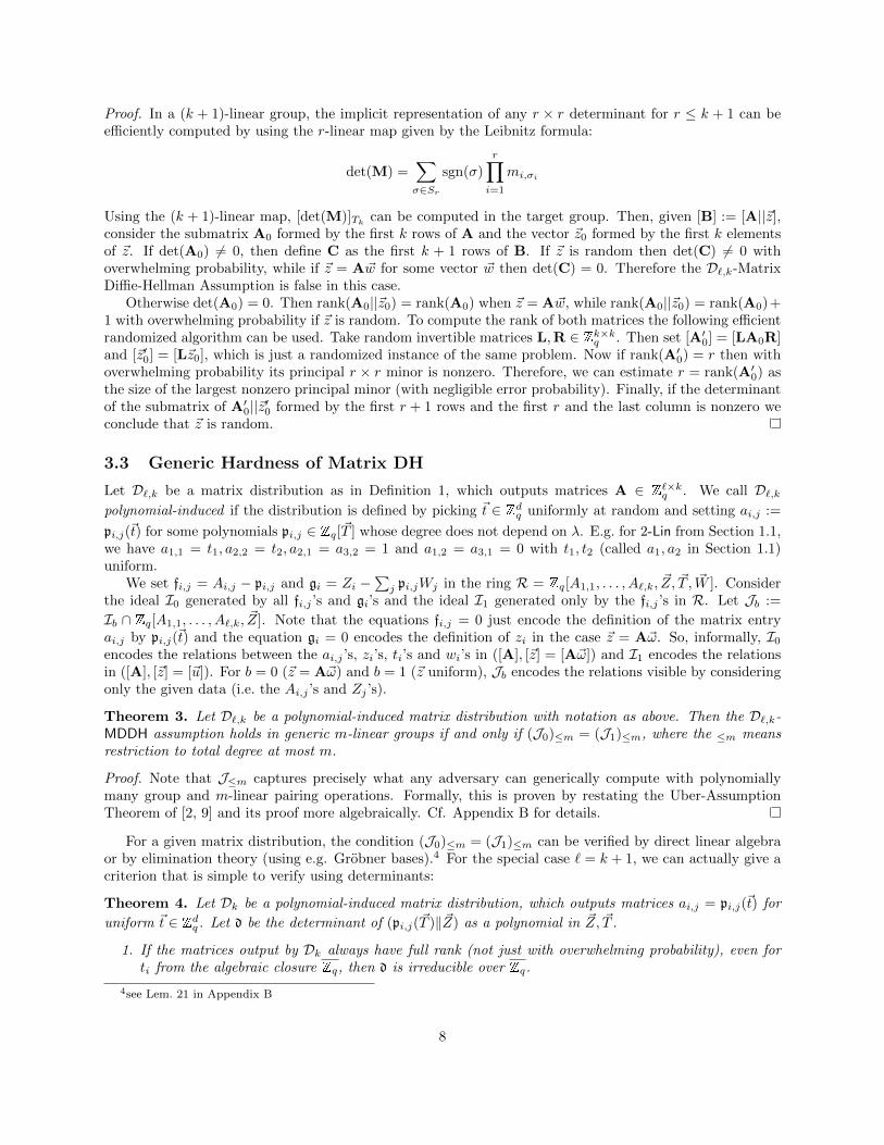
Proof. In a (k + 1)-linear group, the implicit representation of any r × r determinant for r ≤ k + 1 can beefficiently computed by using the r-linear map given by the Leibnitz formula:

det(M) =∑σ∈Sr

sgn(σ)

r∏i=1

mi,σi

Using the (k + 1)-linear map, [det(M)]Tk can be computed in the target group. Then, given [B] := [A||~z],consider the submatrix A0 formed by the first k rows of A and the vector ~z0 formed by the first k elementsof ~z. If det(A0) 6= 0, then define C as the first k + 1 rows of B. If ~z is random then det(C) 6= 0 withoverwhelming probability, while if ~z = A~w for some vector ~w then det(C) = 0. Therefore the D`,k-MatrixDiffie-Hellman Assumption is false in this case.

Otherwise det(A0) = 0. Then rank(A0||~z0) = rank(A0) when ~z = A~w, while rank(A0||~z0) = rank(A0)+1 with overwhelming probability if ~z is random. To compute the rank of both matrices the following efficientrandomized algorithm can be used. Take random invertible matrices L,R ∈ Zk×kq . Then set [A′0] = [LA0R]and [~z′0] = [L~z0], which is just a randomized instance of the same problem. Now if rank(A′0) = r then withoverwhelming probability its principal r × r minor is nonzero. Therefore, we can estimate r = rank(A′0) asthe size of the largest nonzero principal minor (with negligible error probability). Finally, if the determinantof the submatrix of A′0||~z′0 formed by the first r + 1 rows and the first r and the last column is nonzero weconclude that ~z is random.

3.3 Generic Hardness of Matrix DH

Let D`,k be a matrix distribution as in Definition 1, which outputs matrices A ∈ Z`×kq . We call D`,kpolynomial-induced if the distribution is defined by picking ~t ∈ Zdq uniformly at random and setting ai,j :=

pi,j(~t) for some polynomials pi,j ∈ Zq[~T ] whose degree does not depend on λ. E.g. for 2-Lin from Section 1.1,we have a1,1 = t1, a2,2 = t2, a2,1 = a3,2 = 1 and a1,2 = a3,1 = 0 with t1, t2 (called a1, a2 in Section 1.1)uniform.

We set fi,j = Ai,j − pi,j and gi = Zi −∑j pi,jWj in the ring R = Zq[A1,1, . . . , A`,k, ~Z, ~T , ~W ]. Consider

the ideal I0 generated by all fi,j ’s and gi’s and the ideal I1 generated only by the fi,j ’s in R. Let Jb :=

Ib ∩ Zq[A1,1, . . . , A`,k, ~Z]. Note that the equations fi,j = 0 just encode the definition of the matrix entryai,j by pi,j(~t) and the equation gi = 0 encodes the definition of zi in the case ~z = A~ω. So, informally, I0encodes the relations between the ai,j ’s, zi’s, ti’s and wi’s in ([A], [~z] = [A~ω]) and I1 encodes the relationsin ([A], [~z] = [~u]). For b = 0 (~z = A~ω) and b = 1 (~z uniform), Jb encodes the relations visible by consideringonly the given data (i.e. the Ai,j ’s and Zj ’s).

Theorem 3. Let D`,k be a polynomial-induced matrix distribution with notation as above. Then the D`,k-MDDH assumption holds in generic m-linear groups if and only if (J0)≤m = (J1)≤m, where the ≤m meansrestriction to total degree at most m.

Proof. Note that J≤m captures precisely what any adversary can generically compute with polynomiallymany group and m-linear pairing operations. Formally, this is proven by restating the Uber-AssumptionTheorem of [2, 9] and its proof more algebraically. Cf. Appendix B for details.

For a given matrix distribution, the condition (J0)≤m = (J1)≤m can be verified by direct linear algebraor by elimination theory (using e.g. Grobner bases).4 For the special case ` = k + 1, we can actually give acriterion that is simple to verify using determinants:

Theorem 4. Let Dk be a polynomial-induced matrix distribution, which outputs matrices ai,j = pi,j(~t) for

uniform ~t ∈ Zdq . Let d be the determinant of (pi,j(~T )‖~Z) as a polynomial in ~Z, ~T .

1. If the matrices output by Dk always have full rank (not just with overwhelming probability), even forti from the algebraic closure Zq, then d is irreducible over Zq.

4see Lem. 21 in Appendix B

8

2. If all pi,j have degree at most one and d is irreducible over Zq and the total degree of d is k + 1, thenthe Dk-MDDH assumption holds in generic k-linear groups.

This theorem and generalizations for non-linear pi,j and non-irreducible d are proven in Appendix Busing tools from algebraic geometry.

3.4 Examples of D`,k-MDDH

Let D`,k be a matrix distribution and A ← D`,k. Looking ahead to our applications, [A] will correspondto the public-key (or common reference string) and [A~w] ∈ G` will correspond to a ciphertext. We definethe representation size REG(D`,k) of a given polynomial-induced matrix distribution D`,k with linear pi,j ’sas the minimal number of group elements it takes to represent [A] for any A ∈ D`,k. We will be interestedin families of distributions D`,k such that that Matrix Diffie-Hellman Assumption is hard in k-linear groups.By Lemma 2 we obtain a family of strictly weaker assumptions. Our goal is to obtain such a family ofassumptions with small (possibly minimal) representation.

Example 1. Let U`,k be the uniform distribution over Z`×kq .

The next lemma says that U`,k-MDDH is the weakest possible assumption among all D`,k-Matrix Diffie-Hellman Assumptions. However, U`,k has poor representation, i.e., REG(U`,k) = `k.

Lemma 5. Let D`,k be any matrix distribution. Then D`,k-MDDH⇒ U`,k-MDDH.

Proof. Given an instance ([A], [A~w]) ofD`,k, if L ∈ Z`×`q and R ∈ Zk×kq are two random invertible matrices, itis possible to get a properly distributed instance of the U`,k-matrix DH problem as ([LAR], [LA~w]). Indeed,LAR has a distribution statistically close to the uniform distribution5 in Zk×`q , while LA~w = LAR~v for

~v = R−1 ~w. Clearly, ~v has the uniform distribution in Zkq .

Example 2 (k-Linear Assumption/k-Lin). We define the distribution Lk as follows

A =

a1 0 . . . 0 00 a2 . . . 0 0

0 0. . . 0

.... . .

...0 0 . . . 0 ak1 1 . . . 1 1

∈ Z(k+1)×k

q ,

where ai ← Z∗q . The transformation matrix T ∈ Z1×kq is given as T = ( 1

a1, . . . , 1

ak). Note that the distribution

(A,A~w) can be compactly written as (a1, . . . , ak, a1w1, . . . , akwk, w1 + . . .+wk) = (a1, . . . , ak, b1, . . . , bk,b1a1

+

. . . + bkak

) with ai ← Z∗q , bi, wi ← Zq. Hence the Lk-Matrix Diffie-Hellman Assumption is an equivalent

description of the k-linear Assumption [3, 24, 42] with REG(Lk) = k.

It was shown in [42] that k-Lin holds in the generic k-linear group model and hence k-Lin forms a familyof increasingly strictly weaker assumptions. Furthermore, in [7] it was shown that 2-Lin⇒ BDDH.

Example 3 (k-Cascade Assumption/k-Casc). We define the distribution Ck as follows

A =

a1 0 . . . 0 01 a2 . . . 0 0

0 1. . . 0

.... . .

...0 0 . . . 1 ak0 0 . . . 0 1

,

5If A has full-rank (that happens with overwhelming probability) then LAR is uniformly distributed in the set of full-rank

matrices in Z`×kq , which implies that it is close to uniform in Z`×k

q .

9

where ai ← Z∗q . The transformation matrix T ∈ Z1×kq is given as T = (± 1

a1·...·ak ,∓1

a2·...·ak . . . ,1ak

). Note that

(A,A~w) can be compactly written as (a1, . . . , ak, a1w1, w1+a2w2 . . . , wk−1+akwk, wk) = (a1, . . . , ak, b1, . . . , bk,bkak− bk−1

ak−1ak+ bk−2

ak−2ak−1ak− . . .± b1

a1·...·ak ). We have REG(Ck) = k.

Matrix A bears resemblance to a cascade which explains the assumption’s name. Indeed, in order tocompute the right lower entry wk of matrix (A,A~w) from the remaining entries, one has to “descend” thecascade to compute all the other entries wi (1 ≤ i ≤ k − 1) one after the other.

A more compact version of Ck is obtained by setting all ai := a.

Example 4. (Symmetric k-Cascade Assumption) We define the distribution SCk as Ck but now ai = a,where a ← Z∗q . Then (A,A~w) can be compactly written as (a, aw1, w1 + aw2, . . . , wk−1 + awk, wk) =

(a, b1, . . . , bk,bka −

bk−1

a2 + bk−2

a3 − . . .±b1ak

). We have REG(Ck) = 1.

Observe that the same trick cannot be applied to the k-Linear assumption k-Lin, as the resulting Sym-metric k-Linear assumption does not hold in k-linear groups. However, if we set ai := a + i − 1, we obtainanother matrix distribution with compact representation.

Example 5. (Incremental k-Linear Assumption) We define the distribution ILk as Lk with ai = a+ i− 1,for a← Z∗q . The transformation matrix T ∈ Z1×k

q is given as T = ( 1a , . . . ,

1a+k−1 ). (A,A~w) can be compactly

written as (a, aw1, (a+ 1)w2, . . . , (a+ k− 1)wk, w1 + . . .+wk) = (a, b1, . . . , bk,b1a + b2

a+1 + . . .+ bka+k−1 ). We

also have REG(ILk) = 1.

The last three examples need some work to prove its generic hardness.

Theorem 6. k-Casc, k-SCasc and k-ILin are hard in generic k-linear groups.

Proof. We need to consider the (statistically close) variants with ai ∈ Zq rather that Z∗q . The determinant

polynomial for Ck is d(a1, . . . , ak, z1, . . . , zk+1) = a1 · · · akzk+1−a1 · · · ak−1zk+ . . .+(−1)kz1, which has totaldegree k + 1. As all matrices in Ck have rank k, because the determinant of the last k rows in A is always1, by Theorem 4 we conclude that k-Casc is hard in k-linear groups. As SCk is a particular case of Ck,the determinant polynomial for SCk is d(a, z1, . . . , zk+1) = akzk+1 − ak−1zk + . . . + (−1)kz1. As before, byTheorem 4, k-SCasc is hard in k-linear groups. Finally, in the case of k-ILin we will show in the next sectionits equivalence to k-SCasc and therefore it is generically hard in k-linear groups.

The previous examples can be related to some known assumptions from Section 2.3. Figure 1 depictsthe relations that are also stated in next theorem, except the equivalence of k-ILin and k-SCasc which isaddressed in the next section. We stress that this equivalence together with Theorem 7 imply that k-SCascis a stronger assumption than k-Lin, previously unknown [17].

Theorem 7. For any k ≥ 2, the following holds:

(k + 1)-PDDH⇒ k-Casc ;

(k + 1)-EDDH⇒ k-SCasc⇒ k-Casc ; k-ILin⇒ k-Lin ;

k-Casc⇒ (k + 1)-Casc ; k-SCasc⇒ (k + 1)-SCasc

Further, in k-linear groups, k-Casc⇒ k-MLDDH.

Proof. The proof of all implications can be found in Appendix A.

4 Uniqueness of One-Parameter Matrix DH Problems

Some differently-looking MDDH assumptions can be tightly equivalent, or isomorphic, meaning that there isa very tight generic reduction between the corresponding problems. These reductions are mainly based onthe algebraic nature of the MDDH problems.

10

DDH 2-ILin 3-EDDH 3-PDDH 3-ILin 4-EDDH 4-PDDH . . .

2-Lin 2-SCasc 2-Casc 3-Lin 3-SCasc 3-Casc . . .

BDDH 3-MLDDH . . .︸ ︷︷ ︸hard in generic groups

easy in 2-linear groups

︸ ︷︷ ︸hard in 2-linear groups

easy in 3-linear groups

︸ ︷︷ ︸hard in 3-linear groups

easy in 4-linear groups

Figure 1: Relation between various assumptions and their generic hardness in k-linear groups.

The simplest and most compact polynomial-induced matrix distributions Dk are the one-parameter linearones, where Dk outputs matrices A(t) = A0 + A1t for a uniformly distributed t ∈ Zq, and fixed A0,A1 ∈Z

(k+1)×kq . The two examples of them given in [17] are SCk and ILk.

A natural question is whether such a tight algebraic reduction exists between SCk and ILk. In thissection we prove a much stronger result, which states there exists essentially a single one-parameter linearMDDH problem. Indeed, we show that all one-parameter linear Dk-MDDH problems are isomorphic to SCk.This result is heavily related to the one-parameter nature of the problems considered, and it seems to be notgeneralizable to broader families of MDDH problems (e.g., trying to relate Ck and Lk, or dealing with thecase ` > k + 1).

4.1 Hardness

Theorem 4 gives an easy-to-check sufficient condition ensuring the Dk-MDDH assumption holds in generic k-linear groups for certain matrix distributions Dk, including the one-parameter linear ones. For this particularfamily, the sufficient condition is that all matrices A(t) = A0+A1t have full-rank for all t ∈ Zq, the algebraic

closure of the finite field Zq, and the determinant d of (A(T )‖~Z) as a polynomial in ~Z, T has total degreek+ 1. We first show that indeed it is also a necessary condition for the hardness of the Dk-MDDH problem.

Theorem 8. Let Dk be a one-parameter linear matrix distribution, producing matrices A(t) = A0 + A1t,

such that Dk-MDDH assumption is hard generically in k-linear groups. Then, the determinant d of (A(T )‖~Z)

is an irreducible polynomial in Zq[~Z, T ] with total degree k + 1, and the rank of A0 + A1t is always k, forall t ∈ Zq.

Proof. The proof just consists in finding a nonzero polynomial h ∈ Zq[~Z, T ] of degree at most k such thath(A(t)~w, t) = 0 for all t ∈ Zq and ~w ∈ Zkq , and then using it to solve the Dk-MDDH problem. If the totaldegree of d is at most k, then we can simply let h = d6. Otherwise, assume that the degree of d is k+ 1. If dis reducible, from Lemma 22 it follows that d can be split as d = cd0, where c ∈ Zq[T ] and d0 ∈ Zq[~Z, T ] arenonconstant. Clearly, if c(t) 6= 0 then d0(A(t)~w, t) = 0 for all ~w ∈ Zkq , which means that as a polynomial in

Zq[ ~W, T ], d0(T,A(T ) ~W ) has too many roots, so it is the zero polynomial. Therefore, we are done by takingh = d0.

Finally, observe that d(~z, t) =∑k+1i=0 ci(t)zi, where ~z = (z1, . . . , zk+1) and the ci(t) are the (signed) k-

minors of A(t). Therefore, if A(t0) has rank less than k for some t0 ∈ Zq then d(~z, t0) = 0 for all ~z ∈ Zk+1q ,

6Actually, it is assumed that d 6= 0, i.e., some matrices output by Dk have full-rank. Otherwise, it is not hard finding thepolynomial h based on a nonzero maximal minor of A(t), by adding to it an extra row and the column ~Z.

11

which means that ci(t0) = 0 for all i. As a consequence, T − t0 divides all ci and hence it divides d, that is,d is reducible.

Once we have found the polynomial h of degree at most k, an efficient distinguisher can use the k-linear map to evaluate [h(~z, t)]Tk from an instance ([A(t)], [~z]) of the Dk-MDDH problem, where [t] can becomputed easily from [A(t)] because A0 and A1 are known. If ~z = A(t)~w then h(~z, t) = 0, while for arandomly chosen ~z, h(~z, t) 6= 0 with overwhelming probability7. Then the distinguisher succeeds with anoverwhelming probability.

4.2 Isomorphic Problems

From now on, we consider in this section a one-parameter linear matrix distribution Dk such that Dk-MDDHassumption holds in generic k-linear groups. This in particular means that using Theorem 8, the polynomiald is irreducible in Zq[~Z, T ] with total degree k+ 1, and that the rank of A0 + A1t is always k, for all t ∈ Zq.Clearly the rank of A0 is k, but also A1 has rank k. Indeed, it is easy to see that the coefficients of themonomials of degree k + 1 in d are exactly the (signed) k-minors of A1, so they cannot be all zero.

There are some natural families of maps that generically transform MDDH problems into MDDH problems.As mentioned in previous sections, some examples of them are left and right multiplication by an invertible

constant matrix. More precisely, let L ∈ GLk+1(Zq), the set of all invertible matrices in Z(k+1)×(k+1)q , and

R ∈ GLk(Zq). Given some matrix distribution Dk, we write D′k = LDkR to denote the matrix distributionresulting from sampling a matrix from Dk and multiplying on the left and on the right by L and R.

This mapping between matrix distrutions can be used to transform any distinguisher for D′k-MDDH intoa distinguisher for Dk-MDDH with the same advantage and essentially the same running time. Indeed,a ‘real’ instance ([A], [A~w]) of a MDDH problem can be transformed into a ‘real’ instance of the otherMDDH problem ([A′], [A′ ~w′]) = (L[A]R,L[A~w]) with the right distribution, because LA~w = A′ ~w′, where~w′ = R−1 ~w is uniformly distributed. Similarly, a ‘random’ instance ([A], [~z]) is transformed into anotherone ([A′], [~z′]) = (L[A]R,L[~z]). From an algebraic point of view, we can see the above transformation aschanging the bases used to represent certain linear maps as matrices.

In the particular case of one-parameter linear matrix distributions, one can write A′(t) = LA(t)R =LA0R + LA1Rt, which simply means defining A′0 = LA0R and A′1 = LA1R. Consider the injective linearmaps f0, f1 : Zkq → Zk+1

q defined by f0(~w) = A0 ~w and f1(~w) = A1 ~w. We need the following technicallemma.

Lemma 9. If Dk is generically hard in k-linear groups, no nontrivial subspace U ⊂ Zkq exists such thatf0(U) = f1(U).

Proof. Assume for contradiction a nontrivial subspace U exists such that f0(U) = f1(U), and consider thenatural automorphism φ : U → U defined as φ = f−11 ◦f0. It is well defined due to the injectivity of f0 and f1.Then, there exists an eigenvector ~v 6= ~0 of φ for some eigenvalue λ ∈ Zq. The equation φ(~v) = f−11 ◦f0(~v) = λ~v

implies (f0−λf1)(~v) = ~0. Therefore, f0−λf1 is no longer injective and A(−λ) = A0−λA1 has rank strictlyless than k, which contradicts Theorem 8.

Applying the lemma iteratively one can build special bases for the spaces Zkq and Zk+1q , and obtain

canonical forms simultaneously for A0 and A1, as described in the proof of the following theorem, whichhas some resemblance to the construction of Jordan normal forms of endomorphisms. The proof is rathertechnical, and it can be found in Appendix C.

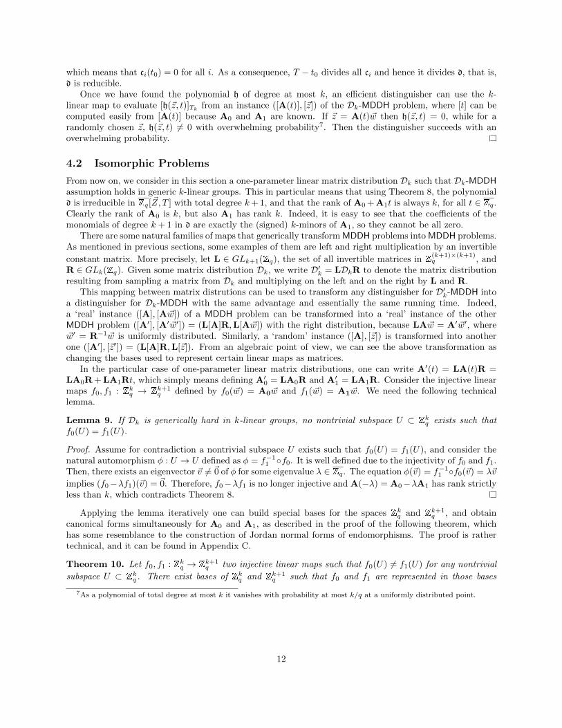
Theorem 10. Let f0, f1 : Zkq → Zk+1q two injective linear maps such that f0(U) 6= f1(U) for any nontrivial

subspace U ⊂ Zkq . There exist bases of Zkq and Zk+1q such that f0 and f1 are represented in those bases

7As a polynomial of total degree at most k it vanishes with probability at most k/q at a uniformly distributed point.

12

respectively by the matrices

J0 =

0 · · · 0

1. . .

......

. . . 00 · · · 1

J1 =

1 · · · 0

0. . .

......

. . . 10 · · · 0

Corollary 1. All one-parameter linear hard Dk-MDDH problems are isomorphic to the SCk-MDDH problem,i.e., there exist invertible matrices L ∈ GLk+1(Zq) and R ∈ GLk(Zq) such that Dk = LSCkR.

Proof. Combining the previous results, the maps f0, f1 defined from the hardDk-MDDH problem are injectiveand they can be represented in the bases given in Theorem 10. In terms of matrices this means that thereexist L ∈ GLk+1(Zq) and R ∈ GLk(Zq) such that A0 = LJ0R and A1 = LJ1R, that is,

A(t) = L

t · · · 0

1. . .

......

. . . t0 · · · 1

R

which concludes the proof.

As an example, we show an explicit isomorphism between SC2-MDDH and IL2-MDDH problems.t 00 t+ 11 1

=

−1 0 01 1 10 0 1

t 01 t0 1

(−1 01 1

)We stress that ‘isomorphic’ does not mean ‘identical’, and it is still useful having at hand different represen-tations of essentially the same computational problem, as it would help finding applications.

5 Basic applications

5.1 Public-Key encryption

Let Gen be a group generating algorithm and D`,k be a matrix distribution that outputs a matrix over Z`×kq

such that the first k-rows form an invertible matrix with overwhelming probability. We define the followingkey-encapsulation mechanism KEMGen,D`,k = (Gen,Enc,Dec) with key-space K = G`−k.

• Gen(1λ) runs G ← Gen(1λ) and A ← D`,k. Let A0 be the first k rows of A and A1 be the last ` − krows of A. Define T ∈ Z(`−k)×k

q as the transformation matrix T = A1A−10 . The public/secret-key is

pk = (G, [A] ∈ G`×k), sk = (pk ,T ∈ Z(`−k)×kq )

• Encpk picks ~w ← Zkq . The ciphertext/key pair is

[~c] = [A0 ~w] ∈ Gk, [K] = [A1 ~w] ∈ G`−k

• Decsk ([~c] ∈ Gk) recomputes the key as [K] = [T~c] ∈ G`−k.

Correctness follows by the equation T · ~c = T ·A0 ~w = A1 ~w. The public key contains REG(D`,k) and theciphertext k group elements. An example scheme from the k-SCasc Assumption is given in Appendix E.1.

Theorem 11. Under the D`,k-MDDH Assumption KEMGen,D`,k is IND-CPA secure.

Proof. By the D`,k Matrix Diffie-Hellman Assumption, the distribution of (pk , [~c], [K]) = ((G, [A]), [A~w]) iscomputationally indistinguishable from ((G, [A]), [~u]), where ~u← Z`q.

13

5.2 Hash Proof System

Let D`,k be a matrix distribution. We build a universal1 hash proof system HPS = (Param,Pub,Priv), whosehard subset membership problem is based on the D`,k Matrix Diffie-Hellman Assumption.

• Param(1λ) runs G ← Gen(1λ) and picks A← D`,k. Define the language

V = VA = {[~c] = [A~w] ∈ G` : ~w ∈ Zkq} ⊆ C = G`.

The value ~w ∈ Zkq is a witness of [~c] ∈ V. Let SK = Z`q, PK = Gk, and K = G. For sk = ~x ∈ Z`q,define the projection µ(sk) = [~x>A] ∈ Gk. For [~c] ∈ C and sk ∈ SK we define

Λsk ([~c]) := [~x> · ~c] . (3)

The output of Param is params =(S = (G, [A]),K, C,V,PK,SK,Λ(·)(·), µ(·)

).

• Priv(sk , [~c]) computes [K] = Λsk ([~c]).

• Pub(pk , [~c], ~w). Given pk = µ(sk) = [~x>A], [~c] ∈ V and a witness ~w ∈ Zkq such that [~c] = [A · ~w] thepublic evaluation algorithm Pub(pk , [~c], ~w) computes [K] = Λsk ([~c]) as

[K] = [(~x> ·A) · ~w] .

Correctness follows by (3) and the definition of µ. Clearly, under the D`,k-Matrix Diffie-Hellman Assumption,the subset membership problem is hard in HPS.

We now show that Λ is a universal1 projective hash function. Let [~c] ∈ C \ V. Then the matrix (A||~c) ∈Z`×(k+1)q is of full rank and consequently (~x> · A||~x> · ~c) ≡ (~x>A||u) for ~x ← Zkq and u ← Zq. Hence,

(pk ,Λsk ([~c]) = ([~x>A], [~x>~c]) ≡ ([~x>A], [u]) = ([~x>A], [K]).We remark that Λ can be transformed into a universal2 projective hash function by applying a four-wise

independent hash function [29]. Alternatively, one can construct a computational version of a universal2projective hash function as follows. Let SK = (Z`q)

2, PK = (Gk)2, and K = G. For sk = (~x1, ~x2) ∈ (Z`q)2,

define the projection µ(sk) = [~x>1 A, ~x>2 A] ∈ (Gk)2. For [~c] ∈ C and sk ∈ SK, define Λsk ([~c]) := [(t~x>1 +~x>2 )·~c],where t = H(~c) and H : C → Zq is a collision-resistant hash function. The corresponding Priv and Pubalgorithms are adapted accordingly. It is easy to verify that for all values [~c1], [~c2] ∈ C\V with H(~c1) 6= H(~c2),we have (pk ,Λsk ([~c1],Λsk ([~c2]) ≡ (pk , [K1], [K2]), for K1,K2 ← Zq.

5.3 Pseudo-random Functions

Let Gen be a group generating algorithm and D`,k be a matrix distribution that outputs a matrix over Z`×kq

such that the first k-rows form an invertible matrix with overwhelming probability. We define the followingpseudo-random function PRFGen,D`,k = (Gen,F) with message space {0, 1}n. For simplicity we assume that`− k divides k.

• Gen(1λ) runs G ← Gen(1λ), ~h ∈ Zkq , and Ai,j ← D`,k for i = 1, . . . , n and j = 1, . . . , t := k/(` − k)

and computes the transformation matrices Ti,j ∈ Z(`−k)×kq of Ai,j ∈ Z`×kq (cf. Definition 3). For

i = 1, . . . , n define the aggregated transformation matrices

Ti =

Ti,1

...Ti,t

∈ Zk×kq

The key is defined asK = (G,~h,T1, . . . ,Tn).

14

• FK(x) computes

FK(x) =

[ ∏i:xi=1

Ti · ~h

]∈ Gk.

PRFGen,Lk (i.e., setting D`,k = Lk) is the PRF from Lewko and Waters [31]. A more efficient PRF from thek-SCasc Assumption is given in Appendix E.2.

Note that the elements T1, . . . ,Tt of the secret-key consist of the transformation matrices of indepen-dently sampled matrices Ai,j . Interestingly, for a number of distributions D`,k the distribution of thetransformation matrix T is the same. For example, the transformation matrix for Lk consists of a uniformrow vector, so does the transformation matrix for Ck and for Uk+1,k. Consequently, PRFGen,Ck = PRFGen,Lk =PRFGen,Uk+1,k

and in light of the theorem below, PRFGen,Lk proposed by Lewko and Waters can also be provedon the weakest of all MDDH assumptions, namely the Uk+1,k-MDDH assumption.

Theorem 12. Under the D`,k-MDDH Assumption PRFGen,D`,k is a secure pseudo-random function.

Proof. For our proof we require the reader to be familiar with the augmented cascade construction of Bonehet al. [6]. For one aggregated transformation matrix T1 ∈ Zk×kq and ~h ∈ Zkq we define f : Zk×kq ×Gk×{0, 1} →Gk as the function

f(T1, [~h], b) :=

{[~h] if b = 0

[T1~h] if b = 1

.

The definition of f also explains the choice of t = k/(` − k) as the the augmented cascade constructionrequires range of f to be Gk. Then PRFGen,D`,k is obtained directly from f using the augmented cascadeconstruction (via a hybrid argument over 1 ≤ i ≤ n). To show that it is a secure pseudo-random function itsuffices to show that f is parallel secure [6], i.e., that for every polynomial m,([

~h1

T1~h1

], . . . ,

[~hm

T1~hm

])∈ (G2k)m

is pseudo-random, where ~hi ← Zkq ,

T1 =

T1,1

...T1,t

∈ Zk×kq ,

and T1,j (1 ≤ j ≤ t) are transformation matrices of A1,j ← D`,k. By a hybrid argument over j = 1, . . . , t itis sufficient to show that ([

~h1

T1,1~h1

], . . . ,

[~hm

T1,1~hm

])∈ (G`)m

is pseudo-random (for one single transformation matrix T1,1 of A1,1 ← D`,k) which in turn follows directlyby Lemma 1 (random self-reducibility of D`,k-MDDH).

We remark that the reduction is independent of the number of queries, i.e., it loses a factor of nk =nt(` − k), where the factor n stems from the augmented cascade Theorem [6], the factor t from the hybridargument over j, and the factor `− k from Lemma 1.

5.4 Groth-Sahai Non-interactive Zero-Knowledge Proofs

Groth and Sahai gave a method to construct non-interactive witness-indistinguishable (NIWI) and non-interactive zero-knowledge (NIZK) proofs for satisfiability of a set of equations in a bilinear group PG. (Forformal definitions of NIWI and NIZK proofs we refer to [22].) The equations in the set can be of differenttypes, but they can be written in a unified way as

n∑j=1

f(aj , yj) +

m∑i=1

f(xi, bi) +

m∑i=1

n∑j=1

f(xi, γijyj) = t, (4)

15

where A1, A2, AT are Zq-modules, ~x ∈ Am1 , ~y ∈ An2 are the variables, ~a ∈ An1 , ~b ∈ Am2 , Γ = (γij) ∈ Zm×nq ,t ∈ AT are the constants and f : A1 × A2 → AT is a bilinear map. More specifically, considering onlysymmetric bilinear groups, equations are of one of these types:

i) Pairing product equations, with A1 = A2 = G, AT = GT , f([x], [y]) = [xy]T ∈ GT .

ii) Multi-scalar multiplication equations, with A1 = Zq, A2 = AT = G, f(x, [y]) = [xy] ∈ G.

iii) Quadratic equations in Zq, with A1 = A2 = AT = Zq, f(x, y) = xy ∈ Zq.

Overview. The GS proof system allows to construct NIWI and NIZK proofs for satisfiability of a set ofequations of the type (4), i.e., proofs that there is a choice of variables — the witness — satisfying allequations simultaneously. The prover gives to the verifier a commitment to each element of the witnessand some additional information, the proof. Commitments and proof satisfy some related set of equationscomputable by the verifier because of their algebraic properties. We stress that to compute the proof, theprover needs the randomness which it used to create the commitments. To give new instantiations of GSproofs we need to specify the distribution of the common reference string, which includes the commitmentkeys and some maps whose purpose is roughly to give some algebraic structure to the commitment space.

Commitments. We will now construct commitments to elements in Zq and G. The commitment key[U] = ([~u1], . . . , [~uk+1]) ∈ G`×(k+1) is of the form

[U] =

{[A||A~w] binding key (soundness setting)

[A||A~w − ~z] hiding key (WI setting),

where A ← D`,k, ~w ← Zkq , and ~z ∈ Z`q, ~z /∈ Im(A) is a fixed, public vector. The two types of commitmentkeys are computationally indistinguishable based on the D`,k-MDDH Assumption.

To commit to [y] ∈ G using randomness ~r ← Zk+1q we define maps ι : G→ Z`q and p : G` → Zq as

ι([y]) = y · ~z, p([~c]) = ~ξ> · ~c, defining com[U],~z([y];~r) := [ι([y]) + U~r] ∈ G`,

where ~ξ ∈ Z`q is an arbitrary vector such that ~ξ>A = ~0 and ~ξ> · ~z = 1. Note that, given [y], ι([y]) isnot efficiently computable, but [ι([y])] is, and this suffices to compute the commitment. On a binding key(soundness setting) we have that p([ι([y])]) = y for all [y] ∈ G and that p([~ui]) = 0 for all i = 1 . . . k + 1. So

p(com[U],~z([y];~r)) = ~ξ>(~zy + U~r) = ~ξ>~zy + ~ξ>(A||A~w)~r = y and the commitment is perfectly binding. Ona hiding key (WI setting), ι([y]) ∈ Span(~u1, . . . , ~uk+1) for all [y] ∈ G which implies that the commitmentsare perfectly hiding.

To commit to a scalar x ∈ Zq using randomness ~s← Zkq we define the maps ι′ : Zq → Z`q and p′ : G` → Zq

asι′(x) = x · (~uk+1 + ~z), p′([~c]) = ~ξ>~c, defining com′[U],~z(x;~s) := [ι′(x) + A~s] ∈ G`.

where ~ξ is defined as above. Note that, given x, ι(x) is not efficiently computable, but [ι(x)] is, and thissuffices to compute the commitment. On a binding key (soundness setting) we have that p′([ι′(x)]) = x forall x ∈ Zq and p′([~ui]) = 0 for all i = 1 . . . k so the commitment is perfectly binding. On a hiding key (WIsetting), ι′(x) ∈ Span(~u1, . . . , ~uk) for all x ∈ Zq, which implies that the commitment is perfectly hiding.

It will also be convenient to define a vector of commitments as com[U],~z([~y]; R) = [ι([~y>]) + UR] and

com′[U],~z(~x; S) = [ι′(~x>) + AS], where [~y] ∈ Gm, ~x ∈ Znq , R← Z(k+1)×mq , S← Zk×nq and the inclusion maps

are defined component-wise.

Inclusion and projection maps. As we have seen, commitments are elements of G`. The main ideaof GS NIWI and NIZK proofs is to give some algebraic structure to the commitment space (in this case,G`) so that the commitments to a solution in A1, A2 of a certain set of equations satisfy a related set of

16

equations in some larger modules. For this purpose, if [~x] ∈ G` and [~y] ∈ G`, we define the bilinear mapF : G` ×G` → Z`×`q defined implicitly as:

F ([~x], [~y]) = ~x ·~y>,

as well as its symmetric variant F ([~x], [~y]) = 12 F ([~x], [~y])+ 1

2 F ([~y], [~x]). Additionally, for any two row vectors ofelements of G` of equal length r [X] = [~x1, . . . ,~xr] and [Y] = [~y1, . . . ,~yr], we define the maps • , • associatedwith F and F as [X] • [Y] = [

∑ri=1 F ([~xi], [~yi])]T and [X]• [Y] = [

∑ri=1 F ([~xi], [~yi])]T . To complete the details

of the new instantiation, we must specify for each type of equation, for both F ′ = F and F ′ = F :

a) some maps ιT and pT such that for all x ∈ A1, y ∈ A2, [~x] ∈ G`, [~y] ∈ G`,

F ′([ι1(x)], [ι2(y)]) = ιT (f(x, y)) and pT ([F ′([~x], [~y])]T ) = f(p1([~x]), p2([~y])),

where ι1, ι2 are either ι or ι′ and p1, p2 either [p] or p′, according to the appropriate A1, A2 for eachequation,

b) matrices H1, . . . ,Hη ∈ Zk1×k2q , where k1, k2 are the number of columns of U1,U2 respectively andwhich, in the witness indistinguishability setting, are a basis of all the matrices which are a solution ofthe equation [U1H] • [U2] = [0]T if F ′ = F or [U1H] • [U2] = [0]T if F ′ = F , where U1,U2 are eitherU or A, depending on the modules A1, A2. These matrices are necessary to randomize the NIWI andNIZK proofs.

To present the instantiations in concise form, in the following Hr,s,m,n = (hij) ∈ Zm×nq denotes the matrixsuch that hrs = −1, hsr = 1 and hij = 0 for (i, j) /∈ {(r, s), (s, r)}. In summary, the elements which must bedefined are:

• Pairing product equations. In this case, A1 = A2 = G, AT = GT , ι1 = ι2 = ι, p1 = p2 = [p],U1 = U2 = U and both for F ′ = F and F ′ = F ,

ιT ([z]T ) = z · ~z · ~z> ∈ Z`×`q pT ([Z]T ) = [~ξ>Z~ξ]T ,

where Z = (Zij)1≤i,j≤` ∈ Z`×`q . The equation [UH] • [U] = [0]T admits no solution, while all the

solutions to [UH] • [U] = [0]T are generated by{Hr,s,k+1,k+1

}1≤r<s≤k+1

.

• Multi-scalar multiplication equations. In this case, A1 = Zq, A2 = AT = G, ι1 = ι′, ι2 = ι,

p1 = p′, p2 = [p], U1 = A, U2 = U and for both F ′ = F and F ′ = F ,

ιT ([z]) = F ′([ι′(1)], [ι([z])]) pT ([Z]T ) = [~ξ>Z~ξ].

The equation [AH] • [U] = [0]T admits no solution, while all the solutions to [AH] • [U] = [0]T aregenerated by

{Hr,s,k,k+1

}1≤r<s≤k.

• Quadratic equations. In this case, A1 = A2 = AT = Zq, ι1 = ι2 = ι′, p1 = p2 = p′ and

U1 = U2 = A, for both F ′ = F and F ′ = F , we define

ιT (z) = F ′([ι′(1)], [ι′(z)]) pT ([Z]T ) = ~ξ>Z~ξ.

The equation [AH] • [A] = [0]T admits no solution, while all the solutions to [AH] • [A] = [0]T aregenerated by

{Hr,s,k,k

}1≤r<s≤k.

To argue that the equation [U1H] • [U2] = [0]T admits no solution, for each of the cases above, it issufficient to argue that the vectors F ([~ui], [~uj ]) are linearly independent. This holds regardless of the matrix

distribution D`,k from basic linear algebra, since F ([~ui], [~uj ]) was defined as the implicit representation ofthe outer product of ~ui and ~uj and ~u1, . . . , ~uk+1 are linearly independent.

Proof and Verification. For completeness, we now describe how do the prover and the verifier proceed.Define k1, k2 as the number of columns of U1,U2 respectively. On input PG, [U], ~z, a set of equations anda set of witnesses ~x ∈ Am1 ,~y ∈ An2 the prover proceeds as follows:

17

D`,k-MDDH instantiation elements of G elements of Zq

Commitment to a Variable ` 0

Pairing product equation `(k + 1) 0

- Linear equation: k + 1 0

Multi-scalar multiplication equation `(k + 1) 0

- Linear equation with variables in G 0 k + 1

- Linear equation with variables in Zq k 0

Quadratic equation `k 0

- Linear equation 0 k

Table 1: Size of the proofs based on the D`,k-MDDH Assumption.

1. Commit to ~x and ~y as[C] = [ι1(~x>) + U1R], [D] = [ι2(~y>) + U2S]

where R← Zk1×mq , S← Zk2×nq .

2. For each equation of the type (4), pick T← Zk1×k2q and output ([Π], [Θ]), defined as:

[Π] := [ι2(~b>)R> + ι2(~y>)Γ>R> + U2SΓ>R> −U2T> +

∑1≤i≤η

riU2H>i ]

[Θ] := [ι1(~a>)S> + ι1(~x>)ΓS> + U1T]

The proof described above is for a general equation, the same optimizations for special types of equation asin the full version of [22] apply. In particular, when the map used is the symmetric map F , the size of theproof can be reduced. In addition, the size of the proof can also be reduced when all the elements in eitherA1 or A2 are constants. Taking these optimizations into account, we give the size of the commitments andthe proof for the different types of equations in Table 1.

To verify a proof, on input the commitments [C], [D] and a proof ([Π], [Θ]), the verifier checks if

[ι1(~a>)] •′ [D] + [C] •′ [ι2(~b>)] + [C] •′ [DΓ>] = [ιT (t)]T + [U1] •′ [Π] + [Θ] •′ [U2],

where •′ is either • or •, depending on whether F ′ is F or F . If the equation is satisfied, the verifier acceptsthe proof for this equation and rejects otherwise. In general, the verification cost depends on ` and k,though a bit might be gained in pairing computations when using batch verification techniques and if somecomponents of the commitment keys are trivial or are repeated, i.e. if the D`,k admits short representation.

Efficiency. We emphasize that for D`,k = L2 and ~z = (0, 0, 1)> and for D`,k = DDH and ~z = (0, 1)>

(in the natural extension to asymmetric bilinear groups), we recover the 2-Lin and the SXDH instantiationsof [22]. While the size of the proofs depends only on ` and k, both the size of the CRS and the cost ofverification increase with REG(D`,k). In particular, in terms of efficiency, the SC2 Assumption is preferableto the 2-Lin Assumption but the main reason to consider more instantiations of GS proofs is to obtain moreefficient proofs for a large class of languages in Section 6.

6 More efficient proofs for some CRS dependent languages

6.1 More efficient subgroup membership proofs

Let [U] be the commitment key defined in last section as part of a D`,k-MDDH instantiation, for someA ← D`,k. In this section we show a new technique to obtain proofs of membership in the languageLA,PG := {[A~r], ~r ∈ Zkq} ⊂ G`.

18

Intuition. Our idea is to exploit the special algebraic structure of commitments in GS proofs, namely theobservation that if [~Φ] = [A~r] ∈ LA,PG then [~Φ] = com[U](0;~r). Therefore, to prove that [~Φ] ∈ LA,PG , weproceed as if we were giving a GS proof of satisfability of the equation x = 0 where the randomness usedfor the commitment to x is ~r. In particular, no commitments have to be given in the proof, which results inshorter proofs. To prove zero-knowledge we rewrite the equation x = 0 as x · δ = 0. The real proof is just astandard GS proof with the commitment to δ = 1 being ι′(1) = com[U](1;~0), while in the simulated proofthe trapdoor allows to open ι′(1) as a commitment to 0, so we can proceed as if the equation was the trivialone x ·0 = 0, for which it is easy to give a proof of satisfiability. For the 2-Lin Assumption, our proof consistsof only 6 group elements, whereas without using our technique the proof consists of 12 elements. Details arein Appendix D.5. More generally, in Appendix D.1 we will prove the following theorem.

Theorem 13. Let A ← D`,k, where D`,k is a matrix distribution. There exists a Non-Interactive Zero-Knowledge Proof for the language LA,PG, with perfect completeness, perfect soundness and composable zero-knowledge of k` group elements based on the D`,k-MDDH Assumption.

Applications. For a typical application scenario of Theorem 13, think of [A] as part of the public parame-ters of the hash proof system of Section 5.2. Proving that a ciphertext is well-formed is proving membershipin LA,PG . For instance, in [32] Libert and Yung combine a proof of membership in 2-Lin with a one-timesignature scheme to obtain publicly verifiable ciphertexts. With our result, we reduce the size of their ci-phertexts from 15 to 9 group elements. We stress that in our construction the setup of the CRS can be builton top of the encryption key so that proofs can be simulated without the decryption key, which is essentialin their case. Another application is to show that two ciphertexts encrypt the same message under the samepublic key, a common problem in electronic voting or anonymous credentials. There are many other settingsin which subgroup membership problems naturally appear, for instance the problem of certifying public keysor given some plaintext m, the problem of proving that a certain ciphertext is an encryption of [m].

6.2 More efficient proofs of validity of ciphertexts

The techniques of the previous section can be extended to prove the validity of a ciphertext. More specifically,given A ← D`,k, and some vector ~z ∈ Z`q, ~z /∈ Im(A), we show how to give a more efficient proof ofmembership in the space:

LA,~z,PG = {[~c] : ~c = A~r +m~z} ⊂ G`,

where (~r, [m]) ∈ Zkq ×G is the witness. This is also a proof of membership in the subspace of G` spanned bythe columns of [A] and the vector [~z], but the techniques given in Section 6.1 do not apply. The reason is thatpart of the witness, [m], is in the group G and not in Zq, while to compute the subgroup membership proofsas described in Section 6.1 all of the witness has to be in Zq. In particular, since GS are non-interactivezero-knowledge proofs of knowledge when the witnesses are group elements, the proof guarantees both thatthe ~c is well-formed and that the prover knows [m].

In a typical application, [~c] will be the ciphertext of some encryption scheme, in which case ~r will be theciphertext randomness and [m] the message. Deciding membership in this space is trivial when Im(A) and~z span all of Z`q, so in particular our result is meaningful when ` > k + 1. In Appendix D.2 we prove thefollowing theorem:

Theorem 14. Let D`,k be a matrix distribution and let A ← D`,k. There exists a Non-Interactive Zero-Knowledge Proof for the language LA,~z,PG of (k + 2)` group elements with perfect completeness, perfectsoundness and composable zero-knowledge based on the D`,k-MDDH Assumption.

Applications. A proof that a ciphertext is well formed is used, for instance, in [16]. Using this result, wecan give a proof that the 2-Lin Cramer-Shoup ciphertext is well formed which takes only 20 group elementsas opposed to 23 using standard techniques.

19

6.3 More efficient proofs of plaintext equality

The encryption scheme derived from the KEM given in Section 5.1 corresponds to a commitment in GSproofs. That is, if pkA = (G, [A] ∈ G`×k), for some A← D`,k, given ~r ∈ Zkq ,

EncpkA([m];~r) = [~c] = [A~r + (0, . . . , 0,m)>] = [A~r +m · ~z] = com[A||A~w]([m];~s),

where ~s> := (~r>, 0) and ~z := (0, . . . , 0, 1)>. Therefore, given two (potentially distinct) matrix distributionsD`1,k1 , D′`2,k2 and A ← D`1,k1 ,B ← D′`2,k2 , proving equality of plaintexts of two ciphertexts encryptedunder pkA, pkB , corresponds to proving that two commitments under different keys open to the same value.Our proof will be more efficient because we do not give any commitments as part of the proof, since theciphertexts themselves play this role. More specifically, given [~cA] = EncpkA([m]) and [~cB ] = EncpkB ([m])we will treat [~cA] as a commitment to the variable [x] ∈ A1 = G and [~cB ] as a commitment to the variable[y] ∈ A2 = G and prove that the quadratic equation e([x], [1]) · e([−1], [y]) = [0]T is satisfied. The zero-knowledge simulator will open ι1([1]), ι2([−1]) as commitments to the [0] variable and simulate a proof forthe equation e([x], [0]) · e([0], [y]) = [0]T , which is trivially satisfiable and can be simulated.

More formally, let

LA,B,~z1,~z2,PG := {([~cA], [~cB ]) : [~cA] = [A~r +m~z1], [~cB ] = [B~s+ ~z2]} ⊂ G`1 ×G`2

where ~r ∈ Zk1q , ~s ∈ Zk2q ,m ∈ Zq, ~z1 ∈ Z`1q , and ~z1 /∈ Im(A) and ~z2 ∈ Z`2q , ~z2 /∈ Im(B). In Appendix D.3 weprove:

Theorem 15. Let D`1,k1 and D′`2,k2 be two matrix distributions and let A ← D`1,k1 ,B ← D′`2,k2 . Thereexists a Non-Interactive Zero-Knowledge Proof for the language LA,B,~z1,~z2,PG of `1(k2 + 1) + `2(k1 + 1)group elements with perfect completeness, perfect soundness and composable zero-knowledge based on theD`1,k1-MDDH and the D`2,k2-MDDH Assumption.

Applications. In [26], we reduce the size of the proof by 4 group elements from 18 to 22, while in [23] wesave 9 elements although their proof is quite inefficient altogether. We note that even if both papers give aproof that two ciphertexts under two different 2-Lin public keys correspond to the same value, the proof in[23] is more inefficient because it must use GS proofs for pairing product equations instead of multi-scalarmultiplication equations. Other examples include [10, 15]. We note that our approach is easily generalizableto prove more general statements about plaintexts, for instance to prove membership in L′A,B,~z1,~z2,PG :=

{([~cA], [~cB ]) : [~cA] = [A~r + (0, . . . , 0,m)>], [~cB ] = [B~s + (0, . . . , 0, 2m)>], ~r ∈ Zk1q , ~s ∈ Zk2q } ⊂ G`1 × G`2

or in general to show that some linear relation between a set of plaintexts encrypted under two differentpublic-keys holds.

References

[1] O. Blazy, D. Pointcheval, and D. Vergnaud. Round-optimal privacy-preserving protocols with smoothprojective hash functions. In R. Cramer, editor, TCC 2012, volume 7194 of LNCS, pages 94–111,Taormina, Sicily, Italy, Mar. 19–21, 2012. Springer, Berlin, Germany. 3

[2] D. Boneh, X. Boyen, and E.-J. Goh. Hierarchical identity based encryption with constant size ciphertext.In R. Cramer, editor, EUROCRYPT 2005, volume 3494 of LNCS, pages 440–456, Aarhus, Denmark,May 22–26, 2005. Springer, Berlin, Germany. 2, 8, 25

[3] D. Boneh, X. Boyen, and H. Shacham. Short group signatures. In M. Franklin, editor, CRYPTO 2004,volume 3152 of LNCS, pages 41–55, Santa Barbara, CA, USA, Aug. 15–19, 2004. Springer, Berlin,Germany. 1, 5, 9

[4] D. Boneh and M. K. Franklin. Identity-based encryption from the Weil pairing. In J. Kilian, editor,CRYPTO 2001, volume 2139 of LNCS, pages 213–229, Santa Barbara, CA, USA, Aug. 19–23, 2001.Springer, Berlin, Germany. 1, 5

20

[5] D. Boneh, S. Halevi, M. Hamburg, and R. Ostrovsky. Circular-secure encryption from decision Diffie-Hellman. In D. Wagner, editor, CRYPTO 2008, volume 5157 of LNCS, pages 108–125, Santa Barbara,CA, USA, Aug. 17–21, 2008. Springer, Berlin, Germany. 1, 2

[6] D. Boneh, H. W. Montgomery, and A. Raghunathan. Algebraic pseudorandom functions with improvedefficiency from the augmented cascade. In E. Al-Shaer, A. D. Keromytis, and V. Shmatikov, editors,ACM CCS 10, pages 131–140, Chicago, Illinois, USA, Oct. 4–8, 2010. ACM Press. 1, 3, 15, 38

[7] D. Boneh, A. Sahai, and B. Waters. Fully collusion resistant traitor tracing with short ciphertexts andprivate keys. In S. Vaudenay, editor, EUROCRYPT 2006, volume 4004 of LNCS, pages 573–592, St.Petersburg, Russia, May 28 – June 1, 2006. Springer, Berlin, Germany. 1, 3, 5, 9

[8] D. Boneh and A. Silverberg. Applications of multilinear forms to cryptography. Cryptology ePrintArchive, Report 2002/080, 2002. http://eprint.iacr.org/. 5

[9] X. Boyen. The uber-assumption family (invited talk). In S. D. Galbraith and K. G. Paterson, editors,PAIRING 2008, volume 5209 of LNCS, pages 39–56, Egham, UK, Sept. 1–3, 2008. Springer, Berlin,Germany. 2, 8, 25

[10] J. Camenisch, N. Chandran, and V. Shoup. A public key encryption scheme secure against key dependentchosen plaintext and adaptive chosen ciphertext attacks. In A. Joux, editor, EUROCRYPT 2009, volume5479 of LNCS, pages 351–368, Cologne, Germany, Apr. 26–30, 2009. Springer, Berlin, Germany. 4, 20

[11] D. Cox, J. Little, and D. O’Shea. Ideal, Varieties and Algorithms. Springer, second edition, 1996. 25,26, 27

[12] R. Cramer and V. Shoup. A practical public key cryptosystem provably secure against adaptive chosenciphertext attack. In H. Krawczyk, editor, CRYPTO’98, volume 1462 of LNCS, pages 13–25, SantaBarbara, CA, USA, Aug. 23–27, 1998. Springer, Berlin, Germany. 1

[13] R. Cramer and V. Shoup. Universal hash proofs and a paradigm for adaptive chosen ciphertext securepublic-key encryption. In L. R. Knudsen, editor, EUROCRYPT 2002, volume 2332 of LNCS, pages45–64, Amsterdam, The Netherlands, Apr. 28 – May 2, 2002. Springer, Berlin, Germany. 1, 3, 6

[14] R. Cramer and V. Shoup. Design and analysis of practical public-key encryption schemes secure againstadaptive chosen ciphertext attack. SIAM Journal on Computing, 33(1):167–226, 2003. 6

[15] Y. Dodis, K. Haralambiev, A. Lopez-Alt, and D. Wichs. Cryptography against continuous memoryattacks. In 51st FOCS, pages 511–520, Las Vegas, Nevada, USA, Oct. 23–26, 2010. IEEE ComputerSociety Press. 4, 20

[16] Y. Dodis, K. Haralambiev, A. Lopez-Alt, and D. Wichs. Efficient public-key cryptography in thepresence of key leakage. In M. Abe, editor, ASIACRYPT 2010, volume 6477 of LNCS, pages 613–631,Singapore, Dec. 5–9, 2010. Springer, Berlin, Germany. 4, 19

[17] A. Escala, G. Herold, E. Kiltz, C. Rafols, and J. Villar. An algebraic framework for Diffie-Hellmanassumptions. In R. Canetti and J. A. Garay, editors, CRYPTO 2013, Part II, volume 8043 of LNCS,pages 129–147, Santa Barbara, CA, USA, Aug. 18–22, 2013. Springer, Berlin, Germany. 2, 3, 10, 11

[18] M. Fischlin, B. Libert, and M. Manulis. Non-interactive and re-usable universally composable stringcommitments with adaptive security. In D. H. Lee and X. Wang, editors, ASIACRYPT 2011, volume7073 of LNCS, pages 468–485, Seoul, South Korea, Dec. 4–8, 2011. Springer, Berlin, Germany. 4, 32,36

[19] D. M. Freeman. Converting pairing-based cryptosystems from composite-order groups to prime-ordergroups. In H. Gilbert, editor, EUROCRYPT 2010, volume 6110 of LNCS, pages 44–61, French Riviera,May 30 – June 3, 2010. Springer, Berlin, Germany. 1, 2

21

[20] D. Galindo, J. Herranz, and J. L. Villar. Identity-based encryption with master key-dependent messagesecurity and leakage-resilience. In S. Foresti, M. Yung, and F. Martinelli, editors, ESORICS 2012,volume 7459 of LNCS, pages 627–642, Pisa, Italy, Sept. 10–12, 2012. Springer, Berlin, Germany. 2

[21] R. Gennaro and Y. Lindell. A framework for password-based authenticated key exchange. In E. Biham,editor, EUROCRYPT 2003, volume 2656 of LNCS, pages 524–543, Warsaw, Poland, May 4–8, 2003.Springer, Berlin, Germany. http://eprint.iacr.org/2003/032.ps.gz. 1, 3

[22] J. Groth and A. Sahai. Efficient noninteractive proof systems for bilinear groups. SIAM J. Comput.,41(5):1193–1232, 2012. 1, 3, 15, 18

[23] D. Hofheinz and T. Jager. Tightly secure signatures and public-key encryption. In R. Safavi-Naini andR. Canetti, editors, CRYPTO 2012, volume 7417 of LNCS, pages 590–607, Santa Barbara, CA, USA,Aug. 19–23, 2012. Springer, Berlin, Germany. 4, 20, 36

[24] D. Hofheinz and E. Kiltz. Secure hybrid encryption from weakened key encapsulation. In A. Menezes,editor, CRYPTO 2007, volume 4622 of LNCS, pages 553–571, Santa Barbara, CA, USA, Aug. 19–23,2007. Springer, Berlin, Germany. 1, 5, 9, 31, 38

[25] A. Joux. A one round protocol for tripartite Diffie-Hellman. Journal of Cryptology, 17(4):263–276, Sept.2004. 1

[26] J. Katz and V. Vaikuntanathan. Round-optimal password-based authenticated key exchange. In Y. Ishai,editor, TCC 2011, volume 6597 of LNCS, pages 293–310, Providence, RI, USA, Mar. 28–30, 2011.Springer, Berlin, Germany. 4, 20, 35, 36

[27] E. Kiltz. A tool box of cryptographic functions related to the Diffie-Hellman function. In C. P. Ran-gan and C. Ding, editors, INDOCRYPT 2001, volume 2247 of LNCS, pages 339–350, Chennai, India,Dec. 16–20, 2001. Springer, Berlin, Germany. 3, 5

[28] E. Kiltz. Chosen-ciphertext security from tag-based encryption. In S. Halevi and T. Rabin, editors,TCC 2006, volume 3876 of LNCS, pages 581–600, New York, NY, USA, Mar. 4–7, 2006. Springer,Berlin, Germany. 1

[29] E. Kiltz, K. Pietrzak, M. Stam, and M. Yung. A new randomness extraction paradigm for hybridencryption. In A. Joux, editor, EUROCRYPT 2009, volume 5479 of LNCS, pages 590–609, Cologne,Germany, Apr. 26–30, 2009. Springer, Berlin, Germany. 14

[30] A. B. Lewko, T. Okamoto, A. Sahai, K. Takashima, and B. Waters. Fully secure functional encryption:Attribute-based encryption and (hierarchical) inner product encryption. In H. Gilbert, editor, EURO-CRYPT 2010, volume 6110 of LNCS, pages 62–91, French Riviera, May 30 – June 3, 2010. Springer,Berlin, Germany. 1, 3

[31] A. B. Lewko and B. Waters. Efficient pseudorandom functions from the decisional linear assumption andweaker variants. In E. Al-Shaer, S. Jha, and A. D. Keromytis, editors, ACM CCS 09, pages 112–120,Chicago, Illinois, USA, Nov. 9–13, 2009. ACM Press. 15

[32] B. Libert and M. Yung. Non-interactive CCA-secure threshold cryptosystems with adaptive security:New framework and constructions. In R. Cramer, editor, TCC 2012, volume 7194 of LNCS, pages75–93, Taormina, Sicily, Italy, Mar. 19–21, 2012. Springer, Berlin, Germany. 4, 19, 31, 37

[33] S. Meiklejohn, H. Shacham, and D. M. Freeman. Limitations on transformations from composite-order toprime-order groups: The case of round-optimal blind signatures. In M. Abe, editor, ASIACRYPT 2010,volume 6477 of LNCS, pages 519–538, Singapore, Dec. 5–9, 2010. Springer, Berlin, Germany. 1

[34] M. Naor and O. Reingold. Number-theoretic constructions of efficient pseudo-random functions. In 38thFOCS, pages 458–467, Miami Beach, Florida, Oct. 19–22, 1997. IEEE Computer Society Press. 1, 3

22

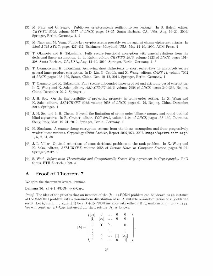
[35] M. Naor and G. Segev. Public-key cryptosystems resilient to key leakage. In S. Halevi, editor,CRYPTO 2009, volume 5677 of LNCS, pages 18–35, Santa Barbara, CA, USA, Aug. 16–20, 2009.Springer, Berlin, Germany. 1, 2

[36] M. Naor and M. Yung. Public-key cryptosystems provably secure against chosen ciphertext attacks. In22nd ACM STOC, pages 427–437, Baltimore, Maryland, USA, May 14–16, 1990. ACM Press. 4

[37] T. Okamoto and K. Takashima. Fully secure functional encryption with general relations from thedecisional linear assumption. In T. Rabin, editor, CRYPTO 2010, volume 6223 of LNCS, pages 191–208, Santa Barbara, CA, USA, Aug. 15–19, 2010. Springer, Berlin, Germany. 1, 3

[38] T. Okamoto and K. Takashima. Achieving short ciphertexts or short secret-keys for adaptively securegeneral inner-product encryption. In D. Lin, G. Tsudik, and X. Wang, editors, CANS 11, volume 7092of LNCS, pages 138–159, Sanya, China, Dec. 10–12, 2011. Springer, Berlin, Germany. 1

[39] T. Okamoto and K. Takashima. Fully secure unbounded inner-product and attribute-based encryption.In X. Wang and K. Sako, editors, ASIACRYPT 2012, volume 7658 of LNCS, pages 349–366, Beijing,China, December 2012. Springer. 1

[40] J. H. Seo. On the (im)possibility of projecting property in prime-order setting. In X. Wang andK. Sako, editors, ASIACRYPT 2012, volume 7658 of LNCS, pages 61–79, Beijing, China, December2012. Springer. 1

[41] J. H. Seo and J. H. Cheon. Beyond the limitation of prime-order bilinear groups, and round optimalblind signatures. In R. Cramer, editor, TCC 2012, volume 7194 of LNCS, pages 133–150, Taormina,Sicily, Italy, Mar. 19–21, 2012. Springer, Berlin, Germany. 1

[42] H. Shacham. A cramer-shoup encryption scheme from the linear assumption and from progressivelyweaker linear variants. Cryptology ePrint Archive, Report 2007/074, 2007. http://eprint.iacr.org/.1, 5, 9, 31, 38

[43] J. L. Villar. Optimal reductions of some decisional problems to the rank problem. In X. Wang andK. Sako, editors, ASIACRYPT, volume 7658 of Lecture Notes in Computer Science, pages 80–97.Springer, 2012. 2

[44] S. Wolf. Information-Theoretically and Computionally Secure Key Agreement in Cryptography. PhDthesis, ETH Zuerich, 1999. 5

A Proof of Theorem 7

We split the theorem in several lemmas.

Lemma 16. (k + 1)-PDDH⇒ k-Casc.

Proof. The idea of the proof is that an instance of the (k + 1)-PDDH problem can be viewed as an instanceof the C-MDDH problem with a non-uniform distribution of ~w. A suitable re-randomization of ~w yields theresult. Let (G, [x1], . . . , [xk+1], [z]) be a (k+1)-PDDH instance with either z ∈ Zq uniform or z = x1 · · ·xk+1.We will construct a k-Casc instance from that, setting [A] as follows:

[A] =

[x1] 0 . . . 0 0[1] [x2] . . . 0 0

0 [1]. . . 0

.... . .

...0 0 . . . [1] [xk]0 0 . . . 0 [1]

,

23

Let [~b>] :=((−1)k+1[z], 0, 0, . . . , 0, [xk+1]

)T. Since A has full rank, ~b is in the span of the columns of A iff

det(A‖~b) = 0. Since det(A‖~b) = x1 · · ·xk − z, this depends on the distribution of z as desired. To obtain a

properly distributed k-Casc instance (G, [A], [~b′]), we set [~b′] = [~b] +∑i wi[~ai] for uniform wi ∈ Zq. Clearly,

if ~b is in the span of the columns of A, ~b′ will be a uniform element in the span of the columns of A, whereasif it is not, ~b′ will be uniform in all of Zk+1

q .

Lemma 17. (k + 1)-EDDH⇒ k-SCasc.

Proof. The proof is analogous to the proof of the preceding Lemma 16. Let (G, [x], [z]) be a (k + 1)-EDDHinstance with either z ∈ Zq uniform or z = xk+1. We will construct a k-SCasc instance from that, defining[A] as the following k × (k + 1)-matrix:

[A] =

[x] 0 . . . 0 0[1] [x] . . . 0 0

0 [1]. . . 0

.... . .

...0 0 . . . [1] [x]0 0 . . . 0 [1]

,

Set [~b>] :=((−1)k+1[z], 0, 0, . . . , 0, [x]

). As above, ~b is in the span of the columns of A if and only if

z = xk+1. To obtain a properly distributed k-SCasc instance (G, [A], [~b′]), we set [~b′] = [~b] +∑i wi[~ai] for

uniform wi ∈ Zq.

Lemma 18. In k-linear groups, k-Casc⇒ k-MLDDH.

Proof. Assume for the purpose of contradiction that k-MLDDH does not hold. To break the k-Casc problem,we are given an instance [A], [~z], where A← Ck and we have to distinguish between ~z = A~w for uniform ~w

and uniform ~z. Or, equivalently, we have to test if the determinant of matrix B = A||~z ∈ Z(k+1)×(k+1)q is

zero. We claim thatdet(B) = a1 · . . . · akzk+1 + Tk(a1, . . . , ak, z1, . . . , zk+1),

where Tk only contains k-linear terms. (This can be proved by induction using the Laplace expansion.)Hence, to test whether det(B) = 0, one computes [b]Tk = [−Tk(a1, . . . , ak, z1, . . . , zk+1)]Tk using the k-linearmap and the oracle k-MLDDH([a1], . . . , [ak], [zk+1], [b]Tk) to check if a1 · . . . · akzk+1 = −b.

Lemma 19. k-SCasc⇒ k-Casc, k-ILin⇒ k-Lin

Proof. Both implications follow by simple rerandomization arguments. A k-SCasc instance ([a1], . . . , [ak], [a1w1],[w1+a2w2], . . . , [wk−1+akwk], [wk]) can be transformed into a k-Casc instance by picking α1, α2, . . . , αk ← Z∗qand computing ([aα1], [aα2], . . . , [aαk], [aw1], [w1+aw2

α1], . . . , [wk−1+akwk

α1···αk−1], [ wk

α1···αk ]). Similarly, a k-ILin instance

([a], [aw1], [(a + 1)w2], . . . , [(a + k − 1)wk], [w1 + . . . + wk]) can be transformed into a k-Lin instance bypicking random α1, α2, . . . , αk ← Z∗q and computing ([aα1], [(a + 1)α2], . . . , [(a + k − 1)αk], [aw1α1], [(a +1)w2α2], . . . , [(a+ k − 1)wkαk], [w1 + . . .+ wk]).

Lemma 20. k-Casc⇒ (k + 1)-Casc, k-SCasc⇒ (k + 1)-SCasc.

Proof. To show the first implication, we transform a given instance of the k-Casc problem D1 = ([a1], . . . , [ak],[a1w1], [w1 + a2w2], . . . , [wk−1 + akwk], [wk]) into an instance of the (k + 1)-Casc problem by picking uni-form wk+1 ← Zq and [ak+1] ← G and computing D2 = ([a1], . . . , [ak+1], [a1w1], [w1 + a2w2], . . . , [wk−1 +akwk], [wk+ak+1wk+1], [wk+1]). Note that D2 is pseudorandom iff D1 is pseudorandom. The same reductionalso works in the symmetric case.

24

B Proofs for the Generic Hardness results

In this section, we give the remaining proofs for the results on the D`,k-MDDH assumption in generic m-lineargroups from Section 3.3. We refer to reader to e.g. [11] for necessary background on the algebraic materialsuch as polynomial rings, ideals, Grobner bases, varieties and irreducibility used in this section. Note thatin this paper irreducibility is not implicit in the definition of a variety.Recall that our setup is that D`,k is a matrix distribution which outputs ai,j = pi,j(~t) for uniform ~t ∈ Zdqand possibly multivariate polynomials pi,j , whose degree does not depend on λ and hence not on q. Thedistributions ([A], [~z] = [A~ω]) respectively ([A], [~z] = [~u]) for A← D`,k, ~ω ← Zkq , ~u← Z`q are denoted by D0

respectively D1. In order to describe all of these data, we consider the polynomial ring R = Zq[ ~A, ~Z, ~T , ~W ],

introducing formal variables ~A = A1,1, . . . , A`,k to describe the matrix A, ~Z = Z1, . . . , Z` to describe the

vector ~z, ~T = T1, . . . Td for some d to describe the underlying t’s used to sample the ai,j ’s via ai,j = pi,j(~t), and

formal variables ~W = W1, . . . ,Wk to describe ~ω (which only appears in D0). Note that we shorthand write~A for the collection of all Ai,j ’s if the structure as a matrix is not crucial. Furthermore, we write A = p(~t)

or ~a = ~p(~t), meaning that ai,j = pi,j(~t). We further consider the polynomial subring S = Zq[ ~A, ~Z] ⊂ R todescribe the publicly known expressions. We can now encode our distributions D0 and D1 by polynomialsin the following way: let fi,j = Ai,j − pi,j(~T ) and gi = Zi −

∑j pi,j(

~T )Wj . Let G0 be the set of all f’s andg’s, whereas G1 only consists of the f’s, but not the g’s. The generators Gb span the ideals Ib over R, whichencode all the relations in Db for b ∈ {0, 1}. Of course, I1 ⊂ I0.

We consider Jb = Ib ∩ S, which are ideals in S encoding the relations between the known data. Wewill show that (Jb)≤m, where ≤m denotes restriction to total degree at most m, captures exactly what canbe generically computed by an adversary performing only polynomially many group and m-linear pairingoperations:

B.1 Proof of Theorem 3

Let D`,k be a matrix distribution with polynomial defining equations and I0, I1 be as above. Then theD`,k-MDDH assumption holds in generic m-linear groups if and only if J0 and J1 are equal up to totaldegree m, i.e. (J0)≤m = (J1)≤m.

Proof. The proof is analogous to the one from [2, 9], apart from being stated more algebraically. Let D bea ppt distinguisher with input from Db for either b = 0 or b = 1. Let κ = poly(λ) be an upper bound on thenumber of D’s oracle queries and initial input group elements. We will replace the oracles D has access to,show that this replacement can only be detected with negligible probability and show that D’s advantagewith the replaced oracles is zero.

Our replacement of D’s oracles is as follows: We replace (the random representation of) G and itsassociated oracles by (a random representation8 of) the quotient Q = R/Ib. Similarly GT is replaced byan isomorphic copy Q′ of R/Ib (with another random representation independent from the one for G). Theoracle for e is replaced by an oracle computing the product in Q and outputting the (representation of the)associated element in Q′. The initial elements [ai,j ] respectively [zi] are replaced by π(Ai,j) ∈ Q respectivelyπ(Zi) ∈ Q, where π respectively π′ denotes the projection π : R → Q respectively π′ : R → Q′. Thegenerators g and gT are replaced by π(1) ∈ Q and π′(1) ∈ Q′. The representations of Q and Q′ are as usualdefined on demand by keeping a list of all elements queried so far and choosing random representations fornew elements; queries with representations as input that have not been previously defined produce an invalidanswer ⊥, as do queries using the wrong isomorphic copy and/or mixing them. Note that we assume herethat in the random group model the representations are sufficiently long, say a generous ≥ 5 log q, such thatrepresentations are hard to guess and the sets of representations for G and GT are disjoint with overwhelmingprobability.

8Strictly speaking, only those polynomially many elements ever appearing even have a well-defined representation. Notethat Q is infinite.

25

By Buchberger’s First Criterion [11], the given generating set Gb is actually a Grobner basis with respectto any lexicographic ordering, where any Zi’s are larger than any Ai,j ’s and both are larger than any Ti’s orWi’s. We identify elements from R/Ib by their remainders modulo Gb. Note that computing this remainderjust means replacing any occurrence of Ai,j by pi,j and, if b = 0, additionally replacing Zi by

∑j pi,jWj .

After D has run, we sample ~t ← Zdq , ~ω ← Zkq , ~u ← Z`q. For any remainder h ∈ Q, define ev(h) as

ev(h) = [h(0, ~u,~t, ~ω)] ∈ G, where we plug in ~u for ~Z, ~t for ~T and ~ω for ~W . Note that there are no Ai,j ’s in hand in the case b = 0 no Zi’s occur either. For h′ ∈ Q′ we define ev(h′) ∈ GT analogously.

Since D can only apply e in Q, but not in Q′, any element seen in Q by D can be written as a sum ofelements initially presented to D. Elements seen in Q′ can be written as sums of m-fold products of suchelements. So let k1, . . . , kr ∈ S≤1 and k′1, . . . , k

′r′ ∈ S≤m with r + r′ ≤ κ be the elements constructed by D.

Let hi := ki mod Ib ∈ Q and h′i := k′i mod Ib ∈ Q′. The distinct elements among the hi and h′i are exactly thedistinct elements from Q respectively Q′ seen by D, whereas the ki and k′i keep track of how D constructedthose. Note that modIb need not be injective on S≤m.

Since computing modIb is just a replacement of each Ai,j and possibly Zi by a polynomial of degree atmost deg + 1, the total degree of all remainders hi and h′i is bounded by the constant (deg + 1)m, wheredeg is the upper bound on the total degree of the pi,j , which is independent of the security parameter λ byassumption. Let Good denote the event that for all hi 6= hj we have ev(hi) 6= ev(hj) and for all h′i 6= h′j wehave ev(h′i) 6= ev(h′j). By construction, if Good occurs, the view of D with the replaced oracles is identicalto the view if D would have had access to the original oracles. Since each such equality ev(hi) = ev(hj) orev(h′i) = ev(h′j) is a non-zero polynomial equation of total degree at most (deg + 1)m in uniformly chosen

unknowns from Zq, each one holds only with probability at most (deg+1)m

q = negl(λ). Since there are only

polynomially many pairs i 6= j, Good occurs with overwhelming probability of at least 1 − κ(κ−1)(deg+1)m

2q .

Furthermore, D’s view can only depend on b if we have ki − kj ≡ 0 mod I0 but ki − kj 6≡ 0 mod I1 (or theanalogous in Q′) for some elements ki, kj constructed by D. We know that any ki or k′i is in S≤m. So, sinceI0 ∩ S≤m = (J0)≤m = (J1)≤m = I1 ∩ S≤m, D’s view (with the replaced oracles) does not depend on b.

For the other direction of the theorem, note that if there exists k ∈ (J0)≤m \ (J1)≤m then it is easy toconstruct a ppt distinguisher D that computes h = [k(ai,j , zi)]T ∈ GT . If b = 0, we always have h = [0]Twhereas if b = 1, we have h = [0]T only with probability at most (deg+1)m

q = negl(λ).

The ideals J0 and J1 can be computed from I0 and I1 using elimination theory. If we use Grobner basesfor that, the condition (J0)≤m = (J1)≤m can be rephrased as follows:

Lemma 21. Let notation be as before and m > 0. Let < be an elimination order on the monomials of Rsuch any monomial containing any Ti or Wi is larger than any monomial from S. Further assume that,restricted to the monomials of S, < sorts by total degree first. Let H0 respectively H1 be reduced Grobnerbases for I0 respectively I1 w.r.t. <. Then the following are equivalent:

1. (J0)≤m = (J1)≤m

2. H0 ∩ S≤m = H1 ∩ S≤m

3. H0 ∩ S≤m does not involve any Zi’s.

4. There exists a not necessarily reduced Grobner basis H ′0 for I0 such that H ′0 ∩ S≤m does not involveany Zi’s.

Proof. First, note that by the elimination theorem of Grobner bases [11], Jb is an ideal over S with reducedGrobner basis Hb ∩ S.

(1) ⇒ (2) : Assume (J0)≤m = (J1)≤m. Let h ∈ H0 ∩ S≤m, but assume towards a contradictionh /∈ H1 ∩ S≤m. Since h ∈ I1 ∩ S≤m, there must be some k ∈ H1 ∩ S, k 6= h such that the leading term ofk divides the leading term of h. By assumption, < sorts by total degree first, so the total degree of k is atmost m. Hence k ∈ I0 ∩ S≤m with leading term diving that of h, contradicting the reducedness of H0 ∩ S.The other inclusion H1 ∩ S≤m ⊂ H0 ∩ S≤m is analogous.

26

(2)⇒ (3) : H1 does not involve any Zi’s, since the generating set G1 does not.(3)⇒ (4) : Obvious.(4) ⇒ (1) : Assume H ′0 ∩ S≤m does not involve any Zi. We first show that for any h ∈ H ′0 ∩ S≤m we

have h ∈ I1. To see this, write h =∑i,j ci,jfi,j +

∑i digi as a linear combination in our original generators

G0 with polynomial coefficients ci,j , di ∈ R. Plugging in 0 for all Wi’s and Zi’s into this equation does notaffect h by assumption and eliminates all gi, so we obtain h =

∑i,j c′i,jfi,j for some c′i,j showing h ∈ I1.

Now let k ∈ I0∩S≤m = (J0)≤m be arbitrary. Since H ′0∩S is a Grobner basis w.r.t to <, which sorts by totaldegree first, we have k =

∑i eihi for some ei ∈ S and hi ∈ H ′0 ∩ S≤deg k. Since we have shown that all the hi

that appear here are in I1, we have k ∈ I1, showing (J0)≤m ⊂ (J1)≤m. The other inclusion is trivial.

B.2 Proof of Theorem 4 and Generalizations

Theorem 4 will follow as a corollary from the following lemma, which is a generalization to non-linear pi,jand non-irreducible d:

Lemma 22. Let notation be as before. We assume that ` = k+ 1 and A can be full rank for some values of~t. Let d be the determinant of (p(~T )‖~Z) as a polynomial in ~Z, ~T and consider the ideal J := I0∩Zq[ ~A, ~Z, ~T ]

over Zq[ ~A, ~Z, ~T ]. Then there exists a unique (up to scalar) decomposition d = c · d0 over Zq, where c only

involves the ~T and d0 is irreducible over the algebraic closure Zq. Furthermore, J is generated by G1 andd0.

Proof. Since A can be full rank, there exists some ~z,~t with d(~z,~t) 6= 0, so d is not the zero polynomial. Forthe existence and uniqueness of c and d0, consider the (up to scalar) unique decomposition d = ce11 ce22 · · · cess of

d into distinct irreducible polynomials ci in Zq[~Z, ~T ]. Since d is linear in the Zi’s, only one factor, w.l.o.g. cswith es = 1, can contain any of the Zi’s. Note that this implies that cs is linear in the Zi’s as well. So wehave the up to scalar unique decomposition d(~Z, ~T ) = c(~T )d0(~Z, ~T ) with d0 = cs and c = ce11 · · · c

es−1

s−1 , whichhas the desired properties, provided that d0 and c actually have coefficients in the base field Zq rather thanZq.

To show the latter, write d =∑i aiZi with ai ∈ Zq[~T ]. Since by construction c divides d, for all 1 ≤ i ≤

`, 1 ≤ j ≤ s − 1 we have ai = cejj · bi,j for some bi,j ∈ Zq[~T ] and indeed c is nothing but the gcd of the ai.

Since ai ∈ Zq[~T ], it follows that σ(ai) = ai = σ(cj)ej · σ(bi,j), where σ is the (coefficient-wise) Frobenius. So

σ(cj)ej divides each ai, hence every Frobenius-conjugate must appear in the decomposition c = ce11 · · · c

es−1

s−1with the same multiplicity, showing c ∈ Zq[~T ]. It follows that d0 = d

c is also in the base field.For the second part of the lemma, we first observe that both ideals I0 and I1 are radical: Since they

can be generated by polynomials of the form Ai,j − pi,j(~T ), Zi − qi(~T , ~W ) expressing one set of variables as

functions of another disjoint set of variables, the quotient R/I0 respectively R/I1 is isomorphic to Zq[~T , ~W ]

respectively Zq[~Z, ~T , ~W ]. Since these quotients have no nilpotent elements, the ideals I0, I1 are radical. Itfollows that J is radical, since intersection with a polynomial subring preserves being radical. Since d0 isirreducible, the quotient Zq[ ~A, ~Z, ~T ]/(G1, d0), which is isomorphic to Zq[~Z, ~T ]/(d0), contains no nilpotent

elements, hence the ideal generated by I1 and d0 in Zq[ ~A, ~Z, ~T ] is radical. It thus suffices to considerthe corresponding varieties (all varieties are over the algebraic closure Zq) V (G1, d0) and V (J ) by theNullstellensatz. Let V (I1) be the variety associated to I1. By the Closure Theorem [11], the variety V (J )associated to J is given by the Zariski closure of {(~a, ~z,~t) ∈ V (I1) | ∃~ω, s.t. zi =

∑j ωjai,j}. Let us start

by showing V (G1, d0) ⊂ V (J ):If for some value of ~t, c(~t) = 0, then det(p(~t)‖~z) = 0 for all values of ~z, hence p(~t) has rank < k. Consider

the variety Vbad of all (~a, ~z,~t) ∈ V (I1) such that A = (ai,j) has rank < k, which is indeed an algebraicset (consider det(A‖~ei) = 0 for canonical basis vectors ~ei) and Vbad ⊃ V (c, I1). Outside of this bad set,A = p(~t) has full rank k and hence there exists ~ω such that ~z = A · ~ω if and only if det(A‖~z) = 0, orequivalently, since c(~t) 6= 0, d0(~z,~t) = 0. It follows that V (G1, d0) \ Vbad ⊂ V (J ). By the same argument as

in the previous paragraph, since d0 is irreducible over Zq, the quotient Zq[ ~A, ~Z, ~T ]/(G1, d0) ∼= Zq[~Z, ~T ]/(d0)

has no zero divisors and so V (G1, d0) is irreducible. Since (~a,~0,~t) ∈ V (G1, d0) for any ~t with p(~t) full rank,

27

we have Vbad + V (G1, d0). From this and the irreducibility of V (G1, d0), we can then deduce that the Zariskiclosure of V (G1, d0) \ Vbad ⊂ V (J ) is all of V (G1, d0), so we have V (G1, d0) ⊂ V (J )

For the other direction, consider (~a, ~z,~t) such that ~a = ~p(~t) and there exists ~ω with zi =∑j ωjai,j .

We need to show d0(~z,~t) = 0. For this, note that det(p(~T )‖∑jWjpi,j(~T )) is the zero polynomial. So

d(∑jWjpi,j(~T ), ~T ) = c(~T ) · d0(

∑jWjpi,j(~T )) is the zero polynomial. Since c(~T ) is not the zero polynomial,

as otherwise d(~Z, ~T ) would be the zero polynomial, we have that d0(∑jWjpi,j(~T ), ~T ) is the zero polynomial.

It follows that d0(~z,~t) = d0(∑j ωjpi,j(~t),~t) = 0, finishing the proof of V (G1, d0) ⊃ V (J ).

This lemma allows us to easily prove Theorem 4, which states:

Let ` = k + 1 and Dk+1,k be a matrix distribution, which outputs matrices A = p(~t) for uniform ~t. Let

d be the determinant of (p(~T )‖~Z) as a polynomial in ~Z, ~T .

1. If the matrices output by Dk+1,k always have full rank (not just with overwhelming probability), evenfor ti from the algebraic closure Zq, then d is irreducible over Zq.

2. If all pi,j have degree at most 1, d is irreducible over Zq and the total degree of d is k + 1, then theDk+1,k-MDDH assumption holds in generic k-linear groups.

Proof. Let notation be as in the lemmas above.(1): If c is non-constant, it would have some roots (~z,~t) in Zq. At these roots p(~t) can’t have full rank, sincedet(p(~t)‖~z) = 0 for all ~z. Hence d = d0, which is irreducible over Zq.(2): W.l.o.g. we may assume that ~p is injective (otherwise we drop some T -variables), so we can express theTi’s as linear polynomials in the Ai,j ’s. Computing a Grobner basis (for an appropriate elimination ordering)for J0 = J ∩ S from J just means expressing all Ti’s by Ai,j ’s. Since J is generated by d = d0 and G1 bythe above Lemma 22, a Grobner basis for J0 is just given by G1 and d, expressed by the Ai,j ’s. Since thisinvertible linear variable substitution does not change total degree, the theorem follows.

C Proof of Theorem 10

The proof is rather technical because we need an explicit construction of a sequence of subspaces withspecial properties. The key idea is using a consequence of Lemma 9: for any nontrivial subspace U ⊂ Zkq ,

dim(f0(U)+f1(U)) > dimU , and for any nontrivial subspace V ⊂ f0(Zkq )∩f1(Zkq ), dim(f−10 (V )+f−11 (V )) >dimV . This allows us to build a sequence of subspaces with strictly increasing dimensions having someinteresting properties. We will then use these subspaces to build the bases claimed in the theorem.

Consider the following sequences of subspaces, for a suitable value of m ∈ Z

U1 ⊂ U2 ⊂ · · · ⊂ Um = Zkq ; V1 ⊂ V2 ⊂ · · · ⊂ Vm ⊂ Zk+1q

such that Vi = f0(Ui) ∩ f1(Ui) and Ui−1 = f−10 (Vi) ∩ f−11 (Vi). The sequences are well defined because weknow that Vi ⊂ f0(Ui) and Ui−1 ⊂ f−10 (Vi), and then Ui−1 ⊂ f−10 (Vi) ⊂ f−10 (f0(Ui)) = Ui, since f0 isinjective, and similarly Vi−1 ⊂ f0(Ui−1) ⊂ f0(f−10 (Vi)) ⊂ Vi. On the other hand, from the injectivity of themaps dimUi = dim f0(Ui) = dim f1(Ui) and dimVi = dim f−10 (Vi) = dim f−11 (Vi). Now, by Lemma 9 weknow that f0(Ui) 6= f1(Ui), if Ui is nontrivial, and similarly f−10 (Vi) 6= f−11 (Vi), if Vi is nontrivial. Therefore,if dimVi > 0 then

dimUi−1 = dim(f−10 (Vi) ∩ f−11 (Vi)) < dimVi

and if dimUi > 0 thendimVi = dim(f0(Ui) ∩ f1(Ui)) < dimUi

On the other hand, since f−10 (Vi) ⊂ Ui and f−11 (Vi) ⊂ Ui then f−10 (Vi) + f−11 (Vi) ⊂ Ui, and analogouslyf0(Ui) + f1(Ui) ⊂ Vi+1. Putting all equations together, if Ui is nontrivial,

1 ≤ dimUi − dimVi = dimUi − dim(f0(Ui) ∩ f1(Ui)) = dim(f0(Ui) + f1(Ui))− dimUi ≤ dimVi+1 − dimUi

28

and similarly, if Vi is nontrivial, 1 ≤ dimVi − dimUi−1 ≤ dimUi − dimVi. But

dimUm − dimVm = dim(f0(Um) + f1(Um))− dimUm = dimZk+1q − dimZkq = 1

and then all the equalities hold. As a consequence, if k is even, taking k = 2m we have shown thatdimVi = 2i − 1 and dimUi = 2i. Otherwise, we take k = 2m − 1 and dimVi = 2i − 2 and dimUi = 2i − 1(hence, V1 is trivial here).

In addition, the previous equalities of dimensions imply the corresponding equalities of subspaces Ui =f−10 (Vi) + f−11 (Vi) and Vi+1 = f0(Ui) + f1(Ui), which in particular mean that a generating set of Ui can beconstructed by computing the preimages of a generating set in Vi for both f0 and f1 (these preimages alwaysexist for vectors in any Vi ⊂ Vm = f0(Um) ∩ f1(Um)). Similarly, we can build a generating set of Vi+1 byapplying f0 and f1 to a generating set of Ui. We will also use the fact that Zm+1

q = f0(Um) + f1(Um) to

complete a basis of Zk+1q .

At this point, we have constructed two sequences of subspaces which dimensions grow regularly, and wecan build bases of the spaces by cleverly picking vectors from them. We consider separately the cases k evenand k odd.

For k = 2m, we know that dimV1 = 1. Let ~y ∈ Zk+1q be a nonzero vector in V1. Then, ~x0 = f−10 (~y) and

~x1 = f−11 (~y) form a basis of U1, since it is a generating set and dimU1 = 2. Similarly, we build a generatingset {f1(~x0), f0(~x0), f1(~x1), f0(~x1)} of V2, but actually f0(~x0) = f1(~x1) = ~y. Since dimV2 = 3 we know thatthe three different vectors form a basis. Observe that we can write it as {(f1 ◦ f−10 )(~y), ~y, (f0 ◦ f−11 )(~y)},where f−10 (and similarly f−11 ) denotes here the inverse map of f0 restricted to its image f0(Zkq ), so it is welldefined on any subspace Vi. Now, computing the preimages for f0 and f1 and removing the repeated vectorswe can build a basis of U2. Following the same procedure iteratively, we can build the bases

B1 = {(f−10 ◦ f1)m−1(~x0), . . . , (f−10 ◦ f1)(~x0), ~x0, ~x1, (f−11 ◦ f0)(~x1), . . . , (f−11 ◦ f0)m−1(~x1)}

andB2 = {(f1 ◦ f−10 )m(~y), . . . , (f1 ◦ f−10 )(~y), ~y, (f0 ◦ f−11 )(~y), . . . , (f0 ◦ f−11 )m(~y)}

of Zkq and Zk+1q , respectively, with the property that the images of the vectors in B1 by f0 are exactly the

last k vectors in B2, and the images of the vectors in B1 by f1 are exactly the first k vectors in B2. This isthe same as saying that f0 and f1 are represented in those bases by the matrices J0 and J1, respectively.

The proof for the odd case k = 2m − 1 proceeds similarly, but starting from a nonzero vector ~x ∈ U1,computing the two images ~y0 = f0(~x) and ~y1 = f1(~x), and then applying the same iterative procedure asbefore to obtain the bases

B1 = {(f−10 ◦ f1)m−1(~x), . . . , (f−10 ◦ f1)(~x), ~x, (f−11 ◦ f0)(~x), . . . , (f−11 ◦ f0)m−1(~x)}

andB2 = {(f1 ◦ f−10 )m(~y1), . . . , (f1 ◦ f−10 )(~y1), ~y1, ~y0, (f0 ◦ f−11 )(~y0), . . . , (f0 ◦ f−11 )m(~y0)}

of Zkq and Zk+1q , respectively, with exactly the same property as before.

D Details of the proofs for some CRS dependent languages

In this section we give the technical exposition of the results announced in Section 6. The results in thissection are based on arbitrary D`,k-matrix assumptions in some group G, with the only restriction that amatrix A ← D`,k should have full rank with overwhelming probability. Although to build our proofs weimplicitly use the GS framework — following the intuition given in Sections 6.1 and 6.3— we have preferredto give the proofs without using the GS notation.

29

D.1 More efficient NIZK subgroup membership proofs

We now proceed to give the technical exposition of the results announced in Section 6.1. Define H := {H ∈Zk×kq : H + H> = 0}. We first describe how to construct the NIZK proof of membership in LA,PG of sizek`.

Setup. At the setup stage, some group PG = (G,GT , q, e,P)← PGen(1λ) is specified.Common reference string. We define [U] = ([~u1], . . . , [~uk+1]) as [A||A~w + ~z] in the soundness settingand [A||A~w] in the witness indistinguishability setting, where A← D`,k, ~w ← Zkq , and ~z ∈ Z`q, ~z /∈ Im(A).The common reference string is σ := (PG, [U], ~z).Simulation trapdoor. The simulation trapdoor τ is the vector ~w ∈ Zkq .

Prover. On input σ, a vector [~Φ] = [A~r] ∈ LA,PG and the witness ~r ∈ Zkq , the prover chooses a matrixH← H and computes

[Π] = [~uk+1~r> + AH].

Verifier. On input σ, [~Φ], [Π], the verifier checks if [~Φ~u>k+1 + ~uk+1~Φ>]T = [ΠA> + AΠ>]T .

Simulator. On input σ, [~Φ], τ the simulator picks a matrix H′ ← H and computes

[Πsim] = [~Φ~w> + AH′].

To prove Theorem 13 from Section 6.1 we just need to see that the proof satisfies the required properties.

Proof. (Proof of Theorem 13) First, it is clear that under the D`,k-MDDH Assumption, the soundness andthe WI setting are computationally indistinguishable.

Completeness. To see completeness, we see that a real proof satisfies the verification equation. Indeed, inthe soundness setting, the left term of the verification equation is:

[~Φ~u>k+1 + ~uk+1~Φ>]T = [A~r(A~w + ~z)> + (A~w + ~z)(A~r)>]T

= [A(~r ~w> + ~w~r>)A> + A~r~z> + ~z~r>A>]T

while the right term in the real proof is:

[ΠA> + AΠ>]T = [A(~w~r> + ~w~r>)A> + A(H + H>)A> + A~r~z> + ~z~r>A>]T (5)

= [A(~r ~w> + ~w~r>)A> + A~r~z> + ~z~r>A>]T . (6)

This proves perfect completeness.

Soundness. Let ~ξ ∈ Z`q be any vector such that ~ξ>A = ~0, ~ξ>~z = 1. This implies that in the soundness

setting, ~ξ>~uk+1 = 1. Therefore, if [Π] is any proof that satisfies the verification equation, multiplying on

the left by ~ξ> and the right by ~ξ,

~ξ>[~Φ~u>k+1 + ~uk+1~Φ>]T ~ξ = ~ξ>[ΠA> + AΠ>]T ~ξ,

we obtain

[~ξ>~Φ + ~Φ>~ξ]T = [0]T . (7)

Since [~ξ>~Φ + ~Φ>~ξ]T = 2[~ξ>~Φ]T , from this last equation it follows that [~ξ>~Φ]T = [0]T . This holds for any

vector ~ξ such that ~ξ>A = ~0 and ~ξ>~z = 1, which implies that [Φ] ∈ LA,PG , which proves perfect soundness.

Composable Zero-Knowledge. We will now see that, in the witness indistinguishability setting, both areal proof and a simulated proof have the same distribution when [Φ] ∈ LA,PG . We first note that they bothsatisfy the verification equation. Indeed, the left term of the verification equation in the WI setting is

[~Φ~u>k+1 + ~uk+1~Φ>]T = [A(~r ~w> + ~w~r>)A>]T ,

30

which is obviously equal to the right term of the verification equation for the real proof (rewrite equation(5) in the WI setting). On the other hand, if [Φ] ∈ LA,PG , the right term of the verification equation for asimulated proof is:

[ΠsimA> + AΠ>sim]T = [A(~r ~w> + ~w~r>)A> + A(H′ + (H′)>)A>]T

= [A(~r ~w> + ~w~r>)A>]T ,

for some H′ ∈ H.We now argue that an honestly generated proof [Π] and a simulated proof [Πsim] have the same distri-

bution. By construction, there exist some matrices Θ and Θ′ such that [Π] = [AΘ] and [Πsim] = [AΘ′].Now, if [Π1] = [AΘ1] and [Π2] = [AΘ2] are two proofs, real or simulated, which satisfy the verificationequation, then necessarily [(Π1 −Π2)A> + A(Π1 −Π2)]T = [A((Θ1 −Θ2) + (Θ1 −Θ2)>)A>]T = 0.

Since with overwhelming probability, A has rank k, it must hold that (Θ1−Θ2) + (Θ1−Θ2)> = 0, thatis, it must hold that (Θ1−Θ2) ∈ H. By construction, both for honestly generated proofs [Π] and simulatedproofs these difference is uniformly distributed in H.

D.1.1 Efficiency comparison

To prove that [~Φ] ∈ LA,PG , for some A← D`,k with a GS instantiation based on a (possibly unrelated) D`′,k′ -matrix DH problem using standard GS proofs, one would prove that the following equation is satisfiable forall i = 1 . . . `:

r1[u1,i] + . . .+ rk[uk,i] = [Φi], (8)

that is, one needs to prove that ` linear equations with k variables are satisfied. Therefore, according toTable 1, the verifier must be given k`′ elements of G for the commitments and `k′ elements of G for theproof. On the other hand, proving [~Φ] ∈ LA,PG using our approach requires `k elements of G, correspondingto the size of the proof of one quadratic equation.

Application example 1. The standard proof of membership in LA,PG , when A← 2-Lin based on thesame assumption (with ` = `′ = 3, k = k′ = 2), requires 12 group elements, while with our approach only6 elements are required9. This reduces the ciphertext size of one of the instantiations of [32] from 15 to 9group elements.

Application example 2. With our results we can also give a more efficient proof of correct opening of theCramer Shoup ciphertext. We briefly recall the CS encryption scheme based on the 2-Lin-Assumption ([42],[24]). The public key consists of the description of some group G and a tuple [a1, a2, X1, X2, X3, X4, X5, X6] ∈G8. Given a message [m] ∈ G, a ciphertext is constructed by picking random r, s ∈ Zq and setting

C := [r(a1, 0, 1, X5, X1 + αX3) + s(0, a2, 1, X6, X2 + αX4) + (0, 0,m, 0, 0)],

where α is the hash of some components of the ciphertext and possibly some label. To prove that a ciphertextopens to a (known) message [m], substract [m] from the third component of the ciphertext and provemembership in LAα,PG , where Aα is defined as:

Aα :=

a1 00 a21 1X5 X6

X1 + αX3 X2 + αX4

=

1 0 0 0 0 00 1 0 0 0 00 0 1 0 0 00 0 0 1 0 00 0 0 0 1 α

a1 00 a21 1X5 X6

X1 X2

X3 X4

.

Denote Mα,C, the two matrices of the right term of the previous equation such that Aα = MαC. Thematrix Aα depends on α and is different for each ciphertext, so it cannot be included in the CRS. Instead,

9A detailed comparison for 2-Lin case is given in Appendix D.5. The same results hold for the Symmetric 2-cascadeassumption.

31

we include the matrix [UC ] := [C||C~w+~zC ] in the soundness setting and [UC ] := [C||C~w] in the WI setting,for ~zC /∈ Im(C), for instance ~z>C := (0, 0, 0, 0, 1, 0). To prove membership in LAα,PG as we explained, wewould make the proof with respect to the CRS [Uα] := [MαUC ]. Clearly, if ~z> := (0, 0, 0, 0, 1), [Uα] =[Aα||Aα ~w + ~z] in the soundness setting and [Uα] = [Aα||Aα ~w] in the WI, as required. The resulting proofconsists of 10 group elements, as opposed to 16 using standard GS proofs. This applies to the result of [18],Section 3.

D.2 More efficient NIZK proof of validity of ciphertexts

In this section we complete the exposition of the results announced in section 6.2. More specifically, givenA ← D`,k, and some vector ~z ∈ Z`q, ~z /∈ Im(A), we show how to give a more efficient proof of membershipin the space:

LA,~z,PG = {[~c] : ~c = A~r +m~z} ⊂ G`,

where (~r, [m]) ∈ Zkq ×G is the witness. We note that a part of the witness, [m], is in the group G and not inZq, while to compute the subgroup membership proofs as described in Appendix D.1 all of the witness hasto be in Zq. Deciding membership in this space is trivial when Im(A) and ~z span all of Z`q, so throughout

this section we will assume that ` > k + 1 and in particular, that there exists some non-zero vector ~s ∈ Z`qsuch that ~s /∈ 〈Im(A), ~z〉.

Define H := {H ∈ Z(k+2)×(k+2)q : H + H> = 0}. We first show how to construct a NIZK proof of

membership in LA,~z,PG of size (k + 2)`.

Setup. At the setup stage, some group PG = (G,GT , q, e,P)← PGen(1λ) is specified.Common reference string. We define [U] = ([~u1], . . . , [~uk+2]) as [A||~z||A~w] in the soundness setting and[A||~z||A~w + ~s] in the witness indistinguishability setting, where A ← D`,k, ~w ← Zkq , and ~s /∈ 〈Im(A), ~z〉.The common reference string is σ := (PG, [U], ~s, ~z).Simulation trapdoor. The simulation trapdoor τ is the vector ~w ∈ Zkq .

Prover. On input σ, a vector [~c] = [A~r + m~z] ∈ LA,~z,PG and the witness (~r, [m]) ∈ Zkq ×G, the proverchooses a matrix H← H and computes

[Π] = [~s(~r>,m, 0) + UH].

Verifier. On input σ, [~c], [Π], the verifier checks if [~c~s> + ~s~c>]T = [ΠU> + UΠ>]T .Simulator. On input σ, [~c], τ the simulator picks a matrix H′ ← H and computes

[Πsim] = [~c(~w>, 0,−1) + UH′].

We stress that the prover does not need to know m ∈ Zq to compute the proof, since ~s ∈ Z`q is known

and so [m] ∈ G is sufficient to compute [~s>m].

Proof. (Proof of Theorem 14) First, it is clear that under the D`,k-MDDH Assumption, the soundness andthe WI setting are computationally indistinguishable.

Perfect Completeness. To see completeness, Note that by definition

[~c] = [U

~rm0

].

Therefore, in the soundness setting, the left term of the verification equation is:

[~c~s> + ~s~c>]T = [U

~rm0

~s> + ~s U(~r>,m, 0)]T

32

while the right term in the real proof is:

[ΠU> + UΠ>]T = [~s(~r>,m, 0)U> + U

~rm0

~s> + U(H + H>)U>]T . (9)

Since H ∈ H, perfect completeness follows.

Perfect Soundness. Let ~ξ ∈ Z`q be any vector such that ~ξ>U = ~0 and ~ξ>~s = 1. If [Π] is any proof that

satisfies the verification equation, multiplying on the left by ~ξ> and the right by ~ξ in the soundness setting,

~ξ>[~c~s> + ~s~c>]T ~ξ = ~ξ>[ΠA> + AΠ>]T ~ξ,

we obtain

[~ξ>~c+ ~c>~ξ]T = 2[~ξ>~c]T = [0]T . (10)

Since this holds for any vector ~ξ such that ~ξ>U = ~0 and ~ξ>~s = 1, this implies that [~c] ∈ LA,~z,PG , whichproves perfect soundness.

Composable Zero-Knowledge. We will now see that, in the witness indistinguishability setting, botha real proof and a simulated proof have the same distribution when [~c] ∈ LA,~z,PG . We first note that theyboth satisfy the verification equation. Indeed, the left term of the equation in the WI setting is the same asbefore and obviously equal to the right term of the equation for the real proof (rewrite equation (9) in theWI setting). On the other hand, if ~c ∈ LA,~z,PG , the right term of the verification equation for a simulatedproof is:

[ΠsimU> + UΠ>sim]T = [~c(~w>, 0,−1)U> + U

~w0−1

~c>]T = [~c~s> + ~s~c>]T .

We now argue that an honestly generated proof [Π] and a simulated proof [Πsim] have the same distri-bution. By construction, there exist some matrices Θ and Θ′ such that [Π] = [UΘ] and [Πsim] = [UΘ′].Now, if [Π1] = [UΘ1] and [Π2] = [UΘ2] are two proofs, real or simulated, which satisfy the verificationequation, then necessarily [(Π1 −Π2)U> + U(Π1 −Π2)]T = [U((Θ1 −Θ2) + (Θ1 −Θ2)>)U>]T = 0.

Since with overwhelming probability, U has rank k+ 2, it must hold that (Θ1 −Θ2) + (Θ1 −Θ2)> = 0,that is, it must hold that (Θ1 − Θ2) ∈ H. By construction, both for honestly generated proofs [Π] andsimulated proofs these difference is uniformly distributed in H.

D.2.1 Efficiency comparison

The proof requires `(k + 2) group elements. For simplicity, we assume ~z> = (0, . . . , 0, 1) ∈ Z`q. There aretwo possible approaches to prove ciphertext validity based on a D`′,k′ - matrix assumption. In the first one,one commits to ~r, [m] (which requires `′(k + 1) group elements) and then one proves that

[~c`−1] = [A`−1 ~w], [~c`] = [A` ~w +m],

where ~c`−1,A`−1 denote the first `−1 rows of ~c and A and ~c`,A` the last row. In this case, for the proof weneed to give k′(`− 1) elements for the first `− 1 equations and `′(k + 1) for the last equation (although thelast equation is also linear, the witness is in Zq and G so the proof is the same size of a quadratic equation,see Table 1). The second approach is to write the statement as a pairing product equation, in which casethe prover commits to [~r], [m] (which requires `′(k + 1) group elements) and it proves that:

[~c`−1]T = [A`−1 ~w]T , [~c`]T = [A` ~w +m]T .

33

Now, all the equations are linear pairing product equations and the total cost of the proof is `(k′ + 1).Therefore, in total we need `′(k + 1) + `′(k + 1) + k′(` − 1) group elements using the first approach and`′(k + 1) + `(k′ + 1) using the second. The

Application example 1. We can use our results to show that the 2-Lin-based Cramer Shoup encryptionscheme described is a well formed ciphertext for some (secret) message [m]. Let Aα,Mα,C the matricesdescribed in the second example of Section D.1.1. To apply our results in this section, include in the CRS thematrix [UC ] := [C||~zC ||C~w + ~sC ] in the soundness setting and [UC ] := [C||~z||C~w] in the WI setting, where~s>C := (0, 0, 0, 0, 1, 0) and ~z>C := (0, 0, 1, 0, 0, 0). To prove that a ciphertext is valid for a certain value of α,we would proceed as we just described with respect to the CRS [Uα] = [MαUC ]. In this application, in ourcase the size of the proof is of 20 group elements (` = 5, k = 2), while a proof of ciphertext validity based on2-Lin would require 24 group elements using the most efficient of the two approaches for these parameters.(`′ = 3, k′ = 2, k = 2, ` = 5).

D.3 More efficient NIZK proofs for plaintext equality

We now provide missing details from Section 6.3. Given two matrix distributions D`1,k1 , D′`2,k2 and twomatrices A ← D`1,k1 ,B ← D′`2,k2 , we now give the technical details on how to give shorter proofs ofmembership for the language

LA,B,~z1,~z2,PG := {([~cA], [~cB ]) : [~cA] = [A~r +m~z1], [~cB ] = [B~s+m~z2]} ⊂ G`1 ×G`2

where ~r ∈ Zk1q , ~s ∈ Zk2q ,m ∈ Zq, ~z1 ∈ Z`1q , ~z1 /∈ Im(A) and ~z2 ∈ Z`2q , ~z2 /∈ Im(B). This corresponds toproving equality of plaintexts of two ciphertexts encrypted under pkA, pkB . We emphasize that the plaintextis the group element [m] ∈ G and not m ∈ Zq.

Setup. At the setup stage, some group PG = (G,GT , q, e,P)← PGen(1λ) is specified.Common reference string.The common reference string σ specifies [U] = ([~u1, . . . , ~uk1+1]) and [V] =([~v1, . . . , ~vk2+1]), which are

([U], [V]) =

{([A||A~w1], [B||B~w2]) soundness setting

([A||A~w1 − ~z1], [B||B~w2 − ~z2]) WI setting,

where ~w1 ← Zk1q , ~w2 ← Zk2q , ~z1 ∈ Z`1q , ~z1 /∈ Im(A) and ~z2 ∈ Z`2q , ~z2 /∈ Im(B). The common reference stringis σ := (PG, [U], [V], ~z1, ~z2).Simulation trapdoor. In the WI setting, the trapdoor is τ = (~w1, ~w2) ∈ Zk1q × Zk2q .Prover. On input the common reference string σ, ([~cA], [~cB ]) ∈ LA,B,~z1,~z2,PG and the witness (~r,~s) ∈Zk1q × Zk2q , pick T← Z

(k1+1)×(k2+1)q and return

[Π] = [~z2(~r>, 0)−VT>] ∈ G`2×(k1+1)

[Θ] = [−~z1(~s>, 0) + UT] ∈ G`1×(k2+1).

Verifier. On input PG, σ, [~cA], [~cB ] the verifier checks if

[~cA~z>2 − ~z>1 ~c>B ]T = [UΠ> + ΘV>]T .

Simulator. On input PG, σ, [~cA], [~cB ], τ = (~w1, ~w2) the simulator picks T← Z(k1+1)×(k2+1)q and returns

[Πsim] = [−~cB(~w>1 ,−1)−VT>], [Θsim] = [~cA(~w>2 ,−1) + UT].

Proof. (Proof of Theorem 15) First, it is clear that under the D`,k-MDDH Assumption, the soundness andthe WI setting are computationally indistinguishable.

34

Perfect completeness. Note that the ciphertexts can be written as:

[~cA] = [U

(~r0

)+m~z1], [~cB ] = [V

(~s0

)+m~z2],

therefore, the left term of the equation is of the form:

[~cA~z>2 − ~z1~c>B ]T = [U

(~r0

)~z>2 − ~z>1 (~s>, 0)V> +m(~z1~z

>2 − ~z1~z>2 )]T = [U

(~r0

)~z>2 − ~z>1 (~s>, 0)V>]T ,

from which it can easily be seen that an honestly generated proof satisfies the verification equation.

Perfect soundness. Let ~ξ1 ∈ Z`1q be any vector such that ~ξ>1 A = ~0, ~ξ>1 ~z1 = 1 and let ~ξ2 ∈ Z`2q be any

vector such that ~ξ>2 B = ~0, ~ξ>2 ~z2 = 1. Let [Π,Θ] be any proof that satisfies the verification equation. In thesoundness setting, the verification equation holds if and only if

~ξ>1 [~cA~z>2 − ~z>1 ~c>B ]T ~ξ2 = ~ξ>1 [UΠ> + ΘV>]T ~ξ2,

from which it follows that

[(~ξ>1 ~cA)− (~c>B~ξ2)]T = [0]T (11)

which implies that ~ξ>1 ~cA = ~c>B~ξ2. Since this holds for any possible ~ξ1, ~ξ2 meeting the aforementioned

conditions, one can easily conclude that m1 = m2, as required.

Composable zero-knowledge Clearly, an honestly generated proof also satisfies the verification equationin the WI setting. On the other hand, a simulated proof satisfies the verification equation, since,

[~cA~z>2 − ~z1~c>B ]T = [~cA(V(~w>2 ,−1)>)> −U(~w>1 ,−1)>~c>B ]T =

= [(~cA(~w>2 ,−1) + UT)V>]T − [U((~w>1 ,−1)>~c>B −TV>)]T ,

for any T← Z(k1+1)×(k2+1)q . In the WI setting, [~cA], [~z1] ∈ Span([~u1], . . . , [~uk1+1]) and [~cB ], [~z2] ∈ Span([~v1],

. . . , [~vk2+1]). In either case (real or simulated), the matrix T is random, so we can think of Θ as uniformlydistributed. On the other hand, for any fixed Θ, any two proofs [Π], [Π′] which satisfy the verificationequation, it must hold that 0 = [U(Π−Π′)>]. In the WI setting, since [~cB ] ∈ Span([~v1], . . . , [~vk2+1]), bothfor the real and the simulated proof this equation holds if and only if there exists a non-zero matrix Hsuch that 0 = [UHV>]. Such a matrix does not exist because in the WI setting U and V have full rank.Therefore, both for real and simulated proofs, [Θ] and [Π] are uniformly distributed among all the proofsthat satisfy the verification equation.

D.3.1 Efficiency comparison

The size of our proof of membership in ([~cA], [~cB ]) ∈ LA,B,~z1,~z2,PG for some A ← D1`1,k1

, B ← D2`2,k2

, is`1(k2 + 1) + `2(k1 + 1). The size of a standard proof depends on general of the specific A,B, ~z1, ~z2. Wediscuss several examples of applications below.

Example of application 1. When `1 = k1 + 1, `2 = k2 + 1, ~z>1 = (0, . . . , 0, 1) ∈ Zk1+1q and ~z>2 =

(0, . . . , 0, 1) ∈ Zk2+1q the natural approach is the one described in [26], namely, if we denote by A0 and ~cA,0

the first k1 rows of A and ~cA, A1 and ~cA,1 the last row, by B0 and ~cB,0 the first k2 rows of B and of ~cB andB1,~cB,1 the last row, one would prove that the following equations are satisfied

[A0~x] = [~cA,0]

[B0~y] = [~cB,0]

[A1~x]− [B1~y] = [~cA,1]− [~cB,1] .

35

That is, one needs to prove that (k1 + k2 + 1) linear multiscalar multiplication equations are satisfiable withk1 + k2 variables. Therefore, if one uses an instantiation of GS based on some Dk-MDDH problem, oneneeds (k1 + k2 + 1)k group elements for the proof and (k1 + k2)(k+ 1) group elements for the commitments,whereas in our case we give a total of 2(k1 + 1)(k2 + 1) group elements. For the special case of 2-Lin, withA ← L2, B ← L2 a proof based on the 2-Lin instantiation of GS proofs as described in [26] requires thus22 elements as opposed to 18. On the other hand, for the encryption scheme of Hofheinz and Jager withtight security reduction to 2-Lin [23] we need to make a proof for equality of plaintexts written as a pairingproduct equation. This is because the authors need to convert an OR of sets of pairing product equationsinto an AND of pairing product equations. In terms of pairing product equations, equality of plaintexts isexpressed as

e([A0~x], [1]) = e([~cA,0], 1)

e([B0~y], [1]) = e([~cB,0], 1)

e([A1~x]− [B1~y], [1]) = e([~cA,1 − ~cB,1], [1])

and requires longer proofs, namely (k1 + k2 + 1)(k+ 1) group elements for the proof and (k1 + k2)(k+ 1) forthe commitments. In this case, for 2-Lin the proof is reduced from 27 to 18.

D.3.2 More general relations

We think our results can be extended to give more efficient arguments of knowledge for affine relationsamong ciphertexts encrypted under more than two different public keys. More specifically, given someordered sequence of matrices A1, . . . ,An independently sampled from D1

`1,k1, . . . ,Dm`n,kn , some vectors ~zi,

~zi /∈ Im(Ai), and some ciphertexts [~ci] = [Ai~ri + mi~zi], one could use similar techniques to prove that theciphertexts are such that

∑ni=1 bi[mi] = [t], for some constants b1, . . . , bn ∈ Zq and [t] ∈ G.

D.4 Commitment schemes

The languages for which we have given more efficient proofs in this section arise naturally when one triesto prove statements about ciphertexts, but they naturally extend to more general commitment schemes(obviously a ciphertext can be seen as a special type of commitment). For instance, in [18], the authorsprove that a Cramer Shoup ciphertext encrypts the same value as a Groth-Sahai commitment based on2-Lin. To get a more efficient proof for this statement or also for the statement that two Groth Sahaicommitments based on different matrix assumptions correspond to the same value, we can essentially usethe same approach as the one of section 6.3.

D.5 Subgroup membership proofs for 2-Lin

In this section we exemplify our approach from Section 6.1 (Appendix D.1) for the 2-Lin case. Let

A =

a1 00 a21 1

= (~u1, ~u2), A← L2,

and

[u3] =

{[w1~u1 + w2~u2] binding key (soundness setting)

[w1~u1 + w2~u2 − (0, 0, 1)>] hiding key (WI setting),

for w1, w2 ← Zq. We exemplify our new approach to prove [Φ] ∈ LA,PG ⊂ G3. To simplify the notation wedefine ~v := ~u3 + (0, 0, 1)>. With this notation, [ι′(x)] := [x~v].

36

Standard Groth-Sahai proof. In the standard approach, used for instance in [32], the prover will showthat there are two values r1, r2 ∈ Zq such that the following equations hold:

[r1a1] = [Φ1] (12)

[r2a2] = [Φ2] (13)

[r1 + r2] = [Φ3]. (14)

Therefore, we are in the setting of multiscalar multiplication with A1 = Zq and A2 = G. The proof consistsof the commitments to r1, r2, which are two vectors [~cr1 ], [~cr2 ] ∈ G3 such that

(~cr1 ,~cr2) = (ι′(r1), ι′(r2)) + A

(s11 s12s21 s22

)= (r1~v, r2~v) + A

(s11 s12s21 s22

)and the vector

[~π(r1,r2)] =[(

(a1, 0)S>, (0, a2)S>, (1, 1)S>)]

= ([s11a1], [s21a1], [s12a2], [s22a2], [s11 + s12], [s21 + s22]).

Therefore, in total, the proof requires 12 group elements.To simulate the proof, we proceed as if we were proving that the equations

[r1a1] = [δΦ1]

[r2a2] = [δΦ2]

[r1 + r2] = [δΦ3],

are satisfied by the all zero witness, with the commitment to δ = 0 being com′[U],~z(0; (w1, w2)>), which, in

the witness indistinguishability setting, is equal to [ι′(1)] = [~v] = [A~w].

New approach. To construct the proof, the prover needs to sample uniformly at random from the spaceH := {H ∈ Z2×2

q : H + H> = 0}. To sample H ← H, pick a random value h ← Zq and define H =(0 h−h 0

). The proof is then defined as:

[Π] = [~u3(r1, r2) + AH] =

[r1v1] [r2v1 + ha1][r1v2 − a2h] [r2v2][r1v3 − h] [r2v3 + h]

The proof consists of 6 group elements, as claimed.

For simulation, we sample some H′ ← H as before and we define:

[Πsim] = [~Φ(w1, w2) + AH′].

E Concrete Examples from the k-SCasc Assumption

As we promote the k-SCasc Assumption as a replacement of the k-Lin Assumption, we give two concreteinstantiations of a KEM and a PRF based on it.

E.1 Key Encapsulation

We build a KEMGen,SCk from k-SCasc (Example 4).

• Gen(1λ) runs G ← Gen(1λ) and picks a← Zq. The public/secret-key is

pk = (G, ([a]) ∈ G), sk = a ∈ Zq.

37

• Encpk picks ~w ← Zkq . The ciphertext/key pair is

[~c] = ([aw1], [w1 + aw2] . . . , [wk−1 + awk])T ∈ Gk, [K] = [wk] ∈ G.

• Decsk ([~c] ∈ Gk) recomputes the key as

[K] = [~x>~c] ∈ G,

where the transformation vector ~x ∈ Zkq is computed from a as xi = (−1)k−iak−i

(such that ~x>A0 =

(0, . . . , 0, 1)T where A0 consists of the top k rows of matrix A from Example 4).

Security of KEMGen,SCk follows from Theorem 11. Note that the size of the public/secret key is constant,compared to linear (in k) for the k-Lin-based KEM [24, 42]. The ciphertext size remains the same, however.

E.2 Pseudo-random function

We build PRFGen,SCk = (Gen,F) from k-SCasc.

• Gen(1λ) runs G ← Gen(1λ) and picks ai,j ← Zq for 1 ≤ i ≤ n, 1 ≤ j ≤ k and ~h← Zkq . The secret-key

is K = ((ai,j),~h).

• FK(x) computes

FK(x) =

[ ∏i:xi=1

Ti · ~h

]∈ Gk,

where

Ti =

(−1)k−1

aki,1. . . −1

a2i,1

1ai,1

......

(−1)k−1

aki,k. . . −1

a2i,k

1ai,k

∈ Zk×kq ,

where the transformation matrices Ti,j of Ai,j ← SCk are the row vectors of Ti. Security of PRFGen,SCkfollows from Theorem 12. Note that the size of the secret-key K is nk, compared to nk2 for the k-Lin-basedPRF [6].

38