Aggregation

Prof. Lutz Hendricks

Econ720

November 14, 2018

1 / 32

Notes on Aggregation

We have assumed a representative household.How restrictive is this assumption?If households are not identical, do they "aggregate" into arepresentative household?

Recall the Perpetual Youth model:there was a representative household, but the Euler equation wasdifferent from that of an individual.

2 / 32

Example with Heterogeneity

Example with Heterogeneity

I Consider a Cass-Koopmans model with two types ofhouseholds, i = 1,2.

I Demographics:I The population of each type is constant (Ni).

I Preferences are identical:∫

∞

0 e−ρ t c1−σ−11−σ

dt.I Endowments:

I Each household starts with capital ki0.

I Each has one unit of type i time at any moment.

4 / 32

Example with Heterogeneity

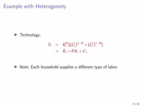
I Technology:

Yt = Kθt [(L1

t )1−θ + (L2t )1−θ ]

= Kt + δ Kt + Ct.

I Note: Each household supplies a different type of labor.

5 / 32

Household

I The household problem is entirely standard.I Solution is ki

t and cit which satisfy Euler equation

g(ci

t)

= (r−ρ)/σ (1)

and budget constraint:

ki = rki + wi− ci (2)

I Boundary conditions: ki0 given and TVC.

6 / 32

Firm

I Factor prices equal marginal products.I q = Fk and wi = FLi .

7 / 32

Equilibrium

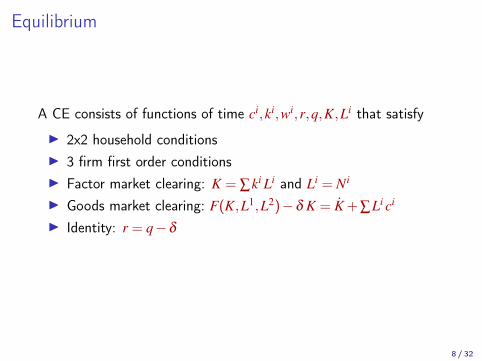
A CE consists of functions of time ci,ki,wi,r,q,K,Li that satisfy

I 2x2 household conditionsI 3 firm first order conditionsI Factor market clearing: K = ∑ki Li and Li = Ni

I Goods market clearing: F(K,L1,L2)−δ K = K + ∑Li ci

I Identity: r = q−δ

8 / 32

Representative Household

I We now show that the entire economy behaves as if arepresentative household chose consumption.

I From lifetime budget constraint:present value of consumption = present value of income +initial assets

ci0Π0 = ki

0 + PV0(wi)

where

Π0 =∫

∞

0exp

(∫ t

0[g(cτ )− rτ ]dτ

)

9 / 32

Representative Household

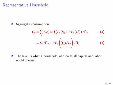
I Aggregate consumption

C0 = ∑i

Lici0 = ∑

iLi(ki

0 + PV0(wi))/Π0 (3)

= K0/Π0 + PV0

(∑

iwiLi

)/Π0 (4)

I The level is what a household who owns all capital and laborwould choose.

10 / 32

Representative Household

The growth rate of aggregate consumption obeys the individualEuler equation:

g(Ct) =∑i Lici

t

∑i Licit

= ∑i

Licit

∑i Licitg(ci

t)

= g(ci

t)

(5)

Why is this true?Because the marginal propensity to consume out of capital / laborincome is the same for all households.

This would fail if utility were not iso-elastic.

Then g(ci

t)

= (rt−ρ)/σ(ci

t)is not independent of the level of ci

t

11 / 32

Steady State

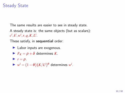
The same results are easier to see in steady state.A steady state is: the same objects (but as scalars):ci,ki,wi,r,q,K,Li.These satisfy, in sequential order:

I Labor inputs are exogenous.I FK = ρ + δ determines K.I r = ρ .I wi = (1−θ)(K/Li)θ determines wi.

12 / 32

Steady State

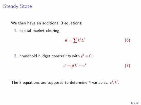
We then have an additional 3 equations:

1. capital market clearing:

K = ∑ki Li (6)

2. household budget constraints with ki = 0:

ci = ρ ki + wi (7)

The 3 equations are supposed to determine 4 variables: ci,ki.

13 / 32

Steady State

I The steady state is not unique.I Any ki that sum to K are a steady state.I For any ki pair we pick, the budget constraints tell us the

corresponding steady state consumption levels.

14 / 32

Why is the steady state not unique?

I Both households have the same marginal propensity toconsume: ρ .

I Redistribute a bit of k1 to k2. Aggregate C is unchanged. Allmarkets clear.

I Effectively, the households behave as if they were one - arepresentative household.

I This is good: when it works, we don’t have to explicitly modelheterogeneous households.

15 / 32

The Representative Household

The representative household

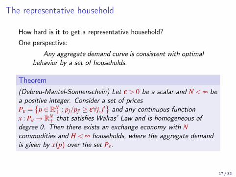
How hard is it to get a representative household?One perspective:

Any aggregate demand curve is consistent with optimalbehavior by a set of households.

Theorem(Debreu-Mantel-Sonnenschein) Let ε > 0 be a scalar and N < ∞ bea positive integer. Consider a set of pricesPε =

{p ∈ RN

+ : pj/pj′ ≥ ε∀j, j′}and any continuous function

x : Pε → RN+ that satisfies Walras’ Law and is homogeneous of

degree 0. Then there exists an exchange economy with Ncommodities and H < ∞ households, where the aggregate demandis given by x(p) over the set Pε .

17 / 32

Why is aggregation so hard?

I The problem is income effects.I Changing prices effectively redistributes income across

households.I If the income elasticities of various goods are very different,

demand curves could be upward sloping over some intervals.I But there is hope if income effects are not too strong.

18 / 32

Gorman aggregation

Theorem(Gorman aggregation) Consider an economy with a finite number Nof commodities and a set H of households. Suppose that thepreferences of household i ∈ H can be represented by an indirectutility function of the form

vi (p,yi)= ai (p) + b(p)yi

then these preferences can represented by those of a representativehousehold with indirect utility

v(p,y) =∫

ai (p)di + b(p)y

where y is aggregate income.

19 / 32

Gorman aggregation

I Key feature of Gorman preferences:I All households have the same constant propensity to consume

out of income.

I This is why redistributing income does not changeconsumption.

I Then aggregate income is sufficient to figure out demand.

20 / 32

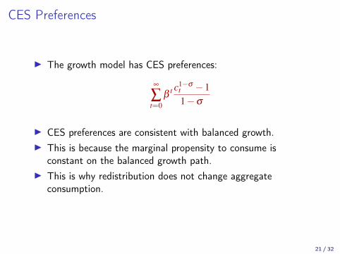
CES Preferences

I The growth model has CES preferences:

∞

∑t=0

βt c1−σ

t −11−σ

I CES preferences are consistent with balanced growth.I This is because the marginal propensity to consume is

constant on the balanced growth path.I This is why redistribution does not change aggregate

consumption.

21 / 32

Implications

Exact aggregation is rare.How worried should we be?

One faction of economists views representative agent models as toymodels.

Another faction is more pragmatic:

I start with a simple modelI check whether heterogeneity makes a quantitatively significant

difference

22 / 32

Application: Labor Supply Elasticity

Application: Labor supply elasticity

How responsive are hours worked to wages?Micro literature:

I weak correlation of hours and wages in panel dataI labor supply elasticities are near 0

Macro literature:

I over the business cycle, small wage fluctuations lead to largemovements in hours

I labor supply elasticity must be large

How to reconcile?

24 / 32

Model

Household maximizes

T

∑a=1

βa

[c1−1/η

1−1/η−α

h1+1/γ

1 + 1/γ

](8)

Present value budget constraint

T

∑a=1

βaca =

T

∑a=1

βa (1− τ)eahaw + z (9)

Assumptions:

I interest rate = discount rateI z: lump sum transfer that rebates labor income tax revenueI ea: productivity

25 / 32

How could one estimate the labor supply elasticity?

First order conditions:

Uc = c−1/ηa = λ (10)

−Uh = αh1/γa = (1− τ)λeaw (11)

where λ is the marginal utility of wealth (Lagrange multiplier).Estimation equation:

lnha = b(λ ) + γ lnea (12)

where

I b(λ ) depends on parameters and λ

I in the regression, ea can be replaced by the observed wage perhour

26 / 32

Micro elasticities

Equations of the form

∆lnhit = γ∆ln(wit (1− τit)) + Xitβ + εit (13)

have been estimated many times in the micro literature.

Consensus result: the labor supply elasticity (γ) is near 0.MaCurdy (1983): a 10% permanent wage change implies a 0.8%change in hours.

27 / 32

Take-away messages

1. The labor supply elasticity is a preference parameter.2. If preferences are age invariant, the labor supply elasticity is

the same for all ages.3. Then the aggregate labor supply elasticity is the same as the

individual one.4. The labor supply elasticity is small.

28 / 32

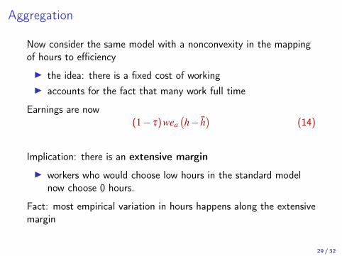
Aggregation

Now consider the same model with a nonconvexity in the mappingof hours to efficiency

I the idea: there is a fixed cost of workingI accounts for the fact that many work full time

Earnings are now(1− τ)wea

(h− h

)(14)

Implication: there is an extensive margin

I workers who would choose low hours in the standard modelnow choose 0 hours.

Fact: most empirical variation in hours happens along the extensivemargin

29 / 32

Macro results

Rogerson and Wallenius (2009) calibrate such a modelResults:

1. The estimated micro labor supply elasticity is only about halfthe size of γ

2. The aggregate labor supply elasticity is large: a 20% increasein the tax implies a 75% decrease in labor supply

Intuition:

I small elasticity at the intensive margin (estimated by microelasticities),

I but large elasticity at the extensive margin.I also large changes in retirement ages

30 / 32

Reading

I Acemoglu (2009), ch. 5.I The labor supply elasticity material is based on Keane and

Rogerson (2012)

31 / 32

References I

Acemoglu, D. (2009): Introduction to modern economic growth,MIT Press.

Keane, M. and R. Rogerson (2012): “Micro and macro labor supplyelasticities: A reassessment of conventional wisdom,” Journal ofEconomic Literature, 50, 464–476.

MaCurdy, T. E. (1983): “A simple scheme for estimating anintertemporal model of labor supply and consumption in thepresence of taxes and uncertainty,” International EconomicReview, 265–289.

Rogerson, R. and J. Wallenius (2009): “Micro and macroelasticities in a life cycle model with taxes,” Journal of Economictheory, 144, 2277–2292.

32 / 32